/


Text
Prolog Programming
for Artificial Intelligence
FOURTH EDITION
«. * # >St*A v. kit-,
Ivan Bratko
Prolog
Programming
for Artificial
Intelligence
Visit the Prolog Programming for Artificial Intelligence, 4th
edition Companion Website at www.pearsoned.co.uk/bratko
to find valuable student learning material including:
PROLOG code available to download
Additional problems and solutions
We work with leading authors to develop the strongest
educational materials in computer science, bringing
cutting-edge thinking and best learning practice to a
global market.
Under a range of well-known imprints, including
Addison Wesley, we craft high quality print and
electronic publications which help readers to understand
and apply their content, whether studying or at work.
To find out more about the complete range of our
publishing, please visit us on the World Wide Web at:
www.pearson.com/uk
log
rog ramming for
Artificial Intelligence
Fourth edition
IVAN BRATKO
Faculty of Computer and Information Science
Ljubljana University
and
J. Stefan Institute
Addison Wesley
is an imprint of
PEARSON
Harlow, England • London • New York • Boston • San Francisco • Toronto
Sydney • Tokyo • Singapore • Hong Kong • Seoul • Taipei • New Delhi
Cape Town • Madrid • Mexico City • Amsterdam • Munich • Paris • Milan
Pearson Education Limited
Edinburgh Gate
Harlow
Essex CM20 2JE
England
and Associated Companies throughout the world
Visit us on the World Wide Web at:
www.pearson.com/uk
First published 1986
Second edition 1990
Third edition 2001
Fourth edition 2012
(D Addison-Wesley Publishers Limited 1986, 1990
© Pearson Education Limited 2001, 2012
The right of Ivan Bratko to be identified as author of this work has been asserted by
him in accordance with the Copyright, Designs and Patents Act 1988.
All rights reserved. No part of this publication may be reproduced, stored in a
retrieval system, or transmitted in any form or by any means, electronic, mechanical,
photocopying, recording or otherwise, without either the prior written permission of the
publisher or a licence permitting restricted copying in the United Kingdom issued by the
Copyright Licensing Agency Ltd, Saffron House, 6-10 Kirby Street, London EC1N 8TS.
The programs in this book have been included for their instructional value.
They have been tested with care but are not guaranteed for any particular purpose.
The publisher does not offer any warranties or representations nor
does it accept any liabilities with respect to the programs.
Pearson Education is not responsible for the content of third-party Internet sites.
ISBN: 978-0-321-41746-6
British Library Cataloguing-in-Publication Data
A catalogue record for this book is available from the British Library
Library of Congress Cataloging-in-Publication Data
Bratko, Ivan, 1946-
Prolog programming for artificial intelligence / Ivan Bratko. - 4th ed.
p. cm.
ISBN 978-0-321-41746-6 (pbk.)
1. Artificial intelligence-Data processing. 2. Prolog (Computer program language)
I. Title.
Q336.B74 2011
006.30285'5133~dc23
2011010795
10 987654321
14 13 12 11
Typeset in 9/12pt Stone Serif by 73
Printed and bound in Great Britain by Henry Ling Ltd, Dorchester, Dorset
Contents
Foreword (from Patrick Winston's Foreword to the Second Edition) xiii
Preface xvii
PART I The Prolog Language 1
1 Introduction to Prolog
1.1 Defining relations by facts
1.2 Defining relations by rules
1.3 Recursive rules
1.4 Running the program with a Prolog system
1.5 How Prolog answers questions
1.6 Declarative and procedural meaning of programs
1.7 A robot's world - preview of things to come
1.8 Crosswords, maps and schedules
Summary
References
2 Syntax and Meaning of Prolog Programs
2.1 Data objects
2.2 Matching
2.3 Declarative meaning of Prolog programs
2.4 Procedural meaning
2.5 Order of clauses and goals
2.6 The relation between Prolog and logic
Summary
References
3 Lists, Operators, Arithmetic
3.1 Representation of lists
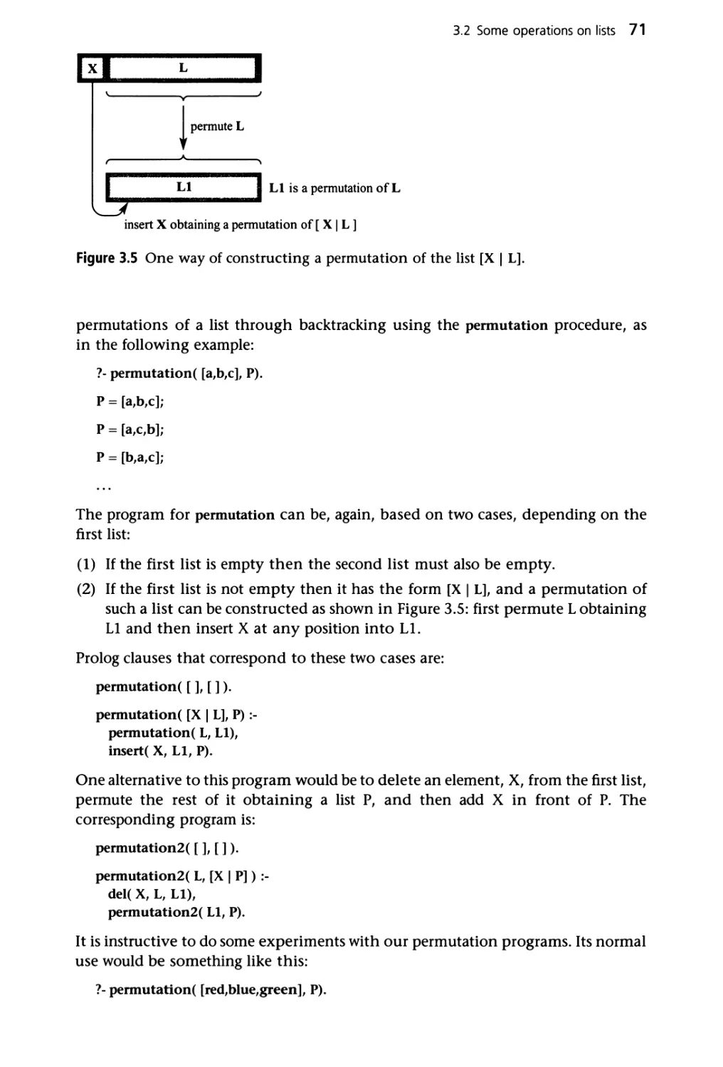
3.2 Some operations on lists
3.3 Operator notation
3.4 Arithmetic
Summary
3
3
8
13
17
18
21
22
27
30
31
32
32
39
44
47
52
57
58
59
60
60
62
74
79
85
4 Programming Examples 86
4.1 Finding a path in a graph 86
4.2 Robot task planning 90
4.3 Trip planning 97
4.4 Solving cryptarithmetic problems 103
4.5 The eight-queens problem 105
4.6 WordNet ontology 115
Summary 124
5 Controlling Backtracking 126
5.1 Preventing backtracking 126
5.2 Examples of using cut 131
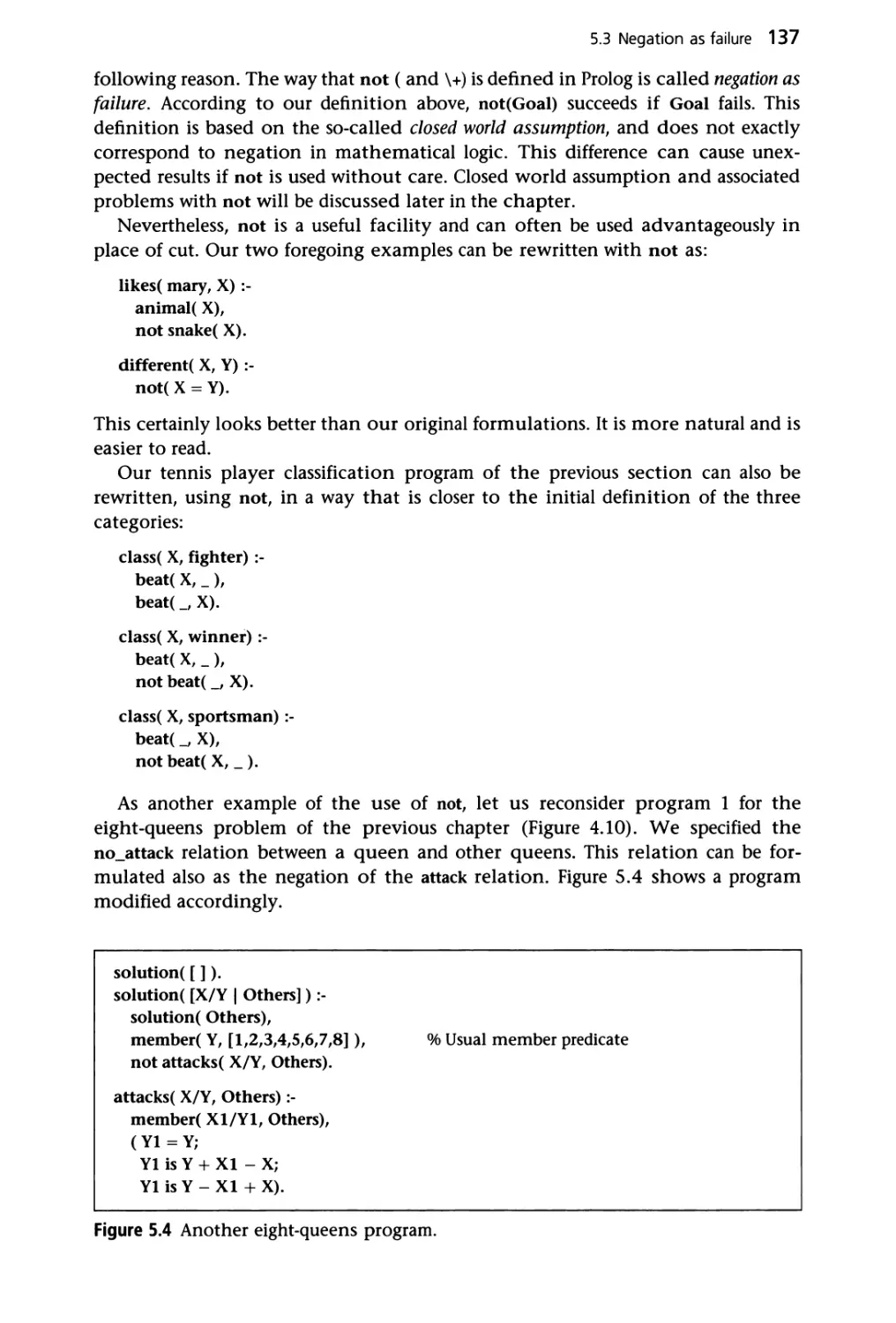
5.3 Negation as failure 135
5.4 Closed world assumption, and problems with cut and negation 138
Summary 142
References 142
6 Built-in Predicates 143
6.1 Testing the type of terms 143
6.2 Constructing and decomposing terms: = .., functor, arg, name 150
6.3 Various kinds of equality and comparison 155
6.4 Database manipulation 157
6.5 Control facilities 160
6.6 bagof, setof and findall 161
6.7 Input and output 164
Summary 175
Reference to Prolog standard 176
7 Constraint Logic Programming 177
7.1 Constraint satisfaction and logic programming 177
7.2 CLP over real numbers: CLP(R), CLP(Q) 184
7.3 Examples of CLP(R) programming: blocks in boxes 188
7.4 CLP over finite domains: CLP(FD) 191
Summary 195
References 196
8 Programming Style and Technique 197
8.1 General principles of good programming 197
8.2 How to think about Prolog programs 199
8.3 Programming style 201
Contents vii
8.4 Debugging 204
8.5 Improving efficiency 206
Summary 219
References 220
9 Operations on Data Structures 221
9.1 Sorting lists 221
9.2 Representing sets by binary trees 225
9.3 Insertion and deletion in a binary dictionary 231
9.4 Displaying trees 235
9.5 Graphs 237
Summary 244
References 245
10 Balanced Trees 246
10.1 2-3 trees 246
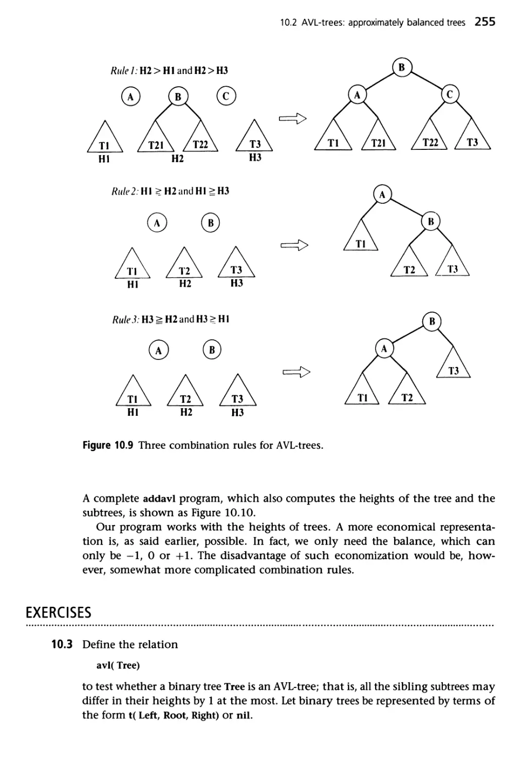
10.2 AVL-trees: approximately balanced trees 253
Summary 256
References and historical notes 257
PART II Prolog in Artificial Intelligence 259
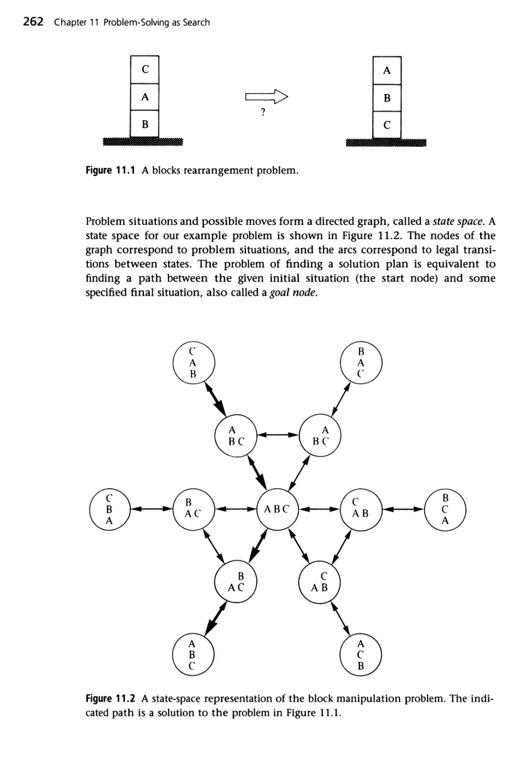
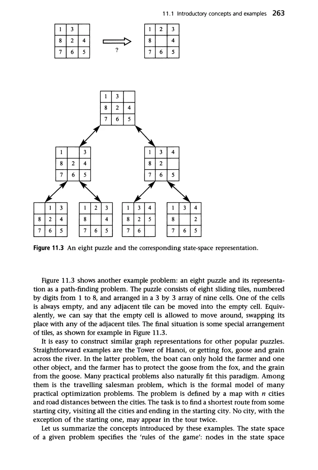
11 Problem-Solving as Search 261
11.1 Introductory concepts and examples 261
11.2 Depth-first search and iterative deepening 265
11.3 Breadth-first search 271
11.4 Analysis of basic search techniques 275
Summary 278
References 279
12 Heuristic Search and the A* Algorithm 280
12.1 Best-first search 280
12.2 Best-first search applied to the eight puzzle 289
12.3 Best-first search applied to scheduling 294
Summary 298
References and historical notes 299
13 Best-First Search: Minimizing Time and Space 301
13.1 Time and space complexity of the A* algorithm 301
13.2 IDA* - iterative deepening A* algorithm 302
VIM Contents
13.3 RBFS - recursive best-first search 305
13.4 RTA* - real-time A* algorithm 311
Summary 316
References 317
14 Problem Decomposition and AND/OR Graphs 318
14.1 AND/OR graph representation of problems 318
14.2 Examples of AND/OR representation 322
14.3 Basic AND/OR search procedures 325
14.4 Best-first AND/OR search 330
Summary 341
References 342
15 Knowledge Representation and Expert Systems 343
15.1 Functions and structure of an expert system 343
15.2 Representing knowledge with if-then rules 345
15.3 Forward and backward chaining in rule-based systems 348
15.4 Generating explanation 353
15.5 Introducing uncertainty 357
15.6 Semantic networks and frames 360
Summary 367
References 368
16 Probabilistic Reasoning with Bayesian Networks 370
16.1 Probabilities, beliefs and Bayesian networks 370
16.2 Some formulas from probability calculus 375
16.3 Probabilistic reasoning in Bayesian networks 376
16.4 d-separation 381
Summary 383
References 383
17 Planning 385
17.1 Representing actions 385
17.2 Deriving plans by means-ends analysis 388
17.3 Goal regression 393
17.4 Combining regression planning with best-first heuristic 396
17.5 Uninstantiated actions and goals 399
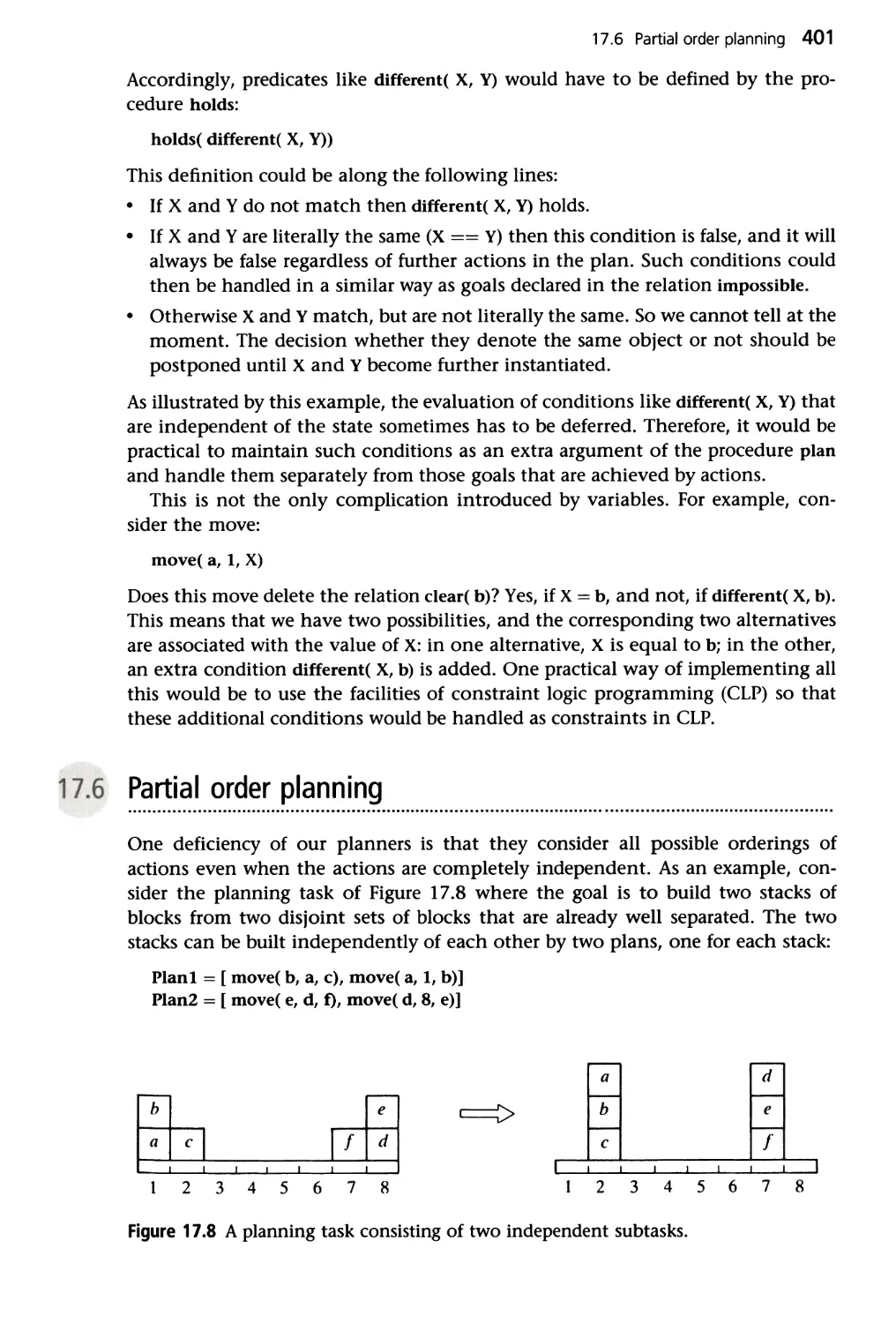
17.6 Partial order planning 401
Summary 403
References and historical notes 404
Contents ix
18 Partial Order Planning and GRAPHPLAN 406
18.1 Partial order planning 406
18.2 An implementation of partial order planning 410
18.3 GRAPHPLAN 417
18.4 Implementation of GRAPHPLAN 422
Summary 426
References and historical notes 427
19 Scheduling, Simulation and Control with CLP 429
19.1 Scheduling with CLP 429
19.2 A simulation program with constraints 436
19.3 Simulation and control of dynamic systems 440
Summary 445
20 Machine Learning 446
20.1 Introduction 446
20.2 The problem of learning concepts from examples 448
20.3 Learning relational descriptions: a detailed example 454
20.4 Learning simple if-then rules 459
20.5 Induction of decision trees 467
20.6 Learning from noisy data and tree pruning 474
20.7 Success of learning 481
Summary 483
References and notes on other approaches 485
21 Inductive Logic Programming 489
21.1 Introduction 489
21.2 Constructing Prolog programs from examples 492
21.3 Program HYPER 503
Summary 520
References and historical notes 520
22 Qualitative Reasoning 522
22.1 Common sense, qualitative reasoning and naive physics 522
22.2 Qualitative reasoning about static systems 526
22.3 Qualitative reasoning about dynamic systems 530
22.4 A qualitative simulation program 536
22.5 Discussion of the qualitative simulation program 546
Summary 550
References and historical notes 551
23 Language Processing with Grammar Rules 554
23.1 Grammar rules in Prolog 554
23.2 Handling meaning 561
23.3 Defining the meaning of natural language 566
Summary 576
References 576
24 Game Playing 578
24.1 Two-person, perfect-information games 578
24.2 The minimax principle 580
24.3 The alpha-beta algorithm: an efficient implementation of minimax 582
24.4 Minimax-based programs: refinements and limitations 586
24.5 Pattern knowledge and the mechanism of 'advice' 588
24.6 A chess endgame program in Advice Language 0 591
Summary 603
References and historical notes 603
25 Meta-Programming 606
25.1 Meta-programs and meta-interpreters 606
25.2 Prolog meta-interpreters 607
25.3 Top level interpreter for constraint logic programming 611
25.4 Abductive reasoning 612
25.5 Query-the-user interpreter 617
25.6 Explanation-based generalization 621
25.7 Pattern-directed programming and blackboard systems 627
25.8 A simple theorem prover as a pattern-directed program 634
Summary 639
References 640
Appendix A Some Differences Between Prolog
Implementations 641
Appendix B Some Frequently Used Predicates 643
Solutions to Selected Exercises 646
Index 665
Supporting resources
Visit www.pearsoned.co.uk/bratko to find valuable online resources:
Companion Website for students
• PROLOG code available to download
• Additional problems and solutions
For instructors
• PowerPoint slides
• Password-protected solutions for lecturers
Also: The Companion Website provides the following features:
• Online help and support to assist with website usage and troubleshooting
For more information please contact your local Pearson Education sales representative
or visit www.pearsoned.co.uk/bratko
From Patrick Winston's Foreword
to the Second Edition
I can never forget my excitement when I saw my first Prolog-style program in
action. It was part of Terry Winograd's famous Shrdlu system, whose blocks-
world problem solver arranged for a simulated robot arm to move blocks around
a screen, solving intricate problems in response to human-specified goals.
Winograd's blocks-world problem solver was written in Microplanner, a
language which we now recognize as a sort of Prolog. Nevertheless, in spite of
the defects of Microplanner, the blocks-world problem solver was organized
explicitly around goals, because a Prolog-style language encourages programmers
to think in terms of goals. The goal-oriented procedures for grasping, clearing,
getting rid of, moving, and ungrasping made it possible for a clear, transparent,
concise program to seem amazingly intelligent.
Winograd's blocks-world problem solver permanently changed the way I think
about programs. I even rewrote the blocks-world problem solver in Lisp for my
Lisp textbook because that program unalterably impressed me with the power of
the goal-oriented philosophy of programming and the fun of writing goal-
oriented programs.
But learning about goal-oriented programming through Lisp programs is like
reading Shakespeare in a language other than English. Some of the beauty comes
through, but not as powerfully as in the original. Similarly, the best way to learn
about goal-oriented programming is to read and write goal-oriented programs in
Prolog, for goal-oriented programming is what Prolog is all about.
In broader terms, the evolution of computer languages is an evolution away
from low-level languages, in which the programmer specifies how something is
to be done, toward high-level languages, in which the programmer specifies
simply what is to be done. With the development of Fortran, for example,
programmers were no longer forced to speak to the computer in the procrustian
low-level language of addresses and registers. Instead, Fortran programmers could
speak in their own language, or nearly so, using a notation that made only
moderate concessions to the one-dimensional, 80-column world.
Fortran and nearly all other languages are still how-type languages, however.
In my view, modern Lisp is the champion of these languages, for Lisp in its
Common Lisp form is enormously expressive, but how to do something is still
what the Lisp programmer is allowed to be expressive about. Prolog, on the other
hand, is a language that clearly breaks away from the how-type languages,
encouraging the programmer to describe situations and problems, not the
detailed means by which the problems are to be solved.
Consequently, an introduction to Prolog is important for all students of
Computer Science, for there is no better way to see what the notion of what-type
programming is all about.
xiv From Patrick Winston's Foreword to the Second Edition
In particular, the chapters of this book clearly illustrate the difference between
how-type and what-type thinking. In the first chapter, for example, the
difference is illustrated through problems dealing with family relations. The Prolog
programmer straightforwardly describes the grandfather concept in explicit,
natural terms: a grandfather is a father of a parent. Here is the Prolog notation:
grandfather X, Z):- father( X, Y), parent( Y, Z).
Once Prolog knows what a grandfather is, it is easy to ask a question: who are
Patrick's grandfathers, for example. Here again is the Prolog notation, along with
a typical answer:
?- grandfather X, patrick).
X = james;
X = carl
It is Prolog's job to figure out how to solve the problem by combing through a
database of known father and parent relations. The programmer specifies only
what is known and what question is to be solved. The programmer is more
concerned with knowledge and less concerned with algorithms that exploit the
knowledge.
Given that it is important to learn Prolog, the next question is how. I believe
that learning a programming language is like learning a natural language in
many ways. For example, a reference manual is helpful in learning a
programming language, just as a dictionary is helpful in learning a natural language. But
no one learns a natural language with only a dictionary, for the words are only
part of what must be learned. The student of a natural language must learn the
conventions that govern how the words are put legally together, and later, the
student should learn the art of those who put the words together with style.
Similarly, no one learns a programming language from only a reference manual,
for a reference manual says little or nothing about the way the primitives of the
language are put to use by those who use the language well. For this, a textbook is
required, and the best textbooks offer copious examples, for good examples are
distilled experience, and it is principally through experience that we learn.
In this book, the first example is on the first page, and the remaining pages
constitute an example cornucopia, pouring forth Prolog programs written by a
passionate Prolog programmer who is dedicated to the Prolog point of view. By
carefully studying these examples, the reader acquires not only the mechanics of
the language, but also a personal collection of precedents, ready to be taken
apart, adapted, and reassembled together into new programs. With this
acquisition of precedent knowledge, the transition from novice to skilled programmer is
already under way.
Of course, a beneficial side effect of good programming examples is that they
expose a bit of interesting science as well as a lot about programming itself. The
science behind the examples in this book is Artificial Intelligence. The reader
learns about such problem-solving ideas as problem reduction, forward and
backward chaining, 'how' and 'why' questioning, and various search techniques.
In fact, one of the great features of Prolog is that it is simple enough for
students in introductory Artificial Intelligence subjects to learn to use
immediately. I expect that many instructors will use this book as part of their Artificial
From Patrick Winston's Foreword to the Second Edition XV
Intelligence subjects so that their students can see abstract ideas immediately
reduced to concrete, motivating form.
Among Prolog texts, I expect this book to be particularly popular, not only
because of its examples, but also because of a number of other features:
• Careful summaries appear throughout.
• Numerous exercises reinforce all concepts.
• Structure selectors introduce the notion of data abstraction.
• Explicit discussions of programming style and technique occupy an entire
chapter.
• There is honest attention to the problems to be faced in Prolog programming, as
well as the joys.
Features like this make this a well done, enjoyable, and instructive book.
I keep the first edition of this textbook in my library on the outstanding-
textbooks shelf, programming languages section, for as a textbook it exhibited all
the strengths that set the outstanding textbooks apart from the others, including
clear and direct writing, copious examples, careful summaries, and numerous
exercises. And as a programming language textbook, I especially liked its
attention to data abstraction, emphasis on programming style, and honest treatment
of Prolog's problems as well as Prolog's advantages.
I dedicate the fourth edition of this book
to my mother, the kindest person I know,
and to my father, who, during world war II
escaped from a concentration camp by
digging an underground tunnel, which he
described in his novel, The Telescope
Preface
Prolog
Prolog is a programming language based on a small set of basic mechanisms,
including pattern matching, tree-based data structuring and automatic
backtracking. This small set constitutes a surprisingly powerful and flexible
programming framework. Prolog is especially well suited for problems that involve
objects - in particular, structured objects - and relations between them. For
example, it is an easy exercise in Prolog to express spatial relationships between
objects, such as the blue sphere is behind the green one. It is also easy to state a
more general rule: if object X is closer to the observer than object Y, and Y is
closer than Z, then X must be closer than Z. Prolog can now reason about the
spatial relationships and their consistency with respect to the general rule.
Features like this make Prolog a powerful language for artificial intelligence (AI)
and non-numerical programming in general.
There are well-known examples of symbolic computation whose
implementation in other standard languages took tens of pages of indigestible code. When
the same algorithms were implemented in Prolog, the result was a crystal-clear
program easily fitting on one page. As an illustration of this fact, the famous
WARPLAN planning program, written by David Warren, is often quoted. For
example, Russell and Norvig1 say 'WARPLAN is also notable in that it was the
first planner to be written in a logic programming language (Prolog) and is one
of the best examples of the economy that can sometimes be gained with logic
programming: WARPLAN is only 100 lines of code, a small fraction of the size of
comparable planners of the time'. Chapter 18 of this book contains much more
complicated planning algorithms (partial-order planning and GRAPHPLAN) that
still fit into fewer than 100 lines of Prolog code.
Development of Prolog
Prolog stands for programming in logic - an idea that emerged in the early 1970s
to use logic as a programming language. The early developers of this idea
included Robert Kowalski at Edinburgh (on the theoretical side), Maarten van
Emden at Edinburgh (experimental demonstration) and Alain Colmerauer at
Marseilles (implementation). David D.H. Warren's efficient implementation at
Edinburgh in the mid-1970s greatly contributed to the popularity of Prolog. A
more recent development is constraint logic programming (CLP), usually
implemented as part of a Prolog system. CLP extends Prolog with constraint
processing, which has proved in practice to be an exceptionally flexible tool for
1S. Russell, P. Norvig, Artificial Intelligence: A Modern Approach, 3rd edn (Prentice-Hall, 2010).
problems like scheduling and logistic planning. In 1996 the official ISO standard
for Prolog was published.
Learning Prolog
Since Prolog has its roots in mathematical logic it is often introduced through
logic. However, such a mathematically intensive introduction is not very
useful if the aim is to teach Prolog as a practical programming tool. Therefore this
book is not concerned with the mathematical aspects, but concentrates on the
art of making the few basic mechanisms of Prolog solve interesting problems.
Whereas conventional languages are procedurally oriented, Prolog introduces
the descriptive, or declarative, view. This greatly alters the way of thinking
about problems and makes learning to program in Prolog an exciting
intellectual challenge. Many believe that every student of computer science
should learn something about Prolog at some point because Prolog enforces
a different problem-solving paradigm complementary to other programming
languages.
Contents of the book
Part I of the book introduces the Prolog language and shows how Prolog
programs are developed. Programming with constraints in Prolog is also
introduced. Techniques to handle important data structures, such as trees and graphs,
are also included because of their general importance. In Part II, Prolog is applied
to a number of areas of AI, including problem solving and heuristic search,
programming with constraints, knowledge representation and expert systems,
planning, machine learning, qualitative reasoning, language processing and game
playing. AI techniques are introduced and developed in depth towards their
implementation in Prolog, resulting in complete programs. These can be used as
building blocks for sophisticated applications. The concluding chapter, on meta-
programming, shows how Prolog can be used to implement other languages and
programming paradigms, including pattern-directed programming, abductive
reasoning, and writing interpreters for Prolog in Prolog. Throughout, the
emphasis is on the clarity of programs; efficiency tricks that rely on implementation-
dependent features are avoided.
New to this edition
All the material has been revised and updated. The main new features of this
edition include:
• Most of the existing material on AI techniques has been systematically updated.
• The coverage and use of constraint logic programming (CLP) has been
strengthened. An introductory chapter on CLP appears in the first, Prolog
language, part of the book, to make CLP more visible and available earlier as a
Preface xix
powerful programming tool independent of AI. The second part includes
expanded coverage of specific techniques of CLP, and its application in advanced
planning techniques.
• The coverage of planning methods has been deepened in a new chapter that
includes implementations of partial order planning and the GRAHPLAN
approach.
• The treatment of search methods now includes RTA* (real-time A* search).
• The chapter on meta-programming has been extended by abductive reasoning,
query-the-user facility, and a sketch of CLP interpreter, all implemented as
Prolog meta-interpreters.
• Programming examples have been refreshed throughout the book, making them
more interesting and practical. One such example in Chapter 4 introduces the
well-known lexical database WordNet, and its application to semantic reasoning
for word sense disambiguation.
Audience for the book
This book is for students of Prolog and AI. It can be used in a Prolog course or in
an AI course in which the principles of AI are brought to life through Prolog. The
reader is assumed to have a basic general knowledge of computers, but no
knowledge of AI is necessary. No particular programming experience is required; in fact,
plentiful experience and devotion to conventional procedural programming - for
example in C or Java - might even be an impediment to the fresh way of
thinking Prolog requires.
The book uses standard syntax
Among several Prolog dialects, the Edinburgh syntax, also known as DEC-10
syntax, is the most widespread, and is the basis of the ISO standard for Prolog. It
is also used in this book. For compatibility with the various Prolog
implementations, this book only uses a relatively small subset of the built-in features that are
shared by many Prologs.
How to read the book
In Part I, the natural reading order corresponds to the order in the book.
However, the part of Section 2.4 that describes the procedural meaning of Prolog in a
more formalized way can be skipped. Chapter 4 presents programming examples
that can be read (or skipped) selectively. Chapter 10 on advanced tree
representations can be skipped.
Part II allows more flexible reading strategies as most of the chapters are
intended to be mutually independent. However, some topics will still naturally
be covered before others, such as basic search strategies (Chapter 11). Figure P.l
summarizes the natural precedence constraints among the chapters.
1
\
2
I
3
I
4 (Selectively)
5
I
6
7
8—► 9—► 10
\
11
12 15 17 19 20 22 23 24 25
/\ I I T
13 14 16 18 21
Figure P.1 Precedence constraints among the chapters.
Program code and course materials
Source code for all the programs in the book and relevant course materials are
accessible from the companion website (www.pearsoned.co.uk/bratko).
Acknowledgements
Donald Michie was responsible for first inducing my interest in Prolog. I am
grateful to Lawrence Byrd, Fernando Pereira and David H.D. Warren, once
members of the Prolog development team at Edinburgh, for their programming advice
and numerous discussions. The book greatly benefited from comments and
suggestions to the previous editions by Andrew McGettrick and Patrick H. Winston.
Other people who read parts of the manuscript and contributed significant
comments include: Damjan Bojadziev, Rod Bristow, Peter Clark, Frans Coenen, David
C. Dodson, Saso Dzeroski, Bogdan Filipic, Wan Fokkink, Matjaz Gams, Peter G.
Greenfield, Marko Grobelnik, Chris Hinde, Tadej Janez, Igor Kononenko, Matevz
Kovacic, Eduardo Morales, Igor Mozetic, Timothy B. Niblett, Dan Peterc, Uros
Pompe, Robert Rodosek, Aleksander Sadikov, Agata Saje, Claude Sammut, Cem
Say, Ashwin Srinivasan, Dorian Sue, Peter Tancig, Tanja Urbancic, Mark Wallace,
William Walley, Simon Weilguny, Blaz Zupan and Darko Zupanic. Special thanks
Preface xxi
to Cem Say for testing many programs and his gift of finding hidden errors.
Several readers helped by pointing out errors in the previous editions, most
notably G. Oulsnam and Iztok Tvrdy. I would also like to thank Patrick Bond,
Robert Chaundy, Rufus Curnow, Philippa Fiszzon and Simon Lake of Pearson
Education for their work in the process of producing this book. Simon Plumtree,
Debra Myson-Etherington, Karen Mosman, Julie Knight and Karen Sutherland
provided support in the previous editions. Much of the artwork was done by
Darko Simersek. Finally, this book would not be possible without the stimulating
creativity of the international logic programming community.
Ivan Bratko
January 2011
PART I
The Prolog Language
1 Introduction to Prolog 3
2 Syntax and Meaning of Prolog Programs 32
3 Lists, Operators, Arithmetic 60
4 Programming Examples 86
5 Controlling Backtracking 126
6 Built-in Predicates 143
7 Constraint Logic Programming 177
8 Programming Style and Technique 197
9 Operations on Data Structures 221
10 Balanced Trees 246
ter 1 .
Introduction to Prolog
1.1 Defining relations by facts 3
1.2 Defining relations by rules 8
1.3 Recursive rules 13
1.4 Running the program with a Prolog system 17
1.5 How Prolog answers questions 18
1.6 Declarative and procedural meaning of programs 21
1.7 A robot's world - preview of things to come 22
1.8 Crosswords, maps and schedules 27
This chapter reviews basic mechanisms of Prolog through example programs. Although
the treatment is largely informal many important concepts are introduced, such as:
Prolog clauses, facts, rules and procedures. Prolog's built-in backtracking mechanism
and the distinction between declarative and procedural meanings of a program are
discussed.
Defining relations by facts
Prolog is a programming language for symbolic, non-numeric computation. It is
specially well suited for solving problems that involve objects and relations
between objects. Figure 1.1 shows an example: a family relation. The fact that
Tom is a parent of Bob can be written in Prolog as:
parent( torn, bob).
Here we choose parent as the name of a relation; torn and bob are its arguments. For
reasons that will become clear later we write names like torn with an initial
lowercase letter. The whole family tree of Figure 1.1 is denned by the following Prolog
program:
parent( pam, bob).
parent( torn, bob).
parent( torn, Hz).
parent( bob, ann).
parent( bob, pat).
parent( pat, jim).
4 Chapter 1 Introduction to Prolog
Figure 1.1 A family tree.
This program consists of six clauses. Each of these clauses declares one fact about
the parent relation. For example, parent( torn, bob) is a particular instance of the
parent relation. In general, a relation is denned as the set of all its instances.
When this program has been communicated to the Prolog system, Prolog can
be posed some questions about the parent relation. For example: Is Bob a parent
of Pat? This question can be communicated to the Prolog system by typing:
?- parent( bob, pat).
Having found this as an asserted fact in the program, Prolog will answer:
yes
A further query can be:
?- parent( liz, pat).
Prolog answers:
no
because the program does not mention anything about Liz being a parent of Pat. It
also answers 'no' to the question:
?- parent( torn, ben).
More interesting questions can also be asked. For example: Who is Liz's parent?
?- parent( X, liz).
Prolog will now tell us what is the value of X such that the above statement is true.
So the answer is:
X = tom
1.1 Defining relations by facts 5
The question Who are Bob's children? can be communicated to Prolog as:
?- parent( bob, X).
This time there is more than just one possible answer. Prolog first answers with one
solution:
X = ann
We may now request another solution (by typing a semicolon), and Prolog will
find:
X = pat
If we request further solutions (semicolon again), Prolog will answer 'no' because all
the solutions have been exhausted.
Our program can be asked an even broader question: Who is a parent of
whom? That is:
Find X and Y such that X is a parent of Y.
This is expressed in Prolog by:
?- parent( X, Y).
Prolog now finds all the parent-child pairs one after another. The solutions will be
displayed one at a time as long as we tell Prolog we want more solutions, until all
the solutions have been found. The answers are output as:
X = pam
Y = bob;
X = tom
Y = bob;
X = tom
Y = liz;
We can always stop the stream of solutions by typing a return instead of a
semicolon.
Our example program can be asked still more complicated questions like: Who
is a grandparent of Jim? This query has to be broken down into two steps, as
illustrated by Figure 1.2.
(1) Who is a parent of Jim? Assume that this is some Y.
(2) Who is a parent of Y? Assume that this is some X.
parent I x
MM \ grandparent
parent I /
(jimf
Figure 1.2 The grandparent relation expressed as a composition of two parent relations.
6 Chapter 1 Introduction to Prolog
Such a composed query is written in Prolog as a sequence of two simple ones:
?- parent( Y, jim), parent( X, Y).
The answer will be:
X = bob
Y = pat
Our composed query can be read: Find such X and Y that satisfy the following two
requirements:
parent( Y, jim) and parent( X, Y)
If we change the order of the two requirements the logical meaning remains the
same. We can indeed try this with the query:
?- parent( X, Y), parent( Y, jim).
which will produce the same result.
In a similar way we can ask: Who are Tom's grandchildren?
?- parent( torn, X), parent( X, Y).
Prolog's answers are:
X = bob
Y = arm;
X = bob
Y = pat
Yet another question could be: Do Ann and Pat have a common parent? This can be
expressed again in two steps:
(1) Who is a parent, X, of Ann?
(2) Is X also a parent of Pat?
The corresponding question to Prolog is:
?- parent( X, ann), parent( X, pat).
The answer is:
X = bob
Our example program has helped to illustrate some important points:
• It is easy in Prolog to define a relation, such as the parent relation, by stating the
n-tuples of objects that satisfy the relation.
1.1 Defining relations by facts 7
• The user can easily query the Prolog system about relations denned in the
program.
• A Prolog program consists of clauses. Each clause terminates with a full stop.
• The arguments of relations can (among other things) be: concrete objects, or
constants (such as torn and ann), or general objects such as X and Y. Objects of
the first kind in our program are called atoms. Objects of the second kind are
called variables. Atoms are distinguished from variables by syntax. Atoms are
strings that start with a lower-case letter. The names of variables are strings that
start with an upper-case letter or an underscore. Later we will see some other
syntactic forms for atoms and variables.
• Questions to Prolog consist of one or more goals. A sequence of goals, such as:
parent( X, ann), parent( X, pat)
means the conjunction of the goals:
X is a parent of Ann, and
X is a parent of Pat.
The word 'goals' is used because Prolog interprets questions as goals that are to
be satisfied. To 'satisfy a goal' means to logically deduce the goal from the
program.
• An answer to a question can be either positive or negative, depending on
whether the corresponding goal can be satisfied or not. In the case of a positive
answer we say that the corresponding goal was satisfiable and that the goal
succeeded. Otherwise the goal was unsatisfiable and it failed.
• If several answers satisfy the question then Prolog will find as many of them as
desired by the user.
EXERCISES
1.1 Assuming the parent relation as defined in this section (see Figure 1.1), what will be
Prolog's answers to the following questions?
(a) ?- parent( jim, X).
(b) ?-parent( X, jim).
(c) ?- parent( pam, X), parent( X, pat).
(d) ?- parent( pam, X), parent( X, Y), parent( Y, jim).
1.2 Formulate in Prolog the following questions about the parent relation:
(a) Who is Pat's parent?
(b) Does Liz have a child?
(c) Who is Pat's grandparent?
8 Chapter 1 Introduction to Prolog
1.2 Defining relations by rules
Our example program can be easily extended in many interesting ways. Let us
first add the information on the sex of the people that occur in the parent
relation. This can be done by simply adding the following facts to our program:
female( pam).
male( torn).
male( bob).
female( liz).
female( pat).
female( ann).
male( jim).
The relations introduced here are male and female. These relations are unary (or
one-place) relations. A binary relation like parent defines a relation between pairs of
objects; on the other hand, unary relations can be used to declare simple yes/no
properties of objects. The first unary clause above can be read: Pam is a female. We
could convey the same information declared in the two unary relations with one
binary relation, sex, instead. An alternative piece of program would then be:
sex( pam, feminine).
sex( torn, masculine).
sex( bob, masculine).
As our next extension to the program, let us introduce the mother relation. We
could define mother in a similar way as the parent relation; that is, by simply
providing facts about the mother relation, each fact mentioning one pair of people
such that one is the mother of the other:
mother( pam, bob).
mother( pat, jim).
However, imagine we had a large database of people. Then the mother relation can
be defined much more elegantly by making use of the fact that it can be logically
derived from the already known relations parent and female. This alternative way
can be based on the following logical statement:
For all X and Y,
X is the mother of Y if
X is a parent of Y, and X is female.
This formulation is already close to the formulation in Prolog. In Prolog this is
written as:
mother(X, Y) :. parent( X, Y), female(X).
The Prolog symbol ':-' is read as 'if. This clause can also be read as:
For all X and Y,
if X is a parent of Y and X is female then
X is the mother of Y.
1.2 Defining relations by rules 9
Prolog clauses such as this are called rules. There is an important difference between
facts and rules. A fact like:
parent( torn, liz).
is something that is always, unconditionally, true. On the other hand, rules specify
things that are true if some condition is satisfied. Therefore we say that rules have:
• a condition part (the right-hand side of the rule) and
• a conclusion part (the left-hand side of the rule).
The conclusion part is also called the head of a clause and the condition part the
body of a clause. This terminology is illustrated by:
mother( X, Y) :- parent( X, Y),female( X).
goal goal
head body
If the condition part 'parent( X, Y), female( X)' is true then a logical consequence of
this is mother( X, Y). Note that the comma between the goals in the body means
conjunction: for the body to be true, all the goals in the body have to be true.
How are rules actually used by Prolog? Consider the following example. Let us
ask our program whether Pam is the mother of Bob:
?- mother(pam, bob).
There is no fact about mother in the program. The only way to consider this
question is to apply the rule about mother. The rule is general in the sense that it
is applicable to any objects X and Y; therefore it can also be applied to such
particular objects as pam and bob. To apply the rule to pam and bob, X has to be
substituted with pam, and Y with bob. We say that the variables X and Y become
instantiated to:
X = pam and Y = bob
After the instantiation we have obtained a special case of our general rule. The
special case is:
mother( pam, bob) :- parent( pam, bob), female( pam).
The condition part has become:
parent( pam, bob), female( pam)
Now Prolog tries to find out whether the condition part is true. So the initial goal:
mother( pam, bob)
has been replaced with the goals:
parent( pam, bob), female( pam)
These two (new) goals happen to be trivial as they can be found as facts in the
program. This means that the conclusion part of the rule is also true, and Prolog
will answer the question with yes.
10 Chapter 1 Introduction to Prolog
x),emale (x
parent | , mother parent I x
Y ) | grandparent
i
parent | '
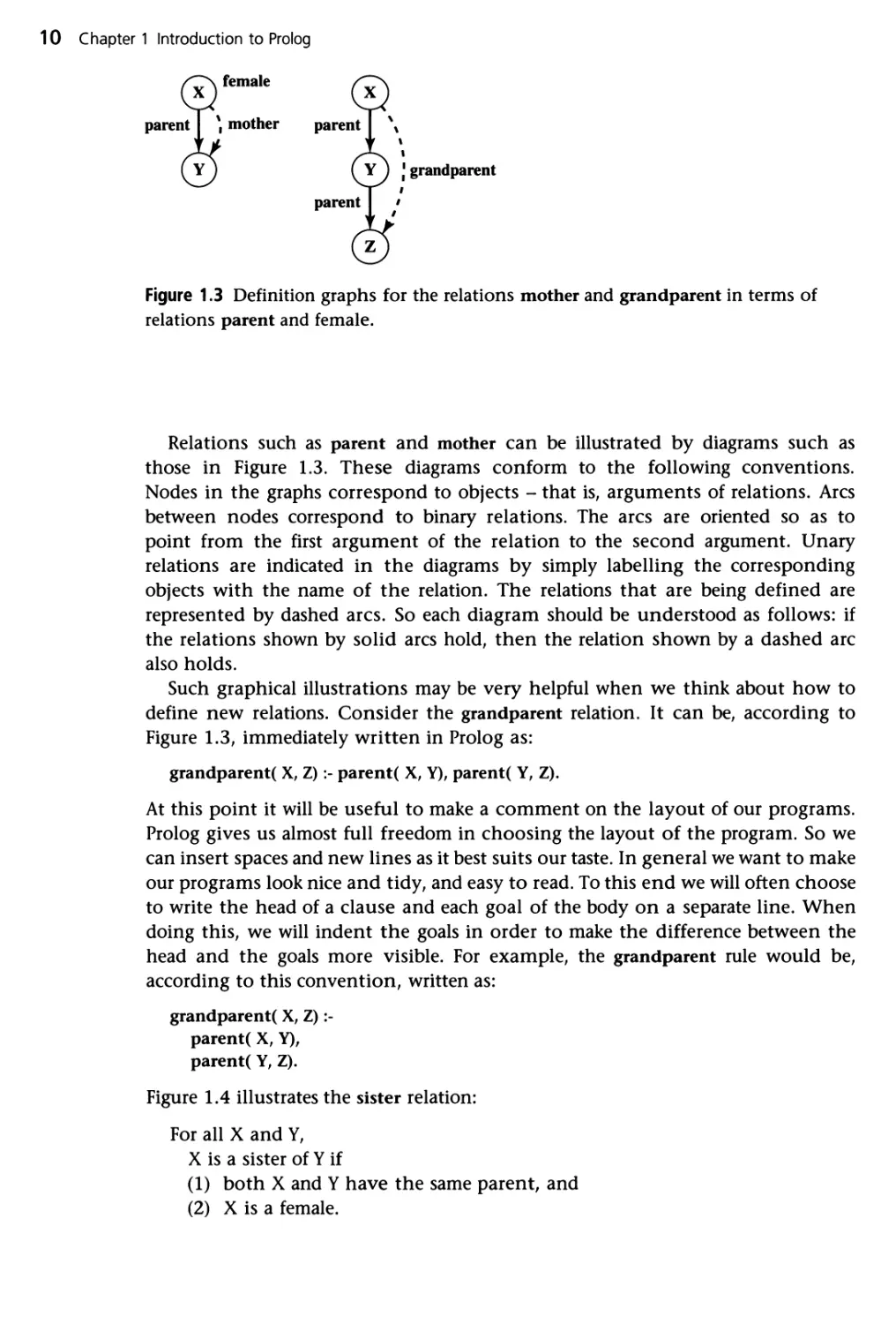
Figure 1.3 Definition graphs for the relations mother and grandparent in terms of
relations parent and female.
Relations such as parent and mother can be illustrated by diagrams such as
those in Figure 1.3. These diagrams conform to the following conventions.
Nodes in the graphs correspond to objects - that is, arguments of relations. Arcs
between nodes correspond to binary relations. The arcs are oriented so as to
point from the first argument of the relation to the second argument. Unary
relations are indicated in the diagrams by simply labelling the corresponding
objects with the name of the relation. The relations that are being defined are
represented by dashed arcs. So each diagram should be understood as follows: if
the relations shown by solid arcs hold, then the relation shown by a dashed arc
also holds.
Such graphical illustrations may be very helpful when we think about how to
define new relations. Consider the grandparent relation. It can be, according to
Figure 1.3, immediately written in Prolog as:
grandparent( X, Z):- parent( X, Y), parent( Y, Z).
At this point it will be useful to make a comment on the layout of our programs.
Prolog gives us almost full freedom in choosing the layout of the program. So we
can insert spaces and new lines as it best suits our taste. In general we want to make
our programs look nice and tidy, and easy to read. To this end we will often choose
to write the head of a clause and each goal of the body on a separate line. When
doing this, we will indent the goals in order to make the difference between the
head and the goals more visible. For example, the grandparent rule would be,
according to this convention, written as:
grandparent( X, Z) :-
parent( X, Y),
parent( Y, Z).
Figure 1.4 illustrates the sister relation:
For all X and Y,
X is a sister of Y if
(1) both X and Y have the same parent, and
(2) X is a female.
1.2 Defining relations by rules 11
parent / \ parent
female ( X ) *"vY)
^—/ sister Vl/
Figure 1.4 Defining the sister relation.
The graph in Figure 1.4 can be translated into Prolog as:
sister( X, Y) :-
parent( Z, X),
parent( Z, Y),
female( X).
Notice the way in which the requirement 'both X and Y have the same parent' has
been expressed. The following logical formulation was used: some Z must be a
parent of X, and this same Z must be a parent of Y. An alternative, but less elegant,
way would be to say: Zl is a parent of X, and Z2 is a parent of Y, and Zl is equal to
Z2. We can now ask:
?- sister( ann, pat).
The answer will be 'yes', as expected (see Figure 1.1). Therefore we might conclude
that the sister relation, as denned, works correctly. There is, however, a rather subtle
flaw in our program, which is revealed if we ask the question Who is Pat's sister?:
?- sister( X, pat).
Prolog will find two answers, one of which may come as a surprise:
X = aim;
X = pat
So, Pat is a sister to herself?! This is not what we had in mind when defining the
sister relation. However, according to our rule about sisters, Prolog's answer is
perfectly logical. Our rule about sisters does not mention that X and Y must be
different if they are to be sisters. As this is not required Prolog (rightfully) assumes
that X and Y can be the same, and will as a consequence find that any female who
has a parent is a sister of herself.
To correct our rule about sisters we have to add that X and Y must be
different. We can state this as X \= Y. An improved definition of the sister relation
can then be:
sister( X, Y) :-
parent( Z, X),
parent( Z, Y),
female( X),
X\=Y.
12 Chapter 1 Introduction to Prolog
Some important points of this section are:
• Prolog programs can be extended by simply adding new clauses.
• Prolog clauses are of three types: facts, rules and questions.
• Facts declare things that are always, unconditionally, true.
• Rules declare things that are true depending on a given condition.
• By means of questions the user can ask the program what things are true.
• A Prolog clause consists of the head and the body. The body is a list
of goals separated by commas. Commas between goals are understood as
conjunctions.
• A fact is a clause that just has the head and no body. Questions only have the
body. Rules consist of the head and the (non-empty) body.
• In the course of computation, a variable can be substituted by another object.
We say that a variable becomes instantiated.
• Variables are assumed to be universally quantified and are read as 'for all'.
Alternative readings are, however, possible for variables that appear only in the
body. For example:
hasachild( X) :- parent( X, Y).
can be read in two ways:
(a) For all X and Y,
if X is a parent of Y then
X has a child.
(b) For all X,
X has a child if
there is some Y such that X is a parent of Y.
Logically, both readings are equivalent.
EXERCISES
1.3 Translate the following statements into Prolog rules:
(a) Everybody who has a child is happy (introduce a one-argument relation
happy).
(b) For all X, if X has a child who has a sister then X has two children (introduce
new relation hastwochildren).
1.4 Define the relation grandchild using the parent relation. Hint: It will be similar to
the grandparent relation (see Figure 1.3).
1.5 Define the relation aunt( X, Y) in terms of the relations parent and sister.
As an aid you can first draw a diagram in the style of Figure 1.3 for the aunt
relation.
1.3 Recursive rules 13
Recursive rules
Let us add one more relation to our family program, the ancestor relation. This
relation will be defined in terms of the parent relation. The whole definition can
be expressed with two rules. The first rule will define the direct (immediate)
ancestors and the second rule the indirect ancestors. We say that some X is an
indirect ancestor of some Z if there is a chain of parents between X and Z, as
illustrated in Figure 1.5. In our example of Figure 1.1, Tom is a direct ancestor of
Liz and an indirect ancestor of Pat.
The first rule is simple and can be written in Prolog as:
ancestor( X, Z) :-
parent( X, Z).
The second rule, on the other hand, is more complicated. The chain of parents may
present some problems because the chain can be arbitrarily long. One attempt to
define indirect ancestors could be as shown in Figure 1.6. According to this, the
ancestor relation would be defined by a set of clauses as follows:
ancestor( X, Z) :-
parent( X, Z).
ancestor( X, Z) :-
parent( X, Y),
parent (Y, Z).
ancestor( X, Z) :-
parent( X, Yl),
parent( Yl, Y2),
parent( Y2, Z).
ancestor( X, Z) :-
parent( X, Yl),
parent( Yl, Y2),
parent( Y2, Y3),
parent( Y3, Z).
parent I • ancestor
(a)
I
J ancestor
parent
Figure 1.5 Examples of the ancestor relation: (a) X is a direct ancestor of Z; (b) X is an
indirect ancestor of Z.
Chapter 1 Introduction to Prolog
parent
parent
Y ) J ancestor
parent
parent \
Yl
! ancestor
parent
Y2
ancestor
parent
Y3
parent
Figure 1.6 Ancestor-successor pairs at various distances.
This program is lengthy and, more importantly, it only works to some extent. It
would only discover ancestors to a certain depth in a family tree because the length
of the chain of people between the ancestor and the successor would be limited by
the length of our ancestor clauses.
There is, however, a much more elegant and correct formulation of the
ancestor relation. It will work for ancestors at any depth. The key idea is to define
the ancestor relation in terms of itself. Figure 1.7 illustrates the idea:
For all X and Z,
X is an ancestor of Z if
there is a Y such that
(1) X is a parent of Y and
(2) Y is an ancestor of Z.
parent
■ ancestor
ancestor
Figure 1.7 Recursive formulation of the ancestor relation.
1.3 Recursive rules 15
A Prolog clause with the above meaning is:
ancestor( X, Z) :-
parent( X, Y),
ancestor( Y, Z).
We have thus constructed a complete program for the ancestor relation, which
consists of two rules: one for direct ancestors and one for indirect ancestors. Both
rules are rewritten together as:
ancestor( X, Z) :-
parent( X, Z).
ancestor( X, Z) :-
parent( X, Y),
ancestor( Y, Z).
The key to this formulation was the use of ancestor itself in its definition. Such a
definition may look surprising in view of the question: When defining something,
can we use this same thing that has not yet been completely defined? Such
definitions are called recursive definitions. Logically, they are perfectly correct and
understandable, which is also intuitively obvious if we look at Figure 1.7. But will
the Prolog system be able to use recursive rules in computation? It turns out that
Prolog can indeed easily use recursive definitions. Recursive programming is, in
fact, one of the fundamental principles of programming in Prolog. It is not
possible to solve tasks of any significant complexity in Prolog without the use of
recursion.
Going back to our program, we can ask Prolog: Who are Pam's successors?
That is: Who is a person that has Pam as his or her ancestor?
?- ancestor( pam, X).
X = bob;
X = ann;
X = pat;
X = jim
Prolog's answers are, of course, correct and they logically follow from our
definition of the ancestor and the parent relation. There is, however, a rather
important question: How did Prolog actually use the program to find these
answers?
An informal explanation of how Prolog does this is given in the next section.
But first let us put together all the pieces of our family program, which was
extended gradually by adding new facts and rules. The final program is shown
in Figure 1.8. Looking at Figure 1.8, two further points are in order here: the
first will introduce the term 'procedure', the second will be about comments in
programs.
The program in Figure 1.8 defines several relations - parent, male, female,
ancestor, etc. The ancestor relation, for example, is defined by two clauses. We say
that these two clauses are about the ancestor relation. Sometimes it is convenient
to consider the whole set of clauses about the same relation. Such a set of clauses
is called a procedure.
16 Chapter 1 Introduction to Prolog
In Figure 1.8, comments like 'Pam is a parent of Bob' were added to the
program. Comments are, in general, ignored by the Prolog system. They only serve
as a further clarification to a person who reads the program. Comments are
distinguished in Prolog from the rest of the program by being enclosed in special
brackets '/*' and '*/'. Thus comments in Prolog look like this:
/* This is a comment */
Another method, more practical for short comments, uses the percent
character '%'. Everything between '%' and the end of the line is interpreted as a
comment:
% This is also a comment
parent(pam, bob).
parent(torn, bob).
parent(torn, liz).
parent(bob, ann).
parent(bob, pat).
parent(pat, jim).
female( pam).
male( torn).
male( bob).
female( liz).
female( ann).
female( pat).
male( jim).
mother(X, Y) :-
parent( X, Y),
female( X).
grandparent( X, Z) :-
parent( X, Y),
parent(Y, Z).
sister(X, Y) :-
parent( Z, X),
parent( Z, Y),
female( X),
X\ = Y.
ancestor( X, Z) :-
parent( X, Z).
ancestor( X, Z) :-
parent( X, Y),
ancestor( Y, Z).
% Pam is a parent of Bob
% Pam is female
% Tom is male
% X is the mother of Y if
% X is a parent of Y and
% X is female
% X is a grandparent of Z if
% X is a parent of Y and
% Y is a parent of Z
% X is a sister of Y if
% X and Y have the same parent and
% X is female and
% X and Y are different
% Rule al: X is ancestor of Z
% Rule a2: X is ancestor of Z
Figure 1.8 The family program.
1.4 Running the program with a Prolog system 17
EXERCISE
1.6 Consider the following alternative definition of the ancestor relation:
ancestor( X, Z) :-
parent( X, Z).
ancestor( X, Z) :-
parent( Y, Z),
ancestor( X, Y).
Does this also seem to be a correct definition of ancestors? Can you modify the
diagram of Figure 1.7 so that it would correspond to this new definition?
1.4 Running the program with a Prolog system
How can a program like our family program be run on the computer? Here is a
simple and typical way.
There are several good quality and freely available Prologs, such as SWI Prolog,
YAP Prolog and CIAO Prolog. Constraint programming system ECLiPSe also
includes Prolog. Another well-known, well-maintained and inexpensive (for
academic use) Prolog is SICStus Prolog. We will now assume that a Prolog system
has already been downloaded and installed on your computer.
In the following we describe, as an example, roughly how the family program
is run with the SICStus Prolog system. The procedure with other Prologs is
essentially the same; only the interface details of interacting with Prolog may vary.
Suppose that our family program has already been typed into the computer
using a plain text editor, such as Notepad. Suppose this file has been saved into a
chosen directory, say 'prolog_progs', as a text file 'family.pl'. SICStus Prolog
expects Prolog programs to be saved with name extension 'pi'.
Now you can start your Prolog system. When started, SICStus Prolog will open a
window for interaction with the user. It will be displaying the prompt '?-', which
means that Prolog is waiting for your questions or commands. First, you need to tell
Prolog that the 'working directory' will be your chosen directory 'prolog_progs'. This
can be done through the 'Working directory' entry in the 'File' menu. Prolog will
now expect to read program files from the selected directory 'prolog_progs'. Then
you tell Prolog to read in your program from file 'family.pl' by:
?- consult( family).
or equivalently:
?- [family].
Prolog will read the file family.pl and answer something to the effect 'File family.pl
successfully consulted', and again display the prompt'?-'. Then your conversation
with Prolog may proceed like this:
?- parent( torn, X).
X = bob;
X = liz;
18 Chapter 1 Introduction to Prolog
no
?- ancestor( X, aim).
X = bob;
X = pam;
1.5 How Prolog answers questions
This section explains informally how Prolog answers questions. A question to
Prolog is always a sequence of one or more goals. To answer a question, Prolog
tries to satisfy all the goals. What does it mean to satisfy a goal? To satisfy a goal
means to demonstrate that the goal is true, assuming that the relations in the
program are true. In other words, to satisfy a goal means to demonstrate that the
goal logically follows from the facts and rules in the program. If the question
contains variables, Prolog also has to find what are the particular objects (in place of
variables) for which the goals are satisfied. The particular instantiation of
variables to these objects is displayed to the user. If Prolog cannot demonstrate for
any instantiation of variables that the goals logically follow from the program,
then Prolog's answer to the question will be 'no'.
An appropriate view of the interpretation of a Prolog program in
mathematical terms is then as follows: Prolog accepts facts and rules as a set of axioms, and
the user's question as a conjectured theorem; then it tries to prove this theorem -
that is, to demonstrate that it can be logically derived from the axioms.
We will illustrate this view by a classical example. Let the axioms be:
All men are fallible.
Socrates is a man.
A theorem that logically follows from these two axioms is:
Socrates is fallible.
The first axiom above can be rewritten as:
For all X, if X is a man then X is fallible.
Accordingly, the example can be translated into Prolog as follows:
fallible( X):- man( X). % All men are fallible
man( socrates). % Socrates is a man
?- fallible( socrates). % Socrates is fallible?
yes
A more complicated example from the family program of Figure 1.8 is:
?- ancestor( torn, pat).
We know that parent( bob, pat) is a fact. Using this fact and rule al we can conclude
ancestor( bob, pat). This is a derived fact: it cannot be found explicitly in our
program, but it can be derived from the facts and rules in the program. An inference
step, such as this, can be written as:
parent( bob, pat) => ancestor( bob, pat)
1.5 How Prolog answers questions 19
This can be read: from parent( bob, pat) it follows that ancestor( bob, pat), by rule al.
Further, we know that parent( torn, bob) is a fact. Using this fact and the derived fact
ancestor( bob, pat) we can conclude ancestor( torn, pat), by rule a2. We have thus
shown that our goal statement ancestor( torn, pat) is true. This whole inference
process of two steps can be written as:
parent( bob, pat) =>■ ancestor( bob, pat)
parent( torn, bob) and ancestor( bob, pat) => ancestor( torn, pat)
We will now show how Prolog finds such a proof that the given goals follow
from the given program. Prolog starts with the goals and, using rules in the
program, substitutes the current goals with new goals, until new goals happen to be
simple facts. Let us see how this works for the question:
?- mother( pam, bob).
Prolog tries to prove the goal mother( pam, bob). To do this, Proog looks for clauses
about the mother relation. So it finds the rule:
mother( X, Y) :- parent( X, Y), female( X).
This rule is true for all X and Y, so it must also be true for the special case when
X = pam, and Y = bob. We say that variables X and Y get 'instantiated', and this
results in the special case of the mother rule:
mother( pam, bob) :- parent( pam, bob), female( pam).
The head of this clause is the goal Prolog wants to prove. If Prolog manages to prove
the body of the clause, then it will have proved mother(pam,bob). Prolog therefore
substitutes the original goal mother(pam,bob) with the goals in the body:
parent( pam, bob), female( pam)
These now become Prolog's next goals. Prolog tries to prove them in turn: first
parent (pam,bob), and then female (pam). The first goal is easy because Prolog finds that
parent(pam,bob) is given as a fact in the program. So it remains to prove female(pam).
Prolog finds that this is also given as a fact in the program, so it is also true. Thus the
proof of mother(pam,bob) is completed and Prolog answers the question with 'yes'.
Now consider a more complicated question that involves recursion:
?- ancestor( torn, pat).
To satisfy this goal, Prolog will try to find a clause in the program about the ancestor
relation. There are two clauses relevant to this end: the clauses labelled by al and
a2. We say that the heads of these rules match the goal.
The two clauses, al and a2, represent two alternative ways for Prolog to
proceed. This is graphically illustrated in Figure 1.9 which shows the complete
execution trace. We now follow Figure 1.9. Prolog first tries the clause that appears
first in the program, that is ah
ancestor( X, Z):- parent( X, Z).
Since the goal is ancestor(tom,pat), the variables in the rule must be instantiated as
follows:
X = torn, Z = pat
20 Chapter 1 Introduction to Prolog
ancestor! torn, pat)
"ft K
by rule a 1
parent( torn, pat)
no
by rule a2
parent( torn, Y)
ancestor( Y, pat)
A
by fact parent(tom,bob), Y = bob
ancestor! bob, pat)
A
by rule al
parent( bob, pat)
yes, by fact parent(bob,pat)
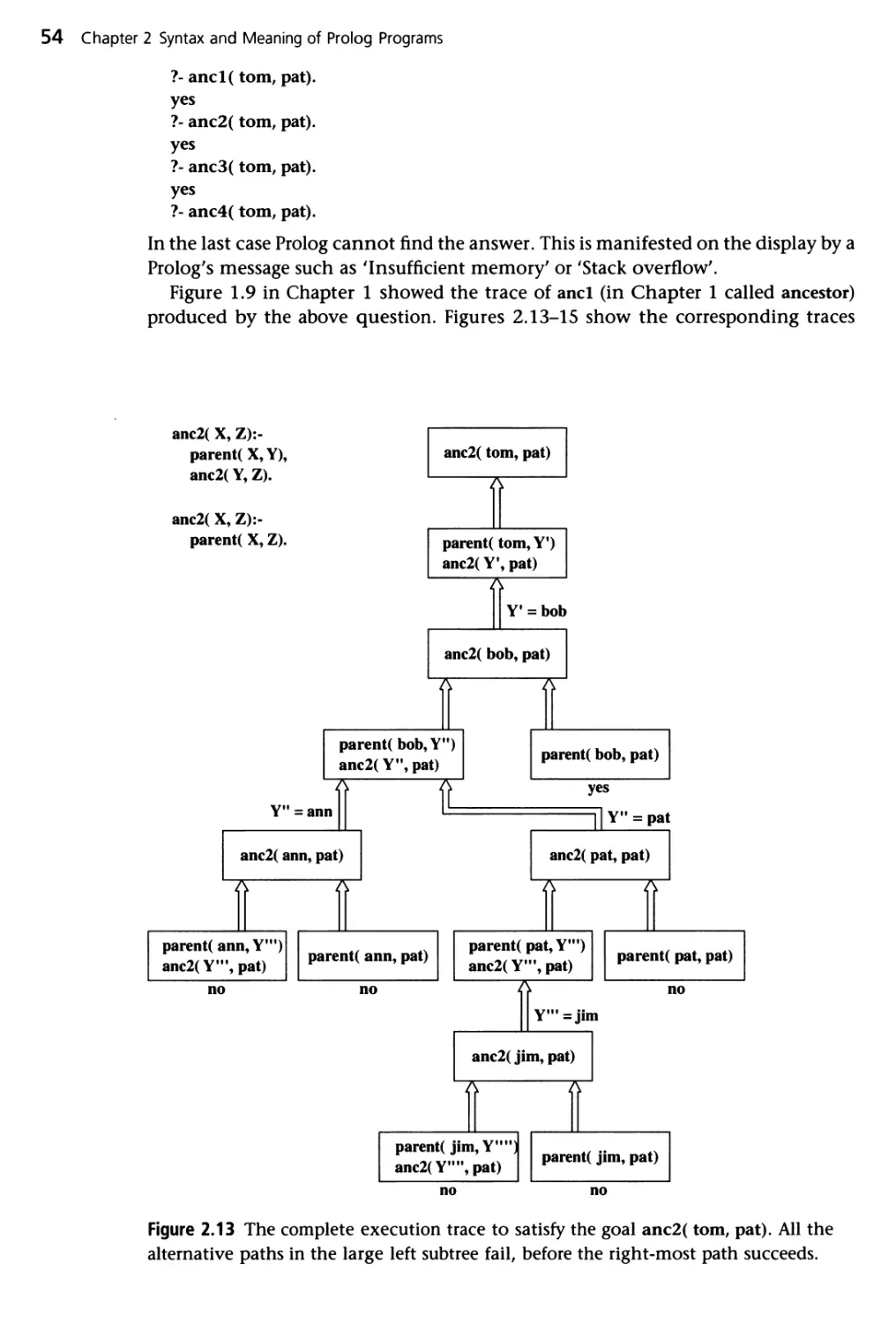
Figure 1.9 The complete execution trace to satisfy the goal ancestor( torn, pat). The
left-hand branch fails, but the right-hand branch proves the goal is satisfiable.
The original goal ancestor( torn, pat) is then replaced by a new goal:
parent( torn, pat)
There is no clause in the program whose head matches the goal parent(tom,pat),
therefore this goal fails. This means the first alternative with rule al has failed. Now
Prolog backtracks to the original goal in order to try the alternative way to derive the
top goal ancestor(tom,pat). The rule a2 is thus tried:
ancestor( X, Z) :-
parent( X, Y),
ancestor( Y, Z).
As before, the variables X and Z become instantiated as:
X = torn, Z = pat
But Y is not instantiated yet. The top goal ancestor( torn, pat) is replaced by two
goals:
parent( torn, Y),
ancestor( Y, pat)
Prolog tries to satisfy the two goals in the order in which they appear. The first goal
matches two facts in the program: parent(tom,bob) and parent(tom,liz). Prolog first
tries to use the fact that appears first in the program. This forces Y to become
instantiated to bob. Thus the first goal has been satisfied, and the remaining goal
has become:
ancestor( bob, pat)
To satisfy this goal the rule a J is used again. Note that this (second) application of
the same rule has nothing to do with its previous application. Therefore, Prolog
1.6 Declarative and procedural meaning of programs 21
uses a new set of variables in the rule each time the rule is applied. To indicate this
we shall rename the variables in rule al for this application as follows:
ancestor( X', Z') :-
parent( X', Z').
The head has to match our current goal ancestor( bob, pat). Therefore:
X' = bob, 11 = pat
The current goal is replaced by:
parent( bob, pat)
This goal is immediately satisfied because it appears in the program as a fact. This
completes the execution trace in Figure 1.9.
Here is a summary of the goal execution mechanism of Prolog, illustrated by
the trace in Figure 1.9. An execution trace has the form of a tree. The nodes of the
tree correspond to goals, or to lists of goals that are to be satisfied. The arcs
between the nodes correspond to the application of (alternative) program clauses
that transform the goals at one node into the goals at another node. The top goal
is satisfied when a path is found from the root node (top goal) to a leaf node
labelled 'yes'. A leaf is labelled 'yes' if it is a simple fact. The execution of Prolog
programs is the searching for such paths. During the search Prolog may enter an
unsuccessful branch. When Prolog discovers that a branch fails it automatically
backtracks to the previous node and tries to apply an alternative clause at that
node. Automatic backtracking is one of the distinguishing features of Prolog.
EXERCISE
1.7 Try to understand how Prolog derives answers to the following questions, using the
program of Figure 1.8. Try to draw the corresponding derivation diagrams in the
style of Figure 1.9. Will any backtracking occur at particular questions?
(a) ?- parent( pam, bob).
(b) ?- mother( pam, bob).
(c) ?- grandparent(pam, ann).
(d) ?- grandparent( bob, jim).
1.6 Declarative and procedural meaning of programs
In our examples so far it has always been possible to understand the results of
the program without exactly knowing how the system actually found the results.
It therefore makes sense to distinguish between two levels of meaning of Prolog
programs; namely,
• the declarative meaning and
• the procedural meaning.
Chapter 1 Introduction to Prolog
The declarative meaning is concerned only with the relations denned by the program.
The declarative meaning thus determines what will be the output of the program. On
the other hand, the procedural meaning also determines how this output is obtained;
that is, how the relations are actually derived by the Prolog system.
The ability of Prolog to work out many procedural details on its own is
considered to be one of its specific advantages. It encourages the programmer to consider
the declarative meaning of programs relatively independently of their procedural
meaning. Since the results of the program are, in principle, determined by its
declarative meaning, this should be (in principle) sufficient for writing programs.
This is of practical importance because the declarative aspects of programs are
usually easier to understand than the procedural details. To take full advantage of
this, the programmer should concentrate mainly on the declarative meaning and,
whenever possible, avoid being distracted by the execution details. These should
be left to the greatest possible extent to the Prolog system itself.
This declarative approach indeed often makes programming in Prolog easier
than in typical procedurally oriented programming languages such as C or Java.
Unfortunately, however, the declarative approach is not always sufficient. It will
later become clear that, especially in large programs, the procedural aspects
cannot be completely ignored by the programmer for practical reasons of execution
efficiency. Nevertheless, the declarative style of thinking about Prolog programs
should be encouraged and the procedural aspects ignored to the extent that is
permitted by practical constraints.
1.7 A robot's world - preview of things to come
In this section we preview some other features of Prolog programming. The
preview will be through an example, without in-depth explanation of the illustrated
features. The details of their syntax and meaning will be covered in chapters that
follow.
Consider a robot that can observe and manipulate simple objects on a table.
Figure 1.10 shows a scene from the robot's world. For simplicity, all the objects are
blocks of unit size. The coordinates on the table are just integers, so the robot can
only distinguish between a finite number of positions of the objects. The robot
can observe the objects with a camera that is mounted on the ceiling. The blocks
a, d and e are visible by the camera, whereas blocks b and c are not. The robot's
vision system can recognize the names of the visible blocks and the x-y positions
MXy
Figure 1.10 A robot's world.
1.7 A robot's world - preview of things to come 23
of the blocks. Now assume that the vision information is stored in a Prolog
program as the three place relation see:
% see( Block, X, Y): Block is observed by camera at coordinates X and Y
see( a, 2, 5).
see( d, 5, 5).
see( e, 5, 2).
Assume also that the robot keeps track of what each block is standing on, e.g. that
block a is on block b. Let this information be stored as binary relation on:
% on( Block, Object): Block is standing on Object
on( a, b).
on( b, c).
on( c, table).
on( d, table).
on( e, table).
The robot may be interested in some simple questions about its world. For example,
what are all the blocks in this world? Each block has to be supported by something,
so relation 'on' offers one way of finding all the blocks:
?- on( Block, _).
Block = a;
Block = b;
Note the underscore character in the question. We are only interested in Block, and
not in what the block is standing on. The underscore indicates an 'anonymous'
variable. It stands for anything, and we are not interested in its value.
The robot may ask about pairs of visible blocks that have the same y-coordinate.
This is an attempt at asking about such pairs of blocks Bl and B2:
?- see( Bl, _, Y), see( B2, _, Y). % Bl and B2 both seen at the same Y
Bl = a, B2 = a;
Bl = a, B2 = d;
Bl = e, B2 = e
Some answers are a surprise! The intention was that Bl and B2 are not the same, but
we did not state this in the question. So Prolog quite logically also considers the
cases when Bl = B2, and thus reports also the cases like Bl = B2 = a, Bl = B2 = e, etc.
We can correct the question as:
?- see( Bl, _, Y), see( B2, _, Y), Bl \= B2. % Bl and B2 not equal
Bl = a, B2 = d;
Bl = d, B2 = a;
no
The robot may find non-visible blocks B by the question:
?- on( B, _), % B is on something, so B is a block
on( _, B). % Something is on B, so B is not visible
B=b;
24 Chapter 1 Introduction to Prolog
B = c;
no
Equivalently, we may ask:
?- on( B, _), % B is on something, so B is a block
not see( B, _, _). % B is not seen by the camera
B = b;
The condition not see( B, _, _) is Prolog's negation of see( B, _, _). This is not exactly the
same as negation in mathematics, which will be discussed in Chapter 5. To emphasize
this difference with respect to mathematics, a more standard notation for negation in
Prolog is '\+' instead of 'not'. So the negated condition is written as \+ see(B,_,_).
Now suppose the robot wants to find the left-most visible block(s). That is,
find the block(s) with minimum ^-coordinate. The usual algorithm for such a
task is roughly: loop over all the blocks, whereby for each block check whether
its ^-coordinate is less than the minimum x-coordinate Xmin of the blocks
considered so far. If yes, update Xmin (set Xmin to the ^-coordinate of the current
block). When the loop is over, Xmin is equal to the minimum ^-coordinate. We
may do the same in Prolog, but there is a simpler way, not possible in other
programming languages. The question about the left-most block B can be stated as:
B is seen at ^-coordinate X, and there is no other block B2 whose ^-coordinate is
X2, such that X2 is less than X. A corresponding question to Prolog is:
?- see( B, X, _),
not ( see( B2, X2, J, X2 < X). % Not B2 seen at X2 and X2 < X
B = a, X = 2
To be able to manipulate the blocks, the robot has to reason about the relations
between the blocks and to determine the exact blocks' positions. For example, to
move block b on block d, the robot first has to know whether block b is free to
grasp. This can be found by asking Prolog:
?- on(What, b). % What is on block b?
What = a
If Prolog would have answered 'no', then block b would have been directly accessible
for grasping. But now the robot knows that b is not clear, so the robot first has to
remove block a from the top of b, by, say, moving a from b to the table. To do that,
the robot first has to check that block a is accessible, by asking Prolog:
?- on(What, a),
no
OK, this means that block a can be grasped immediately as there is nothing on top
of a. But to grasp a, the robot has to move the arm to the position of a. Therefore it
has to work out the precise x-y-z coordinates of block a. x-y coordinates for block a
are easy - they can simply be obtained by asking Prolog:
?- see( a, X, Y).
X = 2, Y = 5
It is harder to work out the z-coordinate of block a. The robot may now reason like
this. First, find all the blocks between a and the table by the query:
1.7 A robot's world - preview of things to come 25
?- on( a, Bl), on( Bl, B2), on( B2, B3).
Bl = b, B2 = c, B3 = table
This can be used to determine the z-coordinates of blocks a, b and c as follows. Since
c is on the table, c's z-coordinate Zc is 0 (adopting the convention that for the
blocks on the table, Z = 0). Since b is on c and all the blocks are of unit size 1, Zb =
Zc+ 1=0 + 1 = 1. Similarly, since a is on b, Za = Zb + 1 = 2.
We will now implement the idea above as the predicate z( B, Z) to compute for
any given block B its z-coordinate Z. If B is on the table then Z = 0:
z(B,0) :-
on( B, table).
For the cases when B is not on the table, but on another block, BO, Figure 1.11
shows important relations between B and BO, and their z-coordinates. These
relations translate into Prolog as the following recursive definition:
z(B, Z) :-
on( B, BO),
z( BO, ZO),
Z is ZO + 1.
The last line in this clause Z is ZO + 1 has a form we have not seen before. This makes
Prolog carry out numerical computation. The expression to the right of 'is' is
numerically evaluated, and the result is assigned to the variable on the left of 'is'.
We will look into details of numeric operations in Chapter 3. We can ask Prolog:
?- z( a, Za).
Za = 2
There are interesting variations of the predicate z. Let us look into these, again
without going into detailed explanation at this stage. One idea is to shorten the
definition of z above by substituting Z in the head of the clause with ZO + 1. To
avoid confusion we will call this new predicate zz. The first clause about zz is
analogous to that of z, and the second clause is:
zz( B, ZO + 1) :-
on( B, BO),
zz( BO, ZO).
This looks equivalent and more elegant. It basically says: z-coordinate of B is ZO + 1
where ZO is the z-coordinate of the block underneath B. However, this definition
does not make Prolog carry out numerical summation, and Prolog's answer will
now be different:
?- zz( a, Za).
Za = 0 + 1 + 1
on
d
B
BO
ZO
Z is ZO + 1
Figure 1.11 Relations between blocks B and BO, and their z-coordinates.
Chapter 1 Introduction to Prolog
This answer also makes sense, and it is in some respect more interesting than
the answer Za = 2. This time, Prolog has actually constructed a formula for computing
Za, but did not evaluate the formula. The resulting formula indicates how the result
Za = 2 comes about. But once the formula has been constructed, we can force Prolog
to actually evaluate it, for example by extending the query with an 'is' goal:
?- zz( a, ZaFormula), Za is ZaFormula.
ZaFormula = 0+1 + 1, Za = 2
Let us develop the idea in predicate zz a bit further. Suppose that the blocks are not
of equal size. We can choose to denote the blocks' heights by symbolic expressions.
For example, the height of a block B will be denoted in the program by the
expression height(B). Specifically, the heights of the blocks in our robot's world will
be height(a), height(b), etc. We can then generalize the predicate zz, obtaining its
variant zzz, by modifying the second clause of zz as follows:
zzz( B, Z0 + height(BO) ) :-
on( B, BO),
zzz( BO, Z0).
Our question about the z-coordinate of block a will now be answered as:
?- zzz( a, Za).
Za = 0 + height(c) + height(b)
This formula looks even more interesting because it explicitly tells how the
z-coordinate of block a is determined. However, this time we cannot make Prolog
evaluate the formula simply with 'is' because the formula contains non-numerical
symbols, not just numbers.
We can complete our robot program with the predicate to determine the
x and y coordinates of a block. First, for blocks that are visible by the camera,
their x-y coordinates are simply retrieved from the see predicate. Second, for non-
visible blocks we may use the fact that all the blocks in the same column have
the same x-y coordinates. So, a block B that is under block BO 'inherits' x-y
coordinates from block BO. This translates into Prolog as:
% xy( B, X, Y): x-y coordinates of block B are X and Y
xy( B, X, Y) :-
see( B, X, Y).
xy( B, X, Y) :-
on( BO, B),
xy( BO, X, Y).
The robot may find all three coordinates of block a with the question:
?- xy(a,X,Y),z(a,Z).
X = 2, Y = 5, Z = 2
This completes our robot example. We implemented the robot's reasoning to
determine objects' coordinates from sensory information. The knowledge of these
coordinates enables the robot to carry out actions to manipulate the objects. We
did not implement the robot's planning procedure which would allow the robot to
find plans -that is sequences of actions to achieve goals given to the robot. A task the
user may give to the robot is to re-arrange the column of blocks a, b and c into a
1.8 Crosswords, maps and schedules 27
column in the reverse order of blocks from top to bottom. The user may state this
by setting the goals for the robot: achieve on(c,b) and on(b,a). After the next couple
of chapters, we will be sufficiently equipped to program automatic search for such
plans. We will look into more sophisticated AI methods for planning in Part II of
this book.
Crosswords, maps and schedules
In this section we look at three additional example programs that show how we
can sometimes use Prolog's built-in backtracking mechanism to solve, practically
without effort, problems that appear a bit tricky otherwise. These examples are:
solving a crossword puzzle, colouring a map and scheduling a meeting. All the
three programs will be easy and straightforward, although they may seem a little
longer than one would ideally expect. In later chapters we will soon learn data
structures that will enable the shortening of these programs.
Solving crossword puzzles
Figure 1.12 shows a small crossword puzzle and a program that solves the puzzle.
The cells in the puzzle are to be filled with letters. The cells are labelled LI,
L2, ..., LI6. In the program, these labels will be the names of the variables whose
values will be found by the program when solving the puzzle. The possible
values of these variables are the letters from the given vocabulary. The vocabulary is
given by the predicates word with 3 to 6 arguments. For example, the clause
word( g,r,e,e,n).
says that 'green' is an allowed word to use in a solution. Note that each letter of the
word is a separate argument of the predicate. The program in Figure 1.12 defines a
Ll"
L6
L9
L15
L2
L10
L3
L7
Lll
L4
L12
L5
L8
L13
L16
L14
Words that may be used in the solution
word( d,o,g).
word( f,o,u,r).
word( b,a,k,e,r).
word( p,r,o,l,o,g).
word( r,u,n).
word( l,o,s,t).
word( f,o,r,u,m).
word( v,a,n,i,s,h).
word( t,o,p).
word( m,e,s,s).
word( g,r,e,e,n).
word( w,o,n,d,e,r).
word( f,i,v,e).
word( u,n,i,t).
word( s,u,p,e,r).
word( y,e,l,l,o,w).
solution(Ll,L2/L3/L4,L5/L6,L7/L8/L9/L10/Lll/L12,L13/L14,L15,L16)
word( L1,L2,L3,L4,L5),
word( L9,L10,L11,L12,L13,L14),
word( L1,L6,L9,L15),
word(L3,L7,Lll),
word( L5,L8,L13,L16).
% Top horizontal word
% Second horizontal word
% First vertical word
% Second vertical word
% Third vertical word
Figure 1.12 A crossword puzzle and a program to solve it. All the cells labelled U are to be
filled with letters so that the horizontally or vertically adjacent letters form legal words
from the given vocabulary.
28 Chapter 1 Introduction to Prolog
vocabulary of 16 words. The predicate solution, whose arguments are all the 16
letters in the puzzle, states the constraints that have to be satisfied by these letters:
(a) they must all belong to allowed words, and (b) they must satisfy the structure of
the puzzle, that is the way the words are put into the puzzle. For example, the top
horizontal word and the left-most vertical word both start with the same letter, LI.
L3 is both the third letter of the top horizontal word and the first letter of the
second vertical word. To solve the puzzle, Prolog is asked:
?-solution(Ll,L2,L3,L4,L5,L6,L7,L8,L9,L10,Lll,L12,L13,L14,L15,L16).
The solution is conveyed by the values of variables LI, L2, The reader may try to
find how many solutions the puzzle has.
1.8.2 Colouring a map
The problem of map colouring is: given a map with a number of countries,
paint each country with one of the available colours, but avoid painting
neighbouring countries with the same colour. It is known that four colours suffice to
paint any map. Let these colours be red, blue, green and yellow. In the program
in Figure 1.13, the problem is tackled as follows. The relation n(Colourl,Colour2)
gives the possible pairs of colours of neighbouring countries. Any combination
of two colours is fine as long the two colours are different, for example:
n( red, green).
n( red, blue).
n( red, yellow).
The program in Figure 1.13 can be used to colour the map of a part of Central
Europe that covers ten countries (Italy, Slovenia, Austria, Croatia, etc.) and the
% Map colouring
% Possible pairs
n( red, green).
n( green, red).
n( blue, red).
n( yellow, red)
of colours of neighbour countries
n( red, blue).
n( green, blue).
n( blue, green).
n( yellow, green).
% Part of Europe (IT = Italy, SI = Slovenia
colours( IT, SI,
SEA = blue,
HR, CH, AT, HU, DE, SK,
n( red, yellow).
n( green, yellow).
n( blue, yellow).
n( yellow, blue).
i, HR = Croatia, CH = Switzerland, ...)
CZ, PL, SEA) :-
% Adriatic Sea has to be coloured blue
n( IT, CH), n( IT, AT), n( IT, SI), n( IT, SEA), % Italy and Switzerland are neighbours, etc.
n( SI, AT), n
n( HR, HU),
n( AT, CH),
n( CH, DE),
n( HU, SK),
n( DE, SK), i
(SI, HR), n( SI, HU), n( SI, SEA),
n( HR, SEA),
n( AT, DE), n( AT, HU), n
a( DE, CZ), n( DE, PL),
n( SK, CZ), n( SK, PL),
n( CZ, PL).
( AT, SK), n( AT, CZ),
Figure 1.13 Colouring the map of part of Europe.
1.8 Crosswords, maps and schedules 29
Adriatic Sea. In the program, for each country there is a variable which will be
assigned a value - a suitable colour. For brevity, the names of these variables are
chosen as the countries' e-mail codes. The program specifies the neighbouring
relations among the countries and the sea in the map. This is done by requiring, for
example, n(IT,AT), which means that the neighbours Italy and Austria will be
assigned different colours. The program will automatically, through Prolog's built-
in backtracking, search among possible colourings of the countries and ensure to
produce 'legal' colourings only. The program also states that the sea must always be
blue. To colour this part of Europe, the question to Prolog is:
?- colours( IT, SI, HR, CH, AT, HU, DE, SK, CZ, PL, SEA).
IT = red
SI = green
This is, of course, just one possible solution, in which Italy is painted red, Slovenia
green, etc.
1.8.3 Scheduling a meeting
Suppose we are in charge of organizing a large project meeting according to the
following specifications. The meeting takes one day and is organized in three
sessions, each of them devoted to a separate topic of the project: artificial
intelligence, bioinformatics and databases. Each session takes half a day, the morning
or the afternoon. Each session concerns a topic, and at least two participants of a
session have to be experts in the session's topic. As long as we have ensured the
participation of two experts on a session's topic, the other participants of the
meeting are free to choose which sessions to attend. The problem is to assign
times and experts to the three sessions. One question also is, would it be possible
to shorten the duration of the whole meeting so that all three sessions are
squeezed into the morning?
In the program shown in Figure 1.14, the predicate schedule generates
schedules that satisfy the above constraints. The predicate has nine arguments that
specify the complete schedule, that is for each of the three sessions: the time and
the two experts on the session's topic. So, three arguments per each session
which gives the total of nine arguments. Each triplet of these arguments has to
satisfy the predicate session which relates the session's topic with the topic's
experts. There must be no conflict between the sessions in terms of the experts:
an expert cannot attend two sessions at the same time. A query to Prolog to
produce a schedule is:
?- schedule( Ta, Al, A2, Tb, Bl, B2, Td, Dl, D2).
Is there an express meeting possible, lasting just half a day, with the same
ambitions regarding the experts? In that case all the three sessions have to be at
the same time T:
?- schedule( T, Al, A2, T, Bl, B2, T, Dl, D2).
Again, a comment on all the three programs of this section is in order. They were
all rather easy exercises exploiting Prolog's automatic backtracking. On the other
30 Chapter 1 Introduction to Prolog
% Scheduling a meeting
% schedule( TimeA, Al, A2; TimeB, Bl; B2, TimeD, Dl; D2):
% Time A and experts Al, A2 assigned to session on Artificial Intelligence,
% TimeB, Bl, B2 assigned to session on bioinformatics, and similar for databases
schedule( Ta, Al, A2, Tb, Bl, B2, Td, Dl,
session( Ta, artificial_intelligence, Al,
session( Tb, bioinformatics, Bl, B2),
session( Td, databases, Dl, D2),
no_conflict( Ta, Al, A2, Tb, Bl, B2),
no_conflict( Ta, Al, A2, Td, Dl, D2),
no_conflict( Tb, Bl, B2, Td, Dl, D2).
D2):-
A2),
% Session AI at time Ta, with experts Al and A2
% Bioinformatics at Tb, with experts Bl, B2
% Databases at Td, with experts Dl and D2
% No conflict between AI and Bioinfo
% No conflict between Databases and AI
% No conflict between Bioinfo and Databases
% session( Time, Topic, PI, P2):
% session at Time on Topic attended by responsible experts PI, P2
session( Time, Topic, PI, P2) :-
time( Time),
expert( Topic, PI),
expert( Topic, P2),
PI \= P2.
% Time is morning or afternoon
% Person PI is expert on Topic
% P2 is also expert on Topic
% PI, P2 different persons
% no_conflict( Timel, PI, P2, Time2, Ql, Q2):
% There is no time conflict between two sessions at Timel and Time2
% and experts PI, P2, and Ql, Q2, respectively
no_conflict( Timel, _, _, Time2, _, _) :-
Timel \= Time2.
no_conflict( Time, PI, P2, Time, Ql, Q2)
PI \= Ql, PI \= Q2,
P2 \=Q1, P2 \=Q2.
% Possible times of sessions
time( morning). time( afternoon).
% Experts for topics
expert( bioinformatics, barbara).
expert(artificial_intelligence, adam).
expert( artificial_intelligence, barbara).
expert(databases, danny).
:-
% Two sessions at different times - not conflict
% Two sessions at the same time
% No overlap between experts
expert( bioinformatics, ben).
expert( artificial_intelligence, ann).
expert(databases, adam).
Figure 1.14 Scheduling a project meeting and assigning experts to sessions.
hand, they are rather wordy because at this time we are not yet able to use language
constructs that will enable much shorter statements of the same ideas.
Summary
• Prolog programming consists of denning relations and querying about relations.
• A program consists of clauses. These are of three types: facts, rules and questions.
References 31
• A relation can be specified by facts, simply stating the n-tuples of objects that
satisfy the relation, or by stating rules about the relation.
• A procedure is a set of clauses about the same relation.
• Querying about relations, by means of questions, resembles querying a database.
Prolog's answer to a question consists of a set of objects that satisfy the question.
• In Prolog, to establish whether an object satisfies a query is often a complicated
process that involves logical inference, exploring among alternatives and
possibly backtracking. All this is done automatically by the Prolog system and is, in
principle, hidden from the user.
• Two types of meaning of Prolog programs are distinguished: declarative and
procedural. The declarative view is advantageous from the programming point
of view. Nevertheless, the procedural details often have to be considered by the
programmer as well.
• The following concepts have been introduced in this chapter:
clause, fact, rule, question
the head of a clause, the body of a clause
recursive rule, recursive definition
procedure
atom, variable
instantiation of a variable
goal
goal is satisfiable, goal succeeds
goal is unsatisfiable, goal fails
backtracking
declarative meaning, procedural meaning
References
Various implementations of Prolog use different syntactic conventions. However, most of
them follow the tradition of the so-called Edinburgh syntax (also called DEC-10 syntax,
established by the historically influential implementation of Prolog for the DEC-10 computer;
Pereira et al. 1978; Bowen 1981). The Edinburgh syntax also forms the basis of the ISO
international standard for Prolog ISO/IEC 13211-1 (Deransart et al. 1996). Major Prolog
implementations now largely comply with the standard. In this book we use a subset of the
standard syntax, with some small and insignificant differences. In rare cases of such
differences, there is a note to this effect at an appropriate place.
Bowen, D.L. (1981) DECsystem-10 Prolog User's Manual. University of Edinburgh: Department
of Artificial Intelligence.
Deransart, P., Ed-Bdali, A. and Ceroni, L. (1996) Prolog: The Standard. Berlin: Springer-Verlag.
Pereira, L.M., Pereira, F. and Warren, D.H.D. (1978) User's Guide to DECsystem-10 Prolog.
University of Edinburgh: Department of Artificial Intelligence.
Chapter
S ntax and Meaning of Prolog
Programs
2.1 Data objects 32
2.2 Matching 39
2.3 Declarative meaning of Prolog programs 44
2.4 Procedural meaning 47
2.5 Order of clauses and goals 52
2.6 The relation between Prolog and logic 57
This chapter gives a systematic treatment of the syntax and semantics of basic
concepts of Prolog, and introduces structured data objects. The topics included are:
• simple data objects (atoms, numbers, variables)
• structured objects
• matching -the fundamental operation on objects
• declarative (non-procedural) meaning of a program
• procedural meaning of a program
• relation between the declarative and procedural meanings of a program
• altering the procedural meaning by reordering clauses and goals.
Most of these topics have already been reviewed in Chapter 1. Here the treatment will
become more detailed.
2.1 Data objects
Figure 2.1 shows the types of data objects in Prolog. The Prolog system
recognizes the type of an object in the program by its syntactic form. This is
possible because the syntax of Prolog specifies different forms for each type of
data object. We have already seen a method for distinguishing between atoms
and variables in Chapter 1: variables start with upper-case letters whereas atoms
start with lower-case letters. No additional information (such as data-type
declaration) has to be communicated to Prolog in order to recognize the type of an
object.
2.1 Data objects 33
data objects
simple objects structures
/ \
constants variables
atoms numbers
Figure 2.1 Data objects in Prolog.
2.1.1 Atoms and numbers
In Chapter 1 we have seen some examples of atoms and variables. In general,
however, atoms can take more complicated forms - that is, strings of the
following characters:
• upper-case letters A, B, .. ., Z
• lower-case letters a, b, .. ., z
• digits 0, 1, 2, . . . , 9
• special characters such as+ -*/<> = :.&_~
Atoms can be constructed in three ways:
(1) Strings of letters, digits and the underscore character,'_', starting with a
lowercase letter:
anna
nil
x25
x_25
x_25AB
x_
x y
alpha_beta_procedure
missjfones
(2) Strings of special characters:
+
When using atoms of this form, some care is necessary because some strings
of special characters already have a predefined meaning. An example is ':-'.
34 Chapter 2 Syntax and Meaning of Prolog Programs
(3) Strings of characters enclosed in single quotes. This is useful if we want, for
example, to have an atom that starts with a capital letter. By enclosing it in
quotes we make it distinguishable from variables:
'Tom'
'South_America'
'Sarah Jones'
Numbers used in Prolog include integer numbers and real numbers. The syntax
of integers is simple, as illustrated by the following examples:
1 1313 0 -97
Not all integer numbers can be represented in a computer, therefore the range of
integers is limited to an interval between some smallest and some largest number
permitted by a particular Prolog implementation.
The syntax of real numbers is as shown by the following examples:
3.14 -0.0035 100.2 7.15E-9
The last example uses the exponent notation and is equivalent to 0.00000000715.
Some care is needed when using real numbers because of numerical errors that arise
due to rounding when doing arithmetic. For example, the evaluation of the
expression:
10000000000 + 0.0000001 - 10000000000
may result in 0 instead of the correct result 0.0000001.
2.1.2 Variables
Variables are strings of letters, digits and underscore characters. They start with
an upper-case letter or an underscore character:
X
Result
Object2
Participantjist
ShoppingList
_A
_x23
_23
When a variable appears in a clause once only, we do not have to give it a name. We
can use the so-called 'anonymous' variable, which is written as a single underscore
character. For example, let us consider the following rule:
has_a_child( X):- parent( X, Y).
This rule says: for all X, X has a child if X is a parent of some Y. We are denning the
property has_a_child which does not depend on the name of the child. In such a
case it is appropriate to use an anonymous variable. The clause above can thus be
rewritten:
has_a_child( X):- parent( X, _).
2.1 Data objects 35
Each time a single underscore character occurs in a clause it represents a new
anonymous variable. For example, we can define that an object is visible if it is seen
by the camera at some x-y coordinates:
visible( Object) :- see( Object,., _).
This is equivalent to:
visible( Object) :- see( Object, X, Y).
But this is, of course, quite different from:
visible( Object) :- see( Object, X, X).
If an anonymous variable appears in a question then its value is not output
when Prolog answers the question. If we are interested in people who have
children, but not in the names of the children, then we can simply ask:
?- parent( X, _).
The lexical scope of variable names is one clause. This means that, for example, if
the name X15 occurs in two clauses, then it signifies two different variables. But
each occurrence of X15 within the same clause means the same variable. The
situation is different for constants: the same atom always means the same object in
any clause, throughout the whole program.
2.1.3 Structures
Structured objects (or simply structures) are objects that have several components.
For example, the date can be viewed as a structure with three components: day,
month, year. The components themselves can, in turn, be structures. Although
composed of several components, structures are treated in the program as single
objects. In order to combine the components into a single object we have to
choose a functor. A suitable functor for our example is date. Then the date 1 May
2001 can be written as (see Figure 2.2):
date( 1, may, 2001)
All the components in this example are constants (two integers and one
atom). Components can also be variables or other structures. Any day in May
can be represented by the structure:
date( Day, may, 2001)
date date( 1, may, 2001)
may 2001 functor arguments
(a) (b)
Figure 2.2 Date is an example of a structured object: (a) as it is represented as a tree; (b) as
it is written in Prolog.
Chapter 2 Syntax and Meaning of Prolog Programs
4
3
2
1
(6.4)
(4.2)
P1 = (\A)
(7.1)
12 3 4 5 6 7 8
Figure 2.3 Some simple geometric objects.
Note that Day is a variable and can be instantiated to any object at some later point
in the execution.
This method for data structuring is simple and powerful. It is one of the reasons
why Prolog is so naturally applied to problems that involve symbolic manipulation.
Syntactically, all data objects in Prolog are terms. For example,
may
and
date( 1, may, 2001)
are terms.
All structured objects can be pictured as trees (see Figure 2.2 for an example).
The root of the tree is the functor, and the children of the root are the
components. If a component is also a structure then it is a subtree of the tree that
corresponds to the whole structured object. Our next example will show how
structures can be used to represent some simple geometric objects (see Figure 2.3).
A point in two-dimensional space is defined by its two coordinates; a line
segment is defined by two points; and a triangle can be defined by three points. Let
us choose the following functors:
point for points,
seg for line segments, and
triangle for triangles.
Then the objects in Figure 2.3 can be represented as follows:
PI = point(l,l)
P2 = point(2,3)
S = seg( PI, P2) = seg( point(l,l), point(2,3))
T = triangle( point(4,2), point(6,4), point(7,l))
The corresponding tree representation of these objects is shown in Figure 2.4.
The functor at the root of the tree is called the principal functor of the term. So
seg is the principal functor in the term seg(point(l,l),point(2,3)).
If in the same program we also had points in three-dimensional space then we
could use another functor, point3, say, for their representation:
point3( X, Y, Z)
2.1 Data objects 37
PI = point
S = seg
point
point
point
Figure 2.4 Tree representation of the objects in Figure 2.3.
We can, however, use the same name, point, for points in both two and three
dimensions, and write for example:
point( XI, Yl) and point( X, Y, Z)
If the same name appears in the program in two different roles, as is the case for
point above, the Prolog system will recognize the difference by the number of
arguments, and will interpret this name as two functors: one of them with two
arguments and the other one with three arguments. This is so because each functor
is defined by two things:
(1) the name, whose syntax is that of atoms;
(2) the arity - that is, the number of arguments.
As already explained, all structured objects in Prolog are trees, represented in
the program by terms. We will study two more examples to illustrate how
naturally complicated data objects can be represented by Prolog terms. Figure 2.5
shows the tree structure that corresponds to the arithmetic expression:
(a + b)*(c-5)
+
Figure 2.5 A tree structure that corresponds to the arithmetic expression (a + b) *
(c - 5).
38 Chapter 2 Syntax and Meaning of Prolog Programs
According to the syntax of terms introduced so far this can be written, using the
symbols '*', '+' and '-' as functors, as follows:
*(+(a,b),-(c,5))
This is, of course, a legal Prolog term, but it is not in the form that we would
normally use. We would normally prefer the usual infix notation as used in
mathematics. In fact, Prolog also allows us to use the infix notation so that the
symbols '*', '+' and '-' are written as infix operators. Details of how the
programmer can define his or her own operators will be discussed in Chapter 3.
As the last example we consider some simple electric circuits shown in
Figure 2.6. The right-hand side of the figure shows the tree representation of these
circuits. The atoms rl, r2, r3 and r4 are the names of the resistors. The functors
seq
/\
rl r2
par
/\
rl r2
par
/\
rl par
/\
r2 r3
par
/\
rl seq
/\
par r4
/\
r2 r3
Figure 2.6 Some simple electric circuits and their tree representations: (a) sequential
composition of resistors rl and r2; (b) parallel composition of two resistors; (c) parallel
composition of three resistors; (d) parallel composition of rl and another circuit.
rl r2
(a)
rl
r2
r4
r3
(d)
2.2 Matching 39
par and seq denote the parallel and the sequential compositions of resistors
respectively. The corresponding Prolog terms are:
seq( rl, r2)
par( rl, r2)
par( rl, par( r2, r3))
par( rl, seq( par( r2, r3), r4))
We can in principle construct a circuit of any complexity. For example, a
sequential circuit consisting of 10 resistors is represented by:
seq( rl, seq( r2, seq( r3, seq( r4, seq( r5, seq( r6, seq( r7, seq( r8, seq( r9, rlu)))))))))
EXERCISES
2.1 Which of the following are syntactically correct Prolog objects? What kinds of
object are they (atom, number, variable, structure)?
(a) Diana
(b) diana
(c) 'Diana'
(d) _diana
(e) 'Diana goes south'
(f) goes( diana, south)
(g) 45
(h) 5(X,Y)
(i) +(north, west)
(j) three( Black( Cats))
2.2 Suggest a representation for rectangles, squares and circles as structured Prolog
objects. Use an approach similar to that in Figure 2.4. For example, a rectangle can
be represented by four points (or maybe three points only). Write some example
terms that represent some concrete objects of these types using the suggested
representation.
(22) Matching
In the previous section we have seen how terms can be used to represent
complex data objects. The most important operation on terms is matching. Matching
alone can produce some interesting computation.
Given two terms, we say that they match if:
(1) they are identical, or
(2) the variables in both terms can be instantiated to objects in such a way that
after the substitution of variables by these objects the terms become identical.
Chapter 2 Syntax and Meaning of Prolog Programs
For example, the terms date( D, M, 2001) and date( Dl, may, Yl) match. One
instantiation that makes both terms identical is:
• D is instantiated to Dl
• M is instantiated to may
• Yl is instantiated to 2001
This instantiation is more compactly written in the familiar form in which Prolog
outputs results:
D = D1
M = may
Yl= 2001
On the other hand, the terms date( D, M, 2001) and date( Dl, Ml, 1444) do not
match because the third arguments 2001 and 1444 do not match. The terms
date( X, Y, Z) and point( X, Y, Z) do not match because their functors date and point
are different.
Matching is a process that takes as input two terms and checks whether they
match. If the terms do not match we say that matching fails. If they do match
then matching succeeds and it also instantiates the variables in both terms to
such values that the terms become identical.
Let us consider again the matching of the two dates. The request for this
operation can be communicated to the Prolog system by the following question,
using the operator '=':
?- date( D, M, 2001) = date( Dl, may, Yl).
We have already mentioned the instantiation D = Dl, M = may, Yl = 2001, which
achieves the match. There are, however, other instantiations that also make both
terms identical. Two of them are as follows:
D = l
Dl = 1
M = may
Yl = 2001
D = third
Dl = third
M = may
Yl = 2001
These two instantiations are said to be less general than the first one because they
constrain the values of the variables D and Dl stronger than necessary. For making
both terms in our example identical, it is only important that D and Dl have the
same value, although this value can be anything. Matching in Prolog always results
in the most general instantiation. This is the instantiation that commits the
variables to the least possible extent, thus leaving the greatest possible freedom
for further instantiations if further matching is required. As an example consider
the following question:
2.2 Matching 41
?- date( D, M, 2001) = date( Dl, may, Yl),
date( D, M, 2001) = date( 15, M, Y).
To satisfy the first goal, Prolog instantiates the variables as follows:
D = D1
M = may
Yl = 2001
After having satisfied the second goal, the instantiation becomes more specific as
follows:
D = 15
Dl = 15
M = may
Yl =2001
Y = 2001
This example also shows that variables, during the execution of consecutive goals,
typically become instantiated to increasingly more specific values.
The general rules to decide whether two terms, S and T, match are as follows:
(1) If S and T are constants then S and T match only if they are the same
object.
(2) If S is a variable and T is anything, then they match, and S is instantiated
to T. Conversely, if T is a variable then T is instantiated to S.
(3) If S and T are structures then they match only if
(a) S and T have the same principal functor, and
(b) all their corresponding components match.
The resulting instantiation is determined by the matching of the components.
The last of these rules can be visualized by considering the tree representation of
terms, as in the example of Figure 2.7. The matching process starts at the root
(the principal functors). As both functors match, the process proceeds to the
arguments where the pairs of corresponding arguments are matched. So the
whole matching process can be thought of as consisting of the following
sequence of (simpler) matching operations:
triangle = triangle,
point(l,l) = X,
A = point(4,Y),
point(2,3) = point(2,Z).
The whole matching process succeeds because all the matchings in the sequence
succeed. The resulting instantiation is:
X = point(l,l)
A = point(4,Y)
Z = 3
Chapter 2 Syntax and Meaning of Prolog Programs
triangle
point
point
triangle
point
point
Figure 2.7 Matching triangle( point(l,l), A, point(2,3)) = triangle( X, point(4,Y),
point(2,Z))
The following example will illustrate how matching alone can be used for
interesting computation. Let us return to the simple geometric objects of
Figure 2.4, and define a piece of program for recognizing horizontal and vertical
line segments. 'Vertical' is a property of segments, so it can be formalized in
Prolog as a unary relation. Figure 2.8 helps to formulate this relation. A segment is
vertical if the ^-coordinates of its end-points are equal, otherwise there is no other
restriction on the segment. The property 'horizontal' is similarly formulated, with
point(X.Yl)
point(X.Y)
point! \ I. Y)
point(X,Y)
Figure 2.8 Illustration of vertical and horizontal line segments.
2.2 Matching 43
only x and y interchanged. The following program, consisting of two facts, does
the job:
vertical( seg( point(Xl,Yl), point(Xl,Y2))).
horizontal( seg( point(Xl,Yl), point(X2,Yl))).
The following conversation is possible with this program:
?- vertical( seg( point(l,l), point(l,2))).
yes
?- vertical* seg( point(l,l), point(2,Y))).
no
?- horizontal* seg( point(l,l), point(2,Y))).
Y=l
The first question was answered 'yes' because the goal in the question matched one
of the facts in the program. For the second question no match was possible. In the
third question, Y was forced to become 1 by matching the fact about horizontal
segments.
A more general question to the program is: Are there any vertical segments
that start at the point (2,3)?
?- vertical* seg( point(2,3), P)).
P = point(2,Y)
This answer means: Yes, any segment that ends at any point (2,Y), which means
anywhere on the vertical line x = 2. It should be noted that Prolog's actual answer
would probably not look as neat as above, but (depending on the Prolog
implementation used) something like this:
P = point(2,_136)
This is, however, only a cosmetic difference. Here _136 is a variable that has not
been instantiated. _136 is a legal variable name that the system has constructed
during the execution. The system has to generate new names in order to rename
the user's variables in the program. This is necessary for two reasons: first, because
the same name in different clauses signifies different variables, and second, in
successive applications of the same clause, its 'copy' with a new set of variables is
used each time.
Another interesting question to our program is: Is there a segment that is both
vertical and horizontal?
?- vertical* S), horizontal* S).
S = seg( point(X,Y), point(X,Y) )
This answer says: Yes, any segment that is degenerated to a point has the property
of being vertical and horizontal at the same time. The answer was, again, derived
simply by matching. As before, some internally generated names may appear in the
answer, instead of the variable names X and Y.
44 Chapter 2 Syntax and Meaning of Prolog Programs
EXERCISES
2.3 Will the following matching operations succeed or fail? If they succeed, what are
the resulting instantiations of variables?
(a) point( A, B) = point( 1, 2)
(b) point( A, B) = point( X, Y, Z)
(c) plus(2,2) = 4
(d) +(2, D) = +(E, 2)
(e) triangle( point(-l,0), P2, P3) = triangle( PI, point(l,0), point(0,Y))
The resulting instantiation defines a family of triangles. How would you describe
this family?
2.4 Using the representation for line segments as described in this section, write a term
that represents any vertical line segment at x = 5.
2.5 Assume that a rectangle is represented by the term rectangle( PI, P2, P3, P4) where
the P's are the vertices of the rectangle positively ordered. Define the relation:
regular( R)
which is true if R is a rectangle whose sides are vertical and horizontal.
2.3 Declarative meaning of Prolog programs
We have already seen in Chapter 1 that Prolog programs can be understood in
two ways: declaratively and procedurally. In this and the next section we will
consider a more formal definition of the declarative and procedural meanings of
programs in basic Prolog. But first let us look at the difference between these two
meanings again.
Consider a clause:
p -.- a r.
where P, Q and R have the syntax of terms. Some alternative declarative readings of
this clause are:
P is true if Q and R are true.
From Q and R follows P.
Two alternative procedural readings of this clause are:
To solve problem P, first solve the subproblem Q and then the subproblem R.
To satisfy P, first satisfy Q and then R.
The difference between the declarative readings and the procedural ones is that the
latter do not only define the logical relations between the head of the clause and
the goals in the body, but also the order in which the goals are processed.
Let us now formalize the declarative meaning.
2.3 Declarative meaning of Prolog programs 45
The declarative meaning of programs determines whether a given goal is true,
and if so, for what values of variables it is true. To precisely define the declarative
meaning we need to introduce the concept of instance of a clause. An instance of
a clause C is the clause C with each of its variables substituted by some term. A
variant of a clause C is such an instance of the clause C where each variable is
substituted by another variable. For example, consider the clause:
ancestor( X, Y):- parent( X, Y).
Two variants of this clause are:
ancestor( A, B):- parent( A, B).
ancestor( XI, X2):- parent( XI, X2).
Instances of this clause are:
ancestor( peter, Z):- parent( peter, Z).
ancestor( peter, barry):- parent( peter, barry ).
Given a program and a goal G, the declarative meaning says:
A goal G is true (that is, satisfiable, or logically follows from the program) if and
only if:
(1) there is a clause C in the program such that
(2) there is a clause instance I of C such that
(a) the head of I is identical to G, and
(b) all the goals in the body of I are true.
This definition extends to Prolog questions as follows. In general, a question
to the Prolog system is a list of goals separated by commas. A list of goals is true
if all the goals in the list are true for the same instantiation of variables. The
values of the variables result from the most general instantiation.
A comma between goals thus denotes the conjunction of goals: they all have
to be true. But Prolog also accepts the disjunction of goals: any one of the goals
in a disjunction has to be true. Disjunction is indicated by a semicolon. For
example,
P:- Q; R.
is read: P is true if Q is true or R is true. The meaning of this clause is thus the same
as the meaning of the following two clauses together:
P:-Q.
P:-R.
The comma binds stronger than the semicolon. So the clause:
P:- Q, R; S, T, U.
is understood as:
P:-(Q,R);(S,T,U).
46 Chapter 2 Syntax and Meaning of Prolog Programs
and means the same as the clauses:
P:-Q,R
P :- S, T, U.
The intended nesting of conjunctions and disjunctions can always be explicitly
stated bv parentheses.
stated by parentheses
EXERCISES
2.6 Consider the following program:
f( 1, one).
f( s(l), two).
f( s(s(l)), three).
f( s(s(s(X))), N) :-
f( X, N).
How will Prolog answer the following questions? Whenever several answers are
possible, give at least two.
(a) ?-f(s(l),A).
(b) ?- f( s(s(l)), two).
(C) ?- f( 5(5(5(5(5(5(1)))))), C).
(d) ?-f( D, three),
2.7 The following program says that two people are relatives if
(a) one is an ancestor of the other, or
(b) they have a common ancestor, or
(c) they have a common successor:
relatives( X, Y) :-
ancestor( X, Y).
relatives( X, Y) :-
ancestor( Y, X).
relatives( X, Y):- % X and Y have a common ancestor
ancestor( Z, X),
ancestor( Z, Y).
relatives( X, Y):- % X and Y have a common successor
ancestor( X, Z),
ancestor( Y, Z).
Can you shorten this program by using the semicolon notation?
2.8 Rewrite the following program without using the semicolon notation.
translate( Number, Word) :-
Number = 1, Word = one;
Number = 2, Word = two;
Number = 3, Word = three.
2.4 Procedural meaning 47
2.4 Procedural meaning
The procedural meaning specifies how Prolog answers questions. To answer a
question means to try to satisfy a list of goals. Thus the procedural meaning of
Prolog is a procedure for executing a list of goals with respect to a given
program. To 'execute goals' means: try to satisfy them.
Let us call this procedure execute. As shown in Figure 2.9, the inputs to and
the outputs from this procedure are:
input: a program and a goal list
output: a success/failure indicator and an instantiation of variables
The meaning of the two output results is as follows:
(1) The success/failure indicator is 'yes' if the goals are satisfiable and 'no'
otherwise. We say that 'yes' signals a successful termination and 'no' a
failure.
(2) An instantiation of variables is only produced in the case of a successful
termination; in the case of failure there is no instantiation.
In Chapter 1, we have already discussed informally what procedure execute
does, under the heading 'How Prolog answers questions'. What follows in the
rest of this section is just a more formal and systematic description of this
process, and can be skipped without seriously affecting the understanding of the rest
of the book.
Particular operations in the goal execution process are illustrated by the
example in Figure 2.10. It may be helpful to study Figure 2.10 before reading the
following general description.
To execute a list of goals:
G!,G
2/
,G
m
goal list
program
w~
\
^
execute
i ^~
—^^^
»
success/failure indicator
instantiation of variables
Figure 2.9 Input/output view of the procedure that executes a list of goals.
Chapter 2 Syntax and Meaning of Prolog Programs
PROGRAM
big( bear). % Clause 1
big( elephant). % Clause 2
small( cat). % Clause 3
brown( bear). % Clause 4
black( cat). % Clause 5
gray( elephant). % Clause 6
dark( Z):- % Clause 7: Anything black is dark
black( Z).
dark( Z):- % Clause 8: Anything brown is dark
brown( Z).
QUESTION
?- dark( X), big( X). % Who is dark and big?
EXECUTION TRACE
(1) Initial goal list: dark( X), big( X).
(2) Scan the program from top to bottom looking for a clause whose head matches the first
goal dark( X). Clause 7 found:
dark( Z) :- black( Z).
Replace the first goal by the instantiated body of clause 7, giving a new goal list:
black( X), big( X)
(3) Scan the program to find a match with black( X). Clause 5 found: black( cat). This
clause has no body, so the goal list, properly instantiated, shrinks to:
big( cat)
(4) Scan the program for the goal big( cat). No clause found. Therefore backtrack to
step (3) and undo the instantiation X = cat. Now the goal list is again:
black( X); big( X)
Continue scanning the program below clause 5. No clause found. Therefore
backtrack to step (2) and continue scanning below clause 7. Clause 8 is found:
dark( Z) :- brown( Z).
Replace the first goal in the goal list by brown( X), giving:
brown( X), big( X)
(5) Scan the program to match brown( X), finding brown( bear). This clause has no
body, so the goal list shrinks to:
big( bear)
(6) Scan the program and find clause big( bear). It has no body so the goal list shrinks
to empty. This indicates successful termination, and the corresponding variable
instantiation is:
X = bear
Figure 2.10 An example to illustrate the procedural meaning of Prolog: a sample trace of
the procedure execute
the procedure execute does the following:
• If the goal list is empty then terminate with success.
• If the goal list is not empty then continue with (the following) operation
called 'SCANNING'.
2.4 Procedural meaning 49
• SCANNING: Scan through the clauses in the program from top to bottom
until the first clause, C, is found such that the head of C matches the first
goal Gi. If there is no such clause then terminate with failure.
If there is such a clause C of the form
H :- Bj, • • • / Bn.
then rename the variables in C to obtain a variant C of C, such that C and
the list Gi,..., Gm have no common variables. Let C be
hi :- D\,. . . , Bn .
Match Gi and H'; let the resulting instantiation of variables be S.
In the goal list Gi, G2, . . . , Gm, replace Gi with the list B/, . . . , Bn',
obtaining a new goal list
Bj, ..., Bn, G2, . . ., Gm
(Note that if C is a fact then n = 0 and the new goal list is shorter than the
original one; such shrinking of the goal list may eventually lead to the
empty list and thereby a successful termination.)
Substitute the variables in this new goal list with new values as specified in
the instantiation S, obtaining the goal list
Bn t» // s-> 1 /-> /
1 / • ••/Dn / ^2 t • ' ' 1 um
• Execute (recursively with this same procedure) this new goal list. If the
execution of this new goal list terminates with success then terminate the
execution of the original goal list also with success. If the execution of the new
goal list is not successful then abandon this new goal list and go back to
SCANNING through the program. Continue the scanning with the clause that
immediately follows the clause C (C is the clause that was last used) and try to
find a successful termination using some other clause.
This procedure is written in an algorithmic notation in Figure 2.11.
When a given question has several answers, in which order are they generated
by Prolog? In practice, it is often useful to know this order. The procedural
meaning of Prolog determines the order. Consider the list of goals Gi, G2 where
both Gi and G2 have several solutions. A solution of the whole goal list is a pair:
(a solution of Gi, a solution of G2). The order in which these pairs are generated
through backtracking is:
(1st solution of Gi, 1st solution of G2)
(1st solution of Gi, 2nd solution of G2)
(1st solution of Gi, last solution of G2)
(2nd solution of Gi, 1st solution of G2)
(last solution of Gi, last solution of G2)
Concretely, here is a program that defines that beef, chicken and fish are kinds of
meat, and red, rose and white are kinds of wine:
meat( beef). meat( chicken). meat( fish).
wine( red). wine( rose). wine( white).
50 Chapter 2 Syntax and Meaning of Prolog Programs
procedure execute (Program, GoalList, Success);
Input arguments:
Program: list of clauses
GoalList: list of goals
Output argument:
Success: truth value; Success will become true if GoalList is true with respect to Program
Local variables:
Goal: goal
OtherGoals: list of goals
Satisfied: truth value
MatchOK: truth value
Instant: instantiation of variables
H, IT, Bl, BV, ...,Bn, Bri: goals
Auxiliary functions:
empty(L): returns true if L is the empty list
head(L): returns the first element of list L
tail(L): returns the rest of L
append(Ll,L2): appends list L2 at the end of list LI
match(Tl,T2,MatchOK,Instant): tries to match terms Tl and T2; if succeeds
then MatchOK is true and Instant is the corresponding instantiation of variables
substitute(Instant, Goals): substitutes variables in Goals according to instantiation Instant
begin
if empty(GoalList) then Success := true
else
begin
Goal := head{GoalList);
OtherGoals := tail(GoalList);
Satisfied := false;
while not Satisfied and "more clauses in program" do
begin
Let next clause in Program be
H:-B1, . . . , Bn.
Construct a variant of this clause
H':- BV, . . . , Bn'.
match(Goal,If,MatchOK,Instant);
if MatchOK then
begin
NewGoals := append([BV, . . . ,Bri], OtherGoals);
NewGoals := substitute(Instant,NewGoals);
execute(Program,NewGoals,Satisfied)
end
end;
Success := Satisfied
end
end;
Figure 2.11 Executing Prolog goals.
2.4 Procedural meaning 51
Now we generate through backtracking all the combinations of meat M and wine
W:
?- meat( M), wine( W).
M = beef, W = red;
M = beef, W = rose;
M = beef, W = white;
M = chicken, W = red;
M = chicken, W = rose;
M = fish, W = white;
no
Several additional remarks are in order here regarding the procedure execute as
presented. First, it was not explicitly described how the final resulting
instantiation of variables is produced. It is the instantiation S which led to a successful
termination, and was possibly further refined by additional instantiations that
were done in the nested recursive calls to execute.
Whenever a recursive call to execute fails, the execution returns to
SCANNING, continuing at the program clause C that had been last used before. As the
application of the clause C did not lead to a successful termination Prolog has to
try an alternative clause to proceed. What effectively happens is that Prolog
abandons this whole part of the unsuccessful execution and backtracks to the
point (clause C) where this failed branch of the execution was started. When
the procedure backtracks to a certain point, all the variable instantiations that
were done after that point are undone. This ensures that Prolog systematically
examines all the possible alternative paths of execution until one is found that
eventually succeeds, or until all of them have been shown to fail.
We have already seen that even after a successful termination the user can
force the system to backtrack to search for more solutions. In our description of
execute this detail was left out.
Of course, in actual implementations of Prolog, several other refinements have
to be added to execute. One of them is to reduce the amount of scanning
through the program clauses to improve efficiency. So a practical Prolog
implementation will not scan through all the clauses of the program, but will only
consider the clauses about the relation in the current goal.
EXERCISE
2.9 Consider the program in Figure 2.10 and simulate, in the style of Figure 2.10,
Prolog's execution of the question:
?- big( X), dark( X).
Compare your execution trace with that of Figure 2.10 when the question was
essentially the same, but with the goals in the order:
?- dark( X), big( X).
In which of the two cases Prolog does more work before the answer is found?
Chapter 2 Syntax and Meaning of Prolog Programs
2.5 Order of clauses and goals
2.5.1 Danger of indefinite looping
Consider the following clause:
p:-p.
This says that 'p is true if p is true'. This is declaratively perfectly correct, but
procedurally is quite useless. In fact, such a clause can cause problems to Prolog.
Consider the question:
Using the clause above, the goal p is replaced by the same goal p; this will be in turn
replaced by p, etc. In such a case Prolog will enter an infinite loop not noticing that
no progress is being made.
This example is a simple way of getting Prolog to loop indefinitely. However,
similar looping could have occurred in some of our previous example programs if
we changed the order of clauses, or the order of goals in the clauses. In such
cases Prolog tries to solve a problem in such a way that a solution is never
reached, although a solution exists. Such situations are not unusual in Prolog
programming. Infinite loops are, also, not unusual in other programming
languages. What is unusual in Prolog, in comparison with other languages, is that a
Prolog program may be declaratively correct, but at the same time be
procedurally incorrect in that it is not able to produce an answer to a question although
the answer exists. This may happen because Prolog tries to reach an answer by
choosing a wrong path. And if we are unlucky, this path may be infinite.
We can usually prevent looping by reordering goals and clauses in the program.
There are several other methods that preclude infinite loops, and these are more
general and robust than the reordering method. These techniques will be used
regularly later in the book, especially in those chapters that deal with path finding,
problem solving and search. But for now, it will be instructive to consider some
examples of how the order of goals and clauses affects procedural meaning.
2.5.2 Program variations through reordering of clauses and goals
In the family example programs of Chapter 1, there was a latent danger of
producing a cycling behaviour. Our program to specify the ancestor relation in
Chapter 1 was:
ancestor( Parent, Child) :-
parent( Parent, Child).
ancestor( Ancestor, Successor) :-
parent( Ancestor, Child),
ancestor( Child, Successor).
Let us analyse some variations of this program. All the variations will clearly have
the same declarative meaning, but not the same procedural meaning. According to
2.5 Order of clauses and goals 53
the declarative semantics of Prolog we can, without affecting the declarative
meaning, change:
(1) the order of clauses in the program, and
(2) the order of goals in the bodies of clauses.
The ancestor procedure consists of two clauses, and one of them has two goals in
the body. There are, therefore, four variations of this program, all with the same
declarative meaning. The four variations are obtained by:
(1) swapping both clauses, and
(2) swapping the goals for each order of clauses.
The corresponding four procedures, called ancl, anc2, anc3 and anc4, are shown in
Figure 2.12.
There are important differences in the behaviour of these four declaratively
equivalent procedures. To demonstrate these differences, consider the parent
relation as shown in Figure 1.1 of Chapter 1. Now, what happens if we ask
whether Tom is an ancestor of Pat using the four variations of the ancestor
relation:
% Four versions of the ancestor program
% The original version
ancl( X, Z) :-
parent( X, Z).
ancl( X, Z) :-
parent( X, Y),
ancl( Y, Z).
% Variation 1: swap clauses of the original version
anc2( X, Z) :-
parent( X, Y),
anc2( Y, Z).
anc2( X, Z) :-
parent( X, Z).
% Variation 2: swap goals
anc3( X, Z) :-
parent( X, Z).
anc3( X, Z) :-
anc3( X, Y),
parent( Y, Z).
% Variation 3: swap goals
anc4( X, Z) :-
anc4( X, Y),
parent( Y, Z).
anc4( X, Z) :-
parent( X, Z).
in second clause of the original version
and clauses of the original version
Figure 2.12 Four versions of the ancestor program.
54 Chapter 2 Syntax and Meaning of Prolog Programs
?- ancl( torn, pat).
yes
?- anc2( torn, pat).
yes
?- anc3( torn, pat).
yes
?- anc4( torn, pat).
In the last case Prolog cannot find the answer. This is manifested on the display by a
Prolog's message such as 'Insufficient memory' or 'Stack overflow'.
Figure 1.9 in Chapter 1 showed the trace of and (in Chapter 1 called ancestor)
produced by the above question. Figures 2.13-15 show the corresponding traces
anc2( X, Z):-
parent( X, Y),
anc2( Y, Z).
anc2( X, Z):-
parent( X, Z).
anc2( torn, pat)
7T
parent( torn, Y')
anc2( Y', pat)
7T
Y' = bob
anc2( bob, pat)
ft
7T
Y" = ann
parent* bob, Y")
anc2( Y", pat)
parent( bob, pat)
yes
anc2( ann, pat)
71
ft
Y" = pat
parent( ann, Y'")
anc2(YM,,pat)
anc2( pat, pat)
ft
parent( ann, pat)
ft
no
no
parent(pat,Y,M)
anc2(Ym,pat)
"ft
Ym=jim
parent( pat, pat)
no
anc2( jim, pat)
ft
ft
parent(jim,Y"")
anc2(Y"",pat)
parent( jim, pat)
no
no
Figure 2.13 The complete execution trace to satisfy the goal anc2( torn, pat). All the
alternative paths in the large left subtree fail, before the right-most path succeeds.
2.5 Order of clauses and goals 55
anc3( X, Z):-
parent( X, Z).
anc3( X, Z):-
anc3( X, Y),
parent* Y, Z).
anc3( torn, pat)
A
A
parent( torn, pat)
no
anc3( torn, Y')
parent( Y', pat)
ft
parent( torn, Y')
parent( Y', pat)
A
Y' = bob
parent( bob, pat)
yes
Figure 2.14 The execution trace to satisfy the goal anc3( torn, pat).
anc4( X, Z):-
anc4( X, Y),
parent* Y, Z).
anc4( X, Z):-
parent* X, Z).
anc4( torn, pat)
A
anc4( torn, Y')
parent* Y', pat)
A
anc4( torn, Y")
parent( Y", Y')
parent* Y', pat)
A
anc4( torn, Y'")
parent( Y'", Y")
parent( Y'\ Y')
parent* Y', pat)
A
etc.
Figure 2.15 Infinite execution trace to satisfy the goal anc4( torn, pat).
for anc2, anc3 and anc4. Figure 2.15 clearly shows that anc4 is hopeless, and
Figure 2.13 indicates that anc2 is rather inefficient compared to ancl: anc2 does
much more searching and backtracking in the family tree.
This comparison reminds us of a general practical heuristic in problem
solving: it is usually best to try the simplest idea first. In our case, all the versions of
the ancestor relation are based on two ideas:
56 Chapter 2 Syntax and Meaning of Prolog Programs
(1) the simpler idea is to check whether the two arguments of the ancestor relation
satisfy the parent relation;
(2) the more complicated idea is to find somebody 'between' both people
(somebody who is related to them by the parent and ancestor relations).
Of the four variations of the ancestor relation, and does simplest things first. In
contrast, anc4 always tries complicated things first. anc2 and anc3 are between the
two extremes. Even without a detailed study of the execution traces, and should be
preferred merely on the grounds of the rule 'try simple things first'. This is a general
useful principle in programming.
Our four variations of the ancestor predicate can be further compared by
considering the question: What types of questions can particular variations answer,
and what types can they not answer? It turns out that and and anc2 are both
able to reach an answer for any type of question about ancestors; anc4 can never
reach an answer; and anc3 sometimes can and sometimes cannot. One example
in which anc3 fails is:
?- anc3( liz, jim).
This question again brings the system into an infinite sequence of recursive calls.
Thus anc3 also cannot be considered procedurally correct.
EXERCISE
2.10 Prolog implementations usually provide debugging facilities that enable the interactive
tracing of the execution of goals. Such tracing gives similar insights as our diagrammatic
traces in Figures 1.9 and 2.13-15. A typical use of the Prolog trace facility is as follows.
Assume that you have already started your Prolog system and consulted the files with
the parent relation and the versions of the ancestor relation in Figure 2.12. The
interaction with Prolog to trace the execution of the goal ancl( tom,pat) will look
something like this (with explanatory comments added):
?- trace. % This command puts Prolog into the trace mode
yes
?- ancl( torn, pat).
1
2
2
3
3
4
5
5
4
1
yes
1 Call: ancl( tomcat) ?
2 Call: parent( tomcat) ?
2 Fail: parent( tomcat) ?
2 Call: parent( tom,_1035) ?
2 Exit: parent( tom,bob) ?
2 Call: ancl( bob,pat) ?
3 Call: parent( bob,pat) ?
3 Exit: parent( bob,pat) ?
2 Exit: ancl( bob,pat) ?
1 Exit: ancl( tom,pat) ?
% Prolog says it started to execute ancl(...)
% Now Prolog stops, user may press "enter" key
% Prolog started to execute subgoal parent(...)
% User presses "enter" again
% Prolog says that this subgoal has failed
% Prolog now tries 2nd clause of ancl
% parent( tom,bob) succeeded
% ancl( tom,pat) succeeded
The left column shows the consecutive numbers of the goals tried, and the
numbers in the next column are the levels of 'calling' the goals (i.e. number of clause
2.6 The relation between Prolog and logic 57
applications before a goal is reached). Compare this Prolog trace with the
diagram of Figure 1.9 and find the correspondences. Trace with Prolog the goals
anc2( tom,pat), anc3( torn,pat) and anc4( tom,pat). Compare these Prolog traces
with Figures 2.13-15.
5.3 Combining declarative and procedural views
The foregoing section has shown that the order of goals and clauses does matter.
Furthermore, there are programs that are declaratively correct, but do not work
in practice. Such discrepancies between the declarative and procedural meaning
may appear annoying. One may argue: Why not simply forget about the
declarative meaning? This argument can be brought to an extreme with a clause
such as:
ancestor( X, Z) :- ancestor( X, Z).
which is declaratively correct, but is completely useless as a working program.
The reason why declarative thinking about programs should nevertheless be
encouraged is that declarative descriptions are normally easier to formulate and
understand than procedural descriptions. Progress in programming technology is
often achieved by moving away from procedural details toward declarative views.
The system itself, not the programmer, should carry the burden of filling in the
procedural details. Prolog does help toward this end, although, as we have seen
in this section, it only helps partially: often it does work out the procedural
details itself adequately, and sometimes it does not. The philosophy adopted by
many is that it is better to have at least some declarative meaning rather than
none ('none' is the case in most other programming languages). The practical side
of this view is that it is usually rather easy to get a working program once we
have a program that is declaratively correct. Consequently, a useful practical
approach that usually works is to concentrate on the declarative aspects of the
problem, then test the resulting program, and if it fails procedurally try to
rearrange the clauses and goals into a suitable order.
.6 The relation between Prolog and logic
Prolog is related to mathematical logic, so its syntax and meaning can be
specified most concisely with references to logic. Prolog is indeed often defined that
way. However, such an introduction to Prolog assumes that the reader is familiar
with certain concepts of mathematical logic. These concepts are, on the other
hand, certainly not necessary for understanding and using Prolog as a
programming tool, which is the aim of this book. For the reader who is especially
interested in the relation between Prolog and logic, the following are some basic links
to mathematical logic, together with some appropriate references.
Prolog's syntax is that of the first-order predicate logic formulas written in the
so-called clause form (a conjunctive normal form in which quantifiers are not
explicitly written), and further restricted to Horn clauses only (clauses that have
at most one positive literal). Clocksin and Mellish (1987) give a Prolog program
that transforms a first-order predicate calculus formula into the clause form. The
58 Chapter 2 Syntax and Meaning of Prolog Programs
procedural meaning of Prolog is based on the resolution principle for mechanical
theorem proving introduced by Robinson in his classic paper (1965). Prolog uses
a special strategy for resolution theorem proving called SLD. An introduction to
the first-order predicate calculus and resolution-based theorem proving can be
found in several general books on artificial intelligence (Genesereth and Nilsson
1987; Ginsberg 1993; Poole et al. 1998; Russell and Norvig 2010; see also Flach
1994). Mathematical questions regarding the properties of Prolog's procedural
meaning with respect to logic are analysed by Lloyd (1991).
Matching in Prolog corresponds to what is called unification in logic. However,
we avoid the word unification because matching, for efficiency reasons in most
Prolog systems, is implemented in a way that does not exactly correspond to
unification (see Exercise 2.11). But from the practical point of view this
approximation to unification is quite adequate. Proper unification requires the so-called
occurs check: does a given variable occur in a given term? The occurs check would
make matching inefficient.
EXERCISE
2.11 What happens if we ask Prolog:
?- X = f( X).
Should this request for matching succeed or fail? According to the definition of
unification in logic this should fail, but what happens according to our definition
of matching in Section 2.2? Try to explain why many Prolog implementations
answer the question above with:
X = f(f(f(f(f(f(f(f(f(f(f(f(f(f(...
Summary
So far we have covered a kind of basic Prolog, also called 'pure Prolog'. It is 'pure'
because it corresponds closely to formal logic. Extensions whose aim is to tailor
the language toward some practical needs will be covered later in the book
(Chapters 3, 5, 6). Important points of this chapter are:
• Simple objects in Prolog are atoms, variables and numbers. Structured objects, or
structures, are used to represent objects that have several components.
• Structures are constructed by means of functors. Each functor is denned by its
name and arity.
• The type of object is recognized entirely by its syntactic form.
• The lexical scope of variables is one clause. Thus the same variable name in two
clauses means two different variables.
• Structures can be naturally pictured as trees. Prolog can be viewed as a language
for processing trees.
• The matching operation takes two terms and tries to make them identical by
instantiating the variables in both terms.
References 59
• Matching, if it succeeds, results in the most general instantiation of variables.
• The declarative semantics of Prolog defines whether a goal is true with respect to a
given program, and if it is true, for what instantiation of variables it is true.
• A comma between goals means the conjunction of goals. A semicolon between
goals means the disjunction of goals.
• The procedural semantics of Prolog is a procedure for satisfying a list of goals in the
context of a given program. The procedure outputs the truth or falsity of the goal
list and the corresponding instantiations of variables. The procedure
automatically backtracks to examine alternatives.
• The declarative meaning of programs in 'pure Prolog' does not depend on the
order of clauses and the order of goals in clauses.
• The procedural meaning does depend on the order of goals and clauses. Thus the
order can affect the efficiency of the program; an unsuitable order may even lead
to infinite recursive calls.
• Given a declaratively correct program, changing the order of clauses and goals
can improve the program's efficiency while retaining its declarative correctness.
Reordering is one method of preventing indefinite looping.
• There are other more general techniques, apart from reordering, to prevent
indefinite looping and thereby make programs procedurally robust.
• Concepts discussed in this chapter are:
data objects: atom, number, variable, structure
term
functor, arity of a functor
principal functor of a term
matching of terms
most general instantiation
declarative semantics
instance of a clause, variant of a clause
procedural semantics
executing goals
References
Clocksin, W.F. and Mellish, C.S. (1987) Programming in Prolog, second edn. Berlin: Springer-
Verlag.
Flach, P. (1994) Simply Logical: Intelligent Reasoning by Example. Chichester, UK: Wiley.
Genesereth, M.R. and Nilsson, N.J. (1987) Logical Foundation of Artificial Intelligence. Palo Alto,
CA: Morgan Kaufmann.
Ginsberg, M. (1993) Essentials of Artificial Intelligence. San Francisco, CA: Morgan Kaufmann.
Lloyd, J.W. (1991) Foundations of Logic Programming, second edn. Berlin: Springer- Verlag.
Poole, D., Mackworth, A. and Gaebel, R. (1998) Computational Intelligence: A Logical Approach.
Oxford University Press.
Robinson, AJ. (1965) A machine-oriented logic based on the resolution principle. JACM 12:
23^1.
Russell, S. and Norvig, P. (2010) Artificial Intelligence: A Modern Approach, third edn. Prentice
Hall.
Chapter 3
Lists, Operators, Arithmetic
3.1 Representation of lists 60
3.2 Some operations on lists 62
3.3 Operator notation 74
3.4 Arithmetic 79
In this chapter we will study a special notation for lists, one of the simplest and most
useful structures, and some programs for typical operations on lists. We will also look
at simple arithmetic and the operator notation, which often improves the readability
of programs. Basic Prolog of Chapter 2, extended with these three additions, becomes
a convenient framework for writing interesting programs.
3.1 Representation of lists
The list is a simple data structure widely used in non-numeric programming. A
list is a sequence of any number of items, such as ann, tennis, torn, skiing. Such a
list can be written in Prolog as:
[ ann, tennis, torn, skiing]
As we will see in a moment, this is, just a friendlier syntax for standard Prolog terms
that represent list structures. As we have already seen in Chapter 2, all structured
objects in Prolog are trees. Lists are no exception to this.
How can a list be represented as a structured Prolog object? We have to
consider two cases: a list is either empty or non-empty. In the first case, the list is
simply written as the Prolog atom []. In the second case, the list can be viewed as
consisting of two things:
(1) the first item, called the head of the list;
(2) the remaining part of the list, called the tail.
For our example list,
[ ann, tennis, torn, skiing]
the head is ann and the tail is the list:
[ tennis, torn, skiing]
In general, the head can be anything (any Prolog object - a constant, a variable, a
tree, and also a list again). The tail has to be a list. The head and the tail are then
3.1 Representation of lists 61
ann
tennis
torn
skiing [ ]
Figure 3.1 Tree representation of the list [ ann, tennis, torn, skiing]
combined into a structure by the functor '.':
.(Head, Tail)
Since Tail is in turn a list, it is either empty or it has its own head and tail. Therefore,
to represent lists of any length, no additional principle for structuring objects is
needed. Our example list is represented in the standard Prolog notation as the term:
.(ann,.(tennis, .(torn,.(skiing, []))))
Figure 3.1 shows the corresponding tree structure. Note that the empty list appears
in this tree. This is because the one but last tail is a single item list:
[ skiing]
This list has the empty list as its tail:
[ skiing] = .( skiing, [ ])
This example shows how the general principle for structuring data objects in Prolog
also applies to lists of any length. As our example also shows, however, the standard
notation with dots and possibly deep nesting of subterms in the tail can produce
rather confusing expressions. This is the reason why Prolog provides the friendlier
notation for lists, so that they can be written as sequences of items enclosed in
square brackets. A programmer can use both notations, but the square bracket
notation is, of course, normally preferred. We will be aware, however, that this is
only a cosmetic improvement and that our lists will be in any case internally
represented as binary trees. When such terms are output they are automatically
converted into the list notation. Thus the following conversation with Prolog is
possible:
?- [a,b,c] = .(a, .(b, .(c, []))).
yes
?- Listl = [a,b,c], List2 = .( a, .( b,.(c, [ ]))).
Listl = [a,b,c]
List2 = [a,b,c]
?- Hobbies 1 = .(tennis,.( music, [ ])),
Hobbies2 = [ skiing, food],
L = [ ann, Hobbiesl, torn, Hobbies2].
Chapter 3 Lists, Operators, Arithmetic
Hobbies 1 = [ tennis, music]
Hobbies2 = [ skiing, food)
L = [ ann, [tennis,music], torn, [skiing,food] ]
This example also confirms that the elements of a list can be objects of any kind; in
particular they can also be lists.
It is often practical to treat the whole tail as a single object. For example, let:
L = [a,b,c]
Then we could write:
Tail = [b,c] and L = .(a, Tail)
To express this in the square bracket notation for lists, Prolog provides another
notational extension, the vertical bar, which separates the head and the tail:
L = [ a | Tail]
The vertical bar notation is in fact more general: we can list any number of
elements followed by '|' and the list of remaining items. Thus alternative ways of
writing the list [a,b,c] are:
[a,b,c] = [a | [b,c] ] = [a,b | [c] ] = [a,b,c | [ ] ]
To summarize:
• A list is a data structure that is either empty or consists of two parts: a head and a
tail. The tail itself has to be a list.
• Lists are handled in Prolog as a special case of binary trees. For improved
readability Prolog provides a special notation for lists, thus accepting lists
written as:
[Iteml, Item2,...]
or
[ Head | Tail]
or, generally,
[ Iteml, Item2,... | Others]
3.2 Some operations on lists
Lists can be used to represent sets, although strictly speaking there is a difference:
the order of elements in a set does not matter while the order of items in a list
does; also, the same object can occur repeatedly in a list. Still, the most common
operations on lists are similar to those on sets. Common operations include:
• checking whether some object is an element of a list, which corresponds to
checking for the set membership;
• concatenation of two lists, obtaining a third list, which may correspond to the
union of sets;
• adding a new object to a list, or deleting an object from it.
3.2 Some operations on lists 63
In the remainder of this section we give programs for these and some other
operations on lists.
3.2.1 Membership
Let us implement the membership relation as:
member( X, L)
where X is an object and L is a list. The goal member( X, L) is true if X occurs in L.
Here are some examples:
• member( b, [a,b,c]) is true
• member( b, [a,[b,c]]) is not true
• member( [b,c], [a,[b,c]]) is true
The program for the membership relation can be based on the following observation:
X is a member of L if either:
(1) X is the head of L, or
(2) X is a member of the tail of L.
This can be written in two clauses:
member( X, [X | Tail]).
member( X, [Head | Tail]) :-
member( X, Tail).
When programming in other languages, we usually think of member as a procedure
to find a given item in a given list. Prolog allows several other, surprising uses
of predicate member - uses that in other languages we normally would not even
think of. We will look at these in the following examples. Let us start with the
normal use:
?- member( b, [ a, b, c]). % Check whether b is in [a,b,c]
yes
We can generate through backtracking all the members of a given list:
?- member( X, [ a, b, c]). % Find such X that X is member of [a,b,c]
X = a;
X = b;
X = c;
no
More imaginatively, we may also reverse the question: Find lists that contain a
given item, e.g. 'apple':
?- member( apple, L).
L = [ apple | _A]; % Any list that has "apple" as the head
L = [ _A, apple | _B]; % First item is anything, second is "apple"
L = [_A,_B,apple|_C];
64 Chapter 3 Lists, Operators, Arithmetic
Another idea is: find lists that contain a, b and c:
?- member( a, L), member( b, L), member( c, L).
L = [ a, b, c | _A] ;
L = [ a , b,_A, c | _B] ;
L = [a,b,_A,_B,c|_C];
L = [ a, b, _A, _B, _C, c | _D] ;
These results may be interesting, but one might prefer the program also to generate
permutations of a, b and c. In the query above, Prolog never gets to alternative
permutations of a, b and c because of the order in which the solutions are
generated. First, a is put in the list as the list's head, then b as the second element
of the list, and then (potentially infinitely many!) lists that contain c are generated.
Can we somehow force Prolog to generate permutations instead? Yes, we just have
to fix the length of the list to three elements only:
?- L = [_,_, _], % L is any list with exactly three elements
member( a, L), member( b, L), member( c, L).
L = [ a, b, c] ;
L = [ a, c, b] ;
L = [ b, a, c];
L = [ c, a, b];
L = [ b, c, a] ;
L = [ c, b, a] ;
no
As a final example of using member, consider a simple word-by-word translation
between English and Spanish using a dictionary. Let a dictionary be represented as a
list of pairs of words. Let these pairs be terms of the form
p( EnglishWord, Spanish Word)
Here we will define a simple dictionary as part of the query to Prolog. We can then
translate 'two' into Spanish, and 'tres' into English with the query:
?- Diet = [ p( one, uno), p( two, dos), p( three, tres)], % A small dictionary
member( p( two, Sp), Diet), % Translate two into Spanish
member( p( En, tres), Diet). % Translate tres into English
Sp = dos, En = three
What is the time complexity of our member procedure? This can be easily worked
out by studying the execution of a query like ?- member( d, [a,b,c,d,e,f]). In this
execution, the member predicate is recursively called on lists [b,c,d,e,f], then
[c,d,e,f] and then [d,e,f]. This recursive call succeeds by the first clause of
member, and thus recursion is over. Accordingly, it is easy to see that the member
procedure scans the list linearly until the element sought for is encountered as the
head of the remaining part of the list. So the time complexity is linear in the length
of the list.
In the dictionary example above, using a list to represent a large dictionary
will be inefficient, but for small dictionaries this does not matter.
3.2 Some operations on lists 65
Concatenation
For concatenating lists we will define the relation:
conc( LI, L2, L3)
Here LI and L2 are lists, and L3 is their concatenation. For example,
conc( [a,b], [c,d], [a,b,c,d])
is true, but
conc( [a,b], [c,d], [a,b,a,c,d])
is false. In the definition of cone we will have again two cases, depending on the
first argument, LI:
(1) If the first argument is the empty list then the second and the third arguments
must be the same list (call it L); this is expressed by the following Prolog fact:
conc( [ ], L, L).
(2) If the first argument of cone is a non-empty list then it has a head and a tail and
must look like this:
[X | LI]
Figure 3.2 illustrates the concatenation of [X | LI] and some list L2. The result
of the concatenation is the list [X | L3] where L3 is the concatenation of LI and
L2. In Prolog this is written as:
conc( [X | LI], L2, [X | L3]) :-
conc( LI, L2, L3).
This program can now be used for concatenating given lists, for example:
?- conc( [a,b,c], [1,2,3], L).
L = [a,b,c, 1,2,3]
?- conc( [a,[b,c],d], [a,[ ],b], L).
L = [a, [b,c], d, a, [ ], b]
[X|L1]
El
v
LI
mc
L2
3
J
V
L3
1*1
V
L3
—v
J
/
IXIL3]
Figure 3.2 Concatenation of lists.
Chapter 3 Lists, Operators, Arithmetic
Although the cone program looks rather simple it can be used flexibly in many
other ways. For example, we can use cone in the inverse direction for decomposing a
given list into two lists, as follows:
?- conc( LI, L2, [a,b,c]).
Ll = []
L2 = [a,b,c];
LI = [a]
L2 = [b,c];
LI = [a,b]
L2 = [c];
LI = [a,b,c]
L2 = [ ];
no
It is possible to decompose the list [a,b,c] in four ways, all of which were found by
our program through backtracking.
We can also use our program to look for a certain pattern in a list. For
example, we can find the months that precede and the months that follow a given
month, as in the following goal:
?- conc(Before, [may | After],
[jan,feb,mar,apr,may,jun,jul,aug,sep,oct,nov,dec]).
Before = [jan,feb,mar,apr]
After = [jun,jul,aug,sep,oct,nov,dec].
Further, we can find the immediate predecessor and the immediate successor of
May by asking:
?- conc(_, [Monthl,may,Month2 | _],
[jan,feb,mar,apr,may,jun,jul,aug,sep,oct,nov,dec]).
Month 1 = apr
Month2 = jun
Further still, we can, for example, delete from some list, LI, everything that follows
three successive occurrences of z in LI together with the three z's. For example:
?- LI = [a,b,z,z,c,z,z,z,d,e], % A given list
conc( L2, [z,z,z | _], LI). % L2 is LI up to 3 z's
LI = [a,b,z,z,c,z,z,z,d,e]
L2 = [a,b,z,z,c]
We have already programmed the membership relation. Using cone, however,
the membership relation could be elegantly programmed by the clause:
memberl( X, L) :-
conc( LI, [X | L2], L).
This clause says: X is a member of list L if L can be decomposed into two lists so
that the second one has X as its head. Of course, memberl defines the same
relation as member. We have just used a different name to distinguish between
3.2 Some operations on lists 67
the two implementations. Note that the above clause can be written using
anonymous variables as:
memberl( X, L) :-
conc( _, [X | J, L).
It is interesting to compare both implementations of the membership relation,
member and memberl. member has a rather straightforward procedural meaning,
which is as follows:
To check whether some X is a member of some list L:
(1) first check whether the head of L is equal to X, and then
(2) check whether X is a member of the tail of L.
On the other hand, the declarative reading of memberl is straightforward, but its
procedural meaning is not so obvious. An interesting exercise is to find how
memberl actually computes something. An example execution trace will give some
idea: let us consider the question:
?- memberl( b, [a,b,c]).
Figure 3.3 shows the execution trace. From the trace we can infer that memberl
behaves similarly to member. It scans the list, element by element, until the item in
question is found or the list is exhausted.
The list membership and concatenation relations are so commonly used in
Prolog that they are often provided as built-in predicates in Prolog systems. In
such cases, concatenation usually appears under the name append.
EXERCISES
3.1 (a) Write a goal, using cone, to delete the last three elements from a list L producing
another list LI. Hint: L is the concatenation of LI and a three-element list,
(b) Write a goal to delete the first three elements and the last three elements from a
list L producing list L2.
3.2 Define the relation
last( Item, List)
so that Item is the last element of a list List. Write two versions: (a) using the cone
relation, (b) without cone.
3.2.3 Adding an item
To add an item to a list, it is easiest to put the new item in front of the list so
that it becomes the new head. If X is the new item and the list to which X is
added is L then the resulting list is simply:
[X|L]
So we actually need no procedure for adding a new element in front of the list.
Nevertheless, if we want to define such a procedure explicitly, it can be written as the fact:
add( X, L, [X | L]).
Chapter 3 Lists, Operators, Arithmetic
memberl(b,[a,b,c])
A
conc(Ll,[b|L2],[a,b,c])
A
1st clause of cone
Matching:
Ll = []
[b|L2] = [a,b,c]
fail because b 4 a
A
2nd clause of cone
Matching:
L1 = [X|L1'J
[b|L2]=L2'
[a,b,c] = [X|L3]
This forces:
X=a,L3' = [b,c]
no
conc(Ll,[b|L2],[b,c])
A
1st clause of cone
Matching:
Ll'=[]
[b|L2] = [b,c]
This forces:
L2 = [c]
yes
Figure 3.3 Procedure memberl finds an item in a given list by sequentially searching
the list.
3.2.4 Deleting an Item
Deleting an item, X, from a list, L, can be programmed as a relation
del( X, L, LI)
where LI is equal to the list L with the item X removed. The del relation can be
defined similarly to the membership relation. We have, again, two cases:
(1) If X is the head of the list then the result after the deletion is the tail of the list.
(2) If X is in the tail then it is deleted from there.
del( X, [X | Tail], Tail).
del( X, [Y | Tail], [Y | Taill]) :-
del( X, Tail, Taill).
3.2 Some operations on lists 69
Like member, del is also non-deterministic. If there are several occurrences of X in
the list then del will be able to delete any one of them by backtracking. Of course,
each alternative execution will only delete one occurrence of X, leaving the others
untouched. For example:
?- del( a, [a,b,a,a], L).
L = [b,a,a];
L = [a,b,a];
L = [a,b,a];
no
del will fail if the list does not contain the item to be deleted, del can also be used in
the inverse direction, to add an item to a list by inserting the new item anywhere in
the list. For example, if we want to insert a at any place in the list [1,2,3] then we can
do this by asking the question: What is L such that after deleting a from L we obtain
[1,2,3]?
?-del(a, L, [1,2,3]).
L = [a,l,2,3];
L = [l,a,2,3];
L = [l,2,a,3];
L = [l,2,3,a];
no
In general, the operation of inserting X at any place in some list List giving
BiggerList can be defined by the clause:
insert( X, List, BiggerList) :-
del( X, BiggerList, List).
In member 1 we elegantly implemented the membership relation by using cone.
We can also use del to test for membership. The idea is simple: some X is a
member of List if X can be deleted from List:
member2( X, List) :-
del( X, List, _).
Sublist
Let us now consider the sublist relation. This relation has two arguments, a list L
and a list S such that S occurs within L as its sublist. So,
sublist( [c,d,e], [a,b,c,d,e,f])
is true, but
sublist( [c,e], [a,b,c,d,e,f])
70 Chapter 3 Lists, Operators, Arithmetic
L
LI
L2
member( X, L)
y
|X|L2]
L
r-^nr
L3
sublist( S, L)
~v—
L2
Figure 3.4 The member and sublist relations.
is not. The Prolog program for sublist can be based on the same idea as memberl,
only this time the relation is more general (see Figure 3.4). Accordingly, the relation
can be formulated as:
S is a sublist of L if:
(1) L can be decomposed into two lists, LI and L2, and
(2) L2 can be decomposed into two lists, S and some L3.
As we have seen before, the cone relation can be used for decomposing lists. So the
above formulation can be expressed in Prolog as:
sublist( S, L) :-
conc( LI, L2, L),
conc( S, L3, L2).
Of course, the sublist procedure can be used flexibly in several ways. Although it was
designed to check if some list occurs as a sublist within another list it can also be
used, for example, to find all the sublists of a given list:
?- sublist( S, [a,b,c]).
S = N;
S = [a];
S = [a,b];
S = [a,b,c];
S = N;
S = [b];
3.2.6 Permutations
Sometimes it is useful to generate permutations of a given list. To this end, we
will define the permutation relation with two arguments. The arguments are two
lists such that one is a permutation of the other. The intention is to generate
3.2 Some operations on lists 71
i - i
permute L
I LI J LI is a permutation of L
insert X obtaining a permutation of [ X | L ]
Figure 3.5 One way of constructing a permutation of the list [X | L].
permutations of a list through backtracking using the permutation procedure, as
in the following example:
?- permutation ([a,b,c], P).
P = [a,b,c];
P = [a,c,b];
P = [b,a,c];
The program for permutation can be, again, based on two cases, depending on the
first list:
(1) If the first list is empty then the second list must also be empty.
(2) If the first list is not empty then it has the form [X | L], and a permutation of
such a list can be constructed as shown in Figure 3.5: first permute L obtaining
LI and then insert X at any position into LI.
Prolog clauses that correspond to these two cases are:
permutation( [],[]).
permutation( [X | L], P) :-
permutation( L, LI),
insert( X, LI, P).
One alternative to this program would be to delete an element, X, from the first list,
permute the rest of it obtaining a list P, and then add X in front of P. The
corresponding program is:
permutation2( [],[]).
permutation2( L, [X | P]) :-
del( X, L, LI),
permutation2( LI, P).
It is instructive to do some experiments with our permutation programs. Its normal
use would be something like this:
?- permutation( [red,blue,green], P).
72 Chapter 3 Lists, Operators, Arithmetic
This would result in all six permutations, as intended:
P = [ red, blue, green];
P = [ red, green, blue];
P = [ blue, red, green];
P = [ blue, green, red];
P = [ green, red, blue];
p = [ green, blue, red];
no
Another attempt to use permutation is:
?- permutation( L, [a,b,c]).
Our first version, permutation, will now instantiate L successfully to all six
permutations. If the user then requests more solutions, the program would never
answer 'no' because it would get into an infinite loop trying to find another
permutation when there is none. Our second version, permutation2, will in this case
find only the first (identical) permutation and then immediately get into an infinite
loop. Thus, some care is necessary when using these permutation programs.
EXERCISES
3.3 Define two predicates
evenlength( List) and oddlength( List)
so that they are true if their argument is a list of even or odd length respectively. For
example, the list [a,b,c,d] is 'evenlength' and [a,b,c] is 'oddlength'.
3.4 Define the relation
reverse( List, ReversedList)
that reverses lists. For example, reverse( [a,b,c,d], [d,c,b,a]).
3.5 Define the predicate palindrome( List). A list is a palindrome if it reads the same in
the forward and in the backward direction. For example, [m,a,d,a,m].
3.6 Define the relation
shift( Listl, List2)
so that List2 is Listl 'shifted rotationally' by one element to the left. For example,
?- shift( [1,2,3,4,5], LI),
shift( LI, L2).
produces:
LI = [2,3,4,5,1]
L2 = [3,4,5,1,2]
3.2 Some operations on lists 73
7 Define the relation
translate( Listl, List2)
to translate a list of numbers between 0 and 9 to a list of the corresponding words.
For example:
translate( [3,5,1,3], [three,five,one,three])
Use the following as an auxiliary relation:
means( 0, zero). means( 1, one). means( 2, two). ...
8 Define the relation
subset( Set, Subset)
where Set and Subset are two lists representing two sets. We would like to be able to
use this relation not only to check for the subset relation, but also to generate all
possible subsets of a given set. For example:
?- subset( [a,b,c], S).
S = [a,b,c];
S = [a,b];
S = [a,c];
S = [a];
S = [b,c];
S = [b];
9 Define the relation
dividelist( List, Listl, List2)
so that the elements of List are partitioned between Listl and List2, and Listl and
List2 are of approximately the same length. For example:
dividelist( [a,b,c,d,e], [a,c,e], [b,d]).
0 Define the predicate
equal_length( LI, L2)
which is true if lists LI and L2 have equal number of elements.
1 Define the relation
flatten( List, FlatList)
where List can be a list of lists, and FlatList is List 'flattened' so that the elements of
List's sublists (or sub-sublists) are reorganized as one plain list. For example:
?- flatten( [a,b,[c,d],[ ],[[[e]]],f], L).
L = [a,b,c,d,e,f]
74 Chapter 3 Lists, Operators, Arithmetic
3.3 Operator notation
In mathematics we are used to writing expressions like
2*a + b*c
where + and * are operators, and 2, a, b, are arguments. In particular, + and * are
said to be infix operators because they appear between the two arguments. Such
expressions can be represented as trees, as in Figure 3.6, and can be written as
Prolog terms in which + and * appear as functors:
+(*(2,a), *(b,c))
Since we normally prefer to have such expressions written in the usual, infix style
with operators, Prolog caters for this notational convenience. Prolog will therefore
accept our expression written simply as:
2*a + b*c
This is, however, only the external representation of this object, and is
equivalent to the standard form +( *( 2, a), *( b, c)). Such a term will be written out by
Prolog, again, in the more readable, infix notation. Thus operators in Prolog are
no more than a notational extension. If we write a + b, Prolog will handle it
exactly as if it had been written as +(a,b).
In order that Prolog properly understands expressions such as a + b*c, Prolog
has to know that * binds stronger than +. In Prolog, the convention is that
operators with lower precedence bind stronger, and the operator with the highest
precedence in a term is the principal functor of the term. Therefore in Prolog,
the precedence of + is defined higher than the precedence of *, and therefore *
binds stronger than +. The precedence of operators decides what is the correct
interpretation of an expression. For example, the expression a + b*c is
understood as
+(a, *(b,c))
and not as
*( +(a,b), c)
We can always explicitly indicate with parentheses what the intended
interpretation is. The expression a + b*c means the same as a + (b*c). If the other
interpretation is intended in which * is the principal functor, then the expression
has to be written as (a + b)*c.
Figure 3.6 Tree representation of the expression 2* + b*c.
3.3 Operator notation 75
A programmer can define his or her own operators. So, for example, we can
define the atoms has and supports as infix operators and then write in the
program facts like:
peter has information,
floor supports table.
These facts are exactly equivalent to:
has( peter, information).
supports( floor, table).
A programmer can define new operators by inserting into the program special kinds
of clauses, sometimes called directives, which act as operator definitions. An
operator definition must appear in the program before any expression containing
that operator. For our example, the operator has can be defined by the directive:
:- op( 600, xfx, has).
This tells Prolog that we want to use 'has' as an operator, whose precedence is
600 and its type is 'xfx', which is a kind of infix operator. The form of the specifier
'xfx' suggests that the operator, denoted by 'f, is between the two arguments
denoted by 'x'.
Notice that operator definitions do not specify any operation or action. In
principle, no operation on data is associated with an operator (except in very special
cases). Operators are normally used, as functors, only to combine objects into
structures and not to invoke actions on data, although the word 'operator'
appears to suggest an action.
Operator names are atoms. An operator's precedence must be in some range
which depends on the implementation. We will assume that the range is
between 1 and 1200.
There are three groups of operator types which are indicated by type specifiers
such as xfx. The three groups are:
(1) infix operators of three types:
xfx xfy yfx
(2) prefix operators of two types:
fx fy
(3) postfix operators of two types:
xf yf
The specifiers are chosen so as to reflect the structure of the expression where 'f
represents the operator and 'x' and 'y' represent arguments. An 'f appearing
between the arguments indicates that the operator is infix. The prefix and postfix
specifiers have only one argument, which follows or precedes the operator
respectively.
There is a difference between 'x' and 'y'. To explain this we need to introduce
the notion of the precedence of argument. If an argument is enclosed in
parentheses or it is an unstructured object then its precedence is 0; if an argument is a
structure then its precedence is equal to the precedence of its principal functor.
Chapter 3 Lists, Operators, Arithmetic
precedence 500 precedence 500
Figure 3.7 Two interpretations of the expression a - b - c assuming that'-' has
precedence 500. If'-' is of type yfx, then interpretation 2 is invalid because the precedence of
b - c is not less than the precedence of '-'.
'x' represents an argument whose precedence must be strictly lower than that of
the operator, 'y' represents an argument whose precedence is lower or equal to
that of the operator.
These rules help to disambiguate expressions with several operators of the
same precedence. For example, the expression
a - b - c
is normally understood as (a -b) -c, and not as a - (b -c). To achieve the normal
interpretation the operator '-' has to be defined as yfx. Figure 3.7 shows why the
second interpretation is then ruled out.
As another example consider the prefix operator not. If not is defined as fy
then the expression
not not p
is legal; but if not is defined as fx then this expression is illegal because the
argument to the first not is not p, which has the same precedence as not itself. In
this case the expression has to be written with parentheses:
not( not p)
For convenience, some operators are predefined in the Prolog system so that they
can be readily used, and no definition is needed for them. What these operators
are and what their precedences are depend on the implementation of Prolog. We
will assume that this set of 'standard' operators is as if defined by the clauses in
Figure 3.8. The operators in this figure are a subset of those defined in the Prolog
standard, plus the operator not. As Figure 3.8 also shows, several operators can be
declared by one clause if they all have the same precedence and if they are all of the
same type. In this case the operators' names are written as a list.
The use of operators can greatly improve the readability of programs. As an
example let us assume that we are writing a program for manipulating Boolean
expressions. In such a program we may want to state, for example, one of de
Morgan's equivalence theorems, which can in mathematics be written as:
~(A & B) < === > ~A v ~B
One way to state this in Prolog is by the clause:
equivalence( not( and( A, B)), or( not( A), not( B))).
3.3 Operator notation 77
- op( 1200, xfx, [:-, -->] ).
- op( 1200, fx [:-, ?-]).
- op(1100, xfy,';').
- op( 1050, xfy, -> ).
- op( 1000, xfy,',').
- op( 900, fy, [ not, \+]).
- op( 700, xfx, [=, \=, ==, \ = =,=..]).
- op( 700, xfx, [ is, =: =, =\=, <,=<,>, >=, @<, @=<, @>, @>=]).
- op( 500, yfx, [ + , - ]).
- op( 400, yfx, [ *, /, //, mod]).
- op( 200, xfx, **).
- op( 200, xfy, A).
- op( 200, fy, - )•
Figure 3.8 A set of predefined operators.
However, it is in general a good programming practice to try to retain as much
resemblance as possible between the original problem notation and the notation
used in the program. In our example, this can be achieved almost completely by
using operators. A suitable set of operators for our purpose can be defined as:
- op( 800, xfx, < = = = >). % Logical equivalence
- op( 700, xfy, v). % Disjunction
- op( 600, xfy, &). % Conjunction
- op( 500, fy, ~). % Negation
Now the de Morgan's theorem can be written as the fact:
~(A &B)< = = = >~Av ~B.
According to our specification of operators above, this term is understood as shown
in Figure 3.9.
To summarize:
• The readability of programs can be often improved by using the operator
notation. Operators can be infix, prefix or postfix.
<= = =>
&
\
A B A B
Figure 3.9 Interpretation of the term ~(A &B)< = = = >~Av ~B.
78 Chapter 3 Lists, Operators, Arithmetic
• In principle, no operation on data is associated with an operator except in special
cases. Operator definitions do not define any action, they only introduce new
notation. Operators, as functors, only hold together components of structures.
• A programmer can define his or her own operators. Each operator is defined by
its name, precedence and type.
• The precedence is an integer within some range, usually between 1 and 1200.
The operator with the highest precedence in the expression is the principal
functor of the expression. Operators with lowest precedence bind strongest.
• The type of an operator depends on two things: (1) the position of the operator
with respect to the arguments, and (2) the precedence of the arguments
compared to the precedence of the operator itself. In a specifier like xfy, x
indicates an argument whose precedence is strictly lower than that of the
operator; y indicates an argument whose precedence is less than or equal to that
of the operator.
EXERCISES
3.12 Assume the operator definitions
:- op( 300, xfx, plays).
:- op( 200, xfy, and).
Then the following two terms are syntactically legal objects:
Terml = jimmy plays football and squash
Term2 = susan plays tennis and basketball and volleyball
How are these terms understood by Prolog? What are their principal functors and
what is their structure?
3.13 Suggest an appropriate definition of operators ('was', 'of, 'the') to be able to write
clauses like
diana was the secretary of the department.
and then ask Prolog:
?- Who was the secretary of the department.
Who = diana
?- diana was What.
What = the secretary of the department
3.14 Consider the program:
t( 0+1,1+0).
t( X+0+1, X+1+0).
t( X+l+1, Z) :-
t( X+l, XI),
t( Xl+1, Z).
3.4 Arithmetic 79
How will this program answer the following questions if'+' is an infix operator of
type yfx (as usual):
(a) ?-t(0+l,A).
(b) ?-t( 0+1+1, B).
(c) ?-1( 1+0+1+1+1, C).
(d) ?-1( D, 1+1+1+0).
3.15 In the previous section, relations involving lists were written as:
member( Element, List),
conc( Listl, List2, List3),
del( Element, List, NewList),...
Suppose that we would prefer to write these relations as:
Element in List,
concatenating Listl and List2 gives List3,
deleting Element from List gives NewList,...
Define 'in', 'concatenating', 'and', etc. as operators to make this possible. Also,
redefine the corresponding procedures.
3,4 Arithmetic
Some of the predefined operators can be used for basic arithmetic operations.
These are:
addition
subtraction
multiplication
division
power
integer division
modulo, the remainder of integer division
Notice that this is an exceptional case in which an operator may in fact invoke an
operation. But even in such cases an additional indication to perform arithmetic
will be necessary. The following question is a naive attempt to request arithmetic
computation:
?- X = 1 + 2.
Prolog will simply answer
X = l + 2
and not X = 3 as one might possibly expect. The reason is simple: the expression
1+2 merely denotes a Prolog term where + is the functor and 1 and 2 are its
arguments. The operator '=' in the question above just requires the matching of X
and 1+2. There is nothing in the question to force Prolog to actually carry out the
/
**
//
mod
80 Chapter 3 Lists, Operators, Arithmetic
addition operation. A special predefined operator, is, is provided to circumvent this
problem. The is operator will force evaluation. So the way to actually invoke
arithmetic is:
?- X is 1 + 2.
Now the answer will be:
X = 3
The addition here was carried out by a special procedure that is associated with the
operator is. We call such procedures built-in procedures, or built-in predicates.
Different implementations of Prolog may use somewhat different notations for
arithmetic. In this book, '/' denotes real division, the operator // denotes integer
division, and mod denotes the remainder. Accordingly, the question:
?- X is 5/2,
Y is 5//2,
Z is 5 mod 2.
is answered by:
X = 2.5
Y = 2
Z=l
The left argument of the is operator is a simple object - a variable or a number.
The right argument is an arithmetic expression composed of arithmetic
operators, numbers and variables. The is operator will force the evaluation of
the expression, and then the result of the evaluation will be matched with the
object on the left of is. All the variables in the expression must already be
instantiated to numbers at the time of execution of this goal. The precedence of
the predefined arithmetic operators (see Figure 3.8) is such that the associativity of
arguments with operators is the same as normally in mathematics. Parentheses can
be used to indicate a different nesting of an expression. Note that +, -, *, / and // are
defined as yfx, which means that evaluation is carried out from left to right. For
example,
X is 5 - 2 - 1
is interpreted as:
X is (5 - 2) - 1
Prolog implementations also provide standard functions such as sin(X),
cos(X), atan(X), log(X), exp(X), etc. These functions can appear to the right of
operator is.
Arithmetic is also involved when comparing numerical values. We can, for
example, test whether the product of 277 and 37 is greater than 10000 by the
goal:
?- 277 * 37 > 10000.
yes
Note that, similarly to is, the '>' operator also forces the evaluation.
3.4 Arithmetic 81
Suppose that we have in the program a relation born that relates the names of
people with their birth years. Then we can retrieve the names of people born
between 1980 and 1990 inclusive with the following question:
?- born( Name, Year),
Year >= 1980,
Year =< 1990.
The comparison operators are as follows:
X > Y X is greater than Y
X < Y X is less than Y
X >= Y X is greater than or equal to Y
X =< Y X is less than or equal to Y
X =:= Y the values of X and Y are equal
X =\= Y the values of X and Y are not equal
Notice the difference between the matching operator '=' and '=:='; for example, in
the goals X = Y and X =:= Y. The first goal will cause the matching of the objects X
and Y, and will, if X and Y match, possibly instantiate some variables in X and Y.
There will be no evaluation. On the other hand, X =:= Y causes the arithmetic
evaluation and cannot cause any instantiation of variables. These differences are
illustrated by the following examples:
?-1 + 2 =:= 2 + 1.
yes
7-1 + 2 = 2 + 1.
no
?-1 + A = B + 2.
A = 2
B = l
Let us further illustrate the use of arithmetic operations by two simple
examples. The first is computing the greatest common divisor; the second is counting
the items in a list. Given two positive integers, X and Y, their greatest common
divisor, D, can be found according to three cases:
(1) If X and Y are equal then D is equal to X.
(2) If X < Y then D is equal to the greatest common divisor of X and the difference
Y- X.
(3) If Y < X then do the same as in case (2) with X and Y interchanged.
It can be easily shown by an example that these three rules actually work.
Choosing, for example, X = 20 and Y = 25, the above rules would give D = 5 after
a sequence of subtractions.
These rules can be formulated into a Prolog program by defining a three-argument
relation, say:
gcd( X, Y, D)
82 Chapter 3 Lists, Operators, Arithmetic
The three rules are then expressed as three clauses, as follows:
gcd( X, X, X).
gcd(X,Y,D) :-
X<Y,
YlisY-X,
gcd( X, Yl, D).
gcd( X, Y, D) :-
Y<X,
gcd( Y, X, D).
Of course, the last goal in the third clause could be equivalently replaced by the two
goals:
XI isX-Y,
gcd( XI, Y, D)
Our next example involves counting which requires some arithmetic. The task
will be to compute the length of a list; that is, we have to count the items in the
list. We will define the procedure:
length( List, N)
which will count the elements in a list List and instantiate N to their number. As
was the case with our previous relations involving lists, it is useful to consider two
cases:
(1) If the list is empty then its length is 0.
(2) If the list is not empty then List = [Head | Tail]; then its length is equal to 1 plus
the length of the tail Tail.
These two cases correspond to the following program:
length( [ ], 0).
length( [_ | Tail], N) :-
length( Tail, Nl),
N is 1 + Nl.
An application of length can be:
?- length( [ a, b, [ c, d], e], N).
N = 4
Note that in the second clause of length, the two goals of the body cannot be
swapped. The reason for this is that Nl has to be instantiated before the goal
N is 1 + Nl
can be processed. With the built-in procedure is, a relation has been introduced
that is sensitive to the order of processing and therefore the procedural
considerations have become vital.
It is interesting to see what happens if we try to program the length relation
without the use of is. Such an attempt can be:
3.4 Arithmetic 83
lengthl( [ ], 0).
lengthl( [_ | Tail], N) :-
lengthl( Tail, Nl),
N = l +N1.
Now the goal
?-lengthl([a,b,[c,d],e],N).
will produce the answer:
N = l+(l+(l+(l+0))).
The addition was never explicitly forced and was therefore not carried out at all. But
in lengthl we can, unlike in length, swap the goals in the second clause:
length 1( [_ | Tail], N) :-
N = 1 + Nl,
lengthl( Tail, Nl).
This version of lengthl will produce the same result as the original version. It can
also be written shorter, as follows,
length 1( [_ | Tail], 1 + N) :-
lengthl(Tail, N).
still producing the same result. We can, however, use lengthl to find the number of
elements in a list as follows:
?- length 1( [ a, b, c], N), Length is N.
N=l+(l+(l+0))
Length = 3
Here, the predicate lengthl constructed a formula for computing the length, and
then this formula was evaluated by is.
Finally we note that the predicate length is often provided as a built-in predicate.
To summarize:
• Built-in procedures can be used for doing arithmetic.
• Arithmetic operations have to be explicitly requested by the built-in procedure
is. There are built-in procedures associated with the predefined operators +, - *, /
, // and mod.
• At the time that evaluation is carried out, all arguments must be already
instantiated to numbers.
• The values of arithmetic expressions can be compared by operators such as <, =<,
etc. These operators force the evaluation of their arguments.
EXERCISES
3.16 Define the relation
max( X, Y, Max)
so that Max is the greater of two numbers X and Y.
Chapter 3 Lists, Operators, Arithmetic
3.17 Define the predicate
maxlist( List, Max)
so that Max is the greatest number in the list of numbers List.
3.18 Define the predicate
sumlist( List, Sum)
so that Sum is the sum of a given list of numbers List.
3.19 Define the predicate
ordered( List)
which is true if List is an ordered list of numbers. For example,
ordered( [1,5,6,6,9,12]).
3.20 Define the predicate
subsum( Set, Sum, SubSet)
so that Set is a list of numbers, SubSet is a subset of these numbers, and the sum of
the numbers in SubSet is Sum. For example:
?- subsum( [1,2,5,3,2], 5, Sub).
Sub = [1,2,2];
Sub = [2,3];
Sub = [5];
3.21 Define the procedure
between( Nl, N2, X)
which, for two given integers Nl and N2, generates through backtracking all the
integers X that satisfy the constraint Nl < X < N2.
3.22 Define the operators 'if, 'then', 'else' and ':=' so that the following becomes a legal
term:
if X > Y then Z := X else Z := Y
Choose the precedences so that 'if will be the principal functor. Then define
the predicate 'if as a small interpreter for a kind of 'if-then-else' statement of the
form
if Vail > Val2 then Var := Val3 else Var := Val4
where Vail, Val2, Val3 and Val4 are numbers (or variables instantiated to numbers)
and Var is a variable. The meaning of the 'if predicate should be: if the value of Vail
is greater than the value of Val2 then Var is instantiated to Val3, otherwise to Val4.
Here is an example of the use of this interpreter:
Summary 85
?- X = 2, Y = 3,
Val2 is 2*X,
Val4 is 4*X,
if Y > Val2 then Z := Y else Z := Val4,
if Z > 5 then W := 1 else W := 0.
X = 2
Y = 3
Z = 8
W= 1
Val2 = 4
Val4 = 8
Summary
• The list is a frequently used structure. It is either empty or consists of a head and
a tail which is a list as well. Prolog provides a special notation for lists.
• Common operations on lists, programmed in this chapter, are: list membership,
concatenation, adding an item, deleting an item, sublist.
• The operator notation allows the programmer to tailor the syntax of programs
toward particular needs. Using operators the readability of programs can be
greatly improved.
• New operators are denned by the directive op, stating the name of an operator,
its type and precedence.
• In principle, there is no operation associated with an operator; operators are
merely a syntactic device providing an alternative syntax for terms.
• Arithmetic is done by built-in procedures. Evaluation of an arithmetic
expression is forced by the procedure is and by the comparison predicates <, =<, etc.
• Concepts introduced in this chapter are:
list, head of list, tail of list
list notation
operators, operator notation
infix, prefix and suffix operators
precedence of an operator
arithmetic built-in procedures
Chapter
Programming Examples
4.1 Finding a path in a graph 86
4.2 Robot task planning 90
4.3 Trip planning 97
4.4 Solving cryptarithmetic problems 103
4.5 The eight-queens problem 105
4.6 WordNet ontology 115
Prolog matching, data structures and backtracking are a powerful programming tool.
In this chapter we will develop the skill of using this tool through programming
examples: finding a path in a graph which can be used as a building block in many
applications, planning to solve robot's tasks, planning a trip, solving cryptarithmetic problems,
eight queens on the chessboard, reasoning about the meaning of words using the
well-known WordNet ontology. The programming examples in this chapter can be
read or skipped selectively, except Section 4.1 on path finding which is useful for
subsequent programming examples.
4.1 Finding a path in a graph
Graph structures are a very useful abstract representation for many problems.
The first example in Chapter 1 of this book involved a graph showing family
relations (Figure 1.1). In general, a graph is defined by a set of nodes and a set of
connections between nodes. Connections can be directed, shown as arrows, or
undirected, shown as lines without arrows. Directed connections are called arcs
or links, undirected connections are called edges. In this section we will be mainly
interested in directed graphs, that is graphs with (directed) links like the one in
Figure 4.1.
Here are some examples of representing problems with graphs:
• An undirected graph showing direct flights, operated by an air company,
between cities. Notice that this is a rather abstract representation of flight
connections - distances, locations, etc. have been abstracted away.
• A graph showing links between web pages.
• A graph representing a computer network.
• A graph representing a social structure where a link between nodes PI and P2
means that PI knows P2.
4.1 Finding a path in a graph 87
a *<—^
link( a, b). link( a, c).
link( b, d). link( c, d).
link( c, f). link( d, e).
link( d9 f). link( f, a).
t
e
Figure 4.1 A directed graph and its representation in Prolog.
The most common type of question concerning a graph is: Is there a path from
node X to node Y? And if there is, show the path. This is an abstract version of
many concrete practical questions like: How can I travel from Ljubljana to
Manchester? How can a user navigate from web page X to page Y, possibly
following links to intermediate pages? How many links of the type 'PI knows P2' in
a social network are needed to get from any person in the world to any other
person, by following a chain of 'knows' links between people. This is known to
be surprisingly small - no more than seven links.
All these concrete questions can be answered by the same algorithms that
work on abstract graphs where nodes and links have no concrete meaning (as in
Figure 4.1). We will here look at some basic ways of finding a path between
nodes in a graph. These techniques will be implemented by short programs and
will work well on (relatively) small graphs of, say, 1000 nodes. In practice, much
larger graphs often occur. In artificial intelligence, there exist much more
sophisticated methods for searching large graphs. We will look at those in Part II of
this book. Here we will consider basic ideas.
First, consider the predicate
path( StartNode, EndNode)
which is true if there exists a path from StartNode to EndNode in the given graph. A
path exists if
(1) StartNode and EndNode are both the same node, or
(2) there is a link from StartNode to a NextNode, and there is a path from NextNode
to EndNode.
These two rules are written in Prolog as:
path( Node, Node).
path( StartNode, EndNode) :-
link( StartNode, NextNode),
path( NextNode, EndNode).
Let us try some questions with this predicate. First, is there a path from a to e:
?- path(a,e).
yes
► f
88 Chapter 4 Programming Examples
Second, which nodes X are reachable from a:
?- path( a, X).
X = a;
X = b;
X = d;
X = e;
X = f;
X = a;
X = b;
Prolog has found that a is connected in turn to a itself, then b, then d, then e, then
f, and then a again, b again, etc. The second answer X = a means that Prolog has
made a complete cycle a-b-d-f-a which connects a to itself. This would be followed
by X = b, X = d, etc., repeating the same answers for the second time. This complete
loop will keep repeating indefinitely. Unfortunately, it is thus never found that a is
also connected to c. We may ask about this explicitly:
?- path( a, c).
Prolog would enter the above-mentioned loop and stay in the loop until it runs out
of memory. It would then stop and display something like 'Insufficient memory'.
The reason why Prolog never gets out of the cycle can be understood by tracing
the execution of our program. This would show that Prolog, starting at node a,
makes one step forward according to link( a,NextNode). It finds NextNode = b, and
then recursively calls path( b,c). This call again makes one step further, from b to d.
Then again, it makes one step further to e. Then it tries to make another step
forward from e, but that is not possible. Therefore Prolog backtracks to node d, to
find an alternative step forward, this time moving from d to f, then from f to a, and
then from a to b again, and then the whole loop repeats. The alternative
step forward from a to c is never tried because Prolog keeps extending the cyclical
path a-b-d-....
The style in which our program searches a graph is called depth-first Whenever
there is a choice between alternatives where to continue the search, the program
chooses a current deepest alternative. For example, the program starts at node a
and then moves from a to b. Now it has two alternatives: either move from b to d,
or from a to c. The former alternative is 'deeper' (i.e. farthest from the start of the
search), therefore the move from b to d is chosen. The reason why Prolog
eventually runs out of memory is that each recursive call takes some memory, because
Prolog has to remember where to return in the event that backtracking occurs.
So our simple program, using the depth-first search, has a problem. It should
be noted that this problem does not occur when the graph to be searched is
finite and has no cyclical path. The problem can be fixed in many ways, for
example by limiting the depth of search, or by checking for node repetition on
the currently expanded path. All this will be done later in the book. But for now
we will leave this program as is, and consider a little more interesting version of
the path predicate with a third argument added:
path( Start, End, Path)
4.1 Finding a path in a graph 89
This is true if Path is a path between nodes Start and End in the graph. Path is
represented as a list of nodes. So, for example:
?- path( a, e, Path).
Path = [ a, b, d, e]
This new path predicate can be defined simply by adding a third argument to our
previous path program:
path( Node, Node, [ Node]).
path( StartNode, EndNode, [ StartNode | Rest]) :-
link( StartNode, NextNode),
path( NextNode, EndNode, Rest).
Note that there is no confusion between the two path predicates. Since they have
different arity, they are easily distinguishable and Prolog treats them as two
different predicates. Let us try the question, what are all the nodes reachable from
node a:
?- Path( a, End, Path).
End = a, Path = [a];
End = b, Path = [a,b] ;
End = d, Path = [a,b,d] ;
End = e, Path = [a,b,d,e];
End = f, Path = [a,b,d,f] ;
End = a, Path = [a,b,d,f,a]
This time we can see explicitly the paths and it becomes obvious that the last
answer was obtained after completing a full cycle from a to a. Again, the program
keeps extending the path and never reports that node c can also be reached from a.
Also, if we ask ?- path( a, c, P), Prolog again gets into an infinite loop and stops when
all memory is exhausted. This time, however, there is an easy way round this
problem. The trick consists of forcing the path to be of limited length, so that when
the length has been reached during the search, the search cannot continue. To this
end, we can use our cone predicate of Chapter 3, defined as:
conc( [ ], L, L).
conc( [X | LI], L2, [X | L3]) :-
conc( LI, L2, L3).
Suppose we ask Prolog the following question (which might look quite pointless on
first glance):
?- conc( L, _, _).
L = [];
L = [_];
L = [_,_];
L = [_,_,_];
Prolog generates through backtracking general lists of increasing length. This is
exactly what is needed to constrain the path length. First we construct a general
path (with all the elements uninstantiated) and then ask Prolog to find a path
90 Chapter 4 Programming Examples
according to this template. If a path is found then that is it, otherwise Prolog will
backtrack and generate a longer path template, etc.:
?- conc( Path, _, _), path( a, c, Path).
Path = [ a, c];
Path = [ a, c, f, a, c];
Path = [ a, c, d, f, a, c];
This is a very useful programming trick that can often be used. It forces Prolog in
effect to search the graph in breadth-first manner. In this regime, Prolog tries all the
ways of finding a path of length 1, then all the paths of length 2, etc., until a path
between the given nodes is found. Above we have used cone because it is already
available as one of the frequently used predicates. A slightly more elegant way of
achieving the same effect would be to define a special predicate, say list(L), which is
true if its argument L is a list. It can also be used to generate general lists of
increasing length:
list( [ ]).
list( [ _ | L])
list( L).
% Empty list is a list
% This is also a list if
% L is a list
An equivalent question to find paths between a to c would now be:
?- list( Path), path( a, c, Path).
4.2 Robot task planning
In this section we will illustrate the use of graph search of the previous section
for simple robot task planning.
Consider a mobile robot whose task is the cleaning of a room. Figure 4.2
shows a situation in this robot's world. The robot is at the door, and there is a
piece of rubbish (an empty can or a banana peel, say) in the middle of the room,
and a waste basket in one of the corners of the room. We assume the robot
knows how to execute basic commands like go( door,middle) (go from the door to
the middle) or drop (drop whatever the robot is currently holding into the
door
corner2
corner 1
Figure 4.2 A robot's world.
4.2 Robot task planning 91
basket). To execute such commands, the robot may use its vision system, which
recognizes objects and their locations.
A concrete task for the robot is specified by goals the robot is to achieve. Such a
goal may be: rubbish in the basket. The task planning problem is to find a
sequence of robot actions such that the goal of the task is achieved after executing
this sequence. A plan to achieve the goal 'rubbish in basket' may be: go to the
middle of the room, pick up rubbish, go to corner 2, drop rubbish into basket.
To develop such a planning program, we first have to design a representation
of the robot's world, and define the 'rules of the game', that is define the
possible actions the robot can perform. The current state of the robot's world is
defined by three things: the positions of the robot, rubbish and basket. For
example, the state shown in Figure 4.2 is determined by:
(1) Robot at door.
(2) Basket in corner 2.
(3) Rubbish in the middle of room.
The positions of the robot and the basket can be any location on the floor. These
locations could be defined e.g. by triples of real numbers to give the x-y-z
coordinates. But we will here choose to refer to locations by their symbolic names
like door or corner2. The location of the rubbish can, in addition, be in_basket or
held (when the robot is holding the rubbish). For the rubbish, it will be useful to
state explicitly in the program that some locations are on the floor. This can be
done, for example, by referring to the location 'on the floor at the middle' by the
Prolog term floor(middle), and not just middle. This will make it explicit that when
the rubbish is at floor(middle), this is on the floor. This distinction is significant
because we will allow the robot only to pick up rubbish from the floor, and not
from the basket.
It is convenient to combine all the three pieces of location information into
one structured object. Let us choose the word 'state' as the functor to hold the
three components together. Then the state of the world of Figure 4.2 is
represented by the structured object:
state( door, corner2, floor(middle))
If the goal of the robot's task is 'rubbish in basket', this goal can be specified by
stating that the robot's plan has to bring the world into a state of the form:
state( _, _, in_basket)
This says that in the goal state the robot may be anywhere, the basket may be
anywhere, and the rubbish must be in the basket.
Now, we have to specify the possible actions the robot can perform. These
actions change the world from one state to another. We assume a 'well-behaved'
robot that never drops rubbish on the floor, and never pushes rubbish around.
So there are four types of actions:
pickup, pick up rubbish from floor
drop, drop rubbish into basket
push( Posl, Pos2), push basket from position Posl to Pos2
go( Posl, Pos2), go from Posl to Pos2
Chapter 4 Programming Examples
Not all actions are possible in every state of the world. For example, the action
'drop' is only possible if the robot is holding rubbish next to the basket. Such rules
can be formalized in Prolog as a three-place relation named action:
action( Statel, Action, State2)
The three arguments of the relation specify an action thus:
Statel » State2
Action
Statel is the state before the action is executed, and State2 is the state after the
action.
The move drop can be defined by the Prolog fact, written here in three lines
for better readability:
action( state( Pos, Pos, held), % Robot and basket both at Pos, rubbish held by robot
drop, % Action drop
state( Pos, Pos, in_basket)). % After action: rubbish in basket
This clause says that after the action, both the robot and the basket remained at
position Pos, and rubbish ended in the basket. The clause actually specifies a whole
set of possible actions because it is applicable to any situation that matches the
specified state before the move. Such a specification is therefore sometimes also
called an action schema. Using Prolog variables, such schemas can be easily
programmed in Prolog.
In a similar way, we can express the fact that the robot can move from any
position Posl to any position Pos2 on the floor:
action( state( Posl, Pos2, Pos3),
go( Posl, NewPosl), % Go from Posl to NewPosl
state( NewPosl, Pos2, Pos3)).
Note that this clause says many things, including:
• the action is 'go from some position Posl to NewPosl'
• the locations of basket and rubbish Pos2 and Pos3 remain unchanged.
The robot can pick up the rubbish when both the robot and the rubbish are at the
same position on the floor:
action( state( Posl, Pos2, floor(Posl),
pickup,
state( Posl, Pos2, held)).
The remaining type of move, 'push', can be similarly specified (see Figure 4.4).
The type of question that our program will have to answer is: Can the robot,
starting in some initial state, clean rubbish into basket? And if yes, what is the
plan, i.e. sequence of actions, to do that. This can be formulated as a predicate
plan( StartState, GoalState, Plan)
which is true if there exists a sequence of possible actions Plan that change StartState
into GoalState. A plan may contain any number of actions, including zero actions.
4.2 Robot task planning 93
The obvious idea is to represent plans as lists of actions. The request to clean the
room in the state of Figure 4.2 can be stated by the question:
?- plan( state( door, corner2, floor(middle)), state( _, _, in_basket), Plan).
This requires that in the goal state, the rubbish is in the basket, and we do not care
about the positions of the robot and the basket. Our program should answer with:
Plan = [ go(door,middle), pickup, go(middle,corner2), drop]
Note that this is like finding a path in a graph which we studied in Section 4.1. In
the case of the robot, the nodes of the graph correspond to the states of the robot's
world, and the links between states correspond to robot's actions that transform a
state into a new state. Analogously to our program path(StartNode,GoalNode,Path) of
Section 4.1, the definition of predicate plan can be based on two observations:
(1) If goal state is equal to the start state then the goal is trivially achieved, no
action is needed. We say this in Prolog by the clause:
plan( State, State, [ ]). % Start state and goal state are equal, nothing to do
(2) In other cases, one or more actions are necessary. The robot can achieve the
goal state from any state Statel, if there is some action Actionl from Statel to
some state State2, such that the goal state can be achieved from State2 with
some further actions RestOfPlan. This principle is illustrated in Figure 4.3. A
Prolog clause that corresponds to this is:
plan( Statel, GoalState, [ Actionl | RestOfPlan]) :-
action( Statel, Actionl, State2), % Make first action resulting in State2
plan( State2, GoalState, RestOfPlan). % Find rest of plan from State2
The complete planning program is shown in Figure 4.4. Let us ask Prolog to
achieve 'rubbish in basket' from the initial state shown in Figure 4.2:
?- plan( state(door, corner2, floor(middle)), state( Rob, Bas, in_basket), Plan).
This question specifies completely the initial state, and partially the goal state. In
the goal state, we insist that the location of the rubbish is in_basket, but we leave
the position Rob of the robot and Bas of the basket unspecified. Here is Prolog's
answer:
Plan = [ go(door,middle), pickup, go(middle,corner2), drop]
Rob = corner2, Bas = corner2
This includes the plan as expected, and in addition this says that in the goal state
both the robot and the basket are in corner 2.
plan
Actionl
Statel )— >
Figure 4.3 Recursive formulation of plan.
94 Chapter 4 Programming Examples
% State of the robot's world = state( RobotLocation, BasketLocation, RubbishLocation)
% action( State, Action, NewState): Action in State produces NewState
% We assume robot never drops rubbish to floor, and never pushes rubbish around
action( state( Posl, Pos2, floor(Posl)),
pickup,
state( Posl, Pos2, held)).
action( state( Pos, Pos, held),
drop,
state( Pos, Pos, in_basket)).
action( state( Pos, Pos, Loc),
push( Pos, NewPos),
state( NewPos, NewPos, Loc)).
action( state( Posl, Pos2, Loc),
go( Posl, NewPosl),
state( NewPosl, Pos2, Loc)).
% plan( StartState, FinalState, Plan)
plan( State, State, [ ]).
% Robot and rubbish both at Posl
% Pick up rubbish from floor
% Rubbish now held by robot
% Robot and basket both at Pos
% Drop rubbish to basket
% Rubbish now in basket
% Robot and basket both at Pos
% Push basket from Pos to NewPos
% Robot and basket now at NewPos
% Go from Posl to NewPosl
% To achieve State from State itself, do nothing
plan( Statel, GoalState, [ Actionl | RestOfPlan]) :-
action( Statel, Actionl, State2), % Make first action resulting in State2
plan( State2, GoalState, RestOfPlan). % Find rest of plan
Figure 4.4 A task planning program.
Let us now study how the planning program finds such plans. For simplicity
we consider an easier question: How can the robot grasp the rubbish?
?- SO = state(door, corner2, floor(middle)), plan( SO, state( _, _, held), Plan).
Plan = [ go( door,middle), pickup]
How did the robot find this plan? The only action possible in the initial state is go,
which brings the robot to the new position Pos, where Pos is a variable. This means
that the robot can go anywhere. In the resulting state state( Pos,corner2,floor(middle))
the robot first tries to do the action pickup as this is the first action specified in the
program. It may appear that now Prolog has to search through all possible locations
Pos, to find that when Pos is equal to middle, the action pickup is possible. However, no
such search through possible locations is needed here. The desired position for the
robot is simply found through matching between the current goal and the Prolog fact
about action pickup:
action( state( Pos, corner2, floor( middle)), Actionl, SecondState) =
action( state( Posl, Pos2, floor( Posl)), pickup, state( Posl, Pos2, held)).
This matching requires, among other things, that:
Pos = Posl, floor( middle) = floor( Posl)
4.2 Robot task planning 95
In other words, the rule about pickup requires that both the robot and the rubbish
are at the same position. This causes the matching Pos = middle, which does the
trick. So the resulting SecondState = state( middle, corner2, held).
Let us now try to find alternative plans for cleaning the room in the state of
Figure 4.2. Here is what happens:
?- SO = state(door, corner2, floor(middle)), plan( SO, state( _, _, in_basket), Plan).
Plan = [ go( door, middle), pickup, go( middle, corner2), drop];
Plan = [ go( door, middle), pickup, go( middle, corner2), drop, push( corner2,_A)];
Plan = [ go( door, middle), pickup, go( middle, corner2), drop, push( corner2,_A),
push( _A, _B)1
Here the symbols _A and _B are new variable names generated by Prolog. All the
three alternative plans share the same initial part: go to middle, pickup, go to
corner 2, drop. The first plan stops here, the second plan adds another action push
basket to _A, and the third plan adds to this another push action. So the alternative
plans are generated by simply appending to the first plan increasingly many
pushing actions. This is not incorrect; all these are possible plans that achieve the
goal. But it would be more interesting to also show some other, shorter alternative
plans like: go to corner 2, push basket to middle, pickup, drop. Our program, as
used above, will never find this alternative short plan, but will just keep
lengthening the plan by arbitrarily pushing the basket around. The next plan is generated by
extending the previous solution plan. This is the same depth-first search mechanism
that we noticed in our path-finding program in Section 4.1. Figure 4.5 illustrates
the robot's search space among possible plans. The search progresses in depth-first
manner. It tends towards increasing depth along the left branch of the tree. This
style of search only backtracks - returns upwards - when the current branch
terminates. As the left branch can be extended by adding arbitrarily many push
actions, the branch never terminates and the search will never return to shallower
levels.
Can we somehow make Prolog generate alternative solutions so that all
alternative shorter plans are generated before the longer ones? Yes, this can be done
in several ways that will be discussed in later chapters. But here we can readily
employ the simple technique that was discussed in Section 4.1 - generation of
plan templates of increasing length. Using cone as such a generator, the question
to Prolog is:
?- SO = state( door, corner2, floor( middle)), % Initial state
conc( Plan _, _), % Generate plan templates, short first
plan( SO, state( _, _, in_basket), Plan).
Plan = [ go(door,middle), pickup, go(middle,corner2), drop] ;
Plan = [ go(door,corner2), push(corner2,middle), pickup, drop)] ;
Plan = [go(door,middle), pickup, go(middle,corner2), drop, push(corner2,_A)];
Here two alternative 4-action plans are found first. In the first plan, the robot first
goes to the middle and then to corner 2; in the second, the robot first goes to corner 2
and then pushes the box to the middle. The third plan consists of five actions. Of
course, there are infinitely many plans. Longer plans are obtained just by inserting
arbitrarily many go and push actions.
96 Chapter 4 Programming Examples
[ state( door, corner2, floor(middle)) J
go( door, PI)
state( PI, corner2, floor(middle))
pickup
PI = middle
push( corner2, P2)
PI = corner2
state( middle, corner2, held)
state( P2, P2, floor(middle))
go( middle, P2)
pickup
P2 = middle
state( P2, corner2, held)
state( middle, middle, held)
drop
P2 = corner2
drop
[ state( corner2, corner2, injbasket)) 1 [ state( middle, middle, injbasket) J
push( corner2,P3)
\
go(...)
push(...)
state( P3, P3, in_basket»
push( P3, P4)
Figure 4.5 Search for robot's plans of unlimited length by procedure plan. Thick ovals
indicate the start state and all the goal states. Actions that are not applicable are not
shown in this diagram. The search starts at the top (start state) and proceeds downwards
in the depth-first manner. Alternative actions are tried in the left-to-right order, so the
successful four-action plan on the left (ending with the robot and basket in corner 2) is
found first. Alternative plans are found by indefinitely extending the left-hand branch
of the tree. So the alternative four-action plan on the right (ending with the robot and
basket in the middle of the room) is never encountered by this search.
The locations in our program so far have all been denoted by symbols like
middle for 'the middle of the room'. Suppose that we wanted to work with
numerical x-y coordinates in cm. Let the middle be at the point (300,200). Can
we use our planning program also with locations represented this way? Yes,
easily! Let us choose to represent the x-y points by terms of the form point(X,Y).
So, the position on the floor in the middle of the room would be represented by
point(300,200). Let the robot's x-y coordinates at the door be (0,200), and the
basket's position in corner 2 be (600,400). Then the question to our planner is:
?- SO = state( point(0,200), point(600,400), floor(point(300,200))),
plan( SO, state( _, _, in_basket), Plan).
Plan = [ go( point(0,200), point(300,200)), pickup,
go( point(300,200), point(600,400)), drop]
4.3 Trip planning 97
EXERCISES
4.1 Experiment with the planning program of Figure 4.4. For example, use the program
to solve the task with multiple goals: rubbish in basket, and basket in corner 1, and
robot at door. What happens when using the procedure plan on its own, and
combination of procedures cone and plan?
4.2 Explain why was it useful to represent the location Pos of the rubbish on the floor
by the term floor(Pos) and not just Pos (e.g. floor(middle) and not just middle). Hint:
Omit the functor floor in the program and correspondingly simplify the clause for
action pickup. Then study what happens when asking the questions:
?- action( state( R, corner2, held), pickup, NewState).
?- plan( state( door, corner2, middle), state( _, _, in_basket), Plan).
?- conc( Plan, _, _), plan( state( door, corner2, middle), state( _, _, in_basket), Plan).
4.3 Trip planning
Suppose you are spending a holiday at Riva del Garda, the northern-most town
on the shore of the lake Lago di Garda in Italy. You would like to explore by a
boat trip other neighbouring towns on the northern shores of the lake, which
would give you a chance to enjoy the wonderful scenery from the boat.
Figure 4.6 shows an approximate map of the area and boat connections
between the towns on the lake. You would like to plan a trip according to a
sightseeing plan and the timetable of boat transfers. Say you would like something like
Riva
Limone
Torbole
Malcesine
Campione
From Riva
Riva
Torbole
Limone
Malcesine
Campione
8:00
-
8:35
8:55
-
9:10
9:25
9:55
10:15
-
To Riva
Campione
Malcesine
Limone
Torbole
Riva
-
9:00
9:20
9:50
10:05
-
10:25
10:50
11:20
11:35
Figure 4.6 An approximate map of the northern part of lake Lago di Garda with its towns
Riva, Torbole, etc., and part of a simplified timetable of boat connections between the
towns. Dashed lines indicate boat routes between the towns. A dash in the timetable
means that the particular route does not include the corresponding town.
98 Chapter 4 Programming Examples
this: start at Riva after 9 a.m., have a lunch break at Limone not later than
1 p.m., continue to Malcesine, spend there at least 1.5 hours for sightseeing, and
then take a return route back to Riva that would include a view of Torbole from
the lake. In this section we will develop a simple trip advisor that helps to find
suitable schedules according to the given specifications and boat timetable.
Let us first decide on how the timetable will be represented in Prolog. Here is
one possibility. We can choose to store each boat route as a list of towns and
times. For example, the first column of the timetable from Riva says: depart Riva
at 8:00, stop at Limone at 8:35, and immediately continue to Malcesine, arriving
at 8:55. Each such boat route can be represented as one Prolog fact about the
timetable relation, which will thus begin with:
timetable( [ riva at 8:00, limone at 8:35, malcesine at 8:55 ]).
timetable( [ riva at 9:10, torbole at 9:25, limone at 9:55, malcesine at 10:15 ]).
For this to be syntactically legal, we have to declare two binary operators 'at' and':'
for example as:
:- op( 100, xfx, at).
:- op( 50, xfx, :).
The starting part of the program in Figure 4.7 shows a timetable according to our
chosen representation. This is in fact only part of the actual timetable between
these towns.
It will be useful to introduce some auxiliary predicates first. One such
predicate is
sail( Placel at Timel, Place2 at Time2)
which is true if there is a direct connection between Placel and Place2, departing
Placel at Timel and arriving at Place2 at Time2. This is true if there is a boat route
that includes the two places and times at adjacent positions in the corresponding
list, which can be stated as:
sail( PlaceTimel, PlaceTime2) :-
timetable( Route),
conc( _, [ PlaceTimel, PlaceTime2 | _ ], Route).
Here PlaceTimel and PlaceTime2 are structures of the form Place at Time. Another
useful predicate denned in Figure 4.7 is time_diff( T1,T2, Diff) where Tl and T2 are
two given times in our chosen representation, and Diff is the difference in minutes
between Tl and T2. For example:
?- time_diff( 9:50, 11:10, D).
D = 80
The predicate before(Tl,T2), meaning time Tl is before T2, is also defined in
Figure 4.7.
Our main predicate will be:
schedule( Placel at Timel, Place2 at Time2, Schedule)
This is true if Schedule is a list of boat transfers and boat stops between Placel and
Place2 at given times, that are possible according to the given timetable. A schedule
4.3 Trip planning 99
% Trip planner
:- op( 100, xfx, at).
:- op( 50, xfx,:).
% Part of timetable between the Northern towns of Lago di Garda
timetable( [ riva at 8:00, limone at 8:35, malcesine at 8:55 ]).
% Start from Riva at 8:00, land in Limone at 8:35, continue to Malcesine, land at 8:55
timetable( [ riva at 9:10, torbole at 9:25, limone at 9:55, malcesine at 10:15 ]).
timetable( [ riva at 9:45, torbole at 10:00, limone at 10:30, malcesine at 10:50 ]).
timetable( [ riva at 11:45, torbole at 12:00, limone at 12:30, malcesine at 12:50 ]).
timetable( [ riva at 13:10, limone at 13:32, malcesine at 13:45 ]).
timetable( [ riva at 14:05, limone at 14:40, malcesine at 15:00 ]).
timetable( [ riva at 15:00, limone at 15:36, malcesine at 15:57, campione at 16:13 ]).
timetable( [ riva at 16:20, torbole at 16:35, limone at 17:05, malcesine at 17:25 ]).
timetable( [ riva at 18:05, torbole at 18:20, limone at 18:50, malcesine at 19:10 ]).
timetable( [ malcesine at 9:00, limone at 9:20, torbole at 9:50, riva at 10:05 ]).
timetable( [ malcesine at 10:25, limone at 10:50, torbole at 11:20, riva at 11:35 ]).
timetable( [ malcesine at 11:25, limone at 11:45, riva at 12:20 ]).
timetable( [ campione at 12:55, malcesine at 13:12, limone at 13:34, riva at 14:10 ]).
timetable( [ malcesine at 13:45, limone at 13:59, riva at 14:20 ]).
timetable( [ malcesine at 15:05, limone at 15:25, riva at 16:00 ]).
timetable( [ malcesine at 16:30, limone at 16:50, torbole at 17:20, riva at 17:35 ]).
timetable( [ malcesine at 18:15, limone at 18:35, torbole at 19:05, riva at 19:20 ]).
timetable( [ malcesine at 19:15, limone at 19:35, torbole at 20:05, riva at 20:20 ]).
% schedule( StartPLace at StartTime, EndPlace at EndTime, Schedule)
schedule( Start, Destination, [ depart( Start), arrive( Next) | Rest]) :-
list( Rest), % Rest of schedule is a list, try short schedules first
sail( Start, Next),
rest_schedule( Next, Destination, Rest).
rest_schedule( Place, Place, []). % Already at destination - empty schedule
rest_schedule( CurrentPlace, Destination, [ arrive( Next) | Rest]) :-
sail( CurrentPlace, Next), % Stay onboard, continue immediately to town Next
rest_schedule( Next, Destination, Rest).
rest_schedule( Place at Timel, Destination, [ stay( Place, Timel, Time2) | Rest]) :-
% Stay at Place until Time2
sail( Place at Time2, _),
before( Timel, Time2), % Time2 is a later departure time
schedule( Place at Time2, Destination, Rest). % Continue at Time2
sail( Placel, Place2) :- % Direct connection between Placel and Place2
timetable( List),
conc( _, [ Placel, Place2 | J, List).
time_diff( Hl:Minl, H2:Min2, Diff) :- % Difference in minutes between given times
Diff is 60 * (H2 - HI) + Min2 - Mini.
Figure 4.7 Planning trips by boat on Lago di Garda.
100 Chapter 4 Programming Examples
Figure 4.7 Contd
before( Timel, Time2) :-
time_diff( Timel, Time2, Diff),
Diff > 0.
Hst(N).
list( [ _ | L]) :-
list( L).
% Timel is before Time2
will be a list of events of the types: 'depart from', 'arrive at', and 'stay at'. Here is an
example schedule:
[ depart( riva at 9:10), anrive( torbole at 9:25), arrive( limone at 9:55),
stay( limone, 9:55, 10:30), depart( limone at 10:30), arrive( malcesine at 10:50) ]
This says: depart from Riva at 9:10, arrive at Torbole at 9:25 and stay on board,
arrive at Limone at 9:55, disembark from ship and stay at Limone until 10:30,
depart Limone at 10:30, arrive Malcesine at 10:50. Our predicate schedule will be
implemented so that we will be able to ask Prolog to find schedules, say, from Riva
at 9:10 with destination Malcesine:
?- schedule( riva at 9:10, malcesine at FinalTime, Schedule).
Schedule = [depart(riva at 9:10), arrive(torbole at 9:25),
arrive(limone at 9:55), arrive (malcesine at 10:15)],
FinalTime = 10:15 ;
Schedule = [depart(riva at 9:10), arrive(torbole at 9:25),
arrive(limone at 9:55), stay(limone,9:55,10:30),
depart(limone at 10:30), arrive(malcesine at 10:50)],
FinalTime = 10:50 ? ;
The complete trip advisor program is shown in Figure 4.7. Let us here explain the
predicate schedule( StartPlace at StartTime, Destination, Schedule), which is defined by:
schedule( Start, Destination, [ depart( Start), arrive( Next) | Rest]) :-
list( Rest), % Rest of schedule is a list, try short schedules first
sail( Start, Next),
rest_schedule( Next, Destination, Rest).
A schedule has to begin with a 'depart' followed by an 'arrive'. We will not allow a
schedule to begin or end with 'stay'. The goal list(Rest) constructs through
backtracking general lists (to accommodate schedules) of increasing length. This is
another application of the path search technique that was introduced in Section 4.1,
which ensures that short schedules are constructed before longer, possibly infinite ones.
There must be a sail in the timetable from start place at start time to Next, and then the
rest of the schedule must be possible from Next to Destination. The definition of
4.3 Trip planning 101
predicate rest_schedule( CurrentPlace, Destination, Rest) consists of three Prolog clauses,
each of them handling one of the three possible cases:
(1) rest of schedule is empty, or
(2) we stay on board and continue immediately to the next town (which requires
an immediate sail in timetable from current place), or
(3) we disembark from the ship and stay at the current place until a later sail from
the current place.
Now let us ask our trip planner some questions, for example, can I travel from
Campione to Riva, stay at Riva for at least 45 minutes, and return to Campione the
same day?
?- schedule( campione at Start, campione at End, Schedule),
member( stay( riva, Tl, T2), Schedule), % Stay at Riva
time_diff(Tl,T2,D), D >= 45. % for at least 45 min
Schedule = [depart(campione at 12:55), arrive(malcesine at 13:12),
arrive(limone at 13:34), arrive(riva at 14:10), stay(riva,14:10,15:0),
depart(riva at 15:0), arrive(limone at 15:36),
arrive(malcesine at 15:57), arrive(campione at 16:13)]
Consider the same question the other way round, visit Campione from Riva and
return to Riva on the same day. According to our timetable this is not possible. Prolog
will however not answer this question with a simple 'no'. Instead, it will indefinitely
keep trying longer and longer schedules. One simple way to prevent this infinite loop
is to limit the allowed length of the schedule to, say, 15. This can be done by:
?- length( MaxList, 15), % MaxList is list of 15 variables
conc( Schedule, _, MaxList), % Schedule cannot be longer than MaxList
schedule( riva at Start, riva at End, Schedule),
member( stay( campione, Tl, T2), Schedule), % Stay at Campione
time_diff(Tl,T2,D), D >= 45. % for at least 45 min
no
Now the schedule is limited to 15 events, and Prolog will quickly realize that there
is no solution to this query.
Now let us ask a more complicated question: Start at Riva after 9 a.m., stay at
Limone for lunch for at least 90 minutes beginning after 11:30 and before 1 p.m.
and finishing before 2:30 p.m., stay at Malcesine for at least 1.5 hours, return to
Riva by 18:30. This can be formulated as the following question:
?- schedule( riva at Start, riva at End, Schedule), % Start at Riva, end at Riva
member( stay(limone,TLl,TL2), Schedule), % Include stay at Limone
member( stay(malcesine,TMl,TM2), Schedule), % Include stay at Malcesine
member( arrive( torbole at _), Schedule), % Include a view of Torbole from boat
before( 9:00, Start), % Start trip after 9 am
before( End, 18:30), % End trip before 6:30 pm
before(ll:30,TLl), before( TL1,13:00), % Arive Limone between 11:30 and 13:00
time_diff( TL1, TL2, DL), DL >= 90, % Stay at Limone for at least 90 min
time_diff( TM1, TM2, DM), DM >= 90. % Stay at Malcesine for at least 90 min
102 Chapter 4 Programming Examples
Schedule = [ depart(riva at 11:45), arrive(torbole at 12:0),
arrive(limone at 12:30), stay(limone, 12:30,14:40), depart(limone at 14:40),
arrive(malcesine at 15:0), stay(malcesine, 15:0,16:30),
depart(malcesine at 16:30), arrive(limone at 16:50),
arrive(torbole at 17:20), arrive(riva at 17:35)]
It should be admitted that our program pays no attention to efficiency, and
sometimes does much more work than necessary. For (relatively) small timetables,
like ours, this does not matter. But this issue would have to be addressed in the case
of larger scheduling problems. A substantial source of inefficiency is the particular
way that we have been phrasing our questions to Prolog about suitable schedules.
For example, our last question required that first a complete schedule is built, and
only then it is checked whether the schedule satisfies the user's specification of
times and inclusion of towns. This can be combinatorially very expensive. If a
full schedule is constructed and then it turns out that there is something wrong at
the beginning of the schedule, Prolog will backtrack to the beginning of the
schedule only after it had tried all the alternative remainders of the schedule after
the false beginning. So it will generate many remainder schedules although this is
not the place where the problem occurred. In such cases, it is much better to check
constraints as soon as possible to avoid futile generation of alternatives in the non-
critical part of the schedule.
EXERCISE
4.3 Consider the following two questions that are logically equivalent:
(a) ?- schedule( riva at Start, riva at End, Schedule),
member( arrive( malcesine at _), Schedule), before( 17:00, Start).
(b) ?- sail( riva at Start, _), before( 17:00, Start),
schedule( riva at Start, riva at End, Schedule),
member( arrive( malcesine at _), Schedule).
Compare the ways Prolog constructs the answer in case (a) and in case (b). Which
question produces the answer more efficiently? Why? Can we simplify question (b) to:
?- before( 17:00, Start),
schedule( riva at Start, riva at End, Schedule),
member( arrive( malcesine at _), Schedule).
You can also measure the actual Prolog execution times when answering these
questions. This can be done by a Prolog built-in predicate which is for this purpose
typically called by statistics! runtime, T). T is a list of two values: first, total
execution time in milliseconds from the start of the Prolog session, and second,
execution time since the previous call of statistics! runtime, _). For example:
?- statistics! runtime, Tl), schedule!...), statistics! runtime, T2).
Suppose Prolog answered, among other things, T2 = [ 1315, 215]. This means that to
solve the query schedule!...), Prolog needed 215 msec.
4.4 Solving cryptarithmetic problems 103
.4 Solving cryptarithmetic problems
An example of a cryptarithmetic puzzle is:
DONALD
+ GE RALD
ROBERT
The problem here is to assign decimal digits to the letters D, O, N, etc., so that the
above sum is valid. All letters have to be assigned different digits, otherwise trivial
solutions are possible - all letters equal zero.
We will define the predicate
donald( ListOfLetters)
where ListOfLetters is a list of variables, each of them corresponding to one of the
letters in the puzzle. In the above puzzle, the list of distinct variables corresponding
to the letters in the puzzle is [D,0,N,A,L,G,E,R,B,T]. This predicate, when called by
the question
?- donald( [D,0,N,A,L,G,E,R,B,T]). % All the distinct letters in the puzzle
will instantiate the variables D, O, N, etc. to distinct decimal digits so that the
required summation is valid. Note that the predicate donald will only be able to
solve our particular puzzle, but not other cryptarithmetic puzzles.
Here is a simple idea for solving the puzzle. First, assign one of available
decimal digits to each of the variables in the list [ D, O, N, ...]. All the variables must
be assigned different digits. Then check whether the assignment satisfies the
arithmetic condition stated by the puzzle. If yes, this assignment is a solution.
Otherwise Prolog will try other assignments through backtracking. A program
that does this is shown in Figure 4.8. An appropriate question to Prolog which
solves the puzzle and displays the solution in a reasonably clear way is:
?- donald( [D,0,N,A,L,G,E,R,B,T]), % Solve puzzle
LI = [D,0,N,A,L,D], L2=[G,E,R,A,L,D], L3=[R,0,B,E,R,T]. % The three lists
A = 4
B = 3
LI = [5,2,6,4,8,5]
L2 = [1,9,7,4,8,5]
L3 = [7,2,3,9,7,0]
The three lists above were introduced only for display purposes, to make the digit
by digit summation obvious. Later, in Chapter 6 more practical built-in facilities for
formatting the displayed information will be introduced.
A couple of comments are in order regarding the program of Figure 4.8. The
program is clear and elegant. But the way the search for a solution is carried out
by this program is very inefficient, so it may take several tens of seconds before
the solution is found. Much more efficient search is possible which only requires
a fraction of a second to solve this problem. One such solution will be presented
in Chapter 6. The deficiency of the program in Figure 4.8 is that the program
104 Chapter 4 Programming Examples
% Solving cryptarithmetic puzzle
% DONALD
% + G E R A L D
%
% ROBERT
% donald( Digits): Digits is a list of digits assigned to letters in the above puzzle
donald( [D,0,N,A,L,G,E,R,B,T]) :- % All the letters in the puzzle
assign( [0,1,2,3,4,5,6,7,8,9], [D,0,N,A,L,G,E,R,B,T]), % Assign digits to letters
100000*D + 10000*0 + 1000*N +100* A + 10*L + D + % Number 1 plus
100000*G + 10000*E + 1000*R + 100* A + 10*L + D =:= % Number 2 equals
100000*R + 10000*0 + 1000*B + 100*E + 10*R + T. % Number 3
% assign( Digits, Vars): Assign chosen distinct digits from list Digits to variables in list Vars
assign( _, [ ]). % No variable to be assigned a digit
assign( Digs, [D | Vars]) :-
del( D, Digs, Digsl), % Deleting D from list Digs gives Digsl
assign( Digsl, Vars). % Assign digits to remaining variables
Figure 4.8 Solving cryptarithmetic puzzle DONALD + GERALD = ROBERT.
constructs a complete assignment of digits to all the letters, and only then is the
assignment checked for arithmetic validity. A much better approach is to build
only part of the assignment and then check this part immediately. For example,
start by assigning digits to the right-most letters of the three numbers (D and T
in our puzzle) and check that the summation is correct for this column, i.e.
(D+D) mod 10 = T. If this is not true then this partial assignment should be
abandoned immediately because there is no point in assigning digits to the
remaining letters.
EXERCISE
4.4 Another drawback of our program is that it only solves the particular puzzle
DONALD + GERALD = ROBERT. But to solve another famous puzzle SEND +
MORE = MONEY, we would have to write another program. Of course, we can just
modify the variables list and the arithmetic condition in the program. It would be
more elegant, however, if our program would be more general, and capable of
solving any puzzle, whereby the required arithmetic condition would be specified
in the Prolog query. One way of doing this is to introduce three additional
arguments to our main predicate - three lists representing the three numbers. So
the main predicate would be, say,
puzzle( Letters, Listl, List2, List3)
4.5 The eight-queens problem 105
Then the question for DONALD + GERALD = ROBERT would be:
?- LI = [D,0,N,A,L,D], L2 = [G,E,R,A,L,D], L3 = [R,0,B,E,R,T],
puzzle( [D,0,N,A,L,G,E,R,B,T], Ll, L2, L3).
Or a question for SEND + MORE = MONEY would be:
?- Ll = [0,S,E,N,D], L2 = [0,M,O,R,E], L3 = [M,0,N,E,Y],
puzzle( [S,E,N,D,M,0,R,Y], Ll, L2, L3).
Define the predicate puzzle. An idea: Introduce an auxiliary predicate list_number
(Digits, N) where Digits is a list of decimal digits that represents a number, and N is
the number represented by Digits. For example: list_number( [ 1,4,3], 143).
4.5 The eight-queens problem
The problem here is to place eight queens on the empty chessboard in such a
way that no queen attacks any other queen. A solution is shown in Figure 4.9.
We will develop a program to solve this puzzle as a unary predicate
solution( Pos)
which is true if and only if Pos represents a position with eight queens that do not
attack each other. It will be interesting to compare various ideas for programming
this problem. Therefore we will present three programs based on somewhat
different representations of the problem.
4.5.1 Program 1
First, we have to choose a representation of the board position. One natural
choice is to represent the position by a list of eight items, each of them
corresponding to one queen. Each item in the list will specify a square of the board
f 1 \
- : 1
3 5*
1
\ -3.
*
12 3 4 5 6 7 8
Figure 4.9 A solution to the eight-queens problem. This position can be represented by
the list [ 1/4, 2/2, 3/7, 4/3, 5/6, 6/8, 7/5, 8/1]
106 Chapter 4 Programming Examples
on which the corresponding queen is standing. Further, each square can be
specified by a pair of coordinates (X and Y) on the board, where each coordinate
is an integer between 1 and 8. In the program we can write such a pair as:
X/Y
where, of course, the V operator is not meant to indicate division, but it simply
combines both coordinates together into a pair (X, Y) of coordinates, that is a
square. The position in Figure 4.9 will thus be represented by the list [1/4, 2/2, 3/7,
4/3, 5/6, 6/8, 7/5, 8/1].
Having chosen this representation, the problem is to find such a list of the
form:
[ Xl/Yl, X2/Y2, X3/Y3,..., X8/Y8]
which satisfies the no-attack requirement. Our procedure solution will have to
search for a proper instantiation of the variables XI, Yl, X2, Y2,..., X8, Y8. As we
know that all the queens will have to be in different columns to prevent vertical
attacks, we can immediately constrain the choice and so make the search task
easier. We can thus fix the X-coordinates so that the solution list will fit the
following, more specific template:
[ 1/Y1, 2/Y2, 3/Y3,..., 8/Y8]
We are interested in solutions on a board of size 8 by 8. However, in programming,
the key to the solution is often in considering a more general problem.
Paradoxically, it is often the case that the solution for the more general problem is easier to
formulate than that for the more specific, original problem. The original problem is
then simply solved as a special case of the more general problem.
The creative part of the problem is to find a suitable generalization of the
original problem. In our case, a good idea is to generalize the number of queens (the
number of columns in the list) from 8 to any number, including zero. The
solution predicate can then be formulated by considering two cases:
Case 1 The list of queens is empty: the empty list is certainly a solution because
there is nothing to attack.
Case 2 The list of queens is non-empty: then it looks like this:
[ X/Y | Others]
In case 2, the first queen is at some square X/Y and the other queens are at squares
specified by the list Others. If this is to be a solution then the following conditions
must hold:
(1) There must be no attack between the queens in the list Others; that is, Others
itself must also be a solution.
(2) X and Y must be integers between 1 and 8.
(3) A queen at square X/Y must not attack any of the queens in the list Others.
To program the first condition we can simply use the solution relation itself. The
second condition can be specified as follows: Y will have to be an integer between
1 and 8. This can be stated in the program by the condition member( Y,
[1,2,3,4,5,6,7,8]). On the other hand, we do not have to worry about X since the
4.5 The eight-queens problem 107
solution list will have to match the template in which the X-coordinates are already
specified. So the template will ensure that X will be an integer between 1 and 8. We
can implement the third condition as another relation, noattack. All this can then
be written in Prolog as follows:
solution( [X/Y | Others]) :-
solution( Others),
member( Y, [1,2,3,4,5,6,7,8]),
noattack( X/Y, Others).
It now remains to define the noattack relation:
noattack( Q Qlist)
Again, this can be broken down into two cases:
(1) If the list Qlist is empty then the relation is certainly true because there is no
queen to be attacked.
(2) If Qlist is not empty then it has the form [ Ql | Qlistl] and now two conditions
must be satisfied:
(a) the queen at Q must not attack the queen at Ql, and
(b) the queen at Q must not attack any of the queens in Qlistl.
To ensure that a queen at some square does not attack another square is easy: the
two squares must not be in the same row, the same column or the same diagonal.
Our solution template guarantees that all the queens are in different columns, so it
only remains to specify explicitly that:
• the Y-coordinates of the queens are different, and
• they are not in the same diagonal, either upward or downward; that is, the
absolute distance between the squares in the X-direction must not be equal to
the absolute distance in the Y-direction.
Figure 4.10 shows the complete program. To make the program easier to use a
template list has been added. This list can be retrieved in a question for generating
solutions. So we can now ask:
?- template( S), solution( S).
and the program will generate solutions as follows:
S = [ 1/4, 2/2, 3/7, 4/3, 5/6, 6/8, 7/5, 8/1];
S = [ 1/5, 2/2, 3/4, 4/7, 5/3, 6/8, 7/6, 8/1];
S = [ 1/3, 2/5, 3/2, 4/8, 5/6, 6/4, 7/7, 8/1];
These solutions are generated quickly without a noticeable delay, so the complexity
of search is not problematic. It is nevertheless instructive to analyse the search
complexity involved to understand that the program in fact carries out the search
in a quite intelligent manner which results in relatively low complexity. As a first,
rough estimate of the size of the search space, we can consider the number of all
possible positions with eight queens on the board. This number is equal to the
number of all possible combinations of the Y-coordinates of the eight queens. Each
queen has the choice among eight possible Y-coordinates, so the total number is
108 Chapter 4 Programming Examples
% solution( BoardPosition) if BoardPosition is a list of non-attacking queens
solution( [ ]).
solution( [X/Y | Others]) :-
solution( Others),
member( Y, [1,2,3,4,5,6,7,8]),
noattack( X/Y, Others).
noattack( _,[]).
noattack( X/Y, [Xl/Yl | Others])
Y = \ = Yl,
Yl - Y = \ = XI - X,
Yl - Y = \ = X - XI,
noattack( X/Y, Others).
member( Item, [Item | Rest]).
member( Item, [First | Rest]) :-
member( Item, Rest).
% A solution template
template( [1/Y1,2/Y2,3/Y3,4/Y4,5/Y5,6/Y6,7/Y7,8/Y8]). I
Figure 4.10 Program 1 for the eight-queens problem.
88 = 16,777,216. Fortunately, our program only searches a small fraction of this.
To get a better estimate of the actual complexity of search by our program, it will be
useful to study how the program actually generates alternative board positions.
This is defined by the following clause in the program:
solution( [X/Y | Others]) :- % First queen at X/Y, other queens at Others
solution( Others), % Find solution for all other queens
member( Y, [1,2,3,4,5,6,7,8]), % Choose Y coordinate of first queen
noattack( X/Y, Others). % First queen does not attack others
Suppose that this clause is applied to finding a safe configuration of eight queens.
Then the list Others contains seven queens' positions in columns 2, 3, ... , 8. The
program first finds a solution for these seven queens, that is it places 'safely' the
seven right-most queens on the board. Then it adds another queen into the
leftmost column by trying all the possibilities for this queen (Y = 1, Y = 2,...), and checks
that the left-most queen does not attack any of the other seven queens. Notice that
the left-most queen is only added to the board position if the remaining seven queens
are already safely placed. For an unsafe configuration of the right-most seven queens,
the program does not get to executing the goal member(Y,[l,2,...]), so many hopeless
trials are thus saved. The same mechanism applies also to the other seven right-most
queens, and then to the six right-most queens, etc. This leads to enormous savings in
comparison with the total number of all possible positions.
Another way of looking at this is as follows. The program constructs a position
by starting with the empty board, and then placing queens on the board one
after another. In which column is the first queen placed, which is the second,
etc.? Studying the recursive behaviour of the above clause about solution reveals
% First queen at X/Y, other queens at Others
% Find solution for all other queens
% Choose Y coordinate of first queen
% First queen does not attack others
% Nothing to attack
% Different Y-coordinates
% Different upward diagonals
% Different downward diagonals
4.5 The eight-queens problem 109
that the first queen is placed in the right-most column, that is column 8. The
first try for column 8 is Y-coordinate = 1. The second queen is then placed in
the column next to the right-most one, that is column 7. The first try for
column 7 is again Y-coordinate = 1. By now we have two queens on the board,
one at square 8/1, and the other one at 7/1. The program immediately checks
whether these two queens are safe, and finds they attack each other. The
program now does not even try to place the remaining six queens to the left of
column 7, because there is no way of completing the current position into a safe
configuration. Thus all the 86 = 262,144 possible placements of the remaining
six queens are skipped, which saves a lot of work. The program immediately
backtracks to the queen in column 7 and now tries the square 7/2. The queens at
7/2 and 8/1 again attack each other, so the placing of the remaining six queens
is skipped again. Now square 7/3 is tried which turns out to be safe with respect
to the queen at 8/1. Only now the program moves on to column 6 and tries to
place the remaining six queens. This indicates that a lot fewer than 88
placements of queens will actually be tried. It is hard to work out exactly how many
queen placements will be tried before the first complete solution for eight queens
is found. This is easier to answer by making our program count automatically all the
trials of placing a queen on the board. Such a counter would have to be inserted just
after the call member(Y,[l,2,...]). In Chapter 6 we will see how such a counter can be
programmed. For now we just state that the number of all the queen placement
trials is 876 before the first complete solution for eight queens is found.
EXERCISE
4.5 When searching for a solution, the program of Figure 4.10 explores alternative values
for the Y-coordinates of the queens. At which place in the program is the order of
alternatives defined? How can we easily modify the program to change the order in
which the alternative values for Y-coordinates are tried? Experiment with different
orders with the view of studying the time efficiency of the program.
4.5.2 Program 2
In the board representation of program 1, each solution had the form:
[ 1/Y1, 2/Y2, 3/Y3,..., 8/Y8]
because the queens were simply placed in consecutive columns. No information is
lost if the X-coordinates are omitted. So a more economical representation of the
board position can be used, retaining only the Y-coordinates of the queens:
[Yl, Y2, Y3,...,Y8]
To prevent the horizontal attacks, no two queens can be in the same row. This
imposes a constraint on the Y-coordinates. The queens have to occupy all the rows
1, 2,..., 8. The choice that remains is the order of these eight numbers. Each
solution is therefore represented by a permutation of the list
[1,2,3,4,5,6,7,8]
110 Chapter 4 Programming Examples
Such a permutation, S, is a solution if all the queens are safe. So we can write:
solution( S) :-
permutation( [1,2,3,4,5,6,7,8], S),
safe( S).
We have already programmed the permutation relation in Chapter 3, but the safe
relation remains to be specified. We can split its definition into two cases:
(1) S is the empty list: this is certainly safe as there is nothing to attack.
(2) S is a non-empty list of the form [Queen | Others]. This is safe if the list Others is
safe, and Queen does not attack any queen in the list Others.
In Prolog, this is:
safe( [ ]).
safe( [Queen | Others]) :-
safe( Others),
noattack( Queen, Others).
The noattack relation here is slightly trickier. The difficulty is that the queens'
positions are only defined by their Y-coordinates, and the X-coordinates are not
explicitly present. This problem can be circumvented by a small generalization of
the noattack relation, as illustrated in Figure 4.11. The goal
noattack( Queen, Others)
is meant to ensure that Queen does not attack Others when the X-distance between
Queen and Others is equal to 1. What is needed is the generalization of the
X-distance between Queen and Others. So we add this distance as a third argument
of the noattack relation:
noattack( Queen, Others, Xdist)
Accordingly, the noattack goal in the safe relation has to be modified to:
noattack( Queen, Others, 1)
The noattack relation can now be formulated according to two cases, depending on
the list Others: if Others is empty then there is no target and certainly no attack; if
Queen
Others
(b)
•
/
(
/
/
/
•
V
/'
t
•
/
J
-*
•\)
Y'
A
/■
f
X-6\s\ = 3
Figure 4.11 (a) X-distance between Queen and Others is 1. (b) X-distance between Queen
and Others is 3.
4.5 The eight-queens problem 111
% solution( Queens): Queens is a list of Y-coordinates of eight non-attacking queens
solution(Queens) :-
permutation( [1,2,3,4,5,6,7,8], Queens),
safe( Queens).
permutation ([],[]).
permutation( List, [Head | Tail]) :-
del( Head, List, Listl), % Choose head of permuted list
permutation( Listl, Tail). % Permute remaining elements of List
% del( Item, List, NewList): deleting Item from List gives NewList
del( Item, [Item | List], List).
del( Item, [First | List], [First | Listl]) :-
del( Item, List, Listl).
% safe( Queens): Queens is a list of Y-coordinates of non-attacking queens
safe( [ ]).
safe( [Queen | Others]) :-
safe( Others),
noattack( Queen, Others, 1).
% noattack( Queen, Queens, Dist):
% Queen does not attack any queen in Queens at horizontal distance Dist
noattack( _, [],_).
noattack( Y, [Yl | Ylist], Xdist) :-
Yl - Y =\= Xdist, % Not upward diagonal attack
Y - Yl =\= Xdist, % Not downward diagonal attack
Distl is Xdist + 1,
noattack( Y, Ylist, Distl).
Figure 4.12 Program 2 for the eight-queens problem.
Others is non-empty then Queen must not attack the first queen in Others (which is
Xdist columns to the right of Queen), nor any queen in the tail of Others at Xdist + 1.
This leads to the program shown in Figure 4.12.
Program 3
Our third program for the eight-queens problem will be based on the following
reasoning. Each queen has to be placed on some square. Each square belongs to
some column, some row, some upward diagonal and some downward diagonal
of the board. Queens attack each other along columns, rows and diagonals.
Therefore, to make sure that all the queens are safe, each queen must be placed
112 Chapter 4 Programming Examples
u = x - y
-7 -2 +7
Figure 4.13 The relation between columns, rows, upward and downward diagonals. The
indicated square has coordinates: x = 2, y = 4, u = 2 - 4 = -2, v = 2 + 4 = 6.
in a different column, a different row, a different upward and a different downward
diagonal. It is thus natural to consider a richer representation with four coordinates:
x columns
y rows
u upward diagonals
v downward diagonals
The four coordinates are not independent: given x and y, u and v are determined
(Figure 4.13 illustrates). For example, as:
u = x - y
v = x +y
The domains for all four dimensions are:
Dx = [1,2,3,4,5,6,7,8]
Dy = [1,2,3,4,5,6,7,8]
Du = [-7,-6,-5,-4,-3,-2,-1,0,1,2,3,4,5,6,7]
Dv = [2,3,4,5,6,7,8,9,10,11,12,13,14,15,16]
The eight-queens problem can now be stated as follows: select eight 4-tuples
(X,Y,U,V) from the domains (X from Dx, Y from Dy, etc.), never using the same
element twice from any of the domains. Of course, once X and Y are chosen, U and V
are determined. The solution can then be, roughly speaking, as follows: given all four
domains, select the position of the first queen, delete the corresponding items from
4.5 The eight-queens problem 113
% solution( Ylist): Ylist is a list of Y-coordinates of eight non-attacking queens
solution( Ylist):-
sol( Ylist,
[1,2,3,4,5,6,7,8],
[1,2,3,4,5,6,7,8],
[-7,-6,-5,-4,-3,-2,-1,0,1,2,3,4,5,6,7],
[2,3,4,5,6,7,8,9,10,11,12,13,14,15,16]).
sol( [],[], Dy, Du, Dv).
sol( [Y | Ylist], [X | Dxl], Dy, Du, Dv) :-
del( Y, Dy, Dyl),
U is X-Y,
del( U, Du, Dul),
V is X + Y,
del( V, Dv, Dvl),
sol( Ylist, Dxl, Dyl, Dul, Dvl).
del( Item, [Item | List], List).
del( Item, [First | List], [First | Listl]) :-
del( Item, List, Listl).
% Y-coordinates of queens
% Domain for X-coordinates
% Domain for Y-coordinates
% Upward diagonals
% Downward diagonals
% Choose a Y-coordinate
% Corresponding upward diagonal
% Remove it
% Corresponding downward diagonal
% Remove it
% Use remaining values
Figure 4.14 Program 3 for the eight-queens problem.
the four domains, and then use the rest of the domains for placing the rest of the
queens. A program based on this idea is shown in Figure 4.14. The board position is,
again, represented by a list of Y-coordinates. The key relation in this program is
sol( Ylist, Dx, Dy, Du, Dv)
which instantiates the Y-coordinates (in Ylist) of the queens, assuming that the
queens are placed in consecutive columns taken from Dx. All Y-coordinates and the
corresponding U- and V-coordinates are taken from the lists Dy, Du and Dv. The top
procedure, solution, can be invoked by the question:
?- solution( S).
This will cause the invocation of sol with the complete domains that correspond to
the problem space of eight queens.
The sol procedure is general in the sense that it can be used for solving the
N-queens problem (on a chessboard of size N by N). It is only necessary to
properly set up the domains Dx, Dy, Du and Dv which depend on N.
Let us mechanize the generation of the domains. For that we need a procedure
gen( Nl, N2, List)
which will, for two given integers Nl and N2, produce the list:
List = [ Nl, N1 + 1, Nl + 2,..., N2 - 1, N2]
Such a procedure is:
gen( N, N, [N]).
114 Chapter 4 Programming Examples
gen( Nl, N2, [Nl | List]) :-
Nl < N2,
M is Nl + 1,
gen( M, N2, List).
The top level predicate, solution, has to be accordingly generalized to
solution( N, S)
where N is the size of the board and S is a solution represented as a list of
Y-coordinates of N queens. The generalized solution predicate is:
solution( N, S) :-
gen( 1, N, Dxy), % Dxy - domain for X and Y
Nulisl-N, Nu2isN-l,
gen( Nul, Nu2, Du),
Nv2 is N + N,
gen( 2, Nv2, Dv),
sol( S, Dxy, Dxy, Du, Dv).
For example, a solution to the twelve-queens problem is generated by:
?- solution( 12, S).
S = [1,3,5,8,10,12,6,11,2,7,9,4]
4.5.4 Concluding remarks
The three solutions to the eight-queens problem show how the same problem
can be approached in different ways. We also varied the representation of data.
Sometimes the representation was more economical, sometimes it was more
explicit and partially redundant. The drawback of the more economical
representation is that some information has to be recomputed whenever it is required.
At several points, the key step toward the solution was to generalize the
problem. Paradoxically, by considering a more general problem, the solution became
easier to formulate. This generalization principle is a kind of standard technique
that can often be applied.
Of the three programs, the third one illustrates best how to approach general
problems of constructing under constraints a structure from a given set of elements.
Although all three programs solve the eight-queens problem quickly, a
natural question is: Which of the three programs is most efficient? In this respect,
program 2 is considerably inferior while the other two programs are similar.
The reason is that permutation-based program 2 constructs complete
permutations while the other two programs are able to recognize and reject unsafe
permutations when they are only partially constructed. Program 3 avoids some of
the arithmetic computation that is essentially captured in the redundant board
representation this program uses.
EXERCISE
4.6 Let the squares of the chessboard be represented by pairs of their coordinates of the
form X/Y, where both X and Y are between 1 and 8.
4.6 WordNet ontology 115
(a) Define the relation jump( Squarel, Square2) according to the knight jump on the
chessboard. Assume that Squarel is always instantiated to a square while
Square2 can be uninstantiated. For example:
?- jump( l/l, S).
S = 3/2;
S = 2/3;
no
(b) Define the relation knightpath ( Path) where Path is a list of squares that
represent a legal path of a knight on the empty chessboard.
(c) Using this knightpath relation, write a question to find any knight's path of
length 4 moves from square 2/1 to the opposite edge of the board (Y = 8) that
goes through square 5/4 after the second move.
WordNet ontology
Consider the following four sentences:
(1) John found a keyboard and a mouse.
(2) John spotted a mouse and a hamster.
(3) John pressed the mouse button.
(4) John scared the smaller rodent.
Suppose you are told that these sentences were taken from two different stories, a
pair of sentences from each of the two stories. Which pair of sentences are likely to
belong to the same story, and which to the other? That is, which pairs of sentences
are about the same topics? This is not difficult for a human to decide, but it requires
some knowledge of the semantics of natural language. So the question is rather
more difficult for a computer.
To answer such questions by a computer, one straightforward attempt is to
look for common words in the given sentences. Let us just consider the nouns in
the sentences. Then we may reason as follows: 'John' appears in all the sentences,
so this provides no indication about which sentences belong together. 'Mouse'
appears in the first three sentences, which sets them apart from sentence 4. But
which of the first three sentences should be paired with sentence 4? To answer
this, simple word occurrences do not suffice. The particular senses of words have
to be considered as well. A human quickly finds that the word 'mouse' appears in
two senses: first, as a computer mouse in sentences 1 and 3, and second as an
animal in sentence 2. The intended senses can be guessed from the context in
which 'mouse' appears. In sentence 1, the context includes the word 'keyboard'
which is semantically associated with the mouse device, and in sentence 3 the
context includes 'button' which is part of the mouse device (but not part of
animal mouse). On the other hand, sentence 2 includes the word 'hamster' which
associates better with animal mouse than with computer mouse. Sentence 4
contains 'rodent' which better associates with the animals mouse and hamster (both
116 Chapter 4 Programming Examples
being rodents) than with electronic devices. So sentences 1 and 3 are likely to
belong to one story, and sentences 2 and 4 to the other. We say that in the
example above, the meaning of the various occurrences of the word 'mouse' was
ambiguous and it had to be disambiguated.
In this section we will look at WordNet", a well-known, freely available lexical
database that can be used for automated disambiguation and other kinds of
reasoning about the semantic relations between words, phrases, sentences or documents,
including Web pages. In WordNet, English words are related to their possible
meanings, which are in turn related by various semantic relations, such as similarity or
generality. Intended uses of WordNet include automatic text analysis and artificial
intelligence. WordNet was created and is being developed further at Princeton
University under the direction of George A. Miller, a professor of psychology.
4.6.1 Elements of WordNet
WordNet can be viewed as a database of relations between words, their properties
and meanings. There is a publicly available Prolog version of WordNet (http://
wordnet.princeton.edu/wordnet/) where all these relations are defined as a (rather
large) Prolog program. Each of these relations appears in a separate file named
according to the following format: wn_<relation>.pl, where <relation> is the name
of a WordNet relation. For example, the file wn_s.pl contains all the clauses (facts)
about the relation s, and wn_hyp.pl contains all the clauses about relation hyp,
etc. These relations will be explained later. Only a subset of these files will suffice
for our experiments with WordNet. These files can be loaded into Prolog by:
?- [ wn_s, wn_g, wn_sim, wn_hyp, wn_mp, wn_mm].
We will now briefly look at what there is in WordNet and in the files defining
WordNet relations. Let us first consider some types of entities that appear as
arguments in these relations. These types are:
• words, in their basic forms (e.g. 'device', but not 'devices');
• senses, a word can be used in various senses, such as 'mouse' as an animal, or
'mouse' as an electronic device;
• types of words, like noun, verb or adjective;
• synsets; a synset is a set of synonymous word senses.
Synset is a fundamental concept in WordNet. 'Synset' is a word introduced by WordNet
itself. A synset is a set of words, used in such senses that make these words synonymous.
A word can be used in various senses. For example, the word 'plane' may mean:
(1) an aircraft (noun);
(2) an unbounded two-dimensional shape (noun, in mathematics);
(3) to travel on the surface of water (verb);
(4) having the property of surface without slope, like 'a plane surface' (adjective).
Each of these is a sense of word 'plane'. Each of these belongs to a different
synset. Other words in some senses may belong to the same synset. Figure 4.15
illustrates these relations.
4.6 WordNet ontology 117
Words
aeroplane
plane
sheet
Word senses
aeroplane/n/1
plane/n/1*
plane/n/2-
sheet/n/4-
sheet/n/3 ■
sail/n/1
sail/v/4
Synsets
102691156
113861050 (in mathematics: 2-dimensional shape)
104127904
- 201846320 (to travel on water)
Figure 4.15 Examples of words, word senses and synsets from WordNet. Notation like
'plane/n/2' means: sense no. 2 of the noun 'plane'.
Synsets, words and the senses of words are in WordNet defined by the relation s:
s( SynsetID, WordNumber, Word, Type, Sense, Count)
The name s of this relation comes from 'synset'. The arguments are:
SynsetID = synset identifier (a number) to which Word with Sense belongs
WordNumber = the consecutive number of Word among words in this synset
Word = a word
Type = type of word like noun or verb
Sense = identifier (a number) of the particular sense of Word
Count = the number of occurrences of this sense of Word in a text corpus; this
indicates how common this word sense is
Another useful relation that clarifies the meaning of a synset is:
g( SynsetID, Explanation)
g stands for 'gloss', and Explanation is a glossary clarification of the meaning of
SynsetID.
In the Prolog version of WordNet, relations like s/6 and g/2 are defined in files
wn_s.pl and wn_g.pl respectively. So we can consult these two files by ?- [wn_s,
wn_g]. Then we can, for example, retrieve the senses of word 'plane' by:
?- s( Synset, _, plane, Type, SenseNo, _), g( Synset, Gloss).
Synset = 102691156
Type = n
SenseNo = 5
Gloss = 'an aircraft that has a fixed wing and is powered by propellers or jets; .. .';
Synset = 113861050
Type = n
SenseNo = 2
Gloss = '(mathematics) an unbounded two-dimensional shape; .. /
118 Chapter 4 Programming Examples
Two senses of 'plane' above are aircraft and mathematical concept of a plane. In
addition, there are quite a few other senses of 'plane', including 'to travel on the
surface of water'.
There are about a dozen other relations between synsets defined in WordNet. Here
we will mention another four which will suffice for our experiments with the system:
sim( SI, S2) The two synsets SI and S2 contain adjectives with similar meaning
Let us play with s and sim a little. For example, are there words with similar
meaning as the word 'comprehensive'?
?- s( Synl, _, comprehensive, _, _, _), % "comprehensive" belongs to Synl
sim( Synl, Syn2), % synset Syn2 is similar to Synl
s( Syn2, _, SimilarWord, _, _, _). % SimilarWord belongs to Syn2
SimilarWord = 'across-the-board' ;
SimilarWord = 'all-embracing' ;
SimilarWord = 'all-encompassing' ;
SimilarWord = 'all-inclusive'
There are many adjectives similar to 'comprehensive'. In Prolog's answers above,
the numbers Synl and Syn2 were omitted. We can use the relation sim for example
to change a given sentence to a sentence with a similar meaning by replacing a
word in the sentence with a similar word. In the following, a sentence will be
represented as a list of words. For example, the sentence 'John gave a
comprehensive talk' will be represented by the list
[ John, gave, a, comprehensive, talk]
Here is a predicate that does this:
% rephrase( Sentence, Word, NewSentence):
% Replace Word in Sentence by a similar word
rephrase( Sentence, Word, NewSentence) :-
conc( Prefix, [Word | Postfix], Sentence), % Divide Sentence into Prefix, Word and Postfix
s( Synl, _, Word, _, _, _), % Word belongs to synset Synl
sim( Synl, Syn2), % Syn2 is similar to Synl
s( Syn2, _, SimilarWord, _, _, _), % SimilarWord belongs to Syn2
conc( Prefix, [SimilarWord | Postfix], NewSentence). % Put together new sentence
Here is a query that generates such re-wordings of 'John gave a comprehensive talk':
?- rephrase( [ John, gave, a, comprehensive, talk], comprehensive, NewSentence).
Prolog generates altogether 38 new sentences. Many of them make good sense and
some answers look quite clever. Here are some of these sentences:
NewSentence = [ John, gave, a, 'all-embracing', talk] ;
NewSentence = [ John, gave, a, 'all-inclusive', talk] ;
NewSentence = [ John, gave, a, cosmopolitan, talk];
NewSentence = [ John, gave, a, general, talk];
NewSentence = [ John, gave, a, plenary, talk];
NewSentence = [ John, gave, a, super, talk];
NewSentence = [John, gave, a, umbrella, talk];
4.6 WordNet ontology 119
There are some grammatical imperfections in the use of article 'a' (instead of 'an')
which, with our present knowledge of Prolog, will have to be tolerated for now. We
can try a further example:
?- rephrase( [ John, has, a, bad, computer], bad, NewSentence).
NewSentence = [John, has, a, nonfunctional, computer];
NewSentence = [John, has, a, dreadful, computer];
NewSentence = [John, has, a, terrible, computer];
NewSentence = [John, has, a, lousy, computer];
These are, again, only some of the many Prolog's answers.
The following relations define hypernyms and meronyms. A hypernym of a word is
a more general word, e.g. 'device' is a hypernym of 'keyboard'. Meronym is roughly
a part-of relation, e.g. a 'leg' is a part of a 'table'. This is more specifically called the
part meronym. There are other types of meronyms, like member meronym, e.g.: a
'player' is a member of a 'team'. The corresponding predicates in WordNet are:
hyp( SI, S2) synset S2 contains hypernyms of synset SI
mm( SI, S2) SI is a member meronym of S2
mp( SI, S2) SI is a part meronym of S2
All these relations hold between nouns.
Reasoning about the meaning of words with WordNet
Let us now return to our initial question illustrated by the four sentences 'John
found a keyboard and a mouse', etc. How can we reason with WordNet about
the semantic relations between the sentences? One question is, for example,
what is the meaning of 'mouse' in 'John found a keyboard and a mouse'? Is it an
animal mouse or a computer mouse? The idea is to look into the context in
which the word appears, that is other words in the same sentence. Concretely in
our example sentences, what senses of the words 'mouse' and 'keyboard', or
'mouse' and 'hamster', are connected by the WordNet relations.
The following are some examples of how relations between word senses, or syn-
sets, are found. To run these examples, we load some of the WordNet Prolog files:
?- [wn_s, wn_hyp, wn_mm, wn_mp, wn_g].
Now we can explore how words in our sentences are related by these basic relations
in WordNet. Let us consider the words 'mouse' and 'hamster' in sentence 2. What
senses of these two words are related by WordNet relations? For example, do they
belong to the same synset? Here is an appropriate query:
?- s( Syn, _, mouse, Tl, Senl, _), % Senl is a sense number of mouse, Syn is the synset
s( Syn, _, hamster, T2, Sen2, _). % Sense Sen2 of hamster belongs to the same synset Syn
no
Further simple queries would show that mouse and hamster are not directly
connected by any of the relations in WordNet. We can then try indirect
120 Chapter 4 Programming Examples
connections, for example: do 'mouse' and 'hamster' in some sense belong to a
common more general concept:
?- s( SI, _, mouse, _, Sensl,_), % SI is a synset to which "mouse" belongs
s( S2, _, hamster, _, Sens2, _), % S2 is a synset to which "hamster" belongs
hyp( SI, S), hyp(S2,S), % SI and S2 have a common hypernym S
s(S,_,Word, _,_,_). % A corresponding more general word
SI = 102330245
Sensl = 1,
Word = rodent,
S = 102329401,
This says that 'mouse' and 'hamster' in the above senses are both kinds of rodent.
We can also check the sense no. 1 of 'mouse' with the glossary:
?- g( 102330245, G).
G = 'any of numerous small rodents typically resembling diminutive rats ...'
So, WordNet's sense no. 1 of 'mouse' is an animal.
Synsets can be related by several other relations, other than hyp. Here is an
auxiliary predicate that will help to retrieve such relationships of the kinds hyp,
mm and mp, in any direction:
r0( Synl, Syn2, rel( Rel, SI, S2))
This means that synsets Synl and Syn2 are in relation Rel, in the direction from
51 to S2. Here, either SI = Synl and S2 = Syn2, or the other way round: SI = Syn2 and
52 = Synl. This depends on the direction of the relation. This predicate is defined in
Figure 4.16. It can be used to see whether two synsets are in any of the relations
hyp, mm or mp. However, we are also interested in indirect connections between
synsets, as in the example above between 'mouse' and 'hamster' which are
indirectly connected via 'rodent'. That is, we are interested in paths that follow
the hyp, mm and mp relations between synsets. This is programmed in Figure 4.16 as:
s_path( Synl, Syn2, Path)
Here Path connects synsets Synl and Syn2. A path is represented as a list of
relationships rel( Rel, SI, S2) where Rel is one of the relations hyp, mm or mp
that hold in WordNet between synsets SI and S2. The last line of this procedure is
\+ mentioned( Syn2, L), which requires that Syn is not a member of list L. The
symbol '\+' means a kind of negation, which will be discussed in detail in Chapter 5.
This requirement prevents cyclic paths and thus avoids some of the search
complexity. We are only looking for non-cyclic paths between synsets because
cyclic paths are of no interest in this case.
Finally, the predicate word_path( SynList, WordList) in Figure 4.16 converts a
list SynList of relationships between synsets into a list of relationships between
words and their types and senses that correspond to the synsets in SynList. The
notation Word/Type/Sense means a word of type Type and sense number Sense.
For example mouse/n/4 (word 'mouse' of type noun and sense 4) means a
computer mouse. For each synset in SynList, only one word-type-sense (a
member of this synset) is included in WordList.
4.6 WordNet ontology 121
% r0( Synl, Syn2, rel( Rel, SI, S2)):
% Synl and Syn2 are in relation Rel, in direction from SI to S2
r0( Synl, Syn2, rel( Rel, SI, S2)) :-
( SI = Synl, S2 = Syn2; % Choose first and second arg. of relation between Synl and Syn2
SI = Syn2, S2 = Synl),
( hyp( SI, S2), Rel = hyp; % Check hyp relation
mm( SI, S2), Rel = mm; % Check mm relation
mp( SI, S2), Rel = mp % Check mp relation
).
% r( Wl/Tl/Senl, W2/T2/Sen2, MaxLength, WordPath):
% Sense Senl of word Wl of type Tl is related to sense Sen2 of word W2 of type T2
% by a chain WordPath of basic relations given in WordNet;
% chain contains at most MaxLength relations
r( Wl/Tl/Senl, W2/T2/Sen2, MaxLength, WordPath) :-
length( MaxList, MaxLength), % MaxList is a general list of length MaxLength
conc( SynPath, _, MaxList), % SynPath = list not longer than MaxLength
% Shorter lists SynPath are tried first
s( Synl, _, Wl, Tl, Senl, J,
s( Syn2, _, W2, T2, Sen2, J,
s_path( Synl, Syn2, SynPath),
word_path( SynPath, WordPath),
mentioned( Wl/Tl/Senl, WordPath), % Word Wl mentioned in WordPath
mentioned( W2/T2/Sen2, WordPath). % Word W2 mentioned in WordPath
% s_path( Synl, Syn2, Path):
% Path connects synsets Synl and Syn2; Path is list of relationships rel( Rel, SI, S2)
s_path( Syn, Syn, [ ]). % Path from synset to itself
s_path( Synl, Syn2, [Rel | L]) :-
s_path( Synl, Syn, L), % Path from Synl to one-but-last synset Syn on the path
r0( Syn, Syn2, Rel), % Last step on the path: direct relation between Syn and Syn2
\+ mentioned( Syn2, L). % Syn2 is not mentioned in path L
% word_path( SynList, WordList):
% WordList is list of relationships between triples Word/Type/Sense
% that correspond to synsets in SynList
word_path( [], []).
word_path( [ rel(Rel,Synl,Syn2) | SynRels], [ rel(Rel,Wl/Tl/Senl,W2/T2/Sen2) | WordRels]) :-
s( Synl, _, Wl, Tl, Senl, J,
s( Syn2, _, W2, T2, Sen2, J,
word_path( SynRels, WordRels).
% mentioned( X, RelationChain): X is mentioned in list RelationChain as an argument of a relation
mentioned( X, L) :-
member( Rel, L),
( Rel = rel( _, X, J; Rel = rel( _, _, X)).
Figure 4.16 Searching for paths between words and synsets in WordNet.
122 Chapter 4 Programming Examples
We can now use our predicate r, defined in Figure 4.16, to analyse the likely
senses of the words in our four sentences. The words of interest are 'mouse' and
'keyboard' in sentence 1, 'mouse' and 'hamster' in sentence 2, etc. We will, quite
arbitrarily, assume that two words are related if there is a path of WordNet
relations of length three at the most between the two words. Here is the question for
sentence 1:
?- r( keyboard/Tl/Senl, mouse/T2/Sen2, 3, Path). % Path of length up to 3 relations
Tl = n,
Senl = 1,
T2 = n,
Sen2 = 4,
Path = [rel( hyp, mouse/n/4, 'electronic device'/n/l), rel( hyp,
'electronic device' /n/1, device/n/1), rel( hyp, keyboard/n/l, device/n/1)].
This says that noun 'keyboard' in sense no. 1 is connected with noun 'mouse' in
sense no. 4. Path tells that the connection is: (1) mouse/n/4 is a kind of 'electronic
device'/n/l, and (2) this is in turn a kind of device/n/1, and (3) keyboard/n/l is a kind of
device/n/1. An appropriate question for sentence 2 is:
?- r( mouse/Tl/Senl, hamster/T2/Sen2, 3, Path).
Path = [ rel( hyp, hamster/n/1, rodent/n/1), rel( hyp, mouse/n/1, rodent/n/1)].
This answer tells that mouse/n/1 and hamster/n/1 are related by a path of length 2
because they are both a kind of rodent/n/1. An appropriate question for sentence 3 is:
?- r( mouse/Tl/Senl, button/T2/Sen2, 3, Path).
Path = [ rel( hyp, 'mouse button'/n/l, button/n/2),
rel( mp, 'mouse button'/n/l, mouse/n/4)].
This says that mouse/n/4 and button/n/2 are related because 'mouse button'/n/l is a
kind of button/n/2, and 'mouse button'/n/l is a part of mouse/n/4 (WordNet's
relation mp stands for 'meronym part', which is the part-of relation). For sentence 4,
the only word to be analysed is 'rodent', and the only possible sense is: rodent/n/1.
These connections are illustrated in Figure 4.17.
So far we have determined with the help of WordNet the likely senses in
which the words in our sentences are used. That is, we have disambiguated the
words' senses. This was based on connections between word senses within a
sentence. Now the question is which sentences (with their words used in these
senses) belong together. The idea now is to investigate connections between
word senses that appear between sentences. For example, when analysing whether
sentences 1 and 2 belong to the same story, we check whether keyboard/n/l or
mouse/n/4 from sentence 1 is connected with either mouse/n/1 or hamster/n/1.
Two relevant questions in this respect are:
?- r( keyboard/n/l, mouse/n/1, 3, Path).
no
?- r( mouse/n/1, mouse/n/4, 3, Path).
no
Checking all the possible pairs of word senses, our programs say that no word sense
in sentence 1 is connected to any of the word senses in sentence 2. We can now
proceed to analysing pairs of word senses appearing in sentences 1 and 3, then 1
4.6 WordNet ontology 123
device/n/1
Sentence 1
Sentence 3
keyboard/n/1
button/n/2
hyp
'electronic device 7n/l
mouse/n/4
hypiS. / mp
'mouse buttonVn/1
Sentence 2
rodent/n/1
Sentence 4
hyp v^
rodent/n/1
hyp
Figure 4.17 Some WordNet relations between word senses (in bold face) in the four
sentences. The notation mouse/n/4 means word 'mouse' of type noun and sense no. 4.
Words in sentences 1 and 3 form a cluster, and words in sentences 2 and 4 form another
cluster.
and 4, then 2 and 3 etc. Dashed links in Figure 4.17 show the discovered 'inter-
sentence' connections between word senses. Finally, examining the inter-sentence
connections we determine which sentences are related. Figure 4.17 shows no
connections between sentences 1 and 2, between sentences 1 and 4, and between
sentences 3 and 4. On the other hand, there are inter-sentence connections
between pairs of sentences 1 and 3, and 2 and 4. The conclusion is that sentences
1 and 3 belong to one story, and sentences 2 and 4 to the other story.
In this section we looked at some ideas about how an ontology like WordNet
can be applied to word sense disambiguation, and to the analysis of semantic
similarity of sentences or whole texts, e.g. whole documents. Such techniques
can be used in semantic document clustering or document retrieval (where
documents could be papers represented by their abstracts, and these would be
compared for semantic similarity with user search queries). Other similar applications
would include searching for relevant documents on the web. Of course, we only
considered some initial ideas and played with them in a very rudimentary form.
For example, we could introduce the degree of relatedness between word senses,
124 Chapter 4 Programming Examples
sentences and whole documents by, say, giving more weight to shorter paths and
to more common word senses. In general, the meaning of natural language is
very tricky, and this difficulty is also reflected in WordNet. Some paths of
relationships between words in WordNet turn out to be longer than one would
intuitively expect, so the length of these paths may not be a very precise
indicator of a common sense intuition about how close word senses are. Another
difficulty is simply the complexity. WordNet is quite a large database and includes
hundreds of thousands of Prolog facts. So serious attention would have to be
paid to the efficiency of programs using WordNet.
PROJECT
In the above examples, we analysed intra- and inter-sentence connections
between words by manually asking Prolog to check the relations between pairs of
word senses with the predicate r/4. Write a program that will perform all this
automatically and partition a set of lists of words into clusters of related lists of
words. A user's question to this program would be, for example:
?- partition( [ [ keyboard, mouse], [mouse, hamster], [ mouse, button], [rodent]],
Clusterl, Cluster2).
Clusterl = [ [ keyboard/n/1, mouse/n/4], [mouse/n/4, button/n/2] ]
Cluster2 = [ [ mouse/n/1, hamster/n/1], [ rodent/n/1 ]
Note: This project will become easier after learning further elements of Prolog in
Chapters 5 and 6.
Summary
The examples of this chapter illustrate some strong points and characteristic
features of Prolog programming:
• Abstract path finding in a graph appears in various forms as part of many
programming problems. Prolog's built-in automatic backtracking searches for a
path in depth-first manner. We looked at a simple technique which forces Prolog
to search essentially in breadth-first manner, which is often preferred to depth-
first search.
• As in the case of eight queens, the same problem can be approached in different
ways by varying the representation of the problem. Often, introducing
redundancy into the representation saves computation. This entails trading space for time.
• When searching a combinatorial space of candidate solutions, it is generally best
to check as soon as possible whether (partial) conditions for a solution are
satisfied, before a complete candidate solution is constructed. This often leads to
enormous savings in computation time. This was done, for example, in our
programs 1 and 3 for the eight-queens problem, but not in the cryptarithmetic
program, nor in the travel planning program.
Summary 125
• Often, the key step toward a solution is to generalize the problem. Paradoxically,
by considering a more general problem the solution may become easier to
formulate.
Chapter 5
Controlling Backtracking
5.1 Preventing backtracking 126
5.2 Examples of using cut 131
5.3 Negation as failure 135
5.4 Closed world assumption, and problems with cut and negation 138
We have already seen that a programmer can control the execution of a program
through the ordering of clauses and goals. In this chapter we will look at another
control facility, called 'cut', for preventing backtracking. The cut also extends the
expressive power of Prolog and enables the definition of a kind of negation, called 'negation
as failure' and associated with the 'closed world assumption'.
5.1 Preventing backtracking
Prolog will automatically backtrack if this is necessary for satisfying a goal.
Automatic backtracking is a useful programming concept because it relieves the
programmer of the burden of programming backtracking explicitly. On the other
hand, uncontrolled backtracking may cause inefficiency in a program. Therefore
we sometimes want to control, or to prevent, backtracking. We can do this in
Prolog by using the 'cut' facility.
Let us first study the behaviour of a simple example program whose execution
involves some backtracking. We will identify those points at which the
backtracking is useless and leads to inefficiency.
Consider a regulation about the state of alert due to pollution. Figure 5.1
shows the relation between the concentration X of the pollutant and the degree
of alert Y, which can be normal, or alertl, or alert2. The relation between X and Y
can be specified by three rules:
Rule 1: if X < 3 then Y = normal
Rule 2: if 3 < X and X < 6 then Y = alertl
Rule 3: if 6 < X then Y = alert2
This can be written in Prolog as a binary relation:
f (X, Y)
5.1 Preventing backtracking 127
State of alert Y
normal alert 1 alert2
I 1 1 ►
0 3 6
Concentration X
Figure 5.1 State of alert as a function of pollution level.
as follows:
f( X, normal) :- X < 3. % Rule 1
f(X, alertl) :- 3 =< X, X<6. % Rule 2
f(X, alert2) :- 6 =< X. % Rule 3
This program, of course, assumes that X is already instantiated to a number before
f(X,Y) is executed, as required by the comparison operators.
We will make two experiments with this program. Each experiment will reveal
some source of inefficiency in the program, and we will remove each source in
turn by using the cut mechanism.
5.1.1 Experiment 1
Suppose that the concentration X of the pollutant was measured, and the result
was X = 2. Now an administrator, not being familiar with the regulations, may
wonder whether the concentration 2 is unsafe and should be the cause of alarm.
To find out about this, Prolog can be asked the question: ?- f( 2, alertl). But let us
assume the user asks the following, equivalent question:
?-f(2, Y), Y = alertl.
Let us analyse how Prolog looks for an answer. When executing the first goal, f(2,Y),
Y becomes instantiated to normal. So the second goal becomes
normal = alertl
which fails, and so does the whole goal list. This is straightforward, but before
admitting that the goal list is not satisfiable, Prolog tries, through backtracking, two
useless alternatives. The detailed trace is shown in Figure 5.2.
The three rules about the f relation are mutually exclusive so that one of them
at most will succeed. Therefore we know that as soon as one rule succeeds there
is no point in trying to use the other rules, as they are bound to fail. But Prolog
of course does not know this. In the example of Figure 5.2, rule 1 has become
known to succeed at the point indicated by 'CUT'. In order to prevent futile
backtracking at this point we have to tell Prolog explicitly not to backtrack.
We can do this by using the cut mechanism. The cut is written as '!' and is
inserted between goals as a kind of pseudo-goal. Our program, rewritten with
cuts, is:
f( X, normal) :- X < 3, !.
f(X, alertl) :- 3 =< X, X<6,!.
f( X, alert2) :- 6 =< X.
128 Chapter 5 Controlling Backtracking
Rule 1
Y = normal
f(2,Y)
Y = alertl
A
Rule 2
Y = alertl
Rule 3
Y = alert2
2<3
normal = alertl
3=<2
2<6
alertl = alertl
6=<2
alert2 = alertl
A
no
no
CUT
normal = alertl
no
Figure 5.2 At the point marked 'CUT' we already know that the rules 2 and 3 are bound
to fail.
The cut will now prevent backtracking at the points at which it appears in the
program. If we now ask:
?- f( 2, Y), Y = alertl.
Prolog will produce the same left-hand branch as in Figure 5.2. This branch will fail
at the goal normal = alertl. Now Prolog will try to backtrack, but not beyond the
point marked '!' in the program. The alternative branches that correspond to 'rule
2' and 'rule 3' will not be generated.
The new program, equipped with cuts, is in general more efficient than the
original version without cuts. When the execution fails, the new program will
recognize this sooner than the original program.
To conclude, we have improved the efficiency by adding cuts. If the cuts are
now removed in this example, the program will still produce the same result; it
will sometimes only spend more time. In our case, by introducing the cut
we only changed the procedural meaning of the program; that is, the results of
the program were not affected. We will see later that using a cut may affect the
results as well.
5.1.2 Experiment 2
Let us now perform a second experiment with the second version of our
program. Suppose we ask:
?- f( 7, Y).
Y = alert2
Let us trace what has happened. All three rules were tried before the answer was
obtained. This produced the following sequence of goals:
5.1 Preventing backtracking 129
Try rule 1: 7 < 3 fails, so backtrack and try rule 2 (cut was not reached)
Try rule 2: 3 =< 7 succeeds, but then 7 < 6 fails, backtrack and try rule 3
(cut was not reached)
Try rule 3: 6 =< 7 succeeds
This trace reveals another source of inefficiency. First it is established that X < 3 is
not true (7 < 3 fails). The next goal is 3 =< X ( 3 =< 7 succeeds). But we know that
once the first test has failed, the second test is bound to succeed as it is the negation
of the first. Therefore the second test is redundant and the corresponding goal can
be omitted. The same is true about the goal 6 =< X in rule 3. This leads to the
following, more economical formulation of the three rules:
if X < 3 then Y = normal,
otherwise if X < 6 then Y = alert 1,
otherwise Y = alert2.
We can now omit the conditions in the program that are guaranteed to be true
whenever they are executed. This leads to the third version of the program:
f( X, normal) :- X < 3, !.
f( X, alertl) :- X < 6, !.
f( X, alert2).
This program produces the same answers to our example questions as our original
version, but it is more efficient than both previous versions. But what happens if we
now remove the cuts? The program becomes:
f( X, normal) :- X < 3.
f( X, alertl):- X < 6.
f( X, alert2).
This may produce multiple solutions, some of which are not correct. For example:
?- f( 1, Y).
Y = normal;
Y = alertl;
Y = alert2;
no
It is important to notice that, in contrast to the second version of the program, this
time the cuts not only affect the procedural behaviour, but also change the results
of the program. This may produce completely unacceptable results. Suppose X = 2
and the user suspects that this may correspond to alertl, and asks:
?- f( 2, alertl).
yes
Try to work out by tracing our program 3 how this unexpected answer is produced.
Also, work out why a more careful formulation of this question still works fine:
?- f( 2, Y), Y = alertl.
no
These examples show that cut may be useful and may enable improved efficiency.
But there may be problems with cut that require special attention. These will be
analysed later in this chapter.
130 Chapter 5 Controlling Backtracking
A more precise meaning of the cut mechanism is as follows:
Let us call the 'parent goal' the goal that matched the head of the clause
containing the cut. When the cut is encountered as a goal it succeeds
immediately, but it commits the system to all choices made between the time
the 'parent goal' was invoked and the time the cut was encountered. All the
remaining alternatives between the parent goal and the cut are discarded.
To clarify this definition, consider a clause of the form:
H :- Bl, B2,..., Bm,!,..., Bn.
Let us assume that this clause was invoked by a goal G that matched H. Then G is
the parent goal. At the moment that the cut is encountered, the system has already
found some solution of the goals Bl,..., Bm. When the cut is executed, this
(current) solution of Bl,..., Bm becomes frozen and all possible remaining
alternatives are discarded. Also, the goal G now becomes committed to this clause:
any attempt to match G with the head of some other clause is precluded.
Let us apply these rules to the following example:
C :- P, a R, !, S, T, U.
C:-V.
A :- B, C, D.
?-A.
Here A, B, C, D, P, etc. have the syntax of terms. The cut will affect the execution of
the goal C as illustrated by Figure 5.3. Backtracking will be possible within the goal
list P, Q, R; however, as soon as the cut is reached, all alternative solutions of the
goal list P, Q, R are suppressed. The alternative clause about C,
C :-V.
will also be discarded. However, backtracking will still be possible within the goal
list S, T, U. The 'parent goal' of the clause containing the cut is the goal C in the
clause:
A :- B, C, D.
A
B ^T^TC^T^D
P ^ Q Z^- R -^ S ^ T ^ U * V
Figure 5.3 The effect of the cut on the execution. Starting with A, the solid arrows
indicate the sequence of calls; the dashed arrows indicate backtracking. There is 'one
way traffic' between R and S.
5.2 Examples of using cut 131
Therefore the cut will only affect the execution of the goal C. On the other hand, it
will be 'invisible' from goal A. So automatic backtracking within the goal list B, C, D
will remain active regardless of the cut within the clause used for satisfying C.
5.2 Examples of using cut
5.2.1 Computing maximum
The procedure for finding the larger of two numbers can be programmed as the
relation
max( X, Y, Max)
where Max = X if X is greater than or equal to Y, and Max is Y if X is less than Y.
This corresponds to the following two clauses:
max( X, Y, X) :- X >= Y.
max( X, Y, Y) :- X < Y.
These two rules are mutually exclusive. If the first one succeeds then the second one
will fail. If the first one fails then the second must succeed. Therefore a more
economical formulation, with 'otherwise', is possible:
If X > Y then Max = X,
otherwise Max = Y.
This is written in Prolog using a cut as:
max( X, Y, X) :- X >= Y, !.
max( X, Y, Y).
It should be noted that the use of this procedure requires care. It is safe if in the goal
max(X,Y,Max) the argument Max is not instantiated. The following example of
incorrect use illustrates the problem:
?- max( 3,1,1).
yes
The following reformulation of max overcomes this limitation:
max( X, Y, Max) :-
X > = Y, !, Max = X
Max = Y.
5.2.2 Single-solution membership
We have been using the relation
member( X, L)
132 Chapter 5 Controlling Backtracking
for establishing whether X is in list L. The program was:
member( X, [X | L]).
member( X, [Y | L]):- member( X, L).
This is non-deterministic: if X occurs several times then any occurrence can be
found. An 'occurrence' here means that an element of L matches X. Let us now
change member into a deterministic procedure which will find only the first
occurrence. The change is simple: we only have to prevent backtracking as soon as
X is found, which happens when the first clause succeeds. The modified program is:
member( X, [X | L]):-!.
member( X, [Y | L]):- member( X, L).
This program will generate just one solution. For example:
?- member( X, [a,b,c]).
X = a;
no
5.2.3 Adding an element to a list without duplication
Often we want to add an item X to a list L so that X is added only if X is not yet
in L. If X is already in L then the list remains the same because we do not want
to have redundant duplicates in L. The add relation has three arguments:
add( X, L, LI)
where X is the item to be added, L is the list to which X is to be added and LI is the
resulting new list. Our rule for adding can be formulated as:
If X is a member of list L then LI = L,
otherwise LI is equal to L with X inserted.
It is easiest to insert X in front of L so that X becomes the head of LI. This is then
programmed as follows:
add( X, L, L) :- member( X, L), !.
add( X, L, [X | L]).
The behaviour of this procedure is illustrated by the following example:
?- add( a, [b,c], L).
L = [a,b,c]
?- add( X, [b,c], L).
L = [b,c]
X = b
?- add( a, [b,c,X], L).
L = [b,c,a]
X = a
5.2 Examples of using cut 133
Similar to the foregoing example with max, add(X,Ll,L2) is intended to be called
with L2 uninstantiated. Otherwise the result may be unexpected: for example
add( a, [a], [a,a]) succeeds.
This example is instructive because we cannot easily program the 'non-
duplicate add' without the use of cut or another construct derived from the cut.
If we omit the cut in the foregoing program then the add relation will also add
duplicate items. For example:
?- add( a, [a,b,c], L).
L = [a,b,c];
L = [a,a,b,c]
So the cut is necessary here to specify the intended relation, and not only to
improve efficiency. The next example also illustrates this point.
Classification into categories
Assume we have a database of results of tennis games played by members of a
club. The pairings were not arranged in any systematic way, so each player just
played some other players. The results are in the program represented as facts
like:
beat( torn, jim).
beat( ann, torn).
beat( pat, jim).
We want to define a relation
class( Player, Category)
that ranks the players into categories. We have just three categories:
winner: every player who won all his or her games is a winner
fighter: any player that won some games and lost some
sportsman: any player who lost all his or her games
For example, if all the results available are just those above then Ann and Pat are
winners, Tom is a fighter and Jim is a sportsman.
It is easy to specify the rule for a fighter:
X is a fighter if
there is some Y such that X beat Y and
there is some Z such that Z beat X.
Now a rule for a winner:
X is a winner if
X beat some Y and
X was not beaten by anybody.
This formulation contains 'not' which we will only define in the next section. So
for now the formulation of winner appears trickier. The same problem occurs with
sportsman. The problem can be circumvented by combining the definition of
134 Chapter 5 Controlling Backtracking
winner with that of fighter, and using the 'otherwise' connective. Such a
formulation is:
If X beat somebody and X was beaten by somebody
then X is a fighter,
otherwise if X beat somebody
then X is a winner,
otherwise if X got beaten by somebody
then X is a sportsman.
This formulation can be readily translated into Prolog. The mutual exclusion of the
three alternative categories is indicated by the cuts:
class( X, fighter) :-
beat( X, _),
beat( _, X),!.
class( X, winner) :-
beat( X, _),!.
class( X, sportsman) :-
beat( _, X).
Notice that the cut in the clause for winner is not necessary. Care is, again, needed
when using such procedures containing cuts. Here is what can happen:
?- class( torn, C).
C = fighter; % As intended
no
?- class( torn, sportsman).
yes % Not as intended
The call of class is safe if the second argument is not instantiated. Otherwise we may
get an unintended result.
EXERCISES
5.1 Let a program be:
P(l).
p( 2) :- !.
P(3).
Write all Prolog's answers to the following questions:
(a) ?-p(X).
(b) ?-p(X),p(Y).
(c) ?- p( X),!, p( Y).
5.3 Negation as failure 135
The following relation classifies numbers into three classes: positive, zero and
negative:
class( Number, positive):- Number > 0.
class( 0, zero).
class( Number, negative):- Number < 0.
Define this procedure in a more efficient way using cuts.
Define the procedure
split( Numbers, Positives, Negatives)
which splits a list of numbers into two lists: positive ones (including zero) and
negative ones. For example:
split( [ 3, -1, 0, 5, -2 ], [ 3, 0, 5 ], [ -1, -2 ])
Propose two versions: one with a cut and one without.
Negation as failure
'Mary likes all animals but snakes'. How can we say this in Prolog? It is easy to
express one part of this statement: Mary likes any X if X is an animal. This is in
Prolog:
likes( mary, X):- animal( X).
But we have to exclude snakes. This can be done by using a different formulation:
If X is a snake then 'Mary likes X' is not true,
otherwise if X is an animal then Mary likes X.
That something is not true can be said in Prolog by using a special goal, fail, which
always fails, thus forcing the parent goal to fail. The above formulation is translated
into Prolog, using fail, as follows:
likes( mary, X) :-
snake( X),!, fail.
likes( mary, X) :-
animal( X).
The first rule here will take care of snakes: if X is a snake then the cut will prevent
backtracking (thus excluding the second rule) and fail will cause the failure. These
two clauses can be written more compactly as one clause:
likes( mary, X) :-
snake( X),!, fail
animal (X).
We can use the same idea to define the relation
different X, Y)
136 Chapter 5 Controlling Backtracking
which is true if X and Y are different. We have to be more precise, however, because
'different' can be understood in several ways:
• X and Y are not literally the same;
• X and Y do not match;
• the values of arithmetic expressions X and Y are not equal.
Let us choose here that X and Y are different if they do not match. The key to saying
this in Prolog is:
If X and Y match then different(X,Y) fails,
otherwise different(X,Y) succeeds.
We again use the cut and fail combination:
different* X, X):-!, fail.
different* X, Y).
This can also be written as one clause:
different* X, Y) :-
X = Y, !, fail
true.
true is a goal that always succeeds.
These examples indicate that it would be useful to have a unary predicate
'not' such that
not( Goal)
is true if Goal is not true. We will now define the not relation as follows:
If Goal succeeds then not( Goal) fails,
otherwise not( Goal) succeeds.
This definition can be written in Prolog as:
not( P) :-
P,!, fail
true.
Henceforth, we will assume that not is a built-in Prolog procedure that behaves as
denned here. We will also assume that not is denned as a prefix operator, so that we
can also write the goal
not( snake(X))
equivalently as:
not snake( X)
Some Prolog implementations, in fact, support this notation. If not, then we can
always define not ourselves as above. Alternatively, in many Prologs, not Goal is
written as \+ Goal. In this book, we will be using not and \+ as equivalent. The more
mysterious \+ notation is also recommended in the Prolog standard for the
5.3 Negation as failure 137
following reason. The way that not ( and \+) is defined in Prolog is called negation as
failure. According to our definition above, not(Goal) succeeds if Goal fails. This
definition is based on the so-called closed world assumption, and does not exactly
correspond to negation in mathematical logic. This difference can cause
unexpected results if not is used without care. Closed world assumption and associated
problems with not will be discussed later in the chapter.
Nevertheless, not is a useful facility and can often be used advantageously in
place of cut. Our two foregoing examples can be rewritten with not as:
likes( mary, X) :-
animal( X),
not snake( X).
different X, Y) :-
not( X = Y).
This certainly looks better than our original formulations. It is more natural and is
easier to read.
Our tennis player classification program of the previous section can also be
rewritten, using not, in a way that is closer to the initial definition of the three
categories:
class( X, fighter) :-
beat( X, _),
beat( _, X).
class( X, winner) :-
beat(X,_),
not beat( _, X).
class( X, sportsman) :-
beat(_,X),
not beat( X, _).
As another example of the use of not, let us reconsider program 1 for the
eight-queens problem of the previous chapter (Figure 4.10). We specified the
no_attack relation between a queen and other queens. This relation can be
formulated also as the negation of the attack relation. Figure 5.4 shows a program
modified accordingly.
solution( [ ]).
solution( [X/Y | Othersl) :-
solution( Others),
member( Y, [1,2,3,4,5,6,7,8]),
not attacks( X/Y, Others).
attacks( X/Y, Others) :-
member( Xl/Yl, Others),
(Y1=Y;
Yl is Y + XI - X;
Yl is Y - XI + X).
% Usual member predicate
Figure 5.4 Another eight-queens program.
138 Chapter 5 Controlling Backtracking
EXERCISES
5.4 Given two lists, Candidates and RuledOut, write a sequence of goals (using member
and not) that will through backtracking find all the items in Candidates that are not
in RuledOut.
5.5 Define the set subtraction relation
set_difference( Setl, Set2, SetDifference)
where all the three sets are represented as lists. For example:
set_difference( [a,b,c,d], [b,d,e,f], [a,c])
5.6 Define the predicate
unifiable( Listl, Term, List2)
where List2 is the list of all the members of Listl that match Term, but are not
instantiated by this matching. For example:
?- unifiable( [X, b, t(Y)], t(a), List).
List = [X, t(Y)]
Note that X and Y have to remain uninstantiated although the matching with t(a)
does cause their instantiation. Hint: Use not( Terml = Term2). If Terml = Term2
succeeds then not( Terml = Term2) fails and the resulting instantiation is
undone!
5.4 Closed world assumption, and problems with
cut and negation
Using the cut facility we get something, but not for nothing. The advantages and
disadvantages of using cut were illustrated by examples in the previous sections.
Let us summarize, first, the advantages:
(1) With cut we can often improve the efficiency of the program. The idea is to
explicitly tell Prolog: do not try other alternatives because they are bound to
fail.
(2) Using cut we can specify mutually exclusive rules; so we can express rules of
the form:
if condition P then conclusion Q
otherwise conclusion R
In this way, cut enhances the expressive power of the language.
The reservations against the use of cut stem from the fact that we can lose the
valuable correspondence between the declarative and procedural meaning of
programs. If there is no cut in the program we can change the order of clauses and
goals, and this will only affect the efficiency or termination of the program, not
the declarative meaning. On the other hand, in programs with cuts, a change in
5.4 Closed world assumption, and problems with cut and negation 139
the order of clauses may affect the declarative meaning. This means that we can
get different results. The following example illustrates:
p :- a, b.
p :- c.
The declarative meaning of this program is: p is true if and only if a and b are both
true or c is true. This can be written as a logic formula:
p <^=> (a & b) v c
We can change the order of the two clauses and the declarative meaning remains
the same. Let us now insert a cut:
p :- a,!, b.
p :-c.
The declarative meaning is now:
p <^=> (a & b) v (~a & c)
If we swap the clauses,
p :-c.
p :- a, !, b.
then the meaning becomes:
p <=> c v (a & b)
The important point is that when we use the cut facility we have to pay more
attention to the procedural aspects. Unfortunately, this additional difficulty
increases the probability of a programming error.
In our examples in the previous sections we have seen that sometimes the
removal of a cut from the program can change the declarative meaning of the
program. But there were also cases in which the cut had no effect on the
declarative meaning. The use of cuts of the latter type is less delicate, and therefore cuts
of this kind are sometimes called 'green cuts'. From the point of view of
readability of programs, green cuts are 'innocent' and their use is quite acceptable.
When reading a program, green cuts can simply be ignored.
In contrast, cuts that do affect the declarative meaning are called 'red cuts'.
Red cuts are the ones that make programs hard to understand, and they should
be used with special care.
Cut is often used in combination with a special goal, fail. In particular, we
defined the negation (not) of a goal as the failure of the goal. The negation, so
defined, is just a special, more restricted way of using cut. For reasons of clarity
we will prefer to use not instead of the cut-fail combination (whenever possible),
because the negation is intuitively clearer than the cut-fail combination.
It should be noted that not may also cause problems, and so should also be
used with care. The problem is that not, as defined here, does not correspond
exactly to negation in mathematics. Let us consider an example - a single clause
program:
round( ball).
140 Chapter 5 Controlling Backtracking
Let us ask this program:
?- round( ball),
yes
Prolog says 'yes' which means: 'Yes, it logically follows from the program that ball is
round.' Now, let us ask:
?- round( earth).
no
By 'no' Prolog actually means to say: 'It is not possible to derive from the program
that Earth is round, so I don't know.' Prolog's 'no' is to be understood as 'don't
know, there is not enough information in the program to prove this goal'. Finally,
let us ask:
?- not round( earth).
yes
It should be noted that, according to Prolog's answers to the previous two
questions, this last answer is not quite appropriate. Namely, here 'yes' does not
mean that 'not round(earth)' logically follows from the program. Prolog's 'yes' here
is the result of the particular definition of negation in Prolog, that is negation as
failure. Inference by negation as failure is based on the 'closed world assumption'
(abbreviated CWA). According to CWA, every Prolog program is assumed to state
everything that is true in the world described by the program. Accordingly,
everything that is not stated by the program (or is not derivable from the program) is
assumed to be false, and consequently, its negation is assumed true. The program
states round(ball), but says nothing about Earth. Therefore, relying on CWA, Prolog
infers that round(earth) is false, and further not round(earth) must be true.
This deserves special care because in everyday life we do not normally assume
that 'the world is closed'. When we do not explicitly state in a program that
Earth is round, we do not really mean to imply that Earth is not round.
Another aspect that requires special care is the quantification of variables under
not. To illustrate this aspect, consider the following program about restaurants:
good_standard( jeanluis).
expensive( jeanluis).
good_standard( francesco).
reasonable( Restaurant) :-
not expensive( Restaurant).
The usual question of interest is:
?- good_standard( X), reasonable( X).
Prolog will answer:
X = francesco
If we ask apparently the same question
% A restaurant is reasonably priced if
% it is not expensive
?- reasonable( X), good_standard( X).
5.4 Closed world assumption, and problems with cut and negation 141
then Prolog will answer:
no
Why did Prolog not find Francesco this time? This looks like a bug, although it
accidentally conveys an instructive message unrelated to Prolog: it is better to
first consider quality before price and not the other way round! The reader is
invited to trace the program to understand why we get different answers
when asking what seems to be a logically equivalent question. The key difference
between both questions is that the variable X is, in the first case, already instantiated
when reasonable( X) is executed, whereas X in reasonable( X) is not yet instantiated in
the second case. In the first case, the negated goal is not expensive(francesco),
whereas in the second case the negated goal is not expensive(X). The general
hint is: not Goal works safely if the variables in Goal are instantiated at the time
not Goal is called. Otherwise we may get unexpected results for reasons explained in
the sequel.
The problem with uninstantiated negated goals arises from unfortunate
change of the quantification of variables in negation as failure. In the usual
interpretation in Prolog, the question:
?- expensive( X).
means: Does there exist X such that expensive( X) is true? If yes, what is X? So X is
existentially quantified. Accordingly Prolog answers X = jeanluis. But the following
question may produce a surprise:
?- not expensive( X).
no
The question is not interpreted as: Does there exist X such that not expensive(X)?
The expected answer might be X = francesco. But Prolog answers 'no' because
negation as failure changes the quantification to universal. The question not
expensive(X) is interpreted as:
not( exists X such that expensive( X))
This is equivalent to:
For all X: not expensive( X)
That is: Is it true that nobody is expensive? This explains why Prolog answers no. As
already stated, to avoid such possible surprises due to subtleties in quantification of
variables, it is usually a good idea to ensure that the variables under a negated goal
are instantiated before this goal is executed. Without variables, there can be no
confusion about their quantification.
We have discussed in detail problems with cut, which also indirectly occur in
not. The intention of the discussion has been to warn users about the necessary
care, not to discourage the use of cut. Cut is useful and often necessary. And
after all, the kind of complications that are incurred by cut in Prolog commonly
occur when programming in other languages as well.
142 Chapter 5 Controlling Backtracking
Summary
• The cut facility prevents backtracking. It is used both to improve the efficiency of
programs and to enhance the expressive power of the language.
• Efficiency is improved by explicitly telling Prolog (with cut) not to explore
alternatives that we know are bound to fail.
• Cut makes it possible to formulate mutually exclusive conclusions through rules
of the form:
if Condition then Conclusionl otherwise Conclusion2
• Cut makes it possible to introduce negation as failure: not Goal is defined through
the failure of Goal.
• Two special goals are sometimes useful: true always succeeds, fail always fails.
• There are also some reservations against cut: inserting a cut may destroy the
correspondence between the declarative and procedural meaning of a program.
Therefore, it is part of good programming style to use cut with care and not to
use it without reason.
• not defined through failure does not exactly correspond to negation in
mathematical logic. Negation as failure makes the closed world assumption (CWA).
Therefore, the use of not also requires special care.
• not appears to change the usual quantification of variables in Prolog goals, which
may result in unintended results. To avoid this, it is often useful to ensure that
the variables in a negated goal get instantiated before the goal is executed.
• In many Prologs, not is written as '\+'
References
The distinction between 'green cuts' and 'red cuts' was proposed by van Emden (1982). Le
(1993) proposed a different negation for Prolog which is mathematically advantageous, but
computationally more expensive.
Le, T.V. (1993) Techniques of Prolog Programming. John Wiley & Sons.
van Emden, M. (1982) Red and green cuts. Logic Programming Newsletter: 2.
Chapter 6
•uilt-in Predicates
6.1 Testing the type of terms 143
6.2 Constructing and decomposing terms: =.., functor, arg, name 150
6.3 Various kinds of equality and comparison 155
6.4 Database manipulation 157
6.5 Control facilities 160
6.6 bagof, setofand findall 161
6.7 Input and output 164
Prolog implementations usually include a large number of built-in predicates. In this
chapter we look at a 'classical' repertoire of built-in predicates that are also part of
Prolog standard. These features enable the programming of operations that are not
possible using only the features introduced so far. One set of such predicates
manipulates terms: testing whether some variable has been instantiated to an integer, taking
terms apart, constructing new terms, etc. Another useful set of procedures
manipulates the 'database': they add new clauses to the program or remove existing ones.
Another set of built-in predicates generates sets of solutions, yet another enables
input and output of data.
The built-in predicates largely depend on the implementation of Prolog. However,
the predicates discussed in this chapter are provided by many Prolog implementations.
Various implementations provide additional features.
: 6.1 Testing the type of terms
6.1.1 Predicates var, nonvar, atom, integer, float, number,
atomic, compound
Terms may be of different types: variable, integer, atom, etc. If a term is a
variable then it can be, at some point during the execution of the program,
instantiated or uninstantiated. Further, if it is instantiated, its value can be an atom, a
structure, etc. It is sometimes useful to know what the type of this value is. For
example, we may want to add the values of two variables, X and Y, by:
Z is X + Y
144 Chapter 6 Built-in Predicates
Before this goal is executed, X and Y have to be instantiated to numbers. If we
are not sure that X and Y will indeed be instantiated to numbers at this point
then we should check this in the program before arithmetic is done.
To this end we can use the built-in predicate number. number( X) is true if X is
a number or if it is a variable whose value is a number. We say that X must
'currently stand for' a number. The goal of adding X and Y can then be protected by
the following test on X and Y:
..., number( X), number( Y), Z is X + Y,...
If X and Y are not both numbers then no arithmetic will be attempted. So the
number goals 'guard' the goal Z is X + Y before meaningless execution.
Built-in predicates of this sort are: var, nonvar, atom, integer, float, number,
atomic, compound. Their meaning is as follows:
var( X) succeeds if X is currently an uninstantiated variable
nonvar( X) succeeds if X is not a variable, or X is an already instantiated variable
atom( X) is true if X currently stands for an atom
integer( X) is true if X currently stands for an integer
float( X) is true if X currently stands for a real number
number( X) is true if X currently stands for a number
atomic( X) is true if X currently stands for a number or an atom
compound( X) is true if X currently stands for a compound term (a structure)
The following example questions to Prolog illustrate the use of these built-in
predicates:
?- var( Z), Z = 2.
Z = 2
?- Z = 2, var( Z).
no
?- integer( Z), Z = 2.
no
?- Z = 2, integer( Z), nonvar( Z).
Z = 2
?- atom( 3.14).
no
?- atomic( 3.14).
yes
?- atom( = =>).
yes
?- atom( p(l)).
no
?- compound (2 + X).
yes
6.1 Testing the type of terms 145
We will illustrate the need for atom by an example. We would like to count
how many times a given atom occurs in a given list of objects. To this purpose
we will define a procedure:
count( A, L, N)
where A is the atom, L is the list and N is the number of occurrences. The first
attempt to define count could be:
count(_,[],0).
count( A, [A | L], N):-!,
count( A, L, Nl), % Nl = number of occurrences in tail
NisNl + 1.
count( A, [_ | LI, N) :-
count( A, L, N).
Now let us try to use this procedure on some examples:
?- count( a, [a,b,a,a], N).
N = 3
?- count( a, [a,b,X,Yl, Na).
Na = 3
?- count( b, [a,b,X,Yl, Nb).
Nb = 3
?- L = [a, b, X, Y], count( a, L, Na), count( b, L, Nb).
Na = 3
Nb= 1
X = a
Y = a
In the last example, X and Y both became instantiated to a and therefore we only
got Nb = 1; but this is not what we had in mind. We are interested in the number
of real occurrences of the given atom, and not in the number of terms that match
this atom. According to this more precise definition of the count relation we have
to check whether the head of the list is an atom. The modified program is as
follows:
count( _, [ ], 0).
count( A, [B | LI, N) :
atom( B), A = B,!,
count( A, L, Nl),
N is Nl + 1
count ( A, L, N).
% B is atom A?
% Count in tail
% Otherwise just count the tail
146 Chapter 6 Built-in Predicates
The following, more complex programming exercise in solving cryptarith-
metic puzzles makes use of the nonvar predicate.
6.1.2 A cryptarithmetic puzzle using nonvar
We have tackled the cryptarithmetic puzzle DONALD + GERALD = ROBERT in
Section 4.4. We wrote an elegant program that solves the puzzle, but we also
noted that the program was rather inefficient. Here we will write a much more
efficient program in which the digit-by-digit summation will be implemented.
The built-in predicate nonvar will enable the new approach. Also, the new
program will be more flexible in that it will work for any cryptarithmetic puzzle.
We will define a relation
sum( Nl, N2, N)
where Nl, N2 and N represent the three numbers of a given cryptarithmetic puzzle.
The goal sum(Nl,N2,N) is true if there is an assignment of digits to the letters such
that Nl + N2 = N. Each number will be represented as a list of decimal digits. For
example, the number 225 would be represented by the list [2,2,5]. As these digits
are not known in advance, an uninstantiated variable will stand for each digit.
Using this representation, the problem can be depicted as:
[D,0,N,A,L,D]
+ [G,E,R,A,L,D]
= [R,0,B,E,R,T]
The task is to find such an instantiation of the variables D, O, N, etc., for
which the sum is valid. When the sum relation has been programmed, the puzzle
can be stated to Prolog by the question:
?- sum( [D,0,N,A,L,D], [G,E,R,A,L,D], [R,0,B,E,R,T ]).
To define the sum relation on lists of digits, we have to implement the actual
rules for doing summation in the decimal number system. The summation is
done digit by digit, starting with the right-most digits, continuing toward the
left, always taking into account the carry digit from the right. It is also necessary
to maintain a set of available digits; that is, digits that have not yet been used for
instantiating variables already encountered. So, in general, besides the three
numbers Nl, N2 and N, some additional information is involved, as illustrated in
Figure 6.1:
• carry digit before the summation of the numbers;
• carry digit after the summation;
• set of digits available before the summation;
• remaining digits, not used in the summation.
To formulate the sum relation we will use, once again, the principle of
generalization of the problem: we will introduce an auxiliary, more general relation, suml.
suml has some extra arguments, which correspond to the foregoing additional
information:
suml( Nl, N2, N, CI, C, Digitsl, Digits)
Numberl = [Dn,Di2, ...,Dn,...]
Number2 = [D21, D22,..., D2i,... ]
Number3 = [D3i,D32,... ,D3i,.. ]
Here carry
must be 0
0
Numberl
+ Number2
= Number3
- Carry from
the right
C CI
Di
D
2i
D
3i
6.1 Testing the type of terms 147
s- Here carry
0
Figure 6.1 Digit by digit summation. The relations at the indicated ith digit position are:
D3i = (CI + Dn + D2i) mod 10; C = (CI + Dn + D2i) div 10.
Nl, N2 and N are our three numbers, as in the sum relation, CI is carry from the
right (before summation of Nl and N2), and C is carry to the left (after the
summation). The following example illustrates:
?-suml( [H,E], [6,E], [U,S], 1, 1, [1,3,4,7,8,9], Digits).
H = 8
E-3
S = 7
U = 4
Digits = [1,9]
This corresponds to the following summation:
1 <- ^1
8 3
6 3
4 7
As Figure 6.1 shows, CI and C have to be 0 if Nl, N2 and N are to satisfy the sum
relation. Digits 1 is the list of available digits for instantiating the variables in Nl, N2
and N; Digits is the list of digits that were not used in the instantiation of these
variables. Since we allow the use of any decimal digit in satisfying the sum relation,
the definition of sum in terms of suml is as follows:
sum( Nl, N2, N) :-
suml( Nl, N2, N, 0, 0, [0,1,2,3,4,5,6,7,8,9], J.
The burden of the problem has now shifted to the suml relation. This relation is,
however, general enough that it can be defined recursively. We will assume,
without loss of generality, that the three lists representing the three numbers are
of equal length. Our example problem, of course, satisfies this constraint; if not, a
'shorter' number can be prefixed by zeros.
148 Chapter 6 Built-in Predicates
The definition of suml can be divided into two cases:
(1) The three numbers are represented by empty lists. Then:
suml( [ ], [ ], [ ], C, C, Digs, Digs).
(2) All three numbers have some left-most digit and the remaining digits on their
right. So they are of the form:
[Dl | NIL [D2 | N2], [D | N]
In this case two conditions must be satisfied:
(a) The three numbers Nl, N2 and N have to satisfy the suml relation, giving
some carry digit, C2, to the left, and leaving some unused subset of decimal
digits, Digs2.
(b) The left-most digits Dl, D2 and D, and the carry digit C2 have to satisfy the
relation indicated in Figure 6.1: C2, Dl and D2 are added giving D and a
carry to the left. This condition will be formulated in our program as the
relation digitsum.
Translating this case into Prolog we have:
suml( [Dl | NIL [D2 | N2], [D | N], CI, C, Digsl, Digs) :-
suml( Nl, N2, N, CI, C2, Digsl, Digs2),
digitsum( Dl, D2, C2, D, C, Digs2, Digs).
It only remains to define the digitsum relation in Prolog. There is one subtle detail
that involves the use of the metalogical predicate nonvar. Dl, D2 and D have to be
decimal digits. If any of them is not yet instantiated then it has to become
instantiated to one of the digits in the list Digs2. This digit has to be deleted from
the set of available digits. If Dl, D2 or D is already instantiated then, of course, the
set of available digits will remain the same. This is realized in the program as a non-
deterministic deletion of an item from a list. If this item is non-variable then
nothing is deleted (no instantiation occurs). This is programmed as:
del_var( Item, List, List) :-
nonvar( Item),!. % Item already instantiated
del_var( Item, [Item | List], List). % Delete the head
del_var( Item, [A | List], [A | Listl]) :-
del_var( Item, List, Listl). % Delete Item from tail
A complete program along these lines for cryptarithmetic puzzles is shown in
Figure 6.2. The program also includes the definition of two puzzles. The question to
Prolog about DONALD, GERALD and ROBERT, using this program, would be:
?- puzzlel( Nl, N2, N), sum( Nl, N2, N).
Sometimes this puzzle is made easier by providing part of the solution as an
additional constraint that D be equal 5. The puzzle in this form can be
communicated to Prolog using suml:
6.1 Testing the type of terms 149
% Solving cryptarithmetic puzzles
sum( Nl, N2, N) :-
suml(Nl, N2,N,
0,0,
[0,1,2,3,4,5,6,7,8,9], _).
suml( [],[],[], C, C, Digits, Digits).
% Numbers represented as lists of digits
% Carries from right and to left both 0
% All available digits
suml( [Dl | Nl], [D2 | N2], [D | N], CI, C, Digsl, Digs) :-
suml( Nl, N2, N, CI, C2, Digsl, Digs2),
digitsum( Dl, D2, C2, D, C, Digs2, Digs).
digitsum( Dl, D2, CI, D, C, Digsl, Digs) :-
del_var( Dl, Digsl, Digs2),
del_var( D2, Digs2, Digs3),
del_var( D, Digs3, Digs),
S is Dl + D2 + CI,
D is S mod 10,
C is S // 10.
del_var( A, L, L) :-
nonvar( A),!.
del_var( A, [A | L], L).
del_var( A, [B | L], [B | LI]) :-
del_var( A, L, LI).
% Some puzzles
puzzle 1( [D,0,N,A,L,D],
[G,E,R,A,L,D],
[R,0,B,E,R,T]).
puzzle2( [0,S,E,N,D],
[0,M,O,R,E],
[M,0,N,E,Y]).
% Select an available digit for Dl
% Select an available digit for D2
% Select an available digit for D
% Remainder
% Integer division
% A already instantiated
% Delete the head
% Delete from tail
Figure 6.2 A program for cryptarithmetic puzzles.
?- suml( [5,0,N,A,L,5],
[G,E,R,A,L,5],
[R,0,B,E,R,T],
0,0, [0,1,2,3,4,6,7,8,9],.).
It is interesting that in both cases there is only one solution. That is, there is only
one way of assigning digits to letters.
EXERCISES
6.1 Write a procedure simplify to symbolically simplify summation expressions
with numbers and symbols (lower-case letters). Let the procedure rearrange
the expressions so that all the symbols precede numbers. These are examples of its use:
150 Chapter 6 Built-in Predicates
?- simplify(1 + 1 + a, E).
E = a + 2
?- simplify( l + a + 4 + 2 + b + c, E).
E=a+b+c+7
?- simplify( 3 + x + x, E).
E = 2*x + 3
6.2 Define the procedure:
add_to_tail( Item, List)
to store a new element into a list. Assume that all of the elements that can be stored
are non-variables. List contains all the stored elements followed by a tail that is not
instantiated and can thus accommodate new elements. For example, let the
existing elements stored be a, b and c. Then
List = [a, b, c | Tail]
where Tail is a variable. The goal
add_to_tail( d, List)
will cause the instantiation
Tail = [d | NewTail] and List = [a, b, c, d | NewTail]
Thus the structure can, in effect, grow by accepting new items. Define also the
corresponding membership relation.
6.2 Constructing and decomposing terms: =.., functor,
arg, name
There are three built-in predicates for decomposing terms and constructing new
terms: functor, arg and '=..'. We will first look at =.., which is written as an infix
operator and reads as 'univ'. The goal
Term =.. L
is true if L is a list that contains the principal functor of Term, followed by its
arguments. The following examples illustrate:
?- f( a, b) =.. L.
L = [f, a, b]
?- T =.. [rectangle, 3, 5].
T = rectangle( 3, 5)
?-Z=..[p,X,f(X,Y)].
Z = p( X, f(X,Y))
6.2 Constructing and decomposing terms: =.., functor, arg, name 151
Why would we want to decompose a term into its components - its functor and its
arguments? Why construct a new term from a given functor and arguments? The
following example illustrates the need for this.
Let us consider a program that manipulates geometric figures. Figures are
squares, rectangles, triangles, circles, etc. They can, in the program, be
represented as terms such that the functor indicates the type of figure, and the
arguments specify the size of the figure, as follows:
square( Side)
triangle* Sidel, Side2, Side3)
circle( R)
One operation on such figures can be enlargement. We can implement this as the
predicate
enlarge( Fig, Factor, Figl)
where Fig and Figl are geometric figures of the same type (same functor), and the
parameters of Figl are those of Fig multiplied by Factor. For simplicity, we will
assume that all the parameters of Fig are already known; that is, instantiated to
numbers, and so is Factor. One way of programming the enlarge relation is:
enlarge( square(A), F, square(Al)) :-
Al is F*A.
enlarge( circle(R), F, circle(Rl)) :-
Rl is F*R1.
enlarge( rectangle(A,B), F, rectangle(Al,Bl)) :-
Al is F*A, Bl is F*B.
This works, but it is awkward when there are many different figure types. We have
to foresee all types that may possibly occur. Thus, we need an extra clause for each
type although each clause says essentially the same thing: take the parameters of
the original figure, multiply all the parameters by the factor, and make a figure of
the same type with new parameters.
One (unsuccessful) attempt to handle, at least, all one-parameter figures with
one clause could be:
enlarge( Type(Par), F, Type(Parl)) :-
Pari is F*Par.
However, this is normally not allowed in Prolog because the functor has to be an
atom; so the variable Type would not be accepted syntactically as a functor. The
correct method is to use the predicate '=..'. Then the enlarge procedure can be
stated completely generally, for any type of object, as follows:
enlarge( Fig, F, Figl) :-
Fig =.. [Type | Parameters],
multiplylist( Parameters, F, Parametersl),
Figl =.. [Type | Parametersl].
152 Chapter 6 Built-in Predicates
multiplylist( [],_,[]).
multiplylist( [X | L], F, [XI | LI]) :-
XI is F*X, multiplylist( L, F, LI).
Our next example of using the '=..' predicate comes from symbolic
manipulation of formulas where a frequent operation is to substitute some subexpression
by another expression. We will define the relation
substitute( Subterm, Term, Subterml, Terml)
as follows: if all occurrences of Subterm in Term are substituted by Subterml then we
get Terml. For example:
?- substitute( sin(x), 2*sin(x)*f(sin(x)), t, F).
F = 2*t*f(t)
By 'occurrence' of Subterm in Term we will mean something in Term that matches
Subterm. We will look for occurrences from top to bottom. So the goal
?- substitute! a+b, f( a, A+B), v, F).
will produce
F = f( a, v), A = a, B = b
and not
F = f( a, v + v), A = a + b, B = a + b
In denning the substitute relation we have to consider the following decisions
depending on the case:
If Subterm = Term then Terml = Subterml;
otherwise if Term is 'atomic' (not a structure)
then Terml = Term (nothing to be substituted),
otherwise the substitution is to be carried out on the arguments of Term.
These rules can be converted into a Prolog program, shown in Figure 6.3.
Here is an example of using the substitute predicate. Suppose we have
symbolic expressions like x*sin((x+y)/2), and we would like to evaluate such an
expression for some given numerical values of the symbols in the expression, for
example x = 1 and y = 2.14. This can be implemented as a predicate like:
eval( Exp, SymbolValues, Val)
which computes the value Val of symbolic expression Exp for the values of the
symbols given in the list SymbolValues. For example:
?- eval( x*sin((x+y)/2), [ x = 1, y = 2.14], V).
V = 0.9999996829318346 % V is the value of the expression for x=l and y=2.14
Here is a definition of eval, using substitute:
eval( Exp, SymbolValues, Val) :-
subst_symbols( Exp, SymbolValues, Expl), % Substitute symbols by their values
Val is Expl.
6.2 Constructing and decomposing terms: =.., functor, arg, name 153
% substitute( Subterm, Term, Subterml, Terml):
% if all occurrences of Subterm in Term are substituted with Subterml then we get Terml.
% Case 1: Substitute whole term
substitute( Term, Term, Terml, Terml):-!.
% Case 2: Nothing to substitute if Term atomic
substitute( _, Term, _, Term) :-
atomic( Term), !.
% Case 3: Do substitution on arguments
substitute( Sub, Term, Subl, Terml) :-
Term =.. [F | Args],
substlist( Sub, Args, Subl, Argsl),
Terml =.. [F | Argsl].
substlist( _,[],_,[]).
substlist( Sub, [Term | Terms], Subl, [Terml | Termsl]) :-
substitute( Sub, Term, Subl, Terml),
substlist( Sub, Terms, Subl, Termsl).
Figure 6,3 A procedure for substituting a subterm of a term by another subterm.
subst_symbols( Exp, [ ], Exp). % No symbol to substitute
subst_symbols( ExpO, [ Symbol = Number | SymbolValues], Exp) :-
substitute( Symbol, ExpO, Number, Expl), % Subst. Symbol by Number giving Expl
subst_symbols( Expl, SymbolValues, Exp). % Substitute remaining symbols
Terms that are constructed by the '=..' predicate can, of course, also be used
as goals. The advantage of this is that the program itself can, during execution,
generate and execute goals of forms that were not necessarily foreseen at the
time of writing the program. A sequence of goals illustrating this effect would be
something like the following:
obtain( Functor),
compute( Arglist),
Goal =.. [Functor | Arglist],
Goal
Here, obtain and compute are some user-defined procedures for getting the
components of the goal to be constructed. The goal is then constructed by '=..',
and invoked for execution by simply stating its name, Goal.
An implementation of Prolog may require that all the goals, as they appear in
the program, are syntactically either atoms or structures with an atom as the
principal functor. Thus a variable, regardless of its eventual instantiation, in such a
case may not be syntactically acceptable as a goal. This problem is circumvented
by another built-in predicate, call, whose argument is the goal to be executed.
Accordingly, the above example would be rewritten as:
% Get arguments
% Perform substitution on them
% Construct Terml
Goal =.. [Functor | Arglist],
call( Goal)
154 Chapter 6 Built-in Predicates
Sometimes we may want to extract from a term just its principal functor or one of
its arguments. We can, of course, use the '=..' predicate. But it can be neater, and
also more efficient, to use one of the other two built-in procedures for manipulating
terms: functor and arg. Their meaning is as follows: a goal
functor( Term, F, N)
is true if F is the principal functor of Term and N is the arity of F. A goal
arg( N, Term, A)
is true if A is the Nth argument in Term, assuming that arguments are numbered
from left to right starting with 1. The following examples illustrate:
?- functor( t( f(X), X, t), Fun, Arity).
Fun = t
Arity = 3
?-arg(2,f(X,t(a),t(b)),Y).
Y = t(a)
?- functor( D, date, 3),
arg( 1, D, 29),
arg( 2, D, June),
arg( 3, D, 1982).
D = date( 29, June, 1982)
The last example shows a special application of the functor predicate. The goal
functor(D,date,3) generates a 'general' term whose principal functor is date with
three arguments. The term is general in that the three arguments are uninstantiated
variables whose names are generated by Prolog. For example:
D = date( _5, _6, _7)
These three variables are then instantiated in the example above by the three arg goals.
Related to this set of built-in predicates is the predicate name for constructing
or decomposing atoms:
name( A, L)
is true if L is the list of ASCII codes of the characters in atom A. For example:
?- name( abc, L), name( A, [97,98,98,97]).
L = [97,98,99], A = abba % ASCII code of "a" is 97, of "b" is 98, etc.
EXERCISES
6.3 Define the predicate ground( Term) so that it is true if Term does not contain any
uninstantiated variables.
6.4 The substitute procedure of this section only produces the 'outer-most' substitution
when there are alternatives. Modify the procedure so that all possible alternative
substitutions are produced through backtracking. For example:
6.3 Various kinds of equality and comparison 155
?- substitute( a+b, f(A+B), new, NewTerm).
A = a
B = b
NewTenn = f( new);
A = a+b
B = a+b
NewTerm = f( new+new)
Our original version only finds the first answer.
6.5 Define the relation
subsumes( Terml, Term2)
so that Terml is more general than Term2. For example:
?- subsumes( X, c).
yes
?- subsumes* g(X), g(t(Y))).
yes
?- subsumes( f(X,X), f(a,b)).
no
.3 Various kinds of equality and comparison
When do we consider two terms to be equal? Until now we have introduced
three kinds of equality in Prolog. The first was based on matching, written as:
X = Y
This is true if X and Y match. Another type of equality was written as:
XisE
This is true if X matches the value of the arithmetic expression E. We also had:
El =:= E2
This is true if the values of the arithmetic expressions El and E2 are equal. In
contrast, when the values of two arithmetic expressions are not equal, we write:
El =\= E2
Sometimes we are interested in a stricter kind of equality: the literal equality of two
terms. This kind of equality is implemented as another built-in predicate written as
an infix operator '==':
Tl == T2
This is true if terms Tl and T2 are identical; that is, they have exactly the same
structure and all the corresponding components are the same. In particular, the
156 Chapter 6 Built-in Predicates
names of the variables also have to be the same. The complementary relation is 'not
identical', written as:
Tl \== T2
Here are some examples:
?- f( a, b) == f( a, b).
yes
?- f( a, b) == f( a, X).
no
?-f(a,X)==f(a,Y).
no
?- X = Y, f( a, X) == f( a, Y).
yes
?- X \== Y.
yes
?-t(X,f(a,Y))==t(X,f(a,Y)).
yes
As an example, let us redefine the relation
count( Term, List, N)
from Section 6.1. This time let N be the number of literal occurrences of the term
Term in a list List:
count( _, [ ], 0).
count( Term, [Head | L ], N) :-
Term == Head,!,
count( Term, L, Nl),
N is Nl + 1
count( Term, L, N).
We have already seen predicates that compare terms arithmetically, for
example X + 2 < 5. Another set of built-in predicates compares terms alphabetically
and thus defines an ordering relation on terms. For example, the goal
X@<Y
is read: term X precedes term Y. The precedence between simple terms is
determined by alphabetical or numerical ordering. The precedence between
structures is determined by the precedence of their principal functors. If the
principal functors are equal, then the precedence between the top-most, left-most
functors in the subterms in X and Y decides. Examples are:
?- paul @< peter.
6.4 Database manipulation 157
yes
?- f(2) @< f(3).
yes
?- g(2) @< f(3).
no
?- g(2) @>= f(3).
yes
?- f( a, g(b), c) @< f( a, h(a), a).
yes
All the built-in predicates in this family are @<, @=<, @>, @>= with their obvious
meanings.
.4 Database manipulation
According to the relational model of databases, a database is a specification of a set
of relations. A Prolog program can be viewed as such a database: the specification of
relations is partly explicit (facts) and partly implicit (rules). Some built-in predicates
make it possible to update this database during the execution of the program. This is
done by adding (during execution) new clauses to the program or by deleting
existing clauses. Predicates that serve these purposes are assert, asserta, assertz and retract.
A goal of the form
assert( C)
always succeeds and, as its side effect, causes a clause C to be 'asserted' - that is,
added to the database. A goal of the form
retract( C)
does the opposite: it deletes a clause that matches C. If there is no such clause then
retract fails.
In this way a program can modify itself during its execution. This can be
useful, for example in a program that interacts with the environment and maintains
the current state of the world. Consider the blocks world of Chapter 1, where
part of the state of the world was specified by the relation on(Block,Something).
A possible state of three blocks a, b and c in this world can be defined by:
on( a, b). on( b, table). on( c, table).
Now a robot that operates in this world executes the action move(a,b,c), meaning:
move block a from b to c. As the result of this action, a is on c, and a is no longer on
b. Using retract and assert, the effects of such an action can be programmed as:
move( X, Y, Z) :- % Move X from Y to Z
retract( on( X, Y)), % X is no longer on Y
assert( on( X, Z)). % Now X is on Z
158 Chapter 6 Built-in Predicates
The program can now be made to simulate the robot's action of moving a from b
to c by:
?- move( a, b, c).
The result of this will be the modified relation on as follows:
on( b, table). on( c, table). on( a, c).
Clauses of any form can be asserted or retracted. However, depending
on the implementation of Prolog, it may be required that predicates
manipulated through assert/retract be declared as dynamic, using the directive
dynamic( Predicatelndicator). For example:
:- dynamic on/2. % Binary predicate on is "dynamic"
Predicates that are only introduced by assert, and not by consult, are automatically
assumed as dynamic.
Asserted clauses do not have to be facts, they can also be rules which are used
by the Prolog interpreter as usual. For example, our familiar predicate member
can be input into Prolog by the following asserts:
?- assert( member( X, [ X | _]),
assert( (member( X, [ _ | L]) :- member( X, L)).
In the second assert, an extra pair of parentheses is necessary for syntactic reasons
when asserting a rule (because of very high priority of the operator':-').
The next example illustrates that retract is non-deterministic: a whole set of
clauses can, through backtracking, be removed by a single retract goal. For
example, we can remove all the clauses about the on/2 relation with:
:- retract( on( X, Y)), fail.
no
Here is what happened before Prolog answered 'no': first, retract( on( X, Y))
removed the first clause of the on relation. Then fail forced Prolog to backtrack to
retract( on( X, Y)), which removed the second fact about the on relation, etc. In the
end, Prolog says 'no' because by that time all the backtrack choices have been
exhausted (there is nothing left to retract about the on relation).
When asserting a clause, we may want to specify the position at which the
new clause is inserted to the database. The predicates asserta and assertz enable us
to control the position of insertion. The goal
asserta( C)
adds C at the beginning of the database. The goal
assertz( C)
adds C at the end of the database. We will assume that assert is equivalent to
assertz, as usual in Prolog implementations. The following example illustrates these
effects:
?- assert( p(b)), assertz( p(c)), assert( p(d)), asserta( p(a)).
yes
6.4 Database manipulation 159
?- P( X).
X = a;
X = b;
X = c;
X = d
One useful application of asserta is to store already computed answers to
questions. For example, let there be a predicate:
solve( Problem, Solution)
defined in the program. We may now ask some question and request that the
answer be remembered for future questions:
?- solve( problem 1, Solution),
asserta( solve( problem 1, Solution)).
If the first goal above succeeds then the answer (Solution) is stored and used, as any
other clause, in answering further questions. The advantage of such a 'memoiza-
tion' of answers is that a further question that matches the asserted fact will
normally be answered much quicker than the first one. The result now will be
simply retrieved as a fact, and not computed through a possibly time-consuming
process. This technique of storing derived solutions is also called 'caching'.
An extension of this idea is to use assert for generating all solutions in the
form of a table of facts. For example, we can generate a table of products of all
pairs of integers between 0 and 9 as follows: generate a pair of integers X and Y,
compute Z is X*Y, assert the three numbers as one line of the product table, and
then force the failure. The failure will cause, through backtracking, another pair
of integers to be found and so another line tabulated, etc. The following
procedure maketable implements this idea:
maketable :-
L = [0,1,2,3,4,5,6,7,8,9],
member( X, L), % Choose first factor X
member( Y, L), % Choose second factor Y
Z is X*Y,
assert( product(X,Y,Z)),
fail.
The question
?- maketable.
will, of course, not succeed, but it will, as a side effect, add the whole product table
to the database. After that we can ask, for example, what pairs give the product 8:
?- product( A, B, 8).
A=l
B = 8;
A = 2
B = 4;
A remark on the style of programming should be made at this stage. The
foregoing examples illustrate some obviously useful applications of assert and retract.
160 Chapter 6 Built-in Predicates
However, their use requires special care. Excessive and careless use of these
facilities cannot be recommended as good programming style. By asserting and
retracting we modify the program. Therefore relations that hold at some point
will not be true at some other time. At different times the same questions receive
different answers. A lot of asserting and retracting may thus obscure the meaning
of the program. The resulting behaviour of the program may become difficult to
understand, difficult to explain and difficult to trust.
EXERCISES
6.6 (a) Write a Prolog question to remove the whole product table from the database,
(b) Modify the question so that it only removes those entries where the product is 0.
6.7 Define the relation
copy_term( Term, Copy)
which will produce a copy of Term so that Copy is Term with all its variables
renamed. This can be easily programmed by using asserta and retract. In some
Prologs copy_term is provided as a built-in predicate.
6.5 Control facilities
So far we have covered most of the extra control facilities except repeat. For
completeness the complete set is presented here.
• cut, written as '!', prevents backtracking. It was introduced in Chapter 5. A useful
predicate is once( P) defined in terms of cut as:
once( P) :- P, !.
once( P) produces one solution only. The cut, nested in once, does not prevent
backtracking in other goals.
• fail is a goal that always fails.
• true is a goal that always succeeds.
• not( P) is negation as failure that behaves exactly as if defined as:
not( P):- P,!, fail; true.
Some problems with cut and not were discussed in detail in Chapter 5.
• (P -> Q; R) is an if-then-else construct. It is read as: if P then Q else R. The arrow
'->' is an infix operator whose priority is less than that of';' and greater than that
of a comma. For example, we can define M as the larger of X and Y (assuming
that X and Y have numerical values) as:
( X >= Y -> M = X; M = Y)
For example:
?- X = 10, member( Y, I 5, 15]), ( X >= Y -> M = X; M = Y).
X = 10, Y = 5, M = 10 ;
6.6 bagof, setof and findall 161
X = 10, Y = 15, M = 15 ;
no
Note that the if-then-else construct behaves as if denned by:
(p > a- R) > p, h q.
( P -> Q; R) :- R.
• call( P) invokes a goal P. It succeeds if P succeeds.
• repeat is a goal that always succeeds. Its special property is that it is non-
deterministic; therefore, each time it is reached by backtracking it generates
another alternative execution branch, repeat behaves as if denned by:
repeat.
repeat:- repeat.
A typical way of using repeat is illustrated by the following procedure dosquares
which reads a sequence of numbers and outputs their squares. The sequence is
concluded with the atom stop, which serves as a signal for the procedure to
terminate.
dosquares :-
repeat,
read( X),
( X = stop,!
Y is X*X, write(Y),
fail
)■
bagof, setof and findall
We can generate, by backtracking, all the objects, one by one, that satisfy some
goal. Each time a new solution is generated, the previous one disappears and is not
accessible any more. However, sometimes we would prefer to have all the generated
solutions available together - for example, collected into a list. The built-in
predicates bagof, setof and findall serve this purpose.
The goal
bagof( X, P, L)
will produce the list L of all the objects X such that a goal P is satisfied. Of course,
this usually makes sense only if X and P have some common variables. For example,
let us have these facts in the program:
age( peter, 7).
age( ann, 5).
age( pat, 8).
age( torn, 5).
162 Chapter 6 Built-in Predicates
Then we can obtain the list of all the children of age 5 by the goal:
?- bagof( Child, age( Child, 5), List).
List = [ aim, torn]
If, in the above goal, we leave the age unspecified, then we get, through
backtracking, three lists of children, corresponding to the three age values:
?- bagof( Child, age( Child, Age), List).
Age = 7
List = [ peter];
Age = 5
List = [ arm, torn];
Age = 8
List = [ pat];
no
We may prefer to have all of the children in one list regardless of their age. This can
be achieved by explicitly stating in the call of bagof that we do not care about the
value of Age as long as such a value exists. This is stated as:
?- bagof( Child, Age A age( Child, Age), List).
List = [ peter, ann, pat, torn]
Syntactically, 'A' is a predefined infix operator of type xfy.
If there is no solution for P in the goal bagof( X, P, L), then the bagof goal
simply fails. If the same object X is found repeatedly, then all of its occurrences
will appear in L, which leads to duplicate items in L.
The predicate setof is similar to bagof. The goal
setof( X, P, L)
will again produce a list L of objects X that satisfy P. Only this time the list L will be
ordered, and duplicate items, if there are any, will be eliminated. The ordering of
the objects is according to the built-in predicate @<, which defines the ordering
among terms. For example:
?- setof( Child, Age A age( Child, Age), ChildList),
setof( Age, Child A age( Child, Age), AgeList).
ChildList = [ ann, pat, peter, torn]
AgeList = 15, 7, 8]
There is no restriction on the kind of objects that are collected. So we can, for
example, construct the list of children ordered by their age, by collecting pairs of
the form Age/Child:
?- setof( Age/Child, age( Child, Age), List).
List = [5/ann, 5/tom, 7/peter, 8/pat]
Another predicate of this family, similar to bagof, is findall.
findall( X, P, L)
6.6 bagof, setofand findall 163
findall( X, Goal, Xlist) :-
call( Goal),
assertz( queue(X)),
fail;
assertz( queue(bottom)),
collect( Xlist).
collect( L) :-
retract( queue(X)), !,
( X == bottom,!, L = [ ]
L = [X | Rest], collect( Rest)).
% Find a solution
% Assert it
% Try to find more solutions
% Mark end of solutions
% Collect the solutions
% Retract next solution
% End of solutions?
% Otherwise add X and collect the rest
Figure 6.4 An implementation of the findall relation.
produces, again, a list of objects that satisfy condition P. The difference with respect
to bagof is that all of the objects X are collected regardless of (possibly) different
solutions for variables in P that are not shared with X. This difference is shown in
the following example:
?- findall( Child, age( Child, Age), List).
List = [ peter, ann, pat, torn]
If there is no object X that satisfies P then findall will succeed with L = [ ].
If findall were not available as a built-in predicate then it could be
programmed as follows. All solutions for P are generated by forced backtracking.
Each solution is, when generated, immediately asserted into the database so
that it is not lost when the next solution is found. After all the solutions have
been generated and asserted, they have to be collected into a list and retracted
from the database. This whole process can be imagined as all the solutions
generated forming a queue. Each newly generated solution is, by assertion, added to
the end of this queue. When the solutions are collected the queue dissolves.
Note, in addition, that the end of this queue has to be marked, for example, by
the atom 'bottom' (which, of course, should be different from any solution that
is possibly expected). An implementation of findall along these lines is shown as
Figure 6.4.
EXERCISES
6.8 Use bagof to define the relation powerset( Set, Subsets) to compute the set of all
subsets of a given set (all sets represented as lists).
6.9 Use bagof to define the relation
copy_term( Term, Copy)
such that Copy is Term with all its variables renamed.
164 Chapter 6 Built-in Predicates
6.7 Input and output
The method of communication between the user and the program that we have
been using up to now consists of user questions to the program and program
answers in terms of instantiations of variables. This method of communication is
simple and suffices to get the information in and out. However, it is often not
sufficient because it is too rigid. Extensions to this basic communication method
are needed in the following areas:
• input of data in forms other than questions - for example, in the form of English
sentences,
• output of information in any format desired, and
• input from and output to any computer file or device and not just the keyboard
and display.
We will now look at built-in facilities for reading data from computer files and
for outputting data to files. These procedures can also be used for formatting
data objects in the program to achieve a desired output representation of these
objects. We will also look at facilities for reading programs and for constructing
and decomposing atoms. Built-in predicates for input and output depend on the
implementation of Prolog. We will study here a simple and handy repertoire of
such predicates, which is part of many Prolog implementations. However, the
manual should be consulted for details and specificities. Many Prolog
implementations provide various additional facilities not covered here. Such extra
facilities handle windows, provide graphics primitives for drawing on the screen,
input information from the mouse, and so on.
6.7.1 Communication with files
We will first consider the question of directing input and output to files, and
then how data can be input and output in different forms.
Figure 6.5 shows a general situation in which a Prolog program communicates
with several files. The program can, in principle, read data from several input
files, also called input streams, and output data to several output files, also called
User
terminal
user
Input
streams
filel
file 2
user
Output
streams
Figure 6.5 Communication between a Prolog program and several files.
6.7 Input and output 165
output streams. Data coming from the user's keyboard is treated as just another
input stream. Data output on the display is, analogously, treated as another
output stream. Both of these pseudo-files are referred to by the name user. The
names of other files can be chosen by the programmer.
At any time during the execution of a Prolog program, only two files are
'active': one for input and one for output. These two files are called the current
input stream and the current output stream respectively. At the beginning of
execution these two streams correspond to the computer keyboard and display. The
current input stream can be changed to another file, Filename, by the goal
see( Filename)
Such a goal succeeds (unless there is something wrong with Filename) and causes, as
a side effect, that input is switched from the previous input stream to Filename. So a
typical example of using the see predicate is the following sequence of goals, which
reads something from filel and then switches back to the keyboard:
see( filel),
read_from_file( Information),
see( user),
The current output stream can be changed by a goal of the form:
tell( Filename)
A sequence of goals to output some information to file3, and then redirect
succeeding output back to the monitor, is:
tell( file3),
write_on_file( Information),
tell( user),
The goal
seen
closes the current input file. The goal
told
closes the current output file.
We will assume here that files can only be processed sequentially although
many Prolog implementations also handle files with random access. In
sequential files, each request to read something from an input file will cause reading at
the current position in the current input stream. After the reading, the current
position will move to the next unread item. So the next request for reading will
start reading at this new current position. If a request for reading is made at the
end of a file, then the information returned by such a request is the atom
end_of_file.
Writing is similar. Each request to output information will append this
information at the end of the current output stream. It is not possible to move
backward and to overwrite part of the file.
166 Chapter 6 Built-in Predicates
We will here only consider 'text-files' - that is, files of characters. Characters
are letters, digits and special characters. Some of them are said to be non-
printable because when they are output on the monitor they do not appear on
the screen. They may, however, have other effects, such as spacing between
columns and lines.
There are two main ways in which files can be viewed in Prolog, depending
on the form of information. One way is to consider a character as the basic
element of the file. Accordingly, one input or output request will cause a single
character to be read or written. The built-in predicates for this are get, getO and
put.
The other way of viewing a file is to consider bigger units of information as
basic building blocks of the file. Such a natural bigger unit is a Prolog term. So
each input/output request of this type transfers a whole term from the current
input stream or to the current output stream respectively. Predicates for transfer
of terms are read and write. Of course, in this case, the information in the file has
to be in a form that is consistent with the syntax of terms.
What kind of file organization is chosen will, of course, depend on the
problem. Whenever the problem specification will allow the information to be
naturally squeezed into the syntax of terms, we will prefer to use a file of terms. It
will then be possible to transfer a whole meaningful piece of information with a
single request. On the other hand, there are problems whose nature dictates that
files are viewed as sequences of characters. An example is the processing of
natural language sentences, say, to generate a dialogue in English between the system
and the user. In such cases, files will have to be viewed as sequences of
characters that cannot be parsed into Prolog terms.
6.7.2 Processing files of terms
The built-in predicate read is used for reading terms from the current input
stream. The goal
read( X)
will cause the next term, T, to be read, and this term will be matched with X. If X is
a variable then, as a result, X will become instantiated to T. If matching does not
succeed then the goal read( X) fails. The predicate read is deterministic, so in the
case of failure there will be no backtracking to input another term. Each term in the
input file must be followed by a full stop and a space or carriage-return.
If read( X) is executed when the end of the current input file has been reached
then X will become instantiated to the atom end_of_file.
The built-in predicate write outputs a term. So the goal
write( X)
will output the term X on the current output file. X will be output in the same
standard syntactic form in which Prolog normally displays values of variables. A
useful feature of Prolog is that the write procedure 'knows' to display any term no
matter how complicated it may be.
6.7 Input and output 167
As an example, the following piece of program reads a term X from file filel,
computes Y, and writes Y to file file2. It adds a full stop after Y so that Y can be
later read from file2 with a read command:
see( filel), read( X),
p( X, Y), % Compute Y that is in relation p with X
tell( file2), write( Y), write(.), % Write full stop after Y
Typically, there are additional built-in predicates for formatting the output.
They insert spaces and new lines into the output stream. The goal
tab( N)
causes N spaces to be output. The predicate nl (which has no arguments) causes the
start of a new line at output.
The following examples will illustrate how the interaction between the user
and the program can be implemented. Let us assume that we have a procedure
that computes the cube of a number:
cube( N, C) :-
C is N * N * N.
Suppose we want to use this for calculating the cubes of a sequence of numbers. We
could do this by a sequence of questions:
?- cube( 5, Y).
Y=125
?- cube( 12, Z).
Z = 1728
For each number, we had to type in the corresponding goal. Let us now
modify this program so that the cube procedure will read the data from the user
interactively. Now the program will keep reading data and outputting their cubes
until the atom stop is read. The program will also prompt the user when the next
number is needed by displaying 'Next item, please:'. The results will be displayed
in a friendlier form like 'Cube of 5 is 125'. A conversation with this new version
of cube would then be, for example, as follows:
?- cube.
Next item, please: 5.
Cube of 5 is 125
Next item, please: 12.
Cube of 12 is 1728
Next item, please: stop.
yes
Everything underlined above was typed in by the user. All the rest was generated by
Prolog. To carry out such a conversation, the cube procedure can be denned as:
168 Chapter 6 Built-in Predicates
cube :-
write( 'Next item, please':),
read( X),
process( X).
process( stop) :-!.
process( N) :-
C is N * N * N,
write( 'Cube of), write( N), write( 'is'),
write( C), nl,
cube.
It may appear that the above cube procedure could be simplified. However,
the following attempt to simplify is not correct:
cube :-
write( 'Next item, please:')/
( read( stop), ! % All done
read( N),
C is N * N * N,
write( 'Cube of), write( N), write( 'is'), write( C), nl,
cube).
The reason why this is wrong can be seen easily if we trace the program with input
data 5, say. The goal read( stop) will fail when the number is read, and this number
will be lost. The next read goal will input the next term, that is number 12. Another
defect is that it can happen that the stop signal is read by the goal read(N), which
would then cause a request to multiply non-numeric data.
In the following we will look at some typical examples of operations that
involve reading and writing. We start with displaying lists.
Besides the standard Prolog format for displaying lists, there are several other
natural forms. The following procedure:
writelist( L)
outputs a list L so that each element of L is written on a separate line:
writelist( [ ]).
writelist( [X | L]) :-
write( X), nl,
writelist( L).
For example, we can display a list of lists as:
?- writelist( [ [a,b,c], [d,e,f], [g,h,i] ]).
[ a, b, c]
[ d, e, f]
[ g, h, i]
A list of integer numbers can be shown as a bar graph. The following procedure,
bars, will display a list in this form, assuming that the numbers in the list are
6.7 Input and output 169
sufficiently small. An example of using bars is:
?- bars( [3,4,6,5]).
***
****
******
*****
The bars procedure can be defined as follows:
bars( [ ]).
bars( [N | L]) :-
stars( N), nl,
bars( L).
stars(N) :-
N>0,
write( *),
Nl is N -1,
stars( Nl).
stars( N) :-
N=<0.
A typical sequence of goals to process a whole file, F, looks like this:
..., see( F), processfile, see( user),...
Here processfile is a procedure to read and process each term in F, one after another,
until the end of the file is encountered. A typical schema for processfile is:
processfile :-
read( Term), % Assuming Term not a variable
process( Term).
process( end_of_file) :-!. % All done
process( Term) :-
treat( Term), % Process current item
processfile. % Process rest of file
Here treat( Term) represents whatever is to be done with each term. An example
would be a procedure to display each term together with its consecutive number.
Let us call this procedure showfile. It has to have an additional argument to count
the terms read:
showfile( N) :-
read( Term),
show( Term, N).
show( end_of_file, _) :- !. % All done
show( Term, N) :-
write( N), tab( 2), write( Term), nl,
Nl is N + 1,
showfile( Nl).
170 Chapter 6 Built-in Predicates
EXERCISES
6.10 Let f be a file of terms. Define a procedure
findterm( Term)
that displays on the monitor the first term in f that matches Term.
6.11 Let f be a file of terms. Write a procedure
findallterms( Term)
that displays on the monitor all the terms in f that match Term. Make sure that
Term is not instantiated in the process (which could prevent its match with terms
that occur later in the file).
6.7.3 Processing files of characters
A character is written on the current output stream with the goal
put( C)
where C is the ASCII code (a number between 0 and 127) of the character to be
output. For example, the question
?- put( 65), put( 66), put( 67).
causes the following output:
ABC
65 is the ASCII code of 'A', 66 of 'B', 67 of 'C.
A single character can be read from the current input stream by the goal:
getO( C)
This causes the current character to be read from the input stream, and the variable
C becomes instantiated to the ASCII code of this character. A variation of the
predicate getu is get, which is used for reading non-blank characters. So the goal
get( C)
will cause the skipping over of all non-printable characters (such as blanks) from
the current input position in the input stream up to the first printable character.
This character is then also read and C is instantiated to its ASCII code.
As an example of using predicates that transfer single characters let us define a
procedure, squeeze, to do the following: read a sentence from the current input
stream, and output the same sentence reformatted so that multiple blanks between
words are replaced by single blanks. For simplicity we will assume that any input
sentence processed by squeeze ends with a full stop and that words are separated
simply by one or more blanks, but no other character. An acceptable input is then:
The robot tried to pour wine out of the bottle.
6.7 Input and output 171
The goal squeeze would output this in the form:
The robot tried to pour wine out of the bottle.
The squeeze procedure will have a similar structure to the procedures for
processing files in the previous section. First, it will read the first character, output
this character, and then complete the processing depending on this character.
There are three alternatives that correspond to the following cases: the character
is either a full stop, a blank or a letter. The mutual exclusion of the three
alternatives is achieved in the program by cuts:
squeeze :-
getO( C),
put( C),
dorest( C).
dorest( 46):-!.
dorest( 32):-!,
get(C),
put( C),
dorest( C).
dorest( Letter):
squeeze.
EXERCISE
6.12 Generalize the squeeze procedure to handle commas as well. All blanks immediately
preceding a comma are to be removed, and we want to have one blank after each
comma.
6.7.4 Constructing and decomposing atoms
It is sometimes desirable to have information, read as a sequence of characters,
represented in the program as an atom. The built-in predicate name can be used
to this end. name relates atoms and their ASCII encodings:
name( A, L)
is true if L is the list of ASCII codes of the characters in A. There are two typical uses
of name:
(1) given an atom, break it down into single characters;
(2) given a list of characters, combine them into an atom.
An example of the first kind of application would be a program that deals with
orders, taxis and drivers. These could be, in the program, represented by atoms such as:
orderl, order2, driverl, driver2, taxial, taxilux
The following predicate:
taxi( X)
% 46 is ASCII for full stop, all done
% 32 is ASCII for blank
% Skip other blanks
172 Chapter 6 Built-in Predicates
tests whether an atom X represents a taxi:
taxi( X) :-
name( X, Xlist),
name( taxi, Tlist),
conc( Tlist, _, Xlist). % Is word 'taxi' prefix of X?
The next example illustrates the use of combining characters into atoms. We
will define a predicate:
getsentence( Wordlist)
that reads a free-form natural language sentence and instantiates Wordlist to some
internal representation of the sentence. One choice for the internal representation,
which enables further processing of the sentence, is this: each word of the input
sentence is represented as a Prolog atom; the whole sentence is represented as a list
of atoms. For example, if the current input stream is:
Mary was pleased to see the robot fail.
then the goal getsentence( Sentence) will cause the instantiation:
Sentence = [ 'Mary', was, pleased, to, see, the, robot, fail]
For simplicity, we will assume that each sentence terminates with a full stop and
that there are no punctuation symbols within the sentence.
The program is shown in Figure 6.6. The procedure getsentence first reads the
current input character, Char, and then supplies this character to the procedure
getrest to complete the job. getrest has to react properly according to three cases:
(1) Char is the full stop: then everything has been read.
(2) Char is the blank: ignore it, getsentence from rest of input.
(3) Char is a letter: first read the word, Word, which begins with Char, and then use
getsentence to read the rest of the sentence, producing Wordlist. The cumulative
result is the list [Word | Wordlist].
The procedure that reads the characters of one word is:
getletters( Letter, Letters, Nextchar)
The three arguments are:
(1) Letter is the current letter (already read) of the word being read.
(2) Letters is the list of letters (starting with Letter) up to the end of the word.
(3) Nextchar is the input character that immediately follows the word read.
Nextchar must be a non-letter character.
We conclude this example with a comment on the possible use of the getsentence
procedure. It can be used in a program to process text in natural language.
Sentences represented as lists of words are in a form that is suitable for further
processing in Prolog. A simple example is to look for certain keywords in input
sentences. A much more difficult task would be to grammatically parse the
sentence and understand it; that is, to extract from the sentence its meaning,
6.7 Input and output 173
/*
Procedure getsentence reads in a sentence and combines the words into a list of atoms.
For example
getsentence( Wordlist)
produces
Wordlist = [ 'Mary', was, pleased, to, see,
if the input sentence is:
Mary was pleased to see the robot fail.
*/
getsentence( Wordlist) :-
getO( Char),
getrest( Char, Wordlist).
getrest( 46, [ ]) :-!.
getrest( 32, Wordlist):-!,
getsentence( Wordlist).
getrest( Letter, [Word | Wordlist] :-
getletters( Letter, Letters, Nextchar),
name( Word, Letters),
getrest( Nextchar, Wordlist).
getletters( 46, [ ], 46) :-!.
getletters( 32, [ ], 32):-!.
getletters( Let, [Let | Letters], Nextchar) :-
getO( Char),
getletters( Char, Letters, Nextchar).
the, robot, fail]
% End of sentence: 46 = ASCII for '.'
% 32 = ASCII for blank
% Skip the blank
% Read letters of current word
% End of word: 46 = full stop
% End of word: 32 = blank
Figure 6.6 A procedure to transform a sentence into a list of atoms.
represented in some chosen formalism. This is an important research area of
Artificial Intelligence, and is introduced in Chapter 23.
EXERCISES
6.13 Define the relation
starts( Atom, Character)
to check whether Atom starts with Character.
6.14 Define the procedure plural that will convert nouns into their plural form. For
example:
?- plural( table, X).
X = tables
174 Chapter 6 Built-in Predicates
6.15 Write the procedure
search( KeyWord, Sentence)
that will, each time it is called, find a sentence in the current input file that
contains the given KeyWord. Sentence should be in its original form, represented as
a sequence of characters or as an atom (procedure getsentence of this section can be
accordingly modified).
6.7.5 Reading programs
We can communicate our programs to the Prolog system by means of built-in
predicates that consult or compile files with programs. The details of 'consulting'
and compiling files depend on the implementation of Prolog. Here we look at
some basic facilities that are available in many Prologs.
We tell Prolog to read a program from a file F with a goal of the form
consult( F), for example:
?- consult( program3).
Depending on the implementation, the file name program3 will typically have an
extension like 'pi' indicating that it is a Prolog program file. The effect of this goal
will be that all the clauses in file program3 are read and loaded into the memory, so
they will be used by Prolog when answering further questions from the user.
Another file may be 'consulted' at some later time during the same session.
Basically, the effect is again that the clauses from this new file are added into the
memory. However, details depend on the implementation and other
circumstances. If the new file contains clauses about a procedure defined in the
previously consulted file, then the new clauses may be simply added at the end of
the current set of clauses, or the previous definition of this procedure may be
entirely replaced by the new one.
Several files may be consulted by the same consult goal, for example:
?- consult( [ program3, program4, queens]).
Such a question can also be written more simply as:
?- [ program3, program4, queens].
Consulted programs are used by a Prolog interpreter. If a Prolog implementation also
features a compiler, then programs can be loaded in a compiled form. This enables
more efficient execution with a typical speed-up factor of 5 or 10 between the
interpreted and compiled code. Programs are loaded into memory in the compiled
form by the built-in predicate compile, for example:
?- compile( program3).
or
?- compile( [ program4, queens, program6]).
Compiled programs are more efficiently executed, but interpreted programs are
easier to debug because they can be inspected and traced by Prolog's debugging
Summary 175
facilities. Therefore an interpreter is typically used in the program development
phase, and a compiler is used with the final program.
It should be noted, again, that the details of consulting and compiling files
depend on the implementation of Prolog. Usually a Prolog implementation also
allows the user to enter and edit the program interactively.
Summary
A Prolog implementation normally provides a set of built-in procedures to
accomplish several useful operations that are not possible in pure Prolog. In this
chapter, such a set of predicates available in many Prolog implementations was
introduced.
The type of a term can be tested by the following predicates:
var( X)
nonvar( X)
atom( X)
integer( X)
float( X)
atomic( X)
compound( X)
X is a (non-instantiated) variable
X is not a variable
X is an atom
X is an integer
X is a real number
X is either an atom or a number
X is a structure
Terms can be constructed or decomposed:
Term =.. [ Functor | ArgumentList]
functor( Term, Functor, Arity)
arg( N, Term, Argument)
name( Atom, CharacterCodes)
Terms can be compared:
X = Y X and Y match
X == Y X and Y are identical
X \== Y X and Y are not identical
X =:= Y X and Y are arithmetically equal
X =\= Y X and Y are not arithmetically equal
X < Y arithmetic value of X is less than Y (related: =<, >, >=)
X @< Y term X precedes term Y (related: @=<, @>, @>=)
A Prolog program can be viewed as a relational database that can be updated by
the following procedures:
assert( Clause) add Clause to the program
asserta( Clause) add at the beginning
assertz( Clause) add at the end
retract( Clause) remove a clause that matches Clause
All the objects that satisfy a given condition can be collected into a list by the
predicates:
bagof( X, P, L) L is the list of all X that satisfy condition P
setof( X, P, L) L is the sorted list of all X that satisfy condition P
findall( X, P, L) similar to bagof
176 Chapter 6 Built-in Predicates
repeat is a control facility that generates an unlimited number of alternatives for
backtracking.
Input and output (other than that associated with querying the program) are
done using built-in procedures. This chapter introduced a simple repertoire of
such procedures that can be found in many Prolog implementations.
This repertoire assumes that files are sequential. There is the current input stream
and the current output stream. The computer keyboard and display are treated as
files called user.
Switching between streams is done by:
see( File) File becomes the current input stream
tell( File) File becomes the current output stream
seen close the current input stream
told close the current output stream
Files are read and written in two ways:
as sequences of characters
as sequences of terms
Built-in procedures for reading and writing characters and terms are:
read( Term)
write( Term)
put( CharCode)
getO( CharCode)
get( CharCode)
input next term
output Term
output character with the given ASCII code
input next character
input next 'printable' character
no procedures help formatting:
nl
tab(N)
output new line
output N blanks
• Many Prolog implementations provide additional facilities to handle
nonsequential files, windows, provide graphics primitives, input information from
the mouse, etc.
Reference to Prolog standard
For some of the predicates mentioned in this chapter, ISO standard for Prolog (Deransart et al.
1996) recommends different names from those used in most Prolog implementations.
However, the predicates are conceptually the same, so compatibility is only a matter of
renaming. The concerned predicates in this chapter are: see(Filename); tell(Filename),
get(Code), put(Code), name(Atom,CodeList). The corresponding predicate names in
the standard are: set_input(Filename), set_output(Filename), get_code(Code),
put_code(Code), atom_codes(Atom,CodeList).
Deransart, P., Ed-Bdali, A. and Ceroni, L. (1996) Prolog: The Standard. Berlin: Springer-Verlag.
Chapter 7
Constraint Logic Programming
7.1 Constraint satisfaction and logic programming 177
7.2 CLP over real numbers: CLP(R), CLP(Q) 184
7.3 Example of CLP(R) programming: blocks in boxes 188
7.4 CLP over finite domains: CLP(FD) 191
Constraint programming is a powerful paradigm for formulating and solving problems
that can be naturally defined in terms of constraints among a set of variables. Solving
such problems consists of finding such combinations of values of the variables that
satisfy the constraints. This is called constraint satisfaction. Constraint logic programming
(CLP) combines the constraint approach with logic programming. In CLP, constraint
satisfaction is embedded into a logic programming language, such as Prolog.
Programming with constraints is a kind of declarative programming and requires a special way
of thinking about problems. In this chapter we introduce CLP and develop through
programming examples the skill of solving problems with constraints.
7.1 Constraint satisfaction and logic programming
7.1.1 Motivation
Let us look at some initial examples that illustrate the need for CLP. Consider
the query:
?- X + 1 = 5.
In Prolog this matching fails, so Prolog's answer is 'no'. However, if the user's intention
is that X is a number and '+' is arithmetic addition, then the answer X = 4 would be
more desirable. Using the built-in predicate is instead of '=' does not quite achieve
this interpretation. But constraint logic programming (CLP) does. In the syntactic
convention for CLP that we will be using, this query will be written as:
?- { X + 1 = 5 }. % Numerical constraint
X = 4
The constraint above is enclosed in curly brackets, which distinguishes it from the
usual Prolog goals. The constraint is handled by a specialized constraint solver that
'understands' operations on real numbers, and can typically solve sets of equations
or inequations of certain types.
178 Chapter 7 Constraint Logic Programming
As a next example, consider the conversion of temperature from Fahrenheit
to Centigrade. For this, we may define the predicate:
convert( Centigrade, Fahrenheit) :-
Centigrade is ( Fahrenheit - 32)*5/9.
This can be used to convert 95 degrees Fahrenheit into Centigrade:
?- convert( C, 95).
C = 35
But we cannot use this to convert from Centigrade to Fahrenheit because the built-
in predicate is expects everything on the right-hand side instantiated. So in this
case we get an error message like:
?- convert( 35, F).
Instantiation error in argument of is/2
To make the procedure work in both directions, we can test which of the arguments
is instantiated to a number, and then use the conversion formula properly
rewritten for each case. All this is much more elegant in CLP, where the same
formula, interpreted as a numerical constraint, works in both directions:
convert( Centigrade, Fahrenheit) :-
{ Centigrade = ( Fahrenheit - 32)*5/9 }.
?- convert( 35, F).
F = 95
?- convert( C, 95).
C = 35
Our CLP program even works when neither of the two arguments is instantiated:
?- convert( C, F).
{ F = 32.0 + 1.8*C }
As the numerical calculation in this case is not possible, the answer is a general
formula, meaning: the solution is a set of all F and C that satisfy this formula.
Notice that this formula, produced by the CLP system, is a simplification of the
constraint in our convert program.
7.1.2 Constraint satisfaction
In this section we will consider a general statement of constraint satisfaction
problems. A constraint satisfaction problem is stated as follows:
Given:
(1) a set of variables,
(2) the domains from which the variables can take values, and
(3) constraints that the variables have to satisfy.
Find:
An assignment of values to the variables, so that these values satisfy all the
given constraints.
7.1 Constraint satisfaction and logic programming 179
■** d
Figure 7.1 Precedence constraints among tasks a, b, c, d.
Often there are several assignments that satisfy the constraints. In optimization
problems, we can specify a criterion to choose among the assignments that satisfy
the constraints.
The constraint satisfaction approach, and in particular its combination with
logic programming, has proved to be a very successful tool for a large variety of
problems. Typical examples come from scheduling, logistics, and resource
management in production, transportation and placement. These problems involve
assigning resources to activities, like machines to jobs, people to rosters, crew to
trains or planes, doctors and nurses to duties and wards, etc.
Let us look at a typical example from scheduling. Let there be four tasks a, b, c
and d whose durations are 2, 3, 5 and 4 hours respectively. Let there be these
precedence constraints among the tasks: task a has to precede tasks b and c, and
b has to precede d (Figure 7.1). The problem is to find the start times Ta, Tb, Tc
and Td of the corresponding tasks so that the finishing time Tf of the schedule is
minimal. Assume the earliest start time is 0.
The corresponding constraint satisfaction problem can be formally stated as
follows:
Variables: Ta, Tb, Tc, Td, Tf
Domains: All the variables' domains are non-negative real numbers
Constraints:
Ta + 2 <Tb (task a which takes 2 hours precedes b)
Ta + 2 <Tc (a precedes c)
Tb + 3 <Td (b precedes d)
Tc + 5<Tf (c finished by Tf)
Td + 4<Tf (d finished by Tf)
Criterion: minimize Tf
This constraint satisfaction problem has a set of solutions which all minimize the
finishing time. This set of solutions can be stated as:
Ta = 0
Tb = 2
2<Tc<4
Td=5
Tf=9
All the starting times are determined, except for task c which may start at any time
in the interval between 2 and 4.
It is straightforward to solve this scheduling problem in Prolog with CLP
facilities. Such CLP facilities are typically available in a Prolog system as a library of
180 Chapter 7 Constraint Logic Programming
predicates that handle constraints. A typical way to load such a library into
Prolog is:
?- use_module( library( clpr)).
Library clpr consulted
The result of this query is that the library is loaded that deals with constraints
among real numbers, which is what we need for our CLP problem. Now all we have
to do is to state the constraints among the variables representing the start times of
tasks, and the optimization criterion:
?- { Ta =< 0, % Task a cannot start before time 0
Ta + 2 =< Tb, % Task b cannot start before a has finished
Ta + 2 =< Tc, % a precedes c
Tb + 3 =< Td, % b precedes d
Tc + 5 =< Tf, % c finished by finishing time Tf
Td + 4 =< Tf}, % d finished by Tf
minimize( Tf). % Look for schedules with minimal finishing time
Prolog's answer is:
Ta = 0.0
Tb = 2.0
Td = 5.0
Tf = 9.0
{Tc =< 4.0}
{Tc >= 2.0)
The curly brackets tell Prolog that the inequalities are to be handled as constraints
by the constraint solver, and not by Prolog's own built-in predicate '=<'.
7.1.3 Satisfying constraints
In this section we outline some techniques used in solving sets of constraints.
Constraint satisfaction problems are often depicted as graphs, called constraint
networks. The nodes in the graph correspond to the variables, and the arcs
correspond to the constraints. For each binary constraint p(X,Y) between the variables
X and Y, there are two directed arcs (X,Y) and (Y,X) in the graph. To find a
solution of a constraint satisfaction problem, various consistency algorithms can be
used. These algorithms are best viewed as operating over constraint networks.
They check the consistency of the domains of variables with respect to
constraints. We show the main ideas of such algorithms below. It should be noted
that we only present a consistency technique operating on binary constraints,
although constraints can in general be of any arity.
Consider variables X and Y whose domains are Dx and Dy respectively. Let
there be a binary constraint p(X, Y) between X and Y. The arc (X, Y) is said to be
arc consistent if for each value of X in Dx, there is some value for Y in Dy
satisfying the constraint p(X,Y). If (X,Y) is not arc consistent, then all the values in Dx
for which there is no corresponding value in Dy may be deleted from Dx. This
makes (X,Y) arc consistent.
7.1 Constraint satisfaction and logic programming 181
For example, consider the variables X and Y whose domains are sets of all
integers between 0 and 10 inclusive, written as:
Dx = 0.. 10, Dy = 0.. 10
Let there be the constraint p(X,Y): X + 4 < Y. Now, the arc (X,Y) is not arc
consistent. For example, for X = 7 there is no value of Y in Dy satisfying p(7,Y). To
make the arc (X,Y) consistent, the domain Dx is reduced to Dx = 0.. 6. Similarly,
the arc {Y,X) can be made consistent by reducing Dy: Dy = 4.. 10. By such a
reduction of Dx and Dy we do not lose any solution of the constraint problem
because the discarded values clearly cannot be part of any solution.
After reducing domain Dx, some other arc may become inconsistent. For an
arc of the form (Z,X) there may be values of Z for which, after reducing Dx, there
may no longer be any corresponding value in Dx. Then in turn the arc (Z,X) can
be made consistent by correspondingly reducing the domain Dz. So this effect
may propagate throughout the network, possibly cyclically, for some time until
either all the arcs become consistent, or some domain becomes empty. In the
latter case the constraints are clearly not satisfiable. In the case where all the arcs
are consistent, there are again two cases:
(1) Each domain has a single value; this means we have a single solution to the
constraint problem.
(2) All the domains are non-empty, and at least one domain has multiple values.
For case 2, the arc consistency, of course, does not guarantee that all possible
combinations of domain values are solutions to the constraint problem. It may
even be that no combination of values actually satisfies all the constraints.
Therefore some combinatorial search is needed over the reduced domains to find a
solution. One possibility is to choose one of the multi-valued domains and try to
assign repeatedly its values to the corresponding variable. Assigning a particular
value to the variable means reducing the variable's domain, possibly causing
inconsistent arcs to appear again. So the consistency algorithm can be applied
again to further reduce the domains of variables, etc. If the domains are finite, this
will eventually result in either an empty domain, or all the domains single-valued.
The search can be done differently, not necessarily by choosing a single value from
a domain. An alternative policy may be to choose a non-singleton domain and split
it into two approximately equal size subsets. The algorithm is then applied to both
subsets.
For illustration let us consider how this algorithm may work on our
scheduling example. Let the domains of all the variables be integers between 0 and 10.
Figure 7.2 shows the constraint network and the trace of a constraint satisfaction
algorithm. Initially, at step 'Start', all the domains are 0.. 10. In each execution
step, one of the arcs in the network is made consistent. In step 1, arc (Tb,Ta) is
considered, which reduces the domain of Tb to 2.. 10. Next, arc (Td,Tb) is
considered, which reduces the domain of Td to 5.. 10, etc. After step 8 all the
arcs are consistent and all the reduced domains are multi-valued. As we are
interested in the minimal finishing time, assigning Tf= 9 may now be tried (9 being
the minimum value in the domain Tf at this moment). Arc consistency is then
executed again, reducing all the domains to singletons except the domain of
Tc to 2.. 4.
182 Chapter 7 Constraint Logic Programming
Tb + 3 < Td
Step Arc Ta Tb Tc Td Tf
Start
1
2
3
4
5
6
7
8
{Tb,Ta)
(Td,Tb)
(Tf,Td)
(Td,Tf)
(Tb,Td)
(Ta,Tb)
(Tcja)
(Tcjf)
0..10
0..1
0..10
2..10
2..3
0..10 0..10 0..10
5.. 10
9.. 10
5..6
2.. 10
2..5
Figure 7.2 Top: constraint network for the scheduling problem. Bottom: an arc
consistency execution trace.
Notice how consistency techniques exploit the constraints to reduce the
domains of variables as soon as new information is available. New information
triggers the related constraints, which results in reduced domains of the
concerned variables. Such execution can be viewed as data-driven. Constraints
are active in the sense that they do not wait to be explicitly called by the
programmer, but activate automatically when relevant information appears. This
idea of data-driven computation is further discussed in Chapter 25 under
'Pattern-directed programming'.
EXERCISES
7.1 Try to execute the arc consistency algorithm with different orders of the arcs. What
happens?
7.2 Execute the arc consistency algorithm on the final state of the trace in Figure 7.2,
after Tf is assigned value 9.
7.1.4 Extending Prolog to constraint logic programming
Let us now consider the relation between Prolog and constraint satisfaction. Pure
Prolog itself can be viewed as a rather specific constraint satisfaction language
where all the constraints are of very limited form. They are just equalities
between terms. These equality constraints are checked by Prolog's matching of
terms. Constraints among the arguments of a predicate are also stated in terms of
7.1 Constraint satisfaction and logic programming 183
other predicates, that is predicate calls in the body of a Prolog rule. But these
predicate calls all eventually unfold to matching. Prolog can be extended to a
'real' CLP language by introducing other types of constraints in addition to
matching. Of course, the Prolog interpreter has to be enhanced so that it can
handle these other types of constraints. A CLP system that can handle arithmetic
equality and inequality constraints can directly solve our example scheduling
problem as stated above.
A program with constraints is interpreted roughly as follows. A list of goals
may contain goals of two types: (a) the usual Prolog goals, that is calls of Prolog
predicates, and (b) constraint goals, such as numerical equalities and inequalities.
During the execution of such a list of goals, a set CurrConstr of current
constraints is maintained. Initially this set is empty. The goals in the list are
executed one by one in the usual order. Normal Prolog goals are processed as usual.
When a constraint goal Constr is processed, the constraints Constr and CurrConstr
are merged, giving NewConstr. The domain-specialized constraint solver then
tries to satisfy NewConstr. Two basic outcomes are possible:
(a) NewConstr is found to be unsatisfiable, which corresponds to the goal's failure
and causes backtracking;
(b) NewConstr is not found to be unsatisfiable, and constraints in NewConstr are
simplified as much as possible by the constraint solver.
For example, let CurrConstr be { X =< 3 }. Now, if Constr is { X > 5} then NewConstr is
the conjunction { X =< 3, X > 5}, which the constraint solver recognizes as
unsatisfiable. If on the other hand, Constr is { X =< 2} then NewConstr is { X =< 3,
X =< 2}, which is simplified by the constraint solver to NewConstr = { X =< 2}. The
remaining goals in the list are executed with the so updated set of current
constraints.
The extent of simplification depends on the current state of the information
about the variables, as well as on the abilities of the particular constraint solver
to use this information effectively. In fact, the power of a CLP system depends
on the constraint solver's ability to simplify merged constraints. A completely
impotent constraint solver would always simply add conjunctively new
constraints to the existing constraints. As a result, the constraints would just keep
accumulating, and such a weak constraint solver would never solve them, nor
simplify them, nor recognize their unsatisfiability.
CLP systems differ in the domains and types of constraints they can process.
Families of CLP techniques appear under names of the form CLP(X) where X
stands for the domain. For example, in CLP(R) the domains of the variables are
real numbers, and constraints are arithmetic equalities, inequalities and dis-
equalities over real numbers. CLP(X) systems over other domains include: CLP(Z)
(integers), CLP(Q) (rational numbers), CLP(B) (Boolean domains) and CLP(FD)
(user-defined finite domains). Available domains and types of constraints in
actual implementations largely depend on the available techniques for solving
particular types of constraints. In CLP(R), for example, linear equalities and
inequalities are typically available because efficient techniques exist for handling
these types of constraints. On the other hand, the use of non-linear constraints
is very limited.
184 Chapter 7 Constraint Logic Programming
In the remainder of this chapter we will look in more detail at CLP(R), CLP(Q)
and CLP(FD) using the syntactic conventions for CLP in SICStus Prolog and SWI
Prolog (see references at the end of the chapter).
7.2 CLP over real numbers: CLP(R), CLP(Q)
As in our examples so far, we will be using the following notational convention
for CLP(R). A set of constraints is inserted into a Prolog clause as a goal enclosed
in curly brackets. Individual constraints are separated by commas and
semicolons. As in Prolog, a comma means conjunction, and a semicolon means
disjunction. So the conjunction of constraints CI, C2 and C3 is written as:
{ CI, C2, C3}
Each constraint is of the form:
Exprl Operator Expr2
Both Exprl and Expr2 are usual arithmetic expressions. They may, depending on
the particular CLP(R) system, also include calls to some standard functions, such as
sin(X). The operator can be one of the following, depending on the type of
constraint:
= for equations
=\= for disequations
<, =<, >, >= for inequations
A typical constraint solver can handle sets of linear equations, inequations
and disequations. Here are some examples:
?-{3*X-2*Y = 6, 2*Y = X}.
X = 3.0
Y= 1.5
?- { Z =< X-2, Z =< 6-X, Z+l = 2}.
Z= 1.0
{X >= 3.0}
{X =< 5.0)
A CLP(R) solver also includes a linear optimization facility. This finds the extreme
value of a given linear expression inside the region that satisfies the given linear
constraints. The built-in CLP(R) predicates for this are:
minimize( Expr)
maximize( Expr)
In these two predicates, Expr is a linear expression in terms of variables that appear
in linear constraints. The predicates find the variable values that satisfy these
constraints and respectively minimize or maximize the value of the expression. For
example:
?- { X =< 5}, maximize(X).
X = 5.0
7.2 CLP over real numbers: CLP(R), CLP(Q) 185
?- { X = < 5, 2 =< X), minimize* 2*X + 3).
X = 2.0
?- { X >=2, Y >=2, Y =< X+l, 2*Y =< 8-X, Z = 2*X + 3*Y}, maximize(Z).
X = 4.0
Y = 2.0
Z = 14.0
?- { X =< 5}, minimize* X).
no
In the last example, X was not bounded downwards, therefore the minimization
goal failed.
It should be noted that minimize and maximize find the optimum within the
current numerical constraints, but not over alternative solutions of Prolog goals.
For example:
?- { 0 =< X}, { X =< 5; X =< 10}, maximize(X).
X = 5.0 ? ;
X = 10.0
The results are two maximum values for X, one for each of the two alternative
executions of the disjunction in the question. So this is not combinatorial
optimization over all the executions, which would result in only one, global
maximal value X = 10.
The following CLP(R) predicates find the supremum (least upper bound) or
infimum (greatest lower bound) of an expression:
sup( Expr, MaxVal)
inf( Expr, MinVal)
Expr is a linear expression in terms of linearly constrained variables. MaxVal and
MinVal are the maximum and the minimum values that this expression takes
within the region where the constraints are satisfied. Unlike with maximize/1 and
minimize/1, the variables in Expr do not get instantiated to the extreme points. For
example:
?- { 2 =< X, X =< 5), inf( X, Min), sup( X, Max).
Max = 5.0
Min = 2.0
{X >= 2.0}
{X =< 5.0}
?- {X >=2, Y >=2, Y =< X+l, 2*Y =< 8 - X, Z = 2*X + 3*Y},
sup(Z,Max), inf(Z,Min), maximize(Z).
X = 4.0
Y = 2.0
Z = 14.0
Max = 14.0
Min = 10.0
The next example further illustrates the flexibility of constraints in
comparison with Prolog standard arithmetic facilities. Consider the predicate fib( N,F) for
computing F as the Nth Fibonacci number: F(0) = 1, F(l) = 1, F(2) = 2, F(3) = 3,
186 Chapter 7 Constraint Logic Programming
F(4) = 5, etc. In general, for N > 1, F(N) = F(N - 1) + F(N - 2). Here is a Prolog
definition of fib/2:
fib( N, F) :-
N = 0, F = 1
N = l, F=l
N>=2,
Nl is N - 1, fib(Nl,Fl),
N2 is N - 2, fib(N2,F2),
F is Fl + F2.
An intended use of this program is:
?- fib( 6,F).
F= 13
Consider, however, a question in the opposite direction:
?- fib( N, 13).
It would be nice if the program would answer N = 6 since the 6th Fibonacci number
is 13. But the above query produces an error because the goal N > 1 is executed with
N uninstantiated. However, our fib/2 program can be made more flexible by
rewriting it in CLP(R):
fib( N, F) :-
|N = 0, F=l|
|N = 1,F=1}
{ N >= 2, F = F1+F2, Nl = N-l, N2 = N-2},
fib( Nl, Fl),
fib( N2, F2).
This definition follows exactly the original Prolog formulation, but all the
arithmetic is accomplished by CLP(R) constraints. This now enables the execution
in the opposite direction: given a Fibonacci number F, what is its index N?
?- fib( N, 13).
N = 6
However, this program still gets into trouble when asked an unsatisfiable question:
?- fib( N, 4).
The program keeps trying to find two consecutive Fibonacci numbers Fl and F2
such that Fl + F2 = 4. It keeps generating larger and larger solutions for Fl and F2,
all the time hoping that eventually their sum will be equal 4. It does not realize that
once their sum has exceeded 4, it will only be increasing and so it can never become
equal to 4. Finally this hopeless search ends in a memory overflow. It is instructive
to see how this can be fixed by adding some obvious extra constraints to the fib
procedure. It is easy to see that for all N, the N-th Fibonacci number F(N) > N.
Therefore the variables Nl, Fl, N2 and F2 in our program must always satisfy the
7.2 CLP over real numbers: CLP(R), CLP(Q) 187
constraints: Fl >= Nl, F2 >= N2. These extra constraints can be added to the
constraints in the third disjunct of the body of the fib clause. This clause then
becomes:
fib( N, F) :-
{ N >= 2, F = F1+F2, Nl = N-l, N2 = N-2,
Fl >= Nl, F2 >= N2), % Computationally useful extra constraints
fib( Nl, Fl),
fib( N2, F2).
The extra constraints are logically redundant, but they enable the program to
realize that the above question fails:
?- fib( N, 4).
no
The recursive calls of fib in effect expand the expression for F in the condition F = 4:
4 = F = Fl + F2 =
Fl' + F2' + F2 =
Fl" + F2" + F2' + F2
Each time this expression is expanded, new constraints are added to the previous
constraints. At the time that the four-term sum expression is obtained, the
constraint solver finds out that the accumulated constraints are a contradiction
that cannot be satisfied. In particular, at that time Nl and N2 become constrained
to Nl >= 3 and N2 >= 2. Consequently, Fl >= 3 and F2 >= 2, and therefore Fl + F2
cannot be equal to 4 as required in the query.
Let us briefly mention CLP(Q), a close relative to CLP(R). The difference is that
in CLP(R) real numbers are approximated by floating point numbers, whereas the
domain Q is rational numbers, that is quotients between two integers. They can
be used as another approximation to real numbers. The domain Q may have the
advantage over the domain R (represented as floating point numbers) in that the
solutions of some arithmetic constraints can be stated exactly as quotients of
integers, whereas floating point numbers are only approximations. Here is an
example:
?- { X = 2*Y, Y = 1-X }.
A CLP(Q) solver gives: X = 2/3, Y = 1/3. A CLP(R) solver gives something like:
X = 0.666666666, Y = 0.333333333.
EXERCISE
7.3 Demonstrate precisely how in the example query above '?- fib(N,4).' the constraint
solver may realize that the accumulated constraints are not satisfiable.
188 Chapter 7 Constraint Logic Programming
7.3 Example of CLP(R) programming: blocks in boxes
Consider the following problem. Let there be a given set of parcels, do they all fit
into a given box; or, given a set of pallets, do they fit into a given container?
And if yes, how can they be placed into the container so that they fit? We will
assume that all the parcels and pallets are rectangular, and will be referring to
them as blocks to be fitted into a box. For simplicity, we will also assume that all
the blocks are aligned with the sides of the box. For a start we will consider the
planar, two-dimensional version of the problem where all the blocks are to be
arranged in the X-Y plane. So our problem is reduced to that of fitting given
rectangles (referred to as 'blocks') into another rectangle (referred to as 'box').
Figure 7.3 shows an example.
We will represent the dimensions of an object in the program by the term
dim(Dx,Dy). Accordingly, block bl and box boxl will be defined by the facts:
block( bl, dim( 5.0, 3.0)).
box( boxl, dim( 6.0, 6.0)).
Figure 7.4 shows a program that solves our example problem of Figure 7.3. Let us
explain the predicates in this program.
A block can be placed into the box at some position and orientation. The
position of a block in the box is determined by the coordinates of the left-
bottom corner of the block, relative to the left-bottom corner of the box. For
example, the position of block b2 in the box is given by the term pos(0.0,3.0).
The position of block b3 is given by the term pos(5.0,Y) where there is some
freedom in the value of Y: 0 < Y < 0.6. Each block occupies a rectangle in the plane.
Such a rectangle is specified by its position Pos and dimensions Dim, and is
represented in our program by a term of the form rect( Pos, Dim). In Figure 7.3,
block b2 occupies the rectangle rect( pos(0.0,3.0), dim(6.0,2.0)).
>
bl,5x3 b2,2x6 b3, 1 x 2.4 b4,1x5 box,6x6
(a)
(b)
Figure 7.3 Placing blocks into a box (two-dimensional version), (a) There are four blocks
bl, b2, b3, b4 of given dimensions (bl of size 5x3, etc.), and a box of size 6 x 6. Do they
fit into the box? (b) One solution (some of the blocks were rotated by 90 degrees).
7.3 Example of CLP(R) programming: blocks in boxes 189
% Placing blocks into a box
% This is a planar version, all blocks and boxes are rectangles
% Blocks and boxes are to be aligned with x,y axes
% block( BlockName, dim(Width, Length)):
% specification of a block dimensions, height does not matter
block( bl, dim( 5.0, 3.0)). % Block bl has size 5 by 3
block( b2, dim( 2.0, 6.0)).
block( b3, dim( 1.0, 2.4)).
block(b4, dim(1.0, 5.0)).
box( boxl, dim( 6.0, 6.0)). % Box boxl has size 6 by 6
box( box2, dim( 7.0, 5.0)).
box( box3, dim( 6.0, 5.0)).
% Representation of rectangles:
% rect( pos(X,Y), dim(A,B)) represents a rectangle of size A by B at position pos(X,Y)
% rotate( Rectangle, RotatedRectangle):
% Rotation of rectangle in X-Y plane, always aligned with X-Y axes
rotate( rect( Pos, Dim), rect( Pos, Dim)). % Zero rotation
rotate( rect( Pos, dim( A, B)), rect( Pos, dim( B, A))). % Rotated by 90 degrees
% block_rectangle( BlockName, Rectangle):
% Rectangle is a minimal rectangle that accommodates block BlockName
block_rectangle( BlockName, rect( Pos, Dim)) :- % Rectangle at any position
block( BlockName, DimO), % Dimensions of BlockName
rotate( rect( Pos, DimO), rect( Pos, Dim)). % Block possibly rotated
% inside( Rectanglel, Rectangle2): Rectanglel completely inside Rectangle2
inside( rect( pos( XI, Yl), dim( Dxl, Dyl)), rect( pos( X2, Y2), dim( Dx2, Dy2))) :-
{ XI >= X2, Yl >= Y2, Xl+Dxl =< X2+Dx2, Yl+Dyl =< Y2+Dy2}.
% no_overlap( Recti, Rect2): Rectangles Recti and Rect2 do not overlap
no_overlap( rect( pos(Xl,Yl), dim(Dxl,Dyl)), rect( pos(X2,Y2), dim(Dx2,Dy2))) :-
{ XI + Dxl =< X2; X2 + Dx2 =< XI; % Rectangles left or right of each other
Yl + Dyl =< Y2; Y2 + Dy2 =< Yl j. % Rectangles above or below of each other
% fit( Box, Blockl, Block2, Block3, Block4):
% The 4 blocks, whose rectangles are Blockl, Block2, ... fit into a box
fit( BoxName, Blockl, Block2, Block3, Block4) :-
box( BoxName, Dim), Box = rect( pos( 0.0, 0.0), Dim),
block_rectangle( bl, Blockl), inside( Blockl, Box), % Block bl inside Box
block_rectangle( b2, Block2), inside( Block2, Box), % Block b2 inside Box
block_rectangle( b3, Block3), inside( Block3, Box),
block_rectangle( b4, Block4), inside( Block4, Box),
no_overlap( Blockl, Block2), % No overlap between blocks bl and b2
no_overlap( Blockl, Block3), % No overlap between bl and b3
no_overlap( Blockl, Block4),
no_overlap( Block2, Block3),
no_overlap( Block2, Block4),
no_overlap( Block3, Block4).
Figure 7.4 Fitting four blocks into a box.
190 Chapter 7 Constraint Logic Programming
A block can be placed into a box in its original orientation or after it has been
rotated. We have constrained the choice of orientation to X or Y direction, so
there are only two orientations possible. If a block is rotated by 90 degrees,
the effect is that the block's X and Y dimensions are swapped. For example,
rotating a block with dimensions dim(5.0,3.0) results in dim(3.0,5.0). Predicate
block_rectangle( BlockName, Rectangle) constructs for a given block a
corresponding rectangle, and takes care of the two possible orientations of a block. For
example:
?- block_rectangle( bl, Rectangle).
Rectangle = rect( P, dim( 5.0, 3.0));
Rectangle = rect( P, dim( 3.0, 5.0))
This means block bl will occupy a rectangle of size 5 by 3 or 3 by 5, at some
unspecified position P.
To ensure that all the blocks are placed into the box safely, (1) there must
be no overlap between any pair of blocks, and (2) all the blocks must be inside
the box. The predicates no_overlap and inside in the program of Figure 7.4
enforce these types of conditions. inside(Rl,R2) is true if rectangle Rl is
completely inside rectangle R2. no_overlap(Rl,R2) is true if rectangles Rl and R2 do
not overlap, although they may touch. The no-overlap condition between two
rectangles Rl and R2 is satisfied in any of the following four cases:
• Rl is completely to the left of R2 (no overlap in X-direction), or
• Rl is completely to the right of R2 (no overlap in X-direction), or
• Rl is completely below R2 (no overlap in Y-direction), or
• Rl is completely above R2 (no overlap in Y-direction).
These conditions are formulated as CLP(R) constraints as follows. Let rectangle Rl
be of size dim(Dxl,Dyl) at position pos(Pxl,Pyl), and rectangle R2 of size
dim(Dx2,Dy2) at position pos(Px2,Py2). Then the first case above (Rl left of R2) is
expressed by the constraint:
{ Pxl + Dxl =< Px2 }
The other three cases are handled analogously.
Finally, the predicate fit( Box, Recti, Rect2,...) is true if all the four blocks,
placed into rectangles Recti, Rect2,..., fit into Box.
Before loading the program of Figure 7.4 into Prolog, we, of course, have to
load the CLP(R) library with:
?- use_module( library( clpr)).
For the case of our particular four blocks, the question:
?- ht( boxl, Rl, R2, R3, R4).
also produces, among other solutions, the one illustrated in Figure 7.3:
Rl = rect( pos( 0.0, 0.0), dim( 5.0, 3.0)),
R2 = rect( pos( 0.0, 3.0), dim( 6.0, 2.0)),
R3 = rect( pos( 5.0, A), dim( 1.0, 2.4)),
R4 = rect( pos( B, 5.0), dim( 5.0, 1.0)),
{ A >= 0.0 }, { A =< 0.6},
{ B >= 0.0), {B =< 1.0}
7.4 CLP over finite domains: CLP(FD) 191
The results presented above were slightly reformatted for better readability. The
reader may also try whether the four blocks fit the boxes box2 and box3.
EXERCISES
7.4 Run times of our program for just four blocks are trivial. However, how about larger
numbers of blocks? If the program of Figure 7.4 was extended to handle any
number of blocks, its complexity would grow rapidly with the number of blocks.
Fortunately, our program usually recognizes many hopeless alternatives quite early,
so that large subsets of hopeless alternatives are not fully explored at all. Analyse
where in the program the sources of combinatorial complexity occur and work out
the order of complexity in the worst case.
7.5 The fit/5 predicate in our program only works for four blocks. All the blocks and
pairs of blocks are explicitly enumerated to check for the no-overlap requirement.
Extending the program in this style for a larger number of blocks (beyond 10, say)
would become too cumbersome. Re-define the fit predicate as:
fit( Box, [ BlockNamel/Rectangle 1, BlockName2/Rectangle2,...])
which would work for a list of blocks of any (reasonable) length.
7.6 Modify the program of Figure 7.4 for the case of three-dimensional blocks and
boxes. The structure of the program and the main principles will remain the same,
so that relatively straightforward modifications are needed: (1) dimensions and
positions become three-dimensional, like dim(5.0, 3.0, 2.0); (2) instead of two
possible orientations of blocks, there will now be six (resulting from 90 degree
rotations about three axes X, Y and Z); (3) the no-overlap condition between
rectangles being 'before' or 'after' in either X or Y directions will now have to
include also the two cases for the Z direction.
7 4 CLP over finite domains: CLP(FD)
CLP over finite domains comprises some specific mechanisms. We will here
illustrate these by some typical examples, using the typical notation and predicates
from the CLP(FD) library of some Prolog systems. Our examples will be
completely compatible with SICStus Prolog, and largely with SWI Prolog. We will
here only introduce a subset of these predicates, those needed for our examples.
Domains of variables will be sets of integers. The predicate in/2 is used to state
the domain of a variable, written as:
X in Set
where Set can be:
{Integerl, Integer2,...}
Terml..Term2
Setl \/ Set2
Setl A Set2
\Setl
set of given integers
set of integers between Terml and Term2
union of Setl and Set2
intersection of Setl and Set2
complement of Setl
192 Chapter 7 Constraint Logic Programming
Arithmetic constraints have the form:
Expl Relation Exp2
where Expl and Exp2 are arithmetic expressions, and Relation can be:
#= equal
#\= not equal
#< less than
#> greater than
#=< less or equal
#>= greater or equal
For example:
?- X in 1..5, Y in 0..4,
X #< Y, Z #= X+Y+l.
X in 1..3
Y in 2..4
Zin 3..7
?-Xin 1..5, Xin\{4).
X in (1..3) \/ {5}
Predicate indomain(X) assigns through backtracking possible values to X, for example:
?- X in 1..3, indomain(X).
X = l;
X = 2;
X = 3
There are some useful predicates on lists of variables:
domain( L, Min, Max)
meaning: all the variables in list L have domains Min.. Max.
all_different( L)
meaning: all the variables in L must have different values.
labeling( Options, L)
generates concrete possible values of the variables in list L. Options is a list of
options regarding the order in which the variables in L are 'labelled'. If Options = [ ]
then by default the variables are labelled from left to right, taking the possible
values one by one from the smallest to the largest. This simplest labelling strategy
will satisfy for all the examples in this chapter, although it will not always be the
most efficient. Here are some examples:
?- domain( [X,Y], 1, 2), labeling( [ ], [X,Y]).
X=l, Y=l;
X=l, Y=2;
X=2, Y=l;
X=2, Y=2
7.4 CLP over finite domains: CLP(FD) 193
This is how permutations can be generated using all_different and labeling:
?- L = [X,Y,Z], domain( L, 1, 3), all_different( L), labeling( [ ], L).
L = [1,2,3], X = 1, Y = 2, Z = 3;
L = [1,3,2], X = 1, Y = 3, Z = 2;
L = [2,1,3], X = 2, Y = 1, Z = 3;
It is easy to solve cryptarithmetic puzzles using these primitives. Consider the
puzzle:
DONALD
+ GERALD
ROBERT
Each letter above is to be substituted by a different decimal digit so that the
numbers add up. Figure 7.5 shows a CLP(FD) program to solve this puzzle. The
query to this program is:
?- solve( Nl, N2, N3).
Nl = [5,2,6,4,8,5]
N2 = [1,9,7,4,8,5]
N3 = [7,2,3,9,7,0]
Figure 7.6 shows a CLP(FD) program for the familiar eight-queens problem. It
is instructive to note that both programs, cryptarithmetic and eight queens, have
the following basic structure: first, the domains of variables are defined, then
constraints are imposed, and finally the labelling finds concrete solutions. This is
a usual structure of CLP(FD) programs.
Finally, let us consider optimization problems with CLP(FD), such as the
minimization of the finishing time in scheduling. Built-in CLP(FD) predicates useful
for optimization are:
minimize( Goal, X) and maximize( Goal, X)
% Cryptarithmetic puzzle DONALD + GERALD = ROBERT in CLP(FD)
solve( [D,0,N,A,L,D], [G,E,R,A,L,D], [R,0,B,E,R,T]) :-
Vars = [D,0,N,A,L,G,E,R,B,T],
domain( Vars, 0, 9),
all_different( Vars),
100000*D + 10000*0 + 1000*N + 100*A + 10*L + D
100000*G + 10000*E + 1000*R + 100*A + 10*L + D
100000*R + 10000*0 + 1000*B + 100*E + 10*R + T,
labeling( [], Vars).
% All variables in the puzzle
% They are all decimal digits
% They are all different
+
#=
Figure 7.5 A cryptarithmetic puzzle in CLP(FD).
194 Chapter 7 Constraint Logic Programming
% 8 queens in CLP(FD)
solution(Ys) :-
*S = L —/ —/ _/ _/ —t —/ —/ —J;
domain ( Ys, 1, 8),
all_different( Ys),
safe( Ys),
labeling( [], Ys).
safc(D).
safe( [Y | Ys]) :-
no_attack( Y, Ys, 1),
safe( Ys).
% no_attack( Y, Ys, D):
% queen at Y doesn't attack
% Ys is list of Y-coordinates of queens
% There are 8 queens
% All the coordinates have domains 1..8
% All different to avoid horizontal attacks
% Constrain to prevent diagonal attacks
% Find concrete values for Ys
% 1 = horizontal distance between queen Y and Ys
any queen at Ys;
% D is column distance between first queen and other queens
no_attack( Y, [], J.
no_attack( Yl, [Y2 | Ys], D)
D#\=Y1-Y2,
D #\= Y2-Y1,
Dl is D + 1,
no_attack( Yl, Ys, Dl).
:-
Figure 7.6 A CLP(FD) program for eight queens.
which find such a solution of Goal that minimizes (maximizes) the value of X.
Typically Goal is an 'indomain' or a labelling goal. For example:
?- X in 1.. 20, V #= X*(20-X), maximize* indomain(X), V).
X = 10, V = 100
Another example is: find optimal values of X and Y between 1 and 20 so that the
product X*Y is maximized, under the constraint that 2*X + Y does not exceed 40:
?- domain( [ X, Y], 1, 20),
2*X + Y #=<40,
maximize* labeling* [], [ X, Y]), X*Y).
X = 10, Y = 20
Our simple scheduling problem of Figure 7.1 can be solved by the following query:
?- StartTimes = [Ta,Tb,Tc,Td,Tf], % Tf finishing time
domain* StartTimes, 0, 20),
Ta + 2 #=< Tb, % a precedes b
Ta + 2 #=< Tc, % a precedes c
Tb + 3 #=< Td, % b precedes d
Tc + 5 #=< Tf, % c finishes by Tf
Td + 4 #=< Tf, % d finishes by Tf
minimize* labeling* [ ], StartTimes), Tf).
StartTimes = [0,2,2,5,9]
Here only one optimal solution is generated.
Summary 195
EXERCISES
7.7 Measure the time needed by the program in Figure 7.5 to solve the cryptarithmetic
puzzle. Then replace the labelling goal by:
labeling( [ff], Vars)
The labelling option 'ff stands for 'first fail'. That is, the variable with currently the
smallest domain will be assigned a value first. Having the smallest domain, this
variable is generally the most likely one to cause a failure. This labelling strategy aims
at discovering inconsistency as soon as possible, thus avoiding futile search through
inconsistent alternatives. Measure the execution time of the modified program. It
will be helpful to use the built-in predicate to measure computation time:
statistics( runtime, V)
A call of this predicate instantiates V to a list of the form [ Tl, T2] where Tl is the
program's run time in milliseconds since the start of the Prolog session, and T2 is
the run time since the last call of statistics(runtime,...). A question to measure time
Time to solve the puzzle is then, for example:
?- statistics( runtime, _), solve(...), statistics( runtime, [ _, Time]).
In fact, the time needed by the program to solve this puzzle will probably be too
small (something like one or a few milliseconds) for reliable measurement with the
statistics predicate. Therefore, to obtain reliable measurements, the call of solve
should be repeated, say, a thousand times. Write also a timing predicate
repeat(Goal,N) that N times repeats the execution of Goal.
7.8 Generalize the eight-queens CLP(FD) program to an N queens program. For large N,
a good labelling strategy for N queens is 'middle-out', which starts in the middle of
the domain and then continues with values further and further away from the
middle. Implement this labelling strategy and compare its efficiency
experimentally with the straight labelling (as in Figure 7.6).
Summary
• Constraint satisfaction problems are stated in terms of variables, domains of
variables and constraints among the variables.
• Constraint satisfaction problems are often represented as constraint networks.
• Consistency algorithms operate on constraint networks and reduce the domains
of variables.
• Constraint logic programming (CLP) combines the constraint satisfaction
approach and logic programming.
• CLP systems differ in types of domains and constraints. CLP systems include
CLP(R) (over real numbers), CLP(Q) (over rational numbers), CLP(Z) (over
integers), CLP(FD) (over finite domains), CLP(B) (over Booleans).
• The power of a CLP system mainly depends on the power of specialized solvers
that can solve systems of specific types of constraints, and possibly optimize a
given measure within the constraints.
196 Chapter 7 Constraint Logic Programming
• One aspect in CLP programming is specifying constraints that are as strong as
possible. The stronger the constraints, the more they reduce the search space and
thus contribute to efficiency. Even adding redundant constraints may improve
efficiency.
• Typical practical application areas for CLP include scheduling, logistics and
resource management.
• In this chapter, CLP programs were presented for simple scheduling, packing, a
cryptarithmetic puzzle and eight queens.
• Concepts discussed in this chapter are:
constraint satisfaction problems
constraint satisfaction
constraint networks
arc consistency algorithms
constraint logic programming (CLP)
CLP(R), CLP(Q), CLP(FD)
branch-and-bound method
References
Marriott and Stuckey (1998), Apt (2003) and Dechter (2003) are excellent books on techniques
of constraint satisfaction and CLP programming. Rossi, van Beek and Walsh (2006) edited a
multi-author collection of chapters that provides a detailed state-of-the-art on a number of
key topics in constraint satisfaction. Van Hentenryck (1989) is a well-known earlier discussion
of various programming techniques in CLP. Jaffar and Maher (1994) and Mackworth (1992)
survey constraint solving techniques. Ongoing research in this area appears in the specialized
journal Constraints (published by Springer), as well as in Artificial Intelligence Journal. The
Fibonacci example in this chapter is similar to the one given by Cohen (1990).
The syntax for constraints in this chapter is as used in the SICStus Prolog (SICStus 2010). It is
also largely compatible with that used in SWI Prolog (2010).
Apt, K.R. (2003) Principles of Constraint Programming. Cambridge: Cambridge University Press.
Cohen, J. (1990) Constraint logic programming languages. Communications of the ACM
33: 52-68.
Dechter, R. (2003) Constraint Processing. San Francisco: Morgan Kaufmann.
Jaffar, J. and Maher, M. (1994) Constraint logic programming: a survey. Journal of Logic
Programming 19-20: 503-581.
Mackworth, A.K. (1992) Constraint satisfaction. In: Shapiro, S.C. (ed.) Encyclopedia of Artificial
Intelligence, second edition. New York: Wiley.
Marriott, K. and Stuckey, P.J. (1998) Programming with Constraints: an Introduction. Cambridge,
MA: The MIT Press.
Rossi, F., van Beek, P. and Walsh, T. (2006) Handbook of Constraint Programming (Foundations of
Artificial Intelligence). Elsevier Science.
SICStus Prolog (2010) http://www.sics.se/isl/sicstuswww/site/index.html
SWI Prolog (2010) http://www.swi-prolog.org/
Van Hentenryck, P. (1989) Constraint Satisfaction in Logic Programming. Cambridge, MA:
MIT Press.
Chapter 8
Programming Style and Technique
8.1 General principles of good programming 197
8.2 How to think about Prolog programs 199
8.3 Programming style 201
8.4 Debugging 204
8.5 Improving efficiency 206
In this chapter we will review some general principles of good programming and
discuss the following questions in particular: How to think about Prolog programs? What
are the elements of good programming style in Prolog? How to debug Prolog
programs? How to make Prolog programs more efficient?
8.1 General principles of good programming
What is a good program? Answering this question is not trivial as there are
several criteria for judging how good a program is. Generally accepted criteria
include the following:
• Correctness. Above all, a good program should be correct. That is, it should do
what it is supposed to do. This may seem a trivial, self-explanatory requirement.
However, in the case of complex programs, correctness is often not attained. A
common mistake when writing programs is to neglect this obvious criterion and
pay more attention to other criteria, such as efficiency or external glamour of the
program.
• User-friendliness. A good program should be easy to use and interact with.
• Efficiency. A good program should not needlessly waste computer time and
memory space.
• Readability. A good program should be easy to read and easy to understand. It
should not be more complicated than necessary. Clever programming tricks that
obscure the meaning of the program should be avoided. The general
organization of the program and its layout help its readability.
• Modifiability. A good program should be easy to modify and to extend.
Transparency and modular organization of the program help modifiability.
• Robustness. A good program should be robust. It should not crash immediately
when the user enters some incorrect or unexpected data. The program should, in
the case of such errors, stay 'alive' and behave reasonably (should report errors).
198 Chapter 8 Programming Style and Technique
• Documentation. A good program should be properly documented. The minimal
documentation is the program's code including sufficient program comments,
and examples of running the program.
The importance of particular criteria depends on the problem and on the
circumstances in which the program is written, and on the environment in which
it is used. There is no doubt that correctness has the highest priority. The issues
of readability, user-friendliness, modifiability, robustness and documentation are
usually given, at least, as much priority as the issue of efficiency.
There are some general guidelines for practically achieving the above criteria.
One important rule is to first think about the problem to be solved, and only
then to start writing the actual code in the programming language used. Once
we have developed a good understanding of the problem and the solution is well
thought through, the actual coding will be fast and easy, and there is a good
chance that we will soon get a correct program.
A common mistake is to start writing the code even before the full definition
of the problem has been understood. A fundamental reason why early coding is
bad practice is that the thinking about the problem and the ideas for a solution
should be done in terms that are most relevant to the problem. These terms are
usually far from the syntax of the programming language used, and they may
include natural language statements and pictorial representation of ideas.
Such a formulation of the solution will have to be transformed into the
programming language, but this transformation process may not be easy. A good
approach is to use the principle of stepwise refinement. The initial formulation of
the solution is referred to as the 'top-level solution', and the final program as the
'bottom-level solution'.
According to the principle of stepwise refinement, the final program is
developed through a sequence of transformations, or 'refinements', of the solution. We
start with the first, top-level solution and then proceed through a sequence of
solutions; these are all equivalent, but each solution in the sequence is expressed in
more detail. In each refinement step, concepts used in previous formulations are
elaborated to greater detail and their representation gets closer to the
programming language. It should be realized that refinement applies both to procedure
definitions and to data structures. In the initial stages we normally work with
more abstract, bulky units of information whose structure is refined later.
Such a strategy of top-down stepwise refinement has the following advantages:
• it allows for formulation of rough solutions in terms that are most relevant to
the problem;
• in terms of such powerful concepts, the solution should be succinct and simple,
and therefore likely to be correct;
• each refinement step should be small enough so that it is intellectually
manageable; if so, the transformation of a solution into a new, more detailed
representation is likely to be correct, and so is the resulting solution at the next
level of detail.
In the case of Prolog we may talk about the stepwise refinement of relations. If
the problem suggests thinking in algorithmic terms, then we can also talk about
refinement of algorithms, adopting the procedural point of view in Prolog.
8.2 How to think about Prolog programs 199
In order to properly refine a solution at some level of detail, and to introduce
useful concepts at the next lower level, we need ideas. Therefore programming is
creative, especially so for beginners. With experience, programming gradually
becomes less of an art and more of a craft. But, nevertheless, a major question is:
How do we get ideas? Most ideas come from experience, from similar problems
whose solutions we know. If we do not know a direct programming solution,
another similar problem could be helpful. Another source of ideas is everyday
life. For example, if the problem is to write a program to sort a list of items we
may get an idea from considering the question: How would I myself sort a set of
exam papers according to the alphabetical order of students?
General principles of good programming outlined in this section basically
apply to Prolog as well. We will discuss some details with particular reference to
Prolog in the following sections.
How to think about Prolog programs
One characteristic feature of Prolog is that it allows for both the procedural and
declarative way of thinking about programs. The two approaches have been
discussed in detail in Chapter 2, and illustrated by examples throughout the text.
Which approach will be more effective and practical depends on the problem.
Declarative solutions are usually easier to develop, but may lead to an inefficient
program.
During the process of developing a solution we have to find ideas for reducing
problems to one or more easier subproblems. An important question is: How do
we find proper subproblems? There are several general principles that often work
in Prolog programming. These will be discussed in the following sections.
Use of recursion
The principle here is to split the problem into cases belonging to two groups:
(1) trivial, or 'boundary' cases;
(2) 'general' cases where the solution is constructed from solutions of (simpler)
versions of the original problem itself.
In Prolog we use this technique all the time. Let us look at one more example:
processing a list of items so that each item is transformed by the same
transformation rule. Let this procedure be
maplist( List, F, NewList)
where List is an original list, F is a transformation rule (a binary relation) and
NewList is the list of all transformed items. The problem of transforming List can be
split into two cases:
(1) Boundary case: List = [ ]
if List = [ ] then NewList = [ ], regardless of F
200 Chapter 8 Programming Style and Technique
(2) General case: List = [X | Tail]
To transform a list of the form [X | Tail], do:
transform the item X by rule F obtaining NewX, and
transform the list Tail obtaining NewTail;
the whole transformed list is [NewX | NewTail].
In Prolog:
maplist( [],_,[]).
maplist( [X | Tail], F, [NewX | NewTail]) :-
G =.. [F, X, NewX],
call( G),
maplist( Tail, F, NewTail).
Suppose we have a list of numbers and want to compute the list of their squares.
maplist can be used for this as follows:
square( X, Y) :-
Y is X*X.
?- maplist( [2, 6, 5], square, Squares).
Squares = [ 4, 36, 25]
One reason why recursion so naturally applies to defining relations in Prolog
is that data objects themselves often have a recursive structure. Lists and trees are
such objects. A list is either empty (boundary case) or has a head and a tail that
is itself a list (general case). A binary tree is either empty (boundary case) or it
has a root and two subtrees that are themselves binary trees (general case).
Therefore, to process a whole non-empty tree, we must do something with the root,
and process the subtrees.
8.2.2 Generalization
It is often a good idea to generalize the original problem, so that the solution to
the generalized problem can be formulated recursively. The original problem
is then solved as a special case of its more general version. Generalization of a
relation typically involves the introduction of one or more extra arguments. A
major problem, which may require deeper insight into the problem, is how to
find the right generalization.
As an example let us revisit the eight-queens problem. The original problem
was to place eight queens on the chessboard so that they do not attack each
other. Let us call the corresponding relation:
eightqueens( Pos)
This is true if Pos is a position with eight non-attacking queens. A good idea in this
case is to generalize the number of queens from eight to N. The number of queens
now becomes the additional argument:
nqueens( Pos, N)
The advantage of this generalization is that there is an immediate recursive
formulation of the nqueens relation:
8.3 Programming style 201
(1) Boundary case: N = 0
To safely place zero queens is trivial.
(2) General case: N > 0
To safely place N queens on the board, satisfy the following:
achieve a safe configuration of (N -1) queens; and
add the remaining queen so that she does not attack any other queen.
Once the generalized problem has been solved, the original problem is easy:
eightqueens( Pos):- nqueens( Pos, 8).
8.2.3 Using pictures
When searching for ideas about a problem, it is often useful to introduce some
graphical representation of the problem. A picture may help us to perceive some
essential relations in the problem. Then we just have to describe what we see in
the picture in the programming language.
The use of pictorial representations is often useful in problem solving in
general; it seems, however, that it works with Prolog particularly well. The
following arguments explain why:
(1) Prolog is particularly suitable for problems that involve objects and relations
between objects. Often, such problems can be naturally illustrated by graphs in
which nodes correspond to objects and arcs correspond to relations.
(2) Structured data objects in Prolog are naturally pictured as trees.
(3) The declarative meaning of Prolog facilitates the translation of pictorial
representations into Prolog because, in principle, the order in which the
picture is described does not matter. We just put what we see into the program
in any order. (For practical reasons of the program's efficiency this order will
possibly have to be polished later.)
8.3 Programming style
The purpose of conforming to some stylistic conventions is:
• to reduce the danger of programming errors; and
• to produce programs that ate readable and easy to understand, easy to debug and
to modify.
We will review here some ingredients of good programming style in Prolog: some
general rules of good style, tabular organization of long procedures and commenting.
8.3.1 Some rules of good style
• Program clauses should be short. Their body should ideally contain no more
than a few goals.
202 Chapter 8 Programming Style and Technique
• Procedures should be short because long procedures are hard to understand.
However, long procedures are acceptable if they have some uniform structure
(this will be discussed later in this section).
• Mnemonic names for procedures and variables should be used. Names should
indicate the meaning of relations and the role of data objects.
• The layout of programs is important. Spacing, blank lines and indentation
should be consistently used for the sake of readability. Clauses about the same
procedure should be clustered together; there should be blank lines between
clauses (unless, perhaps, there are numerous facts about the same relation); each
goal can be placed on a separate line. Prolog programs sometimes resemble
poems for the aesthetic appeal of ideas and form.
• Stylistic conventions of this kind may vary from program to program as they
depend on the problem and personal taste. It is important, however, that the
same conventions are used consistently throughout the whole program.
• The cut operator should be used with care. Cut should not be used if it can be
easily avoided. It is better to use, where possible, 'green cuts' rather than 'red
cuts'. As discussed in Chapter 5, a cut is called 'green' if it can be removed
without altering the declarative meaning of the clause. The use of 'red cuts'
should be restricted to clearly denned constructs such as not or the selection
between alternatives. An example of the latter construct is:
//Condition then Goall else Goal2
This translates into Prolog, using cut, as:
Condition, !, % Condition true?
Goall % If yes then Goall
Goal2 % Otherwise Goal2
• The not procedure can also lead to surprising behaviour, as it is related to cut. We
have to be well aware of how not is defined in Prolog. This was discussed in
Chapter 5. However, if there is a dilemma between not and cut, the former is
perhaps better than some obscure construct with cut.
• Program modification by assert and retract can grossly degrade the transparency
of the program's behaviour. In particular, the same program will answer the
same question differently at different times. In such cases, if we want to
reproduce the same behaviour we have to make sure that the whole previous
state, which was modified by assertions and retractions, is completely restored.
• The use of a semicolon may obscure the meaning of a clause. The readability can
sometimes be improved by splitting the clause containing the semicolon into
more clauses; but this will, possibly, be at the expense of the length of the
program and its efficiency.
To illustrate some points of this section consider the relation
merge( Listl, List2, List3)
where Listl and List2 are ordered lists that merge into List3. For example:
merge( [2,4,7], [1,3,4,8], [1,2,3,4,4,7,8])
8.3 Programming style 203
The following is an implementation of merge in bad style:
merge( Listl, List2, List3) :-
Listl = [],!, List3 = List2; % First list empty
List2 = [],!, List3 = Listl; % Second list empty
Listl = [X | Restl],
List2 = [Y | Rest2],
( X < Y, !,
Z = X, % Z is head of List3
merge( Restl, List2, Rest3);
Z = Y,
merge( Listl, Rest2, Rest3)),
List3 = [Z | Rest3].
Here is a better version which avoids semicolons:
merge( [ ], List, List) :- !. % The cut prevents redundant solutions
merge( List, [ ], List).
merge( [X | Restl], [Y | Rest2], [X | Rest3]) :-
X < Y, !,
merge( Restl, [Y | Rest2], Rest3).
merge( Listl, [Y | Rest2], [Y | Rest3]) :-
merge( Listl, Rest2, Rest3).
8.3.2 Tabular organization of long procedures
Long procedures are acceptable if they have some uniform structure. Typically,
such a form is a set of facts when a relation is effectively defined in the tabular
form. Advantages of such an organization of a long procedure are:
• Its structure is easily understood.
• Incrementability: it can be refined by simply adding new facts.
• It is easy to check and correct or modify (by simply replacing some fact
independently of other facts).
8.3.3 Commenting
Program comments should explain in the first place what the program is
about and how to use it, and only then the details of the solution method
used and other programming details. The main purpose of comments is to
enable the user to use the program, to understand it and to possibly modify it.
Comments should describe, in the shortest form possible, everything that is
essential to these ends. Under-commenting is a usual fault, but a program can
also be over-commented. Explanation of details that are obvious from the
program code itself is only a needless burden to the program.
Long passages of comments should precede the code they refer to, while short
comments should be interspersed with the code itself. Information that should,
in general, be included in comments comprises the following:
er 8 Programming Style and Technique
• What the program does, how it is used (for example, what goal is to be invoked
and what are the expected results), examples of using the program.
• What are top-level predicates?
• How are main concepts (objects) represented?
• Execution time and memory requirements of the program.
• What are the program's limitations?
• Are there any special system-dependent features used?
• What is the meaning of the predicates in the program? What are their
arguments? Which arguments are 'input' and which are 'output', if known?
(Input arguments have fully specified values, without uninstantiated variables,
when the predicate is called.)
• Algorithmic and implementation details.
• The following conventions are often used when describing predicates. References
to a predicate are made by stating the predicate's name and its arity, written as:
PredicateName / Arity
For example, merge( Listl, List2, List3) would be referred to as merge/3. The input/
output modes of the arguments are indicated by prefixing arguments' names
by '+' (input) or '-' (output). For example, merge( +Listl, +List2, -List3) indicates
that the first two arguments of merge are input, and the third one is output.
Debugging
When a program does not do what it is expected to do the main problem is to
locate the error(s). It is easier to locate an error in a part of the program (or a
module) than in the program as a whole. Therefore, a good principle of
debugging is to start by testing smaller units of the program, and when these can be
trusted, to test bigger modules or the whole program.
Debugging in Prolog is facilitated by two things: first, Prolog is an interactive
language so any part of the program can be directly invoked by a proper
question to the Prolog system; second, Prolog implementations usually provide
special debugging aids. The basis for debugging aids is tracing. 'Tracing a goal' means
that the information regarding the goal's satisfaction is displayed during
execution. This information includes:
• Entry information: the predicate name and the values of arguments when the
goal is invoked.
• Exit information: in the case of success, the values of arguments that satisfy the
goal; otherwise an indication of failure.
• Re-entry information: invocation of the same goal caused by backtracking.
Between entry and exit, the trace information for all the subgoals of this goal can be
obtained. So we can trace the execution of our question all the way down to the
lowest level goals until facts are encountered. Such detailed tracing may turn out to
be impractical due to the excessive amount of tracing information; therefore, the
8.4 Debugging 205
user can specify selective tracing. There are two selection mechanisms: first,
suppress tracing information beyond a certain level; second, trace only some
specified subset of predicates, and not all of them.
Such debugging aids are activated by system-dependent built-in predicates. A
typical subset of such predicates is as follows:
trace
triggers exhaustive tracing of goals that follow.
notrace
stops further tracing.
spy( P)
specifies that a predicate P be traced. This is used when we are particularly
interested in the named predicate and want to avoid tracing information from
other goals (either above or below the level of a call of P). Several predicates can be
simultaneously active for 'spying'.
nospy( P)
stops 'spying' P.
Tracing beyond a certain depth can be suppressed by special commands
during execution. There may be several other debugging commands available, such
as returning to a previous point of execution. After such a return we can, for
example, repeat the execution at a greater detail of tracing.
As an example of how Prolog debugging aids may help, consider this (faulty)
program for the familiar cone relation:
conc( [], L, L).
conc( [X | LI], L2, [X | L3]) :-
conc( LI, LI, L3).
What is wrong here? Yes, the last line should be conc( LI, L2, L3). How can Prolog
help the programmer to find this? First, when we load this program with
consult(conc_program) (assuming the program is in the file conc_program.pl), a
Prolog system will typically issue a warning like: 'L2 - a singleton variable'. This
means that the variable L2 only appears once in the clause. Singleton variables
are not necessarily errors. But they can take any value and are thus unrelated to the
other variables in the clause. Often, such variables only appear as a result of
the programmer's typing errors. If such a variable can indeed take any value, it can
be replaced by an anonymous variable ('_'). It is a useful practice to consistently use
an anonymous variable whenever the programmer actually means 'any value' to
make this explicit to the reader, and make good use of singleton error warnings. If
such a convention is adopted, a warning about a singleton variable signals a typo.
Now, suppose that in our case the programmer ignored the singleton variable
warning, and noticed that the program is not producing intended results, for
example:
?- conc( [a,b], [c,d], L3]).
L3 = [a,b]
er 8 Programming Style and Technique
To find the bug, the programmer may now use trace:
?- trace, conc( [a,b], [c,d], L3).
1 Call: conc( [a,b], [c,d],_533) ? % Here the programmer types "return"
2 Call: conc( [b], [b], _1170) ?
At this point, it will probably become clear to the programmer that the second
argument in this recursive call is wrong, which is where the error is.
Improving efficiency
There are several aspects of efficiency, including the most common ones,
execution time and space requirements of a program. Another aspect is the time
needed by the programmer to develop the program.
The traditional computer architecture is not particularly suitable for the Prolog
style of program execution - that is, satisfying a list of goals. Therefore, the
limitations of time and space may be experienced earlier in Prolog than in many
other programming languages. Whether this will cause difficulties in a practical
application depends on the problem. The issue of time efficiency is practically
meaningless if a Prolog program that is run a few times per day takes 1 second of
CPU time and a corresponding program in some other language, say Java, takes
0.1 seconds. The difference in efficiency will perhaps matter if the two programs
take 50 minutes and 5 minutes respectively.
On the other hand, in many areas of application Prolog will greatly reduce the
program development time. Prolog programs will be easier to write, to
understand and to debug than in other languages. Problems that gravitate toward the
'Prolog domain' involve symbolic computation, structured data objects and
relations between them, possibly combined with search. In particular, Prolog has
been successfully applied in areas such as planning and scheduling, symbolic
problem solving in general, databases, prototyping, implementation of
programming languages, discrete and qualitative simulation, architectural design,
machine learning, natural language understanding, expert systems, and other
areas of artificial intelligence. On the other hand, numerical mathematics is an
area for which Prolog is not a natural candidate.
With respect to the execution efficiency, executing a compiled program is
generally more efficient than interpreting the program. Therefore, if the Prolog system
contains both an interpreter and a compiler, then the compiler should be used if
efficiency is critical.
If a program suffers from inefficiency then it can often be radically improved
by improving the algorithm itself. To this end, the procedural aspects of the
program have to be studied. A simple way of improving the execution efficiency is
to find a better ordering of clauses of procedures, and of goals in the bodies of
clauses. Another relatively simple method is to provide guidance to the Prolog
system by means of cuts.
Ideas for improving the efficiency of a program usually come from a deeper
understanding of the problem. A more efficient algorithm can, in general, result
from improvements of two kinds:
8.5 Improving efficiency 207
• Improving search efficiency by avoiding unnecessary backtracking and stopping
the execution of useless alternatives as soon as possible.
• Using more suitable data structures to represent objects in the program, so that
operations on objects can be implemented more efficiently.
We will study both kinds of improvements by looking at examples. Yet
another technique of improving efficiency will be illustrated by an example. This
technique, called caching, is based on asserting into the database intermediate
results that are likely to be needed again in the future computation. Instead of
repeating the computation, such results are simply retrieved as already known
facts.
8.5.1 Improving efficiency in a map colouring program
In this example, a simple idea of search reordering in map colouring will convert
a practically unacceptable time complexity into a trivial one.
The map colouring problem is to assign each country in a given map one of
four given colours in such a way that no two neighbouring countries are painted
with the same colour. There is a theorem which guarantees that this is always
possible.
Let us assume that a map is specified by the neighbour relation
ngb( Country, Neighbours)
where Neighbours is the list of countries bordering on Country. So the map of
Europe would be specified (in alphabetical order) as:
ngb( albania, [greece, macedonia, montenegro, Serbia]).
ngb( andorra, [france, spain]).
ngb( austria, [czech_republic, germany, hungary, italy, liechtenstein,
Slovakia, slovenia, Switzerland]).
Let a solution be represented as a list of pairs of the form
Country/Colour
which specifies a colour for each country in a given map. For the given map, the
names of countries are fixed in advance, and the problem is to find the values for
the colours. Thus, for Europe, the problem is to find a proper instantiation of
variables CI, C2, C3, etc. in the list:
[ albania/Cl, andorra/C2, austria/C3,... ]
Now let us define the predicate
colours( Country_colour_list)
which is true if the Country_colour_list satisfies the map colouring constraint with
respect to a given ngb relation. Let the four colours be yellow, blue, red and green.
The condition that no two neighbouring countries are of the same colour can be
formulated in Prolog as follows:
colours( [ ]).
208 Chapter 8 Programming Style and Technique
colours( [Country/Colour | Rest]) :-
colours( Rest),
member( Colour, [yellow, blue, red, green]),
\+ ( member( Countryl/Colour, Rest), neighbour( Country, Countryl)).
neighbour( Country, Countryl) :-
ngb( Country, Neighbours),
member( Countryl, Neighbours).
Here, member( X,L) is, as usual, the list membership relation. This will work well for
simple maps, with a small number of countries. Europe might be problematic,
however. One attempt to colour Europe could be as follows: first, create a list of
pairs Country/Colour of all the countries in the map, Colour being a distinct
uninstantiated variable for each country, and then apply the predicate colours on
this list:
?- findall( Cntry/Colour, ngb( Cntry, _), CountryColourList),
colours( CountryColourList).
However, it depends on luck whether this will work well or not. It may take just a
fraction of a second to find a solution, but if the order of the countries in the list is
unfortunate it may take unreasonably long, hours or more, for the search to find a
legal colouring among the possibilities.
A detailed study of the way Prolog tries to satisfy the colours goal reveals the
source of inefficiency. The order in which the countries are assigned colours
corresponds to the order in the list (starting at the end), which was in our case
generally independent of the neighbour relation between countries. If the order in the
list does not reflect geographic neighbourhood, the colouring process starts at
some end of the map, continues at some other end, etc., moving around more or
less randomly. This may easily lead to a situation in which a country that is to be
coloured is surrounded by many other countries, already painted with all four
available colours. Then backtracking is necessary, which leads to inefficiency.
The following example illustrates a problematic order. Suppose the countries
are coloured in the order:
CnO, ... long list of countries here, ... , Cnl, Cn2, Cn3, Cn4,...
Let country CnO have many neighbours, Cnl, ..., Cn4 being among them. Our
program will colour the right-hand side of the list first, so these neighbours will be
coloured before country CnO. Suppose that the four neighbours have been coloured
by different colours. Therefore this colouring is doomed to fail, because there is no
options left for CnO. But the program will first colour all the countries in the long
list in the middle before noticing, when colouring CnO, that this attempt has gone
astray. The decisive mistake occurred quite early, but the program will only
gradually backtrack to the four neighbours. Before that, it will try in vain all the
possible colourings of the long list in the middle, which may result in disastrous
combinatorial complexity.
It is clear, then, that the efficiency depends on the order in which the
countries are coloured. Intuition suggests a simple colouring strategy that should
work better than random: start with some country that has many neighbours,
and then proceed to the neighbours, then to the neighbours of neighbours, etc.
8.5 Improving efficiency 209
For Europe, then, Germany (having most neighbours) is a good candidate to start
with. Of course, when the template country/colour list is constructed, Germany
has to be put at the end of the list and other countries have to be added at the
front of the list. In this way the colouring algorithm, which starts at the rear
end, will commence with Germany and proceed from there from neighbour to
neighbour. Such a neighbour-based country/colour template has a good chance
of colouring the map of Europe quickly.
We can construct a properly ordered list of countries manually, but we can
also do it automatically with the following procedure makelist. It starts the
construction with some specified country (Germany in our case) and collects the
countries into a list called Closed. Each country is first put into another list,
called Open, before it is transferred to Closed. Each time that a country is
transferred from Open to Closed, its neighbours are added to Open.
makelist( List) :-
collect( [germany], [ ], List).
collect( [ ], Closed, Closed).
collect( [X | Open], Closed, List) :-
member( X, Closed), !,
collect( Open, Closed, List).
collect( [X | Open], Closed, List) :-
ngb( X, Ngbs),
conc( Ngbs, Open, Openl),
collect( Openl, IX | Closed], List).
% Start with Germany
% No more candidates for Closed
% X has already been collected?
% Discard X
% Find X's neighbours
% Put them to Openl
% Collect the Rest
The cone relation is, as usual, the list concatenation relation.
8.5.2 Improving efficiency of list concatenation by difference lists
In our programs so far, the concatenation of lists has been programmed as:
conc( [ ], L, L).
conc( [X | LI], L2, [X | L3]) :-
conc( LI, L2, L3).
This is inefficient when the first list is long. The following example explains why:
?- conc( [a,b,c], [d,e], L).
This produces the following sequence of goals:
conc( [a,b,c], [d,e], L)
conc( [b,c], [d,e], L')
conc( [c], [d,e], L")
conc( [ ], [d,e], L'")
true
where L = [a | L']
where V = [b | L"]
where L" = [c | L'"]
where V" = [d,e]
This shows that the program in effect scans the entire first list, until the empty list
is encountered.
210 Chapter 8 Programming Style and Technique
But could we not simply skip the whole of the first list in a single step and
append the second list, instead of gradually working down the first list? To do
this, we need to know where the end of a list is; that is, we need another
representation of lists. One solution is the data structure called difference list. In
difference list representation, a list is represented by a pair of lists. For example, the
list
[a,b,c]
can be represented by the two lists:
LI = [a,b,c,d,e]
L2 = [d,e]
Such a pair of lists, which we will for brevity choose to write as L1-L2, represents the
'difference' between LI and L2. This of course only works if L2 is a suffix of LI. Note
that the same list can be represented by several 'difference pairs'. So the list [a,b,c]
can be represented, for example, by
[a,b,c] - [ ]
or
[a,b,c,d,e] - [d,e]
or
[a,b,c,d,e | T] - [d,e | T]
or
[a,b,c | T] - T
where T is any list. The empty list is represented by any pair of the form L-L.
The second member of the pair indicates the end of the list, so the end is
directly accessible. This can be used for an efficient implementation of
concatenation. The method is illustrated in Figure 8.1. With the help of this figure,
we can reason about the concatenation of LI and L2, represented by difference
lists as follows:
LI is represented by Al - Zl
L2 is represented by A2 - Z2
L3 is represented by Al - Z2
Al Zl A2 Z2
' >r-
L3
Figure 8.1 Concatenation of lists represented by difference pairs. LI is represented by
Al - Zl, L2 by A2 -Z2, and the result L3 by Al - Z2 when Zl = A2 must be true.
8.5 Improving efficiency 211
For Al - Z2 to represent the concatenation, it is clear from Figure 8.1 that Zl must be
equal to A2. This can be implemented as the following conc_d predicate:
conc_d( Al - Zl, A2 - Z2, Al - Z2) :-
Zl = A2.
Equivalently, this can be written simply as a Prolog fact:
conc_d( Al - Zl, Zl - Z2, Al - Z2).
Let us use conc_d to concatenate the lists [a,b,c], represented by the pair [a,b,c |
T1]-T1, and the list [d,e], represented by [d,e | T2]-T2:
?- conc_d( [a,b,c | Tl] - Tl, [d,e | T2] - T2, L).
The concatenation is done just by matching this goal with the clause about conc_d,
giving:
Tl = [d,e | T2]
L = [a,b,c,d,e | T2] - T2
Due to its efficiency, this difference lists technique for list concatenation is very
popular, although it cannot be used as flexibly as our usual cone procedure.
8.5.3 Last call optimization and accumulators
Recursive calls normally take up memory space, which is only freed after the
return from the call. A large number of nested recursive calls may lead to
shortage of memory. In special cases, however, it is possible to execute nested
recursive calls without requiring extra memory. In such a case a recursive procedure
has a special form, called tail recursion. A tail-recursive procedure only has one
recursive call, and this call appears as the last goal of the last clause in the
procedure. In addition, the goals preceding the recursive call must be deterministic, so
that no backtracking occurs after this last call. We can force this determinism by
placing a cut just before the recursive call. Typically a tail-recursive procedure
looks like this:
p(...):- % No recursive call in the body of this clause
p(...):- % No recursive call in the body of this clause
p(...):-
...,!, % The cut ensures no backtracking
p(...). % Tail-recursive call
In the cases of such tail-recursive procedures, no information is needed upon the
return from a call. Therefore such recursion can be carried out simply as iteration in
which a next cycle in the loop does not require additional memory. A Prolog system
will typically notice such an opportunity of saving memory and realize tail recursion
as iteration. This is called tail recursion optimization, or last call optimization.
When memory efficiency is critical, tail-recursive formulations of procedures
help. Often it is indeed possible to re-formulate a recursive procedure into a tail-
recursive one. Let us consider the predicate for computing the sum of a list of
numbers:
sumlist( List, Sum)
212 Chapter 8 Programming Style and Technique
Here is a simple first definition:
sumlist( [ ], 0).
sumlist( [ First | Rest], Sum) :-
sumlist( Rest, SumO),
Sum is X + SumO.
This is not tail recursive, so the summation over a very long list will require many
recursive calls and therefore a lot of memory. However, we know that in a typical
procedural language such summation can be carried out as a simple iterative loop.
How can we make sumlist tail recursive and enable Prolog too to carry it out as
iteration? Unfortunately we cannot simply swap the goals in the body of the
second clause, because the is goal can only be executed after SumO has been
computed. But the following is a common trick that does it:
sumlist( List, Sum) :-
sumlist( List, 0, Sum). % Call auxiliary predicate
% sumlist( List, PartialSum, TotalSum):
% TotalSum = PartialSum + sum over List
sumlist( [ ], Sum, Sum). % Total sum = partial sum
sumlist( [ First | Rest ], PartialSum, TotalSum) :-
NewPartialSum is PartialSum + First,
sumlist( Rest, NewPartialSum, TotalSum).
This is now tail recursive and Prolog can benefit from last call optimization.
The technique of making our sumlist procedure tail recursive as above is
frequently used. To define our target predicate sumlist/2, we introduced an
auxiliary predicate sumlist/3. The additional argument, PartialSum, enabled a tail-
recursive formulation. Such extra arguments are called accumulators. The final
result is gradually accumulated in such an accumulator during successive
recursive calls.
Here is another famous example of tail-recursion formulation through
introducing an accumulator argument:
reverse( List, ReversedList)
ReversedList has the same elements as List, but in the reverse order. The following is
a first, straightforward attempt:
reverse( [ ], [ ]).
reverse( [X | Rest], Reversed) :-
reverse( Rest, RevRest),
conc( RevRest, [X], Reversed). % Append X at end of RevRest
This is not tail recursive. Apart from that, it is also very inefficient because of the
goal conc(RevRest, [X], Reversed), which requires time proportional to the length of
RevRest. Therefore, to reverse a list of length n, the procedure above will require
time proportional to n2. But, of course, a list can be reversed in linear time.
Therefore, due to its inefficiency, the procedure above is also known as 'naive
reverse'. A much more efficient version below introduces an accumulator:
8.5 Improving efficiency 213
reverse( List, Reversed) :-
reverse( List, [ ], Reversed).
% reverse( List, PartReversed, Reversed):
% Reversed is obtained by adding the elements of List in reverse order
% to PartReversed
reverse( [ ], Reversed, Reversed). % Nothing to add to Reversed
reverse( [X | Rest], PartReversed, TotalReversed) :-
reverse( Rest, [X | PartReversed], TotalReversed). % Add X to accumulator
This is efficient (time is linear in the length of list) and tail recursive.
8.5.4 Simulating arrays with arg
The list structure is the easiest representation for sets in Prolog. However,
accessing an item in a list is done by scanning the list. This takes time proportional to
the length of the list. For long lists this is very inefficient. Tree structures,
discussed in Chapters 9 and 10, offer much more efficient access. However, often it
is possible to access an element of a structure through the element's index. In
such cases, array structures, provided in other programming languages, are the
most effective because they enable direct access to a required element.
There is no array facility in Prolog, but arrays can be simulated to some extent
by using the built-in predicates arg and functor. Here is an example. The goal:
functor( A, f, 100)
makes a structure with 100 elements:
A = f( _,_,_,...)
In other languages, a typical example statement that involves direct access to an
element of an array is:
A[60] : = 1
This initializes the value of the 60th element of array A to 1. We can achieve
analogous effect in Prolog by the goal:
arg( 60, A, 1)
This directly accesses the 60th component of the compound term A, which as the
result gets instantiated to:
A = f( _,...,_, 1, _,..., _) % 60th component equal 1
The point is that time needed to access the Nth component of a structure does not
depend on N. Another typical example statement from other programming
languages is:
X : = A[60]
This translates into our simulated array in Prolog as:
arg( 60, A, X)
214 Chapter 8 Programming Style and Technique
This is much more efficient than having a list of 100 elements and accessing the
60th element by nested recursion down the list. However, the updating of the
value of an element in a simulated array is awkward. Once the values in an array
have been initialized, they can be changed, for example:
A[60] : = A[601 + 1
A straightforward way to simulate such an update of a single value in an array
in Prolog would be as follows: build a whole new structure with 100 components
using functor, insert the new value at the appropriate place in the structure, and
fill all the other components by the corresponding components of the previous
structure. All this is awkward and very inefficient. One idea to improve this is to
provide uninstantiated 'holes' in the components of the structure, so that future
values of array elements can be accommodated in these holes. So we can, for
example, store successive update values in a list in which the rest of the list is an
uninstantiated variable - a 'hole' for future values. As an example consider the
following updates of the value of variable X in a procedural language:
X : = 1; X : = 2; X : = 3
These updates can be simulated in Prolog with the 'holes' technique as follows:
X = [ 1 | Restl] % Corresponds to X : = 1, Restl is hole for future values
Restl = [ 2 | Rest2] % Corresponds to X : = 2, Rest 2 is hole for future values
Rest2 = [ 3 | Rest3] % Corresponds to X : = 3
At this point X = [ 1, 2, 3 | Rest3]. Obviously the whole history of the values of X is
maintained, and the current value is the one just preceding the 'hole'. If there are
many successive updates, the 'current' value gets nested deep, and the technique
becomes inefficient again. A further idea, to overcome this source of inefficiency, is
to throw away the previous values at the moment when a list gets too long, and
start again with a list consisting of just a head and an uninstantiated tail.
In spite of these potential complications, in many cases the simulation of
arrays with arg is simple and works well. One such example is our solution 3 for
the eight-queens problem in Chapter 4 (Figure 4.14). This program places a next
queen into a currently free column (X-coordinate), row (Y-coordinate), upward
diagonal (U-coordinate) and downward diagonal (V-coordinate). The sets of
currently free coordinates are maintained, and when a new queen is placed the
corresponding occupied coordinates are deleted from these sets. The deletion of
U- and V-coordinates in Figure 4.14 involves scanning the corresponding lists,
which is inefficent. Efficiency can easily be improved by simulated arrays. So the
set of all 15 upward diagonals can be represented by the following term with
15 components:
"U = *H —t t t —i —t t —> —t —> —i —i t t t —)
Consider placing a queen at the square (X,Y) = (1,1). This square lies on the 8th
upward diagonal. The fact that this diagonal is now occupied can be marked by
instantiating the 8th component of Du to 1 (that is, the corresponding
X-coordinate):
arg(8, Du, 1)
8.5 Improving efficiency 215
Now Du becomes:
*-JU = *H —t —t _/ _/ _/ _/ _/ 1/ _/ _/ _/ _/ _/ _/ —)
If later a queen is attempted to be placed at (X,Y) = (3,3)/ also lying on the 8th
diagonal, this would require:
arg( 8, Du, 3) % Here X = 3
This will fail because the 8th component of Du is already 1. So the program will not
allow another queen to be placed on the same diagonal. This implementation of
the sets of upward and downward diagonals leads to a considerably more efficient
program than the one in Figure 4.14.
8.5.5 Improving efficiency by asserting derived facts
Sometimes during computation the same goal has to be satisfied again and
again. As Prolog has no special mechanism to discover such situations whole
computation sequences are repeated.
As an example consider a program to compute the Nth Fibonacci number for
a given N. The Fibonacci sequence is:
1, 1,2,3,5,8, 13,...
Each number in the sequence, except for the first two, is the sum of the previous
two numbers. We will define a predicate
fib( N, F)
to compute, for a given N, the Nth Fibonacci number, F. We count the numbers in
the sequence starting with N = 1. The following fib program deals first with the first
two Fibonacci numbers as two special cases, and then specifies the general rule
about the Fibonacci sequence:
fib( 1, 1). % 1st Fibonacci number
fib( 2, 1). % 2nd Fibonacci number
fib( N, F):- % Nth Fib. number, N > 2
N>2,
Nl is N -1, fib( Nl, Fl),
N2 is N - 2, fib( N2, F2),
F is Fl + F2. % Nth number is the sum of its two predecessors
This program tends to redo parts of the computation. This is easily seen if we trace
the execution of the following goal:
?- fib( 6, F).
Figure 8.2 illustrates this computational process. For example, the third Fibonacci
number, f{3), is needed in three places and the same computation is repeated each
time.
This can be easily avoided by remembering each newly computed Fibonacci
number. The idea is to use the built-in procedure asserta and to add these
216 Chapter 8 Programming Style and Technique
f(6)
f(S)
I
+
f(4)
I
+
f(4)
f(3)
f(3)
f(2)
I
1
f(3)
f(2) f(2) f(D
f(2)
HI)
\
f(2)
f(l)
1 1
Figure 8.2 Computation of the 6th Fibonacci number by procedure fib.
(intermediate) results as facts to the database. These facts have to precede other
clauses about fib to prevent the use of the general rule in cases where the result
is already known. The modified procedure, fib2, differs from fib only in this
assertion:
fib2( 1, 1).
fib2( 2, 1).
fib2( N, F) :-
N>2,
Nl is N - 1, fib2( Nl, Fl),
N2 is N - 2, fib2( N2, F2),
F is Fl + F2,
asserta( fib2( N, F)).
% 1st Fibonacci number
% 2nd Fibonacci number
% Nth Fib. number, N > 2
% Remember Nth number
This program will try to answer any fib2 goal by first looking at stored facts about
this relation, and only then resort to the general rule. As a result, when a goal
fib2( N, F) is executed all Fibonacci numbers, up to the Nth number, will get
tabulated. Figure 8.3 illustrates the computation of the 6th Fibonacci number by
fib2. A comparison with Figure 8.2 shows the saving in the computational
complexity. For greater N, the savings would be much more substantial.
8.5 Improving efficiency 217
Figure 8.3 Computation of the 6th Fibonacci number by procedure fib2, which
remembers previous results. This saves some computation in comparison with fib, see
Figure 8.2.
Asserting intermediate results, also called caching, is a standard technique for
avoiding repeated computations. It should be noted, however, that in the case of
Fibonacci numbers we can preferably avoid repeated computation by using
another algorithm, rather than by asserting intermediate results. This other
algorithm will lead to a program that is more difficult to understand, but more
efficient to execute. The idea this time is not to define the Nth Fibonacci number
simply as the sum of its two predecessors and leave the recursive calls to unfold
the whole computation 'downwards' to the two initial Fibonacci numbers.
Instead, we can work 'upwards', starting with the initial two numbers, and
compute the numbers in the sequence one by one in the forward direction. We have
to stop when we have computed the Nth number. Most of the work in such a
program is done by the procedure:
forwardfib( M, N, Fl, F2, F)
Here, Fl and F2 are the (M - l)st and Mth Fibonacci numbers, and F is the Nth
Fibonacci number. Figure 8.4 helps to understand the forwardfib relation.
According to this figure, forwardfib finds a sequence of transformations to reach a final
configuration (when M = N) from a given starting configuration. When forwardfib
218 Chapter 8 Programming Style and Technique
o—0
N
Starting
configuration,
here M = 2
Transition from
configuration M
toM+ 1
Final
configuration,
here M = N
Figure 8.4 Relations in the Fibonacci sequence. A 'configuration', depicted by a large
circle, is defined by three things: an index M and two consecutive Fibonacci numbers
fQA -1) and f(M).
is invoked, all the arguments except F have to be instantiated, and M has to be less
than or equal to N. The program is:
fib3( N, F) :-
forwardfib( 2, N, 1,1, F).
forwardfib( M, N, Fl, F2, F2) :-
M>=N.
forwardfib( M, N, Fl, F2, F) :-
M<N,
NextM is M + 1,
NextF2 is Fl + F2,
forwardfib( NextM, N, F2, NextF2, F).
Notice that forwardfib is tail recursive, and M, Fl and F2 are accumulator
arguments.
% The first two Fib. numbers are 1
% Nth Fibonacci number reached
% Nth number not yet reached
EXERCISES
8.1 Procedures subl, sub2 and sub3, shown below, all implement the sublist relation.
subl is a more procedural definition whereas sub2 and sub3 are written in a more
declarative style. Study the behaviour, with reference to efficiency, of these three
procedures on some sample lists. Two of them behave nearly equivalently and have
similar efficiency. Which two? Why is the remaining one less efficient?
subl( List, Sublist) :-
prefix( List, Sublist).
subl( [_ | Tail], Sublist) :-
subl( Tail, Sublist).
prefix( _,[]).
prefix( [X | Listl], [X | List2])
prefix( Listl, List2).
% Sublist is sublist of Tail
Summary 219
sub2( List, Sublist) :-
conc( Listl, List2, List),
conc( List3, Sublist, Listl).
sub3( List, Sublist) :-
conc( Listl, List2, List),
conc( Sublist, _, List2).
8.2 Define the relation
add_at_end( List, Item, NewList)
to add Item at the end of List producing NewList. Let both lists be represented by
difference pairs.
8.3 Define the relation
reverse( List, ReversedList)
where both lists are represented by difference pairs.
8.4 Rewrite the collect procedure of Section 8.5.1 using difference pair representation
for lists so that the concatenation can be done more efficiently.
8.5 The following procedure computes the maximum value in a list of numbers:
max( [X], X).
max( [X | Rest], Max) :-
max( Rest, MaxRest),
( MaxRest >= X, !, Max = MaxRest
>
Max = X).
Transform this into a tail-recursive procedure. Hint: Introduce accumulator
argument MaxSoFar.
8.6 Rewrite program 3 for eight queens (Figure 4.14) using simulated array with arg to
represent the sets of free diagonals, as discussed in Section 8.5.4. Measure the
improvement in efficiency.
8.7 Implement the updating of the value of an element of an array simulated by functor
and arg, using 'holes' for future values along the lines discussed in Section 8.5.4.
Summary
• There are several criteria for evaluating programs:
correctness
user-friendliness
efficiency
readability
modifiability
robustness
documentation
220 Chapter 8 Programming Style and Technique
• The principle of stepwise refinement is a good way of organizing the program
development process. Stepwise refinement applies to relations, algorithms and
data structures.
• In Prolog, the following techniques often help to find ideas for refinements:
Using recursion: identify boundary and general cases of a recursive definition.
Generalization: consider a more general problem that may be easier to solve
than the original one.
Using pictures: graphical representation may help to identify important
relations.
• It is useful to conform to some stylistic conventions to reduce the danger of
programming errors, make programs easier to read, debug and modify.
• Prolog systems usually provide program debugging aids. Trace facilities are most
useful.
• There are many ways of improving the efficiency of a program. Simple
techniques include:
reordering of goals and clauses
controlling backtracking by inserting cuts
remembering (by asserta) solutions that would otherwise be computed again
• More sophisticated techniques aim at better algorithms (improving search
efficiency in particular) and better data structures. Frequently used programming
techniques of this kind are:
difference lists
tail recursion, last call optimization
accumulator arguments
simulating arrays with functor and arg
References
Ross (1989) and O'Keefe (1990) explore in depth the efficiency issues, program design and
programming style in Prolog. Sterling (1990) edited a collection of papers describing the
design of large Prolog programs for a number of practical applications.
O'Keefe, R.A. (1990) The Craft of Prolog. Cambridge, MA: MIT Press.
Ross, P. (1989) Advanced Prolog: Techniques and Examples. Harlow: Addison-Wesley.
Sterling, L. (1990) The Practice of Prolog. Cambridge, MA: MIT Press.
Chapter
Operations on Data Structures
9.1 Sorting lists 221
9.2 Representing sets by binary trees 225
9.3 Insertion and deletion in a binary dictionary 231
9.4 Displaying trees 235
9.5 Graphs 237
One fundamental question in programming is how to represent complex data objects,
such as sets, and efficiently implement operations on such objects. The theme of this
chapter is some frequently used data structures that belong to three big families: lists,
trees and graphs. We will examine ways of representing these structures in Prolog,
and develop programs for some operations on these structures, such as sorting a list,
representing data sets by tree structures, storing data in trees and retrieving data from
trees, and path finding in graphs.
9.1 Sorting lists
A list can be sorted if there is an ordering relation between the items in the list.
We will for the purpose of this discussion assume that there is an ordering relation
gt( X, Y)
meaning that X is greater than Y, whatever 'greater than' means. If our items are
numbers then the gt relation will perhaps be defined as:
gt(X,Y):-X>Y.
If the items are atoms then the gt relation can correspond to the alphabetical order,
for example defined by:
gt( X, Y) :- X @> Y.
Remember that this relation also orders compound terms.
Let
sort( List, Sorted)
denote a relation where List is a list of items and Sorted is a list of the same items
sorted in the ascending order according to the gt relation. We will develop three
definitions of this relation in Prolog, based on different ideas for sorting a list. The
first idea is as follows:
222 Chapter 9 Operations on Data Structures
To sort a list, List:
• Find two adjacent elements, X and Y, in List such that gt( X, Y) and swap X
and Y in List, obtaining Listl; then sort Listl.
• If there is no pair of adjacent elements, X and Y, in List such that gt( X, Y),
then List is already sorted.
The purpose of swapping two elements, X and Y, that occur out of order, is that
after the swapping the new list is closer to a sorted list. After a sufficient amount of
swapping we should end up with all the elements in order. This principle of sorting
is known as bubble sort. The corresponding Prolog procedure will be therefore called
bubblesort:
bubblesort( List, Sorted) :-
swap( List, Listl),!, % A useful swap in List?
bubblesort( Listl, Sorted).
bubblesort( Sorted, Sorted). % Otherwise list is already sorted
swap( [X, Y | Rest], [Y, X | Rest]) :- % Swap first two elements
gt( X, Y).
swap( [Z | Rest], [Z | Restl]):- % Swap elements in tail
swap( Rest, Restl).
Another simple sorting algorithm is insertion sort, which is based on the following
idea:
To sort a non-empty list, L = [X | T]:
(1) Sort the tail T of L.
(2) Insert the head, X, of L into the sorted tail at such a position that the
resulting list is sorted. The result is the whole sorted list.
This translates into Prolog as the following insertsort procedure:
insertsort( [],[]).
insertsort( [X | Tail], Sorted) :-
insertsort( Tail, SortedTail), % Sort the tail
insert( X, SortedTail, Sorted). % Insert X at proper place
insert( X, [Y | Sorted], [Y | Sortedl]) :-
gt( X, Y), !,
insert( X, Sorted, Sortedl).
insert( X, Sorted, [X | Sorted]).
The sorting procedures bubblesort and insertsort are simple, but inefficient. Of
the two procedures, insertion sort is the more efficient one. However, the
average time that insertsort requires for sorting a list of length n grows proportionally
to n2. For long lists, therefore, a much better sorting algorithm is quicksort. This is
based on the following idea, which is illustrated in Figure 9.1.
15,3,7,8,1,4,7,61
U
delete X, X = 5
V
[7,8,7,6] 1
sort
V
V
sort
[1,3,4,5,6,7,7,8] 1
Figure 9.1 Sorting a list by quicksort.
9.1 Sorting lists 223
To sort a non-empty list, L:
(1) Delete some element X from L and split the rest of L into two lists, called
Small and Big, as follows: all elements in L that are greater than X belong to
Big, and all others to Small.
(2) Sort Small obtaining SortedSmall.
(3) Sort Big obtaining SortedBig.
(4) The whole sorted list is the concatenation of SortedSmall and
[ X | SortedBig].
If the list to be sorted is empty then the result of sorting is also the empty list. A
Prolog implementation of quicksort is shown in Figure 9.2. In this implementation,
the element X that is deleted from L is simply the head of L. The splitting is
programmed as a four-argument relation:
split( X, L, Small, Big)
The time complexity of this algorithm depends on how lucky we are when
splitting the list to be sorted. If the list is split into two lists of approximately
equal lengths then the time complexity of this sorting procedure is of the order
224 Chapter 9 Operations on Data Structures
% quicksort List, SortedList): sort List by the quicksort algorithm
quicksort [],[]).
quicksort! [X | Tail], Sorted) :-
split( X, Tail, Small, Big),
quicksort( Small, SortedSmall),
quicksort! Big, SortedBig),
conc( SortedSmall, [X | SortedBig], Sorted).
split( X, [],[],[]).
split! X, [Y | Tail], [Y | Small], Big) :-
gt( X, Y), !,
split! X, Tail, Small, Big).
split! X, [Y | Tail], Small, [Y | Big]) :-
split! X, Tail, Small, Big).
Figure 9.2 Quicksort.
n log n where n is the length of the list to be sorted. If, on the contrary, splitting
always results in one list far bigger than the other, then the complexity is in the
order of n2. Analysis would show that the average performance of quicksort is,
fortunately, closer to the best case than to the worst case.
The program in Figure 9.2 can be further improved by a better
implementation of the concatenation operation. Using the difference-pair representation of
lists, introduced in Chapter 8, concatenation is reduced to triviality. To use this
idea in our sorting procedure, the lists in the program of Figure 9.2 can be
represented by pairs of lists of the form A-Z as follows:
SortedSmall is represented by Al - Zl
SortedBig is represented by A2 - Z2
Then the concatenation of the lists SortedSmall and [X | SortedBig] corresponds to
the concatenation of pairs:
Al - Zl and [X | A2] - Z2
The resulting concatenated list is represented by:
Al - Z2 where Zl = [X | A2]
The empty list is represented by any pair Z-Z. Introducing these changes
systematically into the program of Figure 9.2 we get a more efficient implementation of
quicksort, programmed as quicksort2 in Figure 9.3. The procedure quicksort still uses
the usual representation of lists, but the actual sorting is done by the more efficient
quicksorts, which uses the difference-pair representation. The relation between the
two procedures is:
quicksort! L, S) :-
quicksort2( L, S - [ ]).
9.2 Representing sets by binary trees 225
% quicksort( List, SortedList): sort List with the quicksort algorithm
quicksort^ List, Sorted) :-
quicksort2( List, Sorted - []).
% quicksort2( List, SortedDiffList): sort List,
quicksort2( [ ], Z - Z).
quicksort2( [X | Tail], Al - Z2) :-
split( X, Tail, Small, Big),
quicksort2( Small, Al - [X | A2]),
quicksort2( Big, A2 - Z2).
result is represented as difference list
Figure 9.3 A more efficient implementation of quicksort using difference-pair
representation for lists. Relation split( X, List, Small, Big) is as defined in Figure 9.2.
EXERCISES
9.1 Write a procedure to merge two sorted lists producing a third list. For example:
?- merge( [2,5,6,6,8], [1,3,5,9], L).
L = [1,2,3,5,5,6,6,8,9]
9.2 The difference between the sorting programs of Figures 9.2 and 9.3 is in the
representation of lists - the latter uses difference lists. Transformation between
plain lists and difference lists is straightforward and could be mechanized. Carry
out the corresponding changes systematically in the program of Figure 9.2 to
transform it into the program of Figure 9.3.
9.3 Our quicksort program performs badly when the list to be sorted is already sorted or
almost sorted. Analyse why.
9.4 Another good idea for sorting a list is the merge-sort algorithm. It avoids the
weakness of quicksort that occurs when lists Small and Big happen to be of very
different lengths. Merge-sort is based on dividing the list, then sorting smaller lists,
and then merging these sorted smaller lists. Accordingly, to sort a list L:
• divide L into two lists, LI and L2, of approximately equal length;
• sort LI and L2 giving SI and S2;
• merge SI and S2 giving L sorted.
The complexity of merge-sort is of the order n log n. Implement merge-sort and
compare its efficiency with the quicksort program.
9.2 Representing sets by binary trees
A set of objects is often represented as a list. A disadvantage of using the list
representation is that the set membership testing is inefficient. The predicate
226 Chapter 9 Operations on Data Structures
root
I a )
left subtree I J V ° 7 "8ht subtree
Figure 9.4 A binary tree.
member( x, L) to test whether X is a member of a list L is usually programmed as:
member( X, [X | L]).
member( X, [Y | L]) :-
member( X, L).
To find X in a list L, this procedure scans the list element by element until X is
found or the end of the list is encountered. This is very inefficient in the case of
long lists.
There are various tree structures for representing sets that facilitate more
efficient implementation of the set membership relation. We will here consider
binary trees.
A binary tree is either empty or it consists of three things:
• a root;
• a left subtree;
• a right subtree.
The root can be anything, but the subtrees have to be binary trees again. Figure 9.4
shows an example. This tree represents the set {a, b, c, d}. The elements of the set
are stored as nodes of the tree. In Figure 9.4, the empty subtrees are not pictured; for
example, the node b has two subtrees that are both empty.
There are many ways to represent a binary tree by a Prolog term. One simple
possibility is to make the root of a binary tree the principal functor of the term,
and the subtrees its arguments. Accordingly, the example tree of Figure 9.4
would be represented by:
a( b, c(d))
Among other disadvantages, this representation requires another functor for each
node of the tree. This can lead to trouble if nodes themselves are structured objects.
A better and more usual way to represent binary trees is as follows: we need a
special symbol to represent the empty tree, and we need a functor to construct a
non-empty tree from its three components (the root and the two subtrees). We
will make the following choice regarding the functor and the special symbol:
• Let the atom nil represent the empty tree.
• Let the functor be t so the tree that has a root X, a left subtree L and a right
subtree R is represented by the term t( L, X, R) (see Figure 9.5).
9.2 Representing sets by binary trees 227
Figure 9.5 A representation of binary trees.
In this representation, the example tree of Figure 9.4 is represented by the term:
t( t( nil, b, nil), a, t( t( nil, d, nil), c, nil))
Let us now consider the set membership relation, here named in. A goal
in( X, T)
is true if X is a node in a tree T. The in relation can be denned by the following rules:
X is in a tree T if:
• the root of T is X, or
• X is in the left subtree of T, or
• X is in the right subtree of T.
These rules directly translate into Prolog:
in( X, t( _, X, _)).
in( X, t( L, _, _)) :-
in( X, L).
in(X,t(_,_,R)):-
in( X, R).
Obviously, the goal
in( X, nil)
will fail for any X.
Let us investigate the behaviour of this procedure. In the following examples,
T is the tree of Figure 9.4. The goal
in( X, T)
will, through backtracking, find all the data in the set in the following order:
X = a; X = b; X = c; X = d
Now let us consider efficiency. The goal
in( a, T)
succeeds immediately by the first clause of the procedure in. On the other hand, the
goal
in( d, T)
228 Chapter 9 Operations on Data Structures
will cause several recursive calls of in before d is eventually found. Similarly, the goal
in( e, T)
will fail only after the whole tree has been searched by recursive calls of in on all the
subtrees of T.
The time needed to find an item in a tree is generally proportional to n, the
number of elements stored in the tree. This is, then, as inefficient as representing
a set by a list. A major improvement can, however, be achieved if there is an
ordering relation between the data in the set. Then the data in the tree can be
ordered from left to right according to this relation. We say that a tree t( Left, X,
Right) is ordered from left to right if:
(1) all the nodes in the left subtree, Left, are less than X; and
(2) all the nodes in the right subtree, Right, are greater than X; and
(3) both subtrees are also ordered.
Such a binary tree is called a binary dictionary, or a binary search tree. Figure 9.6
shows an example.
The advantage of ordering is that, to search for an object in a binary
dictionary, it is always sufficient to search at most one subtree. The key to this
economization when searching for X is that we can by comparing X and the root
immediately discard at least one of the subtrees. For example, let us search for
the item 6 in the tree of Figure 9.6. We start at the root, 5, compare 6 and 5, and
establish 6 > 5. As all the data in the left subtree must be less than 5, the only
remaining possibility to find 6 is the right subtree. So we continue the search in
the right subtree, moving to node 8, etc.
The general method for searching in the binary dictionary is:
To find an item X in a dictionary D:
• if X is the root of D then X has been found, otherwise
• if X is less than the root of D then search for X in the left subtree of D,
otherwise search for X in the right subtree of D;
• if D is empty the search fails.
Figure 9.6 A binary dictionary. Item 6 is reached by following the indicated
path 5 -+ 8 ^ 6.
9.2 Representing sets by binary trees 229
% in( X, Tree): X in binary dictionary Tree
in(X,t(_,X,_)).
in( X, t( Left, Root, Right)) :-
gt( Root, X),
in( X, Left).
in( X, t( Left, Root, Right)) :-
gt( X, Root),
in( X, Right).
% Root greater than X
% Search left subtree
% X greater than Root
% Search right subtree
Figure 9.7 Finding an item X in a binary dictionary.
These rules are programmed as the procedure in in Figure 9.7. The relation gt( X, Y)
means: X is greater than Y. If the items stored in the tree are numbers then this
relation is simply X > Y.
In a way, the in procedure itself can be also used for constructing a binary
dictionary. For example, the following sequence of goals will construct a dictionary
D that contains the elements 5, 3, 8:
?- in( 5, D), in( 3, D), in( 8, D).
D = t( t( Dl, 3, D2), 5, t( D3, 8, D4)).
The variables Dl, D2, D3 and D4 are four unspecified subtrees. They can be
anything and D will still contain the given items 3, 5 and 8. The dictionary that is
constructed depends on the order of the goals in the question (Figure 9.8).
A comment is in order here on the search efficiency in dictionaries. Generally
speaking, the search for an item in a dictionary is more efficient than searching
in a list. What is the improvement? Let n be the number of items in our data set.
If the set is represented by a list then the expected search time will be
proportional to its length n. On average, we have to scan the list up to something like
D3 D4
Figure 9.8 (a) Tree D that results from the sequence of goals: in( 5, D), in( 3, D), in( 8, D).
(b) Tree resulting from: in( 3, D), in( 5, D), in( 8, D).
230 Chapter 9 Operations on Data Structures
half-way through it. If the set is represented by a binary dictionary, the search
time will be roughly proportional to the height of the tree. The height of a tree
is the length of a longest path between the root and a leaf in the tree. The
height, however, depends on the shape of the tree.
We say that a tree is (approximately) balanced if, for each node in the tree, its
two subtrees accommodate an approximately equal number of items. If a
dictionary with n nodes is nicely balanced then its height is proportional to log n.
We say that a balanced tree has logarithmic complexity. The difference between n
and log n is the improvement of a balanced dictionary over a list. This holds,
unfortunately, only when a tree is approximately balanced. If the tree gets out of
balance its performance will degrade. In extreme cases of totally unbalanced
trees, a tree is in effect reduced to a list. In such a case the tree's height is n, and
the tree's performance is equally poor as that of a list. Therefore we are always
interested in balanced dictionaries. Methods of achieving this objective will be
discussed in Chapter 10.
EXERCISES
9.5 Define the predicates
(a) binarytree( Object)
(b) dictionary( Object)
to recognize whether Object is a binary tree or a binary dictionary respectively,
written in the notation of this section.
9.6 Define the procedure
height( BinaryTree, Height)
to compute the height of a binary tree. Assume that the height of the empty tree is
0, and that of a one-element tree is 1.
9.7 Define the relation
linearize( Tree, List)
to collect all the nodes in Tree into a list.
9.8 Define the relation
maxelement( D, Item)
so that Item is the largest element stored in the binary dictionary D.
9.9 Modify the procedure
in( Item, BinaryDictionary)
by adding the third argument, Path, so that Path is the path between the root of the
dictionary and Item.
9.3 Insertion and deletion in a binary dictionary 231
Insertion and deletion in a binary dictionary
When maintaining a dynamic set of data we may want to insert new items into
the set and also delete some old items from the set. So one common repertoire of
operations on a set of data, S, is:
in( X, S) X is a member of S
add( S, X, SI) Add X to S giving SI
del( S, X, SI) Delete X from S giving SI
Let us now define the add relation. It is easiest to insert new data at the
bottom level of the tree, so that a new item becomes a leaf of the tree at such
a position that the ordering of the tree is preserved. Figure 9.9 shows changes in
a tree during a sequence of insertions. Let us call this kind of insertion
addleaf( D, X, Dl).
Rules for adding at the leaf level are:
• The result of adding X to the empty tree is the tree t( nil, X, nil).
• If X is the root of D then Dl = D (no duplicate item gets inserted).
• If the root of D is greater than X then insert X into the left subtree of D; if the
root of D is less than X then insert X into the right subtree.
Figure 9.10 shows a corresponding program.
Figure 9.9 Insertion into a binary dictionary at the leaf level. The trees correspond to the
following sequence of insertions: add( Dl, 6, D2), add( D2, 7, D3), add( D3, 4, D4).
232 Chapter 9 Operations on Data Structures
% addleaf( Tree,
% inserting X
addleaf( nil, X,
addleaf( t( Left,
addleaf( t( Left,
gt( Root, X),
addleaf( Left,
addleaf( t( Left,
gt( X, Root),
X, NewTree):
as a leaf into binary dictionary Tree gives NewTree
t( nil, X, nil)).
X, Right), X, t( Left, X,
Root, Right), X, t( Left!
X,Leftl).
Root, Right), X, t( Left,
addleaf( Right, X, Rightl).
Right)).
L, Root, Right) ) :-
Root, Rightl)) :-
Figure 9.10 Inserting an item as a leaf into the binary dictionary.
Let us now consider the delete operation. It is easy to delete a leaf, but deleting
an internal node is more complicated. The deletion of a leaf can be in fact
defined as the inverse operation of inserting at the leaf level:
delleaf( Dl, X, D2) :-
addleaf( D2, X, Dl).
Unfortunately, if X is an internal node then this does not work because of the
problem illustrated in Figure 9.11. X has two subtrees, Left and Right. After X is
removed, we have a hole in the tree and Left and Right are no longer connected to
the rest of the tree. They cannot both be directly connected to the father of X, A,
because A can accommodate only one of them.
If one of the subtrees Left and Right is empty then the solution is simple: the
non-empty subtree is connected to A. If they are both non-empty then one idea
is as shown in Figure 9.12. The left-most node of Right, Y, is transferred from its
current position upwards to fill the gap after X. After this transfer, the tree
delete X
=0
Left Right
Figure 9.11 Deleting X from a binary dictionary. The problem is how to patch up the
tree after X is removed.
9.3 Insertion and deletion in a binary dictionary 233
remove X />- -\ transfer Y
Left Right Left V^ Right Left Right 1
Figure 9.12 Filling the gap after removal of X.
% del( Tree, X, NewTree):
% deleting X from binary dictionary Tree gives NewTree
del( t( nil, X, Right), X, Right).
del( t( Left, X, nil), X, Left).
del( t( Left, X, Right), X, t( Left, Y, Rightl)) :-
delmin( Right, Y, Rightl).
del( t( Left, Root, Right), X, t( Leftl, Root, Right)) :-
gt( Root, X),
del( Left, X, Leftl).
del( t( Left, Root, Right), X, t( Left, Root, Rightl)) :-
gt( X, Root),
del( Right, X, Rightl).
% delmin( Tree, Y, NewTree):
% delete minimal item Y in binary dictionary Tree producing NewTree
delmin( t( nil, Y, Right), Y, Right).
delmin( t( Left, Root, Right), Y, t( Leftl, Root, Right)) :-
delmin( Left, Y, Leftl).
Figure 9.13 Deleting from the binary dictionary.
remains ordered. Of course, the same idea works symmetrically, with the transfer
of the right-most node of Left.
According to these considerations, the operation to delete an item from the
binary dictionary is programmed in Figure 9.13. The transfer of the left-most
node of the right subtree is accomplished by the relation
delmin( Tree, Y, Treel)
where Y is the minimal (that is, the left-most) node of Tree, and Treel is Tree with Y
deleted.
There is another elegant solution to add and delete. The add relation can be
defined non-deterministically so that a new item is inserted at any level of the
tree, not just at the leaf level. The rules are:
234 Chapter 9 Operations on Data Structures
To add X to a binary dictionary D either:
• add X at the root of D (so that X becomes the new root), or
• if the root of D is greater than X then insert X into the left subtree of D,
otherwise insert X into the right subtree of D.
The difficult part of this is the insertion at the root of D. Let us formulate this
operation as a relation
addroot( D, X, Dl)
where X is the item to be inserted at the root of D and Dl is the resulting dictionary
with X as its root. Figure 9.14 illustrates the relations between X, D and Dl. The
remaining question is now: What are the subtrees LI and L2 in Figure 9.14 (or Rl
and R2 alternatively)? The answer can be derived from the following constraints:
• LI and L2 must be binary dictionaries;
• the set of nodes in LI and L2 is equal to the set of nodes in L;
• all the nodes in LI are less than X, and all the nodes in L2 are greater than X.
The relation that imposes all these constraints is just our addroot relation. Namely,
if X were added as the root into L, then the subtrees of the resulting tree would be
just LI and L2. In Prolog, LI and L2 must satisfy the goal:
addroot( L, X, t( LI, X, L2))
The same constraints apply to Rl and R2:
addroot( R, X, t( Rl, X, R2))
Figure 9.14 Inserting X at the root of a binary dictionary.
9.4 Displaying trees 235
% add( Tree, X, NewTree):
% inserting X at any level of binary dictionary'
add( Tree, X, NewTree) :-
addroot( Tree, X, NewTree).
add( t( L, Y, R), X, t( LI, Y, R)) :-
gt( Y, X),
add( L, X, LI).
add( t( L, Y, R), X, t( L, Y, Rl)) :-
gt( X, Y),
add( R, X, Rl).
% addroot( Tree, X, NewTree): inserting ]
addroot( nil, X, t( nil, X, nil)).
addroot( t( L, Y, R), X, t( LI, X, t( L2, Y,
gt( Y, X),
addroot( L, X, t( LI, X, L2)).
addroot( t( L, Y, R), X, t( t( L, Y, Rl), X,
gt( X, Y),
addroot( R, X, t( Rl, X, R2)).
rree gives NewTree
% Add X as new root
% Insert X into left subtree
% Insert X into right subtree
K as the root into Tree gives NewTree
R))) :-
R2)) :-
% Insert into empty tree
Figure 9.15 Insertion into the binary dictionary at any level of the tree.
Figure 9.15 shows a complete program for the 'non-deterministic' insertion into the
binary dictionary.
The nice thing about this insertion procedure is that there is no restriction on
the level of insertion. Therefore add can be used in the inverse direction in order
to delete an item from the dictionary. For example, the following goal list
constructs a dictionary D containing the items 3, 5, 1, 6, and then deletes 5, yielding
a dictionary DD:
add( nil, 3, Dl), add( Dl, 5, D2), add( D2, 1, D3),
add( D3, 6, D), add( DD, 5, D)
4 Displaying trees
Like all data objects in Prolog, a binary tree, T, can be directly output by the
built-in procedure write. However, the goal
write( T)
will only output all the information, but will not graphically indicate the actual
tree structure. It can be rather tiring to imagine the actual tree structure from a
Prolog term that represents that tree. Therefore it is often desirable to have a tree
typed out in a way that graphically indicates its structure.
There is a relatively simple method for displaying trees in such a form. The
trick is to display a tree growing from left to right, and not from top to bottom
236 Chapter 9 Operations on Data Structures
(a)
right subtree
(b)
left subtree
Figure 9.16 (a) A tree as normally pictured, (b) The same tree as typed out by the
procedure show (arcs are added for clarity).
as trees are usually pictured. The tree is rotated to the left so that the root
becomes the left-most element, and the leaves are moved to the right. Figure 9.16
illustrates.
Let us define a procedure
show( T)
to display a tree T in the form indicated in Figure 9.16. The principle is:
To show a non-empty tree, T:
(1) show the right subtree of T, indented by some distance, H, to the right;
(2) write the root of T;
(3) show the left subtree of T indented by distance H to the right.
The indentation distance H, which can be appropriately chosen, is an additional
parameter for displaying trees. Introducing H we have the procedure
show2( T, H)
to display T indented H spaces from the left margin. The relation between the
procedures show and show2 is:
show( T) :- show2( T, 0).
The complete program, which indents by 2, is shown in Figure 9.17. The principle
of achieving such an output format can be easily adopted for displaying other types
of trees.
9.5 Graphs 237
% show( Tree): display binary tree
show(Tree) :-
show2( Tree, 0).
% show2( Tree, Indent): display Tree indented by Indent |
show2(nil, _).
show2( t( Left, X, Right), Indent) :
Ind2 is Indent + 2,
show2( Right, Ind2),
tab( Indent), write( X), nl,
show2( Left, Ind2).
Figure 9.17 Displaying a binary tree.
EXERCISE
9.10 Our procedure for displaying trees shows a tree in an unusual orientation, so that
the root is on the left and the leaves of the tree are on the right. Write a (more
difficult) procedure to display a tree in the usual orientation with the root at the
top and the leaves at the bottom.
9.5 Graphs
9.5.1 Representing graphs
Graph structures are used in many applications for representing relations
between various things: relations among people in social networks, among
computers in computer networks, among pages on the web, items in mind maps,
items in ontologies, etc. Mathematically, a graph is defined by a set of nodes and
a set of edges, where each edge is a pair of nodes. When the edges are directed
they are also called arcs. Arcs are represented by ordered pairs. Such a graph is a
directed graph. The edges can be attached costs, names or any kind of labels,
depending on the application. Figure 9.18 shows examples.
(a) (*
(d
Figure 9.18 (a) A graph, (b) A directed graph with costs attached to the arcs.
% Indentation of subtrees
% Display right subtree
% Write root
% Display left subtree
238 Chapter 9 Operations on Data Structures
Graphs can be represented in Prolog in several ways. One method is to
represent each edge or arc separately as one clause. The graphs in Figure 9.18 can be
thus represented by sets of clauses, for example:
connected( a, b).
connected( b, c).
arc( s, t, 3).
arc( t, v, 1).
arc( u, t, 2).
Another method is to represent a whole graph as one data object. A graph can
be thus represented as a pair of two sets: nodes and edges. Each set can be
represented as a list; each edge is a pair of nodes. Let us choose the functor graph to
combine both sets into a pair, and the functor e for edges. Then one way to
represent the (undirected) graph in Figure 9.18 is:
Gl = graph( [a,b,c,d], [e(a,b), e(b,d), e(b,c), e(c,d)])
To represent a directed graph we can choose the functors digraph and a (for arcs).
The directed graph of Figure 9.18 is then:
G2 = digraph( [s,t,u,v], [a(s,t,3), a(t,v,l), a(t,u,5), a(u,t,2), a(v,u,2)])
Here each arc is a triple: two nodes and the cost of the arc. If each node is connected
to at least one other node then we can omit the list of nodes from the
representation as the set of nodes is then implicitly specified by the list of edges.
Yet another method is to associate with each node a list of nodes that are
adjacent to that node. Then a graph is a list of pairs consisting of a node plus its
adjacency list. Our example graphs can then, for example, be represented by:
Gl = [ a -> [b], b -> [a,c,d], c -> [b,d], d -> [b,c] ]
G2 = [ s -> [t/3], t -> [u/5, v/1], u -> [t/2], v -> [u/2] ]
The symbols '- >' and '/' above are, of course, infix operators.
What will be the most suitable representation will depend on the application
and on operations to be performed on graphs. Two typical operations are:
• find a path between two given nodes;
• find a subgraph, with some specified properties, of a graph.
Finding a spanning tree of a graph is an example of the latter operation. In the
following sections we will look at programs for finding a path and for finding a
spanning tree. We have already seen examples of path finding in Chapter 4. Here
we will introduce some additional aspects of this.
9.5.2 Finding a path
Let G be a graph, and A and Z two nodes in G. Let us define the relation
path( A, Z, G, P)
where P is an acyclic path between A and Z in G. P is represented as a list of nodes
9.5 Graphs 239
on the path. If G is the graph in the left-hand side of Figure 9.18 then the following
goals are true:
path( a, d, G, [a,b,d])
path( a, d, G, [a,b,c,d])
Since a path must not contain any cycle, a node can appear in the path at most
once. One method to find a path is:
To find an acyclic path, P, between A and Z in a graph, G:
If A = Z then P = [A], otherwise
find an acyclic path, PI, from some node Y to Z, and find a path from A to
Y avoiding the nodes in PI.
This formulation implies another relation: find a path under the restriction of
avoiding some subset of nodes (PI above). We will, accordingly, define another
procedure:
pathl ( A, Pathl, G, Path)
As illustrated in Figure 9.19, the arguments are:
• A is a node,
• G is a graph,
• Pathl is a path in G,
• Path is an acyclic path in G that goes from A to the beginning of Pathl and
continues along Pathl up to its end.
The relation between path and pathl is:
path( A, Z, G, Path):- pathl( A, [Z], G, Path).
Figure 9.19 suggests a recursive definition of pathl. The boundary case arises when
the start node of Pathl (Y in Figure 9.19) coincides with the start node of Path, A. If
the start nodes do not coincide then there must be a node, X, such that:
(1) Y is adjacent to X, and
(2) X is not in Pathl, and
(3) Path must satisfy the relation pathl( A, [X | Pathl], G, Path).
Path
Figure 9.19 The pathl relation: Path is a path between A and Z; the last part of Path
overlaps with Pathl.
240 Chapter 9 Operations on Data Structures
% path( A, Z, Graph, Path): Path is an acyclic
path( A, Z, Graph, Path) :-
pathl( A, [Z], Graph, Path).
pathl( A, [A | Pathl], _, [A | Pathl]).
pathl( A, [Y | Pathl], Graph, Path) :-
adjacent( X, Y, Graph),
\+ member( X, Pathl),
pathl( A, [X, Y | Pathl], Graph, Path).
path
from A to Z
% No-cycle
in Graph
condition
Figure 9.20 Finding an acyclic path, Path, from A to Z in Graph.
A complete program is shown in Figure 9.20. This program constructs a path from A
to Z backwards, starting at Z. member is the usual list membership relation. The
relation
adjacent( X, Y, G)
means that there is an arc from X to Y in graph G. The definition of this relation
depends on the representation of graphs. If G is represented as a pair of two sets,
nodes and edges,
G = graph( Nodes, Edges)
then:
adjacent( X, Y, graph( Nodes, Edges)) :-
member( e(X,Y), Edges)
member( e(Y,X), Edges).
A classical problem on graphs is to find a Hamiltonian path; that is, an acyclic
path comprising all the nodes in the graph. Using path this can be done as follows:
hamiltonian ( Graph, Path) :-
path( _, _, Graph, Path),
covers( Path, Graph).
covers( Path, Graph) :-
\+ ( node( N, Graph), \+ member( N, Path)).
Here, node( N, Graph) means: N is a node in Graph.
We can attach costs to paths. The cost of a path is the sum of the costs of
the arcs in the path. If there are no costs attached to the arcs then we can talk
about the length instead, counting 1 for each arc in the path. Our path and
pathl relations can be modified to handle costs by introducing an additional
argument, the cost, for each path:
path( A, Z, G, P, C)
pathl( A, PI, CI, G, P, C)
Here, C is the cost of P and CI is the cost of PI. The relation adjacent now also has
an extra argument, the cost of an arc. Figure 9.21 shows a path-finding program
that computes a path and its cost.
9.5 Graphs 241
% path( A, Z, Graph, Path, Cost):
% Path is an acyclic path with cost Cost from A to Z in Graph
path( A, Z, Graph, Path, Cost) :-
pathl( A, [Z], 0, Graph, Path, Cost).
pathl( A, [A | Pathl], Costl, Graph, [A | Pathl], Costl).
pathl( A, [Y | Pathl], Costl, Graph, Path, Cost) :-
adjacent( X, Y, CostXY, Graph),
\+ member( X, Pathl),
Cost2 is Costl + CostXY,
pathl( A, [X, Y | Pathl], Cost2, Graph, Path, Cost).
Figure 9.21 Path-finding in a graph: Path is an acyclic path with cost Cost from A to Z
in Graph.
This procedure can be used for finding a minimum cost path. We can find such
a path between two nodes, nodel and node2, in some graph Graph by the goals:
path( nodel, node2, Graph, MinPath, MinCost),
\+ (path( nodel, node2, Graph, _, Cost), Cost < MinCost)
We can also find a maximum cost path between any pair of nodes in a graph Graph
by the goals:
path( _, _, Graph, MaxPath, MaxCost),
\+ (path( _, _, Graph, _, Cost), Cost > MaxCost)
It should be noted that this is a very inefficient way for finding minimal or maximal
paths. This method unselectively investigates possible paths and is completely
unsuitable for large graphs because of its high time complexity. The path-finding
problem frequently arises in Artificial Intelligence. We will study more efficient and
sophisticated methods for finding optimal paths in Chapters 11-13.
Finding a spanning tree of a graph
A graph is said to be connected if there is a path from any node to any other
node. Let G = (V, E) be a connected graph with the set of nodes V and the set of
edges E. A spanning tree of G is a connected graph T = (V, E') where E' is a subset
of E such that:
(1) T is connected, and
(2) there is no cycle in T.
These two conditions guarantee that T is a tree. For the left-hand side graph of
Figure 9.18, there are three spanning trees, which correspond to three lists of edges:
Treel = [a-b, b-c, c-d]
Tree2 = [a-b, b-d, d-c]
Tree3 = [a-b, b-d, b-c]
242 Chapter 9 Operations on Data Structures
Here each term of the form X-Y denotes an edge between nodes X and Y. We can
pick any node in such a list as the root of a tree. Spanning trees are of interest, for
example, in communication problems because they provide, with the minimum
number of communication lines, a path between any pair of nodes.
We will define a procedure
stree( G, T)
where T is a spanning tree of G. We will assume that G is connected. We can
imagine constructing a spanning tree algorithmically as follows: Start with the
empty set of edges and gradually add new edges from G, taking care that a cycle is
never created, until no edge can be added because it would create a cycle.
The resulting set of edges defines a spanning tree. The no-cycle condition can
be maintained by a simple rule: an edge can be added only if one of its nodes is
already in the growing tree, and the other node is not yet in the tree. A program
that implements this idea is shown in Figure 9.22. The key relation in this
% Finding a spanning tree of a graph
%
% Trees and graphs are represented by
% For example: Graph = [a-b, b-c, b-d
r lists of their edges.
, c-d]
% stree( Graph, Tree): Tree is a spanning tree of Graph
stree( Graph, Tree) :-
member( Edge, Graph),
spread( [Edge], Tree, Graph).
% spread( Tree 1, Tree, Graph): Tree 1 '
spread( Treel, Tree, Graph) :-
addedge( Treel, Tree2, Graph),
spread( Tree2, Tree, Graph).
spread( Tree, Tree, Graph) :-
\+ addedge( Tree, _, Graph).
% addedge( Tree, NewTree, Graph):
spreads to1 spanning tree Tree of Graph
% No edge can be added without creating a cycle
% add an edge from Graph to Tree without creating a cycle
addedge( Tree, [A-B | Tree], Graph)
adjacent( A, B, Graph),
node( A, Tree),
\+ node( B, Tree).
adjacent( Nodel, Node2, Graph) :-
member( Nodel-Node2, Graph)
member(Node2-Nodel, Graph).
node( Node, Graph) :-
adjacent( Node, _, Graph).
:-
% Nodes A and B adjacent in Graph
% A in Tree
% A-B doesn't create a cycle in Tree
% Node is a node in Graph if
% Node is adjacent to anything in Graph
Figure 9.22 Finding a spanning tree of a graph: an 'algorithmic' program. The program
assumes that the graph is connected.
9.5 Graphs 243
program is:
spread( Treel, Tree, G)
All the three arguments are sets of edges. G is a connected graph; Treel and Tree are
subsets of G such that they both represent trees. Tree is a spanning tree of G
obtained by adding zero or more edges of G to Treel. We can say that 'Treel gets
spread to Tree'.
It is interesting that we can also develop a working program for constructing a
spanning tree in another, completely declarative way, by simply stating
mathematical definitions. We will assume that both graphs and trees are represented by
lists of their edges, as in the program of Figure 9.22. The definitions we need are:
(1) T is a spanning tree of G if:
• T is a subset of G, and
• T is a tree, and
• T 'covers' G; that is, each node of G is also in T.
% Finding a spanning tree
% Graphs and trees are represented as lists of edges.
% stree( Graph, Tree): Tree is a spanning tree of Graph
stree( Graph, Tree) :-
subset( Graph, Tree),
tree( Tree),
covers( Tree, Graph).
tree( Tree) :-
connected( Tree),
\+ hasacycle( Tree).
% connected( Graph): there is a path between any two nodes in Graph
connected( Graph) :-
\+ ( node( A, Graph), node( B, Graph), \+ path( A, B,
hasacycle( Graph) :-
adjacent( Nodel, Node2, Graph),
path( Nodel, Node2, Graph, [Nodel, X, Y | _]).
% covers( Tree, Graph): every node of Graph is in Tree
covers( Tree, Graph) :-
\+ ( node( Node, Graph), \+ node( Node, Tree)).
% subset( Listl, List2): List2 represents a subset of Listl
subset( [],[]).
subset( [X | Set], Subset) :-
subset(Set, Subset).
subset( [X | Set], [X | Subset]) :-
subset(Set, Subset).
Graph, _)).
% Path of length > 1
% X not in subset
% X included in subset
Figure 9.23 Finding a spanning tree of a graph: a 'declarative' program. Relations node
and adjacent are as in Figure 9.22.
244 Chapter 9 Operations on Data Structures
(2) A set of edges T is a tree if:
• T is connected, and
• T has no cycle.
Using our path program of the previous section, these definitions can be
stated in Prolog as shown in Figure 9.23. It should be noted that this program is
rather elegant in that it closely follows a declarative mathematical definition,
and does not complicate this definition by algorithmic issues; the program is,
however, very inefficient.
EXERCISES
9.11 Consider spanning trees of graphs that have costs attached to edges. Let the cost of
a spanning tree be defined as the sum of the costs of all the edges in the tree. Write
a program to find a minimum-cost spanning tree of a given graph.
9.12 Experiment with the spanning tree programs in Figures 9.22 and 9.23, and
measure their execution times. Identify the sources of inefficiency in the second
program.
Summary
In this chapter we studied Prolog implementations of some frequently used data
structures and associated operations on them. We looked at:
• Lists:
sorting lists:
bubble sort
insertion sort
quicksort
efficiency of these procedures
• Representing sets as binary trees and binary dictionaries:
searching for an item in a tree
adding an item
deleting an item
adding as a leaf, adding as the root
the balance of trees, how balance affects the efficiency of these operations
displaying trees
• Graphs:
representing graphs
finding a path in a graph
finding a spanning tree of a graph
References 245
References
In this chapter we have tackled in Prolog classic topics of sorting and of maintaining data
structures for representing sets. These topics are covered in general books on algorithms and
data structures, for example Aho, Hopcroft and Ullman (1983), Cormen et al (2009) and
Gonnet and Baeza-Yates (1991). The Prolog program for insertion at any level of the binary
tree (Section 9.3) was first shown to the author by M. van Emden (personal communication).
Aho, A.V., Hopcroft, J.E. and Ullman, J.D. (1983) Data Structures and Algorithms. Addison-
Wesley.
Cormen, T.H., Leiserson, C.E., Rivest, R. and Stein, C. (2009) Introduction to Algorithms, third
edn. Cambridge, MA: The MIT Press.
Gonnet, G.H. and Baeza-Yates, R. (1991) Handbook of Algorithms and Data Structures in Pascal
and C (second edn). Addison-Wesley.
Chapter 0
Balanced Trees
10.1 2-3 trees 246
10.2 AVL-trees: approximately balanced trees 253
In this chapter we look at advanced techniques for representing data sets by trees. The
key idea is to keep the tree balanced, or approximately balanced, in order to prevent
the tree from degenerating toward a list. Such tree-balancing schemes guarantee
relatively fast, logarithmic-time data-access even in the worst case. Two such schemes are
presented in this chapter: 2-3 trees and AVL-trees. (The knowledge of this chapter is
not a prerequisite to any other chapter.)
10.1 2-3 trees
A binary tree is said to be height-balanced if both its subtrees are of
approximately equal height, and they are also balanced. The height of a balanced tree is
approximately log n where n is the number of nodes in the tree. The time
needed to evaluate the relations in, add and delete on binary dictionaries grows
proportionally with the height of the tree. On balanced dictionaries, then, all
these operations can be done in time that is in the order of log n. The
logarithmic growth of the complexity of the set membership testing is a definite
improvement over the list representation of sets, where the complexity grows
linearly with the size of the data set. However, poor balance of a tree will
degrade the performance of the dictionary. In extreme cases, the binary
dictionary degenerates into a list, as shown in Figure 10.1. The form of the
dictionary depends on the sequence in which the data are inserted. In the best case
we get a good balance with performance in the order log n, and in the worst case
the performance is in the order n. Analysis shows that on average, assuming that
any sequence of data is equally likely, the complexity of in, add and delete is still
in the order log n. So the average performance is, fortunately, closer to the best
case than to the worst case. There are, however, several rather simple schemes for
keeping good balance of the tree regardless of the data sequence. Such schemes
guarantee the worst case performance of in, add and delete in the order log n. One
of them is the 2-3 tree; another scheme is the AVL-tree.
The 2-3 tree is defined as follows: it is either empty, or it consists of a single
node, or it is a tree that satisfies the following conditions:
• each internal node has two or three children, and
• all the leaves are at the same level.
10.1 2-3 trees 247
Figure 10.1 A totally unbalanced binary dictionary. Its performance is reduced to that of
a list.
Figure 10.2 A 2-3 dictionary. The indicated path corresponds to searching for the
item 10.
A 2-3 dictionary is a 2-3 tree in which the data items are stored in the leaves,
ordered from left to right. Figure 10.2 shows an example. The internal nodes
contain labels that specify the minimal elements of the subtrees as follows:
• if an internal node has two subtrees, this internal node contains the minimal
element of the second subtree;
• if an internal node has three subtrees then this node contains the minimal
elements of the second and of the third subtree.
To search for an item, X, in a 2-3 dictionary we start at the root and move
toward the bottom level according to the labels in the internal nodes. Let the
root contain the labels Ml and M2. Then:
• if X < Ml then continue the search in the left subtree, otherwise
• if X < M2 then continue the search in the middle subtree, otherwise
• continue the search in the right subtree.
248 Chapter 10 Balanced Trees
Figure 10.3 Inserting into a 2-3 dictionary. The tree first grows in breadth and then
upwards.
If the root only contains one label, M, then proceed to the left subtree if X < M, and
to the right subtree otherwise. This is repeated until the leaf level is reached, and at
this point X is either successfully found or the search fails.
As all the leaves are at the same level, the 2-3 tree is perfectly balanced with
respect to the heights of the subtrees. All search paths from the root to a leaf are
of the same length which is of the order log n, where n is the number of items
stored in the tree.
When inserting new data, the 2-3 tree can also grow in breadth, not only in
depth. Each internal node that has two children can accommodate an additional
child, which results in the breadth-wise growth. If, on the other hand, a node with
three children accepts another child then this node is split into two nodes, each of
them taking over two of the total of four children. The so-generated new internal
node gets incorporated further up in the tree. If this happens at the top level then
the tree is forced to grow upwards. Figure 10.3 illustrates these principles.
Insertion into the 2-3 dictionary will be programmed as the relation
add23( Tree, X, NewTree)
where NewTree is obtained by inserting X into Tree. The main burden of insertion
will be transferred to two auxiliary relations, both called ins. The first one has three
arguments:
ins( Tree, X, NewTree)
where NewTree is the result of inserting X into Tree. Tree and NewTree have the same
height. But, of course, it is not always possible to preserve the same height after
insertion. Therefore we have another ins relation, with five arguments, to cater for
this case:
ins( Tree, X, NTa, Mb, NTb)
Here, when inserting X into Tree, Tree is split into two trees: NTa and NTb. Both
NTa and NTb have the same height as Tree. Mb is the minimal element of NTb.
Figure 10.4 shows an example.
In the program, a 2-3 tree will be represented, depending on its form, as follows:
• nil represents the empty tree.
• 1(X) represents a single node tree, a leaf with item X.
10.1 2-3 trees 249
Figure 10.4 The objects in the figure satisfy the relation ins( Tree, 6, NTa, Mb, NTb).
• n2( Tl, M, T2) represents a tree with two subtrees, Tl and T2; M is the minimal
element of T2.
• n3( Tl, M2, T2, M3, T3) represents a tree with three subtrees, Tl, T2 and T3; M2 is
the minimal element of T2, and M3 is the minimal element of T3.
Tl, T2 and T3 are all 2-3 trees.
The relation between add23 and ins is: if after insertion the tree does not grow
upwards then simply:
add23( Tree, X, NewTree) :-
ins( Tree, X, NewTree).
If, however, the height after insertion increases, then ins determines the two
subtrees, Tl and T2, which are then combined into a bigger tree:
add23( Tree, X, n2( Tl, M, T2)) :-
ins( Tree, X, Tl, M, T2).
The ins relation is more complicated because it has to deal with many cases:
inserting into the empty tree, a single node tree, a tree of type n2 or n3. Additional
subcases arise from insertion into the first, second or third subtree. Accordingly, ins
will be denned by a set of rules so that each clause about ins will deal with one of
the cases. Figure 10.5 illustrates some of these cases. The cases in this figure
translate into Prolog as follows:
Case a
ins( n2( Tl, M, T2), X, n2( NT1, M, T2)) :-
gt( M, X), % M greater than X
ins( Tl, X, NT1).
Case b
ins( n2( Tl, M, T2), X, n3( NTla, Mb, NTlb, M, T2)) :-
gt( M, X),
ins( Tl, X, NTla, Mb, NTlb).
Case c
ins( n3( Tl, M2, T2, M3, T3), X, n2( NTla, Mb, NTlb), M2, n2( T2, M3, T3)) :-
gt( M2, X),
ins( Tl, X, NTla, Mb, NTlb).
250 Chapter 10 Balanced Trees
Figure 10.5 Some cases of the ins relation:
(a) ins( n2( Tl, M, T2), X, n2( NT1, M, T2));
(b) ins( n2( Tl, M, T2), X, n3( NTla, Mb, NTlb, M, T2));
(c) ins( n3( Tl, M2, T2, M3, T3), X, n2( NTla, Mb, NTlb), M2, n2( T2, M3, T3)).
Figure 10.6 shows the complete program for inserting into the 2-3 dictionary.
Figure 10.7 shows a program for displaying 2-3 trees.
Our program occasionally does some unnecessary backtracking. If the three-
argument ins fails then the five-argument ins is called, which redoes part of the
work. This source of inefficiency can easily be eliminated by, for example,
redefining ins as:
ins2( Tree, X, NewTrees)
NewTrees is a list of length 1 or 3, as follows:
NewTrees = [ NewTree] if ins( Tree, X, NewTree)
NewTrees = [ NTa, Mb, NTb] if ins( Tree, X, NTa, Mb, NTb)
The add23 relation would be, accordingly, redefined as:
add23( T, X, Tl) :-
ins2( T, X, Trees),
combine( Trees, Tl).
The combine relation has to produce a single tree, Tl, from the list Trees.
10.1 2-3 trees 251
% Insertion in the 2-3 dictionary
add23( Tree, X, Treel) :-
ins( Tree, X, Treel).
add23( Tree, X, n2( Tl, M2, T2)) :-
ins( Tree, X, Tl, M2, T2).
add23( nil, X, 1(X)).
ins( 1(A), X, 1(A), X, 1(X)) :-
gt( X, A).
ins( 1(A), X, 1(X), A, 1(A)) :-
gt( A, X).
ins( n2( Tl, M, T2), X, n2( NT1,
gt( M, X),
ins( Tl, X, NT1).
ins( n2( Tl, M, T2), X, n3( NTla
gt( M, X),
ins( Tl, X, NTla, Mb, NTlb).
M, T2)) :-
, Mb, NTlb,
ins( n2( Tl, M, T2), X, n2( Tl, M, NT2)) :-
gt( X, M),
ins( T2, X, NT2).
ins( n2( Tl, M, T2), X, n3( Tl, M, NT2a, Mb,
gt( X, M),
ins( T2, X, NT2a, Mb, NT2b).
ins( n3( Tl, M2, T2, M3, T3), X,
gt( M2, X),
ins( Tl, X, NT1).
ins( n3( Tl, M2, T2, M3, T3), X,
gt( M2, X),
ins( Tl, X, NTla, Mb, NTlb).
ins( n3( Tl, M2, T2, M3, T3), X,
gt( X, M2), gt( M3, X),
ins( T2, X, NT2).
ins( n3( Tl, M2, T2, M3, T3), X,
gt( X, M2), gt( M3, X),
ins( T2, X, NT2a, Mb, NT2b).
ins( n3( Tl, M2, T2, M3, T3), X,
gt( X, M3),
ins( T3, X, NT3).
ins( n3( Tl, M2, T2, M3, T3), X,
gt( X, M3),
ins( T3, X, NT3a, Mb, NT3b).
% Add X to Tree giving Treel
% Tree grows in breadth
% Tree
M, T2))
, NT2b))
n3( NT1, M2, T2, M3,
n2( NTla, Mb, NTlb)
n3( Tl, M2,
n2( Tl, M2,
n3( Tl, M2,
n2( Tl, M2,
NT2, M3,
grows upwards
"
•
T3)) :-
, M2, n2( T2, M3,
T3)) :-
NT2a), Mb, n2( NT2b, M3,
T2, M3, NT3)) :-
T2), M3,
T3)) :-
T3)) :-
n2( NT3a, Mb, NT3b)) :-
Figure 10.6 Inserting in the 2-3 dictionary. In this program, an attempt to insert a
duplicate item will fail.
252 Chapter 10 Balanced Trees
% Displaying 2-3 dictionary
show(T) :-
show( T, 0).
show(nil, _).
show( 1(A), H) :-
tab( H), write( A), nl.
show( n2( Tl, M, T2), H) :-
HI is H + 5,
show( T2, HI),
tab(H), write(--), nl,
tab( H), write( M), nl,
tab(H), write(--), nl,
show(Tl, HI).
show( n3( Tl, M2, T2, M3, T3), H) :-
HI is H + 5,
show( T3, HI),
tab(H), write(--), nl,
tab( H), write( M3), nl,
show( T2, HI),
tab( H), write( M2), nl,
tab(H), write(--), nl,
show(Tl, HI).
«* c
15
--
13
""
12
10
„ _
8
7
5
™ ™
4
3
15
13
12
10
8
7
5
4
3
1
Figure 10.7 Left: a program to display a 2-3 dictionary. Right: the dictionary of Figure
10.2 as displayed by this program.
EXERCISES
10.1 Define the relation
in( Item, Tree)
to search for Item in a 2-3 dictionary Tree.
10.2 Modify the program of Figure 10.6 to avoid backtracking (define relations ins2 and
combine).
10.2 AVL-trees: approximately balanced trees 253
10.2 AVL-trees: approximately balanced trees
AVL-tree is a binary tree that has the following properties:
(1) Its left subtree and right subtree differ in height by 1 at the most.
(2) Both subtrees themselves are also AVL-trees.
This definition allows for trees that are slightly out of balance. It can be shown that
the height of an AVL-tree is always, even in the worst case, roughly proportional to
log n where n is the number of nodes in the tree. This guarantees the logarithmic
performance for the operations in, add and del.
Operations on the AVL-dictionary are essentially the same as on binary
dictionaries, with some additions to maintain approximate balance of the tree. If
the tree gets out of approximate balance after an insertion or deletion then some
additional mechanism will get it back into the required degree of balance. To
implement this mechanism efficiently, we have to maintain some additional
information about the balance of the tree. Essentially we only need the
difference between the heights of its subtrees, which is either -1, 0 or +1. For the
sake of simplicity of the operations involved we will, however, prefer to maintain
the complete heights of trees and not only the differences.
We will define the insertion relation as:
addavl( Tree, X, NewTree)
where both Tree and NewTree are AVL-dictionaries such that NewTree is Tree with X
inserted. AVL-trees will be represented by terms of the form:
t( Left, A, Right) / Height
where A is the root, Left and Right are the subtrees, and Height is the height of the
tree. The empty tree is represented by nil/0. Now let us consider the insertion of X
into a non-empty AVL-dictionary:
Tree = t( L, A, R)/H
We will start our discussion by only considering the case where X is greater than A.
Then X is to be inserted into R and we have the following relation:
addavl( R, X, t( Rl, B, R2)/Hb)
Figure 10.8 illustrates the following ingredients from which NewTree is to be
constructed:
L, A, Rl, B, R2
What can be the heights of L, R, Rl and R2? L and R can only differ in height by 1 at
the most. Figure 10.8 shows what the heights of Rl and R2 can be. As only one
item, X, has been inserted into R, at most one of the subtrees Rl and R2 can have
the height ft + 1.
In the case that X is less than A then the situation is analogous with left and
right subtrees interchanged. Therefore, in any case, we have to construct NewTree
from three trees (let us call them Treel, Tree2 and Tree3), and two single items,
A and B. Let us now consider the question: How can we combine these five
254 Chapter 10 Balanced Trees
(a)
h- 1
h
h+ 1
possible
heights
ofR
Hb= {
addavl(R,X,t(Rl,B,R2)/Hb)
h- 1
h
h+ 1
h + 2
(c)
©
©
Figure 10.8 The problem of AVL insertion: (a) AVL-tree before inserting X, X > A;
(b) AVL-tree after inserting X into R; (c) ingredients from which the new tree is to be
constructed.
ingredients to make NewTree so that NewTree is an AVL-dictionary? The order
from left to right in NewTree has to be:
Treel, A, Tree2, B, Tree3
We have to consider three cases:
(1) The middle tree, Tree2, is taller than both other trees.
(2) Treel is at least as tall as Tree2 and Tree3.
(3) Tree3 is at least as tall as Tree2 and Treel.
Figure 10.9 shows how NewTree can be constructed in each of these cases. In case 1,
the middle tree Tree2 has to be decomposed and its parts incorporated into
NewTree. The three rules of Figure 10.9 are easily translated into Prolog as a relation:
combine( Treel, A, Tree2, B, Tree3, NewTree)
The last argument, NewTree, is an AVL-tree constructed from five ingredients, the
first five arguments. Rule 1, for example, becomes:
combine(
Tl/Hl, A, t(T21,B,T22) / H2, C, T3/H3,
t( t(Tl/Hl,A,T21)/Ha, B, t(T22,C,T3/H3)/Hc)/Hb)
H2 > HI, H2 > H3,
Ha is HI + 1,
He is H3 + 1,
Hb is Ha + 1.
% Five ingredients
% Their combination
% Middle tree is tallest
% Height of left subtree
% Height of right subtree
% Height of the whole tree
10.2 AVL-trees: approximately balanced trees 255
K//W:H2>HlandH2>H3
© © ©
$>
ftu/c2.HI?H2andHI>H3
© ©
£>
Rule.IH3 S H2 and H3 2; HI
© ©
£>
Figure 10.9 Three combination rules for AVL-trees.
A complete addavl program, which also computes the heights of the tree and the
subtrees, is shown as Figure 10.10.
Our program works with the heights of trees. A more economical
representation is, as said earlier, possible. In fact, we only need the balance, which can
only be -1, 0 or +1. The disadvantage of such economization would be,
however, somewhat more complicated combination rules.
EXERCISES
10.3 Define the relation
avl( Tree)
to test whether a binary tree Tree is an AVL-tree; that is, all the sibling subtrees may
differ in their heights by 1 at the most. Let binary trees be represented by terms of
the form t( Left, Root, Right) or nil.
256 Chapter 10 Balanced Trees
% addavl( Tree, X, NewTree): insertion into AVL-
% Tree = t( Left, Root, Right)/HeightOfTree
% Empty tree = nil/0
addavl( nil/O, X, t( nil/0, X, nil/0)/l).
addavl( t( L, Y, R)/Hy, X, NewTree) :-
gt( Y, X),
addavl( L, X, t( LI, Z, L2)/_ ),
combine( LI, Z, L2, Y, R, NewTree).
addavl( t( L, Y, R)/Hy, X, NewTree) :-
gt( X, Y),
addavl( R, X, t( Rl, Z, R2)/_),
combine( L, Y, Rl, Z, R2, NewTree).
% combine( Treel, A, Tree2, B, Tree3, NewTree):
dictionary
% Add X to empty tree
% Add X to non-empty tree
% Add into left subtree
% Combine ingredients of NewTree
% Add into right subtree
% combine Treel, Tree2, Tree3 and nodes A and B into an AVL-tree
combine( Tl/Hl, A, t( T21, B, T22)/H2, C, T3/H3,
t( t(Tl/Hl,A,T21)/Ha, B, t(T22,C,T3/H3)/Hc)/Hb) :-
H2 > HI, H2 > H3,
Ha is HI + 1,
He is H3 + 1,
HbisHa+1.
combine( Tl/Hl, A, T2/H2, C, T3/H3, t( Tl/Hl
HI >= H2, HI >= H3,
maxl( H2, H3, He),
maxl( HI, He, Ha).
% Middle subtree tallest
, A, t(T2/H2,C,T3/H3)/Hc)/Ha) :-
% Tall left subtree
combine( Tl/Hl, A, T2/H2, C, T3/H3, t( t(Tl/Hl,A,T2/H2)/Ha, C, T3/H3)/Hc) :-
H3 >= H2, H3 >= HI,
maxl( HI, H2, Ha),
maxl( Ha, H3, He).
maxl(U, V, M) :-
U > V, !, M is U + 1
MisV+1.
% Tall right subtree
% M is 1 + max. of U and V
Figure 10.10 AVL-dictionary insertion. In this program, an attempt to insert a duplicate
will fail. See Figure 10.9 for combine.
10.4 Trace the execution of the AVL insertion algorithm, starting with the empty tree
and successively inserting 5, 8, 9, 3, 1, 6, 7. How is the root item changing during
this process?
Summary
• 2-3 trees and AVL-trees, implemented in this chapter, are types of balanced trees.
• Balanced, or approximately balanced, trees guarantee efficient execution of the
three basic operations on trees: looking for an item, adding or deleting an item.
All these operations can be done in time proportional to log n, where n is the
number of nodes in the tree.
References and historical notes 257
References and historical notes
2-3 trees and AVL-trees are examples of various balanced tree structures that appear as
standard material in books on algorithms and data structures, such as Cormen et al. (2009).
AVL-trees are named after their authors Adelson-Velskii and Landis who introduced the idea
of balanced trees in their famous paper in 1962. Adelson-Velskii is also known as one of the
authors of the first computer chess world champion program KAISSA. Operations on AVL trees
are described in detail in Knuth's classic book (1998). 2-3 trees were invented by Hopcroft in
1970 (unpublished) and described in detail, among others, by Aho, Hopcroft and Ullman
(1974, 1983). 2-3 trees are a special case of more general B-trees, introduced by Bayer and
McCreight (1972), also described in detail in Cormen et al (2009). A Prolog program for AVL-
tree insertion that only uses tree-bias information (that is, the difference between the heights
of the subtrees -1, 0 or +1, and not the complete height) was published by van Emden (1981).
Adelson-Velskii, G.M. and Landis, E.M. (1962) An algorithm for the organization of
information, Soviet Mathematics Doklady 3: 1259-1263.
Aho, A.V., Hopcroft, J.E. and Ullman, J.D. (1974) The Design and Analysis of Computer
Algorithms. Addison-Wesley.
Aho, A.V., Hopcroft, J.E. and Ullman, J.D. (1983) Data Structures and Algorithms. Addison-Wesley.
Bayer, R. and McCreight, E.M. (1972) Organization and maintenance of large ordered indexes.
Acta Informatica, 1: 173-189.
Cormen,T.H., Leiserson, C.E., Rivest, R. and Stein, C. (2009) Introduction to Algorithms, third
edn. Cambridge, MA: The MIT Press.
Knuth, D.E. (1998) The Art of Computer Programming, Volume 3: Sorting and Searching, second
edn. Addison-Wesley.
van Emden, M. (1981) In: Logic Programming Newsletter 2.
RTI
log in Artificial Intelligence
11 Problem-Solving as Search 261
12 Heuristic Search and the A* Algorithm 280
13 Best-First Search: Minimizing Time and Space 301
14 Problem Decomposition and AND/OR Graphs 318
15 Knowledge Representation and Expert Systems 343
16 Probabilistic Reasoning with Bayesian Networks 370
17 Planning 385
18 Partial Order Planning and GRAPH PLAN 406
19 Scheduling, Simulation and Control with CLP 429
20 Machine Learning 446
21 Inductive Logic Programming 489
22 Qualitative Reasoning 522
23 Language Processing with Grammar Rules 544
24 Game Playing 578
25 Meta-Programming 606
Chapter 11
Problem-Solving as Search
11.1 Introductory concepts and examples 261
11.2 Depth-first search and iterative deepening 265
11.3 Breadth-first search 271
11.4 Analysis of basic search techniques 275
This chapter is centred around a general scheme, called state space, for representing
problems. A state space is a graph whose nodes correspond to problem situations, and a
given problem is reduced to finding a path in this graph. We will study examples of
formulating problems using the state-space approach, and discuss general methods for
solving problems represented in this formalism. Problem solving involves graph searching
and exploring alternatives. The basic strategies for exploring alternatives, presented in
this chapter, are the depth-first search, breadth-first search and iterative deepening.
11.1 Introductory concepts and examples
Let us consider the example in Figure 11.1. The problem is to find a plan for a
robot to rearrange a stack of blocks as shown in the figure. The robot is only
allowed to move one block at a time. A block can be grasped only when its top is
clear. A block can be put on the table or on some other block. To find a required
plan, we have to find a sequence of moves that accomplish the given task.
We can think of this problem as a problem of exploring among possible
alternatives. In the initial problem situation we are only allowed one alternative: put
block C on the table. After C has been put on the table, we have three alternatives:
• put A on table, or
• put A on C, or
• put C on A.
We will not seriously consider putting C on the table as this clearly has no effect on
the situation.
As this example illustrates, we have, in such a problem, two types of concept:
(1) Problem situations.
(2) Legal moves, or actions, that transform problem situations into other
situations.
262 Chapter 11 Problem-Solving as Search
O
B
B
Figure 11.1 A blocks rearrangement problem.
Problem situations and possible moves form a directed graph, called a state space. A
state space for our example problem is shown in Figure 11.2. The nodes of the
graph correspond to problem situations, and the arcs correspond to legal
transitions between states. The problem of finding a solution plan is equivalent to
finding a path between the given initial situation (the start node) and some
specified final situation, also called a goal node.
Figure 11.2 A state-space representation of the block manipulation problem. The
indicated path is a solution to the problem in Figure 11.1.
11.1 Introductory concepts and examples 263
Ml
8
7
3
2
6
4
5
0>
rr
8
7
2
6
3\
4
5
\l
8
7
3
2
6
4
5
111 I 3 I
8 2 4
7 6 5
13 12 3
8 2 4 I 8 [I
7 I 6 I 5 I I 7 I 6 I 5
13 4
8 2
7 6 5
134 134
8 2 5 8 |~2
7 6 7 6 5
Figure 11.3 An eight puzzle and the corresponding state-space representation.
Figure 11.3 shows another example problem: an eight puzzle and its
representation as a path-finding problem. The puzzle consists of eight sliding tiles, numbered
by digits from 1 to 8, and arranged in a 3 by 3 array of nine cells. One of the cells
is always empty, and any adjacent tile can be moved into the empty cell. Equiv-
alently, we can say that the empty cell is allowed to move around, swapping its
place with any of the adjacent tiles. The final situation is some special arrangement
of tiles, as shown for example in Figure 11.3.
It is easy to construct similar graph representations for other popular puzzles.
Straightforward examples are the Tower of Hanoi, or getting fox, goose and grain
across the river. In the latter problem, the boat can only hold the farmer and one
other object, and the farmer has to protect the goose from the fox, and the grain
from the goose. Many practical problems also naturally fit this paradigm. Among
them is the travelling salesman problem, which is the formal model of many
practical optimization problems. The problem is defined by a map with n cities
and road distances between the cities. The task is to find a shortest route from some
starting city, visiting all the cities and ending in the starting city. No city, with the
exception of the starting one, may appear in the tour twice.
Let us summarize the concepts introduced by these examples. The state space
of a given problem specifies the 'rules of the game': nodes in the state space
264 Chapter 11 Problem-Solving as Search
correspond to situations, and arcs correspond to 'legal moves', or actions, or
solution steps. A particular problem is defined by:
• a state space,
• a start node,
• a goal condition (a condition to be reached); 'goal nodes' are those nodes that
satisfy this condition.
We can attach costs to legal moves or actions. For example, costs attached to
moving blocks in the block manipulation problem would indicate that some
blocks are harder to move than others. In the travelling salesman problem,
moves correspond to direct city-to-city journeys. Naturally, the costs of such
moves are the distances between the cities.
In cases where costs are attached to moves, we are normally interested in
minimum cost solutions. The cost of a solution is the sum of the costs of the arcs
along the solution path. Even if no costs are given we may have an optimization
problem: we may be interested in shortest solutions.
Before presenting some programs that implement classical algorithms for
searching state spaces, let us first discuss how a state space can be represented in
a Prolog program.
We will represent a state space by a relation
s( X, Y)
which is true if there is a legal move in the state space from a node X to a node Y.
We will say that Y is a successor of X. If there are costs associated with moves then
we will add a third argument, the cost of the move:
s( X, Y, Cost)
This relation can be represented in the program explicitly by a set of facts. For
typical state spaces of any significant complexity this would be, however,
impractical or impossible. Therefore the successor relation, s, is usually defined implicitly
by stating the rules for computing successor nodes of a given node.
Another question of general importance is, how to represent problem
situations, that is nodes themselves. The representation should be compact, but it
should also enable efficient execution of operations required; in particular, the
evaluation of the successor relation, and possibly the associated costs.
As an example, let us consider the block manipulation problem of Figure 11.1.
We will consider a more general case, so that there are altogether any number of
blocks that are arranged in one or more stacks. The number of stacks will be
limited to some given maximum to make the problem more interesting. This may
also be a realistic constraint because a robot that manipulates blocks may be only
given a limited working space on the table.
A problem situation can be represented as a list of stacks. Each stack can be, in
turn, represented by a list of blocks in that stack ordered so that the top block in
the stack is the head of the list. Empty stacks are represented by empty lists.
Allowing three stacks only, the initial situation of the problem in Figure 11.1 can
be thus represented by:
[[c,a,b], [],[]]
11.2 Depth-first search and iterative deepening 265
A goal situation is any arrangement with the ordered stack of all the blocks. There
are three such situations:
[[a,b,cL [Ml]
[U,[a,b,c],[]]
[[],[],[a,b,c]]
The successor relation can be programmed according to the following rule: Sit-
uation2 is a successor of Situationl if there are two stacks, Stackl and Stack2, in
Situation 1, and the top block of Stackl can be moved to Stack2. As all situations
are represented as lists of stacks, this is translated into Prolog as:
s( Stacks, [Stackl, [Topi | Stack2] | OtherStacks]) :- % Move Topi to Stack2
del( [Topi | Stackl], Stacks, Stacksl), % Find first stack
del( Stack2, Stacksl, OtherStacks). % Find second stack
del( X, [X | L], L).
del( X, [Y | L], [Y | LI]) :-
del( X, L, LI).
The goal condition for our example problem is:
goal( Situation) :-
member( [a,b,c], Situation).
We will program search algorithms as a relation
solve( Start, Solution)
where Start is the start node in the state space, and Solution is a path between Start and
any goal node. For our block manipulation problem, the corresponding call can be:
?- solve( [ [c,a,b], [],[]], Solution).
As the result of a successful search, Solution becomes a list of block arrangements.
This list represents a plan for transforming the initial state into a state in which all
the three blocks are in one stack arranged as [a,b,c].
11.2 Depth-first search and iterative deepening
Given a state-space formulation of a problem, there are many approaches to
finding a solution path. Two basic search strategies are: depth-first search and
breadth-first search. In this section we will implement depth-first search and its
variation called iterative deepening.
We will start the development of this algorithm and its variations with a simple
idea:
To find a solution path, Sol, from a given node, N, to some goal node:
• if N is a goal node then Sol = [N], or
• if there is a successor node, Nl, of N, such that there is a path Soil from Nl
to a goal node, then Sol = [ N | Soil].
266 Chapter 11 Problem-Solving as Search
Figure 11.4 A simple state space: a is the start node, fand j are goal nodes. The order in
which the depth-first strategy visits the nodes in this state space is: a, b, d, h, e, i, j. The
solution found is: [a,b,e,j]. On backtracking, the other solution is discovered: [a,c,f].
This translates into Prolog as:
solve(N, [N]) :-
goal(N).
solve( N, [ N | Soil]) :-
s( N, Nl),
solve( Nl, Soil).
This program is an implementation of the depth-first strategy. It is called
'depth-first' because of the order in which the alternatives in the state space are
explored. Whenever the depth-first algorithm is given a choice of continuing the
search from several nodes, it always decides to choose a deepest one. A 'deepest'
node is one that is farthest from the start node. Figure 11.4 illustrates the order in
which the nodes are visited. This order corresponds to the Prolog trace when
answering the question:
?- solve( a, Sol).
The depth-first search is most amenable to the recursive style of programming
in Prolog. The reason for this is that Prolog itself, when executing goals, explores
alternatives in the depth-first fashion.
The depth-first search is simple and easy to program, and may work well in
certain cases. The eight-queens programs of Chapter 4 were, in fact, examples of
depth-first search. A state-space formulation of the eight-queens problem that
could be used by the solve procedure above can be as follows:
• nodes are board positions with zero or more queens placed in consecutive files of
the board;
• a successor node is obtained by placing another queen anywhere in the next file
so that she does not attack any of the existing queens;
• the start node is the empty board represented by the empty list;
• a goal node is any position with eight queens (the successor rule guarantees that
the queens do not attack each other).
11.2 Depth-first search and iterative deepening 267
Representing the board position as a list of Y-coordinates of the queens, this can be
programmed as:
s( Queens, [Queen | Queens]) :-
member( Queen, [1,2,3,4,5,6,7,8]), % Place Queen into any row
noattack( Queen, Queens).
goal( [_,_,_,_,_,_,_,_]). % Position with 8 queens
The noattack relation requires that Queen does not attack any of the Queens; it can
be easily programmed as in Chapter 4. The question
?- solve( [], Solution).
will produce a list of board positions with increasing number of queens. The list will
end with a safe configuration of eight queens. It will also find alternative solutions
through backtracking.
The depth-first search often works well, as in this example, but there are many
ways in which our simple solve procedure can run into trouble. Whether this will
actually happen or not depends on the state space. To embarrass our solve
procedure with the problem of Figure 11.4, a slight modification of this problem is
sufficient: add an arc from h to d, thus creating a cycle (Figure 11.5). The search
would in this case proceed as follows: start at a and descend to h following the
left-most branch of the graph. At this point, in contrast with Figure 11.4, h has a
successor, d. Therefore the execution will not backtrack from h, but proceed to d
instead. Then the successor of d, h, will be found, etc., resulting in cycling
between d and h.
An obvious improvement of our depth-first program is to add a cycle-detection
mechanism. Accordingly, any node that is already in the path from the start node
to the current node should not be considered again. We can formulate this as a
relation:
depthfirst( Path, Node, Solution)
Figure 11.5 Starting at a, the depth-first search ends in cycling between d and h: a, b, d,
h, d,h, d
268 Chapter 11 Problem-Solving as Search
( ystart node
• / Path
\ C J Node
Solution v f
Figure 11.6 Relation depthfirst( Path, Node, Solution).
As illustrated in Figure 11.6, Node is the state from which a path to a goal state is to
be found; Path is a list of already visited nodes between the start node and Node;
Solution is Path extended via Node to a goal node.
For the sake of ease of programming, paths will be in our program represented
by lists in the inverse order. The argument Path can be used for cycle detection to
prevent the algorithm from considering those successors of Node that have
already been encountered. A corresponding depth-first search program is shown
in Figure 11.7.
With the cycle-detection mechanism, our depth-first procedure will find
solution paths in state spaces such as that in Figure 11.5. There are, however,
state spaces in which this program will still easily get lost. Many state spaces are
infinite. In such a space, the depth-first algorithm may miss a goal node,
proceeding along an infinite branch of the graph. The program may then
indefinitely explore this infinite part of the space, never getting closer to a goal. The
eight-queens state space, as defined in this section, may seem to be susceptible to
this kind of trap. However, this space is, incidentally, finite. Because by the
limited choice of Y-coordinates, eight queens at most can be placed safely.
% solve( Node, Solution):
% Solution is an acyclic path (in reverse
solve( Node, Solution) :-
depthfirst( [ ], Node, Solution).
% depthfirst( Path, Node, Solution):
% extending the path [Node | Path] to a
depthfirst( Path, Node, [Node | Path]) :
goal( Node).
depthfirst( Path, Node, Sol) :-
s( Node, Nodel),
\+ member( Nodel, Path),
depthfirst( [Node | Path], Nodel, Sol).
order) between Node and a goal
goal gives Solution
% Prevent <
i cycle
Figure 11.7 A depth-first search program that avoids cycling.
11.2 Depth-first search and iterative deepening 269
% depthfirst2( Node, Solution, Maxdepth):
% Solution is a path, not longer than Maxdepth, from Node to i
depthfirst2( Node, [Node], _) :-
goal( Node).
depthfirst2( Node, [Node | Sol], Maxdepth) :-
Maxdepth > 0,
s( Node, Nodel),
Maxl is Maxdepth - 1,
depthfirst2( Nodel, Sol, Maxl).
i goal
Figure 11.8 A depth-limited, depth-first search program.
To avoid aimless infinite non-cyclic branches, we can limit the depth of
search. We then define the depth-first search procedure as:
depthfirst2( Node, Solution, Maxdepth)
The search is not allowed to go in depth beyond Maxdepth. This constraint can be
programmed by decreasing the depth limit at each recursive call, and not allowing
this limit to become negative. The resulting program is shown in Figure 11.8.
A difficulty with the depth-limited program in Figure 11.8 is that we have to
guess a suitable limit in advance. If we set the limit too low - that is, less than any
solution path - then the search will fail. If we set the limit too high, the search will
become too complex. To circumvent this difficulty, we can execute the depth-
limited search iteratively, varying the depth limit: start with a very low depth limit
and gradually increase the limit until a solution is found. This technique is called
iterative deepening. It can be implemented by modifying the program of Figure 11.8
in the following way. The depthfirst2 procedure can be called from another
procedure which would, on each recursive call, increase the limit by 1.
There is, however, a more elegant implementation based on a procedure
path( Nodel, Node2, Path)
where Path is an acyclic path, in reverse order, between nodes Nodel and Node2 in
the state space. Let the path be represented as a list of nodes in the inverse order.
Then path can be written as:
path( Node, Node, [Node]). % Single node path
path( FirstNode, LastNode, [LastNode | Path]) :-
path( FirstNode, OneButLast, Path), % Path up to one-but-last node
s( OneButLast, LastNode), % Last step
\+ member( LastNode, Path). % No cycle
Let us find some paths starting with node a in the state space of Figure 11.4:
?- path( a, Last, Path).
Last = a
Path = [a];
Last = b
Path = [b,a];
270 Chapter 11 Problem-Solving as Search
Last = c
Path = [c,a];
Last = d
Path = [d,b,a];
The path procedure generates, for the given initial node, all possible acyclic paths of
increasing length. This is exactly what we need in the iterative deepening
approach: generate paths of increasing length until a path is generated that ends
with a goal node. This immediately gives a depth-first iterative deepening search
program:
depth_first_iterative_deepening( Node, Solution) :-
path( Node, GoalNode, Solution),
goal( GoalNode).
This technique is in fact very useful in practice, as long as the combinatorial
complexity of the problem does not require the use of problem-specific heuristics.
The procedure is simple and, even if it does not do anything very clever, it does not
waste much time or space. In comparison with some other search strategies, such as
breadth first (discussed in the next section), the main advantage of iterative
deepening is that it requires relatively little memory space. At any point of
execution, the space requirements are basically reduced to one path between the
start node of the search and the current node. Paths are generated, checked and
forgotten, which is in contrast to some other search procedures (like breadth-first
search) that, during search, keep many candidate paths at the same time. A
disadvantage of iterative deepening is the consequence of its main strength: on
each iteration, when the depth limit is increased, the paths previously computed
have to be recomputed and extended to the new limit. In typical search problems,
however, this recomputation does not critically affect the overall computation
time. Typically, most computation is done at the deepest level of search; therefore,
repeated computation at upper levels adds relatively little to the total time.
EXERCISES
11.1 Write a depth-first search procedure (with cycle detection)
depthfirstl( CandidatePath, Solution)
to find a solution path Solution as an extension of CandidatePath. Let both paths be
represented as lists of nodes in the inverse order, so that the goal node is the head
of Solution.
11.2 Write a depth-first procedure that combines both the cycle-detection and the
depth-limiting mechanisms of the procedures in Figures 11.7 and 11.8.
11.3 The procedure depth_first_iterative_deepening/2 in this section may get into an
indefinite loop if there is no solution path in the state space. It keeps searching for
longer solution paths even when it is obvious that there do not exist any longer
paths than those already searched. The same problem may occur when the user
11.3 Breadth-first search 271
requests alternative solutions after all the solutions have already been found. Write
an iterative deepening search program that will look for paths of length /+1 only if
there was at least one path found of length i.
11.4 Experiment with the depth-first programs of this section in the blocks world
planning problem of Figure 11.1.
11.5 Write a procedure
show( Situation)
to display a problem state, Situation, in the blocks world. Let Situation be a list of
stacks, and a stack in turn a list of blocks. The goal
show( [ [a], [e,d], [c,b] ])
should display the corresponding situation; for example, as:
e c
a d b
11.3 Breadth-first search
In contrast to the depth-first search strategy, the breadth-first search strategy
chooses to first visit those nodes that are closest to the start node. This results in
a search process that tends to develop more into breadth than into depth, as
illustrated by Figure 11.9.
The breadth-first search is not so easy to program as the depth-first search.
The reason for this difficulty is that we have to maintain a set of alternative
candidate nodes, not just one as in depth-first search. This set of candidates is the
whole growing bottom edge of the search tree. However, even this set of nodes is
not sufficient if we also want to extract a solution path from the search process.
Figure 11.9 A simple state space: a is the start node, fand j are goal nodes. The order in
which the breadth-first strategy visits the nodes in this state space is: a, b, c, d, e, f. The
shorter solution [a,c,f] is found before the longer one [a,b,e,j].
272 Chapter 11 Problem-Solving as Search
Therefore, instead of maintaining a set of candidate nodes, we maintain a set of
candidate paths. Then,
breadthfirst( Paths, Solution)
is true if some path from a candidate set Paths can be extended to a goal node.
Solution is such an extended path.
We will use the following representation for the set of candidate paths. The
set will be represented as a list of paths, and each path will be a list of nodes in
the inverse order; that is, the head will be the most recently generated node, and
the last element of the list will be the start node of the search. The search is
initiated with a single element candidate set:
[ [StartNode] ]
An outline for breadth-first search is:
To do the breadth-first search when given a list of candidate paths:
• if the head of the first path is a goal node then this path is a solution of the
problem, otherwise
• remove the first path from the candidate list and generate the list of all
possible one-step extensions of this path, add this list of extensions at the end
of the candidate list, and execute breadth-first search on this updated list.
For our example problem of Figure 11.9, this process develops as follows:
(1) Start with the initial candidate list:
[[a]]
(2) Generate extensions of path [a]:
[ [b,a], [c,a] ]
Note that all paths are represented in the inverse order.
(3) Remove the first candidate path, [b,a], from the set and generate extensions of
this path:
[ [d,b,a], [e,b,a] ]
Add the list of extensions to the end of the candidate list:
[ [c,a], [d,b,a], [e,b,a] ]
(4) Remove [c,a] and add its extensions to the end of the candidate list, producing:
[ [d,b,a], [e,b,a], [f,c,a], [g,c,a] ]
In further steps, [d,b,a] and [e,b,a] are extended and the modified candidate list
becomes:
[ [f,c,a], [g,c,a], [h,d,b,a], [i,e,b,a], [j,e,b,a] ]
Now the search process encounters [f,c,a], which contains a goal node, f. Therefore
this path is returned as a solution.
A program that carries out this process is shown in Figure 11.10. In
this program all one-step extensions are generated by using the built-in
procedure findall. A test to prevent the generation of cyclic paths is also made.
11.3 Breadth-first search 273
% solve( Start, Solution):
% Solution is a path (in reverse order) from Start to a
solve( Start, Solution) :-
breadthfirst( [ [Start] ], Solution).
% breadthfirst( [ Pathl, Path2, ...], Solution):
% Solution is an extension to a goal of one of paths
breadthfirst( [ [Node | Path] | _], [Node | Path]) :-
goal( Node).
breadthfirst( [Path | Paths], Solution) :-
extend( Path, NewPaths),
conc( Paths, NewPaths, Paths 1),
breadthfirst( Paths 1, Solution).
extend( [Node | Path], NewPaths) :-
findall( [NewNode, Node | Path],
goal
( s( Node, NewNode), \+ member( NewNode, [Node | Path])),
NewPaths).
Figure 11.10 An implementation of breadth-first search.
member and cone are the list membership and list concatenation relations
respectively.
A drawback of this program is the inefficiency of the cone operation. This can
be rectified by using the difference-pair representation of lists introduced in
Chapter 8. The set of candidate paths would then be represented by a pair of
lists, Paths and Z, written as:
Paths - Z
Introducing this representation into the program of Figure 11.10, it can be
systematically transformed into the program shown in Figure 11.11. This
transformation is left as an exercise for the reader.
% solve( Start, Solution):
% Solution is a path (in reverse order) from Start
solve( Start, Solution) :-
breadthfirst( [ [Start] | Z] - Z,
breadthfirst( [ [Node | Path] | _
goal( Node).
breadthfirst( [Path | Paths] - Z,
extend( Path, NewPaths),
conc( NewPaths, Zl, Z),
Paths \==Z1,
Solution).
to a goal
.]-_, [Node | Path]) :-
Solution) :-
breadthfirst( Paths - Zl, Solution).
% Add NewPaths at end
% Set of candidates not empty
Figure 11.11 A more efficient program than that of Figure 11.10 for the breadth-first
search. The improvement is based on using the difference-pair representation for the list
of candidate paths. Procedure extend is as in Figure 11.10.
274 Chapter 11 Problem-Solving as Search
EXERCISES
11.6 Let the state space be a tree with uniform branching b, and let the solution length
be d. For the special case b = 2 and d = 3, how many nodes are generated in the
worst case by breadth-first search and by iterative deepening (counting regenerated
nodes as well)? Denote by N(b,d) the number of nodes generated by iterative
deepening in the general case. Find a recursive formula giving N(b, d) in terms of
N(M-l).
11.7 Rewrite the breadth-first program of Figure 11.10 using the difference-pair
representation for the list of candidate paths, and show that the result can be the
program in Figure 11.11. In Figure 11.11, what is the purpose of the goal:
Paths \==Z1
Test what happens if this goal is omitted; use the state space of Figure 11.9. The
difference should only show when trying to find more solutions when there are
none left.
11.8 How can the search programs of this section be used for searching from a starting set
of nodes instead of a single start node?
11.9 How can the search programs of this chapter be used to search in the backward
direction; that is, starting from a goal node and progressing toward the start node
(or a start node in the case of multiple start nodes)? Hint: redefine the s relation. In
what situations would the backward search be advantageous over the forward search?
11.10 Sometimes it is beneficial to search bidirectionally; that is, to work from both ends,
the start and the goal. The search ends when both ends come together. Define the
search space (relation s) and the goal relation for a given graph so that our search
procedures would, in effect, perform bidirectional search.
11.11 Three search procedures findl, find2 and find3 defined below use different search
strategies. Identify these strategies.
findl ( Node, [Node]) :-
goal( Node).
findl( Node, [Node | Path]) :-
s( Node, Nodel),
findl (Nodel, Path).
find2( Node, Path) :-
conc( Path, _, _), % Usual conc/3 for list concatenation
ftndl( Node, Path).
find3( Node, Path) :-
goal( Goal),
find3( Node, [Goal], Path).
find3( Node, [Node | Path], [Node | Path]).
find3( Node, [Node2 | Path2], Path) :-
s( Nodel, Node2),
find3( Node, [Nodel, Node2 | Path2], Path).
11.4 Analysis of basic search techniques 275
11.12 Study the following search program and describe its search strategy:
% search( Start, Pathl - Path2): Find path from start node S to a goal node
% Solution path is represented by two lists Pathl and Path2
search( S, PI - P2) :-
similar_length( PI, P2), % Lists of approximately equal lengths
goal( G),
path2( G, P2, N),
pathl( S, PI, N).
pathl( N, [N], N).
pathl( First, [First | Rest], Last) :-
s( First, Second),
pathl( Second, Rest, Last).
path2( N, [N], N).
path2( First, [First | Rest], Last) :-
s( Second, First),
path2( Second, Rest, Last).
similar_length( Listl, List2) :-
equal_length( List2, List),
( Listl = List; Listl = [_ | List]).
equal_length( [],[]).
equal_length( [XI | LI], [X2 | L2]) :-
equal_length( LI, L2).
11.13 Experiment with various search techniques in the blocks world planning problem.
11.14 The breadth-first programs of this chapter only check for repeated nodes that
appear in the same candidate path. In graphs, a node can be reached by different
paths. This is not detected by our programs, which, therefore, duplicate the search
below such nodes. Modify the programs of Figures 11.10 and 11.11 to prevent this
unnecessary work.
ill.4 Analysis of basic search techniques
We will now analyse and compare the basic search techniques. First we will
consider their application to searching graphs, then comment on the optimality of
solutions they produce. Finally we will analyse their time and space complexity.
Examples so far might have made the wrong impression that our search
programs only work for state spaces that are trees and not general graphs.
However, when a graph is searched it, in effect, unfolds into a tree so that some paths
are possibly copied in other parts of the tree. Figure 11.12 illustrates this. So our
programs work on graphs as well, although they may unnecessarily duplicate
some work in cases where a node is reached by various paths. In cases when
many paths lead to the same node this may become extremely inefficient.
Repetition of work can be prevented by checking for repetition of a node in all
the candidate paths, and not only in the path in which the node was generated.
% Lists of similar length
% Lists of equal length
276 Chapter 11 Problem-Solving as Search
Figure 11.12 (a) A state space: a is the start node, (b) The tree of all possible non-cyclic
paths from a as effectively developed by the breadth-first search program of Figure 11.10.
Of course, such checking is only possible in our breadth-first programs where
alternative paths are available for checking.
Our breadth-first search programs generate solution paths, one after another,
ordered according to their lengths: shortest solutions come first. This is
important if optimality (with respect to length) is a concern. The breadth-first strategy
is guaranteed to produce a shortest solution first. This is, of course, not true for
the depth-first strategy. However, depth-first iterative deepening performs depth-
first search to increasing depth limits and is thus bound to find the shortest
solutions first. So iterative deepening in a way simulates breadth-first search.
Our programs do not, however, take into account any costs associated with
the arcs in the state space. If the minimal cost of the solution path is the
optimization criterion (and not its length) then the breadth-first search is not
sufficient. The best-first search of Chapter 12 will aspire to optimize the cost.
The typical problem associated with search is the combinatorial complexity. For
non-trivial problem domains the number of alternatives to be explored is so high
that the complexity becomes most critical. It is easy to see how this happens. To
simplify the analysis let us assume the state space is a tree with uniform
branching b. That is, each node in the tree, except the leaves, has exactly b successors.
Assume a shortest solution path has length d, and there are no leaves in the tree
at depth d or less. The number of alternative paths of length d from the start
node is bd. Breadth-first search will explore the number of paths of order bd,
0(bd). The number of candidate paths grows very fast with their length, which
leads to what is called combinatorial explosion.
Let us now compare the complexity of the basic search algorithms. The time
complexity is usually measured as the number of nodes generated by a search
algorithm. The space complexity is usually measured as the maximum number of
nodes that have to be stored in memory during search.
Consider breadth-first search in a tree with branching factor b and a shortest
solution path of length d. The number of nodes at consecutive levels in the tree
grows exponentially with depth, so the number of nodes generated by breadth-
first search is:
1 + b + b2 + b3 h
11.4 Analysis of basic search techniques 277
The total number of nodes up to the solution depth d is O(^). So the time
complexity of breadth-first search is 0(bd). Breadth-first search maintains all the
candidate paths in memory, so its space complexity is also 0(bd).
Analysis of unlimited depth-first search is less clear because it may completely
miss the solution path of length d and get lost in an infinite subtree. To facilitate
the analysis let us consider depth-first search limited to a maximum depth dmax
so that d < dm.AX. Time complexity of this is 0(fcf/",ax). Space complexity is
however only 0(dmAX). Depth-first search only maintains the currently
explored path between the start node and the current node of the search.
Compared to breadth-first search, depth-first search has the advantage of much lower
space complexity, and the disadvantage of no guarantee regarding the
optimality.
Iterative deepening performs (d+1) depth-first searches to increasing depths:
0, 1, ..., d. So its space complexity is 0(d). It visits the start node (d + 1) times,
the children of the start node d times, etc. In the worst case the number of nodes
generated is:
(d+l)*l+d * b + (d-l) * b2 + ---+l*db
This is also 0(bli). In fact, the overhead, in comparison with breadth-first search, of
regenerating shallow nodes, is surprisingly small. It can be shown that the ratio
between the number of nodes generated by iterative deepening and those
generated by breadth-first search is approximately b/(b - 1). For b ^ 2 this
overhead of iterative deepening is relatively small in view of the enormous space
advantage over breadth-first search. In this sense iterative deepening combines the
best properties of breadth-first search (optimality guarantee) and depth-first search
(space economy), and it is therefore in practice often the best choice among the
basic search methods.
Let us also consider bidirectional search (Exercises 11.10-12). In cases when it
is applicable (goal node known) it may result in considerable savings. Assume a
search graph with uniform branching b in both directions, and the bidirectional
search is realized as breadth-first search in both directions. Let a shortest solution
path have length d, so the bidirectional search will stop when both breadth-first
searches meet, that is when they both get to half-way between the start and the
goal node. That is when each of them has progressed to depth about d/2 from
their corresponding ends. The complexity of each of them is thus roughly bd/z.
Under these favourable circumstances bidirectional search succeeds to find a
solution of length d needing approximately equal resources as breadth-first search
would need to solve a simpler problem of length d/2. Table 11.1 summarizes the
comparison of the basic search techniques.
The basic search techniques do not do anything clever about the
combinatorial explosion. They treat all the candidates as equally promising, and do not use
any problem-specific information to guide the search in a more promising
direction. They are uninformed in this sense. Therefore, basic search techniques are not
sufficient for solving large-scale problems. For such problems, problem-specific
information has to be used to guide the search. Such guiding information is
called heuristic. Algorithms that use heuristics perform heuristic search. The next
chapter presents such a search method.
278 Chapter 11 Problem-Solving as Search
Table 11.1 Approximate complexities of the basic search techniques, b is the
branching factor, d is the shortest solution length, dmax is the depth limit for depth-
first search, d ^ dmax.
Breadth-first
Depth-first
Iterative deepening
Bidirectional, if applicable
Time
bd
fo"max
bd
bd/2
Space
bd
"max
d
bd/2
Shortest solution
guaranteed
yes
no
yes
yes
Summary
State space is a formalism for representing problems.
State space is a directed graph whose nodes correspond to problem situations
and arcs to possible moves. A particular problem is defined by a start node and a
goal condition. A solution of the problem then corresponds to a path in the graph.
Thus problem solving is reduced to searching for a path in a graph.
Optimization problems can be modelled by attaching costs to the arcs of a state
space.
Three basic search strategies that systematically explore a state space are depth
first, breadth first and iterative deepening.
The depth-first search is easiest to program, but is susceptible to cycling. Two
simple methods to prevent cycling are: limit the depth of search; test for
repeated nodes.
Implementation of the breadth-first strategy is more complicated as it requires
maintaining the set of candidates. This can be most easily represented as a list of
lists.
The breadth-first search always finds a shortest solution path first, but this is not
the case with the depth-first strategy.
Breadth-first search requires more space than depth-first search. In practice,
space is often the critical limitation.
Depth-first iterative deepening combines the desirable properties of depth-first
and breadth-first search.
In the case of large state spaces there is the danger of combinatorial explosion. The
basic search strategies are poor tools for combating this difficulty. Heuristic
guidance is required in such cases.
Concepts introduced in this chapter are:
state space
start node, goal condition, solution path
search strategy
depth-first search
breadth-first search
iterative deepening search
bidirectional search
heuristic search
References 279
References
The basic search strategies are described in any general text on artificial intelligence, for
example Russell and Norvig (2010). Kowalski (1980) showed how logic can be used for
implementing these principles. Korf (1985) analysed the comparative advantages of iterative
deepening.
Korf, R.E. (1985) Depth-first iterative deepening: an optimal admissible tree search. Artificial
Intelligence 27: 97-109.
Kowalski, R. (1980) Logic for Problem Solving. North-Holland.
Russell, S. and Norvig, P. (2010) Artificial Intelligence: A Modern Approach, 3rd edn. Prentice
Hall.
Chapter 1
Heuristic Search and the A* Algorithm
12.1 Best-first search 280
12.2 Best-first search applied to the eight puzzle 289
12.3 Best-first search applied to scheduling 294
Graph searching in problem solving typically leads to the problem of combinatorial
complexity due to the proliferation of alternatives. Heuristic search aspires to fight this
problem efficiently. One way of using heuristic information about a problem is to
compute numerical heuristic estimates for the nodes in the state space. Such an estimate
of a node indicates how promising a node is with respect to reaching a goal node. The
idea is to continue the search always from the most promising node in the candidate set.
The best-first search programs of this chapter are based on this principle.
12.1 Best-first search
A best-first search program can be derived as a refinement of a breadth-first
search program. The best-first search also starts at the start node and maintains
the set of candidate paths. The breadth-first search always chooses for expansion
a shortest candidate path (that is, shallowest tip nodes of the search). The best-
first search refines this principle by computing a heuristic estimate for each
candidate and chooses for expansion the best candidate according to this estimate.
We will from now on assume that a cost function is defined for the arcs of the
state space. So c(n,ri) is the cost of moving from a node n to its successor ri in
the state space.
Let the heuristic estimator be a function f, such that for each node n of the
space, f{ri) estimates the 'difficulty' of n. Accordingly, the most promising current
candidate node is the one that minimizes f. We will use here a specially
constructed function f which leads to the well-known A* algorithm. f{n) will be
constructed so as to estimate the cost of a best solution path from the start node,
s, to a goal node, under the constraint that this path goes through n. Let us
suppose that there is such a path and that a goal node that minimizes its cost is t.
Then the estimate f\n) can be constructed as the sum of two terms, as illustrated
in Figure 12.1:
f{ri) = g(n) + h(n)
g(n) is an estimate of the cost of an optimal path from s to n; h{n) is an estimate of
the cost of an optimal path from n to t.
12.1 Best-first search 281
Figure 12.1 Construction of a heuristic estimate f(n) of the cost of the cheapest path
from s to r via n: f(n) = g(n) + h(n).
When a node n is encountered by the search process we have the following
situation: a path from s to n must have already been found, and its cost can be
computed as the sum of the arc costs on the path. This path is not necessarily an
optimal path from s to n (there may be a better path from s to n, not yet found
by the search), but its cost can serve as an estimate g(n) of the minimal cost from
5 to n. The other term, h{ri), is more problematic because the 'world' between n
and r has not been explored by the search until this point. Therefore, h(n) is
typically a heuristic guess, based on the algorithm's general knowledge about the
particular problem. As h depends on the problem domain there is no universal
method for constructing h. Concrete examples of how such a heuristic guess can
be made will be shown later. Let us assume for now that a function h is given,
and concentrate on details of our best-first program.
We can imagine the best-first search to work as follows. The search process
consists of a number of competing subprocesses, each of them exploring its own
alternative; that is, exploring its own subtree. Subtrees have subtrees: these are
explored by subprocesses of subprocesses, etc. Among all these competing
processes, only one is active at each time: the one that deals with the currently
most promising alternative; that is, the alternative with the lowest f-value. The
remaining processes have to wait until the current f-estimates change so that
some other alternative becomes more promising. Then the activity is switched to
this alternative. We can imagine this activate-deactivate mechanism to work as
follows: the process working on the currently top-priority alternative is given
some budget and the process is active until this budget is exhausted. During this
activity, the process keeps expanding its subtree and reports a solution if a goal
node was encountered. The budget for this run is denned by the heuristic
estimate of the closest competing alternative.
Figure 12.2 shows an example of such behaviour. Given a map, the task is to
find the shortest route between the start city s and the goal city r. In estimating
the cost of the remaining route distance from a city X to the goal we simply use
the straight-line distance denoted by dist(X, r). So:
f(X) = g(X) + h(X) = g(X) + dist(X, t)
282 Chapter 12 Heuristic Search and the A* Algorithm
f(a) = 2 + 5 = 7 [a
4 + 4
-©
6 + 4
9 + 3
= 120
f(e) = 2 + 7 = 9
•'-'''y^,(b -
4= 11
•*
V..»*
T
'O
9 + 2 = 11
11+0= 11
Figure 12.2 Finding the shortest route from 5 to t in a map. (a) The map with links
labelled by their lengths; the numbers in the boxes are straight-line distances to t
(b) The order in which the map is explored by a best-first search. Heuristic estimates are
based on straight-line distances. The dotted line indicates the switching of activity
between alternate paths. The line shows the ordering of nodes according to their
^-values; that is, the order in which the nodes are expanded (not the order in which they
are generated).
12.1 Best-first search 283
In this example, we can imagine the best-first search as consisting of two
processes, each of them exploring one of the two alternative paths: Process 1 the
path via a, Process 2 the path via e. Figure 12.2b shows how the activity switches
between these two processes. In initial stages, Process 1 is more active because
/"-values along its path are lower than along the other path. At the moment that
Process 1 is at c and Process 2 still at e, the situation changes. The evaluations of
the competing nodes c and e are:
f(c)=g{c) + h{c) = 6 + 4 = 10
f(e)=g(e) + h(e) = 2 + 7 = 9
So f(e) < f(c), and now Process 2 proceeds to /"and Process 1 waits. Here, however,
fif) = 7 + 4 = 11
m = io
Now f(c) < f{f), therefore Process 2 is stopped and Process 1 is allowed to proceed,
but only to d when f{d) = 12 > 11. Process 2, invoked at this point, now runs
smoothly up to the goal t.
The search thus outlined, starting with the start node, keeps generating new
successor nodes, always progressing in the most promising direction according to
the /-values. During this process, a search tree is generated whose root is the start
node of the search. Our best-first search program will thus keep expanding this
search tree until a solution is found. This tree will be represented in the program
by terms of two forms:
(1) 1( N, F/G) represents a single node tree (a leaf); N is a node in the state space, G is
g(N) (cost of the path found from the start node to N); F is f{N) = G + h(N).
(2) t( N, F/G, Subs) represents a tree with non-empty subtrees; N is the root of the
tree, Subs is a list of its subtrees; G is g(N); F is the updated f-value of N - that is,
the /"-value of the most promising successor of N; the list Subs is ordered
according to increasing f-values of the subtrees. The first element of Subs is the
most promising subtree.
For example, consider the search in Figure 12.2 again. At the moment that the node
5 has been expanded, the search tree consists of three nodes: the root s and its
children, a and e. In our program this search tree will be represented by the term:
t( s, 7/0, [l(a,7/2), l(e,9/2)])
The /-value of the root s is equal to 7, that is the f-value of the root's most promising
successor a. The search tree is now expanded by expanding the most promising
subtree a. The closest competitor to a is e whose Rvalue is 9. Therefore, a is allowed
to expand as long as the Rvalue of a does not exceed 9. Thus, the nodes b and c are
generated. f[c) = 10, so the bound for expansion has been exceeded and alternative
a is no longer allowed to grow. At this moment, the search tree is:
t( s, 9/0, [l(e,9/2), t(a,10/2, [t(b,10/4, [l(c,10/6)]) ]) ])
Notice that now the f-value of node a is 10 while that of node s is 9. They have been
updated because new nodes, b and c, have been generated. Now the most promising
successor of s is e, whose /-value is 9.
284 Chapter 12 Heuristic Search and the A* Algorithm
The updating of the /-values is necessary to enable the program to recognize
the most promising subtree at each level of the search tree (that is, the tree that
contains the most promising tip node). This modification of /"-estimates leads, in
fact, to a generalization of the definition of f. The generalization extends the
definition of the function ffrom nodes to trees. For a single node tree (a leaf), n, we
have the original definition:
f(n)=g(n) + h(n)
For a tree, T, whose root is n, and n's subtrees are Si, S2, etc.,
f(T) = mm f (Si)
i
A best-first program along these lines is shown as Figure 12.3.
The key procedure is expand, which has six arguments illustrated in Figure 12.4:
expand( P, Tree, Bound, Treel, Solved, Solution)
It expands a current (sub)tree Tree as long as the f-value of this tree remains less or
equal to Bound. The arguments of expand are:
P Path between the start node and Tree.
Tree Current search (sub)tree.
Bound /-limit for expansion of Tree.
Treel Tree expanded within Bound; consequently, the /-value of Treel is
greater than Bound (unless a goal node has been found during the
expansion).
Solved Indicator whose value is 'yes', 'no' or 'never'; these values indicate
whether a goal node has been found during expansion of Tree.
Solution A solution path from the start node 'through Treel' to a goal node
within Bound (if such a goal node exists).
P, Tree and Bound are 'input' parameters to expand; that is, they are already
instantiated whenever expand is called, expand produces three kinds of results,
which is indicated by the value of the argument Solved as follows:
(1) Solved = yes.
Solution = a solution path found by expanding Tree within Bound.
Treel = uninstantiated.
(2) Solved = no.
Treel = Tree expanded so that its /-value exceeds Bound (Figure 12.4
illustrates)
Solution = uninstantiated.
(3) Solved = never.
Treel and Solution = uninstantiated.
The last case indicates that Tree is a 'dead' alternative and should never be given
another chance by reactivating its exploration. This case arises when the /-value of
Tree is less or equal to Bound, but the tree cannot grow because no leaf in it has any
successor at all, or such a successor would create a cycle.
Some clauses about expand deserve explanation. The clause that deals with the
most complicated case when Tree has subtrees - that is,
Tree = t( N, F/G, [T | Ts])
12.1 Best-first search 285
% bestfirst( Start, Solution): Solution is a path from Start to a goal
bestfirst( Start, Solution) :-
expand( [], 1( Start, 0/0), 9999, _, yes, Solution). % Assume 9999 is > any f-value
% expand( Path, Tree, Bound, Treel, Solved, Solution):
% Path is path between start node of search and subtree Tree,
% Treel is Tree expanded within Bound,
% if goal found then Solution is solution path and Solved = yes
% Case 1: goal leaf-node, construct a solution path
expand( P, 1( N, _), _, _, yes, [N | P]) :-
goal(N).
% Case 2: leaf-node, f-value less than Bound
% Generate successors and expand them within Bound
expand( P, 1(N, F/G), Bound, Treel, Solved, Sol) :-
F =< Bound,
( bagof( M/C, ( s(N, M, C), \+ member(M, P)), Succ),
!, % Node N has successors
succlist( G, Succ, Ts), % Make subtrees Ts
bestf( Ts, Fl), % f-value of best successor
expand( P, t(N, Fl/G, Ts), Bound, Treel, Solved, Sol)
Solved = never % N has no successors - dead end
).
% Case 3: non-leaf, f-value less than Bound
% Expand the most promising subtree; depending on
% results, procedure continue will decide how to proceed
expand( P, t(N, F/G, [T | Ts]), Bound, Treel, Solved, Sol) :-
F =< Bound,
bestf( Ts, BF), min( Bound, BF, Boundl), % Boundl = min( Bound, BF)
expand( [N | P], T, Boundl, Tl, Solvedl, Sol),
continue( P, t(N, F/G, [Tl | Ts]), Bound, Treel, Solvedl, Solved, Sol).
% Case 4: non-leaf with empty subtrees
% This is a dead end which will never be solved
expand( _, t(_, _, []), _, _, never, _) :- !.
% Case 5: value greater than Bound
% Tree may not grow
expand( _, Tree, Bound, Tree, no, _) :-
f( Tree, F), F > Bound.
% continue( Path, Tree, Bound, NewTree, SubtreeSolved, TreeSolved, Solution)
continue( _,_,_,_, yes, yes, Sol).
continue( P, t(N, F/G, [Tl | Ts]), Bound, Treel, no, Solved, Sol) :-
insert( Tl, Ts, NTs),
bestf( NTs, Fl),
expand( P, t(N, Fl/G, NTs), Bound, Treel, Solved, Sol).
Figure 12.3 An implementation of the A* algorithm.
286 Chapter 12 Heuristic Search and the A* Algorithm
Figure 12.3 Contd
continue( P, t(N, F/G, [_ | Ts]),
bestf( Ts, Fl),
Bound, Treel, never, Solved, Sol) :-
expand( P, t(N, Fl/G, Ts), Bound, Treel, Solved, Sol)
% succlist( GO, [Nodel/Costl, .
..], [l(BestNode, BestF/G),
% make list of search leaves ordered by their f-values
succlist( _,[],[]).
succlist( GO, [N/C | NCs], Ts) :
G is GO + C,
h( N, H),
F is G + H,
succlist( GO, NCs, Tsl),
insert( 1(N, F/G), Tsl, Ts).
-
•
...]):
% Heuristic term h(N)
% Insert T into list of trees Ts preserving order with respect to f-values
insert( T, Ts, [T | Ts]) :-
f( T, F), bestf( Ts, Fl),
F=<F1,!.
insert( T, [Tl | Ts], [Tl | Tsl])
insert( T, Ts, Tsl).
% Extract f-value
f( K_, F/_), F).
f(t(_, F/_,_),F).
bestf( [T | _], F) :-
f( T, F).
bestf( [],9999).
:-
% f-value of a leaf
% f-value of a tree
% Best f-value of a list of trees
% No trees: bad f-value
says the following. First, the most promising subtree, T, is expanded. This
expansion is not given the bound Bound, but possibly some lower value, depending on
the f-values of the other competing subtrees, Ts. This ensures that the currently
growing subtree is always the most promising subtree. The expansion process
then switches between the subtrees according to their f-values. After the best
candidate has been expanded, an auxiliary procedure continue decides what to
do next; this depends on the type of result produced by this expansion. If a
solution was found then this is returned, otherwise expansion continues.
The clause that deals with the case
Tree = 1( N, F/G)
generates successor nodes of N together with the costs of the arcs between N and
successor nodes. Procedure succlist makes a list of subtrees from these successor
nodes, also computing their #-values and f-values as shown in Figure 12.5. The
resulting tree is then further expanded as far as Bound permits. If, on the other
hand, there were no successors, then this leaf is abandoned for ever by instantiating
Solved = 'never'.
12.1 Best-first search 287
Tree 1
Tree
f> Bound
Figure 12.4 The expand relation: expanding Tree until the f-value exceeds Bound results
in Treel.
Other relations are:
s( N, M, C) M is a successor node of N in the state space; C is the cost of the arc from
NtoM.
h( N, H) H is a heuristic estimate of the cost of the best path from node N to a goal
node.
The program also uses the predicates member/2 and min/3, assuming their usual
definitions.
Application of this best-first search program to some example problems will be
shown in the next section. But first some general, concluding comments on this
program. It is a variation of a heuristic algorithm known in the literature as the
A* algorithm (see references at the end of the chapter). A* has attracted a great
g(M) = g(N) + C
f(M)=g(M) + h(M)
Figure 12.5 Relation between the g-va\ue of node N, and the f- and ^-values of its
children in the search space.
288 Chapter 12 Heuristic Search and the A* Algorithm
deal of attention. It is one of the fundamental algorithms of the field of artificial
intelligence, and probably the most famous. We will mention here an important
result from the mathematical analysis of A*:
A search algorithm is said to be admissible if it always produces an optimal
solution (that is, a minimum-cost path) provided that a solution exists at all.
Our implementation, which produces all solutions through backtracking, can
be considered admissible if the first solution found is optimal. Let, for each
node n in the state space, h*(n) denote the cost of an optimal path from n to a
goal node. A theorem about the admissibility of A* says: an A* algorithm that
uses a heuristic function h such that for all nodes n in the state space
h(n) < h*(n)
is admissible.
This result is of great practical value. Even if we do not know the exact value of
h* we just have to find a lower bound of h* and use it as h in A*. This is
sufficient guarantee that A* will produce an optimal solution.
There is a trivial lower bound, namely:
h(n) = 0, for all n in the state space
This indeed guarantees admissibility. The disadvantage of h = 0 is, however, that it
has no heuristic power and does not provide any guidance for the search. A* using
h = 0 behaves similarly to the breadth-first search. It in fact reduces to the breadth-
first search in the case that the arc-cost function c(n, ri) = 1 for all arcs (n, ri) in the
state space. The lack of heuristic power results in high complexity. We would
therefore like to have h, which is a lower bound of h* (to ensure admissibility), and
which is also as close as possible to h* (to ensure efficiency). Ideally, if we knew h*,
we would use h* itself: A* using h* finds an optimal solution directly, without any
backtracking at all.
An important detail should be mentioned about the program of Figure 12.3.
This program does avoid cyclic paths by checking whether a new node appears
earlier on the same path. However, the program does not check whether a new node
has been reached previously by some alternative path. This can lead to very
significant inefficiency. The subtree rooted at this node will possibly be re-generated
for each alternative path by which this node has been reached. Depending on the
shape of state space, the number of alternative paths to the same node may grow
exponentially with the depth of the node. This may result in intolerable amount of
unnecessary repeated work. A common solution to avoid this is roughly as follows.
When a new node is generated during search, it is checked not only whether a
cycle has appeared, but also whether the same node has appeared anywhere else in
the search graph so far. If yes, then the g values of both copies of the node are
compared. If the new copy's g value is greater, then this is a clearly inferior
alternative and it is immediately abandoned. If the new g is lower, then the new copy
of the node is retained for further exploration.
A terminological comment regarding A* is in order to clarify a possible
confusion. In the literature, A* is sometimes defined so that the definition of A*
12.2 Best-first search applied to the eight puzzle 289
already includes the property h < h* from the admissibility theorem. A*, when
so defined, is of course automatically admissible.
EXERCISES
12.1 Define the problem-specific relations s, goal and h for the route-finding problem of
Figure 12.2. Inspect the behaviour of our A* program on this problem.
12.2 The following statement resembles the admissibility theorem: 'For every search
problem, if A* finds an optimal solution then h(n) < h*(n) for all nodes n in the
state space.' Is this correct?
12.3 Let h\,hz and h3 be three admissible heuristic functions (hi < h*) alternatively used
by A* on the same state space. Combine these three functions into another
heuristic function h which will also be admissible and guide the search at least as
well as any of the three functions /?, alone.
12.4 A mobile robot moves in the x-y plane among obstacles. All the obstacles are
rectangles aligned with the x and y axes. The robot can only move in the directions
x and y, and is so small that it can be approximated by a point. The robot has to
plan collision-free paths between its current position to some given goal position.
The robot aims at minimizing the path length and the changes of the direction of
movement (let the cost of one change of direction be equal to one unit of length
travelled). The robot uses the A* algorithm to find optimal paths. Define the
predicates s( State,NewState, Cost) and h( State,H) (preferably admissible) to be used
by the A* program for this search problem. Assume that the goal position for the
robot is defined by the predicate goal( Xg/Yg) where Xg and Yg are the x and y
coordinates of the goal point. The obstacles are represented by the predicate
obstacle( Xmin/Ymin, Xmax/Ymax)
where Xmin/Ymin is the bottom left corner of the obstacle, and Xmax/Ymax is its
top right corner.
12. Best-first search applied to the eight puzzle
If we want to apply the best-first search program of Figure 12.3 to some particular
problem we have to add problem-specific relations. These relations define the
particular problem ('rules of the game') and also convey heuristic information about
how to solve that problem. This heuristic information is supplied in the form of a
heuristic function.
Problem-specific predicates are:
s( Node, Nodel, Cost)
This is true if there is an arc, costing Cost, between Node and Nodel, in the state
space.
goal( Node)
290 Chapter 12 Heuristic Search and the A* Algorithm
is true if Node is a goal node in the state space.
h( Node, H)
H is a heuristic estimate of the cost of a cheapest path from Node to a goal node.
In this and the following sections we will define these relations for two
example problem domains: the eight puzzle (described in Section 11.1) and a task-
scheduling problem.
Problem-specific relations for the eight puzzle are shown in Figure 12.6. A
node in the state space is some configuration of the tiles on the board. In the
program, this is represented by a list of the current positions of the tiles. Each
position is specified by a pair of coordinates: X/Y. The order of items in the list is
as follows:
(1) the current position of the empty square,
(2) the current position of tile 1,
(3) the current position of tile 2,
The goal situation (see Figure 11.3) is defined by the clause:
goal([2/2,l/3,2/3,3/3,3/2,3/l,2/l,l/l,l/2]).
An auxiliary relation is:
mandist( SI, S2, D)
D is the 'Manhattan distance' between squares SI and S2; that is, the distance
between SI and S2 in the horizontal direction plus the distance between SI and S2
in the vertical direction.
We want to minimize the length of solutions. Therefore, we define the cost of
all the arcs in the state space to equal 1. In the program of Figure 12.6, three
example starting positions from Figure 12.7 are also defined.
The heuristic function, h, is programmed as:
h( Pos, H)
Pos is a board position; H is a combination of two measures:
(1) totdist: the 'total distance' of the eight tiles in Pos from their 'home squares'.
For example, in the starting position of the puzzle in Figure 12.7(a), totdist = 4.
(2) seq: the 'sequence score' that measures the degree to which the tiles are already
ordered in the current position with respect to the order required in the goal
configuration, seq is computed as the sum of scores for each tile according to
the following rules:
- a tile in the centre scores 1;
- a tile on a non-central square scores 0 if the tile is, in the clockwise direction,
followed by its proper successor;
- such a tile scores 2 if it is not followed by its proper successor.
For example, for the starting position of the puzzle in Figure 12.7(a), seq = 6.
12.2 Best-first search applied to the eight puzzle 291
/* Problem-specific procedures for the eight puzzle
Current situation is represented as a list of positions of the tiles, with first item in the
list corresponding to the empty square.
Example:
3
2
1
1 2 3
8 4
7 6 5
This position is represented by:
[2/2, 1/3, 2/3, 3/3, 3/2, 3/1, 2/1, 1/1, 1/2]
1 2 3
'Empty' can move to any of its neighbours, which means that 'empty' and its
neighbour interchange their positions.
*/
% D is I A-B
% s( Node, SuccessorNode, Cost)
s( [Empty | Tiles], [Tile | Tilesl], 1) :-
swap( Empty, Tile, Tiles, Tilesl).
swap( Empty, Tile, [Tile | Ts], [Empty | Ts])
mandist( Empty, Tile, 1).
swap( Empty, Tile, [Tl | Ts], [Tl | Tsl]) :-
swap( Empty, Tile, Ts, Tsl).
mandist( X/Y, Xl/Yl, D) :-
dif( X, XI, Dx),
dif(Y,Yl,Dy),
D is Dx + Dy.
dif(A, B, D) :-
D is A-B, D >= 0, !
D is B-A.
% Heuristic estimate h is the sum of distances of each tile
% from its 'home' square plus 3 times 'sequence' score
h( [Empty | Tiles], H) :-
goal( [Emptyl | GoalSquares]),
totdist( Tiles, GoalSquares, D),
seq( Tiles, S),
H is D + 3*S.
totdist([],[],0).
totdist( [Tile | Tiles], [Square | Squares], D)
mandist( Tile, Square, Dl),
totdist( Tiles, Squares, D2),
D is Dl + D2.
% seq( TilePositions, Score): sequence score
% All arc costs are 1
% Swap Empty and Tile in Tiles
% Manhattan distance = 1
% D is Manh. dist. between two squares
% Total distance from home squares
% Sequence score
Figure 12.6 Problem-specific predicates for the eight puzzle, to be used with the best-first
search of Figure 12.3.
292 Chapter 12 Heuristic Search and the A* Algorithm
Figure 12.6 Contd
seq( [First | OtherTiles], S) :-
seq( [First | OtherTiles ], First, S).
seq( [Tilel, Tile2 | Tiles], First, S) :-
score( Tilel, Tile2, SI),
seq( [Tile2 | Tiles], First, S2),
S is SI + S2.
seq( [Last], First, S) :-
score( Last, First, S).
score(2/2,_,l) :- !.
score( 1/3, 2/3, 0)
score( 2/3, 3/3, 0)
score( 3/3, 3/2, 0)
score( 3/2, 3/1, 0)
score( 3/1, 2/1, 0)
score( 2/1, 1/1, 0)
score( 1/1, 1/2, 0)
score( 1/2, 1/3, 0)
:- !.
:- !.
:- !.
:- !.
:- !.
:- !.
:- !.
:- !.
score(_, _, 2).
goal( [2/2,1/3,2/3,3/3,3/2,3/1,2/1,1/1,1/2]).
% Display a solution path as a list of board positions
showsol( [ ]).
showsol( [P | L]) :-
showsol( L),
nl,write('---'),
showpos( P).
% Display a board position
showpos( [S0,S1,S2,S3,S4,S5,S6,S7,S8]) :-
member( Y, [3,2,1]),
nl, member( X, [1,2,3]),
member( Tile-X/Y,
% Tile in centre scores 1
% Proper successor scores 0
% Tiles out of sequence score 2
% Goal squares for tiles
% Order of Y-coordinates
% Order of X-coordinates
% Tile on square X/Y
[' '-S0,1-S1,2-S2,3-S3,4-S4,5-S5,6-S6,7-S7,8-S8]),
write( Tile),
fail
true.
% Starting positions for some puzzles
startl( [2/2,1/3,3/2,2/3,3/3,3/1,2/1,1/1,1/2]).
start2( [2/1,1/2,1/3,3/3,3/2,3/1,2/2,1/1,2/3]).
start3( [2/2,2/3,1/3,3/1,1/2,2/1,3/3,1/1,3/2]).
% Backtrack to next square
% All squares done
% Requires 4 steps
% Requires 5 steps
% Requires 18 steps
% An example query: ?- start 1( Pos), bestfirst( Pos, Sol), showsol( Sol).
12.2 Best-first search applied to the eight puzzle 293
[T
8
I 7
3
6
~4~]
2
5
\T
1
1 7
8
6
~3~|
4
5 J
rr
4
1 7
i
5
T]
8I
3
(a) (b) (c)
Figure 12.7 Three starting positions for the eight puzzle: (a) requires four steps;
(b) requires five steps; (c) requires 18 steps.
The heuristic estimate, H, is computed as:
H = totdist + 3 * seq
This heuristic function works well in the sense that it very efficiently directs the
search toward the goal. For example, when solving the puzzles of Figure 12.7(a) and
(b), no node outside the shortest solution path is ever expanded before the first
solution is found. This means that the shortest solutions are found directly in these
cases without any backtracking. Even the difficult puzzle of Figure 12.7(c) is solved
almost directly. A drawback of this heuristic is, however, that it is not admissible: it
does not guarantee that the shortest solution path will always be found before any
longer solution. The h function used does not satisfy the admissibility condition:
h^ h* for all the nodes. For example, for the initial position in Figure 12.7(a),
h = 4 + 3 * 6 == 22, h* = 4
On the other hand, the 'total distance' measure itself is admissible: for all positions:
totdist < h*
This inequality can be easily proved by the following argument: if we relaxed the
problem by allowing the tiles to climb on top of each other, then each tile could
travel to its home square along a trajectory whose length is exactly the Manhattan
distance between the tile's initial square and its home square. So the optimal
solution in the relaxed puzzle would be exactly of length totdist. In the original
problem, however, there is interaction between the tiles and they have to avoid
each other. This can prevent the tiles from moving along the shortest trajectories,
which ensues our optimal solution's length be equal or greater than totdist. This
means that A* using heuristic function h = totdist is guaranteed to find shortest
solutions for eight puzzles. This property is so attractive that totdist alone is indeed
usually employed when experimenting with A*-like algorithms in the eight or
fifteen puzzle domains.
EXERCISE
12.5 Modify the best-first search program of Figure 12.3 to count the number of nodes
generated in the search. One easy way is to keep the current number of nodes asserted
as a fact, and update it by retract and assert whenever new nodes are generated.
Experiment with various heuristic functions for the eight puzzle with respect to their
heuristic power, which is reflected in the number of nodes generated.
294 Chapter 12 Heuristic Search and the A* Algorithm
1.2.3 Best-first search applied to scheduling
Let us consider the following task-scheduling problem. We are given a set of
tasks, t\, r2, ... , with their execution times D\, D2, ... respectively. The tasks are
to be executed on a set of m identical processors. Any task can be executed on
any processor, but each processor can only execute one task at a time. There is a
precedence relation between tasks which tells what tasks, if any, have to be
completed before some other task can be started. The scheduling problem is to assign
tasks to processors so that the precedence relation is not violated and that all the
tasks together are processed in the shortest possible time. The time that the last
task in a schedule is completed is called the finishing time of the schedule. We
want to minimize the finishing time over all permissible schedules.
Figure 12.8 shows such a task-scheduling problem and two permissible
schedules, one of which is optimal. This example shows an interesting property of
optimal schedules; namely, that they may include 'idle time' for processors. In
the optimal schedule of Figure 12.8, processor 2 after having executed task r2
waits for two time units although it could start executing task r7.
Time
o
v>
O
O
O
v>
<D
O
O
2 4
h
h
13
h
<6
'<
2 i
h
h
24 33
'5
1
1
U
\
13
'6
idle
'■
24
h
h
'4
Figure 12.8 A task-scheduling problem with seven tasks and three processors. The top
part of the diagram shows the task precedence relation and the duration of the tasks.
Task ts, for example, requires 20 time units, and its execution can only start after three
other tasks, t\, tz and t$, have been completed. Two permissible schedules are shown; an
optimal one with the finishing time 24, and a suboptimal one with the finishing time
33. In this problem any optimal schedule has to include idle time. Adapted from
Coffman/Denning, Operating Systems Theory, © 1973, p. 86, Prentice Hall, Englewood
Cliffs, New Jersey.
12.3 Best-first search applied to scheduling 295
One way to construct a schedule is roughly as follows. We start with the
empty schedule (with void time slots for each processor) and gradually insert
tasks one by one into the schedule until all the tasks have been inserted. Usually
there are alternatives at any such insertion step because there are several
candidate tasks waiting to be processed. Therefore, the scheduling problem is one of
search. Accordingly, we can formulate the scheduling problem as a state-space
search problem as follows:
• states are partial schedules;
• a successor state of some partial schedule is obtained by adding a not yet
scheduled task to this schedule; another possibility is to leave a processor that
has completed its current task idle;
• the start state is the empty schedule;
• any schedule that includes all the tasks in the problem is a goal state;
• the cost of a solution (which is to be minimized) is the finishing time of a goal
schedule;
• accordingly, the cost of a transition between two (partial) schedules whose
finishing times are F\ and F2 respectively is the difference F2- F\.
Some refinements are needed to this rough scenario. First, we decide to fill the
schedule according to increasing times so that tasks are inserted into the schedule
from left to right. Also, each time a task is added, the precedence constraint has to
be checked. Further, there is no point in leaving a processor idle indefinitely if there
are still some candidate tasks waiting. So we decide to leave a processor idle only
until some other processor finishes its current task, and then consider again
assigning a task to it.
Now let us decide on the representation of problem situations - that is, partial
schedules. We need the following information:
(1) list of waiting tasks and their execution times,
(2) current engagements of the processors;
We will also add for convenience:
(3) the finishing time of the (partial) schedule; that is, the latest end-time of the
current engagements of the processors.
The list of waiting tasks and their execution times will be represented in the
program as a list of the form:
[ Taskl/Dl, Task2/D2, ... ]
The current engagements of the processors will be represented by a list of tasks
currently being processed; that is, pairs of the form:
Task/FinishingTime
There are m such pairs in the list, one for each processor. We will always add a new
task to a schedule at the moment that the first current execution is completed. To
this end, the list of current engagements will be kept ordered according to
296 Chapter 12 Heuristic Search and the A* Algorithm
increasing finishing times. The three components of a partial schedule (waiting
tasks, current engagements and finishing time) will be combined in the program
into a single expression of the form:
WaitingList * ActiveTasks * FinishingTime
In addition to this information we have the precedence constraint, which will be
specified in the program as a relation:
prec( TaskX, TaskY)
Now let us consider a heuristic estimate. We will use a rather straightforward
heuristic function, which will not provide a very efficient guidance to the search
algorithm. The function will be admissible and will hence guarantee an optimal
schedule. It should be noted, however, that a much more powerful heuristic
would be needed for large scheduling problems.
Our heuristic function will be an optimistic estimate of the finishing time of a
partial schedule completed with all currently waiting tasks. This optimistic
estimate will be computed under the assumption that two constraints on the actual
schedule be relaxed:
(1) remove the precedence constraint;
(2) allow (unrealistically) that a task can be executed in a distributed fashion on
several processors, and that the sum of the execution times of this task over all
these processors is equal to the originally specified execution time of this task
on a single processor.
Let the execution times of the currently waiting tasks be Dlf D2,..., and the
finishing times of the current processors engagements be F\, F2, Such an
optimistically estimated finishing time, Finall, to complete all the currently active
and all the waiting tasks, is:
Finall = (Y^D,+Y,F)
m
where m is the number of processors. Let the finishing time of the current partial
schedule be:
Fin = mnx(Fj)
i
Then the heuristic estimate H (an extra time needed to complete the partial
schedule with the waiting tasks) is:
if Finall > Fin then H = Finall - Fin else H = 0
A complete program that defines the state-space relations for task scheduling
as outlined above is shown in Figure 12.9. The figure also includes a specification
of the particular scheduling problem of Figure 12.8. These definitions can now be
used by the best-first search program of Figure 12.3. One of the optimal solutions
produced by best-first search in the thus specified problem space is an optimal
schedule of Figure 12.8.
12.3 Best-first search applied to scheduling 297
/* Problem-specific relations for task scheduling
Nodes in the state space are partial schedules specified by:
[ WaitingTaskl/Dl, WaitingTask2/D2, ...]*[ Taskl/Fl, Task2/F2, ...] * FinTime
The first list specifies the waiting tasks and their durations; the second list specifies the
currently executed tasks and their finishing times, ordered so that Fl ^ F2, F2 ^ F3 —
Fintime is the latest completion time of current engagements of the processors.
*/
% s( Node, SuccessorNode, Cost)
s( Tasksl * [_/F | Activel] * Finl, Tasks2 * Active2 * Fin2, Cost) :-
del( Task/D, Tasksl, Tasks2), % Pick a waiting task
\+ ( member( T/_, Tasks2), before( T, Task)), % Check precedence
\+ ( member( Tl/Fl, Activel), F < Fl, before( Tl, Task)), % Active tasks too
Time is F + D, % Finishing time of activated task
insert( Task/Time, Activel, Active2, Finl, Fin2),
Cost is Fin2 - Finl.
s( Tasks * [_/F | Activel] * Fin, Tasks * Active2 * Fin, 0) :-
% Leave processor idle
insertidle( F, Activel, Active2).
before( Tl, T2) :-
prec( Tl, T2).
before( Tl, T2) :-
prec( T, T2),
before( Tl, T).
insert( S/A, [T/B | L], [S/A, T/B | L], F, F)
A =< B, !.
insert( S/A, [T/B | L], [T/B | LI], Fl, F2) :
insert( S/A, L, LI, Fl, F2).
insert(S/A,[], [S/A],_,A).
insertidle( A, [T/B | L], [idle/B, T/B | L])
A < B, !.
insertidle( A, [T/B | L], [T/B | LI]) :-
insertidle( A, L, LI).
del( A, [A | L], L).
del( A, [B | L], [B | LI]) :-
del( A, L, LI).
goal( []*_*_)•
% Task Tl before T2
% according to precedence
% Task lists are ordered
% Leave processor idle
% until first greater finishing time
% Delete item from list
% Goal state: no task waiting
% Heuristic estimate of a partial schedule is based on an
% optimistic estimate of the final finishing time of this
% partial schedule extended by all the remaining waiting tasks.
Figure 12.9 Problem-specific predicates for the task-scheduling problem. The particular
scheduling problem of Figure 12.8 is also defined by its precedence graph and an initial
(empty) schedule as a start node of search.
298 Chapter 12 Heuristic Search and the A* Algorithm
Figure 12.9 Contd
h( Tasks * Processors * Fin, H) :-
totaltime( Tasks, Tottime),
sumnum( Processors, Ftime, N),
Finall is ( Tottime + Ftime)/N,
( Finall > Fin, !, H is Finall - Fin
H=0
)•
totaltime([], 0).
totaltime( [_/D | Tasks], T) :-
totaltime( Tasks, Tl),
T is Tl + D.
sumnum( [], 0, 0).
sumnum( [_/T | Procs], FT, N) :-
sumnum( Procs, FT1, Nl),
N is Nl + 1,
FT is FT1 + T.
% A task-precedence graph
prec(tl, t4). prec(tl, t5). prec( t2,
prec( t3, t5). prec( t3, t6). prec( t3,
% A start node
t4).
t7).
% Total duration of waiting tasks
% Ftime is sum of finishing times
% of processors, N is their number
prec( t2, t5).
start( [tl/4, t2/2, t3/2, t4/20, t5/20, t6/ll, t7/ll] * [idle/0, idle/0, idle/0] * 0).
% An example query: ?- start( Problem), bestfirst( Problem, Sol).
PROJECT
In general, scheduling problems are known to be combinatorially difficult. Our
simple heuristic function does not provide very powerful guidance. Propose
other functions and experiment with them.
Summary
• Heuristic information can be used to estimate how far a node is from a nearest
goal node in the state space. In this chapter we considered the use of numerical
heuristic estimates.
• The best-first heuristic principle guides the search process so as to always expand
the node that is currently the most promising according to the heuristic
estimates. The well-known A* algorithm that uses this principle was
programmed in this chapter.
References and historical notes 299
• To use A* for solving a concrete problem, a state space, a goal predicate and a
heuristic function have to be defined. For complex problems, the difficult part is
to find a good heuristic function.
• The admissibility theorem helps to establish whether A*, using a particular
heuristic function, will always find an optimal solution.
• In this chapter best-first search was applied to the eight puzzle problem and a
task-scheduling problem.
• Concepts discussed in this chapter are:
heuristic estimates
heuristic search
best-first search
algorithm A*
admissibility of search algorithms, admissibility theorem
References and historical notes
The best-first search program of this chapter is a variation of many similar algorithms of which
A* is the most popular. Descriptions of A* can be found in general text books on artificial
intelligence, such as Russell and Norvig (2010), and Nilsson (1998). Doran and Michie (1966)
originated the best-first search guided by distance-to-goal estimate. The admissibility theorem
was discovered by Hart, Nilsson and Raphael (1968). In the literature, the property h^h* is
sometimes included in the definition of A*. An excellent and rigorous treatment of many
variations of best-first search algorithms and related mathematical results is provided by
Pearl (1984).
The eight puzzle was used in artificial intelligence as a test problem for studying heuristic
principles by several researchers -for example, Doran and Michie (1966) and Michie and Ross
(1970).
Our task-scheduling problem and its variations arise in numerous applications in which
servicing of requests for resources is to be planned. Our example task-scheduling problem in
Section 12.3 is borrowed from Coffman and Denning (1973).
Finding good heuristics is important and difficult, therefore the study of heuristics is one of
the central themes of artificial intelligence. There are, however, also some limitations on how
far we can get in the refinement of heuristics. It may appear that to solve any combinatorial
problem efficiently we only have to find a powerful heuristic. However, there are problems
(including many scheduling problems) for which no general heuristic exists that would
guarantee both efficiency and admissibility in all cases. Many theoretical results that pertain
to this limitation issue are collected in Garey and Johnson (1979).
Coffman, E.G. and Denning, P.J. (1973) Operating Systems Theory. Prentice Hall.
Doran, J. and Michie, D. (1966) Experiments with the graph traverser program. Proc. Royal
Society of London 294(A): 235-259.
Garey, M.R. and Johnson, D.S. (1979) Computers and Intractability. W.H. Freeman.
Hart, P.E., Nilsson, N.J. and Raphael, B. (1968) A formal basis for the heuristic determination
of minimum cost paths. IEEE Transactions on Systems Sciences and Cybernetics SSC-4(2): 100-
107.
Michie, D. and Ross, R. (1970) Experiments with the adaptive graph traverser. Machine
Intelligence 5: 301-308.
300 Chapter 12 Heuristic Search and the A* Algorithm
Nilsson; N.J. (1998) Artificial Intelligence: A New Synthesis. San Francisco, CA: Morgan
Kaufmann Publishers.
Pearl; J. (1984) Heuristics: Intelligent Search Strategies for Computer Problem Solving. Addison-
Wesley.
Russell; S.J. and Norvig; P. (2010) Artificial Intelligence: A Modern Approach, third edn. Prentice
Hall.
Chapter 13
Best-First Search: Minimizing Time
and Space
13.1 Time and space complexity of the A* algorithm 301
13.2 IDA* - iterative deepening A* algorithm 302
13.3 RBFS - recursive best-first search 305
13.4 RTA* - real-time A* algorithm 311
Typically, the time and space complexity of the A* algorithm grows exponentially with
the depth of search. In practical applications, it depends on the particular
circumstances which of the two resources is more critical: time or space. In many practical
situations space is more critical. Several variations of the A* algorithm have been
developed that save space, at the expense of time. In this chapter we will look at two
space-saving techniques in the context of best-first search: IDA* (iterative deepening
A*), and RBFS (recursive best-first search). In some situations, on the other hand, time
is the critical resource. This happens when the problem-solver is working under
realtime circumstances. The algorithm has to produce answers quickly, at the time when
they are needed by an online application, even if they are way off optimal. One of
such algorithms is RTA* (real-time A*), also described in this chapter.
13.1 Time and space complexity of the A* algorithm
Heuristic guidance in best-first search typically reduces the search to visiting only
a small part of the problem space. This can be viewed as the reduction of
effective branching of search tree. If the 'average' branching in the problem space is
b, then heuristic guidance effectively results in average branching f where b' is
typically substantially less than b. This means that heuristic guidance typically
reduces the search effort very significantly. In fact, the savings typically grow
exponentially with the depth of search.
In spite of such a drastic reduction of search effort, the order of the complexity
of A* (and our implementation of it in Figure 12.3) is still exponential in the
depth of search. This holds for both time and space complexity because the
algorithm maintains all the generated nodes in the memory. In practical applications,
it depends on the particular circumstances which of the two resources is more
critical: time or space. Perhaps, in most practical situations space is more critical.
A* may use up all the available memory in a matter of minutes. After that the
search practically cannot proceed although the user would find it acceptable that
302 Chapter 13 Best-First Search: Minimizing Time and Space
the algorithm would run for hours or even days. Suppose we want to construct
a timetable for the whole school for the next semester that will start in a
month. Then we would not mind the program running for days to produce a
really good timetable. The situation is quite different if the program's decisions
are needed in real time, practically immediately, for example by a robot that has
to react quickly by performing appropriate actions in a changing world. Then a
suboptimal action is usually better than no action at all. In such a situation the
program's runtime is critical as it has to produce a decision in real time.
Several variations of the A* algorithm have been developed that save space, at
the expense of time. The basic idea is similar to depth-first iterative deepening
discussed in Chapter 11. Space requirements are reduced from exponential to
linear in the depth of search. The price is the increase of algorithm's runtime
because many nodes in the search space have to be re-generated again and again.
In situations at the other extreme, when the best-first search algorithm has to
produce solutions in real time, short runtimes are typically achieved by
sacrificing the optimality of solutions.
In the following sections we will look at two space-saving techniques in the
context of best-first search. The first of them is called IDA* (iterative deepening A*); the
second one appears under the name RBFS (recursive best-first search). Then we will
consider the RTA* algorithm (real-time A*) as a representative of search algorithms
that minimize computation time at the expense of the quality of solutions.
13.2 IDA* - iterative deepening A* algorithm
IDA* is similar to depth-first iterative deepening, with the following
difference. In iterative deepening, depth-first searches are performed to increasing
depth limits. On each iteration the depth-first search is bounded by the
current depth limit. In IDA*, however, the successive depth-first searches are
bounded by the current limit in the values of the nodes (heuristic /-values of
the nodes). So the basic search mechanism in IDA* is again depth-first, which
has very low space complexity. IDA* can be stated as follows:
Bound := f(StartNode);
Repeat
perform depth-first search starting with StartNode, subject to
condition that a node N is expanded only if f(N) < Bound;
if this depth-first search encounters a goal node
then signal 'solution found',
else
compute NewBound as the minimum of the /-values of
the nodes reached just outside Bound:
NewBound = min{ f(N) | N generated by this search, f(N) > Bound}
Bound := NewBound
until solution found.
To illustrate this algorithm, consider IDA* applied to the route-finding problem
(Figure 12.2b; let f(s) = 6). IDA* proceeds as follows:
13.2 IDA* -iterative deepening A* algorithm 303
Bound = f(s) = 6
Perform depth-first search limited by f< 6. This search expands s, generating a
and e, and finds:
f(a) = 7 > Bound
f(e) = 9 > Bound
NewBound = min{ 7, 9} = 7
Perform depth-first search limited by f < 7, starting with node 5.
The nodes just outside this bound are b and e.
NewBound = min { f{b), f{e)\ = min{ 8, 9} = 8
From now on, the bound changes as follows: 9 (f(e)), 10 (f(c)), 11 (f(f)). For
each of these values, depth-first search is performed.
When depth-first search is performed with Bound = 11, solution is found.
This example is only intended to illustrate how IDA* works, although the example
makes the algorithm look awkward because of repeated depth-first searches.
However, in large search problems IDA*'s space economy could be very beneficial
while the overheads of repeated searches could be quite acceptable. How bad these
overheads are depends on the properties of the search space, in particular on the
properties of the evaluation function f. The favourable cases are those when many
nodes have equal /-values. In such cases each successive depth-first search explores
many new nodes, more than the number of regenerated nodes. So the overhead is
comparatively small. Unfavourable cases are those when the /-values tend not to be
shared among many nodes. In the extreme case each node has a different /-value.
Then many successive /-bounds are needed, and each new depth-first search will
only generate one new node whereas all the rest will be the regeneration of the
already generated (and forgotten) nodes. In such extreme cases the overheads of
IDA* are of course unacceptable.
Another property of interest of IDA* regards the admissibility. Let /(N) be
defined as g(N) + h(N) for all nodes N. If h is admissible (Ji(N) < fc*(N) for all N)
then IDA* is guaranteed to find an optimal solution.
A possible drawback of IDA* is that it does not guarantee that the nodes are
explored in the best-first order (i.e. the order of increasing /-values). Suppose now
that f is an evaluation function not necessarily of the form f = g + h. If function f
is not monotonic then the best-first order is not guaranteed. Function f is said to
be monotonic if its value monotonically increases along the paths in the state space.
That is: /"is monotonic if for all pairs of nodes N and N': if s(N, N') then f(N) <
/"(N'). The reason for a non best-first order is that with non-monotonic f, the f-
bound may become so large that nodes with different /-values will be expanded for
the first time by this depth-first search. This depth-first search will keep expanding
nodes as long as they are within the Abound, and will not care about the order
in which they are expanded. This may lead IDA* to find a suboptimal solution
even in cases when A*, using the same evaluation function, is guaranteed to find
an optimal solution. In principle we are always interested in best-first order because
we expect that the function /"reflects the quality of solutions.
One easy way of implementing IDA* in Prolog is shown in Figure 13.1. This
program largely exploits Prolog's backtracking mechanism. The /-bound is
maintained as a fact of the form
next_bound( Bound)
304 Chapter 13 Best-First Search: Minimizing Time and Space
% idastar( Start, Solution):
% Perform IDA* search; Start is the start node
idastar( Start, Solution) :-
retract( next_bound(_)), fail
asserta( next_bound( 0)),
idastarO( Start, Solution).
idastarO( Start, Sol) :-
retract( next_bound( Bound)),
asserta( next_bound( 99999)),
f( Start, F),
df( [Start], F, Bound, Sol)
next_bound( NextBound),
NextBound < 99999,
idastarO( Start, Sol).
, Solution is solution path
% Clear next_bound
% Initialize bound
% Current bound
% Initialize next bound
% f-value of start node
% Find solution; if not, change bound
% Bound finite
% Try with new bound
% df( Path, F, Bound, Sol):
% Perform depth-first search within Bound
% Path is the path from start node so far (in reverse order)
% F is the f-value of the current node, i.e. the head of Path
df( [N | Ns], F, Bound, [N | Ns]) :-
F =< Bound,
goal(N).
df( [N | Ns], F, Bound, Sol) :-
F =< Bound,
s( N, Nl), \+ member( Nl, Ns),
f( Nl, Fl),
df( [N1,N | Ns], Fl, Bound, Sol).
df( _, F, Bound, _) :-
F > Bound,
update_next_bound( F),
fail.
update_next_bound( F) :-
next_bound( Bound),
Bound =< F, !
retract( next_bound( Bound)),!,
asserta( next_bound( F)).
% Succeed: solution found
% Node N within f-bound
% Expand N
% Beyond Bound
% Just update next bound
% and fail
% Do not change next bound
% Lower next bound
Figure 13.1 An implementation of the IDA* algorithm.
which is updated through assert and retract. On each iteration, the bound for depth-
first search is retrieved from this fact. Then (through retract and assert on this fact),
the bound for the next iteration is initialized to 99999. That is a large value
assumed greater than any possible /-value. The depth-first search is programmed to
only allow the expanding of a node N if f(N) < Bound. If, on the other hand,
13.3 RBFS - recursive best-first search 305
f(N) > Bound then the value /"(N) is compared to NextBound (stored under
next_bound(NextBound)). If f(N) < NextBound then the next_bound fact is updated
to store f(N).
EXERCISES
13.1 Construct an example state space and the function ffor which IDA* would not
expand nodes in the best-first order.
13.2 Apply the IDA* program of Figure 13.1 to the eight puzzle using the definitions of
the successor relation s/3 and totdist/3 as in Figure 12.6. Use just total distance
(totdist/3) as the heuristic function h (to ensure admissibility). Define also
the predicate f/2 (needed by the IDA* program) so that f(N) = g(N) + h(N). To
enable the computation of £(N), keep the £-value of a node explicitly as part of the
representation of the node (e.g. N = G:TilePositions). Experiment with the eight
puzzles defined in Figure 12.6. Try also the start state [1/2,3/3,3/1,1/3,3/2,1/1,2/3,2/
1,2/2]. Compare the execution times and lengths of solutions found by A* (using
heuristic function of Figure 12.6) and IDA* (using just total distance).
13.3 RBFS - recursive best-first search
IDA* is a valuable idea and very easy to implement, but in unfavourable
situations the overheads of re-generating nodes become unacceptable. Therefore a
better, although more complicated space-saving technique is the so-called RBFS
('recursive best-first search'). RBFS is very similar to our A* program of Figure 12.3
(which also is recursive in the same sense as RBFS!). The difference between our
A* program and RBFS is that A* keeps in memory all the already generated nodes
whereas RBFS only keeps the current search path and the sibling nodes along this
path. When RBFS temporarily suspends the search of a subtree (because it no
longer looks the best), it 'forgets' that subtree to save space. So RBFS's space
complexity is (as in IDA*) only linear in the depth of search. The only thing that RBFS
remembers of such an abandoned subtree is the updated Rvalue of the root of the
subtree. The Rvalues are updated through backing-up the /-values in the same
way as in the A* program. To distinguish between the 'static' evaluation function
fand these backed-up values, we write (for a node N):
f(N) = value of node N returned by the evaluation function (always the same
during search)
F(N) = backed-up /"-value (changes during search because it depends on the
descendent nodes of N)
F(N) is denned as follows:
F(N) = /"(N) if N has (never) been expanded by the search
F(N) = min{ F(N, | N, is a child of N}
As the A* program, RBFS also explores subtrees within a given /-bound. The bound
is determined by the F-values of the siblings along the current search path (the
306 Chapter 13 Best-First Search: Minimizing Time and Space
smallest F-value of the siblings, that is the F-value of the closest competitor to the
current node). Suppose that a node N is currently the best node in the search tree
(i.e. has the lowest F-value). Then N is expanded and N's children are explored up
to some f-bound Bound. When this bound is exceeded (manifested by F(N) >
Bound) then all the nodes generated below N are 'forgotten'. However, the updated
value F(N) is retained and is used in deciding about how to continue search.
The F-values are not only determined by backing-up the values from a node's
children, but can also be inherited from the node's parents. Such inheritance
occurs as follows. Let there be a node N which is about to be expanded by the
search. If F(N) > f(N) then we know that N must have already been expanded
earlier and F(N) was determined from N's children, but the children have then
been removed from the memory. Now suppose a child N, of N is generated again
and N,'s static value f(N,) is also computed again. Now F(N,) is determined as
follows:
if f(Ni) < F(N) then F(N,) = F(N) else F(Nf) = f(N{)
This can be written shorter as:
F(N,) = max{F(N), f(N,)}
Thus in the case f (N,) < F(N), N,'s F-value is inherited from N,'s parent N. This is
justified by the following argument: when N, was generated (and removed) earlier,
the value F(N,) was necessarily > F(N). Otherwise, by the back-up rule, F(N) would
have been smaller.
To illustrate how RBFS works, consider the route-finding problem of
Figure 12.2. Figure 13.2 shows selected snapshots of the current path (including
the siblings along the path) kept in the memory. The search keeps switching (as
in A*) between the alternative paths. However, when such a switch occurs, the
previous path is removed from the memory to save space. In Figure 13.2, the
numbers written next to the nodes are the nodes' F-values. At snapshot (A), node
a is the best candidate node (F(a) < F(e)). Therefore the subtree below a is
searched with Bound = 9 (i.e. F(e), the closest -the only competitor). When this
search reaches node c (snapshot B), it is found that F(c) = 10 > Bound. Therefore
this path is (temporarily) abandoned, the nodes c and b removed from the
memory and the value F{c) = 10 backed-up to node a, so F(a) becomes 10 (snapshot
C). Now e is the best competitor (F{e) = 9 < 10 = F(a))f and its subtree is searched
with Bound = 10 = F(a). This search stops at node /"because F(f) = 11 > Bound
(snapshot D). Node e is removed, and F{e) becomes 11 (snapshot E). Now the
search switches to a again with Bound =11. When b is regenerated, it is found
that f(b) = 8 < F(a). Therefore node b inherits its F-value from node a, so F(b)
becomes 10. Next c is regenerated and c also inherits its F-value from b, so F(c)
becomes 10. The Bound = 11 is exceeded at snapshot F, the nodes d, c and b are
removed and F{d) = 12 is backed-up to node a (snapshot G). Now the search
switches to node e and runs smoothly to the goal r.
Let us now formulate the RBFS algorithm more formally. The algorithm is
centred around the updating of the F-values of nodes. So a good way to formulate
the algorithm is by defining a function:
NewF( N, F(N), Bound)
13.3 RBFS - recursive best-first search 307
©"
(G) (H)
A A
12 0 Q 11 12 0 (7) 11
t"
11
(C)
A
100 ©9
(D) (E) (F)
AAA
10 0 0 9 10 0 011 10 0 0 11
f
12 ©
Figure 13.2 The trace of the RBFS algorithm on the route problem of Figure 12.2. The
figures next to the nodes are the nodes' F-values (which change during search).
where N is a node whose current F-value is F(N). The function carries out the search
within Bound, starting with node N, and computes the new F-value of N, NewF,
resulting from this search. The new value is determined at the moment that the
bound is exceeded. If, however, a goal is found before this, then the function
terminates, signalling success as a side effect. The function NewF is denned in
Figure 13.3.
A Prolog implementation of RBFS is shown in Figure 13.4. This program is
similar to the A* program of Figure 12.3. The heart of the program is the
procedure
rbfs( Path, SiblingNodes, Bound, NewBestFF, Solved, Solution)
308 Chapter 13 Best-First Search: Minimizing Time and Space
function NewF( N, F(N), Bound)
begin
if F(N) > Bound then NewF := F(N)
else if goal(N) then exit search with success
else if N has no children then NewF := infinity (dead end)
else
begin
for each child N,- ofN do
if f[N) < F(N) then F(N,) := max( F(N), flN/))
else F(N,) := flN,);
50rt children N, w increasing order of their F-values;
while F(Ni) < Bound and F(N0 < infinity do
begin
Boundl := min( Bound, F-value of best sibling ofNi);
F(NX) := NewF( N1; F^), Boundl);
reorder nodes N1; N2/ ... according to new F(Ni)
end
NewF := F(NX)
end
Figure 13.3 The updating of F-values in RBFS search.
% Linear-space best-first search; the RBFS algorithm
% The program assumes 99999 is greater than any f-value
% bestfirst( Start, Solution): Solution is a path from Start to a goal
bestfirst( Start, Solution) :-
rbfs( [], [ (Start, 0/0/0) ], 99999, _, yes, Solution).
% rbfs( Path, SiblingNodes, Bound, NewBestFF, Solved, Solution):
% Path = path so far in reverse order
% SiblingNodes = children of head of Path
% Bound = upper bound on F-value for search from SiblingNodes
% NewBestFF = best f-value after searching just beyond Bound
% Solved = yes, no, or never
% Solution = solution path if Solve = yes
%
% Representation of nodes: Node = ( State, G/F/FF)
% where G is cost till State, F is static f-value of State,
% FF is backed-up value of State
rbfs( Path, [ (Node, G/F/FF) | Nodes], Bound, FF, no, _) :-
FF > Bound, !.
Figure 13.4 A best-first search program that only requires space linear in the depth of
search (RBFS algorithm).
13.3 RBFS - recursive best-first search 309
Figure 13.4 Contd
rbfs( Path, [ (Node, G/F/FF) | _], _, _, yes, [Node | Path]) :-
F = FF, % Only report solution once, when first reached; then F=FF
goal( Node).
rbfs( _,[],_,_, never, _) :- !. % No candidates, dead end!
rbfs( Path, [ (Node, G/F/FF) | Ns], Bound, NewFF, Solved, Sol) :-
FF =< Bound, % Within Bound: generate children
findall( Child/Cost,
( s( Node, Child, Cost), \+ member( Child, Path)),
Children),
inherit( F, FF, InheritedFF), % Children may inherit FF
succlist( G, InheritedFF, Children, SuccNodes), % Order children
bestff( Ns, NextBestFF), % Closest competitor FF among siblings
min( Bound, NextBestFF, Bound2), !,
rbfs( [Node | Path], SuccNodes, Bound2, NewFF2, Solved2, Sol),
continue(Path, [(Node,G/F/NewFF2)|Ns], Bound, NewFF, Solved2, Solved, Sol).
% continue( Path, Nodes, Bound, NewFF, ChildSolved, Solved, Solution)
continue( Path, [N | Ns], Bound, NewFF, never, Solved, Sol) :- !,
rbfs( Path, Ns, Bound, NewFF, Solved, Sol). % Node N a dead end
continue( _,_,_,_, yes, yes, Sol).
continue( Path, [ N | Ns], Bound, NewFF, no, Solved, Sol) :-
insert( N, Ns, NewNs), !, % Ensure siblings are ordered by values
rbfs( Path, NewNs, Bound, NewFF, Solved, Sol).
succlist( _,_,[],[]).
succlist( GO, InheritedFF, [Node/C | NCs], Nodes) :-
G is GO + C,
h( Node, H),
F is G + H,
max( F, InheritedFF, FF),
succlist( GO, InheritedFF, NCs, Nodes2),
insert( (Node, G/F/FF), Nodes2, Nodes).
inherit( F, FF, FF) :- % Child inherits father's FF if
FF > F,!. % father's FF greater than father's F
inherit( F, FF, 0).
insert( (N, G/F/FF), Nodes, [ (N, G/F/FF) | Nodes]) :-
bestff( Nodes, FF2),
FF =< FF2,!.
insert( N, [Nl | Ns], [Nl | Nsl]) :-
insert( N, Ns, Nsl).
bestff( [ (N, F/G/FF) | Ns], FF). % First node - best FF
bestff([ ], 99999). % No nodes - FF = 'infinite'
310 Chapter 13 Best-First Search: Minimizing Time and Space
which carries out the RBFS algorithm. The arguments are:
Path Path so far from start node of search in reverse order.
SiblingNodes The children of the last node in the path so far, i.e. the head of
Path.
Bound Upper bound on F-values for extending the search from
SiblingNodes.
NewBestFF The best F-value after extending search just beyond Bound.
Solved Indicates the success of search below SiblingNodes (Solved = yes
if a goal was found, no if search went just beyond Bound, never
if this is a dead end).
Solution Solution path if Solve = yes, otherwise undefined.
The representation of the nodes includes, besides a state in the state space also the
path costs, f-values and F-values as follows:
Node = ( State, G/F/FF)
where G is the cost of the path from the start state to State, F is static value /(State),
and FF is the current backed-up value F(State). It should be noted that variable F in
the program denotes an f-value, and FF in the program denotes an F-value. The
procedure rbfs carries out the search below SiblingNodes within Bound, and
computes NewBestFF according to the function NewF in Figure 13.3.
Let us summarize the important properties of the RBFS algorithm. First, its
space complexity is linear in the depth of search. The price for this is the time
needed to regenerate already generated nodes. However, these overheads are
substantially smaller than in IDA*. Second, like A* and unlike IDA*, RBFS expands
the nodes in the best-first order even in the case of a non-monotonic /-function.
EXERCISES
13.3 Consider the route-finding problem of Figure 12.2. How many nodes are generated
by A*, IDA* and RBFS on this problem (counting also the regenerated nodes)?
13.4 Consider the state space in Figure 13.5. Let a be the start node and / the goal node.
Give the order in which nodes are generated (including regeneration) by the RBFS
Figure 13.5 A state space; the numbers next to the nodes are the nodes' /"-values; / is the
goal node.
13.4 RTA* - real-time A* algorithm 311
algorithm. How are the backed-up values F(b) and F(c) changing during this
process?
13.5 Inheritance of F-values in RBFS saves time (prevents unnecessary regeneration of
nodes). Explain how. Hint: Consider the search by RBFS of the binary tree in which
for each node its f-value is equal to the depth of the node in the tree. Study the
execution of RBFS with and without inheritance of F-values on this state space up
to depth 8.
13.6 Compare the A*, IDA* and RBFS programs on the eight-puzzle problems. Measure
execution times and the number of nodes generated during search, including the
regenerated nodes (add node counters to the programs).
13.4 RTA* - real-time A* algorithm
Consider a robot that uses the A* algorithm for planning its tasks. The robot
receives a specification of a task in terms of goals to be achieved. Then the robot
starts A* to work out a detailed optimal plan of robot's actions for achieving the
goals. The robot waits until A* produces a complete solution plan, and then
starts executing the plan. This is fine as long as the search problem solved by A*
is not too complex. For complex problems, however, this approach will be
completely inappropriate as the robot may have to wait for hours before a plan is
ready to be executed. In a real-time environment, this would be unacceptable.
The robot, or any agent in general, has to make a decision about its next action
quickly, even in cases when the complete solution is not yet known. Notice that
such a situation does not only occur when a physical agent is to act in a
changing world. Suppose we are using A* to compute a schedule for a complex
scheduling problem. It may easily take too long (like years, or much more) to
compute an optimal schedule with, say, A* or RBFS. In such a case, it is not
possible to wait until a complete solution emerges. It is better to irreversibly make
some scheduling decisions before the complete schedule has been worked out,
and continue the computation of the rest of the schedule from there.
In this section we will look at a search algorithm that is more suitable for such
a real-time environment. This approach is known as RTA*, which stands for
'realtime A*'. The name RTA* for this algorithm may not be the most appropriate,
but this name has become established in the literature.
To describe the RTA* algorithm, it is easiest if we assume a physical agent, a
robot, whose actions cause moving between the physical states of the agent and
its environment. The robot starts at some state and wants to reach a given goal
state. Instead of working out a complete solution path between the start state
and a goal state, the idea of RTA* is just to perform some relatively inexpensive
lookahead which stops well before a goal state is found. A lookahead limited by a
fixed depth D means to effectively generate all the nodes that can be reached
from the current state in no more than D steps. Then the tip nodes of this look-
ahead search are evaluated, and their values are backed up to the immediate
successors of the current physical state of the robot. The robot then makes an
actual physical move to the best looking immediate successor state, and
continues the planning and execution from this next state. We will denote the
312 Chapter 13 Best-First Search: Minimizing Time and Space
Physical start state
Physical end state
Figure 13.6 The RTA* method. The circles represent the physical states of the robot and
its environment, and the arrows represent the actions actually executed by the robot.
The triangles represent the robot's 'lookahead' - the depth-limited planning, which is
the robot's 'thinking' about the consequences of available actions.
evaluation function for states as f, as usual. The function f can be denned as the
sum f — g + h as in A*. So for a given state 5, f(s) is the value of s in terms of
how costly it will be to reach a goal state from s. The lower f is, the better. g(s) is
the cost of the path from the current physical state to state s, and h(s) is an
estimate of the cost of the rest of the path to the goal. As illustrated in Figure 13.6,
the solving of a task by RTA* thus consists of the following procedure:
Let currentjstate be the initial physical state of the robot and its
environment; While currentjstate is not a goal state repeat the following two steps:
(1) 'Planning': find the most promising successor state of current_state by a
fixed depth lookahead.
(2) 'Execution': physically perform the action that brings the robot from the
current state to the most promising successor state; update currentjstate to
become this successor state.
By splitting the task into planning and execution, RTA* can solve much larger
problems than A*, although suboptimally. RTA* only peforms local optimization,
within the current lookahead. This may be myopic and may produce decisions
that will later turn to be inferior. However, as they have already been executed
by the robot, they cannot be retracted.
In the RTA* algorithm, there are two distinguishing states: (a) the start state,
which is the robot's physical state where the solving of the task begins; and (b)
the current state, which is the actual physical state of the robot after some actions
have possibly been executed. The values f(s) and g(s) for a state s are measured
relative to the current state (and not relative to the start state). So g(s) is the cost of
path from the current state to s. Visited states are states that have been physically
visited, that is the robot has moved to these states during the execution of RTA*.
Figure 13.7 shows a sketch of the RTA* algorithm. Here are some further
details of this algorithm. The depth of lookahead d is a parameter of the
13.4 RTA* - real-time A* algorithm 313
Let current state s := start_state;
While goal not found do:
Plan: evaluate successors of s by lookahead of fixed depth d;
bestjs := successor with min. backed-up f value;
second_best_f := f value of the second best successor;
Store s among 'visited nodes' and store f(s) := second_best_f;
Execute: current state s := best_s ;
If s is a goal node then goal has been found, exit the while loop.
Figure 13.7 RTA* algorithm.
algorithm. The lookahead can be done by the depth-first search to limited depth
d. A node n encountered during this lookahead is assigned its heuristic h value as
follows:
• if goal(n) then return h(ri) = 0, don't search beyond n
• if visited(n) then return h(n) = previously stored f(n), don't search beyond n
• if n is at lookahead horizon (that is at search-depth limit) then evaluate n
statically by heuristic function h(ri)
• if n is not at lookahead horizon then generate n's successors and back up /"-value
from them
Notice that for a visited node s, its f-value is stored as f(s) = f {secondjbest_successof).
This may look strange -why not store the f-value of the best successor? The reason
is as follows (see Figure 13.8). If the best successor (according to the lookahead)
bestjs subsequently turns out as a bad decision, the robot may at some later point
return to state s. This time the robot should not repeat the same bad decision, but
should consider s's second best successor. Otherwise, the problem-solver would
find bestjs as the most promising successor again, possibly make the same bad
decision and repeat the same loop.
current node
store f(s) = second_best_f
current node later (i&a
\^__J) Thick arrows: executed moves
Figure 13.8 Illustration of why RTA* stores the second best /-value. If the move from
current state to its best successor was a mistake, the robot may complete a loop shown
by thick arrows, and become confronted by the same decision next time round. This
time the robot should avoid the same mistake.
314 Chapter 13 Best-First Search: Minimizing Time and Space
Already
searched
alpha = best/
Figure 13.9 Alpha pruning: if evaluation function fis monotonic then the subtree
rooted at node n can be pruned, that is disregarded during the lookahead.
If evaluation function f is monotonic then another improvement is possible,
called alpha pruning. This idea is a simpler version of the so-called alpha-beta
pruning in game tree search, which will be discussed later in the chapter on
game playing. During lookahead done by depth-limited depth-first search, the
nodes at the search horizon are evaluated in the order from left to right. RTA*
maintains the best /-value encountered so far during this lookahead. Let this
value be denoted as alpha. Let now a node n be encountered before the look-
ahead horizon; if f{ri) > alpha then subtree of n can be pruned. The reason is
that all the descendants of n will have f-values greater or equal f in), and none of
them will possibly improve on the best /"value so far (see Figure 13.9). Many
evaluation functions are monotonic, for example the Manhattan distance based
evaluation in the eight puzzle. Therefore alpha pruning may lead to significant
speed ups.
Figure 13.10 shows a Prolog implementation of RTA* that also performs alpha-
pruning. This program maintains the set of visited nodes by asserting these
nodes, together with their 'second-best' /-values, under the predicate visited/2.
Before RTA* search starts, all the previously stored visited nodes are retracted by
the built-in predicate retractall. The best f-value so far is also maintained through
assert and retract. The lookahead depth limit is a parameter of the program stored
as the asserted fact about the predicate lookahead_depth.
A further development of RTA* is LRTA*, which stands for 'Learning RTA*'.
LRTA* learns in a way to become better at solving problems from the same
domain. This can be done by successively solving multiple problem instances
with different start states and the same goal, or the same problem in multiple
trials. In the latter case, the same problem is solved several times (trials) whereby
the programs' 'experience' accumulates by remembering 'deep' heuristic values
(that is values of states obtained by lookahead). These values are transferred
between trials as a table of visited nodes with their backed-up heuristic values. In
such a table used by LRTA*, the best successors' f are stored (rather than the
second best f as in RTA*). Best f is the appropriate information to be transferred
between trials, whereas second best is appropriate within a single trial.
13.4 RTA* - real-time A* algorithm 315
% Real-time A*
% rta( StartNode, SolutionPath)
rta( StartNode, [StartNode | Rest]) :-
retractall( visited( _, _)), % Retract all previously stored visited nodes
rta( [StartNode | Rest]). % Perform RTA* search to find a solution path
% rta( [Node | Rest]): find a solution path from Node to a goal state
rta([Node]) :-
goal( Node).
rta( [ Node, BestSucc | Rest]) :-
setof( F/Cost/Succ,
HA( s( Node, Succ, Cost), h( Succ, H), F is Cost + H),
SuccList), % Successor nodes ordered according to shallow F
best( SuccList, none, 999999, 999999, _/C/BestSucc, SecondBestF),
DeepH is C + SecondBestF,
update_visited( Node, DeepH), % Store Node's second best f value
rta( [BestSucc | Rest]).
% best( NodeList, BestSoFar, BestFsoFar, SecondBestFsoFar, BestNode, SecondBestF):
% BestNode is the best node among NodeList according to fixed depth lookahead
best( [], BestSoFar, _, SecondBestF, BestSoFar, SecondBestF) :- !.
best( [Node | Nodes], BestSoFar, BestFsoFar, SecondBestFsoFar, BestNode, SecondBestF) :-
lookahead_depth( D),
lookahead( Node, DeepF, D, SecondBestFsoFar), % Obtain "deep" F by D-move lookahead
(
DeepF < BestFsoFar,!, % New best
best( Nodes, Node, DeepF, BestFsoFar, BestNode, SecondBestF)
DeepF < SecondBestFsoFar, !, % New second best
best( Nodes, BestSoFar, BestFsoFar, DeepF, BestNode, SecondBestF)
best( Nodes, BestSoFar, BestFsoFar, SecondBestFsoFar, BestNode, SecondBestF)
)•
update_visited( Node, DeepH) :- % DeepH is Node's heuristic value for next encounter
retractall( visited( Node, _)), % Retract previous value if any
asserta( visited( Node, DeepH)).
% lookahead( ShallowF/G/Node; DeepF, LookaheadDepth, Bound)
% DeepF is Node's F-value after lookahead to LookaheadDepth
% In case of monotonic F, alpha-pruning is possible when current F >= Bound
% Alpha-pruning is not implemented in this version
lookahead( ShallowF/G/Node, DeepF, LookaheadDepth, Bound) :-
asserta( bestF( Bound)), % We have to improve on Bound else alpha-prune
lookahead( ShallowF/G/Node, LookaheadDepth),
retract( bestF( DeepF)).
Figure 13.10 An implementation of RTA*. To change the depth limit for lookahead after the program
has been consulted, lookahead_depth/l has first to be retracted, and then a new definition asserted.
316 Chapter 13 Best-First Search: Minimizing Time and Space
Figure 13.10 Contd
lookahead( _/G/Node; D) :-
goal( Node), !, DeepF = G
visited( Node, DeepH),!, DeepF
D = 0,!, h( Node, H), DeepF is G
),
update_bestF( DeepF).
lookahead( _/G/Node, D) :-
s( Node, ChildNode, Cost),
Gl is G + Cost,
h( ChildNode, HI), Fl is Gl + HI
bestF( Bound), Fl < Bound,
Dl is D - 1,
lookahead( _/Gl/ChildNode, Dl)
fail
true.
update_bestF( F) :-
bestF( BestFsoFar),
BestFsoFar =< F, !
retract( bestF( J), !,
asserta( bestF( F)).
% Goal node
is G + DeepH % Already visited
+ H % Lookahead depth reached
% Here lookahead depth not
/
% Child's F must be lower than Bound, else z
/
% Look at other successor nodes
% Do not change best F
% Update best F
% lookahead_depth( SearchDepthLimit): lookahead depth, to be set by user
:- asserta( lookahead_depth( 1)).
yet reached
ilpha-prune
% Depth limit for lookahead set to 1, for example
Summary
• The time and space requirements of A* typically grow exponentially with
solution length. In practical applications, space is often more critical than time.
Special techniques for best-first search aim at saving space at the expense of time,
or saving time at the expense of the quality of solutions.
• IDA* is a simple space-efficient best-first search algorithm based on a similar idea
as iterative deepening. Overheads due to node regeneration in IDA* are
acceptable in cases when many nodes in the state space have equal /-values. When the
nodes tend not to share /-values the overheads become unacceptable.
• RBFS is a more sophisticated space-efficient best-first search algorithm that
generally regenerates fewer nodes than IDA*.
• The space requirements of both IDA* and RBFS are very modest. They only grow
linearly with the depth of search.
• The RTA* algorithm is a real-time version of A*, used in situations where quick
decisions are needed even if they may be suboptimal.
References 317
• Concepts discussed in this chapter are:
algorithms IDA*, RBFS and RTA*
space-efficiency of best-first search
monotonicity of evaluation function
real-time best-first search
References
Richard Korf contributed the key ideas of the algorithms of this chapter. An early description
of IDA* appeared in Korf (1985). The RBFS algorithm was introduced and analysed by Korf
(1993), and RTA* in Korf (1990). Russell and Norvig (2010) discuss further ideas for space-
bounded search.
Korf, R.E. (1985) Depth-first iterative-deepening: an optimal admissible tree search. Artificial
Intelligence 27: 97-109.
Korf, R.E. (1990) Real-time heuristic search, Artificial Intelligence 42: 189-211.
Korf, R.E. (1993) Linear-space best-first search. Artificial Intelligence 62: 41-78.
Russell, S.J. and Norvig, P. (2010) Artificial Intelligence: A Modern Approach, third edn. Prentice
Hall.
Chapter 14
Problem Decomposition
and AND/OR Graphs
14.1 AND/OR graph representation of problems 318
14.2 Examples of AND/OR representation 322
14.3 Basic AND/OR search procedures 325
14.4 Best-first AND/OR search 330
AND/OR graphs are a suitable representation for problems that can be naturally
decomposed into mutually independent subproblems. Examples of such problems
include route finding, design, symbolic integration, game playing, theorem proving,
etc. In this chapter we will develop programs for searching AND/OR graphs, including
a heuristically guided best-first AND/OR search.
14.1 AND/OR graph representation of problems
In Chapters 11-13, problem solving was centred around the state-space
representation of problems. Accordingly, problem solving was reduced to finding a
path in a state-space graph. Another representation, the AND/OR graph
representation, more naturally suits certain kinds of problems. This representation
relies on the decomposition of problems into subproblems. Decomposition into
subproblems is advantageous if the subproblems are mutually independent, and
can therefore be solved independently of each other.
Let us illustrate this with an example. Consider the problem of finding a route
in a road map between two cities, as shown in Figure 14.1. We will disregard
path lengths for the moment. The problem could, of course, be formulated as
path finding in a state space. The corresponding state space would look just like
the map: the nodes in the state space correspond to cities, the arcs correspond to
direct connections between cities, arc costs correspond to distances between
cities. However, let us construct another representation of this problem, based on a
natural decomposition of the problem.
In the map of Figure 14.1, there is also a river. Let us assume that there
are only two bridges at which the river can be crossed, one bridge at city f and
the other at city g. Obviously, our route will have to include one of the bridges;
so it will have to go through f or through g. We have, then, two major
alternatives:
14.1 AND/OR graph representation of problems 319
Figure 14.1 Finding a route from a to z in a road map. The river has to be crossed at fox g.
An AND/OR representation of this problem is shown in Figure 14.2.
To find a path between a and z, find either
(1) a path from a to z via f, or
(2) a path from a to z via #.
Each of these two alternative problems can now be decomposed as follows:
(1) To find a path from a to z via f:
1.1 find a path from a to f, and
1.2 find a path from fto z.
(2) To find a path from a to z via g:
2.1 find a path from a to #, and
2.2 find a path from g to z.
To summarize, we have two main alternatives for solving the original problem: (1)
via f or (2) via g. Further, each of these alternatives can be decomposed into two
subproblems (1.1 and 1.2, or 2.1 and 2.2 respectively). What is important here is
that (in both alternatives) each of the subproblems can be solved independently of
the other. Such a decomposition can be pictured as an AND/OR graph (Figure 14.2).
Notice the curved arcs which indicate the AND relationship between subproblems.
Of course, the graph in Figure 14.2 is only the top part of a corresponding AND/OR
tree. Further decomposition of subproblems could be based on the introduction of
additional intermediate cities.
What are goal nodes in such an AND/OR graph? Goal nodes correspond to
subproblems that are trivial or 'primitive'. In our example, such a subproblem
would be 'find a route from a to c', for there is a direct connection between cities
a and c in the road map.
Some important concepts have been introduced in this example. An AND/OR
graph is a directed graph in which nodes correspond to problems, and arcs
320 Chapter 14 Problem Decomposition and AND/OR Graphs
Figure 14.2 An AND/OR representation of the route-finding problem of Figure 14.1.
Nodes correspond to problems or subproblems, and curved arcs indicate that all (both)
subproblems have to be solved.
indicate relations between problems. There are also relations among arcs
themselves. These relations are AND and OR, depending on whether we have to solve
just one of the successor problems or several (see Figure 14.3). In principle, a
node can issue both AND-related arcs and OR-related arcs. We will, however,
assume that each node has either only AND successors or only OR successors.
Each AND/OR graph can be transformed into this form by introducing auxiliary
OR nodes if necessary. Then, a node that only issues AND arcs is called an AND
node; a node that only issues OR arcs is called an OR node.
In the state-space representation, a solution to the problem was a path in the
state space. What is a solution in the AND/OR representation? A solution, of
course, has to include all the subproblems of an AND node. Therefore, a solution
is not a path any more, but it is a tree. Such a solution tree, T, is defined as
follows:
• the original problem, P, is the root node of T;
• if P is an OR node then exactly one of its successors (in the AND/OR graph),
together with its own solution tree, is in T;
• if P is an AND node then all of its successors (in the AND/OR graph), together
with their solution trees, are in T.
Figure 14.3 (a) To solve P solve any of P\ or P2 or ... (b) To solve Q solve all Qi and Q2...
14.1 AND/OR graph representation of problems 321
Figure 14.4 (a) An AND/OR graph: d, g and h are goal nodes; a is the problem to be
solved, (b) and (c) Two solution trees whose costs are 9 and 8 respectively. The cost of a
solution tree is here defined as the sum of all the arc costs in the solution tree.
Figure 14.4 illustrates this definition. In this figure, there are costs attached to
arcs. Using costs we can formulate an optimization criterion. We can, for
example, define the cost of a solution graph as the sum of all the arc costs in the
graph. As we are normally interested in the minimum cost, the solution graph in
Figure 14.4(c) will be preferred.
But we do not have to base our optimization measure on the costs of arcs.
Sometimes it is more natural to associate costs with nodes rather than arcs, or
with both arcs and nodes.
To summarize:
• AND/OR representation is based on the philosophy of decomposing a problem
into subproblems.
• Nodes in an AND/OR graph correspond to problems; links between nodes
indicate relations between problems.
• A node that issues OR links is an OR node. To solve an OR node, one of its
successor nodes has to be solved.
• A node that issues AND links is an AND node. To solve an AND node, all of its
successors have to be solved.
322 Chapter 14 Problem Decomposition and AND/OR Graphs
• For a given AND/OR graph, a particular problem is specified by two things:
- a start node, and
- a goal condition for recognizing goal nodes.
• Goal nodes (or 'terminal' nodes) correspond to trivial (or 'primitive') problems.
• A solution is represented by a solution graph, a subgraph of the AND/OR graph.
• The state-space representation can be viewed as a special case of the AND/OR
representation in which all the nodes are OR nodes.
• To benefit from the AND/OR representation, AND-related nodes should
represent subproblems that can be solved independently of each other. The
independency criterion can be somewhat relaxed, as follows: there must exist
an ordering of AND subproblems so that solutions of subproblems that come
earlier in this ordering are not destroyed when solving later subproblems. This
will be illustrated by the Tower of Hanoi example in the next section.
• Costs can be attached to arcs or nodes or both in order to formulate an
optimization criterion.
14.2 Examples of AND/OR representation
14.2.1 AND/OR representation of route finding
For the shortest route problem of Figure 14.1, an AND/OR graph including a cost
function can be defined as follows:
• OR nodes are of the form X-Z, meaning: find a shortest path from X to Z.
• AND nodes are of the form
X-Z via Y
meaning: find a shortest path from X to Z under the constraint that the path
goes through Y.
• A node X-Z is a goal node (primitive problem) if X and Z are directly connected
in the map.
• The cost of each goal node X-Z is the given road distance between X and Z.
• The costs of all other (non-terminal) nodes are 0.
The cost of a solution graph is the sum of the costs of all the nodes in the solution
graph (in our case, this is just the sum over the terminal nodes). For the problem of
Figure 14.1, the start node is a-z. Figure 14.5 shows a solution tree of cost 9. This
tree corresponds to the path [a,b,d,f,i,z]. This path can be reconstructed from the
solution tree by visiting all the leaves in this tree in the left-to-right order.
14.2.2 The Tower of Hanoi problem
The Tower of Hanoi problem, shown in Figure 14.6, is another classic example of
effective application of the AND/OR decomposition scheme. For simplicity, we will
14.2 Examples of AND/OR representation 323
Figure 14.5 The cheapest solution tree for the route problem of Figure 14.1 formulated
as an AND/OR graph.
M. 1 I ^ I 1 -=k
12 3 12 3
Figure 14.6 The Tower of Hanoi problem.
consider a simple version of this problem, containing three disks only:
There are three pegs, 1, 2 and 3, and three disks, a, b and c (a being the
smallest and c being the biggest). Initially, all the disks are stacked on peg 1.
The problem is to transfer them all on to peg 3. Only one disk can be moved at
a time, and no disk can ever be placed on top of a smaller disk.
This problem can be viewed as the problem of achieving the following set of goals:
(1) Disk a on peg 3.
(2) Disk b on peg 3.
(3) Disk c on peg 3.
324 Chapter 14 Problem Decomposition and AND/OR Graphs
These goals are, unfortunately, not independent. For example, disk a can
immediately be placed on peg 3, satisfying the first goal. This will, however, prevent the
fulfilment of the other two goals (unless we undo the first goal again). Fortunately,
there is a convenient ordering of these goals so that a solution can easily be derived
from this ordering. The ordering can be found by the following reasoning: goal 3
(disk c on peg 3) is the hardest because moving disk c is subject to most constraints.
A good idea that often works in such situations is: try to achieve the hardest goal
first. The logic behind this principle is: as other goals are easier (not as constrained
as the hardest) they can hopefully be achieved without the necessity of undoing
this hardest goal.
The problem-solving strategy that results from this principle in our task is:
First satisfy the goal 'disk c on peg 3',
then satisfy the remaining goals.
But the first goal cannot immediately be achieved: disk c cannot move in the initial
situation. Therefore, we first have to prepare this move and our strategy is refined
to:
(1) Enable moving disk c from 1 to 3.
(2) Move disk c from 1 to 3.
(3) Achieve remaining goals: a on 3, and b on 3.
Disk c can only move from 1 to 3 if both a and b are stacked on peg 2. Then, our
initial problem of moving a, b and c from peg 1 to peg 3 is reduced to three
subproblems:
To move a, b and c from 1 to 3:
(1) move a and b from 1 to 2, and
(2) move c from 1 to 3, and
(3) move a and b from 2 to 3.
Problem 2 is trivial (one-step solution). The other two subproblems can be solved
independently of problem 2 because disks a and b can be moved regardless of the
position of disk c. To solve problems 1 and 3, the same decomposition principle can
be applied (disk b is the hardest this time). Accordingly, problem 1 is reduced to
three trivial subproblems:
To move a and b from 1 to 2:
(1) move a from 1 to 3, and
(2) move b from 1 to 2, and
(3) move a from 3 to 2.
14.2.3 AND/OR formulation of game playing
Games like chess and checkers can naturally be viewed as problems, represented
by AND/OR graphs. Such games are called two-person, perfect-information games,
and we will assume here that there are only two possible outcomes: WIN or LOSS.
(We can think of games with three outcomes - WIN, LOSS and DRAW - as also
14.3 Basic AND/OR search procedures 325
us-to-move position
them-to-move positions
us-to-move
Figure 14.7 An AND/OR formulation of a two-person game; the players are 'us' and
'them'.
having just two outcomes: WIN and NO-WIN.) As the two players move in turn
we have two kinds of positions, depending on who is to move. Let us call the two
players 'us' and 'them', so the two kinds of positions are: 'us-to-move' positions
and 'them-to-move' positions. Assume that the game starts in an us-to-move
position P. Each alternative us-move in this position leads to one of them-to-move
positions Qi, Q2, . . . (Figure 14.7). Further, each alternative them-move in Qi
leads to one of the positions Ru, R\2, .... In the AND/OR tree of Figure 14.7,
nodes correspond to positions, and arcs correspond to possible moves. Us-to-
move levels alternate with them-to-move levels. To win in the initial position, P,
we have to find a move from P to Q,, for some i, so that the position Qj is won.
Thus, P is won if Qi or Q2 or . . . is won. Therefore position P is an OR node. For
all /, position Q, is a them-to-move position, so if it is to be won for us it has to
be won after each them-move. Thus Q, is won if all Rn and Ri2 and ... are won.
Accordingly, all them-to-move positions are AND nodes. Goal nodes are those
positions that are won by the rules of the game; for example, their king
checkmated in chess. Those positions that are lost by the rules of the game correspond
to unsolvable problems. To solve the game we have to find a solution tree that
guarantees our victory regardless of the opponent's replies. Such a solution tree,
then, is a complete strategy for winning the game: for each possible continuation
that can be chosen by the opponent, there is a move in such a strategy tree that
forces a win.
.3 Basic AND/OR search procedures
In this section we will only be interested in finding some solution of the
problem, regardless of its cost. So for the purposes of this section we can ignore the
costs of links or nodes in an AND/OR graph.
The simplest way of searching AND/OR graphs in Prolog is to use Prolog's own
search mechanism. This happens to be trivial as Prolog's procedural meaning
itself is nothing but a procedure for searching AND/OR graphs. For example, the
326 Chapter 14 Problem Decomposition and AND/OR Graphs
AND/OR graph of Figure 14.4 (ignoring the arc costs) can be specified by the
following clauses:
a :- b. % a is an OR node with two successors, b and c
a :- c.
b :- d, e. % b is an AND node with two successors, d and e
e :- h.
c :- f, g.
f :- h; i. % f is an OR node
d. g. h. % d, g and h are goal nodes
To see whether problem a can be solved we can simply ask:
?-a.
Now Prolog will automatically search the graph of Figure 14.4 in the depth-first
fashion and answer 'yes', after having visited that part of the search graph
corresponding to the solution tree in Figure 14.4(b).
The advantage of this approach to programming AND/OR search is its
simplicity. There are disadvantages, however:
• We only get an answer 'yes' or 'no', not a solution tree as well. We could
reconstruct the solution tree from the program's trace, but this can be awkward
and insufficient if we want a solution tree explicitly accessible as an object in the
program.
• This program is hard to extend so as to be able to handle costs as well.
• If our AND/OR graph were a general graph, containing cycles, then Prolog with
its depth-first strategy could enter an indefinite recursive loop.
Let us rectify these deficiencies gradually. We will first define our own depth-first
search procedure for AND/OR graphs.
To begin with, we will change the representation of AND/OR graphs in the
program. For that we will introduce a binary relation represented in the infix
notation with the operator '--->'. For example, node a linked to its two OR
successors will be represented by the clause:
a --->or: [b,c].
The symbols '--->' and ':' are both infix operators that can be defined by:
:- op( 600, xfx, --->).
:- op( 500, xfx, :).
The complete AND/OR graph of Figure 14.4 is thus specified by the clauses:
a ---> or : [b,c].
b --->and : [d,e].
c --->and : [f,g].
e ---> or : [h].
f---> or : [h,i].
goal( d). goal( g). goal( h).
14.3 Basic AND/OR search procedures 327
The depth-first AND/OR procedure can be constructed from the following
principles:
To solve a node, N, use the following rules:
(1) If N is a goal node then it is trivially solved.
(2) If N has OR successors then solve one of them (attempt them one after
another until a solvable one is found).
(3) If N has AND successors then solve all of them (attempt them one after
another until they have all been solved).
If the above rules do not produce a solution then assume the problem cannot
be solved.
A corresponding program can be as follows:
solve( Node) :-
goal( Node).
solve( Node) :-
Node - - -> or : Nodes, % Node is an OR node
member( Nodel, Nodes), % Select a successor Nodel of Node
solve( Nodel).
solve( Node) :-
Node - - -> and : Nodes, % Node is an AND node
solveall( Nodes). % Solve all Node's successors
solveall( [ ]).
solveall( [Node | Nodes]) :-
solve( Node),
solveall( Nodes).
member is the usual list membership relation.
This program still has the following disadvantages:
• it does not produce a solution tree, and
• it is susceptible to infinite loops, depending on the properties of the AND/OR
graph (cycles).
The program can easily be modified to produce a solution tree. We have to modify
the solve relation so that it has two arguments:
solve( Node, SolutionTree)
Let us represent a solution tree as follows. We have three cases:
(1) If Node is a goal node then the corresponding solution tree is Node itself.
(2) If Node is an OR node then its solution tree has the form:
Node - - -> Subtree
where Subtree is a solution tree for one of the successors of Node.
(3) If Node is an AND node then its solution tree has the form:
Node - - -> and : Subtrees
where Subtrees is the list of solution trees of all of the successors of Node.
For example, in the AND/OR graph of Figure 14.4, the first solution of the top node
a is represented by:
a - - -> b - - -> and : [d, e - - -> h]
The three forms of a solution tree correspond to the three clauses about our
solve relation. So our initial solve procedure can be altered by simply modifying
each of the three clauses; that is, by just adding solution tree as the second
argument to solve. The resulting program is shown as Figure 14.8. An additional
procedure in this program is show for displaying solution trees. For example, the
solution tree of Figure 14.4 is displayed by show in the following form:
a - - -> b - - -> d
e - - -> h
The program of Figure 14.8 is still prone to infinite loops. One simple way to
prevent infinite loops is to keep trace of the current depth of the search and
prevent the program from searching beyond some depth limit. We can do this by
simply introducing another argument to the solve relation:
As before, Node represents a problem to be solved, and SolutionTree is a solution not
deeper than MaxDepth. MaxDepth is the allowed depth of search in the graph. In the
case that MaxDepth = 0 no further expansion is allowed; otherwise, if MaxDepth > 0
then Node can be expanded and its successors are attempted with a lower depth
limit MaxDepth -1. This can easily be incorporated into the program of Figure 14.8.
For example, the second clause about solve becomes:
328 Chapter 14 Problem Decomposition and AND/OR Graphs
solve( Node, SolutionTree, MaxDepth)
solve( Node, Node - - -> Tree, MaxDepth) :-
MaxDepth > 0,
Node - - -> or : Nodes,
member( Nodel, Nodes),
Depth 1 is MaxDepth -1,
solve( Nodel, Tree, Depthl).
trydepths( Node, SolTree, Depth) :-
solve( Node, SolTree, Depth)
Depthl is Depth + 1,
trydepths( Node, SolTree, Depthl).
% Node is an OR node
% Select a successor Node 1 of Node
% New depth limit
% Solve successor with lower limit
% Get new depth limit
% Try higher depth limit
This depth-limited, depth-first procedure can also be used in the iterative
deepening regime, thereby simulating the breadth-first search. The idea is to do the depth-
first search repetitively, each time with a greater depth limit, until a solution is
found. That is, try to solve the problem with depth limit 0, then with 1, then with
2, etc. Such a program is:
iterative_deepening( Node, SolTree) :-
trydepths( Node, SolTree, 0). % Try search with increasing depth limit, start with 0
14.3 Basic AND/OR search procedures 329
% Depth-first AND/OR search
% solve( Node, SolutionTree):
% find a solution tree for Node in an AND/OR graph
solve( Node, Node) :-
goal( Node).
solve( Node, Node---> Tree) :-
Node ---> or : Nodes,
member( Nodel, Nodes),
solve( Nodel, Tree).
solve( Node, Node ---> and : Trees) :-
Node ---> and : Nodes,
solveall( Nodes, Trees).
% Solution tree of goal node is Node itself
% Node is an OR node
% Select a successor Nodel of Node
% Node is an AND node
% Solve all Node's successors
% solveall( [Nodel, Node2, ...], [SolutionTree 1, SolutionTree2, ...] )
solveall( [], []).
solveall( [Node | Nodes], [Tree | Trees]) :-
solve( Node, Tree),
solveall( Nodes, Trees).
show( Tree) :-
show( Tree, 0).
% Display solution tree
% Indented by 0
% show( Tree, H): display solution tree indented by H
show( Node---> Tree, H) :- !,
write( Node), write(' ---> ')/
HI is H + 7,
show(Tree, HI).
show( and : [T], H) :- !,
show(T).
show( and : [T | Ts], H) :- !,
show( T, H),
tab( H),
show( and : Ts, H).
show( Node, H) :-
write( Node), nl.
% Display single AND tree
% Display AND list of solution trees
Figure 14.8 Depth-first search for AND/OR graphs. This program does not avoid infinite
cycling. Procedure solve finds a solution tree and procedure show displays such a tree.
show assumes that each node only takes one character on output.
As with iterative deepening in state space (see Chapter 11), a disadvantage of
this breadth-first simulation is that the program researches top parts of the
search space each time that the depth limit is increased. On the other hand,
the important advantage as compared with genuine breadth-first search is space
economy.
330 Chapter 14 Problem Decomposition and AND/OR Graphs
EXERCISES
14.1 Complete the depth-limited, depth-first AND/OR search program according to the
procedure outlined in this section.
14.2 Define in Prolog an AND/OR space for the Tower of Hanoi problem and use this
definition with the search procedures of this section.
14.3 Consider some simple two-person, perfect-information game without chance and
define its AND/OR representation. Use a depth-first AND/OR search program to
find winning strategies in the form of AND/OR trees.
14.4 Best-first AND/OR search
14.4.1 Heuristic estimates and the search algorithm
The basic search procedures of the previous section search AND/OR graphs
systematically and exhaustively, without any heuristic guidance. For complex
problems such procedures are too inefficient due to the combinatorial complexity of
the search space. Heuristic guidance that aims to reduce the complexity by
avoiding useless alternatives becomes necessary. The heuristic guidance
introduced in this section will be based on numerical heuristic estimates of the
difficulty of problems in the AND/OR graph. The program that we shall develop is an
implementation of the algorithm known as AO*. It can be viewed as a
generalization of the A* best-first search program for the state-space representation of
Chapter 12.
Let us begin by introducing an optimization criterion based on the costs of
arcs in the AND/OR graph. First, we extend our representation of AND/OR
graphs to include arc costs. For example, the AND/OR graph of Figure 14.4 can
be represented by the following clauses:
a ---> or : [b/1, c/3].
b--->and:[d/l, e/1].
c-->and:[f/2,g/l].
e ---> or : [h/6].
f--->or:[h/2, i/3].
goal( d). goal( g). goal( h).
We shall define the cost of a solution tree as the sum of all the arc costs in the
tree. The optimization objective is to find a minimum-cost solution-tree. For
illustration, see Figure 14.4 again.
It is useful to define the cost of a node in the AND/OR graph as the cost of the
node's optimal solution tree. So defined, the cost of a node corresponds to the
difficulty of the node.
We shall now assume that we can estimate the costs of nodes (without
knowing their solution trees) in the AND/OR graph with some heuristic function h.
14.4 Best-first AND/OR search 331
Such estimates will be used for guiding the search. Our heuristic search program
will begin the search with the start node and, by expanding already visited
nodes, gradually grow a search tree. This process will grow a tree even in cases
where the AND/OR graph itself is not a tree; in such a case the graph unfolds
into a tree by duplicating parts of the graph.
The search process will at any time of the search select the 'most promising'
candidate solution tree for the next expansion. Now, how is the function h used
to estimate how promising a candidate solution tree is? Or, how promising a
node (the root of a candidate solution tree) is?
For a node N in the search tree, H(N) will denote its estimated difficulty. For a
tip node N of the current search tree, H(N) is simply h(N). On the other hand, for
an interior node of the search tree we do not have to use function h directly
because we already have some additional information about such a node; that is,
we already know its successors. Therefore, as Figure 14.9 shows, for an interior
OR node N we approximate its difficulty as:
H{N) = mm(cost(N,Ni)+H{Ni))
i
where cost(N, Nj) is the cost of the arc from N to Nh The minimization rule in
this formula is justified by the fact that, to solve N, we just have to solve one of
its successors.
The difficulty of an AND node N is approximated by:
H(N) = ^2(cost(N,Ni)+H(Ni))
i
We say that the H-value of an interior node is a 'backed-up' estimate.
OR node
H(N) = min (cost (N, Ni) + H(Ni))
cost(N,Nl) ' T x '
AND node
H(N) = I (cost(N, Ni) + H(Ni))
i
cost(N,Nl)
Figure 14.9 Estimating the difficulty, H, of problems in the AND/OR graph.
332 Chapter 14 Problem Decomposition and AND/OR Graphs
In our search program, it will be more practical to use (instead of the H-
values) another measure, F, denned in terms of H, as follows. Let a node M be
the predecessor of N in the search tree, and the cost of the arc from M to N be
cost(M, N), then we define:
F(N) = cost(M, N) + H(N)
Accordingly, if M is the parent node of N, and N\, N2, ... are N's children, then:
F(N) = cost{M, N) + min F{N}), if N is an OR node
F{N) = cost(M, N) + J2 W')' if N is an AND node
The start node 5 of the search has no predecessor, but let us choose the cost of
its (virtual) incoming arc as 0. Now, if h for all goal nodes in the AND/OR graph
is 0, and an optimal solution tree has been found, then F(S) is just the cost of
this solution tree (that is, the sum of all the costs of its arcs).
At any stage of the search, each successor of an OR node represents an
alternative candidate solution subtree. The search process will always decide to
continue the exploration at that successor whose F-value is minimal. Let us return to
Figure 14.4 again and trace such a search process when searching the AND/OR
graph of this figure. Initially, the search tree is just the start node a, and then the
tree grows until a solution tree is found. Figure 14.10 shows some snapshots
taken during the growth of the search tree. We shall assume for simplicity that
h — 0 for all the nodes. Numbers attached to nodes in Figure 14.10 are the F-val-
ues of the nodes (of course, these change during the search as more information
is accumulated). Here are some explanatory remarks to Figure 14.10.
Expanding the initial search tree (snapshot A) produces tree B. Node a is an
OR node, so we now have two candidate solution subtrees: b and c. As F{b) =
1 < 3 = F{c), alternative b is selected for expansion. Now, how far can
alternative b be expanded? The expansion can proceed until either:
(1) the F-value of node b has become greater than that of its competitor c, or
(2) it has become clear that a solution tree has been found.
So candidate b starts to grow with the upper bound for F(b): F(b) < 3 = F(c). First, b's
successors d and e are generated (snapshot C) and the F-value of b is increased to 3.
As this does not exceed the upper bound, the candidate tree rooted in b continues
to expand. Node d is found to be a goal node, and then node e is expanded,
resulting in snapshot D. At this point F(b) = 9 > 3, which stops the expansion of
alternative b. This prevents the process from realizing that h is also a goal node
and that a solution tree has already been generated. Instead, the activity now
switches to the competing alternative c. The bound on F(c) for expanding this
alternative is set to 9, since at this point F(b) = 9. Within this bound the candidate
tree rooted in c is expanded until the situation of snapshot E is reached. Now the
process realizes that a solution tree (which includes goal nodes h and g) has been
found, and the whole process terminates. Notice that the cheaper of the two
possible solution trees was reported a solution by this process -that is, the solution
tree in Figure 14.4(c).
(A)
0o
14.4 Best-first AND/OR search 333
(B)
a) 1
candidate 1
candidate 1
candidate 2
candidate 1
Figure 14.10 A trace of a best-first AND/OR search (using h = 0) solving the problem of
Figure 14.4.
14.4.2 Search program
A program that implements the ideas of the previous section is given in
Figure 14.12. Before explaining some details of this program, let us consider the
representation of the search tree that this program uses.
334 Chapter 14 Problem Decomposition and AND/OR Graphs
There are several cases, as shown in Figure 14.11. The different forms of the
search tree arise from combining the following possibilities with respect to the
tree's size and 'solution status':
• Size:
(1) the tree is either a single node tree (a leaf), or
(2) it has a root and (non-empty) subtrees.
• Solution status:
(1) the tree has already been discovered to be solved (the tree is a solution tree),
or
(2) it is still just a candidate solution tree.
The principal functor used to represent the tree indicates a combination of these
possibilities. This can be one of the following:
leaf solvedleaf tree solvedtree
Further, the representation comprises some or all of the following information:
• root node of the tree,
• F-value of the tree,
• the cost C of the arc in the AND/OR graph pointing to the tree,
• list of subtrees,
• relation among subtrees (AND or OR).
The list of subtrees is always ordered according to increasing F-values. A subtree can
already be solved. Such subtrees are accommodated at the end of the list.
Now to the program of Figure 14.12. The top-level relation is
andor( Node, SolutionTree)
where Node is the start node of the search. The program produces a solution tree (if
one exists) with the aspiration that this will be an optimal solution. Whether it will
really be a cheapest solution depends on the heuristic function h used by the
algorithm. There is a theorem that talks about this dependence on h. The theorem
is similar to the admissibility theorem about the state-space, best-first search of
Chapter 12 (algorithm A*). Let COST(N) denote the cost of a cheapest solution tree
of a node N. If for each node N in the AND/OR graph the heuristic estimate h(N) <
COST(N) then andor is guaranteed to find an optimal solution. If h does not satisfy
this condition then the solution found may be suboptimal. A trivial heuristic
function that satisfies the admissibility condition is h = 0 for all the nodes. The
disadvantage of this function is, of course, lack of heuristic power.
The key relation in the program of Figure 14.12 is:
expand( Tree, Bound, Treel, Solved)
Tree and Bound are 'input' arguments, and Treel and Solved are 'output' arguments.
Their meaning is:
Tree is a search tree that is to be expanded.
Bound is a limit for the F-value within which Tree is allowed to expand.
Solved is an indicator whose value indicates one of the following three
cases:
Case I: Search leaf
F = C + h(N)
Case 2: Search tree with OR subtrees
N) F = C + min F.
Case 3: Search tree with AND subtrees
C
F=C+!F,
Case 4: Solved leaf
F=C
Case 5: Solution tree rooted at OR node
C
14.4 Best-first AND/OR search 335
leaf(N,F,C)
tree(N,F,C,or:[Tl,T2,...D
tree(N,F,t\and:[Tl,T2,...])
solvedleaf (N,F)
A^) F=C + F
so!vedtree(N,F,T)
Case 6: Solution tree rooted at AND node
C
n\ f=c+if.
solvedtree(N,F,and:[Tl,T2,...])
Figure 14.11 Representation of the search tree.
336 Chapter 14 Problem Decomposition and AND/OR Graphs
/* BEST-FIRST AND/OR SEARCH
This program only generates one solution. This solution is guaranteed to be a cheapest one if the
heuristic function used is a lower bound of the actual costs of solution trees.
Search tree is either:
tree( Node, F, C, SubTrees)
leaf( Node, F, C)
solvedtree( Node, F, SubTrees)
solvedleaf( Node, F)
C is the cost of the arc pointing to Node
F = C + H, where H is the heuristic estimate of<
SubTrees are always ordered so that:
tree of candidate solutions
leaf of a search tree
solution tree
leaf of solution tree
an optimal solution subtree rooted in
(1) all solved subtrees are at the end of a list;
(2) other (unsolved subtrees) are ordered according to ascending F-values.
*/
:- op( 500, xfx, :).
:- op( 600, xfx, --->).
andor( Node, SolutionTree) :-
expand( leaf( Node, 0, 0), 9999, SolutionTree, yes). % Assuming
% Procedure expand( Tree, Bound, NewTree, Solved)
% expands Tree with Bound producing NewTree whose
% 'solution-status' is Solved
% Case 1: bound exceeded
expand( Tree, Bound, Tree, no) :-
f( Tree, F), F > Bound, !.
% In all remaining cases F < Bound
% Case 2: goal encountered
% Bound exceeded
expand( leaf( Node, F, C), _, solvedleaf( Node, F), yes) :-
goal( Node), !.
% Case 3: expanding a leaf
expand( leaf( Node, F, C), Bound, NewTree, Solved) :-
expandnode( Node, C, Treel), !,
expand( Treel, Bound, NewTree, Solved)
Solved = never, !.
% Case 4: expanding a tree
% No successors, dead end
Node
9999 > any F-value
Figure 14.12 Best-first AND/OR search program.
14.4 Best-first AND/OR search 337
Figure 14.12 Contd
expand( tree( Node, F, C, SubTrees), Bound, NewTree, Solved) :-
Bound 1 is Bound - C,
expandlist( SubTrees, Bound 1, NewSubs, Solved 1),
continue( Solved 1, Node, C, NewSubs, Bound, NewTree, Solved).
% expandlist( Trees, Bound, NewTrees, Solved)
% expands tree list Trees with Bound producing
% NewTrees whose 'solved-status' is Solved
expandlist( Trees, Bound, NewTrees, Solved) :-
selecttree( Trees, Tree, OtherTrees, Bound, Bound 1),
expand( Tree, Boundl, NewTree, Solvedl),
combine( OtherTrees, NewTree, Solvedl, NewTrees, Solved).
% 'continue' decides how to continue after expanding a tree list
continue( yes, Node, C, SubTrees, _, solvedtree( Node, F, SubTrees), yes) :-
backup( SubTrees, H), F is C + H, !.
continue( never, _, _, _, _, _, never) :-!.
continue( no, Node, C, SubTrees, Bound, NewTree, Solved) :-
backup( SubTrees, H), F is C + H, !,
expand( tree( Node, F, C, SubTrees), Bound, NewTree, Solved).
% 'combine' combines results of expanding a tree and a tree list
combine( or : _, Tree, yes, Tree, yes) :-!. % OR list solved
combine( or : Trees, Tree, no, or : NewTrees, no) :-
insert( Tree, Trees, NewTrees), !. % OR list still unsolved
combine( or : [ ], _, never, _, never) :-!. % No more candidates
combine( or : Trees, _, never, or : Trees, no):-!. % There are more candidates
combine( and : Trees, Tree, yes, and : [Tree | Trees], yes) :-
aIlsolved( Trees), !. % AND list solved
combine( and : _, _, never, _, never) :-!. % AND list unsolvable
combine( and : Trees, Tree, YesNo, and : NewTrees, no) :-
insert( Tree, Trees, NewTrees), !. % AND list still unsolved
% 'expandnode' makes a tree of a node and its successors
expandnode( Node, C, tree( Node, F, C, Op : SubTrees)) :-
Node - - -> Op : Successors,
evaluate( Successors, SubTrees),
backup( Op : SubTrees, H), F is C + H.
evaluate( [],[]).
evaluate( [Node/C | NodesCosts], Trees) :-
h( Node, H), F is C + H,
evaluate( NodesCosts, Trees 1),
insert( leaf( Node, F, C), Treesl, Trees).
% 'allsolved' checks whether all trees in a tree list are solved
338 Chapter 14 Problem Decomposition and AND/OR Graphs
Figure 14.12 Contd
allsolved( [ ]).
allsolved( [Tree | Trees]) :-
solved( Tree),
allsolved( Trees).
solved( solvedtree( _,_,_)).
solved( solvedleaf( _,_)).
f( Tree, F) :-
arg( 2, Tree, F), !.
% insert( Tree, Trees, NewTrees) inserts Tree into
% tree list Trees producing NewTrees
insert(T, [ ], [T]) :-!.
insert( T, [Tl | Ts], [T, Tl | Ts]) :-
solved( Tl), !.
insert( T, [Tl | Ts], [Tl | Tsl]) :-
solved( T),
insert( T, Ts, Tsl),!.
insert( T, [Tl | Ts], [T, Tl | Ts]) :-
f(T,F),f(Tl,Fl),F=<Fl, !.
insert( T, [Tl | Ts], [Tl | Tsl]) :-
insert(T, Ts, Tsl).
% Extract F-value of a tree
% F is the 2nd argument in Tree
% 'backup' finds the backed-up F-value of AND/OR tree list
backup( or : [Tree | _], F) :-
f(Tree,F), !.
backup( and : [ ], 0) :-!.
backup( and : [Treel | Trees], F) :-!.
f( Treel, Fl),
backup( and : Trees, F2),
FisFl + F2, !.
backup( Tree, F) :-
f(Tree, F).
% First tree in OR list is best
% Relation selecttree( Trees, BestTree, OtherTrees, Bound, Boundl):
% OtherTrees is an AND/OR list Trees without its best member BestTree;
% Bound is expansion bound for Trees, Boundl is
% expansion bound for BestTree
selecttree( Op : [Tree], Tree, Op : [ ], Bound, Bound) :-!. % The only candidate
selecttree( Op : [Tree | Trees], Tree, Op : Trees, Bound, Boundl) :-
backup( Op : Trees, F),
( op = or, !, min( Bound, F, Boundl);
Op = and, Boundl is Bound - F).
min( A, B, A) :- A < B, !.
min(A, B, B).
14.4 Best-first AND/OR search 339
(1) Solved = yes: Tree can be expanded within bound so as to comprise a solution
tree Treel;
(2) Solved = no: Tree can be expanded to Treel so that the F-value of Treel exceeds
Bound, and there was no solution subtree before the F-value overstepped
Bound;
(3) Solved = never: Tree is unsolvable.
Treel is, depending on the cases above, either a solution tree, an extension of Tree
just beyond Bound, or uninstantiated in the case Solved = never.
Procedure
expandlist( Trees, Bound, Treesl, Solved)
is similar to expand. As in expand, Bound is a limit of the expansion of a tree, and
Solved is an indicator of what happened during the expansion ('yes', 'no' or
'never'). The first argument is, however, a list of trees (an AND list or an OR list):
Trees = or : [Tl, T2, ... ] or Trees = and : [Tl, T2, ... ]
expandlist selects the most promising tree T (according to F-values) in Trees. Due to
the ordering of the subtrees this is always the first tree in Trees. This most promising
subtree is expanded with a new bound Bound 1. Bound 1 depends on Bound and also
on the other trees in Trees. If Trees is an OR list then Bound 1 is the lower of Bound
and the F-value of the next best tree in Trees. If Trees is an AND list then Boundl is
Bound minus the sum of the F-values of the remaining trees in Trees. Treesl depends
on the case indicated by Solved. In the case Solved = no, Treesl is the list Trees with
the most promising tree in Trees expanded with Boundl. In the case Solved = yes,
Treesl is a solution of the list Trees (found within Bound). If Solved = never, Treesl is
uninstantiated.
The procedure continue, which is called after expanding a tree list, decides
what to do next, depending on the results of expandlist. It either constructs a
solution tree, or updates the search tree and continues its expansion, or signals
'never' in the case that the tree list was found unsolvable.
Another procedure,
combine( OtherTrees, NewTree, Solvedl, NewTrees, Solved)
relates several objects dealt with in expandlist. NewTree is the expanded tree in the
tree list of expandlist, OtherTrees are the remaining, unchanged trees in the tree list,
and Solvedl indicates the 'solution-status' of NewTree. combine handles several
cases, depending on Solvedl and on whether the tree list is an AND list or an OR list.
For example, the clause
combine( or : _, Tree, yes, Tree, yes).
says: in the case that the tree list is an OR list, and the just expanded tree was
solved, and its solution tree is Tree, then the whole list has also been solved, and its
solution is Tree itself. Other cases are best understood from the code of combine
itself.
For displaying a solution tree, a procedure similar to show of Figure 14.8 can
be defined. This procedure is left as an exercise for the reader.
340 Chapter 14 Problem Decomposition and AND/OR Graphs
14.4.3 Example of problem-defining relations: route finding
Let us now formulate the route-finding problem as an AND/OR search so that
this formulation can be directly used by our andor procedure of Figure 14.12. We
shall assume that the road map is represented by a relation
s( Cityl, City2, D)
meaning that there is a direct connection between Cityl and City2 of distance D.
Further, we shall assume there is a relation
key( Cityl - City2, City3)
meaning: to find a route from Cityl to City2 we should consider paths that go
through City3 (City3 is a 'key point' between Cityl and City2). For example, in the
map of Figure 14.1, fand g are key points between a and z:
key( a-z, f). key( a-z, g).
We shall implement the following principles of route finding:
To find a route between two cities X and Z:
(1) if there are key points Yl, Y2, . . . between X and Z then find either
• route from A to Z via Yl, or
• route from A to Z via Y2, or
(2) if there is no key point between X and Z then simply find some neighbour
city Y of X such that there is a route from Y to Z.
We have, then, two kinds of problems that will be represented as:
(1) X-Z find a route from X to Z
(2) X-Z via Y find a route from X to Z through Y
Here 'via' is an infix operator with precedence higher than that of'-' and lower than
that of '- - ->'. The corresponding AND/OR graph can now be implicitly defined by
the following piece of program:
:- op( 560, xfx, via).
% Expansion rule for problem X-Z when
% there are key points between X and Z,
% costs of all arcs are equal 0
X-Z - - -> or: ProblemList
:- bagof( (X-Z via Y)/0, key( X-Z, Y), ProblemList), !.
% Expansion rule for problem X-Z with no key points
X-Z - - -> or: ProblemList
:- bagof( ( Y-Z)/D, s( X, Y, D), ProblemList).
% Reduce a 'via problem' to two AND-related subproblems
X-Z via Y ---> and : [(X-Y)/0, ( Y-Z)/0].
goal( X-X). % To go from X to X is trivial
The function h could be defined, for example, as the air distance between cities.
Summary 341
EXERCISES
14.4 Let an AND/OR graph be defined by:
a--->or:[b/l,c/2].
b--->and:[d/l,e/lj.
c--->and:[e/l,f/l].
d--->or:[h/6].
e--->or:[h/2].
f--->or:[h/4,i/2].
goal(h). goal(i).
Draw all the solution trees and calculate their costs. Suppose this graph is searched
by the AO* algorithm, where the start node is a, and the heuristic fa-values of the
nodes b, d, e, h and i are all 0. Give the intervals for the values h{c) and h(f) that
allow AO* to find the optimal solution.
14.5 Write a procedure
show2( SolutionTree)
to display a solution tree found by the andor program of Figure 14.12. Let the
display format be similar to that of the show procedure of Figure 14.8, so that show2
can be written as a modification of show, using a different tree representation.
Another useful modification would be to replace the goal write( Node) in show by a
user-defined procedure
writenode( Node, H)
which outputs Node in some suitable form, and instantiates H to the number of
characters that Node takes if output in this form. H is then used for proper
indentation of subtrees.
Summary
• AND/OR graph is a formalism for representing problems. It naturally suits
problems that are decomposable into independent subproblems. Game playing
is an example of such problems.
• Nodes of an AND/OR graph are of two types: AND nodes and OR nodes.
• A concrete problem is defined by a start node and a goal condition. A solution of
a problem is represented by a solution graph.
• Costs of arcs and nodes can be introduced into an AND/OR graph to model
optimization problems.
• Solving a problem, represented by an AND/OR graph, involves searching the
graph. The depth-first strategy searches the graph systematically and is easy to
program. However, it may suffer from inefficiency due to combinatorial explosion.
342 Chapter 14 Problem Decomposition and AND/OR Graphs
• Heuristic estimates can be introduced to estimate the difficulty of problems, and
the best-first heuristic principle can be used to guide the search. Implementing
this strategy is more difficult.
• Prolog programs for depth-first search, depth-first iterative deepening and best-
first search of AND/OR graphs were developed in this chapter.
• Concepts introduced in this chapter are:
AND/OR graphs
AND arcs, OR arcs
AND nodes, OR nodes
solution graph, solution tree
arc costs, node costs
heuristic estimates in AND/OR graphs, backed-up estimates
depth-first search in AND/OR graphs
iterative deepening in AND/OR graphs
best-first search in AND/OR graphs
References
AND/OR graphs and related search algorithms are part of the classical artificial intelligence
problem-solving and game-playing machinery. An early example of their application is a
symbolic integration program (Slagle 1963). Prolog itself does AND/OR search. AND/OR
graphs can be found in general books on artificial intelligence (Russell and Norvig 2010). Our
best-first AND/OR program is a variation of an algorithm known as AO*. Formal properties of
AO* (including its admissibility) have been studied by several authors; Pearl (1984) gives a
comprehensive account of these results.
Pearl, J. (1984) Heuristics: Intelligent Search Strategies for Computer Problem Solving. Addison-
Wesley.
Russell, S.J. and Norvig, P. (2010) Artificial Intelligence: A Modern Approach, third edn. Prentice
Hall.
Slagle, J.R. (1963) A heuristic program that solves symbolic integration problems in freshman
calculus. In: Computers and Thought (Feigenbaum, E. and Feldman, J., eds). McGraw-Hill.
Chapter 15
Knowledge Representation
and Expert Systems
15.1 Functions and structure of an expert system 343
15.2 Representing knowledge with if-then rules 345
15.3 Forward and backward chaining in rule-based systems 348
15.4 Generating explanation 353
15.5 Introducing uncertainty 357
15.6 Semantic networks and frames 360
An expert system is a program that behaves like an expert for some problem domain.
It uses domain-specific knowledge, and it should be capable of explaining its decisions
and the underlying reasoning. Typically, an expert system is expected to be able to
deal with uncertain and incomplete information. In this chapter we will review basic
concepts in representing knowledge and building expert systems.
15.1 Functions and structure of an expert system
An expert system is a program that behaves like an expert in some, usually
narrow, domain of application. Typical applications include tasks such as
medical diagnosis, locating equipment failures, or interpreting measurement
data. Expert systems have to be capable of solving problems that require expert
knowledge in the application domain. They should possess that knowledge in
some form. Therefore they are also called knowledge-based systems. However, not
every knowledge-based system can be considered an expert system. We take the
view that an expert system also has to be capable, in some way, of explaining its
behaviour and its decisions to the user, as human experts do. Such an
explanation feature is especially necessary in uncertain domains (like medical diagnosis)
to enhance the user's confidence in the system's advice, or to enable the user to
detect a possible flaw in the system's reasoning. Therefore, expert systems have
to have a friendly user-interaction capability that will make the system's
reasoning transparent to the user.
An additional feature that is typically required of an expert system is the
ability to deal with uncertainty and incompleteness. Information about the problem
to be solved can be incomplete or unreliable; relations in the problem domain
can be approximate. For example, we may not be quite sure that some symptom
344 Chapter 15 Knowledge Representation and Expert Systems
is present in the patient, or that some measurement data are absolutely correct;
some drug may cause some problem, but usually does not. All this requires
reasoning with uncertainty.
To build an expert system we have, in general, to develop the following
functions:
• problem-solving function capable of using domain-specific knowledge - this may
require dealing with uncertainty;
• user-interaction function, which includes explanation of the system's intentions
and decisions during and after the problem-solving process.
Each of these functions can be very complicated, and may depend on the domain
of application and practical requirements. Various intricate problems may arise in
the design and implementation. This involves the representation of knowledge and
associated reasoning. In this chapter we will develop a framework of basic ideas that
can be further refined.
It is convenient to divide the development of an expert system into three
main modules, as illustrated in Figure 15.1:
(1) a knowledge base,
(2) an inference engine,
(3) a user interface.
A knowledge base comprises the knowledge that is specific to the domain of
application, including such things as simple facts about the domain, rules or
constraints that describe relations or phenomena in the domain, and possibly also
methods, heuristics and ideas for solving problems in this domain. An inference
engine knows how to actively use the knowledge in the base. A user interface caters
for smooth communication between the user and the system, also providing
the user with an insight into the problem-solving process carried out by the
inference engine. It is convenient to view the inference engine and the interface
as one module, usually called an expert system shell, or simply a shell for brevity.
The foregoing scheme separates knowledge from algorithms that use the
knowledge. This division is suitable for the following reasons: the knowledge
base clearly depends on the application. On the other hand, the shell is, in
principle at least, domain independent. Thus a rational way of developing expert
systems for several applications consists of developing a shell that can be used
universally, and then to plug in a new knowledge base for each application. Of
Knowledge
base
-^
'^^■-
Inference
engine
-^ ^
^———■ ^
Shell
User
interface
n
User
Figure 15.1 The structure of expert systems.
15.2 Representing knowledge with if-then rules 345
course, all the knowledge bases will have to conform to the same formalism that
is 'understood' by the shell. According to practical experience in complex expert
systems the scenario with one shell and many knowledge bases will not work
quite so smoothly unless the application domains are indeed very similar.
Nevertheless, even if modifications of the shell from one domain to another are
necessary, at least the main principles can be retained.
This chapter presents some basic expert systems techniques. In particular, we
will look at representing knowledge with if-then rules, basic inference
mechanisms in rule-based expert systems (such as forward or backward chaining),
enhancing rule-based representation with uncertainty, semantic networks and
frame-based representation of knowledge. Bayesian networks are the most
common formalism for representing uncertain knowledge. They will be the topic of
the next chapter.
15.2 Representing knowledge with if-then rules
In principle, any consistent formalism in which we can express knowledge about
some problem domain can be considered for use in an expert system. However,
the language of if-then rules, also called production rules, is traditionally the most
popular formalism for representing knowledge in expert systems. In general, such
rules are conditional statements, but they can have various interpretations.
Examples are:
• if precondition P then conclusion C;
• if situation S then action A;
• if conditions CI and C2 hold then condition C does not hold.
If-then rules usually turn out to be a natural form of expressing knowledge, and
have the following desirable features:
• Modularity: each rule defines a small, relatively independent piece of knowledge.
• Incrementability: new rules can be added to the knowledge base relatively
independently of other rules.
• Modifiability (as a consequence of modularity): old rules can be changed
relatively independent of other rules.
• Support system's transparent.
This last property is an important and distinguishing feature of expert systems. By
transparency of the system we mean the system's ability to explain its decisions and
solutions. If-then rules facilitate answering the following basic types of user's
questions:
(1) 'How' questions: How did you reach this conclusion?
(2) 'Why' questions: Why are you interested in this information?
Mechanisms, based on if-then rules, for answering such questions will be discussed
later.
If-then rules often define logical relations between concepts of the problem
domain. Purely logical relations can be characterized as belonging to 'categorical
346 Chapter 15 Knowledge Representation and Expert Systems
knowledge', 'categorical' because they are always meant to be absolutely true.
However, in some domains, such as medical diagnosis, 'soft' or probabilistic
knowledge prevails. It is 'soft' in the sense that empirical regularities are usually
only valid to a certain degree (often but not always). In such cases if-then rules
may be modified by adding a probabilistic qualification to their logical
interpretation. For example:
//condition A then conclusion B follows with certainty F
Figures 15.2, 15.3 and 15.4 give an idea of the variety of ways of expressing
knowledge by if-then rules. They show example rules from three different
knowledge-based systems: MYCIN for medical consultation, AL/X for diagnosing
equipment failures and AL3 for problem solving in chess.
In general, if you want to develop a serious expert system for some chosen
domain then you have to consult actual experts for that domain and learn a great
deal about it yourself. Extracting some understanding of the domain from experts
and literature, and moulding this understanding into a chosen knowledge-
representation formalism is called knowledge elicitation. This is, as a rule, a
complex effort that we cannot go into here. But we do need some domain and a
small knowledge base as material to carry out our examples in this chapter.
Consider the toy knowledge base shown in Figure 15.5. It is concerned with
if
1 the infection is primary bacteremia, and
2 the site of the culture is one of the sterilesites, and
3 the suspected portal of entry of the organism is the gastrointestinal tract
then
there is suggestive evidence (0.7) that the identity of the organism is bacteroides.
Figure 15.2 An if-then rule from the MYCIN system for medical consultation (Shortliffe
1976). The parameter 0.7 says to what degree the rule can be trusted.
if
the pressure in V-01 reached relief valve lift pressure
then
if
the relief valve on V-01 has lifted [N = 0.005, S = 400]
NOT the pressure in V-01 reached relief valve lift pressure,
V-01 has lifted
then
and the relief valve on
the V-01 relief valve opened early (the set pressure has drifted) [N =
S = 2000]
: 0.001,
Figure 15.3 Two rules from an AL/X demonstration knowledge base for fault diagnosis
(Reiter 1980). N and S are the 'necessity' and 'sufficiency' measures. S estimates to what
degree the condition part of the rule suffices to infer the conclusion part. N estimates to
what degree the truth of the condition part is necessary for the conclusion to be true.
15.2 Representing knowledge with if-then rules 347
if
1 there is a hypothesis, H, that a plan P succeeds, and
2 there are two hypotheses,
H\, that a plan R\ refutes plan P, and
Hz, that a plan R2 refutes plan P, and
3 there are facts: Hi is false, and H2 is false
then
1 generate the hypothesis, H^, that the combined plan *R\ or R2' refutes plan P,
and
2 generate the fact: H3 implies not(H)
Figure 15.4 A rule for plan refinement in chess problem solving from the AL3 system
(Bratko 1982).
kitchen-dry
halLwet
leak-in.bathroom
window
problem_in_kitchen
bathroom_dry
window_closed
x
leak_in_kitchen
kitchen
bathroom
i
hall
no_water_from_outside
no.rain
Figure 15.5 A toy knowledge base to diagnose leaks in water appliances in the flat shown.
diagnosing the problem of water leaking in a flat. A problem can arise either in
the bathroom or in the kitchen. In either case, the leakage also causes a problem
(water on the floor) in the hall. Apart from its overall naivety, this knowledge
base only assumes single faults; that is, the problem may be in the bathroom or
the kitchen, but not in both of them at the same time. This knowledge base is
shown in Figure 15.5 as an inference network. Nodes in the network correspond to
propositions and links correspond to rules in the knowledge base. Arcs that
connect some of the links indicate the conjunctive connection between the
corresponding propositions. Accordingly, the rule about a problem in the kitchen in
this network is:
if hall_wet and bathroom_dry then problem_in_kitchen
The network representation of Figure 15.5 is, in fact, an AND/OR graph as discussed
in Chapter 14. This indicates the relevance of AND/OR representation of problems
in the context of rule-based expert systems.
348 Chapter 15 Knowledge Representation and Expert Systems
15.3 Forward and backward chaining in rule-based systems
Once knowledge is represented in some form, we need a reasoning procedure to
draw conclusions from the knowledge base. There are two basic ways of
reasoning with if-then rules:
• backward chaining, and
• forward chaining.
Both of these procedures are very easily implemented in Prolog. In fact,
procedures for searching AND/OR graphs, presented in Chapter 14, can be used here.
On the other hand, there is often an emphasis in expert systems on the style of
search, from its semantic point of view, in relation to the human reasoning; that
is, it is desirable to sequence the reasoning in ways that humans find natural in
the domain of application. This is important when interaction with the user
occurs during the reasoning process and we want to make this process transparent
to the user. This section sketches, in Prolog, the basic reasoning procedures as
they appear in the context of expert systems, although they are similar to
searching AND/OR graphs.
15.3.1 Backward chaining
With our example knowledge base of Figure 15.5, reasoning in the backward
chaining style may proceed as follows. We start with a hypothesis - for example,
leak_in_kitchen - then we reason backwards in the inference network. To confirm
the hypothesis, we need problem_in_kitchen and no_water_from_outside to be
true. The former is confirmed if we find that the hall is wet and the bathroom is
dry. The latter is confirmed, for example, if we find that the window was
closed.
This style of reasoning is called backward chaining because we follow a chain
of rules backwards from the hypothesis (leak_in_kitchen) to the pieces of
evidence (hall_wet, etc.). This is trivially programmed in Prolog - this is, in fact,
Prolog's own built-in style of reasoning. The straightforward way is to state the
rules in the knowledge base as Prolog rules:
leak_in_bathroom :-
hall_wet,
kitchen_dry.
problem_in_kitchen :-
hall_wet,
bathroom_dry.
no_water_from_outside :-
window_closed
no_rain.
leak_in_kitchen :-
problem_in_kitchen,
no_water_from_outside.
15.3 Forward and backward chaining in rule-based systems 349
The observed pieces of evidence can be stated as Prolog facts:
hall_wet.
bathroom_dry.
windo w_closed.
The hypothesis can now be checked by:
?- leak_in_kitchen.
yes
Using Prolog's own syntax for rules, as in the foregoing, has certain disadvantages
however:
(1) This syntax may not be the most suitable for a user unfamiliar with Prolog; for
example, the domain expert should be able to read the rules, specify new rules
and modify them.
(2) The knowledge base is not syntactically distinguishable from the rest of the
program; a more explicit distinction between the knowledge base and the rest
of the program may be desirable.
It is easiest to tailor the syntax of expert rules to our taste by using Prolog operator
notation. For example, we can choose to use 'if, 'then', 'and' and 'of as operators,
appropriately declared as:
:- op( 800, fx, if).
:- op( 700, xfx, then).
:- op( 300, xfy, or).
:- op( 200, xfy, and).
This suffices to write our example rules of Figure 15.5 as:
if
hall_wet and kitchen_dry
then
leak_in_bathroom.
if
hall_wet and bathroom_dry
then
problem_in_kitchen.
if
window_closed or no_rain
then
no_water_from_outside.
Let the observable findings be stated as a procedure fact:
fact( hall_wet).
fact( bathroom_dry).
fact( windo w_closed).
350 Chapter 15 Knowledge Representation and Expert Systems
% A simple backward chaining rule interpreter
- op( 800, fx, if).
.- op( 700, xfx, then).
- op( 300, xfy, or).
:- op( 200, xfy, and).
is_true( P) :-
fact( P).
is_true( P) :-
if Condition then P,
is_true( Condition).
is_true( PI and P2) :-
is_true( PI),
is_true( P2).
is_trae( PI or P2) :-
is_true( PI)
is_true( P2).
% A relevant rule
% whose condition is true
Figure 15.6 A backward chaining interpreter for if-then rules.
Of course, we now need a new interpreter for rules in the new syntax. Such an
interpreter can be defined as the procedure
is_true( P)
where proposition P is either given in procedure fact or can be derived using rules.
The new rule interpreter is given in Figure 15.6. Note that it still does backward
chaining in the depth-first manner. The interpreter can now be called by the
question:
?- is_true( leak_in_kitchen).
yes
A major practical disadvantage of the simple inference procedures in this section is
that the user has to state all the relevant information as facts in advance, before the
reasoning process is started. So the user may state too much or too little. Therefore,
it would be better for the information to be provided by the user interactively in a
dialogue when it is needed. A simple example of such a dialogue facility will be
programmed in Section 15.4.
15.3.2 Forward chaining
In backward chaining we start with a hypothesis (such as leak in the kitchen) and
work backwards, according to the rules in the knowledge base, toward easily
confirmed findings (such as the hall is wet). Sometimes it is more natural to reason in
the opposite direction, from the 'if part to the 'then' part. Forward chaining does
15.3 Forward and backward chaining in rule-based systems 351
% Simple forward chaining in Prolog
forward :-
new_derived_fact( P),
f
write( 'Derived:')/ write( P), nl,
assert( fact( P)),
forward
write('No more facts').
new_derived_fact( Concl) :-
if Cond then Concl,
\+ fact( Concl),
composed_fact( Cond).
composed_fact( Cond) :-
fact( Cond).
composed_fact( Condi and Cond2) :-
composed_fact( Condi),
composed_fact( Cond2).
composed_fact( Condi or Cond2) :-
composed_fact( Condi)
composed_fact( Cond2).
% A new fact
% Continue
% All facts derived
% A rule
% Rule's conclusion not yet a fact
% Condition true?
% Simple fact
% Both conjuncts true
Figure 15.7 A forward chaining rule interpreter.
not start with a hypothesis, but with some confirmed findings. Once we have
observed that the hall is wet and the bathroom is dry, we conclude that there is a
problem in the kitchen; also, having noticed the kitchen window is closed, we
infer that no water came from the outside; this leads to the final conclusion that
there is a leak in the kitchen.
Programming simple forward chaining in Prolog is still easy if not exactly as
trivial as backward chaining. Figure 15.7 shows a forward chaining interpreter,
assuming that rules are, as before, in the form:
if Condition then Conclusion
where Condition can be an AND/OR expression. For simplicity we assume
throughout this chapter that rules do not contain variables. This interpreter
starts with what is already known (stated in the fact relation), derives all
conclusions that follow from this and adds (using assert) the conclusions to the fact
relation. For assert to work, in some Prologs the predicate fact has to be declared as
dynamic by:
:- dynamic( fact/1).
Our example knowledge base is run by this interpreter thus:
352 Chapter 15 Knowledge Representation and Expert Systems
?- forward.
Derived: problem_in_kitchen
Derived: no_water_from_outside
Derived: leak_in_kitchen
No more facts
15.3.3 Forward chaining vs backward chaining
If-then rules form chains that, in Figure 15.5, go from left to right. The elements
on the left-hand side of these chains are input information, while those on the
right-hand side are derived information:
input information —►•••-► derived information
These two kinds of information have a variety of names, depending on the context
in which they are used. Input information can be called data (for example,
measurement data) or findings or manifestations. Derived information can be called
hypotheses to be proved, or causes of manifestations, or diagnoses, or explanations
that explain findings. So chains of inference steps connect various types of
information, such as:
data —>•••—> goals
evidence ->•••—► hypotheses
findings, observations —>•••—> explanations, diagnoses
manifestations —>...-» diagnoses, causes
Both forward and backward chaining involve search, but they differ in the direction
of search. Backward chaining searches from goals to data, from diagnoses to
findings, etc. In contrast, forward chaining searches from data to goals, from
findings to explanations or diagnoses, etc. As backward chaining starts with goals
we say that it is goal driven. Similarly, since forward chaining starts with data we say
that it is data driven.
An obvious question is: Which is better, forward or backward chaining? The
answer depends on the problem. If we want to check whether a particular
hypothesis is true then it is more natural to chain backward, starting with the
hypothesis in question. On the other hand, if there are many competing
hypotheses, and there is no reason to start with one rather than another, it may be
better to chain forward. In particular, forward chaining is more natural in
monitoring tasks where the data are acquired continuously and the system has to
detect whether an anomalous situation has arisen; a change in the input data
can be propagated in the forward chaining fashion to see whether this change
indicates some fault in the monitored process or a change in the performance
level. In choosing between forward or backward chaining, simply the shape of
the rule network can also help. If there are a few data nodes (the left flank of the
network) and many goal nodes (right flank) then forward chaining looks more
appropriate; if there are few goal nodes and many data nodes then vice versa.
Expert tasks are usually more intricate and call for a combination of chaining
in both directions. In medicine, for example, some initial observations in the
patient typically trigger doctor's reasoning in the forward direction to generate
some initial diagnostic hypothesis. This initial hypothesis has to be confirmed or
15.4 Generating explanation 353
rejected by additional evidence, which is done in the backward chaining style. In
our example of Figure 15.5, observing the hall wet may trigger the following
inference steps:
hall, wet
P_^ leak_in_bathroom
^^^'-^■■"^^^backward
kitchen_dry
EXERCISE
15.1 Write a program that combines forward and backward chaining in the style
discussed in this section.
15.4 Generating explanation
There are standard ways of generating explanation in rule-based systems. Two
usual types of explanation are called 'how' and 'why' explanation. Let us
consider first the 'how' explanation. When the system comes up with an answer, the
user may ask: How did you find this answer? The typical explanation consists of
presenting the user with the trace of how the answer was derived. Suppose the
system has just found that there is a leak in the kitchen and the user is asking
'How?'. The explanation can be along the following line:
Because:
(1) there is a problem in the kitchen, which was concluded from hall wet and
bathroom dry, and
(2) no water came from outside, which was concluded from window closed.
Such an explanation is in fact a proof tree of how the final conclusion follows from
rules and facts in the knowledge base. Let '<=' be defined as an infix operator. Then
we can choose to represent the proof tree of a proposition P in one of the following
forms, depending on the case:
(1) If P is a fact then the whole proof tree is just P itself.
(2) If P was derived using a rule
if Cond then P
then the proof tree is
P <= ProofCond
where ProofCond is a proof tree of Cond.
(3) Let PI and P2 be propositions whose proof trees are Proof 1 and Proof2. If P is PI
and P2 then the proof tree is Proofl and Proof2. If P is PI or P2 then the proof
tree is either Proofl or Proof2.
354 Chapter 15 Knowledge Representation and Expert Systems
% is_true( P, Proof) Proof is a proof that P is true
:- op( 800, xfx, <=).
is_true( P, P) :-
fact( P).
is_true( P, P <= CondProof) :-
if Cond then P,
is_true( Cond, CondProof).
is_true( PI and P2, Proofl and Proof2) :-
is_true( PI, Proofl),
is_true( P2, Proof2).
is_trae( PI or P2, Proof) :-
is_true( PI, Proof)
is_true( P2, Proof).
Figure 15.8 Generating proof trees as 'how' explanation.
Constructing proof trees in Prolog is straightforward and can be achieved by
refining the predicate is_true of Figure 15.6 according to the three cases above.
Figure 15.8 shows such a modified is_true predicate. Notice that proof trees of this
kind are essentially the same as solution trees for problems represented by AND/OR
graphs. Displaying proof trees in some user-friendly format can be programmed
similarly to displaying AND/OR solution trees.
In contrast to 'how' explanation, the 'why' explanation is required during the
reasoning process, not at the end of it. This requires user interaction with the
reasoning process. The system asks the user for information at the moment that the
information is needed. When asked, the user may answer 'Why?', thus triggering
the 'why' explanation. Consider again the leaks knowledge base of Figure 15.5.
Now suppose that the facts like fact( hall_wet) are not given in advance, but they
are to be acquired from the user during the interactive reasoning process. We will
now program such an interactive expert system shell, including the 'why'
explanation, capable of the following dialogue with the user (user's answers are in italic):
?- is_true( leak_in_kitchen, How_explanation).
Is it true:hall_wet?
Please answer yes, no, or why
|: yes.
Is it true:bathroom_dry?
Please answer yes, no, or why
|: yes.
Is it true:window_closed?
Please answer yes, no, or why
|: no.
15.4 Generating explanation 355
Is it true:no_rain?
Please answer yes, no, or why
|: why. % User doesn't know about rain, so wants to learn why rain matters
To explore whether no_water_from_outside is true, using rule
if window_closed or no_rain then no_water_from_outside
To explore whether leak_in_kitchen is true, using rule
if problem_in_kitchen and no_water_from_outside then leak_in_kitchen
Is it true:no_rain?
Please answer yes, no, or why
|: yes.
How_explanation =
(leak_in_kitchen <=
(problem_in_kitchen <= (hall_wet <= was_told)
and (bathroom_dry <= was_told))
and (no_water_from_outside <= (no_rain <= was_told)))
The display of How_explanation here was manually formatted for readability. In the
answer to the user's how-question, the chain of two rules was displayed that
connect the current goal no_rain with the original goal leak_in_kitchen.
To enable the 'real-time' querying the user about goals, some kinds of goals
will be declared as askable, meaning that they can be asked of the user. This is
added to the knowledge base as:
askable( hall_wet).
askable( kitchen_dry).
Whenever the program during backward chaining encounters such a goal P, the
program may ask the user whether P is true. Then the user may answer by 'yes', 'no'
or 'why'. The latter answer means the user is wondering why this piece of
information is needed. This is particularly natural in situations when the user does
not know an answer and would need to spend some effort to find out about the
answer.
In the case that the user says 'yes', the program asserts into the program the
clause fact(P). Also in the case of answer 'yes' or 'no', the program asserts
the clause already_asked(P) to avoid asking the same question in the future. In
the case of 'why', an appropriate explanation consists of a chain of rules
connecting G with the original goal (leak_in_kitchen in our example). Figure 15.9
presents an interactive expert system shell implemented along these lines.
The program in Figure 15.9 is rather simplistic. For example, it would not work
well in cases when a goal asked of the user contains variables, like temperature(City,T).
In such cases, the user, in addition to answering 'yes', would also have to specify
concrete values of the variables for which the goal is true. The mechanism of
querying the user, and of storing the answers would be more sophisticated and
complicated. An expert system shell in Prolog that does this can be found in
Bratko (2001).
356 Chapter 15 Knowledge Representation and Expert Systems
% Interaction with user and why and how explanation
:- op( 800, xfx, <=).
% is_true( P, Proof): Proof is a proof that P is true
is_true( P, Proof) :-
explore( P, Proof, []).
% explore( P, Proof, Trace):
% Proof is an explanation for P; Trace is a chain of rules between P's ancestor goals
explore( P, P, _) :-
fact( P).
explore( PI and P2, Proof 1 and Proof2, Trace)
explore( PI, Proof 1, Trace),
explore( P2, Proof2, Trace).
explore( PI or P2, Proof, Trace) :- !,
(
explore( PI, Proof, Trace)
explore( P2, Proof, Trace)
)•
explore( P, P <= CondProof, Trace) :-
if Cond then P,
explore( Cond, CondProof, [ if Cond then P
explore( P, Proof, Trace) :-
askable( P),
\+ fact( P),
\+ already_asked( P),
ask_user( P, Proof, Trace).
ask_user( P, Proof, Trace) :-
nl, write( 'Is it true:'), write( P), write(?), nl,
read( Answer),
process_answer( Answer, P, Proof, Trace).
process_answer( yes, P, P <= was_told, _) :-
asserta( fact(P)),
asserta( already_asked( P)).
process_answer( no, P, _, _) :-
asserta( already_asked( P)),
fail.
process_answer( why, P, Proof, Trace) :-
display_rule_chain( Trace, 0), nl,
ask_user( P, Proof, Trace).
display_rule_chain( [], _).
:-
% Pis a fact
i
% A rule relevant to P
1 Trace]).
% P may be asked of user
% P not already known fact
% P not yet asked of user
write( 'Please answer yes, no, or why'), nl,
display_rule_chain( [if C then P | Rules], Indent)
nl, tab( Indent), write( 'To explore whether
nl, tab( Indent), write( if C then P),
Nextlndent is Indent + 2,
display_rule_chain( Rules, Nextlndent).
:- dynamic already_asked/l.
% Process user's answer
% User told P is true
% Make sure not to ask again about P
% User told P is not true
% User requested why-explanation
% Ask about P again
:-
'), write( P), write(' is true, using rule'),
Figure 15.9 Interactive expert system shell with how and why explanation.
15.5 Introducing uncertainty 357
15.5 Introducing uncertainty
15.5.1 A simple uncertainty scheme
In the foregoing discussion, the representation assumes problem domains that
are categorical; that is, answers to all questions are either true or false, not
somewhere between. As data, rules were also categorical: 'categorical implications'.
However, many expert domains are not categorical. Typical expert behaviour is
full of guesses (although highly articulated) that are usually true, but there can
be exceptions. Both data about a particular problem and general rules can be less
than certain. We can model uncertainty by assigning some qualification, other
than just true or false, to assertions. Such qualification can be expressed by
descriptors - for example, true, highly likely, likely, unlikely, impossible. Alternatively,
the degree of belief can be expressed by a real number in some interval - for
example, between 0 and 1 or -5 and +5. Such numbers are known by a variety
of names, such as 'certainty factor', 'measure of belief or 'subjective probability'.
The most principled possibility is to use probabilities because of their solid
mathematical foundation. However, correct reasoning with probabilities
according to the probability calculus is typically more demanding than the reasoning
in simpler, ad hoc uncertainty schemes.
We will discuss the use of probabilities in association with Bayesian networks
in Chapter 16. In this section we will extend our rule-based representation with a
simpler uncertainty scheme that only very roughly approximates probabilities.
Each proposition will be added a number between 0 and 1 as a certainty
qualification. We will choose to represent this as a pair of the form:
Proposition : CertaintyFactor
This notation applies to rules as well. So the following form defines a rule and the
degree of certainty to which the rule is valid:
if Condition then Conclusion : Certainty.
In any representation with uncertainty we need a way of combining the certainties
of propositions and rules. For example, let there be two propositions PI and P2
whose certainties are CI and C2. What is the certainty of logical combinations PI
and P2, PI or P2? The following is one simple scheme for combining certainties. Let
PI and P2 be propositions, and c(Pl) and c(P2) denote their certainties. Then:
c(Pl andPZ) = min{c{P\), c(P2))
c(Pl orP2) = max(c(Pl), c(P2))
If there is a rule
if PI then P2 : C
then
c(P2) = c(Pl) * C
For simplicity we assume that no more than one rule ever bears on the same
assertion. If there were two rules bearing on the same assertion in the knowledge
358 Chapter 15 Knowledge Representation and Expert Systems
% Rule interpreter with certainties
% certainty( Proposition, Certainty)
certainty( P, Cert) :-
given( P, Cert).
certainty( Condi and Cond2, Cert)
certainty( Condi, Certl),
certainty( Cond2, Cert2),
min( Certl, Cert2, Cert).
certainty( Condi or Cond2, Cert) :•
certainty( Condi, Certl),
certainty( Cond2, Cert2),
max( Certl, Cert2, Cert).
certainty( P, Cert) :-
if Cond then P : CI,
certainty( Cond, C2),
Cert is CI * C2.
Figure 15.10 An interpreter for rules with certainties.
base, they could be transformed using the or operator into equivalent rules that
satisfy this assumption. Figure 15.10 shows a rule interpreter for this uncertainty
scheme. The interpreter assumes that the user specifies the certainty estimates for
the observables (left-most nodes in the rule network) by the relation
given( Proposition, Certainty)
Now we can 'soften' some rule in our knowledge base of Figure 15.5. For example:
if
hall_wet and bathroom_dry
then
problem_in_kitchen: 0.9.
A situation in which the hall is wet, the bathroom is dry, the kitchen is not dry, the
window is not closed and we think that there was no rain but are not quite sure can
be specified as:
given( hall_wet, 1). % Hall is wet
given( bathroom_dry, 1). % Bathroom is dry
given ( kitchen_dry, 0). % Kitchen is not dry
given( no_rain, 0.8). % Probably no rain, but not sure
given( window_closed, 0). % Window not closed
Now we can ask about a leak in the kitchen:
?- certainty( leak_in_kitchen, C).
C=0.8
This is obtained as follows. The facts that the hall is wet and the bathroom is
dry indicate a problem in the kitchen with certainty 0.9. Since there was some
15.5 Introducing uncertainty 359
possibility of rain, the certainty of no_water_from_outside is 0.8. Finally, the
certainty of leak_in_kitchen is min(0.8,0.9) = 0.8.
15.5.2 Difficulties in handling uncertainty
The question of handling uncertain knowledge has been historically much
researched and debated. Typical controversial issues were the usefulness of
probability theory in handling uncertainty in expert systems on the one hand and
drawbacks of ad hoc uncertainty schemes on the other. Our ultra-simple
approach in Section 15.5.1 belongs to the latter, and can be easily criticized. For
example, suppose the certainty of a is 0.5 and that of b is 0. Then in our scheme
the certainty of a or b is 0.5. Now suppose that the certainty of b increases to 0.5.
In our scheme this change will not affect the certainty of a or b at all, which is
counter-intuitive.
Many schemes for handling uncertainty that do not quite respect the axioms
of probability have been proposed, used and investigated. The most common
problem in such schemes typically stems from ignoring some dependences
between propositions. For example, let there be a rule:
if a or b then c
The certainty of c should not only depend on the certainty of a and b, but also on
any correlation between a and b; that is, whether they tend to occur together or
they depend on each other in some other way. Completely correct treatment of
these dependencies is more complicated than it had often been considered
practical, and may require information that is not normally available. The
difficulties were therefore often dodged by making the assumption of independence
of events, such as a and b in the rule above. Under such independence
assumption,
pic) = p(a) + p(b) - p(a) * p(b)
where p{a) denotes the probability of a, etc. Unfortunately, the independence
assumption is not generally justifiable. In practice it is often simply not true, and
may therefore lead to incorrect and counter-intuitive results. The generally correct
formula is:
p(c) = p(a) + p(b) - p(a) * p(b \ a)
This requires the knowledge of the conditional probability p(b \ a), that is the
probability of b given that a is true. It has often been admitted that such departures
from mathematically sound handling of uncertainty may be unsafe in general, but
it has also been argued that they are solutions that work in practice. Along with
this, it has been argued that probability theory, although mathematically sound, is
impractical and not really appropriate for the following reasons:
• Human experts seem to have trouble thinking in terms of actual probabilities;
their likelihood estimates do not quite correspond to probabilities as defined
mathematically.
360 Chapter 15 Knowledge Representation and Expert Systems
• Mathematically correct probabilistic treatment requires either information that
is not available or some simplification assumptions that are not really quite
justified in a practical application. In the latter case, the treatment would
become mathematically unsound again.
To illustrate these difficulties, consider the computation of the probability of a
more complex conjunction of events:
p(ab cde) = p(a) * p(b\a) * p(c|a b) * p(d\ab c) *p(e\ab cd)
Obviously, complicated conditional probabilities are required. These are typically
hard to obtain in reality. If the probabilities are estimated from data, a lot of data is
required. The number of possible conditions in conditional probabilities grows
exponentially with the number of variables (we have to take into account any
combination of the variables and their negations). So the situation becomes
exponentially more complex with the number of variables.
Conversely, there have been equally eager arguments in favour of
mathematically well-justified approaches based on the probability theory. Both of the
foregoing objections regarding probability have been convincingly answered in
favour of probability theory. In ad hoc schemes that 'work in practice', dangers
clearly arise from simplifications that involve unsafe assumptions. In the next
chapter we introduce Bayesian networks - a representation that allows correct
treatment of probability and at the same time enables relatively economical
treatment of dependences.
EXERCISE
15.2 Let an expert system approximate the probability of the union of two events by the
same formula as in our simple uncertainty scheme:
p(A or B) % max(p(A),p(B))
Under what condition does this formula give probabilistically correct results? In
what situation does the formula make the greatest error, what is the error?
15.6 Semantic networks and frames
In this section we look at two other frameworks with a long tradition in AI for
representing knowledge: semantic networks and frames. These differ from rule-
based representations in that they are directed to representing, in a structured
way, large sets of facts. The set of facts is structured and possibly compressed:
facts can be abstracted away when they can be reconstructed through inference.
Both semantic networks and frames use the mechanism of inheritance in a
similar way as in object-oriented programming.
Semantic networks and frames can be easily implemented in Prolog.
Essentially, this amounts to adopting, in a disciplined way, a particular style of
programming and organizing a program.
15.6 Semantic networks and frames 361
15.6.1 Semantic networks
A semantic network consists of entities and relations between the entities. It is
customary to represent a semantic network as a graph. There are various types of
semantic network with various conventions, but usually nodes of the graph
correspond to entities, while relations are shown as links labelled by the names of
relations. Figure 15.11 shows such a network. The relation name isa stands for 'is
a'. This network represents the following facts:
• A bird is a kind of animal.
• Flying is the normal moving method of birds.
• An albatross is a bird.
• Albert is an albatross, and so is Ross.
Notice that isa sometimes relates a class of objects with a superclass of the class
(animal is a superclass of bird, i.e. a bird is a kind of animal), and sometimes an
instance of a class with the class itself (Albert is an albatross).
A network of this kind is immediately translated into Prolog facts; for example, as:
isa( bird, animal).
isa( ross, albatross).
moving_method( bird, fly).
movingjmethod( kiwi, walk).
animal
daylight
isa
activc.at ■ movine.method
bird - ► fly
colour
Black-and-white
colour
Ross
brown
moving_method
walk
Albert
Kim
night
Figure 15.11 A semantic network.
362 Chapter 15 Knowledge Representation and Expert Systems
In addition to these facts, which are explicitly stated, some other facts can be
inferred from the network. Ways of inferring other facts are built into a semantic
network type representation as part of the representation. A typical built-in
principle of inference is inheritance. So, in Figure 15.11, the fact 'albatross flies' is
inherited from the fact 'birds fly'. Similarly, through inheritance, we have 'Ross
flies' and 'Kim walks'. Facts are inherited through the isa relation. In Prolog, we can
state that the method of moving is inherited as:
moving_method( X, Method) :-
isa ( X, SuperX), % Climb isa hierarchy
moving_method( SuperX, Method).
It is a little awkward to state a separate inheritance rule for each relation that can be
inherited. Therefore, it is better to state a more general rule about facts: facts can be
either explicitly stated in the network or inherited:
fact( Fact) :- % Fact not a variable; Fact = Rel( Argl, Arg2)
Fact, !. % Fact explicitly given - do not inherit
fact( Fact) :-
Fact = . . [ Rel, Argl, Arg2],
isa( Argl, SuperArg), % Climb isa hierarchy
SuperFact =.. [ Rel, SuperArg, Arg2],
fact( SuperFact).
Our semantic network can now be asked some questions:
?- fact( moving_method( kim, Method)).
Method = walk
This was inherited from the explicitly given fact that kiwis walk. On the other
hand:
?- fact( moving_method( albert, Method)).
Method = fly
This was inherited from the class bird. Note that in climbing up the isa hierarchy,
the inherited fact is the one encountered first.
15.6.2 Frames
The frame representation of knowledge can be viewed as a predecessor of the
idea of object oriented programming. In frame representation, facts are clustered
around objects. 'Object' here means either a concrete physical object or a more
abstract concept, such as a class of objects, or even a situation. Good candidates
for representation by frames are, for example, the typical meeting situation or
game conflict situation. Such situations have, in general, some common
stereotype structure that can be filled with details of a particular situation.
A frame is a data structure whose components are called slots. Slots have
names and accommodate information of various kinds. So, in slots, we can find
simple values, references to other frames, or procedures that can compute the
15.6 Semantic networks and frames 363
slot value from other information. A slot may also be left unfilled. Unfilled slots
can be filled through inference. As in semantic networks, the most common
principle of inference is inheritance. When a frame represents a class of objects
(such as albatross) and another frame represents a superclass of this class (such as
bird), then the class frame can inherit values from the superclass frame.
Some knowledge about birds can be put into frames as follows:
frame: bird
a_kind_of: animal
moving_method: fly
active_at: daylight
This frame stands for the class of all birds. Its three slots say that birds are a kind of
animal (animal is a superclass of bird), that a typical bird flies and that a bird is
active during daylight. Here are the frames for two subclasses of bird - albatross and
kiwi:
frame: albatross
a_kind_of: bird
colour: black_and_white
size: 115
frame: kiwi
a_kind_of: bird
moving_method: walk
active_at: night
colour: brown
size: 40
Albatross is a very typical bird and it inherits the flying ability and daylight activity
from the frame bird. Therefore, nothing is stated about moving_method and
active_at in the albatross frame. On the other hand, kiwi is a rather untypical bird,
and the usual moving_method and active_at values for birds have to be overruled in
the case of the kiwi. We can also have a particular instance of a class; for example, an
albatross called Albert:
frame: Albert
instance_of: albatross
size: 120
Notice the difference between the two relations a_kind_of and instance_of. The
former is the relation between a class and a superclass, while the latter is the
relation between a member of a class and the class.
The information in our example frames can be represented in Prolog as a set
of facts, one fact for each slot value. This can be done in various ways. We will
choose the following format for these facts:
Frame_name( Slot, Value)
The advantage of this format is that now all the facts about a particular frame are
collected together under the relation whose name is the name of the frame itself.
Figure 15.12 gives some frames in this format.
364 Chapter 15 Knowledge Representation and Expert Systems
% A frame is represented as a set of Prolog facts:
% frame__name( Slot, Value)
% where Value is either a simple value or a procedure
% Frame bird: the prototypical bird
bird( a_kind_of, animal).
bird( moving_method, fly).
bird( active_at, daylight).
% Frame albatross: albatross is a typical bird with some
% extra facts: it is black and white, and it is 115 cm long
albatross( a_kind_of, bird).
albatross( colour, black_and_white).
albatross( size, 115).
% Frame kiwi: kiwi is a rather untypical bird in that it
% walks instead of flies, and it is active at night
kiwi( a_kind_of, bird).
kiwi( moving_method, walk).
kiwi( active_at, night).
kiwi( size, 40).
kiwi( colour, brown).
% Frame albert: an instance of a big albatross
albert( instance_of, albatross).
albert( size, 120).
% Frame ross: an instance of a baby albatross
ross( instance_of, albatross).
ross( size, 40).
% Frame animal: slot relative_size obtains its value by
% executing procedure relative_size
animal( relative_size, execute( relative_size( Object, Value), Object, Value)).
Figure 15.12 Some frames.
To use such a set of frames, we need a procedure for retrieving facts about slot
values. Let us implement such a fact retriever as a Prolog procedure
value( Frame, Slot, Value)
where Value is the value of slot Slot in frame Frame. If the slot is filled - that is, its
value is explicitly stated in the frame - then this is the value; otherwise the value is
obtained through inference - for example, inheritance. To find a value by
inheritance, we have to move from the current frame to a more general frame
according to the a_kind_of relation or instance_of relation between frames. Such a
move leads to a 'parent frame' and the value may be found in this frame explicitly,
15.6 Semantic networks and frames 365
or through further inheritance. This direct retrieval or retrieval by inheritance can
be stated in Prolog as:
value( Frame, Slot, Value) :-
Query = .. [ Frame, Slot, Value],
Query, !. % Value directly retrieved
value( Frame, Slot, Value) :-
parent( Frame, ParentFrame), % A more general frame
value( ParentFrame, Slot, Value).
parent( Frame, ParentFrame) :-
(Query = .. [ Frame, a_kind_of, ParentFrame]
Query = .. [ Frame, instance_of, ParentFrame]),
Query.
This is sufficient to find values from frames in Figure 15.12, as in the questions:
?- value( albert, active_at, AlbertTime).
AlbertTime = daylight
?- value( kiwi, active_at, KiwiTime).
KiwiTime = night
Let us now consider a more complicated case of inference when a procedure
for computing the value is given in the slot instead of the value itself. For
example, one slot for all animals could be their relative size with respect to the
typical size of a grown-up instance of their species. Stated in percentages, for the
two albatrosses in Figure 15.12, the relative sizes are: Albert 104 percent, Ross
35 percent. These figures are obtained as the ratio (in percentage) between the
size of the particular individual and the typical size of the individual's class. For
Ross, this is:
40/115 * 100% = 34.78%
Thus, the value for the slot relative_size is obtained by executing a procedure. This
procedure is universal for all the animals, so it is rational to define the slot
relative_size in the frame animal and fill this slot by the corresponding procedure.
The frame interpreter value should now be able to answer the question:
?- value( ross, relative_size, R).
R = 34.78
The way this result is obtained should be something like the following. We start at
the frame ross and, seeing no value for relative_size, climb up the chain of relations
instance_of (to get to frame albatross), a_kind_of (to get to frame bird) and a_kind_of
again, to get finally to frame animal. Here we find the procedure for computing
relative size. This procedure needs the value in slot size of frame ross. This value can
be obtained through inheritance by our existing value procedure. It remains to
extend the procedure value to handle the cases where a procedure in a slot is to be
executed. Before we do that, we need to consider how such a procedure can be
(indirectly) represented as the content of a slot. Let the procedure for computing
366 Chapter 15 Knowledge Representation and Expert Systems
the relative size be implemented as a Prolog predicate:
relative_size( Object, RelativeSize) :-
value( Object, size, ObjSize),
value( Object, instance_of, ObjClass),
value( ObjClass, size, ClassSize),
RelativeSize is ObjSize/ClassSize * 100. % Percentage of class size
We can now fill the slot relative_size in frame animal with the call of this procedure.
In order to prevent the arguments Object and RelativeSize getting lost in
communication between frames, we also have to state them as part of the relative_size
slot information. The contents of this slot can all be put together as one Prolog
term; for example, as:
execute( relative_size( Object, RelSize), Object, RelSize)
The relative_size slot of frame animal is then specified by:
animal( relative_size, execute( relative_size( Obj, Val), Obj, Val)).
Now we are ready to modify the procedure value to handle procedural slots. First,
we have to realize that the information found in a slot can be a procedure call;
therefore, it has to be further processed by carrying out this call. This call may need,
as arguments, slot values of the original frame in question. In our example, this
original frame was ross. Our old procedure value forgets about this frame while
climbing up to more general frames. Therefore, we have to introduce the original
frame as an additional argument. The following piece of program does this:
value( Frame, Slot, Value) :-
value( Frame, Frame, Slot, Value).
% Directly retrieving information in slot of (super)frame
value( Frame, SuperFrame, Slot, Value) :-
Query =.. [ SuperFrame, Slot, Information],
Query,
process( Information, Frame, Value), !.
% Inferring value through inheritance
value( Frame, SuperFrame, Slot, Value) :-
parent( SuperFrame, ParentSuperFrame),
value( Frame, ParentSuperFrame, Slot, Value).
% process( Information, Frame, Value)
process( execute( Goal, Frame, Value), Frame, Value) :-!,
Goal.
process( Value, _, Value). % A value, not procedure call
With this extension of our frame interpreter we have got close to the programming
paradigm of object oriented programming. Although the terminology in that
paradigm is usually different, the computation is essentially based on triggering
the execution of procedures that belong to various frames.
Of the many subtleties of inference among frames, we have not addressed the
question of multiple inheritance. This problem arises when a frame has more than
% Value directly retrieved
% Information is either a value
% or a procedure call
Summary 367
one 'parent' frame (according to the relation instance_of or a_kind_of). Then, an
inherited slot value may potentially come from more than one parent frame and
the question of which one to adopt arises. Our procedure value, as it stands,
simply takes the first value encountered, found by the depth-first search among the
frames that potentially can supply the value. However, other strategies or tie-
breaking rules may be more appropriate.
EXERCISES
15.3 Trace the execution of the query
?- value( ross, relative_size, Value).
to make sure you understand clearly how information is passed throughout the
frame network in our frame interpreter.
15.4 Let geometric figures be represented as frames. The following clauses represent a
square si and a rectangle r2 and specify the method for computing the area of a
figure:
sl( instance_of, square).
sl( side, 5).
r2( instance_of, rectangle).
r2( length, 6).
r2( width, 4).
square( a_kind_of, rectangle).
square( length, execute( value(Obj,side,L), Obj, L)).
square( width, execute( value(Obj,side,W), Obj, W)).
rectangle( area, execute( area(Obj,A), Obj, A)).
area( Obj, A) :-
value( Obj, length, L), value( Obj, width, W),
A is L*W.
How will the frame interpreter programmed in this section answer the question:
?- value( r2, length, A), value( si, length, B), value( si, area, C).
Summary
• Typical functions required of an expert system are: solving problems in a given
domain, explaining the problem-solving process, and handling uncertain and
incomplete information.
• It is convenient to view an expert system as consisting of two modules: a shell
and a knowledge base. A shell, in turn, consists of an inference mechanism and a
user interface.
• Building an expert system shell involves decisions regarding the knowledge
representation formalism, the inference mechanism, the user interaction facility
and the treatment of uncertainty.
368 Chapter 15 Knowledge Representation and Expert Systems
• If-then rules, or production rules, are a popular form of representing knowledge
in expert systems.
• Two basic ways of reasoning in rule-based systems are: backward and forward
chaining.
• Two usual types of explanation are associated with user's questions 'How? ' and
'Why?'. A proof tree can be used as a 'how' explanation. A chain of rules between
the current question and the main question can be used as a 'why' explanation.
• Reasoning with uncertainty can be incorporated into the basic rule
representation, and forward or backward chaining schemes. However, such additions to
rules may make unjustified assumptions that simplify the probabilistic
dependences between the variables in the domain.
• Other traditional knowledge representation schemes, suitable for representing
large sets of facts in a structured way, are semantic networks and frames. Here
facts can be directly retrieved or inferred through built-in mechanisms such as
inheritance.
• In this chapter, stylized Prolog implementations were developed for backward
and forward chaining, generating proof trees, interaction with the user and why-
explanation, interpreting rules with uncertainty, reasoning in belief networks,
inheritance in semantic networks and frames.
• Concepts discussed in this chapter are:
expert systems
knowledge base, expert system shell, inference engine
if-then rules, production systems
backward chaining, forward chaining
data driven inference
goal driven inference
'how' explanation, 'why' explanation
categorical knowledge, uncertain knowledge
semantic networks
frames
inheritance
References
General books on artificial intelligence, such as Russell and Norvig (2010), Luger (2009) and
Poole and Mackworth (2010), include substantial coverage of knowledge representation and
reasoning. The coverage of knowledge representation usually also includes ontologies. An
ontology is a formal specification of domain-level concepts possibly in terms of logic, that is in
terms of constants, functions and predicates. Jackson (1999) is one of a number of
introductory texts on expert systems that includes a description of some well-known and
historically important systems. An early and influential expert system MYCIN is described by
Shortliffe (1976). Buchanan and Shortliffe (1984) is a collection of papers related to the
MYCIN experiments. Pearl (1988) is a classic book on uncertainty and probabilistic reasoning
in expert systems. Shafer and Pearl (1990) is a collection of papers on reasoning about
uncertainty. Minsky (1975) is the classic paper on frame-type representation. Various
approaches to knowledge representation for common sense reasoning, including time and
space, are described by Davis (1990). Some of the examples in this chapter are taken from
Bratko (1982), Reiter (1980) and Shortliffe (1976).
References 369
Bratko, I. (1982) Knowledge-based problem-solving in AL3. In: Machine Intelligence 10 (Hayes,
J.E., Michie, D. and Pao, Y.H., eds). Ellis Horwood.
Bratko, I. (2001) Prolog Programming for Artificial Intelligence, third edn. Pearson Education.
Buchanan, B.G. and Shortliffe, E.H. (eds) (1984) Rule-based Expert Systems: The MYCIN
Experiments of the Stanford Heuristic Programming Project. Addison-Wesley.
Davis, E. (1990) Representations of Commonsense Knowledge. San Mateo, CA: Morgan Kaufmann.
Jackson, P. (1999) Introduction to Expert Systems, third edn. Harlow: Addison-Wesley.
Luger, G.F. (2009) Artificial Intelligence, fifth edn. Harlow: Addison-Wesley.
Minsky, M. (1975) A framework for representing knowledge. In: The Psychology of Computer
Vision (Winston, P., ed.). McGraw-Hill.
Pearl, J. (1988) Probabilistic Reasoning in Intelligent Systems: Networks of Plausible Inference. San
Mateo, CA: Morgan Kaufmann.
Poole, D. and Mackworth, A.(2010) Computational Intelligence: A Logical Approach. Oxford
University Press.
Reiter, J. (1980) AL/X: An Expert System Using Plausible Inference. Oxford: Intelligent Terminals
Ltd.
Russell, S. and Norvig, P. (2010) Artificial Intelligence: A Modern Approach, third edn. Prentice
Hall.
Shafer, G. and Pearl, J. (eds) (1990) Readings in Uncertain Reasoning. San Mateo, CA: Morgan
Kaufmann.
Shortliffe, E. (1976) Computer-based Medical Consultations: MYCIN. Elsevier.
ter 16
Probabilistic Reasoning with
Bayesian Networks
16.1 Probabilities, beliefs and Bayesian networks 370
16.2 Some formulas from probability calculus 375
16.3 Probabilistic reasoning in Bayesian networks 376
16.4 d-separation 381
Bayesian networks, also called belief networks, provide a way of using the probability
calculus for handling uncertainty in knowledge representation. Bayesian networks
enable economical handling of probabilistic dependencies, exploiting independences, and
natural representation of causality. In this chapter we will study how dependences and
independences between variables are stated by Bayesian networks, and implement a
method for computing conditional probabilities for Bayesian network models.
Probabilities, beliefs and Bayesian networks
The main question addressed by Bayesian networks, also called belief networks, is:
How to handle uncertainty correctly, in a principled and practical way? We
already noted in Chapter 15 that these two goals of mathematical correctness
and practicality are hard to achieve together, but Bayesian networks offer a good
solution.
Let us first define a framework for discussion. We will be assuming that a state
of the world is defined by a vector of variables that randomly take values from
their domains (sets of their possible values). We will in all our examples limit the
discussion to Boolean random variables only, whose possible values are true or
false. For example, 'burglary' and 'alarm' are such variables. Variable 'alarm' is
true when the alarm is sounding, and 'burglary' is true when the house has been
broken into. Otherwise these variables are false. A state of such a world at some
time is completely specified by giving the values of all the variables at this time.
It should be noted that the limitation to Boolean variables is not significant. It
will be quite obvious how to apply the approach to multi-valued domains.
When variables are Boolean, it is natural to consider them as events. For
example, event 'alarm' happens when variable alarm = true.
An agent (a human or an expert system) usually cannot tell for sure whether
such a variable is true or false. So instead the agent can only reason about
the probability that a variable is true. Probabilities in this context are used as a
16.1 Probabilities, beliefs and Bayesian networks 371
measure of the agent's beliefs. The agent's beliefs, of course, depend on how
much the agent knows about the world. Therefore such beliefs are also called
subjective probabilities, meaning that they 'belong to the subject'. 'Subjective' here
does not mean 'arbitrary'. Although these probabilities model an agent's
subjective beliefs, they still conform to the calculus of probability theory.
Let us introduce some notation. Let X and Y be propositions, then:
X AY is the conjunction of X and Y (also written as XY)
XV Y is the disjunction of X and Y
~X is the negation of X
p(X) denotes the probability that proposition X is true. p(X\Y) denotes the
conditional probability that X is true given that Y is true.
A typical question about the world is: Given that the values of some variables
have been observed, what are the probabilities of specific values of some other
variables of interest? Or, given that some events have been observed, what are
the probabilities of some other events? For example, alarm sounding has been
observed, what is the probability that burglary has occurred?
The main difficulty is how to handle dependences among variables in the
problem. Let there be n binary variables in the problem, then 2" - 1 numbers are
needed to define the complete probability distribution among the 2" possible
states of the world. This is usually too many! It is not only impractical and
computationally expensive. It is usually impossible to make reasonable estimates of
all these probabilities because there is not enough information available.
In fact, usually not all these probabilities are necessary. The complete
probability distribution does not make any assumptions regarding independence
among the variables. But it is usually unnecessary to be so cautious. Fortunately,
some things are independent after all.
Therefore, to make the probabilistic approach practical, we have to exploit
these independences. We need economical means of stating dependences among
the variables, and at the same time benefit (in terms of complexity) from those
things that actually are independent.
Bayesian networks provide an elegant way of declaring how things depend on
each other, and what things are independent of each other. In Bayesian networks
this can be stated in a natural and intuitive way.
Figure 16.1 shows an example Bayesian network about a burglary alarm
system. The intention is that the sensor may be triggered by a burglar when the
Burglary Lightning
Sensor
Alarm Call
Figure 16.1 A Bayesian network. When a burglar breaks into the house, he is likely to
trigger the sensor. The sensor is in turn supposed to trigger a sound alarm and start an
automatic phone call with a warning. A powerful electric storm may also trigger the
sensor.
372 Chapter 16 Probabilistic Reasoning with Bayesian Networks
house is broken into. However, a vigorous bolt of lightning may also trigger the
sensor. The sensor is supposed to trigger a sound alarm and a warning phone
call. A typical question that such a Bayesian network helps to answer is
something like: Suppose the weather is fine and we hear the alarm. Given these two
facts, what is the probability of burglary?
The structure of this Bayesian network indicates some probabilistic
dependences, as well as independences. It says, for example, that burglary is
independent of lightning. If, however, it becomes known that alarm is true, then under
this condition the probability of burglary is no longer independent of lightning.
In our example network, it is intuitively obvious that links in the network
indicate causality. Burglary is a cause of triggering the sensor. The sensor may in
turn cause an alarm. So the structure of the network allows us to reason like this:
if alarm is true then burglary becomes likely as it is one of the causes that
explain the alarm. If then we learn there was a heavy storm, burglary becomes
less likely. Alarm is explained by another cause, lightning, so the first possible
cause becomes less likely.
In this example the reasoning was both diagnostic and predictive: knowing
alarm is true (consequence, or symptom of burglary), we inferred diagnostically
that it might have been caused by burglary. Then we learned about the storm,
and inferred predictively that it might have caused the alarm.
Let us now define more formally what exactly is stated by the links in a
Bayesian network. What kind of probabilistic inferences can we make given a
Bayesian network?
First, we define that a node Z is a descendant of node X if there is a path,
following directed links in the network, from X to Z.
Now suppose that Y\, Y2,... are the parents of X in a Bayesian network. By
definition, the Bayesian network implies the following relation of probabilistic
independence: X is independent of X's non-descendants given X's parents. So to
compute the probability of X, it is sufficient to take into account X's descendants
and X's parents Y\, Y2, etc. All the possible effects of other variables on X are
accumulated through X's parents. This can be illustrated by our example network
of Figure 16.1. Suppose we know that the sensor is on (Sensor = true), and we are
interested in the probability of Alarm. All other nodes in the network are Alarm's
non-descendants, and given that Alarm's parents are known (Sensor is the only
parent), the probability of Alarm does not depend on any other variable.
Formally:
p( Alarm \ Burglary A Lightning A Sensor A Call) = p( Alarm \ Sensor)
Let us clarify this by another example, see Figure 16.2. In this network, the
following simplification is possible:
p( c | a A b) = p( c | b)
According to the above rule about independencies, c is independent of c's non-
decendants given c's parents, b, the only parent of c is given, so c is independent of
a. On the other hand, the following example shows that the application of the rule
about independence requires care. Can
p( c | b A d A f)
16.1 Probabilities, beliefs and Bayesian networks 373
a
\
b
\
c e
Figure 16.2 How can the conditional probabilities be simplified in this Bayesian
network? p( c | a A b) can be simplified to p( c \ b); p( c \ b A d A f) cannot be simplified.
be simplified? f is c's non-descendant, so it would be tempting to simplify this
probability to p( c \ b A d). This is, however, not possible. To be safe, the condition
'given X's parents' in the rule about independence on non-descendents has to be
interpreted as 'given X's parents and nothing else'. In our last example, d is also
given and therefore /""cannot be neglected. Assuming that the links in the network
all indicate positive influences, the following intuitive reasoning demonstrates why
not. c causes d, so knowing d is true makes c more likely. On the other hand, e also
causes d, so if e is true then c is 'less needed' as a cause of d. In our case, e is not
given, but f is given. Knowing that fis true makes e more likely, and that in turn
makes c less likely.
The structure of a Bayesian network thus states dependences and
independences between variables. This meaning of the links in a network turns out to
provide a practical means to (a) define probabilistic relations (both dependencies
and independencies) among the variables in a world, and (b) answer questions
about this world.
The links in a Bayesian network have natural causal interpretation. It should
be noted, however, that links do not necessarily represent causes. Even if the
links are directed the other way round, from consequences to causes, the
network may still be probabilistically correct. Later we will look at this again.
To complete the representation of a probabilistic model by a Bayesian
network, we have to, in addition to specifying the structure, also specify some
probabilities, that is give some actual numbers. The probabilities are required as
follows. For the nodes that have no parents ('root causes'), a priori probabilities
are specified. In our case burglary and lightning are root causes. For other nodes
X, we have to specify the conditional probabilities of the form:
p( X | State of X's parents)
In the network of Figure 16.1, Sensor has two parents: Burglary and Lightning. There
are four possible combined states of the two parents: Burglary and Lightning, Burglary
and not Lightning, etc. These states will be written as logical formulas Burglary A
Lightning, Burglary A ^Lightning, etc. So the complete specification of this Bayesian
network can be:
piBurglary) = 0.001
p(Lightning) = 0.02
piSensor \ Burglary A Lightning) = 0.9
piSensor \ Burglary A ^Lightning) = 0.9
piSensor \ ^Burglary A Lightning) = 0.1
374 Chapter 16 Probabilistic Reasoning with Bayesian Networks
p(Sensor \ ^Burglary A ^Lightning) = 0.001
p(Alarm \ Sensor) = 0.95
p{Alarm \ ^Sensor) = 0.001
p(Call | Sensor) = 0.9
p(Call | ~Sensor) = 0.0
This complete specification comprises ten probabilities. If the structure of the
network (stating the independences) were not provided, the complete specification
would require 25 - 1 = 31 probabilities. There are 2" possible states of a world
comprising n Boolean variables. The network structure plus 10 numbers convey
information equivalent to 31 numbers. So the structure by its implicit definition of
some independences in this network saves 21 numbers. In networks with more
nodes the savings could of course be much greater.
How much can be saved depends on the problem. If every variable in the
problem depends on everything else, then of course no saving is possible.
However, if the problem does permit savings, then the savings will depend on the
structure of a Bayesian network. Different Bayesian networks can be drawn for
the same problem, but some networks are better than others. The general rule is
that good networks respect causality between the variables. So we should make a
directed link from X to Y if X causes Y. For example, in the burglary domain,
although it is possible to reason from alarm to burglary, it would lead to an
awkward network if we started constructing the network with a link from alarm to
burglary. That would require more links in the network. Also it would be more
difficult to estimate the required probabilities in a 'non-causal' direction, such as
p{burglary \ alarm). It is the nodes with many parents that require much data to
be specified. A conditional probability of a node is required for every possible
state combination of all the parents. The number of possible states grows
exponentially with the number of parents.
EXERCISES
16.1 Often it is possible to make interesting qualitative inferences about probabilities in a
Bayesian network without knowing exact numerical values of probabilities in the
network. Consider the network in Figure 16.3a. Let both a and c be very rare events,
and let all the links in the network correspond to the causality between events. So
p(b | a) » p(b | ~a). Also d is much more likely when b and/or c happen. Determine
the relation (<, >, or =) between the following probabilities:
(a) p{a) : p(a \ c) (Which is larger, p(a) or p(a \ c))
(b) p(a) : p(a \ d)
(c) p(a\d):p(a\cd)
(d) p(d | be): p(d \ abc)
16.2 Consider the Bayesian network in Figure 16.3b. The structure of the network enables
the simplification of some conditional probabilities. For example, p( e \ a A c) =
p( e | c). Here, the condition part a N c was simplified into c. In the conditional
probabilities below, how can the condition parts be simplified as much as possible
by considering the structure of this Bayesian network?
16.2 Some formulas from probability calculus 375
(a) (b)
a
a
bed
b c
Figure 16.3 Two Bayesian networks
(a) p( c | ~a A b A e)
(b) p( c | ~a A fc A d A e )
(c) p( c | ~b A d A e)
16.2 Some formulas from probability calculus
In the following we recall some formulas from the probability calculus that will
be useful for reasoning in Bayesian networks. Let X and Y be propositions. Then:
p(~X) = 1 -p(X)
p(X A Y) =p(X)p(Y | X) =p(Y)p(X | y)
p(X\/Y)=p(X)+p(Y)-p(XAY)
p(X) =p(XAY) +p(X A ~Y)=p(Y)p(X I Y) +p(~y)/7(x | ~V)
Propositions X and F are said to be independent ifp(X \ Y) = p(X) and p(Y \ X) = p(Y).
That is: knowing Y does not affect the belief in X and vice versa. If X and Y are
independent then:
p(X A Y) = p(X) p(Y)
Propositions X and Y are disjoint if they cannot both be true at the same time:
p{X A Y) = 0 andp(X | Y) = 0 andp(7 | X) = 0.
Let X\, ..., Xn be propositions; then:
p(X, A ... AX„) =p(X,)p(X2 | X,)p(X3 | X, AX2) ...p(X„ | X, A ... A X„ _ ,)
If all Xi are independent of each other then this simplifies into:
p(Xx A ... A X„) = p(Xx) p(X2) p(X3)... p(X„)
Finally, we will need Bayes' theorem:
p(x\Y)=p(xy
P(Y)
This formula, which follows from the law for conjunction p(X A Y) above, is
useful for reasoning between causes and effects. Considering burglary as a cause of
alarm, it is natural to think in terms of what proportion of burglaries trigger
alarm. That is p(alarm | burglary). But when we hear the alarm, we are interested
376 Chapter 16 Probabilistic Reasoning with Bayesian Networks
in knowing the probability of its cause, that is: p(burglary | alarm). Bayes'
formula helps:
p(burglary | alarm) = p(burglary)P(a ^j^ ary)
A variant of Bayes' theorem takes into account background knowledge B. It
allows us to reason about the probability of a hypothesis H, given evidence E, all
in the presence of background knowledge B:
P(H|£,B)=P(H,B)^MM)
16.3 Probabilistic reasoning in Bayesian networks
In this section we will implement a program that computes conditional
probabilities in Bayesian networks. Given a Bayesian network, we would like this
interpreter to answer queries of the form: What is the probability of some
propositions, given some other propositions? Example queries are:
p( burglary | alarm) = ?
p( burglary A lightning) = ?
p( burglary | alarm A ~lightning) = ?
p( alarm A ~call | burglary) = ?
The interpreter will derive an answer to any of these questions by recursively
applying the following rules:
(1) Probability of conjunction:
p( X! A X2 | Cond) =p(Xl\ Cond) * p( X2 \ Xx A Cond)
(2) Probability of a certain event:
p( X | Yx A ... A X A ... ) = 1
(3) Probability of impossible event:
p( X | Fj A ... A ~X A ...) = 0
(4) Probability of negation:
p( ~X | Cond) = 1 - p(X | Cond)
(5) If condition involves a descendant of X then use Bayes' theorem:
If Y is a descendant of X in the Bayesian network then use the general form
of Bayes' formula:
p(X | Y A Cond) = p(X | Cond) * p(Y \ X A Cond) / p(Y \ Cond)
(6) Cases when condition Cond does not involve a descendant of X:
(a) If X has no parents then p(X | Cond) = p(X), p(X) given in the network
16.3 Probabilistic reasoning in Bayesian networks 377
(b) If X has parents Parents then
p(X | Cond) = Yl P(x\ S)P(S I Cond)
Sepossiblejtates(Parents)
As an example consider the question: What is the probability of burglary given
alarm?
p(burglary | alarm) = ?
By rule 5 above:
p(burglary | alarm) = p(burglary) * p(alarm | burglary) /p(alarm)
By rule 6:
p(alarm | burglary) = p(alarm | sensor) p(sensor | burglary) +
p(alarm | ~sensor) p(~sensor | burglary)
By rule 6:
p(sensor | burglary) =
p(sensor | burglary A lightning) p(burglary A lightning | burglary) +
p(sensor | ~burglary A lightning) p(~burglary A lightning | burglary) +
p(sensor | burglary A ~lightning) p(burglary A ~lightning | burglary) +
p(sensor | ~burglary A ~lightning) p(~burglary A ^lightning | burglary)
Using rules 1, 2, 3 and 4 at various places, and the conditional probabilities given in
the network, we have:
p(sensor | burglary) = 0.9 * 0.02 + 0 + 0.9 * 0.98 + 0 = 0.9
p(alarm | burglary) = 0.95 * 0.9 + 0.001 * (1 -0.9) = 0.8551
Using rules 1, 4 and 6 several times we get:
p(alarm) = 0.00467929
Finally:
p(burglary | alarm) = 0.001 * 0.8551 / 0.00467929 = 0.182741
The reasoning along these lines is implemented by the program in Figure 16.4.
The conjunction Xj A X2 A ... of propositions is represented by a list of the
propositions [X1,X2, ... ]. The negation ~X is represented by the Prolog term not X.
The main predicate in this program is:
prob( Proposition, Cond, P)
where P is the conditional probability of Proposition given Cond. The program
expects a Bayesian network to be represented by the following relations:
parent( ParentNode, Node): defines the structure of the network
p( X, ParentsState, P): P is the conditional probability of X given the state of the parents
ParentsState
p(X, P): X is a root node and P is its probability
Figure 16.5 defines the Bayesian network of Figure 16.1 using these predicates. The
following conversation with the Bayesian network program of Figure 16.4 and the
378 Chapter 16 Probabilistic Reasoning with Bayesian Networks
% Reasoning in Bayesian networks
% Bayesian network is represented by relations:
% parent( ParentNode, Node)
% p( Node, ParentStates, Prob):
% Prob is conditional probability of Node given
% values of parent variables ParentStates, for example: |
% p( alarm, [ burglary, not earthquake], 0.99)
% p( Node, Prob):
% probability of node without parents
% prob( Event, Condition, P):
% probability of Event, given Cond, is P;
% Event is a variable, its negation, or a list
% of simple events representing their conjunction I
:- op( 900, fy, not).
prob( [X | Xs], Cond, P) :- !,
prob( X, Cond, Px),
prob( Xs, [X | Cond], PRest),
P is Px * PRest.
prob([],_, 1) :- !.
prob( X, Cond, 1) :-
member( X, Cond), !.
prob( X, Cond, 0) :-
member( not X, Cond), !.
prob( not X, Cond, P) :- !,
prob( X, Cond, P0),
P is 1 - P0.
% Prefix operator 'not'
% Probability of conjunction
% Empty conjunction
% Cond implies X
% Cond implies X is false
% Probability of negation
% Use Bayes rule if condition involves a descendant of X
prob( X, CondO, P) :-
delete( Y, CondO, Cond),
predecessor( X, Y), !,
prob( X, Cond, Px),
prob( Y, [X | Cond], PyGivenX),
prob( Y, Cond, Py),
P is Px * PyGivenX / Py.
% Y is a descendant of X
% Assuming Py > 0
% Cases when condition does not involve a descendant
prob( X, Cond, P) :-
p( X, P), !. % X a root cause - its probability given
prob( X, Cond, P) :- !,
findall( (CONDi,Pi), p(X,CONDi,Pi), CPlist),
sum_probs( CPlist, Cond, P).
% Conditions on parents
Figure 16.4 An interpreter for Bayesian networks.
16.3 Probabilistic reasoning in Bayesian networks 379
Figure 16.4 cont.
% sum_probs( CondsProbs, Cond, WeightedSum)
% CondsProbs is a list of conditions and corresponding probabilities,
% WeightedSum is weighted sum of probabilities
sum_probs( [], _, 0).
sum_probs( [ (CONDl,Pl) | CondsProbs], COND,
prob( CONDI, COND, PCI),
sum_probs( CondsProbs, COND, PRest),
P is PI * PCI + PRest.
predecessor( X, not Y) :- !,
predecessor( X, Y).
predecessor( X, Y) :-
parent( X, Y).
predecessor( X, Z) :-
parent( X, Y),
predecessor^ Y, Z).
member(X, [X | _]).
member( X, [_ | L]) :-
member( X, L).
delete( X, [X | L], L).
delete( X, [Y | L], [Y | L2]) :-
delete( X, L, L2).
of Conds given Cond
P) :-
% Negated variable Y
% Bayesian network 'sensor'
parent(burglary, sensor).
parent( lightning, sensor),
parent(sensor, alarm).
parent( sensor, call).
p( burglary, 0.001).
p( lightning, 0.02).
p( sensor, [ burglary, lightning], 0.9).
p( sensor, [ burglary, not lightning], 0.9).
p( sensor, [ not burglary, lightning], 0.1).
p( sensor, [ not burglary, not lightning], 0.001).
p( alarm, [ sensor], 0.95).
p( alarm, [ not sensor], 0.001).
p( call, [ sensor], 0.9).
p( call, [ not sensor], 0.0).
Figure 16.5 A specification of the Bayesian network of Figure 16.1 as expected by the
program of Figure 16.4.
% Burglary tends to trigger sensor
% Strong lightning may trigger sensor
380 Chapter 16 Probabilistic Reasoning with Bayesian Networks
network of Figure 16.5 is possible. Suppose we receive a warning phone call, so we
want to know about burglary:
?- prob( burglary, [call], P).
P = 0.232137
Now we learn there was a heavy storm, so:
?- prob( burglary, [call, lightning], P).
P = 0.00892857
As the warning call can be explained by strong lightning, burglary becomes much
less likely. However, if the weather was fine then burglary becomes more likely:
?- prob( burglary, [call, not lightning], P).
P = 0.473934
It should be noted that our implementation of Bayesian networks aimed at a short
and clear program. As a result, the program is rather inefficient. This is no problem
for small Bayesian networks like the one defined by Figure 16.5, but it would be for
a larger network. The problem is that, roughly, the computational complexity of
reasoning with Bayesian networks grows exponentially with the number of parents
of a node in the network because of the summation over all possible states of the
parents. The number of possible states grows exponentially with the number of
parents.
EXERCISES
16.3 For the Bayesian network of Figure 16.3b, express the conditional probability
p{ b | c) in terms of probabilities that must be given by the definition of this network.
16.4 The program below specifies a Bayesian network according to the conventions used
in the program of Figure 16.4.
parent(a,c). parent(b,c). parent(b,d). parent(c,e).
p(a, 0.1). % p(a) = 0.1
p(b, 0.2).
p(c, [a,b], 0.5). % p(c | a A b) = 0.5
p(c, [not a, b], 0.0). % p( c | ~a A b) = 0.0
p(c, [a, not b], 0.9).
p(c, [not a, not b], 0.4).
p(d, [b], 0.9).
p(d, [not b], 0.1).
p(e, [c], 0.6).
p(e, [not c], 0.1).
In questions (a)-(c), estimate without numerical calculation which of the
mentioned probabilities is greater:
(a) p(a)oip(a \e)l
(b) p(c | a) or p(c \ ad)?
(c) p(e) oi p(e \ d)?
16.4 d-separation 381
Calculate the probabilities:
(d) p(a \bc) = ?
(e) p(a\c) = ?
(f) Run the program of Figure 16.4 to check your answers to the questions (a)-(e).
4 d-separation
In this section we look into the concept of d-separation (dependency-directed
separation) which is helpful in determining conditional independences in a
Bayesian network.
Let £ be a subset of the variables (nodes) in a Bayesian network. We will refer
to this set as 'evidence set' or 'evidence nodes'. Evidence nodes correspond to the
variables that are given, that is their values are known. These variables represent
the evidence from which we try to infer other probabilities in the network
conditioned on the evidence. The question that d-separation answers is, which
variables in the network are conditionally independent given this evidence?
d-separation between nodes in a Bayesian network, given an evidence set, is
denned in terms of topological properties of the network so that if two nodes are
d-separated they are conditionally independent. Let Vlf Vf be two variables in
the network. Nodes V4 and Vj are conditionally independent given set £ if £
d-separates Vj and Vj . This means:
p(V, AV^ E) = piVil E) * piVilE)
Set £ d-separates Vu Vt if all (undirected) paths between Vj and Vj are 'blocked' by £.
A path between Vj and Vf is blocked by the nodes £ if there is a 'blocking node'
Vb in £ on the path. Vb blocks the path if one of the following cases holds (see
Figure 16.6):
Case 1: Vb is in set £ and both arcs on the path lead out of Vb, or
Case 2: Vb is in set £ and one arc on the path leads into Vb and one out, or
Case 3: Neither Vb nor any descendant of Vb is in E, and both arcs on the path
lead into Vb
The three cases correspond to the following relations respectively: (1) Vb is a
common cause of V4 and Vj; (2) Vb is a more direct cause of Vj than V4 is, and (3) Vb
is a common consequence of Vj and Vj.
We can illustrate the three cases by examples from the network in Figure 16.1.
Sensor is a common cause of both Alarm and Call, so according to case 1 Sensor
blocks the path between Alarm and Call. In calculating conditional probabilities,
this enables the following simplification:
p ( Call | Alarm A Sensor) = p ( Call | Sensor)
Considering the path from Burglary to Call, Sensor is a more direct cause of Call
than Burglary is. Therefore Sensor blocks this path, which enables the
simplification:
p ( Call | Burglary A Sensor) = p ( Call | Sensor)
382 Chapter 16 Probabilistic Reasoning with Bayesian Networks
Case 1: Vb is a common cause, and Vb is in set E
s \
V:
Case 2: Vh is a 'closer, more direct cause' of V-. than ^ is; Vb is in set E
V;
i
\
\
V:
Case 3: Vb is a common consequence of Vt and Vf; Vb is not in E, nor is Vd and any other
descendant of Vb
V; V;
<?
Figure 16.6 Three cases when a node Vb blocks a path between nodes Vx and Vy Arrows
indicate directed links in the network, double-arrowed curves indicate undirected paths
in the network.
References 383
Sensor is a common consequence of Burglary and Lightning, and so are Alarm and
Call. Therefore Burglary and Lightning are independent only if none of the nodes
Alarm, Call and Sensor is in the evidence set.
EXERCISE
16.5 Find all evidence sets E that d-separate a and d in Figure 16.3b.
Summary
• In the probabilistic approach to the handling of uncertainty in knowledge
representation, a major problem is how to cope with numerous conditional
probabilities. An economical way is needed to state (conditional) dependences
and independences among the variables in the problem.
• Bayesian networks provide an elegant way of declaring how variables depend on
each other, and under what conditions variables are independent.
• The structure of a Bayesian network implies statements of probabilistic
independence as follows: a node is independent of the node's non-descendants
given the node's parents.
• Links in a Bayesian network most naturally correspond to causal relations
between variables. However, a Bayesian network may still correctly (although
possibly less elegantly) represent probabilistic (in)dependences even if links do
not correspond to causality.
• The concept of d-separation helps in determining conditional independences
between variables.
• In this chapter we developed a program for probabilistic reasoning in Bayesian
networks. This largely relies on the Bayes formula for conditional probabilities.
• Concepts discussed in this chapter:
Bayesian networks, belief networks
Bayes formula
d-separation
References
There are a number of books on Bayesian networks. Pearl (1988) is a frequently
referenced book on uncertainty and probabilistic reasoning based on Bayesian
networks. Jensen (2002) and Darwiche (2009) are among more recent books on
this topic. The book by Neapolitan (2004) covers the foundations of Bayesian
networks and also methods that enable Bayesian networks to be automatically
constructed from data. Shafer and Pearl (1990) is a collection of important papers
on reasoning about uncertainty. General books on artificial intelligence, such as
Russell and Norvig (2010), typically include sections on Bayesian networks.
Darwiche, A. (2009) Modeling and Reasoning with Bayesian Networks. Cambridge University
Press.
384 Chapter 16 Probabilistic Reasoning with Bayesian Networks
Jensen, F.V. (2002) Bayesian Networks and Decision Graphs. Berlin: Springer-Verlag.
Neapolitan, R.E. (2004) Learning Bayesian Networks. Prentice-Hall.
Pearl, J. (1988) Probabilistic Reasoning in Intelligent Systems: Networks of Plausible Inference. San
Mateo, CA: Morgan Kaufmann.
Russell, S. and Norvig, P. (2010) Artificial Intelligence: A Modem Approach, third edn. Prentice
Hall.
Shafer, G. and Pearl, J. (eds) (1990) Readings in Uncertain Reasoning. San Mateo, CA: Morgan
Kaufmann.
Chapter
Planning
17.1 Representing actions 385
17.2 Deriving plans by means-ends analysis 388
17.3 Goal regression 393
17.4 Combining regression planning with best-first heuristic 396
17.5 Uninstantiated actions and goals 399
17.6 Partial order planning 401
Planning is a topic of traditional interest in artificial intelligence. It involves reasoning
about the effects of actions and the sequencing of available actions to achieve a given
goal. In this chapter we develop several simple planners that illustrate the principles of
planning.
17.1 Representing actions
Figure 17.1 shows an example of a planning task. It can be solved by searching
in a corresponding state space, as discussed in Chapter 11. However, here the
problem will be represented in a way that makes it possible to reason explicitly
about particular effects of actions among which the planner can choose. This
will help the planner to determine whether an action is relevant to a goal to be
achieved.
Actions change the current state of the planning world, thereby causing the
transition to a new state. However, an action does not normally change
everything in the current state, just some component(s) of the state. A good
representation should therefore take into account this 'locality' of the effects of
actions. To facilitate the reasoning about such local effects of actions, a state will
be represented as a list of relationships that are currently true. Of course, we
choose to mention only those relationships that pertain to the planning
problem. For planning in the blocks world, such relationships are:
on( Block, Object)
and
clear( Object)
The latter condition requires that there is nothing on the top of Object. In planning
in the blocks world, such a relationship is important because a block to be moved
386 Chapter 17 Planning
c
a
b
I i...-. . 1
12 3 4
£>
a
J L
3 4
Figure 17.1 A planning problem in the blocks world: find a sequence of actions that
achieve the goals: a on b, and b on c. These actions transform the initial state (on the
left) into a final state (on the right).
must be clear, and a block or place to which the block is moved must also be clear.
Object can be a block or a place. In our example, a, b and c are blocks, and 1, 2, 3 and
4 are places. The initial state of the world in Figure 17.1 can then be represented by
the list of relationships:
[ clear( 2), clear( 4), clear( b), clear( c), on( a, 1), on( b, 3), on(c, a)]
Notice that we distinguish between a relation and a relationship. For example,
on( c, a) is a relationship; that is, a particular instance of the relation on. Relation on
is, on the other hand, the set of all on relationships.
Each available action is defined in terms of its precondition and its effects. For
example, consider the action of moving block b from location 3 to block c,
denoted by move(b,3,c). For this action to be possible, both b and c must be clear,
and b must be on 3. After this action is executed, b is on c and 3 becomes clear.
If move(b,3,c) is executed in the initial state in Figure 17.1 then a new state is
obtained:
[ on(b,c), clear(3), clear( 2), clear( 4), clear( b), on( a, 1), on(c, a)]
The action added the relationships on(b,c) and clear(3), and deleted on(b,3) and
clear(c).
The effects of an action can be positive and negative. A positive effect adds
some relationship to the current state, a negative effect deletes some relationship
from the current state. The way of defining a planning domain in terms of
actions' preconditions and effects is referred to as STRIPS-like representation,
after the early planner STRIPS used in the famous Shakey robot project (Fikes and
Nilsson 1971).
We will be using in this chapter the following version of this representation.
Each action is specified by three things:
(1) precondition: a condition that has to be satisfied in a situation for the action to
be possible;
(2) add-list: a list of relationships that the action establishes in the situation -these
conditions become true after the action is executed;
(3) delete-list: a list of relationships that the action destroys.
Preconditions will be defined by the predicate:
can( Action, Cond)
which says: Action can only be executed in a situation in which condition Cond
17.1 Representing actions 387
holds. The effects of an action will be denned by two predicates:
adds( Action, AddRels)
deletes( Action, DelRels)
Here AddRels is a list of relationships that Action establishes. After Action is
executed in a state, AddRels is added to the state to obtain the new state. DelRels is
a list of relationships that Action destroys. These relationships are removed from the
state to which Action is applied.
For our blocks world actions will be of the form:
move( Block, From, To)
where Block is the block to be moved, From is the block's current position and To is
its new position. A complete definition of this action is given in Figure 17.2.
% Definition of action move( Block, From, To) in blocks world
% can( Action, Condition): Action possible if Condition true
can( move( Block, From, To),
block( Block),
object( To),
To \== Block,
object( From),
From \== To,
Block \== From.
% adds( Action, Relationships)
[ clear( Block), clear( To), on( Block, From)]) :-
% Block to be moved
% To' is a block or a place
% Block cannot be moved to itself
% 'From' is a block or a place
% Move to new position
% Block not moved from itself
Action establishes Relationships
adds( move^Fron^To), [ on(X,To), clear(From)]).
% deletes( Action, Relationships): Action destroys Relationships
deletes( move(X,From,To), [ on(X,From), clear(To)]).
object(X) :-
place( X)
/
block( X).
% A blocks world
block( a).
block(b).
block( c).
place( 1).
place( 2).
place( 3).
place( 4).
% A state in the blocks world
%
% c
% a b
%
% place 12 3 4
% X is an object if
% X is a place
% or
% X is a block
statel( [ clear(2), clear(4), clear(b), clear(c), on(a,l), on(b,3), on(c,a) ]).
Figure 17.2 A definition of the planning domain for the blocks world.
388 Chapter 17 Planning
A definition of possible actions for a planning problem implicitly defines the
space of all possible plans. Such a space will also be referred to as a planning
domain.
The goal of a plan is stated in terms of relationships that are to be established.
For the blocks world task in Figure 17.1, the goal can be stated as the list of
relationships:
[ on( a, b), on( b, c)]
In the next section we will show how such a representation can be used in a process
known as 'means-ends analysis' by which a plan can be derived.
EXERCISES
17.1 Extend the blocks world definition of Figure 17.2 to include other types of objects,
such as pyramids, balls and boxes. Add the corresponding extra condition 'safe-to-
stack' in the can relation. For example, it is not safe to stack a block on a pyramid; a
ball can be safely put into a box, but not on a block (it might roll off).
17.2 Define the planning domain for the cleaning robot of Section 4.2 where the actions
are 'go', 'push', 'pickup' and 'drop'.
17.2 Deriving plans by means-ends analysis
Consider the initial state of the planning problem in Figure 17.1. Let the goal be:
on( a, b). The planner's problem is to find a plan - that is, a sequence of actions -
that achieves this goal. A typical planner would reason as follows:
(1) Find an action that achieves on( a, b). By looking at the adds predicate, it is
found that such an action has the form
move( a, From, b)
for any From. Such an action will certainly have to be part of the plan, but we
cannot execute it immediately in our initial state.
(2) Now enable the action move( a, From, b). Look at the can predicate to find the
action's precondition. This is:
[ clear( a), clear( b), on( a, From)]
In the initial state we already have clear(b) and on( a, From) (where From = 1).
But clear(a) is not true in the initial state. So this is a remaining precondition to
be made true to enable move(a,l,b). Now the planner concentrates on clear(a) as
the new goal to be achieved.
(3) Look at the adds relation again to find an action that achieves clear( a). This is
any action of the form
move( Block, a, To)
17.2 Deriving plans by means-ends analysis 389
The precondition for this action is:
[ clear( Block), clear( To), on( Block, a)]
This is satisfied in our initial situation if:
Block = c and To = 2
So move( c, a, 2) can be executed in the initial state, resulting in a new state.
This new state is obtained from the initial state by removing from the initial
state all the relationships that the action deletes, and adding all the
relationships that the action adds. This produces the new state:
[ clear( a), clear( b), clear( c), clear( 4), on( a, 1), on( b, 3), on( c, 2)]
Now the action move( a, 1, b) can be executed, which achieves the final goal
on( a, b). The plan found can be written as the list:
[ move( c, a, 2), move( a, 1, b)]
This style of reasoning is called means-ends analysis. The means are the available
actions, the ends are the goals to be achieved. Notice that in the foregoing example
a correct plan was found immediately, without any backtracking. The example thus
illustrates how the reasoning about goals and effects of actions directs the planning
process in a proper direction. Unfortunately, it is not true that backtracking can
always be avoided in this way. On the contrary, combinatorial complexity due to
search among alternative actions is typical of planning. It should be admitted that
even our example, that we solved without search (no backtracking), would require
search if the problem definition in Figure 17.2 was used strictly. Namely, this
definition requires that actions are fully instantiated, i.e. contain no variables.
Therefore in our example there would still be search among alternative
instantiations that would result from satisfying the condition object(From), etc.
What is the advantage of means-ends planning in comparison with simple
state-space search? Means-ends reasoning draws the planner to considering only
those actions that pertain to the current goals. This can be illustrated by slightly
extending the domain definition of Figure 17.2. Let the blocks be painted. Each
block's vertical faces are of different colours: red, green, blue and yellow. If a block
is rotated about the vertical axis and viewed from the side (as in Figure 17.1) then
the block, from the perspective of the observer, changes its colour. To take the
colours of blocks into account, we need another relationship as part of the state
description: colour(Block,Colour), saying that Block is currently seen to be of colour
Colour. Let us add the actions of the form rotate(Block,Colour,NewColour) to the
domain definition. The precondition for such an action is clear(Block) (so that the
robot can grasp the block) and colour(Block,Colour). The effect of such an action is
that Block changes its colour from Colour to NewColour. We now have actions of
type move and of type rotate.
Now suppose that the goal is on(a,b) again. The state space search would
generate all possible actions in the initial state, and then again all possible actions in
the next states. That is, the search would consider both the possible move actions
and rotate actions. In contrast to this, a means-ends planner would only look at
actions that achieve the goal on(a,b), and then the actions that establish the
preconditions of such actions. The preconditions are of the forms on(_,_) and
clear(_), but never of the form colour(_,_). Therefore the means-ends analysis
390 Chapter 17 Planning
Condition Goal Goals
OPrePlan /^ Action ^~N PostPlan ^\
KJ —<j <J
State MidStatel MidState2 FinalState
Figure 17.3 One way of means-ends planning.
would find no reason to consider rotational actions when solving this task. The
effect of this is that the search space of the means-ends planner is considerably
smaller than that of the state-space search. In effect, the means-ends planner
would manage, in this case, to abstract away everything that has to do with the
colors because it is not relevant.
One way of planning by means-ends analysis is illustrated in Figure 17.3. It
can be stated as follows:
To solve a list of goals Goals in state State, leading to state FinalState, do:
If all the Goals are true in State then FinalState = State. Otherwise do the
following steps:
(1) Select a still unsolved goal Goal in Goals.
(2) Find an action Action that adds Goal to the current state.
(3) Enable Action by solving the precondition Condition of Action, giving
MidStatel.
(4) Apply Action to MidStatel, giving MidState2 (in MidState2, Goal is true).
(5) Solve Goals in MidState2, leading to FinalState.
This is programmed in Prolog in Figure 17.4 as the procedure:
plan( State, Goals, Plan, FinalState)
State and FinalState are the initial and final states of the plan respectively. Goals is
the list of goals to be achieved and Plan is a list of actions that achieve the goals. It
should be noted that this planning program assumes a definition of the planning
domain in which all the actions and goals are fully instantiated; that is, they do not
contain any variables. For the blocks world, this instantiation is forced by the
predicate can defined in Figure 17.2. Variables would require more complicated
treatment which will be discussed later.
In the second clause of the procedure plan, there is the goal conc(Plan,_,_).
This goal forces the planner to search among plans in the iterative deepening
fashion: plans of increasing lengths are searched so that all the plans of length n
are tried before trying plans of length n + 1.
The planner can now be used to find a plan for placing block a on b, starting
in the initial state of Figure 17.1, as follows:
?- Start = [ clear( 2), clear( 4), clear( b), clear( c), on( a, 1), on( b, 3), on( c, a)],
plan( Start, [ on( a, b)], Plan, FinState).
Plan = [ move( c, a, 2), move( a, 1, b)]
FinState = [ on( a, b), clear( 1), on( c, 2), clear( a), clear( 4), clear( c), on( b, 3)]
17.2 Deriving plans by means-ends analysis 391
% A simple means-ends planner
% plan( State, Goals, Plan, FinalState)
plan( State, Goals, [ ], State) :-
satisfied( State, Goals).
plan( State, Goals, Plan, FinalState) :-
conc( Plan, _, _),
conc( PrePlan, [Action | PostPlan], Plan),
select( State, Goals, Goal),
achieves( Action, Goal),
can( Action, Condition),
plan( State, Condition, PrePlan, MidStatel),
apply( MidStatel, Action, MidState2),
plan( MidState2, Goals, PostPlan, FinalState).
% satisfied( State, Goals): Goals are true in State
satisfied( State, [ ]).
satisfied( State, [Goal | Goals]) :-
member( Goal, State),
satisfied( State, Goals).
select( State, Goals, Goal) :-
member( Goal, Goals),
\+ member( Goal, State).
% Plan empty
% Goals true in State
% Try plans of increasing length
% Divide Plan to PrePlan, Action and PostPlan
% Select a goal
% Relevant action
% Enable Action
% Apply Action
% Achieve remaining goals
% Goal not satisfied already
% achieves( Action, Goal): Goal is in add-list of Action
achieves( Action, Goal) :-
adds( Action, Goals),
member(Goal, Goals).
% apply( State, Action, NewState): Action executed
apply( State, Action, NewState) :-
deletes(Action, DelList),
delete_all( State, DelList, Statel), !,
adds( Action, Add List),
conc( AddList, Statel, NewState).
in State produces NewState
% delete_all( LI, L2, Diff) if Diff is set-difference of LI and L2
delete_all( [],_,[ ]).
delete_all( [X | LI], L2, Diff) :-
member( X, L2),!,
delete_all( LI, L2, Diff).
delete_all( [X | LI], L2, [X | Diff]) :-
delete_all( LI, L2, Diff).
Figure 17.4 A simple means-ends planner.
This is smooth, the shortest plan was found as one should expect from iterative
deepening search. However, further experiments with our planner reveal a
surprising difficulty. Let us try the task in Figure 17.1. The initial state in Figure 17.1 is
defined by the predicate statel in Figure 17.2. So the task of Figure 17.1 can be
392 Chapter 17 Planning
solved by:
?- statel( Start), plan( Start, [ on( a, b), on( b, c)], Plan, _).
This produces a surprising answer:
Plan = [ move( c, a, 2), move( b, 3, a), move( b, a, c), move( a, 1, b) ]
The second move above is superfluous and makes no sense. Let us investigate how
it came to be included in the plan at all and why even the breadth-first search,
realized as iterative deepening, resulted in a plan longer than optimal: four actions
when three would suffice.
We have to answer two questions. First, what reasoning led the planner to
construct the funny plan above? Second, why did the planner not find the
optimal plan in which the mysterious move( b, 3, a) is not included? Let us
start with the first question. The last move, move( a, 1, b), achieves the goal
on( a, b). The first three moves achieve the precondition for move( a, 1, b), in
particular the condition clear( a). The third move clears a, and part of the
precondition for the third move is on( b, a). This is achieved by the second
move, move( b, 3, a). The first move clears a to enable the second move. This
explains the reasoning behind our awkward plan and also illustrates what sort
of exotic ideas may appear during means-ends planning.
The second question is: Why after move( c, a, 2) did the planner not immediately
consider move( b, 3, c), which leads to the optimal plan? The reason is that the
planner was working on the goal on( a, b) all the time. The action move( b, 3, c) is
completely superfluous to this goal and hence not tried. Our four-step plan
achieves on( a, b) and, by chance, also on( b, c). So on( b, c) is a result of luck and not
of any purposeful effort by the planner. Blindly pursuing just the goal on( a, b) and
relevant preconditions, the planner saw no reason for move( b, 3, c) before
move( b, 3, a).
It follows from the above example that the means-ends mechanism of
planning as implemented in our planners is incomplete. It does not suggest all
relevant actions to the planning process. The reason for this lies in its locality.
The planner only considers those actions that pertain to the current goal and
disregards other goals until the current goal is achieved. Therefore, it does not
(unless by accident) produce plans in which actions that pertain to different
goals are interleaved. In the literature, this limited planning mechanism is
referred to as linear planning. The goals are achieved one by one in a linear order. The
key to completeness that ensures that optimal plans are within the search space,
is to enable interaction between different goals. This will be done in the next
section through the mechanism of goal regression.
One deficiency of our simple planner is that it occasionally includes actions in
the plan which destroy already achieved goals. To prevent this, the mechanism
of goal protection is sometimes added to the planner. This mechanism keeps track
of the goals already achieved and avoids actions that destroy these 'protected'
goals. Unfortunately, it is not always possible to construct a plan without
temporarily destroying a protected goal and then re-achieving it. So the use of
goal protection is limited.
17.3 Goal regression 393
EXERCISES
17.3 Trace by hand the means-ends planning process for achieving on( a, 3) from the
initial situation of Figure 17.1.
17.4 The natural places where domain-specific planning knowledge can be introduced
into our planner are the predicates select and achieves. They select the next goal to
be attempted (determining the order in which goals are achieved) and the action to
be tried. Redefine these two predicates for the blocks world, so that the goals and
actions are more intelligently selected. For this purpose, it is useful to add the
current state State as an extra argument to the predicate achieves.
17.3 Goal regression
Suppose we want a set of goals Goals to be true in some state S. Let the state just
before S be SO and the action in SO be A. Now let us ask the question: What goals
GoalsO have to be true in SO to ensure Goals are true in S? This question is
illustrated by:
state SO: GoalsO -g~ state S: Goals
So, given Goals and A, what is the set GoalsO? GoalsO must have the following
properties:
(1) Action A must be possible in SO, therefore GoalsO must include the
preconditions for A.
(2) For each goal G in Goals either:
- action A adds G, or
- G is in GoalsO and A does not delete G.
Determining GoalsO from given Goals and action A is called regressing Goals through
action A. Of course, this is of interest only for those actions A that achieve some
goal G in Goals. The relations between various sets of goals and conditions in goal
regression are illustrated in Figure 17.5.
The mechanism of goal regression can be used for planning in the following
way:
can(A) Goals
6%
del(A) add(A)
Figure 17.5 Relations between various sets of conditions in goal regression through
action A. The shaded area represents the resulting regressed goals GoalsO: GoalsO =
can (A) u Goals -add(A). Notice that the intersection between Goals and the delete-list of
A must be empty.
394 Chapter 17 Planning
To achieve a list of goals Goals from some initial situation StartState, do:
If Goals are true in StartState then the empty plan suffices;
Otherwise select a goal G in Goals and an action A that achieves G; then
regress Goals through A obtaining NewGoals and find a plan for achieving
NewGoals from StartState.
This can be improved for better efficiency by observing that some combinations
of goals are impossible. For example, on(a,b) and clear(b) cannot be true at the
same time. This can be formulated as the relation
impossible( Goal, Goals)
which says that Goal is not possible in combination with goals Goals; that is, both
Goal and Goals can never be achieved because they are incompatible. For our blocks
world, such incompatible combinations can be defined as follows:
impossible( on( X, X), _ ). % Block cannot be on itself
impossible( on( X, Y), Goals) :-
member( clear( Y), Goals)
member( on( X, Yl), Goals), Yl \== Y % Block cannot be in two places
member( on( XI, Y), Goals), XI \== X. % Two blocks cannot be in same place
impossible( clear( X), Goals) :-
member( on( _, X), Goals).
A planner based on goal regression as outlined here is programmed in Figure 17.6.
This program considers candidate plans in the breadth-first style (or iterative
deepening) when shorter plans are tried first. This is ensured by the goal
conc( PrePlan, [Action], Plan)
in the procedure plan. This planner finds the optimal, three-step plan for the
problem of Figure 17.1.
% A means-ends planner with goal regression
% plan( State, Goals, Plan)
plan( State, Goals, [ ]) :-
satisfied( State, Goals).
plan( State, Goals, Plan) :-
conc( PrePlan, [Action], Plan),
select( State, Goals, Goal),
achieves( Action, Goal),
can( Action, Condition),
preserves( Action, Goals),
% Goals true in State
% Divide plan achieving breadth-first effect
% Select a goal
% Ensure Action contains no variables
% Protect Goals
regress( Goals, Action, RegressedGoals), % Regress Goals through Action
plan( State, RegressedGoals, PrePlan).
Figure 17.6 A planner based on goal regression. The planner performs an iterative
deepening search.
17.3 Goal regression 395
Figure 17.6 contd
satisfied( State, Goals) :-
delete_all( Goals, State, [ ]).
select( State, Goals, Goal) :-
member( Goal, Goals).
achieves( Action, Goal) :-
adds( Action, Goals),
member( Goal, Goals).
preserves( Action, Goals) :-
deletes( Action, Relations),
\+ ( member( Goal, Relations),
member( Goal, Goals)).
regress( Goals, Action, RegressedGoals) :-
adds( Action, NewRelations),
delete_all( Goals, NewRelations, RestGoals),
can( Action, Condition),
addnew( Condition, RestGoals, RegressedGoals).
% addnew( NewGoals, OldGoals, AllGoals):
% AllGoals is the union of NewGoals and OldGoals
% NewGoals and OldGoals must be compatible
addnew( [ ], L, L).
addnew( [Goal | _ ], Goals, _ ) :-
impossible( Goal, Goals),
fail.
addnew( [X | LI], L2, L3) :-
member( X, L2),!,
addnew( LI, L2, L3).
addnew( [X | LI], L2, [X | L3]) :-
addnew( LI, L2, L3).
% All Goals in State
% Select Goal from Goals
% A simple selection principle
% Action does not destroy Goals
% Regress Goals through Action
% Add precond., check imposs.
% Goal incompatible with Goals
% Cannot be added
% Ignore duplicate
% delete_all( LI, L2, Diff): Diff is set-difference of lists LI and L2
delete_all( [],_,[ ]).
delete_all( [X | LI], L2, Diff) :-
member( X, L2),!,
delete_all( LI, L2, Diff).
delete_all( [X | LI], L2, [X | Diff]) :-
delete_all( LI, L2, Diff).
EXERCISE
17.5 Trace the planning process, based on goal regression, for achieving on( a, b) from
the initial situation of Figure 17.1. Suppose the plan is:
[ move( c, a, 2), move( a, 1, b)]
396 Chapter 17 Planning
If the goal-list after the second action of the plan is [ on( a, b)], what are the
regressed goal-lists before the second move and before the first move?
17.4 Combining regression planning with best-first heuristic
The planners developed thus far only use a very basic search strategy: breadth-
first search (realized as iterative deepening). This strategy is completely
uninformed in the sense that it does not use any domain-specific knowledge in
choosing among alternatives. Consequently, our planners are in general very
inefficient. There are several ways of introducing heuristic guidance, based on
domain knowledge, into our planners. Some natural places where
domain-specific planning knowledge can be introduced into the planners are as follows:
• relation select( State, Goals, Goal), which decides in what order the goals are
attempted. For example, a piece of useful knowledge about building block
structures is that, at any time, every block has to be supported, and therefore
structures have to be built in the bottom-up order. A heuristic selection rule
based on this would say: the 'top-most' on relations should be achieved last (that
is, they should be selected first by the goal regression planner as it builds plans
backwards). Another heuristic would suggest that the selection of those goals
that are already true in the initial situation should be deferred.
• relation achieves( Action, Goal), which chooses among alternative actions that
achieve the given goal will be tried first. Some actions seem better, for example,
because they achieve several goals simultaneously; alternatively, through
experience, we may be able to tell that some action's precondition will be easier to
satisfy than others.
• decision about which of the alternative regressed goal sets to consider next:
continue working on the one that looks easiest, because that one will probably
be accomplished by the shortest plan.
This last possibility indicates how our planner can be made to search in a best first
manner. This involves heuristically estimating the difficulty of alternative goal sets.
Among alternative goal sets, the one that looks easiest is regressed first.
To use our best-first search programs of Chapters 12 and 13, we have to
specify the corresponding state space and a heuristic function; that is, we have to
define the following:
(1) A successor relation between the nodes in the state space s( Nodel, Node2, Cost).
(2) The goal nodes of the search by relation goal( Node).
(3) A heuristic function by relation h( Node, HeuristicEstimate).
(4) The start node of the search.
One way is that goal sets correspond to nodes in the state space. Then, in the state
space there will be a link between two goal sets Goals 1 and Goals2 if there is an
action A such that:
(1) A adds some goal in Goals 1,
(2) A does not destroy any goal in Goals 1, and
17.4 Combining regression planning with best-first heuristic 397
(3) Goals2 is the result of regressing Goalsl through action A, as already defined by
predicate regress in Figure 17.6:
regress( Goalsl, A, Goals2)
For simplicity we will assume that all the actions have the same cost, and will
accordingly assign cost 1 to all the links in the state space. Thus the successor
relation will look like this:
s( Goalsl, Goals2, 1) :-
member( Goal, Goalsl),
achieves(Action, Goal),
can( Action, Condition),
preserves( Action, Goalsl),
regress( Goalsl, Action, Goals2).
The goal condition for this state space is: a goal set that is true in the initial
situation of the plan is a goal node of the state-space search. That means the goal
set is a subset of the initial state. The start node for state-space search is the list of
goals to be achieved by the plan.
Although the representation above contains all the essential information, it
has a small deficiency. This is due to the fact that our best-first search program
finds a solution path as a sequence of states and does not include actions
between states. For example, the sequence of states (i.e. goal-lists) for achieving
on( a, b) in the initial situation in Figure 17.1 is:
[ [ clear( c), clear( 2), on( c, a), clear( b), on( a, 1)], % True in initial situation
[ clear( a), clear( b), on( a, 1)], % True after move(c,a,2)
[ on( a, b)l ] % True after move(a,l,b)
Notice that the best-first program returns the solution path in the inverse order. In
our case this is in fact an advantage because plans are built in the backward
direction, so the inverse sequence returned by the search program corresponds to
the actual order in the plan. It is, however, awkward that the actions are not
explicitly mentioned in the plan, although they could be reconstructed from the
differences between adjacent goal-lists. But we can easily get actions explicitly into
the solution path. We only have to add, to each state, the action that follows the
state. So nodes of the state space become pairs of the form:
Goals -> Action
The state-space implementation in Figure 17.7 contains this representational detail.
This implementation uses a very crude heuristic function. This is simply the
number of yet unsatisfied goals in the goal-list. Even if this is a very simplistic
estimate of the difficulty of a goal set it works much better than no heuristic at all.
The state-space definition in Figure 17.7 can now be used by the best-first
programs of Chapters 12 and 13 as follows. We have to consult the planning
problem definition in terms of relations adds, deletes and can (Figure 17.2 for
the blocks world). We also have to supply the relation impossible and the
relation start, which describes the initial situation of the plan. For the situation in
Figure 17.1, this is:
start( [ on( a, 1), on( b, 3), on( c, a), clear( b), clear( c), clear( 2), clear( 4)].
% Select a goal
% A relevant action to achieve Goal
398 Chapter 17 Planning
% State-space representation of means-ends
:- op( 300, xfy, ->).
planning with goal regression
s( Goals -> NextAction, NewGoals -> Action, 1):- % All costs are 1
member( Goal, Goals),
achieves( Action, Goal),
can( Action, Condition),
preserves( Action, Goals),
regress( Goals, Action, NewGoals).
goal( Goals -> Action) :-
start( State)
satisfied( State, Goals).
h( Goals -> Action, H) :-
start( State),
delete_all( Goals, State, Unsatisfied),
length( Unsatisfied, H).
% User-defined initial situation
% Goals true in initial situation
% Heuristic estimate
% Unsatisfied goals
% Number of unsatisfied goals
Figure 17.7 A state-space definition for means-ends planning based on goal regression.
Predicates satisfied, achieves, preserves, regress, addnew and delete_all are as defined in
Figure 17.6.
To solve the task of Figure 17.1 by our means-ends best-first planner, we can now
call the best-first procedure by:
?- bestfirst( [ on( a, b), on( b, c)] -> stop, Plan).
The null action stop is added here because in our representation each goal-list must
be followed, at least syntactically, by an action. But [ on( a, b), on( b, c)] is the final
goal-list of the plan, which is not followed by any actual action. The solution is
presented by the following list of goal-lists and actions between them:
Plan = [
[ clear( 2), on( c, a), clear( c), on( b, 3), clear( b), on( a, 1)] -> move( c, a, 2),
[ clear( c), on( b, 3), clear( a), clear( b), on( a, 1)] -> move( b, 3, c),
[ clear( a), clear( b), on( a, 1), on( b, c)] -> move( a, 1, b),
[ on( a, b), on( b, c)] -> stop]
Although this best-first planner uses the simple-minded heuristic estimates, it is fast
compared with our other planners.
EXERCISES
17.6 Consider the simple heuristic function for the blocks world of Figure 11.1. Does this
function satisfy the condition of the admissibility theorem for best-first search?
(See Chapter 12 for the admissibility theorem.)
17.7 The example heuristic function for the blocks world developed in this chapter
simply counts the goals to be achieved. This is very crude as some goals are clearly
more difficult than others. For example, it is trivial to achieve on( a, b) if blocks a
17.5 Uninstantiated actions and goals 399
and b are already clear, whereas it is difficult if a and b are buried under high stacks
of other blocks. Therefore, a better heuristic function would try to estimate the
difficulty of individual goals - for example, take into account the number of blocks
to be removed before the block of interest could be moved. Propose such better
heuristic functions and experiment with them.
17.8 Modify the planning state-space definition of Figure 17.7 to introduce the cost of
actions:
s( Statel, State2, Cost)
The cost can, for example, depend on the weight of the object moved and the
distance by which it is moved. Use this definition to find minimal cost plans in the
blocks world.
7.5 Uninstantiated actions and goals
The planners developed in this chapter are implemented in programs made as
simple as possible to illustrate the principles. No thought has been given to their
efficiency. By choosing better representations and corresponding data structures,
significant improvements in efficiency are possible. Our planners can also be
enhanced by allowing uninstantiated variables in goals and actions. This is
briefly discussed in this section.
All our algorithms were greatly simplified by the requirement that all the goals
for the planner should always be completely instantiated. This requirement was
attained by an appropriate definition of the planning domain (relations adds,
deletes and can). In Figure 17.2, for example, the complete instantiation of
variables is forced by the can relation, defined as:
can( move( Block, From, To), [ clear( Block), clear( To), on( Block, From)]) :-
block( Block),
object( To),
Goals like block( Block) above force the instantiation of variables. This may lead to
the generation of numerous irrelevant alternative moves that are considered by the
planner. For example, consider the situation in Figure 17.1 when the planner is
asked to achieve the goal clear( a). The relation achieves proposes this general move
to achieve clear( a):
move( Something, a, Somewhere)
Then the precondition is found by:
can( move( Something, a, Somewhere), Condition)
This forces, through backtracking, various alternative instantiations of Something
and Somewhere. So all the following moves are considered before the one that
works is found:
move( b, a, 1)
move( b, a, 2)
move( b, a, 3)
400 Chapter 17 Planning
move( b, a, 4)
move( b, a, c)
move( c, a, 1)
move( c, a, 2)
A more powerful representation that avoids this inefficiency would allow
uninstantiated variables in goals. For the blocks world, for example, one attempt to
define such an alternative predicate can would simply be:
can( move( Block, From, To), [ clear( Block), clear( To), on( Block, From)]).
Now consider the situation in Figure 17.1 and the goal clear( a) again. Relation
achieves again proposes the action:
move( Something, a, Somewhere)
This time, when can is evaluated, the variables remain uninstantiated, and the
precondition list is:
[ clear( Something), clear( Somewhere), on( Something, a)]
Notice that this goal-list, which the planner now has to attempt, contains variables.
The goal-list is satisfied immediately in the initial situation if:
Something = c, Somewhere = 2
The key to this improvement in efficiency, where the right move was found
virtually without search, is that uninstantiated moves and goals stand for sets of
alternative moves and goals. Their instantiation is deferred until later, when it
becomes clear what their values should be. On the other hand, the specification in
Figure 17.2 forces immediate instantiation of actions and thereby also goals in
action preconditions.
The foregoing example demonstrates the power of representation with
variables. However, this method is not without complications. First, the
foregoing attempt to define can is inadequate because it allows, in the situation of
Figure 17.1, the move:
move( c, a, c)
As a result we get a situation where block c is on itself! Thus, a better definition of
can would not allow a block to be moved to itself, as well as other similar
restrictions. Here is such a definition:
can(move( Block, From, To),
[ clear( Block), clear( To), on( Block, From), different! Block, To),
different! From, To), different( Block, From)]).
Here different X, Y) means that X and Y do not denote the same object. A condition
like different( X, Y) does not depend on the state of the world. So it cannot be made
true by an action, but it has to be checked by evaluating the corresponding
predicate. One way to handle such quasi goals is to add the following extra clause
to the procedure satisfied in our planners:
satisfied! State, [Goal | Goals]) :-
holds( Goal), % Goal independent of State
satisfied! Goals).
17.6 Partial order planning 401
Accordingly, predicates like different* X, Y) would have to be defined by the
procedure holds:
holds( different* X, Y»
This definition could be along the following lines:
• If X and Y do not match then different* X, Y) holds.
• If X and Y are literally the same (X == Y) then this condition is false, and it will
always be false regardless of further actions in the plan. Such conditions could
then be handled in a similar way as goals declared in the relation impossible.
• Otherwise X and Y match, but are not literally the same. So we cannot tell at the
moment. The decision whether they denote the same object or not should be
postponed until X and Y become further instantiated.
As illustrated by this example, the evaluation of conditions like different* X, Y) that
are independent of the state sometimes has to be deferred. Therefore, it would be
practical to maintain such conditions as an extra argument of the procedure plan
and handle them separately from those goals that are achieved by actions.
This is not the only complication introduced by variables. For example,
consider the move:
move* a, 1, X)
Does this move delete the relation clear* b)? Yes, if X = b, and not, if different* X, b).
This means that we have two possibilities, and the corresponding two alternatives
are associated with the value of X: in one alternative, X is equal to b; in the other,
an extra condition different* X, b) is added. One practical way of implementing all
this would be to use the facilities of constraint logic programming (CLP) so that
these additional conditions would be handled as constraints in CLP.
17.6 Partial order planning
One deficiency of our planners is that they consider all possible orderings of
actions even when the actions are completely independent. As an example,
consider the planning task of Figure 17.8 where the goal is to build two stacks of
blocks from two disjoint sets of blocks that are already well separated. The two
stacks can be built independently of each other by two plans, one for each stack:
Planl = [ move* b, a, c), move* a, 1, b)]
Plan2 = [ move* e, d, f), move* d, 8, e)]
nr
a
c
/
e
' d
L 1 L 1 _ 1 1 1 __l I
c>
12 3 4 5 6 7 8
a
J L
J L
5 6
/
8
Figure 17.8 A planning task consisting of two independent subtasks.
402 Chapter 17 Planning
The important point is that these two plans do not interact with each other.
Therefore, only the order of actions within each plan is important; it does not
matter in which order the two plans are executed - first PI and then P2, or first P2
and then PI, or it is even possible to switch between them and execute a bit of one
and then a bit of the other. For example, this is an admissible execution sequence:
[ move( b, a, c), move( e, d, f), move( d, 8, e), move( a, 1, b)]
If two robots are available, PI and P2 can also be executed in parallel. In spite of
this, our planners would, in the planning process, potentially consider all 24
permutations of the four actions, although there are essentially only four
alternatives -two permutations for each of the two constituent plans. This problem
arises from the fact that our planners strictly insist on complete ordering of actions
in a plan. An improvement then would be to allow, in the cases when the order
does not matter, the precedence between actions to remain unspecified. Thus our
plans would be partially ordered sets of actions, instead of totally ordered sequences.
Planners that allow partial ordering are called partial order planners (sometimes also
non-linear planners).
Let us look at a rough idea of how partial-order plans could be constructed, by
considering the example of Figure 17.1 again. The following is a sketch of how a
non-linear planner may solve this problem. Analysing the goals on( a, b) and
on( b, c), the planner concludes that the following two actions will have to be
included into the plan:
Ml = move( a, X, b)
M2 = move( b, Y, c)
There is no other way of achieving the two goals. But the order in which these two
actions are to be executed is not yet specified. Now consider the preconditions of
the two actions. The precondition for move( a, X, b) contains clear( a). This is not
satisfied in the initial situation; therefore, we need an action of the form:
M3 = move( U, a, V)
This has to precede the move Ml, so we now have a constraint on the order of the
actions:
before( M3, Ml)
Now we check whether M2 and M3 can be the same move that achieves the
objectives of both. This is not the case, so the plan will have to include three
different moves. Now the planner has to answer the question: Is there a
permutation of the three moves [ Ml, M2, M3] such that M3 precedes Ml, the permutation is
executable in the initial situation and the overall goals are satisfied in the resulting
state? Due to the precedence constraint, only three out of altogether six
permutations are taken into account:
[ M3, Ml, M2]
[ M3, M2, Ml]
[ M2, M3, Ml]
The second of these satisfies the execution constraint by the instantiation: U = c,
V = 2, X = 1, Y = 3. As can be seen from this example, the combinatorial complexity
cannot be completely avoided by partial order planning, but it can be alleviated.
Summary 403
c
d
a
b
. 1 .„.! .1. .._L ._ J J
0 12 3 4 5 6
Figure 17.9 A planning task in another blocks world: Achieve on( a, c), on( b, c), on( c, d).
In Chapter 18 we will develop a partial order planning program, and
implement another method, called GRAPHPLAN, that also produces a kind of partial
order plans.
PROJECTS
Develop a program, using the techniques of this chapter, for planning in a more
interesting variation of the simple blocks world used throughout this chapter.
Figure 17.9 shows an example task in this new world. The new world contains
blocks of different sizes and the stability of structures has to be taken into
account. To make the problem easier, assume that blocks can only be placed at
whole-numbered positions, and they always have to be properly supported, so
that they are always stable. Also assume that they are never rotated by the robot
and the move trajectories are simple: straight up until the block is above any
other block, then horizontally, and then straight down. Design specialized
heuristics to be used by this planner.
A robot world, more realistic and interesting than the one defined in Figure 17.2,
would also comprise perception actions by a camera or touch sensor. For example,
the action look( Position, Object) would recognize the object seen by the camera at
Position (that is, instantiate variable Object). In such a world it is realistic to assume
that the scene is not completely known to the robot, so it will possibly include, in
its plan, actions whose only purpose is to acquire information. This can be further
complicated by the fact that some measurements of this kind cannot be done
immediately, as some objects cannot be seen (bottom objects cannot be seen by a
top-view camera). Introduce other relevant goal relations and modify our planners if
necessary.
Modify the goal regression planner of Figure 17.6 so that it will correctly handle
variables in goals and actions, according to the discussion in Section 17.5.
Summary
In planning, available actions are represented in a way that enables explicit
reasoning about their effects and their preconditions. This can be done by
stating, for each action, its precondition, its add-list (relationships the action
establishes) and delete-list (relationships the action destroys). Such
representations are referred to as STRIPS-like representations.
Means-ends derivation of plans is based on finding actions that achieve given
goals and enabling the preconditions for such actions.
404 Chapter 17 Planning
• Goal protection is a mechanism that prevents a planner destroying goals already
achieved.
• Means-ends planning involves search through the space of relevant actions. The
usual search techniques therefore apply to planning as well: depth-first, breadth-
first, iterative deepening and best-first search.
• To reduce search complexity, domain-specific knowledge can be used at several
stages of means-ends planning, such as: which goal in the given goal-list should
be attempted next; which action among the alternative actions should be tried
first; heuristically estimating the difficulty of a goal-list in best-first search.
• Goal regression is a process that determines which goals have to be true before an
action, to ensure that given goals are true after the action. Planning with goal
regression typically involves backward chaining of actions.
• Allowing uninstantiated variables in goals and actions can make planning more
efficient; however, on the other hand, it significantly complicates the planner.
• Partial order planning recognizes the fact that actions in plans need not be
always totally ordered. Leaving the order unspecified whenever possible allows
economical treatment of sets of equivalent permutations of actions.
• Concepts discussed in this chapter are:
action precondition, add-list, delete-list
means-ends principle of planning
goal protection
goal regression
partial order planning
References and historical notes
The early studies of basic ideas of means-ends problem solving and planning in artificial
intelligence were done by Newell, Shaw and Simon (1960). These ideas were implemented in
the celebrated program GPS (General Problem Solver) whose behaviour is studied in detail in
Ernst and Newell (1969). Another historically important planning program is STRIPS (Fikes
and Nilsson 1971; 1993), which can be viewed as an implementation of GPS. STRIPS
introduced the representation of the planning domain by the relations adds, deletes and
can, which is also used in this chapter and is the basis for many further developments in
planning. Two other logic-based representations for planning (not discussed in this chapter)
are situation calculus (Kowalski 1979) and event calculus (Kowalski and Sergot 1986;
Shanahan 1997). The mechanisms of STRIPS, and various related ideas and refinements, are
described in Nilsson (1980), where the elegant formulations of planning in logic by Green and
Kowalski are also presented. Warren's (1974) program WARPLAN is an early interesting
planner written in Prolog. It can be viewed as another implementation of STRIPS, refined in a
certain respect. The WARPLAN program appeared in other places in the literature - for
example, in Coelho and Cotta (1988). WARPLAN consists of less than a hundred lines of
Prolog code, and is therefore often mentioned in the literature as an illustration of the
particular compactness of programs often achieved in Prolog. The planning programs in this
book further illustrate this compactness. Waldinger (1977) studied phenomena of interaction
among conjunctive goals, among them also the principle of goal regression. Goal regression
corresponds to determining the weakest precondition used in proving program correctness.
Difficulties that a planner with goal protection may have with the problem of Figure 17.1 are
known in the literature as the Sussman anomaly (see, for example, Waldinger 1977). Early
developments of partial order planning are Sacerdoti (1977) and Tate (1977). Allen, Hendler
References and historical notes 405
and Tate (1990) edited a collection of classic papers on planning to that date. Ghallab et al.
(2004) is an excellent book on planning that covers all major developments. The general
books on AI by Russell and Norvig (2010) and by Poole et al. (1998) include substantial
material on planning. High quality papers on planning appear in the Artificial Intelligence
journal: see, for example, AIJ volume 76 (1995), a special issue on planning and scheduling.
Partial order planning and GRAPHPLAN will be studied in Chapter 18 where references
relevant to these topics are given.
In our treatment in this chapter, we assumed that all the information about the domain
and the current state of the world is known to the planner, there is no uncertainty, and the
effects of executing actions are always as expected. In the real world, these assumptions may
not be true. For example, in robotics all of the mentioned complications typically occur.
Ghallab et al. (2004) and Russell and Norvig (2010) also present methods that address these
complications.
Artificial Intelligence Vol. 76. (1995) Special issue on Planning and Scheduling.
Allen, J., Hendler, J. and Tate, A. (eds) (1990) Readings in Planning. San Mateo, CA: Morgan
Kaufmann.
Coelho, H. and Cotta, J.C. (1988) Prolog by Example. Berlin: Springer-Verlag.
Ernst, G.W. and Newell, A. (1969) GPS: A Case Study in Generality and Problem Solving. New
York: Academic Press.
Fikes, R.E. and Nilsson, N.J. (1971) STRIPS: a new approach to the application of theorem
proving to problem solving. Artificial Intelligence 2: 189-208.
Fikes, R.E. and Nilsson, N.J. (1993) STRIPS, a retrospective. Artificial Intelligence 59: 227-232.
Ghallab, M., Nau, D. and Traverso, P. (2004) Automated Planning: Theory and Practice. Elsevier/
Morgan Kaufmann.
Kowalski, R. (1979) Logic for Problem Solving. North-Holland.
Kowalski, R. and Sergot, M. (1986) A logic-based calculus of events. New Generation Computing
4: 67-95.
Newell, A., Shaw, J.C. and Simon, H.A. (1960) Report on a general problem-solving program
for a computer. Information Processing: Proc. Int. Conf. on Information Processing. Paris:
UNESCO.
Nilsson, N.J. (1980) Principles of Artificial Intelligence. Palo Alto, CA: Tioga; also Berlin: Springer-
Verlag.
Poole, D., Mackworth, A. and Goebel, R. (1998) Computational Intelligence: A Logical Approach.
Oxford University Press.
Russell, S. and Norvig, P. (2010) Artificial Intelligence: A Modern Approach, third edn. Prentice
Hall.
Sacerdoti, E.D. (1977) A Structure for Plans and Behavior. New York: Elsevier.
Shanahan, M. (1997) Solving the Frame Problem: Mathematical Investigation of the Common Sense
Law of Inertia. Cambridge, MA: MIT Press.
Tate, A. (1977) Generating project networks. Proc. IJCAI77. Cambridge, MA.
Waldinger, R.J. (1977) Achieving several goals simultaneously. In: Machine Intelligence 8
(Elcock, E.W. and Michie, D., eds). Chichester: Ellis Horwood. Distributed by Wiley.
Warren, D.H.D. (1974) WARPLAN: A System for Generating Plans. University of Edinburgh:
Department of Computational Logic, Memo 76.
Chapter 18
Pa tlal Order Planning
and GRAPH PLAN
18.1 Partial order planning 406
18.2 An implementation of partial order planning 410
18.3 GRAPHPLAN 417
18.4 Implementation of GRAPHPLAN 422
In this chapter we discuss planning techniques that produce plans as partially ordered
sets of actions. We will implement two approaches. The first is called partial order
planning, or POP for short. The second is based on the GRAPHPLAN technique which
employs the so-called planning graphs. These graphs enable efficient representation of
possible sequences of actions by accumulating 'mutually exclusive' constraints that
state which actions and which conditions cannot occur at the same time. This approach
is well known for its computational efficiency.
18.1 Partial order planning
Consider a simple planning domain illustrated by Figure 18.1. There are a
number of robots that move in a rectangular grid. Each cell of the grid can
accommodate one robot at the most, so the robots have to avoid each other. The
robots may move simultaneously. Possible actions in this world are of the form
go( Robot, Celll, Cell2)
which means that Robot moves from Celll to Cell2. Allowed moves are
Manhattanlike: a robot may move into an unoccupied adjacent cell in directions left, right, up
or down, but not diagonally. A state of the world is defined by a set of relationships
of two types:
at( Robot, Celll) and clear( Cell2)
which means: Robot is in Celll, and Cell2 is unoccupied. So at(a,l) means that robot
a is in cell 1. On the other hand, the fact that cell 1 is not clear will be denoted by
the negation, written as ~clear(l). In the sequel, such elementary properties of a
state will be also called literals or (simple) conditions.
Suppose that the initial situation in such a robot world is as shown in
Figure 18.1, and that the goals of a plan are: { at(a,2), at(c,6)}. A partially ordered
plan (POP) for this task is a set of three actions {Al, A2, A3}, where Al = go(a,l,2),
18.1 Partial order planning 407
4
,®
5
2®
6
M
Figure 18.1 Three robots a, b and c moving in a 3 by 2 grid. The cells of the grid are
numbered 1, ..., 6. A robot may move into a horizontally or vertically adjacent
unoccupied cell, e.g. go(a,l,4).
A2 = go(b,2,5), A3 = go(c,3,6) and there is the ordering constraint: before(A2,Al).
Any linearization of this plan, written as a Prolog list, makes a schedule that
solves the task. There are three linearizations in our case:
[A2, Al, A3], or [ A2, A3, Al], or [ A3, A2, Al]
Another possible schedule for this plan is the variation of the last two schedules so
that A2 and A3 are executed in parallel.
The robots-on-grid domain is formally specified in Figure 18.2. The planning
domain representation is similar to that used in Chapter 17. The difference is that
the two predicates adds(Action,PositiveEffects) and deletes(Action,NegativeEffects) are
replaced by a single predicate:
effects( Action, Effects)
where Effects is a list of both positive and negative effects of Action. The
relationships that Action deletes from the current state appear negated in the list Effects. For
example, after the move go(Robot,A,B), clear(B) is no longer true. This is stated by
including the literal ~clear(B) in Effects.
In Figure 18.2, the predicate
inconsistent! Literall, Literal2)
defines pairs of inconsistent literals, that is literals that cannot be both true at the
same time.
We will now look at the POP planning algorithm. Each partial order plan, or
POP, is defined by:
• a set of actions {Ai; Aj, ...}
• a set of ordering constraints like before(Aj, Aj) (Ai is before Aj)
• a set of causal links.
Causal links are of the form:
causes( Aj, P, Aj)
This is read as: action A} achieves condition P for action A}. The intuition behind
this is: P is one of the preconditions for action Aj, and action A} (partially) enables
action Aj by achieving P. Of course, for this to work Aj has to occur before Aj. An
example of a causal link for the domain of Figure 18.1 is:
causes( go(b,2,5), clear(2), go(a,l,2))
The action go(b,2,5) causes clear(2) for action go(a,l,2).
408 Chapter 18 Partial Order Planning and GRAPHPLAN
% A planning domain: robots a, b and c move in grid 3 by 2
:- op( 100, fx, ~). % Operator for negated conditions
% Precondition of action: robot R goes from cell A to B
can( go(R,A,B), [ at(R,A), clear(B)]) :-
robot(R), adjacent(A,B).
% Effects of action go( Robot, CellA, CellB):
% After the action at(Robot,CellB) and clear(CellA) become true,
% and at(Robot,CellA) and clear(CellB) become false
effects( go(R,A,B), [ at(R,B), clear(A), ~at(R,A), -clear(B)l).
robot(a). robot(b). robot(c).
adjacent(A,B) :- % Cells A and B are adjacent in the grid
n(A,B); n(B,A).
% n( A, B): Cells A and B are "ordered" neighbours
n(l,2). n(2,3). n(4,5). n(5,6). n(l,4). n(2,5). n(3,6).
% inconsistent Gl, G2): goals Gl and G2 inconsistent
inconsistent G, ~G). % Negated goals always inconsistent
inconsistent ~G, G).
inconsistent( at(R,Cl), at(R,C2)) :-
CI \== C2. % Robot cannot be at different places at the same time
inconsistent at(_,C), clear(C)). % A cell cannot be both clear and occupied at a time
inconsistent clear(C), at(_,C)).
inconsistent( at(Rl,C), at(R2,C)) :- % Two robots cannot be in the same cell at a time
Rl \== R2.
stateO( [ at(a,l), at(b,2), at(c,3), clear(4), clear(5), clear(6)]). % The state of Fig. 18.1
Figure 18.2 A planning domain specification for the robots-on-grid world of Figure 18.1.
The purpose of a causal link causes(A,P,B) is to 'protect' condition P in the time
interval between actions A and B. That is to ensure that no action that destroys P
is inserted into the plan between actions A and B. We say that action C conflicts
with the causal link causes(A,P,B) if C's effect is to make P false. If such an action
C is added to the plan, such a conflict is resolved by additional ordering
constraints: before(C,A), or before(B,C). This ensures that C is outside the time interval
between actions A and B (see Figure 18.3).
A plan is consistent if there is no cycle in the ordering constraints and no
conflict between actions and causal links. For example, a plan that contains
before(A,B) and before(B,A) contains a cycle, it is therefore not consistent, and
obviously impossible to execute. Consistent POPs have an important property:
every linearization of a consistent plan is a total-order solution, that is every total-
order schedule consistent with the constraints is executable.
A POP planning algorithm based on the concepts introduced in the previous
paragraphs is as follows. The algorithm searches a space of partial order plans. This space
18.1 Partial order planning 409
causes(A,P,B)
A P holds between A and B B
**x „->' Time
before(C,A)^-x ,*'' before(B,C)
s C '
Figure 18.3 If action C conflicts with the causal link causes(A,P,B) then insert C either
before A or after B, to make sure P is preserved in the interval between A and B.
is a search graph (a state space) whose nodes are POPs. Before denning the
successor relation between the nodes (POPs), let us define the start node. The start
node of search is the POP that contains just two virtual actions called Start and
Finish, with the constraint before(Start,Finish). The precondition of action Start is
just true (i.e. always satisfied), and the precondition of Finish is the conjunction
of the user-specified goals of the plan. All these preconditions are 'open' in the
sense that currently the plan does not ensure that they are true at the time of
action Finish. The effects of Start are all the literals that are true in the given start
state of the plan. So the virtual action Start formally establishes that just after
Start everything is true that is known to be true in the start state of the plan. All
other actions A that will be inserted into the POP will be constrained to occur in
time between Start and Finish: before( Start, A) and before(A,Finish).
We say that an action A in a POP has an open precondition P if P is among A's
preconditions, and it is not ensured in the POP that P holds at the time that A is
executed. Such an open precondition can be 'closed' by, for example, inserting
an action, whose effect is P, before action A. Of course, it also has to be ensured
by appropriate ordering constraints that P stays true until A happens. This leads
to the following definition of the successor relations between POPs in the search
space. Let Plan be a partially ordered plan. A successor of Plan is a refinement of
Plan such that this refinement 'closes' one of the open preconditions in Plan. A
successor of Plan is obtained as follows:
• Select an action A in Plan, such that A has an open precondition P
• Find an action B that achieves P
• B may be an existing action in Plan, or a new action not yet in Plan; if action B is
new then add B to Plan and constrain: before(Start,B) and before(B,A)
• Add to Plan the causal link causes(B,P,A)
• Add appropriate ordering constraints to resolve all conflicts between:
(a) the new causal link and all the existing actions in Plan, and
(b) action B (if it is a new action) and the existing causal links in Plan.
A POP with no open precondition is a solution to our planning problem.
Any linearization of such a POP is a total-order plan that guarantees that all the
specified goals of the plan are true just before the last, virtual action Finish. Of
course, as already mentioned, actions in such a POP can also be executed in parallel
as long as such an execution schedule does not violate the ordering constraints in
the POP.
410 Chapter 18 Partial Order Planning and GRAPHPLAN
EXERCISE
18.1 Use the POP algorithm to construct a partial order plan for the 3-robot, 6-cell problem
of Figure 18.1, with the goal at(a,3).
18.2 An implementation of partial order planning
Our implementation of POP planning will be based on the following outline. We
will use elements of CLP(FD) (constraint logic programming over finite domains,
see Chapter 7) to handle the ordering constraints. The use of CLP for this is, of
course, not necessary, but it will be convenient and will lead to a short program.
The structures used to represent a POP will slightly differ in details from the
general standard outline of POP planning in the previous section. A POP will be
represented by the term pop( Actions, OpenPreconditions, TrueConditions, Finish).
As the formal setting of the planning problem does not involve real times,
actions will be assigned discrete time points represented by integers. These time
points will just be the indexes of actions that will respect the ordering
constraints, and Finish (finishing time of the plan) will be the highest index, that is
the latest symbolic time point. This time information together with the
corresponding ordering constraints between time points will accomplish a similar role
to that of causal links between actions and literals. Therefore there will be no
need for causal links in our implementation. The remaining three components of
a plan are three sets, all represented as Prolog lists:
Actions, partially ordered set of actions included so far in the plan.
OpenConditions, set of outstanding goals (open preconditions) yet to be
achieved by the plan.
TrueConditions, set of conditions already achieved by Actions.
Initially, list Actions is empty, OpenConditions are the given goals of the plan, and
TrueConditions are the literals that are true in start state. All items in these sets are
attached times (integers - symbolic time points). For each action, there is a time
attached to the action at which the action will be executed. Each of the open
conditions has a time attached to it stating when the condition has to be true. That
is, the condition is needed as a precondition of an action that will happen at that
time. Each literal in TrueConditions is accompanied by a time interval saying when
the literal is guaranteed to hold during the execution of the plan. In the program,
all these sets will be represented by lists as follows:
Actions = [Actionl: Timel, Action2: Time2,... ]
OpenConditions = [ GoallrTimel, Goal2: Time2,... 1
TrueConditions = [ Condi: Timel/Time2,... ]
In TrueConditions, a time interval between two times Timel and Time2 is denoted
by the term Timel/Time2. For example, consider the three-robot domain of
Figure 18.1. Let the goals of the plan be: robot a at cell 2, and robot c at cell 6.
18.2 An implementation of partial order planning 411
The corresponding initial values of the three lists are:
Actions = [ 1
OpenConds = [ at(a,2): Finish, at(c,6): Finish]
TrueConds = [ at(a,l): Start/Ta, at(b,2): Start/Tb, at(c,3): Start/Tc, clear(4): Start/Td,...]
Here Start and Finish are the start time and finishing time of the plan. In our
representation, relying on CLP(FD), the virtual actions 'Start' and 'Finish' are not
needed. The start time Start and finishing time Finish of the plan will suffice. Notice
that additional time points Ta, Tb, Tc, etc. were introduced to represent the upper ends
of the time intervals in which at(a,l), at(b,2), at(c,3), etc. hold respectively. CLP(FD)
constraints on these times are also set: Start < Ta Ta =< Finish, Start < Tb, Tb =< Finish,
etc. In the program, according to CLP(FD) notational conventions in Prolog (see
Chapter 7), these constraints will be written as: Start #< Ta, Ta #=< Finish, etc.
We will now roughly follow what the planner does when putting together a
plan, but will leave out some details. The planner first selects an open condition,
say at(a,2), and deletes it from OpenConds. It then does the following:
• Choose an action that achieves at(a,2), say go(a,l,2), and 'stamps' it with a time
Tl;
• Add 'time-stamped' preconditions of go(a,l,2):Tl, at(a,l):Tl and clear(2):Tl, to
OpenConds;
• Add the achieved goal at(a,2):Tl/Finish to TrueConds (Tl/Finish means that this
goal will be true between the times Tl and Finish; that is, the goal will be
protected until the end of the plan);
• Add the other effect of go(a,l,2):Tl, clear(l):Tl/T2, to TrueConds. Note that
clear(l) does not have to hold until Finish. It will hold till some time T2 and for
now there is no constraint regarding T2 other than Tl.
The three lists are now:
Actions = [ go(a,l,2): Tl]
OpenConds = [ at(a,l):Tl, clear(2):Tl, at(c,6): Finish]
TrueConds = [ at(a,2):T1/Finish, clear(l):Tl/T2, at(a,l): Start/Ta,...]
The planner will also set CLP(FD) constraints on the times: Start < Tl, Tl < Finish,
Tl < T2 and T2 =< Finish.
Let the planner now select the open condition clear(2):Tl, and find an action
that achieves clear(2), say go(b,2,5):T3. T3 must be before Tl to achieve clear(2)
in time for action go(a,l,2):Tl. After adding the preconditions for go(b,2,5) to
OpenConds, and updating TrueConds, the three lists become:
Actions = [ go(b,2,5):T3, go(a,l,2): Tl]
OpenConds = [ at(b,2):T3, clear(5):T3, at(a,l):Tl, clear(2):Tl, at(c,6): Finish]
TrueConds = [ clear(2):T3/T4, at(b,5):T3/T5, at(a,2):Tl/Finish, clear(l):Tl/T2, at(a,l):
Start/Ta,...]
Also, the additional time constraints are set: T3 < Tl, Start < T3, T3 < Finish, T3 < T4,
T4 =< Finish, T3 < T5, T5 =< Finish. Two additional time points T4 and T5 were
introduced as the upper ends of the time intervals in which clear(2) and at(b,5) will
be true. Considering now OpenConds and TrueConds, all the open conditions may
already be true (appearing in TrueConds) except at(c,6):Finish. An action that
412 Chapter 18 Partial Order Planning and GRAPHPLAN
achieves at(c,6) is go(c,3,6). After adding this action to Actions, and updating
OpenConds and TrueConds accordingly, the three lists become:
Actions = [ go(c,3,6):T6, go(b,2,5):T2, go(a,l,2): Tl]
OpenGoals = [ at(c,3):T6, clear(6):T6, at(b,2):T3, clear(5):T3, at(a,l):Tl, clear(2):Tl]
TrueConds = [ at(c,6):T6/Finish, clear(3):T6/T7, clear(2):T3/T4, at(b,5):T3/T5,
at(a,2):Tl/Finish, clear(l):Tl/T2, at(a,l): Start/Ta,...]
Among others, the time constraints regarding T6 are also added: Start < T6 and
T6 =< Finish.
At this moment, the planner realizes that all the OpenConds are implied by
TrueConds after satisfying the relevant ordering constraints. Namely, all the goals
appear in TrueConds, and all the relevant time constraints are satisfiable. Thus
the complete plan now appears in Actions whose times have to satisfy the
ordering constraints:
• Actions = [ go(c,3,6):T6, go(b,2,5):T3, go(a,l,2): Tl]
• Constraints: Start < T6 < Finish, Start < T3 < Tl < Finish
This means that go(b,2,5) has to be executed before go(a,l,2), and go(c,3,6) may be
executed at any time before Finish, regardless of the other two actions.
Our trace of the planner's search was simplified in several respects. Whenever
there was a choice among open preconditions, or among actions to achieve a
chosen condition, we 'guessed' the right choice. The algorithm actually has to
search among these alternatives. Another important detail that we omitted above
is the checking for consistency among conditions when new conditions are
added to TrueConds. For example, let a new condition to be added be at(a,2):Tl,
where there is already the condition clear(2):T2/T3 in TrueConds. The conditions
clear(2) and at(a,2) are not consistent, so they cannot be true at the same time.
Therefore, to ensure the consistency of the plan, the planner has to resolve this
conflict by adding the ordering constraints which ensure that there is no overlap
between these inconsistent conditions. In this case, the time Tl must be either
before T2, or after T3: Tl < T2, or T3 < Tl.
The planning algorithm illustrated by the example trace above is shown in
Figure 18.4. The algorithm is non-deterministic in the sense that it contains
statements like: 'choose an action', 'do either ... or ...'. A non-deterministic algorithm
is assumed that it always makes a right guess, for example selects a right goal and
chooses a right action. The actual program will, of course, have to search among
these alternatives. Our program will perform iterative deepening search.
In the POP algorithm above, the effects of actions are added to TrueConds as
literals with time intervals, for example Goal:Timel/Time2. This means that Goal
will become true at Timel (or, more precisely, 'just after' Timel, after the action
that causes it) and will stay true in the interval between Timel and some yet
unspecified time Time2. Time, when Goal is needed, has to be within this
interval, so: Timel < Time =< Time2. This is because Action:Timel was added to the
plan to achieve Goal that has to be true at Time. Therefore Goal has to be
protected until Time. Once Goal:Timel/Time is added to TrueConds, no action that
destroys Goal will be allowed in Plan at any time between Timel and Time.
The time and precedence constraints will be handled in the program through
CLP(FD) (see Chapter 7). The domains of time variables will be intervals of
integers. The precise conventions about the handling of time in the program will
18.2 An implementation of partial order planning 413
Given:
Initial state SO = [ Condi, Cond2, ...] (conditions that are true in initial state)
Goals of plan Goals = [ Goall, Goal2, ...]
Find:
Partially ordered plan Plan = [ Actionl:Timel, Action2:Time2, ...]
begin
TrueConds := [ Condl:0/Tl, Cond2:0/T2, ...]
(these conditions are true at time 0 until some times Tl, T2, ...)
OpenConds := [ Goall:Finish, Goal2:Finish,...] (all goals true at time Finish, 0 < Finish)
Plan := [ ] (start with empty plan - no action yet)
while TrueConds do not entail OpenGoals do
select an open goal GoahTime in OpenConds;
delete GoahTime from OpenConds;
do either
if Goal:Tl/T2 is in TrueCond then constrain Tl < Time =< T2
(in this case Goal is already achieved if the two constraints are satisfiable)
or (add a new action to plan)
begin
choose Action that achieves Goal;
add Action:Timel to Plan; constrain Timel < Time;
let [ Condi, Cond2, ...] be the effects, other than Goal, of Action;
add [ Goal:Timel/Time2, Condl:Timel/T21, Cond2:Timel/T22, ...] to TrueConds;
set constraints Timel < Time =<Time2;
set appropriate time constraints to prevent any conflict between literals in
TrueConds and Action;
let [ PreCondl, PreCond2, ...] be preconditions of Action;
add [ Precondl:Timel, PreCond2:Timel, ...] to OpenConds
end
end_while
(Note: Plan now contains a set of actions and their execution times that achieve Goals)
end
Figure 18.4 A partial order planning algorithm. Some obvious constraints are not stated explicitly, for
example all the actions must occur between start time 0 and finishing time Finish.
be as follows. All actions occur at integer times. This incurs no loss of generality
because the actions have no durations. Their (partial) order in time is all that
matters. Each action takes a 'small' amount of time, when the action's effects
become true. For example, let the action move(b,2,5) occur at time = 1, written
in the program as move(b,2,5):l. This requires that the preconditions of this move
are true at time = 1, which will be written in the program as: at(b,2):l, clear(5):l.
The effects of the action will not yet be true at time 1, but 'just after' 1. The
effects will stay true at least until the next time point, i.e. time = 2.
Figure 18.5 shows a partial order planning program written according to the
above design. This program performs iterative deepening search in the space of
POPs. The current 'depth limit' means the maximal number of actions in the
plan. So the planner in the first place minimizes the number of actions in the
plan, and then the finishing time for the given set of actions. The program
finally instantiates, within the accumulated ordering constraints, all the action
414 Chapter 18 Partial Order Planning and GRAPHPLAN
% Partial Order Planner, using CLP(FD) and iterative deepening search
%
% Partially ordered plan = pop( Actions, OpenConditions, TrueConditions, FinishingTime)
%
% Actions = [ Actionl:Timel, Action2:Time2, ...] Actions and their execution times
% OpenConditions = [ Condi:Timel, Cond2:Time2, ...]
% TrueConds = [ Condl:Timell/Timel2, Cond2:Time21/Time22, ... ]
% Note: Ordering constraints are implemented as CLP(FD) constraints
:- use_module(library(clpfd)). % Load library for CLP(FD)
:- op( 100, fx, ~). % Notation for negative effects of an action
% plan( StartState, Goals, Plan, Finish):
% Plan is partially ordered plan that achieves Goals from StartState at time Finish
plan( StartState, Goals, Plan) :-
add_intervals( 0, StartState, TrueConds, Finish), % StartState true at time 0
add_times( Finish, Goals, OpenConds), % Goals should be true at time Finish
EmptyPlan = pop( [ ], OpenConds, TrueConds, Finish), % No actions in initial plan
MaxActions in 0..100, % Maximally 100 actions in plan
indomain( MaxActions), % Enforce iterative deepening search
Finish in 1..Max Actions, % Domain for finishing time of Plan
depth_first( EmptyPlan, SolutionPath, MaxActions), % Search in space of POP's
once( indomain( Finish)), % Minimize finishing time
conc( _, [Plan], SolutionPath). % Working plan is last element of solution path
% s( POP, NewPOP): successor relation between partially ordered plans
% NewPOP is POP with the first open condition in POP achieved
s( pop( Acts, [Cond:Time | OpenPs], TrueConds, Fin), pop( Acts, OpenPs, TrueConds, Fin)) :-
member( Cond:Timel/Time2, TrueConds), % Cond already true between Timel and Time2
Timel #< Time, Time #=< Time2. % Constrain Time to interval Timel/Time2
s( pop( Acts, [Cond.Time | OpenPsO], TrueCondsO, Fin),
pop( [Actionl:Timel | Acts], OpenPs, TrueConds, Fin)) :-
effects( Actionl, Effects), % Look for action that may achieve Cond
del( Cond, Effects, RestEffects), % Cond in Effects, that is Actionl achieves Cond
can( Actionl, PreCondsl), % Preconditions for Actionl
0 #< Timel, Timel #< Time, % Actionl must occur after 0 and before Time
add_times( Timel, PreCondsl, NewOpenPs), % Add Timel to all preconditions
add_intervals( Timel, RestEffects, RestEffectsTimes, Fin), % Add time intervals to all effects
Time #=< Time2, % Achieved condition must be true until Time
add_conds( [ Cond:Timel/Time2 | RestEffectsTimes], TrueCondsO, TrueConds),
% Add effects to TrueCondsO
conc( NewOpenPs, OpenPsO, OpenPs). % Add preconditions of Action to goals
% add_conds( Conds, TrueConds, NewTrueConds):
% Add conditions Conds to list TrueConds, and set corresponding precedence constraints
add_conds( [], TrueConds, TrueConds).
add_conds( [ CondTime | Conds], TrueCondsO, TrueConds) :-
no_conflict( CondTime, TrueCondsO), % No conflict between CondTime and TrueCondsO
add_conds( Conds, [ CondTime | TrueCondsO], TrueConds).
Figure 18.5 Partial order planning program.
18.2 An implementation of partial order planning 41 5
Figure 18.5 contd
% no_conflict( CondTime, TrueCondsO):
% Set constraints to ensure no conflict between CondTime and TrueCondsO
no_conflict( _, []).
no_conflict( CondTime, [CondlTimel | TrueConds]) :-
no_conflict 1 ( CondTime, Cond ITime 1),
no_conflict( CondTime, TrueConds).
no_conflictl( CondA:Tal/Ta2, CondB:Tbl/Tb2) :-
inconsistent( CondA, CondB), !, % CondA inconsistent with CondB
(Ta2 #=< Tbl; Tb2 #=< Tal) % Ensure no time overlap between CondA and CondB
true. % Case when CondA consistent with CondB - no constraint needed
% add_times( Time, Conds, TimedConds)
add_times( _, [], []).
add_times( Time, [Cond | Conds], [CondTime | TimedConds]) :-
add_times( Time, Conds, TimedConds).
% add_intervals( Time, Conds, TimedConds, Finish):
% every condition in Conds true from Time till some later time
add_intervals( _, [], [], _).
add_intervals( Time, [Cond | Conds], [Cond:Time/Time2 | TimedConds], Finish) :-
Time #< Time2, Time2 #=< Finish, % Cond true from Time until Time2 =< Finish
add_intervals( Time, Conds, TimedConds, Finish).
% depth_first( POP, SolutionPath, MaxActionsInPOP):
% Depth-first search, with respect to number of actions, among partially ordered plans
depth_first( POP, [POP], J :-
POP = pop( _,[],_,_). % No open preconditions - this is a working plan
depth_first( First, [First | Rest], MaxActions) :-
First = pop( Acts, _, _, J,
length (Acts, NActs),
(NActs < MaxActions, ! % # actions in plan is below MaxActions
Second = pop( Acts, _, _, _)), % # actions in plan at maximum, no action may be added
s( First, Second),
depth_first( Second, Rest, MaxActions).
% Display all possible execution schedules of a partial order plan
show_pop( pop( Actions, _, _, _)) :-
instantiate_times( Actions), % Instantiate times of actions for readability
setof( T:A, member( A:T, Actions), Sorted), % Sort actions according to times
nl, write('Actions = ')> write( Sorted), % Write schedule
fail % Backtrack to produce other schedules
nl, nl. % All schedues produced
% instantiate_times( Actions): instantiate times of actions respecting ordering constraints
instantiate_times( []).
instantiate_times( [_:T | Acts]) :-
indomain( T), % A value in domain of T
instantiate_times( Acts).
416 Chapter 18 Partial Order Planning and GRAPHPLAN
times that are still not completely determined by the minimization of the
finishing time. The program writes out all the possible execution schedules. This
may be impractically many in some cases.
To find plans in our example domain illustrated by Figure 18.1, the programs
of Figures 18.2 and 18.5 are to be read into Prolog. The latter program also loads
the CLP(FD) library. Also the definitions of the frequently used predicates for lists
(member/2, conc/3, del/3) have to be loaded. Then a question may be:
?- stateO(S), pIan(S, [at(a,3)], P), show_pop(P).
Actions = [l:go(b,2,5), l:go(c,3,6), 2:go(a,l,2), 3:go(a,2,3)]
Actions = [l:go(b,2,5), 2:go(a,l,2), 2:go(c,3,6), 3:go(a,2,3)]
Here the procedure show_pop displayed the POP P as alternative lists of actions. The
actions are prefixed by their times to achieve the ordering of lists according to time.
The plan comprises four actions and constraints like go(b,2,5) occurs before
go(a,l,2). This gives rise to two execution schedules shown in the Prolog's answer
above. The actions with the same time, such as go(b,2,5) and go(c,3,6) can be
executed in any order, or in parallel. A more interesting task is to find a plan for
swapping the positions of robots a and c:
?- stateO(S), plan(S, [ at(a,3), at(c,l)], P), show_pop(P).
Actions = [l:go(c,3,6), 2:go(c,6,5), 3:go(c,5,4), 4:go(b,2,5), 5:go(a,l,2), 6:go(a,2,3),
6:go(c,4,l)]
The resulting plan has only one shortest schedule in which the last two actions may
be executed in parallel. The program execution time for this planning task is well
below 1 second.
EXERCISES
18.2 Experiment with the POP program of this section in robots-on-grid domains with
larger grids and more robots, and observe how the program's execution time
depends on the size of the problem.
18.3 Extend the planning domain definition of Figures 18.1 and 18.2 to a Sokoban-like
domain. In this domain, there are boxes in the grid, in addition to robots. Like a
robot, a box occupies a whole cell. A robot at a cell adjacent to a box can push the
box to the next cell. Unlike with the usual Sokoban rules, if boxes are aligned in
adjacent cells, the robot can push a whole column of boxes. Experiment with our
POP planner in this domain, study the time complexity of the tasks in this domain,
and observe if any cooperation patterns between the robots emerge.
18.4 In our treatment, we assumed the classic formulation of the planning problem
where actions have no durations. They happen instantaneously, so their effects
appear practically at the same times as the actions. Our representation of ordering
constraints with CLP(FD) easily enables us to take into account the durations of
actions. If an action executed at time T takes 5 time units to execute, its effects will
become true at T+5. Extend the planning domain representation of Figure 18.2 to
allow the specification of actions' durations (as integers), and modify the program
of Figure 18.5 to take into account the durations and to minimize the actual plan
finishing time.
18.3 GRAPHPLAN 417
18.3 GRAPHPLAN
The GRAPHPLAN planning method generates partially ordered plans that are
represented by sequences of levels of actions. Each level consists of actions that
can be executed in arbitrary order, including parallel execution. In our
implementation, such sequences of levels will be represented by lists of lists. As an
example, consider the robots-on-grid domain of Figure 18.1, and assume that the
goals of the plan are at(a,2) and at(c,6). The solution plan consists of three
actions: go(a,l,2), go(b,2,5) and go(c,3,6). These actions cannot be executed
arbitrarily: go(b,2,5) must occur before go(a,l,2). To respect this constraint, in GRAPH-
PLAN the three actions are organized in two levels. For our example, there are
two such plans, Planl and Plan2, written as lists of lists:
Planl = [ [ go(b,2,5), go(c,3,6)], [ go(a,l,2)] ]
Plan2 = [ [ go(b,2,5)], [ go(a,l,2), go(c,3,6)] ]
Planl says: first execute the actions go(b,2,5) and go(c,3,6) in any order or in parallel,
and then execute go(a,l,2). Plan2 says: first execute go(b,2,5), and then in any order
the actions go(a,l,2) and go(c,3,6). In general, the representation of partially ordered
plans by levelled plans often has computational advantages: it is compact and
enables efficient computation.
The GRAPHPLAN method employs the so-called planning graphs. Levelled
plans of actions can eventually be extracted from a planning graph. A planning
graph is a structure that roughly represents what may happen when sequences of
actions are applied to the initial state of a planning problem. In a planning
graph, nodes are organized into levels as illustrated by Figure 18.6. From left to
right, the first level nodes correspond to state literals, the second level nodes
correspond to actions, the third level corresponds to state literals, the next level
again to actions, etc.
The left-most level corresponds to the start state of the planning problem. It
consists of the literals that are true in the start state. The second level consists of
actions that may be executed in the start state. That is, the preconditions of
these actions are included in the start level. The third level consists of literals
that result from the actions in the second level, that is effects of the actions.
Consider the sequence of three adjacent levels in a planning graph: StateLevel,
followed by ActionLevel, followed by NextStateLevel. Roughly, the intuition
behind this is as follows. StateLevel consists of preconditions of the actions
in ActionLevel, and NextStateLevel consists of the effects of the actions in
ActionLevel. The arcs between the items of consecutive levels indicate which
literals in particular are the preconditions of which actions, and which literals
Level 1 Level 2 Level 3
literal 1 -"^^^ _• action 1 ► literaBl -n*^^
literal2 <^^^ action2 ^^^ > literal32 ^
literaB ' S^^ action3 jt literal33 --^
Figure 18.6 The structure of a planning graph.
418 Chapter 18 Partial Order Planning and GRAPHPLAN
are the effects of which actions. An arc of form 'Literal —> Action' means that
Literal is a precondition of Action. An arc of form 'Action —> Literal' means that
Literal is an effect of Action. All the items of a level belong to the same time
unit. The left-to-right order of levels corresponds to increasing times.
An action level may contain actions as defined by the planning domain
definition. In addition to these actions, it also contains so-called persistence
actions. Persistence actions are virtual actions that preserve literals from the
previous state level. If a literal is true in a state level, and no action in the next
action level affects this literal, then the literal will be true in the next state level.
Each literal P has its own persistence action denoted by persist(P). The
precondition of persist(P) is P, and the effect is also P.
Figure 18.7 shows part of the planning graph for the robots-on-grid domain
and the start state of Figure 18.1. Let us look at the top-left corner of this figure.
The literal at(a,l) is a precondition of the actions persist(at(a,l)) and go(a,l,4). The
(only) effect of persist(at(a,l)) is at(a,l). Two effects of go(a,l,4) are at(a,4) and
~at(a,l). There are two other effects of go(a,l,4): c(l) and ~c(4). They are also part
of this planning graph, but they are not shown in Figure 18.7 for space reasons
(like many other literals and actions).
The literals at(a,l) and ~at(a,l) are inconsistent because they cannot both be true
at the same time, that is at the same level. Therefore we say that the actions
persist(at(a,l)) and go(a,l,4) have inconsistent effects. The GRAPHPLAN algorithm
thus infers that the two actions cannot both actually happen at the same time.
Such pairs of actions that belong to the same level are said to be mutually exclusive,
or mutex for short. Only one of them may actually happen, or none of them. That
means that a plan extracted from the planning graph of Figure 18.7 may, at this
level, include persist(at(a,l)) or go(a,l,4) or neither of these two actions. We will
associate a Boolean variable with each action and each literal in the planning
graph. Such a variable indicates whether an action is actually included in the plan
at its level, or whether a literal is actually true at its level. We will call such
variables indicator variables, or simply indicators, because they indicate the presence of
an action or literal in the plan. For example, the action's persist(at(a,l)) indicator is
PAal, and the action's go(a,l,4) indicator is Mal4 (see Figure 18.7). The fact that
these actions are mutex can be stated by a logical constraint between the indicator
variables: PAal a Mal4 => false (PAal a Mal4 implies false). This can be written
alternatively using negation as: ~ ( PAal a Ma 14).
Now, consider the pair of actions go(a,l,4) and go(b,2,5). These two actions are
not mutex and therefore they can both be included in the plan at the same level.
This means that they can be actually executed in any order: first go(a,l,4) and
then go(b,2,5) or vice versa, or even in parallel. Looking at Figure 18.1, obviously
both robots a and b can move upwards simultaneously. As already stated, the
actions that belong to the same level of a plan can be executed in any (partial)
order, with any degree of parallelism.
In general, two actions are mutex if:
(a) Their preconditions are inconsistent, or
(b) Their effects are inconsistent, or
(c) An effect of one action is inconsistent with a precondition of the other action,
or vice versa. This case of mutex actions is called interference.
StateLevelO
ActionLevell
persist(at(a,l))
PAal
go(a,l,4)
Mal4
StateLevell
go(b,2,5)
Mb25
persist(at(cr3»
PAc3
go(c3,6)
Mc36
► persist(c(6))
PC6
ActionLevell
18.3 GRAPHPLAN 419
StateLevell
go(a,l,2)-
Mal2
■>- at(a,2)
Aa2
► persist(at(c,6))
PAc6
go(c3,6)-
Mc36*
at(c,6)
Ac6'
Figure 18.7 Part of planning graph for the robots-on-grid problem of Figure 18.1. For
space and clarity reasons, many actions and literals are omitted, especially at the
rightmost StateLevel2. The goals of the plan are at(a,2) and at(c,6). Some actions and literals
are accompanied by their 'indicator variables', for example action go(a,l,4) has the
indicator variable Mal4. These variables are named mnemonically to indicate their
associated action or literal. Indicator variables are Boolean variables that indicate
whether their corresponding actions (literals) actually happen (are actually true). For
example, if Ma 14 is true then go (a, 1,4) is actually included in the plan. If Ma 14 is false
then go(a,l,4) is not actually included (does not happen). If Aal is true then at(a,l) is
true, else false. Some actions or literals occur at several levels in the graph, at(c,6) for
example. For distinction, their indicator variables are Ac6 and Ac6'.
Some pairs of literals are always inconsistent, for example P and ~P. In
addition to these, there are also domain-specific inconsistencies. In our robot
domain, examples of such inconsistencies are: a cell cannot be occupied and
clear at the same time, or a robot cannot be at two different places at the same
time. There may also be domain-specific mutex actions. For example, a robot
cannot simultaneously move to two different locations. In our planner, the user
will have a chance to state such domain-specific inconsistencies as part of the
planning domain definition. The inconsistencies just mentioned can be stated by
the following Prolog clauses:
420 Chapter 18 Partial Order Planning and GRAPHPLAN
inconsistent! at(_,C), c(Q). % A cell cannot be both clear and occupied at a time
inconsistent! at(R,Cl), at(R,C2)) :-
CI \== C2. % Robot cannot be at different places at a time
inconsistent! go(R,Pl,P2), go(R,P3,P4)) :-
PI \== P3; P2 \== P4. % A robot can only make one move at a time
Now assume that the planning graph (partly) shown in Figure 18.7 has already
been constructed. How can a partial order plan be extracted from such a
planning graph?
The goals of the plan are at(a,2) and at(c,6). These literals appear in StateLevel2,
and their indicator variables are Aa2 and Ac6'. For the goals to be achieved by an
extracted plan, both Aa2 and Ac6' must be true. Let us now consider how Aa2
can be ensured true in the graph of Figure 18.7. There is only one action,
go(a,l,2), that achieves at(a,2). Therefore we have this relation:
Mal2 <*=> Aa2,
and since Aa2=true, Mai2 must also be true. The preconditions of go(a,l,2) are
at(a,l) and c(2). Therefore we have the following logical relation between the
corresponding indicator variables:
Mal2 => Aal a C2
Since Ma 12 is true, both Aal and C2 must be true. The only action that results in
at(a,l) is persist(at(a,l)). Therefore
PAal «=> Aal
Since Aal is true, PAal must be true. Now since persist(at(a,l)) and go(a,l,4) are
mutex because of inconsistent effects, Ma 14 must be false. Since the only action
that achieves c(2) is m(b,2,5), Mb25 must be true.
Until now we have been looking at the upper part of the planning graph of
Figure 18.7. So far we have inferred that, to ensure the goal at(a,2), the action
indicator variables must be: Mai4 = false, and all of PAal, Mb25 and Mal2 are
true. Now let us turn to the bottom part of the planning graph.
The goal at(c,6) has to be true, which can be achieved by persist(at(c,6)) or
go(c,3,6). These two actions are mutex, so there are two possibilities:
(a) PAc6 = true, and Mc36' = false, or
(b) PAc6 = false, and Mc36' = true
Further reasoning with the constraints on remaining indicator variables in the
bottom part of the planning graph eventually gives two possibilities:
(a) PAc6 = true, and Mc36' = false, and Mc36 = true, and PAc3 = false, or
(b) PAc6 = false, and Mc36' = true, PAc3 = true, and Mc36 = false
Combining this with the solution for the upper part of the graph, and ignoring the
persist actions, gives two GRAPHPLAN plans: action go(b,2,5) at the first level of the
plan, go(a,l,2) at the second level, and go(c,3,6) at either first or second level. These
are our familiar two levelled plans.
This whole procedure of finding relatively simple plans looks rather
complicated. Nevertheless, there are two items of good news. First, the construction of
18.3 GRAPHPLAN 421
planning graphs can be done relatively efficiently, in time polynomial in the
length of the plan. A planning graph is not yet a solution plan. A plan still has
to be extracted from the planning graph. As we saw in the foregoing example,
one way of extracting a plan is by satisfying the set of logical constraints
between the indicator variables. Second, although this task is generally complex,
there are efficient constraint satisfaction algorithms that work efficiently on
average.
Let us summarize important points that the above example helped to
illustrate. The literals that appear at a state level of the planning graph may be
actually true at that level, but they are not guaranteed to be true. The truth of a
literal depends on the constraints among the literal and other literals and actions
in the graph. Some literals and actions are mutex, so if one of them is true the
other one must be false. It is necessary to solve the corresponding Boolean
constraints to see which literals may be made true by selecting actions for inclusion
into a plan. However, if a literal does not appear at a level then it definitely
cannot be true at that level. This also holds for actions. If an action does not appear
at an action level, then this action definitely cannot be part of a plan at that
level. In brief, literals that appear at a state level are only potentially true, and
actions that appear at an action level can only potentially appear in a plan at that
level.
A planning graph can be used in several ways. As illustrated by the foregoing
example, a plan can be found by solving the corresponding Boolean constraint
satisfaction problem. The implementation of GRAPHPLAN in the next section
will be based on this approach. Alternatively, a planning graph can be used as a
source of heuristics for other planning methods. For example, if a goal literal
does not appear in the first N state levels of the planning graph, the planning
problem cannot be solved in up to N - 1 time steps (that is N - 1 levels of sets
of concurrently executable actions).
The obvious construction of a planning graph is by starting with the state
level which corresponds to the start state of the planning problem. Then
continue with an action level which includes actions that are potentially executable
in this state level, and construct the next state level that contains the effects of
these actions, etc. We finish with a state level in which all goal literals appear
and can also all be demonstrated to be true simultaneously. Alternatively, we
may start with the goal level and work backward in the style of goal regression
until we have generated a state level in which all the start state literals are true.
In the event that our planning problem is unsolvable, there is a question: can we
somehow detect when to stop expanding the planning graph because the
situation has become hopeless? The answer is yes, but the test is not simple.
Basically, the algorithm should stop when two successive state levels become
equivalent. However, it is not enough to check whether the sets of literals at
both levels are the same. The sets of literals may be the same, but at the more
recent level the sets of alternative satisfiable literals may be larger than those of
the previous level. So what counts are the sets of satisfiable literals. When these
are the same at two consecutive state levels this means there will be no further
progress.
422 Chapter 18 Partial Order Planning and GRAPHPLAN
18.4 Implementation of GRAPHPLAN
In the program in Figure 18.8, a planning graph is represented as a list of lists:
PlanningGraph = [ StateLevN, ActionLevN, StateLevNl,...]
StateLevelN and ActionLevelN are the most recently generated levels. So the last
element of PlanningGraph represents the initial state of the planning problem. The
levels are lists:
StateLevel = [ P1/TP1, P2/TP2,...]
ActionLevel = [ A1/TA1, ...]
A term of the form P/TP represents a literal P and its indicator variable TP, and
similar for actions A/TA. The program basically starts with a planning graph that
only contains the start state level, and then carries out the following loop:
(1) Suppose the current planning graph be PlanGraph = [ StateLevel | RestOfGraph],
where StateLevel is the most recent state level.
(2) Check if all the goals of the plan are satisfiable in StateLevel.
(3) If yes, then extract a plan from PlanGraph (just take all the actions whose
indicators are true and omit all persist actions), and stop.
(4) If the goals of the plan are not all satisfiable then expand PlanGraph with
another action level and state level, obtaining NewPlanGraph, and recursively
repeat the loop.
Boolean indicator variables and constraints between them are simulated as
CLP(FD) variables and constraints. In this simulation, integer 0 means false, and
any integer greater than 0 means true. For actions, the indicators in CLP(FD) will
have integer domains {0,1}. For an indicator TA, this is specified in the program
code as:
TA in 0..1
Indicators for literals have integer domains not constrained to a particular interval. A
literal indicator TP will be either 1 (meaning literal P is true), or defined by a CLP(FD)
constraint of the form T #= TAl + TA2 +..., where TAl, TA2,..., are action indicators.
In the program, these variables appear in CLP(FD) constraints of these forms:
TP #> 0 requires that literal P is true (TP is P's indicator).
TA #=< TP TA implies TP (P is A's precondition; A may only happen if P is true).
T1*T2 #= 0 Tl and T2 cannot be both true (mutually exclusive actions or literals).
TP #= TPO + TA This is used when P is an effect of A: if A happens P is true.
In the last case, TPO is of the form TAl + TA2 + ... . So TP is the sum of action
indicators. All these actions cause P as one of their effects. This states that if all the
action indicators TAl, TA2, etc. are false then P is false, else at least one cause of P is
true and so TP #> 0, meaning that P is true.
Constraints are added as soon as new literals or actions are added to the
planning graph. Eventually, the satisfiability of the accumulated constraints is tested
by 'labelling' of all action indicators, which is written in the program as:
labeling( [ ], AVars)
18.4 Implementation of GRAPHPLAN 423
% GRAPHPLAN planner with CLP(FD)
% Representation of a planning graph:
% PlanningGraph = [ StateLevN, ActionLevN, StateLevNl, ...] where Nl = N-l
% Level N is the most recently generated level
% StateLevel = [ L1/TL1, L2/TL2, ...] , TL1, TL2, ... are Boolean indicator variables of LI, L2, ...
% ActionLevel = [ A1/TA1,...], TA1 is Bolean indicator variable of Al
:- op( 100, fx, ~). % Negation of literal
% plan( StartState, Goals, Plan)
plan( StartState, Goals, Plan) :-
findall( P/l, member( P, StartState), StartLevel), % Start level of planning graph
setof( action( A, PreCond, Effects), (effects( A, Effects), can( A, PreCond)), AllActions),
% AllActions is a list of all available actions in the planning domain
graphplan( [StartLevel], Goals, Plan, AllActions).
graph plan ([ StateLevel | PlanGraph], Goals, Plan, AllActs) :-
satisfied! StateLevel, Goals), % Goals true in StateLevel
extract_plan( [ StateLevel | PlanGraph], Plan)
expand( StateLevel, ActionLevel, NewStateLev, AllActs), % Generate new action and state levels
graphplan( [ NewStateLev, ActionLevel, StateLevel | PlanGraph ], Goals, Plan, AllActs).
% satisfied( StateLevel, Goals): Goals are true in StateLevel
satisfied( _, []).
satisfied( StateLevel, [G | Goals]) :-
member( G/TG, StateLevel),
TG #> 0, % G must be true
satisfied! StateLevel, Goals).
% extract_plan( PlanningGraph, Plan):
% Extract sequence of "parallel action levels", omit "persist" actions from PlanningGraph
extract_plan( [ _ ], []). % Just single state level, no-action plan
extract_plan( [ _, ActionLevel | RestOfGraph], Plan) :-
collect_vars( ActionLevel, AVars),
labeling( [ ], AVars),
findall( A, ( member( A/1, ActionLevel), A \= persist(_)), Actions), % Actions to be executed
extract_plan( RestOfGraph, RestOfPlan),
conc( RestOfPlan, [Actions], Plan).
% expand( StateLevel, ActionLevel, NextStateLevel, AllActs):
% Given StateLevel, find set of possible actions ActionLevel from AllActs and
% NextStateLevel through ActionLevel. Also set up Boolean constraints
% among literals and actions. These constraints are necessary for actions
% performed on StateLevel to result in NextStateLevel
Figure 18.8 An implementation of GRAPHPLAN.
424 Chapter 18 Partial Order Planning and GRAPHPLAN
Figure 18.8 contd
expand( StateLev, ActionLev, NextStateLev, AllActs) :-
add_actions( StateLev, AllActs, [ ], ActionLevl, [ ], NextStateLev 1),
findall( action( persist(P), [P], [P]), member( P/_, StateLev), PersistActs),
% All persist actions for StateLev
add_actions( StateLev, PersistActs, ActionLevl, ActionLev, NextStateLevl, NextStateLev),
mutex_constr( ActionLev), % Set up mutex constraints between actions
mutex_constr( NextStateLev). % Set up mutex constr. between literals
% add_actions( StateLev, Acts, ActLevO, ActLev, NextStateLevO, NextStateLev):
% ActLev = ActLevO + Acts that are potentially possible in StateLev
% NextStateLev = NextStateLevO + effects of Acts that are potentially possible in StateLev
% Set up constraints between actions in ActLev and both state levels
add_actions( _, [ ], ActionLev, ActionLev, NextStateLev, NextStateLev).
add_actions( StateLev, [ action( A, PreCond, Effects) | Acts], ActLevO, ActLev, NextLevO,
NextLev) :-
TA in 0..1, % Boolean indicator variable for action A
includes( StateLev, PreCond, TA), % A is potentially possible in StateLev
add_effects( TA, Effects, NextLevO, NextLevl), !,
add_actions( StateLev, Acts, [A/TA | ActLevO], ActLev, NextLevl, NextLev)
add_actions( StateLev, Acts, ActLevO, ActLev, NextLevO, NextLev).
% includes( StateLev, PreCond, TA):
% All preconditions of action A whose indicator variable is TA are included in StateLev
includes( _, [],_).
includes( StateLev, [P | Ps], TA) :-
member( P/T, StateLev),
TA #=< T, % If action A occurs then P must be true
includes( StateLev, Ps, TA).
% add_effects( TA, Effects, StateLev, ExpandedStateLev):
% Add effects of action A to StateLev giving ExpandedStateLevel, constrain TA and state literals
add_effects( _, [ ], StateLev, StateLev).
add_effects( TA, [P | Ps], StateLevO, ExpandedState)
( del( P/TP, StateLevO, StateLevl), !,
NewTP #= TP+TA,
StateLev = [ P/NewTP | StateLevl]
StateLev = [P/TA | StateLevO], !
);
add_effects( TA, Ps, StateLev, ExpandedState).
% mutex_constr( List):
% For all pairs PI, P2 in List: if PI, P2 are mutex then set constraint ~(P1 and P2)
% P's are either literals or actions
% Conditions or actions can be mutex because they are inconsistent
% Actions can also be mutex because of interference
% Add support of action for P
% Truth of P equivalent to TA
18.4 Implementation of GRAPHPLAN 425
Figure 18.8 contd
mutex_constr( []).
mutex_constr( [P | Ps]) :-
mutex_constrl( P, Ps),
mutex_constr( Ps).
% mutex_constrl( P, Ps):
% set up mutex constr. between P and all PI in Ps
mutex_constrl( _, [ ]).
mutex_constrl( P/T, [ Pl/Tl | Rest]) :-
( mutex( P, PI), !, T * Tl #= 0 % T and Tl cannot be both true
true
),
mutex_constrl( P/T, Rest).
mutex( P, ~P) :-!. % Negated conditions are always mutually exclusive
mutex( ~P, P) :-!.
mutex( A, B) :- % Domain-specific pair of inconsistent literals or actions
inconsistent A, B), !. % Defined by the user in planning domain definition
% Actions Al, A2 mutually exclusive due to interference;
% that is action Al's effect is inconsistent with A2's precondition, or vice versa
mutex( Al, A2) :-
( can( Al, Precond), effects( A2, Effects)
can( A2, Precond), effects( Al, Effects)
),
member( PI, Precond),
member( P2, Effects),
mutex( PI, P2), !.
% collect_vars( Level, List_of_vars): collect into a list all the truth variables in Level
collect_vars( [], []).
collect_vars( [ X/V | Rest], Vars) :-
(X \= persist(_), var( V), !, Vars = [V | RestVars ] % Include V if V is "non-persist" variable
Vars = RestVars),
collect_vars( Rest, RestVars). % Collect rest of variables
where AVars is the list of all the action indicators. The 'labelling' of action
indicators only is sufficient because the literal indicators are all defined in terms of
action indicators.
The program can now be used as follows. First load the CLP(FD) library with
(this detail depends on the Prolog implementation):
?- use_module(library(clpfd)).
426 Chapter 18 Partial Order Planning and GRAPHPLAN
Then read into Prolog the programs of Figures 18.8 (GRAPHPLAN), a definition
of a planning domain (for example Figure 18.2, robots-on-grid domain), and the
definition of frequently used predicates (including member/2, del/3). A definition
of the 'persist' action should be included in the domain definition (Figure 18.2):
can( persist(P), [P]).
effects( persist(P), [P]).
Now suppose that the start state of the robots is the state shown in Figure 18.1
(denned under stateO predicate in Figure 18.2), and the goal of the plan is to swap
the positions of robots a and c. The corresponding question to Prolog, and Prolog's
answer are:
?- stateO(S), plan( S, [ at(a,3), at(c,l)], Plan).
S = [at(a,l),at(b,2),at(c,3),clear(4),clear(5),clear(6)],
Plan = [[go(a,l,4)],[go(b,2,l),go(a,4,5)],[go(c,3,2)/go(b,l,4),go(a,5/6)],[go(c,2,l),go(a/6,3)]]
This plan contains 8 actions that are arranged into 4 levels. This means the plan can
be executed in 4 time steps. It is interesting to compare this plan with the one
obtained with the POP planner in Section 18.2. The POP contains 7 actions only,
but their execution requires 6 time steps. The differences are due to different
criteria that our GRAPHPLAN and POP planner minimize. POP minimizes the
number of actions in the plan, whereas GRAPHPLAN minimizes the number of
levels in the plan.
EXERCISE
18.5 Experiment with the POP planner and GRAPHPLAN program of this chapter in
various planning domains (like robots on grid, blocks world, Sokoban), and
compare the solutions and efficiency of both planners.
Summary
• A partial order plan, or POP for short, is defined by a set of actions and a set of
ordering constraints between actions.
• Partial order planning rests on the least commitment principle in the sense that
the execution order of the actions in a plan is kept as flexible as possible, and so
the ordering constraints are kept to a minimum.
• A partial order planning algorithm searches the space of (partly completed)
POPs. The algorithm maintains a set of 'causal links'. Each causal link specifies
that some action A achieves a condition P for an action B, where P is a
precondition of B. These links are used to ensure that another action does not
destroy this precondition before action B occurs. Such conflicts between actions
and conditions are resolved by setting ordering constraints between actions.
• In this chapter we implemented a POP planner that handles the ordering
constraints by means of CLP(FD) constraints in Prolog.
References and historical notes 427
• The GRAPHPLAN method generates partially ordered plans represented as
sequences of levels of actions, called 'levelled plans'. A level of actions consists
of actions that can be executed in parallel or in any order.
• A planning graph is a structure that represents in a relatively compact manner all
possible sequences of states and actions starting from some start state. A
planning graph consists of interchanging levels of actions and state literals. If
two actions or two literals that belong to the same level cannot occur (or be true)
at the same time, they are said to be mutually exclusive, or mutex for short. There
are constraints between actions and state literals that indicate the mutex
relations, and possibly other relations between actions and literals.
• A literal that appears at a state level may be true at that level; however, this is not
guaranteed. Similarly, an action that appears at an action level may potentially be
part of a plan. However, if a literal does not appear at a state level then it
definitely cannot be true at that level. This also holds for actions.
• A planning graph can be constructed relatively efficiently, in time polynomial in
the length of the plan. A plan can be extracted from a planning graph by
satisfying the set of constraints among literals and actions. An alternative use of
a planning graph is as a source of heuristic information for, say a heuristic state-
space planner. Planners that use planning graphs in one way or another are
generally among the most competitive.
• In this chapter, a GRAPHPLAN planner was implemented in which a set of
Boolean constraints are solved as CLP(FD) constraints in Prolog.
References and historical notes
Early developments of partial order planning are Sacerdoti's (1975; 1977) planner NOAH, and
Tate's (1975; 1977) planner NONLIN. The GRAPHPLAN approach was introduced by Blum
and Furst (1995; 1997). Partial order planning dominated the field of planning for 20 years
until the planning graph technique was invented with an immediate effect of drastically
improving the efficiency of planning. Weld published two excellent survey papers on
planning in 1994 and 1999. The first one concentrates on partial order planning, while the
second reflects the sudden shift of attention to GRAPHPLAN and SATPLAN (another successful
planning approach that relies on translation of the planning problem to a satisfiability
problem). About 2000, in another important development the much earlier state-space
approach was revived with powerful heuristics that made state-space search very competitive
with other approaches (e.g. Hoffmann and Nebel 2001). All this is also reflected in the most
successful programs in International Planning Competitions that are associated with the
ICAPS conferences (Int. Conferences on Automated Planning and Scheduling). Although in
terms of computational efficiency, partial order planning now seems to be inferior, it still has
several other advantages. These include natural extensions to the handling of actual time and
durations of actions, and natural treatment of distributed or multi-agent planning. Also, plans
generated by this approach are easier to understand by humans which is very desirable in
some applications. All these developments in planning are covered comprehensively in the
excellent book by Ghallab, Nau and Traverso (2004). Russell and Norvig (2010) also provide an
excellent treatment of these topics in their general AI book.
Blum, A.L. and Furst, M.L. (1995; 1997) Fast Planning through Planning Graph Analysis. Proc.
IfCAI'95, pp. 1636-1642. Extended version appeared in Artificial Intelligence 90: 281-300
(1997).
428 Chapter 18 Partial Order Planning and GRAPHPLAN
Ghallab, M., Nau, D. and Traverso, P. (2004) Automated Planning: Theory and Practice. Elsevier/
Morgan Kaufmann.
Hoffmann, J. and Nebel, B. (2001) The FF planning system: fast plan generation through
heuristic search. JAIR 14: 253-302.
Russell, S. and Norvig, P. (2010) Artificial Intelligence: A Modem Approach, third edn. Prentice
Hall.
Sacerdoti, E.D. (1975) The nonlinear nature of plans. Proc. IJCAI7S, pp. 206-214.
Sacerdoti, E.D. (1977) A Structure for Plans and Behavior. Elsevier/North-Holland.
Tate, A. (1975) Using Goal Structure to Direct Search in a Problem Solver. PhD thesis, University of
Edinburgh.
Tate, A. (1977) Generating project networks. Proc. IJCAI 77. Cambridge, MA.
Weld, D.S. (1994) An introduction to least commitment planning. AI Magazine 15: 17-61.
Weld, D.S. (1999) Recent advances in AI planning. AI Magazine 20: 93-122.
Chapte 19
Scheduling, Simulation and
Control with CLP
19.1 Scheduling with CLP 429
19.2 A simulation program with constraints 436
19.3 Simulation and control of dynamic systems 440
In this chapter we look at applications of constraint logic programming (CLP) to
scheduling and simulation. In a simulation program electric circuit structure will be
automatically translated into a set of CLP(R) constraints. It will be possible to run this
simulation program not only for the analysis of the circuit as usual, but also for the
design of the circuit. A simulator of dynamic systems will translate a system's model
into a set of CLP(R) constraints. These constraints will be possible to run not only in
the usual forward simulation manner, but also in the backward manner: given the
final state of the system, run time backward to find the initial state. Orf given the goal
of the system's behaviour, find the best control sequence that brings the system from
the initial state to a state that achieves the goal. We will use the facilities of CLP
introduced in Chapter 7.
19.1 Scheduling with CLP
19.1.1 Problem representation
Scheduling problems considered in this section comprise the following elements:
• A set of tasks T\,..., T„.
• Durations D\,..., Dn of the tasks.
• Precedence constraints given as the relation
prec( T„ Tj)
which says that the task T-, has to be completed by the time 7} can start.
• A set of m processors that are available for executing the tasks.
• Resource constraints: which tasks may be executed by which processors (which
processors are suitable for a particular task).
The problem is to find a schedule whose finishing time is minimal. A schedule
assigns a processor to each task, and states the starting time for each task. Of course,
430 Chapter 19 Scheduling, Simulation and Control with CLP
a schedule has to satisfy all the precedence and resource constraints: each task has
to be executed by a suitable processor, and no processor can execute two tasks at
the same time. The variables in the corresponding CLP formulation of the
scheduling problem are: start times Si,..., Sn, and names PI,..., Pn of the processors
assigned to tasks.
An easy special case of this scheduling problem is when there is no constraint
on resources. In this case resources are assumed unlimited, so there is a free
processor always available to do any task at any time. Therefore, in this case only
the constraints corresponding to the precedences among the tasks have to be
satisfied. These can be stated in a straightforward way. Suppose we have a
precedence constraint regarding tasks a and b: prec(a,b). Let the duration of task a be
Da, and the starting times of a and b be Sa and Sb. To satisfy the precedence
constraint, Sa and Sb have to satisfy the constraint:
{ Sa + Da =< Sb }
In addition we require that no task Ti may start before time 0, and all the tasks must
be completed by the finishing time FinTime of the schedule:
{ Si >= 0, Si + Di = < FinTime }
We will specify a particular scheduling task by the following predicates:
tasks( [Taskl/Durationl, Task2/Duration2,... ])
This gives the list of all the task names and their durations.
prec( Taskl, Task2)
This specifies the precedence between tasks Taskl and Task2.
resource( Task, [ Procl, Proc2,... ])
This states that Task can be carried out by any of the processors Procl, Proc2, etc.
Notice that this is a similar scheduling problem specification as used in Chapter 12,
where a best-first heuristic search was applied to find a best schedule. The
formulation here is in fact a little more general. In Chapter 12 resource constraints only
consisted of the limited number of processors, but they were all suitable for any task.
19.1.2 Scheduling without resource constraints
We will first consider the simple case with no resource constraints. One simple
way of solving this kind of scheduling problem was shown in Chapter 7, but that
solution would be very awkward for large problems. The program in Figure 19.1
is a more general realization of the same idea. This program assumes a definition
of a concrete scheduling problem using the representation described above. The
main predicate is:
schedule( Schedule, FinTime)
where Schedule is a best schedule for the problem specified by the predicates tasks
and prec. FinTime is the finishing time of this schedule. The representation of a
schedule is:
Schedule = [ Taskl/Startl/Durationl, Task2/Start2/Duration2,... ]
19.1 Scheduling with CLP 431
% Scheduling with CLP with unlimited resources
schedule( Schedule, FinTime) :-
tasks( TasksDurs),
precedence_constr( TasksDurs, Schedule
minimize( FinTime).
precedence_constr( [], [], FinTime).
>, FinTime),
% Construct precedence constraints
precedence_constr( [T/D | TDs], [T/Start/D | Rest], FinTime) :-
{ Start >= 0,
Start + D =< FinTime},
precedence_constr( TDs, Rest, FinTime),
prec constr( T/Start/D, Rest).
prec_constr( _, []).
prec_constr( T/S/D, [T1/S1/D1 | Rest]) :-
( prec(T,Tl), !, {S+D=<S1}
•
prec( Tl, T), !, { Sl+Dl =< S}
true),
prec_constr( T/S/D, Rest).
% List of tasks to be scheduled
tasks( [ tl/5, t2/7, t3/10, t4/2, t5/9]).
% Precedence constraints
prec( tl, t2). prec( tl, t4). prec( t2, t3).
% Earliest start at 0
% Must finish by FinTime
% Case when task T precedes Tl
% Case when task Tl precedes T
% Case of no
prec( t4, t5).
precedence constr. between T and Tl
Figure 19.1 Scheduling with precedence constraints and no resource constraints.
The procedure schedule basically does the following:
(1) Construct the inequality constraints between the starting times in the
schedule, corresponding to the precedences among the tasks.
(2) Minimize the finishing time within the constructed inequality constraints.
As all the constraints are linear inequalities, this amounts to a linear optimization
problem - a built-in facility in CLP(R).
The predicate
precedence_constr( TasksDurations, Schedule, FinTime)
constructs the constraints among the start times of the tasks in Schedule, and the
schedule's finishing time FinTime. The predicate
prec_constr( Task/Start/Duration, RestOfSchedule)
constructs the constraints between the start time Start of Task and the start times in
RestOfSchedule, so that these constraints on start times correspond to the
precedence constraints among the tasks.
432 Chapter 19 Scheduling, Simulation and Control with CLP
The program in Figure 19.1 also comprises the definition of a simple
scheduling problem with five tasks. The scheduler is executed by the question:
?- schedule( Schedule, FinTime).
FinTime= 22,
Schedule = [U/0/5,t2/5/7,t3/12/10,t4/S4/2,t5/S5/9],
{S5 = < 13}
{S4>= 5}
{S4-S5=< -2}
For tasks t4 and t5 there is some freedom regarding their start times. All the start
times S4 and S5 for t4 and t5 within the indicated intervals achieve optimal
finishing time of the schedule. The other three tasks (tl, t2 and t3) are on the
critical path and their starting times cannot be moved.
19.1.3 Scheduling with resource constraints
Now let us consider the more difficult type of scheduling problems, those with
resource constraints. For example, in the scheduling problem in Chapter 12
(Section 12.3), there were three processors altogether. Although any of the processors
can execute any of the tasks, this constraint means that three tasks at the most
may be processed at the same time.
This time we have to deal with two types of constraints:
(1) Precedences between tasks, and
(2) Resource constraints.
The precedence constraints can be handled in the same way as in the program of
Figure 19.1. Now consider the resource constraints. Handling resource constraints
involves assigning some processor to each task. This can be done by introducing,
for each task Ti, another variable Pi whose possible values are the names of the
processors. Correspondingly we will slightly extend the representation of a
schedule to:
Schedule = [ Taskl/Procl/Startl/Durl, Task2/Proc2/Start2/Dur2,... 1
where Procl is the processor assigned to Taskl, Start 1 is the starting time of Taskl
and Durl is its duration. Using this representation of a schedule, we will now
develop the program in Figure 19.2 as an extension of the program of Figure 19.1.
Our main predicate is again:
schedule( BestSchedule, BestTime)
which finds a schedule with the minimum finishing time BestTime. Inequality
constraints on start times due to precedences between tasks are again constructed
by the predicate
precedence_constr( TasksDurations, Schedule, FinTime)
This is almost the same as in Figure 19.1. The only slight difference is due to the
different representation of a schedule.
Let us now deal with resource constraints. This cannot be done so efficiently
as with precedence constraints. To satisfy resource constraints, an optimal
19.1 Scheduling with CLP 433
% Scheduling with CLP with limited resources
schedule( BestSchedule, BestTime) :-
tasks(TasksDurs),
precedence_constr( TasksDurs, Schedule, FinTime), % Set up precedence inequalities
initializejxnmd, % Initialize bound on finishing time
assign_processors( Schedule, FinTime), % Assign processors to tasks
minimize( FinTime),
update_bound( Schedule, FinTime),
fail % Backtrack to find more schedules
bestsofar( BestSchedule, BestTime). % Final best
% precedence_constr( TasksDurs, Schedule, FinTime):
% For given tasks and their durations, construct a structure Schedule
% comprising start time variables. These variables and finishing time FinTime
% are constrained by inequalities due to precedences.
precedence_constr( [], [], FinTime).
precedence_constr( [T/D | TDs], [T/Proc/Start/D | Rest], FinTime) :-
{ Start >= 0, % Earliest start at 0
Start + D =< FinTime }, % Must finish by FinTime
precedence_constr( TDs, Rest, FinTime),
prec_constr( T/Proc/Start/D, Rest).
prec_constr( _, []).
prec_constr( T/P/S/D, [T1/P1/S1/D1 | Rest]) :-
( prec(T,Tl), !, { S+D =< SI}
prec( Tl, T),!, { Sl+Dl =< S}
true),
prec_constr( T/P/S/D, Rest).
% assign_processors( Schedule, FinTime):
% Assign processors to tasks in Schedule
assign_processors( [], FinTime).
assign_processors( [T/P/S/D | Rest], FinTime) :-
assign_processors( Rest, FinTime),
resource( T, Processors), % T can be executed by any of Processors
member( P, Processors), % Choose one of suitable processors
resource_constr( T/P/S/D, Rest), % Impose resource constraints
bestsofar( _, BestTimeSoFar),
{ FinTime < BestTimeSoFar }. % New schedule better than best so far
Figure 19.2 A CLP(R) scheduling program for problems with precedence and resource
constraints.
434 Chapter 19 Scheduling, Simulation and Control with CLP
Figure 19.2 contd
% resource_constr( ScheduledTask, TaskList):
% Construct constraints to ensure no resource conflict
% between ScheduledTask and TaskList
resource_constr( _, []).
resource_constr( Task, [Taskl | Rest]) :-
no_conflict( Task, Taskl),
resource_constr( Task, Rest).
no_conflict( T/P/S/D, T1/P1/S1/D1) :-
p \== pi, f o/0 Different processors
prec( T, Tl),! % Already constrained
prec( Tl, T), ! % Already constrained
{ S + D =< SI % Same processor, no time overlap
SI + Dl =< S}.
initializejxmnd :-
retract(bestsofar(_,_)), fail
assert( bestsofar( dummy_schedule, 9999)). % Assuming 9999 >
% update_bound( Schedule, FinTime):
% update best schedule and time
update_bound( Schedule, FinTime) :-
retract( bestsofar( _, _)), !,
assert( bestsofar( Schedule, FinTime)).
% List of tasks to be scheduled
tasks( [tl/4,t2/2,t3/2, t4/20, t5/20, t6/ll, t7/ll]).
% Precedence constraints
prec( tl, t4). prec( tl, t5). prec( t2, t4). prec( t2, t5).
prec( t2, t6). prec( t3, t5). prec( t3, t6). prec( t3, t7).
% resource( Task, Processors):
% Any processor in Processors suitable for Task
resource( _, [1,2,3]). % Three processors, all suitable for any task
any finishing time
assignment of processors to tasks is needed. This requires a search among
possible assignments, and there is no general way to do this in polynomial time. In
general, the time complexity of finding best assignments of processors to tasks
grows exponentially with the number of tasks. In the program of Figure 19.2,
this search is done according to the branch-and-bound method, roughly as
follows. Alternative schedules are non-deterministically constructed one by one
(generate a schedule and fail). The best schedule so far is asserted in the database
as a fact. Each time a new schedule is constructed, the best-so-far is updated.
19.1 Scheduling with CLP 435
When a new schedule is being constructed, the best-so-far finishing time is used
as an upper bound on the finishing time of the new schedule. As soon as it is
found that a new, partially built schedule cannot possibly better the best-so-far
time, the new schedule is abandoned.
This is implemented in Figure 19.2 as follows. Procedure assign_processors non-
deterministically assigns suitable processors to tasks, one at a time. Assigning a
processor to a task results in additional constraints on start times, to ensure that
there is no time overlap between tasks assigned to the same processor. So each
time a processor is assigned to a task, the partial schedule is refined. Each time a
partial schedule is so refined, it is checked whether it has any chance of bettering
the best schedule so far. For the current partial schedule to have any such
chance, FinTime has to be less than the best time so far. In the program this is
done by constraining:
{ FinTime < BestTimeSoFar}
If this constraint is incompatible with the other current constraints, then this
partial schedule has no hope. As more resource constraints will have to be satisfied
to complete the schedule, the actual finishing time may eventually only become
worse. So if FinTime < BestTimeSoFar is not satisfiable, then the partial schedule is
abandoned; otherwise another task is assigned a processor, etc. Whenever a
complete schedule is built, its finishing time is guaranteed to be less than the best
finishing time found so far. Therefore the best-so-far is updated. Finally, when the
best-so-far cannot be bettered, the search stops. Of course, this algorithm only
produces one of possibly many best schedules.
It should be noted that this process has high combinatorial complexity due to
the exponential number of possible assignments of processors to tasks. Bounding
the current partial schedule by BestTimeSoFar leads to abandoning whole sets of
bad schedules before they are completely built. How much computation time is
saved by this depends on how good the upper bound is. If the upper bound is
tight, bad schedules will be recognized and abandoned at an early stage thus
saving more time. So the sooner some good schedule is found, the sooner a tight
upper bound is applied and more search space is pruned away.
Figure 19.2 also includes the specification, according to our representation
convention, of the scheduling problem of Figure 12.8. The question to schedule
this problem is:
?- schedule( Schedule, FinTime).
FinTime = 24
Schedule = [ tl/3/0/4, t2/2/0/2, t3/l/0/2, t4/3/4/20, t5/2/4/20, t6/l/2/ll, t7/l/13/ll]
Task tl is executed by processor 3 starting at time 0, task t2 by processor 2 starting at
0, etc. There is one more point of interest in this scheduling problem. All the three
available processors are equivalent, so permuting the assignments of the processors
to the tasks has no effect. Therefore it makes no sense to search through all the
permutations as they should give the same results. We could avoid these useless
permutations by, for example, fixing processor 1 to task X7, and limiting the choice
for task t6 to processors 1 and 2 only. This can be done easily by changing the
predicate resource. Although this is in general a good idea, it turns out that it is not
worth doing in this particular exercise. Although this would reduce the number of
436 Chapter 19 Scheduling, Simulation and Control with CLP
possible assignments by a factor of 6, the time saving is, possibly surprisingly,
insignificant. The reason is that, once an optimal schedule is found, this gives a
tight upper bound on the finishing time, and then other possible processor
assignments are abandoned very quickly.
EXERCISES
19.1 Experiment with the program in Figure 19.2. Try different resource specifications,
aiming at removing useless permutations, and timing the program's running times.
What are the improvements?
19.2 The program in Figure 19.2 initializes the upper bound on the finishing times
(best so far) to a high value that is obviously a gross overestimate. This makes sure
that an optimal schedule is within the bound, and will be found by the program.
This policy, although safe, is inefficient because such a loose upper bound does not
constrain the search well. Investigate different policies of initializing and changing
the upper bound, for example, starting with a very low bound and increasing it if
necessary (if no schedule exists within this bound). Compare the run times of
various policies. Measure the run time for the case when the bound is immediately
set to the true minimal finishing time.
19.2 A simulation program with constraints
Numerical simulation can be sometimes done very elegantly with CLP(R). It is
particularly appropriate when a simulated system can be viewed as consisting of
a number of components and connections among the components. Electrical
circuits are examples of such systems. Resistors and capacitors are examples of
components. Real-valued parameters and variables are associated with
components, such as electrical resistances, voltages and currents. Such a setting fits well
the style of constraint programming. The laws of physics impose constraints on
the variables associated with components. Connections between components
impose additional constraints. So to carry out numerical simulation with CLP(R)
for a family of systems, such as electrical networks, we have to define the laws
for the types of components in the domain, and the laws for connecting
components. These laws are stated as constraints on variables. To simulate a concrete
system from such a family, we then have to specify the concrete components
and connections in the system. This will cause the CLP interpreter to set up the
constraints for the complete system, and carry out the simulation by satisfying
the constraints. Of course, this approach is effective if the types of constraint in
the simulated domain are handled efficiently by our particular CLP system.
In this section we will apply this approach to the simulation of electrical
circuits consisting of resistors, diodes and batteries. The relations between
voltages and currents in such circuits are piecewise linear. Given that our CLP(R)
system efficiently handles linear equations and inequations, it is a suitable tool
for simulating such circuits.
Figure 19.3 shows our components and connections, and the corresponding
constraints enforced by the components and connections. We can define these
19.2 A simulation program with constraints 437
(a) 11 R
(b)
12
(c)
(d)
• >
VI
11
• >
VI
11
• >
VI
11
<
H 1-
—il-
u
N
\s\
u
• •
< •
V2
12
< •
V2
W
12
V2
^^^
12
—>
V1-V2 = I1 *R
II = —12
V1-V2 = U
II = —12
VI V2
II +12 = 0
II >0=>V1=V2
II = 0=>V1<V2
VI =V2
II +12 = 0
(e) II VI V2 12
<
V31
V1=V2 = V3
II +12 + 13 = 0
I3t
Figure 19.3 Components and connections for electrical circuits, and the corresponding
constraints; (a) resistor; (b) battery; (c) diode; (d, e) connection between two or three
terminals.
elements in a CLP(R) program as follows. A resistor has some resistance R and two
terminals Tl and T2. The variables associated with each terminal are the electrical
potential V and the current I (directed into the resistor). So a terminal T is a pair
(V,I). The lawful behaviour of the resistor can then be denned by the predicate:
resistor( (V1,I1), (V2,I2), R) :-
{I1=-I2,V1-V2 = I1 *R}.
The behaviour of the battery can be denned similarly, as shown in the
program of Figure 19.4. The figure also gives a definition of the diode.
For connections, it is best to define the general case when any number of
terminals are connected:
conn( [ Terminall, Terminate,... ])
The voltages at all the terminals must be equal, and the sum of the currents into all
of the terminals must be equal to 0.
It is now easy to compose circuits to be simulated. Figure 19.5 shows some
circuits. The figure also gives definitions of these circuits executable by our
simulator in CLP(R). Consider circuit (a). The following example illustrates that
our simulator can, to some extent, also be used for design, not only for
simulation. In the definition of predicate circuit_a in Figure 19.5, we have chosen
to make the terminal T21 one of the arguments of this predicate. This makes it
possible to 'read' the voltage and current at this point in the circuit. The
potential at terminal T2 is fixed to 0, the battery has 10 V, but the resistors are left
unspecified (they also are arguments of circuit_a).
438 Chapter 19 Scheduling, Simulation and Control with CLP
% Electric circuit simulator in CLP(R)
% resistor( Tl, T2, R):
% R = resistance; Tl, T2 its terminals
resistor( (V1,I1), (V2,I2), R) :-
{I1 = -I2,V1-V2 = I1 *R}.
% diode( Tl, T2):
% Tl, T2 terminals of a diode
% Diode open in direction from Tl to T2
diode( (V1,I1), (V2,I2)) :-
{ 11 + 12 = 0},
{11 > 0, VI = V2 % Diode open
11 = 0, VI =< V2}. % Diode closed
battery( (V1,I1), (V2,I2), Voltage) :-
{11 + 12 = 0, Voltage = VI - V2 }.
% conn( [T1,T2, ...]):
% Terminals Tl, T2, ... connected
% Therefore all electrical potentials are equal, and sum of currents =
conn( Terminals) :-
conn( Terminals, 0).
conn( [ (V,I) ], Sum) :-
{ Sum + 1 = 0}.
conn( [ (V1,I1), (V2,I2) | Rest], Sum) :-
{ VI = V2, Suml = Sum + 11},
conn( [ (V2,12) | Rest], Suml).
= 0
Figure 19.4 Constraints for some electrical components and connections.
Consider the question: What should the resistors be so that the voltage at
terminal T21 is 6 V and the current is 1 A?
?- circuit_a( Rl, R2, (6, 1)).
Rl = 4.0
R2 = 6.0
Let us now consider the more complex circuit (b). A question may be: Given
the battery voltage 10 V, what are the electrical potentials and the current at the
'middle' resistor R5?
?- circuit_b(10, _, _, _, _, T51, T52).
T51 = ( 7.340425531914894, 0.0425531914893617)
T52 = ( 5.212765957446809, -0.0425531914893617)
So the potentials at the terminals of R5 are 7.340 V and 5.213 V respectively, and
the current is 0.04255 A.
19.2 A simulation program with constraints 439
(a) Tl
^^™^^"^™^"™™™™™
10V
t
R
Til
7i
i
i T12
A T21
R2 J J
T2
circuit_a( Rl, R2, T21) :-
T2 = (0,_),
battery( Tl, T2, 10),
resistor(Tll,T12, Rl),
resistor( T21, T22, R2),
conn([Tl,Tll]),
conn( [ T12, T21]),
conn( [ T2, T22]).
-T
T22
% Terminal T2 at potential 0
% Battery 10 V
(b) Tl Til T21
^
U
X X \
Rl
T12
T31
R3 1
T2 T
circuit_b( U, Tl 1, T21, T3
T2 = (0,_),
battery(Tl, T2, U),
resistor(Tll,T12, 5),
resistor( T21, T22, 10),
resistor( T31, T32,15),
resistor( T41, T42, 10),
resistor( T51, T52, 50),
conn( [Tl, T11,T21]),
conn( [T12, T31, T51]),
conn( [T22, T41, T52]),
conn( [T2, T32, T42]).
|T51 T52
1 1 1 i
T 1 1 *
1 R5
I 1
R2
T22
1 T41
R4
r
32 T42
U, T41, T51, T52) :-
% Terminal T2 at potential 0
% Rl = 5
% R2 = 10
% R3 = 15
% R4 = 10
% R5 = 50
Figure 19.5 Two electrical circuits.
440 Chapter 19 Scheduling, Simulation and Control with CLP
EXERCISE
19.3 Experiment with the program in Figure 19.4. Define other circuits. For example,
extend the circuit of Figure 19.5(b) by adding a diode in series with resistor R5. How
does this affect the voltage at T51? Try also the opposite orientation of the diode.
19.3 Simulation and control of dynamic systems
In dynamic systems, the values of the variables in the system change in time.
Consider the spring and mass system in Figure 19.6. Let X denote the position of
the block. When X = 0, the spring is at rest length, exerting no force on the
block. V will denote the velocity of the block. Suppose that initially X = 1 and V
= 0, so the block is not moving, and the spring is extended and is pulling the
block back towards X = 0. The spring is exerting a negative force F on the block
which causes a negative acceleration A < 0. Negative acceleration causes V to
become negative, and the block starts moving to the left. It crosses X = 0 and
continues moving to the left. When X < 0, the spring is pulling the block to the
right, but due to inertia the block is still moving left for some time. As the
surface is very smooth, imagine it is ice, we will neglect friction. Under such
conditions, the block will reach X = -1, and then start moving to the right, and so
on. So when the only force acting on the block is that of the spring, the block
will keep oscillating between X = -1 and +1.
A physics model of this system can be stated in terms of differential equations
as follows:
F = - k * X (k is the coefficient of the spring)
A = F/m (m is the mass of the block)
dX/dt = V (Velocity V is time derivative of X)
dV/dt = A (Acceleration A is time derivative of V)
In the sequel, we will for simplicity consider the case m = 1 and k = 1. Also we will
omit units like kg from the notation.
A numerical simulator of such a system typically starts with some initial time T(),
say T() = 0, and an initial state, that is initial values of the system variables. In our
example, the initial state was X(0) = 1, V(0) = 0. The simulator then iteratively
increases time in small steps DT, say DT = 0.01 second, and computes the next
state by making numerical approximations, for example for spring and block:
T,+1 = T| + DT
A(T,) = -X(T0
X(TI+1) = X(T|) + VCTi) *DT
V(Ti+1) = V(T0 + A(T0 * DT
PVWVsA/vWvV^
X
Figure 19.6 The spring and mass system. The block slides left or right on a frictionless
surface.
19.3 Simulation and control of dynamic systems 441
This is a simple method for numerically solving a differential equation. It is an
approximation, but its error is often tolerable. In general, the error is small if time
step DT is small.
This can be programmed in Prolog as the predicate
simulate( InitialState, Behaviour)
which means: starting with InitialState, the simulation produces the system's
Behaviour which is a list of system's states until the end of the simulation run.
The simulation will end when a user-defined predicate stop is true.
simulate! State, [State]) :-
stop( State). % User-defined stopping criterion
simulate! State, [State | Rest]) :-
transition! State, NextState), % Transition to next state, defined by system model
simulate! NextState, Rest).
Each system state can be represented as a list of system variable values. The state of
the system usually contains those variables that determine the future behaviour of
the system, X and V in our case. For convenience we will also include time T as part
of the state. The transition predicate depends on the simulated system, and can be
viewed as a model of the system. For the spring-mass system, the system's variables
are X and V. So a state will be represented by a list [T,X,V]. Then a model of this
system can be defined as:
transition! [ Tl, XI, VI], [ T2, X2, V2]) :-
time_step( DT), % Simulation time-step
T2 is Tl + DT, % Next time point
Al is -XI, % Approx. acceleration in interval T1..T2
V2 is VI + A * DT, % Velocity change due to acceleration
X2 is XI + VI * DT. % X change due to velocity
We have to add a definition of time step and stopping condition as, say:
time_step( 0.01).
stop! [ Time, _, _]) :-
Time >= 9.999999. % Run for 10 seconds, allow for numerical error
We are ready to run our simulation example from time 0 to time 10 with:
?- simulate! [0.0, 1.0, 0.0], Behaviour).
Behaviour = [ [ 0.0, 1.0, 0.0], . . .]
This is basically the usual approach to numerical simulation of dynamic systems. It
is useful of course, but limited by the fixed order of numerical calculation according
to increasing time. For example, we cannot run the simulator backwards: given a
final state, what is the initial state? Or, more interestingly, can we use the simulator
to answer a control type question like: I can affect the block with an external force F
(in addition to the spring force) of magnitude, say, between -1 and 1. I want to
bring the block from X = 0 to X > 3. How should F change in time to achieve the
objective X > 3 as soon as possible?
Such questions cannot be, at least directly, answered by our rigid simulator
that computes state by state in the time order. However, our simulator can be
442 Chapter 19 Scheduling, Simulation and Control with CLP
easily made more flexible by implementing the relations between the variables as
CLP(R) constraints. Then the numerical calculations can be done in any order.
Our predicate simulate above is in fact already capable of executing such CLP(R)
models, so just a system's model, i.e. transition predicate, has to be re-written
with constraints. This is straightforward:
transition( [ Tl, XI, VI], [ T2, X2, V2]) :-
time_step( DT), % Simulation time-step
{ T2 = Tl + DT, % Next time point
Al = -XI, % Approx. acceleration in interval T1..T2
V2 = VI + A * DT, % Velocity change due to acceleration
X2 = XI + VI * DT }. % X change due to velocity
This can now be easily used for simulation in reverse order of time, or for asking
other questions like: The block starts at XO = 0, and reaches X = 1 in 1 second, what
should be the initial velocity V0 at time 0? We make sure the simulation ends at
time 1 by:
stop( [ T, _, _]):- T >= 0.999999. % Final time is 1 second, allow numerical error
Then we run the simulator with initial state [ 0.0, 0.0, V0] and require that the last
state of the simulation is of the form [ T, 1.0, VI:
?- simulate( [ 0.0, 0.0, V0], Beh),
conc( _,[[_, 1.0, J 1, Beh). % In the final state X = 1.0
V0= 1.182493564
So the initial velocity should be about 1.18.
It should be noted that this increased flexibility of our simulator due to the
use of CLP does not come without a price. The simulator now sets up constraints
in the form of equations or inequalities and then solves them. Of course, this
may be much more time consuming than running a straightforward simulation
where a next state is always numerically computed from time point to time
point. Also, the CLP(R) simulation has to take into account the capabilities of
the underlying constraint solver. This is typically limited to linear equalities or
inequalities, and non linear constraints have to be handled by other means.
In a CLP(R) formulation of the transition relation, we can easily improve the
model numerically, to compute the next state more accurately than the
foregoing straightforward model. The difference will be in the numerical integration
between the current time point and the next time point. For example, in our
computation model, average acceleration A in the time interval between
successive time points Tj and Ti+1 is approximated by:
A = -X(Ti)
This formula assumes that average acceleration due to spring force between T{ and
Ti+i is constant, as if X was constant during the whole time interval. Instead, a
better approximation takes the average of the accelerations at T{ and TI+i:
A = -(X(Ti) + X(TI+1))/2
This is easily stated in the program as the CLP(R) constraint { A = -(XI + X2)/2 },
although at the time the constraint is executed X2 is not yet known. An equivalent
19.3 Simulation and control of dynamic systems 443
formulation using Prolog's built-in is predicate would be more complicated.
Similarly, a better formula for the next X value is:
X(T1+1) = X(T,) + DT * ( V(Ti) + V(Tl+1))/2
A numerically more accurate transition predicate is thus:
transition [ Tl, XI, VI], [ T2, X2, V2]) :-
time_step( DT),
{ T2 = Tl + DT, % Next time point
A = -(XI + X2)/2 % Approx. average acceleration in interval X1..X2
V2 = VI + A*DT, % Velocity increases due to acceleration A
X2 = XI + (VI + V2)/2*DT }. % X change due to average velocity in interval
Now let us extend our spring-and-mass model to enable the computation of
control. An external control force F, acting on the block, is included in the
model as another component of the system's state. This force is assumed to be
constant, Fi; during the interval (Ti; Ti+1). The formula for acceleration now also
has to take Fj into account:
A = Fi-(X(Ti) + X(Ti + I))/2
This is easily stated in the program as a CLP(R) constraint. Figure 19.7 shows such
an extended spring-and-mass model together with the top-level simulator and the
predicate show_behaviour(B). This procedure displays the behaviour resulting from
% simulate( InitialState, Behaviour):
% Starting with InitialState, simulation produces Behaviour
% Behaviour is a sequence of system's states until end of simulation
% Time is included as part of the system's state
simulate( State, [State]) :-
stop( State). % User-defined stopping criterion
simulate( State, [State | Rest]) :-
transition ( State, NextState), % Transition to next state, defined by system model
simulate! NextState, Rest).
% Spring and block system model with control force applied to the block
% This model assumes that spring coefficient K = 1, and mass = 1
% System's state variables are X (position of mass), V (velocity of mass)
% X = 0 when the spring is at rest position (exerts no force on mass)
% Also included as part of the state are time T and external force F
transition( [ Tl, XI, VI, Fl], [ T2, X2, V2, F2]) :-
control( [T1,X1,V1,F1]), % Impose constraints on control force F
time_step( DT),
{ T2 = Tl + DT, % Next time point
A = Fl - (XI + X2)/2, % Approx. average acceleration in interval XI..X2
V2 = VI + A*DT, % Velocity increases due to acceleration A
X2 = XI + (VI + V2)/2*DT}. % X change due to average velocity in interval
Figure 19.7 A simulator for dynamic systems with a model of spring-and-mass system
including external control force, with which it is possible to control the system.
444 Chapter 19 Scheduling, Simulation and Control with CLP
Figure 19.7 contd
time_step( 0.1).
stateO( [0.0, 0.0, 0.0, _]).
stop( [ T, X, V, F]) :-
{ X >= 3.0},
maximize(X)
{T>20}.
% Simulation time step
% State at time 0, with X = 0, V = 0
% Stop when X reaches 3
% Find control to maximize X at this point
% Alternatively, give up at time 20
% Control rule that determines constraints on control force
control( [ _, _, _, F]) :-
{ -1.0=<F, F=<1.0}.
% Control with limited force: choose force in interval -1..1
% show_behaviour( Behaviour):
show_behaviour( []).
show_behaviour( [S | L])
show_state(S),
show_behaviour( L).
show_state( [ ]) :-
nl.
show_state( [X | Xs]) :- !
round3(X,Xr),
write(Xr)/ write('\t'),
show_state( Xs).
•■
write Behaviour in tabular form, one row per time point
% Round X to 3 decimals
% Write Xr and move to next tab position
round3(X, Y) :- % Y
number(X), !,
Y is round(1000*X)/1000
Y = X.
is X rounded to 3 decimal digits after the decimal point
% Here X is not a number
a simulation run in a tabular form, so that each output line corresponds to a time
point and shows the values of the system's variables at that time.
In Figure 19.7, the control force is determined in the program by the predicate:
control( [T,X,V,F])
This predicate would typically implement a control rule (or 'control strategy')
which determines the control force F depending on the other state variables. In our
case, however, we want the program itself to find the values for F at each simulation
time point so that the system will move from state X = 0 and V = 0 to a goal state
where X > 3. Let the control force be limited to the interval -1 to +1. This is stated
by the control predicate as:
control( [_,_,_, F]) :-
{ -1.0 = < F, F = < 1.0}.
Summary 445
The goal of control can be stated in the stopping condition:
stop([T,X,V,F]):-
{ X >= 3.0),
maximize(X).
This says that simulation stops as soon as the condition X > 3 can be satisfied, and
when this happens we also want to maximize X which reflects the criterion that we
want to achieve (the goal X > 3) as soon as possible. For efficiency, it is appropriate
that the time step is increased to 0.1. Prolog can now be asked to compute the
control force to achieve the goal of control:
?- simulate( [0.0,0.0,0.0, J, B), show_behaviour(B).
The results show that the goal is achieved at time 4.8 seconds when X = 3.082 and
V = 1.085. The output simulation behaviour shows that control force F is -1.0
between time 0.0 and 1.6, and from then on F = 1. So, the block first has to be
pushed to the left, away from the goal, to accumulate some energy in the spring.
Only then the force direction changes to the right. It is interesting that a naive
approach to controlling this system by always pushing to the right, towards the
goal (F is always 1) would actually fail to ever reach X = 3. In this case, the block
would be oscillating between X = 0 and 2. If the available control force was weaker,
like |F| < 0.5, then the force would have to change direction more than once, to
achieve the goal by an increasing oscillation.
These examples show some flexibility of simulation using CLP(R). Again, there
are limitations in what the CLP(R) system can handle. For example, a usual
criterion in optimal control is the minimization of the time integral of the square of
control force. This corresponds to the minimization of the sum of Fj2 over all i.
This criterion is non-linear and its implementation in CLP(R) would not be so
straightforward.
Summary
In this chapter, CLP programs were presented for scheduling and for numerical
simulation and control. We applied the branch-and-bound method for
combinatorial optimization of a schedule. In two case studies on simulation, we
developed: (a) a static simulator for electrical circuits of arbitrary structure, and (b) a
simulator for a dynamic system; it was shown how control can be automatically
synthesized so that the system achieves a given goal in time.
Chapter 20
Machine Learning
20.1 Introduction 446
20.2 The problem of learning concepts from examples 448
20.3 Learning relational descriptions: a detailed example 454
20.4 Learning simple if-then rules 459
20.5 Induction of decision trees 467
20.6 Learning from noisy data and tree pruning 474
20.7 Success of learning 481
By learning, a program improves its performance at future tasks. A weather forecast
program may learn from past weather data to predict weather in the future. In a
medical application, a program may learn from past patient records to diagnose new
patients. A robot may learn about its environment through performing experiments.
Of the forms of learning, learning concepts from examples is the most common and
best understood. Learning algorithms depend on the language in which the learned
concepts are represented. In this chapter we develop programs that learn concepts
represented by if-then rules and decision trees. We also look at learning from noisy
data, when examples possibly contain errors.
20.1 Introduction
There are many forms of learning. For a start, let us consider some possibilities
regarding the interaction between the learning program ('learner') and a human
user or the program's environment in general ('teacher'). In this respect, learning
can range from 'learning by being told' to 'learning by discovery'. In the former
case, the learner is explicitly told what is to be learned. In this sense,
programming is a kind of learning by being told. The main burden in this type of
learning is on the teacher although the learner's task can also be difficult as it may
not be easy to understand what the teacher had in mind. So learning by being
told may require intelligent communication including a learner's model of the
teacher. At the other extreme, in learning by discovery, the learner
autonomously discovers new concepts merely from unstructured observations or by
planning and performing experiments in the environment. There is no teacher
involved here and all the burden is on the learner. The learner's environment
plays the role of a teacher, or an oracle.
20.1 Introduction 447
Between these two extremes lies another form of learning: learning from
examples. Here the initiative is distributed between the teacher and the learner.
The teacher provides examples for learning and the learner is supposed to make
generalizations about the examples - that is, find a kind of theory, explaining the
given examples.
As an illustration of learning from examples consider Figure 20.8. This is an
image that a robot receives from its camera. There are a number of objects like a
key or a nut in the image, and we want the robot to learn to recognize these
objects. So the robot has to learn to distinguish keys from nuts, scissors from
pens, etc. The intended result of learning is that, when the robot is shown a new
object, the robot is able to classify this object into one of the five possible classes:
nut, pen, key, etc. To help the robot in learning, we provide for each of the
objects in Figure 20.8 the class to which the object belongs. The way the robot
may now learn is roughly as follows. The robot's basic vision system extracts
descriptive features of the objects' silhouettes: size, shape, and the number of
holes. Then the robot tries to find features, or combinations of features, that
distinguish between different classes. For example, the nuts all have compact shape
and have one hole. The pens' silhouettes are long and have no holes. The robot
may generalize these observations and speculate that all the nuts in the world
have one hole, and all the pens have none. To distinguish between nuts and
pens, then, it suffices to consider just the number of holes in their silhouettes.
The learner's task to generalize from examples can be difficult. The teacher can
help the learner by selecting good training examples and by describing the
examples in a language that permits formulating elegant general rules. In a sense,
learning from examples exploits the known empirical observation that experts
(that is 'teachers') find it easier to produce good examples than to provide
explicit and complete general theories. Learning from examples is also called
inductive learning. Inductive learning is the most researched kind of learning in
artificial intelligence and this research has produced many solid results. From
examples, several types of task can be learned: one can learn to diagnose a
patient or a plant disease, to predict weather, to predict the biological activity of
a new chemical compound, to determine the biological degradability of
chemicals, to predict mechanical properties of steel on the basis of its chemical
characteristics, to make better financial decisions, to control a dynamic system, or to
improve efficiency in solving symbolic integration problems.
Machine learning techniques have been applied to all these particular tasks
and many others. Practical methods exist that can be effectively used in complex
applications. One application scenario is in association with knowledge
acquisition for expert systems. Knowledge is acquired automatically from examples,
thus helping to alleviate the knowledge-acquisition bottleneck. Another way of
applying machine learning methods is knowledge discovery in databases (KDD), or
data mining. Data in a database are used as examples for inductive learning to
discover interesting patterns in large amounts of data. For example, it can be
found with data mining, that in a supermarket a customer who buys spaghetti is
likely also to buy Parmesan cheese.
In this chapter we will be mostly concerned with learning concepts from
examples. We will first define the problem of learning concepts from examples
more formally. To illustrate key ideas we will then follow a detailed example of
448 Chapter 20 Machine Learning
learning concepts represented by semantic networks. Then we will look at
induction of rules and decision trees.
20.2 The problem of learning concepts from examples
20.2.1 Concepts as sets
The problem of learning concepts from examples can be formalized as follows.
Let U be a universal set of objects - that is, all of the objects that the learner may
encounter. There is, in principle, no limitation on the size of U. A concept C can
be formalized as a subset of objects in U. To learn concept C means to learn to
recognize objects in C. In other words, once C is learned, the system is able, for
any object X in U, to recognize whether X is in C.
This definition of concept is sufficiently general to enable the formalization of
such diverse concepts as an arch, a certain disease, arithmetic multiplication, or
the concept of poisonous:
• The concept of poisonous: For example, in the world U of mushrooms, the
concept 'poisonous' is the set of all poisonous mushrooms.
• The concept of an arch in the blocks world: The universal set U is the set of all
structures made of blocks in a blocks world. Arch is the subset of U containing all
the arch-like structures and nothing else.
• The concept of multiplication: The universal set U is the set of tuples of numbers.
Mult is the set of all triples of numbers (a, b, c) such that a * b = c. More formally:
Mult = [(a, b, c) | a * b = c\
For example, the triple ( 2, 3, 6) is in concept Mult, and (2, 5, 6) is not.
• The concept of a certain disease D: U is the set of all possible patient descriptions
in terms of some chosen repertoire of features. D is the set of all those
descriptions of patients that suffer from the disease in question.
20.2.2 Examples and hypotheses
To introduce some terminology, consider the following, hypothetical problem of
learning whether a mushroom is edible or poisonous. We have collected a
number of example mushrooms and for each of them we have an expert opinion.
Suppose that each mushroom is (unrealistically simply!) described just by its
height and its width. We say that each of our example objects has two attributes:
height and width, in centimetres. In our case both attributes are numerical. In
addition, for each example mushroom its class is also given: poisonous or edible.
The class of an object is sometimes also called the label. From the point of view
of the concept 'edible', the two class values are appropriately abbreviated into '+'
(edible) and '-' (not edible). Accordingly, the given edible mushrooms are
positive examples for the concept 'edible'. The given poisonous mushrooms are
negative examples for the concept 'edible'.
20.2 The problem of learning concepts from examples 449
_ ?
? ~
+
+ + +
+ + +
+ ? + +
+ +
0 12 3 4 5 w
Figure 20.1 Examples for learning about mushrooms. The attributes are W (width) and
H (height) of a mushroom. The pluses indicate examples of edible mushrooms, the
minuses examples of poisonous ones. The three mushrooms labelled by '?' are new,
unknown cases to be classified as 'edible' or 'poisonous'.
Figure 20.1 shows our learning data. To learn about mushrooms, then, means
being able to classify a new mushroom into one of the two classes '+' or '-'.
Suppose now that we have a new mushroom whose attributes are: W = 3.0, H = 0.9.
This mushroom is marked with '?' in Figure 20.1. Is it edible or poisonous?
Looking at the examples in Figure 20.1, most people would say 'edible' without much
thought. Of course, there is no guarantee that this mushroom actually is edible,
and there may be a surprise. So this classification is still a hypothesis. However,
this hypothesis seems very likely because the attribute values of this mushroom
are similar to those of many known edible mushrooms, and dissimilar to all the
poisonous ones. In general, the main assumption in machine learning is that
objects that look similar in some way, also belong to the same class. Generally,
the world appears to be kind in that this similarity assumption is usually true in
real life, and this is what makes machine learning from examples possible and
effective. However, how one determines that two objects are similar and others
are not is another question. What is the best measure of similarity, either explicit
or implicit? This depends on the domain of learning, and learning systems differ
significantly in this respect.
For the same reason of similarity, another mushroom with W = 5 and H = 3.5
would quite obviously seem to be poisonous. However, a mushroom with W = 3.0
and H = 2.5 is hard to decide and any classification seems both reasonable
and risky.
Usually the result of learning is a concept description, or a classifier that will
classify new objects. Such a classifier can be stated in various ways, using various
formalisms. These formalisms are alternatively called concept description languages
or hypothesis languages. The reason for calling them hypothesis languages is that
they describe the learner's hypotheses, on the basis of the learning data, about
the target concept. Usually the learner can never be completely sure that a
hypothesis, induced from the data, exactly corresponds to the target concept. In
most practical applications, the learned description is only an approximation to
the target concept.
H
4
3
2
1
450 Chapter 20 Machine Learning
H
—
.• • \ '.
.' / 9 \\
/ : \( + + + V
/ / I + + +
/ \ \\ + ? + +
<# 1 1 X
k
?
1 '. ^
1 '. *
) \ ^
| \ \
0
w
Figure 20.2 Four hypotheses about edible mushrooms: hypothesis 1 solid black line,
hypothesis 2 dashed line, hypothesis 3 dotted line, hypothesis 4 thick grey line.
Here are three possible hypotheses that can be induced from the mushroom
data (see Figure 20.2):
Hypothesis 1:
Hypothesis 2:
If 2 < W and W < 4 and H < 2
then 'edible' else 'poisonous'
If H > W then 'poisonous'
else if H > 6 - W then 'poisonous'
else 'edible'
Hypothesis 3: If H < 3 - (W - 3)2 then 'edible' else 'poisonous'
All three hypotheses are stated in the form of if-then rules. Another popular
hypothesis language in machine learning in AI is that of decision trees. Hypothesis 1
is represented as a decision tree shown in Figure 20.3. Internal nodes of the tree are
labelled by attributes, the leaves by classes and branches correspond to attribute
values. For example, the left-most branch corresponds to W < 2. The left-most leaf
says that a mushroom that falls into this leaf is poisonous (class '-'). An object falls
into a particular leaf if the object satisfies all the conditions along the path from the
W<2
True / \ False
V \
2
/ \
W>4
False / \ True
H>2
False / \ True
+
Figure 20.3 Hypothesis 1 represented by a decision tree. Internal nodes of the tree are
labelled by attributes, the leaves by classes, and branches correspond to attribute values.
For example, the left-most branch corresponds to W < 2. The left-most leaf says that a
mushroom that falls into this leaf is poisonous (class '-')• An object falls into a particular
leaf if the object satisfies all the conditions along the path from the root to the leaf.
20.2 The problem of learning concepts from examples 451
root to the leaf. For example, a mushroom with W = 3.0 and H = 0.9 is classified by
this tree as follows. We start at the root, where the condition is W < 2. For our
mushroom, W = 3.0, and the condition at the root is false. So we proceed to the right
branch to the condition W > 4. For our mushroom, this is false, and we proceed to
the next condition H > 2. Our mushroom has H = 0.9, therefore we proceed to the
left branch and end up in the leaf labelled'+ '. The tree says our mushroom is edible!
All the four hypotheses in Figure 20.2 are consistent with the data: they classify
all the learning objects into the same class as given in the examples. However,
there are differences between the hypotheses when classifying new objects.
According to hypotheses 1 and 4, a mushroom with W = 3 and H = 2.5 is
classified as poisonous; according to hypotheses 2 and 3, this mushroom is edible.
From the point of view of the concept 'edible', hypothesis 1 is said to be more
specific than hypotheses 2 and 3. Hypotheses 2 and 3 are said to be more general
than hypothesis 1. The set of edible mushrooms according to hypothesis 1 is a
subset of those edible according to hypothesis 2 or 3. On the other hand,
hypothesis 2 is neither more general nor more specific than hypothesis 3.
A hypothesis does not have to be easily representable by a mathematical
formula as was the case with hypotheses 1, 2 and 3. Hypothesis 4, in contrast, has a
rather irregular shape. This is also quite a legitimate hypothesis, and is consistent
with the data, but it is awkward to represent concisely. It could be represented by
a table specifying this irregular borderline between edible and poisonous
mushrooms. However, such a representation might not be allowed by a particular
learning system (possibly because it takes too much space), and this would make
it impossible to induce by such a system.
20.2.3 Description languages for objects and concepts
For any kind of learning we need a language for describing objects and a
language for describing concepts (hypothesis language). In general we distinguish
between two major kinds of description:
• relational descriptions and
• attribute-value descriptions.
In a relational description, an object is described in terms of its components and
the relations between them. A relational description of an arch may say the
following: an arch is a structure consisting of three components (two posts and a
lintel); each component is a block; both posts support the lintel; the posts do not
touch. Such a description is relational because it talks about relations between
components. On the other hand, in an attribute-value description we describe an
object in terms of its global features. Such a description is a vector of attribute
values. An attribute description may, for example, mention the attributes length,
height and colour. So an attribute-value description of a particular arch may be:
length = 9 m, height = 7 m, colour = yellow.
Attribute-value descriptions are a special case of relational descriptions.
Attributes can be formalized as components of an object. So an attribute-value
description is always easily translated into a relational description language. On
the other hand, transforming a relational description into an attribute-value
description is often awkward and sometimes impossible.
452 Chapter 20 Machine Learning
Description languages that can be used in machine learning are of course
similar to those that can be used for representing knowledge in general. Some
formalisms often used in machine learning are:
• attribute-value vectors to represent objects;
• if-then rules to represent concepts;
• decision trees to represent concepts;
• semantic networks;
• predicate logic of various types (for example, Prolog).
Semantic networks, if-then rules and decision trees will be used later in this
chapter. Using predicate logic in machine learning is called inductive logic
programming (ILP). ILP is the topic of Chapter 21.
20.2.4 Accuracy of hypotheses
The problem of learning from examples is usually formulated as follows. There
is some target concept C that we want to learn about. There is some hypothesis
language L in which we can state hypotheses about C. No definition of C is
known, and the only source of information for learning about C is a set of
classified examples. Usually, examples are pairs (Object, Class) where Class says what
concept Object belongs to. The aim of learning is to find a formula H in the
hypothesis language L so that H corresponds as well as possible to the target
concept C. However, how can we know how well H corresponds to C? The only way
to estimate how well H corresponds to C is to use the example set S. We can
evaluate how well H performs on the example set S. If H usually classifies the
examples in S correctly (that is, into the same classes as given in the examples),
then we may hope that H will classify other, new objects correctly as well. So
one sensible policy is to choose, among possible hypotheses, one that re-classifies
all the example objects into the same class as given in the set S. Such a
hypothesis is said to be consistent with the data. A consistent hypothesis has 100 percent
classification accuracy on the learning data. Of course, we are more interested in
a hypothesis's predictive accuracy. How well does the hypothesis predict the
class of new objects, those not given in S? The prediction accuracy is the
probability of correctly classifying a randomly chosen object in the domain of
learning. Possibly surprisingly, it sometimes turns out that hypotheses that achieve
the highest accuracy on the learning data S will not stand the best chance of also
achieving the highest accuracy on new data, outside S. This observation pertains
particularly to the case of learning from noisy data when the learning data
contain errors. This will be discussed in Section 20.6.
The most usual criterion of success in inductive machine learning is the
predictive accuracy of the induced hypothesis. How accurately will the induced
classifier classify new objects? Ways of estimating the accuracy of induced
hypotheses will be discussed in Section 20.7. However, there are other criteria of
success, most notably the criterion of comprehensibility or 'understandability' of
induced hypotheses. How meaningful is an induced hypothesis to a human
expert? This aspect will also be discussed in more detail in Section 20.7.
20.2 The problem of learning concepts from examples 453
20.2.5 Bias in machine learning and Ockham's razor
Usually, there are several hypotheses that seem to fit the learning data well. For
the mushrooms example, we have seen four hypotheses that all look reasonable,
but of course there are many more. There is a question, why would the learning
system prefer one of them over the others?
To make this choice, a learning system needs a bias. This is a criterion that
decides how to make such choices among competing hypotheses. So the system
may in principle prefer more general hypotheses to more specific ones, or just
the opposite. More precisely, such kind of bias is called preference bias. Examples
of preference bias in machine learning are: maximally general hypothesis,
maximally specific hypothesis, maximal estimated prediction accuracy, minimal
description length (MDL), maximally compressive hypothesis, etc. According to
the MDL bias, the system prefers hypotheses whose encodings are as short as
possible. This may be associated with a complicated question of how to obtain a
minimum length encoding, but intuitively this is quite a sensible criterion: we
prefer short and simple hypotheses over long and complicated. Among our four
mushroom hypotheses, hypothesis 1 looks obviously simpler than hypothesis 4.
The criterion of maximally compressive hypothesis is related to MDL. A
hypothesis is compressive in the sense that it is a shorter representation of the given
examples. Once we have a hypothesis that is consistent with the learning data,
we no longer need the data. The information contained in the learning examples
can be reconstructed from the hypothesis. So a short hypothesis may substitute
thousands of examples. In this sense a hypothesis consistent with the examples
can be viewed as a compressed representation of the examples.
The preference for short hypotheses is also similar to a much older and more
general principle called Ockham's razor. William of Ockham (also spelled Occam)
was a fourteenth century English philosopher who strongly argued in favour of
simplicity: 'Entities should not be multiplied unnecessarily.' This principle has
been adopted in science as: Given two explanations of the data, all other things
being equal, the simpler explanation is preferable. Or, given two scientific theories
about the same observed phenomenon, the simpler one should be preferred
(unless there is some other reason to believe the opposite). Ockham's razor is also
a useful principle in general, and in engineering in particular.
In machine learning this principle is also reflected in the methods for learning
from noisy data. In particular, we will later in this chapter look at the technique
of pruning decision trees, where smaller trees are often more accurate than larger
trees.
A fascinating question that has been discussed is whether there is something
much deeper behind Ockham's razor, in addition to mere convenience. Namely,
is it the case that nature itself prefers short and simple laws, so that short and
simple scientific theories about natural phenomena have greater chance to be
true? There is no definitive answer, but the practice of machine learning provides
some empirical evidence in favour of this thesis.
Another type of bias in machine learning is language bias. A learning system
uses a language for describing hypotheses. A hypothesis language may be
limited, so that some hypotheses cannot even be expressed in that language.
Therefore, many hypotheses are simply out of scope already at the start of learning.
454 Chapter 20 Machine Learning
For example, consider such a limited hypothesis language that only allows the
separation boundary between positive and negative examples to be a straight
line. None of our four mushroom hypotheses can be represented by such a
restricted language. In fact, there is even no hypothesis at all in this (linear
separation) language that would be consistent with the mushroom data. To represent
a hypothesis consistent with the data, we need at least two straight line segments
(hypothesis 2 in Figure 20.2).
20.3 Learning relational descriptions: a detailed example
In this section we look largely informally at a detailed example of learning
relational descriptions. This example is concerned with learning in the blocks world
and helps to develop the understanding of some key principles in learning.
Learning about structures in the blocks world, and about arches in particular,
was introduced as a study domain by Winston (1975) in his early work in
machine learning. Our treatment will basically, although not entirely, follow
Winston's program called ARCHES. Although ARCHES is not a state-of-the-art
learning program, it is a good illustration of some important mechanisms
involved in learning.
The program ARCHES can be made to learn the concept of an arch from
examples as shown in Figure 20.4. The given examples are processed sequentially
and the learner gradually updates the current hypothesis about the arch concept.
In the case of Figure 20.4, after all four examples have been processed by the
An arch
Not an arch
Not an arch
An arch
Figure 20.4 A sequence of four examples and counter-examples for learning the concept
of arch.
20.3 Learning relational descriptions: a detailed example 455
learner, the hypothesis (that is, the learner's final understanding of an arch) may
informally look like this:
(1) An arch consists of three parts; let us call them postl, post2 and lintel.
(2) postl and post2 are rectangles; lintel can be a more general figure, a kind of
polygon, for example (this may be concluded from examples 1 and 4 in
Figure 20.4).
(3) postl and post2 must not touch (this can be concluded from the negative
example 2).
(4) postl and post2 must support lintel (this can be concluded from the negative
example 3).
In general, when a concept is learned by sequentially processing the learning
examples, the learning process proceeds through a sequence of hypotheses, Hi,
H2, etc., about the concept that is being learned. Each hypothesis in this
sequence is a further refined approximation to the target concept and is the
result of the examples seen so far. After the next example is processed, the
current hypothesis is updated resulting in the next hypothesis. This process can
be stated as the following algorithm:
To learn a concept C from a given sequence of examples Ei, E2,..., E„ (where fy
must be a positive example of C) do:
(1) Adopt Ex as the initial hypothesis Hi about C.
(2) Process all the remaining examples: for each E, (i = 2, 3, ...) do:
2.1 Match the current hypothesis H/_i with E,-; let the result of matching be
some description D of the differences between Hw and E,.
2.2 Act on H,_i according to D and according to whether E,- is a positive or
a negative example of C. The result of this is a refined hypothesis H,
about C.
The final result of this procedure is H„, which represents the system's
understanding of the concept C as learned from the given examples. In an actual
implementation, steps 2.1 and 2.2 need some refinements. These are complicated
and vary between different learning systems. To illustrate some ideas and
difficulties, let us consider in more detail the case of learning about the arch from
the examples in Figure 20.4.
First, we have to become more specific about the representation. The ARCHES
program uses semantic networks to represent both learning examples and
concept descriptions. Figure 20.5 shows examples of such semantic networks.
These are graphs in which nodes correspond to entities and links indicate
relations between entities.
The first example, represented by a semantic network, becomes the current
hypothesis of what an arch is (see Hi in Figure 20.5). The three circles in the
middle layer correspond to the three parts of an arch: the left post, the lintel and
the right post.
The second example (E2 in Figure 20.5) is a negative example of an arch. It is
easy to match E2 to Hi. As both networks are very similar it is easy to establish
456 Chapter 20 Machine Learning
haspart
touch
haspart
must.not.touch
must_not_touch
isa
C triangle ^J
^^Trectangle \+r
isa
Q stable.poly J
rectangle
must.not.touch
Figure 20.5 Evolving hypotheses about the arch. At each stage the current hypothesis Hj
is compared with the next example Ei+1 and the next, refined hypothesis Hi+1, is
produced.
20.3 Learning relational descriptions: a detailed example 457
the correspondence between the nodes and links in H] and E2. The result of
matching shows the difference D between H! and E2. The difference is that there
is an extra relation, touch, in E2. Since this is the only difference, the system
concludes that this must be the reason why E2 is not an arch. The system now
updates the current hypothesis H! by applying the following general heuristic
principle of learning:
if
example is negative and
example contains a relation R which is not in the current hypothesis H
then
forbid R in H (add must_not_R in H)
The result of applying this rule on H! will be a new hypothesis H2 (see Figure 20.5).
Notice that the new hypothesis has an extra link must_not_touch, which imposes an
additional constraint on a structure should it be an arch. Therefore we say that this
new hypothesis H2 is more specific than Hx.
The next negative example in Figure 20.4 is represented by the semantic
network E3 in Figure 20.5. Matching this to the current hypothesis H2 reveals two
differences: two support links, present in H2, are not present in E3. Now the
learner has to make a guess between three possible explanations:
(1) E3 is not an arch because the left support link is missing, or
(2) E3 is not an arch because the right support link is missing, or
(3) E3 is not an arch because both support links are missing.
Accordingly, the learner has to choose between the three possible ways of updating
the current hypothesis. Let us assume that the learner's mentality is more radical
than conservative, thus favouring explanation 3. The learner will thus assume that
both support links are necessary and will therefore convert both support links in H2
into must_support links in the new hypothesis H3 (see Figure 20.5). The situation of
missing links can be handled by the following condition-action rule, which is
another general heuristic about learning:
if
example is negative and
example does not contain a relation R which is present in the
current hypothesis H
then
require R in the new hypothesis (add must_R in H)
Notice again that, as a result of processing a negative example, the current
hypothesis has become still more specific since further necessary conditions are
introduced: two must_support links. Notice also that the learner could have chosen
a more conservative action; namely, to introduce just one must_support link instead
of two. Obviously, then, the individual learning style can be modelled through the
set of condition-action rules the learner uses to update the current hypothesis. By
varying these rules the learning style can be varied between conservative and
cautious to radical and reckless. This is another example of bias in a learning
program. In our example, the program made a more radical decision that led to a
458 Chapter 20 Machine Learning
/
figure
/\
polygon circle
/\
convex _ poly concave, poly
/\
stable.poly unstable.poly
triangle rectangle trapezium unstable-triangle hexagon
Figure 20.6 A hierarchy of concepts.
more specific hypothesis than necessary. We say that this program is biased so that
it prefers more specific hypotheses than more general ones. Another way of dealing
with the three alternatives would be to keep all three of them as possible
candidates, and see later which one turns out to be better. This would lead to a
search among alternatives, and would lead to the typical problem of combinatorial
complexity.
The last example, E4, in our training sequence is again positive. Matching the
corresponding semantic networks E4 to H3 shows the difference: the top part is a
triangle in E4 and a rectangle in H:i. The learner might now redirect the
corresponding isa link in the hypothesis from rectangle to a new object class:
rectangle_or_triangle. An alternative reaction in a learning program is based on a
predefined hierarchy of concepts. Suppose that the learner has, as the domain-
specific background knowledge, a taxonomy of concepts, as in Figure 20.6.
Having found that, according to this taxonomy, rectangle and triangle are both a
kind of stable polygon, the learner may update the current hypothesis to obtain
H4 (see Figure 20.5).
Notice that this time a positive example has been processed which resulted in a
more general new hypothesis (stable polygon instead of rectangle). We say that
the current hypothesis was generalized. The new hypothesis now allows the top
part to be a trapezium although no example of an arch with a trapezium was ever
shown to the learner. If the system is now shown the structure in Figure 20.7 and
asked to classify it, it would declare it as an arch since it completely satisfies the
system's final understanding of an arch - that is, the hypothesis H4.
Here are some important points illustrated by the foregoing example:
• The procedure for matching an object to a hypothesis depends on the hypothesis
language and learning system. Matching is often complicated and can be
computationally complex. For example, in the case of semantic networks used
20.4 Learning simple if-then rules 459
haspart
£=^ - m
Figure 20.7 Left: a new object; right: its representation. This object matches the concept
definition H4 of the arch in Figure 20.5, using the concept hierarchy of Figure 20.6.
as a hypothesis language, we may have to try all possible candidate
correspondences between the nodes in the two networks that are being matched to
establish the best fit.
• Given two hypotheses, one of them may be more general than the other, or
more specific than the other; or they cannot be compared with respect to their
generality or specificity.
• Modifications of a hypothesis during the learning process enhance either: the
generality of the hypothesis in order to make the hypothesis match a given
positive example; or the specificity of the hypothesis in order to prevent the
hypothesis from matching a negative example.
• Concept modification principles for a given learning system can be represented
as condition-action rules. By means of such rules, the 'mentality' of the learning
system can be modelled, ranging from conservative to reckless. The 'mentality'
of a program is a kind of bias in machine learning.
The second edition of this book (Bratko, Prolog Programming for Artificial Intelligence,
Addison-Wesley 1990) includes a Prolog implementation of learning relational
descriptions as discussed in this section. Here we omit this implementation, although
the ARCHES program is a very good illustration of fundamental concepts in machine
learning. However, there are learning algorithms that have established themselves as
more effective learning tools for practical applications. These include the learning of
if-then rules (Section 20.4) and decision trees (Section 20.5). We return to the learning
of relational descriptions in the next chapter, using the framework of inductive logic
programming. There we develop a more general relational learning program which
we also apply to the ARCHES problem as an example.
20.4 Learning simple if-then rules
20.4.1 Describing objects and concepts by attributes
In this section we look at a kind of learning where examples and hypotheses are
described in terms of a set of attributes. In principle, attributes can be of various
types, depending on their possible values. So an attribute can be numerical or
460 Chapter 20 Machine Learning
Figure 20.8 A photograph of some objects belonging to five classes.
non-numerical. Further, if the attribute is non-numerical, its set of values can be
ordered or unordered. We will limit ourselves to non-numerical attributes with
unordered value sets. Such a set is typically small, containing a few values only.
An object is described by specifying concrete values of the attributes in the
object. Such a description is then a vector of attribute values.
Figure 20.8 shows some objects that will be used as an illustration in this
section. These objects belong to five classes: nut, screw, key, pen and scissors.
Suppose that these objects have been shown to a vision system. Their image has
been captured by a camera and further processed by a vision program. The vision
program then extracts the attribute values for each object from the camera
image. In our case, the attributes are: the size, the shape and the number of
holes in an object. Let the possible values of these attributes be:
size: small, large
shape: long, compact, other
holes: none, 1, 2, 3, many
Assume that the vision system extracted the three attribute values for each object.
Figure 20.9 shows the attribute definitions and these examples represented as a set
of Prolog clauses of the form:
example* Class, [ Attributel = Vail, Attribute2 = Val2,...]).
Now assume that these examples are communicated to a learning program that is
supposed to learn about the five classes. The result of learning will be a description
of the classes in the form of rules that can be used for classifying new objects. The
format of rules is exemplified by the following possible rules for the classes nut and
key:
nut <== [[ size = small, holes = 1]]
20.4 Learning simple if-then rules 461
attribute*
attribute!
attribute!
example(
example(
example(
example(
example(
example(
example(
example(
example(
example(
example(
example(
[ size, |
[ shape, |
[ holes, |
nut, |
screw, |
key, |
nut, |
key, |
screw,
nut, |
pen, |
scissors, |
pen, |
scissors, |
key, |
small, large]).
long, compact, other]).
none, 1, 2, 3, many]).
size = small, shape =
" size = small, shape =
" size = small, shape =
" size = small, shape =
[ size = large, shape =
[ size = small, shape =
[ size = small, shape =
' size = large, shape =
' size = large, shape =
' size = large, shape =
size = large, shape =
' size = small, shape =
= compact,
: long,
: long,
= compact,
long,
= compact,
: compact,
: long,
: long,
long,
= other,
= other,
holes =
holes =
holes =
holes =
holes =
holes =
holes =
holes =
holes =
holes =
holes =
holes =
U).
: none]).
= 1])-
U).
U).
: none]).
= 1]>.
= none]).
2]).
= none]).
2]).
2]).
Figure 20.9 Attribute definitions and examples for learning to recognize objects from
their silhouettes (from Figure 20.8).
The meaning of this rule is:
An object is a nut if
its size is small and
it has 1 hole.
A possible rule for class key is:
key <== [[ shape = long, holes = 1], [ shape = other, holes = 2]]
This means:
An object is a key if
its shape is long and
it has 1 hole
or
its shape is 'other' and
it has 2 holes.
The general form of such rules is:
Class <= = [ Conjl, Conj2,...]
where Conjl, Conj2, etc., are lists of attribute values of the form:
[ Attl = Vail, Att2 = Val2,...]
A class description [ Conjl, Conj2,...] is interpreted as follows:
(1) an object matches the description if the object satisfies at least one of Conjl,
Conj2, etc.;
(2) an object satisfies a list of attribute values Conj if all the attribute values in Conj
are as in the object.
462 Chapter 20 Machine Learning
For example, an object described by:
[ size = small, shape = long, holes = 1]
matches the rule for key by satisfying the first attribute-value list in the rule. Thus
attribute values in Conj are related conjunctively: none of them may be
contradicted by the object. On the other hand, the lists Conjl, Conj2, etc., are related
disjunctively: at least one of them has to be satisfied.
The matching between an object and a concept description can be stated in
Prolog as:
match( Object, Description) :-
member( Conjunction, Description),
satisfy(Object, Conjunction).
satisfy( Object, Conjunction) :-
\+(
member( Att = Val, Conjunction), % Value in concept
member( Att = ValX, Object), % and value in object
ValX \== Val). % are different
Notice that this definition allows for partially specified objects when some attribute
value may be unspecified -that is, not included in the attribute-value list. In such a
case this definition assumes that the unspecified value satisfies the requirement in
Conjunction.
20.4.2 Inducing rules from examples
Now we will consider how rules can be constructed from a set of examples. As
opposed to the arches example of the previous section, a class description will
not be constructed by processing the examples sequentially one-by-one. Instead,
all the examples will be processed 'in one shot'. This is also called batch learning
as opposed to incremental learning. In practice, batch learning is more common.
The main requirement here will be that the constructed class description
matches exactly the examples belonging to the class. That is, the description is
satisfied by all the examples of this class and no other example.
When an object matches a description, we say that the description covers the
object. Thus we have to construct a description for the given class that covers all
the examples of this class and no other example. Such a description is said to be
complete and sound: complete because it covers all the positive examples and
sound because it covers no negative example.
A widely used approach to constructing a consistent hypothesis as a set of if-
then rules is the covering algorithm shown in Figure 20.10. It is called the
'covering' algorithm because it gradually covers all the positive examples of the
concept learned. The covering algorithm starts with the empty set of rules. It then
iteratively induces rule by rule. No rule may cover any negative example, but has
to cover some positive examples. Whenever a new rule is induced, it is added to
the hypothesis, and the positive examples covered by the rule are removed from
the example set. The next rule is induced with this new, reduced example set,
and so on until all the positive examples are covered.
20.4 Learning simple if-then rules 463
To induce a list of rules RULELIST for
RULELIST := empty;
E:=S;
while E contains positive examples
begin
RULE := InduceOneRule(E);
Add RULE to RULELIST;
Remove from E all the examples
end
a set S of classified
do
covered by RULE
examples,
do:
Figure 20.10 The covering algorithm. Procedure InduceOneRule(E) generates a rule that
covers some positive examples and no negative ones.
The covering algorithm in Figure 20.10 insists on consistent rules. The
induced rules have to cover all the positive examples and no negative one. In
practice, especially when learning from noisy data, relaxed variants of the
covering algorithm are used. In such variants, the algorithm may finish before all the
positive examples are covered. Also, the procedure InduceOneRule may be
allowed to cover some negative examples in addition to positive ones, provided
that the covered positive examples have a sufficiently convincing majority.
Figure 20.11 gives an implementation of the covering algorithm. The procedure
learn( Examples, Class, Description)
in this program constructs a consistent description for Class and Examples. It works
roughly as follows:
To cover all the examples of class Class in Examples do:
if no example in Examples belongs to Class then
Description = [ ] (all positive examples covered),
otherwise Description = [Conj | Conjs] where Conj and Conjs
are obtained as follows:
(1) construct a list Conj of attribute values that covers at least one positive
example of Class and no example of any other class;
(2) remove from Examples all the examples covered by Conj and cover the
remaining, uncovered objects by description Conjs.
Each attribute-value list is constructed by the procedure:
learn_conj( Examples, Class, Conjunction)
The attribute-value list Conjunction emerges gradually, starting with the empty list
and adding to this list conditions of the form:
Attribute = Value
Notice that, in this way, the attribute-value list becomes more and more specific (it
covers fewer objects). The attribute-value list is acceptable when it becomes so
specific that it only covers positive examples of Class.
464 Chapter 20 Machine Learning
% Learning of simple if-then rules
:- op( 300, xfx, <==).
% learn( Class): collect learning examples into a list, construct and
% output a description for Class, and assert the corresponding rule about Class
learn( Class) :-
bagof( example( ClassX, Obj), example( ClassX, Obj), Examples), % Collect examples
learn( Examples, Class, Description), % Induce rule
nl, write( Class), write('<==')/ nl, % Output rule
writelist( Description),
assert( Class <== Description). % Assert rule
% learn( Examples, Class, Description):
% Description covers exactly the examples of class Class in list Examples
learn( Examples, Class, [ ]) :-
\+ member( example( Class, _), Examples). % No example to cover
learn( Examples, Class, [Conj | Conjs]) :-
learn_conj( Examples, Class, Conj),
remove( Examples, Conj, RestExamples), % Remove examples that match Conj
learn( RestExamples, Class, Conjs). % Cover remaining examples
% learn_conj( Examples, Class, Conj):
% Conj is a list of attribute values satisfied by some examples of class Class and
% no other class
learn_conj( Examples, Class,[ ]) :-
\+ ( member( example( ClassX, _ ) Examples), % There is no example
ClassX \ == Class), !. % of different class
learn_conj( Examples, Class, [Cond | Conds]) :-
choose_cond( Examples, Class, Cond), % Choose attribute value
filter( Examples, [ Cond], Examples 1),
learn_conj( Examples 1, Class, Conds).
choose_cond( Examples, Class, AttVal) :-
findall( AV/Score, score( Examples, Class, AV, Score), AVs),
best( AVs, AttVal). % Best score attribute value
best( [ AttVal/J, AttVal).
best ([ AV0/S0, AV1/S1 | AVSlist], AttVal) :-
SI > SO,!, % AVI better than AVO
best( [AV1/S1 | AVSlist], AttVal)
best( [AV0/S0 | AVSlist], AttVal).
% filter( Examples, Condition, Examples 1):
% Examplesl contains elements of Examples that satisfy Condition
Figure 20.11 A program that induces if-then rules.
20.4 Learning simple if-then rules 465
Figure 20.11 contd
filter( Examples, Cond, Examples!.) :-
findall( example( Class, Obj),
( member( example( Class, Obj), Examples), satisfy( Obj, Cond)),
Examplesl).
% remove( Examples, Conj, Examplesl):
% removing from Examples those examples that are covered by Conj gives Examplesl
remove( [],_,[]).
remove( [example( Class, Obj) | Es], Conj, Esl) :-
satisfy( Obj, Conj), !,
remove( Es, Conj, Esl).
remove( [E | Es], Conj, [E | Esl]) :-
remove( Es, Conj, Esl).
satisfy( Object, Conj) :-
\+ ( member( Att = Val, Conj),
member( Att = ValX, Object),
ValX \ == Val).
score( Examples, Class, AttVal, Score) :-
candidate( Examples, Class, AttVal),
filter( Examples, [ AttVal], Examplesl),
length( Examplesl, Nl),
count_pos( Examplesl, Class, NPosl),
NPosl > 0,
Score is (NPosl + 1) / (Nl + 2).
candidate( Examples, Class, Att = Val) :-
attribute( Att, Values),
member( Val, Values),
suitable( Att = Val, Examples, Class).
suitable( AttVal, Examples, Class) :-
member( example( ClassX, ObjX), Exampl<
ClassX \ == Class,
\+ satisfy( ObjX, [ AttVal]),!.
% count_pos( Examples, Class, N):
% First example matches Conj
% Remove it
% Retain first example
% A suitable attribute value
% Examplesl satisfy condition Att = Val
% Length of list
% Number of positive examples
% At least one positive example
% Laplace probability estimate
% An attribute
% A value
% At least one negative example
es), % must not match AttVal
% Negative example
% that does not match
% N is the number of positive examples of Class
count_pos( [ ], _, 0).
count_pos( [example( ClassX,_) | Examples],
count_pos( Examples, Class, Nl),
( ClassX = Class, !, N is Nl + 1; N = Nl).
writelist( [ ]).
writelist( [X | L]) :-
tab( 2), write( X), nl,
writelist( L).
Class, N) :-
466 Chapter 20 Machine Learning
The process of constructing such a conjunction is highly combinatorial. Each
time a new attribute-value condition is added, there are almost as many
alternative candidates to be added as there are attribute-value pairs. It is not easy to
immediately see which of them is the best. In general, we would like to cover all
the positive examples with as few rules as possible, and with as short rules as
possible. Thus learning can be viewed as a search among possible descriptions
with the objective of minimizing the length of the concept description. Because
of the high combinatorial complexity of this search, we normally have to resort
to some heuristic. The program in Figure 20.11 relies on a heuristic scoring
function that is used locally. At each point, only the best-estimated attribute value is
added to the list, immediately disregarding all other candidates. The search is
thus reduced to a deterministic procedure without any backtracking. This is also
called greedy search or hill-climbing. It is 'greedy' because it always chooses the
best-looking alternative. However, in such search there is a risk of missing the
shortest concept description.
Our heuristic scoring function is based on the following intuition: a useful
attribute-value condition should discriminate well between positive and negative
examples. Also, we are interested in general rules. That is, rules that cover many
examples. Thus, a rule should cover as many positive examples as possible and as
few negative examples as possible. Figure 20.12 shows the construction of such a
heuristic scoring function. This function is in our program implemented as the
procedure:
score( Examples, Class, AttributeValue, Score)
Score is the probability of a positive case in the area denoted by ATTVAL. The
rationale is that this probability is the accuracy of future predictions by the rule
that covers the subspace ATTVAL. How can this probability be estimated? Let n
be the number of positive examples in ATTVAL, and N the number of all examples
in ATTVAL. This is our sample for estimating the probability of Class in the
subspace covered by the rule. A simple estimate of this probability is n/N. This is
fine for large N. But for small N, this is problematic because it depends too much on
chance. A more reliable estimate is therefore the Laplace estimate of probability,
Figure 20.12 Heuristic scoring of an attribute value. POS is the set of positive examples
of the class to be learned; NEG is the set of negative examples of this class. The shaded
area, ATTVAL, represents the set of objects that satisfy the attribute-value condition. The
heuristic score of this attribute value is the probability of a positive case in the subspace
denoted by ATTVAL.
20.5 Induction of decision trees 467
which will be discussed in more detail later, in Section 20.6 on learning decision
trees from noisy data. According to the Laplace estimate, Score is defined as:
Score = ——-
N + 2
The program in Figure 20.11 can be run to construct some class descriptions
for the examples in Figure 20.9 with the query:
?- learn( nut), learn( key), learn( scissors),
nut <==
[ shape = compact, holes = 1]
key <==
[ shape = other, size = small]
[ holes = 1, shape = long]
scissors <==
[ holes = 2, size = large]
The procedure learn also asserts rules about the corresponding classes in the
program. These rules can be used to classify new objects. A corresponding
recognition procedure that uses the learned descriptions is:
classify( Object, Class) :-
Class <== Description, % Learned rule about Class
member( Conj, Description), % A conjunctive condition
satisfy( Object, Conj). % Object satisfies Conj
20.5 Induction of decision trees
20.5.1 Basic tree induction algorithm
Induction of decision trees is probably the most widespread approach to
machine learning. In this case, hypotheses are represented by decision trees.
Induction of trees is efficient and easy to program.
Figure 20.13 shows a decision tree that can be induced from the example data
of Figure 20.9 (that is, the objects in Figure 20.8). Internal nodes in the tree are
labelled with attributes. The leaves of the tree are labelled with classes or the
symbol 'null', 'null' indicates that no learning example corresponds to that leaf.
Branches in the tree are labelled with attribute values. In classifying an object, a
path is traversed in the tree starting at the root node and ending at a leaf. At
each internal node, we follow the branch labelled by the attribute value in the
object. For example, an object described by:
[ size = small, shape = compact, holes = 1]
would be, according to this tree, classified as a nut (following the path: holes = 1,
shape = compact). Notice that, in this case, the attribute value size = small is not
needed to classify the object.
In comparison with if-then rules to describe classes, discussed in the previous
section, trees are a more constrained representation. This has both advantages
and disadvantages. Some concepts are more awkward to represent with trees
than with rules: although every rule-based description can be translated into a
468 Chapter 20 Machine Learning
none
f size ) ( shape
small large long compact other
/ \ / i \
pen key nut null
null
screw
key
scissors
Figure 20.13 A decision tree induced from examples of Figure 20.9 (shown graphically in
Figure 20.8).
corresponding decision tree, the resulting tree may have to be much lengthier
than the rule-based description. This is an obvious disadvantage of trees.
On the other hand, the fact that trees are more constrained reduces the
combinatorial complexity of the learning process. This may lead to substantial
improvement in the efficiency of learning. Decision tree learning is one of the
most efficient forms of learning. It should be noted, however, that
computational efficiency of learning is only one criterion of success in learning, as will be
discussed later in this chapter.
The basic tree induction algorithm is as shown in Figure 20.14. The algorithm
aims at constructing a smallest tree consistent with the learning data. However,
search among all such trees is prohibitive because of combinatorial complexity.
Therefore the common approach to tree induction is heuristic, without a
guarantee of optimality. The algorithm in Figure 20.14 is greedy in the sense that it
To construct a decision tree T for a learning set S do:
if all the examples in S belong to the same class, C,
then the result is a single node tree labelled C
otherwise
select the most 'informative' attribute, A, whose values are v1;.. .,v„;
partition S into 51;.. .,Sn according to the values of A;
construct (recursively) subtrees Ti,.. .,T„ for Si,.. .,S„;
final result is the tree whose root is A and whose subtrees are T1;.. .,T„,
and the links between A and the subtrees are labelled by Vi,.. .,v„;
thus the decision tree looks like this:
Figure 20.14 The basic tree induction algorithm.
20.5 Induction of decision trees 469
always chooses 'the most informative' attribute, and it never backtracks. There is
no guarantee of finding a smallest tree. On the other hand, the algorithm is fast
and has been found to work well in practical applications.
Even in its simplest implementation, this basic algorithm needs some
refinements:
(1) If S is empty then the result is a single-node tree labelled 'null'.
(2) Each time a new attribute is selected, only those attributes that have not yet
been used in the upper part of the tree are considered.
(3) If S is not empty, and not all the objects in S belong to the same class, and there
is no attribute left to choose, then the result is a single-node tree. It is useful to
label this node with the list of all the classes represented in S, together with
their relative frequencies in S. Such a tree is sometimes called a class probability
tree, instead of a decision tree. In such a case, the set of available attributes is
not sufficient to distinguish between class values of some objects (objects that
belong to different classes have exactly the same attribute values).
(4) We have to specify the criterion for selecting the 'most informative' attribute.
This will be discussed in the next section.
20.5.2 Selecting 'the best' attribute
Criteria for selecting 'the best' attribute are a much investigated topic in machine
learning. Basically, these criteria measure the 'impurity', with respect to class, of
a set of examples. A good attribute should split the examples in subsets as pure
as possible. For example, let there be 10 examples in a learning set. Six of the
examples belong to class '+', and four to class '-'. There are two binary
attributes, A with values a\ and a2, and B with values b\ and b2. Figure 20.15
shows what happens if we choose A or B as the root attribute of the decision
tree. Which attribute does a better job? An ideal attribute would split the set of
examples into completely pure subsets, one with '+' examples only, and the
other with '-' only. Neither A nor B is ideal, but B comes much closer to this
goal because B's two subsets are much purer than those of A. In B's left subset,
class '+' has an 83 percent majority, and in B's right subset, '-' has a 75 percent
majority. In both subsets of A, the majority class only has 60 percent majority.
In fact, attribute A appears to be useless because it made no contribution in
terms of purity with respect to the original set of 10 examples.
One approach to attribute selection exploits ideas from information theory.
Such a criterion can be developed as follows. To classify an object, a certain
amount of information is needed. After we have learned the value of some
attribute of the object, we only need some remaining amount of information to
A B
{+,+,+,-,-} {+,+,+,-,-} {+,+,+,+,+,-} {+,-,-,-}
Figure 20.15 Attribute B is better than A because B splits the example set into much
purer subsets than A does.
470 Chapter 20 Machine Learning
classify the object. This remaining amount will be called the 'residual information'.
Of course, residual information should be smaller than the initial information. The
'most informative' attribute is the one that minimizes the residual information.
The amount of information is determined by the well-known entropy formula. For a
domain exemplified by the learning set S, the average amount of information /
needed to classify an object is given by the entropy measure:
i = -£p(0iog2p(0
c
where c stands for classes and p(c) is the probability that an object in S belongs
to class c. This formula nicely corresponds to the intuition about impurity. For a
completely pure set, the probability of one of the classes is 1, and 0 for all other
classes. For such a set, information 7 = 0. On the other hand, information / is
maximal in the case that the probabilities of all the classes are equal.
After applying an attribute A, the set S is partitioned into subsets according to
the values of A. The residual information Jres is then equal to the weighted sum
of the amounts of information for the subsets:
/res(A) = - £>(v) Y,P(C I v)10g2p(C | v)
v c
where v stands for the values of A, p(v) is the probability of value v in set S, and
p(c | v) is the conditional probability of class c given that attribute A has value v.
The probabilities p(v) and p(c \ v) are usually approximated by statistics on set S.
Further refinements can be made to the information-theoretic criterion given
above. A defect of this criterion is that it tends to favour attributes with many
values. Such an attribute will tend to split the set S into many small subsets. If
these subsets are very small, with just a few examples, they will tend to be pure
anyway, regardless of the genuine correlation between the attribute and the
class. The straightforward 7res will thus give such an attribute undeserved credit.
One way of rectifying this is information gain ratio. This ratio takes into account
the amount of information 1(A) needed to determine the value of an attribute A:
W = -£p(v)log2(p(v))
1(A) will tend to be higher for attributes with more values. Information gain ratio
is defined as:
The attribute to choose is the one that has the highest gain ratio.
Another idea of circumventing the problem with many-valued attributes is the
binarization of attributes. An attribute is binarized by splitting the set of its values
into two subsets. As a result, the splitting results in a new (binary) attribute
whose two values correspond to the two subsets. When such a subset contains
more than one value, it can be split further into two subsets, giving rise to
another binary attribute, etc. Such a 'subsidiary' attribute can be used further
down the tree. When choosing a good split, the criterion generally is to
maximize the information gain of the obtained binary attribute. After all the
attributes have been made binary, the problem of comparing many-valued attributes
20.5 Induction of decision trees 471
with few-valued attributes disappears. The straightforward residual information
criterion gives a fair comparison of the (binary) attributes.
There exist other sensible measures of impurity, like the Gini index, denned by:
G/m = X>(*)p(/) = l-5>(02
where i and / are classes. After applying attribute A, the resulting Gini index is:
Gm/(>l) = ^p(v)^p(/|v)/7(/|v)
v I?}
where v stands for values of A and p(i | v) denotes the conditional probability of
class / given that attribute A has value v.
It should be noted that impurity measures are used here to assess the effect of
a single attribute. Therefore, the criterion 'most informative' is local in the sense
that it does not reliably predict the combined effect of several attributes applied
jointly. The basic tree induction algorithm is based on this local minimization of
impurity. Therefore this algorithm is greedy again, as was the case with our rule
learning algorithm. As mentioned earlier, global optimization would be
computationally much more expensive.
EXERCISES
20.1 Consider the problem of learning from objects' silhouettes (Figure 20.9). Calculate
the entropy of the whole example set with respect to class, the residual information
for attributes 'size' and 'holes', the corresponding information gains and gain
ratios. Estimate the probabilities needed in the calculations simply by the relative
frequencies, e.g. p(nut) = 3/12 or p(nut | holes=l) = 3/5.
20.2 Disease D occurs in 25 percent of all the cases. Symptom S is observed in 75 percent
of the patients suffering from disease D, and only in one sixth of other cases.
Suppose we are building a decision tree for diagnosing disease D, so the classes are
just D (person has D) and ~D (does not have D). S is one of the attributes. What are
the information gain and gain ratio of attribute S?
20.5.3 Implementing decision-tree learning
Let us now sketch a Prolog procedure to induce decision trees:
induce_tree( Attributes, Examples, Tree)
where Tree is a decision tree induced from Examples using attributes in list
Attributes. If the examples and attributes are represented as in Figure 20.9, we can
collect all the examples and available attributes into lists, used as arguments for our
induction procedure:
induce_tree( Tree) :-
findall( example( Class, Obj), example( Class, Obj), Examples),
findall( Att, attribute! Art, _), Attributes),
induce_tree( Attributes, Examples, Tree).
472 Chapter 20 Machine Learning
The form of the tree depends on the following three cases:
(1) Tree = null if the example set is empty.
(2) Tree = leaf( Class) if all of the examples are of the same class Class.
(3) Tree = tree( Attribute, [ Vail: SubTreel, Val2 : Subtree^ ...]) if examples belong to
more than one class, Attribute is the root of the tree, Vail, Val2,... are Attribute's
values, and SubTreel, SubTree2, ... are the corresponding decision subtrees.
These three cases are handled by the following three clauses:
% induce_tree( Attributes, Examples, Tree)
induce_tree( _ , [ ], null) :-!. % No examples
induce_tree( _ , [example( Class, _) | Examples], leaf( Class)) :-
\+ ( member( example( ClassX, _), Examples), % No other example
ClassX \== Class), !. % of different class
induce_tree( Attributes, Examples, tree( Attribute, SubTrees)) :-
choose_attribute( Attributes, Examples, Attribute), % Best attribute
del( Attribute, Attributes, RestAtts), % Delete Attribute
attribute( Attribute, Values),
induce_trees( Attribute, Values, RestAtts, Examples, SubTrees).
induce_trees induces decision SubTrees for subsets of Examples according to Values of
Attribute:
% induce_trees( Att, Vals, RestAtts, Examples, SubTrees)
induce_trees( _,[],_,_,[]). % No values, no subtrees
induce_trees( Att, [Vail | ValsJ, RestAtts, Exs, [Vail : Treel | Trees]) :-
attval_subset( Att = Vail, Exs, ExampleSubset),
induce_tree( RestAtts, ExampleSubset, Treel),
induce_trees( Att, Vals, RestAtts, Exs, Trees).
attval_subset( Attribute = Value, Examples, Subset) is true if Subset is the subset of
examples in Examples that satisfy the condition Attribute = Value:
attval_subset( Attribute Value, Examples, ExampleSubset) :-
findall( example( Class, Obj),
( member( example( Class, Obj), Examples),
satisfy( Obj, [ AttributeValue])),
ExampleSubset).
The predicate satisfy( Object, Description) is defined as in Figure 20.11. The predicate
choose_attribute selects the attribute that discriminates well among the classes. This
involves the impurity criterion. The following clause minimizes the chosen
impurity measure using setof. setof will order the available attributes according to
increasing impurity:
choose_attribute( Atts, Examples, BestAtt) :-
setof( Impurity/Att,
( member( Att, Atts), impurityl ( Examples, Att, Impurity)),
[ Minlmpurity/BestAtt | _ ]).
Predicate
impurity 1( Examples, Attribute, Impurity)
20.5 Induction of decision trees 473
implements a chosen impurity measure. Impurity is the combined impurity of
the subsets of examples after dividing the list Examples according to the values of
Attribute.
We leave the completion of this program as an exercise.
EXERCISES
20.3 Implement a chosen impurity measure by writing the impurityl predicate. This
measure can be, for example, the residual information content or Gini index as
discussed previously in this section. For the examples in Figure 20.9 and attribute
size, use of the Gini index as impurity measure gives:
?- Examples = ... % Examples from Figure 20.9
impurityl( Examples, size, Impurity).
Impurity = 0.647619
Approximating probabilities by relative frequencies, Impurity is calculated as
follows:
Impurity = Gini( size)
= p(small) * (p(nut | small) *p(screw | small) + ...)+ p(large) *(...)
= 7/12 * (3/7 * 2/7 + ...) + 5/12 *(...)
= 7/12 * 0.653061 + 5/12 * 0.64
= 0.647619
20.4 Complete the tree induction program of this section and test it on some
learning problem, for example the one in Figure 20.9. Note that the procedure
choose_attribute, using setof, is very inefficient and can be improved. Also add a
procedure
show( DecisionTree)
for displaying decision trees in a readable form. For the tree in Figure 20.13, a
suitable form is:
holes
none
size
small ==> screw
large ==> pen
1
shape
long ==> key
compact ==> nut
other ==> null
2
size
small ==> key
large ==> scissors
3 == > null
many ==> null
474 Chapter 20 Machine Learning
20.6 Learning from noisy data and tree pruning
In many applications the data for learning are imperfect. One common problem
is errors in attribute values and class values. In such cases we say that the data
are noisy. Noise of course makes the learning task more difficult and requires
special mechanisms. In the case of noise, we usually abandon the consistency
requirement that induced hypotheses correctly reclassify the learning examples.
We allow the learned hypothesis to misclassify some of the learning objects. This
concession is sensible because of possible errors in the data. We hope the mis-
classified learning objects are those that contain errors. Misclassifying such
objects only indicates that erroneous data have in fact been successfully ignored.
Inducing decision trees from noisy data with the basic tree induction
algorithm has two problems: first, induced trees unreliably classify new objects and,
second, induced trees tend to be large and thus hard to understand. It can be
shown that some of this tree complexity is just the result of noise in the learning
data. The learning algorithm, in addition to discovering genuine regularities in
the problem domain, also traces noise in the data.
As an example, consider a situation in which we are to construct a subtree of a
decision tree, and the current subset of objects for learning is S. Let there be 100
objects in S, 99 of them belonging to class CI and one of them to class C2.
Knowing that there is noise in the learning data and that all these objects have
the same values of the attributes already selected up to this point in the decision
tree, it seems plausible that the class C2 object is in S only as a result of an error
in the data. If so, it is best to ignore this object and simply return a leaf of the
decision tree labelled with class CI. Since the basic tree induction algorithm
would in this situation further expand the decision tree, we have, by stopping at
this point, in effect pruned a subtree of the complete decision tree.
Tree pruning is the key to coping with noise in tree induction programs. A
program may effectively prune decision trees by using some criterion that
indicates whether to stop expanding the tree or not. The stopping criterion would
typically take into account the number of examples in the node, the prevalence
of the majority class at the node, to what extent an additional attribute selected
at this node would reduce the impurity of the example set, etc.
This kind of pruning, accomplished through stopping the tree expansion, is
called forward pruning as opposed to another kind of pruning, called post-pruning.
Post-pruning is done after the learning program has first constructed the complete
decision tree consistent with the data. Then parts of the tree that seem unreliable
are pruned away. This is illustrated in Figure 20.16. After the bottom parts of the
tree are removed, the accuracy of the tree on new data may increase. This may
appear paradoxical because by pruning we in fact throw away some information.
How can accuracy increase after that?
This can be explained by that we are actually pruning the unreliable parts of
the tree, those that contribute to the tree's misclassification errors most. These
are the parts of the tree that mainly trace noise in the data and not the genuine
regularities in the learning domain. Intuitively it is easy to see why the bottom
parts of the tree are the least reliable. Our top-down tree induction algorithm
takes into account all the learning data when building the top of the tree. When
20.6 Learning from noisy data and tree pruning 475
Figure 20.16 Pruning of decision trees. After pruning, the accuracy may increase.
moving down the tree, the learning data get fragmented among the subtrees. So
the lower parts of the tree are induced from less data. The smaller the data set,
the greater the danger that it is critically affected by noise. This is why the lower
parts of the tree are generally less reliable.
Of the two types of pruning, forward pruning and post-pruning, the latter is
considered better because it exploits the information provided by the complete
tree. Forward pruning, on the other hand, only exploits the information in the
top part of the tree.
Post-pruning starts at the bottom of the tree, prunes (some of) the leaves, and
continues to prune upwards until it decides it has pruned enough. The big
question is, how to decide exactly when to prune and when not to prune. If we
prune too little then our tree will overfit the data. It will also fit the noise in the
data. If we prune too much then we may also throw away healthy information
and the accuracy will decrease. Figure 20.17 shows a typical dependence between
the size of the tree and its accuracy. Two kinds of accuracy are shown in the
figure: accuracy on learning data, and accuracy on new data. The accuracy vs size
dependence in Figure 20.17 is actually a simplification. In reality, there are
several trees of the same size and different accuracy. Anyway, this simplification
suffices to illustrate the main points. Accuracy on learning data never decreases
with the size of the tree. A larger tree can better fit the data. But it is the
accuracy on new data that we are mainly interested in. Generally, for small trees this
100%
A
Accuracy
1 Optimal size ►
Size of tree (number of nodes)
Figure 20.17 Relation between the size of a decision tree and the tree's accuracy. Dotted
curve: accuracy on learning data; solid line: accuracy on new data.
476 Chapter 20 Machine Learning
T
• Prune here?
Figure 20.18 Deciding about pruning.
accuracy also increases with the size of the tree. However, unlike the accuracy on
learning data, the accuracy on new data usually reaches an optimum at the tree's
optimal size. Trees larger than this tend to overfit the data and their accuracy on
new data decreases with the size of the tree again. In post-pruning, we start with
a large tree, completely consistent with the data, and with pruning we keep
reducing the size of the tree. Looking at Figure 20.17, it would seem very easy to
decide when to stop pruning: it is exactly at the size where accuracy is maximal.
The problem is, however, that in reality we do not have a diagram like one in
Figure 20.17 available for our learning data. So, how can we know that we have
not pruned too little or too much? This is an intricate question and there are
several methods that offer different, more or less satisfactory answers. We will
now look at one method of post-pruning, known as minimal error priming.
The key decision in post-pruning is whether to prune the subtrees below a
given node or not. Figure 20.18 illustrates the situation. T is a decision tree
whose root is node s, T1; T2, ... are T's subtrees, and p, are the probabilities of a
random object passing from s to subtree T,. T can be in turn a subtree of a larger
decision tree. The question is to decide whether to prune below s (i.e. remove
the subtrees Ti, ... ), or not to prune. We here formulate a criterion based on the
minimization of the expected classification error. We assume that the subtrees
T\, ... have already been optimally pruned using the same criterion on their
subtrees.
The classification accuraqr of a decision tree T is the probability that T will
correctly classify a randomly chosen new object. The classification error of T is the
opposite, i.e. the probability of incorrect classification. Let us analyse the error
for the two cases:
(1) If T is pruned just below s then s becomes a leaf, s is then labelled with the most
likely class C at 5, and everything in this leaf is classified into class C. The error
at s is the probability that a random object that falls into s belongs to a class
other than C. This is called the static error at 5:
e(s) = p(class ^ C \ s)
(2) If the tree is not pruned just below s, then its error is the weighted sum of the
errors £(7]), E(T2), ... of the optimally pruned subtrees T1; T2, ... :
p,£(T,) + p2E(T2) + ...
This is called the backed-up error.
20.6 Learning from noisy data and tree pruning 477
The decision rule about pruning below s then is: if the static error is less than
or equal to the backed-up error then prune, otherwise do not prune. Accordingly
we can define the error of the optimally pruned tree T as:
E(T) = min(e(s),5>E(T,))
Of course, if T has no subtrees then simply E(T) = e(s).
The remaining question is how to estimate the static error e(s), which boils
down to the probability of the most likely class C at node 5? The evidence we
can use for this estimate is the set of examples that fall into node 5. Let this set
be 5, the total number of examples in 5 be N, and the number of examples of
class C be n. Now, the estimate of the probability of C at 5 is, in fact, an intricate
problem. Most people would immediately propose that we just take the
proportion n/N (relative frequency) of class C examples at node s. This is
reasonable if the number of examples at s is large, but obviously becomes debatable if
this number is small. For instance let there be just one example at s. Then the
proportion of the most likely class is 1/1 = 100 percent, and the error estimate is
0/1 =0. But given that we only have one example at 5, this estimate is
statistically completely unreliable. Suppose we were able to get another learning
example at s, and that this example was of another class. This single additional
example would then drastically change the estimate from 100 to 50 percent!
Another good illustration of the intricacies in estimating probabilities is the
outcome of a flip of a particular coin. Suppose that in the first experiment with
the coin we get the head. The relative frequency now gives that the probability
of the head is 1. This is completely counterintuitive because our a priori
expectation is that this probability is 0.5. Even if this coin is not quite 'honest', the
probability of the head should still be close to 0.5, and the estimate 1 is
obviously inappropriate. This example also indicates that the probability estimate
should depend not only on the experiments, but also on the prior expectation
about this probability.
Obviously we need a more elaborate estimate than relative frequency. We here
present one such estimate, called m-estimate, that has a good mathematical
justification. According to the m-estimate, the expected probability of event C is:
n+pam
P N + m
Here pa is the a priori probability of C, and m is a parameter of the estimate, m
is chosen by domain expert as explained below. The formula is derived using
the Bayesian approach to probability estimation. Roughly, the Bayesian
procedure assumes that there is some, possibly very vague, a priori knowledge about
the probability of event C. This prior knowledge is stated as the prior probability
distribution for event C. Then experiments are performed giving additional
information about the probability of C. Prior probability distribution is updated
with this new, experimental information, using Bayes' formula for conditional
probability. The m-estimate formula above gives the expected value p of this
distribution. So the formula allows us to take into account the prior
expectation about the probability of C, which is useful if we have some background
478 Chapter 20 Machine Learning
knowledge about C in addition to the given examples. This prior expectation is
in the m-estimate formula expressed by pa and m, as discussed below.
The m-estimate formula can be rewritten as:
_ m n N
P~Pa*N + m + N*N + m
This provides a nice interpretation of the m-estimate: probability p is simply equal
to the a priori probability pa, modified by the evidence coming from N examples. If
there are no examples then N = 0 and p = pa. If there are many examples (N very
large) then p = n/N. Otherwise p is between these two values. The strength of the
prior probability is varied by the value of parameter m (m > 0): the larger m, the
greater the relative weight of the prior probability.
Parameter m has a specially useful interpretation in dealing with noisy data. If
the domain expert believes that the data are very noisy and the background
knowledge is trustworthy, then he or she will set m high (e.g. m = 100, giving
much weight to prior probability). If on the other hand the learning data are
trustworthy and the prior probability less so then m will be set low (e.g. m = 0.2,
thus giving much weight to the data). In practice, to avoid the uncertainty with
appropriate setting of parameter m, we can try various values for m. In this way a
sequence of differently pruned trees is obtained, each tree being optimal with
respect to a different value of m. Such a sequence of trees can then be studied by
the domain expert, who may be able to decide which of the trees make more
sense.
There is now one remaining and non-trivial question: How to determine the
prior probability pa? If there is expert knowledge available then this should be
used in setting pa. If not, the commonly used technique is to determine the prior
probabilities by statistics on the complete learning data (not just the fragment of
it at node s), using simply the relative frequency estimate on the complete, large
set. An alternative (often inferior to this) is to assume that all the classes are a
priori equally likely and have uniform prior probability distribution. This
assumption leads to a special case of the m-estimate, known as the Laplace estimate. If
there are k possible classes altogether, then for this special case we have:
pa = Ilk, m = k
So the Laplace probability estimate is:
_ n+ 1
P~N + k
This is handy because it does not require parameters pa and m. On the other
hand, it is based on the usually incorrect assumption of the classes being a priori
equally likely. Also, it does not allow the user to take into account the estimated
degree of noise.
Figure 20.19 shows the pruning of a decision tree by minimum-error pruning,
using the m-estimate. There are three classes x, y and z in this learning problem,
whose prior probabilities are 0.4 for class x, 0.3 for class y, and 0.3 for class z. In
this tree, the class frequencies of the examples falling into nodes are inserted
into the nodes. For example, the left-most leaf of the tree has class frequencies
20.6 Learning from noisy data and tree pruning 479
15,0,0] [0,1,0] [1,0,2] [1,0,0] [0,3,2] [0,0,4]
Figure 20.19 Minimal-error pruning of a decision tree. Triples of numbers in square
brackets are the numbers of class x, y and z examples that fall into the corresponding
nodes. The other numbers attached to the nodes are accuracy estimates. For internal
nodes, the first number is a static accuracy estimate and the second number is a backed
up estimate. The higher of the two numbers (in bold face) is propagated upwards.
[5,0,0], meaning that there are five examples of class x in this leaf, and no
example of any other class. Let us choose m = 8. The m-estimates of probabilities of
the three classes for this leaf are:
p( x | leftmostjeaf) = (nx + m * px0) / (N + m) = (5 + 8 * 0.4) / (5 4- 8) = 0.6308
p( y | leftmostjeaf) = (0 + 8 * 0.3) / (5 + 8) = 0.1846
p( z | leftmostjeaf) = (0 + 8* 0.3) / (5 + 8) = 0.1846
Accordingly, the most likely class in this leaf is x, and all the objects falling into this
leaf will be classified into class x. Now we proceed to the next leaf, that is the
middle child of node B:
p( x | middleJeaf) = (0 + 8 * 0.4) / (1 + 8) = 0.3556
p( y J middle Jeaf) = (1 +8*0.3) / (1 + 8) = 0.3778
p( z | middle Jeaf) = (0 + 8 * 0.3) / (1 + 8) = 0.2667
According to these estimates, class y is the most likely, and the leaf will classify into
y. The estimates for the right leaf of node B are:
p( x | right Jeaf) = (1 + 8 * 0.4) / (3 + 8) = 0.3818
p( y | right Jeaf) = (0 + 8 * 0.3) / (3 + 8) = 0.2182
p( z | right Jeaf) = (2 + 8*0.3) / (3 + 8) = 0.4
This leaf will classify into class z. The backed up accuracy at node B is the weighted
sum of the accuracies of the leaves:
Backed_up_accuracy(B) = 5/9 * 0.6308 + 1/9 * 0.3778 + 3/9 * 0.4 = 0.5257
Static accuracy at node B is the probability of the most probable class at B. This is x:
Static_accuracy(B) = p( x | B) = (6 + 8*0.4) / (9 + 8) = 0.5412
As backed up accuracy is lower than static accuracy at B, the decision is to prune the
successor nodes of B. Next, pruning continues at node C. Here the backed up
accuracy is 0.4677 which is slightly better than static accuracy at C which is 0.4667.
480 Chapter 20 Machine Learning
Therefore there is no pruning below C. Now we turn to node A, the root. Here we
have:
Backed_up_accuracy(A) = 9/19*0.5412 + 10/19*0.4677 = 0.5025
Static_accuracy(A) = 0.3852
Static accuracy at A is the probability of z which is the most probable class at A
according to the m-estimate. It is much better not to prune here. Finally, optimally
pruned tree according to this pruning method has accuracy 0.5025, which is
somewhat better than 0.4, that is the prior probability of the a priori most likely
class x.
The use of m-estimate for estimating the error at the nodes of a decision tree can
be criticized on the following grounds. The m-estimate formula assumes that the
available data are a random sample. However, this is not true for the data subsets
at the nodes of a decision tree. During tree construction, the data subsets at the
nodes of a tree have been selected by the attribute selection criterion among
possible partitions, according to the attributes, of the learning data. In spite of this
theoretical reservation, experience has shown that minimal-error pruning with m-
estimate works well in practice. When exploring data with decision trees,
experimenting with various values of parameter m for pruning is particularly useful.
The minimum-error pruning strategy can in principle use any approach to
estimating errors. In any case, the expected error of the pruned tree will be
minimized. Of course, a pruned tree thus obtained is only optimal with respect to the
particular error estimates. One alternative approach to estimating errors is to
partition the available learning data 5 into two subsets: 'growing set' and 'pruning
set'. The growing set is used to build a complete decision tree consistent with the
'growing' data. The pruning set is used just to measure the error at the nodes of
the tree, and then prune so as to minimize this error. Since the pruning set is
independent of the growing set, we can simply classify the examples in the
pruning set by the decision tree and count the tree's errors. This gives an estimate of
predictive accuracy on new data. The approach with a pruning set is sensible
when the learning data are ample. However, it is at a disadvantage when the
learning data are scarce. In such a case, holding out a pruning set means even
less data for growing the tree.
EXERCISES
20.5 A volcano ejects lava completely randomly. In long-term statistics, the volcano
was, on average, active one day in ten days and inactive the remaining days. In the
most recent 30 days it was active 25 days. This recently increased activity was taken
into account by experts in the forecast for the next day. The radio news said that
the probability of the volcano being active the next day was at least 30 percent. The
prediction on TV quoted the probability between 50 and 60 percent. Both experts,
on radio and TV, were known to use the m-estimate method. How can the
difference in their estimates be explained?
20.6 Write a procedure
prunetree( Tree, PrunedTree)
20.7 Success of learning 481
that prunes a decision tree Tree according to the minimum-error pruning method
discussed in this section. The leaves of Tree contain class frequency information
represented as lists of integers. Use the Laplace estimate in the program. Let the
number of classes be stored in the program as a fact: number_of_classes( K).
20.7 Success of learning
We started this chapter by considering the ARCHES style of learning relational
descriptions. ARCHES is a good illustration of the main principles and ideas in
learning. Also, its sequential style of processing examples is perhaps closer to
human learning than the one-shot learning in the other two approaches
discussed in this chapter. On the other hand, the learning of attribute-value
descriptions, in the form of either rules or trees, is simpler and better understood than
learning relational descriptions. Therefore, the simpler approaches have until
now enjoyed more attention and success in practical applications.
Learning is inherently a combinatorial process. It involves search among
possible hypotheses. This search can be heuristically guided. It can also be
significantly constrained by the 'linguistic bias'; that is, the effect of the hypothesis
language only allowing certain forms of hypotheses to be constructed. Both our
algorithms for learning if-then rules and decision trees were very strongly
heuristically guided - for example, by the impurity criterion. Therefore, these
algorithms are efficient, although in our Prolog implementation (Figure 20.11) the
evaluation of such a heuristic itself is not efficiently implemented. These
heuristics require the computation of certain statistics for which Prolog is not the
most suitable.
In general, the success of learning is measured by several criteria. In the
following sections we will look at some usual criteria, and discuss the benefits of
tree pruning in the view of these criteria.
20.7.1 Criteria for success of learning
Here are some usual criteria for measuring the success of a learning system:
• Classification accuracy: This is usually defined as the percentage of objects
correctly classified by the induced hypothesis H. We distinguish between two
types of classification accuracy:
(1) Accuracy on new objects; that is, those not contained in the training set S.
(2) Accuracy on the objects in S. (Of course, this is only interesting when
inconsistent hypotheses are allowed.)
• Comprehensibility (understandability) of the induced hypothesis H: It is often
important for the generated description to be comprehensible in order to tell the
user something interesting about the application domain. Such a description can
also be used by people directly, without machine help, as an enhancement to a
person's own knowledge. In this sense, machine learning is one approach to
computer-aided synthesis of new knowledge. Donald Michie (1986) was an early
proponent of this idea which is now commonly exploited, often under the terms
482 Chapter 20 Machine Learning
data mining or KDD (knowledge discovery in data). The comprehensibility
criterion is also very important when the induced descriptions are used in an
expert system whose behaviour has to be easy to understand.
• Computational complexity: What are the required computer resources in terms of
time and space? Usually, we distinguish between two types of complexity:
(1) Generation complexity (resources needed to induce a concept description
from examples).
(2) Execution complexity (complexity of classifying an object using the
induced description).
20.7.2 Estimating the accuracy of learned hypotheses
The usual question after learning has been done is: How well will the learned
hypothesis predict the class in new data? Of course, when new data become
available, this accuracy can simply be measured by classifying the new objects
and comparing their true class with the class predicted by the hypothesis. The
difficulty is that we would like to estimate the accuracy before any new data
become available.
The usual approach to estimating the accuracy on new data is to randomly
split the available data into two sets: training set and test set. Then we run the
learning program on the training set, and test the induced hypothesis on the test
set as if this was new, future data. This approach is simple and unproblematic if
a lot of data is available. A common situation is, however, shortage of data.
Suppose we are learning to diagnose in a particular area of medicine. We are
limited to the data about past patients, and the amount of data cannot be increased.
When the amount of learning data is small, this may not be sufficient for
successful learning. The shortage of data is then aggravated by holding out part of
the data as a test set.
When the number of learning examples is small, the results of learning and
testing are susceptible to large statistical fluctuations. They depend heavily on
the particular split into a training set and test set. To alleviate this statistical
uncertainty, the learning and testing is repeated a number of times (typically,
ten times), each time for a different random split. The accuracy results are then
averaged and their variance gives an idea of the stability of the estimate.
An elaboration of this type of repetitive testing is k-fold cross-validation. Here
the complete learning set is randomly split into k subsets. Then the learning and
testing is repeated for each of the subsets as follows: the ith subset is removed
from the data, the rest of the data is used as a training set, and the ith subset
is then used for testing the induced hypothesis. The k accuracy results so
obtained are averaged and their variance is computed. There is no particular
method to choose k, but the choice k = 10 is the most usual in machine learning
experiments.
A particular case of cross-validation arises when the subsets only contain one
element. In each iteration, the learning is done on all the data but one example,
and the induced hypothesis is tested on the remaining example. This form of
cross-validation is called 'leave-one-out'. It is sensible when the amount of
available data is particularly small.
Summary 483
20.7.3 How pruning affects accuracy and transparency of decision trees
Pruning of decision trees is of fundamental importance because of its beneficial
effects when dealing with noisy data. Pruning affects two measures of success of
learning: first, the classification accuracy of a decision tree on new objects and,
second, the transparency of a decision tree. Let us consider both of these effects
of pruning.
The comprehensibility of a description depends on its structure and size. A
well-structured decision tree is easier to understand than a completely
unstructured tree. On the other hand, if a decision tree is small (consisting of just ten or
so nodes) then it is easy to understand regardless of its structure. Since pruning
reduces the size of a tree, it contributes to the comprehensibility of a decision
tree. As has been shown experimentally in many noisy domains, such as medical
diagnosis, the reduction of tree size can be dramatic. The number of nodes is
reduced to, say, 10 percent of their original number, while retaining at least the
same level of classification accuracy.
Tree pruning can also improve the classification accuracy of a tree. This effect
of pruning may appear counter-intuitive since, by pruning, we throw away some
information, and it would seem that as a result some accuracy should be lost.
However, in the case of learning from noisy data, an appropriate amount of
pruning normally improves the accuracy. This phenomenon can be explained in
statistical terms: statistically, pruning works as a sort of noise suppression
mechanism. By pruning, we eliminate errors in learning data that are due to noise,
rather than throw away healthy information.
Projects
Carry out a typical project in machine learning research. This consists of
implementing a learning algorithm, and testing its accuracy on experimental data sets
using the 10-fold cross-validation. If you use a tree learning method, you may
investigate how tree pruning affects the accuracy on new data. Investigate the
effect of minimal error pruning when varying the value of parameter m in
m-estimate. Many real-life learning data sets are electronically available for such
experiments from the well-known UCI Repository for Machine Learning
(University of California at Irvine; http://archive.ics.uci.edu/ml/). Another
common type of machine learning project is to compare the performance of selected
learning methods on chosen data sets. This is usually done by using freely
available software platforms for machine learning that contain implementations of
many learning methods (for example Orange, www.ailab.si/orange/, or Weka,
www.cs.waikato.ac.nz/ml/weka/).
Summary
• Machine learning takes many forms along several dimensions, including:
learning by being told, learning from examples, learning by discovery; learning
from attribute-value data or from relational data; learning various types of
descriptions, including if-then rules, decision trees, neural networks, relational
descriptions; learning data can be processed sequentially (incremental learning)
484 Chapter 20 Machine Learning
or all in one shot (batch learning). Learning concepts from examples is also
called inductive learning. Inductive learning from attribute-value data has
attained most success in practical applications and is most common.
• Learning from examples involves:
objects and concepts as sets;
positive and negative examples of concept to be learned;
hypotheses about target concept;
hypothesis language.
• The goal of learning from examples is to construct a hypothesis that 'explains'
sufficiently well the given examples. Hopefully such a hypothesis will accurately
classify future examples as well. A hypothesis is consistent with the learning
examples if it classifies all the learning data as given in the examples.
• The inductive learning process involves search among possible hypotheses. This
is inherently combinatorial. To reduce computational complexity, typically this
process is heuristically guided.
• During its construction, a hypothesis may be generalized or specialized.
Normally, the final hypothesis is a generalization of the positive examples.
• Preference bias is a criterion for choosing among competing hypotheses. Language
bias a priori excludes some, typically many, hypotheses from consideration.
• Ockham's razor is a well-known principle that argues for simplicity. In machine
learning it is applied as a criterion that favours simple hypotheses.
• Programs developed in this chapter are:
A program that learns if-then rules from examples defined by attribute-value
vectors.
A program that learns decision trees from examples defined by attribute-value
vectors.
• The pruning of decision trees is a powerful approach to learning from noisy data.
Minimal-error pruning method was presented in detail.
• Difficulty of estimating probabilities from small samples was discussed, and the
m-estimate was introduced. A special case of m-estimate is the Laplace estimate.
• Criteria for assessing the success of a method of learning from examples include:
accuracy of induced hypotheses;
comprehensibility of learned concept descriptions;
computational efficiency both in inducing a hypothesis from data, and in
classifying new objects with the induced hypothesis.
• The expected accuracy of learned hypotheses on new data is usually estimated by
cross-validation. Ten-fold cross-validation is the most common. The leave-one-
out method is a special form of cross-validation.
• Concepts discussed in this chapter are:
machine learning
learning concepts from examples, inductive learning
data mining, knowledge discovery in data (KDD)
hypothesis languages
References and notes on other approaches 485
relational descriptions
attribute-value descriptions
generality and specificity of hypotheses
generalization and specialization of descriptions
bias in machine learning, preference bias, language bias
Ockham's razor (also spelled Occam's razor)
ARCHES-type learning of relational descriptions
learning of if-then rules
top-down induction of decision trees
learning from noisy data
tree pruning, post-pruning, minimal-error pruning
estimating probabilities
cross-validation
References and notes on other approaches
The books by Bishop (2007), Mitchell (1997), and Witten and Frank (2005) are excellent
textbooks on machine learning (ML). Kononenko and Kukar (2007) cover remarkably many
topics of ML in a compact way. In Michalski, Bratko and Kubat (1998), ML applications are
presented in a variety of areas, ranging from engineering to medicine, biology and music.
Michie etal. (1994) is a well-known empirical evaluation of many learning methods on many
learning problems. Current research in machine learning is published in the AI literature,
most notably in the journals Machine Learning, Journal of Machine Learning Research, Artificial
Intelligence and Journal of Artificial Intelligence Research, and at annual conferences ICML (Int.
Conf. on Machine Learning), ECML (European Conf. on Machine Learning), COLT
(Computational Learning Theory) and ALT (Algorithmic Learning Theory). Many classical papers on
ML are included in Michalski, Carbonell and Mitchell (1983, 1986) and Kodratoff and
Michalski (1990). Gillies (1996) investigates implications of the technical developments in
ML and its applications regarding a traditional controversy in the philosophy of science.
Many data sets for experimentation with new ML methods are electronically available
from the UCI Repository (University of California at Irvine; http://archive.ics.uci.edu/ml/).
There are ML environments that comprise collections of ML methods. Excellent, freely
available such systems are Orange (www.ailab.si/orange/), and Weka (www.cs.waikato.ac.nz/
ml/weka/). The latter is connected to the Witten and Frank (2005) book.
Our example of learning relational descriptions (Section 20.3) follows the ideas of an early
learning program ARCHES (Winston 1975). The program in Section 20.4 that constructs
if-then rules is a simple version of the AQ-type learning. The AQ family of learning programs
was developed by Michalski and his co-workers (for example, Michalski 1983). CN2 is a well-
known algorithm for learning if-then rules (Clark and Niblett 1989). CN2 is based on AQ, but
Clark and Niblett carefully retained only the simple and most useful of many ideas from AQ,
while omitting complications with diminishing return. The popularity of CN2 and its various
refinements is largely due to this rational design choice. ABCN2 (Argument-based CN2;
Mozina et ah 2007) is an extension of CN2 towards learning from 'argumented' examples,
where a domain expert can help the learning program by providing arguments as an
explanation for selected examples.
Induction of decision trees is one of the most widely used approaches to learning, also
known under the name TDIDT (top-down induction of decision trees, coined by Quinlan
1986). The popular, reference implementation known as C4.5 is documented in Quinlan
(1993). TDIDT learning was much influenced by Quinlan's early program ID3, Iterative
Dichotomizer 3 (Quinlan 1979), and tree induction is therefore often simply referred
486 Chapter 20 Machine Learning
to as ID3. Tree induction was also studied outside AI by Breiman and his co-workers (1984),
who independently discovered several pertinent mechanisms, including pruning of decision
trees. The technique of minimal-error tree pruning was introduced by Niblett and Bratko
(1986) and improved with the ra-estimate in Cestnik and Bratko (1991). Esposito etal. (1997)
carried out detailed experimental comparison of various methods of tree pruning. Structuring
decision trees to improve their transparency was studied by Shapiro (1987).
Machine learning is an enormous field. Let us mention some of the many interesting
approaches and developments in machine learning that could not be covered in this chapter.
An early attempt at machine learning is Samuel's (1959) learning program that played the
game of checkers. This program improved its position-evaluation function through the
experience it obtained in the games it played.
Mitchell (1982) developed the influential idea of version space as an attempt to handle
economically the search among alternative concept descriptions.
In reinforcement learning (Sutton and Barto 1998) the learner explores its environment by
performing actions and receiving rewards from the environment. In learning to act so as to
maximize the reward, the difficulty is that the reward may be delayed, so it is not clear which
particular actions are to be blamed for success or failure.
In instance-based learning, related to case-based reasoning (Kolodner 1993), the learner
reasons about a given case by comparing it to similar previous cases. Aha etal (2005) edited a
collection of review papers on the topic.
Neural networks (covered by most books on ML; Haykin (2008) is a comprehensive
treatment) is a large area of learning which aspires to some extent to resemble biological
learning. The learning occurs through adjustment of numerical weights associated with
artificial neurons in the network. Neural networks have not been at the centre of AI because
they lack explicit symbolic representation of what has been learned. Hypotheses resulting
from neural learning can be very good predictors, but are generally hard to understand and
interpret by humans.
Support Vector Machine (SVM; developed by Vapnik and colleagues) is a very powerful
classification learning method, probably the most practical to use if you do not know much
about specific properties of the learning domain. SVM is probably the first and easiest off the
shelf tool to try on a new data set. Roughly, 'support vectors' are special data points that define
'the safest' separation between data points of different classes. This aims at maximizing
the accuracy on new data. Cristianini and Shawe-Taylor (2000) is a textbook on SVMs.
An interesting approach to learning is explanation-based learning (e.g. Mitchell et al. 1986),
also known as analytical learning. Here the learning system uses background knowledge to
'explain' a given example by a deductive process. As a result, background knowledge gets
compiled into a more efficiently executable form. One approach to explanation-based
generalization is programmed in Chapter 25 of this book as a kind of meta-programming
exercise.
Some learning programs learn by autonomous discovery. They discover new concepts
through exploration, making their own experiments. A celebrated example of this kind of
program is AM, Automatic Mathematician (Lenat 1982). AM, for example, starting with the
concepts of set and 'bag', discovered the concepts of number, addition, multiplication, prime
number, etc. Shrager and Langley (1990) edited a collection of papers on ML for scientific
discovery. Discovery Science is an annual conference for this area.
Logic formalisms are used as a hypothesis language in the approach to learning called
inductive logic programming (ILP), which is studied in the next chapter of this book.
The mathematical theory of learning is also known as COLT (computational learning
theory; e.g. Kearns and Vazirani 1994, Vapnik 1998). It is concerned with questions like: How
many examples are needed so that it is likely to attain some specified accuracy of the induced
hypothesis? What are various theoretical complexities of learning for different classes of
hypothesis languages?
References and notes on other approaches 487
In our treatment in this chapter, the learning data were assumed to be labelled: each
learning example was labelled by its class. This learning setting is called supervised learning in
the sense that there is a 'supervisor' (or 'teacher') who provided the class information. The
opposite is unsupervised learning where only non-labelled example data points are given, but
there is no class information. Clustering is an approach to unsupervised learning, aiming at
partitioning the given data set into clusters so that similar objects end up in the same cluster
(Everitt etal. 2001).
Aha, D.W., Marling, C. and Watson, I. (2005) The Knowledge Engineering Review, special issue
on case-based reasoning, Volume 20 (3). Cambridge University Press.
Bishop, CM. (2007) Pattern Recognition and Machine Learning. Springer-Verlag.
Breiman, L., Friedman, J.H., Olshen, R.A. and Stone, C.J. (1984) Classification and Regression
Trees. Belmont, CA: Wadsworth Int. Group.
Cestnik, B. and Bratko, I. (1991) On estimating probabilities in tree pruning. Proc. European
Conf. on Machine Learning, Porto, Portugal. Berlin: Springer-Verlag.
Clark, P. and Niblett, T. (1989) The CN2 induction algorithm. Machine Learning 3: 262-284.
Cristianini, N. and Shawe-Taylor, J. (2000) An introduction to Support Vector Machines and other
kernel-based learning methods. Cambridge University Press.
Esposito, F., Malerba, D. and Semeraro, G. (1997) A comparative analysis of methods
for pruning decision trees. IEEE Trans. Pattern Analysis and Machine Intelligence 19:
416-491.
Everitt, B.S., Landau, S. and Leese, M. (2001) Cluster Analysis, 4th edn. Arnold Publishers.
Gillies, D. (1996) Artificial Intelligence and Scientific Method. Oxford University Press.
Haykin, S. (2008) Neural Networks: A Comprehensive Foundation. Prentice Hall.
Kearns, MJ. and Vazirani, U.V. (1994) An Introduction to Computational Learning Theory.
Cambridge, MA: MIT Press.
Kodratoff, Y. and Michalski, R.S. (1990) Machine Learning: An Artificial Intelligence Approach,
Vol. III. Morgan Kaufmann.
Kolodner, J.L. (1993) Case-Based Reasoning. San Francisco, CA: Morgan Kaufmann.
Kononenko, I. and Kukar, M. (2007) Machine Learning and Data Mining: Introduction to Principles
and Algorithms. Chichester, UK: Horwood.
Lenat, D.B. (1982) AM: discovery in mathematics as heuristic search. In: Knowledge-Based
Systems in Artificial Intelligence (Davis, R. and Lenat, D.B., eds). McGraw-Hill.
Michalski, R.S. (1983) A theory and methodology of inductive learning. In: Machine Learning:
An Artificial Intelligence Approach (Michalski, R.S., Carbonell, J.G. and Mitchell, T.M., eds).
Tioga Publishing Company.
Michalski, R.S., Bratko, I., and Kubat, M. (eds) (1998) Machine Learning and Data Mining:
Methods and Applications. Wiley.
Michalski, R.S., Carbonell, J.G. and Mitchell, T.M. (eds) (1983) Machine Learning: An Artificial
Intelligence Approach. Palo Alto, CA: Tioga Publishing Company.
Michalski, R.S., Carbonell, J.G. and Mitchell, T.M. (eds) (1986) Machine Learning: An Artificial
Intelligence Approach, Volume II. Los Altos, CA: Morgan Kaufmann.
Michie, D. (1986) The superarticulacy phenomenon in the context of software manufacture.
Proc. of the Royal Society, London, A 405: 189-212. Also reprinted in Expert Systems:
Automating Knowledge Acquisition (Michie, D. and Bratko, I.). Harlow, England: Addison-
Wesley.
Michie, D., Spiegelhalter, DJ. and Taylor, C.C. (1994) Machine Learning, Neural and Statistical
Classification. Hertfordshire, UK: Ellis Horwood.
Mitchell, T.M. (1982) Generalization as search. Artificial Intelligence 18: 203-226.
Mitchell, T.M. (1997) Machine Learning. McGraw-Hill.
488 Chapter 20 Machine Learning
Mitchell, T.M., Keller, R.M. and Kedar-Cabelli, S.T. (1986) Explanation-based generalisation: a
unifying view. Machine Learning 1: 47-80.
Mozina, M., Zabkar, J. and Bratko, I. (2007) Argument based machine learning. Artificial
Intelligence 171: 922-937.
Niblett, T. and Bratko, I. (1986) Learning decision rules in noisy domains. In: Research and
Development in Expert Systems III (Bramer, M.A., ed.). Cambridge University Press.
Orange environment for machine learning (www.ailab.si/orange/)
Quinlan, J.R. (1979) Discovering rules by induction from large collections of examples. In:
Expert Systems in the Microelectronic Age (Michie, D., ed.). Edinburgh University Press.
Quinlan, J.R. (1986) Induction of decision trees. Machine Learning 1: 81-106.
Quinlan, J.R. (1993) C4.5 Programs for Machine Learning. San Mateo, CA: Morgan Kaufmann.
Samuel, A.L. (1959) Some studies in machine learning using the game of checkers. IBM Journal
of Research and Development 3: 211-229. Also in Computers and Thought (Feigenbaum, E.A.
and Feldman, I., eds). McGraw-Hill, 1963.
Shapiro, A. (1987) Structured Induction in Expert Systems. Glasgow: Turing Institute Press, in
association with Addison-Wesley.
Shrager, J. and Langley, P. (1990) Computational Models of Scientific Discovery and Theory
Formation. San Mateo, CA: Morgan Kaufmann.
Sutton, R.S. and Barto, A.G. (1998) Reinforcement Learning: An Introduction. Cambridge, MA:
MIT Press.
Vapnik, V.N. (1998) Statistical Learning Theory. Wiley.
Weka environment for machine learning (www.cs.waikato.ac.nz/ml/weka/).
Winston, P.H. (1975) Learning structural descriptions from examples. In: The Psychology of
Computer Vision (Winston, P.H., ed.). McGraw-Hill.
Witten, I.H. and Frank, E. (2005) Data Mining: Practical Machine Learning Tools and Techniques,
second edn. Elsevier.
Chapter 21
Inductive Logic Programming
21.1 Introduction 489
21.2 Constructing Prolog programs from examples 492
21.3 Program HYPER 503
Inductive logic programming is an approach to machine learning where definitions of
relations are induced from examples. In ILP, logic is used as a hypothesis language and
the result of learning is usually just a Prolog program. So Prolog programs are
automatically constructed from examples. For instance, the user provides some examples of how
lists are sorted and how they are not, and a program for sorting lists is constructed
automatically. In comparison with other approaches to machine learning, ILP provides a very
general way of specifying 'background knowledge', that is knowledge known to the
learner before the learning starts. The price for this flexibility in ILP is a generally high
computational complexity. In this chapter we develop an ILP program, called HYPER
(Hypothesis Refiner), that is capable of solving typical learning exercises in the ILP
setting.
21.1 Introduction
Inductive logic programming (ILP) is an approach to machine learning. It is a
way of learning relations from examples. In ILP, logic is used as a language for
defining hypotheses. Thus the result of learning is a formula in predicate logic,
usually just a Prolog program.
In this framework machine learning looks like automatic programming when
the user (a 'programmer') does not write programs directly. Instead, the user
only specifies by examples what the intended program is supposed to do.
Examples indicate what the intended program should do, and counter
examples indicate what the program should not do. In addition, the user also
specifies some 'background' predicates that may be used in writing the intended,
new program.
Here is an example of such automatic programming in Prolog. Suppose we
already have predicates parent(X,Y), male(X) and female(X), defining some family
relations as in Figure 1.1 (in Chapter 1). Now we want to find a definition of a
new predicate has_daughter(X). Let there be some examples about this new
predicate. Suppose there are two positive examples:
has_daughter(tom), has_daughter(bob)
490 Chapter 21 Inductive Logic Programming
There are two negative examples:
has_daughter(pam), has_daughter(jim)
The learning task is to find a definition of the predicate has_daughter(X) in terms of
the predicates parent, male and female, so that it is true for all the given positive
examples and not true for any of the given negative examples. An ILP program may
come up with the following hypothesis about has_daughter:
has_daughter( X) :-
parent( X, Y),
female( Y).
This hypothesis explains all the given examples.
Notice here the typical feature of relational learning as opposed to attribute-
value learning. The property has_daughter of X above is defined not only in terms
of X's attributes. Instead, to determine whether an object X has the property
has_daughter, look at another object Y related to X, and check properties of Y.
Let us now introduce some technical terminology of ILP. In the foregoing
example, the predicate to be learned, has_daughter, is called a target predicate. The
given predicates parent, male and female are called background knowledge (BK), or
background predicates. This is the knowledge known to the learner before the
learning starts. So the background predicates determine the language in which
the learner can express hypotheses about the target predicate.
We can now state the usual formulation of the ILP problem:
Given:
(1) A set of positive examples E+ and a set of negative examples E_, and
(2) Background knowledge BK, stated as a set of logic formulas, such that the
examples E+ cannot be derived from BK
Find:
A hypothesis H, stated as a set of logic formulas, such that:
(1) All the examples in E+ can be derived from BK and H, and
(2) No negative example in E_ can be derived from BK and H.
We also say that H, together with BK, has to cover all the positive examples, and
must not cover any of the negative examples. Such a hypothesis H is said to be
complete (covers all the positive examples) and consistent (does not cover any
negative example).
Usually both BK and H are simply sets of Prolog clauses, that is Prolog
programs. So from the viewpoint of automatic programming in Prolog this
corresponds to the following. Suppose our target predicate is p(X) and we have,
among others, a positive example p(a) and a negative example p(b). A possible
conversation with program BK would be:
?- p(a). % A positive example
no % Cannot be derived from BK
?- p(b). % A negative example
no % Cannot be derived from BK
21.1 Introduction 491
Now suppose an ILP system would be called to automatically induce an additional
set of clauses H and add them to the program BK. The conversation with the so
extended program BK plus H would now be:
?- p(a). % A positive example
yes % Can be derived from BK and H
?- p(b). % A negative example
no % Cannot be derived from BK and H
Well-known exercises in ILP are the automatic construction of Prolog programs to
concatenate or sort lists. The programs are constructed from positive examples of
how lists are concatenated or sorted, and from negative examples of how they are
not. In this chapter we will develop an ILP program called HYPER, and apply it to
such exercises.
Let us here consider the motivation for ILP in comparison with other, not logic-
based approaches to machine learning that are essentially at the level of attribute-
value learning. ILP's strength rests in the power of its hypothesis language, and
the way of incorporating background knowledge into the learning process. The
hypothesis language allows for relational definitions that may even involve
recursion. This is usually not possible with other approaches to machine learning.
In ILP, background knowledge can in principle be any Prolog program. This
enables the user to provide in a very natural way prior domain-specific
knowledge to be used in learning. The use of background knowledge enables the user
to develop a good problem representation and to introduce problem-specific
constraints into the learning process. By contrast, attribute-value learners can
typically accept background knowledge in rather limited forms only, for example in
the form of relevant new attributes. In ILP on the other hand, if the problem is
to learn about properties of chemical compounds, the molecular structures can
be introduced as background knowledge in terms of the atoms and bonds
between them. If the learning task is to automatically construct a model of a
physical system from its observed behaviours, the complete mathematical
apparatus that is considered relevant to the modelling domain can be included in
background knowledge. If this involves the treatment of time and space, axioms
of reasoning about time and space may be included as background knowledge. In
a typical application of ILP, the emphasis is on the development of a good
representation of examples together with relevant background knowledge. A general
purpose ILP system is then applied to carry out the induction.
The power of hypothesis language and flexibility of background knowledge in
ILP do not come without a price. This flexibility adds to the combinatorial
complexity of the learning task. Therefore attribute-value learning, such as decision
trees, is much more efficient than ILP. Therefore in learning problems where
attribute-value representations are adequate, attribute-value learning is
recommended for efficiency reasons.
In this chapter we will develop an ILP program called HYPER (Hypothesis
refiner), which constructs Prolog programs through gradual refinement of some
starting hypotheses. To illustrate the main ideas, we will first develop a simple
and inefficient version of it, called MINIHYPER. This will then be elaborated into
HYPER.
492 Chapter 21 Inductive Logic Programming
21.2 Constructing Prolog programs from examples
21.2.1 Representation of a learning problem
Let us consider again the family relations example to see how hypotheses may be
constructed automatically from examples. Suppose that our BK and the examples
are as in Figure 21.1. The corresponding family graph is similar to the one in
Figure 1.1 (in Chapter 1), with the addition that Pat has a daughter, Eve. The
program developed in this section will assume the representational conventions
% Learning from family relations
% Background knowledge
backliteral( parent(X,Y), [X,Y]).
backliteral( male(X), [X]).
backliteral( female(X), [X]).
prolog_predicate( parent(_,_)).
prolog_predicate( male(_)).
prolog_predicate( female(_)).
parent(pam, bob).
parent(torn, bob).
parent(torn, liz).
parent(bob, ann).
parent(bob, pat).
parent( pat, jim).
parent( pat, eve).
female( pam).
male( torn).
male( bob).
female( liz).
female( ann).
female( pat).
male( jim).
female( eve).
% Positive examples
ex( has_daughter(tom)).
ex( has_daughter(bob)).
ex( has_daughter(pat)).
% Negative examples
nex( has_daughter(pam)).
nex( has_daughter(jim)).
start_hyp( [ [has_daughter(X)] / [X] ])
% A background literal with vars. [X, Y]
% Goal parent(_,_) executed directly by Prolog
% Tom has a daughter
% Pam doesn't have a daughter
% Starting hypothesis
Figure 21.1 A definition of the problem of learning predicate has_daughter.
21.2 Constructing Prolog programs from examples 493
illustrated in Figure 21.1. The positive examples are represented by the predicate
ex(Example), e.g.:
ex( has_daughter(tom)). % Tom has a daughter
The negative examples are represented by the predicate nex(Example), e.g.:
nex( has_daughter(pam)). % Pam does not have a daughter
The predicate backliteral specifies the form of literals that the ILP program may use
as goals when constructing Prolog clauses. For example,
backliteral( parent(X,Y), [X,Y]).
says that literals of the form parent(X,Y), with the variables X and Y possibly renamed,
are part of the hypothesis language. The second argument in backliteral is a list of the
variables in the literal. Such 'background literals' can be added as goals to the body of
clauses that are being constructed. Background literals are calls to BK predicates that
may be specified directly in Prolog. The predicate prolog_predicate specifies goals that
are to be directly executed by the Prolog interpreter. For example,
prolog_predicate( parent(X,Y)).
says that goals that match parent(X,Y) are evaluated by Prolog directly, executing
the BK predicate parent. Other goals, such as has_daughter(tom), will be executed by
a Prolog-like interpreter with special properties that we will implement specifically
for use in ILP.
21.2.2 Refinement graph
Let us now consider how a complete and consistent hypothesis can be generated for
the learning problem of Figure 21.1. We may start with some overly general
hypothesis that is complete (covers all the positive examples), but inconsistent (also
covers negative examples). Such a hypothesis will have to be specialized in a way to
retain its completeness and attain consistency. This can be done by searching
a space of possible hypotheses and their refinements. Each refinement takes a
hypothesis HI and produces a more specific hypothesis H2, so that H2 covers
a subset of the cases covered by HI.
Such a space of hypotheses and their refinements is called a refinement graph.
Figure 21.2 shows part of such a refinement graph for the learning problem
of Figure 21.1. The nodes of this graph correspond to hypotheses, the arcs
between hypotheses correspond to refinements. There is a directed arc between
hypotheses HI and H2 if H2 is a refinement of HI.
Once we have a refinement graph, the learning problem is reduced to
searching this graph. The start node of search is some over-general hypothesis. A goal
node of search is a hypothesis that is consistent and complete. In our example of
Figure 21.2, it is sufficient that all the hypotheses are just single clauses. In
general, hypotheses consist of multiple clauses.
To implement this approach we have to design two things:
(1) A refinement operator that will generate refinements of hypotheses (such an
operator defines a refinement graph).
(2) A search procedure to carry out the search.
494 Chapter 21 Inductive Logic Programming
has_daughter(X) :-
parent(Y, Z).
has_daughter(X) :-
parent(X, Z).
has_daughter(X) :-
parent(X, Z),
female(U).
has_daughter(X) :-
parent(X, Z),
female(Z).
Figure 21.2 Part of the refinement graph for the learning problem of Figure 21.1. Many
possible refinements are omitted in this diagram.
In the graph of Figure 21.2, there are two types of refinement. A refinement of a
clause is obtained by either:
(1) matching two variables in the clause, or
(2) adding a background literal to the body of the clause.
An example of the first type of refinement is:
has_daughter(X) :- parent(Y,Z).
is refined into
has_daughter(X) :- parent(X,Z).
by matching X=Y. An example of the second type of refinement is:
has_daughter(X).
is refined into
has_daughter(X) :- parent(Y,Z).
There are a few important points to notice. First, each refinement is a
specialization. That is, a successor of a hypothesis in the refinement graph only covers a
subset of the cases covered by the hypothesis's predecessor. Therefore it suffices
that, during search, we only consider complete hypotheses. An incomplete
hypothesis can never be refined into a complete one.
A second point about a refinement operator is that it has to produce
sufficiently 'small' refinement steps. Otherwise a refinement operator may fail to
generate the target hypothesis. Too coarse an operator may jump from a complete
has_daughter(X).
has_daughter(X)
male(Y).
has_daughter(X)
female(Y).
I
i
has_daughter(X)
male(X).
/\
has_daughter(X)
female(Y),
parent(S,T).
/ w
21.2 Constructing Prolog programs from examples 495
and inconsistent hypothesis straight to an incomplete and consistent one,
overjumping a consistent and complete hypothesis in between.
There is another type of refinement, one concerned with refining variables to
structured terms. For example, the clause:
member( XI, LI) :- member( XI, L3).
may be refined into
member( XI, [X2 | L2]) :- member( XI, L3).
where the variable LI is refined into the structure [X2 | L2]. For simplicity, the
program MINIHYPER that we will develop in this section will not be able to handle
problems that require structured terms. We will defer this until the next section
when we develop a more sophisticated program HYPER.
Another point obvious from Figure 21.2 is the combinatorial complexity of
refinement graphs and the ensuing search complexity. Again, in MINIHYPER we
will not worry about this and simply use the uninformed iterative deepening
search. This will also later be improved to a best-first search in HYPER.
21.2.3 Program MINIHYPER
We are now ready to start writing our first ILP program. We will choose to
represent hypotheses as lists of clauses:
Hypothesis = [Clausel, Clause2, ... ]
Each clause will be represented by a list of literals (the head of the clause followed
by the body literals) and the list of variables in the clause:
Clause = [Head, BodyLiterall, BodyLiteral2,... ] / [Varl, Var2,... ]
For example, the hypothesis
pred(X,Y) :- parent(X,Y).
pred(X,Z) :- parent(X,Y), pred(Y,Z).
is in this convention represented as:
[ [pred(Xl,Yl), parent(Xl,Yl)] / [X1,Y1],
[pred(X2,Z2), parent(X2,Y2), pred(Y2,Z2)] / [X2,Y2,Z2] ]
Although it is not strictly necessary explicitly to represent the list of variables in a
clause, it is handy for the implementation of hypothesis refinement by matching
variables. Notice that we need different names of variables for each clause in a
hypothesis because they actually are different variables.
To test whether a hypothesis covers an example we need a Prolog-like
interpreter for hypotheses represented as above. To this end we will define the
predicate:
prove( Goal, Hypothesis, Answer)
that for a given Goal and Hypothesis finds Answer indicating whether Goal can be
logically derived from Hypothesis. This predicate will basically try to prove Goal
from Hypothesis in a way similar to Prolog itself. Programming this is an exercise in
496 Chapter 21 Inductive Logic Programming
meta-programming which is discussed in more detail in Chapter 25. A specific
difficulty in our case is the danger of infinite loops. Our refinement operator may
easily generate a recursive clause like
[ p(X), p(X)]
which stands for p(X) :- p(X). This may lead to an infinite loop. We have to make
our prove predicate immune from such loops. An easy way to do this is by limiting
the length of proofs. When proving Goal, if the number of predicate calls reaches
this limit, then the procedure prove will simply stop without reaching a definitive
answer. The argument Answer of prove will therefore have the following possible
meanings:
Answer = yes: Goal has been derived from Hypothesis within proof limit
Answer = no: Goal definitively cannot be derived from Hypothesis even if
the limit was relaxed
Answer = maybe: proof search was terminated because maximum proof length
D was reached
The case 'Answer = maybe' means any one of the following three possibilities if Goal
was executed by the standard Prolog interpreter:
(1) The standard Prolog interpreter (with no limit on proof length) would get
into infinite loop.
(2) The standard Prolog interpreter would eventually find a proof of length
greater than limit D.
(3) The standard Prolog interpreter would find, at some length greater than D,
that this derivation alternative fails. Therefore it would backtrack to another
alternative and there possibly find a proof (of length possibly no greater
than D), or fail, or get into an infinite loop.
Figure 21.3 gives the program code for prove. The proof-length limit is specified by
the predicate:
max_proof_length( D)
D is by default set to 6, but it can be adjusted depending on the particular learning
problem. Calls of background predicates (declared with prolog_predicate) are simply
delegated to the standard Prolog interpreter and they do not incur an increase in
proof length. So only the calls of the target predicates defined in the hypothesis
count.
The learning program will react to 'maybe' cautiously as follows:
(1) When proving a positive example, 'maybe' is treated as 'the example not
covered'.
(2) When proving a negative example, 'maybe' is treated as not 'not covered',
that is as covered.
A rationale behind this cautious interpretation of 'maybe' is that, among the
possible complete hypotheses, computationally efficient ones are preferred. The
answer 'maybe' at best indicates that the hypothesis is computationally inefficient,
and at worst that it is incomplete.
21.2 Constructing Prolog programs from examples 497
% Interpreter for hypotheses
% prove( Goal, Hypo, Answ):
% Answ = yes, if Goal derivable from
% Answ = no, if Goal not derivable
Hypo in at most D steps
% Answ = maybe, if search terminated after D steps inconclusively
prove( Goal, Hypo, Answer) :-
max_proof_length( D),
prove( Goal, Hypo, D, RestD),
(RestD >= 0, Answer = yes
RestD < 0, !, Answer = maybe
).
prove( Goal, _, no).
% prove( Goal, Hyp, MaxD, RestD):
% MaxD allowed proof length, RestD
% Count only proof steps using Hyp
prove( G, H, D, D) :-
D < 0, !.
prove([], _,D, D) :- !.
prove( [Gl | Gs], Hypo, DO, D) :- !,
prove( Gl, Hypo, DO, Dl),
prove( Gs, Hypo, Dl, D).
prove(G, _, D, D) :-
prolog_predicate( G),
call( G).
prove( G, Hyp, DO, D) :-
DO =< 0, !, D is DO-1
Dl is DO-1,
member( Clause/Vars, Hyp),
copy_term( Clause, [Head | Body]),
G = Head,
prove( Body, Hyp, Dl, D).
% Proved
% Maybe, but it looks like inf. loop
% Otherwise Goal definitely cannot be proved
'remaining length' after proof;
% Proof length overstepped
% Background predicate in Prolog?
% Call of background predicate
% Proof too long
% Remaining proof length
% A clause in Hyp
% Rename variables in clause
% Match clause's head with goal
% Prove G using Clause
Figure 21.3 A loop-avoiding interpreter for hypotheses.
The rest of the MINIHYPER program is given in Figure 21.4. The predicates in
this program are as follows.
refine( Clause, Vars, NewClause, NewVars)
Refines a given clause Clause with variables Vars and produces a refined clause
NewClause with new variables NewVars. The refined clause is obtained by
matching two variables in Vars or by adding a new background literal to Clause.
New literals are only added until user-defined maximal clause length is reached
(defined by predicate max_clause_length(MaxL)).
refine_hyp( Hyp, NewHyp)
498 Chapter 21 Inductive Logic Programming
% Program MINIHYPER
% induce( Hyp):
% induce a consistent and complete hypoth*
% refining start hypotheses
^sis Hyp by gradually
induce( Hyp) :-
iter_deep( Hyp, 0). % Iterative deepening starting with max
iter_deep( Hyp, MaxD) :-
write( 'MaxD = '), write( MaxD), nl,
start_hyp( HypO),
complete( HypO),
depth_first( HypO, Hyp, MaxD)
NewMaxD is MaxD + 1,
iter_deep( Hyp, NewMaxD).
depth 0
% HypO covers all positive examples
% Depth-limited depth-first search
% depth_first( HypO, Hyp, MaxD):
% refine HypO into consistent and complete Hyp in at most MaxD steps
depth_first( Hyp, Hyp, _) :-
consistent( Hyp).
depth_first( HypO, Hyp, MaxDO) :-
MaxDO > 0,
MaxDl is MaxDO - 1,
refine_hyp( HypO, Hypl),
complete( Hypl),
depth_first( Hypl, Hyp, MaxDl).
complete( Hyp) :-
\+ (ex( E),
once( prove( E, Hyp, Answer)),
Answer \== yes).
% Hypl covers all positive <
examples
% Hyp covers all positive examples
% A positive example
% Prove it with Hyp
% Possibly not proved
consistent( Hyp) :- % Hypothesis does not possibly cover any negative example
not (nex( E), % A negative example
once( prove( E, Hyp, Answer)), % Prove it with Hyp
Answer \== no). % Possibly provable
% refine_hyp( HypO, Hyp):
% refine hypothesis HypO into Hyp
refine_hyp( HypO, Hyp) :-
conc( Clausesl, [ClauseO/VarsO | Clauses2], HypO), % Choose ClauseO from HypO
conc( Clausesl, [Clause/Vars | Clauses2], Hyp), % New hypothesis
refine( ClauseO, VarsO, Clause, Vars). % Refine the Clause
% refine( Clause, Args, NewClause, NewArgs):
% refine Clause with arguments Args giving
% Refine by unifying arguments
refine( Clause, Args, Clause, NewArgs) :-
conc( Argsl, [A | Args2], Args),
member( A, Args2),
conc( Argsl, Args2, NewArgs).
NewClause with NewArgs
% Select a variable A
% Match it with another one
Figure 21.4 MINIHYPER - a simple ILP program.
21.2 Constructing Prolog programs from examples 499
Figure 21.4 contd
% Refine by adding a literal
refine( Clause, Args, NewClause, NewArgs)
length( Clause, L),
max_clause_length( MaxL),
L < MaxL,
backliteral( Lit, Vars),
conc( Clause, [Lit], NewClause);
conc( Args, Vars, NewArgs).
% Default parameter settings
max_proof_length( 6). % Max. proof length, counting calls to 'non-Prolog' pred.
max_clause_length( 3). % Max. number of literals in a clause
Refines a hypothesis Hyp producing NewHyp by non-deterministically choosing a
clause in Hyp and refining that clause.
induce( Hyp)
Induces a consistent and complete hypothesis Hyp for the given learning problem,
by iterative deepening search of the refinement graph starting with a start
hypothesis (given by predicate start_hyp(StartHyp)).
iter_deep( Hyp, MaxD)
Finds a complete and consistent hypothesis Hyp by iterative deepening search,
starting with depth-limit MaxD and increasing the limit until Hyp is found.
Complete iterative-deepening search is carried out by iter_deep(Hyp,0).
depth_first( HypO, Hyp, MaxD)
Performs depth-first search limited to depth MaxD, starting with a hypothesis HypO.
If search succeeds within MaxD then Hyp is a complete and consistent hypothesis
obtained in no more than MaxD successive refinements of HypO.
complete( Hyp)
True if Hyp covers all the given positive examples (under the 'cautious'
interpretation of Answer in prove/3).
consistent Hyp)
True if Hyp does not cover any of the given negative examples (under the cautious
interpretation of Answer in prove/3).
To use MINIHYPER, the code in Figures 21.3 and 21.4 is to be loaded into
Prolog, together with the frequently used predicates member/2, conc/3, once/1 and
copy_term/2, and a definition of the learning problem (such as the one in Figure 21.1).
The parameters max_proof_length and max_clause_length can of course be redefined as
appropriate for the particular learning problem.
% Background knowledge literal
% Add literal to body of clause
% Add literal's variables
500 Chapter 21 Inductive Logic Programming
For example, learning the predicate has_daughter(X) of Figure 21.1 looks as
follows:
?- induce(H).
MaxD = 0
MaxD = 1
MaxD = 2
MaxD = 3
MaxD = 4
H = [[has_daughter(A),parent(A,B),female(B)]/[A,B]]
The increasing depth limits in iterative deepening search are displayed as
MaxD = Limit. A consistent and complete hypothesis is found at refinement depth
4 (cf. Figure 21.2). If we add counters of hypotheses to the program, they would
show the number of all generated hypotheses was 105, and 25 of these were refined.
The resulting hypothesis H above, translated into the usual Prolog syntax is:
has_daughter(A) :- parent(A,B), female(B).
This corresponds to our target predicate.
EXERCISE
21.1 Experiment with MINIHYPER with modified sets of examples about has_daughter.
How do these modifications affect the results?
Let us now consider a slightly more complicated learning exercise: learning the
predecessor relation, using the same background knowledge as in Figure 21.1. This
is more difficult because it requires a recursive definition, but this is exactly what
ILP enables. We may define some positive and negative examples as follows:
ex( predecessor( pam, bob)).
ex( predecessor( pam, jim)).
ex( predecessor( torn, aim)).
ex( predecessor( torn, jim)).
ex( predecessor( torn, liz)).
nex( predecessor( liz, bob)).
nex( predecessor( pat, bob)).
nex( predecessor( pam, liz)).
nex( predecessor( liz, jim)).
nex( predecessor( liz, liz)).
'Guessing' that our target hypothesis comprises two clauses, we may define a start
hypothesis as:
start_hyp( [ [predecessor(Xl,Yl)] / [XI,Yl],
[predecessor(X2,Y2)] / [X2,Y2] ]).
The relevant background predicates are:
backliteral( parent(X,Y), [X,Y]).
backliteral( predecessor(X,Y), [X,Y]).
prolog_predicate( parent(X,Y)).
21.2 Constructing Prolog programs from examples 501
EXERCISE
21.2 Work out how many refinement steps are needed to obtain the target hypothesis
from the start hypothesis above.
We may now try to run MINIHYPER with this problem specification, but it will
turn out to be too inefficient. The search space up to the required refinement
depth is large. In addition, our search procedure repeatedly generates equal
hypotheses that are reachable by different refinement paths. This leads to
repeated generation of large subspaces.
We will upgrade MINIHYPER to HYPER in the next section. However, we may
just make the predecessor exercise possible for MINIHYPER with the following
trick. To control the search complexity (not quite without 'guessing' the result of
learning) we may constrain the background literals parent(X,Y) and
predecessor^, Y) to be called with the first argument X instantiated. This can be done
by requiring that X be an atom by the following modified definition of
background knowledge:
backliteral( [atom(X), parent(X,Y)], [X,Y]).
backliteral( [atom(X), predecessor(X,Y)], [X,Y]).
prolog_predicate( parent(X,Y)).
prolog_predicate( atom(X)).
This means that in a clause refinement a pair of literals is added to the clause, the
first literal being atom(X). In testing the completeness of such a hypothesis, the
goals in the body will fail unless the argument X is instantiated (tested by atom(X)).
This will render many useless hypotheses incomplete and they will immediately be
discarded from search. The search task now becomes easier, although it may still
take considerable time, in the order of minutes depending on the computer and
implementation of Prolog. Eventually the goal induce(H) will result in:
H = [[predecessor(A,B),[atom(A),parent(A,C)],[atom(C),predecessor(C,B)]] / [A,C,B],
[predecessor(D,E),[atom(D),parent(D,E)]]/[D,E]]
This is an expected definition of predecessor.
It is clear that MINIHYPER will soon run out of steam when faced with
slightly more difficult learning problems. In the next section we will therefore
make several improvements.
EXERCISE
21.3 Run MINIHYPER with the predecessor exercise and measure the execution time.
How many hypotheses are generated, how many are refined? The 'guard' literal
atom(X) in the background literals above is helpful, but there is a problem. At the
moment that a literal pair like [atom(X),parent(X,Y)] is added, all the goals to it will
fail (because X is a new variable not yet matched to anything else). Only after a
further refinement, when X is matched to an existing variable, may such a literal
502 Chapter 21 Inductive Logic Programming
succeed. So after a refinement with matching, such a hypothesis may become more
general. This is different from the usual case when refinements produce more
specific hypotheses. This anomaly in the case of atom(X) makes the refinement
process non-monotonic: the hypotheses along a refinement path are not
necessarily increasingly more specific. In this case an incomplete hypothesis may
become complete after a refinement which violates the basic assumption on which
the search of the hypothesis space is based! However, in this particular case the
search still works. Find a sequence of refinements of complete hypotheses in the
refinement graph that, despite this anomaly, leads to the target hypothesis.
21.2.4 Generalization, specialization and 0-subsumption
As usual in machine learning, the space of candidate hypotheses in ILP is
partially ordered by the relations 'more general than' or 'more specific than'. A
hypothesis HI is more general than H2 if HI covers at least all the cases covered
by H2. Our refinement operator corresponds to such a generality relation
between hypotheses. This generality relation between hypotheses can be
determined syntactically - refinements are just syntactic operations on hypotheses.
There is another generality relation frequently used in ILP, called 0-sub-
sumption. Although we will not be directly using 0-subsumption in the programs
in this chapter, we will introduce it here for completeness.
First let us define the notion of substitution. A substitution 0 = {Varl/Terml,
Var2/Term2, ...} is a mapping of variables Varl, Var2, etc. into terms Terml,
Term2, etc. A substitution 0 is applied to a clause C by substituting the clause's
variables by terms as specified in 0. The application of substitution 0 to clause C
is written as CO. For example:
C = has_daughter(X) :- parent(X,Y), female(Y).
0 = { X/tom, Y/liz}
CO = has_daughter(tom) :- parent(tom,liz), female(liz).
Now we can define 0-subsumption. It is a generality relation between clauses.
Clause C\ 0-subsumes clause C2 if there is a substitution 0 such that every literal in
C\0 occurs in C2. For example, the clause
parent(X,Y).
0-subsumes the clause
parent(X,liz).
where 0 = { Y/liz }. The clause
has_daughter(X) :- parent(X,Y).
0-subsumes the clause
has_daughter(X) :- parent(X,Y), female(Y).
where 0 = {}. The notion of 0-subsumption provides a way of syntactically
checking the generality between clauses. If clause C\ 0-subsumes clause Ci then
21.3 Program HYPER 503
C2 logically follows from C\, so C\ is more general than C2. C\, together with the
rest of a hypothesis, enables the coverage of at least all the examples covered by C2
and the rest of the hypothesis. There is a simple relation between our refinement
operator and 0-subsumption. The refinement operator takes a clause C\ and
produces clause C2 so that C\ 0-subsumes C2.
EXERCISE
21.4 Let there be the fact C0:
num(O).
Let clause Ci be:
num( s(X)) :- num( X).
and clause C2 be:
num( s(s(X))) :- num( X).
Is the hypothesis {Co,Ci} more general than hypothesis {Co,C2}? Does clause C\
0-subsume clause C2?
2-1.3 Program HYPER
We will now introduce the following improvements into the ILP program of
Figure 21.4:
(1) To prevent useless refinements by inappropriate matches, the variables in
clauses will be typed. Only the variables of the same type will be allowed to
match in clause refinements.
(2) Handling structured terms: the refinement operator will also refine variables
into terms.
(3) Distinction between input and output arguments of literals: the refinement
operator will immediately take care of instantiating the input arguments.
(4) Best-first search of refinement graph instead of iterative deepening.
Let us discuss the details of these improvements.
21.3.1 Refinement operator
The refinement operator will be as in MINIHYPER, but enhanced with the types
of arguments and distinction between input and output arguments. To introduce
some syntactic conventions consider the problem definition for learning about
the predicate member(X,L) (Figure 21.5). The clause
backliteral( member(X,L), [Lrlist], [X:item]).
504 Chapter 21 Inductive Logic Programming
% Problem definition for learning about member(X,L)
backliteral( member(X,L), [L:list], [X:item]). % Background literal
% Refinement of terms
term( list, [X|L], [ X:item, L:list]).
term(list, [],[]).
prolog_predicate( fail). % No background predicate in Prolog
start_clause( [ member(X,L) ] / [ X:item, L:list]).
% Positive and negative examples
ex( member( a, [a])).
ex( member( b, [a,b])).
ex( member( d, [a,b,c,d,e])).
nex( member( b, [a])).
nex( member( d, [a,b])).
nex( member( f, [a,b,c,d,e])).
Figure 21.5 Problem definition for learning list membership.
says that member(X,L) is a background literal (enabling recursive calls) where L is an
input variable of type list, and X is an output variable of type item. The general
form of defining background literals is:
backliteral( Literal, InArgs, OutArgs)
InArgs and OutArgs are the lists of input and output arguments respectively:
InArgs = [Inl:TypeIl, In2:TypeI2, ...]
OutArgs = [Outl:Type01, Out2: Type02,... ]
where Inl, In2,... are the names of input variables, and Typell, TypeI2,... are their
types. Similarly the list OutArgs specifies the output variables and their types.
The meaning of input and output is as follows. If an argument of a literal is
input then it is supposed to be instantiated whenever the literal is executed. In
refining a clause, this means that when such a literal is added to the body of the
clause, each of its input variables has to be immediately matched with some
existing variable in the clause. In the example above, whenever the literal member(X,L)
is added to a clause, the variable L has to be immediately matched with an
existing variable (also of type 'list'). Such a matching should take care that the input
argument is instantiated at the time the literal is executed. Output arguments may
be matched with other variables later. So in clause refinement, the treatment of
output variables is the same as the treatment of all the variables in MINIHYPER.
However, the type restrictions prevent the matching of variables of different types.
So X of type item cannot be matched with L of type list.
Possible refinements of variables into structured terms are defined by the
predicate:
term( Type, Term, Vars)
21.3 Program HYPER 505
This says that a variable of type Type in a clause can be replaced by a term Term. Vars
is the list of variables and their types that occur in Term. So in Figure 21.5, the
clauses
term( list, [X|L], [ X:item, L:list]).
term( list, [],[]).
say that a variable of type list can be refined into [X|L] where X is of type item and L
is of type list, or this variable is replaced by the constant [] (with no variables). We
assume throughout that':' has been introduced as an infix operator.
In Figure 21.5, the clause
start_clause( [ member(X,L) ] / [ X:item, L:list]).
declares the form of clauses in the start hypotheses in the refinement graph. Each
start hypothesis is a list of up to some maximum number of (copies of) start clauses.
The list of start hypotheses will be generated automatically. The maximum number
of clauses in a hypothesis is defined by the predicate max_clauses. This can be set
appropriately by the user according to specifics of the learning problem.
Let us now state the refinement operator in HYPER in accordance with the
foregoing discussion. To refine a clause, perform one of the following:
(1) Match two variables in the clause, e.g. XI = X2. Only variables of the same
type can be matched.
(2) Refine a variable in the clause into a background term. Only terms defined
by the predicate term/3 may be used and the type of the variable and the
type of the term have to match.
(3) Add a background literal to the clause. All of the literal's input arguments
have to be matched (non-deterministically) with the existing variables (of
the same type) in the clause.
As in MINIHYPER, to refine a hypothesis Ho, choose one of the clauses Co in Ho,
refine clause Co into C, and obtain a new hypothesis H by replacing Co in H0 with C.
Figure 21.6 shows a sequence of refinements when learning about member.
In the HYPER program, we will add to this some useful heuristics that often
save complexity. First, if a clause is found in Ho that alone covers a negative
example, then only refinements arising from this clause are generated. The
reason is that such a clause necessarily has to be refined before a consistent
hypothesis is obtained. The second heuristic is that 'redundant' clauses (which contain
several copies of the same literal) are discarded. And third, 'unsatisfiable clauses'
are discarded. A clause is unsatisfiable if its body cannot be derived by predicate
prove from the current hypothesis.
This refinement operator aims at producing least specific specializations (LSS). A
specialization H of a hypothesis Ho is said to be least specific if there is no other
specialization of Ho more general than H. However, our refinement operator
really only approximates LSS. This refinement operator does LSS under the
constraint that the number of clauses in a hypothesis after the refinement stays the
same. Without this restriction, an LSS operator would have to increase the
number of clauses in a hypothesis. This would lead to a rather impractical refinement
operator due to complexity. The number of clauses in a refined hypothesis could
506 Chapter 21 Inductive Logic Programming
member(Xl,Ll).
member(X2,L2).
1 Refine term LI = [X3|L3]
member(Xl, [X3|L3]).
member(X2,L2).
1 Match XI = X3
member(Xl, [X1|L3]).
member(X2,L2).
1 Refine term L2 = [X4|L4]
member(Xl, [X1|L3]).
member(X2, [X4|L4]).
1 Add literal member (X5,L5) and match input L5 =
member(Xl, [X1|L3]).
member(X2, [X4|L4]) :- member (X5,L4).
1 Match X2 = X5
member(Xl, [X1|L3]).
member(X2, [X4|L4]) :- member (X2,L4).
= L4
Figure 21.6 The sequence of refinements from a start hypothesis to a target hypothesis.
Notice the fourth step when a literal is added and its input argument immediately
matched with an existing variable of the same type.
become very large. The limitation in our program to preserve the number of
clauses in the hypothesis after its refinement is, however, not overly restrictive. If
a solution requires a hypothesis with more clauses, then such a hypothesis can
be generated from another start hypothesis that has a sufficient number of
clauses.
21.3.2 Search
Search starts with a set of start hypotheses. This is the set of all possible bags of
user-defined start clauses, up to some maximal number of clauses in a
hypothesis. Multiple copies of a start clause typically appear in a start hypothesis. A
typical start clause is something rather general and neutral, such as: conc( LI, L2, L3).
In search, the refinement graph is treated as a tree (if several paths lead to the
same hypothesis, several copies of this hypothesis appear in the tree). The search
starts with multiple start hypotheses that become the roots of disjoint search
trees. Therefore strictly speaking the search space is a forest.
HYPER performs a best-first search using an evaluation function Cost(Hypo-
thesis) that takes into account the size of a hypothesis as well as its accuracy
with respect to the given examples. The cost of a hypothesis H is defined heuris-
tically as:
Cost(H) = wi * Size(H) + w2 * NegCover(H)
21.3 Program HYPER 507
where NegCover(H) is the number of negative examples covered by H. The
definition of 'H covers example E' is understood under the cautious interpretation
of Answer in predicate prove. W\ and wz are weights. The size of a hypothesis is
defined as a weighted sum of the number of literals and number of variables in the
hypothesis:
Size(#) = kx* #literals(H) + k2 * #variables(tf)
The actual code of HYPER in this chapter uses the following settings of the weights:
Wi = 1,W2 = 10, k\ = 10, ^2 = 1; which corresponds to:
Cost(H) = #variables(#) + 10 * #literals(H) + 10 * NegCover(tf)
These settings are ad hoc, but their relative magnitudes are intuitively justified as
follows. Variables in a hypothesis increase its complexity, so they should be taken
into account. However, the literals increase the complexity more, hence they
contribute to the cost with a greater weight. A covered negative example
contributes to a hypothesis's cost as much as a literal. This corresponds to the intuition
that an extra literal should at least prevent one negative example from being
covered. Experiments show that, somewhat surprisingly, these weights can be
varied considerably without critically affecting the search performance (see
reference (Bratko 1999) at the end of this chapter).
21.3.3 Program HYPER
Figure 21.7 shows an implementation of the foregoing design as program HYPER.
The main predicates in this program are:
refine_hyp( HypO, Hyp)
Refines hypothesis HypO into Hyp by refining one of the clauses in HypO.
refine( Clause, Vars, NewClause, NewVars)
Refines a given clause Clause with variables Vars and produces a refined clause
NewClause with variables NewVars. The refined clause is obtained by matching
two variables of the same type in Vars, or by refining a variable in Vars into a
term, or by adding a new background literal to Clause.
induce_hyp( Hyp)
Induces a consistent and complete hypothesis Hyp for the given learning
problem. It does best-first search by calling predicate best_search/2.
best_search( Hyps, Hyp)
Starts with a set of start hypotheses Hyps, generated by predicate start_hyps/l,
and performs best-first search of the refinement forest until a consistent and
complete hypothesis Hyp is found. It uses the cost of hypotheses as the
evaluation function to guide the search. Each candidate hypothesis is combined with
its cost into a term of the form Cost:Hypothesis. When the list of such terms is
sorted (by merge sort), the hypotheses are sorted according to their increasing
costs.
prove( Goal, Hyp, Answer)
Proof-length limited interpreter defined in Figure 21.3.
508 Chapter 21 Inductive Logic Programming
% Program HYPER (Hypothesis Refiner) for learning in logic
:- op( 500, xfx,:).
% induce( Hyp):
% induce a consistent and complete hypothesis Hyp by gradually
% refining start hypotheses
induce( Hyp) :-
init_counts,!,
start_hyps( Hyps),
best_search( Hyps, _:Hyp).
% Initialize counters of hypotheses
% Get starting hypotheses
% Specialized best-first search
% best_search( CandidateHyps, FinalHypothesis)
best_search( [Hyp | Hyps], Hyp) :-
show_counts, % Display counters of hypotheses
Hyp = 0:H, % cost = 0: H doesn't cover any neg. examples
complete(H). % H covers all positive examples
best_search( [C0:H0 | HypsO], H) :-
write('Refining hypo with cost')/ write( CO),
write(:), nl, show_hyp(H0), nl,
all_refinements( HO, NewHs), % All refinements of HO
add_hyps( NewHs, HypsO, Hyps),!,
addl( refined), % Count refined hypos
best_search( Hyps, H).
all_refinements( HO, Hyps) :-
findall( C:H,
(refine_hyp(HO,H),
once(( addl( generated),
complete(H),
addl( complete),
eval(H,C)
))),
Hyps).
% add_hyps( Hypsl, Hyps2, Hyps):
% merge Hypsl and Hyps2 in order of costs
add_hyps( Hypsl, Hyps2, Hyps) :-
mergesort( Hypsl, OrderedHypsl),
merge( Hyps2, OrderedHypsl, Hyps).
complete( Hyp) :-
\+ (ex( P),
once( prove( P, Hyp, Answ)),
Answ \== yes).
% H new hypothesis
% Count generated hypos
% H covers all pos. exampl.
% Count complete hypos
% C is cost of H
, giving Hyps
% Hyp covers all positive examples
% A positive example
% Prove it with Hyp
% Possibly not proved
% eval( Hypothesis, Cost):
% Cost of Hypothesis = Size + 10 * # covered negative examples
eval( Hyp, Cost) :-
size( Hyp, S),
covers_neg( Hyp, N),
% Size of hypothesis
% Number of covered neg. examples
Figure 21.7 The HYPER program. The procedure prove/3 is as in Figure 21.3.
21.3 Program HYPER 509
Figure 21.7 contd
( N = 0, !, Cost is 0;
Cost is S + 10*N).
% No covered neg. examples
% size( Hyp, Size):
% Size = kl*#literals + k2*#variables in hypothesis;
% Settings of parameters: kl=10, k2=l
size([], 0).
size( [CsO/VsO | RestHyp], Size) :-
length(CsO, LO),
length( VsO, NO),
size( RestHyp, SizeRest),
Size is 10*L0 + NO + SizeRest.
% covers_neg( H, N):
% N is number of neg. examples possibly covered by H
% Example possibly covered if prove/3 returns 'yes' or 'maybe'
covers_neg( Hyp, N) :- % Hyp covers N negative examples
findall( 1, (nex(E), once(prove(E,Hyp,Answ)), Answ \== no), L),
length( L, N).
% unsatisfiable( Clause, Hyp):
% Clause can never be used in any proof, that
% Clause's body cannot be proved from Hyp
unsatisfiable( [Head | Body], Hyp) :-
once( prove( Body, Hyp, Answ)), Answ = no.
start_hyps( Hyps) :-
max_clauses( M),
setof( C:H,
(start_hyp(H,M), add 1 (generated),
complete(H), add 1 (complete), eval(H,C)),
Hyps).
is:
% Set of starting hypotheses
% start_hyp( Hyp, MaxClauses):
% A starting hypothesis with no more than MaxClauses
start_hyp( [],_).
start_hyp( [C | Cs], M) :-
M > 0, Ml is M - 1,
start_clause( C),
start_hyp( Cs, Ml).
% refine_hyp( HypO, Hyp):
% refine hypothesis HypO into Hyp
% A user-defined start clause
refine_hyp( HypO, Hyp) :-
choose_clause( HypO, ClauseO/VarsO, Clauses 1, Clauses2), % Choose a clause
conc( Clausesl, [Clause/Vars | Clauses2], Hyp), % New hypothesis
refine( ClauseO, VarsO, Clause, Vars), % Refine chosen clause
non_redundant( Clause), % No redundancy in Clause
\+ unsatisfiable( Clause, Hyp). % Clause not unsatisfiable
510 Chapter 21 Inductive Logic Programming
Figure 21.7 contd
choose_clause( Hyp, Clause, Clauses 1, Clauses2) :- % Choose Clause from Hyp
conc( Clauses 1, [Clause | Clauses2], Hyp), % Choose a clause
nex(E), % A negative example E
prove( E, [Clause], yes), % Clause itself covers E
! % Clause must be refined
conc( Clauses 1, [Clause | Clauses2], Hyp)
% refine( Clause, Args, NewClause, NewArgs)
% refine Clause with variables Args giving ]
% Refine by unifying arguments
refine( Clause, Args, Clause, NewArgs) :-
conc( Argsl, [A | Args2], Args),
member( A, Args2),
conc( Argsl, Args2, NewArgs).
% Refine a variable to a term
refine( Clause, ArgsO, Clause, Args) :-
del( Var:Type, ArgsO, Argsl),
term( Type, Var, Vars),
conc( Argsl, Vars, Args).
% Refine by adding a literal
refine( Clause, Args, NewClause, NewArgs)
length( Clause, L),
max_clause_length( MaxL),
L < MaxL,
backliteral( Lit, InArgs, RestArgs),
conc( Clause, [Lit], NewClause),
connect_inputs( Args, InArgs),
conc( Args, RestArgs, NewArgs).
% Otherwise choose any clause
NewClause with NewArgs
% Select a variable A
% Match it with another one
% Delete Var.Type from ArgsO
% Var becomes term of type Type
% Add variables in the new term
% Background knowledge literal
% Add literal to body of clause
% Connect literal's inputs to other args.
% Add rest of literal's arguments
% non_redundant( Clause): Clause has no obviously redundant literals
non_redundant( [_]).
non_redundant( [Litl | Lits]) :-
\+ literal_member( Litl, Lits),
non_redundant( Lits).
% Single literal clause
literal_member( X, [XI | Xs]) :- % X literally equal to member of list
X==X1, !
literal_member( X, Xs).
% show_hyp( Hypothesis):
% Write out Hypothesis in readable form with variables names A, B, ...
show_hyp( [ ]) :- nl.
show_hyp( [C/Vars | Cs]) :- nl,
copy_term( C/Vars, Cl/Varsl),
name_vars( Varsl, ['A','B','C','D','E','F','G
'/H'/I'/J'/K'/L'/M'/N']),
21.3 Program HYPER 511
Figure 21.7 contd
show_clause( CI),
show_hyp( Cs),!.
show_clause( [Head | Body]) :-
write( Head),
(Body = [];write(' :-'), nl),
write_body( Body).
write_body( [ ]) :-
write('.'), !-
write_body( [G | Gs]) :- !,
tab( 2), write( G),
(Gs = [], !, writer/)/ nl
write(','), nl,
write_body( Gs)
).
name_vars( [], _).
name_vars( [NamerType | Xs], [Name | Names]) :-
name_vars( Xs, Names).
% connect_inputs( Vars, Inputs):
% Match each variable in list Inputs with a
connect_inputs( _,[]).
connect_inputs( S, [X | Xs]) :-
member( X, S),
connect_inputs( S, Xs).
% merge( LI, L2, L3), all lists sorted
merge([], L, L) :- !.
merge(L, [], L) :- !.
merge([Xl|Ll], [X2|L2], [X1|L3]) :-
variable in list Vars
XI @=< X2,!, % XI 'lexicographically precedes' X2 (built-in predicate)
merge( LI, [X2|L2], L3).
merge( LI, [X2|L2], [X2|L3]) :-
merge( LI, L2, L3).
% mergesort( LI, L2): sort LI giving L2
mergesort( [],[]) :- !.
mergesort( [X], [X]) :- !.
mergesort( L, S) :-
split( L, LI, L2),
mergesort( LI, SI),
mergesort( L2, S2),
merge( SI, S2, S).
% split( L, LI, L2): split L into lists of approx.
split( [],[],[]).
split([X],[X],[]).
equal length
512 Chapter 21 Inductive Logic Programming
Figure 21.7 contd
split( [X1,X2 | L], [X1|L1], [X2|L2]]
split( L, LI, L2).
% Counters of generated, complete
init_counts :-
retract( counter(_,_)), fail
assert( counter( generated, 0)),
assert( counter( complete, 0)),
assert( counter( refined, 0)).
addl( Counter) :-
retract( counter( Counter, N)),!,
assert( counter( Counter, Nl)).
show_counts :-
I :-
and refined hypotheses
% Delete old counters
% Initialize counter 'generated'
% Initialize counter 'complete'
% Initialize counter 'refined'
NlisN+1,
counter(generated, NG), counter( refined, NR), counter( complete, NC),
nl, write( 'Hypotheses generated:'), write(NG),
nl, write( 'Hypotheses refined:'), write(NR),
ToBeRefined is NC - NR,
nl, write( 'To be refined: '), write( ToBeRefined), nl.
% Parameter settings
max_proof_length( 6). % Max.
max_clauses( 4). % Max.
max_clause_length( 5). % Max.
proof length, counting calls to preds. in hypothesis
number of clauses in hypothesis
number of literals in a clause
eval( Hyp, Cost)
Evaluation function for hypotheses. Cost takes into account both the size of Hyp
and the number of negative examples covered by Hyp. If Hyp does not cover any
negative example then Cost = 0. In such a case Hyp is consistent and complete.
start_hyps( Hyps)
Generates a set Hyps of start hypotheses for search. Each start hypothesis is a list
of up to MaxClauses start clauses. MaxClauses is defined by the user with the
predicate max_clauses. Start clauses are defined by the user with the predicate
start_clause.
show_hyp( Hyp)
Displays hypothesis Hyp in the usual Prolog format.
init_counts, show_counts, add 1 (Counter)
Initializes, displays and updates counters of hypotheses. Three types of
hypotheses are counted separately: generated (the number of all generated hypotheses),
complete (the number of generated hypotheses that cover all the positive
examples), and refined (the number of all refined hypotheses).
start_clause( Clause)
21.3 Program HYPER 513
User-defined start clauses, normally something very general like:
start_clause( [ member(X,L) ] / [ X:item, L:list]).
max_proof_length(D), max_clauses(MaxClauses), max_clause_length(MaxLength)
Predicates defining the parameters: maximum proof length, maximum number
of clauses in a hypothesis, and maximum number of literals in a clause. For
example, for learning member/2 or conc/3, MaxClauses=2 suffices. Default settings
in the program of Figure 21.7 are:
max_proof_length(6). max_clauses(4). max_clause_length(5).
The program in Figure 21.7 also needs the frequently used predicates:
once/1, member/2, conc/3, del/3, length/2, copy_term/2.
As an illustration let us execute HYPER on the problem of learning about the
predicate member(X,L). The problem definition in Figure 21.5 has to be loaded
into Prolog in addition to HYPER. The question is:
?- induce(H), show_hyp(H).
During the execution HYPER keeps displaying the current counts of hypotheses
(generated, refined and waiting-to-be-refined), and the hypothesis currently being
refined. The final results are:
Hypotheses generated: 105
Hypotheses refined: 26
To be refined: 15
member(A,[A|B]).
member(C,[A|B]) :-
member(C,B).
The induced hypothesis is as expected. Before this hypothesis was found, 105
hypotheses were generated all together, 26 of them were refined, and 15 of them
were still in the list of candidates to be refined. The difference 105 - 26 - 15 = 64
hypotheses were found to be incomplete and were therefore discarded
immediately. The needed refinement depth for this learning problem is 5 (Figure 21.6). The
total number of possible hypotheses in the refinement space defined by the
(restricted) refinement operator in HYPER is several thousands. HYPER only
searched a fraction of this (less than 10 percent). Experiments show that in more
complex learning problems (list concatenation, path finding) this fraction is much
smaller.
EXERCISE
21.5 Define the learning problem, according to the conventions in Figure 21.5, for
learning predicate conc(Ll, L2, L3) (list concatenation) and run HYPER with this
definition. Work out the refinement depth of the target hypothesis and estimate
the size of the refinement tree to this depth for a two-clause start hypothesis.
Compare this size with the number of hypotheses generated and refined by HYPER.
514 Chapter 21 Inductive Logic Programming
21.3.4 Experiments with HYPER
HYPER with its refinement restrictions and heuristic search is much more
effective than MINI HYPER. However, HYPER too is faced with the generally high
complexity of learning in logic. It is interesting to explore where a boundary
between feasible and infeasible learning problems lies for HYPER. The boundary
can be considerably extended by cleverly designing the specification of the
learning problem (background knowledge, input and output variables in background
literals, set of examples). We will here look at some illustrative learning exercises
with HYPER.
Simultaneously learning two predicates odd(L) and even(L)
HYPER can be applied without modification to multi-predicate learning, that is
learning several predicates simultaneously where one predicate may be defined
in terms of another one. This may even involve mutual recursion when the
predicates learned call each other. We will here illustrate this by learning the
predicates odd(List) and even(List) (true for lists of odd or even length respectively).
Figure 21.8 shows a definition of this learning problem. The result of learning is:
Hypotheses generated: 85
Hypotheses refined: 16
To be refined: 29
even([l).
even([A,B|C]) :-
even(C).
odd([A|B]) :-
even(B).
% Inducing odd and even length for lists
backliteral( even( L), [ L:list], [ ]).
backliteral( odd( L), [ L:list], [ 1).
term( list, [X|L], [ X:item, L:list]).
term( list, [],[]).
prolog_predicate( fail).
start_clause([ odd( L) ] / [ L:list]).
start_clause([ even( L) ] / [ L:list]).
ex( even( [])).
ex( even( [a,b])).
ex( odd( [a])).
ex( odd( [b,c,dl)).
ex( odd( [a,b,c,d,e])).
ex( even( [a,b,c,d])).
nex( even( [a])).
nex( even( [a,b,c])).
nex(odd([])).
nex( odd( [a,b])).
nex( odd( [a,b,c,d])).
Figure 21.8 Learning about odd-length and even-length lists simultaneously.
21.3 Program HYPER 515
This corresponds to the target concept. However, HYPER found a definition that
is not mutually recursive. By just requesting another solution (by typing a
semicolon as usual), HYPER continues the search and next finds a mutually recursive
definition:
Hypotheses generated: 115
Hypotheses refined: 26
To be refined: 32
even([]).
odd([A|B]) :-
even(B).
even([A|B]) :-
odd(B).
The first, non-mutually recursive definition can be prevented by a more restrictive
definition of term refinement. Such a more restrictive definition would allow lists
to be refined to depth 1 only. This can be achieved by replacing type list with type
list(D), and changing the first clause about list refinement into:
term( list(D), [X|L], [ X:item, L:list(l)]) :- var(D).
This definition prevents a variable of type list(l) from being refined further. So
terms like [X,Y|L] cannot be generated. Of course, the other clause about term and
the start_clause predicate would have to be modified accordingly.
Learning predicate path(StartNode, GoalNode, Path)
Figure 21.9 shows a domain definition for learning the predicate path in a
directed graph (specified by the background predicate link/2). The learning is
accomplished smoothly, resulting in:
Hypotheses generated: 401
Hypotheses refined: 35
To be refined: 109
path(A,A,[A]).
path(A,C,[A,B|E]) :-
link(A,B),
path(B,C,[D|E]).
The last line of the induced definition may appear surprising, but it is in this
context, in fact, equivalent to the expected path(B,C,[B|E]) and requires one
refinement step less. The fact that only 35 hypotheses were refined in this search
may appear rather surprising in the view of the following facts. The refinement
depth of the path hypothesis found above is 12. An estimate shows that the size
of the refinement tree to this depth exceeds 1017 hypotheses! Only a tiny
fraction of this is actually searched. This can be explained by the fact that the
hypothesis completeness requirement constrains the search in this case
particularly effectively.
Learning insertion sort
Figure 21.10 gives a definition for this learning problem. This definition invites
debate because background knowledge is very specifically targeted at inducing
516 Chapter 21 Inductive Logic Programming
% Learning about path: path(StartNode,GoalNode,Path)
% A directed graph
link(a,b).
link(a,c).
link(b,c).
link(b,d).
link(d,e).
backliteral( link(X,Y), [ X:item], [ Y:item]).
backliteral( path(X,Y,L), [ X:item], [ Y.item, L:list]).
term( list, [X|L], [ X:item, L:list]).
term( list, [],[]).
prolog_predicate( link(X,Y)).
start_clause( [ path(X,Y,L)] / [X:item,Y:item,L:list]).
% Examples
ex( path( a, a, [a])).
ex( path( b, b, [b])).
ex( path( e, e, [e])).
ex( path( f, f, [f])).
ex( path( a, c, [a,c])).
ex( path( b, e, [b,d,e])).
ex( path( a, e, [a,b,d,e])).
nex( path(a, a, [])).
nex( path( a, a, [b])).
nex( path( a, a, [b,b])).
nex( path( e, d, [e,d])).
nex( path( a, d, [a,b,c])).
nex( path( a, c, [a])).
nex( path( a, c, [a,c,a,c])).
nex( path( a, d, [a,d])).
Figure 21.9 Learning about a path in a graph.
insertion sort. The obvious comment is that, when defining such background
knowledge, we almost have to know the solution already. This, however,
illustrates a typical problem with machine learning. To make the learning most
effective, we have to present the learning program with as good a representation as
possible, including background knowledge. This inevitably requires speculation
by the user about possible solutions. In our case of sorting, the learning problem
would be very hard without such a helpful definition of background knowledge.
Even so this turns out to be the hardest problem among our experiments so far.
The code of Figure 21.10 requires extra explanation of somewhat tricky details.
In a goal sort(Ll,L2), LI is expected to be instantiated, whereas L2 is an output
argument that gets instantiated after the execution of sort. To make sure that the
induced sort will work with L2 uninstantiated, one of the examples is specified as:
ex( [ sort( [c,a,b], L), L = [a,b,c] ]).
21.3 Program HYPER 517
% Learning sort
backliteral( sort( L, S), [Lrlist], [Srlist])
backliteral( insert_sorted( X, LI, L2),
term( list, [X | L], [Xritem, Lrlist]).
term(list, [],[]).
a
[Xritem, Llrlist], [L2rlist]).
prolog_predicate( insert_sorted( X, LO, L)).
prolog_predicate( X=Y).
start_clause( [sort(Ll,L2)] / [Llrlist, L2:listl).
ex(sort( [],[])).
ex( sort( [a], [a])).
ex( [ sort( [c,a,bl, L), L = [a,b,c] ]).
ex( sort( [b,a,cl, [a,b,c])).
ex( sort( [c,d,b,e,a], [a,b,c,d,e])).
ex( sort( [a,d,c,b], [a,b,c,d])).
nex(sort([l,[a])).
nex( sort( [a,b], [a])).
nex( sort( [a,cl, [b,c])).
nex( sort( [b,a,d,c], [b,a,d,c])).
nex( sort( [a,c,b], [a,c,b])).
nex(sort([], [b,c,d])).
insert_sorted( X, L, _) :-
var(X),!, fail
var( L), !, fail
L = [Y|_], var(Y),!, fail.
insert_sorted( X, [], [X]) :- !.
insert_sorted( X, [Y | L], [X,Y | L]) :-
% Uninstantiated 2nd arg. of sort!
% Guarding clause: test instantiation of args.
X @< Y,!. % Term X lexicographically precedes term Y (built-in)
insert_sorted( X, [Y | L], [Y | LI]) :-
insert_sorted( X, L, LI).
Figure 21.10 Learning insertion sort.
This ensures that sort is called with L uninstantiated, so that sort has to construct
(not only recognize!) the result L, and only then is this checked for correctness.
Care is also needed when defining the background predicate insert_sorted(X,Ll,L2),
to make sure that the arguments are instantiated as expected (e.g. X must not be a
variable). The results are:
Hypotheses generatedr 3708
Hypotheses refined: 284
To be refined: 448
518 Chapter 21 Inductive Logic Programming
sort([ ],[]).
sort([A|B],D) :-
sort(B,C),
insert_sorted(A,C,D).
Learning about the arch
This is similar to the relational learning example in Chapter 20, where examples
are structures made of blocks (Figure 21.11), and there is a hierarchy among the
types of blocks (ako(X,Y): Y is a kind of X; similar to Figure 20.6). The examples
are triples of blocks. The first two blocks in a triple are the sides of an arch, the
third block is the top. So one positive example is arch(al,bl,cl) where al, bl and
cl are all rectangles, both al and bl support cl and there is no touch relation
between al and bl. The blocks a2, b2 and c2 form a negative example
(nex(a2,b2,c2)) because block c2 is not supported by a2 and b2. The blocks a5, b5
and c5 form another negative example because c5 is not a 'stable polygon'. The
arch learning problem is defined in Figure 21.12. The background predicates in
this figure also include negation (\+) applied to touch/2 and support/2. This
background predicate is executed directly by Prolog as negation as failure, as usual. In
comparison with Figure 20.4, there are a few additional negative examples to
constrain the choice of consistent hypotheses. The result of learning is:
Hypotheses generated: 368
Hypotheses refined: 10
To be refined: 251
arch(A,B,C) :-
support(B,C),
\+ touch(A,B),
support(A,C),
isa(C,stable_poly).
% Arch consists of posts A and B, and top C
% B supports C
% A and B do not touch
% A supports C
% C is a stable polygon
al
cl
bl
a2
b2
c2
c3
a3
b3
/
a4
c4
\
b4
\
a5
c5
/:
b5
Figure 21.11 A blocks world with two examples of an arch and three counter examples.
The blocks al, bl and cl form one example, the blocks a4, b4 and c4 form the other
example. The blocks a2, b2 and c2 form one of the counter examples.
21.3 Program HYPER 519
% Learning about arch
backliteral(isa(X,Y), [Xrobject], []) :-
member( Y, [polygon, convex_poly, stable_poly, unstable_poly, triangle,
rectangle, trapezium, unstable_triangle, hexagon]). % Any figure
backliteral( support(X,Y), [Xiobject, Yiobject], [ ]).
backliteral( touch(X,Y), [Xiobject, Yiobject], [ ]).
backliteral(\+(G), [X:object,Y:object], []) :-
G = touch(X,Y); G = support(X,Y).
prolog_predicate( isa(X,Y)).
prolog_predicate( support(X,Y)).
prolog_predicate( touch(X,Y)).
prolog_predicate( \+ (G)).
ako( polygon, convex_poly).
ako( convex_poly, stable_poly).
ako( convex_poly, unstable_poly).
ako( stable_poly, triangle).
ako( stable_poly, rectangle).
ako( stable_poly, trapezium).
ako( unstable_poly, unstable_triangle)
ako( unstable poly, hexagon).
% Convex polygon is a kind of polygon
% Stable polygon is a kind of convex polygon
% Unstable polygon is a kind of convex poly.
% Triangle is a kind of stable polygon
% Rectangle is a kind of stable polygon
% Trapezium is a kind of stable polygon
% Unstable triangle is a.k.o. unstable poly.
% Hexagon is a kind of unstable polygon
ako( rectangle, X) :-
member( X, [al,a2,a3,a4,a5,bl,b2,b3,b4,b5,cl,c2,c3]). % All rectangles
ako( triangle, c4).
ako( unstable_triangle, c5).
isa( Figurel, Figure2) :-
ako( Figure2, Figurel).
isa( FigO, Fig) :-
ako( Figl, FigO),
isa( Figl, Fig).
support(al,cl). support (bl,cl).
support(a3,c3). support(b3,c3).
support(a4,c4). support(b4,c4).
support(a5,c5). support(b5,c5).
start_clause( [ arch(X,Y,Z)] / [Xiobject,
ex( arch(al,bl,cl)).
ex( arch(a4,b4,c4)).
nex( arch(a2,b2,c2)).
nex( arch(a3,b3,c3)).
nex( arch(a5,b5,c5)).
nex( arch(al,b2,cl)).
nex( arch(a2,bl,cl)).
% Stable triangle
% Triangle upside down
% Figurel is a Figure2
touch(a3,b3).
Y:object,Z:object]).
Figure 21.12 Learning the concept of arch.
520 Chapter 21 Inductive Logic Programming
Summary
• Inductive logic programming (ILP) combines logic programming and machine
learning.
• ILP is inductive learning using logic as the hypothesis language. ILP is also an
approach to automatic programming from examples.
• In comparison with other approaches to machine learning: (1) ILP uses a more
expressive hypothesis language that allows recursive definitions of hypotheses,
(2) ILP allows more general form of background knowledge, (3) ILP generally has
greater combinatorial complexity than attribute-value learning.
• In a refinement graph over clauses, nodes correspond to logic clauses, and arcs
correspond to refinements between clauses.
• In a refinement graph over hypotheses, nodes correspond to sets of logic clauses
(Prolog programs), and arcs to refinements between hypotheses.
• A refinement of a clause (a hypothesis) results in a more specific clause
(hypothesis).
• A clause can be refined by: (1) matching two variables in the clause, or
(2) substituting a variable with a term, or (3) adding a literal to the body of the
clause.
• 0-subsumption is a generality relation between clauses that can be determined
syntactically based on substitution of variables.
• Program HYPER developed in this chapter induces Prolog programs from
examples by searching a refinement graph over hypotheses.
• Concepts discussed in this chapter are:
inductive logic programming
clause refinement
hypothesis refinement
refinement graphs over clauses or hypotheses
0-subsumption
automatic programming from examples
References and historical notes
The term inductive logic programming was introduced by Stephen Muggleton (1991). The
early work in this area, before the term was actually introduced, includes Plotkin (1969),
Shapiro (1983) and Sammut and Banerji (1986). The HYPER program of this chapter is based
on Bratko (1999). The book by Lavrac and Dzeroski (1994) is a good introduction to ILP; the
book by De Raedt (2008) gives a good and more comprehensive up-to-date coverage of the
field. Muggleton (1992) and De Raedt (1996) edited collections of papers on ILP. FOIL
(Quinlan 1990), Progol (Muggleton 1995) and Aleph (Srinivasan 2007) are among the best-
known publically available ILP systems. Bratko etal. (1998) review a number of applications of
ILP.
Bratko, I. (1999) Refining complete hypotheses in ILP. Inductive Logic Programming; Proc. ILP-99
(Dzeroski, S. and Flach, P., eds). LNAI1634, Springer.
References and historical notes 521
Bratko, I., Muggleton, S. and Karalic, A. (1998) Applications of inductive logic programming.
In: Machine Learning and Data Mining: Methods and Applications (Michalski, R.S., Bratko, I.
and Kubat, M., eds). Chichester: Wiley.
De Raedt, L. (ed.) (1996) Advances in Inductive Logic Programming. Amsterdam: IOS Press.
De Raedt, L. (2008) Logical and Relational Learning. Springer.
Lavrac, N. and Dzeroski, S. (1994) Inductive Logic Programming: Techniques and Applications.
Chichester: Ellis Horwood.
Muggleton, S. (1991) Inductive logic programming. New Generation Computings: 295-318.
Muggleton, S. (ed.) (1992) Inductive Logic Programming. London: Academic Press.
Muggleton, S. (1995) Inverse entailment and Progol. New Generation Computing 13: 245-286.
Plotkin, G. (1969) A note on inductive generalisation. In: Machine Intelligence 5 (Meltzer, B.
and Michie, D, eds). Edinburgh University Press.
Quinlan, J.R. (1990) Learning logical definitions from relations. Machine Learning 5: 239-266.
Sammut, C. and Banerji, R. (1986) Learning concepts by asking questions. In: Machine
Learning: An Artificial Intelligence Approach, Volume II. (Michalski, R.S., Carbonell, J. and
Mitchell, T., eds). San Mateo, CA: Morgan Kaufmann.
Shapiro, E. (1983) Algorithmic Program Debugging. Cambridge, MA: MIT Press.
Srinivasan, A. (2007) The Aleph Manual. Oxford University, Computer Laboratory (http://
www.comlab.ox.ac.uk/activities/machinelearning/Aleph/aleph_toc.html).
Chapter 2
Qualitative Reasoning
22.1 Common sense, qualitative reasoning and naive physics 522
22.2 Qualitative reasoning about static systems 526
22.3 Qualitative reasoning about dynamic systems 530
22.4 A qualitative simulation program 536
22.5 Discussion of the qualitative simulation program 546
Traditional quantitative modelling and simulation give precise numerical answers. For
everyday use, such answers are often overly elaborate. When filling a bath tub, it is
sufficient to know that the level of water will reach the top of the bath tub if the
inflow of water is not stopped in time. We do not have to know the level precisely at
any point in time. A common sense description of the tub-filling process is qualitative:
The level of water will keep increasing and will eventually reach the top, which will
cause overflow...'. This gives just a useful summary of a possibly large amount of
quantitative information. Qualitative reasoning is an area in artificial intelligence
concerned with the formalization of and algorithms for qualitative modelling and
simulation of the physical world.
22.1 Common sense, qualitative reasoning and naive physics
22.1.1 Quantitative vs qualitative reasoning
Consider the bath tub in Figure 22.1. Assume the tub is initially empty, there is a
constant flow from the tap, and that the drain is closed, so there is no outflow.
What will happen?
To answer this question, the physicist's solution would be to write down a
differential equation model of this system, and run this model by numerical
simulation. The numerical simulation would produce a table with, say, 1593
rows, giving the exact values of the level of water at consecutive tabulated time
points. The table would show, for example, that the level will reach the top of
the tub at 62.53 cm in 159.3 seconds. For everyday use, such an elaborate answer
is an overkill. A common sense answer that suffices for everyday purposes is
rather something like this: The water level will keep increasing and will
eventually reach the top. After this, water will overflow and cause a flood in the
22.1 Common sense, qualitative reasoning and naive physics 523
~i
Figure 22.1 Bath tub with some input flow and closed drain.
bathroom.' The physicist's answer was quantitative, giving precise numerical
information. The common sense answer was qualitative, just giving a useful
summary of the large amount of quantitative information.
The area of qualitative reasoning in artificial intelligence is concerned with
the formalization of and algorithms for qualitative reasoning about the world,
producing qualitative, non-numerical answers to questions that are typically
answered numerically by 'proper' physics. To emphasize the contrast between
the 'proper' physics as taught in schools, and the qualitative, common sense
reasoning about the physical world, the qualitative physics is sometimes also called
naive physics.
22.1.2 Qualitative abstraction of quantitative information
Qualitative reasoning is often viewed as an abstraction of quantitative reasoning.
Accordingly, in qualitative reasoning some numerical details are discarded;
instead, a rather simpler qualitative summary of these numerical details is
retained. There are many ways of abstracting away from detailed numerical
information. Table 22.1 gives some examples of quantitative statements and their
qualitative abstractions, typical of qualitative reasoning in AI. The abstraction
principles in these examples are discussed in the following paragraphs.
Table 22.1 Examples of quantitative statements and their qualitative abstractions
Quantitative statement
Qualitative statement
Level(3.2 s) =
Level(3.2 s) =
d/dt Level(3.2
2.6
2.6
s) =
Amount = Level *
Time
0.0
0.1
159.3
cm
cm
= 0.12 m/s
(Level + 5.7)
Amount
0.00
0.02
62.53
Level (tl) = zero.. top
Level(tl) = pos
Level(tl) increasing
M+(Amount, Level)
Amount(start.. end) = zero.. top/inc
524 Chapter 22 Qualitative Reasoning
Abstraction of numbers into symbolic values and intervals
Quantitative statement: Level at 3.2 s is 2.6 cm, formally written as:
Level(3.2s) = 2.6 cm
Qualitative abstraction: Level at time tl is between the bottom and the top of the
bath tub. This may be written formally as:
Level{t\) = zero.. top
Notice here that 3.2 s has been replaced by a symbolic time point tl. So instead of
giving exact time, this just says that there is a time point, referred to as tl, at which
Level has the given qualitative value. Regarding this qualitative value, the whole set
of numbers between 0 and 62.53 has been collapsed into a symbolic interval
zero.. top. A further abstraction would be to disregard the top of the tub as an
important value, and simply state: Level at time tl is positive, written as:
Level(tl) = pos
Abstraction of time derivatives into directions of change
Quantitative statement about the time derivative of Level:
^-Level(3.2s) = 0.12m/s
Qualitative abstraction: Level at time tl is increasing.
Abstraction of functions into monotonic relations
Quantitative statement: Amount = Level * (Level + 5.7)
A qualitative abstraction: For Level > 0, Amount is a monotonically increasing
function of Level, written formally as: M+ (Amount, Level). That is, if Level
increases then Amount increases as well, and vice versa.
Abstraction of increasing time sequences
A whole table giving the values of Amount at consecutive time points between
time 0 and 159.3 s may be abstracted into a single qualitative statement: The
value of Amount in the time interval between start and end is between zero and
full, and is increasing. This can be formally written as:
Amount(start.. end) = zero.. full/inc
Qualitative reasoning is related to qualitative modelling. Numerical models are an
abstraction of the real world. Qualitative models are often viewed as a further
abstraction of numerical models. In this abstraction some quantitative information
is abstracted away. For example, a quantitative model of the water flow in a river
may state that the flow Flow depends on the level Level of water in the river in some
complicated way which also takes into account the shape of the river bed. In a
qualitative model this may be abstracted into a monotonically increasing relation:
M+(Level, Flow)
This just says that the greater the level the greater the flow, without specifying this
in any more concrete and detailed way. Obviously, it is much easier to design such
coarse qualitative models than precise quantitative models.
22.1 Common sense, qualitative reasoning and naive physics 525
22.1.3 Motivation and uses for qualitative modelling and reasoning
This section discusses advantages and disadvantages of qualitative modelling
with respect to the traditional, quantitative modelling. Of course, there are many
situations where a qualitative model, due to lack of precise numerical
information, is not sufficient. However, there are also many situations in which a
qualitative model has advantages.
First, qualitative modelling is easier than quantitative modelling. Precise
relations among the variables in the system to be modelled may be hard or
impossible to determine, but it is usually still possible to state some qualitative
relations among the variables. Also, even if a complete quantitative model is
known, such a model still requires the knowledge of all the, possibly many,
numerical parameters in the model. For example, a numerical physiological
model may require the precise electrical conductance of a neuron, its length and
width, etc. These parameters may be hard or impossible to measure. Yet, to run
such a numerical model, a numerical simulator will require the values of all
these parameters to be specified by the user before the simulation can start.
Usually the user will then make some guesses at these parameters and hope
that they are not too far off their real values. But then the user will not know
how far the simulation results are from the truth. The user will typically not
know even if the obtained results are qualitatively correct. With a qualitative
model, much of such guesswork can be avoided, and in the end the user will at
least be sure about the qualitative correctness of the simulations. So,
paradoxically, quantitative results, although more precise than qualitative results, are in
greater danger of being incorrect and completely useless, because the
accumulated error may become too gross. For example, in an ecological model, even
without knowing the precise parameters of growth and mortality rates for the
species in the model, a qualitative model may answer the question whether
certain species will eventually become extinct, or possibly different species will
interchange their temporal domination in time cycles. A qualitative simulator
may find such an answer by finding all the possible qualitative behaviours that
correspond to all possible combinations of the values of the parameters in the
model.
Another point is that for many tasks, numerical precision is not required.
Often it only obscures the essential properties of the system. Generic tasks in
which qualitative modelling is often more appropriate include functional
reasoning, diagnosis and structural synthesis. We will look at these tasks in the
following paragraphs.
Functional reasoning is concerned with questions like: How does a device or a
system work? For example:
How does the thermostat work?
How does a lock work?
How does a clock work?
How does the refrigerator attain its cooling function?
How does the heart achieve its blood-pumping function?
In all these cases we are interested in the (qualitative) mechanism of how the
system works. If the numerical values of the parameters of the system change a
526 Chapter 22 Qualitative Reasoning
little, usually the basic functional mechanism is still the same. All hearts are a little
different, but the basic functional principle is always the same.
In a diagnostic task we are interested in defects that caused the observed
abnormal behaviour of the system. Usually, we are only interested in those deviations
from the normal state that caused a behaviour that is qualitatively different from
normal.
The problem of structural synthesis is: Given some basic building blocks, find
their combination which achieves a given function. For example, put the
available components together to achieve the effect of cooling. In other words, invent
the refrigerator from 'first principles'. The basic building blocks can be available
technical components, or just the laws of physics, or materials with certain
properties. In such design from first principles, the goal is to synthesize a structure
capable of achieving some given function through some mechanism. In the
early, most innovative stage of design, this mechanism is described qualitatively.
Only at a later stage of design, when the structure is already known, does
quantitative synthesis also become important.
The use of qualitative models requires qualitative reasoning. In the remainder
of this chapter we will discuss and implement some ideas for qualitative
modelling and reasoning. First, in Section 22.2, we look at static systems (where the
quantities in the system do not change in time). In Section 22.3 we look at
qualitative reasoning about dynamic systems, which also requires reasoning about
changes in time. The mathematical basis for the approach in the latter section
consists of qualitative differential equations (QDE), an abstraction of ordinary
differential equations.
22.2 Qualitative reasoning about static systems
Consider simple electric circuits consisting of switches, bulbs and batteries
(Figure 22.2). Switches can be open or closed (off or on), bulbs can be light or
dark, blown or intact. We are interested in questions related to prediction,
diagnosis or control. A diagnostic question about circuit 1 is: If the switch is on and
the bulb is dark, what is the state of the bulb? Simple qualitative reasoning
suffices to see that the bulb is blown.
A more interesting diagnostic question about circuit 2 is: Seeing that bulb 2 is
light and bulb 3 dark, can we reliably conclude that bulb 3 is blown? Qualitative
reasoning confirms that bulb 3 is necessarily blown. For bulb 2 to be light, there
must be a non-zero current in bulb 2, and switch 2 must be on. If there is a
nonzero current in bulb 2, there must be a non-zero voltage on bulb 2. This requires
that switch 3 is off. The same non-zero voltage is on bulb 3. So with the same
voltage, bulb 2 is light and bulb 3 is dark; therefore, bulb 3 must be blown.
In our qualitative model of these circuits, electric currents and voltages will
just have qualitative values 'pos', 'zero' and 'neg'. The abstraction rule for
converting a real number X into a qualitative value is:
if X > 0 then pos
if X = 0 then zero
if X < 0 then neg
22.2 Qualitative reasoning about static systems 527
SI Bl S2 B2
SwVolt BulbVolt
► ►
Circuit 1
Circuit 2
Figure 22.2 Simple circuits made of switches, bulbs and batteries.
In standard, numerical models of electric circuits, we use some basic laws such as
Kirchhoff s laws and Ohm's law. Kirchhoff's laws state that (1) the sum of all the
voltages along any closed loop in a circuit is 0, and (2) the sum of all the currents
into any vertex in a circuit is 0. To apply these laws in a qualitative model, we need
a qualitative version of arithmetic summation. In our program, the usual
arithmetic summation X + Y = Z will be reduced to a qualitative summation,
implemented as the predicate:
qsum( X, Y, Z)
The qsum relation can be denned simply by a set of facts. These state, for example,
that the sum of two positive numbers is a positive number:
qsum( pos, pos, pos).
The sum of a positive and a negative number can be anything:
qsum( pos, neg, pos).
qsum( pos, neg, zero).
qsum( pos, neg, neg).
This summation is 'non-deterministic'. Due to lack of precise information, lost
in the qualitative abstraction, we sometimes cannot tell what the actual result
of summation is. This kind of non-determinism is rather typical of qualitative
reasoning.
The program in Figure 22.3 specifies a qualitative model of our circuits, and
carries out the qualitative reasoning about this model. A model of a circuit
specifies the components of the circuit, and takes into account the connections
among the components. The qualitative behaviour of the two types of
component, switches and bulbs, is defined by the predicates:
switch( SwitchPosition, Voltage, Current)
bulb( BulbState, Lightness, Voltage, Current)
Their qualitative behaviours are simple and can be stated by Prolog facts. For
example, an open switch has zero current and the voltage can be anything:
switch( off, Any Voltage, zero).
528 Chapter 22 Qualitative Reasoning
% Modelling simple electric circuits
% Qualitative values of voltages and currents are:
% Definition of switch
% switch( SwitchPosition, Voltage, Current)
switch( on, zero, AnyCurrent).
switch( off, Any Voltage, zero).
% Definition of bulb
% bulb( BulbState, Lightness, Voltage, Current)
bulb( blown, dark, Any Voltage, zero).
bulb( ok, light, pos, pos).
bulb( ok, light, neg, neg).
bulb( ok, dark, zero, zero).
neg, zero
% A simple circuit consisting of a bulb, switch and battery
circuit 1( SwitchPos, BulbState, Lightness) :-
switch( SwitchPos, SwVolt, Curr),
bulb( BulbState, Lightness, BulbVolt, Curr),
qsum( SwVolt, BulbVolt, pos).
, pos
% Switch on: zero vc
Dltage
% Switch off: zero current
% Battery voltage =
% A more interesting circuit made of a battery, three bulbs and
% three switches
circuit2( Swl, Sw2, Sw3, Bl, B2, B3, LI, L2, L3)
switch( Swl, VSwl, CI),
bulb( Bl, LI, VB1, CI),
switch( Sw2, VSw2, C2),
bulb( B2, L2, VB2, C2),
qsum( VSw2, VB2, V3),
switch( Sw3, V3, CSw3),
bulb( B3, L3, V3, CB3),
qsum( VSwl, VB1, VI),
qsum( VI, V3, pos),
qsum( CSw3, CB3, C3),
qsum( C2, C3, CI).
%qsum(Ql, Q2, Q3):
% Q3 = Ql + Q2, qualitative sum over domain
qsum( pos, pos, pos). qsum( pos, zero,
qsum( pos, neg, zero). qsum( pos, neg,
qsum( zero, zero, zero). qsum( zero, neg,
qsum( neg, pos, zero). qsum( neg, pos,
qsum( neg, neg, neg).
:-
i [pos,zero,neg]
pos).
neg).
neg).
neg).
qsum( pos, neg,
qsum( zero, pos
qsum( neg, pos,
qsum( neg, zero
pos
pos).
, pos).
pos).
/ neg).
Figure 22.3 Qualitative modelling program for simple circuits.
A blown bulb is dark, has no current and any voltage:
bulb( blown, dark, Any Voltage, zero).
An intact bulb is light unless both the voltage and current in the bulb are zero. Here
we are assuming that any non-zero current is sufficiently large to make a bulb light.
22.2 Qualitative reasoning about static systems 529
The voltage and the current are either both zero, both positive, or both negative.
Notice that this is a qualitative abstraction of Ohm's law:
Voltage = Resistance * Current
Since Resistance is positive, Voltage and Current must have the same sign and
therefore the same qualitative value.
Once our components have been denned, it is easy to define a whole circuit. A
particular circuit is defined by a predicate, such as:
circuitl( SwPos, BulbState, Lightness)
Here the switch position, the state of the bulb and the lightness have been assumed
to be the important properties of the circuit, hence they were made the arguments
of circuitl. Other quantities in the circuit, such as the current in the bulb, are not
visible from the outside of predicate circuitl. The model of the circuit consists of
stating that these arguments have to obey:
(1) The laws of the bulb
(2) The laws of the switch
(3) The (qualitative) Kirchhoff's law: switch voltage + bulb voltage = battery voltage.
The physical connections between the components are also reflected in that the
switch current is equal to the bulb current.
The model of circuit 2, although more complex, is constructed in a similar way.
Here are some usual types of questions that the program of Figure 22.3 answers
easily.
Prediction-type question
What will be the observable result of some 'input' to the system (switch
positions), given some functional state of the system (bulbs OK or blown)? For
example, what happens if we turn on all the switches, and all the bulbs are OK?
?- circuit2(on,on,on,ok,ok,ok,Ll,L2,L3).
LI = light
L2 = dark
L3 = dark
Diagnostic-type question
Given the inputs to the system and some observed manifestations, what is the
system's functional state: normal or malfunctioning; what is the failure? For
example, if bulb 1 is light, bulb 3 is dark, and switch 3 is off, what are the states
of the bulbs?
?- circuit2( _, _, off, Bl, B2, B3, light, _, dark).
Bl=ok
B2 = ok
B3 = blown
Control-type question
What should be the control input to achieve the desired output? For example,
what should be the positions of the switches to make bulb 3 light, assuming all
the bulbs are intact?
530 Chapter 22 Qualitative Reasoning
?- circuit2( SwPosl, SwPos2, SwPos3, ok, ok, ok, _, _, light).
SwPosl = on
SwPos2 = on
SwPos3 = off;
SwPosl = on
SwPos2 = off
SwPos3 = off
EXERCISES
22.1 Define the qualitative multiplication relation over signs:
qmult( A, B, C)
where C = A*B, and A, B and C can be qualitative values pos, zero or neg.
22.2 Define qualitative models of a resistor and a diode:
resistor( Voltage, Current)
diode( Voltage, Current)
The diode only allows current in one direction. In a resistor, the signs of Voltage
and Current are the same. Define qualitative models of some circuits with resistors,
diodes and batteries.
.3 Qualitative reasoning about dynamic systems
In this section we consider an approach to qualitative reasoning about dynamic
systems. The approach considered here is based on the so-called qualitative
differential equations (QDE). QDEs can be viewed as a qualitative abstraction of
ordinary differential equations. To develop the intuition and basic ideas of this
approach, let us consider an example of filling the bath tub with an open drain
(Figure 22.4). To begin with we will carry out informally some qualitative
reasoning about this system. The variables we observe are: the flow into the tub, the
flow out, the amount of water in the tub, and the level of water.
i
Figure 22.4 Bath tub with open drain and constant input flow.
22.3 Qualitative reasoning about dynamic systems 531
Level
top
steady
increasing
zero
Time
Figure 22.5 The behaviour of water level in time.
Let the process start with an empty bath tub. The outflow at the drain
depends on the level of water: the higher the level, the greater the outflow. The
inflow is constant. Net flow is the difference between the inflow and outflow.
Initially the level is low, the inflow is greater than the outflow, and therefore the
amount of water in the tub is increasing. Therefore the level is also increasing,
which causes the outflow to increase. So at some time, the outflow may become
equal to the inflow. According to a precise quantitative analysis, this only
happens after a 'very long' time (infinite). When this happens, both flows are at
equilibrium and the level of water becomes steady. The (quantitative) time
behaviour of the water level looks like the one in Figure 22.5.
The quantitative behaviour of the level in Figure 22.5 can be simplified into a
qualitative behaviour as follows. Initially, the level is zero and increasing. We
choose to represent this as:
Level = zero/inc
In the subsequent time interval, the level is between zero and top, and it is
increasing. We do not qualitatively distinguish between the exact numerical values
between zero and top. We take that these values are all sufficiently similar and
therefore qualitatively the same. So we write:
Level = zero.. top/inc
The next qualitative change occurs when the level stops increasing and becomes
steady:
Level = zero.. top/std
This is the final qualitative state of the water level.
We will now formalize in more detail the qualitative reasoning indicated
above. First we define a qualitative model of the bath tub system. The variables in
the system are:
Level = level of water
Amount = amount of water
Inflow = input flow
Outflow = output flow
Netflow = net flow (Netflow = Inflow - Outflow)
For each variable we specify its distinguished values, called landmarks. Typically we
include minus infinity (minf), zero and infinity (inf) among the landmarks. For
532 Chapter 22 Qualitative Reasoning
Level, the top of the bath tub is also an important value, so we choose also to
include it among the landmarks. On the other hand, as the level is always non-
negative, there is no need for including minf among the landmarks for Level. The
landmarks are always ordered. So for Level we have the following ordered set of
landmarks:
zero < top < inf
For Amount we may choose these landmarks:
zero < full < inf
Now we define the dependences among the variables in the model. These
dependences are called constraints because they constrain the values of the variables.
We will use some types of constraints typical of qualitative reasoning. One
such constraint states the dependence between Amount and Level: the greater the
amount of water, the greater the level. We write:
Mq ( Amount, Level)
In general the notation M+(X,Y) means that Y is a monotonically increasing
function of X: whenever X increases, Y also increases and vice versa. MJ(X,Y)
means that Y is a monotonically increasing function of Y such that Y(0) = 0. We
say that (0,0) is a pair of corresponding values for this M+ relationship. Another pair
of corresponding values for this M+ relationship is (full,top). Notice that M+(X,Y) is
equivalent to M+(Y,X).
The monotonically increasing constraint is very convenient and often greatly
alleviates the definition of models. By stating M J (Amount, Level), we just say that
the level will rise whenever the amount increases, and the level will drop
whenever the amount decreases. Notice that this is true for every container of any
shape. If instead we wanted to state the precise quantitative functional relation
Amount = f(Level)
this would depend on the shape of the container, illustrated in Figure 22.6.
Qualitatively, however, the relation between the level and the amount is always
monotonically increasing, regardless of the shape of the container. So to define a
qualitative model of the bath tub, we do not have to study the intricacies of the
shape. This often greatly simplifies the modelling task. Our simplified, qualitative
model still suffices for reliably deriving some important properties of the modelled
system. For example, if there is a flow into a container with no outflow, the amount
will be increasing and therefore the level will be increasing as well. So there will be
some time point when the level reaches the top and water starts overflowing. All
(possibly complicated) containers share this qualitative behaviour.
Similarly, the precise relation between Outflow and Level may be complicated.
Qualitatively, we may simply state that it is monotonically increasing.
The types of constraints we will be using in our qualitative models are shown
in Table 22.2. In the bath tub model we have the following constraints:
Mq( Amount, Level)
M£( Level, Outflow)
sum( Outflow, Netflow, Inflow) % Netflow = Inflow-Outflow
deriv( Amount, Netflow)
Inflow = constant = inflow/std
22.3 Qualitative reasoning about dynamic systems 533
Amount
Level
Amount
Level
Amount
Level
Figure 22.6 The precise relation between the amount and the level depends on the shape
of a container. However, the amount is always a monotonically increasing function
of the level.
Table 22.2 Types of qualitative constraints.
M+(X,Y)
M"(X,Y)
sum(X,Y,Z)
minus(X,Y)
mult(X,Y,Z)
deriv(X,Y)
Y is a monotonically increasing function of X
Y is a monotonically decreasing function of X
Z = X+Y
Y = -X
Z = X*Y
Y = dX/dt (Y is time derivative of X)
As usual, variable names start with capital letters, and constants start with lower
case letters.
Sometimes it helps to illustrate the constraints by a graph. The nodes of the
graph correspond to the variables in the model; the connections among the
nodes correspond to the constraints. Figure 22.7 shows our bath tub model
represented by such a graph.
Now let us carry out some qualitative simulation reasoning using the model in
Figure 22.7. Without causing ambiguity, we will use a somewhat liberal notation.
Writing Amount=zero will mean: the qualitative value of Amount is zero. Writing
534 Chapter 22 Qualitative Reasoning
deriv
Amount ► Netflow
A
Mq ( + ) ► Inflow = inflow/std
Level ^ ► Outflow
Figure 22.7 A graphical representation of the bath tub model.
Amount=zero/inc will mean: the qualitative value of Amount is zero and it is
increasing. We start with the initial condition:
Amount = zero
Due to the constraint MJ between Amount and Level (Figure 22.7), we infer:
Level = zero
This is propagated through the other MJ constraint to infer:
Outflow = zero
Now the constraint Outflow + Netflow = Inflow instantiates to:
zero + Netflow = inflow
This yields: Netflow = inflow
Now consider the deriv constraint between Amount and Netflow, that is Netflow
is equal to the time derivative of Amount. Since Netflow = inflow > zero, we infer
that Amount must be increasing:
Amount = zero/inc
Propagating this through the M J constraints we have:
Level = zero/inc
Outflow = zero/inc
Now the constraint Outflow + Netflow = Inflow instantiates to:
zero/inc + Netflow = inflow/std
To satisfy this constraint, Netflow has to be:
Netflow = inflow/dec
Thus we have the complete initial qualitative state of the bath tub:
Amount = zero/inc
Level = zero/inc
Outflow = zero/inc
Netflow = inflow/dec
Now let us consider the possible transitions to a next qualitative state of the system.
We assume that all the variables behave smoothly: their values change
continuously in time, and their time derivatives are continuous. Consequently, a
22.3 Qualitative reasoning about dynamic systems 535
variable that is negative cannot become positive without first becoming zero. So a
negative quantity can in the next time point either stay negative or become zero.
Similarly, a variable that is increasing can either stay increasing or become steady.
But it cannot instantaneously become decreasing, it has to become steady first. In
other words, if a variable's direction of change is 'inc' then it can either stay 'inc' or
become 'std', but not 'dec'. Another constraint on possible transitions is that a
changing variable cannot spend more than an instant at a landmark value.
Therefore a transition from 'zero/inc' to 'zero/inc' is not possible.
The smoothness assumption is obviously reasonable in our bath tub system, at
least when the level is between zero and top, so there is no water overflow.
Given the smoothness constraint, the next qualitative state of Level is:
Level = zero.. top/inc
This value, and the constraints in the model of Figure 22.7 determine the qualitative
states of the other variables. So the next qualitative state of the system is:
Level = zero. .top/inc
Amount = zero. .full/inc
Outflow = zero. .inflow/inc
Netflow = zero. .inflow/dec
What are the next possible qualitative states of Level? There are now four
possibilities:
zero.. top/inc
zero.. top/std
top/std
top/inc
In the first case Level's qualitative value is the same as in the previous state. Then
our model determines that the other variables also stay unchanged. So the previous
qualitative state description still holds, and there is no need to introduce a new
qualitative state in this case. Notice that, as in this case, a qualitative state may last
for a whole time interval.
The remaining three possible transitions correspond to three alternative
behaviours of the system:
(1) Level stops increasing and becomes steady before it has reached the top. The
constraints in Figure 22.7 dictate that the other variables also become steady
and there is no change from now on. So the final state of the simulation in this
case is:
Level = zero.. top/std
Amount = zero.. full/std
Outflow = inflow/std
Netflow = zero/std
Strictly, this steady state is only reached after infinite time, but that makes no
difference in our qualitative description, because it does not take into account
the durations of time intervals.
(2) Level becomes steady exactly at the moment when it reaches the top. Although
this is theoretically possible, in reality this is an unlikely coincidence. Then all
Level =
536 Chapter 22 Qualitative Reasoning
the other variables become steady, and this is again a final state of the
simulation, similar to case 1.
(3) The level reaches the top and is at this moment still increasing. Then water starts
flowing over the top and our model of Figure 22.7 no longer holds. At this point
there is a discontinuous change into a new 'operating region'. A new model
would now be needed for this new operating region. Discontinuous transition
between operating regions would also require a special treatment. This will not
be done here. Exiting the operating region of the model in Figure 22.7 will
therefore be regarded here as another final state.
This example shows that a qualitative model may exhibit several qualitative
behaviours. A real bath tub with its concrete physical parameters and a constant
inflow will, of course, only behave in one of these three ways. Our qualitative
model is a rather gross abstraction of reality. All the numerical information about
the bath tub has been abstracted away. Therefore the qualitative simulation could
not decide which of the three qualitative behaviours would correspond to an actual
tub. Instead, the qualitative simulation in our case quite sensibly states that three
alternatives are possible.
This section demonstrated some basic ideas for qualitative modelling and
simulation. These ideas are developed into a qualitative simulation program in
the next section.
22.4 A qualitative simulation program
Figure 22.8 shows a qualitative simulation program that executes QDE models
along the lines of the previous section. The following paragraphs describe details
of this implementation.
% An interpreter for Qualitative Differential Equations
:- op( 100, xfx, ..).
:- op( 500, xfx, :).
% landmarks( Domain, [ Landl, Land2,... ]
% Landl, Land2 etc. are landmarks for domain Domain
% This is part of qualitative model definition, user-defined
% correspond( Constraint):
% Constraint specifies corresponding values for a type of constr.
correspond( sum( Doml:zero, Dom2:zero, Dom3:zero)).
correspond( sum( Doml:L, Dom2:zero, Doml:L)) :-
qmag( Doml:L), L \== zero, not (L = _.._). % L is nonzero landmark in Doml
correspond( sum( Doml:zero, Dom2:L, Dom2:L)) :-
qmag( Dom2:L), L \== zero, \+ (L = _.._). % L is nonzero landmark in Dom2
Figure 22.8 A simulation program for qualitative differential equations. The program
uses the usual list predicates member/2 and conc/3.
22.4 A qualitative simulation program 537
Figure 22.8 contd
correspond( sum( VI, V2, V3)) :-
correspond( VI, V2, V3).
% qmag( Domain:QualMagnitude)
qmag( Domain:Qm) :-
landmarks( Domain, Lands),
qmag( Lands, Qm).
qmag( Lands, L) :-
member( L, Lands),
L \== minf, L \== inf.
qmag( Lands, LI.. L2) :-
conc( _, [L1,L2 | _], Lands).
% User-defined corr. values
% A finite landmark
% Interval
% Two adjacent landmarks
% relative_qmag( Domainl:QM, Domain2:Landmark, Sign):
% Sign is the sign of the difference between QM and Landmark
% if QM < Landmark then Sign =
relative_qmag( Domain:Ma.. Mb,
landmarks( Domain, Lands),
neg, etc.
Domain-.Land
( compare_lands( Ma, Land, Lands, neg), Sign
Sign = pos
).
relative_qmag( Domain:Ml, Domain:M2, Sign)
landmarks( Domain, Lands),
compare_lands( Ml, M2, Lands,
% qdir( Qdir, Sign):
% Qdir is qualitative direction of
qdir( dec, neg).
qdir( std, zero).
qdir( inc, pos).
% Laws of qualitative summation
% qsum( Ql, Q2, Q3):
Sign), !.
Sign)
= neg,
;«
change with sign Sign
% Q3 = Ql + Q2, qualitative sum over domain
qsum( pos, pos, pos).
qsum( pos, zero, pos).
qsum( pos, neg, pos).
qsum( pos, neg, zero).
qsum( pos, neg, neg).
qsum( zero, pos, pos).
qsum( zero, zero, zero).
qsum( zero, neg, neg).
qsum( neg, pos, pos).
qsum( neg, pos, zero).
qsum( neg, pos, neg).
qsum( neg, zero, neg).
qsum( neg, neg, neg).
•- i
I
pos,zero,neg]
538 Chapter 22 Qualitative Reasoning
Figure 22.8 contd
% qdirsum( Dl, D2, D3):
% qualitative sum over directions of change
qdirsum( Dl, D2, D3) :-
qdir( Dl, Ql), qdir( D2, Q2), qdir( D3, Q3),
qsum( Ql, Q2, Q3).
% sum( QV1, QV2, QV3):
% QV1 = QV2 + QV3,
% qualitative sum over qualitative values of form Domain: Qmag/Dir
% When called, this predicate assumes that the
% domains of all three arguments are instantiated
sum(Dl:QMl/Dirl, D2:QM2/Dir2, D3:QM3/Dir3) :-
qdirsum( Dirl, Dir2, Dir3), % Directions of change: Dirl + Dir2 = Dir3
qmag( D1:QM1), qmag( D2:QM2), qmag( D3:QM3),
% QM1+QM2=QM3 must be consistent with all corresponding values:
\+(
correspond( sum( D1-.V1, D2:V2, D3:V3)), % VI + V2 = V3
relative_qmag( D1:QM1, D1:V1, Signl),
relative_qmag( D2:QM2, D2:V2, Sign2),
relative_qmag( D3:QM3, D3:V3, Sign3),
\+ qsum( Signl, Sign2, Sign3)).
% mplus( X, Y):
% Y is a monotonically increasing function of X
mplus(Dl:QMl/Dir, D2:QM2/Dir) :- % Equal directions of change
qmag( D1:QM1), qmag( D2:QM2),
% QM1, QM2 consistent with all corresponding values between Dl, D2:
\+ (correspond( D1:V1, D2:V2),
relative_qmag( D1:QM1, D1:V1, Signl),
relative_qmag( D2:QM2, D2:V2, Sign2),
Signl \== Sign2).
% deriv( Varl, Var2):
% time derivative of Varl is qualitatively equal Var2
deriv( Doml:Qmagl/Dirl, Dom2:Qmag2/Dir2) :-
qdir( Dirl, Signl),
qmag( Dom2:Qmag2),
relative_qmag( Dom2:Qmag2, Dom2:zero, Sign2), % Sign2 = sign of Qmag2
Signl = Sign 2.
% transition( Domain:Qmagl/Dirl, Domain:Qmag2/Dir2):
% Variable state transitions between 'close' time points
transition! Dom:Ll.. L2/std, Dom:Ll.. L2/Dir2) :-
qdir( Dir2, AnySign).
transition( Dom:Ll.. L2/inc, Dom:Ll.. L2/inc).
transition! Dom:Ll.. L2/inc, Dom:Ll.. L2/std).
transition! Dom:Ll.. L2/inc, Dom:L2/inc) :-
L2 \== inf.
22.4 A qualitative simulation program 539
Figure 22.8 contd
transition( DomrLl.. L2/inc, Dom:L2/std) :-
L2 \== inf.
transition( DomrLl.. L2/dec, DomrLl.. L2/dec).
transition( DomrLl.. L2/dec, DomrLl.. L2/std).
transition( DomrLl.. L2/dec, DomrLl/dec) :-
LI \== minf.
transition( DomrLl.. L2/dec, Dom:Ll/std) :-
LI \== minf.
transition( Dom:Ll/std, Dom:Ll/std) r-
L1\==A..B.
transition( DomrLl/std, DomrLl.. L2/inc) :-
qmag( DomrLl.. L2).
transition( DomrLl/std, DomrLO.. LI /dec) :-
qmag( DomrLO.. LI).
transition( DomrLl/inc, DomrLl.. L2/inc) :-
qmag( DomrLl.. L2).
transition( DomrLl/dec, DomrLO.. Ll/dec) :-
qmag( DomrLO.. LI).
% system_trans( State 1, State2):
% System state transition;
% system state is a list of variable values
system_trans( [ ], [ ]).
system_trans( [Vail | Valsl], [Val2 | Vals2]) :-
transition( Vail, Val2),
system_trans( Valsl, Vals2).
% LI not an interval
% legal_trans( Statel, State2):
% possible transition between states according to model
legal_trans( Statel, State2) :-
system_trans( State 1, State2),
Statel \== State2, %
legalstate( State2). %
Qualitatively different next state
Legal according to model
% simulate( SystemStates, MaxLength):
% SystemStates is a sequence of states of simulated system
% not longer than MaxLength
simulate( [State], MaxLength) :-
(MaxLength = 1
\+ legal_trans( State, _)
),!■
% Max length reached
% No legal next state
Chapter 22 Qualitative Reasoning
Figure 22.8 contd
simulate( [State l,State2 | Rest], MaxLength) :-
MaxLength > 1, NewMaxL is MaxLength - 1,
legal_trans( Statel, State2),
simulate( [State2 | Rest], NewMaxL).
% simulate( InitialState, QualBehaviour, MaxLength)
simulate( InitialState, [InitialState | Rest], MaxLength) :-
legalstate( InitialState), % Satisfy system's model
simulate( [InitialState | Rest], MaxLength).
% compare_lands( XI, X2, List, Sign):
% if XI before X2 in List then Sign = neg
% if X2 before XI then Sign = pos else Sign = zero
compare_lands( XI, X2, [First | Rest], Sign) :-
XI = X2, !, Sign = zero
XI = First, !, Sign = neg
X2 = First, !, Sign = pos
compare_lands( XI, X2, Rest, Sign).
4.1 Representation of qualitative states
The variables in the model can take qualitative values from domains. For
example, Outflow and Netflow can have a value in terms of the landmarks from the
domain 'flow', defined by the bath tub model. A domain is defined by its name
and its landmarks, for example:
landmarks( flow, [ minf, zero, inflow, inf]).
A qualitative state of a variable has the form:
Domain: QMag/Dir
QMag is a qualitative magnitude, which can be a landmark or the interval between two
adjacent landmarks, written as Landl.. Land2. Dir is a direction of change whose
possible values are: inc, std, dec. Two example qualitative states of Outflow are:
flow: inflow/dec
flow: zero.. inflow/dec
A qualitative state of a system is the list of qualitative states of the system's variables.
For example, the initial state of the bath tub system consists of the values of the
four variables Level, Amount, Outflow and Netflow:
[ level:zero/inc, amount:zero/inc, flow:zero/inc, flow:inflow/dec ]
A qualitative behaviour is a list of consecutive qualitative states.
22.4 A qualitative simulation program 541
22.4.2 Constraints
The program of Figure 22.8 implements three types of QDE constraints as the
predicates: deriv( X, Y), sum( X, Y, Z), mplus( X, Y). The arguments X, Y and Z are
all qualitative states of variables. We look at each of these constraints in turn.
Constraint deriv( X, Y): Y is qualitatively the time derivative of X. This is very
simple to check: the direction of change of X has to agree with the sign of Y.
Constraint mplus( X, Y): Y is a monotonically increasing function of X. Here X
and Y have the form Dx:QmagX/DirX and Dy:QmagY/DirY. First, the directions of
change have to be consistent: DirX = DirY. Second, the given corresponding
values have to be respected. The technique of checking this is based on 'relative
qualitative magnitudes' of X and Y (relative with respect to the pairs of
corresponding values). For example, the relative qualitative magnitude of
levelrzero.. top with respect to top is neg. For each pair of corresponding values,
the qualitative magnitudes of X and Y are transformed into the relative
qualitative magnitudes. The resulting relative qualitative magnitude of X has to be
equal to that of Y.
Constraint sum( X, Y, Z): X + Y = Z, where all X, Y and Z are qualitative states
of variables of the form Domain:Qmag/Dir. Both the directions of change and the
qualitative magnitudes have to be consistent with the summation constraint.
First, the consistency of directions of change is checked. For example,
inc + std = inc
is true, and
inc + std = std
is false. Second, the qualitative magnitudes must be consistent with summation. In
particular, they have to be consistent with respect to all the given corresponding
values among X, Y and Z. The following are three examples of qualitative
magnitudes satisfying the sum constraint:
flow:zero + flowrinflow = flow:inflow
flow.zero.. inflow + flowrzero.. inflow = flowrinflow
flow.zero.. inflow + flow:zero.. inflow = flow:zero.. inflow
However, the following is false:
flow:zero.. inflow + flow:inflow = flowrinflow
The technique of checking the consistency of qualitative magnitudes with
respect to the corresponding values is as follows. First transform the given
qualitative magnitudes into the relative qualitative magnitudes (relative to the
corresponding values). Then check the consistency of these relative qualitative
values with respect to qualitative summation. As an example consider:
sum( flowrzero.. inflow/inc, flowrzero.. inflow/dec, flowrinflow/std)
First, the directions of change satisfy the constraint: inc+dec = std. Second, consider
the generally valid triple of corresponding values for summation:
correspond( sum( Dlrzero, D2:Land, D2:Land))
542 Chapter 22 Qualitative Reasoning
Dl and D2 are domains, and Land is a landmark in D2. Applying this to the flow
domain we have:
correspond( sum( flow:zero, flow.inflow, flow: inflow))
Are the qualitative magnitudes in our sum constraint consistent with these
corresponding values? To check this, the three qualitative magnitudes in the sum
constraint are transformed into the relative qualitative magnitudes as follows:
flow:zero.. inflow is 'pos' with respect to flow:zero
flow:zero.. inflow is 'neg' with respect to flow:inflow
flow:inflow is 'zero' with respect to flow:inflow
Now these relative qualitative magnitudes have to satisfy the constraint
qsum( pos, neg, zero). This is true.
The mathematical basis for this procedure for checking the sum constraint is
as follows. Let the constraint be sum(X,Y,Z) with a triple of corresponding values
(xO,yO,zO). We can express X, Y and Z in terms of their differences from the
corresponding values:
X = xO + AX, Y = yO + AY, Z = zO + AZ
The sum constraint then means:
xO + AX + yO + AY = zO + AZ
Since xO + yO = zO, it follows that AX + AY = AZ. The signs of AX, AY and AZ are
the relative qualitative magnitudes of X, Y and Z with respect to xO, yO and zO.
These relative qualitative magnitudes have to satisfy the relation qsum.
22.4.3 Qualitative state transitions
A key relation in the program of Figure 22.8 is:
transition! QualStatel, QualState2)
where QualStatel and QualState2 are consecutive qualitative states of a variable.
They both have the form: Domain:Qmag/Dir. The transition relation defines the
possible transitions between qualitative states of variables, respecting the
assumption about the 'smoothness' of variables. According to the smoothness assumption,
the variables in the system may, within the same operating region, only change
in time continuously and smoothly. For example, if a variable is approaching a
landmark, it may reach the landmark, but may not jump over it. Similarly, if the
direction of change of a variable is inc, it may remain inc, or become std, but cannot
become dec before becoming std first. The transition predicate also makes sure that a
non-steady variable can only stay at a landmark value for an instant, but not
longer. Consecutive qualitative states correspond to consecutive time points that
are, in principle, infinitesimally close to each other. To avoid generating infinite
sequences of indistinguishable qualitative states during simulation, the simulator
only generates a next system's state when there is some qualitative change with
respect to the previous state. As a consequence of this, a qualitative state of the
system may hold for as short as a single time point, or it may hold over a whole
22.4 A qualitative simulation program 543
% A bath tub model
landmarks( amount, [ zero, full, inf]).
landmarks(level, [ zero, top, inf]).
landmarks( flow, [ minf, zero, inflow,
correspond( amountizero, levelrzero).
correspond( amount:full, levelrtop).
legalstate( [ Level, Amount, Outflow,
mplus( Amount, Level),
mplus( Level, Outflow),
Inflow = flow:inflow/std,
sum( Outflow, Netflow, Inflow),
deriv( Amount, Netflow),
\+ overflowing( Level).
overflowing( levelrtop.. inf/_).
initial( [ level: zero/inc,
amount: zero/inc,
flow: zero/inc,
flow: inflow/dec ]).
inf]).
Netflow]) :
-
% Constant inflow
% Netflow = Inflow - Outflow
% Water not over the top
% Over the top
% Initial level
% Initial amount
% Initial outflow
% Initial inflow
Figure 22.9 A qualitative model of bath tub.
time interval. Such a time interval comprises all the consecutive time points in
which there is no qualitative change.
Figure 22.9 shows our bath tub model in the format expected by the simulator
in Figure 22.8. The query to start the simulation from the empty bath tub, with a
maximum length of 10 states, is:
?- initial( S), simulate( S, Behaviour, 10).
The first of Prolog's answers (slightly edited) to this query is:
S = [level :zero/inc,amount:zero/inc,flow:zero/inc,flow:inflow/dec]
Behaviour = [
[level:zero/inc,amount:zero/inc,flow:zero/inc,flow:inflow/dec],
[levelrzero.. top/inc,amount:zero.. full/inc, flowizero.. inflow/inc,
flow:zero.. inflow/dec],
[levelrzero.. top/std,amount:zero.. full/std, flow:inflow/std,flow:zero/std] ]
Our simulator of Figure 22.8 can easily be used for running other models.
Figure 22.10 shows an electric circuit with two capacitors and a resistor. Figure 22.11
shows a qualitative model of this dynamic circuit and the corresponding initial
state. In the initial state, the left capacitor has some initial voltage whereas the right
capacitor is empty. The query to start the simulation and the simulator's answer
(slightly edited) are:
?- initial( S), simulate( S, Behaviour, 10).
Behaviour =
[ [volt:vO/dec,volt:zero/inc,.. ],
[volt:zero.. vO/dec,volt:zero.. vO/inc,... ],
[voltrzero.. vO/std,volt:zero.. vO/std, ... ] ]
544 Chapter 22 Qualitative Reasoning
UR
R
UC1
CI
C2
UC2
Figure 22.10 An electric circuit with two capacitors and a resistor.
% Qualitative model of electric circuit with resistor and capacitors
landmarks( volt, [minf, zero, vO, inf]).
landmarks( voltR, [minf, zero, vO, inf|).
landmarks( current, [minf, zero, inf]).
correspond( voltRrzero, currentrzero).
legalstate( [ UC1, UC2, UR, CurrR]) :-
sum( UR, UC2, UC1),
mplus( UR, CurrR),
deriv( UC2, CurrR),
sum( CurrR, current:CurrCl, current:zero/std),
deriv( UC1, current:CurrCl).
% Voltage on capacitors
% Voltage on resistor
% Ohm's law for resistor
% CurrCl = - CurrR
% CurrCl = d/dt UC1
initial( [ volt:v0/dec, volt:zero/inc, voltR:vO/dec, current :zero.. inf/dec]).
Figure 22.11 A qualitative model of the circuit in Figure 22.10.
Basically this says that the voltage on capacitor CI will be decreasing and the
voltage on C2 will be increasing until both voltages become equal (the current in
and voltage on the resistor become zero).
EXERCISES
22.3 There are two variables in the system: X and Y. Their (quantitative) time behaviours
have the form:
X(t) = al*sin(kl*t), Y(t) = a2*sin(k2*t)
al, a2, kl and k2 are constant parameters of the system, all of them greater than 0.
The initial time point is tO = 0, so the initial qualitative state of the system is:
X(t0) = Y(t0) = zero/inc. (a) Give all the possible sequences of the first three
qualitative states of this system, (b) Now suppose that there is a qualitative
constraint between X and Y: MJ(X,Y). Give all the possible sequences of the first
three qualitative states of the system consistent with this constraint.
22.4 A qualitative simulation program 545
v y
Container A Container B
Figure 22.12 U-tube; two containers connected by a thin pipe.
22.4 A qualitative model of a system contains variables X, Y and Z, and the constraints:
M+(X,Y)
sum(X,Y,Z)
The landmarks for the three variables are:
X, Y: minf, zero, inf
Z: minf, zero, landz, inf
At time tO, the qualitative value of x is x(tO) = zero/inc. What are the qualitative
values Y(tO) and Z(tO)? What are the possible qualitative values of X, Y and Z
in the next qualitative state of the system which holds over time interval tO.. tl,
until the next qualitative change? After the next qualitative change, at time tl,
what are the possible new qualitative values X(tl), Y(tl) and Z(tl)?
22.5 Define a qualitative model of the 'U-tube' system (Figure 22.12) in the form of a
Prolog program expected by the simulator of Figure 22.8. In this system the two
containers are connected by a thin pipe (so thin that the inertia of water flow in the
pipe can be neglected). Experiment with the model and the initial state as indicated
in Figure 22.12.
22.6 Extend the simulator in Figure 22.8 by implementing other qualitative constraints
that typically appear in QDEs: minus(X,Y) (X = -Y), m_minus(X,Y) (Y is a
monotonically decreasing function of X), mult(X,Y,Z) (Z = X * Y).
22.7 Consider the following qualitative model of accelerated motion:
landmarks( x, [ minf, zero, xl, inf]).
landmarks( v, [ minf, zero, vO, inf]).
legalstate( [ X, V]) :-
V = v:_/inc, % Positive acceleration
deriv( X, V).
initial( [ x:zero.. xl/inc, v:vO/inc]).
The qualitative simulation program of Figure 22.8 produces the following (Prolog's
output slightly edited):
?- initial( S), simulate( S, Behav, 3).
Behav = [ [x : zero .. xl / inc, v : vO / inc],
[x : zero .. xl / inc, v : vO .. inf / inc],
[x : xl / inc, v : vO .. inf / inc] ] ;
Behav = [ [x : zero .. xl / inc, v : vO / inc],
[x: xl / inc, v : vO .. inf / inc],
[x: xl .. inf / inc, v : vO .. inf / inc] ]
546 Chapter 22 Qualitative Reasoning
The second of the two generated behaviours is, strictly speaking, not correct. The
problem is in the transition between the first and the second state of the system.
The first state includes v:vO/inc, which can only last for a single point in time (the
value of an increasing variable can only be at a landmark for an instant, not longer).
The second state includes x:xl/inc, so this is also a time-point state. However, a
time-point state cannot be immediately followed by another time-point state.
There has to be a time interval in between the two time points (time interval in
which X would reach xl from the interval zero.. xl). It does not help to argue that
X can be arbitrarily close to xl in the initial state. No matter how close the initial X
is to xl, there is always another real number between the initial X and xl, and X
will first have to move to this number before reaching xl. How can the program in
Figure 22.8 be modified to fix this deficiency? Hint: modify procedure legal.trans.
2 .5 Discussion of the qualitative simulation program
Our qualitative simulator of the previous section is largely based on the QSIM
algorithm (Kuipers 1986; 1994). In the interest of simplicity, there are some
differences between the program in Figure 22.8 and the original QSIM algorithm:
somewhat different treatment of time intervals, which simplifies the qualitative state
transition table a little; not all of the constraint types have been implemented; our
program does not generate new landmarks during simulation, whereas QSIM does.
Regardless of these differences, the following discussion of advantages and
drawbacks applies in general to this kind of simulation based on QDEs.
Let us start with some advantages. It has already been emphasized that building
qualitative models is generally easier than quantitative models, and that
qualitative models are more appropriate for some types of tasks. The QSIM-type
qualitative simulation also has an elegant advantage over numerical simulation in that
the simulation time step is adaptive, whereas in numerical simulation the time
step is normally fixed. This flexibility in qualitative simulation can be particularly
advantageous in comparison with fixed step numerical simulation in cases where
the modelled system changes its behaviour abruptly. As an illustration of this,
consider the bath tub again. When the water level is below the top, the system
behaves according to the specified constraints in the model. When the level
reaches the top, overflowing may begin and transition to another 'operating
region' occurs. So the laws in the model change abruptly. For simulation it is
therefore important to detect exactly the moment when the level reaches the top.
In QSIM, a variable reaching its landmark is defined as a qualitative change, so the
very time point when Level=top is automatically generated by the simulator. On
the other hand, in a numerical simulator with fixed time step it will be unlikely
that the level will exactly equal the top at one of the generated time points. Most
likely, the next simulated level value will be either under the top, or, incorrectly, a
little over the top.
Let us now discuss some problems of QSIM-type simulation. Qualitative
simulation naturally appears to be computationally more economical than numerical
simulation. However, paradoxically exactly the opposite may happen in practice.
The reason lies in the non-determinism of qualitative simulation. Our simple
22.5 Discussion of the qualitative simulation program 547
bath tub model produced three different behaviours. In more complex models,
the number of possible behaviours often grows exponentially with their length,
which may result in combinatorial explosion. This may render qualitative
simulation practically useless.
In the bath tub case, non-determinism was due to the lack of information in
the model. All the three generated behaviours were consistent with the model.
Real bath tubs are possible whose actual behaviours correspond to the three
qualitative behaviours found by the simulator. So the simulator's results quite
reasonably branch three ways. However, a more problematic kind of combinatorial
branching in QSIM-type simulation is also possible. This kind of simulation may
sometimes generate behaviours that do not correspond to any concrete
quantitative instance of the qualitative model. Such behaviours are simply incorrect; they
are inconsistent with the given qualitative model. Technically they are called
spurious behaviours.
As an example consider a simple oscillating system consisting of a sliding
block and a spring (see Figure 19.6). We assume zero friction between the block
and the surface. Assume that initially at time £0 the spring is at its 'rest length'
(X = zero) and the block has some initial velocity vO to the right. Then X will be
increasing and the spring will be pulling the block back, causing negative
acceleration of the block, until the block stops and starts moving backwards. It will
then cross zero with some negative velocity, reach the extreme position on the
left, and return to X = zero. As there is no friction, we may expect that the block's
velocity will be at that time vO again. Now the whole cycle will be repeated. The
resulting behaviour is steady oscillation.
Let us try to model this with our simulator of Figure 22.8. A quantitative
model is:
d2
m
X is the position of the block, A is its acceleration, m is its mass, and k is the
coefficient of the spring. An appropriate qualitative model is given in Figure 22.13.
Let us execute this model from the initial state with:
?- initial( S), simulate( S, Beh, 11).
The generated behaviour Beh is as expected up to state 8:
[ x:minf.. zero/inc, v:zero.. vO/inc, arzero.. inf/dec]
Here the behaviour branches three ways. In the first branch the behaviour
continues as follows:
[x:minf.. zero/inc, v:vu/inc, arzero.. inf/dec]
[x:minf.. zero/inc, v:vu.. inf/inc, a:zero.. inf/dec]
[x:zero/inc, v:vO.. inf/std, a:zero/dec]
Here the velocity has reached the initial velocity vO already before X became equal
to zero. At the time when X = zero, velocity is already greater than vO. This looks
548 Chapter 22 Qualitative Reasoning
% Model of block on spring
landmarks( x, [ minf, zero, inf]).
landmarks( v, [ minf, zero, vO, inf|).
landmarks( a, [ minf, zero, inf]).
correspond( x:zero, a:zero).
legalstate( [ X, V, A]) :-
deriv( X, V),
deriv( V, A),
MinusA = a:_,
sum( A, MinusA, a:zero/std),
mplus( X, MinusA).
initial( [ x:zero/inc, v:vO/std, a:zero/dec]).
% Position of block
% Velocity of block
% Acceleration of block
% MinusA = -A
% Spring pulling mass back
Figure 22.13 A qualitative model of the block and spring system.
like a physically impossible case: the total energy in the system has increased, and
the behaviour looks like an increasing oscillation. In the second branch, state 8 is
followed by this:
[x:zero/inc, v:zero.. vO/std, a:zero/dec]
[x:zero.. inf/inc, v:zero.. vO/dec, a:minf.. zero/dec]
[x:zero.. inf/std, v:zero/dec, a:minf.. zero/std]
Here the block has reached X = zero with velocity lower than vO. The total energy
in the system here is less than in the initial state, so this appears to be a decreasing
oscillation. In the third branch, state 8 is followed by:
[x:zero/inc, v:vO/std, a:zero/dec]
etc.
This corresponds to the expected case of steady oscillation.
The question is: Are the two unexpected behaviours only a consequence of lack
of information in the qualitative model, or is there a problem in the simulation
algorithm? It can be shown that, in fact, the model, although qualitative, contains
enough information to allow the steady oscillation only. Therefore the other two
behaviours, increasing and decreasing oscillations, are mathematically inconsistent
with the model. They are said to be spurious. The weakness is in the simulation
algorithm. The immediate question is then: Why not quickly fix the bug in
the algorithm? The difficulty is that this is not a simple bug, but a complicated
computational problem: How to check qualitative behaviours against all the
constraints imposed by the model? QSIM-type simulation algorithm checks
the consistency of individual states, but not also their sequences as a whole.
Although improvements have been found that eliminate many spurious
behaviours, a complete solution has not been discovered.
Given this drawback of the QSIM-type simulation, do we have any guarantees
regarding the results of simulation? There is a theorem (Kuipers 1986) that QSIM is
guaranteed to generate all qualitative behaviours consistent with the model. So
incorrectness is limited to the opposite cases: QSIM may generate incorrect
22.5 Discussion of the qualitative simulation program 549
Q3, spurious
QDE
/n
' i \
1 i *
' i *
' i i
i »
DEI
DE2 -T-
Sl
*► S2
DE3 ► S3
Figure 22.14 Qualitative abstractions of differential equations and their solutions. QDE
is the qualitative abstraction of three differential equations DEI, DE2 and DE3. SI, S2
and S3 are respective solutions of the three differential equations. Qualitative
behaviours Ql, Q2 and Q3 are generated as solutions of QDE. Ql is the qualitative abstraction
of SI, Q2 is the abstraction of both S2 and S3. Q3 is spurious because it is not the
abstraction of the solution of any corresponding differential equation.
behaviours, those not consistent with the model (spurious behaviours).
Figure 22.14 illustrates the relations between the abstraction levels involved:
differential equations and their solutions at the quantitative level, and QDEs and
qualitative behaviours generated by QSIM at the qualitative level. Those generated
behaviours that are not abstractions of any quantitative solutions are spurious.
The practical significance of the 'one sided' correctness of QSIM is the
following. Suppose that a QSIM-type simulator has generated some qualitative
behaviours from our model. Now we know that this set is complete in the sense that
there exists no other behaviour of our modelled system that is not included
among the results. We know that nothing else can happen. However, we have
no guarantee that all the generated behaviours are in fact possible.
One way to eliminate spurious behaviours is to add more constraints to the
model, whereby the correctness of the model should be preserved. This is not
easy in general, but it is straightforward in the case of the block and spring
system. We know that the energy in this system must be constant, because there is
no loss of energy through friction, and there is no input of energy into the
system. The total energy is the sum of kinetic and potential energy. So the energy
conservation constraint is:
\mV2 + \kX2 = const.
m is the mass of the block, and k is the coefficient of the spring. A weaker version of
this constraint is sufficient for our purpose. Namely, a consequence of the above
energy conservation constraint is: whenever X = 0, V2 = vo2. An equivalent
constraint is: if V = v0 then X = 0, and if X = 0 then V = vq or V = -v0. The
following modification of the block and spring model of Figure 22.13 does not
generate any spurious solutions:
550 Chapter 22 Qualitative Reasoning
legalstate( [ X, V, A]) :-
deriv( X, V),
deriv( V, A),
MinusA = a:_,
sum( A, MinusA, a:zero/std), % MinusA = -A
mplus( X, MinusA), % Spring pulling block back
energy( X, V). % Weak energy conservation constraint
energy(X, V) :-
V = v:vO/_, !, X = x:zero/_ % If V=vO, X must be zero
X = x:zero/_, !, V = v:minf.. zero/_ % Here V must be -vO
true. % Otherwise X non-zero, no constraint on V
Summary
'Proper physics' solutions often comprise more numerical details than are
needed for everyday purposes. Common sense, qualitative reasoning and 'naive
physics' are therefore more appropriate in such cases.
Qualitative modelling and reasoning is usually viewed as an abstraction of
quantitative modelling and reasoning. Numbers are reduced to their signs,
symbolic values (sometimes called landmarks) or intervals. Time may be
simplified into symbolic time points and intervals. Time derivatives may
be simplified into directions of change (increasing, decreasing or steady).
Concrete functional relationships may be simplified into more vague ones, such
as monotonic relationships.
Qualitative models are easier to construct than quantitative models. Due to lack
of numerical precision, qualitative models are not always sufficient, but they are
generally appropriate for the tasks of diagnosis, functional reasoning, and design
from 'first principles'.
In qualitative reasoning, arithmetic operations are reduced to qualitative
arithmetic. An example is qualitative summation over the signs pos, zero and
neg. Typically, qualitative arithmetic is non-deterministic.
Qualitative differential equations (QDE) are an abstraction of differential
equations. QSIM is a qualitative simulation algorithm for models defined by
QDEs. The main underlying assumption in QSIM-type simulation is that of
'smoothness': within the same 'operating region', the values of variables can
only change smoothly.
The difficulty of ensuring correctness of qualitative simulation is asymmetrical
in the following sense. It is relatively easy to ensure that all the behaviours
consistent with the given QDEs are, in fact, generated by the simulator. On the
other hand, it is hard to ensure that only the behaviours consistent with
the given QDEs are generated. This problem is known as the problem of spurious
behaviours.
References and historical notes 551
• Concepts discussed in this chapter are:
qualitative reasoning
qualitative modelling
common sense and naive physics
qualitative abstractions
landmarks
qualitative arithmetic
qualitative summation
qualitative differential equations (QDEs)
monotonic functional constraints
qualitative value, qualitative state of a variable
qualitative simulation
the QSIM algorithm
smoothness assumption in qualitative simulation of dynamic systems
smooth qualitative transitions
spurious behaviours
References and historical notes
Bobrow (1984) edited a special issue of the Artificial Intelligence journal entitled 'Qualitative
Reasoning about Physical Systems'. Some papers in that volume became classical references in
the qualitative reasoning field, such as the papers by de Kleer and Brown (1984) on
Confluences, and by Forbus 1984 on Qualitative Process Theory. Although these papers are more
interested in descriptions at higher levels than qualitative differential equations (QDE), they
are strongly related to QDEs. QDEs can be viewed as the underlying low-level formalism to
which these higher-level descriptions can be compiled, de Kleer and Williams (1991) edited
another special issue on qualitative reasoning of the Artificial Intelligence journal. A useful
selection of important papers published prior to 1990 was edited by Weld and de Kleer (1990).
Faltings and Struss (1992), and Bredeweg and Struss (2003) are two other collections of papers
on qualitative reasoning. A specialized forum for rapid publication of ongoing research in
qualitative reasoning is the annual Workshop on Qualitative Reasoning.
The qualitative simulation program for dynamic systems in this chapter is based on the
QSIM algorithm (Kuipers 1986) for QDE models. In the interest of simplicity, our program
does not implement the full repertoire of qualitative constraints in QSIM, it does not
introduce new landmarks during simulation, and it does not make explicit difference between
time points and time intervals. Makarovic (1991), and Sacks and Doyle (1992) analyse among
other, the difficulties of QSIM-style simulation. Improvements that alleviate the problem of
spurious behaviours, and some other developments of QSIM, are described in Kuipers (1994).
Further contributions to the treatment of spurious behaviours are Say (1998a, 1998b) and Say
and Kuru (1993). Exercise 22.7 was suggested by Cem Say (personal communication).
Of course, qualitative reasoning about physical systems does not have to be based on
differential equations or their direct abstraction. An approach that does not assume any
underlying connection to differential equations was applied by Bratko, Mozetic and Lavrac
(1989) in the modelling of a complex physiological system. A model of the heart explaining
the relations between cardiac arrhythmias and ECG signals was defined in terms of logic-based
qualitative descriptions. Forbus and Falkenhainer (1992), Kay et ah (2000), and Sue et al.
(2004) explore an interesting idea of combining qualitative and numerical simulation.
An important practical question is how to construct qualitative models, and can this be
automated. Bratko and Sue (2003) is a review of work on automatic learning of qualitative
models from data. Automated construction of QDE models of dynamic systems from observed
552 Chapter 22 Qualitative Reasoning
behaviours was first studied by Coiera (1989), followed by Bratko et al. (1991), Kraan et al.
(1991), Say and Kuru (1996), and Hau and Coiera (1997). Small scale QDE-type models were
synthesized from given behaviours in all these works. More recent developments in learning
of QDE-type models include Coghill et al (2008) and Srinivasan and King (2008). Mozetic
(1987; also described in Bratko et al. 1989) synthesized by means of machine learning a
substantial non-QDE-type qualitative model of the electrical behaviour of the heart. Kay et al.
(2000), Sue (2003) and Sue et al. (2004) study the learning of combinations of qualitative and
quantitative models.
Bredeweg et al. (2009) describe GARP3 (http://hcs.science.uva.nl/QRM/software/), a
comprehensive publicly available system for qualitative modelling and simulation that has
been frequently applied, among others, to ecological modelling.
Bobrow, D.G. (ed.) (1984) Artificial Intelligence 24: Special Volume on Qualitative Reasoning
about Physical Systems. Also appeared as: Qualitative Reasoning about Physical Systems.
Cambridge, MA: MIT Press 1985.
Bratko, I., Mozetic, I. and Lavrac, N. (1989) KARDIO: a Study in Deep and Qualitative Knowledge
for Expert Systems. Cambridge, MA: MIT Press.
Bratko, I., Muggleton, S. and Varsek, A. (1991) Learning qualitative models of dynamic systems.
Proc. Inductive Logic Programming ILP-91 (Brazdil, P., ed.), Viana do Castelo, Portugal. Also
in: Inductive Logic Programming (Muggleton, S., ed.). London: Academic Press 1992.
Bratko, I. and Sue, D. (2003) Learning qualitative models. Al Magazine 24: 107-119.
Bredeweg, B., Linnebank, F., Bouwer, A. and Liem, J. (2009) Garp3 - Workbench for
qualitative modelling and simulation. Ecological Informatics, 4: 263-281 (Special issue:
Qualitative models of ecological systems).
Bredeweg, B. and Struss, P. (2003, eds) Al Magazine 24: Special issue on Qualitative Reasoning.
Coghill, G., Srinivasan, A. and King, D.R. (2008) Qualitative system identification from
imperfect data. Journal of Artificial Intelligence Research 32: 825-877.
Coiera, E. (1989) Generating qualitative models from example behaviours. DCS Report No. 8901,
School of Computer Sc. and Eng., Univ. of New South Wales, Sydney, Australia,
de Kleer, J. and Brown, J.S. (1984) Qualitative physics based on confluences. Artificial
Intelligence Journal 24: 7-83.
de Kleer, J. and Williams, B.C. (eds) (1991) Artificial Intelligence 51: Special Issue on
Qualitative Reasoning about Physical Systems II.
Faltings, B. and Struss, P. (eds) (1992) Recent Advances in Qualitative Physics. Cambridge, MA:
MIT Press.
Forbus, K.D. (1984) Qualitative process theory. Artificial Intelligence 24: 85-168.
Forbus, K. and Falkenhainer, B.C. (1992) Self-explanatory simulations: integrating qualitative
and quantitative knowledge. In: Recent Advances in Qualitative Physics (Faltings, B. and
Struss, P., eds). Cambridge, MA: MIT Press.
Hau, D.T. and Coiera, E.W. (1997) Learning qualitative models of dynamic systems. Machine
Learning Journal 26: 177-211.
Kay, H., Rinner, B. and Kuipers, B. (2000) Semi-quantitative system identification. Artificial
Intelligence 119: 103-140.
Kraan, I.C., Richards, B.L. and Kuipers, B.J. (1991) Automatic abduction of qualitative models.
Proc. 5th Int. Workshop on Qualitative Reasoning about Physical Systems.
Kuipers, B.J. (1986) Qualitative simulation. Artificial Intelligence 29: 289-338 (also in Weld
and de Kleer (1990)).
Kuipers, B.J. (1994) Qualitative Reasoning: Modeling and Simulation with Incomplete Knowledge.
Cambridge, MA: MIT Press.
Makarovic, A. (1991) Parsimony in Model-Based Reasoning. Enschede: Twente University, PhD
Thesis, ISBN 90-9004255-5.
References and historical notes 553
Mozetic, I. (1987) The role of abstractions in learning qualitative models. Proc. Fourth Int.
Workshop on Machine Learning, Irvine, CA: Morgan Kaufmann.
Sacks, E.P. and Doyle, J. (1992) Prolegomena to any future qualitative physics. Computational
Intelligences: 187-209.
Say, A.C.C. (1998a) L'Hopital's filter for QSIM. IEEE Trans. Pattern Analysis and Machine
Intelligence 20: 1-8.
Say, A.C.C. (1998b) Improved infinity filtering in qualitative simulation. Proc. Qualitative
Reasoning Workshop 98, Menlo Park, CA: AAAI Press.
Say, A.C.C. and Kuru, S. (1993) Improved filtering for the QSIM algorithm. IEEE Trans. Pattern
Analysis and Machine Intelligence 15: 967-971.
Say, A.C.C. and Kuru, S. (1996) Qualitative system identification: deriving structure from
behavior. Artificial Intelligence 83: 75-141.
Srinivasan, A. and King, R.D. (2008) Incremental identification of qualitative models of
biological systems using inductive logic programming. Journal of Machine Learning Research
9: 1475-1533.
Sue, D. (2003) Machine Reconstruction of Human Control Strategies. Frontiers in Artificial
Intelligence and Applications Series, Vol. 99. Amsterdam: IOS Press.
Sue, D., Vladusic, D. and Bratko, I. (2004) Qualitatively faithful quantitative prediction.
Artificial Intelligence 158: 189-214.
Weld, D.S. and de Kleer, J. (1990) Readings in Qualitative Reasoning about Physical Systems, San
Mateo, CA: Morgan Kaufmann.
Chapter 3
Language Processing with
Grammar Rules
23.1 Grammar rules in Prolog 554
23.2 Handling meaning 561
23.3 Defining the meaning of natural language 566
Many Prolog implementations provide a notational extension called DCG (definite
clause grammars). This makes it very easy to implement formal grammars in Prolog. A
grammar stated in DCG is directly executable by Prolog as a syntactic parser.
DCG also facilitates the handling of the semantics of a language so that the meaning
of a sentence can be interleaved with the syntax. This chapter shows how DCG enables
elegant definitions of the syntax and meaning of non-trivial natural language
sentences, such as: 'Every woman that admires a man that paints likes Monet'.
23.1 Grammar rules in Prolog
Grammar is a formal device for defining languages. Formally, a language is a set
of sequences of symbols. Such a sequence of symbols can be abstract, without
any practical meaning, or, more interestingly, it can be a statement in a
programming language, or a whole program; it can also be a sentence in a natural
language such as English.
One popular grammar notation is BNF (Backus-Naur form), which is
commonly used in the definition of programming languages. We will start our
discussion by considering BNF. A grammar comprises production rules. Here is a
simple BNF grammar of two rules:
(s) ::=ab
(s ) ::=a (s) b
The first rule says: whenever the symbol s appears in a string, it can be rewritten
with the sequence ab. The second rule says that s can be rewritten with the
sequence a, followed by s, followed by b. In this grammar, s is always enclosed by
brackets '()'. This indicates that s is a non-terminal symbol of the grammar. On the
other hand, a and b are terminal symbols. Terminal symbols can never be rewritten.
In BNF, the two production rules above are normally written together as one rule:
(s ) ::= ab \ a (s) b
But for the purpose of this chapter we will be using the expanded, longer form.
23.1 Grammar rules in Prolog 555
A grammar can be used to generate a string of symbols, called a sentence. The
generation process always begins with some starting non-terminal symbol, s in
our example. Then symbols in the current sequence are replaced by other strings
according to the grammar rules. The generation process terminates when the
current sequence does not contain any non-terminal symbol. In our example
grammar, the generation process can proceed as follows. Start with:
5
Now by the second rule, 5 is replaced by:
a s b
The second rule can be used again giving:
a a sbb
Applying the first rule, a sentence is finally produced:
a aabbb
Obviously, our grammar can generate other sentences - for example, ab, aabb, etc.
In general, this grammar generates strings of the form anbn for n = 1,2,3, The
set of sentences, generated by a grammar, is called the language defined by the
grammar.
Our example grammar is simple and very abstract. However, we can use
grammars to define much more interesting languages. Formal grammars are used for
defining programming languages and also subsets of natural languages.
Our next grammar is still very simple, but slightly less abstract. Suppose a
robot arm can be sent sequences of commands:
up: move one step upwards, and
down: move one step downwards
Here are two examples of command sequences that such a robot would accept:
up
up up down up down
Such a sequence triggers the corresponding sequence of steps performed by the
robot. We will call a sequence of steps a 'move'. A move, then, consists of one step,
or a step followed by a move. This is captured by the following grammar:
(move) ::= (step)
(move) ::= (step) (move)
(step) ::= up
(step) ::= down
We will use this grammar later to illustrate how the meaning can be handled within
Prolog's grammar notation.
As shown earlier, a grammar generates sentences. In the opposite direction,
a grammar can be used to recognize a given sentence. A recognizer decides
whether a given sentence belongs to some language; that is, it recognizes whether
the sentence can be generated by the corresponding grammar. The recognition
process is essentially the inverse of generation. In recognition, the process starts
556 Chapter 23 Language Processing with Grammar Rules
with a given string of symbols, to which grammar rules are applied in the
opposite direction: if the current string contains a substring, equal to the right-hand
side of some rule in the grammar, then this substring is rewritten with the left-
hand side of this rule. The recognition process terminates successfully when the
complete given sentence has been reduced to the starting non-terminal symbol of
the grammar. If there is no way of reducing the given sentence to the starting
non-terminal symbol, then the recognizer rejects the sentence.
In such a recognition process, the given sentence is effectively disassembled
into its constituents; therefore, this process is often also called parsing. To
implement a grammar normally means to write a parsing program for the grammar.
We will see that in Prolog such parsing programs can be written very easily.
What makes this particularly elegant in Prolog is a special grammar rule
notation, called DCG (definite clause grammar). Many Prolog implementations
support this special notation for grammars. A grammar written in DCG is already a
parsing program for this grammar. To transform a BNF grammar into DCG we
only have to change some notational conventions. Our example BNF grammars
can be written in DCG as follows:
s -> [ a], [ b].
s --> [ a], s, [ b].
move --> step,
move --> step, move.
step --> [ up],
step --> [ down].
Notice the differences between the BNF and DCG notations. '::=' is replaced by
'-->'. Non-terminals are not in brackets any more, but terminals are in square
brackets, thereby making them Prolog lists. In addition, symbols are now separated
by commas, and each rule is terminated by a full stop as every Prolog clause.
In Prolog implementations that accept the DCG notation, our transformed
grammars can be immediately used as recognizers or parsers of sentences. Such a
parser expects sentences to be represented as difference lists of terminal symbols.
(Difference-list representation was introduced in Chapter 8.) So each sentence is
represented by two lists: the sentence represented is the difference between both
lists. The two lists are not unique, for example:
aabb can be represented by lists [ a, a, b, b] and [ ]
or by lists [ a, a, b, b, c] and [ c]
or by lists [ a, a, b, b, 1,0,1] and [ 1, 0,1]
Taking into account this representation of sentences, our example DCG can be
asked to recognize some sentences by questions:
?- s( [ a, a, b, b], [ ]). % Recognize string aabb
yes
?- s([a,a,b],[]).
no
23.1 Grammar rules in Prolog 557
?- move( [ up, up, down], []).
yes
?- move( [ up, up, left], []).
no
?- move([ up, X, up], []).
X = up;
X = down;
no
Let us now explain how Prolog uses the given DCG to answer such questions. When
Prolog consults grammar rules, it automatically converts them into normal Prolog
clauses. In this way, Prolog converts the given grammar rules into a program for
parsing sentences generated by the grammar. The following example illustrates this
conversion. Our four DCG rules about robot moves are converted into four clauses:
move( List, Rest) :-
step( List, Rest).
move( Listl, Rest) :-
step( Listl, List2),
move( List2, Rest).
step( [up | Rest], Rest).
step( [down | Rest], Rest).
What is actually achieved by this conversion? Let us look at the move procedure.
The relation move has two arguments - two lists:
move( List, Rest)
is true if the difference of the lists List and Rest is an acceptable move. Example
relationships are
move( [ up, down, up], [ ]).
or
move( [ up, down, up, a, b, c], [ a, b, c])
or:
move( [ up, down, up], [ down, up])
Figure 23.1 illustrates what is meant by the clause:
move( Listl, Rest) :-
step( Listl, List2),
move( List2, Rest).
The clause can be read as:
The difference of lists Listl and Rest is a move if
the difference between Listl and List2 is a step and
the difference between List2 and Rest is a move.
This also explains why difference-list representation is used: the pair (Listl, Rest)
represents the concatenation of the lists represented by the pairs ( Listl, List2) and
558 Chapter 23 Language Processing with Grammar Rules
move move( Listl, Rest) :-
t A s step( Listl, List2),
move( List2, Rest),
step move
/ A w A *
l ■ ■ 1
Rest
—v
List2
Listl
Figure 23.1 Relations between sequences of symbols.
( List2, Rest). As shown in Chapter 8, concatenating lists in this way is much more
efficient than with cone.
Now we are ready to formulate more generally the translation between DCG
and standard Prolog. Each DCG rule is translated into a Prolog clause according
to the following basic scheme: let the DCG rule be:
n --> nl, n2,..., nn.
If all nl, n2,..., nn are non-terminals then the rule is translated into the clause:
n( Listl, Rest) :-
nl( Listl, List2),
n2( List2, List3),
nn( Listn, Rest).
If any of nl, n2,..., nn is a non-terminal (in square brackets in the DCG rule) then
it is handled differently. It does not appear as a goal in the clause, but is directly
inserted into the corresponding list. As an example, consider the DCG rule:
n --> nl, [ t2], n3, [ t4].
where nl and n3 are non-terminals, and t2 and t4 are terminals. This is translated
into the clause:
n( Listl, Rest) :-
nl( Listl, [t2 | List3]),
n3( List3, [t4 | Rest]).
More interesting examples of grammars come from programming languages and
natural languages. In both cases they can be elegantly implemented using DCG.
Here is an example grammar for a simple subset of English:
sentence --> noun_phrase, verb_phrase.
verb_phrase --> verb, noun_phrase.
noun_phrase --> determiner, noun.
determiner --> [ a].
determiner --> [ the].
23.1 Grammar rules in Prolog 559
noun --> [ cat],
noun --> [ mouse].
verb --> [ scares],
verb --> [ hates].
Example sentences generated by this grammar are:
[ the, cat, scares, a, mouse]
[ the, mouse, hates, the, cat]
[ the, mouse, scares, the, mouse]
Let us add nouns and verbs in plural to enable the generation of sentences like
[ the, mice, hate, the, cats]:
noun --> [ cats],
noun --> [ mice].
verb --> [ scare],
verb --> [ hate].
The grammar thus extended will generate the intended sentence. However, in
addition, it will unfortunately also generate some unintended, incorrect English
sentences, such as:
[ the, mouse, hate, the cat]
The problem lies in the rule:
sentence --> noun_phrase, verb_phrase.
This states that any noun phrase and verb phrase can be put together to form a
sentence. But in English and many other languages, the noun phrase and verb
phrase in a sentence are not independent: they have to agree in number. Both have
to be either singular or plural. This is called context dependence. A phrase depends on
the context in which it occurs. Context dependences cannot be directly handled
by BNF grammars, but they can be easily handled by DCG grammars, using an
extension that DCG provides with respect to BNF - namely, arguments that can be
added to non-terminal symbols of the grammar. For example, we may add
'number' as an argument of noun phrase and verb phrase:
noun__phrase( Number)
verb_phrase( Number)
With this argument added we can easily modify our example grammar to force
number agreement between the noun phrase and verb phrase:
sentence( Number) --> noun_phrase( Number), verb_phrase( Number).
verb_phrase( Number) --> verb( Number), noun_phrase( Numberl).
noun__phrase( Number) --> determined Number), noun( Number).
noun( singular) --> [ mouse].
noun( plural) --> [ mice].
560 Chapter 23 Language Processing with Grammar Rules
When DCG rules are read by Prolog and converted into Prolog clauses, the
arguments of non-terminals are simply added to the usual two list arguments, with
the convention that the two lists come last. Thus:
sentence( Number) --> noun_phrase( Number), verb_phrase( Number).
is converted into:
sentence( Number, Listl, Rest) :-
noun_phrase( Number, Listl, List2),
verb_phrase( Number, List2, Rest).
Questions to Prolog now have to be modified accordingly so that the extra
arguments are included:
?- sentence( plural, [ the, mice, hate, the, cats], []).
yes
?- sentence( plural, [ the, mice, hates, the, cats], []).
no
?- sentence( plural, [ the, mouse, hates, the, cat], []).
no
?- sentence( Number, [ the, mouse, hates, the, cat], []).
Number = singular
?- sentence( singular, [ the, What, hates, the, cat], []).
What = cat;
What = mouse;
no
EXERCISES
23.1 Translate into standard Prolog the DCG rule:
s --> [ a], s, [ b].
23.2 Write a Prolog procedure
translate( DCGrule, PrologClause)
that translates a given DCG rule into the corresponding Prolog clause.
23.3 One DCG rule in our grammar about robot moves is:
move —> step, move.
If this rule is replaced by
move --> move, step.
the language, defined by the so-modified grammar, is the same. However, the
corresponding recognition procedure in Prolog is different. Analyse the difference.
23.2 Handling meaning 561
What is the advantage of the original grammar? How would the two grammars
handle the question:
?- move( [ up, left], []).
232 Handling meaning
23.2.1 Constructing parse trees
Let us first illustrate by an example the concept of a parse tree. According to our
example grammar, the sentence
[ the, cat, scares, the, mice]
is parsed as shown by the parse tree of Figure 23.2. Some parts of the sentence are
called phrases - those parts that correspond to non-terminals in the parse tree. In our
example, [ the, mice] is a phrase corresponding to the non-terminal noun_phrase;
[ scares, the, mice] is a phrase corresponding to verb_phrase. Figure 23.2 shows how
the parse tree of a sentence contains, as subtrees, parse trees of phrases.
Here now is a definition of parse tree. The parse tree of a phrase is a tree with
the following properties:
(1) All the leaves of the tree are labelled by terminal symbols of the grammar.
(2) All the internal nodes of the tree are labelled by non-terminal symbols; the root
of the tree is labelled by the non-terminal that corresponds to the phrase.
(3) The parent-children relation in the tree is as specified by the rules of the
grammar. For example, if the grammar contains the rule
s -> P> q> r-
sentence
noun.phrase
verb_phrase
determiner
the
noun
cat
verb
scares
determiner
noun
the
mice
Figure 23.2 The parse tree of the sentence 'The cat scares the mice'.
562 Chapter 23 Language Processing with Grammar Rules
then the tree may contain the node s whose children are p, q and r:
Sometimes it is useful to have the parse tree explicitly represented in the program
to perform some computation on it - for example, to extract the meaning of a
sentence. The parse tree can be easily constructed by adding arguments to
nonterminals in the DCG notation. We can conveniently represent a parse tree by a
Prolog term whose functor is the root of the tree and whose arguments are the
subtrees of the tree. For example, the parse tree for the noun phrase 'the cat'
would be represented as:
noun_phrase( determined the), noun( cat))
To generate a parse tree, a DCG grammar can be modified by adding to each
nonterminal its parse tree as an argument. For example, the parse tree of a noun phrase
in our grammar has the form:
noun_phrase( DetTree, NounTree)
Here DetTree and NounTree are the parse trees of a determiner and a noun
respectively. Adding these parse trees as arguments into our noun phrase grammar
rule results in the modified rule:
noun_phrase( noun_phrase( DetTree, NounTree)) -->
determined DetTree), noun( NounTree).
This rule can be read as:
A noun phrase whose parse tree is noun_phrase( DetTree, NounTree) consists of:
• a determiner whose parse tree is DetTree, and
• a noun whose parse tree is NounTree.
We can now modify our whole grammar accordingly. To ensure number
agreement, we can retain the number as the first argument and add the parse tree as the
second argument. Here is part of the modified grammar:
sentence( Number, sentence( NP, VP)) -->
noun_phrase( Number, NP),
verb_phrase( Number, VP).
verb_phrase( Number, verb_phrase( Verb, NP)) -->
verb( Number, Verb),
noun_phrase( Numberl, NP).
noun_phrase( Number, noun_phrase( Det, Noun)) —>
determined Det),
noun( Number, Noun).
determined determined the)) --> [ the].
noun( singular, noun( cat)) --> [ cat].
noun( plural, noun( cats)) --> [ cats].
23.2 Handling meaning 563
When this grammar is read by Prolog it is automatically translated into a standard
Prolog program. The first grammar rule above is translated into the clause:
sentence( Number, sentence( NP, VP), List, Rest) :-
noun_phrase( Number, NP, List, RestO),
verb_phrase( Number, VP, RestO, Rest).
Accordingly, a question to Prolog to parse a sentence has to be stated in this format;
for example:
?- sentence( Number, ParseTree, [ the, mice, hate, the, cat], []).
Number = plural
ParseTree = sentence( noun_phrase( determined the), noun( mice)),
verb_phrase( verb( hate), noun_phrase( determined the),
noun( cat))))
23.2.2 From the parse tree to the meaning
Prolog grammars are particularly well suited for the treatment of the meaning of
a language, a natural language in particular. Arguments that are attached to
nonterminal symbols of a grammar can be used to handle the meaning of sentences.
One approach to extract the meaning involves two stages:
(1) Generate the parse tree of a given sentence.
(2) Process the parse tree to compute the meaning.
Of course this is only practical if the syntactic structure, represented by the parse
tree, also reflects the semantic structure; that is, both the syntactic and semantic
decomposition have similar structures. In such a case, the meaning of a sentence
can be composed from the meanings of the syntactic phrases into which the
sentence has been parsed.
A simple example will illustrate this two-stage method. For simplicity we will
consider robot moves again. A grammar about robot moves that generates the
parse tree is:
move( move( Step)) —> step( Step).
move( move( Step, Move)) —> step( Step), move( Move).
step( step( up)) —> [ up].
step( step( down)) —> [ down].
Let us define the meaning of a move as the distance between the robot's position
before the move and after it. Let each step be 1 mm in either the positive or
negative direction. So the meaning of the move 'up up down up' is 1 + 1 - 1 + 1 = 2.
The distance of a move can be computed from the move's parse tree as illustrated in
Figure 23.3. The corresponding arithmetic is:
distance('wp up down up') =
distance ('up') + distance ('up down up') = 1 + 1 = 2
564 Chapter 23 Language Processing with Grammar Rules
move
distance = I
up down up
V v '
1
distance = 1
Figure 23.3 Extracting the meaning of a move as its distance.
The following procedure computes the meaning of a move (as the corresponding
distance) from the move's parse tree:
% meaning( ParseTree, Value)
meaning( move( Step, Move), Dist) :-
meaning( Step, Dl),
meaning( Move, D2),
Dist is Dl + D2.
meaning( move( Step), Dist) :-
meaning( Step, Dist).
meaning( step( up), 1).
meaning( step( down), -1).
This can be used to compute the meaning of the move 'up up down up' by:
?- move( Tree, [ up, up, down, up], []), meaning( Tree, Dist).
Dist = 2
Tree = move( step( up), move( step( up), move( step( down), move( step( up)))))
EXERCISE
23.4 Is it possible to use this grammar and the meaning procedure for the inverse task;
that is, to find a move with the given distance - for example:
?- move( Tree, Move, [ ]), meaning( Tree, 5).
Discuss this application.
23.2 Handling meaning 565
23.2.3 Interleaving syntax and semantics in DCG
The DCG notation actually makes it possible to incorporate the meaning directly
into a grammar, thereby avoiding the intermediate construction of the parse
tree. There is another notational extension, provided by DCG, that is useful in
this respect. This extension allows us to insert normal Prolog goals into grammar
rules. Such goals have to be enclosed in curly brackets to make them
distinguishable from other symbols of the grammar. Thus everything enclosed in curly
brackets is, when encountered, executed as normal Prolog goals. This execution
may, for example, involve arithmetic computation.
This feature can be used to rewrite our robot move grammar so that the
meaning extraction is interleaved directly with the syntax. To do that, we have to add
the meaning; that is, the move's distance as an argument of the non-terminals
move and step. For example
move( Dist)
now denotes a move phrase whose meaning is Dist. A corresponding grammar is:
move( D) --> step( D).
move( D) --> step( Dl), move( D2), {D is Dl + D2}.
step( 1) --> [ up].
step( -1) --> [ down].
The second rule here exemplifies the curly bracket notation. This rule can be read as
follows:
A move whose meaning is D consists of:
• a step whose meaning is Dl, and
• a move whose meaning is D2, where the relation D is Dl + D2 must also be
satisfied.
In fact, handling semantics by incorporating the meaning formation rules directly
into a DCG grammar is so convenient that the intermediate stage of constructing
the parse tree is often avoided altogether. Avoiding such an intermediate stage
results in a 'collapsed' program. The usual advantages of this are a shorter and more
efficient program, but there are also disadvantages: the collapsed program may be
less transparent, less flexible and harder to modify.
As a further illustration of this technique of interleaving the syntax and
meaning, let us make our robot example a little more interesting. Suppose that the robot
can be in one of two gears: gl or g2. When a step command is received in gear gl,
the robot will move by 1 mm up or down; in gear g2 it will move by 2 mm. Let the
whole program for the robot consist of the gear commands (to switch to gear gl
or g2) and step commands, finally ending with stop. Example programs are:
stop
gl up up stop
gl up up g2 down up stop
gl gl g2 up up gl up down up g2 stop
The meaning (that is, the distance) of the last program is:
Dist = 2 * (1 + 1) + 1 * (1 - 1 + 1) = 5
566 Chapter 23 Language Processing with Grammar Rules
To handle such robot programs, our existing robot move grammar has to be
extended with the following rules:
prog( 0) --> [ stop].
prog( Dist) --> gear( _), prog( Dist).
prog( Dist) --> gear( G), move( D), prog( Distl), {Dist is G * D + Distl}.
gear( 1) --> [ gl].
gear(2)»>[g2].
23.3 Defining the meaning of natural language
23.3.1 Meaning of simple sentences in logic
Defining the meaning of natural language is an extremely difficult problem that
is the subject of on-going research. An ultimate solution to the problem of
formalizing the complete syntax and meaning of a language like English is far away.
But (relatively small) subsets of natural languages have been successfully
formalized and consequently implemented as working programs.
In denning the meaning of a language, the first question is: How will the
meaning be represented? There are of course many alternatives, and good choice
will depend on the particular application. The important question therefore is:
What will the meaning extracted from natural language text be used for? One
application is natural language access to a database. This involves answering
natural language questions regarding information in the database and updating the
database by new information extracted from natural language input. In such a
case, the target representation of the meaning extraction process would be a
language for querying and updating the database.
Logic has been accepted as a good candidate for representing the meaning of
natural language sentences. In this section we will show how interpretations in
logic of natural language sentences can be constructed using the DCG notation.
The logical interpretations will be encoded as Prolog terms. We will only look at
some interesting ideas, so many details necessary for a more general coverage
will be omitted. A more complete treatment would be far beyond the scope of
this book.
To start with, it is best to look at some natural language sentences and phrases
and try to express in logic what they mean. Let us consider first the sentence
'John paints'. The natural way to express the meaning of this sentence in logic,
as a Prolog term, is:
paints( John)
Notice that 'paints' here is an intransitive verb and therefore the corresponding
predicate paints only has one argument.
Our next example sentence is 'John likes Annie'. The formalized meaning of
this can be:
likes( John, annie)
The verb 'likes' is transitive and accordingly the predicate likes has two arguments.
23.3 Defining the meaning of natural language 567
Let us now try to define, by DCG rules, the meaning of such simple sentences.
We will start with the bare syntax and then gradually incorporate the meaning
into these rules. Here is a grammar that comfortably covers the syntax of our
example sentences:
sentence --> noun_phrase, verb_phrase.
noun_phrase —> proper_noun.
verb_phrase --> intrans_verb. % Intransitive verb
verb_phrase --> trans_verb, noun_phrase. % Transitive verb
intrans_verb --> [ paints].
trans_verb —> [ likes].
proper_noun —> [ John].
proper_noun —> [ annie].
Now let us incorporate meaning into these rules. We will start with the simpler
categories - noun and verb - and then proceed to the more complicated ones. Our
foregoing examples suggest the following definitions. The meaning of proper noun
john is simply john:
proper_noun( john) --> [ john].
The meaning of an intransitive verb like 'paints' is slightly more complicated. It can
be stated as
paints( X)
where X is a variable whose value only becomes known from the context; that is,
from the noun phrase. Correspondingly, the DCG rule for paints is:
intrans_verb( paints( X)) --> [ paints].
Let us now look at the question: How can we construct from the two meanings,
john and paints( X), the intended meaning of the whole sentence: paints( john)? We
have to force the argument X of paints to become equal to john.
It may be helpful at this point to consider Figure 23.4. This shows how
the meanings of phrases accumulate in the meaning of the whole sentence. To
achieve the effects of the propagation of the meanings of phrases, we can
first simply define that noun_phrase and verb_phrase receive their meanings from
proper_noun and intrans_verb respectively:
noun_phrase( NP) --> proper_noun( NP).
verb_phrase( VP) --> intrans_verb( VP).
It remains to define the meaning of the whole sentence. Here is a first attempt:
sentence( S) --> noun_phrase( NP), verb_phrase( VP), {compose( NP, VP, S)}.
The goal compose( NP, VP, S) has to assemble the meanings of the noun phrase john
and the verb phrase paints( X). For example, this is what we want compose to do:
?- compose(john, paints(X), S).
X = john
S = paints(john)
568 Chapter 23 Language Processing with Grammar Rules
paints(john)
John
sentence
proper, noun
intrans.verb
John
paints
paints( X)
Figure 23.4 The parse tree of the sentence 'John paints' with meaning attached to the
nodes. The logical meaning of each phrase is attached to the corresponding
nonterminal in the tree. The arrows indicate how the meanings of phrases accumulate.
In general, compose(NP, VP, S) has to find argument X in VP, match X = NP, and
produce S = VP. The following definition does it:
compose( NP, VP, VP)
arg( 1, VP, NP).
% The first, i.e. the only, argument in VP in NP
This works, but there is a shorter method. We can avoid the extra predicate compose
if we make the argument X in term paints( X) 'visible' from the outside of the term,
so that it becomes accessible for instantiation. This can be achieved by redefining
the meaning of verb_phrase and intrans_verb so that X becomes an extra argument:
intrans_verb( X, paints( X)) --> [ paints].
verb_phrase( X, VP) --> intrans_verb( X, VP).
This makes the argument X easily accessible and facilitates a simpler definition of
the meaning of a sentence:
sentence( VP) —> noun_phrase( X), verb_phrase( X, VP).
This forces the argument X of the verb's meaning to become equal to the meaning
of the noun phrase.
This technique of making parts of meanings visible is a rather common trick
in incorporating meaning into DCG rules. The technique essentially works as
follows. The meaning of a phrase is defined in a 'skeleton' form - for example,
paints( SomeActor). This defines the general form of the meaning, but leaves
some of it uninstantiated (here, variable SomeActor). Such an uninstantiated
variable serves as a slot that can be filled later depending on the meaning of
other phrases in the context. This filling of slots can be accomplished by
23.3 Defining the meaning of natural language 569
Prolog's matching. To facilitate this, however, slots are made visible by being
added as extra arguments to non-terminals. We will adopt the following
convention regarding the order of these arguments: first will come the 'visible
slots' of the phrase's meaning, followed by the meaning itself - for example,
verb_phrase( X, VPMeaning).
This technique can be applied to transitive verbs as follows. The meaning of
the verb 'likes' is likes( Somebody, Something) (somebody likes something) where
Somebody and Something are slots that should be visible from outside. Thus:
trans_verb( Somebody, Something, likes( Somebody, Something)) --> [ likes].
A verb phrase with a transitive verb contains a noun phrase that provides the value
for Something. Therefore:
verb_phrase( Somebody, VP) -->
trans_verb( Somebody, Something, VP), noun_phrase( Something).
The foregoing discussion has introduced some basic ideas; the DCG rules given
handle but the simplest sentences. When noun phrases contain determiners like 'a'
and 'every', the meaning expressions become more complicated. We will look at
this in the next section.
23.3.2 Meaning of determiners 'a' and 'every1
Sentences that contain determiners such as 'a' are much more difficult to handle
than those in the previous section. Let us consider an example sentence: 'A man
paints'. It would now be a gross mistake to think that the meaning of this
sentence is paints( man). The sentence really says: There exists some man that
paints. In logic this is phrased as:
There exists an X such that
X is a man and X paints.
In logic, the variable X here is said to be existentially quantified ('there exists'). We
will choose to represent this by the Prolog term:
exists( X, man( X) and paints( X))
The first argument in this term is a variable, X - the variable that is meant to be
existentially quantified, and is assumed to be declared as an infix operator:
:- op( 100, xfy, and).
The syntactic entity that dictates this logic interpretation is, possibly surprisingly,
the determiner 'a'. So 'a' in a way dominates the whole sentence. To better
understand how the meaning is constructed, let us look at the noun phrase 'a
man'. Its meaning is:
There exists some X such that
X is a man.
However, in sentences where the phrase 'a man' appears, such as 'a man paints', we
always want to say something else about this man (not only that he exists, but also
570 Chapter 23 Language Processing with Grammar Rules
that he paints). So a suitable form for the meaning of the noun phrase 'a man' is:
exists( X, man( X) and Assertion)
where Assertion is some statement about X. This statement about X depends on the
context; that is, on the verb phrase that follows the noun phrase 'a man'. The
variable Assertion will only be instantiated when the context in which it appears
becomes known.
A similar line of thought leads us to find a proper formulation of the meaning
of the determiner 'a'. This determiner indicates that:
There exists some X such that
X has some property (for example, man( X)) and
some further assertion about X holds (for example, paints( X)).
As a Prolog term this can be represented as:
exists( X, Property and Assertion)
Both variables Property and Assertion are slots for meanings from the context to be
plugged in. To facilitate the importation of the meanings from other phrases in
context, we can, as explained in the previous section, make parts of the meaning of
determiner 'a' visible. A suitable DCG rule for determiner 'a' is:
determined X, Prop, Assn, exists( X, Prop and Assn)) --> [ a].
The logical meaning of the tiny determiner 'a' may seem surprisingly complicated.
Another determiner, 'every', can be handled in a similar way. Consider the
sentence: 'Every woman dances'. The logic interpretation of this is:
For all X,
if X is a woman then X dances.
We will represent this by the following Prolog term:
all( X, woman( X) => dances( X))
where '=>' is an infix operator denoting logical implication. Determiner 'every'
thus indicates a meaning whose skeleton structure is:
all( X, Property => Assertion)
A DCG rule that defines the meaning of determiner 'every' and makes the slots in
the skeleton visible is:
determined X, Prop, Assn, all( X, Prop => Assn)) --> [ every].
Having defined the meaning of determiners, we shall now concentrate on how
their meaning integrates with the meanings of other phrases in the context,
leading finally to the meaning of the whole sentence. We can get a first idea by
looking again at the sentence 'A man paints' whose meaning is:
exists( X, man( X) and paints( X))
We have already defined the meaning of 'a' as:
exists( X, Prop and Assn)
23.3 Defining the meaning of natural language 571
exists( X, man( X) and paints( X))
exists( X, man( X)and Assn)
r
exists( X, Prop and Assn)
determiner
noun
man
man( X)
intrans.verb
paints
paints( X)
Figure 23.5 Accumulation of meaning for the sentence 'A man paints'. Determiner 'a' dictates the
overall form of the meaning of the sentence. Arrows indicate the importation of meaning between
phrases.
Comparing these two meanings it is immediately obvious that the main structure
of the meaning of the sentence is dictated by the determiner. The meaning of the
sentence can be assembled as illustrated by Figure 23.5: start with the skeleton
meaning enforced by 'a':
exists( X, Prop and Assn)
Prop then becomes instantiated by the noun and Assn by the verb phrase. The
main structure of the meaning of the sentence is received from the noun phrase.
Notice that this is different from the simpler grammar in the previous section
where it was the verb phrase that provided the sentence's meaning structure. Again,
applying the technique of making some parts of the meaning visible, the relations
between meanings indicated in Figure 23.5 can be stated by the following
DCG rules:
sentence( S) — > noun_phrase( X, Assn, S), verb_phrase( X, Assn).
noun_phrase( X, Assn, S) --> determined X, Prop, Assn, S), noun( X, Prop).
verb_phrase( X, Assn) --> intrans_verb( X, Assn).
intrans_verb( X, paints( X)) --> [ paints].
determined X, Prop, Assn, exists( X, Prop and Assn)) --> [ a].
noun( X, man( X)) --> [ man].
This grammar can be asked to construct the meaning of 'A man paints':
?- sentence( S, [ a, man, paints], []).
S = exists( X, man( X) and paints( X))
572 Chapter 23 Language Processing with Grammar Rules
Prolog's answer was polished by replacing a Prolog-generated variable name like
_123 with X.
The grammar of the previous section handles sentences like 'John paints'.
Now that we have modified our grammar we need to ensure that this new
grammar that can handle 'A man paints' can also handle the simpler 'John paints'. To
do this, the meaning of proper nouns has to be incorporated into the new noun
phrase. The following rules accomplish this:
proper_noun( John) --> [ John].
noun_phrase( X, Assn, Assn) --> proper_noun( X).
This last rule simply says that the whole meaning of this kind of noun phrase is the
same as the value in the second 'visible slot' - that is, Assn. This slot's value is
obtained from the context (from the verb phrase) as in the question:
?- sentence( S, [ John, paints], [ ]).
S = paints( John)
EXERCISE
23.5 Study how our modified grammar constructs the meaning of 'John paints'.
Essentially the following should happen: the meaning received from the verb
phrase becomes the noun phrase's meaning, which eventually becomes the
sentence's meaning.
23.3.3 Handling relative clauses
Nouns can be qualified by relative clauses - for example, 'Every man that paints
admires Monet'. The phrase 'every man that paints' is a noun phrase in which
'that paints' is a relative clause. To cover this syntactically, our grammar rules
about noun phrase can be redefined as follows:
noun_phrase --> determiner, noun, rel_clause.
reLclause --> [ that], verb_phrase.
rel_clause -->[]. % Empty relative clause
Let us now consider the meaning of such noun phrases. The sentence 'Every man
that paints admires Monet' logically means:
For all X,
if X is a man and X paints
then X admires Monet.
This can be represented as the Prolog term:
all( X, man( X) and paints( X) => admires( X, monet))
where it is assumed that the operator 'and' binds stronger than '=>'. Thus a suitable
form for the logical meaning of the noun phrase 'every man that paints' is:
all( X, man( X) and paints( X) => Assn)
23.3 Defining the meaning of natural language 573
In general, this form is:
all( X, Propl and Prop2 => Assn)
Propl is determined by the noun, Prop2 by the verb phrase of the relative clause and
Assn by the verb phrase of the sentence. DCG rules for the noun phrase that ensure
this are:
rel_clause( X, Propl, Propl and Prop2) —> [ that], verb_phrase( X, Prop2).
noun_phrase( X, Assn, S) -->
determined X, Propl2, Assn, S), noun( X, Propl),
rel_clause( X, Propl, Prop 12).
To cover the case of the empty relative clause we have to add:
rel_clause( X, Propl, Propl) --> [].
Figure 23.6 gives a complete DCG with the features developed in this section,
including determiners 'a' and 'every', and relative clauses. This grammar is capable
of extracting the logical meaning of sentences, such as:
John paints.
Every man that paints admires Monet.
Annie admires every man that paints.
Every woman that admires a man that paints likes Monet.
For example, these sentences can be submitted to our grammar as the
questions:
?- sentence( Meaningl, [ every, man, that, paints, admires, monet], []).
Meaningl = all( X, man( X) and paints( X) => admires( X, monet))
?- sentence( Meaning2, [ annie, admires, every, man, that, paints], []).
Meaning2 = all( X, man( X) and paints( X) => admires( annie, X))
?- sentence( Meaning3, [ every, woman, that, admires, a, man, that, paints, likes,
monet], []).
Meaning3 = all( X, woman( X) and exists( Y, ( man( Y) and paints( Y))
and admires( X, Y)) => likes( X, monet))
A further interesting problem concerns the use of the meanings extracted from
natural language input to answer questions. For example, how can we modify our
program so that, after it has processed the given sentences, it can answer questions
like: 'Does Annie admire anybody who admires Monet?' The answer to this
logically follows from the sentences above, and we just have to make our program
do some necessary reasoning. In general, we need a theorem prover to deduce
answers from the meanings represented in logic. Of course, it is most practical to
simply use Prolog itself as such a theorem prover. To do that we would have to
translate the logical meanings into equivalent Prolog clauses. This exercise in
574 Chapter 23 Language Processing with Grammar Rules
:- op( 100, xfy, and).
:- op( 150, xfy, =>).
sentence( S) -->
noun_phrase( X, Assn, S), verb_phrase( X, Assn).
noun_phrase( X, Assn, S) -->
determined X, Propl2, Assn, S), noun( X, Propl), rel_clause( X, Propl, Propl2).
noun_phrase( X, Assn, Assn) —>
proper_noun( X).
verb_phrase( X, Assn) -->
trans_verb( X, Y, Assnl), noun_phrase( Y, Assnl, Assn).
verb_phrase( X, Assn) -->
intrans_verb( X, Assn).
rel_clause( X, Propl, Propl and Prop2) -->
[ that], verb_phrase( X, Prop2).
rel_clause( X, Propl, Propl) --> [].
determined X, Prop, Assn, all( X, Prop => Assn)) --> [ every],
determined X, Prop, Assn, exists( X, Prop and Assn)) --> [ a].
noun( X, man( X)) --> [ man].
noun( X, woman( X)) --> [ woman].
proper_noun( John) --> [ John].
proper_noun( annie) --> [ annie].
proper_noun( monet) --> [ monet].
trans_verb( X, Y, likes( X, Y)) --> [ likes].
trans_verb( X, Y, admires( X, Y)) --> [ admires].
intrans_verb( X, paints( X)) —> [ paints].
% Some tests
testl( Meaning) :-
sentence( Meaning, [ John, paints], []).
test2( Meaning) :-
sentence( Meaning, [ a, man, paints], []).
test3( Meaning) :-
sentence( Meaning, [ every, man, that, paints, admires, monet], []).
test4( Meaning) :-
sentence( Meaning, [ annie, admires, every, man, that, paints], []).
tests(Meaning) :-
sentence( Meaning, [ every, woman, that, admires, a, man, that, paints, likes,
monet], []).
Figure 23.6 A DCG handling the syntax and meaning of a small subset of natural
language.
23.3 Defining the meaning of natural language 575
general requires some work, but in some cases such a translation is trivial. Here are
some easily translatable meanings written as Prolog clauses:
paints( John).
admires( X, monet) :-
man( X),
paints( X).
admires( annie, X) :-
man( X),
paints( X).
The example query 'Does Annie admire anybody who admires Monet?' would have
to be translated into the Prolog query:
?- admires( annie, X), admires( X, monet).
X = John
EXERCISES
23.6 State in logic the meaning of the sentences:
(a) Mary knows all important artists.
(b) Every teacher who teaches French and studies music understands Chopin.
(c) A charming lady from Florida runs a beauty shop in Sydney.
23.7 The grammar of Figure 23.6 can also be executed in the opposite direction: given a
meaning, generate a sentence with this meaning. For example, we may try the
opposite of tests in Figure 23.6 as follows:
?- M = all(X,woman(X) and exists(Y,(man(Y) and paints(Y)) and admires(X,Y))
=> likes(X,monet)), sentence( M, S, []).
The first Prolog's answer is:
S = [every, woman,that,admires,a,man,that,paints,likes,monet]
M = all(_022C,woman(_022C) and exists(_02FC,(man(_02FC) and paints(_02FC))
and admires(_022C,_02FC)) => likes(_022C,monet))
This is as expected. However, if we want another solution then we get a surprise:
M = all(monet,woman(monet) and exists(_0364,(man(_0364) and paints(_0364))
and admires(monet,_0364)) => likes(monet,monet))
S = [monet,likes,every,woman,that,admires,a,man,that,paints]
Explain how this was obtained, and suggest a modification of the grammar to
prevent this. Hint: The problem is that the grammar allows a quantified variable
(e.g. X in all(X,...)) to match a proper noun (monet); this can easily be prevented.
23.8 Extend the grammar of Figure 23.6 to handle composite sentences with
connectives 'if, 'then', 'and', 'or', 'neither', 'nor', etc. For example: John paints
and Annie sings. If Annie sings then every teacher listens.
576 Chapter 23 Language Processing with Grammar Rules
PROJECT
Modify the grammar of Figure 23.6 to represent the meaning of sentences as
directly executable Prolog clauses. Write a program that reads natural language
sentences in normal text format (not as lists) and asserts their meaning as Prolog
clauses. Extend the grammar to handle simple questions in natural language
which would result in a complete conversation system for a small subset of
natural language. You may also consider use of the grammar to generate sentences
with the given meaning as natural language answers to the user.
Summary
• Standard grammar notations, such as BNF, can be trivially translated into the
DCG notation (definite clause grammars). A grammar in DCG can be read and
executed directly by Prolog as a recognizer for the language defined by the
grammar.
• The DCG notation allows non-terminal symbols of the grammar to have
arguments. This enables the treatment of context dependences in a grammar
and direct incorporation of the semantics of a language into its grammar.
• Interesting DCG grammars have been written that cover the syntax and
meaning of non-trivial subsets of natural language.
References
Language processing and linguistic theories is one of the areas in which Prolog
implementations can be particularly compact. Prototypes at least, to verify linguistic ideas and play with
them, in Prolog often require practically negligible amount of coding in comparison with
other languages. The DCG definitions of the syntax and meaning of natural language in this
chapter follow the classical paper by Pereira and Warren (1980). In their excellent book,
Pereira and Shieber (1987) give many further developments of this, including an elegant
connection between the corresponding mathematical basis for denning meaning and its
implementation in Prolog. Szpakowicz (1987) gives an example of applying DCG in
programming language translation. Exercise 23.8 is borrowed from Kononenko and Lavrac (1988),
who also give a solution. The books by Allen (1994), and Jurafsky and Martin (2008) cover a
variety of topics in natural language processing. The books by Covington (1994), Gazdar and
Mellish (1989), and Nugues (2006) do this using Prolog.
Allen, J.F. (1994) Natural Language Understanding, 2nd edn. Redwood City, CA: Benjamin/
Cummings.
Covington, M.A. (1994) Natural Language Processing for Prolog Programmers. Englewood Cliffs,
NJ: Prentice Hall.
Gazdar, G. and Mellish, C. (1989) Natural Language Processing in Prolog. Harlow: Addison-
Wesley.
Jurafsky, D. and Martin, J.H. (2008) Speech and Language Processing, 2nd edn. Prentice-Hall.
Kononenko, I. and Lavrac, N. (1988) Prolog through Examples: A Practical Programming Guide.
Wilmslow, UK: Sigma Press.
Nugues, P.M. (2006) An Introduction to Language Processing with Perl and Prolog. Springer.
References 577
Pereira, F.C.N, and Shieber, S.M. (1987) Prolog and Natural-Language Analysis. Menlo Park, CA:
CSLI -Center for the Study of Language and Information. Also available in electronic form
from Microtome Publishing (2002).
Pereira, F.C.N, and Warren, D.H.D. (1980) Definite clause grammars for language analysis -a
survey of the formalism and comparison with augmented transition networks. Artificial
Intelligence 13: 231-278.
Szpakowicz, S. (1987) Logic grammars. BYTE (August): 185-195.
ter
Game Playing
24.1 Two-person, perfect-information games 578
24.2 The minimax principle 580
24.3 The alpha-beta algorithm: an efficient implementation of minimax 582
24.4 Minimax-based programs: refinements and limitations 586
24.5 Pattern knowledge and the mechanism of 'advice' 588
24.6 A chess endgame program in Advice Language 0 591
In this chapter we will consider techniques for playing two-person, perfect-information
games, such as chess. For interesting games, trees of possible continuations are far too
complex to be searched exhaustively, so other approaches are necessary. The usual
method is based on the minimax principle, efficiently implemented as the alpha-beta
algorithm. In addition to this standard technique, we will develop in this chapter a
program based on the Advice Language approach for introducing pattern knowledge
into a chess-playing program. This rather detailed example further illustrates how well
Prolog is suited for the implementation of knowledge-based systems.
Two-person, perfect-information games
The kind of games that we are going to discuss in this chapter are called two-person,
perfect-information games. Examples of games of this kind are chess, checkers
and go. In such games there are two players that make moves alternately, and both
players have the complete information of the current situation in the game. Thus
this definition excludes most card games. The game is over when a position is
reached that qualifies as 'terminal' by the rules of the game - for example, mate in
chess. The rules also determine what is the outcome of the game that has ended in
this terminal position.
Such a game can be represented by a game tree. The nodes in such a tree
correspond to situations, and the arcs correspond to moves. The initial situation of the
game is the root node; the leaves of the tree correspond to terminal positions.
In most games of this type the outcome of the game can be win, loss or draw.
We will now consider games with just two outcomes: win and loss. Games where a
draw is a possible outcome can be reduced to two outcomes: win, not-win. The two
players will be called 'us' and 'them'. 'Us' can win in a non-terminal 'us-to-move'
position if there is a legal move that leads to a won position. On the other hand, a
24.1 Two-person, perfect-information games 579
non-terminal 'them-to-move' position is won for 'us' if all the legal moves from
this position lead to won positions. These rules correspond to AND/OR tree
representation of problems discussed in Chapter 14. The concepts from AND/OR trees
and games correspond as follows:
game positions problems
terminal won position goal node, trivially solved problem
terminal lost position unsolvable problem
won position solved problem
us-to-move position OR node
them-to-move position AND node
Clearly, many concepts from searching AND/OR trees can be adapted for searching
game trees.
A simple program that finds whether an us-to-move position is won can be
defined as follows:
won( Pos) :-
terminalwon( Pos). % A terminal won position
won( Pos) :-
\+ terminallost( Pos),
move( Pos, Posl), % A legal move to Posl
\+ ( move( Posl, Pos2), % No opponent's move leads to a
\+ won( Pos2)). % not-won position
The rules of the game are built into the predicates move( Pos, Posl) to generate legal
moves, and terminalwon( Pos) and terminallost( Pos) to recognize terminal positions
that are won or lost by the rules of the game. The last rule above says, through the
double negation: there is no them-move that leads to a not-won position. In other
words: all them-moves lead to a won position for us.
As with analogous programs for searching AND/OR graphs, the above program
uses the depth-first strategy. In addition, this program does not prevent cycling
between positions. This may cause problems as the rules of some games allow
repetition of positions. However, this repetition is often only superficial. By rules of
chess, for example, after a three-fold repetition the game can be claimed a draw.
The foregoing program shows the basic principle. However, much more
powerful techniques are necessary for dealing in practice with complicated games like
chess or go. The combinatorial complexity of these games makes our naive
search algorithm, which only stops at terminal positions of the game, completely
infeasible. Figure 24.1 illustrates this point with respect to chess. The search
space of astronomical proportions includes some 10120 positions. It can be
argued that equal positions in the tree of Figure 24.1 occur at different places.
Still, it has been shown that the number of different positions is far beyond
anything manageable by foreseeable computers.
PROJECT
Write a program to play some simple game (like nim) using the straightforward
AND/OR search approach.
580 Chapter 24 Game Playing
initial position
~ 30 successor positions
80 ply =
40 moves
-30x30= 1000 positions
100040 positions
Figure 24.1 The complexity of game trees in chess. The estimates here are based on an
approximation that there are about 30 legal moves from each chess position,
and that terminal positions occur at a depth of 40 moves. One move is 2 plies
(1 half-move by each side).
24.2 The minimax principle
As searching game trees exhaustively is not feasible for interesting games, other
methods that rely on searching only part of the game tree have been developed.
Among these, a standard technique used in computer game playing (chess) is
based on the minimax principle. A game tree is only searched up to a certain
depth, typically a few moves, and then the tip nodes of the search tree are
evaluated by some evaluation function. The idea is to assess these terminal search
positions without searching beyond them, thus saving time. These terminal
position estimates then propagate up the search tree according to the minimax
principle. This yields position values for all the positions in the search tree. The
move that leads from the initial, root position to its most promising successor
(according to these values) is then actually played in the game.
Notice that we distinguish between a 'game tree' and a 'search tree'. A search
tree is a part of the game tree (upper part) - that is, the part that is explicitly
generated by the search process. Thus, terminal search positions do not have to
be terminal positions of the game.
Much depends on the evaluation function, which, in most games of interest,
has to be a heuristic estimator that estimates the winning chances from the
point of view of one of the players. The higher the value the higher the player's
chances are to win, and the lower the value the higher the opponent's chances
are to win. As one of the players will tend to achieve a high position value, and
the other a low value, the two players will be called MAX and MIN respectively.
Whenever MAX is to move, he or she will choose a move that maximizes the
value; in contrast, MIN will choose a move that minimizes the value. Given
the values of the bottom-level positions in a search tree, this principle (called
minimax) will determine the values of all the other positions in the search tree.
24.2 The minimax principle 581
Figure 24.2 Static values (bottom level) and minimax backed-up values in a search
tree. The indicated moves constitute the main variation - that is, the minimax optimal
play for both sides.
Figure 24.2 illustrates. In the figure, levels of positions with MAX to move
alternate with those with MIN to move. The bottom-level position values are
determined by the evaluation function. The values of the internal nodes can be
computed in a bottom-up fashion, level by level, until the root node is reached.
The resulting root value in Figure 24.2 is 4, and accordingly the best move for
MAX in position a is a-b. The best MIN's reply is b-d, etc. This sequence of play is
also called the main variation. The main variation defines the 'minimax-optimal'
play for both sides. Notice that the value of the positions along the main
variation does not vary. Accordingly, correct moves are those that preserve the value
of the game.
We distinguish between the bottom-level values and the backed-up values.
The former values are called 'static' since they are obtained by a 'static'
evaluation function, as opposed to backed-up values that are obtained 'dynamically' by
propagation of static values up the tree.
The value propagation rules can be formalized as follows. Let us denote the
static value of a position P by:
v(P)
and the backed-up value by:
V{P)
Let Pi,...,P„ be legal successor positions of P. Then the relation between static
values and backed-up values can be defined as:
V(P) = v(P) if P is a terminal position in a search tree (n = 0)
V(P) = max V(Pi) if P is a MAX-to-move position
V(P) = min V(Pj) if P is a MIN-to-move position
582 Chapter 24 Game Playing
% minimax( Pos, BestSucc, Val):
% Pos is a position, Val is its minimax value;
% best move from Pos leads to
minimax( Pos, BestSucc, Val) :-
moves( Pos, PosList), !,
best( PosList, BestSucc, Val)
staticval( Pos, Val).
best( [ Pos], Pos, Val) :-
minimax( Pos, _, Val), !.
position BestSucc
% Legal moves in Pos produce PosList
% Pos has no successors: evaluate statically
best( [Posl | PosList], BestPos, BestVal) :-
minimax( Posl, _, Vail),
best( PosList, Pos2, Val2),
betterof( Posl, Vail, Pos2, Val2, BestPos, BestVal).
betterof( PosO, ValO, Posl, Vail,
min_to_move( PosO),
ValO > Vail,!
max_to_move( PosO),
ValO < Vail,!.
betterof( PosO, ValO, Posl, Vail,
PosO, ValO) :- % PosO better than Posl
% MIN to move in PosO
% MAX prefers the greater value
% MAX to move in PosO
% MIN prefers the lesser value
Posl, Vail). % Otherwise Posl better than PosO
Figure 24.3 A straightforward implementation of the minimax principle.
A Prolog program that computes the minimax backed-up value for a given
position is shown in Figure 24.3. The main relation in this program is
minimax( Pos, BestSucc, Val)
where Val is the minimax value of a position Pos, and BestSucc is the best successor
position of Pos (the move to be played to achieve Val). The relation
moves( Pos, PosList)
corresponds to the legal-move rules of the game: PosList is the list of legal successor
positions of Pos. The predicate moves is assumed to fail if Pos is a terminal search
position (a leaf of the search tree). The relation
best( PosList, BestPos, BestVal)
selects the 'best' position BestPos from a list of candidate positions PosList. BestVal is
the value of BestPos, and hence also of Pos. 'Best' is here either maximum or
minimum, depending on the side to move.
24.3 The alpha-beta algorithm: an efficient implementation of minimax
The program in Figure 24.3 systematically visits all the positions in the search
tree, up to its terminal positions in a depth-first fashion, and statically evaluates
all the terminal positions of this tree. Usually not all this work is necessary in
24.3 The alpha-beta algorithm: an efficient implementation of minimax 583
order to correctly compute the minimax value of the root position. Accordingly,
the search algorithm can be economized. The improvement can be based on the
following idea: Suppose that there are two alternative moves; once one of them
has been shown to be clearly inferior to the other, it is not necessary to know
exactly how much inferior it is for making the correct decision. For example, we
can use this principle to reduce the search in the tree of Figure 24.2. The search
process here proceeds as follows:
(1) Start with position a.
(2) Move down to b.
(3) Move down to d.
(4) Take the maximum of d's successors yielding V(d) = 4.
(5) Backtrack to b and move down to e.
(6) Consider the first successor of e whose value is 5. At this point MAX (who is to
move in e) is guaranteed at least the value of 5 in position e regardless of other
(possibly better) alternatives from e. This is sufficient for MIN to realize that, at
node b, the alternative e is inferior to d, even without knowing the exact value
of e.
On these grounds we can neglect the second successor of e and simply assign to e an
approximate value 5. This approximation will, however, have no effect on the
computed value of b and, hence, of a.
The celebrated alpha-beta algorithm for efficient minimaxing is based on this
idea. Figure 24.4 illustrates the action of the alpha-beta algorithm on our
example tree of Figure 24.2. As Figure 24.4 shows, some of the backed-up values are
approximate. However, these approximations are sufficient to determine the root
value precisely. In the example of Figure 24.4, the alpha-beta principle reduces
the search complexity from eight static evaluations (as originally in Figure 24.2)
to five static evaluations.
( 4 ) a MAX to move
4 )b 7 2 ) c MIN to move
' ;g MAX
Figure 24.4 The tree of Figure 24.2 searched by the alpha-beta algorithm. The alpha-beta
search prunes the nodes shown by dotted lines, thus economizing the search. As a result,
some of the backed-up values are inexact (nodes c, e, and f, compare with Figure 24.2).
However, these approximations suffice for determination of the root value and the main
variation correctly.
584 Chapter 24 Game Playing
As said before, the key idea of the alpha-beta pruning is to find a 'good enough'
move, not necessarily the best, that is sufficiently good to make the correct
decision. This idea can be formalized by introducing two bounds, usually denoted
Alpha and Beta, on the backed-up value of a position. The meaning of these
bounds is: Alpha is the minimal value that MAX is already guaranteed to achieve,
and Beta is the maximal value that MAX can hope to achieve. From MIN's point of
view, Beta is the worst value for MIN that MIN is guaranteed to achieve. Thus, the
actual value (that is to be found) lies between Alpha and Beta. If a position has
been shown to have a value that lies outside the Alpha-Beta interval then this is
sufficient to know that this position is not in the main variation, without knowing
the exact value of this position. We only have to know the exact value of this
position if this value is between Alpha and Beta. Formally, we can define a 'good
enough' backed-up value V(P, Alpha, Beta) of a position P, with respect to Alpha
and Beta, as any value that satisfies the following requirements:
V{P, Alpha, Beta) < Alpha if V(P) < Alpha
V(P, Alpha, Beta) = V(P) if Alpha < V(P) g Beta
V{P, Alpha, Beta) > Beta if V(P) > Beta
Obviously we can always compute the exact value V(P) of a root position P by
setting the bounds as follows:
V(P, - infinity, + infinity) = V{P)
Figure 24.5 shows a Prolog implementation of the alpha-beta algorithm. The main
relation is
alphabeta( Pos, Alpha, Beta, GoodPos, Val)
where GoodPos is a 'good enough' successor of Pos, so that its value Val satisfies the
requirements stated above:
Val = V {Pos, Alpha, Beta)
The procedure
boundedbest( PosList, Alpha, Beta, GoodPos, Val)
finds a 'good enough' position GoodPos in the list PosList so that the backed-up
value Val of GoodPos is a good enough approximation with respect to Alpha and
Beta.
The alpha-beta interval may get narrower (but never wider!) at deeper
recursive calls of the alpha-beta procedure. The relation
newbounds( Alpha, Beta, Pos, Val, New Alpha, NewBeta)
defines the new interval ( NewAlpha, NewBeta). This is always narrower than or equal
to the old interval (Alpha, Beta). So at deeper levels in the search tree, the Alpha-Beta
bounds tend to shrink, and positions at deeper levels are evaluated with tighter
bounds. Narrower intervals allow for grosser approximations, and thus more tree
pruning. An interesting question is now: How much effort does the alpha-beta
algorithm save compared with the exhaustive minimax search program of Figure 24.3?
24.3 The alpha-beta algorithm: an efficient implementation of minimax 585
% The alpha-beta algorithm
alphabeta( Pos, Alpha, Beta, GoodPos, Val) :-
moves( Pos, PosList),!,
boundedbest( Poslist, Alpha, Beta, GoodPos, Val);
staticval( Pos, Val). % Static value of Pos
boundedbest( [Pos | PosList], Alpha, Beta, GoodPos, GoodVal) :-
alphabeta( Pos, Alpha, Beta, _, Val),
goodenough( PosList, Alpha, Beta, Pos, Val, GoodPos, GoodVal).
goodenough( [],_,_, Pos, Val, Pos, Val) :- !. % No other candidate
goodenough( _, Alpha, Beta, Pos, Val, Pos, Val) :-
min_to_move( Pos), Val > Beta,!; % Maximizer attained upper bound
max_to_move( Pos), Val < Alpha,!. % Minimizer attained lower bound
goodenough( PosList, Alpha, Beta, Pos, Val, GoodPos, GoodVal) :-
newbounds( Alpha, Beta, Pos, Val, NewAlpha, NewBeta), % Refine bounds
boundedbest( PosList, NewAlpha, NewBeta, Posl, Vail),
betterof( Pos, Val, Posl, Vail, GoodPos, GoodVal).
newbounds( Alpha, Beta, Pos, Val, Val, Beta) :-
min_to_move( Pos), Val > Alpha,!. % Maximizer increased lower bound
newbounds( Alpha, Beta, Pos, Val, Alpha, Val) :-
max_to_move( Pos), Val < Beta,!. % Minimizer decreased upper bound
newbounds( Alpha, Beta, _, _, Alpha, Beta). % Otherwise bounds unchanged
betterof( Pos, Val, Posl, Vail, Pos, Val) :- % Pos better than Posl
min__to__move( Pos), Val > Vail, !;
max_to_move( Pos), Val < Vail,!.
betterof( _, _, Posl, Vail, Posl, Vail). % Otherwise Posl better
Figure 24.5 An implementation of the alpha-beta algorithm.
The efficiency of the alpha-beta search depends on the order in which positions
are searched. It is advantageous to consider strong moves for each side first. It is
easy to demonstrate by examples that if the order is unfortunate then the alpha-
beta procedure will have to visit all the positions visited by the exhaustive
minimax search. That means that in the worst case alpha-beta will have no
advantage over the exhaustive minimax search. If the order is favourable,
however, savings can be significant. Let N be the number of terminal search positions
statically evaluated by the exhaustive minimax algorithm. It has been proved that
in the best case, when the strongest move is always considered first, the alpha-beta
algorithm will only have to statically evaluate y/N positions.
On a similar note, this same result is relevant in a practical aspect in
tournament play. In a tournament, a chess-playing program is usually given a certain
amount of time for computing the next move in the game, and the depth to
which the program can search will depend on this amount of time. The alpha-
beta algorithm will be able, in the best case, to search twice as deep as the
exhaustive minimax search. Experience in computer game playing shows that the
ability to search deeper is very important. Between two programs, each using the
same evaluation function, the program that searches deeper will play better.
586 Chapter 24 Game Playing
The economization effect of the alpha-beta algorithm can also be expressed in
terms of the effective branching factor (number of branches stemming from each
internal node) of the search tree. Assume that the game tree has a uniform
branching factor b. Due to the pruning effect, alpha-beta will only search some
of the branches, thus effectively reducing the branching factor. The reduction is,
in the best case, from b to \Jb. In chess-playing programs the effective branching
factor due to the alpha-beta pruning becomes about 6 compared to the total of
about 30 legal moves. A less optimistic view on this result is that in chess, even
with alpha-beta, deepening the search by 1 ply (one half-move) increases the
number of terminal search positions by a factor of about 6.
PROJECT
Consider a two-person game (for example, some non-trivial version of tic-tac-toe).
Write game-definition relations (legal moves and terminal game positions) and
propose a static evaluation function to be used for playing the game with the
alpha-beta procedure.
24.4 Minimax-based programs: refinements and limitations
The minimax principle, together with the alpha-beta algorithm, is the basis of
many successful game-playing programs, most notably chess programs. The
general scheme of such a program is: perform the alpha-beta search on the current
position in the game, up to some fixed depth limit (dictated by the time
constraints imposed by tournament rules), using a game-specific evaluation function
for evaluating the terminal positions of the search. Then execute the best move
(according to alpha-beta) on the play board, accept the opponent's reply, and
start the same cycle again.
The two basic ingredients, then, are the alpha-beta algorithm and a heuristic
evaluation function. To build a good program for a complicated game like chess
many refinements to this basic scheme are needed. We will briefly review some
standard techniques.
Much depends on the evaluation function. If we had a perfect evaluation
function we would only have to consider the immediate successors of the current
position, thus practically eliminating search. But for games like chess, any
evaluation function of practically acceptable computational complexity will
necessarily be just a heuristic estimate. This estimate is based on 'static' features of the
position (for example, the number of pieces on the board) and will therefore be
more reliable in some positions than in others. Consider for example such a
material-based evaluation function for chess and imagine a position in which
White is a knight up. This function will, of course, assess the position in White's
favour. This is fine if the position is quiescent, Black having no violent threat at
his disposal. On the other hand, if Black can capture the White's queen on the
next move, such an evaluation can result in a disastrous blunder, as it will not be
able to perceive the position dynamically. Clearly, we can better trust the static
evaluation in quiescent positions than in turbulent positions in which each side
24.4 Minimax-based programs: refinements and limitations 587
has direct threats of capturing the opponent's pieces. Obviously, we should use
the static evaluation only in quiescent positions. Therefore a standard trick is to
extend the search in turbulent positions beyond the depth limit until a quiescent
position is reached. In particular, this extension includes sequences of piece
captures in chess.
Another refinement is heuristic pruning. This aims at achieving a greater depth
limit by disregarding some less promising continuations. This technique will
prune branches in addition to those that are pruned by the alpha-beta technique
itself. Therefore this entails the risk of overlooking some good continuation and
incorrectly computing the minimax value.
Yet another technique is progressive deepening. The program repeatedly executes
the alpha-beta search, first to some shallow depth, and then increases the depth
limit on each iteration. The process stops when the time limit has been reached.
The best move according to the deepest search is then played. This technique
has the following advantages:
• enables the time control; when the time limit is reached there will always be
some best move found so far;
• the minimax values of the previous iteration can be used for preliminary
ordering of positions on the next iteration, thus helping the alpha-beta
algorithm to search strong moves first.
Progressive deepening entails some overhead (researching upper parts of the game
tree), but this is relatively small compared with the total effort.
A known problem with programs that belong to this general scheme is the
'horizon effect'. Imagine a chess position in which the program's side inevitably
loses a knight. But the loss of the knight can be delayed at the cost of a lesser
sacrifice, a pawn say. This intermediate sacrifice may push the actual loss of the
knight beyond the search limit (beyond the program's 'horizon'). Not seeing
the eventual loss of the knight, the program will then prefer this variation to the
quick death of the knight. So the program will eventually lose both the pawn
(unnecessarily) and the knight. The extension of search up to a quiescent
position can alleviate the horizon effect.
There is, however, a more fundamental limitation of the minimax-based
programs, which lies in the limited form of the domain-specific knowledge they use.
This becomes very conspicuous when we compare the best chess programs with
human chess masters. Strong programs search millions (and more) of positions
before deciding on the move to play. It is known from psychological studies that
human masters typically search just a few tens of positions, at most a few
hundred. Despite this apparent inferiority, a chess master may still offer some
resistance to a program. The masters' advantage lies in their knowledge, which far
exceeds that contained in the programs. Games between machines and strong
human players show that the enormous advantage in the calculating power
cannot always completely compensate for the lack of knowledge.
Knowledge in minimax-based programs takes three main forms:
• evaluation function,
• tree-pruning heuristics,
• quiescence heuristics.
588 Chapter 24 Game Playing
The evaluation function reduces many aspects of a game situation into a single
number, and this reduction can have a detrimental effect. A good player's
understanding of a game position, on the contrary, spans many dimensions.
Let us consider an example from chess: an evaluation function will evaluate a
position as equal simply by stating that its value is 0. A master's assessment of the
same position can be much more informative and indicative of a further course of
the game. For example, Black is a pawn up, but White has a good attacking
initiative that compensates the material, so chances are equal.
In chess, minimax-based programs usually play best in sharp tactical struggles
when precise calculation of forced variations is decisive. Their weakness is more
likely to show in quiet positions where their play may fall short of long-range
plans that prevail in such slow, strategic games. Lack of a plan makes an
impression that the program keeps wandering during the game from one idea to
another. It should be noted, however, that even such subtle weaknesses are very
rarely perceived in games of the present leading chess programs.
In the rest of this chapter we will consider another approach to game playing,
based on introducing pattern knowledge into a program by means of 'advice'.
This enables the programming of goal-oriented, plan-based behaviour of a game-
playing program.
24.5 Pattern knowledge and the mechanism of 'advice'
24.5.1 Goals and move-constraints
The method of representing game-specific knowledge that we consider in this
section belongs to the family of Advice Languages. In Advice Languages the user
specifies, in a declarative way, what ideas should be tried in certain types of
situations. Ideas are formulated in terms of goals and means of achieving the goals.
An Advice Language interpreter then finds out, through search, which idea
actually works in a given situation.
The fundamental concept in Advice Languages is a 'piece-of-advice'. A piece-
of-advice suggests what to do (or to try to do) next in a certain type of position.
Generally speaking, advice is expressed in terms of goals to be achieved, and
means of achieving these goals. The two sides are called 'us' and 'them'; advice
always refers to the 'us' point of view. Each piece-of advice has four ingredients:
• better-goal: a goal to be achieved;
• holding-goal: a goal to be maintained during play toward the better-goal;
• us-move-constraints: a predicate on moves that selects a subset of all legal us-
moves (moves that should be considered of interest with respect to the goals
specified);
• them-move-constraints: a predicate to select moves to be considered by 'them'
(moves that may undermine the goals specified).
As a simple example from the chess endgame king and pawn vs king, consider the
straightforward idea of queening the pawn by simply pushing the pawn forward.
This can be expressed in the form of advice as:
24.5 Pattern knowledge and the mechanism of 'advice' 589
• better-goal: pawn queened;
• holding-goal: pawn is not lost;
• us-move-constraints: pawn move;
• them-move-constraints: approach the pawn with the king.
24.5.2 Satisfiability of advice
We say that a given piece-of-advice is satisfiable in a given position if 'us' can
force the achievement of the better-goal specified in the advice under the
conditions that:
(1) the holding-goal is never violated,
(2) all the moves played by 'us' satisfy us-move-constraints,
(3) 'them' is only allowed to make moves that satisfy them-move-constraints.
The concept of a forcing-tree is associated with the satisfiability of a piece-of-
advice. A forcing-tree is a detailed strategy that guarantees the achievement of the
better-goal under the constraints specified by the piece-of-advice. A forcing-tree
thus specifies exactly what moves 'us' has to play on any 'them' reply. More
precisely, a forcing-tree T for a given position P and a piece-of-advice A is a subtree
of the game tree such that:
• the root node of T is P;
• all the positions in T satisfy the holding-goal;
• all the terminal nodes in T satisfy the better-goal, and no internal node in T
satisfies the better-goal;
• there is exactly one us-move from each internal us-to-move position in T; and
that move must satisfy the us-move-constraints;
• T contains all them-moves (that satisfy the them-move-constraints) from each
non-terminal them-to-move position in T.
Each piece-of-advice can be viewed as a definition of a small special game with
the following rules. Each opponent is allowed to make moves that satisfy his or
her move-constraints; a position that does not satisfy the holding-goal is won for
'them'; a position that satisfies the holding-goal and the better-goal is won for 'us'.
A non-terminal position is won for 'us' if the piece-of-advice is satisfiable in this
position. Then 'us' will win by executing a corresponding forcing-tree in the play.
24.5.3 Integrating pieces-of-advice into rules and advice-tables
In Advice Languages, individual pieces-of-advice are integrated in the complete
knowledge representation schema through the following hierarchy. A piece-of-
advice is part of an if-then rule. A collection of if-then rules is an advice-table. A
set of advice-tables is structured into a hierarchical network. Each advice-table
has the role of a specialized expert to deal with some specific subproblem of the
whole domain. An example of such a specialized expert is an advice-table that
knows how to mate in the king and rook vs king ending in chess. This table is
summoned when such an ending occurs in a game.
590 Chapter 24 Game Playing
For simplicity, we will consider a simplified version of an Advice Language in
which we will only allow for one advice-table. We shall call this version Advice
Language 0, or ALO for short. Here the structure of ALO is already syntactically
tailored toward an easy implementation in Prolog.
A program in ALO is called an advice-table. An advice-table is an ordered
collection of if-then rules. Each rule has the form:
RuleName :: if Condition then AdviceList
Condition is a logical expression that consists of predicate names connected by
logical connectives and, or, not. AdviceList is a list of names of pieces-of-advice. An
example of a rule called 'edge_rule', from the king and rook vs king ending, can be:
edge_rule ::
if their_king_on_edge and our_king_close
then [ mate_in_2, squeeze, approach, keeproom, divide].
This rule says: if in the current position their king is on the edge and our king is
close to their king (or more precisely, kings are less than four squares apart), then
try to satisfy, in the order of preference as stated, the pieces-of-advice: 'mate_in_2',
'squeeze', 'approach', 'keeproom', 'divide'. This advice-list specifies pieces-of-advice
in the decreasing order of ambition: first try to mate in two moves, if that is not
possible then try to 'squeeze' the opponent's king toward a corner, etc. Notice that
with an appropriate definition of operators, the rule above is a syntactically correct
Prolog clause.
Each piece-of-advice will be specified by a Prolog clause of the form:
advice( AdviceName,
BetterGoal:
HoldingGoal:
Us_Move_Constraints :
Them_Move_Constraints).
The goals are expressions that consist of predicate names and logical connectives
and, or, not. Move-constraints are, again, expressions that consist of predicate
names and the connectives and and then: and has the usual logical meaning, then
prescribes the ordering. For example, a move-constraint of the form
MCI then MC2
says: first consider those moves that satisfy MCI, and then those that satisfy MC2.
For example, a piece-of-advice to mate in 2 moves in the king and rook vs
king ending, written in this syntax, is:
advice( mate_in_2,
mate:
not rooklost:
(depth = 0) and legal then (depth = 2) and checkmove :
(depth = 1) and legal).
Here the better-goal is mate, the holding-goal is not rooklost (rook is not lost). The
us-move-constraints say: at depth 0 (the current board position) try any legal move,
then at depth 2 (our second move) try checking moves only. The depth is measured
in plies. Them-move-constraints are: any legal move at depth 1.
24.6 A chess endgame program in Advice Language 0 591
In playing, an advice-table is then used by repeating, until the end of the
game, the following main cycle: build a forcing-tree, then play according to this
tree until the play exits the tree; build another forcing-tree, etc. A forcing-tree is
generated each time as follows: take the current board position Pos and scan the
rules in the advice-table one by one; for each rule, match Pos with the
precondition of the rule, and stop when a rule is found such that Pos satisfies its
precondition. Now consider the advice-list of this rule: process pieces-of-advice in
this list one by one until a piece-of-advice is found that is satisfiable in Pos. This
results in a forcing-tree that is the detailed strategy to be executed across the
board.
Notice the importance of the ordering of rules and pieces-of-advice. The rule
used is the first rule whose precondition matches the current position. There
must be for any possible position at least one rule in the advice-table whose
precondition will match the position. Thus an advice-list is selected. The first
satisfiable piece-of-advice in this list is applied.
An advice-table is thus largely a non-procedural program. An ALO interpreter
accepts a position and by executing an advice-table produces a forcing-tree
which determines the play in that position.
24.6 A chess endgame program in Advice Language 0
Implementation of an ALO-based game-playing program can be conveniently
divided into three modules:
(1) an ALO interpreter,
(2) an advice-table in ALO,
(3) a library of predicates (including rules of the game) used in the advice-table.
This structure corresponds to the usual structure of knowledge-based systems as
follows:
• The ALO interpreter is an inference engine.
• The advice-table and the predicate library constitute a knowledge base.
24.6.1 A miniature ALO interpreter
A miniature, game-independent ALO interpreter is implemented in Prolog in
Figure 24.6. This program also performs the user interaction during play. The
central function of the program is the use of knowledge in an ALO advice-table;
that is, interpreting an ALO advice-program for the generation of forcing-trees
and their execution in a game. The basic forcing-tree generation algorithm is
similar to the depth-first search in AND/OR graphs of Chapter 14; a forcing-tree
corresponds to an AND/OR solution tree.
For simplicity, in the program of Figure 24.6 'us' is supposed to be White, and
'them' is Black. The program is started through the procedure
playgame( Pos)
592 Chapter 24 Game Playing
% A miniature implementation of Advice Language 0
%
% This program plays a game from a given starting position using knowledge
% represented in Advice Language 0
op(200, xfy, [:, ::].
op(220, xfy, ..)•
op( 185, fx, if).
op( 190, xfx, then).
op( 180, xfy, or).
op( 160, xfy, and).
op( 140, fx, not).
playgame( Pos) :-
playgame( Pos, nil).
playgame( Pos, ForcingTree) :-
show( Pos),
(end_of_game( Pos),
write( 'End of game1), nl, !
% Play a game starting in Pos
% Start with empty forcing-tree
% End of game?
playmove( Pos, ForcingTree, Posl, ForcingTreel), !,
playgame( Posl, ForcingTreel)
)■
% Play 'us1 move according to forcing-tree
playmove( Pos, Move .. FTreel, Posl, FTreel) :-
side( Pos, w),
legalmove( Pos, Move, Posl),
showmove( Move).
% Read 'them1 move
playmove( Pos, FTree, Posl, FTreel) :-
side( Pos, b),
write( Tour move:'),
read( Move),
(legalmove( Pos, Move, Posl),
subtree( FTree, Move, FTreel),!
write( 'Illegal move'), nl,
playmove( Pos, FTree, Posl, FTreel)
% White = 'us'
% Move down forcing-tree
)■
% If current forcing-tree is empty generate a new one
playmove( Pos, nil, Posl, FTreel) :-
side( Pos, w),
resetdepth( Pos, PosO), % PosO = Pos with depth 0
strategy( PosO, FTree),!, % Generate new forcing-tree
playmove( PosO, FTree, Posl, FTreel).
% Select a forcing-subtree corresponding to Move
subtree( FTrees, Move, FTree) :-
member( Move .. FTree, FTrees),!.
Figure 24.6 A miniature implementation of Advice Language 0.
24.6 A chess endgame program in Advice Language 0 593
Figure 24.6 contd
subtree(_, _, nil).
strategy( Pos, ForcingTree) :-
Rule :: if Condition then AdviceList,
holds( Condition, Pos, _), !,
member( AdviceName, AdviceList),
nl, write( Trying1), write( AdviceName),
satisfiable( AdviceName, Pos, ForcingTree), !
satisfiable( AdviceName, Pos, FTree) :-
advice(AdviceName, Advice),
sat( Advice, Pos, Pos, FTree).
sat( Advice, Pos, RootPos, FTree) :-
holdinggoal( Advice, HG),
holds( HG, Pos, RootPos),
satl( Advice, Pos, RootPos, FTree).
satl( Advice, Pos, RootPos, nil) :-
bettergoal( Advice, BG),
holds( BG, Pos, RootPos), !.
satl( Advice, Pos, RootPos, Move .. FTrees) :-
side( Pos, w), !,
usmoveconstr( Advice, UMC),
move( UMC, Pos, Move, Posl),
sat( Advice, Posl, RootPos, FTrees).
satl( Advice, Pos, RootPos, FTrees) :-
side( Pos, b), !,
themmoveconstr( Advice, TMC),
bagof( Move .. Posl, move( TMC, Pos, Move, Posl), MPlist),
satall( Advice, MPlist, RootPos, FTrees). % Satisfiable in all successors
satall( _,[],_,[]).
satall( Advice, [Move .. Pos | MPlist], RootPos, [Move .. FT | MFTs]) :-
sat( Advice, Pos, RootPos, FT),
satall( Advice, MPlist, RootPos, MFTs).
% Interpreting holding and better-goals:
% A goal is an AND/OR/NOT combination of predicate names
holds( Goall and Goal2, Pos, RootPos) :- !,
holds( Goall, Pos, RootPos),
holds( Goal2, Pos, RootPos).
holds( Goall or Goal2, Pos, RootPos) :- !,
( holds( Goall, Pos, RootPos)
holds( Goal2, Pos, RootPos)
).
holds( not Goal, Pos, RootPos) :- !,
\+ holds( Goal, Pos, RootPos).
% Find forcing-tree for Pos
% Consult advice-table
% Match Pos against precondition
% Try pieces-of-advice in turn
% Satisfy AdviceName in Pos
% Retrieve piece-of-advice
% 'sat1 needs two positions
% for comparison predicates
% Holding-goal satisfied
% Better-goal satisfied
% White = 'us1
% A move satisfying move-constr.
% Black = 'them1
594 Chapter 24 Game Playing
Figure 24.6 contd
!
!
holds( Pred, Pos, RootPos) :-
( Cond =.. [ Pred, Pos]
Cond =.. [ Pred, Pos, RootPos]),
call( Cond).
% Interpreting move-constraints
move( MCI and MC2, Pos, Move, Posl)
move( MCI, Pos, Move, Posl),
move( MC2, Pos, Move, Posl).
move( MCI then MC2, Pos, Move, Posl)
( move( MCI, Pos, Move, Posl)
move( MC2, Pos, Move, Posl)
)•
% Selectors for components of piece-of-advice
bettergoal( BG : _, BG).
holdinggoal( BG : HG : _, HG).
usmoveconstr( BG : HG : UMC : _, UMC).
themmoveconstr( BG : HG : UMC : TMC, TMC).
member( X, [X | L]).
member( X, [Y | L]) :-
member( X, L).
% Most predicates do not depend on RootPos
where Pos is a chosen initial position of a game to be played. If it is 'them' to move
in Pos then the program reads a move from the user, otherwise the program
consults the advice-table that is attached to the program, generates a forcing-tree
and plays its move according to the tree. This continues until the end of the game is
reached as specified by the predicate end_of_game (mate, for example).
A forcing-tree is a tree of moves, represented in the program by the following
structure
Move .. [ Replyl .. Ftreel, Reply2 .. Ftree2,... ]
where'..' is an infix operator; Move is the first move for 'us'; Replyl, Reply2, etc. are
the possible 'them' replies; and Ftreel, Ftree2, etc. are forcing-subtrees that
correspond to each of the 'them' replies respectively.
24.6.2 An advice-program for the king and rook vs king ending
A broad strategy for winning with the king and rook against the sole opponent's
king is to force the king to the edge, or into a corner if necessary, and then
deliver mate in a few moves. An elaboration of this broad principle is:
24.6 A chess endgame program in Advice Language 0 595
While making sure that stalemate is never created or the rook left
undefended under attack, repeat until mate:
(1) Look for a way to mate the opponent's king in two moves.
(2) If the above is not possible, then look for a way to constrain further the area
on the chessboard to which the opponent's king is confined by our rook.
(3) If the above is not possible, then look for a way to move our king closer to
the opponent's king.
(4) If none of the above pieces-of-advice 1, 2 or 3 works, then look for a way of
maintaining the present achievements in the sense of 2 and 3 (that is,
make a waiting move).
(5) If none of 1, 2, 3 or 4 is attainable, then look for a way of obtaining a
position in which our rook divides the two kings either vertically or
horizontally.
These principles are implemented in detail as an ALO advice-table in Figure 24.7.
This table can be run by the ALO interpreter of Figure 24.6. Figure 24.8 illustrates
the meaning of some of the predicates used in the table and the way the table
works.
The predicates used in the table are:
Goal predicates
mate their king mated
stalemate their king stalemated
rooklost their king can capture our rook
rookexposed their king can attack our rook before our king can get to defend
the rook
newroomsmaller area to which their king is restricted by our rook has shrunk
rookdivides rook divides both kings either vertically or horizontally
okapproachedcsquare our king approached 'critical square', see Figure 24.9; here this
means that the Manhattan distance has decreased
lpatt 'L-pattern' (Figure 24.9)
roomgt2 the 'room' for their king is greater than two squares
Move-constraints predicates
depth = N move occurring at depth = N in the search tree
legal any legal move
checkmove checking move
rookmove a rook move
nomove fails for any move
kingdiagfirst a king move, with preference for diagonal king moves
The arguments of these predicates are either positions (goal predicates) or moves
(move-constraints predicates). Goal predicates can have one or two arguments. One
argument is always the current search node; the second argument (if it exists) is the
root node of the search tree. The second argument is needed in the so-called
comparison predicates, which compare in some respect the root position and the
596 Chapter 24 Game Playing
% King and rook vs king in Advice Language 0
% Rules
edge_rule :: if their_king_edge and kings_close
then [ mate__in_2, squeeze, approach, keeproom,
divide_in_2, divide_in_3 ].
else_rule :: if true
then [ squeeze, approach, keeproom, divide_in_2, divide_in_3 ].
% Pieces-of-advice
advice( mate_in_2,
mate :
not rooklost and their_king_edge :
(depth = 0) and legal then (depth = 2) and checkmove :
(depth =1) and legal).
advice( squeeze,
newroomsmaller and not rookexposed and
rookdivides and not stalemate :
not rooklost:
(depth = 0) and rookmove :
nomove).
advice( approach,
okapproachedcsquare and not rookexposed and not stalemate and
(rookdivides or lpatt) and (roomgt2 or not our_king_edge):
not rooklost:
(depth = 0) and kingdiagfirst:
nomove).
advice( keeproom,
themtomove and not rookexposed and rookdivides and okorndle and
(roomgt2 or not okedge):
not rooklost:
(depth = 0) and kingdiagfirst:
nomove).
advice( divide_in_2,
themtomove and rookdivides and not rookexposed :
not rooklost:
(depth < 3) and legal:
(depth < 2) and legal).
advice( divide_in_3,
themtomove and rookdivides and not rookexposed :
not rooklost:
(depth < 5) and legal:
(depth < 4) and legal).
Figure 24.7 An ALO advice-table for king and rook vs king. The table consists of two rules
and six pieces-of-advice.
24.6 A chess endgame program in Advice Language 0 597
*
i
0
\l
k
5
squeeze
4>~
0
a
BLACK REPLY
J
>
0-
r
r
a
keeproom
-<-
If
B
0
BLACK REPLY
J
)
r
r
■a
e
squeeze
a
0
Figure 24.8 A game fragment played by the advice-table of Figure 24.7, illustrating the
method of squeezing their king toward a corner. Pieces-of-advice used in this sequence
are keeproom (waiting move preserving 'room') and squeeze ('room' has shrunk). The
area to which their king is confined by our rook ('room') is shadowed. After the last
squeeze, 'room' shrinks from eight to six squares.
(a)
0
k.
B
(b)
0
B
Figure 24.9 (a) Illustration of the 'critical square' (a crucial square in the squeezing
manoeuvres, indicated by a cross); the White king approaches the critical square by
moving as indicated, (b) The three pieces form an L-shaped pattern.
598 Chapter 24 Game Playing
current search position. An example is the predicate newroomsmaller, which tests
whether the 'room' for their king has shrunk (Figure 24.8). These predicates,
together with chess rules for king and rook vs king, and a board displaying
procedure ( show( Pos)), are programmed in Figure 24.10.
% Predicate library for king and rook vs king
% Position is represented by: Side.. Wx : Wy.. Rx : Ry.. Bx : By.. Depth
% Side is side to move ('w* or 'b')
% Wx, Wy are X and Y-coordinates of White king
% Rx, Ry are X and Y-coordinates of White rook
% Bx, By are coordinates of Black king
% Depth is depth of position in search tree
% Selector relations
side( Side.._, Side).
wk(__..WK..__,WK).
wr(__.._..WR..__,WR).
bk(__.._..__..BK..__,BK).
depth( _.._.._.._.. Depth, Depth).
resetdepth(S..W..R..B..D, S..W..R..B
% Some relations between squares
n(N, Nl) :-
( Nl is N + 1;
Nl is N - 1),
in( Nl).
in(N) :-
N > 0, N < 9.
diagngb( X : Y, XI : Yl) :-
n( X, XI), n( Y, Yl).
verngb( X : Y, X : Yl) :-
n( Y, Yl).
horngb( X : Y, XI : Y) :-
n( X, XI).
ngb(S,Sl) :-
diagngb( S, SI);
horngb( S, SI);
verngb( S, SI).
end_of_game( Pos) :-
mate( Pos).
% Move-constraints predicates
% These are specialized move generators:
% move( MoveConstr, Pos, Move, NewPos)
move( depth < Max, Pos, Move, Posl) :-
depth( Pos, D),
D < Max, !.
Figure 24.10 Predicate library for king and rook vs king.
% Side to move in position
% White king coordinates
% White rook coordinates
% Black king coordinates
% Depth of position in search tree
0). % Copy of position with depth 0
% Neighbour integers 'within board1
% Diagonal neighbour squares
% Vertical neighbour squares
% Horizontal neighbour squares
% Neighbour squares, first diagonal
24.6 A chess endgame program in Advice Language 0 599
Figure 24.10 contd
move( depth = D, Pos, Move, Posl)
depth( Pos, D), !.
move( kingdiagfirst, w.. W.. R.. B.
Dl is D + 1,
ngb(W,Wl),
\+ngb(Wl,B),
Wl \== R.
move( rookmove, w.. W.. Rx : Ry..
Dl is D + 1,
coord( I),
( R = Rx : I; R = I: Ry),
R \== Rx : Ry,
\+ inway( Rx : Ry, W, R).
:-
.D, W-Wl, b..Wl..R..B..Dl) :-
% 'ngb' generates diagonal moves first
% Must not move into check
% Must not collide with rook
B..D, Rx:Ry-R, b..W..R..B..Dl) :-
% Integer between 1 and 8
% Move vertically or horizontally
% Must have moved
% White king not in way
move( checkmove, Pos, R-Rx : Ry, Posl) :-
wr( Pos, R),
bk( Pos, Bx : By),
(Rx = Bx; Ry = By), % Rook and Black king in line
move( rookmove, Pos, R-Rx : Ry, Posl).
move( legal, w.. P, M, PI) :-
(MC = kingdiagfirst; MC = rookmove),
move( MC, w.. P, M, PI).
move(legal, b..W..R..B..D,B-Bl,
Dl is D + 1,
ngb( B, Bl),
\+check(w..W..R..Bl..Dl).
legalmove( Pos, Move, Posl) :-
move( legal, Pos, Move, Posl).
check(_..W..Rx : Ry..Bx : By.._)
ngb( W, Bx : By);
( Rx = Bx; Ry = By),
Rx : Ry \== Bx : By,
\+ inway( Rx : Ry, W, Bx : By).
inway( S, SI, SI) :-!.
inway( XI : Y, X2 : Y, X3 : Y) :-
ordered( XI, X2, X3),!.
inway( X : Yl, X : Y2, X : Y3) :-
ordered( Yl, Y2, Y3).
ordered( Nl, N2, N3) :-
Nl < N2, N2 < N3;
N3 < N2, N2 < Nl.
coord(l). coord(2). coord(3).
coord(5). coord(6). coord(7).
% Goal predicates
true( Pos).
themtomove( b.. _).
W..W..R..B1..D1) :-
% Kings too close
% Not rook captured
coord(4).
coord(8).
% Black = 'them' to move
600 Chapter 24 Game Playing
Figure 24.10 contd
mate( Pos) :-
side( Pos, b),
check( Pos),
\+ legalmove( Pos, _, _ ).
stalemate(Pos) :-
side( Pos, b),
\+ check( Pos),
\+ legalmove( Pos, _, _ ).
newroomsmaller( Pos, RootPos)
room( Pos, Room),
room( RootPos, Root Room),
Room < RootRoom.
rookexposed( Side.. W.. R.. B..
dist( W, R, Dl),
dist( B, R, D2),
(Side = w, !, Dl > D2 + 1
Side = b, !, Dl > D2).
_) :-
okapproachedcsquare( Pos, RootPos) :-
okcsquaremdist( Pos, Dl),
okcsquaremdist( RootPos, D2),
Dl < D2.
okcsquaremdist( Pos, Mdist) :-
wk( Pos, WK),
cs( Pos, CS),
manhdist( WK, CS, Mdist).
rookdivides( _.. Wx : Wy.. Rx :
ordered( Wx, Rx, Bx), !;
ordered( Wy, Ry, By).
lpatt( ..W..R..B.. ) :-
manhdist( W, B, 2),
manhdist( R, B, 3).
okorndle(_..W..R.._,_..Wl.
dist( W, R, D),
dist( Wl, Rl, Dl),
D=<D1.
roomgt2( Pos) :-
room( Pos, Room),
Room > 2.
our_king_edge( _.. X : Y.. _ ) :-
( X = 1, !; X = 8, !; Y = 1, !; Y =
their_king_edge( _.. W.. R.. X :
( X = 1, !; X = 8, !; Y = 1, !; Y =
kings_close( Pos) :-
wk( Pos, WK), bk( Pos, BK),
dist( WK, BK, D),
D<4.
% Manhattan distance between WK and critical square
% Critical square
Ry.. Bx : By.
.Rl.._) :-
-8).
Y.._) :-
= 8).
•_) :-
% L-pattern
% White king on edge
% Black king on edge
% Distance between kings < 4
24.6 A chess endgame program in Advice Language 0 601
Figure 24.10 contd
rooklost( ..W..B..B.. ).
rooklost(b..W..R..B.. ) :-
ngb( B, R),
\+ ngb( W, R).
dist( X : Y, XI : Yl, D) :-
absdiff( X, XI, Dx),
absdiff( Y, Yl, Dy),
max( Dx, Dy, D).
absdiff( A, B, D) :-
A > B, !, D is A - B;
D is B - A.
max( A, B, M) :-
A>=B, !, M = A;
M = B.
manhdist( X : Y, XI : Yl, D) :-
absdiff( X, XI, Dx),
absdiff( Y, Yl, Dy),
D is Dx + Dy.
room( Pos, Room) :-
wr( Pos, Rx : Ry),
bk( Pos, Bx : By),
( Bx < Rx, SideX is Rx - 1; Bx >
( By < Ry, SideY is Ry - 1; By >
Room is SideX * SideY, !
Room is 64.
Rx, SideX
Ry, SideY
cs(_..W..Rx : Ry..Bx :By.._, Cx : Cy) :-
( Bx < Rx, !, Cx is Rx - 1; Cx is Rx + 1),
( By < Ry, !, Cy is Ry - 1; Cy is Ry + 1).
% Display procedures
show( Pos) :-
nl,
coord( Y), nl,
coord( X),
writepiece( X : Y, Pos),
fail.
show( Pos) :-
side( Pos, S), depth( Pos, D),
nl, write( 'Side= '), write( S),
write(' Depth= '), write( D), nl
writepiece( Square, Pos) :-
wk( Pos, Square), !, write( 'W'),
wr( Pos, Square),!, write( 'R');
bk( Pos, Square), !, write( 'B');
write( '.').
showmove( Move) :-
nl, write( Move), nl.
% Rook has been captured
% Black king attacks rook
% White king does not defend
% Distance in king moves
% Manhattan distance
% Area to which B. king is confined
is 8 - Rx),
is 8 - Ry),
% Rook in line with Black king
% 'Critical square'
602 Chapter 24 Game Playing
An example of how this advice-program plays is shown in Figure 24.8. The
game would continue from the last position of Figure 24.8 as in the following
variation (assuming 'them' moves as given in the variation). The algebraic chess
notation is used where the files of the chessboard are numbered 'a', 'b', 'c', etc,
and ranks are numbered 1, 2, 3, etc. For example, the move 'BK b7' means: move
the Black king to the square in file 'b' and rank 7.
. . .
WKd5
WKc5
WRc6
WRb6
WKb5
WKc6
WKc7
WRc6
WRa6
BKb7
BKc7
BKb7
BKa7
BKa8
BKa7
BKa8
BKa7
BKa8
mate
Some questions can now be asked. First, is this advice-program correct in the
sense that it mates against any defence if the game starts from any king and rook
vs king position? It is shown in Bratko (1978) by means of a formal proof that
an advice-table, effectively the same as the one in Figure 24.7, is correct in this
sense.
Another question can be: Is this advice program optimal in the sense that it
always delivers mate in the smallest number of moves? It can easily be shown by
examples that the program's play is not optimal in this sense. It is known that
optimal variations (optimally played by both sides) in this ending are at most 16
moves long. Although our advice-table can be rather far from this optimum, it
was shown that the number of moves needed by this advice-table is still very
safely under 50. This is important because of the 50-moves rule in chess: in
endgames such as king and rook vs king, the stronger side has to mate within 50
moves; if not, a draw can be claimed.
Here is a final comment on our KRK advice program. The overall mating
strategy is quite logical and clear: force BK to a corner and then deliver mate. But
there are some details that spoil the elegance, like 'our king approached critical
square'. It should be noted that our program is only allowed a very modest
amount of lookahead search. This is why such specific patterns are needed. If the
program were allowed to do a little deeper lookahead search then these details
would no longer be needed. It would be possible to determine correct decisions
simply by search.
PROJECT
Consider some other simple chess endgame, such as king and pawn vs king, and
write an ALO program (together with the corresponding predicate definitions) to
play this endgame.
References and historical notes 603
Summary
• Two-person games fit the formalism of AND/OR graphs. AND/OR search
procedures can be therefore used to search game trees.
• The straightforward depth-first search of game trees is easy to program, but is too
inefficient for playing interesting games. In such cases, the minimax principle,
in association with an evaluation function and depth-limited search, offers a
more feasible approach.
• The alpha-beta algorithm is an efficient implementation of the minimax
principle. The efficiency of alpha-beta depends on the order in which
alternatives are searched. In the best case, alpha-beta in effect reduces the branching
factor of a game tree to its square root. This means that alpha-beta may be able to
search within the same time limit twice as deep as straightforward minimax.
• Some refinements to the basic alpha-beta algorithm include: extending the
search until a quiescent position is reached, progressive deepening and heuristic
pruning.
• Numerical evaluation is a very restrictive form of applying game-specific
knowledge. A more knowledge-intensive approach to game playing should
provide for pattern-based knowledge. Advice Languages realize such an
approach, where knowledge is represented in terms of goals and means of
achieving goals.
• Programs written in this chapter are: an implementation of minimax and alpha-
beta, an interpreter for Advice Language 0, and an advice-table for playing the
king and rook vs king chess endgame.
• Concepts discussed in this chapter are:
two-person, perfect-information games
game trees
evaluation function, minimax principle
static values, backed-up values
alpha-beta algorithm
progressive deepening, heuristic pruning, quiescence heuristics
horizon effect
Advice Languages
goals, constraints, piece-of-advice, advice-table
References and historical notes
The minimax principle, implemented as the alpha-beta algorithm, is the most popularly used
approach to game-playing programs, and in particular to chess programs. An early reference to
the minimax principle is Shannon (1950). The development of the alpha-beta technique had a
rather complicated history when several researchers independently discovered or
implemented the method or at least part of it. This interesting story is described by Knuth and Moore
(1975), who also present a more compact formulation of the alpha-beta algorithm using the
'neg-max' principle instead of minimax, and give a mathematical analysis of its performance.
Pearl (1984) gives a comprehensive treatment of several minimax-based algorithms and their
analyses. Kaindl (1990) also reviews search algorithms for games. Piatt etal. (1996) introduce a
604 Chapter 24 Game Playing
more recent variation of alpha-beta search. There is another interesting question regarding the
minimax principle: Knowing that the static evaluation is only reliable to some degree, will the
minimax backed-up values be more reliable than the static values themselves? Pearl (1984)
also collected early results of mathematical analyses that pertain to this question. Further
papers (e.g. Lustrek et al. 2006) on error propagation in minimax trees explain when and why
the minimax look ahead is beneficial. Nau et al. (2010) analyse game properties that indicate
when it is best not to search at all.
Bramer (1983), Frey (1983), and Marsland and Schaeffer (1990) edited collections of papers
on computer game playing, and chess in particular. On-going research on computer game
playing is published in Advances in Computer Games conferences and a series of books
resulting from these conferences (previously called Advances in Computer Chess), and in the
ICGA Journal (Journal of Int. Computer Games Association).
The Advice Language approach to using pattern knowledge in chess was introduced by
Michie, and further developed in Bratko and Michie (1980), and Bratko (1982, 1984). The king
and rook vs king advice-program of this chapter is a slight modification of the advice-table
that was mathematically proved correct in Bratko (1978).
Other interesting experiments in knowledge-intensive approach to chess (as opposed to
search-intensive approaches) include Berliner (1977), Pitrat (1977) and Wilkins (1980).
Interest in knowledge-intensive chess programming has unfortunately declined over time,
due to competitive success of the search-intensive, 'brute force' approach to chess
programming usually implemented as alpha-beta search. Increasing power of computer hardware
made it possible to search hundreds of millions of positions per second, so the sheer power
more than compensates for the lack of more subtle chess knowledge. The brute force approach
culminated in 1997 in the eventual defeat of the then world leading chess player Gary
Kasparov by the program Deep Blue (Hsu et al. 1990, Campbell et al. 2002), an extreme
example of brute force. This win by the computer over the best human chess player was
generally regarded as an immense triumph of artificial intelligence, although the true key to
computer victory lay in the sheer computing power. The chess battle between humans and
computers over decades was eventually decided when another famous chess program, Fritz,
defeated the then world champion Vladimir Kramnik in 2006. It became clear that since then
humans have stood no chance against computers at chess. Interestingly, the situation is quite
different in the game of go. In go, the computer's lack of knowledge still cannot be completely
compensated for by superiority in search, because of greater combinatorial complexity of go.
In go, therefore, a more promising approach than alpha-beta search seems to be a more recent
idea called Monte Carlo search (Coulom 2007). In Monte Carlo search, the decision with
regard to the best move is based on statistics of a large number of random simulated games
which all start from the current board position in the game. Paradoxically, Monte Carlo search
is a further step away from knowledge-intensive game playing.
Another victory of extreme brute force is the complete solution of the game of checkers in
the form of a computer generated gigantic table-base (Schaeffer et al. 2007). The computation
of this table-base required computation resources of epic proportions, in addition to many
tricks to reduce the computation. The table-base gives a best move for any checkers position
and is therefore capable of perfect play. This means that the old game of checkers has been
completely solved by machine.
However, the competitive successes do not remove the known shortcoming of brute-force
programs: they cannot explain their play in conceptual terms. So from the points of view of
explanation, commentary and teaching, the knowledge-intensive approach remains
necessary. Computer-generated table-bases for chess endgames (for example, king and queen vs
king and rook) are obscure to humans. Although they give the best move in any position of
the endgame, they are of very limited use by humans. The tables lack conceptualization and
they are much too large for a human to memorize. So a human player can hardly learn from
such a table-base to improve his or her play in the tabulated endgame.
References and historical notes 605
Guid and Bratko (2006) used chess playing programs to evaluate the performance of
historical leading chess players. This enabled a comparison to be made of chess champions
that never met across the board. Some results were rather surprising to many chess players and
this computer-based analysis can be viewed as one step toward answering the eternal question
that intrigues many chess players: Who was the best chess player of all time? Of course, this is
one of those questions for which there will never be a definitive and generally agreed answer.
Berliner, H.J. (1977) A representation and some mechanisms for a problem solving chess
program. In: Advances in Computer Chess 1 (M.R.B. Clarke, ed.). Edinburgh University Press.
Bramer, MA. (ed.) (1983) Computer Game Playing: Theory and Practice. Chichester: Ellis
Horwood and John Wiley.
Bratko, I. (1978) Proving correctness of strategies in the AL1 assertional language. Information
Processing Letters 7: 223-230.
Bratko, I. (1982) Knowledge-based problem solving in AL3. In: Machine Intelligence 10
(Hayes, J., Michie, D. and Pao, J.H., eds). Ellis Horwood (an abbreviated version also
appears in Bramer 1983).
Bratko, I. (1984) Advice and planning in chess end-games. In: Artificial and Human Intelligence
(Amarel, S., Elithorn, A. and Banerji, R.; eds). North-Holland.
Bratko, I. and Michie, D. (1980) An advice program for a complex chess programming task.
Computer Journal 23: 353-359.
Campbell, M.S., Hoane, A.J. and Hsu, F.-H. (2002) Deep Blue, Artificial Intelligence 134: 57-S3.
Coulom, R. (2007) Efficient selectivity and backup operators in Monte-Carlo tree search.
Springer Lecture Notes In Computer Science Vol. 4630: Proc. 5th Int. Conf. on Computers and
Games, pp. 72^83.
Frey, P.W. (ed.) (1983) Chess Skill in Man and Machine, second edn. Berlin: Springer-Verlag.
Guid, M. and Bratko, I. (2006) Computer analysis of world chess champions. ICGA Journal 29:
65-73.
Hsu, F.-H., Anantharaman, T.S., Campbell, M.S. and Nowatzyk, A. (1990) A grandmaster chess
machine. Scientific American 263: 44-50.
Lustrek, M., Gams, M. and Bratko, I. (2006) Is real-valued minimax pathological? Artificial
Intelligence 170: 620-642.
Kaindl, H. (1990) Tree searching algorithms. In: Computers, Chess and Cognition (Marsland,
A.T. and Schaeffer, J., eds). Berlin: Springer-Verlag.
Knuth, D.E. and Moore, R.W. (1975) An analysis of alpha-beta pruning. Artificial Intelligence 6:
293-326.
Marsland, A.T. and Schaeffer, J. (eds) (1990) Computers, Chess and Cognition. Berlin: Springer-
Verlag.
Nau, D.S., Lustrek, M, Parker, A., Bratko, I. and Gams, M. (2010) When is it better not to look
ahead? Artificial Intelligence 174: 1323-1338.
Pearl, J. (1984) Heuristics: Intelligent Search Strategies for Computer Problem Solving. Reading, MA:
Addison-Wesley.
Pitrat, J. (1977) A chess combination program which uses plans. Artificial Intelligence 8: 275-
321.
Plaat, A., Schaeffer, J., Pijls, W. and de Bruin, A. (1996) Best-first fixed-depth minimax
algorithms. Artificial Intelligence 87: 255-293.
Schaeffer, J., Burch, N., Bjornsson, Y., Kishimoto, A., Mueller, M., Lake, R., Lu, P. and
Sutphen, S. (2007) Checkers is solved. Science 317: 1518-1522.
Shannon, C.E. (1950) Programming a computer for playing chess. Philosophical Magazine 41:
256-275.
Wilkins, D.E. (1980) Using patterns and plans in chess. Artificial Intelligence 14: 165-203.
Chapter 5
Meta-Programming
25.1 Meta-programs and meta-interpreters 606
25.2 Prolog meta-interpreters 607
25.3 Top level interpreter for constraint logic programming 611
25.4 Abductive reasoning 612
25.5 Query-the-user interpreter 617
25.6 Explanation-based generalization 621
25.7 Pattern-directed programming and blackboard systems 627
25.8 A simple theorem prover as a pattern-directed program 634
Due to its symbol-manipulation capabilities, Prolog is a powerful language for
implementing other languages and programming paradigms. In this chapter we discuss the
writing of Prolog meta-interpreters - that is, interpreters for Prolog in Prolog. Such
meta-interpreters extend the functionality of standard interpreter in different ways,
for example to Prolog with constraints or to Prolog that reasons abductively, or to
Prolog that queries the user. We look at a special program-compilation technique,
called explanation-based generalization, that was invented as an approach to machine
learning. We also develop a simple interpreter for another programming paradigm
called pattern-directed programming.
25.1 Meta-programs and meta-interpreters
A meta-program is a program that takes other programs as data. Interpreters and
compilers are examples of meta-programs. Meta-interpreter is an interpreter for a
language written in that same language. So a Prolog meta-interpreter is an
interpreter for Prolog, itself written in Prolog.
Due to its symbol-manipulation capabilities, Prolog is a powerful language for
meta-programming. Therefore, it is often used as an implementation language
for other languages. Prolog is particularly suitable as a language for rapid
prototyping where we are interested in implementing new ideas quickly. This is
important when we want to develop a new language or a new programming
paradigm or program architecture. New ideas are rapidly implemented and
experimented with. In prototyping the emphasis is on bringing new ideas to life
quickly and cheaply, so that they can be immediately tested. On the other hand,
there is not much emphasis on efficiency of implementation. Once the ideas are
25.2 Prolog meta-interpreters 607
developed, a prototype may have to be re-implemented, possibly in another,
more efficient programming language. Even if this is necessary, the prototype is
useful because it helps to speed up the creative development stage.
Several meta-programs can be found in previous chapters of this book; for
example, if-then rule interpreters of Chapter 15. They process the language of if-
then rules, which is, in fact, a programming language, although programs
written in it are usually called knowledge bases because of their specific contents.
Another example is the interpreter for hypotheses in ILP in Chapter 21. In this
chapter we show some further examples to illustrate how easily meta-programs
can be written in Prolog:
• writing Prolog meta-interpreters;
• explanation-based generalization;
• implementing other programming paradigms in Prolog, in particular pattern-
directed programming.
25.2 Prolog meta-interpreters
25.2.1 Basic Prolog meta-interpreter
A Prolog meta-interpreter takes a Prolog program and a Prolog goal, and executes
the goal with respect to the program; that is, the meta-interpreter attempts to
prove that the goal logically follows from the program. However, to be of any
practical interest, the meta-interpreter must not behave exactly as the original
Prolog interpreter; it has to offer some additional functionality, such as
generating a proof tree or tracing the execution of programs.
We will, for simplicity, assume that the program has already been consulted
by the Prolog system that executes the meta-interpreter. So our meta-interpreter
can be stated as a procedure prove with one argument, the goal to be satisfied:
prove( Goal)
The simplest Prolog meta-interpreter is trivial:
prove( Goal) :-
call( Goal).
Here all the work has been delegated (by call) to the original Prolog interpreter, and
our meta-interpreter behaves exactly like the original Prolog interpreter. This is of
course of no practical value because it does not provide any additional feature. To
enable features such as the generation of proof trees, we first have to reduce the
'grain size' of the interpreter. This reduction in granularity of the meta-interpreter
is made possible by a built-in predicate, provided in many Prolog implementations:
clause( Head, Body)
This 'retrieves' a clause from the consulted program. Head is the head of the
retrieved clause and Body is its body. For a unit clause (a fact), Body = true. In a non-
unit clause (a rule), the body can contain one or several goals. If it contains one
608 Chapter 25 Meta-Programming
goal, then Body is this goal. If the body contains several goals then they are
retrieved as a pair:
Body = ( FirstGoal, OtherGoals)
The comma in this term is a built-in infix operator. In the standard Prolog notation,
this pair is equivalently written as:
,( FirstGoal, OtherGoals)
Here OtherGoals may again be a pair consisting of another goal and remaining
goals. In a call clause( Head, Body), the first argument Head must not be a variable.
Suppose the consulted program contains the usual member procedure. Then the
clauses of member can be retrieved by:
?- clause( member( X, L), Body).
X = _14
L = [_14 | _15]
Body = true;
X = _14
L = [_15 | _16]
Body = member( _14, _16)
For efficiency, in some Prologs the built-in predicate clause/2 only retrieves clauses
that belong to dynamic predicates. Such predicates have to be declared in the
program as dynamic with a directive dynamic before the clauses about this
predicate appear. For example, the predicate member/2 can be declared as dynamic
with the directive:
:- dynamic member/2.
Figure 25.1 shows a basic meta-interpreter for Prolog at the level of granularity that
has proved to be useful for most purposes. It should be noted, however, that this is a
meta-interpreter for pure Prolog only. It does not handle built-in predicates, in
particular the cut. The usefulness of this basic meta-interpreter lies in the fact that it
provides a scheme that can be easily modified to obtain interesting effects. One
such well-known extension results in a trace facility for Prolog. Another possibility
is to prevent the Prolog interpreter from getting into infinite loops, by limiting the
depth of subgoal calls (Exercise 25.2). Yet another example is an extension of Prolog
to the handling of constraints, resulting in an interpreter for CLP.
% The basic Prolog meta-interpreter
prove( true).
prove( ( Goall, Goal2)) :-
prove( Goall),
prove( Goal2).
prove( Goal) :-
clause( Goal, Body),
prove( Body).
Figure 25.1 The basic Prolog meta-interpreter.
25.2 Prolog meta-interpreters 609
EXERCISES
25.1 What happens if we try to execute the meta-interpreter of Figure 25.1 with itself-
for example, by:
?- prove( prove( member( X, [a, b, c]))).
There is a problem because our meta-interpreter cannot execute built-in predicates
such as clause. How could the meta-interpreter be easily modified to be able to
execute itself, as in the query above? Another modification might be needed in that
prove itself would be declared as dynamic.
25.2 Modify the meta-interpreter of Figure 25.1 by limiting the depth of Prolog's search for
proof. Let the modified meta-interpreter be the predicate prove( Goal, DepthLimit),
which only succeeds if DepthLimit > 0. Each recursive call reduces the limit.
25.2.2 A tracing meta-interpreter
A first attempt to extend the basic meta-interpreter of Figure 25.1 to a tracing
interpreter is:
prove( true):-!.
prove( ( Goall, Goal2)):-!,
prove( Goall), prove( Goal2).
prove( Goal) :-
write( 'Call:'), write( Goal), nl,
clause( Goal, Body),
prove( Body),
write( 'Exit:'), write( Goal), nl.
The cuts are needed here to prevent the display of 'true' and composite goals of the
form (Goall, Goal2). This tracer has several defects: there is no trace of failed goals and
no indication of backtracking when the same goal is re-done. The tracer in Figure 25.2
is an improvement in these respects. To aid readability, it also indents the displayed
goals proportionally to the depth of inference at which they are called. It is, however,
still restricted to pure Prolog only. An example call of this tracer is:
?- trace( (member( X, [ a, b]), member( X, [ b, c]))).
Call: member( _0085, [ a, b])
Exit: member( a, [ a, b])
Call: member( a, [ b, c])
Call: member( a, [ c])
Call: member( a, [ ])
Fail: member( a, [ ])
Fail: member( a, [ c])
Fail: member( a, [ b, c])
Redo: member( a, [ a, b])
Call: member( _0085, [ b])
Exit: member( b, [ b])
Exit: member( b, [ a, b])
Call: member( b, [ b, c])
Exit: member( b, [ b, c])
610 Chapter 25 Meta-Programming
% trace( Goal): execute Prolog goal displaying
trace( Goal) :-
trace( Goal, 0).
trace( true, Depth):-!.
trace( ( Goall, Goal2), Depth):-!,
trace( Goall, Depth),
trace( Goal2, Depth).
trace( Goal, Depth) :-
display( 'Call: ', Goal, Depth),
clause( Goal, Body),
Depthl is Depth + 1,
trace( Body, Depthl),
display( 'Exit: ', Goal, Depth),
display_redo( Goal, Depth).
trace( Goal, Depth) :-
display( 'Fail: ', Goal, Depth),
fail.
display( Message, Goal, Depth) :-
tab( Depth), write( Message),
write( Goal), nl.
display_redo( Goal, Depth) :-
true
display( 'Redo:', Goal, Depth),
fail.
trace information
% Red cut; Depth = depth of call
% Red cut
% All alternatives exhausted
% First succeed simply
% Then announce backtracking
% Force backtracking
Figure 25.2 A Prolog meta-interpreter for tracing programs in pure Prolog.
This tracer outputs the following information for each goal executed:
(1) The goal to be executed (Call: Goal).
(2) Trace of the subgoals (indented).
(3) If the goal is satisfied then its final instantiation is displayed (Exit:
InstantiatedGoal); if the goal is not satisfied then Fail: Goal is displayed.
(4) In the case of backtracking to a previously satisfied goal, the message is:
Redo: InstantiatedGoal (instantiation in the previous solution of this goal).
Of course, it is possible to further shape the tracing interpreter according to specific
users' requirements.
25.2.3 Generating proof trees
Another well-known extension of the basic interpreter of Figure 25.1 is the
generation of proof trees. So after a goal is satisfied, its proof tree is available for
further processing. In Chapter 15, the generation of proof trees was implemented
for rule-based expert systems. Although the syntax of rules there was different
from Prolog, the principles of generating a proof tree are the same. These
principles are easily introduced into the meta-interpreter of Figure 25.1. For
example, we may choose to represent a proof tree depending on the case as follows:
25.3 Top level interpreter for constraint logic programming 611
(1) For a goal true, the proof tree is true.
(2) For a pair of goals ( Goall, Goal2), the proof tree is the pair ( Proofl, Proof2) of
the proof trees of the two goals.
(3) For a goal Goal that matches the head of a clause whose body is Body, the proof
tree is Goal <== Proof, where Proof is the proof tree of Body.
This can be incorporated into the basic meta-interpreter of Figure 25.1 as follows:
:- op( 500, xfy, <==).
prove( true, true).
prove( (Goall, Goal2), ( Proofl, Proof2)) :-
prove( Goall, Proofl),
prove( Goal2, Proof2).
prove( Goal, Goal <== Proof) :-
clause( Goal, Body),
prove( Body, Proof).
Such a proof tree can be used in various ways. In Chapter 15 it was used as the basis
for generating the 'how' explanation in an expert system. In Section 25.6 we will
look at another interesting use of a proof tree, explanation-based generalization.
25.3 Top level interpreter for constraint logic programming
It is also easy, in principle, to extend the basic Prolog meta-interpreter to an
interpreter for CLP (constraint logic programming, see Chapter 7). The top level
of such an interpreter is shown in Figure 25.3 as procedure solve( Goal). Goal can
be a usual Prolog goal, or a constraint goal, for example { X + 2 < 3 * Y) in CLP(R).
So this meta-interpreter proves Prolog goals as in the basic Prolog meta-
interpreter. But in addition to this, the meta-interpreter also has to solve
solve( Goal) :-
solve( Goal, [ ], Constr). % Start with
empty constraints, Constr is sufficient condition for Goal
% solve( Goal, InputConstraints, OutputConstraints)
solve( true, ConstrO, ConstrO).
solve( (Gl, G2), ConstrO, Constr)
solve( Gl, ConstrO, Constrl),
solve( G2, Constrl, Constr).
solve( G, ConstrO, Constr) :-
prolog_soal( G),
clause( G, Body),
solve( Body, ConstrO, Constr).
solve( G, ConstrO, Constr) :-
constraint_goal( G),
merge_constraints( ConstrO, G,
•_ f
Constr).
% "true'' is trivially solved, no change in constraints
% Conjunction of goals Gl and G2
% Constrl is condition for Gl and ConstrO
% Constr is condition for G2 and Constrl
% G is a Prolog goal
% A clause about G
% G is a constraint goal
% Add G to ConstrO and check satisfiability
Figure 25.3 Top level of an interpreter for CLP.
612 Chapter 25 Meta-Programming
constraints when constraint goals appear in the program code. To handle
constraints, we need a more general predicate:
solve( Goal, ConstraintsO, Constraints)
Here ConstraintsO is a set of 'input' constraints, that is constraints that must be true
before Goal is called. Constraints is a set of 'output' constraints, that is constraints
that have to be true for both ConstraintsO and Goal to be true. We will assume that
sets of constraints are represented as lists, so the empty list, [ ], will mean no
constraints. The top level call of a goal has no input constraints, therefore:
solve( Goal) :-
solve( Goal, [ ], Constr). % Start with empty constraints
The definition of solve/3 basically follows the definition of the basic Prolog meta-
interpreter, with appropriate handling of constraints arguments. There is an
additional clause that handles the situation when Goal is a constraint goal. In that
case, the predicate call
merge_constraints( ConstrO, Goal, Constr)
adds Goal to input constraints. The resulting new set of constraints is then
simplified and checked for satisfiability. So the burden of solving sets of constraints
is delegated to the predicate merge_constraints. It is here where the power of the
underlying constraint solver lies. A good constraint solver will usually detect
whether the constraints are satisfiable at all. If not, then merge_constraints will fail
and this execution path will be abandoned. For example, a CLP(R) constraint solver
should reply:
?- merge_constraints( [ { X >= 10}], {X < 0}, Constr).
no
Of course, in difficult cases merge_constraints can just add Goal to the list of
constraints and do nothing with it. A trivial, but completely impotent, constraint
solver may just accumulate constraints and never simplify them or detect the
unsatisfiability. Such a vacuous constraint solver will present the user with a 'raw'
final result, that is accumulated constraints unprocessed, and it will be up to the
user to decide what to do with it.
25.4 Abductive reasoning
The best known form of logical reasoning is deduction. Given some logical
statements, we may apply rules of deduction to infer other statements that logically
follow. One of such deductive rules of inference is called modus ponens. Suppose
that it is known that a implies b (written as a —► b), and that a is known to be
true. Then we may infer by deduction that b is also true. In fact, b logically
follows from the formulas: a —> b and a. This inference rule can be written as:
a^b
a
b
25.4 Abductive reasoning 613
Everything above the line is a precondition for applying the rule, and below the
line is the consequence of the inference rule.
As a concrete example, assume that the following statements are known to be
true:
(1) For any patient, if the patient has pneumonia then the patient has a high
temperature.
(2) John has pneumonia.
Using our inference rule, it follows that John has a high temperature.
This is all logical and correct, but may actually not be very useful. In practice,
we normally observe that the patient has a high temperature, and then it may be
found through further investigation that he is suffering from pneumonia. To
infer, at this point, that the patient has a high temperature is of no interest any
more. From the practical medical point of view, a more interesting kind of
reasoning in this situation is the other way round. Having observed that the patient
has a high temperature, we would like to find a reason for this high temperature.
One possible, hypothetical reason is pneumonia. This kind of inference can be
formalized by the following, abductive, inference rule:
a^b
b
a
Our medical example can be adjusted to this inference scheme by assuming that
the following two statements are true:
(1) For any patient, if the patient has pneumonia then the patient has a high
temperature.
(2) John has a high temperature.
Using the abductive inference rule above, we can infer that John has pneumonia.
There is, however, something a bit unusual with this inference. Conclusions
inferred by deduction are logically necessarily true. However, in contrast to this,
in our case the conclusion does not logically follow from the two sentences that
John necessarily has pneumonia. Instead of pneumonia, John may be suffering
from malaria, or some other disease that also causes a high temperature. Therefore
we say that abductive inference is not logically sound.
So, how can the above abductive inference nevertheless make sense? The
inference is of interest under these circumstances: Given that John has a high
temperature, we would like to know the reason for it, to decide on the treatment.
Abductive inference produces a possible reason for his high temperature. But this
reason may not in fact be true. Even so it does have some value from the medical
point of view. It suggests one among alternative diagnoses that we have to take
into account and explore further. Given the undesirable observation - high
temperature - pneumonia is a possible cause (or explanation) for the observation. So,
abductive inference should be understood not as 'John definitively has
pneumonia', but as Tt is not unreasonable to consider that John has pneumonia'.
As suggested by our example, abductive reasoning is a useful tool for medical
diagnosis. Even if not logically sound, it may be useful and sometimes even
614 Chapter 25 Meta-Programming
necessary in practice, although possibly risky. Another well-known tricky
example from medicine illustrates the possible risk involved. The following statement
is true:
If a patient has acute myocardial infarction, then the patient has severe chest
pain.
Now consider we have a patient with severe chest pain. Since the situation is
critical, there is no time for very thorough analyses and time consuming tests. For a
quick decision, the doctor has to make an abductive inference step: acute
myocardial infarction would explain the pain. This condition requires a quick
decision by the doctor about treatment. So the doctor decides that the patient
receives aspirin to prevent blood clotting. In most cases, this is, in fact, the correct
decision. Unfortunately, it may be fatal because it is also true that:
If a patient has aortic dissection, then the patient has severe chest pain.
So, aortic dissection is another possible diagnosis, although it is much more rare.
However, if this latter diagnosis is in fact true, then aspirin is exactly what this
patient should not receive.
Abductive reasoning is also the key to technical diagnosis, and people do it all
the time in everyday life. For example, we enter a dark room and switch on the
light. We observe no light, so we are interested in diagnosing the problem. By
using some knowledge about electrical devices, we can infer through abductive
reasoning possible diagnoses that explain the failure. One possibility is that the
bulb is blown; another one is that the light is connected to a fuse that has
melted, etc.
Abductive reasoning can be implemented by yet another modification of the
basic Prolog meta-interpreter. Here we have a goal that cannot be logically
derived from the program. Some other assumptions, in addition to what is stated
in the program, are needed to prove the goal is true. This will be implemented as
the predicate
abduce( Goal, Delta)
which will, for a given goal Goal, compute Delta. Delta is a list of abduced facts that
'explain' Goal in the context of the rest of the program. The logical relation is: Goal
does not follow from the program alone, but Goal does follow from the program
and Delta. If the facts in Delta are added to the program, then the usual Prolog
interpreter would answer the query about Goal with 'yes'.
The predicate abduce (Figure 25.4) basically follows the basic Prolog meta-
interpreter, with the main difference being the abduction of facts which are
accumulated in Delta. Only facts about the so-called abducible predicates can be
abduced. In the light diagnosis example, the fact that a fuse has melted is
abducible. This is declared in the program by the Prolog fact:
abducible( melted( Fuse)).
An example of using abduce to explain why centre light is not working, is:
?- abduce(not_working(centre_light), D).
D = [melted(fusel), connected(centre_light,fusel)]
25.4 Abductive reasoning 615
% A Prolog meta-interpreter with abductive
reasoning
% abduce( Goal, Delta):
% Delta is a list of abduced literals when proving Goal
% Goal logically follows from the program under the assumption that Delta is true
abduce( Goal, Delta) :-
abduce( Goal, [], Delta, 0, _).
% abduce( Goal, DeltaO, Delta, NO, N):
% DeltaO is "accumulator" variable with Delta as its final value
% NO is next "free index" for "numbering variables" in abduced goals, N is final free index
abduce( true, Delta, Delta, N, N) :- !.
abduce( ( Goall, Goal2), DeltaO, Delta, NO, N) :- !,
abduce( Goall, DeltaO, Deltal, NO, Nl), % Prove Goall by extending DeltaO to Deltal
abduce( Goal2, Deltal, Delta, Nl, N). % Prove Goal2 by extending Deltal to Delta
abduce( Goal, DeltaO, Delta, NO, N) :-
clause( Goal, Body),
abduce( Body, DeltaO, Delta, NO, N).
% Abduction reasoning steps
abduce( Goal, Delta, Delta, N, N) :-
member( Goal, Delta).
abduce( Goal, Delta, [Goal | Delta], NO, N)
abducible( Goal),
numbervars( Goal, NO, N).
% An example domain: diagnosing faults in
:- dynamic not_working/l, no_current/l,
not_working( Light) :-
bulb_in( Light, Bulb),
blown( Bulb).
not_working( Device) :-
no_current( Device).
no_current( Device) :-
switch( Switch),
connected( Device, Switch),
broken( Switch).
no_current( Device) :-
fuse( Fuse),
connected( Device, Fuse),
melted( Fuse).
switch( switchl). switch( switch2).
% Prove Body by extending DeltaO to Delta
% Goal already abduced
% Goal is abducible
% Replace variables in Goal by Skolem constants
lights
switch/1, fuse/1.
% Bulb inside Light
% No electric current in the device
% No electric current in Device
% Switch of Device is broken
fuse( fusel).
abducible( broken( Switch)). abducible( melted( Fuse)).
abducible( blown( Bulb)). abducible( bulb_in( Light, Bulb)).
abducible( connected( Device, SwitchOrFuse)).
Figure 25.4 Abductive reasoning implemented as Prolog meta-interpreter.
616 Chapter 25 Meta-Programming
A possible explanation of why the centre light is not working is that fusel has
melted and the light is connected to this fuse. A somewhat more complicated
example is an explanation that the bulb inside the centre light is blown. This
answer would appear as:
D = [ blown(A), bulb_in(centre_light, A)]
Now, in this case we do not know the particular bulb, therefore it appears in the
answer as variable A. This answer is meant to say: there exists some bulb A which is
blown and is inside the centre light. There is a complication associated with such
variables. A is actually the program-invented name that denotes some concrete
object. A may not be matched as normal Prolog variables with any other object.
Therefore, from Prolog's point of view A is a constant. Such constants are in logic
called Skolem constants. A Skolem constant is introduced to replace an existentially
quantified variable and denotes a concrete object. But since we do not know the
name of this object, we invent some unique name to be able to refer to it.
Intuitively this can be understood as follows. Consider the logical formula saying:
there exists X such that blown(X). We may equivalently replace this by mentioning
a concrete object, referring to it as, say, objectl23, such that blown(objectl23). Here,
objectl23 is again a Skolem constant. Our program will generate Skolem constants
with the built-in predicate
numbvervars( Term, NO, N)
which replaces all the variables in Term by atoms (i.e. constants) constructed in such a
way that these constant are as if numbered by integer numbers NO, NO + 1,..., N-l.
So N is the next free number for numbering further variables if needed. For
example:
?- T = p( X, g(a,X,Y)), numbervars( T, 0, N), display(T).
p($VAR(0),g(a,$VAR(0),$VAR(l)))
N = 2,
T = p(A,g(a,A,B)),
X = A,
Y = B
This example shows that variables X and Y have been replaced ('numbered') by
atoms '$VAR(0)' and '$VAR(1)', and the next 'free' index is N = 2. The atoms like
'$VAR(0)', '$VAR(l)' were constructed by Prolog as distinct new atoms, different
from any other atom in the program. Such new atoms are written out in a polished
form by Prolog as A, B, etc. to look like variables. The built-in predicate display(
Term) used above writes out a Prolog term in the unpolished form, so that all the
details, like the strange atoms '$VAR(0)' etc., are explicitly visible.
To implement abduce/2, it is convenient to introduce an auxiliary predicate:
abduce( Goal, DeltaO, Delta, NO, N)
The extra arguments serve as accumulator variables for accumulating abduced facts
and for counting the introduced Skolem variables. DeltaO is the initial list of facts
before Goal is abductively proved, Delta is the extended list of abduced facts with
those needed to prove Goal. NO is the initial 'free' index for numbervars, and N is
the next free index after proving Goal. Figure 25.4 shows a complete abductive
prover together with a definition of our diagnosis domain about lights.
25.5 Query-the-user interpreter 617
Here are some questions that illustrate the use of this interpreter:
?- abduce( not_working( centrejight), D).
D = [blown(A),bulb_in(centre_light,A)l ? ;
D = [broken(switchl),connected(centre_light,switchl)] ? ;
D = [broken(switch2),connected(centre_light,switch2)] ? ;
D = [melted(fusel),connected(centre_light,fusel)] ? ;
no
The answers say that a non-working light can be attributed to a blown bulb, a
broken switch or a melted fuse. Next, we may switch on both the centre and wall
lights, and observe that neither of them is working. Suppose also that we would like
to see a 'minimum' diagnosis, that is one that requires the least number of abduced
facts (i.e. least number of assumptions):
?- conc( D, _, _), % Shortest explanations first
abduce( ( not_working( centrejight), not_working( walljight)), D).
D=[connected(wall_light,switchl),broken(switchl),connected(centre_light,switchl)]?;
D=[connected(wall_light,switch2),broken(switch2),connected(centre_light,switch2)]?;
D=[connected(wall_light,fusel),melted(fusel),connected(centre_light,fusel)] ?;
D=[blown(B),bulb_in(wall_light,B),blown(A),bulb_in(centre_light,A)]?;
Minimal diagnoses are: Both lights are connected to the same broken switch, or
they are both connected to the same melted fuse.
25.5 Query-the-user interpreter
Query-the-user interpreter is similar to the interpreter with abduction. However,
rather than assuming facts about abducible goals through abductive inference, it
asks the user about askable goals. An implementation of such a meta-interpreter
is shown in Figure 25.5 as the predicate:
prove_qu( Goal)
Here Goal is true if Goal follows from the Prolog program and facts interactively
provided by the user. The user is prompted by the interpreter to provide such facts
when the interpreter encounters a goal that is declared as 'askable'. That means, it is
appropriate to ask the user about such a goal. For example, consider the diagnostic
domain of Figure 25.4. Let the user ask why the central light is not working. Then,
while deriving an answer, the program may find that it is of interest to know what
fuse the central light is connected to, and whether that fuse is melted. Having no
information about this in the program, it is appropriate at this moment to ask the
user about such a fuse. The advantage of querying the user is in that the user does
not have to prepare in advance a complete base of facts about the home appliances,
switch and fuse connections, their states, etc. Instead, the program prompts the
user for relevant facts only at the time when this information is actually needed.
The program in Figure 25.5 basically follows the basic meta-interpreter, with
additions similar to those in the abductive interpreter. Instead of assuming
something to be true, the program asks the user whether something is true, and then
618 Chapter 25 Meta-Programming
% Prolog interpreter with query-the-user facility
% prove_qu( Goal):
% Goal logically follows from the program and user's answers
prove_qu( true) :- !.
prove_qu( ( Goall, Goal2)) :- !,
prove_qu( Goall),
prove_qu( Goal2).
prove_qu( Goal) :-
prolog( Goal),
Goal.
% User-declared as 'Prolog goal'
% Prove this goal by original Prolog interpreter
prove_qu( Goal) :-
clause( Goal, Body),
prove_qu( Body).
prove_qu( Goal) :-
askable( Goal),
user_answer( 1, Goal).
% Body can be proved if AnswersO is extended to Answers
% Goal may be asked of the user
% Now query the user
% user_answer( N, Goal):
% retrieve previous user's answers about Goal, indexed N or higher
% then ask user for further solutions of Goal, assert answers
user_answer( N, Goal) :- % Retrieve user's answers about Goal indexed N or higher
last_index( Last), N =< Last,
( was_told( N, Goal) % Answer indexed N
Nl is N + 1, user_answer( Nl, Goal)
).
user_answer( _, Goal) :-
\+ (numbervars( Goal, 1, _),
end_answers( Goal)),
ask_user( Goal),
read( Answer),
( Answer = no, !,
asserta( end_answers( Goal)), fail
copy_term( Goal, GoalCopy),
Answer = GoalCopy,
next_index( I),
assertz( was_told( I, Answer)),
user_answer( I, Goal)
).
% Freeze variables in Goal
% Further solutions of Goal possible
% Ask user about Goal
% User says no (further) solution
% Make sure to never ask about Goal again
% Index for next answer to be asserted
% New fact about Goal, assert it
% More facts about Goal?
ask_user( Goal) :-
nl, write( 'Known facts about'), write( Goal), write(:), nl,
( \+ was_told( _, Goal), write(' None so far'), nl,!; true),
( was_told( _, Goal), write(' '), write( Goal), nl, fail; true),
nl, write( 'Any (other) solution?'), nl,
write( 'Answer with "no" or instantiated goal'), write( Goal), nl
% Display all known solutions
Figure 25.5 Prolog meta-interpreter with query-the-user facility.
25.5 Query-the-user interpreter 619
Figure 25.5 contd
next_index( I) :-
retract( last_index( Last)),!,
I is Last + 1,
asserta( last_index( I)).
:- dynamic last_index/l, was_told/2, end_answers/l.
last_index( 0). % Initialize index
% Example program to be interpreted by query-the-user interpreter:
% finding chains of supervisors
:- dynamic supervisor_chain/3, chain/3, supervised/2.
askable( supervised( Person 1, Person2)). % Person 1 supervised Person2
prolog( conc( LI, L2, L3)).
prolog( length( L, N)).
supervisor_chain( PI, P2, Chain) :-
1 length( MaxChain, 10),
conc( Chain, _, MaxChain),
chain( PI, P2, Chain).
chain( P0; PI, [P0; PI]) :-
supervised( PO, PI).
chain( PO, P, [PO, PI | Chain]) :-
supervised( PO, PI),
chain( PI, P, [PI | Chain]).
% conc/3 to be executed by original Prolog interpreter
% length/2 to be executed by original Prolog
% PI supervised P2 directly, or "indirectly" through Pi's student
% Longest allowed chain length is 10
% Generate lists - shortest first
% PO supervised PI directly
% PO "supervised" P indirectly
% PO supervised PI
remembers the user's answers. This interaction with the user makes this
interpreter more complicated than our previous meta-interpreters. First, when asked
about a goal, the user not only tells whether the goal is true or not, but also
specifies for what values of the arguments the goal is true. For example, the
program asks the user whether connected(Device,switchl) is true. The user may
say that this is true for both the centre light and the wall light. All the answers
are recorded, and it is not appropriate for the program to ask the user the same
question again. When the user says that there are no further answers to a given
question, the program should not repeat the question.
Another complication consists of the sharing of facts between several goals.
Suppose some answers have been collected from the user when solving some
goal. If these answers are relevant later to the solving of another goal, these
answers must be recalled and reused in solving this second goal. So, answers
generated at some goal may be consumed at some other goal later. This
interaction between goals' producing and consuming answers can become a bit
tricky. Suppose the interpreter is solving a list of goals of the form:..., Gl,...,
G2, Gl and G2 are goals about the same predicate. At Gl, several solutions of
Gl may be extracted from the user. When the interpreter has progressed to G2,
these solutions applicable to G2 have to be reused ('consumed') at G2. If these
solutions do not suffice to solve the remaining goals, the interpreter backtracks
to G2 and may ask the user for more solutions of G2. Then, if the program
620 Chapter 25 Meta-Programming
backtracks further back to Gl, first the solutions generated at G2 have to be
consumed by Gl, and then the user may be asked for more solutions of Gl, etc.
To enable a reasonable flow of user-program interaction, the answers by the
user are indexed so that each answer receives a unique index. Therefore user's
answers are asserted as:
was_told( Index, Answer)
The starting index is 1. The user's answers are reused in the order of increasing
index, which also reflects the chronological order. When user's answers are
collected, they are asserted with indices starting from the last index used. So the
program has to keep track of the highest index so far.
Notice that the interaction with the user has to result in a natural interactive
behaviour so that this behaviour makes sense from the user's point of view. Since
time order in a behaviour is important, the program in Figure 25.5 has to pay
attention to the procedural aspects. Therefore it is not as elegant and logically
clear as our other meta-interpreters.
For illustration, a simple domain definition is added to the interpreter in
Figure 25.5. The domain consists of the relations between PhD students and their
supervisors. The program also considers 'indirect supervisors'. Suppose John
supervised Mary and Mary in turn supervised Patrick. Then we will say that there
is a supervisor chain [ John, mary, patrick] between John and Patrick. The
program only knows the general definition of the supervisor_chain/3 relation, while
the direct supervisor relation is left undefined and declared as askable of the user.
Suppose we would like to know whether there is a chain of supervisors between
John and Patrick. Here the interaction with the user is carried out by our query-
the-user interpreter:
?- prove_qu( supervisor_chain( John, patrick, L)).
Known facts about supervised( John, _780):
None so far % Currently nothing known about John's students
Any (other) solution?
Answer with 'no' or instantiated goal supervised( John, _780)
|: supervised( John, mark). % User tells that John supervised Mark
Known facts about supervised(john,_780):
supervised(john,mark)
Any (other) solution?
Answer with 'no' or instantiated goal supervised( John, _780)
|: supervised( John, mary). % User tells John also supervised Mary
Known facts about supervised(john,_780):
supervised( John, mark)
supervised( John, mary)
Any (other) solution?
Answer with 'no' or instantiated goal supervised(john,_780)
|: no. % User says John supervised no other student
Known facts about supervised( mark, _782):
None so far
25.6 Explanation-based generalization 621
Any (other) solution?
Answer with 'no' or instantiated goal supervisee^ mark, _782)
|: no. % User says Mark did not supervise anybody
Known facts about supervised(mary,_782):
None so far
Any (other) solution?
Answer with 'no' or instantiated goal supervised( mary, _782)
|: supervised( mary, patrick). % User says Mary supervised Patrick
L = [ john, mary, patrick] % Program found supervisor chain John-Mary-Patrick
The following further question shows that the interpreter remembered the user-
supplied facts till now about who supervised whom, and only asks for further
relevant information:
?- prove_qu( supervisor_chain( mary, sarah, L)).
Known facts about supervised( mary, _780):
supervised( mary, patrick) % Interpreter already knows Mary supervised Patrick
Any (other) solution?
Answer with 'no' or instantiated goal supervised(mary,_780)
|: no. % User says Mary did not supervise anybody else
Known facts about supervised( patrick, _782):
None so far
Any (other) solution?
Answer with 'no' or instantiated goal supervised(patrick,_782)
% Interpreter knows Mary supervised Patrick
% so it is relevant to know whom Patrick supervised
|: supervised( patrick, sarah). % User says Patrick supervised Sarah
L = [ mary, patrick, sarah]
25.6 Explanation-based generalization
The idea of explanation-based generalization comes from machine learning,
where the objective is to generalize given examples into general descriptions of
concepts. Explanation-based generalization (EBG) is a way of building such
descriptions from typically one example only. The lack of examples is compensated for
by the system's 'background knowledge', usually called domain theory.
EBG rests on the following idea for building generalized descriptions: given an
instance of the target concept, use the domain theory to explain how this
instance in fact satisfies the concept. Then analyse the explanation and try to
generalize it so that it applies not only to the given instance, but also to a set of
'similar' instances. This generalized explanation then becomes part of the
concept description and can be subsequently used in recognizing instances of this
concept. It is also required that the constructed concept description must be
'operational'; that is, it must be stated in terms of concepts declared by the user
as operational. Intuitively, a concept description is operational if it is (relatively)
easy to use. It is entirely up to the user to specify what is operational.
622 Chapter 25 Meta-Programming
In an implementation of EBG, these abstract ideas have to be made more
concrete. One way of realizing them in the logic of Prolog is:
• A concept is realized as a predicate.
• A concept description is a predicate definition.
• An explanation is a proof tree that demonstrates how the given instance satisfies
the target concept.
• A domain theory is represented as a set of available predicates defined as a Prolog
program.
The task of explanation-based generalization can then be stated as:
Given:
- A domain theory: A set of predicates available to the explanation-based
generalize^ including the target predicate whose operational definition is to
be constructed.
- Operationally criteria: These specify the operational predicates, that is predicates
that may be used in the target predicate definition.
- Training example: A set of facts describing a particular situation and an instance
of the target concept, so that this instance can be derived from the given set of
facts and the domain theory.
Find:
- A generalization of the training instance and an operational definition of the
target concept; this definition consists of a sufficient condition (in terms of the
operational predicates) for this generalized instance to satisfy the target concept.
Thus stated, explanation-based generalization can be viewed as a kind of program
compilation from one form into another. The original program defines the target
concept in terms of domain theory predicates. The compiled program defines the
same target concept (or subconcept) in terms of the 'target language' - that is,
operational predicates only. The compilation mechanism provided by EBG is rather
unusual. Execute the original program on the given example, which results in a
proof tree. Then generalize this proof tree so that the structure of the proof tree is
retained, but the constants are replaced by variables whenever possible. In the
generalized proof tree thus obtained, some nodes mention operational predicates.
The tree is then reduced so that only these 'operational nodes' and the root are
retained. The result constitutes an operational definition of the target concept.
All this is best understood by an example of EBG at work. Figure 25.6 defines
two domains for EBG. The first domain theory is about giving a gift, while the
second is about lift movements. Let us consider the first domain. Let the training
instance be:
gives( John, John, chocolate)
Our proof-generating meta-interpreter finds this proof:
gives( John, John, chocolate) <==
( feels_sorry_for( John, John) <== sad( John),
would_comfort( chocolate, John) <== likes( john, chocolate)
)
25.6 Explanation-based generalization 623
% A domain theory: about gifts
gives( Personl, Person2, Gift) :-
likes( Person 1, Person2),
would_please( Gift, Person2).
gives( Personl, Person2, Gift) :-
feels_sorry_for( Personl, Person2),
would_comfort( Gift, Person2).
would_please( Gift, Person) :-
needs( Person, Gift).
would_comfort( Gift, Person) :-
likes( Person, Gift).
feels_sorry_for( Personl, Person2) :-
likes( Personl, Person2),
sad( Person2).
feels_sorry_for( Person, Person) :-
sad( Person).
% Operational predicates
operational likes( _,_)).
operational needs( _, _ )).
operational sad( _)).
% An example situation
likes( John, annie).
likes( annie, John).
likes( john, chocolate).
needs( annie, tennis_racket).
sad( john).
% Another domain theory: about lift movement
% go( Level, GoalLevel, Moves) if
% list of moves Moves brings lift from Level to GoalLevel
go( Level, GoalLevel, Moves) :-
move_list( Moves, Distance), % A move list and distance travelled
Distance =:= GoalLevel - Level.
move_list( [ ], 0).
move_list( [Movel | Moves], Distance + Distancel) :-
move_list( Moves, Distance),
move( Movel, Distancel).
move( up, 1).
move( down, -1).
operational A =:= B).
Figure 25.6 Two problem-definitions for explanation-based generalization.
624 Chapter 25 Meta-Programming
This proof can be generalized by replacing constants john and chocolate by
variables:
gives( Person, Person, Thing) <==
( feels_sorry_for( Person, Person) <== sad( Person),
would_comfort( Thing, Person) <== likes( Person, Thing)
)
Predicates sad and likes are specified as operational in Figure 25.6. An operational
definition of the predicate gives is now obtained by eliminating all the nodes from
the proof tree, apart from the root node and the 'operational' nodes. This results in:
gives( Person, Person, Thing) <==
(sad( Person),
likes( Person, Thing)
)
Thus a sufficient condition Condition for gives( Person, Person, Thing) is:
Condition = (sad( Person), likes( Person, Thing))
This new definition can now be added to our original program with:
asserta( ( gives( Person, Person, Thing):- Condition))
As a result, we have the following new clause about gives. The new clause only
requires the evaluation of operational predicates:
gives( Person, Person, Thing) :-
sad( Person),
likes( Person, Thing).
Through the generalization of the given instance
gives( john, john, chocolate)
a definition (in operational terms) of giving as self-consolation was derived as one
general case of gives. Another case of this concept would result from the example:
gives( john, annie, tennis_racket).
The explanation-based generalization would in this case produce the clause:
gives( Person 1, Person2, Thing) :-
likes( Personl, Person2),
needs( Person2, Thing).
The lift domain in Figure 25.6 is slightly more complicated and we will only
experiment with it when we have EBG implemented in Prolog.
EBG can be programmed as a two-stage process: first, generate a proof tree for
the given example, and, second, generalize this proof tree and extract the
'operational nodes' from it. Our proof-generating meta-interpreter could be used for this.
The two stages are, however, not necessary. A more direct way is to modify the
basic meta-interpreter of Figure 25.1 so that the generalization is intertwined with
the process of proving the given instance. The so-modified meta-interpreter, which
carries out EBG, will be called ebg and will have three arguments:
ebg( Goal, GenGoal, Condition)
25.6 Explanation-based generalization 625
% ebg( Goal, GeneralizedGoal, SufficientCondition):
% SufficientCondition in terms of operational predicates guarantees that
% generalization of Goal, GeneralizedGoal, is true.
% GeneralizedGoal must not be a variable
ebg( true, true, true).
ebg( Goal, GenGoal, GenGoal) :-
operational GenGoal),
call( Goal).
ebg( ( Goall, Goal2), ( Genl, Gen2), Cond):-!,
ebg( Goall, Genl, Condi),
ebg( Goal2, Gen2, Cond2),
and( Condi, Cond2, Cond). % Cond = ( Condi, Cond2) simplified
ebg( Goal, GenGoal, Cond) :-
\+ operational Goal),
clause( GenGoal, GenBody),
copy_term( ( GenGoal, GenBody), ( Goal, Body)), % Fresh copy of ( GenGoal, GenBody)
ebg( Body, GenBody, Cond).
% and( Condi, Cond2, Cond):
% Cond is (possibly simplified) conjunction of Condi and Cond2
and( true, Cond, Cond):-!. % (true and Cond) <==> Cond
and( Cond, true, Cond):-!. % (Cond and true) <==> Cond
and( Condi, Cond2, (Condi, Cond2)).
Figure 25.7 Explanation-based generalization.
where Goal is the given example to be proved, GenGoal is the generalized goal,
and Condition is the derived sufficient condition for GenGoal. Condition is stated
in terms of operational predicates only. Figure 25.7 shows such a generalizing
meta-interpreter. For our gift domain of Figure 25.6, ebg can be called as:
?- ebg( gives( John, John, chocolate), gives( X, Y, Z), Condition).
X = Y
Condition = (sad( X), likes( X, Z))
Let us now try the lift domain. Let the goal to be solved and generalized be to
find a move sequence Moves that brings the lift from level 3 to level 6:
go( 3, 6, Moves)
We can invoke ebg and cash the resulting generalized goal and its condition by:
?- Goal = go( 3, 6, Moves),
GenGoal = go( Level 1, Level2, GenMoves),
ebg( Goal, GenGoal, Condition),
asserta( ( GenGoal:- Condition)).
Goal = go( 3, 6, [ up, up, up])
GenGoal = go( Level 1, Level2, [ up, up, up])
Condition = (0 + 1 + 1 + 1 =:= Level2 - Levell)
Moves = [ up, up, up]
626 Chapter 25 Meta-Programming
The resulting new clause about go is:
go( Level 1, Level2, [ up, up, up]) :-
0+1 + 1 + 1 =:= Level2 - Levell.
By means of EBG, the straight three-step upward movement has thus been
generalized to any two levels at distance three. To solve the goal go( 3, 6, Moves),
the original program performs a search among sequences of up/down actions.
Using the new derived clause, moving up between any two levels at distance three
(for example, go( 7,10, Moves)) is solved immediately, without search.
The ebg meta-interpreter in Figure 25.7 is, again, a derivation of the basic
meta-interpreter of Figure 25.1. This new meta-interpreter calls the built-in
procedure copy_term. The call
copy_term( Term, Copy)
constructs, for a given term Term, a copy Copy of this term with variables renamed.
This is useful when we want to preserve a term as it is together with all its variables,
while at the same time processing the term so that its variables may become
instantiated. We can use the copy in this processing, so that the variables in the
original term remain unaffected.
The last clause of the ebg procedure deserves special explanation. The call
clause( GenGoal, GenBody)
retrieves a clause that can be used to prove the generalized goal. This means that
the meta-interpreter is actually trying to prove the generalized goal. The next line,
however, imposes a constraint on this:
copy_term( ( GenGoal, GenBody), ( Goal, Body))
This requires that GenGoal and Goal match. The matching is done on the copy of
GenGoal, so that the variables in the general goal remain intact. The point of
requiring this match is to limit the execution of the generalized goal to those
alternative branches (clauses) that are applicable to the given example (Goal). In
this way the example guides the execution of the generalized goal. This guidance is
the essence of program compilation in the EBG style. Without this guidance, a
proof for GenGoal could possibly be found that does not work for Goal. In such a
case the generalization would not correspond to the example at all.
Once an example has been generalized and stated in terms of operational
predicates, it can be added as a new clause to the program to answer future
similar questions by evaluating operational predicates only. In this way the EBG
compilation technique transforms a program into an 'operational' language. The
translated program can be executed by an interpreter that only 'knows' the
operational language. One possible advantage of this can be a more efficient
program. The efficiency may be improved in two ways: first, operational predicates
may be easier to evaluate than other predicates; second, the sequence of
predicate evaluation indicated by the example may be more suitable than the one in
the original program, so that failed branches do not appear in the compiled
definition at all. When a program is compiled by the EBG technique, care is needed
during compilation so that new clauses do not interfere in an uncontrolled way
with the original clauses.
25.7 Pattern-directed programming and blackboard systems 627
EXERCISE
25.3 It may appear that the same compilation effect achieved in EBG can be obtained
without an example, simply by substituting goals in the original concept definition
by their subgoals, taken from corresponding clauses of the domain theory, until all
the goals are reduced to operational subgoals. This procedure is called unfolding (a
goal 'unfolds' into subgoals). Discuss this idea with respect to EBG and show that
the guidance by an example in EBG is essential. Also show that, on the other hand,
EBG-generated new concept definitions are only a generalization of given examples
and are therefore not necessarily equivalent to the original program (new concept
definitions may be incomplete).
25.7 Pattern-directed programming and blackboard systems
25.7.1 Pattern-directed architecture and blackboard systems
By pattern-directed systems we refer to an architecture for program systems. This
architecture is better suited for certain types of problems than conventional
systems organization. The main difference between conventional systems and
pattern-directed systems is in the mechanisms of invocation of program
modules. In conventional organization, modules of the system call each other
according to a fixed, explicitly predefined scheme. Each program module decides which
module will be executed next by explicitly calling other modules. The
corresponding flow of execution is sequential and deterministic.
In contrast to this, in pattern-directed organization the modules of the system
are not directly called by other modules. Instead, they are 'called' by patterns that
occur in their 'data environment'. Therefore such modules are called pattern-
directed modules. A pattern-directed program is a collection of pattern-directed
modules. Each module is defined by:
(1) a precondition pattern, and
(2) an action to be executed if the data environment matches the pattern.
The execution of program modules is triggered by patterns that occur in the
system's environment. The data environment is usually called the database. We can
imagine such a system as shown in Figure 25.8.
There are some notable observations about Figure 25.8. There is no hierarchy
among modules, and there is no explicit indication about which module can
invoke which other module. Modules communicate with the database rather
than with other modules directly. The structure itself, in principle, permits
execution of several modules in parallel, since the state of the database may
simultaneously satisfy several preconditions and thus, in principle, fire several modules
at the same time. Consequently such an organization can also serve as a natural
model of parallel computation in which each module would be physically
implemented by its own processor.
Pattern-directed architecture has certain advantages. One major advantage is
that the design of the system does not require all the connections between
628 Chapter 25 Meta-Programming
Data environment
Figure 25.8 A pattern-directed system. Rectangles represent pattern-directed modules.
Arrows indicate modules' triggering patterns occurring in data.
modules to be carefully planned and denned in advance. Consequently, each
module can be designed and implemented relatively autonomously. This renders
a high degree of modularity. The modularity is manifested, for example, in that
the removal of some module from the system is not necessarily fatal. After the
removal, the system would often still be able to solve problems, only the way of
solving problems might change. The same is true for the addition of new
modules and for modifications of the existing modules. If similar modifications are
carried out in systems with conventional organization, at least the calls between
modules have to be properly modified.
The high degree of modularity is especially desirable in systems with complex
knowledge bases because it is difficult to predict in advance all the interactions
between individual pieces of knowledge in the base. The pattern-directed
architecture offers a natural solution to this: each piece of knowledge, represented by
an if-then rule, can be regarded as a pattern-directed module.
Let us further elaborate the basic scheme of pattern-directed systems with the
view on an implementation. Figure 25.8 suggests that the parallel
implementation would be most natural. However, let us assume the system is to be
implemented on a traditional sequential processor. Then in a case that the triggering
patterns of several modules simultaneously occur in the database there is a
conflict: which of all these potentially active modules will actually be executed? The
set of potentially active modules is called a conflict set. In an actual
implementation of the scheme of Figure 25.8 on a sequential processor, we need an
additional program module, called the control module. The control module resolves
the conflict by choosing and activating one of the modules in the conflict set.
One simple rule of resolving conflicts can be based on a predefined, fixed
ordering of modules.
25.7 Pattern-directed programming and blackboard systems 629
Conflict
set
Module 1
Module 2
Module 3
Module 4
Module 5
Condition 1
Condition 2
Condition 3
Condition 4
Condition 5
-M a
W)
c
1c
ate
E
E
CD
•4—»
Pat
w
w-
w
w-
W
w-
c
o
^-*
3
sol
a
y
C
Con
Action 1
Action 2
-► Action 3
Action 4
Action 5
Database
Figure 25.9 The basic life cycle of pattern-directed systems. In this example the database
satisfies the condition pattern of modules 1, 3 and 4; module 3 is chosen for execution.
The basic life cycle of pattern-directed systems, then, consists of three steps:
(1) Pattern matching: find in the database all the occurrences of the condition
patterns of the program modules. This results in a conflict set.
(2) Conflict resolution: choose one of the modules in the conflict set.
(3) Execution: execute the module that was chosen in step 2.
This implementation scheme is illustrated in Figure 25.9.
The architecture of pattern-directed systems is very similar to that of
blackboard systems. The main idea is the same, although the terminology is different,
the one in blackboard systems being more imaginative. In blackboard systems, a
set of pattern-directed modules are imagined as a committee of experts, all
cooperatively solving the same complex problem. The problem specification is
displayed on a common blackboard observed by all the experts. Each expert is a
specialist in a narrow area of expertise. So different experts are competent for
different aspects of the problem, and hopefully they will be able to solve the
problem jointly. The collaboration between the experts happens just as in pattern-
directed modules. The experts are making their contributions to the solution by
modifying the contents on the blackboard. This has the same role as the data
environment in pattern-directed systems. The experts may, possibly
concurrently, add notes and comments, or rewrite parts of information on the
blackboard. This process continues until a solution emerges.
25.7.2 Prolog programs as pattern-directed systems
Prolog programs themselves can be viewed as pattern-directed systems. Without
much elaboration, the correspondence between Prolog and pattern-directed
systems is along the following lines:
• Each Prolog clause in the program can be viewed as a pattern-directed module.
The module's condition part is the head of the clause, the action part is specified
by the clause's body.
630 Chapter 25 Meta-Programming
• The system's database is the current list of goals that Prolog is trying to satisfy.
• A clause is fired if its head matches the first goal in the database.
• To execute a module's action (body of a clause) means: replace the first goal in
the database with the list of goals in the body of the clause (with the proper
instantiation of variables).
• The process of module invocation is non-deterministic in the sense that several
clauses' heads may match the first goal in the database, and any one of them
can, in principle, be executed. This non-determinism is actually implemented in
Prolog through backtracking.
25.7.3 Writing pattern-directed programs: an example
Pattern-directed systems can also be viewed as a particular style of writing
programs and thinking about problems, called pattern-directed programming.
To illustrate this, consider an elementary programming exercise: computing
the greatest common divisor D of two integer numbers A and B. The classical
Euclid's algorithm can be written as follows:
To compute the greatest common divisor, D, of A and B:
While A and 2? are not equal, repeat the following:
if A > B then replace A with A -B
else replace B with B -A.
When this loop is over, A and B are equal; now the greatest common divisor D
is A (otB).
We can define the same process by two pattern-directed modules:
Module 1
Condition There are two numbers X and Y in the database such that X > Y.
Action Replace X in the database with the difference X - Y.
Module 2
Condition There is a number X in the database.
Action Output X and stop.
Whenever the condition of Module 1 is satisfied, so is the condition of Module 2
and we have a conflict. This will be resolved by a simple control rule: Module 1 is
always preferred to Module 2. Initially the database contains the two numbers A
andB.
As a pleasant surprise, our pattern-directed program in fact solves a more general
problem: computing the greatest common divisor of any number of integers. If
several integers are stored in the database the system will output the greatest
common divisor of all of them. Figure 25.10 shows a possible sequence of changes in
the database before the result is obtained, when the initial database contains four
numbers: 25, 10, 15, 30. Notice that a module's precondition can be satisfied at
several places in the database.
In this chapter we will implement an interpreter for a simple language for
specifying pattern-directed systems, and illustrate the flavour of pattern-directed
programming by programming exercises.
25.7 Pattern-directed programming and blackboard systems 631
Figure 25.10 A possible execution of the pattern-directed program for computing the
greatest common divisor of a set of numbers. In this example the database initially
contains the numbers 25, 10, 15 and 30. Vertical arrows connect numbers with their
replacements. The final state of the database is: 5, 5, 5, 5.
25.7.4 A simple interpreter for pattern-directed programs
Let us choose the following syntax for specifying pattern-directed modules:
ConditionPart ---> ActionPart
The condition part is a list of conditions
[ Condi, Cond2, Cond3,. . . ]
where Condi, Cond2, etc. are Prolog goals. The precondition is satisfied if all the
goals in the list are satisfied. The action part is a list of actions:
[ Actionl, Action2,. . . ]
Each action is, again, simply a Prolog goal. To execute an action list, all the actions
in the list have to be executed. That is, all the corresponding goals have to be
satisfied. Among available actions there will be actions that manipulate the
database: add, delete or replace objects in the database. The action 'stop' stops
further execution.
Figure 25.11 shows our pattern-directed program for computing the greatest
common divisor written in this syntax.
The simplest way to implement this pattern-directed language is to use
Prolog's own built-in database mechanism. Adding an object into the database
and deleting an object can be accomplished simply by the built-in procedures:
assertz( Object) retract( Object)
Replacing an object with another object is also easy:
replace( Objectl, Object2) :-
retract( Objectl),!,
assertz( Object2).
The cut in this clause is used to prevent retract from deleting (through
backtracking) more than one object from the database.
632 Chapter 25 Meta-Programming
% Production rules for finding greatest common
:- op( 300, fx
[ number X, ]
[ NewX is X -
[ number X]
, number).
divisor (Euclid algorithm)
number Y, X > Y ] -->
- Y, replace( number X, number NewX) ].
---> [ write( X), stop ].
% An initial database
number 25.
number 10.
number 15.
number 30.
Figure 25.11 A pattern-directed program to find the greatest common divisor of a set
of numbers.
A small interpreter for pattern-directed programs along these lines is shown in
Figure 25.12. This interpreter is perhaps an oversimplification in some respects.
In particular, the conflict resolution rule in the interpreter is extremely simple
and rigid: always execute the first potentially active pattern-directed module (in
% A small interpreter for pattern-directed programs
% The system's database is manipulated through assert/retract
:-op( 800, xfx, --->).
% run: execute pattern-directed modules until action 'stop' is triggered
run :-
Condition - - -> Action,
test( Condition),
execute( Action).
% test( [ Condition 1, Condition^
test([ ]).
test( [First | Rest]) :-
call( First),
test( Rest).
% execute( [ Action 1, Action2,..
execute( [ stop]) :-!.
execute( [ ]) :-
run.
execute( [First | Rest]) :-
call( First),
execute( Rest).
replace( A, B):-
retract( A), !,
assertz( B).
% A production rule
% Precondition satisfied?
. . . ]) if all conditions true
% Empty condition
% Test conjunctive condition
. ]): execute list of actions
% Stop execution
% Empty action (execution cycle completed)
% Continue with next execution cycle
% Replace A with B in database
% Retract once only
Figure 25.12 A small interpreter for pattern-directed programs.
25.7 Pattern-directed programming and blackboard systems 633
the order as they are written). So the programmer's control is reduced just to the
ordering of modules. The initial state of the database for this interpreter has to
be asserted as Prolog facts, possibly by consulting a file. Then the execution is
triggered by the goal:
?- ran.
25.7.5 Possible improvements
Our simple interpreter for pattern-directed programs is sufficient for illustrating
some ideas of pattern-directed programming. For more complex applications it
should be elaborated in several respects. Here are some critical comments and
indications for improvements.
In our interpreter, the conflict resolution is reduced to a fixed, predefined
order. Much more flexible schemas are often desired. To enable more
sophisticated control, all the potentially active modules should be found and fed into a
special, user-programmable control module.
When the database is large and there are many pattern-directed modules in
the program then pattern matching can become extremely inefficient. The
efficiency in this respect can be improved by a more sophisticated organization of
the database. This may involve the indexing of the information in the database,
or partitioning of the information into sub-bases, or partitioning of the set of
pattern-directed modules into subsets. The idea of partitioning is to make only a
subset of the database or of the modules accessible at any given time, thus
reducing the pattern matching to such a subset only. Of course, in such a case we
would need a more sophisticated control mechanism that would control the
transitions between these subsets in the sense of activating and de-activating a
subset. A kind of meta-rule could be used for that.
Unfortunately our interpreter, as programmed, precludes any backtracking due
to the way that the database is manipulated through assertz and retract. So we
cannot study alternative execution paths. This can be improved by using a
different implementation of the database, avoiding Prolog's assertz and retract. One
way would be to represent the whole state of the database by a Prolog term
passed as an argument to the ran procedure. The simplest possibility is to
organize this term as a list of objects in the database. The interpreter's top level could
then look like this:
ran( State) :-
Condition ---> Action,
test( Condition, State),
execute( Action, State).
The execute procedure would then compute a new state and call ran with this new
state.
PROJECT
Implement an interpreter for pattern-directed programs that does not maintain
its database as Prolog's own internal database (with assertz and retract), but as a
634 Chapter 25 Meta-Programming
procedure argument according to the foregoing remark. Such a new interpreter
would allow for automatic backtracking. Try to design a representation of the
database that would facilitate efficient pattern matching.
25.8 A simple theorem prover as a pattern-directed program
Let us implement a simple theorem prover as a pattern-directed system. The prover
will be based on the resolution principle, a popular method for mechanical theorem
proving. We will limit our discussion to proving theorems in the simple proposi-
tional logic just to illustrate the principle, although our resolution mechanism will
be easily extendable to handle the first-order predicate calculus (logic formulas that
contain variables). Basic Prolog itself is a special case of a resolution-based theorem
prover.
The theorem-proving task can be defined as: given a formula, show that the
formula is a theorem; that is, the formula is always true regardless of the
interpretation of the symbols that occur in the formula. For example, the formula
p v ~p
read as 'p or not p', is always true regardless of the meaning of p.
We will be using the following symbols as logic operators:
~ negation, read as 'not'
& conjunction, read as 'and'
v disjunction, read as 'or'
=► implication, read as 'implies'
The precedence of these operators is such that 'not' binds strongest, then 'and',
then 'or', and then 'implies'.
In the resolution method we negate the conjectured theorem and then try to
show that this negated formula is a contradiction. If the negated formula is in
fact a contradiction then the original formula must be a tautology. Thus the idea
is: demonstrating that the negated formula is a contradiction is equivalent to
proving that the original formula is a theorem (always holds). The process that
aims at detecting the contradiction consists of a sequence of resolution steps.
Let us illustrate the principle with a simple example. Suppose we want to
prove that the following propositional formula is a theorem:
(a =» b) & (b =*► c) =» (a => c)
This formula is read as: if b follows from a, and c follows from b, then c follows from a.
Before the resolution process can start we have to get our negated, conjectured
theorem into a form that suits the resolution process. The suitable form is the
conjunctive normal form, which looks like this:
(Pi V p2 V ...) & (<?i V q2 V ...) & (ri V r2 V ...) & • • •
Here all p's, q's and r's are literals, that is simple propositions or their negations. This
form is also called the clause form. Each conjunct is called a clause. So (p\ v p2 v ...) is
a clause.
25.8 A simple theorem prover as a pattern-directed program 635
We can transform any propositional formula into this form. For our example
theorem, this transformation can proceed as follows. The theorem is:
(a^b)&{b^c)=>(a^> c)
The negated theorem is:
~ {a => b) & (b =» c) => {a =► c)
The following known equivalence rules will be useful when transforming this
formula into the normal conjunctive form:
(1) x => y is equivalent to ~* V y
(2) ~(x V y) is equivalent to ~* & ~y
(3) ~(x & y) is equivalent to ~x V ~y
(4) ~(~x) is equivalent to x
Applying rule 1 to our formula we get:
~ ( ~ ((a =► b) & (b =► c)) v {a =* c))
By rules 2 and 4 we get:
(a=> b) &(b^>c) & ~(a =^> c)
Using rule 1 at several places we get:
(~a v b) & (~b v c) & ~(~a v c)
By rule 2 we finally get the clause form we need:
(~a v b) & (~b v c) & a & ~c
This consists of four clauses: (~fl v b), {~b V c), a, ~c. Now the resolution process
can start.
The basic resolution step can occur any time that there are two clauses such
that some proposition p occurs in one of them, and ~p occurs in the other. Let
two such clauses be
pv Y and ~py z
where p is a proposition, and Y and Z are propositional formulas. Then the
resolution step on these two clauses produces a third clause:
YM Z
It can be shown that this clause logically follows from the two initial clauses. So by
adding the clause (Y v Z) to our formula we do not alter the validity of the formula.
The resolution process thus generates new clauses. If the 'empty clause' (usually
denoted by 'nil') occurs then this will signal that a contradiction has been found.
The empty clause nil is generated from two clauses of the forms:
x and ~x
which is obviously a contradiction.
Figure 25.13 shows the resolution process that starts with our negated
conjectured theorem and ends with the empty clause.
636 Chapter 25 Meta-Programming
~avb ~bv c a ~c
~av c
nil
Figure 25.13 Proving the theorem (a =► b) & (b =► c) => (a =»• c) by the resolution
method. The top line is the negated theorem in the clause form. The empty clause at the
bottom signals that the negated theorem is a contradiction.
Figure 25.14 shows how this resolution process can be formulated as a pattern-
directed program. This program operates on clauses asserted into the database.
The resolution principle can be formulated as a pattern-driven activity:
if
there are two clauses CI and C2, such that P is a (disjunctive)
subexpression of CI, and ~? is a subexpression of C2
then
remove P from CI (giving CA), remove ~P from C2 (giving CB), and add
into the database a new clause: CA v CB.
Written in our pattern-directed language this becomes:
[ clause( CI), delete( P, CI, CA),
clause( C2), delete( ~P, C2, CB) ] —>
[ assertz( clause( CA v CB)) ].
This rule needs a little elaboration to prevent repeated actions on the same clauses,
which would merely produce new copies of already existing clauses. The program
in Figure 25.14 records into the database what has already been done, by asserting:
done( CI, C2, P)
The condition parts of rules will then recognize and prevent such repeated actions.
The rules in Figure 25.14 also deal with some special cases that would otherwise
require the explicit representation of the empty clause. Also, there are two rules
that just simplify clauses when possible. One of these rules recognizes true clauses
such as
a v b\i ~a
and removes them from the database since they are useless for detecting a
contradiction. The other rule removes redundant sub-expressions. For example,
this rule would simplify the clause
ay by a
into a V b.
25.8 A simple theorem prover as a pattern-directed program 637
% Production rules for resolution theorem proving
% Contradicting clauses
[ clause( X), clause( ~X) ]--->
[ write('Contradiction found'), stop].
% Remove a true clause
[ clause( C), in( P, C), in( ~P, C) ] —>
[ retract( C) ].
% Simplify a clause
[ clause( C), delete( P, C, CI), in( P, CI) ] --->
[ replace( clause( C), clause( CI)) ].
% Resolution step, a special case
[ clause( P), clause( C), delete( ~P, C, CI), \+ done( P, C, P) ] --->
[ assertz( clause( CI)), assertz( done( P, C, P)) ].
% Resolution step, a special case
[ clause( ~P), clause( C), delete( P, C, CI), \+ done( ~P, C, P) ] --->
[ assertz( clause( CI)), assertz( done( ~P, C, P)) ].
% Resolution step, general case
[ clause( CI), delete( P, CI, CA),
clause( C2), delete( ~P, C2, CB), \+ done( C1,C2,P) 1 --->
[ assertz( clause( CA v CB)), assertz( done( CI, C2, P)) ].
% Last rule: resolution process stuck
[]--->[ write( 'Not contradiction'), stop].
% delete( P, E, El) if deleting a disjunctive sub-expression P from E gives
delete( X, X v Y, Y).
delete( X, Y v X, Y).
delete( X, Y v Z, Y v Zl) :-
delete( X, Z, Zl).
delete( X, Y v Z, Yl v Z) :-
delete( X, Y, Yl).
% in( P, E) if P is a disjunctive subexpression in E
in( X, X).
in(X, Y):-
delete( X, Y, _).
El
Figure 25.14 A pattern-directed program for simple resolution theorem proving.
A remaining question is how to translate a given propositional formula into
the clause form. This is not difficult, and the program of Figure 25.15 does it.
The procedure
translate( Formula)
translates a formula into a set of clauses CI, C2, etc., and asserts these clauses into
the database as:
638 Chapter 25 Meta-Programming
clause( CI).
clause( C2).
Now the pattern-directed theorem prover can be triggered by the goal run. So, to
prove a conjectured theorem using these programs, we translate the negated
theorem into the clause form and start the resolution process. For our example
theorem, this is done by the question:
?- translate( ~(( a => b) & (b => c) => (a => c))), run.
% Translating a propositional formula into (asserted) clauses
:- op( 100; fy, ~). % Negation
:- op( 110, xfy, &). % Conjunction
:- op( 120, xfy, v). % Disjunction
:- op( 130, xfy; =>). % Implication
% translate( Formula): translate propositional Formula
% into clauses and assert each resulting clause C as clause( C)
translate( F & G) :- % Translate conjunctive formula
!; % Red cut
translate( F);
translate! G).
translate! Formula) :-
transform( Formula, NewFormula),
translate! NewFormula).
translate! Formula) :-
assert( clause! Formula)).
% Transformation step on Formula
% Red cut
% No more transformation possible
% Transformation rules for propositional formulas
% transform! Formula1, Formula2):
% Formula2 is equivalent to Formula 1, but closer to clause form
transform! ~( ~X); X).
transform( X => Y; -X v Y).
transform( - ( X & Y); -X v ~Y).
transform( ~ ( X v Y), ~X & ~Y).
transform( X&YvZ;(XvZ)&(Yv Z)).
transform( X v Y & Z, (X v Y) & ( X v Z)).
transform( X v Y, XI v Y) :-
transform! X, XI).
transform( X v Y; X v Yl) :-
transform( Y; Yl).
transform! — X; ~ XI) :-
transform( X; XI).
% Eliminate double negation
% Eliminate implication
% De Morgan's law
% De Morgan's law
% Distribution
% Distribution
% Transform sub-expression
% Transform sub-expression
% Transform sub-expression
Figure 25.15 Translating a propositional calculus formula into a set of (asserted) clauses.
Summary 639
The program will respond with 'Contradiction found', meaning that the original
formula is a theorem.
Summary
• Meta-programs treat other programs as data. A Prolog meta-interpreter is an
interpreter for Prolog in Prolog.
• It is easy to write Prolog meta-interpreters that generate execution traces, proof
trees and offer other extra features.
• Abduction is a kind of logical inference that aims at finding possible
explanations of observations. Results of abductive reasoning do not necessarily
follow from the given formulas, so they have the status of hypothetical
explanations.
• Abductive reasoning can also be implemented as an extension of the basic Prolog
meta-interpreter.
• Another extension of the basic meta-interpreter implements the query-the-user
facility.
• Explanation-based generalization is a special technique for program
compilation. It can be viewed as symbolic execution of a program, guided by a specific
example. Explanation-based generalization was invented as an approach to
machine learning.
• A pattern-directed program is a collection of pattern-directed modules whose
execution is triggered by patterns in the 'database'.
• Prolog programs themselves can be viewed as pattern-directed systems.
• Pattern-directed system architecture is similar to blackboard architecture.
• The parallel implementation of pattern-directed systems would be most natural.
The sequential implementation requires conflict resolution among the modules
in the conflict set.
• A simple interpreter for pattern-directed programs was implemented in this
chapter and applied to resolution-based theorem proving in propositional
logic.
• Concepts discussed in this chapter are:
meta-programs, meta-interpreters
abduction, abductive reasoning
query-the-user interpreter
explanation-based generalization
pattern-directed systems, pattern-directed architecture
pattern-directed programming
pattern-directed module
blackboard systems, blackboard architecture
conflict set, conflict resolution
resolution-based theorem proving, resolution principle
640 Chapter 25 Meta-Programming
References
Writing Prolog meta-interpreters is part of the traditional Prolog programming culture.
Shoham (1994) and Sterling and Shapiro (1994) give some other examples of Prolog meta-
interpreters.
The idea of explanation-based generalization was developed in the area of machine
learning. The formulation used in this chapter is as in the paper by Mitchell, Keller and
Kedar-Cabelli (1986). Our EBG program is similar to that in Kedar-Cabelli and McCarty (1987).
This program is a delightful illustration of how elegantly a complicated symbolic method can
be implemented in Prolog. With this program, Kedar-Cabelli and McCarty transformed pages
of previous vague descriptions of EBG into a succinct, crystal clear and immediately
executable description.
Waterman and Hayes-Roth (1978) is the classical book on pattern-directed systems. Several
elaborations of the basic pattern-directed architecture can be found under the name
blackboard systems. A collection of papers on blackboard systems is Engelmore and Morgan (1988).
Our illustrative application of pattern-directed programming is a basic example of mechanical
theorem proving. Fundamentals of automated reasoning and mechanical theorem are covered
in many general books on artificial intelligence, such as those by Genesereth and Nilsson
(1987), Ginsberg (1993), Poole et al. (1998) and Russell and Norvig (2010). Robinson and
Voronkov (2001) is a comprehensive collection of material on this topic.
Engelmore, R. and Morgan, T. (eds) (1988) Blackboard Systems. Reading, MA: Addison-Wesley.
Genesereth, M.R. and Nilsson, N.J. (1987) Logical Foundation of Artificial Intelligence. Palo Alto,
CA: Morgan Kaufmann.
Ginsberg, M. (1993) Essentials of Artificial Intelligence. San Francisco, CA: Morgan Kaufmann.
Kedar-Cabelli, S.T. and McCarty, L.T. (1987) Explanation-based generalization as resolution
theorem proving. In: Proc. 4th Int. Machine Learning Workshop, Irvine, CA: Morgan
Kaufmann.
Mitchell, T.M., Keller, R.M. and Kedar-Cabelli, S.T. (1986) Explanation-based generalization: a
unifying view. Machine Learning 1: 47^80.
Poole, D., Mackworth, A. and Gaebel, R. (1998) Computational Intelligence: A Logical Approach.
Oxford University Press.
Robinson, A.J.A. and Voronkov, A. (eds) (2001) Handbook of Automated Reasoning. North-
Holland.
Russell, S. and Norvig, P. (2010) Artificial Intelligence: A Modern Approach, third edn. Prentice
Hall.
Shoham, Y. (1994) Artificial Intelligence Techniques in Prolog. San Francisco, CA: Morgan
Kaufmann.
Sterling, L. and Shapiro, E. (1994) The Art of Prolog, second edn. Cambridge, MA: MIT Press.
Waterman, D.A. and Hayes-Roth, F. (eds) (1978) Pattern-Directed Inference Systems. London:
Academic Press.
Appendix A
Some Differences Between
Prolog Implementations
The syntax for Prolog in this book follows the tradition of the Edinburgh Prolog,
which has been adopted by the majority of Prolog implementations and also the
ISO standard for Prolog. Typically implementations of Prolog offer many
additional features. Generally, the programs in the book use a subset of what is
provided in a typical implementation, and is included in the ISO standard.
However, there are still some differences between various Prologs that may require
small changes when executing the programs in the book with a particular Prolog.
This appendix draws attention to some of such more likely differences.
Dynamic and static predicates
The ISO standard and typical Prolog implementations distinguish between static
and dynamic predicates. Static predicates may be compiled into a more efficient
code than dynamic ones. Only dynamic predicates can be manipulated by assert,
asserta, assertz and retract, and can be retrieved by clause( Head, Body). A predicate
is assumed static, unless announced in the program by a declaration of the form:
:- dynamic PredicateName/ PredicateArity.
For example:
:- dynamic counter/2.
Predicates introduced through assert(a/z) only, are automatically assumed as dynamic.
Assert and retract
The standard only includes the predicates asserta and assertz, but not assert.
Virtually all the implementations also provide assert. If assert is not available, assertz
can simply be used instead. To remove all the clauses about a predicate, built-in
predicates retractall( Clause) or abolish( PredicateName/Arity) may be provided.
Undefined predicates
In some Prologs, a call to a predicate not defined in the program at all, simply
fails. Other Prologs in such cases complain with an error message. In such
642 Appendix A Some Differences Between Prolog Implementations
Prologs, undefined predicates can be made to fail (without error messages) by a
built-in predicate like:
unknown( _, fail).
Negation as failure: not and ' \+'
In this book we use not Goal and \+ Goal interchangably for negation as failure.
Many Prologs (and the standard) use only the notation
\+ Goal
to emphasize that this is not the proper logical negation, but negation defined
through failure. For compatibility with these Prologs, only '\+' should be used.
Alternatively, the (prettier) notation with not can be introduced as a user-defined
predicate (see Appendix B) with exactly the same effect as '\+\
Predicate name( Atom, CodeList)
This predicate is provided by most implementations, but not included in the
standard (instead: atom_codes/2). There are small differences between Prologs in
the behaviour of name in special cases, e.g. when the first argument is a number.
Loading programs with consult and reconsult
Loading programs with consult and reconsult varies between implementations.
Differences occur when programs are loaded from multiple files and the same
predicate is defined in more than one file (the new clauses about the same
predicate may simply be added to the old clauses; alternatively, just the clauses in the
most recent file are loaded, abandoning the previous clauses about the same
predicate).
Modules
In some Prologs, the program can be divided into modules so that predicate
names are local to a module unless they are specifically made visible from other
modules. This is useful when writing large programs, when predicates with the
same name and arity may mean different things in different modules.
Built-in predicates
Various Prologs provide, in addition to the usual repertoire of built-in predicates,
many other built-in predicates. In some Prologs, the frequently used predicates
on lists may already be built-in as, for example: member(X,List), append(Listl,
List2,List3) and length(List,Length).
Appendix B
Some Frequently Used
Predicates
Some basic predicates such as member/2 and conc/3 are used in many programs
throughout the book. To avoid repetition, the definition of such predicates is
usually not included in the program's listing. To run a program, these frequently
used predicates also have to be loaded into Prolog. This is done most easily by
consulting (or compiling) a file, such as one given in this appendix, that defines
these predicates. The listing below includes some predicates that may already be
included among the built-in predicates, depending on the implementation of
Prolog. For example, negation as failure written as not Goal is also included
below for compatibility with Prologs that only use the notation \+ Goal instead.
When loading into Prolog the definition of a predicate that is already built-in,
Prolog will typically just issue a warning message and ignore the new definition.
% File frequent.pl: Library of frequently used predicates
% Negation as failure
% This is normally available as a built-in predicate,
% often written with the prefix operator '\+', e.g. \+ likes( mary, snakes)
% The definition below is only given for compatibility among Prolog implementations
:- op( 900, fy, not).
not Goal :-
Goal,!, fail
true.
% once( Goal): produce one solution of Goal only (the first solution only)
% This may already be provided as a built-in predicate
once( Goal) :-
Goal,!.
% member( X, List): X is a member of List
% This may already be a built-in predicate
member( X, [ X | _ ]). % X is head of list
member( X, [ _ | Rest]) :-
member( X, Rest). % X is in body of list
644 Appendix B Some Frequently Used Predicates
% conc( LI, L2, L3): list L3 is the concatenation of lists LI and L2
% This may already be built-in as append(Ll,L2,L3)
conc( [], L, L).
conc( [X | LI], L2, [X | L3]) :-
once( LI, L2, L3).
% del( X, LO, L): List L is equal to list LO with X deleted
% Note: Only one occurrence of X is deleted
% Fail if X is not in LO
del( X, [X | Rest], Rest). % Delete the head
del( X, [Y | RestO], [Y | Rest]) :-
del( X, RestO, Rest). % Delete from tail
% subset( Set, Subset): list Set contains all the elements of list Subset
% Note: The elements of Subset appear in Set in the same order as in Subset
subset( [], []).
subset( [First | Rest], [First | Sub]):- % Retain First in subset
subset( Rest, Sub).
subset( [First | Rest], Sub):- % Remove First
subset( Rest, Sub).
% set_difference( Setl, Set2, Set3): Set3 is the list representing
% the difference of the sets represented by lists Setl and Set2
% Normal use: Setl and Set2 are input arguments, Set3 is output
set_difference( [], _, []).
set_difference( [X | SI], S2, S3) :-
member( X, S2), !, % X in set S2
set_difference( SI, S2, S3).
set_difference( [X | SI], S2, [X | S3]):- % X not in S2
set_difference( SI, S2, S3).
% length( List, Length): Length is the length of List
% Note: length/2 may already be included among built-in predicates
% The definition below is tail-recursive
% It can also be used to generate efficiently list of given length
length( L, N) :-
length( L, 0, N).
length( [], N, N).
length( [_ | L], NO, N) :-
Nl is NO + 1,
length( L, Nl, N).
% max( X, Y, Max): Max = max(X,Y)
max( X, Y, Max) :-
X >= Y, !, Max = X
Max = Y.
Appendix B Some Frequently Used Predicates 645
% min( X, Y, Min): Min = min(X,Y)
min( X, Y, Min) :-
X =< Y,!, Min = X
Min = Y.
% copy_term( Tl, T2): term T2 is equal to Tl with variables renamed
% This may already be available as a built-in predicate
% Procedure below assumes that copy_term is called so that T2 matches Tl
copy_term( Term, Copy) :-
asserta( term_to_copy( Term)),
retract( term_to_copy( Copy)),!.
% tab( N): write N blanks on current output stream
% This is usually available as a built-in predicate
tab( N) :-
N< 1.
tab( N) :-
N>0,
write (''),
NlisN-1,
tab( Nl).
Solutions to Selected Exercises
Chapter 1
1.1 (a) no
(b) X = pat
(c) X = bob
(d) X = bob, Y = pat
1.2 (a) ?- parent( X, pat).
(b) ?- parent( Hz, X).
(c) ?- parent( Y, pat), parent( X, Y).
1.3 (a) happy(X):-
parent( X, Y).
(b) hastwochildren( X) :-
parent( X, Y),
sister( Z, Y).
1.4 grandchild* X, Z) :-
parent( Y, X),
parent( Z, Y).
1.5 aunt( X, Y) :-
parent( Z, Y),
sister( X, Z).
1.6 Yes it is.
1.7 (a) no backtracking
(b) no backtracking
(c) no backtracking
(d) backtracking
Chapter 2
2.1 (a) variable
(b) atom
(c) atom
(d) variable
(e) atom
647 Solutions to Selected Exercises
(0 structure
(g) number
(h) syntactically incorrect
(i) structure
(j) syntactically incorrect
2.3 (a) A = 1, B = 2
(b) no
(c) no
(d) D = 2, E = 2
(e) PI = point(-l,0)
P2 = point(l,0)
P3 = point(0,Y)
This can represent the family of triangles with two vertices on the .x-axis at 1
and -1 respectively, and the third vertex anywhere on the y-axis.
2.4 seg( point(5,Yl), point(5,Y2))
2.5 regular( rectangle( point(Xl,Yl), point(X2,Yl), point(X2,Y3), point(Xl,Y3))).
% This assumes that the first point is the left bottom vertex.
2.6 (a) A = two
(b) no
(c) C = one
(d) D = s(s(l));
D = s(s(s(s(s(l)))))
2.7 relatives* X, Y) :-
ancestor* X, Y)
ancestor( Y, X)
ancestor(Z, X),
ancestor( Z, Y)
ancestor( X, Z),
ancestor( Y, Z).
2.8 translate( 1, one).
translate( 2, two).
translate( 3, three).
2.9 In the case of Figure 2.10 Prolog does slightly more work.
2.11 According to the definition of matching of Section 2.2, this succeeds. X becomes a
sort of circular structure in which X itself occurs as one of the arguments.
Solutions to Selected Exercises 648
Chapter 3
3.1 (a) conc( LI, [_, _, J, L)
(b) conc( [_, _, _ | L2], [_, _, J, L)
3.2 (a) last( Item, List) :-
conc(_, [Item], List).
(b) last( Item, [Item]).
last( Item, [First | Rest]) :-
last( Item, Rest).
3.3 evenlength( []).
evenlength( [First | Rest]) :-
oddlength( Rest).
oddlength( [First | Rest]) :-
evenlength( Rest).
3.4 reverse( [], []).
reverse( [First | Rest], Reversed) :-
reverse( Rest, ReversedRest),
conc( ReversedRest, [First], Reversed).
3.5 % This is easy using reverse
palindrome( List) :-
reverse( List, List).
% Alternative solution, not using reverse
palindrome 1( []).
palindrome 1( [J ).
palindrome 1( List) :-
conc( [First | Middle], [First], List),
palindrome 1( Middle).
3.6 shift( [First | Rest], Shifted) :-
conc( Rest, [First], Shifted).
3.7 translate( [], []).
translate( [Head | Tail], [Headl | Taill] :-
means( Head, Headl),
translate( Tail, Taill).
3.8 % The following assumes the order of elements in Subset as in Set
subset( [], []).
subset( [First | Rest], [First | Sub]):- % Retain First in subset
subset( Rest, Sub).
subset( [First | Rest], Sub) :- % Remove First
subset(Rest, Sub).
649 Solutions to Selected Exercises
3.9 dividelist( [], [], []). % Nothing to divide
dividelist( [X], [X], []). % Divide one-element list
dividelist( [X, Y | List], [X | Listl], [Y | List2]) :-
dividelist( List, Listl, List2).
3.10 equal_length( [], []).
equal_length( [_ | LI, [_ | L2) :-
equal_length( LI, L2).
3.11 flatten( [Head | Tail], FlatList):- % Flatten non-empty list
flatten( Head, FlatHead),
flatten( Tail, FlatTail),
conc( FlatHead, FlatTail, FlatList).
flatten( [], []). % Flatten empty list
flatten( X, [ X]). % Flatten a non-list
% Note: On backtracking this program produces rubbish
3.12 Terml = plays( jimmy, and( football, squash))
Term2 = plays( susan, and( tennis, and( basketball, volleyball)) )
3.13 :- op( 300, xfx, was).
:- op( 200, xfx, of).
:- op( 100, fx, the).
3.14 (a) A = 1 + 0
(b) B = 1 + 1 + 0
(c) C=l+l+l+l+0
(d) D = 1 + 1 + 0 + 1;
D = 1 + 0 + 1 + 1;
D=0+1+1+1 % Further backtracking causes indefinite cycling
3.15 :- op( 100, xfx, in).
:- op( 300, fx, concatenating).
:- op( 200, xfx, gives).
:- op( 100, xfx, and).
:- op( 300, fx, deleting).
:- op( 100, xfx, from).
% List membership
Item in [Item | List].
Item in [First | Rest] :-
Item in Rest.
% List concatenation
concatenating [] and List gives List.
concatenating [X | LI] and L2 gives [X | L3] :-
concatenating LI and L2 gives L3.
Solutions to Selected Exercises 650
% Deleting from a list
deleting Item from [Item | Rest] gives Rest.
deleting Item from [First | Rest] gives [First | NewRest]
deleting Item from Rest gives NewRest.
3.16 max( X, Y, X) :-
X >= Y.
max( X, Y, Y) :-
X < Y.
3.17 maxlist( [ X], X).
maxlist( [X, Y | Rest], Max) :-
maxlist( [Y | Rest], Max Rest),
max( X, MaxRest, Max).
3.18 sumlist( [], 0).
sumlist( [First | Rest], Sum) :-
sumlist( Rest, SumRest),
Sum is First + SumRest.
% Maximum of single-element list
% At least two elements in list
% Max is the greater of X and MaxRest
3.19 ordered( [X]).
ordered( [X, Y | Rest]) :-
X=< Y,
ordered( [Y | Rest]).
3.20 subsum( [], 0, []).
subsum( [N | List], Sum, [N | Sub])
Suml is Sum - N,
subsum( List, Suml, Sub).
subsum( [N | List], Sum, Sub) :-
subsum( List, Sum, Sub).
% Single-element list is ordered
% N is in subset
% N is not in subset
3.21 between( Nl, N2, Nl) :-
Nl = < N2
between( Nl, N2, X) :-
Nl < N2,
NewNl is Nl + 1,
between( NewNl, N2, X).
3.22 :- op( 900, fx, if).
:- op( 800, xfx, then).
:- op( 700, xfx, else).
:- op( 600, xfx, : =).
if Vail > Val2 then Var :=Val3 else Anything
Vail > Val2,
Var = Val3.
if Vail > Val2 then Anything else Var :=Val4
Vail = < Val2,
Var = Val4.
651 Solutions to Selected Exercises
Chapter 4
4.5 The order is defined in the goal member( Y, [1,2,3,4,5,6,7,8]).
4.6 (a) jump( X/Y, Xl/Yl) :-
(
dxy( Dx, Dy)
dxy( Dy, Dx),
),
XI is X + Dx,
inboard( XI),
Yl is Y + Dy,
inboard(Yl).
dxy( 2, 1).
dxy( 2, -1).
dxy(-2, 1).
dxy(-2,-l).
inboard( Coord) :-
0 < Coord,
Coord < 9.
(b) knightpath( [Square]).
knightpath( [SI, S2 | Rest]) :-
jump( SI, S2),
knightpath( [S2 | Rest]).
(c) ?- knightpath( [2/l,R,5/4,S,X/8]).
% Knight jump from X/Y to Xl/Yl
% Knight distances in x and y directions
% or the other way round]
% XI is within chessboard
% Yl is within chessboard
% 2 squares to right, 1 forward
% 2 squares to right, 1 backward
% 2 to left, 1 forward
% 2 to left, 1 backward
% Coordinate within chessboard
% Knight sitting on Square
Chapter 5
5.1 (a) X = 1;
X = 2;
(b) X = 1
Y = l;
X = l
Y = 2;
X = 2
Y=l;
X = 2
Y = 2;
(c) X = l
Y = l;
X = l
Y = 2;
5.2 Assume that procedure class is called with second argument uninstantiated.
class( Number, positive) :-
Number > 0,!.
class( 0, zero):-!.
class( Number, negative).
Solutions to Selected Exercises 652
5.3 split( [], [], []).
split( [X | L], [X | LI], L2) :-
X > = 0, !,
split( L, LI, L2).
split( [X | L], LI, [X | L2]) :-
split( L, LI, L2).
5.4 member( Item, Candidates), \+ member( Item, RuledOut)
5.5 set_difference( [], _, []).
set_difference( [X | LI], L2, L) :-
member( X, L2), !,
set_difference( LI, L2, L).
set_difference( [X | LI], L2, [X | L]) :-
set_difference( LI, L2, L).
5.6 unifiable( [], _, []).
unifiable( [First | Rest], Term, List) :-
\+ ( First = Term), !,
unifiable( Rest, Term, List),
unifiable( [First | Rest], Term, [First | List]) :-
unifiable( Rest, Term, List).
Chapter 6
6.2 add_to_tail( Item, List) :-
var( List), !,
List = [Item | Tail].
add_to_tail( Item, [_ | Tail]):
add_to_tail( Item, Tail).
member2( X, List) :-
var( List), !,
fail.
member2( X, [X | Tail]).
member2( X, L I Tail]) :-
member2( X, Tail).
6.5 % subsumes( Terml, Term2):
% Terml subsumes Term2, e.g. subsumes( t(X,a,f(Y)), t(A,a,f(g(B))))
% Assume Terml and Term2 do not contain the same variable
% In the following procedure, subsuming variables get instantiated
% to terms of the form literally( SubsumedTerm)
subsumes( Atoml, Atom2) :-
atomic( Atoml), !,
Atoml = = Atom2.
subsumes( Var, Term) :-
var( Var), !, % Variable subsumes anything
Var = literally( Term). % To handle other occurrences of Var
% List represents empty list
% List represents empty list
% so X cannot be a member
653 Solutions to Selected Exercises
subsumes( literally( Terml), Term2):-!, % Another occurrence of Term2
Terml = = Term2.
subsumes( Terml, Term2) :- % Terml not a variable
nonvar( Term2),
Terml = . . [Fun | Argsl],
Term2 = . . [Fun | Args2],
subsumes_list( Argsl, Args2).
subsumes_list( [], []).
subsumes_list( [Firstl | Restl], [First2 | Rest2]) :-
subsumes( Firstl, First2),
subsumes_list( Restl, Rest2).
6.6 (a) ?- retract( product( X, Y, Z)), fail.
(b) ?- retract( product( X, Y, 0)), fail.
6.7 copy_term( Term, Copy) :-
asserta( term_to_copy( Term)),
retract(term_to_copy( Copy)).
6.9 copy_term( Term, Copy) :-
bagof( X, X = Term, [Copy]).
6.10 findterm( Term) :-
read( Term), !,
write( Term)
findterm( Term).
% Assuming current input stream is file f
% Current term in F matches Term?
% If yes, display it
% Otherwise process the rest of file
6.11 findallterms( Term) :-
read( CurrentTerm),
process(CurrentTerm, Term).
process( end_of_file, _):-!-
process( CurrentTerm, Term) :-
( not( CurrentTerm = Term), !
% Assuming CurrentTerm not a variable
% Terms do not match
write( CurrentTerm), nl
),
findallterms( Term).
% Otherwise output current term
% Do the rest of file
6.13 starts( Atom, Character) :-
name( Character, [Code]),
name( Atom, [Code I J )-
6.14 plural( Noun, Nouns) :-
name( Noun, CodeList),
name( s, CodeS),
conc( CodeList, CodeS, NewCodeList),
name( Nouns, NewCodeList).
Solutions to Selected Exercises 654
Chapter 7
7.1 We get the same result regardless of the order.
7.5
% fit( BoxName, [ BlockNamel/Rectangle 1, BlockName2/Rectangle2, ...])
fit( BoxName, BlocksRects) :-
box( BoxName, Dim), Box = rect( pos( 0.0, 0.0), Dim),
fit2( Box, BlocksRects).
fit2( Box, []). % No blocks to fit Box
fit2( Box, [ BlockName/Rect | BlocksRects]) :-
fit2( Box, BlocksRects), % Remaining blocks fit into Box
block_rectangle( BlockName, Rect),
inside( Rect, Box),
no_overlaps( Rect, BlocksRects).
no_overlaps( _, []).
no_overlaps( Rect, [_/Rectl | BlocksRects]) :-
no_overlap( Rect, Recti),
no_overlaps( Rect, BlocksRects).
Chapter 8
8.2 add_at_end( LI - [Item | Z2], Item, LI
8.3 reverse( A - Z, L - L):-
A= = Z, !.
reverse( [X | L] - Z, RL - RZ) :-
reverse( L - Z, RL - [X | RZ]).
8.6 % Eight-queens program
sol( Ylist) :-
functor( Du, u, 15),
functor( Dv, v, 15),
sol (Ylist,
[1,2,3,4,5,6,7,8],
[1,2,3,4,5,6,7,8],
Du, Dv).
sol( [], [], [], _, J.
sol( [Y | Ys], [X | XL], YLO, Du, Dv) :-
del( Y, YLO, YL),
U is X+Y-l,
arg( U, Du, X),
V is X-Y+8,
arg(V,Dv,X),
sol( Ys, XL, YL, Du, Dv).
del( X, [X | L], L).
del( X, [Y | L0], [Y | L]) :-
del( X, L0, L).
-Z2).
% Result is empty list if
% A - Z represents empty list
% Non-empty list
% Set of upward diagonals
% Set of downward diagonals
% Set of X-coordinates
% Set of Y-coordinates
% Choose a Y coordinate
% Upward diagonal free
% Downward diagonal free
655 Solutions to Selected Exercises
Chapter 9
9.4 % mergesort( List, SortedList): use the merge-sort algorithm
mergesort( [], []).
mergesort( [X], [X]).
mergesort( List, SortedList) :-
divide( List, Listl, List2), % Divide into approx. equal lists
mergesort( Listl, Sortedl),
mergesort( List2, Sorted2),
merge( Sortedl, Sorted2, SortedList). % Merge sorted lists
divide( [], [], []).
divide( [X], [X], []).
divide( [X, Y | L], [X | LI], [Y | L2]:- % Put X, Y into separate lists
divide( L, LI, L2).
% merge( Listl, List2, List3): See Section 8.3.1
9.5 (a) binarytree( nil).
binarytree( t( Left, Root, Right)) :-
binarytree( Left),
binarytree( Right).
9.6 height( nil, 0).
height( t( Left, Root, Right), H) :-
height( Left, LH),
height( Right, RH),
max( LH, RH, MH),
H is 1 + MH.
max( A, B, A) :-
A > = B,!.
max( A, B, B).
9.7 linearize( nil, []).
linearize( t( Left, Root, Right), List) :-
linearize( Left, Listl),
linearize( Right, List2),
conc( Listl, [Root | List2], List).
9.8 maxelement( t(_, Root, nil), Root):-!. % Root is right-most element
maxelement( t(_, _, Right), Max):- % Right subtree non-empty
maxelement( Right, Max).
9.9 in( Item, t( _, Item, J, [Item]).
in( Item, t( Left, Root, _), [Root | Path]) :-
gt( Root, Item),
in( Item, Left, Path).
in( Item, t( _, Root, Right), [Root | Path]) :-
gt( Item, Root),
in( Item, Right, Path).
Solutions to Selected Exercises 656
9.10 % Display a binary tree from top to bottom
% This program assumes that each node is just one character
show( Tree) :-
dolevels( Tree, 0, more).
dolevels( Tree, Level, alldone):-!.
dolevels( Tree, Level, more) :-
traverse( Tree, Level, 0, Continue), nl,
NextLevel is Level + 1,
dolevels( Tree, NextLevel, Continue).
traverse( nil, _,_,_).
traverse( t( Left, X, Right), Level, Xdepth, Continue) :-
NextDepth is Xdepth + 1,
traverse( Left, Level, NextDepth, Continue),
( Level = Xdepth, !,
write( X), Continue = more
% Do all levels from top
% No more nodes beyond Level
% Do all levels from Level
% Output nodes at Level
% Do lower levels
% Traverse left subtree
% Node X at Level?
% Output node, more to do
write(' ') % Otherwise leave space
),
traverse( Right, Level, NextDepth, Continue). % Traverse right subtree
Chapter 10
10.1 in( Item, 1( Item)).
in( Item, n2( Tl, M, T2))
gt( M, Item), !,
in( Item, Tl)
% Item found in leaf
% Node has two subtrees
% Item not in second subtree
% Search first subtree
in( Item, T2).
in( Item, n3( Tl, M2, T2, M3, T3))
gt(M2, Item), !,
in( Item, Tl)
% Otherwise search the second
% Node has three subtrees
% Item not in second or third
% Search first subtree
gt(M3, Item), !,
in( Item, T2)
% Item not in third subtree
% Search second subtree
in( Item, T3).
10.3 avl( Tree) :-
avl( Tree, Height).
avl( nil, 0).
avl( t( Left, Root, Right), H) :-
avl( Left, HL),
avl( Right, HR),
( HL is HR; HL is HR + 1; HL is HR
maxl( HL, HR, H).
maxl( U, V, M) :-
U > V, !, M is U + 1
% Search third subtree
% Tree is AVL-tree with height Height
% Empty tree is AVL and has height 0
1), % Subtrees heights almost equal
% M is 1 + max of U and V
MisV + 1.
10.4 The item at the root is initially 5, then 8, and finally 5 again.
657 Solutions to Selected Exercises
Chapter 11
11.1 depthfirstl( [Node | Path], [Node | Path]) :-
goal( Node).
depthfirstl( [Node | Path], Solution) :-
s(Node, Nodel),
\+ member( Nodel, Path),
depthfirstl( [Nodel, Node | Path], Solution).
11.3 % Iterative deepening search that stops increasing depth
% when there is no path to current depth
iterative_deepening( Start, Solution) :-
idjpath( Start, Node, [], Solution),
goal( Node).
% path( First, Last, Path): Path is a list of nodes between First and Last
path( First, First, [First]).
path( First, Last, [First, Second | Rest]) :-
s( First, Second),
path( Second, Last, [Second | Rest]).
% Iterative deepening path generator
% id_path( First, Last, Template, Path): Path is a path between First and
% Last not longer than template list Template. Alternative paths are
% generated in the order of increasing length
id_path( First, Last, Template, Path) :-
Path = Template,
path( First, Last, Path)
copy_term( Template, P),
path( First, _, P),!, % At least one path of Template length
idjpath( First, Last, [_ | Template], Path). % Longer template
11.6 Breadth-first search: 15 nodes; iterative deepening: 26 nodes
N(b, 0) = 1
N(b, d) = N(b, d-\) + {bd+x - \)/(b - 1) for d > 0
11.8 solve( StartSet, Solution) :- % StartSet is list of start nodes
bagof( [Node], member( Node, StartSet), CandidatePaths),
breadthfirst( CandidatePaths, Solution).
11.9 Backward search is advantageous if the branching in the backward direction is
lower than in the forward direction. Backward search is only applicable if a goal
node is explicitly known.
% Let 6origs( Nodel, Node2)' be the original state-space relation
% Define new s relation:
s( Nodel, Node2) :-
origs( Node2, Nodel).
11.10 % States for bidirectional search are pairs of nodes StartNode-EndNode
% of the original state space, denoting start and goal of search
s( Start - End, NewStart - NewEnd) :-
origs( Start, NewStart), % A step forward
origs( NewEnd, End). % A step backward
Solutions to Selected Exercises 658
% goal( Start - End) for bidirectional search
goal( Start - Start). % Start equal end
goal( Start - End) :-
origs( Start, End). % Single step to end
11.11 findl: depth-first search; find2: iterative deepening (conc(Path,_,_) generates list
templates of increasing length forcing findl into iterative deepening regime; find3:
backward search.
11.12 Bidirectional search with iterative deepening from both ends.
Chapter 12
12.2 Not correct, h < fa* is sufficient for admissibility, but not necessary.
12.3 h(n) = max{hx(ri), h2(n), h3(n)}
Chapter 13
13.2 % Specification of eight puzzle for IDA*
s(Depth:State, NewDepth:NewState) :-
s( State, NewState, _),
NewDepth is Depth + 1.
f( Depth:[Empty | Tiles], F) :-
goal( [EmptyO | TilesO]),
totdist( Tiles, TilesO, Dist),
F is Depth + Dist. % Use total dist. as heuristic function
goal(_:[2/2,l/3,2/3,3/3,3/2,3/l,2/l,l/l,l/2]).
% Initial states for IDA* are of the form 0:State, where State
% is a start state for A* (Figure 12.6)
showpos( Depth:State) :-
showpos( State).
For initial state [1/2,3/3,3/1,1/3,3/2,1/1,2/3,2/1,2/2]: A* (using non-admissible
heuristic) quickly finds a solution of length 38; IDA* (using total distance
heuristic) needs much more time, but finds optimal solution of length 24.
13.4 Order: a, b, c, f, g, ), k, d, e, f, g, j, \, k, m, ), I
Updates of F{b) and F(c): F(b) = 2, F(c) = 1, F(c) = 3, F(b) = 5
Chapter 14
14.4 There are three solution trees whose costs are: 8, 10 and 11. Intervals: 0<h(c) < 9,
0<h(f) < 5.
Chapter 15
15.2 No error when p(A|B) = 1 or p(B|A) = 1. Greatest error (0.5) when p(A) = p(B) =
0.5andp(A|B) = 0.
15.4 A = 6, B = 5, C = 25.
659 Solutions to Selected Exercises
Chapter 16
16.1
(a) p(a)=p(a\c)
(b) p(a)<p(a\d)
(c) p(a\d)>p(a\cd)
(d) p(d\bc) = p(d\abc)
16.2
(a) p( c | ~fl A b A e) = p( c | ~a A e)
(b) p{c | ~aAbAdAe) = p( c \ ~aAdAe)
(c) p( c | ~ bAdAe) = p(c\ ~bAdAe) (Cannot be simplified)
16.3 p(b \c) = [p(b\ a) p(a) p{c \ a) + p(b \ ~a) p(~a) p(c \ -a)] / [ p(a) p(c \ a) + p(~a)
p{c | ~a) ]
16.5 E = {}, E = {b}, E = {c}, E = {c,e}, E = {b,c}, E = {b,c,e}
Chapter 17
17.6 No. The reason is that one action may achieve more than one goal simultaneously.
Chapter 19
19.3 A diode in series with R5, in direction from left to right, should not affect the
voltage at T51. A diode in the opposite direction affects this voltage.
Chapter 20
20.1 Whole example set: I = 2.2925
Ires(size) = 1.5422, Gain(size) = 0.7503
Info(size) = 0.9799, GainRatio(size) = 0.7503/0.9799 = 0.7657
Ires(holes) = 0.9675, Gain(holes) = 1.324
Info(holes) = 1.5546, GainRatio(holes) = 0.8517
20.2 Gain = I - Ires
I = -(p(D) log p(D) + p(~D) log p(~D))
= -(0.25 log 0.25 + 0.75 log 0.75) = 0.8113
To compute Ires we need p(S), p(~S), p(D | S), p(D | ~S)
p(S) = p(S | D) p(D) + p(S | ~D) p(~D) = 0.75 * 0.25 + 1/6 * 0.75 = 0.3125
Using Bayes formula:
p(D | S) = p(D) p(S | D) / p(S) = 0.25 * 0.75 / 0.3125 = 0.6
p(~D|S) = 0.4
p(D | ~S) = p(D)*p(~S | D) / p(~S) = 0.25 * 0.25 / (1-0.3125) = 0.09090
Ires = p(S)*I(D | S) + p(~S)*I(D | ~S) = 0.6056
Notation I(D | S) means information of disease given symptom present.
Gain = 0.2057
GainRatio = Gain(S) / I(S) = 0.2057/0.8960 = 0.2296
Solutions to Selected Exercises 660
20.6 % prunetree( Tree, PrunedTree): PrunedTree is optimally pruned Tree
% with respect to estimated classification error
% Assume trees are binary:
% Tree = leaf( Node, ClassFrequencyList), or
% Tree = tree( Root, LeftSubtree, RightSubtree)
prunetree( Tree, PrunedTree) :-
prune( Tree, PrunedTree, Error, Frequency List).
% prune( Tree, PrunedTree, Error, FrequencyList):
% PrunedTree is optimally pruned Tree with classification Error,
% FrequencyList is the list of frequencies of classes at root of Tree
prune( leaf( Node, FreqList), leaf( Node, FreqList), Error, FreqList) :-
static_error( FreqList, Error).
prune( tree( Root, Left, Right), PrunedT, Error, FreqList) :-
prune( Left, Leftl, LeftError, LeftFreq),
prune( Right, Right 1, RightError, RightFreq),
sumlists( LeftFreq, RightFreq, FreqList), % Add corresponding elements
static_error( FreqList, StaticErr),
sum( LeftFreq, Nl),
sum( RightFreq, N2),
BackedErr is (Nl * LeftError + N2 * RightError) / (Nl + N2),
decide( StaticErr, BackedErr, Root, FreqList, Leftl, Rightl, Error, PrunedT).
% Decide to prune or not:
decide( StatErr, BackErr, Root, FreqL, _, _, StatErr, leaf( Root, FreqL)) :-
StatErr = < BackErr, !. % Static error smaller: prune subtrees
% Otherwise do not prune:
decide( _, BackErr, Root, _, Left, Right, BackErr, tree( Root, Left, Right)).
% static_error( ClassFrequencyList, Error): estimated classification error
static_error( FreqList, Error) :-
max( FreqList, Max), % Maximum number in FreqList
sum( FreqList, All), % Sum of numbers in FreqList
number_of_classes( NumClasses),
Error is (All -Max + NumClasses -1) / (All + NumClasses).
sum( [], 0).
sum( [Number | Numbers], Sum) :-
sum( Numbers, Suml),
Sum is Suml + Number.
max( [X], X).
max( [X,Y | List], Max) :-
X > Y, !, max( [X | List], Max)
max( [Y | List], Max).
sumlists( [], [], []).
sumlists( [XI | LI], [X2 | L2], [X3 | L3]) :-
X3 is XI + X2,
sumlists( LI, L2, L3).
661 Solutions to Selected Exercises
% A tree
treel( tree( a, % Root
tree( b, leaf( e, [3,2]), leaf( f, [1,0])), % Left subtree
tree( c, tree( d, leaf( g/ [1,1]), leaf( h, [0,1])), leaf( i, [1,0])))).
number_of_classes( 2).
% Test query: ?- treel( Tree), prunetree( Tree, PrunedTree).
Chapter 21
21.2 Seven steps.
21.3 The number of hypotheses generated is 373179, the number of hypotheses refined
is 66518.
21.4 {C0, C\} is more general than {C0, C2}. C\ does not 0-subsume C2.
Chapter 22
22.1 qmult( pos, pos, pos).
qmult( pos, zero, zero).
qmult( pos, neg, neg).
22.2 resistor( pos, pos).
resistor( zero, zero).
resistor( neg, neg).
diode( zero, pos).
diode( zero, zero).
diode( neg, zero).
22.3 (a) First state: X = zero/inc, y = zero/inc
Second state: X = zero .. inf/inc, Y = zero .. inf/inc
Third state: X = zero .. inf/std, Y = zero .. inf/inc, or
X = zero .. inf/std, Y = zero .. inf/std, or
X = zero .. inf/inc, Y = zero .. inf/std
(b) The same as answer (a) except that the third state can only be:
X = zero .. inf/std, Y = zero .. inf/std
22.4 At T = tO: X = zero/inc, Y = zero/inc, Z = zero/inc
At T = tl: X = zero . . inf/inc, Y = zero . . inf/inc, Z = zero .. landz/inc
At T = t2: X = zero . . inf/inc, Y = zero . . inf/inc, Z = landz/inc, or
X = zero .. inf/std, Y = zero . . inf/std, Z = zero .. landz/std, or
X = zero .. inf/std, Y = zero .. inf/std, Z = landz/std
Note: These results can also be obtained by the simulator of Figure 22.8 and the
following model that corresponds to this exercise:
Solutions to Selected Exercises 662
landmarks( x, [minf,zero,inf]).
landmarks( y, [minf,zero,inf]).
landmarks( z, [minf,zero,landz,inf]).
correspond( x:zero, y:zero).
legalstate( [X,Y,Z]) :-
mplus( X, Y),
sum( X, Y, Z).
initial( [x:zero/inc, y:YO, z:ZO]).
The query is:
?- initial(S), simulate(S,Beh,3).
22.5 % Model of U-tube
% levAO, levBO are initial levels in containers A and B
% fABO is the initial flow from A to B, fBAO is the initial flow from B to A
landmarks( level, [ zero, levBO, levAO, inf]).
landmarks( leveldiff, [minf, zero, inf]).
landmarks( flow, [minf, fBAO, zero, fABO, inf]).
correspond( leveldiff:zero, flow:zero).
correspond( flow:fABO, flow:fBAO, flow.zero).
legalstate( [ LevA, LevB, FlowAB, FlowBA]) :-
deriv( LevA, FlowBA),
deriv( LevB, FlowAB),
sum( FlowAB, FlowBA, flow:zero/std), % FlowBA = -FlowAB
DiffAB = leveldiff:_,
sum( LevB, DiffAB, LevA), % DiffAB = LevA - LevB
mplus( DiffAB, FlowAB).
initial ([ level:levAO/dec, level:levBO/inc, flow:fABO/dec, flow:fBAO/inc]).
22.7 legal_trans( State 1, State2) :-
system_trans( Statel, State2),
Statel \ = = State2,
not (point_state( Statel),
point_state( State2)),
legalstate( State2).
point_state( State) :-
member( _:Qmag/Dir, State),
not (Qmag = _.._)*
Dir \ = = std.
% Qualitatively different next state
% Not Statel a time-point state
% and State2 also a time-point state
% Legal according to model
% Qmag a landmark, not interval
% Not steady
Chapter 23
23.1 s( [a | List], Rest) :-
s( List, [b | Rest]).
23.3 The modified definition is less efficient and may lead to indefinite cycling.
663 Solutions to Selected Exercises
Chapter 25
25.1
:- dynamic prove/1.
prove( true).
prove( clause( Head, Body))
clause( Head; Body).
prove( A \= B) :-
A\=B.
prove( ( Goall, Goal2)) :- !,
prove( Goall),
prove( Goal2).
prove( Goal) :-
Goal \= true,
Goal \= (_ \= J,
Goal \= clause( _, _),
clause( Goal; Body),
prove( Body).
:- dynamic member/2.
member( X, [X | J).
member( X, [_ | L]) :-
member( X, L).
% Prove "clause" by calling built-in clause/2
% Prove "\=" by calling built-in "\="
% Goal must not be "true"
% Goal must not be "\="
% Goal must not be "clause"
Index
2-3 dictionary 247
2-3 tree 246
insertion into 250
search 247
A* algorithm 280, 301
admissibility of 288
admissibility theorem 288
applied to scheduling 294
A* program 285
complexity of 301
heuristic estimates in 280, 281
heuristic function in 280, 281
'a', determiner 569
ABCN2 485
abductive reasoning 612
abolish, built-in predicate 641
accumulator 212
argument 212
action in planning 386
persistence action 418
action schema 92
adding item to list 67
admissibility 288
of A* algorithm 288
of AO* algorithm 342
Advice Language 588
advice-table 589
better-goal 588
forcing-tree 589
holding-goal 588
move-constraints 588
piece-of-advice 588
AL/X expert system 346
AL0 advice language 590, 591
AL3 knowledge-based system 346
algorithm A* 330
algorithms 198
alpha pruning 314
alpha-beta algorithm 582
alpha-beta pruning 314, 583
analytical learning 486
AND/OR graph
AO* algorithm 330
best-first search 330
depth-first search 326
heuristic estimates 330
iterative deepening search 328, 329
route finding 340
search program 333
solution tree 334
AND/OR representation 318
game playing 324
route finding 318, 322
tower of Hanoi 322
anonymous variable 34
AO* algorithm 330
admissibility of 342
AO* program 336
arc consistency 180
ARCHES program 454, 485
arg, built-in predicate 150
arithmetic comparison operators, >, <, >=,
=<,=:=, =\= 81
arithmetic operations, +, -, *, /, **, //,
mod 79
arity 37, 58
arrays with arg 213
assert, built-in predicate 157, 202, 641
asserta, built-in predicate 158, 641
assertz, built-in predicate 158, 641
atom in Prolog 32, 33
atom, built-in predicate 143
atomic, built-in predicate 143
attribute selection 469
attribute-value descriptions 451
automatic backtracking 21
autonomous discovery 486
AVL-dictionary 253
insertion into 256
AVL-tree 253
backed-up error 476
background knowledge 490
background predicates 490
backtracking in Prolog 20, 21
preventing 126
Backus-Naur form (BNF) grammar 554, 556
backward chaining 348
bagof, built-in predicate 161
balanced tree 246
batch learning 462
Bayes' theorem 375
Bayesian network 360, 370
d-separation 381
belief network 368, 370
belief, measure of 357
best-first AND/OR search 330
best-first search 280, 301
eight puzzle 289
scheduling 294
space-saving techniques 302
bias, in machine learning 453
bidirectional search 274
binarization of attributes 470
binary dictionary 228
binary relation 8, 10
binary tree 225
deletion 231
insertion at root 234
insertion 231
blackboard systems 629
blocks world 387
BNF grammar 554, 556, 559
body of clause 9, 12
branch-and-bound method 434
breadth-first search 90, 124,
265, 271
bubble sort 222
built-in comparison predicates @<, @=<,
@>, @>= 156
built-in equality predicates =, is, =:=, =\=,
= =, \= = 155
built-in predicate 83, 143, 642
abolish 641
arg 150
asserta 158, 641
assertz 158, 641
assert 157, 202, 641
atomic 143
atom 143
bagof 161
call 153
clause 608
compile 174
compound 143
consult 174
copy-term 626
dynamic 158
fail 139
findall 161
float 143
functor 150
getO 150
get 170
integer 143
is 83
name 150
nl 168
nonvar 143
nospy 205
notrace 205
not 136
number 143
once 160
put(C) 170
read 166
reconsult 642
repeat 161
retract 157, 202
retractall 641
see 165
seen 165
setof 161
tab 167
told 165
trace 205
true 139
unknown 642
var 143
write 166
= .. 150
\+ 136
caching of answers 159
caching results 217
call, built-in predicate 154
case-based reasoning 486
categorical knowledge 345
causal link, in planning 407
certainty factor 357
chaining of rules 348
backward 348
data-driven 352
forward 350
goal-driven 352
chess programming 586
inALO 591
heuristic pruning 587
horizon effect 587
king and rook vs. king 594
pattern knowledge 588
progressive deepening 587
quiescence heuristic 586
quiescent position 586, 587
CIAO Prolog 17
class probability tree 469
clause form 57
Index 667
clause in Prolog 4, 7, 12, 202
body of 9, 12
head of 9, 12
instance of 45
order of 52, 53
variant of 45
clause, built-in predicate 608
closed world assumption 137, 140
CLP 177
CLP(B) 183
CLP(FD) 183, 410, 422
CLP(Q) 183, 184
CLP(R) 183, 184, 429, 436
CLP(Z) 183
CN2 485
COLT (computational learning theory) 486
combinatorial complexity 276
combinatorial explosion 276, 278
comments in Prolog 203
common sense reasoning 522
comparison operator 81
compiled code 174
compile, built-in predicate 174
composed query 6
compound, built-in predicate 143
cone 65, 644
concatenation of lists 65
concept description 449
concept description language 449, 451
concept, formalization of 447
conflict set in pattern-directed
programming 628
conjunction of goals 7, 45
consistency algorithm 180
constant in Prolog 7
constraint logic programming 177
blocks in boxes example 188
CLP(B) 183
CLP(FD) 183, 410, 422
CLP(Q) 183, 184
CLP(R) 183, 184, 429, 436
CLP(Z) 183
over finite domains 191
over real numbers 184
scheduling 429
simulation with 436
top level interpreter 611
constraint network 180
constraint programming 177
constraint satisfaction 177, 178
constraints
scheduling with 432
scheduling without 430
consult, built-in predicate 174, 642
consulting programs 174
context dependence 559
control module 628
copy_term, built-in predicate 626, 645
covering algorithm 462
cross validation 482, 484
crossword puzzles 27
cryptarithmetic puzzle 103, 146
with CLP 193
current input/output stream 165, 176
cut 27
green 139
improving efficiency with 128
meaning of 129, 130
mutually exclusive rules 138
problems with 136, 138
red 139
use of 131, 202
cut-fail combination 139
cut operator, programming style 202
CWA 140
d-separation 381
data-driven chaining 352
data mining 447, 482
data object in Prolog 32
database manipulation in Prolog 157
DCG grammar 556, 565
debugging in Prolog 204
decision tree 450
induction of 467
pruning of 483
declarative meaning 21, 44, 45, 57, 59
declarative semantics of Prolog 59
definite clause grammar (DCG)
556, 565
del 68
deleting item from list 68
dependency-directed separation 381
depth-first AND/OR search 326
depth-first search 88, 95, 124, 265
derived fact 18
diagnostic reasoning 372
difference lists 209
directive op 75
disambiguation 116, 122
disjunction of goals 45
documentation, programming 197
domain theory 621
dynamic, directive 158, 641
dynamic, predicate 158, 641
dynamic systems
qualitative reasoning 530
simulation and control 440
EBG 621
ECLiPSe 17
Edinburgh syntax for Prolog 31
efficiency, programming 197, 206
eight puzzle 263, 289
eight queens problem 105, 137
with CLP 194
end_of_file 165
entropy formula 470
'every', determiner 569
execution trace 21
expert system 343
AL/X 346
explanation 353
how question 345
MYCIN 346
structure of 344
uncertainty 357
why question 345
expert system shell 344
explanation-based generalization 621
explanation-based learning 486
fact in Prolog 12
fail, built-in predicate 139
file user 165
files in Prolog 164
findall, built-in predicate 161
first-order predicate logic 57
float, built-in predicate 143
forward chaining 348, 350
frame representation 362
frames 360
frequently used predicates 643
functional reasoning 525
functor 35, 58
arity of 37, 58
principal 36
functor, built-in predicate 150
fx, operator type 75
fy, operator type 75
game playing, AND/OR formulation of
game tree 578
games
heuristic pruning 587
horizon effect 587
minimax principle 580
progressive deepening 587
two-person, perfect information 578
generalization of problem 200
generalization principle 114
get, built-in predicate 170
getO, built-in predicate 170
Gini index 471
goal
driven reasoning 352
execution 47
fails 7,47
in Prolog 7
protection 392
regression 392, 393
satisfiable 7, 18
succeeds 7, 47
tracing 205
goal-driven chaining 352
goal nodes 322
goals
conjunction of 45
disjunction of 45
list of 48
order of 52, 53, 54
grammatical context dependence 559
grammatical parsing 556
graph
path finding 86, 238
spanning tree of 241
structure in Prolog 237
GRAPHPLAN 417
program 423
greatest common divisor 81
greedy search 466
green cut 139, 202
growing set 480
Hamiltonian path 240
head of clause 9, 12
head of list 60
heuristic information 277
heuristic pruning in game programs 587
heuristic search 277, 301
hill-climbing search 466
horizon effect, in game playing 587
how explanation 353
HYPER program 491, 495, 503, 507
hypothesis
consistent 452
generality and specificity 451
language 449
in machine learning 450
most specific 451
ID3 485
IDA* algorithm 302
admissibility of 303
ILP 452,489
incremental learning 462
indefinite looping 52
Index 669
independence assumption 359
inductive learning 447
decision trees 467
rules 462
Inductive Logic Programming (ILP)
452, 489
inference engine 344
inference network 347
infix notation 38
infix operator 74, 75
information gain ratio 470
inheritance
in frame representation 362
multiple 366
in semantic network 362
input in Prolog 164
input stream 164
insert 69
inserting into list 69
insertion sort 222
instance-based learning 486
instance of clause 45
instantiated variable 9, 12, 19
instantiation 39
of variables 9, 19, 59
most general 40
integer, built-in predicate 143
interference between actions 418
interpreted code 174
is, built-in predicate 80, 83
iterative deepening 265, 269
iterative deepening A* algorithm 302
Iterative Dichotomizer 3 485
KDD 447
k-fold cross validation 482
Kirchhoff's laws 527
knowledge base 344
knowledge-based system 343
knowledge discovery in databases
447, 482
knowledge elicitation 346
knowledge representation
Bayesian network 370
belief network 370
frames 362
if-then rules 345
production rules 345
semantic networks 361
landmark in qualitative reasoning 531
language bias in machine learning 453,
484
last call optimization 211
learning by being told 446
learning by discovery 446
learning decision trees 467
learning from examples 447
learning if-then rules 459
learning RTA* algorithm 314
least specific specialization 505
leave-on-out cross-validation 482
length 644
length of list program 82, 83
lexical scope of variable 35
linear planning 392
list
adding item to 67
concatenation 65
decomposition of 66
deleting item from 68
difference list 209
of goals 48
head of 60
inserting item into 69
length of 82
membership relation 63
notation 61
operations on 62
permutation 70
in Prolog 60
representation 60
reverse, naive 212
sorting 221
sublist relation 69
tail of 60
literal 406
logic 57
first-order 57
resolution principle 58
unification in 58
looping, indefinite 52
LRTA* 314
m-estimate of probability 478
machine learning 446
attributes and class
attribute selection 469
batch learning 462
bias in 453
classification accuracy 476, 481
classification error 476
comprehensibility 452, 481
concept description language 449
concepts as sets 448
covering algorithm 462
criteria for success 481
decision trees 467
forward pruning 474
growing set 480
hypothesis language 449
incremental learning 462
inductive learning 447
Inductive Logic Programming 452, 489
learning from examples 447
learning if-then rules 459
minimal error pruning 476
noisy data 474
post-pruning 474
pruning set 480
target concept 449
test set 482
training set 482
tree pruning 474
understandability 452
map, colouring 28, 207
matching of terms 39, 40, 41, 58
mathematical logic 57
max 644
MDL, minimal description length 453
meaning
declarative 22, 44, 45, 57
of natural language with DCG 566
procedural 22, 44, 47, 57
of Prolog 22, 44
means-ends analysis 388
means-ends planning 389
meeting scheduling 29
member 63, 643
merge 202
merge sort 225
meta-interpreter 606
meta-interpreter for Prolog 607
meta-program, meta-programming 606
min 645
MINIHYPER program 491,495
minimal description length (MDL) 453
minimal error pruning 476
minimax principle in games 580
modifiability, programming 197
modules in Prolog 642
monotonically increasing constraint 532
monotonically increasing function 532
most general instantiation 40, 59
multiple inheritance 366
multi-predicate learning 514
MYCIN expert system 346, 368
naive physics 523
naive reverse 212
name, built-in predicate 150, 171
natural language
defining meaning of 566
meaning in logic of 566
negation as failure 135, 642
neural networks 486
nl, built-in predicate 168
noisy data in learning 474
non-linear planning 402
nonvar, built-in predicate 143
not 136
notrace, built-in predicate 205
number, built-in predicate 143
numbers in Prolog 33
object
in Prolog, structured 35
type of 32
occurs check 58
Ockham's razor 453, 484
Ohm's law 527, 529
once, predicate 160, 643
ontology 368
op, directive 75
operator 74, 75
comparison 81
infix 74, 75
postfix 75
predefined 76, 77
prefix 75
standard 76
type of 78
operator definition 75
operator notation 74, 77, 85
operator precedence 74, 75, 76
operator types
fx, fy, xfx, xfy, yfx 75
order of clauses 52, 53
order of goals 52, 53
output in Prolog 164
output stream 165
parse tree 561
parsing 556
partial order plan 407
partial order planning 401, 406
causal link 407
program 414
path finding 86, 238
pattern-directed module 627
pattern-directed program, interpreter for
631
pattern-directed programming 627, 630
pattern-directed system 627, 629
permutation 70
permutation of list 70
Index
persistence actions 418
planning 385
best-first heuristic 396
goal protection 392
goal regression 393
linear 392
means-ends 389
means-ends analysis 388
non-linear 402
partial order 401, 406
regression 393, 396
uninstantiated actions and goals 399
planning graphs 417
planning of trip 97
postfix operator 75
precedence of argument 75
precedence of operator 74, 75, 76
predefined operators 45, 76, 77
predicate logic 57
first-order 57
predictive reasoning 372
preference bias 453, 484
prefix operator 75
preventing backtracking 126
principal functor 36
POP, partial order plan 407
POP algorithm 407
probabilistic knowledge 346
probabilistic reasoning 368, 376
probability calculus 375
probability estimation 477
procedural meaning 21, 44, 47, 57, 59
procedural semantics of Prolog 59
procedure, in Prolog 15
production rule 554
program comments 203
program layout 202
programming style 197, 201
progressive deepening in game programs
587
Prolog 3
answering questions 18
atom 32
clause 4, 12
commenting 203
compiler 174
data object 32
declarative meaning of 21, 59
declarative semantics of 59
execution trace 20, 21
fact 12
interpreter 174
meaning of 22
meta-interpreter 607
picture use 201
procedural meaning of 59
procedural semantics of 59
procedure 15
program running 17
recursion 199
rule 9
simple objects 58
tabular organization of long procedures
203
term 36
variable 7, 12, 34
proof tree 353, 610
propositional logic 634
pruning set 480
pure Prolog 59
put, built-in predicate 170
QDE 526, 530
QSIM algorithm 550
qualitative abstraction 523
qualitative behaviour 540
qualitative differential equation 526,
530, 550
qualitative magnitude 540
qualitative modelling 524
qualitative reasoning 522
qualitative simulation program 536, 546
qualitative state of system 540
qualitative state transition 542
quantitative reasoning 522
query in Prolog 4, 6
query-the-user interpreter 617
question in Prolog 4, 7, 12, 21
quicksort 222
quiescent position 586, 587
RBFS algorithm 305
program 308
properties of 310
read, built-in predicate 166
readability, programming 197
reading programs 174
real-time A* algorithm 311
reasoning
in belief networks 370
common sense 522
diagnostic 372
functional 525
predictive 372
qualitative 522
probabilistic 376
quantitative 522
with uncertainty 368
reconsult, built-in predicate 642
recursion 15
tail recursion 211
use of 199
recursive best-first search 305
recursive definition 15
recursive programming 15
recursive rule 13, 15
red cut 139, 202
refinement graph 493
over clauses 520
over hypotheses 520
refinement operator 493, 503
regression, goal 393
through action 393
reinforcement learning 486
relation 7
arguments of 10
binary 8, 10
unary 8, 10
relational descriptions 451
relations, refinement of 198
relationship 4
repeat, built-in predicate 161
resolution principle 58, 634
resolution step 634
resolution-based theorem proving
58, 634
retract, built-in predicate 157, 202
retractall, built-in predicate 641
robot task planning 90
robot's world 22
robustness, programming 197
RTA* algorithm 311
rule in Prolog 8, 9, 12
rule, recursive 13, 15
rule-based systems 353
rules, programming style 201
satisfiability of advice 589
scheduling, best-first search 294
scheduling, CLP 429
problems 429
with resource constraints 132
without resource constraints 430
scheduling, meeting 29
search
A* algorithm 301
alpha-beta 584
AND/OR depth-first 326
AO* algorithm 330
best-first 301
best-first AND/OR 330
bidirectional 274
breadth-first 265
complexity of basic techniques 276
depth-first 265
greedy 466
heuristic 301
hill-climbing 466
IDA* algorithm 302
in graphs 277
iterative deepening 265, 276
RBFS algorithm 305
RTA* 311
see, built-in predicate 165
seen built-in predicate 165
semantic network 360
semantic structure 563
semantics of Prolog 59
set_difference 644
setof, built-in predicate 161
SICStus Prolog 17
simple objects in Prolog 58
simulation with CLP(R) 436
Skolem constants 616
SLD resolution 58
SLD theorem proving strategy 58
slots 362
solution graph 322
sorting lists 221
spanning tree 241
spurious behaviour in qualitative
simulation 547, 549
spy, built-in predicate 205
standard functions in Prolog 80
standard operator 76
state space 261, 262
representation in Prolog 264
static error 476
static predicate 641
static systems, qualitative reasoning
526
stepwise refinement 198
STRIPS 403,404
structured object 35
structures in Prolog 58
subjective probability 357, 371
sublist 69
subset 644
substitute, predicate 152, 153
Support Vector Machine (SVM) 486
SWI Prolog 17
synset, in WordNet 116
syntactic structure 563
tab, built-in predicate 167
tail of list 60
Index 673
tail recursion 211
target predicate 490
TDIDT 485
tell, built-in predicate 165
term in Prolog 36
term matching 39, 40, 41, 58
terms, constructing and decomposing
150
test set 482
told, built-in predicate 165
Tower of Hanoi problem 263, 322
trace of Prolog program 21
trace, built-in predicate 205
tracing
a goal 205
meta-interpreter 609
Prolog programs 205
training set 482
travelling salesman problem 263
tree
2-3 246
balanced 246
displaying 235
tree pruning in machine learning 474
trip planning 97
true, built-in predicate 139
type of operator 78
unary relation 8, 10
uncertainty in expert systems 357
undefined predicates 641
unfolding 627
unification in logic 58
unification in logic, occurs check 58
univ, built-in predicate 150
universally quantified variable 12
unknown, built-in predicate 642
user, pseudo file 165
user-friendliness, programming 197
var, built-in predicate 143
variable in Prolog 7, 12, 34
anonymous 34
instantiated 9, 12, 19
instantiation of 9
lexical scope of 35
universally quantified 12
variant of clause 45
visited states 312
WARPLAN 404
why explanation 353
WordNet 115
elements 116
meaning of words with 119
write, built-in predicate 166
xfx, operator type 75
xfy, operator type 75
YAP Prolog 17
yfx, operator type 75
!, cut 127
;, predefined operator 45
@<, @=<, @>, @>=, built-in comparison
predicates 156
\+, built-in predicate 136, 642
= . ., built-in predicate 150
=, is, =:=, = \ =, = =, \ = =, built-in
equality predicates 155
>, <, >=, =<, =:=, =\=, comparison
operators 81
0-subsumption 502
Prolog Programming ivan Bratko
for Artificial Intelligence
FOURTH EDITION
The fourth edition of this best-selling guide to Prolog and Artificial Intelligence has been updated
to include key developments in the field while retaining its lucid approach to these topics Divided into
two parts, the first part of the book introduces the programming language Prolog, while the second part
teaches Artificial Intelligence using Prolog as a tool for the implementation of Al techniques.
Prolog has its roots in logic; however the main aim of this book is to teach Prolog as a practical
programming tool. This text therefore concentrates on the art of using the basic mechanisms of Prolog
to solve interesting problems. The fourth edition has been fully revised and extended to provide an even
greater range of applications, which further enhance its value as a self-contained guide to Prolog, Al or Al
Programming for students and professional programmers alike.
Features:
• Combined approach to Prolog and Al allows flexibility for learning and teaching
• Provides a thorough representation of Al, emphasizing practical techniques and Prolog implementations
• Prolog programs in the book are available for download from the book's companion website at
www.pearsoned.co.uk/bratko. Lecturers visiting the website have access to PowerPoint slides.
New for this edition:
• Coverage of constraint logic programming (CLP) is extended and now introduced earlier in the book,
in the Prolog part
• Most of the existing chapters on Al techniques have been systematically improved and updated
• Coverage of planning methods is deepened in a new chapter that includes implementations of partial
order planning and the GRAPHPLAN approach
• The treatment of search methods now includes an RTA* program (real-time A* search)
• The chapter on meta-programming (now chapter 25) is extended by the addition of sections
on abductive reasoning, query-the-user interpreter, and a sketch of CLP interpreter, all implemented
as Prolog meta-interpreters
• Programming examples are refreshed throughout the book, making them more interesting and practical.
One such example introduces semantic reasoning with the well-known lexical database WordNet®
Author:
Professor Ivan Bratko leads the Al Lab in the Faculty of Computer and Information Science at the University
of Ljubljana. He has taught Prolog worldwide, as well as applied Prolog in medical expert systems, robot
programming, qualitative modelling and computer chess research.
ISBN 978-0-321-41746-6
Cover Painting: Robert Delaunay
Addison Wesley Simultaneous Windows (2nd motif, 1st part) (Les fenetres
iS an imprint Of simultanees[2e motif, lrepartie]p9U
Solomon R. Guggenheim Museum, New York
Solomon R. Guggenheim Founding Collection. By Gift 9 "780321"417466">
41.464 . .
www.Dearson-books.com
o L & M SERVICES B.V. The Hague 20101202 M
PEARSON