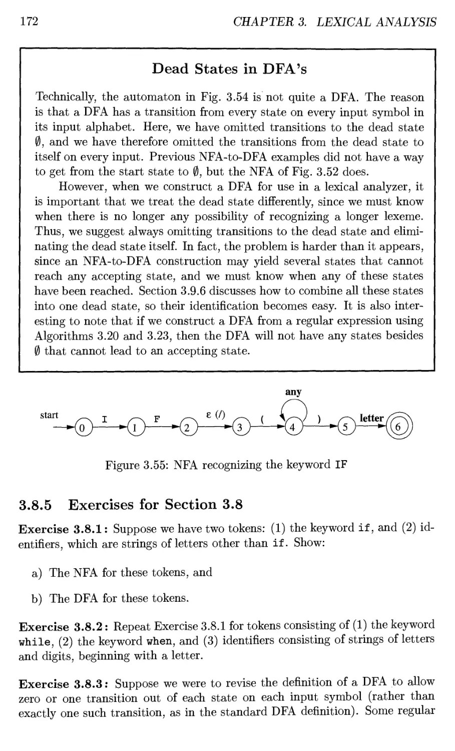
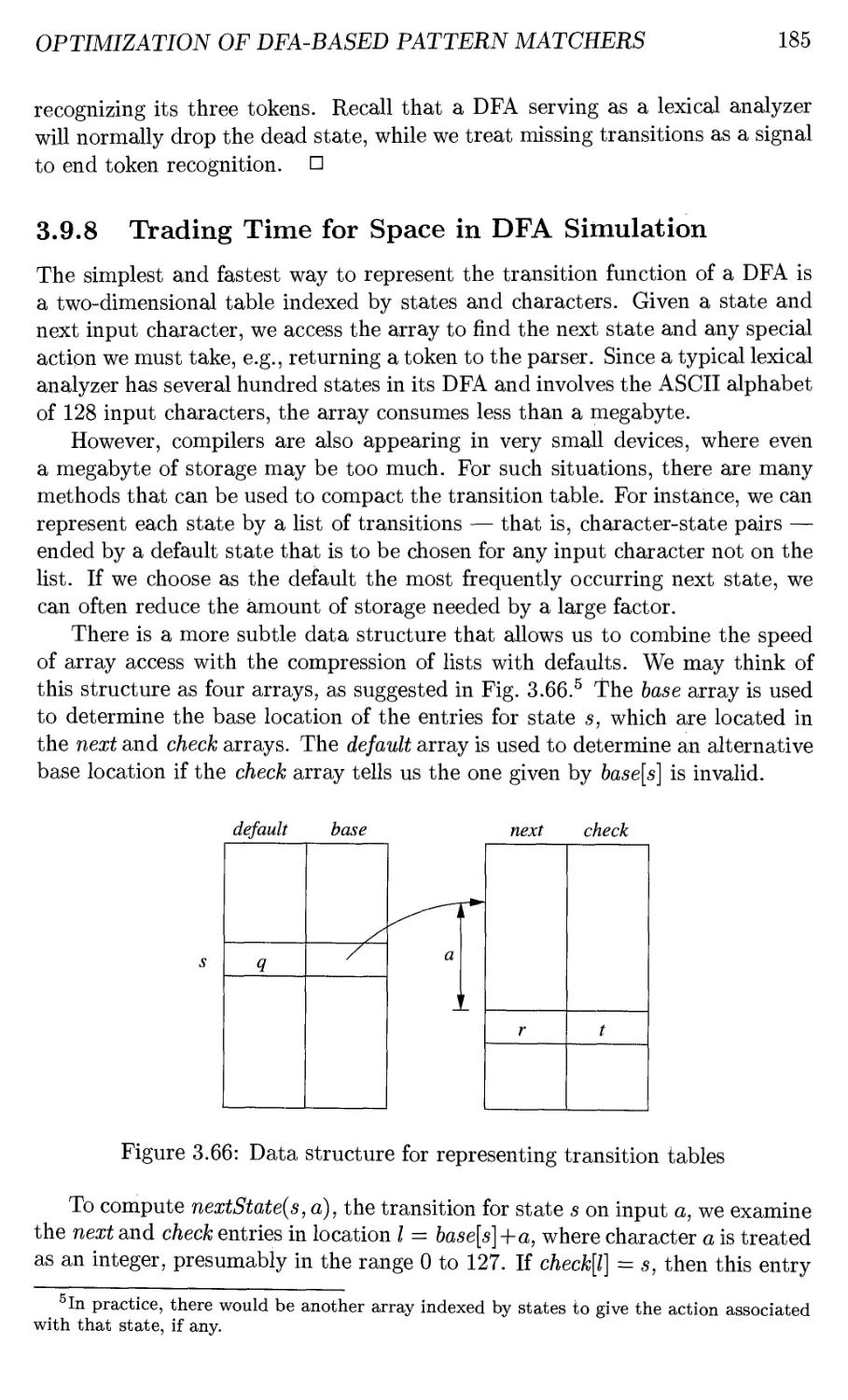
/


Author: Aho A.V. Lam M.S. Sethi R. Ullman J.D.
Tags: programming computer science machine code compilation
ISBN: 0-321-48681-1
Year: 2007


Text
Compilers
Principles, Techniques, & Tools
Second Edition
Sgntax
Alfred V. Aho
Monica S. Lam
Ravi Sethi
Jeffrey D. Ullman
Compilers
Principles, Techniques, & Tools
Second Edition
Alfred V. Aho
Columbia University
Monica S. Lam
Stanford University
Ravi Sethi
Avaya
Jeffrey D. Ullman
Stanford University
PEARSON
Addison
Wesley
Boston San Francisco New York
London Toronto Sydney Tokyo Singapore Madrid
Mexico City Munich Paris Cape Town Hong Kong Montreal
Publisher Greg Tobin
Executive Editor Michael Hirsch
Acquisitions Editor Matt Goldstein
Project Editor Katherine Harutunian
Associate Managing Editor Jeffrey Holcomb
Cover Designer Joyce Cosentino Wells
Digital Assets Manager Marianne Groth
Media Producer Bethany Tidd
Senior Marketing Manager Michelle Brown
Marketing Assistant Sarah Milmore
Senior Author Support/
Technology Specialist Joe Vetere
Senior Manufacturing Buyer Carol Melville
Cover Image Scott Ullman of Strange Tonic Productions
(www.strangetonic.com)
Many of the designations used by manufacturers and sellers to distinguish their
products are claimed as trademarks. Where those designations appear in this
book, and Addison-Wesley was aware of a trademark claim, the designations
have been printed in initial caps or all caps.
This interior of this book was composed in LATEX.
Library of Congress Cataloging-in-Publication Data
Compilers : principles, techniques, and tools I Alfred V. Aho ... [et al.]. -- 2nd ed.
p. cm.
Rev. ed. of: Compilers, principles, techniques, and tools I Alfred V. Aho, Ravi
Sethi, Jeffrey D. Ullman. 1986.
ISBN 0-321-48681-1 (alk. paper)
1. Compilers (Computer programs) I. Aho, Alfred V. II. Aho, Alfred V.
Compilers, principles, techniques, and tools.
QA76.76.C65A37 2007
005.4'53~dc22
2006024333
Copyright © 2007 Pearson Education, Inc. All rights reserved. No part of this
publication may be reproduced, stored in a retrieval system, or transmitted, in
any form or by any means, electronic, mechanical, photocopying, recording, or
otherwise, without the prior written permission of the publisher. Printed in the
United States of America. For information on obtaining permission for use of
material in this work, please submit a written request to Pearson Education,
Inc., Rights and Contracts Department, 75 Arlington Street, Suite 300, Boston,
MA 02116, fax your request to 617-848-7047, or e-mail at
http://www.pearsoned.com/legal/permissions.htm.
Preface
In the time since the 1986 edition of this book, the world of compiler design
has changed significantly. Programming languages have evolved to present new
compilation problems. Computer architectures offer a variety of resources of
which the compiler designer must take advantage. Perhaps most interestingly,
the venerable technology of code optimization has found use outside compilers.
It is now used in tools that find bugs in software, and most importantly, find
security holes in existing code. And much of the "front-end" technology —
grammars, regular expressions, parsers, and syntax-directed translators — are
still in wide use.
Thus, our philosophy from previous versions of the book has not changed.
We recognize that few readers will build, or even maintain, a compiler for a
major programming language. Yet the models, theory, and algorithms
associated with a compiler can be applied to a wide range of problems in software
design and software development. We therefore emphasize problems that are
most commonly encountered in designing a language processor, regardless of
the source language or target machine.
Use of the Book
It takes at least two quarters or even two semesters to cover all or most of the
material in this book. It is common to cover the first half in an undergraduate
course and the second half of the book — stressing code optimization — in
a second course at the graduate or mezzanine level. Here is an outline of the
chapters:
Chapter 1 contains motivational material and also presents some background
issues in computer architecture and programming-language principles.
Chapter 2 develops a miniature compiler and introduces many of the
important concepts, which are then developed in later chapters. The compiler itself
appears in the appendix.
Chapter 3 covers lexical analysis, regular expressions, finite-state machines, and
scanner-generator tools. This material is fundamental to text-processing of all
sorts.
v
VI
PREFACE
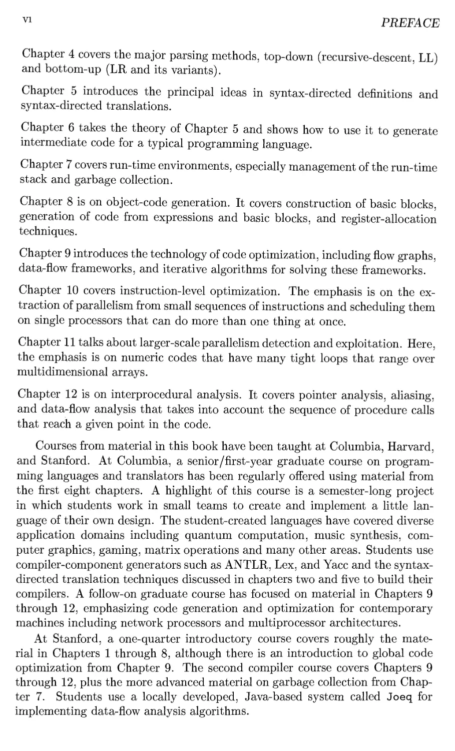
Chapter 4 covers the major parsing methods, top-down (recursive-descent, LL)
and bottom-up (LR and its variants).
Chapter 5 introduces the principal ideas in syntax-directed definitions and
syntax-directed translations.
Chapter 6 takes the theory of Chapter 5 and shows how to use it to generate
intermediate code for a typical programming language.
Chapter 7 covers run-time environments, especially management of the run-time
stack and garbage collection.
Chapter 8 is on object-code generation. It covers construction of basic blocks,
generation of code from expressions and basic blocks, and register-allocation
techniques.
Chapter 9 introduces the technology of code optimization, including flow graphs,
data-flow frameworks, and iterative algorithms for solving these frameworks.
Chapter 10 covers instruction-level optimization. The emphasis is on the
extraction of parallelism from small sequences of instructions and scheduling them
on single processors that can do more than one thing at once.
Chapter 11 talks about larger-scale parallelism detection and exploitation. Here,
the emphasis is on numeric codes that have many tight loops that range over
multidimensional arrays.
Chapter 12 is on interprocedural analysis. It covers pointer analysis, aliasing,
and data-flow analysis that takes into account the sequence of procedure calls
that reach a given point in the code.
Courses from material in this book have been taught at Columbia, Harvard,
and Stanford. At Columbia, a senior /first-year graduate course on
programming languages and translators has been regularly offered using material from
the first eight chapters. A highlight of this course is a semester-long project
in which students work in small teams to create and implement a little
language of their own design. The student-created languages have covered diverse
application domains including quantum computation, music synthesis,
computer graphics, gaming, matrix operations and many other areas. Students use
compiler-component generators such as ANTLR, Lex, and Yacc and the syntax-
directed translation techniques discussed in chapters two and five to build their
compilers. A follow-on graduate course has focused on material in Chapters 9
through 12, emphasizing code generation and optimization for contemporary
machines including network processors and multiprocessor architectures.
At Stanford, a one-quarter introductory course covers roughly the
material in Chapters 1 through 8, although there is an introduction to global code
optimization from Chapter 9. The second compiler course covers Chapters 9
through 12, plus the more advanced material on garbage collection from
Chapter 7. Students use a locally developed, Java-based system called Joeq for
implementing data-flow analysis algorithms.
PREFACE
vn
Prerequisites
The reader should possess some "computer-science sophistication," including
at least a second course on programming, and courses in data structures and
discrete mathematics. Knowledge of several different programming languages
is useful.
Exercises
The book contains extensive exercises, with some for almost every section. We
indicate harder exercises or parts of exercises with an exclamation point. The
hardest exercises have a double exclamation point.
Gradiance On-Line Homeworks
A feature of the new edition is that there is an accompanying set of on-line
homeworks using a technology developed by Gradiance Corp. Instructors may
assign these homeworks to their class, or students not enrolled in a class may
enroll in an "omnibus class" that allows them to do the homeworks as a tutorial
(without an instructor-created class). Gradiance questions look like ordinary
questions, but your solutions are sampled. If you make an incorrect choice you
are given specific advice or feedback to help you correct your solution. If your
instructor permits, you are allowed to try again, until you get a perfect score.
A subscription to the Gradiance service is offered with all new copies of this
text sold in North America. For more information, visit the Addison-Wesley
web site www.aw.com/gradiance or send email to computing@aw.com.
Support on the World Wide Web
The book's home page is
dragonbook. Stanford.edu
Here, you will find errata as we learn of them, and backup materials. We hope
to make available the notes for each offering of compiler-related courses as we
teach them, including homeworks, solutions, and exams. We also plan to post
descriptions of important compilers written by their implementers.
Acknowledgements
Cover art is by S. D. Ullman of Strange Tonic Productions.
Jon Bentley gave us extensive comments on a number of chapters of an
earlier draft of this book. Helpful comments and errata were received from:
Vlll
PREFACE
Domenico Bianculli, Peter Bosch, Marcio Buss, Marc Eaddy, Stephen Edwards,
Vibhav Garg, Kim Hazelwood, Gaurav Kc, Wei Li, Mike Smith, Art Stamness,
Krysta Svore, Olivier Tardieu, and Jia Zeng. The help of all these people is
gratefully acknowledged. Remaining errors are ours, of course.
In addition, Monica would like to thank her colleagues on the SUIF
compiler team for an 18-year lesson on compiling: Gerald Aigner, Dzintars Avots,
Saman Amarasinghe, Jennifer Anderson, Michael Carbin, Gerald Cheong, Amer
Diwan, Robert French, Anwar Ghuloum, Mary Hall, John Hennessy, David
Heine, Shih-Wei Liao, Amy Lim, Benjamin Livshits, Michael Martin, Dror
Maydan, Todd Mowry, Brian Murphy, Jeffrey Oplinger, Karen Pieper,
Martin Rinard, Olatunji Ruwase, Constantine Sapuntzakis, Patrick Sathyanathan,
Michael Smith, Steven Tjiang, Chau-Wen Tseng, Christopher Unkel, John
Whaley, Robert Wilson, Christopher Wilson, and Michael Wolf.
A. V. A., Chatham NJ
M. S. L., Menlo Park CA
R. S., Far Hills NJ
J. D. U., Stanford CA
June, 2006
Table of Contents
1 Introduction 1
1.1 Language Processors 1
1.1.1 Exercises for Section 1.1 3
1.2 The Structure of a Compiler 4
1.2.1 Lexical Analysis 5
1.2.2 Syntax Analysis 8
1.2.3 Semantic Analysis 8
1.2.4 Intermediate Code Generation 9
1.2.5 Code Optimization 10
1.2.6 Code Generation 10
1.2.7 Symbol-Table Management 11
1.2.8 The Grouping of Phases into Passes 11
1.2.9 Compiler-Construction Tools 12
1.3 The Evolution of Programming Languages 12
1.3.1 The Move to Higher-level Languages 13
1.3.2 Impacts on Compilers 14
1.3.3 Exercises for Section 1.3 14
1.4 The Science of Building a Compiler 15
1.4.1 Modeling in Compiler Design and Implementation .... 15
1.4.2 The Science of Code Optimization 15
1.5 Applications of Compiler Technology 17
1.5.1 Implementation of High-Level Programming Languages . 17
1.5.2 Optimizations for Computer Architectures 19
1.5.3 Design of New Computer Architectures 21
1.5.4 Program Translations 22
1.5.5 Software Productivity Tools 23
1.6 Programming Language Basics 25
1.6.1 The Static/Dynamic Distinction 25
1.6.2 Environments and States 26
1.6.3 Static Scope and Block Structure 28
1.6.4 Explicit Access Control 31
1.6.5 Dynamic Scope 31
1.6.6 Parameter Passing Mechanisms 33
ix
x TABLE OF CONTENTS
1.6.7 Aliasing 35
1.6.8 Exercises for Section 1.6 35
1.7 Summary of Chapter 1 36
1.8 References for Chapter 1 38
2 A Simple Syntax-Directed Translator 39
2.1 Introduction 40
2.2 Syntax Definition 42
2.2.1 Definition of Grammars 42
2.2.2 Derivations 44
2.2.3 Parse Trees 45
2.2.4 Ambiguity 47
2.2.5 Associativity of Operators 48
2.2.6 Precedence of Operators 48
2.2.7 Exercises for Section 2.2 51
2.3 Syntax-Directed Translation 52
2.3.1 Postfix Notation 53
2.3.2 Synthesized Attributes 54
2.3.3 Simple Syntax-Directed Definitions 56
2.3.4 Tree Traversal 56
2.3.5 Translation Schemes 57
2.3.6 Exercises for Section 2.3 60
2.4 Parsing 60
2.4.1 Top-Down Parsing 61
2.4.2 Predictive Parsing 64
2.4.3 When to Use e-Productions 65
2.4.4 Designing a Predictive Parser 66
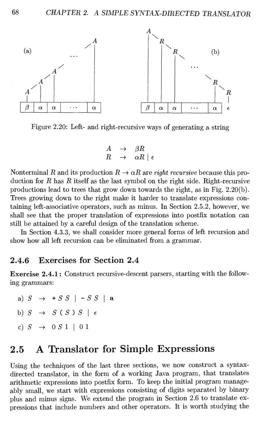
2.4.5 Left Recursion 67
2.4.6 Exercises for Section 2.4 68
2.5 A Translator for Simple Expressions 68
2.5.1 Abstract and Concrete Syntax 69
2.5.2 Adapting the Translation Scheme 70
2.5.3 Procedures for the Nonterminals 72
2.5.4 Simplifying the Translator 73
2.5.5 The Complete Program 74
2.6 Lexical Analysis 76
2.6.1 Removal of White Space and Comments 77
2.6.2 Reading Ahead 78
2.6.3 Constants 78
2.6.4 Recognizing Keywords and Identifiers 79
2.6.5 A Lexical Analyzer 81
2.6.6 Exercises for Section 2.6 84
2.7 Symbol Tables 85
2.7.1 Symbol Table Per Scope 86
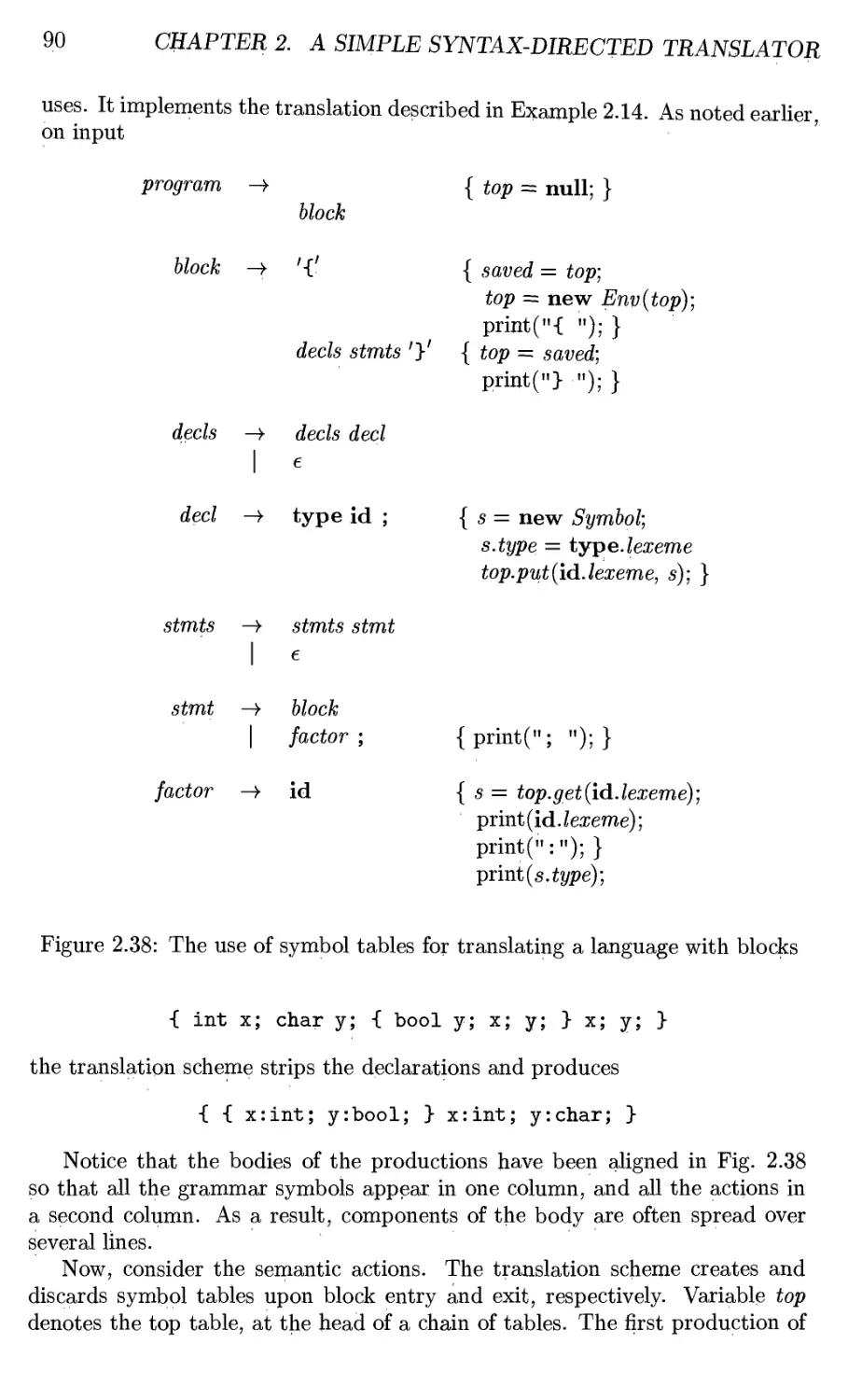
2.7.2 The Use of Symbol Tables 89
TABLE OF CONTENTS xi
2.8 Intermediate Code Generation 91
2.8.1 Two Kinds of Intermediate Representations 91
2.8.2 Construction of Syntax Trees 92
2.8.3 Static Checking 97
2.8.4 Three-Address Code 99
2.8.5 Exercises for Section 2.8 105
2.9 Summary of Chapter 2 105
3 Lexical Analysis 109
3.1 The Role of the Lexical Analyzer 109
3.1.1 Lexical Analysis Versus Parsing 110
3.1.2 Tokens, Patterns, and Lexemes Ill
3.1.3 Attributes for Tokens 112
3.1.4 Lexical Errors 113
3.1.5 Exercises for Section 3.1 114
3.2 Input Buffering 115
3.2.1 Buffer Pairs 115
3.2.2 Sentinels 116
3.3 Specification of Tokens 116
3.3.1 Strings and Languages 117
3.3.2 Operations on Languages 119
3.3.3 Regular Expressions 120
3.3.4 Regular Definitions 123
3.3.5 Extensions of Regular Expressions 124
3.3.6 Exercises for Section 3.3 125
3.4 Recognition of Tokens 128
3.4.1 Transition Diagrams 130
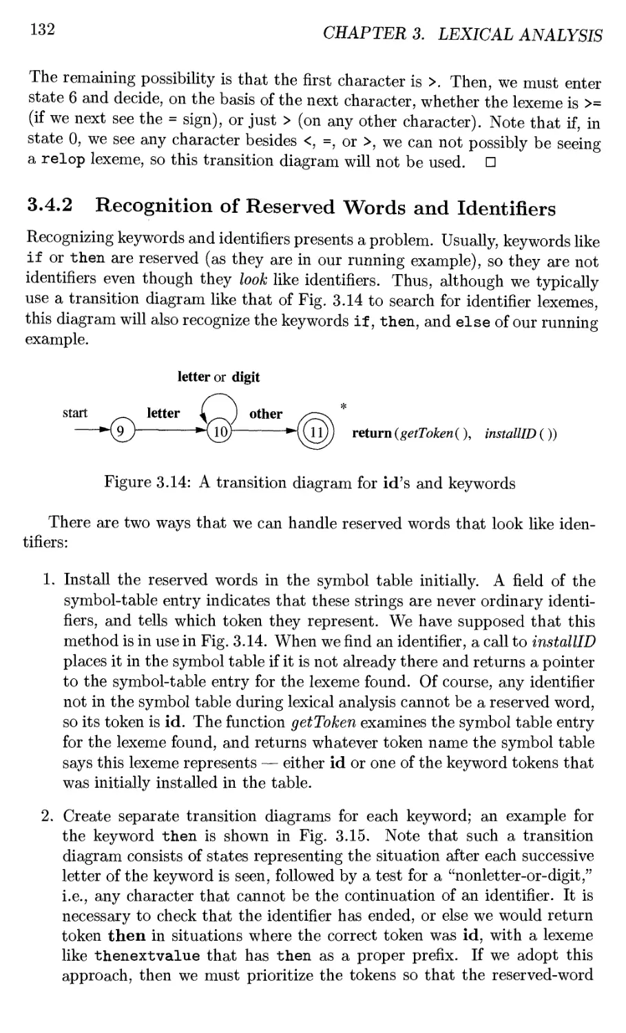
3.4.2 Recognition of Reserved Words and Identifiers 132
3.4.3 Completion of the Running Example 133
3.4.4 Architecture of a Transition-Diagram-Based Lexical
Analyzer 134
3.4.5 Exercises for Section 3.4 136
3.5 The Lexical-Analyzer Generator Lex 140
3.5.1 Use of Lex 140
3.5.2 Structure of Lex Programs 141
3.5.3 Conflict Resolution in Lex 144
3.5.4 The Lookahead Operator 144
3.5.5 Exercises for Section 3.5 146
3.6 Finite Automata 147
3.6.1 Nondeterministic Finite Automata 147
3.6.2 Transition Tables 148
3.6.3 Acceptance of Input Strings by Automata 149
3.6.4 Deterministic Finite Automata 149
3.6.5 Exercises for Section 3.6 151
3.7 From Regular Expressions to Automata 152
Xll
TABLE OF CONTENTS
3.7.1 Conversion of an NFA to a DFA 152
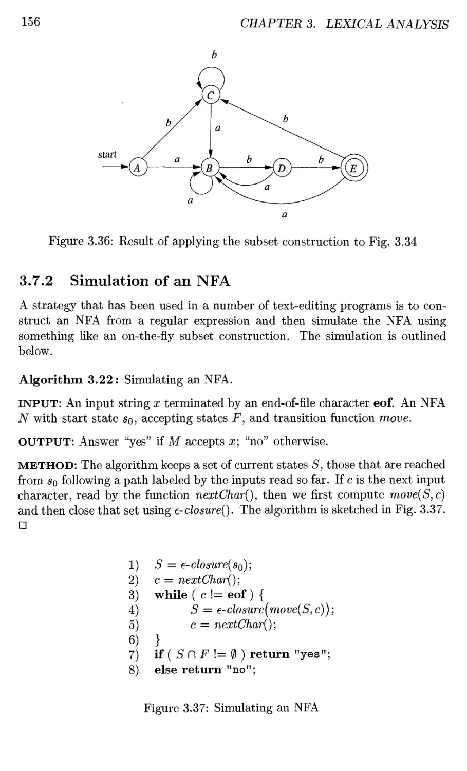
3.7.2 Simulation of an NFA 156
3.7.3 Efficiency of NFA Simulation 157
3.7.4 Construction of an NFA from a Regular Expression . . . 159
3.7.5 Efficiency of String-Processing Algorithms 163
3.7.6 Exercises for Section 3.7 166
3.8 Design of a Lexical-Analyzer Generator 166
3.8.1 The Structure of the Generated Analyzer 167
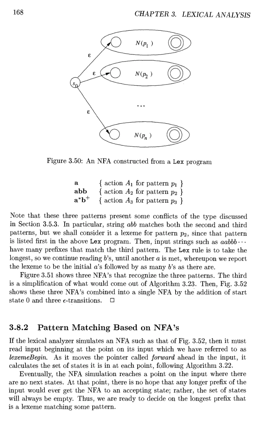
3.8.2 Pattern Matching Based on NFA's 168
3.8.3 DFA's for Lexical Analyzers 170
3.8.4 Implementing the Lookahead Operator 171
3.8.5 Exercises for Section 3.8 172
3.9 Optimization of DFA-Based Pattern Matchers 173
3.9.1 Important States of an NFA 173
3.9.2 Functions Computed From the Syntax Tree 175
3.9.3 Computing unliable, firstpos, and lastpos 176
3.9.4 Computing followpos 177
3.9.5 Converting a Regular Expression Directly to a DFA . . . 179
3.9.6 Minimizing the Number of States of a DFA 180
3.9.7 State Minimization in Lexical Analyzers 184
3.9.8 Trading Time for Space in DFA Simulation 185
3.9.9 Exercises for Section 3.9 186
3.10 Summary of Chapter 3 187
3.11 References for Chapter 3 189
4 Syntax Analysis 191
4.1 Introduction 192
4.1.1 The Role of the Parser 192
4.1.2 Representative Grammars 193
4.1.3 Syntax Error Handling 194
4.1.4 Error-Recovery Strategies 195
4.2 Context-Free Grammars 197
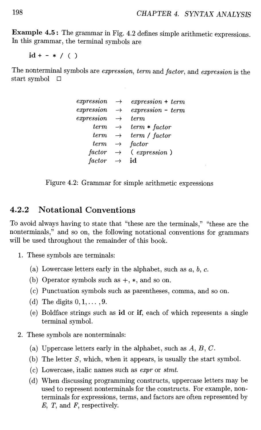
4.2.1 The Formal Definition of a Context-Free Grammar .... 197
4.2.2 Notational Conventions 198
4.2.3 Derivations 199
4.2.4 Parse Trees and Derivations 201
4.2.5 Ambiguity 203
4.2.6 Verifying the Language Generated by a Grammar .... 204
4.2.7 Context-Free Grammars Versus Regular Expressions . . . 205
4.2.8 Exercises for Section 4.2 206
4.3 Writing a Grammar 209
4.3.1 Lexical Versus Syntactic Analysis 209
4.3.2 Eliminating Ambiguity 210
4.3.3 Elimination of Left Recursion 212
4.3.4 Left Factoring 214
TABLE OF CONTENTS xin
4.3.5 Non-Context-Free Language Constructs 215
4.3.6 Exercises for Section 4.3 216
4.4 Top-Down Parsing 217
4.4.1 Recursive-Descent Parsing 219
4.4.2 FIRST and FOLLOW 220
4.4.3 LL(1) Grammars 222
4.4.4 Nonrecursive Predictive Parsing 226
4.4.5 Error Recovery in Predictive Parsing 228
4.4.6 Exercises for Section 4.4 231
4.5 Bottom-Up Parsing 233
4.5.1 Reductions 234
4.5.2 Handle Pruning 235
4.5.3 Shift-Reduce Parsing 236
4.5.4 Conflicts During Shift-Reduce Parsing 238
4.5.5 Exercises for Section 4.5 240
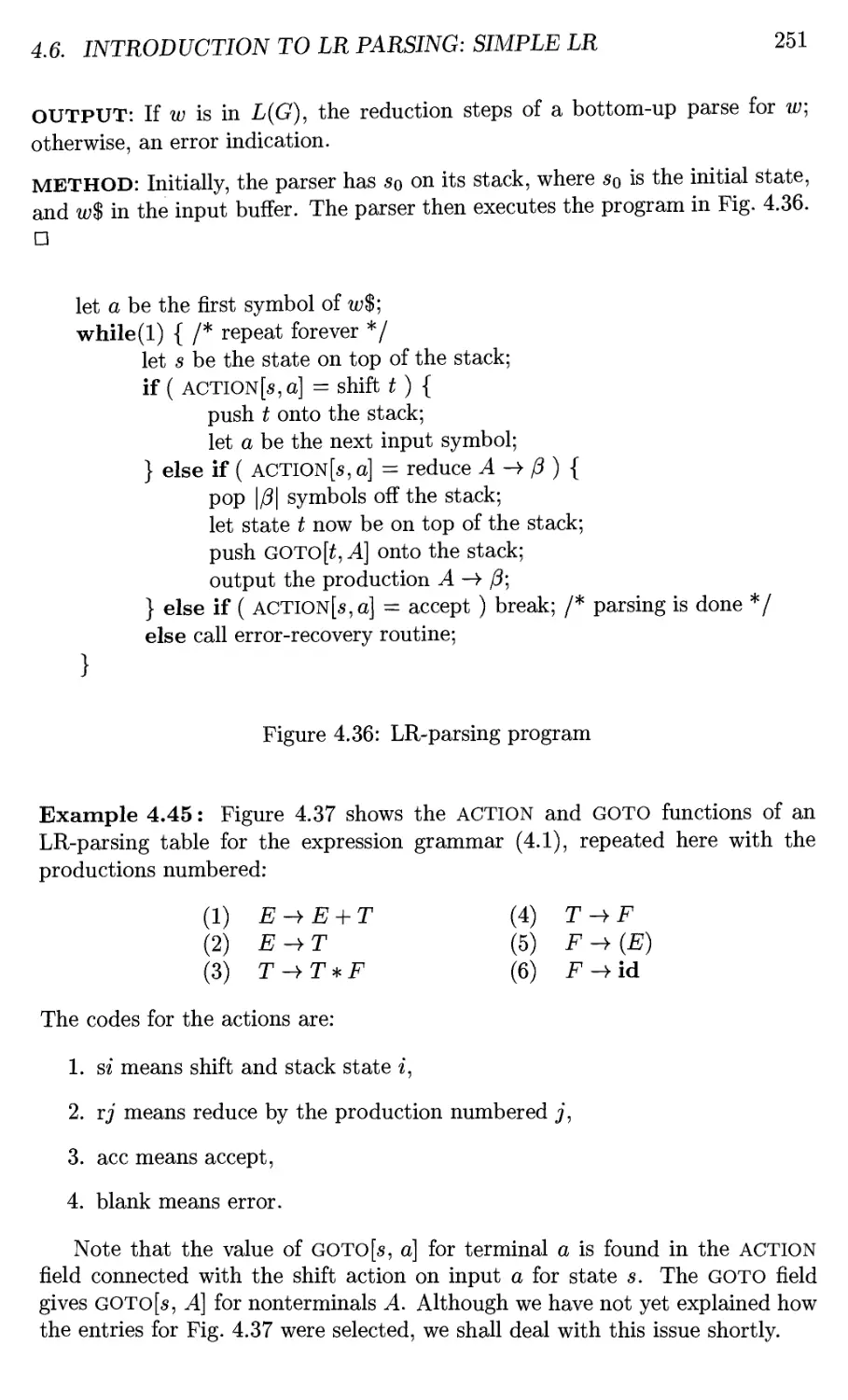
4.6 Introduction to LR Parsing: Simple LR 241
4.6.1 Why LR Parsers? 241
4.6.2 Items and the LR(0) Automaton 242
4.6.3 The LR-Parsing Algorithm 248
4.6.4 Constructing SLR-Parsing Tables 252
4.6.5 Viable Prefixes 256
4.6.6 Exercises for Section 4.6 257
4.7 More Powerful LR Parsers 259
4.7.1 Canonical LR(1) Items 260
4.7.2 Constructing LR(1) Sets of Items 261
4.7.3 Canonical LR(1) Parsing Tables 265
4.7.4 Constructing LALR Parsing Tables 266
4.7.5 Efficient Construction of LALR Parsing Tables 270
4.7.6 Compaction of LR Parsing Tables 275
4.7.7 Exercises for Section 4.7 277
4.8 Using Ambiguous Grammars 278
4.8.1 Precedence and Associativity to Resolve Conflicts .... 279
4.8.2 The "Dangling-Else" Ambiguity 281
4.8.3 Error Recovery in LR Parsing 283
4.8.4 Exercises for Section 4.8 285
4.9 Parser Generators 287
4.9.1 The Parser Generator Yacc 287
4.9.2 Using Yacc with Ambiguous Grammars 291
4.9.3 Creating Yacc Lexical Analyzers with Lex 294
4.9.4 Error Recovery in Yacc 295
4.9.5 Exercises for Section 4.9 297
4.10 Summary of Chapter 4 297
4.11 References for Chapter 4 300
XIV
TABLE OF CONTENTS
5 Syntax-Directed Translation 303
5.1 Syntax-Directed Definitions 304
5.1.1 Inherited and Synthesized Attributes 304
5.1.2 Evaluating an SDD at the Nodes of a Parse Tree 306
5.1.3 Exercises for Section 5.1 309
5.2 Evaluation Orders for SDD's 310
5.2.1 Dependency Graphs 310
5.2.2 Ordering the Evaluation of Attributes 312
5.2.3 S-Attributed Definitions 312
5.2.4 L-Attributed Definitions 313
5.2.5 Semantic Rules with Controlled Side Effects 314
5.2.6 Exercises for Section 5.2 317
5.3 Applications of Syntax-Directed Translation 318
5.3.1 Construction of Syntax Trees 318
5.3.2 The Structure of a Type 321
5.3.3 Exercises for Section 5.3 323
5.4 Syntax-Directed Translation Schemes 324
5.4.1 Postfix Translation Schemes 324
5.4.2 Parser-Stack Implementation of Postfix SDT's 325
5.4.3 SDT's With Actions Inside Productions 327
5.4.4 Eliminating Left Recursion From SDT's 328
5.4.5 SDT's for L-Attributed Definitions 331
5.4.6 Exercises for Section 5.4 336
5.5 Implementing L-Attributed SDD's 337
5.5.1 Translation During Recursive-Descent Parsing 338
5.5.2 On-The-Fly Code Generation 340
5.5.3 L-Attributed SDD's and LL Parsing 343
5.5.4 Bottom-Up Parsing of L-Attributed SDD's 348
5.5.5 Exercises for Section 5.5 352
5.6 Summary of Chapter 5 353
5.7 References for Chapter 5 354
6 Intermediate-Code Generation 357
6.1 Variants of Syntax Trees 358
6.1.1 Directed Acyclic Graphs for Expressions 359
6.1.2 The Value-Number Method for Constructing DAG's . . . 360
6.1.3 Exercises for Section 6.1 362
6.2 Three-Address Code 363
6.2.1 Addresses and Instructions 364
6.2.2 Quadruples 366
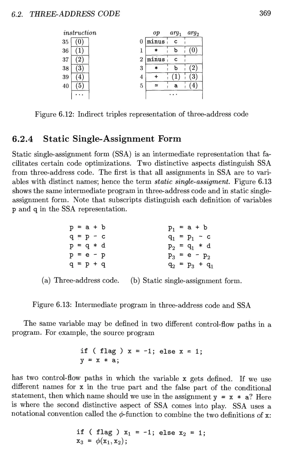
6.2.3 Triples 367
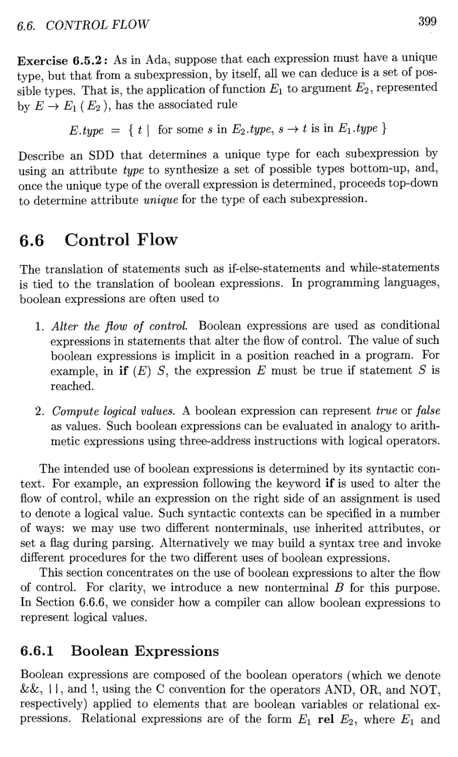
6.2.4 Static Single-Assignment Form 369
6.2.5 Exercises for Section 6.2 370
6.3 Types and Declarations 370
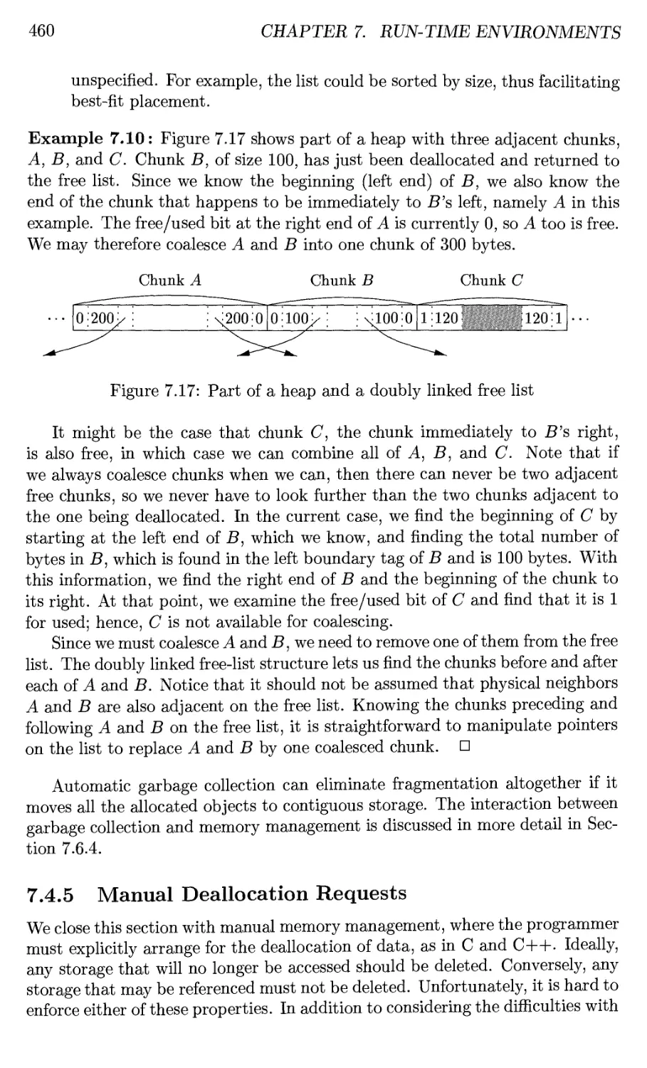
6.3.1 Type Expressions 371
TABLE OF CONTENTS xv
6.3.2 Type Equivalence 372
6.3.3 Declarations 373
6.3.4 Storage Layout for Local Names 373
6.3.5 Sequences of Declarations 376
6.3.6 Fields in Records and Classes 376
6.3.7 Exercises for Section 6.3 378
6.4 Translation of Expressions 378
6.4.1 Operations Within Expressions 378
6.4.2 Incremental Translation 380
6.4.3 Addressing Array Elements 381
6.4.4 Translation of Array References 383
6.4.5 Exercises for Section 6.4 384
6.5 Type Checking 386
6.5.1 Rules for Type Checking 387
6.5.2 Type Conversions 388
6.5.3 Overloading of Functions and Operators 390
6.5.4 Type Inference and Polymorphic Functions 391
6.5.5 An Algorithm for Unification 395
6.5.6 Exercises for Section 6.5 398
6.6 Control Flow 399
6.6.1 Boolean Expressions 399
6.6.2 Short-Circuit Code 400
6.6.3 Flow-of-Control Statements 401
6.6.4 Control-Flow Translation of Boolean Expressions 403
6.6.5 Avoiding Redundant Gotos 405
6.6.6 Boolean Values and Jumping Code 408
6.6.7 Exercises for Section 6.6 408
6.7 Backpatching 410
6.7.1 One-Pass Code Generation Using Backpatching 410
6.7.2 Backpatching for Boolean Expressions 411
6.7.3 Flow-of-Control Statements 413
6.7.4 Break-, Continue-, and Goto-Statements 416
6.7.5 Exercises for Section 6.7 417
6.8 Switch-Statements 418
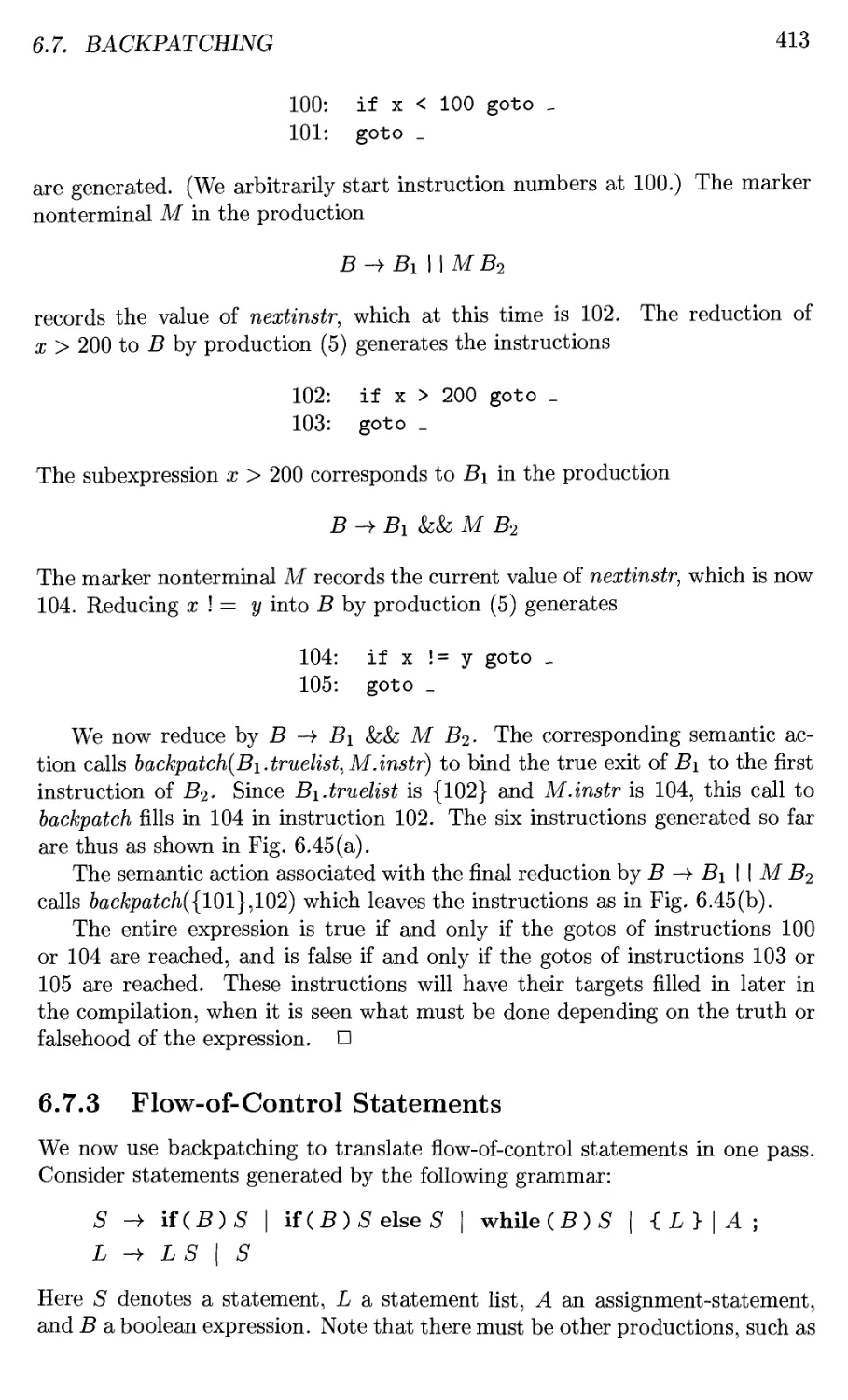
6.8.1 Translation of Switch-Statements 419
6.8.2 Syntax-Directed Translation of Switch-Statements .... 420
6.8.3 Exercises for Section 6.8 421
6.9 Intermediate Code for Procedures 422
6.10 Summary of Chapter 6 424
6.11 References for Chapter 6 425
TABLE OF
Run-Time Environments 427
7.1 Storage Organization 427
7.1.1 Static Versus Dynamic Storage Allocation 429
7.2 Stack Allocation of Space 430
7.2.1 Activation Trees 430
7.2.2 Activation Records 433
7.2.3 Calling Sequences 436
7.2.4 Variable-Length Data on the Stack 438
7.2.5 Exercises for Section 7.2 440
7.3 Access to Nonlocal Data on the Stack 441
7.3.1 Data Access Without Nested Procedures 442
7.3.2 Issues With Nested Procedures 442
7.3.3 A Language With Nested Procedure Declarations 443
7.3.4 Nesting Depth 443
7.3.5 Access Links 445
7.3.6 Manipulating Access Links 447
7.3.7 Access Links for Procedure Parameters 448
7.3.8 Displays 449
7.3.9 Exercises for Section 7.3 451
7.4 Heap Management 452
7.4.1 The Memory Manager 453
7.4.2 The Memory Hierarchy of a Computer 454
7.4.3 Locality in Programs 455
7.4.4 Reducing Fragmentation 457
7.4.5 Manual Deallocation Requests 460
7.4.6 Exercises for Section 7.4 463
7.5 Introduction to Garbage Collection 463
7.5.1 Design Goals for Garbage Collectors 464
7.5.2 Reachability 466
7.5.3 Reference Counting Garbage Collectors 468
7.5.4 Exercises for Section 7.5 470
7.6 Introduction to Trace-Based Collection 470
7.6.1 A Basic Mark-and-Sweep Collector 471
7.6.2 Basic Abstraction 473
7.6.3 Optimizing Mark-and-Sweep 475
7.6.4 Mark-and-Compact Garbage Collectors 476
7.6.5 Copying collectors 478
7.6.6 Comparing Costs 482
7.6.7 Exercises for Section 7.6 482
7.7 Short-Pause Garbage Collection 483
7.7.1 Incremental Garbage Collection 483
7.7.2 Incremental Reachability Analysis 485
7.7.3 Partial-Collection Basics 487
7.7.4 Generational Garbage Collection 488
7.7.5 The Train Algorithm 490
TABLE OF CONTENTS xvu
7.7.6 Exercises for Section 7.7 493
7.8 Advanced Topics in Garbage Collection 494
7.8.1 Parallel and Concurrent Garbage Collection 495
7.8.2 Partial Object Relocation 497
7.8.3 Conservative Collection for Unsafe Languages 498
7.8.4 Weak References 498
7.8.5 Exercises for Section 7.8 499
7.9 Summary of Chapter 7 500
7.10 References for Chapter 7 502
8 Code Generation 505
8.1 Issues in the Design of a Code Generator 506
8.1.1 Input to the Code Generator 507
8.1.2 The Target Program 507
8.1.3 Instruction Selection 508
8.1.4 Register Allocation 510
8.1.5 Evaluation Order 511
8.2 The Target Language 512
8.2.1 A Simple Target Machine Model 512
8.2.2 Program and Instruction Costs 515
8.2.3 Exercises for Section 8.2 516
8.3 Addresses in the Target Code 518
8.3.1 Static Allocation 518
8.3.2 Stack Allocation 520
8.3.3 Run-Time Addresses for Names 522
8.3.4 Exercises for Section 8.3 524
8.4 Basic Blocks and Flow Graphs 525
8.4.1 Basic Blocks 526
8.4.2 Next-Use Information 528
8.4.3 Flow Graphs 529
8.4.4 Representation of Flow Graphs 530
8.4.5 Loops 531
8.4.6 Exercises for Section 8.4 531
8.5 Optimization of Basic Blocks 533
8.5.1 The DAG Representation of Basic Blocks 533
8.5.2 Finding Local Common Subexpressions 534
8.5.3 Dead Code Elimination 535
8.5.4 The Use of Algebraic Identities 536
8.5.5 Representation of Array References 537
8.5.6 Pointer Assignments and Procedure Calls 539
8.5.7 Reassembling Basic Blocks From DAG's 539
8.5.8 Exercises for Section 8.5 541
8.6 A Simple Code Generator 542
8.6.1 Register and Address Descriptors 543
8.6.2 The Code-Generation Algorithm 544
XV111
TABLE OF CONTENTS
8.6.3 Design of the Function getReg 547
8.6.4 Exercises for Section 8.6 548
8.7 Peephole Optimization 549
8.7.1 Eliminating Redundant Loads and Stores 550
8.7.2 Eliminating Unreachable Code 550
8.7.3 Flow-of-Control Optimizations 551
8.7.4 Algebraic Simplification and Reduction in Strength .... 552
8.7.5 Use of Machine Idioms 552
8.7.6 Exercises for Section 8.7 553
8.8 Register Allocation and Assignment 553
8.8.1 Global Register Allocation 553
8.8.2 Usage Counts 554
8.8.3 Register Assignment for Outer Loops 556
8.8.4 Register Allocation by Graph Coloring 556
8.8.5 Exercises for Section 8.8 557
8.9 Instruction Selection by Tree Rewriting 558
8.9.1 Tree-Translation Schemes 558
8.9.2 Code Generation by Tiling an Input Tree 560
8.9.3 Pattern Matching by Parsing 563
8.9.4 Routines for Semantic Checking 565
8.9.5 General Tree Matching 565
8.9.6 Exercises for Section 8.9 567
8.10 Optimal Code Generation for Expressions 567
8.10.1 Ershov Numbers 567
8.10.2 Generating Code From Labeled Expression Trees 568
8.10.3 Evaluating Expressions with an Insufficient Supply of
Registers 570
8.10.4 Exercises for Section 8.10 572
8.11 Dynamic Programming Code-Generation 573
8.11.1 Contiguous Evaluation 574
8.11.2 The Dynamic Programming Algorithm 575
8.11.3 Exercises for Section 8.11 577
8.12 Summary of Chapter 8 578
8.13 References for Chapter 8 579
9 Machine-Independent Optimizations 583
9.1 The Principal Sources of Optimization 584
9.1.1 Causes of Redundancy 584
9.1.2 A Running Example: Quicksort 585
9.1.3 Semantics-Preserving Transformations 586
9.1.4 Global Common Subexpressions 588
9.1.5 Copy Propagation 590
9.1.6 Dead-Code Elimination 591
9.1.7 Code Motion 592
9.1.8 Induction Variables and Reduction in Strength 592
TABLE OF CONTENTS xix
9.1.9 Exercises for Section 9.1 596
9.2 Introduction to Data-Flow Analysis 597
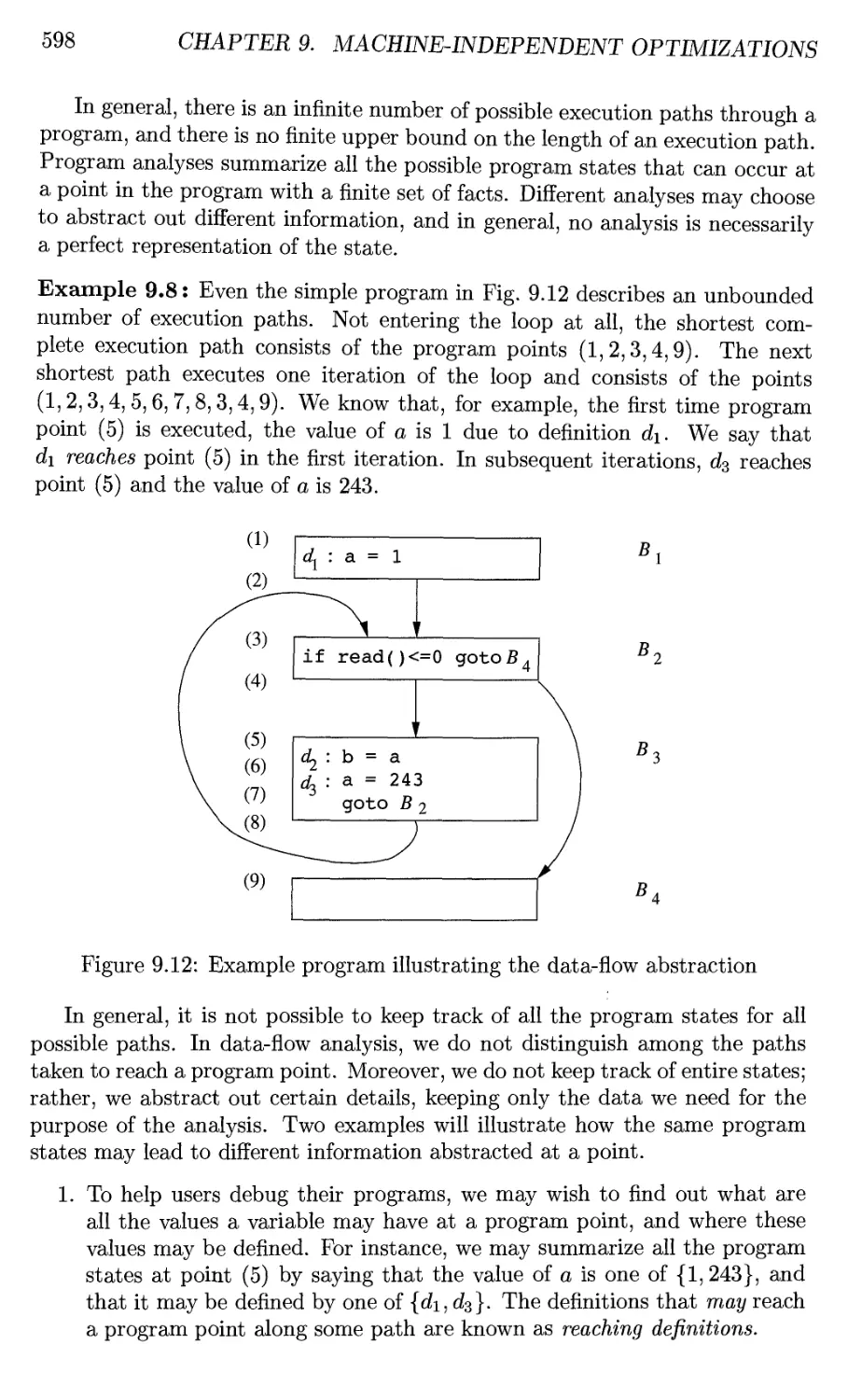
9.2.1 The Data-Flow Abstraction 597
9.2.2 The Data-Flow Analysis Schema 599
9.2.3 Data-Flow Schemas on Basic Blocks 600
9.2.4 Reaching Definitions 601
9.2.5 Live-Variable Analysis 608
9.2.6 Available Expressions 610
9.2.7 Summary 614
9.2.8 Exercises for Section 9.2 615
9.3 Foundations of Data-Flow Analysis 618
9.3.1 Semilattices 618
9.3.2 Transfer Functions 623
9.3.3 The Iterative Algorithm for General Frameworks 626
9.3.4 Meaning of a Data-Flow Solution 628
9.3.5 Exercises for Section 9.3 631
9.4 Constant Propagation 632
9.4.1 Data-Flow Values for the Constant-Propagation
Framework 633
9.4.2 The Meet for the Constant-Propagation Framework . . . 633
9.4.3 Transfer Functions for the Constant-Propagation
Framework 634
9.4.4 Monotonicity of the Constant-Propagation Framework . . 635
9.4.5 Nondistributivity of the Constant-Propagation Framework 635
9.4.6 Interpretation of the Results 637
9.4.7 Exercises for Section 9.4 637
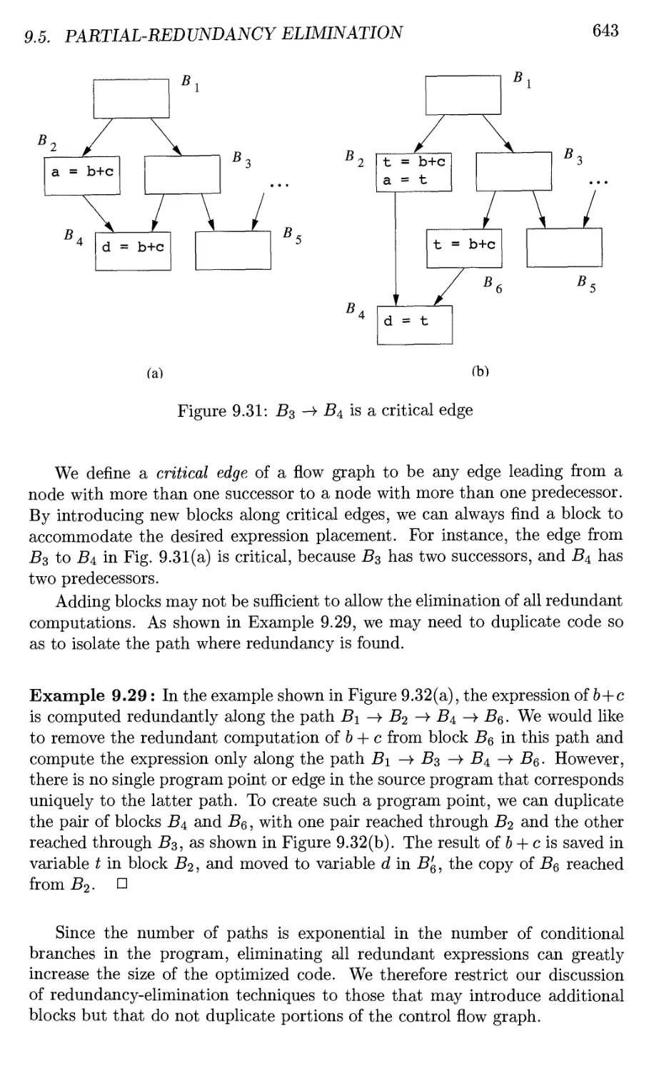
9.5 Partial-Redundancy Elimination 639
9.5.1 The Sources of Redundancy 639
9.5.2 Can All Redundancy Be Eliminated? 642
9.5.3 The Lazy-Code-Motion Problem 644
9.5.4 Anticipation of Expressions 645
9.5.5 The Lazy-Code-Motion Algorithm 646
9.5.6 Exercises for Section 9.5 655
9.6 Loops in Flow Graphs 655
9.6.1 Dominators 656
9.6.2 Depth-First Ordering 660
9.6.3 Edges in a Depth-First Spanning Tree 661
9.6.4 Back Edges and Reducibility 662
9.6.5 Depth of a Flow Graph 665
9.6.6 Natural Loops 665
9.6.7 Speed of Convergence of Iterative Data-Flow Algorithms . 667
9.6.8 Exercises for Section 9.6 669
9.7 Region-Based Analysis 672
9.7.1 Regions 672
9.7.2 Region Hierarchies for Reducible Flow Graphs 673
xx TABLE OF CONTENTS
9.7.3 Overview of a Region-Based Analysis 676
9.7.4 Necessary Assumptions About Transfer Functions .... 678
9.7.5 An Algorithm for Region-Based Analysis 680
9.7.6 Handling Nonreducible Flow Graphs 684
9.7.7 Exercises for Section 9.7 686
9.8 Symbolic Analysis 686
9.8.1 Affine Expressions of Reference Variables 687
9.8.2 Data-Flow Problem Formulation 689
9.8.3 Region-Based Symbolic Analysis 694
9.8.4 Exercises for Section 9.8 699
9.9 Summary of Chapter 9 700
9.10 References for Chapter 9 703
10 Instruction-Level Parallelism 707
10.1 Processor Architectures 708
10.1.1 Instruction Pipelines and Branch Delays 708
10.1.2 Pipelined Execution 709
10.1.3 Multiple Instruction Issue 710
10.2 Code-Scheduling Constraints 710
10.2.1 Data Dependence 711
10.2.2 Finding Dependences Among Memory Accesses 712
10.2.3 Tradeoff Between Register Usage and Parallelism 713
10.2.4 Phase Ordering Between Register Allocation and Code
Scheduling 716
10.2.5 Control Dependence 716
10.2.6 Speculative Execution Support 717
10.2.7 A Basic Machine Model 719
10.2.8 Exercises for Section 10.2 720
10.3 Basic-Block Scheduling 721
10.3.1 Data-Dependence Graphs 722
10.3.2 List Scheduling of Basic Blocks 723
10.3.3 Prioritized Topological Orders 725
10.3.4 Exercises for Section 10.3 726
10.4 Global Code Scheduling 727
10.4.1 Primitive Code Motion 728
10.4.2 Upward Code Motion 730
10.4.3 Downward Code Motion 731
10.4.4 Updating Data Dependences 732
10.4.5 Global Scheduling Algorithms 732
10.4.6 Advanced Code Motion Techniques 736
10.4.7 Interaction with Dynamic Schedulers 737
10.4.8 Exercises for Section 10.4 737
10.5 Software Pipelining 738
10.5.1 Introduction 738
10.5.2 Software Pipelining of Loops 740
TABLE OF CONTENTS xxi
10.5.3 Register Allocation and Code Generation 743
10.5.4 Do-Across Loops 743
10.5.5 Goals and Constraints of Software Pipelining 745
10.5.6 A Software-Pipelining Algorithm 749
10.5.7 Scheduling Acyclic Data-Dependence Graphs 749
10.5.8 Scheduling Cyclic Dependence Graphs 751
10.5.9 Improvements to the Pipelining Algorithms 758
10.5.10Modular Variable Expansion 758
10.5.11 Conditional Statements 761
10.5.12Hardware Support for Software Pipelining 762
10.5.13Exercises for Section 10.5 763
10.6 Summary of Chapter 10 765
10.7 References for Chapter 10 766
11 Optimizing for Parallelism and Locality 769
11.1 Basic Concepts 771
11.1.1 Multiprocessors 772
11.1.2 Parallelism in Applications 773
11.1.3 Loop-Level Parallelism 775
11.1.4 Data Locality 777
11.1.5 Introduction to Affine Transform Theory 778
11.2 Matrix Multiply: An In-Depth Example 782
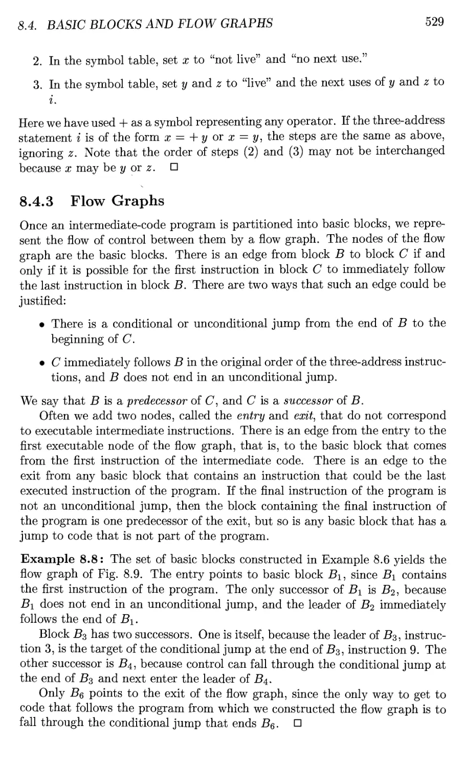
11.2.1 The Matrix-Multiplication Algorithm 782
11.2.2 Optimizations 785
11.2.3 Cache Interference 788
11.2.4 Exercises for Section 11.2 788
11.3 Iteration Spaces 788
11.3.1 Constructing Iteration Spaces from Loop Nests 788
11.3.2 Execution Order for Loop Nests 791
11.3.3 Matrix Formulation of Inequalities 791
11.3.4 Incorporating Symbolic Constants 793
11.3.5 Controlling the Order of Execution 793
11.3.6 Changing Axes 798
11.3.7 Exercises for Section 11.3 799
11.4 Affine Array Indexes 801
11.4.1 Affine Accesses 802
11.4.2 Affine and Nonaffine Accesses in Practice 803
11.4.3 Exercises for Section 11.4 804
11.5 Data Reuse 804
11.5.1 Types of Reuse 805
11.5.2 Self Reuse 806
11.5.3 Self-Spatial Reuse 809
11.5.4 Group Reuse 811
11.5.5 Exercises for Section 11.5 814
11.6 Array Data-Dependence Analysis 815
xxn TABLE OF CONTENTS
11.6.1 Definition of Data Dependence of Array Accesses 816
11.6.2 Integer Linear Programming 817
11.6.3 The GCD Test 818
11.6.4 Heuristics for Solving Integer Linear Programs 820
11.6.5 Solving General Integer Linear Programs 823
11.6.6 Summary 825
11.6.7 Exercises for Section 11.6 826
11.7 Finding Synchronization-Free Parallelism 828
11.7.1 An Introductory Example 828
11.7.2 Affine Space Partitions 830
11.7.3 Space-Partition Constraints 831
11.7.4 Solving Space-Partition Constraints 835
11.7.5 A Simple Code-Generation Algorithm 838
11.7.6 Eliminating Empty Iterations 841
11.7.7 Eliminating Tests from Innermost Loops 844
11.7.8 Source-Code Transforms 846
11.7.9 Exercises for Section 11.7 851
11.8 Synchronization Between Parallel Loops 853
11.8.1 A Constant Number of Synchronizations 853
11.8.2 Program-Dependence Graphs 854
11.8.3 Hierarchical Time 857
11.8.4 The Parallelization Algorithm 859
11.8.5 Exercises for Section 11.8 860
11.9 Pipelining 861
11.9.1 What is Pipelining? 861
11.9.2 Successive Over-Relaxation (SOR): An Example 863
11.9.3 Fully Permutable Loops 864
11.9.4 Pipelining Fully Permutable Loops 864
11.9.5 General Theory 867
11.9.6 Time-Partition Constraints 868
11.9.7 Solving Time-Partition Constraints by Farkas' Lemma . . 872
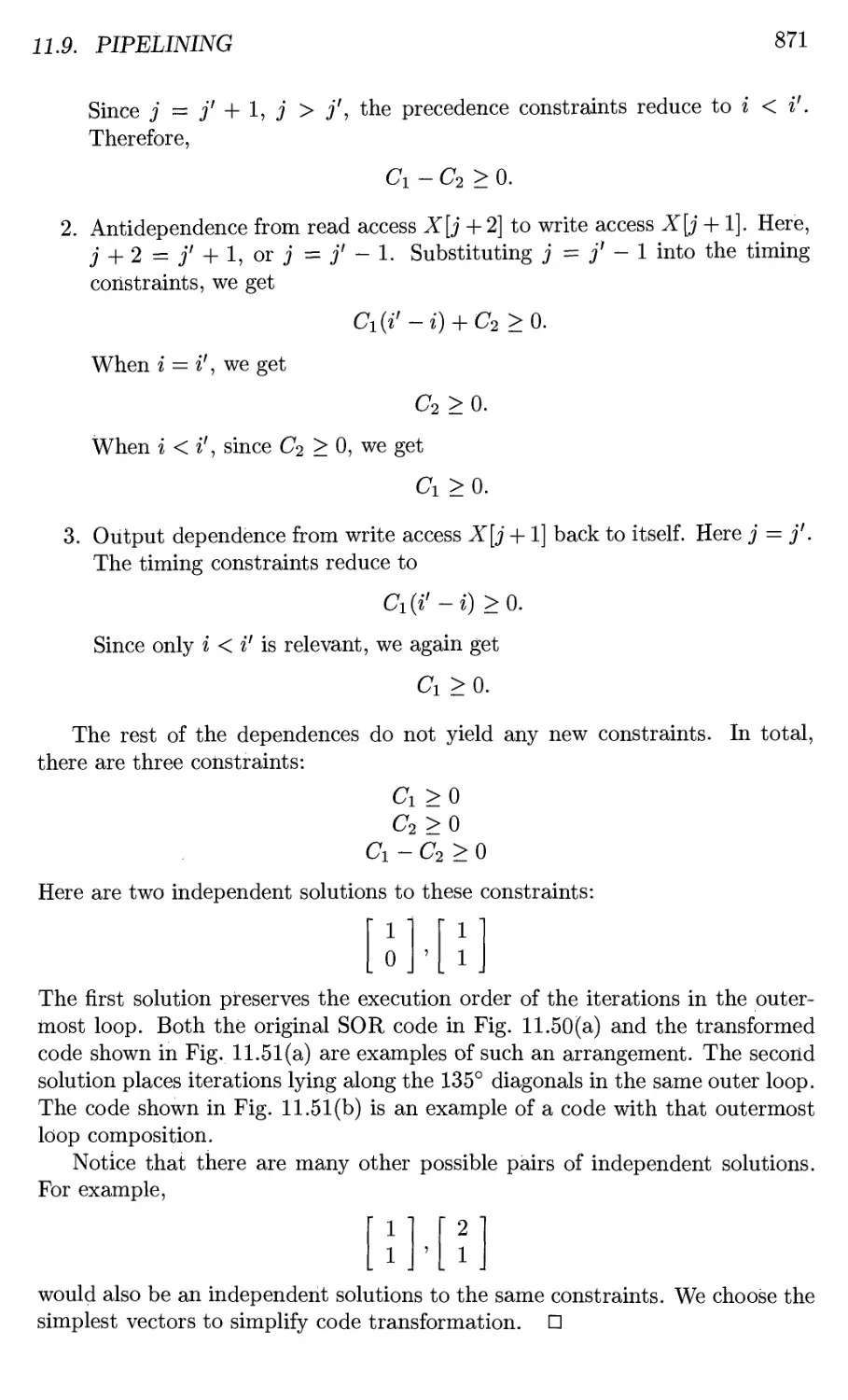
11.9.8 Code Transformations 875
11.9.9 Parallelism With Minimum Synchronization 880
11.9.10Exercises for Section 11.9 882
11.10 Locality Optimizations 884
11.10.1 Temporal Locality of Computed Data 885
11.10.2 Array Contraction 885
11.10.3 Partition Interleaving 887
11.10.4Putting it All Together 890
11.10.5 Exercises for Section 11.10 892
11.11 Other Uses of Affine Transforms 893
11.11.1 Distributed memory machines 894
11.11.2 Multi-Instruction-Issue Processors 895
11.11.3 Vector and SIMD Instructions 895
11.11.4 Prefetching 896
TABLE OF CONTENTS xxm
11.12 Summary of Chapter 11 897
11.13 References for Chapter 11 899
12 Interprocedural Analysis 903
12.1 Basic Concepts 904
12.1.1 Call Graphs 904
12.1.2 Context Sensitivity 906
12.1.3 Call Strings 908
12.1.4 Cloning-Based Context-Sensitive Analysis 910
12.1.5 Summary-Based Context-Sensitive Analysis 911
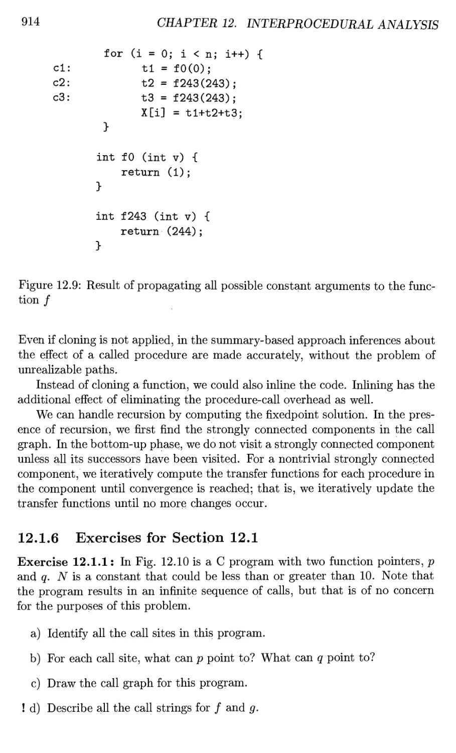
12.1.6 Exercises for Section 12.1 914
12.2 Why Interprocedural Analysis? 916
12.2.1 Virtual Method Invocation 916
12.2.2 Pointer Alias Analysis 917
12.2.3 Parallelization 917
12.2.4 Detection of Software Errors and Vulnerabilities 917
12.2.5 SQL Injection 918
12.2.6 Buffer Overflow 920
12.3 A Logical Representation of Data Flow 921
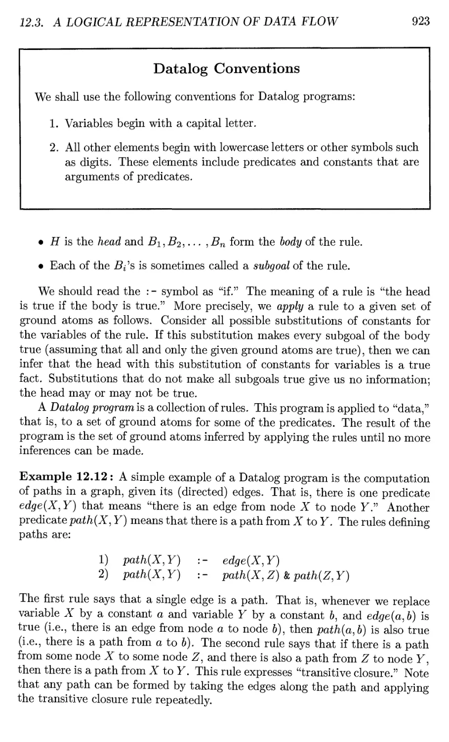
12.3.1 Introduction to Datalog 921
12.3.2 Datalog Rules 922
12.3.3 Intensional and Extensional Predicates 924
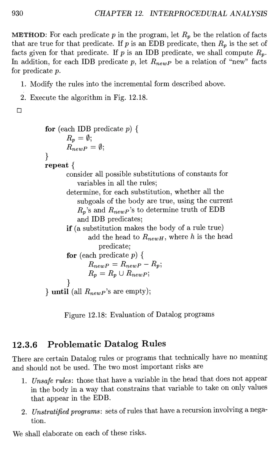
12.3.4 Execution of Datalog Programs 927
12.3.5 Incremental Evaluation of Datalog Programs 928
12.3.6 Problematic Datalog Rules 930
12.3.7 Exercises for Section 12.3 932
12.4 A Simple Pointer-Analysis Algorithm 933
12.4.1 Why is Pointer Analysis Difficult 934
12.4.2 A Model for Pointers and References 935
12.4.3 Flow Insensitivity 936
12.4.4 The Formulation in Datalog 937
12.4.5 Using Type Information 938
12.4.6 Exercises for Section 12.4 939
12.5 Context-Insensitive Interprocedural Analysis 941
12.5.1 Effects of a Method Invocation 941
12.5.2 Call Graph Discovery in Datalog 943
12.5.3 Dynamic Loading and Reflection 944
12.5.4 Exercises for Section 12.5 945
12.6 Context-Sensitive Pointer Analysis 945
12.6.1 Contexts and Call Strings 946
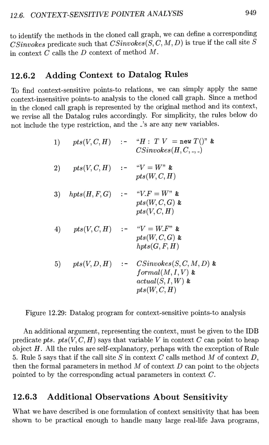
12.6.2 Adding Context to Datalog Rules 949
12.6.3 Additional Observations About Sensitivity 949
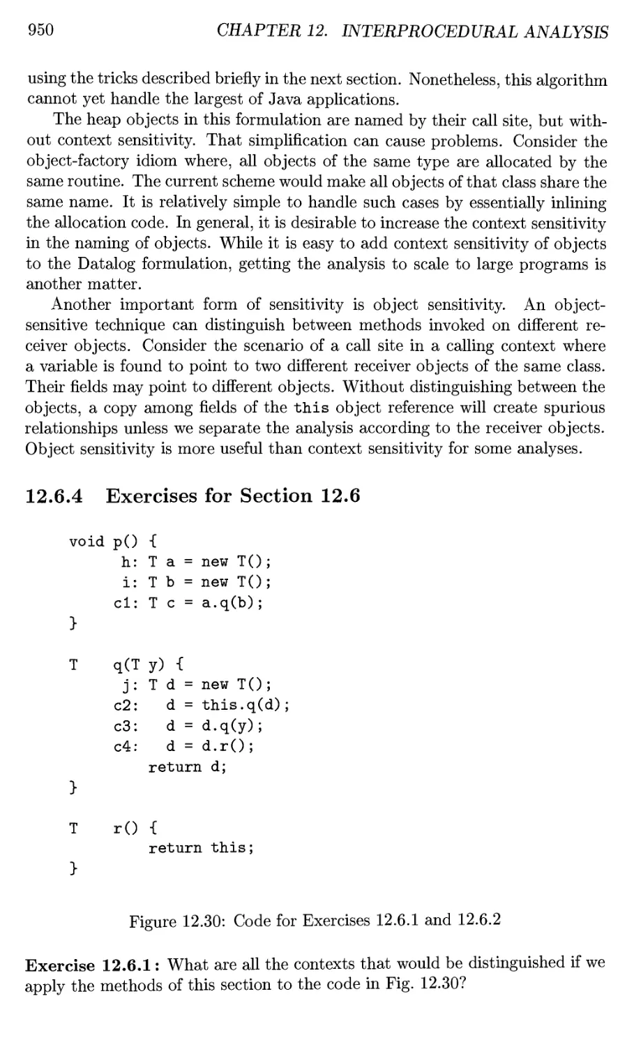
12.6.4 Exercises for Section 12.6 950
12.7 Datalog Implementation by BDD's 951
12.7.1 Binary Decision Diagrams 951
xxiv TABLE OF CONTENTS
12.7.2 Transformations on BDD's 953
12.7.3 Representing Relations by BDD's 954
12.7 .4 Relational Operations as BDD Operations 954
12.7.5 Using BDD's for Points-to Analysis 957
12.7.6 Exercises for Section 12.7 958
12.8 Summary of Chapter 12 958
12.9 References for Chapter 12 961
A A Complete Front End 965
A.l The Source Language 965
A.2 Main 966
A.3 Lexical Analyzer 967
A.4 Symbol Tables and Types 970
A.5 Intermediate Code for Expressions 971
A.6 Jumping Code for Boolean Expressions 974
A.7 Intermediate Code for Statements 978
A.8 Parser 981
A.9 Creating the Front End 986
B Finding Linearly Independent Solutions 989
Index 993
Chapter 1
Introduction
Programming languages are notations for describing computations to people
and to machines. The world as we know it depends on programming languages,
because all the software running on all the computers was written in some
programming language. But, before a program can be run, it first must be
translated into a form in which it can be executed by a computer.
The software systems that do this translation are called compilers.
This book is about how to design and implement compilers. We shall
discover that a few basic ideas can be used to construct translators for a wide
variety of languages and machines. Besides compilers, the principles and
techniques for compiler design are applicable to so many other domains that they
are likely to be reused many times in the career of a computer scientist. The
study of compiler writing touches upon programming languages, machine
architecture, language theory, algorithms, and software engineering.
In this preliminary chapter, we introduce the different forms of language
translators, give a high level overview of the structure of a typical compiler,
and discuss the trends in programming languages and machine architecture
that are shaping compilers. We include some observations on the relationship
between compiler design and computer-science theory and an outline of the
applications of compiler technology that go beyond compilation. We end with
a brief outline of key programming-language concepts that will be needed for
our study of compilers.
1.1 Language Processors
Simply stated, a compiler is a program that can read a program in one
language — the source language — and translate it into an equivalent program in
another language — the target language; see Fig. 1.1. An important role of the
compiler is to report any errors in the source program that it detects during
the translation process.
1
2
CHAPTER 1. INTRODUCTION
Fig
source program
1
Compiler
target program
"ure 1.1: A compiler
If the target program is an executable machine-language program, it can
then be called by the user to process inputs and produce outputs; see Fig. 1.2.
input
Target Program
output
Figure 1.2: Running the target program
An interpreter is another common kind of language processor. Instead of
producing a target program as a translation, an interpreter appears to directly
execute the operations specified in the source program on inputs supplied by
the user, as shown in Fig. 1.3.
source program
input
Interpreter
output
Figure 1.3: An interpreter
The machine-language target program produced by a compiler is usually
much faster than an interpreter at mapping inputs to outputs . An interpreter,
however, can usually give better error diagnostics than a compiler, because it
executes the source program statement by statement.
Example 1.1: Java language processors combine compilation and
interpretation, as shown in Fig. 1.4. A Java source program may first be compiled into
an intermediate form called bytecodes. The bytecodes are then interpreted by a
virtual machine. A benefit of this arrangement is that bytecodes compiled on
one machine can be interpreted on another machine, perhaps across a network.
In order to achieve faster processing of inputs to outputs, some Java
compilers, called just-in-time compilers, translate the bytecodes into machine language
immediately before they run the intermediate program to process the input. □
1.1. LANGUAGE PROCESSORS 3
source program
r
Translator
1
intermediate program —»-
input —•*■
Figure 1.4: A hybrid compiler
In addition to a compiler, several other programs may be required to create
an executable target program, as shown in Fig. 1.5. A source program may be
divided into modules stored in separate files. The task of collecting the source
program is sometimes entrusted to a separate program, called a preprocessor.
The preprocessor may also expand shorthands, called macros, into source
language statements.
The modified source program is then fed to a compiler. The compiler may
produce an assembly-language program as its output, because assembly
language is easier to produce as output and is easier to debug. The assembly
language is then processed by a program called an assembler that produces
relocatable machine code as its output.
Large programs are often compiled in pieces, so the relocatable machine
code may have to be linked together with other relocatable object files and
library files into the code that actually runs on the machine. The linker resolves
external memory addresses, where the code in one file may refer to a location
in another file. The loader then puts together all of the executable object files
into memory for execution.
1.1.1 Exercises for Section 1.1
Exercise 1.1.1: What is the difference between a compiler and an interpreter?
Exercise 1.1.2 : What are the advantages of (a) a compiler over an interpreter
(b) an interpreter over a compiler?
Exercise 1.1.3 : What advantages are there to a language-processing system in
which the compiler produces assembly language rather than machine language?
Exercise 1.1.4: A compiler that translates a high-level language into another
high-level language is called a source-to-source translator. What advantages are
there to using C as a target language for a compiler?
Virtual
Machine
output
Exercise 1.1.5: Describe some of the tasks that an assembler needs to
perform.
4
CHAPTER 1. INTRODUCTION
source program
L__
Preprocessor
modified source program
Compiler
target assembly program
Assembler
relocatable machine code
Linker/Loader
T
library files
relocatable object files
target machine code
Figure 1.5: A language-processing system
1.2 The Structure of a Compiler
Up to this point we have treated a compiler as a single box that maps a source
program into a semantically equivalent target program. If we open up this box
a little, we see that there are two parts to this mapping: analysis and synthesis.
The analysis part breaks up the source program into constituent pieces and
imposes a grammatical structure on them. It then uses this structure to
create an intermediate representation of the source program. If the analysis part
detects that the source program is either syntactically ill formed or
semantically unsound, then it must provide informative messages, so the user can take
corrective action. The analysis part also collects information about the source
program and stores it in a data structure called a symbol table, which is passed
along with the intermediate representation to the synthesis part.
The synthesis part constructs the desired target program from the
intermediate representation and the information in the symbol table. The analysis part
is often called the front end of the compiler; the synthesis part is the back end.
If we examine the compilation process in more detail, we see that it operates
as a sequence of phases, each of which transforms one representation of the
source program to another. A typical decomposition of a compiler into phases
is shown in Fig. 1.6. In practice, several phases may be grouped together,
and the intermediate representations between the grouped phases need not be
constructed explicitly. The symbol table, which stores information about the
1.2. THE STRUCTURE OF A COMPILER
5
character stream
Lexical Analyzer
token stream
Syntax Analyzer
syntax tree
Semantic Analyzer
Symbol Table
syntax tree
Intermediate Code Generator
intermediate representation
t
Machine-Independent
Code Optimizer
intermediate representation
i
Code Generator
target-machine code
i
Machine-Dependent
Code Optimizer
target-machine code
t
Figure 1.6: Phases of a compiler
entire source program, is used by all phases of the compiler.
Some compilers have a machine-independent optimization phase between
the front end and the back end. The purpose of this optimization phase is to
perform transformations on the intermediate representation, so that the back
end can produce a better target program than it would have otherwise
produced from an unoptimized intermediate representation. Since optimization is
optional, one or the other of the two optimization phases shown in Fig. 1.6 may
be missing.
1.2.1 Lexical Analysis
The first phase of a compiler is called lexical analysis or scanning. The
lexical analyzer reads the stream of characters making up the source program
6
CHAPTER 1. INTRODUCTION
and groups the characters into meaningful sequences called lexemes. For each
lexeme, the lexical analyzer produces as output a token of the form
(token-name, attribute-value)
that it passes on to the subsequent phase, syntax analysis. In the token, the
first component token-name is an abstract symbol that is used during syntax
analysis, and the second component attribute-value points to an entry in the
symbol table for this token. Information from the symbol-table entry is needed
for semantic analysis and code generation.
For example, suppose a source program contains the assignment statement
position = initial + rate * 60 (1.1)
The characters in this assignment could be grouped into the following lexemes
and mapped into the following tokens passed on to the syntax analyzer:
1. position is a lexeme that would be mapped into a token (id, 1), where id
is an abstract symbol standing for identifier and 1 points to the symbol-
table entry for position. The symbol-table entry for an identifier holds
information about the identifier, such as its name and type.
2. The assignment symbol = is a lexeme that is mapped into the token (=).
Since this token needs no attribute-value, we have omitted the second
component. We could have used any abstract symbol such as assign for
the token-name, but for notational convenience we have chosen to use the
lexeme itself as the name of the abstract symbol.
3. initial is a lexeme that is mapped into the token (id, 2), where 2 points
to the symbol-table entry for initial.
4. + is a lexeme that is mapped into the token (+).
5. rate is a lexeme that is mapped into the token (id, 3), where 3 points to
the symbol-table entry for rate.
6. * is a lexeme that is mapped into the token (*).
7. 60 is a lexeme that is mapped into the token (60).1
Blanks separating the lexemes would be discarded by the lexical analyzer.
Figure 1.7 shows the representation of the assignment statement (1.1) after
lexical analysis as the sequence of tokens
(id,l)(=)(id,2)(+)(id,3)(*)(60) (1.2)
In this representation, the token names =, +, and * are abstract symbols for
the assignment, addition, and multiplication operators, respectively.
technically speaking, for the lexeme 60 we should make up a token like (number, 4),
where 4 points to the symbol table for the internal representation of integer 60 but we shall
defer the discussion of tokens for numbers until Chapter 2. Chapter 3 discusses techniques
for building lexical analyzers.
1.2. THE STRUCTURE OF A COMPILER
7
position
initial
rate
SYMBOL TABLE
position = initial + rate * 60
Lexical Analyzer
<id,l> <=> <id,2> <+> <id,3> <*> <60>
i
Syntax Analyzer
= t
(id, if^ ^: + ^
(id, 2) ^ *
(id, 3)
60
Semantic Analyzer
= t
(id, iy^ ^: +
(id, 2) j^ * ^
(id, 3) inttofloat
| 60
Intermediate Code Generator
+
tl = inttofloat(60)
t2 = id3 * tl
t3 = id2 + t2
idl = t3
*
Code Optimizer
t
tl = id3 * 60.0
idl = id2 + tl
Code Generator
LDF R2, id3
MULF R2, R2, #60.0
LDF Rl, id2
ADDF Rl, Rl, R2
STF idl, Rl
Figure 1.7: Translation of an assignment statement
8
CHAPTER 1. INTRODUCTION
1.2.2 Syntax Analysis
The second phase of the compiler is syntax analysis or parsing. The parser uses
the first components of the tokens produced by the lexical analyzer to create
a tree-like intermediate representation that depicts the grammatical structure
of the token stream. A typical representation is a syntax tree in which each
interior node represents an operation and the children of the node represent the
arguments of the operation. A syntax tree for the token stream (1.2) is shown
as the output of the syntactic analyzer in Fig. 1.7.
This tree shows the order in which the operations in the assignment
position = initial + rate * 60
are to be performed. The tree has an interior node labeled * with (id, 3) as
its left child and the integer 60 as its right child. The node (id, 3) represents
the identifier rate. The node labeled * makes it explicit that we must first
multiply the value of rate by 60. The node labeled + indicates that we must
add the result of this multiplication to the value of initial. The root of the
tree, labeled =, indicates that we must store the result of this addition into the
location for the identifier position. This ordering of operations is consistent
with the usual conventions of arithmetic which tell us that multiplication has
higher precedence than addition, and hence that the multiplication is to be
performed before the addition.
The subsequent phases of the compiler use the grammatical structure to help
analyze the source program and generate the target program. In Chapter 4
we shall use context-free grammars to specify the grammatical structure of
programming languages and discuss algorithms for constructing efficient syntax
analyzers automatically from certain classes of grammars. In Chapters 2 and 5
we shall see that syntax-directed definitions can help specify the translation of
programming language constructs.
1.2.3 Semantic Analysis
The semantic analyzer uses the syntax tree and the information in the symbol
table to check the source program for semantic consistency with the language
definition. It also gathers type information and saves it in either the syntax tree
or the symbol table, for subsequent use during intermediate-code generation.
An important part of semantic analysis is type checking, where the compiler
checks that each operator has matching operands. For example, many
programming language definitions require an array index to be an integer; the compiler
must report an error if a floating-point number is used to index an array.
The language specification may permit some type conversions called
coercions. For example, a binary arithmetic operator may be applied to either a
pair of integers or to a pair of floating-point numbers. If the operator is applied
to a floating-point number and an integer, the compiler may convert or coerce
the integer into a floating-point number.
1.2. THE STRUCTURE OF A COMPILER
9
Such a coercion appears in Fig. 1.7. Suppose that position, initial, and
rate have been declared to be floating-point numbers, and that the lexeme 60
by itself forms an integer. The type checker in the semantic analyzer in Fig. 1.7
discovers that the operator * is applied to a floating-point number rate and
an integer 60. In this case, the integer may be converted into a floating-point
number. In Fig. 1.7, notice that the output of the semantic analyzer has an
extra node for the operator inttofloat, which explicitly converts its integer
argument into a floating-point number. Type checking and semantic analysis
are discussed in Chapter 6.
1.2.4 Intermediate Code Generation
In the process of translating a source program into target code, a compiler may
construct one or more intermediate representations, which can have a variety
of forms. Syntax trees are a form of intermediate representation; they are
commonly used during syntax and semantic analysis.
After syntax and semantic analysis of the source program, many
compilers generate an explicit low-level or machine-like intermediate representation,
which we can think of as a program for an abstract machine. This
intermediate representation should have two important properties: it should be easy to
produce and it should be easy to translate into the target machine.
In Chapter 6, we consider an intermediate form called three-address code,
which consists of a sequence of assembly-like instructions with three operands
per instruction. Each operand can act like a register. The output of the
intermediate code generator in Fig. 1.7 consists of the three-address code sequence
tl = inttofloat(60)
t2 = id3 * tl
t3 = id2 + t2 ^ }
idl = t3
There are several points worth noting about three-address instructions.
First, each three-address assignment instruction has at most one operator on the
right side. Thus, these instructions fix the order in which operations are to be
done; the multiplication precedes the addition in the source program (1.1).
Second, the compiler must generate a temporary name to hold the value computed
by a three-address instruction. Third, some "three-address instructions" like
the first and last in the sequence (1.3), above, have fewer than three operands.
In Chapter 6, we cover the principal intermediate representations used in
compilers. Chapters 5 introduces techniques for syntax-directed translation
that are applied in Chapter 6 to type checking and intermediate-code generation
for typical programming language constructs such as expressions, flow-of-control
constructs, and procedure calls.
10
CHAPTER 1. INTRODUCTION
1.2.5 Code Optimization
The machine-independent code-optimization phase attempts to improve the
intermediate code so that better target code will result. Usually better means
faster, but other objectives may be desired, such as shorter code, or target code
that consumes less power. For example, a straightforward algorithm generates
the intermediate code (1.3), using an instruction for each operator in the tree
representation that comes from the semantic analyzer.
A simple intermediate code generation algorithm followed by code
optimization is a reasonable way to generate good target code. The optimizer can deduce
that the conversion of 60 from integer to floating point can be done once and for
all at compile time, so the inttofloat operation can be eliminated by replacing
the integer 60 by the floating-point number 60.0. Moreover, t3 is used only
once to transmit its value to idl so the optimizer can transform (1.3) into the
shorter sequence
tl = id3 * 60.0 . ..
idl = id2 + tl ^ '
There is a great variation in the amount of code optimization different
compilers perform. In those that do the most, the so-called "optimizing compilers,"
a significant amount of time is spent on this phase. There are simple
optimizations that significantly improve the running time of the target program
without slowing down compilation too much. The chapters from 8 on discuss
machine-independent and machine-dependent optimizations in detail.
1.2.6 Code Generation
The code generator takes as input an intermediate representation of the source
program and maps it into the target language. If the target language is machine
code, registers Or memory locations are selected for each of the variables used by
the program. Then, the intermediate instructions are translated into sequences
of machine instructions that perform the same task. A crucial aspect of code
generation is the judicious assignment of registers to hold variables.
For example, using registers Rl and R2, the intermediate code in (1.4) might
get translated into the machine code
LDF R2, id3
MULF R2, R2, #60.0
LDF Rl, id2 (1.5)
ADDF Rl, Rl, R2
STF idl, Rl
The first operand of each instruction specifies a destination. The F in each
instruction tells us that it deals with floating-point numbers. The code in
1.2. THE STRUCTURE OF A COMPILER
11
(1.5) loads the contents of address id3 into register R2, then multiplies it with
floating-point constant 60.0. The # signifies that 60.0 is to be treated as an
immediate constant. The third instruction moves id2 into register Rl and the
fourth adds to it the value previously computed in register R2. Finally, the value
in register Rl is stored into the address of idl, so the code correctly implements
the assignment statement (1.1). Chapter 8 covers code generation.
This discussion of code generation has ignored the important issue of
storage allocation for the identifiers in the source program. As we shall see in
Chapter 7, the organization of storage at run-time depends on the language
being compiled. Storage-allocation decisions are made either during intermediate
code generation or during code generation.
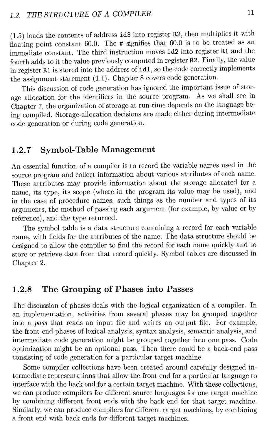
1.2.7 Symbol-Table Management
An essential function of a compiler is to record the variable names used in the
source program and collect information about various attributes of each name.
These attributes may provide information about the storage allocated for a
name, its type, its scope (where in the program its value may be used), and
in the case of procedure names, such things as the number and types of its
arguments, the method of passing each argument (for example, by value or by
reference), and the type returned.
The symbol table is a data structure containing a record for each variable
name, with fields for the attributes of the name. The data structure should be
designed to allow the compiler to find the record for each name quickly and to
store or retrieve data from that record quickly. Symbol tables are discussed in
Chapter 2.
1.2.8 The Grouping of Phases into Passes
The discussion of phases deals with the logical organization of a compiler. In
an implementation, activities from several phases may be grouped together
into a pass that reads an input file and writes an output file. For example,
the front-end phases of lexical analysis, syntax analysis, semantic analysis, and
intermediate code generation might be grouped together into one pass. Code
optimization might be an optional pass. Then there could be a back-end pass
consisting of code generation for a particular target machine.
Some compiler collections have been created around carefully designed
intermediate representations that allow the front end for a particular language to
interface with the back end for a certain target machine. With these collections,
we can produce compilers for different source languages for one target machine
by combining different front ends with the back end for that target machine.
Similarly, we can produce compilers for different target machines, by combining
a front end with back ends for different target machines.
12
CHAPTER 1. INTRODUCTION
1.2.9 Compiler-Construction Tools
The compiler writer, like any software developer, can profitably use modern
software development environments containing tools such as language editors,
debuggers, version managers, profilers, test harnesses, and so on. In addition
to these general software-development tools, other more specialized tools have
been created to help implement various phases of a compiler.
These tools use specialized languages for specifying and implementing
specific components, and many use quite sophisticated algorithms. The most
successful tools are those that hide the details of the generation algorithm and
produce components that can be easily integrated into the remainder of the
compiler. Some commonly used compiler-construction tools include
1. Parser generators that automatically produce syntax analyzers from a
grammatical description of a programming language.
2. Scanner generators that produce lexical analyzers from a
regular-expression description of the tokens of a language.
3. Syntax-directed translation engines that produce collections of routines
for walking a parse tree and generating intermediate code.
4. Code-generator generators that produce a code generator from a collection
of rules for translating each operation of the intermediate language into
the machine language for a target machine.
5. Data-flow analysis engines that facilitate the gathering of information
about how values are transmitted from one part of a program to each
other part. Data-flow analysis is a key part of code optimization.
6. Compiler-construction toolkits that provide an integrated set of routines
for constructing various phases of a compiler.
We shall describe many of these tools throughout this book.
1.3 The Evolution of Programming Languages
The first electronic computers appeared in the 1940's and were programmed in
machine language by sequences of O's and l's that explicitly told the computer
what operations to execute and in what order. The operations themselves
were very low level: move data from one location to another, add the contents
of two registers, compare two values, and so on. Needless to say, this kind
of programming was slow, tedious, and error prone. And once written, the
programs were hard to understand and modify.
1.3. THE EVOLUTION OF PROGRAMMING LANGUAGES 13
1.3.1 The Move to Higher-level Languages
The first step towards more people-friendly programming languages was the
development of mnemonic assembly languages in the early 1950's. Initially,
the instructions in an assembly language were just mnemonic representations
of machine instructions. Later, macro instructions were added to assembly
languages so that a programmer could define parameterized shorthands for
frequently used sequences of machine instructions.
A major step towards higher-level languages was made in the latter half of
the 1950's with the development of Fortran for scientific computation, Cobol
for business data processing, and Lisp for symbolic computation. The
philosophy behind these languages was to create higher-level notations with which
programmers could more easily write numerical computations, business
applications, and symbolic programs. These languages were so successful that they
are still in use today.
In the following decades, many more languages were created with innovative
features to help make programming easier, more natural, and more robust.
Later in this chapter, we shall discuss some key features that are common to
many modern programming languages.
Today, there are thousands of programming languages. They can be
classified in a variety of ways. One classification is by generation. First-generation
languages are the machine languages, second-generation the assembly languages,
and third-generation the higher-level languages like Fortran, Cobol, Lisp, C,
C++, C#, and Java. Fourth-generation languages are languages designed
for specific applications like NOMAD for report generation, SQL for database
queries, and Postscript for text formatting. The term fifth-generation language
has been applied to logic- and constraint-based languages like Prolog and OPS5.
Another classification of languages uses the term imperative for languages
in which a program specifies how a computation is to be done and declarative
for languages in which a program specifies what computation is to be done.
Languages such as C, C++, C#, and Java are imperative languages. In
imperative languages there is a notion of program state and statements that change
the state. Functional languages such as ML and Haskell and constraint logic
languages such as Prolog are often considered to be declarative languages.
The term von Neumann language is applied to programming languages
whose computational model is based on the von Neumann computer
architecture. Many of today's languages, such as Fortran and C are von Neumann
languages.
An object-oriented language is one that supports object-oriented
programming, a programming style in which a program consists of a collection of objects
that interact with one another. Simula 67 and Smalltalk are the earliest major
object-oriented languages. Languages such as C++, C#, Java, and Ruby are
more recent object-oriented languages.
Scripting languages are interpreted languages with high-level operators
designed for "gluing together" computations. These computations were originally
14
CHAPTER 1. INTRODUCTION
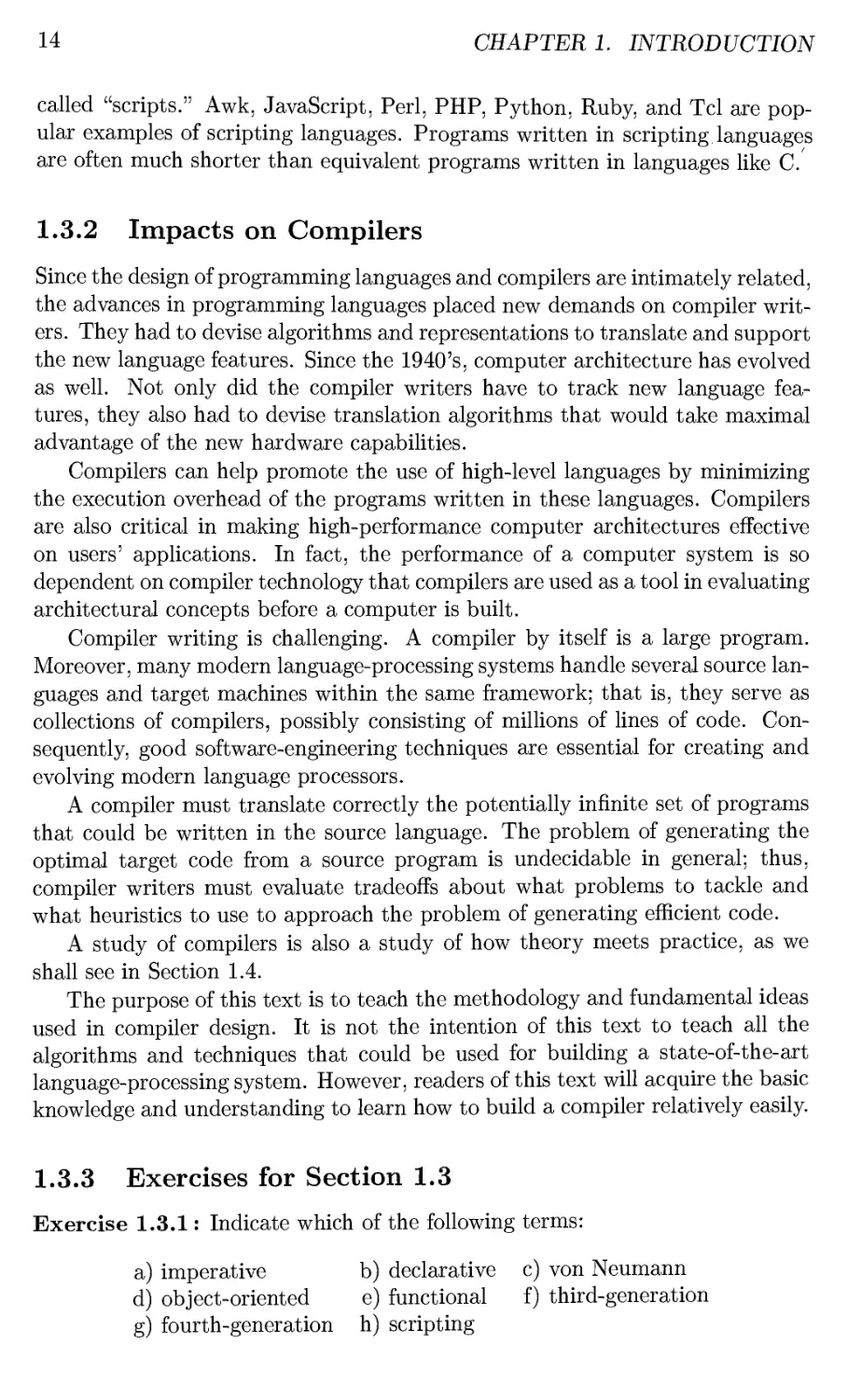
called "scripts." Awk, JavaScript, Perl, PHP, Python, Ruby, and Tel are
popular examples of scripting languages. Programs written in scripting languages
are often much shorter than equivalent programs written in languages like C.
1.3.2 Impacts on Compilers
Since the design of programming languages and compilers are intimately related,
the advances in programming languages placed new demands on compiler
writers. They had to devise algorithms and representations to translate and support
the new language features. Since the 1940's, computer architecture has evolved
as well. Not only did the compiler writers have to track new language
features, they also had to devise translation algorithms that would take maximal
advantage of the new hardware capabilities.
Compilers can help promote the use of high-level languages by minimizing
the execution overhead of the programs written in these languages. Compilers
are also critical in making high-performance computer architectures effective
on users' applications. In fact, the performance of a computer system is so
dependent on compiler technology that compilers are used as a tool in evaluating
architectural concepts before a computer is built.
Compiler writing is challenging. A compiler by itself is a large program.
Moreover, many modern language-processing systems handle several source
languages and target machines within the same framework; that is, they serve as
collections of compilers, possibly consisting of millions of lines of code.
Consequently, good software-engineering techniques are essential for creating and
evolving modern language processors.
A compiler must translate correctly the potentially infinite set of programs
that could be written in the source language. The problem of generating the
optimal target code from a source program is undecidable in general; thus,
compiler writers must evaluate tradeoffs about what problems to tackle and
what heuristics to use to approach the problem of generating efficient code.
A study of compilers is also a study of how theory meets practice, as we
shall see in Section 1.4.
The purpose of this text is to teach the methodology and fundamental ideas
used in compiler design. It is not the intention of this text to teach all the
algorithms and techniques that could be used for building a state-of-the-art
language-processing system. However, readers of this text will acquire the basic
knowledge and understanding to learn how to build a compiler relatively easily.
1.3.3 Exercises for Section 1.3
Exercise 1.3.1: Indicate which of the following terms:
a) imperative b) declarative c) von Neumann
d) object-oriented e) functional f) third-generation
g) fourth-generation h) scripting
1.4. THE SCIENCE OF BUILDING A COMPILER
15
apply to which of the following languages:
1) C 2) C++ 3) Cobol 4) Fortran 5) Java
6) Lisp 7) ML 8) Perl 9) Python 10) VB.
1.4 The Science of Building a Compiler
Compiler design is full of beautiful examples where complicated real-world
problems are solved by abstracting the essence of the problem mathematically. These
serve as excellent illustrations of how abstractions can be used to solve
problems: take a problem, formulate a mathematical abstraction that captures the
key characteristics, and solve it using mathematical techniques. The problem
formulation must be grounded in a solid understanding of the characteristics of
computer programs, and the solution must be validated and refined empirically.
A compiler must accept all source programs that conform to the specification
of the language; the set of source programs is infinite and any program can be
very large, consisting of possibly millions of lines of code. Any transformation
performed by the compiler while translating a source program must preserve the
meaning of the program being compiled. Compiler writers thus have influence
over not just the compilers they create, but all the programs that their
compilers compile. This leverage makes writing compilers particularly rewarding;
however, it also makes compiler development challenging.
1.4.1 Modeling in Compiler Design and Implementation
The study of compilers is mainly a study of how we design the right
mathematical models and choose the right algorithms, while balancing the need for
generality and power against simplicity and efficiency.
Some of most fundamental models are finite-state machines and regular
expressions, which we shall meet in Chapter 3. These models are useful for
describing the lexical units of programs (keywords, identifiers, and such) and for
describing the algorithms used by the compiler to recognize those units. Also
among the most fundamental models are context-free grammars, used to
describe the syntactic structure of programming languages such as the nesting of
parentheses or control constructs. We shall study grammars in Chapter 4.
Similarly, trees are an important model for representing the structure of programs
and their translation into object code, as we shall see in Chapter 5.
1.4.2 The Science of Code Optimization
The term "optimization" in compiler design refers to the attempts that a
compiler makes to produce code that is more efficient than the obvious code.
"Optimization" is thus a misnomer, since there is no way that the code produced
by a compiler can be guaranteed to be as fast or faster than any other code
that performs the same task.
16
CHAPTER 1. INTRODUCTION
In modern times, the optimization of code that a compiler performs has
become both more important and more complex. It is more complex because
processor architectures have become more complex, yielding more opportunities
to improve the way code executes. It is more important because massively
parallel computers require substantial optimization, or their performance suffers by
orders of magnitude. With the likely prevalence of multicore machines
(computers with chips that have large numbers of processors on them), all compilers
will have to face the problem of taking advantage of multiprocessor machines.
It is hard, if not impossible, to build a robust compiler out of "hacks."
Thus, an extensive and useful theory has been built up around the problem of
optimizing code. The use of a rigorous mathematical foundation allows us to
show that an optimization is correct and that it produces the desirable effect
for all possible inputs. We shall see, starting in Chapter 9, how models such
as graphs, matrices, and linear programs are necessary if the compiler is to
produce well optimized code.
On the other hand, pure theory alone is insufficient. Like many real-world
problems, there are no perfect answers. In fact, most of the questions that
we ask in compiler optimization are undecidable. One of the most important
skills in compiler design is the ability to formulate the right problem to solve.
We need a good understanding of the behavior of programs to start with and
thorough experimentation and evaluation to validate our intuitions.
Compiler optimizations must meet the following design objectives:
• The optimization must be correct, that is, preserve the meaning of the
compiled program,
• The optimization must improve the performance of many programs,
• The compilation time must be kept reasonable, and
• The engineering effort required must be manageable.
It is impossible to overemphasize the importance of correctness. It is trivial
to write a compiler that generates fast code if the generated code need not
be correct! Optimizing compilers are so difficult to get right that we dare say
that no optimizing compiler is completely error-free! Thus, the most important
objective in writing a compiler is that it is correct.
The second goal is that the compiler must be effective in improving the
performance of many input programs. Normally, performance means the speed of
the program execution. Especially in embedded applications, we may also wish
to minimize the size of the generated code. And in the case of mobile devices,
it is also desirable that the code minimizes power consumption. Typically, the
same optimizations that speed up execution time also conserve power. Besides
performance, usability aspects such as error reporting and debugging are also
important.
Third, we need to keep the compilation time short to support a rapid
development and debugging cycle. This requirement has become easier to meet as
1.5. APPLICATIONS OF COMPILER TECHNOLOGY
17
machines get faster. Often, a program is first developed and debugged without
program optimizations. Not only is the compilation time reduced, but more
importantly, unoptimized programs are easier to debug, because the
optimizations introduced by a compiler often obscure the relationship between the source
code and the object code. Turning on optimizations in the compiler sometimes
exposes new problems in the source program; thus testing must again be
performed on the optimized code. The need for additional testing sometimes deters
the use of optimizations in applications, especially if their performance is not
critical.
Finally, a compiler is a complex system; we must keep the system
simple to assure that the engineering and maintenance costs of the compiler are
manageable. There is an infinite number of program optimizations that we
could implement, and it takes a nontrivial amount of effort to create a correct
and effective optimization. We must prioritize the optimizations, implementing
only those that lead to the greatest benefits on source programs encountered in
practice.
Thus, in studying compilers, we learn not only how to build a compiler, but
also the general methodology of solving complex and open-ended problems. The
approach used in compiler development involves both theory and
experimentation. We normally start by formulating the problem based on our intuitions on
what the important issues are.
1.5 Applications of Compiler Technology
Compiler design is not only about compilers, and many people use the
technology learned by studying compilers in school, yet have never, strictly speaking,
written (even part of) a compiler for a major programming language. Compiler
technology has other important uses as well. Additionally, compiler design
impacts several other areas of computer science. In this section, we review the
most important interactions and applications of the technology.
1.5.1 Implementation of High-Level Programming
Languages
A high-level programming language defines a programming abstraction: the
programmer expresses an algorithm using the language, and the compiler must
translate that program to the target language. Generally, higher-level
programming languages are easier to program in, but are less efficient, that is, the target
programs run more slowly. Programmers using a low-level language have more
control over a computation and can, in principle, produce more efficient code.
Unfortunately, lower-level programs are harder to write and — worse still —
less portable, more prone to errors, and harder to maintain. Optimizing
compilers include techniques to improve the performance of generated code, thus
offsetting the inefficiency introduced by high-level abstractions.
18
CHAPTER 1. INTRODUCTION
Example 1.2: The register keyword in the C programming language is an
early example of the interaction between compiler technology and language
evolution. When the C language was created in the mid 1970s, it was considered
necessary to let a programmer control which program variables reside in
registers. This control became unnecessary as effective register-allocation techniques
were developed, and most modern programs no longer use this language feature.
In fact, programs that use the register keyword may lose efficiency, because
programmers often are not the best judge of very low-level matters like register
allocation. The optimal choice of register allocation depends greatly on the
specifics of a machine architecture. Hardwiring low-level resource-management
decisions like register allocation may in fact hurt performance, especially if the
program is run on machines other than the one for which it was written. □
The many shifts in the popular choice of programming languages have been
in the direction of increased levels of abstraction. C was the predominant
systems programming language of the 80's; many of the new projects started
in the 90's chose C++; Java, introduced in 1995, gained popularity quickly
in the late 90's. The new programming-language features introduced in each
round spurred new research in compiler optimization. In the following, we give
an overview on the main language features that have stimulated significant
advances in compiler technology.
Practically all common programming languages, including C, Fortran and
Cobol, support user-defined aggregate data types, such as arrays and structures,
and high-level control flow, such as loops and procedure invocations. If we just
take each high-level construct or data-access operation and translate it directly
to machine code, the result would be very inefficient. A body of compiler
optimizations, known as data-flow optimizations, has been developed to analyze
the flow of data through the program and removes redundancies across these
constructs. They are effective in generating code that resembles code written
by a skilled programmer at a lower level.
Object orientation was first introduced in Simula in 1967, and has been
incorporated in languages such as Smalltalk, C++, C#, and Java. The key
ideas behind object orientation are
1. Data abstraction and
2. Inheritance of properties,
both of which have been found to make programs more modular and easier to
maintain. Object-oriented programs are different from those written in many
other languages, in that they consist of many more, but smaller, procedures
(called methods in object-oriented terms). Thus, compiler optimizations must
be able to perform well across the procedural boundaries of the source program.
Procedure inlining, which is the replacement of a procedure call by the body
of the procedure, is particularly useful here. Optimizations to speed up virtual
method dispatches have also been developed.
1.5. APPLICATIONS OF COMPILER TECHNOLOGY
19
Java has many features that make programming easier, many of which have
been introduced previously in other languages. The Java language is type-safe;
that is, an object cannot be used as an object of an unrelated type. All array
accesses are checked to ensure that they lie within the bounds of the array.
Java has no pointers and does not allow pointer arithmetic. It has a built-in
garbage-collection facility that automatically frees the memory of variables that
are no longer in use. While all these features make programming easier, they
incur a run-time overhead. Compiler optimizations have been developed to
reduce the overhead, for example, by eliminating unnecessary range checks and
by allocating objects that are not accessible beyond a procedure on the stack
instead of the heap. Effective algorithms also have been developed to minimize
the overhead of garbage collection.
In addition, Java is designed to support portable and mobile code. Programs
are distributed as Java bytecode, which must either be interpreted or compiled
into native code dynamically, that is, at run time. Dynamic compilation has also
been studied in other contexts, where information is extracted dynamically at
run time and used to produce better-optimized code. In dynamic optimization,
it is important to minimize the compilation time as it is part of the execution
overhead. A common technique used is to only compile and optimize those
parts of the program that will be frequently executed.
1.5.2 Optimizations for Computer Architectures
The rapid evolution of computer architectures has also led to an insatiable
demand for new compiler technology. Almost all high-performance systems
take advantage of the same two basic techniques: parallelism and memory
hierarchies. Parallelism can be found at several levels: at the instruction level,
where multiple operations are executed simultaneously and at the processor
level, where different threads of the same application are run on different
processors. Memory hierarchies are a response to the basic limitation that we can
build very fast storage or very large storage, but not storage that is both fast
and large.
Parallelism
All modern microprocessors exploit instruction-level parallelism. However, this
parallelism can be hidden from the programmer. Programs are written as if all
instructions were executed in sequence; the hardware dynamically checks for
dependencies in the sequential instruction stream and issues them in parallel
when possible. In some cases, the machine includes a hardware scheduler that
can change the instruction ordering to increase the parallelism in the program.
Whether the hardware reorders the instructions or not, compilers can rearrange
the instructions to make instruction-level parallelism more effective.
Instruction-level parallelism can also appear explicitly in the instruction set.
VLIW (Very Long Instruction Word) machines have instructions that can issue
20
CHAPTER 1. INTRODUCTION
multiple operations in parallel. The Intel IA64 is a well-known example of such
an architecture. All high-performance, general-purpose microprocessors also
include instructions that can operate on a vector of data at the same time.
Compiler techniques have been developed to generate code automatically for
such machines from sequential programs.
Multiprocessors have also become prevalent; even personal computers
often have multiple processors. Programmers can write multithreaded code for
multiprocessors, or parallel code can be automatically generated by a
compiler from conventional sequential programs. Such a compiler hides from the
programmers the details of finding parallelism in a program, distributing the
computation across the machine, and minimizing synchronization and
communication among the processors. Many scientific-computing and engineering
applications are computation-intensive and can benefit greatly from parallel
processing. Parallelization techniques have been developed to translate
automatically sequential scientific programs into multiprocessor code.
Memory Hierarchies
A memory hierarchy consists of several levels of storage with different speeds
and sizes, with the level closest to the processor being the fastest but
smallest. The average memory-access time of a program is reduced if most of its
accesses are satisfied by the faster levels of the hierarchy. Both parallelism and
the existence of a memory hierarchy improve the potential performance of a
machine, but they must be harnessed effectively by the compiler to deliver real
performance on an application.
Memory hierarchies are found in all machines. A processor usually has
a small number of registers consisting of hundreds of bytes, several levels of
caches containing kilobytes to megabytes, physical memory containing
megabytes to gigabytes, and finally secondary storage that contains gigabytes and
beyond. Correspondingly, the speed of accesses between adjacent levels of the
hierarchy can differ by two or three orders of magnitude. The performance of a
system is often limited not by the speed of the processor but by the performance
of the memory subsystem. While compilers traditionally focus on optimizing
the processor execution, more emphasis is now placed on making the memory
hierarchy more effective.
Using registers effectively is probably the single most important problem in
optimizing a program. Unlike registers that have to be managed explicitly in
software, caches and physical memories are hidden from the instruction set and
are managed by hardware. It has been found that cache-management policies
implemented by hardware are not effective in some cases, especially in scientific
code that has large data structures (arrays, typically). It is possible to improve
the effectiveness of the memory hierarchy by changing the layout of the data,
or changing the order of instructions accessing the data. We can also change
the layout of code to improve the effectiveness of instruction caches.
1.5. APPLICATIONS OF COMPILER TECHNOLOGY
21
1.5.3 Design of New Computer Architectures
In the early days of computer architecture design, compilers were developed
after the machines were built. That has changed. Since programming in high-
level languages is the norm, the performance of a computer system is determined
not by its raw speed but also by how well compilers can exploit its features.
Thus, in modern computer architecture development, compilers are developed
in the processor-design stage, and compiled code, running on simulators, is used
to evaluate the proposed architectural features.
RISC
One of the best known examples of how compilers influenced the design of
computer architecture was the invention of the RISC (Reduced Instruction-Set
Computer) architecture. Prior to this invention, the trend was to develop
progressively complex instruction sets intended to make assembly programming
easier; these architectures were known as CISC (Complex Instruction-Set
Computer). For example, CISC instruction sets include complex memory-addressing
modes to support data-structure accesses and procedure-invocation instructions
that save registers and pass parameters on the stack.
Compiler optimizations often can reduce these instructions to a small
number of simpler operations by eliminating the redundancies across complex
instructions. Thus, it is desirable to build simple instruction sets; compilers can
use them effectively and the hardware is much easier to optimize.
Most general-purpose processor architectures, including PowerPC, SPARC,
MIPS, Alpha, and PA-RISC, are based on the RISC concept. Although the
x86 architecture—the most popular microprocessor—has a CISC instruction
set, many of the ideas developed for RISC machines are used in the
implementation of the processor itself. Moreover, the most effective way to use a
high-performance x86 machine is to use just its simple instructions.
Specialized Architectures
Over the last three decades, many architectural concepts have been proposed.
They include data flow machines, vector machines, VLIW (Very Long
Instruction Word) machines, SIMD (Single Instruction, Multiple Data) arrays of
processors, systolic arrays, multiprocessors with shared memory, and
multiprocessors with distributed memory. The development of each of these architectural
concepts was accompanied by the research and development of corresponding
compiler technology.
Some of these ideas have made their way into the designs of embedded
machines. Since entire systems can fit on a single chip, processors need no
longer be prepackaged commodity units, but can be tailored to achieve better
cost-effectiveness for a particular application. Thus, in contrast to general-
purpose processors, where economies of scale have led computer architectures
22
CHAPTER 1. INTRODUCTION
to converge, application-specific processors exhibit a diversity of computer
architectures. Compiler technology is needed not only to support programming
for these architectures, but also to evaluate proposed architectural designs.
1.5.4 Program Translations
While we normally think of compiling as a translation from a high-level
language to the machine level, the same technology can be applied to translate
between different kinds of languages. The following are some of the important
applications of program-translation techniques.
Binary Translation
Compiler technology can be used to translate the binary code for one machine
to that of another, allowing a machine to run programs originally compiled for
another instruction set. Binary translation technology has been used by various
computer companies to increase the availability of software for their machines.
In particular, because of the domination of the x86 personal-computer
market, most software titles are available as x86 code. Binary translators have
been developed to convert x86 code into both Alpha and Sparc code. Binary
translation was also used by Transmeta Inc. in their implementation of the x86
instruction set. Instead of executing the complex x86 instruction set directly in
hardware, the Transmeta Crusoe processor is a VLIW processor that relies on
binary translation to convert x86 code into native VLIW code.
Binary translation can also be used to provide backward compatibility.
When the processor in the Apple Macintosh was changed from the Motorola MC
68040 to the PowerPC in 1994, binary translation was used to allow PowerPC
processors run legacy MC 68040 code.
Hardware Synthesis
Not only is most software written in high-level languages; even hardware
designs are mostly described in high-level hardware description languages like
Verilog and VHDL (Very high-speed integrated circuit Hardware Description
Language). Hardware designs are typically described at the register
transfer level (RTL), where variables represent registers and expressions represent
combinational logic. Hardware-synthesis tools translate RTL descriptions
automatically into gates, which are then mapped to transistors and eventually to a
physical layout. Unlike compilers for programming languages, these tools often
take hours optimizing the circuit. Techniques to translate designs at higher
levels, such as the behavior or functional level, also exist.
Database Query Interpreters
Besides specifying software and hardware, languages are useful in many other
applications. For example, query languages, especially SQL (Structured Query
1.5. APPLICATIONS OF COMPILER TECHNOLOGY
23
Language), are used to search databases. Database queries consist of predicates
containing relational and boolean operators. They can be interpreted or
compiled into commands to search a database for records satisfying that predicate.
Compiled Simulation
Simulation is a general technique used in many scientific and engineering
disciplines to understand a phenomenon or to validate a design. Inputs to a
simulator usually include the description of the design and specific input parameters
for that particular simulation run. Simulations can be very expensive. We
typically need to simulate many possible design alternatives on many different input
sets, and each experiment may take days to complete on a high-performance
machine. Instead of writing a simulator that interprets the design, it is faster
to compile the design to produce machine code that simulates that particular
design natively. Compiled simulation can run orders of magnitude faster than
an interpreter-based approach. Compiled simulation is used in many state-of-
the-art tools that simulate designs written in Verilog or VHDL.
1.5.5 Software Productivity Tools
Programs are arguably the most complicated engineering artifacts ever
produced; they consist of many many details, every one of which must be correct
before the program will work completely. As a result, errors are rampant in
programs; errors may crash a system, produce wrong results, render a system
vulnerable to security attacks, or even lead to catastrophic failures in critical
systems. Testing is the primary technique for locating errors in programs.
An interesting and promising complementary approach is to use data-flow
analysis to locate errors statically (that is, before the program is run).
Dataflow analysis can find errors along all the possible execution paths, and not
just those exercised by the input data sets, as in the case of program testing.
Many of the data-flow-analysis techniques, originally developed for compiler
optimizations, can be used to create tools that assist programmers in their
software engineering tasks.
The problem of finding all program errors is undecidable. A data-flow
analysis may be designed to warn the programmers of all possible statements violating
a particular category of errors. But if most of these warnings are false alarms,
users will not use the tool. Thus, practical error detectors are often neither
sound nor complete. That is, they may not find all the errors in the program,
and not all errors reported are guaranteed to be real errors. Nonetheless,
various static analyses have been developed and shown to be effective in finding
errors, such as dereferencing null or freed pointers, in real programs. The fact
that error detectors may be unsound makes them significantly different from
compiler optimizations. Optimizers must be conservative and cannot alter the
semantics of the program under any circumstances.
24
CHAPTER 1. INTRODUCTION
In the balance of this section, we shall mention several ways in which
program analysis, building upon techniques originally developed to optimize code
in compilers, have improved software productivity. Of special importance are
techniques that detect statically when a program might have a security
vulnerability.
Type Checking
Type checking is an effective and well-established technique to catch
inconsistencies in programs. It can be used to catch errors, for example, where an
operation is applied to the wrong type of object, or if parameters passed to a
procedure do not match the signature of the procedure. Program analysis can
go beyond finding type errors by analyzing the flow of data through a program.
For example, if a pointer is assigned null and then immediately dereferenced,
the program is clearly in error.
The same technology can be used to catch a variety of security holes, in
which an attacker supplies a string or other data that is used carelessly by the
program. A user-supplied string can be labeled with a type "dangerous." If
this string is not checked for proper format, then it remains "dangerous," and
if a string of this type is able to influence the control-flow of the code at some
point in the program, then there is a potential security flaw.
Bounds Checking
It is easier to make mistakes when programming in a lower-level language than
a higher-level one. For example, many security breaches in systems are caused
by buffer overflows in programs written in C. Because C does not have array-
bounds checks, it is up to the user to ensure that the arrays are not accessed
out of bounds. Failing to check that the data supplied by the user can overflow
a buffer, the program may be tricked into storing user data outside of the
buffer. An attacker can manipulate the input data that causes the program to
misbehave and compromise the security of the system. Techniques have been
developed to find buffer overflows in programs, but with limited success.
Had the program been written in a safe language that includes automatic
range checking, this problem would not have occurred. The same data-flow
analysis that is used to eliminate redundant range checks can also be used to
locate buffer overflows. The major difference, however, is that failing to
eliminate a range check would only result in a small run-time cost, while failing to
identify a potential buffer overflow may compromise the security of the system.
Thus, while it is adequate to use simple techniques to optimize range checks,
sophisticated analyses, such as tracking the values of pointers across procedures,
are needed to get high-quality results in error detection tools.
1.6. PROGRAMMING LANGUAGE BASICS
25
Memory-Management Tools
Garbage collection is another excellent example of the tradeoff between
efficiency and a combination of ease of programming and software reliability.
Automatic memory management obliterates all memory-management errors (e.g.,
"memory leaks"), which are a major source of problems in C and C++
programs. Various tools have been developed to help programmers find memory
management errors. For example, Purify is a widely used tool that dynamically
catches memory management errors as they occur. Tools that help identify
some of these problems statically have also been developed.
1.6 Programming Language Basics
In this section, we shall cover the most important terminology and distinctions
that appear in the study of programming languages. It is not our purpose to
cover all concepts or all the popular programming languages. We assume that
the reader is familiar with at least one of C, C++, C#, or Java, and may have
encountered other languages as well.
1.6.1 The Static/Dynamic Distinction
Among the most important issues that we face when designing a compiler for
a language is what decisions can the compiler make about a program. If a
language uses a policy that allows the compiler to decide an issue, then we say
that the language uses a static policy or that the issue can be decided at compile
time. On the other hand, a policy that only allows a decision to be made when
we execute the program is said to be a dynamic policy or to require a decision
at run time.
One issue on which we shall concentrate is the scope of declarations. The
scope of a declaration of x is the region of the program in which uses of x refer to
this declaration. A language uses static scope or lexical scope if it is possible to
determine the scope of a declaration by looking only at the program. Otherwise,
the language uses dynamic scope. With dynamic scope, as the program runs,
the same use of x could refer to any of several different declarations of x.
Most languages, such as C and Java, use static scope. We shall discuss static
scoping in Section 1.6.3.
Example 1.3 : As another example of the static/dynamic distinction, consider
the use of the term "static" as it applies to data in a Java class declaration. In
Java, a variable is a name for a location in memory used to hold a data value.
Here, "static" refers not to the scope of the variable, but rather to the ability of
the compiler to determine the location in memory where the declared variable
can be found. A declaration like
public static int x;
26
CHAPTER 1. INTRODUCTION
makes x a class variable and says that there is only one copy of re, no matter how
many objects of this class are created. Moreover, the compiler can determine a
location in memory where this integer x will be held. In contrast, had "static"
been omitted from this declaration, then each object of the class would have its
own location where x would be held, and the compiler could not determine all
these places in advance of running the program. □
1.6.2 Environments and States
Another important distinction we must make when discussing programming
languages is whether changes occurring as the program runs affect the values of
data elements or affect the interpretation of names for that data. For example,
the execution of an assignment such as x = y + 1 changes the value denoted by
the name x. More specifically, the assignment changes the value in whatever
location is denoted by x.
It may be less clear that the location denoted by x can change at run time.
For instance, as we discussed in Example 1.3, if x is not a static (or "class")
variable, then every object of the class has its own location for an instance
of variable x. In that case, the assignment to x can change any of those
"instance" variables, depending on the object to which a method containing that
assignment is applied.
environment state
names locations values
(variables)
Figure 1.8: Two-stage mapping from names to values
The association of names with locations in memory (the store) and then
with values can be described by two mappings that change as the program runs
(see Fig. 1.8):
1. The environment is a mapping from names to locations in the store. Since
variables refer to locations ("1-values" in the terminology of C), we could
alternatively define an environment as a mapping from names to variables.
2. The state is a mapping from locations in store to their values. That is, the
state maps 1-values to their corresponding r-values, in the terminology of
C.
Environments change according to the scope rules of a language.
Example 1.4: Consider the C program fragment in Fig. 1.9. Integer i is
declared a global variable, and also declared as a variable local to function /.
When / is executing, the environment adjusts so that name i refers to the
1.6. PROGRAMMING LANGUAGE BASICS
27
int i; /* global i */
void f(---) {
int i; /* local i */
i = 3; /* use of local i */
}
x = i + 1; /* use of global i */
Figure 1.9: Two declarations of the name i
location reserved for the i that is local to /, and any use of z, such as the
assignment i = 3 shown explicitly, refers to that location. Typically, the local
% is given a place on the run-time stack.
Whenever a function g other than / is executing, uses of i cannot refer to
the i that is local to /. Uses of name i in g must be within the scope of some
other declaration of i. An example is the explicitly shown statement x = i+1,
which is inside some procedure whose definition is not shown. The i in i + 1
presumably refers to the global i. As in most languages, declarations in C must
precede their use, so a function that comes before the global i cannot refer to
it. □
The environment and state mappings in Fig. 1.8 are dynamic, but there are
a few exceptions:
1. Static versus dynamic binding of names to locations. Most binding of
names to locations is dynamic, and we discuss several approaches to this
binding throughout the section. Some declarations, such as the global i
in Fig. 1.9, can be given a location in the store once and for all, as the
compiler generates object code.2
2. Static versus dynamic binding of locations to values. The binding of
locations to values (the second stage in Fig. 1.8), is generally dynamic as
well, since we cannot tell the value in a location until we run the program.
Declared constants are an exception. For instance, the C definition
#define ARRAYSIZE 1000
2 Technically, the C compiler will assign a location in virtual memory for the global i,
leaving it to the loader and the operating system to determine where in the physical memory
of the machine i will be located. However, we shall not worry about "relocation" issues such
as these, which have no impact on compiling. Instead, we treat the address space that the
compiler uses for its output code as if it gave physical memory locations.
28
CHAPTER 1. INTRODUCTION
Names, Identifiers, and Variables
Although the terms "name" and "variable," often refer to the same thing,
we use them carefully to distinguish between compile-time names and the
run-time locations denoted by names.
An identifier is a string of characters, typically letters or digits, that
refers to (identifies) an entity, such as a data object, a procedure, a class,
or a type. All identifiers are names, but not all names are identifiers.
Names can also be expressions. For example, the name x.y might denote
the field y of a structure denoted by x. Here, x and y are identifiers, while
x.y is a name, but not an identifier. Composite names like x.y are called
qualified names.
A variable refers to a particular location of the store. It is common for
the same identifier to be declared more than once; each such declaration
introduces a new variable. Even if each identifier is declared just once, an
identifier local to a recursive procedure will refer to different locations of
the store at different times.
binds the name ARRAYS IZE to the value 1000 statically. We can determine
this binding by looking at the statement, and we know that it is impossible
for this binding to change when the program executes.
1.6.3 Static Scope and Block Structure
Most languages, including C and its family, use static scope. The scope rules
for C are based on program structure; the scope of a declaration is determined
implicitly by where the declaration appears in the program. Later languages,
such as C++, Java, and C#, also provide explicit control over scopes through
the use of keywords like public, private, and protected.
In this section we consider static-scope rules for a language with blocks,
where a block is a grouping of declarations and statements. C uses braces { and
} to delimit a block; the alternative use of begin and end for the same purpose
dates back to Algol.
Example 1.5 : To a first approximation, the C static-scope policy is as follows:
1. A C program consists of a sequence of top-level declarations of variables
and functions.
2. Functions may have variable declarations within them, where variables
include local variables and parameters. The scope of each such declaration
is restricted to the function in which it appears.
1.6. PROGRAMMING LANGUAGE BASICS 29
Procedures, Functions, and Methods
To avoid saying "procedures, functions, or methods," each time we want
to talk about a subprogram that may be called, we shall usually refer to
all of them as "procedures." The exception is that when talking explicitly
of programs in languages like C that have only functions, we shall refer
to them as "functions." Or, if we are discussing a language like Java that
has only methods, we shall use that term instead.
A function generally returns a value of some type (the "return type"),
while a procedure does not return any value. C and similar languages,
which have only functions, treat procedures as functions that have a special
return type "void," to signify no return value. Object-oriented languages
like Java and C++ use the term "methods." These can behave like either
functions or procedures, but are associated with a particular class.
3. The scope of a top-level declaration of a name x consists of the entire
program that follows, with the exception of those statements that lie
within a function that also has a declaration of x.
The additional detail regarding the C static-scope policy deals with variable
declarations within statements. We examine such declarations next and in
Example 1.6. □
In C, the syntax of blocks is given by
1. One type of statement is a block. Blocks can appear anywhere that other
types of statements, such as assignment statements, can appear.
2. A block is a sequence of declarations followed by a sequence of statements,
all surrounded by braces.
Note that this syntax allows blocks to be nested inside each other. This
nesting property is referred to as block structure. The C family of languages
has block structure, except that a function may not be denned inside another
function.
We say that a declaration D "belongs" to a block B if B is the most closely
nested block containing D; that is, D is located within 5, but not within any
block that is nested within B.
The static-scope rule for variable declarations in a block-structured
languages is as follows. If declaration D of name x belongs to block B, then the
scope of D is all of B, except for any blocks B' nested to any depth within B,
in which x is redeclared. Here, x is redeclared in B' if some other declaration
D' of the same name x belongs to B'.
30
CHAPTER 1. INTRODUCTION
An equivalent way to express this rule is to focus on a use of a name x.
Let Bi,B2,... ,Bk be all the blocks that surround this use of x, with Bj, the
smallest, nested within Bk-i, which is nested within Bk_2, and so on. Search
for the largest i such that there is a declaration of x belonging to B{. This use
of x refers to the declaration in B{. Alternatively, this use of x is within the
scope of the declaration in B{.
mainQ {
int a = 1; d
int b = 1;
{
int
{
}
{
}
^cou
b = 2;
int a =
cout «
'int b =
cout «
3;
a « b;
4;
a « b;
t « a « b;
B3
j
#4
)
B2
J
}
^cout « a « b; ,
}
Figure 1.10: Blocks in a C++ program
Example 1.6: The C++ program in Fig. 1.10 has four blocks, with several
definitions of variables a and b. As a memory aid, each declaration initializes
its variable to the number of the block to which it belongs.
For instance, consider the declaration int a = 1 in block B1. Its scope
is all of B1, except for those blocks nested (perhaps deeply) within B\ that
have their own declaration of a. B2, nested immediately within Bi, does not
have a declaration of a, but B3 does. 54 does not have a declaration of a, so
block B3 is the only place in the entire program that is outside the scope of the
declaration of the name a that belongs to B\. That is, this scope includes B±
and all of B2 except for the part of B2 that is within B3. The scopes of all five
declarations are summarized in Fig. 1.11.
From another point of view, let us consider the output statement in block
£4 and bind the variables a and b used there to the proper declarations. The
list of surrounding blocks, in order of increasing size, is B±,B2,B1. Note that
B3 does not surround the point in question. B± has a declaration of 6, so it
is to this declaration that this use of b refers, and the value of b printed is 4.
However, 54 does not have a declaration of o, so we next look at B2. That
block does not have a declaration of a either, so we proceed to B\. Fortunately,
1.6. PROGRAMMING LANGUAGE BASICS
31
Declaration
int a = 1
int b = 1
int b = 2
int a = 3
int b = 4
Scope
Bi-B3
Bi - B2
B2-BA
B3
B±
Figure 1.11: Scopes of declarations in Example 1.6
there is a declaration int a = 1 belonging to that block, so the value of a
printed is 1. Had there been no such declaration, the program would have been
erroneous. □
1.6.4 Explicit Access Control
Classes and structures introduce a new scope for their members. If p is an
object of a class with a field (member) x, then the use of x in p.x refers to
field x in the class definition. In analogy with block structure, the scope of a
member declaration x in a class C extends to any subclass C", except if C has
a local declaration of the same name x.
Through the use of keywords like public, private, and protected, object-
oriented languages such as C++ or Java provide explicit control over access
to member names in a superclass. These keywords support encapsulation by
restricting access. Thus, private names are purposely given a scope that includes
only the method declarations and definitions associated with that class and any
"friend" classes (the C++ term). Protected names are accessible to subclasses.
Public names are accessible from outside the class.
In C++, a class definition may be separated from the definitions of some
or all of its methods. Therefore, a name x associated with the class C may
have a region of the code that is outside its scope, followed by another region (a
method definition) that is within its scope. In fact, regions inside and outside
the scope may alternate, until all the methods have been denned.
1.6.5 Dynamic Scope
Technically, any scoping policy is dynamic if it is based on factor(s) that can
be known only when the program executes. The term dynamic scope, however,
usually refers to the following policy: a use of a name x refers to the declaration
of x in the most recently called procedure with such a declaration. Dynamic
scoping of this type appears only in special situations. We shall consider two
examples of dynamic policies: macro expansion in the C preprocessor and method
resolution in object-oriented programming.
32
CHAPTER 1. INTRODUCTION
Declarations and Definitions
The apparently similar terms "declaration" and "definition" for program-
ming-language concepts are actually quite different. Declarations tell us
about the types of things, while definitions tell us about their values. Thus,
int i is a declaration of i, while i = 1 is a definition of '%.
The difference is more significant when we deal with methods or other
procedures. In C++, a method is declared in a class definition, by giving
the types of the arguments and result of the method (often called the
signature for the method. The method is then denned, i.e., the code for
executing the method is given, in another place. Similarly, it is common
to define a C function in one file and declare it in other files where the
function is used.
Example 1.7: In the C program of Fig. 1.12, identifier a is a macro that
stands for expression (x + 1). But what is xl We cannot resolve x statically,
that is, in terms of the program text.
#define a (x+1)
int x = 2;
void b() { int x = 1; printf 07,d\n" , a); }
void c() { printf("7,d\n", a); }
void main() { b(); c(); }
Figure 1.12: A macro whose names must be scoped dynamically
In fact, in order to interpret x, we must use the usual dynamic-scope rule.
We examine all the function calls that are currently active, and we take the most
recently called function that has a declaration of x. It is to this declaration that
the use of x refers.
In the example of Fig. 1.12, the function main first calls function b. As b
executes, it prints the value of the macro a. Since (x + 1) must be substituted
for o, we resolve this use of x to the declaration int x=l in function b. The
reason is that b has a declaration of x, so the (x + 1) in the printf in b refers
to this x. Thus, the value printed is 1.
After b finishes, and c is called, we again need to print the value of macro
a. However, the only x accessible to c is the global x. The printf statement
in c thus refers to this declaration of x, and value 2 is printed. □
Dynamic scope resolution is also essential for polymorphic procedures, those
that have two or more definitions for the same name, depending only on the
1.6. PROGRAMMING LANGUAGE BASICS
33
Analogy Between Static and Dynamic Scoping
While there could be any number of static or dynamic policies for scoping,
there is an interesting relationship between the normal (block-structured)
static scoping rule and the normal dynamic policy. In a sense, the dynamic
rule is to time as the static rule is to space. While the static rule asks us to
find the declaration whose unit (block) most closely surrounds the physical
location of the use, the dynamic rule asks us to find the declaration whose
unit (procedure invocation) most closely surrounds the time of the use.
types of the arguments. In some languages, such as ML (see Section 7.3.3), it
is possible to determine statically types for all uses of names, in which case the
compiler can replace each use of a procedure name p by a reference to the code
for the proper procedure. However, in other languages, such as Java and C++,
there are times when the compiler cannot make that determination.
Example 1.8 : A distinguishing feature of object-oriented programming is the
ability of each object to invoke the appropriate method in response to a message.
In other words, the procedure called when x.mQ is executed depends on the
class of the object denoted by x at that time. A typical example is as follows:
1. There is a class C with a method named ra().
2. D is a subclass of C, and D has its own method named ra().
3. There is a use of m of the form #.ra(), where x is an object of class C.
Normally, it is impossible to tell at compile time whether x will be of class
C or of the subclass D. If the method application occurs several times, it is
highly likely that some will be on objects denoted by x that are in class C but
not D, while others will be in class D. It is not until run-time that it can be
decided which definition of m is the right one. Thus, the code generated by the
compiler must determine the class of the object x, and call one or the other
method named m. □
1.6.6 Parameter Passing Mechanisms
All programming languages have a notion of a procedure, but they can differ
in how these procedures get their arguments. In this section, we shall consider
how the actual parameters (the parameters used in the call of a procedure)
are associated with the formal parameters (those used in the procedure
definition). Which mechanism is used determines how the calling-sequence code
treats parameters. The great majority of languages use either "call-by-value,"
or "call-by-reference," or both. We shall explain these terms, and another
method known as "call-by-name," that is primarily of historical interest.
34
CHAPTER 1. INTRODUCTION
Call-by-Value
In call-by-value, the actual parameter is evaluated (if it is an expression) or
copied (if it is a variable). The value is placed in the location belonging to
the corresponding formal parameter of the called procedure. This method is
used in C and Java, and is a common option in C++, as well as in most
other languages. Call-by-value has the effect that all computation involving the
formal parameters done by the called procedure is local to that procedure, and
the actual parameters themselves cannot be changed.
Note, however, that in C we can pass a pointer to a variable to allow that
variable to be changed by the callee. Likewise, array names passed as
parameters in C, C++, or Java give the called procedure what is in effect a pointer
or reference to the array itself. Thus, if a is the name of an array of the calling
procedure, and it is passed by value to corresponding formal parameter x, then
an assignment such as x[i] = 2 really changes the array element a[2]. The
reason is that, although x gets a copy of the value of a, that value is really a
pointer to the beginning of the area of the store where the array named a is
located.
Similarly, in Java, many variables are really references, or pointers, to the
things they stand for. This observation applies to arrays, strings, and objects
of all classes. Even though Java uses call-by-value exclusively, whenever we
pass the name of an object to a called procedure, the value received by that
procedure is in effect a pointer to the object. Thus, the called procedure is able
to affect the value of the object itself.
Call-by-Reference
In call-by-reference, the address of the actual parameter is passed to the callee as
the value of the corresponding formal parameter. Uses of the formal parameter
in the code of the callee are implemented by following this pointer to the location
indicated by the caller. Changes to the formal parameter thus appear as changes
to the actual parameter.
If the actual parameter is an expression, however, then the expression is
evaluated before the call, and its value stored in a location of its own. Changes
to the formal parameter change this location, but can have no effect on the
data of the caller.
Call-by-reference is used for "ref" parameters in C++ and is an option in
many other languages. It is almost essential when the formal parameter is a
large object, array, or structure. The reason is that strict call-by-value requires
that the caller copy the entire actual parameter into the space belonging to
the corresponding formal parameter. This copying gets expensive when the
parameter is large. As we noted when discussing call-by-value, languages such
as Java solve the problem of passing arrays, strings, or other objects by copying
only a reference to those objects. The effect is that Java behaves as if it used
call-by-reference for anything other than a basic type such as an integer or real.
1.6. PROGRAMMING LANGUAGE BASICS
35
Call-by-Name
A third mechanism — call-by-name — was used in the early programming
language Algol 60. It requires that the callee execute as if the actual parameter
were substituted literally for the formal parameter in the code of the callee, as
if the formal parameter were a macro standing for the actual parameter (with
renaming of local names in the called procedure, to keep them distinct). When
the actual parameter is an expression rather than a variable, some unintuitive
behaviors occur, which is one reason this mechanism is not favored today.
1.6.7 Aliasing
There is an interesting consequence of call-by-reference parameter passing or
its simulation, as in Java, where references to objects are passed by value. It
is possible that two formal parameters can refer to the same location; such
variables are said to be aliases of one another. As a result, any two variables,
which may appear to take their values from two distinct formal parameters, can
become aliases of each other, as well.
Example 1.9 : Suppose a is an array belonging to a procedure p, and p calls
another procedure q(x,y) with a call q(a,a). Suppose also that parameters
are passed by value, but that array names are really references to the location
where the array is stored, as in C or similar languages. Now, x and y have
become aliases of each other. The important point is that if within q there is
an assignment x[10] = 2, then the value of y[!0] also becomes 2. □
It turns out that understanding aliasing and the mechanisms that create it
is essential if a compiler is to optimize a program. As we shall see starting in
Chapter 9, there are many situations where we can only optimize code if we
can be sure certain variables are not aliased. For instance, we might determine
that x = 2 is the only place that variable x is ever assigned. If so, then we can
replace a use of x by a use of 2; for example, replace a = x+3 by the simpler
a = 5. But suppose there were another variable y that was aliased to x. Then
an assignment y = 4 might have the unexpected effect of changing x. It might
also mean that replacing a = x+3 by a = 5 was a mistake; the proper value of
a could be 7 there.
1.6.8 Exercises for Section 1.6
Exercise 1.6.1: For the block-structured C code of Fig. 1.13(a), indicate the
values assigned to w, x, y, and z.
Exercise 1.6.2: Repeat Exercise 1.6.1 for the code of Fig. 1.13(b).
Exercise 1.6.3: For the block-structured code of Fig. 1.14, assuming the usual
static scoping of declarations, give the scope for each of the twelve declarations.
36
CHAPTER 1. INTRODUCTION
int w, x, y, z; int w, x, y, z;
int i = 4; int j = 5; int i = 3; int j = 4;
{ int j = 7; { int i = 5;
i = 6; w=i+j;
w = i + j; }
> x = i + j;
x = i + j; { int j = 6;
{ int i = 8; i = 7;
y = i + j; y = i + j;
> }
z = i + j; z = i + j;
(a) Code for Exercise 1.6.1 (b) Code for Exercise 1.6.2
Figure 1.13: Block-structured code
{ int w, x, y, z; /* Block Bl */
{ int x, z; /* Block B2 */
{ int w, x; /* Block B3 */ }
}
{ int w, x; /* Block B4 */
{ int y, z; /* Block B5 */ }
}
Figure 1.14: Block structured code for Exercise 1.6.3
Exercise 1.6.4: What is printed by the following C code?
#define a (x+1)
int x = 2;
void b() { x = a; printf ("7,d\n", x); }
void c() { int x = 1; printf ("7,d\n"), a; }
void mainQ { b(); c(); }
1.7 Summary of Chapter 1
♦ Language Processors. An integrated software development environment
includes many different kinds of language processors such as compilers,
interpreters, assemblers, linkers, loaders, debuggers, profilers.
♦ Compiler Phases. A compiler operates as a sequence of phases, each of
which transforms the source program from one intermediate
representation to another.
1.7. SUMMARY OF CHAPTER 1
37
♦ Machine and Assembly Languages. Machine languages were the first-
generation programming languages, followed by assembly languages.
Programming in these languages was time consuming and error prone.
♦ Modeling in Compiler Design. Compiler design is one of the places where
theory has had the most impact on practice. Models that have been found
useful include automata, grammars, regular expressions, trees, and many
others.
♦ Code Optimization. Although code cannot truly be "optimized," the
science of improving the efficiency of code is both complex and very
important. It is a major portion of the study of compilation.
♦ Higher-Level Languages. As time goes on, programming languages take
on progressively more of the tasks that formerly were left to the
programmer, such as memory management, type-consistency checking, or parallel
execution of code.
♦ Compilers and Computer Architecture. Compiler technology influences
computer architecture, as well as being influenced by the advances in
architecture. Many modern innovations in architecture depend on compilers
being able to extract from source programs the opportunities to use the
hardware capabilities effectively.
♦ Software Productivity and Software Security. The same technology that
allows compilers to optimize code can be used for a variety of program-
analysis tasks, ranging from detecting common program bugs to
discovering that a program is vulnerable to one of the many kinds of intrusions
that "hackers" have discovered.
♦ Scope Rules. The scope of a declaration of x is the context in which uses
of x refer to this declaration. A language uses static scope or lexical scope
if it is possible to determine the scope of a declaration by looking only at
the program. Otherwise, the language uses dynamic scope.
♦ Environments. The association of names with locations in memory and
then with values can be described in terms of environments, which map
names to locations in store, and states, which map locations to their
values.
♦ Block Structure. Languages that allow blocks to be nested are said to
have block structure. A name sina nested block B is in the scope of a
declaration D of x in an enclosing block if there is no other declaration
of x in an intervening block.
♦ Parameter Passing. Parameters are passed from a calling procedure to
the callee either by value or by reference. When large objects are passed
by value, the values passed are really references to the objects themselves,
resulting in an effective call-by-reference.
38
CHAPTER 1. INTRODUCTION
♦ Aliasing. When parameters are (effectively) passed by reference, two
formal parameters can refer to the same object. This possibility allows a
change in one variable to change another.
1.8 References for Chapter 1
For the development of programming languages that were created and in use
by 1967, including Fortran, Algol, Lisp, and Simula, see [7]. For languages that
were created by 1982, including C, C++, Pascal, and Smalltalk, see [1].
The GNU Compiler Collection, gcc, is a popular source of open-source
compilers for C, C++, Fortran, Java, and other languages [2]. Phoenix is a
compiler-construction toolkit that provides an integrated framework for
building the program analysis, code generation, and code optimization phases of
compilers discussed in this book [3].
For more information about programming language concepts, we
recommend [5,6]. For more on computer architecture and how it impacts compiling,
we suggest [4].
1. Bergin, T. J. and R. G. Gibson, History of Programming Languages, ACM
Press, New York, 1996.
2. http://gcc.gnu.org/.
3. http://research.microsoft. com/phoenix/default.aspx .
4. Hennessy, J. L. and D. A. Patterson, Computer Organization and
Design: The Hardware/Software Interface, Morgan-Kaufmann, San
Francisco, CA, 2004.
5. Scott, M. L., Programming Language Pragmatics, second edition, Morgan-
Kaufmann, San Francisco, CA, 2006.
6. Sethi, R., Programming Languages: Concepts and Constructs, Addison-
Wesley, 1996.
7. Wexelblat, R. L., History of Programming Languages, Academic Press,
New York, 1981.
Chapter 2
A Simple Syntax-Directed
Translator
This chapter is an introduction to the compiling techniques in Chapters 3
through 6 of this book. It illustrates the techniques by developing a working
Java program that translates representative programming language statements
into three-address code, an intermediate representation. In this chapter, the
emphasis is on the front end of a compiler, in particular on lexical analysis,
parsing, and intermediate code generation. Chapters 7 and 8 show how to
generate machine instructions from three-address code.
We start small by creating a syntax-directed translator that maps infix
arithmetic expressions into postfix expressions. We then extend this translator to
map code fragments as shown in Fig. 2.1 into three-address code of the form
in Fig. 2.2.
The working Java translator appears in Appendix A. The use of Java is
convenient, but not essential. In fact, the ideas in this chapter predate the
creation of both Java and C.
{
int i; int j; float [100] a; float v; float x;
while ( true ) {
do i = i+1; while ( a[i] < v );
do j = j-1; while ( a[j] > v );
if ( i >= j ) break;
x = a[i]; a[i] = a[j] ; a[j] = x;
}
}
Figure 2.1: A code fragment to be translated
39
CHAPTER 2. A SIMPLE SYNTAX-DIRECTED TRANSLATOR
1
2
3
4
5
6
7
8
9
10
11
12:
13:
14:
: i = i + 1
: tl = a [ i ]
: if tl < v goto
J = J " 1
t2 = a [ j ]
if t2 > v goto
ifFalse i >= j
goto 14
x = a [ i ]
t3 = a [ j ]
a [ i ] = t3
a [ j ] = x
goto 1
Fi gure 2.2: Simplified intermediate code for the program fragment in Fig. 2.1
2.1 Introduction
The analysis phase of a compiler breaks up a source program into constituent
pieces and produces an internal representation for it, called intermediate code.
The synthesis phase translates the intermediate code into the target program.
Analysis is organized around the "syntax" of the language to be compiled.
The syntax of a programming language describes the proper form of its
programs, while the semantics of the language defines what its programs mean; that
is, what each program does when it executes. For specifying syntax, we present
a widely used notation, called context-free grammars or BNF (for Backus-Naur
Form) in Section 2.2. With the notations currently available, the semantics of
a language is much more difficult to describe than the syntax. For specifying
semantics, we shall therefore use informal descriptions and suggestive examples.
Besides specifying the syntax of a language, a context-free grammar can be
used to help guide the translation of programs. In Section 2.3, we introduce
a grammar-oriented compiling technique known as syntax-directed translation.
Parsing or syntax analysis is introduced in Section 2.4.
The rest of this chapter is a quick tour through the model of a compiler
front end in Fig. 2.3. We begin with the parser. For simplicity, we consider the
syntax-directed translation of infix expressions to postfix form, a notation in
which operators appear after their operands. For example, the postfix form of
the expression 9 - 5 + 2 is 95 - 2+. Translation into postfix form is rich enough
to illustrate syntax analysis, yet simple enough that the translator is shown in
full in Section 2.5. The simple translator handles expressions like 9-5 + 2,
consisting of digits separated by plus and minus signs. One reason for starting
with such simple expressions is that the syntax analyzer can work directly with
the individual characters for operators and operands.
2.1. INTRODUCTION
41
source
program
Lexical
Analyzer
tokens
raisei
<
Symbol
Table
syntax
tree
Intermediate
Code
Generator
three-address
code
Figure 2.3: A model of a compiler front end
A lexical analyzer allows a translator to handle multicharacter constructs
like identifiers, which are written as sequences of characters, but are treated
as units called tokens during syntax analysis; for example, in the expression
count+1, the identifier count is treated as a unit. The lexical analyzer in
Section 2.6 allows numbers, identifiers, and "white space" (blanks, tabs, and
newlines) to appear within expressions.
Next, we consider intermediate-code generation. Two forms of
intermediate code are illustrated in Fig. 2.4. One form, called abstract syntax trees or
simply syntax trees, represents the hierarchical syntactic structure of the source
program. In the model in Fig. 2.3, the parser produces a syntax tree, that
is further translated into three-address code. Some compilers combine parsing
and intermediate-code generation into one component.
do-while
body
>
i = i + 1
tl = a [ i ]
if tl < v goto 1
assign
(b)
+
(a)
Figure 2.4: Intermediate code for "do i = i + 1; while ( a [i] < v);"
The root of the abstract syntax tree in Fig. 2.4(a) represents an entire do-
while loop. The left child of the root represents the body of the loop, which
consists of only the assignment i = i + 1;. The right child of the root
represents the condition a[i] <v. An implementation of syntax trees appears in
Section 2.8(a).
The other common intermediate representation, shown in Fig. 2.4(b), is a
42 CHAPTER 2. A SIMPLE SYNTAX-DIRECTED TRANSLATOR
sequence of "three-address" instructions; a more complete example appears in
Fig. 2.2. This form of intermediate code takes its name from instructions of
the form x = y op z, where op is a binary operator, y and z the are addresses
for the operands, and x is the address for the result of the operation. A three-
address instruction carries out at most one operation, typically a computation,
a comparison, or a branch.
In Appendix A, we put the techniques in this chapter together to build a
compiler front end in Java. The front end translates statements into assembly-
level instructions.
2.2 Syntax Definition
In this section, we introduce a notation — the "context-free grammar," or
"grammar" for short — that is used to specify the syntax of a language.
Grammars will be used throughout this book to organize compiler front ends.
A grammar naturally describes the hierarchical structure of most
programming language constructs. For example, an if-else statement in Java can have
the form
if ( expression ) statement else statement
That is, an if-else statement is the concatenation of the keyword if, an
opening parenthesis, an expression, a closing parenthesis, a statement, the keyword
else, and another statement. Using the variable expr to denote an
expression and the variable stmt to denote a statement, this structuring rule can be
expressed as
stmt —> if ( expr ) stmt else stmt
in which the arrow may be read as "can have the form." Such a rule is called a
production. In a production, lexical elements like the keyword if and the
parentheses are called terminals. Variables like expr and stmt represent sequences of
terminals and are called nonterminals.
2.2.1 Definition of Grammars
A context-free grammar has four components:
1. A set of terminal symbols, sometimes referred to as "tokens." The
terminals are the elementary symbols of the language denned by the grammar.
2. A set of nonterminals, sometimes called "syntactic variables." Each
nonterminal represents a set of strings of terminals, in a manner we shall
describe.
3. A set of productions, where each production consists of a nonterminal,
called the head or left side of the production, an arrow, and a sequence of
2.2. SYNTAX DEFINITION
43
Tokens Versus Terminals
In a compiler, the lexical analyzer reads the characters of the source
program, groups them into lexically meaningful units called lexemes, and
produces as output tokens representing these lexemes. A token consists of two
components, a token name and an attribute value. The token names are
abstract symbols that are used by the parser for syntax analysis. Often,
we shall call these token names terminals, since they appear as terminal
symbols in the grammar for a programming language. The attribute value,
if present, is a pointer to the symbol table that contains additional
information about the token. This additional information is not part of the
grammar, so in our discussion of syntax analysis, often we refer to tokens
and terminals synonymously.
terminals and/or nonterminals, called the body or right side of the
production. The intuitive intent of a production is to specify one of the written
forms of a construct; if the head nonterminal represents a construct, then
the body represents a written form of the construct.
4. A designation of one of the nonterminals as the start symbol.
We specify grammars by listing their productions, with the productions
for the start symbol listed first. We assume that digits, signs such as < and
<=, and boldface strings such as while are terminals. An italicized name is a
nonterminal, and any nonitalicized name or symbol may be assumed to be a
terminal.1 For notational convenience, productions with the same nonterminal
as the head can have their bodies grouped, with the alternative bodies separated
by the symbol |, which we read as "or."
Example 2.1: Several examples in this chapter use expressions consisting of
digits and plus and minus signs; e.g., strings such as 9-5+2, 3-1, or 7. Since a
plus or minus sign must appear between two digits, we refer to such expressions
as "lists of digits separated by plus or minus signs." The following grammar
describes the syntax of these expressions
list —y list + digit
list —> list - digit
list —> digit
digit ->• 0 | 1 | 2 | 3
1 Individual italic letters will be used for additional purposes, especially when grammars
are studied in detail in Chapter 4. For example, we shall use X, Y, and Z to talk about a
symbol that is either a terminal or a nonterminal. However, any italicized name containing
two or more characters will continue to represent a nonterminal.
The productions are:
(2.1)
(2.2)
(2.3)
4 | 5 | 6 | 7 | 8 | 9 (2.4)
44 CHAPTER 2. A SIMPLE SYNTAX-DIRECTED TRANSLATOR
The bodies of the three productions with nonterminal list as head equiva-
lently can be grouped:
list ->• list + digit | list - digit | digit
According to our conventions, the terminals of the grammar are the symbols
+ -0123456789
The nonterminals are the italicized names list and digit, with list being the start
symbol because its productions are given first. □
We say a production is for a nonterminal if the nonterminal is the head of
the production. A string of terminals is a sequence of zero or more terminals.
The string of zero terminals, written as e, is called the empty string.2
2.2.2 Derivations
A grammar derives strings by beginning with the start symbol and repeatedly
replacing a nonterminal by the body of a production for that nonterminal. The
terminal strings that can be derived from the start symbol form the language
defined by the grammar.
Example 2.2 : The language defined by the grammar of Example 2.1 consists
of lists of digits separated by plus and minus signs. The ten productions for the
nonterminal digit allow it to stand for any of the terminals 0,1,... , 9. From
production (2.3), a single digit by itself is a list. Productions (2.1) and (2.2)
express the rule that any list followed by a plus or minus sign and then another
digit makes up a new list.
Productions (2.1) to (2.4) are all we need to define the desired language.
For example, we can deduce that 9-5+2 is a list as follows.
a) 9 is a list by production (2.3), since 9 is a digit.
b) 9-5 is a list by production (2.2), since 9 is a list and 5 is a digit.
c) 9-5+2 is a list by production (2.1), since 9-5 is a list and 2 is a digit.
□
Example 2.3 : A somewhat different sort of list is the list of parameters in a
function call. In Java, the parameters are enclosed within parentheses, as in
the call max (x ,y) of function max with parameters x and y. One nuance of such
lists is that an empty list of parameters may be found between the terminals
( and ). We may start to develop a grammar for such sequences with the
productions:
technically, e can be a string of zero symbols from any alphabet (collection of symbols).
2.2. SYNTAX DEFINITION
45
call ->• id ( optparams )
optparams —> params | e
params ->• params , param \ param
Note that the second possible body for optparams ("optional parameter list")
is e, which stands for the empty string of symbols. That is, optparams can be
replaced by the empty string, so a call can consist of a function name followed
by the two-terminal string (). Notice that the productions for params are
analogous to those for list in Example 2.1, with comma in place of the arithmetic
operator + or -, and param in place of digit. We have not shown the productions
for param, since parameters are really arbitrary expressions. Shortly, we shall
discuss the appropriate productions for the various language constructs, such
as expressions, statements, and so on. □
Parsing is the problem of taking a string of terminals and figuring out how
to derive it from the start symbol of the grammar, and if it cannot be derived
from the start symbol of the grammar, then reporting syntax errors within the
string. Parsing is one of the most fundamental problems in all of compiling;
the main approaches to parsing are discussed in Chapter 4. In this chapter, for
simplicity, we begin with source programs like 9-5+2 in which each character
is a terminal; in general, a source program has multicharacter lexemes that are
grouped by the lexical analyzer into tokens, whose first components are the
terminals processed by the parser.
2.2.3 Parse Trees
A parse tree pictorially shows how the start symbol of a grammar derives a
string in the language. If nonterminal A has a production A -> XYZ, then a
parse tree may have an interior node labeled A with three children labeled X,
y, and Z, from left to right:
A
X Y Z
Formally, given a context-free grammar, a parse tree according to the
grammar is a tree with the following properties:
1. The root is labeled by the start symbol.
2. Each leaf is labeled by a terminal or by e.
3. Each interior node is labeled by a nonterminal.
4. If A is the nonterminal labeling some interior node and Xi, X2, • ■. , Xn are
the labels of the children of that node from left to right, then there must
be a production A -+ XxX2---Xn. Here, Xi, X2,... , Xn each stand
46 CHAPTER 2. A SIMPLE SYNTAX-DIRECTED TRANSLATOR
Tree Terminology
Tree data structures figure prominently in compiling.
• A tree consists of one or more nodes. Nodes may have labels, which
in this book typically will be grammar symbols. When we draw a
tree, we often represent the nodes by these labels only.
• Exactly one node is the root. All nodes except the root have a unique
parent; the root has no parent. When we draw trees, we place the
parent of a node above that node and draw an edge between them.
The root is then the highest (top) node.
• If node N is the parent of node M, then M is a child of N. The
children of one node are called siblings. They have an order, from
the left, and when we draw trees, we order the childen of a given
node in this manner.
• A node with no children is called a leaf. Other nodes — those with
one or more children — are interior nodes.
• A descendant of a node N is either N itself, a child of iV, a child of
a child of N, and so on, for any number of levels. We say node N is
an ancestor of node M if M is a descendant of N.
for a symbol that is either a terminal or a nonterminal. As a special case,
if A ->• e is a production, then a node labeled A may have a single child
labeled e.
Example 2.4: The derivation of 9-5+2 in Example 2.2 is illustrated by the
tree in Fig. 2.5. Each node in the tree is labeled by a grammar symbol. An
interior node and its children correspond to a production; the interior node
corresponds to the head of the production, the children to the body.
In Fig. 2.5, the root is labeled list, the start symbol of the grammar in
Example 2.1. The children of the root are labeled, from left to right, list, +,
and digit. Note that
list -> list + digit
is a production in the grammar of Example 2.1. The left child of the root is
similar to the root, with a child labeled - instead of +. The three nodes labeled
digit each have one child that is labeled by a digit. □
From left to right, the leaves of a parse tree form the yield of the tree, which
is the string generated or derived from the nonterminal at the root of the parse
2.2. SYNTAX DEFINITION
47
Figure 2.5: Parse tree for 9-5+2 according to the grammar in Example 2.1
tree. In Fig. 2.5, the yield is 9-5+2; for convenience, all the leaves are shown
at the bottom level. Henceforth, we shall not necessarily line up the leaves in
this way. Any tree imparts a natural left-to-right order to its leaves, based on
the idea that if X and Y are two children with the same parent, and X is to
the left of y, then all descendants of X are to the left of descendants of Y.
Another definition of the language generated by a grammar is as the set of
strings that can be generated by some parse tree. The process of finding a parse
tree for a given string of terminals is called parsing that string.
2.2.4 Ambiguity
We have to be careful in talking about the structure of a string according to a
grammar. A grammar can have more than one parse tree generating a given
string of terminals. Such a grammar is said to be ambiguous. To show that a
grammar is ambiguous, all we need to do is find a terminal string that is the
yield of more than one parse tree. Since a string with more than one parse tree
usually has more than one meaning, we need to design unambiguous grammars
for compiling applications, or to use ambiguous grammars with additional rules
to resolve the ambiguities.
Example 2.5 : Suppose we used a single nonterminal string and did not
distinguish between digits and lists, as in Example 2.1. We could have written the
grammar
string —> string + string \ string - string |0|1|2|3|4|5|6|7|8|9
Merging the notion of digit and list into the nonterminal string makes superficial
sense, because a single digit is a special case of a list.
However, Fig. 2.6 shows that an expression like 9-5+2 has more than one
parse tree with this grammar. The two trees for 9-5+2 correspond to the two
ways of parenthesizing the expression: (9-5)+2 and 9-(5+2). This second
parenthesization gives the expression the unexpected value 2 rather than the
customary value 6. The grammar of Example 2.1 does not permit this
interpretation. □
48 CHAPTER 2. A SIMPLE SYNTAX-DIRECTED TRANSLATOR
string strinq
string + string string - string
string - string 2 9 string + string
I I I I
9 5 5 2
Figure 2.6: Two parse trees for 9-5+2
2.2.5 Associativity of Operators
By convention, 9+5+2 is equivalent to (9+5)+2 and 9-5-2 is equivalent to
(9-5)-2. When an operand like 5 has operators to its left and right,
conventions are needed for deciding which operator applies to that operand. We
say that the operator + associates to the left, because an operand with plus signs
on both sides of it belongs to the operator to its left. In most programming
languages the four arithmetic operators, addition, subtraction, multiplication,
and division are left-associative.
Some common operators such as exponentiation are right-associative. As
another example, the assignment operator = in C and its descendants is right-
associative; that is, the expression a=b=c is treated in the same way as the
expression a=(b=c).
Strings like a=b=c with a right-associative operator are generated by the
following grammar:
right —> letter = right \ letter
letter —> a | b | • • • | z
The contrast between a parse tree for a left-associative operator like - and
a parse tree for a right-associative operator like = is shown by Fig. 2.7. Note
that the parse tree for 9-5-2 grows down towards the left, whereas the parse
tree for a=b=c grows down towards the right.
2.2.6 Precedence of Operators
Consider the expression 9+5*2. There are two possible interpretations of this
expression: (9+5)*2 or 9+(5*2). The associativity rules for + and * apply to
occurrences of the same operator, so they do not resolve this ambiguity. Rules
defining the relative precedence of operators are needed when more than one
kind of operator is present.
We say that * has higher precedence than + if * takes its operands before +
does. In ordinary arithmetic, multiplication and division have higher precedence
than addition and subtraction. Therefore, 5 is taken by * in both 9+5*2 and
9*5+2; i.e., the expressions are equivalent to 9+(5*2) and (9*5)+2, respectively.
2.2. SYNTAX DEFINITION
49
list right
list - digit letter = right
/i\ i i /i\
list - digit 2 a letter = right
5 b letter
9 c
Figure 2.7: Parse trees for left- and right-associative grammars
Example 2.6 : A grammar for arithmetic expressions can be constructed from
a table showing the associativity and precedence of operators. We start with
the four common arithmetic operators and a precedence table, showing the
operators in order of increasing precedence. Operators on the same line have
the same associativity and precedence:
left-associative: + -
left-associative: * /
We create two nonterminals expr and term for the two levels of precedence,
and an extra nonterminal factor for generating basic units in expressions. The
basic units in expressions are presently digits and parenthesized expressions.
factor —> digit | ( expr)
Now consider the binary operators, * and /, that have the highest
precedence. Since these operators associate to the left, the productions are similar
to those for lists that associate to the left.
term —> term * factor
| term I factor
| factor
Similarly, expr generates lists of terms separated by the additive operators.
expr —> expr + term
| expr - term
| term
The resulting grammar is therefore
expr ->• expr + term \ expr - term \ term
term -> term * factor \ term I factor \ factor
factor ->• digit | ( expr)
50 CHAPTER 2. A SIMPLE SYNTAX-DIRECTED TRANSLATOR
Generalizing the Expression Grammar of Example 2.6
We can think of a factor as an expression that cannot be "torn apart" by
any operator. By "torn apart," we mean that placing an operator next
to any factor, on either side, does not cause any piece of the factor, other
than the whole, to become an operand of that operator. If the factor is a
parenthesized expression, the parentheses protect against such "tearing,"
while if the factor is a single operand, it cannot be torn apart.
A term (that is not also a factor) is an expression that can be torn
apart by operators of the highest precedence: * and /, but not by the
lower-precedence operators. An expression (that is not a term or factor)
can be torn apart by any operator.
We can generalize this idea to any number n of precedence levels. We
need n + 1 nonterminals. The first, like factor in Example 2.6, can never be
torn apart. Typically, the production bodies for this nonterminal are only
single operands and parenthesized expressions. Then, for each precedence
level, there is one nonterminal representing expressions that can be torn
apart only by operators at that level or higher. Typically, the productions
for this nonterminal have bodies representing uses of the operators at that
level, plus one body that is just the nonterminal for the next higher level.
With this grammar, an expression is a list of terms separated by either + or
- signs, and a term is a list of factors separated by * or / signs. Notice that
any parenthesized expression is a factor, so with parentheses we can develop
expressions that have arbitrarily deep nesting (and arbitrarily deep trees). □
Example 2.7: Keywords allow us to recognize statements, since most
statement begin with a keyword or a special character. Exceptions to this rule
include assignments and procedure calls. The statements denned by the
(ambiguous) grammar in Fig. 2.8 are legal in Java.
In the first production for stmt, the terminal id represents any identifier.
The productions for expression are not shown. The assignment statements
specified by the first production are legal in Java, although Java treats = as an
assignment operator that can appear within an expression. For example, Java
allows a = b = c, which this grammar does not.
The nonterminal stmts generates a possibly empty list of statements. The
second production for stmts generates the empty list e. The first production
generates a possibly empty list of statements followed by a statement.
The placement of semicolons is subtle; they appear at the end of every body
that does not end in stmt. This approach prevents the build-up of semicolons
after statements such as if- and while-, which end with nested substatements.
When the nested substatement is an assignment or a do-while, a semicolon will
be generated as part of the substatement. □
2.2. SYNTAX DEFINITION
51
stmt —> id = expression ;
| if ( expression ) stmt
| if ( expression ) stmt else stmt
| while ( expression ) simi
| do stmt while ( expression ) ;
| { stmts }
stmts —> stmts stmt
Figure 2.8: A grammar for a subset of Java statements
2.2.7 Exercises for Section 2.2
Exercise 2.2.1: Consider the context-free grammar
5 -* 55+ | 55* | a
a) Show how the string aa+a* can be generated by this grammar.
b) Construct a parse tree for this string.
c) What language does this grammar generate? Justify your answer.
Exercise 2.2.2 : What language is generated by the following grammars? In
each case justify your answer.
a) 5 -* 0 5 1 | 0 1
b) 5 ->• + 5 5 | - 5 S | a
c) 5 ->• 5 ( 5 ) 5 | e
d) 5 ->• a5b5|b5a5|e
e)5^ a|5 + 5|55|5*|(5)
Exercise 2.2.3: Which of the grammars in Exercise 2.2.2 are ambiguous?
Exercise 2.2.4: Construct unambiguous context-free grammars for each of
the following languages. In each case show that your grammar is correct.
a) Arithmetic expressions in postfix notation.
b) Left-associative lists of identifiers separated by commas.
c) Right-associative lists of identifiers separated by commas.
d) Arithmetic expressions of integers and identifiers with the four binary
operators +, -, *, /.
52 CHAPTER 2. A SIMPLE SYNTAX-DIRECTED TRANSLATOR
! e) Add unary plus and minus to the arithmetic operators of (d).
Exercise 2.2.5:
a) Show that all binary strings generated by the following grammar have
values divisible by 3. Hint. Use induction on the number of nodes in a
parse tree.
num ->• 11 | 1001 | num 0 | num num
b) Does the grammar generate all binary strings with values divisible by 3?
Exercise 2.2.6: Construct a context-free grammar for roman numerals.
2.3 Syntax-Directed Translation
Syntax-directed translation is done by attaching rules or program fragments to
productions in a grammar. For example, consider an expression expr generated
by the production
expr —> exprx + term
Here, expr is the sum of the two subexpressions exprx and term. (The subscript
in exprx is used only to distinguish the instance of expr in the production body
from the head of the production). We can translate expr by exploiting its
structure, as in the following pseudo-code:
translate exprx;
translate term;
handle +;
Using a variant of this pseudocode, we shall build a syntax tree for expr in
Section 2.8 by building syntax trees for exprx and term and then handling + by
constructing a node for it. For convenience, the example in this section is the
translation of infix expressions into postfix notation.
This section introduces two concepts related to syntax-directed translation:
• Attributes. An attribute is any quantity associated with a programming
construct. Examples of attributes are data types of expressions, the
number of instructions in the generated code, or the location of the first
instruction in the generated code for a construct, among many other
possibilities. Since we use grammar symbols (nonterminals and terminals)
to represent programming constructs, we extend the notion of attributes
from constructs to the symbols that represent them.
2.3. SYNTAX-DIRECTED TRANSLATION
53
• (Syntax-directed) translation schemes. A translation scheme is a notation
for attaching program fragments to the productions of a grammar. The
program fragments are executed when the production is used during
syntax analysis. The combined result of all these fragment executions, in
the order induced by the syntax analysis, produces the translation of the
program to which this analysis/synthesis process is applied.
Syntax-directed translations will be used throughout this chapter to
translate infix expressions into postfix notation, to evaluate expressions, and to build
syntax trees for programming constructs. A more detailed discussion of syntax-
directed formalisms appears in Chapter 5.
2.3.1 Postfix Notation
The examples in this section deal with translation into postfix notation. The
postfix notation for an expression E can be denned inductively as follows:
1. If E is a variable or constant, then the postfix notation for E is E itself.
2. If E is an expression of the form E\ op E2, where op is any binary
operator, then the postfix notation for E is E{ E'2 op, where E[ and E'2
are the postfix notations for E\ and E2, respectively.
3. If E is a parenthesized expression of the form (E\), then the postfix
notation for E is the same as the postfix notation for E\.
Example 2.8 : The postfix notation for (9-5)+2 is 95-2+. That is, the
translations of 9, 5, and 2 are the constants themselves, by rule (1). Then, the
translation of 9-5 is 95- by rule (2). The translation of (9-5) is the same
by rule (3). Having translated the parenthesized subexpression, we may apply
rule (2) to the entire expression, with (9-5) in the role of E\ and 2 in the role
of E2, to get the result 95-2+.
As another example, the postfix notation for 9- (5+2) is 952+-. That is, 5+2
is first translated into 52+, and this expression becomes the second argument
of the minus sign. □
No parentheses are needed in postfix notation, because the position and
arity (number of arguments) of the operators permits only one decoding of a
postfix expression. The "trick" is to repeatedly scan the postfix string from the
left, until you find an operator. Then, look to the left for the proper number
of operands, and group this operator with its operands. Evaluate the operator
on the operands, and replace them by the result. Then repeat the process,
continuing to the right and searching for another operator.
Example 2.9: Consider the postfix expression 952+-3*. Scanning from the
left, we first encounter the plus sign. Looking to its left we find operands 5 and
2. Their sum, 7, replaces 52+, and we have the string 97-3*. Now, the leftmost
54 CHAPTER 2. A SIMPLE SYNTAX-DIRECTED TRANSLATOR
operator is the minus sign, and its operands are 9 and 7. Replacing these by
the result of the subtraction leaves 23*. Last, the multiplication sign applies to
2 and 3, giving the result 6. □
2.3.2 Synthesized Attributes
The idea of associating quantities with programming constructs—for example,
values and types with expressions—can be expressed in terms of grammars. We
associate attributes with nonterminals and terminals. Then, we attach rules to
the productions of the grammar; these rules describe how the attributes are
computed at those nodes of the parse tree where the production in question is
used to relate a node to its children.
A syntax-directed definition associates
1. With each grammar symbol, a set of attributes, and
2. With each production, a set of semantic rules for computing the values of
the attributes associated with the symbols appearing in the production.
Attributes can be evaluated as follows. For a given input string x, construct
a parse tree for x. Then, apply the semantic rules to evaluate attributes at each
node in the parse tree, as follows.
Suppose a node N in a parse tree is labeled by the grammar symbol X. We
write X.a to denote the value of attribute a of X at that node. A parse tree
showing the attribute values at each node is called an annotated parse tree. For
example, Fig. 2.9 shows an annotated parse tree for 9-5+2 with an attribute
t associated with the nonterminals expr and term. The value 95-2+ of the
attribute at the root is the postfix notation for 9-5+2. We shall see shortly how
these expressions are computed.
expr.t = 95-2+
expr.t = 95- + term.t = 2
expr.t = 9 - term.t = 5 2
term.t = 9 5
Figure 2.9: Attribute values at nodes in a parse tree
An attribute is said to be synthesized if its value at a parse-tree node N is
determined from attribute values at the children of N and at N itself. Synthesized
2.3. SYNTAX-DIRECTED TRANSLATION
55
attributes have the desirable property that they can be evaluated during a
single bottom-up traversal of a parse tree. In Section 5.1.1 we shall discuss another
important kind of attribute: the "inherited" attribute. Informally, inherited
attributes have their value at a parse-tree node determined from attribute values
at the node itself, its parent, and its siblings in the parse tree.
Example 2.10 : The annotated parse tree in Fig. 2.9 is based on the syntax-
directed definition in Fig. 2.10 for translating expressions consisting of digits
separated by plus or minus signs into postfix notation. Each nonterminal has a
string-valued attribute t that represents the postfix notation for the expression
generated by that nonterminal in a parse tree. The symbol 11 in the semantic
rule is the operator for string concatenation.
Production
expr —> exprx + term
expr —> exprx - term
expr —> term
term —> 0
term —> 1
term —> 9
Semantic Rules
expr.t = expr.t \\ term.t || '+'
expr.t = expr.t \\ term.t \\ '-'
expr.t = term.t
term.t = '0'
term.t = '1'
term.t = '9'
Figure 2.10: Syntax-directed definition for infix to postfix translation
The postfix form of a digit is the digit itself; e.g., the semantic rule
associated with the production term ->• 9 defines term.t to be 9 itself whenever this
production is used at a node in a parse tree. The other digits are translated
similarly. As another example, when the production expr ->• term is applied,
the value of term.t becomes the value of expr.t.
The production expr ->• exprx + term derives an expression containing a plus
operator.3 The left operand of the plus operator is given by exprx and the right
operand by term. The semantic rule
expr.t = exprx.t \\ term.t || '+'
associated with this production constructs the value of attribute expr.t by
concatenating the postfix forms exprx.t and term.t of the left and right operands,
respectively, and then appending the plus sign. This rule is a formalization of
the definition of "postfix expression." □
3In this and many other rules, the same nonterminal {expr, here) appears several times.
The purpose of the subscript 1 in exprx is to distinguish the two occurrences of expr in the
production; the "1" is not part of the nonterminal. See the box on "Convention Distinguishing
Uses of a Nonterminal" for more details.
56 CHAPTER 2. A SIMPLE SYNTAX-DIRECTED TRANSLATOR
Convention Distinguishing Uses of a Nonterminal
In rules, we often have a need to distinguish among several uses of the
same nonterminal in the head and/or body of a production; e.g., see
Example 2.10. The reason is that in the parse tree, different nodes labeled
by the same nonterminal usually have different values for their
translations. We shall adopt the following convention: the nonterminal appears
unsubscripted in the head and with distinct subscripts in the body. These
are all occurrences of the same nonterminal, and the subscript is not part
of its name. However, the reader should be alert to the difference
between examples of specific translations, where this convention is used, and
generic productions like A ->• XiX2:... ,Xn, where the subscripted X's
represent an arbitrary list of grammar symbols, and are not instances of
one particular nonterminal called X.
2.3.3 Simple Syntax-Directed Definitions
The syntax-directed definition in Example 2.10 has the following important
property: the string representing the translation of the nonterminal at the head
of each production is the concatenation of the translations of the nonterminals
in the production body, in the same order as in the production, with some
optional additional strings interleaved. A syntax-directed definition with this
property is termed simple.
Example 2.11: Consider the first production and semantic rule from Fig. 2.10:
Production Semantic Rule (2 „
expr^t exprx + term expr.t = exprx.t || term.t || '+'
Here the translation expr.t is the concatenation of the translations of exprx and
term, followed by the symbol +. Notice that expn and term appear in the
same order in both the production body and the semantic rule. There are no
additional symbols before or between their translations. In this example, the
only extra symbol occurs at the end. □
When translation schemes are discussed, we shall see that a simple syntax-
directed definition can be implemented by printing only the additional strings,
in the order they appear in the definition.
2.3.4 Tree Traversals
Tree traversals will be used for describing attribute evaluation and for specifying
the execution of code fragments in a translation scheme. A traversal of a tree
starts at the root and visits each node of the tree in some order.
2.3. SYNTAX-DIRECTED TRANSLATION
57
A depth-first traversal starts at the root and recursively visits the children
of each node in any order, not necessarily from left to right. It is called "depth-
first" because it visits an unvisited child of a node whenever it can, so it visits
nodes as far away from the root (as "deep") as quickly as it can.
The procedure visit(N) in Fig. 2.11 is a depth first traversal that visits the
children of a node in left-to-right order, as shown in Fig. 2.12. In this traversal,
we have included the action of evaluating translations at each node, just before
we finish with the node (that is, after translations at the children have surely
been computed). In general, the actions associated with a traversal can be
whatever we choose, or nothing at all.
procedure visit(node N) {
for ( each child C of N, from left to right ) {
visit(C);
}
evaluate semantic rules at node N;
}
Figure 2.11: A depth-first traversal of a tree
Figure 2.12: Example of a depth-first traversal of a tree
A syntax-directed definition does not impose any specific order for the
evaluation of attributes on a parse tree; any evaluation order that computes an
attribute a after all the other attributes that a depends on is acceptable.
Synthesized attributes can be evaluated during any bottom-up traversal, that is, a
traversal that evaluates attributes at a node after having evaluated attributes
at its children. In general, with both synthesized and inherited attributes, the
matter of evaluation order is quite complex; see Section 5.2.
2.3.5 Translation Schemes
The syntax-directed definition in Fig. 2.10 builds up a translation by attaching
strings as attributes to the nodes in the parse tree. We now consider an
alternative approach that does not need to manipulate strings; it produces the same
translation incrementally, by executing program fragments.
58 CHAPTER 2. A SIMPLE SYNTAX-DIRECTED TRANSLATOR
Preorder and Postorder Traversals
Preorder and postorder traversals are two important special cases of depth-
first traversals in which we visit the children of each node from left to right.
Often, we traverse a tree to perform some particular action at each
node. If the action is done when we first visit a node, then we may refer
to the traversal as a preorder traversal. Similarly, if the action is done
just before we leave a node for the last time, then we say it is a postorder
traversal of the tree. The procedure visit(N) in Fig. 2.11 is an example of
a postorder traversal.
Preorder and postorder traversals define corresponding orderings on
nodes, based on when the action at a node would be performed. The
preorder of a (sub)tree rooted at node N consists of N, followed by the
preorders of the subtrees of each of its children, if any, from the left. The
postorder of a (sub)tree rooted at N consists of the postorders of each of
the subtrees for the children of N, if any, from the left, followed by N
itself.
A syntax-directed translation scheme is a notation for specifying a
translation by attaching program fragments to productions in a grammar. A
translation scheme is like a syntax-directed definition, except that the order of
evaluation of the semantic rules is explicitly specified.
Program fragments embedded within production bodies are called semantic
actions. The position at which an action is to be executed is shown by enclosing
it between curly braces and writing it within the production body, as in
rest —> + term {print ('+')} rest\
We shall see such rules when we consider an alternative form of grammar for
expressions, where the nonterminal rest represents "everything but the first
term of an expression." This form of grammar is discussed in Section 2.4.5.
Again, the subscript in resh distinguishes this instance of nonterminal rest in
the production body from the instance of rest at the head of the production.
When drawing a parse tree for a translation scheme, we indicate an action
by constructing an extra child for it, connected by a dashed line to the node
that corresponds to the head of the production. For example, the portion of
the parse tree for the above production and action is shown in Fig. 2.13. The
node for a semantic action has no children, so the action is performed when
that node is first seen.
Example 2.12: The parse tree in Fig. 2.14 has print statements at extra
leaves, which are attached by dashed lines to interior nodes of the parse tree.
The translation scheme appears in Fig. 2.15. The underlying grammar
generates expressions consisting of digits separated by plus and minus signs. The
2.3. SYNTAX-DIRECTED TRANSLATION
59
rest
term {print ('+')} resti
Figure 2.13: An extra leaf is constructed for a semantic action
actions embedded in the production bodies translate such expressions into
postfix notation, provided we perform a left-to-right depth-first traversal of the tree
and execute each print statement when we visit its leaf.
expr
expr
term {print ('+')}
expr
term {print ('-')} 2 {print ('2')}
term
5 {print ('5')}
9 {print('9')}
Figure 2.14: Actions translating 9-5+2 into 95-2+
expr —> exprx + term {print ('+')}
expr —> exprx - term {print('-')}
expr —> term
term ->• 0 {print ('0')}
term —> 1 {print ('1')}
term —> 9
{print ('9')}
Figure 2.15: Actions for translating into postfix notation
The root of Fig. 2.14 represents the first production in Fig. 2.15. In a
postorder traversal, we first perform all the actions in the leftmost subtree of
the root, for the left operand, also labeled expr like the root. We then visit the
leaf + at which there is no action. We next perform the actions in the subtree
for the right operand term and, finally, the semantic action { print('+') } at the
extra node.
Since the productions for term have only a digit on the right side, that digit
is printed by the actions for the productions. No output is necessary for the
production expr ->• term, and only the operator needs to be printed in the
60 CHAPTER 2. A SIMPLE SYNTAX-DIRECTED TRANSLATOR
action for each of the first two productions. When executed during a postorder
traversal of the parse tree, the actions in Fig. 2.14 print 95-2+. □
Note that although the schemes in Fig. 2.10 and Fig. 2.15 produce the same
translation, they construct it differently; Fig. 2.10 attaches strings as attributes
to the nodes in the parse tree, while the scheme in Fig. 2.15 prints the translation
incrementally, through semantic actions.
The semantic actions in the parse tree in Fig. 2.14 translate the infix
expression 9-5+2 into 95-2+ by printing each character in 9-5+2 exactly once,
without using any storage for the translation of subexpressions. When the
output is created incrementally in this fashion, the order in which the characters
are printed is significant.
The implementation of a translation scheme must ensure that semantic
actions are performed in the order they would appear during a postorder traversal
of a parse tree. The implementation need not actually construct a parse tree
(often it does not), as long as it ensures that the semantic actions are
performed as if we constructed a parse tree and then executed the actions during
a postorder traversal.
2.3.6 Exercises for Section 2.3
Exercise 2.3.1: Construct a syntax-directed translation scheme that
translates arithmetic expressions from infix notation into prefix notation in which an
operator appears before its operands; e.g., — xy is the prefix notation for x — y.
Give annotated parse trees for the inputs 9-5+2 and 9-5*2.
Exercise 2.3.2: Construct a syntax-directed translation scheme that
translates arithmetic expressions from postfix notation into infix notation. Give
annotated parse trees for the inputs 95-2* and 952*-.
Exercise 2.3.3: Construct a syntax-directed translation scheme that
translates integers into roman numerals.
Exercise 2.3.4: Construct a syntax-directed translation scheme that
translates roman numerals into integers.
Exercise 2.3.5: Construct a syntax-directed translation scheme that
translates postfix arithmetic expressions into equivalent infix arithmetic expressions.
2.4 Parsing
Parsing is the process of determining how a string of terminals can be generated
by a grammar. In discussing this problem, it is helpful to think of a parse tree
being constructed, even though a compiler may not construct one, in practice.
However, a parser must be capable of constructing the tree in principle, or else
the translation cannot be guaranteed correct.
2.4. PARSING
61
This section introduces a parsing method called "recursive descent," which
can be used both to parse and to implement syntax-directed translators. A
complete Java program, implementing the translation scheme of Fig. 2.15, appears
in the next section. A viable alternative is to use a software tool to generate
a translator directly from a translation scheme. Section 4.9 describes such a
tool — Yacc; it can implement the translation scheme of Fig. 2.15 without
modification.
For any context-free grammar there is a parser that takes at most 0(n3)
time to parse a string of n terminals. But cubic time is generally too
expensive. Fortunately, for real programming languages, we can generally design a
grammar that can be parsed quickly. Linear-time algorithms suffice to parse
essentially all languages that arise in practice. Programming-language parsers
almost always make a single left-to-right scan over the input, looking ahead one
terminal at a time, and constructing pieces of the parse tree as they go.
Most parsing methods fall into one of two classes, called the top-down and
bottom-up methods. These terms refer to the order in which nodes in the parse
tree are constructed. In top-down parsers, construction starts at the root and
proceeds towards the leaves, while in bottom-up parsers, construction starts at
the leaves and proceeds towards the root. The popularity of top-down parsers
is due to the fact that efficient parsers can be constructed more easily by hand
using top-down methods. Bottom-up parsing, however, can handle a larger class
of grammars and translation schemes, so software tools for generating parsers
directly from grammars often use bottom-up methods.
2.4.1 Top-Down Parsing
We introduce top-down parsing by considering a grammar that is well-suited
for this class of methods. Later in this section, we consider the construction
of top-down parsers in general. The grammar in Fig. 2.16 generates a subset
of the statements of C or Java. We use the boldface terminals if and for for
the keywords "if" and "for", respectively, to emphasize that these character
sequences are treated as units, i.e., as single terminal symbols. Further, the
terminal expr represents expressions; a more complete grammar would use a
nonterminal expr and have productions for nonterminal expr. Similarly, other
is a terminal representing other statement constructs.
The top-down construction of a parse tree like the one in Fig. 2.17, is done
by starting with the root, labeled with the starting nonterminal stmt, and
repeatedly performing the following two steps.
1. At node N, labeled with nonterminal A, select one of the productions for
A and construct children at N for the symbols in the production body.
2. Find the next node at which a subtree is to be constructed, typically the
leftmost unexpanded nonterminal of the tree.
For some grammars, the above steps can be implemented during a single
left-to-right scan of the input string. The current terminal being scanned in the
62 CHAPTER 2. A SIMPLE SYNTAX-DIRECTED TRANSLATOR
stmt —> expr ;
| if ( expr ) stmt
| for ( optexpr ; optexpr ; optexpr ) stmt
| other
optexpr —> e
| expr
Figure 2.16: A grammar for some statements in C and Java
for ( optexpr ; optexpr ; optexpr ) stmt
e expr expr other
Figure 2.17: A parse tree according to the grammar in Fig. 2.16
input is frequently referred to as the lookahead symbol. Initially, the lookahead
symbol is the first, i.e., leftmost, terminal of the input string. Figure 2.18
illustrates the construction of the parse tree in Fig. 2.17 for the input string
for ( ; expr ; expr ) other
Initially, the terminal for is the lookahead symbol, and the known part of the
parse tree consists of the root, labeled with the starting nonterminal stmt in
Fig. 2.18(a). The objective is to construct the remainder of the parse tree in
such a way that the string generated by the parse tree matches the input string.
For a match to occur, the nonterminal stmt in Fig. 2.18(a) must derive a
string that starts with the lookahead symbol for. In the grammar of Fig. 2.16,
there is just one production for stmt that can derive such a string, so we select it,
and construct the children of the root labeled with the symbols in the production
body. This expansion of the parse tree is shown in Fig. 2.18(b).
Each of the three snapshots in Fig. 2.18 has arrows marking the lookahead
symbol in the input and the node in the parse tree that is being considered.
Once children are constructed at a node, we next consider the leftmost child. In
Fig. 2.18(b), children have just been constructed at the root, and the leftmost
child labeled with for is being considered.
When the node being considered in the parse tree is for a terminal, and
the terminal matches the lookahead symbol, then we advance in both the parse
tree and the input. The next terminal in the input becomes the new lookahead
symbol, and the next child in the parse tree is considered. In Fig. 2.18(c), the
arrow in the parse tree has advanced to the next child of the root, and the arrow
2.4. PARSING
63
PARSE stmt
TREE ♦
(a)
INPUT for ( ; expr ; expr ) other
for ( optexpr ; optexpr ; optexpr ) stmt
(b)
INPUT for ( ; expr ; expr ) other
for ( optexpr ; optexpr ; optexpr ) stmt
(c) —
INPUT for ( ; expr ; expr ) other
Figure 2.18: Top-down parsing while scanning the input from left to right
in the input has advanced to the next terminal, which is (. A further advance
will take the arrow in the parse tree to the child labeled with nonterminal
optexpr and take the arrow in the input to the terminal ;.
At the nonterminal node labeled optexpr, we repeat the process of selecting a
production for a nonterminal. Productions with e as the body ("e-productions")
require special treatment. For the moment, we use them as a default when
no other production can be used; we return to them in Section 2.4.3. With
nonterminal optexpr and lookahead ;, the e-production is used, since ; does
not match the only other production for optexpr, which has terminal expr as
its body.
In general, the selection of a production for a nonterminal may involve trial-
and-error; that is, we may have to try a production and backtrack to try another
production if the first is found to be unsuitable. A production is unsuitable
if, after using the production, we cannot complete the tree to match the input
64 CHAPTER 2. A SIMPLE SYNTAX-DIRECTED TRANSLATOR
string. Backtracking is not needed, however, in an important special case called
predictive parsing, which we discuss next.
2.4.2 Predictive Parsing
Recursive-descent parsing is a top-down method of syntax analysis in which
a set of recursive procedures is used to process the input. One procedure is
associated with each nonterminal of a grammar. Here, we consider a simple form
of recursive-descent parsing, called predictive parsing, in which the lookahead
symbol unambiguously determines the flow of control through the procedure
body for each nonterminal. The sequence of procedure calls during the analysis
of an input string implicitly defines a parse tree for the input, and can be used
to build an explicit parse tree, if desired.
The predictive parser in Fig. 2.19 consists of procedures for the
nonterminals stmt and optexpr of the grammar in Fig. 2.16 and an additional procedure
match, used to simplify the code for stmt and optexpr. Procedure match(t)
compares its argument t with the lookahead symbol and advances to the next input
terminal if they match. Thus match changes the value of variable lookahead, a
global variable that holds the currently scanned input terminal.
Parsing begins with a call of the procedure for the starting nonterminal stmt.
With the same input as in Fig. 2.18, lookahead is initially the first terminal for.
Procedure stmt executes code corresponding to the production
stmt —> for ( optexpr ; optexpr ; optexpr ) stmt
In the code for the production body — that is, the for case of procedure stmt —
each terminal is matched with the lookahead symbol, and each nonterminal
leads to a call of its procedure, in the following sequence of calls:
match(for); matched);
optexpr0; match(';'); optexpr (); match{';'); optexprQ;
match(')'); stmtQ;
Predictive parsing relies on information about the first symbols that can be
generated by a production body. More precisely, let a be a string of grammar
symbols (terminals and/or nonterminals). We define FIRST(ck) to be the set of
terminals that appear as the first symbols of one or more strings of terminals
generated from a. If a is e or can generate e, then e is also in FIRST (a).
The details of how one computes FIRST(ck) are in Section 4.4.2. Here, we
shall just use ad hoc reasoning to deduce the symbols in FIRST(ck); typically, a
will either begin with a terminal, which is therefore the only symbol in FIRST (a),
or a will begin with a nonterminal whose production bodies begin with
terminals, in which case these terminals are the only members of FIRST(ck).
For example, with respect to the grammar of Fig. 2.16, the following are
correct calculations of FIRST.
2.4. PARSING
65
void stmtQ {
switch ( lookahead ) {
case expr:
match(expr); matchQ;'); break;
case if:
match(if); match('('); match(expr); match(')'); stmtQ;
break;
case for:
match(for); match(' (');
optexprQ; matchQ;'); optexprQ; matchQ;'); optexprQ;
match(')'); stmtQ; break;
case other;
match (other); break;
default:
report("syntax error");
}
}
void optexprQ {
if ( lookahead == expr ) match (expr);
}
void ma£c/i(terminal t) {
if ( lookahead == t) lookahead = nextTerminal;
else report("syntax error");
}
Figure 2.19: Pseudocode for a predictive parser
FlRST(stmt) = {expr, if, for, other}
FIRST(expr ;) = {expr}
The FIRST sets must be considered if there are two productions A —> a and
A -*■ (3. Ignoring e-productions for the moment, predictive parsing requires
FIRST(ck) and FIRST(/5) to be disjoint. The lookahead symbol can then be used
to decide which production to use; if the lookahead symbol is in FIRST(ck), then
a is used. Otherwise, if the lookahead symbol is in FlRST(/5), then (3 is used.
2.4.3 When to Use e-Productions
Our predictive parser uses an e-production as a default when no other
production can be used. With the input of Fig. 2.18, after the terminals for and ( are
matched, the lookahead symbol is ;. At this point procedure optexpr is called,
and the code
66 CHAPTER 2. A SIMPLE SYNTAX-DIRECTED TRANSLATOR
if ( lookahead == expr ) match(expr);
in its body is executed. Nonterminal optexpr has two productions, with bodies
expr and e. The lookahead symbol ";" does not match the terminal expr, so
the production with body expr cannot apply. In fact, the procedure returns
without changing the lookahead symbol or doing anything else. Doing nothing
corresponds to applying an e-production.
More generally, consider a variant of the productions in Fig. 2.16 where
optexpr generates an expression nonterminal instead of the terminal expr:
optexpr —> expr
I e
Thus, optexpr either generates an expression using nonterminal expr or it
generates e. While parsing optexpr, if the lookahead symbol is not in FIRST(ezpr),
then the e-production is used.
For more on when to use e-productions, see the discussion of LL(1) grammars
in Section 4.4.3.
2.4.4 Designing a Predictive Parser
We can generalize the technique introduced informally in Section 2.4.2, to apply
to any grammar that has disjoint FIRST sets for the production bodies belonging
to any nonterminal. We shall also see that when we have a translation scheme —
that is, a grammar with embedded actions — it is possible to execute those
actions as part of the procedures designed for the parser.
Recall that a predictive parser is a program consisting of a procedure for
every nonterminal. The procedure for nonterminal A does two things.
1. It decides which A-production to use by examining the lookahead symbol.
The production with body a (where a is not e, the empty string) is used
if the lookahead symbol is in FIRST(q;). If there is a conflict between
two nonempty bodies for any lookahead symbol, then we cannot use this
parsing method on this grammar. In addition, the e-production for A, if
it exists, is used if the lookahead symbol is not in the FIRST set for any
other production body for A.
2. The procedure then mimics the body of the chosen production. That
is, the symbols of the body are "executed" in turn, from the left. A
nonterminal is "executed" by a call to the procedure for that nonterminal,
and a terminal matching the lookahead symbol is "executed" by reading
the next input symbol. If at some point the terminal in the body does
not match the lookahead symbol, a syntax error is reported.
Figure 2.19 is the result of applying these rules to the grammar in Fig. 2.16.
2.4. PARSING
67
Just as a translation scheme is formed by extending a grammar, a syntax-
directed translator can be formed by extending a predictive parser. An
algorithm for this purpose is given in Section 5.4. The following limited construction
suffices for the present:
1. Construct a predictive parser, ignoring the actions in productions.
2. Copy the actions from the translation scheme into the parser. If an action
appears after grammar symbol X in production p, then it is copied after
the implementation of X in the code for p. Otherwise, if it appears at the
beginning of the production, then it is copied just before the code for the
production body.
We shall construct such a translator in Section 2.5.
2.4.5 Left Recursion
It is possible for a recursive-descent parser to loop forever. A problem arises
with "left-recursive" productions like
expr —> expr + term
where the leftmost symbol of the body is the same as the nonterminal at the
head of the production. Suppose the procedure for expr decides to apply this
production. The body begins with expr so the procedure for expr is called
recursively. Since the lookahead symbol changes only when a terminal in the
body is matched, no change to the input took place between recursive calls of
expr. As a result, the second call to expr does exactly what the first call did,
which means a third call to expr, and so on, forever.
A left-recursive production can be eliminated by rewriting the offending
production. Consider a nonterminal A with two productions
A ->• Aa | (3
where a and (3 are sequences of terminals and nonterminals that do not start
with A. For example, in
expr —> expr + term \ term
nonterminal A = expr, string a = + term, and string (3 = term.
The nonterminal A and its production are said to be left recursive, because
the production A ->• Aa has A itself as the leftmost symbol on the right side.4
Repeated application of this production builds up a sequence of a's to the right
of A, as in Fig. 2.20(a). When A is finally replaced by (3, we have a (3 followed
by a sequence of zero or more en's.
The same effect can be achieved, as in Fig. 2.20(b), by rewriting the
productions for A in the following manner, using a new nonterminal R:
4 In a general left-recursive grammar, instead of a production A -> Aa, the nonterminal A
may derive Aa through intermediate productions.
68 CHAPTER 2. A SIMPLE SYNTAX-DIRECTED TRANSLATOR
(a)
A
X
A
R
\
R
(b)
A'
X
A'
X
A'
\
R
\
R
Figure 2.20: Left- and right-recursive ways of generating a string
A -+ /3R
R -+ aR | e
Nonterminal R and its production R -+ ai? are right recursive because this
production for R has R itself as the last symbol on the right side. Right-recursive
productions lead to trees that grow down towards the right, as in Fig. 2.20(b).
Trees growing down to the right make it harder to translate expressions
containing left-associative operators, such as minus. In Section 2.5.2, however, we
shall see that the proper translation of expressions into postfix notation can
still be attained by a careful design of the translation scheme.
In Section 4.3.3, we shall consider more general forms of left recursion and
show how all left recursion can be eliminated from a grammar.
2.4.6 Exercises for Section 2.4
Exercise 2.4.1: Construct recursive-descent parsers, starting with the
following grammars:
a) S -+ +S S | -S S | a
b) S -+ S (S) S | e
c) S -+ 0 5 110 1
2.5 A Translator for Simple Expressions
Using the techniques of the last three sections, we now construct a syntax-
directed translator, in the form of a working Java program, that translates
arithmetic expressions into postfix form. To keep the initial program
manageably small, we start with expressions consisting of digits separated by binary
plus and minus signs. We extend the program in Section 2.6 to translate
expressions that include numbers and other operators. It is worth studying the
2.5. A TRANSLATOR FOR SIMPLE EXPRESSIONS
69
translation of expressions in detail, since they appear as a construct in so many
languages.
A syntax-directed translation scheme often serves as the specification for
a translator. The scheme in Fig. 2.21 (repeated from Fig. 2.15) defines the
translation to be performed here.
expr —> expr + term { print('+') }
| expr - term { print('-') }
| term
term -)-0 { print('O') }
| 1 { print('l') }
| 9 { print('9') }
Figure 2.21: Actions for translating into postfix notation
Often, the underlying grammar of a given scheme has to be modified before
it can be parsed with a predictive parser. In particular, the grammar underlying
the scheme in Fig. 2.21 is left recursive, and as we saw in the last section, a
predictive parser cannot handle a left-recursive grammar.
We appear to have a conflict: on the one hand we need a grammar that
facilitates translation, on the other hand we need a significantly different
grammar that facilitates parsing. The solution is to begin with the grammar for
easy translation and carefully transform it to facilitate parsing. By eliminating
the left recursion in Fig. 2.21, we can obtain a grammar suitable for use in a
predictive recursive-descent translator.
2.5.1 Abstract and Concrete Syntax
A useful starting point for designing a translator is a data structure called
an abstract syntax tree. In an abstract syntax tree for an expression, each
interior node represents an operator; the children of the node represent the
operands of the operator. More generally, any programming construct can be
handled by making up an operator for the construct and treating as operands
the semantically meaningful components of that construct.
In the abstract syntax tree for 9-5+2 in Fig. 2.22, the root represents the
operator +. The subtrees of the root represent the subexpressions 9-5 and
2. The grouping of 9-5 as an operand reflects the left-to-right evaluation of
operators at the same precedence level. Since - and + have the same precedence,
9-5+2 is equivalent to (9-5)+2.
Abstract syntax trees, or simply syntax trees, resemble parse trees to an
extent. However, in the syntax tree, interior nodes represent programming
constructs while in the parse tree, the interior nodes represent nonterminals.
Many nonterminals of a grammar represent programming constructs, but others
70 CHAPTER 2. A SIMPLE SYNTAX-DIRECTED TRANSLATOR
/ \
2
/ \
9 5
Figure 2.22: Syntax tree for 9-5+2
are "helpers" of one sort of another, such as those representing terms, factors,
or other variations of expressions. In the syntax tree, these helpers typically are
not needed and are hence dropped. To emphasize the contrast, a parse tree is
sometimes called a concrete syntax tree, and the underlying grammar is called
a concrete syntax for the language.
In the syntax tree in Fig. 2.22, each interior node is associated with an
operator, with no "helper" nodes for single productions (a production whose
body consists of a single nonterminal, and nothing else) like expr —> term or for
e-productions like rest —> e.
It is desirable for a translation scheme to be based on a grammar whose parse
trees are as close to syntax trees as possible. The grouping of subexpressions
by the grammar in Fig. 2.21 is similar to their grouping in syntax trees. For
example, subexpressions of the addition operator are given by expr and term in
the production body expr+ term.
2.5.2 Adapting the Translation Scheme
The left-recursion-elimination technique sketched in Fig. 2.20 can also be
applied to productions containing semantic actions. First, the technique extends
to multiple productions for A. In our example, A is expr, and there are two left-
recursive productions for expr and one that is not left recursive. The technique
transforms the productions A ->• Aa \ A/3 | 7 into
A -> 7.R
R -> aR I /3R I e
Second, we need to transform productions that have embedded actions, not
just terminals and nonterminals. Semantic actions embedded in the productions
are simply carried along in the transformation, as if they were terminals.
Example 2.13 : Consider the translation scheme of Fig. 2.21. Let
A = expr
a = + term { print('+') }
/3 = - term { print('-') }
7 = term
2.5. A TRANSLATOR FOR SIMPLE EXPRESSIONS
71
Then the left-recursion-eliminating transformation produces the translation
scheme in Fig. 2.23. The expr productions in Fig. 2.21 have been transformed
into the productions for expr, and a new nonterminal rest plays the role of R.
The productions for term are repeated from Fig. 2.21. Figure 2.24 shows how
9-5+2 is translated using the grammar in Fig. 2.23. CI
expr —> term rest
rest ->• + term { print('+') } rest
| - term { print('-') } rest
I e
term ->• 0 { print('O') }
| 1 { print('1') }
| 9 { print('9') }
Figure 2.23: Translation scheme after left-recursion elimination
expr
term
9 {print ('9')}
rest
term {pririt('-')} rest
5 {print ('5')} + term {print ('+')}
2 {print ('2')}
Figure 2.24: Translation of 9-5+2 to 95-2+
rest
Left-recursion elimination must be done carefully, to ensure that we preserve
the ordering of semantic actions. For example, the transformed scheme in
Fig. 2.23 has the actions { print('+') } and { print('-') } in the middle of
a production body, in each case between nonterminals term and rest. If the
actions were to be moved to the end, after rest, then the translations would
become incorrect. We leave it to the reader to show that 9-5+2 would then be
translated incorrectly into 952+-, the postfix notation for 9-(5+2), instead of
the desired 95-2+, the postfix notation for (9-5)+2.
72 CHAPTER 2. A SIMPLE SYNTAX-DIRECTED TRANSLATOR
2.5.3 Procedures for the Nonterminals
Functions expr, rest, and term in Fig. 2.25 implement the syntax-directed
translation scheme in Fig. 2.23. These functions mimic the production bodies of
the corresponding nonterminals. Function expr implements the production
expr ->• term rest by the calls termQ followed by restQ.
void exprQ {
termQ; restQ;
}
void restQ {
if ( lookahead == '+' ) {
match('+'); termQ; print ('+'); restQ;
}
else if ( lookahead == '-' ) {
match('-'); termQ; print('-'); restQ;
}
else { } /* do nothing with the input */ ;
}
void termQ {
if ( lookahead is a digit ) {
t= lookahead; matchilookahead); print(f);
}
else report ("syntax error");
}
Figure 2.25: Pseudocode for nonterminals expr, rest, and term.
Function rest implements the three productions for nonterminal rest in
Fig. 2.23. It applies the first production if the lookahead symbol is a plus
sign, the second production if the lookahead symbol is a minus sign, and the
production rest -> e in all other cases. The first two productions for rest are
implemented by the first two branches of the if-statement in procedure rest.
If the lookahead symbol is +, the plus sign is matched by the call match('+').
After the call termQ, the semantic action is implemented by writing a plus
character. The second production is similar, with - instead of +. Since the
third production for rest has e as its right side, the last else-clause in function
rest does nothing.
The ten productions for term generate the ten digits. Since each of these
productions generates a digit and prints it, the same code in Fig. 2.25
implements them all. If the test succeeds, variable t saves the digit represented by
lookahead so it can be written after the call to match. Note that match changes
2.5. A TRANSLATOR FOR SIMPLE EXPRESSIONS
73
the lookahead symbol, so the digit needs to be saved for later printing.5
2.5.4 Simplifying the Translator
Before showing a complete program, we shall make two simplifying
transformations to the code in Fig. 2.25. The simplifications will fold procedure rest
into procedure expr. When expressions with multiple levels of precedence are
translated, such simplifications reduce the number of procedures needed.
First, certain recursive calls can be replaced by iterations. When the last
statement executed in a procedure body is a recursive call to the same
procedure, the call is said to be tail recursive. For example, in function rest, the
calls of restQ with lookahead + and - are tail recursive because in each of these
branches, the recursive call to rest is the last statement executed by the given
call of rest.
For a procedure without parameters, a tail-recursive call can be replaced
simply by a jump to the beginning of the procedure. The code for rest can be
rewritten as the pseudocode of Fig. 2.26. As long as the lookahead symbol is
a plus or a minus sign, procedure rest matches the sign, calls term to match
a digit, and continues the process. Otherwise, it breaks out of while loop and
returns from rest.
void restQ {
while ( true ) {
if ( lookahead == '+' ) {
match('+'); termQ; print('+'); continue;
}
else if ( lookahead == '-' ) {
matchQ-'); termQ; print('-'); continue;
}
break ;
}
}
Figure 2.26: Eliminating tail recursion in the procedure rest of Fig. 2.25.
Second, the complete Java program will include one more change. Once
the tail-recursive calls to rest in Fig. 2.25 are replaced by iterations, the only
remaining call to rest is from within procedure expr. The two procedures can
therefore be integrated into one, by replacing the call restQ by the body of
procedure rest.
As a minor optimization, we could print before calling match to avoid the need to save
the digit. In general, changing the order of actions and grammar symbols is risky, since it
could change what the translation does.
74 CHAPTER 2. A SIMPLE SYNTAX-DIRECTED TRANSLATOR
2.5.5 The Complete Program
The complete Java program for our translator appears in Fig. 2.27. The first
line of Fig. 2.27, beginning with import, provides access to the package Java, io
for system input and output. The rest of the code consists of the two classes
Parser and Postfix. Class Parser contains variable lookahead and functions
Parser, expr, term, and match.
Execution begins with function main, which is denned in class Postfix.
Function main creates an instance parse of class Parser and calls its function
expr to parse an expression.
The function Parser, with the same name as its class, is a constructor,
it is called automatically when an object of the class is created. Notice from
its definition at the beginning of class Parser that the constructor Parser
initializes variable lookahead by reading a token. Tokens, consisting of single
characters, are supplied by the system input routine read, which reads the next
character from the input file. Note that lookahead is declared to be an integer,
rather than a character, to anticipate the fact that additional tokens other than
single characters will be introduced in later sections.
Function expr is the result of the simplifications discussed in Section 2.5.4;
it implements nonterminals expr and rest in Fig. 2.23. The code for expr
in Fig. 2.27 calls term and then has a while-loop that forever tests whether
lookahead matches either ' + ' or '-'. Control exits from this while-loop when
it reaches the return statement. Within the loop, the input/output facilities of
the System class are used to write a character.
Function term uses the routine isDigit from the Java class Character
to test if the lookahead symbol is a digit. The routine isDigit expects to
be applied to a character; however, lookahead is declared to be an integer,
anticipating future extensions. The construction (char) lookahead casts or
coerces lookahead to be a character. In a small change from Fig. 2.25, the
semantic action of writing the lookahead character occurs before the call to
match.
The function match checks terminals; it reads the next input terminal if the
lookahead symbol is matched and signals an error otherwise by executing
throw new Error("syntax error");
This code creates a new exception of class Error and supplies it the string
syntax error as an error message. Java does not require Error exceptions
to be declared in a throws clause, since they are meant to be used only for
abnormal events that should never occur.6
6Error handling can be streamlined using the exception-handling facilities of Java. One
approach is to define a new exception, say SyntaxError, that extends the system class Exception.
Then, throw SyntaxError instead of Error when an error is detected in either term or match.
Further, handle the exception in main by enclosing the call parse.exprO within a try
statement that catches exception SyntaxError, writes a message, and terminates. We would need
to add a class SyntaxError to the program in Fig. 2.27. To complete the extension, in addition
to IOException, functions match and term must now declare that they can throw SyntaxError.
Function expr, which calls them, must also declare that it can throw SyntaxError.
2.5. A TRANSLATOR FOR SIMPLE EXPRESSIONS
75
import j ava.io. *;
class Parser {
static int lookahead;
public Parser() throws lOException {
lookahead = System.in.read();
}
void expr() throws lOException {
term();
while(true) {
if ( lookahead == ' + ' ) {
match('+'); term(); System.out.write('+');
}
else if( lookahead == '-' ) {
match('-'); term(); System.out.write('-');
}
else return;
}
}
void term() throws lOException {
if( Character.isDigit((char)lookahead) ) {
System.out.write((char)lookahead); match(lookahead);
}
else throw new Error("syntax error");
}
void match(int t) throws lOException {
if( lookahead == t ) lookahead = System.in.read();
else throw new ErrorC'syntax error");
}
}
public class Postfix {
public static void main(String[] args) throws lOException {
Parser parse = new Parser();
parse.expr(); System. out.write('\n');
}
}
Figure 2.27: Java program to translate infix expressions into postfix form
76 CHAPTER 2. A SIMPLE SYNTAX-DIRECTED TRANSLATOR
A Few Salient Features of Java
Those unfamiliar with Java may find the following notes on Java helpful
in reading the code in Fig. 2.27:
• A class in Java consists of a sequence of variable and function
definitions.
• Parentheses enclosing function parameter lists are needed even if
there are no parameters; hence we write expr() and term(). These
functions are actually procedures, because they do not return values,
signified by the keyword void before the function name.
• Functions communicate either by passing parameters "by value"
or by accessing shared data. For example, the functions expr()
and termO examine the lookahead symbol using the class variable
lookahead that they can all access since they all belong to the same
class Parser.
• Like C, Java uses = for assignment, == for equality, and != for
inequality.
• The clause "throws IOException" in the definition of term()
declares that an exception called IOException can occur. Such an
exception occurs if there is no input to be read when the function
match uses the routine read. Any function that calls match must also
declare that an IOException can occur during its own execution.
2.6 Lexical Analysis
A lexical analyzer reads characters from the input and groups them into "token
objects." Along with a terminal symbol that is used for parsing decisions,
a token object carries additional information in the form of attribute values.
So far, there has been no need to distinguish between the terms "token" and
"terminal," since the parser ignores the attribute values that are carried by a
token. In this section, a token is a terminal along with additional information.
A sequence of input characters that comprises a single token is called a
lexeme. Thus, we can say that the lexical analyzer insulates a parser from the
lexeme representation of tokens.
The lexical analyzer in this section allows numbers, identifiers, and "white
space" (blanks, tabs, and newlines) to appear within expressions. It can be used
to extend the expression translator of the previous section. Since the expression
grammar of Fig. 2.21 must be extended to allow numbers and identifiers, we
2.6. LEXICAL ANALYSIS
77
shall take this opportunity to allow multiplication and division as well. The
extended translation scheme appears in Fig. 2.28.
expr ->• expr + term { print('+') }
| expr - term { print ('-') }
| term
term ->• term * factor { print('*') }
| term I factor { print('/') }
| factor
factor —> ( expr)
| num { print(mim.ya/tte) }
| id { print (id. lexeme) }
Figure 2.28: Actions for translating into postfix notation
In Fig. 2.28, the terminal num is assumed to have an attribute mim.value,
which gives the integer value corresponding to this occurrence of num.
Terminal id has a string-valued attribute written as id.lexeme; we assume this string
is the actual lexeme comprising this instance of the token id.
The pseudocode fragments used to illustrate the workings of a lexical
analyzer will be assembled into Java code at the end of this section. The approach
in this section is suitable for hand-written lexical analyzers. Section 3.5
describes a tool called Lex that generates a lexical analyzer from a specification.
Symbol tables or data structures for holding information about identifiers are
considered in Section 2.7.
2.6.1 Removal of White Space and Comments
The expression translator in Section 2.5 sees every character in the input, so
extraneous characters, such as blanks, will cause it to fail. Most languages
allow arbitrary amounts of white space to appear between tokens. Comments
are likewise ignored during parsing, so they may also be treated as white space.
If white space is eliminated by the lexical analyzer, the parser will never
have to consider it. The alternative of modifying the grammar to incorporate
white space into the syntax is not nearly as easy to implement.
The pseudocode in Fig. 2.29 skips white space by reading input characters
as long as it sees a blank, a tab, or a newline. Variable peek holds the next
input character. Line numbers and context are useful within error messages to
help pinpoint errors; the code uses variable line to count newline characters in
the input.
78 CHAPTER 2. A SIMPLE SYNTAX-DIRECTED TRANSLATOR
for ( ; ; peek = next input character ) {
if ( peek is a blank or a tab ) do nothing;
else if ( peek is a newline ) line = line+1;
else break;
}
Figure 2.29: Skipping white space
2.6.2 Reading Ahead
A lexical analyzer may need to read ahead some characters before it can decide
on the token to be returned to the parser. For example, a lexical analyzer for
C or Java must read ahead after it sees the character >. If the next character
is =, then > is part of the character sequence >=, the lexeme for the token for
the "greater than or equal to" operator. Otherwise > itself forms the "greater
than" operator, and the lexical analyzer has read one character too many.
A general approach to reading ahead on the input, is to maintain an input
buffer from which the lexical analyzer can read and push back characters. Input
buffers can be justified on efficiency grounds alone, since fetching a block of
characters is usually more efficient than fetching one character at a time. A
pointer keeps track of the portion of the input that has been analyzed; pushing
back a character is implemented by moving back the pointer. Techniques for
input buffering are discussed in Section 3.2.
One-character read-ahead usually suffices, so a simple solution is to use a
variable, say peek, to hold the next input character. The lexical analyzer in
this section reads ahead one character while it collects digits for numbers or
characters for identifiers; e.g., it reads past 1 to distinguish between 1 and 10,
and it reads past t to distinguish between t and true.
The lexical analyzer reads ahead only when it must. An operator like * can
be identified without reading ahead. In such cases, peek is set to a blank, which
will be skipped when the lexical analyzer is called to find the next token. The
invariant assertion in this section is that when the lexical analyzer returns a
token, variable peek either holds the character beyond the lexeme for the current
token, or it holds a blank.
2.6.3 Constants
Anytime a single digit appears in a grammar for expressions, it seems reasonable
to allow an arbitrary integer constant in its place. Integer constants can be
allowed either by creating a terminal symbol, say num, for such constants or
by incorporating the syntax of integer constants into the grammar. The job
of collecting characters into integers and computing their collective numerical
value is generally given to a lexical analyzer, so numbers can be treated as single
units during parsing and translation.
2.6. LEXICAL ANALYSIS
79
When a sequence of digits appears in the input stream, the lexical analyzer
passes to the parser a token consisting of the terminal num along with an
integer-valued attribute computed from the digits. If we write tokens as tuples
enclosed between ( ), the input 31 + 28 + 59 is transformed into the sequence
(num, 31) (+) (num, 28) (+) (num, 59)
Here, the terminal symbol + has no attributes, so its tuple is simply (+). The
pseudocode in Fig. 2.30 reads the digits in an integer and accumulates the value
of the integer using variable v.
if ( peek holds a digit ) {
v = 0;
do {
v = v * 10 + integer value of digit peek,
peek = next input character;
} while ( peek holds a digit );
return token (num, v);
}
Figure 2.30: Grouping digits into integers
2.6.4 Recognizing Keywords and Identifiers
Most languages use fixed character strings such as for, do, and if, as
punctuation marks or to identify constructs. Such character strings are called keywords.
Character strings are also used as identifiers to name variables, arrays,
functions, and the like. Grammars routinely treat identifiers as terminals to
simplify the parser, which can then expect the same terminal, say id, each time
any identifier appears in the input. For example, on input
count = count + increment; (2.6)
the parser works with the terminal stream id = id + id. The token for id has
an attribute that holds the lexeme. Writing tokens as tuples, we see that the
tuples for the input stream (2.6) are
(id, "count") (=) (id, "count") (+) (id, "increment") (;)
Keywords generally satisfy the rules for forming identifiers, so a mechanism
is needed for deciding when a lexeme forms a keyword and when it forms an
identifier. The problem is easier to resolve if keywords are reserved; i.e., if they
cannot be used as identifiers. Then, a character string forms an identifier only
if it is not a keyword.
80 CHAPTER 2. A SIMPLE SYNTAX-DIRECTED TRANSLATOR
The lexical analyzer in this section solves two problems by using a table to
hold character strings:
• Single Representation. A string table can insulate the rest of the compiler
from the representation of strings, since the phases of the compiler can
work with references or pointers to the string in the table. References can
also be manipulated more efficiently than the strings themselves.
• Reserved Words. Reserved words can be implemented by initializing the
string table with the reserved strings and their tokens. When the lexical
analyzer reads a string or lexeme that could form an identifier, it first
checks whether the lexeme is in the string table. If so, it returns the
token from the table; otherwise, it returns a token with terminal id.
In Java, a string table can be implemented as a hash table using a class
called Hashtable. The declaration
Hashtable words = new HashtableQ;
sets up words as a default hash table that maps keys to values. We shall use it
to map lexemes to tokens. The pseudocode in Fig. 2.31 uses the operation get
to look up reserved words.
if ( peek holds a letter ) {
collect letters or digits into a buffer b;
s = string formed from the characters in 6;
w = token returned by words.get(s);
if ( w is not null ) return w;
else {
Enter the key-value pair (s, (id, s)) into words
return token (id, s);
}
}
Figure 2.31: Distinguishing keywords from identifiers
This pseudocode collects from the input a string s consisting of letters and
digits beginning with a letter. We assume that s is made as long as possible;
i.e., the lexical analyzer will continue reading from the input as long as it
encounters letters and digits. When something other than a letter or digit, e.g.,
white space, is encountered, the lexeme is copied into a buffer b. If the table
has an entry for s, then the token retrieved by words.get is returned. Here, s
could be either a keyword, with which the words table was initially seeded, or
it could be an identifier that was previously entered into the table. Otherwise,
token id and attribute s are installed in the table and returned.
2.6. LEXICAL ANALYSIS
81
2.6.5 A Lexical Analyzer
The pseudocode fragments so far in this section fit together to form a function
scan that returns token objects, as follows:
Token scanQ {
skip white space, as in Section 2.6.1;
handle numbers, as in Section 2.6.3;
handle reserved words and identifiers, as in Section 2.6.4;
/* if we get here, treat read-ahead character peek as a token */
Token t = new Token(peek);
peek = blank /* initialization, as discussed in Section 2.6.2 */ ;
return t;
}
The rest of this section implements function scan as part of a Java package
for lexical analysis. The package, called lexer has classes for tokens and a class
Lexer containing function scan.
The classes for tokens and their fields are illustrated in Fig. 2.32; their
methods are not shown. Class Token has a field tag that is used for parsing
decisions. Subclass Num adds a field value for an integer value. Subclass Word
adds a field lexeme that is used for reserved words and identifiers.
class Token
int tag
class Num class Word
int value string lexeme
Figure 2.32: Class Token and subclasses Num and Word
Each class is in a file by itself. The file for class Token is as follows:
1) package lexer; // File Token.java
2) public class Token {
3) public final int tag;
4) public Token(int t) { tag = t; }
5) }
Line 1 identifies the package lexer. Field tag is declared on line 3 to be final
so it cannot be changed once it is set. The constructor Token on line 4 is used
to create token objects, as in
new Token('+')
which creates a new object of class Token and sets its field tag to an integer
representation of ' + '. (For brevity, we omit the customary method toString,
which would return a string suitable for printing.)
82 CHAPTER 2. A SIMPLE SYNTAX-DIRECTED TRANSLATOR
Where the pseudocode had terminals like num and id, the Java code uses
integer constants. Class Tag implements such constants:
1) package lexer; // File Tag.java
2) public class Tag {
3) public final static int
4) NUM = 256, ID = 257, TRUE = 258, FALSE = 259;
5) }
In addition to the integer-valued fields NUM and ID, this class defines two
additional fields, TRUE and FALSE, for future use; they will be used to illustrate the
treatment of reserved keywords.7
The fields in class Tag are public, so they can be used outside the package.
They are static, so there is just one instance or copy of these fields. The
fields are final, so they can be set just once. In effect, these fields represent
constants. A similar effect is achieved in C by using define-statements to allow
names such as NUM to be used as symbolic constants, e.g.:
#define NUM 256
The Java code refers to Tag.NUM and Tag. ID in places where the pseudocode
referred to terminals num and id. The only requirement is that Tag.NUM and
Tag. ID must be initialized with distinct values that differ from each other and
from the constants representing single-character tokens, such as ' +' or ' *'.
1) package lexer; II File Num.Java
2) public class Num extends Token {
3) public final int value;
4) public Num(int v) { super(Tag.NUM); value = v; }
5) >
1) package lexer; II File Word.java
2) public class Word extends Token {
3) public final String lexeme;
4) public Word(int t, String s) {
5) super(t); lexeme = new String(s);
6) >
7)
Figure 2.33: Subclasses Num and Word of Token
Classes Num and Word appear in Fig. 2.33. Class Num extends Token by
declaring an integer field value on line 3. The constructor Num on line 4 calls
super (Tag. NUM), which sets field tag in the superclass Token to Tag.NUM.
7ASCII characters are typically converted into integers between 0 and 255. We therefore
use integers greater than 255 for terminals.
2.6. LEXICAL ANALYSIS
83
1) package lexer; //File Lexer.java
2) import java.io.*; import java.util.*;
3) public class Lexer {
4) public int line = 1;
5) private char peek = ' ';
6) private Hashtable words = new HashtableO;
7) void reserve(Word t) { words.put(t. lexeme, t); }
8) public Lexer() {
9) reserve( new Word(Tag.TRUE, "true") );
10) reserve( new Word(Tag.FALSE, "false") );
11) >
12) public Token scan() throws IOException {
13) for( ; ; peek = (char)System.in.read() ) {
14) if( peek == ' ' II peek == '\t' ) continue;
15) else if ( peek == '\n' ) line = line + 1;
16) else break;
17) }
/* continues in Fig. 2.35 */
Figure 2.34: Code for a lexical analyzer, part 1 of 2
Class Word is used for both reserved words and identifiers, so the constructor
Word on line 4 expects two parameters: a lexeme and a corresponding integer
value for tag. An object for the reserved word true can be created by executing
new Word(Tag.TRUE, "true")
which creates a new object with field tag set to Tag.TRUE and field lexeme set
to the string "true".
Class Lexer for lexical analysis appears in Figs. 2.34 and 2.35. The integer
variable line on line 4 counts input lines, and character variable peek on line 5
holds the next input character.
Reserved words are handled on lines 6 through 11. The table words is
declared on line 6. The helper function reserve on line 7 puts a string-word
pair in the table. Lines 9 and 10 in the constructor Lexer initialize the table.
They use the constructor Word to create word objects, which are passed to the
helper function reserve. The table is therefore initialized with reserved words
"true" and "false" before the first call of scan.
The code for scan in Fig. 2.34-2.35 implements the pseudocode fragments
in this section. The for-statement on lines 13 through 17 skips blank, tab,
and newline characters. Control leaves the for-statement with peek holding a
non-white-space character.
The code for reading a sequence of digits is on lines 18 through 25. The
function isDigit is from the built-in Java class Character. It is used on
line 18 to check whether peek is a digit. If so, the code on lines 19 through 24
84 CHAPTER 2. A SIMPLE SYNTAX-DIRECTED TRANSLATOR
18) if( Character.isDigit(peek) ) {
19) int v = 0;
20) do {
21) v = 10*v + Character.digit(peek, 10);
22) peek = (char)System.in.read();
23) } while ( Character.isDigit(peek) );
24) return new Num(v);
25) }
26) if( Character.isLetter(peek) ) {
27) StringBuffer b = new StringBufferO ;
28) do {
29) b.append(peek);
30) peek = (char)System.in.read();
31) } while( Character.isLetterOrDigit(peek) )
32) String s = b.toStringO ;
33) Word w = (Word)words.get(s);
34) if ( w != null ) return w;
35) w = new Word(Tag.ID, s);
36) words.put(s, w);
37) return w;
38) }
39) Token t = new Token(peek);
40) peek = > >;
41) return t;
42) }
43) }
Figure 2.35: Code for a lexical analyzer, part 2 of 2
accumulates the integer value of the sequence of digits in the input and returns
a new Num object.
Lines 26 through 38 analyze reserved words and identifiers. Keywords true
and false have already been reserved on lines 9 and 10. Therefore, line 35 is
reached if string s is not reserved, so it must be the lexeme for an identifier.
Line 35 therefore returns a new word object with lexeme set to s and tag set
to Tag. ID. Finally, lines 39 through 41 return the current character as a token
and set peek to a blank that will be stripped the next time scan is called.
2.6.6 Exercises for Section 2.6
Exercise 2.6.1: Extend the lexical analyzer in Section 2.6.5 to remove
comments, defined as follows:
2.7. SYMBOL TABLES
85
a) A comment begins with II and includes all characters until the end of
that line.
b) A comment begins with /* and includes all characters through the next
occurrence of the character sequence */.
Exercise 2.6.2 : Extend the lexical analyzer in Section 2.6.5 to recognize the
relational operators <, <=, ==, !=, >=, >•
Exercise 2.6.3 : Extend the lexical analyzer in Section 2.6.5 to recognize
floating point numbers such as 2., 3.14, and .5.
2.7 Symbol Tables
Symbol tables are data structures that are used by compilers to hold information
about source-program constructs. The information is collected incrementally by
the analysis phases of a compiler and used by the synthesis phases to generate
the target code. Entries in the symbol table contain information about an
identifier such as its character string (or lexeme), its type, its position in storage,
and any other relevant information. Symbol tables typically need to support
multiple declarations of the same identifier within a program.
From Section 1.6.1, the scope of a declaration is the portion of a program
to which the declaration applies. We shall implement scopes by setting up a
separate symbol table for each scope. A program block with declarations8 will
have its own symbol table with an entry for each declaration in the block. This
approach also works for other constructs that set up scopes; for example, a class
would have its own table, with an entry for each field and method.
This section contains a symbol-table module suitable for use with the Java
translator fragments in this chapter. The module will be used as is when we
put together the translator in Appendix A. Meanwhile, for simplicity, the main
example of this section is a stripped-down language with just the key constructs
that touch symbol tables; namely, blocks, declarations, and factors. All of the
other statement and expression constructs are omitted so we can focus on the
symbol-table operations. A program consists of blocks with optional
declarations and "statements" consisting of single identifiers. Each such statement
represents a use of the identifier. Here is a sample program in this language:
{ int x; char y; { bool y; x; y; } x; y; } (2.7)
The examples of block structure in Section 1.6.3 dealt with the definitions and
uses of names; the input (2.7) consists solely of definitions and uses of names.
The task we shall perform is to print a revised program, in which the
declarations have been removed and each "statement" has its identifier followed by
a colon and its type.
8In C, for instance, program blocks are either functions or sections of functions that are
separated by curly braces and that have one or more declarations within them.
86 CHAPTER 2. A SIMPLE SYNTAX-DIRECTED TRANSLATOR
Who Creates Symbol-Table Entries?
Symbol-table entries are created and used during the analysis phase by the
lexical analyzer, the parser, and the semantic analyzer. In this chapter,
we have the parser create entries. With its knowledge of the syntactic
structure of a program, a parser is often in a better position than the
lexical analyzer to distinguish among different declarations of an identifier.
In some cases, a lexical analyzer can create a symbol-table entry as
soon as it sees the characters that make up a lexeme. More often, the
lexical analyzer can only return to the parser a token, say id, along with
a pointer to the lexeme. Only the parser, however, can decide whether to
use a previously created symbol-table entry or create a new one for the
identifier.
Example 2.14: On the above input (2.7), the goal is to produce:
{ { x:int; yrbool; } x:int; y:char; }
The first x and y are from the inner block of input (2.7). Since this use of x
refers to the declaration of x in the outer block, it is followed by int, the type
of that declaration. The use of y in the inner block refers to the declaration of
y in that very block and therefore has boolean type. We also see the uses of x
and y in the outer block, with their types, as given by declarations of the outer
block: integer and character, respectively. □
2.7.1 Symbol Table Per Scope
The term "scope of identifier z" really refers to the scope of a particular
declaration of x. The term scope by itself refers to a portion of a program that is
the scope of one or more declarations.
Scopes are important, because the same identifier can be declared for
different purposes in different parts of a program. Common names like i and x often
have multiple uses. As another example, subclasses can redeclare a method
name to override a method in a superclass.
If blocks can be nested, several declarations of the same identifier can appear
within a single block. The following syntax results in nested blocks when stmts
can generate a block:
block ->• '{' decls stmts '}'
(We quote curly braces in the syntax to distinguish them from curly braces for
semantic actions.) With the grammar in Fig. 2.38, decls generates an optional
sequence of declarations and stmts generates an optional sequence of statements.
2.7. SYMBOL TABLES
87
Optimization of Symbol Tables for Blocks
Implementations of symbol tables for blocks can take advantage of the
most-closely nested rule. Nesting ensures that the chain of applicable
symbol tables forms a stack. At the top of the stack is the table for
the current block. Below it in the stack are the tables for the enclosing
blocks. Thus, symbol tables can be allocated and deallocated in a
stacklike fashion.
Some compilers maintain a single hash table of accessible entries; that
is, of entries that are not hidden by a declaration in a nested block. Such
a hash table supports essentially constant-time lookups, at the expense of
inserting and deleting entries on block entry and exit. Upon exit from a
block B, the compiler must undo any changes to the hash table due to
declarations in block B. It can do so by using an auxiliary stack to keep
track of changes to the hash table while block B is processed.
Moreover, a statement can be a block, so our language allows nested blocks,
where an identifier can be redeclared.
The most-closely nested rule for blocks is that an identifier x is in the scope
of the most-closely nested declaration of x; that is, the declaration of x found
by examining blocks inside-out, starting with the block in which x appears.
Example 2.15: The following pseudocode uses subscripts to distinguish a-
mong distinct declarations of the same identifier:
1) { int xi; int yx\
2) { int w2; bool y2; int z2;
3) ••• w2 ■•■;■•• xi ■■■;••■ y2 ■■■• ..- z2 •••;
4) }
5) ••• W0 •■■;■■■ XX .■■;•.. Vl .-■;
6) }
The subscript is not part of an identifier; it is in fact the line number of the
declaration that applies to the identifier. Thus, all occurrences of x are within
the scope of the declaration on line 1. The occurrence of y on line 3 is in the
scope of the declaration of y on line 2 since y is redeclared within the inner block.
The occurrence of y on line 5, however, is within the scope of the declaration
of y on line 1.
The occurrence of w on line 5 is presumably within the scope of a declaration
of w outside this program fragment; its subscript 0 denotes a declaration that
is global or external to this block.
Finally, z is declared and used within the nested block, but cannot be used
on line 5, since the nested declaration applies only to the nested block. □
88 CHAPTER 2. A SIMPLE SYNTAX-DIRECTED TRANSLATOR
The most-closely nested rule for blocks can be implemented by chaining
symbol tables. That is, the table for a nested block points to the table for its
enclosing block.
Example 2.16 : Figure 2.36 shows symbol tables for the pseudocode in
Example 2.15. Bx is for the block starting on line 1 and B2 is for the block starting at
line 2. At the top of the figure is an additional symbol table B0 for any global
or default declarations provided by the language. During the time that we are
analyzing lines 2 through 4, the environment is represented by a reference to
the lowest symbol table — the one for B2. When we move to line 5, the symbol
table for B2 becomes inaccessible, and the environment refers instead to the
symbol table for Bi, from which we can reach the global symbol table, but not
the table for B2. □
Bi
So:
X
y
int
int
w
Bo
w
V
z
int
dooI
int
Figure 2.36: Chained symbol tables for Example 2.15
The Java implementation of chained symbol tables in Fig. 2.37 defines a
class Env, short for environment.9 Class Env supports three operations:
• Create a new symbol table. The constructor Env(p) on lines 6 through
8 of Fig. 2.37 creates an Env object with a hash table named table.
The object is chained to the environment-valued parameter p by setting
field next to p. Although it is the Env objects that form a chain, it is
convenient to talk of the tables being chained.
• Put a new entry in the current table. The hash table holds key-value
pairs, where:
- The key is a string, or rather a reference to a string. We could
alternatively use references to token objects for identifiers as keys.
- The value is an entry of class Symbol. The code on lines 9 through
11 does not need to know the structure of an entry; that is, the code
is independent of the fields and methods in class Symbol.
9 "Environment" is another term for the collection of symbol tables that are relevant at a
point in the program.
2.7. SYMBOL TABLES
89
1) package symbols; II File Env.java
2) import java.util.*;
3) public class Env {
4) private Hashtable table;
5) protected Env prev;
6) public Env(Env p) {
7) table = new HashtableO ; prev = p;
8) >
9) public void put(String s, Symbol sym) {
10) table.put(s, sym);
11) >
12) public Symbol get(String s) {
13) for( Env e = this; e != null; e = e.prev ) {
14) Symbol found = (Symbol)(e.table.get(s));
15) if ( found != null ) return found;
16) }
17) return null;
18) }
19) }
Figure 2.37: Class Env implements chained symbol tables
• Get an entry for an identifier by searching the chain of tables, starting
with the table for the current block. The code for this operation on lines
12 through 18 returns either a symbol-table entry or null.
Chaining of symbol tables results in a tree structure, since more than one
block can be nested inside an enclosing block. The dotted lines in Fig. 2.36 are
a reminder that chained symbol tables can form a tree.
2.7.2 The Use of Symbol Tables
In effect, the role of a symbol table is to pass information from declarations to
uses. A semantic action "puts" information about identifier x into the symbol
table, when the declaration of x is analyzed. Subsequently, a semantic action
associated with a production such as factor —> id "gets" information about
the identifier from the symbol table. Since the translation of an expression
Ei op E2, for a typical operator op, depends only on the translations of Ei and
E2, and does not directly depend on the symbol table, we can add any number
of operators without changing the basic flow of information from declarations
to uses, through the symbol table.
Example 2.17: The translation scheme in Fig. 2.38 illustrates how class Env
can be used. The translation scheme concentrates on scopes, declarations, and
90 CHAPTER 2. A SIMPLE SYNTAX-DIRECTED TRANSLATOR
uses. It implements the translation described in Example 2.14. As noted earlier,
on input
program ->• { top = null; }
block
block ->•'{' { saved = top;
top = new Env(top);
print("{ "); }
decls stmts '}' { top = saved;
print("} "); }
decls —> decls decl
I e
decl ->• type id ; { s = new Symbol;
s.type = type.lexeme
top.put(id.lexeme, s); }
stmts —> stmts stmt
I e
stmt —> block
| factor ; {print("; »); }
factor —> id { s = top.get(id.lexeme);
print (id. lexeme);
print(":"); }
print (s.type);
Figure 2.38: The use of symbol tables for translating a language with blocks
{ int x; char y; { bool y; x; y; } x; y; }
the translation scheme strips the declarations and produces
{ { x:int; y:bool; } x:int; yrchar; }
Notice that the bodies of the productions have been aligned in Fig. 2.38
so that all the grammar symbols appear in one column, and all the actions in
a second column. As a result, components of the body are often spread over
several lines.
Now, consider the semantic actions. The translation scheme creates and
discards symbol tables upon block entry and exit, respectively. Variable top
denotes the top table, at the head of a chain of tables. The first production of
2.8. INTERMEDIATE CODE GENERATION
91
the underlying grammar is program -* block. The semantic action before block
initializes top to null, with no entries.
The second production, block -> '{' declsstmts'}', has actions upon block
entry and exit. On block entry, before decls, a semantic action saves a reference
to the current table using a local variable saved. Each use of this production
has its own local variable saved, distinct from the local variable for any other
use of this production. In a recursive-descent parser, saved would be local to
the procedure for block. The treatment of local variables of a recursive function
is discussed in Section 7.2. The code
top = new Env(top);
sets variable top to a newly created new table that is chained to the previous
value of top just before block entry. Variable top is an object of class Env; the
code for the constructor Env appears in Fig. 2.37.
On block exit, after '}', a semantic action restores top to its value saved on
block entry. In effect, the tables form a stack; restoring top to its saved value
pops the effect of the declarations in the block.10 Thus, the declarations in the
block are not visible outside the block.
A declaration, decls —> type id results in a new entry for the declared
identifier. We assume that tokens type and id each have an associated attribute,
which is the type and lexeme, respectively, of the declared identifier. We shall
not go into all the fields of a symbol object s, but we assume that there is a
field type that gives the type of the symbol. We create a new symbol object s
and assign its type properly by s.type = type.lexeme. The complete entry is
put into the top symbol table by top.put(id.lexeme, s).
The semantic action in the production factor —> id uses the symbol table
to get the entry for the identifier. The get operation searches for the first entry
in the chain of tables, starting with top. The retrieved entry contains any
information needed about the identifier, such as the type of the identifier. □
2.8 Intermediate Code Generation
The front end of a compiler constructs an intermediate representation of the
source program from which the back end generates the target program. In
this section, we consider intermediate representations for expressions and
statements, and give tutorial examples of how to produce such representations.
2.8.1 Two Kinds of Intermediate Representations
As was suggested in Section 2.1 and especially Fig. 2.4, the two most important
intermediate representations are:
10Instead of explicitly saving and restoring tables, we could alternatively add static
operations push and pop to class Env.
92 CHAPTER 2. A SIMPLE SYNTAX-DIRECTED TRANSLATOR
• Trees, including parse trees and (abstract) syntax trees.
• Linear representations, especially "three-address code."
Abstract-syntax trees, or simply syntax trees, were introduced in Section
2.5.1, and in Section 5.3.1 they will be reexamined more formally. During
parsing, syntax-tree nodes are created to represent significant programming
constructs. As analysis proceeds, information is added to the nodes in the form
of attributes associated with the nodes. The choice of attributes depends on
the translation to be performed.
Three-address code, on the other hand, is a sequence of elementary program
steps, such as the addition of two values. Unlike the tree, there is no hierarchical
structure. As we shall see in Chapter 9, we need this representation if we are
to do any significant optimization of code. In that case, we break the long
sequence of three-address statements that form a program into "basic blocks,"
which are sequences of statements that are always executed one-after-the-other,
with no branching.
In addition to creating an intermediate representation, a compiler front end
checks that the source program follows the syntactic and semantic rules of the
source language. This checking is called static checking; in general "static"
means "done by the compiler."11 Static checking assures that certain kinds
of programming errors, including type mismatches, are detected and reported
during compilation.
It is possible that a compiler will construct a syntax tree at the same time
it emits steps of three-address code. However, it is common for compilers to
emit the three-address code while the parser "goes through the motions" of
constructing a syntax tree, without actually constructing the complete tree
data structure. Rather, the compiler stores nodes and their attributes needed
for semantic checking or other purposes, along with the data structure used for
parsing. By so doing, those parts of the syntax tree that are needed to construct
the three-address code are available when needed, but disappear when no longer
needed. We take up the details of this process in Chapter 5.
2.8.2 Construction of Syntax Trees
We shall first give a translation scheme that constructs syntax trees, and later,
in Section 2.8.4, show how the scheme can be modified to emit three-address
code, along with, or instead of, the syntax tree.
Recall from Section 2.5.1 that the syntax tree
11 Its opposite, "dynamic," means "while the program is running." Many languages also
make certain dynamic checks. For instance, an object-oriented language like Java sometimes
must check types during program execution, since the method applied to an object may
depend on the particular subclass of the object.
2.8. INTERMEDIATE CODE GENERATION
93
op
/ \
Ei E2
represents an expression formed by applying the operator op to the
subexpressions represented by E\ and E2. Syntax trees can be created for any construct,
not just expressions. Each construct is represented by a node, with children
for the semantically meaningful components of the construct. For example, the
semantically meaningful components of a C while-statement:
while ( expr ) stmt
are the expression expr and the statement stmt.12 The syntax-tree node for such
a while-statement has an operator, which we call while, and two children—the
syntax trees for the expr and the stmt.
The translation scheme in Fig. 2.39 constructs syntax trees for a
representative, but very limited, language of expressions and statements. All the
nonterminals in the translation scheme have an attribute n, which is a node of
the syntax tree. Nodes are implemented as objects of class Node.
Class Node has two immediate subclasses: Expr for all kinds of expressions,
and Stmt for all kinds of statements. Each type of statement has a corresponding
subclass of Stmt; for example, operator while corresponds to subclass While.
A syntax-tree node for operator while with children x and y is created by the
pseudocode
new While (x,y)
which creates an object of class While by calling constructor function While,
with the same name as the class. Just as constructors correspond to operators,
constructor parameters correspond to operands in the abstract syntax.
When we study the detailed code in Appendix A, we shall see how methods
are placed where they belong in this hierarchy of classes. In this section, we
shall discuss only a few of the methods, informally.
We shall consider each of the productions and rules of Fig. 2.39, in turn.
First, the productions defining different types of statements are explained,
followed by the productions that define our limited types of expressions.
Syntax Trees for Statements
For each statement construct, we define an operator in the abstract syntax. For
constructs that begin with a keyword, we shall use the keyword for the operator.
Thus, there is an operator while for while-statements and an operator do for
do-while statements. Conditionals can be handled by defining two operators
12The right parenthesis serves only to separate the expression from the statement. The left
parenthesis actually has no meaning; it is there only to please the eye, since without it, C
would allow unbalanced parentheses.
94 CHAPTER 2. A SIMPLE SYNTAX-DIRECTED TRANSLATOR
program —> block
block ->• '{' stmts '}'
stmts —> stmtsi stmt
I e
stmt —> expr ;
| if ( expr ) stmti
| while ( expr )
| do stmti while
| block
expr —> rel = exprx
| rel
rel —> rel\ < add
| rel\ <= add
I add
->• addi + term
I term
term —> term\ * factor
| factor
factor ->• ( expr )
I num
return block.n; }
block.n = stmts.n; }
stmts.n = new Seq(stmtsi.n, stmtn); }
stmts.n = null; }
stmt.n = new Eval(expr.n); }
stmtn = new If(expr.n, stmti.n); }
stmti
stmt.n = new While (expr.n, stmti.n); }
( e#pr );
stmt.n = new Do (stmti.n> expr.n); }
stmt.n = block.n; }
expr.n = new Assign('—, rein, expr.n); }
expr.n = rein; }
rein = new Rel('<', rek.n, add.n); }
rein = new Rel('<\ reh.n, add.n); }
rein = add.n; }
.n = new Op ('+', addi.n, term.n); }
add.n = term.n; }
term.n = new Op('*',termi.n>factor.n); }
term.n = factor.n; }
factor.n = expr.n; }
factor.n = new Num (num.value); }
Figure 2.39: Construction of syntax trees for expressions and statements
2.8. INTERMEDIATE CODE GENERATION
95
ifelse and if for if-statements with and without an else part, respectively. In our
simple example language, we do not use else, and so have only an if-statement.
Adding else presents some parsing issues, which we discuss in Section 4.8.2.
Each statement operator has a corresponding class of the same name, with
a capital first letter; e.g., class If corresponds to if. In addition, we define
the subclass Seq, which represents a sequence of statements. This subclass
corresponds to the nonterminal stmts of the grammar. Each of these classes are
subclasses of Stmt, which in turn is a subclass of Node.
The translation scheme in Fig. 2.39 illustrates the construction of syntax-
tree nodes. A typical rule is the one for if-statements:
stmt ->• if ( expr ) stmti { stmtn = new If(expr.n, stmti.n); }
The meaningful components of the if-statement are expr and stmti. The
semantic action defines the node stmtn as a new object of subclass If. The code
for the constructor If is not shown. It creates a new node labeled if with the
nodes expr.n and stmti.n as children.
Expression statements do not begin with a keyword, so we define a new
operator eval and class Eval, which is a subclass of Stmt, to represent expressions
that are statements. The relevant rule is:
stmt ->• expr ; { stmtn = new Eval (expr.n); }
Representing Blocks in Syntax Trees
The remaining statement construct in Fig. 2.39 is the block, consisting of a
sequence of statements. Consider the rules:
stmt —> block { stmtn = block.n; }
block ->• '{' stmts '}' { block.n = stmts.n; }
The first says that when a statement is a block, it has the same syntax tree as
the block. The second rule says that the syntax tree for nonterminal block is
simply the syntax tree for the sequence of statements in the block.
For simplicity, the language in Fig. 2.39 does not include declarations. Even
when declarations are included in Appendix A, we shall see that the syntax
tree for a block is still the syntax tree for the statements in the block. Since
information from declarations is incorporated into the symbol table, they are
not needed in the syntax tree. Blocks, with or without declarations, therefore
appear to be just another statement construct in intermediate code.
A sequence of statements is represented by using a leaf null for an empty
statement and a operator seq for a sequence of statements, as in
stmts -> stmtsi stmt { stmts.n = new Seq(stmtsi.n, stmtn); }
96 CHAPTER 2. A SIMPLE SYNTAX-DIRECTED TRANSLATOR
Example 2.18: In Fig. 2.40 we see part of a syntax tree representing a block
or statement list. There are two statements in the list, the first an if-statement
and the second a while-statement. We do not show the portion of the tree
above this statement list, and we show only as a triangle each of the necessary
subtrees: two expression trees for the conditions of the if- and while-statements,
and two statement trees for their substatements. □
seq
seq
null
Figure 2.40: Part of a syntax tree for a statement list consisting of an if-
statement and a while-statement
Syntax Trees for Expressions
Previously, we handled the higher precedence of * over + by using three
nonterminals expr, term, and factor. The number of nonterminals is precisely one
plus the number of levels of precedence in expressions, as we suggested in
Section 2.2.6. In Fig. 2.39, we have two comparison operators, < and <= at one
precedence level, as well as the usual + and * operators, so we have added one
additional nonterminal, called add.
Abstract syntax allows us to group "similar" operators to reduce the number
of cases and subclasses of nodes in an implementation of expressions. In this
chapter, we take "similar" to mean that the type-checking and code-generation
rules for the operators are similar. For example, typically the operators + and *
can be grouped, since they can be handled in the same way — their requirements
regarding the types of operands are the same, and they each result in a single
three-address instruction that applies one operator to two values. In general,
the grouping of operators in the abstract syntax is based on the needs of the
later phases of the compiler. The table in Fig. 2.41 specifies the correspondence
between the concrete and abstract syntax for several of the operators of Java.
In the concrete syntax, all operators are left associative, except the
assignment operator =, which is right associative. The operators on a line have the
2.8. INTERMEDIATE CODE GENERATION
97
Concrete Syntax Abstract Syntax
=
II
&&
== ! =
<= >= >
+ -
* / °/.
i
~ unary
[]
assign
cond
cond
rel
rel
op
op
not
minus
access
Figure 2.41: Concrete and abstract syntax for several Java operators
same precedence; that is, == and != have the same precedence. The lines are
in order of increasing precedence; e.g., == has higher precedence than the
operators && and =. The subscript unary in -unary is solely to distinguish a leading
unary minus sign, as in -2, from a binary minus sign, as in 2-a. The operator
[] represents array access, as in a[i].
The abstract-syntax column specifies the grouping of operators. The
assignment operator = is in a group by itself. The group cond contains the conditional
boolean operators && and I I. The group rel contains the relational comparison
operators on the lines for == and <. The group op contains the arithmetic
operators like + and *. Unary minus, boolean negation, and array access are in
groups by themselves.
The mapping between concrete and abstract syntax in Fig. 2.41 can be
implemented by writing a translation scheme. The productions for nonterminals
expr, rel, add, term, and factor in Fig. 2.39 specify the concrete syntax for a
representative subset of the operators in Fig. 2.41. The semantic actions in
these productions create syntax-tree nodes. For example, the rule
term -> term\ * factor { term.n = new Op ('V, term\.n, factor.n); }
creates a node of class Op, which implements the operators grouped under op
in Fig. 2.41. The constructor Op has a parameter '*' to identify the actual
operator, in addition to the nodes term\.n and factor.n for the subexpressions.
2.8.3 Static Checking
Static checks are consistency checks that are done during compilation. Not only
do they assure that a program can be compiled successfully, but they also have
the potential for catching programming errors early, before a program is run.
Static checking includes:
• Syntactic Checking. There is more to syntax than grammars. For
example, constraints such as an identifier being declared at most once in a
98 CHAPTER 2. A SIMPLE SYNTAX-DIRECTED TRANSLATOR
scope, or that a break statement must have an enclosing loop or switch
statement, are syntactic, although they are not encoded in, or enforced
by, a grammar used for parsing.
• Type Checking. The type rules of a language assure that an operator or
function is applied to the right number and type of operands. If conversion
between types is necessary, e.g., when an integer is added to a float, then
the type-checker can insert an operator into the syntax tree to represent
that conversion. We discuss type conversion, using the common term
"coercion," below.
L-values and R-values
We now consider some simple static checks that can be done during the
construction of a syntax tree for a source program. In general, complex static checks
may need to be done by first constructing an intermediate representation and
then analyzing it.
There is a distinction between the meaning of identifiers on the left and
right sides of an assignment. In each of the assignments
i = 5;
i = i + 1;
the right side specifies an integer value, while the left side specifies where the
value is to be stored. The terms l-value and r-value refer to values that are
appropriate on the left and right sides of an assignment, respectively. That is,
r-values are what we usually think of as "values," while /-values are locations.
Static checking must assure that the left side of an assignment denotes an
lvalue. An identifier like i has an /-value, as does an array access like a [2].
But a constant like 2 is not appropriate on the left side of an assignment, since
it has an r-value, but not an /-value.
Type Checking
Type checking assures that the type of a construct matches that expected by
its context. For example, in the if-statement
if ( expr ) stmt
the expression expr is expected to have type boolean.
Type checking rules follow the operator/operand structure of the abstract
syntax. Assume the operator rel represents relational operators such as <=.
The type rule for the operator group rel is that its two operands must have the
same type, and the result has type boolean. Using attribute type for the type
of an expression, let E consist of rel applied to E\ and E2. The type of E can
be checked when its node is constructed, by executing Code like the following:
2.8. INTERMEDIATE CODE GENERATION
99
if ( Ei.type == E2.type ) E.type = boolean;
else error;
The idea of matching actual with expected types continues to apply, even
in the following situations:
• Coercions. A coercion occurs if the type of an operand is automatically
converted to the type expected by the operator. In an expression like
2 * 3.14, the usual transformation is to convert the integer 2 into an
equivalent floating-point number, 2.0, and then perform a floating-point
operation on the resulting pair of floating-point operands. The language
definition specifies the allowable coercions. For example, the actual rule
for rel discussed above might be that E^.type and E2.type are convertible
to the same type. In that case, it would be legal to compare, say, an
integer with a float.
• Overloading. The operator + in Java represents addition when applied
to integers; it means concatenation when applied to strings. A symbol is
said to be overloaded if it has different meanings depending on its context.
Thus, + is overloaded in Java. The meaning of an overloaded operator is
determined by considering the known types of its operands and results.
For example, we know that the + in z = x + y is concatenation if we know
that any of x, y, or z is of type string. However, if we also know that
another one of these is of type integer, then we have a type error and
there is no meaning to this use of +.
2.8.4 Three-Address Code
Once syntax trees are constructed, further analysis and synthesis can be done
by evaluating attributes and executing code fragments at nodes in the tree.
We illustrate the possibilities by walking syntax trees to generate three-address
code. Specifically, we show how to write functions that process the syntax tree
and, as a side-effect, emit the necessary three-address code.
Three-Address Instructions
Three-address code is a sequence of instructions of the form
x = y op z
where x, y, and z are names, constants, or compiler-generated temporaries; and
op stands for an operator.
Arrays will be handled by using the following two variants of instructions:
x [ y ] = z
x= y [ z~\
100 CHAPTER 2. A SIMPLE SYNTAX-DIRECTED TRANSLATOR
The first puts the value of z in the location x[y], and the second puts the value
of y[z] in the location x.
Three-address instructions are executed in numerical sequence unless forced
to do otherwise by a conditional or unconditional jump. We choose the following
instructions for control flow:
if False x goto L if # is false, next execute the instruction labeled L
if True x goto L if # is true, next execute the instruction labeled L
goto L next execute the instruction labeled L
A label L can be attached to any instruction by prepending a prefix L:. An
instruction can have more than one label.
Finally, we need instructions that copy a value. The following three-address
instruction copies the value of y into x:
x= y
Translation of Statements
Statements are translated into three-address code by using jump instructions
to implement the flow of control through the statement. The layout in Fig. 2.42
illustrates the translation of if expr then stmti. The jump instruction in the
layout
if False x goto after
jumps over the translation of stmti if expr evaluates to false. Other statement
constructs are similarly translated using appropriate jumps around the code for
their components.
code to compute
exprinto x
if False x goto after
code for stmti
after—*- ;
Figure 2.42: Code layout for if-statements
For concreteness, we show the pseudocode for class If in Fig. 2.43. Class
If is a subclass of Stmt, as are the classes for the other statement constructs.
Each subclass of Stmt has a constructor — If in this case — and a function gen
that is called to generate three-address code for this kind of statement.
2.8. INTERMEDIATE CODE GENERATION
101
class If extends Stmt {
Expr E] Stmt 5;
public If {Expr x, Stmt y) { E = x; S = y\ after = newlabelQ] }
public void gen() {
Expr n = E.rvalueQ]
emit( "ifFalse " + n.toStringQ + " goto " + after);
S.genQ;
emit (after + ":");
}
}
Figure 2.43: Function gen in class //generates three-address code
The constructor If in Fig. 2.43 creates syntax-tree nodes for if-statements.
It is called with two parameters, an expression node x and a statement node
y, which it saves as attributes E and S. The constructor also assigns attribute
after a unique new label, by calling function newlabelQ. The label will be used
according to the layout in Fig. 2.42.
Once the entire syntax tree for a source program is constructed, the function
gen is called at the root of the syntax tree. Since a program is a block in
our simple language, the root of the syntax tree represents the sequence of
statements in the block. All statement classes contain a function gen.
The pseudocode for function gen of class IfIn Fig. 2.43 is representative. It
calls E.rvalueQ to translate the expression E (the boolean-valued expression
that is part of the if-statements) and saves the result node returned by E.
Translation of expressions will be discussed shortly. Function gen then emits a
conditional jump and calls S.genQ to translate the substatement S.
Translation of Expressions
We now illustrate the translation of expressions by considering expressions
containing binary operators op, array accesses, and assignments, in addition to
constants and identifiers. For simplicity, in an array access y[z], we require that
y be an identifier.13 For a detailed discussion of intermediate code generation
for expressions, see Section 6.4.
We shall take the simple approach of generating one three-address
instruction for each operator node in the syntax tree for an expression. No code is
generated for identifiers and constants, since they can appear as addresses in
instructions. If a node x of class Expr has operator op, then an instruction is
emitted to compute the value at node x into a compiler generated "temporary"
name, say t. Thus, i-j+k translates into two instructions
13This simple language supports a[a[n]], but not a[m][n]. Note that a[a[n]] has the
form a[£T], where E is a[n].
102 CHAPTER 2. A SIMPLE SYNTAX-DIRECTED TRANSLATOR
tl = i - j
t2 = tl + k
With array accesses and assignments comes the need to distinguish between
lvalues and r-values. For example, 2*a[i] can be translated by computing the
r-value of a [i] into a temporary, as in
tl = a [ i ]
t2 = 2 * tl
But, we cannot simply use a temporary in place of a[i], if a[i] appears on
the left side of an assignment.
The simple approach uses the two functions lvalue and rvalue, which appear
in Fig. 2.44 and 2.45, respectively. When function rvalue is applied to a nonleaf
node x, it generates instructions to compute x into a temporary, and returns
a new node representing the temporary. When function lvalue is applied to a
nonleaf, it also generates instructions to compute the subtrees below x, and
returns a node representing the "address" for x.
We describe function lvalue first, since it has fewer cases. When applied
to a node x, function lvalue simply returns x if it is the node for an identifier
(i.e., if x is of class Id). In our simple language, the only other case where
an expression has an /-value occurs when x represents an array access, such as
a[i]. In this case, x will have the form Access(y, z), where class Access is a
subclass of Expr, y represents the name of the accessed array, and z represents
the offset (index) of the chosen element in that array. From the pseudo-code
in Fig. 2.44, function lvalue calls rvalue(z) to generate instructions, if needed,
to compute the r-value of z. It then constructs and returns a new Access node
with children for the array name y and the r-value of z.
Expr lvalue(x : Expr) {
if ( x is an Id node ) return x;
else if ( x is an Access (y, z) node and y is an Id node ) {
return new Access (y, rvalue(z));
}
else error;
}
Figure 2.44: Pseudocode for function lvalue
Example 2.19: When node x represents the array access a[2*k], the call
lvalue(x) generates an instruction
t = 2 * k
and returns a new node x' representing the /-value a[t], where t is a new
temporary name.
In detail, the code fragment
2.8. INTERMEDIATE CODE GENERATION
103
return new Access (y, rvalue(z));
is reached with y being the node for a and z being the node for expression 2*k.
The call rvalue(z) generates code for the expression 2*k (i.e., the three-address
statement t = 2 * k) and returns the new node z' representing the temporary
name t. That node z' becomes the value of the second field in the new Access
node x' that is created. □
Expr rvalue(x : Expr) {
if ( x is an Id or a Constant node ) return x;
else if ( x is an Op (op, y, z) or a Rel (op, y, z) node ) {
t = new temporary;
emit string for t = rvalue(y) op rvalue(z);
return a new node for t;
}
else if ( x is an Access (y,z) node ) {
t = new temporary;
call lvalue(x), which returns Access(y,z')\
emit string for t = Access(y, z')\
return a new node for t\
}
else if ( x is an Assign (y, z) node ) {
z' = rvalue(z);
emit string for lvalue(y) = z';
return z'\
}
}
Figure 2.45: Pseudocode for function rvalue
Function rvalue in Fig. 2.45 generates instructions and returns a possibly
new node. When x represents an identifier or a constant, rvalue returns x itself.
In all other cases, it returns an Id node for a new temporary t. The cases are
as follows:
• When x represents y op z, the code first computes y' = rvalue(y) and
z' = rvalue(z). It creates a new temporary t and generates an
instruction t = y' op z' (more precisely, an instruction formed from the string
representations of t, y', op, and z'). It returns a node for identifier t.
• When x represents an array access y [0], we can reuse function lvalue.
The call lvalue{x) returns an access y [z'l, where z' represents an identifier
holding the offset for the array access. The code creates a new temporary
£, generates an instruction based on t = y Lz'l, and returns a node for t.
104 CHAPTER 2. A SIMPLE SYNTAX-DIRECTED TRANSLATOR
• When x represents y = z, then the code first computes z' = rvalue{z). It
generates an instruction based on lvalue(y) = z' and returns the node z'.
Example 2.20: When applied to the syntax tree for
a[i] = 2*a[j-k]
function rvalue generates
t3 = j - k
t2 = a [ t3 ]
tl = 2 * t2
a [ i ] = tl
That is, the root is an Assign node with first argument a[i] and second
argument 2*a[j-k]. Thus, the third case applies, and function rvalue recursively
evaluates 2*a[j-k]. The root of this subtree is the Op node for *, which causes
a new temporary tl to be created, before the left operand, 2 is evaluated, and
then the right operand. The constant 2 generates no three-address code, and
its r-value is returned as a Constant node with value 2.
The right operand a[j-k] is an Access node, which causes a new temporary
t2 to be created, before function lvalue is called on this node. Recursively,
rvalue is called on the expression j -k. As a side-effect of this call, the three-
address statement t3 = j - k is generated, after the new temporary t3 is
created. Then, returning to the call of lvalue on a[j-k], the temporary t2 is
assigned the r-value of the entire access-expression, that is, t2 = a [ t3 ].
Now, we return to the call of rvalue on the Op node 2*a [j -k], which earlier
created temporary tl. A three-address statement tl = 2 * 12 is generated as
a side-effect, to evaluate this multiplication-expression. Last, the call to rvalue
on the whole expression completes by calling lvalue on the left side a[i] and
then generating a three-address instruction a [i] = tl, in which the right
side of the assignment is assigned to the left side. □
Better Code for Expressions
We can improve on function rvalue in Fig. 2.45 and generate fewer three-address
instructions, in several ways:
• Reduce the number of copy instructions in a subsequent optimization
phase. For example, the pair of instructions t = i+1 and i = t can be
combined into i = i+1, if there are no subsequent uses of t.
• Generate fewer instructions in the first place by taking context into
account. For example, if the left side of a three-address assignment is an
array access a[t], then the right side must be a name, a constant, or a
temporary, all of which use just one address. But if the left side is a name
x, then the right side can be an operation y op z that uses two addresses.
2.9. SUMMARY OF CHAPTER 2 105
We can avoid some copy instructions by modifying the translation functions
to generate a partial instruction that computes, say j+k, but does not commit
to where the result is to be placed, signified by a null address for the result:
null = j + k (2.8)
The null result address is later replaced by either an identifier or a temporary,
as appropriate. It is replaced by an identifier if j+k is on the right side of an
assignment, as in i=j+k;, in which case (2.8) becomes
i = j + k
But, if j+k is a subexpression, as in j+k+1, then the null result address in (2.8)
is replaced by a new temporary t, and a new partial instruction is generated
t = j + k
null = t + 1
Many compilers make every effort to generate code that is as good as or
better than hand-written assembly code produced by experts. If code-optimization
techniques, such as the ones in Chapter 9 are used, then an effective strategy
may well be to use a simple approach for intermediate code generation, and
rely on the code optimizer to eliminate unnecessary instructions.
2.8.5 Exercises for Section 2.8
Exercise 2.8.1: For-statements in C and Java have the form:
for ( exprx ; expr2 ; expr3 ) stmt
The first expression is executed before the loop; it is typically used for
initializing the loop index. The second expression is a test made before each iteration
of the loop; the loop is exited if the expression becomes 0. The loop itself can be
thought of as the statement {stmt expr3;}. The third expression is executed
at the end of each iteration; it is typically used to increment the loop index.
The meaning of the for-statement is similar to
exprx; while ( expr2 ) {stmt expr3; }
Define a class For for for-statements, similar to class If in Fig. 2.43.
Exercise 2.8.2: The programming language C does not have a boolean type.
Show how a C compiler might translate an if-statement into three-address code.
2.9 Summary of Chapter 2
The syntax-directed techniques in this chapter can be used to construct compiler
front ends, such as those illustrated in Fig. 2.46.
106 CHAPTER 2. A SIMPLE SYNTAX-DIRECTED TRANSLATOR
if( peek == '\n' ) line = line + 1;
_L
Lexical Analyzer
(if) (() (id, "peek") (eq) (const, '\n') ())
(id, "line") (assign) (id, "line") (+) (num, 1) (;)
. X .
Syntax-Directed Translator
1: tl = (int) '\n'
2: ifFalse peek == tl goto 4
3: line = line + 1
4:
Figure 2.46: Two possible translations of a statement
4- The starting point for a syntax-directed translator is a grammar for the
source language. A grammar describes the hierarchical structure of
programs. It is denned in terms of elementary symbols called terminals and
variable symbols called nonterminals. These symbols represent language
constructs. The rules or productions of a grammar consist of a nonterminal
called the head or left side of a production and a sequence of terminals
and nonterminals called the body or right side of the production. One
nonterminal is designated as the start symbol.
4 In specifying a translator, it is helpful to attach attributes to programming
construct, where an attribute is any quantity associated with a construct.
Since constructs are represented by grammar symbols, the concept of
attributes extends to grammar symbols. Examples of attributes include
an integer value associated with a terminal num representing numbers,
and a string associated with a terminal id representing identifiers.
4* A lexical analyzer reads the input one character at a time and produces
as output a stream of tokens, where a token consists of a terminal symbol
along with additional information in the form of attribute values. In
Fig. 2.46, tokens are written as tuples enclosed between ( ). The token
(id, "peek") consists of the terminal id and a pointer to the symbol-table
entry containing the string "peek". The translator uses the table to keep
or
if
peek (int)
+
'\n'
2.9. SUMMARY OF CHAPTER 2
107
track of reserved words and identifiers that have already been seen.
♦ Parsing is the problem of figuring out how a string of terminals can be
derived from the start symbol of the grammar by repeatedly replacing a
nonterminal by the body of one of its productions. Conceptually, a parser
builds a parse tree in which the root is labeled with the start symbol,
each nonleaf corresponds to a production, and each leaf is labeled with
a terminal or the empty string e. The parse tree derives the string of
terminals at the leaves, read from left to right.
♦ Efficient parsers can be built by hand, using a top-down (from the root to
the leaves of a parse tree) method called predictive parsing. A predictive
parser has a procedure for each nonterminal; procedure bodies mimic the
productions for nonterminals; and, the flow of control through the
procedure bodies can be determined unambiguously by looking one symbol
ahead in the input stream. See Chapter 4 for other approaches to parsing.
♦ Syntax-directed translation is done by attaching either rules or program
fragments to productions in a grammar. In this chapter, we have
considered only synthesized attributes — the value of a synthesized attribute at
any node x can depend only on attributes at the children of #, if any. A
syntax-directed definition attaches rules to productions; the rules compute
attribute vales. A translation scheme embeds program fragments called
semantic actions in production bodies. The actions are executed in the
order that productions are used during syntax analysis.
♦ The result of syntax analysis is a representation of the source program,
called intermediate code. Two primary forms of intermediate code are
illustrated in Fig. 2.46. An abstract syntax tree has nodes for programming
constructs; the children of a node give the meaningful sub constructs.
Alternatively, three-address code is a sequence of instructions in which each
instruction carries out a single operation.
♦ Symbol tables are data structures that hold information about identifiers.
Information is put into the symbol table when the declaration of an
identifier is analyzed. A semantic action gets information from the symbol
table when the identifier is subsequently used, for example, as a factor in
an expression.
Chapter 3
Lexical Analysis
In this chapter we show how to construct a lexical analyzer. To implement a
lexical analyzer by hand, it helps to start with a diagram or other description for
the lexemes of each token. We can then write code to identify each occurrence of
each lexeme on the input and to return information about the token identified.
We can also produce a lexical analyzer automatically by specifying the
lexeme patterns to a lexical-analyzer generator and compiling those patterns into
code that functions as a lexical analyzer. This approach makes it easier to
modify a lexical analyzer, since we have only to rewrite the affected patterns, not
the entire program. It also speeds up the process of implementing the lexical
analyzer, since the programmer specifies the software at the very high level of
patterns and relies on the generator to produce the detailed code. We shall
introduce in Section 3.5 a lexical-analyzer generator called Lex (or Flex in a
more recent embodiment).
We begin the study of lexical-analyzer generators by introducing regular
expressions, a convenient notation for specifying lexeme patterns. We show
how this notation can be transformed, first into nondeterministic automata
and then into deterministic automata. The latter two notations can be used as
input to a "driver," that is, code which simulates these automata and uses them
as a guide to determining the next token. This driver and the specification of
the automaton form the nucleus of the lexical analyzer.
3.1 The Role of the Lexical Analyzer
As the first phase of a compiler, the main task of the lexical analyzer is to
read the input characters of the source program, group them into lexemes, and
produce as output a sequence of tokens for each lexeme in the source program.
The stream of tokens is sent to the parser for syntax analysis. It is common
for the lexical analyzer to interact with the symbol table as well. When the
lexical analyzer discovers a lexeme constituting an identifier, it needs to enter
that lexeme into the symbol table. In some cases, information regarding the
109
110
CHAPTER 3. LEXICAL ANALYSIS
kind of identifier may be read from the symbol table by the lexical analyzer to
assist it in determining the proper token it must pass to the parser.
These interactions are suggested in Fig. 3.1. Commonly, the interaction is
implemented by having the parser call the lexical analyzer. The call, suggested
by the getNextToken command, causes the lexical analyzer to read characters
from its input until it can identify the next lexeme and produce for it the next
token, which it returns to the parser.
source
>rogram
Lexical
Analyzer
token
getNextToken
Symbol
Table
Parser
to semantic
analysis
Figure 3.1: Interactions between the lexical analyzer and the parser
Since the lexical analyzer is the part of the compiler that reads the source
text, it may perform certain other tasks besides identification of lexemes. One
such task is stripping out comments and whitespace (blank, newline, tab, and
perhaps other characters that are used to separate tokens in the input). Another
task is correlating error messages generated by the compiler with the source
program. For instance, the lexical analyzer may keep track of the number
of newline characters seen, so it can associate a line number with each error
message. In some compilers, the lexical analyzer makes a copy of the source
program with the error messages inserted at the appropriate positions. If the
source program uses a macro-preprocessor, the expansion of macros may also
be performed by the lexical analyzer.
Sometimes, lexical analyzers are divided into a cascade of two processes:
a) Scanning consists of the simple processes that do not require tokenization
of the input, such as deletion of comments and compaction of consecutive
whitespace characters into one.
b) Lexical analysis proper is the more complex portion, where the scanner
produces the sequence of tokens as output.
3.1.1 Lexical Analysis Versus Parsing
There are a number of reasons why the analysis portion of a compiler is normally
separated into lexical analysis and parsing (syntax analysis) phases.
3.1. THE ROLE OF THE LEXICAL ANALYZER
111
1. Simplicity of design is the most important consideration. The separation
of lexical and syntactic analysis often allows us to simplify at least one
of these tasks. For example, a parser that had to deal with comments
and whitespace as syntactic units would be considerably more complex
than one that can assume comments and whitespace have already been
removed by the lexical analyzer. If we are designing a new language,
separating lexical and syntactic concerns can lead to a cleaner overall
language design.
2. Compiler efficiency is improved. A separate lexical analyzer allows us to
apply specialized techniques that serve only the lexical task, not the job
of parsing. In addition, specialized buffering techniques for reading input
characters can speed up the compiler significantly.
3. Compiler portability is enhanced. Input-device-specific peculiarities can
be restricted to the lexical analyzer.
3.1.2 Tokens, Patterns, and Lexemes
When discussing lexical analysis, we use three related but distinct terms:
• A token is a pair consisting of a token name and an optional attribute
value. The token name is an abstract symbol representing a kind of
lexical unit, e.g., a particular keyword, or a sequence of input characters
denoting an identifier. The token names are the input symbols that the
parser processes. In what follows, we shall generally write the name of a
token in boldface. We will often refer to a token by its token name.
• A pattern is a description of the form that the lexemes of a token may take.
In the case of a keyword as a token, the pattern is just the sequence of
characters that form the keyword. For identifiers and some other tokens,
the pattern is a more complex structure that is matched by many strings.
• A lexeme is a sequence of characters in the source program that matches
the pattern for a token and is identified by the lexical analyzer as an
instance of that token.
Example 3.1: Figure 3.2 gives some typical tokens, their informally described
patterns, and some sample lexemes. To see how these concepts are used in
practice, in the C statement
printf("Total = %d\n", score);
both printf and score are lexemes matching the pattern for token id, and
"Total = 7,d\n" is a lexeme matching literal. □
In many programming languages, the following classes cover most or all of
the tokens:
112
CHAPTER 3. LEXICAL ANALYSIS
Token
if
else
comparison
id
number
literal
Informal Description
characters i, f
characters e, 1, s, e
< or > or <= or >= or == or ! =
letter followed by letters and digits
any numeric constant
anything but ", surrounded by " 's
Sample Lexemes
if
else
<=, ! =
pi, score, D2
3.14159, 0,6.02e23
"core dumped"
Figure 3.2: Examples of tokens
1. One token for each keyword. The pattern for a keyword is the same as
the keyword itself.
2. Tokens for the operators, either individually or in classes such as the token
comparison mentioned in Fig. 3.2.
3. One token representing all identifiers.
4. One or more tokens representing constants, such as numbers and literal
strings.
5. Tokens for each punctuation symbol, such as left and right parentheses,
comma, and semicolon.
3.1.3 Attributes for Tokens
When more than one lexeme can match a pattern, the lexical analyzer must
provide the subsequent compiler phases additional information about the
particular lexeme that matched. For example, the pattern for token number
matches both 0 and 1, but it is extremely important for the code generator to
know which lexeme was found in the source program. Thus, in many cases the
lexical analyzer returns to the parser not only a token name, but an attribute
value that describes the lexeme represented by the token; the token name
influences parsing decisions, while the attribute value influences translation of
tokens after the parse.
We shall assume that tokens have at most one associated attribute, although
this attribute may have a structure that combines several pieces of information.
The most important example is the token id, where we need to associate with
the token a great deal of information. Normally, information about an
identifier — e.g., its lexeme, its type, and the location at which it is first found (in
case an error message about that identifier must be issued) — is kept in the
symbol table. Thus, the appropriate attribute value for an identifier is a pointer
to the symbol-table entry for that identifier.
3.1. THE ROLE OF THE LEXICAL ANALYZER 113
Tricky Problems When Recognizing Tokens
Usually, given the pattern describing the lexemes of a token, it is relatively
simple to recognize matching lexemes when they occur on the input.
However, in some languages it is not immediately apparent when we have seen
an instance of a lexeme corresponding to a token. The following example
is taken from Fortran, in the fixed-format still allowed in Fortran 90. In
the statement
DO 5 I = 1.25
it is not apparent that the first lexeme is D05I, an instance of the identifier
token, until we see the dot following the 1. Note that blanks in fixed-format
Fortran are ignored (an archaic convention). Had we seen a comma instead
of the dot, we would have had a do-statement
DO 5 I = 1,25
in which the first lexeme is the keyword DO.
Example 3.2 : The token names and associated attribute values for the
Fortran statement
E = M * C ** 2
are written below as a sequence of pairs.
<id, pointer to symbol-table entry for E>
<assign_op>
<id, pointer to symbol-table entry for M>
<mult_op>
<id, pointer to symbol-table entry for C>
<exp_op>
<number, integer value 2>
Note that in certain pairs, especially operators, punctuation, and keywords,
there is no need for an attribute value. In this example, the token number has
been given an integer-valued attribute. In practice, a typical compiler would
instead store a character string representing the constant and use as an attribute
value for number a pointer to that string. □
3.1.4 Lexical Errors
It is hard for a lexical analyzer to tell, without the aid of other components,
that there is a source-code error. For instance, if the string f i is encountered
for the first time in a C program in the context:
114
CHAPTER 3. LEXICAL ANALYSIS
fi ( a == f(x)) ...
a lexical analyzer cannot tell whether f i is a misspelling of the keyword if or
an undeclared function identifier. Since f i is a valid lexeme for the token id,
the lexical analyzer must return the token id to the parser and let some other
phase of the compiler — probably the parser in this case — handle an error
due to transposition of the letters.
However, suppose a situation arises in which the lexical analyzer is unable
to proceed because none of the patterns for tokens matches any prefix of the
remaining input. The simplest recovery strategy is "panic mode" recovery. We
delete successive characters from the remaining input, until the lexical analyzer
can find a well-formed token at the beginning of what input is left. This recovery
technique may confuse the parser, but in an interactive computing environment
it may be quite adequate.
Other possible error-recovery actions are:
1. Delete one character from the remaining input.
2. Insert a missing character into the remaining input.
3. Replace a character by another character.
4. Transpose two adjacent characters.
Transformations like these may be tried in an attempt to repair the input. The
simplest such strategy is to see whether a prefix of the remaining input can
be transformed into a valid lexeme by a single transformation. This strategy
makes sense, since in practice most lexical errors involve a single character. A
more general correction strategy is to find the smallest number of
transformations needed to convert the source program into one that consists only of valid
lexemes, but this approach is considered too expensive in practice to be worth
the effort.
3.1.5 Exercises for Section 3.1
Exercise 3.1.1: Divide the following C++ program:
float limitedSquare(x) float x {
/* returns x-squared, but never more than 100 */
return (x<=-10.0||x>=10.0)?100:x*x;
}
into appropriate lexemes, using the discussion of Section 3.1.2 as a guide. Which
lexemes should get associated lexical values? What should those values be?
Exercise 3.1.2: Tagged languages like HTML or XML are different from
conventional programming languages in that the punctuation (tags) are either very
numerous (as in HTML) or a user-definable set (as in XML). Further, tags can
often have parameters. Suggest how to divide the following HTML document:
3.2. INPUT BUFFERING
Here is a photo of <B>my house</B>:
<PXIMG SRC = "house.gif"><BR>
See <A HREF = "morePix.html">More Pictures</A> if you
liked that one.<P>
into appropriate lexemes. Which lexemes should get associated lexical values,
and what should those values be?
3.2 Input Buffering
Before discussing the problem of recognizing lexemes in the input, let us examine
some ways that the simple but important task of reading the source program
can be speeded. This task is made difficult by the fact that we often have
to look one or more characters beyond the next lexeme before we can be sure
we have the right lexeme. The box on "Tricky Problems When Recognizing
Tokens" in Section 3.1 gave an extreme example, but there are many situations
where we need to look at least one additional character ahead. For instance,
we cannot be sure we've seen the end of an identifier until we see a character
that is not a letter or digit, and therefore is not part of the lexeme for id. In
C, single-character operators like -, =, or < could also be the beginning of a
two-character operator like ->, ==, or <=. Thus, we shall introduce a two-buffer
scheme that handles large lookaheads safely. We then consider an improvement
involving "sentinels" that saves time checking for the ends of buffers.
3.2.1 Buffer Pairs
Because of the amount of time taken to process characters and the large number
of characters that must be processed during the compilation of a large source
program, specialized buffering techniques have been developed to reduce the
amount of overhead required to process a single input character. An
important scheme involves two buffers that are alternately reloaded, as suggested in
Fig. 3.3.
M : * C : * : * : 2 :eof
—I
forward
lexemeBegin
Figure 3.3: Using a pair of input buffers
Each buffer is of the same size N, and iV is usually the size of a disk block,
e.g., 4096 bytes. Using one system read command we can read JV characters
into a buffer, rather than using one system call per character. If fewer than N
characters remain in the input file, then a special character, represented by eof,
116
CHAPTER 3. LEXICAL ANALYSIS
marks the end of the source file and is different from any possible character of
the source program.
Two pointers to the input are maintained:
1. Pointer lexemeBegin, marks the beginning of the current lexeme, whose
extent we are attempting to determine.
2. Pointer forward scans ahead until a pattern match is found; the exact
strategy whereby this determination is made will be covered in the balance
of this chapter.
Once the next lexeme is determined, forward is set to the character at its right
end. Then, after the lexeme is recorded as an attribute value of a token returned
to the parser, lexemeBegin is set to the character immediately after the lexeme
just found. In Fig. 3.3, we see forward has passed the end of the next lexeme,
** (the Fortran exponentiation operator), and must be retracted one position
to its left.
Advancing forward requires that we first test whether we have reached the
end of one of the buffers, and if so, we must reload the other buffer from the
input, and move forward to the beginning of the newly loaded buffer. As long
as we never need to look so far ahead of the actual lexeme that the sum of the
lexeme's length plus the distance we look ahead is greater than JV, we shall
never overwrite the lexeme in its buffer before determining it.
3.2.2 Sentinels
If we use the scheme of Section 3.2.1 as described, we must check, each time we
advance forward, that we have not moved off one of the buffers; if we do, then
we must also reload the other buffer. Thus, for each character read, we make
two tests: one for the end of the buffer, and one to determine what character
is read (the latter may be a multiway branch). We can combine the buffer-end
test with the test for the current character if we extend each buffer to hold a
sentinel character at the end. The sentinel is a special character that cannot
be part of the source program, and a natural choice is the character eof.
Figure 3.4 shows the same arrangement as Fig. 3.3, but with the sentinels
added. Note that eof retains its use as a marker for the end of the entire input.
Any eof that appears other than at the end of a buffer means that the input
is at an end. Figure 3.5 summarizes the algorithm for advancing forward.
Notice how the first test, which can be part of a multiway branch based on the
character pointed to by forward, is the only test we make, except in the case
where we actually are at the end of a buffer or the end of the input.
3.3 Specification of Tokens
Regular expressions are an important notation for specifying lexeme patterns.
While they cannot express all possible patterns, they are very effective in spec-
3.3. SPECIFICATION OF TOKENS
117
Can We Run Out of Buffer Space?
In most modern languages, lexemes are short, and one or two characters
of lookahead is sufficient. Thus a buffer size JV in the thousands is ample,
and the double-buffer scheme of Section 3.2.1 works without problem.
However, there are some risks. For example, if character strings can be
very long, extending over many lines, then we could face the possibility
that a lexeme is longer than JV. To avoid problems with long character
strings, we can treat them as a concatenation of components, one from
each line over which the string is written. For instance, in Java it is
conventional to represent long strings by writing a piece on each line and
concatenating pieces with a + operator at the end of each piece.
A more difficult problem occurs when arbitrarily long lookahead may
be needed. For example, some languages like PL/I do not treat
keywords as reserved; that is, you can use identifiers with the same name as
a keyword like DECLARE. If the lexical analyzer is presented with text of a
PL/I program that begins DECLARE ( ARG1, ARG2,. . . it cannot be sure
whether DECLARE is a keyword, and ARG1 and so on are variables being
declared, or whether DECLARE is a procedure name with its arguments. For
this reason, modern languages tend to reserve their keywords. However, if
not, one can treat a keyword like DECLARE as an ambiguous identifier, and
let the parser resolve the issue, perhaps in conjunction with symbol-table
lookup.
ifying those types of patterns that we actually need for tokens. In this section
we shall study the formal notation for regular expressions, and in Section 3.5
we shall see how these expressions are used in a lexical-analyzer generator.
Then, Section 3.7 shows how to build the lexical analyzer by converting regular
expressions to automata that perform the recognition of the specified tokens.
3.3.1 Strings and Languages
An alphabet is any finite set of symbols. Typical examples of symbols are
letters, digits, and punctuation. The set {0,1} is the binary alphabet. ASCII is an
important example of an alphabet; it is used in many software systems. Uni-
M : * :eof C : * : * : 2 :eof
eof
~~1
forward
lexemeBegin
Figure 3.4: Sentinels at the end of each buffer
118
CHAPTER 3. LEXICAL ANALYSIS
switch ( * forwards-+ ) {
case eof:
if (forward is at end of first buffer ) {
reload second buffer;
forward = beginning of second buffer;
}
else if (forward is at end of second buffer ) {
reload first buffer;
forward = beginning of first buffer;
}
else /* eof within a buffer marks the end of input */
terminate lexical analysis;
break;
Cases for the other characters
}
Figure 3.5: Lookahead code with sentinels
Implementing Multiway Branches
We might imagine that the switch in Fig. 3.5 requires many steps to
execute, and that placing the case eof first is not a wise choice. Actually, it
doesn't matter in what order we list the cases for each character. In
practice, a multiway branch depending on the input character is be made in
one step by jumping to an address found in an array of addresses, indexed
by characters.
code, which includes approximately 100,000 characters from alphabets around
the world, is another important example of an alphabet.
A string over an alphabet is a finite sequence of symbols drawn from that
alphabet. In language theory, the terms "sentence" and "word" are often used
as synonyms for "string." The length of a string s, usually written |s|, is the
number of occurrences of symbols in s. For example, banana is a string of
length six. The empty string, denoted e, is the string of length zero.
A language is any countable set of strings over some fixed alphabet. This
definition is very broad. Abstract languages like 0, the empty set, or {e}, the
set containing only the empty string, are languages under this definition. So
too are the set of all syntactically well-formed C programs and the set of all
grammatically correct English sentences, although the latter two languages are
difficult to specify exactly. Note that the definition of "language" does not
require that any meaning be ascribed to the strings in the language. Methods
for defining the "meaning" of strings are discussed in Chapter 5.
3.3. SPECIFICATION OF TOKENS
119
Terms for Parts of Strings
The following string-related terms are commonly used:
1. A prefix of string s is any string obtained by removing zero or more
symbols from the end of s. For example, ban, banana, and e are
prefixes of banana.
2. A suffix of string s is any string obtained by removing zero or more
symbols from the beginning of s. For example, nana, banana, and e
are suffixes of banana.
3. A substring of s is obtained by deleting any prefix and any suffix
from s. For instance, banana, nan, and e are substrings of banana.
4. The proper prefixes, suffixes, and substrings of a string s are those,
prefixes, suffixes, and substrings, respectively, of s that are not e or
not equal to s itself.
5. A subsequence of s is any string formed by deleting zero or more
not necessarily consecutive positions of s. For example, baan is a
subsequence of banana.
If x and y are strings, then the concatenation of x and y, denoted xy, is the
string formed by appending y to x. For example, if x = dog and y = house,
then xy = doghouse. The empty string is the identity under concatenation;
that is, for any string s, es = se = s.
If we think of concatenation as a product, we can define the "exponentiation"
of strings as follows. Define s° to be e, and for all i > 0, define si to be si~1s.
Since es = s, it follows that s1 = s. Then s2 = ss, s3 = sss, and so on.
3.3.2 Operations on Languages
In lexical analysis, the most important operations on languages are union,
concatenation, and closure, which are defined formally in Fig. 3.6. Union is the
familiar operation on sets. The concatenation of languages is all strings formed
by taking a string from the first language and a string from the second
language, in all possible ways, and concatenating them. The (Kleene) closure of a
language L, denoted L*, is the set of strings you get by concatenating L zero
or more times. Note that L°, the "concatenation of L zero times," is defined to
be {e}, and inductively, U is lS-lL. Finally, the positive closure, denoted L+,
is the same as the Kleene closure, but without the term L°. That is, e will not
be in L+ unless it is in L itself.
120 CHAPTER 3. LEXICAL ANALYSIS
Operation ,
Union of L and M
Concatenation of L and M
Kleene closure of L
Positive closure of L
Definition and Notation
L U M = {s | 5 is in L or 5 is in M}
LM = {si | s is in L and t is in M}
L* =U£0 #
L+ =U^i L*
Figure 3.6: Definitions of operations on languages
Example 3.3 i Let L be the set of letters {A, B,... , Z, a, b,..., z} and let D
be the set of digits {0,1,... 9}. We may think of L and D in two, essentially
equivalent, ways. One way is that L and D are, respectively, the alphabets of
uppercase and lowercase letters and of digits. The second way is that L and D
are languages, all of whose strings happen to be of length one. Here are some
other languages that can be constructed from languages L and D, using the
operators of Fig. 3.6:
1. L U D is the set of letters and digits — strictly speaking the language
with 62 strings of length one, each of which strings is either one letter or
one digit.
2. LD is the set of 520 strings of length two, each consisting of one letter
followed by one digit.
3. LA is the set of all 4-letter strings.
4. L* is the set of all strings of letters, including e, the empty string.
5. L(L U D)* is the set of all strings of letters and digits beginning with a
letter.
6. D+ is the set of all strings of one or more digits.
□
3.3.3 Regular Expressions
Suppose we wanted to describe the set of valid C identifiers. It is almost
exactly the language described in item (5) above; the only difference is that the
underscore is included among the letters.
In Example 3.3, we were able to describe identifiers by giving names to sets
of letters and digits and using the language operators union, concatenation,
and closure. This process is so useful that a notation called regular expressions
has come into common use for describing all the languages that can be built
from these operators applied to the symbols of some alphabet. In this notation,
if letter^ is established to stand for any letter or the underscore, and digit- is
3.3. SPECIFICATION OF TOKENS
121
established to stand for any digit, then we could describe the language of C
identifiers by:
letter- ( letter^ \ digit )*
The vertical bar above means union, the parentheses are used to group
subexpressions, the star means "zero or more occurrences of," and the juxtaposition
of letter^ with the remainder of the expression signifies concatenation.
The regular expressions are built recursively out of smaller regular
expressions, using the rules described below. Each regular expression r denotes a
language L(r), which is also defined recursively from the languages denoted by
r's subexpressions. Here are the rules that define the regular expressions over
some alphabet E and the languages that those expressions denote.
BASIS: There are two rules that form the basis:
1. e is a regular expression, and L(e) is {e}, that is, the language whose sole
member is the empty string.
2. If a is a symbol in E, then a is a regular expression, and X(a) = {a}, that
is, the language with one string, of length one, with a in its one position.
Note that by convention, we use italics for symbols, and boldface for their
corresponding regular expression.1
INDUCTION: There are four parts to the induction whereby larger regular
expressions are built from smaller ones. Suppose r and s are regular expressions
denoting languages L(r) and L(s), respectively.
1. (r)|(s) is a regular expression denoting the language L(r) U L(s).
2. (r)(s) is a regular expression denoting the language L(r)L(s).
3. (r)* is a regular expression denoting (L(r))*.
4. (r) is a regular expression denoting L(r). This last rule says that we can
add additional pairs of parentheses around expressions without changing
the language they denote.
As defined, regular expressions often contain unnecessary pairs of
parentheses. We may drop certain pairs of parentheses if we adopt the conventions
that:
a) The unary operator * has highest precedence and is left associative.
b) Concatenation has second highest precedence and is left associative.
however, when talking about specific characters from the ASCII character set, we shall
generally use teletype font for both the character and its regular expression.
122
CHAPTER 3. LEXICAL ANALYSIS
c) | has lowest precedence and is left associative.
Under these conventions, for example, we may replace the regular expression
(a)l((b)*(c)) by a|b*c. Both expressions denote the set of strings that are either
a single a or are zero or more 6's followed by one c.
Example 3.4: Let E = {a, 6}.
1. The regular expression a|b denotes the language {a, 6}.
2. (a|b) (a|b) denotes {aa, ab, ba, bb}, the language of all strings of length two
over the alphabet E. Another regular expression for the same language is
aa|ab|ba|bb.
3. a* denotes the language consisting of all strings of zero or more a's, that
is, {e, a,aa, aaa,...}.
4. (a|b)* denotes the set of all strings consisting of zero or more instances
of a or 6, that is, all strings of a's and 6's: {e, a, 6, aa, ab, 6a, 66, aaa,...}.
Another regular expression for the same language is (a*b*)*.
5. a|a*b denotes the language {a, 6, ab, aab, aaab,...}, that is, the string a
and all strings consisting of zero or more a's and ending in 6.
□
A language that can be defined by a regular expression is called a regular
set. If two regular expressions r and s denote the same regular set, we say they
are equivalent and write r = s. For instance, (a|b) = (b|a). There are a number
of algebraic laws for regular expressions; each law asserts that expressions of
two different forms are equivalent. Figure 3.7 shows some of the algebraic laws
that hold for arbitrary regular expressions r, s, and t.
Law
r\s = s\r
r\(s\t) = (r\s)\t
r(st) = (rs)t
r(s\t) = rs\rt; (s\t)r = sr\tr
er = re = r
r* = (r|e)*
„** — „*
Description
| is commutative
| is associative
Concatenation is associative
Concatenation distributes over |
e is the identity for concatenation
e is guaranteed in a closure
* is idempotent
Figure 3.7: Algebraic laws for regular expressions
3.3. SPECIFICATION OF TOKENS
123
3.3.4 Regular Definitions
For notational convenience, we may wish to give names to certain regular
expressions and use those names in subsequent expressions, as if the names were
themselves symbols. If E is an alphabet of basic symbols, then a regular
definition is a sequence of definitions of the form:
d\ ->• r\
d2 ->• r2
where:
1. Each di is a new symbol, not in E and not the same as any other of the
d's, and
2. Each Ti is a regular expression over the alphabet E U {d\, d2,..., dj-i}-
By restricting ri to E and the previously defined d's, we avoid recursive
definitions, and we can construct a regular expression over E alone, for each r^. We
do so by first replacing uses of d\ in r2 (which cannot use any of the d's except
for d\), then replacing uses of d\ and d2 in r3 by n and (the substituted) r2,
and so on. Finally, in rn we replace each di, for i = 1,2,... ,n — 1, by the
substituted version of r^, each of which has only symbols of E.
Example 3.5: C identifiers are strings of letters, digits, and underscores. Here
is a regular definition for the language of C identifiers. We shall conventionally
use italics for the symbols defined in regular definitions.
letter^ ->• A|B|---|Z|a|b|---|z|_
digit ->• 0 J 1 J • • • J 9
id —> letter^ ( letter- \ digit )*
□
Example 3.6 : Unsigned numbers (integer or floating point) are strings such
as 5280, 0.01234, 6.336E4, or 1.89E-4. The regular definition
digit
digits
optionalFraction
optionalExponent
number
-t
->•
->•
->•
->•
0 | 1 |.-.| 9
digit digit"
. digits | e
( E ( + | - | e ) digits ) \ e
digits optionalFraction optionalExponent
is a precise specification for this set of strings. That is, an optionalFraction is
either a decimal point (dot) followed by one or more digits, or it is missing (the
empty string). An optionalExponent, if not missing, is the letter E followed by
an optional + or - sign, followed by one or more digits. Note that at least one
digit must follow the dot, so number does not match 1., but does match 1.0.
□
124 CHAPTER 3. LEXICAL ANALYSIS
3.3.5 Extensions of Regular Expressions
Since Kleene introduced regular expressions with the basic operators for union,
concatenation, and Kleene closure in the 1950s, many extensions have been
added to regular expressions to enhance their ability to specify string patterns.
Here we mention a few notational extensions that were first incorporated into
Unix utilities such as Lex that are particularly useful in the specification lexical
analyzers. The references to this chapter contain a discussion of some regular-
expression variants in use today.
1. One or more instances. The unary, postfix operator + represents the
positive closure of a regular expression and its language. That is, if r is a
regular expression, then (r)+ denotes the language (L(r)) . The operator
+ has the same precedence and associativity as the operator *. Two useful
algebraic laws, r* = r+\e and r+ = rr* = r*r relate the Kleene closure
and positive closure.
2. Zero or one instance. The unary postfix operator ? means "zero or one
occurrence." That is, r? is equivalent to r|e, or put another way, L(r?) =
L(r) U {e}. The ? operator has the same precedence and associativity as
* and +.
3. Character classes. A regular expression ai\a2\ • ■ • |an, where the a^'s
are each symbols of the alphabet, can be replaced by the shorthand
[aia2 •••an]. More importantly, when oi, a2,... , an form a logical
sequence, e.g., consecutive uppercase letters, lowercase letters, or digits, we
can replace them by a\-an, that is, just the first and last separated by
a hyphen. Thus, [abc] is shorthand for a|b|c, and [a-z] is shorthand for
a|b|•••|z.
Example 3.7: Using these shorthands, we can rewrite the regular definition
of Example 3.5 as:
letter.. ->• [A-Za-z_]
digit ->• [0-9]
id —> letter.. ( letter \ digit )*
The regular definition of Example 3.6 can also be simplified:
digit ->• [0-9]
digits —> digit+
number ->• digits (. digits)? ( E [+-]? digits)?
□
3.3. SPECIFICATION OF TOKENS
125
3.3.6 Exercises for Section 3.3
Exercise 3.3.1: Consult the language reference manuals to determine (i) the
sets of characters that form the input alphabet (excluding those that may only
appear in character strings or comments), (ii) the lexical form of numerical
constants, and (Hi) the lexical form of identifiers, for each of the following
languages: (a) C (b) C++ (c) C# (d) Fortran (e) Java (f) Lisp (g) SQL.
Exercise 3.3.2 : Describe the languages denoted by the following regular
expressions:
a) a(a|b)*a.
b) ((e|a)b*)*.
c) (a|b)*a(a|b)(a|b).
d) a*ba*ba*ba*.
!! e) (aa|bb)*((ab|ba)(aa|bb)*(ab|ba)(aa|bb)*)*.
Exercise 3.3.3 : In a string of length n, how many of the following are there?
a) Prefixes.
b) Suffixes.
c) Proper prefixes.
! d) Substrings.
! e) Subsequences.
Exercise 3.3.4: Most languages are case sensitive, so keywords can be written
only one way, and the regular expressions describing their lexeme is very simple.
However, some languages, like SQL, are case insensitive, so a keyword can be
written either in lowercase or in uppercase, or in any mixture of cases. Thus,
the SQL keyword SELECT can also be written select, Select, or sElEcT, for
instance. Show how to write a regular expression for a keyword in a case-
insensitive language. Illustrate the idea by writing the expression for "select"
in SQL.
Exercise 3.3.5: Write regular definitions for the following languages:
a) All strings of lowercase letters that contain the five vowels in order.
b) All strings of lowercase letters in which the letters are in ascending
lexicographic order.
c) Comments, consisting of a string surrounded by /* and */, without an
intervening */, unless it is inside double-quotes (").
126
CHAPTER 3. LEXICAL ANALYSIS
!! d) All strings of digits with no repeated digits. Hint: Try this problem first
with a few digits, such as {0,1,2}.
!! e) All strings of digits with at most one repeated digit.
!! f) All strings of a's and 6's with an even number of a's and an odd number
of 6's.
g) The set of Chess moves, in the informal notation, such as p-k4 or kbpxqn.
!! h) All strings of a's and 6's that do not contain the substring abb.
i) All strings of a's and 6's that do not contain the subsequence a66.
Exercise 3.3.6: Write character classes for the following sets of characters:
a) The first ten letters (up to "j") in either upper or lower case.
b) The lowercase consonants.
c) The "digits" in a hexadecimal number (choose either upper or lower case
for the "digits" above 9).
d) The characters that can appear at the end of a legitimate English sentence
(e.g., exclamation point).
The following exercises, up to and including Exercise 3.3.10, discuss the
extended regular-expression notation from Lex (the lexical-analyzer generator
that we shall discuss extensively in Section 3.5). The extended notation is listed
in Fig. 3.8.
Exercise 3.3.7: Note that these regular expressions give all of the following
symbols (operator characters) a special meaning:
\ "."$[]* + ?{>!/
Their special meaning must be turned off if they are needed to represent
themselves in a character string. We can do so by quoting the character within a
string of length one or more; e.g., the regular expression "**" matches the string
**. We can also get the literal meaning of an operator character by preceding
it by a backslash. Thus, the regular expression \*\* also matches the string
**. Write a regular expression that matches the string "\.
Exercise 3.3.8: In Lex, a complemented character class represents any
character except the ones listed in the character class. We denote a complemented
class by using * as the first character; this symbol (caret) is not itself part of
the class being complemented, unless it is listed within the class itself. Thus,
[~A-Za-z] matches any character that is not an uppercase or lowercase letter,
and [~\~] represents any character but the caret (or newline, since newline
cannot be in any character class). Show that for every regular expression with
complemented character classes, there is an equivalent regular expression
without complemented character classes.
3.3. SPECIFICATION OF TOKENS 127
Expression
C
\c
nSn
.
^
$
w
r«]
r*
r+
y*?
r{m,n)
r\r<i
n 1 r2
(r)
ri/r2
Matches
the one non-operator character c
character c literally
string s literally
any character but newline
beginning of a line
end of a line
any one of the characters in string s
any one character not in string s
zero or more strings matching r
one or more strings matching r
zero or one r
between m and n occurrences of r
an r\ followed by an r2
an r\ or an r2
same as r
r\ when followed by r2
Example
a
\*
"**"
a.*b
~abc
abc$
[abc]
[~abc]
a*
a+
a?
a[l,5]
ab
a|b
(a|b)
abc/123
Figure 3.8: Lex regular expressions
Exercise 3.3.9: The regular expression r{m,n} matches from m to n
occurrences of the pattern r. For example, a [1,5] matches a string of one to five a's.
Show that for every regular expression containing repetition operators of this
form, there is an equivalent regular expression without repetition operators.
Exercise 3.3.10: The operator " matches the left end of a line, and $ matches
the right end of a line. The operator " is also used to introduce complemented
character classes, but the context always makes it clear which meaning is
intended. For example, ~[~aeiou]*$ matches any complete line that does not
contain a lowercase vowel.
a) How do you tell which meaning of " is intended?
b) Can you always replace a regular expression using the " and $ operators
by an equivalent expression that does not use either of these operators?
Exercise 3.3.11: The UNIX shell command sh uses the operators in Fig. 3.9
in filename expressions to describe sets of file names. For example, the filename
expression *.o matches all file names ending in .o; sortl.? matches all
filenames of the form sort. c, where c is any character. Show how sh filename
128
CHAPTER 3. LEXICAL ANALYSIS
Expression
V
V
*
?
w
Matches
string s literally
character c literally
any string
any character
any character in s
Example
'V
V
*. o
sortl.?
sortl.[cso]
Figure 3.9: Filename expressions used by the shell command sh
expressions can be replaced by equivalent regular expressions using only the
basic union, concatenation, and closure operators.
Exercise 3.3.12: SQL allows a rudimentary form of patterns in which two
characters have special meaning: underscore (_) stands for any one character
and percent-sign (%) stands for any string of 0 or more characters. In addition,
the programmer may define any character, say e, to be the escape character, so
e preceding an e preceding _, 7,, or another e gives the character that follows its
literal meaning. Show how to express any SQL pattern as a regular expression,
given that we know which character is the escape character.
3.4 Recognition of Tokens
In the previous section we learned how to express patterns using regular
expressions. Now, we must study how to take the patterns for all the needed tokens
and build a piece of code that examines the input string and finds a prefix that
is a lexeme matching one of the patterns. Our discussion will make use of the
following running example.
stmt -> if expr then stmt
| if expr then stmt else stmt
I e
expr —> term relop term
| term
term —*■ id
| number
Figure 3.10: A grammar for branching statements
Example 3.8: The grammar fragment of Fig. 3.10 describes a simple form
of branching statements and conditional expressions. This syntax is similar to
that of the language Pascal, in that then appears explicitly after conditions.
3.4. RECOGNITION OF TOKENS
129
For relop, we use the comparison operators of languages like Pascal or SQL,
where = is "equals" and <> is "not equals," because it presents an interesting
structure of lexemes.
The terminals of the grammar, which are if, then, else, relop, id, and
number, are the names of tokens as far as the lexical analyzer is concerned. The
patterns for these tokens are described using regular definitions, as in Fig. 3.11.
The patterns for id and number are similar to what we saw in Example 3.7.
digit
digits
number
letter
id
if
then
else
relop
-*
-*
-*
-*
-*
-*
-*
->•
->•
[0-9]
digit+
digits (. digits)! ( E [+-]? digits )?
[A-Za-z]
letter ( letter \ digit )*
if
then
else
< | > | <= | >= | = | <>
Figure 3.11: Patterns for tokens of Example 3.8
For this language, the lexical analyzer will recognize the keywords if, then,
and else, as well as lexemes that match the patterns for relop, id, and number.
To simplify matters, we make the common assumption that keywords are also
reserved words: that is, they are not identifiers, even though their lexemes
match the pattern for identifiers.
In addition, we assign the lexical analyzer the job of stripping out white-
space, by recognizing the "token" ws defined by:
ws —> ( blank | tab | newline )+
Here, blank, tab, and newline are abstract symbols that we use to express
the ASCII characters of the same names. Token ws is different from the other
tokens in that, when we recognize it, we do not return it to the parser, but rather
restart the lexical analysis from the character that follows the whitespace. It is
the following token that gets returned to the parser.
Our goal for the lexical analyzer is summarized in Fig. 3.12. That table
shows, for each lexeme or family of lexemes, which token name is returned to
the parser and what attribute value, as discussed in Section 3.1.3, is returned.
Note that for the six relational operators, symbolic constants LT, LE, and so
on are used as the attribute value, in order to indicate which instance of the
token relop we have found. The particular operator found will influence the
code that is output from the compiler. □
130
CHAPTER 3. LEXICAL ANALYSIS
Lexemes
Any ws
if
then
else
Any id
Any number
<
<=
=
<>
>
>=
Token Name
-
if
then
else
id
number
relop
relop
relop
relop
relop
relop
Attribute Value
-
-
-
-
Pointer to table entry
Pointer to table entry
LT
LE
EQ
NE
GT
GE
Figure 3.12: Tokens, their patterns, and attribute values
3.4.1 Transition Diagrams
As an intermediate step in the construction of a lexical analyzer, we first convert
patterns into stylized flowcharts, called "transition diagrams." In this section,
we perform the conversion from regular-expression patterns to transition
diagrams by hand, but in Section 3.6, we shall see that there is a mechanical way
to construct these diagrams from collections of regular expressions.
Transition diagrams have a collection of nodes or circles, called states. Each
state represents a condition that could occur during the process of scanning
the input looking for a lexeme that matches one of several patterns. We may
think of a state as summarizing all we need to know about what characters we
have seen between the lexemeBegin pointer and the forward pointer (as in the
situation of Fig. 3.3).
Edges are directed from one state of the transition diagram to another.
Each edge is labeled by a symbol or set of symbols. If we are in some state
s, and the next input symbol is a, we look for an edge out of state s labeled
by a (and perhaps by other symbols, as well). If we find such an edge, we
advance the forward pointer arid enter the state of the transition diagram to
which that edge leads. We shall assume that all our transition diagrams are
deterministic, meaning that there is never more than one edge out of a given
state with a given symbol among its labels. Starting in Section 3.5, we shall
relax the condition of determinism, making life much easier for the designer
of a lexical analyzer, although trickier for the implementer. Some important
conventions about transition diagrams are:
1. Certain states are said to be accepting, or final. These states iridicate that
a lexeme has been found, although the actual lexeme may not consist of
all positions between the lexemeBegin and forward pointers. We always
3.4. RECOGNITION OF TOKENS 131
indicate an accepting state by a double circle, and if there is an action
to be taken — typically returning a token and an attribute value to the
parser — we shall attach that action to the accepting state.
2. In addition, if it is necessary to retract the forward pointer one position
(i.e., the lexeme does not include the symbol that got us to the accepting
state), then we shall additionally place a * near that accepting state. In
our example, it is never necessary to retract forward by more than one
position, but if it were, we could attach any number of *'s to the accepting
state.
3. One state is designated the start state, or initial state; it is indicated by
an edge, labeled "start," entering from nowhere. The transition diagram
always begins in the start state before any input symbols have been read.
Example 3.9 : Figure 3.13 is a transition diagram that recognizes the lexemes
matching the token relop. We begin in state 0, the start state. If we see < as the
first input symbol, then among the lexemes that match the pattern for relop
we can only be looking at <, <>, or <=. We therefore go to state 1, and look at
the next character. If it is =, then we recognize lexeme <=, enter state 2, and
return the token relop with attribute LE, the symbolic constant representing
this particular comparison operator. If in state 1 the next character is >, then
instead we have lexeme <>, and enter state 3 to return an indication that the
not-equals operator has been found. On any other character, the lexeme is <,
and we enter state 4 to return that information. Note, however, that state 4
has a * to indicate that we must retract the input one position.
return ( relop LE)
return ( relop NE)
return ( relop LT)
EQ)
return ( relop GE)
return ( relop GT)
Figure 3.13: Transition diagram for relop
On the other hand, if in state 0 the first character we see is =, then this one
character must be the lexeme. We immediately return that fact from state 5.
132
CHAPTER 3. LEXICAL ANALYSIS
The remaining possibility is that the first character is >. Then, we must enter
state 6 and decide, on the basis of the next character, whether the lexeme is >=
(if we next see the = sign), or just > (on any other character). Note that if, in
state 0, we see any character besides <, =, or >, we can not possibly be seeing
a relop lexeme, so this transition diagram will not be used. □
3.4.2 Recognition of Reserved Words and Identifiers
Recognizing keywords and identifiers presents a problem. Usually, keywords like
if or then are reserved (as they are in our running example), so they are not
identifiers even though they look like identifiers. Thus, although we typically
use a transition diagram like that of Fig. 3.14 to search for identifier lexemes,
this diagram will also recognize the keywords if, then, and else of our running
example.
letter or digit
start ^^^ letter \^-^J other /^\
Kj) **© *\@) retum (getToken (), installlD ())
Figure 3.14: A transition diagram for id's and keywords
There are two ways that we can handle reserved words that look like
identifiers:
1. Install the reserved words in the symbol table initially. A field of the
symbol-table entry indicates that these strings are never ordinary
identifiers, and tells which token they represent. We have supposed that this
method is in use in Fig. 3.14. When we find an identifier, a call to installlD
places it in the symbol table if it is not already there and returns a pointer
to the symbol-table entry for the lexeme found. Of course, any identifier
not in the symbol table during lexical analysis cannot be a reserved word,
so its token is id. The function getToken examines the symbol table entry
for the lexeme found, and returns whatever token name the symbol table
says this lexeme represents — either id or one of the keyword tokens that
was initially installed in the table.
2. Create separate transition diagrams for each keyword; an example for
the keyword then is shown in Fig. 3.15. Note that such a transition
diagram consists of states representing the situation after each successive
letter of the keyword is seen, followed by a test for a "nonletter-or-digit,"
i.e., any character that cannot be the continuation of an identifier. It is
necessary to check that the identifier has ended, or else we would return
token then in situations where the correct token was id, with a lexeme
like thenextvalue that has then as a proper prefix. If we adopt this
approach, then we must prioritize the tokens so that the reserved-word
3.4. RECOGNITION OF TOKENS
133
tokens are recognized in preference to id, when the lexeme matches both
patterns. We do not use this approach in our example, which is why the
states in Fig. 3.15 are unnumbered.
Figure 3.15: Hypothetical transition diagram for the keyword then
3.4.3 Completion of the Running Example
The transition diagram for id's that we saw in Fig. 3.14 has a simple structure.
Starting in state 9, it checks that the lexeme begins with a letter and goes to
state 10 if so. We stay in state 10 as long as the input contains letters and digits.
When we first encounter anything but a letter or digit, we go to state 11 and
accept the lexeme found. Since the last character is not part of the identifier,
we must retract the input one position, and as discussed in Section 3.4.2, we
enter what we have found in the symbol table and determine whether we have
a keyword or a true identifier.
The transition diagram for token number is shown in Fig. 3.16, and is so
far the most complex diagram we have seen. Beginning in state 12, if we see a
digit, we go to state 13. In that state, we can read any number of additional
digits. However, if we see anything but a digit or a dot, we have seen a number
in the form of an integer; 123 is an example. That case is handled by entering
state 20, where we return token number and a pointer to a table of constants
where the found lexeme is entered. These mechanics are not shown on the
diagram but are analogous to the way we handled identifiers.
digit digit digit
Figure 3.16: A transition diagram for unsigned numbers
If we instead see a dot in state 13, then we have an "optional fraction."
State 14 is entered, and we look for one or more additional digits; state 15 is
used for that purpose. If we see an E, then we have an "optional exponent,"
whose recognition is the job of states 16 through 19. Should we, in state 15,
instead see anything but E or a digit, then we have come to the end of the
fraction, there is no exponent, and we return the lexeme found, via state 21.
134
CHAPTER 3. LEXICAL ANALYSIS
The final transition diagram, shown in Fig. 3.17, is for whitespace. In that
diagram, we look for one or more "whitespace" characters, represented by delim
in that diagram — typically these characters would be blank, tab, newline, and
perhaps other characters that are not considered by the language design to be
part of any token.
Figure 3.17: A transition diagram for whitespace
Note that in state 24, we have found a block of consecutive whitespace
characters, followed by a nonwhitespace character. We retract the input to
begin at the nonwhitespace, but we do not return to the parser. Rather, we
must restart the process of lexical analysis after the whitespace.
3.4.4 Architecture of a Transition-Diagram-Based Lexical
Analyzer
There are several ways that a collection of transition diagrams can be used
to build a lexical analyzer. Regardless of the overall strategy, each state is
represented by a piece of code. We may imagine a variable state holding the
number of the current state for a transition diagram. A switch based on the
value of state takes us to code for each of the possible states, where we find
the action of that state. Often, the code for a state is itself a switch statement
or multiway branch that determines the next state by reading and examining
the next input character.
Example 3.10: In Fig. 3.18 we see a sketch of getRelopO, a C++ function
whose job is to simulate the transition diagram of Fig. 3.13 and return an object
of type TOKEN, that is, a pair consisting of the token name (which must be relop
in this case) and an attribute value (the code for one of the six comparison
operators in this case). getRelopO first creates a new object retToken and
initializes its first component to RELOP, the symbolic code for token relop.
We see the typical behavior of a state in case 0, the case where the current
state is 0. A function nextChar() obtains the next character from the input
and assigns it to local variable c. We then check c for the three characters we
expect to find, making the state transition dictated by the transition diagram
of Fig. 3.13 in each case. For example, if the next input character is =, we go
to state 5.
If the next input character is not one that can begin a comparison operator,
then a function f ail() is called. What f ail() does depends on the global error-
recovery strategy of the lexical analyzer. It should reset the forward pointer
to lexemeBegin, in order to allow another transition diagram to be applied to
3.4. RECOGNITION OF TOKENS
135
TOKEN getRelopO
{
TOKEN retToken = new(RELOP);
while(1) { /* repeat character processing until a return
or failure occurs */
switch(state) {
case 0: c = nextCharO;
if ( c == '<' ) state = 1;
else if ( c == '=' ) state = 5;
else if ( c == '>' ) state = 6;
else fail(); /* lexeme is not a relop */
break;
case 1: ...
case 8: retract();
retToken.attribute = GT;
return(retToken);
}
}
}
Figure 3.18: Sketch of implementation of relop transition diagram
the true beginning of the unprocessed input. It might then change the value
of state to be the start state for another transition diagram, which will search
for another token. Alternatively, if there is no other transition diagram that
remains unused, fail() could initiate an error-correction phase that will try
to repair the input and find a lexeme, as discussed in Section 3.1.4.
We also show the action for state 8 in Fig. 3.18. Because state 8 bears a *,
we must retract the input pointer one position (i.e., put c back on the input
stream). That task is accomplished by the function retract (). Since state 8
represents the recognition of lexeme >=, we set the second component of the
returned object, which we suppose is named attribute, to GT, the code for this
operator. □
To place the simulation of one transition diagram in perspective, let us
consider the ways code like Fig. 3.18 could fit into the entire lexical analyzer.
1. We could arrange for the transition diagrams for each token to be tried
sequentially. Then, the function f ail() of Example 3.10 resets the pointer
forward and starts the next transition diagram, each time it is called.
This method allows us to use transition diagrams for the individual
keywords, like the one suggested in Fig. 3.15. We have only to use these
before we use the diagram for id, in order for the keywords to be reserved
words.
136
CHAPTER 3. LEXICAL ANALYSIS
2. We could run the various transition diagrams "in parallel," feeding the
next input character to all of them and allowing each one to make
whatever transitions it required. If we use this strategy, we must be careful
to resolve the case where one diagram finds a lexeme that matches its
pattern, while one or more other diagrams are still able to process input.
The normal strategy is to take the longest prefix of the input that matches
any pattern. That rule allows us to prefer identifier thenext to keyword
then, or the operator -> to -, for example.
3. The preferred approach, and the one we shall take up in the following
sections, is to combine all the transition diagrams into one. We allow the
transition diagram to read input until there is no possible next state, and
then take the longest lexeme that matched any pattern, as we discussed
in item (2) above. In our running example, this combination is easy,
because no two tokens can start with the same character; i.e., the first
character immediately tells us which token we are looking for. Thus, we
could simply combine states 0, 9, 12, and 22 into one start state, leaving
other transitions intact. However, in general, the problem of combining
transition diagrams for several tokens is more complex, as we shall see
shortly.
3.4.5 Exercises for Section 3.4
Exercise 3.4.1: Provide transition diagrams to recognize the same languages
as each of the regular expressions in Exercise 3.3.2.
Exercise 3.4.2 : Provide transition diagrams to recognize the same languages
as each of the regular expressions in Exercise 3.3.5.
The following exercises, up to Exercise 3.4.12, introduce the Aho-Corasick
algorithm for recognizing a collection of keywords in a text string in time
proportional to the length of the text and the sum of the length of the keywords.
This algorithm uses a special form of transition diagram called a trie. A trie is
a tree-structured transition diagram with distinct labels on the edges leading
from a node to its children. Leaves of the trie represent recognized keywords.
Knuth, Morris, and Pratt presented an algorithm for recognizing a single
keyword &1&2 • ■ • bn in a text string. Here the trie is a transition diagram with
n states, 0 through n. State 0 is the initial state, and state n represents
acceptance, that is, discovery of the keyword. From each state s from 0 through
n - 1, there is a transition to state s + 1, labeled by symbol 6S+1. For example,
the trie for the keyword ababaa is:
©—KD—KD—KD—KD—KD—w
In order to process text strings rapidly and search those strings for a
keyword, it is useful to define, for keyword b\b2---bn and position s in that keyword
(corresponding to state s of its trie), a failure function, /(s), computed as in
3.4. RECOGNITION OF TOKENS
137
Fig. 3.19. The objective is that M2 ■■■&/(*) is the longest proper prefix of
6i62 • • • bs that is also a suffix of 6162 • • • bs. The reason f(s) is important is that
if we are trying to match a text string for 6162 • • • bn, and we have matched the
first s positions, but we then fail (i.e., the next position of the text string does
not hold 6s+i), then f(s) is the longest prefix of 6162 • • • 6n that could possibly
match the text string up to the point we are at. Of course, the next character of
the text string must be 6/(«)+i, or else we still have problems and must consider
a yet shorter prefix, which will be &/(/(«))■
1) t = 0;
2) /(1) -0;
3) for (s = 1; s < n; s + +) {
4) while (* > 0 && 6s+i ! = bt+1) t = f(t);
5) if (6s+i == bt+i) {
6) t = t+l;
7) /(«+l) = t;
}
8) else f(s + 1) = 0;
}
Fi gure 3.19: Algorithm to compute the failure function for keyword 6162 • • • 6n
As an example, the failure function for the trie constructed above for ababaa
is:
s
f(s)
1
0
2
0
3
1
4
2
5
3
6
1
For instance, states 3 and 1 represent prefixes aba and a, respectively. /(3) = 1
because a is the longest proper prefix of aba that is also a suffix of aba. Also,
/(2) = 0, because the longest proper prefix of ab that is also a suffix is the
empty string.
Exercise 3.4.3: Construct the failure function for the strings:
a) abababaab.
b) aaaaaa.
c) abbaabb.
Exercise 3.4.4: Prove, by induction on s, that the algorithm of Fig. 3.19
correctly computes the failure function.
Exercise 3.4.5 : Show that the assignment t = f(t) in line (4) of Fig. 3.19 is
executed at most n times. Show that therefore, the entire algorithm takes only
0{n) time on a keyword of length n.
138
CHAPTER 3. LEXICAL ANALYSIS
Having computed the failure function for a keyword b\b2 ■ ■ • 6n, we can scan
a string a\a2 • • -am in time 0(m) to tell whether the keyword occurs in the
string. The algorithm, shown in Fig. 3.20, slides the keyword along the string,
trying to make progress by matching the next character of the keyword with the
next character of the string. If it cannot do so after matching s characters, then
it "slides" the keyword right s — f(s) positions, so only the first /(s) characters
of the keyword are considered matched with the string.
1) s = 0;
2) for (i = 1; i < m; i++) {
3) while (s > 0 kk a{ ! = bs+1) s = /(a);
4) if (di == bs+i) s = s + 1;
5) if (s == n) return "yes";
}
6) return "no";
Figure 3.20: The KMP algorithm tests whether string axa^-- -am contains a
single keyword b\b2 ■ ■ ■ bn as a substring in 0(m + n) time
Exercise 3.4.6: Apply Algorithm KMP to test whether keyword ababaa is a
substring of:
a) abababaab.
b) abababbaa.
Exercise 3.4.7: Show that the algorithm of Fig. 3.20 correctly tells whether
the keyword is a substring of the given string. Hint: proceed by induction on
i. Show that for all i, the value of s after line (4) is the length of the longest
prefix of the keyword that is a suffix of a\a2 • ■ • ai.
Exercise 3.4.8: Show that the algorithm of Fig. 3.20 runs in time 0(m + n),
assuming that function / is already computed and its values stored in an array
indexed by s.
Exercise 3.4.9 : The Fibonacci strings are defined as follows:
1. si = b.
2. s2 = a.
3. Sk = Sk-iSk-2 for k > 2.
For example, S3 = ab, S4 = aba, and S5 = abaab.
a) What is the length of sn?
3.4. RECOGNITION OF TOKENS
139
b) Construct the failure function for s6.
c) Construct the failure function for s7.
!! d) Show that the failure function for any sn can be expressed by /(1) =
/(2) = 0, and for 2 < j < |s„|, f(j) is j - \sk-i\, where fc is the largest
integer such that |s&| < j1 + 1.
!! e) In the KMP algorithm, what is the largest number of consecutive
applications of the failure function, when we try to determine whether keyword
Sk appears in text string Sfc+i?
Aho and Corasick generalized the KMP algorithm to recognize any of a
set of keywords in a text string. In this case, the trie is a true tree, with
branching from the root. There is one state for every string that is a prefix
(not necessarily proper) of any keyword. The parent of a state corresponding
to string bib2---bk is the state that corresponds to 6i&2 — ^*—i- A state is
accepting if it corresponds to a complete keyword. For example, Fig. 3.21
shows the trie for the keywords he, she, his, and hers.
Figure 3.21: Trie for keywords he, she, his, hers
The failure function for the general trie is denned as follows. Suppose s
is the state that corresponds to string b\b2 ■ ■ ■ bn. Then f(s) is the state that
corresponds to the longest proper suffix of b\ b2 ■ ■ • bn that is also a prefix of
some keyword. For example, the failure function for the trie of Fig. 3.21 is:
s
/00
1
0
2
0
3
0
4
1
5
2
6
0
7
3
8
0
9
3
Exercise 3.4.10: Modify the algorithm of Fig. 3.19 to compute the failure
function for general tries. Hint: The major difference is that we cannot simply
test for equality or inequality of bs+\ and bt+i in lines (4) and (5) of Fig. 3.19.
Rather, from any state there may be several transitions out on several
characters, as there are transitions on both e and i from state 1 in Fig. 3.21. Any of
140
CHAPTER 3. LEXICAL ANALYSIS
those transitions could lead to a state that represents the longest suffix that is
also a prefix.
Exercise 3.4.11: Construct the tries and compute the failure function for the
following sets of keywords:
a) aaa, abaaa, and ababaaa.
b) all, fall, fatal, llama, and lame.
c) pipe, pet, item, temper, and perpetual.
Exercise 3.4.12 : Show that your algorithm from Exercise 3.4.10 still runs in
time that is linear in the sum of the lengths of the keywords.
3.5 The Lexical-Analyzer Generator Lex
In this section, we introduce a tool called Lex, or in a more recent
implementation Flex, that allows one to specify a lexical analyzer by specifying regular
expressions to describe patterns for tokens. The input notation for the Lex tool
is referred to as the Lex language and the tool itself is the Lex compiler. Behind
the scenes, the Lex compiler transforms the input patterns into a transition
diagram and generates code, in a file called lex.yy.c, that simulates this
transition diagram. The mechanics of how this translation from regular expressions
to transition diagrams occurs is the subject of the next sections; here we only
learn the Lex language.
3.5.1 Use of Lex
Figure 3.22 suggests how Lex is used. An input file, which we call lex.l, is
written in the Lex language and describes the lexical analyzer to be generated.
The Lex compiler transforms lex.l to a C program, in a file that is always
named lex. yy. c. The latter file is compiled by the C compiler into a file called
a.out, as always. The C-compiler output is a working lexical analyzer that can
take a stream of input characters and produce a stream of tokens.
The normal use of the compiled C program, referred to as a. out in Fig. 3.22,
is as a subroutine of the parser. It is a C function that returns an integer, which
is a code for one of the possible token names. The attribute value, whether it
be another numeric code, a pointer to the symbol table, or nothing, is placed
in a global variable yylval,2 which is shared between the lexical analyzer and
parser, thereby making it simple to return both the name and an attribute value
of a token.
2Incidentally, the yy that appears in yylval and lex.yy.c refers to the Yacc parser-
generator, which we shall describe in Section 4.9, and which is commonly used in conjunction
with Lex.
3.5. THE LEXICAL-ANALYZER GENERATOR LEX
141
Lex source program
lex.l
lex.yy.c
Input stream
1
Lex
compiler
C
compiler
a. out
lex.yy.c
_^ a. out
Sequence of tokens
Figure 3.22: Creating a lexical analyzer with Lex
3.5.2 Structure of Lex Programs
A Lex program has the following form:
declarations
translation rules
auxiliary functions
The declarations section includes declarations of variables, manifest constants
(identifiers declared to stand for a constant, e.g., the name of a token), and
regular definitions, in the style of Section 3.3.4.
The translation rules each have the form
Pattern { Action }
Each pattern is a regular expression, which may use the regular definitions of
the declaration section. The actions are fragments of code, typically written in
C, although many variants of Lex using other languages have been created.
The third section holds whatever additional functions are used in the actions.
Alternatively, these functions can be compiled separately and loaded with the
lexical analyzer.
The lexical analyzer created by Lex behaves in concert with the parser as
follows. When called by the parser, the lexical analyzer begins reading its
remaining input, one character at a time, until it finds the longest prefix of the
input that matches one of the patterns P{. It then executes the associated action
Ai. Typically, Ai will return to the parser, but if it does not (e.g., because Pi
describes whitespace or comments), then the lexical analyzer proceeds to find
additional lexemes, until one of the corresponding actions causes a return to
the parser. The lexical analyzer returns a single value, the token name, to
the parser, but uses the shared, integer variable yylval to pass additional
information about the lexeme found, if needed.
142
CHAPTER 3. LEXICAL ANALYSIS
Example 3.11: Figure 3.23 is a Lex program that recognizes the tokens of
Fig. 3.12 and returns the token found. A few observations about this code will
introduce us to many of the important features of Lex.
In the declarations section we see a pair of special brackets, '/,{ and '/,}.
Anything within these brackets is copied directly to the file lex.yy.c, and is
not treated as a regular definition. It is common to place there the definitions of
the manifest constants, using C #def ine statements to associate unique integer
codes with each of the manifest constants. In our example, we have listed in a
comment the names of the manifest constants, LT, IF, and so on, but have not
shown them defined to be particular integers.3
Also in the declarations section is a sequence of regular definitions. These
use the extended notation for regular expressions described in Section 3.3.5.
Regular definitions that are used in later definitions or in the patterns of the
translation rules are surrounded by curly braces. Thus, for instance, delim is
defined to be a shorthand for the character class consisting of the blank, the
tab, and the newline; the latter two are represented, as in all UNIX commands,
by backslash followed by t or n, respectively. Then, ws is defined to be one or
more delimiters, by the regular expression {delim}+.
Notice that in the definition of id and number, parentheses are used as
grouping metasymbols and do not stand for themselves. In contrast, E in the
definition of number stands for itself. If we wish to use one of the Lex
metasymbols, such as any of the parentheses, +, *, or ?, to stand for themselves, we
may precede them with a backslash. For instance, we see \. in the definition of
number, to represent the dot, since that character is a metasymbol representing
"any character," as usual in UNIX regular expressions.
In the auxiliary-function section, we see two such functions, installID()
and installNum(). Like the portion of the declaration section that appears
between '/,{...'/,}, everything in the auxiliary section is copied directly to file
lex.yy.c, but may be used in the actions.
Finally, let us examine some of the patterns and rules in the middle section of
Fig. 3.23. First, ws, an identifier declared in the first section, has an associated
empty action. If we find whitespace, we do not return to the parser, but look
for another lexeme. The second token has the simple regular expression pattern
if. Should we see the two letters if on the input, and they are not followed
by another letter or digit (which would cause the lexical analyzer to find a
longer prefix of the input matching the pattern for id), then the lexical analyzer
consumes these two letters from the input and returns the token name IF, that
is, the integer for which the manifest constant IF stands. Keywords then and
else are treated similarly.
The fifth token has the pattern defined by id. Note that, although keywords
like if match this pattern as well as an earlier pattern, Lex chooses whichever
3If Lex is used along with Yacc, then it would be normal to define the manifest constants
in the Yacc program and use them without definition in the Lex program. Since lex.yy.c is
compiled with the Yacc output, the constants thus will be available to the actions in the Lex
program.
3.5. THE LEXICAL-ANALYZER GENERATOR LEX
143
'/.{
'/.}
/* definitions of manifest constants
LT, LE, EQ, NE, GT, GE,
IF, THEN, ELSE, ID, NUMBER, RELOP */
/* regular definitions */
delim
ws
letter
digit
id
number
'///.
{ws}
if
then
else
{id}
{number}
ii—u
IIS"
[ \t\n]
{delim}+
[A-Za-z]
[0-9]
{letter}({letter}|{digit})*
{digit}+(\.{digit}+)?(E[+-]?{digit}+)?
{/* no action and no return */}
{return(IF);}
{return(THEN);}
{return(ELSE);}
{yylval = (int) installID(); return(ID);}
{yylval = (int) installNumO; return (NUMBER);}
{yylval = LT; return(RELOP);}
{yylval = LE; return(RELOP);}
{yylval = EQ; return(RELOP);}
{yylval = NE; return(RELOP);}
{yylval = GT; return(RELOP);}
{yylval = GE; return(RELOP);}
int installlD() {/* function to install the lexeme, whose
first character is pointed to by yytext
and whose length is yyleng, into the
symbol table and return a pointer
thereto */
}
int installNumO {/* similar to installlD, but puts
numerical constants into a separate table */
}
Figure 3.23: Lex program for the tokens of Fig. 3.12
144
CHAPTER 3. LEXICAL ANALYSIS
pattern is listed first in situations where the longest matching prefix matches
two or more patterns. The action taken when id is matched is threefold:
1. Function installID() is called to place the lexeme found in the symbol
table.
2. This function returns a pointer to the symbol table, which is placed in
global variable yylval, where it can be used by the parser or a later
component of the compiler. Note that installlDO has available to it
two variables that are set automatically by the lexical analyzer that Lex
generates:
(a) yytext is a pointer to the beginning of the lexeme, analogous to
lexemeBegin in Fig. 3.3.
(b) yyleng is the length of the lexeme found.
3. The token name ID is returned to the parser.
The action taken when a lexeme matching the pattern number is similar, using
the auxiliary function installNum(). □
3.5.3 Conflict Resolution in Lex
We have alluded to the two rules that Lex uses to decide on the proper lexeme
to select, when several prefixes of the input match one or more patterns:
1. Always prefer a longer prefix to a shorter prefix.
2. If the longest possible prefix matches two or more patterns, prefer the
pattern listed first in the Lex program.
Example 3.12 : The first rule tells us to continue reading letters and digits to
find the longest prefix of these characters to group as an identifier. It also tells
us to treat <= as a single lexeme, rather than selecting < as one lexeme and =
as the next lexeme. The second rule makes keywords reserved, if we list the
keywords before id in the program. For instance, if then is determined to be
the longest prefix of the input that matches any pattern, and the pattern then
precedes {id}, as it does in Fig. 3.23, then the token THEN is returned, rather
than ID. □
3.5.4 The Lookahead Operator
Lex automatically reads one character ahead of the last character that forms
the selected lexeme, and then retracts the input so only the lexeme itself is
consumed from the input. However, sometimes, we want a certain pattern to
be matched to the input only when it is followed by a certain other characters.
If so, we may use the slash in a pattern to indicate the end of the part of the
3.5. THE LEXICAL-ANALYZER GENERATOR LEX
145
pattern that matches the lexeme. What follows / is additional pattern that
must be matched before we can decide that the token in question was seen, but
what matches this second pattern is not part of the lexeme.
Example 3.13: In Fortran and some other languages, keywords are not
reserved. That situation creates problems, such as a statement
IF(I,J) = 3
where IF is the name of an array, not a keyword. This statement contrasts with
statements of the form
IF( condition ) THEN ...
where IF is a keyword. Fortunately, we can be sure that the keyword IF is
always followed by a left parenthesis, some text — the condition — that may
contain parentheses, a right parenthesis and a letter. Thus, we could write a
Lex rule for the keyword IF like:
IF / \( .* \) {letter}
This rule says that the pattern the lexeme matches is just the two letters IF.
The slash says that additional pattern follows but does not match the lexeme.
In this pattern, the first character is the left parentheses. Since that character is
a Lex metasymbol, it must be preceded by a backslash to indicate that it has its
literal meaning. The dot and star match "any string without a newline." Note
that the dot is a Lex metasymbol meaning "any character except newline." It
is followed by a right parenthesis, again with a backslash to give that character
its literal meaning. The additional pattern is followed by the symbol letter,
which is a regular definition representing the character class of all letters.
Note that in order for this pattern to be foolproof, we must preprocess
the input to delete whitespace. We have in the pattern neither provision for
whitespace, nor can we deal with the possibility that the condition extends over
lines, since the dot will not match a newline character.
For instance, suppose this pattern is asked to match a prefix of input:
IF(A<(B+C)*D)THEN...
the first two characters match IF, the next character matches \(, the next nine
characters match . *, and the next two match \) and letter. Note the fact that
the first right parenthesis (after C) is not followed by a letter is irrelevant; we
only need to find some way of matching the input to the pattern. We conclude
that the letters IF constitute the lexeme, and they are an instance of token if.
□
146
CHAPTERS. LEXICAL ANALYSIS
3.5.5 Exercises for Section 3.5
Exercise 3.5.1: Describe how to make the following modifications to the Lex
program of Fig. 3.23:
a) Add the keyword while.
b) Change the comparison operators to be the C operators of that kind.
c) Allow the underscore (_) as an additional letter.
! d) Add a new pattern with token STRING. The pattern consists of a double-
quote ("), any string of characters and a final double-quote. However,
if a double-quote appears in the string, it must be escaped by preceding
it with a backslash (\), and therefore a backslash in the string must be
represented by two backslashes. The lexical value, which is the string
without the surrounding double-quotes, and with backslashes used to
escape a character removed. Strings are to be installed in a table of strings.
Exercise 3.5.2 : Write a Lex program that copies a file, replacing each
nonempty sequence of white space by a single blank.
Exercise 3.5.3: Write a Lex program that copies a C program, replacing each
instance of the keyword float by double.
Exercise 3.5.4: Write a Lex program that converts a file to "Pig latin."
Specifically, assume the file is a sequence of words (groups of letters) separated
by whitespace. Every time you encounter a word:
1. If the first letter is a consonant, move it to the end of the word and then
add ay.
2. If the first letter is a vowel, just add ay to the end of the word.
All nonletters are copied intact to the output.
Exercise 3.5.5: In SQL, keywords and identifiers are case-insensitive. Write
a Lex program that recognizes the keywords SELECT, FROM, and WHERE (in any
combination of capital and lower-case letters), and token ID, which for the
purposes of this exercise you may take to be any sequence of letters and digits,
beginning with a letter. You need not install identifiers in a symbol table, but
tell how the "install" function would differ from that described for case-sensitive
identifiers as in Fig. 3.23.
3.6. FINITE AUTOMATA
147
3.6 Finite Automata
We shall now discover how Lex turns its input program into a lexical analyzer.
At the heart of the transition is the formalism known as finite automata. These
are essentially graphs, like transition diagrams, with a few differences:
1. Finite automata are recognizers; they simply say "yes" or "no" about each
possible input string.
2. Finite automata come in two flavors:
(a) Nondeterministic finite automata (NFA) have no restrictions on the
labels of their edges. A symbol can label several edges out of the
same state, and e, the empty string, is a possible label.
(b) Deterministic finite automata (DFA) have, for each state, and for
each symbol of its input alphabet exactly one edge with that symbol
leaving that state.
Both deterministic and nondeterministic finite automata are capable of
recognizing the same languages. In fact these languages are exactly the same
languages, called the regular languages, that regular expressions can describe.4
3.6.1 Nondeterministic Finite Automata
A nondeterministic finite automaton (NFA) consists of:
1. A finite set of states S.
2. A set of input symbols E, the input alphabet. We assume that e, which
stands for the empty string, is never a member of E.
3. A transition function that gives, for each state, and for each symbol in
E U {e} a set of next states.
4. A state so from S that is distinguished as the start state (or initial state).
5. A set of states F, a subset of S, that is distinguished as the accepting
states (or final states).
We can represent either an NFA or DFA by a transition graph, where the
nodes are states and the labeled edges represent the transition function. There
is an edge labeled a from state s to state t if and only if t is one of the next
states for state s and input a. This graph is very much like a transition diagram,
except:
4There is a small lacuna: as we defined them, regular expressions cannot describe the
empty language, since we would never want to use this pattern in practice. However, finite
automata can define the empty language. In the theory, 0 is treated as an additional regular
expression for the sole purpose of defining the empty language.
148
CHAPTER 3. LEXICAL ANALYSIS
a) The same symbol can label edges from one state to several different states,
and
b) An edge may be labeled by e, the empty string, instead of, or in addition
to, symbols from the input alphabet.
Example 3.14: The transition graph for an NFA recognizing the language
of regular expression (a|b)*abb is shown in Fig. 3.24. This abstract example,
describing all strings of a's and 6's ending in the particular string abb, will be
used throughout this section. It is similar to regular expressions that describe
languages of real interest, however. For instance, an expression describing all
files whose name ends in .o is any*.o, where any stands for any printable
character.
start
Figure 3.24: A nondeterministic finite automaton
Following our convention for transition diagrams, the double circle around
state 3 indicates that this state is accepting. Notice that the only ways to get
from the start state 0 to the accepting state is to follow some path that stays
in state 0 for a while, then goes to states 1, 2, and 3 by reading abb from the
input. Thus, the only strings getting to the accepting state are those that end
in abb. D
3.6.2 Transition Tables
We can also represent an NFA by a transition table, whose rows correspond to
states, and whose columns correspond to the input symbols and e. The entry for
a given state and input is the value of the transition function applied to those
arguments. If the transition function has no information about that state-input
pair, we put 0 in the table for the pair.
Example 3.15: The transition table for the NFA of Fig. 3.24 is shown in
Fig. 3.25. □
The transition table has the advantage that we can easily find the transitions
on a given state and input. Its disadvantage is that it takes a lot of space, when
the input alphabet is large, yet most states do not have any moves on most of
the input symbols.
3.6. FINITE AUTOMATA
149
State
0
1
2
3
a
{0,1}
0
0
0
b
{0}
{2}
{3}
0
e
0
0
0
0
Figure 3.25: Transition table for the NFA of Fig. 3.24
3.6.3 Acceptance of Input Strings by Automata
An NFA accepts input string x if and only if there is some path in the transition
graph from the start state to one of the accepting states, such that the symbols
along the path spell out x. Note that e labels along the path are effectively
ignored, since the empty string does not contribute to the string constructed
along the path.
Example 3.16: The string aabb is accepted by the NFA of Fig. 3.24. The
path labeled by aabb from state 0 to state 3 demonstrating this fact is:
Note that several paths labeled by the same string may lead to different states.
For instance, path
aabb
0 ► 0 ► 0 ► 0 *► 0
is another path from state 0 labeled by the string aabb. This path leads to
state 0, which is not accepting. However, remember that an NFA accepts a
string as long as some path labeled by that string leads from the start state
to an accepting state. The existence of other paths leading to a nonaccepting
state is irrelevant. □
The language defined (or accepted) by an NFA is the set of strings labeling
some path from the start to an accepting state. As was mentioned, the NFA of
Fig. 3.24 defines the same language as does the regular expression (a|b)*abb,
that is, all strings from the alphabet {a, 6} that end in abb. We may use L{A)
to stand for the language accepted by automaton A.
Example 3.17: Figure 3.26 is an NFA accepting L(aa*|bb*). String aaa is
accepted because of the path
Note that e's "disappear" in a concatenation, so the label of the path is aaa
□
3.6.4 Deterministic Finite Automata
A deterministic finite automaton (DFA) is a special case of an NFA where:
150
CHAPTER 3. LEXICAL ANALYSIS
start
Figure 3.26: NFA accepting aa*|bb*
1. There are no moves on input e, and
2. For each state s and input symbol a, there is exactly one edge out of s
labeled a.
If we are using a transition table to represent a DFA, then each entry is a single
state, we may therefore represent this state without the curly braces that we
use to form sets.
While the NFA is an abstract representation of an algorithm to recognize
the strings of a certain language, the DFA is a simple, concrete algorithm for
recognizing strings. It is fortunate indeed that every regular expression and
every NFA can be converted to a DFA accepting the same language, because it
is the DFA that we really implement or simulate when building lexical analyzers.
The following algorithm shows how to apply a DFA to a string.
Algorithm 3.18: Simulating a DFA.
INPUT: An input string x terminated by an end-of-file character eof. A DFA
D with start state s0j accepting states F, and transition function move.
OUTPUT: Answer "yes" if D accepts x; "no" otherwise.
METHOD: Apply the algorithm in Fig. 3.27 to the input string x. The function
move(s,c) gives the state to which there is an edge from state s on input c.
The function nextChar returns the next character of the input string x. □
Example 3.19: In Fig. 3.28 we see the transition graph of a DFA accepting
the language (a|b)*abb, the same as that accepted by the NFA of Fig. 3.24.
Given the input string ababb, this DFA enters the sequence of states 0,1,2,1,2,3
and returns "yes." □
3.6. FINITE AUTOMATA
151
s = s0;
c = nextCharQ;
while ( c != eof) {
s = move(s,c);
c = nextCharQ;
}
if ( s is in F ) return "yes";
else return "no";
Figure 3.27: Simulating a DFA
Figure 3.28: DFA accepting (a|b)*abb
3.6.5 Exercises for Section 3.6
Exercise 3.6.1: Figure 3.19 in the exercises of Section 3.4 computes the failure
function for the KMP algorithm. Show how, given that failure function, we
can construct, from a keyword b\b2 ■ ■ ■ bn an n + 1-state DFA that recognizes
.*&i&2 • • • bn, where the dot stands for "any character." Moreover, this DFA can
be constructed in 0{n) time.
Exercise 3.6.2 : Design finite automata (deterministic or nondeterministic)
for each of the languages of Exercise 3.3.5.
Exercise 3.6.3: For the NFA of Fig. 3.29, indicate all the paths labeled aabb.
Does the NFA accept aabb?
Figure 3.29: NFA for Exercise 3.6.3
152
CHAPTER 3. LEXICAL ANALYSIS
Figure 3.30: NFA for Exercise 3.6.4
Exercise 3.6.4: Repeat Exercise 3.6.3 for the NFA of Fig. 3.30.
Exercise 3.6.5 : Give the transition tables for the NFA of:
a) Exercise 3.6.3.
b) Exercise 3.6.4.
c) Figure 3.26.
3.7 From Regular Expressions to Automata
The regular expression is the notation of choice for describing lexical analyzers
and other pattern-processing software, as was reflected in Section 3.5.
However, implementation of that software requires the simulation of a DFA, as in
Algorithm 3.18, or perhaps simulation of an NFA. Because an NFA often has a
choice of move on an input symbol (as Fig. 3.24 does on input a from state 0)
or on e (as Fig. 3.26 does from state 0), or even a choice of making a transition
on e or on a real input symbol, its simulation is less straightforward than for a
DFA. Thus often it is important to convert an NFA to a DFA that accepts the
same language.
In this section we shall first show how to convert NFA's to DFA's. Then, we
use this technique, known as "the subset construction," to give a useful
algorithm for simulating NFA's directly, in situations (other than lexical analysis)
where the NFA-to-DFA conversion takes more time than the direct simulation.
Next, we show how to convert regular expressions to NFA's, from which a DFA
can be constructed if desired. We conclude with a discussion of the time-space
tradeoffs inherent in the various methods for implementing regular expressions,
and see how to choose the appropriate method for your application.
3.7.1 Conversion of an NFA to a DFA
The general idea behind the subset construction is that each state of the
constructed DFA corresponds to a set of NFA states. After reading input
3.7. FROM REGULAR EXPRESSIONS TO AUTOMATA
153
axa2 • ■ • an, the DFA is in that state which corresponds to the set of states that
the NFA can reach, from its start state, following paths labeled a\a2 ■ • ■ an.
It is possible that the number of DFA states is exponential in the number
of NFA states, which could lead to difficulties when we try to implement this
DFA. However, part of the power of the automaton-based approach to lexical
analysis is that for real languages, the NFA and DFA have approximately the
same number of states, and the exponential behavior is not seen.
Algorithm 3.20: The subset construction of a DFA from an NFA.
INPUT: An NFA N.
OUTPUT: A DFA D accepting the same language as N.
METHOD: Our algorithm constructs a transition table Dtran for D. Each
state of D is a set of NFA states, and we construct Dtran so D will simulate
"in parallel" all possible moves N can make on a given input string. Our first
problem is to deal with e-transitions of N properly. In Fig. 3.31 we see the
definitions of several functions that describe basic computations on the states
of N that are needed in the algorithm. Note that 5 is a single state of N, while
T is a set of states of N.
Operation
e-closure{s)
e- closure(T)
move(T, a)
Description
Set of NFA states reachable from NFA state s
on e-transitions alone.
Set of NFA states reachable from some NFA state s
in set T on e-transitions alone; = Us ;n t e-closure(s).
Set of NFA states to which there is a transition on
input symbol a from some state s in T.
Figure 3.31: Operations on NFA states
We must explore those sets of states that N can be in after seeing some input
string. As a basis, before reading the first input symbol, N can be in any of the
states of e-closure(so), where s0 is its start state. For the induction, suppose
that N can be in set of states T after reading input string x. If it next reads
input a, then N can immediately go to any of the states in move(T, a). However,
after reading a, it may also make several e-transitions; thus N could be in any
state of e-closure(move(T, a)) after reading input xa. Following these ideas, the
construction of the set of D's states, Dstates, and its transition function Dtran,
is shown in Fig. 3.32.
The start state of D is e-closure(so), and the accepting states of D are all
those sets of iV's states that include at least one accepting state of N. To
complete our description of the subset construction, we need only to show how
154
CHAPTER 3. LEXICAL ANALYSIS
initially, e-closure(so) is the only state in Dstates, and it is unmarked;
while ( there is an unmarked state T in Dstates ) {
mark T;
for ( each input symbol a ) {
U = e-closure(move(T,a));
if ( U is not in Dstates )
add U as an unmarked state to Dstates;
Dtran[T, a] = U;
}
}
Figure 3.32: The subset construction
e-closure(T) is computed for any set of NFA states T. This process, shown in
Fig. 3.33, is a straightforward search in a graph from a set of states. In this
case, imagine that only the e-labeled edges are available in the graph. D
push all states of T onto stack;
initialize e-closure(T) to T;
while ( stack is not empty ) {
pop £, the top element, off stack;
for ( each state u with an edge from t to u labeled e )
if ( u is not in e-closure(T) ) {
add u to e-closure{T);
push u onto stack;
}
}
Figure 3.33: Computing e-closure{T)
Example 3.21: Figure 3.34 shows another NFA accepting (a|b)*abb; it
happens to be the one we shall construct directly from this regular expression in
Section 3.7. Let us apply Algorithm 3.20 to Fig. 3.29.
The start state A of the equivalent DFA is e-doswe(O), or A = {0,1,2,4,7},
since these are exactly the states reachable from state 0 via a path all of whose
edges have label e. Note that a path can have zero edges, so state 0 is reachable
from itself by an e-labeled path.
The input alphabet is {a, b}. Thus, our first step is to mark A and compute
Dtran[A,a] = e-closure(move(A,a)) and Dtran[A,b] = e-closure(move(A,b)).
Among the states 0, 1, 2, 4, and 7, only 2 and 7 have transitions on a, to
3 and 8, respectively. Thus, move(A,a) = {3,8}. Also, e-closure({3,8} =
{1,2,3,4,6,7,8}, so we conclude
3.7. FROM REGULAR EXPRESSIONS TO AUTOMATA
155
e
*{s)—hJ) *{@
e
Figure 3.34: NFA N for (a|b)*abb
Dtran[A,a] = e-closure(move(A,a)) = e-cZos«re({3,8}) = {1,2,3,4,6,7,8}
Let us call this set B, so Dtrun[A,a] = B.
Now, we must compute Dtran[A,b]. Among the states in A, only 4 has a
transition on 6, and it goes to 5. Thus,
Dtran[A,b] = e-closure{{5}) = {1,2,4,6,7}
Let us call the above set C, so Dtran[A, b] = C.
NFA State DFA State
{0,1,2,4,7} A
{1,2,3,4,6,7,8} B
{1,2,4,5,6,7} C
{1,2,4,5,6,7,9} D
{1,2,3,5,6,7,10} E
a
B
B
B
B
B
b
C
D
C
E
C
Figure 3.35: Transition table Dtran for DFA D
If we continue this process with the unmarked sets B and C, we eventually
reach a point where all the states of the DFA are marked. This conclusion is
guaranteed, since there are "only" 211 different subsets of a set of eleven NFA
states. The five different DFA states we actually construct, their
corresponding sets of NFA states, and the transition table for the DFA D are shown in
Fig. 3.35, and the transition graph for D is in Fig. 3.36. State A is the start
state, and state E, which contains state 10 of the NFA, is the only accepting
state.
Note that D has one more state than the DFA of Fig. 3.28 for the same
language. States A and C have the same move function, and so can be merged. We
discuss the matter of minimizing the number of states of a DFA in Section 3.9.6.
□
156
CHAPTER 3. LEXICAL ANALYSIS
start
■&^
Figure 3.36: Result of applying the subset construction to Fig. 3.34
3.7.2 Simulation of an NFA
A strategy that has been used in a number of text-editing programs is to
construct an NFA from a regular expression and then simulate the NFA using
something like an on-the-fiy subset construction. The simulation is outlined
below.
Algorithm 3.22: Simulating an NFA.
INPUT: An input string x terminated by an end-of-file character eof. An NFA
N with start state so, accepting states F, and transition function move.
OUTPUT: Answer "yes" if M accepts x; "no" otherwise.
METHOD: The algorithm keeps a set of current states 5, those that are reached
from so following a path labeled by the inputs read so far. If c is the next input
character, read by the function nextCharQ, then we first compute move(S,c)
and then close that set using e-closure(). The algorithm is sketched in Fig. 3.37.
□
1) S = e-closure(so);
2) c = nextCharQ;
3) while ( c != eof) {
4) S = e-closure(move(S,c));
5) c = nextCharQ;
6) }
7) if ( S n F != 0 ) return "yes";
8) else return "no";
Figure 3.37: Simulating an NFA
3.7. FROM REGULAR EXPRESSIONS TO AUTOMATA
157
3.7.3 Efficiency of NFA Simulation
If carefully implemented, Algorithm 3.22 can be quite efficient. As the ideas
involved are useful in a number of similar algorithms involving search of graphs,
we shall look at this implementation in additional detail. The data structures
we need are:
1. Two stacks, each of which holds a set of NFA states. One of these stacks,
oldStates, holds the "current" set of states, i.e., the value of S on the right
side of line (4) in Fig. 3.37. The second, newStates, holds the "next" set
of states — S on the left side of line (4). Unseen is a step where, as we
go around the loop of lines (3) through (6), newStates is transferred to
oldStates.
2. A boolean array alreadyOn, indexed by the NFA states, to indicate which
states are in newStates. While the array and stack hold the same
information, it is much faster to interrogate alreadyOn[s] than to search for
state s on the stack newStates. It is for this efficiency that we maintain
both representations.
3. A two-dimensional array move[s,a] holding the transition table of the
NFA. The entries in this table, which are sets of states, are represented
by linked lists.
To implement line (1) of Fig. 3.37, we need to set each entry in array
already On to FALSE, then for each state s in e-closure(so), push s onto oldStates
and set alreadyOn[s] to TRUE. This operation on state s, and the implementation
of line (4) as well, are facilitated by a function we shall call addState(s). This
function pushes state s onto newStates, sets alreadyOn[s] to TRUE, and calls
itself recursively on the states in move[s,e] in order to further the computation
of e-closure(s). However, to avoid duplicating work, we must be careful never
to call addState on a state that is already on the stack newStates. Figure 3.38
sketches this function.
9) addState(s) {
10) push s onto newStates;
11) alreadyOn[s] = TRUE;
12) for ( t on move[s, e] )
13) if ( [alreadyOn(t) )
14) addState{t);
15) }
Figure 3.38: Adding a new state s, which is known not to be on newStates
We implement line (4) of Fig. 3.37 by looking at each state s on oldStates.
We first find the set of states move[s,c], where c is the next input, and for each
158
CHAPTER 3. LEXICAL ANALYSIS
of those states that is not already on newStates, we apply addState to it. Note
that addState has the effect of computing the e-closure and adding all those
states to newStates as well, if they were not already on. This sequence of steps
is summarized in Fig. 3.39.
16) for ( s on oldStates ) {
17) for ( t on move[s,c] )
18) if ( \ alreadyOn[t] )
19) addState(t)\
20) pop s from oldStates;
21) }
22) for ( s on newStates ) {
23) pop s from newStates;
24) push s onto oldStates;
25) alreadyOn[s] = FALSE;
26) }
Figure 3.39: Implementation of step (4) of Fig. 3.37
Now, suppose that the NFA N has n states and m transitions; i.e., m is the
sum over all states of the number of symbols (or e) on which the state has a
transition out. Not counting the call to addState at line (19) of Fig. 3.39, the
time spent in the loop of lines (16) through (21) is 0(n). That is, we can go
around the loop at most n times, and each step of the loop requires constant
work, except for the time spent in addState. The same is true of the loop of
lines (22) through (26).
During one execution of Fig. 3.39, i.e., of step (4) of Fig. 3.37, it is only
possible to call addState on a given state once. The reason is that whenever
we call addState(s), we set alreadyOn[s] to TRUE at line (11) of Fig. 3.39. Once
alreadyOn[s] is TRUE, the tests at line (13) of Fig. 3.38 and line (18) of Fig. 3.39
prevent another call.
The time spent in one call to addState, exclusive of the time spent in
recursive calls at line (14), is 0(1) for lines (10) and (11). For lines (12) and (13),
the time depends on how many e-transitions there are out of state s. We do
not know this number for a given state, but we know that there are at most m
transitions in total, out of all states. As a result, the aggregate time spent in
lines (11) over all calls to addState during one execution of the code of Fig. 3.39
is 0(m). The aggregate for the rest of the steps of addState is 0{n), since it is
a constant per call, and there are at most n calls.
We conclude that, implemented properly, the time to execute line (4) of
Fig. 3.37 is 0(n + m). The rest of the while-loop of lines (3) through (6) takes
0(1) time per iteration. If the input x is of length k, then the total work in
that loop is 0((k(n + m)). Line (1) of Fig. 3.37 can be executed in 0(n + m)
time, since it is essentially the steps of Fig. 3.39 with oldStates containing only
3.7. FROM REGULAR EXPRESSIONS TO AUTOMATA
159
Big-Oh Notation
An expression like 0(n) is a shorthand for "at most some constant times
n." Technically, we say a function /(n), perhaps the running time of some
step of an algorithm, is 0(g{n)) if there are constants c and no, such that
whenever n > n0, it is true that /(n) < cg(n). A useful idiom is "0(1),"
which means "some constant." The use of this big-oh notation enables
us to avoid getting too far into the details of what we count as a unit of
execution time, yet lets us express the rate at which the running time of
an algorithm grows.
the state so- Lines (2), (7), and (8) each take 0(1) time. Thus, the running
time of Algorithm 3.22, properly implemented, is 0((k(n + m)). That is, the
time taken is proportional to the length of the input times the size (nodes plus
edges) of the transition graph.
3.7.4 Construction of an NFA from a Regular Expression
We now give an algorithm for converting any regular expression to an NFA
that defines the same language. The algorithm is syntax-directed, in the sense
that it works recursively up the parse tree for the regular expression. For each
subexpression the algorithm constructs an NFA with a single accepting state.
Algorithm 3.23: The McNaughton-Yamada-Thompson algorithm to convert
a regular expression to an NFA.
INPUT: A regular expression r over alphabet E.
OUTPUT: An NFA N accepting L(r).
METHOD: Begin by parsing r into its constituent subexpressions. The rules
for constructing an NFA consist of basis rules for handling subexpressions with
no operators, and inductive rules for constructing larger NFA's from the NFA's
for the immediate subexpressions of a given expression.
BASIS: For expression e construct the NFA
start r^ e
-MO
Here, i is a new state, the start state of this NFA, and / is another new state,
the accepting state for the NFA.
For any subexpression a in E, construct the NFA
start _
a
160
CHAPTER 3. LEXICAL ANALYSIS
where again i and / are new states, the start and accepting states, respectively.
Note that in both of the basis constructions, we construct a distinct NFA, with
new states, for every occurrence of e or some a as a subexpression of r.
INDUCTION: Suppose N(s) and N(t) are NFA's for regular expressions s and
£, respectively.
a) Suppose r = s\t. Then N(r), the NFA for r, is constructed as in Fig. 3.40.
Here, i and / are new states, the start and accepting states of N(r),
respectively. There are e-transitions from i to the start states of N(s)
and N(t), and each of their accepting states have e-transitions to the
accepting state /. Note that the accepting states of N(s) and N(t) are
not accepting in N(r). Since any path from % to / must pass through
either N(s) or N(t) exclusively, and since the label of that path is not
changed by the e's leaving i or entering /, we conclude that N(r) accepts
L(s) U L(t), which is the same as L(r). That is, Fig. 3.40 is a correct
construction for the union operator.
start
Figure 3.40: NFA for the union of two regular expressions
b) Suppose r = st. Then construct N(r) as in Fig. 3.41. The start state of
N(s) becomes the start state of N(r), and the accepting state of N(t) is
the only accepting state of N(r). The accepting state of N(s) and the
start state of N(t) are merged into a single state, with all the transitions
in or out of either state. A path from i to / in Fig. 3.41 must go first
through iV(s), and therefore its label will begin with some string in L(s).
The path then continues through N(t), so the path's label finishes with a
string in L(t). As we shall soon argue, accepting states never have edges
out and start states never have edges in, so it is not possible for a path to
re-enter N(s) after leaving it. Thus, N(r) accepts exactly L(s)L(t), and
is a correct NFA for r = st.
start
Figure 3.41: NFA for the concatenation of two regular expressions
3.7. FROM REGULAR EXPRESSIONS TO AUTOMATA
161
c) Suppose r - s*. Then for r we construct the NFA N(r) shown in Fig. 3.42.
Here, i and f are new states, the start state and lone accepting state of
N(r). To get from i to /, we can either follow the introduced path labeled
e, which takes care of the one string in L(s)°, or we can go to the start
state of N(s), through that NFA, then from its accepting state back to
its start state zero or more times. These options allow N(r) to accept all
the strings in L(s)1, L(s)2, and so on, so the entire set of strings accepted
by N(r) is L(s*).
start
Figure 3.42: NFA for the closure of a regular expression
d) Finally, suppose r — (s). Then L(r) — L(s), and we can use the NFA
N(s) as N(r).
□
The method description in Algorithm 3.23 contains hints as to why the
inductive construction works as it should. We shall not give a formal correctness
proof, but we shall list several properties of the constructed NFA's, in addition
to the all-important fact that N(r) accepts language L(r). These properties
are interesting in their own right, and helpful in making a formal proof.
1. N(r) has at most twice as many states as there are operators and operands
in r. This bound follows from the fact that each step of the algorithm
creates at most two new states.
2. JV(r) has one start state and one accepting state. The accepting state has
no outgoing transitions, and the start state has no incoming transitions.
3. Each state of N(r) other than the accepting state has either one outgoing
transition on a symbol in E or two outgoing transitions, both on e.
Example 3.24: Let us use Algorithm 3.23 to construct an NFA for r =
(a|b)*abb. Figure 3.43 shows a parse tree for r that is analogous to the parse
trees constructed for arithmetic expressions in Section 2.2.3. For subexpression
r\, the first a, we construct the NFA:
162
CHAPTER 3. LEXICAL ANALYSIS
Figure 3.43: Parse tree for (a|b)*abb
rio
start
■G>-^
State numbers have been chosen for consistency with what follows. For r2 we
construct:
b
start
■&
We can now combine iV(ri) and iV(r2), using the construction of Fig. 3.40 to
obtain the NFA for r3 = ri|r2; this NFA is shown in Fig. 3.44.
@_iU0
start
<U
y&-r<D
Figure 3.44: NFA for r3
The NFA for r± = (r3) is the same as that for r3. The NFA for r5 = (r3)* is
then as shown in Fig. 3.45. We have used the construction in Fig. 3.42 to build
this NFA from the NFA in Fig. 3.44.
Now, consider subexpression r^, which is another a. We use the basis
construction for a again, but we must use new states. It is not permissible to reuse
3.7. FROM REGULAR EXPRESSIONS TO AUTOMATA
163
start
Figure 3.45: NFA for r5
the NFA we constructed for r\, even though r\ and r6 are the same expression.
The NFA for r6 is:
start ^
To obtain the NFA for r? — r^r^, we apply the construction of Fig. 3.41. We
merge states 7 and 7', yielding the NFA of Fig. 3.46. Continuing in this fashion
with new NFA's for the two subexpressions b called rg and r10, we eventually
construct the NFA for (a|b)*abb that we first met in Fig. 3.34. □
start
Figure 3.46: NFA for r7
3.7.5 Efficiency of String-Processing Algorithms
We observed that Algorithm 3.18 processes a string x in time 0(|#|), while in
Section 3.7.3 we concluded that we could simulate an NFA in time proportional
to the product of \x\ and the size of the NFA's transition graph. Obviously, it
164
CHAPTER 3. LEXICAL ANALYSIS
is faster to have a DFA to simulate than an NFA, so we might wonder whether
it ever makes sense to simulate an NFA.
One issue that may favor an NFA is that the subset construction can, in the
worst case, exponentiate the number of states. While in principle, the number
of DFA states does not influence the running time of Algorithm 3.18, should
the number of states become so large that the transition table does not fit in
main memory, then the true running time would have to include disk I/O and
therefore rise noticeably.
Example 3.25: Consider the family of languages described by regular
expressions of the form Ln = (a|b)*a(a|b)n_1, that is, each language Ln consists of
strings of a's and 6's such that the nth character to the left of the right end
holds a. An n + 1-state NFA is easy to construct. It stays in its initial state
under any input, but also has the option, on input a, of going to state 1. From
state 1, it goes to state 2 on any input, and so on, until in state n it accepts.
Figure 3.47 suggests this NFA.
a
o
b
Figure 3.47: An NFA that has many fewer states than the smallest equivalent
DFA
However, any DFA for the language Ln must have at least 2n states. We
shall not prove this fact, but the idea is that if two strings of length n can
get the DFA to the same state, then we can exploit the last position where
the strings differ (and therefore one must have a, the other b) to continue the
strings identically, until they are the same in the last n - 1 positions. The DFA
will then be in a state where it must both accept and not accept. Fortunately,
as we mentioned, it is rare for lexical analysis to involve patterns of this type,
and we do not expect to encounter DFA's with outlandish numbers of states in
practice. □
However, lexical-analyzer generators and other string-processing systems
often start with a regular expression. We are faced with a choice of converting
the regular expression to an NFA or DFA. The additional cost of going to a DFA
is thus the cost of executing Algorithm 3.23 on the NFA (one could go directly
from a regular expression to a DFA, but the work is essentially the same). If
the string-processor is one that will be executed many times, as is the case for
lexical analysis, then any cost of converting to a DFA is worthwhile. However,
in other string-processing applications, such as grep, where the user specifies
one regular expression and one or several files to be searched for the pattern
3.7. FROM REGULAR EXPRESSIONS TO AUTOMATA
165
of that expression, it may be more efficient to skip the step of constructing a
DFA, and simulate the NFA directly.
Let us consider the cost of converting a regular expression r to an NFA by
Algorithm 3.23. A key step is constructing the parse tree for r. In Chapter 4
we shall see several methods that are capable of constructing this parse tree in
linear time, that is, in time 0(|r|), where \r\ stands for the size of r — the sum
of the number of operators and operands in r. It is also easy to check that each
of the basis and inductive constructions of Algorithm 3.23 takes constant time,
so the entire time spent by the conversion to an NFA is 0(|r|).
Moreover, as we observed in Section 3.7.4, the NFA we construct has at
most \r\ states and at most 2|r| transitions. That is, in terms of the analysis
in Section 3.7.3, we have n < \r\ and m < 2|r|. Thus, simulating this NFA on
an input string x takes time 0(\r\ x \x\). This time dominates the time taken
by the NFA construction, which is 0(\r\), and therefore, we conclude that it is
possible to take a regular expression r and string x, and tell whether x is in
L{r) in time 0{\r\ x \x\).
The time taken by the subset construction is highly dependent on the
number of states the resulting DFA has. To begin, notice that in the subset
construction of Fig. 3.32, the key step, the construction of a set of states U from
a set of states T and an input symbol a, is very much like the construction of
a new set of states from the old set of states in the NFA simulation of
Algorithm 3.22. We already concluded that, properly implemented, this step takes
time at most proportional to the number of states and transitions of the NFA.
Suppose we start with a regular expression r and convert it to an NFA. This
NFA has at most \r\ states and at most 2|r| transitions. Moreover, there are
at most \r\ input symbols. Thus, for every DFA state constructed, we must
construct at most \r\ new states, and each one takes at most 0(\r\ + 2|r|) time.
The time to construct a DFA of s states is thus 0(\r\2s).
In the common case where s is about \r\, the subset construction takes time
0(|r|3). However, in the worst case, as in Example 3.25, this time is 0(|r|22lrl).
Figure 3.48 summarizes the options when one is given a regular expression r
and wants to produce a recognizer that will tell whether one or more strings x
are in L(r).
Automaton
NFA
DFA typical case
DFA worst case
Initial
0(\r\)
0(\r\3)
0(|rf2M)
Per String
0(\r\ x |s|)
0(|*|)
0(|s|)
Figure 3.48: Initial cost and per-string-cost of various methods of recognizing
the language of a regular expression
If the per-string cost dominates, as it does when we build a lexical analyzer,
166
CHAPTER 3. LEXICAL ANALYSIS
we clearly prefer the DFA. However, in commands like grep, where we run the
automaton on only one string, we generally prefer the NFA. It is not until \x\
approaches \r\3 that we would even think about converting to a DFA.
There is, however, a mixed strategy that is about as good as the better of
the NFA and the DFA strategy for each expression r and string x. Start off
simulating the NFA, but remember the sets of NFA states (i.e., the DFA states)
and their transitions, as we compute them. Before processing the current set of
NFA states and the current input symbol, check to see whether we have already
computed this transition, and use the information if so.
3.7.6 Exercises for Section 3.7
Exercise 3.7.1: Convert to DFA's the NFA's of:
a) Fig. 3.26.
b) Fig. 3.29.
c) Fig. 3.30.
Exercise 3.7.2 : use Algorithm 3.22 to simulate the NFA's:
a) Fig. 3.29.
b) Fig. 3.30.
on input aabb.
Exercise 3.7.3: Convert the following regular expressions to deterministic
finite automata, using algorithms 3.23 and 3.20:
a) (a|b)*.
b) (a*|b*)*.
c) ((e|a)b*)*.
d) (a|b)*abb(a|b)*.
3.8 Design of a Lexical-Analyzer Generator
In this section we shall apply the techniques presented in Section 3.7 to see
how a lexical-analyzer generator such as Lex is architected. We discuss two
approaches, based on NFA's and DFA's; the latter is essentially the
implementation of Lex.
3.8. DESIGN OF A LEXICAL-ANALYZER GENERATOR
167
3.8.1 The Structure of the Generated Analyzer
Figure 3.49 overviews the architecture of a lexical analyzer generated by Lex.
The program that serves as the lexical analyzer includes a fixed program that
simulates an automaton; at this point we leave open whether that automaton
is deterministic or nondeterministic. The rest of the lexical analyzer consists of
components that are created from the Lex program by Lex itself.
Input buffer
lexeme
lexemeBegin
forward
Automaton
simulator
Lex
program
Lex
compiler
Transition
table
Actions
Figure 3.49: A Lex program is turned into a transition table and actions, which
are used by a finite-automaton simulator
These components are:
1. A transition table for the automaton.
2. Those functions that are passed directly through Lex to the output (see
Section 3.5.2).
3. The actions from the input program, which appear as fragments of code
to be invoked at the appropriate time by the automaton simulator.
To construct the automaton, we begin by taking each regular-expression
pattern in the Lex program and converting it, using Algorithm 3.23, to an NFA.
We need a single automaton that will recognize lexemes matching any of the
patterns in the program, so we combine all the NFA's into one by introducing
a new start state with e-transitions to each of the start states of the NFA's iV*
for pattern pj. This construction is shown in Fig. 3.50.
Example 3.26: We shall illustrate the ideas of this section with the following
simple, abstract example:
168
CHAPTER 3. LEXICAL ANALYSIS
Fi gure 3.50: An NFA constructed from a Lex program
a { action A\ for pattern pi }
abb { action A% for pattern p2 }
a*b+ { action A3 for pattern p3 }
Note that these three patterns present some conflicts of the type discussed
in Section 3.5.3. In particular, string abb matches both the second and third
patterns, but we shall consider it a lexeme for pattern p2, since that pattern
is listed first in the above Lex program. Then, input strings such as aabbb ■ • ■
have many prefixes that match the third pattern. The Lex rule is to take the
longest, so we continue reading 6's, until another a is met, whereupon we report
the lexeme to be the initial a's followed by as many 6's as there are.
Figure 3.51 shows three NFA's that recognize the three patterns. The third
is a simplification of what would come out of Algorithm 3.23. Then, Fig. 3.52
shows these three NFA's combined into a single NFA by the addition of start
state 0 and three e-transitions. □
3.8.2 Pattern Matching Based on NFA's
If the lexical analyzer simulates an NFA such as that of Fig. 3.52, then it must
read input beginning at the point on its input which we have referred to as
lexemeBegin. As it moves the pointer called forward ahead in the input, it
calculates the set of states it is in at each point, following Algorithm 3.22.
Eventually, the NFA simulation reaches a point on the input where there
are no next states. At that point, there is no hope that any longer prefix of the
input would ever get the NFA to an accepting state; rather, the set of states
will always be empty. Thus, we are ready to decide on the longest prefix that
is a lexeme matching some pattern.
3.8. DESIGN OF A LEXICAL-ANALYZER GENERATOR
169
start
-£>-M©
start
■dy^-&-^-&
start
£>
start
Figure 3.51: NFA's for a, abb, and a*b+
1)—MW)
(?)-^^(4^^^>
Figure 3.52: Combined NFA
0
1
3
7
a
a
2
4
7
a*b +
0
Figure 3.53: Sequence of sets of states entered when processing input aaba
170
CHAPTER 3. LEXICAL ANALYSIS
We look backwards in the sequence of sets of states, until we find a set that
includes one or more accepting states. If there are several accepting states in
that set, pick the one associated with the earliest pattern pi in the list from
the Lex program. Move the forward pointer back to the end of the lexeme, and
perform the action Ai associated with pattern pi.
Example 3.27: Suppose we have the patterns of Example 3.26 and the input
begins aaba. Figure 3.53 shows the sets of states of the NFA of Fig. 3.52 that
we enter, starting with e-closure of the initial state 0, which is {0,1,3,7}, and
proceeding from there. After reading the fourth input symbol, we are in an
empty set of states, since in Fig. 3.52, there are no transitions out of state 8 on
input a.
Thus, we need to back up, looking for a set of states that includes an
accepting state. Notice that, as indicated in Fig. 3.53, after reading a we are
in a set that includes state 2 and therefore indicates that the pattern a has
been matched. However, after reading aab, we are in state 8, which indicates
that a*b+ has been matched; prefix aab is the longest prefix that gets us to an
accepting state. We therefore select aab as the lexeme, and execute action A3,
which should include a return to the parser indicating that the token whose
pattern is p3 = a*b+ has been found. □
3.8.3 DFA's for Lexical Analyzers
Another architecture, resembling the output of Lex, is to convert the NFA
for all the patterns into an equivalent DFA, using the subset construction of
Algorithm 3.20. Within each DFA state, if there are one or more accepting
NFA states, determine the first pattern whose accepting state is represented,
and make that pattern the output of the DFA state.
Example 3.28: Figure 3.54 shows a transition diagram based on the DFA
that is constructed by the subset construction from the NFA in Fig. 3.52. The
accepting states are labeled by the pattern that is identified by that state. For
instance, the state {6,8} has two accepting states, corresponding to patterns
abb and a*b+. Since the former is listed first, that is the pattern associated
with state {6,8}. □
We use the DFA in a lexical analyzer much as we did the NFA. We simulate
the DFA until at some point there is no next state (or strictly speaking, the
next state is 0, the dead state corresponding to the empty set of NFA states).
At that point, we back up through the sequence of states we entered and, as
soon as we meet an accepting DFA state, we perform the action associated with
the pattern for that state.
Example 3.29: Suppose the DFA of Fig. 3.54 is given input abba. The
sequence of states entered is 0137,247,58,68, and at the final a there is no
transition out of state 68. Thus, we consider the sequence from the end, and in this
case, 68 itself is an accepting state that reports pattern p2 = abb. □
3.8. DESIGN OF A LEXICAL-ANALYZER GENERATOR
171
a*b+ abb a*b+
Figure 3.54: Transition graph for DFA handling the patterns a, abb, and a*b+
3.8.4 Implementing the Lookahead Operator
Recall from Section 3.5.4 that the Lex lookahead operator / in a Lex pattern
ri/f2 is sometimes necessary, because the pattern r\ for a particular token may
need to describe some trailing context r2 in order to correctly identify the actual
lexeme. When converting the pattern ri/r2 to an NFA, we treat the I as if it
were e, so we do not actually look for a / on the input. However, if the NFA
recognizes a prefix xy of the input buffer as matching this regular expression,
the end of the lexeme is not where the NFA entered its accepting state. Rather
the end occurs when the NFA enters a state s such that
1. s has an e-transition on the (imaginary) /,
2. There is a path from the start state of the NFA to state s that spells out
x.
3. There is a path from state s to the accepting state that spells out y.
4. x is as long as possible for any xy satisfying conditions 1-3.
If there is only one e-transition state on the imaginary / in the NFA, then
the end of the lexeme occurs when this state is entered for the last time as the
following example illustrates. If the NFA has more than one e-transition state
on the imaginary /, then the general problem of finding the correct state s is
much more difficult.
Example 3.30: An NFA for the pattern for the Fortran IF with lookahead,
from Example 3.13, is shown in Fig. 3.55. Notice that the e-transition from
state 2 to state 3 represents the lookahead operator. State 6 indicates the
presence of the keyword IF. However, we find the lexeme IF by scanning backwards
to the last occurrence of state 2, whenever state 6 is entered. □
172
CHAPTER 3. LEXICAL ANALYSIS
Dead States in DFA's
Technically, the automaton in Fig. 3.54 is not quite a DFA. The reason
is that a DFA has a transition from every state on every input symbol in
its input alphabet. Here, we have omitted transitions to the dead state
0, and we have therefore omitted the transitions from the dead state to
itself on every input. Previous NFA-to-DFA examples did not have a way
to get from the start state to 0, but the NFA of Fig. 3.52 does.
However, when we construct a DFA for use in a lexical analyzer, it
is important that we treat the dead state differently, since we must know
when there is no longer any possibility of recognizing a longer lexeme.
Thus, we suggest always omitting transitions to the dead state and
eliminating the dead state itself. In fact, the problem is harder than it appears,
since an NFA-to-DFA construction may yield several states that cannot
reach any accepting state, and we must know when any of these states
have been reached. Section 3.9.6 discusses how to combine all these states
into one dead state, so their identification becomes easy. It is also
interesting to note that if we construct a DFA from a regular expression using
Algorithms 3.20 and 3.23, then the DFA will not have any states besides
0 that cannot lead to an accepting state.
any
start j F e (/) ( \ ) ) letter
—(o) ^) ^y—^) ^) ^)—-
Figure 3.55: NFA recognizing the keyword IF
3.8.5 Exercises for Section 3.8
Exercise 3.8.1: Suppose we have two tokens: (1) the keyword if, and (2)
identifiers, which are strings of letters other than if. Show:
a) The NFA for these tokens, and
b) The DFA for these tokens.
Exercise 3.8.2 : Repeat Exercise 3.8.1 for tokens consisting of (1) the keyword
while, (2) the keyword when, and (3) identifiers consisting of strings of letters
and digits, beginning with a letter.
Exercise 3.8.3: Suppose we were to revise the definition of a DFA to allow
zero or one transition out of each state on each input symbol (rather than
exactly one such transition, as in the standard DFA definition). Some regular
3.9. OPTIMIZATION OF DFA-BASED PATTERN MATCHERS 173
expressions would then have smaller "DFA's" than they do under the standard
definition of a DFA. Give an example of one such regular expression.
Exercise 3.8.4: Design an algorithm to recognize Lex-lookahead patterns of
the form ri/r2, where n and r2 are regular expressions. Show how your
algorithm works on the following inputs:
a) (abcd\abc)/d
b) (a\ab)/ba
c) aa * /a*
3.9 Optimization of DFA-Based Pattern
Matchers
In this section we present three algorithms that have been used to implement
and optimize pattern matchers constructed from regular expressions.
1. The first algorithm is useful in a Lex compiler, because it constructs a
DFA directly from a regular expression, without constructing an
intermediate NFA. The resulting DFA also may have fewer states than the DFA
constructed via an NFA.
2. The second algorithm minimizes the number of states of any DFA, by
combining states that have the same future behavior. The algorithm
itself is quite efficient, running in time 0(n log n), where n is the number
of states of the DFA.
3. The third algorithm produces more compact representations of transition
tables than the standard, two-dimensional table.
3.9.1 Important States of an NFA
To begin our discussion of how to go directly from a regular expression to a
DFA, we must first dissect the NFA construction of Algorithm 3.23 and consider
the roles played by various states. We call a state of an NFA important if it has a
non-e out-transition. Notice that the subset construction (Algorithm 3.20) uses
only the important states in a set T when it computes e-closure(move(T,a)), the
set of states reachable from T on input a. That is, the set of states move(s,a)
is nonempty only if state s is important. During the subset construction, two
sets of NFA states can be identified (treated as if they were the same set) if
they:
1. Have the same important states, and
2. Either both have accepting states or neither does.
174
CHAPTER 3. LEXICAL ANALYSIS
When the NFA is constructed from a regular expression by Algorithm 3.23,
we can say more about the important states. The only important states are
those introduced as initial states in the basis part for a particular symbol
position in the regular expression. That is, each important state corresponds to a
particular operand in the regular expression.
The constructed NFA has only one accepting state, but this state, having
no out-transitions, is not an important state. By concatenating a unique right
endmarker # to a regular expression r, we give the accepting state for r a
transition on #, making it an important state of the NFA for (r)#. In other
words, by using the augmented regular expression (r)#, we can forget about
accepting states as the subset construction proceeds; when the construction is
complete, any state with a transition on # must be an accepting state.
The important states of the NFA correspond directly to the positions in
the regular expression that hold symbols of the alphabet. It is useful, as we
shall see, to present the regular expression by its syntax tree, where the leaves
correspond to operands and the interior nodes correspond to operators. An
interior node is called a cat-node, or-node, or star-node if it is labeled by the
concatenation operator (dot), union operator |, or star operator *, respectively.
We can construct a syntax tree for a regular expression just as we did for
arithmetic expressions in Section 2.5.1.
Example 3.31: Figure 3.56 shows the syntax tree for the regular expression
of our running example. Cat-nodes are represented by circles. □
Figure 3.56: Syntax tree for (a|b)*abb#
Leaves in a syntax tree are labeled by e or by an alphabet symbol. To each
leaf not labeled e, we attach a unique integer. We refer to this integer as the
OPTIMIZATION OF DFA-BASED PATTERN MATCHERS
175
position of the leaf and also as a position of its symbol. Note that a symbol
can have several positions; for instance, a has positions 1 and 3 in Fig. 3.56.
The positions in the syntax tree correspond to the important states of the
constructed NFA.
Example 3.32 : Figure 3.57 shows the NFA for the same regular expression as
Fig. 3.56, with the important states numbered and other states represented by
letters. The numbered states in the NFA and the positions in the syntax tree
correspond in a way we shall soon see. □
e
^y^sy-^Q-^G
e
Figure 3.57: NFA constructed by Algorithm 3.23 for (a|b)*abb#
3.9.2 Functions Computed From the Syntax Tree
To construct a DFA directly from a regular expression, we construct its syntax
tree and then compute four functions: nullable, firstpos, lastpos, and followpos,
defined as follows. Each definition refers to the syntax tree for a particular
augmented regular expression (r)#.
1. nullable(ri) is true for a syntax-tree node n if and only if the subexpression
represented by n has e in its language. That is, the subexpression can be
"made null" or the empty string, even though there may be other strings
it can represent as well.
2. firstpos(n) is the set of positions in the subtree rooted at n that
correspond to the first symbol of at least one string in the language of the
subexpression rooted at n.
3. lastpos{n) is the set of positions in the subtree rooted at n that
correspond to the last symbol of at least one string in the language of the
subexpression rooted at n.
176
CHAPTER 3. LEXICAL ANALYSIS
4. followpos(p), for a position p, is the set of positions q in the entire syntax
tree such that there is some string x = oio2 ---an in L((r)#) such that
for some i, there is a way to explain the membership of x in L((r)#) by
matching ai to position p of the syntax tree and ai+i to position q.
Example 3.33: Consider the cat-node n in Fig. 3.56 that corresponds to the
expression (a|b)*a. We claim nullable(ri) is false, since this node generates all
strings of o's and 6's ending in an a; it does not generate e. On the other hand,
the star-node below it is mailable; it generates e along with all other strings of
o's and 6's.
firstpos{n) = {1,2,3}. In a typical generated string like oo, the first position
of the string corresponds to position 1 of the tree, and in a string like ba, the
first position of the string comes from position 2 of the tree. However, when
the string generated by the expression of node n is just o, then this o comes
from position 3.
lastpos(n) = {3}. That is, no matter what string is generated from the
expression of node n, the last position is the o from position 3 of the tree.
followpos is trickier to compute, but we shall see the rules for doing so
shortly. Here is an example of the reasoning: followpos(l) = {1, 2, 3}. Consider
a string • • -ac- • ■, where the c is either o or b, and the o comes from position 1.
That is, this o is one of those generated by the a in expression (a|b)*. This
o could be followed by another o or b coming from the same subexpression, in
which case c comes from position 1 or 2. It is also possible that this a is the
last in the string generated by (a|b)*, in which case the symbol c must be the
o that comes from position 3. Thus, 1, 2, and 3 are exactly the positions that
can follow position 1. □
3.9.3 Computing nuUable, firstpos, and lastpos
We can compute unliable, firstpos, and lastpos by a straightforward recursion
on the height of the tree. The basis and inductive rules for nuUable and firstpos
are summarized in Fig. 3.58. The rules for lastpos are essentially the same as
for firstpos, but the roles of children c\ and c2 must be swapped in the rule for
a cat-node.
Example 3.34: Of all the nodes in Fig. 3.56 only the star-node is mailable.
We note from the table of Fig. 3.58 that none of the leaves are mailable, because
they each correspond to non-e operands. The or-node is not mailable, because
neither of its children is. The star-node is mailable, because every star-node is
mailable. Finally, each of the cat-nodes, having at least one nonnullable child,
is not mailable.
The computation of firstpos and lastpos for each of the nodes is shown in
Fig. 3.59, with firstpos(n) to the left of node n, and lastpos(n) to its right. Each
of the leaves has only itself for firstpos and lastpos, as required by the rule for
non-e leaves in Fig. 3.58. For the or-node, we take the union of firstpos at the
OPTIMIZATION OF DFA-BASED PATTERN MATCHERS 177
Node n
A leaf labeled e
A leaf with position i
An or-node n = Ci|c2
A cat-node n = C1C2
A star-node n = c\ *
nullable(n)
true
false
nullable(ci) or
nullable(c2)
nullable(ci) and
nullable(c2)
true
firstpos(n)
0
«
firstpos(a) U firstpos(c2)
if ( nullable{c\) )
firstpos(ci) U firstpos(c2)
else firstpos(c\)
firstpos(d)
Figure 3.58: Rules for computing unliable and firstpos
children and do the same for lastpos. The rule for the star-node says that we
take the value of firstpos or lastpos at the one child of that node.
Now, consider the lowest cat-node, which we shall call n. To compute
firstpos(n), we first consider whether the left operand is mailable, which it is
in this case. Therefore, firstpos for n is the union of firstpos for each of its
children, that is {1,2} U {3} = {1,2,3}. The rule for lastpos does not
appear explicitly in Fig. 3.58, but as we mentioned, the rules are the same as
for firstpos, with the children interchanged. That is, to compute lastpos(n) we
must ask whether its right child (the leaf with position 3) is mailable, which it
is not. Therefore, lastpos(n) is the same as lastpos of the right child, or {3}.
□
3.9.4 Computing followpos
Finally, we need to see how to compute followpos. There are only two ways
that a position of a regular expression can be made to follow another.
1. If n is a cat-node with left child c\ and right child c2, then for every
position i in lastpos(ci), all positions in firstpos(c2) are in followpos(i).
2. If n is a star-node, and i is a position in lastpos(n)> then all positions in
firstpos(n) are in followpos{i).
Example 3.35 : Let us continue with our running example; recall that firstpos
and lastpos were computed in Fig. 3.59. Rule 1 for followpos requires that we
look at each cat-node, and put each position in firstpos of its right child in
followpos for each position in lastpos of its left child. For the lowest cat-node in
Fig. 3.59, that rule says position 3 is in followpos(l) and followpos{2). The next
cat-node above says that 4 is in followpos(3), and the remaining two cat-nodes
give us 5 in followpos(4) and 6 in followpos(5).
178
CHAPTER 3. LEXICAL ANALYSIS
{1,2,3} o {6}
{5} b{5]
{6} #{6}
{4} b {4}
{3} a {3}
(1} a {1} (2} b \2\
Figure 3.59: firstpos and lastpos for nodes in the syntax tree for (a|b)*abb#
We must also apply rule 2 to the star-node. That rule tells us positions 1 and
2 are in both followpos(l) and followpos(2), since both firstpos and lastpos for
this node are {1,2}. The complete sets followpos are summarized in Fig. 3.60.
□
Node n
1
2
3
4
5
6
followpos(n)
{1,2,3}
{1,2,3}
{4}
{5}
{6}
0
Figure 3.60: The function followpos
We can represent the function followpos by creating a directed graph with
a node for each position and an arc from position i to position j if and only if
j is in followpos(i). Figure 3.61 shows this graph for the function of Fig. 3.60.
It should come as no surprise that the graph for followpos is almost an NFA
without e-transitions for the underlying regular expression, and would become
one if we:
1. Make all positions in firstpos of the root be initial states,
2. Label each arc from i to j by the symbol at position i, and
OPTIMIZATION OF DFA-BASED PATTERN MATCHERS 179
Figure 3.61: Directed graph for the function followpos
3. Make the position associated with endmarker # be the only accepting
state.
3.9.5 Converting a Regular Expression Directly to a DFA
Algorithm 3.36 : Construction of a DFA from a regular expression r.
INPUT: A regular expression r.
OUTPUT: A DFA D that recognizes L(r).
METHOD:
1. Construct a syntax tree T from the augmented regular expression (r)#.
2. Compute nullable, firstpos, lastpos, and followpos for T, using the methods
of Sections 3.9.3 and 3.9.4.
3. Construct Dstates, the set of states of DFA D, and Dtran, the transition
function for D, by the procedure of Fig. 3.62. The states of D are sets of
positions in T. Initially, each state is "unmarked," and a state becomes
"marked" just before we consider its out-transitions. The start state of
D is firstpos(n0), where node no is the root of T. The accepting states
are those containing the position for the endmarker symbol #.
□
Example 3.37: We can now put together the steps of our running example
to construct a DFA for the regular expression r = (a|b)*abb. The syntax tree
for (r)# appeared in Fig. 3.56. We observed that for this tree, nullable is true
only for the star-node, and we exhibited firstpos and lastpos in Fig. 3.59. The
values of followpos appear in Fig. 3.60.
The value of firstpos for the root of the tree is {1,2,3}, so this set is the
start state of D. Call this set of states A. We must compute Dtran[A, a]
and Dtran[A,b]. Among the positions of A, 1 and 3 correspond to a, while 2
corresponds to b. Thus, Dtran[A,a] = followpos(1) U followpos(3) = {1,2,3,4},
180
CHAPTER 3. LEXICAL ANALYSIS
initialize Dstates to contain only the unmarked state firstpos(n0),
where n0 is the root of syntax tree T for (r)#;
while (there is an unmarked state S in Dstates ) {
mark S;
for ( each input symbol a ) {
let U be the union of followpos(p) for all p
in S that correspond to a;
if ( U is not in Dstates )
add U as an unmarked state to Dstates;
Dtran[S, a] = U;
}
}
Figure 3.62: Construction of a DFA directly from a regular expression
and Dtran[A, b] = followpos(2) = {1,2,3}. The latter is state A, and so does
not have to be added to Dstates, but the former, B = {1,2,3,4}, is new, so we
add it to Dstates and proceed to compute its transitions. The complete DFA is
shown in Fig. 3.63. □
Figure 3.63: DFA constructed from Fig. 3.57
3.9.6 Minimizing the Number of States of a DFA
There can be many DFA's that recognize the same language. For instance, note
that the DFA's of Figs. 3.36 and 3.63 both recognize language L((a|b)*abb).
Not only do these automata have states with different names, but they don't
even have the same number of states. If we implement a lexical analyzer as
a DFA, we would generally prefer a DFA with as few states as possible, since
each state requires entries in the table that describes the lexical analyzer.
The matter of the names of states is minor. We shall say that two automata
are the same up to state names if one can be transformed into the other by doing
nothing more than changing the names of states. Figures 3.36 and 3.63 are not
the same up to state names. However, there is a close relationship between the
OPTIMIZATION OF DFA-BASED PATTERN MATCHERS 181
states of each. States A and C of Fig. 3.36 are actually equivalent, in the sense
that neither is an accepting state, and on any input they transfer to the same
state — to B on input a and to C on input b. Moreover, both states A and C
behave like state 123 of Fig. 3.63. Likewise, state B of Fig. 3.36 behaves like
state 1234 of Fig. 3.63, state D behaves like state 1235, and state E behaves
like state 1236.
It turns out that there is always a unique (up to state names) minimum
state DFA for any regular language. Moreover, this minimum-state DFA can be
constructed from any DFA for the same language by grouping sets of equivalent
states. In the case of L((a|b)*abb), Fig. 3.63 is the minimum-state DFA, and it
can be constructed by partitioning the states of Fig. 3.36 as {A, C}{B}{D}{E}.
In order to understand the algorithm for creating the partition of states
that converts any DFA into its minimum-state equivalent DFA, we need to
see how input strings distinguish states from one another. We say that string
x distinguishes state s from state t if exactly one of the states reached from
s and t by following the path with label a; is an accepting state. State s is
distinguishable from state t if there is some string that distinguishes them.
Example 3.38: The empty string distinguishes any accepting state from any
nonaccepting state. In Fig. 3.36, the string bb distinguishes state A from state
B, since bb takes A to a nonaccepting state C, but takes B to accepting state
E. □
The state-minimization algorithm works by partitioning the states of a DFA
into groups of states that cannot be distinguished. Each group of states is then
merged into a single state of the minimum-state DFA. The algorithm works
by maintaining a partition, whose groups are sets of states that have not yet
been distinguished, while any two states from different groups are known to be
distinguishable. When the partition cannot be refined further by breaking any
group into smaller groups, we have the minimum-state DFA.
Initially, the partition consists of two groups: the accepting states and the
nonaccepting states. The fundamental step is to take some group of the current
partition, say A = {sx, s2, • •. , s*;}, and some input symbol a, and see whether
a can be used to distinguish between any states in group A. We examine the
transitions from each of si, s2, • • • > «fc on input a, and if the states reached fall
into two or more groups of the current partition, we split A into a collection of
groups, so that Si and Sj are in the same group if and only if they go to the
same group on input a. We repeat this process of splitting groups, until for
no group, and for no input symbol, can the group be split further. The idea is
formalized in the next algorithm.
Algorithm 3.39 : Minimizing the number of states of a DFA.
INPUT: A DFA D with set of states 5, input alphabet E, state state s0, and
set of accepting states F.
OUTPUT: A DFA D' accepting the same language as D and having as few
states as possible.
182
CHAPTER 3. LEXICAL ANALYSIS
Why the State-Minimization Algorithm Works
We need to prove two things: that states remaining in the same group in
Ilnnal are indistinguishable by any string, and that states winding up in
different groups are distinguishable. The first is an induction on i that
if after the iih iteration of step (2) of Algorithm 3.39, s and t are in the
same group, then there is no string of length i or less that distinguishes
them. We shall leave the details of the induction to you.
The second is an induction on i that if states s and t are placed in
different groups at the ith iteration of step (2), then there is a string that
distinguishes them. The basis, when s and t are placed in different groups
of the initial partition, is easy: one must be accepting and the other not,
so e distinguishes them. For the induction, there must be an input a and
states p and q such that s and t go to states p and q, respectively, on input
a. Moreover, p and q must already have been placed in different groups.
Then by the inductive hypothesis, there is some string x that distinguishes
p from q. Therefore, ax distinguishes s from t.
METHOD:
1. Start with an initial partition II with two groups, F and S - F, the
accepting and nonaccepting states of D.
2. Apply the procedure of Fig. 3.64 to construct a new partition nnew-
initially, let Ilnew = II;
for ( each group G of II ) {
partition G into subgroups such that two states s and t
are in the same subgroup if and only if for all
input symbols a, states s and t have transitions on a
to states in the same group of II;
/* at worst, a state will be in a subgroup by itself */
replace G in nnew by the set of all subgroups formed;
}
Figure 3.64: Construction of nnew
3. If nnew = n, let nfinal = n and continue with step (4). Otherwise, repeat
step (2) with Ilnew in place of II.
4. Choose one state in each group of nfinai as the representative for that
group. The representatives will be the states of the minimum-state DFA
D'. The other components of D' are constructed as follows:
OPTIMIZATION OF DFA-BASED PATTERN MATCHERS 183
Eliminating the Dead State
The minimization algorithm sometimes produces a DFA with one dead
state — one that is not accepting and transfers to itself on each input
symbol. This state is technically needed, because a DFA must have a
transition from every state on every symbol. However, as discussed in
Section 3.8.3, we often want to know when there is no longer any possibility
of acceptance, so we can establish that the proper lexeme has already been
seen. Thus, we may wish to eliminate the dead state and use an automaton
that is missing some transitions. This automaton has one fewer state than
the minimum-state DFA, but is strictly speaking not a DFA, because of
the missing transitions to the dead state.
(a) The state state of D' is the representative of the group containing
the start state of D.
(b) The accepting states of D' are the representatives of those groups
that contain an accepting state of D. Note that each group contains
either only accepting states, or only nonaccepting states, because we
started by separating those two classes of states, and the procedure
of Fig. 3.64 always forms new groups that are subgroups of previously
constructed groups.
(c) Let s be the representative of some group G of IIfinal, and let the
transition of D from s on input a be to state t. Let r be the
representative of f s group H. Then in D', there is a transition from s
to r on input a. Note that in D, every state in group G must go to
some state of group H on input a, or else, group G would have been
split according to Fig. 3.64.
Example 3.40: Let us reconsider the DFA of Fig. 3.36. The initial partition
consists of the two groups {A, B, C, £>}{£}, which are respectively the
nonaccepting states and the accepting states. To construct nnew, the procedure of
Fig. 3.64 considers both groups and inputs a and b. The group {E} cannot be
split, because it has only one state, so {E} will remain intact in nnew
The other group {A, B, C, D} can be split, so we must consider the effect of
each input symbol. On input a, each of these states goes to state B, so there
is no way to distinguish these states using strings that begin with a. On input
6, states A, B, and C go to members of group {A, B, C, £>}, while state D goes
to E, a member of another group. Thus, in nnew, group {A,B,C,D} is split
into {A,B, C}{D}, and nnew for this round is {A,B,C}{D}{E}.
184
CHAPTER 3. LEXICAL ANALYSIS
In the next round, we can split {A, B, C} into {A, C} {£}, since A and
C each go to a member of {A, B, C} on input b, while B goes to a member of
another group, {D}. Thus, after the second round, nnew = {A, C}{B}{D}{E}.
For the third round, we cannot split the one remaining group with more than
one state, since A and C each go to the same state (and therefore to the same
group) on each input. We conclude that nfinal = {A, C}{B}{D}{E}.
Now, we shall construct the minimum-state DFA. It has four states,
corresponding to the four groups of IIfinal, and let us pick A, B, D, and E as the
representatives of these groups. The initial state is A, and the only accepting
state is E. Figure 3.65 shows the transition function for the DFA. For instance,
the transition from state E on input b is to A, since in the original DFA, E goes
to C on input 6, and A is the representative of C's group. For the same reason,
the transition on b from state A is to A itself, while all other transitions are as
in Fig. 3.36. □
State
A
B
D
E
a
B
B
B
B
b
A
D
E
A
Figure 3.65: Transition table of minimum-state DFA
3.9.7 State Minimization in Lexical Analyzers
To apply the state minimization procedure to the DFA's generated in
Section 3.8.3, we must begin Algorithm 3.39 with the partition that groups
together all states that recognize a particular token, and also places in one group
all those states that do not indicate any token. An example should make the
extension clear.
Example 3.41: For the DFA of Fig. 3.54, the initial partition is
{0137,7}{247}{8,58}{7}{68}{0}
That is, states 0137 and 7 belong together because neither announces any token.
States 8 and 58 belong together because they both announce token a*b+. Note
that we have added a dead state 0, which we suppose has transitions to itself
on inputs a and b. The dead state is also the target of missing transitions on a
from states 8, 58, and 68.
We must split 0137 from 7, because they go to different groups on input a.
We also split 8 from 58, because they go to different groups on b. Thus, all
states are in groups by themselves, and Fig. 3.54 is the minimum-state DFA
OPTIMIZATION OF DFA-BASED PATTERN MATCHERS
185
recognizing its three tokens. Recall that a DFA serving as a lexical analyzer
will normally drop the dead state, while we treat missing transitions as a signal
to end token recognition. □
3.9.8 Trading Time for Space in DFA Simulation
The simplest and fastest way to represent the transition function of a DFA is
a two-dimensional table indexed by states and characters. Given a state and
next input character, we access the array to find the next state and any special
action we must take, e.g., returning a token to the parser. Since a typical lexical
analyzer has several hundred states in its DFA and involves the ASCII alphabet
of 128 input characters, the array consumes less than a megabyte.
However, compilers are also appearing in very small devices, where even
a megabyte of storage may be too much. For such situations, there are many
methods that can be used to compact the transition table. For instance, we can
represent each state by a list of transitions — that is, character-state pairs —
ended by a default state that is to be chosen for any input character not on the
list. If we choose as the default the most frequently occurring next state, we
can often reduce the amount of storage needed by a large factor.
There is a more subtle data structure that allows us to combine the speed
of array access with the compression of lists with defaults. We may think of
this structure as four arrays, as suggested in Fig. 3.66.5 The base array is used
to determine the base location of the entries for state s, which are located in
the next and check arrays. The default array is used to determine an alternative
base location if the check array tells us the one given by base[s] is invalid.
default base next check
r t
Figure 3.66: Data structure for representing transition tables
To compute nextState(s, a), the transition for state s on input a, we examine
the next and check entries in location I = base[s]+a, where character a is treated
as an integer, presumably in the range 0 to 127. If check[l] = s, then this entry
5In practice, there would be another array indexed by states to give the action associated
with that state, if any.
, ^
186
CHAPTER 3. LEXICAL ANALYSIS
is valid, and the next state for state s on input a is next[l]. If check[l] ^ s, then
we determine another state t = defaults] and repeat the process as if t were
the current state. More formally, the function nextState is denned as follows:
int nextState(s, a) {
if ( check[base[s] +a] = s ) return next[base[s] + a];
else return nextState(default[s],a);
}
The intended use of the structure of Fig. 3.66 is to make the next-check
arrays short by taking advantage of the similarities among states. For instance,
state t, the default for state s, might be the state that says "we are working on
an identifier," like state 10 in Fig. 3.14. Perhaps state s is entered after seeing
the letters th, which are a prefix of keyword then as well as potentially being
the prefix of some lexeme for an identifier. On input character e, we must go
from state 5 to a special state that remembers we have seen the, but otherwise,
state s behaves as t does. Thus, we set check[base[s] + e] to s (to confirm that
this entry is valid for s) and we set next[base[s] + e] to the state that remembers
the. Also, default[s] is set to t.
While we may not be able to choose base values so that no next-check entries
remain unused, experience has shown that the simple strategy of assigning base
values to states in turn, and assigning each base[s] value the lowest integer so
that the special entries for state s are not previously occupied utilizes little
more space than the minimum possible.
3.9.9 Exercises for Section 3.9
Exercise 3.9.1: Extend the table of Fig. 3.58 to include the operators (a) ?
and (b) +.
Exercise 3.9.2: Use Algorithm 3.36 to convert the regular expressions of
Exercise 3.7.3 directly to deterministic finite automata.
Exercise 3.9.3: We can prove that two regular expressions are equivalent by
showing that their minimum-state DFA's are the same up to renaming of states.
Show in this way that the following regular expressions: (a|b)*, (a*|b*)*, and
((e|a)b*)* are all equivalent. Note: You may have constructed the DFA's for
these expressions in response to Exercise 3.7.3.
Exercise 3.9.4: Construct the minimum-state DFA's for the following regular
expressions:
a) (a|b)*a(a|b).
b) (a|b)*a(a|b)(a|b).
c) (a|b)*a(a|b)(a|b)(a|b).
3.10. SUMMARY OF CHAPTER 3
187
Do you see a pattern?
Exercise 3.9.5: To make formal the informal claim of Example 3.25, show
that any deterministic finite automaton for the regular expression
(a|b)*a(a|b)(a|b)-..(a|b)
where (a|b) appears n — 1 times at the end, must have at least 2n states. Hint:
Observe the pattern in Exercise 3.9.4. What condition regarding the history of
inputs does each state represent?
3.10 Summary of Chapter 3
♦ Tokens. The lexical analyzer scans the source program and produces as
output a sequence of tokens, which are normally passed, one at a time to
the parser. Some tokens may consist only of a token name while others
may also have an associated lexical value that gives information about
the particular instance of the token that has been found on the input.
♦ Lexemes. Each time the lexical analyzer returns a token to the parser,
it has an associated lexeme — the sequence of input characters that the
token represents.
♦ Buffering. Because it is often necessary to scan ahead on the input in
order to see where the next lexeme ends, it is usually necessary for the
lexical analyzer to buffer its input. Using a pair of buffers cyclicly and
ending each buffer's contents with a sentinel that warns of its end are two
techniques that accelerate the process of scanning the input.
♦ Patterns. Each token has a pattern that describes which sequences of
characters can form the lexemes corresponding to that token. The set
of words, or strings of characters, that match a given pattern is called a
language.
♦ Regular Expressions. These expressions are commonly used to describe
patterns. Regular expressions are built from single characters, using
union, concatenation, and the Kleene closure, or any-number-of,
operator.
♦ Regular Definitions. Complex collections of languages, such as the
patterns that describe the tokens of a programming language, are often
defined by a regular definition, which is a sequence of statements that each
define one variable to stand for some regular expression. The regular
expression for one variable can use previously defined variables in its regular
expression.
188
CHAPTER 3. LEXICAL ANALYSIS
♦ Extended Regular-Expression Notation. A number of additional
operators may appear as shorthands in regular expressions, to make it easier
to express patterns. Examples include the + operator (one-or-more-of),
? (zero-or-one-of), and character classes (the union of the strings each
consisting of one of the characters).
♦ Transition Diagrams. The behavior of a lexical analyzer can often be
described by a transition diagram. These diagrams have states, each
of which represents something about the history of the characters seen
during the current search for a lexeme that matches one of the possible
patterns. There are arrows, or transitions, from one state to another,
each of which indicates the possible next input characters that cause the
lexical analyzer to make that change of state.
♦ Finite Automata. These are a formalization of transition diagrams that
include a designation of a start state and one or more accepting states,
as well as the set of states, input characters, and transitions among
states. Accepting states indicate that the lexeme for some token has been
found. Unlike transition diagrams, finite automata can make transitions
on empty input as well as on input characters.
♦ Deterministic Finite Automata. A DFA is a special kind of finite
automaton that has exactly one transition out of each state for each input
symbol. Also, transitions on empty input are disallowed. The DFA is
easily simulated and makes a good implementation of a lexical analyzer,
similar to a transition diagram.
♦ Nondeterministic Finite Automata. Automata that are not DFA's are
called nondeterministic. NFA's often are easier to design than are DFA's.
Another possible architecture for a lexical analyzer is to tabulate all the
states that NFA's for each of the possible patterns can be in, as we scan
the input characters.
4- Conversion Among Pattern Representations. It is possible to convert any
regular expression into an NFA of about the same size, recognizing the
same language as the regular expression defines. Further, any NFA can
be converted to a DFA for the same pattern, although in the worst case
(never encountered in common programming languages) the size of the
automaton can grow exponentially. It is also possible to convert any non-
deterministic or deterministic finite automaton into a regular expression
that defines the same language recognized by the finite automaton.
4 Lex. There is a family of software systems, including Lex and Flex,
that are lexical-analyzer generators. The user specifies the patterns for
tokens using an extended regular-expression notation. Lex converts these
expressions into a lexical analyzer that is essentially a deterministic finite
automaton that recognizes any of the patterns.
3.11. REFERENCES FOR CHAPTER 3
189
♦ Minimization of Finite Automata. For every DFA there is a minimum-
state DFA accepting the same language. Moreover, the minimum-state
DFA for a given language is unique except for the names given to the
various states.
3.11 References for Chapter 3
Regular expressions were first developed by Kleene in the 1950's [9]. Kleene was
interested in describing the events that could be represented by McCullough and
Pitts' [12] finite-automaton model of neural activity. Since that time regular
expressions and finite automata have become widely used in computer science.
Regular expressions in various forms were used from the outset in many
popular Unix utilities such as awk, ed, egrep, grep, lex, sed, sh, and vi. The
IEEE 1003 and ISO/IEC 9945 standards documents for the Portable Operating
System Interface (POSIX) define the POSIX extended regular expressions which
are similar to the original Unix regular expressions with a few exceptions such
as mnemonic representations for character classes. Many scripting languages
such as Perl, Python, and Tel have adopted regular expressions but often with
incompatible extensions.
The familiar finite-automaton model and the minimization of finite
automata, as in Algorithm 3.39, come from Huffman [6] and Moore [14]. Non-
deterministic finite automata were first proposed by Rabin and Scott [15]; the
subset construction of Algorithm 3.20, showing the equivalence of deterministic
and nondeterministic finite automata, is from there.
McNaughton and Yamada [13] first gave an algorithm to convert regular
expressions directly to deterministic finite automata. Algorithm 3.36 described
in Section 3.9 was first used by Aho in creating the Unix regular-expression
matching tool egrep. This algorithm was also used in the regular-expression
pattern matching routines in awk [3]. The approach of using nondeterministic
automata as an intermediary is due Thompson [17]. The latter paper also
contains the algorithm for the direct simulation of nondeterministic finite automata
(Algorithm 3.22), which was used by Thompson in the text editor QED.
Lesk developed the first version of Lex and then Lesk and Schmidt created
a second version using Algorithm 3.36 [10]. Many variants of Lex have been
subsequently implemented. The GNU version, Flex, can be downloaded, along
with documentation at [4]. Popular Java versions of Lex include JFlex [7] and
JLex [8].
The KMP algorithm, discussed in the exercises to Section 3.4 just prior to
Exercise 3.4.3, is from [11]. Its generalization to many keywords appears in [2]
and was used by Aho in the first implementation of the Unix utility f grep.
The theory of finite automata and regular expressions is covered in [5]. A
survey of string-matching techniques is in [1].
1. Aho, A. V., "Algorithms for finding patterns in strings," in Handbook of
Theoretical Computer Science (J. van Leeuwen, ed.), Vol. A, Ch. 5, MIT
190
CHAPTER 3. LEXICAL ANALYSIS
Press, Cambridge, 1990.
2. Aho, A. V. and M. J. Corasick, "Efficient string matching: an aid to
bibliographic search," Comm. ACM 18:6 (1975), pp. 333-340.
3. Aho, A. V., B. W. Kernighan, and P. J. Weinberger, The AWK
Programming Language, Addison-Wesley, Boston, MA, 1988.
4. Flex home page http://www.gnu.org/software/flex/, Free Software
Foundation.
5. Hopcroft, J. E., R. Motwani, and J. D. Ullman, Introduction to Automata
Theory, Languages, and Computation, Addison-Wesley, Boston MA, 2006.
6. Huffman, D. A., "The synthesis of sequential machines," J. Franklin Inst.
257 (1954), pp. 3-4, 161, 190, 275-303.
7. JFlex home page http://jflex.de/ .
8. http://www.cs.princeton.edu/~appel/modern/j ava/JLex .
9. Kleene, S. C, "Representation of events in nerve nets," in [16], pp. 3-40.
10. Lesk, M. E., "Lex - a lexical analyzer generator," Computing Science
Tech. Report 39, Bell Laboratories, Murray Hill, NJ, 1975. A similar
document with the same title but with E. Schmidt as a coauthor, appears
in Vol. 2 of the Unix Programmer's Manual, Bell laboratories, Murray Hill
NJ, 1975; see http://dinosaur.compilertools.net/lex/index.html.
11. Knuth, D. E., J. H. Morris, and V. R. Pratt, "Fast pattern matching in
strings," SIAM J. Computing 6:2 (1977), pp. 323-350.
12. McCullough, W. S. and W. Pitts, "A logical calculus of the ideas
immanent in nervous activity," Bull. Math. Biophysics 5 (1943), pp. 115-133.
13. McNaughton, R. and H. Yamada, "Regular expressions and state graphs
for automata," IRE Trans, on Electronic Computers EC-9:1 (1960), pp.
38-47.
14. Moore, E. F., "Gedanken experiments on sequential machines," in [16],
pp. 129-153.
15. Rabin, M. O. and D. Scott, "Finite automata and their decision
problems," IBM J. Res. and Devel. 3:2 (1959), pp. 114-125.
16. Shannon, C. and J. McCarthy (eds.), Automata Studies, Princeton Univ.
Press, 1956.
17. Thompson, K., "Regular expression search algorithm," Comm. A CM 11:6
(1968), pp. 419-422.
Chapter 4
Syntax Analysis
This chapter is devoted to parsing methods that are typically used in compilers.
We first present the basic concepts, then techniques suitable for hand
implementation, and finally algorithms that have been used in automated tools. Since
programs may contain syntactic errors, we discuss extensions of the parsing
methods for recovery from common errors.
By design, every programming language has precise rules that prescribe the
syntactic structure of well-formed programs. In C, for example, a program is
made up of functions, a function out of declarations and statements, a statement
out of expressions, and so on. The syntax of programming language constructs
can be specified by context-free grammars or BNF (Backus-Naur Form)
notation, introduced in Section 2.2. Grammars offer significant benefits for both
language designers and compiler writers.
• A grammar gives a precise, yet easy-to-understand, syntactic specification
of a programming language.
• From certain classes of grammars, we can construct automatically an
efficient parser that determines the syntactic structure of a source program.
As a side benefit, the parser-construction process can reveal syntactic
ambiguities and trouble spots that might have slipped through the initial
design phase of a language.
• The structure imparted to a language by a properly designed grammar
is useful for translating source programs into correct object code and for
detecting errors.
• A grammar allows a language to be evolved or developed iteratively, by
adding new constructs to perform new tasks. These new constructs can
be integrated more easily into an implementation that follows the
grammatical structure of the language.
191
192
CHAPTER 4. SYNTAX ANALYSIS
4.1 Introduction
In this section, we examine the way the parser fits into a typical compiler. We
then look at typical grammars for arithmetic expressions. Grammars for
expressions suffice for illustrating the essence of parsing, since parsing techniques
for expressions carry over to most programming constructs. This section ends
with a discussion of error handling, since the parser must respond gracefully to
finding that its input cannot be generated by its grammar.
4.1.1 The Role of the Parser
In our compiler model, the parser obtains a string of tokens from the lexical
analyzer, as shown in Fig. 4.1, and verifies that the string of token names
can be generated by the grammar for the source language. We expect the
parser to report any syntax errors in an intelligible fashion and to recover from
commonly occurring errors to continue processing the remainder of the program.
Conceptually, for well-formed programs, the parser constructs a parse tree and
passes it to the rest of the compiler for further processing. In fact, the parse
tree need not be constructed explicitly, since checking and translation actions
can be interspersed with parsing, as we shall see. Thus, the parser and the rest
of the front end could well be implemented by a single module.
source
Lexical
Analyzer
token
get next
\token
Parser
Symbol
Table
parse i
tree '
i
Rest of
Front End
intermediate
representation
Figure 4.1: Position of parser in compiler model
There are three general types of parsers for grammars: universal, top-down,
and bottom-up. Universal parsing methods such as the Cocke-Younger-Kasami
algorithm and Earley's algorithm can parse any grammar (see the bibliographic
notes). These general methods are, however, too inefficient to use in production
compilers.
The methods commonly used in compilers can be classified as being either
top-down or bottom-up. As implied by their names, top-down methods build
parse trees from the top (root) to the bottom (leaves), while bottom-up methods
start from the leaves and work their way up to the root. In either case, the
input to the parser is scanned from left to right, one symbol at a time.
4.1. INTRODUCTION
193
The most efficient top-down and bottom-up methods work only for
subclasses of grammars, but several of these classes, particularly, LL and LR
grammars, are expressive enough to describe most of the syntactic constructs in
modern programming languages. Parsers implemented by hand often use LL
grammars; for example, the predictive-parsing approach of Section 2.4.2 works
for LL grammars. Parsers for the larger class of LR grammars are usually
constructed using automated tools.
In this chapter, we assume that the output of the parser is some
representation of the parse tree for the stream of tokens that comes from the lexical
analyzer. In practice, there are a number of tasks that might be conducted
during parsing, such as collecting information about various tokens into the
symbol table, performing type checking and other kinds of semantic analysis,
and generating intermediate code. We have lumped all of these activities into
the "rest of the front end" box in Fig. 4.1. These activities will be covered in
detail in subsequent chapters.
4.1.2 Representative Grammars
Some of the grammars that will be examined in this chapter are presented here
for ease of reference. Constructs that begin with keywords like while or int, are
relatively easy to parse, because the keyword guides the choice of the grammar
production that must be applied to match the input. We therefore concentrate
on expressions, which present more of challenge, because of the associativity
and precedence of operators.
Associativity and precedence are captured in the following grammar, which
is similar to ones used in Chapter 2 for describing expressions, terms, and
factors. E represents expressions consisting of terms separated by + signs, T
represents terms consisting of factors separated by * signs, and F represents
factors that can be either parenthesized expressions or identifiers:
E ->• E + T | T
T -> T * F | F (4.1)
F -► ( E ) | id
Expression grammar (4.1) belongs to the class of LR grammars that are suitable
for bottom-up parsing. This grammar can be adapted to handle additional
operators and additional levels of precedence. However, it cannot be used for
top-down parsing because it is left recursive.
The following non-left-recursive variant of the expression grammar (4.1) will
be used for top-down parsing:
E
E'
T
V
F
->
->■
->■
->■
->■
T E'
+ T E'
FT
* FT'
(E) |
1 c
1 c
id
194 CHAPTER 4. SYNTAX ANALYSIS
The following grammar treats + and * alike, so it is useful for illustrating
techniques for handling ambiguities during parsing:
E -> E + E \ E * E \ (E) \ id (4.3)
Here, E represents expressions of all types. Grammar (4.3) permits more than
one parse tree for expressions like a + b*c.
4.1.3 Syntax Error Handling
The remainder of this section considers the nature of syntactic errors and
general strategies for error recovery. Two of these strategies, called panic-mode and
phrase-level recovery, are discussed in more detail in connection with specific
parsing methods.
If a compiler had to process only correct programs, its design and
implementation would be simplified greatly. However, a compiler is expected to assist
the programmer in locating and tracking down errors that inevitably creep into
programs, despite the programmer's best efforts. Strikingly, few languages have
been designed with error handling in mind, even though errors are so
commonplace. Our civilization would be radically different if spoken languages had
the same requirements for syntactic accuracy as computer languages. Most
programming language specifications do not describe how a compiler should
respond to errors; error handling is left to the compiler designer. Planning the
error handling right from the start can both simplify the structure of a compiler
and improve its handling of errors.
Common programming errors can occur at many different levels.
• Lexical errors include misspellings of identifiers, keywords, or operators —
e.g., the use of an identifier elipseSize instead of ellipseSize — and
missing quotes around text intended as a string.
• Syntactic errors include misplaced semicolons or extra or missing braces;
that is, "{" or "}." As another example, in C or Java, the appearance
of a case statement without an enclosing switch is a syntactic error
(however, this situation is usually allowed by the parser and caught later
in the processing, as the compiler attempts to generate code).
• Semantic errors include type mismatches between operators and operands.
An example is a return statement in a Java method with result type void.
• Logical errors can be anything from incorrect reasoning on the part of
the programmer to the use in a C program of the assignment operator =
instead of the comparison operator ==. The program containing = may
be well formed; however, it may not reflect the programmer's intent.
The precision of parsing methods allows syntactic errors to be detected very
efficiently. Several parsing methods, such as the LL and LR methods, detect
4.1. INTRODUCTION
195
an error as soon as possible; that is, when the stream of tokens from the lexical
analyzer cannot be parsed further according to the grammar for the language.
More precisely, they have the viable-prefix property, meaning that they detect
that an error has occurred as soon as they see a prefix of the input that cannot
be completed to form a string in the language.
Another reason for emphasizing error recovery during parsing is that many
errors appear syntactic, whatever their cause, and are exposed when parsing
cannot continue. A few semantic errors, such as type mismatches, can also be
detected efficiently; however, accurate detection of semantic and logical errors
at compile time is in general a difficult task.
The error handler in a parser has goals that are simple to state but
challenging to realize:
• Report the presence of errors clearly and accurately.
• Recover from each error quickly enough to detect subsequent errors.
• Add minimal overhead to the processing of correct programs.
Fortunately, common errors are simple ones, and a relatively straightforward
error-handling mechanism often suffices.
How should an error handler report the presence of an error? At the very
least, it must report the place in the source program where an error is detected,
because there is a good chance that the actual error occurred within the previous
few tokens. A common strategy is to print the offending line with a pointer to
the position at which an error is detected.
4.1.4 Error-Recovery Strategies
Once an error is detected, how should the parser recover? Although no strategy
has proven itself universally acceptable, a few methods have broad
applicability. The simplest approach is for the parser to quit with an informative error
message when it detects the first error. Additional errors are often uncovered
if the parser can restore itself to a state where processing of the input can
continue with reasonable hopes that the further processing will provide meaningful
diagnostic information. If errors pile up, it is better for the compiler to give
up after exceeding some error limit than to produce an annoying avalanche of
"spurious" errors.
The balance of this section is devoted to the following recovery strategies:
panic-mode, phrase-level, error-productions, and global-correction.
Panic-Mode Recovery
With this method, on discovering an error, the parser discards input symbols
one at a time until one of a designated set of synchronizing tokens is found.
The synchronizing tokens are usually delimiters, such as semicolon or }, whose
role in the source program is clear and unambiguous. The compiler designer
196
CHAPTER 4. SYNTAX ANALYSIS
must select the synchronizing tokens appropriate for the source language. While
panic-mode correction often skips a considerable amount of input without
checking it for additional errors, it has the advantage of simplicity, and, unlike some
methods to be considered later, is guaranteed not to go into an infinite loop.
Phrase-Level Recovery
On discovering an error, a parser may perform local correction on the remaining
input; that is, it may replace a prefix of the remaining input by some string that
allows the parser to continue. A typical local correction is to replace a comma
by a semicolon, delete an extraneous semicolon, or insert a missing semicolon.
The choice of the local correction is left to the compiler designer. Of course,
we must be careful to choose replacements that do not lead to infinite loops, as
would be the case, for example, if we always inserted something on the input
ahead of the current input symbol.
Phrase-level replacement has been used in several error-repairing compilers,
as it can correct any input string. Its major drawback is the difficulty it has in
coping with situations in which the actual error has occurred before the point
of detection.
Error Productions
By anticipating common errors that might be encountered, we can augment the
grammar for the language at hand with productions that generate the erroneous
constructs. A parser constructed from a grammar augmented by these error
productions detects the anticipated errors when an error production is used
during parsing. The parser can then generate appropriate error diagnostics
about the erroneous construct that has been recognized in the input.
Global Correction
Ideally, we would like a compiler to make as few changes as possible in processing
an incorrect input string. There are algorithms for choosing a minimal sequence
of changes to obtain a globally least-cost correction. Given an incorrect input
string x and grammar G, these algorithms will find a parse tree for a related
string y, such that the number of insertions, deletions, and changes of tokens
required to transform x into y is as small as possible. Unfortunately, these
methods are in general too costly to implement in terms of time and space, so
these techniques are currently only of theoretical interest.
Do note that a closest correct program may not be what the programmer had
in mind. Nevertheless, the notion of least-cost correction provides a yardstick
for evaluating error-recovery techniques, and has been used for finding optimal
replacement strings for phrase-level recovery.
4.2. CONTEXT-FREE GRAMMARS
197
4.2 Context-Free Grammars
Grammars were introduced in Section 2.2 to systematically describe the syntax
of programming language constructs like expressions and statements. Using
a syntactic variable stmt to denote statements and variable expr to denote
expressions, the production
stmt ->■ if ( expr ) stmt else stmt (4.4)
specifies the structure of this form of conditional statement. Other productions
then define precisely what an expr is and what else a stmt can be.
This section reviews the definition of a context-free grammar and introduces
terminology for talking about parsing. In particular, the notion of derivations
is very helpful for discussing the order in which productions are applied during
parsing.
4.2.1 The Formal Definition of a Context-Free Grammar
Prom Section 2.2, a context-free grammar (grammar for short) consists of
terminals, nonterminals, a start symbol, and productions.
1. Terminals are the basic symbols from which strings are formed. The term
"token name" is a synonym for "terminal" and frequently we will use the
word "token" for terminal when it is clear that we are talking about just
the token name. We assume that the terminals are the first components
of the tokens output by the lexical analyzer. In (4.4), the terminals are
the keywords if and else and the symbols "(" and ")."
2. Nonterminals are syntactic variables that denote sets of strings. In (4.4),
stmt and expr are nonterminals. The sets of strings denoted by
nonterminals help define the language generated by the grammar. Nonterminals
impose a hierarchical structure on the language that is key to syntax
analysis and translation.
3. In a grammar, one nonterminal is distinguished as the start symbol, and
the set of strings it denotes is the language generated by the grammar.
Conventionally, the productions for the start symbol are listed first.
4. The productions of a grammar specify the manner in which the
terminals and nonterminals can be combined to form strings. Each production
consists of:
(a) A nonterminal called the head or left side of the production; this
production defines some of the strings denoted by the head.
(b) The symbol -K Sometimes : := has been used in place of the arrow.
(c) A body or right side consisting of zero or more terminals and
nonterminals. The components of the body describe one way in which
strings of the nonterminal at the head can be constructed.
198
CHAPTER 4. SYNTAX ANALYSIS
Example 4.5: The grammar in Fig. 4.2 defines simple arithmetic expressions.
In this grammar, the terminal symbols are
id+ - * / ( )
The nonterminal symbols are expression, term and factor, and expression is the
start symbol □
expression
expression
expression
term
term
term
factor
factor
-)•
-)•
-)•
-)•
->■
->■
-)•
-)•
expression + term
expression - term
term
term * factor
term / factor
factor
( expression )
id
Figure 4.2: Grammar for simple arithmetic expressions
4.2.2 Notational Conventions
To avoid always having to state that "these are the terminals," "these are the
nonterminals," and so on, the following notational conventions for grammars
will be used throughout the remainder of this book.
1. These symbols are terminals:
(a) Lowercase letters early in the alphabet, such as a, b, c.
(b) Operator symbols such as +, *, and so on.
(c) Punctuation symbols such as parentheses, comma, and so on.
(d) The digits 0,1,... ,9.
(e) Boldface strings such as id or if, each of which represents a single
terminal symbol.
2. These symbols are nonterminals:
(a) Uppercase letters early in the alphabet, such as A, B, C.
(b) The letter S, which, when it appears, is usually the start symbol.
(c) Lowercase, italic names such as expr or stmt.
(d) When discussing programming constructs, uppercase letters may be
used to represent nonterminals for the constructs. For example,
nonterminals for expressions, terms, and factors are often represented by
E, T, and F, respectively.
4.2. CONTEXT-FREE GRAMMARS
199
3. Uppercase letters late in the alphabet, such as X, Y, Z, represent grammar
symbols; that is, either nonterminals or terminals.
4. Lowercase letters late in the alphabet, chiefly u,v,...,z, represent
(possibly empty) strings of terminals.
5. Lowercase Greek letters, a, /5, 7 for example, represent (possibly empty)
strings of grammar symbols. Thus, a generic production can be written
as A ->• a, where A is the head and a the body.
6. A set of productions A -» cci, A-KX2,... , A ->■ ak with a common head
A (call them A-productions), may be written A ->■ ai | 0¾ | • • • | (¾. Call
ccx, 0:2,... , ak the alternatives for ^4.
7. Unless stated otherwise, the head of the first production is the start
symbol.
Example 4.6: Using these conventions, the grammar of Example 4.5 can be
rewritten concisely as
E ->• E + T \ E - T \ T
T -)> T * F \ T I F \ F
F ->• ( E ) I id
The notational conventions tell us that E, T, and F are nonterminals, with i?
the start symbol. The remaining symbols are terminals. □
4.2.3 Derivations
The construction of a parse tree can be made precise by taking a derivational
view, in which productions are treated as rewriting rules. Beginning with the
start symbol, each rewriting step replaces a nonterminal by the body of one of its
productions. This derivational view corresponds to the top-down construction
of a parse tree, but the precision afforded by derivations will be especially helpful
when bottom-up parsing is discussed. As we shall see, bottom-up parsing is
related to a class of derivations known as "rightmost" derivations, in which the
rightmost nonterminal is rewritten at each step.
For example, consider the following grammar, with a single nonterminal E,
which adds a production E ->• - E to the grammar (4.3):
E -)> E + E I E * E I - E \ (E) \ id (4.7)
The production E ->■ - E signifies that if E denotes an expression, then - E
must also denote an expression. The replacement of a single E by - E will be
described by writing
E => -E
200
CHAPTER 4. SYNTAX ANALYSIS
which is read, UE derives -E." The production E ->• ( E ) can be applied
to replace any instance of E in any string of grammar symbols by (E), e.g.,
E * E ^> (E) * E or E * E =½ E * (E). We can take a single E and repeatedly
apply productions in any order to get a sequence of replacements. For example,
E^-E^ -(E) => -(id)
We call such a sequence of replacements a derivation of —(id) from E. This
derivation provides a proof that the string -(id) is one particular instance of
an expression.
For a general definition of derivation, consider a nonterminal A in the middle
of a sequence of grammar symbols, as in aAft, where a and /5 are arbitrary
strings of grammar symbols. Suppose A ->■ 7 is a production. Then, we write
aA(3 => aj(3. The symbol => means, "derives in one step." When a sequence
of derivation steps a\ => a>2 =>• • • • =>• an rewrites a\ to ani we say a\ derives
an. Often, we wish to say, "derives in zero or more steps." For this purpose,
we can use the symbol => . Thus,
1. a => cc, for any string cc, and
2. If a =>- /5 and /5 =>- 7, then a =>- 7.
Likewise, => means, "derives in one or more steps."
If S => a, where S is the start symbol of a grammar G, we say that a is a
sentential form of G. Note that a sentential form may contain both terminals
and nonterminals, and may be empty. A sentence of G is a sentential form with
no nonterminals. The language generated by a grammar is its set of sentences.
Thus, a string of terminals w is in L(G), the language generated by G, if and
only if w is a sentence of G (or S =>• w). A language that can be generated by
a grammar is said to be a context-free language. If two grammars generate the
same language, the grammars are said to be equivalent.
The string -(id + id) is a sentence of grammar (4.7) because there is a
derivation
E^-E^ -(E) ^-{E + E)^ -(id + E) => -(id + id) (4.8)
The strings E, -E, -(E),... , -(id + id) are all sentential forms of this
grammar. We write E ^ -(id + id) to indicate that -(id + id) can be derived
from E.
At each step in a derivation, there are two choices to be made. We need
to choose which nonterminal to replace, and having made this choice, we must
pick a production with that nonterminal as head. For example, the following
alternative derivation of -(id + id) differs from derivation (4.8) in the last two
steps:
E^-E^ -(E) => -(E + E)^ -(E + id) => -(id + id) (4.9)
4.2. CONTEXT-FREE GRAMMARS
201
Each nonterminal is replaced by the same body in the two derivations, but the
order of replacements is different.
To understand how parsers work, we shall consider derivations in which the
nonterminal to be replaced at each step is chosen as follows:
1. In leftmost derivations, the leftmost nonterminal in each sentential is
always chosen. If a => (3 is a step in which the leftmost nonterminal in a is
replaced, we write a =>- (3.
lm
2. In rightmost derivations, the rightmost nonterminal is always chosen; we
write a => (3 in this case.
rm
Derivation (4.8) is leftmost, so it can be rewritten as
E^ -E=> -(E) ^ -{E + E)=> -(id + E)=> -(id + id)
lm lm lm lm lm
Note that (4.9) is a rightmost derivation.
Using our notational conventions, every leftmost step can be written as
wAj =>- wSj, where w consists of terminals only, A ^- 5 is the production
lm
applied, and 7 is a string of grammar symbols. To emphasize that a derives (3
by a leftmost derivation, we write a =$■ (3. If S => a, then we say that a is a
lm lm
left-sentential form of the grammar at hand.
Analogous definitions hold for rightmost derivations. Rightmost derivations
are sometimes called canonical derivations.
4.2.4 Parse Trees and Derivations
A parse tree is a graphical representation of a derivation that filters out the
order in which productions are applied to replace nonterminals. Each interior
node of a parse tree represents the application of a production. The interior
node is labeled with the nonterminal A in the head of the production; the
children of the node are labeled, from left to right, by the symbols in the body
of the production by which this A was replaced during the derivation.
For example, the parse tree for -(id + id) in Fig. 4.3, results from the
derivation (4.8) as well as derivation (4.9).
The leaves of a parse tree are labeled by nonterminals or terminals and, read
from left to right, constitute a sentential form, called the yield or frontier of the
tree.
To see the relationship between derivations and parse trees, consider any
derivation ax => a2 =>- • • • =>- an, where a\ is a single nonterminal A. For each
sentential form ai in the derivation, we can construct a parse tree whose yield
is ai. The process is an induction on i.
BASIS: The tree for ati = A is a single node labeled A.
202
CHAPTER 4. SYNTAX ANALYSIS
E
/ \
E
E + E
id id
Figure 4.3: Parse tree for -(id + id)
INDUCTION: Suppose we already have constructed a parse tree with yield
a,i-i = X\X2- • • Xk (note that according to our notational conventions, each
grammar symbol X{ is either a nonterminal or a terminal). Suppose ai is
derived from c^_i by replacing Xj, a nonterminal, by j3 = Y\Y2 • • • Ym. That
is, at the ith. step of the derivation, production Xj ->■ (3 is applied to ai-\ to
derive at = XXX2 • • • Xj-ifiXj+i • • • Xu-
To model this step of the derivation, find the jth leaf from the left in the
current parse tree. This leaf is labeled Xj. Give this leaf m children, labeled
Yi, Y2, • • • , Ym, from the left. As a special case, if m = 0, then /5 = e, and we
give the jth leaf one child labeled e.
Example 4.10: The sequence of parse trees constructed from the derivation
(4.8) is shown in Fig. 4.4. In the first step of the derivation, E =>- —E. To
model this step, add two children, labeled - and E, to the root E of the initial
tree. The result is the second tree.
In the second step of the derivation, — E => —(E). Consequently, add three
children, labeled (, E, and ), to the leaf labeled E of the second tree, to
obtain the third tree with yield —(E). Continuing in this fashion we obtain the
complete parse tree as the sixth tree. □
Since a parse tree ignores variations in the order in which symbols in
sentential forms are replaced, there is a many-to-one relationship between derivations
and parse trees. For example, both derivations (4.8) and (4.9), are associated
with the same final parse tree of Fig. 4.4.
In what follows, we shall frequently parse by producing a leftmost or a
rightmost derivation, since there is a one-to-one relationship between parse
trees and either leftmost or rightmost derivations. Both leftmost and rightmost
derivations pick a particular order for replacing symbols in sentential forms, so
they too filter out variations in the order. It is not hard to show that every parse
tree has associated with it a unique leftmost and a unique rightmost derivation.
4.2. CONTEXT-FREE GRAMMARS
203
E =►
E =►
\
#
/l\
( E )
/l\
E + E
E
/ \
E
E
/ \
E
/l\
( s )
/l\
E + E
id
=>•
=>•
#
/ \
E
/W
( # )
E
/ \
#
/l\
( E )
/l\
.# + E
id id
Figure 4.4: Sequence of parse trees for derivation (4.8)
4.2.5 Ambiguity
Prom Section 2.2.4, a grammar that produces more than one parse tree for some
sentence is said to be ambiguous. Put another way, an ambiguous grammar is
one that produces more than one leftmost derivation or more than one rightmost
derivation for the same sentence.
Example 4.11: The arithmetic expression grammar (4.3) permits two distinct
leftmost derivations for the sentence id + id * id:
E
=>
=>
=>
=>
=>
E + E
id + E
id + E * E
id + id * E
id + id * id
E
=>
=>
=>
=>
=>
E*E
E + E*E
id + E * E
id + id * E
id + id * id
The corresponding parse trees appear in Fig. 4.5.
Note that the parse tree of Fig. 4.5(a) reflects the commonly assumed
precedence of + and *, while the tree of Fig. 4.5(b) does not. That is, it is customary
to treat operator * as having higher precedence than +, corresponding to the
fact that we would normally evaluate an expression like a + b * c as a + (b * c),
rather than as (a + b) * c. □
For most parsers, it is desirable that the grammar be made unambiguous,
for if it is not, we cannot uniquely determine which parse tree to select for a
sentence. In other cases, it is convenient to use carefully chosen ambiguous
grammars, together with disambiguating rules that "throw away" undesirable
parse trees, leaving only one tree for each sentence.
204 CHAPTER 4. SYNTAX ANALYSIS
E
E + E
1 /!\
id E * E
id id
(a)
Figure 4.5: Two
parse
E
id
E
E *
l\
+ E
id
(b)
trees for id+id*id
E
id
4.2.6 Verifying the Language Generated by a Grammar
Although compiler designers rarely do so for a complete programming-language
grammar, it is useful to be able to reason that a given set of productions
generates a particular language. Troublesome constructs can be studied by writing
a concise, abstract grammar and studying the language that it generates. We
shall construct such a grammar for conditional statements below.
A proof that a grammar G generates a language L has two parts: show that
every string generated by G is in L, and conversely that every string in L can
indeed be generated by G.
Example 4.12 : Consider the following grammar:
S->(S) S | e (4.13)
It may not be initially apparent, but this simple grammar generates all
strings of balanced parentheses, and only such strings. To see why, we shall
show first that every sentence derivable from S is balanced, and then that every
balanced string is derivable from S. To show that every sentence derivable from
S is balanced, we use an inductive proof on the number of steps n in a derivation.
BASIS: The basis is n = 1. The only string of terminals derivable from S in
one step is the empty string, which surely is balanced.
INDUCTION: Now assume that all derivations of fewer than n steps produce
balanced sentences, and consider a leftmost derivation of exactly n steps. Such
a derivation must be of the form
S^ {S)S^ (x)S^ (x)y
lm lm lm
The derivations of x and y from S take fewer than n steps, so by the inductive
hypothesis x and y are balanced. Therefore, the string (x)y must be balanced.
That is, it has an equal number of left and right parentheses, and every prefix
has at least as many left parentheses as right.
4.2. CONTEXT-FREE GRAMMARS
205
Having thus shown that any string derivable from S is balanced, we must
next show that every balanced string is derivable from S. To do so, use induction
on the length of a string.
BASIS: If the string is of length 0, it must be e, which is balanced.
INDUCTION: First, observe that every balanced string has even length.
Assume that every balanced string of length less than 2n is derivable from 5,
and consider a balanced string w of length 2n, n > 1. Surely w begins with a
left parenthesis. Let (x) be the shortest nonempty prefix of w having an equal
number of left and right parentheses. Then w can be written as w = (x)y where
both x and y are balanced. Since x and y are of length less than 2n, they are
derivable from S by the inductive hypothesis. Thus, we can find a derivation
of the form
S=>(S)S^> (a)S4 (x)y
proving that w = (x)y is also derivable from S. □
4.2.7 Context-Free Grammars Versus Regular
Expressions
Before leaving this section on grammars and their properties, we establish that
grammars are a more powerful notation than regular expressions. Every
construct that can be described by a regular expression can be described by a
grammar, but not vice-versa. Alternatively, every regular language is a context-free
language, but not vice-versa.
For example, the regular expression (a|b)*abb and the grammar
A0 ->• aA0 | bA0 \ aAx
Ai ->• bA2
A2 ->■ bA3
A3 ->• e
describe the same language, the set of strings of a's and 6's ending in abb.
We can construct mechanically a grammar to recognize the same language
as a nondeterministic finite automaton (NFA). The grammar above was
constructed from the NFA in Fig. 3.24 using the following construction:
1. For each state i of the NFA, create a nonterminal A^
2. If state i has a transition to state j on input a, add the production Ai ->
aAj. If state i goes to state j on input e, add the production Ai ->■ Aj.
3. If i is an accepting state, add Ai —> e.
4. If i is the start state, make Ai be the start symbol of the grammar.
206
CHAPTER 4. SYNTAX ANALYSIS
On the other hand, the language L = {anbn | n > 1} with an equal number
of a's and 6's is a prototypical example of a language that can be described
by a grammar but not by a regular expression. To see why, suppose L were
the language defined by some regular expression. We could construct a DFA D
with a finite number of states, say k, to accept L. Since D has only k states, for
an input beginning with more than k a's, D must enter some state twice, say
Si, as in Fig. 4.6. Suppose that the path from Si back to itself is labeled with
a sequence o?~%. Since a1 bl is in the language, there must be a path labeled bl
from Si to an accepting state /. But, then there is also a path from the initial
state so through Si to / labeled a^b1, as shown in Fig. 4.6. Thus, D also accepts
a?bl, which is not in the language, contradicting the assumption that L is the
language accepted by D.
path labeled a^~l
path labeled bl
Figure 4.6: DFA D accepting both alb% and aJ'6\
Colloquially, we say that "finite automata cannot count," meaning that
a finite automaton cannot accept a language like {anbn \ n > 1} that would
require it to keep count of the number of a's before it sees the 6's. Likewise, "a
grammar can count two items but not three," as we shall see when we consider
non-context-free language constructs in Section 4.3.5.
4.2.8 Exercises for Section 4.2
Exercise 4.2.1: Consider the context-free grammar:
S ->• S S + \S S * \a
and the string aa + a*.
a) Give a leftmost derivation for the string.
b) Give a rightmost derivation for the string.
c) Give a parse tree for the string.
! d) Is the grammar ambiguous or unambiguous? Justify your answer.
! e) Describe the language generated by this grammar.
Exercise 4.2.2: Repeat Exercise 4.2.1 for each of the following grammars and
strings:
4.2. CONTEXT-FREE GRAMMARS
207
a) S ->• 0 S 1 | 0 1 with string 000111.
b) S ->■ + S S \ * S S \ a with string + * aaa.
c) S -* S(S)S\e with string (()()).
d) S ->• 5 + 5|55|(5)|5*|a with string {a + a)* a.
e) S ->• ( L ) | a and L-> L , S \ S with string ((a, a), a, (a)).
f) 5 ->■ aS'&S'l&S'aS'le with string aabbab.
g) The following grammar for boolean expressions:
bexpr —> bexpr or bterm | bterm
bterm —> bterm and bfactor \ bfactor
bj"actor —>■ not bfactor | ( feerspr ) | true | false
Exercise 4.2.3: Design grammars for the following languages:
a) The set of all strings of 0s and Is such that every 0 is immediately followed
by at least one 1.
! b) The set of all strings of 0s and Is that are palindromes; that is, the string
reads the same backward as forward.
! c) The set of all strings of 0s and Is with an equal number of 0s and Is.
!! d) The set of all strings of 0s and Is with an unequal number of 0s and Is.
! e) The set of all strings of 0s and Is in which Oil does not appear as a
substring.
!! f) The set of all strings of 0s and Is of the form xy, where x ^ y and x and
y are of the same length.
Exercise 4.2.4: There is an extended grammar notation in common use. In
this notation, square and curly braces in production bodies are metasymbols
(like —> or |) with the following meanings:
i) Square braces around a grammar symbol or symbols denotes that these
constructs are optional. Thus, production A ->• X [Y] Z has the same
effect as the two productions A -+ XY Z and A-+ X Z.
ii) Curly braces around a grammar symbol or symbols says that these
symbols may be repeated any number of times, including zero times. Thus,
A —^ X {Y Z} has the same effect as the infinite sequence of productions
A^X, A^XY Z, A->XY ZY Z,&ndso on.
208
CHAPTER 4. SYNTAX ANALYSIS
Show that these two extensions do not add power to grammars; that is, any
language that can be generated by a grammar with these extensions can be
generated by a grammar without the extensions.
Exercise 4.2.5 : Use the braces described in Exercise 4.2.4 to simplify the
following grammar for statement blocks and conditional statements:
stmt —> if expr then stmt else stmt
| if stmt then stmt
| begin stmtList end
stmtList —> stmt; stmtList \ stmt
Exercise 4.2.6: Extend the idea of Exercise 4.2.4 to allow any regular
expression of grammar symbols in the body of a production. Show that this extension
does not allow grammars to define any new languages.
Exercise 4.2.7: A grammar symbol X (terminal or nonterminal) is useless if
there is no derivation of the form S => wXy => wxy. That is, X can never
appear in the derivation of any sentence.
a) Give an algorithm to eliminate from a grammar all productions containing
useless symbols.
b) Apply your algorithm to the grammar:
S ->• 0 | A
A -> AB
B ->• 1
Exercise 4.2.8: The grammar in Fig. 4.7 generates declarations for a
single numerical identifier; these declarations involve four different, independent
properties of numbers.
stmt
optionList
option
mode
scale
precision
base
-)•
-)•
-)•
-)•
-)•
-)•
-)•
declare id optionList
optionList option \ e
mode | scale \ precision \ base
real | complex
fixed | floating
single | double
binary | decimal
Figure 4.7: A grammar for multi-attribute declarations
a) Generalize the grammar of Fig. 4.7 by allowing n options At, for some
fixed n and for i = 1,2 ... ,n, where Ai can be either a* or bi. Your
grammar should use only 0(n) grammar symbols and have a total length
of productions that is 0(n).
4.3.
WRITING A GRAMMAR
209
! b) The grammar of Fig. 4.7 and its generalization in part (a) allow
declarations that are contradictory and/or redundant, such as:
declare foo real fixed real floating
We could insist that the syntax of the language forbid such declarations;
that is, every declaration generated by the grammar has exactly one value
for each of the n options. If we do, then for any fixed n there is only a finite
number of legal declarations. The language of legal declarations thus has
a grammar (and also a regular expression), as any finite language does.
The obvious grammar, in which the start symbol has a production for
every legal declaration has n! productions and a total production length
of 0(n x n!). You must do better: a total production length that is
0(n2n).
!! c) Show that any grammar for part (b) must have a total production length
of at least 2n.
d) What does part (c) say about the feasibility of enforcing nonredundancy
and noncontradiction among options in declarations via the syntax of the
programming language?
4.3 Writing a Grammar
Grammars are capable of describing most, but not all, of the syntax of
programming languages. For instance, the requirement that identifiers be declared
before they are used, cannot be described by a context-free grammar. Therefore,
the sequences of tokens accepted by a parser form a superset of the
programming language; subsequent phases of the compiler must analyze the output of
the parser to ensure compliance with rules that are not checked by the parser.
This section begins with a discussion of how to divide work between a lexical
analyzer and a parser. We then consider several transformations that could be
applied to get a grammar more suitable for parsing. One technique can
eliminate ambiguity in the grammar, and other techniques — left-recursion
elimination and left factoring — are useful for rewriting grammars so they become
suitable for top-down parsing. We conclude this section by considering some
programming language constructs that cannot be described by any grammar.
4.3.1 Lexical Versus Syntactic Analysis
As we observed in Section 4.2.7, everything that can be described by a regular
expression can also be described by a grammar. We may therefore reasonably
ask: "Why use regular expressions to define the lexical syntax of a language?"
There are several reasons.
210
CHAPTER 4. SYNTAX ANALYSIS
1. Separating the syntactic structure of a language into lexical and non-
lexical parts provides a convenient way of modularizing the front end of
a compiler into two manageable-sized components.
2. The lexical rules of a language are frequently quite simple, and to describe
them we do not need a notation as powerful as grammars.
3. Regular expressions generally provide a more concise and easier-to-under-
stand notation for tokens than grammars.
4. More efficient lexical analyzers can be constructed automatically from
regular expressions than from arbitrary grammars.
There are no firm guidelines as to what to put into the lexical rules, as
opposed to the syntactic rules. Regular expressions are most useful for describing
the structure of constructs such as identifiers, constants, keywords, and white
space. Grammars, on the other hand, are most useful for describing nested
structures such as balanced parentheses, matching begin-end's, corresponding
if-then-else's, and so on. These nested structures cannot be described by regular
expressions.
4.3.2 Eliminating Ambiguity
Sometimes an ambiguous grammar can be rewritten to eliminate the ambiguity.
As an example, we shall eliminate the ambiguity from the following "dangling-
else" grammar:
stmt —»■ if expr then stmt
| if expr then stmt else stmt (4.14)
| other
Here "other" stands for any other statement. According to this grammar, the
compound conditional statement
if Ei then Si else if E2 then S2 else S3
stmt.
if expr then stmt else stmt
Ex ... . -.
then stmt else stmt
/ \ AJ1
S2 <%
Figure 4.8: Parse tree for a conditional statement
4.3. WRITING A GRAMMAR
211
has the parse tree shown in Fig. 4.8.1 Grammar (4.14) is ambiguous since the
string
if Ex then if E2 then Sx else S2 (4.15)
has the two parse trees shown in Fig. 4.9.
stmt
stmt
E2 Si
Figure 4.9: Two parse trees for an ambiguous sentence
In all programming languages with conditional statements of this form, the
first parse tree is preferred. The general rule is, "Match each else with the
closest unmatched then."2 This disambiguating rule can theoretically be
incorporated directly into a grammar, but in practice it is rarely built into the
productions.
Example 4.16: We can rewrite the dangling-else grammar (4.14) as the
following unambiguous grammar. The idea is that a statement appearing between
a then and an else must be "matched"; that is, the interior statement must
not end with an unmatched or open then. A matched statement is either an
if-then-else statement containing no open statements or it is any other kind
of unconditional statement. Thus, we may use the grammar in Fig. 4.10. This
grammar generates the same strings as the dangling-else grammar (4.14), but
it allows only one parsing for string (4.15); namely, the one that associates each
else with the closest previous unmatched then. □
lrThe subscripts on E and S are just to distinguish different occurrences of the same
nonterminal, and do not imply distinct nonterminals.
2We should note that C and its derivatives are included in this class. Even though the C
family of languages do not use the keyword then, its role is played by the closing parenthesis
for the condition that follows if.
212
CHAPTER 4. SYNTAX ANALYSIS
stmt —»■ matchedstmt
| openstmt
matchedstmt ->• if expr then matchedstmt else matchedstmt
| other
openstmt ->■ if ercpr then s£m£
| if ercpr then matchedstmt else openstmt
Figure 4.10: Unambiguous grammar for if-then-else statements
4.3.3 Elimination of Left Recursion
A grammar is left recursive if it has a nonterminal A such that there is a
derivation A => Aa for some string a. Top-down parsing methods cannot
handle left-recursive grammars, so a transformation is needed to eliminate left
recursion. In Section 2.4.5, we discussed immediate left recursion, where there
is a production of the form A —>■ Aa. Here, we study the general case. In
Section 2.4.5, we showed how the left-recursive pair of productions A —> Aa | /?
could be replaced by the non-left-recursive productions:
A->/3A'
A' ->• aA' | e
without changing the strings derivable from A. This rule by itself suffices for
many grammars.
Example 4.17: The non-left-recursive expression grammar (4.2), repeated
here,
E->T E'
E' -> + T E'
T -^ FT'
T'->*FT'
F->{E) | id
is obtained by eliminating immediate left recursion from the expression
grammar (4.1). The left-recursive pair of productions E-t E + T \ T are replaced
by E ->• T E' and E' -> + T E' | e. The new productions for T and T' are
obtained similarly by eliminating immediate left recursion. □
Immediate left recursion can be eliminated by the following technique, which
works for any number of ^-productions. First, group the productions as
A ->• Acti | Aa2 | • • • | Aam | /¾ | /¾ | • • • | /3„
where no /¾ begins with an A. Then, replace the ^-productions by
4.3. WRITING A GRAMMAR
213
A->faA' | faA | ••• | PnA'
A'-* ctiA' | a2A' | ••• | amA' \ e
The nonterminal A generates the same strings as before but is no longer left
recursive. This procedure eliminates all left recursion from the A and A'
productions (provided no at is e), but it does not eliminate left recursion involving
derivations of two or more steps. For example, consider the grammar
SA~*AA° I'd. (4-18)
A -*■ A c | S d | e v
The nonterminal S is left recursive because S => Aa => Sda, but it is not
immediately left recursive.
Algorithm 4.19, below, systematically eliminates left recursion from a
grammar. It is guaranteed to work if the grammar has no cycles (derivations of the
form A =>• A) or e-productions (productions of the form A —> e). Cycles can be
eliminated systematically from a grammar, as can e-productions (see Exercises
4.4.6 and 4.4.7).
Algorithm 4.19 : Eliminating left recursion.
INPUT: Grammar G with no cycles or e-productions.
OUTPUT: An equivalent grammar with no left recursion.
METHOD: Apply the algorithm in Fig. 4.11 to G. Note that the resulting
non-left-recursive grammar may have e-productions. □
1) arrange the nonterminals in some order Ai,A2,-.. ,An.
2) for ( each i from 1 to n ) {
3) for ( each j from 1 to i — 1 ) {
4) replace each production of the form Ai —»■ Ajj by the
productions Ai ->■ 6^ | £27 | • • • | Skj, where
Aj —>■ Si | 82 I • • • \ Sk are all current ^-productions
5) }
6) eliminate the immediate left recursion among the ^-productions
7) }
Figure 4.11: Algorithm to eliminate left recursion from a grammar
The procedure in Fig. 4.11 works as follows. In the first iteration for i =
1, the outer for-loop of lines (2) through (7) eliminates any immediate left
recursion among A\-productions. Any remaining A\ productions of the form
Ai ->• ALa must therefore have I > 1. After the i - 1st iteration of the outer for-
loop, all nonterminals Ak, where k < i, are "cleaned"; that is, any production
Ak -*■ Ata, must have I > k. As a result, on the ith iteration, the inner loop
214
CHAPTER 4. SYNTAX ANALYSIS
of lines (3) through (5) progressively raises the lower limit in any production
Ai ->• Ama, until we have m > i. Then, eliminating immediate left recursion
for the Ai productions at line (6) forces m to be greater than i.
Example 4.20: Let us apply Algorithm 4.19 to the grammar (4.18).
Technically, the algorithm is not guaranteed to work, because of the e-production, but
in this case, the production A ->■ e turns out to be harmless.
We order the nonterminals 5, A. There is no immediate left recursion
among the ^-productions, so nothing happens during the outer loop for i = 1.
For i = 2, we substitute for S in A ->■ S d to obtain the following A-productions.
A-> A c | A a d \ b d | e
Eliminating the immediate left recursion among these A-productions yields the
following grammar.
S->Aa | b
A-^bdA' | A'
A' ->cA' | ad A' | e
□
4.3.4 Left Factoring
Left factoring is a grammar transformation that is useful for producing a
grammar suitable for predictive, or top-down, parsing. When the choice between
two alternative A-productions is not clear, we may be able to rewrite the
productions to defer the decision until enough of the input has been seen that we
can make the right choice.
For example, if we have the two productions
stmt —> if expr then stmt else stmt
| if expr then stmt
on seeing the input if, we cannot immediately tell which production to choose
to expand stmt. In general, if A -)• a(3i \ a(32 are two A-productions, and the
input begins with a nonempty string derived from a, we do not know whether
to expand A to afii or a/32. However, we may defer the decision by expanding
A to aA'. Then, after seeing the input derived from a, we expand A' to /¾ or
to /¾. That is, left-factored, the original productions become
A ->• aA'
A'-* (3i | /¾
Algorithm 4.21: Left factoring a grammar.
INPUT: Grammar G.
OUTPUT: An equivalent left-factored grammar.
4.3. WRITING A GRAMMAR
215
METHOD: For each nonterminal A, find the longest prefix a common to two
or more of its alternatives. If a ^ e — i.e., there is a nontrivial common
prefix — replace all of the A-productions A -> afc \ a(52 \ • ■ • \ a$n | 7, where
7 represents all alternatives that do not begin with a, by
A ->• aA' I 7
A'-+/¾ I /¾ I ••• I (3n
Here A' is a new nonterminal. Repeatedly apply this transformation until no
two alternatives for a nonterminal have a common prefix. □
Example 4.22: The following grammar abstracts the "dangling-else"
problem:
S ->• i E t S I i E t S e S | a f .
E -► b {^l6)
Here, i, t, and e stand for if, then, and else; E and S stand for "conditional
expression" and "statement." Left-factored, this grammar becomes:
S-^iEtS S' I a
S'-^eS I e (4.24)
E-*b
Thus, we may expand S to iEtSS' on input i, and wait until iEtS has been
seen to decide whether to expand S' to eS or to e. Of course, these grammars
are both ambiguous, and on input e, it will not be clear which alternative for
S' should be chosen. Example 4.33 discusses a way out of this dilemma. □
4.3.5 Non-Context-Free Language Constructs
A few syntactic constructs found in typical programming languages cannot be
specified using grammars alone. Here, we consider two of these constructs,
using simple abstract languages to illustrate the difficulties.
Example 4.25: The language in this example abstracts the problem of
checking that identifiers are declared before they are used in a program. The language
consists of strings of the form wcw, where the first w represents the declaration
of an identifier w, c represents an intervening program fragment, and the second
w represents the use of the identifier.
The abstract language is Lx = {wcw \ w is in (a|b)*}. L\ consists of
all words composed of a repeated string of a's and 6's separated by c, such
as aabcaab. While it is beyond the scope of this book to prove it, the non-
context-freedom of Lx directly implies the non-context-freedom of programming
languages like C and Java, which require declaration of identifiers before their
use and which allow identifiers of arbitrary length.
For this reason, a grammar for C or Java does not distinguish among
identifiers that are different character strings. Instead, all identifiers are represented
216
CHAPTER 4. SYNTAX ANALYSIS
by a token such as id in the grammar. In a compiler for such a language,
the semantic-analysis phase checks that identifiers are declared before they are
used. □
Example 4.26: The non-context-free language in this example abstracts the
problem of checking that the number of formal parameters in the declaration of a
function agrees with the number of actual parameters in a use of the function.
The language consists of strings of the form anbmcndm. (Recall an means a
written n times.) Here an and bm could represent the formal-parameter lists of
two functions declared to have n and m arguments, respectively, while cn and
dm represent the actual-parameter lists in calls to these two functions.
The abstract language is L2 = {anbmcndm \ n > 1 and m > 1}. That is, L2
consists of strings in the language generated by the regular expression a*b*c*d*
such that the number of a's and c's are equal and the number of 6's and cfs are
equal. This language is not context free.
Again, the typical syntax of function declarations and uses does not concern
itself with counting the number of parameters. For example, a function call in
C-like language might be specified by
stmt —>• id ( exprJist )
exprJist —> exprJist , expr
| expr
with suitable productions for expr. Checking that the number of parameters in
a call is correct is usually done during the semantic-analysis phase. □
4.3.6 Exercises for Section 4.3
Exercise 4.3.1: The following is a grammar for regular expressions over
symbols a and b only, using + in place of | for union, to avoid conflict with the use
of vertical bar as a metasymbol in grammars:
rexpr —> rexpr + rterm \ rterm
rterm —> rterm rfactor \ rfactor
rfactor —> rfactor * | rprimary
rprimary —> a | b
a) Left factor this grammar.
b) Does left factoring make the grammar suitable for top-down parsing?
c) In addition to left factoring, eliminate left recursion from the original
grammar.
d) Is the resulting grammar suitable for top-down parsing?
Exercise 4.3.2: Repeat Exercise 4.3.1 on the following grammars:
4.4. TOP-DOWN PARSING
217
a) The grammar of Exercise 4.2.1.
b) The grammar of Exercise 4.2.2(a).
c) The grammar of Exercise 4.2.2(c).
d) The grammar of Exercise 4.2.2(e).
e) The grammar of Exercise 4.2.2(g).
Exercise 4.3.3: The following grammar is proposed to remove the "dangling-
else ambiguity" discussed in Section 4.3.2:
stmt —> if expr then stmt
| matchedStmt
matchedStmt ->• if expr then matchedStmt else stmt
| other
Show that this grammar is still ambiguous.
4.4 Top-Down Parsing
Top-down parsing can be viewed as the problem of constructing a parse tree for
the input string, starting from the root and creating the nodes of the parse tree
in preorder (depth-first, as discussed in Section 2.3.4). Equivalently, top-down
parsing can be viewed as finding a leftmost derivation for an input string.
Example 4.27: The sequence of parse trees in Fig. 4.12 for the input id+id*id
is a top-down parse according to grammar (4.2), repeated here:
E
E'
T
V
F
->•
->•
->•
->•
->•
T E'
+ T E'
FT'
* FT'
(E) |
This sequence of trees corresponds to a leftmost derivation of the input. □
At each step of a top-down parse, the key problem is that of determining
the production to be applied for a nonterminal, say A. Once an A-production
is chosen, the rest of the parsing process consists of "matching" the terminal
symbols in the production body with the input string.
The section begins with a general form of top-down parsing, called recursive-
descent parsing, which may require backtracking to find the correct
A-production to be applied. Section 2.4.2 introduced predictive parsing, a special case of
recursive-descent parsing, where no backtracking is required. Predictive parsing
chooses the correct A-production by looking ahead at the input a fixed number
of symbols, typically we may look only at one (that is, the next input symbol).
218 CHAPTER 4. SYNTAX ANALYSIS
E =* E => E => E => E => E
lm / \ lm / \ lm / \ lm / \ lm / \
T E' T E' T E' T E' T E'
/\, /\ /\ /I /l\
FT' FT' FT' F T' + T E'
id id e id e
=^ E =► E =► E
lm / \ lm / \ lm / \
T E' T E' T ' E'
/i, / w , /i, / w /i A .
F T' + T E' F T + T E' F T + T E'
,1 / \ , II / \ II / \
id e F T' id e F T' id e F T'
I I /l\
id id * F T'
Figure 4.12: Top-down parse for id + id * id
For example, consider the top-down parse in Fig. 4.12, which constructs
a tree with two nodes labeled E'. At the first E' node (in preorder), the
production E' —> -+-TE' is chosen; at the second E' node, the production E' —> e
is chosen. A predictive parser can choose between ^'-productions by looking
at the next input symbol.
The class of grammars for which we can construct predictive parsers looking
k symbols ahead in the input is sometimes called the LL(k) class. We discuss the
LL(1) class in Section 4.4.3, but introduce certain computations, called FIRST
and FOLLOW, in a preliminary Section 4.4.2. From the FIRST and FOLLOW
sets for a grammar, we shall construct "predictive parsing tables," which make
explicit the choice of production during top-down parsing. These sets are also
useful during bottom-up parsing,
In Section 4.4.4 we give a nonrecursive parsing algorithm that maintains
a stack explicitly, rather than implicitly via recursive calls. Finally, in
Section 4.4.5 we discuss error recovery during top-down parsing.
4.4. TOP-DOWN PARSING
219
4.4.1 Recursive-Descent Parsing
void A() {
1) Choose an A-production, A ->• X1X2 • • • X^;
2) for (i = 1 to k ) {
3) if ( X{ is a nonterminal )
4) call procedure Xj();
5) else if ( X; equals the current input symbol a )
6) advance the input to the next symbol;
7) else /* an error has occurred */;
}
}
Figure 4.13: A typical procedure for a nonterminal in a top-down parser
A recursive-descent parsing program consists of a set of procedures, one for each
nonterminal. Execution begins with the procedure for the start symbol, which
halts and announces success if its procedure body scans the entire input string.
Pseudocode for a typical nonterminal appears in Fig. 4.13. Note that this
pseudocode is nondeterministic, since it begins by choosing the A-production
to apply in a manner that is not specified.
General recursive-descent may require backtracking; that is, it may require
repeated scans over the input. However, backtracking is rarely needed to parse
programming language constructs, so backtracking parsers are not seen
frequently. Even for situations like natural language parsing, backtracking is not
very efficient, and tabular methods such as the dynamic programming
algorithm of Exercise 4.4.9 or the method of Earley (see the bibliographic notes)
are preferred.
To allow backtracking, the code of Fig. 4.13 needs to be modified. First, we
cannot choose a unique A-production at line (1), so we must try each of several
productions in some order. Then, failure at line (7) is not ultimate failure, but
suggests only that we need to return to line (1) and try another A-production.
Only if there are no more A-productions to try do we declare that an input
error has been found. In order to try another A-production, we need to be able
to reset the input pointer to where it was when we first reached line (1). Thus,
a local variable is needed to store this input pointer for future use.
Example 4.29: Consider the grammar
S ->• c Ad
A ->• a b I a
To construct a parse tree top-down for the input string w = cad, begin with a
tree consisting of a single node labeled 5, and the input pointer pointing to c,
the first symbol ofw.S has only one production, so we use it to expand S and
220
CHAPTER 4. SYNTAX ANALYSIS
obtain the tree of Fig. 4.14(a). The leftmost leaf, labeled c, matches the first
symbol of input w, so we advance the input pointer to a, the second symbol of
w, and consider the next leaf, labeled A.
S S S
c A d c A d c A d
/\ I
a b a
(a) (b) (c)
Figure 4.14: Steps in a top-down parse
Now, we expand A using the first alternative A ->• a b to obtain the tree of
Fig. 4.14(b). We have a match for the second input symbol, a, so we advance
the input pointer to e/, the third input symbol, and compare d against the next
leaf, labeled b. Since b does not match d, we report failure and go back to A to
see whether there is another alternative for A that has not been tried, but that
might produce a match.
In going back to A, we must reset the input pointer to position 2, the
position it had when we first came to A, which means that the procedure for A
must store the input pointer in a local variable.
The second alternative for A produces the tree of Fig. 4.14(c). The leaf
a matches the second symbol of w and the leaf d matches the third symbol.
Since we have produced a parse tree for w, we halt and announce successful
completion of parsing. □
A left-recursive grammar can cause a recursive-descent parser, even one
with backtracking, to go into an infinite loop. That is, when we try to expand
a nonterminal A, we may eventually find ourselves again trying to expand A
without having consumed any input.
4.4.2 FIRST and FOLLOW
The construction of both top-down and bottom-up parsers is aided by two
functions, FIRST and FOLLOW, associated with a grammar G. During top-
down parsing, FIRST and FOLLOW allow us to choose which production to
apply, based on the next input symbol. During panic-mode error recovery, sets
of tokens produced by FOLLOW can be used as synchronizing tokens.
Define FIRST(a), where a is any string of grammar symbols, to be the set
of terminals that begin strings derived from a. If a =>- e, then e is also in
first (a). For example, in Fig. 4.15, A ^ cry, so c is in FIRST(A).
For a preview of how FIRST can be used during predictive parsing, consider
two A-productions A -t a j (3, where first(q;) and first(/5) are disjoint sets.
We can then choose between these A-productions by looking at the next input
4.4. TOP-DOWN PARSING
221
Figure 4.15: Terminal c is in first(A) and a is in FOLLOW(A)
symbol a, since a can be in at most one of FIRST (a) and FIRST(/5), not both.
For instance, if a is in FIRST(/5) choose the production A -t (3. This idea will
be explored when LL(1) grammars are defined in Section 4.4.3.
Define FOLLOW(A), for nonterminal A, to be the set of terminals a that can
appear immediately to the right of A in some sentential form; that is, the set
of terminals a such that there exists a derivation of the form S => aAa(3, for
some a and /5, as in Fig. 4.15. Note that there may have been symbols between
A and a, at some time during the derivation, but if so, they derived e and
disappeared. In addition, if A can be the rightmost symbol in some sentential
form, then $ is in FOLLOW(A); recall that $ is a special "endmarker" symbol
that is assumed not to be a symbol of any grammar.
To compute FIRST(X) for all grammar symbols X, apply the following rules
until no more terminals or e can be added to any FIRST set.
1. If X is a terminal, then first(X) = {X}.
2. If X is a nonterminal and X ->• Y{Y2 • • • 1¾ is a production for some k > 1,
then place a in FIRST(X) if for some i, ais in FIRST(Yi), and e is in all of
FIRST(Yi),... ,FIRST(Fi_i); that is, Yi • • • Yt-i 4 e. If e is in FIRST(Y})
for all j = 1, 2,... , k, then add e to FIRST(X). For example, everything
in first(Fi) is surely in first(X). If ?i does not derive e, then we add
nothing more to first(X), but if Yx 4 e, then we add first(F2), and
so on.
3. If X ->• e is a production, then add e to FIRST(X).
Now, we can compute FIRST for any string X1X2---Xn as follows. Add to
FIRST(XiX2 • ••Xn) all non-e symbols of FIRST(Xi). Also add the non-e
symbols of FIRST(X2), if e is in FIRST(Xi); the non-e symbols of FIRST(X3), if e is
in FlRST(Xi) and FIRST(X2); and so on. Finally, add e to FIRST(XiX2 • ■ ■ Xn)
if, for all i, e is in FIRST (Xi).
To compute FOLLOW (A) for all nonterminals A, apply the following rules
until nothing can be added to any FOLLOW set.
1. Place $ in FOLLOW(S), where S is the start symbol, and $ is the input
right endmarker.
222
CHAPTER 4. SYNTAX ANALYSIS
2. If there is a production A -> aB/3, then everything in first(^) except e
is in FOLLOW(2?).
3. If there is a production A -+ aB, or a production A ->• aB/3, where
FIRST(/5) contains e, then everything in FOLLOW(A) is in F0LL0W(5).
Example 4.30: Consider again the non-left-recursive grammar (4.28). Then:
1. FIRST(F) = FlRST(r) = first(F) = {(,id}. To see why, note that the
two productions for F have bodies that start with these two terminal
symbols, id and the left parenthesis. T has only one production, and its
body starts with F. Since F does not derive e, FIRST(T) must be the
same as first(F). The same argument covers first(jS).
2. FIRST(£") = {+, e}. The reason is that one of the two productions for E'
has a body that begins with terminal +, and the other's body is e.
Whenever a nonterminal derives e, we place e in FIRST for that nonterminal.
3. FIRST(T') = {*,e}. The reasoning is analogous to that for FIRST(£").
4. FOLLOW(i£) = FOLLOW(#') = {),$}. Since E is the start symbol,
FOLLOW(jB') must contain $. The production body ( E ) explains why the
right parenthesis is in FOLLOW(.E'). For £", note that this nonterminal
appears only at the ends of bodies of -B'-productions. Thus, FOLLOW(£")
must be the same as FOLLOW(K).
5. FOLLOW(T) = FOLLOW(T') = {+,),$}• Notice that T appears in bodies
only followed by E'. Thus, everything except e that is in FIRST(E1) must
be in FOLLOW(T); that explains the symbol +. However, since first(JE7')
contains e (i.e., E' =>- e), and E' is the entire string following T in the
bodies of the ^-productions, everything in FOLLOW(.E') must also be in
FOLLOW(T). That explains the symbols $ and the right parenthesis. As
for X", since it appears only at the ends of the T-productions, it must be
that FOLLOW(T') = FOLLOW(T).
6. FOLLOW^) = {+,*,),$}. The reasoning is analogous to that for T in
point (5).
□
4.4.3 LL(1) Grammars
Predictive parsers, that is, recursive-descent parsers needing no backtracking,
can be constructed for a class of grammars called LL(1). The first "L" in LL(1)
stands for scanning the input from left to right, the second "L" for producing
a leftmost derivation, and the "1" for using one input symbol of lookahead at
each step to make parsing action decisions.
4.4. TOP-DOWN PARSING
223
Transition Diagrams for Predictive Parsers
Transition diagrams are useful for visualizing predictive parsers. For
example, the transition diagrams for nonterminals E and E' of grammar (4.28)
appear in Fig. 4.16(a). To construct the transition diagram from a
grammar, first eliminate left recursion and then left factor the grammar. Then,
for each nonterminal A,
1. Create an initial and final (return) state.
2. For each production A ->• XXX2 ■ • • Xk, create a path from the initial
to the final state, with edges labeled Xi,X2,... , Xfc. If A —> e, the
path is an edge labeled e.
Transition diagrams for predictive parsers differ from those for lexical
analyzers. Parsers have one diagram for each nonterminal. The labels of
edges can be tokens or nonterminals. A transition on a token (terminal)
means that we take that transition if that token is the next input symbol.
A transition on a nonterminal A is a call of the procedure for A.
With an LL(1) grammar, the ambiguity of whether or not to take an
e-edge can be resolved by making e-transitions the default choice.
Transition diagrams can be simplified, providecl the sequence of
grammar symbols along paths is preserved. We may also substitute the
diagram for a nonterminal A in place of an edge labeled A. The diagrams in
Fig. 4.16(a) and (b) are equivalent: if we trace paths from E to an
accepting state and substitute for E', then, in both sets of diagrams, the grammar
symbols along the paths make up strings of the form T + T-\ \-T. The
diagram in (b) can be obtained from (a) by transformations akin to those
in Section 2.5.4, where we used tail-recursion removal and substitution of
procedure bodies to optimize the procedure for a nonterminal.
The class of LL(1) grammars is rich enough to cover most programming
constructs, although care is needed in writing a suitable grammar for the source
language. For example, no left-recursive or ambiguous grammar can be LL(1).
A grammar G is LL(1) if and only if whenever A ->• a | /3 are two distinct
productions of G, the following conditions hold:
1. For no terminal a do both a and /3 derive strings beginning with a.
2. At most one of a and /3 can derive the empty string.
3. If /3 =>- e, then a does not derive any string beginning with a terminal
in FOLLOw(A). Likewise, if a ^- e, then /3 does not derive any string
beginning with a terminal in FOLLOw(A).
224
CHAPTER 4. SYNTAX ANALYSIS
(a) (b)
Figure 4.16: Transition diagrams for nonterminals E and E' of grammar 4.28
The first two conditions are equivalent to the statement that FlRST(a:) and
FlRST(/5) are disjoint sets. The third condition is equivalent to stating that if
e is in first(/5), then first(q;) and FOLLOW(A) are disjoint sets, and likewise
if e is in FIRST(o;).
Predictive parsers can be constructed for LL(1) grammars since the proper
production to apply for a nonterminal can be selected by looking only at the
current input symbol. Flow-of-control constructs, with their distinguishing
keywords, generally satisfy the LL(1) constraints. For instance, if we have the
productions
stmt —)■ if ( expr ) stmt else stmt
| while ( expr ) stmt
| { stmtJist }
then the keywords if, while, and the symbol { tell us which alternative is the
only one that could possibly succeed if we are to find a statement.
The next algorithm collects the information from FIRST and FOLLOW sets
into a predictive parsing table M[A,a], a two-dimensional array, where A is a
nonterminal, and a is a terminal or the symbol $, the input endmarker. The
algorithm is based on the following idea: the production A —> a is chosen if
the next input symbol a is in FIRST (cc). The only complication occurs when
a = e or, more generally, a => e. In this case, we should again choose A —> a,
if the current input symbol is in FOLLOW(A), or if the $ on the input has been
reached and $ is in FOLLOW(A).
Algorithm 4.31: Construction of a predictive parsing table.
INPUT: Grammar G.
OUTPUT: Parsing table M.
METHOD: For each production A ->• a of the grammar, do the following:
1. For each terminal a in FIRST (A), add A ->• a to M[A,a).
2. If e is in FlRST(a), then for each terminal b in FOLLOW(A), add A -+ a
to M[A,b}. If e is in FIRST(q;) and $ is in FOLLOW(A), add A -> a to
M[A, $] as well.
4.4. TOP-DOWN PARSING
225
If, after performing the above, there is no production at all in M[A,a], then
set M[A, a] to error (which we normally represent by an empty entry in the
table). □
Example 4.32 : For the expression grammar (4.28), Algorithm 4.31 produces
the parsing table in Fig. 4.17. Blanks are error entries; nonblanks indicate a
production with which to expand a nonterminal.
NONTERMINAL
E
E'
T
r
F
INPUT SYMBOL
id
E^TE'
T -+FT'
F-Md
+
E' -+ +TE'
r -+e
*
T' -+ *FT'
(
E^TE'
T -+ FT'
F -+(E)
)
E' -+e
T' -+e
$
E' -+ e
T' -+e
Figure 4.17: Parsing table M for Example 4.32
Consider production E -+ TE'. Since
FIRST(r#') = FIRST(r) = {(,id}
this production is added to M[E,(] and M[E, id]. Production E' ->• +TE' is
added to M[E',+] since FlRST(+r£;') = {+}. Since FOLLOW(^') = {),$},
production E' -t e is added to M[E',)] and M[E', $]. □
Algorithm 4.31 can be applied to any grammar G to produce a parsing table
M. For every LL(1) grammar, each parsing-table entry uniquely identifies a
production or signals an error. For some grammars, however, M may have
some entries that are multiply defined. For example, if G is left-recursive or
ambiguous, then M will have at least one multiply denned entry. Although left-
recursion elimination and left factoring are easy to do, there are some grammars
for which no amount of alteration will produce an LL(1) grammar.
The language in the following example has no LL(1) grammar at all.
Example 4.33: The following grammar, which abstracts the dangling-else
problem, is repeated here from Example 4.22:
S -+ iEtSS' | a
S' -+ eS \e
E -+ b
The parsing table for this grammar appears in Fig. 4.18. The entry for M[S', e)
contains both S' -+ eS and S' -+ e.
The grammar is ambiguous and the ambiguity is manifested by a choice in
what production to use when an e (else) is seen. We can resolve this ambiguity
226
CHAPTER 4. SYNTAX ANALYSIS
Non -
TERMINAL
S
S'
E
Input Symbol
a
S-+a
b
E-*b
e
S'->eS
i
S ->• iEtSS'
t
$
5"->e
Figure 4.18: Parsing table M for Example 4.33
by choosing S' -»• eS. This choice corresponds to associating an else with the
closest previous then. Note that the choice S' ->• e would prevent e from ever
being put on the stack or removed from the input, and is surely wrong. □
4.4.4 Nonrecursive Predictive Parsing
A nonrecursive predictive parser can be built by maintaining a stack explicitly,
rather than implicitly via recursive calls. The parser mimics a leftmost
derivation. If w is the input that has been matched so far, then the stack holds a
sequence of grammar symbols a such that
S =>• wd
lm
The table-driven parser in Fig. 4.19 has an input buffer, a stack containing a
sequence of grammar symbols, a parsing table constructed by Algorithm 4.31,
and an output stream. The input buffer contains the string to be parsed,
followed by the endmarker $. We reuse the symbol $ to mark the bottom of the
stack, which initially contains the start symbol of the grammar on top of $.
The parser is controlled by a program that considers X, the symbol on top
of the stack, and a, the current input symbol. If X is a nonterminal, the parser
chooses an X-production by consulting entry M[X, a] of the parsing table M.
(Additional code could be executed here, for example, code to construct a node
in a parse tree.) Otherwise, it checks for a match between the terminal X and
current input symbol a.
The behavior of the parser can be described in terms of its configurations,
which give the stack contents and the remaining input. The next algorithm
describes how configurations are manipulated.
Algorithm 4.34: Table-driven predictive parsing.
INPUT: A string w and a parsing table M for grammar G.
OUTPUT: If w is in L(G), a leftmost derivation of w; otherwise, an error
indication.
4.4. TOP-DOWN PARSING
227
Input
a
+
b
$
Stack
Predictive
Parsing
Program
Parsing
Table
M
Output
Figure 4.19: Model of a table-driven predictive parser
METHOD: Initially, the parser is in a configuration with w$ in the input buffer
and the start symbol S of G on top of the stack, above $. The program in
Fig. 4.20 uses the predictive parsing table M to produce a predictive parse for
the input. □
set ip to point to the first symbol of w;
set X to the top stack symbol;
while ( X ^ $ ) { /* stack is not empty */
if ( X is a ) pop the stack and advance ip;
else if ( X is a terminal ) errorQ;
else if ( M[X,a] is an error entry ) errorQ;
else if ( M[X,a] = X ->■ Y{Y2 ■ • • Yk ) {
output the production X ->• Y\ Y2 • ■ • Y*.;
pop the stack;
push Ffc, y"fc_!,... , Yi onto the stack, with Yx on top;
}
set X to the top stack symbol;
}
Figure 4.20: Predictive parsing algorithm
Example 4.35 : Consider grammar (4.28); we have already seen its the parsing
table in Fig. 4.17. On input id + id * id, the nonrecursive predictive parser
of Algorithm 4.34 makes the sequence of moves in Fig. 4.21. These moves
correspond to a leftmost derivation (see Fig. 4.12 for the full derivation):
E^ TE'^ FT'E'^ idT'E'^ idE'^ id + TE'^ •••
lm Irn lm lm Irn Irn
228
CHAPTER 4. SYNTAX ANALYSIS
Matched
id
id
id
id +
id +
id +
id + id
id + id
id + id *
id + id *
id + id *
id + id *
id + id *
id
id
id
Stack
E%
TE'%
FT'E'%
id T'E'%
T'E'%
E'%
+ TE'%
TE'%
FT'E'%
id T'E'%
T'E'%
* FT'E'%
FT'E'%
id T'E'%
T'E'%
E'%
%
Input
id + id * id$
id + id * id$
id + id * id$
id + id * id$
+ id * id$
+ id * id$
+ id * id$
id * id$
id * id$
id * id$
*id$
*id$
id$
id$
$
$
$
Action
output E -+ TE'
output T -+ FT'
output F —> id
match id
output T' -)• e
output E' -+ + TE1
match +
output T -+ FT'
output F —> id
match id
output T'->* FT'
match *
output F -+ id
match id
output V -+ e
output E' -+ e
Figure 4.21: Moves made by a predictive parser on input id + id * id
Note that the sentential forms in this derivation correspond to the input that
has already been matched (in column MATCHED) followed by the stack contents.
The matched input is shown only to highlight the correspondence. For the same
reason, the top of the stack is to the left; when we consider bottom-up parsing,
it will be more natural to show the top of the stack to the right. The input
pointer points to the leftmost symbol of the string in the INPUT column. □
4.4.5 Error Recovery in Predictive Parsing
This discussion of error recovery refers to the stack of a table-driven predictive
parser, since it makes explicit the terminals and nonterminals that the parser
hopes to match with the remainder of the input; the techniques can also be
used with recursive-descent parsing.
An error is detected during predictive parsing when the terminal on top of
the stack does not match the next input symbol or when nonterminal A is on
top of the stack, a is the next input symbol, and M[A,a] is error (i.e., the
parsing-table entry is empty).
Panic Mode
Panic-mode error recovery is based on the idea of skipping symbols on the
the input until a token in a selected set of synchronizing tokens appears. Its
4.4. TOP-DOWN PARSING
229
effectiveness depends on the choice of synchronizing set. The sets should be
chosen so that the parser recovers quickly from errors that are likely to occur
in practice. Some heuristics are as follows:
1. As a starting point, place all symbols in FOLLOW (A) into the
synchronizing set for nonterminal A. If we skip tokens until an element of
FOLLOW (A) is seen and pop A from the stack, it is likely that parsing
can continue.
2. It is not enough to use FOLLOW(A) as the synchronizing set for A. For
example, if semicolons terminate statements, as in C, then keywords that
begin statements may not appear in the FOLLOW set of the
nonterminal representing expressions. A missing semicolon after an assignment
may therefore result in the keyword beginning the next statement
being skipped. Often, there is a hierarchical structure on constructs in a
language; for example, expressions appear within statements, which
appear within blocks, and so on. We can add to the synchronizing set of a
lower-level construct the symbols that begin higher-level constructs. For
example, we might add keywords that begin statements to the
synchronizing sets for the nonterminals generating expressions.
3. If we add symbols in FIRST (A) to the synchronizing set for nonterminal
A, then it may be possible to resume parsing according to A if a symbol
in first (A) appears in the input.
4. If a nonterminal can generate the empty string, then the production
deriving e can be used as a default. Doing so may postpone some error
detection, but cannot cause an error to be missed. This approach reduces
the number of nonterminals that have to be considered during error
recovery.
5. If a terminal on top of the stack cannot be matched, a simple idea is to
pop the terminal, issue a message saying that the terminal was inserted,
and continue parsing. In effect, this approach takes the synchronizing set
of a token to consist of all other tokens.
Example 4.36 : Using FIRST and FOLLOW symbols as synchronizing tokens
works reasonably well when expressions are parsed according to the usual
grammar (4.28). The parsing table for this grammar in Fig. 4.17 is repeated in
Fig. 4.22, with "synch" indicating synchronizing tokens obtained from the
FOLLOW set of the nonterminal in question. The FOLLOW sets for the
nonterminals are obtained from Example 4.30.
The table in Fig. 4.22 is to be used as follows. If the parser looks up entry
M[A, a) and finds that it is blank, then the input symbol a is skipped. If the
entry is "synch," then the nonterminal on top of the stack is popped in an
attempt to resume parsing. If a token on top of the stack does not match the
input symbol, then we pop the token from the stack, as mentioned above.
230
CHAPTER 4. SYNTAX ANALYSIS
NONTERMINAL
E
E'
T
r
F
INPUT SYMBOL
id
E -+TE'
T -+ FT'
F->id
+
E -+ +TE'
synch
T' -+e
synch
*
T' -»■ *FT'
synch
(
E -+TE'
T -+ FT'
F->(E)
)
synch
E -+e
synch
T'->e
synch
$
synch
E -+e
synch
T' -+6
synch
Figure 4.22: Synchronizing tokens added to the parsing table of Fig. 4.17
On the erroneous input) id * + id, the parser and error recovery mechanism
of Fig. 4.22 behave as in Fig. 4.23. □
Stack
E$
E$
TE'$
FT'E' $
id T'E'$
T'E'%
* FT'E' $
FT'E' $
T'E'%
E'%
+ TE'$
TE'$
FT'E' $
id T'E' $
T'E'%
E'%
%
Input
)id
id
id
id
id
* + id$
* + id$
* + id$
* + id$
* + id$
* + id$
* + id$
+ id$
+ id$
+ id$
+ id$
id$
id$
id$
$
$
$
Remark
error, skip )
id is in FIRST (E)
error, M[F, +] = synch
F has been popped
Figure 4.23: Parsing and error recovery moves made by a predictive parser
The above discussion of panic-mode recovery does not address the important
issue of error messages. The compiler designer must supply informative error
messages that not only describe the error, they must draw attention to where
the error was discovered.
4.4. TOP-DOWN PARSING
231
Phrase-level Recovery
Phrase-level error recovery is implemented by filling in the blank entries in
the predictive parsing table with pointers to error routines. These routines
may change, insert, or delete symbols on the input and issue appropriate error
messages. They may also pop from the stack. Alteration of stack symbols or the
pushing of new symbols onto the stack is questionable for several reasons. First,
the steps carried out by the parser might then not correspond to the derivation
of any word in the language at all. Second, we must ensure that there is no
possibility of an infinite loop. Checking that any recovery action eventually
results in an input symbol being consumed (or the stack being shortened if the
end of the input has been reached) is a good way to protect against such loops.
4.4.6 Exercises for Section 4.4
Exercise 4.4.1: For each of the following grammars, devise predictive parsers
and show the parsing tables. You may left-factor and/or eliminate left-recursion
from your grammars first.
a) The grammar of Exercise 4.2.2(a).
b) The grammar of Exercise 4.2.2(b).
c) The grammar of Exercise 4.2.2(c).
d) The grammar of Exercise 4.2.2(d).
e) The grammar of Exercise 4.2.2(e).
f) The grammar of Exercise 4.2.2(g).
Exercise 4.4.2: Is it possible, by modifying the grammar in any way, to
construct a predictive parser for the language of Exercise 4.2.1 (postfix expressions
with operand a)?
Exercise 4.4.3: Compute FIRST and FOLLOW for the grammar of Exercise
4.2.1.
Exercise 4.4.4: Compute FIRST and FOLLOW for each of the grammars of
Exercise 4.2.2.
Exercise 4.4.5 : The grammar S ->• a S a \ a a generates all even-length
strings of a's. We can devise a recursive-descent parser with backtrack for this
grammar. If we choose to expand by production S -> a a first, then we shall
only recognize the string aa. Thus, any reasonable recursive-descent parser will
try S ->• a S a first.
a) Show that this recursive-descent parser recognizes inputs aa, aaaa, and
aaaaaaaa, but not aaaaaa.
232
CHAPTER 4. SYNTAX ANALYSIS
!! b) What language does this recursive-descent parser recognize?
The following exercises are useful steps in the construction of a "Chomsky
Normal Form" grammar from arbitrary grammars, as defined in Exercise 4.4.8.
Exercise 4.4.6: A grammar is e-free if no production body is e (called an
e-productiori).
a) Give an algorithm to convert any grammar into an e-free grammar that
generates the same language (with the possible exception of the empty
string — no e-free grammar can generate e).
b) Apply your algorithm to the grammar S ->• aSbS \ bSaS | e. Hint: First
find all the nonterminals that are unliable, meaning that they generate e,
perhaps by a long derivation.
Exercise 4.4.7: A single production is a production whose body is a single
nonterminal, i.e., a production of the form A —>• A.
a) Give an algorithm to convert any grammar into an e-free grammar, with
no single productions, that generates the same language (with the possible
exception of the empty string) Hint: First eliminate e-productions, and
then find for which pairs of nonterminals A and B does A => B by a
sequence of single productions.
b) Apply your algorithm to the grammar (4.1) in Section 4.1.2.
c) Show that, as a consequence of part (a), we can convert a grammar into
an equivalent grammar that has no cycles (derivations of one or more
steps in which A => A for some nonterminal A).
Exercise 4.4.8: A grammar is said to be in Chomsky Normal Form (CNF) if
every production is either of the form A ->• BC or of the form A ->• a, where
A, B, and C are nonterminals, and a is a terminal. Show how to convert
any grammar into a CNF grammar for the same language (with the possible
exception of the empty string — no CNF grammar can generate e).
Exercise 4.4.9: Every language that has a context-free grammar can be
recognized in at most 0(n3) time for strings of length n. A simple way to do so,
called the Cocke- Younger-Kasami (or CYK) algorithm is based on dynamic
programming. That is, given a string aia2 • • • an, we construct an n-by-n table T
such that Tij is the set of nonterminals that generate the substring a;ai+i • • • a,j.
If the underlying grammar is in CNF (see Exercise 4.4.8), then one table entry
can be filled in in 0(n) time, provided we fill the entries in the proper order:
lowest value of j - i first. Write an algorithm that correctly fills in the entries
of the table, and show that your algorithm takes 0(ns) time. Having filled in
the table, how do you determine whether aia2 • • • an is in the language?
4.5. BOTTOM-UP PARSING
233
Exercise 4.4.10: Show how, having filled in the table as in Exercise 4.4.9,
we can in 0(n) time recover a parse tree for axa2 • • -an. Hint: modify the
table so it records, for each nonterminal A in each table entry Tij, some pair of
nonterminals in other table entries that justified putting A in Tij.
Exercise 4.4.11: Modify your algorithm of Exercise 4.4.9 so that it will find,
for any string, the smallest number of insert, delete, and mutate errors (each
error a single character) needed to turn the string into a string in the language
of the underlying grammar.
stmt —> if e then stmt stmtTail
| while e do stmt
| begin list end
I s
stmtTail —> else stmt
I e
list —> stmt UstTail
list Tail —> ; list
->• e
Figure 4.24: A grammar for certain kinds of statements
Exercise 4.4.12: In Fig. 4.24 is a grammar for certain statements. You may
take e and s to be terminals standing for conditional expressions and "other
statements," respectively. If we resolve the conflict regarding expansion of
the optional "else" (nonterminal stmtTail) by preferring to consume an else
from the input whenever we see one, we can build a predictive parser for this
grammar. Using the idea of synchronizing symbols described in Section 4.4.5:
a) Build an error-correcting predictive parsing table for the grammar.
b) Show the behavior of your parser on the following inputs:
(i) if e then s ; if e then s end
(ii) while e do begin s ; if e then s ; end
4.5 Bottom-Up Parsing
A bottom-up parse corresponds to the construction of a parse tree for an input
string beginning at the leaves (the bottom) and working up towards the root
(the top). It is convenient to describe parsing as the process of building parse
trees, although a front end may in fact carry out a translation directly without
building an explicit tree. The sequence of tree snapshots in Fig. 4.25 illustrates
CHAPTER 4. SYNTAX ANALYSIS
F * id T * id T * F T E
id F F id T * F T
I I II /|\
id id F id T * F
id F id
id
Figure 4.25: A bottom-up parse for id * id
a bottom-up parse of the token stream id * id, with respect to the expression
grammar (4.1).
This section introduces a general style of bottom-up parsing known as shift-
reduce parsing. The largest class of grammars for which shift-reduce parsers can
be built, the LR grammars, will be discussed in Sections 4.6 and 4.7. Although
it is too much work to build an LR parser by hand, tools called automatic parser
generators make it easy to construct efficient LR parsers from suitable
grammars. The concepts in this section are helpful for writing suitable grammars
to make effective use of an LR parser generator. Algorithms for implementing
parser generators appear in Section 4.7.
4.5.1 Reductions
We can think of bottom-up parsing as the process of "reducing" a string w to
the start symbol of the grammar. At each reduction step, a specific substring
matching the body of a production is replaced by the nonterminal at the head
of that production.
The key decisions during bottom-up parsing are about when to reduce and
about what production to apply, as the parse proceeds.
Example 4.37: The snapshots in Fig. 4.25 illustrate a sequence of reductions;
the grammar is the expression grammar (4.1). The reductions will be discussed
in terms of the sequence of strings
id* id, F*id, T*id, T*F, T, E
The strings in this sequence are formed from the roots of all the subtrees in the
snapshots. The sequence starts with the input string id*id. The first reduction
produces F*id by reducing the leftmost id to F, using the production F ->• id.
The second reduction produces T * id by reducing F to T.
Now, we have a choice between reducing the string T, which is the body
of E ->• T, and the string consisting of the second id, which is the body of
F ->• id. Rather than reduce T to E, the second id is reduced to T, resulting
in the string T * F. This string then reduces to T. The parse completes with
the reduction of T to the start symbol E. □
234
id * id
4.5. BOTTOM-UP PARSING
235
By definition, a reduction is the reverse of a step in a derivation (recall that
in a derivation, a nonterminal in a sentential form is replaced by the body of
one of its productions). The goal of bottom-up parsing is therefore to construct
a derivation in reverse. The following derivation corresponds to the parse in
Fig. 4.25:
£=^r=^r*F=^T*id=^F*id=^id*id
This derivation is in fact a rightmost derivation.
4.5.2 Handle Pruning
Bottom-up parsing during a left-to-right scan of the input constructs a
rightmost derivation in reverse. Informally, a "handle" is a substring that matches
the body of a production, and whose reduction represents one step along the
reverse of a rightmost derivation.
For example, adding subscripts to the tokens id for clarity, the handles
during the parse of idi * id2 according to the expression grammar (4.1) are as
in Fig. 4.26. Although T is the body of the production E ->• T, the symbol T is
not a handle in the sentential form T * id2- If T were indeed replaced by E, we
would get the string i£ *id2, which cannot be derived from the start symbol E.
Thus, the leftmost substring that matches the body of some production need
not be a handle.
Right Sentential Form
idi * id2
F *id2
r*id2
T*F
Handle
idi
F
id2
r*F
Reducing Production
F->id
T->F
F->id
E->T * F
Figure 4.26: Handles during a parse of idi * id2
Formally, if S =>• aAw =>• aj3w, as in Fig. 4.27, then production A -»• /5
rm rm
in the position following a is a handle of a(3w. Alternatively, a handle of a
right-sentential form 7 is a production A -»• /5 and a position of 7 where the
string (3 may be found, such that replacing /5 at that position by A produces
the previous right-sentential form in a rightmost derivation of 7.
Notice that the string w to the right of the handle must contain only terminal
symbols. For convenience, we refer to the body (3 rather than A ->• j3 as a handle.
Note we say "a handle" rather than "the handle," because the grammar could
be ambiguous, with more than one rightmost derivation of a/3w. If a grammar
is unambiguous, then every right-sentential form of the grammar has exactly
one handle.
A rightmost derivation in reverse can be obtained by "handle pruning."
That is, we start with a string of terminals w to be parsed. If w is a sentence
236
CHAPTER 4. SYNTAX ANALYSIS
a /3 w
Figure 4.27: A handle A ->• /5 in the parse tree for a(3w
of the grammar at hand, then let w = jn, where jn is the nth right-sentential
form of some as yet unknown rightmost derivation
S = 7o =>" 7l =► 72 => • ■ ■ =► 7n-l => In = W
rm rm rm rm rm
To reconstruct this derivation in reverse order, we locate the handle (3n in
7n and replace /3n by the head of the relevant production An ->• /?n to obtain
the previous right-sentential form 7n_i. Note that we do not yet know how
handles are to be found, but we shall see methods of doing so shortly.
We then repeat this process. That is, we locate the handle /3n_i in jn-i and
reduce this handle to obtain the right-sentential form 7n_2- If by continuing this
process we produce a right-sentential form consisting only of the start symbol
S, then we halt and announce successful completion of parsing. The reverse of
the sequence of productions used in the reductions is a rightmost derivation for
the input string.
4.5.3 Shift-Reduce Parsing
Shift-reduce parsing is a form of bottom-up parsing in which a stack holds
grammar symbols and an input buffer holds the rest of the string to be parsed.
As we shall see, the handle always appears at the top of the stack just before
it is identified as the handle.
We use $ to mark the bottom of the stack and also the right end of the
input. Conventionally, when discussing bottom-up parsing, we show the top of
the stack on the right, rather than on the left as we did for top-down parsing.
Initially, the stack is empty, and the string w is on the input, as follows:
Stack Input
$ w$
During a left-to-right scan of the input string, the parser shifts zero or more
input symbols onto the stack, until it is ready to reduce a string (3 of grammar
symbols on top of the stack. It then reduces (3 to the head of the appropriate
production. The parser repeats this cycle until it has detected an error or until
the stack contains the start symbol and the input is empty:
4.5. BOTTOM-UP PARSING
237
Stack Input
$5 $
Upon entering this configuration, the parser halts and announces successful
completion of parsing. Figure 4.28 steps through the actions a shift-reduce
parser might take in parsing the input string idi *id2 according to the expression
grammar (4.1).
Stack
$
$id!
$F
$r
$r*
$r*id2
$T*F
$T
$E
Input
idi * id2 $
* id2 $
* id2 $
* id2 $
id2$
$
$
$
$
Action
shift
reduce by F —> id
reduce by T —> F
shift
shift
reduce by F —> id
reduce by T ->• T * F
reduce by E —> T
accept
Figure 4.28: Configurations of a shift-reduce parser on input idi*id2
While the primary operations are shift and reduce, there are actually four
possible actions a shift-reduce parser can make: (1) shift, (2) reduce, (3) accept,
and (4) error.
1. Shift. Shift the next input symbol onto the top of the stack.
2. Reduce. The right end of the string to be reduced must be at the top of
the stack. Locate the left end of the string within the stack and decide
with what nonterminal to replace the string.
3. Accept. Announce successful completion of parsing.
4. Error. Discover a syntax error and call an error recovery routine.
The use of a stack in shift-reduce parsing is justified by an important fact:
the handle will always eventually appear on top of the stack, never inside. This
fact can be shown by considering the possible forms of two successive steps
in any rightmost derivation. Figure 4.29 illustrates the two possible cases. In
case (1), A is replaced by j3By, and then the rightmost nonterminal B in the
body (3By is replaced by 7. In case (2), A is again expanded first, but this time
the body is a string y of terminals only. The next rightmost nonterminal B will
be somewhere to the left of y.
In other words:
(1) S => aAz => af3Byz => aftjyz
rm rm rm
(2) S => aBxAz =$■ aBxyz => ajxyz
rm
238
CHAPTER 4. SYNTAX ANALYSIS
a P j y z a 7 x y z
Case (1) Case (2)
Figure 4.29: Cases for two successive steps of a rightmost derivation
Consider case (1) in reverse, where a shift-reduce parser has just reached the
configuration
Stack Input
$a/37 yz%
The parser reduces the handle 7 to B to reach the configuration
$a(3B yz%
The parser can now shift the string y onto the stack by a sequence of zero or
more shift moves to reach the configuration
%a(3By z%
with the handle (3By on top of the stack, and it gets reduced to A.
Now consider case (2). In configuration
$0:7 xyz%
the handle 7 is on top of the stack. After reducing the handle 7 to J3, the parser
can shift the string xy to get the next handle y on top of the stack, ready to be
reduced to A:
%aBxy z%
In both cases, after making a reduction the parser had to shift zero or more
symbols to get the next handle onto the stack. It never had to go into the stack
to find the handle.
4.5.4 Conflicts During Shift-Reduce Parsing
There are context-free grammars for which shift-reduce parsing cannot be used.
Every shift-reduce parser for such a grammar can reach a configuration in which
the parser, knowing the entire stack contents and the next input symbol, cannot
decide whether to shift or to reduce (a shift/reduce conflict), or cannot decide
4.5. BOTTOM-UP PARSING
239
which of several reductions to make (a reduce/reduce conflict). We now give
some examples of syntactic constructs that give rise to such grammars.
Technically, these grammars are not in the LR(fc) class of grammars defined in Section
4.7; we refer to them as non-LR grammars. The k in LR(fc) refers to the number
of symbols of lookahead on the input. Grammars used in compiling usually fall
in the LR(1) class, with one symbol of lookahead at most.
Example 4.38: An ambiguous grammar can never be LR. For example,
consider the dangling-else grammar (4.14) of Section 4.3:
stmt —»■ if expr then stmt
| if expr then stmt else stmt
| other
If we have a shift-reduce parser in configuration
Stack Input
• • • if expr then stmt else • • • $
we cannot tell whether if expr then stmt is the handle, no matter what appears
below it on the stack. Here there is a shift/reduce conflict. Depending on what
follows the else on the input, it might be correct to reduce if expr then sttnt
to stmt, or it might be correct to shift else and then to look for another stmt
to complete the alternative if expr then stmt else stmt.
Note that shift-reduce parsing can be adapted to parse certain
ambiguous grammars, such as the if-then-else grammar above. If we resolve the
shift/reduce conflict on else in favor of shifting, the parser will behave as we
expect, associating each else with the previous unmatched then. We discuss
parsers for such ambiguous grammars in Section 4.8. □
Another common setting for conflicts occurs when we know we have a
handle, but the stack contents and the next input symbol are insufficient to
determine which production should be used in a reduction. The next example
illustrates this situation.
Example 4.39: Suppose we have a lexical analyzer that returns the token
name id for all names, regardless of their type. Suppose also that our
language invokes procedures by giving their names, with parameters surrounded
by parentheses, and that arrays are referenced by the same syntax. Since the
translation of indices in array references and parameters in procedure calls
are different, we want to use different productions to generate lists of actual
parameters and indices. Our grammar might therefore have (among others)
productions such as those in Fig. 4.30.
A statement beginning with p(i,j) would appear as the token stream
id(id, id) to the parser. After shifting the first three tokens onto the stack,
a shift-reduce parser would be in configuration
240
CHAPTER 4. SYNTAX ANALYSIS
(1)
(2)
(3)
(4)
(5)
(6)
(7)
(8)
(9)
stmt
stmt
parameter-list
parameter-list
parameter
expr
expr
exprJist
expr-list
-±
-*
-*
-*
-*
-*
-*
-*
-*
id ( parameter-list)
expr := expr
parameter-list , parameter
parameter
id
id ( exprJist )
id
exprJist , expr
expr
Figure 4.30: Productions involving procedure calls and array references
Stack Input
• •• id ( id , id ) • • •
It is evident that the id on top of the stack must be reduced, but by which
production? The correct choice is production (5) if p is a procedure, but
production (7) if p is an array. The stack does not tell which; information in the
symbol table obtained from the declaration of p must be used.
One solution is to change the token id in production (1) to procid and to
use a more sophisticated lexical analyzer that returns the token name procid
when it recognizes a lexeme that is the name of a procedure. Doing so would
require the lexical analyzer to consult the symbol table before returning a token.
If we made this modification, then on processing p(i, j) the parser would
be either in the configuration
Stack Input
• • • procid ( id , id ) • • •
or in the configuration above. In the former case, we choose reduction by
production (5); in the latter case by production (7). Notice how the symbol
third from the top of the stack determines the reduction to be made, even
though it is not involved in the reduction. Shift-reduce parsing can utilize
information far down in the stack to guide the parse. □
4.5.5 Exercises for Section 4.5
Exercise 4.5.1: For the grammar S ->• 051101 of Exercise 4.2.2(a),
indicate the handle in each of the following right-sentential forms:
a) 000111.
b) 00511.
Exercise 4.5.2: Repeat Exercise 4.5.1 for the grammar S ->■ S S + \S S *\a
of Exercise 4.2.1 and the following right-sentential forms:
4.6. INTRODUCTION TO LR PARSING: SIMPLE LR
241
a) SSS + a* +.
b) SS + a*a+.
c) aaa * a + +.
Exercise 4.5.3: Give bottom-up parses for the following input strings and
grammars:
a) The input 000111 according to the grammar of Exercise 4.5.1.
b) The input aaa * a + + according to the grammar of Exercise 4.5.2.
4.6 Introduction to LR Parsing: Simple LR
The most prevalent type of bottom-up parser today is based on a concept called
LR(fc) parsing; the "L" is for left-to-right scanning of the input, the "R" for
constructing a rightmost derivation in reverse, and the k for the number of
input symbols of lookahead that are used in making parsing decisions. The
cases k = 0 or k = 1 are of practical interest, and we shall only consider LR
parsers with k < 1 here. When (k) is omitted, k is assumed to be 1.
This section introduces the basic concepts of LR parsing and the easiest
method for constructing shift-reduce parsers, called "simple LR" (or SLR, for
short). Some familiarity with the basic concepts is helpful even if the LR
parser itself is constructed using an automatic parser generator. We begin with
"items" and "parser states;" the diagnostic output from an LR parser generator
typically includes parser states, which can be used to isolate the sources of
parsing conflicts.
Section 4.7 introduces two, more complex methods — canonical-LR and
LALR — that are used in the majority of LR parsers.
4.6.1 Why LR Parsers?
LR parsers are table-driven, much like the nonrecursive LL parsers of
Section 4.4.4. A grammar for which we can construct a parsing table using one of
the methods in this section and the next is said to be an LR grammar.
Intuitively, for a grammar to be LR it is sufficient that a left-to-right shift-reduce
parser be able to recognize handles of right-sentential forms when they appear
on top of the stack.
LR parsing is attractive for a variety of reasons:
• LR parsers can be constructed to recognize virtually all programming-
language constructs for which context-free grammars can be written. Non-
LR context-free grammars exist, but these can generally be avoided for
typical programming-language constructs.
242
CHAPTER 4. SYNTAX ANALYSIS
• The LR-parsing method is the most general nonbacktracking shift-reduce
parsing method known, yet it can be implemented as efficiently as other,
more primitive shift-reduce methods (see the bibliographic notes).
• An LR parser can detect a syntactic error as soon as it is possible to do
so on a left-to-right scan of the input.
• The class of grammars that can be parsed using LR methods is a proper
superset of the class of grammars that can be parsed with predictive or
LL methods. For a grammar to be LR(ife), we must be able to recognize
the occurrence of the right side of a production in a right-sentential form,
with k input symbols of lookahead. This requirement is far less stringent
than that for LL(ife) grammars where we must be able to recognize the
use of a production seeing only the first k symbols of what its right side
derives. Thus, it should not be surprising that LR grammars can describe
more languages than LL grammars.
The principal drawback of the LR method is that it is too much work to
construct an LR parser by hand for a typical programming-language grammar.
A specialized tool, an LR parser generator, is needed. Fortunately, many such
generators are available, and we shall discuss one of the most commonly used
ones, Yacc, in Section 4.9. Such a generator takes a context-free grammar and
automatically produces a parser for that grammar. If the grammar contains
ambiguities or other constructs that are difficult to parse in a left-to-right scan
of the input, then the parser generator locates these constructs and provides
detailed diagnostic messages.
4.6.2 Items and the LR(O) Automaton
How does a shift-reduce parser know when to shift and when to reduce? For
example, with stack contents $T and next input symbol * in Fig. 4.28, how
does the parser know that T on the top of the stack is not a handle, so the
appropriate action is to shift and not to reduce TtoE!
An LR parser makes shift-reduce decisions by maintaining states to keep
track of where we are in a parse. States represent sets of "items." An LR(0)
item {item for short) of a grammar G is a production of G with a dot at some
position of the body. Thus, production A ->• XYZ yields the four items
A ->- XYZ
A ->- XYZ
A ->- XYZ
A -> XYZ-
The production A ->■ e generates only one item, A ->■ • .
Intuitively, an item indicates how much of a production we have seen at a
given point in the parsing process. For example, the item A ->■ XYZ indicates
that we hope to see a string derivable from XYZ next on the input. Item
4.6. INTRODUCTION TO LR PARSING: SIMPLE LR 243
Representing Item Sets
A parser generator that produces a bottom-up parser may need to
represent items and sets of items conveniently. Note that an item can be
represented by a pair of integers, the first of which is the number of one
of the productions of the underlying grammar, and the second of which is
the position of the dot. Sets of items can be represented by a list of these
pairs. However, as we shall see, the necessary sets of items often include
"closure" items, where the dot is at the beginning of the body. These can
always be reconstructed from the other items in the set, and we do not
have to include them in the list.
A ->■ XYZ indicates that we have just seen on the input a string derivable from
X and that we hope next to see a string derivable from YZ. Item A —> XYZ-
indicates that we have seen the body XYZ and that it may be time to reduce
XYZ to A.
One collection of sets of LR(0) items, called the canonical LR(0) collection,
provides the basis for constructing a deterministic finite automaton that is used
to make parsing decisions. Such an automaton is called an LR(0) automaton?
In particular, each state of the LR(0) automaton represents a set of items in
the canonical LR(0) collection. The automaton for the expression grammar
(4.1), shown in Fig. 4.31, will serve as the running example for discussing the
canonical LR(0) collection for a grammar.
To construct the canonical LR(0) collection for a grammar, we define an
augmented grammar and two functions, CLOSURE and GOTO. If G is a grammar
with start symbol 5, then G', the augmented grammar for G, is G with a new
start symbol S' and production S' ->■ S. The purpose of this new starting
production is to indicate to the parser when it should stop parsing and announce
acceptance of the input. That is, acceptance occurs when and only when the
parser is about to reduce by S' —> S.
Closure of Item Sets
If I is a set of items for a grammar G, then CLOSURE(I) is the set of items
constructed from I by the two rules:
1. Initially, add every item in I to CLOSURE(J).
2. If A ->• a-Bp is in CLOSURE(I) and B ->• 7 is a production, then add the
item B ->• -7 to CLOSURE(J), if it is not already there. Apply this rule
until no more new items can be added to CLOSURE(J).
3 Technically, the automaton misses being deterministic according to the definition of
Section 3.6.4, because we do not have a dead state, corresponding to the empty set of items. As
a result, there are some state-input pairs for which no next state exists.
244
CHAPTER 4. SYNTAX ANALYSIS
r.
-»0
E'-¥-E
E-+E + T
E^T
T-¥-T*F
T->F
F~>-(E)
F-»id
v
!
ki
il
F'->F-
E^E-+T
l<D
+ fc
r
accept +
T
! T
, id
, (
h
E^T-
T^T *F
*
(
c
F
h
F->id-
J
id
h
F-K -F )
f^f + t
E-+T
T^T*F
T-+-F
F^-(E)
r —t •
1
1U
F
f
1
3
/6
E-*E + -T
T->T*F
T-+F
F->-{E)
F->id
h
T^T*F
F~rb.t{-.JE/ } ■
F-4-id
T
r
id ]
F
A
1
ia ^
Id
4-
F
/8
F-»F-+T
F->( F- )
(
)
)
(
J
)
F
h
E^E + T-
T^T*F
\
*
ho
T^T*F-
In
F-K F )•
)
Figure 4.31: LR(0) automaton for the expression grammar (4.1)
Intuitively, A -»• a-B(3 in CLOSURE(I) indicates that, at some point in the
parsing process, we think we might next see a substring derivable from Bf3
as input. The substring derivable from Bf3 will have a prefix derivable from
B by applying one of the ^-productions. We therefore add items for all the
^-productions; that is, if B -»• 7 is a production, we also include B -»• -7 in
closure(I).
Example 4.40: Consider the augmented expression grammar:
E'
E
T
E
->
->
->
->
E
E + T | T
T*F | F
(E) | id
If I is the set of one item {[E' ->• -E]}, then CLOSURE(J) contains the set
of items /0 in Fig. 4.31.
4.6. INTRODUCTION TO LR PARSING: SIMPLE LR
245
To see how the closure is computed, E' ->• E is put in CLOSURE(J) by
rule (1). Since there is an E immediately to the right of a dot, we add the
^-productions with dots at the left ends: E ->• E + T and E ->• T. Now there
is a T immediately to the right of a dot in the latter item, so we add T ->• -T*F
and T ->• -F. Next, the F to the right of a dot forces us to add F ->• -(E) and
F -»• -id, but no other items need to be added. D
The closure can be computed as in Fig. 4.32. A convenient way to
implement the function closure is to keep a boolean array added, indexed by the
nonterminals of G, such that added[B] is set to true if and when we add the
item B ->• -7 for each J3-production B ->• 7.
SetOfltems CLOSURE(i) {
J = I\
repeat
for ( each item A —> a-B(3 in J )
for ( each production B —> 7 of G )
if ( B -»• -7 is not in J )
add B ->• -7 to J;
until no more items are added to J on one round;
return J;
}
Figure 4.32: Computation of CLOSURE
Note that if one J3-production is added to the closure of/ with the dot at the
left end, then all ^-productions will be similarly added to the closure. Hence,
it is not necessary in some circumstances actually to list the items B —>• -7
added to I by CLOSURE. A list of the nonterminals B whose productions were
so added will suffice. We divide all the sets of items of interest into two classes:
1. Kernel items: the initial item, S' ->• -S, and all items whose dots are not
at the left end.
2. Nonkernel items: all items with their dots at the left end, except for
S' ->• -S.
Moreover, each set of items of interest is formed by taking the closure of a set
of kernel items; the items added in the closure can never be kernel items, of
course. Thus, we can represent the sets of items we are really interested in
with very little storage if we throw away all nonkernel items, knowing that they
could be regenerated by the closure process. In Fig. 4.31, nonkernel items are
in the shaded part of the box for a state.
246
CHAPTER 4. SYNTAX ANALYSIS
The Function GOTO
The second useful function is GOTO (/, X) where I is a set of items and X is a
grammar symbol. GOTO (I, X) is defined to be the closure of the set of all items
[A ->• aX'0\ such that [A ->• a ■ X(3] is in I. Intuitively, the GOTO function
is used to define the transitions in the LR(0) automaton for a grammar. The
states of the automaton correspond to sets of items, and GOTO(/,X) specifies
the transition from the state for I under input X.
Example 4.41: If I is the set of two items {[E' ->£•], [E-> E-+T]}, then
GOTO(/, +) contains the items
E ->• E + -T
T-+ -T*F
T ->■ F
F -> -(E)
F->id
We computed GOTO (/, +) by examining I for items with + immediately to
the right of the dot. E' ->• E- is not such an item, but E -> E- + T is. We
moved the dot over the + to get E ->• E + -T and then took the closure of this
singleton set. □
We are now ready for the algorithm to construct C, the canonical collection
of sets of LR(0) items for an augmented grammar G' — the algorithm is shown
in Fig. 4.33.
void items (G1) {
(7 = CLOSURE({[£'->•£]});
repeat
for ( each set of items I in C )
for ( each grammar symbol X )
if ( GOTO (/, X) is not empty and not in C )
addGOTO(/,X) to C;
until no new sets of items are added to C on a round;
}
Figure 4.33: Computation of the canonical collection of sets of LR(0) items
Example 4.42: The canonical collection of sets of LR(0) items for grammar
(4.1) and the GOTO function are shown in Fig. 4.31. GOTO is encoded by the
transitions in the figure. □
4.6. INTRODUCTION TO LR PARSING: SIMPLE LR
247
Use of the LR(0) Automaton
The central idea behind "Simple LR," or SLR, parsing is the construction from
the grammar of the LR(0) automaton. The states of this automaton are the
sets of items from the canonical LR(0) collection, and the transitions are given
by the GOTO function. The LR(0) automaton for the expression grammar (4.1)
appeared earlier in Fig. 4.31.
The start state of the LR(0) automaton is CLOSURE({[£' ->• -5]}), where S'
is the start symbol of the augmented grammar. All states are accepting states.
We say "state j" to refer to the state corresponding to the set of items Ij.
How can LR(0) automata help with shift-reduce decisions? Shift-reduce
decisions can be made as follows. Suppose that the string 7 of grammar symbols
takes the LR(0) automaton from the start state 0 to some state j. Then, shift
on next input symbol a if state j has a transition on a. Otherwise, we choose
to reduce; the items in state j will tell us which production to use.
The LR-parsing algorithm to be introduced in Section 4.6.3 uses its stack to
keep track of states as well as grammar symbols; in fact, the grammar symbol
can be recovered from the state, so the stack holds states. The next example
gives a preview of how an LR(0) automaton and a stack of states can be used
to make shift-reduce parsing decisions.
Example 4.43 : Figure 4.34 illustrates the actions of a shift-reduce parser on
input id * id, using the LR(0) automaton in Fig. 4.31. We use a stack to hold
states; for clarity, the grammar symbols corresponding to the states on the
stack appear in column SYMBOLS. At line (1), the stack holds the start state 0
of the automaton; the corresponding symbol is the bottom-of-stack marker $.
Line
(1)
(2)
(3)
(4)
(5)
(6)
(?)
(8)
(9)
Stack
0
05
03
02
027
0275
02 710
02
01
Symbols
$
$id
$F
$T
$T*
$T*id
$T*F
$T
$E
Input
id * id $
*id$
*id$
*id$
id$
$
$
$
$
Action
shift to 5
reduce by F —> id
reduce by T -4 F
shift to 7
shift to 5
reduce by F —> id
reduce by T -> T * F
reduce by E ->• T
accept
Figure 4.34: The parse of id * id
The next input symbol is id and state 0 has a transition on id to state 5.
We therefore shift. At line (2), state 5 (symbol id) has been pushed onto the
stack. There is no transition from state 5 on input *, so we reduce. From item
[F ->• id-] in state 5, the reduction is by production F ->• id.
248
CHAPTER 4. SYNTAX ANALYSIS
With symbols, a reduction is implemented by popping the body of the
production from the stack (on line (2), the body is id) and pushing the head of
the production (in this case, F). With states, we pop state 5 for symbol id,
which brings state 0 to the top and look for a transition on F, the head of the
production. In Fig. 4.31, state 0 has a transition on F to state 3, so we push
state 3, with corresponding symbol F\ see line (3).
As another example, consider line (5), with state 7 (symbol *) on top of the
stack. This state has a transition to state 5 on input id, so we push state 5
(symbol id). State 5 has no transitions, so we reduce by F -»• id. When we
pop state 5 for the body id, state 7 comes to the top of the stack. Since state 7
has a transition on F to state 10, we push state 10 (symbol F). O
4.6.3 The LR-Parsing Algorithm
A schematic of an LR parser is shown in Fig. 4.35. It consists of an input,
an output, a stack, a driver program, and a parsing table that has two parts
(ACTION and GOTO). The driver program is the same for all LR parsers; only
the parsing table changes from one parser to another. The parsing program
reads characters from an input buffer one at a time. Where a shift-reduce parser
would shift a symbol, an LR parser shifts a state. Each state summarizes the
information contained in the stack below it.
Input
ai
CLi
an
$
Stack
^m-l
I
LR
Parsing
Program
ACTION
Output
GOTO
Figure 4.35: Model of an LR parser
The stack holds a sequence of states, so^i • • ■ sm, where sm is on top. In the
SLR method, the stack holds states from the LR(0) automaton; the canonical-
LR and LALR methods are similar. By construction, each state has a
corresponding grammar symbol. Recall that states correspond to sets of items, and
that there is a transition from state i to state j if GOTO(/j,X) = Ij. All
transitions to state j must be for the same grammar symbol X. Thus, each state,
except the start state 0, has a unique grammar symbol associated with it.4
4The converse need not hold; that is, more than one state may have the same grammar
4.6. INTRODUCTION TO LR PARSING: SIMPLE LR
249
Structure of the LR Parsing Table
The parsing table consists of two parts: a parsing-action function ACTION and
a goto function GOTO.
1. The ACTION function takes as arguments a state i and a terminal a (or
$, the input endmarker). The value of ACTION[i,a] can have one of four
forms:
(a) Shift j, where j is a state. The action taken by the parser effectively
shifts input a to the stack, but uses state j to represent a.
(b) Reduce A~+ (3. The action of the parser effectively reduces (3 on the
top of the stack to head A.
(c) Accept. The parser accepts the input and finishes parsing.
(d) Error. The parser discovers an error in its input and takes some
corrective action. We shall have more to say about how such error-
recovery routines work in Sections 4.8.3 and 4.9.4.
2. We extend the GOTO function, defined on sets of items, to states: if
GOTO[/;, A] = Ij, then GOTO also maps a state i and a nonterminal A to
state j.
LR-Parser Configurations
To describe the behavior of an LR parser, it helps to have a notation
representing the complete state of the parser: its stack and the remaining input. A
configuration of an LR parser is a pair:
(sq8i •••sm, aiai+1 ■•■«„$)
where the first component is the stack contents (top on the right), and the
second component is the remaining input. This configuration represents the
right-sentential form
X1X2 • • • Xmai(ii+i • • • an
in essentially the same way as a shift-reduce parser would; the only difference is
that instead of grammar symbols, the stack holds states from which grammar
symbols can be recovered. That is, X< is the grammar symbol represented
by state si. Note that s0, the start state of the parser, does not represent a
grammar symbol, and serves as a bottom-of-stack marker, as well as playing an
important role in the parse.
symbol. See for example states 1 and 8 in the LR(0) automaton in Fig. 4.31, which are both
entered by transitions on E, or states 2 and 9, which are both entered by transitions on T.
250 CHAPTER 4. SYNTAX ANALYSIS
Behavior of the LR Parser
The next move of the parser from the configuration above is determined by
reading ah the current input symbol, and sm, the state on top of the stack,
and then consulting the entry ACTION[sm,a;] in the parsing action table. The
configurations resulting after each of the four types of move are as follows
1. If ACTION[sm,a;] = shift s, the parser executes a shift move; it shifts the
next state s onto the stack, entering the configuration
(soSi--sms, ai+1 ■•■an$)
The symbol a^ need not be held on the stack, since it can be recovered
from s, if needed (which in practice it never is). The current input symbol
is now Oi+i<
2. If ACTION[sm,ai] = reduce A —> /5, then the parser executes a reduce
move, entering the configuration
(so*i • ■ • sm-rs, CLidi+i ■ ■ ■ an$)
where r is the length of /5, and s = GOTO[sm_r, A]. Here the parser
first popped r state symbols off the stack, exposing state sm-r. The
parser then pushed s, the entry for GOTO[sm_r, A], onto the stack. The
current input symbol is not changed in a reduce move. For the LR parsers
we shall construct, Xm-r+i ■ ■ ■ Xm, the sequence of grammar symbols
corresponding to the states popped off the stack, will always match /5,
the right side of the reducing production.
The output of an LR parser is generated after a reduce move by executing
the semantic action associated with the reducing production. For the time
being, we shall assume the output consists of just printing the reducing
production.
3. If ACTION[sm,a;] = accept, parsing is completed.
4. If ACTION[sm, Oj] = error, the parser has discovered an error and calls an
error recovery routine.
The LR-parsing algorithm is summarized below. All LR parsers behave
in this fashion; the only difference between one LR parser and another is the
information in the ACTION and GOTO fields of the parsing table.
Algorithm 4.44: LR-parsing algorithm.
INPUT: An input string w and an LR-parsing table with functions ACTION and
GOTO for a grammar G.
4.6. INTRODUCTION TO LR PARSING: SIMPLE LR
251
OUTPUT: If w is in L(G), the reduction steps of a bottom-up parse for w;
otherwise, an error indication.
METHOD: Initially, the parser has s0 on its stack, where s0 is the initial state,
and w$ in the input buffer. The parser then executes the program in Fig. 4.36.
□
let a be the first symbol of w$;
while(l) { /* repeat forever */
let s be the state on top of the stack;
if ( ACTION[s, a] = shift t ) {
push t onto the stack;
let a be the next input symbol;
} else if ( ACTION[s, a] = reduce A-> /3 ) {
pop \/3\ symbols off the stack;
let state t now be on top of the stack;
push GOTO[£, A] onto the stack;
output the production A —»• /5;
} else if ( ACTlON[s,a] = accept ) break; /* parsing is done */
else call error-recovery routine;
}
Figure 4.36: LR-parsing program
Example 4.45: Figure 4.37 shows the ACTION and GOTO functions of an
LR-parsing table for the expression grammar (4.1), repeated here with the
productions numbered:
(1) E->E + T (4) T->F
(2) E ->■ T (5) F ->■ (E)
(3) T-+T*F (6) F-»id
The codes for the actions are:
1. si means shift and stack state i,
2. ij means reduce by the production numbered j,
3. ace means accept,
4. blank means error.
Note that the value of GOTO[s, a] for terminal a is found in the ACTION
field connected with the shift action on input a for state s. The GOTO field
gives GOTo[s, A] for nonterminals A. Although we have not yet explained how
the entries for Fig. 4.37 were selected, we shall deal with this issue shortly.
252
CHAPTER 4. SYNTAX ANALYSIS
State
0
1
2
3
4
5
6
7
8
9
10
11
ACTION
id
s5
s5
s5
s5
+
s6
r2
r4
r6
s6
rl
r3
r5
*
s7
r4
r6
s7
r3
r5
(
s4
s4
s4
s4
)
r2
r4
r6
sll
rl
r3
r5
$
ace
r2
r4
r6
rl
r3
r5
GOTO
E
1
8
T F
2 3
2 3
9 3
10
Figure 4.37: Parsing table for expression grammar
On input id * id + id, the sequence of stack and input contents is shown
in Fig. 4.38. Also shown for clarity, are the sequences of grammar symbols
corresponding to the states held on the stack. For example, at line (1) the LR
parser is in state 0, the initial state with no grammar symbol, and with id the
first input symbol. The action in row 0 and column id of the action field of
Fig. 4.37 is s5, meaning shift by pushing state 5. That is what has happened at
line (2): the state symbol 5 has been pushed onto the stack, and id has been
removed from the input.
Then, * becomes the current input symbol, and the action of state 5 on input
* is to reduce by F ->• id. One state symbol is popped off the stack. State 0
is then exposed. Since the goto of state 0 on F is 3, state 3 is pushed onto the
stack. We now have the configuration in line (3). Each of the remaining moves
is determined similarly. □
4.6.4 Constructing SLR-Parsing Tables
The SLR method for constructing parsing tables is a good starting point for
studying LR parsing. We shall refer to the parsing table constructed by this
method as an SLR table, and to an LR parser using an SLR-parsing table as an
SLR parser. The other two methods augment the SLR method with lookahead
information.
The SLR method begins with LR(0) items and LR(0) automata, introduced
in Section 4.5. That is, given a grammar, G, we augment G to produce G',
with a new start symbol S'. From G\ we construct C, the canonical collection
of sets of items for G' together with the GOTO function.
4.6. INTRODUCTION TO LR PARSING: SIMPLE LR 253
(1)
(2)
(3)
(4)
(5)
(6)
(7)
(8)
(9)
(10)
(11)
(12)
(13)
(14)
Stack
0
05
03
02
027
02 75
02 710
02
01
0 16
0 165
0 163
0169
0 1
Symbols
id
F
T
r*
T*id
T*F
T
E
E +
E + id
E + F
E + T
E
Input
id * id + id $
* id + id $
* id + id $
* id + id $
id + id$
+ id$
+ id$
+ id$
+ id$
id$
$
$
$
$
Action
shift
reduce by F —> id
reduce by T ->• F
shift
shift
reduce by F —> id
reduce by T ->• T * F
reduce by E ->• T
shift
shift
reduce by F ->• id
reduce by T ->• F
reduce by E -* E + T
accept
Figure 4.38: Moves of an LR parser on id * id + id
The ACTION and GOTO entries in the parsing table are then constructed
using the following algorithm. It requires us to know FOLLOW(A) for each
nonterminal A of a grammar (see Section 4.4).
Algorithm 4.46: Constructing an SLR-parsing table.
INPUT: An augmented grammar G'.
OUTPUT: The SLR-parsing table functions ACTION and GOTO for G'.
METHOD:
1. Construct C = {Io,Ii,... ,/n}> the collection of sets of LR(0) items for
G'.
2. State i is constructed from /^. The parsing actions for state i are
determined as follows:
(a) If [A ->• a-aj3] is in J,- and GOTO(J<,a) = Ij, then set ACTION^',a] to
"shift j." Here a must be a terminal.
(b) If [A ->• a-] is in It, then set ACTlON[*,a] to "reduce A ->• a" for all
a in FOLLOW(A); here A may not be S'.
(c) If [S' ->• S-] is in /<, then set action[£, $] to "accept."
If any conflicting actions result from the above rules, we say the grammar
is not SLR(l). The algorithm fails to produce a parser in this case.
254
CHAPTER 4. SYNTAX ANALYSIS
3. The goto transitions for state i are constructed for all nonterminals A
using the rule: If GOTO(Ii,A) = /,-, then GOTO[i,A] = j.
4. All entries not defined by rules (2) and (3) are made "error."
5. The initial state of the parser is the one constructed from the set of items
containing [S' —>• -S].
□
The parsing table consisting of the ACTION and GOTO functions determined
by Algorithm 4.46 is called the SLR(l) table for G. An LR parser using the
SLR(l) table for G is called the SLR(l) parser for G, and a grammar having an
SLR(l) parsing table is said to be SLR(l). We usually omit the "(1)" after the
"SLR," since we shall not deal here with parsers having more than one symbol
of lookahead.
Example 4.47: Let us construct the SLR table for the augmented expression
grammar. The canonical collection of sets of LR(0) items for the grammar was
shown in Fig. 4.31. First consider the set of items Iq:
E' -> E
E-+-E + T
E->-T
r-> -f
F ->■ -(E)
F-> id
The item F ->• -(E) gives rise to the entry ACTION[0, (] = shift 4, and the
item F ->• -id to the entry ACTION[0, id] = shift 5. Other items in /0 yield no
actions. Now consider I\:
E' -> E-
E-> E-+T
The first item yields ACTI0N[1, $] = accept, and the second yields ACTI0N[1, +]
= shift 6. Next consider /2:
E->T-
T ->T-*F
Since FOLLOW(/J) = {$, +,)}, the first item makes
ACTI0N[2,$] = ACTION[2,+] = ACTION[2,)] = reduce E ->• T
The second item makes ACTI0N[2, *] = shift 7. Continuing in this fashion we
obtain the ACTION and GOTO tables that were shown in Fig. 4.31. In that
figure, the numbers of productions in reduce actions are the same as the order
in which they appear in the original grammar (4.1). That is, E ->• E + T is
number 1, E ->• T is 2, and so on. □
4.6. INTRODUCTION TO LR PARSING: SIMPLE LR
255
Example 4.48: Every SLR(l) grammar is unambiguous, but there are many
unambiguous grammars that are not SLR(l). Consider the grammar with
productions
S ->• L = R | R
L ->■ *R | id (4.49)
R ->• L
Think of L and R as standing for lvalue and r-value, respectively, and * as an
operator indicating "contents of."5 The canonical collection of sets of LR(0)
items for grammar (4.49) is shown in Fig. 4.39.
/5: L ->•
idle: S-+L = -R
R-+L
L-+ *R
L->id
I7: L -»• *R-
J8: R->L-
Jo: S->L = R-
Jo:
/1:
J2:
J3:
J4:
£'->•£
S->-L = R
S->-R
L->-*R
L->id
#-► L
S'->S-
S-+L- = R
R->L-
S->R-
L ->• *vR
#-► -L
L-> *R
L ->• id
Figure 4.39: Canonical LR(0) collection for grammar (4.49)
Consider the set of items J2. The first item in this set makes ACTION[2, =]
be "shift 6." Since follow(jR) contains = (to see why, consider the derivation
S =½ L = R => *R = JR), the second item sets ACTI0N[2, =] to "reduce R-t L.n
Since there is both a shift and a reduce entry in ACTI0N[2,=], state 2 has a
shift/reduce conflict on input symbol =.
Grammar (4.49) is not ambiguous. This shift/reduce conflict arises from
the fact that the SLR parser construction method is not powerful enough to
remember enough left context to decide what action the parser should take on
input =, having seen a string reducible to L. The canonical and LALR methods,
to be discussed next, will succeed on a larger collection of grammars, including
5As in Section 2.8.3, an /-value designates a location and an r-value is a value that can be
stored in a location.
256
CHAPTER 4. SYNTAX ANALYSIS
grammar (4.49). Note, however, that there are unambiguous grammars for
which every LR parser construction method will produce a parsing action table
with parsing action conflicts. Fortunately, such grammars can generally be
avoided in programming language applications. □
4.6.5 Viable Prefixes
Why can LR(0) automata be used to make shift-reduce decisions? The LR(0)
automaton for a grammar characterizes the strings of grammar symbols that
can appear on the stack of a shift-reduce parser for the grammar. The stack
contents must be a prefix of a right-sentential form. If the stack holds a and
the rest of the input is x, then a sequence of reductions will take ax to S. In
terms of derivations, S => ax.
rm
Not all prefixes of right-sentential forms can appear on the stack, however,
since the parser must not shift past the handle. For example, suppose
#4 F*id=> (E)* id
rm rm
Then, at various times during the parse, the stack will hold (, (E, and (E), but
it must not hold (-£?)*, since (E) is a handle, which the parser must reduce to
F before shifting *.
The prefixes of right sentential forms that can appear on the stack of a shift-
reduce parser are called viable prefixes. They are defined as follows: a viable
prefix is a prefix of a right-sentential form that does not continue past the right
end of the rightmost handle of that sentential form. By this definition, it is
always possible to add terminal symbols to the end of a viable prefix to obtain
a right-sentential form.
SLR parsing is based on the fact that LR(0) automata recognize viable
prefixes. We say item A -»• /31-/¾ is valid for a viable prefix a fa if there is a
derivation S' => aAw => afafaw. In general, an item will be valid for many
rm rm
viable prefixes.
The fact that A -»• fa-fa is valid for a fa tells us a lot about whether to
shift or reduce when we find a fa on the parsing stack. In particular, if fa ¥" e>
then it suggests that we have not yet shifted the handle onto the stack, so shift
is our move. If fa = e, then it looks as if A ->• fa is the handle, and we should
reduce by this production. Of course, two valid items may tell us to do different
things for the same viable prefix. Some of these conflicts can be resolved by
looking at the next input symbol, and others can be resolved by the methods
of Section 4.8, but we should not suppose that all parsing action conflicts can
be resolved if the LR method is applied to an arbitrary grammar.
We can easily compute the set of valid items for each viable prefix that
can appear on the stack of an LR parser. In fact, it is a central theorem of
LR-parsing theory that the set of valid items for a viable prefix 7 is exactly
the set of items reached from the initial state along the path labeled 7 in the
LR(0) automaton for the grammar. In essence, the set of valid items embodies
4.6. INTRODUCTION TO LR PARSING: SIMPLE LR
257
Items as States of an NFA
A nondeterministic finite automaton N for recognizing viable prefixes can
be constructed by treating the items themselves as states. There is a
transition from A -+ a-Xf3 to A -+ aX-fl labeled X, and there is a
transition from A -+ a-B(3 to B -+ -7 labeled e. Then CLOSURE(I) for
set of items (states of N) I is exactly the e-closure of a set of NFA states
defined in Section 3.7.1. Thus, GOTO(I,X) gives the transition from I
on symbol X in the DFA constructed from N by the subset construction.
Viewed in this way, the procedure items(G') in Fig. 4.33 is just the subset
construction itself applied to the NFA N with items as states.
all the useful information that can be gleaned from the stack. While we shall
not prove this theorem here, we shall give an example.
Example 4.50: Let us consider the augmented expression grammar again,
whose sets of items and GOTO function are exhibited in Fig. 4.31. Clearly, the
string E + T* is a viable prefix of the grammar. The automaton of Fig. 4.31
will be in state 7 after having read E + T*. State 7 contains the items
T -+ T * -F
F -+ -(E)
F-+id
which are precisely the items valid for E+T*. To see why, consider the following
three rightmost derivations
E' => E E' => E E' => E
rm rm rm
=> E + T => E + T => E + T
rm rm rm
=> E + T*F => E + T*F => E + T*F
rm rm rm
=> E + T*(E) => E + T* id
rm
The first derivation shows the validity of T ->• T * -F, the second the validity
ofF->-(E), and the third the validity of F ~+ -id. It can be shown that there
are no other valid items for E + T*, although we shall not prove that fact here.
□
4.6.6 Exercises for Section 4.6
Exercise 4.6.1: Describe all the viable prefixes for the following grammars:
a) The grammar S -+ 0 5 1 | 0 1 of Exercise 4.2.2(a).
258 CHAPTER 4. SYNTAX ANALYSIS
! b) The grammar S->SS+\SS*\aof Exercise 4.2.1.
! c) The grammar S ->• S ( S ) | e of Exercise 4.2.2(c).
Exercise 4.6.2: Construct the SLR sets of items for the (augmented) grammar
of Exercise 4:2.1. Compute the GOTO function for these sets of items. Show
the parsing table for this grammar. Is the grammar SLR?
Exercise 4.6.3: Show the actions of your parsing table from Exercise 4.6.2 on
the input aa * a+.
Exercise 4.6.4: For each of the (augmented) grammars of Exercise 4.2.2(a)-
(g):
a) Construct the SLR sets of items and their GOTO function.
b) Indicate any action conflicts in your sets of items.
c) Construct the SLR-parsing table, if one exists.
Exercise 4.6.5 : Show that the following grammar:
S ->• AaAb\BbB a
A ->• e
B ->• e
is LL(1) but not SLR(l).
Exercise 4.6.6: Show that the following grammar:
S ->• S A | A
A ->• a
is SLR(l) but not LL(1).
Exercise 4.6.7: Consider the family of grammars Gn defined by:
S ->• Ai bi for 1 < i < n
Ai ->• a,j Ai | aj for 1 < i,j < n and i ^ j
Show that:
a) Gn has 2n2 - n productions.
b) Gn has 2n + n2 + n sets of LR(0) items.
c) Gn is SLR(l).
What does this analysis say about how large LR parsers can get?
4.7. MORE POWERFUL LR PARSERS
259
Exercise 4.6.8: We suggested that individual items could be regarded as
states of a nondeterministic finite automaton, while sets of valid items are the
states of a deterministic finite automaton (see the box on "Items as States of
an NFA" in Section 4.6.5). For the grammar S ->• S S + \ S S * \ a of
Exercise 4.2.1:
a) Draw the transition diagram (NFA) for the valid items of this grammar
according to the rule given in the box cited above.
b) Apply the subset construction (Algorithm 3.20) to your NFA from part
(a). How does the resulting DFA compare to the set of LR(0) items for
the grammar?
!! c) Show that in all cases, the subset construction applied to the NFA that
comes from the valid items for a grammar produces the LR(0) sets of
items.
Exercise 4.6.9: The following is an ambiguous grammar:
S -* AS\ b
A -* S A | a
Construct for this grammar its collection of sets of LR(0) items. If we try to
build an LR-parsing table for the grammar, there are certain conflicting actions.
What are they? Suppose we tried to use the parsing table by nondeterminis-
tically choosing a possible action whenever there is a conflict. Show all the
possible sequences of actions on input abab.
4.7 More Powerful LR Parsers
In this section, we shall extend the previous LR parsing techniques to use one
symbol of lookahead on the input. There are two different methods:
1. The "canonical-LR" or just "LR" method, which makes full use of the
lookahead symbol(s). This method uses a large set of items, called the
LR(1) items.
2. The "lookahead-LR" or "LALR" method, which is based on the LR(0)
sets of items, and has many fewer states than typical parsers based on the
LR(1) items. By carefully introducing lookaheads into the LR(0) items,
we can handle many more grammars with the LALR method than with
the SLR method, and build parsing tables that are no bigger than the
SLR tables. LALR is the method of choice in most situations.
After introducing both these methods, we conclude with a discussion of how to
compact LR parsing tables for environments with limited memory.
260
CHAPTER 4. SYNTAX ANALYSIS
4.7.1 Canonical LR(1) Items
We shall now present the most general technique for constructing an LR parsing
table from a grammar. Recall that in the SLR method, state i calls for reduction
by A ->• a if the set of items Ii contains item [A ->• a-] and a is in FOLLOW (A).
In some situations, however, when state i appears on top of the stack, the
viable prefix (3a on the stack is such that (3A cannot be followed by a in any
right-sentential form. Thus, the reduction by A ->• a should be invalid on input
a.
Example 4.51: Let us reconsider Example 4.48, where in state 2 we had item
R ->• L-, which could correspond to A ->• a above, and a could be the = sign,
which is in FOLLOW(jR). Thus, the SLR parser calls for reduction by R ->• L
in state 2 with = as the next input (the shift action is also called for, because
of item S ->• L-=R in state 2). However, there is no right-sentential form of the
grammar in Example 4.48 that begins R = • • • . Thus state 2, which is the
state corresponding to viable prefix L only, should not really call for reduction
of that LtoR. □
It is possible to carry more information in the state that will allow us to
rule out some of these invalid reductions by A —> a. By splitting states when
necessary, we can arrange to have each state of an LR parser indicate exactly
which input symbols can follow a handle a for which there is a possible reduction
to A.
The extra information is incorporated into the state by redefining items to
include a terminal symbol as a second component. The general form of an item
becomes [A —»• a • /5, a], where A —> a/3 is a production and a is a terminal or
the right endmarker $. We call such an object an LR(1) item. The 1 refers
to the length of the second component, called the lookahead of the item.6 The
lookahead has no effect in an item of the form [A ->• a-/3, a], where (3 is not e,
but an item of the form [A ->• a-, a] calls for a reduction by A ->• a only if the
next input symbol is a. Thus, we are compelled to reduce by A ->• a only on
those input symbols a for which [A ->• a-,a] is an LR(1) item in the state on
top of the stack. The set of such o's will always be a subset of FOLLOW(A),
but it could be a proper subset, as in Example 4.51.
Formally, we say LR(1) item [A ->• a-[3, a] is valid for a viable prefix 7 if
there is a derivation S => SAw => 5a(3w, where
rm rm
1. 7 = Sa, and
2. Either a is the first symbol of tu, or w is e and a is $.
Example 4.52: Let us consider the grammar
6Lookaheads that are strings of length greater than one are possible, of course, but we
shall not consider such lookaheads here.
4.7. MORE POWERFUL LR PARSERS
261
S-+B B
B ->a B | b
There is a rightmost derivation S => aaBab => aaaBab. We see that item [B ->•
cm rm
o-B,o] is valid for a viable prefix 7 = aaa by letting S = aa, A = B, w = ab,
a = a, and /5 = i? in the above definition. There is also a rightmost derivation
S =^ BaB => BaaB. From this derivation we see that item [B ->• o-B,$] is
cm rm
valid for viable prefix Baa. □
4.7.2 Constructing LR(1) Sets of Items
The method for building the collection of sets of valid LR(1) items is essentially
the same as the one for building the canonical collection of sets of LR(0) items.
We need only to modify the two procedures CLOSURE and GOTO.
SetOfltems CLOSURE(/) {
repeat
for ( each item [A ->• a-Bf3, a] in I)
for ( each production B —> 7 in G' )
for ( each terminal b in FIRST((3a) )
add [B ->• -7, b] to set I;
until no more items are added to /;
return I;
}
SetOfltems GOTO(/,X) {
initialize J to be the empty set;
for ( each item [A ->• a-X/3, a] in I )
add item [A ->• aX-(3,a] to set J;
return CLOSURE(J);
}
void items(G') {
initialize C to CLOSURE({[£' ->• -5,$]});
repeat
for ( each set of items I in C )
for ( each grammar symbol X )
if ( GOTO(/,X) is not empty and not in C )
add GOTO(/, X) to C;
until no new sets of items are added to C;
}
Figure 4.40: Sets-of-LR(l)-items construction for grammar G'
262
CHAPTER 4. SYNTAX ANALYSIS
To appreciate the new definition of the CLOSURE operation, in particular,
why b must be in FlRST(/5a), consider an item of the form [A ->• a-B/3, a] in the
set of items valid for some viable prefix 7. Then there is a rightmost derivation
S =» SAax =4* 8aB(3ax, where 7 = 8a. Suppose (3ax derives terminal string
rm rm
by. Then for each production of the form B ->• r\ for some r\, we have derivation
S =» ^Bby =4> "yrjby. Thus, [B ->• -rj, 6] is valid for 7. Note that b can be the
rm rm
first terminal derived from (3, or it is possible that /5 derives e in the derivation
(3ax =>- by, and 6 can therefore be a. To summarize both possibilities we say
rm
that b can be any terminal in FIRST(/3ax), where FIRST is the function from
Section 4.4. Note that x cannot contain the first terminal of by, so FlRST(^ax)
= first((3o). We now give the LR(1) sets of items construction.
/0
C^-cC,c/d
C^-d,c/d
{ c
c
d
S
1
r
S'->S;$
h
C
^ C »
, d
h
C^c-C,c/d
C^-cC,c/d
C^-d,c/d
,d
h
C^d-
c/d
c%
c
P
h
S^CC;%
h
'
,d
/7
C->d-,$
/8
C^cC-,c/d
C
c
h
C^CC;%
Figure 4.41: The GOTO graph for grammar (4.55)
Algorithm 4.53: Construction of the sets of LR(1) items.
INPUT: An augmented grammar G'.
OUTPUT: The sets of LR(1) items that are the set of items valid for one or
more viable prefixes of G'.
4.7. MORE POWERFUL LR PARSERS
263
METHOD: The procedures CLOSURE and GOTO and the main routine items
for constructing the sets of items were shown in Fig. 4.40. □
Example 4.54: Consider the following augmented grammar.
S' -> S
S -> C C (4.55)
C -> cC | d
We begin by computing the closure of {[S' ->• -5,8]}. To close, we match
the item [S' ->• -S, $] with the item [A ->• a-Bft, a] in the procedure CLOSURE.
That is, A = S', a = e, B = S, /5 = e, and a = $. Function CLOSURE tells us
to add [B ->• -7, 6] for each production J3 ->• 7 and terminal 6 in FlRST(/3a). In
terms of the present grammar, B —> 7 must be £ —>• CC, and since /5 is e and
a is $, 6 may only be $. Thus we add [S ->• -CC, $].
We continue to compute the closure by adding all items [C —> -7, b] for b
in first(C$). That is, matching [S ->• -CC, $] against [A ->• a-B^a], we have
A = S, a = e, B = C, ft = C, and a = $. Since C does not derive the empty
string, FIRST(C$) = first(C). Since first(C) contains terminals c and d, we
add items [<7 ->• -cC, c], [<7 ->• -c(7,d], [<7 ->• -d,c] and [C ->• -d,d]. None of the
new items has a nonterminal immediately to the right of the dot, so we have
completed our first set of LR(1) items. The initial set of items is
J0: S->-S,$
S -> CC, $
C -> -cC, c/d
C ->• -d, c/d
The brackets have been omitted for notational convenience, and we use the
notation [C ->• -cC, c/d\ as a shorthand for the two items [C ->• -cC, c] and
[C -> -cC, d\.
Now we compute GOTO(J0,X) for the various values of X. For X = S we
must close the item [S' ->• S-, $]. No additional closure is possible, since the
dot is at the right end. Thus we have the next set of items
Ji : S' -> 5-, $
For X = C we close [S ->• C-C, $]. We add the C-productions with second
component $ and then can add no more, yielding
J2 : S -> C-C, $
C ->• -cC, $
C ->• -d, $
Next, let X = c. We must close {[C ->• c-C, c/d\}. We add the C-productions
with second component c/d, yielding
264
CHAPTER 4. SYNTAX ANALYSIS
h : C -► c-C, c/d
C ->■ -cC, c/d
C —»• -d, c/d
Finally, let X = d, and we wind up with the set of items
h '• C ->• d-, c/d
We have finished considering GOTO on I0. We get no new sets from J1} but J2
has goto's on C, c, and d. For GOTO (/2, C) we get
no closure being needed. To compute GOTO(/2, c) we take the closure of
{[C -¥ c-C, $]}, to obtain
I6 : C ->■ c-C, $
C -> -c(7, $
C -> -d, $
Note that I6 differs from /3 only in second components. We shall see that it
is common for several sets of LR(1) items for a grammar to have the same
first components and differ in their second components. When we construct
the collection of sets of LR(0) items for the same grammar, each set of LR(0)
items will coincide with the set of first components of one or more sets of LR(1)
items. We shall have more to say about this phenomenon when we discuss
LALR parsing.
Continuing with the GOTO function for I2, GOTO(/2,d) is seen to be
h : C -► d-, $
Turning now to /3, the GOTO's of /3 on c and d are /3 and I4, respectively, and
GOTO (/3, C) is
/8 : C ->• cC'j c/d
I4 and /5 have no GOTO's, since all items have their dots at the right end. The
GOTO's of Iq on c and d are Iq and /7, respectively, and GOTO(/6, C) is
/9 : C ->■ cC; $
The remaining sets of items yield no GOTO's, so we are done. Figure 4.41
shows the ten sets of items with their goto's. □
4.7. MORE POWERFUL LR PARSERS
265
4.7.3 Canonical LR(1) Parsing Tables
We now give the rules for constructing the LR(1) ACTION and GOTO functions
from the sets of LR(1) items. These functions are represented by a table, as
before. The only difference is in the values of the entries.
Algorithm 4.56: Construction of canonical-LR parsing tables.
INPUT: An augmented grammar G'.
OUTPUT: The canonical-LR parsing table functions ACTION and GOTO for G'.
METHOD.
1. Construct C = {Iq,h, • • • ,In}, the collection of sets of LR(1) items for
G'.
2. State i of the parser is constructed from 1^. The parsing action for state
i is determined as follows.
(a) If [A ->• a-a/3, b] is in It and GOTO(Ji, a) = Ij, then set ACTlON[i, a]
to "shift j." Here a must be a terminal.
(b) If [A ->• a-, a] is in Ii, A ^ S', then set ACTlON[i, a] to "reduce
A ->■ a."
(c) If [S' ->• S-,$] is in Ji} then set ACTiON[i, $] to "accept."
If any conflicting actions result from the above rules, we say the grammar
is not LR(1). The algorithm fails to produce a parser in this case.
3. The goto transitions for state i are constructed for all nonterminals A
using the rule: If GOTO(/^, A) = Ij, then GOTO[i, A] = j.
4. All entries not defined by rules (2) and (3) are made "error."
5. The initial state of the parser is the one constructed from the set of items
containing [S' ->• -5, $].
□
The table formed from the parsing action and goto functions produced by
Algorithm 4.44 is called the canonical LR(1) parsing table. An LR parser using
this table is called a canonical-LR(l) parser. If the parsing action function
has no multiply defined entries, then the given grammar is called an LR(1)
grammar. As before, we omit the "(1)" if it is understood.
Example 4.57: The canonical parsing table for grammar (4.55) is shown in
Fig. 4.42. Productions 1, 2, and 3 are S ->• CC, C ->• cC, and C -> d,
respectively. □
Every SLR(l) grammar is an LR(1) grammar, but for an SLR(l) grammar
the canonical LR parser may have more states than the SLR parser for the
same grammar. The grammar of the previous examples is SLR and has an SLR
parser with seven states, compared with the ten of Fig. 4.42.
266
CHAPTER 4. SYNTAX ANALYSIS
State
0
1
2
3
4
5
6
7
8
9
ACTION
C
s3
s6
s3
r3
s6
r2
d
s4
s7
s4
r3
s7
r2
$
ace
rl
r3
r2
GOTO
S C
1 2
5
8
9
Figure 4.42: Canonical parsing table for grammar (4.55)
4.7.4 Constructing LALR Parsing Tables
We now introduce our last parser construction method, the LALR (lookahead-
LR) technique. This method is often used in practice, because the tables
obtained by it are considerably smaller than the canonical LR tables, yet most
common syntactic constructs of programming languages can be expressed
conveniently by an LALR grammar. The same is almost true for SLR grammars,
but there are a few constructs that cannot be conveniently handled by SLR
techniques (see Example 4.48, for example).
For a comparison of parser size, the SLR and LALR tables for a grammar
always have the same number of states, and this number is typically several
hundred states for a language like C. The canonical LR table would typically
have several thousand states for the same-size language. Thus, it is much easier
and more economical to construct SLR and LALR tables than the canonical
LR tables.
By way of introduction, let us again consider grammar (4.55), whose sets of
LR(1) items were shown in Fig. 4.41. Take a pair of similar looking states, such
as h and I7. Each of these states has only items with first component C ->• d-.
In I4, the lookaheads are c or d; in J7, $ is the only lookahead.
To see the difference between the roles of h and I7 in the parser, note that
the grammar generates the regular language c*dc*d. When reading an input
cc---edec■••cd, the parser shifts the first group of c's and their following d
onto the stack, entering state 4 after reading the d. The parser then calls for a
reduction by C ->• d, provided the next input symbol is c or d. The requirement
that cord follow makes sense, since these are the symbols that could begin
strings in c*d. If $ follows the first d, we have an input like ccd, which is not
in the language, and state 4 correctly declares an error if $ is the next input.
The parser enters state 7 after reading the second d. Then, the parser must
4.7. MORE POWERFUL LR PARSERS
267
see $ on the input, or it started with a string not of the form c*dc*d. It thus
makes sense that state 7 should reduce by C ->• d on input $ and declare error
on inputs c or d.
Let us now replace h and I7 by I47, the union of h and I7, consisting of
the set of three items represented by [C ->• d-, c/d/$]. The goto's on d to h or
/7 from Io, h, h, and I6 now enter /47. The action of state 47 is to reduce on
any input. The revised parser behaves essentially like the original, although it
might reduce d to C in circumstances where the original would declare error,
for example, on input like ccd or cdcdc. The error will eventually be caught; in
fact, it will be caught before any more input symbols are shifted.
More generally, we can look for sets of LR(1) items having the same core,
that is, set of first components, and we may merge these sets with common
cores into one set of items. For example, in Fig. 4.41, /4 and /7 form such a
pair, with core {C —> d-}. Similarly, /3 and /6 form another pair, with core
{C -»• c- C, C -»• -cC, C -»• -d}. There is one more pair, I8 and /9, with common
core {C —> cC-}. Note that, in general, a core is a set of LR(0) items for the
grammar at hand, and that an LR(1) grammar may produce more than two
sets of items with the same core.
Since the core of GOTO (I, X) depends only on the core of I, the goto's of
merged sets can themselves be merged. Thus, there is no problem revising the
goto function as we merge sets of items. The action functions are modified to
reflect the non-error actions of all sets of items in the merger.
Suppose we have an LR(1) grammar, that is, one whose sets of LR(1) items
produce no parsing-action conflicts. If we replace all states having the same core
with their union, it is possible that the resulting union will have a conflict, but
it is unlikely for the following reason: Suppose in the union there is a conflict
on lookahead a because there is an item [A -»• a-, a] calling for a reduction by
A -»• a, and there is another item [B -»• /^-07, b] calling for a shift. Then some
set of items from which the union was formed has item [A -»• a-, a], and since
the cores of all these states are the same, it must have an item [B -»• (3-aj, c]
for some c. But then this state has the same shift/reduce conflict on a, and
the grammar was not LR(1) as we assumed. Thus, the merging of states with
common cores can never produce a shift/reduce conflict that was not present
in one of the original states, because shift actions depend only on the core, not
the lookahead.
It is possible, however, that a merger will produce a reduce/reduce conflict,
as the following example shows.
Example 4.58: Consider the grammar
S' -> S
S ->■ aAd\bBd\aBe\bAe
A ->• c
B ->• c
which generates the four strings acd, ace, bed, and bee. The reader can check
that the grammar is LR(1) by constructing the sets of items. Upon doing so,
268
CHAPTER 4. SYNTAX ANALYSIS
we find the set of items {[A->c, d\, [B ->• o, e]} valid for viable prefix ac and
{[-4 ->• c-, e], [B ->• c-, d]} valid for 6c. Neither of these sets has a conflict, and
their cores are the same. However, their union, which is
A ->• c-, d/e
B ->• c-, d/e
generates a reduce/reduce conflict, since reductions by both A-t c and B -t c
are called for on inputs d and e. □
We are now prepared to give the first of two LALR table-construction
algorithms. The general idea is to construct the sets of LR(1) items, and if no
conflicts arise, merge sets with common cores. We then construct the parsing
table from the collection of merged sets of items. The method we are about to
describe serves primarily as a definition of LALR(l) grammars. Constructing
the entire collection of LR(1) sets of items requires too much space and time to
be useful in practice.
Algorithm 4.59: An easy, but space-consuming LALR table construction.
INPUT: An augmented grammar G'.
OUTPUT: The LALR parsing-table functions ACTION and GOTO for G'.
METHOD:
1. Construct C — {/o5 h, • • • >^n}, the collection of sets of LR(1) items.
2. For each core present among the set of LR(1) items, find all sets having
that core, and replace these sets by their union.
3. Let C — {Jo,Ji,.-. , Jm} be the resulting sets of LR(1) items. The
parsing actions for state i are constructed from J{ in the same manner as
in Algorithm 4.56. If there is a parsing action conflict, the algorithm fails
to produce a parser, and the grammar is said not to be LALR(l).
4. The GOTO table is constructed as follows. If J is the union of one or
more sets of LR(1) items, that is, J = h n h n • • • n h, then the
cores of GOTO (h,X), GOTO (I2,X),... ,GOTO(Jfc,X) are the same, since
/i, J2,... ,h all have the same core. Let K be the union of all sets of
items having the same core as GOTO(/i,X). Then GOTO(J,X) = K.
a
The table produced by Algorithm 4.59 is called the LALR parsing table for
G. If there are no parsing action conflicts, then the given grammar is said to
be an LALR(l) grammar. The collection of sets of items constructed in step
(3) is called the LALR(l) collection.
4.7. MORE POWERFUL LR PARSERS
269
Example 4.60: Again consider grammar (4.55) whose GOTO graph was shown
in Fig. 4.41. As we mentioned, there are three pairs of sets of items that can
be merged, /3 and I6 are replaced by their union:
J36: C->c-C, c/d/%
C ->• -cC, c/d/%
C -> -d, c/d/%
h and I7 are replaced by their union:
/47: C ->d; C/d/%
and Is and /9 are replaced by their union:
I89: C ->• cC; c/d/%
The LALR action and goto functions for the condensed sets of items are shown
in Fig. 4.43.
State
0
1
2
36
47
5
89
ACTION
c d %
s36 s47
ace
s36 s47
s36 s47
r3 r3 r3
rl
r2 r2 r2
GOTO
S C
1 2
5
89
Figure 4.43: LALR parsing table for the grammar of Example 4.54
To see how the GOTO's are computed, consider GOTO(/36, C). In the original
set of LR(1) items, GOTO(/3, C) — /s, and /8 is now part of /8g, so we make
GOTO (/36, C) be /39. We could have arrived at the same conclusion if we
considered /6, the other part of /36. That is, GOTO(/6,C) = /9, and /9 is
now part of I&g. For another example, consider GOTO(/2,c), an entry that is
exercised after the shift action of /2 on input c. In the original sets of LR(1)
items, GOTO(/2, c) = /6. Since /6 is now part of /36, GOTO(/2,c) becomes /36.
Thus, the entry in Fig. 4.43 for state 2 and input c is made s36, meaning shift
and push state 36 onto the stack. □
When presented with a string from the language c*dc*d, both the LR parser
of Fig. 4.42 and the LALR parser of Fig. 4.43 make exactly the same sequence
of shifts and reductions, although the names of the states on the stack may
differ. For instance, if the LR parser puts /3 or /6 on the stack, the LALR
270
CHAPTER 4. SYNTAX ANALYSIS
parser will put I36 on the stack. This relationship holds in general for an LALR
grammar. The LR and LALR parsers will mimic one another on correct inputs.
When presented with erroneous input, the LALR parser may proceed to do
some reductions after the LR parser has declared an error. However, the LALR
parser will never shift another symbol after the LR parser declares an error.
For example, on input ccd followed by $, the LR parser of Fig. 4.42 will put
0334
on the stack, and in state 4 will discover an error, because $ is the next input
symbol and state 4 has action error on $. In contrast, the LALR parser of Fig.
4.43 will make the corresponding moves, putting
0 36 36 47
on the stack. But state 47 on input $ has action reduce C ->• d. The LALR
parser will thus change its stack to
0 36 36 89
Now the action of state 89 on input $ is reduce C —> cC. The stack becomes
0 36 89
whereupon a similar reduction is called for, obtaining stack
02
Finally, state 2 has action error on input $, so the error is now discovered.
4.7.5 Efficient Construction of LALR Parsing Tables
There are several modifications we can make to Algorithm 4.59 to avoid
constructing the full collection of sets of LR(1) items in the process of creating an
LALR(l) parsing table.
• First, we can represent any set of LR(0) or LR(1) items I by its kernel,
that is, by those items that are either the initial item — [S' ->• -S] or
[S' ->• -S, $] — or that have the dot somewhere other than at the beginning
of the production body.
• We can construct the LALR(l)-item kernels from the LR(0)-item kernels
by a process of propagation and spontaneous generation of lookaheads,
that we shall describe shortly.
• If we have the LALR(l) kernels, we can generate the LALR(l) parsing
table by closing each kernel, using the function CLOSURE of Fig. 4.40, and
then computing table entries by Algorithm 4.56, as if the LALR(l) sets
of items were canonical LR(1) sets of items.
4.7. MORE POWERFUL LR PARSERS
271
Example 4.61: We shall use as an example of the efficient LALR(l) table-
construction method the non-SLR grammar from Example 4.48, which we
reproduce below in its augmented form:
S' -> S
S ->■ L = R | R
L ->■ *R | id
R ->• L
The complete sets of LR(0) items for this grammar were shown in Fig. 4.39.
The kernels of these items are shown in Fig. 4.44. □
Jo: S' ->■ >S h: L ->• id-
/i: S'->S- J6: S-+L = -R
J2: S-*L- = R I7: L->*R-
R-+L-
h: S->R- J8: R-+L-
J4: L->*-R J9: S-+L = R-
Figure 4.44: Kernels of the sets of LR(0) items for grammar (4.49)
Now we must attach the proper lookaheads to the LR(0) items in the kernels,
to create the kernels of the sets of LALR(l) items. There are two ways a
lookahead b can get attached to an LR(0) item B —> y-S in some set of LALR(l)
items J:
1. There is a set of items J, with a kernel item A —>• a-ft, a, and J =
GOTO (J, X), and the construction of
GOTO(CLOSURE({[,4 ->• a-/3,a]}),X)
as given in Fig. 4.40, contains [B ->• j-S, b], regardless of a. Such a
lookahead b is said to be generated spontaneously for B —> 7-5.
2. As a special case, lookahead $ is generated spontaneously for the item
S' —>• -S in the initial set of items.
3. All is as in (1), but a = 6, and GOTo(closure({[A ->• a-/?, 6]}),X), as
given in Fig. 4.40, contains [B ->• 7-5,6] only because A ->• a-/3 has 6 as
one of its associated lookaheads. In such a case, we say that lookaheads
propagate from A ->• a-j3 in the kernel of J to J? ->• 7-5 in the kernel of
J. Note that propagation does not depend on the particular lookahead
symbol; either all lookaheads propagate from one item to another, or none
do.
272
CHAPTER 4. SYNTAX ANALYSIS
We need to determine the spontaneously generated lookaheads for each set
of LR(0) items, and also to determine which items propagate lookaheads from
which. The test is actually quite simple. Let # be a symbol not in the grammar
at hand. Let A ->■ a-f3 be a kernel LR(0) item in set I. Compute, for each X,
J = GOTo(CLOSURE({[A -► a>/3, #]}), X). For each kernel item in J, we
examine its set of lookaheads. If # is a lookahead, then lookaheads propagate
to that item from A ->• a-(3. Any other lookahead is spontaneously generated.
These ideas are made precise in the following algorithm, which also makes use
of the fact that the only kernel items in J must have X immediately to the left
of the dot; that is, they must be of the form B —> jX-8.
Algorithm 4.62 : Determining lookaheads.
INPUT: The kernel K of a set of LR(0) items I and a grammar symbol X.
OUTPUT: The lookaheads spontaneously generated by items in I for kernel
items in GOTO(/,X) and the items in I from which lookaheads are propagated
to kernel items in GOTO(/,X).
METHOD: The algorithm is given in Fig. 4.45. □
for ( each item A ->• a-(3 in K ) {
J := CLOSURE({[A ->• cr/3,#]} );
if ( [B —> j-X5, a] is in J, and a is not # )
conclude that lookahead a is generated spontaneously for item
B ->• jX-S in GOTO(/,X);
if( [B ->TX8,#]ismJ)
conclude that lookaheads propagate from A ->• a-(3 in I to
B ->• jX-S in GOTO(/,X);
}
Figure 4.45: Discovering propagated and spontaneous lookaheads
We are now ready to attach lookaheads to the kernels of the sets of LR(0)
items to form the sets of LALR(l) items. First, we know that $ is a
lookahead for S' -)• -S in the initial set of LR(0) items. Algorithm 4.62 gives us all
the lookaheads generated spontaneously. After listing all those lookaheads, we
must allow them to propagate until no further propagation is possible. There
are many different approaches, all of which in some sense keep track of "new"
lookaheads that have propagated into an item but which have not yet
propagated out. The next algorithm describes one technique to propagate lookaheads
to all items.
Algorithm 4.63: Efficient computation of the kernels of the LALR(l)
collection of sets of items.
INPUT: An augmented grammar G'.
4.7. MORE POWERFUL LR PARSERS
273
OUTPUT: The kernels of the LALR(l) collection of sets of items for G'.
METHOD:
1. Construct the kernels of the sets of LR(0) items for G. If space is not at
a premium, the simplest way is to construct the LR(0) sets of items, as in
Section 4.6.2, and then remove the nonkernel items. If space is severely
constrained, we may wish instead to store only the kernel items for each
set, and compute GOTO for a set of items I by first computing the closure
of/.
2. Apply Algorithm 4.62 to the kernel of each set of LR(0) items and
grammar symbol X to determine which lookaheads are spontaneously
generated for kernel items in GOTO(/, X), and from which items in I lookaheads
are propagated to kernel items in GOTO(/,X).
3. Initialize a table that gives, for each kernel item in each set of items, the
associated lookaheads. Initially, each item has associated with it only
those lookaheads that we determined in step (2) were generated
spontaneously.
4. Make repeated passes over the kernel items in all sets. When we visit an
item i, we look up the kernel items to which i propagates its lookaheads,
using information tabulated in step (2). The current set of lookaheads
for i is added to those already associated with each of the items to which
i propagates its lookaheads. We continue making passes over the kernel
items until no more new lookaheads are propagated.
Example 4.64: Let us construct the kernels of the LALR(l) items for the
grammar of Example 4.61. The kernels of the LR(0) items were shown in
Fig. 4.44. When we apply Algorithm 4.62 to the kernel of set of items I0, we
first compute CLOSURE({[#' ->• •#,#]}), which is
S' ->-S, # L ->■ • * R, #/ =
S ->■ L = R, # L ->■ -id, #/ =
S->-R, # R->-L, #
Among the items in the closure, we see two where the lookahead = has been
generated spontaneously. The first of these is L ->• • * R. This item, with * to
the right of the dot, gives rise to [L ->• *-R, =]. That is, = is a spontaneously
generated lookahead for L ->• *-R, which is in set of items I4. Similarly, [L ->•
•id, =] tells us that = is a spontaneously generated lookahead for L ->• id- in
/5-
As # is a lookahead for all six items in the closure, we determine that the
item S' ->• -S in J0 propagates lookaheads to the following six items:
274
CHAPTER 4, SYNTAX ANALYSIS
S' ->• S- in h L -> *R in J4
5" -> L- = jR in J2 L -^ id- in J5
S -> R- in I3 R-> L- in J2
From
J0: 5' -> S
J2: S ->L- = R
J4: L ->• *-jR
J6: S->L = -R
TO
Ji
J2
J2
J3
h
h
h
h
h
h
h
h
h
h
S->L- = R
R->L-
S ->R-
L->*R
L->id-
S->L = -R
L->*-R
L->id-
L->*R-
R->L-
L->*-R
L->id-
R->L-
S->L = R-
Figure 4.46: Propagation of lookaheads
In Fig. 4.47, we show steps (3) and (4) of Algorithm 4.63. The column
labeled Init shows the spontaneously generated lookaheads for each kernel item.
These are only the two occurrences of = discussed earlier, and the spontaneous
lookahead $ for the initial item S' —> -S.
On the first pass, the lookahead $ propagates from S' ->• S in J0 to the
six items listed in Fig. 4.46. The lookahead = propagates from L ->• *R in J4
to items L ->• *R- in J7 and R -> L- in J8. It also propagates to itself and to
L ->• id • in J5, but these lookaheads are already present. In the second and third
passes, the only new lookahead propagated is $, discovered for the successors of
J2 and J4 on pass 2 and for the successor of J6 on pass 3. No new lookaheads are
propagated on pass 4, so the final set of lookaheads is shown in the rightmost
column of Fig. 4.47.
Note that the shift/reduce conflict found in Example 4.48 using the SLR
method has disappeared with the LALR technique. The reason is that only
lookahead $ is associated with R ->• L- in J2, so there is no conflict with the
parsing action of shift on = generated by item S ->■ L-=R in J2. □
4.7. MORE POWERFUL LR PARSERS
Set
/o:
h:
h-
h:
h:
h:
h:
h:
h:
/9:
Item
S' ->-S
S'->S-
S->L- = R
R->L-
S-+R-
L->*-R
L ->• id-
S->L = -R
L->*R-
R-+L-
S->L = R-
LOOKAHEADS
INIT
$
=
=
Pass 1
$
$
$
$
$
=/$
=/$
=
=
Pass 2
$
$
$
$
$
=/$
=/$
$
=/$
=/$
Pass 3
$
$
$
$
$
=/$
=/$
$
=/$
=/$
$
Figure 4.47: Computation of lookaheads
4.7.6 Compaction of LR Parsing Tables
A typical programming language grammar with 50 to 100 terminals and 100
productions may have an LALR parsing table with several hundred states. The
action function may easily have 20,000 entries, each requiring at least 8 bits
to encode. On small devices, a more efficient encoding than a two-dimensional
array may be important. We shall mention briefly a few techniques that have
been used to compress the ACTION and GOTO fields of an LR parsing table.
One useful technique for compacting the action field is to recognize that
usually many rows of the action table are identical. For example, in Fig. 4.42,
states 0 and 3 have identical action entries, and so do 2 and 6. We can therefore
save considerable space, at little cost in time, if we create a pointer for each
state into a one-dimensional array. Pointers for states with the same actions
point to the same location. To access information from this array, we assign
each terminal a number from zero to one less than the number of terminals,
and we use this integer as an offset from the pointer value for each state. In
a given state, the parsing action for the ith. terminal will be found i locations
past the pointer value for that state.
Further space efficiency can be achieved at the expense of a somewhat slower
parser by creating a list for the actions of each state. The list consists of
(terminal-symbol, action) pairs. The most frequent action for a state can be
276
CHAPTER 4. SYNTAX ANALYSIS
placed at the end of the list, and in place of a terminal we may use the notation
"any," meaning that if the current input symbol has not been found so far on
the list, we should do that action no matter what the input is. Moreover, error
entries can safely be replaced by reduce actions, for further uniformity along a
row. The errors will be detected later, before a shift move.
Example 4.65: Consider the parsing table of Fig. 4.37. First, note that the
actions for states 0, 4, 6, and 7 agree. We can represent them all by the list
Symbol Action
id s5
( s4
any error
State 1 has a similar list:
+ s6
$ ace
any error
In state 2, we can replace the error entries by r2, so reduction by production 2
will occur on any input but *. Thus the list for state 2 is
* s7
any r2
State 3 has only error and r4 entries. We can replace the former by the
latter, so the list for state 3 consists of only the pair (any, r4). States 5, 10,
and 11 can be treated similarly. The list for state 8 is
+ s6
) sll
any error
and for state 9
* s7
) sll
any rl
P
We can also encode the GOTO table by a list, but here it appears more
efficient to make a list of pairs for each nonterminal A. Each pair on the list
for A is of the form (currentState,nextState), indicating
GOTO [currentState, A) = next State
4.7. MORE POWERFUL LR PARSERS
277
This technique is useful because there tend to be rather few states in any one
column of the GOTO table. The reason is that the GOTO on nonterminal A
can only be a state derivable from a set of items in which some items have A
immediately to the left of a dot. No set has items with X and Y immediately
to the left of a dot if X ^ Y. Thus, each state appears in at most one GOTO
column.
For more space reduction, we note that the error entries in the goto table are
never consulted. We can therefore replace each error entry by the most common
non-error entry in its column. This entry becomes the default; it is represented
in the list for each column by one pair with any in place of current State.
Example 4.66: Consider Fig. 4.37 again. The column for F has entry 10 for
state 7, and all other entries are either 3 or error. We may replace error by 3
and create for column F the list
CURRENTSTATE NEXTSTATE
7 10
any 3
Similarly, a suitable list for column T is
6 9
any 2
For column E we may choose either 1 or 8 to be the default; two entries are
necessary in either case. For example, we might create for column E the list
4 8
any 1
□
This space savings in these small examples may be misleading, because the
total number of entries in the lists created in this example and the previous one
together with the pointers from states to action lists and from nonterminals
to next-state lists, result in unimpressive space savings over the matrix
implementation of Fig. 4.37. For practical grammars, the space needed for the list
representation is typically less than ten percent of that needed for the matrix
representation. The table-compression methods for finite automata that were
discussed in Section 3.9.8 can also be used to represent LR parsing tables.
4.7.7 Exercises for Section 4.7
Exercise 4.7.1: Construct the
a) canonical LR, and
b) LALR
278
CHAPTER 4. SYNTAX ANALYSIS
sets of items for the grammar S->SS + \SS*\aof Exercise 4.2.1.
Exercise 4.7.2: Repeat Exercise 4.7.1 for each of the (augmented) grammars
of Exercise 4.2.2(a)-(g).
Exercise 4.7.3: For the grammar of Exercise 4.7.1, use Algorithm 4.63 to
compute the collection of LALR sets of items from the kernels of the LR(0) sets
of items.
Exercise 4.7.4: Show that the following grammar
S ->• Aa\b A c\ d c\b da
A ->• d
is LALR(l) but not SLR(l).
Exercise 4.7.5: Show that the following grammar
S ->• Aa\bAc\B c\bB a
A ->■ d
B -> d
is LR(1) but not LALR(l).
4.8 Using Ambiguous Grammars
It is a fact that every ambiguous grammar fails to be LR and thus is not in
any of the classes of grammars discussed in the previous two sections.
However, certain types of ambiguous grammars are quite useful in the specification
and implementation of languages. For language constructs like expressions, an
ambiguous grammar provides a shorter, more natural specification than any
equivalent unambiguous grammar. Another use of ambiguous grammars is in
isolating commonly occurring syntactic constructs for special-case
optimization. With an ambiguous grammar, we can specify the special-case constructs
by carefully adding new productions to the grammar.
Although the grammars we use are ambiguous, in all cases we specify
disambiguating rules that allow only one parse tree for each sentence. In this way,
the overall language specification becomes unambiguous, and sometimes it
becomes possible to design an LR parser that follows the same ambiguity-resolving
choices. We stress that ambiguous constructs should be used sparingly and in
a strictly controlled fashion; otherwise, there can be no guarantee as to what
language is recognized by a parser.
4.8. USING AMBIGUOUS GRAMMARS
279
4.8.1 Precedence and Associativity to Resolve Conflicts
Consider the ambiguous grammar (4.3) for expressions with operators + and
*, repeated here for convenience:
E -> E + E | E * E | (E) | id
This grammar is ambiguous because it does not specify the associativity or
precedence of the operators + and *. The unambiguous grammar (4.1), which
includes productions E ->• E + T and T -*T*F, generates the same language,
but gives -I- lower precedence than *, and makes both operators left associative.
There are two reasons why we might prefer to use the ambiguous grammar.
First, as we shall see, we can easily change the associativity and precedence
of the operators -I- and * without disturbing the productions of (4.3) or the
number of states in the resulting parser. Second, the parser for the
unambiguous grammar will spend a substantial fraction of its time reducing by the
productions E —>• T and T —> F, whose sole function is to enforce associativity
and precedence. The parser for the ambiguous grammar (4.3) will not waste
time reducing by these single productions (productions whose body consists of
a single nonterminal).
The sets of LR(0) items for the ambiguous expression grammar (4.3)
augmented by E' —> E are shown in Fig. 4.48. Since grammar (4.3) is ambiguous,
there will be parsing-action conflicts when we try to produce an LR parsing
table from the sets of items. The states corresponding to sets of items /7 and
/8 generate these conflicts. Suppose we use the SLR approach to constructing
the parsing action table. The conflict generated by /7 between reduction by
E —>• E + E and shift on + or * cannot be resolved, because + and * are each
in FOLLOW(E'). Thus both actions would be called for on inputs + and *. A
similar conflict is generated by 1$, between reduction by E ->• E * E and shift
on inputs + and *. In fact, each of our LR parsing table-construction methods
will generate these conflicts.
However, these problems can be resolved using the precedence and
associativity information for + and *. Consider the input id + id * id, which causes a
parser based on Fig. 4.48 to enter state 7 after processing id + id; in particular
the parser reaches a configuration
Prefix Stack Input
E + E 0147 *id$
For convenience, the symbols corresponding to the states 1, 4, and 7 are also
shown under Prefix.
If * takes precedence over +, we know the parser should shift * onto the
stack, preparing to reduce the * and its surrounding id symbols to an expression.
This choice was made by the SLR parser of Fig. 4.37, based on an unambiguous
grammar for the same language. On the other hand, if + takes precedence over
*, we know the parser should reduce E + E to E. Thus the relative precedence
280
CHAPTER 4. SYNTAX ANALYSIS
E' ->-E
E ->• -E + E
E->-E*E
E ->■ -(E)
E-> id
E' ->E-
E -* E- + E
E->E-*E
E -+ (-E)
E-> -E + E
E-> -E*E
E ->• -(E)
E-> id
£7->id-
E -+E + -E
E -> -E + E
E-> -E*E
E ->• -(E)
E ->id
h:
h:
It-
h:
h:
E-*E*-E
E -> -E + E
E -> -E*E
E -> -(£7)
£7->id
£7 -> (£7-)
E-> E- + E
E -> E-*E
E -> E + E-
E-t E-+E
E -> E-*E
E -^ E* E-
E-+ E- + E
E-> E-*E
E ->■ (£7)-
Figure 4.48: Sets of LR(0) items for an augmented expression grammar
of + followed by * uniquely determines how the parsing action conflict between
reducing E -> E + E and shifting on * in state 7 should be resolved.
If the input had been id + id + id instead, the parser would still reach a
configuration in which it had stack 0 14 7 after processing input id + id. On
input + there is again a shift/reduce conflict in state 7. Now, however, the
associativity of the + operator determines how this conflict should be resolved.
If + is left associative, the correct action is to reduce by E —> E + E. That is,
the id symbols surrounding the first + must be grouped first. Again this choice
coincides with what the SLR parser for the unambiguous grammar would do.
In summary, assuming + is left associative, the action of state 7 on input
+ should be to reduce by E —> E + E, and assuming that * takes precedence
over +, the action of state 7 on input * should be to shift. Similarly, assuming
that * is left associative and takes precedence over +, we can argue that state
8, which can appear on top of the stack only when E * E are the top three
grammar symbols, should have the action reduce E -+ E * E on both + and *
inputs. In the case of input +, the reason is that * takes precedence over +,
while in the case of input *, the rationale is that * is left associative.
4.8. USING AMBIGUOUS GRAMMARS
281
Proceeding in this way, we obtain the LR parsing table shown in Fig. 4.49.
Productions 1 through 4 are E ->• E + E, E ->• E * E, ->• (E), and E ->•
id, respectively. It is interesting that a similar parsing action table would be
produced by eliminating the reductions by the single productions E -»• T and
T ->• F from the SLR table for the unambiguous expression grammar (4.1)
shown in Fig. 4.37. Ambiguous grammars like the one for expressions can be
handled in a similar way in the context of LALR and canonical LR parsing.
State
0
1
2
3
4
5
6
7
8
9
ACTION
id
s3
s3
s3
s3
+
s4
r4
s4
rl
r2
r3
*
s5
r4
s5
s5
r2
r3
(
s2
s2
s2
s2
)
r4
s9
rl
r2
r3
$
ace
r4
rl
r2
r3
GOTO
E
1
6
7
8
Figure 4.49: Parsing table for grammar (4.3)
4.8.2 The "Dangling-Else" Ambiguity
Consider again the following grammar for conditional statements:
stmt —> if expr then stmt else stmt
| if expr then stmt
| other
As we noted in Section 4.3.2, this grammar is ambiguous because it does not
resolve the dangling-else ambiguity. To simplify the discussion, let us consider
an abstraction of this grammar, where i stands for if expr then, e stands for
else, and a stands for "all other productions." We can then write the grammar,
with augmenting production S' -»• S, as
S' -> S
S -> i S e S | iS | a (4'67)
The sets of LR(0) items for grammar (4.67) are shown in Fig. 4.50. The
ambiguity in (4.67) gives rise to a shift/reduce conflict in I4. There, S ->• iS-eS calls
for a shift of e and, since FOLLOW(S) = {e, $}, item S ->• iS- calls for reduction
by S —> iS on input e.
Translating back to the if-then-else terminology, given
282
CHAPTER 4. SYNTAX ANALYSIS
h- S ->• a-
/4: S -> iS-eS
/5: S-^iSe-S
S ->■ -iSeS
/6: 5-4- iSeS-
Figure 4.50: LR(0) states for augmented grammar (4.67)
if expr then stmt
on the stack and else as the first input symbol, should we shift else onto the
stack (i.e., shift e) or reduce if expr then stmt (i.e, reduce by S ->• i5)? The
answer is that we should shift else, because it is "associated" with the previous
then. In the terminology of grammar (4.67), the e on the input, standing for
else, can only form part of the body beginning with the iS now on the top of
the stack. If what follows e on the input cannot be parsed as an 5, completing
body iSeS, then it can be shown that there is no other parse possible.
We conclude that the shift/reduce conflict in /4 should be resolved in favor
of shift on input e. The SLR parsing table constructed from the sets of items
of Fig. 4.48, using this resolution of the parsing-action conflict in /4 on input
e, is shown in Fig. 4.51. Productions 1 through 3 are S ->• iSeS, S ->• iS, and
S —>• a, respectively.
State
0
1
2
3
4
5
a
ACTION
i e a $
s2 s3
ace
s2 s3
r3 r3
s5 r2
s2 s3
rl rl
GOTO
S
1
4
6
/0: S' -► -S
S ->■ -iSeS
S->-a
h: S'~+S-
J2: S->i-SeS
S->i-S
S -* -iSeS
S->-iS
S->-a
Figure 4.51: LR parsing table for the "dangling-else" grammar
4.8. USING AMBIGUOUS GRAMMARS
283
For example, on input iiaea, the parser makes the moves shown in Fig. 4.52,
corresponding to the correct resolution of the "dangling-else." At line (5), state
4 selects the shift action on input e, whereas at line (9), state 4 calls for reduction
by S -»• iS on input $.
Stack
(1)
(2)
(3)
(4)
(5)
(6)
(7)
(8)
(9)
(10)
0
02
0 2 2
02 2 3
02 24
02245
02 2453
0 2 2 4 56
024
01
Symbols
i
ii
iia
as
ii S e
ii Sea
USeS
iS
S
Input
iiaea%
iaea%
aea%
ea%
ea%
a%
$
$
$
$
Action
shift
shift
shift
shift
reduce by S —> a
shift
reduce by S —> a
reduce by S —> iSeS
reduce by S —> iS
accept
Figure 4.52: Parsing actions on input iiaea
By way of comparison, if we are unable to use an ambiguous grammar to
specify conditional statements, then we would have to use a bulkier grammar
along the lines of Example 4.16.
4.8.3 Error Recovery in LR Parsing
An LR parser will detect an error when it consults the parsing action table and
finds an error entry. Errors are never detected by consulting the goto table. An
LR parser will announce an error as soon as there is no valid continuation for
the portion of the input thus far scanned. A canonical LR parser will not make
even a single reduction before announcing an error. SLR and LALR parsers
may make several reductions before announcing an error, but they will never
shift an erroneous input symbol onto the stack.
In LR parsing, we can implement panic-mode error recovery as follows. We
scan down the stack until a state s with a goto on a particular nonterminal
A is found. Zero or more input symbols are then discarded until a symbol
a is found that can legitimately follow A. The parser then stacks the state
GOTO(s, A) and resumes normal parsing. There might be more than one choice
for the nonterminal A. Normally these would be nonterminals representing
major program pieces, such as an expression, statement, or block. For example,
if A is the nonterminal stmt, a might be semicolon or }, which marks the end
of a statement sequence.
This method of recovery attempts to eliminate the phrase containing the
syntactic error. The parser determines that a string derivable from A contains
an error. Part of that string has already been processed, and the result of this
284
CHAPTER 4. SYNTAX ANALYSIS
processing is a sequence of states on top of the stack. The remainder of the
string is still in the input, and the parser attempts to skip over the remainder
of this string by looking for a symbol on the input that can legitimately follow
A. By removing states from the stack, skipping over the input, and pushing
GOTO (s, A) on the stack, the parser pretends that it has found an instance of
A and resumes normal parsing.
Phrase-level recovery is implemented by examining each error entry in the
LR parsing table and deciding on the basis of language usage the most likely
programmer error that would give rise to that error. An appropriate recovery
procedure can then be constructed; presumably the top of the stack and/or first
input symbols would be modified in a way deemed appropriate for each error
entry.
In designing specific error-handling routines for an LR parser, we can fill in
each blank entry in the action field with a pointer to an error routine that will
take the appropriate action selected by the compiler designer. The actions may
include insertion or deletion of symbols from the stack or the input or both,
or alteration and transposition of input symbols. We must make our choices
so that the LR parser will not get into an infinite loop. A safe strategy will
assure that at least one input symbol will be removed or shifted eventually, or
that the stack will eventually shrink if the end of the input has been reached.
Popping a stack state that covers a nonterminal should be avoided, because
this modification eliminates from the stack a construct that has already been
successfully parsed.
Example 4.68: Consider again the expression grammar
E ->• E + E | E * E | (E) | id
Figure 4.53 shows the LR parsing table from Fig. 4.49 for this grammar,
modified for error detection and recovery. We have changed each state that
calls for a particular reduction on some input symbols by replacing error entries
in that state by the reduction. This change has the effect of postponing the
error detection until one or more reductions are made, but the error will still
be caught before any shift move takes place. The remaining blank entries from
Fig. 4.49 have been replaced by calls to error routines.
The error routines are as follows.
el: This routine is called from states 0, 2, 4 and 5, all of which expect the
beginning of an operand, either an id or a left parenthesis. Instead, +, *,
or the end of the input was found.
push state 3 (the goto of states 0, 2, 4 and 5 on id);
issue diagnostic "missing operand."
e2: Called from states 0, 1, 2, 4 and 5 on finding a right parenthesis.
remove the right parenthesis from the input;
issue diagnostic "unbalanced right parenthesis."
4.8. USING AMBIGUOUS GRAMMARS
285
State
0
1
2
3
4
5
6
7
8
9
ACTION
id
s3
e3
s3
r4
s3
s3
e3
rl
r2
r3
+
el
s4
el
r4
el
el
s4
rl
r2
r3
*
el
s5
el
r4
el
el
s5
s5
r2
r3
(
s2
e3
s2
r4
s2
s2
e3
rl
r2
r3
)
e2
e2
e2
r4
e2
e2
s9
rl
r2
r3
$
el
ace
el
r4
el
el
e4
rl
r2
r3
GOTO
E
1
6
7
8
Figure 4.53: LR parsing table with error routines
e3: Called from states 1 or 6 when expecting an operator, and an id or right
parenthesis is found.
push state 4 (corresponding to symbol +) onto the stack;
issue diagnostic "missing operator."
e4: Called from state 6 when the end of the input is found.
push state 9 (for a right parenthesis) onto the stack;
issue diagnostic "missing right parenthesis."
On the erroneous input id +), the sequence of configurations entered by the
parser is shown in Fig. 4.54. □
4.8.4 Exercises for Section 4.8
Exercise 4.8.1: The following is an ambiguous grammar for expressions with
n binary, infix operators, at n different levels of precedence:
E -> E 0i E | E d2 E | • • • E 6n E | ( E ) | id
a) As a function of n, what are the SLR sets of items?
b) How would you resolve the conflicts in the SLR items so that all
operators are left associative, and 6\ takes precedence over 62, which takes
precedence over #3, and so on?
c) Show the SLR parsing table that results from your decisions in part (b).
286
CHAPTER 4. SYNTAX ANALYSIS
Stack
0
03
01
014
0 1 4
0 143
0147
01
Symbols
id
E
E +
E +
E + id
E +
E +
Input
id + )$
+ )$
+ )$
)$
$
$
$
$
Action
"unbalanced right parenthesis"
e2 removes right parenthesis
"missing operand"
el pushes state 3 onto stack
Figure 4.54: Parsing and error recovery moves made by an LR parser
d) Repeat parts (a) and (c) for the unambiguous grammar, which defines
the same set of expressions, shown in Fig. 4.55.
e) How do the counts of the number of sets of items and the sizes of the tables
for the two (ambiguous and unambiguous) grammars compare? What
does that comparison tell you about the use of ambiguous expression
grammars?
Ei
—y Ei u Ei | E2
—y E2 v E$ I E3
En -* En 6 -En+l
En+1 -> ( £1 ) I id
E<
n+l
Figure 4.55: Unambiguous grammar for n operators
Exercise 4.8.2: In Fig. 4.56 is a grammar for certain statements, similar to
that discussed in Exercise 4.4.12. Again, e and s are terminals standing for
conditional expressions and "other statements," respectively.
a) Build an LR parsing table for this grammar, resolving conflicts in the
usual way for the dangling-else problem.
b) Implement error correction by filling in the blank entries in the parsing
table with extra reduce-actions or suitable error-recovery routines.
c) Show the behavior of your parser on the following inputs:
(i) if e then s ; if e then s end
(ii) while e do begin s ; if e then s ; end
4.9. PARSER GENERATORS
287
stmt —> if e then stmt
| if e then s£m£ else stmt
| while e do stmt
| begin fe£ end
I s
list —> list ; s£m£
| stmt
Figure 4.56: A grammar for certain kinds of statements
4.9 Parser Generators
This section shows how a parser generator can be used to facilitate the
construction of the front end of a compiler. We shall use the LALR parser generator
Yacc as the basis of our discussion, since it implements many of the concepts
discussed in the previous two sections and it is widely available. Yacc stands for
"yet another compiler-compiler," reflecting the popularity of parser generators
in the early 1970s when the first version of Yacc was created by S. C. Johnson.
Yacc is available as a command on the UNIX system, and has been used to help
implement many production compilers.
4.9.1 The Parser Generator Yacc
A translator can be constructed using Yacc in the manner illustrated in Fig.
4.57. First, a file, say translate.y, containing a Yacc specification of the
translator is prepared. The UNIX system command
yacc translate.y
transforms the file translate.y into a C program called y.tab.c using the
LALR method outlined in Algorithm 4.63. The program y.tab.c is a
representation of an LALR parser written in C, along with other C routines that the
user may have prepared. The LALR parsing table is compacted as described
in Section 4.7. By compiling y.tab.c along with the ly library that contains
the LR parsing program using the command
cc y.tab.c -ly
we obtain the desired object program a. out that performs the translation
specified by the original Yacc program.7 If other procedures are needed, they can
be compiled or loaded with y.tab.c, just as with any C program.
A Yacc source program has three parts:
7The name ly is system dependent.
288
CHAPTER 4. SYNTAX ANALYSIS
Yacc
specification-
translate, y
y.tab.c —
Yacc
compiler
C
compiler
input
a. out
y. tab.c
a. out
output
Figure 4.57: Creating an input/output translator with Yacc
declarations
°/.°/,
translation rules
7.°/,
supporting C routines
Example 4.69 : To* illustrate how to prepare a Yacc source program, let us
construct a simple desk calculator that reads an arithmetic expression, evaluates
it, and then prints its numeric value. We shall build the desk calculator starting
with the with the following grammar for arithmetic expressions:
E -> E + T \ T
T -> T * F | F
F ->■ (£7)| digit
The token digit is a single digit between 0 and 9. A Yacc desk calculator
program derived from this grammar is shown in Fig. 4.58. □
The Declarations Part
There are two sections in the declarations part of a Yacc program; both are
optional. In the first section, we put ordinary C declarations, delimited by °/0{
and '/,}. Here we place declarations of any temporaries used by the translation
rules or procedures of the second and third sections. In Fig. 4.58, this section
contains only the include-statement
#include <ctype.h>
that causes the C preprocessor to include the standard header file <ctype.h>
that contains the predicate isdigit.
Also in the declarations part are declarations of grammar tokens. In Fig.
4.58, the statement
°/,token DIGIT
4.9. PARSER GENERATORS
289
#include <ctype.h>
7.}
'/.token DIGIT
7o7o
line : expr '\n' { printf("7,d\n", $1); }
expr : expr '+' term { $$ = $1 + $3; }
I term
term : term '*» factor { $$ = $1 * $3; }
I factor
factor : '(' expr ')' { $$ = $2; }
I DIGIT
yylexO {
int c;
c = getchar();
if (isdigit(c)) {
yylval. = c-' 0';
return DIGIT;
}
return c;
}
Figure 4.58: Yacc specification of a simple desk calculator
declares DIGIT to be a token. Tokens declared in this section can then be
used in the second and third parts of the Yacc specification. If Lex is used
to create the lexical analyzer that passes token to the Yacc parser, then these
token declarations are also made available to the analyzer generated by Lex, as
discussed in Section 3.5.2.
The Translation Rules Part
In the part of the Yacc specification after the first %% pair, we put the translation
rules. Each rule consists of a grammar production and the associated semantic
action. A set of productions that we have been writing:
(head) ->• (body)i | <body)2 | ••• | <body)n
would be written in Yacc as
290
CHAPTER 4. SYNTAX ANALYSIS
(head) : (body)i { (semantic action) 1 }
I (body) 2 { (semantic action)2 }
I (body)n { (semantic action)n }
In a Yacc production, unquoted strings of letters and digits hot declared to
be tokens are taken to be nonterminals. A quoted single character, e.g. 'c',
is taken to be the terminal symbol c, as well as the integer code for the token
represented by that character (i.e., Lex would return the character code for ' c'
to the parser, as an integer). Alternative bodies can be separated by a vertical
bar, and a semicolon follows each head with its alternatives and their semantic
actions. The first head is taken to be the start symbol.
A Yacc semantic action is a sequence of C statements. In a semantic action,
the symbol $$ refers to the attribute value associated with the nonterminal of
the head, while $i refers to the value associated with the ith. grammar symbol
(terminal or nonterminal) of the body. The semantic action is performed
whenever we reduce by the associated production, so normally the semantic action
computes a value for $$ in terms of the $i's. In the Yacc specification, we have
written the two ^-productions
E-+E + T | T
and their associated semantic actions as:
expr : expr '+' term { $$ = $1 + $3; }
I term
Note that the nonterminal term in the first production is the third grammar
symbol of the body, while -I- is the second. The semantic action associated with
the first production adds the value of the expr and the term of the body and
assigns the result as the value for the nonterminal expr of the head. We have
omitted the semantic action for the second production altogether, since copying
the value is the default action for productions with a single grammar symbol
in the body. In general, { $$ = $1; } is the default semantic action.
Notice that we have added a new starting production
line : expr '\n' { printf (,,0/,d\n" , $1) ; }
to the Yacc specification. This production says that an input to the desk
calculator is to be an expression followed by a newline character. The semantic
action associated with this production prints the decimal value of the expression
followed by a newline character.
4.9. PARSER GENERATORS
291
The Supporting C-Routines Part
The third part of a Yacc specification consists of supporting C-routines. A
lexical analyzer by the name yylexO must be provided. Using Lex to produce
yylexO is a common choice; see Section 4.9.3. Other procedures such as error
recovery routines may be added as necessary.
The lexical analyzer yylexO produces tokens consisting of a token name
and its associated attribute value. If a token name such as DIGIT is returned,
the token name must be declared in the first section of the Yacc specification.
The attribute value associated with a token is communicated to the parser
through a Yacc-defined variable yylval.
The lexical analyzer in Fig. 4.58 is very crude. It reads input characters
one at a time using the C-function get char (). If the character is a digit, the
value of the digit is stored in the variable yylval, and the token name DIGIT
is returned. Otherwise, the character itself is returned as the token name.
4.9.2 Using Yacc with Ambiguous Grammars
Let us now modify the Yacc specification so that the resulting desk calculator
becomes more useful. First, we shall allow the desk calculator to evaluate a
sequence of expressions, one to a line. We shall also allow blank lines between
expressions. We do so by changing the first rule to
lines : lines expr '\n' { printf (,,0/,g\nM , $2); }
I lines '\n'
I /* empty */
In Yacc, an empty alternative, as the third line is, denotes e.
Second, we shall enlarge the class of expressions to include numbers instead
of single digits and to include the arithmetic operators +, —, (both binary and
unary), *, and /. The easiest way to specify this class of expressions is to use
the ambiguous grammar
E-+E + E\E-E\E*E\E/E\ - E \ number
The resulting Yacc specification is shown in Fig. 4.59.
Since the grammar in the Yacc specification in Fig. 4.59 is ambiguous, the
LALR algorithm will generate parsing-action conflicts. Yacc reports the
number of parsing-action conflicts that are generated. A description of the sets of
items and the parsing-action conflicts can be obtained by invoking Yacc with a
-v option. This option generates an additional file y. output that contains the
kernels of the sets of items found for the grammar, a description of the parsing
action conflicts generated by the LALR algorithm, and a readable
representation of the LR parsing table showing how the parsing action conflicts were
resolved. Whenever Yacc reports that it has found parsing-action conflicts, it
CHAPTER 4. SYNTAX ANALYSIS
#include <ctype.h>
#include <stdio.h>
#def ine YYSTYPE double /* double type for Yacc stack */
'/.}
°/,token NUMBER
'/.left ' + ' '-'
'/.left '*' '/'
°/,right UMINUS
'/.'/.
lines : lines expr '\n' { printf ('7,g\n", $2); }
I lines '\n'
I /* empty */
j
expr : expr '+' expr { $$ = $1 + $3; }
I expr '-' expr { $$ = $1 - $3; }
I expr '*' expr { $$ = $1 * $3; }
I expr '/' expr { $$ = $1 / $3; }
I '(' expr ')' { $$ = $2; }
I '-' expr °/,prec UMINUS { $$ = - $2; }
I NUMBER
°/,°/.
yylex() {
int c;
while ( ( c = getcharO ) == ' ' );
if ( (c == '.') || (isdigit(c)) ) {
ungetc(c, stdin);
scanf(,,0/,lfM, ftyylval);
return NUMBER;
}
return c;
Figure 4.59: Yacc specification for a more advanced desk calculator.
4.9. PARSER GENERATORS 293
is wise to create and consult the file y. output to see why the parsing-action
conflicts were generated and to see whether they were resolved correctly.
Unless otherwise instructed Yacc will resolve all parsing action conflicts
using the following two rules:
1. A reduce/reduce conflict is resolved by choosing the conflicting production
listed first in the Yacc specification.
2. A shift /reduce conflict is resolved in favor of shift. This rule resolves the
shift/reduce conflict arising from the dangling-else ambiguity correctly.
Since these default rules may not always be what the compiler writer wants,
Yacc provides a general mechanism for resolving shift/reduce conflicts. In the
declarations portion, we can assign precedences and associativities to terminals.
The declaration
°/,left ' + ' '-'
makes + and - be of the same precedence and be left associative. We can declare
an operator to be right associative by writing
°/,right '-'
and we can force an operator to be a nonassociative binary operator (i.e., two
occurrences of the operator cannot be combined at all) by writing
Xnonassoc }<}
The tokens are given precedences in the order in which they appear in the
declarations part, lowest first. Tokens in the same declaration have the same
precedence. Thus, the declaration
°/,right UMINUS
in Fig. 4.59 gives the token UMINUS a precedence level higher than that of the
five preceding terminals.
Yacc resolves shift/reduce conflicts by attaching a precedence and
associativity to each production involved in a conflict, as well as to each terminal
involved in a conflict. If it must choose between shifting input symbol a and
reducing by production A-*a, Yacc reduces if the precedence of the production
is greater than that of a, or if the precedences are the same and the associativity
of the production is left. Otherwise, shift is the chosen action.
Normally, the precedence of a production is taken to be the same as that of
its rightmost terminal. This is the sensible decision in most cases. For example,
given productions
E ->• E + E | E + E
294
CHAPTER 4. SYNTAX ANALYSIS
we would prefer to reduce by E -¥ E+E with lookahead +, because the + in
the body has the same precedence as the lookahead, but is left associative.
With lookahead *, we would prefer to shift, because the lookahead has higher
precedence than the + in the production.
In those situations where the rightmost terminal does not supply the proper
precedence to a production, we can force a precedence by appending to a
production the tag
°/0prec (terminal)
The precedence and associativity of the production will then be the same as that
of the terminal, which presumably is defined in the declaration section. Yacc
does not report shift/reduce conflicts that are resolved using this precedence
and associativity mechanism.
This "terminal" can be a placeholder, like UMINUS in Fig. 4.59; this
terminal is not returned by the lexical analyzer, but is declared solely to define a
precedence for a production. In Fig. 4.59, the declaration
Bright UMINUS
assigns to the token UMINUS a precedence that is higher than that of * and /.
In the translation rules part, the tag:
°/,prec UMINUS
at the end of the production
expr : '-' expr
makes the unary-minus operator in this production have a higher precedence
than any other operator.
4.9.3 Creating Yacc Lexical Analyzers with Lex
Lex was designed to produce lexical analyzers that could be used with Yacc. The
Lex library 11 will provide a driver program named yylex (), the name required
by Yacc for its lexical analyzer. If Lex is used to produce the lexical analyzer,
we replace the routine yylex () in the third part of the Yacc specification by
the statement
#include "lex.yy.c"
and we have each Lex action return a terminal known to Yacc. By using
the #include "lex.yy.c" statement, the program yylex has access to Yacc's
names for tokens, since the Lex output file is compiled as part of the Yacc
output file y.tab.c.
Under the UNIX system, if the Lex specification is in the file f irst .1 and
the Yacc specification in second.y, we can say
4.9. PARSER GENERATORS
295
lex first.1
yacc second.y
cc y.tab.c -ly -11
to obtain the desired translator.
The Lex specification in Fig. 4.60 can be used in place of the lexical analyzer
in Fig. 4.59. The last pattern, meaning "any character," must be written \n| .
since the dot in Lex matches any character except newline.
number [0-9]+\e.?I [0-9]*\e. [0-9] +
[ ] { /* skip blanks */ }
{number} { sscanf (yytext, ,,0/,li" , &yylval);
return NUMBER; }
\n|. { return yytext [0]; }
Figure 4.60: Lex specification for yylexQ in Fig. 4.59
4.9.4 Error Recovery in Yacc
In Yacc, error recovery uses a form of error productions. First, the user
decides what "major" nonterminals will have error recovery associated with them.
Typical choices are some subset of the nonterminals generating expressions,
statements, blocks, and functions. The user then adds to the grammar error
productions of the form A —> error a, where A is a major nonterminal and
a is a string of grammar symbols, perhaps the empty string; error is a Yacc
reserved word. Yacc will generate a parser from such a specification, treating
the error productions as ordinary productions.
However, when the parser generated by Yacc encounters an error, it treats
the states whose sets of items contain error productions in a special way. On
encountering an error, Yacc pops symbols from its stack until it finds the
topmost state on its stack whose underlying set of items includes an item of the
form A -> • error a. The parser then "shifts" a fictitious token error onto the
stack, as though it saw the token error on its input.
When a is e, a reduction to A occurs immediately and the semantic action
associated with the production A —>• • error (which might be a user-specified
error-recovery routine) is invoked. The parser then discards input symbols until
it finds an input symbol on which normal parsing can proceed.
If a is not empty, Yacc skips ahead on the input looking for a substring
that can be reduced to a. If a consists entirely of terminals, then it looks for
this string of terminals on the input, and "reduces" them by shifting them onto
the stack. At this point, the parser will have error a on top of its stack. The
parser will then reduce error a to A, and resume normal parsing.
For example, an error production of the form
296
CHAPTER 4. SYNTAX ANALYSIS
#include <ctype.h>
#include <stdio.h>
#define YYSTYPE double /* double type for Yacc stack */
°/.}
°/,token NUMBER
•/.left ' + ' '-'
•/.left '*' '/'
'/.right UMINUS
7.°/.
lines : lines expr '\n' { printf (,,0/0g\n", $2); }
I lines '\n'
I /* empty */
I error >\n' { yyerror("reenter previous line:");
yyerrok; }
j
expr : expr '+' expr { $$ = $1 + $3; }
expr '-' expr { $$ = $1 - $3; }
expr '*' expr { $$ = $1 * $3; }
expr '/' expr { $$ = $1 / $3; }
'(' expr ')' { $$ = $2; }
'-' expr °/,prec UMINUS { $$ = - $2; }
NUMBER
7.°/.
#include "lex.yy.c"
Figure 4.61: Desk calculator with error recovery
stmt —> error ;
would specify to the parser that it should skip just beyond the next semicolon
on seeing an error, and assume that a statement had been found. The semantic
routine for this error production would not need to manipulate the input, but
could generate a diagnostic message and set a flag to inhibit generation of object
code, for example.
Example 4.70: Figure 4.61 shows the Yacc desk calculator of Fig. 4.59 with
the error production
lines : error '\n'
This error production causes the desk calculator to suspend normal parsing
when a syntax error is found on an input line. On encountering the error,
4.10. SUMMARY OF CHAPTER 4
297
the parser in the desk calculator starts popping symbols from its stack until it
encounters a state that has a shift action on the token error. State 0 is such a
state (in this example, it's the only such state), since its items include
lines —> • error ' \n'
Also, state 0 is always on the bottom of the stack. The parser shifts the token
error onto the stack, and then proceeds to skip ahead in the input until it has
found a newline character. At this point the parser shifts the newline onto the
stack, reduces error '\n' to lines, and emits the diagnostic message "reenter
previous line:". The special Yacc routine yyerrok resets the parser to its normal
mode of operation. □
4.9.5 Exercises for Section 4.9
Exercise 4.9.1: Write a Yacc program that takes boolean expressions as input
[as given by the grammar of Exercise 4.2.2(g)] and produces the truth value of
the expressions.
Exercise 4.9.2 : Write a Yacc program that takes lists (as defined by the
grammar of Exercise 4.2.2(e), but with any single character as an element, not
just a) and produces as output a linear representation of the same list; i.e., a
single list of the elements, in the same order that they appear in the input.
Exercise 4.9.3: Write a Yacc program that tells whether its input is a
palindrome (sequence of characters that read the same forward and backward).
Exercise 4.9.4: Write a Yacc program that takes regular expressions (as
defined by the grammar of Exercise 4.2.2(d), but with any single character as an
argument, not just a) and produces as output a transition table for a nonde-
terministic finite automaton recognizing the same language.
4.10 Summary of Chapter 4
♦ Parsers. A parser takes as input tokens from the lexical analyzer and
treats the token names as terminal symbols of a context-free grammar.
The parser then constructs a parse tree for its input sequence of tokens;
the parse tree may be constructed figuratively (by going through the
corresponding derivation steps) or literally.
♦ Context-Free Grammars. A grammar specifies a set of terminal symbols
(inputs), another set of nonterminals (symbols representing syntactic
constructs), and a set of productions, each of which gives a way in which
strings represented by one nonterminal can be constructed from terminal
symbols and strings represented by certain other nonterminals. A
production consists of a head (the nonterminal to be replaced) and a body
(the replacing string of grammar symbols).
298
CHAPTER 4. SYNTAX ANALYSIS
♦ Derivations. The process of starting with the start-nonterminal of a
grammar and successively replacing it by the body of one of its productions is
called a derivation. If the leftmost (or rightmost) nonterminal is always
replaced, then the derivation is called leftmost (respectively, rightmost).
♦ Parse Trees. A parse tree is a picture of a derivation, in which there is
a node for each nonterminal that appears in the derivation. The children
of a node are the symbols by which that nonterminal is replaced in the
derivation. There is a one-to-one correspondence between parse trees,
leftmost derivations, and rightmost derivations of the same terminal string.
♦ Ambiguity. A grammar for which some terminal string has two or more
different parse trees, or equivalently two or more leftmost derivations or
two or more rightmost derivations, is said to be ambiguous. In most cases
of practical interest, it is possible to redesign an ambiguous grammar so
it becomes an unambiguous grammar for the same language. However,
ambiguous grammars with certain tricks applied sometimes lead to more
efficient parsers.
♦ Top-Down and Bottom-Up Parsing. Parsers are generally distinguished
by whether they work top-down (start with the grammar's start symbol
and construct the parse tree from the top) or bottom-up (start with the
terminal symbols that form the leaves of the parse tree and build the
tree from the bottom). Top-down parsers include recursive-descent and
LL parsers, while the most common forms of bottom-up parsers are LR
parsers.
♦ Design of Grammars. Grammars suitable for top-down parsing often are
harder to design than those used by bottom-up parsers. It is necessary
to eliminate left-recursion, a situation where one nonterminal derives a
string that begins with the same nonterminal. We also must left-factor —
group productions for the same nonterminal that have a common prefix
in the body.
♦ Recursive-Descent Parsers. These parsers use a procedure for each
nonterminal. The procedure looks at its input and decides which production
to apply for its nonterminal. Terminals in the body of the production are
matched to the input at the appropriate time, while nonterminals in the
body result in calls to their procedure. Backtracking, in the case when
the wrong production was chosen, is a possibility.
♦ LL(1) Parsers. A grammar such that it is possible to choose the correct
production with which to expand a given nonterminal, looking only at
the next input symbol, is called LL(1). These grammars allow lis to
construct a predictive parsing table that gives, for each nonterminal and
each lookahead symbol, the correct choice of production. Error correction
can be facilitated by placing error routines in some or all of the table
entries that have no legitimate production.
4.10. SUMMARY OF CHAPTER 4
299
♦ Shift-Reduce Parsing. Bottom-up parsers generally operate by choosing,
on the basis of the next input symbol (lookahead symbol) and the contents
of the stack, whether to shift the next input onto the stack, or to reduce
some symbols at the top of the stack. A reduce step takes a production
body at the top of the stack and replaces it by the head of the production.
♦ Viable Prefixes. In shift-reduce parsing, the stack contents are always a
viable prefix — that is, a prefix of some right-sentential form that ends
no further right than the end of the handle of that right-sentential form.
The handle is the substring that was introduced in the last step of the
rightmost derivation of that sentential form.
♦ Valid Items. An item is a production with a dot somewhere in the body.
An item is valid for a viable prefix if the production of that item is used
to generate the handle, and the viable prefix includes all those symbols
to the left of the dot, but not those below.
♦ LR Parsers. Each of the several kinds of LR parsers operate by first
constructing the sets of valid items (called LR states) for all possible
viable prefixes, and keeping track of the state for each prefix on the stack.
The set of valid items guide the shift-reduce parsing decision. We prefer
to reduce if there is a valid item with the dot at the right end of the body,
and we prefer to shift the lookahead symbol onto the stack if that symbol
appears immediately to the right of the dot in some valid item.
♦ Simple LR Parsers. In an SLR parser, we perform a reduction implied by
a valid item with a dot at the right end, provided the lookahead symbol
can follow the head of that production in some sentential form. The
grammar is SLR, and this method can be applied, if there are no parsing-
action conflicts; that is, for no set of items, and for no lookahead symbol,
are there two productions to reduce by, nor is there the option to reduce
or to shift.
♦ Canonical-LR Parsers. This more complex form of LR parser uses items
that are augmented by the set of lookahead symbols that can follow the use
of the underlying production. Reductions are only chosen when there is a
valid item with the dot at the right end, and the current lookahead symbol
is one of those allowed for this item. A canonical-LR parser can avoid some
of the parsing-action conflicts that are present in SLR parsers, but often
has many more states than the SLR parser for the same grammar.
♦ Lookahead-LR Parsers. LALR parsers offer many of the advantages of
SLR and Canonical-LR parsers, by combining the states that have the
same kernels (sets of items, ignoring the associated lookahead sets). Thus,
the number of states is the same as that of the SLR parser, but some
parsing-action conflicts present in the SLR parser may be removed in
the LALR parser. LALR parsers have become the method of choice in
practice.
300
CHAPTER 4. SYNTAX ANALYSIS
♦ Bottom-Up Parsing of Ambiguous Grammars. In many important
situations, such as parsing arithmetic expressions, we can use an ambiguous
grammar, and exploit side information such as the precedence of operators
to resolve conflicts between shifting and reducing, or between reduction by
two different productions. Thus, LR parsing techniques extend to many
ambiguous grammars.
♦ Yacc. The parser-generator Yacc takes a (possibly) ambiguous grammar
and conflict-resolution information and constructs the LALR states. It
then produces a function that uses these states to perform a bottom-up
parse and call an associated function each time a reduction is performed.
4.11 References for Chapter 4
The context-free grammar formalism originated with Chomsky [5], as part of
a study on natural language. The idea also was used in the syntax description
of two early languages: Fortran by Backus [2] and Algol 60 by Naur [26]. The
scholar Panini devised an equivalent syntactic notation to specify the rules of
Sanskrit grammar between 400 B.C. and 200 B.C. [19].
The phenomenon of ambiguity was observed first by Cantor [4] and Floyd
[13]. Chomsky Normal Form (Exercise 4.4.8) is from [6]. The theory of context-
free grammars is summarized in [17].
Recursive-descent parsing was the method of choice for early compilers,
such as [16], and compiler-writing systems, such as META [28] and TMG [25].
LL grammars were introduced by Lewis and Stearns [24]. Exercise 4.4.5, the
linear-time simulation of recursive-descent, is from [3].
One of the earliest parsing techniques, due to Floyd [14], involved the
precedence of operators. The idea was generalized to parts of the language that do
not involve operators by Wirth and Weber [29]. These techniques are rarely
used today, but can be seen as leading in a chain of improvements to LR parsing.
LR parsers were introduced by Knuth [22], and the canonical-LR parsing
tables originated there. This approach was not considered practical, because the
parsing tables were larger than the main memories of typical computers of the
day, until Korenjak [23] gave a method for producing reasonably sized parsing
tables for typical programming languages. DeRemer developed the LALR [8]
and SLR [9] methods that are in use today. The construction of LR parsing
tables for ambiguous grammars came from [1] and [12].
Johnson's Yacc very quickly demonstrated the practicality of generating
parsers with an LALR parser generator for production compilers. The manual
for the Yacc parser generator is found in [20]. The open-source version, Bison,
is described in [10]. A similar LALR-based parser generator called CUP [18]
supports actions written in Java. Top-down parser generators incude Antlr
[27], a recursive-descent parser generator that accepts actions in C++, Java, or
C#, and LLGen [15], which is an LL(l)-based generator.
Dain [7] gives a bibliography on syntax-error handling.
4.11. REFERENCES FOR CHAPTER 4
301
The general-purpose dynamic-programming parsing algorithm described in
Exercise 4.4.9 was invented independently by J. Cocke (unpublished) by
Younger [30] and Kasami [21]; hence the "CYK algorithm." There is a more complex,
general-purpose algorithm due to Earley [11] that tabulates LR-items for each
substring of the given input; this algorithm, while also 0(n3) in general, is only
0(n2) on unambiguous grammars.
1. Aho, A. V., S. C. Johnson, and J. D. Ullman, "Deterministic parsing of
ambiguous grammars," Comm. ACM 18:8 (Aug., 1975), pp. 441-452.
2. Backus, J.W, "The syntax and semantics of the proposed international
algebraic language of the Zurich-ACM-GAMM Conference," Proc. Intl.
Conf. Information Processing, UNESCO, Paris, (1959) pp. 125-132.
3. Birman, A. and J. D. Ullman, "Parsing algorithms with backtrack,"
Information and Control 23:1 (1973), pp. 1-34.
4. Cantor, D. C, "On the ambiguity problem of Backus systems," J. ACM
9:4 (1962), pp. 477-479.
5. Chomsky, N., "Three models for the description of language," IRE Trans,
on Information Theory IT-2:3 (1956), pp. 113-124.
6. Chomsky, N., "On certain formal properties of grammars," Information
and Control 2:2 (1959), pp. 137-167.
7. Dain, J., "Bibliography on Syntax Error Handling in Language
Translation Systems," 1991. Available from the comp. compilers newsgroup; see
http://compilers.iecc.com/comparch/article/91-04-050 .
8. DeRemer, F., "Practical Translators for LR(jfe) Languages," Ph.D. thesis,
MIT, Cambridge, MA, 1969.
9. DeRemer, F., "Simple LR(fe) grammars," Comm. ACM 14:7 (July, 1971),
pp. 453-460.
10. Donnelly, C. and R. Stallman, "Bison: The YACC-compatible Parser
Generator," http://www.gnu.org/software/bison/manual/ .
11. Earley, J., "An efficient context-free parsing algorithm," Comm. ACM
13:2 (Feb., 1970), pp. 94-102.
12. Earley, J., "Ambiguity and precedence in syntax description," Acta In-
formatica 4:2 (1975), pp. 183-192.
13. Floyd, R. W., "On ambiguity in phrase-structure languages," Comm.
ACM 5:10 (Oct., 1962), pp. 526-534.
14. Floyd, R. W., "Syntactic analysis and operator precedence," J. ACM 10:3
(1963), pp. 316-333.
302
CHAPTER 4. SYNTAX ANALYSIS
15. Grime, D and C. J. H. Jacobs, "A programmer-friendly LL(1) parser
generator," Software Practice and Experience 18:1 (Jan., 1988), pp. 29-
38. See also http://www.cs.vu.nl/~ceriel/LLgen.html .
16. Hoare, C. A. R., "Report on the Elliott Algol translator," Computer J.
5:2 (1962), pp. 127-129.
17. Hopcroft, J. E., R. Motwani, and J. D. Ullman, Introduction to Automata
Theory, Languages, and Computation, Addison-Wesley, Boston MA, 2001.
18. Hudson, S. E. et al., "CUP LALR Parser Generator in Java," Available
at http://www2.cs.tum.edu/projects/cup/ .
19. Ingerman, P. Z., "Panini-Backus form suggested," Comm. ACM 10:3
(March 1967), p. 137.
20. Johnson, S. C, "Yacc — Yet Another Compiler Compiler," Computing
Science Technical Report 32, Bell Laboratories, Murray Hill, NJ, 1975.
Available at http://dinosaur.compilertools.net/yacc/ .
21. Kasami, T., "An efficient recognition and syntax analysis algorithm for
context-free languages," AFCRL-65-758, Air Force Cambridge Research
Laboratory, Bedford, MA, 1965.
22. Knuth, D. E., "On the translation of languages from left to right,"
Information and Control 8:6 (1965), pp. 607-639.
23. Korenjak, A. J., "A practical method for constructing LR(fc) processors,"
Comm. ACM 12:11 (Nov., 1969), pp. 613-623.
24. Lewis, P. M. II and R. E. Stearns, "syntax-directed transduction," J.
ACM 15:3 (1968), pp. 465-488.
25. McClure, R. M., "TMG — a syntax-directed compiler," proc. 20th ACM
Natl. Conf. (1965), pp. 262-274.
26. Naur, P. et al., "Report on the algorithmic language ALGOL 60," Comm.
ACM 3:5 (May, 1960), pp. 299-314. See also Comm. ACM 6:1 (Jan.,
1963), pp. 1-17.
27. Parr, T., "ANTLR," http://www.antlr.org/.
28. Schorre, D. V., "Meta-II: a syntax-oriented compiler writing language,"
Proc. 19th ACM Natl. Conf (1964) pp. D1.3-1-D1.3-11.
29. Wirth, N. and H. Weber, "Euler: a generalization of Algol and its formal
definition: Part I," Comm. ACM ^:1 (Jan., 1966), pp. 13-23.
30. Younger, D.H., "Recognition and parsing of context-free languages in time
n3," Information and Control 10:2 (1967), pp. 189-208.
Chapter 5
Syntax-Directed
Translation
This chapter develops the theme of Section 2.3: the translation of languages
guided by context-free grammars. The translation techniques in this chapter
will be applied in Chapter 6 to type checking and intermediate-code generation.
The techniques are also useful for implementing little languages for specialized
tasks; this chapter includes an example from typesetting.
We associate information with a language construct by attaching attributes
to the grammar symbol(s) representing the construct, as discussed in
Section 2.3.2. A syntax-directed definition specifies the values of attributes by
associating semantic rules with the grammar productions. For example, an
infix-to-postfix translator might have a production and rule
Production Semantic Rule ft, ,
E -^Ei+T E.code = Ex .code || T.code || '+'
This production has two nonterminals, E and T; the subscript in Ei
distinguishes the occurrence of E in the production body from the occurrence of E
as the head. Both E and T have a string-valued attribute code. The semantic
rule specifies that the string E.code is formed by concatenating E\.code, T.code,
and the character '+'. While the rule makes it explicit that the translation of
E is built up from the translations of Ei, T, and '+', it may be inefficient to
implement the translation directly by manipulating strings.
From Section 2.3.5, a syntax-directed translation scheme embeds program
fragments called semantic actions within production bodies, as in
E->Ex +T { print'+' } (5.2)
By convention, semantic actions are enclosed within curly braces. (If curly
braces occur as grammar symbols, we enclose them within single quotes, as in
303
304
CHAPTER 5. SYNTAX-DIRECTED TRANSLATION
'{' and '}'.) The position of a semantic action in a production body determines
the order in which the action is executed. In production (5.2), the action
occurs at the end, after all the grammar symbols; in general, semantic actions
may occur at any position in a production body.
Between the two notations, syntax-directed definitions can be more readable,
and hence more useful for specifications. However, translation schemes can be
more efficient, and hence more useful for implementations.
The most general approach to syntax-directed translation is to construct a
parse tree or a syntax tree, and then to compute the values of attributes at the
nodes of the tree by visiting the nodes of the tree. In many cases, translation
can be done during parsing, without building an explicit tree. We shall therefore
study a class of syntax-directed translations called "L-attributed translations"
(L for left-to-right), which encompass virtually all translations that can be
performed during parsing. We also study a smaller class, called "S-attributed
translations" (S for synthesized), which can be performed easily in connection
with a bottom-up parse.
5.1 Syntax-Directed Definitions
A syntax-directed definition (SDD) is a context-free grammar together with
attributes and rules. Attributes are associated with grammar symbols and rules
are associated with productions. If X is a symbol and a is one of its attributes,
then we write X.a to denote the value of a at a particular parse-tree node
labeled X. If we implement the nodes of the parse tree by records or objects,
then the attributes of X can be implemented by data fields in the records that
represent the nodes for X. Attributes may be of any kind: numbers, types, table
references, or strings, for instance. The strings may even be long sequences of
code, say code in the intermediate language used by a compiler.
5.1.1 Inherited and Synthesized Attributes
We shall deal with two kinds of attributes for nonterminals:
1. A synthesized attribute for a nonterminal A at a parse-tree node TV is
defined by a semantic rule associated with the production at N. Note
that the production must have A as its head. A synthesized attribute at
node TV is defined only in terms of attribute values at the children of TV
and at TV itself.
2. An inherited attribute for a nonterminal B at a parse-tree node TV is
defined by a semantic rule associated with the production at the parent
of TV. Note that the production must have B as a symbol in its body. An
inherited attribute at node TV is defined only in terms of attribute values
at TV's parent, TV itself, and TV's siblings.
5.1. SYNTAX-DIRECTED DEFINITIONS 305
An Alternative Definition of Inherited Attributes
No additional translations are enabled if we allow an inherited attribute
B.c at a node TV to be defined in terms of attribute values at the children
of N, as well as at N itself, at its parent, and at its siblings. Such rules can
be "simulated" by creating additional attributes of J3, say B.c\, B.C2, ■ • ■ •
These are synthesized attributes that copy the needed attributes of the
children of the node labeled B. We then compute B.c as an inherited
attribute, using the attributes J3.ci,i3.C2,. ■. in place of attributes at the
children. Such attributes are rarely needed in practice.
While we do not allow an inherited attribute at node N to be defined in terms of
attribute values at the children of node iV, we do allow a synthesized attribute
at node N to be defined in terms of inherited attribute values at node N itself.
Terminals can have synthesized attributes, but not inherited attributes.
Attributes for terminals have lexical values that are supplied by the lexical
analyzer; there are ho semantic rules in the SDD itself for computing the value of
an attribute for a terminal.
Example 5.1: The SDD in Fig. 5.1 is based on our familiar grammar for
arithmetic expressions with operators + and *. It evaluates expressions
terminated by an endmarker n. In the SDD, each of the nonterminals has a single
synthesized attribute, called vol. We also suppose that the terminal digit has
a synthesized attribute lexval, which is an integer value returned by the lexical
analyzer.
Production
1)
2)
3)
4)
5)
6)
7)
L-+ E n
E->Ei + T
E->T
r->Ti * F
T ->F
F->(E)
F ->• digit
Semantic Rules
L.val = E.val
E.val = Ei.val + T.val
E.val = T.val
T.val = Ti.valxF.val
T.val = F.val
F.val= E.val
F.val = digit.lexval
Figure 5.1: Syntax-directed definition of a simple desk calculator
The rule for production 1, L ->• E n, sets L.val to E.val, which we shall see
is the numerical value of the entire expression.
Production 2, E ->• E\ + T, also has one rule, which computes the val
attribute for the head E as the sum of the values at E\ and T. At any parse-
306
CHAPTER 5. SYNTAX-DIRECTED TRANSLATION
tree node TV labeled E, the value of val for E is the sum of the values of val at
the children of node TV labeled E and T.
Production 3, E ->• T, has a single rule that defines the value of val for E
to be the same as the value of val at the child for T. Production 4 is similar to
the second production; its rule multiplies the values at the children instead of
adding them. The rules for productions 5 and 6 copy values at a child, like that
for the third production. Production 7 gives F.val the value of a digit, that is,
the numerical value of the token digit that the lexical analyzer returned. □
An SDD that involves only synthesized attributes is called S-attributed; the
SDD in Fig. 5.1 has this property. In an S-attributed SDD, each rule computes
an attribute for the nonterminal at the head of a production from attributes
taken from the body of the production.
For simplicity, the examples in this section have semantic rules without
side effects. In practice, it is convenient to allow SDD's to have limited side
effects, such as printing the result computed by a desk calculator or interacting
with a symbol table. Once the order of evaluation of attributes is discussed
in Section 5.2, we shall allow semantic rules to compute arbitrary functions,
possibly involving side effects.
An S-attributed SDD can be implemented naturally in conjunction with an
LR parser. In fact, the SDD in Fig. 5.1 mirrors the Yacc program of Fig. 4.58,
which illustrates translation during LR parsing. The difference is that, in the
rule for production 1, the Yacc program prints the value E.val as a side effect,
instead of defining the attribute L.val.
An SDD without side effects is sometimes called an attribute grammar. The
rules in an attribute grammar define the value of an attribute purely in terms
of the values of other attributes and constants.
5.1.2 Evaluating an SDD at the Nodes of a Parse Tree
To visualize the translation specified by an SDD, it helps to work with parse
trees, even though a translator need not actually build a parse tree. Imagine
therefore that the rules of an SDD are applied by first constructing a parse tree
and then using the rules to evaluate all of the attributes at each of the nodes
of the parse tree. A parse tree, showing the value(s) of its attribute(s) is called
an annotated parse tree.
How do we construct an annotated parse tree? In what order do we evaluate
attributes? Before we can evaluate an attribute at a node of a parse tree, we
must evaluate all the attributes upon which its value depends. For example,
if all attributes are synthesized, as in Example 5.1, then we must evaluate the
val attributes at all of the children of a node before we can evaluate the val
attribute at the node itself.
With synthesized attributes, we can evaluate attributes in any bottom-up
order, such as that of a postorder traversal of the parse tree; the evaluation of
S-attributed definitions is discussed in Section 5.2.3.
5.1. SYNTAX-DIRECTED DEFINITIONS
307
For SDD's with both inherited and synthesized attributes, there is no
guarantee that there is even one order in which to evaluate attributes at nodes.
For instance, consider nonterminals A and B, with synthesized and inherited
attributes A.s and B.i, respectively, along with the production and rules
Production Semantic Rules
A^B A.s = B.i;
B.i = A.s + 1
These rules are circular; it is impossible to evaluate either A.s at a node TV or B.i
at the child of TV without first evaluating the other. The circular dependency
of A.s and B.i at some pair of nodes in a parse tree is suggested by Fig. 5.2.
A) A.s
i()
B) B.i
Figure 5.2: The circular dependency of A.s and B.i on one another
It is computationally difficult to determine whether or not there exist any
circularities in any of the parse trees that a given SDD could have to translate.1
Fortunately, there are useful subclasses of SDD's that are sufficient to guarantee
that an order of evaluation exists, as we shall see in Section 5.2.
Example 5.2 : Figure 5.3 shows an annotated parse tree for the input string
3 * 5 + 4 n, constructed using the grammar and rules of Fig. 5.1. The values
of lexval are presumed supplied by the lexical analyzer. Each of the nodes for
the nonterminals has attribute val computed in a bottom-up order, and we see
the resulting values associated with each node. For instance, at the node with
a child labeled *, after computing T.val = 3 and F.val = 5 at its first and third
children, we apply the rule that says T.val is the product of these two values,
or 15. □
Inherited attributes are useful when the structure of a parse tree does not
"match" the abstract syntax of the source code. The next example shows how
inherited attributes can be used to overcome such a mismatch due to a grammar
designed for parsing rather than translation.
1 Without going into details, while the problem is decidable, it cannot be solved by a
polynomial-time algorithm, even if V = AfV, since it has exponential time complexity.
308
CHAPTER 5. SYNTAX-DIRECTED TRANSLATION
E.val=15
L.val = 19
T.val=4
T.val=15
T.val = 3
F.val = 4
F.val = 5 digit .lexval = 4
F.val = 3
digit .lexval = 5
digit .lexval = 3
Figure 5.3: Annotated parse tree for 3 * 5 + 4 n
Example 5.3: The SDD in Fig. 5.4 computes terms like 3*5 and 3*5*7.
The top-down parse of input 3*5 begins with the production T -+ FT'. Here,
F generates the digit 3, but the operator * is generated by T'. Thus, the left
operand 3 appears in a different subtree of the parse tree from *. An inherited
attribute will therefore be used to pass the operand to the operator.
The grammar in this example is an excerpt from a non-left-recursive version
of the familiar expression grammar; we used such a grammar as a running
example to illustrate top-down parsing in Section 4.4.
Production
1)
2)
3)
4)
T-+FT'
T' ->*F T{
r'->e
F ->• digit
Semantic Rules
T'.inh= F.val
T.val = T'.syn
T{.inh = T'.inhx F.val
T'.syn = T[.syn
T'.syn = T'.inh
F.val = digit .lexval
Figure 5.4: An SDD based on a grammar suitable for top-down parsing
Each of the nonterminals T and F has a synthesized attribute val; the
terminal digit has a synthesized attribute lexval. The nonterminal T" has two
attributes: an inherited attribute inh and a synthesized attribute syn.
5.1. SYNTAX-DIRECTED DEFINITIONS
309
The semantic rules are based on the idea that the left operand of the operator
* is inherited. More precisely, the head V of the production V ->• * F T[
inherits the left operand of * in the production body. Given a term x * y * z,
the root of the subtree for * y * z inherits x. Then, the root of the subtree for
* z inherits the value of x * y, and so on, if there are more factors in the term.
Once all the factors have been accumulated, the result is passed back up the
tree using synthesized attributes.
To see how the semantic rules are used, consider the annotated parse tree
for 3 * 5 in Fig. 5.5. The leftmost leaf in the parse tree, labeled digit, has
attribute value lexval = 3, where the 3 is supplied by the lexical analyzer. Its
parent is for production 4, F —> digit. The only semantic rule associated with
this production defines F.val = digit .lexval, which equals 3.
T.val= 15
digit, lexval = 3 * F.val =5 _}'
° Ti.syn
digit .lexval = 5 e
Figure 5.5: Annotated parse tree for 3 * 5
At the second child of the root, the inherited attribute T'.inh is defined by
the semantic rule T'.inh = F.val associated with production 1. Thus, the left
operand, 3, for the * operator is passed from left to right across the children of
the root.
The production at the node for V is V ->• *FT[. (We retain the subscript
1 in the annotated parse tree to distinguish between the two nodes for T'.) The
inherited attribute T[.inhis defined by the semantic rule T[.inh = T'.inhxF.val
associated with production 2.
With T'.inh — 3 and F.val — 5, we get T[.inh = 15. At the lower node
for T{, the production is T' ->• e. The semantic rule T'.syn = T'.inh defines
T{.syn - 15. The syn attributes at the nodes for T' pass the value 15 up the
tree to the node for T, where T.val — 15. □
5.1.3 Exercises for Section 5.1
Exercise 5.1.1: For the SDD of Fig. 5.1, give annotated parse trees for the
following expressions:
15
15
a) (3 + 4)*(5 + 6)n.
310
CHAPTER 5. SYNTAX-DIRECTED TRANSLATION
b) 1*2*3* (4 +5) n.
c) (9 + 8*(7 + 6)+5)*4n.
Exercise 5.1.2: Extend the SDD of Fig. 5.4 to handle expressions as in
Fig. 5.1.
Exercise 5.1.3: Repeat Exercise 5.1.1, using your SDD from Exercise 5.1.2.
5.2 Evaluation Orders for SDD's
"Dependency graphs" are a useful tool for determining an evaluation order for
the attribute instances in a given parse tree. While an annotated parse tree
shows the values of attributes, a dependency graph helps us determine how
those values can be computed.
In this section, in addition to dependency graphs, we define two
important classes of SDD's: the "S-attributed" and the more general "L-attributed"
SDD's. The translations specified by these two classes fit well with the parsing
methods we have studied, and most translations encountered in practice can be
written to conform to the requirements of at least one of these classes.
5.2.1 Dependency Graphs
A dependency graph depicts the flow of information among the attribute
instances in a particular parse tree; an edge from one attribute instance to
another means that the value of the first is needed to compute the second. Edges
express constraints implied by the semantic rules. In more detail:
• For each parse-tree node, say a node labeled by grammar symbol X, the
dependency graph has a node for each attribute associated with X.
• Suppose that a semantic rule associated with a production p defines the
value of synthesized attribute A. b in terms of the value of X.c (the rule
may define A.b in terms of other attributes in addition to X.c). Then,
the dependency graph has an edge from X.c to A.b. More precisely, at
every node N labeled A where production p is applied, create an edge to
attribute b at TV, from the attribute c at the child of TV corresponding to
this instance of the symbol X in the body of the production.2
• Suppose that a semantic rule associated with a production p defines the
value of inherited attribute B.c in terms of the value of X.a. Then, the
dependency graph has an edge from X.a to B.c. For each node iV labeled
B that corresponds to an occurrence of this B in the body of production
p, create an edge to attribute c at N from the attribute a at the node M
2Since a node N can have several children labeled X, we again assume that subscripts
distinguish among uses of the same symbol at different places in the production.
5.2. EVALUATION ORDERS FOR SDD'S 311
that corresponds to this occurrence of X. Note that M could be either
the parent or a sibling of N.
Example 5.4: Consider the following production and rule:
Production Semantic Rule
E ^ Ei + T E.val = Ex .val + T.val
At every node N labeled E, with children corresponding to the body of this
production, the synthesized attribute val at N is computed using the values of
val at the two children, labeled E and T. Thus, a portion of the dependency
graph for every parse tree in which this production is used looks like Fig. 5.6.
As a convention, we shall show the parse tree edges as dotted lines, while the
edges of the dependency graph are solid. □
E val
Ei val 4- T val
Figure 5.6: E.val is synthesized from E\.val and E^.val
Example 5.5 : An example of a complete dependency graph appears in Fig.
5.7. The nodes of the dependency graph, represented by the numbers 1 through
9, correspond to the attributes in the annotated parse tree in Fig. 5.5.
digit 2 lexval e
Figure 5.7: Dependency graph for the annotated parse tree of Fig. 5.5
Nodes 1 and 2 represent the attribute lexval associated with the two leaves
labeled digit. Nodes 3 and 4 represent the attribute val associated with the
two nodes labeled F. The edges to node 3 from 1 and to node 4 from 2 result
312
CHAPTER 5. SYNTAX-DIRECTED TRANSLATION
from the semantic rule that defines F.val in terms of digit.lexval. In fact, F.val
equals digit.lexval, but the edge represents dependence, not equality.
Nodes 5 and 6 represent the inherited attribute T'.inh associated with each
of the occurrences of nonterminal T'. The edge to 5 from 3 is due to the rule
T'.inh = F.val, which defines T'.inh at the right child of the root from F.val
at the left child. We see edges to 6 from node 5 for T'.inh and from node 4
for F.val, because these values are multiplied to evaluate the attribute inh at
node 6.
Nodes 7 and 8 represent the synthesized attribute syn associated with the
occurrences of T'. The edge to node 7 from 6 is due to the semantic rule
V'.syn — T'.inh associated with production 3 in Fig. 5.4. The edge to node 8
from 7 is due to a semantic rule associated with production 2.
Finally, node 9 represents the attribute T.val. The edge to 9 from 8 is due
to the semantic rule, T.val = T'.syn, associated with production 1. □
5.2.2 Ordering the Evaluation of Attributes
The dependency graph characterizes the possible orders in which we can
evaluate the attributes at the various nodes of a parse tree. If the dependency graph
has an edge from node M to node N, then the attribute corresponding to M
must be evaluated before the attribute of N. Thus, the only allowable orders
of evaluation are those sequences of nodes Ni, N2, • • • ,Nk such that if there is
an edge of the dependency graph from Ni to Nj, then i < j. Such an ordering
embeds a directed graph into a linear order, and is called a topological sort of
the graph.
If there is any cycle in the graph, then there are no topological sorts; that is,
there is no way to evaluate the SDD on this parse tree. If there are no cycles,
however, then there is always at least one topological sort. To see why, since
there are no cycles, we can surely find a node with no edge entering. For if there
were no such node, we could proceed from predecessor to predecessor until we
came back to some node we had already seen, yielding a cycle. Make this node
the first in the topological order, remove it from the dependency graph, and
repeat the process on the remaining nodes.
Example 5.6: The dependency graph of Fig. 5.7 has no cycles. One
topological sort is the order in which the nodes have already been numbered: 1,2,... , 9.
Notice that every edge of the graph goes from a node to a higher-numbered node,
so this order is surely a topological sort. There are other topological sorts as
well, such as 1,3,5,2,4,6,7,8,9. □
5.2.3 S-Attributed Definitions
As mentioned earlier, given an SDD, it is very hard to tell whether there exist
any parse trees whose dependency graphs have cycles. In practice, translations
can be implemented using classes of SDD's that guarantee an evaluation order,
5.2. EVALUATION ORDERS FOR SDD'S
313
since they do not permit dependency graphs with cycles. Moreover, the two
classes introduced in this section can be implemented efficiently in connection
with top-down or bottom-up parsing.
The first class is defined as follows:
• An SDD is S-attributed if every attribute is synthesized.
Example 5.7: The SDD of Fig. 5.1 is an example of an S-attributed definition.
Each attribute, L.val, E.val, T.val, and F.val is synthesized. □
When an SDD is S-attributed, we can evaluate its attributes in any bottom-
up order of the nodes of the parse tree. It is often especially simple to evaluate
the attributes by performing a postorder traversal of the parse tree and
evaluating the attributes at a node N when the traversal leaves N for the last time.
That is, we apply the function postorder, defined below, to the root of the parse
tree (see also the box "Preorder and Postorder Traversals" in Section 2.3.4):
postorder(N) {
for ( each child C of iV, from the left ) postorder(C);
evaluate the attributes associated with node iV;
}
S-attributed definitions can be implemented during bottom-up parsing, since
a bottom-up parse corresponds to a postorder traversal. Specifically, postorder
corresponds exactly to the order in which an LR parser reduces a production
body to its head. This fact will be used in Section 5.4.2 to evaluate synthesized
attributes and store them on the stack during LR parsing, without creating the
tree nodes explicitly.
5.2.4 L-Attributed Definitions
The second class of SDD's is called L-attributed definitions. The idea behind
this class is that, between the attributes associated with a production body,
dependency-graph edges can go from left to right, but not from right to left
(hence "L-attributed"). More precisely, each attribute must be either
1. Synthesized, or
2. Inherited, but with the rules limited as follows. Suppose that there is
a production A ->■ XXX2 • • • Xn, and that there is an inherited attribute
Xi.a computed by a rule associated with this production. Then the rule
may use only:
(a) Inherited attributes associated with the head A.
(b) Either inherited or synthesized attributes associated with the
occurrences of symbols XUX2,... , Xt-i located to the left of Xt.
314
CHAPTER 5. SYNTAX-DIRECTED TRANSLATION
(c) Inherited or synthesized attributes associated with this occurrence
of X{ itself, but only in such a way that there are no cycles in a
dependency graph formed by the attributes of this Xt.
Example 5.8: The SDD in Fig. 5.4 is L-attributed. To see why, consider the
semantic rules for inherited attributes, which are repeated here for convenience:
Production Semantic Rule
T->FT' T'.inh = F.val
T' ^*FT{ T[.inh = V.inh x F.val
The first of these rules defines the inherited attribute T' .inh using only F.val,
and F appears to the left of T' in the production body, as required. The second
rule defines T{.inh using the inherited attribute T'.inh associated with the head,
and F. val, where F appears to the left of T[ in the production body.
In each of these cases, the rules use information "from above or from the
left," as required by the class. The remaining attributes are synthesized- Hence,
the SDD is L-attributed. □
Example 5.9 : Any SDD containing the following production and rules cannot
be L-attributed:
Production Semantic Rules
A^BC A.s = B.b;
B.i = f(C.c,A.s)
The first rule, A.s = B.b, is a legitimate rule in either an S-attributed or L-
attributed SDD. It defines a synthesized attribute A.s in terms of an attribute
at a child (that is, a symbol within the production body).
The second rule defines an inherited attribute B.i, so the entire SDD cannot
be S-attributed. Further, although the rule is legal, the SDD cannot be L-
attributed, because the attribute C.c is used to help define B.i, and C is to
the right of B in the production body. While attributes at siblings in a parse
tree may be used in L-attributed SDD's, they must be to the left of the symbol
whose attribute is being defined. □
5.2.5 Semantic Rules with Controlled Side Effects
In practice, translations involve side effects: a desk calculator might print a
result; a code generator might enter the type of an identifier into a symbol table.
With SDD's, we strike a balance between attribute grammars and translation
schemes. Attribute grammars have no side effects and allow any evaluation
order consistent with the dependency graph. Translation schemes impose left-
to-right evaluation and allow semantic actions to contain any program fragment;
translation schemes are discussed in Section 5.4.
We shall control side effects in SDD's in one of the following ways:
5.2. EVALUATION ORDERS FOR SDD'S
315
• Permit incidental side effects that do not constrain attribute evaluation.
In other words, permit side effects when attribute evaluation based on any
topological sort of the dependency graph produces a "correct" translation,
where "correct" depends on the application.
• Constrain the allowable evaluation orders, so that the same translation is
produced for any allowable order. The constraints can be thought of as
implicit edges added to the dependency graph.
As an example of an incidental side effect, let us modify the desk calculator
of Example 5.1 to print a result. Instead of the rule L.val = E.val, which saves
the result in the synthesized attribute L.val, consider:
Production Semantic Rule
1) L ->• E n print(E.val)
Semantic rules that are executed for their side effects, such as print(E.val), will
be treated as the definitions of dummy synthesized attributes associated with
the head of the production. The modified SDD produces the same translation
under any topological sort, since the print statement is executed at the end,
after the result is computed into E. val.
Example 5.10: The SDD in Fig. 5.8 takes a simple declaration D consisting
of a basic type T followed by a list L of identifiers. T can be int or float. For
each identifier on the list, the type is entered into the symbol-table entry for the
identifier. We assume that entering the type for one identifier does not affect
the symbol-table entry for any other identifier. Thus, entries can be updated
in any order. This SDD does not check whether an identifier is declared more
than once; it can be modified to do so.
Production
1)
2)
3)
4)
5)
D^TL
T^int
T ->• float
L —> L\ , id
L ->■ id
Semantic Rules
L.inh = T.type
T. type = integer
T.type = float
Li.inh = L.inh
addType(id. entry, L.inh)
addType(id. entry, L.inh)
Figure 5.8: Syntax-directed definition for simple type declarations
Nonterminal D represents a declaration, which, from production 1, consists
of a type T followed by a list L of identifiers. T has one attribute, T.type, which
is the type in the declaration D. Nonterminal L also has one attribute, which
we call inh to emphasize that it is an inherited attribute. The purpose of L.inh
316
CHAPTER 5. SYNTAX-DIRECTED TRANSLATION
is to pass the declared type down the list of identifiers, so that it can be added
to the appropriate symbol-table entries.
Productions 2 and 3 each evaluate the synthesized attribute T.type, giving
it the appropriate value, integer or float. This type is passed to the attribute
L.inh in the rule for production 1. Production 4 passes L.inh down the parse
tree. That is, the value L\.inh is computed at a parse-tree node by copying the
value of L.inh from the parent of that node; the parent corresponds to the head
of the production.
Productions 4 and 5 also have a rule in which a function addType is called
with two arguments:
1. id. entry, a lexical value that points to a symbol-table object, and
2. L.inh, the type being assigned to every identifier on the list.
We suppose that function addType properly installs the type L.inh as the type
of the represented identifier.
A dependency graph for the input string float idi, id2 , id3 appears in
Fig. 5.9. Numbers 1 through 10 represent the nodes of the dependency graph.
Nodes 1, 2, and 3 represent the attribute entry associated with each of the
leaves labeled id. Nodes 6, 8, and 10 are the dummy attributes that represent
the application of the function addType to a type and one of these entry values.
D
idi 1 entry
Figure 5.9: Dependency graph for a declaration float idi, id2 , id3
Node 4 represents the attribute T.type, and is actually where attribute
evaluation begins. This type is then passed to nodes 5, 7, and 9 representing L.inh
associated with each of the occurrences of the nonterminal L. □
5.2. EVALUATION ORDERS FOR SDD'S
317
5.2.6 Exercises for Section 5.2
Exercise 5.2.1: What are all the topological sorts for the dependency graph
of Fig. 5.7?
Exercise 5.2.2: For the SDD of Fig. 5.8, give annotated parse trees for the
following expressions:
a) int a, b, c.
b) float w, x, y, z.
Exercise 5.2.3: Suppose that we have a production A ->■ BCD. Each of
the four nonterminals A, B, C, and D have two attributes: s is a synthesized
attribute, and i is an inherited attribute. For each of the sets of rules below,
tell whether (i) the rules are consistent with an S-attributed definition (ii) the
rules are consistent with an L-attributed definition, and (Hi) whether the rules
are consistent with any evaluation order at all?
a) A.s = B.i + C.s.
b) A.s - B.i + C.s and D.i - A.i + B.s.
c) A.s = B.s + D.s.
! d) A.s - D.i, B.i = A.s + C.s, C.i = B.s, and D.i = B.i + C.i.
Exercise 5.2.4: This grammar generates binary numbers with a "decimal"
point:
S -> L . L | L
L-*LB\B
£-K)|l
Design an L-attributed SDD to compute S.val, the decimal-number value of
an input string. For example, the translation of string 101.101 should be the
decimal number 5.625. Hint: use an inherited attribute L.side that tells which
side of the decimal point a bit is on.
Exercise 5.2.5 : Design an S-attributed SDD for the grammar and translation
described in Exercise 5.2.4.
Exercise 5.2.6: Implement Algorithm 3.23, which converts a regular
expression into a nondeterministic finite automaton, by an L-attributed SDD on a
top-down parsable grammar. Assume that there is a token char representing
any character, and that char.lexval is the character it represents. You may also
assume the existence of a function new() that returns a new state, that is, a
state never before returned by this function. Use any convenient notation to
specify the transitions of the NFA.
318
CHAPTER 5. SYNTAX-DIRECTED TRANSLATION
5.3 Applications of Syntax-Directed Translation
The syntax-directed translation techniques in this chapter will be applied in
Chapter 6 to type checking and intermediate-code generation. Here, we consider
selected examples to illustrate some representative SDD's.
The main application in this section is the construction of syntax trees. Since
some compilers use syntax trees as an intermediate representation, a common
form of SDD turns its input string into a tree. To complete the translation to
intermediate code, the compiler may then walk the syntax tree, using another
set of rules that are in effect an SDD on the syntax tree rather than the parse
tree. (Chapter 6 also discusses approaches to intermediate-code generation that
apply an SDD without ever constructing a tree explicitly.)
We consider two SDD's for constructing syntax trees for expressions. The
first, an S-attributed definition, is suitable for use during bottom-up parsing.
The second, L-attributed, is suitable for use during top-down parsing.
The final example of this section is an L-attributed definition that deals
with basic and array types.
5.3.1 Construction of Syntax Trees
As discussed in Section 2.8.2, each node in a syntax tree represents a construct;
the children of the node represent the meaningful components of the construct.
A syntax-tree node representing an expression E\ + E2 has label + and two
children representing the subexpressions E\ and E2.
We shall implement the nodes of a syntax tree by objects with a suitable
number of fields. Each object will have an op field that is the label of the node.
The objects will have additional fields as follows:
• If the node is a leaf, an additional field holds the lexical value for the leaf.
A constructor function Leaf (op, vat) creates a leaf object. Alternatively, if
nodes are viewed as records, then Leaf returns a pointer to a new record
for a leaf.
• If the node is an interior node, there are as many additional fields as the
node has children in the syntax tree. A constructor function Node takes
two or more arguments: Node(op,Ci,C2, •. • ,¾) creates an object with
first field op and k additional fields for the k children Ci,... ,C&.
Example 5.11: The S-attributed definition in Fig. 5.10 constructs syntax
trees for a simple expression grammar involving only the binary operators +
and -. As usual, these operators are at the same precedence level and are
jointly left associative. All nonterminals have one synthesized attribute node,
which represents a node of the syntax tree.
Every time the first production E ->■ E\ + T is used, its rule creates a node
with '+' for op and two children, E\.node and T.node, for the subexpressions.
The second production has a similar rule.
5.3. APPLICATIONS OF SYNTAX-DIRECTED TRANSLATION 319
Production
1)
2)
3)
4)
5)
6)
E -* Ei + T
E^Ei-T
E^T
T->(E)
T^id
T -*■ num
Semantic Rules
E.node = new Node('+',E\.node,T'.node)
E.node = new Node('-\E\.node,T.node)
E.node = T.node
T.node = E.node
T.node = new Leaf (id, id. entry)
T.node = new Leaf (num, num. vat)
Figure 5.10: Constructing syntax trees for simple expressions
For production 3, E ->■ T, no node is created, since E.node is the same as
T.node. Similarly, no node is created for production 4, T ->■ (E). The value
of T.node is the same as E.node, since parentheses are used only for grouping;
they influence the structure of the parse tree and the syntax tree, but once their
job is done, there is no further need to retain them in the syntax tree.
The last two T-productions have a single terminal on the right. We use the
constructor Leaf to create a suitable node, which becomes the value of T.node.
Figure 5.11 shows the construction of a syntax tree for the input a — 4 + c.
The nodes of the syntax tree are shown as records, with the op field first.
Syntax-tree edges are now shown as solid lines. The underlying parse tree,
which need not actually be constructed, is shown with dotted edges. The third
type of line, shown dashed, represents the values of E.node and T.node; each
line points to the appropriate syntax-tree node.
At the bottom we see leaves for a, 4 and c, constructed by Leaf. We suppose
that the lexical value id. entry points into the symbol table, and the lexical
value TQ.um.val is the numerical value of a constant. These leaves, or pointers
to them, become the value of T.node at the three parse-tree nodes labeled T,
according to rules 5 and 6. Note that by rule 3, the pointer to the leaf for a is
also the value of E.node for the leftmost E in the parse tree.
Rule 2 causes us to create a node with op equal to the minus sign and
pointers to the first two leaves. Then, rule 1 produces the root node of the
syntax tree by combining the node for - with the third leaf.
If the rules are evaluated during a postorder traversal of the parse tree, or
with reductions during a bpttom-up parse, then the sequence of steps shown in
Fig. 5.12 ends with p5 pointing to the root of the constructed syntax tree. □
With a grammar designed for top-down parsing, the same syntax trees are
constructed, using the same sequence of steps, even though the structure of the
parse trees differs significantly from that of syntax trees.
Example 5.12: The L-attributed definition in Fig. 5.13 performs the same
translation as the S-attributed definition in Fig. 5.10. The attributes for the
grammar symbols E, T, id, and num are as discussed in Example 5.11.
320
CHAPTER 5. SYNTAX-DIRECTED TRANSLATION
to entry for c
to entry for a
Figure 5.11: Syntax tree for a — 4 + c
1) pi = new Leaf (id, entry-a);
2) p2 — new Leaf (num., 4);
3) p3 - new Node('-',p1,p2y,
4) p4 = new Leaf (id, entry-c);
5) p5 = new iVode('+',p3,P4);
Figure 5.12: Steps in the construction of the syntax tree for a — 4 + c
The rules for building syntax trees in this example are similar to the rules
for the desk calculator in Example 5.3. In the desk-calculator example, a term
x * y was evaluated by passing x as an inherited attribute, since x and * y
appeared in different portions of the parse tree. Here, the idea is to build a
syntax tree for x + y by passing x as an inherited attribute, since x and + y
appear in different subtrees. Nonterminal E' is the counterpart of nonterminal
T" in Example 5.3. Compare the dependency graph for a — 4 + c in Fig. 5.14
with that for 3 * 5 in Fig. 5.7.
Nonterminal E' has an inherited attribute ihh and a synthesized attribute
syn. Attribute E'.inh represents the partial syntax tree constructed so far.
Specifically, it represents the root of the tree for the prefix of the input string
that is to the left of the subtree for E'. At node 5 in the dependency graph in
Fig. 5.14, E' .inh denotes the root of the partial syntax tree for the identifier a;
that is, the leaf for a. At node 6, E'.inh denotes the root for the partial syntax
5.3. APPLICATIONS OF SYNTAX-DIRECTED TRANSLATION 321
Production
1)
2)
3)
4)
5)
6)
7)
E-+TE'
E'->+TE[
E' ->-TE[
E' ->e
r->( E)
T->id
T ->• num
Semantic Rules
E.node — E'.syn
E'.inh = T.node
E[.inh = new Node('+',E'.inh,T.node)
E' .syn = E[. syn
E[.inh = new Node('-',E'.inh,T.node)
E'.syn^ E[.syn
E' .syn = E' .inh
T.node = E.node
T.node = new Leaf {id, id. entry)
T.node = new Leaf (nam, nam.vat)
Figure 5.13: Constructing syntax trees during top-down parsing
id 7 entry e
Figure 5.14: Dependency graph for a - 4 + c, with the SDD of Fig. 5.13
tree for the input a — 4. At node 9, E'.inh denotes the syntax tree for a - 4 + c.
Since there is no more input, at node 9, E'.inh points to the root of the
entire syntax tree. The syn attributes pass this value back up the parse tree
until it becomes the value of E.node. Specifically, the attribute value at node 10
is denned by the rule E'.syn = E'.inh associated with the production E' ->• e.
The attribute value at node 11 is denned by the rule E'.syn = E[.syn associated
with production 2 in Fig. 5.13. Similar rules define the attribute values at
nodes 12 and 13. □ !
5.3.2 The Structure qf a Type
Inherited attributes are useful when the structure of the parse tree differs from
the abstract syntax of the input; attributes can then be used to carry informa-
322
CHAPTER 5. SYNTAX-DIRECTED TRANSLATION
tion from one part of the parse tree to another. The next example shows how
a mismatch in structure can be due to the design of the language, and not due
to constraints imposed by the parsing method.
Example 5.13: In C, the type int [2][3] can be read as, "array of 2 arrays
of 3 integers." The corresponding type expression array(2, orm|/(3, integer)) is
represented by the tree in Fig. 5.15. The operator array takes two parameters,
a number and a type. If types are represented by trees, then this operator
returns a tree node labeled array with two children for a number and a type.
array
2 array
3 integer
Figure 5.15: Type expression for int[2][3]
With the SDD in Fig. 5.16, nonterminal T generates either a basic type or
an array type. Nonterminal B generates one of the basic types int and float.
T generates a basic type when T derives B C and C derives e. Otherwise, C
generates array components consisting of a sequence of integers, each integer
surrounded by brackets.
PRODUCTION
T ^ BC
B -»• int
B -»• float
C ->■ [ num
C -»• e
C1
Semantic Rules
T.t = C.t
C.b = B.t
B.t = integer
B.t = float
C.t = array(num.val, C\.t)
Ci.b = C.b
C.t = C.b
Figure 5.16: T generates either a basic type or an array type
The nonterminals B and T have a synthesized attribute t representing a
type. The nonterminal C has two attributes: an inherited attribute b and a
synthesized attribute t. The inherited b attributes pass a basic type down the
tree, and the synthesized t attributes accumulate the result.
An annotated parse tree for the input string int [ 2 ] [ 3] is shown in Fig. 5.17.
The corresponding type expression in Fig. 5.15 is constructed by passing the
type integer from B, down the chain of C's through the inherited attributes b.
The array type is synthesized up the chain of C's through the attributes t.
In more detail, at the root for T ->• B C, nonterminal C inherits the type
from B, using the inherited attribute C.b. At the rightmost node for C, the
5.3. APPLICATIONS OF SYNTAX-DIRECTED TRANSLATION 323
production is C ->• e, so C.t equals C.6. The semantic rules for the production
C ->• [ num ] C\ form C.t by applying the operator array to the operands
num.val and Ci-i. □
T.t = array(2, array(3, integer))
B.t = integer
C.b = integer
C.t = array(2, array(2>, integer))
C.b = integer
C.t = array(3, integer)
C.b = integer
C.t = integer
Figure 5.17: Syntax-directed translation of array types
5.3.3 Exercises for Section 5.3
Exercise 5.3.1: Below is a grammar for expressions involving operator + and
integer or floating-point operands. Floating-point numbers are distinguished
by having a decimal point.
E-±E + T\T
T —»• num . num I num
a) Give an SDD to determine the type of each term T and expression E.
b) Extend your SDD of (a) to translate expressions into postfix notation.
Use the unary operator intToFloat to turn an integer into an equivalent
float.
Exercise 5.3.2 : Give an SDD to translate infix expressions with + and * into
equivalent expressions without redundant parentheses. For example, since both
operators associate from the left, and * takes precedence over +, ((a*(b+c))*(d))
translates into a * (b + c) * d.
Exercise 5.3.3 : Give an SDD to differentiate expressions such as x * (3 * x +
x * x) involving the operators + and *, the variable *, and constants. Assume
that no simplification occurs, so that, for example, 3 * x will be translated into
3 * 1 + 0 * x.
324 CHAPTER 5. SYNTAX-DIRECTED TRANSLATION
5.4 Syntax-Directed Translation Schemes
Syntax-directed translation schemes are a complementary notation to syntax-
directed definitions. All of the applications of syntax-directed definitions in
Section 5.3 can be implemented using syntax-directed translation schemes.
From Section 2.3.5, a syntax-directed translation scheme (SDT) is a context-
free grammar with program fragments embedded within production bodies. The
program fragments are called semantic actions and can appear at any position
within a production body. By convention, we place curly braces around actions;
if braces are needed as grammar symbols, then we quote them.
Any SDT can be implemented by first building a parse tree and then
performing the actions in a left-to-right depth-first order; that is, during a preorder
traversal. An example appears in Section 5.4.3.
Typically, SDT's are implemented during parsing, without building a parse
tree. In this section, we focus on the use of SDT's to implement two important
classes of SDD's:
1. The underlying grammar is LR-parsable, and the SDD is S-attributed.
2. The underlying grammar is LL-parsable, and the SDD is L-attributed.
We shall see how, in both these cases, the semantic rules in an SDD can be
converted into an SDT with actions that are executed at the right time. During
parsing, an action in a production body is executed as soon as all the grammar
symbols to the left of the action have been matched.
SDT's that can be implemented during parsing can be characterized by
introducing distinct marker nonterminals in place of each embedded action; each
marker M has only one production, M —> e. If the grammar with marker
nonterminals can be parsed by a given method, then the SDT can be implemented
during parsing.
5.4.1 Postfix Translation Schemes
By far the simplest SDD implementation occurs when we can parse the grammar
bottom-up and the SDD is S-attributed. In that case, we can construct an SDT
in which each action is placed at the end of the production and is executed along
with the reduction of the body to the head of that production. SDT's with all
actions at the right ends of the production bodies are called postfix SDT's.
Example 5.14: The postfix SDT in Fig. 5.18 implements the desk calculator
SDD of Fig. 5.1, with one change: the action for the first production prints
a value. The remaining actions are exact counterparts of the semantic rules.
Since the underlying grammar is LR, and the SDD is S-attributed, these actions
can be correctly performed along with the reduction steps of the parser. □
5.4. SYNTAX-DIRECTED TRANSLATION SCHEMES
325
L ->• E n { pr'mt(E.val); }
£ ->• Ei + T { E.val = Ei.val + T.vaV, }
E ->• T { E.«a/=r.t;a/; }
T ->■ Ti * F { T.vaf = Ti.val x F.waf; }
T -> F { T.val = F.val; }
F -> (£) { F.val= E.val; }
F ->■ digit { F.va/ = digit.lexval; }
Figure 5.18: Postfix SDT implementing the desk calculator
5.4.2 Parser-Stack Implementation of Postfix SDT's
Postfix SDT's can be implemented during LR parsing by executing the actions
when reductions occur. The attribute(s) of each grammar symbol can be put
on the stack in a place where they can be found during the reduction. The
best plan is to place the attributes along with the grammar symbols (or the LR
states that represent these symbols) in records on the stack itself.
In Fig. 5.19, the parser stack contains records with a field for a grammar
symbol (or parser state) and, below it, a field for an attribute. The three
grammar symbols X YZ are on top of the stack; perhaps they are about to be
reduced according to a production like A ->• X YZ. Here, we show X.x as the
one attribute of X, and so on. In general, we can allow for more attributes,
either by making the records large enough or by putting pointers to records on
the stack. With small attributes, it may be simpler to make the records large
enough, even if some fields go unused some of the time. However, if one or more
attributes are of unbounded size — say, they are character strings — then it
would be better to put a pointer to the attribute's value in the stack record
and store the actual value in some larger, shared storage area that is not part
of the stack.
State/grammar symbol
Synthesized attribute(s)
r
top
Figure 5.19: Parser stack with a field for synthesized attributes
If the attributes are all synthesized, and the actions occur at the ends of the
productions, then we can compute the attributes for the head when we reduce
the body to the head. If we reduce by a production such as A ->• X YZ, then
we have all the attributes of X, Y", and Z available, at known positions on the
stack, as in Fig. 5.19. After the action, A and its attributes are at the top of
the stack, in the position of the record for X.
X
X.x
Y
Y.y
Z
Z.z
Example 5.15 : Let us rewrite the actions of the desk-calculator SDT of Ex-
326
CHAPTER 5. SYNTAX-DIRECTED TRANSLATION
ample 5.14 so that they manipulate the parser stack explicitly. Such stack
manipulation is usually done automatically by the parser.
Production Actions
L ->• E n { print (stack [top - l].vat);
top = top— 1; }
E ->• Ei + T { stack[top - 2].val = stack[top - 2].val + stack[top].val;
top = top — 2; }
E-+T
T ->Ti* F { stack[top - 2].val = stack[top - 2].val x stack[top].val\
top = top — 2; }
T-> F
F -t (E) { stack[top - 2].val = stack[top — l].val;
top = top — 2; }
F ->• digit
Figure 5.20: Implementing the desk calculator on a bottom-up parsing stack
Suppose that the stack is kept in an array of records called stack, with top
a cursor to the top of the stack. Thus, stack[top] refers to the top record on the
stack, stack[top — 1] to the record below that, and so on. Also, we assume that
each record has a field called val, which holds the attribute of whatever grammar
symbol is represented in that record. Thus, we may refer to the attribute E.val
that appears at the third position on the stack as stack[top— 2].val. The entire
SDT is shown in Fig. 5.20.
For instance, in the second production, E —> E\ + T, we go two positions
below the top to get the value of E\, and we find the value of T at the top. The
resulting sum is placed where the head E will appear after the reduction, that
is, two positions below the current top. The reason is that after the reduction,
the three topmost stack symbols are replaced by one. After computing E.val,
we pop two symbols off the top of the stack, so the record where we placed
E.val will now be at the top of the stack.
In the third production, E ->• T, no action is necessary, because the length
of the stack does not change, and the value of T.val at the stack top will simply
become the value of E.val. The same observation applies to the productions
T ->• F and F ->• digit. Production F ->• ( E ) is slightly different. Although
the value does not change, two positions are removed from the stack during the
reduction, so the value has to move to the position after the reduction.
Note that we have omitted the steps that manipulate the first field of the
stack records — the field that gives the LR state or otherwise represents the
grammar symbol. If we are performing an LR parse, the parsing table tells us
what the new state is every time we reduce; see Algorithm 4.44. Thus, we may
5.4. SYNTAX-DIRECTED TRANSLATION SCHEMES
327
simply place that state in the record for the new top of stack. □
5.4.3 SDT's With Actions Inside Productions
An action may be placed at any position within the body of a production.
It is performed immediately after all symbols to its left are processed. Thus,
if we have a production B -+ X {a} Y, the action a is done after we have
recognized X (if X is a terminal) or all the terminals derived from X (if X is
a nonterminal). More precisely,
• If the parse is bottom-up, then we perform action a as soon as this
occurrence of X appears on the top of the parsing stack.
• If the parse is top-down, we perform a just before we attempt to expand
this occurrence of Y (if Y a nonterminal) or check for Y on the input (if
Y is a terminal).
SDT's that can be implemented during parsing include postfix SDT's and
a class of SDT's considered in Section 5.5 that implements L-attributed
definitions. Not all SDT's can be implemented during parsing, as we shall see in the
next example.
Example 5.16: As an extreme example of a problematic SDT, suppose that
we turn our desk-calculator running example into an SDT that prints the prefix
form of an expression, rather than evaluating the expression. The productions
and actions are shown in Fig. 5.21.
L
E
E
T
T
F
F
-*
->
->
->
->
->
->
En
{ print('+'); } Ex + T
T
{ print(V); } 2i *F
F
(E)
digit { print(digit.lexvat); }
Figure 5.21: Problematic SDT for infix-to-prefix translation during parsing
Unfortunately, it is impossible to implement this SDT during either top-
down or bottom-up parsing, because the parser would have to perform critical
actions, like printing instances of * or +, long before it knows whether these
symbols will appear in its input.
Using marker nonterminals M2 and M4 for the actions in productions 2
and 4, respectively, on input 3, a shift-reduce parser (see Section 4.5.3) has
conflicts between reducing by M2 -+ e, reducing by M4 -+ e, and shifting the
digit. □
328
CHAPTER 5. SYNTAX-DIRECTED TRANSLATION
Any SDT can be implemented as follows:
1. Ignoring the actions, parse the input and produce a parse tree as a result.
2. Then, examine each interior node TV, say one for production A ->• a. Add
additional children to TV for the actions in a, so the children of N from
left to right have exactly the symbols and actions of a.
3. Perform a preorder traversal (see Section 2.3.4) of the tree, and as soon
as a node labeled by an action is visited, perform that action.
For instance, Fig. 5.22 shows the parse tree for expression 3*5 + 4 with
actions inserted. If we visit the nodes in preorder, we get the prefix form of the
expression: + * 3 5 4.
{ print('+'); } E
{ print(V); } T * F digit { print(4); }
digit { print(5); }
digit { print(3); }
Figure 5.22: Parse tree with actions embedded
5.4.4 Eliminating Left Recursion Prom SDT's
Since no grammar with left recursion can be parsed deterministically top-down,
we examined left-recursion elimination in Section 4.3.3. When the grammar is
part of an SDT, we also need to worry about how the actions are handled.
First, consider the simple case, in which the only thing we care about is
the order in which the actions in an SDT are performed. For example, if each
action simply prints a string, we care only about the order in which the strings
are printed. In this case, the following principle can guide us:
• When transforming the grammar, treat the actions as if they were
terminal symbols.
5.4. SYNTAX-DIRECTED TRANSLATION SCHEMES
329
This principle is based on the idea that the grammar transformation preserves
the order of the terminals in the generated string. The actions are therefore
executed in the same order in any left-to-right parse, top-down or bottom-up.
The "trick" for eliminating left recursion is to take two productions
A ->• Aa | (3
that generate strings consisting of a (3 and any number of a's, and replace them
by productions that generate the same strings using a new nonterminal R (for
"remainder") of the first production:
A-> (3R
R —»• aR | e
If (3 does not begin with A, then A no longer has a left-recursive production. In
regular-definition terms, with both sets of productions, A is defined by (3(a)*.
See Section 4.3.3 for the handling of situations where A has more recursive or
nonrecursive productions.
Example 5.17: Consider the following ^-productions from an SDT for
translating infix expressions into postfix notation:
E -> Ei + T { print('+'); }
E ->• T
If we apply the standard transformation to E, the remainder of the left-recursive
production is
a = + T { print('+'); }
and /5, the body of the other production is T. If we introduce R for the
remainder of E, we get the set of productions:
E ->• T R
R ->• + T { print('+'); } R
R ->• e
□
When the actions of an SDD compute attributes rather than merely printing
output, we must be more careful about how we eliminate left recursion from a
grammar. However, if the SDD is S-attributed, then we can always construct
an SDT by placing attribute-computing actions at appropriate positions in the
new productions.
We shall give a general schema for the case of a single recursive production,
a single nonrecursive production, and a single attribute of the left-recursive
nonterminal; the generalization to many productions of each type is not hard,
but is notationally cumbersome. Suppose that the two productions are
330
CHAPTER 5. SYNTAX-DIRECTED TRANSLATION
A -► AiY{A.a = g(Ai.a,Y.y)}
A ->■ X {A.a = f(X.x)}
Here, A.a is the synthesized attribute of left-recursive nonterminal A, and X
and Y are single grammar symbols with synthesized attributes X.x and Y.y,
respectively. These could represent a string of several grammar symbols, each
with its own attribute(s), since the schema has an arbitrary function g
computing A.a in the recursive production and an arbitrary function / computing A.a
in the second production. In each case, / and g take as arguments whatever
attributes they are allowed to access if the SDD is S-attributed.
We want to turn the underlying grammar into
A ->■ X R
R ->■ YR | e
Figure 5.23 suggests what the SDT on the new grammar must do. In (a)
we see the effect of the postfix SDT on the original grammar. We apply / once,
corresponding to the use of production A —> X, and then apply g as many times
as we use the production A -> AY. Since R generates a "remainder" of F's,
its translation depends on the string to its left, a string of the form XYY ■ ■ ■ Y.
Each use of the production R —> YR results in an application of g. For R, we
use an inherited attribute R.i to accumulate the result of successively applying
<?, starting with the value of A.a.
A.a = g(g(f(X.x),Y1.y),Y2.y)
A.a = g(f(X.x),Y1,y) Y2 X
A.a = f(X.x) Yi Yi" R.i = g(f(X.x),Y1,y)
X Y2 ^R.i = g(g(f(X.x),Yi.y),Y2.y)
(a) (b)
Figure 5.23: Eliminating left recursion from a postfix SDT
In addition, R has a synthesized attribute R.s, not shown in Fig. 5.23.
This attribute is first computed when R ends its generation of Y symbols, as
signaled by the use of production R ->• e. R.s is then copied up the tree, so
it can become the value of A.a for the entire expression XYY -Y. The case
where A generates XYY is shown in Fig. 5.23, and we see that the value of A.a
at the root of (a) has two uses of g. So does R.i at the bottom of tree (b), and
it is this value of R.s that gets copied up that tree.
To accomplish this translation, we use the following SDT:
5.4. SYNTAX-DIRECTED TRANSLATION SCHEMES
331
A ->• X {R.i = f{X.x)} R {A.a = R.s}
R ->■ Y {R1.i = g(R.i,Y.y} Rx {R.s = R1.s}
R -»• e {jR.s = i^.i}
Notice that the inherited attribute R.i is evaluated immediately before a use
of R in the body, while the synthesized attributes A.a and R.s are evaluated
at the ends of the productions. Thus, whatever values are needed to compute
these attributes will be available from what has been computed to the left.
5.4.5 SDT's for L-Attributed Definitions
In Section 5.4.1, we converted S-attributed SDD's into postfix SDT's, with
actions at the right ends of productions. As long as the underlying grammar is
LR, postfix SDT's can be parsed and translated bottom-up.
Now, we consider the more general case of an L-attributed SDD. We shall
assume that the underlying grammar can be parsed top-down, for if not it is
frequently impossible to perform the translation in connection with either an
LL or an LR parser. With any grammar, the technique below can be
implemented by attaching actions to a parse tree and executing them during preorder
traversal of the tree.
The rules for turning an L-attributed SDD into an SDT are as follows:
1. Embed the action that computes the inherited attributes for a nonterminal
A immediately before that occurrence of A in the body of the production.
If several inherited attributes for A depend on one another in an acyclic
fashion, order the evaluation of attributes so that those needed first are
computed first.
2. Place the actions that compute a synthesized attribute for the head of a
production at the end of the body of that production.
We shall illustrate these principles with two extended examples. The first
involves typesetting. It illustrates how the techniques of compiling can be used
in language processing for applications other than what we normally think of
as programming languages. The second example is about the generation of
intermediate code for a typical programming-language construct: a form of
while-statement.
Example 5.18: This example is motivated by languages for typesetting
mathematical formulas. Eqn is an early example of such a language; ideas from Eqn
are still found in the TjgX typesetting system, which was used to produce this
book.
We shall concentrate on only the capability to define subscripts, subscripts
of subscripts, and so on, ignoring superscripts, built-up fractions, and all other
mathematical features. In the Eqn language, one writes a sub i sub j to set
the expression ati. A simple grammar for boxes (elements of text bounded by
a rectangle) is
332
CHAPTER 5. SYNTAX-DIRECTED TRANSLATION
B -> Bi B2 | Bi sub B2 | ( J5i ) | text
Corresponding to these four productions, a box can be either
1. Two boxes, juxtaposed, with the first, J31} to the left of the other, B2.
2. A box and a subscript box. The second box appears in a smaller size,
lower, and to the right of the first box.
3. A parenthesized box, for grouping of boxes and subscripts. Eqn and TjgX
both use curly braces for grouping, but we shall use ordinary, round
parentheses to avoid confusion with the braces that surround actions in SDT's.
4. A text string, that is, any string of characters.
This grammar is ambiguous, but we can still use it to parse bottom-up if we
make subscripting and juxtaposition right associative, with sub taking
precedence over juxtaposition.
Expressions will be typeset by constructing larger boxes out of smaller ones.
In Fig. 5.24, the boxes for E\ and .height are about to be juxtaposed to form
the box for E\ .height. The left box for E\ is itself constructed from the box
for E and the subscript 1. The subscript 1 is handled by shrinking its box by
about 30%, lowering it, and placing it after the box for E. Although we shall
treat .height as a text string, the rectangles within its box show how it can be
constructed from boxes for the individual letters.
depth'
/ 1 I III ! *l "17 M
height x
'V
depth
Figure 5.24: Constructing larger boxes from smaller ones
In this example, we concentrate on the vertical geometry of boxes only. The
horizontal geometry — the widths of boxes — is also interesting, especially when
different characters have different widths. It may not be readily apparent, but
each of the distinct characters in Fig. 5.24 has a different width.
The values associated with the vertical geometry of boxes are as follows:
a) The point size is used to set text within a box. We shall assume that
characters not in subscripts are set in 10 point type, the size of type in
this book. Further, we assume that if a box has point size p, then its
subscript box has the smaller point size 0.7p. Inherited attribute B.ps
will represent the point size of block B. This attribute must be inherited,
because the context determines by how much a given box needs to be
shrunk, due to the number of levels of subscripting.
5.4. SYNTAX-DIRECTED TRANSLATION SCHEMES
333
b) Each box has a baseline, which is a vertical position that corresponds to
the bottoms of lines of text, not counting any letters, like "g" that extend
below the normal baseline. In Fig. 5.24, the dotted line represents the
baseline for the boxes E, .height, and the entire expression. The baseline
for the box containing the subscript 1 is adjusted to lower the subscript.
c) A box has a height, which is the distance from the top of the box to the
baseline. Synthesized attribute B.ht gives the height of box B.
d) A box has a depth, which is the distance from the baseline to the bottom
of the box. Synthesized attribute B.dp gives the depth of box B.
The SDD in Fig. 5.25 gives rules for computing point sizes, heights, and
depths. Production 1 is used to assign B.ps the initial value 10.
Production
1)
2)
3)
4)
5)
S-+B
B-^B1B2
B->Bi sub B2
B ->• ( £i )
B ->• text
Semantic Rules
B.ps = 10
Bi.ps = B.ps
B2.ps = B.ps
B.ht= max.(Bi.ht,B2-ht)
B.dp = m&x(Bi.dp,B2.dp)
Bi.ps = B.ps
B2.ps = 0.7 x B.ps
B.ht= max(B1.ht,B2.ht- 0.25 x B.ps)
B.dp = max(J3i.dp,B2.dp + 0.25 x B.ps)
Bi.ps = B.ps
B.ht=B1.ht
B.dp = Bi.dp
B.ht= getHt (B.ps, text, lexval)
B.dp = getDp (B .ps, text .lexval)
Figure 5.25: SDD for typesetting boxes
Production 2 handles juxtaposition. Point sizes are copied down the parse
tree; that is, two sub-boxes of a box inherit the same point size from the larger
box. Heights and depths are computed up the tree by taking the maximum.
That is, the height of the larger box is the maximum of the heights of its two
components, and similarly for the depth.
Production 3 handles subscripting and is the most subtle. In this greatly
simplified example, we assume that the point size of a subscripted box is 70%
of the point size of its parent. Reality is much more complex, since subscripts
cannot shrink indefinitely; in practice, after a few levels, the sizes of subscripts
334
CHAPTER 5. SYNTAX-DIRECTED TRANSLATION
shrink hardly at all. Further, we assume that the baseline of a subscript box
drops by 25% of the parent's point size; again, reality is more complex.
Production 4 copies attributes appropriately when parentheses are used.
Finally, production 5 handles the leaves that represent text boxes. In this matter
too, the true situation is complicated, so we merely show two unspecified
functions getHt and getDp that examine tables created with each font to determine
the maximum height and maximum depth of any characters in the text string.
The string itself is presumed to be provided as the attribute lexval of terminal
text.
Our last task is to turn this SDD into an SDT, following the rules for an L-
attributed SDD, which Fig. 5.25 is. The appropriate SDT is shown in Fig. 5.26.
For readability, since production bodies become long, we split them across lines
and line up the actions. Production bodies therefore consist of the contents of
all lines up to the head of the next production. □
Production Actions
1) S -> { B.ps = 10; }
B
2) B ->• {B1.ps = B.ps; }
Bi {B2.ps= B.ps;}
B2 { B.ht= max(Bi.ht,B2.ht)',
B.dp = max.(Bi.dp,B2-dp); }
3) B -> {B1.ps = B.ps; }
£i sub {B2.ps = 0.7 x B.ps; }
B2 { B.ht= max(Bi.ht,B2.ht- 0.2bxB.ps);
B.dp = mdix(Bi.dp,B2.dp + 0.25 x B.ps); }
4) B ->■ ( {Bi.ps= B.ps; }
Bi ) { B.ht= Bx.ht;
B.dp = Bi.dp; }
5) B ->• text { B.ht= getHt (B.ps, text.lexval);
B.dp— getDp (J3.ps, text, lexval);}
Figure 5.26: SDT for typesetting boxes
Our next example concentrates on a simple while-statement and the
generation of intermediate code for this type of statement. Intermediate code will
be treated as a string-valued attribute. Later, we shall explore techniques that
involve the writing of pieces of a string-valued attribute as we parse, thus
avoiding the copying of long strings to build even longer strings. The technique was
introduced in Example 5.17, where we generated the postfix form of an infix
5.4. SYNTAX-DIRECTED TRANSLATION SCHEMES
335
expression "on-the-fly," rather than computing it as an attribute. However, in
our first formulation, we create a string-valued attribute by concatenation.
Example 5.19 : For this example, we only need one production:
S ->• while ( C ) Si
Here, S is the nonterminal that generates all kinds of statements, presumably
including if-statements, assignment statements, and others. In this example, C
stands for a conditional expression — a boolean expression that evaluates to
true or false.
In this flow-of-control example, the only things we ever generate are labels.
All the other intermediate-code instructions are assumed to be generated by
parts of the SDT that are not shown. Specifically, we generate explicit
instructions of the form label L, where L is an identifier, to indicate that L is the
label of the instruction that follows. We assume that the intermediate code is
like that introduced in Section 2.8.4.
The meaning of our while-statement is that the conditional C is evaluated.
If it is true, control goes to the beginning of the code for Si. If false, then control
goes to the code that follows the while-statement's code. The code for Si must
be designed to jump to the beginning of the code for the while-statement when
finished; the jump to the beginning of the code that evaluates C is not shown
in Fig. 5.27.
We use the following attributes to generate the proper intermediate code:
1. The inherited attribute S.next labels the beginning of the code that must
be executed after S is finished.
2. The synthesized attribute S.code is the sequence of intermediate-code
steps that implements a statement S and ends with a jump to S.next.
3. The inherited attribute C.true labels the beginning of the code that must
be executed if C is true.
4. The inherited attribute C.false labels the beginning of the code that must
be executed if C is false.
5. The synthesized attribute C.code is the sequence of intermediate-code
steps that implements the condition C and jumps either to C.true or to
C.false, depending on whether C is true or false.
The SDD that computes these attributes for the while-statement is shown
in Fig. 5.27. A number of points merit explanation:
• The function new generates new labels.
• The variables LI and L2 hold labels that we need in the code. LI is the
beginning of the code for the while-statement, and we need to arrange
336 CHAPTER 5. SYNTAX-DIRECTED TRANSLATION
S ->• while (C)Si LI = new();
L2 = new();
Si. next = LI;
C. false = S.next;
C.true = L2;
S.code ~ label || LI || C.code || label || LI || Si.code
Figure 5.27: SDD for while-statements
that Si jumps there after it finishes. That is why we set Si.next to LI.
L2 is the beginning of the code for Si, and it becomes the value of C.true,
because we branch there when C is true.
• Notice that C.false is set to S.next, because when the condition is false,
we execute whatever code must follow the code for S.
• We use || as the symbol for concatenation of intermediate-code fragments.
The value of S.code thus begins with the label LI, then the code for
condition C, another label L2, and the code for Si.
This SDD is L-attributed. When we convert it into an SDT, the only
remaining issue is how to handle the labels LI and L2, which are variables, and
not attributes. If we treat actions as dummy nonterminals, then such variables
can be treated as the synthesized attributes of dummy nonterminals. Since LI
and L2 do not depend on any other attributes, they can be assigned to the
first action in the production. The resulting SDT with embedded actions that
implements this L-attributed definition is shown in Fig. 5.28. □
S ->• while ( { LI = new(); L2 = new{); C.false = S.next; C.true = L2; }
C) {Si.next=Ll;}
Si { S.code = label || LI || C.code || label || L2 || Si.code; }
Figure 5.28: SDT for while-statements
5.4.6 Exercises for Section 5.4
Exercise 5.4.1: We mentioned in Section 5.4.2 that it is possible to deduce,
from the LR state on the parsing stack, what grammar symbol is represented
by the state. How would we discover this information?
Exercise 5.4.2 : Rewrite the following SDT:
A -> A {a} B | A B {b} \ 0
B -> B {c} A | B A {d} | 1
5.5. IMPLEMENTING L-ATTRIBUTED SDD'S
337
so that the underlying grammar becomes non-left-recursive. Here, a, b, c, and
d are actions, and 0 and 1 are terminals.
Exercise 5.4.3: The following SDT computes the value of a string of O's and
l's interpreted as a positive, binary integer.
B ->• Bx 0 {B.ua/ = 2 x Bi.ua/}
| Bi 1 {B.val = 2 x Bi.val+ 1}
| 1 {B.val = 1}
Rewrite this SDT so the underlying grammar is not left recursive, and yet the
same value of B.val is computed for the entire input string.
Exercise 5.4.4: Write L-attributed SDD's analogous to that of Example 5.19
for the following productions, each of which represents a familiar flow-of-control
construct, as in the programming language C. You may need to generate a three-
address statement to jump to a particular label L, in which case you should
generate goto L.
a) S -> if ( C ) Si else S2
b) S ->• do Si while ( C )
c) S -> '{' L '}'; L -> L S \ e
Note that any statement in the list can have a jump from its middle to
the next statement, so it is not sufficient simply to generate code for each
statement in order.
Exercise 5.4.5 : Convert each of your SDD's from Exercise 5.4.4 to an SDT
in the manner of Example 5.19.
Exercise 5.4.6: Modify the SDD of Fig. 5.25 to include a synthesized attribute
B.le, the length of a box. The length of the concatenation of two boxes is the
sum of the lengths of each. Then add your new rules to the proper positions in
the SDT of Fig. 5.26
Exercise 5.4.7: Modify the SDD of Fig. 5.25 to include superscripts denoted
by operator sup between boxes. If box B2 is a superscript of box J3i, then
position the baseline of B2 0.6 times the point size of B\ above the baseline of
B\. Add the new production and rules to the SDT of Fig. 5.26.
5.5 Implementing L-Attributed SDD's
Since many translation applications can be addressed using L-attributed
definitions, we shall consider their implementation in more detail in this section.
The following methods do translation by traversing a parse tree:
338
CHAPTER 5. SYNTAX-DIRECTED TRANSLATION
1. Build the parse tree and annotate. This method works for any noncircular
SDD whatsoever. We introduced annotated parse trees in Section 5.1.2.
2. Build the parse tree, add actions, and execute the actions in preorder.
This approach works for any L-attributed definition. We discussed how
to turn an L-attributed SDD into an SDT in Section 5.4.5; in particular,
we discussed how to embed actions into productions based on the semantic
rules of such an SDD.
In this section, we discuss the following methods for translation during parsing:
3. Use a recursive-descent parser with one function for each nonterminal.
The function for nonterminal A receives the inherited attributes of A as
arguments and returns the synthesized attributes of A.
4. Generate code on the fly, using a recursive-descent parser.
5. Implement an SDT in conjunction with an LL-parser. The attributes are
kept on the parsing stack, and the rules fetch the needed attributes from
known locations on the stack.
6. Implement an SDT in conjunction with an LR-parser. This method may
be surprising, since the SDT for an L-attributed SDD typically has
actions in the middle of productions, and we cannot be sure during an LR
parse that we are even in that production until its entire body has been
constructed. We shall see, however, that if the underlying grammar is LL,
we can always handle both the parsing and translation bottom-up.
5.5.1 Translation During Recursive-Descent Parsing
A recursive-descent parser has a function A for each nonterminal A, as discussed
in Section 4.4.1. We can extend the parser into a translator as follows:
a) The arguments of function A are the inherited attributes of nonterminal
A.
b) The return-value of function A is the collection of synthesized attributes
of nonterminal A.
In the body of function A, we need to both parse and handle attributes:
1. Decide upon the production used to expand A.
2. Check that each terminal appears on the input when it is required. We
shall assume that no backtracking is needed, but the extension to
recursive-descent parsing with backtracking can be done by restoring the input
position upon failure, as discussed in Section 4.4.1.
5.5. IMPLEMENTING L-ATTRIB UTED SDD 'S
339
3. Preserve, in local variables, the values of all attributes needed to compute
inherited attributes for nonterminals in the body or synthesized attributes
for the head nonterminal.
4. Call functions corresponding to nonterminals in the body of the selected
production, providing them with the proper arguments. Since the
underlying SDD is L-attributed, we have already computed these attributes
and stored them in local variables.
Example 5.20: Let us consider the SDD and SDT of Example 5.19 for while-
statements. A pseudocode rendition of the relevant parts of the function S
appears in Fig. 5.29.
string S(label next) {
string Scode, Ccode; /* local variables holding code fragments */
label LI, L2; /* the local labels */
if ( current input == token while ) {
advance input;
check '('is next on the input, and advance;
LI = new();
L2 = new();
Ccode = C(next,L2);
check ')' is next on the input, and advance;
Scode = 5(L1);
returnC'label" || LI || Ccode || "label" || L2 || Scode);
}
else /* other statement types */
}
Figure 5.29: Implementing while-statements with a recursive-descent parser
We show S as storing and returning long strings. In practice, it would be
far more efficient for functions like S and C to return pointers to records that
represent these strings. Then, the return-statement in function S would not
physically concatenate the components shown, but rather would construct a
record, or perhaps tree of records, expressing the concatenation of the strings
represented by Scode and Ccode, the labels LI and L2, and the two occurrences
of the literal string "label". □
Example 5.21: Now, let us take up the SDT of Fig. 5.26 for typesetting
boxes. First, we address parsing, since the underlying grammar in Fig. 5.26
is ambiguous. The following transformed grammar makes juxtaposition and
subscripting right associative, with sub taking precedence over juxtaposition:
340
CHAPTER 5. SYNTAX-DIRECTED TRANSLATION
S ->■ B
B -> rBi I T
T ->■ FsubTi | F
F ->• ( B ) | text
The two new nonterminals, T and F, are motivated by terms and factors in
expressions. Here, a "factor," generated by F, is either a parenthesized box
or a text string. A "term," generated by T, is a "factor" with a sequence of
subscripts, and a box generated by B is a sequence of juxtaposed "terms."
The attributes of B carry over to T and F, since the new nonterminals also
denote boxes; they were introduced simply to aid parsing. Thus, both T and
F have an inherited attribute ps and synthesized attributes ht and dp, with
semantic actions that can be adapted from the SDT in Fig. 5.26.
The grammar is not yet ready for top-down parsing, since the productions
for B and T have common prefixes. Consider T, for instance. A top-down
parser cannot choose between the two productions for T by looking one symbol
ahead in the input. Fortunately, we can use a form of left-factoring, discussed
in Section 4.3.4, to make the grammar ready. With SDT's, the notion of
common prefix applies to actions as well. Both productions for T begin with the
nonterminal F inheriting attribute ps from T.
The pseudocode in Fig. 5.30 for T(ps) folds in the code for F(ps). After
left-factoring is applied to T —> F sub T\ \ F, there is only one call to F; the
pseudocode shows the result of substituting the code for F in place of this call.
The function T will be called as T(10.0) by the function for B, which we
do not show. It returns a pair consisting of the height and depth of the box
generated by nonterminal T; in practice, it would return a record containing
the height and depth.
Function T begins by checking for a left parenthesis, in which case it must
have the production F ->• (B) to work with. It saves whatever the B inside the
parentheses returns, but if that B is not followed by a right parenthesis, then
there is a syntax error, which must be handled in a manner not shown.
Otherwise, if the current input is text, then the function T uses getHt and
getDp to determine the height and depth of this text.
T then decides whether the next box is a subscript and adjusts the point
size, if so. We use the actions associated with the production B ->• B sub B
in Fig. 5.26 for the height and depth of the larger box. Otherwise, we simply
return what F would have returned: (hl,dl). □
5.5.2 On-The-Fly Code Generation
The construction of long strings of code that are attribute values, as in
Example 5.20, is undesirable for several reasons, including the time it could take
to copy or move long strings. In common cases such as our running code-
generation example, we can instead incrementally generate pieces of the code
into an array or output file by executing actions in an SDT. The elements we
need to make this technique work are:
5.5. IMPLEMENTING L-ATTRIBUTED SDD'S
341
(float, float) r(float ps) {
float hi, /i2, dl, d2; /* locals to hold heights and depths */
/* start code for F(ps) */
if ( current input == '(' ) {
advance input;
{hl,dl) = B(ps);
if (current input != ')' ) syntax error: expected ')';
advance input;
}
else if ( current input == text ) {
let lexical value text.lexval be t;
advance input;
hi = getHt(ps,t);
dl = getDp(ps,t);
}
else syntax error: expected text or '(';
/* end code for F(ps) */
if ( current input == sub ) {
advance input;
(h2,d2) = T(0.7*ps);
return (max(/il,/i2 - 0.25 * ps), max(dl,d2 + 0.25 * ps));
}
return (hl,dl);
}
Figure 5.30: Recursive-descent typesetting of boxes
1. There is, for one or more nonterminals, a main attribute. For
convenience, we shall assume that the main attributes are all string valued. In
Example 5.20, the attributes S.code and C.code are main attributes; the
other attributes are not.
2. The main attributes are synthesized.
3. The rules that evaluate the main attribute(s) ensure that
(a) The main attribute is the concatenation of main attributes of
nonterminals appearing in the body of the production involved, perhaps
with other elements that are not main attributes, such as the string
label or the values of labels LI and L2.
(b) The main attributes of nonterminals appear in the rule in the same
order as the nonterminals themselves appear in the production body.
As a consequence of the above conditions, the main attribute can be constructed
by emitting the non-main-attribute elements of the concatenation. We can rely
342
CHAPTER 5. SYNTAX-DIRECTED TRANSLATION
The Type of Main Attributes
Our simplifying assumption that main attributes are of string type is really
too restrictive. The true requirement is that the type of all the main
attributes must have values that can be constructed by concatenation of
elements. For instance, a list of objects of any type would be appropriate,
as long as we represent these lists in a way that allows elements to be
efficiently appended to the end of the list. Thus, if the purpose of the
main attribute is to represent a sequence of intermediate-code statements,
we could produce the intermediate code by writing statements to the end
of an array of objects. Of course the requirements stated in Section 5.5.2
still apply to lists; for example, main attributes must be assembled from
other main attributes by concatenation in order.
on the recursive calls to the functions for the nonterminals in a production body
to emit the value of their main attribute incrementally.
Example 5.22: We can modify the function of Fig. 5.29 to emit elements of
the main translation S.code instead of saving them for concatenation into a
return value of S.code. The revised function S appears in Fig. 5.31.
void S (label next) {
label LI, L2; /* the local labels */
if ( current input == token while ) {
advance input;
check '(' is next on the input, and advance;
LI = new();
L2 = new();
print(" label", LI);
C(neatf,L2);
check ')' is next on the input, and advance;
print(" label", L2);
S(L1);
}
else /* other statement types */
}
Figure 5.31: On-the-fiy recursive-descent code generation for while-statements
In Fig. 5.31, S and C now have no return value, since their only synthesized
attributes are produced by printing. Further, the position of the print
statements is significant. The order in which output is printed is: first label LI,
then the code for C (which is the same as the value of Ccode in Fig. 5.29), then
5.5. IMPLEMENTING L-ATTRIBUTED SDD'S
343
label L2, and finally the code from the recursive call to S (which is the same
as Scode in Fig. 5.29). Thus, the code printed by this call to S is exactly the
same as the value of Scode that is returned in Fig. 5.29). □
Incidentally, we can make the same change to the underlying SDT: turn the
construction of a main attribute into actions that emit the elements of that
attribute. In Fig. 5.32 we see the SDT of Fig. 5.28 revised to generate code on
the fly.
S ->• while ( { LI = netw(); L2 = new(); C.false = S.next;
C.true = L2; print("label",LI)-, }
C ) { S1.next=Ll; prm£(" label ",L2); }
Si
Figure 5.32: SDT for on-the-fly code generation for while statements
5.5.3 L-Attributed SDD's and LL Parsing
Suppose that an L-attributed SDD is based on an LL-grammar and that we have
converted it to an SDT with actions embedded in the productions, as described
in Section 5.4.5. We can then perform the translation during LL parsing by
extending the parser stack to hold actions and certain data items needed for
attribute evaluation. Typically, the data items are copies of attributes.
In addition to records representing terminals and nonterminals, the parser
stack will hold action-records representing actions to be executed and synth-
esize-records to hold the synthesized attributes for nonterminals. We use the
following two principles to manage attributes on the stack:
• The inherited attributes of a nonterminal A are placed in the stack record
that represents that nonterminal. The code to evaluate these attributes
will usually be represented by an action-record immediately above the
stack record for A; in fact, the conversion of L-attributed SDD's to SDT's
ensures that the action-record will be immediately above A.
• The synthesized attributes for a nonterminal A are placed in a separate
synthesize-record that is immediately below the record for A on the stack.
This strategy places records of several types on the parsing stack, trusting that
these variant record types can be managed properly as subclasses of a "stack-
record" class. In practice, we might combine several records into one, but the
ideas are perhaps best explained by separating data used for different purposes
into different records.
Action-records contain pointers to code to be executed. Actions may also
appear in synthesize-records; these actions typically place copies of the
synthesized attribute(s) in other records further down the stack, where the value of
344
CHAPTER 5. SYNTAX-DIRECTED TRANSLATION
that attribute will be needed after the synthesize-record and its attributes are
popped off the stack.
Let us take a brief look at LL parsing to see the need to make temporary
copies of attributes. From Section 4.4.4, a table-driven LL parser mimics a
leftmost derivation. If w is the input that has been matched so far, then the
stack holds a sequence of grammar symbols a such that 5 4 wa, where S
is the start symbol. When the parser expands by a production A -»• B C, it
replaces A on top of the stack by B C.
Suppose nonterminal C has an inherited attribute C.i. With A -»• B C, the
inherited attribute C.i may depend not only on the inherited attributes of A, but
on all the attributes of B. Thus, we may need to process B completely before
C.i can be evaluated. We therefore save temporary copies of all the attributes
needed to evaluate C.i in the action-record that evaluates C.i. Otherwise, when
the parser replaces A on top of the stack by B C, the inherited attributes of A
will have disappeared, along with its stack record.
Since the underlying SDD is L-attributed, we can be sure that the values
of the inherited attributes of A are available when A rises to the top of the
stack. The values will therefore be available in time to be copied into the
action-record that evaluates the inherited attributes of C. Furthermore, space
for the synthesized attributes of A is not a problem, since the space is in the
synthesize-record for A, which remains on the stack, below B and C, when the
parser expands by A —> B C.
As B is processed, we can perform actions (through a record just above B on
the stack) that copy its inherited attributes for use by C, as needed, and after B
is processed, the synthesize-record for B can copy its synthesized attributes for
use by C, if needed. Likewise, synthesized attributes of A may need temporaries
to help compute their value, and these can be copied to the synthesize-record
for A as B and then C are processed. The principle that makes all this copying
of attributes work is:
• All copying takes place among the records that are created during one
expansion of one nonterminal. Thus, each of these records knows how far
below it on the stack each other record is, and can write values into the
records below safely.
The next example illustrates the implementation of inherited attributes
during LL parsing by diligently copying attribute values. Shortcuts or
optimizations are possible, particularly with copy rules, which simply copy the value of
one attribute into another. Shortcuts are deferred until Example 5.24,. which
also illustrates synthesize-records.
Example 5.23: This example implements the the SDT of Fig. 5.32, which
generates code on the fly for the while-production. This SDT does not have
synthesized attributes, except for dummy attributes that represent labels.
Figure 5.33(a) shows the situation as we are about to use the
while-production to expand 5, presumably because the lookahead symbol on the input is
5.5. IMPLEMENTING L-ATTRIBUTED SDD'S
345
while. The record at the top of stack is for S, and it contains only the inherited
attribute S.next, which we suppose has the value x. Since we are now parsing
top-down, we show the stack top at the left, according to our usual convention.
top
t
—J- (a)
next = x
top
i
while (
Action
snext = x
Ll=?
L2 = ?
C
false = ?
true = ?
)
Action
o/l=?
aZ2 = ?
LI = new
L2 = new
stack[top ■
stack[top
stack[top
stack[top
0;
0;
- 1]. false
- l].true -
- 3] .oil =
- 3] .o/2 =
print(" label", LI);
= snext;
= L2;
LI;
L2;
Figure 5.33: Expansion of S according to the while-statement production
Figure 5.33(b) shows the situation immediately after we have expanded S.
There are action-records in front of the nonterminals C and Si, corresponding
to the actions in the underlying SDT of Fig. 5.32. The record for C has room
for inherited attributes true and false, while the record for S\ has room for
attribute next, as all S'-records must. We show values for these fields as ?,
because we do not yet know their values.
The parser next recognizes while and ( on the input and pops their records
off the stack. Now, the first action is at the top, and it must be executed. This
action-record has a field snext, which holds a copy of the inherited attribute
S.next. When S is popped from the stack, the value of S.next is copied into
the field snext for use during the evaluation of the inherited attributes for C.
The code for the first action generates new values for L\ and L2, which we
shall suppose are y and z, respectively. The next step is to make z the value of
C.true. The assignment stack[top - l].true = LI is written knowing it is only
executed when this action-record is at the top of stack, so top - 1 refers to the
record below it — the record for C.
The first action-record then copies L\ into field all in the second action,
where it will be used to evaluate Si.next. It also copies L2 into a field called
al 2 of the second action; this value is needed for that action-record to print its
output properly. Finally, the first action-record prints label y to the output.
The situation after completing the first action and popping its record off
stack[top — I].next = all;
print( " label" ,al2);
346 CHAPTER 5. SYNTAX-DIRECTED TRANSLATION
top
i
c
false = x
true = z
)
Action
al2 = z
all = y
Si
next = ?
stack[top — l].next = all]
print("la.bel",al2);
Figure 5.34: After the action above C is performed
the stack is shown in Fig. 5.34. The values of inherited attributes in the record
for C have been filled in properly, as have the temporaries all and a/2 in the
second action record. At this point, C is expanded, and we presume that the
code to implement its test containing jumps to labels x and z, as appropriate,
is generated. When the C-record is popped from the stack, the record for )
becomes top and causes the parser to check for ) on its input.
With the action above Si at the top of the stack, its code sets Si.next and
emits label z. When that is done, the record for Si becomes the top of stack,
and as it is expanded, we presume it correctly generates code that implements
whatever kind of statement it is and then jump to label y. □
Example 5.24: Now, let us consider the same while-statement, but with a
translation that produces the output S.code as a synthesized attribute, rather
than by on-the-fly generation. In order to follow the explanation, it is useful to
bear in mind the following invariant or inductive hypothesis, which we assume
is followed for every nonterminal:
• Every nonterminal that has code associated with it leaves that code, as a
string, in the synthesize-record just below it on the stack.
Assuming this statement is true, we shall handle the while-production so it
maintains this statement as an invariant.
Figure 5.35(a) shows the situation just before S is expanded using the
production for while-statements. At the top of the stack we see the record for S; it
has a field for its inherited attribute S.next, as in Example 5.23. Immediately
below that record is the synthesize-record for this occurrence of S. The latter
has a field for S.code, as all synthesize-records for S must have. We also show
it with some other fields for local storage and actions, since the SDT for the
while production in Fig. 5.28 is surely part of a larger SDT.
Our expansion of S is based on the SDT of Fig. 5.28, and it is shown in
Fig. 5.35(b). As a shortcut, during the expansion, we assume that the inherited
attribute S.next is assigned directly to C.false, rather than being placed in the
first action and then copied into the record for C.
Let us examine what each record does when it becomes the top of stack.
First, the while record causes the token while to be matched with the input,
5.5. IMPLEMENTING L-ATTRIBUTED SDD'S
347
top
S
next — x
Synthesize
S. code
code = ?
data
(a)
actions
top
while
Action
Ll=?
L2 = ?
C
false — ?
true =
Synthesize
C.code
code — ?
Si
next — ?
LI = new
L2 — new
stack[top
stack[top
stack[top
stack[top
0;
0;
-i]
-4]
-5]
-5]
true
next
11 =
12 =
= L2;
= L1;
LI;
L2;
siacfc[iop — 3]. Ccode = code;
Synthesize
Si.code
code = ?
Ccode = ?
il=?
J2=?
Synthesize
S.code
code = ?
data
actions
(b)
siacfc[iop — 1]
"label" ||
|| "label"
.code
11 ||
II ^2
=
Ccode
| code;
Figure 5.35: Expansion of S with synthesized attribute constructed on the stack
which it must, or else we would not have expanded S in this way. After while
and ( are popped off the stack, the code for the action-record is executed. It
generates values for LI and L2, and we take the shortcut of copying them
directly to the inherited attributes that need them: Si.next and C.true. The
last two steps of the action cause LI and LI to be copied into the record called
"Synthesize Si.code."
The synthesize-record for Si does double duty: not only will it hold the
synthesized attribute Si.code, but it will also serve as an action-record to complete
the evaluation of the attributes for the entire production S ->■ while (C) Si.
In particular, when it gets to the top, it will compute the synthesized attribute
S. code and place its value in the synthesize-record for the head S.
When C becomes the top of the stack, it has both its inherited attributes
computed. By the inductive hypothesis stated above, we suppose it correctly
generates code to execute its condition and jump to the proper label. We also
assume that the actions performed during the expansion of C correctly place
this code in the record below, as the value of synthesized attribute C.code.
After C is popped, the synthesize-record for C.code becomes the top. Its
code is needed in the synthesize-record for Si.code, because that is where we
concatenate all the code elements to form S.code. The synthesize-record for
C.code therefore has an action to copy C.code into the synthesize-record for
Si.code. After doing so, the record for token ) reaches the top of stack, and
causes a check for ) on the input. Assuming that test succeeds, the record for
Si becomes the top of stack. By our inductive hypothesis, this nonterminal is
348
CHAPTER 5. SYNTAX-DIRECTED TRANSLATION
Can We Handle L-Attributed SDD's on LR
Grammars?
In Section 5.4.1, we saw that every S-attributed SDD on an LR grammar
can be implemented during a bottom-up parse. From Section 5.5.3 every
L-attributed SDD on an LL grammar can be parsed top-down. Since LL
grammars are a proper subset of the LR grammars, and the S-attributed
SDD's are a proper subset of the L-attributed SDD's, can we handle every
LR grammar and L-attributed SDD bottom-up?
We cannot, as the following intuitive argument shows. Suppose we
have a production A —> B C in an LR-grammar, and there is an inherited
attribute B.i that depends on inherited attributes of A. When we reduce
to B, we still have not seen the input that C generates, so we cannot
be sure that we have a body of production A —> B C. Thus, we cannot
compute B.i yet, since we are unsure whether to use the rule associated
with this production.
Perhaps we could wait until we have reduced to C, and know that we
must reduce B C to A. However, even then, we do not know the inherited
attributes of A, because even after reduction, we may not be sure of the
production body that contains this A. We could reason that this decision,
too, should be deferred, and therefore further defer the computation oiB.i.
If we keep reasoning this way, we soon realize that we cannot make any
decisions until the entire input is parsed. Essentially, we have reached the
strategy of "build the parse tree first and then perform the translation."
expanded, and the net effect is that its code is correctly constructed and placed
in the field for code in the synthesize-record for S\.
Now, all the data fields of the synthesize-record for S\ have been filled in, so
when it becomes the top of stack, the action in that record can be executed. The
action causes the labels and code from C.code and Si.code to be concatenated
in the proper order. The resulting string is placed in the record below; that is,
in the synthesize-record for S. We have now correctly computed S.code, and
when the synthesize-record for S becomes the top, that code is available for
placement in another record further down the stack, where it will eventually
be assembled into a larger string of code implementing a program element of
which this S is a part. □
5.5.4 Bottom-Up Parsing of L-Attributed SDD's
We can do bottom-up every translation that we can do top-down. More
precisely, given an L-attributed SDD on an LL grammar, we can adapt the
grammar to compute the same SDD on the new grammar during an LR parse. The
"trick" has three parts:
5.5.
IMPLEMENTING L-ATTRIBUTED SDD'S
349
1. Start with the SDT constructed as in Section 5.4.5, which places
embedded actions before each nonterminal to compute its inherited attributes
and an action at the end of the production to compute synthesized
attributes.
2. Introduce into the grammar a marker nonterminal in place of each
embedded action. Each such place gets a distinct marker, and there is one
production for any marker M, namely M —> e.
3. Modify the action a if marker nonterminal M replaces it in some
production A ->■ a {a} /3, and associate with M->ean action a' that
(a) Copies, as inherited attributes of M, any attributes of A or symbols
of a that action a needs.
(b) Computes attributes in the same way as a, but makes those
attributes be synthesized attributes of M.
This change appears illegal, since typically the action associated with
production M —> e will have to access attributes belonging to grammar
symbols that do not appear in this production. However, we shall
implement the actions on the LR parsing stack, so the necessary attributes will
always be available a known number of positions down the stack.
Example 5.25: Suppose that there is a production A —> B C in an LL
grammar, and the inherited attribute B.i is computed from inherited attribute A.i
by some formula B.i = f(A.i). That is, the fragment of an SDT we care about
is
A^{B.i = f{A.i);}BC
We introduce marker M with inherited attribute MA and synthesized attribute
M.s. The former will be a copy of A.i and the latter will be B.i. The SDT will
be written
A -)> M B C
M -)> {M.i = A.i; M.s = f(M.i);}
Notice that the rule for M does not have A.i available to it, but in fact we
shall arrange that every inherited attribute for a nonterminal such as A appears
on the stack immediately below where the reduction to A will later take place.
Thus, when we reduce e to M, we shall find A.i immediately below it, from
where it may be read. Also, the value of M.s, which is left on the stack along
with M, is really B.i and properly is found right below where the reduction to
B will later occur. □
Example 5.26: Let us turn the SDT of Fig. 5.28 into an SDT that can operate
with an LR parse of the revised grammar. We introduce a marker M before C
and a marker N before Si, so the underlying grammar becomes
350
CHAPTER 5. SYNTAX-DIRECTED TRANSLATION
Why Markers Work
Markers are nonterminals that derive only e and that appear only once
among all the bodies of all productions. We shall not give a formal proof
that, when a grammar is LL, marker nonterminals can be added at any
position in the body, and the resulting grammar will still be LR. The
intuition, however, is as follows. If a grammar is LL, then we can determine
that a string w on the input is derived from nonterminal A, in a derivation
that starts with production A ->■ a, by seeing only the first symbol of w
(or the following symbol if w = e). Thus, if we parse w bottom-up, then
the fact that a prefix of w must be reduced to a and then to S is known as
soon as the beginning of w appears on the input. In particular, if we insert
markers anywhere in a, the LR states will incorporate the fact that this
marker has to be there, and will reduce e to the marker at the appropriate
point on the input.
S -)- while (M C ) N Si
M ->• e
N -)- e
Before we discuss the actions that are associated with markers M and TV, let
us outline the "inductive hypothesis" about where attributes are stored.
1. Below the entire body of the while-production — that is, below while
on the stack — will be the inherited attribute S.next. We may not know
the nonterminal or parser state associated with this stack record, but we
can be sure that it will have a field, in a fixed position of the record, that
holds S.next before we begin to recognize what is derived from this S.
2. Inherited attributes C.true and C.false will be just below the stack record
for C. Since the grammar is presumed to be LL, the appearance of while
on the input assures us that the while-production is the only one that can
be recognized, so we can be sure that M will appear immediately below
C on the stack, and M's record will hold the inherited attributes of C.
3. Similarly, the inherited attribute 5i.neatf must appear immediately below
Si on the stack, so we may place that attribute in the record for N.
4. The synthesized attribute C.code will appear in the record for C. As
always when we have a long string as an attribute value, we expect that
in practice a pointer to (an object representing) the string will appear in
the record, while the string itself is outside the stack.
5. Similarly, the synthesized attribute Si.code will appear in the record for
Si.
5.5. IMPLEMENTING L-ATTRIBUTED SDD'S
351
Let us follow the parsing process for a while-statement. Suppose that a
record holding S.next appears on the top of the stack, and the next input is
the terminal while. We shift this terminal onto the stack. It is then certain
that the production being recognized is the while-production, so the LR parser
can shift "(" and determine that its next step must be to reduce e to M. The
stack at this time is shown in Fig. 5.36. We also show in that figure the action
that is associated with the reduction to M. We create values for LI and L2,
which live in fields of the M-record. Also in that record are fields for C.true and
C.false. These attributes must be in the second and third fields of the record,
for consistency with other stack records that might appear below C in other
contexts and also must provide these attributes for C. The action completes
by assigning values to C.true and C.false, one from the LI just generated, and
the other by reaching down the stack to where we know S.next is found.
?
S.next
while
(
top
M
C.true
C.false
LI
L2
Code executed during
reduction of e to M
LI = new();
LI = new();
C.true = L2;
C.false = stack[top — 3].next;
Figure 5.36: LR parsing stack after reduction of e to M
We presume that the next inputs are properly reduced to C. The synthesized
attribute C.code is therefore placed in the record for C. This change to the stack
is shown in Fig. 5.37, which also incorporates the next several records that are
later placed above C on the stack.
?
S.next
while
(
M
C.true
C.false
LI
LI
C
C code
)
N
Si. next
top
Si
S \. code
Figure 5.37: Stack just before reduction of the while-production body to S
Continuing with the recognition of the while-statement, the parser should
next find ")" on the input, which it pushes onto the stack in a record of its
own. At that point, the parser, which knows it is working on a while-statement
because the grammar is LL, will reduce e to N. The single piece of data
associated with JV is the inherited attribute Si.next Note that this attribute needs
352
CHAPTER 5. SYNTAX-DIRECTED TRANSLATION
to be in the record for N because that will be just below the record for Si. The
code that is executed to compute the value of Si.next is
Si.next = stack[top — 3] .LI;
This action reaches three records below N, which is at the top of stack when
the code is executed, and retrieves the value of LI.
Next, the parser reduces some prefix of the remaining input to 5, which
we have consistently referred to as Si to distinguish it from the S at the head
of the production. The value of Si.code is computed and appears in the stack
record for Si. This step takes us to the condition that is illustrated in Fig. 5.37.
At this point, the parser will reduce everything from while to Si to S. The
code that is executed during this reduction is:
tempCode = label || stack[top — 4].LI || stack[top — 3].code \\
label || stack[top — 4].L2 || stack[top\.code\
top = top — 5;
stack[top].code = tempCode;
That is, we construct the value of S.code in a variable tempCode. That code is
the usual, consisting of the two labels LI and L2, the code for C and the code
for Si. The stack is popped, so S appears where while was. The value of the
code for S is placed in the code field of that record, where it can be interpreted
as the synthesized attribute S.code. Note that we do not show, in any of this
discussion, the manipulation of LR states, which must also appear on the stack
in the field that we have populated with grammar symbols. □
5.5.5 Exercises for Section 5.5
Exercise 5.5.1: Implement each of your SDD's of Exercise 5.4.4 as a recursive-
descent parser in the style of Section 5.5.1.
Exercise 5.5.2: Implement each of your SDD's of Exercise 5.4.4 as a recursive-
descent parser in the style of Section 5.5.2.
Exercise 5.5.3: Implement each of your SDD's of Exercise 5.4.4 with an LL
parser in the style of Section 5.5.3, with code generated "on the fly."
Exercise 5.5.4: Implement each of your SDD's of Exercise 5.4.4 with an LL
parser in the style of Section 5.5.3, but with code (or pointers to the code)
stored on the stack.
Exercise 5.5.5: Implement each of your SDD's of Exercise 5.4.4 with an LR
parser in the style of Section 5.5.4.
Exercise 5.5.6: Implement your SDD of Exercise 5.2.4 in the style of
Section 5.5.1. Would an implementation in the style of Section 5.5.2 be any
different?
5.6. SUMMARY OF CHAPTER 5
353
5.6 Summary of Chapter 5
♦ Inherited and Synthesized Attributes: Syntax-directed definitions may use
two kinds of attributes. A synthesized attribute at a parse-tree node is
computed from attributes at its children. An inherited attribute at a node
is computed from attributes at its parent and/or siblings.
♦ Dependency Graphs: Given a parse tree and an SDD, we draw edges
among the attribute instances associated with each parse-tree node to
denote that the value of the attribute at the head of the edge is computed
in terms of the value of the attribute at the tail of the edge.
♦ Cyclic Definitions: In problematic SDD's, we find that there are some
parse trees for which it is impossible to find an order in which we can
compute all the attributes at all nodes. These parse trees have cycles in
their associated dependency graphs. It is intractable to decide whether
an SDD has such circular dependency graphs.
♦ S-Attributed Definitions: In an S-attributed SDD, all attributes are
synthesized.
♦ L-Attributed Definitions: In an L-attributed SDD, attributes may be
inherited or synthesized. However, inherited attributes at a parse-tree node
may depend only on inherited attributes of its parent and on (any)
attributes of siblings to its left.
♦ Syntax Trees: Each node in a syntax tree represents a construct; the
children of the node represent the meaningful components of the construct.
♦ Implementing S-Attributed SDD's: An S-attributed definition can be
implemented by an SDT in which all actions are at the end of the production
(a "postfix" SDT). The actions compute the synthesized attributes of the
production head in terms of synthesized attributes of the symbols in the
body. If the underlying grammar is LR, then this SDT can be
implemented on the LR parser stack.
♦ Eliminating Left Recursion From SDT's: If an SDT has only side-effects
(no attributes are computed), then the standard left-recursion-elimination
algorithm for grammars allows us to carry the actions along as if they
were terminals. When attributes are computed, we can still eliminate left
recursion if the SDT is a postfix SDT.
♦ Implementing L-attributed SDD's by Recursive-Descent Parsing: If we
have an L-attributed definition on a top-down parsable grammar, we can
build a recursive-descent parser with no backtracking to implement the
translation. Inherited attributes become arguments of the functions for
their nonterminals, and synthesized attributes are returned by that
function.
354 CHAPTER 5. SYNTAX-DIRECTED TRANSLATION
♦ Implementing L-Attributed SDD's on an LL Grammar: Every L-attribut-
ed definition with an underlying LL grammar can be implemented along
with the parse. Records to hold the synthesized attributes for a
nonterminal are placed below that nonterminal on the stack, while inherited
attributes for a nonterminal are stored with that nonterminal on the stack.
Action records are also placed on the stack to compute attributes at the
appropriate time.
♦ Implementing L-Attributed SDD's on an LL Grammar, Bottom-Up: An
L-attributed definition with an underlying LL grammar can be converted
to a translation on an LR grammar and the translation performed in
connection with a bottom-up parse. The grammar transformation introduces
"marker" nonterminals that appear on the bottom-up parser's stack and
hold inherited attributes of the nonterminal above it on the stack.
Synthesized attributes are kept with their nonterminal on the stack.
5.7 References for Chapter 5
Syntax-directed definitions are a form of inductive definition in which the
induction is on the syntactic structure. As such they have long been used informally
in mathematics. Their application to programming languages came with the
use of a grammar to structure the Algol 60 report.
The idea of a parser that calls for semantic actions can be found in Samelson
and Bauer [8] and Brooker and Morris [1]. Irons [2] constructed one of the
first syntax-directed compilers, using synthesized attributes. The class of L-
attributed definitions comes from [6].
Inherited attributes, dependency graphs, and a test for circularity of SDD's
(that is, whether or not there is some parse tree with no order in which the
attributes can be computed) are from Knuth [5]. Jazayeri, Ogden, and Rounds [3]
showed that testing circularity requires exponential time, as a function of the
size of the SDD.
Parser generators such as Yacc [4] (see also the bibliographic notes in
Chapter 4) support attribute evaluation during parsing.
The survey by Paakki [7] is a starting point for accessing the extensive
literature on syntax-directed definitions and translations.
1. Brooker, R. A. and D. Morris, "A general translation program for phrase
structure languages," J. ACM 9:1 (1962), pp. 1-10.
2. Irons, E. T., "A syntax directed compiler for Algol 60," Comm. ACM 4:1
(1961), pp. 51-55.
3. Jazayeri, M., W. F. Odgen, and W. C. Rounds, "The intrinsic
exponential complexity of the circularity problem for attribute grammars,"
Comm. ACM 18:12 (1975), pp. 697-706.
5.7. REFERENCES FOR CHAPTER 5
355
4. Johnson, S. C, "Yacc — Yet Another Compiler Compiler," Computing
Science Technical Report 32, Bell Laboratories, Murray Hill, NJ, 1975.
Available at http://dinosaur.compilertools.net/yacc/ .
5. Knuth, D.E., "Semantics of context-free languages," Mathematical
Systems Theory 2:2 (1968), pp. 127-145. See also Mathematical Systems
Theory 5:1 (1971), pp. 95-96.
6. Lewis, P. M. II, D. J. Rosenkrantz, and R. E. Stearns, "Attributed
translations," J. Computer and System Sciences 9:3 (1974), pp. 279-307.
7. Paakki, J., "Attribute grammar paradigms — a high-level methodology in
language implementation," Computing Surveys 27:2 (1995) pp. 196-255.
8. Samelson, K. and F. L. Bauer, "Sequential formula translation," Comm.
ACM 3:2 (1960), pp. 76-83.
Chapter 6
Intermediate-Code
Generation
In the analysis-synthesis model of a compiler, the front end analyzes a source
program and creates an intermediate representation, from which the back end
generates target code. Ideally, details of the source language are confined to the
front end, and details of the target machine to the back end. With a suitably
defined intermediate representation, a compiler for language i and machine j
can then be built by combining the front end for language i with the back
end for machine j. This approach to creating suite of compilers can save a
considerable amount of effort: m x n compilers can be built by writing just m
front ends and n back ends.
This chapter deals with intermediate representations, static type checking,
and intermediate code generation. For simplicity, we assume that a
compiler front end is organized as in Fig. 6.1, where parsing, static checking, and
intermediate-code generation are done sequentially; sometimes they can be
combined and folded into parsing. We shall use the syntax-directed formalisms of
Chapters 2 and 5 to specify checking and translation. Many of the translation
schemes can be implemented during either bottom-up or top-down parsing,
using the techniques of Chapter 5. All schemes can be implemented by creating
a syntax tree and then walking the tree.
Parser
Static
Checker
Intermediate
Code
Generator
intermediate
code
Code
Generator
front end
-back end
Figure 6.1: Logical structure of a compiler front end
Static checking includes type checking, which ensures that operators are
applied to compatible operands. It also includes any syntactic checks that remain
357
358
CHAPTER 6. INTERMEDIATE-CODE GENERATION
after parsing. For example, static checking assures that a break-statement in
C is enclosed within a while-, for-, or switch-statement; an error is reported if
such an enclosing statement does not exist.
The approach in this chapter can be used for a wide range of intermediate
representations, including syntax trees and three-address code, both of which
were introduced in Section 2.8. The term "three-address code" comes from
instructions of the general form x = y op z with three addresses: two for the
operands y and z and one for the result x.
In the process of translating a program in a given source language into code
for a given target machine, a compiler may construct a sequence of intermediate
representations, as in Fig. 6.2. High-level representations are close to the source
language and low-level representations are close to the target machine. Syntax
trees are high level; they depict the natural hierarchical structure of the source
program and are well suited to tasks like static type checking.
n High Level Low Level _.
Source tj-j-j. t + j-j. Target
p —►■ Intermediate —»- • ■ ■ —»- Intermediate—► p ^
Representation Representation
Figure 6.2: A compiler might use a sequence of intermediate representations
A low-level representation is suitable for machine-dependent tasks like
register allocation and instruction selection. Three-address code can range from
high- to low-level, depending on the choice of operators. For expressions, the
differences between syntax trees and three-address code are superficial, as we
shall see in Section 6.2.3. For looping statements, for example, a syntax tree
represents the components of a statement, whereas three-address code contains
labels and jump instructions to represent the flow of control, as in machine
language.
The choice or design of an intermediate representation varies from compiler
to compiler. An intermediate representation may either be an actual language
or it may consist of internal data structures that are shared by phases of the
compiler. C is a programming language, yet it is often used as an intermediate
form because it is flexible, it compiles into efficient machine code, and its
compilers are widely available. The original C++ compiler consisted of a front end
that generated C, treating a C compiler as a back end.
6.1 Variants of Syntax Trees
Nodes in a syntax tree represent constructs in the source program; the children
of a node represent the meaningful components of a construct. A directed
acyclic graph (hereafter called a DAG) for an expression identifies the common
subexpressions (subexpressions that occur more than once) of the expression.
As we shall see in this section, DAG's can be constructed by using the same
techniques that construct syntax trees.
6.1. VARIANTS OF SYNTAX TREES
359
6.1.1 Directed Acyclic Graphs for Expressions
Like the syntax tree for an expression, a DAG has leaves corresponding to
atomic operands and interior codes corresponding to operators. The difference
is that a node N in a DAG has more than one parent if N represents a
common subexpression; in a syntax tree, the tree for the common subexpression
would be replicated as many times as the subexpression appears in the original
expression. Thus, a DAG not only represents expressions more succinctly, it
gives the compiler important clues regarding the generation of efficient code to
evaluate the expressions.
Example 6.1: Figure 6.3 shows the DAG for the expression
a + a * (b - c) + (b - c) * d
The leaf for a has two parents, because a appears twice in the expression.
More interestingly, the two occurrences of the common subexpression b-c are
represented by one node, the node labeled —. That node has two parents,
representing its two uses in the subexpressions a* (b-c) and (b-c)*d. Even
though b and c appear twice in the complete expression, their nodes each have
one parent, since both uses are in the common subexpression b-c. □
+ *
f X / x
* / d
\ / \ /
a —
/ \
b c
Figure 6.3: Dag for the expression a + a * (b - c) + (b - c) * d
The SDD of Fig. 6.4 can construct either syntax trees or DAG's. It was
used to construct syntax trees in Example 5.11, where functions Leaf and Node
created a fresh node each time they were called. It will construct a DAG if,
before creating a new node, these functions first check whether an identical node
already exists. If a previously created identical node exists, the existing node
is returned. For instance, before constructing a new node, Node(op, left, right)
we check whether there is already a node with label op, and children left and
right, in that order. If so, Node returns the existing node; otherwise, it creates
a new node.
Example 6.2 : The sequence of steps shown in Fig. 6.5 constructs the DAG
in Fig. 6.3, provided Node and Leaf return an existing node, if possible, as
360 CHAPTER 6. INTERMEDIATE-CODE GENERATION
Production
1)
2)
3)
4)
5)
6)
E ->• Ei + T
E->Ei-T
E-+T
T->(E)
r->id
T ->• num
Semantic Rules
E.node = new Node('+',E±.node, T.node)
E.node = new Node('—',E\.node,T.node)
E.node = T.node
T.node = E.node
T.node = new Leaf {id, id. entry)
T.node = new Leaf (num, num. vat)
Figure 6.4: Syntax-directed definition to produce syntax trees or DAG's
1)
2)
3)
4)
5)
6)
7)
8)
9)
10)
11)
12)
13)
Pi =
P2 =
P3 =
P4 =
Ph =
P6 =
P7 =
P8 =
P9 =
PlO
Pll
Pl2
Pl3
= Leaf (id, entry-a)
- Leaf {id, entry-a) -
- Leaf'(id, entry-b)
- Leaf'(id, entry-c)
-- Node('-',p3,pA)
= Node('*',pup&)
-- Node('+',pup6)
- Leaf (id, entry-b) =
= Leaf (id, entry-c) =
= Node('-',p3,pA) =
= Leaf (id, entry-d)
= i\fode(V,p5,pii)
= Node('+',P7,Pi2)
:Pi
P3
PA
= P5
Figure 6.5: Steps for constructing the DAG of Fig. 6.3
discussed above. We assume that entry-a points to the symbol-table entry for
a, and similarly for the other identifiers.
When the call to Leaf (id, entry-a) is repeated at step 2, the node created
by the previous call is returned, so p2 = P\. Similarly, the nodes returned at
steps 8 and 9 are the same as those returned at steps 3 and 4 (i.e., p$ = p3
and pg = P4). Hence the node returned at step 10 must be the same at that
returned at step 5; i.e., pio = p$. □
6.1.2 The Value-Number Method for Constructing DAG's
Often, the nodes of a syntax tree or DAG are stored in an array of records, as
suggested by Fig. 6.6. Each row of the array represents one record, and therefore
one node. In each record, the first field is an operation code, indicating the label
of the node. In Fig. 6.6(b), leaves have one additional field, which holds the
lexical value (either a symbol-table pointer or a constant, in this case), and
6.1. VARIANTS OF SYNTAX TREES
361
interior nodes have two additional fields indicating the left and right children.
+
10
1
2
3
4
5
id
num
+
=
10
1 ! 2
1 ; 3
to entry
for i
(a) DAG (b) Array.
Figure 6.6: Nodes of a DAG for i = i + 10 allocated in an array
In this array, we refer to nodes by giving the integer index of the record
for that node within the array. This integer historically has been called the
value number for the node or for the expression represented by the node. For
instance, in Fig. 6.6, the node labeled + has value number 3, and its left and
right children have value numbers 1 and 2, respectively. In practice, we could
use pointers to records or references to objects instead of integer indexes, but
we shall still refer to the reference to a node as its "value number." If stored
in an appropriate data structure, value numbers help us construct expression
DAG's efficiently; the next algorithm shows how.
Suppose that nodes are stored in an array, as in Fig. 6.6, and each node is
referred to by its value number. Let the signature of an interior node be the
triple (op,/,r), where op is the label, I its left child's value number, and r its
right child's value number. A unary operator may be assumed to have r = Q.
Algorithm 6.3: The value-number method for constructing the nodes of a
DAG.
INPUT: Label op, node I, and node r.
OUTPUT: The value number of a node in the array with signature (op,l,r).
METHOD: Search the array for a node M with label op, left child I, and right
child r. If there is such a node, return the value number of M. If not, create in
the array a new node N with label op, left child I, and right child r, and return
its value number. □
While Algorithm 6.3 yields the desired output, searching the entire array
every time we are asked to locate one node is expensive, especially if the array
holds expressions from an entire program. A more efficient approach is to use a
hash table, in which the nodes are put into "buckets," each of which typically
will have only a few nodes. The hash table is one of several data structures
that support dictionaries efficiently.1 A dictionary is an abstract data type that
1See Aho, A. V., J. E. Hopcroft, and J. D. Ullman, Data Structures and Algorithms,
Addison-Wesley, 1983, for a discussion of data structures supporting dictionaries.
362
CHAPTER 6. INTERMEDIATE-CODE GENERATION
allows us to insert and delete elements of a set, and to determine whether a
given element is currently in the set. A good data structure for dictionaries,
such as a hash table, performs each of these operations in time that is constant
or close to constant, independent of the size of the set.
To construct a hash table for the nodes of a DAG, we need a hash function
h that computes the index of the bucket for a signature (op, /, r), in a way that
distributes the signatures across buckets, so that it is unlikely that any one
bucket will get much more than a fair share of the nodes. The bucket index
h(op, I, r) is computed deterministically from op, I, and r, so that we may repeat
the calculation and always get to the same bucket index for node (op,l,r).
The buckets can be implemented as linked lists, as in Fig. 6.7. An array,
indexed by hash value, holds the bucket headers, each of which points to the
first cell of a list. Within the linked list for a bucket, each cell holds the value
number of one of the nodes that hash to that bucket. That is, node (op,l,r)
can be found on the list whose header is at index h(op,l,r) of the array.
0
Array of bucket
headers indexed
by hash value
20
Figure 6.7: Data structure for searching buckets
Thus, given the input node op, I, and r, we compute the bucket index
h(op,l,r) and search the list of cells in this bucket for the given input node.
Typically, there are enough buckets so that no list has more than a few cells.
We may need to look at all the cells within a bucket, however, and for each
value number v found in a cell, we must check whether the signature (op, l,r)
of the input node matches the node with value number v in the list of cells (as
in Fig. 6.7). If we find a match, we return v. If we find no match, we know
no such node can exist in any other bucket, so we create a new cell, add it to
the list of cells for bucket index h(op, l,r), and return the value number in that
new cell.
6.1.3 Exercises for Section 6.1
Exercise 6.1.1: Construct the DAG for the expression
(Or + y)- (Or + y)*(x- y))) + (Or + y)*(x- y))
List elements
representing nodes
+■ °5 »»3
^ o
6.2. THREE-ADDRESS CODE
363
Exercise 6.1.2: Construct the DAG and identify the value numbers for the
subexpressions of the following expressions, assuming + associates from the left.
a) a + b+ (a + b).
b) a + b + a + b.
c) a + a+ ((a + a + a+ (a + a + a + a)).
6.2 Three-Address Code
In three-address code, there is at most one operator on the right side of an
instruction; that is, no built-up arithmetic expressions are permitted. Thus a
source-language expression like x+y*z might be translated into the sequence of
three-address instructions
ti = y * z
t2 = X + ti
where ti and t2 are compiler-generated temporary names. This unraveling of
multi-operator arithmetic expressions and of nested flow-of-control statements
makes three-address code desirable for target-code generation and optimization,
as discussed in Chapters 8 and 9. The use of names for the intermediate values
computed by a program allows three-address code to be rearranged easily.
Example 6.4: Three-address code is a linearized representation of a syntax
tree or a DAG in which explicit names correspond to the interior nodes of the
graph. The DAG in Fig. 6.3 is repeated in Fig. 6.8, together with a
corresponding three-address code sequence. □
ti = b - c
t2 = a * ti
t3 = a + t2
t4 = ti * d
— t5 = t3 + t4
/ \
b c
(a) DAG (b) Three-address code
Figure 6.8: A DAG and its corresponding three-address code
364
CHAPTER 6. INTERMEDIATE-CODE GENERATION
6.2.1 Addresses and Instructions
Three-address code is built from two concepts: addresses and instructions. In
object-oriented terms, these concepts correspond to classes, and the various
kinds of addresses and instructions correspond to appropriate subclasses.
Alternatively, three-address code can be implemented using records with fields
for the addresses; records called quadruples and triples are discussed briefly in
Section 6.2.2.
An address can be one of the following:
• A name. For convenience, we allow source-program names to appear as
addresses in three-address code. In an implementation, a source name
is replaced by a pointer to its symbol-table entry, where all information
about the name is kept.
• A constant In practice, a compiler must deal with many different types
of constants and variables. Type conversions within expressions are
considered in Section 6.5.2.
• A compiler-generated temporary. It is useful, especially in optimizing
compilers, to create a distinct name each time a temporary is needed. These
temporaries can be combined, if possible, when registers are allocated to
variables.
We now consider the common three-address instructions used in the rest of
this book. Symbolic labels will be used by instructions that alter the flow of
control. A symbolic label represents the index of a three-address instruction in
the sequence of instructions. Actual indexes can be substituted for the labels,
either by making a separate pass or by "backpatching," discussed in Section 6.7.
Here is a list of the common three-address instruction forms:
1. Assignment instructions of the form x = y op z, where op is a binary
arithmetic or logical operation, and x, y, and z are addresses.
2. Assignments of the form x = op y, where op is a unary operation.
Essential unary operations include unary minus, logical negation, shift
operators, and conversion operators that, for example, convert an integer to a
floating-point number.
3. Copy instructions of the form x = y, where x is assigned the value of y.
4. An unconditional jump goto L. The three-address instruction with label
L is the next to be executed.
5. Conditional jumps of the form if x goto L and if False x goto L. These
instructions execute the instruction with label L next if x is true and
false, respectively. Otherwise, the following three-address instruction in
sequence is executed next, as usual.
6.2. THREE-ADDRESS CODE 365
6. Conditional jumps such as if x relop y goto Z/, which apply a relational
operator (<, ==, >=, etc.) to x and y, and execute the instruction with
label L next if x stands in relation relop to y. If not, the three-address
instruction following if x relop y goto L is executed next, in sequence.
7. Procedure calls and returns are implemented using the following
instructions: param x for parameters; callp, n and y = callp, n for procedure
and function calls, respectively; and return y, where y, representing a
returned value, is optional. Their typical use is as the sequence of three-
address instructions
param X\
param 2¾
param xn
call p, n
generated as part of a call of the procedure p(xi,X2,... ,xn)- The
integer n, indicating the number of actual parameters in "call p, n," is
not redundant because calls can be nested. That is, some of the first
param statements could be parameters of a call that comes after p returns
■ its value; that value becomes another parameter of the later call. The
implementation of procedure calls is outlined in Section 6.9.
8. Indexed copy instructions of the form x = yW\ and xW]=y. The
instruction x = y [£] sets x to the value in the location i memory units beyond
location y. The instruction x[i~] =y sets the contents of the location i
units beyond x to the value of y.
9. Address and pointer assignments of the form x = &y, x = *y, and * x = y.
The instruction x = ky sets the r-value of x to be the location (/-value)
of y? Presumably y is a name, perhaps a temporary, that denotes an
expression with an /-value such as A[i] [j], and £ is a pointer name or
temporary. In the instruction x = * y, presumably y is a pointer or a
temporary whose r-value is a location. The r-value of x is made equal
to the contents of that location. Finally, * x = y sets the r-value of the
object pointed to by x to the r-value of y.
Example 6.5: Consider the statement
do i = i+1; while (a[i] < v);
Two possible translations of this statement are shown in Fig. 6.9. The
translation in Fig. 6.9 uses a symbolic label L, attached to the first instruction. The
2Prom Section 2.8.3, I- and r-values are appropriate on the left and right sides of
assignments, respectively.
366
CHAPTER 6. INTERMEDIATE-CODE GENERATION
translation in (b) shows position numbers for the instructions, starting
arbitrarily at position 100. In both translations, the last instruction is a conditional
jump to the first instruction. The multiplication i * 8 is appropriate for an
array of elements that each take 8 units of space. □
ti = i + 1
i = ti
t2 = i * 8
t3 = a [ t2 ]
if t3 < v goto
L
100
101
102
103
104
ti = i + 1
i = ti
t2 = i * 8
t3 = a [ t2 ]
if t3 < v goto 100
(a) Symbolic labels. (b) Position numbers.
Figure 6.9: Two ways of assigning labels to three-address statements
The choice of allowable operators is an important issue in the design of an
intermediate form. The operator set clearly must be rich enough to implement
the operations in the source language. Operators that are close to machine
instructions make it easier to implement the intermediate form on a target
machine. However, if the front end must generate long sequences of instructions
for some source-language operations, then the optimizer and code generator
may have to work harder to rediscover the structure and generate good code
for these operations.
6.2.2 Quadruples
The description of three-address instructions specifies the components of each
type of instruction, but it does not specify the representation of these
instructions in a data structure. In a compiler, these instructions can be implemented
as objects or as records with fields for the operator and the operands. Three
such representations are called "quadruples," "triples," and "indirect triples."
A quadruple (or just "quad') has four fields, which we call op, arg1, arg2,
and result. The op field contains an internal code for the operator. For instance,
the three-address instruction x = y + z is represented by placing + in op, y in
argx, z in arg2, and x in result. The following are some exceptions to this rule:
1. Instructions with unary operators like x = minus y or x = y do not use
arg2- Note that for a copy statement like x = y, op is =, while for most
other operations, the assignment operator is implied.
2. Operators like par am use neither arg2 nor result.
3. Conditional and unconditional jumps put the target label in result.
Example 6.6: Three-address code for the assignment a = b*-c + b*-c;
appears in Fig. 6.10(a). The special operator minus is used to distinguish the
6.2. THREE-ADDRESS CODE
367
unary minus operator, as in - c, from the binary minus operator, as in b - c.
Note that the unary-minus "three-address" statement has only two addresses,
as does the copy statement a = t5.
The quadruples in Fig. 6.10(b) implement the three-address code in (a). □
op argx arg2 result
minus
*
minus
*
+
=
c
b
c
b
t2
t5
ti
t3
t4
ti
t2
t3
t4
t5
a
(a) Three-address code (b) Quadruples
Figure 6.10: Three-address code and its quadruple representation
For readability, we use actual identifiers like a, b, and c in the fields argx,
arg2i and result in Fig. 6.10(b), instead of pointers to their symbol-table entries.
Temporary names can either by entered into the symbol table like programmer-
defined names, or they can be implemented as objects of a class Temp with its
own methods.
6.2.3 Triples
A triple has only three fields, which we call op, arg1, and arg2. Note that
the result field in Fig. 6.10(b) is used primarily for temporary names. Using
triples, we refer to the result of an operation x op y by its position, rather
than by an explicit temporary name. Thus, instead of the temporary ti in
Fig. 6.10(b), a triple representation would refer to position (0). Parenthesized
numbers represent pointers into the triple structure itself. In Section 6.1.2,
positions or pointers to positions were called value numbers.
Triples are equivalent to signatures in Algorithm 6.3. Hence, the DAG and
triple representations of expressions are equivalent. The equivalence ends with
expressions, since syntax-tree variants and three-address code represent control
flow quite differently.
Example 6.7: The syntax tree and triples in Fig. 6.11 correspond to the
three-address code and quadruples in Fig. 6.10. In the triple representation in
Fig. 6.11(b), the copy statement a = t5 is encoded in the triple representation
by placing a in the argx field and (4) in the arg2 field. □
A ternary operation like xli] =y requires two entries in the triple structure;
for example, we can put x and i in one triple and y in the next. Similarly,
x = y [i] can implemented by treating it as if it were the two instructions
ti = minus c
t2 = b * ti
t3 = minus c
t4 = b * t3
t5 = t2 + t4
a = t5
368
CHAPTER 6. INTERMEDIATE-CODE GENERATION
Why Do We Need Copy Instructions?
A simple algorithm for translating expressions generates copy instructions
for assignments, as in Fig. 6.10(a), where we copy t5 into a rather than
assigning t2 +14 to a directly. Each subexpression typically gets its own,
new temporary to hold its result, and only when the assignment operator =
is processed do we learn where to put the value of the complete expression.
A code-optimization pass, perhaps using the DAG of Section 6.1.1 as an
intermediate form, can discover that t5 can be replaced by a.
op argx arg2
a +
/ \
* *
b minus b minus
minus
*
minus
*
+
=
c
b
c
b
(1)
a
(0)
(2)
(3)
(4)
(a) Syntax tree (b) Triples
Figure 6.11: Representations of a + a * (b — c) + (b — c) * d
t = y HI and x = t, where t is a compiler-generated temporary. Note that the
temporary t does not actually appear in a triple, since temporary values are
referred to by their position in the triple structure.
A benefit of quadruples over triples can be seen in an optimizing compiler,
where instructions are often moved around. With quadruples, if we move an
instruction that computes a temporary t, then the instructions that use t require
no change. With triples, the result of an operation is referred to by its position,
so moving an instruction may require us to change all references to that result.
This problem does not occur with indirect triples, which we consider next.
Indirect triples consist of a listing of pointers to triples, rather than a listing
of triples themselves. For example, let us use an array instruction to list pointers
to triples in the desired order. Then, the triples in Fig. 6.11(b) might be
represented as in Fig. 6.12.
With indirect triples, an optimizing compiler can move an instruction by
reordering the instruction list, without affecting the triples themselves. When
implemented in Java, an array of instruction objects is analogous to an
indirect triple representation, since Java treats the array elements as references to
objects.
6.2. THREE-ADDRESS CODE
369
instruction
op argx arg2
35
36
37
38
39
40
(0)
(1)
(2)
(3)
(4)
(5)
minus
*
minus
*
+
=
c
b
c
b
(1)
a
(0)
(2)
(3)
(4)
Figure 6.12: Indirect triples representation of three-address code
6.2.4 Static Single-Assignment Form
Static single-assignment form (SSA) is an intermediate representation that
facilitates certain code optimizations. Two distinctive aspects distinguish SSA
from three-address code. The first is that all assignments in SSA are to
variables with distinct names; hence the term static single-assigment. Figure 6.13
shows the same intermediate program in three-address code and in static single-
assignment form. Note that subscripts distinguish each definition of variables
p and q in the SSA representation.
p = a + b
q = p - c
p = q * d
p = e - p
q = p + q
;e-address code.
px = a + b
qi = Pi ~ c
p2 = qx * d
P3 = e " P2
q2 = Ps + qi
(b) Static single-assignment form.
Figure 6.13: Intermediate program in three-address code and SSA
The same variable may be defined in two different control-flow paths in a
program. For example, the source program
if ( flag ) x = -1; else x = 1;
y = x * a;
has two control-flow paths in which the variable x gets defined. If we use
different names for x in the true part and the false part of the conditional
statement, then which name should we use in the assignment y = x * a? Here
is where the second distinctive aspect of SSA comes into play. SSA uses a
notational convention called the ^-function to combine the two definitions of x:
if ( flag ) xi = -1; else x2 = 1;
x3 = ^(xi,x2);
370
CHAPTER 6. INTERMEDIATE-CODE GENERATION
Here, </>(xi,x2) has the value x1 if the control flow passes through the true
part of the conditional and the value x2 if the control flow passes through the
false part. That is to say, the (^-function returns the value of its argument that
corresponds to the control-flow path that was taken to get to the assignment-
statement containing the ^-function.
6.2.5 Exercises for Section 6.2
Exercise 6.2.1: Translate the arithmetic expression a+ —(b + c) into:
a) A syntax tree.
b) Quadruples.
c) Triples.
d) Indirect triples.
Exercise 6.2.2: Repeat Exercise 6.2.1 for the following assignment
statements:
i. a = b[i] + c[j].
ii. a[i] = b*c - b*d.
Hi. x = f(y+D + 2.
iv. x = *p + &y.
Exercise 6.2.3: Show how to transform a three-address code sequence into
one in which each defined variable gets a unique variable name.
6.3 Types and Declarations
The applications of types can be grouped under checking and translation:
• Type checking uses logical rules to reason about the behavior of a program
at run time. Specifically, it ensures that the types of the operands match
the type expected by an operator. For example, the && operator in Java
expects its two operands to be booleans; the result is also of type boolean.
• Translation Applications. From the type of a name, a compiler can
determine the storage that will be needed for that name at run time. Type
information is also needed to calculate the address denoted by an array
reference, to insert explicit type conversions, and to choose the right
version of an arithmetic operator, among other things.
6.3. TYPES AND DECLARATIONS
371
In this section, we examine types and storage layout for names declared
within a procedure or a class. The actual storage for a procedure call or an
object is allocated at run time, when the procedure is called or the object is
created. As we examine local declarations at compile time, we can, however,
lay out relative addresses, where the relative address of a name or a component
of a data structure is an offset from the start of a data area.
6.3.1 Type Expressions
Types have structure, which we shall represent using type expressions: a type
expression is either a basic type or is formed by applying an operator called a
type constructor to a type expression. The sets of basic types and constructors
depend on the language to be checked.
Example 6.8: The array type int[2] [3] can be read as "array of 2 arrays
of 3 integers each" and written as a type expression array(2, array(3, integer)).
This type is represented by the tree in Fig. 6.14. The operator array takes two
parameters, a number and a type. □
2 array
3 integer
Figure 6.14: Type expression for int [2] [3]
We shall use the following definition of type expressions:
• A basic type is a type expression. Typical basic types for a language
include boolean, char, integer, float, and void; the latter denotes "the
absence of a value."
• A type name is a type expression.
• A type expression can be formed by applying the array type constructor
to a number and a type expression.
• A record is a data structure with named fields. A type expression can
be formed by applying the record type constructor to the field names and
their types. Record types will be implemented in Section 6.3.6 by applying
the constructor record to a symbol table containing entries for the fields.
• A type expression can be formed by using the type constructor ->■ for
function types. We write s-ttfoi "function from type s to type t.n Function
types will be useful when type checking is discussed in Section 6.5.
372 CHAPTER 6. INTERMEDIATE-CODE GENERATION
Type Names and Recursive Types
Once a class is defined, its name can be used as a type name in C++ or
Java; for example, consider Node in the program fragment
public class Node { • • • }
public Node n;
Names can be used to define recursive types, which are needed for
data structures such as linked lists. The pseudocode for a list element
class Cell { int info; Cell next; ••• }
defines the recursive type Cell as a class that contains a field info and
a field next of type Cell. Similar recursive types can be defined in C
using records and pointers. The techniques in this chapter carry over to
recursive types.
• If s and t are type expressions, then their Cartesian product s x t is a
type expression. Products are introduced for completeness; they can be
used to represent a list or tuple of types (e.g., for function parameters).
We assume that x associates to the left and that it has higher precedence
than -+.
• Type expressions may contain variables whose values are type expressions.
Compiler-generated type variables will be used in Section 6.5.4.
A convenient way to represent a type expression is to use a graph. The
value-number method of Section 6.1.2, can be adapted to construct a dag for a
type expression, with interior nodes for type constructors and leaves for basic
types, type names, and type variables; for example, see the tree in Fig. 6.14.3
6.3.2 Type Equivalence
When are two type expressions equivalent? Many type-checking rules have the
form, "if two type expressions are equal then return a certain type else error."
Potential ambiguities arise when names are given to type expressions and the
names are then used in subsequent type expressions. The key issue is whether
a name in a type expression stands for itself or whether it is an abbreviation
for another type expression.
3Since type names denote type expressions, they can set up implicit cycles; see the box
on "Type Names and Recursive Types." If edges to type names are redirected to the type
expressions denoted by the names, then the resulting graph can have cycles due to recursive
types.
6.3. TYPES AND DECLARATIONS
373
When type expressions are represented by graphs, two types are structurally
equivalent if and only if one of the following conditions is true:
• They are the same basic type.
• They are formed by applying the same constructor to structurally
equivalent types.
• One is a type name that denotes the other.
If type names are treated as standing for themselves, then the first two
conditions in the above definition lead to name equivalence of type expressions.
Name-equivalent expressions are assigned the same value number, if we use
Algorithm 6.3. Structural equivalence can be tested using the unification
algorithm in Section 6.5.5.
6.3.3 Declarations
We shall study types and declarations using a simplified grammar that declares
just one name at a time; declarations with lists of names can be handled as
discussed in Example 5.10. The grammar is
D -► T id ; D \ e
T -)> B C | record '{' D '}'
B ->• int | float
C ->■ e | C num ] C
The fragment of the above grammar that deals with basic and array types
was used to illustrate inherited attributes in Section 5.3.2. The difference in
this section is that we consider storage layout as well as types.
Nonterminal D generates a sequence of declarations. Nonterminal T
generates basic, array, or record types. Nonterminal B generates one of the basic
types int and float. Nonterminal C, for "component," generates strings of
zero or more integers, each integer surrounded by brackets. An array type
consists of a basic type specified by B, followed by array components specified by
nonterminal C. A record type (the second production for T) is a sequence of
declarations for the fields of the record, all surrounded by curly braces.
6.3.4 Storage Layout for Local Names
From the type of a name, we can determine the amount of storage that will be
needed for the name at run time. At compile time, we can use these amounts to
assign each name a relative address. The type and relative address are saved in
the symbol-table entry for the name. Data of varying length, such as strings, or
data whose size cannot be determined until run time, such as dynamic arrays,
is handled by reserving a known fixed amount of storage for a pointer to the
data. Run-time storage management is discussed in Chapter 7.
374 CHAPTER 6. INTERMEDIATE-CODE GENERATION
Address Alignment
The storage layout for data objects is strongly influenced by the
addressing constraints of the target machine. For example, instructions to add
integers may expect integers to be aligned, that is, placed at certain
positions in memory such as an address divisible by 4. Although an array of
ten characters needs only enough bytes to hold ten characters, a compiler
may therefore allocate 12 bytes — the next multiple of 4 — leaving 2 bytes
unused. Space left unused due to alignment considerations is referred to as
padding. When space is at a premium, a compiler may pack data so that
no padding is left; additional instructions may then need to be executed
at run time to position packed data so that it can be operated on as if it
were properly aligned.
Suppose that storage comes in blocks of contiguous bytes, where a byte is
the smallest unit of addressable memory. Typically, a byte is eight bits, and
some number of bytes form a machine word. Multibyte objects are stored in
consecutive bytes and given the address of the first byte.
The width of a type is the number of storage units needed for objects of that
type. A basic type, such as a character, integer, or float, requires an integral
number of bytes. For easy access, storage for aggregates such as arrays and
classes is allocated in one contiguous block of bytes.4
The translation scheme (SDT) in Fig. 6.15 computes types and their widths
for basic and array types; record types will be discussed in Section 6.3.6. The
SDT uses synthesized attributes type and width for each nonterminal and two
variables t and w to pass type and width information from a B node in a parse
tree to the node for the production C ->■ e. In a syntax-directed definition, t
and w would be inherited attributes for C.
The body of the T-production consists of nonterminal B, an action, and
nonterminal C, which appears on the next line. The action between B and C
sets t to B.type and w to B.width. If B ->■ int then B.type is set to integer and
B.width is set to 4, the width of an integer. Similarly, if B ->• float then B.type
is float and B.width is 8, the width of a float.
The productions for C determine whether T generates a basic type or an
array type. If C ->• e, then t becomes C.type and w becomes C.width.
Otherwise, C specifies an array component. The action for C ->■ C ram ] C\
forms C.type by applying the type constructor array to the operands num.value
and Ci.type. For instance, the result of applying array might be a tree structure
such as Fig. 6.14.
4Storage allocation for pointers in C and C++ is simpler if all pointers have the same
width. The reason is that the storage for a pointer may need to be allocated before we learn
the type of the objects it can point to.
6.3. TYPES AND DECLARATIONS
375
T -> B {t = B.type; w = B. width; }
C
B ->■ int { B.type = integer; B.width = 4; }
5 ->■ float { B.type = /Zoa£; B.width — 8; }
C ->■ e { C.type — t; C.width = w; }
C —>■ [num] Ci { arra|/(num.vaZtte, C\.type);
C.width = num.yflfce x Ci .width; }
Figure 6.15: Computing types and their widths
The width of an array is obtained by multiplying the width of an element by
the number of elements in the array. If addresses of consecutive integers differ by
4, then address calculations for an array of integers will include multiplications
by 4. Such multiplications provide opportunities for optimization, so it is helpful
for the front end to make them explicit. In this chapter, we ignore other machine
dependencies such as the alignment of data objects on word boundaries.
Example 6.9 : The parse tree for the type int [2] [3] is shown by dotted lines
in Fig. 6.16. The solid lines show how the type and width are passed from J3,
down the chain of C's through variables t and w, and then back up the chain
as synthesized attributes type and width. The variables t and w are assigned
the values of B.type and B.width, respectively, before the subtree with the C
nodes is examined. The values of t and w are used at the node for C ->■ e to
start the evaluation of the synthesized attributes up the chain of C nodes. □
type — array(2, array(3, integer))
width — 24
AT ■'' * = integer- p type = array(2, array{?>, integer))
type = integer w = 4 . u . width _ 24
\ width = 4 .X. •. ^
int [ 2 1 ^\ C type = arm2/(3> inte9er)
L J \ . . width = 12
0 "] \. ' p type = integer
J \ U width = 4
Figure 6.16: Syntax-directed translation of array types
376
CHAPTER 6. INTERMEDIATE-CODE GENERATION
6.3.5 Sequences of Declarations
Languages such as C and Java allow all the declarations in a single procedure
to be processed as a group. The declarations may be distributed within a Java
procedure, but they can still be processed when the procedure is analyzed.
Therefore, we can use a variable, say offset, to keep track of the next available
relative address.
The translation scheme of Fig. 6.17 deals with a sequence of declarations
of the form T id, where T generates a type as in Fig. 6.15. Before the first
declaration is considered, offset is set to 0. As each new name x is seen, x is
entered into the symbol table with its relative address set to the current value
of offset, which is then incremented by the width of the type of x.
P -► { offset = 0; }
D
D —> T id ; { top.put(id.lexeme, T.type, offset);
offset = offset+ T.width; }
D ->• e
Figure 6.17: Computing the relative addresses of declared names
The semantic action within the production D —> T id ; D\ creates a symbol-
table entry by executing top.put(id.lexeme, T.type, offset). Here top denotes
the current symbol table. The method top.put creates a symbol-table entry for
id.lexeme, with type T.type and relative address offset in its data area.
The initialization of offset in Fig. 6.17 is more evident if the first production
appears on one line as:
P -► { offset = 0; } D (6.1)
Nonterminals generating e, called marker nonterminals, can be used to rewrite
productions so that all actions appear at the ends of right sides; see
Section 5.5.4. Using a marker nonterminal M, (6.1) can be restated as:
P -► M D
M -► e { offset = 0; }
6.3.6 Fields in Records and Classes
The translation of declarations in Fig. 6.17 carries over to fields in records and
classes. Record types can be added to the grammar in Fig. 6.15 by adding the
following production
T ->• record '{' D '}'
6.3. TYPES AND DECLARATIONS
377
The fields in this record type are specified by the sequence of declarations
generated by D. The approach of Fig. 6.17 can be used to determine the types
and relative addresses of fields, provided we are careful about two things:
• The field names within a record must be distinct; that is, a name may
appear at most once in the declarations generated by D.
• The offset or relative address for a field name is relative to the data area
for that record.
Example 6.10: The use of a name x for a field within a record does not
conflict with other uses of the name outside the record. Thus, the three uses of
x in the following declarations are distinct and do not conflict with each other:
float x;
record { float x; float y; } p;
record { int tag; float x; float y; } q;
A subsequent assignment x = p. x + q. x; sets variable x to the sum of the fields
named x in the records p and q. Note that the relative address of x in p differs
from the relative address of x in q. □
For convenience, record types will encode both the types and relative
addresses of their fields, using a symbol table for the record type. A record type
has the form record{t), where record is the type constructor, and iisa symbol-
table object that holds information about the fields of this record type.
The translation scheme in Fig. 6.18 consists of a single production to be
added to the productions for T in Fig. 6.15. This production has two semantic
actions. The embedded action before D saves the existing symbol table, denoted
by top and sets top to a fresh symbol table. It also saves the current offset, and
sets offset to 0. The declarations generated by D will result in types and relative
addresses being put in the fresh symbol table. The action after D creates a
record type using top, before restoring the saved symbol table and offset.
T ->■ record '{' { Env.push(top); top = new EnvQ;
Stack.push(offset); offset = 0; }
D '}' { T.type = record(top); T.width = offset]
top = Env.popQ; offset = Stack.popQ; }
Figure 6.18: Handling of field names in records
For concreteness, the actions in Fig. 6.18 give pseudocode for a specific
implementation. Let class Env implement symbol tables. The call Env.push(top)
pushes the current symbol table denoted by top onto a stack. Variable top is
then set to a new symbol table. Similarly, offset is pushed onto a stack called
Stack. Variable offset is then set to 0.
378
CHAPTER 6. INTERMEDIATE-CODE GENERATION
After the declarations in D have been translated, the symbol table top holds
the types and relative addresses of the fields in this record. Further, offset gives
the storage needed for all the fields. The second action sets T.type to record(top)
and T. width to offset. Variables top and offset are then restored to their pushed
values to complete the translation of this record type.
This discussion of storage for record types carries over to classes, since no
storage is reserved for methods. See Exercise 6.3.2.
6.3.7 Exercises for Section 6.3
Exercise 6.3.1: Determine the types and relative addresses for the identifiers
in the following sequence of declarations:
float x;
record { float x; float y; } p;
record { int tag; float x; float y; } q;
Exercise 6.3.2: Extend the handling of field names in Fig. 6.18 to classes and
single-inheritance class hierarchies.
a) Give an implementation of class Env that allows linked symbol tables, so
that a subclass can either redefine a field name or refer directly to a field
name in a superclass.
b) Give a translation scheme that allocates a contiguous data area for the
fields in a class, including inherited fields. Inherited fields must maintain
the relative addresses they were assigned in the layout for the superclass.
6.4 Translation of Expressions
The rest of this chapter explores issues that arise during the translation of
expressions and statements. We begin in this section with the translation of
expressions into three-address code. An expression with more than one operator,
like a + b*c, will translate into instructions with at most one operator per
instruction. An array reference A[i][j] will expand into a sequence of three-address
instructions that calculate an address for the reference. We shall consider type
checking of expressions in Section 6.5 and the use of boolean expressions to
direct the flow of control through a program in Section 6.6.
6.4.1 Operations Within Expressions
The syntax-directed definition in Fig. 6.19 builds up the three-address code for
an assignment statement S using attribute code for S and attributes addr and
code for an expression E. Attributes S.code and E.code denote the three-address
code for S and E, respectively. Attribute E.addr denotes the address that will
6.4. TRANSLATION OF EXPRESSIONS 379
PRODUCTION
S -> id = E ;
E -» Ei + E2
| -Si
| (Si )
1 ^
SEMANTIC RULES
S.code — E.code \\
gen(top.get(id.lexeme) '=' E.addr)
E.addr — new Temp ()
E.code — Ex.code || Ei.code \\
gen(E.addr'=' Ei.addr'+' E2.addr)
E. addr = new Temp ()
E.code — Ei.code \\
gen[E.addr'—' 'minus' Ei.addr)
E.addr — Ei.addr
E.code — Ei.code
E.addr — top.get(id.lexeme)
E.code = "
Figure 6.19: Three-address code for expressions
hold the value of E. Recall from Section 6.2.1 that an address can be a name,
a constant, or a compiler-generated temporary.
Consider the last production, E —> id, in the syntax-directed definition in
Fig. 6.19. When an expression is a single identifier, say x, then x itself holds the
value of the expression. The semantic rules for this production define E.addr
to point to the symbol-table entry for this instance of id. Let top denote the
current symbol table. Function top.get retrieves the entry when it is applied to
the string representation id.lexeme of this instance of id. E.code is set to the
empty string.
When E —> (Ei), the translation of E is the same as that of the
subexpression Ei. Hence, E.addr equals Ei.addr, and E.code equals Ei.code.
The operators + and unary - in Fig. 6.19 are representative of the operators
in a typical language. The semantic rules for E ->■ Ei+E2, generate code to
compute the value of E from the values of Ei and E2. Values are computed
into newly generated temporary names. If E\ is computed into Ei.addr and
E2 into E2.addr, then Ei + E2 translates into t = Ei.addr + E2.addr, where t is
a new temporary name. E.addr is set to t. A sequence of distinct temporary
names ti,t2,... is created by successively executing new Tempi).
For convenience, we use the notation gen(x '=' y '+' z) to represent the
three-address instruction x = y + z. Expressions appearing in place of variables
like x, y, and z are evaluated when passed to gen, and quoted strings like '='
are taken literally.5 Other three-address instructions will be built up similarly
5In syntax-directed definitions, gen builds an instruction and returns it. In translation
schemes, gen builds an instruction and incrementally emits it by putting it into the stream
380
CHAPTER 6. INTERMEDIATE-CODE GENERATION
by applying gen to a combination of expressions and strings.
When we translate the production E ->■ Ei + E2, the semantic rules in
Fig. 6.19 build up E.code by concatenating Ei.code, E2.code, and an
instruction that adds the values of E\ and E2. The instruction puts the result of the
addition into a new temporary name for E, denoted by E.addr.
The translation of E ->■ - Ei is similar. The rules create a new temporary
for E and generate an instruction to perform the unary minus operation.
Finally, the production S ->■ id = E; generates instructions that assign the
value of expression E to the identifier id. The semantic rule for this production
uses function top.get to determine the address of the identifier represented by
id, as in the rules for E ->■ id. S.code consists of the instructions to compute
the value of E into an address given by E.addr, followed by an assignment to
the address top.get(id.lexeme) for this instance of id.
Example 6.11: The syntax-directed definition in Fig. 6.19 translates the
assignment statement a = b + - c ; into the three-address code sequence
ti = minus c
t2 = b + ti
a = t2
□
6.4.2 Incremental Translation
Code attributes can be long strings, so they are usually generated
incrementally, as discussed in Section 5.5.2. Thus, instead of building up E.code as in
Fig. 6.19, we can arrange to generate only the new three-address instructions,
as in the translation scheme of Fig. 6.20. In the incremental approach, gen not
only constructs a three-address instruction, it appends the instruction to the
sequence of instructions generated so far. The sequence may either be retained
in memory for further processing, or it may be output incrementally.
The translation scheme in Fig. 6.20 generates the same code as the syntax-
directed definition in Fig. 6.19. With the incremental approach, the code
attribute is not used, since there is a single sequence of instructions that is created
by successive calls to gen. For example, the semantic rule for E ->■ E\ + E2 in
Fig. 6.20 simply calls gen to generate an add instruction; the instructions to
compute Ei into Ei.addr and E2 into E2.addr have already been generated.
The approach of Fig. 6.20 can also be used to build a syntax tree. The new
semantic action for E ->■ Ei+E2 creates a node by using a constructor, as in
E ->• Ei + E2 { E.addr = new Node(' +',Ei.addr,E2.addr)\ }
Here, attribute addr represents the address of a node rather than a variable or
constant.
of generated instructions.
6.4. TRANSLATION OF EXPRESSIONS
381
S ->■ id = E ; { gen( top.get(id.lexeme) '— E.addr); }
E ^- Ei + E2 { E.addr — new TempQ;
gen{E.addr'=' Ei.addr'+' E2.addr); }
| - Ei { E.addr = new TempQ;
gen(E.addr'— 'minus' Ei.addr); }
| ( Ei ) { E.addr = Ei.addr; }
| id { E.addr = top.get(id.lexeme); }
Figure 6.20: Generating three-address code for expressions incrementally
6.4.3 Addressing Array Elements
Array elements can be accessed quickly if they are stored in a block of
consecutive locations. In C and Java, array elements are numbered 0,1,... , n — 1, for
an array with n elements. If the width of each array element is w, then the ith.
element of array A begins in location
base + i x w (6.2)
where base is the relative address of the storage allocated for the array. That
is, base is the relative address of A[0].
The formula (6.2) generalizes to two or more dimensions. In two dimensions,
we write A[ii][i2] in C and Java for element i2 in row %i. Let Wi be the width
of a row and let w2 be the width of an element in a row. The relative address
of A[ii][i2] can then be calculated by the formula
base + ii x Wi + i2 x w2 (6.3)
In k dimensions, the formula is
base + ii x Wi + i2 x w2 -I +ik x Wk (6.4)
where Wj, for 1 < j < fc, is the generalization of Wi and w2 in (6.3).
Alternatively, the relative address of an array reference can be calculated
in terms of the numbers of elements rij along dimension j of the array and the
width w = Wk of a single element of the array. In two dimensions (i.e., h = 2
and w = io2), the location for A[zi][i2] is given by
base + (ii x n2 + i2) x w (6.5)
In k dimensions, the following formula calculates the same address as (6.4):
base +((••• (h xn2+ i2) x n3 + i3) ■ ■ ■) x nk + ik) x w (6.6)
382
CHAPTER 6. INTERMEDIATE-CODE GENERATION
More generally, array elements need not be numbered starting at 0. In a
one-dimensional array, the array elements are numbered low, low + 1,... , high
and base is the relative address of A[low]. Formula (6.2) for the address of A[i]
is replaced by:
base + (i — low) x w
(6.7)
The expressions (6.2) and (6.7) can be both be rewritten asixw + c, where
the subexpression c = base — low x w can be precalculated at compile time.
Note that c = base when low is 0. We assume that c is saved in the symbol
table entry for A, so the relative address of A[i] is obtained by simply adding
i x w to c.
Compile-time precalculation can also be applied to address calculations for
elements of multidimensional arrays; see Exercise 6.4.5. However, there is one
situation where we cannot use compile-time precalculation: when the array's
size is dynamic. If we do not know the values of low and high (or their
generalizations in many dimensions) at compile time, then we cannot compute
constants such as c. Then, formulas like (6.7) must be evaluated as they are
written, when the program executes.
The above address calculations are based on row-major layout for arrays,
which is used in C and Java. A two-dimensional array is normally stored in
one of two forms, either row-major (row-by-row) or column-major (column-by-
column). Figure 6.21 shows the layout of a 2 x 3 array A in (a) row-major form
and (b) column-major form. Column-major form is used in the Fortran family
of languages.
t
First row
1
,
Second row
\
A[l,l]
A[l,2]
A[l,3]
A[2,l]
A[2,2]
A[2,3]
(a) Row Major
A[l,l]
A[2,l]
A[l,2]
A[2,2]
A[l,3]
A[2,3]
T
First column
id co
Second column
Third column
±
(b) Column Major
Figure 6.21: Layouts for a two-dimensional array.
We can generalize row- or column-major form to many dimensions. The
generalization of row-major form is to store the elements in such a way that,
as we scan down a block of storage, the rightmost subscripts appear to vary
fastest, like the numbers on an odometer. Column-major form generalizes to
the opposite arrangement, with the leftmost subscripts varying fastest.
6.4. TRANSLATION OF EXPRESSIONS
383
6.4.4 Translation of Array References
The chief problem in generating code for array references is to relate the address-
calculation formulas in Section 6.4.3 to a grammar for array references. Let
nonterminal L generate an array name followed by a sequence of index
expressions:
L -» L C E ] | id [ E ]
As in C and Java, assume that the lowest-numbered array element is 0.
Let us calculate addresses based on widths, using the formula (6.4), rather
than on numbers of elements, as in (6.6). The translation scheme in Fig. 6.22
generates three-address code for expressions with array references. It consists of
the productions and semantic actions from Fig. 6.20, together with productions
involving nonterminal L.
{ gen( top.get(id.lexeme) '=' E.addr); }
{ gen(L.addr.base '[' L.addr']' '—' E.addr)) }
{ E.addr = new Tempi);
gen[E.addr'— E\.addr'+' E2-addr); }
{ E.addr = top.get(id.lexeme); }
{ E.addr = new Tempi);
gen(E.addr'— L.array.base'[ L.addr']'); }
L —>• id [ E ] { L.array = top.get(id.lexeme);
L.type — L. array.type, elem;
L.addr = new Temp ();
gen(L.addr'— E.addr'*' L.type.width); }
| L\ [ E ] { L.array = Li.array;
L.type = Li.type, elem;
t = new Tempi);
L.addr = new Temp ();
gen(t '=' E.addr'*' L.type.width); }
gen(L.addr'=' Li.addr'+' t); }
Figure 6.22: Semantic actions for array references
Nonterminal L has three synthesized attributes:
s
E
->
1
1
I
id
L =
E1
id
L
= E ;
--E ;
+ E2
1. L.addr denotes a temporary that is used while computing the offset for
the array reference by summing the terms ij x Wj in (6.4).
384
CHAPTER 6. INTERMEDIATE-CODE GENERATION
2. L.array is a pointer to the symbol-table entry for the array name. The
base address of the array, say, L.array.base is used to determine the actual
/-value of an array reference after all the index expressions are analyzed.
3. L.type is the type of the subarray generated by L. For any type £, we
assume that its width is given by t.width. We use types as attributes,
rather than widths, since types are needed anyway for type checking. For
any array type t, suppose that t.elem gives the element type.
The production S —> id = E; represents an assignment to a nonarray
variable, which is handled as usual. The semantic action for S —>■ L = E; generates
an indexed copy instruction to assign the value denoted by expression E to the
location denoted by the array reference L. Recall that attribute L. array gives
the symbol-table entry for the array. The array's base address — the address
of its Oth element — is given by L.array.base. Attribute L.addr denotes the
temporary that holds the offset for the array reference generated by L. The
location for the array reference is therefore L.array.base[L.addr]. The generated
instruction copies the r-value from address E.addr into the location for L.
Productions E ->■ Ei+E2 and E -»• id are the same as before. The
semantic action for the new production E —»■ L generates code to copy the
value from the location denoted by L into a new temporary. This location is
L. array.base[L.addr], as discussed above for the production S —»• L = E;. Again,
attribute L.array gives the array name, and L.array.base gives its base address.
Attribute L.addr denotes the temporary that holds the offset. The code for the
array reference places the r-value at the location designated by the base and
offset into a new temporary denoted by E.addr.
Example 6.12: Let a denote a 2 x 3 array of integers, and let c, i, and
j all denote integers. Then, the type of a is array(2,array(3, integer)). Its
width w is 24, assuming that the width of an integer is 4. The type of a[i] is
array(3, integer), of width Wi = 12. The type of a[i] [j] is integer.
An annotated parse tree for the expression c + a [i] [j] is shown in Fig. 6.23.
The expression is translated into the sequence of three-address instructions in
Fig. 6.24. As usual, we have used the name of each identifier to refer to its
symbol-table entry. □
6.4.5 Exercises for Section 6.4
Exercise 6.4.1: Add to the translation of Fig. 6.19 rules for the following
productions:
a) E ->• Ei * E2.
b) E ->■ + Ei (unary plus).
Exercise 6.4.2: Repeat Exercise 6.4.1 for the incremental translation of Fig.
6.20.
6.4. TRANSLATION OF EXPRESSIONS
385
E.addr= t$
E.addr= c
E.addr= t4
a. type
= arro|/(2, array(S, integer))
L. array = a
L.type = integer
L.addr= t3
L.array = a / \
L.fa/pe = array(3, integer) C E.addr = j
L.addr =ti \
-- / \ ^\ j
[ E.addr = i ]
Figure 6.23: Annotated parse tree for c + a[i] [j]
ti = i * 12
t2 = j * 4
t3 = ti + t2
t4 = a [ t3 ]
ts = C + t4
Figure 6.24: Three-address code for expression c + a[i] [j]
Exercise 6.4.3: Use the translation of Fig. 6.22 to translate the following
assignments:
a) x = a[i] + b[j].
b) x = a[i][j] + b[i][j].
!c) x = a[b[i][j]][c[k]].
Exercise 6.4.4: Revise the translation of Fig. 6.22 for array references of the
Fortran style, that is, id[Ei,E2, ■ ■ ■ ,En] for an n-dimensional array.
Exercise 6.4.5 : Generalize formula (6.7) to multidimensional arrays, and
indicate what values can be stored in the symbol table and used to compute
offsets. Consider the following cases:
a) An array .A of two dimensions, in row-major form. The first dimension
has indexes running from lx to hi, and the second dimension has indexes
from l2 to /i2- The width of a single array element is w.
386
CHAPTER 6. INTERMEDIATE-CODE GENERATION
Symbolic Type Widths
The intermediate code should be relatively independent of the target
machine, so the optimizer does not have to change much if the code generator
is replaced by one for a different machine. However, as we have described
the calculation of type widths, an assumption regarding how basic types
is built into the translation scheme. For instance, Example 6.12 assumes
that each element of an integer array takes four bytes. Some intermediate
codes, e.g., P-code for Pascal, leave it to the code generator to fill in the
size of array elements, so the intermediate code is independent of the size
of a machine word. We could have done the same in our translation scheme
if we replaced 4 (as the width of an integer) by a symbolic constant.
b) The same as (a), but with the array stored in column-major form.
! c) An array A of k dimensions, stored in row-major form, with elements of
size w. The jth. dimension has indexes running from lj to hj.
! d) The same as (c) but with the array stored in column-major form.
Exercise 6.4.6 : An integer array A[i,j] has index i ranging from 1 to 10 and
index j ranging from 1 to 20. Integers take 4 bytes each. Suppose array A is
stored starting at byte 0. Find the location of:
a) A[4,5] b)A[10,8] c) A[3,17].
Exercise 6.4.7: Repeat Exercise 6.4.6 if A is stored in column-major order.
Exercise 6.4.8: A real array A[iJ,k] has index i ranging from 1 to 4, index
j ranging from 0 to 4, and index k ranging from 5 to 10. Reals take 8 bytes
each. Suppose array A is stored starting at byte 0. Find the location of:
a) A[3,4,5] b)A[l,2,7] c) A[4,3,9].
Exercise 6.4.9: Repeat Exercise 6.4.8 if A is stored in column-major order.
6.5 Type Checking
To do type checking a compiler needs to assign a type expression to each
component of the source program. The compiler must then determine that these
type expressions conform to a collection of logical rules that is called the type
system for the source language.
Type checking has the potential for catching errors in programs. In principle,
any check can be done dynamically, if the target code carries the type of an
6.5. TYPE CHECKING
387
element along with the value of the element. A sound type system eliminates the
need for dynamic checking for type errors, because it allows us to determine
statically that these errors cannot occur when the target program runs. An
implementation of a language is strongly typed if a compiler guarantees that the
programs it accepts will run without type errors.
Besides their use for compiling, ideas from type checking have been used
to improve the security of systems that allow software modules to be imported
and executed. Java programs compile into machine-independent bytecodes that
include detailed type information about the operations in the bytecodes.
Imported code is checked before it is allowed to execute, to guard against both
inadvertent errors and malicious misbehavior.
6.5.1 Rules for Type Checking
Type checking can take on two forms: synthesis and inference. Type synthesis
builds up the type of an expression from the types of its subexpressions. It
requires names to be declared before they are used. The type of E\ + E2 is
defined in terms of the types of E\ and E2 • A typical rule for type synthesis
has the form
if / has type s —> t and x has type s, , ,
then expression f(x) has type t '
Here, / and x denote expressions, and s —>■ t denotes a function from s to t.
This rule for functions with one argument carries over to functions with several
arguments. The rule (6.8) can be adapted for E\ +E2 by viewing it as a function
application add(Ei,E2).6
Type inference determines the type of a language construct from the way it
is used. Looking ahead to the examples in Section 6.5.4, let null be a function
that tests whether a list is empty. Then, from the usage null(x), we can tell
that x must be a list. The type of the elements of x is not known; all we know
is that x must be a list of elements of some type that is presently unknown.
Variables representing type expressions allow us to talk about unknown
types. We shall use Greek letters cc, /?, • • • for type variables in type expressions.
A typical rule for type inference has the form
if f(x) is an expression,
then for some a and /3, f has type a ->■ (3 and x has type a ^ * '
Type inference is needed for languages like ML, which check types, but do not
require names to be declared.
6We shall use the term "synthesis" even if some context information is used to determine
types. With overloaded functions, where the same name is given to more than one function,
the context of E\ + E2 may also need to be considered in some languages.
388
CHAPTER 6. INTERMEDIATE-CODE GENERATION
In this section, we consider type checking of expressions. The rules for
checking statements are similar to those for expressions. For example, we treat
the conditional statement "if (E) 5;" as if it were the application of a function
if to E and S. Let the special type void denote the absence of a value. Then
function if expects to be applied to a boolean and a void; the result of the
application is a void.
6.5.2 Type Conversions
Consider expressions like x + i, where x is of type float and i is of type
integer. Since the representation of integers and floating-point numbers is different
within a computer and different machine instructions are used for operations
on integers and floats, the compiler may need to convert one of the operands of
+ to ensure that both operands are of the same type when the addition occurs.
Suppose that integers are converted to floats when necessary, using a unary
operator (float). For example, the integer 2 is converted to a float in the code
for the expression 2*3.14:
ti = (float) 2
t2 = ti * 3.14
We can extend such examples to consider integer and float versions of the
operators; for example, int* for integer operands and float* for floats.
Type synthesis will be illustrated by extending the scheme in Section 6.4.2
for translating expressions. We introduce another attribute E.type, whose value
is either integer or float. The rule associated with E —> E\ + E2 builds on the
pseudocode
if ( Ei.type = integer and E^-type = integer ) E.type = integer,
else if ( Ei.type = float and E2-type = integer )
As the number of types subject to conversion increases, the number of cases
increases rapidly. Therefore with large numbers of types, careful organization
of the semantic actions becomes important.
Type conversion rules vary from language to language. The rules for Java
in Fig. 6.25 distinguish between widening conversions, which are intended to
preserve information, and narrowing conversions, which can lose information.
The widening rules are given by the hierarchy in Fig. 6.25(a): any type lower
in the hierarchy can be widened to a higher type. Thus, a char can be widened
to an int or to a float, but a char cannot be widened to a short. The narrowing
rules are illustrated by the graph in Fig. 6.25(b): a type s can be narrowed to a
type t if there is a path from s to t. Note that char, short, and byte are pairwise
convertible to each other.
Conversion from one type to another is said to be implicit if it is done
automatically by the compiler. Implicit type conversions, also called coercions,
6.5. TYPE CHECKING
389
double
float
long
int
/ \
short char
byte
(a) Widening conversions (b) Narrowing conversions
Figure 6.25: Conversions between primitive types in Java
are limited in many languages to widening conversions. Conversion is said to
be explicit if the programmer must write something to cause the conversion.
Explicit conversions are also called casts.
The semantic action for checking E —>■ E\ + .¾ uses two functions:
1. max{ti,t2) takes two types t\ and t^ and returns the maximum (or least
upper bound) of the two types in the widening hierarchy. It declares an
error if either t\ or t^ is not in the hierarchy; e.g., if either type is an array
or a pointer type.
2. widen(a, t, w) generates type conversions if needed to widen an address
a of type t into a value of type w. It returns a itself if t and w are the
same type. Otherwise, it generates an instruction to do the conversion
and place the result in a temporary t, which is returned as the result.
Pseudocode for widen, assuming that the only types are integer and float,
appears in Fig. 6.26.
Addr widen(Addr a, Type t, Type w)
if (t = w ) return a;
else if ( t — integer and w = float) {
temp = new Tempi);
gen(temp '=' '(float)' a);
return temp;
}
else error;
}
char
Figure 6.26: Pseudocode for function widen
390
CHAPTER 6. INTERMEDIATE-CODE GENERATION
The semantic action for E ->■ E\ + E2 in Fig. 6.27 illustrates how type
conversions can be added to the scheme in Fig. 6.20 for translating expressions.
In the semantic action, temporary variable ai is either E\. addr, if the type of
Ei does not need to be converted to the type of E, or a new temporary variable
returned by widen if this conversion is necessary. Similarly, a2 is either E2. addr
or a new temporary holding the type-converted value of E2. Neither conversion
is needed if both types are integer or both are float. In general, however, we
could find that the only way to add values of two different types is to convert
them both to a third type.
E —> Ei + E2 { E.type — max(Ei.type,E2.type);
ai = widen(Ei. addr, E\. type, E.type);
a2 = widen(E2. addr, E2. type, E. type);
E.addr = new Temp ();
gen(E.addr'=' ai '+' a2); }
Figure 6.27: Introducing type conversions into expression evaluation
6.5.3 Overloading of Functions and Operators
An overloaded symbol has different meanings depending on its context.
Overloading is resolved when a unique meaning is determined for each occurrence
of a name. In this section, we restrict attention to overloading that can be
resolved by looking only at the arguments of a function, as in Java.
Example 6.13: The + operator in Java denotes either string concatenation
or addition, depending on the types of its operands. User-defined functions can
be overloaded as well, as in
void err() { • ■ • }
void err(String s) { ••• }
Note that we can choose between these two versions of a function err by looking
at their arguments. □
The following is a type-synthesis rule for overloaded functions:
if / can have type s< ->■ ti, for 1 < i < n, where s$ ^ Sj for i ^ j
and x has type Sk, for some 1 < k < n (6.10)
then expression f(x) has type tk
The value-number method of Section 6.1.2 can be applied to type
expressions to resolve overloading based on argument types, efficiently. In a DAG
representing a type expression, we assign an integer index, called a value
number, to each node. Using Algorithm 6.3, we construct a signature for a node,
6.5. TYPE CHECKING
391
consisting of its label and the value numbers of its children, in order from left to
right. The signature for a function consists of the function name and the types
of its arguments. The assumption that we can resolve overloading based on
the types of arguments is equivalent to saying that we can resolve overloading
based on signatures.
It is not always possible to resolve overloading by looking only at the
arguments of a function. In Ada, instead of a single type, a subexpression standing
alone may have a set of possible types for which the context must provide
sufficient information to narrow the choice down to a single type (see Exercise 6.5.2).
6.5.4 Type Inference and Polymorphic Functions
Type inference is useful for a language like ML, which is strongly typed, but
does not require names to be declared before they are used. Type inference
ensures that names are used consistently.
The term "polymorphic" refers to any code fragment that can be executed
with arguments of different types. In this section, we consider parametric
polymorphism, where the polymorphism is characterized by parameters or type
variables. The running example is the ML program in Fig. 6.28, which defines
a function length. The type of length can be described as, "for any type cc,
length maps a list of elements of type a to an integer."
fun length(x) —
if nullix) then 0 else length(tl(x)) + 1;
Figure 6.28: ML program for the length of a list
Example 6.14: In Fig. 6.28, the keyword fun introduces a function definition;
functions can be recursive. The program fragment defines function length with
one parameter x. The body of the function consists of a conditional expression.
The predefined function null tests whether a list is empty, and the predefined
function tl (short for "tail") returns the remainder of a list after the first element
is removed.
The function length determines the length or number of elements of a list
x. All elements of a list must have the same type, but length can be applied to
lists whose elements are of any one type. In the following expression, length is
applied to two different types of lists (list elements are enclosed within "[" and
"]")■•
length{{"sun", "mon", "tue"]) + length{[10,9,8, 7]) (6.11)
The list of strings has length 3 and the list of integers has length 4, so
expression (6.11) evaluates to 7. □
392
CHAPTER 6. INTERMEDIATE-CODE GENERATION
Using the symbol V (read as "for any type") and the type constructor list,
the type of length can be written as
\/a. list(a) ->• integer (6.12)
The V symbol is the universal quantifier, and the type variable to which it
is applied is said to be bound by it. Bound variables can be renamed at will,
provided all occurrences of the variable are renamed. Thus, the type expression
V/5. Ust(/3) ->■ integer
is equivalent to (6.12). A type expression with a V symbol in it will be referred
to informally as a "polymorphic type."
Each time a polymorphic function is applied, its bound type variables can
denote a different type. During type checking, at each use of a polymorphic
type we replace the bound variables by fresh variables and remove the universal
quantifiers.
The next example informally infers a type for length, implicitly using type
inference rules like (6.9), which is repeated here:
if f(x) is an expression,
then for some a and (3, f has type a —> (3 and x has type a
Example 6.15 : The abstract syntax tree in Fig. 6.29 represents the definition
of length in Fig. 6.28. The root of the tree, labeled fun, represents the function
definition. The remaining nonleaf nodes can be viewed as function applications.
The node labeled + represents the application of the operator + to a pair of
children. Similarly, the node labeled if represents the application of an operator
if to a triple formed by its children (for type checking, it does not matter that
either the then or the else part will be evaluated, but not both).
apply 0 +
/ \ / \
null x apply 1
/ \
length apply
/ \
tl x
Figure 6.29: Abstract syntax tree for the function definition in Fig. 6.28
From the body of function length, we can infer its type. Consider the children
of the node labeled if, from left to right. Since null expects to be applied to
lists, x must be a list. Let us use variable aasa placeholder for the type of the
list elements; that is, x has type "list of a"
6.5. TYPE CHECKING
393
Substitutions, Instances, and Unification
If £ is a type expression and S is a substitution (a mapping from type
variables to type expressions), then we write S(t) for the result of consistently
replacing all occurrences of each type variable a in t by S(a). S(t) is
called an instance of t. For example, list(integer) is an instance of list(a),
since it is the result of substituting integer for a in list(a). Note, however,
that integer —> float is not an instance of a —> a, since a substitution must
replace all occurrences of a by the same type expression.
Substitution S is a unifier of type expressions t\ and ¢2 if S(ti) =
S(t2). S is the most general unifier of t\ and £2 if for any other unifier of
t\ and £2, say S", it is the case that for any £, S'(t) is an instance of S(t).
In words, S' imposes more constraints on t than S does.
If null(x) is true, then length(x) is 0. Thus, the type of length must be
"function from list of a to integer." This inferred type is consistent with the
usage of length in the else part, length(tl(x)) + 1. □
Since variables can appear in type expressions, we have to re-examine the
notion of equivalence of types. Suppose Ex of type s ->■ s' is applied to E2 of
type t. Instead of simply determining the equality of s and t, we must "unify"
them. Informally, we determine whether s and t can be made structurally
equivalent by replacing the type variables in s and t by type expressions.
A substitution is a mapping from type variables to type expressions. We
write S(t) for the result of applying the substitution S to the variables in type
expression t; see the box on "Substitutions, Instances, and Unification." Two
type expressions tx and t2 unify if there exists some substitution 5 such that
S(ti) = S(t2). In practice, we are interested in the most general unifier, which
is a substitution that imposes the fewest constraints on the variables in the
expressions. See Section 6.5.5 for a unification algorithm.
Algorithm 6.16 : Type inference for polymorphic functions.
INPUT: A program consisting of a sequence of function definitions followed by
an expression to be evaluated. An expression is made up of function applications
and names, where names can have predefined polymorphic types.
OUTPUT: Inferred types for the names in the program.
METHOD: For simplicity, we shall deal with unary functions only. The type of a
function f{xux2) with two parameters can be represented by a type expression
81X82->■ t, where si and s2 are the types of xx and x2, respectively, and t is the
type of the result f(xux2). An expression /(a, b) can be checked by matching
the type of a with si and the type of b with s2.
394
CHAPTER 6. INTERMEDIATE-CODE GENERATION
Check the function definitions and the expression in the input sequence. Use
the inferred type of a function if it is subsequently used in an expression.
• For a function definition fun idi(id2) = E, create fresh type variables a
and (3. Associate the type a-t /3 with the function idi, and the type a
with the parameter id2. Then, infer a type for expression E. Suppose
a denotes type s and j3 denotes type t after type inference for E. The
inferred type of function idi is s ->■ t. Bind any type variables that remain
unconstrained in s ->■ t by V quantifiers.
• For a function application Ei(E2), infer types for E\ and E2. Since E\ is
used as a function, its type must have the form s ->■ s'. (Technically, the
type of Ei must unify with /9-)-7, where (3 and 7 are new type variables).
Let t be the inferred type of E\. Unify s and t. If unification fails, the
expression has a type error. Otherwise, the inferred type of Ei(E2) is s'.
• For each occurrence of a polymorphic function, replace the bound
variables in its type by distinct fresh variables and remove the V quantifiers.
The resulting type expression is the inferred type of this occurrence.
• For a name that is encountered for the first time, introduce a fresh variable
for its type.
□
Example 6.17: In Fig. 6.30, we infer a type for function length. The root of
the syntax tree in Fig. 6.29 is for a function definition, so we introduce variables
(3 and 7, associate the type /3 —>• 7 with function length, and the type (3 with x;
see lines 1-2 of Fig. 6.30.
At the right child of the root, we view if as a polymorphic function that is
applied to a triple, consisting of a boolean and two expressions that represent
the then and else parts. Its type is Vcc. boolean x a x a —>■ a.
Each application of a polymorphic function can be to a different type, so we
make up a fresh variable on (where i is from "if") and remove the V; see line 3
of Fig. 6.30. The type of the left child of if must unify with boolean, and the
types of its other two children must unify with on.
The predefined function null has type Ma. list(a) -+ boolean. We use a fresh
type variable an (where n is for "null") in place of the bound variable a; see
line 4. From the application of null to x, we infer that the type (3 of x must
match list(an)] see line 5.
At the first child of if, the type boolean for null(x) matches the type expected
by if. At the second child, the type ai unifies with integer, see line 6.
Now, consider the subexpression length(tl(x)) + 1. We make up a fresh
variable at (where t is for "tail") for the bound variable a in the type of tl; see
line 8. From the application tl(x), we infer list(at) -^- list(an); see line 9.
Since length{tl{x)) is an operand of +, its type 7 must unify with integer,
see line 10. It follows that the type of length is list(an) ->■ integer. After the
6.5. TYPE CHECKING 395
Line
1)
2)
3)
4)
5)
6)
7)
8)
9)
10)
11)
12)
13)
Expression :
length :
X
if
null
null(x)
0
+
tl
tl(x)
length(tl(x))
1
length(tl(x)) + 1
if( ••• )
Type
0-+7
/5
boolean x a\ x ai —>• ckj
list(an) —>• boolean
boolean
integer
integer x integer —>• integer
list(at) —>• list(at)
list(at)
7
• integer
: integer
integer
Unify
list(an) = /3
ckj = integer
list(at) = list(an)
7 = integer
Figure 6.30: Inferring a type for the function /en#£/i of Fig. 6.28
function definition is checked, the type variable a:n remains in the type of length.
Since no assumptions were made about an, any type can be substituted for it
when the function is used. We therefore make it a bound variable and write
Man. list(an) —> integer
for the type of length. □
6.5.5 An Algorithm for Unification
Informally, unification is the problem of determining whether two expressions
s and t can be made identical by substituting expressions for the variables in
s and t. Testing equality of expressions is a special case of unification; if s
and t have constants but no variables, then s and t unify if and only if they
are identical. The unification algorithm in this section extends to graphs with
cycles, so it can be used to test structural equivalence of circular types.7
We shall implement a graph-theoretic formulation of unification, where types
are represented by graphs. Type variables are represented by leaves and type
constructors are represented by interior nodes. Nodes are grouped into
equivalence classes; if two nodes are in the same equivalence class, then the type
expressions they represent must unify. Thus, all interior nodes in the same
class must be for the same type constructor, and their corresponding children
must be equivalent.
Example 6.18: Consider the two type expressions
7In some applications, it is an error to unify a variable with an expression containing that
variable. Algorithm 6.19 permits such substitutions.
396
CHAPTER 6. INTERMEDIATE-CODE GENERATION
((ai -)-0:2) x list(a3)) ->• list(a2)
((o3 ->• o4) x &tf(o3)) ->• a5
The following substitution 5 is the most general unifier for these expressions
x S(x)
02 Ot-2
a3 ai
04 0L2
05 \%St{0L2)
This substitution maps the two type expressions to the following expression
((01-)-0:2) x listiax)) ->• list(a2)
The two expressions are represented by the two nodes labeled -*: 1 in Fig. 6.31.
The integers at the nodes indicate the equivalence classes that the nodes belong
to after the nodes numbered 1 are unified. □
-►: 1
/ \
x : 2 list: 8
—>: 3 / list: 6
/ \ /
a\ : 4 «2 : 5
Figure 6.31: Equivalence classes after unification
Algorithm 6.19: Unification of a pair of nodes in a type graph.
INPUT: A graph representing a type and a pair of nodes m and n to be unified.
OUTPUT: Boolean value true if the expressions represented by the nodes m
and n unify; false, otherwise.
METHOD: A node is implemented by a record with fields for a binary operator
and pointers to the left and right children. The sets of equivalent nodes are
maintained using the set field. One node in each equivalence class is chosen to be
the unique representative of the equivalence class by making its set field contain
a null pointer. The set fields of the remaining nodes in the equivalence class will
point (possibly indirectly through other nodes in the set) to the representative.
Initially, each node n is in an equivalence class by itself, with n as its own
representative node.
The unification algorithm, shown in Fig. 6.32, uses the following two
operations on nodes:
-»•: 1
x :2
a5 •■ 8
^:3
list: 6
6.5. TYPE CHECKING
397
boolean unify(Node m, Node n) {
s = find(m); t = find(n);
if ( s = t ) return true;
else if ( nodes s and t represent the same basic type ) return true;
else if (s is an op-node with children si and s2 and
t is an op-node with children h and £2) {
union(s,t);
return unify(si,t\) and unify(s2,^2);
}
else if s or t represents a variable {
union(s,t);
return true;
}
else return false;
}
Figure 6.32: Unification algorithm.
• find(n) returns the representative node of the equivalence class currently
containing node n.
• union(m, n) merges the equivalence classes containing nodes m and n. If
one of the representatives for the equivalence classes of m and n is a non-
variable node, union makes that nonvariable node be the representative
for the merged equivalence class; otherwise, union makes one or the other
of the original representatives be the new representative. This
asymmetry in the specification of union is important because a variable cannot
be used as the representative for an equivalence class for an expression
containing a type constructor or basic type. Otherwise, two inequivalent
expressions may be unified through that variable.
The union operation on sets is implemented by simply changing the set field
of the representative of one equivalence class so that it points to the
representative of the other. To find the equivalence class that a node belongs to, we
follow the set pointers of nodes until the representative (the node with a null
pointer in the set field) is reached.
Note that the algorithm in Fig. 6.32 uses s = find(m) and t = find(n) rather
than m and n, respectively. The representative nodes s and t are equal if m
and n are in the same equivalence class. If s and t represent the same basic
type, the call unify(m, n) returns true. If s and t are both interior nodes for a
binary type constructor, we merge their equivalence classes on speculation and
recursively check that their respective children are equivalent. By merging first,
we decrease the number of equivalence classes before recursively checking the
children, so the algorithm terminates.
398
CHAPTER 6. INTERMEDIATE-CODE GENERATION
The substitution of an expression for a variable is implemented by adding
the leaf for the variable to the equivalence class containing the node for that
expression. Suppose either m or n is a leaf for a variable. Suppose also that
this leaf has been put into an equivalence class with a node representing an
expression with a type constructor or a basic type. Then find will return
a representative that reflects that type constructor or basic type, so that a
variable cannot be unified with two different expressions. □
Example 6.20: Suppose that the two expressions in Example 6.18 are
represented by the initial graph in Fig. 6.33, where each node is in its own
equivalence class. When Algorithm 6.19 is applied to compute unify(l,9), it notes
that nodes 1 and 9 both represent the same operator. It therefore merges 1 and
9 into the same equivalence class and calls unify(2,10) and unify(8,14). The
result of computing unify(l,9) is the graph previously shown in Fig. 6.31. □
-*:1
/ \
x : 2 list: 8
->: 3 / list: 6
/ \ /
ol\ : 4 «2 : 5
Figure 6.33: Initial graph with each node in its own equivalence class
If Algorithm 6.19 returns true, we can construct a substitution S that acts
as the unifier, as follows. For each variable a, find(a) gives the node n that
is the representative of the equivalence class of a. The expression represented
by n is S(a). For example, in Fig, 6.31, we see that the representative for
a3 is node 4, which represents a\. The representative for a5 is node 8, which
represents list(a2). The resulting substitution S is as in Example 6.18.
6.5.6 Exercises for Section 6.5
Exercise 6.5.1: Assuming that function widen in Fig. 6.26 can handle any
of the types in the hierarchy of Fig. 6.25(a), translate the expressions below.
Assume that c and d are characters, s and t are short integers, i and j are
integers, and a; is a float.
a) x = s + c.
b) i = s + c.
^:9
x : 10 Qf5 : 14
:13
«3:7 «4 : 12
c) x = (s + c) * (t + d).
6.6. CONTROL FLOW
399
Exercise 6.5.2: As in Ada, suppose that each expression must have a unique
type, but that from a subexpression, by itself, all we can deduce is a set of
possible types. That is, the application of function E1 to argument E2, represented
by E ->• Ei (E% ), has the associated rule
E.type = { t | for some s in E2.type, s -+ Hs in Ei.type }
Describe an SDD that determines a unique type for each subexpression by
using an attribute type to synthesize a set of possible types bottom-up, and,
once the unique type of the overall expression is determined, proceeds top-down
to determine attribute unique for the type of each subexpression.
6.6 Control Flow
The translation of statements such as if-else-statements and while-statements
is tied to the translation of boolean expressions. In programming languages,
boolean expressions are often used to
1. Alter the flow of control. Boolean expressions are used as conditional
expressions in statements that alter the flow of control. The value of such
boolean expressions is implicit in a position reached in a program. For
example, in if (E) S, the expression E must be true if statement S is
reached.
2. Compute logical values. A boolean expression can represent true or false
as values. Such boolean expressions can be evaluated in analogy to
arithmetic expressions using three-address instructions with logical operators.
The intended use of boolean expressions is determined by its syntactic
context. For example, an expression following the keyword if is used to alter the
flow of control, while an expression on the right side of an assignment is used
to denote a logical value. Such syntactic contexts can be specified in a number
of ways: we may use two different nonterminals, use inherited attributes, or
set a flag during parsing. Alternatively we may build a syntax tree and invoke
different procedures for the two different uses of boolean expressions.
This section concentrates on the use of boolean expressions to alter the flow
of control. For clarity, we introduce a new nonterminal B for this purpose.
In Section 6.6.6, we consider how a compiler can allow boolean expressions to
represent logical values.
6.6.1 Boolean Expressions
Boolean expressions are composed of the boolean operators (which we denote
&&, I I, and !, using the C convention for the operators AND, OR, and NOT,
respectively) applied to elements that are boolean variables or relational
expressions. Relational expressions are of the form Ei rel E2j where Ei and
400
CHAPTER 6. INTERMEDIATE-CODE GENERATION
E2 are arithmetic expressions. In this section, we consider boolean expressions
generated by the following grammar:
B -+ B I | B | B kk B | ! B | ( B ) \ E rel E | true | false
We use the attribute rel. op to indicate which of the six comparison operators
<, <=, =, ! =, >, or >= is represented by rel. As is customary, we assume
that I I and && are left-associative, and that I I has lowest precedence, then
&&, then !.
Given the expression Bi \ \ B2, if we determine that B\ is true, then we
can conclude that the entire expression is true without having to evaluate B2.
Similarly, given Bi&8zB2, if Bi is false, then the entire expression is false.
The semantic definition of the programming language determines whether
all parts of a boolean expression must be evaluated. If the language definition
permits (or requires) portions of a boolean expression to go unevaluated, then
the compiler can optimize the evaluation of boolean expressions by computing
only enough of an expression to determine its value. Thus, in an expression
such as Bi | | B2, neither B\ nor B2 is necessarily evaluated fully. If either B\
or B2 is an expression with side effects (e.g., it contains a function that changes
a global variable), then an unexpected answer may be obtained.
6.6.2 Short-Circuit Code
In short-circuit (or jumping) code, the boolean operators &&, I I, and !
translate into jumps. The operators themselves do not appear in the code; instead,
the value of a boolean expression is represented by a position in the code
sequence.
Example 6.21: The statement
if ( x < 100 I| x > 200 && x != y ) x = 0;
might be translated into the code of Fig. 6.34. In this translation, the boolean
expression is true if control reaches label L2. If the expression is false, control
goes immediately to L1, skipping L2 and the assignment x = 0. □
if x < 100 goto L2
ifFalse x > 200 goto Li
ifFalse x != y goto Li
L2: x = 0
Li:
Figure 6.34: Jumping code
6.6. CONTROL FLOW
401
6.6.3 Flow-of-Control Statements
We now consider the translation of boolean expressions into three-address code
in the context of statements such as those generated by the following grammar:
S -+ if ( B ) Si
S -+ if ( B ) Si else S2
S -+ while ( B ) Si
In these productions, nonterminal B represents a boolean expression and
nonterminal S represents a statement.
This grammar generalizes the running example of while expressions that we
introduced in Example 5.19. As in that example, both B and S have a
synthesized attribute code, which gives the translation into three-address instructions.
For simplicity, we build up the translations B.code and S.code as strings,
using syntax-directed definitions. The semantic rules defining the code attributes
could be implemented instead by building up syntax trees and then emitting
code during a tree traversal, or by any of the approaches outlined in Section 5.5.
The translation of if (B) Si consists of B.code followed by Si.code, as
illustrated in Fig. 6.35(a). Within B.code are jumps based on the value of B. If B
is true, control flows to the first instruction of Si.code, and if B is false, control
flows to the instruction immediately following Si. code.
B.true :
B.false :
B.code
Si. code
LU 1
to 1
to B.true
begin :
B.true :
B.false :
(a) if
B. code
Si.code
goto begin
B. true
B.false
S.next
to 5. true
to B.false
(c) while
B. code
Si. code
goto S.next
S2.code
LU 1
to 1
to B.true
(b) if-else
Figure 6.35: Code for if-, if-else-, and while-statements
The labels for the jumps in B.code and S.code are managed using inherited
attributes. With a boolean expression B, we associate two labels: B.true, the
402
CHAPTER 6. INTERMEDIATE-CODE GENERATION
label to which control flows if B is true, and B.false, the label to which control
flows if B is false. With a statement S, we associate an inherited attribute
S.next denoting a label for the instruction immediately after the code for S.
In some cases, the instruction immediately following S.code is a jump to some
label L. A jump to a jump to L from within S.code is avoided using S.next.
The syntax-directed definition in Fig. 6.36-6.37 produces three-address code
for boolean expressions in the context of if-, if-else-, and while-statements.
Production
Semantic Rules
P -+ S
S —> assign
S -+ if ( B ) Si
S -+ if ( B ) Si else S2
S.next = newlabelQ
P.code = S.code || label(S.next)
S.code = assign, code
B.true = newlabelQ
B.false = Si.next = S.next
S.code = B.code || label(B.true) \\ Si.code
B.true = newlabelQ
B.false = newlabelQ
Si.next = S2-next = S.next
S.code = B.code
|| label(B.true) \\ Si.code
|| ^en('goto' S.next)
|| label(B.false) || S2-code
begin = newlabelQ
B.true = newlabelQ
B.false = S.next
Si. next = begin
S.code = label(begin) || B.code
|| label(B.true) || Si.code
|| ^en('goto' begin)
Si.next = newlabelQ
S2-next = S.next
S.code = Si .code \\ label(Si.next) \\ S2.code
Figure 6.36: Syntax-directed definition for flow-of-control statements.
We assume that newlabelQ creates a new label each time it is called, and that
label(L) attaches label L to the next three-address instruction to be generated.8
8If implemented literally, the semantic rules will generate lots of labels and may attach
more than one label to a three-address instruction. The backpatching approach of Section 6.7
S -+ While ( B ) Si
S -+ Si s2
6.6. CONTROL FLOW
403
A program consists of a statement generated by P ->• 5. The semantic rules
associated with this production initialize S.next to a new label. P.code consists
of S.code followed by the new label S.next. Token assign in the production
5 ->• assign is a placeholder for assignment statements. The translation of
assignments is as discussed in Section 6.4; for this discussion of control flow,
S.code is simply assign.code.
In translating S ->• if (B) S1, the semantic rules in Fig. 6.36 create a new
label B.true and attach it to the first three-address instruction generated for
the statement Si, as illustrated in Fig. 6.35(a). Thus, jumps to B.true within
the code for B will go to the code for Si. Further, by setting B.false to S.next,
we ensure that control will skip the code for Si if B evaluates to false.
In translating the if-else-statement S ->• if (B) Si else 52, the code for the
boolean expression B has jumps out of it to the first instruction of the code for
Si if B is true, and to the first instruction of the code for 52 if B is false, as
illustrated in Fig. 6.35(b). Further, control flows from both Si and 52 to the
three-address instruction immediately following the code for 5 — its label is
given by the inherited attribute S.next. An explicit goto S.next appears after
the code for Si to skip over the code for 52. No goto is needed after 52, since
S2-next is the same as S.next.
The code for 5 —> while (B) Si is formed from B.code and Si.code as shown
in Fig. 6.35(c). We use a local variable begin to hold a new label attached to
the first instruction for this while-statement, which is also the first instruction
for B. We use a variable rather than an attribute, because begin is local to
the semantic rules for this production. The inherited label S.next marks the
instruction that control must flow to if B is false; hence, B.false is set to be
S.next. A new label B.true is attached to the first instruction for Si', the code
for B generates a jump to this label if B is true. After the code for Si we place
the instruction goto begin, which causes a jump back to the beginning of the
code for the boolean expression. Note that Si.next is set to this label begin, so
jumps from within Si. code can go directly to begin.
The code for 5 ->• Si S2 consists of the code for Si followed by the code for
52- The semantic rules manage the labels; the first instruction after the code
for Si is the beginning of the code for 52; and the instruction after the code for
52 is also the instruction after the code for 5.
We discuss the translation of flow-of-control statements further in Section
6.7. There we shall see an alternative method, called "backpatching," which
emits code for statements in one pass.
6.6.4 Control-Flow Translation of Boolean Expressions
The semantic rules for boolean expressions in Fig. 6.37 complement the semantic
rules for statements in Fig. 6.36. As in the code layout of Fig. 6.35, a boolean
expression B is translated into three-address instructions that evaluate B using
creates labels only when they are needed. Alternatively, unnecessary labels can be eliminated
during a subsequent optimization phase.
404
CHAPTER 6. INTERMEDIATE-CODE GENERATION
conditional and unconditional jumps to one of two labels: B.true if B is true,
and B.false if B is false.
Production
B -► Bi 1 1 B2
B -+ £i && £2
£ -+ ! Si
B -* Ex rel £2
5 -+ true
5 -+ false
Semantic Rules
B \.true = B.true
Bi .false = newlabelQ
B2-true = B.true
B2.false = B.false
B.code = Bi.code \\ label(B\.false) \\ B2.code
Bi.true = newlabelQ
Bi .false = B.false
B2.true — B.true
B2.false = B. false
B.code = Bi.code || label(Bi.true) || B2.code
Bi.true = B. false
B i. false = B.true
B.code = Bi. code
B.code = E\.code || E2.code
|| gen('±f' E\.addr rel.op E2.addr 'goto' B.true)
|| #en('goto' B.false)
B.code = gen('goto' B.true)
B.code = gen('goto' B.false)
Figure 6.37: Generating three-address code for booleans
The fourth production in Fig. 6.37, B -+ E\ rel E2, is translated directly
into a comparison three-address instruction with jumps to the appropriate
places. For instance, B of the form a < b translates into:
if a < b goto B.true
goto B.false
The remaining productions for B are translated as follows:
1. Suppose B is of the form Bi \ I B2. If Bi is true, then we immediately
know that B itself is true, so Bi.true is the same as B.true. If B\ is false,
then B2 must be evaluated, so we make Bi.false be the label of the first
instruction in the code for B2. The true and false exits of B2 are the same
as the true and false exits of B, respectively.
6.6. CONTROL FLOW
405
2. The translation of B1 kk B2 is similar.
3. No code is needed for an expression B of the form \BX: just interchange
the true and false exits of B to get the true and false exits of B1.
4. The constants true and false translate into jumps to B.true and B.false,
respectively.
Example 6.22 : Consider again the following statement from Example 6.21:
if ( x < 100 I I x > 200 && x != y ) x = 0; (6.13)
Using the syntax-directed definitions in Figs. 6.36 and 6.37 we would obtain
the code in Fig. 6.38.
if x < 100 goto L2
goto L3
L3: if x > 200 goto L4
goto Li
L4: if x != y goto L2
goto Li
L2: x = 0
Li:
Figure 6.38: Control-flow translation of a simple if-statement
The statement (6.13) constitutes a program generated by P —> S from
Fig. 6.36. The semantic rules for the production generate a new label L\ for
the instruction after the code for S. Statement S has the form if (B) Si, where
Si is x = 0;, so the rules in Fig. 6.36 generate a new label L2 and attach it to
the first (and only, in this case) instruction in Si.code, which is x = 0.
Since I I has lower precedence than &&:, the boolean expression in (6.13)
has the form Bi I I B2, where Bi is x < 100. Following the rules in Fig. 6.37,
Bi.true is L2, the label of the assignment x = 0;. Bi.false is a new label L3,
attached to the first instruction in the code for B2.
Note that the code generated is not optimal, in that the translation has
three more instructions (goto's) than the code in Example 6.21. The instruction
goto L3 is redundant, since L3 is the label of the very next instruction. The
two goto Li instructions can be eliminated by using if False instead of if
instructions, as in Example 6.21. □
6.6.5 Avoiding Redundant Gotos
In Example 6.22, the comparison x > 200 translates into the code fragment:
406
CHAPTER 6. INTERMEDIATE-CODE GENERATION
if x > 200 goto L4
goto Li
L4: •••
Instead, consider the instruction:
ifFalse x > 200 goto Lx
L4: ••■
This ifFalse instruction takes advantage of the natural flow from one
instruction to the next in sequence, so control simply "falls through" to label L4 if
x > 200 is false, thereby avoiding a jump.
In the code layouts for if- and while-statements in Fig. 6.35, the code for
statement S\ immediately follows the code for the boolean expression B. By
using a special label fall (i.e., "don't generate any jump"), we can adapt the
semantic rules in Fig. 6.36 and 6.37 to allow control to fall through from the
code for B to the code for S\. The new rules for S ->• if (B) Si in Fig. 6.36 set
B.true to fall:
B.true = fall
B. false = Si.next — S.next
S.code = B.code || Si.code
Similarly, the rules for if-else- and while-statements also set B.true to fall.
We now adapt the semantic rules for boolean expressions to allow control to
fall through whenever possible. The new rules for B -* Ei rel E2 in Fig. 6.39
generate two instructions, as in Fig. 6.37, if both B.true and B.false are explicit
labels; that is, neither equals fall. Otherwise, if B.true is an explicit label, then
B.false must be fall, so they generate an if instruction that lets control fall
through if the condition is false. Conversely, if B.false is an explicit label, then
they generate an ifFalse instruction. In the remaining case, both B.true and
B.false are fall, so no jump in generated.9
In the new rules for B ->• Bi I I B2 in Fig. 6.40, note that the meaning of
label fall for B is different from its meaning for Bi. Suppose B.true is fall; i.e,
control falls through B, if B evaluates to true. Although B evaluates to true if
Bi does, Bi.true must ensure that control jumps over the code for B2 to get to
the next instruction after B.
On the other hand, if Bi evaluates to false, the truth-value of B is
determined by the value of B2, so the rules in Fig. 6.40 ensure that Bi.false
corresponds to control falling through from Bi to the code for B2.
The semantic rules are for B ->• Bi &&B2 are similar to those in Fig. 6.40.
We leave them as an exercise.
Example 6.23: With the new rules using the special label fall, the program
(6.13) from Example 6.21
9In C and Java, expressions may contain assignments within them, so code must be
generated for the subexpressions E\ and £2, even if both B.true and B.false are fall. If desired,
dead code can be eliminated during an optimization phase.
6.6. CONTROL FLOW
407
test = Ei.addr rel.op E2.
s = if B.true ^ fall and B.false ^ fall then
gen('±f' test 'goto' B.true) || gen('goto' B.false)
else if B.true ^ fall then gen('if' test 'goto' B.true)
else if B.false ± fall then t/en('if False' tes* 'goto' B.false)
else ''
B.code = Ei.code \\ E2.code || s
Figure 6.39: Semantic rules for B -^ Ei rel £2
B\.true — if B.true ^ fall then B.true else newlabelQ
B\ .false = fall
B2.true — B.true
B2 .false = B.false
B.code = if B.true ^ fall then B\.code \\ B2.code
else Bi.code \\ B2.code \\ label{B\.true)
Figure 6.40: Semantic rules for B ->• £?i I I I?2
if ( x < 100 II x > 200 && x != y ) x = 0;
translates into the code of Fig. 6.41.
if x < 100 goto L2
ifFalse x > 200 goto Lx
ifFalse x != y goto Li
L2: x = 0
L
Figure 6.41: If-statement translated using the fall-through technique
As in Example 6.22, the rules for P ->• S create label L\. The difference from
Example 6.22 is that the inherited attribute B.true is fall when the semantic
rules for B ->• Bx \\ B2 are applied (B.false is L\). The rules in Fig. 6.40
create a new label L2 to allow a jump over the code for B2 if B\ evaluates to
true. Thus, B\.true is L2 and Bi.false is fall, since B2 must be evaluated if B\
is false.
The production B -* E\ rel E2 that generates x < 100 is therefore reached
with B.true = L2 and B.false = /a//. With these inherited labels, the rules in
Fig. 6.39 therefore generate a single instruction if x < 100 goto L2. □
408 CHAPTER 6. INTERMEDIATE-CODE GENERATION
6.6.6 Boolean Values and Jumping Code
The focus in this section has been on the use of boolean expressions to alter
the flow of control in statements. A boolean expression may also be evaluated
for its value, as in assignment statements such as x = true; or x = a<b;.
A clean way of handling both roles of boolean expressions is to first build a
syntax tree for expressions, using either of the following approaches:
1. Use two passes. Construct a complete syntax tree for the input, and then
walk the tree in depth-first order, computing the translations specified by
the semantic rules.
2. Use one pass for statements, but two passes for expressions. With this
approach, we would translate E in while (E) Si before Si is examined.
The translation of E, however, would be done by building its syntax tree
and then walking the tree.
The following grammar has a single nonterminal E for expressions:
S -+ id = E ; | if ( E ) S | while (E) S | S S
E -+ E\\E | E&&E | E rel E | E + E \ (E) | id | true | false
Nonterminal E governs the flow of control in S -+ while (E) Si. The same
nonterminal E denotes a value in S -+ id = E; and E -+ E + E.
We can handle these two roles of expressions by using separate
code-generation functions. Suppose that attribute E.n denotes the syntax-tree node for an
expression E and that nodes are objects. Let method jump generate jumping
code at an expression node, and let method rvalue generate code to compute
the value of the node into a temporary.
When E appears in S -+ while (E) Si, method jump is called at node
E.n. The implementation otjump is based on the rules for boolean expressions
in Fig. 6.37. Specifically, jumping code is generated by calling E.n.jump(t,f),
where t is a new label for the first instruction of Si.code and / is the label
S.next.
When E appears in S -+ id = E;, method rvalue is called at node E.n. If E
has the form Ei+E2, the method call E.n.rvalueQ generates code as discussed
in Section 6.4. If E has the form E\ &&E2l we first generate jumping code for
E and then assign true or false to a new temporary t at the true and false exits,
respectively, from the jumping code.
For example, the assignment x = a<b&&c<d can be implemented by the
code in Fig. 6.42.
6.6.7 Exercises for Section 6.6
Exercise 6.6.1: Add rules to the syntax-directed definition of Fig. 6.36 for
the following control-flow constructs:
a) A repeat-statment repeat S while B.
6.6. CONTROL FLOW
409
ifFalse a < b goto Li
ifFalse c > d goto Li
t = true
goto L2
Li: t = false
L2: x = t
Figure 6.42: Translating a boolean assignment by computing the value of a
temporary
! b) A for-loop for (Si; B; S2) S3.
Exercise 6.6.2 : Modern machines try to execute many instructions at the
same time, including branching instructions. Thus, there is a severe cost if the
machine speculatively follows one branch, when control actually goes another
way (all the speculative work is thrown away). It is therefore desirable to
minimize the number of branches. Notice that the implementation of a while-loop
in Fig. 6.35(c) has two branches per interation: one to enter the body from
the condition B and the other to jump back to the code for B. As a result,
it is usually preferable to implement while (B) S as if it were if (B) {
repeat S until \(B) }. Show what the code layout looks like for this translation,
and revise the rule for while-loops in Fig. 6.36.
Exercise 6.6.3 : Suppose that there were an "exclusive-or" operator (true if
and only if exactly one of its two arguments is true) in C. Write the rule for
this operator in the style of Fig. 6.37.
Exercise 6.6.4: Translate the following expressions using the goto-avoiding
translation scheme of Section 6.6.5:
a) if (a==b && c==d || e==f) x == 1;
b) if (a==b || c==d |I e==f) x == 1;
c) if (a==b && c==d && e==f) x == 1;
Exercise 6.6.5 : Give a translation scheme based on the syntax-directed
definition in Figs. 6.36 and 6.37.
Exercise 6.6.6: Adapt the semantic rules in Figs. 6.36 and 6.37 to allow
control to fall through, using rules like the ones in Figs. 6.39 and 6.40.
Exercise 6.6.7: The semantic rules for statements in Exercise 6.6.6 generate
unnecessary labels. Modify the rules for statements in Fig. 6.36 to create labels
as needed, using a special label deferred to mean that a label has not yet been
created. Your rules must generate code similar to that in Example 6.21.
410
CHAPTER 6. INTERMEDIATE-CODE GENERATION
Exercise 6.6.8 : Section 6.6.5 talks about using fall-through code to minimize
the number of jumps in the generated intermediate code. However, it does not
take advantage of the option to replace a condition by its complement, e.g.,
replace if a<b goto L\\ goto L2 by if b >= a goto L2; goto L\. Develop
a SDD that does take advantage of this option when needed.
6.7 Backpatching
A key problem when generating code for boolean expressions and flow-of-control
statements is that of matching a jump instruction with the target of the jump.
For example, the translation of the boolean expression B in if (B) S contains
a jump, for when B is false, to the instruction following the code for S. In a
one-pass translation, B must be translated before S is examined. What then
is the target of the goto that jumps over the code for SI In Section 6.6 we
addressed this problem by passing labels as inherited attributes to where the
relevant jump instructions were generated. But a separate pass is then needed
to bind labels to addresses.
This section takes a complementary approach, called backpatching, in which
lists of jumps are passed as synthesized attributes. Specifically, when a jump
is generated, the target of the jump is temporarily left unspecified. Each such
jump is put on a list of jumps whose labels are to be filled in when the proper
label can be determined. All of the jumps on a list have the same target label.
6.7.1 One-Pass Code Generation Using Backpatching
Backpatching can be used to generate code for boolean expressions and flow-
of-control statements in one pass. The translations we generate will be of the
same form as those in Section 6.6, except for how we manage labels.
In this section, synthesized attributes truelist and falselist of nonterminal B
are used to manage labels in jumping code for boolean expressions. In
particular, B.truelist will be a list of jump or conditional jump instructions into which
we must insert the label to which control goes if B is true. B.falselist likewise is
the list of instructions that eventually get the label to which control goes when
B is false. As code is generated for B, jumps to the true and false exits are left
incomplete, with the label field unfilled. These incomplete jumps are placed
on lists pointed to by B.truelist and B.falselist, as appropriate. Similarly, a
statement S has a synthesized attribute S.nextlist, denoting a list of jumps to
the instruction immediately following the code for S.
For specificity, we generate instructions into an instruction array, and labels
will be indices into this array. To manipulate lists of jumps, we use three
functions:
1. makelist(i) creates a new list containing only i, an index into the array of
instructions; makelist returns a pointer to the newly created list.
6.7. BACKPATCHING
411
2. merge(pi, p2) concatenates the lists pointed to by p: and p2, and returns
a pointer to the concatenated list.
3. backpatch(p,i) inserts i as the target label for each of the instructions on
the list pointed to by p.
6.7.2 Backpatching for Boolean Expressions
We now construct a translation scheme suitable for generating code for boolean
expressions during bottom-up parsing. A marker nonterminal M in the
grammar causes a semantic action to pick up, at appropriate times, the index of the
next instruction to be generated. The grammar is as follows:
B -+ Bi I I M B2 | Bi kk M B2 | ! Bx | (Bx ) \ Ex rel E2 | true | false
M -+ e
The translation scheme is in Fig. 6.43.
1) B -+ Bi | I M B2 { backpatch(Bi.falselist,M.instr);
B.truelist = merge{B\ .truelist, B2.truelist);
B.falselist = B2.falselist; }
2) B ->• Bx kk M B2 { backpatch(Bi.truelist,M.instr)]
B.truelist = B2.truelist;
B.falselist = merge(Bi.falselistJB2.falselist); }
3) B —> ! B\ { B.truelist = B\.falselist)
B.falselist = Bi.truelist; }
4) B ->• ( Bi ) { B.truelist = Bi.truelist;
B.falselist = B\.falselist; }
5) B -+ E\ rel E2 { B.truelist = makelist(nextinstr);
B.falselist = makelist(nextinstr + 1);
emit('±f' Ei.addr rel.op E2.addr 'goto _');
emit('goto _'); }
6) B —> true { B.truelist = makelist(nextinstr);
emit('goto _'); }
7) 5 -+ false { B.falselist—makelist(nextinstr);
emit('goto _'); }
8) M —>• e { M.instr = nextinstr, }
Figure 6.43: Translation scheme for boolean expressions
Consider semantic action (1) for the production B -+ I?i | | M52. If -Bi is
true, then B is also true, so the jumps on Bi.truelist become part of B.truelist
If Bi is false, however, we must next test B2, so the target for the jumps
412
CHAPTER 6. INTERMEDIATE-CODE GENERATION
Bi.falselist must be the beginning of the code generated for B2. This target is
obtained using the marker nonterminal M. That nonterminal produces, as a
synthesized attribute M.instr, the index of the next instruction, just before B2
code starts being generated.
To obtain that instruction index, we associate with the production M ->• e
the semantic action
{ M. instr = nextinstr, }
The variable nextinstr holds the index of the next instruction to follow. This
value will be backpatched onto the Bi.falselist (i.e., each instruction on the
list Bi.falselist will receive M.instr as its target label) when we have seen the
remainder of the production B ->• Bi I I M B2.
Semantic action (2) for B ->• Bi && M B2 is similar to (1). Action (3) for
B ->• \B swaps the true and false lists. Action (4) ignores parentheses.
For simplicity, semantic action (5) generates two instructions, a conditional
goto and an unconditional one. Neither has its target filled in. These
instructions are put on new lists, pointed to by B.truelist and B.falselist, respectively.
B.t = {100}
B.f = {101}
< 100
B.t = {100,104}
B.f = {103,105}
B.t = {102}
B.f = {103}
B.t = {104}
B.f = {103,105}
MA = 104
B.t = {104}
B.f = {105}
x > 200
Figure 6.44: Annotated parse tree for x < 100 II x > 200 && x ! = y
Example 6.24: Consider again the expression
x < 100 I I x > 200 kk x ! = y
An annotated parse tree is shown in Fig. 6.44; for readability, attributes tru-
elist, falselist, and instr are represented by their initial letters. The actions are
performed during a depth-first traversal of the tree. Since all actions appear at
the ends of right sides, they can be performed in conjunction with reductions
during a bottom-up parse. In response to the reduction of x < 100 to B by
production (5), the two instructions
6.7. BACKPATCHING
413
100: if x < 100 goto _
101: goto _
are generated. (We arbitrarily start instruction numbers at 100.) The marker
nonterminal M in the production
B-+Bi \\MB2
records the value of nextinstr, which at this time is 102. The reduction of
x > 200 to B by production (5) generates the instructions
102: if x > 200 goto _
103: goto _
The subexpression x > 200 corresponds to Bi in the production
B ->• Bi && M B2
The marker nonterminal M records the current value of nextinstr, which is now
104. Reducing x ! = y into B by production (5) generates
104: if x != y goto _
105: goto _
We now reduce by B —> B\ && M B2. The corresponding semantic
action calls backpatch(Bi.truelist, M.instr) to bind the true exit of B\ to the first
instruction of B2. Since B\.true\ist is {102} and M.instr is 104, this call to
backpatch fills in 104 in instruction 102. The six instructions generated so far
are thus as shown in Fig. 6.45(a).
The semantic action associated with the final reduction by B ->• B\ \\ M B2
calls backpatch({101},102) which leaves the instructions as in Fig. 6.45(b).
The entire expression is true if and only if the gotos of instructions 100
or 104 are reached, and is false if and only if the gotos of instructions 103 or
105 are reached. These instructions will have their targets filled in later in
the compilation, when it is seen what must be done depending on the truth or
falsehood of the expression. □
6.7.3 Flow-of-Control Statements
We now use backpatching to translate flow-of-control statements in one pass.
Consider statements generated by the following grammar:
S -+ if(5) 5 | if(£)SelseS | while (£)S | { L } | A ;
L -+ LS | S
Here S denotes a statement, L a statement list, A an assignment-statement,
and B a boolean expression. Note that there must be other productions, such as
414
CHAPTER 6. INTERMEDIATE-CODE GENERATION
100
101
102
103
104
105
if x < 100 goto _
goto _
if x > 200 goto 104
goto _
if x != y goto _
goto _
(a) After backpatching 104 into instruction 102.
100.
101
102
103.
104:
105:
if x < 100 goto _
goto 102
if y > 200 goto 104
goto _
if x != y goto _
goto _
(b) After backpatching 102 into instruction 101.
Figure 6.45: Steps in the backpatch process
those for assignment-statements. The productions given, however, are sufficient
to illustrate the techniques used to translate flow-of-control statements.
The code layout for if-, if-else-, and while-statements is the same as in
Section 6.6. We make the tacit assumption that the code sequence in the
instruction array reflects the natural flow of control from one instruction to the
next. If not, then explicit jumps must be inserted to implement the natural
sequential flow of control.
The translation scheme in Fig. 6.46 maintains lists of jumps that are filled in
when their targets are found. As in Fig. 6.43, boolean expressions generated by
nonterminal B have two lists of jumps, B.truelist and B.falselist, corresponding
to the true and false exits from the code for B, respectively. Statements
generated by nonterminals S and L have a list of unfilled jumps, given by attribute
nextlist, that must eventually be completed by backpatching. S.nextlist is a list
of all conditional and unconditional jumps to the instruction following the code
for statement S in execution order. L.nextlist is defined similarly.
Consider the semantic action (3) in Fig. 6.46. The code layout for production
S ->• while (B) Si is as in Fig. 6.35(c). The two occurrences of the marker
nonterminal M in the production
S ->• while Mi ( B ) M2 Si
record the instruction numbers of the beginning of the code for B and the
beginning of the code for Si. The corresponding labels in Fig. 6.35(c) are begin
and B.true, respectively.
6.7. BACKPATCHING
415
1) S-+ifU3)MSi { backpatch(B.truelist, M.instr);
S.nextlist = merge(B.falselist, Si.nextlist); }
2) 5 ->• if (B ) Mi Si N else M2 S2
{ backpatch(B .truelist, Mi.instr);
backpatch(B.falselist, M2-instr);
temp = merge(Si.nextlist, N.nextlist);
S.nextlist = merge(temp, S2-nextlist); }
3) S ->• while Mi (B ) M2 Si
{ backpatch(Si.nextlist, Mi.instr);
backpatch(B.truelist, M2-instr);
S.nextlist = B.falselist;
emit('goto' Mi.instr); }
4) S ->• { £ } { S.nextlist = L.nextlist; }
5) 5 ->• A ; { S.nextlist — null; }
6) M ->• e { M.instr = nextinstr, }
7) N -+ e { N.nextlist = makelist(nextinstr);
emit('goto _'); }
8) L —>• Li M 5 { backpatch(Li.nextlist, M.instr);
L.nextlist = S.nextlist; }
9) L —>• 5 { L.nextlist = S.nextlist; }
Figure 6.46: Translation of statements
Again, the only production for M is M ->• e. Action (6) in Fig. 6.46 sets
attribute M.instr to the number of the next instruction. After the body Si
of the while-statement is executed, control flows to the beginning. Therefore,
when we reduce while Mi (B ) M2 Si to 5, we backpatch Si.nextlist to make
all targets on that list be Mi.instr. An explicit jump to the beginning of the
code for B is appended after the code for Si because control may also "fall out
the bottom." B.truelist is backpatched to go to the beginning of Si by making
jumps on B.truelist go to M2-instr.
A more compelling argument for using S.nextlist and L.nextlist comes when
code is generated for the conditional statement if (B) Si else 52. If control
"falls out the bottom" of Si, as when Si is an assignment, we must include
at the end of the code for Si a jump over the code for 52. We use another
marker nonterminal to generate this jump after Si. Let nonterminal N be this
416
CHAPTER 6. INTERMEDIATE-CODE GENERATION
marker with production N ->• e. N has attribute N.nextlist, which will be a list
consisting of the instruction number of the jump goto _ that is generated by
the semantic action (7) for N.
Semantic action (2) in Fig. 6.46 deals with if-else-statements with the syntax
S -+ if ( £ ) Mi Si JV else M2 S2
We backpatch the jumps when B is true to the instruction Mi.instr, the latter
is the beginning of the code for S\. Similarly, we backpatch jumps when B is
false to go to the beginning of the code for 52. The list S.nextlist includes all
jumps out of S\ and 52, as well as the jump generated by N. (Variable temp is
a temporary that is used only for merging lists.)
Semantic actions (8) and (9) handle sequences of statements. In
L-* LXMS
the instruction following the code for L\ in order of execution is the beginning
of S. Thus the Li.nextlist list is backpatched to the beginning of the code for
S, which is given by M.instr. In L —> S, L.nextlist is the same as S.nextlist.
Note that no new instructions are generated anywhere in these semantic
rules, except for rules (3) and (7). All other code is generated by the semantic
actions associated with assignment-statements and expressions. The flow of
control causes the proper backpatching so that the assignments and boolean
expression evaluations will connect properly.
6.7.4 Break-, Continue-, and Goto-Statements
The most elementary programming language construct for changing the flow of
control in a program is the goto-statement. In C, a statement like goto L sends
control to the statement labeled L — there must be precisely one statement with
label L in this scope. Goto-statements can be implemented by maintaining a
list of unfilled jumps for each label and then backpatching the target when it
is known.
Java does away with goto-statements. However, Java does permit
disciplined jumps called break-statements, which send control out of an enclosing
construct, and continue-statements, which trigger the next iteration of an
enclosing loop. The following excerpt from a lexical analyzer illustrates simple
break- arid continue-statements:
1) for ( ; ; readch() ) {
2) if ( peek == ' ' II peek == '\t' ) continue;
3) else if( peek == '\n' ) line = line + 1;
4) else break;
5) >
Control jumps from the break-statement on line 4 to the next statement after
the enclosing for loop. Control jumps from the continue-statement on line 2 to
code to evaluate readchQ and then to the if-statement on line 2.
6.7. BACKPATCHING
417
If S is the enclosing construct, then a break-statement is a jump to the first
instruction after the code for S. We can generate code for the break by (1)
keeping track of the enclosing statement S, (2) generating an unfilled jump for
the break-statement, and (3) putting this unfilled jump on S.nextlist, where
nextlist is as discussed in Section 6.7.3.
In a two-pass front end that builds syntax trees, S.nextlist can be
implemented as a field in the node for S. We can keep track of S by using the
symbol table to map a special identifier break to the node for the enclosing
statement S. This approach will also handle labeled break-statements in Java,
since the symbol table can be used to map the label to the syntax-tree node for
the enclosing construct.
Alternatively, instead of using the symbol table to access the node for 5,
we can put a pointer to S.nextlist in the symbol table. Now, when a break-
statement is reached, we generate an unfilled jump, look up nextlist through
the symbol table, and add the jump to the list, where it will be backpatched as
discussed in Section 6.7.3.
Continue-statements can be handled in a manner analogous to the break-
statement. The main difference between the two is that the target of the
generated jump is different.
6.7.5 Exercises for Section 6.7
Exercise 6.7.1: Using the translation of Fig. 6.43, translate each of the
following expressions. Show the true and false lists for each subexpression. You
may assume the address of the first instruction generated is 100.
a) a==b && (c==d | I e==f)
b) (a==b I I c==d) || e==f
c) (a==b && c==d) && e==f
Exercise 6.7.2: In Fig. 6.47(a) is the outline of a program, and Fig. 6.47(b)
sketches the structure of the generated three-address code, using the backpatch-
ing translation of Fig. 6.46. Here, i\ through i8 are the labels of the generated
instructions that begin each of the "Code" sections. When we implement this
translation, we maintain, for each boolean expression E, two lists of places in
the code for E, which we denote by E.true and E.false. The places on list
E.true are those places where we eventually put the label of the statement to
which control must flow whenever E is true; E.false similarly lists the places
where we put the label that control flows to when E is found to be false. Also,
we maintain for each statement 5, a list of places where we must put the label
to which control flows when S is finished. Give the value (one of i\ through ig)
that eventually replaces each place on each of the following lists:
(a) E3.false (b) S^.next (c) E4.false (d) Si.next (e) E2.true
418
CHAPTER 6. INTERMEDIATE-CODE GENERATION
while (Ei) {
if (£2)
else {
while (E3
Si-/
if (¾
S3
S2]
«2:
»3 =
i4:
»5:
»e:
»7:
Code
Code
Code
Code
Code
Code
Code
for Ex
for E2
for £3
for Si
for £4
for 52
for S3
(a)
(b)
Figure 6.47: Control-flow structure of program for Exercise 6.7.2
Exercise 6.7.3: When performing the translation of Fig. 6.47 using the scheme
of Fig. 6.46, we create lists S.next for each statement, starting with the
assignment-statements S\, S2, and 53, and proceeding to progressively larger if-
statements, if-else-statements, while-statements, and statement blocks. There
are five constructed statements of this type in Fig. 6.47:
S4: while (E3) Si.
S5: if(E4)S2.
S6'. The block consisting of S5 and 53.
57: The statement if S4 else 56-
58: The entire program.
For each of these constructed statements, there is a rule that allows us
to construct Si.next in terms of other Sj.next lists, and the lists Ek.true and
Ek-false for the expressions in the program. Give the rules for
(a) S4.next (b) Sj.next (c) Se-next (d) St.next (e) Sg.next
6.8 Switch-Statements
The "switch" or "case" statement is available in a variety of languages. Our
switch-statement syntax is shown in Fig. 6.48. There is a selector expression
E, which is to be evaluated, followed by n constant values V\,V2,-' ,Vn that
the expression might take, perhaps including a default "value," which always
matches the expression if no other value does.
6.8. SWITCH-STATEMENTS
419
switch ( E ) {
case V\: S\
case y2'- #2
case yn_i: 5n-i
default: 5n
}
Figure 6.48: Switch-statement syntax
6.8.1 Translation of Switch-Statements
The intended translation of a switch is code to:
1. Evaluate the expression E.
2. Find the value Vj in the list of cases that is the same as the value of the
expression. Recall that the default value matches the expression if none
of the values explicitly mentioned in cases does.
3. Execute the statement Sj associated with the value found.
Step (2) is an n-way branch, which can be implemented in one of several
ways. If the number of cases is small, say 10 at most, then it is reasonable to
use a sequence of conditional jumps, each of which tests for an individual value
and transfers to the code for the corresponding statement.
A compact way to implement this sequence of conditional jumps is to create
a table of pairs, each pair consisting of a value and a label for the corresponding
statement's code. The value of the expression itself, paired with the label for the
default statement is placed at the end of the table at run time. A simple loop
generated by the compiler compares the value of the expression with each value
in the table, being assured that if no other match is found, the last (default)
entry is sure to match.
If the number of values exceeds 10 or so, it is more efficient to construct a
hash table for the values, with the labels of the various statements as entries.
If no entry for the value possessed by the switch expression is found, a jump to
the default statement is generated.
There is a common special case that can be implemented even more
efficiently than by an n-way branch. If the values all lie in some small range,
say min to max, and the number of different values is a reasonable fraction of
max — min, then we can construct an array of max — min "buckets," where
bucket j — min contains the label of the statement with value j; any bucket
that would otherwise remain unfilled contains the default label.
To perform the switch, evaluate the expression to obtain the value j; check
that it is in the range min to max and transfer indirectly to the table entry at
offset j - min. For example, if the expression is of type character, a table of,
420
CHAPTER 6. INTERMEDIATE-CODE GENERATION
say, 128 entries (depending on the character set) may be created and transferred
through with no range testing.
6.8.2 Syntax-Directed Translation of Switch-Statements
The intermediate code in Fig. 6.49 is a convenient translation of the switch-
statement in Fig. 6.48. The tests all appear at the end so that a simple code
generator can recognize the multiway branch and generate efficient code for it,
using the most appropriate implementation suggested at the beginning of this
section.
Li:
L2:
Ln-i:
*-"n-
test:
code to evaluate E into t
goto test
code for S\
goto next
code for 52
goto next
code for Sn-\
goto next
code for Sn
goto next
if t = Vi goto Li
if t = V2 goto L2
if t = Vn-i goto Ln_i
goto Ln
next:
Figure 6.49: Translation of a switch-statement
The more straightforward sequence shown in Fig. 6.50 would require the
compiler to do extensive analysis to find the most efficient implementation. Note
that it is inconvenient in a one-pass compiler to place the branching statements
at the beginning, because the compiler could not then emit code for each of the
statements Si as it saw them.
To translate into the form of Fig. 6.49, when we see the keyword switch, we
generate two new labels test and next, and a new temporary t. Then, as we
parse the expression E, we generate code to evaluate E into t. After processing
E, we generate the jump goto test.
Then, as we see each case keyword, we create a new label Li and enter it into
the symbol table. We place in a queue, used only to store cases, a value-label
pair consisting of the value Vi of the case constant and Li (or a pointer to the
symbol-table entry for Li). We process each statement case Vi: Si by emitting
the label Li attached to the code for Si, followed by the jump goto next.
6.8. SWITCH-STATEMENTS
421
code to evaluate E into t
if t != Vi goto Li
code for S\
goto next
Li: if t != V2 goto L2
code for S2
goto next
L2:
Ln_2: if t != K_i goto Ln_!
code for 5n_i
goto next
Ln_i: code for 5n
next:
Figure 6.50: Another translation of a switch statement
When the end of the switch is found, we are ready to generate the code for
the n-way branch. Reading the queue of value-label pairs, we can generate a
sequence of three-address statements of the form shown in Fig. 6.51. There, t
is the temporary holding the value of the selector expression E, and Ln is the
label for the default statement.
case t V\ Li
case t V2 L2
case t Vn-i Ln_i
case t t Ln
label next
Figure 6.51: Case three-address-code instructions used to translate a switch-
statement
The case t Vi Lj instruction is a synonym for if t = Vi goto Li in Fig. 6.49,
but the case instruction is easier for the final code generator to detect as a
candidate for special treatment. At the code-generation phase, these sequences
of case statements can be translated into an n-way branch of the most efficient
type, depending on how many there are and whether the values fall into a small
range.
6.8.3 Exercises for Section 6.8
Exercise 6.8.1: In order to translate a switch-statement into a sequence of
case-statements as in Fig. 6.51, the translator needs to create the list of value-
422
CHAPTER 6. INTERMEDIATE-CODE GENERATION
label pairs, as it processes the source code for the switch. We can do so, using
an additional translation that accumulates just the pairs. Sketch a syntax-
direction definition that produces the list of pairs, while also emitting code for
the statements Si that are the actions for each case.
6.9 Intermediate Code for Procedures
Procedures and their implementation will be discussed at length in Chapter 7,
along with the run-time management of storage for names. We use the term
function in this section for a procedure that returns a value. We briefly discuss
function declarations and three-address code for function calls. In three-address
code, a function call is unraveled into the evaluation of parameters in
preparation for a call, followed by the call itself. For simplicity, we assume that
parameters are passed by value; parameter-passing methods are discussed in
Section 1.6.6.
Example 6.25: Suppose that a is an array of integers, and that f is a function
from integers to integers. Then, the assignment
n = f(a[i]);
might translate into the following three-address code:
1) ti = i * 4
2) t2 = a [ ti ]
3) param t2
4) t3 = call f, 1
5) n = t3
The first two lines compute the value of the expression a[i] into temporary
t2, as discussed in Section 6.4. Line 3 makes t2 an actual parameter for the
call on line 4 of f with one parameter. Line 5 assigns the value returned by the
function call to t3. Line 6 assigns the returned value to n. □
The productions in Fig. 6.52 allow function definitions and function calls.
(The syntax generates unwanted commas after the last parameter, but is good
enough for illustrating translation.) Nonterminals D and T generate
declarations and types, respectively, as in Section 6.3. A function definition
generated by D consists of keyword define, a return type, the function name,
formal parameters in parentheses and a function body consisting of a statement.
Nonterminal F generates zero or more formal parameters, where a formal
parameter consists of a type followed by an identifier. Nonterminals S and E
generate statements and expressions, respectively. The production for S adds a
statement that returns the value of an expression. The production for E adds
function calls, with actual parameters generated by A. An actual parameter is
an expression.
6.9. INTERMEDIATE CODE FOR PROCEDURES 423
D -> define T id ( F ) { S }
F -> e | T id , F
S -» return £ ;
£ -> id ( A )
A -> e \ E , A
Figure 6.52: Adding functions to the source language
Function definitions and function calls can be translated using concepts that
have already been introduced in this chapter.
• Function types. The type of a function must encode the return type and
the types of the formal parameters. Let void be a special type that
represents no parameter or no return type. The type of a function pop() that
returns an integer is therefore "function from void to integer.11 Function
types can be represented by using a constructor fun applied to the return
type and an ordered list of types for the parameters.
• Symbol tables. Let s be the top symbol table when the function definition
is reached. The function name is entered into s for use in the rest of the
program. The formal parameters of a function can be handled in analogy
with field names in a record (see Fig. 6.18. In the production for D, after
seeing define and the function name, we push s and set up a new symbol
table
Env.push(top); top — new Env(top);
Call the new symbol table, t. Note that top is passed as a parameter in
new Envfap), so the new symbol table t can be linked to the previous
one, s. The new table t is used to translate the function body. We revert
to the previous symbol table s after the function body is translated.
• Type checking. Within expressions, a function is treated like any other
operator. The discussion of type checking in Section 6.5.2 therefore carries
over, including the rules for coercions. For example, if/is a function with
a parameter of type real, then the integer 2 is coerced to a real in the call
/(2)-
•
Function calls. When generating three-address instructions for a function
call id(.E, E,... , E), it is sufficient to generate the three-address
instructions for evaluating or reducing the parameters E to addresses, followed
by a param instruction for each parameter. If we do not want to mix
the parameter-evaluating instructions with the param instructions, the
attribute E.addr for each expression E can be saved in a data structure
424
CHAPTER 6. INTERMEDIATE-CODE GENERATION
such as a queue. Once all the expressions are translated, the param
instructions can be generated as the queue is emptied.
The procedure is such an important and frequently used programming
construct that it is imperative for a compiler to good code for procedure calls and
returns. The run-time routines that handle procedure parameter passing, calls,
and returns are part of the run-time support package. Mechanisms for run-time
support are discussed in Chapter 7.
6.10 Summary of Chapter 6
The techniques in this chapter can be combined to build a simple compiler front
end, like the one in Appendix A. The front end can be built incrementally:
♦ Pick an intermediate representation: An intermediate representation is
typically some combination of a graphical notation and three-address
code. As in syntax trees, a node in a graphical notation represents a
construct; the children of a node represent its subconstructs. Three
address code takes its name from instructions of the form x = y op z, with
at most one operator per instruction. There are additional instructions
for control flow.
♦ Translate expressions: Expressions with built-up operations can be
unwound into a sequence of individual operations by attaching actions to
each production of the form E —> E\ op .¾ • The action either creates
a node for E with the nodes for E\ and 1¾ as children, or it generates
a three-address instruction that applies op to the addresses for E\ and
1¾ and puts the result into a new temporary name, which becomes the
address for E.
♦ Check types: The type of an expression E\ op E2 is determined by the
operator op and the types of E\ and 1¼ • A coercion is an implicit type
conversion, such as from integer to float. Intermediate code contains
explicit type conversions to ensure an exact match between operand types
and the types expected by an operator.
♦ Use a symbol table to implement declarations: A declaration specifies the
type of a name. The width of a type is the amount of storage needed for
a name with that type. Using widths, the relative address of a name at
run time can be computed as an offset from the start of a data area. The
type and relative address of a name are put into the symbol table due to
a declaration, so the translator can subsequently get them when the name
appears in an expression.
♦ Flatten arrays: For quick access, array elements are stored in consecutive
locations. Arrays of arrays are flattened so they can be treated as a one-
6.11. REFERENCES FOR CHAPTER 6
425
dimensional array of individual elements. The type of an array is used to
calculate the address of an array element relative to the base of the array.
♦ Generate jumping code for boolean expressions: In short-circuit or
jumping code, the value of a boolean expression is implicit in the position
reached in the code. Jumping code is useful because a boolean expression
B is typically used for control flow, as in if (B) S. Boolean values can be
computed by jumping to t = true or t = f alse, as appropriate, where t is
a temporary name. Using labels for jumps, a boolean expression can be
translated by inheriting labels corresponding to its true and false exits.
The constants true and false translate into a jump to the true and false
exits, respectively.
♦ Implement statements using control flow: Statements can be translated
by inheriting a label next, where next marks the first instruction after the
code for this statement. The conditional S -» if (B) Si can be translated
by attaching a new label marking the beginning of the code for S\ and
passing the new label and S.next for the true and false exits, respectively,
of B.
♦ Alternatively, use backpatching: Backpatching is a technique for
generating code for boolean expressions and statements in one pass. The idea
is to maintain lists of incomplete jumps, where all the jump instructions
on a list have the same target. When the target becomes known, all the
instructions on its list are completed by filling in the target.
♦ Implement records: Field names in a record or class can be treated as a
sequence of declarations. A record type encodes the types and relative
addresses of the fields. A symbol table object can be used for this purpose.
6.11 References for Chapter 6
Most of the techniques in this chapter stem from the flurry of design and
implementation activity around Algol 60. Syntax-directed translation into
intermediate code was well established by the time Pascal [11] and C [6, 9] were
created.
UNCOL (for Universal Compiler Oriented Language) is a mythical universal
intermediate language, sought since the mid 1950's. Given an UNCOL,
compilers could be constructed by hooking a front end for a given source language
with a back end for a given target language [10]. The bootstrapping techniques
given in the report [10] are routinely used to retarget compilers.
The UNCOL ideal of mixing and matching front ends with back ends has
been approached in a number of ways. A retargetable compiler consists of one
front end that can be put together with several back ends to implement a given
language on several machines. Neliac was an early example of a language with
a retargetable compiler [5] written in its own language. Another approach is to
426
CHAPTER 6. INTERMEDIATE-CODE GENERATION
retrofit a front end for a new language onto an existing compiler. Feldman [2]
describes the addition of a Fortran 77 front end to the C compilers [6] and
[9]. GCC, the GNU Compiler Collection [3], supports front ends for C, C++,
Objective-C, Fortran, Java, and Ada.
Value numbers and their implementation by hashing are from Ershov [1].
The use of type information to improve the security of Java bytecodes is
described by Gosling [4].
Type inference by using unification to solve sets of equations has been
rediscovered several times; its application to ML is described by Milner [7]. See
Pierce [8] for a comprehensive treatment of types.
1. Ershov, A. P., "On programming of arithmetic operations," Comm. ACM
1:8 (1958), pp. 3-6. See also Comm. ACM 1-3 (1958), p. 16.
2. Feldman, S. I., "Implementation of a portable Fortran 77 compiler using
modern tools," ACM SIGPLAN Notices 14:8 (1979), pp. 98-106
3. GCC home page http://gcc.gnu.org/, Free Software Foundation.
4. Gosling, J., "Java intermediate bytecodes," Proc. ACM SIGPLAN
Workshop on Intermediate Representations (1995), pp. 111-118.
5. Huskey, H. D., M. H. Halstead, and R. McArthur, "Neliac — a dialect of
Algol," Comm. ACM3:8 (1960), pp. 463-468.
6. Johnson, S. C, "A tour through the portable C compiler," Bell Telephone
Laboratories, Inc., Murray Hill, N. J., 1979.
7. Milner, R., "A theory of type polymorphism in programming," J.
Computer and System Sciences 17:3 (1978), pp. 348-375.
8. Pierce, B. C, Types and Programming Languages, MIT Press, Cambridge,
Mass., 2002.
9. Ritchie, D. M., "A tour through the UNIX C compiler," Bell Telephone
Laboratories, Inc., Murray Hill, N. J., 1979.
10. Strong, J., J. Wegstein, A. Tritter, J. Olsztyn, O. Mock, and T. Steel,
"The problem of programming communication with changing machines:
a proposed solution," Comm. ACM 1:8 (1958), pp. 12-18. Part 2: 1:9
(1958), pp. 9-15. Report of the Share Ad-Hoc committee on Universal
Languages.
11. Wirth, N. "The design of a Pascal compiler," Software—Practice and
Experience 1:4 (1971), pp. 309-333.
Chapter 7
Run-Time Environments
A compiler must accurately implement the abstractions embodied in the source-
language definition. These abstractions typically include the concepts we
discussed in Section 1.6 such as names, scopes, bindings, data types, operators,
procedures, parameters, and flow-of-control constructs. The compiler must
cooperate with the operating system and other systems software to support these
abstractions on the target machine.
To do so, the compiler creates and manages a run-time environment in which
it assumes its target programs are being executed. This environment deals with
a variety of issues such as the layout and allocation of storage locations for the
objects named in the source program, the mechanisms used by the target
program to access variables, the linkages between procedures, the mechanisms for
passing parameters, and the interfaces to the operating system, input/output
devices, and other programs.
The two themes in this chapter are the allocation of storage locations and
access to variables and data. We shall discuss memory management in some
detail, including stack allocation, heap management, and garbage collection. In
the next chapter, we present techniques for generating target code for many
common language constructs.
7.1 Storage Organization
From the perspective of the compiler writer, the executing target program runs
in its own logical address space in which each program value has a location. The
management and organization of this logical address space is shared between
the compiler, operating system, and target machine. The operating system
maps the logical addresses into physical addresses, which are usually spread
throughout memory.
The run-time representation of an object program in the logical address
space consists of data and program areas as shown in Fig. 7.1. A compiler for a
427
428
CHAPTER 7. RUN-TIME ENVIRONMENTS
language like C++ on an operating system like Linux might subdivide memory
in this way.
Code
Static
Heap
Free Memory
4
Stack
I
Figure 7.1: Typical subdivision of run-time memory into code and data areas
Throughout this book, we assume the run-time storage comes in blocks of
contiguous bytes, where a byte is the smallest unit of addressable memory. A
byte is eight bits and four bytes form a machine word. Multibyte objects are
stored in consecutive bytes and given the address of the first byte.
As discussed in Chapter 6, the amount of storage needed for a name is
determined from its type. An elementary data type, such as a character, integer,
or float, can be stored in an integral number of bytes. Storage for an
aggregate type, such as an array or structure, must be large enough to hold all its
components.
The storage layout for data objects is strongly influenced by the addressing
constraints of the target machine. On many machines, instructions to add
integers may expect integers to be aligned, that is, placed at an address divisible
by 4. Although an array of ten characters needs only enough bytes to hold ten
characters, a compiler may allocate 12 bytes to get the proper alignment, leaving
2 bytes unused. Space left unused due to alignment considerations is referred
to as padding. When space is at a premium, a compiler may pack data so that
no padding is left; additional instructions may then need to be executed at run
time to position packed data so that it can be operated on as if it were properly
aligned.
The size of the generated target code is fixed at compile time, so the
compiler can place the executable target code in a statically determined area Code,
usually in the low end of memory. Similarly, the size of some program data
objects, such as global constants, and data generated by the compiler, such as
information to support garbage collection, may be known at compile time, and
these data objects can be placed in another statically determined area called
Static. One reason for statically allocating as many data objects as possible is
7.1. STORAGE ORGANIZATION
429
that the addresses of these objects can be compiled into the target code. In
early versions of Fortran, all data objects could be allocated statically.
To maximize the utilization of space at run time, the other two areas, Stack
and Heap, are at the opposite ends of the remainder of the address space. These
areas are dynamic; their size can change as the program executes. These areas
grow towards each other as needed. The stack is used to store data structures
called activation records that get generated during procedure calls.
In practice, the stack grows towards lower addresses, the heap towards
higher. However, throughout this chapter and the next we shall assume that
the stack grows towards higher addresses so that we can use positive offsets for
notational convenience in all our examples.
As we shall see in the next section, an activation record is used to store
information about the status of the machine, such as the value of the program
counter and machine registers, when a procedure call occurs. When control
returns from the call, the activation of the calling procedure can be restarted
after restoring the values of relevant registers and setting the program counter
to the point immediately after the call. Data objects whose lifetimes are
contained in that of an activation can be allocated on the stack along with other
information associated with the activation.
Many programming languages allow the programmer to allocate and
deallocate data under program control. For example, C has the functions malloc
and free that can be used to obtain and give back arbitrary chunks of
storage. The heap is used to manage this kind of long-lived data. Section 7.4 will
discuss various memory-management algorithms that can be used to maintain
the heap.
7.1.1 Static Versus Dynamic Storage Allocation
The layout and allocation of data to memory locations in the run-time
environment are key issues in storage management. These issues are tricky because
the same name in a program text can refer to multiple locations at run time.
The two adjectives static and dynamic distinguish between compile time and
run time, respectively. We say that a storage-allocation decision is static, if it
can be made by the compiler looking only at the text of the program, not at
what the program does when it executes. Conversely, a decision is dynamic if
it can be decided only while the program is running. Many compilers use some
combination of the following two strategies for dynamic storage allocation:
1. Stack storage. Names local to a procedure are allocated space on a stack.
We discuss the "run-time stack" starting in Section 7.2. The stack
supports the normal call/return policy for procedures.
2. Heap storage. Data that may outlive the call to the procedure that
created it is usually allocated on a "heap" of reusable storage. We discuss
heap management starting in Section 7.4. The heap is an area of virtual
430
CHAPTER 7. RUN-TIME ENVIRONMENTS
memory that allows objects or other data elements to obtain storage when
they are created and to return that storage when they are invalidated.
To support heap management, "garbage collection" enables the run-time
system to detect useless data elements and reuse their storage, even if the
programmer does not return their space explicitly. Automatic garbage collection
is an essential feature of many modern languages, despite it being a difficult
operation to do efficiently; it may not even be possible for some languages.
7.2 Stack Allocation of Space
Almost all compilers for languages that use procedures, functions, or methods
as units of user-defined actions manage at least part of their run-time memory
as a stack. Each time a procedure1 is called, space for its local variables is
pushed onto a stack, and when the procedure terminates, that space is popped
off the stack. As we shall see, this arrangement not only allows space to be
shared by procedure calls whose durations do not overlap in time, but it allows
us to compile code for a procedure in such a way that the relative addresses of its
nonlocal variables are always the same, regardless of the sequence of procedure
calls.
7.2.1 Activation Trees
Stack allocation would not be feasible if procedure calls, or activations of
procedures, did not nest in time. The following example illustrates nesting of
procedure calls.
Example 7.1: Figure 7.2 contains a sketch of a program that reads nine
integers into an array a and sorts them using the recursive quicksort algorithm.
The main function has three tasks. It calls readArray, sets the sentinels, and
then calls quicksort on the entire data array. Figure 7.3 suggests a sequence of
calls that might result from an execution of the program. In this execution, the
call to partition(l,9) returns 4, so o[l] through o[3] hold elements less than its
chosen separator value v, while the larger elements are in a[5] through a[9]. □
In this example, as is true in general, procedure activations are nested in
time. If an activation of procedure p calls procedure q, then that activation of
q must end before the activation of p can end. There are three common cases:
1. The activation of q terminates normally. Then in essentially any language,
control resumes just after the point of p at which the call to q was made.
2. The activation of q, or some procedure q called, either directly or
indirectly, aborts; i.e., it becomes impossible for execution to continue. In
that case, p ends simultaneously with q.
1 Recall we use "procedure" as a generic term for function, procedure, method, or
subroutine.
7.2. STACK ALLOCATION OF SPACE
431
int a[ll] ;
void readArrayO { /* Reads 9 integers into o[l],...,o[9]. */
int i;
}
int partition(int m, int n) {
/* Picks a separator value v, and partitions a[m ..n] so that
a[m ..p - 1] are less than v, a\p) = v, and o[p + 1.. n] are
equal to or greater than v. Returns p. */
}
void quicksort(int m, int n) {
int i;
if (n > m) {
i = partition(m, n);
quicksort(m, i-1);
quicksort(i+1, n);
}
}
main() {
readArrayO ;
a[0] = -9999;
a [10] = 9999;
quicksort(1,9);
}
Figure 7.2: Sketch of a quicksort program
3. The activation of q terminates because of an exception that q cannot
handle. Procedure p may handle the exception, in which case the activation
of q has terminated while the activation of p continues, although not
necessarily from the point at which the call to q was made. If p cannot handle
the exception, then this activation of p terminates at the same time as the
activation of q, and presumably the exception will be handled by some
other open activation of a procedure.
We therefore can represent the activations of procedures during the running
of an entire program by a tree, called an activation tree. Each node corresponds
to one activation, and the root is the activation of the "main" procedure that
initiates execution of the program. At a node for an activation of procedure p,
the children correspond to activations of the procedures called by this activation
of p. We show these activations in the order that they are called, from left to
right. Notice that one child must finish before the activation to its right can
begin.
432 CHAPTER 7. RUN-TIME ENVIRONMENTS
A Version of Quicksort
The sketch of a quicksort program in Fig. 7.2 uses two auxiliary functions
readArray and partition. The function readArray is used only to load the
data into the array a. The first and last elements of a are not used for
data, but rather for "sentinels" set in the main function. We assume a[0]
is set to a value lower than any possible data value, and a[10] is set to a
value higher than any data value.
The function partition divides a portion of the array, delimited by the
arguments m and n, so the low elements of a[m] through a[n] are at the
beginning, and the high elements are at the end, although neither group is
necessarily in sorted order. We shall not go into the way partition works,
except that it may rely on the existence of the sentinels. One possible
algorithm for partition is suggested by the more detailed code in Fig. 9.1.
Recursive procedure quicksort first decides if it needs to sort more
than one element of the array. Note that one element is always "sorted,"
so quicksort has nothing to do in that case. If there are elements to sort,
quicksort first calls partition, which returns an index i to separate the low
and high elements. These two groups of elements are then sorted by two
recursive calls to quicksort.
Example 7.2: One possible activation tree that completes the sequence of
calls and returns suggested in Fig. 7.3 is shown in Fig. 7.4. Functions are
represented by the first letters of their names. Remember that this tree is only
one possibility, since the arguments of subsequent calls, and also the number of
calls along any branch is influenced by the values returned by partition. □
The use of a run-time stack is enabled by several useful relationships between
the activation tree and the behavior of the program:
1. The sequence of procedure calls corresponds to a preorder traversal of the
activation tree.
2. The sequence of returns corresponds to a postorder traversal of the
activation tree.
3. Suppose that control lies within a particular activation of some procedure,
corresponding to a node N of the activation tree. Then the activations
that are currently open (live) are those that correspond to node N and its
ancestors. The order in which these activations were called is the order
in which they appear along the path to N, starting at the root, and they
will return in the reverse of that order.
7.2. STACK ALLOCATION OF SPACE
433
enter mainQ
enter readArrayO
leave readArrayO
enter quicksort(1,9)
enter partition(1,9)
leave partition(l,9)
enter quicksort(1,3)
leave quicksort(1,3)
enter quicksort(5,9)
leave quicksort(5,9)
leave quicksort(1,9)
leave main()
Figure 7.3: Possible activations for the program of Fig. 7.2
P(l,9)" ¢(1,3) ^¢(5,9)
p(l,3) ¢(1,0) ¢(2,3) p(5,9) ¢(5,5) ¢(7,9)
p(2,3) ¢(2,1) ¢(3,3) p(7,9) ¢(7,7) ¢(9,9)
Figure 7.4: Activation tree representing calls during an execution of quicksort
7.2.2 Activation Records
Procedure calls and returns are usually managed by a run-time stack called the
control stack. Each live activation has an activation record (sometimes called a
frame) on the control stack, with the root of the activation tree at the bottom,
and the entire sequence of activation records on the stack corresponding to the
path in the activation tree to the activation where control currently resides.
The latter activation has its record at the top of the stack.
Example 7.3: If control is currently in the activation ¢(2,3) of the tree of
Fig. 7.4, then the activation record for ¢(2,3) is at the top of the control stack.
Just below is the activation record for ¢(1,3), the parent of ¢(2,3) in the tree.
Below that is the activation record ¢(1,9), and at the bottom is the activation
record for m, the main function and root of the activation tree. □
434
CHAPTER 7. RUN-TIME ENVIRONMENTS
We shall conventionally draw control stacks with the bottom of the stack
higher than the top, so the elements in an activation record that appear lowest
on the page are actually closest to the top of the stack.
The contents of activation records vary with the language being
implemented. Here is a list of the kinds of data that might appear in an activation
record (see Fig. 7.5 for a summary and possible order for these elements):
Actual parameters
Returned values
Control link
Access link
Saved machine status
Local data
Temporaries
Figure 7.5: A general activation record
1. Temporary values, such as those arising from the evaluation of
expressions, in cases where those temporaries cannot be held in registers.
2. Local data belonging to the procedure whose activation record this is.
3. A saved machine status, with information about the state of the machine
just before the call to the procedure. This information typically includes
the return address (value of the program counter, to which the called
procedure must return) and the contents of registers that were used by
the calling procedure and that must be restored when the return occurs.
4. An "access link" may be needed to locate data needed by the called
procedure but found elsewhere, e.g., in another activation record. Access links
are discussed in Section 7.3.5.
5. A control link, pointing to the activation record of the caller.
6. Space for the return value of the called function, if any. Again, not all
called procedures return a value, and if one does, we may prefer to place
that value in a register for efficiency.
7. The actual parameters used by the calling procedure. Commonly, these
values are not placed in the activation record but rather in registers, when
possible, for greater efficiency. However, we show a space for them to be
completely general.
7.2. STACK ALLOCATION OF SPACE
435
Example 7.4: Figure 7.6 shows snapshots of the run-time stack as control
flows through the activation tree of Fig. 7.4. Dashed lines in the partial trees
go to activations that have ended. Since array a is global, space is allocated for
it before execution begins with an activation of procedure main, as shown in
Fig. 7.6(a).
mam
integer o[ll]
mam
(a) Frame for main
mam
¢(1,9)
integer o[ll]
mam
integer m, n_
¢(1,9)
integer i
main
r
(b) r is
main
/ 1
/
r ¢(1,9)
/ 1
/
P(l,9)g(l,3)
/ i
p(l,3)q(l,0)
integer a[ll]
main
r
integer i
activated
integer a[ll]
main
integer m, n
¢(1,9)
integer i
integer m, n
¢(1,3)
integer i
(c) r has been popped and #(1,9) pushed (d) Control returns to ¢(1,3)
Figure 7.6: Downward-growing stack of activation records
When control reaches the first call in the body of main, procedure r is
activated, and its activation record is pushed onto the stack (Fig. 7.6(b)). The
activation record for r contains space for local variable i. Recall that the top of
stack is at the bottom of diagrams. When control returns from this activation,
its record is popped, leaving just the record for main on the stack.
Control then reaches the call to ¢ (quicksort) with actual parameters 1 and
9, and an activation record for this call is placed on the top of the stack, as in
Fig. 7.6(c). The activation record for ¢ contains space for the parameters m
and n and the local variable i, following the general layout in Fig. 7.5. Notice
that space once used by the call of r is reused on the stack. No trace of data
local to r will be available to q(l, 9). When q(l, 9) returns, the stack again has
only the activation record for main.
Several activations occur between the last two snapshots in Fig. 7.6. A
recursive call to ¢(1,3) was made. Activations p(l,3) and ¢(1,0) have begun
and ended during the lifetime of ¢(1,3), leaving the activation record for ¢(1,3)
436
CHAPTER 7. RUN-TIME ENVIRONMENTS
on top (Fig. 7.6(d)). Notice that when a procedure is recursive, it is normal to
have several of its activation records on the stack at the same time. □
7.2.3 Calling Sequences
Procedure calls are implemented by what are known as calling sequences, which
consists of code that allocates an activation record on the stack and enters
information into its fields. A return sequence is similar code to restore the state
of the machine so the calling procedure can continue its execution after the call.
Calling sequences and the layout of activation records may differ greatly,
even among implementations of the same language. The code in a calling
sequence is often divided between the calling procedure (the "caller") and the
procedure it calls (the "callee"). There is no exact division of run-time tasks
between caller and callee; the source language, the target machine, and the
operating system impose requirements that may favor one solution over another.
In general, if a procedure is called from n different points, then the portion of
the calling sequence assigned to the caller is generated n times. However, the
portion assigned to the callee is generated only once. Hence, it is desirable to
put as much of the calling sequence into the callee as possible — whatever the
callee can be relied upon to know. We shall see, however, that the callee cannot
know everything.
When designing calling sequences and the layout of activation records, the
following principles are helpful:
1. Values communicated between caller and callee are generally placed at the
beginning of the callee's activation record, so they are as close as possible
to the caller's activation record. The motivation is that the caller can
compute the values of the actual parameters of the call and place them
on top of its own activation record, without having to create the entire
activation record of the callee, or even to know the layout of that record.
Moreover, it allows for the use of procedures that do not always take
the same number or type of arguments, such as C's printf function.
The callee knows where to place the return value, relative to its own
activation record, while however many arguments are present will appear
sequentially below that place on the stack.
2. Fixed-length items are generally placed in the middle. From Fig. 7.5, such
items typically include the control link, the access link, and the machine
status fields. If exactly the same components of the machine status are
saved for each call, then the same code can do the saving and restoring
for each. Moreover, if we standardize the machine's status information,
then programs such as debuggers will have an easier time deciphering the
stack contents if an error occurs.
3. Items whose size may not be known early enough are placed at the end
of the activation record. Most local variables have a fixed length, which
7.2. STACK ALLOCATION OF SPACE
437
can be determined by the compiler by examining the type of the variable.
However, some local variables have a size that cannot be determined until
the program executes; the most common example is a dynamically sized
array, where the value of one of the callee's parameters determines the
length of the array. Moreover, the amount of space needed for
temporaries usually depends on how successful the code-generation phase is in
keeping temporaries in registers. Thus, while the space needed for
temporaries is eventually known to the compiler, it may not be known when
the intermediate code is first generated.
We must locate the top-of-stack pointer judiciously. A common approach
is to have it point to the end of the fixed-length fields in the activation
record. Fixed-length data can then be accessed by fixed offsets, known to
the intermediate-code generator, relative to the top-of-stack pointer. A
consequence of this approach is that variable-length fields in the activation
records are actually "above" the top-of-stack. Their offsets need to be
calculated at run time, but they too can be accessed from the top-of-
stack pointer, by using a positive offset.
topsp
Parameters and returned value
Control link
Links and saved status
Temporaries and local data
Parameters and returned value
Control link
Links and saved status
Temporaries and local data
Caller's
activation
record
Caller's
responsibility
t
Callee's
responsibility
Callee's
activation
record
J_
Figure 7.7: Division of tasks between caller and callee
An example of how caller and callee might cooperate in managing the stack
is suggested by Fig. 7.7. A register topsp points to the end of the machine-
status field in the current top activation record. This position within the callee's
activation record is known to the caller, so the caller can be made responsible
for setting topsp before control is passed to the callee. The calling sequence
and its division between caller and callee is as follows:
1. The caller evaluates the actual parameters.
438
CHAPTER 7. RUN-TIME ENVIRONMENTS
2. The caller stores a return address and the old value of topsp into the
callee's activation record. The caller then increments topsp to the
position shown in Fig. 7.7. That is, topsp is moved past the caller's local
data and temporaries and the callee's parameters and status fields.
3. The callee saves the register values and other status information.
4. The callee initializes its local data and begins execution.
A suitable, corresponding return sequence is:
1. The callee places the return value next to the parameters, as in Fig. 7.5.
2. Using information in the machine-status field, the callee restores topsp
and other registers, and then branches to the return address that the
caller placed in the status field.
3. Although topsp has been decremented, the caller knows where the return
value is, relative to the current value of topsp; the caller therefore may
use that value.
The above calling and return sequences allow the number of arguments of
the called procedure to vary from call to call (e.g., as in C's printf function).
Note that at compile time, the target code of the caller knows the number and
types of arguments it is supplying to the callee. Hence the caller knows the size
of the parameter area. The target code of the callee, however, must be prepared
to handle other calls as well, so it waits until it is called and then examines the
parameter field. Using the organization of Fig. 7.7, information describing the
parameters must be placed next to the status field, so the callee can find it.
For example, in the printf function of C, the first argument describes the
remaining arguments, so once the first argument has been located, the caller
can find whatever other arguments there are.
7.2.4 Variable-Length Data on the Stack
The run-time memory-management system must deal frequently with the
allocation of space for objects the sizes of which are not known at compile time,
but which are local to a procedure and thus may be allocated on the stack. In
modern languages, objects whose size cannot be determined at compile time are
allocated space in the heap, the storage structure that we discuss in Section 7.4.
However, it is also possible to allocate objects, arrays, or other structures of
unknown size on the stack, and we discuss here how to do so. The reason to
prefer placing objects on the stack if possible is that we avoid the expense of
garbage collecting their space. Note that the stack can be used only for an
object if it is local to a procedure and becomes inaccessible when the procedure
returns.
A common strategy for allocating variable-length arrays (i.e., arrays whose
size depends on the value of one or more parameters of the called procedure) is
7.2. STACK ALLOCATION OF SPACE
439
shown in Fig. 7.8. The same scheme works for objects of any type if they are
local to the procedure called and have a size that depends on the parameters
of the call.
In Fig. 7.8, procedure p has three local arrays, whose sizes we suppose cannot
be determined at compile time. The storage for these arrays is not part of the
activation record for p, although it does appear on the stack. Only a pointer
to the beginning of each array appears in the activation record itself. Thus,
when p is executing, these pointers are at known offsets from the top-of-stack
pointer, so the target code can access array elements through these pointers.
topsp
top
Control link and saved status
Pointer to a
Pointer to b
Pointer to c
Array a
Array b
Array c
Control link and saved status
Activation record
for p
Arrays of p
t
Activation record for
procedure q called by p
Arrays of q
Figure 7.8: Access to dynamically allocated arrays
Also shown in Fig. 7.8 is the activation record for a procedure q, called by p.
The activation record for q begins after the arrays of p, and any variable-length
arrays of q are located beyond that.
Access to the data on the stack is through two pointers, top and topsp.
Here, top marks the actual top of stack; it points to the position at which
the next activation record will begin. The second, topsp is used to find local,
fixed-length fields of the top activation record. For consistency with Fig. 7.7,
we shall suppose that topsp points to the end of the machine-status field. In
Fig. 7.8, topsp points to the end of this field in the activation record for q.
From there, we can find the control-link field for q, which leads us to the place
in the activation record for p where topsp pointed when p was on top.
The code to reposition top and topsp can be generated at compile time,
440
CHAPTER 7. RUN-TIME ENVIRONMENTS
in terms of sizes that will become known at run time. When q returns, topsp
can be restored from the saved control link in the activation record for q. The
new value of top is (the old unrestored value of) topsp minus the length of the
machine-status, control and access link, return-value, and parameter fields (as
in Fig. 7.5) in q's activation record. This length is known at compile time to
the caller, although it may depend on the caller, if the number of parameters
can vary across calls to q.
7.2.5 Exercises for Section 7.2
Exercise 7.2.1: Suppose that the program of Fig. 7.2 uses a partition function
that always picks a[m] as the separator v. Also, when the array a[m],..., a[n]
is reordered, assume that the order is preserved as much as possible. That is,
first come all the elements less than v, in their original order, then all elements
equal to v, and finally all elements greater than v, in their original order.
a) Draw the activation tree when the numbers 9,8, 7,6,5,4,3,2,1 are sorted.
b) What is the largest number of activation records that ever appear together
on the stack?
Exercise 7.2.2: Repeat Exercise 7.2.1 when the initial order of the numbers
is 1,3,5,7,9,2,4,6,8.
Exercise 7.2.3: In Fig. 7.9 is C code to compute Fibonacci numbers
recursively. Suppose that the activation record for / includes the following elements
in order: (return value, argument n, local s, local £); there will normally be
other elements in the activation record as well. The questions below assume
that the initial call is /(5).
a) Show the complete activation tree.
b) What does the stack and its activation records look like the first time /(1)
is about to return?
! c) What does the stack and its activation records look like the fifth time
/(1) is about to return?
Exercise 7.2.4: Here is a sketch of two C functions / and g:
int f(int x) { int i; ••• return i+1; ••• }
int g(int y) { int j; ••• f(j + l) ■•■ }
That is, function g calls /. Draw the top of the stack, starting with the
activation record for g, after g calls /, and / is about to return. You can consider
only return values, parameters, control links, and space for local variables; you
do not have to consider stored state or temporary or local values not shown in
the code sketch. However, you should indicate:
7.3. ACCESS TO NONLOCAL DATA ON THE STACK
441
int f (int n) {
int t, s;
if (n < 2) return 1;
s = f(n-l);
t = f(n-2);
return s+t;
}
Figure 7.9: Fibonacci program for Exercise 7.2.3
a) Which function creates the space on the stack for each element?
b) Which function writes the value of each element?
c) To which activation record does the element belong?
Exercise 7.2.5 : In a language that passes parameters by reference, there is a
function f(x,y) that does the following:
x=x+ 1; y=y+2; return x+y;
If a is assigned the value 3, and then f(a,a) is called, what is returned?
Exercise 7.2.6: The C function f is defined by:
int i(int x, *py, **ppz) {
**ppz += 1; *py += 2; x += 3; return x+y+z;
}
Variable a is a pointer to b; variable b is a pointer to c, and c is an integer
currently with value 4. If we call /(c, b, a), what is returned?
7.3 Access to Nonlocal Data on the Stack
In this section, we consider how procedures access their data. Especially
important is the mechanism for finding data used within a procedure p but that
does not belong to p. Access becomes more complicated in languages where
procedures can be declared inside other procedures. We therefore begin with
the simple case of C functions, and then introduce a language, ML, that permits
both nested function declarations and functions as "first-class objects;" that is,
functions can take functions as arguments and return functions as values. This
capability can be supported by modifying the implementation of the run-time
stack, and we shall consider several options for modifying the stack frames of
Section 7.2.
442
CHAPTER 7. RUN-TIME ENVIRONMENTS
7.3.1 Data Access Without Nested Procedures
In the C family of languages, all variables are denned either within a single
function or outside any function ("globally"). Most importantly, it is impossible
to declare one procedure whose scope is entirely within another procedure.
Rather, a global variable v has a scope consisting of all the functions that follow
the declaration of v, except where there is a local definition of the identifier v.
Variables declared within a function have a scope consisting of that function
only, or part of it, if the function has nested blocks, as discussed in Section 1.6.3.
For languages that do not allow nested procedure declarations, allocation of
storage for variables and access to those variables is simple:
1. Global variables are allocated static storage. The locations of these
variables remain fixed and are known at compile time. So to access any
variable that is not local to the currently executing procedure, we simply
use the statically determined address.
2. Any other name must be local to the activation at the top of the stack.
We may access these variables through the topsp pointer of the stack.
An important benefit of static allocation for globals is that declared
procedures may be passed as parameters or returned as results (in C, a pointer to
the function is passed), with no substantial change in the data-access strategy.
With the C static-scoping rule, and without nested procedures, any name
nonlocal to one procedure is nonlocal to all procedures, regardless of how they are
activated. Similarly, if a procedure is returned as a result, then any nonlocal
name refers to the storage statically allocated for it.
7.3.2 Issues With Nested Procedures
Access becomes far more complicated when a language allows procedure
declarations to be nested and also uses the normal static scoping rule; that is, a
procedure can access variables of the procedures whose declarations surround
its own declaration, following the nested scoping rule described for blocks in
Section 1.6.3. The reason is that knowing at compile time that the declaration
of p is immediately nested within q does not tell us the relative positions of
their activation records at run time. In fact, since either p or q or both may be
recursive, there may be several activation records of p and/or q on the stack.
Finding the declaration that applies to a nonlocal name a; in a nested
procedure p is a static decision; it can be done by an extension of the static-scope
rule for blocks. Suppose x is declared in the enclosing procedure q. Finding
the relevant activation of q from an activation of p is a dynamic decision; it
requires additional run-time information about activations. One possible solution
to this problem is to use "access links," which we introduce in Section 7.3.5.
7.3. ACCESS TO NONLOCAL DATA ON THE STACK
443
7.3.3 A Language With Nested Procedure Declarations
The C family of languages, and many other familiar languages do not support
nested procedures, so we introduce one that does. The history of nested
procedures in languages is long. Algol 60, an ancestor of C, had this capability,
as did its descendant Pascal, a once-popular teaching language. Of the later
languages with nested procedures, one of the most influential is ML, and it
is this language whose syntax and semantics we shall borrow (see the box on
"More about ML" for some of the interesting features of ML):
• ML is a functional language, meaning that variables, once declared and
initialized, are not changed. There are only a few exceptions, such as the
array, whose elements can be changed by special function calls.
• Variables are defined, and have their unchangeable values initialized, by
a statement of the form:
val (name) = (expression)
• Functions are defined using the syntax:
fun (name) ( (arguments) ) = (body)
• For function bodies we shall use let-statements of the form:
let (list of definitions) in (statements) end
The definitions are normally val or fun statements. The scope of each
such definition consists of all following definitions, up to the in, and all the
statements up to the end. Most importantly, function definitions can be
nested. For example, the body of a function p can contain a let-statement
that includes the definition of another (nested) function q. Similarly, q
can have function definitions within its own body, leading to arbitrarily
deep nesting of functions.
7.3.4 Nesting Depth
Let us give nesting depth 1 to procedures that are not nested within any other
procedure. For example, all C functions are at nesting depth 1. However, if a
procedure p is defined immediately within a procedure at nesting depth i, then
give p the nesting depth i + 1.
Example 7.5: Figure 7.10 contains a sketch in ML of our running quicksort
example. The only function at nesting depth 1 is the outermost function, sort,
which reads an array a of 9 integers and sorts them using the quicksort
algorithm. Defined within sort, at line (2), is the array a itself. Notice the form
444
CHAPTER 7. RUN-TIME ENVIRONMENTS
More About ML
In addition to being almost purely functional, ML presents a number of
other surprises to the programmer who is used to C and its family.
• ML supports higher-order functions. That is, a function can take
functions as arguments, and can construct and return other
functions. Those functions, in turn, can take functions as arguments, to
any level.
• ML has essentially no iteration, as in C's for- and while-statements,
for instance. Rather, the effect of iteration is achieved by
recursion. This approach is essential in a functional language, since
we cannot change the value of an iteration variable like i in
"for(i=0; i<10; i++)" of C. Instead, ML would make i a function
argument, and the function would call itself with progressively higher
values of i until the limit was reached.
• ML supports lists and labeled tree structures as primitive data types.
• ML does not require declaration of variable types. Rather, it deduces
types at compile time, and treats it as an error if it cannot. For
example, val x = 1 evidently makes x have integer type, and if we
also see val y = 2*x, then we know y is also an integer.
of the ML declaration. The first argument of array says we want the array
to have 11 elements; all ML arrays are indexed by integers starting with 0, so
this array is quite similar to the C array a from Fig. 7.2. The second argument
of array says that initially, all elements of the array a hold the value 0. This
choice of initial value lets the ML compiler deduce that a is an integer array,
since 0 is an integer, so we never have to declare a type for a.
Also declared within sort are several functions: readArray, exchange, and
quicksort. On lines (4) and (6) we suggest that readArray and exchange each
access the array a. Note that in ML, array accesses can violate the functional
nature of the language, and both these functions actually change values of o's
elements, as in the C version of quicksort. Since each of these three functions is
defined immediately within a function at nesting depth 1, their nesting depths
are all 2.
Lines (7) through (11) show some of the detail of quicksort. Local value v,
the pivot for the partition, is declared at line (8). Function partition is defined
at line (9). In line (10) we suggest that partition accesses both the array a
and the pivot value v, and also calls the function exchange. Since partition is
defined immediately within a function at nesting depth 2, it is at depth 3. Line
7.3. ACCESS TO NONLOCAL DATA ON THE STACK
445
1) fun sort(inputFile, outputFile) =
let
2) val a = array(11,0);
3) fun readArray(inputFile) = ••• ;
4) ... a ■■■ ;
5) fun exchanged,j) =
6) ••• a ••• ;
7) fun quicksort(m,n) =
let
8) val v = • • • ;
9) fun partition(y,z) =
10) • •• a • • • v • •• exchange • • •
in
11) ... a ... v ... partition ••• quicksort
end
in
12) • • • a • • • readArray • • • quicksort • • •
end;
Figure 7.10: A version of quicksort, in ML style, using nested functions
(11) suggests that quicksort accesses variables a and v, the function partition,
and itself recursively.
Line (12) suggests that the outer function sort accesses a and calls the two
procedures readArray and quicksort. □
7.3.5 Access Links
A direct implementation of the normal static scope rule for nested functions is
obtained by adding a pointer called the access link to each activation record. If
procedure p is nested immediately within procedure q in the source code, then
the access link in any activation of p points to the most recent activation of q.
Note that the nesting depth of q must be exactly one less than the nesting depth
of p. Access links form a chain from the activation record at the top of the stack
to a sequence of activations at progressively lower nesting depths. Along this
chain are all the activations whose data and procedures are accessible to the
currently executing procedure.
Suppose that the procedure p at the top of the stack is at nesting depth np,
and p needs to access x, which is an element defined within some procedure q
that surrounds p and has nesting depth nq. Note that nq < np, with equality
only if p and q are the same procedure. To find x, we start at the activation
record for p at the top of the stack and follow the access link np - nq times,
from activation record to activation record. Finally, we wind up at an activation
record for q, and it will always be the most recent (highest) activation record
446
CHAPTER 7. RUN-TIME ENVIRONMENTS
for q that currently appears on the stack. This activation record contains the
element x that we want. Since the compiler knows the layout of activation
records, x will be found at some fixed offset from the position in g's activation
record that we can reach by following the last access link.
Example 7.6 : Figure 7.11 shows a sequence of stacks that might result from
execution of the function sort of Fig. 7.10. As before, we represent function
names by their first letters, and we show some of the data that might appear in
the various activation records, as well as the access link for each activation. In
Fig. 7.11(a), we see the situation after sort has called readArray to load input
into the array a and then called quicksort(l, 9) to sort the array. The access link
from quicksort(l,9) points to the activation record for sort, not because sort
called quicksort but because sort is the most closely nested function surrounding
quicksort in the program of Fig. 7.10.
s
access link
access link
v
(a)
(d)
Figure 7.11: Access links for finding nonlocal data
In successive steps of Fig. 7.11 we see a recursive call to quicksort(l,?>),
followed by a call to partition, which calls exchange. Notice that quicksort(l, 3)'s
access link points to sort, for the same reason that quicksort(l,9ys does.
In Fig. 7.11(d), the access link for exchange bypasses the activation records
for quicksort and partition, since exchange is nested immediately within sort.
That arrangement is fine, since exchange needs to access only the array a, and
the two elements it must swap are indicated by its own parameters i and j. □
s
access link
a
¢(1,9)
access link
V
¢(1,3)
access link
V
(b)
s
access link
a
¢(1,9)
access link
V
¢(1,3)
access link
V
P(l,3)
access link
\
/
/
/
/
(c)
s
access link
a
¢(1,9)
access link
V
¢(1,3)
access link
V
P(l,3)
access link
e(l,3)
access link
\
/
/
/
7.3. ACCESS TO NONLOCAL DATA ON THE STACK 447
7.3.6 Manipulating Access Links
How are access links determined? The simple case occurs when a procedure
call is to a particular procedure whose name is given explicitly in the procedure
call. The harder case is when the call is to a procedure-parameter; in that
case, the particular procedure being called is not known until run time, and the
nesting depth of the called procedure may differ in different executions of the
call. Thus, let us first consider what should happen when a procedure q calls
procedure p, explicitly. There are three cases:
1. Procedure p is at a higher nesting depth than q. Then p must be defined
immediately within q, or the call by q would not be at a position that
is within the scope of the procedure name p. Thus, the nesting depth of
p is exactly one greater than that of q, and the access link from p must
lead to q. It is a simple matter for the calling sequence to include a step
that places in the access link for p a pointer to the activation record of q.
Examples include the call of quicksort by sort to set up Fig. 7.11(a), and
the call of partition by quicksort to create Fig. 7.11(c).
2. The call is recursive, that is, p = q.2 Then the access link for the new
activation record is the same as that of the activation record below it. An
example is the call of quicksort(l, 3) by quicksort(l, 9) to set up Fig. 7.11(b).
3. The nesting depth np of p is less than the nesting depth nq of q. In
order for the call within q to be in the scope of name p, procedure q
must be nested within some procedure r, while p is a procedure defined
immediately within r. The top activation record for r can therefore be
found by following the chain of access links, starting in the activation
record for q, for nq — np + 1 hops. Then, the access link for p must go to
this activation of r.
Example 7.7: For an example of case (3), notice how we-go from Fig. 7.11(c)
to Fig. 7.11(d). The nesting depth 2 of the called function exchange is one
less than the depth 3 of the calling function partition. Thus, we start at the
activation record for partition and follow 3-2+1 = 2 access links, which takes
us from partition's activation record to that of quicksort^!,3) to that of sort.
The access link for exchange therefore goes to the activation record for sort, as
we see in Fig. 7.11(d).
An equivalent way to discover this access link is simply to follow access links
for nq —np hops, and copy the access link found in that record. In our example,
we would go one hop to the activation record for quicksort(l, 3) and copy its
access link to sort. Notice that this access link is correct for exchange, even
though exchange is not in the scope of quicksort, these being sibling functions
nested within sort. □
2ML allows mutually recursive functions, which would be handled the same way.
448
CHAPTER 7. RUN-TIME ENVIRONMENTS
7.3.7 Access Links for Procedure Parameters
When a procedure p is passed to another procedure q as a parameter, and q then
calls its parameter (and therefore calls p in this activation of q), it is possible
that q does not know the context in which p appears in the program. If so, it is
impossible for q to know how to set the access link for p. The solution to this
problem is as follows: when procedures are used as parameters, the caller needs
to pass, along with the name of the procedure-parameter, the proper access link
for that parameter.
The caller always knows the link, since if p is passed by procedure r as an
actual parameter, then p must be a name accessible to r, and therefore, r can
determine the access link for p exactly as if p were being called by r directly.
That is, we use the rules for constructing access links given in Section 7.3.6.
Example 7.8: In Fig. 7.12 we see a sketch of an ML function a that has
functions b and c nested within it. Function b has a function-valued parameter
/, which it calls. Function c defines within it a function d, and c then calls b
with actual parameter d.
fun a(x) =
let
fun b(f) =
... f ... .
fun c(y) =
let
fun d(z) =
in
... b(d) ...
end
in
... c(1) ...
end;
Figure 7.12: Sketch of ML program that uses function-parameters
Let us trace what happens when a is executed. First, a calls c, so we place
an activation record for c above that for a on the stack. The access link for
c points to the record for a, since c is defined immediately within a. Then c
calls b{d). The calling sequence sets up an activation record for 6, as shown in
Fig. 7.13(a).
Within this activation record is the actual parameter d and its access link,
which together form the value of formal parameter / in the activation record
for b. Notice that c knows about d, since d is defined within c, and therefore
c passes a pointer to its own activation record as the access link. No matter
where d was defined, if c is in the scope of that definition, then one of the three
rules of Section 7.3.6 must apply, and c can provide the link.
7.3. ACCESS TO NONLOCAL DATA ON THE STACK 449
a
c
access link
b
access link
"f-~(d,:):-
(a)
(b)
Figure 7.13: Actual parameters carry their access link with them
Now, let us look at what b does. We know that at some point, it uses
its parameter /, which has the effect of calling d. An activation record for d
appears on the stack, as shown in Fig. 7.13(b). The proper access link to place
in this activation record is found in the value for parameter /; the link is to
the activation record for c, since c immediately surrounds the definition of d.
Notice that b is capable of setting up the proper link, even though b is not in
the scope of c's definition. □
7.3.8 Displays
One problem with the access-link approach to nonlocal data is that if the nesting
depth gets large, we may have to follow long chains of links to reach the data
we need. A more efficient implementation uses an auxiliary array d, called the
display, which consists of one pointer for each nesting depth. We arrange that,
at all times, d[i] is a pointer to the highest activation record on the stack for
any procedure at nesting depth i. Examples of a display are shown in Fig. 7.14.
For instance, in Fig. 7.14(d), we see the display d, with d[l] holding a pointer
to the activation record for sort, the highest (and only) activation record for a
function at nesting depth 1. Also, d[2] holds a pointer to the activation record
for exchange, the highest record at depth 2, and d[3] points to partition, the
highest record at depth 3.
The advantage of using a display is that if procedure p is executing, and
it needs to access element x belonging to some procedure q, we need to look
only in d[i], where i is the nesting depth of q; we follow the pointer d[i] to the
activation record for q, wherein x is found at a known offset. The compiler
knows what i is, so it can generate code to access x using d[i] and the offset of
450
CHAPTER 7. RUN-TIME ENVIRONMENTS
d\l]
d\2]
(a)
s
9(1,9)
saved d[2]
d[l]
d[2]
(b)
L
s
¢(1,9)
saved d[2]
¢(1,3)
saved d[2]
d\l]
d\2]
d\S]
(c)
.A(k9.)_.
saved d[2]
saved d[2]
.P(h?)_.
saved d[3]
d\l]
d\2]
d\3]
"S
(d)
Figure 7.14: Maintaining the display
7.3. ACCESS TO NONLOCAL DATA ON THE STACK
451
x from the top of the activation record for q. Thus, the code never needs to
follow a long chain of access links.
In order to maintain the display correctly, we need to save previous values
of display entries in new activation records. If procedure p at depth np is called,
and its activation record is not the first on the stack for a procedure at depth
np, then the activation record for p needs to hold the previous value of d[np],
while d[np] itself is set to point to this activation of p. When p returns, and its
activation record is removed from the stack, we restore d[np] to have its value
prior to the call of p.
Example 7.9 : Several steps of manipulating the display are illustrated in
Fig. 7.14. In Fig. 7.14(a), sort at depth 1 has called quicksort(l,9) at depth 2.
The activation record for quicksort has a place to store the old value of d[2],
indicated as saved d[2], although in this case since there was no prior activation
record at depth 2, this pointer is null.
In Fig. 7.14(b), quicksort(l,9) calls quicksort(l,3). Since the activation
records for both calls are at depth 2, we must store the pointer to quicksort(l: 9),
which was in d[2], in the record for quicksort(l,3). Then, d[2] is made to point
to quicksort{l,2>).
Next, partition is called. This function is at depth 3, so we use the slot d[3]
in the display for the first time, and make it point to the activation record for
partition. The record for partition has a slot for a former value of d[3], but in
this case there is none, so the pointer remains null. The display and stack at
this time are shown in Fig. 7.14(c).
Then, partition calls exchange. That function is at depth 2, so its
activation record stores the old pointer d[2], which goes to the activation record for
quicksort(l:3). Notice that the display pointers "cross"; that is. d[3] points
further down the stack than d[2] does. However, that is a proper situation;
exchange can only access its own data and that of sort, via d[l]. □
7.3.9 Exercises for Section 7.3
Exercise 7.3.1: In Fig. 7.15 is a ML function main that computes Fibonacci
numbers in a nonstandard way. Function f ibO will compute the nth Fibonacci
number for any n > 0. Nested within in is f ibl, which computes the nth
Fibonacci number on the assumption n > 2, and nested within f ibl is f ib2,
which assumes n > 4. Note that neither f ibl nor f ib2 need to check for the
basis cases. Show the stack of activation records that result from a call to main,
up until the time that the first call (to f ibO(D) is about to return. Show the
access link in each of the activation records on the stack.
Exercise 7.3.2: Suppose that we implement the functions of Fig. 7.15 using
a display. Show the display at the moment the first call to f ibO(l) is about to
return. Also, indicate the saved display entry in each of the activation records
on the stack at that time.
452
CHAPTER 7. RUN-TIME ENVIRONMENTS
fun main () {
let
fun fibO(n) =
let
fun fibl(n) =
let
fun fib2(n) = fibl(n-l) + fibl(n-2)
in
if n >= 4 then fib2(n)
else fibO(n-l) + fib0(n-2)
end
in
if n >= 2 then fibl(n)
else 1
end
in
fib0(4)
end;
Figure 7.15: Nested functions computing Fibonacci numbers
7.4 Heap Management
The heap is the portion of the store that is used for data that lives indefinitely, or
until the program explicitly deletes it. While local variables typically become
inaccessible when their procedures end, many languages enable us to create
objects or other data whose existence is not tied to the procedure activation
that creates them. For example, both C++ and Java give the programmer new
to create objects that may be passed — or pointers to them may be passed —
from procedure to procedure, so they continue to exist long after the procedure
that created them is gone. Such objects are stored on a heap.
In this section, we discuss the memory manager, the subsystem that
allocates and deallocates space within the heap; it serves as an interface between
application programs and the operating system. For languages like C or C++
that deallocate chunks of storage manually (i.e., by explicit statements of the
program, such as free or delete), the memory manager is also responsible for
implementing deallocation.
In Section 7.5, we discuss garbage collection, which is the process of finding
spaces within the heap that are no longer used by the program and can therefore
be reallocated to house other data items. For languages like Java, it is the
garbage collector that deallocates memory. When it is required, the garbage
collector is an important subsystem of the memory manager.
7.4. HEAP MANAGEMENT
453
7.4.1 The Memory Manager
The memory manager keeps track of all the free space in heap storage at all
times. It performs two basic functions:
• Allocation. When a program requests memory for a variable or object,3
the memory manager produces a chunk of contiguous heap memory of
the requested size. If possible, it satisfies an allocation request using free
space in the heap; if no chunk of the needed size is available, it seeks to
increase the heap storage space by getting consecutive bytes of virtual
memory from the operating system. If space is exhausted, the memory
manager passes that information back to the application program.
• Deallocation. The memory manager returns deallocated space to the pool
of free space, so it can reuse the space to satisfy other allocation requests.
Memory managers typically do not return memory to the operating
system, even if the program's heap usage drops.
Memory management would be simpler if (a) all allocation requests were
for chunks of the same size, and (b) storage were released predictably, say,
first-allocated first-deallocated. There are some languages, such as Lisp, for
which condition (a) holds; pure Lisp uses only one data element — a two-
pointer cell — from which all data structures are built. Condition (b) also
holds in some situations, the most common being data that can be allocated
on the run-time stack. However, in most languages, neither (a) nor (b) holds
in general. Rather, data elements of different sizes are allocated, and there is
no good way to predict the lifetimes of all allocated objects.
Thus, the memory manager must be prepared to service, in any order,
allocation and deallocation requests of any size, ranging from one byte to as large
as the program's entire address space.
Here are the properties we desire of memory managers:
•
•
Space Efficiency. A memory manager should minimize the total heap
space needed by a program. Doing so allows larger programs to run in
a fixed virtual address space. Space efficiency is achieved by minimizing
"fragmentation," discussed in Section 7.4.4.
Program Efficiency. A memory manager should make good use of the
memory subsystem to allow programs to run faster. As we shall see in
Section 7.4.2, the time taken to execute an instruction can vary widely
depending on where objects are placed in memory. Fortunately, programs
tend to exhibit "locality," a phenomenon discussed in Section 7.4.3, which
refers to the nonrandom clustered way in which typical programs access
memory. By attention to the placement of objects in memory, the memory
manager can make better use of space and, hopefully, make the program
run faster.
3In what follows, we shall refer to things requiring memory space as "objects," even if they
are not true objects in the "object-oriented programming" sense.
454
CHAPTER 7. RUN-TIME ENVIRONMENTS
• Low Overhead. Because memory allocations and deallocations are
frequent operations in many programs, it is important that these operations
be as efficient as possible. That is, we wish to minimize the overhead —
the fraction of execution time spent performing allocation and
deallocation. Notice that the cost of allocations is dominated by small requests;
the overhead of managing large objects is less important, because it
usually can be amortized over a larger amount of computation.
7.4.2 The Memory Hierarchy of a Computer
Memory management and compiler optimization must be done with an
awareness of how memory behaves. Modern machines are designed so that
programmers can write correct programs without concerning themselves with the details
of the memory subsystem. However, the efficiency of a program is determined
not just by the number of instructions executed, but also by how long it takes
to execute each of these instructions. The time taken to execute an instruction
can vary significantly, since the time taken to access different parts of memory
can vary from nanoseconds to milliseconds. Data-intensive programs can
therefore benefit significantly from optimizations that make good use of the memory
subsystem. As we shall see in Section 7.4.3, they can take advantage of the
phenomenon of "locality" — the nonrandom behavior of typical programs.
The large variance in memory access times is due to the fundamental
limitation in hardware technology; we can build small and fast storage, or large and
slow storage, but not storage that is both large and fast. It is simply
impossible today to build gigabytes of storage with nanosecond access times, which
is how fast high-performance processors run. Therefore, practically all modern
computers arrange their storage as a memory hierarchy. A memory hierarchy,
as shown in Fig. 7.16, consists of a series of storage elements, with the smaller
faster ones "closer" to the processor, and the larger slower ones further away.
Typically, a processor has a small number of registers, whose contents are
under software control. Next, it has one or more levels of cache, usually made
out of static RAM, that are kilobytes to several megabytes in size. The next
level of the hierarchy is the physical (main) memory, made out of hundreds of
megabytes or gigabytes of dynamic RAM. The physical memory is then backed
up by virtual memory, which is implemented by gigabytes of disks. Upon a
memory access, the machine first looks for the data in the closest (lowest-level)
storage and, if the data is not there, looks in the next higher level, and so on.
Registers are scarce, so register usage is tailored for the specific applications
and managed by the code that a compiler generates. All the other levels of the
hierarchy are managed automatically; in this way, not only is the programming
task simplified, but the same program can work effectively across machines
with different memory configurations. With each memory access, the machine
searches each level of the memory in succession, starting with the lowest level,
until it locates the data. Caches are managed exclusively in hardware, in order
to keep up with the relatively fast RAM access times. Because disks are rela-
7.4. HEAP MANAGEMENT
455
Typical Sizes
Typical Access Times
> 2GB
256MB - 2GB
128KB - 4MB
16 - 64KB
32 Words
Virtual Memory (Disk)
1
Physical Memory
2nd-Level Cache
1
lst-Level Cache
i
Registers (Processor)
3 - 15 ms
100 - 150 ns
40 - 60 ns
5 - 10 ns
1 ns
Figure 7.16: Typical Memory Hierarchy Configurations
tively slow, the virtual memory is managed by the operating system, with the
assistance of a hardware structure known as the "translation lookaside buffer."
Data is transferred as blocks of contiguous storage. To amortize the cost
of access, larger blocks are used with the slower levels of the hierarchy.
Between main memory and cache, data is transferred in blocks known as cache
lines, which are typically from 32 to 256 bytes long. Between virtual memory
(disk) and main memory, data is transferred in blocks known as pages, typically
between 4K and 64K bytes in size.
7.4.3 Locality in Programs
Most programs exhibit a high degree of locality; that is, they spend most of
their time executing a relatively small fraction of the code and touching only
a small fraction of the data. We say that a program has temporal locality if
the memory locations it accesses are likely to be accessed again within a short
period of time. We say that a program has spatial locality if memory locations
close to the location accessed are likely also to be accessed within a short period
of time.
The conventional wisdom is that programs spend 90% of their time executing
10% of the code. Here is why:
• Programs often contain many instructions that are never executed.
Programs built with components and libraries use only a small fraction of the
provided functionality. Also as requirements change and programs evolve,
legacy systems often contain many instructions that are no longer used.
456
CHAPTER 7. RUN-TIME ENVIRONMENTS
Static and Dynamic RAM
Most random-access memory'is dynamic, which means that it is built of
very simple electronic circuits that lose their charge (and thus "forget"
the bit they were storing) in a short time. These circuits need to be
refreshed — that is, their bits read and rewritten — periodically. On
the other hand, static RAM is designed with a more complex circuit for
each bit, and consequently the bit stored can stay indefinitely, until it is
changed. Evidently, a chip can store more bits if it uses dynamic-RAM
circuits than if it uses static-RAM circuits, so we tend to see large main
memories of the dynamic variety, while smaller memories, like caches, are
made from static circuits.
• Only a small fraction of the code that could be invoked is actually executed
in a typical run of the program. For example, instructions to handle
illegal inputs and exceptional cases, though critical to the correctness of
the program, are seldom invoked on any particular run.
• The typical program spends most of its time executing innermost loops
and tight recursive cycles in a program.
Locality allows us to take advantage of the memory hierarchy of a modern
computer, as shown in Fig. 7.16. By placing the most common instructions and
data in the fast-but-small storage, while leaving the rest in the slow-but-large
storage, we can lower the average memory-access time of a program significantly.
It has been found that many programs exhibit both temporal and spatial
locality in how they access both instructions and data. Data-access patterns,
however, generally show a greater variance than instruction-access patterns.
Policies such as keeping the most recently used data in the fastest hierarchy
work well for common programs but may not work well for some data-intensive
programs — ones that cycle through very large arrays, for example.
We often cannot tell, just from looking at the code, which sections of the
code will be heavily used, especially for a particular input. Even if we know
which instructions are executed heavily, the fastest cache often is not large
enough to hold all of them at the same time. We must therefore adjust the
contents of the fastest storage dynamically and use it to hold instructions that
are likely to be used heavily in the near future.
Optimization Using the Memory Hierarchy
The policy of keeping the most recently used instructions in the cache tends
to work well; in other words, the past is generally a good predictor of future
memory usage. When a new instruction is executed, there is a high
probability that the next instruction also will be executed. This phenomenon is an
7.4. HEAP MANAGEMENT
457
Cache Architectures
How do we know if a cache line is in a cache? It would be too expensive
to check every single line in the cache, so it is common practice to restrict
the placement of a cache line within the cache. This restriction is known
as set associativity. A cache is k-way set associative if a cache line can
reside only in k locations. The simplest cache is a 1-way associative cache,
also known as a direct-mapped cache. In a direct-mapped cache, data with
memory address n can be placed only in cache address n mod s, where s
is the size of the cache. Similarly, a A;-way set associative cache is divided
into k sets, where a datum with address n can be mapped only to the
location n mod (s/k) in each set. Most instruction and data caches have
associativity between 1 and 8. When a cache line is brought into the
cache, and all the possible locations that can hold the line are occupied,
it is typical to evict the line that has been the least recently used.
example of spatial locality. One effective technique to improve the spatial
locality of instructions is to have the compiler place basic blocks (sequences of
instructions that are always executed sequentially) that are likely to follow each
other contiguously — on the same page, or even the same cache line, if
possible. Instructions belonging to the same loop or same function also have a high
probability of being executed together.4
We can also improve the temporal and spatial locality of data accesses in
a program by changing the data layout or the order of the computation. For
example, programs that visit large amounts of data repeatedly, each time
performing a small amount of computation, do not perform well. It is better if we
can bring some data from a slow level of the memory hierarchy to a faster level
(e.g., disk to main memory) once, and perform all the necessary computations
on this data while it resides at the faster level. This concept can be applied
recursively to reuse data in physical memory, in the caches and in the registers.
7.4.4 Reducing Fragmentation
At the beginning of program execution, the heap is one contiguous unit of free
space. As the program allocates and deallocates memory, this space is broken
up into free and used chunks of memory, and the free chunks need not reside in
a contiguous area of the heap. We refer to the free chunks of memory as holes.
With each allocation request, the memory manager must place the requested
chunk of memory into a large-enough hole. Unless a hole of exactly the right
size is found, we need to split some hole, creating a yet smaller hole.
4 As a machine fetches a word in memory, it is relatively inexpensive to prefetch the next
several contiguous words of memory as well. Thus, a common memory-hierarchy feature is
that a multiword block is fetched from a level of memory each time that level is accessed.
458
CHAPTER 7. RUN-TIME ENVIRONMENTS
With each deallocation request, the freed chunks of memory are added back
to the pool of free space. We coalesce contiguous holes into larger holes, as the
holes can only get smaller otherwise. If we are not careful, the memory may
end up getting fragmented, consisting of large numbers of small, noncontiguous
holes. It is then possible that no hole is large enough to satisfy a future request,
even though there may be sufficient aggregate free space.
Best-Fit and Next-Fit Object Placement
We reduce fragmentation by controlling how the memory manager places new
objects in the heap. It has been found empirically that a good strategy for
minimizing fragmentation for real-life programs is to allocate the requested memory
in the smallest available hole that is large enough. This best-fit algorithm tends
to spare the large holes to satisfy subsequent, larger requests. An alternative,
called first-fit, where an object is placed in the first (lowest-address) hole in
which it fits, takes less time to place objects, but has been found inferior to
best-fit in overall performance.
To implement best-fit placement more efficiently, we can separate free space
into bins, according to their sizes. One practical idea is to have many more bins
for the smaller sizes, because there are usually many more small objects. For
example, the Lea memory manager, used in the GNU C compiler gcc, aligns
all chunks to 8-byte boundaries. There is a bin for every multiple of 8-byte
chunks from 16 bytes to 512 bytes. Larger-sized bins are logarithmically spaced
(i.e., the minimum size for each bin is twice that of the previous bin), and
within each of these bins the chunks are ordered by their size. There is always
a chunk of free space that can be extended by requesting more pages from the
operating system. Called the wilderness chunk, this chunk is treated by Lea as
the largest-sized bin because of its extensibility.
Binning makes it easy to find the best-fit chunk.
• If, as for small sizes requested from the Lea memory manager, there is a
bin for chunks of that size only, we may take any chunk from that bin.
• For sizes that do not have a private bin, we find the one bin that is
allowed to include chunks of the desired size. Within that bin, we can use
either a first-fit or a best-fit strategy; i.e., we either look for and select
the first chunk that is sufficiently large or, we spend more time and find
the smallest chunk that is sufficiently large. Note that when the fit is not
exact, the remainder of the chunk will generally need to be placed in a
bin with smaller sizes.
• However, it may be that the target bin is empty, or all chunks in that
bin are too small to satisfy the request for space. In that case, we simply
repeat the search, using the bin for the next larger size(s). Eventually,
we either find a chunk we can use, or we reach the "wilderness" chunk,
from which we can surely obtain the needed space, possibly by going to
the operating system and getting additional pages for the heap.
7.4. HEAP MANAGEMENT
459
While best-fit placement tends to improve space utilization, it may not be
the best in terms of spatial locality. Chunks allocated at about the same time by
a program tend to have similar reference patterns and to have similar lifetimes.
Placing them close together thus improves the program's spatial locality. One
useful adaptation of the best-fit algorithm is to modify the placement in the
case when a chunk of the exact requested size cannot be found. In this case, we
use a next-fit strategy, trying to allocate the object in the chunk that has last
been split, whenever enough space for the new object remains in that chunk.
Next-fit also tends to improve the speed of the allocation operation.
Managing and Coalescing Free Space
When an object is deallocated manually, the memory manager must make its
chunk free, so it can be allocated again. In some circumstances, it may also be
possible to combine (coalesce) that chunk with adjacent chunks of the heap, to
form a larger chunk. There is an advantage to doing so, since we can always
use a large chunk to do the work of small chunks of equal total size, but many
small chunks cannot hold one large object, as the combined chunk could.
If we keep a bin for chunks of one fixed size, as Lea does for small sizes,
then we may prefer not to coalesce adjacent blocks of that size into a chunk of
double the size. It is simpler to keep all the chunks of one size in as many pages
as we need, and never coalesce them. Then, a simple allocation/deallocation
scheme is to keep a bitmap, with one bit for each chunk in the bin. A 1 indicates
the chunk is occupied; 0 indicates it is free. When a chunk is deallocated, we
change its 1 to a 0. When we need to allocate a chunk, we find any chunk with
a 0 bit, change that bit to a 1, and use the corresponding chunk. If there are
no free chunks, we get a new page, divide it into chunks of the appropriate size,
and extend the bit vector.
Matters are more complex when the heap is managed as a whole, without
binning, or if we are willing to coalesce adjacent chunks and move the resulting
chunk to a different bin if necessary. There are two data structures that are
useful to support coalescing of adjacent free blocks:
• Boundary Tags. At both the low and high ends of each chunk, whether
free or allocated, we keep vital information. At both ends, we keep a
free/used bit that tells whether or not the block is currently allocated
(used) or available (free). Adjacent to each free/used bit is a count of the
total number of bytes in the chunk.
• A Doubly Linked, Embedded Free List. The free chunks (but not the
allocated chunks) are also linked in a doubly linked list. The pointers for
this list are within the blocks themselves, say adjacent to the boundary
tags at either end. Thus, no additional space is needed for the free list,
although its existence does place a lower bound on how small chunks can
get; they must accommodate two boundary tags and two pointers, even
if the object is a single byte. The order of chunks on the free list is left
460
CHAPTER 7. RUN-TIME ENVIRONMENTS
unspecified. For example, the list could be sorted by size, thus facilitating
best-fit placement.
Example 7.10: Figure 7.17 shows part of a heap with three adjacent chunks,
A, B, and C. Chunk B, of size 100, has just been deallocated and returned to
the free list. Since we know the beginning (left end) of B, we also know the
end of the chunk that happens to be immediately to I?'s left, namely A in this
example. The free/used bit at the right end of A is currently 0, so A too is free.
We may therefore coalesce A and B into one chunk of 300 bytes.
Chunk A Chunk B Chunk C
0:200^: ;^20oio|o;ioo>; ;■ ^100^|i;i20;.' :..l. :120:1
Figure 7.17: Part of a heap and a doubly linked free list
It might be the case that chunk C, the chunk immediately to B's right,
is also free, in which case we can combine all of A, B, and C. Note that if
we always coalesce chunks when we can, then there can never be two adjacent
free chunks, so we never have to look further than the two chunks adjacent to
the one being deallocated. In the current case, we find the beginning of C by
starting at the left end of B, which we know, and finding the total number of
bytes in B, which is found in the left boundary tag of B and is 100 bytes. With
this information, we find the right end of B and the beginning of the chunk to
its right. At that point, we examine the free/used bit of C and find that it is 1
for used; hence, C is not available for coalescing.
Since we must coalesce A and B, we need to remove one of them from the free
list. The doubly linked free-list structure lets us find the chunks before and after
each of A and B. Notice that it should not be assumed that physical neighbors
A and B are also adjacent on the free list. Knowing the chunks preceding and
following A and B on the free list, it is straightforward to manipulate pointers
on the list to replace A and B by one coalesced chunk. □
Automatic garbage collection can eliminate fragmentation altogether if it
moves all the allocated objects to contiguous storage. The interaction between
garbage collection and memory management is discussed in more detail in
Section 7.6.4.
7.4.5 Manual Deallocation Requests
We close this section with manual memory management, where the programmer
must explicitly arrange for the deallocation of data, as in C and C++. Ideally,
any storage that will no longer be accessed should be deleted. Conversely, any
storage that may be referenced must not be deleted. Unfortunately, it is hard to
enforce either of these properties. In addition to considering the difficulties with
7.4. HEAP MANAGEMENT
461
manual deallocation, we shall describe some of the techniques programmers use
to help with the difficulties.
Problems with Manual Deallocation
Manual memory management is error-prone. The common mistakes take two
forms: failing ever to delete data that cannot be referenced is called a memory-
leak error, and referencing deleted data is a dangling-pointer-dereference error.
It is hard for programmers to tell if a program will never refer to some
storage in the future, so the first common mistake is not deleting storage that will
never be referenced. Note that although memory leaks may slow down the
execution of a program due to increased memory usage, they do not affect program
correctness, as long as the machine does not run out of memory. Many
programs can tolerate memory leaks, especially if the leakage is slow. However, for
long-running programs, and especially nonstop programs like operating systems
or server code, it is critical that they not have leaks.
Automatic garbage collection gets rid of memory leaks by deallocating all
the garbage. Even with automatic garbage collection, a program may still use
more memory than necessary. A programmer may know that an object will
never be referenced, even though references to that object exist somewhere. In
that case, the programmer must deliberately remove references to objects that
will never be referenced, so the objects can be deallocated automatically.
Being overly zealous about deleting objects can lead to even worse problems
than memory leaks. The second common mistake is to delete some storage and
then try to refer to the data in the deallocated storage. Pointers to storage that
has been deallocated are known as dangling pointers. Once the freed storage
has been reallocated to a new variable, any read, write, or deallocation via
the dangling pointer can produce seemingly random effects. We refer to any
operation, such as read, write, or deallocate, that follows a pointer and tries to
use the object it points to, as dereferencing the pointer.
Notice that reading through a dangling pointer may return an arbitrary
value. Writing through a dangling pointer arbitrarily changes the value of the
new variable. Deallocating a dangling pointer's storage means that the storage
of the new variable may be allocated to yet another variable, and actions on
the old and new variables may conflict with each other.
Unlike memory leaks, dereferencing a dangling pointer after the freed storage
is reallocated almost always creates a program error that is hard to debug. As
a result, programmers are more inclined not to deallocate a variable if they are
not certain it is unreferencable.
A related form of programming error is to access an illegal address. Common
examples of such errors include dereferencing null pointers and accessing an
out-of-bounds array element. It is better for such errors to be detected than to
have the program silently corrupt the results. In fact, many security violations
exploit programming errors of this type, where certain program inputs allow
unintended access to data, leading to a "hacker" taking control of the program
462
CHAPTER 7. RUN-TIME ENVIRONMENTS
An Example: Purify
Rational's Purify is one of the most popular commercial tools that helps
programmers find memory access errors and memory leaks in programs.
Purify instruments binary code by adding additional instructions to check
for errors as the program executes. It keeps a map of memory to indicate
where all the freed and used spaces are. Each allocated object is bracketed
with extra space; accesses to unallocated locations or to spaces between
objects are flagged as errors. This approach finds some dangling pointer
references, but not when the memory has been reallocated and a valid
object is sitting in its place. This approach also finds some out-of-bound
array accesses, if they happen to land in the space inserted at the end of
the objects.
Purify also finds memory leaks at the end of a program execution. It
searches the contents of all the allocated objects for possible pointer values.
Any object without a pointer to it is a leaked chunk of memory. Purify
reports the amount of memory leaked and the locations of the leaked
objects. We may compare Purify to a "conservative garbage collector,"
which will be discussed in Section 7.8.3.
and machine. One antidote is to have the compiler insert checks with every
access, to make sure it is within bounds. The compiler's optimizer can discover
and remove those checks that are not really necessary because the optimizer
can deduce that the access must be within bounds.
Programming Conventions and Tools
We now present a few of the most popular conventions and tools that have been
developed to help programmers cope with the complexity in managing memory:
• Object ownership is useful when an object's lifetime can be statically
reasoned about. The idea is to associate an owner with each object at all
times. The owner is a pointer to that object, presumably belonging to
some function invocation. The owner (i.e., its function) is responsible for
either deleting the object or for passing the object to another owner. It
is possible to have other, nonowning pointers to the same object; these
pointers can be overwritten any time, and no deletes should ever be
applied through them. This convention eliminates memory leaks, as well as
attempts to delete the same object twice. However, it does not help solve
the dangling-pointer-reference problem, because it is possible to follow a
nonowning pointer to an object that has been deleted.
• Reference counting is useful when an object's lifetime needs to be
determined dynamically. The idea is to associate a count with each dynamically
7.5. INTRODUCTION TO GARBAGE COLLECTION
463
allocated object. Whenever a reference to the object is created, we
increment the reference count; whenever a reference is removed, we decrement
the reference count. When the count goes to zero, the object can no longer
be referenced and can therefore be deleted. This technique, however, does
not catch useless, circular data structures, where a collection of objects
cannot be accessed, but their reference counts are not zero, since they
refer to each other. For an illustration of this problem, see Example 7.11.
Reference counting does eradicate all dangling-pointer references, since
there are no outstanding references to any deleted objects. Reference
counting is expensive because it imposes an overhead on every operation
that stores a pointer.
• Region-based allocation is useful for collections of objects whose lifetimes
are tied to specific phases in a computation.When objects are created to
be used only within some step of a computation, we can allocate all such
objects in the same region. We then delete the entire region once that
computation step completes. This region-based allocation technique has
limited applicability. However, it is very efficient whenever it can be used-,
instead of deallocating objects one at a time, it deletes all objects in the
region in a wholesale fashion.
7.4.6 Exercises for Section 7.4
Exercise 7.4.1: Suppose the heap consists of seven chunks, starting at address
0. The sizes of the chunks, in order, are 80, 30, 60, 50, 70, 20, 40 bytes. When
we place an object in a chunk, we put it at the high end if there is enough
space remaining to form a smaller chunk (so that the smaller chunk can easily
remain on the linked list of free space). However, we cannot tolerate chunks
of fewer that 8 bytes, so if an object is almost as large as the selected chunk,
we give it the entire chunk and place the object at the low end of the chunk.
If we request space for objects of the following sizes: 32, 64, 48, 16, in that
order, what does the free space list look like after satisfying the requests, if the
method of selecting chunks is
a) First fit.
b) Best fit.
7.5 Introduction to Garbage Collection
Data that cannot be referenced is generally known as garbage. Many high-level
programming languages remove the burden of manual memory management
from the programmer by offering automatic garbage collection, which
deallocates unreachable data. Garbage collection dates back to the initial
implementation of Lisp in 1958. Other significant languages that offer garbage collection
include Java, Perl, ML, Modula-3, Prolog, and Smalltalk.
464
CHAPTER 7. RUN-TIME ENVIRONMENTS
In this section, we introduce many of the concepts of garbage collection.
The notion of an object being "reachable" is perhaps intuitive, but we need to
be precise; the exact rules are discussed in Section 7.5.2. We also discuss, in
Section 7.5.3, a simple, but imperfect, method of automatic garbage collection:
reference counting, which is based on the idea that once a program has lost all
references to an object, it simply cannot and so will not reference the storage.
Section 7.6 covers trace-based collectors, which are algorithms that discover
all the objects that are still useful, and then turn all the other chunks of the
heap into free space.
7.5.1 Design Goals for Garbage Collectors
Garbage collection is the reclamation of chunks of storage holding objects that
can no longer be accessed by a program. We need to assume that objects have
a type that can be determined by the garbage collector at run time. From the
type information, we can tell how large the object is and which components of
the object contain references (pointers) to other objects. We also assume that
references to objects are always to the address of the beginning of the object,
never pointers to places within the object. Thus, all references to an object
have the same value and can be identified easily.
A user program, which we shall refer to as the mutator, modifies the
collection of objects in the heap. The mutator creates objects by acquiring space
from the memory manager, and the mutator may introduce and drop references
to existing objects. Objects become garbage when the mutator program cannot
"reach" them, in the sense made precise in Section 7.5.2. The garbage collector
finds these unreachable objects and reclaims their space by handing them to
the memory manager, which keeps track of the free space.
A Basic Requirement: Type Safety
Not all languages are good candidates for automatic garbage collection. For a
garbage collector to work, it must be able to tell whether any given data element
or component of a data element is, or could be used as, a pointer to a chunk of
allocated memory space. A language in which the type of any data component
can be determined is said to be type safe. There are type-safe languages like
ML, for which we can determine types at compile time. There are other type-
safe languages, like Java, whose types cannot be determined at compile time,
but can be determined at run time. The latter are called dynamically typed
languages. If a language is neither statically nor dynamically type safe, then it
is said to be unsafe.
Unsafe languages, which unfortunately include some of the most
important languages such as C and C++, are bad candidates for automatic garbage
collection. In unsafe languages, memory addresses can be manipulated
arbitrarily: arbitrary arithmetic operations can be applied to pointers to create
new pointers, and arbitrary integers can be cast as pointers. Thus a program
7.5. INTRODUCTION TO GARBAGE COLLECTION 465
theoretically could refer to any location in memory at any time. Consequently,
no memory location can be considered to be inaccessible, and no storage can
ever be reclaimed safely.
In practice, most C and C++ programs do not generate pointers arbitrarily,
and a theoretically unsound garbage collector that works well empirically has
been developed and used. We shall discuss conservative garbage collection for
C and C++ in Section 7.8.3.
Performance Metrics
Garbage collection is often so expensive that, although it was invented decades
ago and absolutely prevents memory leaks, it has yet to be adopted by many
mainstream programming languages. Many different approaches have been
proposed over the years, and there is not one clearly best garbage-collection
algorithm. Before exploring the options, let us first enumerate the performance
metrics that must be considered when designing a garbage collector.
• Overall Execution Time. Garbage collection can be very slow. It is
important that it not significantly increase the total run time of an application.
Since the garbage collector necessarily must touch a lot of data, its
performance is determined greatly by how it leverages the memory subsystem.
• Space Usage. It is important that garbage collection avoid fragmentation
and make the best use of the available memory.
• Pause Time. Simple garbage collectors are notorious for causing
programs — the mutators — to pause suddenly for an extremely long time,
as garbage collection kicks in without warning. Thus, besides
minimizing the overall execution time, it is desirable that the maximum pause
time be minimized. As an important special case, real-time applications
require certain computations to be completed within a time limit. We
must either suppress garbage collection while performing real-time tasks,
or restrict maximum pause time. Thus, garbage collection is seldom used
in real-time applications.
• Program Locality. We cannot evaluate the speed of a garbage collector
solely by its running time. The garbage collector controls the placement
of data and thus influences the data locality of the mutator program. It
can improve a mutator's temporal locality by freeing up space and reusing
it; it can improve the mutator's spatial locality by relocating data used
together in the same cache or pages.
Some of these design goals conflict with one another, and tradeoffs must be
made carefully by considering how programs typically behave. Also objects of
different characteristics may favor different treatments, requiring a collector to
use different techniques for different kinds of objects.
466
CHAPTER 7. RUN-TIME ENVIRONMENTS
For example, the number of objects allocated is dominated by small objects,
so allocation of small objects must not incur a large overhead. On the other
hand, consider garbage collectors that relocate reachable objects. Relocation is
expensive when dealing with large objects, but less so with small objects.
As another example, in general, the longer we wait to collect garbage in a
trace-based collector, the larger the fraction of objects that can be collected.
The reason is that objects often "die young," so if we wait a while, many of
the newly allocated objects will become unreachable. Such a collector thus
costs less on the average, per unreachable object collected. On the other hand,
infrequent collection increases a program's memory usage, decreases its data
locality, and increases the length of the pauses.
In contrast, a reference-counting collector, by introducing a constant
overhead to many of the mutator's operations, can slow down the overall execution
of a program significantly. On the other hand, reference counting does not
create long pauses, and it is memory efficient, because it finds garbage as soon
as it is produced (with the exception of certain cyclic structures discussed in
Section 7.5.3).
Language design can also affect the characteristics of memory usage. Some
languages encourage a programming style that generates a lot of garbage. For
example, programs in functional or almost functional programming languages
create more objects to avoid mutating existing objects. In Java, all objects,
other than base types like integers and references, are allocated on the heap
and not the stack, even if their lifetimes are confined to that of one function
invocation. This design frees the programmer from worrying about the lifetimes
of variables, at the expense of generating more garbage. Compiler optimizations
have been developed to analyze the lifetimes of variables and allocate them on
the stack whenever possible.
7.5.2 Reachability
We refer to all the data that can be accessed directly by a program, without
having to dereference any pointer, as the root set For example, in Java the root
set of a program consists of all the static field members and all the variables
on its stack. A program obviously can reach any member of its root set at
any time. Recursively, any object with a reference that is stored in the field
members or array elements of any reachable object is itself reachable.
Reachability becomes a bit more complex when the program has been
optimized by the compiler. First, a compiler may keep reference variables in
registers. These references must also be considered part of the root set.
Second, even though in a type-safe language programmers do not get to manipulate
memory addresses directly, a compiler often does so for the sake of speeding up
the code. Thus, registers in compiled code may point to the middle of an object
or an array, or they may contain a value to which an offset will be applied to
compute a legal address. Here are some things an optimizing compiler can do
to enable the garbage collector to find the correct root set:
7.5. INTRODUCTION TO GARBAGE COLLECTION
467
• The compiler can restrict the invocation of garbage collection to only
certain code points in the program, when no "hidden" references exist.
• The compiler can write out information that the garbage collector can
use to recover all the references, such as specifying which registers contain
references, or how to compute the base address of an object that is given
an internal address.
• The compiler can assure that there is a reference to the base address of
all reachable objects whenever the garbage collector may be invoked.
The set of reachable objects changes as a program executes. It grows as new
objects get created and shrinks as objects become unreachable. It is important
to remember that once an object becomes unreachable, it cannot become
reachable again. There are four basic operations that a mutator performs to change
the set of reachable objects:
• Object Allocations. These are performed by the memory manager, which
returns a reference to each newly allocated chunk of memory. This
operation adds members to the set of reachable objects.
• Parameter Passing and Return Values. References to objects are passed
from the actual input parameter to the corresponding formal parameter,
and from the returned result back to the callee. Objects pointed to by
these references remain reachable.
• Reference Assignments. Assignments of the form u = v, where u and v
are references, have two effects. First, u is now a reference to the object
referred to by v. As long as u is reachable, the object it refers to is surely
reachable. Second, the original reference in u is lost. If this reference is
the last to some reachable object, then that object becomes unreachable.
Any time an object becomes unreachable, all objects that are reachable
only through references contained in that object also become unreachable.
• Procedure Returns. As a procedure exits, the frame holding its local
variables is popped off the stack. If the frame holds the only reachable
reference to any object, that object becomes unreachable. Again, if the
now unreachable objects hold the only references to other objects, they
too become unreachable, and so on.
In summary, new objects are introduced through object allocations.
Parameter passing and assignments can propagate reachability; assignments and ends
of procedures can terminate reachability. As an object becomes unreachable, it
can cause more objects to become unreachable.
There are two basic ways to find unreachable objects. Either we catch the
transitions as reachable objects turn unreachable, or we periodically locate all
the reachable objects and then infer that all the other objects are unreachable.
Reference counting, introduced in Section 7.4.5, is a well-known approximation
468
CHAPTER 7. RUN-TIME ENVIRONMENTS
Survival of Stack Objects
When a procedure is called, a local variable v, whose object is allocated
on the stack, may have pointers to v placed in nonlocal variables. These
pointers will continue to exist after the procedure returns, yet the space for
v disappears, resulting in a dangling-reference situation. Should we ever
allocate a local like v on the stack, as C does for example? The answer
is that the semantics of many languages requires that local variables cease
to exist when their procedure returns. Retaining a reference to such a
variable is a programming error, and the compiler is not required to fix
the bug in the program.
to the first approach. We maintain a count of the references to an object, as
the mutator performs actions that may change the reachability set. When the
count goes to zero, the object becomes unreachable. We discuss this approach
in more detail in Section 7.5.3.
The second approach computes reachability by tracing all the references
transitively. A trace-based garbage collector starts by labeling ("marking") all
objects in the root set as "reachable," examines iteratively all the references
in reachable objects to find more reachable objects, and labels them as such.
This approach must trace all the references before it can determine any object
to be unreachable. But once the reachable set is computed, it can find many
unreachable objects all at once and locate a good deal of free storage at the same
time. Because all the references must be analyzed at the same time, we have
an option to relocate the reachable objects and thereby reduce fragmentation.
There are many different trace-based algorithms, and we discuss the options in
Sections 7.6 and 7.7.1.
7.5.3 Reference Counting Garbage Collectors
We now consider a simple, although imperfect, garbage collector, based on
reference counting, which identifies garbage as an object changes from being
reachable to unreachable; the object can be deleted when its count drops to
zero. With a reference-counting garbage collector, every object must have a
field for the reference count. Reference counts can be maintained as follows:
1. Object Allocation. The reference count of the new object is set to 1.
2. Parameter Passing. The reference count of each object passed into a
procedure is incremented.
3. Reference Assignments. For statement u = v, where u and v are
references, the reference count of the object referred to by v goes up by one,
and the count for the old object referred to by u goes down by one.
7.5. INTRODUCTION TO GARBAGE COLLECTION
469
4. Procedure Returns. As a procedure exits, all the references held by the
local variables of that procedure activation record must also be
decremented. If several local variables hold references to the same object, that
object's count must be decremented once for each such reference.
5. Transitive Loss of Reachability. Whenever the reference count of an object
becomes zero, we must also decrement the count of each object pointed
to by a reference within the object.
Reference counting has two main disadvantages: it cannot collect
unreachable, cyclic data structures, and it is expensive. Cyclic data structures are quite
plausible; data structures often point back to their parent nodes, or point to
each other as cross references.
Example 7.11: Figure 7.18 shows three objects with references among them,
but no references from anywhere else. If none of these objects is part of the
root set, then they are all garbage, but their reference counts are each greater
than 0. Such a situation is tantamount to a memory leak if we use reference
counting for garbage collection, since then this garbage and any structures like
it are never deallocated. □
No pointers
from outside
Tgi^n
Figure 7.18: An unreachable, cyclic data structure
The overhead of reference counting is high because additional operations are
introduced with each reference assignment, and at procedure entries and exits.
This overhead is proportional to the amount of computation in the program, and
not just to the number of objects in the system. Of particular concern are the
updates made to references in the root set of a program. The concept of deferred
reference counting has been proposed as a means to eliminate the overhead
associated with updating the reference counts due to local stack accesses. That
is, reference counts do not include references from the root set of the program.
An object is not considered to be garbage until the entire root set is scanned
and no references to the object are found.
The advantage of reference counting, on the other hand, is that garbage
collection is performed in an incremental fashion. Even though the total overhead
can be large, the operations are spread throughout the mutator's computation.
470
CHAPTER 7 RUN-TIME ENVIRONMENTS
Although removing one reference may render a large number of objects
unreachable, the operation of recursively modifying reference counts can easily be
deferred and performed piecemeal across time. Thus, reference counting is
particularly attractive algorithm when timing deadlines must be met, as well as for
interactive applications where long, sudden pauses are unacceptable. Another
advantage is that garbage is collected immediately, keeping space usage low.
Figure 7.19: A network of objects
7.5.4 Exercises for Section 7.5
Exercise 7.5.1: What happens to the reference counts of the objects in Fig.
7.19 if:
a) The pointer from A to B is deleted.
b) The pointer from X to A is deleted.
c) The node C is deleted.
Exercise 7.5.2 : What happens to reference counts when the pointer from A
to D in Fig. 7.20 is deleted?
7.6 Introduction to Trace-Based Collection
Instead of collecting garbage as it is created, trace-based collectors run
periodically to find unreachable objects and reclaim their space. Typically, we run the
X
Y
7.6. INTRODUCTION TO TRACE-BASED COLLECTION 471
Figure 7.20: Another network of objects
trace-based collector whenever the free space is exhausted or its amount drops
below some threshold.
We begin this section by introducing the simplest "mark-and-sweep"
garbage collection algorithm. We then describe the variety of trace-based
algorithms in terms of four states that chunks of memory can be put in. This
section also contains a number of improvements on the basic algorithm,
including those in which object relocation is a part of the garbage-collection function.
7.6.1 A Basic Mark-and-Sweep Collector
Mark-and-sweep garbage-collection algorithms are straightforward, stop-the-
world algorithms that find all the unreachable objects, and put them on the list
of free space. Algorithm 7.12 visits and "marks" all the reachable objects in the
first tracing step and then "sweeps" the entire heap to free up unreachable
objects. Algorithm 7.14, which we consider after introducing a general framework
for trace-based algorithms, is an optimization of Algorithm 7.12. By using an
additional list to hold all the allocated objects, it visits the reachable objects
only once.
Algorithm 7.12: Mark-and-sweep garbage collection.
INPUT: A root set of objects, a heap, and a free list, called Free, with all the
unallocated chunks of the heap. As in Section 7.4.4, all chunks of space are
marked with boundary tags to indicate their free/used status and size.
OUTPUT: A modified Free list after all the garbage has been removed.
METHOD: The algorithm, shown in Fig. 7.21, uses several simple data
structures. List Free holds objects known to be free. A list called Unscanned, holds
objects that we have determined are reached, but whose successors we have not
yet considered. That is, we have not scanned these objects to see what other
472
CHAPTER 7 RUN-TIME ENVIRONMENTS
/* marking phase */
1) set the reached-bit to 1 and add to list Unscanned each object
referenced by the root set;
2) while (Unscanned ^ 0) {
3) remove some object o from Unscanned]
4) for (each object d referenced in o) {
5) if (d is unreached; i.e., its reached-bit is 0) {
6) set the reached-bit of d to 1;
7) put d in Unscanned;
}
}
}
/* sweeping phase */
8) Free = 0;
9) for (each chunk of memory o in the heap) {
10) if (o is unreached, i.e., its reached-bit is 0) add o to Free;
11) else set the reached-bit of o to 0;
}
Figure 7.21: A Mark-and-Sweep Garbage Collector
objects can be reached through them. The Unscanned list is empty initially.
Additionally, each object includes a bit to indicate whether it has been reached
(the reached-bit). Before the algorithm begins, all allocated objects have the
reached-bit set to 0.
In line (1) of Fig. 7.21, we initialize the Unscanned list by placing there all
the objects referenced by the root set. The reached-bit for these objects is also
set to 1. Lines (2) through (7) are a loop, in which we, in turn, examine each
object o that is ever placed on the Unscanned list.
The for-loop of lines (4) through (7) implements the scanning of object o.
We examine each object d for which we find a reference within o. If d has
already been reached (its reached-bit is 1), then there is no need to do anything
about o'; it either has been scanned previously, or it is on the Unscanned list
to be scanned later. However, if d was not reached already, then we need to
set its reached-bit to 1 in line (6) and add d to the Unscanned list in line (7).
Figure 7.22 illustrates this process. It shows an Unscanned list with four objects.
The first object on this list, corresponding to object o in the discussion above,
is in the process of being scanned. The dashed lines correspond to the three
kinds of objects that might be reached from o:
1. A previously scanned object that need not be scanned again.
2. An object currently on the Unscanned list.
3. An item that is reachable, but was previously thought to be unreached.
7.6. INTRODUCTION TO TRACE-BASED COLLECTION 473
y
Uns canned -^
^ ___----^^ Free and unreached objects
reached bit = 0
Unscanned and previously scanned objects
reached bit = 1
Figure 7.22: The relationships among objects during the marking phase of a
mark-and-sweep garbage collector
Lines (8) through (11), the sweeping phase, reclaim the space of all the
objects that remain unreached at the end of the marking phase. Note that
these will include any objects that were on the Free list originally. Because the
set of unreached objects cannot be enumerated directly, the algorithm sweeps
through the entire heap. Line (10) puts free and unreached objects on the
Free list, one at a time. Line (11) handles the reachable objects. We set their
reached-bit to 0, in order to maintain the proper preconditions for the next
execution of the garbage-collection algorithm. □
7.6.2 Basic Abstraction
All trace-based algorithms compute the set of reachable objects and then take
the complement of this set. Memory is therefore recycled as follows:
a) The program or mutator runs and makes allocation requests.
b) The garbage collector discovers reachability by tracing.
c) The garbage collector reclaims the storage for unreachable objects.
This cycle is illustrated in Fig. 7.23 in terms of four states for chunks of memory:
Free, Unreached, Unscanned, and Scanned. The state of a chunk might be stored
in the chunk itself, or it might be implicit in the data structures used by the
garbage-collection algorithm.
While trace-based algorithms may differ in their implementation, they can
all be described in terms of the following states:
1. Free. A chunk is in the Free state if it is ready to be allocated. Thus, a
Free chunk must not hold a reachable object.
2. Unreached. Chunks are presumed unreachable, unless proven reachable by
tracing. A chunk is in the Unreached state at any point during garbage
474 CHAPTER 7. RUN-TIME ENVIRONMENTS
allocate
(a) Before tracing: action of mutator
reached from
root set
(b) Discovering reachability by tracing
deallocate
Free JH ( Unreached
ready for
next collection
(c) Reclaiming storage
Figure 7.23: States of memory in a garbage collection cycle
collection if its reachability has not yet been established. Whenever a
chunk is allocated by the memory manager, its state is set to Unreached
as illustrated in Fig. 7.23(a). Also, after a round of garbage collection,
the state of a reachable object is reset to Unreached to get ready for the
next round; see the transition from Scanned to Unreached, which is shown
dashed to emphasize that it prepares for the next round.
Unscanned. Chunks that are known to be reachable are either in state
Unscanned or state Scanned. A chunk is in the Unscanned state if it is
known to be reachable, but its pointers have not yet been scanned. The
transition to Unscanned from Unreached occurs when we discover that a
chunk is reachable; see Fig. 7.23(b).
Scanned. Every Unscanned object will eventually be scanned and
transition to the Scanned state. To scan an object, we examine each of the
pointers within it and follow those pointers to the objects to which they
refer. If a reference is to an Unreached object, then that object is put in
the Unscanned state. When the scan of an object is completed, that object
is placed in the Scanned state; see the lower transition in Fig. 7.23(b). A
Scanned object can only contain references to other Scanned or Unscanned
objects, and never to Unreached objects.
7.6. INTRODUCTION TO TRACE-BASED COLLECTION
475
When no objects are left in the Unscanned state, the computation of
reachability is complete. Objects left in the Unreached state at the end are truly
unreachable. The garbage collector reclaims the space they occupy and places
the chunks in the Free state, as illustrated by the solid transition in Fig. 7.23(c).
To get ready for the next cycle of garbage collection, objects in the Scanned state
are returned to the Unreached state; see the dashed transition in Fig. 7.23(c).
Again, remember that these objects really are reachable right now. The
Unreachable state is appropriate because we shall want to start all objects out
in this state when garbage collection next begins, by which time any of the
currently reachable objects may indeed have been rendered unreachable.
Example 7.13: Let us see how the data structures of Algorithm 7.12 relate
to the four states introduced above. Using the reached-bit and membership on
lists Free and Unscanned, we can distinguish among all four states. The table
of Fig. 7.24 summarizes the characterization of the four states in terms of the
data structure for Algorithm 7.12. □
State
Free
Unreached
Unscanned
Scanned
ON Free
Yes
No
No
No
ON Unscanned
No
No
Yes
No
REACHED-BIT
0
0
1
1
Figure 7.24: Representation of states in Algorithm 7.12
7.6.3 Optimizing Mark-and-Sweep
The final step in the basic mark-and-sweep algorithm is expensive because there
is no easy way to find only the unreachable objects without examining the entire
heap. An improved algorithm, due to Baker, keeps a list of all allocated objects.
To find the set of unreachable objects, which we must return to free space, we
take the set difference of the allocated objects and the reached objects.
Algorithm 7.14: Baker's mark-and-sweep collector.
INPUT: A root set of objects, a heap, a free list Free, and a list of allocated
objects, which we refer to as Unreached.
OUTPUT: Modified lists Free and Unreached, which holds allocated objects.
METHOD: In this algorithm, shown in Fig. 7.25, the data structure for garbage
collection is four lists named Free, Unreached, Unscanned, and Scanned, each
of which holds all the objects in the state of the same name. These lists may
be implemented by embedded, doubly linked lists, as was discussed in
Section 7.4.4. A reached-bit in objects is not used, but we assume that each object
476
CHAPTER 7. RUN-TIME ENVIRONMENTS
contains bits telling which of the four states it is in. Initially, Free is the free
list maintained by the memory manager, and all allocated objects are on the
Unreached list (also maintained by the memory manager as it allocates chunks
to objects).
1) Scanned — 0;
2) Unscanned = set of objects referenced in the root set;
3) while (Unscanned ^ 0) {
4) move object o from Unscanned to Scanned]
5) for (each object d referenced in 6) {
6) if (d is in Unreached)
7) move d from Unreached to Unscanned;
}
}
8) Free = Free U Unreached;
9) Unreached = Scanned;
Figure 7.25: Baker's mark-and-sweep algorithm
Lines (1) and (2) initialize Scanned to be the empty list, and Unscanned to
have only the objects reached from the root set. Note that these objects were
presumably on the list Unreached and must be removed from there. Lines (3)
through (7) are a straightforward implementation of the basic marking
algorithm, using these lists. That is, the for-loop of lines (5) through (7) examines
the references in one unscanned object o, and if any of those references d have
not yet been reached, line (7) changes d to the Unscanned state.
At the end, line (8) takes those objects that are still on the Unreached list
and deallocates their chunks, by moving them to the Free list. Then, line (9)
takes all the objects in state Scanned, which are the reachable objects, and
reinitializes the Unreached list to be exactly those objects. Presumably, as the
memory manager creates new objects, those too will be added to the Unreached
list and removed from the Free list. □
In both algorithms of this section, we have assumed that chunks returned
to the free list remain as they were before deallocation. However, as discussed
in Section 7.4.4, it is often advantageous to combine adjacent free chunks into
larger chunks. If we wish to do so, then every time we return a chunk to the
free list, either at line (10) of Fig. 7.21 or line (8) of Fig. 7.25, we examine the
chunks to its left and right, and merge if one is free.
7.6.4 Mark-and-Compact Garbage Collectors
Relocating collectors move reachable objects around in the heap to eliminate
memory fragmentation. It is common that the space occupied by reachable
objects is much smaller than the freed space. Thus, after identifying all the holes,
7.6. INTRODUCTION TO TRACE-BASED COLLECTION
477
instead of freeing them individually, one attractive alternative is to relocate all
the reachable objects into one end of the heap, leaving the entire rest of the
heap as one free chunk. After all, the garbage collector has already analyzed
every reference within the reachable objects, so updating them to point to the
new locations does not require much more work. These, plus the references in
the root set, are all the references we need to change.
Having all the reachable objects in contiguous locations reduces
fragmentation of the memory space, making it easier to house large objects. Also, by
making the data occupy fewer cache lines and pages, relocation improves a
program's temporal and spatial locality, since new objects created at about the
same time are allocated nearby chunks. Objects in nearby chunks can
benefit from prefetching if they are used together. Further, the data structure for
maintaining free space is simplified; instead of a free list, all we need is a pointer
free to the beginning of the one free block.
Relocating collectors vary in whether they relocate in place or reserve space
ahead of time for the relocation:
• A mark-and-compact collector, described in this section, compacts objects
in place. Relocating in place reduces memory usage.
• The more efficient and popular copying collector in Section 7.6.5 moves
objects from one region of memory to another. Reserving extra space for
relocation allows reachable objects to be moved as they are discovered.
The mark-and-compact collector in Algorithm 7.15 has three phases:
1. First is a marking phase, similar to that of the mark-and-sweep algorithms
described previously.
2. Second, the algorithm scans the allocated section of the heap and
computes a new address for each of the reachable objects. New addresses are
assigned from the low end of the heap, so there are no holes between
reachable objects. The new address for each object is recorded in a structure
called NewLocation.
3. Finally, the algorithm copies objects to their new locations, updating all
references in the objects to point to the corresponding new locations. The
needed addresses are found in NewLocation.
Algorithm 7.15: A mark-and-compact garbage collector.
INPUT: A root set of objects, a heap, and free, a pointer marking the start of
free space.
OUTPUT: The new value of pointer free.
METHOD: The algorithm is in Fig. 7.26; it uses the following data structures:
1. An Unscanned list, as in Algorithm 7.12.
478
CHAPTER 7. RUN-TIME ENVIRONMENTS
2. Reached bits in all objects, also as in Algorithm 7.12. To keep our
description simple, we refer to objects as "reached" or "unreached," when
we mean that their reached-bit is 1 or 0, respectively. Initially, all objects
are unreached.
3. The pointer free, which marks the beginning of unallocated space in the
heap.
4. The table NewLocation. This structure could be a hash table, search tree,
or another structure that implements the two operations:
(a) Set NewLocation(o) to a new address for object o.
(b) Given object o, get the value of NewLocation(o).
We shall not concern ourselves with the exact structure used, although
you may assume that NewLocation is a hash table, and therefore, the
"set" and "get" operations are each performed in average constant time,
independent of how many objects are in the heap.
The first, or marking, phase of lines (1) through (7) is essentially the same
as the first phase of Algorithm 7.12. The second phase, lines (8) through (12),
visits each chunk in the allocated part of the heap, from the left, or low end. As
a result, chunks are assigned new addresses that increase in the same order as
their old addresses. This ordering is important, since when we relocate objects,
we can do so in a way that assures we only move objects left, into space that
was formerly occupied by objects we have moved already.
Line (8) starts the free pointer at the low end of the heap. In this phase,
we use free to indicate the first available new address. We create a new address
only for those objects o that are marked as reached. Object o is given the next
available address at line (10), and at line (11) we increment free by the amount
of storage that object o requires, so free again points to the beginning of free
space.
In the final phase, lines (13) through (17), we again visit the reached objects,
in the same from-the-left order as in the second phase. Lines (15) and (16)
replace all internal pointers of a reached object o by their proper new values,
using the NewLocation table to determine the replacement. Then, line (17)
moves the object o, with the revised internal references, to its new location.
Finally, lines (18) and (19) retarget pointers in the elements of the root set that
are not themselves heap objects, e.g., statically allocated or stack-allocated
objects. Figure 7.27 suggests how the reachable objects (those that are not
shaded) are moved down the heap, while the internal pointers are changed to
point to the new locations of the reached objects. □
7.6.5 Copying collectors
A copying collector reserves, ahead of time, space to which the objects can
move, thus breaking the dependency between tracing and finding free space.
7.6. INTRODUCTION TO TRACE-BASED COLLECTION 479
/* mark */
1) Unscanned - set of objects referenced by the root set;
2) while (Unscanned ^ 0) {
3) remove object o from Unscanned;
4) for (each object o' referenced in o) {
5) if (o' is unreached) {
6) mark o' as reached;
7) put o' on list Unscanned]
}
}
}
/* compute new locations */
8) free = starting location of heap storage;
9) for (each chunk of memory o in the heap, from the low end) {
10) if (o is reached {
11) NewLocation(o) — free;
12) free — free + sizeof(o);
}
}
/* retarget references and move reached objects */
13) for (each chunk of memory o in the heap, from the low end) {
14) if (o is reached) {
15) for (each reference o.r in 6)
16) o.r = NewLocation(o.r);
17) copy o to NewLocation(o);
}
}
18) for (each reference r in the root set)
19) r = NewLocation(r);
Figure 7.26: A Mark-and-Compact Collector
The memory space is partitioned into two semispaces, A and B. The mutator
allocates memory in one semispace, say A, until it fills up, at which point the
mutator is stopped and the garbage collector copies the reachable objects to
the other space, say B. When garbage collection completes, the roles of the
semispaces are reversed. The mutator is allowed to resume and allocate objects
in space B, and the next round of garbage collection moves reachable objects
to space A. The following algorithm is due to C. J. Cheney.
Algorithm 7.16: Cheney's copying collector.
INPUT: A root set of objects, and a heap consisting of the From semispace,
containing allocated objects, and the To semispace, all of which is free.
480
CHAPTER 7. RUN-TIME ENVIRONMENTS
Figure 7.27: Moving reached objects to the front of the heap, while preserving
internal pointers
OUTPUT: At the end, the To semispace holds the allocated objects. A free
pointer indicates the start of free space remaining in the To semispace. The
From semispace is completely free.
METHOD: The algorithm is shown in Fig. 7.28. Cheney's algorithm finds
reachable objects in the From semispace and copies them, as soon as they are
reached, to the To semispace. This placement groups related objects together
and may improve spatial locality.
Before examining the algorithm itself, which is the function Copying
Collector in Fig. 7.28, consider the auxiliary function LookupNewLocation in lines (11)
through (16). This function takes an object o and finds a new location for it
in the To space if o has no location there yet. All new locations are recorded
in a structure NewLocation, and a value of NULL indicates o has no assigned
location.5 As in Algorithm 7.15, the exact form of structure NewLocation may
vary, but it is fine to assume that it is a hash table.
If we find at line (12) that o has no location, then it is assigned the beginning
of the free space within the To semispace, at line (13). Line (14) increments
the free pointer by the amount of space taken by o, and at line (15) we copy o
from the From space to the To space. Thus, the movement of objects from one
semispace to the other occurs as a side effect, the first time we look up the new
location for the object. Regardless of whether the location of o was or was not
previously established, line (16) returns the location of o in the To space.
Now, we can consider the algorithm itself. Line (2) establishes that none of
the objects in the From space have new addresses yet. At line (3), we initialize
two pointers, unscanned and free, to the beginning of the To semispace. Pointer
free will always indicate the beginning of free space within the To space. As we
add objects to the To space, those with addresses below unscanned will be in
the Scanned state, while those between unscanned and free are in the Unscanned
5 In a typical data structure, such as a hash table, if o is not assigned a location, then there
simply would be no mention of it in the structure.
7.6. INTRODUCTION TO TRACE-BASED COLLECTION 481
1) Copying Collector () {
2) for (all objects o in From space) NewLocation(o) =NULL;
3) unscanned — free = starting address of To space;
4) for (each reference r in the root set)
5) replace r with LookupNewLocation(r);
6) while (unscanned ^ free) {
7) o = object at location unscanned;
8) for (each reference o.r within 6)
9) o.r — LookupNewLocation(o.r);
10) unscanned = unscanned + sizeof(o);
}
}
/* Look up the new location for object if it has been moved. */
/* Place object in Unscanned state otherwise. */
11) LookupNewLocation(o) {
12) if (NewLocation(o) = NULL) {
13) NewLocation(o) — free]
14) free = free + sizeof(o);
15) copy o to NewLocation(o);
}
16) return NewLocation(o);
}
Figure 7.28: A Copying Garbage Collector
state. Thus, free always leads unscanned, and when the latter catches up to
the former, there are no more Unscanned objects, and we are done with the
garbage collection. Notice that we do our work within the To space, although
all references within objects examined at line (8) lead us back to the From
space.
Lines (4) and (5) handle the objects reachable from the root set. Note that
as a side effect, some of the calls to LookupNewLocation at line (5) will increase
free, as chunks for these objects are allocated within To. Thus, the loop of lines
(6) through (10) will be entered the first time it is reached, unless there are no
objects referenced by the root set (in which case the entire heap is garbage).
This loop then scans each of the objects that has been added to To and is in the
Unscanned state. Line (7) takes the next unscanned object, o. Then, at lines
(8) and (9), each reference within o is translated from its value in the From
semispace to its value in the To semispace. Notice that, as a side effect, if a
reference within o is to an object we have not reached previously, then the call
to LookupNewLocation at line (9) creates space for that object in the To space
and moves the object there. Finally, line (10) increments unscanned to point
to the next object, just beyond o in the To space. □
482
CHAPTER 7. RUN-TIME ENVIRONMENTS
7.6.6 Comparing Costs
Cheney's algorithm has the advantage that it does not touch any of the
unreachable objects. On the other hand, a copying garbage collector must move
the contents of all the reachable objects. This process is especially expensive for
large objects and for long-lived objects that survive multiple rounds of garbage
collection. We can summarize the running time of each of the four algorithms
described in this section, as follows. Each estimate ignores the cost of processing
the root set.
• Basic Mark-and-Sweep (Algorithm 7.12): Proportional to the number of
chunks in the heap.
• Baker's Mark-and-Sweep (Algorithm 7.14): Proportional to the number
of reached objects.
• Basic Mark-and-Compact (Algorithm 7.15): Proportional to the number
of chunks in the heap plus the total size of the reached objects.
• Cheney's Copying Collector (Algorithm 7.16): Proportional to the total
size of the reached objects.
7.6.7 Exercises for Section 7.6
Exercise 7.6.1: Show the steps of a mark-and-sweep garbage collector on
a) Fig. 7.19 with the pointer A ->• B deleted.
b) Fig. 7.19 with the pointer A ->• C deleted.
c) Fig. 7.20 with the pointer A-+ D deleted.
d) Fig. 7.20 with the object B deleted.
Exercise 7.6.2: The Baker mark-and-sweep algorithm moves objects among
four lists: Free, Unreached, Unscanned, and Scanned. For each of the object
networks of Exercise 7.6.1, indicate for each object the sequence of lists on
which it finds itself from just before garbage collection begins until just after it
finishes.
Exercise 7.6.3: Suppose we perform a mark-and-compact garbage collection
on each of the networks of Exercise 7.6.1. Also, suppose that
i. Each object has size 100 bytes, and
ii. Initially, the nine objects in the heap are arranged in alphabetical order,
starting at byte 0 of the heap.
What is the address of each object after garbage collection?
7.7. SHORT-PAUSE GARBAGE COLLECTION
483
Exercise 7.6.4: Suppose we execute Cheney's copying garbage collection
algorithm on each of the networks of Exercise 7.6.1. Also, suppose that
i. Each object has size 100 bytes,
ii. The unscanned list is managed as a queue, and when an object has more
than one pointer, the reached objects are added to the queue in
alphabetical order, and
Hi. The From semispace starts at location 0, and the To semispace starts at
location 10,000.
What is the value of NewLocation(o) for each object o that remains after garbage
collection?
7.7 Short-Pause Garbage Collection
Simple trace-based collectors do stop-the-world-style garbage collection, which
may introduce long pauses into the execution of user programs. We can reduce
the length of the pauses by performing garbage collection one part at a time.
We can divide the work in time, by interleaving garbage collection with the
mutation, or we can divide the work in space by collecting a subset of the
garbage at a time. The former is known as incremental collection and the
latter is known as partial collection.
An incremental collector breaks up the reachability analysis into smaller
units, allowing the mutator to run between these execution units. The reachable
set changes as the mutator executes, so incremental collection is complex. As
we shall see in Section 7.7.1, finding a slightly conservative answer can make
tracing more efficient.
The best known of partial-collection algorithms is generational garbage
collection; it partitions objects according to how long they have been allocated
and collects the newly created objects more often because they tend to have a
shorter lifetime. An alternative algorithm, the train algorithm, also collects a
subset of garbage at a time, and is best applied to more mature objects. These
two algorithms can be used together to create a partial collector that handles
younger and older objects differently. We discuss the basic algorithm behind
partial collection in Section 7.7.3, and then describe in more detail how the
generational and train algorithms work.
Ideas from both incremental and partial collection can be adapted to
create an algorithm that collects objects in parallel on a multiprocessor; see
Section 7.8.1.
7.7.1 Incremental Garbage Collection
Incremental collectors are conservative. While a garbage collector must not
collect objects that are not garbage, it does not have to collect all the garbage
484
CHAPTER 7. RUN-TIME ENVIRONMENTS
in each round. We refer to the garbage left behind after collection as floating
garbage. Of course it is desirable to minimize floating garbage. In particular,
an incremental collector should not leave behind any garbage that was not
reachable at the beginning of a collection cycle. If we can be sure of such
a collection guarantee, then any garbage not collected in one round will be
collected in the next, and no memory is leaked because of this approach to
garbage collection.
In other words, incremental collectors play it safe by overestimating the set
of reachable objects. They first process the program's root set atomically,
without interference from the mutator. After finding the initial set of unscanned
objects, the mutator's actions are interleaved with the tracing step. During this
period, any of the mutator's actions that may change reachability are recorded
succinctly, in a side table, so that the collector can make the necessary
adjustments when it resumes execution. If space is exhausted before tracing
completes, the collector completes the tracing process, without allowing the mutator
to execute. In any event, when tracing is done, space is reclaimed atomically.
Precision of Incremental Collection
Once an object becomes unreachable, it is not possible for the object to become
reachable again. Thus, as garbage collection and mutation proceed, the set of
reachable objects can only
1. Grow due to new objects allocated after garbage collection starts, and
2. Shrink by losing references to allocated objects.
Let the set of reachable objects at the beginning of garbage collection be R;
let New be the set of allocated objects during garbage collection, and let Lost
be the set of objects that have become unreachable due to lost references since
tracing began. The set of objects reachable when tracing completes is
(R U New) - Lost.
It is expensive to reestablish an object's reachability every time a mutator
loses a reference to the object, so incremental collectors do not attempt to
collect all the garbage at the end of tracing. Any garbage left behind — floating
garbage — should be a subset of the Lost objects. Expressed formally, the set
S of objects found by tracing must satisfy
(R U New) - Lost CSC(RU New)
Simple Incremental Tracing
We first describe a straightforward tracing algorithm that finds the upper bound
R U New. The behavior of the mutator is modified during the tracing as follows:
7.7. SHORT-PAUSE GARBAGE COLLECTION
485
• All references that existed before garbage collection are preserved; that is,
before the mutator overwrites a reference, its old value is remembered and
treated like an additional unscanned object containing just that reference.
• All objects created are considered reachable immediately and are placed
in the Unscanned state.
This scheme is conservative but correct, because it finds R, the set of all the
objects reachable before garbage collection, plus New, the set of all the newly
allocated objects. However, the cost is high, because the algorithm intercepts
all write operations and remembers all the overwritten references. Some of this
work is unnecessary because it may involve objects that are unreachable at the
end of garbage collection. We could avoid some of this work and also improve
the algorithm's precision if we could detect when the overwritten references
point to objects that are unreachable when this round of garbage collection
ends. The next algorithm goes fairly far in these two directions.
7.7.2 Incremental Reachability Analysis
If we interleave the mutator with a basic tracing algorithm, such as
Algorithm 7.12, then some reachable objects may be misclassified as unreachable.
The problem is that the actions of the mutator can violate a key invariant of
the algorithm; namely, a Scanned object can only contain references to other
Scanned or Unscanned objects, never to Unreached objects. Consider the
following scenario:
1. The garbage collector finds object o\ reachable and scans the pointers
within o\, thereby putting 0\ in the Scanned state.
2. The mutator stores a reference to an Unreached (but reachable) object o
into the Scanned object 0\. It does so by copying a reference to o from
an object o2 that is currently in the Unreached or Unscanned state.
3. The mutator loses the reference to o in object o2- It may have
overwritten o2's reference to 0 before the reference is scanned, or o2 may have
become unreachable and never have reached the Unscanned state to have
its references scanned.
Now, 0 is reachable through object o1; but the garbage collector may have seen
neither the reference to 0 in o1 nor the reference to 0 in o2.
The key to a more precise, yet correct, incremental trace is that we must
note all copies of references to currently unreached objects from an object that
has not been scanned to one that has. To intercept problematic transfers of
references, the algorithm can modify the mutator's action during tracing in any
of the following ways:
486
CHAPTER 7. RUN-TIME ENVIRONMENTS
• Write Barriers. Intercept writes of references into a Scanned object ox,
when the reference is to an Unreached object o. In this case, classify o
as reachable and place it in the Unscanned set. Alternatively, place the
written object ox back in the Unscanned set so we can rescan it.
• Read Barriers. Intercept the reads of references in Unreached or
Unscanned objects. Whenever the mutator reads a reference to an object o
from an object in either the Unreached or Unscanned state, classify o as
reachable and place it in the Unscanned set.
• Transfer Barriers. Intercept the loss of the original reference in an
Unreached or Unscanned object. Whenever the mutator overwrites a
reference in an Unreached or Unscanned object, save the reference being
overwritten, classify it as reachable, and place the reference itself in the
Unscanned set.
None of the options above finds the smallest set of reachable objects. If the
tracing process determines an object to be reachable, it stays reachable even
though all references to it are overwritten before tracing completes. That is,
the set of reachable objects found is between (R U New) — Lost and (R U New).
Write barriers are the most efficient of the options outlined above. Read
barriers are more expensive because typically there are many more reads than
there are writes. Transfer barriers are not competitive; because many objects
"die young," this approach would retain many unreachable objects.
Implementing Write Barriers
We can implement write barriers in two ways. The first approach is to
remember, during a mutation phase, all new references written into the Scanned
objects. We can place all these references in a list; the size of the list is
proportional to the number of write operations to Scanned objects, unless duplicates
are removed from the list. Note that references on the list may later be
overwritten themselves and potentially could be ignored.
The second, more efficient approach is to remember the locations where the
writes occur. We may remember them as a list of locations written, possibly
with duplicates eliminated. Note it is not important that we pinpoint the
exact locations written, as long as all the locations that have been written are
rescanned. Thus, there are several techniques that allow us to remember less
detail about exactly where the rewritten locations are.
• Instead of remembering the exact address or the object and field that is
written, we can remember just the objects that hold the written fields.
• We can divide the address space into fixed-size blocks, known as cards,
and use a bit array to remember the cards that have been written into.
7.7. SHORT-PAUSE GARBAGE COLLECTION
487
• We can choose to remember the pages that contain the written locations.
We can simply protect the pages containing Scanned objects. Then, any
writes into Scanned objects will be detected without executing any
explicit instructions, because they will cause a protection violation, and the
operating system will raise a program exception.
In general, by coarsening the granularity at which we remember the written
locations, less storage is needed, at the expense of increasing the amount of
rescanning performed. In the first scheme, all references in the modified objects
will have to be rescanned, regardless of which reference was actually modified.
In the last two schemes, all reachable objects in the modified cards or modified
pages need to be rescanned at the end of the tracing process.
Combining Incremental and Copying Techniques
The above methods are sufficient for mark-and-sweep garbage collection.
Copying collection is slightly more complicated, because of its interaction with the
mutator. Objects in the Scanned or Unscanned states have two addresses, one
in the From semispace and one in the To semispace. As in Algorithm 7.16, we
must keep a mapping from the old address of an object to its relocated address.
There are two choices for how we update the references. First, we can have
the mutator make all the changes in the From space, and only at the end of
garbage collection do we update all the pointers and copy all the contents over
to the To space. Second, we can instead make changes to the representation in
the To space. Whenever the mutator dereferences a pointer to the From space,
the pointer is translated to a new location in the To space if one exists. All the
pointers need to be translated to point to the To space in the end.
7.7.3 Partial-Collection Basics
The fundamental fact is that objects typically "die young." It has been found
that usually between 80% and 98% of all newly allocated objects die within a
few million instructions, or before another megabyte has been allocated. That
is, objects often become unreachable before any garbage collection is invoked.
Thus, is it quite cost effective to garbage collect new objects frequently.
Yet, objects that survive a collection once are likely to survive many more
collections. With the garbage collectors described so far, the same mature
objects will be found to be reachable over and over again and, in the case
of copying collectors, copied over and over again, in every round of garbage
collection. Generational garbage collection works most frequently on the area
of the heap that contains the youngest objects, so it tends to collect a lot of
garbage for relatively little work. The train algorithm, on the other hand, does
not spend a large proportion of time on young objects, but it does limit the
pauses due to garbage collection. Thus, a good combination of strategies is
to use generational collection for young objects, and once an object becomes
488
CHAPTER 7. RUN-TIME ENVIRONMENTS
sufficiently mature, to "promote" it to a separate heap that is managed by the
train algorithm.
We refer to the set of objects to be collected on one round of partial collection
as the target set and the rest of the objects as the stable set. Ideally, a partial
collector should reclaim all objects in the target set that are unreachable from
the program's root set. However, doing so would require tracing all objects,
which is what we try to avoid in the first place. Instead, partial collectors
conservatively reclaim only those objects that cannot be reached through either
the root set of the program or the stable set. Since some objects in the stable
set may themselves be unreachable, it is possible that we shall treat as reachable
some objects in the target set that really have no path from the root set.
We can adapt the garbage collectors described in Sections 7.6.1 and 7.6.4 to
work in a partial manner by changing the definition of the "root set." Instead of
referring to just the objects held in the registers, stack and global variables, the
root set now also includes all the objects in the stable set that point to objects
in the target set. References from target objects to other target objects are
traced as before to find all the reachable objects. We can ignore all pointers to
stable objects, because these objects are all considered reachable in this round
of partial collection.
To identify those stable objects that reference target objects, we can adopt
techniques similar to those used in incremental garbage collection. In
incremental collection, we need to remember all the writes of references from scanned
objects to unreached objects during the tracing process. Here we need to
remember all the writes of references from the stable objects to the target objects
throughout the mutator's execution. Whenever the mutator stores into a
stable object a reference to an object in the target set, we remember either the
reference or the location of the write. We refer to the set of objects holding
references from the stable to the target objects as the remembered set for this
set of target objects. As discussed in Section 7.7.2, we can compress the
representation of a remembered set by recording only the card or page in which the
written object is found.
Partial garbage collectors are often implemented as copying garbage
collectors. Noncopying collectors can also be implemented by using linked lists to
keep track of the reachable objects. The "generational" scheme described below
is an example of how copying may be combined with partial collection.
7.7.4 Generational Garbage Collection
Generational garbage collection is an effective way to exploit the property that
most objects die young. The heap storage in generational garbage collection is
separated into a series of partitions. We shall use the convention of numbering
them 0,1,2,... ,n, with the lower-numbered partitions holding the younger
objects. Objects are first created in partition 0. When this partition fills up,
it is garbage collected, and its reachable objects are moved into partition 1.
Now, with partition 0 empty again, we resume allocating new objects in that
7.7. SHORT-PAUSE GARBAGE COLLECTION
489
partition. When partition 0 again fills,6 it is garbage collected and its reachable
objects copied into partition 1, where they join the previously copied objects.
This pattern repeats until partition 1 also fills up, at which point garbage
collection is applied to partitions 0 and 1.
In general, each round of garbage collection is applied to all partitions
numbered i or below, for some i; the proper i to choose is the highest-numbered
partition that is currently full. Each time an object survives a collection (i.e.,
it is found to be reachable), it is promoted to the next higher partition from
the one it occupies, until it reaches the oldest partition, the one numbered n.
Using the terminology introduced in Section 7.7.3, when partitions i and
below are garbage collected, the partitions from 0 through i make up the target
set, and all partitions above i comprise the stable set. To support finding root
sets for all possible partial collections, we keep for each partition i a remembered
set, consisting of all the objects in partitions above i that point to objects in set
i. The root set for a partial collection invoked on set i includes the remembered
sets for partition i and below.
In this scheme, all partitions below i are collected whenever we collect i.
There are two reasons for this policy:
1. Since younger generations contain more garbage and are collected more
often anyway, we may as well collect them along with an older generation.
2. Following this strategy, we need to remember only the references pointing
from an older generation to a newer generation. That is, neither writes
to objects in the youngest generation nor promoting objects to the next
generation causes updates to any remembered set. If we were to collect
a partition without a younger one, the younger generation would become
part of the stable set, and we would have to remember references that
point from younger to older generations as well.
In summary, this scheme collects younger generations more often, and
collections of these generations are particularly cost effective, since "objects die
young." Garbage collection of older generations takes more time, since it
includes the collection of all the younger generations and contains proportionally
less garbage. Nonetheless, older generations do need to be collected once in
a while to remove unreachable objects. The oldest generation holds the most
mature objects; its collection is expensive because it is equivalent to a full
collection. That is, generational collectors occasionally require that the full tracing
step be performed and therefore can introduce long pauses into a program's
execution. An alternative for handling mature objects only is discussed next.
technically, partitions do not "fill," since they can be expanded with additional disk
blocks by the memory manager, if desired. However, there is normally a limit on the size of a
partition, other than the last. We shall refer to reaching this limit as "filling" the partition.
490
CHAPTER 7. RUN-TIME ENVIRONMENTS
7.7.5 The Train Algorithm
While the generational approach is very efficient for the handling of immature
objects, it is less efficient for the mature objects, since mature objects are moved
every time there is a collection involving them, and they are quite unlikely to
be garbage. A different approach to incremental collection, called the train
algorithm, was developed to improve the handling of mature objects. It can be
used for collecting all garbage, but it is probably better to use the generational
approach for immature objects and, only after they have survived a few rounds
of collection, "promote" them to another heap, managed by the train algorithm.
Another advantage to the train algorithm is that we never have to do a complete
garbage collection, as we do occasionally for generational garbage collection.
To motivate the train algorithm, let us look at a simple example of why it is
necessary, in the generational approach, to have occasional all-inclusive rounds
of garbage collection. Figure 7.29 shows two mutually linked objects in two
partitions i and j, where j > i. Since both objects have pointers from outside
their partition, a collection of only partition i or only partition j could never
collect either of these objects. Yet they may in fact be part of a cyclic garbage
structure with no links from the outside. In general, the "links" between the
objects shown may involve many objects and long chains of references.
Figure 7.29: A cyclic structure across partitions that may be cyclic garbage
In generational garbage collection, we eventually collect partition j, and
since i < j, we also collect i at that time. Then, the cyclic structure will be
completely contained in the portion of the heap being collected, and we can
tell if it truly is garbage. However, if we never have a round of collection that
includes both i and j, we would have a problem with cyclic garbage, just as we
did with reference counting for garbage collection.
The train algorithm uses fixed-length partitions, called cars; a car might be
a single disk block, provided there are no objects larger than disk blocks, or the
car size could be larger, but it is fixed once and for all. Cars are organized into
trains. There is no limit to the number of cars in a train, and no limit to the
number of trains. There is a lexicographic order to cars: first order by train
number, and within a train, order by car number, as in Fig. 7.30.
There are two ways that garbage is collected by the train algorithm:
• The first car in lexicographic order (that is, the first remaining car of the
first remaining train) is collected in one incremental garbage-collection
step. This step is similar to collection of the first partition in the
generational algorithm, since we maintain a "remembered" list of all pointers
7.7. SHORT-PAUSE GARBAGE COLLECTION
491
Train 1
Train 2
Train 3
car 11
car 21
car 12
car 22
car 23
car 24
car 31
car 32
car 33
Figure 7.30: Organization of the heap for the train algorithm
from outside the car. Here, we identify objects with no references at all,
as well as garbage cycles that are contained completely within this car.
Reachable objects in the car are always moved to some other car, so each
garbage-collected car becomes empty and can be removed from the train.
• Sometimes, the first train has no external references. That is, there are
no pointers from the root set to any car of the train, and the remembered
sets for the cars contain only references from other cars in the train, not
from other trains. In this situation, the train is a huge collection of cyclic
garbage, and we delete the entire train.
Remembered Sets
We now give the details of the train algorithm. Each car has a remembered set
consisting of all references to objects in the car from
a) Objects in higher-numbered cars of the same train, and
b) Objects in higher-numbered trains.
In addition, each train has a remembered set consisting of all references from
higher-numbered trains. That is, the remembered set for a train is the union of
the remembered sets for its cars, except for those references that are internal
to the train. It is thus possible to represent both kinds of remembered sets
by dividing the remembered sets for the cars into "internal" (same train) and
"external" (other trains) portions.
Note that references to objects can come from anywhere, not just from
lexicographically higher cars. However, the two garbage-collection processes
deal with the first car of the first train, and the entire first train, respectively.
Thus, when it is time to use the remembered sets in a garbage collection, there
is nothing earlier from which references could come, and therefore there is no
point in remembering references to higher cars at any time. We must be careful,
of course, to manage the remembered sets properly, changing them whenever
the mutator modifies references in any object.
492
CHAPTER 7. RUN-TIME ENVIRONMENTS
Managing Trains
Our objective is to draw out of the first train all objects that are not cyclic
garbage. Then, the first train either becomes nothing but cyclic garbage and is
therefore collected at the next round of garbage collection, or if the garbage is
not cyclic, then its cars may be collected one at a time.
We therefore need to start new trains occasionally, even though there is no
limit on the number of cars in one train, and we could in principle simply add
new cars to a single train, every time we needed more space. For example, we
could start a new train after every k object creations, for some k. That is, in
general, a new object is placed in the last car of the last train, if there is room,
or in a new car that is added to the end of the last train, if there is no room.
However, periodically, we instead start a new train with one car, and place the
new object there.
Garbage Collecting a Car
The heart of the train algorithm is how we process the first car of the first
train during a round of garbage collection. Initially, the reachable set is taken
to be the objects of that car with references from the root set and those with
references in the remembered set for that car. We then scan these objects as
in a mark-and-sweep collector, but we do not scan any reached objects outside
the one car being collected. After this tracing, some objects in the car may
be identified as garbage. There is no need to reclaim their space, because the
entire car is going to disappear anyway.
However, there are likely to be some reachable objects in the car, and these
must be moved somewhere else. The rules for moving an object are:
• If there is a reference in the remembered set from any other train (which
will be higher-numbered than the train of the car being collected), then
move the object to one of those trains. If there is room, the object can
go in some existing car of the train from which a reference emanates, or
it can go in a new, last car if there is no room.
• If there is no reference from other trains, but there are references from
the root set or from the first train, then move the object to any other car
of the same train, creating a new, last car if there is no room. If possible,
pick a car from which there is a reference, to help bring cyclic structures
to a single car.
After moving all the reachable objects from the first car, we delete that car.
Panic Mode
There is one problem with the rules above. In order to be sure that all garbage
will eventually be collected, we need to be sure that every train eventually
becomes the first train, and if this train is not cyclic garbage, then eventually
7.7. SHORT-PAUSE GARBAGE COLLECTION
493
all cars of that train are removed and the train disappears one car at a time.
However, by rule (2) above, collecting the first car of the first train can produce
a new last car. It cannot produce two or more new cars, since surely all the
objects of the first car can fit in the new, last car. However, could we be in a
situation where each collection step for a train results in a new car being added,
and we never get finished with this train and move on to the other trains?
The answer is, unfortunately, that such a situation is possible. The problem
arises if we have a large, cyclic, nongarbage structure, and the mutator manages
to change references in such a way that we never see, at the time we collect
a car, any references from higher trains in the remembered set. If even one
object is removed from the train during the collection of a car, then we are OK,
since no new objects are added to the first train, and therefore the first train
will surely run out of objects eventually. However, there may be no garbage
at all that we can collect at a stage, and we run the risk of a loop where we
perpetually garbage collect only the current first train.
To avoid this problem, we need to behave differently whenever we encounter
a futile garbage collection, that is, a car from which not even one object can be
deleted as garbage or moved to another train. In this "panic mode," we make
two changes:
1. When a reference to an object in the first train is rewritten, we maintain
the reference as a new member of the root set.
2. When garbage collecting, if an object in the first car has a reference from
the root set, including dummy references set up by point (1), then we
move that object to another train, even if it has no references from other
trains. It is not important which train we move it to, as long as it is not
the first train.
In this way, if there are any references from outside the first train to objects
in the first train, these references are considered as we collect every car, and
eventually some object will be removed from that train. We can then leave panic
mode and proceed normally, sure that the current first train is now smaller than
it was.
7.7.6 Exercises for Section 7.7
Exercise 7.7.1: Suppose that the network of objects from Fig. 7.20 is managed
by an incremental algorithm that uses the four lists Unreached, Unscanned,
Scanned, and Free, as in Baker's algorithm. To be specific, the Unscanned list
is managed as a queue, and when more than one object is to be placed on this list
due to the scanning of one object, we do so in alphabetical order. Suppose also
that we use write barriers to assure that no reachable object is made garbage.
Starting with A and B on the Unscanned list, suppose the following events
occur:
i. A is scanned.
494
CHAPTER 7. RUN-TIME ENVIRONMENTS
ii. The pointer A ->• D is rewritten to be A ->• iJ.
m. 5 is scanned.
w>. -D is scanned.
v. The pointer 5 ->• C is rewritten to be B ->• /.
Simulate the entire incremental garbage collection, assuming no more pointers
are rewritten. Which objects are garbage? Which objects are placed on the
Free list?
Exercise 7.7.2: Repeat Exercise 7.7.1 on the assumption that
a) Events (ii) and (v) are interchanged in order.
b) Events (ii) and (v) occur before (i), (Hi), and (iv).
Exercise 7.7.3: Suppose the heap consists of exactly the nine cars on three
trains shown in Fig. 7.30 (i.e., ignore the ellipses). Object o in car 11 has
references from cars 12, 23, and 32. When we garbage collect car 11, where
might o wind up?
Exercise 7.7.4: Repeat Exercise 7.7.3 for the cases that o has
a) Only references from cars 22 and 31.
b) No references other than from car 11.
Exercise 7.7.5: Suppose the heap consists of exactly the nine cars on three
trains shown in Fig. 7.30 (i.e., ignore the ellipses). We are currently in panic
mode. Object Oi in car 11 has only one reference, from object o2 in car 12. That
reference is rewritten. When we garbage collect car 11, what could happen to
oi?
7.8 Advanced Topics in Garbage Collection
We close our investigation of garbage collection with brief treatments of four
additional topics:
1. Garbage collection in parallel environments.
2. Partial relocations of objects.
3. Garbage collection for languages that are not type-safe.
4. The interaction between programmer-controlled and automatic garbage
collection.
7.8. ADVANCED TOPICS IN GARBAGE COLLECTION
495
7.8.1 Parallel and Concurrent Garbage Collection
Garbage collection becomes even more challenging when applied to applications
running in parallel on a multiprocessor machine. It is not uncommon for server
applications to have thousands of threads running at the same time; each of
these threads is a mutator. Typically, the heap will consist of gigabytes of
memory.
Scalable garbage-collection algorithms must take advantage of the presence
of multiple processors. We say a garbage collector is parallel if it uses multiple
threads; it is concurrent if it runs simultaneously with the mutator.
We shall describe a parallel, and mostly concurrent, collector that uses a
concurrent and parallel phase that does most of the tracing work, and then a
stop-the-world phase that guarantees all the reachable objects are found and
reclaims the storage. This algorithm introduces no new basic concepts in garbage
collection per se; it shows how we can combine the ideas described so far to
create a full solution to the parallel-and-concurrent collection problem.
However, there are some new implementation issues that arise due to the nature
of parallel execution. We shall discuss how this algorithm coordinates multiple
threads in a parallel computation using a rather common work-queue model.
To understand the design of the algorithm we must keep in mind the scale
of the problem. Even the root set of a parallel application is much larger,
consisting of every thread's stack, register set and globally accessible variables.
The amount of heap storage can be very large, and so is the amount of reachable
data. The rate at which mutations take place is also much greater.
To reduce the pause time, we can adapt the basic ideas developed for
incremental analysis to overlap garbage collection with mutation. Recall that an
incremental analysis, as discussed in Section 7.7, performs the following three
steps:
1. Find the root set. This step is normally performed atomically, that is,
with the mutator(s) stopped.
2. Interleave the tracing of the reachable objects with the execution of the
mutator(s). In this period, every time a mutator writes a reference that
points from a Scanned object to an Unreached object, we remember that
reference. As discussed in Section 7.7.2, we have options regarding the
granularity with which these references are remembered. In this section,
we shall assume the card-based scheme, where we divide the heap into
sections called "cards" and maintain a bit map indicating which cards are
dirty (have had one or more references within them rewritten).
3. Stop the mutator (s) again to rescan all the cards that may hold references
to unreached objects.
For a large multithreaded application, the set of objects reached by the root
set can be very large. It is infeasible to take the time and space to visit all such
objects while all mutations cease. Also, due to the large heap and the large
496
CHAPTER 7. RUN-TIME ENVIRONMENTS
number of mutation threads, many cards may need to be rescanned after all
objects have been scanned once. It is thus advisable to scan some of these cards
in parallel, while the mutators are allowed to continue to execute concurrently.
To implement the tracing of step (2) above, in parallel, we shall use multiple
garbage-collecting threads concurrently with the mutator threads to trace most
of the reachable objects. Then, to implement step (3), we stop the mutators
and use parallel threads to ensure that all reachable objects are found.
The tracing of step (2) is carried out by having each mutator thread
perform part of the garbage collection, along with its own work. In addition, we
use threads that are dedicated purely to collecting garbage. Once garbage
collection has been initiated, whenever a mutator thread performs some memory-
allocation operation, it also performs some tracing computation. The pure
garbage-collecting threads are put to use only when a machine has idle cycles.
As in incremental analysis, whenever a mutator writes a reference that points
from a Scanned object to an Unreached object, the card that holds this reference
is marked dirty and needs to be rescanned.
Here is an outline of the parallel, concurrent garbage-collection algorithm.
1. Scan the root set for each mutator thread, and put all objects directly
reachable from that thread into the Unscanned state. The simplest
incremental approach to this step is to wait until a mutator thread calls the
memory manager, and have it scan its own root set if that has not already
been done. If some mutator thread has not called a memory allocation
function, but all the rest of tracing is done, then this thread must be
interrupted to have its root set scanned.
2. Scan objects that are in the Unscanned state. To support parallel
computation, we use a work queue of fixed-size work packets, each of which
holds a number of Unscanned objects. Unscanned objects are placed in
work packets as they are discovered. Threads looking for work will
dequeue these work packets and trace the Unscanned objects therein. This
strategy allows the work to be spread evenly among workers in the tracing
process. If the system runs out of space, and we cannot find the space to
create these work packets, we simply mark the cards holding the objects
to force them to be scanned. The latter is always possible because the bit
array holding the marks for the cards has already been allocated.
3. Scan the objects in dirty cards. When there are no more Unscanned
objects left in the work queue, and all threads' root sets have been scanned,
the cards are rescanned for reachable objects. As long as the mutators
continue to execute, dirty cards continue to be produced. Thus, we need
to stop the tracing process using some criterion, such as allowing cards to
be rescanned only once or a fixed number of times, or when the number
of outstanding cards is reduced to some threshold. As a result, this
parallel and concurrent step normally terminates before completing the trace,
which is finished by the final step, below.
7.8. ADVANCED TOPICS IN GARBAGE COLLECTION
497
4. The final step guarantees that all reachable objects are marked as reached.
With all the mutators stopped, the root sets for all the threads can now
be found quickly using all the processors in the system. Because the
reachability of most objects has been traced, only a small number of
objects are expected to be placed in the Unscanned state. All the threads
then participate in tracing the rest of the reachable objects and rescanning
all the cards.
It is important that we control the rate at which tracing takes place. The
tracing phase is like a race. The mutators create new objects and new references
that must be scanned, and the tracing tries to scan all the reachable objects and
rescan the dirty cards generated in the meanwhile. It is not desirable to start
the tracing too much before a garbage collection is needed, because that will
increase the amount of floating garbage. On the other hand, we cannot wait
until the memory is exhausted before the tracing starts, because then mutators
will not be able to make forward progress and the situation degenerates to that
of a stop-the-world collector. Thus, the algorithm must choose the time to
commence the collection and the rate of tracing appropriately. An estimate
of the mutation rate from previous cycles of collection can be used to help in
the decision. The tracing rate is dynamically adjusted to account for the work
performed by the pure garbage-collecting threads.
7.8.2 Partial Object Relocation
As discussed starting in Section 7.6.4, copying or compacting collectors are
advantageous because they eliminate fragmentation. However, these collectors
have nontrivial overheads. A compacting collector requires moving all objects
and updating all the references at the end of garbage collection. A copying
collector figures out where the reachable objects go as tracing proceeds; if
tracing is performed incrementally, we need either to translate a mutator's every
reference, or to move all the objects and update their references at the end.
Both options are very expensive, especially for a large heap.
We can instead use a copying generational garbage collector. It is effective in
collecting immature objects and reducing fragmentation, but can be expensive
when collecting mature objects. We can use the train algorithm to limit the
amount of mature data analyzed each time. However, the overhead of the train
algorithm is sensitive to the size of the remembered set for each partition.
There is a hybrid collection scheme that uses concurrent tracing to reclaim
all the unreachable objects and at the same time moves only a part of the
objects. This method reduces fragmentation without incurring the full cost of
relocation in each collection cycle.
1. Before tracing begins, choose a part of the heap that will be evacuated.
2. As the reachable objects are marked, also remember all the references
pointing to objects in the designated area.
498
CHAPTER 7. RUN-TIME ENVIRONMENTS
3. When tracing is complete, sweep the storage in parallel to reclaim the
space occupied by unreachable objects.
4. Finally, evacuate the reachable objects occupying the designated area and
fix up the references to the evacuated objects.
7.8.3 Conservative Collection for Unsafe Languages
As discussed in Section 7.5.1, it is impossible to build a garbage collector that is
guaranteed to work for all C and C++ programs. Since we can always compute
an address with arithmetic operations, no memory locations in C and C++ can
ever be shown to be unreachable. However, many C or C++ programs never
fabricate addresses in this way. It has been demonstrated that a conservative
garbage collector — one that does not necessarily discard all garbage — can be
built to work well in practice for this class of programs.
A conservative garbage collector assumes that we cannot fabricate an
address, or derive the address of an allocated chunk of memory without an
address pointing somewhere in the same chunk. We can find all the garbage in
programs satisfying such an assumption by treating as a valid address any bit
pattern found anywhere in reachable memory, as long as that bit pattern may
be construed as a memory location. This scheme may classify some data
erroneously as addresses. It is correct, however, since it only causes the collector to
be conservative and keep more data than necessary.
Object relocation, requiring all references to the old locations be updated to
point to the new locations, is incompatible with conservative garbage collection.
Since a conservative garbage collector does not know if a particular bit pattern
refers to an actual address, it cannot change these patterns to point to new
addresses.
Here is how a conservative garbage collector works. First, the memory
manager is modified to keep a data map of all the allocated chunks of memory.
This map allows us to find easily the starting and ending boundary of the chunk
of memory that spans a certain address. The tracing starts by scanning the
program's root set to find any bit pattern that looks like a memory location,
without worrying about its type. By looking up these potential addresses in the
data map, we can find the starting addresses of those chunks of memory that
might be reached, and place them in the Unscanned state. We then scan all the
unscanned chunks, find more (presumably) reachable chunks of memory, and
place them on the work list until the work list becomes empty. After tracing
is done, we sweep through the heap storage using the data map to locate and
free all the unreachable chunks of memory.
7.8.4 Weak References
Sometimes, programmers use a language with garbage collection, but also wish
to manage memory, or parts of memory, themselves. That is, a programmer
may know that certain objects are never going to be accessed again, even though
7.8. ADVANCED TOPICS IN GARBAGE COLLECTION
499
references to the objects remain. An example from compiling will suggest the
problem.
Example 7.17: We have seen that the lexical analyzer often manages a
symbol table by creating an object for each identifier it sees. These objects may
appear as lexical values attached to leaves of the parse tree representing those
identifiers, for instance. However, it is also useful to create a hash table, keyed
by the identifier's string, to locate these objects. That table makes it easier for
the lexical analyzer to find the object when it encounters a lexeme that is an
identifier.
When the compiler passes the scope of an identifier I, its symbol-table
object no longer has any references from the parse tree, or probably any other
intermediate structure used by the compiler. However, a reference to the object
is still sitting in the hash table. Since the hash table is part of the root set of the
compiler, the object cannot be garbage collected. If another identifier with the
same lexeme as I is encountered, then it will be discovered that I is out of scope,
and the reference to its object will be deleted. However, if no other identifier
with this lexeme is encountered, then J's object may remain as uncollect able,
yet useless, throughout compilation. P
If the problem suggested by Example 7.17 is important, then the compiler
writer could arrange to delete from the hash table all references to objects as
soon as their scope ends. However, a technique known as weak references allows
the programmer to rely on automatic garbage collection, and yet not have the
heap burdened with reachable, yet truly unused, objects. Such a system allows
certain references to be declared "weak." An example would be all the references
in the hash table we have been discussing. When the garbage collector scans
an object, it does not follow weak references within that object, and does not
make the objects they point to reachable. Of course, such an object may still
be reachable if there is another reference to it that is not weak.
7.8.5 Exercises for Section 7.8
Exercise 7.8.1: In Section 7.8.3 we suggested that it was possible to garbage
collect for C programs that do not fabricate expressions that point to a place
within a chunk unless there is an address that points somewhere within that
same chunk. Thus, we rule out code like
p = 12345;
x = *p;
because, while p might point to some chunk accidentally, there could be no other
pointer to that chunk. On the other hand, with the code above, it is more likely
that p points nowhere, and executing that code will result in a segmentation
fault. However, in C it is possible to write code such that a variable like p is
guaranteed to point to some chunk, and yet there is no pointer to that chunk.
Write such a program.
500
CHAPTER 7. RUN-TIME ENVIRONMENTS
7.9 Summary of Chapter 7
♦ Run-Time Organization. To implement the abstractions embodied in the
source language, a compiler creates and manages a run-time environment
in concert with the operating system and the target machine. The
runtime environment has static data areas for the object code and the static
data objects created at compile time. It also has dynamic stack and heap
areas for managing objects created and destroyed as the target program
executes.
♦ Control Stack. Procedure calls and returns are usually managed by a
runtime stack called the control stack. We can use a stack because procedure
calls or activations nest in time; that is, if p calls q, then this activation
of q is nested within this activation of p.
♦ Stack Allocation. Storage for local variables can allocated on a run-time
stack for languages that allow or require local variables to become
inaccessible when their procedures end. For such languages, each live activation
has an activation record (or frame) on the control stack, with the root of
the activation tree at the bottom, and the entire sequence of activation
records on the stack corresponding to the path in the activation tree to
the activation where control currently resides. The latter activation has
its record at the top of the stack.
♦ Access to Nonlocal Data on the Stack. For languages like C that do not
allow nested procedure declarations, the location for a variable is either
global or found in the activation record on top of the run-time stack. For
languages with nested procedures, we can access nonlocal data on the
stack through access links, which are pointers added to each activation
record. The desired nonlocal data is found by following a chain of access
links to the appropriate activation record. A display is an auxiliary array,
used in conjunction with access links, that provides an efficient short-cut
alternative to a chain of access links.
♦ Heap Management. The heap is the portion of the store that is used for
data that can live indefinitely, or until the program deletes it explicitly.
The memory manager allocates and deallocates space within the heap.
Garbage collection finds spaces within the heap that are no longer in use
and can therefore be reallocated to house other data items. For languages
that require it, the garbage collector is an important subsystem of the
memory manager.
♦ Exploiting Locality. By making good use of the memory hierarchy,
memory managers can influence the run time of a program. The time taken to
access different parts of memory can vary from nanoseconds to
milliseconds. Fortunately, most programs spend most of their time executing a
relatively small fraction of the code and touching only a small fraction of
7.9. SUMMARY OF CHAPTER 7
501
the data. A program has temporal locality if it is likely to access the same
memory locations again soon; it has spatial locality if it is likely to access
nearby memory locations soon.
♦ Reducing Fragmentation. As the program allocates and deallocates
memory, the heap may get fragmented, or broken into large numbers of small
noncontiguous free spaces or holes. The best fit strategy — allocate the
smallest available hole that satisfies a request — has been found
empirically to work well. While best fit tends to improve space utilization, it
may not be best for spatial locality. Fragmentation can be reduced by
combining or coalescing adjacent holes.
♦ Manual Deallocation. Manual memory management has two common
failings: not deleting data that can not be referenced is a memory-leak
error, and referencing deleted data is a dangling-pointer-dereference error.
♦ Reachability. Garbage is data that cannot be referenced or reached. There
are two basic ways of finding unreachable objects: either catch the
transition as a reachable object turns unreachable, or periodically locate all
reachable objects and infer that all remaining objects are unreachable.
♦ Reference-Counting Collectors maintain a count of the references to an
object; when the count transitions to zero, the object becomes unreachable.
Such collectors introduce the overhead of maintaining references and can
fail to find "cyclic" garbage, which consists of unreachable objects that
reference each other, perhaps through a chain of references.
♦ Trace-Based Garbage Collectors iteratively examine or trace all references
to find reachable objects, starting with the root set consisting of objects
that can be accessed directly without having to dereference any pointers.
♦ Mark-and-Sweep Collectors visit and mark all reachable objects in a first
tracing step and then sweep the heap to free up unreachable objects.
♦ Mark-and-Compact Collectors improve upon mark-and-sweep; they
relocate reachable objects in the heap to eliminate memory fragmentation.
♦ Copying Collectors break the dependency between tracing and finding
free space. They partition the memory into two semispaces, A and B.
Allocation requests are satisfied from one semispace, say A, until it fills
up, at which point the garbage collector takes over, copies the reachable
objects to the other space, say B, and reverses the roles of the semispaces.
♦ Incremental Collectors. Simple trace-based collectors stop the user
program while garbage is collected. Incremental collectors interleave the
actions of the garbage collector and the mutator or user program. The
mutator can interfere with incremental reachability analysis, since it can
502
CHAPTER 7. RUN-TIME ENVIRONMENTS
change the references within previously scanned objects. Incremental
collectors therefore play it safe by overestimating the set of reachable objects;
any "floating garbage" can be picked up in the next round of collection.
♦ Partial Collectors also reduce pauses; they collect a subset of the garbage
at a time. The best known of partial-collection algorithms, generational
garbage collection, partitions objects according to how long they have
been allocated and collects the newly created objects more often because
they tend to have shorter lifetimes. An alternative algorithm, the train
algorithm, uses fixed length partitions, called cars, that are collected into
trains. Each collection step is applied to the first remaining car of the first
remaining train. When a car is collected, reachable objects are moved out
to other cars, so this car is left with garbage and can be removed from
the train. These two algorithms can be used together to create a partial
collector that applies the generational algorithm to younger objects and
the train algorithm to more mature objects.
7.10 References for Chapter 7
In mathematical logic, scope rules and parameter passing by substitution date
back to Prege [8]. Church's lambda calculus [3] uses lexical scope; it has been
used as a model for studying programming languages. Algol 60 and its
successors, including C and Java, use lexical scope. Once introduced by the initial
implementation of Lisp, dynamic scope became a feature of the language;
McCarthy [14] gives the history.
Many of the concepts related to stack allocation were stimulated by blocks
and recursion in Algol 60. The idea of a display for accessing nonlocals in
a lexically scoped language is due to Dijkstra [5]. A detailed description of
stack allocation, the use of a display, and dynamic allocation of arrays appears
in Randell and Russell [16]. Johnson and Ritchie [10] discuss the design of a
calling sequence that allows the number of arguments of a procedure to vary
from call to call.
Garbage collection has been an active area of investigation; see for example
Wilson [17]. Reference counting dates back to Collins [4]. Trace-based collection
dates back to McCarthy [13], who describes a mark-sweep algorithm for fixed-
length cells. The boundary-tag for managing free space was designed by Knuth
in 1962 and published in [11].
Algorithm 7.14 is based on Baker [1]. Algorithm 7.16 is based on Cheney's [2]
nonrecursive version of Fenichel and Yochelson's [7] copying collector.
Incremental reachability analysis is explored by Dijkstra et al. [6]. Lieber-
man and Hewitt [12] present a generational collector as an extension of copying
collection. The train algorithm began with Hudson and Moss [9].
1. Baker, H. G. Jr., "The treadmill: real-time garbage collection without
motion sickness," ACM SIGPLAN Notices 27:3 (Mar., 1992), pp. 66-70.
7.10. REFERENCES FOR CHAPTER 7
503
2. Cheney, C. J., "A nonrecursive list compacting algorithm," Comm. ACM
13:11 (Nov., 1970), pp. 677-678.
3. Church, A., The Calculi of Lambda Conversion, Annals of Math. Studies,
No. 6, Princeton University Press, Princeton, N. J., 1941.
4. Collins, G. E., "A method for overlapping and erasure of lists," Comm.
ACM2:12 (Dec, 1960), pp. 655-657.
5. Dijkstra, E. W., "Recursive programming," Numerische Math. 2 (1960),
pp. 312-318.
6. Dijkstra, E. W., L. Lamport, A. J. Martin, C. S. Scholten, and E. F.
M. Steffens, "On-the-fly garbage collection: an exercise in cooperation,"
Comm. ACM 21:11 (1978), pp. 966-975.
7. Fenichel, R. R. and J. C. Yochelson, "A Lisp garbage-collector for virtual-
memory computer systems", Comm. ACM 12:11 (1969), pp. 611-612.
8. Frege, G., "Begriffsschrift, a formula language, modeled upon that of
arithmetic, for pure thought," (1879). In J. van Heijenoort, From Frege
to Gbdel, Harvard Univ. Press, Cambridge MA, 1967.
9. Hudson, R. L. and J. E. B. Moss, "Incremental Collection of Mature
Objects", Proc. Intl. Workshop on Memory Management, Lecture Notes
In Computer Science 637 (1992), pp. 388-403.
10. Johnson, S. C. and D. M. Ritchie, "The C language calling sequence,"
Computing Science Technical Report 102, Bell Laboratories, Murray Hill
NJ, 1981.
11. Knuth, D. E., Art of Computer Programming, Volume 1: Fundamental
Algorithms, Addison-Wesley, Boston MA, 1968.
12. Lieberman, H. and C. Hewitt, "A real-time garbage collector based on
the lifetimes of objects," Comm. ACM 26:6 (June 1983), pp. 419-429.
13. McCarthy, J., "Recursive functions of symbolic expressions and their
computation by machine," Comm. ACM 3:4 (Apr., 1960), pp. 184-195.
14. McCarthy, J., "History of Lisp." See pp. 173-185 in R. L. Wexelblat (ed.),
History of Programming Languages, Academic Press, New York, 1981.
15. Minsky, M., "A LISP garbage collector algorithm using secondary
storage," A. I. Memo 58, MIT Project MAC, Cambridge MA, 1963.
16. Randell, B. and L. J. Russell, Algol 60 Implementation, Academic Press,
New York, 1964.
17. Wilson, P. R., "Uniprocessor garbage collection techniques,"
ftp://ftp.cs.utexas.edu/pub/garbage/bigsurv.ps
Chapter 8
Code Generation
The final phase in our compiler model is the code generator. It takes as input
the intermediate representation (IR) produced by the front end of the
compiler, along with relevant symbol table information, and produces as output a
semantically equivalent target program, as shown in Fig. 8.1.
The requirements imposed on a code generator are severe. The target
program must preserve the semantic meaning of the source program and be of
high quality; that is, it must make effective use of the available resources of the
target machine. Moreover, the code generator itself must run efficiently.
The challenge is that, mathematically, the problem of generating an optimal
target program for a given source program is undecidable; many of the subprob-
lems encountered in code generation such as register allocation are
computationally intractable. In practice, we must be content with heuristic techniques
that generate good, but not necessarily optimal, code. Fortunately, heuristics
have matured enough that a carefully designed code generator can produce code
that is several times faster than code produced by a naive one.
Compilers that need to produce efficient target programs, include an
optimization phase prior to code generation. The optimizer maps the IR into
IR from which more efficient code can be generated. In general, the code-
optimization and code-generation phases of a compiler, often referred to as the
back end, may make multiple passes over the IR before generating the target
program. Code optimization is discussed in detail in Chapter 9. The
techniques presented in this chapter can be used whether or not an optimization
phase occurs before code generation.
A code generator has three primary tasks: instruction selection, register
source
program
Front
End
intermediate [ Code \ intermediate
code 'Optimizer' code
Code
Generator
target
program
Figure 8.1: Position of code generator
505
506
CHAPTER 8. CODE GENERATION
allocation and assignment, and instruction ordering. The importance of these
tasks is outlined in Section 8.1. Instruction selection involves choosing
appropriate target-machine instructions to implement the IR statements. Register
allocation and assignment involves deciding what values to keep in which
registers. Instruction ordering involves deciding in what order to schedule the
execution of instructions.
This chapter presents algorithms that code generators can use to
translate the IR into a sequence of target language instructions for simple register
machines. The algorithms will be illustrated by using the machine model in
Section 8.2. Chapter 10 covers the problem of code generation for complex modern
machines that support a great deal of parallelism within a single instruction.
After discussing the broad issues in the design of a code generator, we show
what kind of target code a compiler needs to generate to support the
abstractions embodied in a typical source language. In Section 8.3, we outline
implementations of static and stack allocation of data areas, and show how names in
the IR can be converted into addresses in the target code.
Many code generators partition IR instructions into "basic blocks," which
consist of sequences of instructions that are always executed together. The
partitioning of the IR into basic blocks is the subject of Section 8.4. The
following section presents simple local transformations that can be used to
transform basic blocks into modified basic blocks from which more efficient
code can be generated. These transformations are a rudimentary form of code
optimization, although the deeper theory of code optimization will not be taken
up until Chapter 9. An example of a useful, local transformation is the discovery
of common subexpressions at the level of intermediate code and the resultant
replacement of arithmetic operations by simpler copy operations.
Section 8.6 presents a simple code-generation algorithm that generates code
for each statement in turn, keeping operands in registers as long as possible.
The output of this kind of code generator can be readily improved by peephole
optimization techniques such as those discussed in the following Section 8.7.
The remaining sections explore instruction selection and register allocation.
8.1 Issues in the Design of a Code Generator
While the details are dependent on the specifics of the intermediate
representation, the target language, and the run-time system, tasks such as instruction
selection, register allocation and assignment, and instruction ordering are
encountered in the design of almost all code generators.
The most important criterion for a code generator is that it produce
correct code. Correctness takes on special significance because of the number of
special cases that a code generator might face. Given the premium on
correctness, designing a code generator so it can be easily implemented, tested, and
maintained is an important design goal.
8.2. ISSUES IN THE DESIGN OF A CODE GENERATOR 507
8.1.1 Input to the Code Generator
The input to the code generator is the intermediate representation of the source
program produced by the front end, along with information in the symbol table
that is used to determine the run-time addresses of the data objects denoted
by the names in the IR.
The many choices for the IR include three-address representations such as
quadruples, triples, indirect triples; virtual machine representations such as
bytecodes and stack-machine code; linear representations such as postfix
notation; and graphical representations such as syntax trees and DAG's. Many
of the algorithms in this chapter are couched in terms of the representations
considered in Chapter 6: three-address code, trees, and DAG's. The techniques
we discuss can be applied, however, to the other intermediate representations
as well.
In this chapter, we assume that the front end has scanned, parsed, and
translated the source program into a relatively low-level IR, so that the values
of the names appearing in the IR can be represented by quantities that the
target machine can directly manipulate, such as integers and floating-point
numbers. We also assume that all syntactic and static semantic errors have
been detected, that the necessary type checking has taken place, and that type-
conversion operators have been inserted wherever necessary. The code generator
can therefore proceed on the assumption that its input is free of these kinds of
errors.
8.1.2 The Target Program
The instruction-set architecture of the target machine has a significant
impact on the difficulty of constructing a good code generator that produces
high-quality machine code. The most common target-machine architectures
are RISC (reduced instruction set computer), CISC (complex instruction set
computer), and stack based.
A RISC machine typically has many registers, three-address instructions,
simple addressing modes, and a relatively simple instruction-set architecture.
In contrast, a CISC machine typically has few registers, two-address
instructions, a variety of addressing modes, several register classes, variable-length
instructions, and instructions with side effects.
In a stack-based machine, operations are done by pushing operands onto a
stack and then performing the operations on the operands at the top of the
stack. To achieve high performance the top of the stack is typically kept in
registers. Stack-based machines almost disappeared because it was felt that
the stack organization was too limiting and required too many swap and copy
operations.
However, stack-based architectures were revived with the introduction of
the Java Virtual Machine (JVM). The JVM is a software interpreter for Java
bytecodes, an intermediate language produced by Java compilers. The inter-
508
CHAPTER 8. CODE GENERATION
preter provides software compatibility across multiple platforms, a major factor
in the success of Java.
To overcome the high performance penalty of interpretation, which can be
on the order of a factor of 10, just-in-time (JIT) Java compilers have been
created. These JIT compilers translate bytecodes during run time to the native
hardware instruction set of the target machine. Another approach to improving
Java performance is to build a compiler that compiles directly into the machine
instructions of the target machine, bypassing the Java bytecodes entirely.
Producing an absolute machine-language program as output has the
advantage that it can be placed in a fixed location in memory and immediately
executed. Programs can be compiled and executed quickly.
Producing a relocatable machine-language program (often called an object
module) as output allows subprograms to be compiled separately. A set of
relocatable object modules can be linked together and loaded for execution by a
linking loader. Although we must pay the added expense of linking and loading
if we produce relocatable object modules, we gain a great deal of flexibility
in being able to compile subroutines separately and to call other previously
compiled programs from an object module. If the target machine does not
handle relocation automatically, the compiler must provide explicit relocation
information to the loader to link the separately compiled program modules.
Producing an assembly-language program as output makes the process of
code generation somewhat easier. We can generate symbolic instructions and
use the macro facilities of the assembler to help generate code. The price paid
is the assembly step after code generation.
In this chapter, we shall use a very simple RISC-like computer as our target
machine. We add to it some CISC-like addressing modes so that we can also
discuss code-generation techniques for CISC machines. For readability, we use
assembly code as the target language . As long as addresses can be calculated
from offsets and other information stored in the symbol table, the code
generator can produce relocatable or absolute addresses for names just as easily as
symbolic addresses.
8.1.3 Instruction Selection
The code generator must map the IR program into a code sequence that can be
executed by the target machine. The complexity of performing this mapping is
determined by a factors such as
• the level of the IR
• the nature of the instruction-set architecture
• the desired quality of the generated code.
If the IR is high level, the code generator may translate each IR statement
into a sequence of machine instructions using code templates. Such statement-
by-statement code generation, however, often produces poor code that needs
8.2. ISSUES IN THE DESIGN OF A CODE GENERATOR
509
further optimization. If the IR reflects some of the low-level details of the
underlying machine, then the code generator can use this information to generate
more efficient code sequences.
The nature of the instruction set of the target machine has a strong effect
on the difficulty of instruction selection. For example, the uniformity and
completeness of the instruction set are important factors. If the target machine
does not support each data type in a uniform manner, then each exception to
the general rule requires special handling. On some machines, for example,
floating-point operations are done using separate registers.
Instruction speeds and machine idioms are other important factors. If we
do not care about the efficiency of the target program, instruction selection is
straightforward. For each type of three-address statement, we can design a code
skeleton that defines the target code to be generated for that construct. For
example, every three-address statement of the form x = y + z, where x, y, and z
are statically allocated, can be translated into the code sequence
LD RO, y // RO = y (load y into register RO)
ADD RO, RO, z // RO = RO + z (add zto RO)
ST x, RO // x = RO (store RO into x)
This strategy often produces redundant loads and stores. For example, the
sequence of three-address statements
a = b + c
d = a + e
would be translated into
LD
ADD
ST
LD
ADD
ST
RO, b
RO, RO, c
a, RO
RO, a
RO, RO, e
d, RO
// RO
// RO
// a =
// RO
// RO
// d =
Here, the fourth statement is redundant since it loads a value that has just been
stored, and so is the third if a is not subsequently used.
The quality of the generated code is usually determined by its speed and
size. On most machines, a given IR program can be implemented by many
different code sequences, with significant cost differences between the different
implementations. A naive translation of the intermediate code may therefore
lead to correct but unacceptably inefficient target code.
For example, if the target machine has an "increment" instruction (INC),
then the three-address statement a = a + 1 may be implemented more efficiently
by the single instruction INC a, rather than by a more obvious sequence that
loads a into a register, adds one to the register, and then stores the result back
into a:
510
CHAPTER 8. CODE GENERATION
LD RO, a // RO = a
ADD RO, RO, #1 // RO = RO + 1
ST a, RO // a = RO
We need to know instruction costs in order to design good code sequences
but, unfortunately, accurate cost information is often difficult to obtain.
Deciding which machine-code sequence is best for a given three-address construct
may also require knowledge about the context in which that construct appears.
In Section 8.9 we shall see that instruction selection can be modeled as a
tree-pattern matching process in which we represent the IR and the machine
instructions as trees. We then attempt to "tile" an IR tree with a set of
subtrees that correspond to machine instructions. If we associate a cost with each
machine-instruction subtree, we can use dynamic programming to generate
optimal code sequences. Dynamic programming is discussed in Section 8.11.
8.1.4 Register Allocation
A key problem in code generation is deciding what values to hold in what
registers. Registers are the fastest computational unit on the target machine,
but we usually do not have enough of them to hold all values. Values not held
in registers need to reside in memory. Instructions involving register operands
are invariably shorter and faster than those involving operands in memory, so
efficient utilization of registers is particularly important.
The use of registers is often subdivided into two subproblems:
1. Register allocation, during which we select the set of variables that will
reside in registers at each point in the program.
2. Register assignment, during which we pick the specific register that a
variable will reside in.
Finding an optimal assignment of registers to variables is difficult, even
with single-register machines. Mathematically, the problem is NP-complete.
The problem is further complicated because the hardware and/or the operating
system of the target machine may require that certain register-usage conventions
be observed.
Example 8.1: Certain machines require register-pairs (an even and next odd-
numbered register) for some operands and results. For example, on some
machines, integer multiplication and integer division involve register pairs. The
multiplication instruction is of the form
M x, y
where x, the multiplicand, is the even register of an even/odd register pair and
y, the multiplier, is the odd register. The product occupies the entire even/odd
register pair. The division instruction is of the form
8.2. ISSUES IN THE DESIGN OF A CODE GENERATOR 511
D x, y
where the dividend occupies an even/odd register pair whose even register is x;
the divisor is y. After division, the even register holds the remainder and the
odd register the quotient.
Now, consider the two three-address code sequences in Fig. 8.2 in which the
only difference in (a) and (b) is the operator in the second statement. The
shortest assembly-code sequences for (a) and (b) are given in Fig. 8.3.
t = a + b t = a + b
t = t * c t = t + c
t = t/d t = t / d
(a) (b)
Figure 8.2: Two three-address code sequences
L
A
M
D
ST
Rl,a
Rl,b
R0,c
R0,d
Rl,t
L RO,
A RO,
A RO,
SRDA RO,
D RO,
ST Rl,
a
b
c
32
d
t
(a) (b)
Figure 8.3: Optimal machine-code sequences
Ri stands for register i. SRDA stands for Shift-Right-Double-Arithmetic and
SRDA R0,32 shifts the dividend into Rl and clears RO so all bits equal its sign
bit. L, ST, and A stand for load, store, and add, respectively. Note that the
optimal choice for the register into which a is to be loaded depends on what
will ultimately happen to t. □
Strategies for register allocation and assignment are discussed in Section 8.8.
Section 8.10 shows that for certain classes of machines we can construct code
sequences that evaluate expressions using as few registers as possible.
8.1.5 Evaluation Order
The order in which computations are performed can affect the efficiency of the
target code. As we shall see, some computation orders require fewer registers
to hold intermediate results than others. However, picking a best order in
the general case is a difficult NP-complete problem. Initially, we shall avoid
512
CHAPTER 8. CODE GENERATION
the problem by generating code for the three-address statements in the order
in which they have been produced by the intermediate code generator. In
Chapter 10, we shall study code scheduling for pipelined machines that can
execute several operations in a single clock cycle.
8.2 The Target Language
Familiarity with the target machine and its instruction set is a prerequisite
for designing a good code generator. Unfortunately, in a general discussion of
code generation it is not possible to describe any target machine in sufficient
detail to generate good code for a complete language on that machine. In
this chapter, we shall use as a target language assembly code for a simple
computer that is representative of many register machines. However, the code-
generation techniques presented in this chapter can be used on many other
classes of machines as well.
8.2.1 A Simple Target Machine Model
Our target computer models a three-address machine with load and store
operations, computation operations, jump operations, and conditional jumps. The
underlying computer is a byte-addressable machine with n general-purpose
registers, RO, Rl,... , Rn — 1. A full-fledged assembly language would have scores
of instructions. To avoid hiding the concepts in a myriad of details, we shall
use a very limited set of instructions and assume that all operands are integers.
Most instructions consists of an operator, followed by a target, followed by a
list of source operands. A label may precede an instruction. We assume the
following kinds of instructions are available:
• Load operations: The instruction LD dst, addr loads the value in location
addr into location dst This instruction denotes the assignment dst = addr.
The most common form of this instruction is LD r, x which loads the value
in location x into register r. An instruction of the form LD n, r2 is a
register-to-register copy in which the contents of register r2 are copied
into register r\.
• Store operations: The instruction ST x, r stores the value in register r into
the location x. This instruction denotes the assignment x = r.
• Computation operations of the form OP dst, src\,src2, where OP is a
operator like ADD or SUB, and dst, srci, and src2 are locations, not necessarily
distinct. The effect of this machine instruction is to apply the operation
represented by OP to the values in locations src\ and src2, and place the
result of this operation in location dst. For example, SUB ri,r2,r3
computes n = r2 - r3. Any value formerly stored in n is lost, but if n is
r2 or r3, the old value is read first. Unary operators that take only one
operand do not have a src2.
8.2. THE TARGET LANGUAGE
513
• Unconditional jumps: The instruction BR L causes control to branch to
the machine instruction with label L. (BR stands for branch.)
• Conditional jumps of the form Bcond r, L, where r is a register, L is a label,
and cond stands for any of the common tests on values in the register r.
For example, BLTZ r, L causes a jump to label L if the value in register r is
less than zero, and allows control to pass to the next machine instruction
if not.
We assume our target machine has a variety of addressing modes:
• In instructions, a location can be a variable name x referring to the
memory location that is reserved for x (that is, the /-value of x).
• A location can also be an indexed address of the form a{r), where a is
a variable and r is a register. The memory location denoted by a{r) is
computed by taking the /-value of a and adding to it the value in register
r. For example, the instruction LD Rl, a(R2) has the effect of setting
Rl = contents (a + contents (R2)), where contents{x) denotes the contents
of the register or memory location represented by x. This addressing
mode is useful for accessing arrays, where a is the base address of the
array (that is, the address of the first element), and r holds the number
of bytes past that address we wish to go to reach one of the elements of
array a.
• A memory location can be an integer indexed by a register. For
example, LD Rl, 100(R2) has the effect of setting Rl = contents{100 +
contents(R2)), that is, of loading into Rl the value in the memory
location obtained by adding 100 to the contents of register R2. This feature
is useful for following pointers, as we shall see in the example below.
• We also allow two indirect addressing modes: *r means the memory
location found in the location represented by the contents of register r and
*100(r) means the memory location found in the location obtained by
adding 100 to the contents of r. For example, LD Rl, *100(R2) has the
effect of setting Rl = contents {contents (100 + contents (R2))), that is, of
loading into Rl the value in the memory location stored in the memory
location obtained by adding 100 to the contents of register R2.
• Finally, we allow an immediate constant addressing mode. The constant
is prefixed by #. The instruction LD Rl, #100 loads the integer 100 into
register Rl, and ADD Rl, Rl, #100 adds the integer 100 into register Rl.
Comments at the end of instructions are preceded by //.
Example 8.2 : The three-address statement x = y - z can be implemented by
the machine instructions:
514
CHAPTER 8. CODE GENERATION
LD Rl, y // Rl = y
LD R2, z // R2 = z
SUB Rl, Rl, R2 // Rl = Rl - R2
ST x, Rl // x = Rl
We can do better, perhaps. One of the goals of a good code-generation algorithm
is to avoid using all four of these instructions, whenever possible. For example,
y and/or z may have been computed in a register, and if so we can avoid the LD
step(s). Likewise, we might be able to avoid ever storing x if its value is used
within the register set and is not subsequently needed.
Suppose a is an array whose elements are 8-byte values, perhaps real
numbers. Also assume elements of a are indexed starting at 0. We may execute the
three-address instruction b = a[i] by the machine instructions:
LD Rl, i // Rl = i
MUL Rl, Rl, 8 // Rl = Rl * 8
LD R2, a(Rl) // R2 = contents(a + contents(Rl))
ST b, R2 // b = R2
That is, the second step computes 8i, and the third step places in register R2
the value in the ith element of a — the one found in the location that is 8i
bytes past the base address of the array a.
Similarly, the assignment into the array a represented by three-address
instruction a[j] = c is implemented by:
LD Rl, c // Rl = c
LD R2, j // R2 = j
MUL R2, R2, 8 // R2 = R2 * 8
ST a(R2), Rl // contents(a + contents(R2)) = Rl
To implement a simple pointer indirection, such as the three-address
statement x = *p, we can use machine instructions like:
LD Rl, p // Rl = p
LD R2, 0(R1) // R2 = contents(0 + contents(Rl))
ST x, R2 // x = R2
The assignment through a pointer *p = y is similarly implemented in machine
code by:
LD Rl, p // Rl = p
LD R2, y // R2 = y
ST 0(R1), R2 // contents(0 + contents(Rl)) = R2
Finally, consider a conditional-jump three-address instruction like
if x < y goto L
8.2. THE TARGET LANGUAGE
515
The machine-code equivalent would be something like:
LD Rl, x // Rl = x
LD R2, y // R2 = y
SUB Rl, Rl, R2 // Rl = Rl - R2
BLTZ Rl, M // if Rl < 0 jump to M
Here, M is the label that represents the first machine instruction generated from
the three-address instruction that has label L. As for any three-address
instruction, we hope that we can save some of these machine instructions because the
needed operands are already in registers or because the result need never be
stored. □
8.2.2 Program and Instruction Costs
We often associate a cost with compiling and running a program. Depending
on what aspect of a program we are interested in optimizing, some common
cost measures are the length of compilation time and the size, running time
and power consumption of the target program.
Determining the actual cost of compiling and running a program is a
complex problem. Finding an optimal target program for a given source program is
an undecidable problem in general, and many of the subproblems involved are
NP-hard. As we have indicated, in code generation we must often be content
with heuristic techniques that produce good but not necessarily optimal target
programs.
For the remainder of this chapter, we shall assume each target-language
instruction has an associated cost. For simplicity, we take the cost of an
instruction to be one plus the costs associated with the addressing modes of the
operands. This cost corresponds to the length in words of the instruction.
Addressing modes involving registers have zero additional cost, while those
involving a memory location or constant in them have an additional cost of one,
because such operands have to be stored in the words following the instruction.
Some examples:
• The instruction LD RO, Rl copies the contents of register Rl into register
RO. This instruction has a cost of one because no additional memory
words are required.
• The instruction LD RO, M loads the contents of memory location M into
register RO. The cost is two since the address of memory location M is in
the word following the instruction.
• The instruction LD Rl, *100(R2) loads into register Rl the value given
by contents(contents(100 + contents(R2))). The cost is three because the
constant 100 is stored in the word following the instruction.
516
CHAPTER 8. CODE GENERATION
In this chapter we assume the cost of a target-language program on a given
input is the sum of costs of the individual instructions executed when the
program is run on that input. Good code-generation algorithms seek to minimize
the sum of the costs of the instructions executed by the generated target
program on typical inputs. We shall see that in some situations we can actually
generate optimal code for expressions on certain classes of register machines.
8.2.3 Exercises for Section 8.2
Exercise 8.2.1: Generate code for the following three-address statements
assuming all variables are stored in memory locations.
a) x = 1
b) x = a
c) x = a + 1
d) x = a + b
e) The two statements
x = b * c
y = a + x
Exercise 8.2.2: Generate code for the following three-address statements
assuming a and b are arrays whose elements are 4-byte values.
a) The four-statement sequence
x = a[i]
y = b[j]
a[i] = y
b[j] = x
b) The three-statement sequence
x = a[i]
y = b[i]
z = x * y
c) The three-statement sequence
x = a[i]
y = b[x]
a[i] = y
8.2. THE TARGET LANGUAGE 517
Exercise 8.2.3: Generate code for the following three-address sequence
assuming that p and q are in memory locations:
y = *q
q = q + 4
*p = y
p = p + 4
Exercise 8.2.4: Generate code for the following sequence assuming that x, y,
and z are in memory locations:
if x < y goto LI
z = 0
goto L2
LI: z = 1
Exercise 8.2.5 : Generate code for the following sequence assuming hat n is
in a memory location:
s = 0
i = 0
LI: if i > n goto L2
s = s + i
i = i + 1
goto LI
L2:
Exercise 8.2.6: Determine the costs of the following instruction sequences:
LD
LD
ADD
ST
LD
MUL
LD
ST
LD
LD
MUL
ST
RO, y
Rl, z
RO, RO, Rl
x, RO
RO, i
RO, RO, 8
Rl, a(R0)
b, Rl
RO, c
Rl, i
Rl, Rl, 8
a(Rl), RO
d)
LD RO, p
LD Rl, 0(R0)
ST x, Rl
518 CHAPTER 8. CODE GENERATION
e) LD RO, p
LD Rl, x
ST 0(R0), Rl
f) LD RO, x
LD Rl, y
SUB RO, RO, Rl
BLTZ *R3, RO
8.3 Addresses in the Target Code
In this section, we show how names in the IR can be converted into addresses
in the target code by looking at code generation for simple procedure calls and
returns using static and stack allocation. In Section 7.1, we described how each
executing program runs in its own logical address space that was partitioned
into four code and data areas:
1. A statically determined area Code that holds the executable target code.
The size of the target code can be determined at compile time.
2. A statically determined data area Static for holding global constants and
other data generated by the compiler. The size of the global constants
and compiler data can also be determined at compile time.
3. A dynamically managed area Heap for holding data objects that are
allocated and freed during program execution. The size of the Heap cannot
be determined at compile time.
4. A dynamically managed area Stack for holding activation records as they
are created and destroyed during procedure calls and returns. Like the
Heap, the size of the Stack cannot be determined at compile time.
8.3.1 Static Allocation
To illustrate code generation for simplified procedure calls and returns, we shall
focus on the following three-address statements:
• call callee
• return
• halt
• action, which is a placeholder for other three-address statements.
The size and layout of activation records are determined by the code
generator via the information about names stored in the symbol table. We shall first
illustrate how to store the return address in an activation record on a procedure
8.3. ADDRESSES IN THE TARGET CODE
519
call and how to return control to it after the procedure call. For convenience,
we assume the first location in the activation holds the return address.
Let us first consider the code needed to implement the simplest case, static
allocation. Here, a call callee statement in the intermediate code can be
implemented by a sequence of two target-machine instructions:
ST callee. static Area, #here + 20
BR callee. code Area
The ST instruction saves the return address at the beginning of the activation
record for callee, and the BR transfers control to the target code for the called
procedure callee. The attribute before callee. static Area is a constant that gives
the address of the beginning of the activation record for callee, and the attribute
callee. code Area is a constant referring to the address of the first instruction of
the called procedure callee in the Code area of the run-time memory.
The operand #here+ 20 in the ST instruction is the literal return address; it
is the address of the instruction following the BR instruction. We assume that
#here is the address of the current instruction and that the three constants plus
the two instructions in the calling sequence have a length of 5 words or 20 bytes.
The code for a procedure ends with a return to the calling procedure, except
that the first procedure has no caller, so its final instruction is HALT, which
returns control to the operating system. A return callee statement can be
implemented by a simple jump instruction
BR * callee. static Area
which transfers control to the address saved at the beginning of the activation
record for callee.
Example 8.3 : Suppose we have the following three-address code:
// code for c
actiorii
call p
action
halt
// code for p
actions
return
Figure 8.4 shows the target program for this three-address code. We use the
pseudoinstruction ACTION to represent the sequence of machine instructions to
execute the statement action, which represents three-address code that is not
relevant for this discussion. We arbitrarily start the code for procedure c at
address 100 and for procedure p at address 200. We that assume each ACTION
instruction takes 20 bytes. We further assume that the activation records for
these procedures are statically allocated starting at locations 300 and 364,
respectively.
The instructions starting at address 100 implement the statements
520
CHAPTER 8. CODE GENERATION
actiorii; call p; action2; halt
of the first procedure c. Execution therefore starts with the instruction ACTIONi
at address 100. The ST instruction at address 120 saves the return address 140
in the machine-status field, which is the first word in the activation record of p.
The BR instruction at address 132 transfers control the first instruction in the
target code of the called procedure p.
100:
120:
132:
140:
160:
200:
220:
300:
304:
364:
368:
ACTIONi
ST 364, #140
BR 200
ACTI0N2
HALT
ACTION3
BR *364
// code for c
// code for actiorii
// save return address 140 in location 364
// call p
// return to operating system
// code for p
// return to address saved in location 364
// 300-363 hold activation record for c
// return address
// local data for c
// 364-451 hold activation record for p
// return address
// local data for p
Figure 8.4: Target code for static allocation
After executing ACTION3, the jump instruction at location 220 is executed.
Since location 140 was saved at address 364 by the call sequence above, *364
represents 140 when the BR statement at address 220 is executed. Therefore,
when procedure p terminates, control returns to address 140 and execution of
procedure c resumes. □
8.3.2 Stack Allocation
Static allocation can become stack allocation by using relative addresses for
storage in activation records. In stack allocation, however, the position of an
activation record for a procedure is not known until run time. This position is
usually stored in a register, so words in the activation record can be accessed as
offsets from the value in this register. The indexed address mode of our target
machine is convenient for this purpose.
Relative addresses in an activation record can be taken as offsets from any
known position in the activation record, as we saw in Chapter 7. For conve-
8.3. ADDRESSES IN THE TARGET CODE
521
nience, we shall use positive offsets by maintaining in a register SP a pointer to
the beginning of the activation record on top of the stack. When a procedure
call occurs, the calling procedure increments SP and transfers control to the
called procedure. After control returns to the caller, we decrement SP, thereby
deallocating the activation record of the called procedure.
The code for the first procedure initializes the stack by setting SP to the
start of the stack area in memory:
LD SP, M-stackStart // initialize the stack
code for the first procedure
HALT // terminate execution
A procedure call sequence increments SP, saves the return address, and transfers
control to the called procedure:
ADD SP, SP, t caller.recordSize // increment stack pointer
ST *SP, there + 16 // save return address
BR callee.codeArea // return to caller
The operand t caller.recordSize represents the size of an activation record, so
the ADD instruction makes SP point to the next activation record. The operand
there + 16 in the ST instruction is the address of the instruction following BR;
it is saved in the address pointed to by SP.
The return sequence consists of two parts. The called procedure transfers
control to the return address using
BR *0(SP) // return to caller
The reason for using *0(SP) in the BR instruction is that we need two levels
of indirection: 0(SP) is the address of the first word in the activation record
and *0(SP) is the return address saved there.
The second part of the return sequence is in the caller, which decrements
SP, thereby restoring SP to its previous value. That is, after the subtraction SP
points to the beginning of the activation record of the caller:
SUB SP, SP, #caller.recordSize // decrement stack pointer
Chapter 7 contains a broader discussion of calling sequences and the
tradeoffs in the division of labor between the calling and called procedures.
Example 8.4: The program in Fig. 8.5 is an abstraction of the quicksort
program in the previous chapter. Procedure q is recursive, so more than one
activation of q can be alive at the same time.
Suppose that the sizes of the activation records for procedures m, p, and q
have been determined to be msize, psize, and qsize, respectively. The first word
in each activation record will hold a return address. We arbitrarily assume that
the code for these procedures starts at addresses 100, 200, and 300, respectively,
522
CHAPTER 8. CODE GENERATION
actiorii
call q
action
halt
actions
return
action4
call p
actions
call q
action
call q
return
Figure 8.5: Code for Example 8.4
and that the stack starts at address 600. The target program is shown in
Figure 8.6.
We assume that ACTION4 contains a conditional jump to the address 456 of
the return sequence from q; otherwise, the recursive procedure q is condemned
to call itself forever.
If msize, psize, and qsize are 20, 40, and 60, respectively, the first instruction
at address 100 initializes the SP to 600, the starting address of the stack. SP
holds 620 just before control transfers from m to q, because msize is 20.
Subsequently, when q calls p, the instruction at address 320 increments SP to 680,
where the activation record for p begins; SP reverts to 620 after control returns
to q. If the next two recursive calls of q return immediately, the maximum value
of SP during this execution 680. Note, however, that the last stack location used
is 739, since the activation record of q starting at location 680 extends for 60
bytes. □
8.3.3 Run-Time Addresses for Names
The storage-allocation strategy and the layout of local data in an activation
record for a procedure determine how the storage for names is accessed. In
Chapter 6, we assumed that a name in a three-address statement is really a
pointer to a symbol-table entry for that name. This approach has a significant
advantage; it makes the compiler more portable, since the front end need not
be changed even when the compiler is moved to a different machine where a
different run-time organization is needed. On the other hand, generating the
specific sequence of access steps while generating intermediate code can be of
// code for m
// code for p
// code for q
. ADDRESSES IN THE TARGET CODE
100
108
128
136
144
152
160
180
200
220
300
320
328
336
344
352
372
380
388
396
404
424
432
440
448
456
600
LD SP, ■
ACTIONi
ADD SP,
ST *SP,
BR 300
SUB SP,
¢600
SP, #msize
#152
SP, #msize
ACTIONi 2
HALT
ACTION3
BR *0(SP)
ACTION4
ADD SP,
ST *SP,
BR 200
SUB SP,
ACTION5
ADD SP,
BR *SP,
BR 300
SUB SP,
ACTI0N6
ADD SP,
ST *SP,
BR 300
SUB SP,
SP, #qsize
#344
SP, #qsize
SP, #qsize
#396
SP, #qsize
SP, #qsize
#440
SP, #qsize
BR *0(SP)
/I code for m
// initialize the stack
// code for actiorii
// call sequence begins
// push return address
// call q
// restore SP
// code for p
// return
// code for q
// contains a condition
// push return address
// call p
// push return address
// call q
// push return address
// call q
// return
// stack starts here
Figure 8.6: Target code for stack allocation
524
CHAPTER 8. CODE GENERATION
significant advantage in an optimizing compiler, since it lets the optimizer take
advantage of details it would not see in the simple three-address statement.
In either case, names must eventually be replaced by code to access storage
locations. We thus consider some elaborations of the simple three-address copy
statement x = 0. After the declarations in a procedure are processed, suppose
the symbol-table entry for x contains a relative address 12 for x. For consider
the case in which x is in a statically allocated area beginning at address static.
Then the actual run-time address of x is static + 12. Although the compiler can
eventually determine the value of static + 12 at compile time, the position of
the static area may not be known when intermediate code to access the name
is generated. In that case, it makes sense to generate three-address code to
"compute" static + 12, with the understanding that this computation will be
carried out during the code generation phase, or possibly by the loader, before
the program runs. The assignment x = 0 then translates into
static[12] = 0
If the static area starts at address 100, the target code for this statement is
LD 112, #0
8.3.4 Exercises for Section 8.3
Exercise 8.3.1: Generate code for the following three-address statements
assuming stack allocation where register SP points to the top of the stack.
call p
call q
return
call r
return
return
Exercise 8.3.2: Generate code for the following three-address statements
assuming stack allocation where register SP points to the top of the stack.
a) x = 1
b) x = a
c) x = a + 1
d) x = a + b
e) The two statements
x = b * c
y = a + x
8.4. BASIC BLOCKS AND FLOW GRAPHS
525
Exercise 8.3.3: Generate code for the following three-address statements
again assuming stack allocation and assuming a and b are arrays whose
elements are 4-byte values.
a) The four-statement sequence
x = a[i]
y = b[j]
a[i] = y
b[j] = x
b) The three-statement sequence
x = a[i]
y = b[i]
z = x * y
c) The three-statement sequence
x = a[i]
y = b[x]
a[i] = y
8.4 Basic Blocks and Flow Graphs
This section introduces a graph representation of intermediate code that is
helpful for discussing code generation even if the graph is not constructed explicitly
by a code-generation algorithm. Code generation benefits from context. We
can do a better job of register allocation if we know how values are defined
and used, as we shall see in Section 8.8. We can do a better job of instruction
selection by looking at sequences of three-address statements, as we shall see in
Section 8.9.
The representation is constructed as follows:
1. Partition the intermediate code into basic blocks, which are maximal
sequences of consecutive three-address instructions with the properties that
(a) The flow of control can only enter the basic block through the first
instruction in the block. That is, there are no jumps into the middle
of the block.
(b) Control will leave the block without halting or branching, except
possibly at the last instruction in the block.
2. The basic blocks become the nodes of a flow graph, whose edges indicate
which blocks can follow which other blocks.
526
CHAPTER 8. CODE GENERATION
The Effect of Interrupts
The notion that control, once it reaches the beginning of a basic block is
certain to continue through to the end requires a bit of thought. There are
many reasons why an interrupt, not reflected explicitly in the code, could
cause control to leave the block, perhaps never to return. For example, an
instruction like x = y/z appears not to affect control flow, but if z is 0 it
could actually cause the program to abort.
We shall not worry about such possibilities. The reason is as follows.
The purpose of constructing basic blocks is to optimize the code.
Generally, when an interrupt occurs, either it will be handled and control will
come back to the instruction that caused the interrupt, as if control had
never deviated, or the program will halt with an error. In the latter case, it
doesn't matter how we optimized the code, even if we depended on control
reaching the end of the basic block, because the program didn't produce
its intended result anyway.
Starting in Chapter 9, we discuss transformations on flow graphs that turn
the original intermediate code into "optimized" intermediate code from which
better target code can be generated. The "optimized" intermediate code is
turned into machine code using the code-generation techniques in this chapter.
8.4.1 Basic Blocks
Our first job is to partition a sequence of three-address instructions into basic
blocks. We begin a new basic block with the first instruction and keep adding
instructions until we meet either a jump, a conditional jump, or a label on
the following instruction. In the absence of jumps and labels, control proceeds
sequentially from one instruction to the next. This idea is formalized in the
following algorithm.
Algorithm 8.5: Partitioning three-address instructions into basic blocks.
INPUT: A sequence of three-address instructions.
OUTPUT: A list of the basic blocks for that sequence in which each instruction
is assigned to exactly one basic block.
METHOD: First, we determine those instructions in the intermediate code that
are leaders, that is, the first instructions in some basic block. The instruction
just past the end of the intermediate program is not included as a leader. The
rules for finding leaders are:
1. The first three-address instruction in the intermediate code is a leader.
8.4. BASIC BLOCKS AND FLOW GRAPHS
527
2. Any instruction that is the target of a conditional or unconditional jump
is a leader.
3. Any instruction that immediately follows a conditional or unconditional
jump is a leader.
Then, for each leader, its basic block consists of itself and all instructions up to
but not including the next leader or the end of the intermediate program. □
1)
2)
3)
4)
5)
6)
7>
8>
9>
10'
11]
12;
13;
14)
15]
16'
17;
i = 1
J = 1
tl = 10 * i
t2 = tl + j
t3 = 8 * t2
t4 = t3 - 88
a[t4] = 0.0
3=3 + 1
if j <= 10 goto
i = i + 1
if i <= 10 goto
i = 1
t5 = i - 1
t6 = 88 * t5
a[t6] = 1.0
i = i + 1
if i <= 10 goto
(3)
(2)
(13)
Figure 8.7: Intermediate code to set a 10 x 10 matrix to an identity matrix
Example 8.6 : The intermediate code in Fig. 8.7 turns a 10 x 10 matrix a into
an identity matrix. Although it is not important where this code comes from,
it might be the translation of the pseudocode in Fig. 8.8. In generating the
intermediate code, we have assumed that the real-valued array elements take 8
bytes each, and that the matrix a is stored in row-major form.
for i from 1 to 10 do
for j from 1 to 10 do
a[i,j) = 0.0;
for i from 1 to 10 do
a[i,i] = 1.0;
Figure 8.8: Source code for Fig. 8.7
528
CHAPTER 8. CODE GENERATION
First, instruction 1 is a leader by rule (1) of Algorithm 8.5. To find the
other leaders, we first need to find the jumps. In this example, there are three
jumps, all conditional, at instructions 9, 11, and 17. By rule (2), the targets of
these jumps are leaders; they are instructions 3, 2, and 13, respectively. Then,
by rule (3), each instruction following a jump is a leader; those are instructions
10 and 12. Note that no instruction follows 17 in this code, but if there were
code following, the 18th instruction would also be a leader.
We conclude that the leaders are instructions 1, 2, 3, 10, 12, and 13. The
basic block of each leader contains all the instructions from itself until just
before the next leader. Thus, the basic block of 1 is just 1, for leader 2 the
block is just 2. Leader 3, however, has a basic block consisting of instructions 3
through 9, inclusive. Instruction 10's block is 10 and 11; instruction 12's block
is just 12, and instruction 13's block is 13 through 17. □
8.4.2 Next-Use Information
Knowing when the value of a variable will be used next is essential for generating
good code. If the value of a variable that is currently in a register will never be
referenced subsequently, then that register can be assigned to another variable.
The use of a name in a three-address statement is defined as follows. Suppose
three-address statement i assigns a value to i. If statement j has x as an
operand, and control can flow from statement i to j along a path that has
no intervening assignments to x, then we say statement j uses the value of x
computed at statement i. We further say that x is live at statement i.
We wish to determine for each three-address statement x = y + z what the
next uses of x, y, and z are. For the present, we do not concern ourselves with
uses outside the basic block containing this three-address statement.
Our algorithm to determine liveness and next-use information makes a
backward pass over each basic block. We store the information in the symbol table.
We can easily scan a stream of three-address statements to find the ends of
basic blocks as in Algorithm 8.5. Since procedures can have arbitrary side effects,
we assume for convenience that each procedure call starts a new basic block.
Algorithm 8.7: Determining the liveness and next-use information for each
statement in a basic block.
INPUT: A basic block B of three-address statements. We assume that the
symbol table initially shows all nontemporary variables in B as being live on
exit.
OUTPUT: At each statement i: x = y + z in B: we attach to i the liveness and
next-use information of x, y, and z.
METHOD: We start at the last statement in B and scan backwards to the
beginning of B. At each statement i: x = y + z in B, we do the following:
1. Attach to statement i the information currently found in the symbol table
regarding the next use and liveness of x, y, and y.
8.4. BASIC BLOCKS AND FLOW GRAPHS
529
2. In the symbol table, set x to "not live" and "no next use."
3. In the symbol table, set y and z to "live" and the next uses of y and z to
i.
Here we have used + as a symbol representing any operator. If the three-address
statement i is of the form x = + y or x = y, the steps are the same as above,
ignoring z. Note that the order of steps (2) and (3) may not be interchanged
because x may be y or z. □
8.4.3 Flow Graphs
Once an intermediate-code program is partitioned into basic blocks, we
represent the flow of control between them by a flow graph. The nodes of the flow
graph are the basic blocks. There is an edge from block B to block C if and
only if it is possible for the first instruction in block C to immediately follow
the last instruction in block B. There are two ways that such an edge could be
justified:
• There is a conditional or unconditional jump from the end of B to the
beginning of C.
• C immediately follows B in the original order of the three-address
instructions, and B does not end in an unconditional jump.
We say that B is a predecessor of C, and C is a successor of B.
Often we add two nodes, called the entry and exit, that do not correspond
to executable intermediate instructions. There is an edge from the entry to the
first executable node of the flow graph, that is, to the basic block that comes
from the first instruction of the intermediate code. There is an edge to the
exit from any basic block that contains an instruction that could be the last
executed instruction of the program. If the final instruction of the program is
not an unconditional jump, then the block containing the final instruction of
the program is one predecessor of the exit, but so is any basic block that has a
jump to code that is not part of the program.
Example 8.8 : The set of basic blocks constructed in Example 8.6 yields the
flow graph of Fig. 8.9. The entry points to basic block Bi, since Bx contains
the first instruction of the program. The only successor of Bx is B2, because
B\ does not end in an unconditional jump, and the leader of B2 immediately
follows the end of Bx.
Block B3 has two successors. One is itself, because the leader of B3,
instruction 3, is the target of the conditional jump at the end of B3, instruction 9. The
other successor is B4, because control can fall through the conditional jump at
the end of B3 and next enter the leader of B4.
Only Bq points to the exit of the flow graph, since the only way to get to
code that follows the program from which we constructed the flow graph is to
fall through the conditional jump that ends B6. □
530
CHAPTER 8. CODE GENERATION
B1
Bo
B,
B4
B«
ENTRY
i = 1
ti = 10 * i
t2 = ti + j
t3 = 8 * t2
t4 = t3 - 88
j = j + 1
if j <= 10 goto B3
i = i + 1
if i <= 10 goto Bi
i = 1
t5 = i - 1
t6 = 88 * t5
a[t6] = 1.0
i = i + 1
if i <= 10 goto B6
EXIT
Figure 8.9: Flow graph from Fig. 8.7
8.4.4 Representation of Flow Graphs
First, note from Fig. 8.9 that in the flow graph, it is normal to replace the jumps
to instruction numbers or labels by jumps to basic blocks. Recall that every
conditional or unconditional jump is to the leader of some basic block, and it
is to this block that the jump will now refer. The reason for this change is that
after constructing the flow graph, it is common to make substantial changes
to the instructions in the various basic blocks. If jumps were to instructions,
we would have to fix the targets of the jumps every time one of the target
instructions was changed.
Flow graphs, being quite ordinary graphs, can be represented by any of the
data structures appropriate for graphs. The content of nodes (basic blocks)
need their own representation. We might represent the content of a node by a
8.4. BASIC BLOCKS AND FLOW GRAPHS
531
pointer to the leader in the array of three-address instructions, together with a
count of the number of instructions or a second pointer to the last instruction.
However, since we may be changing the number of instructions in a basic block
frequently, it is likely to be more efficient to create a linked list of instructions
for each basic block.
8.4.5 Loops
Programming-language constructs like while-statements, do-while-statements,
and for-statements naturally give rise to loops in programs. Since virtually every
program spends most of its time in executing its loops, it is especially important
for a compiler to generate good code for loops. Many code transformations
depend upon the identification of "loops" in a flow graph. We say that a set of
nodes L in a flow graph is a loop if
1. There is a node in L called the loop entry with the property that no other
node in L has a predecessor outside L. That is, every path from the entry
of the entire flow graph to any node in L goes through the loop entry.
2. Every node in L has a nonempty path, completely within L, to the entry
of L.
Example 8.9 : The flow graph of Fig. 8.9 has three loops:
1. B3 by itself.
2. B6 by itself.
3. {B2jB3jB4}.
The first two are single nodes with an edge to the node itself. For instance,
B3 forms a loop with B3 as its entry. Note that the second requirement for a
loop is that there be a nonempty path from B3 to itself. Thus, a single node
like B2, which does not have an edge B2 ->• B2, is not a loop, since there is no
nonempty path from B2 to itself within {B2}.
The third loop, L = {B2, B3j B4}, has B2 as its loop entry. Note that among
these three nodes, only B2 has a predecessor, Bx, that is not in L. Further, each
of the three nodes has a nonempty path to B2 staying within L. For instance,
B2 has the path B2 ->• B3 ->• B4 ->• B2. U
8.4.6 Exercises for Section 8.4
Exercise 8.4.1: Figure 8.10 is a simple matrix-multiplication program.
a) Translate the program into three-address statements of the type we have
been using in this section. Assume the matrix entries are numbers that
require 8 bytes, and that matrices are stored in row-major order.
532
CHAPTER 8. CODE GENERATION
b) Construct the flow graph for your code from (a).
c) Identify the loops in your flow graph from (b).
for (i=0; i<n; i++)
for (j=0; j<n; j++)
c[i][j] = 0.0;
for (i=0; i<n; i++)
for (j=0; j<n; j++)
for (k-0; k<n; k++)
c[i][j] = c[i][j] + a[i][k]*b[k][j];
Figure 8.10: A matrix-multiplication algorithm
Exercise 8.4.2 : Figure 8.11 is code to count the number of primes from 2 to
n, using the sieve method on a suitably large array a. That is, a[i] is TRUE at
the end only if there is no prime y/i or less that evenly divides i. We initialize
all a[i] to TRUE and then set a[j] to FALSE if we find a divisor of j.
a) Translate the program into three-address statements of the type we have
been using in this section. Assume integers require 4 bytes.
b) Construct the flow graph for your code from (a).
c) Identify the loops in your flow graph from (b).
for (i=2; i<=n; i++)
a[i] = TRUE;
count = 0;
s = sqrt(n);
for (i=2; i<=s; i++)
if (a[i]) /* i has been found to be a prime */ {
count++;
for (j=2*i; j<=n; j = j+i)
a[j] = FALSE; /* no multiple of i is a prime */
}
Figure 8.11: Code to sieve for primes
8.5. OPTIMIZATION OF BASIC BLOCKS
533
8.5 Optimization of Basic Blocks
We can often obtain a substantial improvement in the running time of code
merely by performing local optimization within each basic block by itself. More
thorough global optimization, which looks at how information flows among the
basic blocks of a program, is covered in later chapters, starting with Chapter 9.
It is a complex subject, with many different techniques to consider.
8.5.1 The DAG Representation of Basic Blocks
Many important techniques for local optimization begin by transforming a basic
block into a DAG (directed acyclic graph). In Section 6.1.1, we introduced the
DAG as a representation for single expressions. The idea extends naturally
to the collection of expressions that are created within one basic block. We
construct a DAG for a basic blockas follows:
1. There is a node in the DAG for each of the initial values of the variables
appearing in the basic block.
2. There is a node N associated with each statement s within the block.
The children of N are those nodes corresponding to statements that are
the last definitions, prior to s, of the operands used by s.
3. Node N is labeled by the operator applied at s, and also attached to N
is the list of variables for which it is the last definition within the block.
4. Certain nodes are designated output nodes. These are the nodes whose
variables are live on exit from the block; that is, their values may be
used later, in another block of the flow graph. Calculation of these "live
variables" is a matter for global flow analysis, discussed in Section 9.2.5.
The DAG representation of a basic block lets us perform several code-
improving transformations on the code represented by the block.
a) We can eliminate local common subexpressions, that is, instructions that
compute a value that has already been computed.
b) We can eliminate dead code, that is, instructions that compute a value
that is never used.
c) We can reorder statements that do not depend on one another; such
reordering may reduce the time a temporary value needs to be preserved
in a register.
d) We can apply algebraic laws to reorder operands of three-address
instructions, and sometimes thereby simplify the computation.
534
CHAPTER 8. CODE GENERATION
8.5.2 Finding Local Common Subexpressions
Common subexpressions can be detected by noticing, as a new node M is about
to be added, whether there is an existing node N with the same children, in
the same order, and with the same operator. If so, N computes the same value
as M and may be used in its place. This technique was introduced as the
"value-number" method of detecting common subexpressions in Section 6.1.1.
Example 8.10: A DAG for the block
a = b + c
b = a - d
c = b + c
d = a - d
is shown in Fig. 8.12. When we construct the node for the third statement
c = b + c, we know that the use of b in b + c refers to the node of Fig. 8.12
labeled -, because that is the most recent definition of b. Thus, we do not
confuse the values computed at statements one and three.
Figure 8.12: DAG for basic block in Example 8.10
However, the node corresponding to the fourth statement d = a- d has the
operator - and the nodes with attached variables a and d0 as children. Since
the operator and the children are the same as those for the node corresponding
to statement two, we do not create this node, but add d to the list of definitions
for the node labeled —. □
It might appear that, since there are only three nonleaf nodes in the DAG of
Fig. 8.12, the basic block in Example 8.10 can be replaced by a block with only
three statements. In fact, if b is not live on exit from the block, then we do not
need to compute that variable, and can use d to receive the value represented
by the node labeled -. in Fig. 8.12. The block then becomes
a = b + c
d = a - d
c = d + c
8.5. OPTIMIZATION OF BASIC BLOCKS
535
However, if both b and d are live on exit, then a fourth statement must be
used to copy the value from one to the other.1
Example 8.11: When we look for common subexpressions, we really are
looking for expressions that are guaranteed to compute the same value, no matter
how that value is computed. Thus, the DAG method will miss the fact that the
expression computed by the first and fourth statements in the sequence
a = b + c;
b = b - d
c = c + d
e = b + c
is the same, namely b0 + c0. That is, even though b and c both change between
the first and last statements, their sum remains the same, because b + c =
(b - d) + (c + d). The DAG for this sequence is shown in Fig. 8.13, but does
not exhibit any common subexpressions. However, algebraic identities applied
to the DAG, as discussed in Section 8.5.4, may expose the equivalence. □
bo Co do
Figure 8.13: DAG for basic block in Example 8.11
8.5.3 Dead Code Elimination
The operation on DAG's that corresponds to dead-code elimination can be
implemented as follows. We delete from a DAG any root (node with no ancestors)
that has no live variables attached. Repeated application of this transformation
will remove all nodes from the DAG that correspond to dead code.
Example 8.12 : If, in Fig. 8.13, a and b are live but c and e are not, we can
immediately remove the root labeled e. Then, the node labeled c becomes a
root and can be removed. The roots labeled a and b remain, since they each
have live variables attached. □
1In general, we must be careful, when reconstructing code from DAG's, how we choose
the names of variables. If a variable x is defined twice, or if it is assigned once and the initial
value xq is also used, then we must make sure that we do not change the value of x until we
have made all uses of the node whose value x previously held.
536
CHAPTER 8. CODE GENERATION
8.5.4 The Use of Algebraic Identities
Algebraic identities represent another important class of optimizations on basic
blocks. For example, we may apply arithmetic identities, such as
x+ 0= 0 +x=x x-0=x
x xl — lx x = x x/1 — x
to eliminate computations from a basic block.
Another class of algebraic optimizations includes local reduction in strength,
that is, replacing a more expensive operator by a cheaper one as in:
Expensive Cheaper
x2 = XXX
2 x x = x + x
x/2 = Xx 0.5
A third class of related optimizations is constant folding. Here we evaluate
constant expressions at compile time and replace the constant expressions by
their values.2 Thus the expression 2 * 3.14 would be replaced by 6.28. Many
constant expressions arise in practice because of the frequent use of symbolic
constants in programs.
The DAG-construction process can help us apply these and other more
general algebraic transformations such as commutativity and associativity. For
example, suppose the language reference manual specifies that * is commutative;
that is, x*y = y*x. Before we create a new node labeled * with left child M and
right child N, we always check whether such a node already exists. However,
because * is commutative, we should then check for a node having operator *,
left child N, and right child M.
The relational operators such as < and = sometimes generate unexpected
common subexpressions. For example, the condition x > y can also be tested
by subtracting the arguments and performing a test on the condition code set
by the subtraction.3 Thus, only one node of the DAG may need to be generated
for x — y and x > y.
Associative laws might also be applicable to expose common subexpressions.
For example, if the source code has the assignments
a = b + c;
e = c + d + b;
the following intermediate code might be generated:
2 Arithmetic expressions should be evaluated the same way at compile time as they are at
run time. K. Thompson has suggested an elegant solution to constant folding: compile the
constant expression, execute the target code on the spot, and replace the expression with the
result. Thus, the compiler does not need to contain an interpreter.
3The subtraction can, however, introduce overflows and underflows while a compare
instruction would not.
8.5. OPTIMIZATION OF BASIC BLOCKS
537
a = b + c
t = c + d
e = t + b
If t is not needed outside this block, we can change this sequence to
a = b + c
e = a + d
using both the associativity and commutativity of +.
The compiler writer should examine the language reference manual
carefully to determine what rearrangements of computations are permitted, since
(because of possible overflows or underflows) computer arithmetic does not
always obey the algebraic identities of mathematics. For example, the Fortran
standard states that a compiler may evaluate any mathematically equivalent
expression, provided that the integrity of parentheses is not violated. Thus,
a compiler may evaluate x * y — x * z as x * (y — z), but it may not evaluate
a + (6 — c) as (a + b) — c. A Fortran compiler must therefore keep track of where
parentheses were present in the source language expressions if it is to optimize
programs in accordance with the language definition.
8.5.5 Representation of Array References
At first glance, it might appear that the array-indexing instructions can be
treated like any other operator. Consider for instance the sequence of three-
address statements:
x = a[i]
a[j] = y
z = a[i]
If we think of a[i] as an operation involving a and i, similar to a + i, then
it might appear as if the two uses of a[i] were a common subexpression. In
that case, we might be tempted to "optimize" by replacing the third instruction
z = a[i] by the simpler z = x. However, since j could equal i, the middle
statement may in fact change the value of a[i]; thus, it is not legal to make
this change.
The proper way to represent array accesses in a DAG is as follows.
1. An assignment from an array, like x = a[i], is represented by creating a
node with operator =[] and two children representing the initial value of
the array, a0 in this case, and the index i. Variable x becomes a label of
this new node.
2. An assignment to an array, like a[j] = y, is represented by a new node
with operator []= and three children representing a0, j and y. There is
no variable labeling this node. What is different is that the creation of
538
CHAPTER 8. CODE GENERATION
this node kills all currently constructed nodes whose value depends on a0.
A node that has been killed cannot receive any more labels; that is, it
cannot become a common subexpression.
Example 8.13 : The DAG for the basic block
x = a[i]
a[j] = y
z = a[i]
is shown in Fig. 8.14. The node N for x is created first, but when the node
labeled []= is created, JV is killed. Thus, when the node for z is created, it
cannot be identified with N, and a new node with the same operands a0 and
io must be created instead. □
ao io Jo y0
Figure 8.14: The DAG for a sequence of array assignments
Example 8.14: Sometimes, a node must be killed even though none of its
children have an array like ao in Example 8.13 as attached variable. Likewise,
a node can kill if it has a descendant that is an array, even though none of its
children are array nodes. For instance, consider the three-address code
b = 12 + a
x = b[i]
b[j] = y
What is happening here is that, for efficiency reasons, b has been defined to
be a position in an array a. For example, if the elements of a are four bytes long,
then b represents the fourth element of a. If j and i represent the same value,
then b[i] and b[j] represent the same location. Therefore it is important
to have the third instruction, b[j] = y, kill the node with x as its attached
variable. However, as we see in Fig. 8.15, both the killed node and the node
that does the killing have a0 as a grandchild, not as a child. □
8.5. OPTIMIZATION OF BASIC BLOCKS
539
12 a0 io Jo Yo
Figure 8.15: A node that kills a use of an array need not have that array as a
child
8.5.6 Pointer Assignments and Procedure Calls
When we assign indirectly through a pointer, as in the assignments
x = *p
*q = y
we do not know what p or q point to. In effect, x = *p is a use of every
variable whatsoever, and *q = y is a possible assignment to every variable. As
a consequence, the operator =* must take all nodes that are currently associated
with identifiers as arguments, which is relevant for dead-code elimination. More
importantly, the *= operator kills all other nodes so far constructed in the DAG.
There are global pointer analyses one could perform that might limit the set
of variables a pointer could reference at a given place in the code. Even local
analysis could restrict the scope of a pointer. For instance, in the sequence
p = &x
*P = y
we know that x, and no other variable, is given the value of y, so we don't need
to kill any node but the node to which x was attached.
Procedure calls behave much like assignments through pointers. In the
absence of global data-flow information, we must assume that a procedure uses
and changes any data to which it has access. Thus, if variable x is in the scope
of a procedure P, a call to P both uses the node with attached variable x and
kills that node.
8.5.7 Reassembling Basic Blocks From DAG's
After we perform whatever optimizations are possible while constructing the
DAG or by manipulating the DAG once constructed, we may reconstitute the
three-address code for the basic block from which we built the DAG. For each
540
CHAPTER 8. CODE GENERATION
node that has one or more attached variables, we construct a three-address
statement that computes the value of one of those variables. We prefer to
compute the result into a variable that is live on exit from the block. However, if
we do not have global live-variable information to work from, we need to assume
that every variable of the program (but not temporaries that are generated by
the compiler to process expressions) is live on exit from the block.
If the node has more than one live variable attached, then we have to
introduce copy statements to give the correct value to each of those variables.
Sometimes, global optimization can eliminate those copies, if we can arrange to
use one of two variables in place of the other.
Example 8.15 : Recall the DAG of Fig. 8.12. In the discussion following
Example 8.10, we decided that if b is not live on exit from the block, then the
three statements
a = b + c
d = a - d
c = d + c
suffice to reconstruct the basic block. The third instruction, c = d+ c, must use
d as an operand rather than b, because the optimized block never computes b.
If both b and d are live on exit, or if we are not sure whether or not they
are live on exit, then we need to compute b as well as d. We can do so with the
sequence
a = b + c
d = a - d
b = d
c = d + c
This basic block is still more efficient than the original. Although the number
of instructions is the same, we have replaced a subtraction by a copy, which
tends to be less expensive on most machines. Further, it may be that by doing
a global analysis, we can eliminate the use of this computation of b outside
the block by replacing it by uses of d. In that case, we can come back to this
basic block and eliminate b = d later. Intuitively, we can eliminate this copy if
wherever this value of b is used, d is still holding the same value. That situation
may or may not be true, depending on how the program recomputes d. □
When reconstructing the basic block from a DAG, we not only need to worry
about what variables are used to hold the values of the DAG's nodes, but we
also need to worry about the order in which we list the instructions computing
the values of the various nodes. The rules to remember are
1. The order of instructions must respect the order of nodes in the DAG.
That is, we cannot compute a node's value until we have computed a
value for each of its children.
8.5. OPTIMIZATION OF BASIC BLOCKS 541
2. Assignments to an array must follow all previous assignments to, or
evaluations from, the same array, according to the order of these instructions
in the original basic block.
3. Evaluations of array elements must follow any previous (according to the
original block) assignments to the same array. The only permutation
allowed is that two evaluations from the same array may be done in either
order, as long as neither crosses over an assignment to that array.
4. Any use of a variable must follow all previous (according to the original
block) procedure calls or indirect assignments through a pointer.
5. Any procedure call or indirect assignment through a pointer must follow
all previous (according to the original block) evaluations of any variable.
That is, when reordering code, no statement may cross a procedure call or
assignment through a pointer, and uses of the same array may cross each other
only if both are array accesses, but not assignments to elements of the array.
8.5.8 Exercises for Section 8.5
Exercise 8.5.1: Construct the DAG for the basic block
d = b * c
e = a + b
b = b * c
a = e - d
Exercise 8.5.2 : Simplify the three-address code of Exercise 8.5.1, assuming
a) Only a is live on exit from the block.
b) a, b, and c are live on exit from the block.
Exercise 8.5.3: Construct the basic block for the code in block B6 of Fig. 8.9.
Do not forget to include the comparison i < 10.
Exercise 8.5.4: Construct the basic block for the code in block B3 of Fig. 8.9.
Exercise 8.5.5 : Extend Algorithm 8.7 to process three-statements of the form
a) a[i] = b
b) a = b[i]
c) a = *b
c) *a = b
Exercise 8.5.6: Construct the DAG for the basic block
542
CHAPTER 8. CODE GENERATION
a[i] = b
*p = c
d = a[j]
e = *p
*p = a[i]
on the assumption that
a) p can point anywhere.
b) p can point only to b or d.
Exercise 8.5.7: If a pointer or array expression, such as a[i] or *p is assigned
and then used, without the possibility of being changed in the interim, we can
take advantage of the situation to simplify the DAG. For example, in the
code of Exercise 8.5.6, since p is not assigned between the second and fourth
statements, the statement e = *p can be replaced by e = c, regardless of what
p points to. Revise the DAG-construction algorithm to take advantage of such
situations, and apply your algorithm to the code of Example 8.5.6.
Exercise 8.5.8: Suppose a basic block is formed from the C assignment
statements
x = a + b+c + d + e + f;
y = a + c + e;
a) Give the three-address statements (only one addition per statement) for
this block.
b) Use the associative and commutative laws to modify the block to use the
fewest possible number of instructions, assuming both x and y are live on
exit from the block.
8.6 A Simple Code Generator
In this section, we shall consider an algorithm that generates code for a single
basic block. It considers each three-address instruction in turn, and keeps track
of what values are in what registers so it can avoid generating unnecessary loads
and stores.
One of the primary issues during code generation is deciding how to use
registers to best advantage. There are four principal uses of registers:
• In most machine architectures, some or all of the operands of an operation
must be in registers in order to perform the operation.
• Registers make good temporaries — places to hold the result of a
subexpression while a larger expression is being evaluated, or more generally, a
place to hold a variable that is used only within a single basic block.
8.6. A SIMPLE CODE GENERATOR
543
• Registers are used to hold (global) values that are computed in one basic
block and used in other blocks, for example, a loop index that is
incremented going around the loop and is used several times within the loop.
• Registers are often used to help with run-time storage management, for
example, to manage the run-time stack, including the maintenance of
stack pointers and possibly the top elements of the stack itself.
These are competing needs, since the number of registers available is limited.
The algorithm in this section assumes that some set of registers is available
to hold the values that are used within the block. Typically, this set of
registers does not include all the registers of the machine, since some registers are
reserved for global variables and managing the stack. We assume that the basic
block has already been transformed into a preferred sequence of three-address
instructions, by transformations such as combining common subexpressions.
We further assume that for each operator, there is exactly one machine
instruction that takes the necessary operands in registers and performs that operation,
leaving the result in a register. The machine instructions are of the form
• LD reg, mem
• ST mem, reg
• OP reg, reg, reg
8.6.1 Register and Address Descriptors
Our code-generation algorithm considers each three-address instruction in turn
and decides what loads are necessary to get the needed operands into registers.
After generating the loads, it generates the operation itself. Then, if there is a
need to store the result into a memory location, it also generates that store.
In order to make the needed decisions, we require a data structure that tells
us what program variables currently have their value in a register, and which
register or registers, if so. We also need to know whether the memory location
for a given variable currently has the proper value for that variable, since a new
value for the variable may have been computed in a register and not yet stored.
The desired data structure has the following descriptors:
1. For each available register, a register descriptor keeps track of the variable
names whose current value is in that register. Since we shall use only those
registers that are available for local use within a basic block, we assume
that initially, all register descriptors are empty. As the code generation
progresses, each register will hold the value of zero or more names.
2. For each program variable, an address descriptor keeps track of the
location or locations where the current value of that variable can be found.
The location might be a register, a memory address, a stack location, or
some set of more than one of these. The information can be stored in the
symbol-table entry for that variable name.
544
CHAPTER 8. CODE GENERATION
8.6.2 The Code-Generation Algorithm
An essential part of the algorithm is a function getReg(I), which selects
registers for each memory location associated with the three-address instruction I.
Function getReg has access to the register and address descriptors for all the
variables of the basic block, and may also have access to certain useful data-flow
information such as the variables that are live on exit from the block. We shall
discuss getReg after presenting the basic algorithm. While we do not know the
total number of registers available for local data belonging to a basic block, we
assume that there are enough registers so that, after freeing all available
registers by storing their values in memory, there are enough registers to accomplish
any three-address operation.
In a three-address instruction such as x = y + z, we shall treat + as a generic
operator and ADD as the equivalent machine instruction. We do not, therefore,
take advantage of commutativity of +. Thus, when we implement the operation,
the value of y must be in the second register mentioned in the ADD instruction,
never the third. A possible improvement to the algorithm is to generate code
for both x = y + z and x = z + y whenever + is a commutative operator, and pick
the better code sequence.
Machine Instructions for Operations
For a three-address instruction such as x = y + z, do the following:
1. Use getReg{x = y + z) to select registers for x, y, and z. Call these Rx,
Ry, and Rz.
2. If 2/ is not in Ry (according to the register descriptor for Ry), then issue
an instruction LD Ry,y', where y' is one of the memory locations for y
(according to the address descriptor for y).
3. Similarly, if z is not in Rz, issue and instruction LD Rz, z', where z' is a
location for z.
4. Issue the instruction ADD Rx,Ry,Rz.
Machine Instructions for Copy Statements
There is an important special case: a three-address copy statement of the form
x = y. We assume that getReg will always choose the same register for both
x and y. If y is not already in that register Ry, then generate the machine
instruction LD Ry, y. If y was already in Ry, we do nothing. It is only necessary
that we adjust the register description for Ry so that it includes x as one of the
values found there.
8.6. A SIMPLE CODE GENERATOR
545
Ending the Basic Block
As we have described the algorithm, variables used by the block may wind up
with their only location being a register. If the variable is a temporary used
only within the block, that is fine; when the block ends, we can forget about
the value of the temporary and assume its register is empty. However, if the
variable is live on exit from the block, or if we don't know which variables are
live on exit, then we need to assume that the value of the variable is needed
later. In that case, for each variable x whose location descriptor does not say
that its value is located in the memory location for x, we must generate the
instruction ST x, R, where R is a register in which x's value exists at the end of
the block.
Managing Register and Address Descriptors
As the code-generation algorithm issues load, store, and other machine
instructions, it needs to update the register and address descriptors. The rules are as
follows:
1. For the instruction LD R,x
(a) Change the register descriptor for register R so it holds only x.
(b) Change the address descriptor for x by adding register R as an
additional location.
2. For the instruction ST x, R, change the address descriptor for x to include
its own memory location.
3. For an operation such as ADD Rx,Ry,Rz implementing a three-address
instruction x = y + z
(a) Change the register descriptor for Rx so that it holds only x.
(b) Change the address descriptor for x so that its only location is Rx.
Note that the memory location for x is not now in the address
descriptor for x.
(c) Remove Rx from the address descriptor of any variable other than
x.
4. When we process a copy statement x = y, after generating the load for y
into register Ry, if needed, and after managing descriptors as for all load
statements (per rule 1):
(a) Add x to the register descriptor for Ry.
(b) Change the address descriptor for x so that its only location is Ry.
Example 8.16: Let us translate the basic block consisting of the three-address
statements
546
CHAPTER 8. CODE GENERATION
t = a - b
u = a - c
v = t + u
a = d
d = v + u
Here we assume that t, u, and v are temporaries, local to the block, while a, b,
c, and d are variables that are live on exit from the block. Since we have not
yet discussed how the function getReg might work, we shall simply assume that
there are as many registers as we need, but that when a register's value is no
longer needed (for example, it holds only a temporary, ail of whose uses have
been passed), then we reuse its register.
A summary of all the machine-code instructions generated is in Fig. 8.16.
The figure also shows the register and address descriptors before and after the
translation of each three-address instruction.
Rl R2 R3
t = a - b
LD Rl, a
LD R2, b
SUB R2, Rl, R2
u = a - c
LD R3, c
SUB Rl, Rl, R3
v = t + u
ADD R3, R2, Rl
a = d
LD R2, d
d = v + u
ADD Rl, R3, Rl
exit
ST a, R2
ST d, Rl
1 1 1 1
1 a [ t 1 |
| u | t | c |
1 u 1 t ( v 1
1 u 1 a, d ( v |
| d | a | v |
| d | a | v |
|a,Rl| b | c | d | R2 | | |
| a | b |c,R3| d | R2 | Rl | |
| a | b | c |d | R2 | Rl | R3 |
| R2 | b | c |d,R2| | Rl | R3 |
| R2 | b | c | Rl | | | R3 |
|a,R2| b | c Id, Rl | | | R3 |
Figure 8.16: Instructions generated and the changes in the register and address
descriptors
For the first three-address instruction, t = a-b we need to issue three
instructions, since nothing is in a register initially. Thus, we see a and b loaded
8.6. A SIMPLE CODE GENERATOR
547
into registers Rl and R2, and the value t produced in register R2. Notice that
we can use R2 for t because the value b previously in R2 is not needed within
the block. Since b is presumably live on exit from the block, had it not been
in its own memory location (as indicated by its address descriptor), we would
have had to store R2 into b first. The decision to do so, had we needed R2,
would be taken by getReg.
The second instruction, u = a-c, does not require a load of a, since it is
already in register Rl. Further, we can reuse Rl for the result, u, since the value
of a, previously in that register, is no longer needed within the block, and its
value is in its own memory location if a is needed outside the block. Note that
we change the address descriptor for a to indicate that it is no longer in Rl, but
is in the memory location called a.
The third instruction, v = t+ u, requires only the addition. Further, we can
use R3 for the result, v, since the value of c in that register is no longer needed
within the block, and c has its value in its own memory location.
The copy instruction, a = d, requires a load of d, since it is not in memory.
We show register R2's descriptor holding both a and d. The addition of a to
the register descriptor is the result of our processing the copy statement, and
is not the result of any machine instruction.
The fifth instruction, d = v + u, uses two values that are in registers. Since
u is a temporary whose value is no longer needed, we have chosen to reuse its
register Rl for the new value of d. Notice that d is now in only Rl, and is not
in its own memory location. The same holds for a, which is in R2 and not in
the memory location called a. As a result, we need a "coda" to the machine
code for the basic block that stores the live-on-exit variables a and d into their
memory locations. We show these as the last two instructions. □
8.6.3 Design of the Function getReg
Lastly, let us consider how to implement getReg(I), for a three-address
instruction I. There are many options, although there are also some absolute
prohibitions against choices that lead to incorrect code due to the loss of the
value of one or more live variables. We begin our examination with the case of
an operation step, for which we again use x = y + z as the generic example.
First, we must pick a register for y and a register for z. The issues are the same,
so we shall concentrate on picking register Ry for y. The rules are as follows:
1. If 2/ is currently in a register, pick a register already containing y as Ry.
Do not issue a machine instruction to load this register, as none is needed.
2. If y is not in a register, but there is a register that is currently empty,
pick one such register as Ry.
3. The difficult case occurs when y is not in a register, and there is no register
that is currently empty. We need to pick one of the allowable registers
anyway, and we need to make it safe to reuse. Let R be a candidate
548 CHAPTER 8. CODE GENERATION
register, and suppose v is one of the variables that the register descriptor
for R says is in R. We need to make sure that v's value either is not really
needed, or that there is somewhere else we can go to get the value of R.
The possibilities are:
(a) If the address descriptor for v says that v is somewhere besides R,
then we are OK.
(b) If v is x, the value being computed by instruction I, and x is not
also one of the other operands of instruction I (z in this example),
then we are OK. The reason is that in this case, we know this value
of x is never again going to be used, so we are free to ignore it.
(c) Otherwise, if v is not used later (that is, after the instruction I, there
are no further uses of v, and if v is live on exit from the block, then
v is recomputed within the block), then we are OK.
(d) If we are not OK by one of the first two cases, then we need to
generate the store instruction ST v, R to place a copy of v in its own
memory location. This operation is called a spill.
Since R may hold several variables at the moment, we repeat the above
steps for each such variable v. At the end, R's "score" is the number of
store instructions we needed to generate. Pick one of the registers with
the lowest score.
Now, consider the selection of the register Rx. The issues and options are
almost as for y, so we shall only mention the differences.
1. Since a new value of x is being computed, a register that holds only x is
always an acceptable choice for Rx. This statement holds even if x is one
of y and z, since our machine instructions allows two registers to be the
same in one instruction.
2. If 2/ is not used after instruction I, in the sense described for variable v in
item (3c), and Ry holds only y after being loaded, if necessary, then Ry
can also be used as Rx. A similar option holds regarding z and Rz.
The last matter to consider specially is the case when I is a copy instruction
x—y. We pick the register Ry as above. Then, we always choose Rx — Rv.
8.6.4 Exercises for Section 8.6
Exercise 8.6.1: For each of the following C assignment statements
a) x = a + b*c;
b) x = a/(b+c) - d*(e+f);
c) x = a[i] + 1;
8.7. PEEPHOLE OPTIMIZATION
549
d) a[i] = b[c[i]];
e) a[i][j] = b[i][k] + c[k][j];
f) *p++ = *q++;
generate three-address code, assuming that all array elements are integers
taking four bytes each. In parts (d) and (e), assume that a, b, and c are constants
giving the location of the first (Oth) elements of the arrays with those names,
as in all previous examples of array accesses in this chapter.
Exercise 8.6.2: Repeat Exercise 8.6.1 parts (d) and (e), assuming that the
arrays a, b, and c are located via pointers, pa, pb, and pc, respectively, pointing
to the locations of their respective first elements.
Exercise 8.6.3: Convert your three-address code from Exercise 8.6.1 into
machine code for the machine model of this section. You may use as many registers
as you need.
Exercise 8.6.4: Convert your three-address code from Exercise 8.6.1 into
machine code, using the simple code-generation algorithm of this section, assuming
three registers are available. Show the register and address descriptors after
each step.
Exercise 8.6.5 : Repeat Exercise 8.6.4, but assuming only two registers are
available.
8.7 Peephole Optimization
While most production compilers produce good code through careful
instruction selection and register allocation, a few use an alternative strategy: they
generate naive code and then improve the quality of the target code by applying
"optimizing" transformations to the target program. The term "optimizing" is
somewhat misleading because there is no guarantee that the resulting code is
optimal under any mathematical measure. Nevertheless, many simple
transformations can significantly improve the running time or space requirement of the
target program.
A simple but effective technique for locally improving the target code is
peephole optimization, which is done by examining a sliding window of target
instructions (called the peephole) and replacing instruction sequences within
the peephole by a shorter or faster sequence, whenever possible. Peephole
optimization can also be applied directly after intermediate code generation to
improve the intermediate representation.
The peephole is a small, sliding window on a program. The code in the
peephole need not be contiguous, although some implementations do require
this. It is characteristic of peephole optimization that each improvement may
550
CHAPTER 8. CODE GENERATION
spawn opportunities for additional improvements. In general, repeated passes
over the target code are necessary to get the maximum benefit. In this
section, we shall give the following examples of program transformations that are
characteristic of peephole optimizations:
• Redundant-instruction elimination
• Flow-of-control optimizations
• Algebraic simplifications
• Use of machine idioms
8.7.1 Eliminating Redundant Loads and Stores
If we see the instruction sequence
LD a, R0
ST R0, a
in a target program, we can delete the store instruction because whenever it is
executed, the first instruction will ensure that the value of a has already been
loaded into register R0. Note that if the store instruction had a label, we could
not be sure that the first instruction is always executed before the second, so we
could not remove the store instruction. Put another way, the two instructions
have to be in the same basic block for this transformation to be safe.
Redundant loads and stores of this nature would not be generated by the
simple code generation algorithm of the previous section. However, a naive code
generation algorithm like the one in Section 8.1.3 would generate redundant
sequences such as these.
8.7.2 Eliminating Unreachable Code
Another opportunity for peephole optimization is the removal of unreachable
instructions. An unlabeled instruction immediately following an unconditional
jump may be removed. This operation can be repeated to eliminate a sequence
of instructions. For example, for debugging purposes, a large program may
have within it certain code fragments that are executed only if a variable debug
is equal to 1. In the intermediate representation, this code may look like
if debug == 1 goto LI
goto L2
LI: print debugging information
L2:
One obvious peephole optimization is to eliminate jumps over jumps. Thus,
no matter what the value of debug, the code sequence above can be replaced
by
8.7. PEEPHOLE OPTIMIZATION
551
if debug != 1 goto L2
print debugging information
L2:
If debug is set to 0 at the beginning of the program, constant propagation
would transform this sequence into
if 0 != 1 goto L2
print debugging information
L2:
Now the argument of the first statement always evaluates to true, so the
statement can be replaced by goto L2. Then all statements that print
debugging information are unreachable and can be eliminated one at a time.
8.7.3 Flow-of-Control Optimizations
Simple intermediate code-generation algorithms frequently produce jumps to
jumps, jumps to conditional jumps, or conditional jumps to jumps. These
unnecessary jumps can be eliminated in either the intermediate code or the
target code by the following types of peephole optimizations. We can replace
the sequence
goto Li
LI: goto L2
by the sequence
goto L2
LI: goto L2
If there are now no jumps to LI, then it may be possible to eliminate the
statement LI: goto L2 provided it is preceded by an unconditional jump.
Similarly, the sequence
if a < b goto LI
LI: goto L2
can be replaced by the sequence
if a < b goto L2
LI: goto L2
Finally, suppose there is only one jump to LI and LI is preceded by an
unconditional goto. Then the sequence
552
CHAPTER 8. CODE GENERATION
goto LI
LI: if a < b goto L2
L3:
may be replaced by the sequence
if a < b goto L2
goto L3
L3:
While the number of instructions in the two sequences is the same, we sometimes
skip the unconditional jump in the second sequence, but never in the first. Thus,
the second sequence is superior to the first in execution time.
8.7.4 Algebraic Simplification and Reduction in Strength
In Section 8.5 we discussed algebraic identities that could be used to simplify
DAG's. These algebraic identities can also be used by a peephole optimizer to
eliminate three-address statements such as
x = x + 0
or
x = x * 1
in the peephole.
Similarly, reduction-in-strength transformations can be applied in the
peephole to replace expensive operations by equivalent cheaper ones on the target
machine. Certain machine instructions are considerably cheaper than others
and can often be used as special cases of more expensive operators. For
example, x2 is invariably cheaper to implement as x * x than as a call to an
exponentiation routine. Fixed-point multiplication or division by a power of
two is cheaper to implement as a shift. Floating-point division by a constant
can be approximated as multiplication by a constant, which may be cheaper.
8.7.5 Use of Machine Idioms
The target machine may have hardware instructions to implement certain
specific operations efficiently. Detecting situations that permit the use of these
instructions can reduce execution time significantly. For example, some
machines have auto-increment and auto-decrement addressing modes. These add
or subtract one from an operand before or after using its value. The use of the
modes greatly improves the quality of code when pushing or popping a stack,
as in parameter passing. These modes can also be used in code for statements
like x = x+ 1.
8.8. REGISTER ALLOCATION AND ASSIGNMENT
553
8.7.6 Exercises for Section 8.7
Exercise 8.7.1: Construct an algorithm that will perform
redundant-instruction elimination in a sliding peephole on target machine code.
Exercise 8.7.2 : Construct an algorithm that will do flow-of-control
optimizations in a sliding peephole on target machine code.
Exercise 8.7.3 : Construct an algorithm that will do simple algebraic
simplifications and reductions in strength in a sliding peephole on target machine
code.
8.8 Register Allocation and Assignment
Instructions involving only register operands are faster than those involving
memory operands. On modern machines, processor speeds are often an order
of magnitude or more faster than memory speeds. Therefore, efficient utilization
of registers is vitally important in generating good code. This section presents
various strategies for deciding at each point in a program what values should
reside in registers (register allocation) and in which register each value should
reside (register assignment).
One approach to register allocation and assignment is to assign specific
values in the target program to certain registers. For example, we could decide
to assign base addresses to one group of registers, arithmetic computations to
another, the top of the stack to a fixed register, and so on.
This approach has the advantage that it simplifies the design of a code
generator. Its disadvantage is that, applied too strictly, it uses registers inefficiently;
certain registers may go unused over substantial portions of code, while
unnecessary loads and stores are generated into the other registers. Nevertheless, it is
reasonable in most computing environments to reserve a few registers for base
registers, stack pointers, and the like, and to allow the remaining registers to
be used by the code generator as it sees fit.
8.8.1 Global Register Allocation
The code generation algorithm in Section 8.6 used registers to hold values for
the duration of a single basic block. However, all live variables were stored
at the end of each block. To save some of these stores and corresponding
loads, we might arrange to assign registers to frequently used variables and keep
these registers consistent across block boundaries (globally). Since programs
spend most of their time in inner loops, a natural approach to global register
assignment is to try to keep a frequently used value in a fixed register throughout
a loop. For the time being, assume that we know the loop structure of a flow
graph, and that we know what values computed in a basic block are used outside
that block. The next chapter covers techniques for computing this information.
554
CHAPTER 8. CODE GENERATION
One strategy for global register allocation is to assign some fixed number
of registers to hold the most active values in each inner loop. The selected
values may be different in different loops. Registers not already allocated may
be used to hold values local to one block as in Section 8.6. This approach
has the drawback that the fixed number of registers is not always the right
number to make available for global register allocation. Yet the method is
simple to implement and was used in Fortran H, the optimizing Fortran compiler
developed by IBM for the 360-series machines in the late 1960s.
With early C compilers, a programmer could do some register allocation
explicitly by using register declarations to keep certain values in registers for
the duration of a procedure. Judicious use of register declarations did speed
up many programs, but programmers were encouraged to first profile their
programs to determine the program's hotspots before doing their own register
allocation.
8.8.2 Usage Counts
In this section we shall assume that the savings to be realized by keeping a
variable x in a register for the duration of a loop L is one unit of cost for each
reference to x if x is already in a register. However, if we use the approach in
Section 8.6 to generate code for a block, there is a good chance that after x has
been computed in a block it will remain in a register if there are subsequent
uses of x in that block. Thus we count a savings of one for each use of x in
loop L that is not preceded by an assignment to x in the same block. We also
save two units if we can avoid a store of x at the end of a block. Thus, if x
is allocated a register, we count a savings of two for each block in loop L for
which x is live on exit and in which x is assigned a value.
On the debit side, if x is live on entry to the loop header, we must load x
into its register just before entering loop L. This load costs two units. Similarly,
for each exit block B of loop L at which x is live on entry to some successor of
B outside of L, we must store x at a cost of two. However, on the assumption
that the loop is iterated many times, we may neglect these debits since they
occur only once each time we enter the loop. Thus, an approximate formula for
the benefit to be realized from allocating a register x within loop L is
Y^ use(x,B) + 2*live(x,B) (8.1)
blocks B in L
where use(x, B) is the number of times x is used in B prior to any definition of
x; live(x,B) is 1 if x is live on exit from B and is assigned a value in B, and
Uve{x,B) is 0 otherwise. Note that (8.1) is approximate, because not all blocks
in a loop are executed with equal frequency and also because (8.1) is based
on the assumption that a loop is iterated many times. On specific machines a
formula analogous to (8.1), but possibly quite different from it, would have to
be developed.
8.8. REGISTER ALLOCATION AND ASSIGNMENT
555
Example 8.17: Consider the the basic blocks in the inner loop depicted in
Fig. 8.17, where jump and conditional jump statements have been omitted.
Assume registers RO, Rl, and R2 are allocated to hold values throughout the
loop. Variables live on entry into and on exit from each block are shown in
Fig. 8.17 for convenience, immediately above and below each block, respectively.
There are some subtle points about live variables that we address in the next
chapter. For example, notice that both e and f are live at the end of B\, but of
these, only e is live on entry to B2 and only f on entry to B3. In general, the
variables live at the end of a block are the union of those live at the beginning
of each of its successor blocks.
a
d
e
'
' bcdf
= b + c
= d - b
= a + f
Bi
b, d, e, f live
b, c,d, e,f live
Figure 8.17: Flow graph of an inner loop
To evaluate (8.1) for x = a, we observe that a is live on exit from B1 and
is assigned a value there, but is not live on exit from B2, B3, or B4. Thus,
^2b in l use(aL,B) = 2. Hence the value of (8.1) for x = a is 4. That is, four
units of cost can be saved by selecting a for one of the global registers. The
values of (8.1) for b, c, d, e, and f are 5, 3, 6, 4, and 4, respectively. Thus,
we may select a, b, and d for registers RO, Rl, and R2, respectively. Using RO
for e or f instead of a would be another choice with the same apparent benefit.
Figure 8.18 shows the assembly code generated from Fig. 8.17, assuming that
the strategy of Section 8.6 is used to generate code for each block. We do not
show the generated code for the omitted conditional or unconditional jumps
that end each block in Fig. 8.17, and we therefore do not show the generated
code as a single stream as it would appear in practice. D
556
CHAPTER 8. CODE GENERATION
LD Rl, b
LD R2, d
"
LD R3, c
ADD RO, Rl,
SUB R2, R2,
LD R3, f
ADD R3, RO,
ST e, R3
R3
Rl
R3
By
SUB R3, RO, R2
ST f, R3
Bo
LD R3, f
ADD Rl, R2,
LD R3, c
SUB R3, RO,
ST e, R3
R3
R3
B3
LD R3, c
ADD Rl, R2,
'
R3
[
ST b, Rl
ST d, R2
B4
ST b, Rl
ST a, R2
Figure 8.18: Code sequence using global register assignment
8.8.3 Register Assignment for Outer Loops
Having assigned registers and generated code for inner loops, we may apply the
same idea to progressively larger enclosing loops. If an outer loop L\ contains
an inner loop L2, the names allocated registers in L2 need not be allocated
registers in Li — L2. Similarly, if we choose to allocate x a register in L2 but
not L\, we must load x on entrance to L2 and store x on exit from L2. We leave
as an exercise the derivation of a criterion for selecting names to be allocated
registers in an outer loop L, given that choices have already been made for all
loops nested within L.
8.8.4 Register Allocation by Graph Coloring
When a register is needed for a computation but all available registers are in
use, the contents of one of the used registers must be stored (spilled) into a
memory location in order to free up a register. Graph coloring is a simple,
systematic technique for allocating registers and managing register spills.
In the method, two passes are used. In the first, target-machine
instructions are selected as though there are an infinite number of symbolic registers;
in effect, names used in the intermediate code become names of registers and
8.8. REGISTER ALLOCATION AND ASSIGNMENT
557
the three-address instructions become machine-language instructions. If
access to variables requires instructions that use stack pointers, display pointers,
base registers, or other quantities that assist access, then we assume that these
quantities are held in registers reserved for each purpose. Normally, their use is
directly translatable into an access mode for an address mentioned in a machine
instruction. If access is more complex, the access must be broken into several
machine instructions, and a temporary symbolic register (or several) may need
to be created.
Once the instructions have been selected, a second pass assigns physical
registers to symbolic ones. The goal is to find an assignment that minimizes
the cost of spills.
In the second pass, for each procedure a register-interference graph is
constructed in which the nodes are symbolic registers and an edge connects two
nodes if one is live at a point where the other is defined. For example, a register-
interference graph for Fig. 8.17 would have nodes for names a and d. In block
Bi, a is live at the second statement, which defines d; therefore, in the graph
there would be an edge between the nodes for a and d.
An attempt is made to color the register-interference graph using k colors,
where k is the number of assignable registers. A graph is said to be colored if
each node has been assigned a color in such a way that no two adjacent nodes
have the same color. A color represents a register, and the color makes sure
that no two symbolic registers that can interfere with each other are assigned
the same physical register.
Although the problem of determining whether a graph is ^-colorable is NP-
complete in general, the following heuristic technique can usually be used to do
the coloring quickly in practice. Suppose a node n in a graph G has fewer than
k neighbors (nodes connected to n by an edge). Remove n and its edges from
G to obtain a graph G'. A ft-coloring of G' can be extended to a ft-coloring of
G by assigning n a color not assigned to any of its neighbors.
By repeatedly eliminating nodes having fewer than k edges from the register-
interference graph, either we obtain the empty graph, in which case we can
produce a ft-coloring for the original graph by coloring the nodes in the reverse
order in which they were removed, or we obtain a graph in which each node has
k or more adjacent nodes. In the latter case a ft-coloring is no longer possible.
At this point a node is spilled by introducing code to store and reload the
register. Chaitin has devised several heuristics for choosing the node to spill.
A general rule is to avoid introducing spill code into inner loops.
8.8.5 Exercises for Section 8.8
Exercise 8.8.1: Construct the register-interference graph for the program in
Fig. 8.17.
Exercise 8.8.2: Devise a register-allocation strategy on the assumption that
we automatically store all registers on the stack before each procedure call and
restore them after the return.
558
CHAPTER 8. CODE GENERATION
8.9 Instruction Selection by Tree Rewriting
Instruction selection can be a large combinatorial task, especially on machines
that are rich in addressing modes, such as CISC machines, or on machines with
special-purpose instructions, say, for signal processing. Even if we assume that
the order of evaluation is given and that registers are allocated by a separate
mechanism, instruction selection — the problem of selecting target-language
instructions to implement the operators in the intermediate representation —
remains a large combinatorial task.
In this section, we treat instruction selection as a tree-rewriting problem.
Tree representations of target instructions have been used effectively in code-
generator generators, which automatically construct the instruction-selection
phase of a code generator from a high-level specification of the target machine.
Better code might be obtained for some machines by using DAG's rather than
trees, but DAG matching is more complex than tree matching.
8.9.1 Tree-Translation Schemes
Throughout this section, the input to the code-generation process will be a
sequence of trees at the semantic level of the target machine. The trees are
what we might get after inserting run-time addresses into the intermediate
representation, as described in Section 8.3. In addition, the leaves of the trees
contain information about the storage types of their labels.
Example 8.18 : Figure 8.19 contains a tree for the assignment statement
a[i] =b+l, where the array a is stored on the run-time stack and the
variable b is a global in memory location Mt,. The run-time addresses of locals a
and i are given as constant offsets Ca and d from SP, the register containing
the pointer to the beginning of the current activation record.
The assignment to a[i] is an indirect assignment in which the r-value of
the location for a[i] is set to the r-value of the expression b+ 1. The addresses
of array a and variable i are given by adding the values of the constant Ca and
C{, respectively, to the contents of register SP. We simplify array-address
calculations by assuming that all values are one-byte characters. (Some instruction
sets make special provisions for multiplications by constants, such as 2, 4, and
8, during address calculations.)
In the tree, the ind operator treats its argument as a memory address. As
the left child of an assignment operator, the ind node gives the location into
which the r-value on the right side of the assignment operator is to be stored.
If an argument of a + or ind operator is a memory location or a register, then
the contents of that memory location or register are taken as the value. The
leaves in the tree are labeled with attributes; a subscript indicates the value of
the attribute. □
The target code is generated by applying a sequence of tree-rewriting rules
to reduce the input tree to a single node. Each tree-rewriting rule has the form
8.9. INSTRUCTION SELECTION BY TREE REWRITING 559
replacement +- template { action }
where replacement is a single node, template is a tree, and action is a code
fragment, as in a syntax-directed translation scheme.
A set of tree-rewriting rules is called a tree-translation scheme.
Each tree-rewriting rule represents the translation of a portion of the tree
given by the template. The translation consists of a possibly empty sequence of
machine instructions that is emitted by the action associated with the template.
The leaves of the template are attributes with subscripts, as in the input tree.
Sometimes, certain restrictions apply to the values of the subscripts in the
templates; these restrictions are specified as semantic predicates that must be
satisfied before the template is said to match. For example, a predicate might
specify that the value of a constant fall in a certain range.
A tree-translation scheme is a convenient way to represent the instruction-
selection phase of a code generator. As an example of a tree-rewriting rule,
consider the rule for the register-to-register add instruction:
Ri +- + { ADD Ri, Ri, Rj }
/ \
Ri Rj
This rule is used as follows. If the input tree contains a subtree that matches
this tree template, that is, a subtree whose root is labeled by the operator +
and whose left and right children are quantities in registers i and j, then we
can replace that subtree by a single node labeled Ri and emit the instruction
ADD Ri, Ri, Rj as output. We call this replacement a tiling of the subtree.
More than one template may match a subtree at a given time; we shall describe
shortly some mechanisms for deciding which rule to apply in cases of conflict.
Example 8.19: Figure 8.20 contains tree-rewriting rules for a few instructions
of our target machine. These rules will be used in a running example throughout
this section. The first two rules correspond to load instructions, the next two
560
CHAPTER 8. CODE GENERATION
to store instructions, and the remainder to indexed loads and additions. Note
that rule (8) requires the value of the constant to be 1. This condition would
be specified by a semantic predicate. □
8.9.2 Code Generation by Tiling an Input Tree
A tree-translation scheme works as follows. Given an input tree, the templates
in the tree-rewriting rules are applied to tile its subtrees. If a template matches,
the matching subtree in the input tree is replaced with the replacement node of
the rule and the action associated with the rule is done. If the action contains a
sequence of machine instructions, the instructions are emitted. This process is
repeated until the tree is reduced to a single node, or until no more templates
match. The sequence of machine instructions generated as the input tree is
reduced to a single node constitutes the output of the tree-translation scheme
on the given input tree.
The process of specifying a code generator becomes similar to that of
using a syntax-directed translation scheme to specify a translator. We write a
tree-translation scheme to describe the instruction set of a target machine. In
practice, we would like to find a scheme that causes a minimal-cost instruction
sequence to be generated for each input tree. Several tools are available to help
build a code generator automatically from a tree-translation scheme.
Example 8.20 : Let us use the tree-translation scheme in Fig. 8.20 to generate
code for the input tree in Fig. 8.19. Suppose that the first rule is applied to
load the constant Ca into register R0:
1) R0 <r- Ca { LD R0, #a }
The label of the leftmost leaf then changes from Ca to RQ and the instruction
LD R0, #a is generated. The seventh rule now matches the leftmost subtree
with root labeled +:
7) Rq *- + {ADD R0, R0, SP }
/ \
RQ R$p
Using this rule, we rewrite this subtree as a single node labeled 1¾ and generate
the instruction ADD R0, R0, SP. Now the tree looks like
8.9. INSTRUCTION SELECTION BY TREE REWRITING 561
1)
2)
3)
4)
5)
6)
7)
8)
Ri <— Oa
Ri <- Mx
M <-
/ \
Mx Ri
M <-
. / \
ind .Rj
Ri «— ind
+
/ \
ft <- +
/ \
7¾ ind
1
+
/ \
Ga -R/
Ri <- +
/ \
x?i Rj
ft <- +
/ \
i?i Cl
{ LD Ri, #a }
{ LD Ri, x }
{ST a;, Ri }
{ ST *Ri, Rj }
{ LD Ri, a(Rj) }
{ ADD Ri, Ri, a(Rj) }
{ ADD Ri, Ri, Rj }
{ INC Ri }
Figure 8.20: Tree-rewriting rules for some target-machine instructions
562
CHAPTER 8. CODE GENERATION
At this point, we could apply rule (5) to reduce the subtree
ind
+
Ci -^SP
to a single node labeled, say, R±. We could also use rule (6) to reduce the larger
subtree
+
Ro ind
+
Ci RSp
to a single node labeled Ro and generate the instruction ADD RO, RO, i(SP).
Assuming that it is more efficient to use a single instruction to compute the
larger subtree rather than the smaller one, we choose rule (6) to get
ind +
I / \
Ro Mb Ci
In the right subtree, rule (2) applies to the leaf M&. It generates an instruction
to load b into register Rl, say. Now, using rule (8) we can match the subtree
+
/ \
-Ri C\
and generate the increment instruction INC Rl. At this point, the input tree
has been reduced to
ind R\
Ro
This remaining tree is matched by rule (4), which reduces the tree to a single
node and generates the instruction ST *R0, Rl. We generate the following code
sequence:
LD RO, #a
ADD RO, RO, SP
ADD RO, RO, i(SP)
LD Rl, b
INC Rl
ST *R0, Rl
8.9. INSTRUCTION SELECTION BY TREE REWRITING 563
in the process of reducing the tree to a single node. □
In order to implement the tree-reduction process in Example 8.18, we must
address some issues related to tree-pattern matching:
• How is tree-pattern matching to be done? The efficiency of the code-
generation process (at compile time) depends on the efficiency of the tree-
matching algorithm.
• What do we do if more than one template matches at a given time?
The efficiency of the generated code (at run time) may depend on the
order in which templates are matched, since different match sequences
will in general lead to different target-machine code sequences, some more
efficient than others.
If no template matches, then the code-generation process blocks. At the
other extreme, we need to guard against the possibility of a single node being
rewritten indefinitely, generating an infinite sequence of register move
instructions or an infinite sequence of loads and stores.
To prevent blocking, we assume that each operator in the intermediate code
can be implemented by one or more target-machine instructions. We further
assume that there are enough registers to compute each tree node by itself.
Then, no matter how the tree matching proceeds, the remaining tree can always
be translated into target-machine instructions.
8.9.3 Pattern Matching by Parsing
Before considering general tree matching, we consider a specialized approach
that uses an LR parser to do the pattern matching. The input tree can be
treated as a string by using its prefix representation. For example, the prefix
representation for the tree in Fig. 8.19 is
= ind + + Ca RSP ind + d RSp + Mb Cx
The tree-translation scheme can be converted into a syntax-directed
translation scheme by replacing the tree-rewriting rules with the productions of a
context-free grammar in which the right sides are prefix representations of the
instruction templates.
Example 8.21: The syntax-directed translation scheme in Fig. 8.21 is based
on the tree-translation scheme in Fig. 8.20.
The nonterminals of the underlying grammar are R and M. The terminal
m represents a specific memory location, such as the location for the global
variable b in Example 8.18. The production M -> m in Rule (10) can be
thought of as matching M with m prior to using one of the templates involving
M. Similarly, we introduce a terminal sp for register SP and add the production
R ->• SP. Finally, terminal c represents constants.
Using these terminals, the string for the input tree in Fig. 8.19 is
564
CHAPTER 8. CODE GENERATION
1)
2)
3)
4)
5)
6)
7)
8)
9)
10)
-¾
-¾
M
M
i?i
-¾
jR«
Ri
R
M
-+
-*
-*
-*
-*
-*
-*
-*
-*
-*
Co
Ms
= Mx Ri
= ind Ri Rj
ind + c0 Rj
+ Ri ind + c0 Ej
+ .¾ jRj
+ Ri ci
sp
m
{ LD
{ LD
{ ST
{ ST
{ LD
{ ADD
{ ADD
{ INC
Ri, #a }
Ri, x }
x, Rz }
*R«, Rj }
Ri, a(Rj) }
Ri, Ri, a(Rj) }
Rz, Ri, Rj }
Ri }
Figure 8.21: Syntax-directed translation scheme constructed from Fig. 8.20
= ind + + c0 sp ind + ci sp + nib ci
n
From the productions of the translation scheme we build an LR parser using
one of the LR-parser construction techniques of Chapter 4. The target code is
generated by emitting the machine instruction corresponding to each reduction.
A code-generation grammar is usually highly ambiguous, and some care
needs to be given to how the parsing-action conflicts are resolved when the
parser is constructed. In the absence of cost information, a general rule is to
favor larger reductions over smaller ones. This means that in a reduce-reduce
conflict, the longer reduction is favored; in a shift-reduce conflict, the shift
move is chosen. This "maximal munch" approach causes a larger number of
operations to be performed with a single machine instruction.
There are some benefits to using LR parsing in code generation. First,
the parsing method is efficient and well understood, so reliable and efficient
code generators can be produced using the algorithms described in Chapter 4.
Second, it is relatively easy to retarget the resulting code generator; a code
selector for a new machine can be constructed by writing a grammar to describe
the instructions of the new machine. Third, the quality of the code generated
can be made efficient by adding special-case productions to take advantage of
machine idioms.
However, there are some challenges as well. A left-to-right order of
evaluation is fixed by the parsing method. Also, for some machines with large numbers
of addressing modes, the machine-description grammar and resulting parser can
become inordinately large. As a consequence, specialized techniques are
necessary to encode and process the machine-description grammars. We must also
be careful that the resulting parser does not block (has no next move) while
parsing an expression tree, either because the grammar does not handle some
operator patterns or because the parser has made the wrong resolution of some
parsing-action conflict. We must also make sure the parser does not get into an
8.9. INSTRUCTION SELECTION BY TREE REWRITING 565
infinite loop of reductions of productions with single symbols on the right side.
The looping problem can be solved using a state-splitting technique at the time
the parser tables are generated.
8.9.4 Routines for Semantic Checking
In a code-generation translation scheme, the same attributes appear as in an
input tree, but often with restrictions on what values the subscripts can have.
For example, a machine instruction may require that an attribute value fall in
a certain range or that the values of two attributes be related.
These restrictions on attribute values can be specified as predicates that are
invoked before a reduction is made. In fact, the general use of semantic actions
and predicates can provide greater flexibility and ease of description than a
purely grammatical specification of a code generator. Generic templates can
be used to represent classes of instructions and the semantic actions can then
be used to pick instructions for specific cases. For example, two forms of the
addition instruction can be represented with one template:
R. , , { if (o = l)
^^ y. INC Ri
/ \ else
Ri Ca ADD Ri, Ri, #a }
Parsing-action conflicts can be resolved by disambiguating predicates that
can allow different selection strategies to be used in different contexts. A
smaller description of a target machine is possible because certain aspects of
the machine architecture, such as addressing modes, can be factored into the
attributes. The complication in this approach is that it may become difficult
to verify the accuracy of the translation scheme as a faithful description of the
target machine, although this problem is shared to some degree by all code
generators.
8.9.5 General Tree Matching
The LR-parsing approach to pattern matching based on prefix representations
favors the left operand of a binary operator. In a prefix representation op E\ E2,
the limited-lookahead LR parsing decisions must be made on the basis of some
prefix of E\, since E\ can be arbitrarily long. Thus, pattern matching can miss
nuances of the target-instruction set that are due to right operands.
Instead prefix representation, we could use a postfix representation. But,
then an LR-parsing approach to pattern matching would favor the right
operand.
For a hand-written code generator, we can use tree templates, as in Fig. 8.20,
as a guide and write an ad-hoc matcher. For example, if the root of the input
tree is labeled ind, then the only pattern that could match is for rule (5);
otherwise, if the root is labeled +, then the patterns that could match are for
rules (6-8).
566
CHAPTER 8. CODE GENERATION
For a code-generator generator, we need a general tree-matching algorithm.
An efficient top-down algorithm can be developed by extending the string-
pattern-matching techniques of Chapter 3. The idea is to represent each
template as a set of strings, where a string corresponds to a path from the root to
a leaf in the template. We treat all operands equally by including the position
number of a child, from left to right, in the strings.
Example 8.22: In building the set of strings for an instruction set, we shall
drop the subscripts, since pattern matching is based on the attributes alone,
not on their values.
The templates in Fig. 8.22 have the following set of strings from the root to
a leaf:
C
+ IR
+ 2 ind 1 + 1 C
+ 2 ind 1 + 2 R
+ 2R
The string C represents the template with C at the root. The string +1R
represents the + and its left operand R in the two templates that have + at
the root. □
Ri <- Ca Ri <- + Ri <- +
/ \ / \
Ri ind R Rj
+
/ \
Go, itj
Figure 8.22: An instruction set for tree matching
Using sets of strings as in Example 8.22, a tree-pattern matcher can be
constructed by using techniques for efficiently matching multiple strings in parallel.
In practice, the tree-rewriting process can be implemented by running the
tree-pattern matcher during a depth-first traversal of the input tree and
performing the reductions as the nodes are visited for the last time.
Instruction costs can be taken into account by associating with each tree-
rewriting rule the cost of the sequence of machine instructions generated if that
rule is applied. In Section 8.11, we discuss a dynamic programming algorithm
that can be used in conjunction with tree-pattern matching.
By running the dynamic programming algorithm concurrently, we can select
an optimal sequence of matches using the cost information associated with
each rule. We may need to defer deciding upon a match until the cost of all
alternatives is known. Using this approach, a small, efficient code generator can
8.20. OPTIMAL CODE GENERATION FOR EXPRESSIONS 567
be constructed quickly from a tree-rewriting scheme. Moreover, the dynamic
programming algorithm frees the code-generator designer from having to resolve
conflicting matches or decide upon an order for the evaluation.
8.9.6 Exercises for Section 8.9
Exercise 8.9.1: Construct syntax trees for each of the following statements
assuming all nonconstant operands are in memory locations:
a)x = a*b+c*d;
b) x[i] = y[j] * z[k];
c) x = x + 1;
Use the tree-rewriting scheme in Fig. 8.20 to generate code for each statement.
Exercise 8.9.2: Repeat Exercise 8.9.1 above using the syntax-directed
translation scheme in Fig. 8.21 in place of the tree-rewriting scheme.
Exercise 8.9.3: Extend the tree-rewriting scheme in Fig. 8.20 to apply to
while-statements.
Exercise 8.9.4: How would you extend tree rewriting to apply to DAG's?
8.10 Optimal Code Generation for Expressions
We can choose registers optimally when a basic block consists of a single
expression evaluation, or if we accept that it is sufficient to generate code for a block
one expression at a time. In the following algorithm, we introduce a numbering
scheme for the nodes of an expression tree (a syntax tree for an expression) that
allows us to generate optimal code for an expression tree when there is a fixed
number of registers with which to evaluate the expression.
8.10.1 Ershov Numbers
We begin by assigning to the nodes of an expression tree a number that tells
how many registers are needed to evaluate that node without storing any
temporaries. These numbers are sometimes called Ershov numbers, after A. Ershov,
who used a similar scheme for machines with a single arithmetic register. For
our machine model, the rules are:
1. Label any leaf 1.
2. The label of an interior node with one child is the label of its child.
3. The label of an interior node with two children is
568
CHAPTER 8. CODE GENERATION
(a) The larger of the labels of its children, if those labels are different.
(b) One plus the label of its children if the labels are the same.
Example 8.23: In Fig. 8.23 we see an expression tree (with operators omitted)
that might be the tree for expression (a - b) + e x (c + d) or the three-address
code:
tl = a - b
t2 = c + d
t3 = e * t2
t4 = tl + t3
Each of the five leaves is labeled 1 by rule (1). Then, we can label the interior
node for tl = a-b, since both of its children are labeled. Rule (3b) applies, so
it gets label one more than the labels of its children, that is, 2. The same holds
for the interior node for t2 = c + d.
Figure 8.23: A tree labeled with Ershov numbers
Now, we can work on the node for t3 = e * t2. Its children have labels 1 and
2, so the label of the node for t3 is the maximum, 2, by rule (3a). Finally, the
root, the node for t4 = tl + t3, has two children with label 2, and therefore it
gets label 3. □
8.10.2 Generating Code From Labeled Expression Trees
It can be proved that, in our machine model, where all operands must be in
registers, and registers can be used by both an operand and the result of an
operation, the label of a node is the fewest registers with which the expression
can be evaluated using no stores of temporary results. Since in this model, we
are forced to load each operand, and we are forced to compute the result
corresponding to each interior node, the only thing that can make the generated
code inferior to the optimal code is if there are unnecessary stores of
temporaries. The argument for this claim is embedded in the following algorithm for
generating code with no stores of temporaries, using a number of registers equal
to the label of the root.
Algorithm 8.24: Generating code from a labeled expression tree.
8.20. OPTIMAL CODE GENERATION FOR EXPRESSIONS 569
INPUT: A labeled tree with each operand appearing once (that is, no common
subexpressions).
OUTPUT: An optimal sequence of machine instructions to evaluate the root
into a register.
METHOD: The following is a recursive algorithm to generate the machine code.
The steps below are applied, starting at the root of the tree. If the algorithm
is applied to a node with label k, then only k registers will be used. However,
there is a "base" 6 > 1 for the registers used so that the actual registers used
are Rb,Rb+i,- ■ ■ Rb+k-i- The result always appears in Rb+k-i-
1. To generate machine code for an interior node with label k and two
children with equal labels (which must be k — 1) do the following:
(a) Recursively generate code for the right child, using base 6 + 1. The
result of the right child appears in register Rb+k-
(b) Recursively generate code for the left child, using base 6; the result
appears in Rb+k-i-
(c) Generate the instruction OP Rb+k,Rb+k-i,Rb+k, where OP is the
appropriate operation for the interior node in question.
2. Suppose we have an interior node with label k and children with unequal
labels. Then one of the children, which we'll call the "big" child, has label
k, and the other child, the "little" child, has some label m < k. Do the
following to generate code for this interior node, using base b:
(a) Recursively generate code for the big child, using base 6; the result
appears in register Rb+k-i-
(b) Recursively generate code for the small child, using base 6; the result
appears in register Rb+m-i. Note that since m < k, neither Rb+k-i
nor any higher-numbered register is used.
(c) Generate the instruction OP Rb+k-i, Rb+m-i, Rb+k-i or the
instruction OP Rb+k-i, Rb+k-i, Rb+m-i, depending on whether the big child
is the right or left child, respectively.
3. For a leaf representing operand x, if the base is b generate the instruction
LD RbjX.
D
Example 8.25 : Let us apply Algorithm 8.24 to the tree of Fig. 8.23. Since
the label of the root is 3, the result will appear in R3, and only ifr, R2l and
R3 will be used. The base for the root is b = 1. Since the root has children of
equal labels, we generate code for the right child first, with base 2.
When we generate code for the right child of the root, labeled t3, we find the
big child is the right child and the little child is the left child. We thus generate
code for the right child first, with 6 = 2. Applying the rules for equal-labeled
children and leaves, we generate the following code for the node labeled t2:
570
CHAPTER 8. CODE GENERATION
LD R3, d
LD R2, c
ADD R3, R2, R3
Next, we generate code for the left child of the right child of the root; this node
is the leaf labeled e. Since b = 2, the proper instruction is
LD R2, e
Now we can complete the code for the right child of the root by adding the
instruction
MUL R3, R2, R3
The algorithm proceeds to generate code for the left child of the root, leaving
the result in R2, and with base 1. The complete sequence of instructions is
shown in Fig. 8.24. □
LD R3, d
LD R2, c
ADD R3, R2, R3
LD R2, e
MUL R3, R2, R3
LD R2, b
LD Rl, a
SUB R2, Rl, R2
ADD R3, R2, R3
Figure 8.24: Optimal three-register code for the tree of Fig. 8.23
8.10.3 Evaluating Expressions with an Insufficient Supply
of Registers
When there are fewer registers available than the label of the root of the tree,
we cannot apply Algorithm 8.24 directly. We need to introduce some store
instructions that spill values of subtrees into memory, and we then need to load
those values back into registers as needed. Here is the modified algorithm that
takes into account a limitation on the number of registers.
Algorithm 8.26: Generating code from a labeled expression tree.
INPUT: A labeled tree with each operand appearing once (i.e., no common
subexpressions) and a number of registers r > 2.
OUTPUT: An optimal sequence of machine instructions to evaluate the root into
a register, using no more than r registers, which we assume are Ri, R2, ■ ■ ■ ,Rr-
8.20. OPTIMAL CODE GENERATION FOR EXPRESSIONS 571
METHOD: Apply the following recursive algorithm, starting at the root of the
tree, with base 6 = 1. For a node N with label r or less, the algorithm is exactly
the same as Algorithm 8.24, and we shall not repeat those steps here. However,
for interior nodes with a label k > r, we need to work on each side of the tree
separately and store the result of the larger subtree. That result is brought
back into memory just before node N is evaluated, and the final step will take
place in registers Rr~\ and Rr. The modifications to the basic algorithm are
as follows:
1. Node N has at least one child with label r or greater. Pick the larger
child (or either if their labels are the same) to be the "big" child and let
the other child be the "little" child.
2. Recursively generate code for the big child, using base 6 = 1. The result
of this evaluation will appear in register Rr.
3. Generate the machine instruction ST tk, -Rr, where tk is a temporary
variable used for temporary results used to help evaluate nodes with label
k.
4. Generate code for the little child as follows. If the little child has label r
or greater, pick base 6 = 1. If the label of the little child is j < r, then
pick 6 = r — j. Then recursively apply this algorithm to the little child;
the result appears in Rr.
5. Generate the instruction LD I2r_i,£fc.
6. If the big child is the right child of N, then generate the instruction
OP Rr, Rr, Rr-i. If the big child is the left child, generate OP Rr, Er_i, Rr.
□
Example 8.27: Let us revisit the expression represented by Fig. 8.23, but now
assume that r = 2; that is, only registers Rl and R2 are available to hold
temporaries used in the evaluation of expressions. When we apply Algorithm 8.26
to Fig. 8.23, we see that the root, with label 3, has a label that is larger than
r = 2. Thus, we need to identify one of the children as the "big" child. Since
they have equal labels, either would do. Suppose we pick the right child as the
big child.
Since the label of the big child of the root is 2, there are enough registers.
We thus apply Algorithm 8.24 to this subtree, with 6 = 1 and two registers.
The result looks very much like the code we generated in Fig. 8.24, but with
registers Rl and R2 in place of R2 and R3. This code is
LD R2, d
LD Rl, c
ADD R2, Rl, R2
LD Rl, e
MUL R2, Rl, R2
572
CHAPTER 8. CODE GENERATION
Now, since we need both registers for the left child of the root, we need to
generate the instruction
ST t3, R2
Next, the left child of the root is handled. Again, the number of registers is
sufficient for this child, and the code is
LD R2, b
LD Rl, a
SUB R2, Rl, R2
Finally, we reload the temporary that holds the right child of the root with the
instruction
LD Rl, t3
and execute the operation at the root of the tree with the instruction
ADD R2, R2, Rl
The complete sequence of instructions is shown in Fig. 8.25. □
LD
LD
ADD
LD
MUL
ST
LD
LD
SUB
LD
ADD
R2,
Rl,
R2,
Rl,
R2,
t3,
R2,
Rl,
R2,
Rl,
R2,
d
c
Rl,
e
Rl,
R2
b
a
Rl,
t3
R2,
Figure 8.25: Optimal three-register code for the tree of Fig. 8.23, using only
two registers
8.10.4 Exercises for Section 8.10
Exercise 8.10.1: Compute Ershov numbers for the following expressions:
a) a/(b + c) -d*(e + f).
b) a + b* (c* (d + e)).
8.22. DYNAMIC PROGRAMMING CODE-GENERATION 573
c) (~a + *p) * ((b - *q)/(-c + *r)).
Exercise 8.10.2: Generate optimal code using two registers for each of the
expressions of Exercise 8.10.1.
Exercise 8.10.3: Generate optimal code using three registers for each of the
expressions of Exercise 8.10.1.
Exercise 8.10.4: Generalize the computation of Ershov numbers to expression
trees with interior nodes with three or more children.
Exercise 8.10.5: An assignment to an array element, such as a[i] = x,
appears to be an operator with three operands: a, i, and x. How would you modify
the tree-labeling scheme to generate optimal code for this machine model?
Exercise 8.10.6 : The original Ershov numbers were used for a machine that
allowed the right operand of an expression to be in memory, rather than a
register. How would you modify the tree-labeling scheme to generate optimal
code for this machine model?
Exercise 8.10.7: Some machines require two registers for certain
single-precision values. Suppose that the result of a multiplication of single-register
quantities requires two consecutive registers, and when we divide a/b, the value of
a must be held in two consecutive registers. How would you modify the tree-
labeling scheme to generate optimal code for this machine model?
8.11 Dynamic Programming Code-Generation
Algorithm 8.26 in Section 8.10 produces optimal code from an expression tree
using an amount of time that is a linear function of the size of the tree. This
procedure works for machines in which all computation is done in registers and
in which instructions consist of an operator applied to two registers or to a
register and a memory location.
An algorithm based on the principle of dynamic programming can be used
to extend the class of machines for which optimal code can be generated from
expression trees in linear time. The dynamic programming algorithm applies
to a broad class of register machines with complex instruction sets.
The dynamic programming algorithm can be used to generate code for any
machine with r interchangeable registers R0,R1,... , Rr-1 and load, store, and
add instructions. For simplicity, we assume every instruction costs one unit,
although the dynamic programming algorithm can easily be modified to work
even if each instruction has its own cost.
574
CHAPTER 8. CODE GENERATION
8.11.1 Contiguous Evaluation
The dynamic programming algorithm partitions the problem of generating
optimal code for an expression into the subproblems of generating optimal code
for the subexpressions of the given expression. As a simple example, consider
an expression E of the form E1 + E2. An optimal program for E is formed by
combining optimal programs for E\ and E2, in one or the other order, followed
by code to evaluate the operator +. The subproblems of generating optimal
code for E\ and E2 are solved similarly.
An optimal program produced by the dynamic programming algorithm has
an important property. It evaluates an expression E = E\ op E2
"contiguously." We can appreciate what this means by looking at the syntax tree T for
E:
Here Tx and T2 are trees for E\ and E2, respectively.
We say a program P evaluates a tree T contiguously if it first evaluates those
subtrees of T that need to be computed into memory. Then, it evaluates the
remainder of T either in the order Ti, T2, and then the root, or in the order
T2, I\, and then the root, in either case using the previously computed values
from memory whenever necessary. As an example of noncontiguous evaluation,
P might first evaluate part of T\ leaving the value in a register (instead of
memory), next evaluate T2, and then return to evaluate the rest of I\.
For the register machine in this section, we can prove that given any
machine-language program P to evaluate an expression tree T, we can find an
equivalent program P' such that
1. P' is of no higher cost than P,
2. P' uses no more registers than P, and
3. P' evaluates the tree contiguously.
This result implies that every expression tree can be evaluated optimally by
a contiguous program.
By way of contrast, machines with even-odd register pairs do not always have
optimal contiguous evaluations; the x86 architecture uses register pairs for
multiplication and division. For such machines, we can give examples of expression
trees in which an optimal machine language program must first evaluate into
a register a portion of the left subtree of the root, then a portion of the right
subtree, then another part of the left subtree, then another part of the right,
and so on. This type of oscillation is unnecessary for an optimal evaluation of
any expression tree using the machine in this section.
8.22. DYNAMIC PROGRAMMING CODE-GENERATION 575
The contiguous evaluation property denned above ensures that for any
expression tree T there always exists an optimal program that consists of optimal
programs for subtrees of the root, followed by an instruction to evaluate the
root. This property allows us to use a dynamic programming algorithm to
generate an optimal program for T.
8.11.2 The Dynamic Programming Algorithm
The dynamic programming algorithm proceeds in three phases (suppose the
target machine has r registers):
1. Compute bottom-up for each node n of the expression tree T an array C
of costs, in which the ith component C[i] is the optimal cost of computing
the subtree S rooted at n into a register, assuming i registers are available
for the computation, for 1 < i < r.
2. Traverse T, using the cost vectors to determine which subtrees of T must
be computed into memory.
3. Traverse each tree using the cost vectors and associated instructions to
generate the final target code. The code for the subtrees computed into
memory locations is generated first.
Each of these phases can be implemented to run in time linearly proportional
to the size of the expression tree.
The cost of computing a node n includes whatever loads and stores are
necessary to evaluate S in the given number of registers. It also includes the
cost of computing the operator at the root of S. The zeroth component of
the cost vector is the optimal cost of computing the subtree S into memory.
The contiguous evaluation property ensures that an optimal program for S can
be generated by considering combinations of optimal programs only for the
subtrees of the root of S. This restriction reduces the number of cases that
need to be considered.
In order to compute the costs C[i] at node n, we view the instructions as
tree-rewriting rules, as in Section 8.9. Consider each template E that matches
the input tree at node n. By examining the cost vectors at the corresponding
descendants of n, determine the costs of evaluating the operands at the leaves
of E. For those operands of E that are registers, consider all possible orders in
which the corresponding subtrees of T can be evaluated into registers. In each
ordering, the first subtree corresponding to a register operand can be evaluated
using i available registers, the second using i -1 registers, and so on. To account
for node n, add in the cost of the instruction associated with the template E.
The value C[i] is then the minimum cost over all possible orders.
The cost vectors for the entire tree T can be computed bottom up in time
linearly proportional to the number of nodes in T. It is convenient to store at
each node the instruction used to achieve the best cost for C[i] for each value
576
CHAPTER 8. CODE GENERATION
of i. The smallest cost in the vector for the root of T gives the minimum cost
of evaluating T.
Example 8.28: Consider a machine having two registers RO and Rl, and the
following instructions, each of unit cost:
LD
op
op
LD
ST
Ri,
Ri,
Ri,
Ri,
Mi,
Mi
Ri,
Ri,
Ri
Ri
Ri
Mi
// Ri
// Ri
// Ri
// Ri
// Mi
= Mi
= Ri op Rj
= Ri op Mj
= Ri
= Ri
In these instructions, Ri is either RO or Rl, and Mi is a memory location. The
operator op corresponds to an arithmetic operators.
Let us apply the dynamic programming algorithm to generate optimal code
for the syntax tree in Fig 8.26. In the first phase, we compute the cost vectors
shown at each node. To illustrate this cost computation, consider the cost
vector at the leaf a. C[0], the cost of computing a into memory, is 0 since it is
already there. C[l], the cost of computing a into a register, is 1 since we can
load it into a register with the instruction LD RO, a. C[2], the cost of loading a
into a register with two registers available, is the same as that with one register
available. The cost vector at leaf a is therefore (0,1,1).
(5,5,4)
(0,1,1)
Figure 8.26: Syntax tree for (a-b)+c*(d/e) with cost vector at each node
Consider the cost vector at the root. We first determine the minimum
cost of computing the root with one and two registers available. The machine
instruction ADD RO, RO, M matches the root, because the root is labeled with
the operator +. Using this instruction, the minimum cost of evaluating the
root with one register available is the minimum cost of computing its right
subtree into memory, plus the minimum cost of computing its left subtree into
the register, plus 1 for the instruction. No other way exists. The cost vectors at
the right and left children of the root show that the minimum cost of computing
the root with one register available is 5 + 2 + 1 = 8.
Now consider the minimum cost of evaluating the root with two registers
available. Three cases arise depending on which instruction is used to compute
the root and in what order the left and right subtrees of the root are evaluated.
8.22. DYNAMIC PROGRAMMING CODE-GENERATION
577
1. Compute the left subtree with two registers available into register RO,
compute the right subtree with one register available into register Rl, and
use the instruction ADD RO, RO, Rl to compute the root. This sequence
has cost 2 + 5 + 1 = 8.
2. Compute the right subtree with two registers available into Rl, compute
the left subtree with one register available into RO, and use the instruction
ADD RO, RO, Rl. This sequence has cost 4+2+1 = 7.
3. Compute the right subtree into memory location M, compute the left
subtree with two registers available into register RO, and use the instruction
ADD RO, RO, M. This sequence has cost 5 + 2 + 1 = 8.
The second choice gives the minimum cost 7.
The minimum cost of computing the root into memory is determined by
adding one to the minimum cost of computing the root with all registers
available; that is, we compute the root into a register and then store the result. The
cost vector at the root is therefore (8,8,7).
From the cost vectors we can easily construct the code sequence by making
a traversal of the tree. From the tree in Fig. 8.26, assuming two registers are
available, an optimal code sequence is
LD RO,
LD Rl,
DIV Rl,
MUL RO,
LD Rl,
SUB Rl,
ADD Rl,
c
d
Rl,
RO,
a
Rl,
Rl,
e
Rl
b
RO
// RO = c
// Rl = d
// Rl = Rl / e
// RO = RO * Rl
// Rl = a
// Rl = Rl - b
// Rl = Rl + RO
□
Dynamic programming techniques have been used in a number of compilers,
including the second version of the portable C compiler, PCC2. The technique
facilitates retargeting because of the applicability of the dynamic programming
technique to a broad class of machines.
8.11.3 Exercises for Section 8.11
Exercise 8.11.1: Augment the tree-rewriting scheme in Fig. 8.20 with costs,
and use dynamic programming and tree matching to generate code for the
statements in Exercise 8.9.1.
Exercise 8.11.2 : How would you extend dynamic programming to do optimal
code generation on dags?
578
CHAPTER 8. CODE GENERATION
8.12 Summary of Chapter 8
♦ Code generation is the final phase of a compiler. The code generator maps
the intermediate representation produced by the front end, or if there is a
code optimization phase by the code optimizer, into the target program.
♦ Instruction selection is the process of choosing target-language
instructions for each IR statement.
♦ Register allocation is the process of deciding which IR values to keep
in registers. Graph coloring is an effective technique for doing register
allocation in compilers.
♦ Register assignment is the process of deciding which register should hold
a given IR value.
♦ A retargetable compiler is one that can generate code for multiple
instruction sets.
♦ A virtual machine is an interpreter for a bytecode intermediate language
produced by languages such as Java and C#.
♦ A CISC machine is typically a two-address machine with relatively few
registers, several register classes, and variable-length instructions with
complex addressing modes.
♦ A RISC machine is typically a three-address machine with many registers
in which operations are done in registers.
♦ A basic block is a maximal sequence of consecutive three-address
statements in which flow of control can only enter at the first statement of the
block and leave at the last statement without halting or branching except
possibly at the last statement in the basic block.
♦ A flow graph is a graphical representation of a program in which the nodes
of the graph are basic blocks and the edges of the graph show how control
can flow among the blocks.
♦ A loop in a flow graph is a strongly connected region with a single entry
point called the loop header.
♦ A DA G representation of a basic block is a directed acyclic graph in which
the nodes of the DAG represent the statements within the block and each
child of a node corresponds to the statement that is the last definition of
an operand used in the statement.
♦ Peephole optimizations are local code-improving transformations that can
be applied to a program, usually through a sliding window.
8.23. REFERENCES FOR CHAPTER 8
579
♦ Instruction selection can be done by a tree-rewriting process in which
tree patterns corresponding to machine instructions are used to tile a
syntax tree. We can associate costs with the tree-rewriting rules and
apply dynamic programming to obtain an optimal tiling for useful classes
of machines and expressions.
♦ An Ershov number tells how many registers are needed to evaluate an
expression without storing any temporaries.
♦ Spill code is an instruction sequence that stores a value in a register into
memory in order to make room to hold another value in that register.
8.13 References for Chapter 8
Many of the techniques covered in this chapter have their origins in the earliest
compilers. Ershov's labeling algorithm appeared in 1958 [7]. Sethi and Ullman
[16] used this labeling in an algorithm that they prove generated optimal code
for arithmetic expressions. Aho and Johnson [1] used dynamic programming
to generate optimal code for expression trees on CISC machines. Hennessy
and Patterson [12] has a good discussion on the evolution of CISC and RISC
machine architectures and the tradeoffs involved in designing a good instruction
set.
RISC architectures became popular after 1990, although their origins go
back to computers like the CDC 6600, first delivered in 1964. Many of the
computers designed before 1990 were CISC machines, but most of the general-
purpose computers installed after 1990 are still CISC machines because they are
based on the Intel 80x86 architecture and its descendants, such as the Pentium.
The Burroughs B5000 delivered in 1963 was an early stack-based machine.
Many of the heuristics for code generation proposed in this chapter have been
used in various compilers. Our strategy of allocating a fixed number of registers
to hold variables for the duration of a loop was used in the implementation of
Fortran H by Lowry and Medlock [13].
Efficient register allocation techniques have also been studied from the time
of the earliest compilers. Graph coloring as a register-allocation technique was
proposed by Cocke, Ershov [8], and Schwartz [15]. Many variants of graph-
coloring algorithms have been proposed for register allocation. Our treatment
of graph coloring follows Chaitin [3] [4]. Chow and Hennessy describe their
priority-based coloring algorithm for register allocation in [5]. See [6] for a
discussion of more recent graph-splitting and rewriting techniques for register
allocation.
Lexical analyzer and parser generators spurred the development of pattern-
directed instruction selection. Glanville and Graham [11] used LR-parser
generation techniques for automated instruction selection. Table-driven code
generators evolved into a variety of tree-pattern matching code-generation tools
[14]. Aho, Ganapathi, and Tjiang [2] combined efficient tree-pattern matching
580
CHAPTER 8. CODE GENERATION
techniques with dynamic programming in the code generation tool twig. Fraser,
Hanson, and Proebsting [10] further refined these ideas in their simple efficient
code-generator generator.
1. Aho, A. V. and S. C. Johnson, "Optimal code generation for expression
trees," J. ACM 23:3, pp. 488-501.
2. Aho, A. V., M. Ganapathi, and S. W. K. Tjiang, "Code generation using
tree matching and dynamic programming," A CM Trans. Programming
Languages and Systems 11:4 (1989), pp. 491-516.
3. Chaitin, G. J., M. A. Auslander, A. K. Chandra, J. Cocke, M. E.
Hopkins, and P. W. Markstein, "Register allocation via coloring," Computer
Languages 6:1 (1981), pp. 47-57.
4. Chaitin, G. J., "Register allocation and spilling via graph coloring," ACM
SIGPLANNotices 17:6 (1982), pp. 201-207.
5. Chow, F. and J. L. Hennessy, "The priority-based coloring approach to
register allocation," A CM Trans. Programming Languages and Systems
12:4 (1990), pp. 501-536.
6. Cooper, K. D. and L. Torczon, Engineering a Compiler, Morgan Kauf-
mann, San Francisco CA, 2004.
7. Ershov, A. P., "On programming of arithmetic operations," Comm. ACM
1:8 (1958), pp. 3-6. Also, Comm. ACM 1:9 (1958), p. 16.
8. Ershov, A. P., The Alpha Automatic Programming System, Academic
Press, New York, 1971.
9. Fischer, C. N. and R. J. LeBlanc, Crafting a Compiler with C, Benjamin-
Cummings, Redwood City, CA, 1991.
10. Fraser, C. W., D. R. Hanson, and T. A. Proebsting, "Engineering a
simple, efficient code generator generator," ACM Letters on Programming
Languages and Systems 1:3 (1992), pp. 213-226.
11. Glanville, R. S. and S. L. Graham, "A new method for compiler code
generation," Conf. Rec. Fifth ACM Symposium on Principles of Programming
Languages (1978), pp. 231-240.
12. Hennessy, J. L. and D. A. Patterson, Computer Architecture: A
Quantitative Approach, Third Edition, Morgan Kaufman, San Francisco, 2003.
13. Lowry, E. S. and C. W. Medlock, "Object code optimization," Comm.
ACM 12:1 (1969), pp. 13-22.
8.23. REFERENCES FOR CHAPTER 8
581
14. Pelegri-Llopart, E. and S. L. Graham, "Optimal code generation for
expressions trees: an application of BURS theory," Conf. Rec. Fifteenth
Annual ACM Symposium on Principles of Programming Languages (1988),
pp. 294-308.
15. Schwartz, J. T., On Programming: An Interim Report on the SETL
Project, Technical Report, Courant Institute of Mathematical Sciences,
New York, 1973.
16. Sethi, R. and J. D. Ullman, "The generation of optimal code for arithmetic
expressions," J. ACM 17:4 (1970), pp. 715-728.
Chapter 9
Machine-Independent
Optimizations
High-level language constructs can introduce substantial run-time overhead if
we naively translate each construct independently into machine code. This
chapter discusses how to eliminate many of these inefficiencies. Elimination of
unnecessary instructions in object code, or the replacement of one sequence of
instructions by a faster sequence of instructions that does the same thing is
usually called "code improvement" or "code optimization."
Local code optimization (code improvement within a basic block) was
introduced in Section 8.5. This chapter deals with global code optimization, where
improvements take into account what happens across basic blocks. We begin
in Section 9.1 with a discussion of the principal opportunities for code
improvement.
Most global optimizations are based on data-flow analyses, which are
algorithms to gather information about a program. The results of data-flow analyses
all have the same form: for each instruction in the program, they specify some
property that must hold every time that instruction is executed. The analyses
differ in the properties they compute. For example, a constant-propagation
analysis computes, for each point in the program, and for each variable used by
the program, whether that variable has a unique constant value at that point.
This information may be used to replace variable references by constant values,
for instance. As another example, a liveness analysis determines, for each point
in the program, whether the value held by a particular variable at that point is
sure to be overwritten before it is read. If so, we do not need to preserve that
value, either in a register or in a memory location.
We introduce data-flow analysis in Section 9.2, including several important
examples of the kind of information we gather globally and then use to improve
the code. Section 9.3 introduces the general idea of a data-flow framework,
of which the data-flow analyses in Section 9.2 are special cases. We can use
essentially the same algorithms for all these instances of data-flow analysis, and
583
584 CHAPTER 9. MACHINE-INDEPENDENT OPTIMIZATIONS
we can measure the performance of these algorithms and show their correctness
on all instances, as well. Section 9.4 is an example of the general framework that
does more powerful analysis than the earlier examples. Then, in Section 9.5
we consider a powerful technique, called "partial redundancy elimination," for
optimizing the placement of each expression evaluation in the program. The
solution to this problem requires the solution of a variety of different data-flow
problems.
In Section 9.6 we take up the discovery and analysis of loops in programs.
The identification of loops leads to another family of algorithms for solving
data-flow problems that is based on the hierarchical structure of the loops of
a well-formed ("reducible") program. This approach to data-flow analysis is
covered in Section 9.7. Finally, Section 9.8 uses hierarchical analysis to eliminate
induction variables (essentially, variables that count the number of iterations
around a loop). This code improvement is one of the most important we can
make for programs written in commonly used programming languages.
9.1 The Principal Sources of Optimization
A compiler optimization must preserve the semantics of the original program.
Except in very special circumstances, once a programmer chooses and
implements a particular algorithm, the compiler cannot understand enough about
the program to replace it with a substantially different and more efficient
algorithm. A compiler knows only how to apply relatively low-level semantic
transformations, using general facts such as algebraic identities like i + 0 = i or
program semantics such as the fact that performing the same operation on the
same values yields the same result.
9.1.1 Causes of Redundancy
There are many redundant operations in a typical program. Sometimes the
redundancy is available at the source level. For instance, a programmer may
find it more direct and convenient to recalculate some result, leaving it to
the compiler to recognize that only one such calculation is necessary. But
more often, the redundancy is a side effect of having written the program in a
high-level language. In most languages (other than C or C++, where pointer
arithmetic is allowed), programmers have no choice but to refer to elements of
an array or fields in a structure through accesses like A[i][j] orX-> /1.
As a program is compiled, each of these high-level data-structure accesses
expands into a number of low-level arithmetic operations, such as the
computation of the location of the (i, j)th element of a matrix A. Accesses to the same
data structure often share many common low-level operations. Programmers
are not aware of these low-level operations and cannot eliminate the
redundancies themselves. It is, in fact, preferable from a software-engineering
perspective that programmers only access data elements by their high-level names; the
9.2. THE PRINCIPAL SOURCES OF OPTIMIZATION
585
programs are easier to write and, more importantly, easier to understand and
evolve. By having a compiler eliminate the redundancies, we get the best of
both worlds: the programs are both efficient and easy to maintain.
9.1.2 A Running Example: Quicksort
In the following, we shall use a fragment of a sorting program called quicksort
to illustrate several important code-improving transformations. The C program
in Fig. 9.1 is derived from Sedgewick,1 who discussed the hand-optimization of
such a program. We shall not discuss all the subtle algorithmic aspects of this
program here, for example, the fact that a[0] must contain the smallest of the
sorted elements, and a[max] the largest.
void quicksort(int m, int n)
/* recursively sorts a[m] through a[n] */
{
int i, j;
int v, x;
if (n <= m) return;
/* fragment begins here */
i = m-1; j = n; v = a [n] ;
while (1) {
do i = i+1; while (a[i] < v);
do j = j-1; while (a[j] > v) ;
if (i >= j) break;
x = a[i]; a[i] = a[j] ; a[j] = x; /* swap a[i] , a[j] */
}
x = a[i]; a[i] = a[n] ; a[n] = x; /* swap a[i] , a[n] */
/* fragment ends here */
quicksort(m,j); quicksort(i+1,n);
}
Figure 9.1: C code for quicksort
Before we can optimize away the redundancies in address calculations, the
address operations in a program first must be broken down into low-level
arithmetic operations to expose the redundancies. In the rest of this chapter, we
assume that the intermediate representation consists of three-address statements,
where temporary variables are used to hold all the results of intermediate
expressions. Intermediate code for the marked fragment of the program in Fig. 9.1
is shown in Fig. 9.2.
In this example we assume that integers occupy four bytes. The assignment
x = a[i] is translated as in Section 6.4.4 into the two three-address statements
1R. Sedgewick, "Implementing Quicksort Programs," Comm. ACM, 21, 1978, pp. 847-857.
586
CHAPTER 9. MACHINE-INDEPENDENT OPTIMIZATIONS
(1)
(2)
(3)
(4)
(5)
(6)
(7)
(8)
(9)
(10)
(ID
(12)
(13)
(14)
(15)
i = m-1
3 = n
tl = 4*n
v = a[tl]
i = i+1
t2 = 4*i
t3 = a[t2]
if t3<v goto
3 = j-l
t4 = 4*j
t5 = a[t4]
if t5>v goto
if i>=j goto
t6 = 4*i
x = a[t6]
(5)
(9)
(23)
(16)
(17)
(18)
(19)
(20)
(21)
(22)
(23)
(24)
(25)
(26)
(27)
(28)
(29)
(30)
t7 = 4*i
t8 = 4*j
t9 = a[t8]
a[t7] = t9
tlO = 4*j
a[tl0] = x
goto (5)
til = 4*i
x = a [til]
tl2 = 4*i
tl3 = 4*n
tl4 = a[tl3]
a[tl2] = tl4
tl5 = 4*n
a[tl5] = x
Figure 9.2: Three-address code for fragment in Fig. 9.1
t6 = 4*i
x = a[t6]
as shown in steps (14) and (15) of Fig. 9.2. Similarly, a[j] = x becomes
tlO = 4*j
a[tl0] = x
in steps (20) and (21). Notice that every array access in the original program
translates into a pair of steps, consisting of a multiplication and an array-
subscripting operation. As a result, this short program fragment translates
into a rather long sequence of three-address operations.
Figure 9.3 is the flow graph for the program in Fig. 9.2. Block B\ is the
entry node. All conditional and unconditional jumps to statements in Fig. 9.2
have been replaced in Fig. 9.3 by jumps to the block of which the statements
are leaders, as in Section 8.4. In Fig. 9.3, there are three loops. Blocks B2 and
#3 are loops by themselves. Blocks #2, -S3, -S4, and B$ together form a loop,
with B2 the only entry point.
9.1.3 Semantics-Preserving Transformations
There are a number of ways in which a compiler can improve a program without
changing the function it computes. Common-subexpression elimination, copy
propagation, dead-code elimination, and constant folding are common examples
of such function-preserving (or semantics-preserving) transformations; we shall
consider each in turn.
9.1. THE PRINCIPAL SOURCES OF OPTIMIZATION
587
i = m-1
j = n
tl = 4*n
v = a[tl]
i = i+1
t2 = 4*i
t3 = a[t2]
if t3<v goto B2
j = j-l
t4 = 4*j
t5 = a[t4]
if t5>v goto B.
if i>=j gotoB
t6 = 4*i
x = a[t6]
t7 = 4*i
t8 = 4*j
t9 = a[t8]
a[t7] = t9
tlO = 4*j
a[tlO] = x
goto B2
til
X =
tl2
tl3
tl4
= 4*i
a[tll]
= 4*i
= 4*n
= a[tl3]
a[tl2] = tl4
tl5
= 4*n
a[tl5] = x
Figure 9.3: Flow graph for the quicksort fragment
588 CHAPTER 9. MACHINE-INDEPENDENT OPTIMIZATIONS
Frequently, a program will include several calculations of the same value,
such as an offset in an array. As mentioned in Section 9.1.2, some of these
duplicate calculations cannot be avoided by the programmer because they lie
below the level of detail accessible within the source language. For example,
block B5 shown in Fig. 9.4(a) recalculates 4 * i and 4* j, although none of these
calculations were requested explicitly by the programmer.
t6 = 4*i
x = a[t6]
t7 = 4*i
t8 = 4*j
t9 = a[t8]
a[t7] = t9
tlO = 4*j
a[tlO] = x
goto 5-
t6 = 4*i
x = a[t6]
t8 = 4*j
t9 = a[t8]
a[t6] = t9
a[t8] = x
goto b2
(a) Before. (b) After.
Figure 9.4: Local common-subexpression elimination
9.1.4 Global Common Subexpressions
An occurrence of an expression E is called a common subexpression if E was
previously computed and the values of the variables in E have not changed since
the previous computation. We avoid recomputing E if we can use its previously
computed value; that is, the variable x to which the previous computation of
E was assigned has not changed in the interim.2
Example 9.1: The assignments to t7 and tlO in Fig. 9.4(a) compute the
common subexpressions 4 * i and 4 * j, respectively. These steps have been
eliminated in Fig. 9.4(b), which uses t6 instead of t7 and t8 instead of tlO.
□
Example 9.2 : Figure 9.5 shows the result of eliminating both global and local
common subexpressions from blocks B$ and BQ in the flow graph of Fig. 9.3.
We first discuss the transformation of B5 and then mention some subtleties
involving arrays.
After local common subexpressions are eliminated, B5 still evaluates 4*i and
4 * j, as shown in Fig. 9.4(b). Both are common subexpressions; in particular,
the three statements
2If x has changed, it may still be possible to reuse the computation of E if we assign its
value to a new variable y, as well as to x, and use the value of y in place of a recomputation
of E.
9.1. THE PRINCIPAL SOURCES OF OPTIMIZATION
589
i = m-l
j = n
tl = 4*n
v = a[tl]
i = i+1
t2 = 4*i
t3 = a[t2]
if t3<v goto 52
j = j-l
t4 = 4*j
t5 = a[t4]
if t5>v goto B3
if i>=j goto 5
x = t3
a[t2] = t5
a[t4] = x
goto B2
x = t3
tl4 =
a[t2]
a[tl]
a[tl]
= tl4
= X
Figure 9.5: B& and BQ after common-subexpression elimination
t8 = 4*j
t9 = a[t8]
a[t8] = x
in B5 can be replaced by
t9 = a[t4]
a[t4] = x
using £4 computed in block B3. In Fig. 9.5, observe that as control passes from
the evaluation of 4 * j in B3 to B5, there is no change to j and no change to £4,
so t4 can be used if 4 * j is needed.
Another common subexpression comes to light in B5 after t4 replaces t8.
The new expression a[H] corresponds to the value of a\j] at the source level.
Not only does j retain its value as control leaves B3 and then enters B5, but
590 CHAPTER 9. MACHINE-INDEPENDENT OPTIMIZATIONS
a\j], a value computed into a temporary £5, does too, because there are no
assignments to elements of the array a in the interim. The statements
t9 = a[t4]
a[t6] = t9
in B5 therefore can be replaced by
a[t6] = t5
Analogously, the value assigned to x in block B5 of Fig. 9.4(b) is seen to be
the same as the value assigned to tS in block B2. Block B5 in Fig. 9.5 is the
result of eliminating common subexpressions corresponding to the values of the
source level expressions a[i] and a[j] from B5 in Fig. 9.4(b). A similar series of
transformations has been done to B6 in Fig. 9.5.
The expression a[tl] in blocks B\ and B6 of Fig. 9.5 is not considered a
common subexpression, although tl can be used in both places. After control
leaves B\ and before it reaches B6, it can go through B5, where there are
assignments to a. Hence, a[tl] may not have the same value on reaching B6 as
it did on leaving Bi, and it is not safe to treat a[tl] as a common subexpression.
□
9.1.5 Copy Propagation
Block #5 in Fig. 9.5 can be further improved by eliminating x, using two new
transformations. One concerns assignments of the form u = v called copy
statements, or copies for short. Had we gone into more detail in Example 9.2, copies
would have arisen much sooner, because the normal algorithm for eliminating
common subexpressions introduces them, as do several other algorithms.
a = d+e
X
b = d+e
y
c = d+e
t = d+e
a = t
t
= d+e
b = t
\ /
c = t
(a) (b)
Figure 9.6: Copies introduced during common subexpression elimination
Example 9.3 : In order to eliminate the common subexpression from the
statement c = d+e in Fig. 9.6(a), we must use a new variable t to hold the value of
d + e. The value of variable t, instead of that of the expression d + e, is assigned
to c in Fig. 9.6(b). Since control may reach c = d+e either after the assignment
to a or after the assignment to 6, it would be incorrect to replace c = d+e by
either c = a or by c = b. □
9.1. THE PRINCIPAL SOURCES OF OPTIMIZATION
591
The idea behind the copy-propagation transformation is to use v for u,
wherever possible after the copy statement u = v. For example, the assignment
x = t3 in block B5 of Fig. 9.5 is a copy. Copy propagation applied to B5 yields
the code in Fig. 9.7. This change may not appear to be an improvement, but,
as we shall see in Section 9.1.6, it gives us the opportunity to eliminate the
assignment to x.
x = t3
a[t2] = t5
a[t4] = t3
goto B2
Figure 9.7: Basic block B5 after copy propagation
9.1.6 Dead-Code Elimination
A variable is live at a point in a program if its value can be used subsequently;
otherwise, it is dead at that point. A related idea is dead (or useless) code —
statements that compute values that never get used. While the programmer is
unlikely to introduce any dead code intentionally, it may appear as the result
of previous transformations.
Example 9.4: Suppose debug is set to TRUE or FALSE at various points in the
program, and used in statements like
if (debug) print ...
It may be possible for the compiler to deduce that each time the program
reaches this statement, the value of debug is FALSE. Usually, it is because there
is one particular statement
debug = FALSE
that must be the last assignment to debug prior to any tests of the value of
debug, no matter what sequence of branches the program actually takes. If
copy propagation replaces debug by FALSE, then the print statement is dead
because it cannot be reached. We can eliminate both the test and the print
operation from the object code. More generally, deducing at compile time that
the value of an expression is a constant and using the constant instead is known
as constant folding. □
One advantage of copy propagation is that it often turns the copy
statement into dead code. For example, copy propagation followed by dead-code
elimination removes the assignment to x and transforms the code in Fig 9.7
into
592 CHAPTER 9. MACHINE-INDEPENDENT OPTIMIZATIONS
a[t2] = t5
a[t4] = t3
goto B2
This code is a further improvement of block B5 in Fig. 9.5.
9.1.7 Code Motion
Loops are a very important place for optimizations, especially the inner loops
where programs tend to spend the bulk of their time. The running time of a
program may be improved if we decrease the number of instructions in an inner
loop, even if we increase the amount of code outside that loop.
An important modification that decreases the amount of code in a loop is
code motion. This transformation takes an expression that yields the same
result independent of the number of times a loop is executed (a loop-invariant
computation) and evaluates the expression before the loop." Note that the notion
"before the loop" assumes the existence of an entry for the loop, that is, one
basic block to which all jumps from outside the loop go (see Section 8.4.5).
Example 9.5: Evaluation of limit— 2 is a loop-invariant computation in the
following while-statement:
while (i <= limit-2) /* statement does not change limit */
Code motion will result in the equivalent code
t = limit-2
while (i <= t) /* statement does not change limit or t */
Now, the computation of limit— 2 is performed once, before we enter the loop.
Previously, there would be n +1 calculations of limit— 2 if we iterated the body
of the loop n times. □
9.1.8 Induction Variables and Reduction in Strength
Another important optimization is to find induction variables in loops and
optimize their computation. A variable x is said to be an "induction variable"
if there is a positive or negative constant c such that each time x is assigned, its
value increases by c. For instance, i and tl are induction variables in the loop
containing B2 of Fig. 9.5. Induction variables can be computed with a single
increment (addition or subtraction) per loop iteration. The transformation of
replacing an expensive operation, such as multiplication, by a cheaper one,
such as addition, is known as strength reduction. But induction variables not
only allow us sometimes to perform a strength reduction; often it is possible to
eliminate all but one of a group of induction variables whose values remain in
lock step as we go around the loop.
9.1. THE PRINCIPAL SOURCES OF OPTIMIZATION
593
i = m-1
j = n
tl = 4*n
v = a[tl]
t4 = 4*j
i = i+1
t2 = 4*i
t3 = a[t2]
if t3<v goto 52
j = j-l
t4 = t4-4
t5 = a[t4]
if t5>v goto 53
if i>=j goto 5
x = t3
a[t2] = t5
a[t4] = x
goto 52
x = t3
tl4 = a
a[t2] =
a[tl] =
[tl]
tl4
X
Figure 9.8: Strength reduction applied to 4 * j in block B3
When processing loops, it is useful to work "inside-out"; that is, we shall
start with the inner loops and proceed to progressively larger, surrounding
loops. Thus, we shall see how this optimization applies to our quicksort example
by beginning with one of the innermost loops: Bs by itself. Note that the values
of j and £4 remain in lock step; every time the value of j decreases by 1, the
value of t4 decreases by 4, because 4 * j is assigned to t4. These variables, j
and £4, thus form a good example of a pair of induction variables.
When there are two or more induction variables in a loop, it may be possible
to get rid of all but one. For the inner loop of B3 in Fig. 9.5, we cannot get rid of
either j or t4 completely; t4 is used in B3 and j is used in £4. However, we can
illustrate reduction in strength and a part of the process of induction-variable
elimination. Eventually, j will be eliminated when the outer loop consisting of
blocks B2,B3,B4 and B^ is considered.
594 CHAPTER 9. MACHINE-INDEPENDENT OPTIMIZATIONS
Example 9.6 : As the relationship £4 = 4 * j surely holds after assignment to
tA in Fig. 9.5, and tA is not changed elsewhere in the inner loop around B3, it
follows that just after the statement j = j-1 the relationship t4 = 4 * j + 4
must hold. We may therefore replace the assignment t4 = 4*j by t4 = t4-4.
The only problem is that £4 does not have a value when we enter block 1¾ for
the first time.
Since we must maintain the relationship t4 = 4 * j on entry to the block #3,
we place an initialization of £4 at the end of the block where j itself is initialized,
shown by the dashed addition to block Bi in Fig. 9.8. Although we have added
one more instruction, which is executed once in block B\, the replacement of a
multiplication by a subtraction will speed up the object code if multiplication
takes more time than addition or subtraction, as is the case on many machines.
□
i = m-1
j = n
tl = 4*n
v = a[tl]
t2 = 4*i
t4 = 4*j
t2 = t2+4
t3 = a[t2]
if t3<v goto B 2
t4 = t4-4
t5 = a[t4]
if t5>v goto 53
if t2>t4 gotoS.
a[t7] = t5
a[tlO] = t3
goto B2
tl4 = a[tl]
a[t2] = tl4
a[tl] = t3
Figure 9.9: Flow graph after induction-variable elimination
We conclude this section with one more instance of induction-variable elim-
9.1. THE PRINCIPAL SOURCES OF OPTIMIZATION
595
ination. This example treats i and j in the context of the outer loop containing
B2, B3j B4l and B5.
Example 9.7: After reduction in strength is applied to the inner loops around
B2 and B3, the only use of i and j is to determine the outcome of the test in
block B4. We know that the values of i and £2 satisfy the relationship £2 = 4*i,
while those of j and t4 satisfy the relationship t4 = 4 * j. Thus, the test £2 > £4
can substitute for i > j. Once this replacement is made, i in block B2 and j in
block I?3 become dead variables, and the assignments to them in these blocks
become dead code that can be eliminated. The resulting flow graph is shown
in Fig. 9.9. □
3
4
(5) d = b+d
'
'
(6) d = a+b
(7) e = e+1
(10) a = b*d 6
(11) b = a-d
EXIT
Figure 9.10: Flow graph for Exercise 9.1.1
The code-improving transformations we have discussed have been effective.
In Fig. 9.9, the numbers of instructions in blocks B2 and B3 have been reduced
from 4 to 3, compared with the original flow graph in Fig. 9.3. In Bh, the number
596 CHAPTER 9. MACHINE-INDEPENDENT OPTIMIZATIONS
has been reduced from 9 to 3, and in B6 from 8 to 3. True, Bx has grown from
four instructions to six, but Bx is executed only once in the fragment, so the
total running time is barely affected by the size of Bi.
9.1.9 Exercises for Section 9.1
Exercise 9.1.1: For the flow graph in Fig. 9.10:
a) Identify the loops of the flow graph.
b) Statements (1) and (2) in B\ are both copy statements, in which a and b
are given constant values. For which uses of a and b can we perform copy
propagation and replace these uses of variables by uses of a constant? Do
so, wherever possible.
c) Identify any global common subexpressions for each loop.
d) Identify any induction variables for each loop. Be sure to take into account
any constants introduced in (b).
e) Identify any loop-invariant computations for each loop.
Exercise 9.1.2: Apply the transformations of this section to the flow graph
of Fig. 8.9.
Exercise 9.1.3: Apply the transformations of this section to your flow graphs
from (a) Exercise 8.4.1; (b) Exercise 8.4.2.
Exercise 9.1.4: In Fig. 9.11 is intermediate code to compute the dot product
of two vectors A and B. Optimize this code by eliminating common
subexpressions, performing reduction in strength on induction variables, and eliminating
all the induction variables you can.
dp
i
L: tl
t2
t3
t4
t5
dp
i
if
= 0.
= 0
= i*8
= A[tl]
= i*8
= B[t3]
= t2*t4
= dp+t5
= i+1
i<n goto L
Figure 9.11: Intermediate code to compute the dot product
9.2. INTRODUCTION TO DATA-FLOW ANALYSIS 597
9.2 Introduction to Data-Flow Analysis
All the optimizations introduced in Section 9.1 depend on data-flow analysis.
"Data-flow analysis" refers to a body of techniques that derive information
about the flow of data along program execution paths. For example, one way to
implement global common subexpression elimination requires us to determine
whether two textually identical expressions evaluate to the same value along
any possible execution path of the program. As another example, if the result
of an assignment is not used along any subsequent execution path, then we
can eliminate the assignment as dead code. These and many other important
questions can be answered by data-flow analysis.
9.2.1 The Data-Flow Abstraction
Following Section 1.6.2, the execution of a program can be viewed as a series
of transformations of the program state, which consists of the values of all the
variables in the program, including those associated with stack frames below the
top of the run-time stack. Each execution of an intermediate-code statement
transforms an input state to a new output state. The input state is associated
with the program point before the statement and the output state is associated
with the program point after the statement.
When we analyze the behavior of a program, we must consider all the
possible sequences of program points ("paths") through a flow graph that the
program execution can take. We then extract, from the possible program states
at each point, the information we need for the particular data-flow analysis
problem we want to solve. In more complex analyses, we must consider paths
that jump among the flow graphs for various procedures, as calls and returns
are executed. However, to begin our study, we shall concentrate on the paths
through a single flow graph for a single procedure.
Let us see what the flow graph tells us about the possible execution paths.
• Within one basic block, the program point after a statement is the same
as the program point before the next statement.
• If there is an edge from block Bx to block B2, then the program point after
the last statement of Bi may be followed immediately by the program
point before the first statement of B2.
Thus, we may define an execution path (or just path) from point pi to point pn
to be a sequence of points Pi,p2,■•■ ,Pn such that for each i = 1, 2,... ,n - 1,
either
1. Pi is the point immediately preceding a statement and pi+i is the point
immediately following that same statement, or
2. pi is the end of some block and pi+l is the beginning of a successor block.
598 CHAPTER 9. MACHINE-INDEPENDENT OPTIMIZATIONS
In general, there is an infinite number of possible execution paths through a
program, and there is no finite upper bound on the length of an execution path.
Program analyses summarize all the possible program states that can occur at
a point in the program with a finite set of facts. Different analyses may choose
to abstract out different information, and in general, no analysis is necessarily
a perfect representation of the state.
Example 9.8 : Even the simple program in Fig. 9.12 describes an unbounded
number of execution paths. Not entering the loop at all, the shortest
complete execution path consists of the program points (1,2,3,4,9). The next
shortest path executes one iteration of the loop and consists of the points
(1,2,3,4,5,6,7,8,3,4,9). We know that, for example, the first time program
point (5) is executed, the value of a is 1 due to definition d\. We say that
d\ reaches point (5) in the first iteration. In subsequent iterations, d3 reaches
point (5) and the value of a is 243.
d[ : a = 1 u\
1 t
if read()<=0 gotoflJ B2
I \
^ : b = a \ B3
^ : a = 243
goto B 2 /
B4
Figure 9.12: Example program illustrating the data-flow abstraction
In general, it is not possible to keep track of all the program states for all
possible paths. In data-flow analysis, we do not distinguish among the paths
taken to reach a program point. Moreover, we do not keep track of entire states;
rather, we abstract out certain details, keeping only the data we need for the
purpose of the analysis. Two examples will illustrate how the same program
states may lead to different information abstracted at a point.
1. To help users debug their programs, we may wish to find out what are
all the values a variable may have at a program point, and where these
values may be defined. For instance, we may summarize all the program
states at point (5) by saying that the value of a is one of {1,243}, and
that it may be defined by one of {di, d3}. The definitions that may reach
a program point along some path are known as reaching definitions.
(1)
(2)
(3)
(4)
(5)
(6)
(7)
(8)
(9)
9.2. INTRODUCTION TO DATA-FLOW ANALYSIS
599
2. Suppose, instead, we are interested in implementing constant folding. If a
use of the variable x is reached by only one definition, and that definition
assigns a constant to x, then we can simply replace x by the constant.
If, on the other hand, several definitions of x may reach a single program
point, then we cannot perform constant folding on x. Thus, for constant
folding we wish to find those definitions that are the unique definition of
their variable to reach a given program point, no matter which execution
path is taken. For point (5) of Fig. 9.12, there is no definition that must
be the definition of a at that point, so this set is empty for a at point (5).
Even if a variable has a unique definition at a point, that definition must
assign a constant to the variable. Thus, we may simply describe certain
variables as "not a constant," instead of collecting all their possible values
or all their possible definitions.
Thus, we see that the same information may be summarized differently,
depending on the purpose of the analysis. □
9.2.2 The Data-Flow Analysis Schema
In each application of data-flow analysis, we associate with every program point
a data-flow value that represents an abstraction of the set of all possible program
states that can be observed for that point. The set of possible data-flow values
is the domain for this application. For example, the domain of data-flow values
for reaching definitions is the set of all subsets of definitions in the program.
A particular data-flow value is a set of definitions, and we want to associate
with each point in the program the exact set of definitions that can reach that
point. As discussed above, the choice of abstraction depends on the goal of the
analysis; to be efficient, we only keep track of information that is relevant.
We denote the data-flow values before and after each statement s by lN[s]
and OUT[s], respectively. The data-flow problem is to find a solution to a set
of constraints on the in[s]'s and OUT[s]'s, for all statements s. There are two
sets of constraints: those based on the semantics of the statements ("transfer
functions") and those based on the flow of control.
Transfer Functions
The data-flow values before and after a statement are constrained by the
semantics of the statement. For example, suppose our data-flow analysis involves
determining the constant value of variables at points. If variable a has value v
before executing statement b = a, then both a and b will have the value v after
the statement. This relationship between the data-flow values before and after
the assignment statement is known as a transfer function.
Transfer functions come in two flavors: information may propagate forward
along execution paths, or it may flow backwards up the execution paths. In
a forward-flow problem, the transfer function of a statement s, which we shall
600 CHAPTER 9. MACHINE-INDEPENDENT OPTIMIZATIONS
usually denote /s, takes the data-flow value before the statement and produces
a new data-flow value after the statement. That is,
OUT[s] = /s(lN[s]).
Conversely, in a backward-flow problem, the transfer function fs for statement
s converts a data-flow value after the statement to a new data-flow value before
the statement. That is,
IN[s] = /s(OUT[s]).
Control-Flow Constraints
The second set of constraints on data-flow values is derived from the flow of
control. Within a basic block, control flow is simple. If a block B consists of
statements si,s2,... , sn in that order, then the control-flow value out of Si is
the same as the control-flow value into s;+i. That is,
in[sj+i] = OUT[s;], for alH = 1,2,... , n - 1.
However, control-flow edges between basic blocks create more complex
constraints between the last statement of one basic block and the first statement
of the following block. For example, if we are interested in collecting all the
definitions that may reach a program point, then the set of definitions reaching
the leader statement of a basic block is the union of the definitions after the
last statements of each of the predecessor blocks. The next section gives the
details of how data flows among the blocks.
9.2.3 Data-Flow Schemas on Basic Blocks
While a data-flow schema technically involves data-flow values at each point in
the program, we can save time and space by recognizing that what goes on inside
a block is usually quite simple. Control flows from the beginning to the end of
the block, without interruption or branching. Thus, we can restate the schema
in terms of data-flow values entering and leaving the blocks. We denote the
data-flow values immediately before and immediately after each basic block B
by m[B] and our[5], respectively. The constraints involving m[B] and out[.B]
can be derived from those involving in[s] and OUT[s] for the various statements
s in B as follows.
Suppose block B consists of statements si,... , sn, in that order. If si is the
first statement of basic block B, then IN[B] = IN[si], Similarly, if sn is the last
statement of basic block B, then OUT[.B] = out[s„]. The transfer function of
a basic block B, which we denote fB, can be derived by composing the transfer
functions of the statements in the block. That is, let f8. be the transfer function
of statement st. Then fB = fSn ° ■ ■ ■ ° /*a ° /*i- The relationship between the
beginning and end of the block is
ouT[B] = fB(m[B]).
9.2. INTRODUCTION TO DATA-FLOW ANALYSIS
601
The constraints due to control flow between basic blocks can easily be
rewritten by substituting W[B] and 0\JT[B) for lN[si] and OUT[s„], respectively. For
instance, if data-flow values are information about the sets of constants that
may be assigned to a variable, then we have a forward-flow problem in which
MB] = i J , * D OUT[P].
L J ^sp a predecessor of B
When the data-flow is backwards as we shall soon see in live-variable
analysis, the equations are similar, but with the roles of the IN's and out's reversed.
That is,
W[B] = fB(OVT[B})
0\JT[B] = 11 f IN [S].
^Sa successor of B
Unlike linear arithmetic equations, the data-flow equations usually do not
have a unique solution. Our goal is to find the most "precise" solution that
satisfies the two sets of constraints: control-flow and transfer constraints. That
is, we need a solution that encourages valid code improvements, but does not
justify unsafe transformations — those that change what the program
computes. This issue is discussed briefly in the box on "Conservatism" and more
extensively in Section 9.3.4. In the following subsections, we discuss some of the
most important examples of problems that can be solved by data-flow analysis.
9.2.4 Reaching Definitions
"Reaching definitions" is one of the most common and useful data-flow schemas.
By knowing where in a program each variable x may have been defined when
control reaches each point p, we can determine many things about x. For just
two examples, a compiler then knows whether x is a constant at point p, and
a debugger can tell whether it is possible for x to be an undefined variable,
should x be used at p.
We say a definition d reaches a point p if there is a path from the point
immediately following d to p, such that d is not "killed" along that path. We
kill a definition of a variable x if there is any other definition of x anywhere
along the path.3 Intuitively, if a definition d of some variable x reaches point
p, then d might be the place at which the value of x used at p was last defined.
A definition of a variable x is a statement that assigns, or may assign, a
value to x. Procedure parameters, array accesses, and indirect references all
may have aliases, and it is not easy to tell if a statement is referring to a
particular variable x. Program analysis must be conservative; if we do not
3Note that the path may have loops, so we could come to another occurrence of d along
the path, which does not "kill" d.
602 CHAPTER 9. MACHINE-INDEPENDENT OPTIMIZATIONS
Detecting Possible Uses Before Definition
Here is how we use a solution to the reaching-definitions problem to detect
uses before definition. The trick is to introduce a dummy definition for
each variable x in the entry to the flow graph. If the dummy definition
of x reaches a point p where x might be used, then there might be an
opportunity to use x before definition. Note that we can never be
absolutely certain that the program has a bug, since there may be some reason,
possibly involving a complex logical argument, why the path along which
p is reached without a real definition of x can never be taken.
know whether a statement s is assigning a value to x, we must assume that
it may assign to it; that is, variable x after statement s may have either its
original value before s or the new value created by s. For the sake of simplicity,
the rest of the chapter assumes that we are dealing only with variables that
have no aliases. This class of variables includes all local scalar variables in most
languages; in the case of C and C++, local variables whose addresses have been
computed at some point are excluded.
Example 9.9: Shown in Fig. 9.13 is a flow graph with seven definitions. Let us
focus on the definitions reaching block B2. All the definitions in block B1 reach
the beginning of block B2. The definition d5: j = j-1 in block B2 also reaches
the beginning of block B2, because no other definitions of j can be found in the
loop leading back to B2. This definition, however, kills the definition d2: j = n,
preventing it from reaching B3 or B4. The statement c/4: i = i+1 in B2 does
not reach the beginning of B2 though, because the variable i is always redefined
by d7: i = n3. Finally, the definition d6: a = u2 also reaches the beginning of
block B2. D
By defining reaching definitions as we have, we sometimes allow inaccuracies.
However, they are all in the "safe," or "conservative," direction. For example,
notice our assumption that all edges of a flow graph can be traversed. This
assumption may not be true in practice. For example, for no values of a and
b can the flow of control actually reach statement 2 in the following program
fragment:
if (a == b) statement 1; else if (a == b) statement 2;
To decide in general whether each path in a flow graph can be taken is
an undecidable problem. Thus, we simply assume that every path in the flow
graph can be followed in some execution of the program. In most applications
of reaching definitions, it is conservative to assume that a definition can reach a
point even if it might not. Thus, we may allow paths that are never be traversed
in any execution of the program, and we may allow definitions to pass through
ambiguous definitions of the same variable safely.
9.2. INTRODUCTION TO DATA-FLOW ANALYSIS
603
Conservatism in Data-Flow Analysis
Since all data-flow schemas compute approximations to the ground truth
(as defined by all possible execution paths of the program), we are obliged
to assure that any errors are in the "safe" direction. A policy decision is
safe (or conservative) if it never allows us to change what the program
computes. Safe policies may, unfortunately, cause us to miss some code
improvements that would retain the meaning of the program, but in
essentially all code optimizations there is no safe policy that misses nothing. It
would generally be unacceptable to use an unsafe policy — one that sped
up the code at the expense of changing what the program computes.
Thus, when designing a data-flow schema, we must be conscious of
how the information will be used, and make sure that any approximations
we make are in the "conservative" or "safe" direction. Each schema and
application must be considered independently. For instance, if we use
reaching definitions for constant folding, it is safe to think a definition
reaches when it doesn't (we might think x is not a constant, when in fact
it is and could have been folded), but not safe to think a definition doesn't
reach when it does (we might replace x by a constant, when the program
would at times have a value for x other than that constant).
Transfer Equations for Reaching Definitions
We shall now set up the constraints for the reaching definitions problem. We
start by examining the details of a single statement. Consider a definition
d: u = v+w
Here, and frequently in what follows, + is used as a generic binary operator.
This statement "generates" a definition d of variable u and "kills" all the
other definitions in the program that define variable it, while leaving the
remaining incoming definitions unaffected. The transfer function of definition d
thus can be expressed as
fd(x) = gend U (x - killd) (9.1)
where gend = {d}, the set of definitions generated by the statement, and killd
is the set of all other definitions of u in the program.
As discussed in Section 9.2.2, the transfer function of a basic block can be
found by composing the transfer functions of the statements contained therein.
The composition of functions of the form (9.1), which we shall refer to as "gen-
kill form," is also of that form, as we can see as follows. Suppose there are two
functions fx{x) = genx U {x - kilh) and /2(x) = gen2 U (x - kill2). Then
604
CHAPTER 9. MACHINE-INDEPENDENT OPTIMIZATIONS
d6 :
a = u2
ENTRY
d,
d3
d4 :
d5 :
B3
cL :
'
i = m-1
j = n
a = ul
\
'
i = i+1
j = j-l
'
'
i = u3
'
r
EXIT
1 gen^ ={ dv dy 4, }
kill,
, = { d4, dy d& dj }
SenB2 =f d4> d5 >
kilL = { dv dy dj
genR =(4-}
killB = { <L
genB ={ dj }
killB = { dp d4 }
Figure 9.13: Flow graph for illustrating reaching definitions
h(fi(%)) = gen<2 U (geni U (x — killi) — kills)
= [gens U (geni — kill?)) U (x — (killi U kill?))
This rule extends to a block consisting of any number of statements. Suppose
block B has n statements, with transfer functions f%(x) = geni U (x — killi) for
i = 1,2,... ,n. Then the transfer function for block B may be written as:
where
Ib{x) = gens U (x - killB),
kills = killi U kills U • • • U killr
and
gens = genn U (genn-i - /h7ln) U (#enn_2 - killn-i — killn) U
• • • U [gen\ — killi — kills — ■ • ■ — killn)
9.2. INTRODUCTION TO DATA-FLOW ANALYSIS
605
Thus, like a statement, a basic block also generates a set of definitions and
kills a set of definitions. The gen set contains all the definitions inside the block
that are "visible" immediately after the block — we refer to them as downwards
exposed. A definition is downwards exposed in a basic block only if it is not
"killed" by a subsequent definition to the same variable inside the same basic
block. A basic block's kill set is simply the union of all the definitions killed by
the individual statements. Notice that a definition may appear in both the gen
and kill set of a basic block. If so, the fact that it is in gen takes precedence,
because in gen-kill form, the kill set is applied before the gen set.
Example 9.10: The gen set for the basic block
d\'. a = 3
d2: a = 4
is {0I2} since d\ is not downwards exposed. The kill set contains both d\ and
d2, since d\ kills cfe and vice versa. Nonetheless, since the subtraction of the
kill set precedes the union operation with the gen set, the result of the transfer
function for this block always includes definition cfe. □
Control-Flow Equations
Next, we consider the set of constraints derived from the control flow between
basic blocks. Since a definition reaches a program point as long as there exists
at least one path along which the definition reaches, OUT[P] C m[B] whenever
there is a control-flow edge from P to B. However, since a definition cannot
reach a point unless there is a path along which it reaches, IN[B] needs to be no
larger than the union of the reaching definitions of all the predecessor blocks.
That is, it is safe to assume
m[B] = I J outLP]
^P a predecessor of B
We refer to union as the meet operator for reaching definitions. In any
dataflow schema, the meet operator is the one we use to create a summary of the
contributions from different paths at the confluence of those paths.
Iterative Algorithm for Reaching Definitions
We assume that every control-flow graph has two empty basic blocks, an entry
node, which represents the starting point of the graph, and an exit node to
which all exits out of the graph go. Since no definitions reach the beginning
of the graph, the transfer function for the entry block is a simple constant
function that returns 0 as an answer. That is, OUT[entry] = 0.
The reaching definitions problem is defined by the following equations:
out[entry] = 0
606 CHAPTER 9. MACHINE-INDEPENDENT OPTIMIZATIONS
and for all basic blocks B other than entry,
OUT[B] = genB U (m[B] - killB)
m[B]= II outLPI.
^s P a predecessor of B
These equations can be solved using the following algorithm. The result of
the algorithm is the least fixedpoint of the equations, i.e., the solution whose
assigned values to the IN's and OUT's is contained in the corresponding values
for any other solution to the equations. The result of the algorithm below is
acceptable, since any definition in one of the sets IN or OUT surely must reach
the point described. It is a desirable solution, since it does not include any
definitions that we can be sure do not reach.
Algorithm 9.11: Reaching definitions.
INPUT: A flow graph for which kills and gens have been computed for each
block B.
OUTPUT: w[B] and OUT[£], the set of definitions reaching the entry and exit
of each block B of the flow graph.
METHOD: We use an iterative approach, in which we start with the "estimate"
OUT[.B] = 0 for all B and converge to the desired values of IN and OUT. As
we must iterate until the IN's (and hence the OUT's) converge, we could use a
boolean variable change to record, on each pass through the blocks, whether
any OUT has changed. However, in this and in similar algorithms described
later, we assume that the exact mechanism for keeping track of changes is
understood, and we elide those details.
The algorithm is sketched in Fig. 9.14. The first two lines initialize certain
data-flow values.4 Line (3) starts the loop in which we iterate until convergence,
and the inner loop of lines (4) through (6) applies the data-flow equations to
every block other than the entry. □
Intuitively, Algorithm 9.11 propagates definitions as far as they will go
without being killed, thus simulating all possible executions of the program.
Algorithm 9.11 will eventually halt, because for every B, OUT[B] never shrinks; once
a definition is added, it stays there forever. (See Exercise 9.2.6.) Since the set of
all definitions is finite, eventually there must be a pass of the while-loop during
which nothing is added to any OUT, and the algorithm then terminates. We
are safe terminating then because if the OUT's have not changed, the IN's will
4The observant reader will notice that we could easily combine lines (1) and (2). However,
in similar data-flow algorithms, it may be necessary to initialize the entry or exit node
differently from the way we initialize the other nodes. Thus, we follow a pattern in all iterative
algorithms of applying a "boundary condition" like line (1) separately from the initialization
of line (2).
9.2. INTRODUCTION TO DATA-FLOW ANALYSIS
607
1) out[entry] = 0;
2) for (each basic block B other than entry) out[.B] = 0;
3) while (changes to any OUT occur)
4) for (each basic block B other than entry) {
5) IN[5] = Up a predecessor of B OUT[P];
6) OUT[£] = genB U (in[5] - killB)\
}
Figure 9.14: Iterative algorithm to compute reaching definitions
not change on the next pass. And, if the in's do not change, the OUT's cannot,
so on all subsequent passes there can be no changes.
The number of nodes in the flow graph is an upper bound on the number of
times around the while-loop. The reason is that if a definition reaches a point,
it can do so along a cycle-free path, and the number of nodes in a flow graph is
an upper bound on the number of nodes in a cycle-free path. Each time around
the while-loop, each definition progresses by at least one node along the path
in question, and it often progresses by more than one node, depending on the
order in which the nodes are visited.
In fact, if we properly order the blocks in the for-loop of line (5), there
is empirical evidence that the average number of iterations of the while-loop
is under 5 (see Section 9.6.7). Since sets of definitions can be represented
by bit vectors, and the operations on these sets can be implemented by logical
operations on the bit vectors, Algorithm 9.11 is surprisingly efficient in practice.
Example 9.12: We shall represent the seven definitions di, cfo,... ,ch in the
flow graph of Fig. 9.13 by bit vectors, where bit i from the left represents
definition dj. The union of sets is computed by taking the logical OR of the
corresponding bit vectors. The difference of two sets 5 - T is computed by
complementing the bit vector of T, and then taking the logical AND of that
complement, with the bit vector for S.
Shown in the table of Fig. 9.15 are the values taken on by the IN and OUT
sets in Algorithm 9.11. The initial values, indicated by a superscript 0, as
in 0UT[5]°, are assigned, by the loop of line (2) of Fig. 9.14. They are each
the empty set, represented by bit vector 000 0000. The values of subsequent
passes of the algorithm are also indicated by superscripts, and labeled IN^]1
and OUTf.8]1 for the first pass and m[B]2 and OUT[£]2 for the second.
Suppose the for-loop of lines (4) through (6) is executed with B taking on
the values
B1,B2,B3,Ba,exit
in that order. With B = B1, since out[entry] = 0, in^i]1 is the empty set,
and OUT^i]1 is genBl. This value differs from the previous value OUT^]0, so
608 CHAPTER 9. MACHINE-INDEPENDENT OPTIMIZATIONS
Block B
Bi
B2
B3
BA
EXIT
OUT^]0
000 0000
000 0000
000 0000
000 0000
000 0000
m[BY
000 0000
111 0000
001 1100
001 1110
001 0111
OUT^]1
111 0000
ooi lioo
000 1110
001 0111
001 0111
IN[£]2
000 0000
111 0111
001 1110
001 1110
001 0111
OUT[£]2
111 0000
001 1110
000 1110
0010111
001 0111
Figure 9.15: Computation of IN and OUT
we now know there is a change on the first round (and will proceed to a second
round).
Then we consider B — B2 and compute
IN^]1 = OUT^i]1 U OUT^f
= 111 0000 + 000 0000 = 111 0000
OUT^a]1 = gen[B2] U (in^]1 - kill[B2])
= 000 1100 +(111 0000 - 110 0001) = 001 1100
This computation is summarized in Fig. 9.15. For instance, at the end of the
first pass, OUT[B2]1 = 001 1100, reflecting the fact that d± and d$ are generated
in Bz, while ds reaches the beginning of Bz and is not killed in B%.
Notice that after the second round, OUT[£?2] has changed to reflect the fact
that d§ also reaches the beginning of _B2 and is not killed by £?2 ■ We did not
learn that fact on the first pass, because the path from d§ to the end of -B2,
which is Bs -» .64 -» Bz, is not traversed in that order by a single pass. That is,
by the time we learn that d& reaches the end of B±, we have already computed
IN[.B2] and OUT[.B2] on the first pass.
There are no changes in any of the OUT sets after the second pass. Thus,
after a third pass, the algorithm terminates, with the in's and OUT's as in the
final two columns of Fig. 9.15. □
9.2.5 Live-Variable Analysis
Some code-improving transformations depend on information computed in the
direction opposite to the flow of control in a program; we shall examine one
such example now. In live-variable analysis we wish to know for variable x and
point p whether the value of x at p could be used along some path in the flow
graph starting at p. If so, we say x is live at p; otherwise, x is dead at p.
An important use for live-variable information is register allocation for basic
blocks. Aspects of this issue were introduced in Sections 8.6 and 8.8. After a
value is computed in a register, and presumably used within a block, it is not
9.2. INTRODUCTION TO DATA-FLOW ANALYSIS
609
necessary to store that value if it is dead at the end of the block. Also, if all
registers are full and we need another register, we should favor using a register
with a dead value, since that value does not have to be stored.
Here, we define the data-flow equations directly in terms of IN[B] and
OUT[.B], which represent the set of variables live at the points immediately
before and after block B, respectively. These equations can also be derived
by first defining the transfer functions of individual statements and composing
them to create the transfer function of a basic block. Define
1. defB as the set of variables defined (i.e., definitely assigned values) in B
prior to any use of that variable in B, and
2. uses as the set of variables whose values may be used in B prior to any
definition of the variable.
Example 9.13: For instance, block B<i in Fig. 9.13 definitely uses i. It also
uses j before any redefinition of j, unless it is possible that i and j are aliases
of one another. Assuming there are no aliases among the variables in Fig. 9.13,
then useB2 = {hj}- Also, Bz clearly defines i and j. Assuming there are no
aliases, defs2 = {hi}, as well. □
As a consequence of the definitions, any variable in uses must be considered
live on entrance to block B, while definitions of variables in defB definitely
are dead at the beginning of B. In effect, membership in defB "kills" any
opportunity for a variable to be live because of paths that begin at B.
Thus, the equations relating def and use to the unknowns IN and OUT are
defined as follows:
in [exit] = 0
and for all basic blocks B other than exit,
IN[B] = useB U (OUT[B] - defB)
OUT[B}= I I r IN[5]
wSa successor of B
The first equation specifies the boundary condition, which is that no variables
are live on exit from the program. The second equation says that a variable is
live coming into a block if either it is used before redefinition in the block or
it is live coming out of the block and is not redefined in the block. The third
equation says that a variable is live coming out of a block if and only if it is
live coming into one of its successors.
The relationship between the equations for liveness and the
reaching-definitions equations should be noticed:
610 CHAPTER 9. MACHINE-INDEPENDENT OPTIMIZATIONS
• Both sets of equations have union as the meet operator. The reason is
that in each data-flow schema we propagate information along paths, and
we care only about whether any path with desired properties exist, rather
than whether something is true along all paths.
• However, information flow for liveness travels "backward," opposite to the
direction of control flow, because in this problem we want to make sure
that the use of a variable x at a point p is transmitted to all points prior
to p in an execution path, so that we may know at the prior point that x
will have its value used.
To solve a backward problem, instead of initializing OUT [entry], we
initialize in [exit]. Sets IN and OUT have their roles interchanged, and use and
def substitute for gen and kill, respectively. As for reaching definitions, the
solution to the liveness equations is not necessarily unique, and we want the
solution with the smallest sets of live variables. The algorithm used is essentially
a backwards version of Algorithm 9.11.
Algorithm 9.14: Live-variable analysis.
INPUT: A flow graph with def and use computed for each block.
OUTPUT: in[.B] and OUT[.B], the set of variables live on entry and exit of each
block B of the flow graph.
METHOD: Execute the program in Fig. 9.16. □
in [exit] = 0;
for (each basic block B other than exit) m[B] = 0;
while (changes to any IN occur)
for (each basic block B other than exit) {
OUT[B] = \JS a SUCCessor of B m[S\i
m[B] = useB U (0UT[S] - defB);
}
Figure 9.16: Iterative algorithm to compute live variables
9.2.6 Available Expressions
An expression x + y is available at a point p if every path from the entry node
to p evaluates x + y, and after the last such evaluation prior to reaching p,
there are no subsequent assignments to x or y.5 For the available-expressions
data-flow schema we say that a block kills expression x + yifit assigns (or may
5Note that, as usual in this chapter, we use the operator + as a generic operator, not
necessarily standing for addition.
9.2. INTRODUCTION TO DATA-FLOW ANALYSIS
611
assign) x or y and does not subsequently recompute x + y. A block generates
expression x + yiiit definitely evaluates x + y and does not subsequently define
x or y.
Note that the notion of "killing" or "generating" an available expression is
not exactly the same as that for reaching definitions. Nevertheless, these notions
of "kill" and "generate" behave essentially as they do for reaching definitions.
The primary use of available-expression information is for detecting global
common subexpressions. For example, in Fig. 9.17(a), the expression 4 * i in
block B3 will be a common subexpression if 4 * i is available at the entry point
of block B3. It will be available if i is not assigned a new value in block B%, or
if, as in Fig. 9.17(b), 4 * i is recomputed after i is assigned in B^.
?
tl = 4*i
B2
'
t2 = 4*i
B3
i =
tl = 4*i
tl = 4*i
B2
'
t2 = 4*i
(a)
(b)
Figure 9.17: Potential common subexpressions across blocks
We can compute the set of generated expressions for each point in a block,
working from beginning to end of the block. At the point prior to the block, no
expressions are generated. If at point p set 5 of expressions is available, and q
is the point after p, with statement x = y+z between them, then we form the
set of expressions available at q by the following two steps.
1. Add to S the expression y + z.
2. Delete from S any expression involving variable x.
Note the steps must be done in the correct order, as x could be the same as
y or z. After we reach the end of the block, 5 is the set of generated expressions
for the block. The set of killed expressions is all expressions, say y + z, such
that either y or z is defined in the block, and y + z is not generated by the
block.
Example 9.15: Consider the four statements of Fig. 9.18. After the first, b+c
is available. After the second statement, a - d becomes available, but b + c is
no longer available, because b has been redefined. The third statement does
not make b + c available again, because the value of c is immediately changed.
612 CHAPTER 9. MACHINE-INDEPENDENT OPTIMIZATIONS
After the last statement, a - d is no longer available, because d has changed.
Thus no expressions are generated, and all expressions involving a, b, c, or d
are killed. □
Statement Available Expressions
_
a = b + c
{b + c}
b = a - d
{a-d}
c = b + c
{a-d}
d = a - d
0
Figure 9.18: Computation of available expressions
We can find available expressions in a manner reminiscent of the way
reaching definitions are computed. Suppose U is the "universal" set of all expressions
appearing on the right of one or more statements of the program. For each block
B, let m[B] be the set of expressions in U that are available at the point just
before the beginning of B. Let OUT[P] be the same for the point following the
end of B. Define e^gens to be the expressions generated by B and e-kills to be
the set of expressions in U killed in B. Note that IN, OUT, e-gen, and e-kill can
all be represented by bit vectors. The following equations relate the unknowns
IN and OUT to each other and the known quantities e-gen and e-kill:
out[entry] = 0
and for all basic blocks B other than entry,
OUT[P] = e-geriB U (in[P] - e-killB)
IN [51 = Pi OUT [PI.
J I 'Pa predecessor of B
The above equations look almost identical to the equations for reaching
definitions. Like reaching definitions, the boundary condition is OUT[entry] =
0, because at the exit of the entry node, there are no available expressions.
The most important difference is that the meet operator is intersection rather
than union. This operator is the proper one because an expression is available
at the beginning of a block only if it is available at the end of all its predecessors.
In contrast, a definition reaches the beginning of a block whenever it reaches
the end of any one or more of its predecessors.
9.2. INTRODUCTION TO DATA-FLOW ANALYSIS
613
The use of H rather than U makes the available-expression equations behave
differently from those of reaching definitions. While neither set has a unique
solution, for reaching definitions, it is the solution with the smallest sets that
corresponds to the definition of "reaching," and we obtained that solution by
starting with the assumption that nothing reached anywhere, and building up
to the solution. In that way, we never assumed that a definition d could reach
a point p unless an actual path propagating d to p could be found. In contrast,
for available expression equations we want the solution with the largest sets of
available expressions, so we start with an approximation that is too large and
work down.
It may not be obvious that by starting with the assumption "everything
(i.e., the set U) is available everywhere except at the end of the entry block"
and eliminating only those expressions for which we can discover a path along
which it is not available, we do reach a set of truly available expressions. In
the case of available expressions, it is conservative to produce a subset of the
exact set of available expressions. The argument for subsets being conservative
is that our intended use of the information is to replace the computation of an
available expression by a previously computed value. Not knowing an
expression is available only inhibits us from improving the code, while believing an
expression is available when it is not could cause us to change what the program
computes.
Bi
v
B2
Figure 9.19: Initializing the OUT sets to 0 is too restrictive.
Example 9.16: We shall concentrate on a single block, B2 in Fig. 9.19, to
illustrate the effect of the initial approximation of 0111¾] on in[52]- Let G
and K abbreviate e„genB2 and eJkillB2, respectively. The data-flow equations
for block B2 are
m[B2] = out[Si] n o\jt[B2]
o\JT[B2] = G U {m[B2] - K)
These equations may be rewritten as recurrences, with P and Oj being the jth
614 CHAPTER 9. MACHINE-INDEPENDENT OPTIMIZATIONS
approximations of m[B2] and 0UT[S2], respectively:
P+1 = out[Bi] n Oj
Oj+l = G U (Ij+1 - K)
Starting with 0° = 0, we get I1 = out[5i] n 0° = 0. However, if we start
with 0° = U, then we get 71 = 0ut[5i] fl 0° = 0UT[5i], as we should.
Intuitively, the solution obtained starting with 0° = U is more desirable, because
it correctly reflects the fact that expressions in OUT [Si] that are not killed by
.¾ are available at the end of Bi. □
Algorithm 9.17: Available expressions.
INPUT: A flow graph with eJiills and e^geris computed for each block B. The
initial block is Bi.
OUTPUT: in[B] and OUT[S], the set of expressions available at the entry and
exit of each block B of the flow graph.
METHOD: Execute the algorithm of Fig. 9.20. The explanation of the steps is
similar to that for Fig. 9.14. □
out [entry] = 0;
for (each basic block B other than entry) OUT[S] = U;
while (changes to any OUT occur)
for (each basic block B other than entry) {
W[B] =f]P a predecessor of B OUT[P];
OUT[£] = e-genB U (m[B] - eJkillB)\
}
Figure 9.20: Iterative algorithm to compute available expressions
9.2.7 Summary
In this section, we have discussed three instances of data-flow problems:
reaching definitions, live variables, and available expressions. As summarized in
Fig. 9.21, the definition of each problem is given by the domain of the
dataflow values, the direction of the data flow, the family of transfer functions,
the boundary condition, and the meet operator. We denote the meet operator
generically as A.
The last row shows the initial values used in the iterative algorithm. These
values are chosen so that the iterative algorithm will find the most precise
solution to the equations. This choice is not strictly a part of the definition of
9.2. INTRODUCTION TO DATA-FLOW ANALYSIS
615
the data-flow problem, since it is an artifact needed for the iterative algorithm.
There are other ways of solving the problem. For example, we saw how the
transfer function of a basic block can be derived by composing the transfer
functions of the individual statements in the block; a similar compositional
approach may be used to compute a transfer function for the entire procedure,
or transfer functions from the entry of the procedure to any program point. We
shall discuss such an approach in Section 9.7.
Domain
Direction
Transfer
function
Boundary
Meet (A)
Equations
Initialize
Reaching Definitions
Sets of definitions
Forwards
geriB U (x — kills)
OUT[entry] = 0
u
0UT[B] = /B(IN[B])
IN[B] =
Ap,Pred(B) OUT[P]
OUT[£] = 0
Live Variables
Sets of variables
Backwards
uses U (x — defB)
IN [exit] = 0
u
IN[B] = /B(OUT[B])
OUT[£] =
As,succ(B)™[S]
IN[B] = 0
Available Expressions
Sets of expressions
Forwards
e.geriB U (x — eJeillB)
OUT[entry] = 0
n
OUT[B] = /b(IN[B])
IN[B] =
Ap,vred(B) OUT[P]
OXJT[B] = U
Figure 9.21: Summary of three data-flow problems
9.2.8 Exercises for Section 9.2
Exercise 9.2.1: For the flow graph of Fig. 9.10 (see the exercises for
Section 9.1), compute
a) The gen and kill sets for each block.
b) The IN and OUT sets for each block.
Exercise 9.2.2: For the flow graph of Fig. 9.10, compute the e.gen, e.kill, IN,
and OUT sets for available expressions.
Exercise 9.2.3: For the flow graph of Fig. 9.10, compute the def, use, INj and
OUT sets for live variable analysis.
Exercise 9.2.4: Suppose V is the set of complex numbers. Which of the
following operations can serve as the meet operation for a semilattice on V?
a) Addition: (a + ib) A (c + id) = (a + b) + i(c + d).
b) Multiplication: (a + ib) A (c + id) = (ac - bd) + i(ad+ be).
616 CHAPTER 9. MACHINE-INDEPENDENT OPTIMIZATIONS
Why the Available-Expressions Algorithm Works
We need to explain why starting all OUT's except that for the entry block
with U, the set of all expressions, leads to a conservative solution to the
data-flow equations; that is, all expressions found to be available really
are available. First, because intersection is the meet operation in this
data-flow schema, any reason that an expression x + y is found not to be
available at a point will propagate forward in the flow graph, along all
possible paths, until x + y is recomputed and becomes available again.
Second, there are only two reasons x + y could be unavailable:
1. x + y is killed in block B because x or y is defined without a
subsequent computation of x + y. In this case, the first time we apply the
transfer function /#, x + y will be removed from OUT[.B].
2. x + y is never computed along some path. Since x + y is never in
OUT [entry], and it is never generated along the path in question,
we can show by induction on the length of the path that x + y is
eventually removed from IN's and OUT's along that path.
Thus, after changes subside, the solution provided by the iterative
algorithm of Fig. 9.20 will include only truly available expressions.
c) Componentwise minimum: (a + ib) A (c + id) = min(o, c) + i min(6, d).
d) Componentwise maximum: (a + ib) A (c + id) = max(a, c) + i max(6, d).
Exercise 9.2.5 : We claimed that if a block B consists of n statements, and
the ith statement has gen and kill sets gerii and kilk, then the transfer function
for block B has gen and kill sets gens and kills given by
killB = killi U kilfo U • • • U killn
gens = genn U (genn-i - killn) U (genn-2 - killn-i - killn) U
• • • U (peni - killi — kills - • • • - killn)-
Prove this claim by induction on n.
Exercise 9.2.6: Prove by induction on the number of iterations of the for-loop
of lines (4) through (6) of Algorithm 9.11 that none of the IN's or OUT's ever
shrinks. That is, once a definition is placed in one of these sets on some round,
it never disappears on a subsequent round.
9.2. INTRODUCTION TO DATA-FLOW ANALYSIS
617
Exercise 9.2.7: Show the correctness of Algorithm 9.11. That is, show that
a) If definition d is put in m[B] or OUT[£], then there is a path from d to
the beginning or end of block B, respectively, along which the variable
defined by d might not be redefined.
b) If definition d is not put in m[B] or OUT[£], then there is no path from d
to the beginning or end of block B, respectively, along which the variable
defined by d might not be redefined.
Exercise 9.2.8: Prove the following about Algorithm 9.14:
a) The in's and OUT's never shrink.
b) If variable x is put in w[B] or OUT[£], then there is a path from the
beginning or end of block B, respectively, along which x might be used.
c) If variable x is not put in IN[B] or OUT[.B], then there is no path from the
beginning or end of block B, respectively, along which x might be used.
Exercise 9.2.9 : Prove the following about Algorithm 9.17:
a) The in's and OUT's never grow; that is, successive values of these sets are
subsets (not necessarily proper) of their previous values.
b) If expression e is removed from IN [B] or OUT[.B], then there is a path from
the entry of the flow graph to the beginning or end of block B, respectively,
along which e is either never computed, or after its last computation, one
of its arguments might be redefined.
c) If expression e remains in IN[B] or OUT[.B], then along every path from the
entry of the flow graph to the beginning or end of block B, respectively,
e is computed, and after the last computation, no argument of e could be
redefined.
Exercise 9.2.10: The astute reader will notice that in Algorithm 9.11 we could
have saved some time by initializing OUT[B] to gens for all blocks B. Likewise,
in Algorithm 9.14 we could have initialized IN[B] to genB. We did not do so for
uniformity in the treatment of the subject, as we shall see in Algorithm 9.25.
However, is it possible to initialize OUT[.B] to e^gens in Algorithm 9.17? Why
or why not?
Exercise 9.2.11: Our data-flow analyses so far do not take advantage of the
semantics of conditionals. Suppose we find at the end of a basic block a test
such as
if (x < 10) goto . . .
How could we use our understanding of what the test x < 10 means to improve
our knowledge of reaching definitions? Remember, "improve" here means that
we eliminate certain reaching definitions that really cannot ever reach a certain
program point.
618 CHAPTER 9. MACHINE-INDEPENDENT OPTIMIZATIONS
9.3 Foundations of Data-Flow Analysis
Having shown several useful examples of the data-flow abstraction, we now
study the family of data-flow schemas as a whole, abstractly. We shall answer
several basic questions about data-flow algorithms formally:
1. Under what circumstances is the iterative algorithm used in data-flow
analysis correct?
2. How precise is the solution obtained by the iterative algorithm?
3. Will the iterative algorithm converge?
4. What is the meaning of the solution to the equations?
In Section 9.2, we addressed each of the questions above informally when
describing the reaching-definitions problem. Instead of answering the same
questions for each subsequent problem from scratch, we relied on analogies
with the problems we had already discussed to explain the new problems. Here
we present a general approach that answers all these questions, once and for
all, rigorously, and for a large family of data-flow problems. We first
identify the properties desired of data-flow schemas and prove the implications of
these properties on the correctness, precision, and convergence of the data-flow
algorithm, as well as the meaning of the solution. Thus, to understand old
algorithms or formulate new ones, we simply show that the proposed data-flow
problem definitions have certain properties, and the answers to all the above
difficult questions are available immediately.
The concept of having a common theoretical framework for a class of
schemas also has practical implications. The framework helps us identify the
reusable components of the algorithm in our software design. Not only is
coding effort reduced, but programming errors are reduced by not having to recode
similar details several times.
A data-flow analysis framework (D,V,A,F) consists of
1. A direction of the data flow D, which is either FORWARDS or BACKWARDS.
2. A semilattice (see Section 9.3.1 for the definition), which includes a
domain of values V and a meet operator A.
3. A family F of transfer functions from V to V. This family must include
functions suitable for the boundary conditions, which are constant transfer
functions for the special nodes ENTRY and EXIT in any flow graph.
9.3.1 Semilattices
A semilattice is a set V and a binary meet operator A such that for all x, y,
and z in V:
9.3. FOUNDATIONS OF DATA-FLOW ANALYSIS
619
1. x A x = x (meet is idempotent).
2. x Ay = y Ax (meet is commutative).
3. x A (y A z) = (x A y) A z (meet is associative).
A semilattice has a top element, denoted T, such that
for all x in V, T A x = x.
Optionally, a semilattice may have a bottom element, denoted _L, such that
for all x in V", _L A x = _L.
Partial Orders
As we shall see, the meet operator of a semilattice defines a partial order on
the values of the domain. A relation < is a partial order on a set V if for all x,
y, and z in V:
1. x < x (the partial order is reflexive).
2. If x < y and y < x, then x = y (the partial order is antisymmetric).
3. If x < y and y < z, then x < z (the partial order is transitive).
The pair (V, <) is called a poset, or partially ordered set. It is also convenient
to have a < relation for a poset, defined as
x < y if and only if (x < y) and (x / y).
The Partial Order for a Semilattice
It is useful to define a partial order < for a semilattice (V, A). For all x and y
in V, we define
x < y if and only if x A y = x.
Because the meet operator A is idempotent, commutative, and associative, the
< order as defined is reflexive, antisymmetric, and transitive. To see why,
observe that:
• Reflexivity: for all x, x < x. The proof is that x A x = x since meet is
idempotent.
• Antisymmetry: if x < y and y < x, then x = y. In proof, x < y
means x Ay = x and y < x means y A x = y. By commutativity of A,
x = (x A y) = (y A x) = y.
620 CHAPTER 9. MACHINE-INDEPENDENT OPTIMIZATIONS
• Transitivity: if x < y and y < z, then x < z. In proof, x < y and y < z
means that x A y = x and y A z = y. Then (iAz)= ((a; A y) A z) =
(x A (y A 2;)) = (x Ay) =x, using associativity of meet. Since x A z = x
has been shown, we have x < z, proving transitivity.
Example 9.18: The meet operators used in the examples in Section 9.2 are
set union and set intersection. They are both idempotent, commutative, and
associative. For set union, the top element is 0 and the bottom element is U,
the universal set, since for any subset x of U, 0 U x = x and U U x = U. For
set intersection, T is U and ± is 0. V, the domain of values of the semilattice,
is the set of all subsets of U, which is sometimes called the power set of U and
denoted 2U.
For all x and y in V, x U y = x implies x D y; therefore, the partial order
imposed by set union is D, set inclusion. Correspondingly, the partial order
imposed by set intersection is C, set containment. That is, for set intersection,
sets with fewer elements are considered to be smaller in the partial order.
However, for set union, sets with more elements are considered to be smaller in the
partial order. To say that sets larger in size are smaller in the partial order is
counterintuitive; however, this situation is an unavoidable consequence of the
definitions.6
As discussed in Section 9.2, there are usually many solutions to a set of
dataflow equations, with the greatest solution (in the sense of the partial order <)
being the most precise. For example, in reaching definitions, the most precise
among all the solutions to the data-flow equations is the one with the smallest
number of definitions, which corresponds to the greatest element in the partial
order defined by the meet operation, union. In available expressions, the most
precise solution is the one with the largest number of expressions. Again, it
is the greatest solution in the partial order defined by intersection as the meet
operation. □
Greatest Lower Bounds
There is another useful relationship between the meet operation and the partial
ordering it imposes. Suppose (V, A) is a semilattice. A greatest lower bound (or
gib) of domain elements x and y is an element g such that
1. g<x,
2. g < y, and
3. If z is any element such that z < x and z <y, then z < g.
It turns out that the meet of x and y is their only greatest lower bound. To see
why, let g = x A y. Observe that:
6 And if we defined the partial order to be > instead of <, then the problem would surface
when the meet was intersection, although not for union.
9.3. FOUNDATIONS OF DATA-FLOW ANALYSIS
621
Joins, Lub's, and Lattices
In symmetry to the gib operation on elements of a poset, we may define
the least upper bound (or lub) of elements x and y to be that element b
such that x < b, y < b, and if z is any element such that x < z and y < z,
then b < z. One can show that there is at most one such element b if it
exists.
In a true lattice, there are two operations on domain elements, the
meet A, which we have seen, and the operator join, denoted V, which
gives the lub of two elements (which therefore must always exist in the
lattice). We have been discussing only "semi" lattices, where only one
of the meet and join operators exist. That is, our semilattices are meet
semilattices. One could also speak of join semilattices, where only the join
operator exists, and in fact some literature on program analysis does use
the notation of join semilattices. Since the traditional data-flow literature
speaks of meet semilattices, we shall also do so in this book.
• g < x because (x Ay) A x = x Ay. The proof involves simple uses of
associativity, commutativity, and idempotence. That is,
g Ax = ((x A y) A x) = (x A (y A x)) =
(sA(iA y)) = ((x Ax) Ay) =
(xAy)=g
• 9 < V by a similar argument.
• Suppose z is any element such that z < x and z < y. We claim z < g,
and therefore, z cannot be a gib of x and y unless it is also g. In proof:
(zAg) = (zA(xAy)) = ((zAx) Ay). Since z < x, we know (zAx) = z, so
(z Ag) = (zAy). Since z <y,we know zAy-z, and therefore zAg = z.
We have proven z < g and conclude g = x A y is the only gib of x and y.
Lattice Diagrams
It often helps to draw the domain V as a lattice diagram, which is a graph whose
nodes are the elements of V, and whose edges are directed downward, from x
toy\iy<x. For example, Fig. 9.22 shows the set V for a reaching-definitions
data-flow schema where there are three definitions: di,d2, and d3. Since < is D,
an edge is directed downward from any subset of these three definitions to each
of its supersets. Since < is transitive, we conventionally omit the edge from x
622 CHAPTER 9. MACHINE-INDEPENDENT OPTIMIZATIONS
to y as long as there is another path from x to y left in the diagram. Thus,
although {di,d2,d3} < {di}, we do not draw this edge since it is represented
by the path through {di,d2}, for example.
(T)
{¢,½} {^,^} {^,^}
{Jj, d}, dj (_L )
Figure 9.22: Lattice of subsets of definitions
It is also useful to note that we can read the meet off such diagrams. Since
x A y is the gib, it is always the highest z for which there are paths downward
to z from both x and y. For example, if x is {di} and y is {d^}, then z in
Fig. 9.22 is {di,d2}, which makes sense, because the meet operator is union.
The top element will appear at the top of the lattice diagram; that is, there is
a path downward from T to each element. Likewise, the bottom element will
appear at the bottom, with a path downward from every element to ±.
Product Lattices
While Fig. 9.22 involves only three definitions, the lattice diagram of a typical
program can be quite large. The set of data-flow values is the power set of the
definitions, which therefore contains 2n elements if there are n definitions in
the program. However, whether a definition reaches a program is independent
of the reachability of the other definitions. We may thus express the lattice7 of
definitions in terms of a "product lattice," built from one simple lattice for each
definition. That is, if there were only one definition d in the program, then the
lattice would have two elements: {}, the empty set, which is the top element,
and {d}, which is the bottom element.
Formally, we may build product lattices as follows. Suppose (A,Aa) and
(B,Ab) are (semi)lattices. The product lattice for these two lattices is defined
as follows:
1. The domain of the product lattice is A x B.
7In this discussion and subsequently, we shall often drop the "semi," since lattices like the
one under discussion do have a join or lub operator, even if we do not make use of it.
9.3. FOUNDATIONS OF DATA-FLOW ANALYSIS 623
2. The meet A for the product lattice is defined as follows. If (a, 6) and
(a',b') are domain elements of the product lattice, then
(a, 6) A (a', 6') = (a A a', 6 A 6'). (9.19)
It is simple to express the < partial order for the product lattice in terms
of the partial orders <a and <b for A and B
(a, b) < (a',b') if and only if a <A a1 and b <B b'. (9.20)
To see why (9.20) follows from (9.19), observe that
(a, b) A (a1, b') = (a AA a', b AB b').
So we might ask under what circumstances does (a Aa a',bAs b') = (a, 6)? That
happens exactly when a Aa a' = a and b Ab b' = b. But these two conditions
are the same as a <a a' and b <b b'.
The product of lattices is an associative operation, so one can show that
the rules (9.19) and (9.20) extend to any number of lattices. That is, if we are
given lattices (Ai, Ai) for i = 1, 2,... , k, then the product of all k lattices, in
this order, has domain A\ x A<i x • • • x Ak, a meet operator defined by
(ai,o2j... ,ak) A (61,62,--- ,bk) = (ai Ai 61, a2 A2 62,-.. ,ak Ak bk)
and a partial order defined by
(oi, 02,..-, ak) < (61, 62,... , bk) if and only if 0¾ < 6j for all i.
Height of a Semilattice
We may learn something about the rate of convergence of a data-flow analysis
algorithm by studying the "height" of the associated semilattice. An ascending
chain in a poset (V, <) is a sequence where x\ < x<i < ... < xn. The height
of a semilattice is the largest number of < relations in any ascending chain;
that is, the height is one less than the number of elements in the chain. For
example, the height of the reaching definitions semilattice for a program with
n definitions is n.
Showing convergence of an iterative data-flow algorithm is much easier if the
semilattice has finite height. Clearly, a lattice consisting of a finite set of values
will have a finite height; it is also possible for a lattice with an infinite number
of values to have a finite height. The lattice used in the constant propagation
algorithm is one such example that we shall examine closely in Section 9.4.
9.3.2 Transfer Functions
The family of transfer functions F : V ->■ V in a data-flow framework has the
following properties:
624 CHAPTER 9. MACHINE-INDEPENDENT OPTIMIZATIONS
1. F has an identity function 7, such that I(x) = x for all x in V.
2. F is closed under composition; that is, for any two functions / and g in
F, the function h defined by h(x) = g[f{x)) is in F.
Example 9.21: In reaching definitions, F has the identity, the function where
gen and kill are both the empty set. Closure under composition was actually
shown in Section 9.2.4; we repeat the argument succinctly here. Suppose we
have two functions
fi(x) =GiU(x- Ki) and f2(x) = G2 U (x - K2).
Then
h(fi{x)) = G2U ((Gi U (x - Ki)) - K2).
The right side of the above is algebraically equivalent to
(G2 U (G1 - K2)) U (x - (^ U K2)).
If we let K = K\ U K2 and G = G2 U {G\ — K2), then we have shown that
the composition of /i and /2, which is f(x) = G U (x — K), is of the form
that makes it a member of F. If we consider available expressions, the same
arguments used for reaching definitions also show that F has an identity and is
closed under composition. □
Monotone Frameworks
To make an iterative algorithm for data-flow analysis work, we need for the
data-flow framework to satisfy one more condition. We say that a framework
is monotone if when we apply any transfer function / in F to two members of
V, the first being no greater than the second, then the first result is no greater
than the second result.
Formally, a data-flow framework (D,F, V, A) is monotone if
For all x and y in V and / in F, x < y implies f(x) < f(y). (9.22)
Equivalently, monotonicity can be defined as
For all x and y in V and / in F, f(x Ay) < f(x) A f(y). (9.23)
Equation (9.23) says that if we take the meet of two values and then apply /,
the result is never greater than what is obtained by applying / to the values
individually first and then "meeting" the results. Because the two definitions
of monotonicity seem so different, they are both useful. We shall find one or
the other more useful under different circumstances. Later, we sketch a proof
to show that they are indeed equivalent.
9.3. FOUNDATIONS OF DATA-FLOW ANALYSIS
625
We shall first assume (9.22) and show that (9.23) holds. Since x A y is the
greatest lower bound of x and y, we know that
x A y < x and x Ay < y.
Thus, by (9.22),
f(x Ay) < f(x) and f(x Ay) < f(y).
Since f(x) A f(y) is the greatest lower bound of f(x) and f(y), we have (9.23).
Conversely, let us assume (9.23) and prove (9.22). We suppose x < y and
use (9.23) to conclude f(x) < f(y), thus proving (9.22). Equation (9.23) tells
us
f(xAy)<f(x)Af(y).
But since x < y is assumed, x A y = x, by definition. Thus (9.23) says
f(x)<f(x)Af(y).
Since f(x)Af(y) is the gib of f(x) and f(y), we know f(x) Af(y)< f(y). Thus
f(x)<f(x)Af(y)<f(y)
and (9.23) implies (9.22).
Distributive Frameworks
Often, a framework obeys a condition stronger than (9.23), which we call the
distributivity condition,
f(xAy) = f(x)Af(y)
for all x and y in V and / in F. Certainly, if a = b, then a A b = a by idempot-
ence, so a < b. Thus, distributivity implies monotonicity, although the converse
is not true.
Example 9.24: Let y and z be sets of definitions in the reaching-definitions
framework. Let / be a function defined by f(x) = G U (x — K) for some sets
of definitions G and K. We can verify that the reaching-definitions framework
satisfies the distributivity condition, by checking that
Gu((yUz)-K) = (GU(y- K)) U(Gu(z- K)).
While the equation above may appear formidable, consider first those definitions
in G. These definitions are surely in the sets defined by both the left and right
sides. Thus, we have only to consider definitions that are not in G. In that
case, we can eliminate G everywhere, and verify the equality
(y U z) - K = (y - K) U (z - K).
The latter equality is easily checked using a Venn diagram. □
626 CHAPTER 9. MACHINE-INDEPENDENT OPTIMIZATIONS
9.3.3 The Iterative Algorithm for General Frameworks
We can generalize Algorithm 9.11 to make it work for a large variety of data-flow
problems.
Algorithm 9.25 : Iterative solution to general data-flow frameworks.
INPUT: A data-flow framework with the following components:
1. A data-flow graph, with specially labeled entry and EXIT nodes,
2. A direction of the data-flow D,
3. A set of values V",
4. A meet operator A,
5. A set of functions F, where /# in F is the transfer function for block B,
and
6. A constant value vENTKY or i;EXiT in V", representing the boundary condition
for forward and backward frameworks, respectively.
OUTPUT: Values in V for IN[B] and OUT[B] for each block B in the data-flow
graph.
METHOD: The algorithms for solving forward and backward data-flow
problems are shown in Fig. 9.23(a) and 9.23(b), respectively. As with the familiar
iterative data-flow algorithms from Section 9.2, we compute IN and OUT for
each block by successive approximation. □
It is possible to write the forward and backward versions of Algorithm 9.25
so that a function implementing the meet operation is a parameter, as is a
function that implements the transfer function for each block. The flow graph
itself and the boundary value are also parameters. In this way, the compiler
implementor can avoid recoding the basic iterative algorithm for each data-flow
framework used by the optimization phase of the compiler.
We can use the abstract framework discussed so far to prove a number of
useful properties of the iterative algorithm:
1. If Algorithm 9.25 converges, the result is a solution to the data-flow
equations.
2. If the framework is monotone, then the solution found is the maximum
fixedpoint (MFP) of the data-flow equations. A maximum fixedpoint is a
solution with the property that in any other solution, the values of IN[B]
and OUT[B] are < the corresponding values of the MFP.
3. If the semilattice of the framework is monotone and of finite height, then
the algorithm is guaranteed to converge.
9.3. FOUNDATIONS OF DATA-FLOW ANALYSIS
627
1) OUT[ENTRY] = Gentry;
2) for (each basic block B other than entry) 0\Jt[B] = T;
3) while (changes to any OUT occur)
4) for (each basic block B other than entry) {
5) IN[B] = Ap a predecessor of B OUT[P];
6) Ol)T[B] = fB(m[B]);
}
(a) Iterative algorithm for a forward data-flow problem.
1) IN [EXIT] = VEXIT;
2) for (each basic block B other than exit) m[B] = T;
3) while (changes to any IN occur)
4) for (each basic block B other than exit) {
5) OUT[.B] = As a successor of B IN[^];
6) IN[B] = fB(OVT[B]);
}
(b) Iterative algorithm for a backward data-flow problem.
Figure 9.23: Forward and backward versions of the iterative algorithm
We shall argue these points assuming that the framework is forward. The
case of backwards frameworks is essentially the same. The first property is easy
to show. If the equations are not satisfied by the time the while-loop ends, then
there will be at least one change to an OUT (in the forward case) or IN (in the
backward case), and we must go around the loop again.
To prove the second property, we first show that the values taken on by IN [B]
and OUT[B] for any B can only decrease (in the sense of the < relationship for
lattices) as the algorithm iterates. This claim can be proven by induction.
BASIS: The base case is to show that the value of in[.B] and OUT[.B] after the
first iteration is not greater than the initialized value. This statement is trivial
because IN[B] and OUT[.B] for all blocks B ^ entry are initialized with T.
INDUCTION: Assume that after the kth iteration, the values are all no greater
than those after the (k — l)st iteration, and show the same for iteration k + 1
compared with iteration k. Line (5) of Fig. 9.23(a) has
IN [B] = /\ OUT[P].
P a predecessor of B
Let us use the notation m[B]1 and OUT[B]* to denote the values of IN[B] and
OUT[£] after iteration i. Assuming OUTfPf < OUTfP]*-1, we know that
iNfi?]^1 < m[B]k because of the properties of the meet operator. Next, line (6)
628 CHAPTER 9. MACHINE-INDEPENDENT OPTIMIZATIONS
says
0UT[B] = fB(m[B}).
Since in[£]*+1 < m[B]k, we have OVT[B]k+1 < OUT[B]k by monotonicity.
Note that every change observed for values of IN [B] and OUT[£] is necessary
to satisfy the equation. The meet operators return the greatest lower bound of
their inputs, and the transfer functions return the only solution that is
consistent with the block itself and its given input. Thus, if the iterative algorithm
terminates, the result must have values that are at least as great as the
corresponding values in any other solution; that is, the result of Algorithm 9.25 is
the MFP of the equations.
Finally, consider the third point, where the data-flow framework has finite
height. Since the values of every in[B] and OUT[.B] decrease with each change,
and the algorithm stops if at some round nothing changes, the algorithm is
guaranteed to converge after a number of rounds no greater than the product
of the height of the framework and the number of nodes of the flow graph.
9.3.4 Meaning of a Data-Flow Solution
We now know that the solution found using the iterative algorithm is the
maximum fixedpoint, but what does the result represent from a program-semantics
point of view? To understand the solution of a data-flow framework (D, F, V", A),
let us first describe what an ideal solution to the framework would be. We show
that the ideal cannot be obtained in general, but that Algorithm 9.25
approximates the ideal conservatively.
The Ideal Solution
Without loss of generality, we shall assume for now that the data-flow framework
of interest is a forward-flowing problem. Consider the entry point of a basic
block B. The ideal solution begins by finding all the possible execution paths
leading from the program entry to the beginning of B. A path is "possible"
only if there is some computation of the program that follows exactly that path.
The ideal solution would then compute the data-flow value at the end of each
possible path and apply the meet operator to these values to find their greatest
lower bound. Then no execution of the program can produce a smaller value
for that program point. In addition, the bound is tight; there is no greater
data-flow value that is a gib for the value computed along every possible path
to B in the flow graph.
We now try to define the ideal solution more formally. For each block B in
a flow graph, let /# be the transfer function for B. Consider any path
P = ENTRY ->■ Bi ->■ B2 ->■ . . • ->■ Bk-i ->■ Bk
from the initial node entry to some block Bk. The program path may have
cycles, so one basic block may appear several times on the path P. Define the
9.3. FOUNDATIONS OF DATA-FLOW ANALYSIS
629
transfer function for P, fP, to be the composition of fBl, /s2 • • • , /sfc_i • Note
that fsh is not part of the composition, reflecting the fact that this path is
taken to reach the beginning of block Bk, not its end. The data-flow value
created by executing this path is thus /p (^entry), where uENtry is the result of
the constant transfer function representing the initial node entry. The ideal
result for block B is thus
IDEAL [B] = f\ fp Gentry) •
P, a possible path from entry to B
We claim that, in terms of the lattice-theoretic partial order < for the framework
in question,
• Any answer that is greater than IDEAL is incorrect.
• Any value smaller than or equal to the ideal is conservative, i.e., safe.
Intuitively, the closer the value to the ideal the more precise it is.8 To see
why solutions must be < the ideal solution, note that any solution greater than
IDEAL for any block could be obtained by ignoring some execution path that
the program could take, and we cannot be sure that there is not some effect
along that path to invalidate any program improvement we might make based
on the greater solution. Conversely, any solution less than IDEAL can be viewed
as including certain paths that either do not exist in the flow graph, or that
exist but that the program can never follow. This lesser solution will allow only
transformations that are correct for all possible executions of the program, but
may forbid some transformations that IDEAL would permit.
The Meet-Over-Paths Solution
However, as discussed in Section 9.1, finding all possible execution paths is
undecidable. We must therefore approximate. In the data-flow abstraction, we
assume that every path in the flow graph can be taken. Thus, we can define
the meet-over-paths solution for B to be
MOP[B] = f\ /pKntry).
P, a path from ENTRY to B
Note that, as for IDEAL, the solution MOP[B] gives values for in[B] in forward-
flow frameworks. If we were to consider backward-flow frameworks, then we
would think of MOp[.B] as a value for OUT[.B].
The paths considered in the MOP solution are a superset of all the paths
that are possibly executed. Thus, the MOP solution meets together not only the
data-flow values of all the executable paths, but also additional values associated
8Note that in forward problems, the value ideal [.B] is what we would like m[B] to be. In
backward problems, which we do not discuss here, we would define ideal[.B] to be the ideal
value of ovt[B].
630 CHAPTER 9. MACHINE-INDEPENDENT OPTIMIZATIONS
with the paths that cannot possibly be executed. Taking the meet of the ideal
solution plus additional terms cannot create a solution larger than the ideal.
Thus, for all B we have MOP[i?] < ideal[S], and we will simply say that
MOP < IDEAL.
The Maximum Fixedpoint Versus the MOP Solution
Notice that in the MOP solution, the number of paths considered is still
unbounded if the flow graph contains cycles. Thus, the MOP definition does not
lend itself to a direct algorithm. The iterative algorithm certainly does not first
find all the paths leading to a basic block before applying the meet operator.
Rather,
1. The iterative algorithm visits basic blocks, not necessarily in the order of
execution.
2. At each confluence point, the algorithm applies the meet operator to
the data-flow values obtained so far. Some of these values used were
introduced artificially in the initialization process, not representing the
result of any execution from the beginning of the program.
So what is the relationship between the MOP solution and the solution MFP
produced by Algorithm 9.25?
We first discuss the order in which the nodes are visited. In an iteration, we
may visit a basic block before having visited its predecessors. If the predecessor
is the entry node, OUt[entry] would have already been initialized with the
proper, constant value. Otherwise, it has been initialized to T, a value no
smaller than the final answer. By monotonicity, the result obtained by using T
as input is no smaller than the desired solution. In a sense, we can think of T
as representing no information.
/
\
ENTRY
/ \
A /
'
'
\
/
B3
B4
Figure 9.24: Flow graph illustrating the effect of early meet over paths
What is the effect of applying the meet operator early? Consider the simple
example of Fig. 9.24, and suppose we are interested in the value of in[54]. By
9.3. FOUNDATIONS OF DATA-FLOW ANALYSIS
631
the definition of MOP,
MOP[BA] = ((fBa ofBl)A (fBs o /b2))Kntry)
In the iterative algorithm, if we visit the nodes in the order B\, B2, B3, B±, then
IN[£4] = fBs \[fBx (Gentry) A fBi Gentry)) J
While the meet operator is applied at the end in the definition of MOP, the
iterative algorithm applies it early. The answer is the same only if the
dataflow framework is distributive. If the data-flow framework is monotone but
not distributive, we still have in[-B4] < MOP[£4]. Recall that in general a
solution IN [B] is safe (conservative) if IN [B] < IDEAL [B] for all blocks B. Surely,
MOP[.B] < IDEAL[S].
We now provide a quick sketch of why in general the MFP solution provided
by the iterative algorithm is always safe. An easy induction on i shows that
the values obtained after i iterations are smaller than or equal to the meet over
all paths of length i or less. But the iterative algorithm terminates only if it
arrives at the same answer as would be obtained by iterating an unbounded
number of times. Thus, the result is no greater than the MOP solution. Since
MOP < IDEAL and MFP < MOP, we know that MFP < IDEAL, and therefore the
solution MFP provided by the iterative algorithm is safe.
9.3.5 Exercises for Section 9.3
Exercise 9.3.1: Construct a lattice diagram for the product of three lattices,
each based on a single definition dj, for i = 1,2,3. How is your lattice diagram
related to that in Fig. 9.22?
Exercise 9.3.2: In Section 9.3.3 we argued that if the framework has finite
height, then the iterative algorithm converges. Here is an example where the
framework does not have finite height, and the iterative algorithm does not
converge. Let the set of values V be the nonnegative real numbers, and let the
meet operator be the minimum. There are three transfer functions:
i. The identity, fi(x) = x.
ii. "half," that is, the function fB(x) = x/2.
Hi. "one." that is, the function fo{x) = 1.
The set of transfer functions F is these three plus the functions formed by
composing them in all possible ways.
a) Describe the set F.
b) What is the < relationship for this framework?
632 CHAPTER 9. MACHINE-INDEPENDENT OPTIMIZATIONS
c) Give an example of a flow graph with assigned transfer functions, such
that Algorithm 9.25 does not converge.
d) Is this framework monotone? Is it distributive?
Exercise 9.3.3: We argued that Algorithm 9.25 converges if the framework is
monotone and of finite height. Here is an example of a framework that shows
monotonicity is essential; finite height is not enough. The domain V is {1,2},
the meet operator is min, and the set of functions F is only the identity (//)
and the "switch" function (fs(x) = 3 - x) that swaps 1 and 2.
a) Show that this framework is of finite height but not monotone.
b) Give an example of a flow graph and assignment of transfer functions so
that Algorithm 9.25 does not converge.
Exercise 9.3.4: Let MOPi[B] be the meet over all paths of length i or less from
the entry to block B. Prove that after i iterations of Algorithm 9.25, m[B] <
MOPi[B]. Also, show th&t as a consequence, if Algorithm 9.25 converges, then
it converges to something that is < the MOP solution.
Exercise 9.3.5: Suppose the set F of functions for a framework are all of
gen-kill form. That is, the domain V is the power set of some set, and f(x) =
G U (x — K) for some sets G and K. Prove that if the meet operator is either
(a) union or (b) intersection, then the framework is distributive.
9.4 Constant Propagation
All the data-flow schemas discussed in Section 9.2 are actually simple examples
of distributive frameworks with finite height. Thus, the iterative Algorithm 9.25
applies to them in either its forward or backward version and produces the MOP
solution in each case. In this section, we shall examine in detail a useful
dataflow framework with more interesting properties.
Recall that constant propagation, or "constant folding," replaces expressions
that evaluate to the same constant every time they are executed, by that
constant. The constant-propagation framework described below is different from
all the data-flow problems discussed so far, in that
a) it has an unbounded set of possible data-flow values, even for a fixed flow
graph, and
b) it is not distributive.
Constant propagation is a forward data-flow problem. The semilattice
representing the data-flow values and the family of transfer functions are presented
next.
9.4. CONSTANT PROPAGATION
633
9.4.1 Data-Flow Values for the Constant-Propagation
Framework
The set of data-flow values is a product lattice, with one component for each
variable in a program. The lattice for a single variable consists of the following:
1. All constants appropriate for the type of the variable.
2. The value nac, which stands for not-a-constant. A variable is mapped to
this value if it is determined not to have a constant value. The variable
may have been assigned an input value, or derived from a variable that is
not a constant, or assigned different constants along different paths that
lead to the same program point.
3. The value undef, which stands for undefined. A variable is assigned this
value if nothing may yet be asserted; presumably, no definition of the
variable has been discovered to reach the point in question.
Note that nac and undef are not the same; they are essentially opposites.
nac says we have seen so many ways a variable could be defined that we know
it is not constant; undef says we have seen so little about the variable that we
cannot say anything at all.
The semilattice for a typical integer-valued variable is shown in Fig. 9.25.
Here the top element is undef, and the bottom element is nac. That is, the
greatest value in the partial order is undef and the least is nac. The constant
values are unordered, but they are all less than undef and greater than nac.
As discussed in Section 9.3.1, the meet of two values is their greatest lower
bound. Thus, for all values v,
UNDEF A v = v and NAC Av = NAC.
For any constant c,
c A c = c
and given two distinct constants c\ and c2,
d A C2 = NAC.
A data-flow value for this framework is a map from each variable in the
program to one of the values in the constant semilattice. The value of a variable
v in a map m is denoted by m(v).
9.4.2 The Meet for the Constant-Propagation Framework
The semilattice of data-flow values is simply the product of the semilattices like
Fig. 9.25, one for each variable. Thus, m < m' if and only if for all variables v
we have m(v) < m'(v). Put another way, raAra' = m" iim"(v) = m(v)Am'(v)
for all variables v.
634 CHAPTER 9. MACHINE-INDEPENDENT OPTIMIZATIONS
Fi gure 9.25: Semilattice representing the possible "values" of a single integer
variable
9.4.3 Transfer Functions for the Constant-Propagation
Framework
We assume in the following that a basic block contains only one statement.
Transfer functions for basic blocks containing several statements can be
constructed by composing the functions corresponding to individual statements.
The set F consists of certain transfer functions that accept a map of variables
to values in the constant lattice and return another such map.
F contains the identity function, which takes a map as input and returns
the same map as output. F also contains the constant transfer function for
the entry node. This transfer function, given any input map, returns a map
mo, where mo(v) = undef, for all variables v. This boundary condition makes
sense, because before executing any program statements there are no definitions
for any variables.
In general, let /s be the transfer function of statement s, and let m and ml
represent data-flow values such that ml = /(m). We shall describe /s in terms
of the relationship between m and ml.
1. If s is not an assignment statement, then /s is simply the identity function.
2. If s is an assignment to variable x, then m'(v) = m(v), for all variables
v 7^ x, provided one of the following conditions holds:
(a) If the right-hand-side (RHS) of the statement s is a constant c, then
m'{x) = c.
(b) If the RHS is of the form y + z, then9
{m(y) + m(z) if m(y) and m(z) are constant values
NAC if either m(y) or m(z) is NAC
undef otherwise
(c) If the RHS is any other expression (e.g. a function call or assignment
through a pointer), then m'(x) = NAC.
9As usual, + represents a generic operator, not necessarily addition.
9.4. CONSTANT PROPAGATION
635
9.4.4 Monotonicity of the Constant-Propagation
Framework
Let us show that the constant propagation framework is monotone. First, we
can consider the effect of a function fs on a single variable. In all but case 2(b),
fa either does not change the value of m(x), or it changes the map to return a
constant or nac. In these cases, fs must surely be monotone.
For case 2(b), the effect of fs is tabulated in Fig 9.26. The first and second
columns represent the possible input values of y and z\ the last represents the
output value of x. The values are ordered from the greatest to the smallest in
each column or subcolumn. To show that the function is monotone, we check
that for each possible input value of y, the value of x does not get bigger as the
value of z gets smaller. For example, in the case where y has a constant value
c\, as the value of z varies from undef to c2 to nac, the value of x varies from
undef, to c\ + c2, and then to nac, respectively. We can repeat this procedure
for all the possible values of y. Because of symmetry, we do not even need to
repeat the procedure for the second operand before we conclude that the output
value cannot get larger as the input gets smaller.
m(y)
UNDEF
Ci
NAC
m(z)
UNDEF
C2
NAC
UNDEF
C2
NAC
UNDEF
C2
NAC
m'(x)
UNDEF
UNDEF
NAC
UNDEF
C\ + c2
NAC
NAC
NAC
NAC
Figure 9.26: The constant-propagation transfer function for x = y+z
9.4.5 Nondistributivity of the Constant-Propagation
Framework
The constant-propagation framework as denned is monotone but not
distributive. That is, the iterative solution MFP is safe but may be smaller than the
MOP solution. An example will prove that the framework is not distributive.
Example 9.26: In the program in Fig. 9.27, x and y are set to 2 and 3 in block
Bx, and to 3 and 2, respectively, in block B2. We know that regardless of which
path is taken, the value of z at the end of block B3 is 5. The iterative algorithm
does not discover this fact, however. Rather, it applies the meet operator at
the entry of B3, getting nac's as the values of x and y. Since adding two nac's
636 CHAPTER 9. MACHINE-INDEPENDENT OPTIMIZATIONS
z = x+y
EXIT
Figure 9.27: An example demonstrating that the constant propagation
framework is not distributive
yields a nac, the output produced by Algorithm 9.25 is that z = nac at the exit
of the program. This result is safe, but imprecise. Algorithm 9.25 is imprecise
because it does not keep track of the correlation that whenever x is 2, y is 3,
and vice versa. It is possible, but significantly more expensive, to use a more
complex framework that tracks all the possible equalities that hold among pairs
of expressions involving the variables in the program; this approach is discussed
in Exercise 9.4.2.
Theoretically, we can attribute this loss of precision to the nondistributivity
of the constant propagation framework. Let /i, /2, and /3 be the transfer
functions representing blocks B\, B2 and £3, respectively. As shown in Fig 9.28,
/3(/1 (m0) A /2(m0)) < /3(/i(m0)) A /3(/2(mo))
rendering the framework nondistributive. □
m
m0
/i(m0)
/2 (m0)
/i(m0) A/2 (m0)
/3(/1 (m0) A/2(mo))
/3(/1 (mo))
/3 (/2 (m0))
/3(/i(mo))A/3(/2(mo))
m(x)
UNDEF
2
3
NAC
NAC
2
3
NAC
m(y)
UNDEF
3
2
NAC
NAC
3
2
NAC
m{z)
UNDEF
UNDEF
UNDEF
UNDEF
NAC
5
5
5
Figure 9.28: Example of nondistributive transfer functions
9.4. CONSTANT PROPAGATION
637
9.4.6 Interpretation of the Results
The value undef is used in the iterative algorithm for two purposes: to initialize
the entry node and to initialize the interior points of the program before the
iterations. The meaning is slightly different in the two cases. The first says that
variables are undefined at the beginning of the program execution; the second
says that for lack of information at the beginning of the iterative process, we
approximate the solution with the top element undef. At the end of the
iterative process, the variables at the exit of the entry node will still hold the
undef value, since OUt[entry] never changes.
It is possible that undef's may show up at some other program points.
When they do, it means that no definitions have been observed for that variable
along any of the paths leading up to that program point. Notice that with the
way we define the meet operator, as long as there exists a path that defines a
variable reaching a program point, the variable will not have an undef value.
If all the definitions reaching a program point have the same constant value,
the variable is considered a constant even though it may not be defined along
some program path.
By assuming that the program is correct, the algorithm can find more
constants than it otherwise would. That is, the algorithm conveniently chooses
some values for those possibly undefined variables in order to make the
program more efficient. This change is legal in most programming languages, since
undefined variables are allowed to take on any value. If the language semantics
requires that all undefined variables be given some specific value, then we must
change our problem formulation accordingly. And if instead we are interested in
finding possibly undefined variables in a program, we can formulate a different
data-flow analysis to provide that result (see Exercise 9.4.1).
Example 9.27: In Fig. 9.29, the values of x are 10 and undef at the exit of
basic blocks B2 and B3, respectively. Since undef A 10 = 10, the value of x is
10 on entry to block B±. Thus, block B5, where x is used, can be optimized
by replacing x by 10. Had the path executed been B\ -»■ B3 -> B± -»■ B$, the
value of x reaching basic block B5 would have been undefined. So, it appears
incorrect to replace the use of a; by 10.
However, if it is impossible for predicate Q to be false while Q' is true,
then this execution path never occurs. While the programmer may be aware
of that fact, it may well be beyond the capability of any data-flow analysis to
determine. Thus, if we assume that the program is correct and that all the
variables are defined before they are used, it is indeed correct that the value
of x at the beginning of basic block B5 can only be 10. And if the program
is incorrect to begin with, then choosing 10 as the value of x cannot be worse
than allowing x to assume some random value. □
9.4.7 Exercises for Section 9.4
Exercise 9.4.1: Suppose we wish to detect all possibility of a variable being
638 CHAPTER 9. MACHINE-INDEPENDENT OPTIMIZATIONS
Figure 9.29: Meet of undef and a constant
uninitialized along any path to a point where it is used. How would you modify
the framework of this section to detect such situations?
Exercise 9.4.2: An interesting and powerful data-flow-analysis framework is
obtained by imagining the domain V to be all possible partitions of expressions,
so that two expressions are in the same class if and only if they are certain to
have the same value along any path to the point in question. To avoid having
to list an infinity of expressions, we can represent V by listing only the minimal
pairs of equivalent expressions. For example, if we execute the statements
a = b
c = a + d
then the minimal set of equivalences is {a = b, c = a + d}. From these follow
other equivalences, such as c = b + d and a + e = b + e, but there is no need to
list these explicitly.
a) What is the appropriate meet operator for this framework?
b) Give a data structure to represent domain values and an algorithm to
implement the meet operator.
c) What are the appropriate functions to associate with statements? Explain
the effect that a statement such as a = b+c should have on a partition of
expressions (i.e., on a value in V").
d) Is this framework monotone? Distributive?
9.5. PARTIAL-REDUNDANCY ELIMINATION
639
9.5 Partial-Redundancy Elimination
In this section, we consider in detail how to minimize the number of expression
evaluations. That is, we want to consider all possible execution sequences in
a flow graph, and look at the number of times an expression such as x + y is
evaluated. By moving around the places where x + y is evaluated and keeping
the result in a temporary variable when necessary, we often can reduce the
number of evaluations of this expression along many of the execution paths,
while not increasing that number along any path. Note that the number of
different places in the flow graph where x + y is evaluated may increase, but
that is relatively unimportant, as long as the number of evaluations of the
expression x + y is reduced.
Applying the code transformation developed here improves the performance
of the resulting code, since, as we shall see, an operation is never applied unless
it absolutely has to be. Every optimizing compiler implements something like
the transformation described here, even if it uses a less "aggressive" algorithm
than the one of this section. However, there is another motivation for discussing
the problem. Finding the right place or places in the flow graph at which
to evaluate each expression requires four different kinds of data-flow analyses.
Thus, the study of "partial-redundancy elimination," as minimizing the number
of expression evaluations is called, will enhance our understanding of the role
data-flow analysis plays in a compiler.
Redundancy in programs exists in several forms. As discussed in Section
9.1.4, it may exist in the form of common subexpressions, where several
evaluations of the expression produce the same value. It may also exist in the form of
a loop-invariant expression that evaluates to the same value in every iteration
of the loop. Redundancy may also be partial, if it is found along some of the
paths, but not necessarily along all paths. Common subexpressions and loop-
invariant expressions can be viewed as special cases of partial redundancy; thus
a single partial-redundancy-elimination algorithm can be devised to eliminate
all the various forms of redundancy.
In the following, we first discuss the different forms of redundancy, in order
to build up our intuition about the problem. We then describe the generalized
redundancy-elimination problem, and finally we present the algorithm. This
algorithm is particularly interesting, because it involves solving multiple
dataflow problems, in both the forward and backward directions.
9.5.1 The Sources of Redundancy
Fi gure 9.30 illustrates the three forms of redundancy: common subexpressions,
loop-invariant expressions, and partially redundant expressions. The figure
shows the code both before and after each optimization.
640
CHAPTER 9. MACHINE-INDEPENDENT OPTIMIZATIONS
*2
a =
M
/
= b+c
\
\
e
\
hl
\
b = 7
d = b+c
/
= b+c
/
B4
<> s
/
t = b+c
a = t
\
\
e
\
*l
X
b = 7
t = b+c
d = t
/
= t
/
B4
a = b+c
t = b+c
-^
'
a = t
/
a = b+c
\
\
d
\
Bl
\ "
/
= b+c
J^
/
t = b+c
a = t
\
\
d
\
t
/
= t
/
B4
Bl
X ^
= b+c
/
B4
(a)
(b)
(0
Figure 9.30: Examples of (a) global common subexpression, (b) loop-invariant
code motion, (c) partial-redundancy elimination.
Global Common Subexpressions
In Fig. 9.30(a), the expression b + c computed in block B± is redundant; it has
already been evaluated by the time the flow of control reaches B± regardless of
the path tafcen to get there. As we observe in this example, the value of the
expression may be different on different paths. We can optimize the code by
storing the result of the computations of b + c in blocks Bz and B3 in the same
temporary variable, say t, and then assigning the value of t to the variable e in
block £?4, instead of reevaluating the expression. Had there been an assignment
to either b or c after the last computation of b + c but before block B±, the
expression in block B± would not be redundant.
Formally, we say that an expression b + c is (fully) redundant at point p, if
it is an available expression, in the sense of Section 9.2.6, at that point. That
is, the expression b + c has been computed along all paths reaching p, and the
variables b and c were not redefined after the last expression was evaluated.
The latter condition is necessary, because even though the expression b + c is
textually executed before reaching the point p, the value of b + c computed at
9.5. PARTIAL-REDUNDANCY ELIMINATION 641
Finding "Deep" Common Subexpressions
Using available-expressions analysis to identify redundant expressions only
works for expressions that are textually identical. For example, an
application of common-subexpression elimination will recognize that tl in the
code fragment
tl = b + c; a = tl + d;
has the same value as does t2 in
t2 = b + c; e = t2 + d;
as long as the variables b and c have not been redefined in between. It
does not, however, recognize that a and e are also the same. It is
possible to find such "deep" common subexpressions by re-applying common
subexpression elimination until no new common subexpressions are found
on one round. It is also possible to use the framework of Exercise 9.4.2 to
catch deep common subexpressions.
point p would have been different, because the operands might have changed.
Loop-Invariant Expressions
Fig. 9.30(b) shows an example of a loop-invariant expression. The expression
b + c is loop invariant assuming neither the variable b nor c is redefined within
the loop. We can optimize the program by replacing all the re-executions in
a loop by a single calculation outside the loop. We assign the computation to
a temporary variable, say t, and then replace the expression in the loop by t.
There is one more point we need to consider when performing "code motion"
optimizations such as this. We should not execute any instruction that would
not have executed without the optimization. For example, if it is possible to
exit the loop without executing the loop-invariant instruction at all, then we
should not move the instruction out of the loop. There are two reasons.
1. If the instruction raises an exception, then executing it may throw an
exception that would not have happened in the original program.
2. When the loop exits early, the "optimized" program takes more time than
the original program.
To ensure that loop-invariant expressions in while-loops can be optimized,
compilers typically represent the statement
642 CHAPTER 9. MACHINE-INDEPENDENT OPTIMIZATIONS
while c {
S;
}
in the same way as the statement
if c {
repeat
S;
until not c;
}
In this way, loop-invariant expressions can be placed just prior to the repeat-
until construct.
Unlike common-subexpression elimination, where a redundant expression
computation is simply dropped, loop-invariant-expression elimination requires
an expression from inside the loop to move outside the loop. Thus, this
optimization is generally known as "loop-invariant code motion." Loop-invariant
code motion may need to be repeated, because once a variable is determined to
to have a loop-invariant value, expressions using that variable may also become
loop-invariant.
Partially Redundant Expressions
An example of a partially redundant expression is shown in Fig. 9.30(c). The
expression b + c in block £?4 is redundant on the path B\ —> Bz —> £?4, but not
on the path B\ ^ B3 ^ B±. We can eliminate the redundancy on the former
path by placing a computation of b + c in block B3. All the results of b + c are
written into a temporary variable t, and the calculation in block B± is replaced
with t. Thus, like loop-invariant code motion, partial-redundancy elimination
requires the placement of new expression computations.
9.5.2 Can All Redundancy Be Eliminated?
Is it possible to eliminate all redundant computations along every path? The
answer is "no," unless we are allowed to change the flow graph by creating new
blocks.
Example 9.28: In the example shown in Fig. 9.31(a), the expression of b + c
is computed redundantly in block B± if the program follows the execution path
B\ -»■ Bz -»■ £4. However, we cannot simply move the computation of b + c to
block B3, because doing so would create an extra computation of b + c when
the path B\ -»■ B3 -»■ B5 is taken.
What we would like to do is to insert the computation of b + c only along
the edge from block B3 to block £4. We can do so by placing the instruction
in a new block, say, Bq, and making the flow of control from B3 go through B6
before it reaches B±. The transformation is shown in Fig. 9.31(b). □
9.5. PARTIAL-REDUNDANCY ELIMINATION
643
a = b+c
d = b+c
/
/
t = b+c
a = t
i'
t
/
d = t
\
Bl
\
I
= b+c
/ B6
\
B,
I
B5
fa) (b)
Figure 9.31: B3 -»■ B± is a critical edge
We define a critical edge of a flow graph to be any edge leading from a
node with more than one successor to a node with more than one predecessor.
By introducing new blocks along critical edges, we can always find a block to
accommodate the desired expression placement. For instance, the edge from
B3 to B4 in Fig. 9.31(a) is critical, because B3 has two successors, and B± has
two predecessors.
Adding blocks may not be sufficient to allow the elimination of all redundant
computations. As shown in Example 9.29, we may need to duplicate code so
as to isolate the path where redundancy is found.
Example 9.29: In the example shown in Figure 9.32(a), the expression of b+c
is computed redundantly along the path B\ —> B2 —> B± —> Bq . We would like
to remove the redundant computation of b + c from block Bq in this path and
compute the expression only along the path B\ ->■ B3 ->■ B± ->■ Bq. However,
there is no single program point or edge in the source program that corresponds
uniquely to the latter path. To create such a program point, we can duplicate
the pair of blocks B± and Bq , with one pair reached through B% and the other
reached through B3, as shown in Figure 9.32(b). The result of b + c is saved in
variable t in block Bz, and moved to variable d in B'6, the copy of Bq reached
from Bz. □
Since the number of paths is exponential in the number of conditional
branches in the program, eliminating all redundant expressions can greatly
increase the size of the optimized code. We therefore restrict our discussion
of redundancy-elimination techniques to those that may introduce additional
blocks but that do not duplicate portions of the control flow graph.
644
CHAPTER 9. MACHINE-INDEPENDENT OPTIMIZATIONS
B
(a) (b)
Figure 9.32: Code duplication to eliminate redundancies
9.5.3 The Lazy-Code-Motion Problem
It is desirable for programs optimized with a partial-redundancy-elimination
algorithm to have the following properties:
1. All redundant computations of expressions that can be eliminated without
code duplication are eliminated.
2. The optimized program does not perform any computation that is not in
the original program execution.
3. Expressions are computed at the latest possible time.
The last property is important because the values of expressions found to be
redundant are usually held in registers until they are used. Computing a value
as late as possible minimizes its lifetime — the duration between the time the
value is defined and the time it is last used, which in turn minimizes its usage of
a register. We refer to the optimization of eliminating partial redundancy with
the goal of delaying the computations as much as possible as lazy code motion.
To build up our intuition of the problem, we first discuss how to reason about
partial redundancy of a single expression along a single path. For convenience,
we assume for the rest of the discussion that every statement is a basic block
of its own.
9.5. PARTIAL-REDUNDANCY ELIMINATION
645
Full Redundancy
An expression e in block B is redundant if along all paths reaching B, e has
been evaluated and the operands of e have not been redefined subsequently.
Let 5 be the set of blocks, each containing expression e, that renders e in B
redundant. The set of edges leaving the blocks in 5 must necessarily form a
cutset, which if removed, disconnects block B from the entry of the program.
Moreover, no operands of e are redefined along the paths that lead from the
blocks in S to B.
Partial Redundancy
If an expression e in block B is only partially redundant, the lazy-code-motion
algorithm attempts to render e fully redundant in B by placing additional copies
of the expressions in the flow graph. If the attempt is successful, the optimized
flow graph will also have a set of basic blocks S, each containing expression e,
and whose outgoing edges are a cutset between the entry and B. Like the fully
redundant case, no operands of e are redefined along the paths that lead from
the blocks in S to B.
9.5.4 Anticipation of Expressions
There is an additional constraint imposed on inserted expressions to ensure
that no extra operations are executed. Copies of an expression must be placed
only at program points where the expression is anticipated. We say that an
expression b + c is anticipated at point p if all paths leading from the point p
eventually compute the value of the expression b + c from the values of b and c
that are available at that point.
Let us now examine what it takes to eliminate partial redundancy along an
acyclic path B\ —> B% —> ... —> Bn. Suppose expression e is evaluated only in
blocks B\ and Bn, and that the operands of e are not redefined in blocks along
the path. There are incoming edges that join the path and there are outgoing
edges that exit the path. We see that e is not anticipated at the entry of block
Bi if and only if there exists an outgoing edge leaving block Bj, i < j < n, that
leads to an execution path that does not use the value of e. Thus, anticipation
limits how early an expression can be inserted.
We can create a cutset that includes the edge Bi-i -»■ Bi and that renders
e redundant in Bn if e is either available or anticipated at the entry of Bi. If e
is anticipated but not available at the entry of Bi, we must place a copy of the
expression e along the incoming edge.
We have a choice of where to place the copies of the expression, since there
are usually several cutsets in the flow graph that satisfy all the requirements.
In the above, computation is introduced along the incoming edges to the path
of interest and so the expression is computed as close to the use as possible,
without introducing redundancy. Note that these introduced operations may
themselves be partially redundant with other instances of the same expression
646 CHAPTER 9. MACHINE-INDEPENDENT OPTIMIZATIONS
in the program. Such partial redundancy may be eliminated by moving these
computations further up.
In summary, anticipation of expressions limits how early an expression can
be placed; you cannot place an expression so early that it is not anticipated
where you place it. The earlier an expression is placed, the more redundancy
can be removed, and among all solutions that eliminate the same redundancies,
the one that computes the expressions the latest minimizes the lifetimes of the
registers holding the values of the expressions involved.
9.5.5 The Lazy-Code-Motion Algorithm
This discussion thus motivates a four-step algorithm. The first step uses
anticipation to determine where expressions can be placed; the second step finds
the earliest cutset, among those that eliminate as many redundant operations
as possible without duplicating code and without introducing any unwanted
computations. This step places the computations at program points where the
values of their results are first anticipated. The third step then pushes the
cutset down to the point where any further delay would alter the semantics of
the program or introduce redundancy. The fourth and final step is a simple
pass to clean up the code by removing assignments to temporary variables that
are used only once. Each step is accomplished with a data-flow pass: the first
and fourth are backward-flow problems, the second and third are forward-flow
problems.
Algorithm Overview
1. Find all the expressions anticipated at each program point using a
backward data-flow pass.
2. The second step places the computation where the values of the
expressions are first anticipated along some path. After we have placed copies
of an expression where the expression is first anticipated, the expression
would be available at program point p if it has been anticipated along all
paths reaching p. Availability can be solved using a forward data-flow
pass. If we wish to place the expressions at the earliest possible
positions, we can simply find those program points where the expressions are
anticipated but are not available.
3. Executing an expression as soon as it is anticipated may produce a value
long before it is used. An expression is postponable at a program point if
the expression has been anticipated and has yet to be used along any path
reaching the program point. Postponable expressions are found using a
forward data-flow pass. We place expressions at those program points
where they can no longer be postponed.
4. A simple, final backward data-flow pass is used to eliminate assignments
to temporary variables that are used only once in the program.
9.5. PARTIAL-REDUNDANCY ELIMINATION
647
Preprocessing Steps
We now present the full lazy-code-motion algorithm. To keep the algorithm
simple, we assume that initially every statement is in a basic block of its own,
and we only introduce new computations of expressions at the beginnings of
blocks. To ensure that this simplification does not reduce the effectiveness of
the technique, we insert a new block between the source and the destination of
an edge if the destination has more than one predecessor. Doing so obviously
also takes care of all critical edges in the program.
We abstract the semantics of each block B with two sets: e-uses is the set
of expressions computed in B and e-kills is the set of expressions killed, that
is, the set of expressions any of whose operands are defined in B. Example 9.30
will be used throughout the discussion of the four data-flow analyses whose
definitions are summarized in Fig. 9.34.
Example 9.30: In the flow graph in Fig. 9.33(a), the expression b + c appears
three times. Because the block £9 is part of a loop, the expression may be
computed many times. The computation in block B9 is not only loop invariant;
it is also a redundant expression, since its value already has been used in block
Bf. For this example, we need to compute b+c only twice, once in block B$ and
once along the path after B<i and before Bj. The lazy code motion algorithm
will place the expression computations at the beginning of blocks B± and B§.
□
Anticipated Expressions
Recall that an expression b + c is anticipated at a program point p if all paths
leading from point p eventually compute the value of the expression b + c from
the values of b and c that are available at that point.
In Fig. 9.33(a), all the blocks anticipating b + c on entry are shown as lightly
shaded boxes. The expression b + c is anticipated in blocks B3,B^,B5,Bq, By,
and Bq . It is not anticipated on entry to block B%, because the value of c is
recomputed within the block, and therefore the value of b + c that would be
computed at the beginning of B<i is not used along any path. The expression
b+c is not anticipated on entry to B\, because it is unnecessary along the branch
from B\ to B2 (although it would be used along the path Bi -»■ B5 -»■ Bq).
Similarly, the expression is not anticipated at the beginning of B8, because of
the branch from B8 to Bu. The anticipation of an expression may oscillate
along a path, as illustrated by B7 -»■ B8 -»■ B9.
The data-flow equations for the anticipated-expressions problem are shown
in Fig 9.34(a). The analysis is a backward pass. An anticipated expression at
the exit of a block B is an anticipated expression on entry only if it is not in the
e.kills set. Also a block B generates as new uses the set of ejuses expressions.
At the exit of the program, none of the expressions are anticipated. Since we
are interested in finding expressions that are anticipated along every subsequent
648
CHAPTER 9. MACHINE-INDEPENDENT OPTIMIZATIONS
CD
c = 2 1
T
!a = b+c
f
Y5
B6
d - b+c | anticipated
fa)
(b)
Figure 9.33: Flow graph of Example 9.30
path, the meet operator is set intersection. Consequently, the interior points
must be initialized to the universal set U, as was discussed for the available-
expressions problem in Section 9.2.6.
Available Expressions
At the end of this second step, copies of an expression will be placed at program
points where the expression is first anticipated. If that is the case, an expression
will be available at program point p if it is anticipated along all paths reaching
p. This problem is similar to available-expressions described in Section 9.2.6.
The transfer function used here is slightly different though. An expression is
available on exit from a block if it is
9.5. PARTIAL-REDUNDANCY ELIMINATION
649
Domain
Direction
Transfer
function
Boundary
Meet (A)
Equations
Initialization
Domain
Direction
Transfer
function
Boundary
Meet (A)
Equations
Initialization
(a) Anticipated Expressions
Sets of expressions
Backwards
/b(x) =
e-uses U (x — e-killB)
in [exit] = 0
n
m[B] = fB(ovT[B])
ouT[B} = /\SjSUCc(B)m[S]
in[£] = U
(b) Available Expressions
Sets of expressions
Forwards
/b(x) =
(anticipated[B].in U x) — e-kills
out[entry] ='0
n
0UT[B] = /B(IN[B])
IN[5] = AP,Pred(B) WT[P}
oxjt[B] = U
(c) Postponable Expressions
Sets of expressions
Forwards
/b(x) =
(earliest[B] U x) — ejases
OUT [entry] = 0
n
OUT[B] = fB(lN[B])
m[B] = AP,pred(B) out[P]
out[,B] = U
(d) Used Expressions
Sets of expressions
Backwards
/b(x) =
(ejusbb U x) — latest[B\)
in [exit] = 0
U
HB] = fB(OUT[B})
out[jB] = As,succ(jB)in[5]
IN[£] = 0
earliest[B] = anticipated[B].in - available[B].in
latest[B] = (earliest[B] U postponable[B].in) fl
(ejuseB U -'(P) (earliest[S) U postponable[S].in)
Figure 9.34: Four data-flow passes in partial-redundancy elimination
650 CHAPTER 9. MACHINE-INDEPENDENT OPTIMIZATIONS
Completing the Square
Anticipated expressions (also called "very busy expressions" elsewhere) is a
type of data-flow analysis we have not seen previously. While we have seen
backwards-flowing frameworks such as live-variable analysis (Sect. 9.2.5),
and we have seen frameworks where the meet is intersection such as
available expressions (Sect. 9.2.6), this is the first example of a useful analysis
that has both properties. Almost all analyses we use can be placed in one
of four groups, depending on whether they flow forwards or backwards,
and depending on whether they use union or intersection for the meet.
Notice also that the union analyses always involve asking about whether
there exists a path along which something is true, while the intersection
analyses ask whether something is true along all paths.
1. Either
(a) Available, or
(b) In the set of anticipated expressions upon entry (i.e., it could be
made available if we chose to compute it here),
and
2. Not killed in the block.
The data-flow equations for available expressions are shown in Fig 9.34(b).
To avoid confusing the meaning of IN, we refer to the result of an earlier analysis
by appending "[B].inn to the name of the earlier analysis.
With the earliest placement strategy, the set of expressions placed at block
B, i.e., earliest[B], is defined as the set of anticipated expressions that are not
yet available. That is,
earliest[B] = anticipated[B].in - available[B].in.
Example 9.31: The expression b + c in the flow graph in Figure 9.35 is not
anticipated at the entry of block B3 but is anticipated at the entry of block
£4. It is, however, not necessary to compute the expression b + c in block _B4,
because the expression is already available due to block B2. □
Example 9.32 : Shown with dark shadows in Fig. 9.33(a) are the blocks for
which expression b + c is not available; they are Bi,B2,B3, and B5. The
early-placement positions are represented by the lightly shaded boxes with dark
shadows, and are thus blocks B3 and Bb. Note, for instance, that b + c is
considered available on entry to BA, because there is a path B\ ->• B2 -> B3 ->■
£4 along which b + c is anticipated at least once — at B3 in this case — and
since the beginning of B3, neither b nor c was recomputed. □
9.5. PARTIAL-REDUNDANCY ELIMINATION
651
Bi
1 1 B
■■ b+c
d = b+c 4
f
Figure 9.35: Flow graph for Example 9.31 illustrating the use of availability
Postponable Expressions
The third step postpones the computation of expressions as much as possible
while preserving the original program semantics and minimizing redundancy.
Example 9.33 illustrates the importance of this step.
Example 9.33: In the flow graph shown in Figure 9.36, the expression b + c
is computed twice along the path B\ -»■ B5 -»■ BQ -»■ B7. The expression b + c
is anticipated even at the beginning of block B\. If we compute the expression
as soon as it is anticipated, we would have computed the expression b + c in B\.
The result would have to be saved from the beginning, through the execution
of the loop comprising blocks B^ and B3, until it is used in block B7. Instead
we can delay the computation of expression b + c until the beginning of B$ and
until the flow of control is about to transition from B± to B7. □
Formally, an expression x + y is postponable to a program point p if an early
placement of x + y is encountered along every path from the entry node to p,
and there is no subsequent use of x + y after the last such placement.
Example 9.34: Let us again consider expression b + cm Fig. 9.33. The two
earliest points for b + c are B3 and B5; note that these are the two blocks that
are both lightly and darkly shaded in Fig. 9.33(a), indicating that b + c is both
anticipated and not available for these blocks, and only these blocks. We cannot
postpone b + c from B5 to BQ, because b + c is used in Bh. We can postpone it
from B3 to .64, however.
But we cannot postpone b + c from £4 to B7. The reason is that, although
b + cis not used in £4, placing its computation at B7 instead would lead to a
652 CHAPTER 9. MACHINE-INDEPENDENT OPTIMIZATIONS
Figure 9.36: Flow graph for Example 9.33 to illustrate the need for postponing
an expression
redundant computation of b + c along the path B$ -»■ B6 -»■ B7. As we shall
see, #4 is one of the latest places we can compute b + c. □
The data-flow equations for the postponable-expressions problem are shown
in Fig 9.34(c). The analysis is a forward pass. We cannot "postpone" an
expression to the entry of the program, so OUT[entry] = 0. An expression
is postponable to the exit of block B if it is not used in the block, and either
it is postponable to the entry of B or it is in earliest[B]. An expression is
not postponable to the entry of a block unless all its predecessors include the
expression in their postponable sets at their exits. Thus, the meet operator is
set intersection, and the interior points must be initialized to the top element
of the semilattice — the universal set.
Roughly speaking, an expression is placed at the frontier where an expression
transitions from being postponable to not being postponable. More specifically,
an expression e may be placed at the beginning of a block B only if the
expression is in £?'s earliest or postponable set upon entry. In addition, B is in the
postponement frontier of e if one of the following holds:
1. e is not in postponable[B].out. In other words, e is in ejuses-
2. e cannot be postponed to one of its successors. In other words, there
exists a successor of B such that e is not in the earliest or postponable set
upon entry to that successor.
Expression e can be placed at the front of block B in either of the above
scenarios because of the new blocks introduced by the preprocessing step in the
algorithm.
9.5. PARTIAL-REDUNDANCY ELIMINATION
653
Example 9.35: Fig. 9.33(b) shows the result of the analysis. The light-shaded
boxes represent the blocks whose earliest set includes b + c. The dark shadows
indicate those that include b + c'm their postponable set. The latest placements
of the expressions are thus the entries of blocks B± and B$, since
1. b + c is in the postponable set of B± but not B7, and
2. B5's earliest set includes b + c and it uses b + c.
The expression is stored into the temporary variable t in blocks B4 and B5, and
t is used in place of b + c everywhere else, as shown in the figure. □
Used Expressions
Finally, a backward pass is used to determine if the temporary variables
introduced are used beyond the block they are in. We say that an expression is
used at point p if there exists a path leading from p that uses the expression
before the value is reevaluated. This analysis is essentially liveness analysis (for
expressions, rather than for variables).
The data-flow equations for the used expressions problem are shown in
Fig 9.34(d). The analysis is a backward pass. A used expression at the exit
of a block B is a used expression on entry only if it is not in the latest set.
A block generates, as new uses, the set of expressions in ejuses- At the exit
of the program, none of the expressions are used. Since we are interested in
finding expressions that are used by any subsequent path, the meet operator is
set union. Thus, the interior points must be initialized with the top element of
the semilattice — the empty set.
Putting it All Together
All the steps of the algorithm are summarized in Algorithm 9.36.
Algorithm 9.36: Lazy code motion.
INPUT: A flow graph for which ejuseB and eMlls have been computed for
each block B.
OUTPUT: A modified flow graph satisfying the four lazy code motion conditions
in Section 9.5.3.
METHOD:
1. Insert an empty block along all edges entering a block with more than
one predecessor.
2. Find anticipated[B].in for all blocks B, as denned in Fig. 9.34(a).
3. Find available[B].in for all blocks B as denned in Fig. 9.34(b).
654 CHAPTER 9. MACHINE-INDEPENDENT OPTIMIZATIONS
4. Compute the earliest placements for all blocks B:
earliest[B] = anticipated[B].in - available[B].in
5. Find postponable[B].in for all blocks B as defined in Fig. 9.34(c).
6. Compute the latest placements for all blocks B:
latest[B] = (earliest[B] U postponable[B].in) fl
[e.useB U -i(O (earliestlS] U postponable\S].in)))
\ • 'S in succ[B] *■*'))
Note that -> denotes complementation with respect to the set of all
expressions computed by the program.
7. Find used[B].out for all blocks B, as defined in Fig. 9.34(d).
8. For each expression, say x+y, computed by the program, do the following:
(a) Create a new temporary, say t, for x + y.
(b) For all blocks B such that x + y is in latest[B] n used[B].out, add
t = x+y at the beginning of B.
(c) For all blocks B such that x + y is in
ejuses H (->Z<2ies£[£?] U used.out[B\)
replace every original x + y by t.
a
Summary
Partial-redundancy elimination finds many different forms of redundant
operations in one unified algorithm. This algorithm illustrates how multiple data-flow
problems can be used to find optimal expression placement.
1. The placement constraints are provided by the anticipated-expressions
analysis, which is a backwards data-flow analysis with a set-intersection
meet operator, as it determines if expressions are used subsequent to each
program point on all paths.
2. The earliest placement of an expression is given by program points where
the expression is anticipated but is not available. Available expressions
are found with a forwards data-flow analysis with a set-intersection meet
operator that computes if an expression has been anticipated before each
program point along all paths.
9.6. LOOPS IN FLOW GRAPHS 655
3. The latest placement of an expression is given by program points where
an expression can no longer be postponed. Expressions are postponable
at a program point if for all paths reaching the program point, no use of
the expression has been encountered. Postponable expressions are found
with a forwards data-flow analysis with a set-intersection meet operator.
4. Temporary assignments are eliminated unless they are used by some path
subsequently. We find used expressions with a backwards data-flow
analysis, this time with a set-union meet operator.
9.5.6 Exercises for Section 9.5
Exercise 9.5.1: For the flow graph in Fig. 9.37:
a) Compute anticipated for the beginning and end of each block.
b) Compute available for the beginning and end of each block.
c) Compute earliest for each block.
d) Compute postponable for the beginning and end of each block.
e) Compute used for the beginning and end of each block.
f) Compute latest for each block.
g) Introduce temporary variable t; show where it is computed and where it
is used.
Exercise 9.5.2: Repeat Exercise 9.5.1 for the flow graph of Fig. 9.10 (see the
exercises to Section 9.1). You may limit your analysis to the expressions a + b,
c — a, and b * d.
Exercise 9.5.3: The concepts discussed in this section can also be applied to
eliminate partially dead code. A definition of a variable is partially dead if the
variable is live on some paths and not others. We can optimize the program
execution by only performing the definition along paths where the variable
is live. Unlike partial-redundancy elimination, where expressions are moved
before the original, the new definitions are placed after the original. Develop
an algorithm to move partially dead code, so expressions are evaluated only
where they will eventually be used.
9.6 Loops in Flow Graphs
In our discussion so far, loops have not been handled differently; they have been
treated just like any other kind of control flow. However, loops are important
because programs spend most of their time executing them, and optimizations
656 CHAPTER 9. MACHINE-INDEPENDENT OPTIMIZATIONS
ENTRY
X
= x+y
I
Gx =
J_
1
= x+y
t
EXIT
Figure 9.37: Flow graph for Exercise 9.5.1
that improve the performance of loops can have a significant impact. Thus, it
is essential that we identify loops and treat them specially.
Loops also affect the running time of program analyses. If a program does
not contain any loops, we can obtain the answers to data-flow problems by
making just one pass through the program. For example, a forward data-flow
problem can be solved by visiting all the nodes once, in topological order.
In this section, we introduce the following concepts: dominators, depth-first
ordering, back edges, graph depth, and reducibility. Each of these is needed
for our subsequent discussions on finding loops and the speed of convergence of
iterative data-flow analysis.
9.6.1 Dominators
We say node d of a flow graph dominates node n, written d dam n, if every path
from the entry node of the flow graph to n goes through d. Note that under
this definition, every node dominates itself.
Example 9.37: Consider the flow graph of Fig. 9.38, with entry node 1. The
entry node dominates every node (this statement is true for every flow graph).
Node 2 dominates only itself, since control can reach any other node along a path
that begins with 1-)-3. Node 3 dominates all but 1 and 2. Node 4 dominates
9.6. LOOPS IN FLOW GRAPHS
657
all but 1, 2 and 3, since all paths from 1 must begin with 1-)-2-)-3-)-4 or
1-)-3-)-4. Nodes 5 and 6 dominate only themselves, since flow of control can
skip around either by going through the other. Finally, 7 dominates 7, 8, 9,
and 10; 8 dominates 8, 9, and 10; 9 and 10 dominate only themselves. □
Figure 9.38: A flow graph
A useful way of presenting dominator information is in a tree, called the
dominator tree, in which the entry node is the root, and each node d dominates
only its descendants in the tree. For example, Fig. 9.39 shows the dominator
tree for the flow graph of Fig. 9.38.
Figure 9.39: Dominator tree for flow graph of Fig. 9.38
The existence of dominator trees follows from a property of dominators:
each node n has a unique immediate dominator m that is the last dominator
of n on any path from the entry node to n. In terms of the dom relation, the
658 CHAPTER 9. MACHINE-INDEPENDENT OPTIMIZATIONS
immediate dominator m has that property that if d ^ n and d dam n, then
d dam m.
We shall give a simple algorithm for computing the dominators of every
node n in a flow graph, based on the principle that if pl5p2, •• • ,Pk are all the
predecessors of n, and d ^ n, then d dam n if and only if d dam pi for each i.
This problem can be formulated as a forward data-flow analysis. The data-flow
values are sets of basic blocks. A node's set of dominators, other than itself, is
the intersection of the dominators of all its predecessors; thus the meet operator
is set intersection. The transfer function for block B simply adds B itself to the
set of input nodes. The boundary condition is that the entry node dominates
itself. Finally, the initialization of the interior nodes is the universal set, that
is, the set of all nodes.
Algorithm 9.38: Finding dominators.
INPUT: A flow graph G with set of nodes N, set of edges E and entry node
ENTRY.
OUTPUT: .D(n), the set of nodes that dominate node n, for all nodes n in N.
METHOD: Find the solution to the data-flow problem whose parameters are
shown in Fig. 9.40. The basic blocks are the nodes. D(n) = OUT[n] for all n in
N. □
Finding dominators using this data-flow algorithm is efficient. Nodes in the
graph need to be visited only a few times, as we shall see in Section 9.6.7.
Domain
Direction
Transfer function
Boundary
Meet (A)
Equations
Initialization
Dominators
The power set of N
Forwards
fB(x)=xU{B}
out[entry] = {entry}
n
OUT[£] = /B(IN[B])
MB] = AP,pred(B) out[p]
oxjt[B] = N
Figure 9.40: A data-flow algorithm for computing dominators
Example 9.39: Let us return to the flow graph of Fig. 9.38, and suppose
the for-loop of lines (4) through (6) in Fig. 9.23 visits the nodes in numerical
order. Let D(n) be the set of nodes in OUT[n]. Since 1 is the entry node,
D(l) was assigned {1} at line (1). Node 2 has only 1 for a predecessor, so
9.6. LOOPS IN FLOW GRAPHS
659
Properties of the dom Relation
A key observation about dominators is that if we take any acyclic path
from the entry to node n, then all the dominators of n appear along this
path, and moreover, they must appear in the same order along any such
path. To see why, suppose there were one acyclic path Pi to n along which
dominators a and b appeared in that order and another path Pi to n, along
which b preceded a. Then we could follow Pi to a and Pi ton, thereby
avoiding b altogether. Thus, b would not really dominate a.
This reasoning allows us to prove that dom is transitive: if a dom b
and b dom c, then a dom c. Also, dom is antisymmetric: it is never possible
that both a dom b and b dom a hold, if a ^ b. Moreover, if a and b are
two dominators of n, then either a dom b or b dom a must hold. Finally, it
follows that each node n except the entry must have a unique immediate
dominator — the dominator that appears closest to n along any acyclic
path from the entry to n.
£)(2) = {2} U £>(1). Thus, £)(2) is set to {1, 2}. Then node 3, with predecessors
1, 2, 4, and 8, is considered. Since all the interior nodes are initialized with the
universal set N,
£)(3) = {3} U({l}n {1,2} n {1,2,..., 10} n {1,2,..., 10}) = {1,3}
The remaining calculations are shown in Fig. 9.41. Since these values do not
change in the second iteration through the outer loop of lines (3) through (6)
in Fig. 9.23(a), they are the final answers to the dominator problem. □
£)(4) = {4} U (£)(3) n £)(7)) = {4} U ({1,3} n {1,2,... , 10}) = {1,3,4}
£)(5) = {5} U £)(4) = {5} U {1,3,4} = {1,3,4,5}
£)(6) = {6} U £)(4) = {6} U {1,3,4} = {1,3,4,6}
£)(7) = {7} U (£)(5) n £)(6) n £)(10))
= {7} U ({1,3,4,5} n {1,3,4,6} n {1,2,..., 10}) = {1,3,4, 7}
£)(8) = {8} U £)(7) = {8} U {1,3,4, 7} = {1,3,4, 7,8}
£)(9) = {9} U £)(8) = {9} U {1,3,4, 7,8} = {1,3,4, 7,8,9}
£)(10) = {10} U £)(8) = {10} U {1,3,4, 7,8} = {1,3,4, 7,8,10}
Figure 9.'
41: Completion of the dominator calculation for Example 9.39
660 CHAPTER 9. MACHINE-INDEPENDENT OPTIMIZATIONS
9.6.2 Depth-First Ordering
As introduced in Section 2.3.4, a depth-first search of a graph visits all the
nodes in the graph once, by starting at the entry node and visiting the nodes
as far away from the entry node as quickly as possible. The route of the search
in a depth-first search forms a depth-first spanning tree (DFST). Recall from
Section 2.3.4 that a preorder traversal visits a node before visiting any of its
children, which it then visits recursively in left-to-right order. Also, a postorder
traversal visits a node's children, recursively in left-to-right order, before visiting
the node itself.
There is one more variant ordering that is important for flow-graph analysis:
a depth-first ordering is the reverse of a postorder traversal. That is, in a depth-
first ordering, we visit a node, then traverse its rightmost child, the child to its
left, and so on. However, before we build the tree for the flow graph, we have
choices as to which successor of a node becomes the rightmost child in the tree,
which node becomes the next child, and so on. Before we give the algorithm
for depth-first ordering, let us consider an example.
Example 9.40 : One possible depth-first presentation of the flow graph in
Fig. 9.38 is illustrated in Fig. 9.42. Solid edges form the tree; dashed edges are
the other edges of the flow graph. A depth-first traversal of the tree is given
by: 1-)-3-)-4-)-6-)-7-)-8-)-10, then back to 8, then to 9. We go back to 8
once more, retreating to 7, 6, and 4, and then forward to 5. We retreat from 5
back to 4, then back to 3 and 1. From 1 we go to 2, then retreat from 2, back
to 1, and we have traversed the entire tree.
The preorder sequence for the traversal is thus
1,3,4,6,7,8,10,9,5,2.
The postorder sequence for the traversal of the tree in Fig. 9.42 is
10,9,8,7,6,5,4,3,2,1.
The depth-first ordering, which is the reverse of the postorder sequence, is
1,2,3,4,5,6,7,8,9,10.
□
We now give an algorithm that finds a depth-first spanning tree and a depth-
first ordering of a graph. It is this algorithm that finds the DFST in Fig. 9.42
from Fig. 9.38.
Algorithm 9.41: Depth-first spanning tree and depth-first ordering.
INPUT: A flow graph G.
OUTPUT: A DFST T of G and an ordering of the nodes of G.
9.6. LOOPS IN FLOW GRAPHS
661
©v
~d>
~&
--&
Figure 9.42: A depth-first presentation of the flow graph in Fig. 9.38
METHOD: We use the recursive procedure search(n) of Fig. 9.43. The
algorithm initializes all nodes of G to "unvisited," then calls search(no), where no
is the entry. When it calls search(n), it first marks n "visited" to avoid adding
n to the tree twice. It uses c to count from the number of nodes of G down to
1, assigning depth-first numbers dfn[n] to nodes n as we go. The set of edges
T forms the depth-first spanning tree for G. □
Example 9.42 : For the flow graph in Fig. 9.42, Algorithm 9.41 sets c to 10
and begins the search by calling search(l). The rest of the execution sequence
is shown in Fig. 9.44. □
9.6.3 Edges in a Depth-First Spanning Tree
When we construct a DFST for a flow graph, the edges of the flow graph fall
into three categories.
1. There are edges, called advancing edges, that go from a node m to a proper
descendant of m in the tree. All edges in the DFST itself are advancing
edges. There are no other advancing edges in Fig. 9.42, but, for example,
if 4 —y 8 were an edge, it would be in this category.
2. There are edges that go from a node m to an ancestor of m in the tree
(possibly to m itself). These edges we shall term retreating edges. For
example, 4 —>• 3, 7 —> 4, 10 —>■ 7 and 9 ->• 1 are the retreating edges in
Fig. 9.42.
662 CHAPTER 9. MACHINE-INDEPENDENT OPTIMIZATIONS
void search(n) {
mark n "visited";
for (each successor s of n)
if (s is "unvisited") {
add edge n —> s to T;
searc/i(s);
}
rf/n[n] = c;
c = c — 1;
}
mainQ {
T = 0; /* set of edges */
for (each node n of G)
mark n "unvisited";
c = number of nodes of G;
search(no);
}
Figure 9.43: Depth-first search algorithm
3. There are edges ra —>■ n such that neither m nor n is an ancestor of the
other in the DFST. Edges 2 -> 3 and 5 -> 7 are the only such examples
in Fig. 9.42. We call these edges cross edges. An important property of
cross edges is that if we draw the DFST so children of a node are drawn
from left to right in the order in which they were added to the tree, then
all cross edges travel from right to left.
It should be noted that m —> n is a retreating edge if and only if dfn[m] >
dfn[n]. To see why, note that if m is a descendant of n in the DFST, then
search(m) terminates before search(n), so dfn[m] > dfn[n]. Conversely, if
dfn[m] > dfn[n], then search(m) terminates before search(n), or m = n. But
search(n) must have begun before search(m) if there is an edge m —> n, or else
the fact that n is a successor of m would have made n a descendant of m in the
DFST. Thus the time search(m) is active is a subinterval of the time search(n)
is active, from which it follows that n is an ancestor of m in the DFST.
9.6.4 Back Edges and Reducibility
A back edge is an edge a —> b whose head b dominates its tail a. For any
flow graph, every back edge is retreating, but not every retreating edge is a
back edge. A flow graph is said to be reducible if all its retreating edges in
any depth-first spanning tree are also back edges. In other words, if a graph
is reducible, then all the DFST's have the same set of retreating edges, and
9.6. LOOPS IN FLOW GRAPHS
663
Call search(l)
Call search(3)
Call search(4)
Call search(6)
Call search(7)
Call search(8)
Call searc/i(10)
Return to search{8)
Call searc/i(9)
Return to search(8)
Return to searchij)
Return to search(6)
Return to search{4)
Call search(5)
Return to search(4)
Return to search(3)
Return to search(l)
Call search(2)
Return to search(l)
Node 1 has two successors. Suppose s = 3 is
considered first; add edge 1 -> 3 to T.
Add edge 3 -► 4 to T.
Node 4 has two successors, 4 and 6. Suppose s = 6 is
considered first; add edge 4 -> 6 to T.
Add 6 -► 7 to T.
Node 7 has two successors, 4 and 8. But 4 is already
marked "visited" by search(4), so do nothing when
s = 4. For s = 8, add edge 7 -► 8 to T.
Node 8 has two successors, 9 and 10. Suppose s = 10
is considered first; add edge 8 —> 10.
10 has a successor, 7, but 7 is already marked
"visited." Thus, search(10) completes by setting
dfn[10] = 10 and c = 9.
Set s = 9 and add edge 8 -► 9 to T.
The only successor of 9, node 1, is already "visited,"
so set dfn[9] = 9 and c = 8.
The last successor of 8, node 3, is "visited," so do
nothing for s = 3. At this point, all successors of 8
have been considered, so set dfn[8] = 8 and c = 7.
All of 7's successors have been considered, so set
dfn[7] = 7 and c = 6.
Similarly, 6's successors have been considered, so set
dfn[6] = 6 and c = 5.
Successor 3 of 4 has been "visited," but 5 has not, so
add 4 —> 5 to the tree.
Successor 7 of 5 has been "visited," thus set dfn[5] = 5
and c = 4.
All successors of 4 have been considered, set dfn[4] = 4
and c = 3.
Set dfn[3] = 3 and c = 2.
2 has not been visited yet, so add 1 -> 2 to T.
Set dfn[2] =2, c= 1.
Set dfn[l] = 1 and c = 0.
Figure 9.44: Execution of Algorithm 9.41 on the flow graph in Fig. 9.43
664 CHAPTER 9. MACHINE-INDEPENDENT OPTIMIZATIONS
Why Are Back Edges Retreating Edges?
Suppose a —> b is a back edge; i.e., its head dominates its tail. The
sequence of calls of the function search in Fig. 9.43 that lead to node a
must be a path in the flow graph. This path must, of course, include any
dominator of a. It follows that a call to search(b) must be open when
search(a) is called. Therefore b is already in the tree when a is added to
the tree, and a is added as a descendant of b. Therefore, a —> b must be a
retreating edge.
those are exactly the back edges in the graph. If the graph is nonreducible
(not reducible), however, all the back edges are retreating edges in any DFST,
but each DFST may have additional retreating edges that are not back edges.
These retreating edges may be different from one DFST to another. Thus, if
we remove all the back edges of a flow graph and the remaining graph is cyclic,
then the graph is nonreducible, and conversely.
Flow graphs that occur in practice are almost always reducible. Exclusive
use of structured flow-of-control statements such as if-then-else, while-do,
continue, and break statements produces programs whose flow graphs are always
reducible. Even programs written using goto statements often turn out to be
reducible, as the programmer logically thinks in terms of loops and branches.
Example 9.43: The flow graph of Fig. 9.38 is reducible. The retreating edges
in the graph are all back edges; that is, their heads dominate their respective
tails. □
Example 9.44: Consider the flow graph of Fig. 9.45, whose initial node is 1.
Node 1 dominates nodes 2 and 3, but 2 does not dominate 3, nor vice-versa.
Thus, this flow graph has no back edges, since no head of any edge dominates its
tail. There are two possible depth-first spanning trees, depending on whether
we choose to call search{2) or search^) first, from search(l). In the first case,
edge 3 -)• 2 is a retreating edge but not a back edge; in the second case, 2-)-3
is the retreating-but-not-back edge. Intuitively, the reason this flow graph is
not reducible is that the cycle 2-3 can be entered at two different places, nodes
2 and 3. □
Figure 9.45: The canonical nonreducible flow graph
9.6. LOOPS IN FLOW GRAPHS
665
9.6.5 Depth of a Flow Graph
Given a depth-first spanning tree for the graph, the depth is the largest number
of retreating edges on any cycle-free path. We can prove the depth is never
greater than what one would intuitively call the depth of loop nesting in the
flow graph. If a flow graph is reducible, we may replace "retreating" by "back"
in the definition of "depth," since the retreating edges in any DFST are exactly
the back edges. The notion of depth then becomes independent of the DFST
actually chosen, and we may truly speak of the "depth of a flow graph," rather
than the depth of a flow graph in connection with one of its depth-first spanning
trees.
Example 9.45 : In Fig. 9.42, the depth is 3, since there is a path
10-^7-^4-^3
with three retreating edges, but no cycle-free path with four or more retreating
edges. It is a coincidence that the "deepest" path here has only retreating
edges; in general we may have a mixture of retreating, advancing, and cross
edges in a deepest path. □
9.6.6 Natural Loops
Loops can be specified in a source program in many different ways: they can be
written as for-loops, while-loops, or repeat-loops; they can even be defined using
labels and goto statements. From a program-analysis point of view, it does not
matter how the loops appear in the source code. What matters is whether they
have the properties that enable easy optimization. In particular, we care about
whether a loop has a single-entry node; if it does, compiler analyses can assume
certain initial conditions to hold at the beginning of each iteration through the
loop. This opportunity motivates the need for the definition of a "natural loop."
A natural loop is defined by two essential properties.
1. It must have a single-entry node, called the header. This entry node
dominates all nodes in the loop, or it would not be the sole entry to the
loop.
2. There must be a back edge that enters the loop header. Otherwise, it is
not possible for the flow of control to return to the header directly from
the "loop"; i.e., there really is no loop.
Given a back edge n -» d, we define the natural loop of the edge to be d
plus the set of nodes that can reach n without going through d. Node d is the
header of the loop.
Algorithm 9.46: Constructing the natural loop of a back edge.
INPUT: A flow graph G and a back edge n -» d.
666 CHAPTER 9. MACHINE-INDEPENDENT OPTIMIZATIONS
OUTPUT: The set loop consisting of all nodes in the natural loop of n -» d.
METHOD: Let loop be {n, d}. Mark d as "visited," so that the search does not
reach beyond d. Perform a depth-first search on the reverse control-flow graph
starting with node n. Insert all the nodes visited in this search into loop. This
procedure finds all the nodes that reach n without going through d. □
Example 9.47: In Fig. 9.38, there are five back edges, those whose heads
dominate their tails: 10 -> 7, 7 -> 4, 4 -> 3, 8 -> 3 and 9 -> 1. Note that
these are exactly the edges that one would think of as forming loops in the flow
graph.
Back edge 10-)-7 has natural loop {7,8,10}, since 8 and 10 are the only
nodes that can reach 10 without going through 7. Back edge 7 -> 4 has a
natural loop consisting of {4,5,6, 7,8,10} and therefore contains the loop of
10 -> 7. We thus assume the latter is an inner loop contained inside the former.
The natural loops of back edges 4 —> 3 and 8 —> 3 have the same header,
node 3, and they also happen to have the same set of nodes: {3,4,5,6, 7,8,10}.
We shall therefore combine these two loops as one. This loop contains the two
smaller loops discovered earlier.
Finally, the edge 9 —> 1 has as its natural loop the entire flow graph, and
therefore is the outermost loop. In this example, the four loops are nested
within one another. It is typical, however, to have two loops, neither of which
is a subset of the other. □
In reducible flow graphs, since all retreating edges are back edges, we can
associate a natural loop with each retreating edge. That statement does not
hold for nonreducible graphs. For instance, the nonreducible flow graph in
Fig. 9.45 has a cycle consisting of nodes 2 and 3. Neither of the edges in the
cycle is a back edge, so this cycle does not fit the definition of a natural loop.
We do not identify the cycle as a natural loop, and it is not optimized as such.
This situation is acceptable, because our loop analyses can be made simpler by
assuming that all loops have single-entry nodes, and nonreducible programs are
rare in practice anyway.
By considering only natural loops as "loops," we have the useful property
that unless two loops have the same header, they are either disjoint or one is
nested within the other. Thus, we have a natural notion of innermost loops:
loops that contain no other loops.
When two natural loops have the same header, as in Fig. 9.46, it is hard to
tell which is the inner loop. Thus, we shall assume that when two natural loops
have the same header, and neither is properly contained within the other, they
are combined and treated as a single loop.
Example 9.48: The natural loops of the back edges 3-)-1 and 4 -)• 1 in
Fig. 9.46 are {1,2,3} and {1,2,4}, respectively. We shall combine them into a
single loop, {1,2,3,4}.
However, were there another back edge 2 -)• 1 in Fig. 9.46, its natural
loop would be {1,2}, a third loop with header 1. This set of nodes is properly
9.6. LOOPS IN FLOW GRAPHS 667
Figure 9.46: Two loops with the same header
contained within {1,2,3,4}, so it would not be combined with the other natural
loops, but rather treated as an inner loop, nested within. □
9.6.7 Speed of Convergence of Iterative Data-Flow
Algorithms
We are now ready to discuss the speed of convergence of iterative algorithms.
As discussed in Section 9.3.3, the maximum number of iterations the algorithm
may take is the product of the height of the lattice and the number of nodes
in the flow graph. For many data-flow analyses, it is possible to order the
evaluation such that the algorithm converges in a much smaller number of
iterations. The property of interest is whether all events of significance at a
node will be propagated to that node along some acyclic path. Among the
data-flow analyses discussed so far, reaching definitions, available expressions
and live variables have this property, but constant propagation does not. More
specifically:
• If a definition d is in IN [B], then there is some acyclic path from the block
containing d to B such that d is in the in's and OUT's all along that path.
• If an expression x + y is not available at the entrance to block B, then
there is some acyclic path that demonstrates that either the path is from
the entry node and includes no statement that kills or generates x + y, or
the path is from a block that kills x + y and along the path there is no
subsequent generation of x + y.
• If x is live on exit from block B, then there is an acyclic path from B to
a use of x, along which there are no definitions of x.
We should check that in each of these cases, paths with cycles add nothing. For
example, if a use of x is reached from the end of block B along a path with a
cycle, we can eliminate that cycle to find a shorter path along which the use of
x is still reached from B.
In contrast, constant propagation does not have this property. Consider a
simple program that has one loop containing a basic block with statements
668 CHAPTER 9. MACHINE-INDEPENDENT OPTIMIZATIONS
L: a = b
b = c
c = 1
goto L
The first time the basic block is visited, c is found to have constant value 1, but
both a and b are undefined. Visiting the basic block the second time, we find
that b and c have constant values 1. It takes three visits of the basic block for
the constant value 1 assigned to c to reach a.
If all useful information propagates along acyclic paths, we have an
opportunity to tailor the order in which we visit nodes in iterative data-flow algorithms,
so that after relatively few passes through the nodes we can be sure information
has passed along all the acyclic paths.
Recall from Section 9.6.3 that if a -> b is an edge, then the depth-first
number of b is less than that of a only when the edge is a retreating edge. For
forward data-flow problems, it is desirable to visit the nodes according to the
depth-first ordering. Specifically, we modify the algorithm in Fig. 9.23(a) by
replacing line (4), which visits the basic blocks in the flow graph with
for (each block B other than entry, in depth-first order) {
Example 9.49: Suppose we have a path along which a definition d propagates,
such as
3 -» 5 -► 19 -► 35 -► 16 -► 23 -► 45 -► 4 ->> 10 -► 17
where integers represent the depth-first numbers of the blocks along the path.
Then the first time through the loop of lines (4) through (6) in the algorithm in
Fig. 9.23(a), d will propagate from OUT[3] to in[5] to OUT[5], and so on, up to
OUT[35]. It will not reach in[16] on that round, because as 16 precedes 35, we
had already computed IN[16] by the time d was put in OUT[35]. However, the
next time we run through the loop of lines (4) through (6), when we compute
in[16], d will be included because it is in OUT[35]. Definition d will also
propagate to OUT[16], in[23], and so on, up to OUT[45], where it must wait because
IN[4] was already computed on this round. On the third pass, d travels to in[4],
OUT[4], in[10], OUT[10], and In[17], so after three passes we establish that d
reaches block 17. □
It should not be hard to extract the general principle from this example. If
we use depth-first order in Fig. 9.23(a), then the number of passes needed to
propagate any reaching definition along any acyclic path is no more than one
greater than the number of edges along that path that go from a higher
numbered block to a lower numbered block. Those edges are exactly the retreating
edges, so the number of passes needed is one plus the depth. Of course
Algorithm 9.11 does not detect the fact that all definitions have reached wherever
they can reach, until one more pass has yielded no changes. Therefore, the
upper bound on the number of passes taken by that algorithm with depth-first
9.6. LOOPS IN FLOW GRAPHS
669
A Reason for Nonreducible Flow Graphs
There is one place where we cannot generally expect a flow graph to be
reducible. If we reverse the edges of a program flow graph, as we did
in Algorithm 9.46 to find natural loops, then we may not get a reducible
flow graph. The intuitive reason is that, while typical programs have loops
with single entries, those loops sometimes have several exits, which become
entries when we reverse the edges.
block ordering is actually two plus the depth. A study10 has shown that typical
flow graphs have an average depth around 2.75. Thus, the algorithm converges
very quickly.
In the case of backward-flow problems, like live variables, we visit the nodes
in the reverse of the depth-first order. Thus, we may propagate a use of a
variable in block 17 backwards along the path
3 -► 5 -► 19 -► 35 -► 16 -► 23 -► 45 -► 4 -► 10 -► 17
in one pass to IN [4], where we must wait for the next pass in order to reach
OUT[45]. On the second pass it reaches IN [16], and on the third pass it goes
from OUT[35] to OUT[3].
In general, one-plus-the-depth passes suffice to carry the use of a variable
backward, along any acyclic path. However, we must choose the reverse of
depth-first order to visit the nodes in a pass, because then, uses propagate
along any decreasing sequence in a single pass.
The bound described so far is an upper bound on all problems where cyclic
paths add no information to the analysis. In special problems such as domi-
nators, the algorithm converges even faster. In the case where the input flow
graph is reducible, the correct set of dominators for each node is obtained in
the first iteration of a data-flow algorithm that visits the nodes in depth-first
ordering. If we do not know that the input is reducible ahead of time, it takes
an extra iteration to determine that convergence has occurred.
9.6.8 Exercises for Section 9.6
Exercise 9.6.1: For the flow graph of Fig. 9.10 (see the exercises for
Section 9.1):
i. Compute the dominator relation.
ii. Find the immediate dominator of each node.
10D. E. Knuth, "An empirical study of FORTRAN programs," Software — Practice and
Experience 1:2 (1971), pp. 105-133.
670 CHAPTER 9. MACHINE-INDEPENDENT OPTIMIZATIONS
Hi. Construct the dominator tree.
iv. Find one depth-first ordering for the flow graph.
v. Indicate the advancing, retreating, cross, and tree edges for your answer
to iv.
vi. Is the flow graph reducible?
vii. Compute the depth of the flow graph.
viii. Find the natural loops of the flow graph.
Exercise 9.6.2: Repeat Exercise 9.6.1 on the following flow graphs:
a) Fig. 9.3.
b) Fig. 8.9.
c) Your flow graph from Exercise 8.4.1.
d) Your flow graph from Exercise 8.4.2.
Exercise 9.6.3: Prove the following about the dom relation:
a) If a dom b and b dom c, then a dom c (transitivity).
b) It is never possible that both a dom b and b dom a hold, if a ^ b
(antisymmetry).
c) If a and b are two dominators of n, then either a dom b or b dom a must
hold.
d) Each node n except the entry has a unique immediate dominator — the
dominator that appears closest to n along any acyclic path from the entry
to n.
Exercise 9.6.4: Figure 9.42 is one depth-first presentation of the flow graph of
Fig. 9.38. How many other depth-first presentations of this flow graph are there?
Remember, order of children matters in distinguishing depth-first presentations.
Exercise 9.6.5: Prove that a flow graph is reducible if and only if when we
remove all the back edges (those whose heads dominate their tails), the resulting
flow graph is acyclic.
Exercise 9.6.6: A complete flow graph on n nodes has arcs i -> j between
any two nodes i and j (in both directions). For what values of n is this graph
reducible?
Exercise 9.6.7: A complete, acyclic flow graph on n nodes 1,2,... , n has arcs
i -> j for all nodes i and j such that i < j. Node 1 is the entry.
9.6. LOOPS IN FLOW GRAPHS
671
a) For what values of n is this graph reducible?
b) Does your answer to (a) change if you add self-loops i -» i for all nodes
P.
Exercise 9.6.8: The natural loop of a back edge n -» h was defined to be h
plus the set of nodes that can reach n without going through h. Show that h
dominates all the nodes in the natural loop of n -> h.
Exercise 9.6.9: We claimed that the flow graph of Fig. 9.45 is nonreducible.
If the arcs were replaced by paths of disjoint nodes (except for the endpoints,
of course), then the flow graph would still be nonreducible. In fact, node 1
need not be the entry; it can be any node reachable from the entry along a
path whose intermediate nodes are not part of any of the four explicitly shown
paths. Prove the converse: that every nonreducible flow graph has a subgraph
like Fig. 9.45, but with arcs possibly replaced by node-disjoint paths and node 1
being any node reachable from the entry by a path that is node-disjoint from
the four other paths.
Exercise 9.6.10: Show that every depth-first presentation for every
nonreducible flow graph has a retreating edge that is not a back edge.
Exercise 9.6.11: Show that if the following condition
f(a)Ag(a)Aa<f(g(a))
holds for all functions / and g, and value a, then the general iterative algorithm,
Algorithm 9.25, with iteration following a depth-first ordering, converges within
2-plus-the-depth passes.
Exercise 9.6.12: Find a nonreducible flow graph with two different DFST's
that have different depths.
Exercise 9.6.13: Prove the following:
a) If a definition d is in IN [B], then there is some acyclic path from the block
containing d to B such that d is in the in's and OUT's all along that path.
b) If an expression x + y is not available at the entrance to block B, then
there is some acyclic path that demonstrates that fact; either the path
is from the entry node and includes no statement that kills or generates
x + y, or the path is from a block that kills x + y and along the path there
is no subsequent generation of x + y.
c) If x is live on exit from block B, then there is an acyclic path from B to
a use of x, along which there are no definitions of x.
672 CHAPTER 9. MACHINE-INDEPENDENT OPTIMIZATIONS
9.7 Region-Based Analysis
The iterative data-flow analysis algorithm we have discussed so far is just one
approach to solving data-flow problems. Here we discuss another approach
called region-based analysis. Recall that in the iterative-analysis approach, we
create transfer functions for basic blocks, then find the fixedpoint solution by
repeated passes over the blocks. Instead of creating traosfer functions just for
individual blocks, a region-based analysis finds transfer functions that
summarize the execution of progressively larger regions of the program. Ultimately,
transfer functions for entire procedures are constructed and then applied, to get
the desired data-flow values directly.
While a data-flow framework using an iterative algorithm is specified by
a semilattice of data-flow values and a family of transfer functions closed
under composition, region-based analysis requires more elements. A region-based
framework includes both a semilattice of data-flow values and a semilattice
of transfer functions that must possess a meet operator, a composition
operator, and a closure operator. We shall see what all these elements entail in
Section 9.7.4.
A region-based analysis is particularly useful for data-flow problems where
paths that have cycles may change the data-flow values. The closure operator
allows the effect of a loop to be summarized more effectively than does iterative
analysis. The technique is also useful for interprocedural analysis, where
transfer functions associated with a procedure call may be treated like the transfer
functions associated with basic blocks.
For simplicity, we shall consider only forward data-flow problems in this
section. We first illustrate how region-based analysis works by using the familiar
example of reaching definitions. In Section 9.8 we show a more compelling use
of this technique, when we study the analysis of induction variables.
9.7.1 Regions
In region-based analysis, a program is viewed as a hierarchy of regions, which
are (roughly) portions of a flow graph that have only one point of entry. We
should find this concept of viewing code as a hierarchy of regions intuitive,
because a block-structured procedure is naturally organized as a hierarchy of
regions. Each statement in a block-structured program is a region, as control
flow can only enter at the beginning of a statement. Each level of statement
nesting corresponds to a level in the region hierarchy.
Formally, a region of a flow graph is a collection of nodes N and edges E
such that
1. There is a header h in N that dominates all the nodes in N.
2. If some node m can reach a node n in N without going through h, then
m is also in N.
9.7. REGION-BASED ANALYSIS
673
3. E is the set of all the control flow edges between nodes nx and n2 in N,
except (possibly) for some that enter h.
Example 9.50: Clearly a natural loop is a region, but a region does not
necessarily have a back edge and need not contain any cycles. For example, in
Fig. 9.47, nodes Bx and B2, together with the edge Bx -)• B2, form a region; so
do nodes BUB2, and B3 with edges Bx -)• B2, B2 -» B3, and Bx ->• B3.
However, the subgraph with nodes B2 and B3 with edge B2 ->• B3 does not
form a region, because control may enter the subgraph at both nodes B2 and
B3. More precisely, neither B2 nor B3 dominates the other, so condition (1) for
a region is violated. Even if we picked, say, B2 to be the "header," we would
violate condition (2), since we can reach B3 from Bi without going through B2,
and B\ is not in the "region." □
(ENTRY)
Figure 9.47: Examples of regions
9.7.2 Region Hierarchies for Reducible Flow Graphs
In what follows, we shall assume the flow graph is reducible. If occasionally we
must deal with nonreducible flow graphs, then we can use a technique called
"node splitting" that will be discussed in Section 9.7.6.
To construct a hierarchy of regions, we identify the natural loops. Recall
from Section 9.6.6 that in a reducible flow graph, any two natural loops are
either disjoint or one is nested within the other. The process of "parsing" a
reducible flow graph into its hierarchy of loops begins with every block as a
region by itself. We call these regions leaf regions. Then, we order the natural
loops from the inside out, i.e., starting with the innermost loops. To process a
loop, we replace the entire loop by a node in two steps:
1. First, the body of the loop L (all nodes and edges except the back edges to
the header) is replaced by a node representing a region R. Edges to the
header of L now enter the node for R. An edge from any exit of loop L is
replaced by an edge from R to the same destination. However, if the edge
is a back edge, then it becomes a loop on R. We call R a body region.
674 CHAPTER 9. MACHINE-INDEPENDENT OPTIMIZATIONS
2. Next, we construct a region R' that represents the entire natural loop L.
We call R' a loop region. The only difference between R and R' is that
the latter includes the back edges to the header of loop L. Put another
way, when R' replaces R in the flow graph, all we have to do is remove
the edge from R to itself.
We proceed this way, reducing larger and larger loops to single nodes, first with
a looping edge and then without. Since loops of a reducible flow graph are
nested or disjoint, the loop region's node can represent all the nodes of the
natural loop in the series of flow graphs that are constructed by this reduction
process.
Eventually, all natural loops are reduced to single nodes. At that point,
the flow graph may be reduced to a single node, or there may be several nodes
remaining, with no loops; i.e., the reduced flow graph is an acyclic graph of
more than one node. In the former case we are done constructing the region
hierarchy, while in the latter case, we construct one more body region for the
entire flow graph.
Example 9.51: Consider the control flow graph in Fig. 9.48(a). There is one
back edge in this flow graph, which leads from B± to B2. The hierarchy of
regions is shown in Fig. 9.48(b); the edges shown are the edges in the region
flow graphs. There are altogether 8 regions:
1. Regions Ri,... , R5 are leaf regions representing blocks Bi through B$,
respectively. Every block is also an exit block in its region.
2. Body region Rq represents the body of the only loop in the flow graph; it
consists of regions R2, R3, and i?4 and three interregion edges: Bz -> £3,
#2-^-64, and £3 -> £4. It has two exit blocks, B3 and £4, since they
both have outgoing edges not contained in the region. Figure 9.49(a)
shows the flow graph with Rq reduced to a single node. Notice that
although the edges R3 -» i?5 and i?4 -» #5 have both been replaced by
edge Rq -> R5, it is important to remember that the latter edge represents
the two former edges, since we shall have to propagate transfer functions
across this edge eventually, and we need to know that what comes out of
both blocks B3 and £4 will reach the header of R5.
3. Loop region R7 represents the entire natural loop. It includes one subre-
gion, Rq, and one back edge BA -* B2. It has also two exit nodes, again
£3 and £4. Figure 9.49(b) shows the flow graph after the entire natural
loop is reduced to R7.
4. Finally, body region R8 is the top region. It includes three regions, Ri,
R7, i?5 and three interregion edges, B\ ->■ B2, B3 -> B5, and £4 -> B5.
When we reduce the flow graph to Rg, it becomes a single node. Since
there are no back edges to its header, Bi, there is no need for a final step
reducing this body region to a loop region.
9.7. REGION-BASED ANALYSIS
675
d,: i = m-1
df J = n
dL: a = u 1
5 : (ENTRY)
5 5 (EXIT)
(a)
(b)
Figure 9.48: (a) An example flow graph for the reaching definitions problem
and (b) Its region hierarchy
676 CHAPTER 9. MACHINE-INDEPENDENT OPTIMIZATIONS
a
(a) After reducing to (b) After reducing to
a body region a loop region
Fi gure 9.49: Steps in the reduction of the flow graph of Fig. 9.47 to a single
region
To summarize the process of decomposing reducible flow graphs
hierarchically, we offer the following algorithm.
Algorithm 9.52: Constructing a bottom-up order of regions of a reducible
flow graph.
INPUT: A reducible flow graph G.
OUTPUT: A list of regions of G that can be used in region-based data-flow
problems.
METHOD:
1. Begin the list with all the leaf regions consisting of single blocks of G, in
any order.
2. Repeatedly choose a natural loop L such that if there are any natural
loops contained within L, then these loops have had their body and loop
regions added to the list already. Add first the region consisting of the
body of L (i.e., L without the back edges to the header of L), and then
the loop region of L.
3. If the entire flow graph is not itself a natural loop, add at the end of the
list the region consisting of the entire flow graph.
□
9.7.3 Overview of a Region-Based Analysis
For each region R, and for each subregion R' within R, we compute a transfer
function /jR,in[j?'] that summarizes the effect of executing all possible paths
9.7. REGION-BASED ANALYSIS
677
Where "Reducible" Comes From
We now see why reducible flow graphs were given that name. While we
shall not prove this fact, the definition of "reducible flow graph" used in
this book, involving the back edges of the graph, is equivalent to several
definitions in which we mechanically reduce the flow graph to a single
node. The process of collapsing natural loops described in Section 9.7.2
is one of them. Another interesting definition is that the reducible flow
graphs are all and only those graphs that can be reduced to a single node
by the following two transformations:
T\: Remove an edge from a node to itself.
Ti\ If node n has a single predecessor m, and n is not the entry of the
flow graph, combine m and n.
leading from the entry of R to the entry of R', while staying within R. We say
that a block B within R is an exit block of region R if it has an outgoing edge to
some block outside R. We also compute a transfer function for each exit block
B of R, denoted /j^outib] , that summarizes the effect of executing all possible
paths within R, leading from the entry of R to the exit of B.
We then proceed up the region hierarchy, computing transfer functions for
progressively larger regions. We begin with regions that are single blocks, where
Jb,IN[b] is just the identity function and fB,o\JT[B] is the transfer function for
the block B itself. As we move up the hierarchy,
• If R is a body region, then the edges belonging to R form an acyclic
graph on the subregions of R. We may proceed to compute the transfer
functions in a topological order of the subregions.
• If R is a loop region, then we only need to account for the effect of the
back edges to the header of R.
Eventually, we reach the top of the hierarchy and compute the transfer
functions for region Rn that is the entire flow graph. How we perform each of
these computations will be seen in Algorithm 9.53.
The next step is to compute the data-flow values at the entry and exit of
each block. We process the regions in the reverse order, starting with region
Rn and working our way down the hierarchy. For each region, we compute the
data-flow values at the entry. For region Rn, we apply /^,in[ii] (in[entry])
to get the data-flow values at the entry of the subregions Ria Rn. We repeat
until we reach the basic blocks at the leaves of the region hierarchy.
678 CHAPTER 9. MACHINE-INDEPENDENT OPTIMIZATIONS
9.7.4 Necessary Assumptions About Transfer Functions
In order for region-based analysis to work, we need to make certain assumptions
about properties of the set of transfer functions in the framework. Specifically,
we need three primitive operations on transfer functions: composition, meet
and closure; only the first is required for data-flow frameworks that use the
iterative algorithm.
Composition
The transfer function of a sequence of nodes can be derived by composing the
functions representing the individual nodes. Let /i and /2 be transfer functions
of nodes ri\ and n^. The effect of executing rii followed by ri2 is represented
by /2 ° /i- Function composition has been discussed in Section 9.2.2, and an
example using reaching definitions was shown in Section 9.2.4. To review, let
gerii and killi be the gen and kill sets for /^. Then:
/2 ° hix) — 9en2 U ((peni U (x — killi)) — killi j
— (geni U (geni — killi)) U (x — (killi U killi))
Thus, the gen and kill sets for /2 0 /1 are geni U (geni — kill?) and killi U killi-,
respectively. The same idea works for any transfer function of the gen-kill form.
Other transfer functions may also be closed, but we have to consider each case
separately.
Meet
Here, the transfer functions themselves are values of a semilattice with a meet
operator A/. The meet of two transfer functions /1 and /2, /1 A/ /2, is defined
by (/1 A/ fi)(x) = fi(x) A /2(2;), where A is the meet operator for data-flow
values. The meet operator on transfer functions is used to combine the effect
of alternative paths of execution with the same end points. Where it is not
ambiguous, from now on, we shall refer to the meet operator of transfer functions
also as A. For the reaching-definitions framework, we have
(/iA/2)(x)=/i(x)A/2(x)
= (geni U (x - killi)) U (gen2 U (x - killi))
= (geni U gen2) U (x - (killi n killi))
That is, the gen and kill sets for /1 A /2 are geni U geni and killi n killi,
respectively. Again, the same argument applies to any set of gen-kill transfer
functions.
9.7. REGION-BASED ANALYSIS
679
Closure
If / represents the transfer function of a cycle, then /n represents the effect of
going around the cycle n times. In the case where the number of iterations is
not known, we have to assume that the loop may be executed 0 or more times.
We represent the transfer function of such a loop by /*, the closure of /, which
is defined by
r = A fn-
n>0
Note that /° must be the identity transfer function, since it represents the
effect of going zero times around the loop, i.e., starting at the entry and not
moving. If we let I represent the identity transfer function, then we can write
r = -fA(An-
n>0
Suppose the transfer function / in a reaching definitions framework has a
gen set and a kill set. Then,
f(x) = /(/(*))
= (gen U ((gen U (x — kill)) — kill)
= gen U (x — kill)
f(x) = f(f(x))
= gen U (x — kill)
and so on: any fn(x) is gen U (x - kill). That is, going around a loop doesn't
affect the transfer function, if it is of the gen-kill form. Thus,
f*(x)=lAf1(x)Af(x)A...
= x U (gen U (x — kill))
= gen U x
That is, the gen and kill sets for /* are gen and 0, respectively. Intuitively,
since we might hot go around a loop at all, anything in x will reach the entry
to the loop. In all subsequent iterations, the reaching definitions include those
in the gen set.
680 CHAPTER 9. MACHINE-INDEPENDENT OPTIMIZATIONS
9.7.5 An Algorithm for Region-Based Analysis
The following algorithm solves a forward data-flow-analysis problem on a
reducible flow graph, according to some framework that satisfies the assumptions
of Section 9.7.4. Recall that /j^in[.r'] and fRjo\jT[B] refer to transfer functions
that transform data-flow values at the entry to region R into the correct value
at the entry of subregion R' and the exit of the exit block B, respectively.
Algorithm 9.53: Region-based analysis.
INPUT: A data-flow framework with the properties outlined in Section 9.7.4
and a reducible flow graph G.
OUTPUT: Data-flow values IN[B] for each block B of G.
METHOD:
1. Use Algorithm 9.52 to construct the bottom-up sequence of regions of G,
say R±, i?2, • • • , Rn, where Rn is the topmost region.
2. Perform the bottom-up analysis to compute the transfer functions
summarizing the effect of executing a region. For each region Ri,R2,... ,Rn,
in the bottom-up order, do the following:
(a) If R is a leaf region corresponding to block B, let Jrjn[b] — I, and
Ir,OUT[B] — Ib, the transfer function associated with block B.
(b) If R is a body region, perform the computation of Fig. 9.50(a).
(c) If R is a loop region, perform the computation of Fig. 9.50(b).
3. Perform the top-down pass to find the data-flow values at the beginning
of each region.
(a) w[Rn] = in [entry].
(b) For each region R in {Ri,... -Rn-i}, m the top-down order, compute
W[R] = fR>,lN[R](™[R']),
where R' is the immediate enclosing region of R.
Let us first look at the details of how the bottom-up analysis works. In
line (1) of Fig. 9.50(a) we visit the subregions of a body region, in some
topological order. Line (2) computes the transfer function representing all the possible
paths from the header of R to the header of S; then in lines (3) and (4) we
compute the transfer functions representing all the possible paths from the header
of R to the exits of R — that is, to the exits of all blocks that have successors
outside S. Notice that all the predecessors B' in R must be in regions that
precede S in the topological order constructed at line (1). Thus, /i^ouTfB']
will have been computed already, in line (4) of a previous iteration through the
outer loop.
9.7. REGION-BASED ANALYSIS
681
For loop regions, we perform the steps of lines (1) through (4) in Fig. 9.50(b)
Line (2) computes the effect of going around the loop body region 5 zero or
more times. Lines (3) and (4) compute the effect at the exits of the loop after
one or more iterations.
In the top-down pass of the algorithm, step 3(a) first assigns the boundary
condition to the input of the top-most region. Then if R is immediately
contained in R', we can simply apply the transfer function fR>,w[R] to the data-flow
value w[R'] to compute w[R]. □
1) for (each subregion 5 immediately contained in R, in
topological order) {
2) Jr ,IN[s] — Apredecessors B in R of the header of 5 /fl.OUTW
/* if 5 is the header of region R, then /rsin[s] is the
meet over nothing, which is the identity function */
3) for (each exit block B in 5)
4) Ir,OVT[B] = fs,OVT[B] ° /r,IN[S];
}
(a) Constructing transfer functions for a body region R
1) let S be the body region immediately nested within R; that is,
S is R without back edges from R to the header of R;
2) Jr,W[s] = (Apredecessors B in R of the header of S fs,OVT[B]) 5
3) for (each exit block B in R)
4) Ir,OUT[B] = fs,0\JT[B] ° /r,IN[S];
(b) Constructing transfer functions for a loop region R'
Figure 9.50: Details of region-based data-flow computations
Example 9.54 : Let us apply Algorithm 9.53 to find reaching definitions in the
flow graph in Fig. 9.48(a). Step 1 constructs the bottom-up order in which the
regions are visited; this order will be the numerical order of their subscripts,
i?i,i?2, • • • ,Rn-
The values of the gen and kill sets for the five blocks are summarized below:
B B\ B<i Bs B± B$
genB {di,d2,d3} {d±} {d5} {d6} 0
killB I {dA,db,d6} {di} {d3} {d2} 0
Remember the simplified rules for gen-kill transfer functions, from Section
9.7.4:
682 CHAPTER 9. MACHINE-INDEPENDENT OPTIMIZATIONS
• To take the meet of transfer functions, take the union of the gen's and
the intersection of the kill's.
• To compose transfer functions, take the union of both the gen's and the
kill's. However, as an exception, an expression that is generated by the
first function, not generated by the second, but killed by the second is not
in the gen of the result.
• To take the closure of a transfer function, retain its gen and replace the
kill by 0.
The first five regions Hi,... , i?5 are blocks B1,... ,B5, respectively. For
1 < i < 5, /jRfjNfBi] is the identity function, and /^out^] is the transfer
function for block Bf.
/fii.OUTiBi]^) = (x- killBi) U genBi.
R&
Rr
Rs
Transfer Function
/fl6,IN[fl2] = *
/h6,OUT[b2] = /h2,OUT[b2] ° /fl6,IN[fl2]
/fl6,IN[fl3] = /h6,OUT[b2]
/fl6,OUT[B3] = /h3,OUT[b3] ° /fl6,IN[fl3]
/fl6,IN[fl4] = /h6,OUT[b2] A /fl6,OUT[B3]
/r6,OUT[b4] = /h4,OUT[b4] ° /h6,IN[h4]
/fl7,INffl6] = /f?6,OUT[B4]
/h7,OUT[b3] = /h6,OUT[b3] ° /h7,IN[h6]
/h7,OUT[b4] = /h6,OUT[b4] ° /fl7,IN[fl6]
/ii8,IN[fli] = I
fRB,0\}T[Bx] =/hi,OUT[B!]
/fl8,IN[fl7] = /fl8,OUT[Bi]
/h8,OUT[b3] = /h7,OUT[b3] ° /fl8,IN[fl7]
/h8,OUT[b4] = /h7,OUT[b4] ° /fl8,IN[fl7]
/fl8,IN[flB] = /h8,OUT[b3] a /h8,OUT[b4]
/h8!OUT[b5] = /h5,OUT[b5] ° /fl8,IN[flB]
gen
0
{cZ4}
{^4,^5}
{d4,d5}
{d4,d5,d6}
{d4,d5,de}
{d4,d5,d6}
{¢^4,^5,^6}
0
{<2i,<22,d3}
{1^1,^2,^3}
{¢^2,^4,^5,^6}
{ci3, 1^4,^5,^6}
{¢^2,^3,^4,^5,^6}
{¢^2,^3,^4,^5,^6}
kill
0
{di}
{di}
{^1,^3}
{di}
{di,d2}
0
{di,d3}
{di,d2}
0
{¢^4,^5,^6}
{¢24,^5,0^}
{^1,^3}
{di,d2}
{di}
{di}
Figure 9.51: Computing transfer functions for the flow graph in Fig. 9.48(a),
using region-based analysis
The rest of the transfer functions constructed in Step 2 of Algorithm 9.50
are summarized in Fig. 9.51. Region R6, consisting of regions R2, -R3, and R4,
9.7. REGION-BASED ANALYSIS
683
represents the loop body and thus does not include the back edge £4 ->• B2. The
order of processing these regions will be the only topological order: R2,R3,Ra-
First, R2 has no predecessors within RQ; remember that the edge BA -» B2 goes
outside Rq. Thus, fR6,iN[B2] is the identity function,11 and /^,out[b2] is tne
transfer function for block B2 itself.
The header of region B3 has one predecessor within R6, namely R2. The
transfer function to its entry is simply the transfer function to the exit of B2,
/jR6,OUT[b2]' which has already been computed. We compose this function
with the transfer function of B3 within its own region to compute the transfer
function to the exit of .¾.
Last, for the transfer function to the entry of R±, we must compute
fR6,OUT[B2] A /^,OUT[B3]
because both B2 and B3 are predecessors of B±, the header of R±- This transfer
function is composed with the transfer function fR4,o\jT[B4] t° get the desired
function fR6,ouT[B4]- Notice, for example, that d3 is not killed in this transfer
function, because the path B2 -> B± does not redefine variable a.
Now, consider loop region R7. It contains only one subregion Rq which
represents its loop body. Since there is only one back edge, B± -> B2, to the
header of Rq , the transfer function representing the execution of the loop body
0 or more times is just /^ oUTfs i: tne 9en se* 1S {^4? ^5? ^6} and the kill
set is 0. There are two exits out of region R7, blocks £3 and B±. Thus, this
transfer function is composed with each of the transfer functions of Rq to get
the corresponding transfer functions of R7. Notice, for instance, how (Lq is in
the gen set for Jr7,b3 because of paths like B2 —» B± —» B2 —» #3, or even
B2 —± B3 —± B± —± B2 —± B3.
Finally, consider R8, the entire flow graph. Its subregions are Ri, R?, and
i?5, which we shall consider in that topological order. As before, the transfer
function /r^in^] is simply the identity function, and the transfer function
/fl8,OUT[Bi] is Just /fl^ouTiB!], which in turn is fBl.
The header of R7, which is B2, has only one predecessor, B\, so the transfer
function to its entry is simply the transfer function out of B\ in region R8.
We compose /r8)0UT[.Bi] with the transfer functions to the exits of #3 and JB4
within R7 to obtain their corresponding transfer functions within R8. Lastly, we
consider R5. Its header, B$, has two predecessors within R8, namely B3 and B±.
Therefore, we compute fRsfojjT[B3] A fR8,o\jT[B4] to §et /i*8,lN[BB]- Since the
transfer function of block B5 is the identity function, /i^oUTLBs] = /jR8,IN[bb]-
Step 3 computes the actual reaching definitions from the transfer functions.
In step 3(a), iN[i?8] = 0 since there are no reaching definitions at the beginning
of the program. Figure 9.52 shows how step 3(b) computes the rest of the
data-flow values. The step starts with the subregions of R8. Since the transfer
function from the start of R8 to the start of each of its subregion has been
"Strictly speaking, we mean /fl6jN[fl2], but when a region like R2 is a single block, it is
often clearer if we use the block name rather than the region name in this context.
684 CHAPTER 9. MACHINE-INDEPENDENT OPTIMIZATIONS
computed, a single application of the transfer function finds the data-flow value
at the start each subregion. We repeat the steps until we get the data-flow
values of the leaf regions, which are simply the individual basic blocks. Note
that the data-flow values shown in Figure 9.52 are exactly what we would get
had we applied iterative data-flow analysis to the same flow graph, as must be
the case, of course. □
IN^g] = 0
lN[i*i] = fRsmRl](w[R8]) = 0
w[R7] = fR8mR7](m[R8]) = {di,d2,d3}
w[Rb] = fR^mR5](m[R8]) = {d2,d3,dA,db,d6}
in[R6] = fR7jN[R6](MR7]) = {di,d2,d3,dA,db,d6}
in[Ra] = Ir6,W[r4](Mr6\) = {d2,d3,dA,d5,d6}
w[R3] = fR6mRs](iN[R6]) = {d2,d3,dA,db,de}
W[R2] = fR^m[R2](m[Ro\) = {^1,^2,^3,^4,^5,^6}
Figure 9.52: Final steps of region-based flow analysis
9.7.6 Handling Nonreducible Flow Graphs
If nonreducible flow graphs are expected to be common for the programs to be
processed by a compiler or other program-processing software, then we
recommend using an iterative rather than a hierarchy-based approach to data-flow
analysis. However, if we need only to be prepared for the occasional
nonreducible flow graph, then the following "node-splitting " technique is adequate.
Construct regions from natural loops to the extent possible. If the flow graph
is nonreducible, we shall find that the resulting graph of regions has cycles, but
no back edges, so we cannot parse the graph any further. A typical situation
is suggested in Fig. 9.53(a), which has the same structure as the nonreducible
flow graph of Fig. 9.45, but the nodes in Fig. 9.53 may actually be complex
regions, as suggested by the smaller nodes within.
We pick some region R that has more than one predecessor and is not the
header of the entire flow graph. If R has k predecessors, make k copies of the
entire flow graph R, and connect each predecessor of i?'s header to a different
copy of R. Remember that only the header of a region could possibly have a
predecessor outside that region. It turns out, although we shall not prove it,
that such node splitting results in a reduction by at least one in the number of
regions, after new back edges are identified and their regions constructed. The
resulting graph may still not be reducible, but by alternating a splitting phase
with a phase where new natural loops are identified and collapsed to regions,
we eventually are left with a single region; i.e., the flow graph has been reduced.
9.7. REGION-BASED ANALYSIS
(a) (b)
Figure 9.53: Duplicating a region to make a nonreducible flow graph become
reducible
Example 9.55 : The splitting shown in Fig. 9.53(b) has turned the edge
i?26 -> -¾ into a back edge, since R3 now dominates R^b- These two regions
may thus be combined into one. The resulting three regions — R±, R^a and
the new region — form an acyclic graph, and therefore may be combined into
a single body region. We thus have reduced the entire flow graph to a single
region. In general, additional splits may be necessary, and in the worst case,
the total number of basic blocks could become exponential in the number of
blocks in the original flow graph. □
We must also think about how the result of the data-flow analysis on the
split flow graph relates to the answer we desire for the original flow graph.
There are two approaches we might consider.
1. Splitting regions may be beneficial for the optimization process, and we
can simply revise the flow graph to have copies of certain blocks. Since
each duplicated block is entered along only a subset of the paths that
reached the original, the data-flow values at these duplicated blocks will
tend to contain more specific information than was available at the
original. For instance, fewer definitions may reach each of the duplicated
blocks that reach the original block.
2. If we wish to retain the original flow graph, with no splitting, then after
analyzing the split flow graph, we look at each split block B, and its
corresponding set of blocks Bi,B2,... ,Bk. We may compute IN[B] =
IN [Si] A IN[-B2] A • • • A m[Bk], and similarly for the OUT's.
686 CHAPTER 9. MACHINE-INDEPENDENT OPTIMIZATIONS
9.7.7 Exercises for Section 9.7
Exercise 9.7.1: For the flow graph of Fig. 9.10 (see the exercises for Section
9.1):
i. Find all the possible regions. You may, however, omit from the list the
regions consisting of a single node and no edges.
ii. Give the set of nested regions constructed by Algorithm 9.52.
Hi. Give a Ti-T2 reduction of the flow graph as described in the box on "Where
'Reducible' Comes From" in Section 9.7.2.
Exercise 9.7.2: Repeat Exercise 9.7.1 on the following flow graphs:
a) Fig. 9.3.
b) Fig. 8.9.
c) Your flow graph from Exercise 8.4.1.
d) Your flow graph from Exercise 8.4.2.
Exercise 9.7.3: Prove that every natural loop is a region.
Exercise 9.7.4: Show that a flow graph is reducible if and only it can be
transformed to a single node using:
a) The operations T\ and T2 described in the box in Section 9.7.2.
b) The region definition introduced in Section 9.7.2.
Exercise 9.7.5: Show that when you apply node splitting to a nonreducible
flow graph, and then perform T\-Ti reduction on the resulting split graph, you
wind up with strictly fewer nodes than you started with.
Exercise 9.7.6: What happens if you apply node-splitting and T1-T2
reduction alternately, to reduce a complete directed graph of n nodes?
9.8 Symbolic Analysis
We shall use symbolic analysis in this section to illustrate the use of region-
based analysis. In this analysis, we track the values of variables in programs
symbolically as expressions of input variables and other variables, which we
call reference variables. Expressing variables in terms of the same set of
reference variables draws out their relationships. Symbolic analysis can be used
for a range of purposes such as optimization, parallelization, and analyses for
program understanding.
9.8. SYMBOLIC ANALYSIS
687
1)
2)
3)
4)
5)
6)
7)
x = input ();
y = x-1;
z = y-1;
A[x] = 10;
A[y] = 11;
if (z > x)
z = x;
Figure 9.54: An example program motivating symbolic analysis
Example 9.56: Consider the simple example program in Fig. 9.54. Here, we
use x as the sole reference variable. Symbolic analysis will find that y has the
value x-1 and z has the value x-2 after their respective assignment statements
in lines (2) and (3). This information is useful, for example, in determining that
the two assignments in lines (4) and (5) write to different memory locations and
can thus be executed in parallel. Furthermore, we can tell that the condition
z > x is never true, thus allowing the optimizer to remove the conditional
statement in lines (6) and (7) all together. □
9.8.1 Affine Expressions of Reference Variables
Since we cannot create succinct and closed-form symbolic expressions for all
values computed, we choose an abstract domain and approximate the
computations with the most precise expressions within the domain. We have already
seen an example of this strategy before: constant propagation. In constant
propagation, our abstract domain consists of the constants, an undef symbol
if we have not yet determined if the value is a constant, and a special nac
symbol that is used whenever a variable is found not to be a constant.
The symbolic analysis we present here expresses values as affine expressions
of reference variables whenever possible. An expression is affine with respect to
variables Vi, v2,. ■ ■ ,vn if it can be expressed as cq + c\Vi + • • • + cnvn, where
co,ci,... ,cn are constants. Such expressions are informally known as linear
expressions. Strictly speaking, an affine expression is linear only if cq is zero.
We are interested in affine expressions because they are often used to index
arrays in loops—such information is useful for optimizations and parallelization.
Much more will be said about this topic in Chapter 11.
Induction Variables
Instead of using program variables as reference variables, an affine expression
can also be written in terms of the count of iterations through the loop.
Variables whose values can be expressed as Cii + c0, where i is the count of iterations
through the closest enclosing loop, are known as induction variables.
Example 9.57: Consider the code fragment
688 CHAPTER 9. MACHINE-INDEPENDENT OPTIMIZATIONS
for (m = 10; m < 20; m++)
{ x = m*3; A[x] = 0; }
Suppose we introduce for the loop a variable, say i, representing the number of
iterations executed. The value i is 0 in the first iteration of the loop, 1 in the
second, and so on. We can express variable m as an affine expression of i, namely
m = i + 10. Variable x, which is 3m, takes on values 30,33,... ,57 during
successive iterations of the loop. Thus, x has the affine expression x = 30 + 3*.
We conclude that both m and x are induction variables of this loop. □
Expressing variables as affine expressions of loop indexes makes the series
of values being computed explicit and enables several transformations. The
series of values taken on by an induction variable can be computed with
additions rather than multiplications. This transformation is known as "strength
reduction" and was introduced in Sections 8.7 and 9.1. For instance, we can
eliminate the multiplication x=m*3 from the loop of Example 9.57 by rewriting
the loop as
x = 27;
for (m = 10; m < 20; m++)
{ x = x+3; A[x] = 0; }
In addition, notice that the locations assigned 0 in that loop, &A + 30, SzA +
33,... , SzA + 57, are also affine expressions of the loop index. In fact, this series
of integers is the only one that needs to be computed; we need neither m nor
x. The code above can be replaced simply by:
for (x = &A+30; x <= &A+57; x = x+3)
*x = 0;
Besides speeding up the computation, symbolic analysis is also useful for
parallelization. When the array indexes in a loop are affine expressions of loop
indexes, we can reason about relations of data accessed across the iterations.
For example, we can tell that the locations written are different in each
iteration and therefore all the iterations in the loop can be executed in parallel on
different processors. Such information is used in Chapters 10 and 11 to extract
parallelism from sequential programs.
Other Reference Variables
If a variable is not a linear function of the reference variables already chosen,
we have the option of treating its value as reference for future operations. For
example, consider the code fragment:
a = f();
b = a + 10;
c = a + 11;
9.8. SYMBOLIC ANALYSIS
689
While the value held by a after the function call cannot itself be expressed
as a linear function of any reference variables, it can be used as reference for
subsequent statements. For example, using a as a reference variable, we can
discover that c is one larger than b at the end of the program.
f++) {
1)
2)
3)
4)
5)
6)
7)
8)
a = 0;
for (f = 100; f < 200;
a = a + 1;
b = 10 * a;
c = 0;
for (g = 10; g <
d = b + c;
c = c + 1;
20; g++) {
Figure 9.55: Source code for Example 9.58
Example 9.58: Our running example for this section is based on the source
code shown in Fig. 9.55. The inner and outer loops are easy to understand,
since / and g are not modified except as required by the for-loops. It is thus
possible to replace / and g by reference variables i and j that count the number
of iterations of the outer and inner loops, respectively. That is, we can let
/ = i + 99 and g = j + 9, and substitute for / and g throughout. When
translating to intermediate code, we can take advantage of the fact that each
loop iterates at least once, and so postpone the test for i < 100 and j < 10 to
the ends of the loops. Figure 9.56 shows the flow graph for the code of Fig. 9.55,
after introducing i and j and treating the for-loops as if they were repeat-loops.
It turns out that a, b, c, and d are all induction variables. The sequences of
values assigned to the variables in each line of the code are shown in Figure 9.57.
As we shall see, it is possible to discover the affine expressions for these variables,
in terms of the reference variables i and j. That is, at line (4) a = i, at line (7)
d = lOi + j — 1, and at line (8), c = j. U
9.8.2 Data-Flow Problem Formulation
This analysis finds affine expressions of reference variables introduced (1) to
count the number of iterations executed in each loop, and (2) to hold values
at the entry of regions where necessary. This analysis also finds induction
variables, loop invariants, as well as constants, as degenerate affine expressions.
Note that this analysis cannot find all constants because it only tracks affine
expressions of reference variables.
690
CHAPTER 9. MACHINE-INDEPENDENT OPTIMIZATIONS
a = 0
i = 1
= i + 1
i<100 goto B2
Figure 9.56: Flow graph and its region hierarchy for Example 9.58
Data-Flow Values: Symbolic Maps
The domain of data-flow values for this analysis is symbolic maps, which are
functions that map each variable in the program to a value. The value is either
an afflne function of reference values, or the special symbol naa to represent
a non-afflne expression. If there is only one variable, the bottom value of the
semilattice is a map that sends the variable to naa. The semilattice for n
variables is simply the product of the individual semilattices. We use mNAA to
denote the bottom of the semilattice which maps all variables to naa. We can
define the symbolic map that sends all variables to an unknown value to be the
top data-flow value, as we did for constant propagation. However, we do not
need top values in region-based analysis.
Example 9.59 : The symbolic maps associated with each block for the code
in Example 9.58 are shown in Figure 9.58. We shall see later how these maps
are discovered; they are the result of doing region-based data-flow analysis on
the flow graph of Fig. 9.56.
9.8. SYMBOLIC ANALYSIS
691
line
2
3
7
8
var
a
b
d
c
i = \
i = i,.--,10
1
10
10,... ,19
1,...,10
i = 2
i = i,.-.,io
2
20
20,... , 29
1,...,10
1< i < 100
i = 1,-- ,io
¾
10¾
10i,... , 10¾ + 9
1...10
i = 100
i = i,-.- ,10
100
1000
1000...,1009
1...10
Figure 9.57: Sequence of values seen in program points in Example 9.58.
m
IN[£i]
OUT[.Bi]
IN[S2]
OXJT[B2]
IN[S3]
OUT[S3]
IN[S4]
0\JT[B4]
m(a)
NAA
0
i-1
i
i
i
i
i-1
m{b)
NAA
NAA
NAA
10¾
10¾
10¾
10¾-
10¾- - 10
m(c)
NAA
NAA
NAA
0
i-i
j
j
j
m{d)
NAA
NAA
NAA
NAA
NAA
10¾ + j - 1
10¾ + j - 1
10* + i - 11
Figure 9.58: Symbolic maps of the program in Example 9.58.
The symbolic map associated with the entry of the program is mNAA. At
the exit of B\, the value of a is set to 0. Upon entry to block B2, a has value
0 in the first iteration and increments by one in each subsequent iteration of
the outer loop. Thus a has value i — 1 at the entry of the ith. iteration and
value i at the end. The symbolic map at the entry of B2 maps variables 6, c, d
to naa, because the variables have unknown values on entry to the inner loop.
Their values depend on the number of iterations of the outer loop, so far. The
symbolic map on exit from B2 reflects the assignment statements to a, 6, and
c in that block. The rest of the symbolic maps can be deduced in a similar
manner. Once we have established the validity of the maps in Fig. 9.58, we can
replace each of the assignments to a, 6, c, and d in Fig. 9.55 by the appropriate
affine expressions. That is, we can replace Fig. 9.55 by the code in Fig. 9.59.
□
Transfer Function of a Statement
The transfer functions in this data-flow problem send symbolic maps to
symbolic maps. To compute the transfer function of an assignment statement, we
interpret the semantics of the statement and determine if the assigned
variable can be expressed as an affine expression of the values on the right of the
692 CHAPTER 9. MACHINE-INDEPENDENT OPTIMIZATIONS
1) a = 0;
2) for (i = 1; i <= 100; i++) {
3) a = i;
4) b = 10*i;
5) c = 0;
6) for (j = 1; j <= 10; j++) {
7) d = 10*i + j -1;
8) c = j;
}
}
Figure 9.59: The code of Fig. 9.55 with assignments replaced by affine
expressions of the reference variables i and j
Cautions Regarding Transfer Functions on Value
Maps
A subtlety in the way we define the transfer functions on symbolic maps
is that we have options regarding how the effects of a computation are
expressed. When m is the map for the input of a transfer function, m{x)
is really just "whatever value variable x happens to have on entry". We
try very hard to express the result of the transfer function as an affine
expression of values that are described by the input map.
You should observe the proper interpretation of expressions like
f(m)(x), where / is a transfer function, m a map, and x a variable. As
is conventional in mathematics, we apply functions from the left, meaning
that we first compute /(m), which is a map. Since a map is a function,
we may then apply it to variable x to produce a value.
assignment. The values of all other variables remain unchanged.
The transfer function of statement s, denoted f8, is defined as follows:
1. If s is not an assignment statement, then f8 is the identity function.
2. If s is an assignment statement to variable x, then
fs(m){x)
m{v) for all variables v ^ x
c0 + cim(y) + c2m(z) if x is assigned Co + c\y + c2z,
(ci = 0, or m(y) ^ NAa), and
(c2 = 0, or m{z) ^ naa)
NAA otherwise.
9.8. SYMBOLIC ANALYSIS
693
The expression c0 + clm{y) + c2m(z) is intended to represent all the possible
forms of expressions involving arbitrary variables y and z that may appear on
the right side of an assignment to x and that give x a value that is an affine
transformation on prior values of variables. These expressions are: c0, c0 + y,
c0-y,y + z,x-y,ci*y, and y/(l/a). Note that in many cases, one or more
of c0, ci, and c2 are 0.
Example 9.60: If the assignment is x=y+z, then c0 = 0 and ci = c2 = 1. If
the assignment is x=y/5, then c0 = c2 = 0, and ci = 1/5. □
Composition of Transfer Functions
To compute /2 o /l5 where /i and /2 are defined in terms of input map m,
we substitute the value of m(vi) in the definition of /2 with the definition of
fi(m)(vi). We replace all operations on naa values with naa. That is,
1. If f2(m)(v) = NAA, then (/2 o fi)(m)(v) = NAA.
2. If /2(m)(i;) = Co + J2i cim(vi), then
(/2°/i)(m)(t;)
_ J NAA, if fi(m)(vi) = NAA for some « ^ 0, Cj 7^ 0
~ I co + Ei ci/i W(«i) otherwise
Example 9.61: The transfer functions of the blocks in Example 9.58 can be
computed by composing the transfer functions of their constituent statements.
These transfer functions are defined in Fig. 9.60. □
/
/Bi
/b2
/b3
J B4
/M(a)
0
m(a) + 1
m(a)
m{a)
/M(6)
m(6)
10m(a) + 10
m(6)
m(6)
/(m)(c)
m(c)
0
m{c) + 1
m(c)
/(m)(d)
m(d)
m(d)
m(6) + m{c)
m{d)
Figure 9.60: Transfer Functions of Example 9.58
Solution to Data-Flow Problem
We use the notation m^j[B^\ and OUT^t-E^] to refer to the input and output
data-flow values of block B3 in iteration j of the inner loop and iteration i of
the outer loop. For the other blocks, we use IN^-E^] and OXJTi[Bk] to refer
to these values in the ith iteration of the outer loop. Also, we can see that
694 CHAPTER 9. MACHINE-INDEPENDENT OPTIMIZATIONS
OUT[Bk]
OUT[Si]
0\JTi[B2]
OUTij-ifSa]
OUTi,io[S3]
OUT;-! [£4]
=
>
>
>
>
>
/b(in[B*]),
INi[S2]
INi,i[S3],
^[£3],
INt-[S4],
iNifSa],
for all Bk
1 < i < 10
1 < i < 100
2 < i < 100
1 < i < 100
2 < j < 10
Figure 9.61: Constraints satisfied on each iteration of the nested loops
the symbolic maps shown in Fig. 9.58 satisfy the constraints imposed by the
transfer functions, listed in Fig. 9.61.
The first constraint says that the output map of a basic block is obtained
by applying the block's transfer function to the input map. The rest of the
constraints say that the output map of a basic block must be greater than or
equal to the input map of a successor block in the execution.
Note that our iterative data-flow algorithm cannot produce the above
solution because it lacks the concept of expressing data-flow values in terms of the
number of iterations executed. Region-based analysis can be used to find such
solutions, as we shall see in the next section.
9.8.3 Region-Based Symbolic Analysis
We can extend the region-based analysis described in Section 9.7 to find
expressions of variables in the ith. iteration of a loop. A region-based symbolic
analysis has a bottom-up pass and a top-down pass, like other region-based
algorithms. The bottom-up pass summarizes the effect of a region with a transfer
function that sends a symbolic map at the entry to an output symbolic map at
the exit. In the top-down pass, values of symbolic maps are propagated down
to the inner regions.
The difference lies in how we handle loops. In Section 9.7, the effect of a loop
is summarized with a closure operator. Given a loop with body /, its closure
/* is defined as an infinite meet of all possible numbers of applications of /.
However, to find induction variables, we need to determine if a value of a variable
is an affine function of the number of iterations executed so far. The symbolic
map must be parameterized by the number of the iteration being executed.
Furthermore, whenever we know the total number of iterations executed in a
loop, we can use that number to find the values of induction variables after the
loop. For instance, in Example 9.58, we claimed that a has the value of i after
executing the ith iteration. Since the loop has 100 iterations, the value of a
must be 100 at the end of the loop.
In what follows, we first define the primitive operators: meet and
composition of transfer functions for symbolic analysis. Then show how we use them
to perform region-based analysis of induction variables.
9.8. SYMBOLIC ANALYSIS
695
Meet of Transfer Functions
When computing the meet of two functions, the value of a variable is naa unless
the two functions map the variable to the same value and the value is not naa.
Thus,
(f a f )(m)(v) - I /'HM if /iM(«) = h(m)(v)
(/iA/2)(m)(t;)-| NAA otherwise
Parameterized Function Compositions
To express a variable as an affine function of a loop index, we need to compute
the effect of composing a function some given number of times. If the effect of
one iteration is summarized by transfer function /, then the effect of executing
i iterations, for some i > 0, is denoted f\ Note that when i = 0, fl = /° = 7,
the identify function.
Variables in the program are divided into three categories:
1. If f(m)(x) = m(x) + c, where c is a constant, then fl{m){x) = m(x) + ci
for every value of i > 0. We say that a: is a basic induction variable of the
loop whose body is represented by the transfer function /.
2. If f(m)(x) = m(x), then fl{m)(x) = m(x) for all i > 0. The variable x
is not modified and it remains unchanged at the end of any number of
iterations through the loop with transfer function /. We say that x is a
symbolic constant in the loop.
3. If/(m)(x) = co + cim(xi)-\ h cnm(xn), where each Xk is either a basic
induction variable or a symbolic constant, then for i > 0,
f\m)(x) = co + Ci/^mXaJi) + • • • + cnf\m)(xn).
We say that x is also an induction variable, though not a basic one. Note
that the formula above does not apply if i = 0.
4. In all other cases, fl{m)(x) = naa.
To find the effect of executing a fixed number of iterations, we simply replace
i above by that number. In the case where the number of iterations is unknown,
the value at the start of the last iteration is given by /*. In this case, the only
variables whose values can still be expressed in the affine form are the loop-
invariant variables.
f*(m)(v) = { m^ if ^m^v"> = m^
y Jy ' \ naa otherwise
Example 9.62 : For the innermost loop in Example 9.58, the effect of executing
i iterations, i > 0, is summarized by /^g. From the definition of fBs, we see
that a and b are symbolic constants, c is a basic induction variable as it is
696 CHAPTER 9. MACHINE-INDEPENDENT OPTIMIZATIONS
incremented by one every iteration, d is an induction variable because it is an
affine function the symbolic constant b and basic induction variable c. Thus,
&H(")
m{a) if v = a
m(b) if v = b
m{c) +i if v = c
m(b) + m(c) +i if v = d.
If we could not tell how many times the loop of block B3 iterated, then we
could not use /* and would have to use /* to express the conditions at the end
of the loop. In this case, we would have
Im{a) if v = a
m(b) ifv = b
NAA \£v = C
NAA if v = d.
□
A Region-Based Algorithm
Algorithm 9.63: Region-based symbolic analysis.
INPUT: A reducible flow graph G.
OUTPUT: Symbolic maps m[B] for each block B of G.
METHOD: We make the following modifications to Algorithm 9.53.
1. We change how we construct the transfer function for a loop region. In
the original algorithm we use the /jjjNfs] transfer function to map the
symbolic map at the entry of loop region R to a symbolic map at the
entry of loop body S after executing an unknown number of iterations. It
is defined to be the closure of the transfer function representing all paths
leading back to the entry of the loop, as shown in Fig. 9.50(b). Here we
define /r,j,in[,s] to represent the effect of execution from the start of the
loop region to the entry of the *th iteration. Thus,
fR,i,mS] = ( A fs,OVT[B]J
predecessors B in R of the header of S
2. If the number of iterations of a region is known, the summary of the region
is computed by replacing i with the actual count.
3. In the top-down pass, we compute /r^in^] to nn^ tne symbolic map
associated with the entry of the zth iteration of a loop.
9.8. SYMBOLIC ANALYSIS
697
4. In the case where the input value of a variable m(v) is used on the right-
hand-side of a symbolic map in region R, and m(v) = NAA upon entry to
the\region, we introduce a new reference variable t, add assignment t = v
to the beginning of region R, and all references of m(v) are replaced by t.
If we did not introduce a reference variable at this point, the NAA value
held by v would penetrate into inner loops.
□
/rb,j,in[b3] _ /b3
/rb,j,OUT[B3] = /b3
/r6)IN[B2] = ^
/jReJNfjRs] = /fi2
/r6,OUT[B4] = ^o/i?5,10,OUT[JB3] 0/^2
/R7,*,IN[il6] = /r6,OUT[B4]
/fl7,i,OUT[B4] = /fl6,OUT[B4]
/r8)IN[Bi] = ^
/jR8,IN[jR7] = fBi
fR8,OVT[B4] = /r7,100,OUT[B4] ° /#i
Figure 9.62: Transfer function relations in the bottom-up pass for Example 9.58.
Example 9.64: For Example 9.58, we show how the transfer functions for the
program are computed in the bottom-up pass in Fig. 9.62. Region i?5 is the
inner loop, with body B5. The transfer function representing the path from the
entry of region R$ to the beginning of the jth iteration, j > 1, is f^1. The
transfer function representing the path to the end of the jth iteration, j > 1,
Region Rq consists of blocks B2 and £4, with loop region R$ in the middle.
The transfer functions from the entry of B2 and R$ can be computed in the
same way as in the original algorithm. Transfer function /jR6)out[b3] represents
the composition of block B2 and the entire execution of the inner loop, since
Jb4 is the identity function. Since the inner loop is known to iterate 10 times,
we can replace j by 10 to summarize the effect of the inner loop precisely. The
698 CHAPTER 9. MACHINE-INDEPENDENT OPTIMIZATIONS
I
fR6,jJN[Bs]
fR5,j,OUT[B3]
/r6,in[b2]
/i?6,IN[i?5]
Irr,ovt\b4]
fR7,i,IN[R6]
fR7,i,OXJT[B4]
/rs.IN^i]
fR8,IN[R7]
/¾.QUITO
f(m)(a)
m{a)
m{a)
m{a)
m{a) + 1
m{a) + 1
m(a) + i — 1
m(o) + i
m(a)
0
100
/H(6)
m(6)
m(6)
m(6)
10m (a) + 10
10m (a) + 10
NAA
10m(a) + 10¾
m{b)
m{b)
1000
/M(c)
m{c) + j — 1
m(c) + j
m(c)
0
10
NAA
10
m(c)
m{c)
10
f{m){d)
NAA
m(6) + m(c) +
i-i
m(d)
m(d)
10m (a) + 9
NAA
10m(a) +
10i + 9
m(d)
m{d)
1009
Figure 9.63: Transfer functions computed in the bottom-up pass for
Example 9.58
rest of the transfer functions can be computed in a similar manner. The actual
transfer functions computed are shown in Fig. 9.63.
The symbolic map at the entry of the program is simply mNAA. We use the
top-down pass to compute the symbolic map to the entry to successively nested
regions until we find all the symbolic maps for every basic block. We start by
computing the data-flow values for block Bi in region Rs-
IN [Si] = mNAA
OUT[Bi] = fBl(MBi])
Descending down to regions Rj and R^, we get
IN<[fl2] = /i^UN^lCOUT^])
OUTipa] = /fla(lNi[£2])
Finally, in region R*,, we get
IN*,j[£3] = /i?5),MN[B3](OUTi[JB2])
OVTij[B3] = fBs(lNitj[B3])
Not surprisingly, these equations produce the results we showed in Fig. 9.58.
□
Example 9.58 shows a simple program where every variable used in the
symbolic map has an affine expression. We use Example 9.65 to illustrate why
and how we introduce reference variables in Algorithm 9.63.
9.8. SYMBOLIC ANALYSIS
699
1) for (i = 1; i < n; i++} {
2) a = input ();
3) for (j = 1; j < 10; j++) {
4) a = a - 1;
5) b = j + a;
6) a = a + 1;
}
}
(a) A loop where a fluctuates.
for (i = 1; i < n; i++} {
a = input ();
t = a;
for (j = 1; j < 10; j++) {
a = t - 1;
b = t - 1 + j;
a = t;
}
}
(b) A reference variable t makes b an induction variable.
Figure 9.64: The need to introduce reference variables
Example 9.65: Consider the simple example in Fig. 9.64(a). Let /j be the
transfer function summarizing the effect of executing j iterations of the inner
loop. Even though the value of a may fluctuate during the execution of the
loop, we see that b is an induction variable based on the value of a on entry of
the loop; that is, fj(m)(b) = m(a) — 1 + j. Because a is assigned an input value,
the symbolic map upon entry to the inner loop maps a to NAA. We introduce
a new reference variable t to save the value of a upon entry, and perform the
substitutions as in Fig. 9.64(b). □
9.8.4 Exercises for Section 9.8
Exercise 9.8.1: For the flow graph of Fig. 9.10 (see the exercises for Section
9.1), give the transfer functions for
a) Blocks.
b) Block £4.
c) Block ^5-
700 CHAPTER 9. MACHINE-INDEPENDENT OPTIMIZATIONS
Exercise 9.8.2 : Consider the inner loop of Fig. 9.10, consisting of blocks B3
and £4. If i represents the number of times around the loop, and / is the
transfer function for the loop body (i.e., excluding the edge from B4 to B3)
from the entry of the loop (i.e., the beginning of B3) to the exit from £4, then
what is /*? Remember that / takes as argument a map m, and m assigns a
value to each of variables a, b, d, and e. We denote these values m(a), and so
on, although we do not know their values.
Exercise 9.8.3: Now consider the outer loop of Fig. 9.10, consisting of blocks
B2, B3, B4, and B*,. Let g be the transfer function for the loop body, from the
entry of the loop at B2 to its exit at B5. Let i measure the number of iterations
of the inner loop of B3 and B4 (which count of iterations we cannot know), and
let j measure the number of iterations of the outer loop (which we also cannot
know). What is gil
9.9 Summary of Chapter 9
♦ Global Common Subexpressions: An important optimization is finding
computations of the same expression in two different basic blocks. If one
precedes the other, we can store the result the first time it is computed
and use the stored result on subsequent occurrences.
♦ Copy Propagation: A copy statement, u = v, assigns one variable v to
another, u. In some circumstances, we can replace all uses of u by v, thus
eliminating both the assignment and u.
♦ Code Motion: Another optimization is to move a computation outside the
loop in which it appears. This change is only correct if the computation
produces the same value each time around the loop.
♦ Induction Variables: Many loops have induction variables, variables that
take on a linear sequence of values each time around the loop. Some of
these are used only to count iterations, and they often can be eliminated,
thus reducing the time it takes to go around the loop.
♦ Data-Flow Analysis: A data-flow analysis schema defines a value at each
point in the program. Statements of the program have associated transfer
functions that relate the value before the statement to the value after.
Statements with more than one predecessor must have their value defined
by combining the values at the predecessors, using a meet (or confluence)
operator.
♦ Data-Flow Analysis on Basic Blocks: Because the propagation of
dataflow values within a block is usually quite simple, data-flow equations
are generally set up to have two variables for each block, called IN and
OUT, that represent the data-flow values at the beginning and end of the
9.9. SUMMARY OF CHAPTER 9
701
block, respectively. The transfer functions for the statements in a block
are composed to get the transfer function for the block as a whole.
♦ Reaching Definitions: The reaching-definitions data-flow framework has
values that are sets of statements in the program that define values for
one or more variables. The transfer function for a block kills definitions
of variables that are definitely redefined in the block and adds
("generates" ) in those definitions of variables that occur within the block. The
confluence operator is union, since definitions reach a point if they reach
any predecessor of that point.
♦ Live Variables: Another important data-flow framework computes the
variables that are live (will be used before redefinition) at each point.
The framework is similar to reaching definitions, except that the transfer
function runs backward. A variable is live at the beginning of a block if
it is either used before definition in the block or is live at the end of the
block and not redefined in the block.
♦ Available Expressions: To discover global common subexpressions, we
determine the available expressions at each point — expressions that have
been computed and neither of the expression's arguments were redefined
after the last computation. The data-flow framework is similar to reaching
definitions, but the confluence operator is intersection rather than union.
♦ Abstraction of Data-Flow Problems: Common data-flow problems, such
as those already mentioned, can be expressed in a common mathematical
structure. The values are members of a semilattice, whose meet is the
confluence operator. Transfer functions map lattice elements to lattice
elements. The set of allowed transfer functions must be closed under
composition and include the identity function.
♦ Monotone Frameworks: A semilattice has a < relation defined by a < b
if and only if a A b = a. Monotone frameworks have the property that
each transfer function preserves the < relationship; that is, a < b implies
f{a) < f(b), for all lattice elements a and b and transfer function /.
♦ Distributive Frameworks: These frameworks satisfy the condition that
f{aAb) = /(a) A/(6), for all lattice elements a and b and transfer function
/. It can be shown that the distributive condition implies the monotone
condition.
♦ Rerative Solution to Abstract Frameworks: All monotone data-flow
frameworks can be solved by an iterative algorithm, in which the IN and
OUT values for each block are initialized appropriately (depending on
the framework), and new values for these variables are repeatedly
computed by applying the transfer and confluence operations. This solution
is always safe (optimizations that it suggests will not change what the
702 CHAPTER 9. MACHINE-INDEPENDENT OPTIMIZATIONS
program does), but the solution is certain to be the best possible only if
the framework is distributive.
4 The Constant Propagation Framework: While the basic frameworks such
as reaching definitions are distributive, there are interesting monotone-
but-not-distributive frameworks as well. One involves propagating
constants by using a semilattice whose elements are mappings from the
program variables to constants, plus two special values that represent "no
information" and "definitely not a constant."
4 Partial-Redundancy Elimination: Many useful optimizations, such as code
motion and global common-subexpression elimination, can be generalized
to a single problem called partial-redundancy elimination. Expressions
that are needed, but are available along only some of the paths to a
point, are computed only along the paths where they are not available.
The correct application of this idea requires the solution to a sequence of
four different data-flow problems plus other operations.
4 Dominators: A node in a flow graph dominates another if every path to
the latter must go through the former. A proper dominator is a dominator
other than the node itself. Each node except the entry node has an
immediate dominator — that one of its proper dominators that is dominated
by all the other proper dominators.
4 Depth-First Ordering of Flow Graphs: If we perform a depth-first search
of a flow graph, starting at its entry, we produce a depth-first spanning
tree. The depth-first order of the nodes is the reverse of a postorder
traversal of this tree.
4 Classification of Edges: When we construct a depth-first spanning tree,
all the edges of the flow graph can be divided into three groups:
advancing edges (those that go from ancestor to proper descendant), retreating
edges (those from descendant to ancestor) and cross edges (others). An
important property is that all the cross edges go from right to left in the
tree. Another important property is that of these edges, only the
retreating edges have a head lower than its tail in the depth-first order (reverse
postorder).
4 Back Edges: A back edge is one whose head dominates its tail. Every
back edge is a retreating edge, regardless of which depth-first spanning
tree for its flow graph is chosen.
4 Reducible Flow Graphs: If every retreating edge is a back edge, regardless
of which depth-first spanning tree is chosen, then the flow graph is said to
be reducible. The vast majority of flow graphs are reducible; those whose
only control-flow statements are the usual loop-forming and branching
statements are certainly reducible.
9.10. REFERENCES FOR CHAPTER 9
703
Natural Loops: A natural loop is a set of nodes with a header node that
dominates all the nodes in the set and has at least one back edge entering
that node. Given any back edge, we can construct its natural loop by
taking the head of the edge plus all nodes that can reach the tail of the
edge without going through the head. Two natural loops with different
headers are either disjoint or one is completely contained in the other;
this fact lets us talk about a hierarchy of nested loops, as long as "loops"
are taken to be natural loops.
Depth-First Order Makes the Iterative Algorithm Efficient: The iterative
algorithm requires few passes, as long as propagation of information along
acyclic paths is sufficient; i.e., cycles add nothing. If we visit nodes in
depth-first order, any data-flow framework that propagates information
forward, e.g., reaching definitions, will converge in no more than 2 plus
the largest number of retreating edges on any acyclic path. The same
holds for backward-propagating frameworks, like live variables, if we visit
in the reverse of depth-first order (i.e., in postorder).
Regions: Regions are sets of nodes and edges with a header h that
dominates all nodes in the region. The predecessors of any node other than h
in the region must also be in the region. The edges of the region are all
that go between nodes of the region, with the possible exception of some
or all that enter the header.
Regions and Reducible Flow Graphs: Reducible flow graphs can be parsed
into a hierarchy of regions. These regions are either loop regions, which
include all the edges into the header, or body regions that have no edges
into the header.
Region-Based Data-Flow Analysis: An alternative to the iterative
approach to data-flow analysis is to work up and down the region hierarchy,
computing transfer functions from the header of each region to each node
in that region.
Region-Based Induction Variable Detection: An important application of
region-based analysis is in a data-flow framework that tries to compute
formulas for each variable in a loop region whose value is an affine (linear)
function of the number of times around the loop.
9.10 References for Chapter 9
Two early compilers that did extensive code optimization are Alpha [7] and
Fortran H [16]. The fundamental treatise on techniques for loop optimization
(e.g., code motion) is [1], although earlier versions of some of these ideas appear
in [8]. An informally distributed book [4] was influential in disseminating code-
optimization ideas.
704 CHAPTER 9. MACHINE-INDEPENDENT OPTIMIZATIONS
The first description of the iterative algorithm for data-flow analysis is from
the unpublished technical report of Vyssotsky and Wegner [20]. The scientific
study of data-flow analysis is said to begin with a pair of papers by Allen [2]
and Cocke [3].
The lattice-theoretic abstraction described here is based on the work of Kil-
dall [13]. These frameworks assumed distributivity, which many frameworks do
not satisfy. After a number of such frameworks came to light, the monotonicity
condition was embedded in the model by [5] and [11].
Partial-redundancy elimination was pioneered by [17]. The lazy-code-mo-
tion algorithm described in this chapter is based on [14]
Dominators were first used in the compiler described in [13]. However, the
idea dates back to [18].
The notion of reducible flow graphs comes from [2]. The structure of these
flow graphs, as presented here, is from [9] and [10]. [12] and [15] first connected
reducibility of flow graphs to the common nested control-flow structures, which
explains why this class of flow graphs is so common.
The definition of reducibility by Ti-T2 reduction, as used in region-based
analysis, is from [19]. The region-based approach was first used in a compiler
described in [21].
The static single-assignment (SSA) form of intermediate representation
introduced in Section 6.1 incorporates both data flow and control flow into its
representation. SSA facilitates the implementation of many optimizing
transformations from a common framework [6].
1. Allen, F. E., "Program optimization," Annual Review in Automatic
Programming 5 (1969), pp. 239-307.
2. Allen, F. E., "Control flow analysis," ACM Sigplan Notices 5:7 (1970),
pp. 1-19.
3. Cocke, J., "Global common subexpression elimination," ACM SIGPLAN
Notices 5:7 (1970), pp. 20-24.
4. Cocke, J. and J. T. Schwartz, Programming Languages and Their
Compilers: Preliminary Notes, Courant Institute of Mathematical Sciences,
New York Univ., New York, 1970.
5. Cousot, P. and R. Cousot, "Abstract interpretation: a unified lattice
model for static analysis of programs by construction or approximation of
fixpoints," Fourth ACM Symposium on Principles of Programming
Languages (1977), pp. 238-252.
6. Cytron, R., J. Ferrante, B. K. Rosen, M. N. Wegman, and F. K. Zadeck,
"Efficiently computing static single assignment form and the control
dependence graph," ACM Transactions on Programming Languages and
Systems 13:4 (1991), pp. 451-490.
9.10. REFERENCES FOR CHAPTER 9
705
7. Ershov, A. P., "Alpha — an automatic programming system of high
efficiency," J. ACM 13:1 (1966), pp. 17-24.
8. Gear, C. W., "High speed compilation of efficient object code," Comm.
ACM&S (1965), pp. 483-488.
9. Hecht, M. S. and J. D. Ullman, "Flow graph reducibility," SIAM J.
Computing 1 (1972), pp. 188-202.
10. Hecht, M. S. and J. D. Ullman, "Characterizations of reducible flow
graphs," J. ACM 21 (1974), pp. 367-375.
11. Kam, J. B. and J. D. Ullman, "Monotone data flow analysis frameworks,"
Acta Informatica 7:3 (1977), pp. 305-318.
12. Kasami, T., W. W. Peterson, and N. Tokura, "On the capabilities of while,
repeat, and exit statements," Comm. ACM 16:8 (1973), pp. 503-512.
13. Kildall, G., "A unified approach to global program optimization," ACM
Symposium on Principles of Programming Languages (1973), pp. 194-206.
14. Knoop, J., "Lazy code motion," Proc. ACM SIGPLAN 1992 conference
on Programming Language Design and Implementation, pp. 224-234.
15. Kosaraju, S. R., "Analysis of structured programs," J. Computer and
System Sciences 9:3 (1974), pp. 232-255.
16. Lowry, E. S. and C. W. Medlock, "Object code optimization," Comm.
ACM 12:1 (1969), pp. 13-22.
17. Morel, E. and C. Renvoise, "Global optimization by suppression of partial
redundancies," Comm. ACM 22 (1979), pp. 96-103.
18. Prosser, R. T., "Application of boolean matrices to the analysis of flow
diagrams," AFIPS Eastern Joint Computer Conference (1959), Spartan
Books, Baltimore MD, pp. 133-138.
19. Ullman, J. D., "Fast algorithms for the elimination of common
subexpressions," Acta Informatica 2 (1973), pp. 191-213.
20. Vyssotsky, V. and P. Wegner, "A graph theoretical Fortran source
language analyzer," unpublished technical report, Bell Laboratories, Murray
Hill NJ, 1963.
21. Wulf, W. A., R. K. Johnson, C. B. Weinstock, S. O. Hobbs, and C. M.
Geschke, The Design of an Optimizing Compiler, Elsevier, New York,
1975.
Chapter 10
Instruction-Level
Parallelism
Every modern high-performance processor can execute several operations in a
single clock cycle. The "billion-dollar question" is how fast can a program be
run on a processor with instruction-level parallelism? The answer depends on:
1. The potential parallelism in the program.
2. The available parallelism on the processor.
3. Our ability to extract parallelism from the original sequential program.
4. Our ability to find the best parallel schedule given scheduling constraints.
If all the operations in a program are highly dependent upon one another,
then no amount of hardware or parallelization techniques can make the program
run fast in parallel. There has been a lot of research on understanding the
limits of parallelization. Typical nonnumeric applications have many inherent
dependences. For example, these programs have many data-dependent branches
that make it hard even to predict which instructions are to be executed, let alone
decide which operations can be executed in parallel. Therefore, work in this area
has focused on relaxing the scheduling constraints, including the introduction
of new architectural features, rather than the scheduling techniques themselves.
Numeric applications, such as scientific computing and signal processing,
tend to have more parallelism. These applications deal with large aggregate
data structures; operations on distinct elements of the structure are often
independent of one another and can be executed in parallel. Additional hardware
resources can take advantage of such parallelism and are provided in high-
performance, general-purpose machines and digital signal processors. These
programs tend to have simple control structures and regular data-access
patterns, and static techniques have been developed to extract the available
parallelism from these programs. Code scheduling for such applications is interesting
707
708
CHAPTER 10. INSTRUCTION-LEVEL PARALLELISM
and significant, as they offer a large number of independent operations to be
mapped onto a large number of resources.
Both parallelism extraction and scheduling for parallel execution can be
performed either statically in software, or dynamically in hardware. In fact,
even machines with hardware scheduling can be aided by software scheduling.
This chapter starts by explaining the fundamental issues in using instruction-
level parallelism, which is the same regardless of whether the parallelism is
managed by software or hardware. We then motivate the basic data-dependence
analyses needed for the extraction of parallelism. These analyses are useful for
many optimizations other than instruction-level parallelism as we shall see in
Chapter 11.
Finally, we present the basic ideas in code scheduling. We describe a
technique for scheduling basic blocks, a method for handling highly data-dependent
control flow found in general-purpose programs, and finally a technique called
software pipelining that is used primarily for scheduling numeric programs.
10.1 Processor Architectures
When we think of instruction-level parallelism, we usually imagine a processor
issuing several operations in a single clock cycle. In fact, it is possible for
a machine to issue just one operation per clock1 and yet achieve instruction-
level parallelism using the concept of pipelining. In the following, we shall first
explain pipelining then discuss multiple-instruction issue.
10.1.1 Instruction Pipelines and Branch Delays
Practically every processor, be it a high-performance supercomputer or a
standard machine, uses an instruction pipeline. With an instruction pipeline, a
new instruction can be fetched every clock while preceding instructions are still
going through the pipeline. Shown in Fig. 10.1 is a simple 5-stage instruction
pipeline: it first fetches the instruction (IF), decodes it (ID), executes the
operation (EX), accesses the memory (MEM), and writes back the result (WB).
The figure shows how instructions i, i + 1, i + 2, i + 3, and i + 4 can execute at
the same time. Each row corresponds to a clock tick, and each column in the
figure specifies the stage each instruction occupies at each clock tick.
If the result from an instruction is available by the time the succeeding
instruction needs the data, the processor can issue an instruction every clock.
Branch instructions are especially problematic because until they are fetched,
decoded and executed, the processor does not know which instruction will
execute next. Many processors speculatively fetch and decode the immediately
succeeding instructions in case a branch is not taken. When a branch is found
to be taken, the instruction pipeline is emptied and the branch target is fetched.
1We shall refer to a clock "tick" or clock cycle simply as a "clock," when the intent is
clear.
10.1. PROCESSOR ARCHITECTURES
i + 1 i + 2 i + 3 i + 4
1.
2.
3.
4.
5.
6.
7.
8.
9.
IF
ID
EX
MEM
WB
IF
ID
EX
MEM
WB
IF
ID
EX
MEM
WB
IF
ID
EX
MEM
WB
IF
ID
EX
MEM
WB
Figure 10.1: Five consecutive instructions in a 5-stage instruction pipeline
Thus, taken branches introduce a delay in the fetch of the branch target and
introduce "hiccups" in the instruction pipeline. Advanced processors use
hardware to predict the outcomes of branches based on their execution history and
to prefetch from the predicted target locations. Branch delays are nonetheless
observed if branches are mispredicted.
10.1.2 Pipelined Execution
Some instructions take several clocks to execute. One common example is the
memory-load operation. Even when a memory access hits in the cache, it
usually takes several clocks for the cache to return the data. We say that the
execution of an instruction is pipelined if succeeding instructions not dependent
on the result are allowed to proceed. Thus, even if a processor can issue only
one operation per clock, several operations might be in their execution stages
at the same time. If the deepest execution pipeline has n stages, potentially
n operations can be "in flight" at the same time. Note that not all
instructions are fully pipelined. While floating-point adds and multiplies often are
fully pipelined, floating-point divides, being more complex and less frequently
executed, often are not.
Most general-purpose processors dynamically detect dependences between
consecutive instructions and automatically stall the execution of instructions if
their operands are not available. Some processors, especially those embedded
in hand-held devices, leave the dependence checking to the software in order to
keep the hardware simple and power consumption low. In this case, the compiler
is responsible for inserting "no-op" instructions in the code if necessary to assure
that the results are available when needed.
710
CHAPTER 10. INSTRUCTION-LEVEL PARALLELISM
10.1.3 Multiple Instruction Issue
By issuing several operations per clock, processors can keep even more
operations in flight. The largest number of operations that can be executed
simultaneously can be computed by multiplying the instruction issue width by the
average number of stages in the execution pipeline.
Like pipelining, parallelism on multiple-issue machines can be managed
either by software or hardware. Machines that rely on software to manage their
parallelism are known as VLIW (Very-Long-Instruction-Word) machines, while
those that manage their parallelism with hardware are known as superscalar
machines. VLIW machines, as their name implies, have wider than normal
instruction words that encode the operations to be issued in a single clock.
The compiler decides which operations are to be issued in parallel and encodes
the information in the machine code explicitly. Superscalar machines, on the
other hand, have a regular instruction set with an ordinary sequential-execution
semantics. Superscalar machines automatically detect dependences among
instructions and issue them as their operands become available. Some processors
include both VLIW and superscalar functionality.
Simple hardware schedulers execute instructions in the order in which they
are fetched. If a scheduler comes across a dependent instruction, it and all
instructions that follow must wait until the dependences are resolved (i.e., the
needed results are available). Such machines obviously can benefit from having
a static scheduler that places independent operations next to each other in the
order of execution.
More sophisticated schedulers can execute instructions "out of order."
Operations are independently stalled and not allowed to execute until all the values
they depend on have been produced. Even these schedulers benefit from static
scheduling, because hardware schedulers have only a limited space in which to
buffer operations that must be stalled. Static scheduling can place independent
operations close together to allow better hardware utilization. More
importantly, regardless how sophisticated a dynamic scheduler is, it cannot execute
instructions it has not fetched. When the processor has to take an unexpected
branch, it can only find parallelism among the newly fetched instructions. The
compiler can enhance the performance of the dynamic scheduler by ensuring
that these newly fetched instructions can execute in parallel.
10.2 Code-Scheduling Constraints
Code scheduling is a form of program optimization that applies to the machine
code that is produced by the code generator. Code scheduling is subject to
three kinds of constraints:
1. Control-dependence constraints. All the operations executed in the
original program must be executed in the optimized one.
10.2. CODE-SCHEDULING CONSTRAINTS
711
2. Data-dependence constraints. The operations in the optimized program
must produce the same results as the corresponding ones in the original
program.
3. Resource constraints. The schedule must not oversubscribe the resources
on the machine.
These scheduling constraints guarantee that the optimized program
produces the same results as the original. However, because code scheduling
changes the order in which the operations execute, the state of the memory
at any one point may not match any of the memory states in a sequential
execution. This situation is a problem if a program's execution is interrupted
by, for example, a thrown exception or a user-inserted breakpoint. Optimized
programs are therefore harder to debug. Note that this problem is not specific
to code scheduling but applies to all other optimizations, including partial-
redundancy elimination (Section 9.5) and register allocation (Section 8.8).
10.2.1 Data Dependence
It is easy to see that if we change the execution order of two operations that do
not touch any of the same variables, we cannot possibly affect their results. In
fact, even if these two operations read the same variable, we can still permute
their execution. Only if an operation writes to a variable read or written by
another can changing their execution order alter their results. Such pairs of
operations are said to share a data dependence, and their relative execution
order must be preserved. There are three flavors of data dependence:
1. True dependence: read after write. If a write is followed by a read of the
same location, the read depends on the value written; such a dependence
is known as a true dependence.
2. Antidependence: write after read. If a read is followed by a write to the
same location, we say that there is an antidependence from the read to
the write. The write does not depend on the read per se, but if the write
happens before the read, then the read operation will pick up the wrong
value. Antidependence is a byproduct of imperative programming, where
the same memory locations are used to store different values. It is not a
"true" dependence and potentially can be eliminated by storing the values
in different locations.
3. Output dependence: write after write. Two writes to the same location
share an output dependence. If the dependence is violated, the value of the
memory location written will have the wrong value after both operations
are performed.
Antidependence and output dependences are referred to as storage-related
dependences. These are not "true" dependences and can be eliminated by using
712
CHAPTER 10. INSTRUCTION-LEVEL PARALLELISM
different locations to store different values. Note that data dependences apply
to both memory accesses and register accesses.
10.2.2 Finding Dependences Among Memory Accesses
To check if two memory accesses share a data dependence, we only need to tell
if they can refer to the same location; we do not need to know which location is
being accessed. For example, we can tell that the two accesses *p and (*p)+4
cannot refer to the same location, even though we may not know what p points
to. Data dependence is generally undecidable at compile time. The compiler
must assume that operations may refer to the same location unless it can prove
otherwise.
Example 10.1: Given the code sequence
1) a = 1;
2) *p = 2;
3) x = a;
unless the compiler knows that p cannot possibly point to a, it must conclude
that the three operations need to execute serially. There is an output
dependence flowing from statement (1) to statement (2), and there are two true
dependences flowing from statements (1) and (2) to statement (3). □
Data-dependence analysis is highly sensitive to the programming language
used in the program. For type-unsafe languages like C and C++, where a
pointer can be cast to point to any kind of object, sophisticated analysis is
necessary to prove independence between any pair of pointer-based memory
accesses. Even local or global scalar variables can be accessed indirectly unless we
can prove that their addresses have not been stored anywhere by any
instruction in the program. In type-safe languages like Java, objects of different types
are necessarily distinct from each other. Similarly, local primitive variables on
the stack cannot be aliased with accesses through other names.
A correct discovery of data dependences requires a number of different forms
of analysis. We shall focus on the major questions that must be resolved if the
compiler is to detect all the dependences that exist in a program, and how to
use this information in code scheduling. Later chapters show how these analyses
are performed.
Array Data-Dependence Analysis
Array data dependence is the problem of disambiguating between the values of
indexes in array-element accesses. For example, the loop
for (i = 0; i < n; i++)
A[2*i] = A[2*i+1];
10.2. CODE-SCHEDULING CONSTRAINTS
713
copies odd elements in the array A to the even elements just preceding them.
Because all the read and written locations in the loop are distinct from each
other, there are no dependences between the accesses, and all the iterations in
the loop can execute in parallel. Array data-dependence analysis, often referred
to simply as data-dependence analysis, is very important for the optimization
of numerical applications. This topic will be discussed in detail in Section 11.6.
Pointer-Alias Analysis
We say that two pointers are aliased if they can refer to the same object.
Pointer-alias analysis is difficult because there are many potentially aliased
pointers in a program, and they can each point to an unbounded number of
dynamic objects over time. To get any precision, pointer-alias analysis must be
applied across all the functions in a program. This topic is discussed starting
in Section 12.4.
Interprocedural Analysis
For languages that pass parameters by reference, interprocedural analysis is
needed to determine if the same variable is passed as two or more different
arguments. Such aliases can create dependences between seemingly distinct
parameters. Similarly, global variables can be used as parameters and thus
create dependences between parameter accesses and global variable accesses.
Interprocedural analysis, discussed in Chapter 12, is necessary to determine
these aliases.
10.2.3 Tradeoff Between Register Usage and Parallelism
In this chapter we shall assume that the machine-independent intermediate
representation of the source program uses an unbounded number of pseudoregisters
to represent variables that can be allocated to registers. These variables include
scalar variables in the source program that cannot be referred to by any other
names, as well as temporary variables that are generated by the compiler to
hold the partial results in expressions. Unlike memory locations, registers are
uniquely named. Thus precise data-dependence constraints can be generated
for register accesses easily.
The unbounded number of pseudoregisters used in the intermediate
representation must eventually be mapped to the small number of physical registers
available on the target machine. Mapping several pseudoregisters to the same
physical register has the unfortunate side effect of creating artificial storage
dependences that constrain instruction-level parallelism. Conversely, executing
instructions in parallel creates the need for more storage to hold the values being
computed simultaneously. Thus, the goal of minimizing the number of registers
used conflicts directly with the goal of maximizing instruction-level parallelism.
Examples 10.2 and 10.3 below illustrate this classic trade-off between storage
and parallelism.
714 CHAPTER 10. INSTRUCTION-LEVEL PARALLELISM
Hardware Register Renaming
Instruction-level parallelism was first used in computer architectures as a
means to speed up ordinary sequential machine code. Compilers at the
time were not aware of the instruction-level parallelism in the machine and
were designed to optimize the use of registers. They deliberately reordered
instructions to minimize the number of registers used, and as a result, also
minimized the amount of parallelism available. Example 10.3 illustrates
how minimizing register usage in the computation of expression trees also
limits its parallelism.
There was so little parallelism left in the sequential code that
computer architects invented the concept of hardware register renaming to
undo the effects of register optimization in compilers. Hardware register
renaming dynamically changes the assignment of registers as the program
runs. It interprets the machine code, stores values intended for the same
register in different internal registers, and updates all their uses to refer
to the right registers accordingly.
Since the artificial register-dependence constraints were introduced
by the compiler in the first place, they can be eliminated by using a
register-allocation algorithm that is cognizant of instruction-level
parallelism. Hardware register renaming is still useful in the case when a
machine's instruction set can only refer to a small number of registers. This
capability allows an implementation of the architecture to map the small
number of architectural registers in the code to a much larger number of
internal registers dynamically.
Example 10.2: The code below copies the values of variables in locations a
and c to variables in locations b and d, respectively, using pseudoregisters tl
and t2.
LD tl, a // tl = a
ST b, tl // b = tl
LD t2, c // t2 = c
ST d, t2 // d = t2
If all the memory locations accessed are known to be distinct from each other,
then the copies can proceed in parallel. However, if tl and t2 are assigned the
same register so as to minimize the number of registers used, the copies are
necessarily serialized. □
Example 10.3: Traditional register-allocation techniques aim to minimize
the number of registers used when performing a computation. Consider the
expression
10.2. CODE-SCHEDULING CONSTRAINTS
715
a b
Figure 10.2: Expression tree in Example 10.3
(a + b) + c + (d + e)
shown as a syntax tree in Fig. 10.2. It is possible to perform this computation
using three registers, as illustrated by the machine code in Fig. 10.3.
LD rl,
LD r2,
ADD rl
LD r2,
ADD rl
LD r2,
LD r3,
ADD r2
ADD rl
a
b
rl,
c
, rl,
d
e
r2,
, rl,
r2
r2
r3
r2
// rl = a
// r2 = b
II rl = rl+r2
// r2 = c
II rl = rl+r2
// r2 = d
// r3 = e
II r2 = r2+r3
II rl = rl+r2
Figure 10.3: Machine code for expression of Fig. 10.2
The reuse of registers, however, serializes the computation. The only
operations allowed to execute in parallel are the loads of the values in locations a
and b, and the loads of the values in locations d and e. It thus takes a total of
7 steps to complete the computation in parallel.
Had we used different registers for every partial sum, the expression could
be evaluated in 4 steps, which is the height of the expression tree in Fig. 10.2.
The parallel computation is suggested by Fig. 10.4. □
rl = a
r6 = rl+r2
r8 = r6+r3
r9 = r8+r7
r2 = b
r7 = r4+r5
r3 = c r4 = d r5 = e
Figure 10.4: Parallel evaluation of the expression of Fig. 10.2
716
CHAPTER 10. INSTRUCTION-LEVEL PARALLELISM
10.2.4 Phase Ordering Between Register Allocation and
Code Scheduling
If registers are allocated before scheduling, the resulting code tends to have
many storage dependences that limit code scheduling. On the other hand, if
code is scheduled before register allocation, the schedule created may require
so many registers that register spilling (storing the contents of a register in
a memory location, so the register can be used for some other purpose) may
negate the advantages of instruction-level parallelism. Should a compiler
allocate registers first before it schedules the code? Or should it be the other way
round? Or, do we need to address these two problems at the same time?
To answer the questions above, we must consider the characteristics of the
programs being compiled. Many nonnumeric applications do not have that
much available parallelism. It suffices to dedicate a small number of registers
for holding temporary results in expressions. We can first apply a coloring
algorithm, as in Section 8.8.4, to allocate registers for all the nontemporary
variables, then schedule the code, and finally assign registers to the temporary
variables.
This approach does not work for numeric applications where there are many
more large expressions. We can use a hierarchical approach where code is
optimized inside out, starting with the innermost loops. Instructions are first
scheduled assuming that every pseudoregister will be allocated its own physical
register. Register allocation is applied after scheduling and spill code is added
where necessary, and the code is then rescheduled. This process is repeated for
the code in the outer loops. When several inner loops are considered together
in a common outer loop, the same variable may have been assigned different
registers. We can change the register assignment to avoid having to copy the
values from one register to another. In Section 10.5, we shall discuss the
interaction between register allocation and scheduling further in the context of a
specific scheduling algorithm.
10.2.5 Control Dependence
Scheduling operations within a basic block is relatively easy because all the
instructions are guaranteed to execute once control flow reaches the beginning
of the block. Instructions in a basic block can be reordered arbitrarily, as long as
all the data dependences are satisfied. Unfortunately, basic blocks, especially in
nonnumeric programs, are typically very small; on average, there are only about
five instructions in a basic block. In addition, operations in the same block are
often highly related and thus have little parallelism. Exploiting parallelism
across basic blocks is therefore crucial.
An optimized program must execute all the operations in the original
program. It can execute more instructions than the original, as long as the extra
instructions do not change what the program does. Why would executing extra
instructions speed up a program's execution? If we know that an instruction
10.2. CODE-SCHEDULING CONSTRAINTS
717
is likely to be executed, and an idle resource is available to perform the
operation "for free," we can execute the instruction speculatively. The program runs
faster when the speculation turns out to be correct.
An instruction ix is said to be control-dependent on instruction %i if the
outcome of i2 determines whether z'i is to be executed. The notion of control
dependence corresponds to the concept of nesting levels in block-structured
programs. Specifically, in the if-else statement
if (c) si; else s2;
si and s2 are control dependent on c. Similarly, in the while-statement
while (c) s;
the body s is control dependent on c.
Example 10.4: In the code fragment
if (a > t)
b = a*a;
d = a+c;
the statements b = a*a and d = a+c have no data dependence with any other
part of the fragment. The statement b = a*a depends on the comparison a > t.
The statement d = a+c, however, does not depend on the comparison and can
be executed any time. Assuming that the multiplication a* a does not cause
any side effects, it can be performed speculatively, as long as b is written only
after a is found to be greater than t. □
10.2.6 Speculative Execution Support
Memory loads are one type of instruction that can benefit greatly from
speculative execution. Memory loads are quite common, of course. They have relatively
long execution latencies, addresses used in the loads are commonly available in
advance, and the result can be stored in a new temporary variable without
destroying the value of any other variable. Unfortunately, memory loads can
raise exceptions if their addresses are illegal, so speculatively accessing illegal
addresses may cause a correct program to halt unexpectedly. Besides,
mispredicted memory loads can cause extra cache misses and page faults, which are
extremely costly.
Example 10.5 : In the fragment
if (p != null)
q = *p;
dereferencing p speculatively will cause this correct program to halt in error if
p is null. □
Many high-performance processors provide special features to support
speculative memory accesses. We mention the most important ones next.
718
CHAPTER 10. INSTRUCTION-LEVEL PARALLELISM
Prefetching
The prefetch instruction was invented to bring data from memory to the cache
before it is used. A prefetch instruction indicates to the processor that the
program is likely to use a particular memory word in the near future. If the
location specified is invalid or if accessing it causes a page fault, the processor
can simply ignore the operation. Otherwise, the processor will bring the data
from memory to the cache if it is not already there.
Poison Bits
Another architectural feature called poison bits was invented to allow
speculative load of data from memory into the register file. Each register on the
machine is augmented with a poison bit. If illegal memory is accessed or the
accessed page is not in memory, the processor does not raise the exception
immediately but instead just sets the poison bit of the destination register. An
exception is raised only if the contents of the register with a marked poison bit
are used.
Predicated Execution
Because branches are expensive, and mispredicted branches are even more so
(see Section 10.1), predicated instructions were invented to reduce the number
of branches in a program. A predicated instruction is like a normal instruction
but has an extra predicate operand to guard its execution; the instruction is
executed only if the predicate is found to be true.
As an example, a conditional move instruction CMOVZ R2,R3,R1 has the
semantics that the contents of register R3 are moved to register R2 only if
register Rl is zero. Code such as
if (a == 0)
b = c+d;
can be implemented with two machine instructions, assuming that a, b, c, and
d are allocated to registers Rl, R2, R4, R5, respectively, as follows:
ADD R3, R4, R5
CMOVZ R2, R3, Rl
This conversion replaces a series of instructions sharing a control dependence
with instructions sharing only data dependences. These instructions can then
be combined with adjacent basic blocks to create a larger basic block. More
importantly, with this code, the processor does not have a chance to mispredict,
thus guaranteeing that the instruction pipeline will run smoothly.
Predicated execution does come with a cost. Predicated instructions are
fetched and decoded, even though they may not be executed in the end. Static
schedulers must reserve all the resources needed for their execution and ensure
10.2. CODE-SCHEDULING CONSTRAINTS
719
Dynamically Scheduled Machines
The instruction set of a statically scheduled machine explicitly defines what
can execute in parallel. However, recall from Section 10.1.2 that some
machine architectures allow the decision to be made at run time about what
can be executed in parallel. With dynamic scheduling, the same machine
code can be run on different members of the same family (machines that
implement the same instruction set) that have varying amounts of parallel-
execution support. In fact, machine-code compatibility is one of the major
advantages of dynamically scheduled machines.
Static schedulers, implemented in the compiler by software, can help
dynamic schedulers (implemented in the machine's hardware) better utilize
machine resources. To build a static scheduler for a dynamically
scheduled machine, we can use almost the same scheduling algorithm as for
statically scheduled machines except that no-op instructions left in the
schedule need not be generated explicitly. The matter is discussed further
in Section 10.4.7.
that all the potential data dependences are satisfied. Predicated execution
should not be used aggressively unless the machine has many more resources
than can possibly be used otherwise.
10.2.7 A Basic Machine Model
Many machines can be represented using the following simple model. A machine
M = {R,T), consists of:
1. A set of operation types T, such as loads, stores, arithmetic operations,
and so on.
2. A vector R = [n, r2,...] representing hardware resources, where r» is the
number of units available of the zth kind of resource. Examples of typical
resource types include: memory access units, ALU's, and floating-point
functional units.
Each operation has a set of input operands, a set of output operands, and a
resource requirement. Associated with each input operand is an input latency
indicating when the input value must be available (relative to the start of the
operation). Typical input operands have zero latency, meaning that the values
are needed immediately, at the clock when the operation is issued. Similarly,
associated with each output operand is an output latency, which indicates when
the result is available, relative to the start of the operation.
Resource usage for each machine operation type t is modeled by a two-
dimensional resource-reservation table, RTt. The width of the table is the
720
CHAPTER 10. INSTRUCTION-LEVEL PARALLELISM
number of kinds of resources in the machine, and its length is the duration
over which resources are used by the operation. Entry RTt[i,j] is the number
of units of the jth resource used by an operation of type t, i clocks after it is
issued. For notational simplicity, we assume RTt[i,j] = 0 if i refers to a
nonexistent entry in the table (i.e., i is greater than the number of clocks it takes
to execute the operation). Of course, for any t, i, and j, RTt[i,j] must be less
than or equal to R[j], the number of resources of type j that the machine has.
Typical machine operations occupy only one unit of resource at the time
an operation is issued. Some operations may use more than one functional
unit. For example, a multiply-and-add operation may use a multiplier in the
first clock and an adder in the second. Some operations, such as a divide, may
need to occupy a resource for several clocks. Fully pipelined operations are
those that can be issued every clock, even though their results are not available
until some number of clocks later. We need not model the resources of every
stage of a pipeline explicitly; one single unit to represent the first stage will do.
Any operation occupying the first stage of a pipeline is guaranteed the right to
proceed to subsequent stages in subsequent clocks.
1) a = b
2) c = d
3) b = c
4) d = a
5) c = d
6) a = b
Figure 10.5: A sequence of assignments exhibiting data dependences
10.2.8 Exercises for Section 10.2
Exercise 10.2.1: The assignments in Fig. 10.5 have certain dependences. For
each of the following pairs of statements, classify the dependence as (i) true
dependence, (ii) antidependence, (Hi) output dependence, or (iv) no dependence
(i.e., the instructions can appear in either order):
a) Statements (1) and (4).
b) Statements (3) and (5).
c) Statements (1) and (6).
d) Statements (3) and (6).
e) Statements (4) and (6).
Exercise 10.2.2: Evaluate the expression ((u+v) + (w+x)) + (y+z) exactly as
parenthesized (i.e., do not use the commutative or associative laws to reorder the
10.3. BASIC-BLOCK SCHEDULING
721
additions). Give register-level machine code to provide the maximum possible
parallelism.
Exercise 10.2.3: Repeat Exercise 10.2.2 for the following expressions:
a) (u+ (v + (w + x))] +(y + z).
b) (u + (v + w)) + (x + (y + z)).
If instead of maximizing the parallelism, we minimized the number of registers,
how many steps would the computation take? How many steps do we save by
using maximal parallelism?
Exercise 10.2.4: The expression of Exercise 10.2.2 can be executed by the
sequence of instructions shown in Fig. 10.6. If we have as much parallelism as
we need, how many steps are needed to execute the instructions?
1)
2)
3)
4)
5)
6)
7)
8)
9)
io;
ii)
LD rl,
LD r2,
ADD rl
LD r2,
LD r3,
ADD r2
ADD rl
LD r2,
LD r3,
ADD r2
ADD rl
u
V
rl,
w
X
r2,
rl,
y
2
, r2,
rl,
r2
r3
r2
r3
r2
// rl = u
// r2 = v
II rl = rl
// r2 = w
// r3 = x
II r2 = r2
II rl = rl
// r2 = y
// r3 = z
II r2 = r2
// rl = rl
+ r2
+ r3
+ r2
+ r3
+ r2
Figure 10.6: Minimal-register implementation of an arithmetic expression
Exercise 10.2.5: Translate the code fragment discussed in Example 10.4,
using the CM0VZ conditional copy instruction of Section 10.2.6. What are the
data dependences in your machine code?
10.3 Basic-Block Scheduling
We are now ready to start talking about code-scheduling algorithms. We start
with the easiest problem: scheduling operations in a basic block consisting of
machine instructions. Solving this problem optimally is NP-complete. But in
practice, a typical basic block has only a small number of highly constrained
operations, so simple scheduling techniques suffice. We shall introduce a simple
but highly effective algorithm, called list scheduling, for this problem.
722
CHAPTER 10. INSTRUCTION-LEVEL PARALLELISM
10.3.1 Data-Dependence Graphs
We represent each basic block of machine instructions by a data-dependence
graph, G = (N,E), having a set of nodes N representing the operations in the
machine instructions in the block and a set of directed edges E representing
the data-dependence constraints among the operations. The nodes and edges
of G are constructed as follows:
1. Each operation n in N has a resource-reservation table RTn, whose value
is simply the resource-reservation table associated with the operation type
of n.
2. Each edge e in E is labeled with delay de indicating that the destination
node must be issued no earlier than de clocks after the source node is
issued. Suppose operation n\ is followed by operation n%, and the same
location is accessed by both, with latencies l\ and h respectively. That
is, the location's value is produced l\ clocks after the first instruction
begins, and the value is needed by the second instruction l2 clocks after
that instruction begins (note l\ = 1 and 1% = 0 is typical). Then, there is
an edge n\ —> n% in E labeled with delay l\ — h-
Example 10.6: Consider a simple machine that can execute two operations
every clock. The first must be either a branch operation or an ALU operation
of the form:
OP dst, srcl, src2
The second must be a load or store operation of the form:
LD dst, addr
ST addr, src
The load operation (LD) is fully pipelined and takes two clocks. However,
a load can be followed immediately by a store ST that writes to the memory
location read. All other operations complete in one clock.
Shown in Fig. 10.7 is the dependence graph of an example of a basic block
and its resources requirement. We might imagine that Rl is a stack pointer, used
to access data on the stack with offsets such as 0 or 12. The first instruction
loads register R2, and the value loaded is not available until two clocks later.
This observation explains the label 2 on the edges from the first instruction to
the second and fifth instructions, each of which needs the value of R2. Similarly,
there is a delay of 2 on the edge from the third instruction to the fourth; the
value loaded into R3 is needed by the fourth instruction, and not available until
two clocks after the third begins.
Since we do not know how the values of Rl and R7 relate, we have to consider
the possibility that an address like 8 (Rl) is the same as the address 0 (R7). That
10.3. BASIC-BLOCK SCHEDULING
723
/-
/
/
data
dependences
LD R2,0(R1)
1
r2
ST 4(R1),R2
LD R3,8(R1)
1
r2
ADD R3,R3,R4
I1
ADD R3,R3,R2
^
ST 12(R1),R3
U
ST 0(R7),R7
*1
*2 \
*3 \
H \ \
*5
*6
1
h ///
resource-
reservation
tables
alu mem
Figure 10.7: Data-dependence graph for Example 10.6
is, the last instruction may be storing into the same address that the third
instruction loads from. The machine model we are using allows us to store into
a location one clock after we load from that location, even though the value to
be loaded will not appear in a register until one clock later. This observation
explains the label 1 on the edge from the third instruction to the last. The
same reasoning explains the edges and labels from the first instruction to the
last. The other edges with label 1 are explained by a dependence or possible
dependence conditioned on the value of R7. □
10.3.2 List Scheduling of Basic Blocks
The simplest approach to scheduling basic blocks involves visiting each node of
the data-dependence graph in "prioritized topological order." Since there can
be no cycles in a data-dependence graph, there is always at least one topological
order for the nodes. However, among the possible topological orders, some may
be preferable to others. We discuss in Section 10.3.3 some of the strategies for
724
CHAPTER 10. INSTRUCTION-LEVEL PARALLELISM
Pictorial Resource-Reservation Tables
It is frequently useful to visualize a resource-reservation table for an
operation by a grid of solid and open squares. Each column corresponds to one
of the resources of the machine, and each row corresponds to one of the
clocks during which the operation executes. Assuming that the operation
never needs more than one unit of any one resource, we may represent l's
by solid squares, and O's by open squares. In addition, if the operation
is fully pipelined, then we only need to indicate the resources used at the
first row, and the resource-reservation table becomes a single row.
This representation is used, for instance, in Example 10.6. In Fig. 10.7
we see resource-reservation tables as rows. The two addition operations
require the "alu" resource, while the loads and stores require the "mem"
resource.
picking a topological order, but for the moment, we just assume that there is
some algorithm for picking a preferred order.
The list-scheduling algorithm we shall describe next visits the nodes in the
chosen prioritized topological order. The nodes may or may not wind up being
scheduled in the same order as they are visited. But the instructions are placed
in the schedule as early as possible, so there is a tendency for instructions to
be scheduled in approximately the order visited.
In more detail, the algorithm computes the earliest time slot in which each
node can be executed, according to its data-dependence constraints with the
previously scheduled nodes. Next, the resources needed by the node are checked
against a resource-reservation table that collects all the resources committed so
far. The node is scheduled in the earliest time slot that has sufficient resources.
Algorithm 10.7: List scheduling a basic block.
INPUT: A machine-resource vector R = [ri,r2,-.-], where n is the number
of units available of the zth kind of resource, and a data-dependence graph
G = (N,E). Each operation n in N is labeled with its resource-reservation
table RTn; each edge e = rn -» n2 in E is labeled with de indicating that n2
must execute no earlier than de clocks after n\.
OUTPUT: A schedule 5 that maps the operations in N into time slots in which
the operations can be initiated satisfying all the data and resources constraints.
METHOD: Execute the program in Fig. 10.8. A discussion of what the
"prioritized topological order" might be follows in Section 10.3.3. □
10.3. BASIC-BLOCK SCHEDULING
725
RT = an empty reservation table;
for (each n in N in prioritized topological order) {
s = maxe=p_+n in e(S(p) + de);
/* Find the earliest time this instruction could begin,
given when its predecessors started. */
while (there exists i such that RT[s + i]+ RTn[i] > R)
s = s + 1;
/* Delay the instruction further until the needed
resources are available. */
S(n) = s;
for (all i)
RT[s + i] = RT[s + i] + RTn\i]
}
Figure 10.8: A list scheduling algorithm
10.3.3 Prioritized Topological Orders
List scheduling does not backtrack; it schedules each node once and only once.
It uses a heuristic priority function to choose among the nodes that are ready
to be scheduled next. Here are some observations about possible prioritized
orderings of the nodes:
• Without resource constraints, the shortest schedule is given by the critical
path, the longest path through the data-dependence graph. A metric
useful as a priority function is the height of the node, which is the length
of a longest path in the graph originating from the node.
• On the other hand, if all operations are independent, then the length
of the schedule is constrained by the resources available. The critical
resource is the one with the largest ratio of uses to the number of units
of that resource available. Operations using more critical resources may
be given higher priority.
• Finally, we can use the source ordering to break ties between operations;
the operation that shows up earlier in the source program should be
scheduled first.
Example 10.8: For the data-dependence graph in Fig. 10.7, the critical path,
including the time to execute the last instruction, is 6 clocks. That is, the
critical path is the last five nodes, from the load of R3 to the store of R7. The
total of the delays on the edges along this path is 5, to which we add 1 for the
clock needed for the last instruction.
Using the height as the priority function, Algorithm 10.7 finds an optimal
schedule as shown in Fig. 10.9. Notice that we schedule the load of R3 first,
since it has the greatest height. The add of R3 and R4 has the resources to be
726
CHAPTER 10. INSTRUCTION-LEVEL PARALLELISM
resource-
schedule reservation
table
alu mem
ADD R3,R3,R4
ADD R3,R3,R2
LD R3,8(R1)
LD R2,0(R1)
ST 4(R1),R2
ST 12(R1),R3
ST 0(R7),R7
Figure 10.9: Result of applying list scheduling to the example in Fig. 10.7
scheduled at the second clock, but the delay of 2 for a load forces us to wait
until the third clock to schedule this add. That is, we cannot be sure that R3
will have its needed value until the beginning of clock 3. □
1)
2)
3)
4)
5)
6)
LD Rl, a
LD R2, b
SUB R3, Rl,
ADD R2, Rl,
ST a, R3
ST b, R2
R2
R2
LD Rl, a
LD R2, b
SUB Rl, Rl,
ADD R2, Rl,
ST a, Rl
ST b, R2
R2
R2
LD Rl, a
LD R2, b
SUB R3, Rl,
ADD R4, Rl,
ST a, R3
ST b, R4
R2
R2
(a) (b) (c)
Figure 10.10: Machine code for Exercise 10.3.1
10.3.4 Exercises for Section 10.3
Exercise 10.3.1: For each of the code fragments of Fig. 10.10, draw the data-
dependence graph.
Exercise 10.3.2: Assume a machine with one ALU resource (for the ADD
and SUB operations) and one MEM resource (for the LD and ST operations).
Assume that all operations require one clock, except for the LD, which requires
two. However, as in Example 10.6, a ST on the same memory location can
commence one clock after a LD on that location commences. Find a shortest
schedule for each of the fragments in Fig. 10.10.
10.4. GLOBAL CODE SCHEDULING
727
Exercise 10.3.3: Repeat Exercise 10.3.2 assuming:
i. The machine has one ALU resource and two MEM resources.
ii. The machine has two ALU resources and one MEM resource.
Hi. The machine has two ALU resources and two MEM resources.
1)
2)
3)
4)
5)
6)
7)
LD Rl
ST b,
LD R2
ST c,
LD Rl
ST d,
ST a,
a
Rl
, c
Rl
, d
R2
Rl
Figure 10.11: Machine code for Exercise 10.3.4
Exercise 10.3.4: Assuming the machine model of Example 10.6 (as in
Exercise 10.3.2):
a) Draw the data dependence graph for the code of Fig. 10.11.
b) What are all the critical paths in your graph from part (a)?
! c) Assuming unlimited MEM resources, what are all the possible schedules
for the seven instructions?
10.4 Global Code Scheduling
For a machine with a moderate amount of instruction-level parallelism,
schedules created by compacting individual basic blocks tend to leave many resources
idle. In order to make better use of machine resources, it is necessary to
consider code-generation strategies that move instructions from one basic block
to another. Strategies that consider more than one basic block at a time are
referred to as global scheduling algorithms. To do global scheduling correctly,
we must consider not only data dependences but also control dependences. We
must ensure that
1. All instructions in the original program are executed in the optimized
program, and
2. While the optimized program may execute extra instructions
speculatively, these instructions must not have any unwanted side effects.
728
CHAPTER 10. INSTRUCTION-LEVEL PARALLELISM
10.4.1 Primitive Code Motion
Let us first study the issues involved in moving operations around by way of a
simple example.
Example 10.9 : Suppose we have a machine that can execute any two
operations in a single clock. Every operation executes with a delay of one clock,
except for the load operation, which has a latency of two clocks. For simplicity,
we assume that all memory accesses in the example are valid and will hit in the
cache. Figure 10.12(a) shows a simple flow graph with three basic blocks. The
code is expanded into machine operations in Figure 10.12(b). All the
instructions in each basic block must execute serially because of data dependences; in
fact, a no-op instruction has to be inserted in every basic block.
Assume that the addresses of variables o, 6, c, d, and e are distinct and that
those addresses are stored in registers Rl through R5, respectively. The
computations from different basic blocks therefore share no data dependences. We
observe that all the operations in block B3 are executed regardless of whether
the branch is taken, and can therefore be executed in parallel with operations
from block B\. We cannot move operations from B\ down to .¾, because they
are needed to determine the outcome of the branch.
Operations in block B^ are control-dependent on the test in block B\. We
can perform the load from B% speculatively in block B\ for free and shave two
clocks from the execution time whenever the branch is taken.
Stores should not be performed speculatively because they overwrite the
old value in a memory location. It is possible, however, to delay a store
operation. We cannot simply place the store operation from block B^ in block
B3, because it should only be executed if the flow of control passes through
block i?2- However, we can place the store operation in a duplicated copy of
B3. Figure 10.12(c) shows such an optimized schedule. The optimized code
executes in 4 clocks, which is the same as the time it takes to execute B3 alone.
□
Example 10.9 shows that it is possible to move operations up and down
an execution path. Every pair of basic blocks in this example has a different
"dominance relation," and thus the considerations of when and how instructions
can be moved between each pair are different. As discussed in Section 9.6.1,
a block B is said to dominate block B' if every path from the entry of the
control-flow graph to B' goes through B. Similarly, a block B postdominates
block B' if every path from B' to the exit of the graph goes through B. When
B dominates B' and B' postdominates B, we say that B and B' are control
equivalent, meaning that one is executed when and only when the other is. For
the example in Fig. 10.12, assuming Bi is the entry and B3 the exit,
1. B\ and B3 are control equivalent: B\ dominates B3 and B3 postdominates
Bi,
2. B\ dominates Bz but B% does not postdominate B\, and
10.4. GLOBAL CODE SCHEDULING
729
if (a==0) goto L
L:
c = b
e = d+d
(a) Source program
LD R6,0(R1)
nop
BEQZ R6,L
LD R7,0(R2)
nop
ST 0(R3),R7
L:
LD R8,0(R4)
nop
ADD R8,R8,R8
ST 0(R5),R8
(b) Locally scheduled machine code
LD R6,0(R1), LD R8,0(R4)
LD R7,0(R2)
ADD R8,R8,R8, BEQZ R6,L
ST 0(R5),R8, ST 0(R3),R7
B,'
(c) Globally scheduled machine code
Figure 10.12: Flow graphs before and after global scheduling in Example 10.9
730
CHAPTER 10. INSTRUCTION-LEVEL PARALLELISM
3. Bz does not dominate B3 but B3 postdominates B%.
It is also possible for a pair of blocks along a path to share neither a dominance
nor postdominance relation.
10.4.2 Upward Code Motion
We now examine carefully what it means to move an operation up a path.
Suppose we wish to move an operation from block src up a control-flow path to
block dst. We assume that such a move does not violate any data dependences
and that it makes paths through dst and src run faster. If dst dominates src,
and src postdominates dst, then the operation moved is executed once and only
once, when it should.
If src does not postdominate dst
Then there exists a path that passes through dst that does not reach src. An
extra operation would have been executed in this case. This code motion is
illegal unless the operation moved has no unwanted side effects. If the moved
operation executes "for free" (i.e., it uses only resources that otherwise would
be idle), then this move has no cost. It is beneficial only if the control flow
reaches src.
If dst does not dominate src
Then there exists a path that reaches src without first going through dst. We
need to insert copies of the moved operation along such paths. We know how
to achieve exactly that from our discussion of partial redundancy elimination
in Section 9.5- We place copies of the operation along basic blocks that form a
cut set separating the entry block from src. At each place where the operation
is inserted, the following constraints must be satisfied:
1. The operands of the operation must hold the same values as in the original,
2. The result does not overwrite a value that is still needed, and
3. It itself is not subsequently overwritten befpre reaching src.
These copies render the original instruction in src fully redundant, and it thus
can be eliminated.
We refer to the extra copies of the operation as compensation code. As
discussed in Section 9.5, basic blocks can be inserted along critical edges to create
places for holding such copies. The compensation code can potentially make
some paths run slower. Thus, this code motion improves program execution
only if the optimized paths are executed more frequently than the nonopti-
mized ones.
10.4. GLOBAL CODE SCHEDULING
731
10.4.3 Downward Code Motion
Suppose we are interested in moving an operation from block src down a control-
flow path to block dst. We can reason about such code motion in the same way
as above.
If src does not dominate dst
Then there exists a path that reaches dst without first visiting src. Again, an
extra operation will be executed in this case. Unfortunately, downward code
motion is often applied to writes, which have the side effects of overwriting old
values. We can get around this problem by replicating the basic blocks along
the paths from src to dst, and placing the operation only in the new copy of
dst. Another approach, if available, is to use predicated instructions. We guard
the operation moved with the predicate that guards the src block. Note that
the predicated instruction must be scheduled only in a block dominated by
the computation of the predicate, because the predicate would not be available
otherwise.
If dst does not postdominate src
As in the discussion above, compensation code needs to be inserted so that the
operation moved is executed on all paths not visiting dst. This transformation
is again analogous to partial redundancy elimination, except that the copies are
placed below the src block in a cut set that separates src from the exit.
Summary of Upward and Downward Code Motion
Prom this discussion, we see that there is a range of possible global code
motions which vary in terms of benefit, cost, and implementation complexity.
Figure 10.13 shows a summary of these various code motions; the lines correspond
to the following four cases:
1
2
3
4
up: src postdom dst
down: src dom dst
yes
no
yes
no
dst dom src
dst postdom src
yes
yes
no
no
speculation
code dup.
no
yes
no
yes
compensation
code
no
no
yes
yes
Figure 10.13: Summary of code motions
1. Moving instructions between control-equivalent blocks is simplest and
most cost effective. No extra operations are ever executed and no
compensation code is needed.
732
CHAPTER 10. INSTRUCTION-LEVEL PARALLELISM
2. Extra operations may be executed if the source does not postdominate
(dominate) the destination in upward (downward) code motion. This
code motion is beneficial if the extra operations can be executed for free,
and the path passing through the source block is executed.
3. Compensation code is needed if the destination does not dominate (post-
dominate) the source in upward (downward) code motion. The paths with
the compensation code may be slowed down, so it is important that the
optimized paths are more frequently executed.
4. The last case combines the disadvantages of the second and third case:
extra operations may be executed and compensation code is needed.
10.4.4 Updating Data Dependences
As illustrated by Example 10.10 below, code motion can change the data-
dependence relations between operations. Thus data dependences must be
updated after each code movement.
Example 10.10 : For the flow graph shown in Fig. 10.14, either assignment to
x can be moved up to the top block, since all the dependences in the original
program are preserved with this transformation. However, once we have moved
one assignment up, we cannot move the other. More specifically, we see that
variable x is not live on exit in the top block before the code motion, but it is
live after the motion. If a variable is live at a program point, then we cannot
move speculative definitions to the variable above that program point. □
Figure 10.14: Example illustrating the change in data dependences due to code
motion.
10.4.5 Global Scheduling Algorithms
We saw in the last section that code motion can benefit some paths while
hurting the performance of others. The good news is that instructions are not
all created equal. In fact, it is well established that over 90% of a program's
execution time is spent on less than 10% of the code. Thus, we should aim to
10.4. GLOBAL CODE SCHEDULING
733
make the frequently executed paths run faster while possibly making the less
frequent paths run slower.
There are a number of techniques a compiler can use to estimate execution
frequencies. It is reasonable to assume that instructions in the innermost loops
are executed more often than code in outer loops, and that branches that go
backward are more likely to be taken than not taken. Also, branch statements
found to guard program exits or exception-handling routines are unlikely to be
taken. The best frequency estimates, however, come from dynamic profiling. In
this technique, programs are instrumented to record the outcomes of conditional
branches as they run. The programs are then run on representative inputs to
determine how they are likely to behave in general. The results obtained from
this technique have been found to be quite accurate. Such information can be
fed back to the compiler to use in its optimizations.
Region-Based Scheduling
We now describe a straightforward global scheduler that supports the two
easiest forms of code motion:
1. Moving operations up to control-equivalent basic blocks, and
2. Moving operations speculatively up one branch to a dominating
predecessor.
Recall from Section 9.7.1 that a region is a subset of a control-flow graph that
can be reached only through one entry block. We may represent any procedure
as a hierarchy of regions. The entire procedure constitutes the top-level region,
nested in it are subregions representing the natural loops in the function. We
assume that the control-flow graph is reducible.
Algorithm 10.11: Region-based scheduling.
INPUT: A control-flow graph and a machine-resource description.
OUTPUT: A schedule 5 mapping each instruction to a basic block and a time
slot.
METHOD: Execute the program in Fig. 10.15. Some shorthand terminology
should be apparent: ControlEquiv(B) is the set of blocks that are control-
equivalent to block B, and DominatedSucc applied to a set of blocks is the set
of blocks that are successors of at least one block in the set and are dominated
by all.
Code scheduling in Algorithm 10.11 proceeds from the innermost regions
to the outermost. When scheduling a region, each nested subregion is treated
as a black box; instructions are not allowed to move in or out of a subregion.
They can, however, move around a subregion, provided their data and control
dependences are satisfied.
734
CHAPTER 10. INSTRUCTION-LEVEL PARALLELISM
for (each region R in topological order, so that inner regions
are processed before outer regions) {
compute data dependences;
for (each basic block B of R in prioritized topological order) {
CandBlocks = ControlEquiv(B) U
DominatedSucc( ControlEquiv(B));
Candlnsts = ready instructions in CandBlocks;
for (t = 0,1,... until all instructions from B are scheduled) {
for (each instruction n in Candlnsts in priority order)
if (n has no resource conflicts at time t) {
S(n) = (B,t);
update resource commitments;
update data dependences;
}
update Candlnsts;
}
}
}
Figure 10.15: A region-based global scheduling algorithm
All control and dependence edges flowing back to the header of the region are
ignored, so the resulting control-flow and data-dependence graphs are acyclic.
The basic blocks in each region are visited in topological order. This ordering
guarantees that a basic block is not scheduled until all the instructions it
depends on have been scheduled. Instructions to be scheduled in a basic block B
are drawn from all the blocks that are control-equivalent to B (including B),
as well as their immediate successors that are dominated by B.
A list-scheduling algorithm is used to create the schedule for each basic
block. The algorithm keeps a list of candidate instructions, Candlnsts, which
contains all the instructions in the candidate blocks whose predecessors all have
been scheduled. It creates the schedule clock-by-clock. For each clock, it checks
each instruction from the Candlnsts in priority order and schedules it in that
clock if resources permit. Algorithm 10.11 then updates Candlnsts and repeats
the process, until all instructions from B are scheduled.
The priority order of instructions in Candlnsts uses a priority function
similar to that discussed in Section 10.3. We make one important modification,
however. We give instructions from blocks that are control equivalent to B
higher priority than those from the successor blocks. The reason is that
instructions in the latter category are only speculatively executed in block B.
□
10.4. GLOBAL CODE SCHEDULING
735
Loop Unrolling
In region-based scheduling, the boundary of a loop iteration is a barrier to code
motion. Operations from one iteration cannot overlap with those from another.
One simple but highly effective technique to mitigate this problem is to unroll
the loop a small number of times before code scheduling. A for-loop such as
for (i = 0; i < N; i++) {
S(i);
}
can be written as in Fig. 10.16(a). Similarly, a repeat-loop such as
repeat
S;
until C;
can be written as in Fig. 10.16(b). Unrolling creates more instructions in the
loop body, permitting global scheduling algorithms to find more parallelism.
for (i = 0; i+4 < N; i+=4) {
S(i);
S(i+1);
S(i+2);
S(i+3);
}
for ( ; i < N; i++) {
S(i);
}
repeat {
S;
if (C) break;
S;
if (C) break;
S;
if (C) break;
S;
} until C;
(a) Unrolling a for-loop.
(b) Unrolling a repeat-loop.
Figure 10.16: Unrolled loops
736
CHAPTER 10. INSTRUCTION-LEVEL PARALLELISM
Neighborhood Compaction
Algorithm 10.11 only supports the first two forms of code motion described in
Section 10.4.1. Code motions that require the introduction of compensation
code can sometimes be useful. One way to support such code motions is to
follow the region-based scheduling with a simple pass. In this pass, we can
examine each pair of basic blocks that are executed one after the other, and
check if any operation can be moved up or down between them to improve
the execution time of those blocks. If such a pair is found, we check if the
instruction to be moved needs to be duplicated along other paths. The code
motion is made if it results in an expected net gain.
This simple extension can be quite effective in improving the performance of
loops. For instance, it can move an operation at the beginning of one iteration
to the end of the preceding iteration, while also moving the operation from the
first iteration out of the loop. This optimization is particularly attractive for
tight loops, which are loops that execute only a few instructions per iteration.
However, the impact of this technique is limited by the fact that each code-
motion decision is made locally and independently.
10.4.6 Advanced Code Motion Techniques
If our target machine is statically scheduled and has plenty of instruction-level
parallelism, we may need a more aggressive algorithm. Here is a high-level
description of further extensions:
1. To facilitate the extensions below, we can add new basic blocks along
control-flow edges originating from blocks with more than one predecessor.
These basic blocks will be eliminated at the end of code scheduling if they
are empty. A useful heuristic is to move instructions out of a basic block
that is nearly empty, so that the block can be eliminated completely.
2. In Algorithm 10.11, the code to be executed in each basic block is
scheduled once and for all as each block is visited. This simple approach suffices
because the algorithm can only move operations up to dominating blocks.
To allow motions that require the addition of compensation code, we take
a slightly different approach. When we visit block B, we only schedule
instructions from B and all its control-equivalent blocks. We first try to
place these instructions in predecessor blocks, which have already been
visited and for which a partial schedule already exists. We try to find
a destination block that would lead to an improvement on a frequently
executed path and then place copies of the instruction on other paths to
guarantee correctness. If the instructions cannot be moved up, they are
scheduled in the current basic block as before.
3. Implementing downward code motion is harder in an algorithm that visits
basic blocks in topological order, since the target blocks have yet to be
10.4. GLOBAL CODE SCHEDULING
737
scheduled. However, there are relatively fewer opportunities for such code
motion anyway. We move all operations that
(a) can be moved, and
(b) cannot be executed for free in their native block.
This simple strategy works well if the target machine is rich with many
unused hardware resources.
10.4.7 Interaction with Dynamic Schedulers
A dynamic scheduler has the advantage that it can create new schedules
according to the run-time conditions, without having to encode all these possible
schedules ahead of time. If a target machine has a dynamic scheduler, the static
scheduler's primary function is to ensure that instructions with high latency are
fetched early so that the dynamic scheduler can issue them as early as possible.
Cache misses are a class of unpredictable events that can make a big
difference to the performance of a program. If data-prefetch instructions are
available, the static scheduler can help the dynamic scheduler significantly by placing
these prefetch instructions early enough that the data will be in the cache by
the time they are needed. If prefetch instructions are not available, it is useful
for a compiler to estimate which operations are likely to miss and try to issue
them early.
If dynamic scheduling is not available on the target machine, the static
scheduler must be conservative and separate every data-dependent pair of
operations by the minimum delay. If dynamic scheduling is available, however, the
compiler only needs to place the data-dependent operations in the correct order
to ensure program correctness. For best performance, the compiler should
assign long delays to dependences that are likely to occur and short ones to those
that are not likely.
Branch misprediction is an important cause of loss in performance. Because
of the long misprediction penalty, instructions on rarely executed paths can still
have a significant effect on the total execution time. Higher priority should be
given to such instructions to reduce the cost of misprediction.
10.4.8 Exercises for Section 10.4
Exercise 10.4.1: Show how to unroll the generic while-loop
while (C)
S;
Exercise 10.4.2: Consider the code fragment:
if (x == 0) a = b;
else a = c;
d = a;
738
CHAPTER 10. INSTRUCTION-LEVEL PARALLELISM
Assume a machine that uses the delay model of Example 10.6 (loads take two
clocks, all other instructions take one clock). Also assume that the machine
can execute any two instructions at once. Find a shortest possible execution
of this fragment. Do not forget to consider which register is best used for each
of the copy steps. Also, remember to exploit the information given by register
descriptors as was described in Section 8.6, to avoid unnecessary loads and
stores.
10.5 Software Pipelining
As discussed in the introduction of this chapter, numerical applications tend
to have much parallelism. In particular, they often have loops whose iterations
are completely independent of one another. These loops, known as do-all loops,
are particularly attractive from a parallelization perspective because their
iterations can be executed in parallel to achieve a speed-up linear in the number
of iterations in the loop. Do-all loops with many iterations have enough
parallelism to saturate all the resources on a processor. It is up to the scheduler
to take full advantage of the available parallelism. This section describes an
algorithm, known as software pipelining, that schedules an entire loop at a time,
taking full advantage of the parallelism across iterations.
10.5.1 Introduction
We shall use the do-all loop in Example 10.12 throughout this section to explain
software pipelining. We first show that scheduling across iterations is of great
importance, because there is relatively little parallelism among operations in
a single iteration. Next, we show that loop unrolling improves performance
by overlapping the computation of unrolled iterations. However, the boundary
of the unrolled loop still poses as a barrier to code motion, and unrolling still
leaves a lot of performance "on the table." The technique of software pipelining,
on the other hand, overlaps a number of consecutive iterations continually Until
it runs out of iterations. This technique allows software pipelining to produce
highly efficient and compact code.
Example 10.12 : Here is a typical do-all loop:
for (i = 0; i < n; i++)
D[i] = A[i]*B[i] + c;
Iterations in the above loop write to different memory locations, which are
themselves distinct from any of the locations read. Therefore, there are no
memory dependences between the iterations, and all iterations can proceed in
parallel.
We adopt the following model as our target machine throughout this section.
In this model
10.5.
SOFTWARE PIPELINING
739
• The machine can issue in a single clock: one load, one store, one arithmetic
operation, and one branch operation.
• The machine has a loop-back operation of the form
BL R, L
which decrements register R and, unless the result is 0, branches to
location L.
•
•
Memory operations have an auto-increment addressing mode, denoted by
++ after the register. The register is automatically incremented to point
to the next consecutive address after each access.
The arithmetic operations are fully pipelined; they can be initiated every
clock but their results are not available until 2 clocks later. All other
instructions have a single-clock latency.
If iterations are scheduled one at a time, the best schedule we can get on
our machine model is shown in Fig. 10.17. Some assumptions about the layout
of the data also also indicated in that figure: registers Rl, R2, and R3 hold the
addresses of the beginnings of arrays A, B, and D, register R4 holds the constant
c, and register RIO holds the value n — 1, which has been computed outside the
loop. The computation is mostly serial, taking a total of 7 clocks; only the
loop-back instruction is overlapped with the last operation in the iteration. □
II Rl, R2, R3
II R4
II RIO
LD R5, 0(R1++)
LD R6, 0(R2++)
MUL R7, R5, R6
nop
ADD R8, R7, R4
nop
ST 0(R3++), R8
= &A, &B, &D
= c
= n-1
BL RIO, L
Figure 10.17: Locally scheduled code for Example 10.12
In general, we get better hardware utilization by unrolling several iterations
of a loop. However, doing so also increases the code size, which in turn can
have a negative impact on overall performance. Thus, we have to compromise,
picking a number of times to unroll a loop that gets most of the performance
improvement, yet doesn't expand the code too much. The next example illustrates
the tradeoff.
740
CHAPTER 10. INSTRUCTION-LEVEL PARALLELISM
Example 10.13 : While hardly any parallelism can be found in each iteration
of the loop in Example 10.12, there is plenty of parallelism across the iterations.
Loop unrolling places several iterations of the loop in one large basic block,
and a simple list-scheduling algorithm can be used to schedule the operations
to execute in parallel. If we unroll the loop in our example four times and
apply Algorithm 10.7 to the code, we can get the schedule shown in Fig. 10.18.
(For simplicity, we ignore the details of register allocation for now). The loop
executes in 13 clocks, or one iteration every 3.25 clocks.
A loop unrolled k times takes at least Ik + 5 clocks, achieving a throughput
of one iteration every 2 + b/k clocks. Thus, the more iterations we unroll, the
faster the loop runs. As n ->■ oo, a fully unrolled loop can execute on average an
iteration every two clocks. However, the more iterations we unroll, the larger
the code gets. We certainly cannot afford to unroll all the iterations in a loop.
Unrolling the loop 4 times produces code with 13 instructions, or 163% of the
optimum; unrolling the loop 8 times produces code with 21 instructions, or
131% of the optimum. Conversely, if we wish to operate at, say, only 110% of
the optimum, we need to unroll the loop 25 times, which would result in code
with 55 instructions. □
10.5.2 Software Pipelining of Loops
Software pipelining provides a convenient way of getting optimal resource usage
and compact code at the same time. Let us illustrate the idea with our running
example.
Example 10.14: In Fig. 10.19 is the code from Example 10.12 unrolled five
times. (Again we leave out the consideration of register usage.) Shown in row i
are all the operations issued at clock i; shown in column j are all the operations
from iteration j. Note that every iteration has the same schedule relative to its
beginning, and also note that every iteration is initiated two clocks after the
preceding one. It is easy to see that this schedule satisfies all the resource and
data-dependence constraints.
We observe that the operations executed at clocks 7 and 8 are the same
as those executed at clocks 9 and 10. Clocks 7 and 8 execute operations from
the first four iterations in the original program. Clocks 9 and 10 also execute
operations from four iterations, this time from iterations 2 to 5. In fact, we
can keep executing this same pair of multi-operation instructions to get the
effect of retiring the oldest iteration and adding a new one, until we run out of
iterations.
Such dynamic behavior can be encoded succinctly with the code shown in
Fig. 10.20, if we assume that the loop has at least 4 iterations. Each row in
the figure corresponds to one machine instruction. Lines 7 and 8 form a 2-clock
loop, which is executed n - 3 times, where n is the number of iterations in the
original loop. □
5. SOFTWARE PIPELINING
L: LD
LD
LD
MUL LD
MUL LD
ADD LD
ADD LD
ST MUL LD
ST MUL
ADD
ADD
ST
ST BL (L)
Figure 10.18: Unrolled code for Example 10.12
Clock j = 1 j = 2 j = 3 j = 4 j = 5
1
2
3
4
5
6
7
8
9
10
11
12
13
14
15
16
LD
LD
MUL
ADD
ST
LD
LD
MUL
ADD
ST
LD
LD
MUL
ADD
ST
LD
LD
MUL
ADD
ST
LD
LD
MUL
ADD
ST
Figure 10.19: Five unrolled iterations of the code in Example 10.12
742
CHAPTER 10. INSTRUCTION-LEVEL PARALLELISM
1) LD
2) LD
3) MUL LD
4) LD
5) MUL LD
6) ADD LD
7) L: MUL LD
8) ST ADD LD BL (L)
9) MUL
10) ST ADD
11)
12) ST ADD
13)
14) ST
Figure 10.20: Software-pipelined code for Example 10.12
The technique described above is called software pipelining, because it is the
software analog of a technique used for scheduling hardware pipelines. We can
think of the schedule executed by each iteration in this example as an 8-stage
pipeline. A new iteration can be started on the pipeline every 2 clocks. At
the beginning, there is only one iteration in the pipeline. As the first iteration
proceeds to stage three, the second iteration starts to execute in the first pipeline
stage.
By clock 7, the pipeline is fully filled with the first four iterations. In the
steady state, four consecutive iterations are executing at the same time. A new
iteration is started as the oldest iteration in the pipeline retires. When we run
out of iterations, the pipeline drains, and all the iterations in the pipeline run
to completion. The sequence of instructions used to fill the pipeline, lines 1
through 6 in our example, is called the prolog; lines 7 and 8 are the steady state;
and the sequence of instructions used to drain the pipeline, lines 9 through 14,
is called the epilog.
For this example, we know that the loop cannot be run at a rate faster
than 2 clocks per iteration, since the machine can only issue one read every
clock, and there are two reads in each iteration. The software-pipelined loop
above executes in In + 6 clocks, where n is the number of iterations in the
original loop. As n —> oo, the throughput of the loop approaches the rate of
one iteration every two clocks. Thus, software scheduling, unlike unrolling, can
potentially encode the optimal schedule with a very compact code sequence.
Note that the schedule adopted for each individual iteration is not the
shortest possible. Comparison with the locally optimized schedule shown in
Fig. 10.17 shows that a delay is introduced before the ADD operation. The delay
is placed strategically so that the schedule can be initiated every two clocks
without resource conflicts. Had we stuck with the locally compacted schedule,
10.5. SOFTWARE PIPELINING
743
the initiation interval would have to be lengthened to 4 clocks to avoid resource
conflicts, and the throughput rate would be halved. This example illustrates
an important principle in pipeline scheduling: the schedule must be chosen
carefully in order to optimize the throughput. A locally compacted schedule,
while minimizing the time to complete an iteration, may result in suboptimal
throughput when pipelined.
10.5.3 Register Allocation and Code Generation
Let us begin by discussing register allocation for the software-pipelined loop in
Example 10.14.
Example 10.15: In Example 10.14, the result of the multiply operation in
the first iteration is produced at clock 3 and used at clock 6. Between these
clock cycles, a new result is generated by the multiply operation in the second
iteration at clock 5; this value is used at clock 8. The results from these two
iterations must be held in different registers to prevent them from interfering
with each other. Since interference occurs only between adjacent pairs of
iterations, it can be avoided with the use of two registers, one for the odd iterations
and one for the even iterations. Since the code for odd iterations is different
from that for the even iterations, the size of the steady-state loop is doubled.
This code can be used to execute any loop that has an odd number of iterations
greater than or equal to 5.
if (N >= 5)
N2 = 3 + 2 * floor((N-3)/2);
else
N2 = 0;
for (i = 0; i < N2; i++)
D[i] = A[i]* B[i] + c;
for (i = N2; i < N; i++)
D[i] = A[i]* B[i] + c;
Figure 10.21: Source-level unrolling of the loop from Example 10.12
To handle loops that have fewer than 5 iterations and loops with an even
number of iterations, we generate the code whose source4evel equivalent is
shown in Fig. 10.21. The first loop is pipelined, as seen in the machine-level
equivalent of Fig. 10.22. The second loop of Fig. 10.21 need not be optimized,
since it can iterate at most four times. □
10.5.4 Do-Across Loops
Software pipelining can also be applied to loops whose iterations share data
dependences. Such loops are known as do-across loops.
744
CHAPTER 10. INSTRUCTION-LEVEL PARALLELISM
1.
2.
3.
4.
5.
6.
7. L
8.
9.
10.
11.
12.
13.
14.
15.
16.
LD R5,0(R1++)
LD R6,0(R2++)
LD R5,0(R1++)
LD R6,0(R2++)
LD R5,0(R1++)
LD R6,0(R2++)
.: LD R5,0(R1++)
LD R6,0(R2++)
LD R5,0(R1++)
LD R6,0(R2++)
MUL
MUL
ADD
MUL
ADD
MUL
ADD
MUL
ADD
ADD
R7,R5,R6
R9,R5,R6
R8,R7,R4
R7,R5,R6
R8,R9,R4
R9,R5,R6
R8,R7,R4
R7,R5,R6
R8,R9,R4
R8,R7,R4
ST 0(R3++)
ST 0(R3++)
ST 0(R3++)
ST 0(R3++):
ST 0(R3++):
,R8
,R8 BL R10,L
,R8
,R8
,R8
Figure 10.22: Code after software pipelining and register allocation in
Example 10.15
Example 10.16: The code
for (i = 0; i < n; i++) {
sum = sum + A[i] ;
B[i] = A[i] * b;
}
has a data dependence between consecutive iterations, because the previous
value of sum is added to A[i] to create a new value of sum. It is possible to execute
the summation in O(logn) time if the machine can deliver sufficient parallelism,
but for the sake of this discussion, we simply assume that all the sequential
dependences must be obeyed, and that the additions must be performed in the
original sequential order. Because our assumed machine model takes two clocks
to complete an ADD, the loop cannot execute faster than one iteration every two
clocks. Giving the machine more adders or multipliers will not make this loop
run any faster. The throughput of do-across loops like this one is limited by
the chain of dependences across iterations.
The best locally compacted schedule for each iteration is shown in Fig.
10.23(a), and the software-pipelined code is in Fig. 10.23(b). This software-
pipelined loop starts an iteration every two clocks, and thus operates at the
optimal rate. □
10.5. SOFTWARE PIPELINING
745
II Rl = &A; R2 = &B
II R3 = sum
// R4 = b
II RIO = n-1
L: LD R5, 0(R1++)
MUL R6, R5, R4
ADD R3, R3, R4
ST R6, 0(R2++) BL RIO, L
(a) The best locally compacted schedule.
II Rl = &A; R2 = &B
II R3 = sum
// R4 = b
II RIO = n-2
LD R5, 0(R1++)
MUL R6, R5, R4
L: ADD R3, R3, R4 LD R5, 0(R1++)
ST R6, 0(R2++) MUL R6, R5, R4 BL RIO, L
ADD R3, R3, R4
ST R6, 0(R2++)
(b) The software-pipelined version.
Figure 10.23: Software-pipelining of a do-across loop
10.5.5 Goals and Constraints of Software Pipelining
The primary goal of software pipelining is to maximize the throughput of a
long-running loop. A secondary goal is to keep the size of the code generated
reasonably small. In other words, the software-pipelined loop should have a
small steady state of the pipeline. We can achieve a small steady state by
requiring that the relative schedule of each iteration be the same, and that the
iterations be initiated at a constant interval. Since the throughput of the loop is
simply the inverse of the initiation interval, the objective of software pipelining
is to minimize this interval.
A software-pipeline schedule for a data-dependence graph G = (N, E) can
be specified by
1. An initiation interval T and
2. A relative schedule S that specifies, for each operation, when that
operation is executed relative to the start of the iteration to which it belongs.
746
CHAPTER 10. INSTRUCTION-LEVEL PARALLELISM
Thus, an operation n in the zth iteration, counting from 0, is executed at clock
ixT + S(n). Like all the other scheduling problems, software pipelining has two
kinds of constraints: resources and data dependences. We discuss each kind in
detail below.
Modular Resource Reservation
Let a machine's resources be represented by R = [n,r2,...], where ri is the
number of units of the ith. kind of resource available. If an iteration of a loop
requires n$ units of resource i, then the average initiation interval of a pipelined
loop is at least maxj(rii/ri) clock cycles. Software pipelining requires that the
initiation intervals between any pair of iterations have a constant value. Thus,
the initiation interval must have at least maxi\ni/n] clocks. If max^n^/r^) is
less than 1, it is useful to unroll the source code a small number of times.
Example 10.17: Let us return to our software-pipelined loop shown in Fig.
10.20. Recall that the target machine can issue one load, one arithmetic
operation, one store, and one loop-back branch per clock. Since the loop has
two loads, two arithmetic operations, and one store operation, the minimum
initiation interval based on resource constraints is 2 clocks.
Iteration 1
Ld AluSt
Figure 10.24: Resource requirements of four consecutive iterations from the
code in Example 10.13
Figure 10.24 shows the resource requirements of four consecutive iterations
across time. More resources are used as more iterations get initiated, culmi-
10.5. SOFTWARE PIPELINING
747
nating in maximum resource commitment in the steady state. Let RT be the
resource-reservation table representing the commitment of one iteration, and let
RTS represent the commitment of the steady state. RTS combines the
commitment from four consecutive iterations started T clocks apart. The commitment
of row 0 in the table RTS corresponds to the sum of the resources committed in
RT[0], RT[2], RT[4], and RT[6]. Similarly, the commitment of row 1 in the
table corresponds to the sum of the resources committed in RT[1], RT[3], RT[5],
and RT[7]. That is, the resources committed in the ith row in the steady state
are given by
RTs\i] = Y, RTW-
{t | (t mod 2)=i}
We refer to the resource-reservation table representing the steady state as the
modular resource-reservation table of the pipelined loop.
To check if the software-pipeline schedule has any resource conflicts, we can
simply check the commitment of the modular resource-reservation table. Surely,
if the commitment in the steady state can be satisfied, so can the commitments
in the prolog and epilog, the portions of code before and after the steady-state
loop. □
In general, given an initiation interval T and a resource-reservation table of
an iteration RT, the pipelined schedule has no resource conflicts on a machine
with resource vector R if and only if RTs[i] < R for alii = 0,1,... , T — 1.
Data-Dependence Constraints
Data dependences in software pipelining are different from those we have
encountered so far because they can form cycles. An operation may depend on
the result of the same operation from a previous iteration. It is no longer
adequate to label a dependence edge by just the delay; we also need to distinguish
between instances of the same operation in different iterations. We label a
dependence edge Hi -> n2 with label (S, d) if operation n2 in iteration i must be
delayed by at least d clocks after the execution of operation m in iteration i — S.
Let 5, a function from the nodes of the data-dependence graph to integers, be
the software pipeline schedule, and let T be the initiation interval target. Then
(6 x T) + S(n2) - S(m) > d.
The iteration difference, S, must be nonnegative. Moreover, given a cycle of
data-dependence edges, at least one of the edges has a positive iteration
difference.
Example 10.18: Consider the following loop, and suppose we do not know
the values of p and q:
for (i = 0; i < n; i++)
*(p++) = *(q++) + c;
748
CHAPTER 10. INSTRUCTION-LEVEL PARALLELISM
We must assume that any pair of *(p++) and *(q++) accesses may refer to
the same memory location. Thus, all the reads and writes must execute in
the original sequential order. Assuming that the target machine has the same
characteristics as that described in Example 10.13, the data-dependence edges
for this code are as shown in Fig. 10.25. Note, however, that we ignore the
loop-control instructions that would have to be present, either computing and
testing i, or doing the test based on the value of Rl or R2. □
// Rl, R2 = q, p
// R3 = c
LD R4,0(R1++;
<0,1> .
<1,1> ADD R5,R4,R3
<0,2>
ST 0(R2++),R5
l2
Figure 10.25: Data-dependence graph for Example 10.18
The iteration difference between related operations can be greater than one,
as shown in the following example:
for (i = 2; i < n; i++)
A[i] = B[i] + A[i-2]
Here the value written in iteration % is used two iterations later. The dependence
edge between the store of A[i] and the load of A[i - 2] thus has a difference of
2 iterations.
The presence of data-dependence cycles in a loop imposes yet another limit
on its execution throughput. For example, the data-dependence cycle in Fig.
10.25 imposes a delay of 4 clock ticks between load operations from consecutive
iterations. That is, loops cannot execute at a rate faster than one iteration
every 4 clocks.
The initiation interval of a pipelined loop is no smaller than
max
Z^e in c ^e
c a cycle in G \ J2e -m c <*>e
clocks.
In summary, the initiation interval of each software-pipelined loop is
bounded by the resource usage in each iteration. Namely, the initiation interval must
be no smaller than the ratio of units needed of each resource and the units
10.5. SOFTWARE PIPELINING
749
available on the machine. In addition, if the loops have data-dependence cycles,
then the initiation interval is further constrained by the sum of the delays in
the cycle divided by the sum of the iteration differences. The largest of these
quantities defines a lower bound on the initiation interval.
10.5.6 A Software-Pipelining Algorithm
The goal of software pipelining is to find a schedule with the smallest possible
initiation interval. The problem is NP-complete, and can be formulated as an
integer-linear-programming problem. We have shown that if we know what the
minimum initiation interval is, the scheduling algorithm can avoid resource
conflicts by using the modular resource-reservation table in placing each operation.
But we do not know what the minimum initiation interval is until we can find
a schedule. How do we resolve this circularity?
We know that the initiation interval must be greater than the bound
computed from a loop's resource requirement and dependence cycles as discussed
above. If we can find a schedule meeting this bound, we have found the
optimal schedule. If we fail to find such a schedule, we can try again with larger
initiation intervals until a schedule is found. Note that if heuristics, rather than
exhaustive search, are used, this process may not find the optimal schedule.
Whether we can find a schedule near the lower bound depends on properties
of the data-dependence graph and the architecture of the target machine. We
can easily find the optimal schedule if the dependence graph is acyclic and
if every machine instruction needs only one unit of one resource. It is also
easy to find a schedule close to the lower bound if there are more hardware
resources than can be used by graphs with dependence cycles. For such cases,
it is advisable to start with the lower bound as the initial initiation-interval
target, then keep increasing the target by just one clock with each scheduling
attempt. Another possibility is to find the initiation interval using a binary
search. We can use as an upper bound on the initiation interval the length of
the schedule for one iteration produced by list scheduling.
10.5.7 Scheduling Acyclic Data-Dependence Graphs
For simplicity, we assume for now that the loop to be software pipelined contains
only one basic block. This assumption will be relaxed in Section 10.5.11.
Algorithm 10.19: Software pipelining an acyclic dependence graph.
INPUT: A machine-resource vector R = [ri,r2,...], where n is the number
of units available of the ith kind of resource, and a data-dependence graph
G = (N,E). Each operation n in iV is labeled with its resource-reservation
table RTn; each edge e = m ->• n2 in E is labeled with {Se,de) indicating that
n2 must execute no earlier than de clocks after node ni from the Seth preceding
iteration.
OUTPUT: A software-pipelined schedule 5 and an initiation interval T.
750
CHAPTER 10. INSTRUCTION-LEVEL PARALLELISM
METHOD: Execute the program in Fig. 10.26. □
mainQ {
J2n,iRTn(iJ)
}
T0 = max
3
for (T = T0, T0 + 1,... , until all nodes in N are scheduled) {
RT = an empty reservation table with T rows;
for (each n in N in prioritized topological order) {
so = maxe=p-¥n ^ e(S(p) + de);
for (s = s0, so + 1, • • • , so + T - 1)
if (NodeScheduled(RT, T,n,s) break;
if (n cannot be scheduled in RT) break;
}
}
NodeScheduled(RT, T, n, s) {
RT' = RT;
for (each row i in RTn)
RT'[(s + i) mod T] = RT'[(s + i) mod T] + RTn[i\;
if (foralH, RT'(i) < R) {
RT = RT';
S(n) = s;
return true;
}
else return false;
}
Figure 10.26: Software-pipelining algorithm for acyclic graphs
Algorithm 10.19 software pipelines acyclic data-dependence graphs. The
algorithm first finds a bound on the initiation interval, T0, based on the
resource requirements of the operations in the graph. It then attempts to find
a software-pipelined schedule starting with To as the target initiation interval.
The algorithm repeats with increasingly larger initiation intervals if it fails to
find a schedule.
The algorithm uses a list-scheduling approach in each attempt. It uses a
modular resource-reservation RT to keep track of the resource commitment in
the steady state. Operations are scheduled in topological order so that the
data dependences can always be satisfied by delaying operations. To schedule
an operation, it first finds a lower bound So according to the data-dependence
constraints. It then invokes NodeScheduled to check for possible resource
conflicts in the steady state. If there is a resource conflict, the algorithm tries to
schedule the operation in the next clock. If the operation is found to conflict for
10.5. SOFTWARE PIPELINING
751
T consecutive clocks, because of the modular nature of resource-conflict
detection, further attempts are guaranteed to be futile. At that point, the algorithm
considers the attempt a failure, and another initiation interval is tried.
The heuristics of scheduling operations as soon as possible tends to minimize
the length of the schedule for an iteration. Scheduling an instruction as early
as possible, however, can lengthen the lifetimes of some variables. For example,
loads of data tend to be scheduled early, sometimes long before they are used.
One simple heuristic is to schedule the dependence graph backwards because
there are usually more loads than stores.
10.5.8 Scheduling Cyclic Dependence Graphs
Dependence cycles complicate software pipelining significantly. When
scheduling operations in an acyclic graph in topological order, data dependences with
scheduled operations can impose only a lower bound on the placement of each
operation. As a result, it is always possible to satisfy the data-dependence
constraints by delaying operations. The concept of "topological order" does not
apply to cyclic graphs. In fact, given a pair of operations sharing a cycle,
placing one operation will impose both a lower and upper bound on the placement
of the second.
Let ni and n2 be two operations in a dependence cycle, 5 be a software-
pipeline schedule, and T be the initiation interval for the schedule. A
dependence edge ni —> n2 with label (Si,di) imposes the following constraint on
5(ni) and S(ri2):
(<$i xT) + 5(n2)-5(m)>di.
Similarly, a dependence edge (ni,n2) with label {S2,d2) imposes constraint
(S2xT) + S(ni)-S(n2)>d2.
Thus,
S(ni) + dx - (<*! x T) < S{n2) < 5(ni) - d2 + (S2 x T).
A strongly connected component (SCC) in a graph is a set of nodes where
every node in the component can be reached by every other node in the
component. Scheduling one node in an SCC will bound the time of every other node
in the component both from above and from below. Transitively, if there exists
a path p leading from ri\ to n2, then
S(n2) - 5(m) > Yl (de - (se x T)) (10.1)
e in p
Observe that
752
CHAPTER 10. INSTRUCTION-LEVEL PARALLELISM
• Around any cycle, the sum of the S'a must be positive. If it were 0 or
negative, then it would say that an operation in the cycle either had to
precede itself or be executed at the same clock for all iterations.
• The schedule of operations within an iteration is the same for all iterations;
that requirement is essentially the meaning of a "software pipeline." As
a result, the sum of the delays (second components of edge labels in a
data-dependence graph) around a cycle is a lower bound on the initiation
interval T.
When we combine these two points, we see that for any feasible initiation
interval T, the value of the right side of Equation (10.1) must be negative or zero.
As a result, the strongest constraints on the placement of nodes is obtained
from the simple paths — those paths that contain no cycles.
Thus, for each feasible T, computing the transitive effect of data
dependences on each pair of nodes is equivalent to finding the length of the longest
simple path from the first node to the second. Moreover, since cycles cannot
increase the length of a path, we can use a simple dynamic-programming
algorithm to find the longest paths without the "simple-path" requirement, and
be sure that the resulting lengths will also be the lengths of the longest simple
paths (see Exercise 10.5.7).
Figure 10.27: Dependence graph and resource requirement in Example 10.20
Example 10.20: Figure 10.27 shows a data-dependence graph with four nodes
a, b, c, d. Attached to each node is its resource-reservation table; attached to
each edge is its iteration difference and delay. Assume for this example that the
target machine has one unit of each kind of resource. Since there are three uses
of the first resource and two of the second, the initiation interval must be no less
than 3 clocks. There are two SCC's in this graph: the first is a trivial component
consisting of the node o alone, and the second consists of nodes 6, c, and d. The
longest cycle, b, c, d, b, has a total delay of 3 clocks connecting nodes that are
1 iteration apart. Thus, the lower bound on the initiation interval provided by
data-dependence cycle constraints is also 3 clocks.
10.5. SOFTWARE PIPELINING
753
Placing any of 6, c, or d in a schedule constrains all the other nodes in the
component. Let T be the initiation interval. Figure 10.28 shows the transitive
dependences. Part (a) shows the delay and the iteration difference S, for each
edge. The delay is represented directly, but S is represented by "adding" to the
delay the value —ST.
Figure 10.28(b) shows the length of the longest simple path between two
nodes, when such a path exists; its entries are the sums of the expressions given
by Fig. 10.28(a), for each edge along the path. Then, in (c) and (d), we see the
expressions of (b) with the two relevant values of T, that is, 3 and 4, substituted
for T. The difference between the schedule of two nodes S(n2) - 5(ni) must
be no less than the value given in entry (ni, n2) in each of the tables (c) or (d),
depending on the value of T chosen.
For instance, consider the entry in Fig. 10.28 for the longest (simple) path
from c to 6, which is 2 - T. The longest simple path from cto6isc->-d->-6.
The total delay is 2 along this path, and the sum of the 5's is 1, representing the
fact that the iteration number must increase by 1. Since T is the time by which
each iteration follows the previous, the clock at which b must be scheduled is
at least 2 — T clocks after the clock at which c is scheduled. Since T is at least
3, we are really saying that b may be scheduled T — 2 clocks before c, or later
than that clock, but not earlier.
Notice that considering nonsimple paths from c to b does not produce a
stronger constraint. We can add to the path c —> d —> b any number of iterations
of the cycle involving d and b. If we add k such cycles, we get a path length
of 2 — T + k(3 — T), since the total delay along the path is 3, and the sum of
the 5's is 1. Since T > 3, this length can never exceed 2 — T; i.e., the strongest
lower bound on the clock of b relative to the clock of c is 2 — T, the bound we
get by considering the longest simple path.
For example, from entries (6, c) and (c, b), we see that
S(c)-S(b) > 1
5(6)-5(c) > 2-T.
That is,
5(6) + 1 < S(c) < 5(6) - 2 + T.
If T = 3,
5(6) + 1 < S(c) < 5(6) + 1.
Put equivalently, c must be scheduled one clock after 6. If T = 4, however,
5(6) + 1 < S(c) < 5(6) + 2.
That is, c is scheduled one or two clocks after 6.
Given the all-points longest path information, we can easily compute the
range where it is legal to place a node due to data dependences. We see that
there is no slack in the case when T = 3, and the slack increases as T increases.
□
754
CHAPTER 10. INSTRUCTION-LEVEL PARALLELISM
2
l-T
1
2
1
(a) Original edges.
2
l-T
l-T
3
1
2-T
4
2
1
(b) Longest simple paths.
2
-1
-2
3
1
-1
4
2
1
(c) Longest simple paths (T=3).
2
-2
-3
3
1
-2
4
2
1
(d) Longest simple paths (T=4).
Figure 10.28: Transitive dependences in Example 10.20
Algorithm 10.21: Software pipelining.
INPUT: A machine-resource vector R = [ri,r2,...], where ri is the number
of units available of the zth kind of resource, and a data-dependence graph
G = (N,E). Each operation n in N is labeled with its resource-reservation
table RTn; each edge e = ri\ -> n2 in E is labeled with (5e, de) indicating that
n2 must execute no earlier than de clocks after node ri\ from the £eth preceding
iteration.
OUTPUT: A software-pipelined schedule 5 and an initiation interval T.
METHOD: Execute the program in Fig. 10.29. □
Algorithm 10.21 has a high-level structure similar to that of Algorithm 10.19,
which only handles acyclic graphs. The minimum initiation interval in this case
is bounded not just by resource requirements, but also by the data-dependence
cycles in the graph. The graph is scheduled one strongly connected component
at a time. By treating each strongly connected component as a unit, edges
between strongly connected components necessarily form an acyclic graph. While
the top-level loop in Algorithm 10.19 schedules nodes in the graph in topological
order, the top-level loop in Algorithm 10.21 schedules strongly connected
components in topological order. As before, if the algorithm fails to schedule all the
components, then a larger initiation interval is tried. Note that Algorithm 10.21
behaves exactly like Algorithm 10.19 if given an acyclic data-dependence graph.
Algorithm 10.21 computes two more sets of edges: E' is the set of all edges
whose iteration difference is 0, E* is the all-points longest-path edges. That is,
10.5. SOFTWARE PIPELINING
755
mainQ {
E' = {e\e in E,Se = 0};
T0 = max ( max
'E„(i^n(j,i!
max
c acyclein G
/Lie in c "'
Z-/e in c '
}
for (T = T0, T0 + 1,... or until all SCC's in G are scheduled) {
RT = an empty reservation table with T rows;
E* = AUPairsLongestPath(G,T);
for (each SCC C in (7 in prioritized topological order) {
for (all n in C)
SO (^) = niaxe=p_>n in £*,p scheduled (S(p) + de
first = some n such that So(ft) is a minimum;
so = s0(first);
for (s = s0; s < s0 + T; s = s + 1)
if (SccScheduled (RT, T, C, first, s)) break;
if (C cannot be scheduled in RT) break;
}
}
SccScheduled(RT, T, c, first, s) {
RT' = RT;
if (not NodeScheduled (RT',T, first, s)) return false;
for (each remaining n in c in prioritized
topological order of edges in E') {
&l = maxe=n'_>n in E*,n' in c,n' scheduled ^ (ft ) "I" "e — («e X 1 )]
su = mme=n->n' in E*,ri in c,ri scheduled OyTl ) — de -\- [0e XI);
for (s = si; < min(su, st + T - 1); s = s + 1)
if NodeScheduled(RT',T,n, s) break;
if (n cannot be scheduled in RT') return false;
}
RT = RT';
return true;
}
Fi gure 10.29: A software-pipelining algorithm for cyclic dependence graphs
756
CHAPTER 10. INSTRUCTION-LEVEL PARALLELISM
for each pair of nodes (p, n), there is an edge e in E* whose associated distance
de is the length of the longest simple path from p to n, provided that there is at
least one path from p to n. E* is computed for each value of T, the initiation-
interval target. It is also possible to perform this computation just once with
a symbolic value of T and then substitute for T in each iteration, as we did in
Example 10.20.
Algorithm 10.21 uses backtracking. If it fails to schedule a SCC, it tries to
reschedule the entire SCC a clock later. These scheduling attempts continue for
up to T clocks. Backtracking is important because, as shown in Example 10.20,
the placement of the first node in an SCC can fully dictate the schedule of all
other nodes. If the schedule happens not to fit with the schedule created thus
far, the attempt fails.
To schedule a SCC, the algorithm determines the earliest time each node
in the component can be scheduled satisfying the transitive data dependences
in E*. It then picks the one with the earliest start time as the first node
to schedule. The algorithm then invokes SccScheduled to try to schedule the
component at the earliest start time. The algorithm makes at most T attempts
with successively greater start times. If it fails, then the algorithm tries another
initiation interval.
The SccScheduled algorithm resembles Algorithm 10.19, but has three major
differences.
1. The goal of SccScheduled is to schedule the strongly connected component
at the given time slot s. If the first node of the strongly connected
component cannot be scheduled at s, SccScheduled returns false. The main
function can invoke SccScheduled again with a later time slot if that is
desired.
2. The nodes in the strongly connected component are scheduled in
topological order, based on the edges in E'. Because the iteration differences on
all the edges in E' are 0, these edges do not cross any iteration boundaries
and cannot form cycles. (Edges that cross iteration boundaries are known
as loop carried). Only loop-carried dependences place upper bounds on
where operations can be scheduled. So, this scheduling order, along with
the strategy of scheduling each operation as early as possible, maximizes
the ranges in which subsequent nodes can be scheduled.
3. For strongly connected components, dependences impose both a lower and
upper bound on the range in which a node can be scheduled.
SccScheduled computes these ranges and uses them to further limit the scheduling
attempts.
Example 10.22 : Let us apply Algorithm 10.21 to the cyclic data-dependence
graph in Example 10.20. The algorithm first computes that the bound on the
initiation interval for this example is 3 clocks. We note that it is not possible
to meet this lower bound. When the initiation interval T is 3, the transitive
10.5. SOFTWARE PIPELINING
757
dependences in Fig. 10.28 dictate that S(d) - 5(6) = 2. Scheduling nodes b
and d two clocks apart will produce a conflict in a modular resource-reservation
table of length 3.
Attempt
1
2
3
4
5
6
Initiation
Interval
T = 3
T = 3
T = 3
T = 4
T = 4
T = 4
Node
a
b
c
a
b
c
d
a
b
c
d
a
b
c
d
a
b
c
d
a
b
c
d
Range
(0,oo)
(2,00)
(3,3)
(0,oo)
(2,00)
(4,4)
(5,5)
(0,oo)
(2,00)
(5,5)
(6,6)
(0,oo)
(2,00)
(3,4)
(4,5)
(0,oo)
(2,00)
(4,5)
(5,5)
(0,oo)
(2,00)
(5,6)
(6,7)
Schedule
0
2
0
3
4
0
4
5
0
2
3
0
3
5
0
4
5
6
Modular
Resource
Reservation
s
H
Figure 10.30: Behavior of Algorithm 10.21 on Example 10.20
Figure 10.30 shows how Algorithm 10.21 behaves with this example. It first
tries to find a schedule with a 3-clock initiation interval. The attempt starts by
scheduling nodes a and b as early as possible. However, once node b is placed in
clock 2, node c can only be placed at clock 3, which conflicts with the resource
usage of node a. That is, a and c both need the first resource at clocks that
have a remainder of 0 modulo 3.
The algorithm backtracks and tries to schedule the strongly connected
component {b, c, d} a clock later. This time node b is scheduled at clock 3, and node
c is scheduled successfully at clock 4. Node d, however, cannot be scheduled in
758
CHAPTER 10. INSTRUCTION-LEVEL PARALLELISM
clock 5. That is, both b and d need the second resource at clocks that have a
remainder of 0 modulo 3. Note that it is just a coincidence that the two
conflicts discovered so far are at clocks with a remainder of 0 modulo 3; the conflict
might have occurred at clocks with remainder 1 or 2 in another example.
The algorithm repeats by delaying the start of the SCC {b,c,d} by one
more clock. But, as discussed earlier, this SCC can never be scheduled with an
initiation interval of 3 clocks, so the attempt is bound to fail. At this point,
the algorithm gives up and tries to find a schedule with an initiation interval
of 4 clocks. The algorithm eventually finds the optimal schedule on its sixth
attempt. □
10.5.9 Improvements to the Pipelining Algorithms
Algorithm 10.21 is a rather simple algorithm, although it has been found to
work well on actual machine targets. The important elements in this algorithm
are
1. The use of a modular resource-reservation table to check for resource
conflicts in the steady state.
2. The need to compute the transitive dependence relations to find the legal
range in which a node can be scheduled in the presence of dependence
cycles.
3. Backtracking is useful, and nodes on critical cycles (cycles that place the
highest lower bound on the initiation interval T) must be rescheduled
together because there is no slack between them.
There are many ways to improve Algorithm 10.21. For instance, the
algorithm takes a while to realize that a 3-clock initiation interval is infeasible
for the simple Example 10.22. We can schedule the strongly connected
components independently first to determine if the initiation interval is feasible for
each component.
We can also modify the order in which the nodes are scheduled. The order
used in Algorithm 10.21 has a few disadvantages. First, because nontrivial
SCC's are harder to schedule, it is desirable to schedule them first. Second, some
of the registers may have unnecessarily long lifetimes. It is desirable to pull the
definitions closer to the uses. One possibility is to start with scheduling strongly
connected components with critical cycles first, then extend the schedule on
both ends.
10.5.10 Modular Variable Expansion
A scalar variable is said to be privatizable in a loop if its live range falls within
an iteration of the loop. In other words, a privatizable variable must not be live
upon either entry or exit of any iteration. These variables are so named because
10.5. SOFTWARE PIPELINING
759
Are There Alternatives to Heuristics?
We can formulate the problem of simultaneously finding an optimal
software pipeline schedule and register assignment as an integer-linear-
programming problem. While many integer linear programs can be solved
quickly, some of them can take an exorbitant amount of time. To use an
integer-linear-programming solver in a compiler, we must be able to abort
the procedure if it does not complete within some preset limit.
Such an approach has been tried on a target machine (the SGI R8000)
empirically, and it was found that the solver could find the optimal solution
for a large percentage of the programs in the experiment within a
reasonable amount of time. It turned out that the schedules produced using a
heuristic approach were also close to optimal. The results suggest that,
at least for that machine, it does not make sense to use the integer-linear-
programming approach, especially from a software engineering
perspective. Because the integer-linear solver may not finish, it is still necessary
to implement some kind of a heuristic scheduler in the compiler. Once
such a heuristic scheduler is in place, there is little incentive to implement
a scheduler based on integer programming techniques as well.
different processors executing different iterations in a loop can have their own
private copies and thus not interfere with one another.
Variable expansion refers to the transformation of converting a privatizable
scalar variable into an array and having the ith. iteration of the loop read and
write the zth element. This transformation eliminates the antidependence
constraints between reads in one iteration and writes in the subsequent iterations,
as well as output dependences between writes from different iterations. If all
loop-carried dependences can be eliminated, all the iterations in the loop can
be executed in parallel.
Eliminating loop-carried dependences, and thus eliminating cycles in the
data-dependence graph, can greatly improve the effectiveness of software
pipelining. As illustrated by Example 10.15, we need not expand a privatizable
variable fully by the number of iterations in the loop. Only a small number of
iterations can be executing at a time, and privatizable variables may
simultaneously be live in an even smaller number of iterations. The same storage can thus
be reused to hold variables with nonoverlapping lifetimes. More specifically, if
the lifetime of a register is I clocks, and the initiation interval is T, then only
9 = I"t1 values can be live at any one point. We can allocate q registers to the
variable, with the variable in the z'th iteration using the (i mod g)th register.
We refer to this transformation as modular variable expansion.
Algorithm 10.23: Software pipelining with modular variable expansion.
INPUT: A data-dependence graph and a machine-resource description.
760
CHAPTER 10. INSTRUCTION-LEVEL PARALLELISM
OUTPUT: Two loops, one software pipelined and one unpipelined.
METHOD:
1. Remove the loop-carried antidependences and output dependences
associated with privatizable variables from the data-dependence graph.
2. Software-pipeline the resulting dependence graph using Algorithm 10.21.
Let T be the initiation interval for which a schedule is found, and L be
the length of the schedule for one iteration.
3. Prom the resulting schedule, compute qv, the minimum number of
registers needed by each privatizable variable v. Let Q = maxw qv.
4. Generate two loops: a software-pipelined loop and an unpipelined loop.
The software-pipelined loop has
+ Q
copies of the iterations, placed T clocks apart. It has a prolog with
L
f
l)T
instructions, a steady state with QT instructions, and an epilog of L — T
instructions. Insert a loop-back instruction that branches from the bottom
of the steady state to the top of the steady state.
The number of registers assigned to privatizable variable v is
Qv
qv if Q mod qv = 0
Q otherwise
The variable v in iteration i uses the (i mod q'^th register assigned.
Let n be the variable representing the number of iterations in the source
loop. The software-pipelined loop is executed if
n >
T\+Q-i-
The number of times the loop-back branch is taken is
-r*i+i
n\
Q
Thus, the number of source iterations executed by the software-pipelined
loop is
_ / |"f| - 1 + Qrn if n > \±] + Q - 1
2 ^ 0 otherwise
The number of iterations executed by the unpipelined loop is n3 =n-n2.
10.5. SOFTWARE PIPELINING 761
□
Example 10.24: For the software-pipelined loop in Fig. 10.22, L = 8, T = 2,
and Q = 2. The software-pipelined loop has 7 copies of the iterations, with the
prolog, steady state, and epilog having 6, 4, and 6 instructions, respectively.
Let n be the number of iterations in the source loop. The software-pipelined
loop is executed if n > 5, in which case the loop-back branch is taken
n — 3
2
times, and the software-pipelined loop is responsible for
of the iterations in the source loop. □
Modular expansion increases the size of the steady state by a factor of
Q. Despite this increase, the code generated by Algorithm 10.23 is still fairly
compact. In the worst case, the software-pipelined loop would take three times
as many instructions as that of the schedule for one iteration. Roughly, together
with the extra loop generated to handle the left-over iterations, the total code
size is about four times the original. This technique is usually applied to tight
inner loops, so this increase is reasonable.
Algorithm 10.23 minimizes code expansion at the expense of using more
registers. We can reduce register usage by generating more code. We can use
the minimum qv registers for each variable v if we use a steady state with
T x LCM^
instructions. Here, LCMW represents the operation of taking the least common
multiple of all the g„'s, as v ranges over all the privatizable variables (i.e., the
smallest integer that is an integer multiple of all the g„'s). Unfortunately, the
least common multiple can be quite large even for a few small qv's.
10.5.11 Conditional Statements
If predicated instructions are available, we can convert control-dependent
instructions into predicated ones. Predicated instructions can be
software-pipelined like any other operations. However, if there is a large amount of data-
dependent control flow within the loop body, scheduling techniques described
in Section 10.4 may be more appropriate.
If a machine does not have predicated instructions, we can use the concept
of hierarchical reduction, described below, to handle a small amount of data-
dependent control flow. Like Algorithm 10.11, in hierarchical reduction the
control constructs in the loop are scheduled inside-out, starting with the most
762
CHAPTER 10. INSTRUCTION-LEVEL PARALLELISM
deeply nested structures. As each construct is scheduled, the entire construct is
reduced to a single node representing all the scheduling constraints of its
components with respect to the other parts of the program. This node can then be
scheduled as if it were a simple node within the surrounding control construct.
The scheduling process is complete when the entire program is reduced to a
single node.
In the case of a conditional statement with "then" and "else" branches, we
schedule each of the branches independently. Then:
1. The constraints of the entire conditional statement are conservatively
taken to be the union of the constraints from both branches.
2. Its resource usage is the maximum of the resources used in each branch.
3. Its precedence constraints are the union of those in each branch, obtained
by pretending that both branches are executed.
This node can then be scheduled like any other node. Two sets of code,
corresponding to the two branches, are generated. Any code scheduled in parallel
with the conditional statement is duplicated in both branches. If multiple
conditional statements are overlapped, separate code must be generated for each
combination of branches executed in parallel.
10.5.12 Hardware Support for Software Pipelining
Specialized hardware support has been proposed for minimizing the size of
software-pipelined code. The rotating register file in the Itanium architecture is
one such example. A rotating register file has a base register, which is added to
the register number specified in the code to derive the actual register accessed.
We can get different iterations in a loop to use different registers simply by
changing the contents of the base register at the boundary of each iteration.
The Itanium architecture also has extensive predicated instruction support. Not
only can predication be used to convert control dependence to data dependence
but it also can be used to avoid generating the prologs and epilogs. The body
of a software-pipelined loop contains a superset of the instructions issued in the
prolog and epilog. We can simply generate the code for the steady state and
use predication appropriately to suppress the extra operations to get the effects
of having a prolog and an epilog.
While Itanium's hardware support improves the density of
software-pipelined code, we must also realize that the support is not cheap. Since software
pipelining is a technique intended for tight innermost loops, pipelined loops tend
to be small anyway. Specialized support for software pipelining is warranted
principally for machines that are intended to execute many software-pipelined
loops and in situations where it is very important to minimize code size.
10.5. SOFTWARE PIPELINING
763
1) L
2)
3)
4)
5)
6)
7)
8)
: LD Rl, a(R9)
ST b(R9), Rl
LD R2, c(R9)
ADD R3, Rl, R2
ST c(R9), R3
SUB R4, Rl, R2
ST b(R9), R4
BL R9, L
Figure 10.31: Machine code for Exercise 10.5.2
10.5.13 Exercises for Section 10.5
Exercise 10.5.1: In Example 10.20 we showed how to establish the bounds
on the relative clocks at which b and c are scheduled. Compute the bounds for
each of five other pairs of nodes (i) for general T (ii) for T = 3 (Hi) for T = 4.
Exercise 10.5.2 : In Fig. 10.31 is the body of a loop. Addresses such as a(R9)
are intended to be memory locations, where a is a constant, and R9 is the register
that counts iterations through the loop. You may assume that each iteration
of the loop accesses different locations, because R9 has a different value. Using
the machine model of Example 10.12, schedule the loop of Fig. 10.31 in the
following ways:
a) Keeping each iteration as tight as possible (i.e., only introduce one nop
after each arithmetic operation), unroll the loop twice. Schedule the second
iteration to commence at the earliest possible moment without
violating the constraint that the machine can only do one load, one store, one
arithmetic operation, and one branch at any clock.
b) Repeat part (a), but unroll the loop three times. Again, start each
iteration as soon as you can, subject to the machine constraints.
! c) Construct fully pipelined code subject to the machine constraints. In this
part, you can introduce extra nop's if needed, but you must start a new
iteration every two clock ticks.
Exercise 10.5.3: A certain loop requires 5 loads, 7 stores, and 8 arithmetic
operations. What is the minimum initiation interval for a software pipelining
of this loop on a machine that executes each operation in one clock tick, and
has resources enough to do, in one clock tick:
a) 3 loads, 4 stores, and 5 arithmetic operations.
b) 3 loads, 3 stores, and 3 arithmetic operations.
764
CHAPTER 10. INSTRUCTION-LEVEL PARALLELISM
! Exercise 10.5.4: Using the machine model of Example 10.12, Find the
minimum initiation interval and a uniform schedule for the iterations, for the
following loop:
for (i = 1; i < n; i++) {
A[i] = B[i-1] + 1;
B[i] = A[i-1] + 2;
}
Remember that the counting of iterations is handled by auto-increment of
registers, and no operations are needed solely for the counting associated with the
for-loop.
Exercise 10.5.5 : Prove that Algorithm 10.19, in the special case where every
operation requires only one unit of one resource, can always find a software-
pipeline schedule meeting the lower bound.
Exercise 10.5.6: Suppose we have a cyclic data-dependence graph with nodes
a, 6, c, and d. There are edges from a to b and from c to d with label (0,1)
and there are edges from b to c and from d to a with label (1,1). There are no
other edges.
a) Draw the cyclic dependence graph.
b) Compute the table of longest simple paths among the nodes.
c) Show the lengths of the longest simple paths if the initiation interval T is
2.
d) Repeat (c) if T = 3.
e) For T = 3, what are the constraints on the relative times that each of the
instructions represented by a, 6, c, and d may be scheduled?
Exercise 10.5.7: Give an 0(n3) algorithm to find the length of the longest
simple path in an n-node graph, on the assumption that no cycle has a positive
length. Hint: Adapt Floyd's algorithm for shortest paths (see, e.g., A. V. Aho
and J. D. Ullman, Foundations of Computer Science, Computer Science Press,
New York, 1992).
Exercise 10.5.8: Suppose we have a machine with three instruction types,
which we'll call A, B, and C. All instructions require one clock tick, and the
machine can execute one instruction of each type at each clock. Suppose a loop
consists of six instructions, two of each type. Then it is possible to execute
the loop in a software pipeline with an initiation interval of two. However,
some sequences of the six instructions require insertion of one delay, and some
require insertion of two delays. Of the 90 possible sequences of two A's, two
5's and two C's, how many require no delay? How many require one delay?
10.6. SUMMARY OF CHAPTER 10
765
Hint: There is symmetry among the three instruction types so two sequences
that can be transformed into one another by permuting the names A, B, and
C must require the same number of delays. For example, ABBCAC must be
the same as BCCABA.
10.6 Summary of Chapter 10
+ Architectural Issues: Optimized code scheduling takes advantage of
features of modern computer architectures. Such machines often allow
pipelined execution, where several instructions are in different stages of
execution at the same time. Some machines also allow several instructions
to begin execution at the same time.
♦ Data Dependences: When scheduling instructions, we must be aware of
the effect instructions have on each memory location and register. True
data dependences occur when one instruction must read a location after
another has written it. Antidependences occur when there is a write after
a read, and output dependences occur when there are two writes to the
same location.
♦ Eliminating Dependences: By using additional locations to store data,
antidependences and output dependences can be eliminated. Only true
dependences cannot be eliminated and must surely be respected when the
code is scheduled.
♦ Data-Dependence Graphs for Basic Blocks: These graphs represent the
timing constraints among the statements of a basic block. Nodes
correspond to the statements. An edge from n to m labeled d says that the
instruction m must start at least d clock cycles after instruction n starts.
♦ Prioritized Topological Orders: The data-dependence graph for a basic
block is always acyclic, and there usually are many topological orders
consistent with the graph. One of several heuristics can be used to select
a preferred topological order for a given graph, e.g., choose nodes with
the longest critical path first.
♦ List Scheduling: Given a prioritized topological order for a
data-dependence graph, we may consider the nodes in that order. Schedule each node
at the earliest clock cycle that is consistent with the timing constraints
implied by the graph edges, the schedules of all previously scheduled nodes,
and the resource constraints of the machine.
♦ Interblock Code Motion: Under some circumstances it is possible to move
statements from the block in which they appear to a predecessor or
successor block. The advantage is that there may be opportunities to execute
instructions in parallel at the new location that do not exist at the
original location. If there is not a dominance relation between the old and
766
CHAPTER 10. INSTRUCTION-LEVEL PARALLELISM
new locations, it may be necessary to insert compensation code along
certain paths, in order to make sure that exactly the same sequence of
instructions is executed, regardless of the flow of control.
Do-All Loops: A do-all loop has no dependences across iterations, so any
iterations may be executed in parallel.
Software Pipelining of Do-All Loops: Software pipelining is a technique
for exploiting the ability of a machine to execute several instructions at
once. We schedule iterations of the loop to begin at small intervals,
perhaps placing no-op instructions in the iterations to avoid conflicts between
iterations for the machine's resources. The result is that the loop can be
executed quickly, with a preamble, a coda, and (usually) a tiny inner loop.
Do-Across Loops: Most loops have data dependences from each iteration
to later iterations. These are called do-across loops.
Data-Dependence Graphs for Do-Across Loops: To represent the
dependences among instructions of a do-across loop requires that the edges be
labeled by a pair of values: the required delay (as for graphs representing
basic blocks) and the number of iterations that elapse between the two
instructions that have a dependence.
List Scheduling of Loops: To schedule a loop, we must choose the one
schedule for all the iterations, and also choose the initiation interval at
which successive iterations commence. The algorithm involves deriving
the constraints on the relative schedules of the various instructions in the
loop by finding the length of the longest acyclic paths between the two
nodes. These lengths have the initiation interval as a parameter, and thus
put a lower bound on the initiation interval.
10.7 References for Chapter 10
For a more in-depth discussion on processor architecture and design, we
recommend Hennessy and Patterson [5].
The concept of data dependence was first discussed in Kuck, Muraoka, and
Chen [6] and Lamport [8] in the context of compiling code for multiprocessors
and vector machines.
Instruction scheduling was first used in scheduling horizontal microcode
([2, 3, 11, and 12]). Fisher's work on microcode compaction led him to
propose the concept of a VLIW machine, where compilers directly can control the
parallel execution of operations [3]. Gross and Hennessy [4] used instruction
scheduling to handle the delayed branches in the first MIPS RISC instruction
set. This chapter's algorithm is based on Bernstein and Rodeh's [1] more
general treatment of scheduling of operations for machines with instruction-level
parallelism.
10.7. REFERENCES FOR CHAPTER 10
767
The basic idea behind software pipelining was first developed by Patel and
Davidson [9] for scheduling hardware pipelines. Software pipelining was first
used by Rau and Glaeser [10] to compile for a machine with specialized hardware
designed to support software pipelining. The algorithm described here is based
on Lam [7], which assumes no specialized hardware support.
1. Bernstein, D. and M. Rodeh, "Global instruction scheduling for
superscalar machines," Proc. ACM SIGPLAN 1991 Conference on
Programming Language Design and Implementation, pp. 241-255.
2. Dasgupta, S., "The organization of microprogram stores," Computing
Surveys 11:1 (1979), pp. 39-65.
3. Fisher, J. A., "Trace scheduling: a technique for global microcode
compaction," IEEE Trans, on Computers C-30:7 (1981), pp. 478-490.
4. Gross, T. R. and Hennessy, J. L., "Optimizing delayed branches," Proc.
15th Annual Workshop on Microprogramming (1982), pp. 114-120.
5. Hennessy, J. L. and D. A. Patterson, Computer Architecture: A
Quantitative Approach, Third Edition, Morgan Kaufman, San Francisco, 2003.
6. Kuck, D., Y. Muraoka, and S. Chen, "On the number of operations
simultaneously executable in Fortran-like programs and their resulting
speedup," IEEE Transactions on Computers C-21:12 (1972), pp. 1293-
1310.
7. Lam, M. S., "Software pipelining: an effective scheduling technique for
VLIW machines," Proc. ACM SIGPLAN 1988 Conference on
Programming Language Design and Implementation, pp. 318-328.
8. Lamport, L., "The parallel execution of DO loops," Comm. ACM 17:2
(1974), pp. 83-93.
9. Patel, J. H. and E. S. Davidson, "Improving the throughput of a pipeline
by insertion of delays," Proc. Third Annual Symposium on Computer
Architecture (1976), pp. 159-164.
10. Rau, B. R. and C. D. Glaeser, "Some scheduling techniques and an
easily schedulable horizontal architecture for high performance scientific
computing," Proc. 14th Annual Workshop on Microprogramming (1981),
pp. 183-198.
11. Tokoro, M., E. Tamura, and T. Takizuka, "Optimization of
microprograms," IEEE Trans, on Computers C-30:7 (1981), pp. 491-504.
12. Wood, G., "Global optimization of microprograms through modular
control constructs," Proc. 12th Annual Workshop in Microprogramming
(1979), pp. 1-6.
Chapter 11
Optimizing for Parallelism
and Locality
This chapter shows how a compiler can enhance parallelism and locality in
computationally intensive programs involving arrays to speed up target programs
running on multiprocessor systems. Many scientific, engineering, and
commercial applications have an insatiable need for computational cycles. Examples
include weather prediction, protein-folding for designing drugs, fluid-dynamics
for designing aeropropulsion systems, and quantum chromodynamics for
studying the strong interactions in high-energy physics.
One way to speed up a computation is to use parallelism. Unfortunately, it
is not easy to develop software that can take advantage of parallel machines.
Dividing the computation into units that can execute on different processors in
parallel is already hard enough; yet that by itself does not guarantee a speedup.
We must also minimize interprocessor communication, because communication
overhead can easily make the parallel code run even slower than the sequential
execution!
Minimizing communication can be thought of as a special case of improving
a program's data locality. In general, we say that a program has good data
locality if a processor often accesses the same data it has used recently. Surely
if a processor on a parallel machine has good locality, it does not need to
communicate with other processors frequently. Thus, parallelism and data locality
need to be considered hand-in-hand. Data locality, by itself, is also important
for the performance of individual processors. Modern processors have one or
more level of caches in the memory hierarchy; a memory access can take tens of
machine cycles whereas a cache hit would only take a few cycles. If a program
does not have good data locality and misses in the cache often, its performance
will suffer.
Another reason why parallelism and locality are treated together in this same
chapter is that they share the same theory. If we know how to optimize for data
locality, we know where the parallelism is. You will see in this chapter that the
769
770 CHAPTER 11. OPTIMIZING FOR PARALLELISM AND LOCALITY
program model we used for data-flow analysis in Chapter 9 is inadequate for
parallelization and locality optimization. The reason is that work on data-flow
analysis assumes we don't distinguish among the ways a given statement is
reached, and in fact these Chapter 9 techniques take advantage of the fact that
we don't distinguish among different executions of the same statement, e.g., in
a loop. To parallelize a code, we need to reason about the dependences among
different dynamic executions of the same statement to determine if they can be
executed on different processors simultaneously.
This chapter focuses on techniques for optimizing the class of numerical
applications that use arrays as data structures and access them with simple
regular patterns. More specifically, we study programs that have affine array
accesses with respect to surrounding loop indexes. For example, if i and j are
the index variables of surrounding loops, then Z[i]\j] and Z[i][i + j] are affine
accesses. A function of one or more variables, n,Z2,... ,in is affine if it can
be expressed as a sum of a constant, plus constant multiples of the variables,
i.e., Co + c\X\ + c2X2 + ■ ■ ■ + cnxn, where Co, ci,... , cn are constants. Affine
functions are usually known as linear functions, although strictly speaking,
linear functions do not have the cq term.
Here is a simple example of a loop in this domain:
for (i = 0; i < 10; i++) {
Z[i] = 0;
}
Because iterations of the loop write to different locations, different processors
can execute different iterations concurrently. On the other hand, if there is
another statement Z[j] = 1 being executed, we need to worry about whether
i could ever be the same as j, and if so, in which order do we execute those
instances of the two statements that share a common value of the array index.
Knowing which iterations can refer to the same memory location is
important. This knowledge lets us specify the data dependences that must be honored
when scheduling code for both uniprocessors and multiprocessors. Our objective
is to find a schedule that honors all the data dependences such that operations
that access the same location and cache lines are performed close together if
possible, and on the same processor in the case of multiprocessors.
The theory we present in this chapter is grounded in linear algebra and
integer programming techniques. We model iterations in an n-deep loop nest
as an n-dimensional polyhedron, whose boundaries are specified by the bounds
of the loops in the code. AfHne functions map each iteration to the array
locations it accesses. We can use integer linear programming to determine if
there exist two iterations that can refer to the same location.
The set of code transformations we discuss here fall into two categories:
affine partitioning and blocking. Affine partitioning splits up the polyhedra
of iterations into components, to be executed either on different machines or
one-by-one sequentially. On the other hand, blocking creates a hierarchy of
iterations. Suppose we are given a loop that sweeps through an array row-by-
11.1. BASIC CONCEPTS
771
row. We may instead subdivide the array into blocks and visit all elements in a
block before moving to the next. The resulting code will consist of outer loops
traversing the blocks, and then inner loops to sweep the elements within each
block. Linear algebra techniques are used to determine both the best affine
partitions and the best blocking schemes.
In the following, we first start with an overview of the concepts in parallel
computation and locality optimization in Section 11.1. Then, Section 11.2 is
an extended concrete example — matrix multiplication — that shows how loop
transformations that reorder the computation inside a loop can improve both
locality and the effectiveness of parallelization.
Sections 11.3 to Sections 11.6 present the preliminary information necessary
for loop transformations. Section 11.3 shows how we model the individual
iterations in a loop nest; Section 11.4 shows how we model array index functions
that map each loop iteration to the array locations accessed by the iteration;
Section 11.5 shows how to determine which iterations in a loop refer to the same
array location or the same cache line using standard linear algebra algorithms;
and Section 11.6 shows how to find all the data dependences among array
references in a program.
The rest of the chapter applies these preliminaries in coming up with the
optimizations. Section 11.7 first looks at the simpler problem of finding
parallelism that requires no synchronization. To find the best affine partitioning,
we simply find the solution to the constraint that operations that share a data
dependence must be assigned to the same processor.
Well, not too many programs can be parallelized without requiring any
synchronization. Thus, in Sections 11.8 through 11.9.9, we consider the general
case of finding parallelism that requires synchronization. We introduce the
concept of pipelining, show how to find the affine partitioning that maximizes
the degree of pipelining allowed by a program. We show how to optimize for
locality in Section 11.10. Finally, we discuss how affine transforms are useful
for optimizing for other forms of parallelism.
11.1 Basic Concepts
This section introduces the basic concepts related to parallelization and
locality optimization. If operations can be executed in parallel, they also can be
reordered for other goals such as locality. Conversely, if data dependences in
a program dictate that instructions in a program must execute serially, there
is obviously no parallelism, nor is there any opportunity to reorder
instructions to improve locality. Thus parallelization analysis also finds the available
opportunities for code motion to improve data locality.
To minimize communication in parallel code, we group together all related
operations and assign them to the same processor. The resulting code must
therefore have data locality. One crude approach to getting good data locality
on a uniprocessor is to have the processor execute the code assigned to each
772 CHAPTER 11. OPTIMIZING FOR PARALLELISM AND LOCALITY
processor in succession.
In this introduction, we start by presenting an overview of parallel computer
architectures. We then show the basic concepts in parallelization, the kind of
transformations that can make a big difference, as well as the concepts useful
for parallelization. We then discuss how similar considerations can be used to
optimize locality. Finally, we introduce informally the mathematical concepts
used in this chapter.
11.1.1 Multiprocessors
The most popular parallel machine architecture is the symmetric
multiprocessor (SMP). High-performance personal computers often have two processors,
and many server machines have four, eight, and some even tens of processors.
Moreover, as it has become feasible for several high-performance processors to
fit on a single chip, multiprocessors have become even more widely used.
Processors on a symmetric multiprocessor share the same address space. To
communicate, a processor can simply write to a memory location, which is then
read by any other processor. Symmetric multiprocessors are so named because
all processors can access all of the memory in the system with a uniform access
time. Fig. 11.1 shows the high-level architecture of a multiprocessor. The
processors may have their own first-level, second-level, and in some cases, even
a third-level cache. The highest-level caches are connected to physical memory
through typically a shared bus.
Processor
First-level
Cache
Second-level
Cache
Processor
First-level
Cache
Second-level
Cache
Processor
First-level
Cache
Second-level
Cache
Processor
First-level
Cache
Second-level
Cache
Bus
Memory
Figure 11.1: The symmetric multi-processor architecture
Symmetric multiprocessors use a coherent cache protocol to hide the presence
of caches from the programmer. Under such a protocol, several processors are
11.1. BASIC CONCEPTS
773
allowed to keep copies of the same cache line1 at the same time, provided that
they are only reading the data. When a processor wishes to write to a cache
line, copies from all other caches are removed. When a processor requests data
not found in its cache, the request goes out on the shared bus, and the data
will be fetched either from memory or from the cache of another processor.
The time taken for one processor to communicate with another is about
twice the cost of a memory access. The data, in units of cache lines, must
first be written from the first processor's cache to memory, and then fetched
from the memory to the cache of the second processor. You may think that
interprocessor communication is relatively cheap, since it is only about twice as
slow as a memory access. However, you must remember that memory accesses
are very expensive when compared to cache hits—they can be a hundred times
slower. This analysis brings home the similarity between efficient parallelization
and locality analysis. For a processor to perform well, either on its own or in
the context of a multiprocessor, it must find most of the data it operates on in
its cache.
In the early 2000's, the design of symmetric multiprocessors no longer scaled
beyond tens of processors, because the shared bus, or any other kind of
interconnect for that matter, could not operate at speed with the increasing number
of processors. To make processor designs scalable, architects introduced yet
another level in the memory hierarchy. Instead of having memory that is equally
far away for each processor, they distributed the memories so that each
processor could access its local memory quickly as shown in Fig. 11.2. Remote
memories thus constituted the next level of the memory hierarchy; they are
collectively bigger but also take longer to access. Analogous to the principle in
memory-hierarchy design that fast stores are necessarily small, machines that
support fast interprocessor communication necessarily have a small number of
processors.
There are two variants of a parallel machine with distributed memories:
NUMA (nonuniform memory access) machines and message-passing machines.
NUMA architectures provide a shared address space to the software, allowing
processors to communicate by reading and writing shared memory. On message-
passing machines, however, processors have disjoint address spaces, and
processors communicate by sending messages to each other. Note that even though it
is simpler to write code for shared memory machines, the software must have
good locality for either type of machine to perform well.
11.1.2 Parallelism in Applications
We use two high-level metrics to estimate how well a parallel application will
perform: parallelism coverage which is the percentage of the computation that
runs in parallel, granularity of parallelism, which is the amount of computation
that each processor can execute without synchronizing or communicating with
others. One particularly attractive target of parallelization is loops: a loop may
^ou may wish to review the discussion of caches and cache lines in Section 7.4.
774 CHAPTER 11. OPTIMIZING FOR PARALLELISM AND LOCALITY
Processor
First-level
Cache
Processor
Second-level
Cache
Memory
First-level
Cache
Processor
Second-level
Cache
Memory
First-level
Cache
Processor
Second-level
Cache
Memory
First-level
Cache
Second-level
Cache
Memory
Bus or other Interconnect
Figure 11.2: Distributed memory machines
have many iterations, and if they are independent of each other, we have found
a great source of parallelism.
Amdahl's Law
The significance of parallelism coverage is succinctly captured by Amdahl's Law.
Amdahl's Law states that, if / is the fraction of the code parallelized, and if
the parallelized version runs on a p-processor machine with no communication
or parallelization overhead, the speedup is
1
(l-/) + (//p)'
For example, if half of the computation remains sequential, the computation can
only double in speed, regardless of how many processors we use. The speedup
achievable is a factor of 1.6 if we have 4 processors. Even if the parallelism
coverage is 90%, we get at most a factor of 3 speed up on 4 processors, and a
factor of 10 on an unlimited number of processors.
Granularity of Parallelism
It is ideal if the entire computation of an application can be partitioned into
many independent coarse-grain tasks because we can simply assign the
different tasks to different processors. One such example is the SETI (Search for
Extra-Terrestrial Intelligence) project, which is an experiment that uses home
computers connected over the Internet to analyze different portions of radio
telescope data in parallel. Each unit of work, requiring only a small amount
11.1. BASIC CONCEPTS
775
of input and generating a small amount of output, can be performed
independently of all others. As a result, such a computation runs well on machines over
the Internet, which has relatively high communication latency (delay) and low
bandwidth.
Most applications require more communication and interaction between
processors, yet still allow coarse-grained parallelism. Consider, for example, the
web server responsible for serving a large number of mostly independent
requests out of a common database. We can run the application on a
multiprocessor, with a thread implementing the database and a number of other
threads servicing user requests. Other examples include drug design or airfoil
simulation, where the results of many different parameters can be evaluated
independently. Sometimes the evaluation of even just one set of parameters in
a simulation takes so long that it is desirable to speed it up with paralleliza-
tion. As the granularity of available parallelism in an application decreases,
better interprocessor communication support and more programming effort are
needed.
Many long-running scientific and engineering applications, with their simple
control structures and large data sets, can be more readily parallelized at a finer
grain than the applications mentioned above. Thus, this chapter is devoted
primarily to techniques that apply to numerical applications, and in particular, to
programs that spend most of their time manipulating data in multidimensional
arrays. We shall examine this class of programs next.
11.1.3 Loop-Level Parallelism
Loops are the main target for parallelization, especially in applications using
arrays. Long running applications tend to have large arrays, which lead to
loops that have many iterations, one for each element in the array. It is not
uncommon to find loops whose iterations are independent of one another. We
can divide the large number of iterations of such loops among the processors.
If the amount of work performed in each iteration is roughly the same, simply
dividing the iterations evenly across processors will achieve maximum
parallelism. Example 11.1 is an extremely simple example showing how we can take
advantage of loop-level parallelism.
Example 11.1: The loop
for (i = 0; i < n; i++) {
Z[i] = X[i] - Y[i];
Z[i] = Z[i] * Z[i];
}
computes the square of diferences between elements in vectors X and Y and
stores it into Z. The loop is parallelizable because each iteration accesses a
different set of data. We can execute the loop on a computer with M processors
by giving each processor an unique ID p = 0,1,... , M - 1 and having each
processor execute the same code:
776 CHAPTER 11. OPTIMIZING FOR PARALLELISM AND LOCALITY
Task-Level Parallelism
It is possible to find parallelism outside of iterations in a loop. For example,
we can assign two different function invocations, or two independent loops,
to two processors. This form of parallelism is known as task parallelism.
The task level is not as attractive a source of parallelism as is the loop
level. The reason is that the number of independent tasks is a constant
for each program and does not scale with the size of the data, as does the
number of iterations of a typical loop. Moreover, the tasks generally are
not of equal size, so it is hard to keep all the processors busy all the time.
b = ceil(n/M);
for (i = b*p; i < min(n,b*(p+D); i++) {
Z[i] = X[i] - Y[i];
Z[i] = Z[i] * Z[i];
}
We divide the iterations in the loop evenly among the processors; the pth
processor is given the pth swath of iterations to execute. Note that the number
of iterations may not be divisible by M, so we assure that the last processor
does not execute past the bound of the original loop by introducing a minimum
operation. □
The parallel code shown in Example 11.1 is an SPMD (Single Program
Multiple Data) program. The same code is executed by all processors, but it
is parameterized by an identifier unique to each processor, so different
processors can take different actions. Typically one processor, known as the master,
executes all the serial part of the computation. The master processor, upon
reaching a parallelized section of the code, wakes up all the slave processors.
All the processors execute the parallelized regions of the code. At the end
of each parallelized region of code, all the processors participate in a barrier
synchronization. Any operation executed before a processor enters a
synchronization barrier is guaranteed to be completed before any other processors are
allowed to leave the barrier and execute operations that come after the barrier.
If we parallelize only little loops like those in Example 11.1, then the
resulting code is likely to have low parallelism coverage and relatively fine-grain
parallelism. We prefer to parallelize the outermost loops in a program, as that
yields the coarsest granularity of parallelism. Consider, for example, the
application of a two-dimensional FFT transformation that operates on an n x n data
set. Such a program performs n FFT's on the rows of the data, then another
n FFT's on the columns. It is preferable to assign each of the n independent
FFT's to one processor each, rather than trying to use several processors to
collaborate on one FFT. The code is easier to write, the parallelism coverage
11.1. BASIC CONCEPTS
777
for the algorithm is 100%, and the code has good data locality as it requires no
communication at all while computing an FFT.
Many applications do not have large outermost loops that are parallelizable.
The execution time of these applications, however, is often dominated by time-
consuming kernels, which may have hundreds of lines of code consisting of
loops with different nesting levels. It is sometimes possible to take the kernel,
reorganize its computation and partition it into mostly independent units by
focusing on its locality.
11.1.4 Data Locality
There are two somewhat different notions of data locality that need to be
considered when parallelizing programs. Temporal locality occurs when the same
data is used several times within a short time period. Spatial locality occurs
when different data elements that are located near to each other are used within
a short period of time. An important form of spatial locality occurs when all
the elements that appear on one cache line are used together. The reason is
that as soon as one element from a cache line is needed, all the elements in the
same line are brought to the cache and will probably still be there if they are
used soon. The effect of this spatial locality is that cache misses are minimized,
with a resulting important speedup of the program.
Kernels can often be written in many semantically equivalent ways but with
widely varying data localities and performances. Example 11.2 shows an
alternative way of expressing the computation in Example 11.1.
Example 11.2: Like Example 11.1 the following also finds the squares of
differences between elements in vectors X and Y.
for (i = 0; i < n; i++)
Z[i] = X[i] - Y[i];
for (i = 0; i < n; i++)
Z[i] = Z[i] * Z[i];
The first loop finds the differences, the second finds the squares. Code like this
appears often in real programs, because that is how we can optimize a program
for vector machines, which are supercomputers which have instructions that
perform simple arithmetic operations on vectors at a time. We see that the
bodies of the two loops here are fused as one in Example 11.1.
Given that the two programs perform the same computation, which performs
better? The fused loop in Example 11.1 has better performance because it has
better data locality. Each difference is squared immediately, as soon as it is
produced; in fact, we can hold the difference in a register, square it, and write
the result just once into the memory location Z[i]. In contrast, the code in
Example 11.1 fetches Z[i] once, and writes it twice. Moreover, if the size of
the array is larger than the cache, Z[i] needs to be refetched from memory the
second time it is used in this example. Thus, this code can run significantly
slower. □
778 CHAPTER 11. OPTIMIZING FOR PARALLELISM AND LOCALITY
for (j = 0; j < n; j++)
for (i = 0; i < n; i++)
ZEi.j] = 0;
(a) Zeroing an array column-by-column.
for (i = 0; i < n; i++)
for (j = 0; j < n; j++)
ZEi.j] = 0;
(b) Zeroing an array row-by-row.
b = ceil(n/M);
for (i = b*p; i < min(n,b*(p+l)); i++)
for (j = 0; j < n; j++)
ZEi.j] = 0;
(c) Zeroing an array row-by-row in parallel.
Figure 11.3: Sequential and parallel code for zeroing an array
Example 11.3: Suppose we want to set array Z, stored in row-major order
(recall Section 6.4.3), to all zeros. Fig. 11.3(a) and (b) sweeps through the
array column-by-column and row-by-row, respectively. We can transpose the
loops in Fig. 11.3(a) to arrive at Fig. 11.3(b). In terms of spatial locality, it is
preferable to zero out the array row-by-row since all the words in a cache line
are zeroed consecutively. In the column-by-column approach, even though each
cache line is reused by consecutive iterations of the outer loop, cache lines will
be thrown out before reuse if the size of a colum is greater than the size of the
cache. For best performance, we parallelize the outer loop of Fig. 11.3(b) in a
manner similar to that used in Example 11.1. □
The two examples above illustrate several important characteristics
associated with numeric applications operating on arrays:
• Array code often has many parallelizable loops.
• When loops have parallelism, their iterations can be executed in arbitrary
order; they can be reordered to improve data locality drastically.
• As we create large units of parallel computation that are independent of
each other, executing these serially tends to produce good data locality.
11.1.5 Introduction to Affine Transform Theory
Writing correct and efficient sequential programs is difficult; writing parallel
programs that are correct and efficient is even harder. The level of difficulty
11.1. BASIC CONCEPTS
779
increases as the granularity of parallelism exploited decreases. As we see above,
programmers must pay attention to data locality to get high performance.
Furthermore, the task of taking an existing sequential program and parallelizing it
is extremely hard. It is hard to catch all the dependences in the program,
especially if it is not a program with which we are familiar. Debugging a parallel
program is harder yet, because errors can be nondeterministic.
Ideally, a parallelizing compiler automatically translates ordinary sequential
programs into efficient parallel programs and optimizes the locality of these
programs. Unfortunately, compilers without high-level knowledge about the
application, can only preserve the semantics of the original algorithm, which
may not be amenable to parallelization. Furthermore, programmers may have
made arbitrary choices that limit the program's parallelism.
Successes in parallelization and locality optimizations have been
demonstrated for Fortran numeric applications that operate on arrays with affine
accesses. Without pointers and pointer arithmetic, Fortran is easier to
analyze. Note that not all applications have affine accesses; most notably, many
numeric applications operate on sparse matrices whose elements are accessed
indirectly through another array. This chapter focuses on the parallelization
and optimizations of kernels, consisting of mostly tens of lines.
As illustrated by Examples 11.2 and 11.3, parallelization and locality
optimization require that we reason about the different instances of a loop and
their relations with each other. This situation is very different from data-flow
analysis, where we combine information associated with all instances together.
For the problem of optimizing loops with array accesses, we use three kinds
of spaces. Each space can be thought of as points on a grid of one or more
dimensions.
1. The iteration space is the set of the dynamic execution instances in a
computation, that is, the set of combinations of values taken on by the
loop indexes.
2. The data space is the set of array elements accessed.
3. The processor space is the set of processors in the system. Normally,
these processors are assigned integer numbers or vectors of integers to
distinguish among them.
Given as input are a sequential order in which the iterations are executed and
affine array-access functions (e.g., X[i,j + 1]) that specify which instances in
the iteration space access which elements in the data space.
The output of the optimization, again represented as affine functions, defines
what each processor does and when. To specify what each processor does,
we use an affine function to assign instances in the original iteration space to
processors. To specify when, we use an affine function to map instances in the
iteration space to a new ordering. The schedule is derived by analyzing the
array-access functions for data dependences and reuse patterns.
780 CHAPTER 11. OPTIMIZING FOR PARALLELISM AND LOCALITY
The following example will illustrate the three spaces — iteration, data,
and processor. It will also introduce informally the important concepts and
issues that need to be addressed in using these spaces to parallelize code. The
concepts each will be covered in detail in later sections.
Example 11.4: Figure 11.4 illustrates the different spaces and their relations
used in the following program:
float Z[100];
for (i = 0; i < 10; i++)
Z[i+10] = Z[i];
The three spaces and the mappings among them are as follows:
Region of data accessed
0 1
9 10 11
Data space
Iteration space
Processor space
19 20
pa ...
Affine array
index functions
Affine partitioning
Figure 11.4: Iteration, data, and processor space for Example 11.4
Iteration Space: The iteration space is the set of iterations, whose ID's
are given by the values held by the loop index variables. A d-deep loop
nest (i.e., d nested loops) has d index variables, and is thus modeled by
a d-dimensional space. The space of iterations is bounded by the lower
and upper bounds of the loop indexes. The loop of this example defines a
one-dimensional space of 10 iterations, labeled by the loop index values:
2 = 0,1,... ,9.
Data Space: The data space is given directly by the array declarations.
In this example, elements in the array are indexed by a — 0,1,... ,99.
Even though all arrays are linearized in a program's address space, we
treat n-dimensional arrays as n-dimensional spaces, and assume that the
individual indexes stay within their bounds. In this example, the array is
one-dimensional anyway.
11.1. BASIC CONCEPTS 781
3. Processor Space: We pretend that there are an unbounded number of
virtual processors in the system as our initial parallelization target. The
processors are organized in a multidimensional space, one dimension for
each loop in the nest we wish to parallelize. After parallelization, if we
have fewer physical processors than virtual processors, we divide the
virtual processors into even blocks, and assign a block each to a processor.
In this example, we need only ten processors, one for each iteration of
the loop. We assume in Fig. 11.4 that processors are organized in a one-
dimensional space and numbered 0,1,... , 9, with loop iteration i assigned
to processor i. If there were, say, only five processors, we could assign
iterations 0 and 1 to processor 0, iterations 2 and 3 to processor 1, and
so on. Since iterations are independent, it doesn't matter how we do the
assignment, as long as each of the five processors gets two iterations.
4. Affine Array-Index Function: Each array access in the code specifies a
mapping from an iteration in the iteration space to an array element in
the data space. The access function is affine if it involves multiplying the
loop index variables by constants and adding constants. Both the array
index functions i + 10, and i are affine. From the access function, we can
tell the dimension of the data accessed. In this case, since each index
function has one loop variable, the space of accessed array elements is one
dimensional.
5. Affine Partitioning: We parallelize a loop by using an affine function to
assign iterations in an iteration space to processors in the processor space.
In our example, we simply assign iteration i to processor i. We can also
specify a new execution order with affine functions. If we wish to execute
the loop above sequentially, but in reverse, we can specify the ordering
function succinctly with an affine expression 10 — i. Thus, iteration 9 is
the 1st iteration to execute and so on.
6. Region of Data Accessed: To find the best affine partitioning, it useful to
know the region of data accessed by an iteration. We can get the region of
data accessed by combining the iteration space information with the array
index function. In this case, the array access Z[i + 10] touches the region
{a | 10 < a < 20} and the access Z[i] touches the region {a\0 < a < 10}.
7. Data Dependence: To determine if the loop is parallelizable, we ask if there
is a data dependence that crosses the boundary of each iteration. For this
example, we first consider the dependences of the write accesses in the
loop. Since the access function Z[z + 10] maps different iterations to
different array locations, there are no dependences regarding the order in which
the various iterations write values to the array. Is there a dependence
between the read and write accesses? Since only Z[10], Z[ll],..., Z[19] are
written (by the access Z[i + 10]), and only Z[0], Z[l],..., Z[9] are read
(by the access Z[i]), there can be no dependencies regarding the relative
order of a read and a write. Therefore, this loop is parallelizable. That
782 CHAPTER 11. OPTIMIZING FOR PARALLELISM AND LOCALITY
is, each iteration of the loop is independent of all other iterations, and we
can execute the iterations in parallel, or in any order we choose. Notice,
however, that if we made a small change, say by increasing the upper
limit on loop index i to 10 or more, then there would be dependencies,
as some elements of array Z would be written on one iteration and then
read 10 iterations later. In that case, the loop could not be parallelized
completely, and we would have to think carefully about how iterations
were partitioned among processors and how we ordered iterations.
□
Formulating the problem in terms of multidimensional spaces and afHne
mappings between these spaces lets us use standard mathematical techniques
to solve the parallelization and locality optimization problem generally. For
example, the region of data accessed can be found by the elimination of variables
using the Fourier-Motzkin elimination algorithm. Data dependence is shown to
be equivalent to the problem of integer linear programming. Finally, finding
the affine partitioning corresponds to solving a set of linear constraints. Don't
worry if you are not familiar with these concepts, as they will be explained
starting in Section 11.3.
11.2 Matrix Multiply: An In-Depth Example
We shall introduce many of the techniques used by parallel compilers in an
extended example. In this section, we explore the familiar matrix-multiplication
algorithm to show that it is nontrivial to optimize even a simple and easily
parallelizable program. We shall see how rewriting the code can improve data
locality; that is, processors are able to do their work with far less
communication (with global memory or with other processors, depending on the
architecture) than if the straightforward program is chosen. We shall also discuss how
cognizance of the existence of cache lines that hold several consecutive data
elements can improve the running time of programs such as matrix multiplication.
11.2.1 The Matrix-Multiplication Algorithm
In Fig. 11.5 we see a typical matrix-multiplication program.2 It takes two nxn
matrices, X and Y, and produces their product in a third nxn matrix Z.
Recall that Z^ — the element of matrix Z in row i and column j — must
become YZ=\ xikYkj-
The code of Fig. 11.5 generates n2 results, each of which is an inner product
between one row and one column of the two matrix operands. Clearly, the
2In pseudocode programs in this chapter, we shall generally use C syntax, but to make
multidimensional array accesses — the central issue for most of the chapter — easier to read,
we shall use Fortran-style array references, that is, Z[i,j] instead of Z[i]\j],
11.2. MATRIX MULTIPLY: AN IN-DEPTH EXAMPLE
783
for (i = 0; i < n; i++)
for (j = 0; j < n; j++) {
Z[i,j] = 0.0;
for (k = 0; k < n; k++)
Z[i,j] = Z[i,j] + X[i,k]*Y[k,j];
}
Figure 11.5: The basic matrix-multiplication algorithm
calculations of each of the elements of Z are independent and can be executed
in parallel.
The larger n is, the more times the algorithm touches each element. That is,
there are 3n2 locations among the three matrices, but the algorithm performs
n3 operations, each of which multiplies an element of X by an element of Y
and adds the product to an element of Z. Thus, the algorithm is computation-
intensive and memory accesses should not, in principle, constitute a bottleneck.
Serial Execution of the Matrix Multiplication
Let us first consider how this program behaves when run sequentially on a
uniprocessor. The innermost loop reads and writes the same element of Z, and
uses a row of X and a column of Y. Z[i,j] can easily be stored in a register
and requires no memory accesses. Assume, without loss of generality, that the
matrix is laid out in row-major order, and that c is the number of array elements
in a cache line.
j =
0 1 ... n-\
\F '
' \
' u
IF '
' '
' IF
' 1
' IF
X Y
Figure 11.6: The data access pattern in matrix multiply
Figure 11.6 suggests the access pattern as we execute one iteration of the
outer loop of Fig. 11.5. In particular, the picture shows the first iteration, with
i = 0. Each time we move from one element of the first row of X to the next,
784 CHAPTER 11. OPTIMIZING FOR PARALLELISM AND LOCALITY
we visit each element in a single column of Y. We see in Fig. 11.6 the assumed
organization of the matrices into cache lines. That is, each small rectangle
represents a cache line holding four array elements (i.e., c = 4 and n = 12 in
the picture).
Accessing X puts little burden on the cache. One row of X is spread among
only n/c cache lines. Assuming these all fit in the cache, only n/c cache misses
occur for a fixed value of index i, and the total number of misses for all of X is
n2/c, the minimum possible (we assume n is divisible by c, for convenience).
However, while using one row of X, the matrix-multiplication algorithm
accesses all the elements of Y, column by column. That is, when j = 0, the
inner loop brings to the cache the entire first column of Y. Notice that the
elements of that column are stored among n different cache lines. If the cache
is big enough (or n small enough) to hold n cache lines, and no other uses of
the cache force some of these cache lines to be expelled, then the column for
j = 0 will still be in the cache when we need the second column of Y. In that
case, there will not be another n cache misses reading Y, until j = c, at which
time we need to bring into the cache an entirely different set of cache lines for
Y. Thus, to complete the first iteration of the outer loop (with i = 0) requires
between n2 /c and n2 cache misses, depending on whether columns of cache lines
can survive from one iteration of the second loop to the next.
Moreover, as we complete the outer loop, for i = 1,2, and so on, we may
have many additional cache misses as we read Y, or none at all. If the cache is
big enough that all n2/c cache lines holding Y can reside together in the cache,
then we need no more cache misses. The total number of cache misses is thus
2n2/c, half for X and half for Y. However, if the cache can hold one column of
Y but not all of Y, then we need to bring all of Y into cache again, each time
we perform an iteration of the outer loop. That is, the number of cache misses
is n2/c + n3/c; the first term is for X and the second is for Y. Worst, if we
cannot even hold one column of Y in the cache, then we have n2 cache misses
per iteration of the outer loop and a total of n2/c + n3 cache misses.
Row-by-Row Parallelization
Now, let us consider how we could use some number of processors, say p
processors, to speed up the execution of Fig. 11.5. An obvious approach to parallelizing
matrix multiplication is to assign different rows of Z to different processors. A
processor is responsible for n/p consecutive rows (we assume n is divisible by
p, for convenience). With this division of labor, each processor needs to access
n/p rows of matrices X and Z, but the entire Y matrix. One processor will
compute n2/p elements of Z, performing n3/p multiply-and-add operations to
do so.
While the computation time thus decreases in proportion to p, the
communication cost actually rises in proportion to p. That is, each of p processors
has to read n2/p elements of X, but all n2 elements of Y. The total number
of cache lines that must be delivered to the caches of the p processors is at last
11.2. MATRIX MULTIPLY: AN IN-DEPTH EXAMPLE
785
n2/c + pn2/c; the two terms are for delivering X and copies of Y, respectively.
As p approaches n, the computation time becomes 0{n2) while the
communication cost is 0(n3). That is, the bus on which data is moved between memory
and the processors' caches becomes the bottleneck. Thus, with the proposed
data layout, using a large number of processors to share the computation can
actually slow down the computation, rather than speed it up.
11.2.2 Optimizations
The matrix-multiplication algorithm of Fig. 11.5 shows that even though an
algorithm may reuse the same data, it may have poor data locality. A reuse
of data results in a cache hit only if the reuse happens soon enough, before
the data is displaced from the cache. In this case, n2 multiply-add operations
separate the reuse of the same data element in matrix Y, so locality is poor.
In fact, n operations separate the reuse of the same cache line in Y. In
addition, on a multiprocessor, reuse may result in a cache hit only if the data is
reused by the same processor. When we considered a parallel implementation
in Section 11.2.1, we saw that elements of Y had to be used by every processor.
Thus, the reuse of Y is not turned into locality.
Changing Data Layout
One way to improve the locality of a program is to change the layout of its data
structures. For example, storing Y in column-major order would have improved
the reuse of cache lines for matrix Y. The applicability of this approach is
limited, because the same matrix normally is used in different operations. If Y
played the role of X in another matrix multiplication, then it would suffer from
being stored in column-major order, since the first matrix in a multiplication
is better stored in row-major order.
Blocking
It is sometimes possible to change the execution order of the instructions to
improve data locality. The technique of interchanging loops, however, does not
improve the matrix-multiplication routine. Suppose the routine were written
to generate a column of matrix Z at a time, instead of a row at a time. That
is, make the j-loop the outer loop and the *-loop the second loop. Assuming
matrices are still stored in row-major order, matrix Y enjoys better spatial and
temporal locality, but only at the expense of matrix X.
Blocking is another way of reordering iterations in a loop that can greatly
improve the locality of a program. Instead of computing the result a row or
a column at a time, we divide the matrix up into submatrices, or blocks, as
suggested by Fig. 11.7, and we order operations so an entire block is used over
a short period of time. Typically, the blocks are squares with a side of length
B. If B evenly divides n, then all the blocks are square. If B does not evenly
786 CHAPTER 11. OPTIMIZING FOR PARALLELISM AND LOCALITY
divide n, then the blocks on the lower and right edges will have one or both
sides of length less than B.
-*— B—►
Figure 11.7: A matrix divided into blocks of side B
Figure 11.8 shows a version of the basic matrix-multiplication algorithm
where all three matrices have been blocked into squares of side B. As in
Fig. 11.5, Z is assumed to have been initialized to all O's. We assume that
B divides n; if not, then we need to modify line (4) so the upper limit is
min(zz + B,n), and similarly for lines (5) and (6).
1) for (ii = 0; ii < n; ii = ii+B)
2) for (jj = 0; jj < n; jj = jj+B)
3) for (kk = 0; kk < n; kk = kk+B)
4) for (i = ii; i < ii+B; i++)
5) for (j = jj; j < jj+B; j++)
6) for (k = kk; k < kk+B; k++)
7) Z[i,j] = Z[i,j] + X[i,k]*Y[k,j];
Figure 11.8: Matrix multiplication with blocking
The outer three loops, lines (1) through (3), use indexes ii, jj, and kk, which
are always incremented by B, and therefore always mark the left or upper edge
of some blocks. With fixed values of ii, jj, and kk, lines (4) through (7) enable
the blocks with upper-left corners X[ii,kk] and Y[kk,jj] to make all possible
contributions to the block with upper-left corner Z[ii,jj].
If we pick B properly, we can significantly decrease the number of cache
misses, compared with the basic algorithm, when all of X, Y, or Z cannot fit
in the cache. Choose B such that it is possible to fit one block from each of the
matrices in the cache. Because of the order of the loops, we actually need each
11.2. MATRIX MULTIPLY: AN IN-DEPTH EXAMPLE
787
Another View of Block-Based Matrix Multiplication
We can imagine that the matrices X,Y, and Z of Fig. 11.8 are not n xn
matrices of floating-point numbers, but rather (n/B) x (n/B) matrices
whose elements are themselves B x B matrices of floating-point numbers.
Lines (1) through (3) of Fig. 11.8 are then like the three loops of the
basic algorithm in Fig. 11.5, but with n/B as the size of the matrices,
rather than n. We can then think of lines (4) through (7) of Fig. 11.8
as implementing a single multiply-and-add operation of Fig. 11.5. Notice
that in this operation, the single multiply step is a matrix-multiply step,
and it uses the basic algorithm of Fig. 11.5 on the floating-point numbers
that are elements of the two matrices involved. The matrix addition is
element-wise addition of floating-point numbers.
block of Z in cache only once, so (as in the analysis of the basic algorithm in
Section 11.2.1) we shall not count the cache misses due to Z.
To bring a block of X or Y to the cache takes B2/c cache misses; recall c
is the number of elements in a cache line. However, with fixed blocks from X
and Y, we perform B3 multiply-and-add operations in lines (4) through (7) of
Fig. 11.8. Since the entire matrix-multiplication requires n3 multiply-and-add
operations, the number of times we need to bring a pair of blocks to the cache
is n3/B3. As we require 2B2/c cache misses each time we do, the total number
of cache misses is 2n3/Bc.
It is interesting to compare this figure In3 /Be with the estimates given in
Section 11.2.1. There, we said that if entire matrices can fit in the cache, then
0(n2/c) cache misses suffice. However, in that case, we can pick B = n, i.e.,
make each matrix be a single block. We again get 0(n2 /c) as our estimate of
cache misses. On the other hand, we observed that if entire matrices will not
fit in cache, we require 0(n3/c) cache misses, or even 0{n3) cache misses. In
that case, assuming that we can still pick a significantly large B (e.g., B could
be 200, and we could still fit three blocks of 8-byte numbers in a one-megabyte
cache), there is a great advantage to using blocking in matrix multiplication.
The blocking technique can be reapplied for each level of the memory
hierarchy. For example, we may wish to optimize register usage by holding the
operands of a 2 x 2 matrix multiplication in registers. We choose successively
bigger block sizes for the different levels of caches and physical memory.
Similarly, we can distribute blocks between processors to minimize data
traffic. Experiments showed that such optimizations can improve the performance
of a uniprocessor by a factor of 3, and the speed up on a multiprocessor is close
to linear with respect to the number of processors used.
788 CHAPTER 11. OPTIMIZING FOR PARALLELISM AND LOCALITY
11.2.3 Cache Interference
Unfortunately, there is somewhat more to the story of cache utilization. Most
caches are not fully associative (see Section 7.4.2). In a direct-mapped cache,
if n is a multiple of the cache size, then all the elements in the same row of
an n x n array will be competing for the same cache location. In that case,
bringing in the second element of a column will throw away the cache line of
the first, even though the cache has the capacity to keep both of these lines at
the same time. This situation is referred to as cache interference.
There are various solutions to this problem. The first is to rearrange the
data once and for all so that the data accessed is laid out in consecutive data
locations. The second is to embed the nxn array in a larger mxn array where
m is chosen to minimize the interference problem. Third, in some cases we can
choose a block size that is guaranteed to avoid interference.
11.2.4 Exercises for Section 11.2
Exercise 11.2.1: The block-based matrix-multiplication algorithm of Fig.
11.8 does not have the initialization of the matrix Z to zero, as the code of
Fig. 11.5 does. Add the steps that initialize Z to all zeros in Fig. 11.8.
11.3 Iteration Spaces
The motivation for this study is to exploit the techniques that, in simple settings
like matrix multiplication as in Section 11.2, were quite straightforward. In the
more general setting, the same techniques apply, but they are far less intuitive.
But by applying some linear algebra, we can make everything work in the
general setting.
As discussed in Section 11.1.5, there are three kinds of spaces in our
transformation model: iteration space, data space, and processor space. Here we
start with the iteration space. The iteration space of a loop nest is defined to
be all the combinations of loop-index values in the nest.
Often, the iteration space is rectangular, as in the matrix-multiplication
example of Fig. 11.5. There, each of the nested loops had a lower bound of 0
and an upper bound of n — 1. However, in more complicated, but still quite
realistic, loop nests, the upper and/or lower bounds on one loop index can
depend on the values of the indexes of the outer loops. We shall see an example
shortly.
11.3.1 Constructing Iteration Spaces from Loop Nests
To begin, let us describe the sort of loop nests that can be handled by the
techniques to be developed. Each loop has a single loop index, which we assume
is incremented by 1 at each iteration. That assumption is without loss of
generality, since if the incrementation is by integer c > 1, we can always replace
11.3. ITERATION SPACES
789
uses of the index i by uses of d + a for some positive or negative constant a, and
then increment i by 1 in the loop. The bounds of the loop should be written as
affine expressions of outer loop indices.
Example 11.5 : Consider the loop
for (i = 2; i <= 100; i = i+3)
Z[i] = 0;
which increments i by 3 each time around the loop. The effect is to set to 0 each
of the elements Z[2], Z[5\, Z[8],... , Z[98]. We can get the same effect with:
for (j = 0; j <= 32; j++)
Z[3*j+2] = 0;
That is, we substitute 3j + 2 for i. The lower limit i = 2 becomes j = 0 (just
solve 3j + 2 = 2 for j), and the upper limit i < 100 becomes j < 32 (simplify
3j + 2 < 100 to get j < 32.67 and round down because j has to be an integer).
□
Typically, we shall use for-loops in loop nests. A while-loop or repeat-loop
can be replaced by a for-loop if there is an index and upper and lower bounds
for the index, as would be the case in something like the loop of Fig. 11.9(a).
A for-loop like for (i=0; i<100; i++) serves exactly the same purpose.
However, some while- or repeat-loops have no obvious limit. For example,
Fig. 11.9(b) may or may not terminate, but there is no way to tell what condition
on i in the unseen body of the loop causes the loop to break. Figure 11.9(c)
is another problem case. Variable n might be a parameter of a function, for
example. We know the loop iterates n times, but we don't know what n is at
compile time, and in fact we may expect that different executions of the loop
will execute different numbers of times. In cases like (b) and (c), we must treat
the upper limit on i as infinity.
A d-deep loop nest can be modeled by a d-dimensional space. The
dimensions are ordered, with the kth dimension representing the kth. nested loop,
counting from the outermost loop, inward. A point (xi,x2,--- ,x<i) m this
space represents values for all the loop indexes; the outermost loop index has
value xi, the second loop index has value X2, and so on. The innermost loop
index has value x&.
But not all points in this space represent combinations of indexes that
actually occur during execution of the loop nest. As an affine function of outer
loop indices, each lower and upper loop bound defines an inequality dividing
the iteration space into two half spaces: those that are iterations in the loop
(the positive half space), and those that are not (the negative half space). The
conjunction (logical AND) of all the linear equalities represents the intersection
of the positive half spaces, which defines a convex polyhedron, which we call the
iteration space for the loop nest. A convex polyhedron has the property that if
790 CHAPTER 11. OPTIMIZING FOR PARALLELISM AND LOCALITY
i = 0;
while (i<100) {
<some statements not involving i>
i = i+1;
}
(a) A while-loop with obvious limits.
i = 0;
while (1) {
<some statements>
i = i+1;
}
(b) It is unclear when or if this loop terminates.
i = 0;
while (i<n) {
<some statements not involving i or n>
i = i+1;
}
(c) We don't know the value of n, so we don't
know when this loop terminates.
Figure 11.9: Some while-loops
two points are in the polyhedron, all points on the line between them are also in
the polyhedron. All the iterations in the loop are represented by the points with
integer coordinates found within the polyhedron described by the loop-bound
inequalities. And conversely, all integer points within the polyhedron represent
iterations of the loop nest at some time.
for (i = 0; i <= 5; i++)
for (j = i; j <= 7; j++)
Z[j,i] = 0;
Figure 11.10: A 2-dimensional loop nest
Example 11.6: Consider the 2-dimensional loop nest in Fig. 11.10. We can
model this two-deep loop nest by the 2-dimensional polyhedron shown in Fig.
11.11. The two axes represent the values of the loop indexes i and j. Index i
can take on any integral value between 0 and 5; index j can take on any integral
value such that i < j < 7. □
11.3. ITERATION SPACES
791
i<J j<l
i <5
0< i
Figure 11.11: The iteration space of Example 11.6
Iteration Spaces and Array-Accesses
In the code of Fig. 11.10, the iteration space is also the portion of the array
A that the code accesses. That sort of access, where the array indexes are
also loop indexes in some order, is very common. However, we should not
confuse the space of iterations, whose dimensions are loop indexes, with
the data space. If we had used in Fig. 11.10 an array access like A[2*i,i+j]
instead of A[i, j], the difference would have been apparent.
11.3.2 Execution Order for Loop Nests
A sequential execution of a loop nest sweeps through iterations in its iteration
space in an ascending lexicographic order. A vector i = [i0,ii,... ,in] is
lexicographically less than another vector i' = [i'0,i'i, ■ ■. ,i'n,], written i -< i', if and
only if there exists an m < min(n, n') such that [i0, %x,... , im] = [i'0,i[,... , %\']
and im+1 < i'm+1. Note that m = 0 is possible, and in fact common.
Example 11.7: With i as the outer loop, the iterations in the loop nest in
Example 11.6 are executed in the order shown in Fig. 11.12. □
11.3.3 Matrix Formulation of Inequalities
The iterations in a d-deep loop can be represented mathematically as
{i in Zd | Bi + b > 0}
(11.1)
792 CHAPTER 11. OPTIMIZING FOR PARALLELISM AND LOCALITY
[0,0],
[0,1], [0,2],
[1,1], [1,2],
[2,2],
[0,3],
[1,3],
[2,3],
[3,3],
[0,4],
[1,4],
[2,4],
[3,4],
[4,4],
[0,5],
[1,5],
[2,5],
[3,5],
[4,5],
[5,5],
[0,6],
[1,6],
[2,6],
[3,6],
[4,6],
[5,6],
[0,7]
[1,7]
[2,7]
[3,7]
[4,7]
[5,7]
Figure 11.12: Iteration order for loop nest of Fig. 11.10
Here,
1. Z, as is conventional in mathematics, represents the set of integers —
positive, negative, and zero,
2. B is a d x d integer matrix,
3. b is an integer vector of length d, and
4. 0 is a vector of d 0's.
Example 11.8 : We can write the inequalities of Example 11.6 as in Fig. 11.13.
That is, the range of i is described by i > 0 and i < 5; the range of j is
described by j > i and j < 7. We need to put each of these inequalities in
the form ui + vj + w > 0. Then, [u,v] becomes a row of the matrix B in the
inequality (11.1), and w becomes the corresponding component of the vector
b. For instance, i > 0 is of this form, with u = 1, v = 0, and w = 0. This
inequality is represented by the first row of B and top element of b in Fig. 11.13.
1 0
-1 0
-1 1
0 -1
i
j
+
' 0 "
5
0
7
>
" 0 "
0
0
0
Figure 11.13: Matrix-vector multiplication and a vector inequality represents
the inequalities defining an iteration space
As another example, the inequality i < 5 is equivalent to (-l)i+(0)j+5 > 0,
and is represented by the second row of B and b in Fig. 11.13. Also, j > i
becomes (-1)¾ + (l)j + 0 > 0 and is represented by the third row. Finally, j < 7
becomes (0)* + (-l)j + 7 > 0 and is the last row of the matrix and vector. □
11.3. ITERATION SPACES
793
Manipulating Inequalities
To convert inequalities, as in Example 11.8, we can perform
transformations much as we do for equalities, e.g., adding or subtracting from both
sides, or multiplying both sides by a constant. The only special rule we
must remember is that when we multiply both sides by a negative number,
we have to reverse the direction of the inequality. Thus, i < 5, multiplied
by -1, becomes —i > -5. Adding 5 to both sides, gives —i + 5 > 0, which
is essentially the second row of Fig. 11.13.
11.3.4 Incorporating Symbolic Constants
Sometimes, we need to optimize a loop nest that involves certain variables that
are loop-invariant for all the loops in the nest. We call such variables symbolic
constants, but to describe the boundaries of an iteration space we need to treat
them as variables and create an entry for them in the vector of loop indexes,
i.e., the vector i in the general formulation of inequalities (11.1).
Example 11.9: Consider the simple loop:
for (i = 0; i <= n; i++) {
}
This loop defines a one-dimensional iteration space, with index i, bounded by
i > 0 and i < n. Since n is a symbolic constant, we need to include it as a
variable, giving us a vector of loop indexes [i,ri\. In matrix-vector form, this
iteration space is defined by
::]}■
Notice that, although the vector of array indexes has two dimensions, only the
first of these, representing i, is part of the output — the set of points lying with
the iteration space. □
11.3.5 Controlling the Order of Execution
The linear inequalities extracted from the lower and upper bounds of a loop
body define a set of iterations over a convex polyhedron. As such, the
representation assumes no execution ordering between iterations within the iteration
space. The original program imposes one sequential order on the iterations,
which is the lexicographic order with respect to the loop index variables ordered
from the outermost to the innermost. However, the iterations in the space can
be executed in any order as long as their data dependences are honored (i.e.,
i in Z
■1 1
1 0
>
794 CHAPTER 11. OPTIMIZING FOR PARALLELISM AND LOCALITY
the order in which writes and reads of any array element are performed by the
various assignment statements inside the loop nest do not change).
The problem of how we choose an ordering that honors the data dependences
and optimizes for data locality and parallelism is hard and is dealt with later
starting from Section 11.7. Here we assume that a legal and desirable ordering
is given, and show how to generate code that enforce the ordering. Let us start
by showing an alternative ordering for Example 11.6.
Example 11.10: There are no dependences between iterations in the program
in Example 11.6. We can therefore execute the iterations in arbitrary order,
sequentially or concurrently. Since iteration [i,j] accesses element Z[j,i] in
the code, the original program visits the array in the order of Fig. 11.14(a).
To improve spatial locality, we prefer to visit contiguous words in the array
consecutively, as in Fig. 11.14(b).
This access pattern is obtained if we execute the iterations in the order
shown in Fig. 11.14(c). That is, instead of sweeping the iteration space in
Fig. 11.11 horizontally, we sweep the iteration space vertically, so j becomes
the index of the outer loop. The code that executes the iterations in the above
order is
for (j = 0; j <= 7; j++)
for (i - 0; i <= min(5,j); i++)
ZLj.i] = 0;
□
Given a convex polyhedron and an ordering of the index variables, how do
we generate the loop bounds that sweep through the space in lexicographic
order of the variables? In the example above, the constraint i < j shows up as
a lower bound for index j in the inner loop in the original program, but as an
upper bound for index i, again in the inner loop, in the transformed program.
The bounds of the outermost loop, expressed as linear combinations of
symbolic constants and constants, define the range of all the possible values it can
take on. The bounds for inner loop variables are expressed as linear
combinations of outer loop index variables, symbolic constants and constants. They
define the range the variable can take on for each combination of values in outer
loop variables.
Projection
Geometrically speaking, we can find the loop bounds of the outer loop index
in a two-deep loop nest by projecting the convex polyhedron representing the
iteration space onto the outer dimension of the space. The projection of a
polyhedron on a lower-dimensional space is intuitively the shadow cast by the
object onto that space. The projection of the two-dimensional iteration space in
Fig. 11.11 onto the i axis is the vertical line from 0 to 5; and the projection onto
11.3. ITERATION SPACES
795
£[0,0], Z[1,0],
z[i,i],
Z[0,0]
Z[1,0],
Z[2,0],
Z[3,0],
Z[4,0],
£[5,0],
Z[6,0],
Z[7,0],
Z[2,0],
£[2,1],
Z[2,2],
Z[3,0],
Z[3,l],
Z[3,2],
Z[3,3],
£[4,0],
£[4,1],
£[4,2],
£[4,3],
Z[4,4],
£[5,0],
Z[5,l],
Z[5,2],
£[5,3],
£[5,4],
Z[5,5],
(a) Original access order.
Z[l,l]
Z[2,l]
£[3,1]
Z[4,l]
£[5,1]
Z[6,l]
Z[7,l]
Z[2,2]
Z[3,2],
£[4,2],
£[5,2],
£[6,2],
£[7,2],
Z[3,3]
£[4,3],
Z[5,3],
£[6,3],
£[7,3];
Z[4,4]
Z[5,4],
£[6,4],
£[7,4],
£[6,0],
Z[6,l],
^[6,2],
^[6,3],
£[6,4],
£[6,5],
£[5,5]
£[6,5]
£[7,5]
£[7,0]
£[1,7]
£[7,2]
£[7,3]
£[7,4]
£[7,5]
(b) Preferred order of access.
[0,0]
[0,1],
[0,2],
[0,3],
[0,4],
[0,5],
[0,6],
[0,7],
[1,1]
[1,2],
[1,3],
[1,4],
[1,5],
[1,6],
[1,7],
[2,2]
[2,3],
[2,4],
[2,5],
[2,6],
[2,7],
[3,3]
[3,4],
[3,5],
[3,6],
[3,7],
[4,4]
[4,5],
[4,6],
[4,7],
[5,5]
[5,6]
[5,7]
(c) Preferred order of iterations.
Figure 11.14: Reordering the accesses and iterations for a loop nest
796 CHAPTER 11. OPTIMIZING FOR PARALLELISM AND LOCALITY
the j axis is the horizontal line from 0 to 7. When we project a 3-dimensional
object along the z axis onto a 2-dimensional x and y plane, we eliminate variable
z, losing the height of the individual points and simply record the 2-dimensional
footprint of the object in the x-y plane.
Loop bound generation is only one of the many uses of projection. Projection
can be defined formally as follows. Let 5 be an n-dimensional polyhedron.
The projection of 5 onto the first m of its dimensions is the set of points
(xi,x2,... ,xm) such that for some xm+i,xm+2,... ,xn, vector [xi,x2,... ,xn]
is in 5. We can compute projection using Fourier-Motzkin elimination, as
follows:
Algorithm 11.11: Fourier-Motzkin elimination.
INPUT: A polyhedron S with variables x\,x2,... ,xn. That is, 5 is a set of
linear constraints involving the variables X{. One given variable xm is specified
to be the variable to be eliminated.
OUTPUT: A polyhedron S' with variables x\,... , xm_i, xm+i,... ,xn (i.e., all
the variables of S except for xm) that is the projection of S onto dimensions
other than the mth.
METHOD: Let C be all the constraints in S involving xm. Do the following:
1. For every pair of a lower bound and an upper bound on xm in C, such as
L < C\Xm
c2xm < U
create the new constraint
c2L < ciU
Note that c\ and c2 are integers, but L and U may be expressions with
variables other than xm.
2. If integers c\ and c2 have a common factor, divide both sides by that
factor.
3. If the new constraint is not satisfiable, then there is no solution to 5; i.e.,
the polyhedra S and S' are both empty spaces.
4. S' is the set of constraints S - C, plus all the constraints generated in
step 2.
Note, incidentally, that if xm has u lower bounds and v upper bounds,
eliminating xm produces up to uv inequalities, but no more. □
The constraints added in step (1) of Algorithm 11.11 correspond to the
implications of constraints C on the remaining variables in the system. Therefore,
there is a solution in S' if and only if there exists at least one corresponding
11.3. ITERATION SPACES
797
solution in 5. Given a solution in S' the range of the corresponding xm can
be found by replacing all variables but xm in the constraints C by their actual
values.
Example 11.12 : Consider the inequalities defining the iteration space in Fig.
11.11. Suppose we wish to use Fourier-Motzkin elimination to project the two-
dimensional space away from the i dimension and onto the j dimension. There
is one lower bound on i: 0 < i and two upper bounds: i < j and i < 5. This
generates two constraints: 0 < j and 0 < 5. The latter is trivially true and
can be ignored. The former gives the lower bound on j, and the original upper
bound j < 7 gives the upper bound. □
Loop-Bounds Generation
Now that we have defined Fourier-Motzkin elimination, the algorithm to
generate the loop bounds to iterate over a convex polyhedron (Algorithm 11.13) is
straightforward. We compute the loop bounds in order, from the innermost to
the outer loops. All the inequalities involving the innermost loop index
variables are written as the variable's lower or upper bounds. We then project
away the dimension representing the innermost loop and obtain a polyhedron
with one fewer dimension. We repeat until the bounds for all the loop index
variables are found.
Algorithm 11.13: Computing bounds for a given order of variables.
INPUT: A convex polyhedron 5 over variables vi,... ,vn.
OUTPUT: A set of lower bounds Lj and upper bounds Ui for each Vi, expressed
only in terms of the Vj's, for j <i.
METHOD: The algorithm is described in Fig. 11.15. □
Example 11.14: We apply Algorithm 11.13 to generate the loop bounds that
sweep the the iteration space of Fig. 11.11 vertically. The variables are ordered
j,i. The algorithm generates these bounds:
Li-. 0
Ui: 5,i
Lj : 0
Ur. 7
We need to satisfy all the constraints, thus the bound on i is min(5, j). There
are no redundancies in this example. □
798 CHAPTER 11. OPTIMIZING FOR PARALLELISM AND LOCALITY
Sn = S; /* Use Algorithm 11.11 to find the bounds */
for ( i = n; i > 1; i ) {
LVi = all the lower bounds on vi in Sf,
UVi = all the upper bounds on vi in Sf,
Si-i ~ Constraints returned by applying Algorithm 11.11
to eliminate vi from the constraints Sf,
}
/* Remove redundancies */
S' = 0;
for ( i = 1; i < n; i + + ) {
Remove any bounds in LVi and UVi implied by S';
Add the remaining constraints of Lv. and Uv- on vi to S';
}
Figure 11.15: Code to express variable bounds with respect to a given variable
ordering
[0,0], [
[0,1], [
[0,2], [
[0,3], [
[0,4], [
[0,5], [
[0,6], [
[0,7]
1,1],
1,2],
1,3],
1,4],
1,5],
1,6],
1,7]
[2,2],
[2,3],
[2,4],
[2,5],
[2,6],
[2,7]
[3,3],
[3,4],
[3,5],
[3,6],
[3,7]
[4,4],
[4,5],
[4,6],
[4,7]
[5,5]
[5,6]
[5,7]
Figure 11.16: Diagonalwise ordering of the iteration space of Fig. 11.11
11.3.6 Changing Axes
Note that sweeping the iteration space horizontally and vertically, as discussed
above, are just two of the most common ways of visiting the iteration space.
There are many other possibilities; for example, we can sweep the iteration space
in Example 11.6 diagonal by diagonal, as discussed below in Example 11.15.
Example 11.15 : We can sweep the iteration space shown in Fig. 11.11
diagonally using the order shown in Fig. 11.16. The difference between the
coordinates j and i in each diagonal is a constant, starting with 0 and ending with
7. Thus, we define a new variable k = j - i and sweep through the iteration
space in lexicographic order with respect to k and j. Substituting i = j - k in
the inequalities we get:
0 < j-k
j ~ k < j
<5
<7
11.3. ITERATION SPACES
799
To create the loop bounds for the order described above, we can apply
Algorithm 11.13 to the above set of inequalities with variable ordering k, j.
±j j '. K
Uj : b + k,7
Lk: 0
Uk: 7
From these inequalities, we generate the following code, replacing i by j — k in
array accesses.
for (k = 0; k <= 7; k++)
for (j = k; j <= min(5+k,7); j++)
Z[j,j-k] = 0;
□
In general, we can change the axes of a polyhedron by creating new loop
index variables that represent affine combinations of the original variables, and
defining an ordering on those variables. The hard problem lies in choosing the
right axes to satisfy the data dependences while achieving the parallelism and
locality objectives. We discuss this problem starting with Section 11.7. What
we have established here is that once the axes are chosen, it is straightforward
to generate the desired code, as shown in Example 11.15.
There are many other iteration-traversal orders not handled by this
technique. For example, we may wish to visit all the odd rows in an iteration space
before we visit the even rows. Or, we may want to start with the iterations in
the middle of the iteration space and progress to the fringes. For applications
that have affine access functions, however, the techniques described here cover
most of the desirable iteration orderings.
11.3.7 Exercises for Section 11.3
Exercise 11.3.1: Convert each of the following loops to a form where the loop
indexes are each incremented by 1:
a) for (i=10; i<50; i=i+7) X[i,i+1] = 0;.
b) for (i= -3; i<=10; i=i+2) X[i] = x[i+l];.
c) for (i=50; i>=10; i—) X[i] = 0;.
Exercise 11.3.2 : Draw or describe the iteration spaces for each of the
following loop nests:
a) The loop nest of Fig. 11.17(a).
b) The loop nest of Fig. 11.17(b).
800 CHAPTER 11. OPTIMIZING FOR PARALLELISM AND LOCALITY
for (i = l; i < 30; i++)
for (j = i+2; j < 40-1; j++)
X[i,j] = 0;
(a) Loop nest for Exercise 11.3.2(a).
for (i = 10; i <= 1000; i++)
for (j = i; j < i+10; j++)
X[i,j] = 0;
(b) Loop nest for Exercise 11.3.2(b).
for (i = 0; i < 100; i++)
for (j = 0; j < 100+i; j++)
for (k = i+j; k < 100-i-j; k++)
X[i,j,k] = 0;
(c) Loop nest for Exercise 11.3.2(c).
Figure 11.17: Loop nests for Exercise 11.3.2
c) The loop nest of Fig. 11.17(c).
Exercise 11.3.3: Write the constraints implied by each of the loop nests of
Fig. 11.17 in the form of (11.1). That is, give the values of the vectors i and b
and the matrix B.
Exercise 11.3.4: Reverse each of the loop-nesting orders for the nests of Fig.
11.17.
Exercise 11.3.5 : Use the Fourier-Motzkin elimination algorithm to eliminate
i from each of the sets of constraints obtained in Exercise 11.3.3.
Exercise 11.3.6: Use the Fourier-Motzkin elimination algorithm to eliminate
j from each of the sets of constraints obtained in Exercise 11.3.3.
Exercise 11.3.7: For each of the loop nests in Fig. 11.17, rewrite the code so
the axis i is replaced by the major diagonal, i.e., the direction of the axis is
characterized by i = j. The new axis should correspond to the outermost loop.
Exercise 11.3.8: Repeat Exercise 11.3.7 for the following changes of axes:
a) Replace i by i+j; i.e., the direction of the axis is the lines for which i+j
is a constant. The new axis corresponds to the outermost loop.
b) Replace j by i — 2j. The new axis corresponds to the outermost loop.
11.4. AFFINE ARRAY INDEXES
801
Exercise 11.3.9: Let A, B, and C be integer constants in the following loop,
with C > 1 and B > A:
for (i = A; i <= B; i = i + C)
Z[i] = 0;
Rewrite the loop so the incrementation of the loop variable is 1 and the
initialization is to 0, that is, to be of the form
for (j = 0; j <= D; j++)
Z[E*j + F] = 0;
for integers D, E, and F. Express D, E, and F in terms of A, B, and C.
Exercise 11.3.10: For a generic two-loop nest
for (i = 0; i <= A; i++)
for(j = B*i+C; j <= D*i+E; j++)
with A through E integer constants, write the constraints that define the loop
nest's iteration space in matrix-vector form, i.e., in the form Bi + b = 0.
Exercise 11.3.11: Repeat Exercise 11.3.10 for a generic two-loop nest with
symbolic integer constants m and n as in
for (i = 0; i <= m; i++)
for(j = A*i+B; j <= C*i+n; j++)
As before, A, B, and C stand for specific integer constants. Only i, j, m, and
n should be mentioned in the vector of unknowns. Also, remember that only i
and j are output variables for the expression.
11.4 Affine Array Indexes
The focus of this chapter is on the class of affine array accesses, where each array
index is expressed as affine expressions of loop indexes and symbolic constants.
Affine functions provide a succinct mapping from the iteration space to the data
space, making it easy to determine which iterations map to the same data or
same cache line.
Just as the affine upper and lower bounds of a loop can be represented as a
matrix-vector calculation, we can do the same for affine access functions. Once
placed in the matrix-vector form, we can apply standard linear algebra to find
pertinent information such as the dimensions of the data accessed, and which
iterations refer to the same data.
802 CHAPTER 11. OPTIMIZING FOR PARALLELISM AND LOCALITY
11.4.1 Affine Accesses
We say that an array access in a loop is affine if
1. The bounds of the loop are expressed as affine expressions of the
surrounding loop variables and symbolic constants, and
2. The index for each dimension of the array is also an affine expression of
surrounding loop variables and symbolic constants.
Example 11.16 : Suppose % and j axe loop index variables bounded by affine
expressions. Some examples of affine array accesses are Z[i], Z[i + j + 1], Z[0],
Z[i,i], and Z[2*i + l,3*j — 10]. If n is a symbolic constant for a loop nest, then
Z[3 *n,n — j] is another example of an affine array access. However, Z[i * j]
and Z[n * j] are not affine accesses. □
Each affine array access can be described by two matrices and two vectors.
The first matrix-vector pair is the B and b that describe the iteration space for
the access, as in the inequality of Equation (11.1). The second pair, which we
usually refer to as F and f, represent the function(s) of the loop-index variables
that produce the array index(es) used in the various dimensions of the array
access.
Formally, we represent an array access in a loop nest that uses a vector of
index variables i by the four-tuple T = (F,f, B,b); it maps a vector i within
the bounds
Bi + b > 0
to the array element location
Fi + f
Example 11.17: In Fig. 11.18 are some common array accesses, expressed in
matrix notation. The two loop indexes are i and j, and these form the vector
i. Also, X, Y, and Z are arrays with 1, 2, and 3 dimensions, respectively.
The first access, A[i - 1], is represented by a 1 x 2 matrix F and a vector f
of length 1. Notice that when we perform the matrix-vector multiplication and
add in the vector f, we are left with a single function, i - 1, which is exactly the
formula for the access to the one-dimensional array X. Also notice the third
access, Y\j,j + 1], which, after matrix-vector multiplication and addition, yields
a pair of functions, (j,j + 1). These are the indexes of the two dimensions of
the array access.
Finally, let us observe the fourth access ^[1,2]. This access is a constant,
and unsurprisingly the matrix F is all 0's. Thus, the vector of loop indexes, i,
does not appear in the access function. □
11.4. AFFINE ARRAY INDEXES
803
Access
X[i-1]
Y[i,j]
Y[j,j+1]
Y[l,2]
Z[l,i,2*i+j]
Affine Expression
[1 0]
'10'
0 1
1 1
o o
i—' i—1
1 '
"00'
0 0
"00"
1 0
2 1
i
. J .
i
_ J .
i
. J _
i
. J .
i
. 3 .
+ [-i]
+
+
+
+
r 0 "
0
' 0 '
1
' 1 '
2
" 1 "
0
0
Figure 11.18: Some array accesses and their matrix-vector representations
11.4.2 Affine and Nonaffine Accesses in Practice
There are certain common data access patterns found in numerical programs
that fail to be affine. Programs involving sparse matrices are one important
example. One popular representation for sparse matrices is to store only the
nonzero elements in a vector, and auxiliary index arrays are used to mark
where a row starts and which columns contain nonzeros. Indirect array accesses
are used in accessing such data. An access of this type, such as X[Y[i]], is a
nonaffine access to the array X. If the sparsity is regular, as in banded matrices
having nonzeros only around the diagonal, then dense arrays can be used to
represent the subregions with nonzero elements. In that case, accesses may be
affine.
Another common example of nonaffine accesses is linearized arrays.
Programmers sometimes use a linear array to store a logically multidimensional
object. One reason why this is the case is that the dimensions of the array
may not be known at compile time. An access that would normally look like
Z[i,j] would be expressed as Z[i * n + j], which is a quadratic function. We
can convert the linear access into a multidimensional access if every access can
804 CHAPTER 11. OPTIMIZING FOR PARALLELISM AND LOCALITY
be decomposed into separate dimensions with the guarantee that none of the
components exceeds its bound. Finally, we note that induction-variable
analyses can be used to convert some nonaffine accesses into affine ones, as shown in
Example 11.18.
Example 11.18: We can rewrite the code
j = n;
for (i = 0; i <= n; i++) {
Z[j] = 0;
j = J+2;
}
as
j = n;
for (i = 0; i <= n; i++) {
Z[n+2*i] = 0;
}
to make the access to matrix Z affine. □
11.4.3 Exercises for Section 11.4
Exercise 11.4.1: For each of the following array accesses, give the vector f
and the matrix F that describe them. Assume that the vector of indexes i is
i,j,..., and that all loop indexes have affine limits.
a) X[2*i + 3,2*j-i].
b) Y[i-j,j -k,k-i].
c) Z[3,2*j,k-2*i + l].
11.5 Data Reuse
From array access functions we derive two kinds of information useful for locality
optimization and parallelization:
1. Data reuse: for locality optimization, we wish to identify sets of iterations
that access the same data or the same cache line.
2. Data dependence: for correctness of parallelization and locality loop
transformations, we wish to identify all the data dependences in the code.
Recall that two (not necessarily distinct) accesses have a data dependence if
instances of the accesses may refer to the same memory location, and at
least one of them is a write.
11.5. DATA REUSE
805
In many cases, whenever we identify iterations that reuse the same data, there
are data dependences between them.
Whenever there is a data dependence, obviously the same data is reused.
For example, in matrix multiplication, the same element in the output array
is written 0(n) times. The write operations must be executed in the original
execution order;3 there is reuse because we can allocate the same element to a
register.
However, not all reuse can be exploited in locality optimizations; here is an
example illustrating this issue.
Example 11.19: Consider the following loop:
for (i = 0; i < n; i++)
Z[7i+3] = Z[3i+5] ;
We observe that the loop writes to a different location at each iteration, so there
are no reuses or dependences on the different write operations. The loop,
however, reads locations 5,8,11,14,17,..., and writes locations 3,10,17,24,—
The read and write iterations access the same elements 17, 38, and 59 and so
on. That is, the integers of the form 17 + 21 j for j = 0,1,2,... are all those
integers that can be written both as 7«i = 3 and as 3^ + 5, for some integers
%\ and %2- However, this reuse occurs rarely, and cannot be exploited easily if
at all. □
Data dependence is different from reuse analysis in that one of the accesses
sharing a data dependence must be a write access. More importantly, data
dependence needs to be both correct and precise. It needs to find all dependences
for correctness, and it should not find spurious dependences because they can
cause unnecessary serialization.
With data reuse, we only need to find where most of the exploitable reuses
are. This problem is much simpler, so we take up this topic here in this section
and tackle data dependences in the next. We simplify reuse analysis by ignoring
loop bounds, because they seldom change the shape of the reuse. Much of the
reuse exploitable by affine partitioning resides among instances of the same
array accesses, and accesses that share the same coefficient matrix (what we
have typically called F in the affine index function). As shown above, access
patterns like 7i + 3 and 3¾ + 5 have no reuse of interest.
11.5.1 Types of Reuse
We first start with Example 11.20 to illustrate the different kinds of data reuses.
In the following, we need to distinguish between the access as an instruction in
3 There is a subtle point here. Because of the commutativity of addition, we would get the
same answer to the sum regardless of the order in which we performed the sum. However,
this case is very special. In general, it is far too complex for the compiler to determine what
computation is being performed by a sequence of arithmetic steps followed by writes, and we
cannot rely on there being any algebraic rules that will help us reorder the steps safely.
806 CHAPTER 11. OPTIMIZING FOR PARALLELISM AND LOCALITY
a program, e.g., x = Z [i, j ] , from the execution of this instruction many times,
as we execute the loop nest. For emphasis, we may refer to the statement itself
as a static access, while the various iterations of the statement as we execute
its loop nest are called dynamic accesses.
Reuses can be classified as self versus group. If iterations reusing the same
data come from the same static access, we refer to the reuse as self reuse; if
they come from different accesses, we refer to it as group reuse. The reuse is
temporal if the same exact location is referenced; it is spatial if the same cache
line is referenced.
Example 11.20: Consider the following loop nest:
float Z[n] ;
for (i = 0; i < n; i++)
for (j = 0; j < n; j++)
Z[j+1] = (Z[j] + Z[j+1] + Z[j+2])/3;
Accesses Z[j], Z[j + 1], and Z[j + 2] each have self-spatial reuse because
consecutive iterations of the same access refer to contiguous array elements.
Presumably contiguous elements are very likely to reside on the same cache line.
In addition, they all have self-temporal reuse, since the exact elements are used
over and over again in each iteration in the outer loop. In addition, they all have
the same coefficient matrix, and thus have group reuse. There is group reuse,
both temporal and spatial, between the different accesses. Although there are
An2 accesses in this code, if the reuse can be exploited, we only need to bring
in about n/c cache lines into the cache, where c is the number of words in a
cache line. We drop a factor of n due to self-spatial reuse, a factor of c to due
to spatial locality, and finally a factor of 4 due to group reuse. □
In the following, we show how we can use linear algebra to extract the reuse
information from affine array accesses. We are interested in not just finding
how much potential savings there are, but also which iterations are reusing the
data so that we can try to move them close together to exploit the reuse.
11.5.2 Self Reuse
There can be substantial savings in memory accesses by exploiting self reuse. If
the data referenced by a static access has k dimensions and the access is nested
in a loop d deep, for some d > k, then the same data can be reused nd~k times,
where n is the number of iterations in each loop. For example, if a 3-deep loop
nest accesses one column of an array, then there is a potential savings factor
of n2 accesses. It turns out that the dimensionality of an access corresponds
to the concept of the rank of the coefficient matrix in the access, and we can
find which iterations refer to the same location by finding the null space of the
matrix, as explained below.
11.5. DATA REUSE
807
Rank of a Matrix
The rank of a matrix F is the largest number of columns (or equivalently, rows)
of F that are linearly independent. A set of vectors is linearly independent if
none of the vectors can be written as a linear combination of finitely many other
vectors in the set.
Example 11.21: Consider the matrix
"12 3"
5 7 9
4 5 6
_ 2 1 0 _
Notice that the second row is the sum of the first and third rows, while the
fourth row is the third row minus twice the first row. However, the first and
third rows are linearly independent; neither is a multiple of the other. Thus,
the rank of the matrix is 2.
We could also draw this conclusion by examining the columns. The third
column is twice the second column minus the first column. On the other hand,
any two columns are linearly independent. Again, we conclude that the rank is
2. □
Example 11.22: Let us look at the array accesses in Fig. 11.18. The first
access, X[i — 1], has dimension 1, because the rank of the matrix [1 0] is 1.
That is, the one row is linearly independent, as is the first column.
The Second access, Y[i, j], has dimension 2. The reason is that the matrix
"10'
0 1
has two independent rows (and therefore two independent columns, of course).
The third access, Y[j,j + 1], is of dimension 1, because the matrix
"01'
0 1
has rank 1. Note that the two rows are identical, so only one is linearly
independent. Equivalently, the first column is 0 times the second column, so
the columns are not independent. Intuitively, in a large, square array Y, the
only elements accessed lie along a one-dimensional line, just above the main
diagonal.
The fourth access, y[l,2] has dimension 0, because a matrix of all 0's has
rank 0. Note that for such a matrix, we cannot find a linear sum of even one
row that is nonzero. Finally, the last access, Z[i,i,2* % + j], has dimension 2.
Note that in the matrix for this access
"00"
1 0
2 1
808 CHAPTER 11. OPTIMIZING FOR PARALLELISM AND LOCALITY
the last two rows are linearly independent; neither is a multiple of the other.
However, the first row is a linear "sum" of the other two rows, with both
coefficients 0. □
Null Space of a Matrix
A reference in a d-deep loop nest with rank r accesses 0(nr) data elements
in 0(nd) iterations, so on average, 0(nd~r) iterations must refer to the same
array element. Which iterations access the same data? Suppose an access in
this loop nest is represented by matrix-vector combination F and f. Let i and
i' be two iterations that refer to the same array element. Then Fi + f = Fi' + f.
Rearranging terms, we get
F(i - i') = 0.
There is a well-known concept from linear algebra that characterizes when
i and i' satisfy the above equation. The set of all solutions to the equation
Fv = 0 is called the null space of F. Thus, two iterations refer to the same
array element if the difference of their loop-index vectors belongs to the null
space of matrix F.
It is easy to see that the null vector, v = 0, always satisfies Fv = 0. That
is, two iterations surely refer to the same array element if their difference is
0; in other words, if they are really the same iteration. Also, the null space is
truly a vector space. That is, if Fvi = 0 and Fv2 = 0, then F(vi + v2) = 0
and F(cvi) = 0.
If the matrix F is fully ranked, that is, its rank is d, then the null space of F
consists of only the null vector. In that case, iterations in a loop nest all refer
to different data. In general, the dimension of the null space, also known as the
nullity, is d — r. If d > r, then for each element there is a (d — r)-dimensional
space of iterations that access that element.
The null space can be represented by its basis vectors. A fc-dimensional null
space is represented by k independent vectors; any vector that can be expressed
as a linear combination of the basis vectors belongs to the null space.
Example 11.23: Let us reconsider the matrix of Example 11.21:
"12 3"
5 7 9
4 5 6
2 1 0 _
We determined in that example that the rank of the matrix is 2; thus the nullity
is 3 - 2 = 1. To find a basis for the null space, which in this case must be a
single nonzero vector of length 3, we may suppose a vector in the null space to
11.5. DATA REUSE
809
be [x,y,z] and try to solve the equation
X
y
z
=
' 0 "
0
0
If we multiply the first two rows by the vector of unknowns, we get the two
equations
x + 2y + 3z = 0
5x + 7y + 9z = 0
We could write the equations that come from the third and fourth rows as
well, but because there are no three linearly independent rows, we know that
the additional equations add no new constraints on x, y, and z. For instance,
the equation we get from the third row, 4x + 5y + Qz = 0 can be obtained by
subtracting the first equation from the second.
We must eliminate as many variables as we can from the above equations.
Start by using the first equation to solve for x; that is, x = — 2y — 3z. Then
substitute for x in the second equation, to get — 3y = 6z, or y = —2z. Since
x = — 2y — 3z, and y = —2z, it follows that x = z. Thus, the vector [x,y,z]
is really [z,—2z,z]. We may pick any nonzero value of z to form the one and
only basis vector for the null space. For example, we may choose z = 1 and use
[1, -2,1] as the basis of the null space. □
Example 11.24: The rank, nullity, and null space for each of the references in
Example 11.17 are shown in Fig. 11.19. Observe that the sum of the rank and
nullity in all the cases is the depth of the loop nest, 2. Since the accesses F[z, j]
and Z[l, i, 2 * i + j] have a rank of 2, all iterations refer to different locations.
Accesses J£[z —1] and Y[j, j + 1] both have rank-1 matrices, so 0(n) iterations
refer to the same location. In the former case, entire rows in the iteration space
refer to the same location. In other words, iterations that differ only in the j
dimension share the same location, which is succinctly represented by the basis
of the null space, [0,1]. For Y[j,j + 1], entire columns in the iteration space
refer to the same location, and this fact is succinctly represented by the basis
of the null space, [1,0].
Finally, the access 1^[1,2] refers to the same location in all the iterations.
The null space corresponding has 2 basis vectors, [0,1], [1,0], meaning that all
pairs of iterations in the loop nest refer to exactly the same location. □
11.5.3 Self-Spatial Reuse
The analysis of spatial reuse depends on the data layout of the matrix. C
matrices are laid out in row-major order and Fortran matrices are laid out in
column-major order. In other words, array elements X[i,j] and X[i,j + 1] are
810 CHAPTER 11. OPTIMIZING FOR PARALLELISM AND LOCALITY
Access
X[i-1]
Y[i,j]
Y[j,j + 1]
Y[l,2]
Z[l,i,2*i+j]
Affine Expression
[1 0]
"10'
0 1
"01'
0 1
"00'
0 0
"00"
1 0
2 1
i
. J .
i
. J .
i
. J .
i
i
+ [-i]
+
+
+
+
' o '
0
' 0 "
1
' 1'
2
" 1 "
0
0
RANK
1
2
1
0
2
Nullity
1
0
1
2
0
Basis of
Null Space
" 0
1
" 1
0
1
0
5
0 '
1
Figure 11.19: Rank and nullity of affine accesses
contiguous in C and X[i,j] and X[i + l,j] are contiguous in Fortran. Without
loss of generality, in the rest of the chapter, we shall adopt the C (row-major)
array layout.
As a first approximation, we consider two array elements to share the same
cache line if and only if they share the same row in a two-dimensional array.
More generally, in an array of d dimensions, we take array elements to share
a cache line if they differ only in the last dimension. Since for a typical array
and cache, many array elements can fit in one cache line, there is significant
speedup to be had by accessing an entire row in order, even though, strictly
speaking, we occasionally have to wait to load a new cache line.
The trick to discovering and taking advantage of self-spatial reuse is to drop
the last row from the coefficient matrix F. If the resulting truncated matrix has
rank that is less than the depth of the loop nest, then we can assure spatial
locality by making sure that the innermost loop varies only the last coordinate
of the array.
Example 11.25: Consider the last access, Z[l,z',2 *i + j], in Fig. 11.19. If we
11.5. DATA REUSE
811
delete the last row, we are left with the truncated matrix
"00'
10
The rank of this matrix is evidently 1, and since the loop nest has depth 2, there
is the opportunity for spatial reuse. In this case, since j is the inner-loop index,
the inner loop visits contiguous elements of the array Z stored in row-major
order. Making i the inner-loop index will not yield spatial locality, since as i
changes, both the second and third dimensions change. □
The general rule for determining whether there is self-spatial reuse is as
follows. As always, we assume that the loop indexes correspond to columns of
the coefficient matrix in order, with the outermost loop first, and the innermost
loop last. Then in order for there to be spatial reuse, the vector [0,0,... , 0,1]
must be in the null space of the truncated matrix. The reason is that if this
vector is in the null space, then when we fix all loop indexes but the innermost
one, we know that all dynamic accesses during one run through the inner loop
vary in only the last array index. If the array is stored in row-major order, then
these elements are all near one another, perhaps in the same cache line.
Example 11.26: Note that [0,1] (transposed as a column vector) is in the null
space of the truncated matrix of Example 11.25. Thus, as mentioned there, we
expect that with j as the inner-loop index, there will be spatial locality. On
the other hand, if we reverse the order of the loops, so i is the inner loop, then
the coefficient matrix becomes
"00'
0 1
Now, [0,1] is not in the null space of this matrix. Rather, the null space is
generated by the basis vector [1,0]. Thus, as we suggested in Example 11.25,
we do not expect spatial locality if i is the inner loop.
We should observe, however, that the test for [0,0,... , 0,1] being in the
null space is not quite sufficient to assure spatial locality. For instance, suppose
the access were not Z[l,i,2*i+j] but Z[l,i,2*i + 50*j]. Then, only every
fiftieth element of Z would be accessed during one run of the inner loop, and
we would not reuse a cache line unless it were long enough to hold more than
50 elements. □
11.5.4 Group Reuse
We compute group reuse only among accesses in a loop sharing the same
coefficient matrix. Given two dynamic accesses Fii + fi and Fi2 + f2, reuse of the
same data requires that
Fii + fi = Fi2 + f2
812 CHAPTER 11. OPTIMIZING FOR PARALLELISM AND LOCALITY
or
F(ii-i2) = (f2-fi).
Suppose v is one solution to this equation. Then if w is any vector in the null
space of Fi, w + v is also a solution, and in fact those are all the solutions to
the equation.
Example 11.27: The following 2-deep loop nest
for (i = 1; i <= n; i++)
for (j = 1; j <= n; j++)
Z[i,j] = Z[i-l,j];
has two array accesses, Z[i,j] and Z[i - l,j]. Observe that these two accesses
are both characterized by the coefficient matrix
1 0
0 1
like the second access, F[i,j] in Fig. 11.19. This matrix has rank 2, so there is
no self-temporal reuse.
However, each access exhibits self-spatial reuse. As described in Section
11.5.3, when we delete the bottom row of the matrix, we are left with only the
top row, [1,0], which has rank 1. Since [0,1] is in the null space of this truncated
matrix, we expect spatial reuse. As each incrementation of inner-loop index j
increases the second array index by one, we in fact do access adjacent array
elements, and will make maximum use of each cache line.
Although there is no self-temporal reuse for either access, observe that the
two references Z[i,j] and Z[i — l,j] access almost the same set of array elements.
That is, there is group-temporal reuse because the data read by access Z[i-l,j]
is the same as the data written by access Z[i,j], except for the case i = 1. This
simple pattern applies to the entire iteration space and can be exploited to
improve data locality in the code. Formally, discounting the loop bounds, the
two accesses Z[i,j] and Z[i—l,j] refer to the same location in iterations (ii,ji)
and (i2,J2), respectively, provided
1 0
0 1
Rewriting the terms, we get
h
h
+
0
0
=
1 0
0 1
«2
h
+
-1
0
"10"
0 1
h -i2
. h ~ h _
' -1 "
L °J
That is, ji = J2 and i2 = ii + 1.
Notice that the reuse occurs along the i-axis of the iteration space. That is,
the iteration (12,32) occurs n iterations (of the inner loop) after the iteration
11.5. DATA REUSE
813
(ii,ji). Thus, many iterations are executed before the data written is reused.
This data may or may not still be in the cache. If the cache manages to hold
two consecutive rows of matrix Z, then access Z[i-l,j] does not miss in the
cache, and the total number of cache misses for the entire loop nest is n2/c,
where c is the number of elements per cache line. Otherwise, there will be twice
as many misses, since both static accesses require a new cache line for each c
dynamic accesses. □
Example 11.28: Suppose there are two accesses
A[i,j, i + j] and A[i + l,j - 1, i + j]
in a 3-deep loop nest, with indexes i, j, and k, from the outer to the inner loop.
Then two accesses ii = [n,ji,&i] and i2 = [i2,J2,k2] reuse the same element
whenever
0
0
0
*i
h
I *i J
+
0
0
0
=
h
to
I *2 J
+
1 "
-1
0
One solution to this equation for a vector v = [i\ — i2,ji — J2,ki — /¾] is
v = [1, —1,0]; that is, %\
space of the matrix
«2 + I; ji = J2 — 1, and k\ = &2- However, the null
1 0 0
0 1 0
1 1 0
is generated by the basis vector [0,0,1]; that is, the third loop index, k, can be
arbitrary. Thus, v, the solution to the above equation, is any vector [1, —l,m]
for some m. Put another way, a dynamic access to A[i,j,i + j], in a loop nest
with indexes i, j, and k, is reused not only by other dynamic accesses A[i,j, i+j]
with the same values of i and j and a different value of k, but also by dynamic
accesses A[i + l,j — 1, i + j] with loop index values i + 1, j — 1, and any value
of k. □
Although we shall not do so here, we can reason about group-spatial reuse
analogously. As per the discussion of self-spatial reuse, we simply drop the last
dimension from consideration.
The extent of reuse is different for the different categories of reuse. Self-
temporal reuse gives the most benefit: a reference with a ^-dimensional null
space reuses the same data 0(nk) times. The extent of self-spatial reuse is
limited by the length of the cache line. Finally, the extent of group reuse is
limited by the number of references in a group sharing the reuse.
4It is interesting to observe that, although there is a solution in this case, there would be
no solution if we changed one of the third components from i + j to i + j + 1. That is, in
the example as given, both accesses touch those array elements that lie in the 2-dimensional
subspace S defined by "the third component is the sum of the first two components." If we
changed i + j to i + j + 1, none of the elements touched by the second access would lie in S,
and there would be no reuse at all.
814 CHAPTER 11. OPTIMIZING FOR PARALLELISM AND LOCALITY
11.5.5 Exercises for Section 11.5
Exercise 11.5.1: Compute the ranks of each of the matrices in Fig. 11.20.
Give both a maximal set of linearly dependent columns and a maximal set of
linearly dependent rows.
(a)
0 15'
1 2 6
2 3 7
3 4 8
" 1 2
5 6
9 10
3 2
3
7
12
2
4
8
15
3
"001
0 1 1
1 1 1
5 6 3
(b)
(c)
Figure 11.20: Compute the ranks and null spaces of these matrices
Exercise 11.5.2 : Find a basis for the null space of each matrix in Fig. 11.20.
Exercise 11.5.3: Assume that the iteration space has dimensions (variables)
i, j, and k. For each of the accesses below, describe the subspaces that refer to
the following single elements of the array:
a) A[i,j,i + j]
b) A[i,i + l,i + 2]
!c) A[i,i,j + k]
! d) A[i-j,j-k,k-i]
Exercise 11.5.4: Suppose array A is stored in row-major order and accessed
inside the following loop nest:
for (i = 0; i < 100; i++)
for (j = 0; j < 100; j++)
for (k = 0; k < 100; k++)
<some access to A>
Indicate for each of the following accesses whether it is possible to rewrite the
loops so that the access to A exhibits self-spatial reuse; that is, entire cache
lines are used consecutively. Show how to rewrite the loops, if so. Note: the
rewriting of the loops may involve both reordering and introduction of new
loop indexes. However, you may not change the layout of the array, e.g., by
changing it to column-major order. Also note: in general, reordering of loop
indexes may be legal or illegal, depending on criteria we develop in the next
section. However, in this case, where the effect of each access is simply to set
an array element to 0, you do not have to worry about the effect of reordering
loops as far as the semantics of the program is concerned.
11.6. ARRAY DATA-DEPENDENCE ANALYSIS 815
a) A[i+l,i+k,j] = 0.
!!b) Atj+k5i,i] = 0.
c) A[i,j,k,i+j+k] = 0.
!!d) A[i,j-k,i+j,i+k] = 0.
Exercise 11.5.5: In Section 11.5.3 we commented that we get spatial locality
if the innermost loop varies only as the last coordinate of an array access.
However, that assertion depended on our assumption that the array was stored
in row-major order. What condition would assure spatial locality if the array
were stored in column-major order?
Exercise 11.5.6: In Example 11.28 we observed that the the existence of reuse
between two similar accesses depended heavily on the particular expressions for
the coordinates of the array. Generalize our observation there to determine
for which functions f(i,j) there is reuse between the accesses A[i, j,i + j] and
A[i + l,j-l,f(iJ)].
Exercise 11.5.7: In Example 11.27 we suggested that there will be more cache
misses than necessary if rows of the matrix Z are so long that they do not fit
in the cache. If that is the case, how could you rewrite the loop nest in order
to guarantee group-spatial reuse?
11.6 Array Data-Dependence Analysis
Parallelization or locality optimizations frequently reorder the operations
executed in the original program. As with all optimizations, operations can be
reordered only if the reordering does not change the program's output. Since we
cannot, in general, understand deeply what a program does, code optimization
generally adopts a simpler, conservative test for when we can be sure that the
program output is not affected: we check that the operations on any memory
location are done in the same order in the original and modified programs. In
the present study, we focus on array accesses, so the array elements are the
memory locations of concern.
Two accesses, whether read or write, are clearly independent (can be
reordered) if they refer to two different locations. In addition, read operations
do not change the memory state and therefore are also independent. Following
Section 11.5, we say that two accesses are data dependent if they refer to the
same memory location and at least one of them is a write operation. To be sure
that the modified program does the same as the original, the relative
execution ordering between every pair of data-dependent operations in the original
program must be preserved in the new program.
Recall from Section 10.2.1 that there are three flavors of data dependence:
1. True dependence, where a write is followed by a read of the same location.
816 CHAPTER 11. OPTIMIZING FOR PARALLELISM AND LOCALITY
2. Antidependence, where a read is followed by a write to the same location.
3. Output dependence, which is two writes to the same location.
In the discussion above, data dependence is defined for dynamic accesses.
We say that a static access in a program depends on another as long as there
exists a dynamic instance of the first access that depends on some instance of
the second.5
It is easy to see how data dependence can be used in parallelization. For
example, if no data dependences are found in the accesses of a loop, we can
easily assign each iteration to a different processor. Section 11.7 discusses how
we use this information systematically in parallelization.
11.6.1 Definition of Data Dependence of Array Accesses
Let us consider two static accesses to the same array in possibly different loops.
The first is represented by access function and bounds T = (F,f, B,b) and is
in a d-deep loop nest; the second is represented by T' = (F',f ,B',b') and is
in a d'-deep loop nest. These accesses are data dependent if
1. At least one of them is a write reference and
2. There exist vectors i in Zd and i' in Zd such that
(a) Bi > 0,
(b) B'i' > 0, and
(c) Fi + f = F'i' + f.
Since a static access normally embodies many dynamic accesses, it is also
meaningful to ask if its dynamic accesses may refer to the same memory
location. To search for dependencies between instances of the same static access, we
assume T — T' and augment the definition above with the additional constraint
that i ^ i' to rule out the trivial solution.
Example 11.29: Consider the following 1-deep loop nest:
for (i = 1; i < 10; i++) {
Z[i] = Z[i-1];
}
This loop has two accesses: Z[i - 1] and Z[i\; the first is a read reference and
the second a write. To find all the data dependences in this program, we need
to check if the write reference shares a dependence with itself and with the read
reference:
5Recall the difference between static and dynamic accesses. A static access is an array
reference at a particular location in a program, while a dynamic access is one execution of
that reference.
11.6. ARRAY DATA-DEPENDENCE ANALYSIS 817
1. Data dependence between Z[i - 1] and Z[i]. Except for the first iteration,
each iteration reads the value written in the previous iteration.
Mathematically, we know that there is a dependence because there exist integers
i and i' such that
1 < i < 10, 1 < i' < 10, and i - 1 = i'.
There are nine solutions to the above system of constraints: (i = 2, i' = 1),
(i = S,i' = 2), and so forth.
2. Data dependence between Z[i] and itself. It is easy to see that different
iterations in the loop write to different locations; that is, there are no
data dependencies among the instances of the write reference Z[i].
Mathematically, we know that there does not exist a dependence because there
do not exist integers i and i' satisfying
1 < i < 10, 1 < i' < 10, i = i', and i ^ i'.
Notice that the third condition, i = i', comes from the requirement that
Z[i] and Z[i'] are the same memory location The contradictory fourth
condition, i ^ i', comes from the requirement that the dependence be
nontrivial — between different dynamic accesses.
It is not necessary to consider data dependences between the read reference
Z[i — 1] and itself because any two read accesses are independent. □
11.6.2 Integer Linear Programming
Data dependence requires finding whether there exist integers that satisfy a
system consisting of equalities and inequalities. The equalities are derived from
the matrices and vectors representing the accesses; the inequalities are derived
from the loop bounds. Equalities can be expressed as inequalities: an equality
x — y can be replaced by two inequalities, x > y and y > x.
Thus, data dependence may be phrased as a search for integer solutions that
satisfy a set of linear inequalities, which is precisely the well-known problem
of integer linear programming. Integer linear programming is an NP-complete
problem. While no polynomial algorithm is known, heuristics have been
developed to solve linear programs involving many variables, and they can be
quite fast in many cases. Unfortunately, such standard heuristics are
inappropriate for data dependence analysis, where the challenge is to solve many small
and simple integer linear programs rather than large complicated integer linear
programs.
The data dependence analysis algorithm consists of three parts:
818 CHAPTER 11. OPTIMIZING FOR PARALLELISM AND LOCALITY
1. Apply the GCD (Greatest Common Divisor) test, which checks if there is
an integer solution to the equalities, using the theory of linear
Diophantine equations. If there are no integer solutions, then there are no data
dependences. Otherwise, we use the equalities to substitute for some of
the variables thereby obtaining simpler inequalities.
2. Use a set of simple heuristics to handle the large numbers of typical
inequalities.
3. In the rare case where the heuristics do not work, we use a linear integer
programming solver that uses a branch-and-bound approach based on
Fourier-Motzkin elimination.
11.6.3 The GCD Test
The first subproblem is to check for the existence of integer solutions to the
equalities. Equations with the stipulation that solutions must be integers are
known as Diophantine equations. The following example shows how the issue
of integer solutions arises; it also demonstrates that even though many of our
examples involve a single loop nest at a time, the data dependence formulation
applies to accesses in possibly different loops.
Example 11.30 : Consider the following code fragment:
for (i = 1; i < 10; i++) {
Z[2*i] = ...;
}
for (j = 1; j < 10; j++) {
Z[2*j+1] = ...;
}
The access Z[2*i] only touches even elements of Z, while access Z[2 * j + 1]
touches only odd elements. Clearly, these two accesses share no data
dependence regardless of the loop bounds. We can execute iterations in the second
loop before the first, or interleave the iterations. This example is not as
contrived as it may look. An example where even and odd numbers are treated
differently is an array of complex numbers, where the real and imaginary
components are laid out side by side.
To prove the absence of data dependences in this example, we reason as
follows. Suppose there were integers i and j such that Z[2*i] and Z[2*j + 1]
are the same array element. We get the Diophantine equation
2t = 2j + 1.
There are no integers i and j that can satisfy the above equation. The proof
is that if i is an integer, then 2% is even. If j is an integer, then 2j is even, so
2j + 1 is odd. No even number is also an odd number. Therefore, the equation
11.6. ARRAY DATA-DEPENDENCE ANALYSIS
819
has no integer solutions, and thus there is no dependence between the read and
write accesses. □
To describe when there is a solution to a linear Diophantine equation, we
need the concept of the greatest common divisor (GCD) of two or more integers.
The GCD of integers aua2,... ,an, denoted gcd(ai,a2,...,an), is the largest
integer that evenly divides all these integers. GCD's can be computed efficiently
by the well-known Euclidean algorithm (see the box on the subject).
Example 11.31: gcd(24, 36,54) = 6, because 24/6, 36/6, and 54/6 each have
remainder 0, yet any integer larger than 6 must leave a nonzero remainder when
dividing at least one of 24, 36, and 54. For instance, 12 divides 24 and 36 evenly,
but not 54. □
The importance of the GCD is in the following theorem.
Theorem 11.32 : The linear Diophantine equation
aiXi + a2x2 + ... + anxn = c
has an integer solution for X\, x2, ■ ■ ■ ,xn if and only if gcd(ai, a2, ■ ■ ■ , an)
divides c. □
Example 11.33: We observed in Example 11.30 that the linear Diophantine
equation 2% = 2j + 1 has no solution. We can write this equation as
2% - 2j = 1.
Now gcd(2, -2) = 2, and 2 does not divide 1 evenly. Thus, there is no solution.
For another example, consider the equation
24x + 36y + 54z = 30.
Since gcd(24,36,54) = 6, and 30/6 = 5, there is a solution in integers for x, y,
and z. One solution is x = —1, y = 0, and z = 1, but there are an infinity of
other solutions. □
The first step to the data dependence problem is to use a standard method
such as Gaussian elimination to solve the given equalities. Every time a linear
equation is constructed, apply Theorem 11.32 to rule out, if possible, the
existence of an integer solution. If we can rule out such solutions, then answer
"no". Otherwise, we use the solution of the equations to reduce the number of
variables in the inequalities.
Example 11.34: Consider the two equalities
x - 2y + z = 0
3x + 2y + z = 5
820 CHAPTER 11. OPTIMIZING FOR PARALLELISM AND LOCALITY
The Euclidean Algorithm
The Euclidean algorithm for finding gcd(a, b) works as follows. First,
assume that a and b are positive integers, and a>b. Note that the GCD of
negative numbers, or the GCD of a negative and a positive number is the
same as the GCD of their absolute values, so we can assume all integers
are positive.
If a = b, then gcd(a, b) = a. If a > b, let c be the remainder of a/b.
If c = 0, then b evenly divides a, so gcd(a, b) = b. Otherwise, compute
gcd(b, c); this result will also be gcd(a, b).
To compute gcd(ai,a2,. •. ,an), f°r n > 2, use the Euclidean
algorithm to compute gcd(ai,a2) = c. Then recursively compute
gcd(c, a3,a4,... ,an).
Looking at each equality by itself, it appears there might be a solution. For
the first equality, gcd(l, -2,1) = 1 divides 0, and for the second equality,
gcd(3, 2,1) = 1 divides 5. However, if we use the first equality to solve for
z = 2y - x and substitute for z in the second equality, we get 2x + 4y = 5.
This Diophantine equation has no solution, since gcd(2,4) = 2 does not divide
5 evenly. □
11.6.4 Heuristics for Solving Integer Linear Programs
The data dependence problem requires many simple integer linear programs be
solved. We now discuss several techniques to handle simple inequalities and a
technique to take advantage of the similarity found in data dependence analysis.
Independent-Variables Test
Many of the integer linear programs from data dependence consist of inequalities
that involve only one unknown. The programs can be solved simply by testing
if there are integers between the constant upper bounds and constant lower
bounds independently.
Example 11.35: Consider the nested loop
for (i = 0; i <= 10; i++)
for (j = 0; j <= 10; j++)
Z[i,j] = Z[j+10,i+9];
11.6. ARRAY DATA-DEPENDENCE ANALYSIS
821
To find if there is a data dependence between Z[i, j] and Z[j + 10, i + 9], we ask
if there exist integers i, j, i', and j' such that
0<w',j'<10
i=j' + 10
j=i' + 11
The GCD test, applied to the two equalities above, will determine that there
may be an integer solution. The integer solutions to the equalities are expressed
by
i = h,j=t2,i' =t2-n,j' =h-io.
for any integers t\ and t2. Substituting the variables tx and t2 into the linear
inequalities, we get
0 < h < 10
0 < t2 < 10
0 < t2 - 11 < 10
0 < *i - 10 < 10
Thus, combining the lower bounds from the last two inequalities with the upper
bounds from the first two, we deduce
10 < h < 10
11 < t2 < 10
Since the lower bound on t2 is greater than its upper bound, there is no integer
solution, and hence no data dependence. This example shows that even if there
are equalities involving several variables, the GCD test may still create linear
inequalities that involve one variable at a time. □
Acyclic Test
Another simple heuristic is to find if there exists a variable that is bounded
below or above by a constant. In certain circumstances, we can safely replace
the variable by the constant; the simplified inequalities have a solution if and
only if the original inequalities have a solution. Specifically, suppose every lower
bound on Vi is of the form
Co < CiVi for some Cj > 0.
while the upper bounds on Vi are all of the form
CiVi < C0 + CiVi +...+ d^iVi-i + Ci+iVi+i + ... cn + vn.
where cx, cx,... , c^ are all nonnegative. Then we can replace variable Vi by
its smallest possible integer value. If there is no such lower bound, we simply
822 CHAPTER 11. OPTIMIZING FOR PARALLELISM AND LOCALITY
replace Vi with -co. Similarly, if every constraint involving vt can be expressed
in the two forms above, but with the directions of the inequalities reversed,
then we can replace variable v% with the largest possible integer value, or by oo
if there is no constant upper bound. This step can be repeated to simplify the
inequalities and in some cases determine if there is a solution.
Example 11.36: Consider the following inequalities:
1 < v1,v2 < 10
0 < v3 < 4
V2 < Vi
vi < v3 + 4
Variable v\ is bounded from below by v2 and from above by v3. However, v2
is bounded from below only by the constant 1, and v3 is bounded from above
only by the constant 4. Thus, replacing v2 by 1 and v3 by 4 in the inequalities,
we obtain
1 < vx < 10
1 < vx
vi < 8
which can now be solved easily with the independent-variables test. □
The Loop-Residue Test
Let us now consider the case where every variable is bounded from below and
above by other variables. It is commonly the case in data dependence analysis
that constraints have the form Vi < Vj +c, which can be solved using a simplified
version of the loop-residue test due to Shostack. A set of these constraints can be
represented by a directed graph whose nodes are labeled with variables. There
is an edge from Vi to Vj labeled c whenever there is a constraint vi < Vj + c.
We define the weight of a path to be the sum of the labels of all the edges
along the path. Each path in the graph represents a combination of the
constraints in the system. That is, we can infer that v < v' + c whenever there
exists a path from v to v' with weight c. A cycle in the graph with weight c
represents the constraint v < v + c for each node v on the cycle. If we can
find a negatively weighted cycle in the graph, then we can infer v < v, which is
impossible. In this case, we can conclude that there is no solution and thus no
dependence.
We can also incorporate into the loop-residue test constraints of the form
c < v and v < c for variable v and constant c. We introduce into the system of
inequalities a new dummy variable v0, which is added to each constant upper
and lower bound. Of course, v0 must have value 0, but since the loop-residue
test only looks for cycles, the actual values of the variables never becomes
significant. To handle constant bounds, we replace
11.6. ARRAY DATA-DEPENDENCE ANALYSIS
823
v<cbyv<v0 + c
c < v by vo < v — c.
Example 11.37: Consider the inequalities
1 < V!,V2 < 10
0 < v3 < 4
V2 < Vi
2vY < 2i>3 - 7
The constant upper and lower bounds on v\ become v0 < Vi -1 and v\ < v0 + 10;
the constant bounds on v2 and v3 are handled similarly. Then, converting the
last constraint to v1 < v3 - 4, we can create the graph shown in Fig. 11.21.
The cycle ^1,^3,^0,^1 has weight -1, so there is no solution to this set of
inequalities. □
Figure 11.21: Graph for the constraints of Example 11.37
Memoization
Often, similar data dependence problems are solved repeatedly, because simple
access patterns are repeated throughout the program. One important technique
to speed up data dependence processing is to use memoization. Memoization
tabulates the results to the problems as they are generated. The table of stored
solutions is consulted as each problem is presented; the problem needs to be
solved only if the result to the problem cannot be found in the table.
11.6.5 Solving General Integer Linear Programs
We now describe a general approach to solving the integer linear programming
problem. The problem is NP-complete; our algorithm uses a branch-and-bound
approach that can take an exponential amount of time in the worst case.
However, it is rare that the heuristics of Section 11.6.4 cannot resolve the problem,
and even if we do need to apply the algorithm of this section, it seldom needs
to perform the branch-and-bound step.
824 CHAPTER 11. OPTIMIZING FOR PARALLELISM AND LOCALITY
The approach is to first check for the existence of rational solutions to the
inequalities. This problem is the classical linear-programming problem. If there
is no rational solution to the inequalities, then the regions of data touched by the
accesses in question do not overlap, and there surely is no data dependence. If
there is a rational solution, we first try to prove that there is an integer solution,
which is commonly the case. Failing that, we then split the polyhedron bounded
by the inequalities into two smaller problems and recurse.
Example 11.38: Consider the following simple loop:
for (i = 1; i < 10; i++)
Z[i] = Z[i+10];
The elements touched by access Z[i] are Z[l],... ,Z[9], while the elements
touched by Z[i + 10] are Z[ll],... , Z[19]. The ranges do not overlap and
therefore there are no data dependences. More formally, we need to show that
there are no two dynamic accesses i and i', with 1 < i < 9, 1 < i' < 9, and
i = i' + 10. If there were such integers i and i', then we could substitute i' + 10
for i and get the four constraints on %': 1 < i' < 9 and 1 < %' +10 < 9. However,
%' + 10 < 9 implies %' < — 1, which contradicts 1 < V. Thus, no such integers i
and i' exist. □
Algorithm 11.39 describes how to determine if an integer solution can be
found for a set of linear inequalities based on the Fourier-Motzkin elimination
algorithm.
Algorithm 11.39 : Branch-and-bound solution to integer linear programming
problems.
INPUT: A convex polyhedron Sn over variables Vi,... ,vn.
OUTPUT: "yes" if Sn has an integer solution, "no" otherwise.
METHOD: The algorithm is shown in Fig. 11.22. □
Lines (1) through (3) attempt to find a rational solution to the inequalities.
If there no rational solution, there is no integer solution. If a rational solution
is found, this means that the inequalities define a nonempty polyhedron. It is
relatively rare for such a polyhedron not to include any integer solutions — for
that to happen, the polyhedron must be relatively thin along some dimension
and fit between integer points.
Thus, lines (4) through (9) try to check quickly if there is an integer solution.
Each step of the Fourier-Motzkin elimination algorithm produces a polyhedron
with one fewer dimension than the previous one. We consider the polyhedra in
reverse order. We start with the polyhedron with one variable and assign to that
variable an integer solution roughly in the middle of the range of possible values
if possible. We then substitute the value for the variable in all other polyhedra,
decreasing their unknown variables by one. We repeat the same process until
11.6. ARRAY DATA-DEPENDENCE ANALYSIS
825
1) apply Algorithm 11.13 to Sn to project away variables
vn, vn-i,... , Vi in that order;
2) let Si be the polyhedron after projecting away vi+i, for
i = n — l,n — 2,... ,0;
3) if 50 is false return "no";
/* There is no rational solution if So, which involves
only constants, has unsatisfiable constraints */
4) for (i — 1; i < n; i++) {
5) if (Si does not include an integer value) break;
6) pick a, an integer in the middle of the range for Vi in S^
7) modify Si by replacing Vi by cf,
8) }
9) if (i==n + 1) return "yes";
10) if (i == 1) return "no";
11) let the lower and upper bounds on Vi in Si be
li and Ui, respectively;
12) recursively apply this algorithm to Sn U {vi < \}i\} and
SnU{vi> \Ui]};
13) if (either returns "yes") return "yes" else return "no";
Figure 11.22: Finding an integer solution in inequalities
we have processed all the polyhedra, in which case an integer solution is found,
or we have found a variable for which there is no integer solution.
If we cannot find an integer value for even the first variable, there is no
integer solution (line 10). Otherwise, all we know is that there is no integer
solution including the combination of specific integers we have picked so far, and
the result is inconclusive. Lines (11) through (13) represent the branch-and-
bound step. If variable Vi is found to have a rational but not integer solution,
we split the polyhedron into two with the first requiring that Vi must be an
integer smaller than the rational solution found, and the second requiring that
Vi must be an integer greater than the rational solution found. If neither has a
solution, then there is no dependence.
11.6.6 Summary
We have shown that essential pieces of information that a compiler can glean
from array references are equivalent to certain standard mathematical concepts.
Given an access function T = (F, f, B, b):
1. The dimension of the data region accessed is given by the rank of the
matrix F. The dimension of the space of accesses to the same location is
given by the nullity of F. Iterations whose differences belong to the null
space of F refer to the same array elements.
826 CHAPTER 11. OPTIMIZING FOR PARALLELISM AND LOCALITY
2. Iterations that share self-temporal reuse of an access are separated by
vectors in the null space of F. Self-spatial reuse can be computed similarly
by asking when two iterations use the same row, rather than the same
element. Two accesses Fii + i\ and Fi2 + f2 share easily exploitable
locality along the d direction, if d is the particular solution to the equation
Fd = (fi - f2). In particular, if d is the direction corresponding to the
innermost loop, i.e., the vector [0,0,... , 0,1], then there is spatial locality
if the array is stored in row-major form.
3. The data dependence problem — whether two references can refer to the
same location — is equivalent to integer linear programming. Two access
functions share a data dependence if there are integer-valued vectors i
and i' such that Bi > 0, B'i' > 0, and Fi + f = F'i' + f.
11.6.7 Exercises for Section 11.6
Exercise 11.6.1: Find the GCD's of the following sets of integers:
a) {16,24,56}.
b) {-45,105,240,}.
! c) {84,105,180,315,350}.
Exercise 11.6.2: For the following loop
for (i = 0; i < 10; i++)
A[i] = A[10-i];
indicate all the
a) True dependences (write followed by read of the same location).
b) Antidependences (read followed by write to the same location).
c) Output dependences (write followed by another write to the same
location) .
Exercise 11.6.3: In the box on the Euclidean algorithm, we made a number
of assertions without proof. Prove each of the following:
a) The Euclidean algorithm as stated always works. In particular, gcd(6, c) =
gcd(a, b), where c is the nonzero remainder of a/b.
b) gcd(a, b) =gcd(a, -b).
c) gcd(ai,a2,... ,an) = gcd(gcd(ai,a2),a3,a4,... ,an) for n > 2.
11.6. ARRAY DATA-DEPENDENCE ANALYSIS
827
d) The GCD is really a function on sets of integers; i.e., order doesn't matter.
Show the commutative law for GCD: gcd(a, b) = gcd(b, a). Then, show the
more difficult statement, the associative law for GCD: gcd(gcd(a, b),c) =
gcd(a,gcd(fr,c)). Finally, show that together these laws imply that the
GCD of a set of integers is the same, regardless of the order in which the
GCD's of pairs of integers are computed.
e) If S and T are sets of integers, then gcd(5 U T) = gcd(gcd(5),gcd(T)).
Exercise 11.6.4: Find another solution to the second Diophantine equation
in Example 11.33.
Exercise 11.6.5 : Apply the independent-variables test in the following
situation. The loop nest is
for (i=0; i<100; i++)
for (j=0; j<100; j++)
for (k=0; k<100; k++)
and inside the nest is an assignment involving array accesses. Determine if there
are any data dependences due to each of the following statements:
a) A[i,j,k] = A[i+100,j+100,k+100].
b) A[i,j,k] = A[j+100,k+100,i+100].
c) A[i,j,k] = A[j-50,k-50,i-50].
d) A[i,j,k] = A[i+99,k+100,j].
Exercise 11.6.6: In the two constraints
1 < x <y-10Q
3 < x < 2y - 50
eliminate x by replacing it by a constant lower bound on y.
Exercise 11.6.7: Apply the loop-residue test to the following set of
constraints:
0<z<99 y<x-b$
0<y<99 z<y-QQ
0<z<99
Exercise 11.6.8: Apply the loop-residue test to the following set of
constraints:
0<z<99 y <x-50
0<y < 99 z<y + 40
0<£<99 x <z + 2Q
828 CHAPTER 11. OPTIMIZING FOR PARALLELISM AND LOCALITY
Exercise 11.6.9: Apply the loop-residue test to the following set of
constraints:
0 < x < 99 y < x - 100
0 < y < 99 z <y + 6Q
0<£<99 x <z + bQ
11.7 Finding Synchronization-Free Parallelism
Having developed the theory of affme array accesses, their reuse of data, and
the dependences among them, we shall now begin to apply this theory to paral-
lelization and optimization of real programs. As discussed in Section 11.1.4, it
is important that we find parallelism while minimizing communication among
processors. Let us start by studying the problem of parallelizing an application
without allowing any communication or synchronization between processors at
all. This constraint may appear to be a purely academic exercise; how often
can we find programs and routines that have such a form of parallelism? In
fact, many such programs exist in real life, and the algorithm for solving this
problem is useful in its own right. In addition, the concepts used to solve this
problem can be extended to handle synchronization and communication.
11.7.1 An Introductory Example
Shown in Fig. 11.23 is an excerpt of a C translation (with Fortran-style array
accesses retained for clarity) from a 5000-line Fortran multigrid algorithm to
solve three-dimensional Euler equations. The program spends most its time
in a small number of routines like the one shown in the figure. It is typical
of many numerical programs. These often consist of numerous for-loops, with
different nesting levels, and they have many array accesses, all of which are
affme expressions of surrounding loop indexes. To keep the example short, we
have elided lines from the original program with similar characteristics.
The code of Fig. 11.23 operates on the scalar variable T and a number
of different arrays with different dimensions. Let us first examine the use of
variable T. Because each iteration in the loop uses the same variable T, we
cannot execute the iterations in parallel. However, T is used only as a way
to hold a common subexpression used twice in the same iteration. In the first
two of the three loop nests in Fig. 11.23, each iteration of the innermost loop
writes a value into T and uses the value immediately after twice, in the same
iteration. We can eliminate the dependences by replacing each use of T by the
right-hand-side expression in the previous assignment of T, without changing
the semantics of the program. Or, we can replace the scalar T by an array. We
then have each iteration (j, i) use its own array element T[j,i\.
With this modification, the computation of an array element in each
assignment statement depends only on other array elements with the same values
for the last two components (j and i, respectively). We can thus group all
11.7. FINDING SYNCHRONIZATION-FREE PARALLELISM 829
for (j = 2; j <= jl; j++)
for (i = 2, i <= il, i++) {
AP[j,i] = ...;
T = 1.0/(1.0 + AP[j,i]);
D[2,j,i] = T*AP[j,i];
DW[l,2,j,i] = T*DW[l,2,j,i];
}
for (k = 3; k <= kl-1; k++)
for (j = 2; j <= jl; j++)
for (i = 2; i <= il; i++) {
AM[j,i] = AP[j,i];
AP[j,i] = -..;
T = ...AP[j,i] - AM[j,i]*D[k-l,j,i]...;
D[k,j,i] = T*AP[j,i]j
DW[l,k,j,i] = T*(DW[l,k,j,i] + DW[l,k-l, j ,i]) . . .;
}
for (k = kl-1; k >= 2; k—)
for (j = 2; j <= jl; j++)
for (i = 2; i <= il; i++)
DW[l,k,j,i] = DW[l,k,j,i] + D[k,j,i]*DW[l,k+l,j,i];
Figure 11.23: Code excerpt of a multigrid algorithm
operations that operate on the (j, i)th element of all arrays into one
computation unit, and execute them in the original sequential order. This modification
produces (jl — 1) x (il — 1) units of computation that are all independent of
one another. Notice that second and third nests in the source program involve
a third loop, with index k. However, because there is no dependence between
dynamic accesses with the same values for j and «, we can safely perform the
loops on k inside the loops on j and i — that is, within a computation unit.
Knowing that these computation units are independent enables a number
of legal transforms on this code. For example, instead of executing the code as
originally written, a uniprocessor can perform the same computation by
executing the units of independent operation one unit at a time. The resulting code,
shown in Fig. 11.24, has improved temporal locality, because results produced
are consumed immediately.
The independent units of computation can also be assigned to different
processors and executed in parallel, without requiring any synchronization or
communication. Since there are (jl - 1) x (il - 1) independent units of
computation, we can utilize at most (jl - 1) x (il - 1) processors. By organizing
the processors as if they were in a 2-dimensional array, with ID's (j,i), where
2 < j < jl and 2 < i < il, the SPMD program to be executed by each
processor is simply the body in the inner loop in Fig. 11.24.
830 CHAPTER 11. OPTIMIZING FOR PARALLELISM AND LOCALITY
for (j = 2; j <= jl; j++)
for (i = 2; i <= il; i++) {
APCj.i] = ...;
T[j,i] = 1.0/(1.0 + AP[j,i]);
D[2,j,i] = T[j,i]*AP[j,i];
DW[l,2,j,i] = T[j,i]*DW[l,2,j,i];
for (k = 3; k <= kl-1; k++) {
AM[j,i] = AP[j,i];
APCj.i]
T[j,i] = ...AP[j,i] - AM[j,i]*D[k-l,j,i]...;
D[k,j,i] = T[j,i]*AP[j,i];
DW[l,k,j,i] = T[j,i]*(DW[l,k,j,i] + DW[l,k-l,j,i])...;
}
for (k = kl-1; k >= 2; k—)
DW[l,k,j,i] = DW[l,k,j,i] + D[k,j,i]*DW[l,k+l,j,i];
}
Figure 11.24: Code of Fig. 11.23 transformed to carry outermost parallel loops
The above example illustrates the basic approach to finding synchronization-
free parallelism. We first split the computation into as many independent units
as possible. This partitioning exposes the scheduling choices available. We
then assign computation units to the processors, depending on the number of
processors we have. Finally, we generate an SPMD program that is executed
on each processor.
11.7.2 Affine Space Partitions
A loop nest is said to have k degrees of parallelism if it has, within the nest, k
parallelizable loops — that is, loops such that there are no data dependencies
between different iterations of the loops. For example, the code in Fig. 11.24
has 2 degrees of parallelism. It is convenient to assign the operations in a
computation with k degrees of parallelism to a processor array with k dimensions.
We shall assume initially that each dimension of the processor array has
as many processors as there are iterations of the corresponding loop. After
all the independent computation units have been found, we shall map these
"virtual" processors to the actual processors. In practice, each processor should
be responsible for a fairly large number of iterations, because otherwise there
is not enough work to amortize away the overhead of parallelization.
We break down the program to be parallelized into elementary statements,
such as 3-address statements. For each statement, we find an affine space
partition that maps each dynamic instance of the statement, as identified by its
loop indexes, to a processor ID.
11.7. FINDING SYNCHRONIZATION-FREE PARALLELISM 831
Example 11.40: As discussed above, the code of Fig. 11.23 has two degrees of
parallelism. We view the processor array as a 2-dimensional space. Let (^1,^2)
be the ID of a processor in the array. The parallelization scheme discussed in
Section 11.7.1 can be described by simple affine partition functions. All the
statements in the first loop nest have this same affine partition:
Pi
. Pi .
=
"10"
0 1
" j
i
+
" 0 "
0
All the statements in the second and third loop nests have the following same
affine partition:
Pi
. Pz .
=
"010"
0 0 1
" k '
j
i
+
" 0 "
0
□
The algorithm to find synchronization-free parallelism consists of three steps:
1. Find, for each statement in the program, an affine partition that
maximizes the degree of parallelism. Note that we generally treat the
statement, rather than the single ctCCGSSj ctS the unit of computation. The same
affine partition must apply to each access in the statement. This grouping
of accesses makes sense, since there is almost always dependence among
accesses of the same statement anyway.
2. Assign the resulting independent computation units among the processors,
and choose an interleaving of the steps on each processor. This assignment
is driven by locality considerations.
3. Generate an SPMD program to be executed on each processor.
We shall discuss next how to find the affine partition functions, how to
generate a sequential program that executes the partitions serially, and how to
generate an SPMD program that executes each partition on a different
processor. After we discuss how parallelism with synchronizations is handled in
Sections 11.8 through 11.9.9, we return to Step 2 above in Section 11.10 and
discuss the optimization of locality for uniprocessors and multiprocessors.
11.7.3 Space-Partition Constraints
To require no communication, each pair of operations that share a data
dependence must be assigned to the same processor. We refer to these constraints as
"space-partition constraints." Any mapping that satisfies these constraints
creates partitions that are independent of one another. Note that such constraints
can be satisfied by putting all the operations in a single partition.
Unfortunately, that "solution" does not yield any parallelism. Our goal is to create
832 CHAPTER 11. OPTIMIZING FOR PARALLELISM AND LOCALITY
as many independent partitions as possible while satisfying the space-partition
constraints; that is, operations are not placed on the same processor unless it
is necessary.
When we restrict ourselves to affine partitions, then instead of maximizing
the number of independent units, we may maximize the degree (number of
dimensions) of parallelism. It is sometimes possible to create more independent
units if we can use piecewise affine partitions. A piecewise affine partition
divides instances of a single access into, different sets and allows a different
affine partition for each set. However, we shall not consider such an option
here.
Formally, an affine partition of a program is synchronization free if and only
if for every two (not necessarily distinct) accesses sharing a dependence, T\ —
(Fi,fi,Bi,bi) in statement s\ nested in dx loops, and T2 = (F2,f2,B2,b2) in
statement s2 nested in d2 loops, the partitions (Ci,ci) and (C2,c2) for
statements si and s2, respectively, satisfy the following space-partition constraints:
• For all ii in Zdl and i2 in Zd2 such that
a) Biii +bi >0,
b) B2I2 + b2 > 0, and
c) Fiii +fi =F2i2 + f2,
it is the case that Ciii + ci = C2I2 + c2.
The goal of the parallelization algorithm is to find, for each statement, the
partition with the highest rank that satisfies these constraints.
Shown in Fig. 11.25 is a diagram illustrating the essence of the space-
partition constraints. Suppose there are two static accesses in two loop nests
with index vectors ii and i2. These accesses are dependent in the sense that
they access at least one array element in common, and at least one of them is a
write. The figure shows particular dynamic accesses in the two loops that
happen to access the same array element, according to the affine access functions
Fiii +fi and F2I2 + h- Synchronization is necessary unless the affine partitions
for the two static accesses, Ciii +ci and C2I2 +c2, assign the dynamic accesses
to the same processor.
If we choose an affine partition whose rank is the maximum of the ranks of
all statements, we get the maximum possible parallelism. However, under this
partitioning some processors may be idle at times, while other processors are
executing statements whose affine partitions have a smaller rank. This situation
may be acceptable if the time taken to execute those statements is relatively
short. Otherwise, we can choose an affine partition whose rank is smaller than
the maximum possible, as long as that rank is greater than 0.
We show in Example 11.41 a small program designed to illustrate the power
of the technique. Real applications are usually much simpler than this, but
may have boundary conditions resembling some of the issues shown here. We
shall use this example throughout this chapter to illustrate that programs with
11.7. FINDING SYNCHRONIZATION-FREE PARALLELISM
833
Loops
□ □ □ □ □
□ □ g~&-0-_
□ □ n\] □
□ □ □ n\i
nana n\
a a oc6 a
f a a a a a
a a a a a
~-&3B nan
//l5n nan
^^ a a a a a
v^. .f a a a a a
\ V2+t2
\ qi1+Cl
Array
<^2+C2
LTtl D □ □
Processor ID
Figure 11.25: Space-partition constraints
affine accesses have relatively simple space-partition constraints, that these
constraints can be solved using standard linear algebra techniques, and that the
desired SPMD program can be generated mechanically from the affine
partitions.
Example 11.41: This example shows how we formulate the space-partition
constraints for the program consisting of the small loop nest with two
statements, si and s2, shown in Figure 11.26.
for (i = 1; i <= 100; i++)
for (j = 1; j <= 100; j++) {
X[i,j] = X[i,j] + Y[i-l,j]; /* (si) */
Y[i,j] = Y[i,j] + X[i,j-1]; /* (s2) */
}
Figure 11.26: A loop nest exhibiting long chains of dependent operations
We show the data dependences in the program in Figure 11.27. That is, each
black dot represents an instance of statement s1? and each white dot represents
an instance of statement s2- The dot located at coordinates (i,j) represents the
instance of the statement that is executed for those values of the loop indexes.
Note, however, that the instance of s2 is located just below the instance of si
for the same (i, j) pair, so the vertical scale of j is greater than the horizontal
scale of i.
Notice that X[i,j] is written by si(i,j), that is, by the instance of statement
si with index values i and j. It is later read by s2(i,j + 1), so si(i,j) must
834 CHAPTER 11. OPTIMIZING FOR PARALLELISM AND LOCALITY
/ =4
7 =3
/ =2
/ =1
o
12 3 4 5 6
i
Figure 11.27: Dependences of the code in Example 11.41
precede S2(i,j + 1). This observation explains the vertical arrows from black
dots to white dots. Similarly, Y[i, j] is written by 82(1, j) and later read by
si(i + l,j). Thus, s2(i,j) must precede si(i + 1, j), which explains the arrows
from white dots to black.
It is easy to see from this diagram that this code can be parallelized without
synchronization by assigning each chain of dependent operations to the same
processor. However, it is not easy to write the SPMD program that implements
this mapping scheme. While the loops in the original program have 100
iterations each, there are 200 chains, with half originating and ending with statement
si and the other half originating and ending with «2- The lengths of the chains
vary from 1 to 100 iterations.
Since there are two statements, we are seeking two affine partitions, one for
each statement. We only need to express the space-partition constraints for
one-dimensional afrine partitions. These constraints will be used later by the
solution method that tries to find all the independent one-dimensional affine
partitions and combine them to get multidimensional affine partitions. We can
thus represent the affine partition for each statement by a 1 x 2 matrix and a 1 x 1
vector to translate the vector of indexes [i, j] into a single processor number.
Let {[CnCw], [ci]), ([C21C22], [C2]), be the one-dimensional affine partitions for
the statements si and S2, respectively.
We apply six data dependence tests:
1. Write access X[i, j] and itself in statement si,
2. Write access X[i,j] with read access X[i, j] in statement si,
3. Write access X[i, j] in statement si with read access X[i,j — 1] in
statement S2,
11.7. FINDING SYNCHRONIZATION-FREE PARALLELISM 835
4. Write access Y[i,j] and itself in statement s2,
5. Write access Y[i,j] with read access Y[i,j] in statement s2,
6. Write access Y[iJ] in statement s2 with read access Y[i-1, j] in statement
«1-
We see that the dependence tests are all simple and highly repetitive. The only
dependences present in this code occur in case (3) between instances of accesses
X[i,j] and X[i,j - 1] and in case (6) between Y[i,j] and Y[i-l,j}.
The space-partition constraints imposed by the data dependence between
X[i,j] in statement si and X[i,j - 1] in statement s2 can be expressed in the
following terms:
For all (i, j) and (i',j') such that
1 < i < 100 1 < j < 100
1 < i' < 100 1 < j' < 100
* = *' j = f ~ 1
we have
[ Cn C12 J
+ [ ci ] = [ C2i C22 ]
+ [<*]
That is, the first four conditions say that (i, j) and (i', j') lie within the
iteration space of the loop nest, and the last two conditions say that the dynamic
accesses X[i, j] and X[i,j — 1] touch the same array element. We can derive
the space-partition constraint for accesses Y[i — 1, j] in statement s2 and Y[i, j]
in statement si in a similar manner. □
11.7.4 Solving Space-Partition Constraints
Once the space-partition constraints have been extracted, standard linear
algebra techniques can be used to find the affine partitions satisfying the constraints.
Let us first show how we find the solution to Example 11.41.
Example 11.42 : We can find the affine partitions for Example 11.41 with the
following steps:
1. Create the space-partition constraints shown in Example 11.41. We use
the loop bounds in determining the data dependences, but they are not
used in the rest of the algorithm otherwise.
2. The unknown variables in the equalities are i, i', j, j', Cu, C12, ci, C21,
C22, and c2. Reduce the number of unknowns by using the equalities due
to the access functions: i = i' and j = j' -~ 1. We do so using Gaussian
elimination, which reduces the four variables to two: say tx = i = i', and
t2 = j + 1 = j'. The equality for the partition becomes
[ Cu — C21 C12 — C22 J
h
t2
+ [ Cl - c2 - C22 } = 0.
836 CHAPTER 11. OPTIMIZING FOR PARALLELISM AND LOCALITY
3. The equation above holds for all combinations of t\ and t2- Thus, it must
be that
Cn — C*2l
C12 — C22
Ci - C2 - C22
= 0
= 0
= 0.
If we perform the same steps on the constraint between the accesses
Y[i - l,j] and Y[i,j], we get
Cn — C21 = 0
C12 — C22 = 0
ci - c2 + C2i = 0.
Simplifying all the constraints together, we obtain the following
relationships:
Cn = C21 = —C22 — —C\2 — C2 — C\.
4. Find all the independent solutions to the equations involving only
unknowns in the coefficient matrix, ignoring the unknowns in the constant
vectors in this step. There is only one independent choice in the
coefficient matrix, so the affine partitions we seek can have at most a rank
of one. We keep the partition as simple as possible by setting C\\ = 1.
We cannot assign 0 to C\\ because that will create a rank-0 coefficient
matrix, which maps all iterations to the same processor. It then follows
that C2i = 1, C22 = -1, C12 = -1.
5. Find the constant terms. We know that the difference between the
constant terms, C2 — Ci, must be —1. We get to pick the actual values,
however. To keep the partitions simple, we pick C2 = 0; thus c\ = — 1.
Let p be the ID of the processor executing iteration (i, j). In terms of p, the
affine partition is
*i:[p] = [l -1]
+ [-1]
S2:[p] = [l -1] '. +[0]
That is, the (i,j)th iteration of si is assigned to the processor p = i - j - 1,
and the (i,j)th iteration of s2 is assigned to processor p — i-j. D
Algorithm 11.43: Finding a highest-ranked synchronization-free affine
partition for a program.
INPUT: A program with affine array accesses.
11.7. FINDING SYNCHRONIZATION-FREE PARALLELISM 837
OUTPUT: A partition.
METHOD: Do the following:
1. Find all data-dependent pairs of accesses in a program for each pair of
data-dependent accesses, T\ — (Fi,fi,Bi,bi) in statement s\ nested in
di loops and Ti = (F2,f2,B2,b2) in statement s2 nested in d2 loops.
Let (Ci,ci) and (C2,c2) represent the (currently unknown) partitions of
statements si and s2, respectively. The space-partition constraints state
that if
then
Fiii + fi — F2i2 + f2
Ciii +ci = C2i2 +c2
for all ix and i2, within their respective loop bounds. We shall generalize
the domain of iterations to include all ii in Zdl and i2 in Zd2; that is, the
bounds are all assumed to be minus infinity to infinity. This assumption
makes sense, since an affine partition cannot make use of the fact that an
index variable can take on only a limited set of integer values.
2. For each pair of dependent accesses, we reduce the number of unknowns
in the index vectors.
(a) Note that Fi + f is the same vector as
F f ]
That is, by adding an extra component 1 at the bottom of column-
vector i, we can make the column-vector f be an additional, last
column of the matrix F. We may thus rewrite the equality of the
access functions Fiii + fi = F2i2 + f2 as
[ Fi -F2 (fi-f2) ]
(b) The above equations will in general have more than one solution.
However, we may still use Gaussian elimination to solve the equations
for the components of ix and i2 as best we can. That is, eliminate as
many variables as possible until we are left with only variables that
cannot be eliminated. The resulting solution for ix and i2 will have
the form
= U
838 CHAPTER 11. OPTIMIZING FOR PARALLELISM AND LOCALITY
where U is an upper-triangular matrix and t is a vector of free
variables ranging over all integers.
(c) We may use the same trick as in Step (2a) to rewrite the equality of
the partitions. Substituting the vector (i1} i2,1) with the result from
Step (2b), we can write the constraints on the partitions as
[ Ci -C2 (ci-c2) ]U
= 0.
3. Drop the nonpartition variables. The equations above hold for all
combinations of t if
[ d -C2 (ci - c2) ] U = 0.
Rewrite these equations in the form Ax = 0, where x is a vector of all
the unknown coefficients of the affme partitions.
4. Find the rank of the affme partition and solve for the coefficient matrices.
Since the rank of an affme partition is independent of the value of the
constant terms in the partition, we eliminate all the unknowns that come
from the constant vectors like Ci or c2, thus replacing Ax = 0 by
simplified constraints A'x' = 0. Find the solutions to A'x' = 0, expressing
them as B, a set of basis vectors spanning the null space of A'.
5. Find the constant terms. Derive one row of the desired affme partition
from each basis vector in B, and derive the constant terms using Ax = 0.
□
Note that Step 3 ignores the constraints imposed by the loop bounds on
variables t. The constraints are only stricter as a result, and the algorithm must
therefore be safe. That is, we place constraints on the C's and c's assuming
t is arbitrary. Conceivably, there would be other solutions for the C's and c's
that are valid only because some values of t are impossible. Not searching for
these other solutions may cause us to miss an optimization, but cannot cause
the program to be changed to a program that does something different from
what the original program does.
11.7.5 A Simple Code-Generation Algorithm
Algorithm 11.43 generates affme partitions that split computations into
independent partitions. Partitions can be assigned arbitrarily to different
processors, since they are independent of one another. A processor may be assigned
more than one partition and can interleave the execution of its partitions, as
long as operations within each partition, which normally have data dependences,
are executed sequentially.
11.7. FINDING SYNCHRONIZATION-FREE PARALLELISM 839
It is relatively easy to generate a correct program given an affine partition.
We first introduce Algorithm 11.45, a simple approach to generating code for a
single processor that executes each of the independent partitions sequentially.
Such Code optimizes temporal locality, since array accesses that have several
uses are very close in time. Moreover, the code easily can be turned into an
SPMD program that executes each partition on a different processor. The code
generated is, unfortunately, inefficient; we shall next discuss optimizations to
make the code execute efficiently.
The essential idea is as follows. We are given bounds for the index variables
of a loop nest, and we have determined, in Algorithm 11.43, a partition for the
accesses of a particular statement s. Suppose we wish to generate sequential
code that performs the action of each processor sequentially. We create an
outermost loop that iterates through the processor IDs. That is, each iteration
of this loop performs the operations assigned to a particular processor ID. The
original program is inserted as the loop body of this loop; in addition, a test
is added to guard each operation in the code to ensure that each processor
only executes the operations assigned to it. In this way, we guarantee that the
processor executes all the instructions assigned to it, and does so in the original
sequential order.
Example 11.44: Let us generate code that executes the independent
partitions in Example 11.41 sequentially. The original sequential program is from
Fig. 11.26 is repeated here as Fig. 11.28.
for (i = 1; i <= 100; i++)
for (j = 1; j <= 100; j++) {
X[i,j] = X[i,j] + Y[i-l,j]; /* (si) */
Y[i,j] = Y[i,j] + X[i,j-1]; /* (s2) */
}
Figure 11.28: Repeat of Fig. 11.26
In Example 11.41, the affine partitioning algorithm found one degree of
parallelism. Thus, the processor space can be represented by a single variable
p. Recall also from that example that we selected an affine partition that, for
all values of index variables i and j with 1 < i < 100 and 1 < j < 100, assigned
1. Instance (i,j) of statement si to processor p = i — j — 1, and
2. Instance (i,j) of statement «2 to processor p = i — j.
We can generate the code in three steps:
1. For each statement, find all the processor IDs participating in the
computation. We combine the constraints 1 < i < 100 and 1 < j < 100 with
one of the equations p = i-j-l or p = i-j, and project away i and j
to get the new constraints
840 CHAPTER 11. OPTIMIZING FOR PARALLELISM AND LOCALITY
(a) -100 < p < 98 if we use the function p = i—j — l that we get for
statement si, and
(b) —99 < p < 99 if we use p = i — j from statement s2-
2. Find all the processor IDs participating in any of the statements. When
we take the union of these ranges, we get -100 < p < 99; these bounds
are sufficient to cover all instances of both statements si and S2-
3. Generate the code to iterate through the computations in each partition
sequentially. The code, shown in Fig. 11.29, has an outer loop that iterates
through all the partition IDs participating in the computation (line (1)).
Each partition goes through the motion of generating the indexes of all
the iterations in the original sequential program in lines (2) and (3) so
that it can pick out the iterations the processor p is supposed to execute.
The tests of lines (4) and (6) make sure that statements si and S2 are
executed only when the processor p would execute them.
The generated code, while correct, is extremely inefficient. First, even
though each processor executes computation from at most 99 iterations, it
generates loop indexes for 100 x 100 iterations, an order of magnitude more than
necessary. Second, each addition in the innermost loop is guarded by a test,
creating another constant factor of overhead. These two kinds of inefficiencies
are dealt with in Sections 11.7.6 and 11.7.7, respectively. □
1) for (p = -100; p <= 99; p++)
2) for (i = 1; i <= 100; i++)
3) for (j = 1; j <= 100; j++) {
4) if (p == i-j-1)
5) X[i,j] = X[i,j] + Y[i-l,j]; /* (si) */
6) if (p == i-j)
7) Y[i,j] = X[i,j-1] + Y[i,j]; /* (s2) */
8) }
Figure 11.29: A simple rewriting of Fig. 11.28 that iterates over processor space
Although the code of Fig. 11.29 appears designed to execute on a
uniprocessor, we could take the inner loops, lines (2) through (8), and execute them
on 200 different processors, each of which had a different value for p, from -100
to 99. Or, we could partition the responsibility for the inner loops among any
number of processors less than 200, as long as we arranged that each processor
knew what values of p it was responsible for and executed lines (2) through (8)
for just those values of p.
Algorithm 11.45: Generating code that executes partitions of a program
sequentially.
11.7. FINDING SYNCHRONIZATION-FREE PARALLELISM 841
INPUT: A program P with affine array accesses. Each statement s in the
program has associated bounds of the form Bsi + bs > 0, where i is the vector
of loop indexes for the loop nest in which statement s appears. Also associated
with statement s is a partition Csi+cs = p where p is an m-dimensional vector
of variables representing a processor ID; m is the maximum, over all statements
in program P, of the rank of the partition for that statement.
OUTPUT: A program equivalent to P but iterating over the processor space
rather than over loop indexes.
METHOD: Do the following:
1. For each statement, use Fourier-Motzkin elimination to project out all the
loop index variables from the bounds.
2. Use Algorithm 11.13 to determine bounds on the partition ID's.
3. Generate loops, one for each of the m dimensions of processor space. Let
p = \pi,p2,... ,pm] be the vector of variables for these loops; that is,
there is one variable for each dimension of the processor space. Each loop
variable pi ranges over the union of the partition spaces for all statements
in the program P.
Note that the union of the partition spaces is not necessarily convex. To
keep the algorithm simple, instead of enumerating only those partitions that
have a nonempty computation to perform, set the lower bound of each pi to
the minimum of all the lower bounds imposed by all statements and the upper
bound of each pi to the maximum of all the upper bounds imposed by all
statements. Some values of p may thereby have no operations.
The code to be executed by each partition is the original sequential
program. However, every statement is guarded by a predicate so that only those
operations belonging to the partition are executed. □
An example of Algorithm 11.45 will follow shortly. Bear in mind, however,
that we are still far from the optimal code for typical examples.
11.7.6 Eliminating Empty Iterations
We now discuss the first of the two transformations necessary to generate
efficient SPMD code. The code executed by each processor cycles through all
the iterations in the original program and picks out the operations that it is
supposed to execute. If the code has k degrees of parallelism, the effect is that
each processor performs k orders of magnitude more work. The purpose of the
first transformation is to tighten the bounds of the loops to eliminate all the
empty iterations.
We begin by considering the statements in the program one at a time. A
statement's iteration space to be executed by each partition is the original
iteration space plus the constraint imposed by the affine partition. We can generate
842 CHAPTER 11. OPTIMIZING FOR PARALLELISM AND LOCALITY
tight bounds for each statement by applying Algorithm 11.13 to the new
iteration space; the new index vector is like the original sequential index vector,
with processor ID's added as outermost indexes. Recall that the algorithm will
generate tight bounds for each index in terms of surrounding loop indexes.
After rinding the iteration spaces of the different statements, we combine
them, loop by loop, making the bounds the union of those for each statement.
Some loops end up having a single iteration, as illustrated by Example 11.46
below, and we can simply eliminate the loop and simply set the loop index to
the value for that iteration.
Example 11.46: For the loop of Fig. 11.30(a), Algorithm 11.43 will create
the afRne partition
8i:p = i
s2 :p = j
Algorithm 11.45 will create the code of Fig. 11.30(b). Applying Algorithm 11.13
to statement si produces the bound: p < i < p, or simply i = p. Similarly,
the algorithm determines j — p for statement s2- Thus, we get the code of
Fig. 11.30(c). Copy propagation of variables i and j will eliminate the
unnecessary test and produce the code of Fig. 11.30(d). □
We now return to Example 11.44 and illustrate the step to merge multiple
iteration spaces from different statements together.
Example 11.47: Let us now tighten the loop bounds of the code in
Example 11.44. The iteration space executed by partition p for statement s\ is defined
by the following equalities and inequalities:
-100 < p < 99
1 < i < 100
1 < j < 100
i-p-l=j
Applying Algorithm 11.13 to the above creates the constraints shown in Fig.
11.31(a). Algorithm 11.13 generates the constraint p + 2 < i < 100+p+l
from i—p—1 — j and 1 < j < 100, and tightens the upper bound of p to 98.
Likewise, the bounds for each of the variables for statement s2 are shown in
Fig. 11.31(b).
The iteration spaces for si and s2 in Fig. 11.31 are similar, but as
expected from Fig. 11.27, certain limits differ by 1 between the two. The code in
Fig. 11.32 executes over this union of iteration spaces. For example, for i use
min(l,p+ 1) as the lower bound and max(100,100 + p+1) as the upper bound.
Note that the innermost loop has 2 iterations except that it has only one the
first and last time it is executed. The overhead in generating loop indexes is
thus reduced by an order of magnitude. Since the iteration space executed is
larger than either that of si and s2, conditionals are still necessary to select
when these statements are executed. □
11.7. FINDING SYNCHRONIZATION-FREE PARALLELISM 843
for (i=l; i<=N; i++)
Y[i] = Z[i]; /* (si) */
for (j=l; j<=N; j++)
X[j] = Y[j]; /* (s2) */
(a) Initial code.
for (p=l; p<=N; p++) {
for (i=l; i<=N; i++)
if (p == i)
Y[i] = Z[i]; /* (si) */
for (j=l; j<=N; j++)
if (p == j)
X[j] = Y[j]; /* (s2) */
}
(b) Result of applying Algorithm 11.45.
for (p=l; p<=N; p++) {
i = p;
if (p == i)
Y[i] = Z[i]; /* (si) */
j = p;
if (P == j)
X[j] = Y[j]; /* (s2) */
(c) After applying Algorithm 11.13.
for (p=l; p<=N; p++) {
Y[p] = Z[p]; /* (si) */
X[p] = Y[p]; /* (s2) */
(d) Final code.
Figure 11.30: Code for Example 11.46
844 CHAPTER 11. OPTIMIZING FOR PARALLELISM AND LOCALITY
j : i — p—1 < j < i-p-l
1 < j < 100
i: p + 2 < i < 100 + p +1
1 < i < 100
p: -100 < p < 98
(a) Bounds for statement si.
j : i-p < j < i-p
1 < j < 100
i : p +1 < i < 100 + p
1 < i < 100
p: -99 < p < 99
(b) Bounds for statement S2.
Figure 11.31: Tighter bounds on p, i, and j for Fig. 11.29
11.7.7 Eliminating Tests from Innermost Loops
The second transformation is to remove conditional tests from the inner loops.
As seen from the examples above, conditional tests remain if the iteration spaces
of statements in the loop intersect but not completely. To avoid the need for
conditional tests, we split the iteration space into subspaces, each of which
executes the same set of statements. This optimization requires code to be
duplicated and should only be used to remove conditionals in the inner loops.
To split an iteration space to reduce tests in inner loops, we apply the
following steps repeatedly until we remove all the tests in the inner loops:
1. Select a loop that consists of statements with different bounds.
2. Split the loop using a condition such that some statement is excluded
from at least one of its components. We choose the condition from among
the boundaries of the overlapping different polyhedra. If some statement
has all its iterations in only one of the half planes of the condition, then
such a condition is useful.
3. Generate code for each of these iteration spaces separately.
Example 11.48: Let us remove the conditionals from the code of Fig. 11.32.
Statements si and S2 are mapped to the same set of partition ID's except for
11.7. FINDING SYNCHRONIZATION-FREE PARALLELISM 845
for (p = -100; p <= 99; p++)
for (i = max(l,p+l); i <= min(100,101+p); i++)
for (j = max(l,i-p-D; j <= min(100,i-p); j++) {
if (p == i-j-1)
X[i,j] = X[i,j] + Y[i-l,j]; /* (si) */
if (p == i-j)
Y[i,j] = X[i,j-1] + Y[i,j]; /* (s2) */
}
Figure 11.32: Code of Fig. 11.29 improved by tighter loop bounds
the boundary partitions at either end. Thus, we separate the partition space
into three subspaces:
1. p =-100,
2. -99 < p < 98, and
3. p = 99.
The code for each subspace can then be specialized for the value(s) of p
contained. Figure 11.33 shows the resulting code for each of the three iteration
spaces.
Notice that the first and third spaces do not need loops on i or j, because
for the particular value of p that defines each space, these loops are degenerate;
they have only one iteration. For example, in space (1), substituting p = —100
in the loop bounds restricts i to 1, and subsequently j to 100. The assignments
to p in spaces (1) and (3) are evidently dead code and can be eliminated.
Next we split the loop with index i in space (2). Again, the first and last
iterations of loop index i are different. Thus, we split the loop into three
subspaces:
a) max(l,p + 1) < i < p + 2, where only s2 is executed,
b) max(l,p + 2) < i < min(100,100 +p), where both si and s2 are executed,
and
c) 101 + p < i < min(101 + p, 100), where only si is executed.
The loop nest for space (2) in Fig. 11.33 can thus be written as in Fig. 11.34(a).
Figure 11.34(b) shows the optimized program. We have substituted Fig.
11.34(a) for the loop nest in Fig. 11.33. We also propagated out assignments to
p, i, and j into the array accesses. When optimizing at the intermediate-code
level, some of these assignments will be identified as common subexpressions
and re-extracted from the array-access code. □
846 CHAPTER 11. OPTIMIZING FOR PARALLELISM AND LOCALITY
/* space (1) */
p = -100;
i = l;
j = 100;
X[i,j] = X[i,j] + Y[i-l,j]; /* (si) */
/* space (2) */
for (p = -99; p <= 98; p++)
for (i = max(l,p+l); i <= min(100,101+p); i++)
for (j = max(l,i-p-l); j <= min(100,i-p); j++) {
if (p == i-j-1)
X[i,j] = X[i,j] + Y[i-l,j]; /* (si) */
if (p == i-j)
Y[i,j] = X[i,j-1] + Y[i,j]; /* (s2) */
}
/* space (3) */
p = 99;
i = 100;
j = l;
Y[i,j] = X[i,j-1] + Y[i,j]; /* (s2) */
Figure 11.33: Splitting the iteration space on the value of p
11.7.8 Source-Code Transforms
We have seen how we can derive from simple affine partitions for each statement
programs that are significantly different from the original source. It is not
apparent from the examples seen so far how affine partitions correlate with
changes at the source level. This section shows that we can reason about source
code changes relatively easily by breaking down affine partitions into a series
of primitive transforms.
Seven Primitive Affine Transforms
Every affine partition can be expressed as a series of primitive affine transforms,
each of which corresponds to a simple change at the source level. There are
seven kinds of primitive transforms: the first four primitives are illustrated in
Fig. 11.35, the last three, also known as unimodular transforms, are illustrated
in Fig. 11.36.
The figure shows one example for each primitive: a source, an affine
partition, and the resulting code. We also draw the data dependences for the code
before and after the transforms. From the data dependence diagrams, we see
that each primitive corresponds to a simple geometric transform and induces a
relatively simple code transform. The seven primitives are:
11.7. FINDING SYNCHRONIZATION-FREE PARALLELISM 847
/* space (2) */
for (p = -99; p <= 98; p++) {
/* space (2a) */
if (p >= 0) {
i = p+1;
j = i;
Y[i,j] = X[i,j-1] + Y[i,j]; /* (s2) */
}
/* space (2b) */
for (i = max(l,p+2); i <= min(100,100+p); i++) {
j = i-p-i;
X[i,j] = X[i,j] + Y[i-l,j]; /* (si) */
j = i~P5
Y[i,j] = X[i,j-1] + Y[i,j]; /* (s2) */
}
/* space (2c) */
if (p <= -1) {
i = 101+p;
j = 100;
X[i,j] = X[i,j] + Y[i-l,j]; /* (si) */
}
(a) Splitting space (2) on the value of i.
/* space (1); p = -100 */
X[1,100] = X[1,100] + Y[0,100]; /* (si) */
/* space (2) */
for (p = -99; p <= 98; p++) {
if (p >= 0)
Y[p+l,l] = X[p+1,0] + Y[p+l,l]; /* (s2) */
for (i = max(l,p+2); i <= min(100,100+p); i++) {
X[i,i-p-1] = X[i,i-p-l] + Y[i-l,i-p-l]; /* (si) */
Y[i,i-p] = X[i,i-p-1] + Y[i,i-p]; /* (s2) */
}
if (p <= -1)
X[101+p, 100] = X[101+p,100] + Y[101+p-l,100]; /* (si) */
}
/* space (3); p = 99 */
Y[100,1] = X[100,0] + Y[100,1]; /* (s2) */
(b) Optimized code equivalent to Fig. 11.28.
Figure 11.34: Code for Example 11.48
848 CHAPTER 11. OPTIMIZING FOR PARALLELISM AND LOCALITY
Source Code
Partition
Transformed Code
for (i=l; i<=N; i++)
Y[i] = Z[i]; /*sl*/
for (j=l; j<=N; j++)
X[j] = Y[j]; /*s2*/
Fusion
si :p = i
s2:p = j
for (p=l; p<=N; p++){
Y[p] = Z[p];
X[p] = Y[p];
}
s2
for (p=l; p<=N; p++){
Y[p] = Z[p];
X[p] = Y[p];
}
s2
Fission
si :i = p
s2: j =p
for (i=l; i<=N; i++)
Y[i] = Z[i]; /*sl*/
for (j=l; j<=N; j++)
X[j] = Y[j]; /*s2*/
~ OOOOQ si
H M \j H U
s2
for (i=l; i<=N; i++) {
Y[i] = Z[i]; /*sl*/
X[i] = Y[i-1]; /*s2*/
Re-indexing
si : p = i
s2 :p = i~l
if (N>=1) X[1]=Y[0];
for (p=l; p<=N-l; p++){
Y[p]=Z[p];
X[p+l]=Y[p];
}
if (N>=1) Y[N]=Z[N] ;
s2
urn
o sr
s2
for (i=l; i<=N; i++)
Y[2*i] = Z[2*i] ; /*sl*/
for (j=l; j<=2N; j++)
X[j]=Y[j]; /*s2*/
Q qOs
*i
*2
Scaling
S\ : p = 2 *i
(S2-P = j)
for (p=l; p<=2*N; p++){
if (p mod 2 == 0)
Y[p] = Z[p];
X[p] = Y[p];
}
*2
Figure 11.35: Primitive afRne transforms (I)
11.7. FINDING SYNCHRONIZATION-FREE PARALLELISM 849
Source Code
Partition
Transformed Code
for (i=0; i>=N; i++)
Y[N-i] = Z[i]; /*sl*/
for (j=0; j<=N; j++)
X[j] = Y[j]; /*s2*/
QQQQPO ^i
s2
Reversal
Si : p = N — i
(s2-P = j)
for (p=0; p<=N; p++){
Y[p] = Z[N-p];
X[p] = Y[p];
}
s2
for (i=l; i<=N; i++)
for (j=0; j<=M; j++)
Z[i,j] =
Z[i-l,j];
Permutation
p
=
'0 1"
1 0
i
for (p=0; p<=M; p++)
for (q=l; q<=N; i++)
Z[q,p] = Z[q-l,p]
o-»o
o-»o
o-»o
►
for (i=l; i<=N+M-l; i++)
for (j=max(l,i+N);
j<=min(i,M); j++)
Z[i,j] =
Z[i-l,j-l];
Skewing
ri -ii
-|o 1
+
0
1
r*i
\3
for (p=l; p<=N; p++)
for (q=l; q<=M; q++)
Z[p,q-p] =
Z[p-l,q-p-l]
0-K3
0-K3
0-K3
►
Figure 11.36: Primitive affine transforms (II)
850 CHAPTER 11. OPTIMIZING FOR PARALLELISM AND LOCALITY
Unimodular Transforms
A unimodular transform is represented by just a unimodular coefficient
matrix and no constant vector. A unimodular matrix is a square matrix
whose determinant is ±1. The significance of a unimodular transform is
that it maps an n-dimensional iteration space to another n-dimensional
polyhedron, where there is a one-to-one correspondence between iterations
of the two spaces.
1. Fusion. The fusion transform is characterized by mapping multiple loop
indexes in the original program to the same loop index. The new loop
fuses statements from different loops.
2. Fission. Fission is the inverse of fusion. It maps the same loop index
for different statements to different loop indexes in the transformed code.
This splits the original loop into multiple loops.
3. Re-indexing. Re-indexing shifts the dynamic executions of a statement
by a constant number of iterations. The affine transform has a constant
term.
4. Scaling. Consecutive iterations in the source program are spaced apart by
a constant factor. The affine transform has a positive nonunit coefficient.
5. Reversal Execute iterations in a loop in reverse order. Reversal is
characterized by having —1 as a coefficient.
6. Permutation. Permute the inner and outer loops. The affine transform
consists of permuted rows of the identity matrix.
7. Skewing. Iterate through the iteration space in the loops at an angle. The
affine transform is a unimodular matrix with l's on the diagonal.
A Geometric Interpretation of Parallelization
The affine transforms shown in all but the fission example are derived by
applying the synchronization-free affine partition algorithm to the respective source
codes. (We shall discuss how fission can parallelize code with synchronization
in the next section.) In each of the examples, the generated code has an
(outermost) parallelizable loop whose iterations can be assigned to different processors
and no synchronization is necessary.
These examples illustrate that there is a simple geometric interpretation
of how parallelization works. Dependence edges always point from an earlier
instance to a later instance. So, dependences between separate statements
not nested in any common loop follows the lexical order; dependences between
11.7. FINDING SYNCHRONIZATION-FREE PARALLELISM 851
statements nested in the same loop follows the lexicographic order.
Geometrically, dependences of a two-dimensional loop nest always point within the range
[0°, 180°), meaning that the angle of the dependence must be below 180°, but
no less than 0°.
The affine transforms change the ordering of iterations such that all the
dependences are found only between operations nested within the same iteration
of the outermost loop. In other words, there are no dependence edges at the
boundaries of iterations in the outermost loop. We can parallelize simple source
codes by drawing their dependences and finding such transforms geometrically.
11.7.9 Exercises for Section 11.7
Exercise 11.7.1: For the following loop
for (i = 2; i < 100; i++)
A[i] = A[i-2];
a) What is the largest number of processors that can be used effectively to
execute this loop?
b) Rewrite the code with processor pasa parameter.
c) Set up and find one solution to the space-partition constraints for this
loop.
d) What is the affine partition of highest rank for this loop?
Exercise 11.7.2: Repeat Exercise 11.7.1 for the loop nests in Fig. 11.37.
Exercise 11.7.3: Rewrite the following code
for (i = 0; i < 100; i++)
A[i] = 2*A[i];
for (j = 0; j < 100; j++)
A[j] = A[j] + 1;
so it consists of a single loop. Rewrite the loop in terms of a processor number p
so the code can be partitioned among 100 processors, with iteration p executed
by processor p.
Exercise 11.7.4: In the following code
for (i = 1; i < 100; i++)
for (j = 1; j < 100; j++)
/* (s) */ A[i,j] =
(A[i-l,j] + A[i+l,j] + A[i,j-1] + A[i,j+l])/4;
852 CHAPTER 11. OPTIMIZING FOR PARALLELISM AND LOCALITY
for (i = 0; i <= 97; i++)
A[i] = A[i+2];
(a)
for (i = 1; i <= 100; i++)
for (j = 1; j <= 100; j++)
for (k = 1; k <= 100; k++) {
A[i5j,k] = A[i,j,k] + B[i-l,j,k];
B[i,j,k] = B[i,j,k] + C[i, j-l,k] ;
C[i,j,k] = C[i,j,k] + A[i,j,k-1];
}
1(b)
for (i = 1; i <= 100; i++)
for (j = 1; j <= 100; j++)
for (k = 1; k <= 100; k++) {
A[i,j,k] = A[i,j,k] + B[i-i,j,k];
B[i,j,k] = B[i,j,k] + A[i,j-l,k];
C[i,j,k] = C[i,j,k] + A[i,j,k-1] + B[i,j,k];
}
!(c)
Figure 11.37: Code for Exercise 11.7.2
the only constraints are that the statement s that forms the body of the loop
nest must execute iterations s(i — 1, j) and s(i,j — 1) before executing iteration
s(i,j). Verify that these are the only necessary constraints. Then rewrite the
code so that the outer loop has index variable p, and on the pth iteration of the
outer loop, all instances of s(i,j) such that i + j = p are executed.
Exercise 11.7.5: Repeat Exercise 11.7.4, but arrange that on the pth iteration
of the outer loop, instances of s such that i — j = p are executed.
Exercise 11.7.6: Combine the following loops
for (i = 0; i < 100; i++)
A[i] = B[i];
for (j = 98; j >= 0; j = j-2)
B[i] = i;
into a single loop, preserving all dependencies.
11.8. SYNCHRONIZATION BETWEEN PARALLEL LOOPS 853
Exercise 11.7.7: Show that the matrix
2 1"
1 1
is unimodular. Describe the transformation it performs on a two-dimensional
loop nest.
Exercise 11.7.8: Repeat Exercise 11.7.7 on the matrix
"1 3"
2 5
11.8 Synchronization Between Parallel Loops
Most programs have no parallelism if we do not allow processors to perform any
synchronizations. But adding even a small constant number of synchronization
operations to a program can expose more parallelism. We shall first discuss
parallelism made possible by a constant number of synchronizations in this
section and the general case, where we embed synchronization operations in
loops, in the next.
11.8.1 A Constant Number of Synchronizations
Programs with no synchronization-free parallelism may contain a sequence of
loops, some of which are parallelizable if they are considered independently. We
can parallelize such loops by introducing synchronization barriers before and
after their execution. Example 11.49 illustrates the point.
for (i = 1; i < n; i++)
for (j = 0; j < n; j++)
X[i,j] = f(X[i,j] + X[i-l5j]);
for (i = 0; i < n; i++)
for (j = 1; j < n; j++)
X[i,j] = g(X[i,j] + X[i,j-1]);
Figure 11.38: Two sequential loop nests
Example 11.49 : In Fig. 11.38 is a program representative of an ADI
(Alternating Direction Implicit) integration algorithm. There is no synchronization-
free parallelism. Dependences in the first loop nest require that each processor
works on a column of array X; however, dependences in the second loop nest
require that each processor works on a row of array X. For there to be no
communication, the entire array has to reside on the same processor, hence there
854 CHAPTER 11. OPTIMIZING FOR PARALLELISM AND LOCALITY
is no parallelism. We observe, however, that both loops are independently
parallelizable.
One way to parallelize the code is to have different processors work on
different columns of the array in the first loop, synchronize and wait for all
processors to finish, and then operate on the individual rows. In this way,
all the computation in the algorithm can be parallelized with the introduction
of just one synchronization operation. However, we note that while only one
synchronization is performed, this parallelization requires almost all the data
in matrix X to be transferred between processors. It is possible to reduce the
amount of communication by introducing more synchronizations, which we shall
discuss in Section 11.9.9. □
It may appear that this approach is applicable only to programs consisting
of a sequence of loop nests. However, we can create additional opportunities
for the optimization through code transforms. We can apply loop fission to
decompose loops in the original program into several smaller loops, which can
then be parallelized individually by separating them with barriers. We illustrate
this technique with Example 11.50.
Example 11.50: Consider the following loop:
for (i=l; i<=n; i++) {
X[i] = Y[i] + Z[i]; /* (si) */
W[A[i]] = X[i]; /* (s2) */
}
Without knowledge of the values in array A, we must assume that the access
in statement «2 may write to any of the elements of W. Thus, the instances of
S2 must be executed sequentially in the order they are executed in the original
program.
There is no synchronization-free parallelism, and Algorithm 11.43 will
simply assign all the computation to the same processor. However, at the least,
instances of statement si can be executed in parallel. We can parallelize part
of this code by having different processors perform difference instances of
statement s\. Then, in a separate sequential loop, one processor, say numbered 0,
executes s2, as in the SPMD code shown in Fig. 11.39. □
11.8.2 Program-Dependence Graphs
To find all the parallelism made possible by a constant number of
synchronizations, we can apply fission to the original program greedily. Break up loops
into as many separate loops as possible, and then parallelize each loop
independently.
To expose all the opportunities for loop fission, we use the abstraction of a
program-dependence graph (PDG). A program dependence graph of a program
11.8. SYNCHRONIZATION BETWEEN PARALLEL LOOPS 855
X[p] = Y[p] + Z[p]; /* (si) */
/* synchronization barrier */
if (p == 0)
for (i=l; i<=n; i++)
W[A[i]] = X[i]; /* (s2) */
Figure 11.39: SPMD code for the loop in Example 11.50, with p being a variable
holding the processor ID
is a graph whose nodes are the assignment statements of the program and whose
edges capture the data dependences, and the directions of the data dependence,
between statements. An edge from statement S\ to statement s2 exists whenever
some dynamic instance of Si shares a data dependence with a later dynamic
instance of s2.
To construct the PDG for a program, we first find the data dependences
between every pair of (not necessarily distinct) static accesses in every pair
of (not necessarily distinct) statements. Suppose we determine that there is
a dependence between access T\ in statement S\ and access T2 in statement
s2. Recall that an instance of a statement is specified by an index vector
i = [«i,«2,--. ,«m] where ik is the loop index of the kth outermost loop in
which the statement is embedded.
1. If there exists a data-dependent pair of instances, ii of s\ and 12 of s2,
and ii is executed before 12 in the original program, written ii -<Sls2 *2,
then there is an edge from S\ to s2.
2. Similarly, if there exists a data-dependent pair of instances, ix of S\ and
12 of 82, and 12 -<Sls2 ii, then there is an edge from s2 to S\.
Note that it is possible for a data dependence between two statements s\ and
s2 to generate both an edge from Si to s2 and an edge from s2 back to s\.
In the special case where statements S\ and s2 are not distinct, ii -<Sis2 l2 if
and only if ii -< 12 (ii is lexicographically less than i2). In the general case, s\
and s2 may be different statements, possibly belonging to different loop nests.
Example 11.51: For the program of Example 11.50, there are no dependences
among the instances of statement s\. However, the ith instance of statement
s2 must follow the ith instance of statement S\. Worse, since the reference
W[A[i]] may write any element of array W, the ith instance of s2 depends on
all previous instances of s2. That is, statement s2 depends on itself. The PDG
for the program of Example 11.50 is shown in Fig. 11.40. Note that there is
one cycle in the graph, containing s2 only. □
The program-dependence graph makes it easy to determine if we can split
statements in a loop. Statements connected in a cycle in a PDG cannot be
856 CHAPTER 11. OPTIMIZING FOR PARALLELISM AND LOCALITY
Figure 11.40: Program-dependence graph for the program of Example 11.50
split. If Si -> s2 is a dependence between two statements in a cycle, then
some instance of Si must execute before some instance of s2, and vice versa.
Note that this mutual dependence occurs only if S\ and s2 are embedded in
some common loop. Because of the mutual dependence, we cannot execute all
instances of one statement before the other, and therefore loop fission is not
allowed. On the other hand, if the dependence Si -> s2 is unidirectional, we
can split up the loop and execute all the instances of s\ first, then those of s2.
for (i = 0; i < n; i++) {
Z[i] = Z[i] / W[i]; /* (si) */
for (j = i; j < n; j++) {
X[i,j] = Y[i,j]*Y[i,j]; /* (s2) */
Z[j] = Z[j] + X[i,j]; /* (s3) */
}
}
(a) A program.
(b) Its dependence graph.
Figure 11.41: Program and dependence graph for Example 11.52.
Example 11.52: Figure 11.41(b) shows the program-dependence graph for
the program of Fig. 11.41(a). Statements Si and s3 belong to a cycle in the
graph and therefore cannot be placed in separate loops. We can, however, split
statement s2 out and execute all its instances before executing the rest of the
computation, as in Fig. 11.42. The first loop is parallelizable, but the second
is not. We can parallelize the first loop by placing barriers before and after its
parallel execution. □
11.8. SYNCHRONIZATION BETWEEN PARALLEL LOOPS 857
for (i = 0; i < n; i++)
for (j = i; j < n; j++)
X[i,j] = Y[i,j]*Y[i,j]; /* (s2) */
for (i = 0; i < n; i++) {
Z[i] = Z[i] / W[i]; /* (si) */
for (j = i; j < n; j++)
Z[j] = Z[j] + X[i,j]; /* (s3) */
}
Figure 11.42: Grouping strongly connected components of a loop nest
11.8.3 Hierarchical Time
While the relation -<Sls2 can be very hard to compute in general, there is a
family of programs to which the optimizations of this section are commonly
applied, and for which there is a straightforward way to compute dependencies.
Assume that the program is block structured, consisting of loops and simple
arithmetic operations and no other control constructs. A statement in the
program is either an assignment statement, a sequence of statements, or a loop
construct whose body is a statement. The control structure thus represents a
hierarchy. At the top of the hierarchy is the node representing the statement of
the whole program. An assignment statement is a leaf node. If a statement is
a sequence, then its children are the statements within the sequence, laid out
from left to right according to their lexical order. If a statement is a loop, then
its children are the components of the loop body, which is typically a sequence
of one or more statements.
sO;
LI: for (i = 0; .. .) {
si;
L2: for (j = 0;
s2;
s3;
}
L3: for (k = 0;
s4;
s5;
}
Figure 11.43: A hierarchically structured program
Example 11.53: The hierarchical structure of the program in Fig. 11.43 is
shown in Fig. 11.44. The hierarchical nature of the execution sequence is high-
...) {
... )
858 CHAPTER 11. OPTIMIZING FOR PARALLELISM AND LOCALITY
lighted in Fig. 11.45. The single instance of s0 precedes all other operations,
because it is the first statement executed. Next, we execute all instructions
from the first iteration of the outer loop before those in the second iteration
and so forth. For all dynamic instances whose loop index i has value 0, the
statements si, L2, L3, and s5 are executed in lexical order. We can repeat the
same argument to generate the rest of the execution order. □
si L2 L3 s5
/\ I
s2 s3 s4
Figure 11.44: Hierarchical structure of the program in Example 11.53.
1
2
3
4
5
6
7
8
9
10
11
12
13
so
la
i
i
= 0
= 1
S\
L2
U
S5
Si
i = o
i = i
Jfe = 0
Jfe = l
S2
S3
S2
S3
S4
S4
Figure 11.45: Execution order of the program in Example 11.53.
We can resolve the ordering of two instances from two different statements in
a hierarchical manner. If the statements share common loops, we compare the
values of their common loop indexes, starting with the outermost loop. As soon
as we find a difference between their index values, the difference determines the
ordering. Only if the index values for the outer loops are the same do we need
to compare the indexes of the next inner loop. This process is analogous to
how we would compare time expressed in terms of hours, minutes and seconds.
To compare two times, we first compare the hours, and only if they refer to
11.8. SYNCHRONIZATION BETWEEN PARALLEL LOOPS 859
the same hour would we compare the minutes and so forth. If the index values
are the same for all common loops, then we resolve the order based on their
relative lexical placement. Thus, the execution order for the simple nested-loop
programs we have been discussing is often referred to as "hierarchical time."
Let si be a statement nested in a di-deep loop, and s2 in a d2-deep loop,
sharing d common (outer) loops; note d < dx and d < d2 certainly. Suppose
i = [ii,i2,.. ■ ,idt] is an instance of sx and j = [h,h, - ■ ■ ,jd2] is an instance of
S2-
i -<SlS2 j if and only if either
1. [11,12,--- ,id] ■< \ji,J2,..- ,U], or
2. [ii,i2,... ,id] = \J1J2, ..■ ,jd], and sr appears lexically before s2.
The predicate [i\,i2,... ,id] ■< [ji ,32,--- , 3d] can be written as a disjunction
of linear inequalities:
(*i < ii) V (h = 3\ A %2 < h) V ... V (n = ji A ... A id-\ = jd-i A id < 3d)
A PDG edge from Si to s2 exists as long as the data-dependence condition
and one of the disjunctive clauses can be made true simultaneously. Thus,
we may need to solve up to d or d + 1 linear integer programs, depending on
whether Si appears lexically before s2, to determine the existence of one edge.
11.8.4 The Parallelization Algorithm
We now present a simple algorithm that first splits up the computation into as
many different loops as possible, then parallelizes them independently.
Algorithm 11.54: Maximize the degree of parallelism allowed by 0(1)
synchronizations.
INPUT: A program with array accesses.
OUTPUT: SPMD code with a constant number of synchronization barriers.
METHOD:
1. Construct the program-dependence graph and partition the statements
into strongly connected components (SCC's). Recall from Section 10.5.8
that a strongly connected component is a maximal subgraph of the
original whose every node in the subgraph can reach every other node.
2. Transform the code to execute SCC's in a topological order by applying
fission if necessary.
3. Apply Algorithm 11.43 to each SCC to find all of its synchronization-free
parallelism. Barriers are inserted before and after each parallelized SCC.
□
860 CHAPTER 11. OPTIMIZING FOR PARALLELISM AND LOCALITY
While Algorithm 11.54 finds all degrees of parallelism with 0(1)
synchronizations, it has a number of weaknesses. First, it may introduce unnecessary
synchronizations. As a matter of fact, if we apply this algorithm to a program
that can be parallelized without synchronization, the algorithm will parallelize
each statement independently and introduce a synchronization barrier between
the parallel loops executing each statement. Second, while there may only be a
constant number of synchronizations, the parallelization scheme may transfer
a lot of data among processors with each synchronization. In some cases, the
cost of communication makes the parallelism too expensive, and we may even
be better off executing the program sequentially on a uniprocessor. In the
following sections, we shall next take up ways to increase data locality, and thus
reduce the amount of communication.
11.8.5 Exercises for Section 11.8
Exercise 11.8.1: Apply Algorithm 11.54 to the code of Fig. 11.46.
for (i=0; i<100; i++)
A[i] = A[i] + X[i]; /* (si) */
for (i=0; i<100; i++)
for (j=0; j<100; j++)
B[i,j] = Y[i,j] + A[i] + A[j]; /* (s2) */
Figure 11.46: Code for Exercise 11.8.1
Exercise 11.8.2: Apply Algorithm 11.54 to the code of Fig. 11.47.
for (i=0; i<100; i++)
A[i] = A[i] + X[i]; /* (si) */
for (i=0; i<100; i++) {
B[i] = B[i] + A[i]; /* (s2) */
for (j=0; j<100; j++)
C[j] = Y[j] + B[j]; /* (s3) */
}
Figure 11.47: Code for Exercise 11.8.2
Exercise 11.8.3 : Apply Algorithm 11.54 to the code of Fig. 11.48.
11.9. PIPELINING
861
for (i=0; i<100; i++)
A[i] = A[i] + X[i]; /* (si) */
for (i=0; i<100; i++) {
for (j=0; j<100; j++)
B[j] = A[i] + Y[j]; /* (s2) */
C[i] = B[i] + Z[i]; /* (s3) */
for (j=0; j<100; j++)
D[i,j] = A[i] + B[j]; /* (s4) */
}
Figure 11.48: Code for Exercise 11.8.3
11.9 Pipelining
In pipelining, a task is decomposed into a number of stages to be performed on
different processors. For example, a task computed using a loop of n iterations
can be structured as a pipeline of n stages. Each stage is assigned to a different
processor; when one processor is finished with its stage, the results are passed
as input to the next processor in the pipeline.
In the following, we start by explaining the concept of pipelining in more
detail. We then show a real-life numerical algorithm, known as successive over-
relaxation, to illustrate the conditions under which pipelining can be applied, in
Section 11.9.2. We then formally define the constraints that need to be solved
in Section 11.9.6, and describe an algorithm for solving them in Section 11.9.7.
Programs that have multiple independent solutions to the time-partition
constraints are known as having outermost fully permutable loops; such loops can
be pipelined easily, as discussed in Section 11.9.8.
11.9.1 What is Pipelining?
Our initial attempts to parallelize loops partitioned the iterations of a loop nest
so that two iterations that shared data were assigned to the same processor.
Pipelining allows processors to share data, but generally does so only in a
"local," way, with data passed from one processor to another that is adjacent
in the processor space. Here is a simple example.
Example 11.55: Consider the loop:
for (i = 1; i <= m; i++)
for (j = 1; j <= n; j++)
X[i] = X[i] + Y[i,j];
This code sums up the ith row of Y and adds it to the ith element of X. The
inner loop, corresponding to the summation, must be performed sequentially
862 CHAPTER 11. OPTIMIZING FOR PARALLELISM AND LOCALITY
Time
1
2
3
4
5
6
Processors
1
X[l]+--
X[2}+--
X[3]+=
X[4}+--
=F[1,1]
=y[2,l]
=F[3,1]
=F[4,1]
2
X[1]+=Y[1,2]
X[2]+=Y[2,2]
X[3]+=r[3,2]
X[4]+=r[4,2]
3
X[l}+--
X[2]+=
X[3]+=
X[4}+--
=F[1,3]
=^[2,3]
=^[3,3]
=^[4,3]
Figure 11.49: Pipelined execution of Example 11.55 with m = 4 and n = 3.
because of the data dependence;6 however, the different summation tasks are
independent. We can parallelize this code by having each processor perform
a separate summation. Processor i accesses row i of Y and updates the ith
element of X.
Alternatively, we can structure the processors to execute the summation in a
pipeline, and derive parallelism by overlapping the execution of the summations,
as shown in Fig. 11.49. More specifically, each iteration of the inner loop can
be treated as a stage of a pipeline: stage j takes an element of X generated
in the previous stage, adds to it an element of F, and passes the result to the
next stage. Notice that in this case, each processor accesses a column, instead
of a row, of Y. If Y is stored in column-major form, there is a gain in locality
by partitioning according to columns, rather than by rows.
We can initiate a new task as soon as the first processor is done with the first
stage of the previous task. At the beginning, the pipeline is empty and only the
first processor is executing the first stage. After it completes, the results are
passed to the second processor, while the first processor starts on the second
task, and so on. In this way, the pipeline gradually fills until all the processors
are busy. When the first processor finishes with the last task, the pipeline starts
to drain, with more and more processors becoming idle until the last processor
finishes the last task. In the steady state, n tasks can be executed concurrently
in a pipeline of n processors. □
It is interesting to contrast pipelining with simple parallelism, where
different processors execute different tasks:
• Pipelining can only be applied to nests of depth at least two. We can
treat each iteration of the outer loop as a task and the iterations in the
inner loop as stages of that task.
• Tasks executed on a pipeline may share dependences. Information
pertaining to the same stage of each task is held on the same processor; thus
results generated by the ith stage of a task can be used by the ith stage
6Remember that we do not take advantage of the assumed commutativity and associativity
of addition.
11.9. PIPELINING
863
of subsequent tasks with no communication cost. Similarly, each input
data element used by a single stage of different tasks needs to reside only
on one processor, as illustrated by Example 11.55.
• If the tasks are independent, then simple parallelization has better
processor utilization because processors can execute all at once without having
to pay for the overhead of filling and draining the pipeline. However,
as shown in Example 11.55, the pattern of data accesses in a pipelined
scheme is different from that of simple parallelization. Pipelining may be
preferable if it reduces communication.
11.9.2 Successive Over-Relaxation (SOR): An Example
Successive over-relaxation (SOR) is a technique for accelerating the
convergence of relaxation methods for solving sets of simultaneous linear equations.
A relatively simple template illustrating its data-access pattern is shown in
Fig. 11.50(a). Here, the new value of an element in the array depends on the
values of elements in its neighborhood. Such an operation is performed
repeatedly, until some convergence criterion is met.
for (i = 0; i <= m; i++)
for (j = 0; j <= n; j++)
X[j+1] = 1/3 * (X[j] + X[j+1] + X[j+2])
(a) Original source.
(b) Data dependences in the code.
Figure 11.50: An example of successive over-relaxation (SOR)
Shown in Fig. 11.50(b) is a picture of the key data dependences. We do not
show dependences that can be inferred by the dependences already included in
the figure. For example, iteration [i, j] depends on iterations [i,j — 1], [i,j - 2]
and so on. It is clear from the dependences that there is no synchronization-
free parallelism. Since the longest chain of dependences consists of 0(m + n)
edges, by introducing synchronization, we should be able to find one degree of
parallelism and execute the 0(mn) operations in 0(ra + n) unit time.
864 CHAPTER 11. OPTIMIZING FOR PARALLELISM AND LOCALITY
In particular, we observe that iterations that lie along the 150° diagonals7 in
Fig. 11.50(b) do not share any dependences. They only depend on the iterations
that lie along diagonals closer to the origin. Therefore we can parallelize this
code by executing iterations on each diagonal in order, starting at the origin
and proceeding outwards. We refer to the iterations along each diagonal as a
wavefront, and such a parallelization scheme as wavefronting.
11.9.3 Fully Permutable Loops
We first introduce the notion of full permutability, a concept useful for pipelining
and other optimizations. Loops are fully permutable if they can be permuted
arbitrarily without changing the semantics of the original program. Once loops
are put in a fully permutable form, we can easily pipeline the code and apply
transformations such as blocking to improve data locality.
The SOR code, as it it written in Fig. 11.50(a), is not fully permutable.
As shown in Section 11.7.8, permuting two loops means that iterations in the
original iteration space are executed column by column instead of row by row.
For instance, the original computation in iteration [2,3] would execute before
that of [1,4], violating the dependences shown in Fig. 11.50(b).
We can, however, transform the code to make it fully permutable. Applying
the affine transform
"10"
11
to the code yields the code shown in Fig. 11.51(a). This transformed code
is fully permutable, and its permuted version is shown in Fig. 11.51(c). We
also show the iteration space and data dependences of these two programs in
Fig. 11.51(b) and (d), respectively. From the figure, we can easily see that this
ordering preserves the relative ordering between every data-dependent pair of
accesses.
When we permute loops, we change the set of operations executed in each
iteration of the outermost loop drastically. The fact that we have this degree
of freedom in scheduling means that there is a lot of slack in the ordering
of operations in the program. Slack in scheduling means opportunities for
parallelization. We show later in this section that if a loop has k outermost
fully permutable loops, by introducing just 0(n) synchronizations, we can get
0(k - 1) degrees of parallelism (n is the number of iterations in a loop).
11.9.4 Pipelining Fully Permutable Loops
A loop with k outermost fully permutable loops can be structured as a pipeline
with 0(k - 1) dimensions. In the SOR example, k = 2, so we can structure the
processors as a linear pipeline.
7I.e., the sequences of points formed by repeatedly moving down 1 and right 2.
11.9. PIPELINING
865
for (i = 0; i <= m; i++)
for (j = i; j <= i+n; j++)
X[j-i+l] = 1/3 * (X[j-i] + X[j-i+l] + X[j-i+2])
(a) The code in Fig. 11.50 transformed by
1 0
1 1
(b) Data dependences of the code in (a).
for (j = 0; j <= m+n; j++)
for (i = max(0,j); i <= min(m,j), i++)
X[j-i+l] = 1/3 * (X[j-i] + X[j-i+l] + X[j-i+2])
(c) A permutation of the loops in (a).
(d) Data dependences of the code in (b).
Figure 11.51: Fully permutable version of the code Fig. 11.50
866 CHAPTER 11. OPTIMIZING FOR PARALLELISM AND LOCALITY
We can pipeline the SOR code in two different ways, shown in Fig. 11.52(a)
and Fig. 11.52(b), corresponding to the two possible permutations shown in
Fig. 11.51(a) and (c), respectively. In each case, every column of the iteration
space constitutes a task, and every row constitutes a stage. We assign stage i
to processor i, thus each processor executes the inner loop of the code. Ignoring
boundary conditions, a processor can execute iteration i only after processor
p — 1 has executed iteration i — 1.
/* 0 <= p <= m */
for (j = p; j <= p+n; j++) {
if (p > 0) wait (p-1);
X[j-p+l] = 1/3 * (X[j-p] + X[j-p+l] + X[j-p+2]);
if (p < min (m,j)) signal (p+1);
}
(a) Processors assigned to rows.
/* o <= p <= m+n */
for (i = max(0,p); i <= min(m,p); i++) {
if (p > max(0,i)) wait (p-1);
X[p-i+l] = 1/3 * (X[p-i] + X[p-i+l] + X[p-i+2])
if (p < m+n) & (p > i) signal (p+1);
}
(b) Processors assigned to columns.
Figure 11.52: Two pipelining implementations of the code from Fig. 11.51
Suppose every processor takes exactly the same amount of time to execute
an iteration and synchronization happens instantaneously. Both these pipelined
schemes would execute the same iterations in parallel; the only difference is
that they have different processor assignments. All the iterations executed in
parallel lie along the 135° diagonals in the iteration space in Fig. 11.51(b),
which corresponds to the 150° diagonals in the iteration space of the original
code; see Fig. 11.50(b).
However, in practice, processors with caches do not always execute the same
code in the same amount of time, and the time for synchronization also varies.
Unlike the use of synchronization barriers which forces all processors to operate
in lockstep, pipelining requires processors to synchronize and communicate with
at most two other processors. Thus, pipelining has relaxed wavefronts, allowing
some processors to surge ahead while others lag momentarily. This flexibility
reduces the time processors spend waiting for other processors and improves
parallel performance.
The two pipelining schemes shown above are but two of the many ways
in which the computation can be pipelined. As we said, once a loop is fully
11.9. PIPELINING
867
permutable, we have a lot of freedom in how we wish to parallelize the code.
The first pipeline scheme maps iteration [i,j] to processor i; the second maps
iteration [i, j] to processor j. We can create alternative pipelines by mapping
iteration [i,j] to processor c0i + cij, provided c0 and ci are positive constants.
Such a scheme would create pipelines with relaxed wavefronts between 90° and
180°, both exclusive.
11.9.5 General Theory
The example just completed illustrates the following general theory underlying
pipelining: if we can come up with at least two different outermost loops for a
loop nest and satisfy all the dependences, then we can pipeline the computation.
A loop with k outermost fully permutable loops has k — 1 degrees of pipelined
parallelism.
Loops that cannot be pipelined do not have alternative outermost loops.
Example 11.56 shows one such instance. To honor all the dependences, each
iteration in the outermost loop must execute precisely the computation found
in the original code. However, such code may still contain parallelism in the
inner loops, which can be exploited by introducing at least n synchronizations,
where n is the number of iterations in the outermost loop.
for (i = 0; i < 100; i++) {
for (j = 0; j < 100; j++)
X[j] = X[j] + Y[i,j];
Z[i] = X[A[i]];
}
(a)
(b)
Figure 11.53: A sequential outer loop (a) and its PDG (b)
Example 11.56: Figure 11.53 is a more complex version of the problem we saw
in Example 11.50. As shown in the program dependence graph in Fig. 11.53(b),
statements si and s2 belong to the same strongly connected component.
Because we do not know the contents of matrix A, we must assume that the
access in statement s2 may read from any of the elements of X. There is a true
dependence from statement Si to statement s2 and an antidependence from
/* (si) */
/* (s2) */
868 CHAPTER 11. OPTIMIZING FOR PARALLELISM AND LOCALITY
statement s2 to statement s\. There is no opportunity for pipelining either,
because all operations belonging to iteration i in the outer loop must precede
those in iteration i + 1. To find more parallelism, we repeat the parallelization
process on the inner loop. The iterations in the second loop can be parallelized
without synchronization. Thus, 200 barriers are needed, with one before and
one after each execution of the inner loop. □
11.9.6 Time-Partition Constraints
We now focus on the problem of finding pipelined parallelism. Our goal is to
turn a computation into a set of pipelinable tasks. To find pipelined parallelism,
we do not solve directly for what is to be executed on each processor, like we
did with loop parallelization. Instead, we ask the following fundamental
question: What are all the possible execution sequences that honor the original data
dependences in the loop? Obviously the original execution sequence satisfies all
the data dependences. The question is if there are affine transformations that
can create an alternative schedule, where iterations of the outermost loop
execute a different set of operations from the original, and yet all the dependences
are satisfied. If we can find such transforms, we can pipeline the loop. The
key point is that if there is freedom in scheduling operations, there is
parallelism; details of how we derive pipelined parallelism from such transforms will
be explained later.
To find acceptable reorderings of the outer loop, we wish to find one-
dimensional affine transforms, one for each statement, that map the original
loop index values to an iteration number in the outermost loop. The
transforms are legal if the assignment can satisfy all the data dependences in the
program. The "time-partition constraints," shown below, simply say that if
one operation is dependent upon the other, then the first must be assigned
an iteration in the outermost loop no earlier than that of the second. If they
are assigned in the same iteration, then it is understood that the first will be
executed after than the second within the iteration.
An affine-partition mapping of a program is a legal-time partition if and only
if for every two (not necessarily distinct) accesses sharing a dependence, say
•Fi = <Fi,fi,Bi,bi>
in statement S\, which is nested in d\ loops, and
jr2 = (F2,f2,B2,b2)
in statement s2 nested in d2 loops, the one-dimensional partition mappings
(Ci,ci) and <C2,c2) for statements Si and s2, respectively, satisfy the time-
partition constraints:
• For all ii in Zdl and i2 in Zd2 such that
a) ii -<s1s2 12,
11.9. PIPELINING
869
b) Bih+b! >0,
c) B2i2 + b2 > 0, and
d) Fiii+fi =F2i2+f2,
it is the case that Ciii + ci < C2I2 + c2.
This constraint, illustrated in Fig. 11.54, looks remarkably similar to the
space-partition constraints. It is a relaxation of the space-partition constraints,
in that if two iterations refer to the same location, they do not necessarily have
to be mapped to the same partition; we only require that the original relative
execution order between the two iterations is preserved. That is, the constraints
here have < where the space-partition constraints have =.
□ □ D D □
n-Q-E%Q-TJL__
□ □ S\]D
ODD D\]
"□ □ D^B^
□'""BCdD □
□ DQUD
F,i,+ f,
11 1
\ ^2+f 2
D D D □ □
D D D D □
^P*B D D D
D D □ D □
D D D D D
□ D D D D
Array
qi1+Cl
^2+<2
Time steps
Figure 11.54: Time-Partition Constraints
We know that there exists at least one solution to the time-partition
constraints. We can map operations in each iteration of the outermost loop back
to the same iteration, and all the data dependences will be satisfied. This
solution is the only solution to the time-partition constraints for programs that
cannot be pipelined. On the other hand, if we can find several independent
solutions to time-partition constraints, the program can be pipelined. Each
independent solution corresponds to a loop in the outermost fully permutable
nest. As you can expect, there is only one independent solution to the timing
constraints extracted from the program in Example 11.56, where there is no
pipelined parallelism, and that there are two independent solutions to the SOR
code example.
Example 11.57: Let us consider Example 11.56, and in particular the data
dependences of references to array X in statements S\ and s2. Because the
870 CHAPTER 11. OPTIMIZING FOR PARALLELISM AND LOCALITY
access is not affine in statement s2, we approximate the access by modeling
matrix X simply as a scalar variable in dependence analysis involving statement
s2. Let (ij) be the index value of a dynamic instance of Si and let %' be the
index value of a dynamic instance of s2. Let the computation mappings of
statements sl3 and s2 be ([Cn,Ci2],Ci) and ([C2i],c2), respectively.
Let us first consider the time-partition constraints imposed by dependences
from statement Si to s2. Thus, i < i', the transformed (i,j)th iteration of Si
must be no later than the transformed i'th iteration of s2; that is,
[_ Cu C\2 J
+ ci < C2ii' + c2.
Expanding, we get
Cui + d2j + ci < C2ii' + c2.
Since j can be arbitrarily large, independent of i and i', it must be that C\2 = 0.
Thus, one possible solution to the constraints is
C\\ = C2\ = 1 and Ci2 = ci = c2 = 0.
Similar arguments about the data dependence from s2 to S\ and s2 back to
itself will yield a similar answer. In this particular solution, the fth iteration
of the outer loop, which consists of the instance i of s2 and all instances {%, j)
of Si, are all assigned to timestep i. Other legal choices of Cu, C2\, c\, and c2
yield similar assignments, although there might be timesteps at which nothing
happens. That is, all ways to schedule the outer loop require the iterations
to execute in the same order as in the original code. This statement holds
whether all 100 iterations are executed on the same processor, on 100 different
processors, or anything in between. □
Example 11.58 : In the SOR code shown in Fig. 11.50(a), the write reference
X[j + 1] shares a dependence with itself and with the three read references in
the code. We are seeking computation mapping ([d, C2], c) for the assignment
statement such that
[Cx C2]
+ [ c ] < [ Ci C2 ]
+ [c]
if there is a dependence from (i,j) to (i',j'). By definition, (i,j) -< (i',j'); that
is, either i < i' or (i = i' Aj< j')).
Let us consider three of the pairs of data dependences:
1. True dependence from write access X\j +1] to read access X[j + 2). Since
the instances must access the same location, j + 1 = j' + 2 or j = j' + 1.
Substituting j = j' + 1 into the timing constraints, we get
dii' -i)-C2 >0.
11.9. PIPELINING 871
Since j = j' + 1, j > j', the precedence constraints reduce to i < i'.
Therefore,
Ci - C2 > 0.
2. Antidependence from read access X[j + 2] to write access X[j + 1]. Here,
j + 2 = j' + 1, or j = j' - 1. Substituting j = j' - 1 into the timing
constraints, we get
Ci(i'-i) + C2 >0.
When i = i', we get
C2>0.
When i < i', since C2 > 0, we get
Ci >0.
3. Output dependence from write access X[j + 1] back to itself. Here j = j'.
The timing constraints reduce to
Ci(i'-i) >0.
Since only i < V is relevant, we again get
Ci >0.
The rest of the dependences do not yield any new constraints. In total,
there are three constraints:
Ci >o
C2 >0
Ci - C2 > 0
Here are two independent solutions to these constraints:
" 1 "
0
■>
' 1 "
1
The first solution preserves the execution order of the iterations in the
outermost loop. Both the original SOR code in Fig. 11.50(a) and the transformed
code shown in Fig. 11.51(a) are examples of such an arrangement. The second
solution places iterations lying along the 135° diagonals in the same outer loop.
The code shown in Fig. 11.51(b) is an example of a code with that outermost
loop composition.
Notice that there are many other possible pairs of independent solutions.
For example,
' 11 r 2"
1J' [ 1
would also be an independent solutions to the same constraints. We choose the
simplest vectors to simplify code transformation. □
872 CHAPTER 11. OPTIMIZING FOR PARALLELISM AND LOCALITY
11.9.7 Solving Time-Partition Constraints by Farkas'
Lemma
Since time-partition constraints are similar to space-partition constraints, can
we use a similar algorithm to solve them? Unfortunately, the slight difference
between the two problems translates into a big technical difference between the
two solution methods. Algorithm 11.43 simply solves for Ci,ci,C2, and c2,
such that for all ii in Zdl and i2 in Zd2 if
Fiii + fi = F2i2 + ?2
then
Ciii + ci = C2i2 + c2.
The linear inequalities due to the loop bounds are only used in determining if
two references share a data dependence, and are not used otherwise.
To find solutions to the time-partition constraints, we cannot ignore the
linear inequalities i -< i'; ignoring them often would allow only the trivial
solution of placing all iterations in the same partition. Thus, the algorithm to
find solutions to the time-partition constraints must handle both equalities and
inequalities.
The general problem we wish to solve is: given a matrix A, find a vector
c such that for all vectors x such that Ax > 0, it is the case that cTx > 0.
In other words, we are seeking c such that the inner product of c and any
coordinates in the polyhedron defined by the inequalities Ax > 0 always yields
a nonnegative answer.
This problem is addressed by Farkas' Lemma. Let A be an m x n matrix
of reals, and let c be a real, nonzero n-vector. Farkas' lemma says that either
the primal system of inequalities
Ax > 0, cTx < 0
has a real-valued solution x, or the dual system
ATy = c, y > 0
has a real-valued solution y, but never both.
The dual system can be handled by using Fourier-Motzkin elimination to
project away the variables of y. For each c that has a solution in the dual
system, the lemma guarantees that there are no solutions to the primal system.
Put another way, we can prove the negation of the primal system, i.e., we can
prove that cTx > 0 for all x such that Ax > 0, by finding a solution y to the
dual system: ATy = c and y > 0.
Algorithm 11.59: Finding a set of legal, maximally independent afflne time-
partition mappings for an outer sequential loop.
11.9. PIPELINING
873
About Farkas' Lemma
The proof of the lemma can be found in many standard texts on linear
programming. Farkas' Lemma, originally proved in 1901, is one of the
theorems of the alternative. These theorems are all equivalent but, despite
attempts over the years, a simple, intuitive proof for this lemma or any of
its equivalents has not been found.
INPUT: A loop nest with array accesses.
OUTPUT: A maximal set of linearly independent time-partition mappings.
METHOD: The following steps constitute the algorithm:
1. Find all data-dependent pairs of accesses in a program.
2. For each pair of data-dependent accesses, T\ = (Fi,fi,Bi,bi) in
statement Si nested in &x loops and T2 = (F2, f2, B2, b2) in statement s2 nested
in d2 loops, let (Ci,ci) and (C2,c2) be the (unknown) time-partition
mappings of statements si and s2, respectively. Recall the time-partition
constraints state that
• For all ii in Zdl and i2 in Zd2 such that
a) il ~^sts2 12,
b) Bih+b! >0,
c) B2i2 + b2 > 0, and
d) Fih+fi =F2i2 + f2,
it is the case that Ciii + Ci < C2i2 + c2.
Since ix -<SlS2 i2 is a disjunctive union of a number of clauses, we can
create a system of constraints for each clause and solve each of them
separately, as follows:
(a) Similarly to step (2a) in Algorithm 11.43, apply Gaussian elimination
to the equations
F1i1+fi=F2i2 + f2
to reduce the vector
ii
1
to some vector of unknowns, x.
874 CHAPTER 11. OPTIMIZING FOR PARALLELISM AND LOCALITY
(b) Let c be all the unknowns in the partition mappings. Express the
linear inequality constraints due to the partition mappings as
cTDx > 0
for some matrix D.
(c) Express the precedence constraints on the loop index variables and
the loop bounds as
Ax> 0
for some matrix A.
(d) Apply Farkas' Lemma. Finding x to satisfy the two constraints above
is equivalent to finding y such that
ATy = DTc and y > 0.
Note that cTD here is cT in the statement of Farkas' Lemma, and
we are using the negated form of the lemma.
(e) In this form, apply Fourier-Motzkin elimination to project away the y
variables, and express the constraints on the coefficients c as Ec > 0.
(f) Let E'c' > 0 be the system without the constant terms.
3. Find a maximal set of linearly independent solutions to E'c' > 0 using
Algorithm B.l in Appendix B. The approach of that cottiplex algorithm
is to keep track of the current set of solutions for each of the statements,
then incrementally look for more independent solutions by inserting
constraints that force the solution to be linearly independent for at least one
statement.
4. From each solution of c' found, derive one affine time-partition mapping.
The constant terms are derived using Ec > 0.
□
Example 11.60 : The constraints for Example 11.57 can be written as
[ -Cn -C12 C2i (c2-ci) ]
>0
[-1010]
>0
11.9. PIPELINING
875
Farkas' lemma says that these constraints are equivalent to
" -1 "
0
1
0
[*] =
-On "
— C\2
C21
_ c2 - Ci
Solving this system, we get
Cn — C21 > 0 and C12 = c2 - c\ = 0.
Notice that these constraints are satisfied by the particular solution we obtained
in Example 11.57. □
11.9.8 Code Transformations
If there exist k independent solutions to the time-partition constraints of a loop
nest, then it is possible to transform the loop nest to have k outermost fully
permutable loops, which can be transformed to create &—1 degrees of pipelining,
or to create A; — 1 inner parallelizable loops. Furthermore, we can apply blocking
to fully permutable loops to improve data locality of uniprocessors as well as
reducing synchronization among processors in a parallel execution.
Exploiting Fully Permutable Loops
We can create a loop nest with k outermost fully permutable loops easily from
k independent solutions to the time-partition constraints. We can do so by
simply making the fcth solution the fcth row of the new transform. Once the
affine transform is created, Algorithm 11.45 can be used to generate the code.
Example 11.61: The solutions found in Example 11.58 for our SOR example
were
" 1 "
0
■>
' 1 "
1
Making the first solution the first row and the second solution the second row,
we get the transform
"10"
1 1
which yields the code in Fig. 11.51(a).
Making the second solution the first row instead, we get the transform
"1 1 '
10
which yields the code in Fig. 11.51(c). □
876 CHAPTER 11. OPTIMIZING FOR PARALLELISM AND LOCALITY
It is easy to see that such transforms produce a legal sequential program.
The first row partitions the entire iteration space according to the first solution.
The timing constraints guarantee that such a decomposition does not violate
any data dependences. Then, we partition the iterations in each of the
outermost loop according to the second solution. Again this must be legal because we
are dealing with just subsets of the original iteration space. The same goes for
the rest of the rows in the matrix. Since we can order the solutions arbitrarily,
the loops are fully permutable.
Exploiting Pipelining
We can easily transform a loop with k outermost fully permutable loops into a
code with k — 1 degrees of pipeline parallelism.
Example 11.62: Let us return to our SOR example. After the loops are
transformed to be fully permutable, we know that iteration [i\, i2] can be
executed provided iterations [ii,i2 — 1] and [ii — 1,12] have been executed. We can
guarantee this order in a pipeline as follows. We assign iteration i\ to processor
pi. Each processor executes iterations in the inner loop in the original
sequential order, thus guaranteeing that iteration [i\,%2} executes after [i\,i2 — 1]. In
addition, we require that processor p waits for the signal from processor p — 1
that it has executed iteration [p — 1,£2] before it executes iteration [p, 12]. This
technique generates the pipelined code Fig. 11.52(a) and (b) from the fully
permutable loops Fig. 11.51(a) and (c), respectively. □
In general, given k outermost fully permutable loops, the iteration with
index values (ii,... ,ik) can be executed without violating data-dependence
constraints, provided iterations
[*i - l,*2,--- ,*"*],[*i,*2 - 1,*3,--- >**]>••• >[*1>--- ,h-i,h ~ 1]
have been executed. We can thus assign the partitions of the first k — 1
dimensions of the iteration space to 0(^-1) processors as follows. Each processor is
responsible for one set of iterations whose indexes agree in the first k — 1
dimensions, and vary over all values of the kth index. Each processor executes the
iterations in the kth loop sequentially. The processor corresponding to values
\pi,P2, ■ ■ ■ ,Pk-i] f°r the nrst k — 1 loop indexes can execute iteration i in the
kth loop as long as it receives a signal from processors
[pi - l,p2, • • • ,Pk-l], • • • , [Pl> • • • iPk-2,Pk-l ~ 1}
that they have executed their ith iteration in the kth loop.
Wavefronting
It is also easy to generate k - 1 inner parallelizable loops from a loop with k
outermost fully permutable loops. Although pipelining is preferable, we include
this information here for completeness.
11.9. PIPELINING
877
We partition the computation of a loop with k outermost fully permutable
loops using a new index variable i', where i' is defined to be some combination
of all the indices in the k permutable loop nest. For example, i' = i\ + ... + h
is one such combination.
We create an outermost sequential loop that iterates through the %'
partitions in increasing order; the computation nested within each partition is
ordered as before. The first k — 1 loops within each partition are guaranteed
to be parallelizable. Intuitively, if given a two-dimensional iteration space, this
transform groups iterations along 135° diagonals as an execution of the
outermost loop. This strategy guarantees that iterations within each iteration of the
outermost loop have no data dependence.
Blocking
A A;-deep, fully permutable loop nest can be blocked in ^-dimensions. Instead
of assigning the iterations to processors based on the value of the outer or inner
loop indexes, we can aggregate blocks of iterations into one unit. Blocking is
useful for enhancing data locality as well as for minimizing the overhead of
pipelining.
Suppose we have a two-dimensional fully permutable loop nest, as in Fig.
11.55(a), and we wish to break the computation into bxb blocks. The execution
order of the blocked code is shown in Fig. 11.56, and the equivalent code is in
Fig. 11.55(b).
If we assign each block to one processor, then all the passing of data from one
iteration to another that is within a block requires no interprocessor
communication. Alternatively, we can coarsen the granularity of pipelining by assigning
a column of blocks to one processor. Notice that each processor synchronizes
with its predecessors and successors only at block boundaries. Thus, another
advantage of blocking is that programs only need to communicate data
accessed at the boundaries of the block with their neighbor blocks. Values that
are interior to a block are managed by only one processor.
Example 11.63 : We now use a real numerical algorithm — Cholesky
decomposition — to illustrate how Algorithm 11.59 handles single loop nests with only
pipelining parallelism. The code, shown in Fig. 11.57, implements an 0(n3)
algorithm, operating on a 2-dimensional data array. The executed iteration space
is a triangular pyramid, since j only iterates up to the value of the outer loop
index i, and k only iterates to the value of j. The loop has four statements, all
nested in different loops.
Applying Algorithm 11.59 to this program finds three legitimate time
dimensions. It nests all the operations, some of which were originally nested in
1- and 2-deep loop nests into a 3-dimensional, fully permutable loop nest. The
code, together with the mappings, is shown in Fig. 11.58.
The code-generation routine guards the execution of the operations with the
original loop bounds to ensure that the new programs execute only operations
878 CHAPTER 11. OPTIMIZING FOR PARALLELISM AND LOCALITY
for (i=0; i<n; i++)
for (j=l; j<n; j++) {
<S>
}
(a) A simple loop nest.
for (ii = 0; ii<n; i+=b)
for (jj = 0; jj<n; jj+=b)
for (i = ii*b; i <= min(ii*b-l, n); i++)
for (j = ii*b; j <= min(jj*b-l, n); j++) {
<S>
}
(b) A blocked version of this loop nest.
Figure 11.55: A 2-dimensional loop nest and its blocked version
(a) Before. (b) After.
Figure 11.56: Execution order before and after blocking a 2-deep loop nest.
11.9. PIPELINING
879
for (i = 1; i <= N; i++) {
for (j = 1; j <= i-1; j++) i
for (k = 1; k <= j-1; k++)
X[i,j] = X[i,j] - X[i,k] * X[j,k];
X[i,j] = X[i,j] / X[j,j];
}
for (m = 1; m <= i-1; m++)
X[i,i] = X[i,i] ~ X[i,m] * X[i,m];
X[i,i] = sqrt(X[i,i]);
}
Figure 11.57: Cholesky decomposition
for (i2 = 1; i2 <= N; i2++)
for (j2 = 1; j2 <= 12; J2++) {
/* beginning of code for processor (i2,j2) */
for (k2 = 1; k2 <= i2; k2++) {
II Mapping: i2 = i, j2 = j, k2 = k
if (j2<i2 && k2<j2)
X[i2,j2] = X[i2,j2] - X[i2,k2] * X[j2,k2];
II Mapping: i2 = i, j2 = j, k2 = j
if (j2==k2 && j2<i2)
X[i2,j2] = X[i2,j2] / X[j2,j2];
II Mapping: i2=i,j2=i,k2=m
if (i2==j2 && k2<i2)
X[i2,i2] = X[i2,i2] - X[i2,k2] * X[i2,k2] ;
II Mapping: i2 = i, j2 = i, k2 = i
if (i2==j2 && j2==k2)
X[k2,k2] = sqrt(X[k2,k2]);
}
/* ending of code for processor (i2,j2) */
Figure 11.58: Figure 11.57 written as a fully permutable loop nest
880 CHAPTER 11. OPTIMIZING FOR PARALLELISM AND LOCALITY
that are in the original code. We can pipeline this code by mapping the 3-
dimensional structure to a 2-dimensional processor space. Iterations (i2,j2, k2)
are assigned to the processor with ID (i2,j2). Each processor executes the
innermost loop, the loop with the index k2. Before it executes the kth. iteration,
the processor waits for signals from the processors with ID's (i2 - 1J2) and
(i2,j2 — 1). After it executes its iteration, it signals processors (i2 + l,j2) and
(t2,j2 + l). D
11.9.9 Parallelism With Minimum Synchronization
We have described three powerful parallelization algorithms in the last three
sections: Algorithm 11.43 finds all parallelism requiring no synchronizations,
Algorithm 11.54 finds all parallelism requiring only a constant number of
synchronizations, and Algorithm 11.59 finds all the pipelinable parallelism
requiring 0(n) synchronizations where n is the number of iterations in the outermost
loop. As a first approximation, our goal is to parallelize as much of the
computation as possible, while introducing as little synchronization as necessary.
Algorithm 11.64, below, finds all the degrees of parallelism in a program,
starting with the coarsest granularity of parallelism. In practice, to parallelize a
code for a multiprocessor, we do not need to exploit all the levels of parallelism,
just the outermost possible ones until all the computation is parallelized and
all the processors are fully utilized.
Algorithm 11.64: Find all the degrees of parallelism in a program, with all
the parallelism being as coarse-grained as possible.
INPUT: A program to be parallelized.
OUTPUT: A parallelized version of the same program.
METHOD: Do the following:
1. Find the maximum degree of parallelism requiring no synchronization:
Apply Algorithm 11.43 to the program.
2. Find the maximum degree of parallelism that requires 0(1)
synchronizations: Apply Algorithm 11.54 to each of the space partitions found in
step 1. (If no synchronization-free parallelism is found, the whole
computation is left in one partition).
3. Find the maximum degree of parallelism that requires 0(n)
synchronizations. Apply Algorithm 11.59 to each of the partitions found in step 2
to find pipelined parallelism. Then apply Algorithm 11.54 to each of the
partitions assigned to each processor, or the body of the sequential loop
if no pipelining is found.
4. Find the maximum degree of parallelism with successively greater degrees
of synchronizations: Recursively apply Step 3 to computation belonging
to each of the space partitions generated by the previous step.
11.9. PIPELINING
881
□
Example 11.65: Let us now return to Example 11.56. No parallelism is
found by Steps 1 and 2 of Algorithm 11.54; that is, we need more than a
constant number of synchronizations to parallelize this code. In Step 3, applying
Algorithm 11.59 determines that there is only one legal outer loop, which is the
one in the original code of Fig. 11.53. So, the loop has no pipelined parallelism.
In the second part of Step 3, we apply Algorithm 11.54 to parallelize the inner
loop. We treat the code within a partition like a whole program, the only
difference being that the partition number is treated like a symbolic constant.
In this case the inner loop is found to be parallelizable and therefore the code
can be parallelized with n synchronization barriers. □
Algorithm 11.64 finds all the parallelism in a program at each level of
synchronization. The algorithm prefers parallelization schemes that have less
synchronization, but less synchronization does not mean that the communication
is minimized. Here we discuss two extensions to the algorithm to address its
weaknesses.
Considering Communication Cost
Step 2 of Algorithm 11.64 parallelizes each strongly connected component
independently if no synchronization-free parallelism is found. However, it may
be possible to parallelize a number of the components without synchronization
and communication. One solution is to greedily find synchronization-free
parallelism among subsets of the program dependence graph that share the most
data.
If communication is necessary between strongly connected components, we
note that some communication is more expensive than others. For example,
the cost of transposing a matrix is significantly higher than just having to
communicate between neighboring processors. Suppose si and s2 are statements in
two separate strongly connected components accessing the same data in
iterations ii and i2, respectively. If we cannot find partition mappings (Ci,ci) and
(C2,c2) for statements si and s2, respectively, such that
Ciii + ci - C2i2 + c2 = 0,
we instead try to satisfy the constraint
Ciii + ci - C2i2 + c2 < 6
where S is a small constant.
Trading Communication for Synchronization
Sometimes we would rather perform more synchronizations to minimize
communication. Example 11.66 discusses one such example. Thus, if we cannot
882 CHAPTER 11. OPTIMIZING FOR PARALLELISM AND LOCALITY
parallelize a code with just neighborhood communication among strongly
connected components, we should attempt to pipeline the computation instead
of parallelizing each component independently. As shown in Example 11.66,
pipelining can be applied to a sequence of loops.
Example 11.66: For the ADI integration algorithm in Example 11.49, we
have shown that optimizing the first and second loop nests independently finds
parallelism in each of the nests. However, such a scheme would require that
the matrix be transposed between the loops, incurring 0(n2) data traffic. If
we use Algorithm 11.59 to find pipelined parallelism, we find that we can turn
the entire program into a fully permutable loop nest, as in Fig. 11.59. We then
can apply blocking to reduce the communication overhead. This scheme would
incur 0(ri) synchronizations but would require much less communication. □
for (j = 0; j < n; j++)
for (i = 1; i < n+1; i++) {
if (i < n) X[i,j] = f(X[i,j] + X[i-l,j])
if (j > 0) X[i-l,j] = g(X[i-l,j],X[i-l,j-l]);
}
Figure 11.59: A fully permutable loop nest for the code of Example 11.49
11.9.10 Exercises for Section 11.9
Exercise 11.9.1: In Section 11.9.4, we discussed the possibility of using
diagonals other than the horizontal and vertical axes to pipeline the code of
Fig. 11.51. Write code analogous to the loops of Fig. 11.52 for the diagonals:
(a) 135° (b) 120°.
Exercise 11.9.2: Figure 11.55(b) can be simplified if b divides n evenly.
Rewrite the code under that assumption.
for (i=0; i<100; i++) {
P[i,0] = 1; /* si */
P[i,i] = 1; /* s2 */
}
for (i=2; i<100; i++)
for (j=l; j<i; j++)
P[i,j] = P[i-l,j-l] + P[i-l,j]; /* s3 */
Figure 11.60: Computing Pascal's triangle
11.9. PIPELINING
883
Exercise 11.9.3 : In Fig. 11.60 is a program to compute the first 100 rows of
Pascal's triangle. That is, P[i,j] will become the number of ways to choose j
things out of i, for 0 < j < i < 100.
a) Rewrite the code as a single, fully permutable loop nest.
b) Use 100 processors in a pipeline to implement this code. Write the code for
each processor p, in terms of p, and indicate the synchronization necessary.
c) Rewrite the code using square blocks of 10 iterations on a side. Since the
iterations form a triangle, there will be only 1 + 2 H 1-10 = 55 blocks.
Show the code for a processor (pi,p2) assigned to the pith block in the i
direction and the p2th block in the j direction, in terms of p\ and p2.
for (i=0; i<100; 1++) {
A[i, 0,0] = Bl[i]; /* si */
A[i,99,0] = B2[i]; /* s2 */
}
for (j=l; j<99; j++) {
A[ 0,j,0] = B3[j]; /* s3 */
A[99,j,0] = B4[j]; /* s4 */
}
for (i=0; i<99; i++)
for (j=0; j<99; j++)
for (k=l; k<100; k++)
A[i,j,k] = (4*A[i,j,k-l] + A[i-l,j,k-l] +
A[i+l,j,k-l] + A[i,j-l,k-l] +
A[i,j+l,k-l]; /* s5 */
Figure 11.61: Code for Exercise 11.9.4
Exercise 11.9.4: Repeat Exercise 11.9.2 for the code of Fig. 11.61. However,
note that the iterations for this problem form a 3-dimensional cube of side 100.
Thus, the blocks for part (c) should be 10 x 10 x 10, and there are 1000 of them.
Exercise 11.9.5: Let us apply Algorithm 11.59 to a simple example of the
time-partition constraints. In what follows, assume that the vector i: is (i\,ji),
and vector i2 is (i2, j2); technically, both these vectors are transposed. The
condition ii -<SlS2 i2 consists of the following disjunction:
i. i\ < ^2, or
ii. i\ = i2 and ji < j2.
The other equalities and inequalities are
884 CHAPTER 11. OPTIMIZING FOR PARALLELISM AND LOCALITY
2*i + ji - 10 > 0
h + 2j2 - 20 > 0
h = h+ J2 - 50
ii = j2 + 40
Finally, the time-partition inequality, with unknowns ci, d1, ei, c2, d2, and e2,
is
ciii + dij1 + a < c2i2 + d2J2 + e2.
a) Solve the time-partition constraints for case i — that is, where %-y < i2. In
particular, eliminate as many of i1} j1} i2, and j2 as you can, and set up
the matrices D and A as in Algorithm 11.59. Then, apply Farkas' Lemma
to the resulting matrix inequalities.
b) Repeat part (a) for the case ii, where i± = i2 and j\ < j2.
11.10 Locality Optimizations
The performance of a processor, be it a part of a multiprocessor or not, is
highly sensitive to its cache behavior. Misses in the cache can take tens of clock
cycles, so high cache-miss rates can lead to poor processor performance. In the
context of a multiprocessor with a common memory bus, contention on the bus
can further add to the penalty of poor data locality.
As we shall see, even if we just wish to improve the locality of uniprocessors,
the afrine-partitioning algorithm for parallelization is useful as a means of
identifying opportunities for loop transformations. In this section, we describe three
techniques for improving data locality in uniprocessors and multiprocessors.
1. We improve the temporal locality of computed results by trying to use the
results as soon as they are generated. We do so by dividing a computation
into independent partitions and executing all the dependent operations in
each partition close together.
2. Array contraction reduces the dimensions of an array and reduces the
number of memory locations accessed. We can apply array contraction if
only one location of the array is used at a given time.
3. Besides improving temporal locality of computed results, we also need
to optimize for the spatial locality of computed results, and for both the
temporal and spatial locality of read-only data. Instead of executing each
partition one after the other, we interleave a number of the partitions so
that reuses among partitions occur close together.
11.10. LOCALITY OPTIMIZATIONS
885
11.10.1 Temporal Locality of Computed Data
The affme-partitioning algorithm pulls all the dependent operations together;
by executing these partitions serially we improve temporal locality of computed
data. Let us return to the multigrid example discussed in Section 11.7.1.
Applying Algorithm 11.43 to parallelize the code in Fig 11.23 finds two degrees
of parallelism. The code in Fig 11.24 contains two outer loops that iterate
through the independent partitions serially. This transformed code has
improved temporal locality, since computed results are used immediately in the
same iteration.
Thus, even if our goal is to optimize for sequential execution, it is profitable
to use parallelization to find these related operations and place them together.
The algorithm we use here is similar to that of Algorithm 11.64, which finds all
the granularities of parallelism starting with the outermost loop. As discussed
in Section 11.9.9, the algorithm parallelizes strongly connected components
individually, if we cannot find synchronization-free parallelism at each level. This
parallelization tends to increase communication. Thus, we combine separately
parallelized strongly connected components greedily, if they share reuse.
11.10.2 Array Contraction
The optimization of array contraction provides another illustration of the
tradeoff between storage and parallelism, which was first introduced in the context of
instruction-level parallelism in Section 10.2.3. Just as using more registers
allows for more instruction-level parallelism, using more memory allows for more
loop-level parallelism. As shown in the multigrid example in Section 11.7.1,
expanding a temporary scalar variable into an array allows different iterations
to keep different instances of the temporary variables and to execute at the
same time. Conversely, when we have a sequential execution that operates on
one array element at a time serially, we can contract the array, replace it with
a scalar, and have each iteration use the same location.
In the transformed multigrid program shown in Fig. 11.24, each iteration of
the inner loop produces and consumes a different element of AP, AM, T, and a
row of D. If these arrays are not used outside of the code excerpt, the iterations
can serially reuse the same data storage instead of putting the values in different
elements and rows, respectively. Figure 11.62 shows the result of reducing the
dimensionality of the arrays. This code runs faster than the original, because
it reads and writes less data. Especially in the case when an array is reduced
to a scalar variable, we can allocate the variable to a register and eliminate the
need to access memory altogether.
As less storage is used, less parallelism is available. Iterations in the
transformed code in Fig. 11.62 now share data dependences and no longer can be
executed in parallel. To parallelize the code on P processors, we can expand
each of the scalar variables by a factor of P and have each processor access
its own private copy. Thus, the amount by which the storage is expanded is
886 CHAPTER 11. OPTIMIZING FOR PARALLELISM AND LOCALITY
for (j = 2, j <= jl, j++)
for (i = 2, i <= il, i++) {
AP = ...;
T = 1.0/(1.0 +AP);
D[2] = T*AP;
DW[l,2,j,i] = T*DW[l,2,j,i];
for (k=3, k <= kl-1, k++) {
AM = AP;
AP = ...;
T = ...AP -AM*D[k-l]. ..;
D[k] = T*AP;
DW[l,k,j,i] = T*(DW[l5k5j,i]+DW[l5k-l5j5i])...
}
for (k=kl-l, k>=2, k—)
DW[l,k,j,i] = DW[l,k,j,i] +D[k]*DW[l,k+l,j,i];
}
Figure 11.62: Code of Fig. 11.23 after partitioning (Fig. 11.24) and array
contraction
directly correlated to the amount of parallelism exploited.
There are three reasons it is common to find opportunities for array
contraction:
1. Higher-level programming languages for scientific applications, such as
Matlab and Fortran 90, support array-level operations. Each
subexpression of array operations produces a temporary array. Because the arrays
can be large, every array operation such as a multiply or add would require
reading and writing many memory locations, while requiring relatively few
arithmetic operations. It is important that we reorder operations so that
data is consumed as it is produced and that we contract these arrays into
scalar variables.
2. Supercomputers built in the 80's and 90's are all vector machines, so
many scientific applications developed then have been optimized for such
machines. Even though vectorizing compilers exist, many programmers
still write their code to operate on vectors at a time. The multigrid code
example of this chapter is an example of this style.
3. Opportunities for contraction are also introduced by the compiler. As
illustrated by variable T in the multigrid example, a compiler would
expand arrays to improve parallelization. We have to contract them when
the space expansion is not necessary.
Example 1T.67: The array expression Z — W + X + Y translates to
11.10. LOCALITY OPTIMIZATIONS
887
for (i=0; i<n; i++) T[i] = W[i] + X[i] ;
for (i=0; i<n; i++) Z[i] = T[i] + Y[i];
Rewriting the code as
for (i=0; i<n; i++) { T = W[i] + X[i]; Z[i] = T + Y[i] }
can speed it up considerably. Of course at the level of C code, we would not
even have to use the temporary T, but could write the assignment to Z[i] as a
single statement. However, here we are trying to model the intermediate-code
level at which a vector processor would deal with the operations. □
Algorithm 11.68: Array contraction.
INPUT: A program transformed by Algorithm 11.64.
OUTPUT: An equivalent program with reduced array dimensions.
METHOD: A dimension of an array can be contracted to a single element if
1. Each independent partition uses only one element of the array,
2. The value of the element upon entry to the partition is not used by the
partition, and
3. The value of the element is not live on exit from the partition.
Identify the contractable dimensions — those that satisfy the three
conditions above — and replace them with a single element. □
Algorithm 11.68 assumes that the program has first been transformed by
Algorithm 11.64 to pull all the dependent operations into a partition and execute
the partitions sequentially. It finds those array variables whose elements' live
ranges in different iterations are disjoint. If these variables are not live after the
loop, it contracts the array and has the processor operate on the same scalar
location. After array contraction, it may be necessary to selectively expand
arrays to accommodate for parallelism and other locality optimizations.
The liveness analysis required here is more complex than that described in
Section 9.2.5. If the array is declared as a global variable, or if it is a parameter,
interprocedural analysis is required to ensure that the value on exit is not used.
Furthermore, we need to compute the liveness of individual array elements,
conservatively treating the array as a scalar would be too imprecise.
11.10.3 Partition Interleaving
Different partitions in a loop often read the same data, or read and write the
same cache lines. In this and the next two sections, we discuss how to optimize
for locality when reuse is found across partitions.
888 CHAPTER 11. OPTIMIZING FOR PARALLELISM AND LOCALITY
Reuse in Innermost Blocks
We adopt the simple model that data can be found in the cache if it is reused
within a small number of iterations. If the innermost loop has a large or
unknown bound, only reuse across iterations of the innermost loop translates into
a locality benefit. Blocking creates inner loops with small known bounds,
allowing reuse within and across entire blocks of computation to be exploited.
Thus, blocking has the effect of capitalizing on more dimensions of reuse.
Example 11.69: Consider the matrix-multiply code shown in Fig. 11.5 and
its blocked version in Fig. 11.7. Matrix multiplication has reuse along every
dimension of its three-dimensional iteration space. In the original code, the
innermost loop has n iterations, where n is unknown and can be large. Our simple
model assumes that only the data reused across iterations in the innermost loop
is found in the cache.
In the blocked version, the three innermost loops execute a
three-dimensional block of computation, with B iterations on each side. The block size B is
chosen by the compiler to be small enough so that all the cache lines read and
written within the block of computation fit into the cache. Thus reused data
across iterations in the third outermost loop can be found in the cache. □
We refer to the innermost set of loops with small known bounds as the
innermost block. It is desirable that the innermost block include all the dimensions
of the iteration space that carry reuse, if possible. Maximizing the lengths of
each side of the block is not as important. For the matrix-multiply example, 3-
dimensional blocking reduces the amount of data accessed for each matrix by a
factor of B2. If reuse is present, it is better to accommodate higher-dimensional
blocks with shorter sides than lower-dimensional blocks with longer sides.
We can optimize locality of the innermost fully permutable loop nest by
blocking the subset of loops that share reuse. We can generalize the notion of
blocking to exploit reuses found among iterations of outer parallel loops, also.
Observe that blocking primarily interleaves the execution of a small number
of instances of the innermost loop. In matrix multiplication, each instance of
the innermost loop computes one element of the array answer; there are n2 of
them. Blocking interleaves the execution of a block of instances, computing B
iterations from each instance at a time. Similarly, we can interleave iterations
in parallel loops to take advantage of reuses between them.
We define two primitives below that can reduce the distance between reuses
across different iterations. We apply these primitives repeatedly, starting from
the outermost loop until all the reuses are moved adjacent to each other in the
innermost block.
Interleaving Inner Loops in a Parallel Loop
Consider the case where an outer parallelizable loop contains an inner loop. To
exploit reuse across iterations of the outer loop, we interleave the executions of
11.10. LOCALITY OPTIMIZATIONS
a fixed number of instances of the inner loop, as shown in Fig. 11.63. Creating
two-dimensional inner blocks, this transformation reduces the distance between
reuse of consecutive iterations of the outer loop.
for (i=0; i<n; i++) for (ii=0; ii<n; ii+=4)
for (j=0; j<n; j++) for (j=0; j<n; j++)
<S> for (i=ii; ii<min(n, ii+4); ii+=4)
<S>
(a) Source program. (b) Transformed code.
Figure 11.63: Interleaving 4 instances of the inner loop
The step that turns a loop
for (i=0; i<n; i++)
<S>
into
for (ii=0; ii<n; ii+=4)
for (i=ii; ii<min(n, ii+4); ii+=4)
<S>
is known as stripmining. In the case where the outer loop in Fig. 11.63 has a
small known bound, we need not stripmine it, but can simply permute the two
loops in the original program.
Interleaving Statements in a Parallel Loop
Consider the case where a parallelizable loop contains a sequence of statements
si,S2, • ■ ■ ,sm. If some of these statements are loops themselves, statements
from consecutive iterations may still be separated by many operations. We
can exploit reuse between iterations by again interleaving their executions, as
shown in Fig. 11.64. This transformation distributes a stripmined loop across
the statements. Again, if the outer loop has a small fixed number of iterations,
we need not stripmine the loop but simply distribute the original loop over all
the statements.
We use Si(j) to denote the execution of statement s* in iteration j. Instead of
the original sequential execution order shown in Fig. 11.65(a), the code executes
in the order shown in Fig. 11.65(b).
Example 11.70: We now return to the multigrid example and show how
we exploit reuse between iterations of outer parallel loops. We observe that
references DW[1, k,j,i],DW[l,k-l,j,i], and DW[l,k+l,j,i] in the innermost
loops of the code in Fig. 11.62 have rather poor spatial locality. From reuse
analysis, as discussed in Section 11.5, the loop with index i carries spatial
890 CHAPTER 11. OPTIMIZING FOR PARALLELISM AND LOCALITY
for (i=0; i<n; i++) { for (ii=0; ii<n; ii+=4) {
<S1> for (i=ii; i<min(n,ii+4); i++)
<S2> <S1>
for (i=ii; i<min(n,ii+4); i++)
} <S2>
}
(a) Source program. (b) Transformed code.
Figure 11.64: The statement-interleaving transformation
locality and the loop with index k carries group reuse. The loop with index k
is already the innermost loop, so we are interested in interleaving operations on
DW from a block of partitions with consecutive i values.
We apply the transform to interleave statements in the loop to obtain the
code in Fig. 11.66, then apply the transform to interleave inner loops to obtain
the code in Fig. 11.67. Notice that as we interleave B iterations from loop with
index i, we need to expand variables AP,AM,T into arrays that hold B results
at a time. □
11.10.4 Putting it All Together
Algorithm 11.71 optimizes locality for a uniprocessor, and Algorithm 11.72
optimizes both parallelism and locality for a multiprocessor.
Algorithm 11.71: Optimize data locality on a uniprocessor.
INPUT: A program with affine array accesses.
OUTPUT: An equivalent program that maximizes data locality.
METHOD: Do the following steps:
1. Apply Algorithm 11.64 to optimize the temporal locality of computed
results.
2. Apply Algorithm 11.68 to contract arrays where possible.
3. Determine the iteration subspace that may share the same data or cache
lines using the technique described in Section 11.5. For each statement,
identify those outer parallel loop dimensions that have data reuse.
4. For each outer parallel loop carrying reuse, move a block of the iterations
into the innermost block by applying the interleaving primitives
repeatedly.
11.10. LOCALITY OPTIMIZATIONS
891
si(0),
ai(l),
«i(2),
si(3),
«i(4),
si(5),
si(6),
si(7),
s2(0), ...
s2(l), •••
s2(2), •••
s2(3), ...
s2(4), ...
s2(5), ...
s2(6), ...
S2(7), ...
Sm(0),
8m(l),
Sm(2),
Sm(v)j
Sm(4),
Sm(5))
Sm(6),
Sm(7),
(a) Original order.
S2
Si
S2
Sm
(0),
(0),
'(0),
(4),
(4),
'(4),
si (1),
S2 (1),
Sm(l),
si (5),
s2 (5),
Sm("jj
si (2),
S2 (2),
Sm(2),
si (6),
S2 (6),
Sm(6),
si (3),
S2 (3),
Sml,"),
si (7),
S2 (7),
Sm(7)
(b) Transformed order.
Figure 11.65: Distributing a stripmined loop
5. Apply blocking to the subset of dimensions in the innermost fully per-
mutable loop nest that carries reuse.
6. Block outer fully permutable loop nest for higher levels of memory
hierarchies, such as the third-level cache or the physical memory.
7. Expand scalars and arrays where necessary by the lengths of the blocks.
□
Algorithm 11.72 : Optimize parallelism and data locality for multiprocessors.
INPUT: A program with affine array accesses.
OUTPUT: An equivalent program that maximizes parallelism and data locality.
METHOD: Do the following:
1. Use the Algorithm 11.64 to parallelize the program and create an SPMD
program.
892 CHAPTER 11. OPTIMIZING FOR PARALLELISM AND LOCALITY
for (j = 2, j <= jl, j++)
for (ii = 2, ii <= il, ii+=b) {
for (i = ii; i <= min(ii+b-l,il); i++) {
ib = i-ii+1;
AP[ib] = ...;
T = 1.0/(1.0 +AP[ib]);
D[2,ib] = T*AP[ib];
DW[l,2,j,i] = T*DW[l,2,j,i];
}
for (i = ii; i <= min(ii+b-l,il); i++) {
for (k=3, k <= kl-1, k++)
ib = i-ii+1;
AM = AP [ib];
AP[ib] = ...;
T = . . .AP[ib]-AM*D[ib,k-l] ...;
D[ib,k] = T*AP;
DW[l,k,j,i] = T*(DW[l,k,j,i]+DW[l,k-l,j,i])
for (i = ii; i <= min(ii+b-l,il); i++)
for (k=kl-l, k>=2, k~) {
DW[l,k,j,i] = DW[l,k,j,i] +D[iw,k]*DW[l,k+l, j ,i] ;
/* Ends code to be executed by processor (j,i) */
}
Figure 11.66: Excerpt of Fig. 11.23 after partitioning, array contraction, and
blocking
2. Apply Algorithm 11.71 to the SPMD program produced in Step 1 to
optimize its locality.
□
11.10.5 Exercises for Section 11.10
Exercise 11.10.1: Perform array contraction on the following vector
operations:
for (i=0; i<n; i++) T[i] = A[i] * B[i] ;
for (i=0; i<n; i++) D[i] = T[i] + C[i] ;
Exercise 11.10.2: Perform array contraction on the following vector
operations:
11.11. OTHER USES OF AFFINE TRANSFORMS
893
for (j = 2, j <= jl, j++)
for (ii = 2, ii <= il, ii+=b) {
for (i = ii; i <= min(ii+b-l,il); i++) {
ib = i-ii+1;
AP[ib] = ..-;
T = 1.0/(1.0 +AP[ib]);
D[2,ib] = T*AP[ib];
DW[l,2,j,i] = T*DW[l,2,j,i];
}
for (k=3, k <= kl-1, k++)
for (i = ii; i <= min(ii+b-l,il); i++) {
ib = i-ii+1;
AM = AP [ib] ;
APEib] = ...;
T = . ..AP[ib]-AM*D[ib,k-l]...;
D[ib,k] = T*AP;
DW[l,k,j,i] = T*(DW[l,k,j,i]+DW[l,k-l,j,i])--.;
}
for (k=kl-l, k>=2, k—) {
for (i = ii; i <= min(ii+b-l,il); i++)
DW[l,k,j,i] = DW[l,k,j,i] +D[iw,k] *DW[l,k+l, j ,i] ;
/* Ends code to be executed by processor (j,i) */
}
}
Figure 11.67: Excerpt of Fig. 11.23 after partitioning, array contraction, and
blocking
for (i=0; i<n; i++) T[i] = A[i] + B[i];
for (i=0; i<n; i++) S[i] = C[i] + D[i];
for (i=0; i<n; i++) E[i] = T[i] * S[i];
Exercise 11.10.3: Stripmine the outer loop
for (i=n-l; i>=0; i—)
for (j=0; j<n; j++)
into strips of width 10.
11.11 Other Uses of Affine Transforms
So far we have focused on the architecture of shared memory machines, but
the theory of affine loop transforms has many other applications. We can
apply affine transforms to other forms of parallelism including distributed memory
894 CHAPTER 11. OPTIMIZING FOR PARALLELISM AND LOCALITY
machines, vector instructions, SIMD (Single Instruction Multiple Data)
instructions, as well as multiple-instruction-issue machines. The reuse analysis
introduced in this chapter also is useful for data prefetching, which is an effective
technique for improving memory performance.
11.11.1 Distributed Memory Machines
For distributed memory machines, where processors communicate by sending
messages to each other, it is even more important that processors be assigned
large, independent units of computation, such as those generated by the afflne-
partitioning algorithm. Besides computation partitioning, a number of
additional compilation issues remain:
1. Data allocation. If processors use different portions of an array, they each
only have to allocate enough space to hold the portion used. We can use
projection to determine the section of arrays used by each processor. The
input is the system of linear inequalities representing the loop bounds, the
array access functions, and the affine partitions that map the iterations
to processor IDs. We project away the loop indices and find for each
processor ID the set of array locations used.
2. Communication code. We need to generate explicit code to send and
receive data to and from other processors. At each synchronization point
(a) Determine the data residing on one processor that is needed by other
processors.
(b) Generate the code that finds all the data to be sent and packs it into
a buffer.
(c) Similarly, determine the data needed by the processor, unpack
received messages, and move the data to the right memory locations.
Again, if all accesses are affine, these tasks can be performed by the
compiler, using the affine framework.
3. Optimization. It is not necessary for all the communications to take place
at the synchronization points. It is preferable that each processor sends
data as soon as it is available, and that each processor does not start
waiting for data until it is needed. Such optimizations must be balanced
by the goal of not generating too many messages, since there is a nontrivial
overhead associated with processing each message.
Techniques described here have other applications as well. For example, a
special-purpose embedded system may use coprocessors to offload some of its
computations. Or, instead of demand fetching data into the cache, an embedded
system may use a separate controller to load and unload data into and out of
the cache, or other data buffers, while the processor operates on other data. In
these cases, similar techniques can be used to generate the code to move data
around.
11.11. OTHER USES OF AFFINE TRANSFORMS
895
11.11.2 Multi-Instruction-Issue Processors
We can also use affine loop transforms to optimize the performance of multi-
instruction-issue machines. As discussed in Chapter 10.5, the performance of
a software-pipelined loop is limited by two factors: cycles in precedence
constraints and the usage of the critical resource. By changing the makeup of the
innermost loop, we can improve these limits.
First, we may be able to use loop transforms to create innermost paralleliz-
able loops, thus eliminating precedence cycles altogether. Suppose a program
has two loops, with the outer being parallelizable and the inner not. We can
permute the two loops to make the inner loop parallelizable and so create more
opportunities for instruction-level parallelism. Notice that it is not necessary
for iterations in the innermost loop to be completely parallelizable. It is
sufficient that the cycle of dependences in the loop be short enough so that all the
hardware resources are fully utilized.
We can also relax the limit due to resource usage by improving the usage
balance inside a loop. Suppose one loop only uses the adder, and another uses
only the multiplier. Or, suppose one loop is memory bound and another is
compute bound. It is desirable to fuse each pair of loops in these examples
together so as to utilize all the functional units at the same time.
11.11.3 Vector and SIMD Instructions
Besides multiple-instruction issue, there are two other important forms of
instruction-level parallelism: vector and SIMD operations. In both cases, the
issue of just one instruction causes the same operation to be applied to a vector
of data.
As mentioned previously, many early supercomputers used vector
instructions. Vector operations are performed in a pipelined manner; the elements
in the vector are fetched serially and computations on different elements are
overlapped. In advanced vector machines, vector operations can be chained:
as the elements of the vector results are produced, they are immediately
consumed by operations of another vector instruction without having to wait for
all the results to be ready. Moreover, in advanced machines with scatter/gather
hardware, the elements of the vectors need not be contiguous; an index vector
is used to specify where the elements are located.
SIMD instructions specify that the same operation be performed on
contiguous memory locations. These instructions load data from memory in parallel,
store them in wide registers, and compute on them using parallel hardware.
Many media, graphics, and digital-signal-processing applications can benefit
from these operations. Low-end media processors can achieve instruction-level
parallelism simply by issuing one SIMD instruction at a time. Higher-end
processors can combine SIMD with multiple-instruction issue to achieve higher
performance.
SIMD and vector instruction generation share many similarities with locality
896 CHAPTER 11. OPTIMIZING FOR PARALLELISM AND LOCALITY
optimization. As we find independent partitions that operate on contiguous
memory locations, we stripmine those iterations and interleave these operations
in innermost loops.
SIMD instruction generation poses two additional difficulties. First, some
machines require that the SIMD data fetched from memory be aligned. For
example, they might require that 25,6-byte SIMD operands be placed in
addresses that are multiples of 256. If the source loop operates on just one array
of data, we can generate one main loop that operates on aligned data and
extra code before and after the loop to handle those elements at the boundary.
For loops operating on more than one array, however, it may not be possible
to align all the data at the same time. Second, data used by consecutive
iterations in a loop may not be contiguous. Examples include many important
digital-signal-processing algorithms, such as Viterbi decoders and fast Fourier
transforms. Additional operations to shuffle the data around may be necessary
to take advantage of the SIMD instructions.
11.11.4 Prefetching
No data-locality optimization can eliminate all memory accesses; for one, data
used for the first time must be fetched from memory. To hide the latency
of memory operations, prefetch instructions have been adopted in many high-
performance processors. Prefetch is a machine instruction that indicates to the
processor that certain data is likely to be used soon, and that it is desirable to
load the data into the cache if it is not present already.
The reuse analysis described in Section 11.5 can be used to estimate when
caches misses are likely. There are two important considerations when
generating prefetch instructions. If contiguous memory locations are to be accessed,
we need to issue only one prefetch instruction for each cache line. Prefetch
instructions should be issued early enough so that the data is in the cache by
the time it are used. However, we should not issue prefetch instructions too
far in advance. The prefetch instructions can displace data that may still be
needed; also the prefetched data may be flushed before it is used.
Example 11.73 : Consider the following code:
for (i=0; ii<3; i++)
for (j=0; j<100; j++)
A[i,j] = ...;
Suppose the target machine has a prefetch instruction that can fetch two words
of data at a time, and that the latency of a prefetch instruction takes about
the time to execute six iterations of the loop above. The prefetch code for the
above example is shown in Fig. 11.68.
We unroll the innermost loop twice, so a prefetch can be issued for each cache
line. We use the concept of software pipelining to prefetch data six iterations
before it is used. The prolog fetches the data used in the first six iterations. The
11.12. SUMMARY OF CHAPTER 11
897
for (i=0; ii<3; i++) {
for (j=0; j<6; j+=2)
prefetch(&A[i,j]);
for (j=0; j<94; j+=2) {
prefetch(&A[i,j+6]);
A[i,j] = ...;
A[i,j+1] = ...;
}
for (j=94; j<100; j++)
A[i,j] = ...;
Figure 11.68: Code modified to prefetch data
steady state loop prefetches six iterations ahead as it performs its computation.
The epilog issues no prefetches, but simply executes the remaining iterations.
□
11.12 Summary of Chapter 11
♦ Parallelism and Locality from Arrays. The most important opportunities
for both parallelism and locality-based optimizations come from loops
that access arrays. These loops tend to have limited dependences among
accesses to array elements and tend to access arrays in a regular pattern,
allowing efficient use of the cache for good locality.
♦ Affine Accesses. Almost all theory and techniques for parallelism and
locality optimization assume accesses to arrays are affine: the expressions
for the array indexes are linear functions of the loop indexes.
♦ Iteration Spaces. A loop nest with d nested loops defines a d-dimensional
iteration space. The points in the space are the d-tuples of values that
the loop indexes can assume during the execution of the loop nest. In the
affine case, the limits on each loop index are linear functions of the outer
loop indexes, so the iteration space is a polyhedron.
♦ Fourier-Motzkin Elimination. A key manipulation of iteration spaces is
to reorder the loops that define the iteration space. Doing so requires that
a polyhedral iteration space be projected onto a subset of its dimensions.
The Fourier-Motzkin algorithm replaces the upper and lower limits on a
given variable by inequalities between the limits themselves.
♦ Data Dependences and Array Accesses. A central problem we must solve
in order to manipulate loops for parallelism and locality optimizations
is whether two array accesses have a data dependence (can touch the
898 CHAPTER 11. OPTIMIZING FOR PARALLELISM AND LOCALITY
same array element). When the accesses and loop bounds are affine, the
problem can be expressed as whether there are solutions to a matrix-vector
equation within the polyhedron that defines the iteration space.
♦ Matrix Rank and Data Reuse. The matrix that describes an array access
can tell us several important things about that access. If the rank of the
matrix is as large as possible (minimum of the number of rows and number
of columns), then the access never touches the same element twice as the
loops iterate. If the array is stored in row- (column-)major form, then the
rank of the matrix with the last (first) row deleted tells us whether the
access has good locality; i.e., elements in a single cache line are accessed
at about the same time.
♦ Data Dependence and Diophantine Equations. Just because two accesses
to the same array touch the same region of the array does not mean that
they actually access any element in common. The reason is that each
may skip some elements; e.g., one accesses even elements and the other
accesses odd elements. In order to be sure that there is a data dependence,
we must solve a Diophantine (integer solutions only) equation.
♦ Solving Diophantine Linear Equations. The key technique is to compute
the greatest common divisor (GCD) of the coefficients of the variables.
Only if that GCD divides the constant term will there be integer solutions.
♦ Space-Partition Constraints. To parallelize the execution of a loop nest,
we need to map the iterations of the loop to a space of processors, which
can have one or more dimensions. The space-partition constraints say
that if two accesses in two different iterations share a data dependence
(i.e., they access the same array element), then they must map to the
same processor. As long as the mapping of iterations to processors is
affine, we can formulate the problem in matrix-vector terms.
-♦• Primitive Code Transformations. The transformations used to parallelize
programs with affine array accesses are combinations of seven primitives:
loop fusion, loop fission, re-indexing (adding a constant to loop indexes),
scaling (multiplying loop indexes by a constant), reversal (of a loop index),
permutation (of the order of loops), and skewing (rewriting loops so the
line of passage through the iteration space is no longer along one of the
axes).
♦ Synchronization of Parallel Operations. Sometimes more parallelism can
be obtained if we insert synchronization operations between steps of a
program. For example, consecutive loop nests may have data
dependences, but synchronizations between the loops can allow the loops to be
parallelized separately.
♦ Pipelining. This parallelization technique allows processors to share data,
by synchronously passing certain data (typically array elements) from one
11.13. REFERENCES FOR CHAPTER 11
899
processor to an adjacent processor in the processor space. The method
can improve the locality of the data accessed by each processor.
♦ Time-Partition Constraints. To discover opportunities for pipelining, we
need to discover solutions to the time-partition constraints. These say
that whenever two array accesses can touch the same array element, then
the access in the iteration that occurs first must be assigned to a stage
in the pipeline that occurs no later than the stage to which the second
access is assigned.
♦ Solving Time-Partition Constraints. Farkas' Lemma provides a
powerful technique for finding all the affine time-partition mappings that are
allowed by a given loop nest with array accesses. The technique is
essentially to replace the primal formulation of the linear inequalities that
express the time-partition constraints by their dual.
♦ Blocking. This technique breaks each of several loops in a loop nest into
two loops each. The advantage is that doing so may allow us to work on
small sections (blocks) of a multidimensional array, one block at a time.
That, in turn, improves the locality of the program, letting all the needed
data reside in the cache while working on a single block.
♦ Stripmining. Similar to blocking, this technique breaks only a subset of
the loops of a loop nest into two loops each. A possible advantage is that
a multidimensional array is accessed a "strip" at a time, which may lead
to the best possible cache utilization.
11.13 References for Chapter 11
For detailed discussions of multiprocessor architectures, we refer the reader to
the text by Hennessy and Patterson [9].
Lamport [13] and Kuck, Muraoka, and Chen [6] introduced the concept of
data-dependence analysis. Early data-dependence tests used heuristics to prove
a pair of references to be independent by determining if there are no solutions to
Diophantine equations and systems of real linear inequalities: [5, 6, 26]. May-
dan, Hennessy, and Lam [18] formulated the data-dependence test as integer
linear programming and showed that the problem can be solved exactly and
efficiently in practice. The data-dependence analysis described here is based
on work by Maydan, Hennessy, and Lam [18] and Pugh and Wonnacott [23],
which in turn use techniques of Fourier-Motzkin elimination [7] and Shostak's
algorithm [25].
The 70's and early 80's saw the use of loop transformations to improve
vectorization and parallelization: loop fusion [3], loop fission [1], stripmining
[17], and loop interchange [28]. There were three major experimental paral-
lelizer/vectorizing projects going on at the time: Parafrase led by Kuck at the
University of Illinois Urbana-Champaign [21], the PFC project led by Kennedy
900 CHAPTER 11. OPTIMIZING FOR PARALLELISM AND LOCALITY
at Rice University [4], and the PTRAN project led by Allen at IBM Research
[2].
McKellar and Coffman [19] first discussed using blocking to improve data
locality. Lam, Rothbert, and Wolf [12] provided the first in-depth empirical
analysis of blocking on caches for modern architectures. Wolf and Lam [27]
used linear-algebra techniques to compute data reuse in loops. Sarkar and Gao
[24] introduced the optimization of array contraction.
Lamport [13] was the first to model loops as iteration spaces and used hyper-
planing (a special case of an affme transform) to find parallelism for
multiprocessors. Affme transforms have their root in systolic-array algorithm design [11].
Intended as parallel algorithms directly implemented in VLSI, systolic arrays
require communication to be minimized along with parallelization. Algebraic
techniques were developed to map the computation onto space and time
coordinates. The concept of an afrine schedule and the use of Farkas' Lemma in afrine
transformations were introduced by Feautrier [8]. The affme-transformation
algorithm described here is based on work by Lim et al. [15, 14, 16].
Porterfield [22] proposed one of the first compiler algorithms to prefetch
data. Mowry, Lam, and Gupta [20] applied reuse analysis to minimize the
prefetch overhead and gain an overall performance improvement.
1. Abu-Sufah, W., D. J. Kuck, and D. H. Lawrie, "On the performance
enhancement of paging systems through program analysis and
transformations," IEEE Trans, on Computing C-30:5 (1981), pp. 341-356.
2. Allen, F. E., M. Burke, P. Charles, R. Cytron, and J. Ferrante, "An
overview of the PTRAN analysis system for multiprocessing," J. Parallel
and Distributed Computing 5:5 (1988), pp. 617-640.
3. Allen, F. E. and J. Cocke, "A Catalogue of optimizing transformations,"
in Design and Optimization of Compilers (R. Rustin, ed.), pp. 1-30,
Prentice-Hall, 1972.
4. Allen, R. and K. Kennedy, "Automatic translation of Fortran programs to
vector form," A CM Transactions on Programming Languages and Systems
9:4 (1987), pp. 491-542.
5. Banerjee, U., Data Dependence in Ordinary Programs, Master's thesis,
Department of Computer Science, University of Illinois Urbana-Cham-
paign, 1976.
6. Banerjee, U., Speedup of Ordinary Programs, Ph.D. thesis, Department
of Computer Science, University of Illinois Urbana-Champaign, 1979.
7. Dantzig, G. and B. C. Eaves, "Fourier-Motzkin elimination and its dual,"
J. Combinatorial Theory, A(14) (1973), pp. 288-297.
8. Feautrier, P., "Some efficient solutions to the afrine scheduling problem:
I. One-dimensional time," International J. Parallel Programming 21:5
(1992), pp. 313-348,
11.13. REFERENCES FOR CHAPTER 11
901
9. Hennessy, J. L. and D. A. Patterson, Computer Architecture: A
Quantitative Approach, Third Edition, Morgan Kaufman, San Francisco, 2003.
10. Kuck, D., Y. Muraoka, and S. Chen, "On the number of operations
simultaneously executable in Fortran-like programs and their resulting
speedup," IEEE Transactions on Computers C-21:12 (1972), pp. 1293-
1310.
11. Kung, H. T. and C. E. Leiserson, "Systolic arrays (for VLSI)," in Duff,
I. S. and G. W. Stewart (eds.), Sparse Matrix Proceedings pp. 256-282.
Society for Industrial and Applied Mathematics, 1978.
12. Lam, M. S., E. E. Rothberg, and M. E. Wolf, "The cache performance and
optimization of blocked algorithms," Proc. Sixth International Conference
on Architectural Support for Programming Languages and Operating
Systems (1991), pp. 63-74.
13. Lamport, L., "The parallel execution of DO loops," Comm. ACM 17:2
(1974), pp. 83-93.
14. Lim, A. W-, G. I. Cheong, and M. S. Lam, "An affine partitioning
algorithm to maximize parallelism and minimize communication," Proc. 13th
International Conference on Supercomputing (1999), pp. 228-237.
15. Lim, A. W. and M. S. Lam, "Maximizing parallelism and minimizing
synchronization with affine transforms," Proc. 24th ACM SIGPLAN-SIG-
ACT Symposium on Principles of Programming Languages (1997), pp.
201-214.
16. Lim, A. W-, S.-W. Liao, and M. S. Lam, "Blocking and array
contraction across arbitrarily nested loops using affine partitioning," Proc. ACM
SIGPLAN Symposium on Principles and Practice of Parallel
Programming (2001), pp. 103-112.
17. Loveman. D. B., "Program improvement by source-to-source
transformation," J. ACM 24:1 (1977), pp. 121-145.
18. Maydan, D. E., J. L. Hennessy, and M. S. Lam, "An efficient method for
exact dependence analysis," Proc. ACM SIGPLAN 1991 Conference on
Programming Language Design and Implementation, pp. 1-14.
19. McKeller, A. C. and E. G. Coffman, "The organization of matrices and
matrix operations in a paged multiprogramming environment," Comm.
ACM, 12:3 (1969), pp. 153-165.
20. Mowry, T. C, M. S. Lam, and A. Gupta, "Design and evaluation of a
compiler algorithm for prefetching," Proc. Fifth International Conference on
Architectural Support for Programming Languages and Operating Systems
(1992), pp. 62-73.
902 CHAPTER 11. OPTIMIZING FOR PARALLELISM AND LOCALITY
21. Padua, D. A. and M. J. Wolfe, "Advanced compiler optimziations for
supercomputers," Comm. ACM, 29:12 (1986), pp. 1184-1201.
22. Porterfield, A., Software Methods for Improving Cache Performance on
Supercomputer Applications, Ph.D. Thesis, Department of Computer
Science, Rice University, 1989.
23. Pugh, W. and D. Wonnacott, "Eliminating false positives using the omega
test," Proc. ACM SIGPLAN 1992 Conference on Programming Language
Design and Implementation, pp. 140-151.
24. Sarkar, V. and G. Gao, "Optimization of array accesses by collective loop
transformations," Proc. 5th International Conference on Supercomputing
(1991), pp. 194-205.
25. R. Shostak, "Deciding linear inequalities by computing loop residues," J.
ACM, 28:4 (1981), pp. 769-779.
26. Towle, R. A., Control and Data Dependence for Program
Transformation, Ph.D. thesis, Department of Computer Science, University of Illinois
Urbana-Champaign, 1976.
27. Wolf, M. E. and M. S. Lam, "A data locality optimizing algorithm,"
Proc. SIGPLAN 1991 Conference on Programming Language Design and
Implementation, pp. 30-44.
28. Wolfe, M. J., Techniques for Improving the Inherent Parallelism in
Programs, Master's thesis, Department of Computer Science, University of
Illinois Urbana-Champaign, 1978.
Chapter 12
Interprocedural Analysis
In this chapter, we motivate the importance of interprocedural analysis by
discussing a number of important optimization problems that cannot be solved
with intraprocedural analysis. We begin by describing the common forms of
interprocedural analysis and explaining the difficulties in their implementation.
We then describe applications for interprocedural analysis. For widely used
programming languages like C and Java, pointer alias analysis is key to any
interprocedural analysis. Thus, for much of the chapter, we discuss techniques
needed to compute pointer aliases. To start, we present Datalog, a notation
that greatly hides the complexity of an efficient pointer analysis. We then
describe an algorithm for pointer analysis, and show how we use the abstraction
of binary decision diagrams (BDD's) to implement the algorithm efficiently.
Most compiler optimizations, including those described in Chapters 9, 10,
and 11, are performed on procedures one at a time. We refer to such analyses as
intraprocedural. These analyses conservatively assume that procedures invoked
may alter the state of all the variables visible to the procedures and that they
may create all possible side effects, such as modifying any of the variables visible
to the procedure or generating exceptions that cause the unwinding of the
call stack. Intraprocedural analysis is thus relatively simple, albeit imprecise.
Some optimizations do not need interprocedural analysis, while others may yield
almost no useful information without it.
An interprocedural analysis operates across an entire program, flowing
information from the caller to its callees and vice versa. One relatively simple but
useful technique is to inline procedures, that is, to replace a procedure
invocation by the body of the procedure itself with suitable modifications to account
for parameter passing and the return value. This method is applicable only if
we know the target of the procedure call.
If procedures are invoked indirectly through a pointer or via the method-
dispatch mechanism prevalent in object-oriented programming, analysis of the
program's pointers or references can in some cases determine the targets of
the indirect invocations. If there is a unique target, inlining can be applied.
903
904
CHAPTER 12. INTERPROCEDURAL ANALYSIS
Even if a unique target is determined for each procedure invocation, inlining
must be applied judiciously. In general, it is not possible to inline recursive
procedures directly, and even without recursion, inlining can expand the code
size exponentially.
12.1 Basic Concepts
In this section, we introduce call graphs — graphs that tell us which procedures
can call which. We also introduce the idea of "context sensitivity," where
dataflow analyses are required to take cognizance of what the sequence of procedure
calls has been. That is, context-sensitive analysis includes (a synopsis of) the
current sequence of activation records on the stack, along with the current point
in the program, when distinguishing among different "places" in the program.
12.1.1 Call Graphs
A call graph for a program is a set of nodes and edges such that
1. There is one node for each procedure in the program.
2. There is one node for each call site, that is, a place in the program where
a procedure is invoked.
3. If call site c may call procedure p, then there is an edge from the node for
c to the node for p.
Many programs written in languages like C and Fortran make procedure calls
directly, so the call target of each invocation can be determined statically. In
that case, each call site has an edge to exactly one procedure in the call graph.
However, if the program includes the use of a procedure parameter or function
pointer, the target generally is not known until the program is run and, in fact,
may vary from one invocation to another. Then, a call site can link to many or
all procedures in the call graph.
Indirect calls are the norm for object-oriented programming languages. In
particular, when there is overriding of methods in subclasses, a use of method
m may refer to any of a number of different methods, depending on the subclass
of the receiver object to which it was applied. The use of such virtual method
invocations means that we need to know the type of the receiver before we can
determine which method is invoked.
Example 12.1: Figure 12.1 shows a C program that declares pf to be a global
pointer to a function whose type is "integer to integer." There are two functions
of this type, funl and fun2, and a main function that is not of the type that pf
points to. The figure shows three call sites, denoted cl, c2, and c3; the labels
are not part of the program.
12.1. BASIC CONCEPTS
905
int (*pf)(int);
int fun1(int x) {
if (x < 10)
cl: return (*pf)(x+1);
else
return x;
}
int fun2(int y) {
pf = &funl;
c2: return Opf) (y);
}
void main() {
pf = &fun2;
c3: (*pf)(5);
}
Figure 12.1: A program with a function pointer
The simplest analysis of what pf could point to would simply observe the
types of functions. Functions funl and fun2 are of the same type as what
pf points to, while main is not. Thus, a conservative call graph is shown in
Fig. 12.2(a). A more careful analysis of the program would observe that pf is
made to point to fun2 in main and is made to point to funl in fun2. But there
are no other assignments to any pointer, so, in particular, there is no way for
pf to point to main. This reasoning yields the same call graph as Fig. 12.2(a).
An even more precise analysis would say that at c3, it is only possible for pf
to point to f un2, because that call is preceded immediately by that assignment
to pf. Similarly, at c2 it is only possible for pf to point to funl. As a result,
the initial call to funl can come only from fun2, and funl does not change pf,
so whenever we are within funl, pf points to funl. In particular, at cl, we
can be sure pf points to funl. Thus, Fig. 12.2(b) is a more precise, correct call
graph. □
In general, the presence of references or pointers to functions or methods
requires us to get a static approximation of the potential values of all procedure
parameters, function pointers, and receiver object types. To make an accurate
approximation, interprocedural analysis is necessary. The analysis is iterative,
starting with the statically observable targets. As more targets are
discovered, the analysis incorporates the new edges into the call graph and repeats
discovering more targets until convergence is reached.
906 CHAPTER 12. INTERPROCEDURAL ANALYSIS
(a) (b)
Figure 12.2: Call graphs derived from Fig. 12.1
12.1.2 Context Sensitivity
Interprocedural analysis is challenging because the behavior of each procedure is
dependent upon the context in which it is called. Example 12.2 uses the problem
of interprocedural constant propagation on a small program to illustrate the
significance of contexts.
Example 12.2 : Consider the program fragment in Fig. 12.3. Function / is
invoked at three call sites: cl, c2 and c3. Constant 0 is passed in as the
actual parameter at cl, and constant 243 is passed in at c2 and c3 in each
iteration; the constants 1 and 244 are returned, respectively. Thus, function /
is invoked with a constant in each of the contexts, but the value of the constant
is context-dependent.
As we shall see, it is not possible to tell that tl, t2, and t3 each are assigned
constant values (and thus so is X[i\), unless we recognize that when called in
context cl, / returns 1, and when called in the other two contexts, / returns
244. A naive analysis would conclude that / can return either 1 or 244 from
any call. □
One simplistic but extremely inaccurate approach to interprocedural
analysis, known as context-insensitive analysis, is to treat each call and return
statement as "goto" operations. We create a super control-flow graph where,
besides the normal intraprocedural control flow edges, additional edges are
created connecting
1. Each call site to the beginning of the procedure it calls, and
2. The return statements back to the call sites.1
^he return is actually to the instruction following the call site.
12.1. BASIC CONCEPTS
for (i = 0; i < n; i++) {
cl: tl = f(0);
c2: t2 = f(243);
c3: t3 = f(243);
X[i] = tl+t2+t3;
}
int f (int v) {
return (v+1);
}
Figure 12.3: A program fragment illustrating the need for context-sensitive
analysis
Assignment statements are added to assign each actual parameter to its
corresponding formal parameter and to assign the returned value to the variable
receiving the result. We can then apply a standard analysis intended to be used
within a procedure to the super control-flow graph to find context-insensitive
interprocedural results. While simple, this model abstracts out the important
relationship between input and output values in procedure invocations, causing
the analysis to be imprecise.
Example 12.3 : The super control-flow graph for the program in Fig. 12.3 is
shown in Figure 12.4. Block Bq is the function /. Block B3 contains the call
site cl; it sets the formal parameter v to 0 and then jumps to the beginning of
/, at Bq. Similarly, B± and B5 represent the call sites c2 and c3, respectively.
In i?4, which is reached from the end of / (block i?6), we take the return value
from / and assign it to tl. We then set formal parameter v to 243 and call /
again, by jumping to Bq. Note that there is no edge from B3 to -¾. Control
must flow through / on the way from B3 to B4.
B5 is similar to B4. It receives the return from /, assigns the return value
to t2, and initiates the third call to /. Block B7 represents the return from the
third call and the assignment to X[i\.
If we treat Fig. 12.4 as if it were the flow graph of a single procedure, then
we would conclude that coming into B6, v can have the value 0 or 243. Thus,
the most we can conclude about retval is that it is assigned 1 or 244, but no
other value. Similarly, we can only conclude about tl, t2, and t3 that they can
each be either 1 or 244. Thus, X[i] appears to be either 3, 246, 489, or 732. In
contrast, a context-sensitive analysis would separate the results for each of the
calling contexts and produces the intuitive answer described in Example 12.2:
tl is always 1, t2 and t3 are always 244, and X[i] is 489. □
908
CHAPTER 12. INTERPROCEDURAL ANALYSIS
B, 1 = 0
t3 = retval
t4 = tl+t2
t5 = t4+t3
X[i] = t5
i = i + 1
if i<n goto L
cl: v = 0
tl = retval
c2: v = 243
t2 = retval
C3: v = 243
f: retval = v+1
Figure 12.4: The control-flow graph for Fig. 12.3, treating function calls as
control flow
12.1.3 Call Strings
In Example 12.2, we can distinguish among the contexts by just knowing the
call site that calls the procedure /. In general, a calling context is defined by
the contents of the entire call stack. We refer to the string of call sites on the
stack as the call string.
Example 12.4: Figure 12.5 is a slight modification of Fig. 12.3. Here we have
replaced the calls to / by calls to g, which then calls / with the same argument.
There is an additional call site, c4, where g calls /.
There are three call strings to /: (cl, c4), (c2, c4), and (c3, c4). As we see
in this example, the value of v in function / depends not on the immediate or
last site c4 on the call string. Rather, the constants are determined by the first
element in each of the call strings. □
Example 12.4 illustrates that information relevant to the analysis can be
introduced early in the call chain. In fact, it is sometimes necessary to consider
the entire call string to compute the most precise answer, as illustrated in
Example 12.5.
12.1. BASIC CONCEPTS
909
for (i = 0; i < n; i++) {
cl: tl = g(0);
c2: t2 = g(243);
c3: t3 = g(243);
X[i] = tl+t2+t3;
}
int g (int v) {
c4: return f(v);
}
int f (int v) {
return (v+1);
}
Figure 12.5: Program fragment illustrating call strings
for (i = 0; i < n; i++) {
cl: tl = g(0);
c2: t2 = g(243);
c3: t3 = g(243);
X[i] = tl+t2+t3;
}
int g (int v) {
if (v > 1) {
c4: return g(v-l);
} else {
c5: return f(v);
}
int f (int v) {
return (v+1);
Figure 12.6: Recursive program requiring analysis of complete call strings
910
CHAPTER 12. INTERPROCEDURAL ANALYSIS
Example 12.5 : This example illustrates how the ability to reason about
unbounded call strings can yield more precise results. In Fig. 12.6 we see that if
g is called with a positive value c, then g will be invoked recursively c times.
Each time g is called, the value of its parameter v decreases by 1. Thus, the
value of #'s parameter v in the context whose call string is c2(c4)n is 243 - n.
The effect of g is thus to increment 0 or any negative argument by 1, and to
return 2 on any argument 1 or greater.
There are three possible call strings for /. If we start with the call at cl,
then g calls / immediately, so (cl, c5) is one such string. If we start at c2 or
c3, then we call g a total of 243 times, and then call /. These call strings are
(c2, c4, c4,... , c5) and (c3, c4, c4,... , c5), where in each case there are 242
c4's in the sequence. In the first of these contexts, the value of /'s parameter
v is 0, while in the other two contexts it is 1. □
In designing a context-sensitive analysis, we have a choice in precision. For
example, instead of qualifying the results by the full call string, we may just
choose to distinguish between contexts by their k most immediate call sites.
This technique is known as A;-limiting context analysis. Context-insensitive
analysis is simply a special case of fc-limiting context analysis, where A; is 0. We
can find all the constants in Example 12.2 using a 1-limiting analysis and all the
constants in Example 12.4 using a 2-limiting analysis. However, no fc-limiting
analysis can find all the constants in Example 12.5, provided the constant 243
were replaced by two different and arbitrarily large constants.
Instead of choosing a fixed value k, another possibility is to be fully
context sensitive for all acyclic call strings, which are strings that contain no
recursive cycles. For call strings with recursion, we can collapse all recursive
cycles, in order to bound the number of different contexts analyzed. In
Example 12.5, the calls initiated at call site c2 may be approximated by the call
string: (c2, c4*,c5). Note that, with this scheme, even for programs without
recursion, the number of distinct calling contexts can be exponential in the
number of procedures in the program.
12.1.4 Cloning-Based Context-Sensitive Analysis
Another approach to context-sensitive analysis is to clone the procedure
conceptually, one for each unique context of interest. We can then apply a context-
insensitive analysis to the cloned call graph. Examples 12.6 and 12.7 show the
equivalent of a cloned version of Examples 12.4 and 12.5, respectively. In
reality, we do not need to clone the code, we can simply use an efficient internal
representation to keep track of the analysis results of each clone.
Example 12.6: The cloned version of Fig. 12.5 is shown in Fig. 12.7. Because
every calling context refers to a distinct clone, there is no confusion. For
example, gl receives 0 as input and produces 1 as output, and g2 and g3 both
receive 243 as input and produce 244 as output. □
12.1. BASIC CONCEPTS
911
for (i = 0; i < n; i++) {
cl: tl = gl(0);
c2: t2 = g2(243);
c3: t3 = g3(243);
X[i] = tl+t2+t3;
}
int gl (int v) {
c4.1: rettlrn f l(v);
}
int g2 (int v) {
c4.2: return f2(v);
}
int g3 (int v) {
c4.3: return f3(v);
}
int fl (int v) {
return (v+1);
}
int f2 (int v) {
return (v+1);
}
int f3 (int v) {
return (v+1);
}
Figure 12.7: Cloned version of Fig. 12.5
Example 12.7: The cloned version of Example 12.5 is shown in Fig. 12.8. For
procedure g, we create a clone to represent all instances of g that are first called
from sites cl, c2, and c3. In this case, the analysis would determine that the
invocation at call site cl returns 1, assuming the analysis can deduce that with
v = 0, the test v > 1 fails. This analysis does not handle recursion well enough
to produce the constants for call sites c2 and c3, however. □
12.1.5 Summary-Based Context-Sensitive Analysis
Summary-based interprocedural analysis is an extension of region-based
analysis. Basically, in a summary-based analysis each procedure is represented by
a concise description ("summary") that encapsulates some observable behavior
of the procedure. The primary purpose of the summary is to avoid reanalyzing
a procedure's body at every call site that may invoke the procedure.
Let us first consider the case where there is no recursion. Each procedure is
modeled as a region with a single entry point, with each caller-callee pair sharing
CHAPTER 12. INTERPROCEDURAL ANALYSIS
for (i = 0; i < n; i++) {
tl = gl(0);
t2 = g2(243);
t3 = g3(243);
X[i] = tl+t2+t3;
}
int gl (int v) {
if (v > 1) {
1: return gl(v-l);
} else {
1: return fl(v);
}
int g2 (int v) {
if (v > 1) {
2: return g2(v-l);
} else {
2: return f2(v);
}
int g3 (int v) {
if (v > 1) {
3: return g3(v-l);
} else {
3: return f3(v);
}
int fl (int v) {
return (v+1);
}
int f2 (int v) {
return (v+1);
}
int f3 (int v) {
return (v+1);
}
Figure 12.8: Cloned version of Fig. 12.6
12.1. BASIC CONCEPTS
913
an outer-inner region relationship. The only difference from the intraprocedural
version is that, in the interprocedural case, a procedure region can be nested
inside several different outer regions.
The analysis consists of two parts:
1. A bottom-up phase that computes a transfer function to summarize the
effect of a procedure, and
2. A top-down phase that propagates caller information to compute results
of the callees.
To get fully context-sensitive results, information from different calling contexts
must propagate down to the callees individually. For a more efficient, but less
precise calculation, information from all callers can be combined, using a meet
operator, then propagated down to the callees.
Example 12.8: For constant propagation, each procedure is summarized by a
transfer function specifying how it would propagate constants through its body.
In Example 12.2, we can summarize / as a function that, given a constant c as
an actual parameter to v, returns the constant c+1. Based on this information,
the analysis would determine that tl, t2, and t3 have the constant values 1,
244, and 244, respectively. Note that this analysis does not suffer the inaccuracy
due to unrealizable call strings.
Recall that Example 12.4 extends Example 12.2 by having g call /. Thus,
we could conclude that the transfer function for g is the same as the transfer
function for /. Again we conclude that tl, t2, and t3 have the constant values
1, 244, and 244, respectively.
Now, let us consider what is the value of parameter v in function / for
Example 12.2. As a first cut, we can combine all the results for all calling
contexts. Since v may have values 0 or 243, we can simply conclude that v is
not a constant. This conclusion is fair, because there is no constant that can
replace v in the code.
If we desire more precise results, we can compute specific results for contexts
of interest. Information must be passed down from the context of interest to
determine the context-sensitive answer. This step is analogous to the top-down
pass in region-based analysis. For example, the value of v is 0 at call site cl
and 243 at sites c2 and c3. To get the advantage of constant propagation
within /, we need to capture this distinction by creating two clones, with the
first specialized for input value 0 and the latter with value 243, as shown in
Fig. 12.9. □
With Example 12.8, we see that, in the end, if we wish to compile the
code differently in different contexts, we still need to clone the code. The
difference is that in the cloning-based approach, cloning is performed prior to
the analysis, based on the call strings. In the summary-based approach, the
cloning is performed after the analysis, using the analysis results as a basis.
914
CHAPTER 12. INTERPROCEDURAL ANALYSIS
for (i = 0; i < n; i++) {
cl: tl = f0(0);
c2: t2 = f243(243);
c3: t3 = f243(243);
X[i] = tl+t2+t3;
int fO (int v) {
return (1);
}
int f243 (int v) {
return (244);
}
Figure 12.9: Result of propagating all possible constant arguments to the
function /
Even if cloning is not applied, in the summary-based approach inferences about
the effect of a called procedure are made accurately, without the problem of
unrealizable paths.
Instead of cloning a function, we could also inline the code. Inlining has the
additional effect of eliminating the procedure-call overhead as well.
We can handle recursion by computing the fixedpoint solution. In the
presence of recursion, we first find the strongly connected components in the call
graph. In the bottom-up phase, we do not visit a strongly connected component
unless all its successors have been visited. For a nontrivial strongly connected
component, we iteratively compute the transfer functions for each procedure in
the component until convergence is reached; that is, we iteratively update the
transfer functions until no more changes occur.
12.1.6 Exercises for Section 12.1
Exercise 12.1.1: In Fig. 12.10 is a C program with two function pointers, p
and q. N is a constant that could be less than or greater than 10. Note that
the program results in an infinite sequence of calls, but that is of no concern
for the purposes of this problem.
a) Identify all the call sites in this program.
b) For each call site, what can p point to? What can q point to?
c) Draw the call graph for this program.
! d) Describe all the call strings for / and g.
12.1. BASIC CONCEPTS
915
int (*p) (int) ;
int (*q)(int);
int f(int i) {
if (i < 10)
{p = &g; return (*q)(i);}
else
{p = &f; return (*p)(i);}
}
int g(int j) {
if (j < 10)
{q = &f; return Op)(j);}
else
{q = &g; return (*q)(j);}
}
void main() {
p = &f;
q = &g;
(*p)((*q)(N));
}
Figure 12.10: Program for Exercise 12.1.1
Exercise 12.1.2: In Fig. 12.11 is a function id that is the "identity function";
it returns exactly what it is given as an argument. We also see a code fragment
consisting of a branch and following assignment that sums x + y.
a) Examining the code, what can we tell about the value of z at the end?
b) Construct the flow graph for the code fragment, treating the calls to id
as control flow.
c) If we run a constant-propagation analysis, as in Section 9.4, on your flow
graph from (b), what constant values are determined?
d) What are all the call sites in Fig. 12.11?
e) What are all the contexts in which id is called?
f) Rewrite the code of Fig. 12.11 by cloning a new version of id for each
context in which it is called.
g) Construct the flow graph of your code from (f), treating the calls as control
flow.
916
CHAPTER 12. INTERPROCEDURAL ANALYSIS
int id(int x) { return x;}
if (a == 1) { x = id(2); y = id(3); }
else { x = id(3); y = id(2); }
z = x+y;
Figure 12.11: Code fragment for Exercise 12.1.2
h) Perform a constant-propagation analysis on your flow graph from (g).
What constant values are determined now?
12.2 Why Inter procedural Analysis?
Given how hard interprocedural analysis is, let us now address the important
problem of why and when we wish to use interprocedural analysis. Although
we used constant propagation to illustrate interprocedural analysis, this
interprocedural optimization is neither readily applicable nor particularly beneficial
when it does occur. Most of the benefits of constant propagation can be
obtained simply by performing intraprocedural analysis and inlining procedure
calls of the most frequently executed sections of code.
However, there are many reasons why interprocedural analysis is essential.
Below, we describe several important applications of interprocedural analysis.
12.2.1 Virtual Method Invocation
As mentioned above, object-oriented programs have many small methods. If
we only optimize one method at a time, then there are few opportunities for
optimization. Resolving method invocation enables optimization. A language
like Java dynamically loads its classes. As a result, we do not know at compile-
time to which of (perhaps) many methods named m a use of "m" refers in an
invocation such as x.m().
Many Java implementations use a just-in-time compiler to compile its byte-
codes at run time. One common optimization is to profile the execution and
determine which are the common receiver types. We can then inline the
methods that are most frequently invoked. The code includes a dynamic check on the
type and executes the inlined methods if the run-time object has the expected
type.
Another approach to resolving uses of a method name m is possible as long
as all the source code is available at compile time. Then, it is possible to
perform an interprocedural analysis to determine the object types. If the type
for a variable x turns out to be unique, then a use of x.m() can be resolved.
12.2. WHY INTERPROCEDURAL ANALYSIS?
917
We know exactly what method m refers to in this context. In that case, we can
in-line the code for this m, and the compiler does not even have to include a
test for the type of x.
12.2.2 Pointer Alias Analysis
Even if we do not wish to perform interprocedural versions of the common
dataflow analyses like reaching definitions, these analyses can in fact benefit from
interprocedural pointer analysis. All the analyses presented in Chapter 9 apply
only to local scalar variables that cannot have aliases. However, use of pointers
is common, especially in languages like C. By knowing whether pointers can be
aliases (can point to the same location), we can improve the accuracy of the
techniques from Chapter 9.
Example 12.9 : Consider the following sequence of three statements, which
might form a basic block:
*p = 1;
*q = 2;
x = *p;
Without knowing if p and q can point to the same location — that is, whether
they can be aliases — we cannot conclude that x is equal to 1 at the end of the
block. □
12.2.3 Parallelization
As discussed in Chapter 11, the most effective way to parallelize an
application is to find the coarsest granularity of parallelism, such as that found in
the outermost loops of a program. For this task, interprocedural analysis is
of great importance. There is a significant difference between scalar
optimizations (those based on values of simple variables, as discussed in Chapter 9)
and parallelization. In parallelization, just one spurious data dependence can
render an entire loop not parallelizable, and greatly reduce the effectiveness
of the optimization. Such amplification of inaccuracies is not seen in scalar
optimizations. In scalar optimization, we only need to find the majority of
the optimization opportunities. Missing one opportunity or two seldom makes
much of a difference.
12.2.4 Detection of Software Errors and Vulnerabilities
Interprocedural analysis is not only important for optimizing code. The same
techniques can be used to analyze existing software for many kinds of coding
errors. These errors can render software unreliable; coding errors that hackers
can exploit to take control of, or otherwise damage, a computer system can
pose significant security vulnerability risks.
918
CHAPTER 12. INTERPROCEDURAL ANALYSIS
Static analysis is useful in detecting occurrences of many common error
patterns. For example, a data item must be guarded by a lock. As another
example, disabling an interrupt in the operating system must be followed by a
re-enabling of the interrupt. Since a significant source of errors is the
inconsistencies that span procedure boundaries, interprocedural analysis is of great
importance. PREfix and Metal are two practical tools that use interprocedural
analysis effectively to find many programming errors in large programs. Such
tools find errors statically and can improve software reliability greatly.
However, these tools are both incomplete and unsound, in the sense that they may
not find all errors, and not all reported warnings are real errors. Unfortunately,
the interprocedural analysis used is sufficiently imprecise that, were the tools
to report all potential errors, the large number of false warnings would render
the tools unusable. Nevertheless, even though these tools are not perfect, their
systematic use has been shown to greatly improve software reliability.
When it comes to security vulnerabilities, it is highly desirable that we find
all the potential errors in a program. In 2006, two of the "most popular" forms
of intrusions used by hackers to compromise a system were
1. Lack of input validation on Web applications: SQL injection is one of the
most popular forms of such vulnerability whereby hackers gain control of
a database by manipulating inputs accepted by web applications.
2. Buffer overflows in C and C++ programs. Because C and C++ do not
check if accesses to arrays are in bounds, hackers can write well-crafted
strings into unintended areas and hence gain control of the program's
execution.
In the next section, we shall discuss how we can use interprocedural analysis to
protect programs against such vulnerabilities.
12.2.5 SQL Injection
SQL injection refers to the vulnerability where hackers can manipulate user
input to a Web application and gain unintended access to a database. For
example, banks want their users to be able to make transactions online, provided
they supply their correct password. A common architecture for such a system
is to have the user enter strings into a Web form, and then to have those
strings form part of a database query written in the SQL language. If systems
developers are not careful, the strings provided by the user can alter the meaning
of the SQL statement in unexpected ways.
Example 12.10: Suppose a bank offers its customers access to a relation
AcctData(name, password, balance)
That is, this relation is a table of triples, each consisting of the name of a
customer, the password, and the balance of the account. The intent is that
customers can see their account balance only if they provide both their name and
12.2. WHY INTERPROCEDURAL ANALYSIS?
919
their correct password. Having a hacker see an account balance is not the worst
thing that could occur, but this simple example is typical of more complicated
situations where the hacker could execute payments from the account.
The system might implement a balance inquiry as follows:
1. Users invoke a Web form where they enter their name and password.
2. The name is copied to a variable n and the password to a variable p.
3. Later, perhaps in some other procedure, the following SQL query is
executed:
SELECT balance FROM AcctData
WHERE name = ':n' and password = ':p'
For readers not familiar with SQL, this query says: "Find in the table AcctData
a row with the first component (name) equal to the string currently in variable
n and the second component (password) equal to the string currently in variable
p; print the third component (balance) of that row." Note that SQL uses single
quotes, not double quotes, to delimit strings, and the colons in front of n and
p indicate that they are variables of the surrounding language.
Suppose the hacker, who wants to find Charles Dickens' account balance,
supplies the following values for the strings n and p:
n = Charles Dickens' — p = who cares
The effect of these strange strings is to convert the query into
SELECT balance FROM AcctData
WHERE name = 'Charles Dickens' —' and password = 'who cares'
In many database systems — is a comment-introducing token and has the effect
of making whatever follows on that line a comment. As a result, the query now
asks the database system to print the balance for every person whose name is
'Charles Dickens', regardless of the password that appears with that name
in a name-password-balance triple. That is, with comments eliminated, the
query is:
SELECT balance FROM AcctData
WHERE name = 'Charles Dickens'
□
In Example 12.10, the "bad" strings were kept in two variables, which might
be passed between procedures. However, in more realistic cases, these strings
might be copied several times, or combined with others to form the full query.
We cannot hope to detect coding errors that create SQL-injection vulnerabilities
without doing a full interprocedural analysis of the entire program.
920
CHAPTER 12. INTERPROCEDURAL ANALYSIS
12.2.6 Buffer Overflow
A buffer overflow attack occurs when carefully crafted data supplied by the user
writes beyond the intended buffer and manipulates the program execution. For
example, a C program may read a string $ from the user, and then copy it into
a buffer b using the function call:
strcpy(b,s);
If the string s is actually longer than the buffer b, then locations that are not
part of b will have their values changed. That in itself will probably cause the
program to malfunction or at least to produce the wrong answer, since some
data used by the program will have been changed.
But worse, the hacker who chose the string s can pick a value that will do
more than cause an error. For example, if the buffer is on the run-time stack,
then it is near the return address for its function. An insidiously chosen value
of s may overwrite the return address, and when the function returns, it goes
to a place chosen by the hacker. If hackers have detailed knowledge of the
surrounding operating system and hardware, they may be able to execute a
command that will give them control of the machine itself. In some situations,
they may even have the ability to have the false return address transfer control
to code that is part of the string s, thus allowing any sort of program to be
inserted into the executing code.
To prevent buffer overflows, every array-write operation must be statically
proven to be within bounds, or a proper array-bounds check must be performed
dynamically. Because these bounds checks need to be inserted by hand in C
and C++ programs, it is easy to forget to insert the test or to get the test
wrong. Heuristic tools have been developed that will check if at least some test,
though not necessarily a correct test, has been performed before a strcpy is
called.
Dynamic bounds checking is unavoidable because it is impossible to
determine statically the size of users' input. All a static analysis can do is assure that
the dynamic checks have been inserted properly. Thus, a reasonable strategy is
to have the compiler insert dynamic bounds checking on every write, and use
static analysis as a means to optimize away as many bounds check as possible.
It is no longer necessary to catch every potential violation; moreover, we only
need to optimize only those code regions that execute frequently.
Inserting bounds checking into C programs is nontrivial, even if we do not
mind the cost. A pointer may point into the middle of some array, and we do
not know the extent of that array. Techniques have been developed to keep
track of the extent of the buffer pointed to by each pointer dynamically. This
information allows the compiler to insert array bounds checks for all accesses.
Interestingly enough, it is not advisable to halt a program whenever a buffer
overflow is detected. In fact, buffer overflows do occur in practice, and a
program would likely fail if we disable all buffer overflows. The solution is to extend
the size of the array dynamically to accommodate for the buffer overruns.
12.3. A LOGICAL REPRESENTATION OF DATA FLOW
921
Interprocedural analysis can be used to speed up the cost of dynamic
array bounds checks. For example, suppose we are interested only in catching
buffer overflows involving user-input strings, we can use static analysis to
determine which variables may hold contents provided by the user. Like SQL
injection, being able to track an input as it is copied across procedures is useful
in eliminating unnecessary bounds checks.
12.3 A Logical Representation of Data Flow
To this point, our representation of data-flow problems and solutions can be
termed "set-theoretic." That is, we represent information as sets and compute
results using operators like union and intersection. For instance, when we
introduced the reaching-definitions problem in Section 9.2.4, we computed IN[B]
and OUT[5] for a block B, and we described these as sets of definitions. We
represented the contents of the block B by its gen and kill sets.
To cope with the complexity of interprocedural analysis, we now introduce a
more general and succinct notation based on logic. Instead of saying something
like "definition D is in IN[i?]," we shall use a notation like in(B,D) to mean
the same thing. Doing so allows us to express succinct "rules" about inferring
program facts. It also allows us to implement these rules efficiently, in a way
that generalizes the bit-vector approach to set-theoretic operations. Finally,
the logical approach allows us to combine what appear to be several
independent analyses into one, integrated algorithm. For example, in Section 9.5 we
described partial-redundancy elimination by a sequence of four data-flow
analyses and two other intermediate steps. In the logical notation, all these steps
could be combined into one collection of logical rules that are solved
simultaneously.
12.3.1 Introduction to Datalog
Datalog is a language that uses a Prolog-like notation, but whose semantics is
far simpler than that of Prolog, To begin, the elements of Datalog are atoms
of the form p{X\, X2,... , Xn). Here,
1. p is a predicate — a symbol that represents a type of statement such as
"a definition reaches the beginning of a block."
2. Xi,X2l... ,Xn are terms such as variables or constants. We shall also
allow simple expressions as arguments of a predicate.2
A ground atom is a predicate with only constants as arguments. Every
ground atom asserts a particular fact, and its value is either true or false. It
2Formally, such terms are built from function symbols and complicate the implementation
of Datalog considerably. However, we shall use only a few operators, such as addition or
subtraction of constants, in contexts that do not complicate matters.
922
CHAPTER 12. INTERPROCEDURAL ANALYSIS
is often convenient to represent a predicate by a relation, or table of its true
ground atoms. Each ground atom is represented by a single row, or tuple, of
the relation. The columns of the relation are named by attributes, and each
tuple has a component for each attribute. The attributes correspond to the
components of the ground atoms represented by the relation. Any ground
atom in the relation is true, and ground atoms not in the relation are false.
Example 12.11: Let us suppose the predicate in{B,D) means "definition D
reaches the beginning of block B" Then we might suppose that, for a particular
flow graph, in(bi,di) is true, as are in(b2,di) and in(b2,d2). We might also
suppose that for this flow graph, all other in facts are false. Then the relation
in Fig. 12.12 represents the value of this predicate for this flow graph.
B
h
h
b2
D
d\
d\
d2
Figure 12.12: Representing the value of a predicate by a relation
The attributes of the relation are B and D. The three tuples of the relation
are (6i,di), (62,di)j and (625^2). D
We shall also see at times an atom that is really a comparison between
variables and constants. An example would be X 7^ Y or X = 10. In these
examples, the predicate is really the comparison operator. That is, we can
think of X = 10 as if it were written in predicate form: equals(X, 10). There is
an important difference between comparison predicates and others, however. A
comparison predicate has its standard interpretation, while an ordinary
predicate like in means only what it is defined to mean by a Datalog program
(described next).
A literal is either an atom or a negated atom. We indicate negation with
the word NOT in front of the atom. Thus, NOT in(B,D) is an assertion that
definition D does not reach the beginning of block B.
12.3.2 Datalog Rules
Rules are a way of expressing logical inferences. In Datalog, rules also serve to
suggest how a computation of the true facts should be carried out. The form
of a rule is
H : - Bx & B2 & • • • & Bn
The components are as follows:
• H and B1, B2,... , Bn are literals — either atoms or negated atoms.
12.3. A LOGICAL REPRESENTATION OF DATA FLOW
923
Datalog Conventions
We shall use the following conventions for Datalog programs:
1. Variables begin with a capital letter.
2. All other elements begin with lowercase letters or other symbols such
as digits. These elements include predicates and constants that are
arguments of predicates.
• H is the head and Bi, B2,. ■ ■ ,Bn form the body of the rule.
• Each of the B^s is sometimes called a subgoal of the rule.
We should read the : - symbol as "if." The meaning of a rule is "the head
is true if the body is true." More precisely, we apply a rule to a given set of
ground atoms as follows. Consider all possible substitutions of constants for
the variables of the rule. If this substitution makes every subgoal of the body
true (assuming that all and only the given ground atoms are true), then we can
infer that the head with this substitution of constants for variables is a true
fact. Substitutions that do not make all subgoals true give us no information;
the head may or may not be true.
A Datalog program is a collection of rules. This program is applied to "data,"
that is, to a set of ground atoms for some of the predicates. The result of the
program is the set of ground atoms inferred by applying the rules until no more
inferences can be made.
Example 12.12 : A simple example of a Datalog program is the computation
of paths in a graph, given its (directed) edges. That is, there is one predicate
edge(X, Y) that means "there is an edge from node X to node Y." Another
predicate path(X, Y) means that there is a path from X to Y. The rules defining
paths are:
1) path(X,Y) :- edge(X,Y)
2) path(X, Y) : - path(X, Z) & path(Z, Y)
The first rule says that a single edge is a path. That is, whenever we replace
variable X by a constant a and variable Y by a constant b, and edge(a,b) is
true (i.e., there is an edge from node a to node b), then path(a,b) is also true
(i.e., there is a path from a to b). The second rule says that if there is a path
from some node X to some node Z, and there is also a path from Z to node Y,
then there is a path from X to Y. This rule expresses "transitive closure." Note
that any path can be formed by taking the edges along the path and applying
the transitive closure rule repeatedly.
924
CHAPTER 12. INTERPROCEDURAL ANALYSIS
For instance, suppose that the following facts (ground atoms) are true:
edge(l,2), edge(2,3), and edge(3,4). Then we can use the first rule with
three different substitutions to infer path(l,2), path(2,3), and path(3,4). As
an example, substituting X = 1 and Y = 2 instantiates the first rule to be
path(l,2) : - edge{l,2). Since edge(l,2) is true, we infer path(l,2).
With these three path facts, we can use the second rule several times. If
we substitute X = 1, Z = 2, and Y = 3, we instantiate the rule to be
path(l,$) : - path(l,2) & path(2,3). Since both subgoals of the body have
been inferred, they are known to be true, so we may infer the head: path(l, 3).
Then, the substitution X = 1, Z = 3, and Y = 4 lets us infer the head
path(l,4); that is, there is a path from node 1 to node 4. □
12.3.3 Intensional and Extensional Predicates
It is conventional in Datalog programs to distinguish predicates as follows:
1. EDB, or extensional database, predicates are those that are defined a-
priori. That is, their true facts are either given in a relation or table, or
they are given by the meaning of the predicate (as would be the case for
a comparison predicate, e.g.).
2. IDB, or intensional database, predicates are defined only by the rules.
A predicate must be IDB or EDB, and it can be only one of these. As a result,
any predicate that appears in the head of one or more rules must be an IDB
predicate. Predicates appearing in the body can be either IDB or EDB. For
instance, in Example 12.12, edge is an EDB predicate and path is an IDB
predicate. Recall that we were given some edge facts, such as edge(l,2), but
the path facts were inferred by the rules.
When Datalog programs are used to express data-flow algorithms, the EDB
predicates are computed from the flow graph itself. IDB predicates are then
expressed by rules, and the data-flow problem is solved by inferring all possible
IDB facts from the rules and the given EDB facts.
Example 12.13 : Let us consider how reaching definitions might be expressed
in Datalog. First, it makes sense to think on a statement level, rather than
a block level; that is, the construction of gen and kill sets from a basic block
will be integrated with the computation of the reaching definitions themselves.
Thus, the block bx suggested in Fig. 12.13 is typical. Notice that we identify
points within the block numbered 0,1,... ,n, if n is the number of statements
in the block. The ith. definition is "at" point i, and there is no definition at
point 0.
A point in the program must be represented by a pair (b,n), where & is a
block name and n is an integer between 0 and the number of statements in
block b. Our formulation requires two EDB predicates:
12.3. A LOGICAL REPRESENTATION OF DATA FLOW
925
u x = y+z
bi * *p = u
2 x = v
3
Figure 12.13: A basic block with points between statements
1. def(B, N, X) is true if and only if the JVth statement in block B may define
variable X. For instance, in Fig. 12.13 def(bi,l,x) is true, def(bi,3,x) is
true, and def(bi,2,Y) is true for every possible variable Y that p may
point to at that point. For the moment, we shall assume that Y can be
any variable of the type that p points to.
2. succ(B,N, C) is true if and only if block C is a successor of block B in
the flow graph, and B has N statements. That is, control can flow from
the point N of B to the point 0 of C. For instance, suppose that b2 is
a predecessor of block bi in Fig. 12.13, and b2 has 5 statements. Then
succ(b2,5,bi) is true.
There is one IDB predicate, rd(B,N,C,M,X). It is intended to be true if
and only if the definition of variable X at the Mth statement of block C reaches
the point N in block B. The rules defining predicate rd are in Fig. 12.14.
1) rd(B,N,B,N,X) :- def(B,N,X)
2) rd(B,N,C,M,X) :- rd(B,N - 1,C,M,X) &
def{B, N, Y) &
X^Y
3) rd{B,Q,C,M,X) :- rd(D,N,C,M,X) &
succ(D,N,B)
Figure 12.14: Rules for predicate rd
Rule (1) says that if the Nth statement of block B defines X, then that
definition of X reaches the Nth. point of B (i.e., the point immediately after
the statement). This rule corresponds to the concept of "gen" in our earlier,
set-theoretic formulation of reaching definitions.
Rule (2) represents the idea that a definition passes through a statement
unless it is "killed," and the only way to kill a definition is to redefine its
variable with 100% certainty. In detail, rule (2) says that the definition of
variable X from the Mth statement of block C reaches the point N of block B
if
a) it reaches the previous point N — 1 of B, and
926
CHAPTER 12. INTERPROCEDURAL ANALYSIS
b) there is at least one variable Y, other than X, that may be defined at the
Nth statement of B.
Finally, rule (3) expresses the flow of control in the graph. It says that the
definition of X at the Mth statement of block C reaches the point 0 of B if
there is some block D with N statements, such that the definition of X reaches
the end of D, and B is a successor of D. D
The EDB predicate succ from Example 12.13 clearly can be read off the flow
graph. We can obtain de/from the flow graph as well, if we are conservative and
assume a pointer can point anywhere. If we want to limit the range of a pointer
to variables of the appropriate type, then we can obtain type information from
the symbol table, and use a smaller relation def. An option is to make def
an IDB predicate and define it by rules. These rules will use more primitive
EDB predicates, which can themselves be determined from the flow graph and
symbol table.
Example 12.14: Suppose we introduce two new EDB predicates:
1. assign(B,N,X) is true whenever the ./Vth statement of block B has X
on the left. Note that X can be a variable or a simple expression with an
1-value, like *p.
2. type(X, T) is true if the type of X is T. Again, X can be any expression
with an 1-value, and T can be any expression for a legal type.
Then, we can write rules for def making it an IDB predicate. Figure 12.15
is an expansion of Fig. 12.14, with two of the possible rules for def. Rule (4)
says that the ./Vth statement of block B defines X, if X is assigned by the ./Vth
statement. Rule (5) says that X can also be defined by the ./Vth statement of
block B if that statement assigns to *P, and X is any of the variables of the
type that P points to. Other kinds of assignments would need other rules for
def.
As an example of how we would make inferences using the rules of Fig. 12.15,
let us re-examine the block bx of Fig. 12.13. The first statement assigns a
value to variable x, so the fact assign(bi, 1, x) would be in the EDB. The third
statement also assigns to x, so assign(bx, 3, x) is another EDB fact. The second
statement assigns indirectly through p, so a third EDB fact is assign(bi,2, *p).
Rule (4) then allows us to infer def(b\, l,x) and def(bi,3,x).
Suppose that p is of type pointer-to-integer (*int), and x and y are integers.
Then we may use rule (5), with B = h, N = 2, P = p, T = int, and X equal to
either x or y, to infer def(h,2,x) and def(bi,2,y). Similarly, we can infer the
same about any other variable whose type is integer or coerceable to an integer.
□
12.3. A LOGICAL REPRESENTATION OF DATA FLOW 927
1) rd(B,N,B,N,X) :- def(B,N,X)
2) rd(B,N,C,M,X) :- rd(B,N - 1,C,M,X)
def{B, N, Y) &
X^Y
3) rd{B, 0, C, M,X) :- rd(D, N, C, M, X) &
succ(D,N,B)
4) def{B,N,X) :- assign(B,N,X)
5) def{B,N,X) :- assign(B,N,*P) &
type(X,T)&
type(P, *T)
Figure 12.15: Rules for predicates rd and def
12.3.4 Execution of Datalog Programs
Every set of Datalog rules defines relations for its IDB predicates, as a function
of the relations that are given for its EDB predicates. Start with the assumption
that the IDB relations are empty (i.e., the IDB predicates are false for all
possible arguments). Then, repeatedly apply the rules, inferring new facts
whenever the rules require us to do so. When the process converges, we are
done, aijid the resulting IDB relations form the output of the program. This
process is formalized in the next algorithm, which is similar to the iterative
algorithms discussed in Chapter 9.
Algorithm 12.15 : Simple evaluation of Datalog programs.
INPUT: A Datalog program and sets of facts for each EDB predicate.
OUTPUT: Sets of facts for each IDB predicate.
METHbD: For each predicate p in the program, let Rp be the relation of facts
that are
Execute
true for that predicate. If p is an EDB predicate, then Rp is the set of
facts given for that predicate. If p is an IDB predicate, we shall compute Rp.
the algorithm in Fig. 12.16. □
Examp|e 12.16 : The program in Example 12.12 computes paths in a graph.
To apply Algorithm 12.15, we start with EDB predicate edge holding all the
edges of the graph and with the relation for path empty. On the first round,
rule (2) Vields nothing, since there are no path facts. But rule (1) causes all the
edge fac^s to become path facts as well. That is, after the first round, we know
path(a, b) if and only if there is an edge from a to b.
928
CHAPTER 12. INTERPROCEDURAL ANALYSIS
for (each IDB predicate p)
Rp = $;
while (changes to any Rp occur) {
consider all possible substitutions of constants for
variables in all the rules;
determine, for each substitution, whether all the
subgoals of the body are true, using the current
Rp's to determine truth of EDB and IDB predicates;
if (a substitution makes the body of a rule true)
add the head to Rq if q is the head predicate;
}
Figure 12.16: Evaluation of Datalog programs
On the second round, rule (1) yields no new paths facts, because the EDB
relation edge never changes. However, now rule (2) lets us put together two
paths of length 1 to make paths of length 2. That is, after the second round,
path(a, b) is true if and only if there is a path of length 1 or 2 from a to b.
Similarly, on the third round, we can combine paths of length 2 or less to
discover all paths of length 4 or less. On the fourth round, we discover paths of
length up to to 8, and in general, after the ith. round, path(a, b) is true if and
only if there is a path from a to & of length 2*-1 or less. □
12.3.5 Incremental Evaluation of Datalog Programs
There is an efficiency enhancement of Algorithm 12.15 possible. Observe that a
new IDB fact can only be discovered on round i if it is the result of substituting
constants in a rule, such that at least one of the subgoals becomes a fact that
was just discovered on round i — 1. The proof of that claim is that if all the facts
among the subgoals were known at round % — 2, then the "new" fact would have
been discovered when we made the same substitution of constants on round
To take advantage of this observation, introduce for each IDB predicate p
a predicate newP that will hold only the newly discovered p-facts from the
previous round. Each rule that has one or more IDB predicates among its
subgoals is replaced by a collection of rules. Each rule in the collection is
formed by replacing exactly one occurrence of some IDB predicate q in the
body by newQ. Finally, for all rules, we replace the head predicate h by newH.
The resulting rules are said to be in incremental form.
The relations for each IDB predicate p accumulates all the p-facts, as in
Algorithm 12.15. In one round, we
1. Apply the rules to evaluate the newP predicates.
12.3. A LOGICAL REPRESENTATION OF DATA FLOW
929
Incremental Evaluation of Sets
It is also possible to solve set-theoretic data-flow problems incrementally.
For example, in reaching definitions, a definition can only be newly
discovered to be in IN[B] on the ith round if it was just discovered to be
in Out[P] for some predecessor P of B. The reason we do not generally
try to solve such data-flow problems incrementally is that the bit-vector
implementation of sets is so efficient. It is generally easier to fly through
the complete vectors than to decide whether a fact is new or not.
2. Then, subtract p from newP, to make sure the facts in newP are truly
new.
3. Add the facts in newP to p.
4. Set all the newX relations to 0 for the next round.
These ideas will be formalized in Algorithm 12.18. However, first, we shall give
an example.
Example 12.17: Consider the Datalog program in Example 12.12 again. The
incremental form of the rules is given in Fig. 12.17. Rule (1) does not change,
except in the head because it has no IDB subgoals in the body. However,
rule (2), with two IDB subgoals, becomes two different rules. In each rule, one
of the occurrences of path in the body is replaced by newPath. Together, these
rules enforce the idea that at least one of the two paths concatenated by the
rule must have been discovered on the previous round. □
1) newPath(X,Y) :- edge(X,Y)
2a) newPath{X, Y) : - path(X, Z) &
newPath(Z, Y)
2b) newPath(X, Y) : - newPath(X, Z) &
path(Z, Y)
Figure 12.17: Incremental rules for the path Datalog program
Algorithm 12.18: Incremental evaluation of Datalog programs.
INPUT: A Datalog program and sets of facts for each EDB predicate.
OUTPUT: Sets of facts for each IDB predicate.
930
CHAPTER 12. INTERPROCEDURAL ANALYSIS
METHOD: For each predicate p in the program, let Rp be the relation of facts
that are true for that predicate. If p is an EDB predicate, then Rp is the set of
facts given for that predicate. If p is an IDB predicate, we shall compute Rp.
In addition, for each IDB predicate p, let RnewP be a relation of "new" facts
for predicate p.
1. Modify the rules into the incremental form described above.
2. Execute the algorithm in Fig. 12.18.
□
for (each IDB predicate p) {
RnewP = 05
}
repeat {
consider all possible substitutions of constants for
variables in all the rules;
determine, for each substitution, whether all the
subgoals of the body are true, using the current
RpS and RnewP^ to determine truth of EDB
and IDB predicates;
if (a substitution makes the body of a rule true)
add the head to RnewH, where h is the head
predicate;
for (each predicate p) {
■tlnewP = -tlnewP -tpj
■tip = -tip U -tinewP]
}
} until (all .Rnetyp's are empty);
Figure 12.18: Evaluation of Datalog programs
12.3.6 Problematic Datalog Rules
There are certain Datalog rules or programs that technically have no meaning
and should not be used. The two most important risks are
1. Unsafe rules: those that have a variable in the head that does not appear
in the body in a way that constrains that variable to take on only values
that appear in the EDB.
2. Unstratified programs: sets of rules that have a recursion involving a
negation.
We shall elaborate on each of these risks.
12.3. A LOGICAL REPRESENTATION OF DATA FLOW
931
Rule Safety
Any variable that appears in the head of a rule must also appear in the body.
Moreover, that appearance must be in a subgoal that is an ordinary IDB or
EDB atom. It is not acceptable if the variable appears only in a negated atom,
or only in a comparison operator. The reason for this policy is to avoid rules
that let us infer an infinite number of facts.
Example 12.19: The rule
p(X,Y) :- q{Z) & NOT r{X) & X ±Y
is unsafe for two reasons. Variable X appears only in the negated subgoal
r(X) and the comparison X ^ Y. Y appears only in the comparison. The
consequence is that p is true for an infinite number of pairs (X,Y), as long as
r(X) is false and Y is anything other than X. □
Stratified Datalog
In order for a program to make sense, recursion and negation must be separated.
The formal requirement is as follows. We must be able to divide the IDB
predicates into strata, so that if there is a rule with head predicate p and a
subgoal of the form NOT #(•••), then q is either EDB or an IDB predicate in
a lower stratum than p. As long as this rule is satisfied, we can evaluate the
strata, lowest first, by Algorithm 12.15 or 12.18, and then treat the relations
for the IDB predicates of that strata as if they were EDB for the computation
of higher strata. However, if we violate this rule, then the iterative algorithm
may fail to converge, as the next example shows.
Example 12.20 : Consider the Datalog program consisting of the one rule:
p(X) :- e{X) & NOTp(X)
Suppose e is an EDB predicate, and only e(l) is true. Is p(l) true?
This program is not stratified. Whatever stratum we put p in, its rule has
a subgoal that is negated and has an IDB predicate (namely p itself) that is
surely not in a lower stratum than p.
If we apply the iterative algorithm, we start with Rp = 0, so initially, the
answer is "no; p(l) is not true." However, the first iteration lets us infer p(l),
since both e(l) and NOT p(l) are true. But then the second iteration tells us
p(l) is false. That is, substituting 1 for X in the rule does not allow us to infer
p(l), since subgoal NOT p(l) is false. Similarly, the third iteration says p(l) is
true, the fourth says it is false, and so on. We conclude that this unstratified
program is meaningless, and do not consider it a valid program. □
932
CHAPTER 12. INTERPROCEDURAL ANALYSIS
12.3.7 Exercises for Section 12.3
Exercise 12.3.1: In this problem, we shall consider a reaching-defmitions
data-flow analysis that is simpler than that in Example 12.13. Assume that each
statement by itself is a block, and initially assume that each statement defines
exactly one variable. The EDB predicate pred(I, J) means that statement I is
a predecessor of statement J. The EDB predicate defines (I, X) means that the
variable defined by statement I is X. We shall use IDB predicates in(I, D) and
out(I, D) to mean that definition D reaches the beginning or end of statement
I, respectively. Note that a definition is really a statement number. Fig. 12.19
is a datalog program that expresses the usual algorithm for computing reaching
definitions.
1) kill{I,D) :- defines (I, X) k defines (D,X)
2) out(I,I) :- defines (I, X)
3) out(I,D) :- in(I,D) k NOT kill (I, D)
4) in(I,D) :- out(J, D) k pred(J, I)
Figure 12.19: Datalog program for a simple reaching-defmitions analysis
Notice that rule (1) says that a statement kills itself, but rule (2) assures
that a statement is in its own "out set" anyway. Rule (3) is the normal transfer
function, and rule (4) allows confluence, since I can have several predecessors.
Your problem is to modify the rules to handle the common case where a
definition is ambiguous, e.g., an assignment through a pointer. In this situation,
defines(I,X) may be true for several different X's and one I. A definition is
best represented by a pair (D,X), where D is a statement, and X is one of
the variables that may be defined at D. As a result, in and out become three-
argument predicates; e.g., in(I,D,X) means that the (possible) definition of X
at statement D reaches the beginning of statement I.
Exercise 12.3.2: Write a Datalog program analogous to Fig. 12.19 to
compute available expressions. In addition to predicate defines, use a predicate
eval(I, X,0,Y) that says statement 7 causes expression XOY to be evaluated.
Here, O is the operator in the expression, e.g., +.
Exercise 12.3.3 : Write a Datalog program analogous to Fig. 12.19 to compute
live variables. In addition to predicate defines, assume a predicate use(I,X)
that says statement I uses variable X.
Exercise 12.3.4: In Section 9.5, we defined a data-flow calculation that
involved six concepts: anticipated, available, earliest, postponable, latest, and
used. Suppose, we had written a Datalog program to define each of these in
12.4. A SIMPLE POINTER-ANALYSIS ALGORITHM
933
terms of EDB concepts derivable from the program (e.g., gen and kill
information) and others of these six concepts. Which of the six depend on which
others? Which of these dependences are negated? Would the resulting Datalog
program be stratified?
Exercise 12.3.5 : Suppose that the EDB predicate edge(X, Y) consists of the
following facts:
edge(l,2) edge(2,3) edge{3,4)
edge(4,l) edge(4,b) edge(5,6)
a) Simulate the Datalog program of Example 12.12 on this data, using the
simple evaluation strategy of Algorithm 12.15. Show the path facts
discovered at each round.
b) Simulate the Datalog program of Fig. 12.17 on this data, as part of the
incremental evaluation strategy of Algorithm 12.18. Show the path facts
discovered at each round.
Exercise 12.3.6: The following rule
p(X, Y) : - q(X, Z) & r(Z, W) & NOT p(W, Y)
is part of a larger Datalog program P.
a) Identify the head, body, and subgoals of this rule.
b) Which predicates are certainly IDB predicates of program P?
! c) Which predicates are certainly EDB predicates of P?
d) Is the rule safe?
e) Is P stratified?
Exercise 12.3.7: Convert the rules of Fig. 12.14 to incremental form.
12.4 A Simple Pointer-Analysis Algorithm
In this section, we begin the discussion of a very simple flow-insensitive pointer-
alias analysis assuming that there are no procedure calls. We shall show in
subsequent sections how to handle procedures first context insensitively, then
context sensitively. Flow sensitivity adds a lot of complexity, and is less
important to context sensitivity for languages like Java where methods tend to be
small.
The fundamental question that we wish to ask in pointer-alias analysis is
whether a given pair of pointers may be aliased. One way to answer this question
is to compute for each pointer the answer to the question "what objects can
this pointer point to?" If two pointers can point to the same object, then the
pointers may be aliased.
934
CHAPTER 12. INTERPROCEDURAL ANALYSIS
12.4.1 Why is Pointer Analysis Difficult
Pointer-alias analysis for C programs is particularly difficult, because C
programs can perform arbitrary computations on pointers. In fact, one can read in
an integer and assign it to a pointer, which would render this pointer a potential
alias of all other pointer variables in the program. Pointers in Java, known as
references, are much simpler. No arithmetic is allowed, and pointers can only
point to the beginning of an object.
Pointer-alias analysis must be interprocedural. Without interprocedural
analysis, one must assume that any method called can change the contents of
all accessible pointer variables, thus rendering any intraprocedural pointer-alias
analysis ineffective.
Languages allowing indirect function calls present an additional challenge
for pointer-alias analysis. In C, one can call a function indirectly by calling a
dereferenced function pointer. We need to know what the function pointer can
point to before we can analyze the function called. And clearly, after analyzing
the function called, one may discover more functions that the function pointer
can point to, and therefore the process needs to be iterated.
While most functions are called directly in C, virtual methods in Java cause
many invocations to be indirect. Given an invocation x.m() in a Java program,
there may be many classes to which object x might belong and that have a
method named m. The more precise our knowledge of the actual type of x, the
more precise our call graph is. Ideally, we can determine at compile time the
exact class of x and thus know exactly which method m refers to.
Example 12.21: Consider the following sequence of Java statements:
Object o;
o = new String();
n = o.length();
Here o is declared to be an Object. Without analyzing what o refers to, all
possible methods called "length" declared for all classes must be considered as
possible targets. Knowing that o points to a String will narrow interprocedural
analysis to precisely the method declared for String. □
It is possible to apply approximations to reduce the number of targets. For
example, statically we can determine what are all the types of objects created,
and we can limit the analysis to those. But we can be more accurate if we can
discover the call graph on the fly, based on the points-to analysis obtained at
the same time. More accurate call graphs lead not only to more precise results
but also can reduce greatly the analysis time otherwise needed.
Points-to analysis is complicated. It is not one of those "easy" data flow
problems where we only need to simulate the effect of going around a loop of
statements once. Rather, as we discover new targets for a pointer, all statements
assigning the contents of that pointer to another pointer need to be re-analyzed.
12.4. A SIMPLE POINTER-ANALYSIS ALGORITHM
935
For simplicity, we shall focus mainly on Java. We shall start with flow-
insensitive and context-insensitive analysis, assuming for now that no methods
are called in the program. Then, we describe how we can discover the call graph
on the fly as the points-to results are computed. Finally, we describe one way
of handling context sensitivity.
12.4.2 A Model for Pointers and References
Let us suppose that our language has the following ways to represent and
manipulate references:
1. Certain program variables are of type "pointer to T" or "reference to T,"
where T is a type. These variables are either static or live on the run-time
stack. We call them simply variables.
2. There is a heap of objects. All variables point to heap objects, not to
other variables. These objects will be referred to as heap objects.
3. A heap object can have fields, and the value of a field can be a reference
to a heap object (but not to a variable).
Java is modeled well by this structure, and we shall use Java syntax in examples.
Note that C is modeled less well, since pointer variables can point to other
pointer variables in C, and in principle, any C value can be coerced into a
pointer.
Since we are performing an insensitive analysis, we only need to assert that
a given variable v can point to a given heap object h; we do not have to address
the issue of where in the program v can point to h, or in what contexts v can
point to h. Note, however, that variables can be named by their full name. In
Java, this name can incorporate the module, class, method, and block within
a method, as well as the variable name itself. Thus, we can distinguish many
variables that have the same identifier.
Heap objects do not have names. Approximation often is used to name the
objects, because an unbounded number of objects may be created dynamically.
One convention is to refer to objects by the statement at which they are created.
As a statement can be executed many times and create a new object each time,
an assertion like uv can point to /i" really means "v can point to one or more
of the objects created at the statement labeled h."
The goal of the analysis is to determine what each variable and each field
of each heap object can point to. We refer to this as a points-to analysis;
two pointers are aliased if their points-to sets intersect. We describe here an
inclusion-based analysis; that is, a statement such as v = w causes variable v to
point to all the objects w points to, but not vice versa. While this approach may
seem obvious, there are other alternatives to how we define points-to analysis.
For example, we can define an equivalence-based analysis such that a statement
like v = w would turn variables v and w into one equivalence class, pointing
936
CHAPTER 12. INTERPROCEDURAL ANALYSIS
to all the variables that each can point to. While this formulation does not
approximate aliases well, it provides a quick, and often good, answer to the
question of which variables point to the same kind of objects.
12.4.3 Flow Insensitivity
We start by showing a very simple example to illustrate the effect of ignoring
control flow in points-to analysis.
Example 12.22 : In Fig. 12.20, three objects, h, i, and j, are created and
assigned to variables a, b, and c, respectively. Thus, surely a points to h, b
points to i, and c points to j by the end of line (3).
1)
2)
3)
4)
5)
6)
h:
i:
j:
a = new Object();
b = new Object();
c = new Object();
a = b;
b = c;
c = a;
Figure 12.20: Java code for Example 12.22
If you follow the statements (4) through (6), you discover that after line (4)
a points only to i. After line (5), b points only to j, and after line (6), c points
only to i. □
The above analysis is flow sensitive because we follow the control flow and
compute what each variable can point to after each statement. In other words,
in addition to considering what points-to information each statement
"generates," we also account for what points-to information each statement "kills."
For instance, the statement b = c; kills the previous fact "& points to f and
generates the new relationship "b points to what c points to."
A flow-insensitive analysis ignores the control flow, which essentially assumes
that every statement in the program can be executed in any order. It computes
only one global points-to map indicating what each variable can possibly point
to at any point of the program execution. If a variable can point to two different
objects after two different statements in a program, we simply record that it can
point to both objects. In other words, in flow-insensitive analysis, an assignment
does not "kill" any points-to relations but can only "generate" more points-to
relations. To compute the flow-insensitive results, we repeatedly add the points-
to effects of each statement on the points-to relationships until no new relations
are found. Clearly, lack of flow sensitivity weakens the analysis results greatly,
but it tends to reduce the size of the representation of the results and make the
algorithm converge faster.
12.4. A SIMPLE POINTER-ANALYSIS ALGORITHM
937
Example 12.23 : Returning to Example 12.22, lines (1) through (3) again tell
us a can point to h; b can point to i, and c can point to j. With lines (4)
and (5), a can point to both h and i, and b can point to both i and j. With
line (6), c can point to h,i, and j. This information affects line (5), which in
turn affects line (4), In the end, we are left with the useless conclusion that
anything can point to anything. □
12.4.4 The Formulation in Datalog
Let us now formalize a flow-insensitive pointer-alias analysis based on the
discussion above. We shall ignore procedure calls for now and concentrate on the
four kinds of statements that can affect pointers:
1. Object creation, h: T v = new T(); This statement creates a new heap
object, and variable v can point to it.
2. Copy statement, v = w; Here, v and w are variables. The statement
makes v point to whatever heap object w currently points to; i.e., w is
copied into v.
3. Field store, v.f = w; The type of object that v points to must have a
field /, and this field must be of some reference type. Let v point to heap
object h, and let w point to g. This statement makes the field /, in h
now point to g. Note that the variable v is unchanged.
4. Field load, v = w.f; Here, w is a variable pointing to some heap object
that has a field /, and / points to some heap object h. The statement
makes variable v point to h.
Note that compound field accesses in the source code such as v = w. f. g
will be broken down into two primitive field-load statements:
vl = w.f;
v = vl.g;
Let us now express the analysis formally in Datalog rules. First, there are
only two IDB predicates we need to compute:
1. pts(V,H) means that variable V can point to heap object H.
2. hpts(H, F, G) means that field F of heap object H can point to heap
object G.
The EDB relations are constructed from the program itself. Since the
location of statements in a program is irrelevant when the analysis is flow-
insensitive, we only have to assert in the EDB the existence of statements that
have certain forms. In what follows, we shall make a convenient simplification.
Instead of defining EDB relations to hold the information garnered from the
938
CHAPTER 12. INTERPROCEDURAL ANALYSIS
program, we shall use a quoted statement form to suggest the EDB relation
or relations that represent the existence of such a statement. For example,
"H : TV - new T" is an EDB fact asserting that at statement H there is
an assignment that makes variable V point to a new object of type T. We
assume that in practice, there would be a corresponding EDB relation that would
be populated with ground atoms, one for each statement of this form in the
program.
With this convention, all we need to write the Datalog program is one rule
for each of the four types of statements. The program is shown in Fig. 12.21.
Rule (1) says that variable V can point to heap object H if statement H is an
assignment of a new object to V. Rule (2) says that if there is a copy statement
V = W, and W can point to H, then V can point to H.
1) pts(V,H) :- "H: TV = new T"
2) pts(V,H) :- "V = W"k
pts(W, H)
3) hpts(H, F,G) '- "V.F = W" &
pts(W,G) &
pt8(V,H)
4) pts(V, H) :- «V = W.F" &
pts(W,G) &
hpts(G,F,H)
Figure 12.21: Datalog program for flow-insensitive pointer analysis
Rule (3) says that if there is a statement of the form V.F = W, W can point
to G, and V can point to H, then the F field of H can point to G. Finally,
rule (4) says that if there is a statement of the form V = W.F, W can point to
G, and the F field of G can point to H, then V can point to H. Notice that pts
and hpts are mutually recursive, but this Datalog program can be evaluated by
either of the iterative algorithms discussed in Section 12.3.4.
12.4.5 Using Type Information
Because Java is type safe, variables can only point to types that are
compatible to the declared types. For example, assigning an object belonging to a
superclass of the declared type of a variable would raise a run-time exception.
Consider the simple example in Fig. 12.22, where 5 is a subclass of T. This
program will generate a run-time exception if p is true, because a cannot be
assigned an object of class T. Thus, statically we can conclude that because of
the type restriction, a can only point to h and not g.
12.4.
A SIMPLE POINTER-ANALYSIS ALGORITHM
939
S a;
T b;
if (p) {
g: b = new T();
} else
h: b = new S();
}
a = b;
Figure 12.22: Java program with a type error
Thus, we introduce to our analysis three EDB predicates that reflect
important type information in the code being analyzed. We shall use the following:
1. vType(V,T) says that variable V is declared to have type T.
2. hType(H, T) says that heap object H is allocated with type T. The type
of a created object may not be known precisely if, for example, the object
is returned by a native method. Such types are modeled conservatively
as all possible types.
3. assignable(T, S) means that an object of type S can be assigned to a
variable with the type T. This information is generally gathered from the
declaration of subtypes in the program, but also incorporates information
about the predefined classes of the language. assignable(T,T) is always
true.
We can modify the rules from Fig. 12.21 to allow inferences only if the
variable assigned gets a heap object of an assignable type. The rules are shown
in Fig. 12.23.
The first modification is to rule (2). The last three subgoals say that we can
only conclude that V can point to H if there are types T and S that variable V
and heap object H may respectively have, such that objects of type S can be
assigned to variables that are references to type T. A similar additional
restriction has been added to rule (4). Notice that there is no additional restriction
in rule (3) because all stores must go through variables. Any type restriction
would only catch one extra case, when the base object is a null constant.
12.4.6 Exercises for Section 12.4
Exercise 12.4.1: In Fig. 12.24, h and g are labels used to represent newly
created objects, and are not part of the code. You may assume that objects of
type T have a field /. Use the Datalog rules of this section to infer all possible
pis and hpts facts.
940
CHAPTER 12. INTERPROCEDURAL ANALYSIS
1) pts(V,H) :- UH: TV = new T"
2) pts{V,H) :- uV = Wnk
pts(W, H) &
vType(V,T) &
hType(H,S)&
assignable(T, S)
3) hpts(H, F,G) :- «V.F = W" &
pts(W, G) &
pts(V,H)
4) pts{V,H) :- Y = ^F &
hpts(G,F,H) &
vT2/pe(V,T)&
hType(H, S) &
assignable(T, S)
Figure 12.23: Adding type restrictions to flow-insensitive pointer analysis
h: T a = new T();
g: T b = new T();
T c = a;
a.f = b;
b.f = c;
T d = c.f;
Figure 12.24: Code for Exercise 12.4.1
Exercise 12.4.2: Applying the algorithm of this section to the code
h: T a = new T();
g: b = new T();
T c = a;
would infer that both a and b can point to h and g. Had the code been written
h: T a = new T();
g: b = new T();
T c = b;
we would infer accurately that a can point to h, and b and c can point to
g. Suggest an intraprocedural data-flow analysis that can avoid this kind of
inaccuracy.
12.5. CONTEXT-INSENSITIVE INTERPROCEDURAL ANALYSIS 941
t p(t x) {
h: T a = new T;
a.f = x;
return a;
}
void main() {
g: T b = new T;
b = p(b);
b = b.f;
}
Figure 12.25: Example code for pointer analysis
Exercise 12.4.3 : We can extend the analysis of this section to be interproce-
dural if we simulate call and return as if they were copy operations, as in rule (2)
of Fig. 12.21. That is, a call copies the actuals to their corresponding formals,
and the return copies the variable that holds the return value to the variable
that is assigned the result of the call. Consider the program of Fig. 12.25.
a) Perform an insensitive analysis on this code.
b) Some of the inferences made in (a) are actually "bogus," in the sense that
they do not represent any event that can occur at run-time. The problem
can be traced to the multiple assignments to variable b. Rewrite the code
of Fig. 12.25 so that no variable is assigned more than once. Rerun the
analysis and show that each inferred pts and hpts fact can occur at run
time.
12.5 Context-Insensitive Interprocedural
Analysis
We now consider method invocations. We first explain how points-to analysis
can be used to compute a precise call graph, which is useful in computing precise
points-to results. We then formalize on-the-fly call-graph discovery and show
how Datalog can be used to describe the analysis succinctly.
12.5.1 Effects of a Method Invocation
The effects of a method call such as x = y .n(z) in Java on the points-to
relations can be computed as follows:
1. Determine the type of the receiver object, which is the object that y points
to. Suppose its type is t. Let m be the method named n in the narrowest
942
CHAPTER 12. INTERPROCEDURAL ANALYSIS
superclass of t that has a method named n. Note that, in general, which
method is invoked can only be determined dynamically.
2. The formal parameters of m are assigned the objects pointed to by the
actual parameters. The actual parameters include not just the parameters
passed in directly, but also the receiver object itself. Every method
invocation assigns the receiver object to the this variable.3 We refer to the
this variables as the Oth formal parameters of methods. In x = y .n(z),
there are two formal parameters: the object pointed to by y is assigned
to variable this, and the object pointed to by z is assigned to the first
declared formal parameter of m.
3. The returned object of m is assigned to the left-hand-side variable of the
assignment statement.
In context-insensitive analysis, parameters and returned values are modeled
by copy statements. The interesting question that remains is how to determine
the type of the receiver object. We can conservatively determine the type
according to the declaration of the variable; for example, if the declared variable
has type t, then only methods named n in subtypes of t can be invoked.
Unfortunately, if the declared variable has type Object, then all methods with name
n are all potential targets. In real-life programs that use object hierarchies
extensively and include many large libraries, such an approach can result in many
spurious call targets, making the analysis both slow and imprecise.
We need to know what the variables can point to in order to compute the
call targets; but unless we know the call targets, we cannot find out what all the
variables can point to. This recursive relationship requires that we discover the
call targets on the fly as we compute the points-to set. The analysis continues
until no new call targets and no new points-to relations are found.
Example 12.24: In the code in Fig. 12.26, r is a subtype of s, which itself is a
subtype of t. Using only the declared type information, a.n() may invoke any
of the three declared methods with name n since s and r are both subtypes of
a's declared type, t. Furthermore, it appears that a may point to objects g, h,
and i after line (5).
By analyzing the points-to relationships, we first determine that a can point
to j, an object of type t. Thus, the method declared in line (1) is a call target.
Analyzing line (1), we determine that a also can point to g, an object of type
r. Thus, the method declared in line (3) may also be a call target, and a can
now also point to i, another object of type r. Since there are no more new
call targets, the analysis terminates without analyzing the method declared in
line (2) and without concluding that a can point to h. □
3Remember that variables are distinguished by the method to which they belong, so there
is not just one variable named this, but rather one such variable for each method in the
program.
CONTEXT-INSENSITIVE INTERPROCEDURAL ANALYSIS 943
class t {
1) g: t n() { return new r(); }
}
class s extends t {
2) h: t n() { return new s(); }
}
class r extends s {
3) i: t n() { return new r(); }
}
main () {
4) j: t a = new t();
5) a = a.nO ;
}
Figure 12.26: A virtual method invocation
12.5.2 Call Graph Discovery in Datalog
To formulate the Datalog rules for context-insensitive interprocedural analysis,
we introduce three EDB predicates, each of which is obtainable easily from the
source code:
1. actual(S,I,V) says V is the Iih actual parameter used in call site S.
2. formal(M, I, V) says that V is /th formal parameter declared in method
M.
3. cha(T, N, M) says that M is the method called when N is invoked on a
receiver object of type T. (cha stands for class hierarchy analysis).
Each edge of the call graph is represented by an IDB predicate invokes.
As we discover more call-graph edges, more points-to relations are created as
the parameters are passed in and returned values are passed out. This effect is
summarized by the rules shown in Figure 12.27.
The first rule computes the call target of the call site. That is, "5 : V.N'(...)"
says that there is a call site labeled S that invokes method named N on the
receiver object pointed to by V. The subgoals say that if V can point to heap
object H, which is allocated as type T, and M is the method used when N is
invoked on objects of type T, then call site S may invoke method M.
The second rule says that if site S can call method M, then each formal
parameter of M can point to whatever the corresponding actual parameter of
the call can point to. The rule for handling returned values is left as an exercise.
Combining these two rules with those explained in Section 12.4 create a
context-insensitive points-to analysis that uses a call graph that is computed
on the fly. This analysis has the side effect of creating a call graph using a
944
CHAPTER 12. INTERPROCEDURAL ANALYSIS
1) invokes(S,M) :- «S : VJV(...)" &
pts(V,H) &
/iType(#,T)&
c/m(T, JV, M)
2) pts(V,H) :- invokes{S,M) &
formal(M,I,V) &
actual(S, I, W) &
Figure 12.27: Datalog program for call-graph discovery
context-insensitive and flow-insensitive points-to analysis. This call graph is
significantly more accurate than one computed based only on type declarations
and syntactic analysis.
12.5.3 Dynamic Loading and Reflect ion
Languages like Java allow dynamic loading of classes. It is impossible to
analyze all the possible code executed by a program, and hence impossible to
provide any conservative approximation of call graphs or pointer aliases
statically. Static analysis can only provide an approximation based on the code
analyzed. Remember that all the analyses described here can be applied at the
Java bytecode level, and thus it is not necessary to examine the source code.
This option is especially significant because Java programs tend to use many
libraries.
Even if we assume that all the code to be executed is analyzed, there is
one more complication that makes conservative analysis impossible: reflection.
Reflection allows a program to determine dynamically the types of objects to
be created, the names of methods invoked, as well as the names of the fields
accessed. The type, method, and field names can be computed or derived
from user input, so in general the only possible approximation is to assume the
universe.
Example 12.25 : The code below shows a common use of reflection:
1) String className = ...;
2) Class c = Class.forName(className);
3) Object o = c.newlnstance0;
4) T t = (T) o;
The forName method in the Class library takes a string containing the class
name and returns the class. The method newlnstance returns an instance of
that class. Instead of leaving the object o with type Object, this object is cast
to a superclass T of all the expected classes. □
12.6. CONTEXT-SENSITIVE POINTER ANALYSIS
945
While many large Java applications use reflection, they tend to use common
idioms, such as the one shown in Example 12.25. As long as the application
does not redefine the class loader, we can tell the class of the object if we know
the value of className. If the value of className is defined in the program,
because strings are immutable in Java, knowing what className points to
will provide the name of the class. This technique is another use of points-to
analysis. If the value of className is based on user input, then the points-to
analysis can help locate where the value is entered, and the developer may be
able to limit the scope of its value.
Similarly, we can exploit the typecast statement, line (4) in Example 12.25,
to approximate the type of dynamically created objects. Assuming that the
typecast exception handler has not been redefined, the object must belong to a
subclass of the class T.
12.5.4 Exercises for Section 12.5
Exercise 12.5.1: For the code of Fig. 12.26
a) Construct the EDB relations actual, formal, and cha.
b) Make all possible inferences ofpts and hpts facts.
Exercise 12.5.2 : How would you add to the EDB predicates and rules of
Section 12.5.2 additional predicates and rules to take into account the fact that
if a method call returns an object, then the variable to which the result of the
call is assigned can point to whatever the variable holding the return value can
point to?
12.6 Context-Sensitive Pointer Analysis
As discussed in Section 12.1.2, context sensitivity can improve greatly the
precision of interprocedural analysis. We talked about two approaches to interpro-
cedural analysis, one based on cloning (Section 12.1.4) and one on summaries
(Section 12.1.5). Which one should we use?
There are several difficulties in computing the summaries of points-to
information. First, the summaries are large. Each method's summary must include
the effect of all the updates that the function and all its callees can make, in
terms of the incoming parameters. That is, a method can change the points-to
sets of all data reachable through static variables, incoming parameters and all
objects created by the method and its callees. While complicated schemes have
been proposed, there is no known solution that can scale to large programs.
Even if the summaries can be computed in a bottom-up pass, computing the
points-to sets for all the exponentially many contexts in a typical top-down
pass presents an even greater problem. Such information is necessary for global
queries like finding all points in the code that touch a certain object.
946
CHAPTER 12. INTERPROCEDURAL ANALYSIS
In this section, we discuss a cloning-based context-sensitive analysis. A
cloning-based analysis simply clones the methods, one for each context of
interest. We then apply the context-insensitive analysis to the cloned call graph.
While this approach seems simple, the devil is in the details of handling the
large number of clones. How many contexts are there? Even if we use the
idea of collapsing all recursive cycles, as discussed in Section 12.1.3, it is not
uncommon to find 1014 contexts in a Java application. Representing the results
of these many contexts is the challenge.
We separate the discussion of context sensitivity into two parts:
1. How to handle context sensitivity logically? This part is easy, because we
simply apply the context-insensitive algorithm to the cloned call graph.
2. How to represent the exponentially many contexts? One way is to
represent the information as binary decision diagrams (BDD's), a highly-
optimized data structure that has been used for many other applications.
This approach to context sensitivity is an excellent example of the
importance of abstraction. As we are going to show, we eliminate algorithmic
complexity by leveraging the years of work that went into the BDD abstraction. We
can specify a context-sensitive points-to analysis in just a few lines of Datalog,
which in turn takes advantage of many thousands of lines of existing code for
BDD manipulation. This approach has several important advantages. First,
it makes possible the easy expression of further analyses that use the results
of the points-to analysis. After all, the points-to results on their own are not
interesting. Second, it makes it much easier to write the analysis correctly, as
it leverages many lines of well-debugged code.
12.6.1 Contexts and Call Strings
The context-sensitive points-to analysis described below assumes that a call
graph has been already computed. This step helps make possible a compact
representation of the many calling contexts. To get the call graph, we first run
a context-insensitive points-to analysis that computes the call graph on the fly,
as discussed in Section 12.5. We now describe how to create a cloned call graph.
A context is a representation of the call string that forms the history of the
active function calls. Another way to look at the context is that it is a summary
of the sequence of calls whose activation records are currently on the run-time
stack. If there are no recursive functions on the stack, then the call string —
the sequence of locations from which the calls on the stack were made — is a
complete representation. It is also an acceptable representation, in the sense
that there is only a finite number of different contexts, although that number
may be exponential in the number of functions in the program.
However, if there are recursive functions in the program, then the number
of possible call strings is infinite, and we cannot allow all possible call strings to
represent distinct contexts. There are various ways we can limit the number of
12.6. CONTEXT-SENSITIVE POINTER ANALYSIS
947
distinct contexts. For example, we can write a regular expression that describes
all possible call strings and convert that regular expression to a deterministic
finite automaton, using the methods of Section 3.7. The contexts can then be
identified with the states of this automaton.
Here, we shall adopt a simpler scheme that captures the history of
nonrecursive calls but considers recursive calls to be "too hard to unravel." We begin by
finding all the mutually recursive sets of functions in the program. The process
is simple and will not be elaborated in detail here. Think of a graph whose
nodes are the functions, with an edge from p to q if function p calls function
q. The strongly connected components (SCC's) of this graph are the sets of
mutually recursive functions. As a common special function p that calls
itself, but is not in an SCC with any other function is an SCC by itself. The
nonrecursive functions are also SCC's by themselves. Call an SCC nontrivial
if it either has more than one member (the mutually recursive case), or it has
a single, recursive member. The SCC's that are single, nonrecursive functions
are trivial SCC's.
Our modification of the rule that any call string is a context is as follows.
Given a call string, delete the occurrence of a call site s if
1. s is in a function p.
2. Function q is called at site s (q = p is possible).
3. p and q are in the same strong component (i.e., p and q are mutually
recursive, or p = q and p is recursive).
The result is that when a member of a nontrivial SCC S is called, the call site
for that call becomes part of the context, but calls within S to other functions
in the same SCC are not part of the context. Finally, when a call outside S is
made, we record that call site as part of the context.
Example 12.26: In Fig. 12.28 is a sketch of five methods with some call sites
and calls among them. An examination of the calls shows that q and r are
mutually recursive. However, p, s, and t are not recursive at all. Thus, our
contexts will be lists of all the call sites except s3 and s5, where the recursive
calls between q and r take place.
Let us consider all the ways we could get from p to t, that is, all the contexts
in which calls to t occur:
1. p could call s at s2, and then s could call t at either s7 or s8. Thus, two
possible call strings are (s2,s7) and (s2,s8).
2. p could call q at si. Then, q and r could call each other recursively some
number of times. We could break the cycle:
(a) At s4, where t is called directly by q. This choice leads to only one
context, (si, s4).
948
CHAPTER 12. INTERPROCEDURAL ANALYSIS
void
}
T
}
T
}
P() i
h: T a = new TO;
si: T b = a.q();
s2: b.sO;
q() {
s3: T c = this.rO;
i: T d = new T();
s4: d.t();
return d;
r() {
s5: T e = this.qO ;
s6: e.s();
return e;
void s() {
}
T
}
s7: T f = this.tO;
s8: f = f.t();
t() {
j: T g = new T();
return g;
Figure 12.28: Methods and call sites for a running example
(b) At s6, where r calls s. Here, we can reach t either by the call at s7
or the call at s8. That gives us two more contexts, (sl,s6,s7) and
(sl,s6,s8).
There are thus five different contexts in which t can be called. Notice that all
these contexts omit the recursive cMl sites, s3 and s5. For example, the context
(si, s4) actually represents the infinite set of call strings (si, s3, (s5, s3)n, s4)
for all n > 0. □ '
We now describe how we derive the cloned call graph. Each cloned method
is identified by the method in the program M and a context C. Edges can be
derived by adding the corresponding contexts to each of the edges in the original
call graph. Recall that there is an edge in the original call graph linking call
site S with method M if the predicate invokes(S, M) is true. To add contexts
12.6. CONTEXT-SENSITIVE POINTER ANALYSIS
949
to identify the methods in the cloned call graph, we can define a corresponding
CSinvokes predicate such that CSinvokes(S, C, M, D) is true if the call site S
in context C calls the D context of method M.
12.6.2 Adding Context to Datalog Rules
To find context-sensitive points-to relations, we can simply apply the same
context-insensitive points-to analysis to the cloned call graph. Since a method
in the cloned call graph is represented by the original method and its context,
we revise all the Datalog rules accordingly. For simplicity, the rules below do
not include the type restriction, and the _'s are any new variables.
1) pts(V,C,H) :- "H: TV = new T()" &
CSinvokes(H, C, _, _)
2) pts(V,C,H) :- «V = W"k
pts(W, C, H)
3) hpts(H, F, G) : - "V.F = W" &
pts{W,C,G) &
pts(V,C,H)
4) pts{V, C,H) :- UV = W.FV &
pts{W,C,G) &
hpts(G,F,H)
5) pts(V,D,H) :- CSinvokes(S,C,M,D) &
formal{M,I,V) &
actual{S, I, W) &
pts(W,C,H)
Figure 12.29: Datalog program for context-sensitive points-to analysis
An additional argument, representing the context, must be given to the IDB
predicate pts. pts(V, C, H) says that variable V in context C can point to heap
object H. All the rules are self-explanatory, perhaps with the exception of Rule
5. Rule 5 says that if the call site S in context C calls method M of context D,
then the formal parameters in method M of context D can point to the objects
pointed to by the corresponding actual parameters in context C.
12.6.3 Additional Observations About Sensitivity
What we have described is one formulation of context sensitivity that has been
shown to be practical enough to handle many large real-life Java programs,
950
CHAPTER 12. INTERPROCEDURAL ANALYSIS
using the tricks described briefly in the next section. Nonetheless, this algorithm
cannot yet handle the largest of Java applications.
The heap objects in this formulation are named by their call site, but
without context sensitivity. That simplification can cause problems. Consider the
object-factory idiom where, all objects of the same type are allocated by the
same routine. The current scheme would make all objects of that class share the
same name. It is relatively simple to handle such cases by essentially inlining
the allocation code. In general, it is desirable to increase the context sensitivity
in the naming of objects. While it is easy to add context sensitivity of objects
to the Datalog formulation, getting the analysis to scale to large programs is
another matter.
Another important form of sensitivity is object sensitivity. An object-
sensitive technique can distinguish between methods invoked on different
receiver objects. Consider the scenario of a call site in a calling context where
a variable is found to point to two different receiver objects of the same class.
Their fields may point to different objects. Without distinguishing between the
objects, a copy among fields of the this object reference will create spurious
relationships unless we separate the analysis according to the receiver objects.
Object sensitivity is more useful than context sensitivity for some analyses.
12.6.4 Exercises for Section 12.6
void
}
T
}
T
}
p() i
h: T a =
i: T b =
cl: T c =
q(T y) {
j: T d =
c2: d =
c3: d =
c4: d =
new T();
new T();
a.q(b);
new T();
this.q(d);
d.q(y);
d.rO;
return d;
r() {
return this;
Figure 12.30: Code for Exercises 12.6.1 and 12.6.2
Exercise 12.6.1: What are all the contexts that would be distinguished if we
apply the methods of this section to the code in Fig. 12.30?
12.7. DATALOG IMPLEMENTATION BY BDD'S
951
Exercise 12.6.2 : Perform a context sensitive analysis of the code in Fig. 12.30.
Exercise 12.6.3: Extend the Datalog rules of this section to incorporate the
type and subtype information, following the approach of Section 12.5.
12.7 Datalog Implementation by BDD's
Binary Decision Diagrams (BDD's) are a method for representing boolean
functions by graphs. Since there are 22" boolean functions of n variables, no
representation method is going to be very succinct on all boolean functions. However,
the boolean functions that appear in practice tend to have a lot of regularity. It
is thus common that one can find a succinct BDD for functions that one really
wants to represent.
It turns out that the boolean functions that are described by the Datalog
programs that we have developed to analyze programs are no exception. While
succinct BDD's representing information about a program often must be found
using heuristics and/or techniques used in commercial BDD-manipulating
packages, the BDD approach has been quite successful in practice. In particular,
it outperforms methods based on conventional database-management systems,
because the latter are designed for the more irregular data patterns that appear
in typical commercial data.
It is beyond the scope of this book to cover all of the BDD technology that
has been developed over the years. We shall here introduce you to the BDD
notation. We then suggest how one represents relational data as BDD's and
how one could manipulate BDD's to reflect the operations that are performed
to execute Datalog programs by algorithms such as Algorithm 12.18. Finally,
we describe how to represent the exponentially many contexts in BDD's, the
key to the success of the use of BDD's in context-sensitive analysis.
12.7.1 Binary Decision Diagrams
A BDD represents a boolean function by a rooted DAG. The interior nodes of
the DAG are each labeled by one of the variables of the represented function.
At the bottom are two leaves, one labeled 0 the other labeled 1. Each interior
node has two edges to children; these edges are called "low" and "high." The
low edge is associated with the case that the variable at the node has value 0,
and the high edge is associated with the case where the variable has value 1.
Given a truth assignment for the variables, we can start at the root, and
at each node, say a node labeled x, follow the low or high edge, depending
on whether the truth value for x is 0 or 1, respectively. If we arrive at the
leaf labeled 1, then the represented function is true for this truth assignment;
otherwise it is false.
Example 12.27: In Fig. 12.31 we see a BDD. We shall see the function it
represents shortly. Notice that we have labeled all the "low" edges with 0 and
CHAPTER 12. INTERPROCEDURAL ANALYSIS
Figure 12.31: A binary decision diagram
all the "high" edges by 1. Consider the truth assignment for variables wxyz
that sets w = x = y = 0 and z = 1. Starting at the root, since w = 0 we take
the low edge, which gets us to the leftmost of the nodes labeled x. Since x = 0,
we again follow the low edge from this node, which takes us to the leftmost of
the nodes labeled y. Since y = 0 we next move to the leftmost of the nodes
labeled z. Now, since z = 1, we take the high edge and wind up at the leaf
labeled 1. Our conclusion is that the function is true for this truth assignment.
Now, consider the truth assignment wxyz = 0101, that is, w = y = 0 and
x = z = 1. We again start at the root. Since w = 0 we again move to the
leftmost of the nodes labeled x. But now, since x = 1, we follow the high edge,
which jumps to the 0 leaf. That is, we know not only that truth assignment
0101 makes the function false, but since we never even looked at y or z, any
truth assignment of the form Olyz will also make the function have value 0.
This "short-circuiting" ability is one of the reasons BDD's tend to be succinct
representations of boolean functions. □
In Fig. 12.31 the interior nodes are in ranks — each rank having nodes with
a particular variable as label. Although it is not an absolute requirement, it is
convenient to restrict ourselves to ordered BDD's. In an ordered BDD, there is
an order Xi ,x<2,... ,xn to the variables, and whenever there is an edge from a
parent node labeled xi to a child labeled Xj, then i < j. We shall see that it
is easier to operate on ordered BDD's, and from here we assume all BDD's are
12.7. DATALOG IMPLEMENTATION BY BDD'S
953
ordered.
Notice also that BDD's are DAG's, not trees. Not only will the leaves 0
and 1 typically have many parents, but interior nodes also may have several
parents. For example, the rightmost of the nodes labeled z in Fig. 12.31 has
two parents. This combination of nodes that would result in the same decision
is another reason that BDD's tend to be succinct.
12.7.2 Transformations on BDD's
We alluded, in the discussion above, to two simplifications on BDD's that help
make them more succinct:
1. Short-Circuiting: If a node N has both its high and low edges go to the
same node M, then we may eliminate N. Edges entering N go to M
instead.
2. Node-Merging: If two nodes N and M have low edges that go to the same
node and also have high edges that go to the same node, then we may
merge N with M. Edges entering either N or M go to the merged node.
It is also possible to run these transformations in the opposite direction. In
particular, we can introduce a node along an edge from N to M. Both edges
from the introduced node go to M, and the edge from N now goes to the
introduced node. Note, however, that the variable assigned to the new node
must be one of those that lies between the variables of N and M in the order.
Figure 12.32 shows the two transformations schematically.
0 0
© <2>
v0 0
(a) Short-circuiting (b) Node-merging
Figure 12.32: Transformations on BDD's
954
CHAPTER 12. INTERPROCEDURAL ANALYSIS
12.7.3 Representing Relations by BDD's
The relations with which we have been dealing have components that are taken
from "domains." A domain for a component of a relation is the set of possible
values that tuples can have in that component. For example, the relation
pts(V,H) has the domain of all program variables for its first component and
the domain of all object-creating statements for the second component. If a
domain has more than 2n_1 possible values but no more than 2n values, then
it requires n bits or boolean variables to represent values in that domain.
A tuple in a relation may thus be viewed as a truth assignment to the
variables that represent values in the domains for each of the components of the
tuple. We may see a relation as a boolean function that returns the value true
for all and only those truth assignments that represent tuples in the relation.
An example should make these ideas clear.
Example 12.28: Consider a relation r(A,B) such that the domains of both
A and B are {a, 6, c, d}. We shall encode a by bits 00, b by 01, c by 10, and d
by 11. Let the tuples of relation r be:
A
a
a
d
B
b
c
c
Let us use boolean variables wx to encode the first (A) component and variables
yz to encode the second (B) component. Then the relation r becomes:
w
0
0
1
X
0
0
1
y
0
l
l
z
1
0
0
That is, the relation r has been converted into the boolean function that is
true for the three truth-assignments wxyz = 0001, 0010, and 1110. Notice that
these three sequences of bits are exactly those that label the paths from the
root to the leaf 1 in Fig. 12.31. That is, the BDD in that figure represents this
relation r, if the encoding described above is used. □
12.7.4 Relational Operations as BDD Operations
Now we see how to represent relations as BDD's. But to implement an algorithm
like Algorithm 12.18 (incremental evaluation of Datalog programs), we need
to manipulate BDD's in a way that reflects how the relations themselves are
manipulated. Here are the principal operations on relations that we need to
perform:
12.7.
DATALOG IMPLEMENTATION BY BDD'S
955
1. Initialization: We need to create a BDD that represents a single tuple of
a relation. We'll assemble these into BDD's that represent large relations
by taking the union.
2. Union: To take the union of relations, we take the logical OR of the
boolean functions that represent the relations. This operation is needed
not only to construct initial relations, but also to combine the results of
several rules for the same head predicate, and to accumulate new facts
into the set of old facts, as in the incremental Algorithm 12.18.
3. Projection: When we evaluate a rule body, we need to construct the head
relation that is implied by the true tuples of the body. In terms of the
BDD that represents the relation, we need to eliminate the nodes that
are labeled by those boolean variables that do not represent components
of the head. We may also need to rename the variables in the BDD
to correspond to the boolean variables for the components of the head
relation.
4. Join: To find the assignments of values to variables that make a rule
body true, we need to "join" the relations corresponding to each of the
subgoals. For example, suppose we have two subgoals r(A,B) & s(B, C).
The join of the relations for these subgoals is the set of (a, b, c) triples
such that (a, b) is a tuple in the relation for r, and (b, c) is a tuple in
the relation for s. We shall see that, after renaming boolean variables in
BDD's so the components for the two B's agree in variable names, the
operation on BDD's is similar to the logical AND, which in turn is similar
to the OR operation on BDD's that implements the union.
BDD's for Single Tuples
To initialize a relation, we need to have a way to construct a BDD for the
function that is true for a single truth assignment. Suppose the boolean
variables are xx, x<i,... ,xn, and the truth assignment is axa2 • • • an, where each on
is either 0 or 1. The BDD will have one node Nt for each xi. If a; = 0, then
the high edge from Ni leads to the leaf 0, and the low edge leads to Ni+1, or to
the leaf 1 if i = n. If a* = 1, then we do the same, but the high and low edges
are reversed.
This strategy gives us a BDD that checks whether each xi has the correct
value, for i = 1,2,... ,n. As soon as we find an incorrect value, we jump
directly to the 0 leaf. We only wind up at the 1 leaf if all variables have their
correct value.
As an example, look ahead to Fig. 12.33(b). This BDD represents the
function that is true if and only if x = y = 0, i.e., the truth assignment 00.
956 CHAPTER 12. INTERPROCEDURAL ANALYSIS
Union
We shall give in detail an algorithm for taking the logical OR of BDD's, that
is, the union of the relations represented by the BDD's.
Algorithm 12.29: Union of BDD's.
INPUT: Two ordered BDD's with the same set of variables, in the same order.
OUTPUT: A BDD representing the function that is the logical OR of the two
boolean functions represented by the input BDD's.
METHOD: We shall describe a recursive procedure for combining two BDD's.
The induction is on the size of the set of variables appearing in the BDD's.
BASIS: Zero variables. The BDD's must both be leaves, labeled either 0 or 1.
The output is the leaf labeled 1 if either input is 1, or the leaf labeled 0 if both
are 0.
INDUCTION: Suppose there are k variables, yi,y2,... ,yk found among the
two BDD's. Do the following:
1. If necessary, use inverse short-circuiting to add a new root so that both
BDD's have a root labeled yx.
2. Let the two roots be N and M; let their low children be N0 and Mo, and
let their high children be Nx and Mi. Recursively apply this algorithm to
the BDD's rooted at N0 and Mo. Also, recursively apply this algorithm
to the BDD's rooted at Nx and Mi. The first of these BDD's represents
the function that is true for all truth assignments that have yi = 0 and
that make one or both of the given BDD's true. The second represents
the same for the truth assignments with y± = 1.
3. Create a new root node labeled yx. Its low child is the root of the first
recursively constructed BDD, and its high child is the root of the second
BDD.
4. Merge the two leaves labeled 0 and the two leaves labeled 1 in the
combined BDD just constructed.
5. Apply merging and short-circuiting where possible to simplify the BDD.
□
Example 12.30: In Fig. 12.33(a) and (b) are two simple BDD's. The first
represents the function x OR y, and the second represents the function
NOT x AND NOT y
12.7. DATALOG IMPLEMENTATION BY BDD'S 957
0 10 10 1
(a) (b) (c)
Figure 12.33: Constructing the BDD for a logical OR
Notice that their logical OR is the function 1 that is always true. To apply
Algorithm 12.29 to these two BDD's, we consider the low children of the two
roots and the high children of the two roots; let us take up the latter first.
The high child of the root in Fig. 12.33(a) is 1, and in Fig. 12.33(b) it is 0.
Since these children are both at the leaf level, we do not have to insert nodes
labeled y along each edge, although the result would be the same had we chosen
to do so. The basis case for the union of 0 and 1 is to produce a leaf labeled 1
that will become the high child of the new root.
The low children of the roots in Fig. 12.33(a) and (b) are both labeled y,
so we can compute their union BDD recursively. These two nodes have low
children labeled 0 and 1, so the combination of their low children is the leaf
labeled 1. Likewise, their high children are 1 and 0, so the combination is
again the leaf 1. When we add a new root labeled x, we have the BDD seen in
Fig. 12.33(c).
We are not done, since Fig. 12.33(c) can be simplified. The node labeled y
has both children the node 1, so we can delete the node y and have the leaf 1
be the low child of the root. Now, both children of the root are the leaf 1, so
we can eliminate the root. That is, the simplest BDD for the union is the leaf
1, all by itself. □
12.7.5 Using BDD's for Points-to Analysis
Getting context-insensitive points-to analysis to work is already nontrivial. The
ordering of the BDD variables can greatly change the size of the representation.
Many considerations, as well as trial and error, are needed to come up with an
ordering that allows the analysis to complete quickly.
It is even harder to get context-sensitive points-to analysis to execute
because of the exponentially many contexts in the program. In particular, if we
958
CHAPTER 12. INTERPROCEDURAL ANALYSIS
arbitrarily assign numbers to represent contexts in a call graph, we cannot
handle even small Java programs. It is important that the contexts be numbered
so that the binary encoding of the points-to analysis can be made very
compact. Two contexts of the same method with similar call paths share a lot of
commonalities, so it is desirable to number the n contexts of a method
consecutively. Similarly, because pairs of caller-callees for the same call site share many
similarities, we wish to number the contexts such that the numeric difference
between each caller-callee pair of a call site is always a constant.
Even with a clever numbering scheme for the calling contexts, it is still hard
to analyze large Java programs efficiently. Active machine learning has been
found useful in deriving a variable ordering efficient enough to handle large
applications.
12.7.6 Exercises for Section 12.7
Exercise 12.7.1: Using the encoding of symbols in Example 12.28, develop
a BDD that represents the relation consisting of the tuples (b,b), (c,a), and
(6, a). You may order the boolean variables in whatever way gives you the most
succinct BDD.
Exercise 12.7.2 : As a function of n, how many nodes are there in the most
succinct BDD that represents the exclusive-or function on n variables. That is,
the function is true if an odd number of the n variables are true and false if an
even number are true.
Exercise 12.7.3: Modify Algorithm 12.29 so it produces the intersection
(logical AND) of two BDD's.
Exercise 12.7.4: Find algorithms to perform the following relational
operations on the ordered BDD's that represent them:
a) Project out some of the boolean variables. That is, the function
represented should be true for a given truth assignment a if there was any
truth assignment for the missing variables that, together with a made
the original function true.
b) Join two relations r and s, by combining a tuple from r with one from
s whenever these tuples agree on the attributes that r and s have in
common. It is really sufficient to consider the case where the relations
have only two components, and one from each relation matches; that is,
the relations are r{A,B) and s(B,C).
12.8 Summary of Chapter 12
♦ Interprocedural Analysis: A data-flow analysis that tracks information
across procedure boundaries is said to be interprocedural. Many analyses,
12.8. SUMMARY OF CHAPTER 12 959
such as points-to analysis, can only be done in a meaningful way if they
are interprocedural.
♦ Call Sites: Programs call procedures at certain points referred to as call
sites. The procedure called at a site may be obvious, or it may be
ambiguous, should the call be indirect through a pointer or a call of a virtual
method that has several implementations.
♦ Call Graphs: A call graph for a program is a bipartite graph with nodes
for call sites and nodes for procedures. An edge goes from a call-site node
to a procedure node if that procedure may be called at the site.
+ Inlining: As long as there is no recursion in a program, we can in principle
replace all procedure calls by copies of their code, and use intraprocedural
analysis on the resulting program. This analysis is in effect,
interprocedural.
+ Flow Sensitivity and Context-Sensitivity: A data-flow analysis that
produces facts that depend on location in the program is said to be flow-
sensitive. If the analysis produces facts that depend on the history of
procedure calls is said to be context-sensitive. A data-flow analysis can
be either flow- or context-sensitive, both, or neither.
+ Cloning-Based Context-Sensitive Analysis: In principle, once we establish
the different contexts in which a procedure can be called, we can imagine
that there is a clone of each procedure for each context. In that way, a
context-insensitive analysis serves as a context-sensitive analysis.
+ Summary-Based Context-Sensitive Analysis: Another approach to
interprocedural analysis extends the region-based analysis technique that was
described for intraprocedural analysis. Each procedure has a transfer
function and is treated as a region at each place where that procedure is
called.
+ Applications of Interprocedural Analysis: An important application
requiring interprocedural analysis is the detection of software
vulnerabilities. These are often characterized by having data read from an untrusted
input source by one procedure and used in an exploitable way by another
procedure.
♦ Datalog: The language Datalog is a simple notation for if-then rules that
can be used to describe data-flow analyses at a high level. Collections of
Datalog rules, or Datalog programs, can be evaluated using one of several
standard algorithms.
♦ Datalog Rules: A Datalog rule consists of a body (antecedent) and head
(consequent). The body is one or more atoms, and the head is an atom.
Atoms are predicates applied to arguments that are variables or constants.
960
CHAPTER 12. INTERPROCEDURAL ANALYSIS
The atoms of the body are connected by logical AND, and an atom in the
body may be negated.
♦ IDB and EDB Predicates: EDB predicates in a Datalog program have
their true facts given a-priori. In a data-flow analysis, these predicates
correspond to the facts that can be obtained from the code being analyzed.
IDB predicates are defined by the rules themselves and correspond in a
data-flow analysis to the information we are trying to extract from the
code being analyzed.
♦ Evaluation of Datalog programs: We apply rules by substituting constants
for variables that make the body true. Whenever we do so, we infer that
the head, with the same substitution for variables, is also true. This
operation is repeated, until no more facts can be inferred.
+ Incremental Evaluation of Datalog Programs: An efficiency improvement
is obtained by doing incremental evaluation. We perform a series of
rounds. In one round, we consider only substitutions of constants for
variables that make at least one atom of the body be a fact that was just
discovered on the previous round.
+ Java Pointer Analysis: We can model pointer analysis in Java by a
framework in which there are reference variables that point to heap objects,
which may have fields that point to other heap objects. An insensitive
pointer analysis can be written as a Datalog program that infers two kinds
of facts: a variable can point to a heap object, or a field of a heap object
can point to another heap object.
+ Type Information to Improve Pointer Analysis: We can get more precise
pointer analysis if we take advantage of the fact that reference variables
can only point to heap objects that are of the same type as the variable
or a subtype.
+ Interprocedural Pointer Analysis: To make the analysis interprocedural,
we must add rules that reflect how parameters are passed and return
values assigned to variables. These rules are essentially the same as the
rules for copying one reference variable to another.
♦ Call-Graph Discovery: Since Java has virtual methods, interprocedural
analysis requires that we first limit what procedures can be called at a
given call site. The principal way to discover limits on what can be called
where is to analyze the types of objects and take advantage of the fact
that the actual method referred to by a virtual method call must belong
to an appropriate class.
♦ Context-Sensitive Analysis: When procedures are recursive, we must
condense the information contained in call strings into a finite number of
contexts. An effective way to do so is to drop from the call string any
12.9. REFERENCES FOR CHAPTER 12 961
call site where a procedure calls another procedure (perhaps itself) with
which it is mutually recursive. Using this representation, we can
modify the rules for intraprocedural pointer analysis so the context is carried
along in predicates; this approach simulates cloning-based analysis.
♦ Binary Decision Diagrams: BDD's are a succinct representation of
boolean functions by rooted DAG's. The interior nodes correspond to boolean
variables and have two children, low (representing truth value 0) and high
(representing 1). There are two leaves labeled 0 and 1. A truth assignment
makes the represented function true if and only if the path from the root
in which we go to the low child if the variable at a node is 0 and to the
high child otherwise, leads to the 1 leaf.
♦ BDD's and Relations: A BDD can serve as a succinct representation of
one of the predicates in a Datalog program. Constants are encoded as
truth assignments to a collection of boolean variables, and the function
represented by the BDD is true if an only if the boolean variables represent
a true fact for that predicate.
+ Implementing Data-Flow Analysis by BDD's: Any data-flow analysis that
can be expressed as Datalog rules can be implemented by manipulations
on the BDD's that represent the predicates involved in those rules. Often,
this representation leads to a more efficient implementation of the
dataflow analysis than any other known approach.
12.9 References for Chapter 12
Some of the basic concepts in interprocedural analysis can be found in [1, 6, 7,
and 21]. Callahan et al. [11] describe an interprocedural constant-propagation
algorithm.
Steensgaard [22] published the first scalable pointer-alias analysis. It is
context-insensitive, flow-insensitive, and equivalence-based. A
context-insensitive version of the inclusion-based points-to analysis was derived by
Andersen [2]. Later, Heintze and Tardieu [15] described an efficient algorithm for this
analysis. Fahndrich, Rehof, and Das [14] presented a context-sensitive, flow-
insensitive, equivalence-based analysis that scales to large programs like gcc.
Notable among previous attempts to create a context-sensitive, inclusion-based
points-to analysis is Emami, Ghiya, and Hendren [13], which is a cloning-based
context-sensitive, flow-sensitive, inclusion-based, points-to algorithm.
Binary decision diagrams (BDD's) first appeared in Bryant [9]. Their first
use for data-flow analysis was by Berndl et al. [4]. The application of BDD's to
insensitive pointer analysis is reported by Zhu [25] and Berndl et al. [8]. Whaley
and Lam [24] describe the first context-sensitive, flow-insensitive, inclusion-
based algorithm that has been shown to apply to real-life applications. The
paper describes a tool called bddbddb that automatically translates analysis
962
CHAPTER 12. INTERPROCEDURAL ANALYSIS
described in Datalog into BDD code. Object-sensitivity was introduced by
Milanova, Rountev, and Ryder [18].
For a discussion of Datalog, see Ullman and Widom [23]. Also see Lam et
al. [16] for a discussion of the connection of data-flow analysis to Datalog.
The Metal code checker is described by Engler et al. [12] and the PREfix
checker was created by Bush, Pincus, and Sielaff [10]. Ball and Rajamani [4]
developed a program analysis engine called SLAM using model checking and
symbolic execution to simulate all possible behaviors of a system. Ball et al. [5]
have created a static analysis tool called SDV based on SLAM to find API usage
errors in C device-driver programs by applying BDD's to model checking.
Livshits and Lam [17] describe how context-sensitive points-to analysis can
be used to find SQL vulnerabilities in Java web applications. Ruwase and
Lam [20] describe how to keep track of array extents and insert dynamic bounds
checks automatically. Rinard et al. [19] describe how to extend arrays
dynamically to accommodate for the overflowed contents. Avots et al. [3] extend the
context-sensitive Java points-to analysis to C and show how it can be used to
reduce the cost of dynamic detection of buffer overflows.
1. Allen, F. E., "Interprocedural data flow analysis," Proc. IFIP Congress
1974, pp. 398-402, North Holland, Amsterdam, 1974.
2. Andersen, L., Program Analysis and Specialization for the C Programming
Language, Ph.D. thesis, DIKU, Univ. of Copenhagen, Denmark, 1994.
3. Avots, D., M. Dalton, V. B. Livshits, and M. S. Lam, "Improving software
security with a C pointer analysis," ICSE 2005: Proc. 27th International
Conference on Software Engineering, pp. 332-341.
4. Ball, T. and S. K. Rajamani, "A symbolic model checker for boolean
programs," Proc. SPIN 2000 Workshop on Model Checking of Software,
pp. 113-130.
5. Ball, T., E. Bounimova, B. Cook, V. Levin, J. Lichtenber, C. McGarvey,
B. Ondrusek, S. Rajamani, and A. Ustuner, "Thorough static analysis of
device drivers," EuroSys (2006), pp. 73-85.
6. Banning, J. P., "An efficient way to find the side effects of procedural calls
and the aliases of variables," Proc. Sixth Annual Symposium on Principles
of Programming Languages (1979), pp. 29-41.
7. Barth, J. M., "A practical interprocedural data flow analysis algorithm,"
Comm. ACM 21:9 (1978), pp. 724-736.
8. Berndl, M., O. Lohtak, F. Qian, L. Hendren, and N. Umanee, "Points-
to analysis using BDD's," Proc. ACM SIGPLAN 2003 Conference on
Programming Language Design and Implementation, pp. 103-114.
9. Bryant, R. E., "Graph-based algorithms for Boolean function
manipulation," IEEE Trans, on Computers C-35:8 (1986), pp. 677-691.
12.9. REFERENCES FOR CHAPTER 12
963
10. Bush, W. R., J. D. Pincus, and D. J. Sielaff, "A static analyzer for finding
dynamic programming errors," Software-Practice and Experience, 30:7
(2000), pp. 775-802.
11. Callahan, D., K. D. Cooper, K. Kennedy, and L. Torczon, "Interprocedu-
ral constant propagation," Proc. SIGPLAN1986 Symposium on Compiler
Construction, SIGPLAN Notices, 21:7 (1986), pp. 152-161.
12. Engler, D., B. Chelf, A. Chou, and S. Hallem, "Checking system rules
using system-specific, programmer-written compiler extensions," Proc. Sixth
USENIX Conference on Operating Systems Design and Implementation
(2000). pp. 1-16.
13. Emami, M., R. Ghiya, and L. J. Hendren, "Context-sensitive interproce-
dural points-to analysis in the presence of function pointers," Proc.
SIGPLAN Conference on Programming Language Design and Implementation
(1994), pp. 224-256.
14. Fahndrich, M., J. Rehof, and M. Das, "Scalable context-sensitive flow
analysis using instantiation constraints," Proc. SIGPLAN Conference on
Programming Language Design and Implementation (2000), pp. 253-263.
15. Heintze, N. and O. Tardieu, ""Ultra-fast aliasing analysis using CLA: a
million lines of C code in a second," Proc. of the SIGPLAN Conference on
Programming Language Design and Implementation (2001), pp. 254-263.
16. Lam, M. S., J. Whaley, V. B. Livshits, M. C. Martin, D. Avots, M. Carbin,
and C. Unkel, "Context-sensitive program analysis as database queries,"
Proc. 2005 ACM Symposium on Principles of Database Systems, pp. 1-12.
17. Livshits, V. B. and M. S. Lam, "Finding security vulnerabilities in Java
applications using static analysis" Proc. lJ^th USENIX Security
Symposium (2005), pp. 271-286.
18. Milanova, A., A. Rountev, and B. G. Ryder, "Parameterized object
sensitivity for points-to and side-effect analyses for Java" Proc. 2002 ACM
SIGSOFT International Symposium on Software Testing and Analysis,
PP. 1-11.
19. Rinard, M., C. Cadar, D. Dumitran, D. Roy, and T. Leu, "A dynamic
technique for eliminating buffer overflow vulnerabilities (and other
memory errors)," Proc. 2004 Annual Computer Security Applications
Conference, pp. 82-90.
20. Ruwase, O. and M. S. Lam, "A practical dynamic buffer overflow
detector," Proc. 11th Annual Network and Distributed System Security
Symposium (2004), pp. 159-169.
964
CHAPTER 12. INTERPROCEDURAL ANALYSIS
21. Sharir, M. and A. Pnueli, "Two approaches to interprocedural data flow
analysis," in S. Muchnick and N. Jones (eds.) Program Flow Analysis:
Theory and Applications, Chapter 7, pp. 189-234. Prentice-Hall, Upper
Saddle River NJ, 1981.
22. Steensgaard, B., "Points-to analysis in linear time," Twenty-Third ACM
Symposium on Principles of Programming Languages (1996).
23. Ullman, J. D. and J. Widom, A First Course in Database Systems,
Prentice-Hall, Upper Saddle River NJ, 2002.
24. Whaley, J. and M. S. Lam, "Cloning-based context-sensitive pointer alias
analysis using binary decision diagrams," Proc. ACM SIGPLAN 2004
Conference on Programming Language Design and Implementation, pp.
131-144.
25. Zhu, J., "Symbolic Pointer Analysis," "Proc. International Conference in
Computer-Aided Design (2002), pp. 150-157.
Appendix A
A Complete Front End
The complete compiler front end in this appendix is based on the informally
described simple compiler of Sections 2.5-2.8. The main difference from
Chapter 2 is that the front end generates jumping code for boolean expressions, as
in Section 6.6. We begin with the syntax of the source language, described by
a grammar that needs to be adapted for top-down parsing.
The Java code for the translator consists of five packages: main, lexer,
symbol, parser, and inter. Package inter contains classes for the language
constructs in the abstract syntax. Since the code for the parser interacts with
the rest of the packages, it will be discussed last. Each package is stored as a
separate directory with a file per class.
Going into the parser, the source program consists of a stream of tokens, so
object-orientation has little to do with the code for the parser. Coming out of
the parser, the source program consists of a syntax tree, with constructs or nodes
implemented as objects. These objects deal with all of the following: construct
a syntax-tree node, check types, and generate three-address intermediate code
(see package inter).
A.l The Source Language
A program in the language consists of a block with optional declarations and
statements. Token basic represents basic types.
program
block
deds
decl
type
stmts
-y
-y
-y
-y
-y
-y
block
{ decls stmts }
decls decl \ e
type id ;
type [ mini ] |
stmts stmt 1 e
basic
Treating assignments as statements, rather than as operators within
expressions, simplifies translation.
965
966
APPENDIX A. A COMPLETE FRONT END
Object-Oriented Versus Phase-Oriented
With an object-oriented approach, all the code for a construct is collected
in the class for the construct. Alternatively, with a phase-oriented
approach, the code is grouped by phase, so a type checking procedure would
have a case for each construct, and a code generation procedure would
have a case for each construct, and so on.
The tradeoff is that an object-oriented approach makes it easier to
change or add a construct, such as "for" statements, and a phase-oriented
approach makes it easier to change or add a phase, such as type checking.
With objects, a new construct can be added by writing a self-contained
class, but a change to a phase, such as inserting code for coercions, requires
changes across all the affected classes. With phases, a new construct can
result in changes across the procedures for the phases.
stmt —> loc = bool ;
| if ( bool) stmt
| if ( bool) stmt else stmt
| while ( bool) stmt
| do stmt while ( bool) ;
| break ;
| block
loc —> loc [ bool ] | id
The productions for expressions handle associativity and precedence of
operators. They use a nonterminal for each level of precedence and a nonterminal,
factor, for parenthesized expressions, identifiers, array references, and constants.
bool
join
equality
rel
expr
term
unary
factor
-*■
-y
-y
-y
-y
-y
-y
-y
bool I I join | join
join && equality \ equality
equality == rel \ equality ! = rel \ rel
expr < expr \ expr <= expr \ expr >= expr \
expr > expr J expr
expr + term \ expr - term \ term
term * unary \ term / unary \ unary
! unary \ ~ unary \ factor
( bool) | loc | num | real | true | false
A.2 Main
Execution begins in method main in class Main. Method main creates a lexical
analyzer and a parser and then calls method program in the parser:
1) package main; II File Main.Java
2) import java.io.*; import lexer.*; import parser.*;
A.3. LEXICAL ANALYZER
967
3) public class Main {
4) public static void main(String[] args) throws IOException {
5) Lexer lex = new Lexer();
6) Parser parse = new Parser(lex);
7) parse.program();
8) System.out .writeC\n');
9) >
10) }
A.3 Lexical Analyzer
Package lexer is an extension of the code for the lexical analyzer in
Section 2.6.5. Class Tag defines constants for tokens:
1) package lexer; II File Tag.java
2) public class Tag {
3) public final static int
4) AND = 256, BASIC = 257, BREAK = 258, DO = 259, ELSE = 260,
5) EQ = 261, FALSE = 262, GE = 263, ID = 264, IF = 265,
6) INDEX = 266, LE = 267, MINUS = 268, NE = 269, NUM = 270,
7) OR 271, REAL = 272, TEMP = 273, TRUE = 274, WHILE = 275;
Three of the constants, INDEX, MINUS, and TEMP, are not lexical tokens; they
will be used in syntax trees.
Classes Token and Num are as in Section 2.6.5, with method toString added:
1) package lexer; II File Token.Java
2) public class Token {
3) public final int tag;
4) public Token(int t) { tag = t; }
5) public String toStringQ {return "" + (char)tag;}
6)>
1) package lexer; // File Num.java
2) public class Num extends Token {
3) public final int value;
4) public Num(int v) { super(Tag.NUM); value = v; }
5) public String toStringQ { return "" + value; }
6)>
Class Word manages lexemes for reserved words, identifiers, and composite
tokens like &&. It is also useful for managing the written form of operators in
the intermediate code like unary minus; for example, the source text -2 has the
intermediate form minus 2.
1) package lexer; // File Word.java
2) public class Word extends Token {
3) public String lexeme = "";
4) public Word(String s, int tag) { super(tag); lexeme = s; }
5) public String toStringQ { return lexeme; }
6) public Static final Word
7) and = new Word( "&&", Tag.AND ), or = new Word( "|I", Tag.OR ),
968
APPENDIX A. A COMPLETE FRONT END
8)
9)
10)
11)
12)
13)
14) }
eq = new Word( "=='
le = new Word( "<='
minus = new Word( '
True = new Word( '
False = new Word( '
temp = new Word( '
, Tag.EQ ), ne = new Word( "!="
, Tag.LE ), ge = new Word( ">="
minus", Tag.MINUS ),
true", Tag.TRUE ),
false", Tag.FALSE ),
t", Tag.TEMP );
, Tag.NE )
, Tag.GE )
Class Real is for floating point numbers:
1) package lexer; II File Real.Java
2) public class Real extends Token {
3) public final float value;
4) public ReaKfloat v) { super (Tag.REAL); value = v; }
5) public String toStringQ { return "" + value; }
6)>
The main method in class Lexer, function scan, recognizes numbers,
identifiers, and reserved words, as discussed in Section 2.6.5.
Lines 9-13 in class Lexer reserve selected keywords. Lines 14-16 reserve
lexemes for objects defined elsewhere. Objects Word.True and Word.False
are defined in class Word. Objects for the basic types int, char, bool, and
float are defined in class Type, a subclass of Word. Class Type is from package
symbols.
1) package lexer; II File Lexer.Java
2) import java.io.*; import java.util.*; import symbols.*;
3) public class Lexer {
4) public static int line = 1;
5) char peek = ' ';
6) Hashtable words = new HashtableQ;
7) void reserve(Word w) { words.put(w.lexeme, w); }
8) public LexerQ {
reserve( new Word("if", Tag.IF) )
reserve( new Word("else", Tag.ELSE) )
9)
10)
11)
12)
13)
14)
15)
16)
17)
reserve( new Word("while", Tag.WHILE) )
reserve( new Word("do",
reserve( new Word("break",
reserve( Word.True )
reserve( Type.Int )
reserve( Type.Bool )
Tag.DO) )
Tag.BREAK) )
reserve( Word.False )
reserve( Type.Char )
reserve( Type.Float )
Function readchO (line 18) is used to read the next input character into
variable peek. The name readch is reused or overloaded (lines 19-24) to
help recognize composite tokens. For example, once input < is seen, the call
readch(' = ') reads the next character into peek and checks whether it is =.
18)
19)
20)
21)
22)
23)
24)
void readchO throws IOException { peek = (char)System.in.read(); }
boolean readch(char c) throws IOException {
readchO ;
if( peek != c ) return false;
peek = ' ';
return true;
A.3. LEXICAL ANALYZER
969
Function scan begins by skipping white space (lines 26-30). It recognizes
composite tokens like <= (lines 31-44) and numbers like 365 and 3.14 (lines
45-58), before collecting words (lines 59-70).
25)
26)
27)
28)
29)
30)
31)
32)
33)
34)
35)
36)
37)
38)
39)
40)
41)
42)
43)
44)
45)
46)
47)
48)
49)
50)
51)
52)
53)
54)
55)
56)
57)
58)
59)
60)
61)
62)
63)
64)
65)
66)
67)
68)
69)
70)
public Token scan() throws IOException {
for( ; ; readchO ) {
if( peek == ' ' II peek == '\t' ) continue;
else if( peek == '\n' ) line = line + 1;
else break;
}
switch( peek ) {
case '&':
if( readch('&') ) return Word.and; else
case '|':
if( readch('l') ) return Word.or; else
case '=':
if( readch('=') ) return Word.eq; else
case '!':
if( readch('=') ) return Word.ne; else
case '<':
if( readch('=') ) return Word.le; else
case '>':
if( readch('=') ) return Word.ge; else
}
if( Character.isDigit(peek) ) {
int v = 0;
do {
v = 10*v + Character.digit(peek, 10);
} while( Character.isDigit(peek) );
if( peek != '.' ) return new Num(v);
float x = v; float d = 10;
for(;;) {
readchO ;
if( ! Character.isDigit(peek) ) break
x = x + Character.digit(peek, 10) / d
}
return new Real(x);
}
if( Character.isLetter(peek) ) {
StringBuffer b = new StringBufferQ;
do {
b. append (peek); readchO;
} while( Character.isLetterOrDigit(peek)
String s = b.toStringO ;
Word w = (Word)words.get(s);
if( w != null ) return w;
w = new Word(s, Tag.ID);
words.put(s, w);
return w;
}
return new
return new
return new
return new
return new
return new
readchO ;
d = d*10;
);
Token('&')
TokenOI ')
Token('=')
Token (". ')
Token('<')
Token('>')
Finally, any remaining characters are returned as tokens (lines 71-72).
71) Token tok = new Token(peek); peek = ' ';
72) return tok;
73) }
74) }
970
APPENDIX A. A COMPLETE FRONT END
A.4 Symbol Tables and Types
Package symbols implements symbol tables and types.
Class Env is essentially unchanged from Fig. 2.37. Whereas class Lexer maps
strings to words, class Env maps word tokens to objects of class Id, which is
defined in package inter along with the classes for expressions and statements.
1) package symbols; // File Env.java
2) import java.util.*; import lexer.*; import inter.*;
3) public class Env {
4) private Hashtable table;
5) protected Env prev;
6) public Env(Env n) { table = new HashtableQ; prev = n; }
7) public void put(Token w, Id i) { table.put(w, i); }
8) public Id get(Token w) {
9) for( Env e = this; e != null; e = e.prev ) {
10) Id found = (Id)(e.table.get(w));
11) if( found != null ) return found;
12) }
13) return null;
14) }
15) }
We define class Type to be a subclass of Word since basic type names like int
are simply reserved words, to be mapped from lexemes to appropriate objects by
the lexical analyzer. The objects for the basic types are Type. Int, Type. Float,
Type.Char, and Type.Bool (lines 7-10). All of them have inherited field tag
set to Tag.BASIC, so the parser treats them all alike.
1) package symbols; II File Type.java
2) import lexer.*;
3) public class Type extends Word {
4) public int width = 0; II width is used for storage allocation
5) public Type(String s, int tag, int w) { super(s, tag); width = w; }
6) public static final Type
7) Int = new Type( "int",
8) Float = new Type( "float"
9) Char = new Type( "char",
10) Bool = new Type( "bool",
Functions numeric (lines 11-14) and max (lines 15-20) are useful for type
conversions.
11) public static boolean numeric(Type p) {
12) if (p == Type.Char I I p == Type.Int I I p == Type.Float) return true;
13) else return false;
14) }
15) public static Type max(Type pi, Type p2 ) {
16) if ( ! numeric(pl) I I ! numeric(p2) ) return null;
17) else if ( pi == Type.Float II p2 == Type.Float ) return Type.Float;
18) else if ( pi == Type.Int II p2 == Type.Int ) return Type.Int;
19) else return Type.Char;
20) }
21) }
Tag.
Tag,
Tag.
Tag.
.BASIC,
.BASIC,
.BASIC,
BASIC,
4
8
1
1
),
),
),
);
A.5. INTERMEDIATE CODE FOR EXPRESSIONS
971
Conversions are allowed between the "numeric" types Type.Char, Type.Int,
and Type .Float. When an arithmetic operator is applied to two numeric types,
the result is the "max" of the two types.
Arrays are the only constructed type in the source language. The call to
super on line 7 sets field width, which is essential for address calculations. It
also sets lexeme and tok to default values that are not used.
1) package symbols; II File Array.java
2) import lexer.*;
3) public class Array extends Type {
4) public Type of; II array *of* type
5) public int size = 1; II number of elements
6) public ArrayCint sz, Type p) {
7) super("[]", Tag.INDEX, sz*p.width); size = sz; of = p;
8) >
9) public String toStringO { return " [" + size + "] " + of .toStringO; }
10) }
A.5 Intermediate Code for Expressions
Package inter contains the Node class hierarchy. Node has two subclasses: Expr
for expression nodes and Stmt for statement nodes. This section introduces
Expr and its subclasses. Some of the methods in Expr deal with booleans and
jumping code; they will be discussed in Section A.6, along with the remaining
subclasses of Expr.
Nodes in the syntax tree are implemented as objects of class Node. For error
reporting, field lexline (line 4, file Node.java) saves the source-line number of
the construct at this node. Lines 7-10 are used to emit three-address code.
1) package inter; II File Node.java
2) import lexer.*;
3) public class Node {
4) int lexline = 0;
5) NodeQ { lexline = Lexer.line; }
6) void error(String s) { throw new Error("near line "+lexline+": "+s); }
7) static int labels = 0;
8) public int newlabelQ { return ++labels; }
9) public void emitlabel(int i) { System.out.print("L" + i + ":"); }
10) public void emit(String s) { System.out.println("\t" + s); }
11) }
Expression constructs are implemented by subclasses of Expr. Class Expr
has fields op and type (lines 4-5, file Expr.Java), representing the operator and
type, respectively, at a node.
1) package inter; // File Expr.Java
2) import lexer.*; import symbols.*;
3) public class Expr extends Node {
4) public Token op;
5) public Type type;
6) Expr(Token tok, Type p) { op = tok; type = p; }
972
APPENDIX A. A COMPLETE FRONT END
Method gen (line 7) returns a "term" that can fit the right side of a three-
address instruction. Given expression E = Ex+E2, method gen returns a term
#1+^2, where x± and x2 are addresses for the values of E\ and E2, respectively.
The return value this is appropriate if this object is an address; subclasses of
Expr typically reimplement gen.
Method reduce (line 8) computes or "reduces" an expression down to a
single address; that is, it returns a constant, an identifier, or a temporary name.
Given expression E, method reduce returns a temporary t holding the value of
E. Again, this is an appropriate return value if this object is an address.
We defer discussion of methods jumping and emitjumps (lines 9-18) until
Section A.6; they generate jumping code for boolean expressions.
7) public Expr gen() { return this; }
8) public Expr reduce() { return this; }
9) public void jumping(int t, int f) { emitjumps(toString(), t, f); }
10) public void emitjumps(String test, int t, int f) {
11) if( t != 0 && f != 0 ) {
12) emit("if " + test + " goto L" + t);
13) emit("goto L" + f);
14) }
15) else if( t != 0 ) emit("if " + test + " goto L" + t);
16) else if( i != 0 ) emit("iffalse " + test + " goto L" + f);
17) else ; II nothing since both t and f fall through
18) }
19) public String toStringO { return op.toStringO ; }
20) }
Class Id inherits the default implementations of gen and reduce in class
Expr, since an identifier is an address.
1) package inter; II File Id.Java
2) import lexer.*; import symbols.*;
3) public class Id extends Expr {
4) public int offset; // relative address
5) public Id(Word id, Type p, int b) { super(id, p); offset = b; }
6)>
The node for an identifier of class Id is a leaf. The call super (id,p) (line 5,
file Id.java) saves id and p in inherited fields op and type, respectively. Field
offset (line 4) holds the relative address of this identifier.
Class Op provides an implementation of reduce (lines 5-10, file Op.java)
that is inherited by subclasses Arith for arithmetic operators, Unary for unary
operators, and Access for array accesses. In each case, reduce calls gen to
generate a term, emits an instruction to assign the term to a new temporary
name, and returns the temporary.
1) package inter; II File Op.java
2) import lexer.*; import symbols.*;
3) public class Op extends Expr {
4) public 0p(Token tok, Type p) { super(tok, p); }
5) public Expr reduce() {
6) Expr x = gen();
A.5. INTERMEDIATE CODE FOR EXPRESSIONS
973
7) Temp t = new Temp(type);
8) emit( t.toStringO + " = " + x.toStringO );
9) return t;
10) }
11) >
Class Arith implements binary operators like + and *. Constructor Arith
begins by calling super (tok, null) (line 6), where tok is a token representing
the operator and null is a placeholder for the type. The type is determined
on line 7 by using Type.max, which checks whether the two operands can be
coerced to a common numeric type; the code for Type.max is in Section A.4.
If they can be coerced, type is set to the result type; otherwise, a type error
is reported (line 8). This simple compiler checks types, but it does not insert
type conversions.
1) package inter; II File Arith.java
2) import lexer.*; import symbols.*;
3) public class Arith extends Op {
4) public Expr exprl, expr2;
5) public Arith(Token tok, Expr xl, Expr x2) {
6) super(tok, null); exprl = xl; expr2 = x2;
7) type = Type.max(exprl.type, expr2.type);
8) if (type == null ) error("type error"),*
9) >
10) public Expr gen() {
11) return new Arith(op, exprl.reduce(), expr2.reduce());
12) }
13) public String toStringO {
14) return exprl.toString()+" "+op.toString()+" "+expr2.toString();
15) }
16) }
Method gen constructs the right side of a three-address instruction by
reducing the subexpressions to addresses and applying the operator to the addresses
(line 11, file Arith.java). For example, suppose gen is called at the root for
a+b*c. The calls to reduce return a as the address for subexpression a and a
temporary t as the address for b*c. Meanwhile, reduce emits the instruction
t=b*c. Method gen returns a new Arith node, with operator * and addresses
a and t as operands.1
It is worth noting that temporary names are typed, along with all other
expressions. The constructor Temp is therefore called with a type as a parameter
(line 6, file Temp.Java).2
1) package inter; II File Temp.java
2) import lexer,*; import symbols.*;
3) public class Temp extends Expr {
^or error reporting, field lexline in class Node records the current lexical line number
when a node is constructed. We leave it to the reader to track line numbers when new nodes
are constructed during intermediate code generation.
2An alternative approach might be for the constructor to take an expression node as a
parameter, so it can copy the type and lexical position of the expression node.
974
APPENDIX A. A COMPLETE FRONT END
4) static int count = 0;
5) int number = 0;
6) public Temp(Type p) { super(Word.temp, p); number = ++count; }
7) public String toStringQ { return "t" + number; }
8)>
Class Unary is the one-operand counterpart of class Arith:
1) package inter; // File Unary.Java
2) import lexer.*; import symbols.*;
3) public class Unary extends Op {
4) public Expr expr;
5) public Unary(Token tok, Expr x) { // handles minus, for ! see Not
6) super(tok, null); expr = x;
7) type = Type.max(Type.Int, expr.type);
8) if (type == null ) error("type error");
9) >
10) public Expr gen() { return new Unary(op, expr.reduce()); }
11) public String toStringQ { return op.toString()+" "+expr.toString(); }
12) }
A.6 Jumping Code for Boolean Expressions
Jumping code for a boolean expression B is generated by method jumping,
which takes two labels t and f as parameters, called the true and false exits of
B, respectively. The code contains a jump to t if B evaluates to true, and a
jump to f if B evaluates to false. By convention, the special label 0 means that
control falls through B to the next instruction after the code for B.
We begin with class Constant. The constructor Constant on line 4 takes
a token tok and a type p as parameters. It constructs a leaf in the syntax
tree with label tok and type p. For convenience, the constructor Constant is
overloaded (line 5) to create a constant object from an integer.
1) package inter; II File Constant.Java
2) import lexer.*; import symbols.*;
3) public class Constant extends Expr {
4) public Constant(Token tok, Type p) { super(tok, p); }
5) public Constant(int i) { super(new Num(i), Type.Int); }
6) public static final Constant
7) True = new Constant(Word.True, Type.Bool),
8) False = new Constant(Word.False, Type.Bool);
9) public void jumping(int t, int f) {
10) if ( this == True && t != 0 ) emit("goto L" + t);
11) else if ( this == False && f != 0) emitC'goto L" + f);
12) }
13) }
Method jumping (lines 9-12, file Constant.Java) takes two parameters, labels
t and f. If this constant is the static object True (denned on line 7) and t is
not the special label 0, then a jump to t is generated. Otherwise, if this is the
object False (denned on line 8) and f is nonzero, then a jump to f is generated.
A.6. JUMPING CODE FOR BOOLEAN EXPRESSIONS
975
Class Logical provides some common functionality for classes Or, And, and
Not. Fields x and y (line 4) correspond to the operands of a logical
operator. (Although class Not implements a unary operator, for convenience, it is a
subclass of Logical.) The constructor Logical(tok,a,b) (lines 5-10) builds
a syntax node with operator tok and operands a and b. In doing so it uses
function check to ensure that both a and b are booleans. Method gen will be
discussed at the end of this section.
1) package inter; II File Logical.java
2) import lexer.*; import symbols.*;
3) public class Logical extends Expr {
4) public Expr exprl, expr2;
5) Logical(Token tok, Expr xl, Expr x2) {
6) super(tok, null); II null type to start
7) exprl = xl; expr2 = x2;
8) type = check(exprl.type, expr2.type);
9) if (type == null ) error("type error");
10) }
11) public Type check(Type pi, Type p2) {
12) if ( pi == Type.Bool && p2 == Type.Bool ) return Type.Bool;
13) else return null;
14) }
15) public Expr gen() {
16) int f = newlabelQ; int a = newlabelQ;
17) Temp temp = new Temp(type);
18) this.jumping(0,f);
19) emit (temp. toStringO + " = true");
20) emit("goto L" + a);
21) emitlabel(f); emit(temp.toStringO + " = false");
22) emitlabel(a);
23) return temp;
24) }
25) public String toStringO {
26) return exprl.toString()+" "+op.toString()+" "+expr2.toStringO;
27) }
28) }
In class Or, method jumping (lines 5-10) generates jumping code for a
boolean expression B = B\ \ \B2- For the moment, suppose that neither the
true exit t nor the false exit f of B is the special label 0. Since B is true if B1
is true, the true exit of Bx must be t and the false exit corresponds to the first
instruction of B2. The true and false exits of B2 are the same as those of B.
1) package inter; // File Or.Java
2) import lexer.*; import symbols.*;
3) public class Or extends Logical {
4) public 0r(Token tok, Expr xl, Expr x2) { super(tok, xl, x2); }
5) public void jumping(int t, int f) {
6) int label = t != 0 ? t : newlabeK);
7) exprl.jumping(label, 0);
8) expr2.jumping(t,f);
9) if( t == 0 ) emitlabeKlabel);
10) }
11) >
976
APPENDIX A. A COMPLETE FRONT END
In the general case, t, the true exit of B, can be the special label 0. Variable
label (line 6, file Or.java) ensures that the true exit of Bx is set properly to
the end of the code for B. If t is 0, then label is set to a new label that is
emitted after code generation for both B\ and B2.
The code for class And is similar to the code for Or.
1) package inter; // File And.Java
2) import lexer.*; import symbols.*;
3) public class And extends Logical {
4) public And(Token tok, Expr xl, Expr x2) { super(tok, xl, x2); }
5) public void jumping(int t, int f) {
6) int label = f != 0 ? f : newlabelQ ;
7) exprl.jumpingCO, label);
8) expr2.jumping(t,f);
9) if( f == 0 ) emitlabel(label);
10) }
11) >
Class Not has enough in common with the other boolean operators that we
make it a subclass of Logical, even though Not implements a unary operator.
The superclass expects two operands, so b appears twice in the call to super
on line 4. Only y (declared on line 4, file Logicaljava) is used in the methods
on lines 5-6. On line 5, method jumping simply calls y. jumping with the true
and false exits reversed.
1) package inter; II File Not.java
2) import lexer.*; import symbols.*;
3) public class Not extends Logical {
4) public Not(Token tok, Expr x2) { super(tok, x2, x2); }
5) public void jumping(int t, int f) { expr2.jumping(f, t); }
6) public String toStringO { return op.toString()+" "+expr2.toString(); }
7)>
Class Rel implements the operators <, <=, ==, !=, >=, and >. Function check
(lines 5-9) checks that the two operands have the same type and that they are
not arrays. For simplicity, coercions are not permitted.
1) package inter; II File Rel.java
2) import lexer.*; import symbols.*;
3) public class Rel extends Logical {
4) public Rel(Token tok, Expr xl, Expr x2) { super(tok, xl, x2); }
5) public Type check(Type pi, Type p2) {
6) if ( pi instanceof Array I I p2 instanceof Array ) return null;
7) else if( pi == p2 ) return Type.Bool;
8) else return null;
9) >
10) public void jumping(int t, int f) {
11) Expr a = exprl.reduce();
12) Expr b = expr2.reduce ();
13)
String test = a.toStringO + " " + op.toStringQ + " " + b.toStringO;
14) emitjumps(test, t, f);
15) }
16) }
A.6. JUMPING CODE FOR BOOLEAN EXPRESSIONS
977
Method jumping (lines 10-15, file Reljava) begins by generating code for the
subexpressions x and y (lines 11-12). It then calls method emitjumps defined
on lines 10-18, file Expr.java, in Section A.5. If neither t nor f is the special
label 0, then emitjumps executes the following
12) emit("if " + test + " goto L" + t); II File Expr.java
13) emitC'goto L" + f);
At most one instruction is generated if either t or f is the special label 0 (again,
from file Expr.java):
15) else if( t != 0 ) emitC'if " + test + " goto L" + t);
16) else if( f != 0 ) emitC'iffalse " + test + " goto L" + f);
17) else ; // nothing since both t and f fall through
For another use of emitjumps, consider the code for class Access. The
source language allows boolean values to be assigned to identifiers and array
elements, so a boolean expression can be an array access. Class Access has
method gen for generating "normal" code and method jumping for jumping
code. Method jumping (line 11) calls emitjumps after reducing this array
access to a temporary. The constructor (lines 6-9) is called with a flattened
array a, an index i, and the type p of an element in the flattened array. Type
checking is done during array address calculation.
1) package inter; II File Access.Java
2) import lexer.*; import symbols.*;
3) public class Access extends Op {
4) public Id array;
5) public Expr index;
6) public Access(Id a, Expr i, Type p) { // p is element type after
7) super(new Word("[]M, Tag.INDEX), p); // flattening the array
8) array = a; index = i;
9) >
10) public Expr gen() { return new Access(array, index.reduce(), type); }
11) public void jumping(int t.int f) { emitjumps(reduce().toStringO,t,f); }
12) public String toStringO {
13) return array.toStringO + " [ " + index.toStringO + " ]";
14) }
15) }
Jumping code can also be used to return a boolean value. Class Logical,
earlier in this section, has a method gen (lines 15-24) that returns a temporary
temp, whose value is determined by the flow of control through the jumping code
for this expression. At the true exit of this boolean expression, temp is assigned
true; at the false exit, temp is assigned false. The temporary is declared on
line 17. Jumping code for this expression is generated on line 18 with the true
exit being the next instruction and the false exit being a new label f. The next
instruction assigns true to temp (line 19), followed by a jump to a new label
a (line 20). The code on line 21 emits label f and an instruction that assigns
false to temp. The code fragment ends with label a, generated on line 22.
Finally, gen returns temp (line 23).
978
APPENDIX A. A COMPLETE FRONT END
A.7 Intermediate Code for Statements
Each statement construct is implemented by a subclass of Stmt. The fields for
the components of a construct are in the relevant subclass; for example, class
While has fields for a test expression and a substatement, as we shall see.
Lines 3-4 in the following code for class Stmt deal with syntax-tree
construction. The constructor Stmt() does nothing, since the work is done in the
subclasses. The static object Stmt.Null (line 4) represents an empty sequence
of statements.
1) package inter; // File Stmt.java
2) public class Stmt extends Node {
3) public Stmt() { }
4) public static Stmt Null = new Stmt();
5) public void gen(int b, int a) {} II called with labels begin and after
6) int after = 0; II saves label after
7) public static Stmt Enclosing = Stmt.Null; // used for break stmts
8)>
Lines 5-7 deal with the generation of three-address code. The method gen is
called with two labels b and a, where b marks the beginning of the code for this
statement and a marks the first instruction after the code for this statement.
Method gen (line 5) is a placeholder for the gen methods in the subclasses.
The subclasses While and Do save their label a in the field after (line 6) so
it can be used by any enclosed break statement to jump out of its enclosing
construct. The object Stmt .Enclosing is used during parsing to keep track
of the enclosing construct. (For a source language with continue statements,
we can use the same approach to keep track of the enclosing construct for a
continue statement.)
The constructor for class If builds a node for a statement if (E) S. Fields
expr and stmt hold the nodes for E and S, respectively. Note that expr in
lower-case letters names a field of class Expr; similarly, stmt names a field of
class Stmt.
1) package inter; II File If.Java
2) import symbols.*;
3) public class If extends Stmt {
4) Expr expr; Stmt stmt;
5) public If(Expr x, Stmt s) {
6) expr = x; stmt = s;
7) if( expr.type != Type.Bool ) expr.error("boolean required in if");
8) >
9) public void gen(int b, int a) {
10) int label = newlabel(); // label for the code for stmt
11) expr.jumping(0, a); II fall through on true, goto a on false
12) emitlabel(label); stmt.gen(label, a);
13) }
14) }
The code for an If object consists of jumping code for expr followed by the
code for stmt. As discussed in Section A.6, the call expr. jumping(0 ,f) on line
A.7. INTERMEDIATE CODE FOR STATEMENTS 979
11 specifies that control must fall through the code for expr if expr evaluates
to true, and must flow to label a otherwise.
The implementation of class Else, which handles conditionals with else
parts, is analogous to that of class If:
1) package inter; II File Else.java
2) import symbols. *;
3) public class Else extends Stmt {
4) Expr expr; Stmt stmtl, stmt2;
5) public Else(Expr x, Stmt si, Stmt s2) {
6) expr = x; stmtl = si; stmt2 = s2;
7) if( expr.type != Type.Bool ) expr.error("boolean required in if");
8) }
9) public void gen(int b, int a) {
10) int labell = newlabeK); II labell for stmtl
11) int label2 = newlabeK); // label2 for stmt2
12) expr.jumping(0,label2); II fall through to stmtl on true
13) emitlabel(labell); stmtl.gen(labell, a); emit("goto L" + a);
14) emitlabel(label2); stmt2.gen(label2, a);
15) }
16) }
The construction of a While object is split between the constructor While (),
which creates a node with null children (line 5), and an initialization function
init (x ,s), which sets child expr to x and child stmt to s (lines 6-9). Function
gen(b,a) for generating three-address code (line 10-16) is in the spirit of the
corresponding function gen() in class If. The difference is that label a is saved
in field after (line 11) and that the code for stmt is followed by a jump to b
(line 15) for the next iteration of the while loop.
1) package inter; // File While.Java
2) import symbols.*;
3) public class While extends Stmt {
4) Expr expr; Stmt stmt;
5) public While() { expr = null; stmt = null; }
6) public void init(Expr x, Stmt s) {
7) expr = x; stmt = s;
8) if( expr.type != Type.Bool ) expr.error("boolean required in while");
9) >
10) public void gen(int b, int a) {
11) after = a; // save label a
12) expr.jumping(0, a);
13) int label = newlabeK); // label for stmt
14) emitlabel(label); stmt.gen(label, b);
15) emit("goto L" + b);
16) }
17) }
Class Do is very similar to class While.
1) package inter; // File Do.java
2) import symbols.*;
3) public class Do extends Stmt {
4) Expr expr; Stmt stmt;
980
APPENDIX A. A COMPLETE FRONT END
5) public Do() { expr = null; stmt = null; }
6) public void init(Stmt s, Expr x) {
7) expr = x; stmt = s;
8) if( expr.type != Type.Bool ) expr.error("boolean required in do11);
9) >
10) public void gen(int b, int a) {
11) after = a;
12) int label = newlabelQ; // label for expr
13) stmt.gen(b,label);
14) emitlabel(label);
15) expr.jumping(b.O);
16) }
17) }
Class Set implements assignments with an identifer on the left side and an
expression on the right. Most of the code in class Set is for constructing a node
and checking types (lines 5-13). Function gen emits a three-address instruction
(lines 14-16).
1) package inter; II File Set.Java
2) import lexer.*; import symbols.*;
3) public class Set extends Stmt {
4) public Id id; public Expr expr;
5) public Set(Id i, Expr x) {
6) id = i; expr = x;
7) if ( check (id. type, expr.type) == null ) error("type error11);
8) >
9) public Type check(Type pi, Type p2) {
10) if ( Type.numeric(pi) && Type.numeric(p2) ) return p2;
11) else if ( pi == Type.Bool && p2 == Type.Bool ) return p2;
12) else return null;
13) }
14) public void gen(int b, int a) {
15) emit( id.toStringO + " = " + expr .gen() .toStringO );
16) }
17) }
Class SetElem implements assignments to an array element:
1) package inter; II File SetElem.Java
2) import lexer.*; import symbols.*;
3) public class SetElem extends Stmt {
4) public Id array; public Expr index; public Expr expr;
5) public SetElem(Access x, Expr y) {
6) array = x.array; index = x.index; expr = y;
7) if ( check(x.type, expr.type) == null ) error("type error11);
8) >
9) public Type check(Type pi, Type p2) {
10) if ( pi instanceof Array II p2 instanceof Array ) return null;
11) else if ( pi == p2 ) return p2;
12) else if ( Type.numeric(pi) && Type.numeric(p2) ) return p2;
13) else return null;
14) }
15) public void gen(int b, int a) {
16) String si = index.reduce().toStringO;
17) String s2 = expr.reduce() .toStringO ;
A.8. PARSER
981
18) emit (array. toStringO + " [ " + si + " ] = " + s2);
19) }
20) }
Class Seq implements a sequence of statements. The tests for null
statements on lines 6-7 are for avoiding labels. Note that no code is generated for
the null statement, Stmt.Null, since method gen in class Stmt does nothing.
1) package inter; II File Seq.java
2) public class Seq extends Stmt {
3) Stmt stmtl; Stmt stmt2;
4) public Seq(Stmt si, Stmt s2) { stmtl = si; stmt2 = s2; }
5) public void gen(int b, int a) {
6) if ( stmtl == Stmt.Null ) stmt2.gen(b, a);
7) else if ( stmt2 == Stmt.Null ) stmtl.gen(b, a);
8) else {
9) int label = newlabelQ;
10) stmtl.gen(b,label);
11) emitlabel(label);
12) stmt2.gen(label,a);
13) }
14) }
15) }
A break statement sends control out of an enclosing loop or switch
statement. Class Break uses field stmt to save the enclosing statement construct
(the parser ensures that Stmt.Enclosing denotes the syntax-tree node for
the enclosing construct). The code for a Break object is a jump to the
label stmt.after, which marks the instruction immediately after the code for
stmt.
1) package inter; II File Break.java
2) public class Break extends Stmt {
3) Stmt stmt;
4) public BreakQ {
5) if( Stmt.Enclosing == null ) error("unenclosed break");
6) stmt = Stmt.Enclosing;
7) >
8) public void gen(int b, int a) {
9) emit( "goto L" + stmt.after);
10) }
11) }
A. 8 Parser
The parser reads a stream of tokens and builds a syntax tree by calling the
appropriate constructor functions from Sections A.5-A.7. The current symbol
table is maintained as in the translation scheme in Fig. 2.38 in Section 2.7.
Package parser contains one class, Parser:
1) package parser; // File Parser.Java
2) import java.io.*; import lexer.*; import symbols.*; import inter.*;
982
APPENDIX A. A COMPLETE FRONT END
3) public class Parser {
4) private Lexer lex; // lexical analyzer for this parser
5) private Token look; // lookahead tagen
6) Env top = null; // current or top symbol table
7) int used = 0; // storage used for declarations
8) public Parser(Lexer 1) throws IOException { lex = 1; moveO; >
9) void move() throws IOException { look = lex.scanO; >
10) void error(String s) { throw new ErrorC'near line "+lex.line+": "+s); >
11) void match(int t) throws IOException {
12) if( look.tag == t ) moveO;
13) else error("syntax error");
14) }
Like the simple expression translator in Section 2.5, class Parser has a
procedure for each nonterminal. The procedures are based on a grammar formed
by removing left recursion from the source-language grammar in Section A.l.
Parsing begins with a call to procedure program, which calls block () (line
16) to parse the input stream and build the syntax tree. Lines 17-18 generate
intermediate code.
15) public void programO throws IOException { // program -> block
16) Stmt s = blockO;
17) int begin = s.newlabelO ; int after = s.newlabelQ ;
18) s.emitlabel(begin); s.gen(begin, after); s.emitlabel(after);
19) }
Symbol-table handling is shown explicitly in procedure block.3 Variable
top (declared on line 5) holds the top symbol table; variable savedEnv (line 21)
is a link to the previous symbol table.
20) Stmt blockO throws IOException { II block -> { decls stmts >
21) matchO-C'); Env savedEnv = top; top = new Env(top);
22) declsO; Stmt s = stmts(),■
23) matchC}'); top = savedEnv;
24) return s;
25) }
Declarations result in symbol-table entries for identifiers (see line 36).
Although not shown here, declarations can also result in instructions to reserve
storage for the identifiers at run time.
26) void decls() throws IOException {
27) while( look.tag == Tag.BASIC ) { II D -> type ID ;
28) Type p = type(); Token tok = look; match(Tag.ID); match(';');
29) Id id = new Id((Word)tok, p, used);
30) top.put( tok, id );
31) used = used + p.width;
32) }
33) }
34) Type type() throws IOException {
35) Type p = (Type)look; II expect look.tag == Tag.BASIC
3An attractive alternative is to add methods push and pop to class Env, with the current
table accessible through a static variable Env. top
A.8. PARSER
983
36) match(Tag. BASIC);
37) if( look.tag !='[') return p; II T -> basic
38) else return dims(p); II return array type
39) }
40) Type dims(Type p) throws IOException {
41) match('['); Token tok = look; match(Tag.NUM); match(']');
42) if ( look.tag == ' [' )
43) p = dims(p);
44) return new Array(((Num)tok).value, p);
45) }
Procedure stmt has a switch statement with cases corresponding to the
productions for nonterminal Stmt. Each case builds a node for a construct,
using the constructor functions discussed in Section A.7. The nodes for while
and do statements are constructed when the parser sees the opening keyword.
The nodes are constructed before the statement is parsed to allow any enclosed
break statement to point back to its enclosing loop. Nested loops are handled
by using variable Stmt .Enclosing in class Stmt and savedStmt (declared on
line 52) to maintain the current enclosing loop.
46) Stmt stmts() throws IOException {
47) if ( look.tag == '}' ) return Stmt.Null;
48) else return new Seq(stmt(), stmtsQ);
49) }
50) Stmt stmtQ throws IOException {
51) Expr x; Stmt s, si, s2;
52) Stmt savedStmt; II save enclosing loop for breaks
53) switch( look.tag ) {
54) case ';' :
55) move (),•
56) return Stmt.Null;
57) case Tag.IF:
58) match (Tag. IF); match('('); x = boolQ; match(')');
59) si = stmtQ;
60) if( look.tag != Tag.ELSE ) return new If(x, si);
61) match(Tag.ELSE);
62) s2 = stmtQ;
63) return new Else(x, si, s2);
64) case Tag.WHILE:
65) While whilenode = new While();
66) savedStmt = Stmt.Enclosing; Stmt.Enclosing = whilenode;
67) match(Tag.WHILE); match('C); x = bool(); match(')');
68) si = stmtQ;
69) whilenode.init(x, si);
70) Stmt.Enclosing = savedStmt; // reset Stmt.Enclosing
71) return whilenode;
72) case Tag.DO:
73) Do donode = new DoO;
74) savedStmt = Stmt.Enclosing; Stmt.Enclosing = donode;
75) match(Tag.DO);
76) si = stmt (),•
77) match(Tag.WHILE); match('C); x = bool(); match(')'); matchC;');
78) donode.init(si, x);
79) Stmt.Enclosing = savedStmt; // reset Stmt.Enclosing
80) return donode;
984
APPENDIX A. A COMPLETE FRONT END
81)
82)
83)
84)
85)
86)
87)
88)
case Tag.BREAK:
match(Tag.BREAK); match(
return new BreakO;
case '{':
return block();
default:
return assignO ;
*);
For convenience, the code for assignments appears in an auxiliary procedure,
assign.
90) Stmt assignO throws IOException {
91) Stmt stmt; Token t = look;
92) match(Tag.ID);
93) Id id = top.get(t);
94) if( id == null ) error(t.toString() + " undeclared");
95) if( look.tag == ' = ' ) { // S -> id = E ;
96) moveQ; stmt = new Set (id, bool());
97) }
98) else { // S -> L = E ;
99) Access x = offset(id);
100) match('='); stmt = new SetElem(x, bool());
101) }
102) matchC;');
103) return stmt;
104) }
The parsing of arithmetic and boolean expressions is similar. In each case,
an appropriate syntax-tree node is created. Code generation for the two is
different, as discussed in Sections A.5-A.6.
105) Expr boolO throws IOException {
106) Expr x = joinO;
107) while( look.tag == Tag.OR ) {
108) Token tok = look; moveQ; x = new 0r(tok, x, joinO);
109) }
110) return x;
111) }
112) Expr joinO throws IOException {
113) Expr x = equality();
114) while( look.tag == Tag.AND ) {
115) Token tok = look; moveQ; x = new And(tok, x, equalityO);
116) }
117) return x;
118) }
119) Expr equalityO throws IOException {
120) Expr x = rel();
121) while( look.tag == Tag.EQ || look.tag == Tag.NE ) {
122) Token tok = look; moveO; x = new Rel(tok, x, relQ);
123) }
124) return x;
125) }
126) Expr rel() throws IOException {
127) Expr x = expr();
A.8. PARSER
985
128) switch( look.tag ) {
129) case '<': case Tag.LE: case Tag.GE: case '>':
130) Token tok = look; moveO; return new Rel(tok, x, exprO);
131) default:
132) return x;
133) }
134) }
135) Expr expr() throws IOException {
136) Expr x = termO ;
137) while( look.tag == ' + ' II look.tag == '-' ) {
138) Token tok = look; moveO; x = new Arith(tok, x, termO);
139) }
140) return x;
141) }
142) Expr termO throws IOException {
143) Expr x = unary();
144) while(look.tag == '*' II look.tag == '/' ) {
145) Token tok = look; moveO; x = new Arith(tok, x, unary()),■
146) }
147) return x;
148) }
149) Expr unary() throws IOException {
150) if( look.tag == '-' ) {
151) moveO; return new Unary (Word, minus, unary ());
152) }
153) else if( look.tag == '!' ) {
154) Token tok = look; moveO; return new Not(tok, unary()),■
155) }
156) else return iactor();
157) }
The rest of the code in the parser deals with "factors" in expressions. The
auxiliary procedure offset generates code for array address calculations, as
discussed in Section 6.4.3.
158) Expr factorO throws IOException {
159) Expr x = null;
160) switch( look.tag ) {
161) case '(':
162) moveO; x = bool(); match(')');
163) return x;
164) case Tag.NUM:
165) x = new Constant (look, Type.Int); moveO; return x;
166) case Tag.REAL:
167) x = new Constant (look, Type.Float); moveO; return x;
168) case Tag.TRUE:
169) x = Constant.True; move(); return x;
170) case Tag.FALSE:
171) x = Constant.False; move(); return x;
172) default:
173) error("syntax error");
174) return x;
175) case Tag.ID:
176) String s = look.toStringO ;
177) Id id = top.get(look);
178) if( id == null ) error(look.toString() + " undeclared");
986
APPENDIX A. A COMPLETE FRONT END
179) move (),•
180) if( look.tag != '[' ) return id;
181) else return offset(id);
182) }
183) }
184) Access offset(Id a) throws IOException { // I -> [E] | [E] I
185) Expr i; Expr w; Expr tl, t2; Expr loc; // inherit id
186) Type type = a.type;
187) matchCC); i = boolO; match(>]>); II first index, I -> [ E ]
188) type = ((Array)type).of;
189) w = new Constant(type.width);
190) tl = new Arith(new Token('*'), i, w);
191) loc = tl;
192) while( look.tag =='['){ II multi-dimensional I -> [ E ] I
193) matchCC); i = bool(); match(>]>);
194) type = ((Array)type).of;
195) w = new Constant(type.width);
196) tl = new Arith(new TokenO*'), i, w);
197) t2 = new Arith(new Token('+'), loc, tl);
198) loc = t2;
199) }
200) return new Access(a, loc, type);
201) }
202) }
A.9 Creating the Front End
The code for the packages appears in five directories: main, lexer, symbol,
parser, and inter. The commands for creating the compiler vary from system
to system. The following are from a UNIX implementation:
javac lexer/*.Java
javac symbols/*.Java
javac inter/*.Java
javac parser/*.Java
javac main/*.Java
The javac command creates .class files for each class. The translator can
then be exercised by typing j ava main. Main followed by the source program to
be translated; e.g., the contents of file test
float[100] a;
IX
2)
3)
4)
5)
6)
7)
II File test
int i; int j; float v; float x; flo
while ( true ) {
do i = i+1; while ( a[i] < v);
do j = j-1; while( a[j] > v);
if( i >= j ) break;
x = a[i]; a[i] = a[j] ; a[j] = x;
9) }
On this input, the front end produces
A.9. CREATING THE FRONT END
) L1:L3:
) L5:
) L4:
) L7:
) L6:
) L9:
) L8:
) L10:
[)
) Lll:
)
) L2:
i = i + 1
tl = i * 8
t2 = a [ tl ]
if t2 < v goto
j = j " 1
t3 = j * 8
t4 = a [ t3 ]
if t4 > v goto
iffalse i >= j
goto L2
t5 = i * 8
x = a [ t5 ]
t6 = i * 8
t7 = j * 8
t8 = a [ t7 ]
a [ t6 ] = t8
t9 = j * 8
a [ t9 ] = x
goto LI
L3
L4
goto L8
Try it.
Appendix B
Finding Linearly
Independent Solutions
Algorithm B.l: Finds a maximal set of linearly independent solutions for
Ax > 0, and expresses them as rows of matrix B.
INPUT: An m x n matrix A.
OUTPUT: A matrix B of linearly independent solutions to Ax > 0.
METHOD: The algorithm is shown in pseudocode below. Note that X[y]
denotes the yth. row of matrix X, X[y : z] denotes rows y through z of matrix X,
and X[y : z][u : v] denotes the rectangle of matrix X in rows y through z and
columns u through v. □
989
990 APPENDIX B. FINDING LINEARLY INDEPENDENT SOLUTIONS
M = AT;
ro = 1;
co = 1;
B = Inxn'i /* an n-by-n identity matrix */
while ( true ) {
/* 1. Make M[r$ : r' — l][c0 : c' — 1] into a diagonal matrix with
positive diagonal entries and M[r' : ti][cq : m] = 0.
M[r' : n] are solutions. */
r' = r0;
c = c0;
while ( there exists M[r][c] ^ 0 such that
r — r' and c — c' are both > 0 ) {
Move pivot M[r][c] to M[r'][c'] by row and column
interchange;
Interchange row r with row r' in B;
if (M[r'][c'} <0) {
M[r'] = -l*M[r'];
B[r'] = -l*S[r'];
}
for ( row = ro to n ) {
if ( raw ■£ r' and M[ro«;][c'] ^ 0 {
u = -{M[row][c'}/M[r'][c']);
M[row] = M[row] + u * M[r'];
B[row] = B[row] + u * 5[r'];
}
}
r' = r' + 1;
^ = ^ + 1;
}
/* 2. Find a solution besides M[r' : n]. It must be a
nonnegative combination of M[r0 : r' — l][c0 : m] */
Find kro,... , Ay_i > 0 such that
kroM[r0}[c' : m] + • • • + *V-iM[r' - l][c' : m] > 0;
if ( there exists a nontrivial solution, say A;r > 0 ) {
M[r] = kroM[r0] + •■■ + kr>-iM[r' - 1];
NoMoreSoln = false;
} else /* M[r' : n] are the only solutions */
NoMoreSoln = true;
/* 3. Make M[r0 : rn - l][c0 : m] > 0 */
if ( NoMoreSoln ) { /* Move solutions M[i-' : n] to M[r0 : rn
for ( r = r' to n )
Interchange rows r and ro + r — r' in M and 5;
rn = r0 + n - r' + 1;
else { /* Use row addition to find more solutions */
rn = n + 1;
for ( co/ = c' to m )
if ( there exists M[row][co/] < 0 such that row > ro
if ( there exists M[r][co/] > 0 such that r > r0 )
for ( row = r0 to rn — 1 )
if ( M[row][coZ] <0 ) {
u = \(-M[row][col]/M[r][col])];
M[row] - M[row] + u * M[r];
B[row] = B [row] +u* B[r];
}
else
for ( row = rn - 1 to r0 step -1 )
if ( M[raw][col] <0 {
^n — Tn 1;
Interchange M[row] with M[rn];
Interchange B[row] with 5[rn];
}
}
/* 4. Make M[r0 : rn - 1][1 : c0 - 1] > 0 */
for ( row = r0 to rn - 1 )
for ( co/ = 1 to c0 — 1 )
if (M [raw] [col] <0{
Pick an r such that M[r][co/] > 0 and r < r0;
u = \{~M[row][col]/M[r][col])];
M[row] = M[ro«;] + u * M[r];
5 [row] = B[row] +u* B[r];
}
992 APPENDIX B. FINDING LINEARLY INDEPENDENT SOLUTIONS
/* 5. If necessary, repeat with rows M[rn : n] */
if ( (NoMoreSoln or rn > n or rn == 7¾) {
Remove rows rn to n from 5;
return 5;
}
else {
cn = m + 1;
for ( col = m to 1 step -1 )
if ( there is no M[r][co/] > 0 such that r < rn {
Cn — Cn 1,
Interchange column col with cn in M;
}
ro = rn;
c0 = cnj
}
Index
A
Abstract syntax tree
See Syntax tree
Abu-Sufah, W. 900
Acceptance 149
Accepting state
See Final state
Access link 434, 445-449
Action 58-59, 249, 327
Activation record 433-452
Activation tree 430-433
Actual parameter 33, 434, 942
Acyclic call string 910
Acyclic path 667
Acyclic test 821-822
Ada 391
Address 364, 374
Address descriptor 543, 545-547
Address space 427
Advancing edge 661
Affine array access 781, 801-804,815-
826
Affine expression 687, 770
Affine partitioning 781
Affine space partition 830-838
Affine transformation 778-782, 846-
851
Aho, A. V. 189-190, 301, 579-580
Aho-Corasick algorithm 138-140
Algebraic identities 536, 552
Alias 35, 713, 903, 917, 933
Alignment 374, 428
Allen, F. E. 704, 899-900, 962
Allen, R. 900
Allocation, of memory 453
Alpha 703
Alphabet 117
Ambiguous grammar 47, 203-204,
210-212, 255, 278-283,291-
294
Amdahl's law 774
Analysis 4
Ancestor 46
Andersen, L. 962
Annotated parse tree 54
Anticipated expression 645-648,653
Antidependence 711, 816
Antisymmetry 619
Antlr 300, 302
Architecture 19-22
Arithmetic expression 49-50, 68-69,
378-381, 971-974
Array 373-375, 381-384, 537-539,
541,584,712-713,770,920
See also Affine array access
Array contraction 884-887
ASCII 117
Assembler 3
Assembly language 13, 508
Associativity 48, 122, 279-281, 293,
619
Atom 921
Attribute 54, 112
See also Inherited attribute, Main
attribute, Synthesized
attribute
Attribute grammar 306
Augmented grammar 243
Auslander, M. A. 580
Auto-increment 739
Automaton 147
993
994
INDEX
See also Deterministic finite
automaton, LR(0) automaton,
Nondeterministic finite
automaton
Available expression 610-615, 648-
649, 653
Avots, D. 962-963
B
Back edge 662, 664-665
Back end 4, 357
Backpatching 410-417
Backus, J. W. 300-301
Backus-Naur form
See BNF
Backward flow 610, 615, 618, 627,
669
Baker, H. G. Jr. 502
Baker's algorithm 475-476, 482
Ball, T. 962
Banerjee, U. 900
Banning, J. P. 962
Barth, J. M. 962
Base address 381
Base register 762
Basic block 525-541, 597, 600-601,
721-726
Basic type 371
Bauer, F. L. 354-355
BDD 951-958
Bddbddb 961
Bergin, T. J. 38
Berndl, M. 961-962
Bernstein, D. 766-767
Best-fit 458
Big-oh 159
Binary alphabet 117
Binary decision diagram
See BDD
Binary translation 22
Binning, of chunks 458
Birman, A. 301
Bison 300
Block 29, 86-87, 95
See also Basic block
Block structure
See Static scope
Blocking 770-771, 785-787,877-880
888
BNF
See Context-free grammar
Body 43, 197, 923
Body region 673
Boolean expression 399-400, 403-
409, 411-413, 974-977
Bottom element 619, 622
Bottom-up parser 233-240
See also LR parser, Shift-reduce
parser
Boundary condition 615
Boundary tag 459
Bounds checking 19, 24, 920-921
Bounimoya, E. 962
Branch
See Jump
Branch-and-bound 824-825
Break-statement 416-417
Brooker, R. A. 354
Bryant, R. E. 961-962
Buffer 115-117
Buffer overflow 918, 920-921
Burke, M. 900
Bus 772-773
Bush, W. R. 962-963
Bytecode 2
C
C 13, 18, 25, 28-29, 381, 498, 903,
934
Cache 20, 454-455, 457, 772, 783-
785
Cache interference 788
Cadar, C. 963
Call 365, 423-424,467, 518-522,539
541
Call graph 904-906, 943-944
Call site 904, 950
Call string 908-910, 946-949
Callahan, D. 961, 963
Call-by-name 35
INDEX
995
Call-by-reference 34
Call-by-value 34
Calling sequence 436-438
Canonical derivation
See Rightmost derivation
Canonical LR parser 259, 265-266,
283
Canonical LR(1) set of items 260-
264
Canonical LR(0) set of items 243,
247
Cantor, D. C. 300-301
Carbin, M. 963
Case sensitivity 125
CFG
See Grammar
Chaitin, G. J. 580
Chandra, A. K. 580
Character class 123, 126
Charles, P. 900
Chelf, B. 963
Chen, S. 766-767, 899, 901
Cheney, C. J. 502-503
Cheney's algorithm 479-482
Cheong, G. I. 901
Child 46
Chomsky, N. 300-301
Chomsky Normal Form 232, 300
Chou, A. 963
Chow, F. 579-580
Chunk 457-459
Church, A. 502-503
Circular dependency 307
CISC 21, 507-508
Class 33, 376
Class variable 25-26
Clock 708
Cloning 910-911
Closure 119, 121-122, 243-245,261-
262
See also Positive closure
Closure, of transfer functions 679
Coalescing, of chunks 459-460
Cocke, J. 301, 579-580, 704, 900
Cocke-Younger-Kasami algorithm 232,
301
Code generation 10-11, 505-581, 707-
767
See also Scheduling
Code motion 592
See also Downward code
motion, Loop-invariant
expression, Partial redundancy elim
ination, Upward code
motion
Code optimization 5,10,15-19, 368,
583-705, 769-963
Code scheduling
See Scheduling
Coercion 99, 388-389
Coffman, E. G. 900-901
Coherent cache protocol 772-773
Collins, G. E. 503
Coloring 556-557
Column-major order 382, 785
Comment 77
Common subexpression 533-535, 588-
590, 611, 639-641
Communication 828, 881-882, 894
Commutativity 122, 619
Compile time 25
Complex instruction-set computer
See CISC
Composition 624, 678, 693
Computer architecture
See Architecture
Concatenation 119, 121-122
Concurrent garbage collection 495-
497
Conditional jump 513, 527
Configuration 249
Conflict 144, 565
See also Reduce-reduce conflict,
Shift-reduce conflict
Conservative data-flow analysis 603
Constant 78-79
Constant folding 536, 632-637
Constant propagation
See Constant folding
996
INDEX
Constraint
See Control-dependence constraint,
Data dependence, Resource
constraint
Context sensitivity 906-908,945-951
Context-free grammar
See Grammar
Context-free language 200, 215-216
Context-sensitive analysis 906-907,
945-950
Contiguous evauation 574
Continue-statement 416-417
Control equivalence 728
Control flow 399-409, 413-417, 525
Control link 434
Control-dependence constraint 710,
716-717
Control-flow equation 600, 605
Convex polyhedron 789-790, 795-
796
Cook, B. 962
Cooper, K. D. 580, 963
Copy propagation 590-591
Copy statement 544, 937
Copying garbage collector 478-482,
488, 497-498
Corasick, M. J. 189-190
Cousot, P. 704
Cousot, R. 704
C++ 13, 18, 34, 498
Critical cycle 758
Critical edge 643
Critical path 725
Cross edge 662
CUP 300, 302
Cutset 645
Cyclic garbage 488
CYK algorithm
See Cocke-Younger-Kasami
algorithm
Cytron, R. 704, 900
D
DAG 359-362, 533-541, 951
Dain, J. 300-301
Dalton, M. 962
Dangling else 210-212, 281-283
Dangling pointer 461
Dantzig, G. 900
Das, M. 961, 963
Data abstraction 18
Data dependence 711-715, 732, 747-
749,771,781-782,804-805,
815-826
See also Antidependence,
Output dependence, True
dependence
Data locality 891-892
See also Locality
Data reuse 804-815, 887-888
Data space 779-780
Data-dependence graph 722-723
Data-flow analysis 18, 23, 597-705,
921
Data-flow analysis framework 618
Datalog 921-933
Datalog program 923
Davidson, E. S. 767
Dead code 533, 535, 550, 591-592
Dead state 172, 183
Dead variable 608
Deallocation, of memory 453, 460-
463
Declaration 32, 373, 376
Declarative language 13
Decode 708
Def 609
Definition 32
Definition, of a variable 601
Dependency graph 310-312
Depth, of a flow graph 665
Depth-first order 660
Depth-first search 57
Depth-first spanning tree 660
Dereferencing 461
DeRemer, F. 300-301
Derivation 44-46, 199-202
See also Leftmost derivation, Rig
most derivation
Descendant 46
INDEX
997
Deterministic finite automaton 149-
156,164-166,170-186, 206
DFA
See Deterministic finite
automaton
Dijkstra, E. W. 502-503
Diophantine equation 818-820
Directed acyclic graph
See DAG
Direct-mapped cache 457, 788
Display 449-451
Distributive framework 625, 635-636
Distributivity 122
Do-across loop 743-745
Do-all loop 738
Domain, of a data-flow analysis 599,
615
Domain, of a relation 954
Dominator 656-659, 672, 728
Dominator tree 657
Donnelly, C. 301
Downward code motion 731-732
Dumitran, D. 963
Dynamic access 816
Dynamic loading 944
Dynamic policy 25
Dynamic programming 573-577
See also Cocke-Younger-Kasami
algorithm
Dynamic RAM 456
Dynamic scheduler 719, 737
Dynamic scope 31-33
Dynamic storage 429
See also Heap, Run-time stack
E
Earley, J. 301
Earliest expression 649-650, 654
Eaves, B. C. 900
EDB
See Extensional database
predicate
Edge
See Advancing edge, Back edge,
Critical edge, Cross edge,
Retreating edge
Emami, M. 961, 963
Empty string 44, 118, 121
Engler, D. 963
Entry node 531, 605
Environment 26-28
Epilog 742
e
See Empty string
e-free grammar 232
e-production 63, 65-66
Eqn 331
Equivalence-based analysis 935
Error correction 113-114, 192-196,
228-231
Error production 196
Error recovery 283-284, 295-297
Ershov, A. P 426, 579-580, 705
Ershov number 567-572
Euclidean algorithm 820
Execution path 597, 628
Exit block 677
Exit node 605
Expression 94, 96-97, 101-105, 359,
568-572
See also Arithmetic expression,
Boolean expression, Infix
expression, Postfix
expression, Prefix expression, Reg
ular expression, Type
expression
Extensional database predicate 924
F
Fahndrich, M. 961, 963
Fall-through code 406
Farkas' lemma 872-875
Feautrier, P. 900
Feldman, S. I. 426
Fenichel, R. R. 502-503
Ferrante, J. 704, 900
Fetch 708
Field 377, 584, 935
Field load 937
Field store 937
998
INDEX
Fifth-generation language 13
Final state 130-131, 147, 205
Finite automaton
See Automaton
FIRST 220-222
First-fit 458
First-generation language 13
Firstpos 175-177
Fischer, C. N. 580
Fisher, J. A. 766-767
Fission 848, 850, 854
Fixedpoint
See Maximum fixedpoint
Flex 189-190
Floating garbage 484
Flow graph 529-531
See also Reducible flow graph,
Super control-flow graph
Flow sensitivity 933, 936-937
Floyd, R. W. 300-301
FOLLOW 220-222
Followpos 177-179
Formal parameter 33, 942
Fortran 113, 382, 779, 886
Fortran H 703
Forward flow 615, 618, 627, 668
Fourier-Motzkin algorithm 796-797
Fourth-generation language 13
Fragmentation 457-460
Framework
See Data-flow analysis
framework, Distributive
framework, Monotone framework
Fraser, C. W. 580
Free chunk 457
Free list 459-460, 471
Free state 473
Frege, G. 502-503
Front end 4, 40-41, 357, 986
Frontier
See Yield
Full redundancy 645
Fully permutable loops 861, 864-
867, 875-876
Fully ranked matrix 808
Function 29
See also Procedure
Function call
See Call
Function type 371, 423
Functional language 443
Fusion 848, 850
G
Ganapathi, M. 579-580
Gao, G. 902
Garbage collection 25, 430, 463-499
See also Mark-and-compact, Mark-
and-sweep, Short-pause garbag
collection
GCD 818-820
Gear, C. W. 705
Gen 603, 611
Generational garbage collection 483,
488-489
Gen-kill form 603
Geschke, C. M. 705
Ghiya, R. 961, 963
Gibson, R. G. 38
Glaeser, C. D. 767
Glanville, R. S. 579-580
Global code optimization
See Code optimization
Global variable 442
GNU 38, 426
Gosling, J. 426
GOTO 246, 249, 261
Graham, S. L. 579-580
Grammar 42-50, 197-199, 204-205
See also Ambiguous grammar,
Augmented grammar
Grammar symbol 199
Granularity 917
Granularity, of parallelism 773-775
Graph
See Call graph, DAG,
Data-dependence graph, Dependency
graph, Flow graph, Program-
dependence graph
Graph coloring
INDEX
999
See Coloring
Greatest common divisor
See GCD
Greatest lower bound 620, 622
Gross, T. R. 766-767
Ground atom 921
Group reuse 806, 811-813
Grune, D. 302
Gupta, A. 900-901
H
Hallem, S. 963
Halstead, M. H. 426
Handle 235-236
Hanson, D. R. 580
Hardware register renaming 714
Hardware synthesis 22
Head 42, 197, 923
Header 665, 672
Heap 428-430, 452-463, 518, 935
Hecht, M. S. 705
Height, of a semilattice 623, 626,
628
Heintze, N. 961, 963
Hendren, L. J. 961-963
Hennessy, J. L. 38, 579-580, 766-
767, 899, 901
Hewitt, C. 502-503
Hierarchical reduction 761-762
Hierarchical time 857-859
Higher-order function 444
Hoare, C. A. R. 302
Hobbs, S. O. 705
Hole 457
Hopcroft, J. E. 189-190, 302
Hopkins, M. E. 580
Hudson, R. L. 5Q2-503
Hudson, S. E. 302
Huffman, D. A. 189-190
Huskey, H. D. 426
I
IDB
See Intensional database
predicate
Ideal solution, to a data-flow
problem 628-630
Idempotence 122, 619
Identifier 28, 79-80
Identity function 624
If-statement 401
Immediate dominator 657-658
Imperative language 13
Inclusion-based analysis 935
Increment instruction 509
Incremental evaluation 928-930
Incremental garbage collection 483-
487
Incremental translation
See On-the-fly generation
Independent variables test 820-821
Index 365
Indexed address 513
Indirect address 513
Indirect triples 368-369
Induction variable 592-596, 687-688
Infix expression 40, 52-53
Ingerman, P. Z. 302
Inheritance 18
Inherited attribute 55, 304-305, 307
Initial state
See Start state
Initialization 615
Initiation interval 745
Inlining 903-904, 914
Input buffering
See Buffer
Instruction pipeline 708-709
See also Software pipelining
Integer linear programming 817-825
Intensional database predicate 924
Interleaving 887-890
Intermediate code 9, 91-105, 357-
426, 507, 971-981
Interpreter 2
Interprocedural analysis 713, 903-
964
Interrupt 526
Intersection 612-613, 615, 620, 650
Intraprocedural analysis 903
1000
INDEX
Irons, E. T. 354
Item 242-243
See also Kernel item, Set of items,
Valid item
Iteration space 779-780, 788-799
Iterative data-flow algorithm 605-
607, 610, 614, 626-628
J
Jacobs, C. J. H. 302
Java 2, 13, 18-19, 25, 34, 76, 381,
903, 934, 944
Java virtual machine 507-508
Jazayeri, M. 354
JFlex 189-190
Johnson, R. K. 705
Johnson, S. C. 300-302, 355, 426,
502-503, 579-580
Join 621, 955
Jump 513, 527, 551-552
Jumping code 408, 974-977
Just-in-time compilation 508
JVM
See Java virtual machine
K
Kam, J. B. 705
Kasami, T. 301-302, 705
Kennedy, K. 899-900, 963
Kernel 777
Kernel item 245, 272-273
Kernighan, B. W. 189-190
Keyword 50-51, 79-80, 132-133
Kill 601, 603, 611
Killdall, G. 704-705
Kleene closure
See Closure
Kleene, S. C. 189-190
Knoop, J. 705
Knuth, D. E. 189-190, 300, 302, 354-
355, 502-503
Knuth-Morris-Pratt algorithm 136-
138
Korenjak, A. J. 300, 302
Kosaraju, S. R. 705
Kuck, D. J. 766-767, 899-901
Kung, H. T. 901
L
Label 46, 364, 366
LALR parser 259, 266-275,283, 287
Lam, M. S. 767, 899-902, 961-964
Lamport, L. 503, 766-767, 899-901
Language 44, 118
See also Java, Source language,
Target language
Lastpos 175-177
Latest expression 649, 654
Lattice 621
See also Semilattice
Lattice diagram 621-622
L-attributed definition 313-314, 331-
352
Law
See Associativity, Commutativ-
ity, Distributivity, Idempo-
tence
Lawrie, D. H. 900
Lazy code motion
See Partial redundancy
elimination
Lea 458
Leader 526-527
Leaf 45-46
Leaf region 673
Least upper bound 621
LeBlanc, R. J. 580
Left side
See Head
Left-associativity 48
Left-factoring 214-215
Leftmost derivation 201
Left-recursion 67-68, 71, 212-214,
328-331
Left-sentential form 201
Leiserson, C. E. 901
Lesk, M. E. 189-190
Leu, T. 963
Levin, V. 962
INDEX
1001
Lewis, P. M. II 300, 302, 355
Lex 126-127,140-145,166-167,189-
190, 294-295
Lexeme 111
Lexical analyzer 5-7, 41, 76-84, 86,
109-190, 209-210, 294-295,
967-969
Lexical error 194
Lexical scope
See Static scope
Lexicographic order 791
Liao, S.-W. 901
Lichtenber, J. 962
Lieberman, H. 502-503
Lim, A. W. 901
Linear programming
See Integer linear programming
List scheduling 723-726
Literal 922
Live variable 528-529, 608-610, 615
Livshits, V. B. 962-963
LL grammar 223
LL parser
See Predictive parser
LLgen 300
Load instruction 512
Loader 3
Local code optimization
See Basic block
Locality 455, 769
See also Spatial locality,
Temporal locality
Location 26-28
Logical address 427
Logical error 194
Lohtak, O. 962
Lookahead 78,144-145,171-172, 272-
275
Lookahead-LR parser
See LALR parser
Loop 531, 554, 556, 655-656, 775
See also Do-all loop, Fully per-
mutable loops, Natural loop
Loop fission
See Fission
Loop fusion
See Fusion
Loop nest 780, 791, 797, 862
Loop region 674
Loop reversal
See Reversal
Loop unrolling 735, 740-741, 743
Loop-invariant expression 641-642
Loop-residue test 822-823
Loveman, D. B. 901
Lowry, E. S. 579-580, 705
LR(0) automaton 243, 247-248, 252
LR parser 53-252, 275-277, 325, 348-
352
See also Canonical LR parser,
LALR parser, SLR parser
L-value 26, 98
See also Location
M
Machine language 508
Macro 13
Main attribute 341
Mark-and-compact 476-482
Mark-and-sweep 471-476, 482
Marker nonterminal 349
Markstein, P. W. 580
Martin, A. J. 503
Martin, M. C. 963
Matrix multiplication 782-788
Maximum fixedpoint 626-628, 630-
631
Maydan, D. E. 899, 901
McArthur, R. 426
McCarthy, J. 189-190, 502-503
McClure, R. M. 302
McCullough, W. S. 189-190
McGarvey, C. 962
McKellar, A. C. 900-901
McNaughton, R. 189-190
McNaughton-Yamada-Thompson al
gorithm 159-161
Medlock, C. W. 579-580, 705
Meet 605, 615, 618-619, 622-623,
633, 678, 695
1002
INDEX
Meet-over-paths solution 629-631
Memoization 823
Memory 20, 772-773
See also Heap, Physical
memory, Storage, Virtual
memory
Memory hierarchy 20, 454-455
Memory leak 25, 461
Message-passing machine 773, 894
META 300
Metal 918, 962
Method 29
See also Procedure, Virtual method
Method call
See Call
Method invocation 33
MGU
See Most general unifier
Milanova, A. 962-963
Milner, R. 426
Minimization, of states 180-185
Minsky, M. 503
ML 387, 443-445
Mock, O. 426
Modular resource-reservation table
746-747, 758
Modular variable expansion 758-761
Monotone framework 624-628, 635
Moore, E. F. 189-190
MOP
See Meet-over-paths solution
Morel, E. 705
Morris, D. 354
Mprris, J. H. 189-190
Moss, J. E. B. 502-503
Most general unifier 393
See also Unification
Motwani, R. 189-190, 302
Mowry, T. C. 900-901
Multiprocessor 772-773, 895
See also SIMD, Single-program
multiple data
Muraoka, Y. 766-767, 899, 901
Mutator 464
N
NAA 690
NAC 633
Name 26-28
Narrowing 388-389
Natural loop 667, 673
Naur, P. 300, 302
Neighborhood compaction 736
Neliac 425
Nested procedure declarations 442-
445
Next-fit 458-459
NFA
See Nondeterministic finite
automaton
Node 46
Node merging 953
Nondeterministic finite automaton
147-148,152-175,205, 257
Nonreducible flow graph
See Reducible flow graph
Nonterminal 42-43, 45, 197-198
See also Marker nonterminal
Nonuniform memory access 773
Null space 808-809
Nujlable 175-177
Nullity 808
NUMA
See Nonuniform memory access
O
Object code 358
See also Code generation
Object creation 937
Object ownership 462
Object program 427-428
Object sensitivity 950
Object-oriented language
See C++, Java
Offset 377-378
Ogden, W. F. 354
Olsztyn, J. 426
Ondrusek, B. 962
INDEX
1003
On-the-fly generation 340-343, 380-
381
Optimization
See Code optimization
Ordered BDD 952
Output dependence 711, 816
Overloading 99, 390-391
P
Paakki, J. 354-355
Padua, D. A. 902
Panic-mode garbage collection 492-
493
Panic-mode recovery 195-196, 228-
230, 283-284
Panini 300
Parafrase 899
Parallel garbage collection 495-497
Parallelism 19-20, 707-902, 917
Parameter 422
See also Actual parameter,
Formal parameter, Procedure
parameter
Parameter passing 33-35, 365
Parametric polymorphism 391
See also Polymorphism
Parent 46
Parr, T. 302
Parse tree 45-48, 201-204
See also Annotated parse tree
Parser 8, 41, 45, 60-61, 110-111,
191-302, 981-986
See also Bottom-up parser, Top-
down parser
Parser generator
See Antlr, Bison, CUP, LLgen,
Yacc
Parser state 241-242
See also Set of items
Partial garbage collection 483, 487-
494
Partial order 619-621, 623
Partial redundancy elimination 639-
655
Partially dead variable 655
Partially ordered set
See Poset
Pass 11
Patel, J. H. 767
Path
See Acyclic path, Critical path,
Execution path, Meet-over-
paths solution, Weight, of
a path
Pattern 111
Pattern matching, of trees 563-567
Patterson, D. A. 38, 579-580, 766-
767, 899, 901
Pause time 465
See also Short-pause garbage
collection
P-code 386
PDG
See Program-dependence graph
Peephole optimization 549-552
Pelegri-Llopart, E. 580
Permuation 849-850
Peterson, W. W. 705
PFC 899
Phase 11
Phoenix 38
Phrase-level recovery 196, 231
Physical address 427
Physical memory 454-455
Pierce, B. C. 426
Pincus, J. D. 962-963
Pipeline
See Instruction pipeline,
Pipelining, Software pipelining
Pipelining 861-884
Pitts, W. 189-190
Pnueli, A. 964
Pointer 365, 373, 514, 539, 935
See also Dangling pointer, Stack
pointer
Pointer analysis 713, 903, 917, 933-
951
Poison bit 718
Polyhedron
See Convex polyhedron
1004
INDEX
Polymorphism 391-395
Porterfield, A. 900, 902
Poset 619
Positive closure 123
Postdominator 728
Postfix expression 40, 53-54
Postfix translation scheme 324-327
Postorder traversal 58, 432
See also Depth-first order
Postponable expression 646, 649, 651-
654
Power set 620
Pratt, V. R. 189-190
PRE
See Partial redundancy
elimination
Precedence 48, 121-122, 279-281,
293-294
Predecessor 529
Predicate 921-922
Predicated execution 718, 761
Predictive parser 64-68, 222-231, 343-
348
Prefetch 457
Prefetching 718, 896
Prefix 119, 918, 962
Prefix expression 327
Preorder traversal 58, 432
Preprocessor 3
Prioritized topological order 725-726
Private 31
Privatizable variable 758
Procedure 29, 422-424
Procedure call
See Call
Procedure parameter 448-449
Processor space 779-781, 838-841
Product lattice 622-623
Production 42-43, 45, 197, 199
See also Error production
Proebsting, T. A. 580
Program-dependence graph 854-857
Programming language 12-14, 25-
35
See also Ada, C, C++, Fortran,
Java, ML
Projection 955
Prolog 742
Prosser, R. T. 705
Protected 31
Pseudoregister 713
PTRAN 900
Public 31
Pugh, W. 899, 902
Purify 25, 462
Q
Qian, F. 962
Quadruple 366-368
Quicksort 431-432, 585
R
Rabin, M. O. 189-190
Rajamani, S. K. 962
Randell, B. 502-503
Rank, of a matrix 807-809
Rau, B. R. 767
Reaching definitions 601-608, 615
Read barrier 486
Record 371, 376-378, 584
Recursive descent 338-343
Recursive type 372
Recursive-descent parser 64, 219-222
Reduced instruction-set computer
See RISC
Reduce-reduce conflict 238-240, 293
Reducible flow graph 662, 664, 673-
677, 684-685
Reduction 234, 324
Reduction in strength 536, 552, 592-
596
Reference
See Pointer
Reference count 462-463, 466, 468-
470
Reference variable 34, 686-689
Reflection 944-945
Reflexivity 619
INDEX
1005
Region 672-686, 694-699, 733-734,
911
Region-based allocation 463
Register 18, 20, 454-455, 542-543,
714-715
See also Pseudoregister,
Rotating register file
Register allocation 510-512, 553-557,
570-572, 716, 743
Register assignment 510, 556
Register descriptor 543, 545-547
Register pair 510
Register renaming
See Hardware register
renaming
Regular definition 123
Regular expression 116-122,159-163,
179-180, 189, 210
Rehof, J. 961, 963
Re-indexing 848, 850
Relation 922, 954
Relative address 371, 373, 381
Remembered set 491
Renvoise, C. 705
Reserved word
See Keyword
Resource constraint 711
Resource-reservation table 719-720
See also Modular resource-reservation
table
Retreating edge 661, 664-665
Return 365, 467, 518-522, 906, 942
Return value 434
Reuse
See Data reuse
Reversal 849-850
Right side
See Body
Right-associativity 48
Rightmost derivation 201
Right-sentential form 201, 256
Rinard, M. 962-963
RISC 21, 507-508
Ritchie, D. M. 426, 502-503
Rodeh, M. 766-767
Root 46
Root set 466-467, 488
Rosen, B. K. 704
Rosenkrantz, D. J. 355
Rotating register file 762
Rothberg, E. E. 900-901
Rounds, W. C. 354
Rountev, A. 962-963
Row
See Tuple
Row-major order 382, 785
Roy, D. 963
Rule 922-923
Run time 25
Run-time environment 427
Run-time stack 428-451, 468
Russell, L. J. 502-503
Ruwase, O. 962-963
R-value 26, 98
Ryder, B. G. 962-963
S
Sadgupta, S. 767
Safety
See Conservative data-flow
analysis
Samelson, K. 354-355
Sarkar, V. 902
S-attributed definition 306, 312-313,
324
Scaling 848, 850
Scanned state 474
Scanning 110
See also Lexical analyzer
SCC
See Strongly connected
component
Scheduling 710-711, 716
Scholten, C. S. 503
Schorre, D. V. 302
Schwartz, J. T. 579, 581, 704
Scope 86
Scott, D. 189-190
Scott, M. L. 38
Scripting language 13-14
1006
INDEX
SDD
See Syntax-directed definition
SDT
See Syntax-directed translation
SDV 962
Secondary storage 20
Second-generation language 13
Sedgewick, R. 585
Self reuse 806-811
Semantic analysis 8-9
Semantic error 194
Semantic rule
See Syntax-directed definition
Semantics 40
Semilattice 618-623
Sensitivity
See Context sensitivity, Flow
sensitivity
Sentence 200
Sentential form 200
See also Left-sentential form, Right-
sentential form
Sentinel 116
Set associativity 457
Set of items 243-246, 257
See also Canonical LR(0) set
of items, Canonical LR(1)
set of items
Sethi, R. 38, 579, 581
Shannon, C. 189-190
Sharir, M. 964
Shift-reduce conflict 238-240, 293
Shift-reduce parser 236-240
Short-circuiting 953
Short-pause garbage collection 483-
494
Shostak, R. 902
Side effect 306, 314-316, 727
Sielaff, D. J. 962-963
Signature 361
SIMD 21, 895-896
Simple syntax-directed definition 56
Simulation 23
Single instruction, multiple data
See SIMD
Single production 232
Single-program multiple data 776
Skewing 849-850
SLAM 962
SLR parser 252-257, 283
SMP
See Symmetric multiprocessor
Software pipelining 738-763, 895
Software productivity 23-25
Software vulnerability
See Vulnerability, of software
SOR
See Successive over-relaxation
Sound type system 387
Source language 1
Space
See Data space, Iteration space,
Null space, Processor space
Space-partition constraint 831-838
Spatial locality 455-457, 465, 777,
884
Spatial reuse 806, 809-811
Speculative execution 708, 717-719
Spilling, of registers 716
SPMD
See Single-program multiple data
SQL 22-23
SQL injection 918-919
SSA
See Static single-assignment form
Stable set 488
Stack 325, 518, 520
See also Run-time stack
Stack machine 507
Stack pointer 437
Stallman, R. 301
Start state 131, 147, 205
Start symbol 43, 45, 197
State 147, 205
See also Dead state,
Minimization, of states, Parser state
State (of the program store) 26-28
Statement 93-94, 100-101, 978-981
See also Break-statement, Continue-
statement, If-statement, Switch
INDEX
1007
statement, While-statement
Static access 816
Static allocation 518, 524
Static checking 97-98, 357
See also Type checking
Static policy 25
Static RAM 456
Static scope 25, 28-31, 442
See also Scope
Static single-assignment form 369-
370
Static storage 429, 442
Steady state 742
Stearns, R. E. 300, 302, 355
Steel, T. 426
Steensgaard, B. 961, 964
Steffens, E. F- M. 503
Storage
See Dynamic storage, Static
storage
Storage layout 373
Storage-related dependence
See Antidependence, Output
dependence
Store instruction 512
Stratified Datalog program 930-931
Strength reduction
See Reduction in strength
String 118-119, 373
Strong, J. 426
Strongly connected component 751,
859
Strongly typed language 387
Structure
See Class, Record
Subgoal 923
Subsequence 119
Subset construction 153-154
Substring 119
Successive over-relaxation 863
Successor 529
Suffix 119
Summary-based analysis 911-914
Super control-flow graph 906
Superscalar machine 710
Switch-statement 418-421
Symbol table 4-5, 11, 85-91, 423,
970-971
Symbolic analysis 686-699
Symbolic constant 793
Symbolic map 690
Symmetric multiprocessor 772
Synchronization 828, 832, 853-854,
" 880-882
Syntax 40
See also Grammar
Syntax analysis
See Parser
Syntax error 194
Syntax tree 41, 69-70, 92-93, 318-
321, 358, 367, 981-986
Syntax-directed definition 54-56, 304-
316
Syntax-directed translation 40, 57-
60, 324-352
Synthesis 4
Synthesized attribute 54-56, 304-
305
T
Table
See Relation, Resource-reservatio
table, Symbol table,
Transition table
Tail recursion 73
Takizuka, T. 767
Tamura, E. 767
Tardieu, O. 961, 963
Target code
See Object code
Target language 1
Target set 488
Task parallelism 776
Temporal locality 455-457, 777, 884-
885
Temporal reuse 806
Terminal 42-43, 45, 197-198, 305
TeX 331
Third-generation language 13
Thompson, K. 189-190
1008
INDEX
Three-address code 42, 99, 363-369
Tick
See Clock
Tiling 560-563
Time-partition constraint 868-875,
989-992
Tjiang, S. W. K. 579-580
TMG 300
Token 41, 43, 76, 111
Tokura, N. 705
Tokuro, M. 767
Top element 619, 622
Top-down parser 61-68, 217-233
See also Predictive parser, Recursive-
descent parser
Topological order 312
See also Prioritized topological
order
Torczon, L. 580, 963
Towle, R. A. 902
Trace-based garbage collection 470-
471
See also Mark-and-compact, Mark-
and-sweep
Train algorithm 483, 490-493
Transfer barrier 486
Transfer function 599-600, 603-604,
615,623-624, 629, 634, 676-
679, 691-693
Transition 205
Transition diagram 130-131, 147-
148
See also Automaton
Transition function 147, 150
Transition table 148-149, 185-186
Transitivity 619-620
Traversal 56-57
See also Depth-first search, Pos-
torder traversal, Preorder
traversal
Tree 46, 56
Tree rewriting 558-567
Triple 367-368
Tritter, A. 426
True dependence 711, 815
T1-T2 reduction 677
Tuple 954
Type 938
See also Basic type, Function
type, Recursive type
Type checking 24, 98-99, 370, 386-
398
Type conversion 388-390
See also Coercion
Type equivalence 372-373
Type expression 371-372, 393, 395
Type inference 387, 391-395
Type safety 19, 464-465
Type synthesis 387
Type variable 391
U
Ullman, J. D. 189-190, 301-302, 579,
581, 705, 962, 964
Umanee, N. 962
UNCOL 425
UNDEF 633
Unification 393, 395-398
Union 119, 121-122, 605, 613, 615,
620, 650, 955-957
Unkel, C. 963
Unreachable code
See Dead code
Unreached state 473
Unsafe Datalog rule 930
Unsafe language 498
Unscanned state 474
Upward code motion 730-732
Usage count 554-555
Use 609
Use before definition 602
Used expression 649, 653-654
Used variable 528-529
Ustuner, A. 962
Valid item 256
Value 26-27
Value-number 360-362, 390
INDEX
Variable 26-28 Write barrier 486-487
See also Nonterminal, Reference Wulf, W. A. 705
variable
Variable expansion *
See Modular variable expansion Yacc 287-297 354
Variable-length data 438-440 Yamada, H. 189-190
Vector machine 886, 895-896 Yield 46-47 201
Very-busy expression Yochelson, J. C. 502-503
See Anticipated expression Younger D H 301-302
Very-long instruction word
See VLIW Z
Viable prefix 256-257
Virtual machine 2 Zadeck> F' K' 704
See also Java virtual machine Zhu' J* 961' 964
Virtual memory 454-455
Virtual method 904, 916-917, 934,
941-944
VLIW 19-21, 710
Von Neumann language 13
Vulnerability, of software 917-921
Vyssotsky, V. 704-705
W
Wavefronting 876-877
Weber, H. 300, 302
Wegman, M. N. 704
Wegner, P. 704-705
Wegstein, J. 426
Weight, of a path 822
Weinberger, P. J. 189-190
Weinstock, C. B. 705
Wexelblat, R. L. 38
Whaley, J. 961, 963-964
While-statement 401
White space 41, 77-78
Widening 388-389
Widom, J. 962, 964
Width, of a type 374
Wilderness chunk 458
Wilson, P. R. 502-503
Wirth, N. 300, 302, 426
Wolf, M. E. 900-902
Wolfe, M. J. 902
Wonnacott, D. 899, 902
Wood, G. 767
COMPILERS
This new edition of the classic "Dragon" book has been
completely revised to include the most recent developments in
compiling. The book provides a thorough introduction to compiler design and
continues to emphasize the applicability of compiler technologv to a
broad range of problems in software design and development. The first
half of the book is designed for use in an undergraduate compilers
course, while the second half can be used in a graduate course stressing
code optimization.
New chapters include:
Chapter 7: Run-Time Fnvironmelits
Chapter 10: Instruction-Level Parallelism
Chapter 11: Optimizing for Parallelism and Locality
Chapter 12: Interprocedural Analysis
grodi
lance
Gradiance is a Web-based homework and lab
assessment resource for students and instructors.
For Compilers it offers a collection of homework
sets using a special technique called root questions. Students work
through a problem as if it were a normal homework assignment. Their
knowledge of die solution is then sampled by a randomly chosen
multiple-choice question. When a wrong answer is selected, they receive
a hint and immediate advice that explains why die answer is wrong or
suggests a general approadi to the problem. Students are then allowed
to try the same assignment again. 1'his approach provides immediate
reinforcement of compiler concepts. Using Gradiance allows instructors
to assign, test, and track homework automatically and enhances their
students' overall learning expeiience. A complimentary subscription
is offered when an access code is ordered packaged with a new copy
of this text. Subscriptions may also be purchased online, lor more
information about Gradiance, please visit aw.com/gradiance
PEARSON
Addison
Wesley
Addison Wesley Com pu I i ng
I ending Authors • Quality Products
Visit aw.eom/coinpuling lor more
information about Addison-Wesky
computing books.
9 ^78032^48681311
ISBN D-351-Mflbfll-l