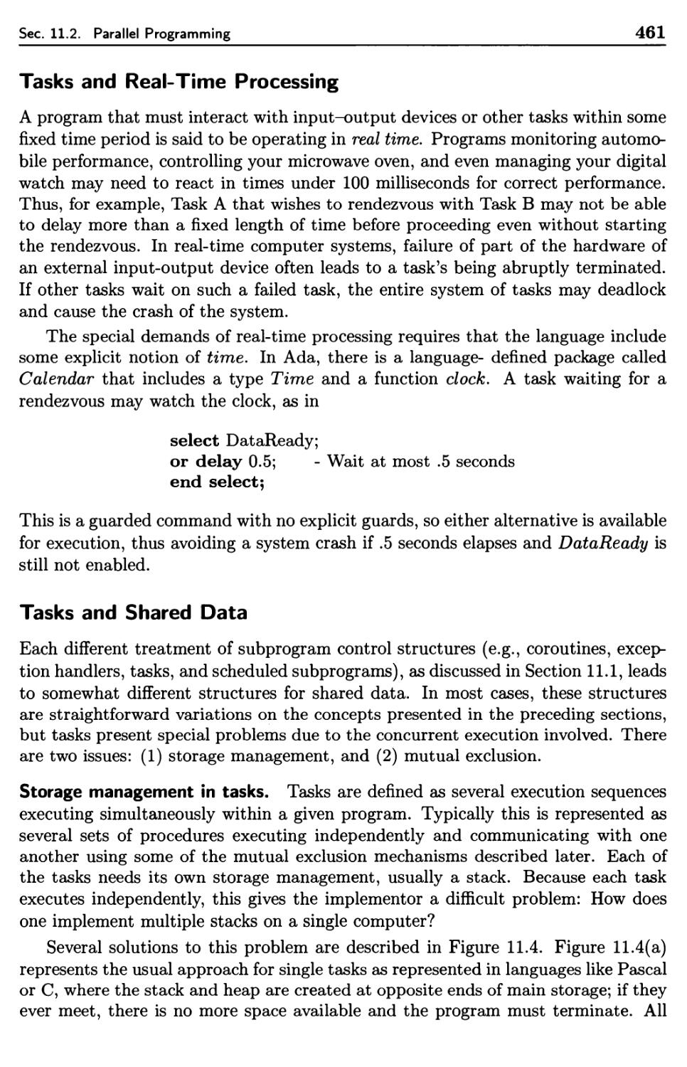
/


Text
Fourth Edition
PROGRAMMING LANGUAGES
Design and Implementation
Terrence W. Pratt
Center of Excellence in Space Data and Information Sciences
NASA Goddard Space Flight Center, Greenbelt, MD
(retired)
Marvin V. Zelkowitz
Department of Computer Science and
Institute for Advanced Computer Studies
University of Maryland, College Park, MD
Frontier
Hall
PRENTICE HALL, Upper Saddle River, New Jersey 07458
Library of Congress Cataloging-in-Publication Data
Pratt, Terrence W.
Programming languages : design and implementation / Terrence W. Pratt, Marvin V.
Zelkowitz. — 4th ed.
p. cm.
Includes bibliographical references and index.
ISBN 0-13-027678-2 (alk. paper)
1. Programming languages (Electronic computers) I. Zelkowitz, Marvin V., 1945- II.
Title.
QA76.7 P7 2000
005.13—dc20 95-19011
CIP
Vice president and editorial director, ECS: Marcia Horton
Acquisition editor: Petra Recter
Associate editor: Sarah Burrows
Editorial assistant: Karen Schultz
Production editor: Leslie Galen
Managing editor: David A. George
Executive managing editor: Vince O'Brien
Art director: Heather Scott
Assistant art director: John Christiana
Cover design: Marjory Dressier
Marketing manager: Jennie Burger
Manufacturing buyer: Dawn Murrin
Manufacturing manager: Trudy Pisciotti
Assistant vice president of production and manufacturing: David W. Riccardi
© 2001, 1996, 1984, 1975 by PRENTICE-HALL, Inc.
Upper Saddle River, New Jersey 07458
All rights reserved. No part of this book may be
reproduced, in any form or by any means,
without permission in writing from the publisher.
The author and publisher of this book have used their best efforts in preparing this book. These
efforts include the development, research, and testing of the theories and programs to determine their
effectiveness. The author and publisher make no warranty of any kind, expressed or implied, with regard
to these programs or to the documentation contained in this book. The author and publisher shall not
be liable in any event for incidental or consequential damages in connection with, or arising out of, the
furnishing, performance, or use of these programs.
Printed in the United States of America
10 9876543
ISBN 0-13-027678-2
Prentice-Hall International (UK) Limited, London
Prentice-Hall of Australia Pty. Limited, Sydney
Prentice-Hall Canada Inc., Toronto
Prentice-Hall Hispanoamericana, S. A., Mexico
Prentice-Hall of India Private Limited, New Delhi
Prentice-Hall of Japan, Inc., Tokyo
Pearson Education Asia, Pte. Ltd.
Editora Prentice-Hall do Brasil, Ltda., Rio de Janeiro
For Kirsten, Randy, Laurie, Aaron, and Elena
Preface
This fourth edition of Programming Languages: Design and Implementation
continues the tradition developed in the earlier editions to describe programming language
design by means of the underlying software and hardware architecture that is
required for execution of programs written in those languages. This provides the
programmer with the ability to develop software that is both correct and efficient
in execution. In this new edition, we continue this approach, as well as improve on
the presentation of the underlying theory and formal models that form the basis for
the decisions made in creating those languages.
Programming language design is still a very active pursuit in the computer
science community as languages are born, age, and eventually die. This fourth
edition represents the vital languages of the early 215t century. Postscript, Java,
HTML, and Perl have been added to the languages discussed in the third edition
to reflect the growth of the World Wide Web as a programming domain. The
discussion of Pascal, FORTRAN, and Ada has been deemphasized in recognition of
these languages' aging in anticipation of possibly dropping them in future editions
of this book.
At the University of Maryland, a course has been taught for the past 25 years
that conforms to the structure of this book. For our junior-level course, we
assume the student already knows C, Java, or C+_1- from earlier courses. We then
emphasize Smalltalk, ML, Prolog, and LISP, as well as include further discussions
of the implementation aspects of C++ . The study of C++ furthers the students'
knowledge of procedural languages with the addition of object-oriented classes, and
the inclusion of LISP, Prolog, and ML provides for discussions of different
programming paradigms. Replacement of one or two of these by FORTRAN, Ada, or Pascal
would also be appropriate.
It is assumed that the reader is familiar with at least one procedural language,
generally C, C++, Java, or FORTRAN. For those institutions using this book at
a lower level, or for others wishing to review prerequisite material to provide a
framework for discussing programming language design issues, Chapters 1 and 2
provide a review of material needed to understand later chapters. Chapter 1 is a
v
vi
Preface
general introduction to programming languages, while Chapter 2 is a brief overview
of the underlying hardware that will execute the given program.
The theme of this book is language design and implementation issues. Chapter
3, and 5 through 12 provide the basis for this course by describing the underlying
grammatical model for programming languages and their compilers (Chapter 3),
elementary data types (Chapter 5), data structures and encapsulation (Chapter 6),
inheritance (Chapter 7), statements (Chapter 8), procedure invocation (Chapter 9),
storage management (Chapter 10), distributed processing (Chapter 11) and network
programming (Chapter 12), which form the central concerns in language design.
Chapter 4 is a more advanced chapter on language semantics that includes an
introduction to program verification, denotational semantics, and the lambda
calculus. It may be skipped in the typical sophomore- or junior-level course. As with
the previous editions of this book, we include a comprehensive appendix that is a
brief summary of the features in the 12 languages covered in some detail in this
book.
The topics in this book cover the 12 knowledge units recommended by the 1991
ACM/IEEE Computer Society Joint Curriculum Task Force for the programming
languages subject area [TUCKER et al. 1991].
Although compiler writing was at one time a central course in the computer
science curriculum, there is increasing belief that not every computer science student
needs to be able to develop a compiler; such technology should be left to the compiler
specialist, and the hole in the schedule produced by deleting such a course might be
better utilized with courses such as software engineering, database engineering, or
other practical use of computer science technology. However, we believe that aspects
of compiler design should be part of the background for all good programmers.
Therefore, a focus of this book is how various language structures are compiled,
and Chapter 3 provides a fairly complete summary of parsing issues.
The 12 chapters emphasize programming language examples in FORTRAN,
Ada, C, Java, Pascal, ML, LISP, Perl, Postscript, Prolog, C++, and Smalltalk.
Additional examples are given in HTML, PL/I, SNOBOL4, APL, BASIC, and COBOL
as the need arises. The goal is to give examples from a wide variety of languages and
let the instructor decide which languages to use as programming examples during
the course.
Although discussing all of the languages briefly during the semester is
appropriate, we do not suggest that the programming parts of this course consist of problems
in each of these languages. We think that would be too superficial in one course.
Ten programs, each written in a different language, would be quite a chore and
would provide the student with little in-depth knowledge of any of these languages.
We assume that each instructor will choose three or four languages and emphasize
those.
All examples in this book, except for the most trivial, were tested on an
appropriate translator; however, as we clearly point out in Section 1.3.3, correct execution
on our local system is no guarantee that the translator is processing programs
according to the language standard. We are sure that Mr. Murphy is at work here,
Preface
vii
and some of the trivial examples may have errors. If so, we apologize for any
problems that may cause.
To summarize, our goals in producing this fourth edition were as follows:
• Provide an overview of the key paradigms used in developing modern
programming languages;
• Highlight several languages, which provide those features, in sufficient detail
to permit programs to be written in each language demonstrating those features;
• Explore the implementation of each language in sufficient detail to provide the
programmer with an understanding of the relationship between a source program
and its execution behavior;
• Provide sufficient formal theory to show where programming language design
fits within the general computer science research agenda;
• Provide a sufficient set of problems and alternative references to allow
students the opportunity to extend their knowledge of this important topic.
We gratefully acknowledge the valuable comments received from the users of the
third edition of this text and from the hundreds of students of CMSC 330 at the
University of Maryland who provided valuable feedback on improving the presentation
contained in this book.
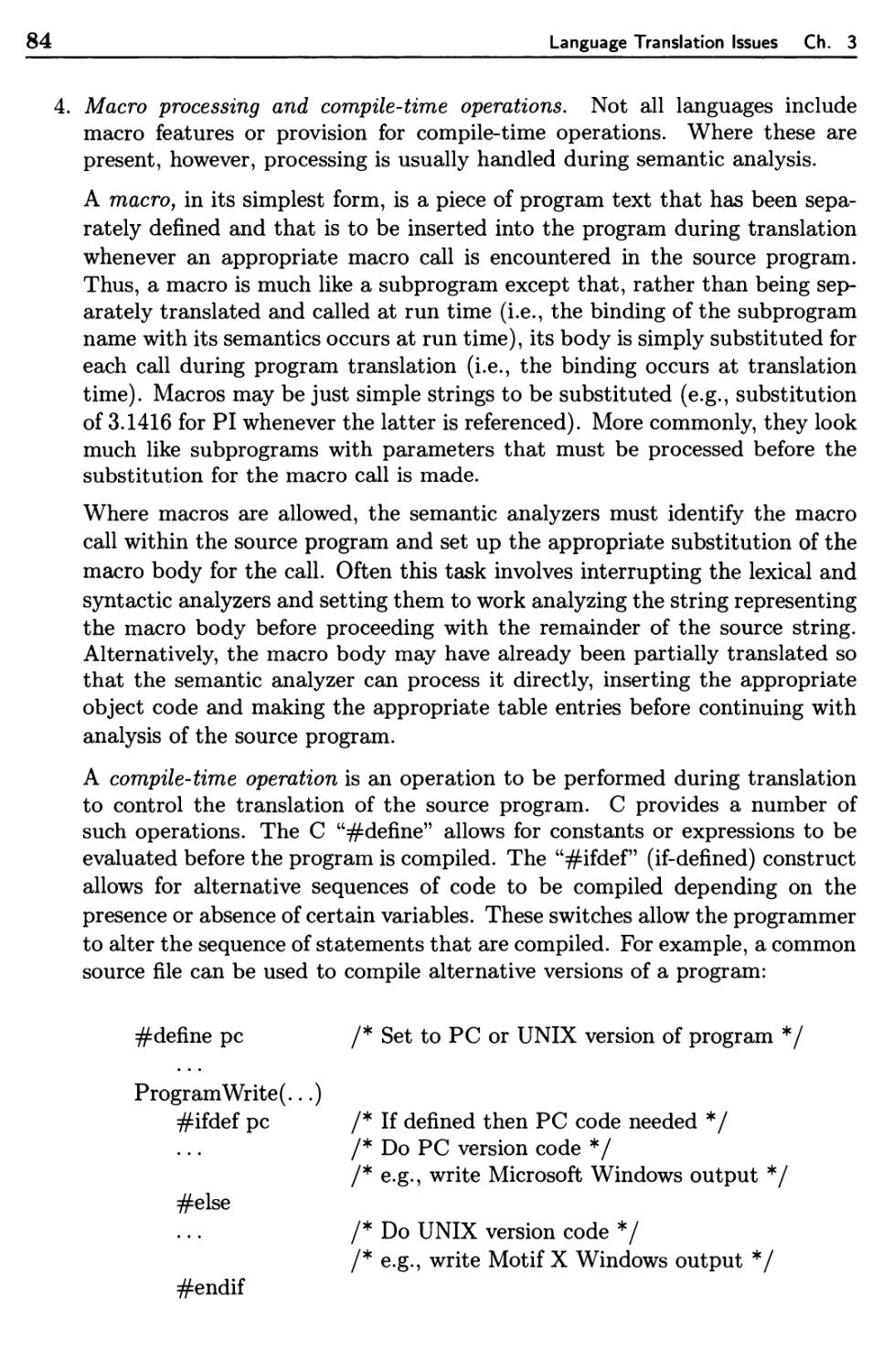
Changes to the Fourth Edition. For users familiar with the third edition, the
fourth edition has the following changes:
1. A chapter was added (Chapter 12) on the World Wide Web. Java was added
as a major programming language, and an overview of HTML and Postscript were
added to move the book away from the classical "FORTRAN number-crunching"
view of compilers.
2. The material on object-oriented design was moved earlier in the text to
indicate its major importance in software design today. In addition, numerous
other changes were made by moving minor sections around to better organize the
material into a more consistent presentation.
3. We have found that the detailed discussions of languages in Part II of the
third edition were not as useful as we expected. A short history of each of the 12
languages was added to the chapter that best represents the major features of that
language, and the language summaries in Part II of the third edition were shortened
as the appendix. Despite these additions, the size of the book has not increased
because we deleted some obsolete material.
Terry Pratt, Howardsville, Virginia
Marv Zelkowitz, College Park, Maryland
Contents
Preface v
1 Language Design Issues 1
1.1 Why Study Programming Languages? 1
1.2 A Short History of Programming Languages 4
1.2.1 Development of Early Languages 4
1.2.2 Evolution of Software Architectures 7
1.2.3 Application Domains 14
1.3 Role of Programming Languages 17
1.3.1 What Makes a Good Language? 19
1.3.2 Language Paradigms 25
1.3.3 Language Standardization 29
1.3.4 Internationalization 33
1.4 Programming Environments 34
1.4.1 Effects on Language Design 34
1.4.2 Environment Frameworks 37
1.4.3 Job Control and Process Languages 38
1.5 C Overview 39
1.6 Suggestions for Further Reading 41
1.7 Problems 42
2 Impact of Machine Architectures 45
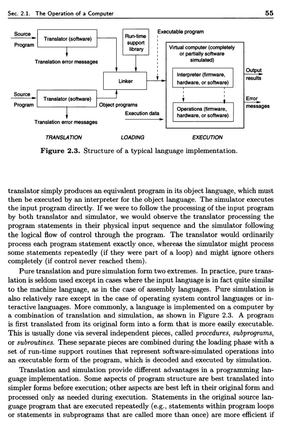
2.1 The Operation of a Computer 45
2.1.1 Computer Hardware 47
2.1.2 Firmware Computers 51
2.1.3 Translators and Virtual Architectures 53
ix
Contents
2.2 Virtual Computers and Binding Times 57
2.2.1 Virtual Computers and Language Implementations 58
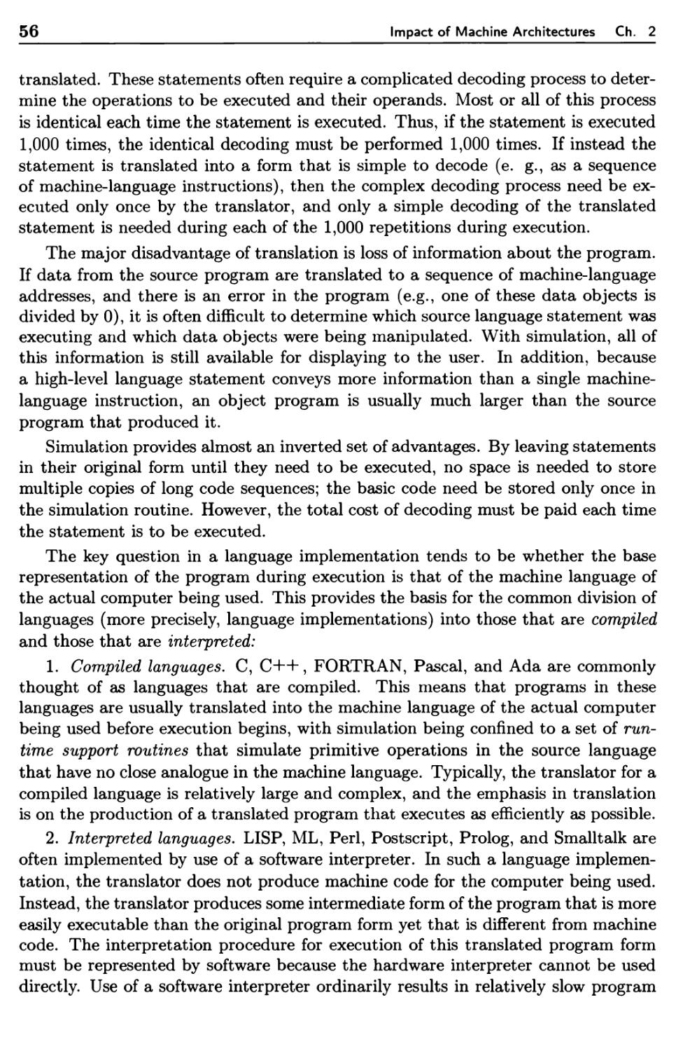
2.2.2 Hierarchies of Virtual Machines 59
2.2.3 Binding and Binding Time 61
2.2.4 Java Overview 65
2.3 Suggestions for Further Reading 67
2.4 Problems 67
Language Translation Issues 69
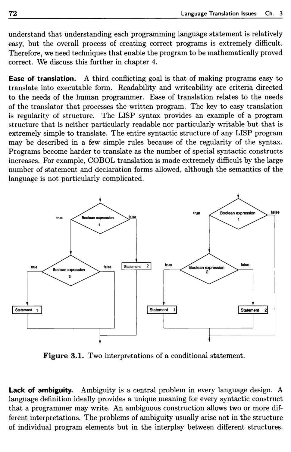
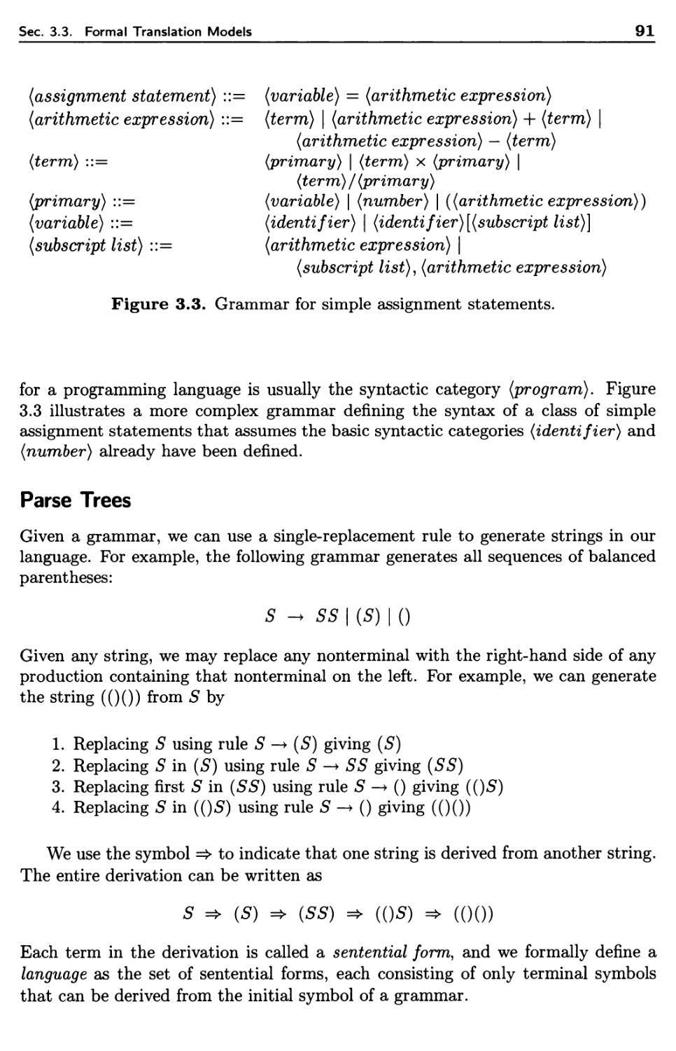
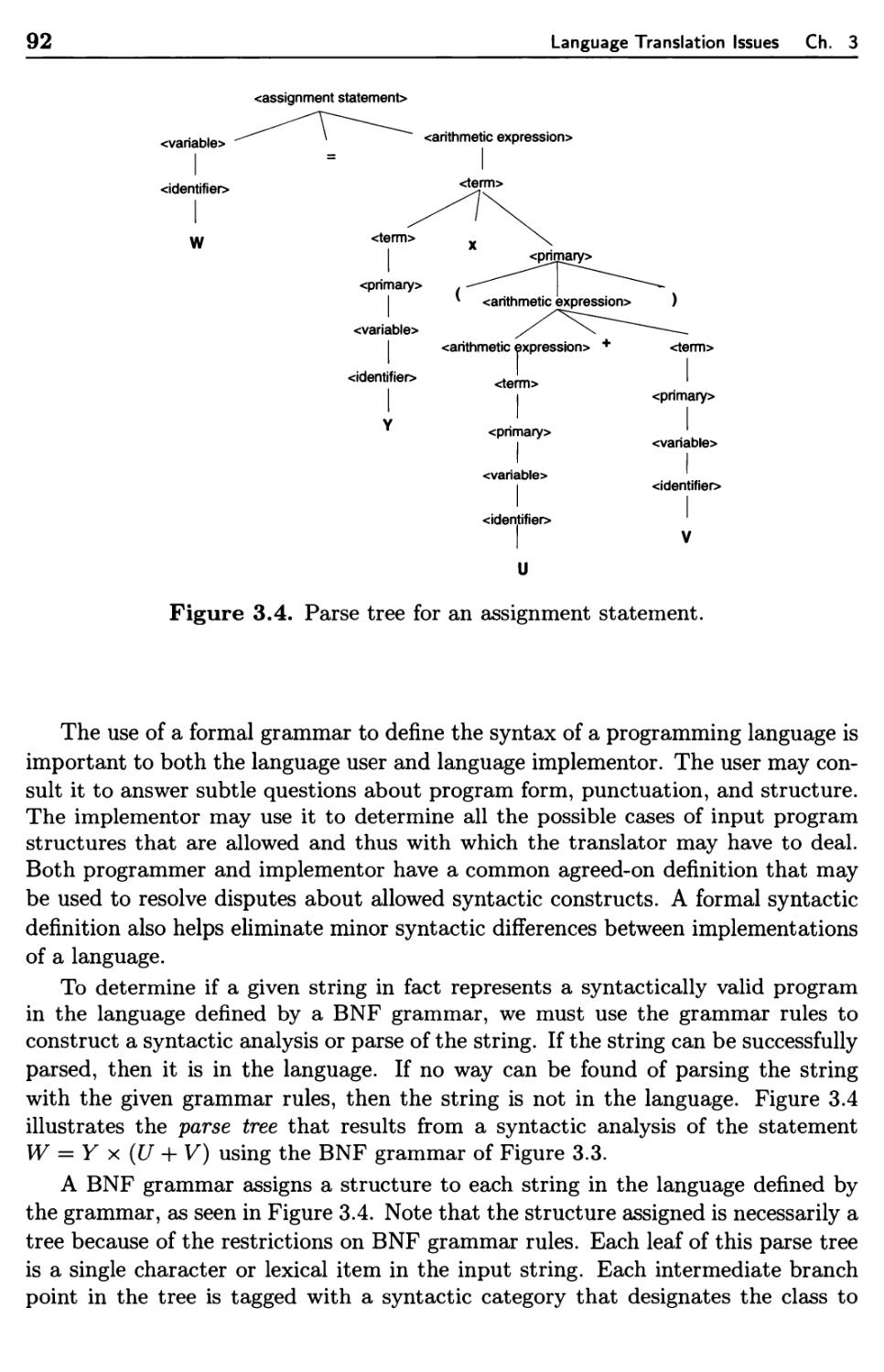
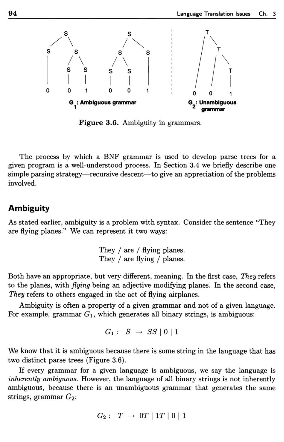
3.1 Programming Language Syntax 69
3.1.1 General Syntactic Criteria 70
3.1.2 Syntactic Elements of a Language 74
3.1.3 Overall Program-Subprogram Structure 77
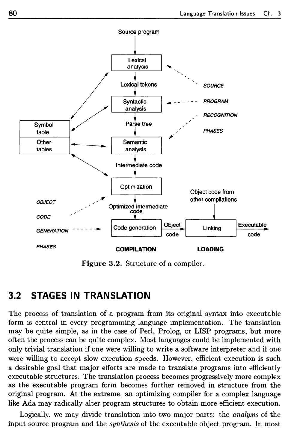
3.2 Stages in Translation 80
3.2.1 Analysis of the Source Program 81
3.2.2 Synthesis of the Object Program 85
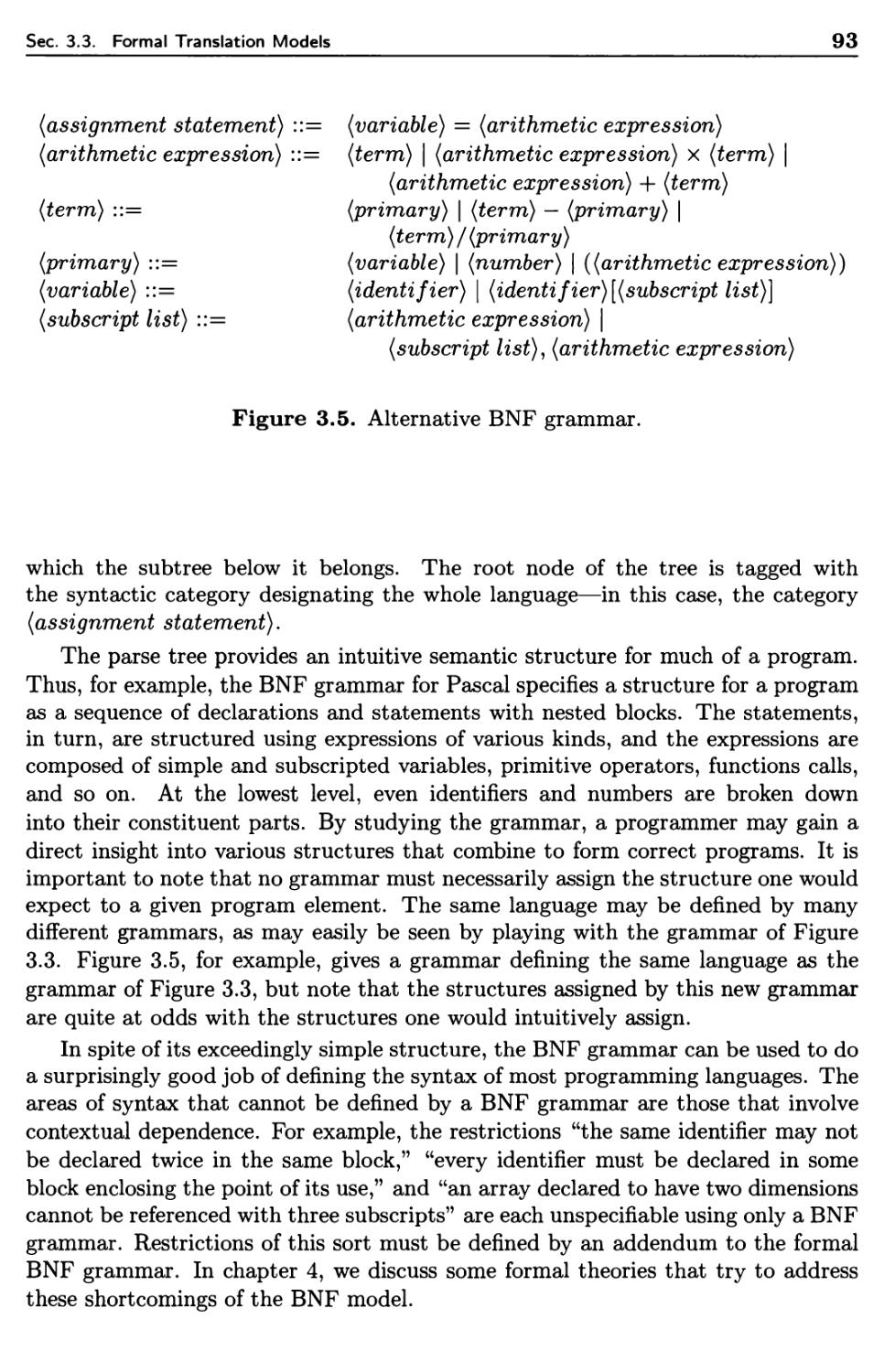
3.3 Formal Translation Models 87
3.3.1 BNF Grammars 88
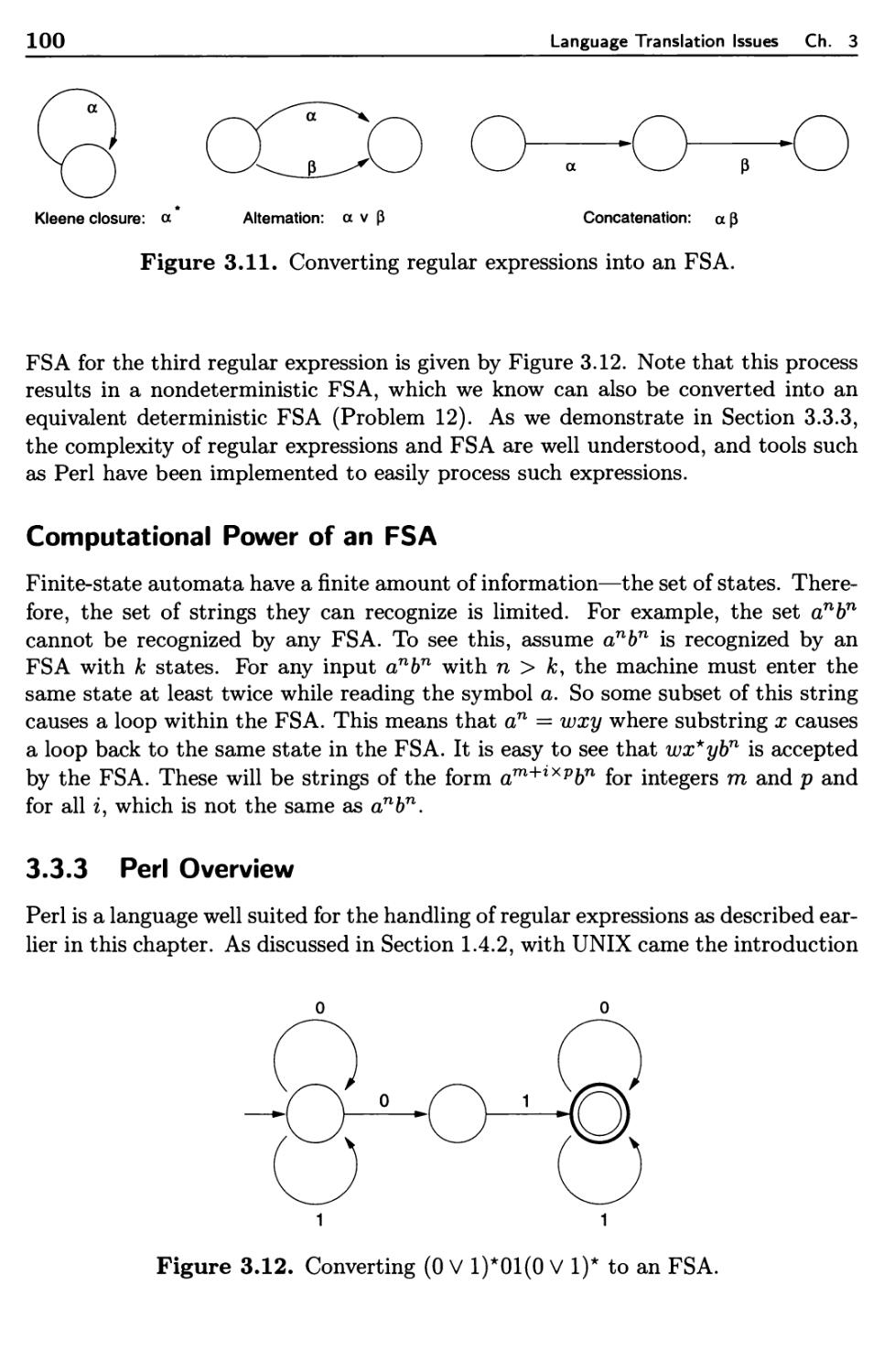
3.3.2 Finite-State Automata 97
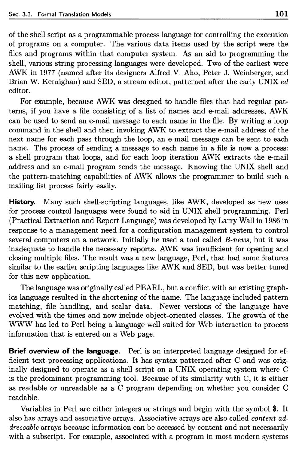
3.3.3 Perl Overview 100
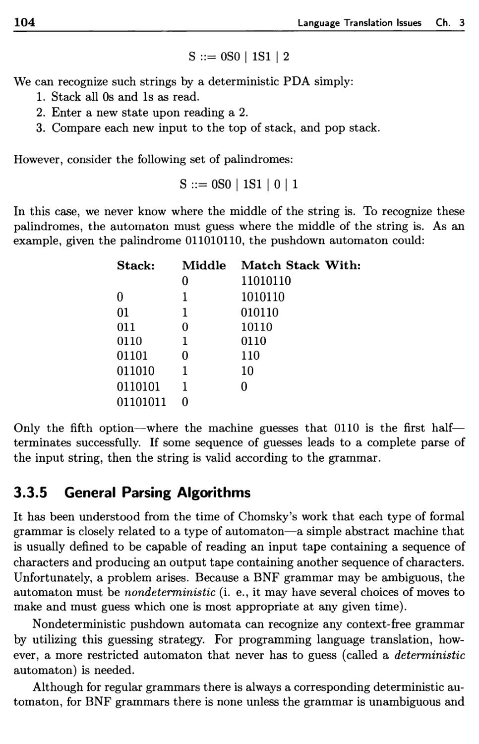
3.3.4 Pushdown Automata 103
3.3.5 General Parsing Algorithms 104
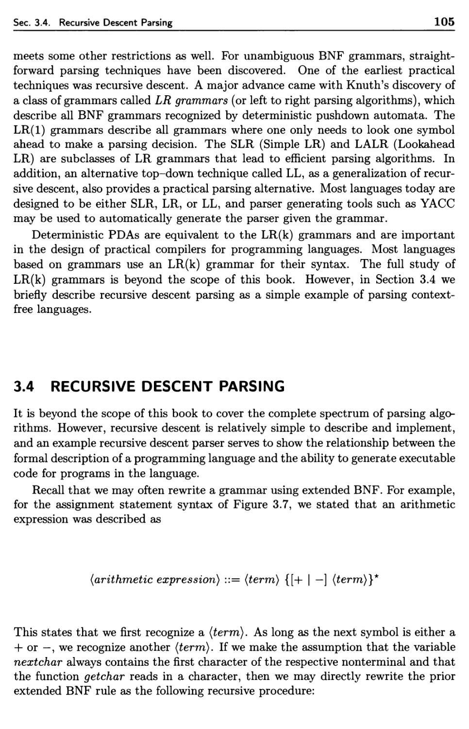
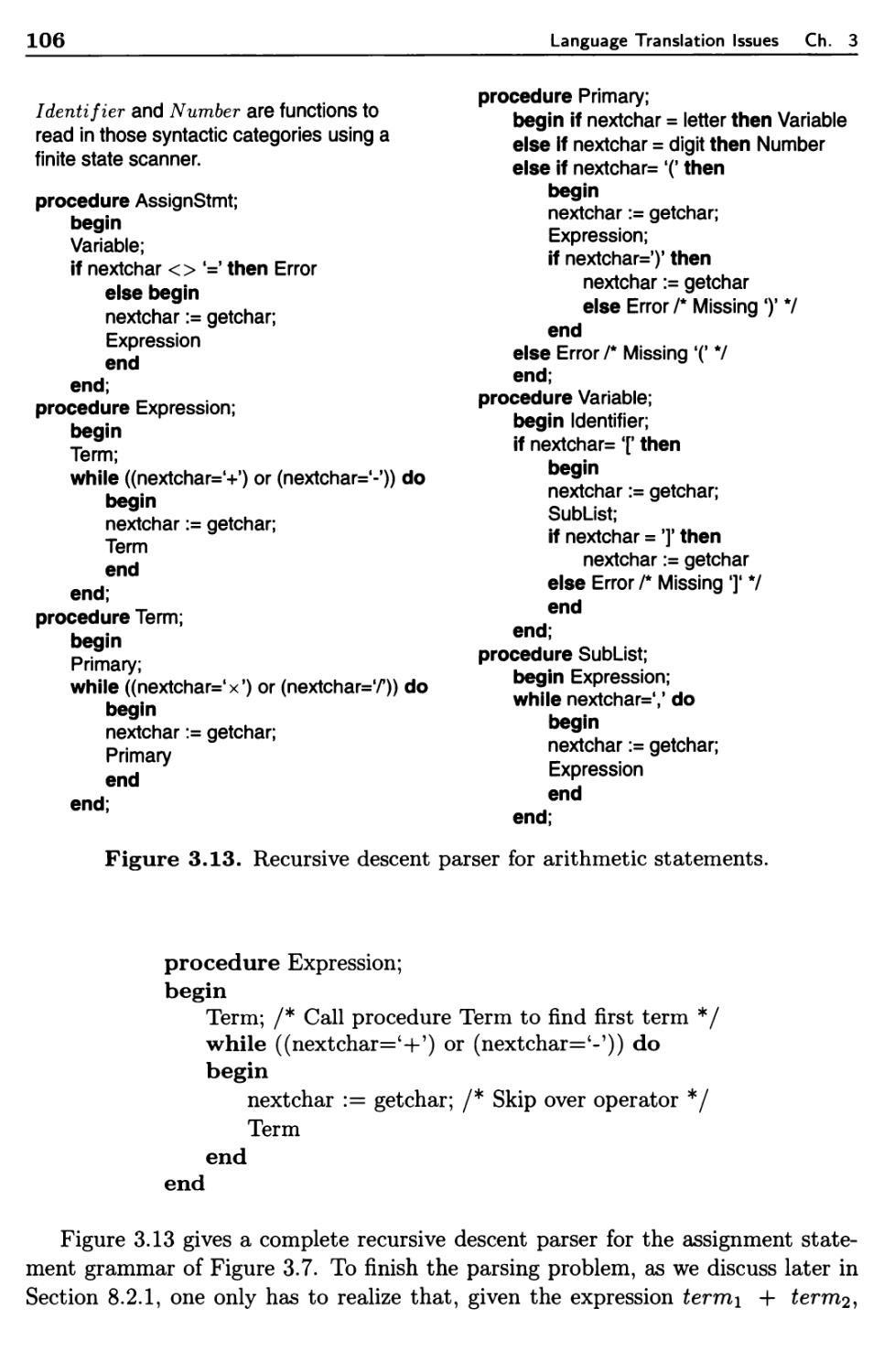
3.4 Recursive Descent Parsing 105
3.5 Pascal Overview 107
3.6 Suggestions for Further Reading 110
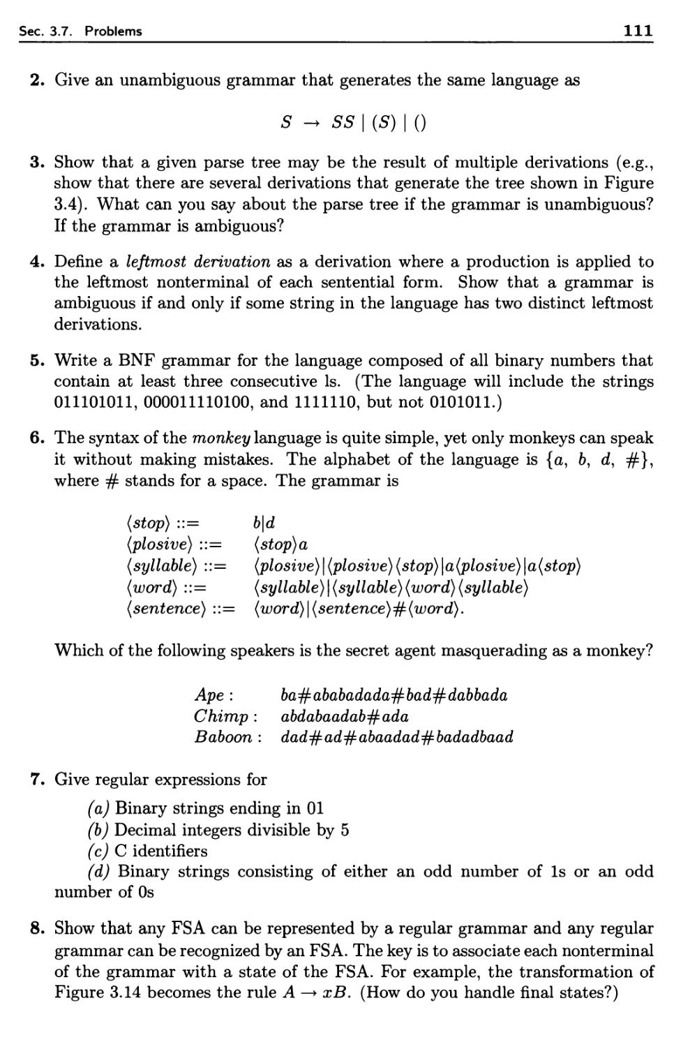
3.7 Problems 110
Modeling Language Properties 113
4.1 Formal Properties of Languages 114
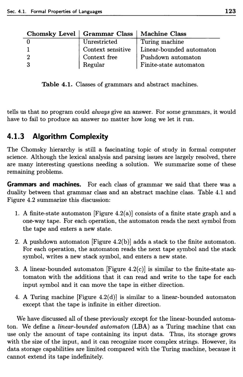
4.1.1 Chomsky Hierarchy 115
4.1.2 Undecidability 118
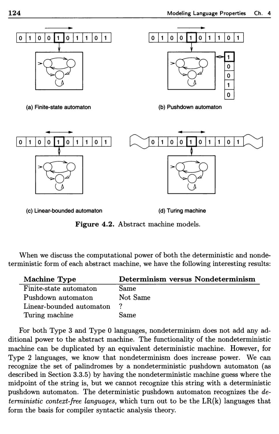
4.1.3 Algorithm Complexity 123
4.2 Language Semantics 125
4.2.1 Attribute Grammars 128
4.2.2 Denotational Semantics 130
4.2.3 ML Overview 138
4.2.4 Program Verification 139
4.2.5 Algebraic Data Types 143
CONTENTS
xi
4.3 Suggestions for Further Reading 146
4.4 Problems 147
5 Elementary Data Types 150
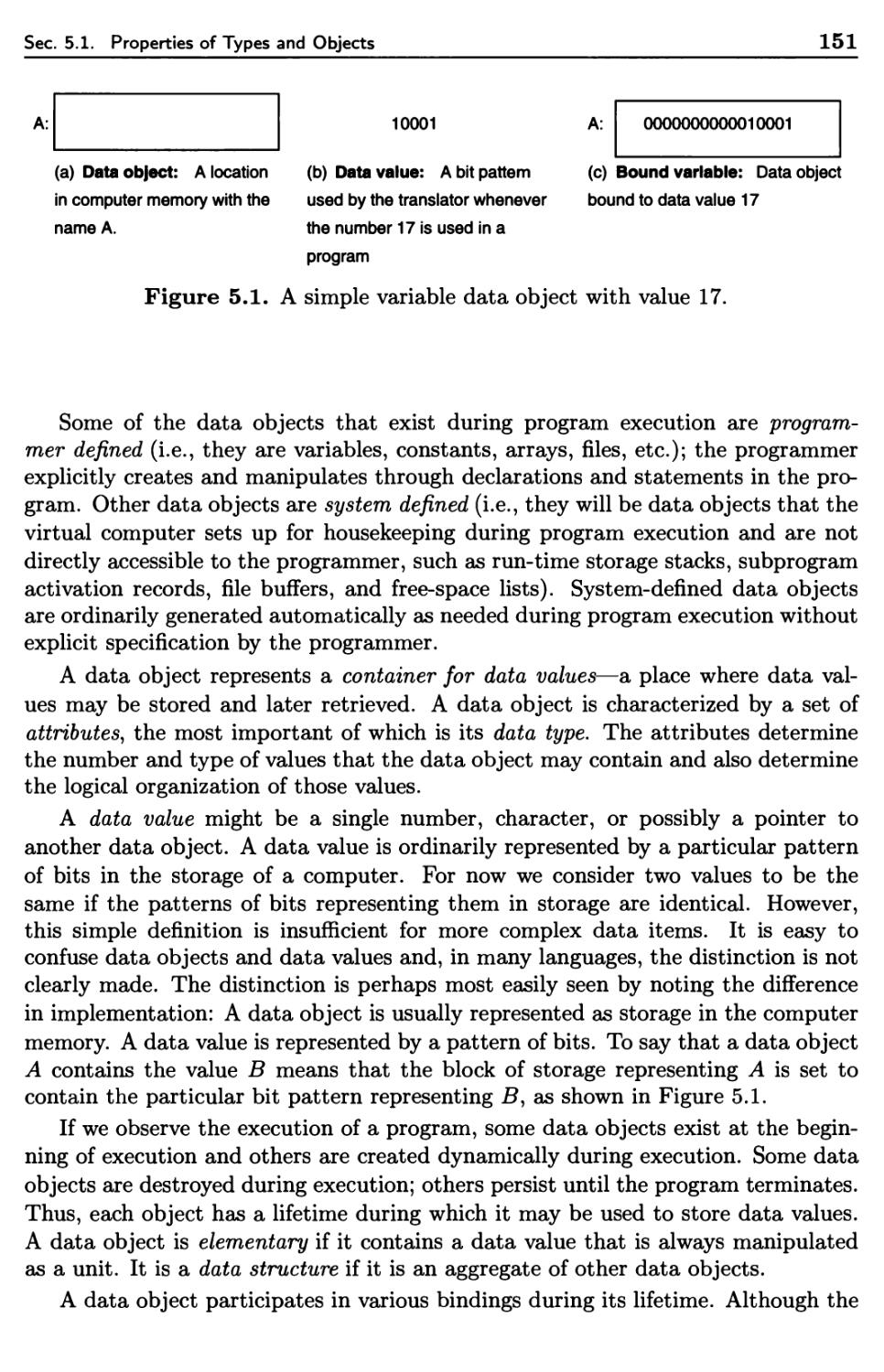
5.1 Properties of Types and Objects 150
5.1.1 Data Objects, Variables, and Constants 150
5.1.2 Data Types 155
5.1.3 Declarations 161
5.1.4 Type Checking and Type Conversion 163
5.1.5 Assignment and Initialization 168
5.2 Scalar Data Types 171
5.2.1 Numeric Data Types 172
5.2.2 Enumerations 179
5.2.3 Booleans 180
5.2.4 Characters 182
5.3 Composite Data Types 182
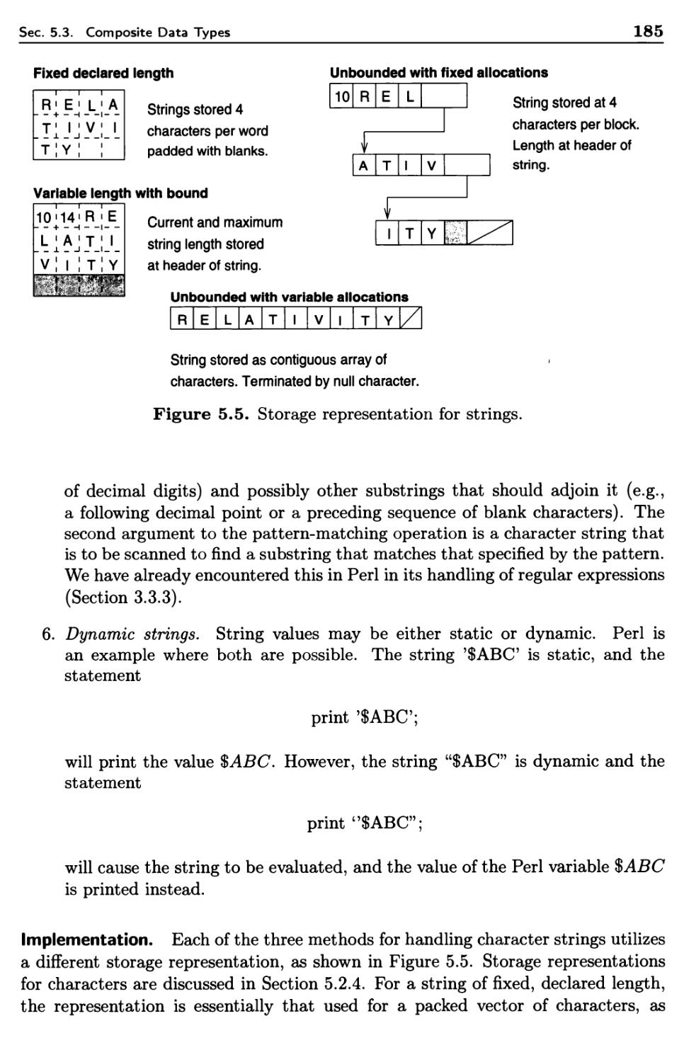
5.3.1 Character Strings 183
5.3.2 Pointers and Programmer-Constructed Data Objects 186
5.3.3 Files and Input-Output 189
5.4 FORTRAN Overview 194
5.5 Suggestions for Further Reading 196
5.6 Problems 196
6 Encapsulation 200
6.1 Structured Data Types 201
6.1.1 Structured Data Objects and Data Types 202
6.1.2 Specification of Data Structure Types 202
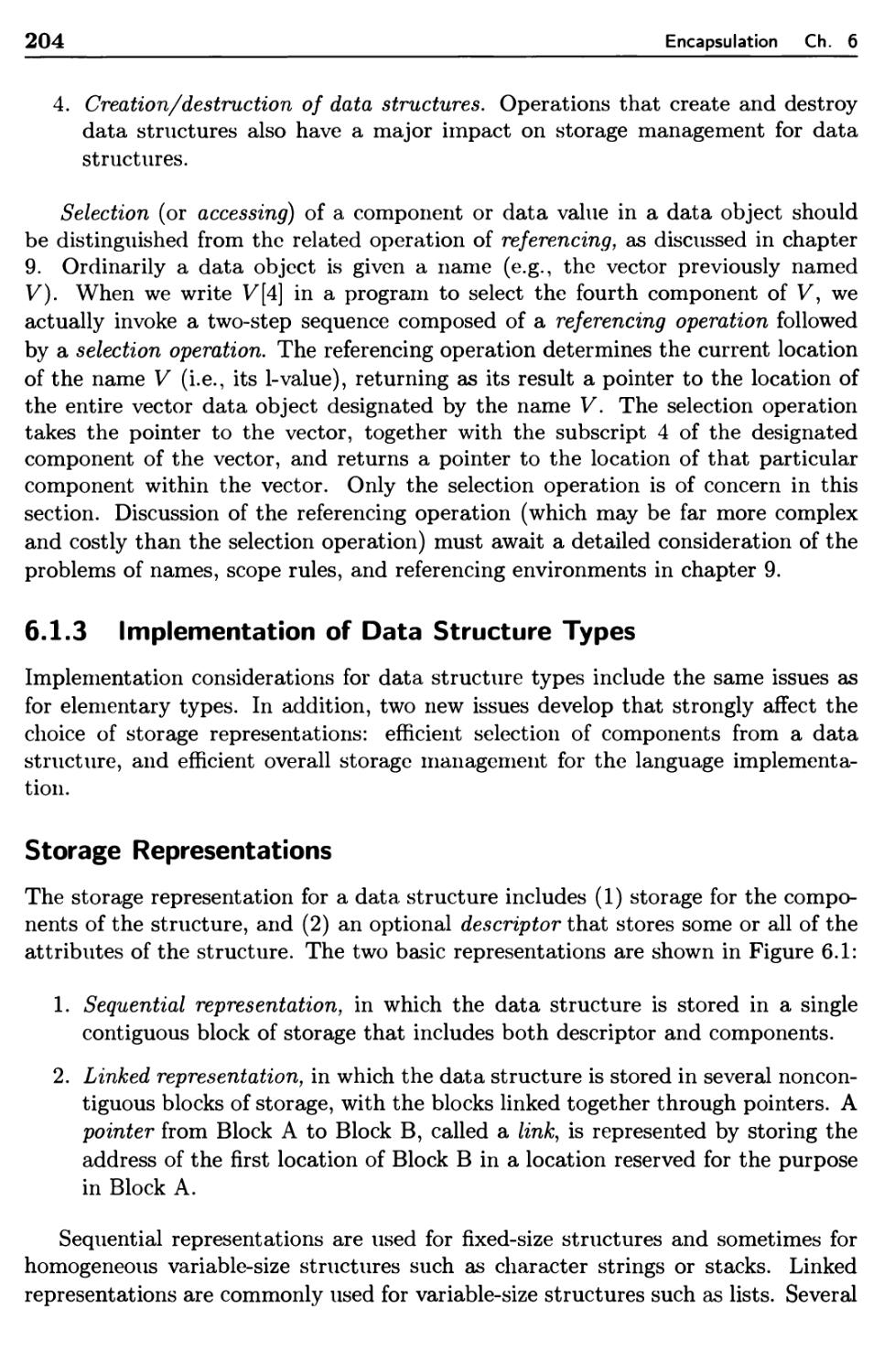
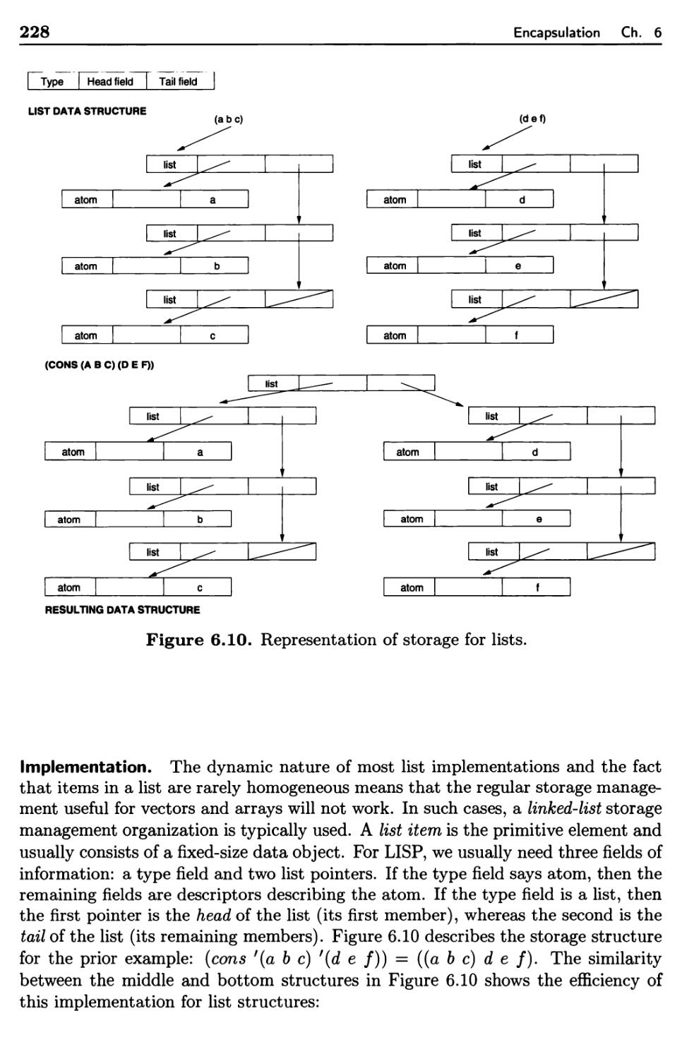
6.1.3 Implementation of Data Structure Types 204
6.1.4 Declarations and Type Checking for Data Structures 208
6.1.5 Vectors and Arrays 209
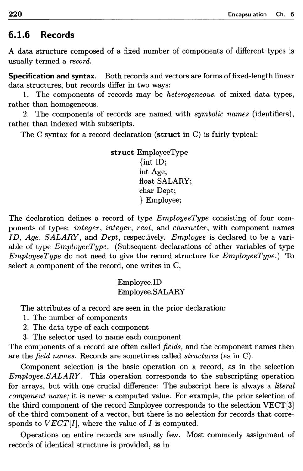
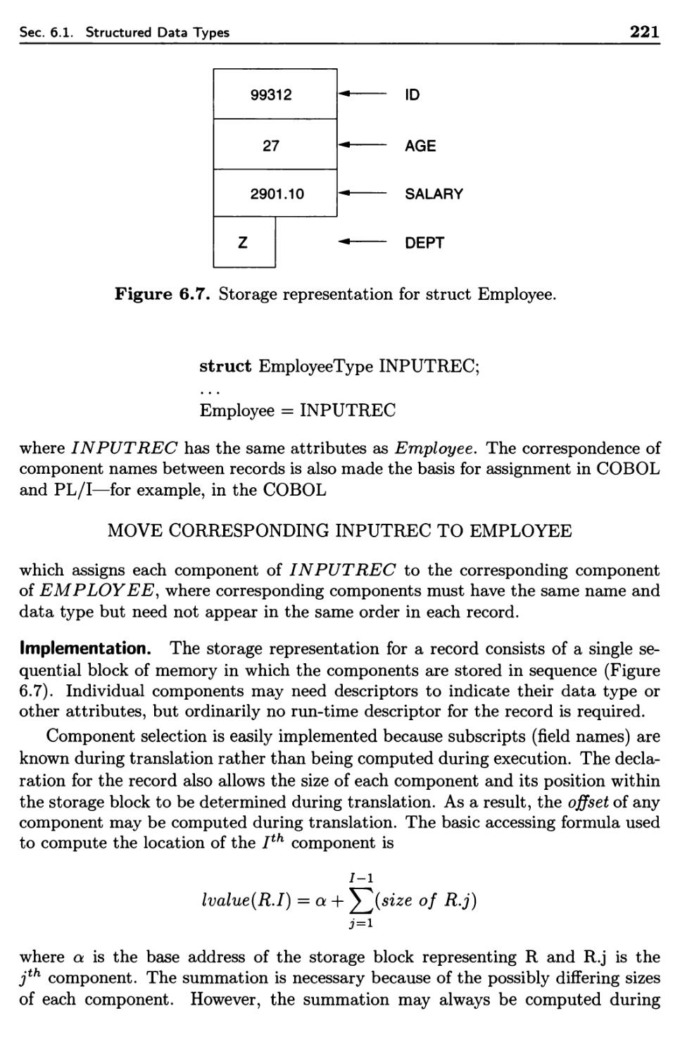
6.1.6 Records 220
6.1.7 Lists 227
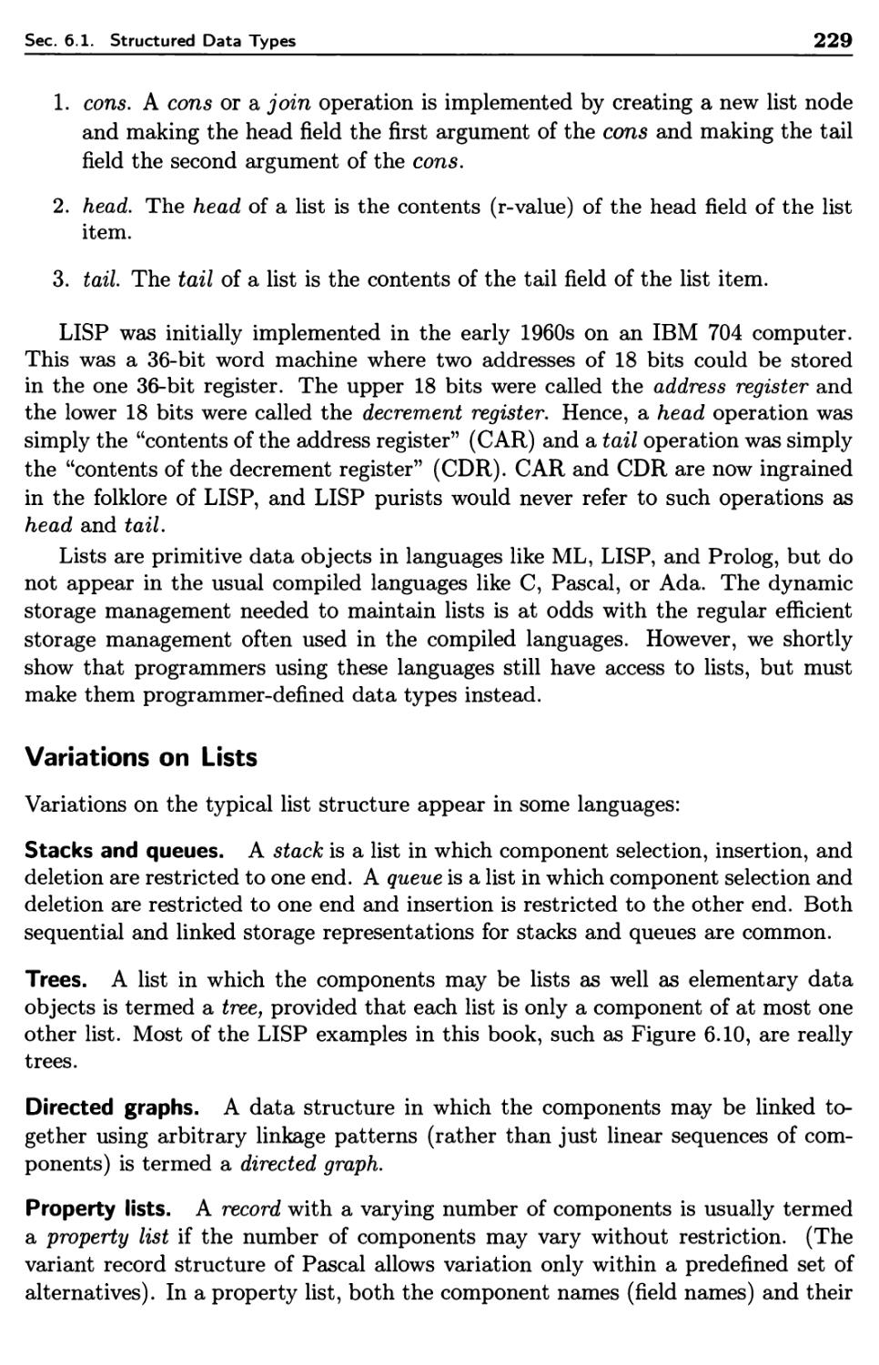
6.1.8 Sets 231
6.1.9 Executable Data Objects 234
6.2 Abstract Data Types 234
6.2.1 Evolution of the Data Type Concept 235
6.2.2 Information Hiding 235
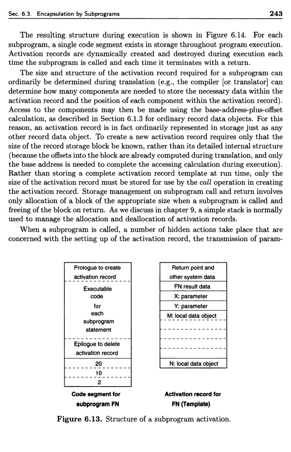
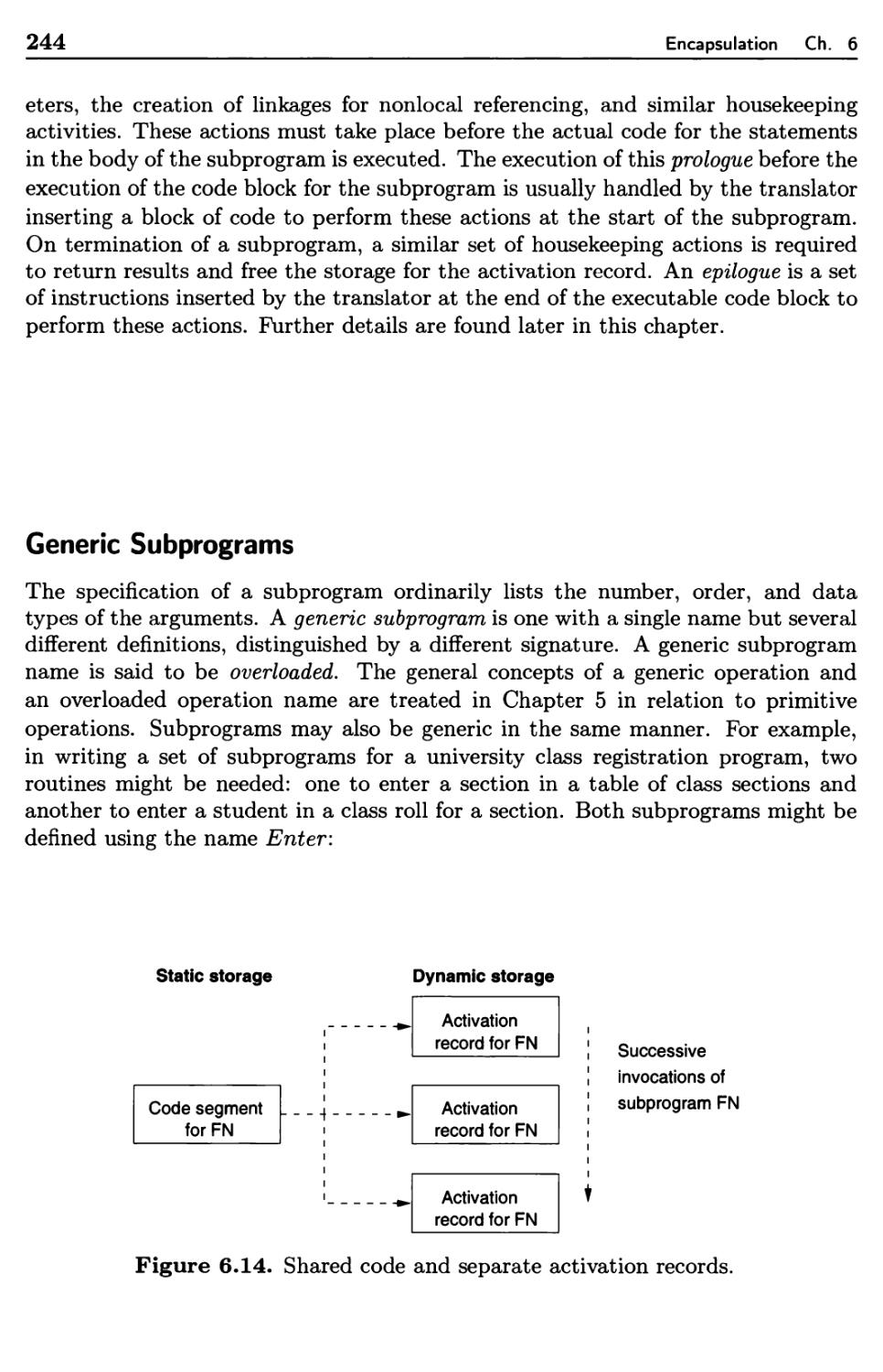
6.3 Encapsulation by Subprograms 238
Contents
6.4
6.5
6.6
6.7
6.3.1 Subprograms as Abstract Operations
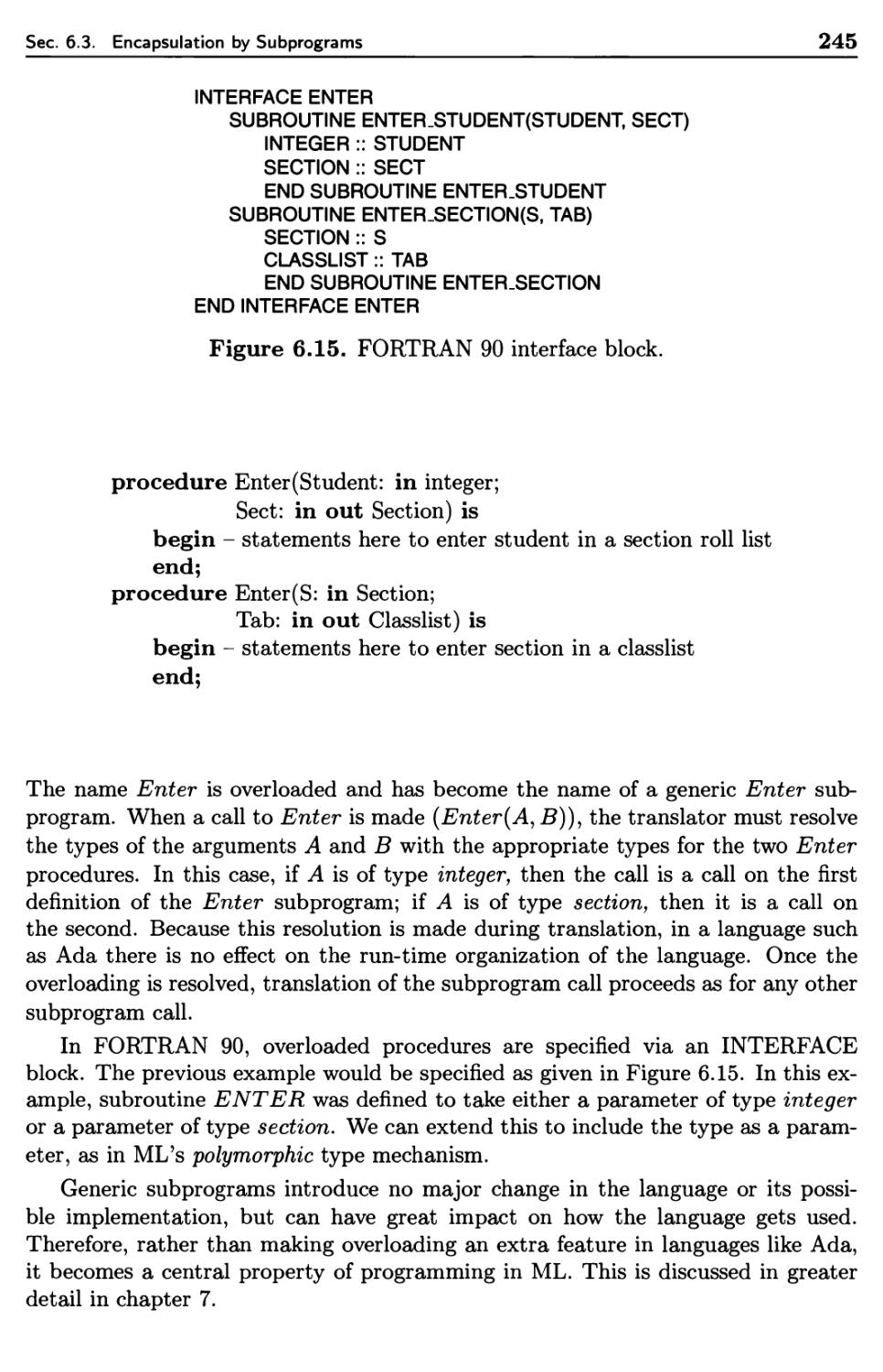
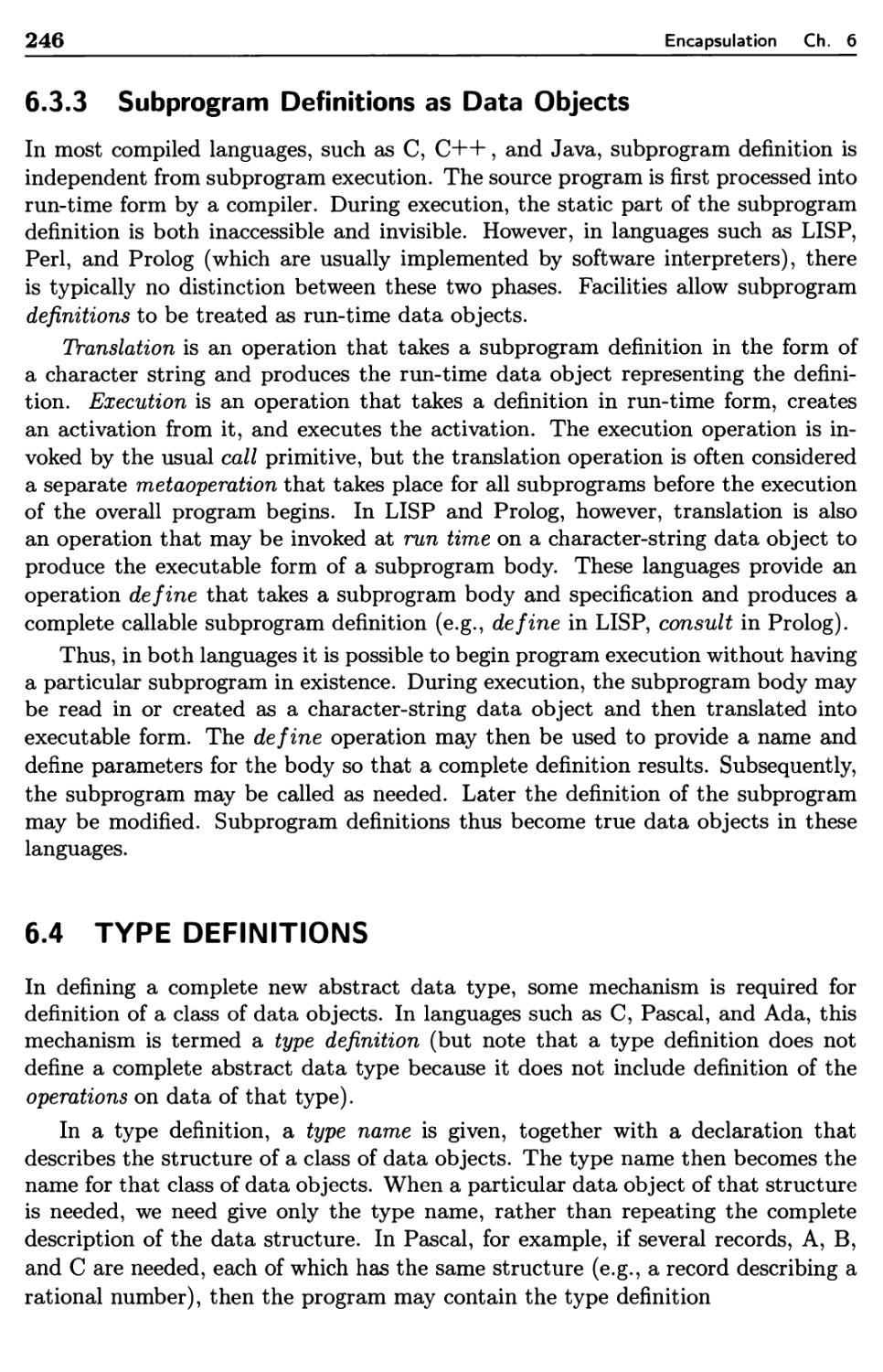
6.3.2 Subprogram Definition and Invocation
6.3.3 Subprogram Definitions as Data Objects
Type Definitions
6.4.1 Type Equivalence
6.4.2 Type Definitions with Parameters
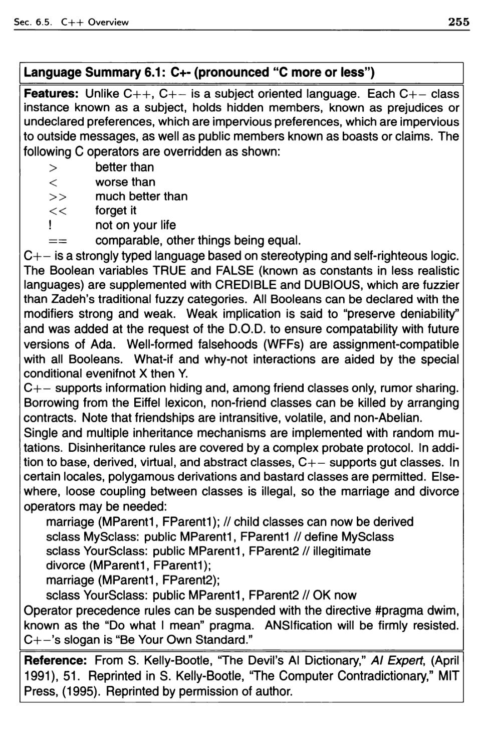
C++ Overview
Suggestions for Further Reading
Problems
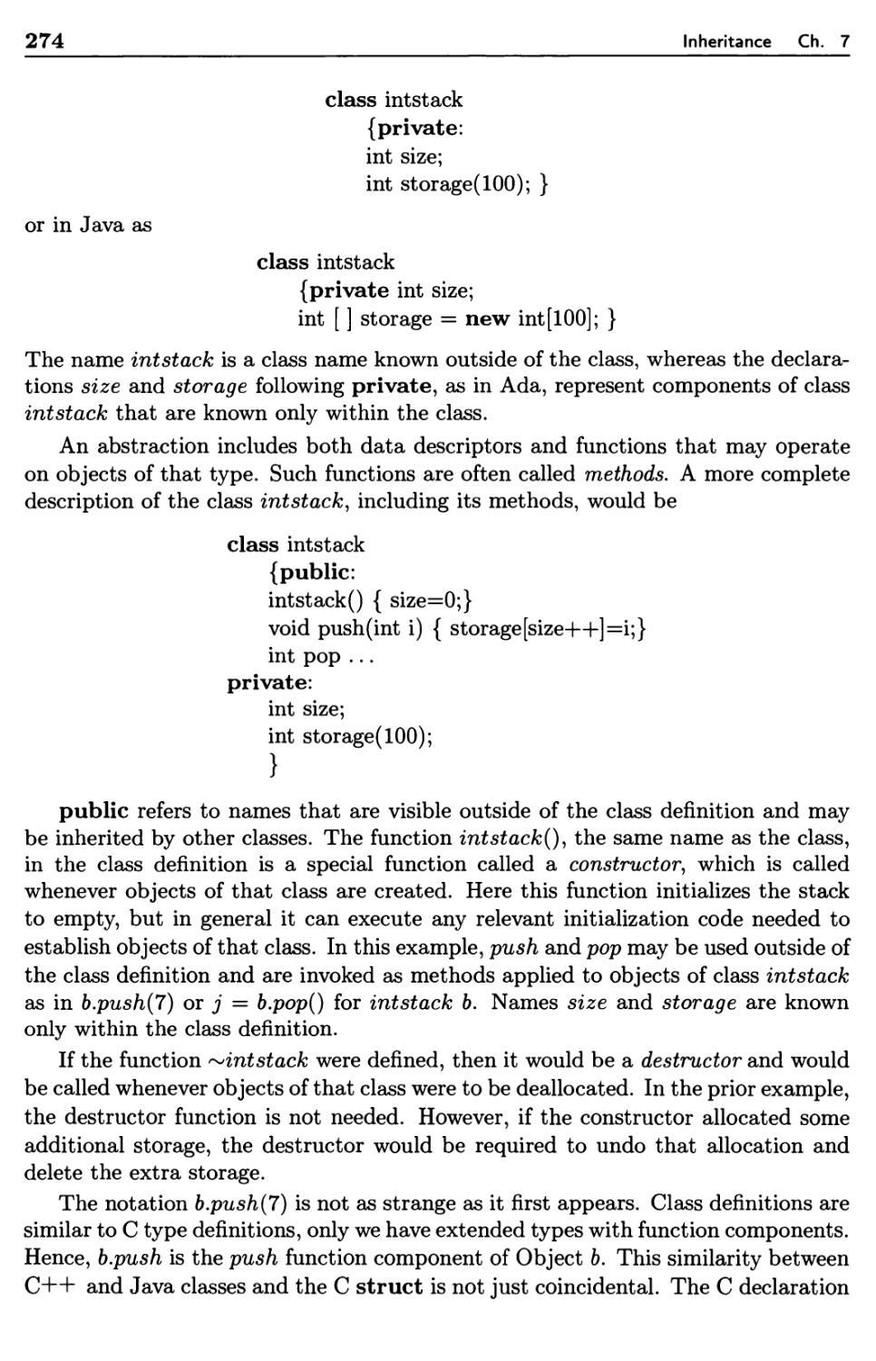
Inheritance
7.1
7.2
7.3
7.4
7.5
Seq
8.1
8.2
8.3
8.4
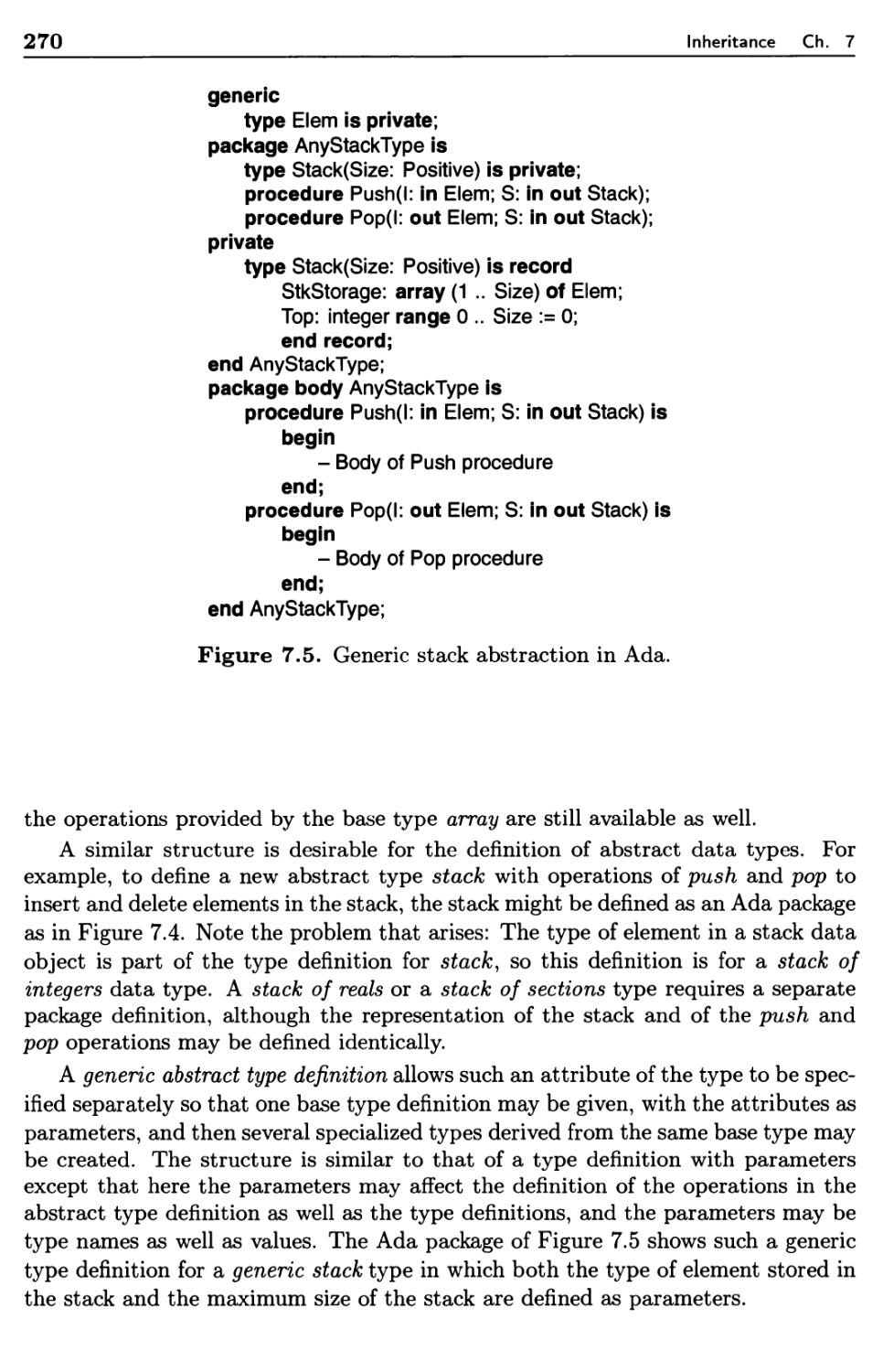
Abstract Data Types Revisited
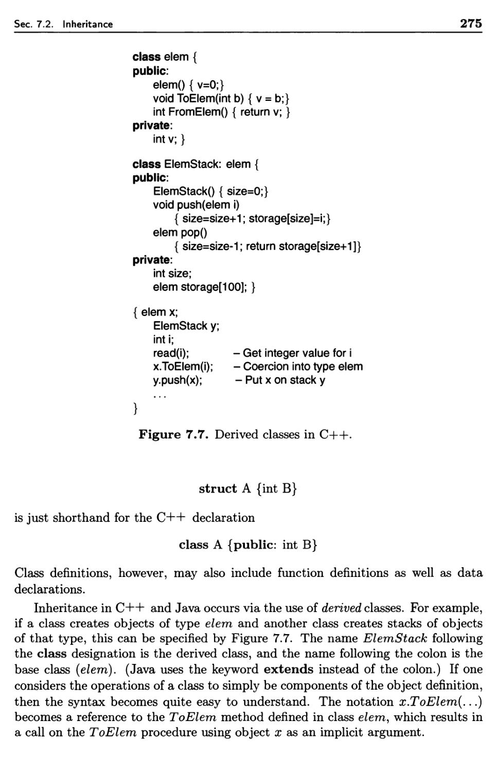
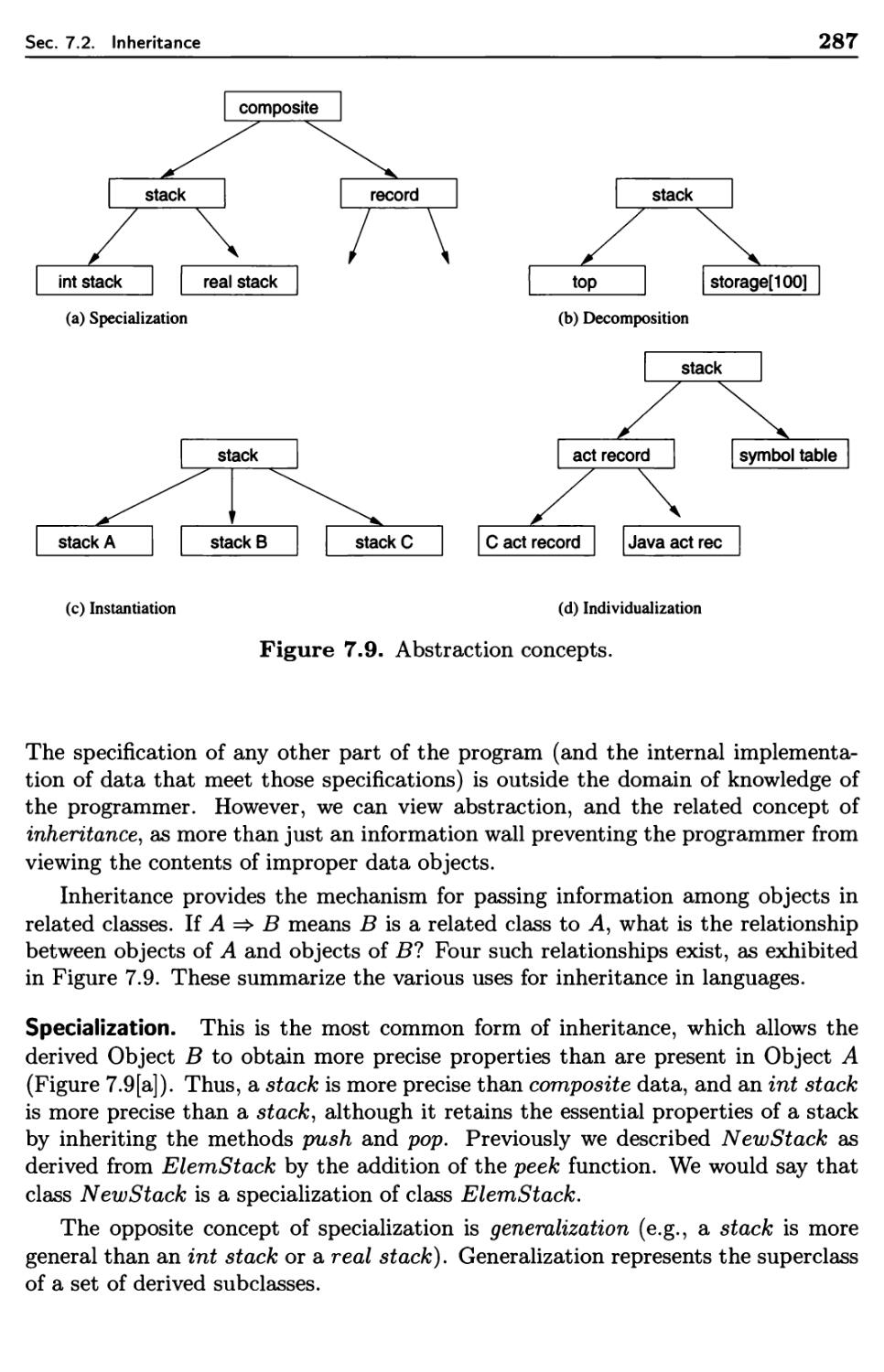
Inheritance
7.2.1 Derived Classes
7.2.2 Methods
7.2.3 Abstract Classes
7.2.4 Smalltalk Overview
7.2.5 Objects and Messages
7.2.6 Abstraction Concepts
Polymorphism
Suggestions for Further Reading
Problems
uence Control
Implicit and Explicit Sequence Control
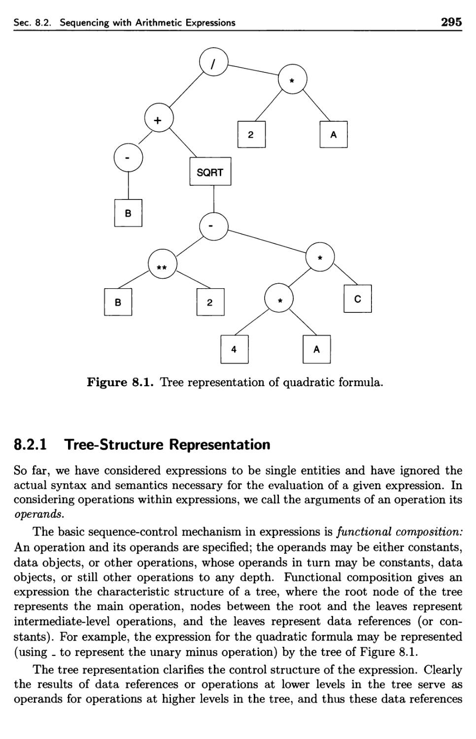
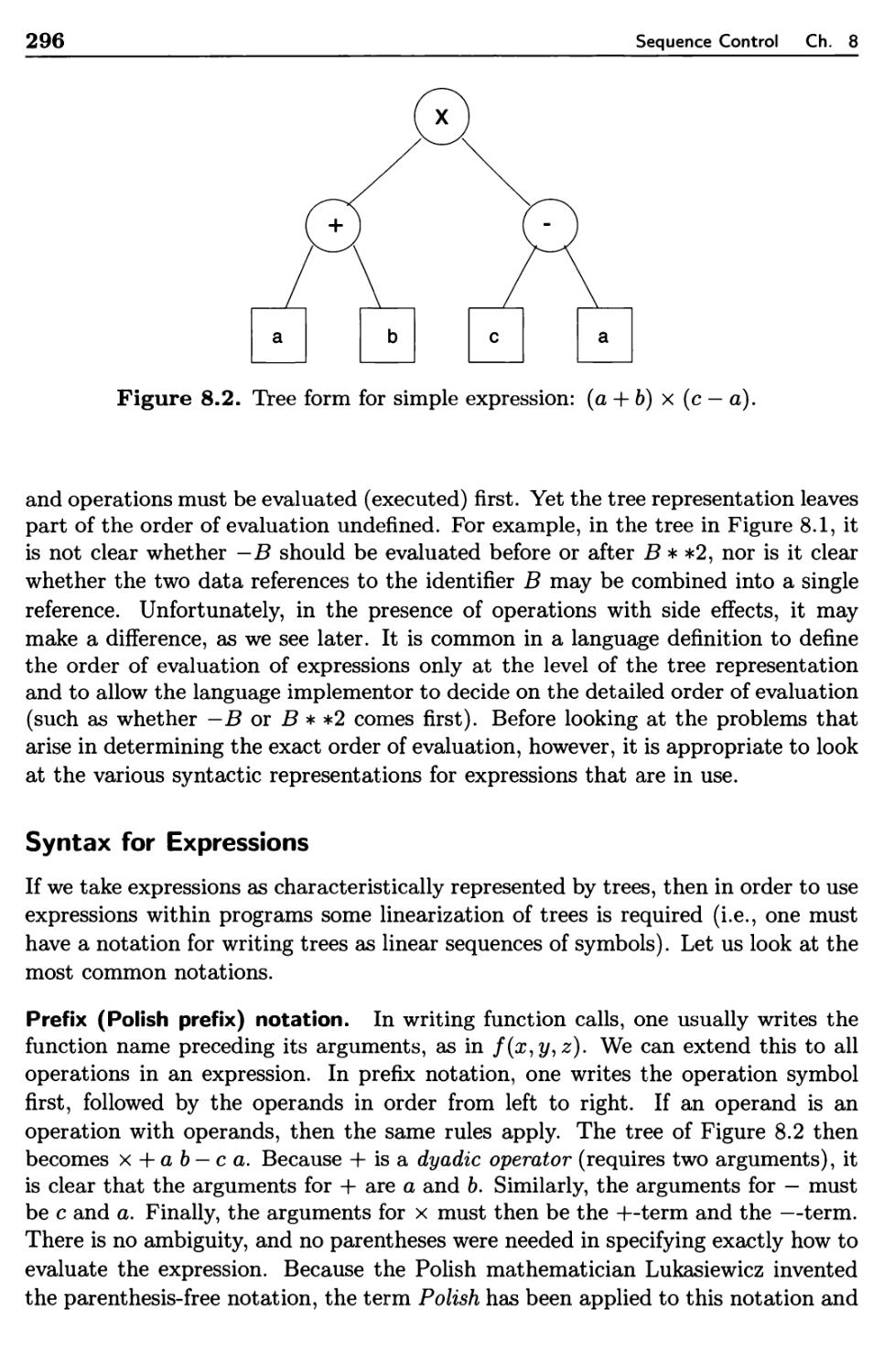
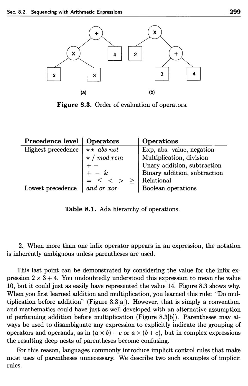
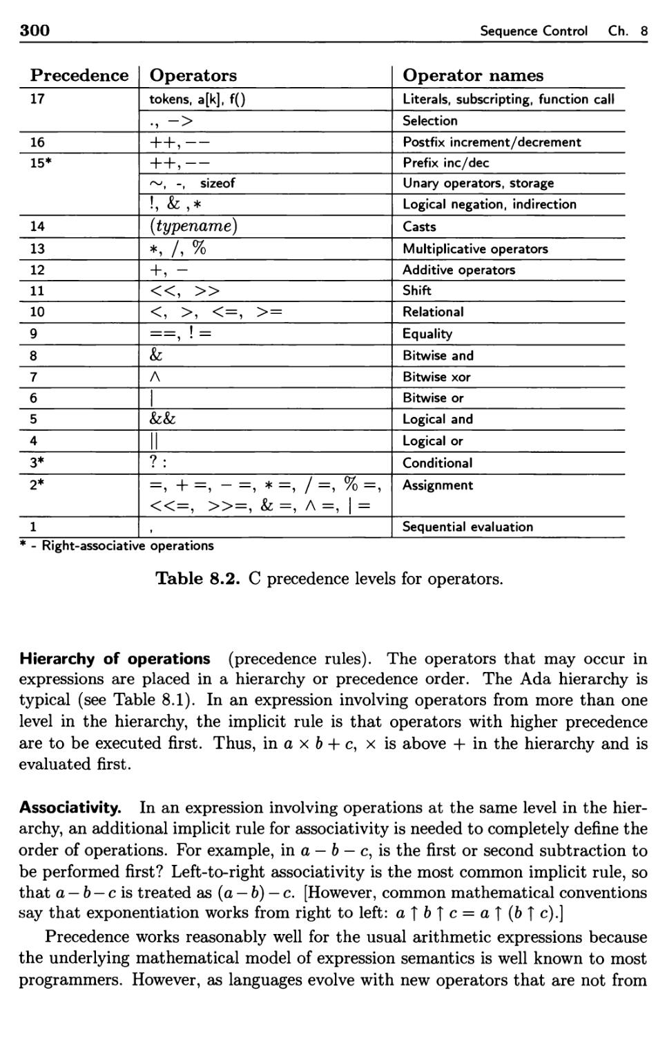
Sequencing with Arithmetic Expressions
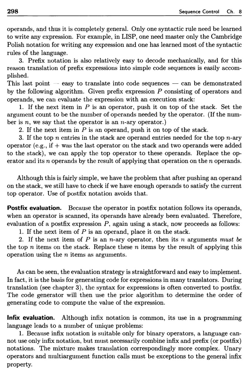
8.2.1 Tree-Structure Representation
8.2.2 Execution-Time Representation
Sequence Control Between Statements
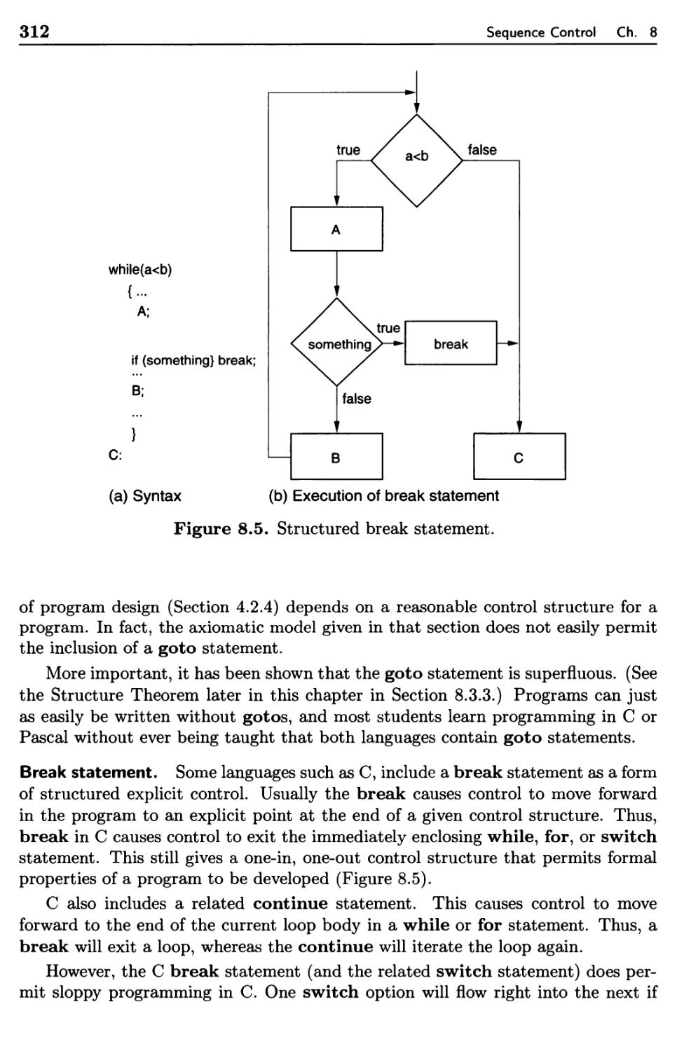
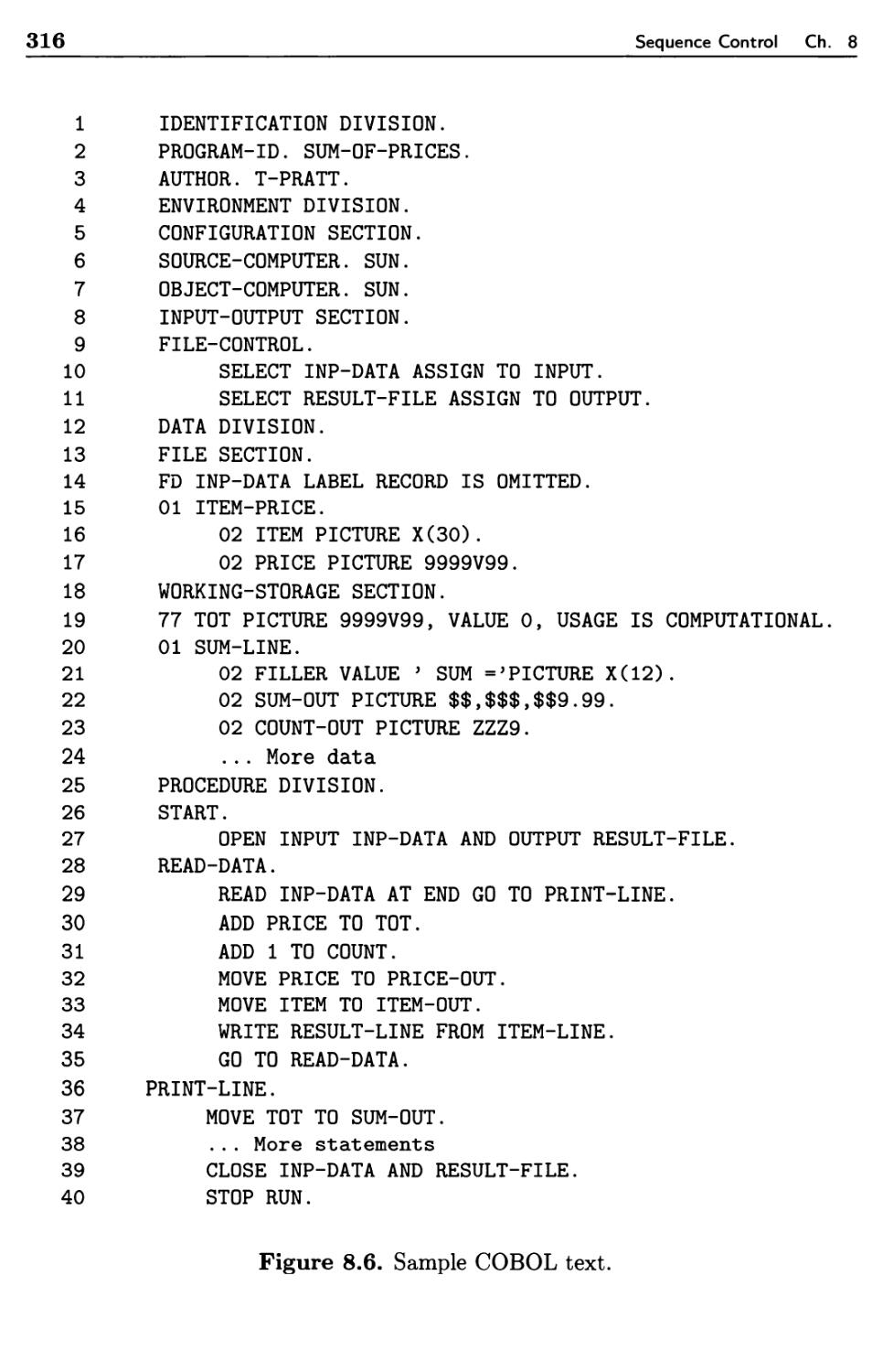
8.3.1 Basic Statements
8.3.2 Structured Sequence Control
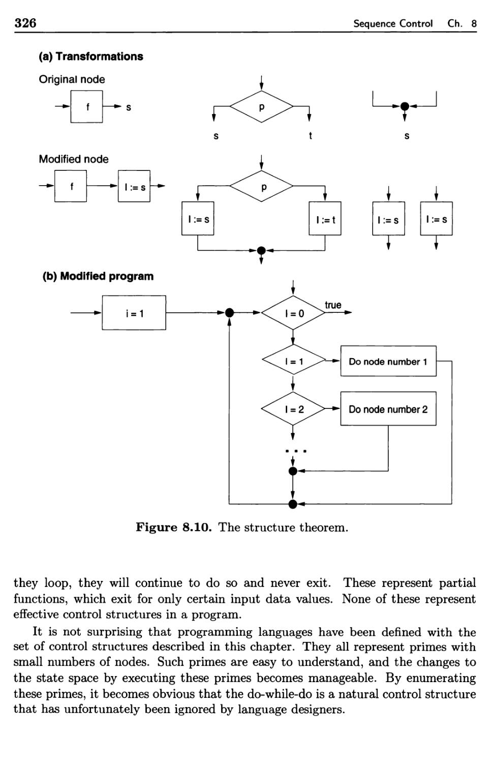
8.3.3 Prime Programs
Sequencing with Nonarithmetic Expressions
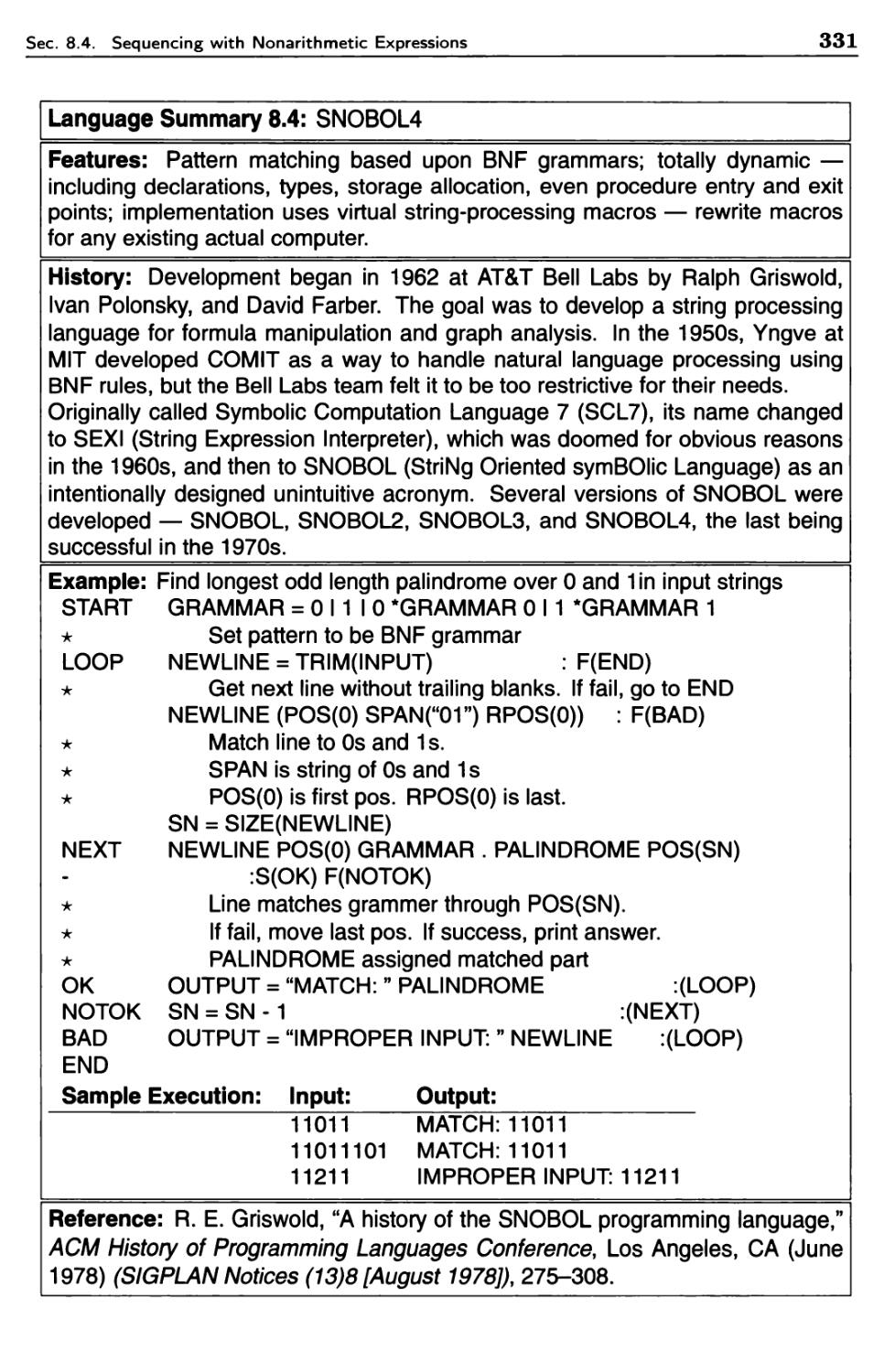
8.4.1 Prolog Overview
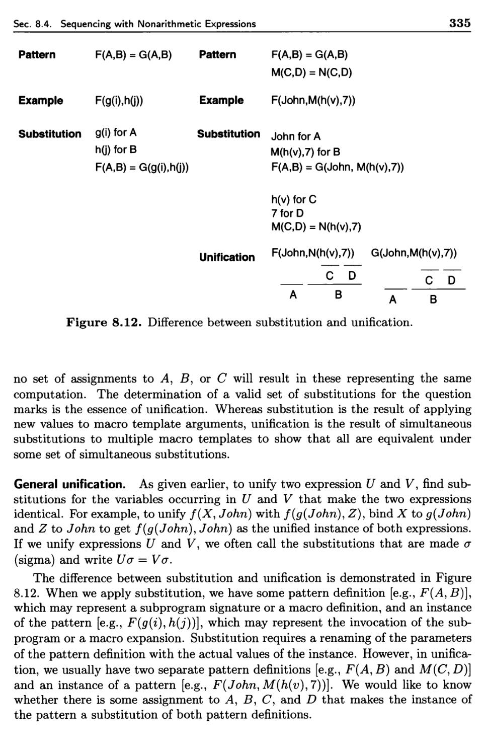
8.4.2 Pattern Matching
8.4.3 Unification
8.4.4 Backtracking
8.4.5 Resolution
238
240
246
246
249
252
254
256
257
264
264
272
273
277
279
280
282
286
288
291
291
293
293
294
295
302
308
308
314
323
327
327
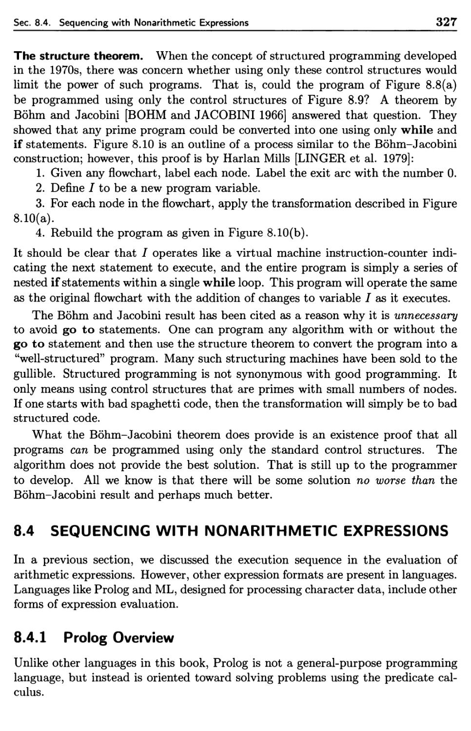
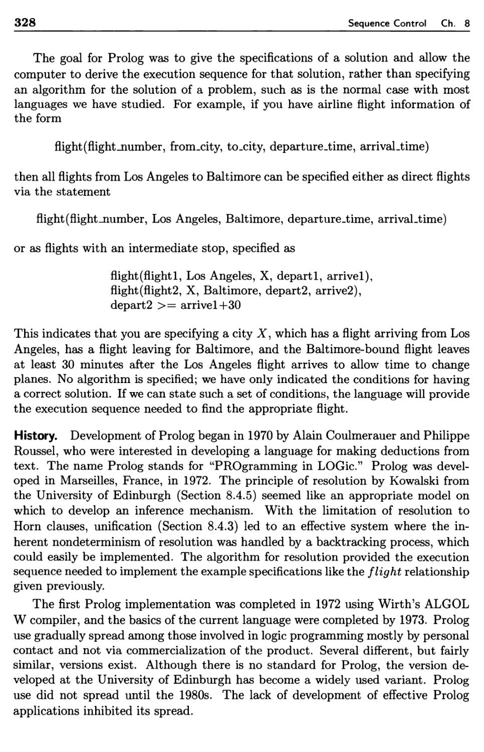
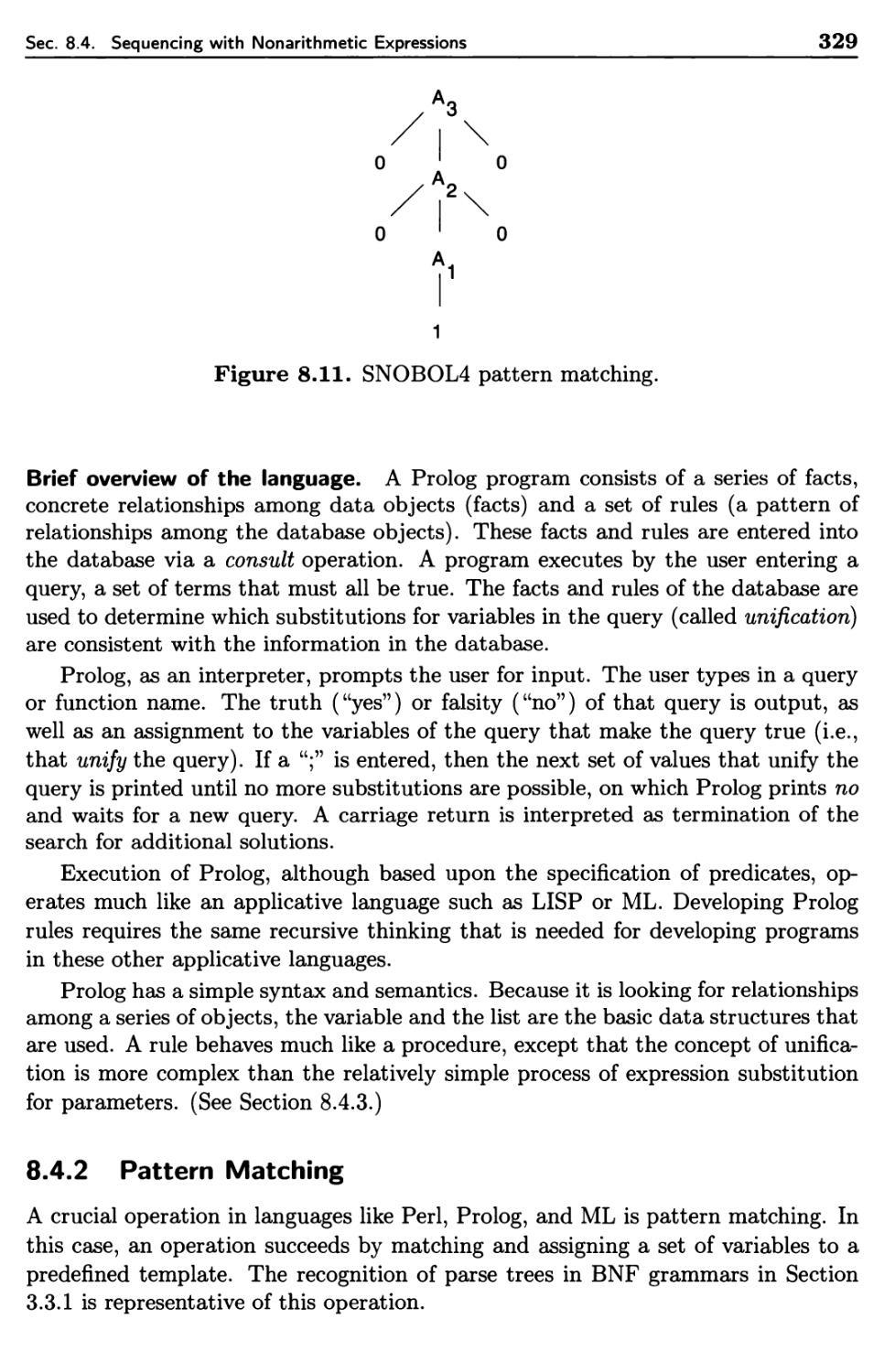
329
333
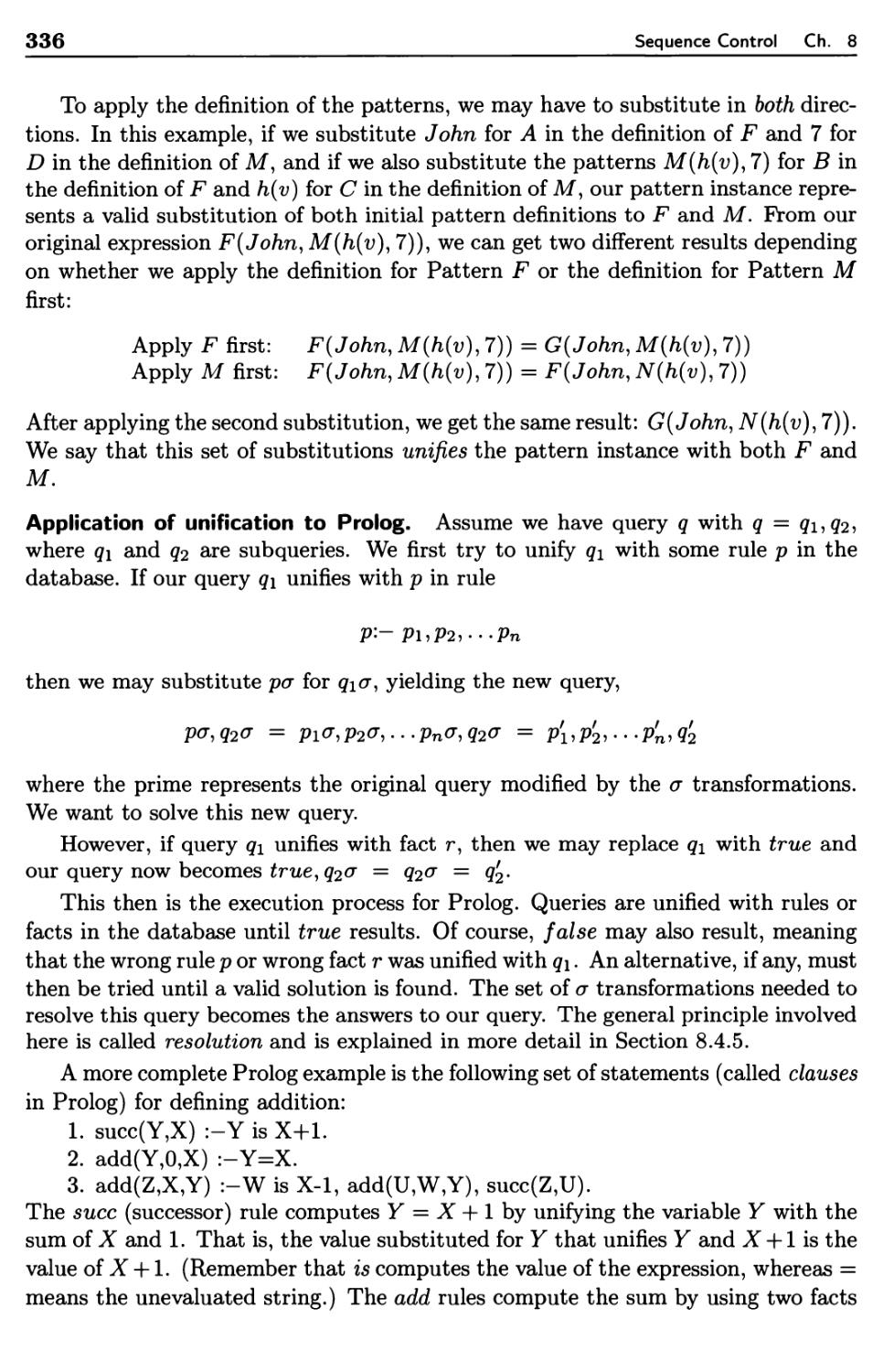
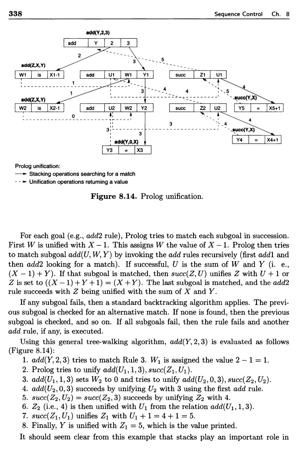
339
340
CONTENTS
xiii
8.5 Suggestions for Further Reading 342
8.6 Problems 342
9 Subprogram Control 345
9.1 Subprogram Sequence Control 345
9.1.1 Simple Call-Return Subprograms 347
9.1.2 Recursive Subprograms 353
9.1.3 The Pascal Forward Declaration 355
9.2 Attributes of Data Control 357
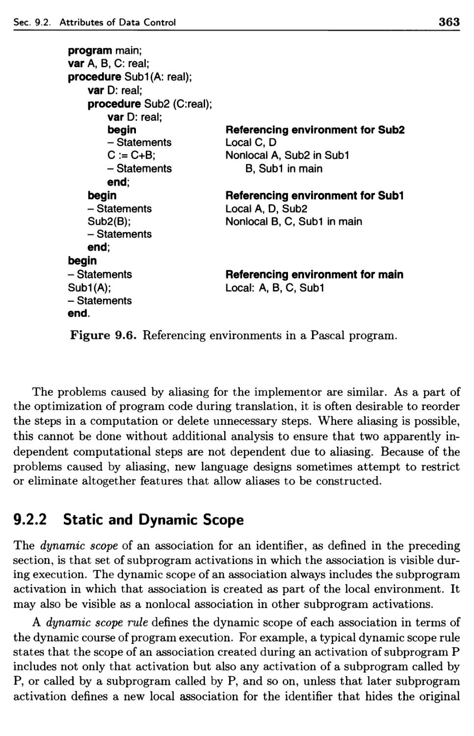
9.2.1 Names and Referencing Environments 358
9.2.2 Static and Dynamic Scope 363
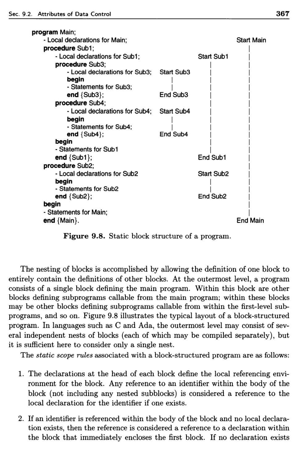
9.2.3 Block Structure 366
9.2.4 Local Data and Local Referencing Environments 368
9.3 Parameter Transmission 374
9.3.1 Actual and Formal Parameters 375
9.3.2 Methods for Transmitting Parameters 377
9.3.3 Transmission Semantics 380
9.3.4 Implementation of Parameter Transmission 382
9.4 Explicit Common Environments 393
9.4.1 Dynamic Scope 396
9.4.2 Static Scope and Block Structure 400
9.5 Suggestions for Further Reading 408
9.6 Problems 408
10 Storage Management 415
10.1 Elements Requiring Storage 416
10.2 Programmer- and System-Controlled Storage 417
10.3 Static Storage Management 419
10.4 Heap Storage Management 419
10.4.1 LISP Overview 420
10.4.2 Fixed-Size Elements 422
10.4.3 Variable-Size Elements 430
10.5 Suggestions for Further Reading 432
10.6 Problems 432
11 Distributed Processing 436
11.1 Variations on Subprogram Control 436
11.1.1 Exceptions and Exception Handlers 437
xiv
Contents
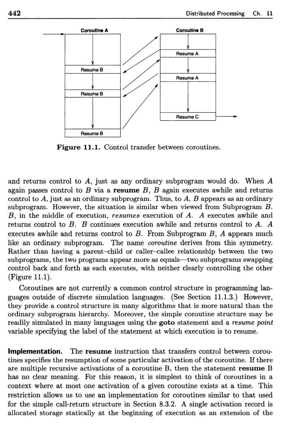
11.1.2 Coroutines 441
11.1.3 Scheduled Subprograms 443
11.2 Parallel Programming 445
11.2.1 Concurrent Execution 447
11.2.2 Guarded Commands 448
11.2.3 Ada Overview 450
11.2.4 Tasks 453
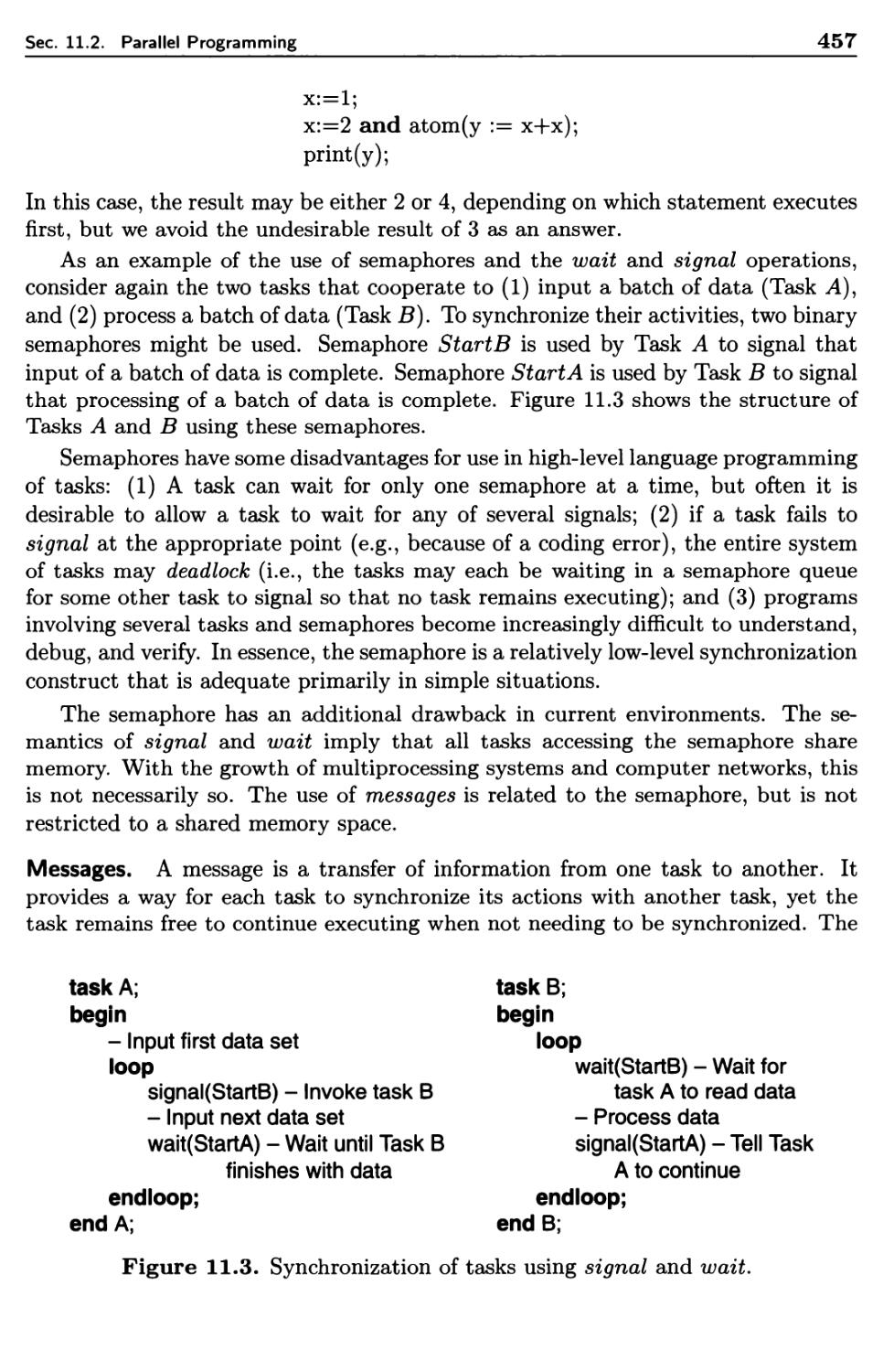
11.2.5 Synchronization of Tasks 455
11.3 Hardware Developments 465
11.3.1 Processor Design 467
11.3.2 System Design 470
11.4 Software Architecture 472
11.4.1 Persistent Data and Transaction Systems 472
11.4.2 Networks and Client-Server Computing 474
11.5 Suggestions for Further Reading 475
11.6 Problems 476
12 Network Programming 479
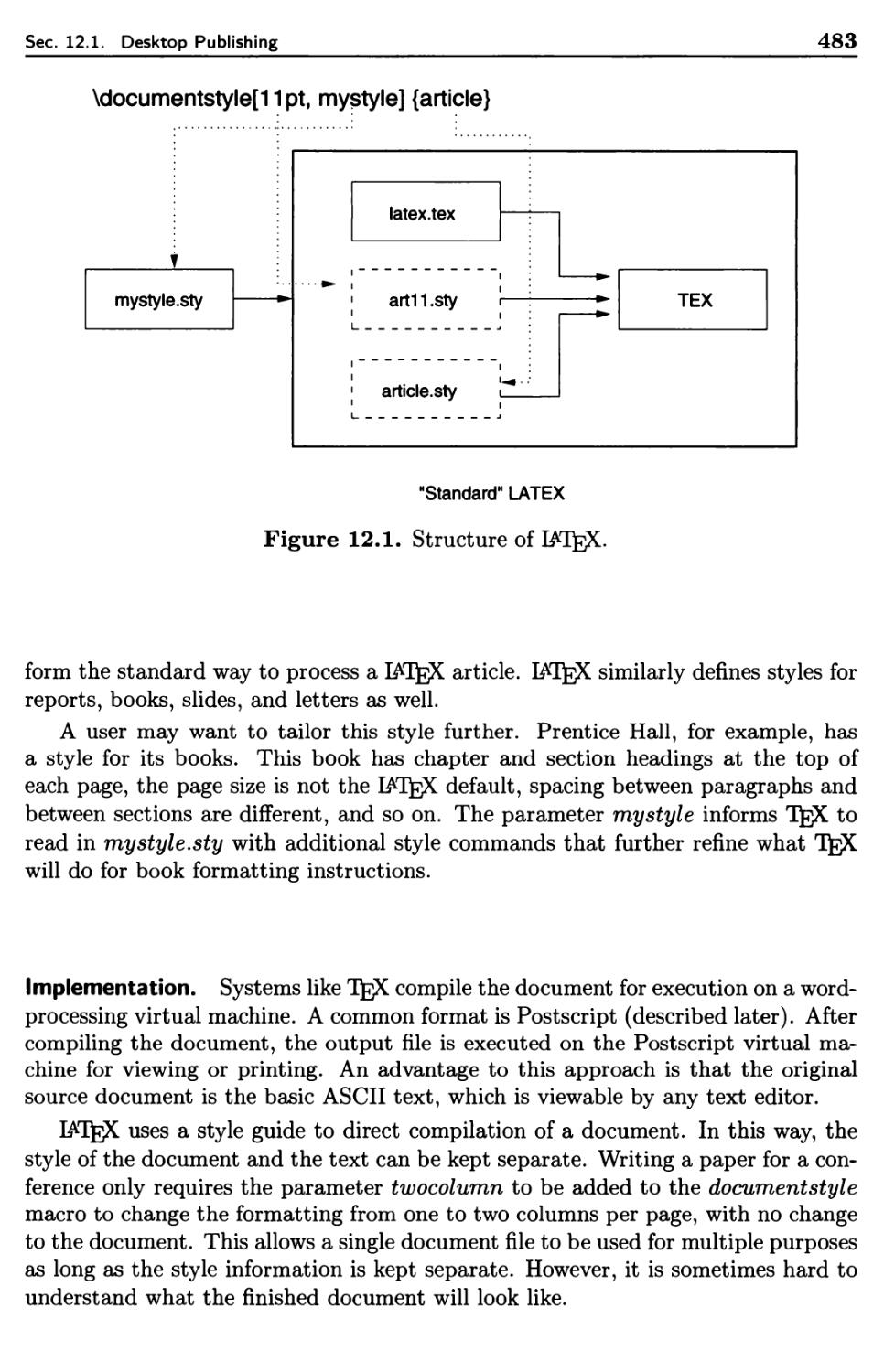
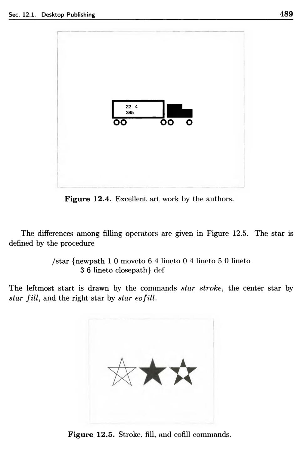
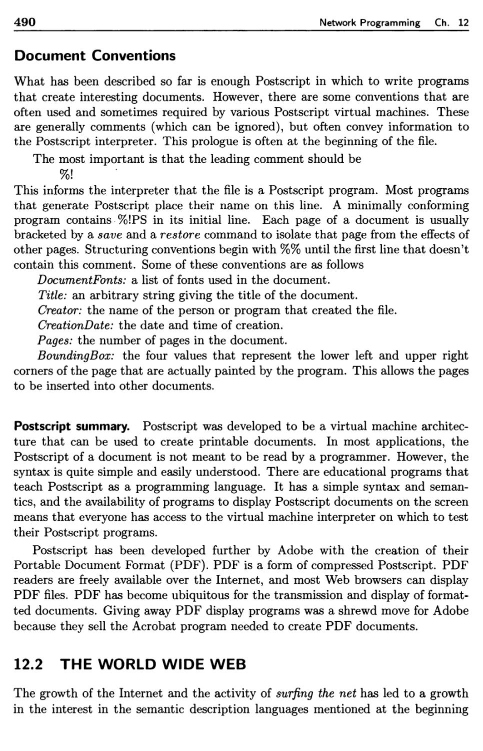
12.1 Desktop Publishing 481
12.1.1 IATfcjX Document Preparation 481
12.1.2 WYSIWYG Editors 484
12.1.3 Postscript 484
12.1.4 Postscript Virtual Machine 485
12.2 The World Wide Web 490
12.2.1 The Internet 491
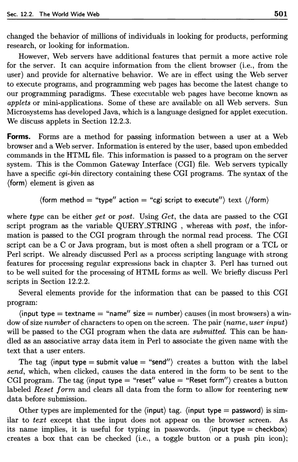
12.2.2 CGI Scripts 502
12.2.3 Java Applets 505
12.2.4 XML 507
12.3 Suggestions for Further Reading 508
12.4 Problems 509
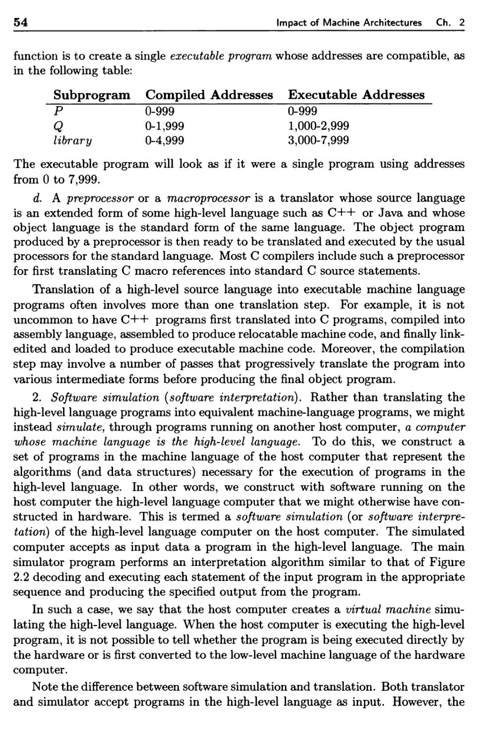
A Language Summaries 510
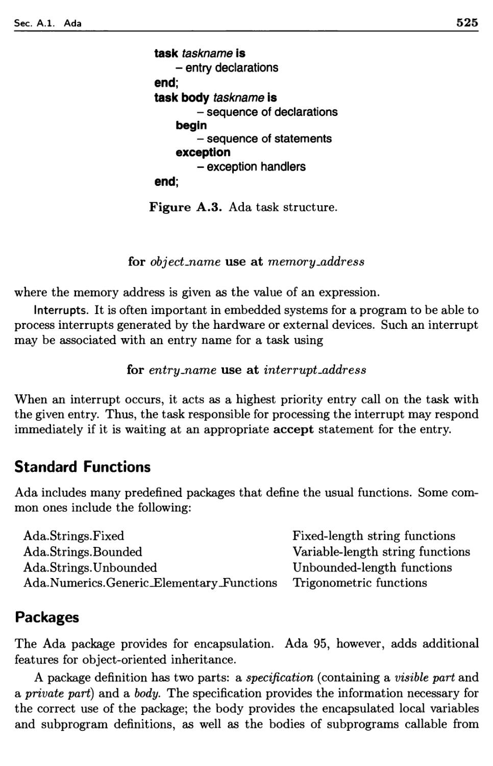
A.l Ada 510
A. 1.1 Data Objects 513
A. 1.2 Sequence Control 520
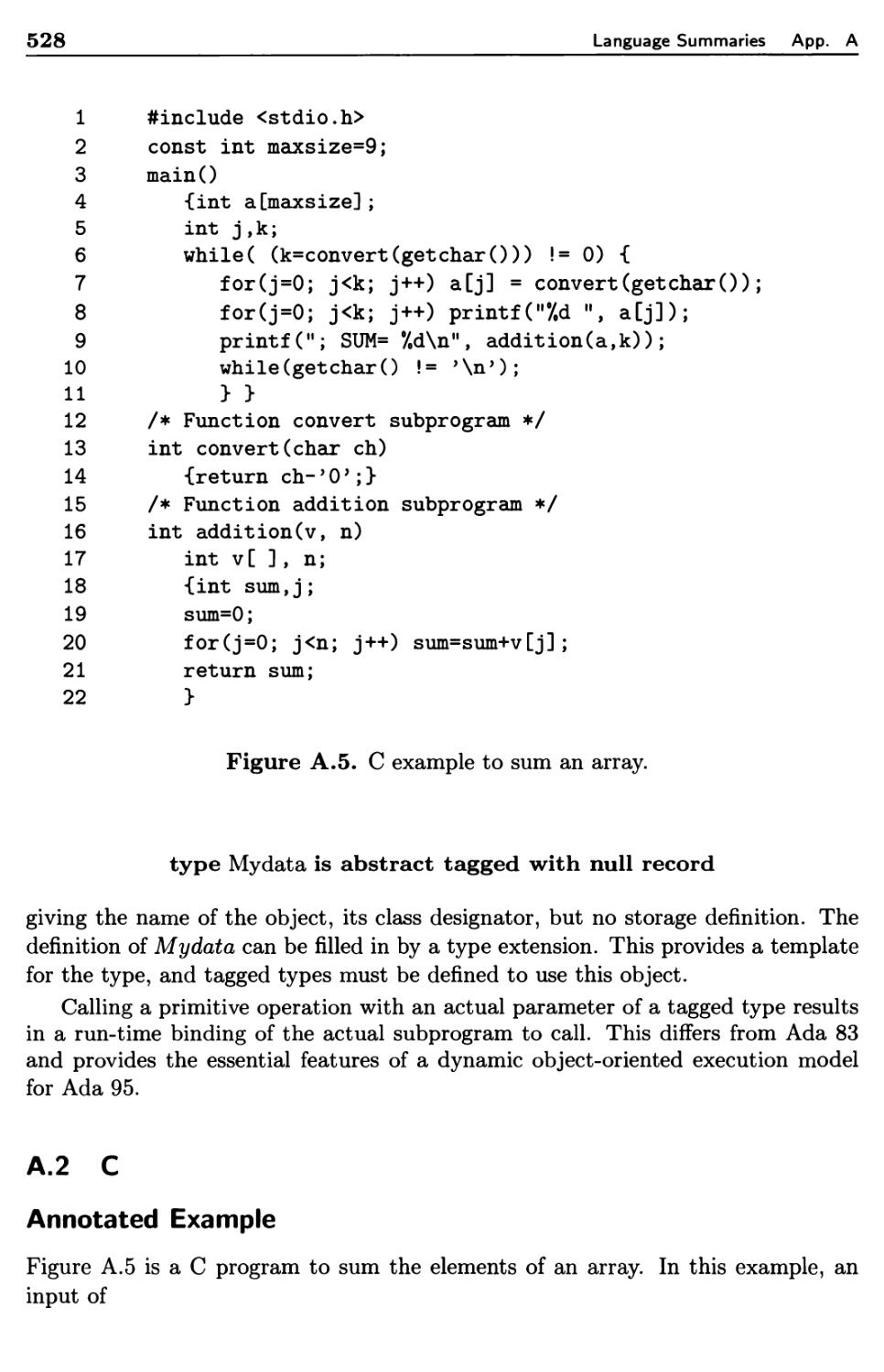
A.2 C 528
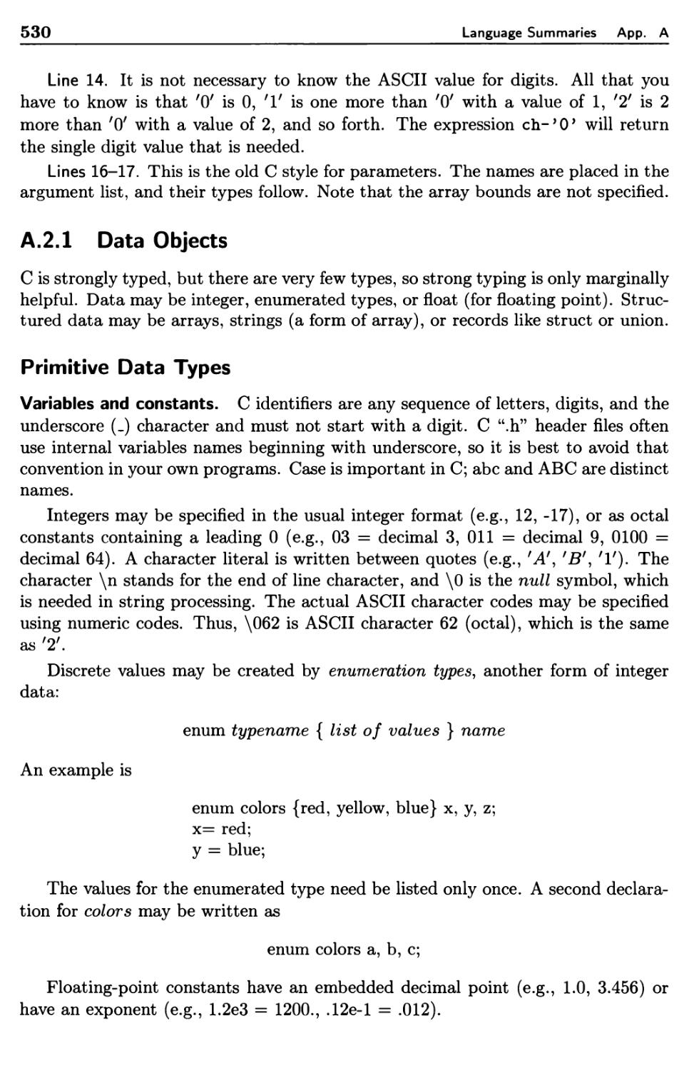
A.2.1 Data Objects 530
A.2.2 Sequence Control 534
CONTENTS
xv
539
541
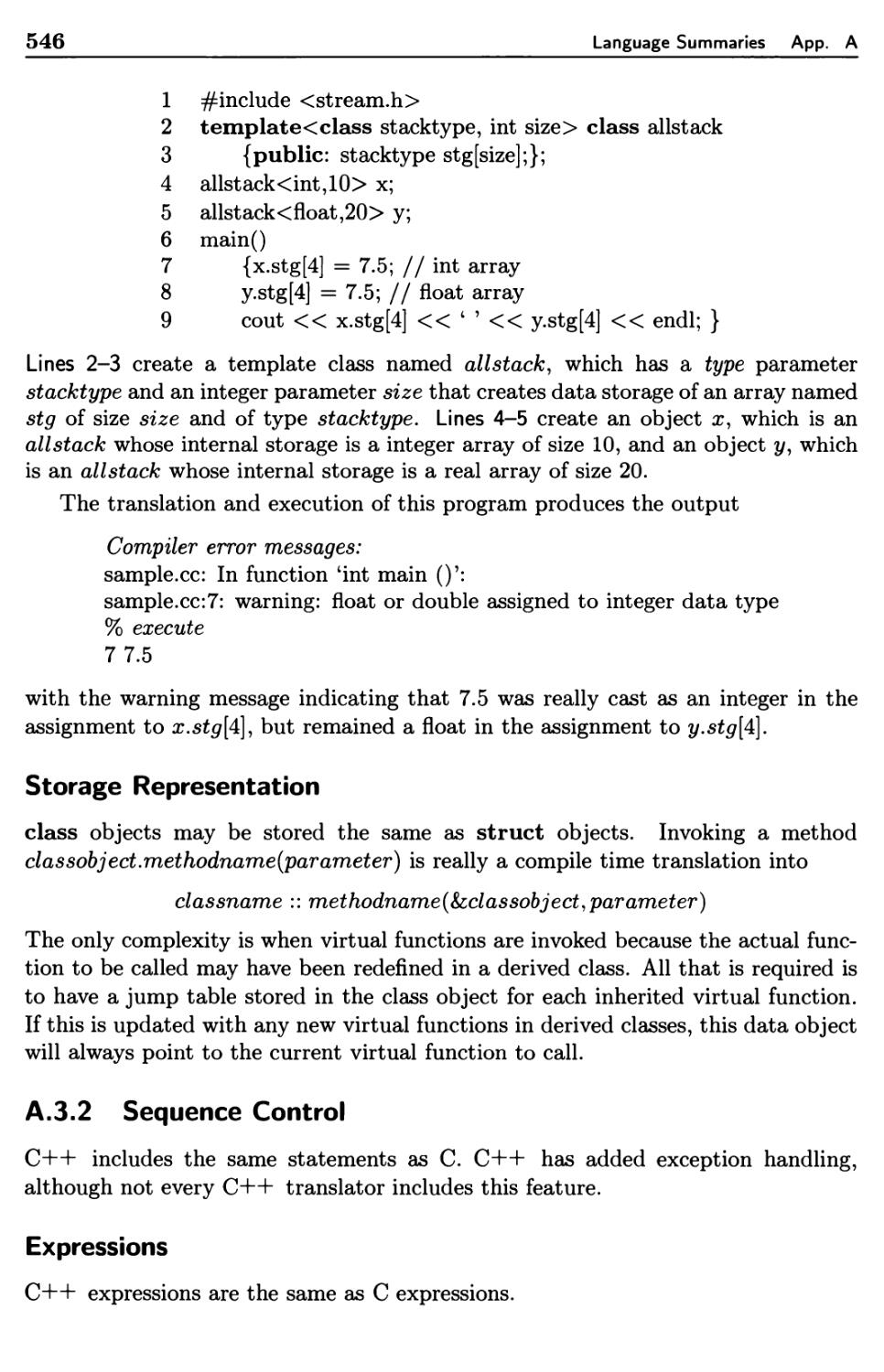
546
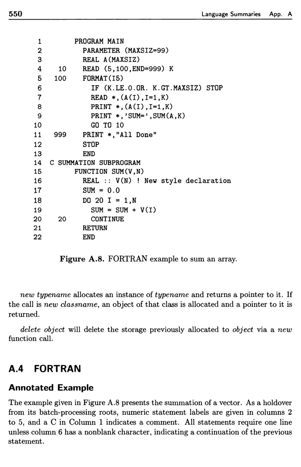
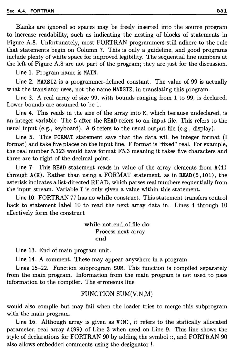
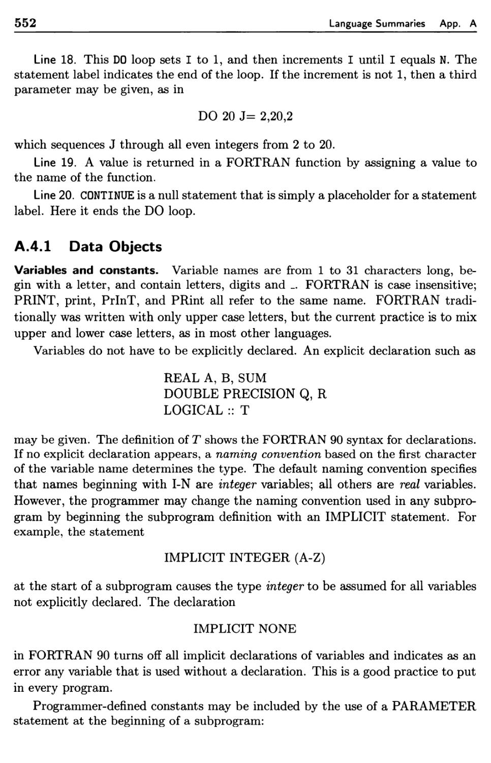
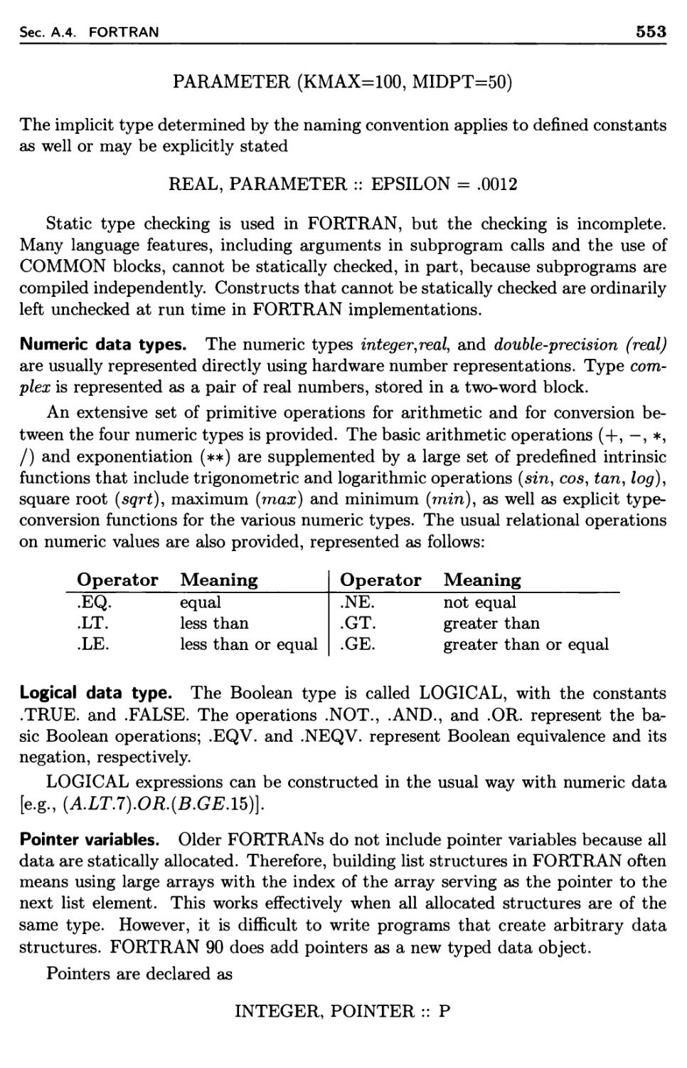
550
552
556
560
562
563
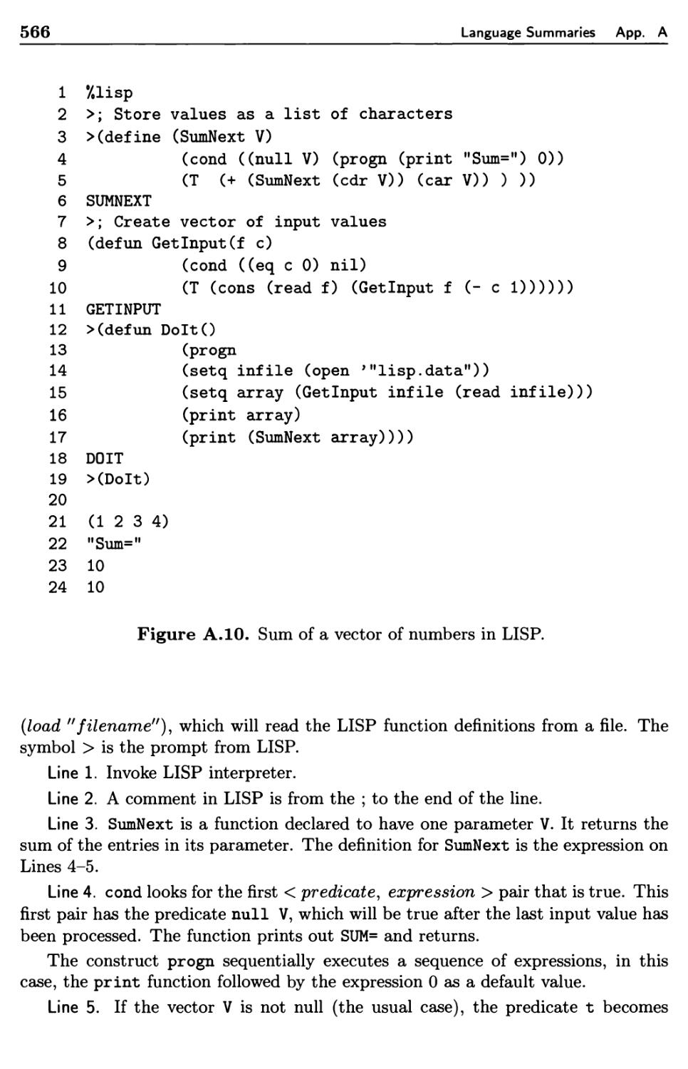
565
567
569
574
576
580
587
589
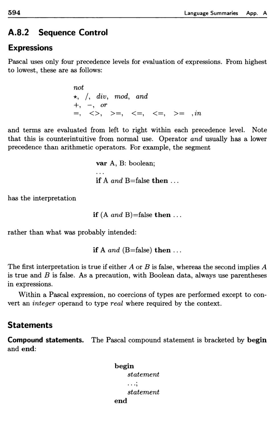
594
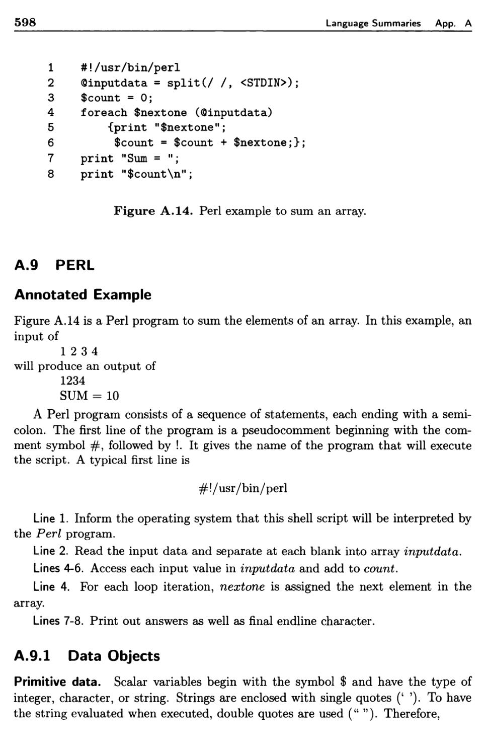
598
598
600
601
601
605
606
608
609
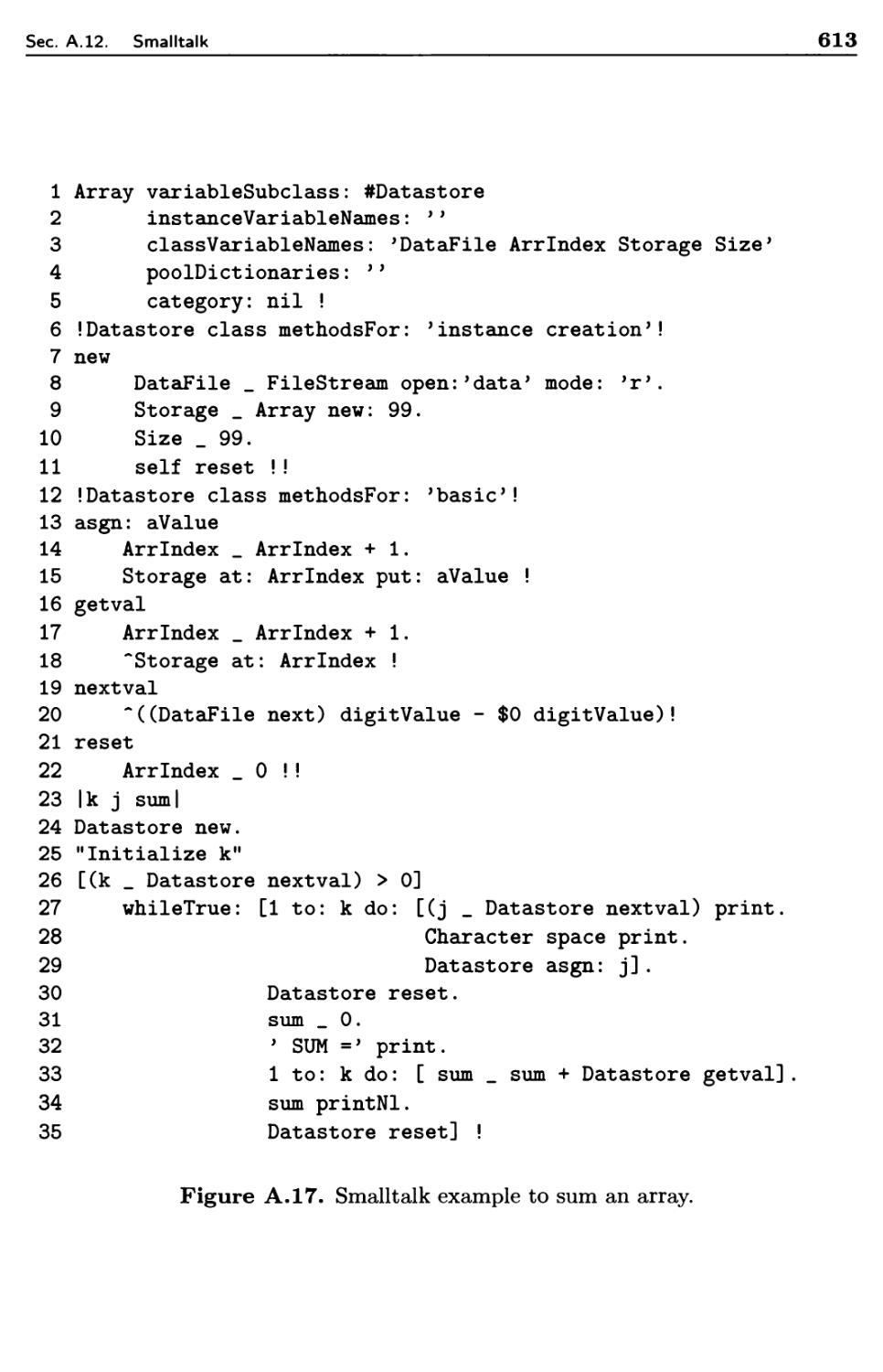
612
615
617
622
References 624
A.3 C++
A.3.1
A.3.2
Data Objects
Sequence Control
A.4 FORTRAN
A.4.1
A.4.2
A.5 Java
A.5.1
A.5.2
A.6 LISP
A.6.1
A.6.2
A.7 ML
A.7.1
A.7.2
A.8 Pascal
A.8.1
A.8.2
A.9 Perl
A.9.1
A.9.2
Data Objects
Sequence Control
Data Objects
Sequence Control
Data Objects
Sequence Control
Data Objects
Sequence Control
Data Objects
Sequence Control
Data Objects
Sequence Control
A. 10 Postscript
A. 10.1 Data Objects
A.10.2
Painting Commands
A. 11 Prolog
A. 11.1 Data Objects
A. 11.2 Sequence Control
A.12 Smalltalk
A.12.1
A.12.2
Data Objects
: Sequence Control
A. 13 Suggestions for Further Reading
Index
633
Chapter 1
Language Design Issues
Any notation for the description of algorithms and data structures may be termed a
programming language; however, in this book we are mostly interested in those that
are implemented on a computer. The sense in which a language may be implemented
is considered in the next two chapters. In the remainder of this book, the design and
implementation of the various components of a language are considered in detail.
The goal is to look at language features, independent of any particular language,
and give examples from a wide class of commonly used languages.
Throughout the book, we illustrate the application of these concepts in the
design of 12 major programming languages and their dialects: Ada, C, C++,
FORTRAN, Java, LISP, ML, Pascal, Perl, Postscript, Prolog, and Smalltalk. In
addition, we also give brief summaries about other languages that have made an
impact on the field. This list includes APL, BASIC, COBOL, Forth, PL/I, and
SNOBOL4. Before approaching the general study of programming languages,
however, it is worth understanding why there is value in such a study to a computer
programmer.
1.1 WHY STUDY PROGRAMMING LANGUAGES?
Hundreds of different programming languages have been designed and implemented.
Even in 1969, Sammet [SAMMET 1969] listed 120 that were fairly widely used, and
many others have been developed since then. Most programmers, however, never
venture to use more than a few languages, and many confine their programming
entirely to one or two. In fact, practicing programmers often work at computer
installations where use of a particular language such as Java, C, or Ada is required.
What is to be gained, then, by study of a variety of different languages that one is
unlikely ever to use?
There are excellent reasons for such a study, provided that you go beneath the
superficial consideration of the "features" of languages and delve into the underlying
design concepts and their effect on language implementation. Six primary reasons
come immediately to mind:
1
2
Language Design Issues Ch. 1
1. To improve your ability to develop effective algorithms. Many languages
provide features, that when used properly, are of benefit to the programmer but,
when used improperly, may waste large amounts of computer time or lead the
programmer into time-consuming logical errors. Even a programmer who has
used a language for years may not understand all of its features. A typical
example is recursion—a handy programming feature that, when properly used,
allows the direct implementation of elegant and efficient algorithms. When
used improperly, it may cause an astronomical increase in execution time. The
programmer who knows nothing of the design questions and implementation
difficulties that recursion implies is likely to shy away from this somewhat
mysterious construct. However, a basic knowledge of its principles and
implementation techniques allows the programmer to understand the relative
cost of recursion in a particular language and from this understanding to
determine whether its use is warranted in a particular programming situation.
New programming methods are constantly being introduced in the literature.
The best use of concepts like object-oriented programming, logic
programming, or concurrent programming, for example, requires an understanding of
languages that implement these concepts. New technology, such as the
Internet and World Wide Web, change the nature of programming. How best
to develop techniques applicable in these new environments depends on an
understanding of languages.
2. To improve your use of your existing programming language. By
understanding how features in your language are implemented, you greatly increase your
ability to write efficient programs. For example, understanding how data such
as arrays, strings, lists, or records are created and manipulated by your
language, knowing the implementation details of recursion, or understanding how
object classes are built allows you to build more efficient programs consisting
of such components.
3. To increase your vocabulary of useful programming constructs. Language
serves both as an aid and a constraint to thinking. People use language
to express thoughts, but language also serves to structure how one thinks, to
the extent that it is difficult to think in ways that allow no direct expression
in words. Familiarity with a single programming language tends to have a
similar constraining effect. In searching for data and program structures
suitable to the solution of a problem, one tends to think only of structures that
are immediately expressible in the languages with which one is familiar. By
studying the constructs provided by a wide range of languages, a programmer
increases his programming vocabulary. The understanding of implementation
techniques is particularly important because, to use a construct while
programming in a language that does not provide it directly, the programmer
must provide an implementation of the construct in terms of the primitive
elements actually provided by the language. For example, the subprogram
control structure known as a coroutine is useful in many programs, but few
Sec. 1.1. Why Study Programming Languages?
3
languages provide a coroutine feature directly. A C or FORTRAN
programmer, however, may readily design a program to use a coroutine structure
and then implement it as a C or a FORTRAN program if familiar with the
coroutine concept and its implementation.
4. To allow a better choice of programming language. A knowledge of a variety
of languages may allow the choice of just the right language for a particular
project, thereby reducing the required coding effort. Applications requiring
numerical calculations can be easily designed in languages like C, FORTRAN,
or Ada. Developing applications useful in decision making, such as in artificial-
intelligence applications, would be more easily written in LISP, ML, or Prolog.
Internet applications are more readily designed using Perl and Java.
Knowledge of the basic features of each language's strengths and weaknesses gives
the programmer a broader choice of alternatives.
5. To make it easier to learn a new language. A linguist, through a deep
understanding of the underlying structure of natural languages, often can learn
a new foreign language more quickly and easily than struggling novices who
understand little of the structure even of their native tongue. Similarly, a
thorough knowledge of a variety of programming language constructs and
implementation techniques allows the programmer to learn a new programming
language more easily when the need arises.
6. To make it easier to design a new language. Few programmers ever think of
themselves as language designers, yet many applications are really a form of
programming language. A designer of a user interface for a large program
such as a text editor, an operating system, or a graphics package must be
concerned with many of the same issues that are present in the design of a
general-purpose programming language. Many new languages are based on
C or Pascal as implementation models. This aspect of program design is
often simplified if the programmer is familiar with a variety of constructs and
implementation methods from ordinary programming languages.
There is much more to the study of programming languages than simply a
cursory look at their features. In fact, many similarities in features are deceiving. The
same feature in two different languages may be implemented in two very different
ways, and thus the two versions may differ greatly in the cost of use. For example,
almost every language provides an addition operation as a primitive, but the cost
of performing an addition in C, COBOL, or Smalltalk may vary by an order of
magnitude.
In this book, numerous language constructs are discussed, accompanied in
almost every case by one or more designs for the implementation of the construct on
a conventional computer. However, no attempt has been made to be comprehensive
in covering all possible implementation methods. The same language or construct,
4
Language Design Issues Ch. 1
if implemented on the reader's local computer, may differ radically in cost or
detail of structure when different implementation techniques have been used or when
the underlying computer hardware differs from the simple conventional structure
assumed here.
1.2 A SHORT HISTORY OF PROGRAMMING LANGUAGES
Programming language designs and implementation methods have evolved
continuously since the earliest high-level languages appeared in the 1950s. Of the 12
languages described in some detail, the first versions of FORTRAN and LISP were
designed during the 1950s; Ada, C, Pascal, Prolog, and Smalltalk date from the
1970s; C++, ML, Perl, and Postscript date from the 1980s; and Java dates from
the 1990s. In the 1960s and 1970s, new languages were often developed as part of
major software development projects. When the U.S. Department of Defense did
a survey as part of its background efforts in developing Ada in the 1970s, it found
that over 500 languages were being used on various defense projects.
1.2.1 Development of Early Languages
We briefly summarize language development during the early days of computing,
generally from the mid-1950s to the early 1970s. Later developments are covered in
more detail as each new language is introduced later in this book.
Numerically based languages. Computer technology dates from the era just
before World War II through the early 1940s. Determining ballistics trajectories by
solving the differential equations of motion was the major role for computers during
World War II, which led to them being called electronic calculators.
In the early 1950s, symbolic notations started to appear. Grace Hopper led a
group at Univac to develop the A-0 language, and John Backus developed Speedcod-
ing for the IBM 701. Both were designed to compile simple arithmetic expressions
into executable machine language.
The real breakthrough occurred in 1957 when Backus managed a team to develop
FORTRAN, or FORmula TRANslator. As with the earlier efforts, FORTRAN
data were oriented around numerical calculations, but the goal was a full-fledged
programming language including control structures, conditionals, and input and
output statements. Because few believed that the resulting language could compete
with hand-coded assembly language, every effort was put into efficient execution,
and various statements were designed specifically for the IBM 704. Concepts like
the three-way arithmetic branch of FORTRAN came directly from the hardware of
the 704, and statements like READ INPUT TAPE seem quaint today. It wasn't
very elegant, but in those days, little was known about elegant programming, and
the language was fast for the given hardware.
FORTRAN was extremely successful and was the dominant language through
Sec. 1.2. A Short History of Programming Languages
5
the 1970s. FORTRAN was revised as FORTRAN II in 1958 and FORTRAN IV a
few years later. Almost every manufacturer implemented a version of the language,
and chaos reigned. Finally in 1966, FORTRAN IV became a standard under the
name FORTRAN 66 and has been upgraded twice since, to FORTRAN 77 and
FORTRAN 90. However, the extremely large number of programs written in these early
dialects has caused succeeding generations of translators to be mostly backward
compatible with these old programs and inhibits the use of modern programming
features.
Because of the success of FORTRAN, there was fear, especially in Europe, of
the domination by IBM of the industry. The German society of applied
mathematics (GAMM) organized a committee to design a universal language. In the United
States, the Association for Computing Machinery (ACM) also organized a similar
committee. Although there was concern by the Europeans of being dominated by
the Americans, the committees merged. Under the leadership of Peter Naur, the
committee developed the International Algorithmic Language (IAL). Although AL-
GOrithmic Language (Algol) was proposed, the name was not approved. However,
common usage forced the official name change, and the language became known as
Algol 58. A revision occurred in 1960, and Algol 60 (with a minor revision in
1962) became the standard academic computing language from the 1960s to the
early 1970s.
Although FORTRAN was designed for efficient execution on an IBM 704, Algol
had very different goals:
1. Algol notation should be close to standard mathematics.
2. Algol should be useful for the description of algorithms.
3. Programs in Algol should be compilable into machine language.
4. Algol should not be bound to a single computer architecture.
These turned out to be very ambitious goals for 1958. To allow for machine
independence, no input or output was included in the language; special procedures
could be written for these operations. Although that certainly made programs
independent of a particular hardware, it also meant that each implementation would
necessarily be incompatible with another. To keep close to pure mathematics, a
subprogram was viewed as a macro substitution, which led to the concept of call by
name parameter passing; as we see in Section 9.3, call by name is extremely hard
to implement efficiently.
Algol never achieved commercial success in the United States, although it did
achieve some success in Europe. But it had a major impact on languages that
followed. As one example, Jules Schwartz of System Development Corporation
(SDC) developed a version of IAL (Jules' Own Version of IAL, or JOVIAL), which
became a standard for U.S. Air Force applications.
Backus was editor of the Algol report denning the language [BACKUS I960].
He used a syntactic notation comparable to the context free language concept
developed by Chomsky [CHOMSKY 1959]. This was the introduction of formal grammar
theory to the programming language world (Section 3.3). Because of his and Naur's
6
Language Design Issues Ch. 1
role in developing Algol, the notation is now called Backus Naur Form (BNF)..
As another example of Algol's influence, Burroughs, a computer vendor that
has since merged with Sperry Univac to form Unisys, discovered the works of the
Polish mathematician, Lukasiewicz. Lukasiewicz had developed a technique that
enabled arithmetic expressions to be written without parentheses using an efficient
stack-based evaluation process. This technique has had a profound effect on
compiler theory. Using methods based on Lukasiewicz's technique, Burroughs developed
the B5500 computer using a stack architecture and soon had an Algol compiler
that was much faster than any existing FORTRAN compiler.
At this point, the story starts to diverge. The concept of user-defined types
developed in the 1960s, and neither FORTRAN nor Algol had such features. Simula-
67, developed by Nygaard and Dahl of Norway, introduced the concept of classes
to Algol. This gave Stroustrup the idea for his C++ classes (Appendix A.3) as
an extension to C in the 1980s. Wirth developed ALGOL-W in the mid-1960s as
an extension to Algol. This met with only minor success; however, around 1970,
he developed Pascal, which became the computer science language of the 1970s.
Another committee tried to duplicate Algol 60's success with ALGOL 68, but the
language was much too complex for most to understand or implement effectively.
With the introduction of its new 360 line of computers in 1963, IBM developed
NPL (New Programming Language) at its Hursley Laboratory in England.
After some complaints by the English National Physical Laboratory, the name was
changed to MPPL (Multi-Purpose Programming Language), which was then
shortened to just PL/I. PL/I merged the numerical attributes of FORTRAN with the
business programming features of COBOL. PL/I achieved modest success in the
1970s (e.g., it was one of the featured languages in the second edition of this book),
but its use today is dwindling as it is replaced by C, C++ and Ada. The educational
subset PL/C achieved modest success in the 1970s as a student PL/I compiler (page
87). BASIC (page 79) was developed to satisfy the numerical calculation needs of
the nonscientist but has been extended far beyond its original goal.
Business languages. Business data processing was an early application domain
to develop after numerical calculations. Grace Hopper led a group at Univac to
develop FLOWMATIC in 1955. The goal was to develop business applications using
a form of Englishlike text. In 1959, the U.S. Department of Defense sponsored a
meeting to develop Common Business Language (CBL), which would be a business-
oriented language that used English as much as possible for its notation. Because
of divergent activities from many companies, a Short Range Committee was formed
to quickly develop this language. Although they thought they were designing an
interim language, the specifications, published in 1960, were the designs for COBOL
(COmmon Business Oriented Language). COBOL was revised in 1961 and 1962,
standardized in 1968, and revised again in 1974 and 1984. (Additional comments
are found on page 315.)
Sec. 1.2. A Short History of Programming Languages
7
Artificial-intelligence languages. Interest in artificial-intelligence languages began
in the 1950s with Information Processing Language (IPL) by the Rand Corporation.
IPL-V was fairly widely known, but its use was limited by its low-level design. The
major breakthrough occurred when John McCarthy of MIT designed List PRocess-
ing (LISP) for the IBM 704. LISP 1.5 became the standard LISP implementation
for many years. More recently, Scheme and Common LISP have continued that
evolution (Appendix A.6).
LISP was designed as a list-processing functional language. Game playing was
a natural test bed for LISP because the usual LISP program would develop a tree
of possible moves (as a linked list) and then walk over the tree searching for the
optimum strategy. Automatic machine translation, where strings of symbols could
be replaced by other strings, was another natural application domain. COMIT, by
Yngve of MIT, was an early language in this domain. Each program statement was
very similar to a context-free production (Section 3.3.1) and represented the set of
replacements that could be made if that string were found in the data. Because
Yngve kept his code proprietary, a group at AT&T Bell Labs decided to develop
their own language, which resulted in SNOBOL (page 331).
Although LISP was designed for general-purpose list-processing applications,
Prolog (Appendix A. 11) was a special-purpose language whose basic control
structure and implementation strategy were based on concepts from mathematical logic.
Systems languages. Because of the need for efficiency, the use of assembly
language held on for years in the systems area long after other application domains
started to use higher level languages. Many systems programming languages, such
as CPL and BCPL, were designed, but were never widely used. C (Appendix A.2)
changed all that. With the development of a competitive environment in UNIX
written mostly in C during the early 1970s, high-level languages have been shown
to be effective in this environment as well as others.
1.2.2 Evolution of Software Architectures
Development of a programming language does not proceed in a vacuum. The
hardware that supports a language has a great impact on language design. Language, as
a means to solve a problem, is part of the overall technology that is employed. The
external environment supporting the execution of a program is termed its operating
or target environment. The environment in which a program is designed, coded,
tested, and debugged, or host environment, may be different from the operating
environment in which the program ultimately is used. The computing industry has
now entered its third major era in the development of computer programs. Each
era has had a profound effect on the set of languages that were used for applications
in each time period.
8
Language Design Issues Ch. 1
Mainframe Era
From the earliest computers in the 1940s through the 1970s, the large mainframe
dominated computing. A single expensive computer filled a room and was attended
to by hordes of technicians.
Batch environments. The earliest and simplest operating environment consists
only of external files of data. A program takes a set of data files as input,
processes the data, and produces a set of output data files (e.g., a payroll program
processes two input files containing master payroll records and weekly pay-period
times and produces two output files containing updated master records and
paychecks). This operating environment is termed batch-processing because the input
data are collected in batches on files and are processed in batches by the program.
The 80-column punched card or Hollerith card, named after Herman Hollerith who
developed the card for use in the 1890 U.S. census, was the ubiquitous sign of
computing in the 1960s.
Languages such as FORTRAN, COBOL, and Pascal were initially designed for
batch-processing environments, although they may be used now in an interactive
or in an embedded-system environment.
Interactive environments. Toward the end of the mainframe era, in the early
1970s, interactive programming made its appearance. Rather than developing a
program on a deck of cards, cathode ray tube terminals were directly connected to
the computer. Based on research in the 1960s at MIT's Project MAC and Multics,
the computer was able to time share by enabling each user to have a small slice of
the computer's processor time. Thus, if 20 users were connected to a computer, and
each user had a time slice of 25 milliseconds, then each user would have two such
slices or 50 milliseconds of computer time each second. Because many users spent
much of their time at a terminal thinking, the few who were actually executing
programs would often get more than their quota of two slices per second.
In an interactive environment, a program interacts directly with a user at a
display console during its execution, by alternately sending output to the display
and receiving input from the keyboard or mouse. Examples include word-processing
systems, spreadsheets, video games, database management systems, and computer-
assisted instruction systems. These examples are all tools with which you may be
familiar.
Effects on language design. In a language designed for batch processing, files are
usually the basis for most of the input-output (I/O) structure. Although a file may
be used for interactive I/O to a terminal, the special needs of interactive I/O are not
addressed in these languages. For example, files are usually stored as fixed-length
records, yet at a terminal, the program would need to read each character as it is
entered on the keyboard. The I/O structure also typically does not address the
requirement for access to special I/O devices found in embedded systems.
In a batch-processing environment, an error that terminates execution of the
Sec. 1.2. A Short History of Programming Languages
9
program is acceptable but costly because often the entire run must be repeated
after the error is corrected. In this environment, too, no external help from the user
in immediately handling or correcting the error is possible. Thus, the error- and
exception-handling facilities of the language emphasize error/exception handling
within the program so that the program may recover from most errors and continue
processing without terminating.
A third distinguishing characteristic of a batch-processing environment is the
lack of timing constraints on a program. The language usually provides no facilities
for monitoring or directly affecting the speed at which the program executes.
The characteristics of interactive I/O are sufficiently different from ordinary file
operations that most languages designed for a batch-processing environment
experience some difficulty in adapting to an interactive environment. These differences
are discussed in Section 5.3.3. As an example, C includes functions for accessing
lines of text from a file and other functions that directly input each character as
typed by the user at a terminal. The direct input of text from a terminal in Pascal,
however, is often very cumbersome. For this reason, C (and its derivative C++)
has grown greatly in popularity as a language for writing interactive programs.
Error handling in an interactive environment is given different treatment. If bad
input data are entered from a keyboard, the program may display an error message
and ask for a correction from the user. Language features for handling the error
within the program (e.g., by ignoring it and attempting to continue) are of lesser
importance. However, termination of the program in response to an error is usually
not acceptable (unlike batch processing).
Interactive programs must often utilize some notion of timing constraints. For
example, in a video game, the failure to respond within a fixed time interval to a
displayed scene would cause the program to invoke some response. An interactive
program that operates so slowly that it cannot respond to an input command in a
reasonable period is often considered unusable.
Personal Computer Era
In hindsight, the mainframe time-sharing era of computing was very short-lived,
lasting perhaps from the early 1970s to the mid-1980s. The Personal Computer
(PC) changed all that.
Personal computers. The 1970s could be called the era of the minicomputer.
These were progressively smaller and cheaper machines than the standard
mainframe of that era. Hardware technology was making great strides forward, and the
microcomputer, which contained the entire machine processor on a single 1- to 2-
inch square piece of plastic and silicon, was becoming faster and cheaper each year.
The standard mainframe of the 1970s shrunk from a room full of cabinets and tape
drives to a decorative office machine perhaps 3 to 5 feet long and 3 to 4 feet high.
In 1978, Apple released the Apple II computer, the first true commercial PC. It
10
Language Design Issues Ch. 1
was a small desktop machine that ran BASIC. This machine had a major impact
on the educational market; however, business was skeptical of minisized Apple and
its minisized computer.
In 1981, all of this changed. The PC was released by IBM, and Lotus developed
1-2-3 based on the Visi-Calc spreadsheet program. This program became the first
of the killer applications (killer aps) that industry had to run. The PC became an
overnight success.
The modern PC era can be traced to January 1984 during the U.S. football Su-
perbowl game. During a commercial on television, Apple announced the Macintosh
computer. The Macintosh contained a windows-based graphical user interface with
a mouse for point-and-click data entry. Although previously developed at the Xerox
Palo Alto Research Center (PARC), the Macintosh was the first commercial
application of this technology. Quickly mimicked by Microsoft for its Windows operating
system, this interface design has become the mainstay of the PC.
Since that time, the machines have gotten cheaper and faster. The PC used to
write this book is about 200 to 400 times faster, has 200 times the main memory,
3,000 times the disk space, and costs only one third of the $5,000 cost of the original
PC 20 years earlier. It is more powerful than the mainframe computers that it
replaced.
Embedded-system environments. An offshoot of the PC is the embedded
computer. A computer system that is used to control part of a larger system such as an
industrial plant, an aircraft, a machine tool, an automobile, or even your toaster is
termed an embedded computer system. The computer system has become an
integral part of the larger system, and the failure of the computer system usually means
failure of the larger system as well. Unlike in the PC environment, where failure
of the program often is simply an inconvenience requiring the program to be rerun,
failure of an embedded application can often be life-threatening, from failure of an
automobile computer causing a car to stall at high speeds on a highway, to failure
of a computer causing a nuclear plant to overheat, to failure of a hospital computer
causing patient monitoring to cease, down to failure of your digital watch causing
you to be late for a meeting. Reliability and correctness are primary attributes for
programs used in these domains. Ada, C, and C++ are used extensively to meet
some of the special requirements of embedded-system environments.
Effects on language design. The PC has again changed the role of languages.
Performance is now less of a concern in many application domains. With the
advent of user interfaces such as windows, each machine executes under control of a
single user. With prices so low, the need to time-share is not present. Developing
languages with good interactive graphics becomes of primary importance.
Today windows-based systems are the primary user interface. PC users are quite
familiar with the tools of the windows interface. They are familiar with windows,
icons, scroll bars, menus, and the assorted other aspects of interacting with the
computer. However, programming such packages can be complex. Vendors of such
Sec. 1.2. A Short History of Programming Languages
11
windowing systems have created libraries of these packages. Accessing these libraries
to enable easy development of windows-based programs is a primary concern of
application developers.
Object-oriented programming is a natural model for this environment. The use
of languages like Java and C++ with its class hierarchy allows for easy incorporation
of packages written by others.
Programs written for embedded systems often operate without an underlying
operating system and without the usual environment of files and I/O devices.
Instead, the program must interact directly with nonstandard I/O devices through
special procedures that take account of the peculiarities of each device. For this
reason, languages for embedded systems often place much less emphasis on files and
file-oriented I/O operations. Access to special devices is often provided through
language features that give access to particular hardware registers, memory locations,
interrupt handlers, or subprograms written in assembly or other low-level languages.
Error handling in embedded systems is of particular importance. Ordinarily,
each program must be prepared to handle all errors internally, taking appropriate
actions to recover and continue. Termination, except in the case of a catastrophic
system failure, is often not an acceptable alternative, and usually there is no user
in the environment to provide interactive error correction.
Embedded systems almost always operate in real time; that is, the operation
of the larger system within which the computer system is embedded requires that
the computer system be able to respond to inputs and produce outputs within
tightly constrained time intervals. For example, a computer controlling the flight
of an aircraft must respond rapidly to changes in its altitude or speed. Real-time
operation of these programs requires language features for monitoring time intervals,
responding to delays of more than a certain length of time (which may indicate
failure of a component of the system), and starting up and terminating actions at
certain designated points in time.
Finally, an embedded computer system is often a distributed system composed
of more than one computer. The program running on such a distributed system
is usually composed of a set of tasks that operate concurrently, each controlling or
monitoring one part of the system. The main program, if there is one, exists only to
initiate execution of the tasks. Once initiated, these tasks usually run concurrently
and indefinitely, because they need to terminate only when the entire system fails
or is shut down for some reason.
Networking Era
Distributed computing. As machines became faster, smaller, and cheaper during
the 1980s, they started to populate the business environment. Companies would
have central machines for handling corporate data, such as payroll, and each
department would have local machines for providing support to that department, order
processing, report writing, and so on. For an organization to run smoothly, informa-
12
Language Design Issues Ch. 1
tion on one machine had to be transferred and processed on another. For example,
the sales office had to send purchase order information to the production
department's computer and the financial department needed the information for billing
and accounting. Local area networks (LANs) using telecommunication lines
between the machines were developed within large organizations using a client-server
model of computing. The server would be a program that provided information
and multiple client programs would communicate with the server to obtain that
information.
An airline reservation system is one well-known example of a client-server
application. The database of airline flight schedules would be on a large mainframe.
Each agent would run a client program that conveyed information to the agent (or
traveler) about flights. If a new flight was desired, the client program would send
information to the server program to receive or download information from the
server to the client application about the new flights. In this way, a single-server
application could serve many client programs.
Internet. The mid-1990s saw the emergence of the distributed LAN into an
international global network, the Internet. In 1970, the Defense Advanced Research
Projects Agency (DARPA) started a research project to link together mainframe
computers into a large reliable and secure network. The goal was to provide
redundancy in case of war so that military planners could access computers across the
nation. Fortunately, the ARPANET was never put to that use, and in the mid-
1980s, the military ARPANET evolved into the research-oriented Internet. Over
time, additional computers were added to the network, and today any user
worldwide can have a machine added to the network. Millions of machines are connected
in a complex and dynamically changing complex of network server machines.
Accessing the Internet in its early days required two classes of computers. A
user would be sitting at a client personal computer. To access information, the
user would connect to an appropriate server machine to get that information. The
protocols for performing those were telnet and file transfer protocol (FTP). The
telnet protocol made it appear as if the user were actually executing as part of the
distant server, whereas FTP simply allowed the client machine to send or receive
files from the server machine. In both cases, the user had to know what machine
contained the information that was desired.
At the same time a third protocol was being developed - Simple Mail Transfer
Protocol (SMTP). SMTP is the basis for today's e-mail. Each user has a local login
name on the client machine, and each machine has a unique machine name (e.g.,
mvz as the login name of an author of this book and aaron.cs.umd.edu as the unique
name for the machine connected to the Internet). Sending a message to an individual
was then a simple manner of using a program that adhered to the SMTP protocol
and sending mail to a user at a specific machine (e.g., mvz@aaron.cs.umd.edu).
What is important here is that the specific location of the machine containing the
user is often unnecessary (e.g., mvz@cs.umd.edu is sufficient). There was no need
to actually know the address of the machine on the Internet.
Sec. 1.2. A Short History of Programming Languages
13
A goal in the late 1980s was to make the retrieval of information as easy to
accomplish as sending e-mail. The breakthrough came in 1989 at CERN, the
European nuclear research facility in Geneva, Switzerland. Berners-Lee developed the
concept of the HyperText markup Language (HTML) hyperlink as a way to navigate
around the Internet. With the development of the Mosaic web browser in 1993
and the HyperText Transfer Protocol (HTTP) addition to Internet technology, the
general population discovered the Internet. By the end of the 20t/l century,
everyone was web surfing, and the entire structure of knowledge acquisition and search
worldwide had changed.
Effects on language design. The use of the World Wide Web (WWW) has again
changed the role of the programming language. Computing is again becoming
centralized, but in a way much different from the earlier mainframe era. Large
information repository servers are being created worldwide. Users will access servers
via the Web to obtain information and use their local client machines for local
processing, such as word processing the information into a report. Rather than
distributing millions of copies of a new software product, a vendor can simply put
the software on the Web and have users download the copies for local use. This
requires the use of languages that allow interaction between the client and server
computers, such as the user being able to download the software and the vendor
being able to charge the user for the privilege of downloading the software. The
rise of Electronic commerce (E-commerce) depends on these features.
The initial Web pages were static. That is, text, pictures, or graphics could be
displayed. Users could click on a Uniform Resource Locator (URL) to access a new
Web page. In order for E-commerce to nourish, however, information had to flow
both ways between client and server, and Web pages needed to be more active. Use
of languages like Perl and Java provide such features.
The Web poses programming language issues that were not apparent in the
previous two eras. Security is one. A user visiting a web site wants to be certain
the owner of that site is not malicious and will not destroy the client machine by
erasing the disk files of the user. Although a problem with time-sharing systems,
this problem did not exist on single user PCs. Access to local user files from the
server web site has to be restricted.
Performance is another critical problem. Although PCs have gotten extremely
fast, the communication lines connecting a user to the Internet are often limited in
speed. In addition, although the machines are fast, if many users are accessing the
same server, then server processing power may be taxed. A way out of that is to
process the information at the client site rather than on the server. This requires
the server to send small executable programs to the client to offload work from the
server to the client. The problem is that the server does not know what kind of
computer the client is, so it is not clear what the executable program needs to look
like. Java was developed specifically to handle this problem, and we discuss it later.
14
Language Design Issues Ch. 1
Era
1960s
Today
Application
Business
Scientific
System
Artificial
intelligence
Business
Scientific
System
Artificial
intelligence
Publishing
Process
New paradigms
Major languages
COBOL
FORTRAN
Assembler
LISP
COBOL, C++, Java,
spreadsheet
FORTRAN, C,
C++, Java
C, C++, Java
LISP, Prolog
TeX, Postscript, word
processing
UNIX shell, TCL,
Perl, Javascript
ML, Smalltalk
Other languages
Assembler
Algol, BASIC, APL
JOVIAL, Forth
SNOBOL
C, PL/I, 4GLs
BASIC
Ada, BASIC, Modula
AWK, Marvel, SED
Eiffel
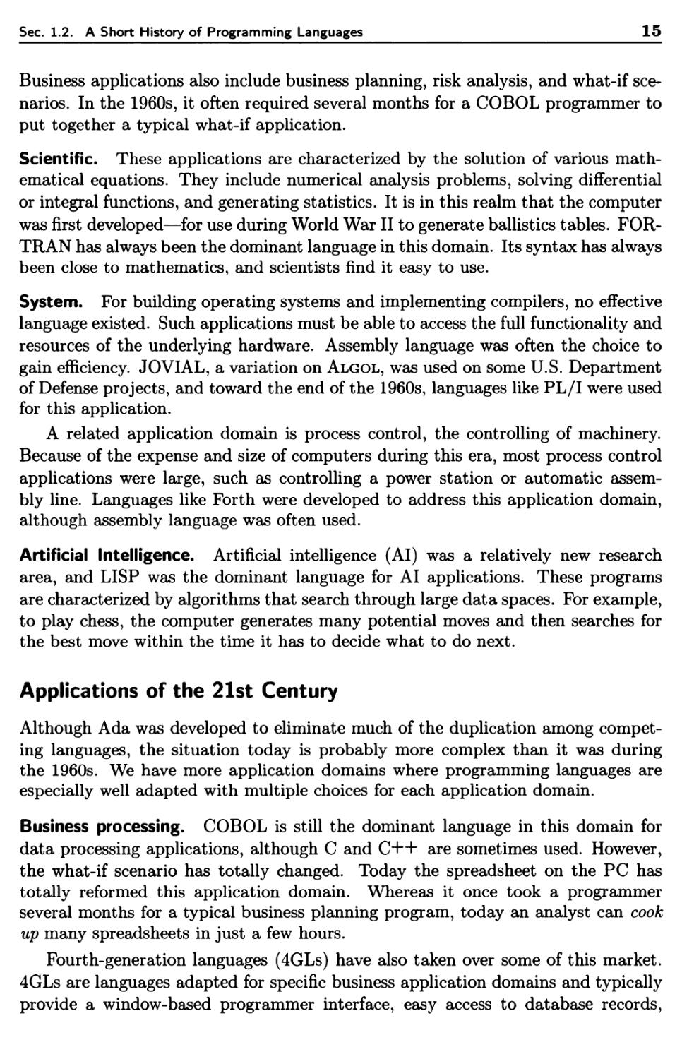
Table 1.1. Languages for various application domains.
1.2.3 Application Domains
The appropriate language to use often depends on the application domain for the
problem to be solved. The appropriate language to use for various application
domains has evolved over the past 30 years. The languages discussed in this book,
plus a few others, are summarized in Table 1.1.
Applications of the 1960s
During the 1960s, most programming could be divided into four basic
programming models: business processing, scientific calculations, systems programming,
and artificial-intelligence applications.
Business processing. Most of these applications were large data processing
applications designed to run on big iron mainframes. These included order-entry
programs, inventory control, personnel management, and payroll. They were
characterized by reading in large amounts of historical data on multiple tape drives,
reading in a smaller set of recent transactions, and writing out a new set of
historical data. For a view of what this looked like, watch any 1960s science fiction movie.
They liked to show lots of spinning tapes to indicate modern computing.
COBOL was developed for these applications. The COBOL designers took great
pains to ensure that such data processing records would be processed correctly.
Sec. 1.2. A Short History of Programming Languages
15
Business applications also include business planning, risk analysis, and what-if
scenarios. In the 1960s, it often required several months for a COBOL programmer to
put together a typical what-if application.
Scientific. These applications are characterized by the solution of various
mathematical equations. They include numerical analysis problems, solving differential
or integral functions, and generating statistics. It is in this realm that the computer
was first developed—for use during World War II to generate ballistics tables.
FORTRAN has always been the dominant language in this domain. Its syntax has always
been close to mathematics, and scientists find it easy to use.
System. For building operating systems and implementing compilers, no effective
language existed. Such applications must be able to access the full functionality and
resources of the underlying hardware. Assembly language was often the choice to
gain efficiency. JOVIAL, a variation on Algol, was used on some U.S. Department
of Defense projects, and toward the end of the 1960s, languages like PL/I were used
for this application.
A related application domain is process control, the controlling of machinery.
Because of the expense and size of computers during this era, most process control
applications were large, such as controlling a power station or automatic
assembly line. Languages like Forth were developed to address this application domain,
although assembly language was often used.
Artificial Intelligence. Artificial intelligence (AI) was a relatively new research
area, and LISP was the dominant language for AI applications. These programs
are characterized by algorithms that search through large data spaces. For example,
to play chess, the computer generates many potential moves and then searches for
the best move within the time it has to decide what to do next.
Applications of the 21st Century
Although Ada was developed to eliminate much of the duplication among
competing languages, the situation today is probably more complex than it was during
the 1960s. We have more application domains where programming languages are
especially well adapted with multiple choices for each application domain.
Business processing. COBOL is still the dominant language in this domain for
data processing applications, although C and C++ are sometimes used. However,
the what-if scenario has totally changed. Today the spreadsheet on the PC has
totally reformed this application domain. Whereas it once took a programmer
several months for a typical business planning program, today an analyst can cook
up many spreadsheets in just a few hours.
Fourth-generation languages (4GLs) have also taken over some of this market.
4GLs are languages adapted for specific business application domains and typically
provide a window-based programmer interface, easy access to database records,
16
Language Design Issues Ch. 1
and special features for generating fill-in-the-blank input forms and elegant output
reports. Sometimes these 4GL compilers generate COBOL programs as output.
E-commerce, a term referring to business activity conducted over the WWW,
did not even exist when the previous edition of this book was published in 1996,
yet it has greatly changed the nature of business programming. Tools that allow
for interaction between the user (i.e., purchaser) and company (i.e., vendor) using
the Web as the intermediary has given rise to new roles for languages. Java was
developed as a language to ensure privacy rights of the user, and process languages
such as Perl and Javascript allow for vendors to obtain critical data from the user
to conduct a transaction.
Scientific. FORTRAN is still hanging on here, too, although FORTRAN 90 is
being challenged by languages like C++ and Java.
System. C, developed toward the end of the 1960s, and its newer variant C++,
dominate this application domain. C provides very efficient execution and allows
the programmer full access to the operating system and underlying hardware. Other
languages like Modula and modern variations of BASIC are also used. Although
intended for this application, Ada has never achieved its goal of becoming a major
language in this domain. Assembly language programming has become an
anachronism.
With the advent of inexpensive microprocessors running cars, microwave ovens,
video games, and digital watches, the need for real-time languages has increased.
C, Ada, and C++ are often used for such real-time processing.
Artificial Intelligence. LISP is still used, although modern versions like Scheme
and Common LISP have replaced the MIT LISP 1.5 of the early 1960s. Prolog has
developed a following. Both languages are adept at searching applications.
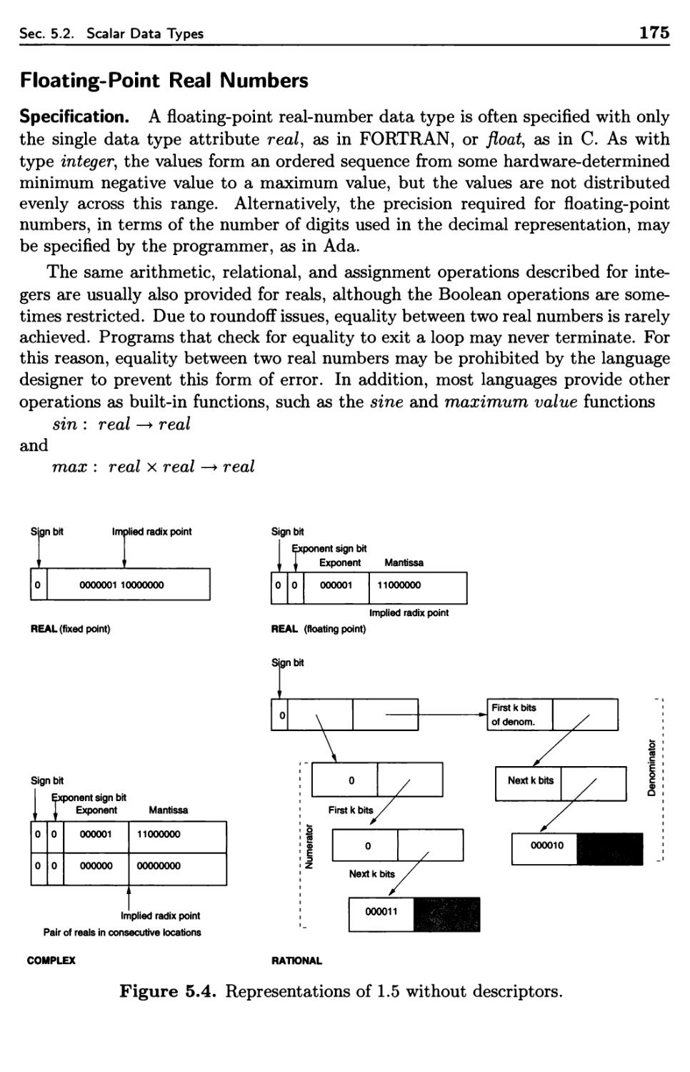
Publishing. Publishing represents a relatively new application domain for
languages. Word processing systems have their own syntax for input commands and
output files. This book was composed using the TfejK text processing system. For
lack of a better term, chapters were compiled as they were written to put in figure
and table references, to place figures, and to compose paragraphs.
The T^jX translator produces a program in the Postscript page description
language. Although Postscript is usually the output of a processor, it does have a
syntax and semantics and can be compiled by an appropriate processor. Often this
is the laser printer that is used to print the document. We know of individuals who
insist on programming directly in Postscript, but this seems to be about as foolish
today as programming in assembly language was in the 1960s. (See Section 12.1.)
Process. During the 1960s, the programmer was the active agent in using a
computer. To accomplish a task, the programmer would write an appropriate command
that the computer would then execute. However, today we often use one program
to control another (e.g., to back up files every midnight, to synchronize time once
Sec. 1.3. Role of Programming Languages
17
an hour, to send an automatic reply to incoming e-mail when on vacation, to
automatically test a program whenever it compiles successfully, etc.). We call such
activities processes, and there is considerable interest in developing languages where
such processes can be specified and then translated to execute automatically.
Within UNIX, the user command language is called the shell, and programs
are called shell scripts. These scripts can be invoked whenever certain enabling
conditions occur. Various other scripting languages have appeared; both TCL and
Perl are used for similar purposes.
New paradigms. New application models are always under study. ML has been
used in programming language research to investigate type theory. Although not a
major language in industry, its popularity is growing. Smalltalk is another
important language. Although commercial Smalltalk use is not very great, it has had a
profound effect on language design. Many of the object-oriented features in C++
and Ada had their origins in Smalltalk.
Languages for various application domains are a continuing source of new
research and development. As our knowledge of compiling techniques improves, and
as our knowledge of how to build complex systems evolves, we are constantly
finding new application domains and require languages that meet the needs of those
domains.
1.3 ROLE OF PROGRAMMING LANGUAGES
Initially, languages were designed to execute programs efficiently. Computers,
costing in the millions of dollars, were the critical resource, whereas programmers,
earning perhaps $10,000 annually, were a minor cost. Any high-level language had
to be competitive with the execution behavior of hand-coded assembly language.
John Backus, chief designer of FORTRAN for IBM in the late 1950s, stated a decade
later [IBM 1966]:
Frankly, we didn't have the vaguest idea how the thing [FORTRAN
language and compiler] would work out in detail. ... We struck out
simply to optimize the object program, the running time, because most
people at that time believed you really couldn't do that kind of thing.
They believed that machine-coded programs would be so terribly
inefficient that it would be impractical for very many applications.
One result we didn't have in mind was this business of having a
system that was designed to be utterly independent of the machine that
the program was ultimately to run on. It turned out to be a very valuable
capability, but we sure didn't have it in mind.
There was nothing organized about our activities. Each part of the
program was written by one or two people who were complete masters
of what they did with very minor exceptions—and the thing just grew
like Topsy. ... [When FORTRAN was distributed] we had the problem
18
Language Design Issues Ch. 1
of facing the fact that these 25,000 instructions weren't all going to be
correct, and that there were going to be difficulties that would show up
only after a lot of use.
By the middle of the 1960s, when the previous quote was made, after the advent
of FORTRAN, COBOL, LISP, and Algol, Backus already realized that
programming was changing. Machines were becoming less expensive, programming costs
were rising, there was a growing need for moving programs from one system to
another, and maintenance of the resulting product was taking a larger share of
computing resources. Rather than compiling programs to work efficiently on a
large, expensive computer, the task of a high-level language was to make it easier
to develop correct programs to solve problems for some given application area.
Compiler technology matured in the 1960s and 1970s (Chapter 3), and language
technology centered on solving domain-specific problems. Scientific computing
generally used FORTRAN, business applications were typically written in COBOL,
military applications were written in JOVIAL, artificial-intelligence applications
were written in LISP, and embedded military applications were to be written in
Ada.
Just like natural languages, programming languages evolve and eventually pass
out of use. Algol from 1960 is no longer used, replaced by Pascal, which in turn is
being replaced by CH—I- and Java. COBOL use is dropping for business applications,
also being replaced by C++. APL, PL/I, and SNOBOL4, all from the 1960s, and
Pascal from the 1970s have all but disappeared.
The older languages still in use have undergone periodic revisions to reflect
changing influences from other areas of computing. Newer languages like C++,
Java, and ML reflect a composite of experience gained in the design and use of
these and the hundreds of other older languages. Some of these influences include
the following:
1. Computer capabilities. Computers have evolved from the small, slow, and
costly vacuum-tube machines of the 1950s to the supercomputers and
microcomputers of today. At the same time, layers of operating system software
have been inserted between the programming language and the underlying
computer hardware. These factors have influenced both the structure and
cost of using the features of high-level languages.
2. Applications. Computer use has spread rapidly from the original
concentration on military, scientific, business, and industrial applications in the 1950s,
where the cost could be justified, to the computer games, PCs, Internet, and
applications in every area of human activity seen today. The requirements
of these new application areas affect the designs of new languages and the
revisions and extensions of older ones.
3. Programming methods. Language designs have evolved to reflect our changing
understanding of good methods for writing large and complex programs and
Sec. 1.3. Role of Programming Languages
19
to reflect the changing environment in which programming is done.
4. Implementation methods. The development of better implementation methods
has affected the choice of features to include in new language designs.
5. Theoretical studies. Research into the conceptual foundations for language
design and implementation, using formal mathematical methods, has
deepened our understanding of the strengths and weaknesses of language features,
which has influenced the inclusion of these features in new language designs.
6. Standardization. The need for standard languages that can be implemented
easily on a variety of computer systems, which allow programs to be
transported from one computer to another, has provided a strong conservative
influence on the evolution of language designs.
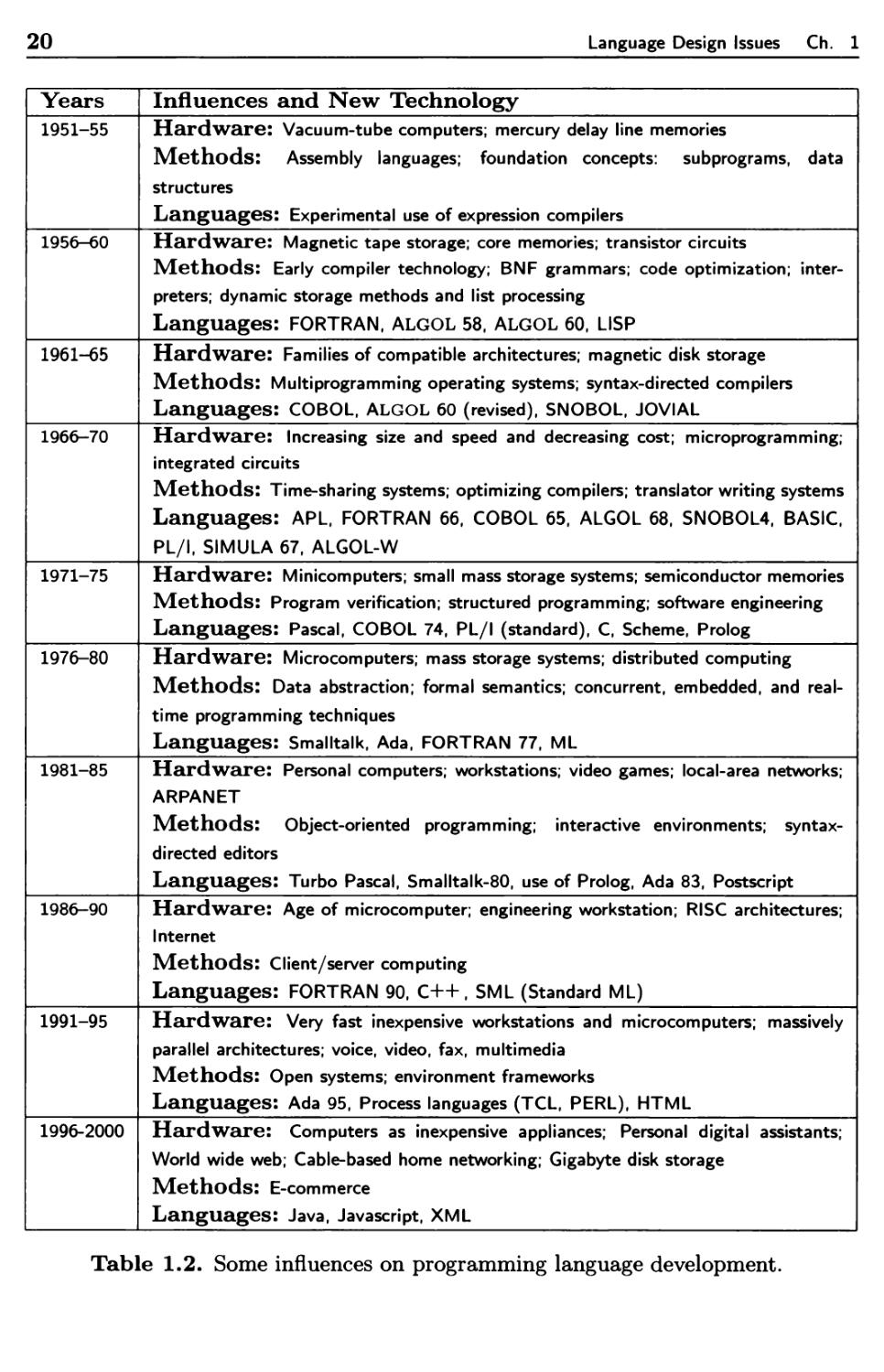
To illustrate, Table 1.2 briefly lists some of the languages and technology
influences that were important during the latter half of the 20t/l century. Many of these
topics are taken up in later chapters. Of course, missing from this table are the
hundreds of languages and influences that have played a lesser but still important
part in this history.
1.3.1 What Makes a Good Language?
Mechanisms to design high-level languages must still be perfected. Each language
in this book has shortcomings, but each is also successful in comparison with the
many hundreds of other languages that have been designed, implemented, used for
a period of time, and then allowed to fall into disuse.
Some reasons for the success or failure of a language may be external to the
language itself. For example, use of COBOL or Ada in the United States was
enforced in certain areas of programming by government mandate. Likewise, part
of the reason for the success of FORTRAN may be attributed to the strong support
of various computer manufacturers that have expended large efforts in providing
sophisticated implementations and extensive documentation for these languages.
Part of the success of SNOBOL4 during the 1970s can be attributed to an excellent
text describing the language [GRISWOLD 1975]. Pascal and LISP have benefited
from their use as objects of theoretical study by students of language design as well
as from actual practical use.
Attributes of a Good Language
Despite the major importance of some of these external influences, it is the
programmer who ultimately, if sometimes indirectly, determines which languages live
and die. Many reasons explain why programmers prefer one language over another.
Let us consider some of these.
20
Language Design Issues Ch. 1
Years
1951-55
1956-60
1961-65
1966-70
1971-75
1976-80
1981-85
1986-90
1991-95
1996-2000
Influences and New Technology
Hardware: Vacuum-tube computers; mercury delay line memories
Methods: Assembly languages; foundation concepts: subprograms, data
structures
Languages: Experimental use of expression compilers
Hardware: Magnetic tape storage; core memories; transistor circuits
Methods: Early compiler technology; BNF grammars; code optimization;
interpreters; dynamic storage methods and list processing
Languages: FORTRAN, ALGOL 58, ALGOL 60, LISP
Hardware: Families of compatible architectures; magnetic disk storage
Methods: Multiprogramming operating systems; syntax-directed compilers
Languages: COBOL, ALGOL 60 (revised), SNOBOL, JOVIAL
Hardware: Increasing size and speed and decreasing cost; microprogramming;
integrated circuits
Methods: Time-sharing systems; optimizing compilers; translator writing systems
Languages: APL, FORTRAN 66, COBOL 65, ALGOL 68, SNOBOL4, BASIC,
PL/I, SIMULA 67, ALGOL-W
Hardware: Minicomputers; small mass storage systems; semiconductor memories
Methods: Program verification; structured programming; software engineering
Languages: Pascal, COBOL 74, PL/I (standard), C, Scheme, Prolog
Hardware: Microcomputers; mass storage systems; distributed computing
Methods: Data abstraction; formal semantics; concurrent, embedded, and
realtime programming techniques
Languages: Smalltalk, Ada, FORTRAN 77, ML
Hardware: Personal computers; workstations; video games; local-area networks;
ARPANET
Methods: Object-oriented programming; interactive environments; syntax-
directed editors
Languages: Turbo Pascal, Smalltalk-80, use of Prolog, Ada 83, Postscript
Hardware: Age of microcomputer; engineering workstation; RISC architectures;
Internet
Methods: Client/server computing
Languages: FORTRAN 90, C++, SML (Standard ML)
Hardware: Very fast inexpensive workstations and microcomputers; massively
parallel architectures; voice, video, fax, multimedia
Methods: Open systems; environment frameworks
Languages: Ada 95, Process languages (TCL, PERL), HTML
Hardware: Computers as inexpensive appliances; Personal digital assistants;
World wide web; Cable-based home networking; Gigabyte disk storage
Methods: E-commerce
Languages: Java, Javascript, XML
Table 1.2. Some influences on programming language development.
Sec. 1.3. Role of Programming Languages
21
1. Clarity, simplicity, and unity. A programming language provides both a
conceptual framework for thinking about algorithms and a means of expressing
those algorithms. The language should be an aid to the programmer long
before the actual coding stage. It should provide a clear, simple, and unified
set of concepts that can be used as primitives in developing algorithms. To
this end, it is desirable to have a minimum number of different concepts, with
the rules for their combination being as simple and regular as possible. We
call this attribute conceptual integrity.
The syntax of a language affects the ease with which a program may be
written, tested, and later understood and modified. The readability of programs
in a language is a central issue here. A syntax that is particularly terse or
cryptic often makes a program easy to write (for the experienced programmer)
but difficult to read when the program must be modified later. APL programs
are often so cryptic that their own designers cannot easily decipher them a
few months after they are completed. Many languages contain syntactic
constructs that encourage misreading by making two almost identical statements
actually mean radically different things. For example, the presence of a blank
character, which is an operator, in a SNOBOL4 statement may entirely alter
its meaning. A language should have the property in which constructs that
mean different things look different; that is, semantic differences should be
mirrored in the language syntax.
2. Orthogonality. The term orthogonality refers to the attribute of being able to
combine various features of a language in all possible combinations, with every
combination being meaningful. For example, suppose a language provides for
an expression that can produce a value, and it also provides for a conditional
statement that evaluates an expression to get a true or false value. These
two features of the language, expression and conditional statement, are
orthogonal if any expression can be used (and evaluated) within the conditional
statement.
When the features of a language are orthogonal, the language is easier to learn
and programs are easier to write because there are fewer exceptions and special
cases to remember. The negative aspect of orthogonality is that a program
will often compile without errors even though it contains a combination of
features that are logically incoherent or extremely inefficient to execute.
3. Naturalness for the application. A language needs a syntax that, when
properly used, allows the program structure to reflect the underlying logical
structure of the algorithm. Ideally, it should be possible to translate such a program
design directly into appropriate program statements that reflect the structure
of the algorithm. Sequential algorithms, concurrent algorithms, logic
algorithms, and others all have differing natural structures that are represented
by programs in those languages.
22
Language Design Issues Ch. 1
The language should provide appropriate data structures, operations, control
structures, and a natural syntax for the problem to be solved. One of the
major reasons for the proliferation of languages is this need for naturalness.
A language particularly suited to a certain class of applications may greatly
simplify the creation of individual programs in that area. Prolog, with its bias
toward deduction properties, and C++, for object-oriented design, are two
languages with an obvious slant toward particular classes of applications.
4. Support for abstraction. Even with the most natural programming language
for an application, there is always a substantial gap remaining between the
abstract data structures and operations that characterize the solution to a
problem and the particular primitive data structures and operations built into
a language. For example, C may be an appropriate language for
constructing a program to do class scheduling for a university, but the abstract data
structures of student, class section, instructor, lecture room and the abstract
operations of assign a student to a class section and schedule a class section in
a lecture room, which are natural to the application, are not provided directly
byC.
A substantial part of the programmer's task is to design the appropriate
abstractions for the problem solution and then implement these abstractions
using the more primitive features provided by the actual programming
language. Ideally, the language should allow data structures, data types, and
operations to be defined and maintained as self-contained abstractions. The
programmer may use them in other parts of the program knowing only their
abstract properties without concern for the details of their implementation.
Both Ada and C++ were developed because of just these shortcomings in the
earlier languages of Pascal and C, respectively.
5. Ease of program verification. The reliability of programs written in a language
is always a central concern. There are many techniques for verifying that a
program correctly performs its required function. A program may be proved
correct by a formal verification method (see Section 4.2), it may be informally
proved correct by desk checking (reading and visually checking the program
text), it may be tested by executing it with test input data and checking
the output results against the specifications, and so on. For large programs,
some combination of all these methods is often used. A language that makes
program verification difficult may be far more troublesome to use than one
that supports and simplifies verification, even though the former may provide
many more features that superficially appear to make programming easier.
Simplicity of semantic and syntactic structure is a primary aspect that tends
to simplify program verification.
6. Programming environment. The technical structure of a programming
language is only one aspect affecting its utility. The presence of an appropriate
programming environment may make a technically weak language easier to
Sec. 1.3. Role of Programming Languages
23
work with than a stronger language that has little external support. A long
list of factors might be included as part of the programming environment.
The availability of a reliable, efficient, and well-documented implementation
of the language must head the list. Special editors and testing packages
tailored to the language may greatly speed the creation and testing of programs.
Facilities for maintaining and modifying multiple versions of a program may
make working with large programs much simpler. Of the languages discussed
in this book, only Smalltalk was specifically designed around a programming
environment consisting of windows, menus, mouse input, and a set of tools to
operate on programs written in Smalltalk.
7. Portability of programs. One important criterion for many programming
projects is the transportability of the resulting programs from the computer
on which they are developed to other computer systems. A language that
is widely available and whose definition is independent of the features of a
particular machine forms a useful base for the production of transportable
programs. Ada, FORTRAN, C, and Pascal all have standardized definitions
allowing for portable applications to be implemented. Others, like ML, come
from a single-source implementation allowing the language designer some
control over portable features of the language.
8. Cost of use. The tricky criterion of cost has been left for last. Cost is certainly
a major element in the evaluation of any programming language, but cost
means many different things:
(a) Cost of program execution. In the early years of computing, questions of
cost were concerned almost exclusively with program execution. Research on
the design of optimizing compilers, efficient register allocation, and the design
of efficient run-time support mechanisms was important. Cost of program
execution, although always of some importance in language design, is of primary
importance for large production programs that will be executed repeatedly.
Today, however, for many applications, speed of execution is not of highest
concern. With desktop machines running at many million instructions per
second and sitting idle much of the time, a 10% or 20% increase in execution
time can be tolerated if it means better diagnostics or easier user control over
development and maintenance of the program.
(b) Cost of program translation. When a language like FORTRAN or C is
used in teaching, the question of efficient translation (compilation) rather
than efficient execution may be paramount. Typically, student programs are
compiled many times while being debugged but are executed only a few times.
In such a case, it is important to have a fast and efficient compiler rather than
a compiler that produces optimized executable code.
(c) Cost of program creation, testing, and use. Yet a third aspect of cost in
a programming language is exemplified by the language Smalltalk and pro-
24
Language Design Issues Ch. 1
cess languages like Perl. For a certain class of problems, a solution may be
designed, coded, tested, modified, and used with a minimum investment of
programmer time and energy. Smalltalk and Perl are cost-effective in that
the overall time and effort expended in solving a problem on the computer
is minimized even though execution time of the program may be higher than
with other languages.
(d) Cost of program maintenance. Many studies have shown that the largest
cost involved in any program that is used over a period of years is not the
cost of initial design, coding, and testing of the program, but total life cycle
costs including development costs and the cost of maintenance of the program
while it is in production use. Maintenance includes the repair of errors
discovered after the program is put into use, changes in the program required
as the underlying hardware or operating system is updated, and extensions
and enhancements to the program that are needed to meet new needs. A
language that makes it easy for a program to be repeatedly modified, repaired,
and extended by different programmers over a period of many years may be,
in the long run, much less expensive to use than any other.
Syntax and Semantics
The syntax of a programming language is what the program looks like. To give the
rules of syntax for a programming language means to tell how statements,
declarations, and other language constructs are written. The semantics of a programming
language is the meaning given to the various syntactic constructs. For example, in
C, to declare a 10-element vector, V, of integers, you would give a declaration, such
as
int V[10];
In contrast, in Pascal, it would be specified as
V: array[0..9] of integer;
Although both create similar data objects at run time, their syntax is very
different. To understand the meaning of the declaration, you need to know the
semantics of both Pascal and C for such array declarations. That is, you need to
know that such a declaration placed at the beginning of a subprogram means to
create the vector on each entry to that subprogram and destroy the vector on exit.
The vector can be referenced by the name V during execution of the subprogram.
In both examples, the elements of V are Vb, ..., Vg.
However, if V is created as a list in LISP, then you need to know that the size of
the object is arbitrary and determined when the object is created, it can be created
at arbitrary times during the execution of the program, and the first member is
referenced as (car V) or (head V).
Sec. 1.3. Role of Programming Languages
25
In programming language manuals and other language descriptions, it is
customary to organize the language description around the various syntactic constructs in
the language. Typically the syntax is given for a language construct such as a
particular type of statement or declaration, then the semantics for that construct is
also given, describing the intended meaning. In Chapter 3, we describe BNF as the
major notation used to describe programming language syntax.
In this text, a different organization is used; it is organized around the structure
associated with the execution of the program. Sometimes these data structures and
operations are tied directly to particular constructs in the syntax of the language,
but often the tie is much less direct. For example, an executing C program may use
a vector V, where V has a structure that is given by the prior declaration. However,
the compiled program may have other data structures, such as a central stack of
subprogram activation records, that are not seen directly in the syntax of programs
at all.
These hidden structures are as important to an understanding of the language as
are the visible structures that correspond directly to something that the programmer
has written in the program. For this reason, the discussion of language elements
here is organized around the executable structures, rather than in terms of syntactic
elements. A particular element may have no syntactic representation in a program,
may be directly represented by a single syntactic element, or may be represented
by several separate syntactic elements that are brought together by the language
translator to produce one virtual computer element.
1.3.2 Language Paradigms
When proponents of various languages meet, the discussions often take the form of
political rallies. Great debates ensue about the efficiency of the array declaration
in C++ versus the array declaration in Java or the value of interpreting versus
compiling a program. In truth, however, the array declarations and translation
issues have very little to do with distinguishing between these languages. There
are often minor syntactic variations that simply reflect the wishes of the language
designers, which have little concrete effect upon the programs written in those
languages. We need to look deeper to understand how languages are constructed.
There are four basic computational models that describe most programming
today: imperative, applicative, rule based, and object oriented. We briefly describe
each of these models.
Imperative languages. Imperative or procedural languages are command-driven or
statement-oriented languages. The basic concept is the machine state, the set of all
values for all memory locations in the computer. A program consists of a sequence
of statements, and the execution of each statement causes the computer to change
the value of one or more locations in its memory, that is, to enter a new state. The
syntax of such languages generally has the form
26
Language Design Issues Ch. 1
statement^
statement^',
Figure 1.1(a) describes this process. Memory consists of a collection of
marbles in boxes, and the execution of a statement (e.g., adding together two variables
to get a third) can be represented as accessing the memory locations (the boxes),
combining these values (the marbles) in some way, and storing the result (a new
marble) in the new location. Program development consists of building the
successive machine states needed to arrive at the solution. This is often the first view one
has of programming, and many widely used languages (e.g., C, C++, FORTRAN,
Algol, PL/I, Pascal, Ada, Smalltalk, and COBOL) support this model. This model
follows from the hardware of the conventional computer that executes instructions
sequentially. It is not surprising that most conventional languages follow this model.
(a) Imperative languages -
Memory is a set of boxes
(b) Applicative languages -
Change how data is accessed from memory
I + I n | | |
* 1 1 II
x I 1 II x x
I I II I I + I
[Same operation as figure (a)]
IX I I I IX
ZLLj x +
xl Ul I
(c) Rule-based -
Use filters to enable state change
Each grid is a possible filter
signifying operation and operands
Figure 1.1. Computational models of programming languages.
Sec. 1.3. Role of Programming Languages
27
Applicative languages. An alternative view of the computation performed by a
programming language is to look at the function that the program represents rather
than just the state changes as the program executes, statement by statement. We
can achieve this by looking at the desired result rather than at the available data.
In other words, rather than looking at the sequence of states that the machine
must pass through in achieving an answer, the question to be asked is: What is the
function that must be applied to the initial machine state by accessing the initial
set of variables and combining them in specific ways to get an answer? Languages
that emphasize this view are called applicative or functional languages.
We can view this model [Figure 1.1(b)] as a lens that takes the initial data and,
by manipulating the view of memory (e.g., as through a lens), produces the desired
answer. Program development proceeds by developing functions from previously
developed functions to build more complex functions that manipulate the initial set
of data until the final function can be used to compute an answer from the initial
data. Rather than looking at the successive machine states of a computation, we
consider the successive functional transformations that we must make on data to
arrive at our answer. Once we have our final answer, we apply this to the initial
data to arrive at a result. The syntax of such languages generally is similar to
functionn(... function2{function\{data))...)
LISP and ML are two functional languages in this book that support this model.
Rule-based languages. Rule-based languages execute by checking for the presence
of a certain enabling condition and, when present, executing an appropriate action.
The most common rule-based language is Prolog, also called a logic programming
language, because the basic enabling conditions are certain classes of predicate logic
expressions (to be discussed more fully in Section 8.4.2). We can describe rule-based
languages in Figure 1.1(c) as a set of filters to apply to the data storage. Execution of
a rule-based language is similar to an imperative language except that statements
are not sequential. Enabling conditions determine the order of execution. The
syntax of such languages generally is similar to the following:
enabling condition\ —* action\
enabling condition^ —* action^
enabling conditionn —* actionn
(Sometimes the rules are written as action if enabling condition with the action
on the left.)
Although Prolog is the most well-known language in this class, many other
languages exist that use this paradigm. The common business application of decision
tables is a form of rule-based programming. In this case, enabling conditions on
data are governed by the presence or absence of enabling data values in a data
28
Language Design Issues Ch. 1
record. Programming often consists of building a matrix (or table) of possible
conditions and then giving appropriate actions if such a condition occurs (hence its
name). BNF parsing techniques (described in chapter 3) and tools like YACC (Yet
Another Compiler Compiler) to parse programs are rule-based techniques that use
the formal syntax of the program as the enabling condition.
Object-oriented programming. As we discuss more fully in chapter 7, object-
oriented programming is becoming an increasingly important computational model.
In this case, complex data objects are built, then a limited set of functions are
designed to operate on those data. Complex objects are designed as extensions of
simpler objects, inheriting properties of the simpler object. As we show, what is
actually happening is that we are trying to use the best of two of the other
computational models. By building concrete data objects, an object-oriented program
gains the efficiency of imperative languages. By building classes of functions that
use a restricted set of data objects, we build the flexibility and reliability of the
applicative model.
Generality of Computational Model
The preceding discussion was careful to use the word supports in describing a
given computational model rather than the word implements. How one uses a
programming language depends upon the programmer. Imperative languages
simplify statement-oriented programming that manipulates the internal machine states
of a computer, but it is possible to write both LISP or Prolog programs that execute
sequentially to perform the same function. It is also relatively easy to write a C
program that consists solely of function calls, and hence seems applicative. It is
important to keep that in mind as we discuss language features later.
Historically, the imperative languages were the first widely used class of
languages and are the dominant form in use today. One of the more interesting research
results of the 1970s and 1980s was that applicative techniques provide for effective
ways to verify programs and show that they are correct. To see this, observe the two
flowgraphs of Figure 1.2. Figure 1.2(a) represents a flowchart of a typical program
design of the 1960s. There is no obvious structure to the program, and control
seems to jump almost randomly. Such programs today are often called spaghetti
code, because the control paths resemble a bowl of spaghetti. In such programs, it
is often difficult to understand the program state at any point during the execution
of the program.
However, Figure 1.2(b) represents a more structured design. We can surround
each segment of the flowgraph by a dotted box. Each of the four dotted boxes in this
figure has a single arrow entering the box and a single arrow leaving. We can view
this program as the composition of four functions, and we can define the behavior
of the program as a function that takes a given state on entering a dotted box
and transforms it into the result state on leaving the dotted box. This, however, is
simply a form of the applicative model we just described. We will discuss this further
Sec. 1.3. Role of Programming Languages
29
o
o
czzu
:
j5^
i i
O
<o
(a) Spaghetti code
(b) Structured code
Figure 1.2. Applicative techniques in imperative languages.
when we describe prime programs in Section 8.3.3. Applying applicative techniques
to imperative programs is behind much of the research in program verification, the
use of formal proofs to show that a program is correct. Some of the predicate and
algebraic techniques discussed in chapter 4 are based on this applicative model. We
also see that object-oriented programming is another approach which, is based on
applying the applicative model to imperative programs.
1.3.3 Language Standardization
What describes a programming language? Consider the following C code:
int i; i = (1 && 2) + 3;
Is this valid C? What is the value of i? How would you answer these questions?1
The following three approaches are most often used:
1. Read the definition in the language reference manual to decide what the
statement means.
2. Write a program on your local computer system to see what happens.
3. Read the definition in the language standard.
Option 2 is probably the most common. Simply sit down and write a two- or three-
line program that tests this condition. Therefore, the concept of a programming
Note that the answers are "yes" aji(^ "4," respectively, for the curious.
30
Language Design Issues Ch. 1
language is closely tied into the particular implementation on your local computer
system. For the more scholarly, a language reference manual, typically published by
the vendor of your local C compiler, can also be checked. Because few have access
to the language standard, Option 3 is rarely employed.
Options 1 and 2 mean that a concept of a programming language is tied to a
particular implementation. But is that implementation correct? What if you want
to move your 50,000-line C program to another computer that has a compiler by
a different vendor? Will the program still compile correctly and produce the same
results when executed? If not, why not? Often language design involves some
intricate details, and one vendor may have a different interpretation from another,
yielding a slightly different execution behavior.
However, one vendor may decide that a new feature added to the language may
enhance its usefulness. Is this legal? For example, if you extend C to add a new
dynamic array declaration, can you still call the language C? If so, programs that
use this new feature on the local compiler will fail to compile if moved to another
system.
To address these concerns, most languages have standard definitions. All
implementations should adhere to this standard. Standards generally come in two
flavors:
1. Proprietary standards. These are definitions by the company that developed
and owns the language. For the most part, proprietary standards do not
work for languages that have become popular and widely used. Variations in
implementations soon appear with many enhancements and incompatibilities.
2. Consensus standards. These are documents produced by organizations based
on an agreement by the relevant participants. Consensus standards, or simply
standards, are the major method to ensure uniformity among several
implementations of a language.
Each country typically has one or more organizations assigned with the role of
developing standards. In the United States, that is the American National
Standards Institute (ANSI). Programming language standards are assigned to
committee X3 of the Computer Business Equipment Manufacturers Association (CBEMA).
The Institute of Electrical and Electronic Engineers (IEEE) also may develop such
standards. In the United Kingdom, the standards role is assumed by the British
Standards Institute (BSI). International standards are produced by the
International Standards Organization (ISO) with headquarters in Geneva, Switzerland.
In the United States, standards are voluntary. The National Institute of
Standards and Technology (NIST), an agency of the United States government, develops
federal standards. These standards are only requirements on vendors that wish to
sell products to federal agencies. Private companies are free to ignore such
standards. However, because of the size of the federal government, these standards often
become adopted, and NIST, ANSI, IEEE, and ISO often work together to develop
Sec. 1.3. Role of Programming Languages
31
many of these standards.
Standards development follows a similar process in all of these organizations.
At some point, a group decides that a language needs a standard definition. The
standards body charters a working group of volunteers to develop that standard.
When the working group agrees on their standard, it is voted on by a larger voting
block of interested individuals. Disagreements are worked out, and the language
standard is produced.
Although it sounds good in theory, the application of standards making is
partially technical and partially political. For example, vendors of compilers have a
strong financial stake in the standards process. After all, they want the standard
to be like their current compiler to avoid having to make changes in their own
implementation. Not only are such changes costly, but users of the compiler, which
employ the features that have changed, now have programs that do not meet the
standard. This makes for unhappy customers.
Therefore, as stated earlier, standards making is a consensus process. Not
everyone gets their way, but one hopes that the resulting language is acceptable to
everyone. Consider the following simple example. During the deliberations for the
1977 FORTRAN standard, it was generally agreed that strings and substrings were
desirable features, since most FORTRAN implementations already had such
features. However, there were several feasible implementations of substrings: If M =
"abcdefg," then the substring "bcde" could be the string from the second to fifth
character of M (M[2:5]) or could be the string starting at Position 2 and extending
for four characters (M[2:4]). It could also be written M[3:6] by counting characters
from the right. Because no consensus could be reached, the decision was simply to
leave this out of the standard. Although not fulfilling most of the goals for a
language as expressed by this chapter, it was the expedient solution that was adopted.
For this reason, standards are useful documents, but the language definition can
get colored by the politics of the day.
To use standards effectively, we need to address three issues:
1. Timeliness. When do we standardize a language?
2. Conformance. What does it mean for a program to adhere to a standard
and for a compiler to compile a standard?
3. Obsolescence. When does a standard age, and how does it get modified?
We consider each question in turn.
Timeliness. One important issue is when to standardize a language. FORTRAN
was initially standardized in 1966 after there were many incompatible versions.
This led to problems because each implementation was different from the others.
At the other extreme, Ada was initially standardized in 1983, before there were
any implementations; therefore, it was not clear when the standard was produced
whether the language would even work. The first effective Ada compilers did not
even appear until 1987, and several idiosyncrasies were identified by these early
implementations. One would like to standardize a language early enough so that
32
Language Design Issues Ch. 1
there is enough experience in using the language, yet not so late as to encourage
many incompatible implementations.
Of the languages in this book, FORTRAN was standardized fairly late, when
there were many incompatible variations; Ada was standardized very early, before
any implementations existed; and C and Pascal were standardized while use was
growing and before there were too many incompatible versions.
Conformance. If there exists a standard for a language, we often talk about
conformance to that standard. A program is conformant if it only uses features defined
in the standard. A conforming compiler is one that, when given a conformant
program, produces an executable program that produces the correct output.
Note that this does not say anything about extensions to the standard. If
a compiler adds additional features, then any program that uses those features
is not conformant, and the standard says nothing about what the results of the
computation should be. Standards generally address conformant programs. Because
of this, most compilers have features that are not addressed by the standard. This
means that one must be careful in using the local implementation as a final authority
as to the meaning of a given feature in a language. (For example, see the Pascal
program anomaly in Figure 9.5 on page 356.)
Obsolescence. As our knowledge and experience of programming evolve, new
computer architectures require new language features. Once we standardize a language,
it seems quaint a few years later. The original FORTRAN 66 standard is quite
out of date without types, nested control structures, encapsulation, block structure,
and the numerous other features in more modern languages.
The standardization process already takes some of this into account. Standards
have to be reviewed every 5 years and either be renewed or dropped. The 5-
year cycle often gets stretched out somewhat, but the process is mostly effective.
FORTRAN was first standardized in 1966, revised in 1978 (called FORTRAN 77,
although the proposed finalization date of 1977 was missed by a few months), and
again in 1990. Ada was standardized in 1983 and revised in 1995.
One problem with updating a standard is what to do with the existing collection
of programs written for the older standard. Companies have significant resources
invested in their software, and to rewrite all of this code for a new version of a
language is quite costly. Because of this, most standards require backward
compatibility; the new standard must include older versions of the language.
There are problems with this. For one, the language can get unwieldy with
numerous obsolete constructs. More damaging, some of these constructs may be
detrimental to good program design. The FORTRAN EQUIVALENCE statement
is one such feature. If A is a real number, and I is an integer, then
EQUIVALENCE (A,I)
A=A+1
1=1+1
Sec. 1.3. Role of Programming Languages
33
assigns A and I to the same storage location. The assignment to A accesses this
location as a real number and adds 1 to it. The assignment to I accesses this location
assuming it is an integer and adds 1 to it. Because the representation of integers
and reals on most computers is different, the results here are very unpredictable.
Leaving this feature in the language is not a good idea.
Recently, the concepts of obsolescent and deprecated features have developed.
A feature is obsolescent if it is a candidate feature that may be dropped in the next
version of the standard. This warns users that the feature is still available, but in
the next 5 to 10 years, it will be dropped. That gives a fair warning to rewrite
any code using that feature. A deprecated feature may become obsolescent with the
next standard, and hence may be dropped after two revisions. This gives a longer
10- to 20-year warning. New programs should not use these features.
Because standard-conforming compilers are allowed to have extensions to the
language, as long as they compile standard-conforming programs correctly, most
compilers have additions that the vendor thinks are useful and will increase
market share for that product. This allows innovation to continue and the language
to evolve. Of course, within the academic community, most faculty do not care
about such standards and will develop their own products that extend and modify
languages as they see fit. This provides a fertile atmosphere where new language
ideas get tried, and some of the better ones make it into commercial languages and
compilers.
1.3.4 Internationalization
With the globalization of commerce and the emergence of the WWW, programming
is increasingly a global activity, and it is important for languages to be readily
usable in multiple countries. There is increasing need for computers to "speak"
many different languages. For example, use of an 8-bit byte, which can store up to
256 different character representations, to represent a character is often insufficient.
This issue has generally gone under the name of internationalization.2
Often local conventions affect the way data are stored and processed. Such
issues as character codes, collating sequences, formats for date and time, and other
local standards affect input and output data. Some of the relevant issues are as
follows[MARTIN 1992]:
Collating sequences. In what collating sequence should the characters be ordered?
• Sorting. The position of non-Roman characters, such as A, 0, 6, 6, and others
is not uniformly defined and may have different interpretations in different
countries.
2Also called the I18N issue, internationalization has 20 characters, and calling it I18N avoids
the arguments as to whether it should be spelled with the British "s" or American "z."
34
Language Design Issues Ch. 1
• Case. Some languages like Japanese, Arabic, Hebrew, and Thai have no
uppercase-lowercase distinction.
• Scanning direction. Most languages read from left to right, but others exist
(e.g., right to left, top to bottom).
Country-specific date formats. 11/26/02 in the United States is 26/11/02 in
England; 26.11.02 in France; 26-XI-02 in Italy, etc.
Country-specific time formats. 5:40 p.m. in the United States is 17:40 in Japan,
17.40 in Germany, 17h40 in France,and so on.
Time zones. Although the general rule is 1 hour of change for each 15 degrees of
longitude, it is more a guideline than a reality. Time zones are generally an integral
number of hours apart, but some vary by 15 or 30 minutes. Time changes (e.g.,
daylight savings time in the United States and summer time in Europe) do not occur
uniformly around the world. Translating local time into a worldwide standard time
is nontrivial. In the southern hemisphere, the transformation for summer time is
opposite that of the northern hemisphere.
Ideographic systems. Some written languages are not based on a small number of
characters forming an alphabet, but instead use large numbers of ideographs (e.g.,
Japanese, Chinese, and Korean). Often 16 bits might be needed to represent text
in those languages.
Currency. Representation of currency (e.g., $, £, ¥) varies by country.
1.4 PROGRAMMING ENVIRONMENTS
A programming environment is the environment familiar to most readers of this
book. It is the environment in which programs are created and tested, and it
tends to have less influence on language design than the operating environment in
which programs are expected to be executed. A programming environment consists
primarily of a set of support tools and a command language for invoking them.
Each support tool is another program that may be used by the programmer as an
aid during one or more of the stages of creation of a program. Typical tools in a
programming environment include editors, debuggers, verifiers, test data generators,
and pretty printers.
1.4.1 Effects on Language Design
Programming environments have affected language design primarily in two major
areas: features aiding separate compilation and assembly of a program from
components and features aiding program testing and debugging.
Sec. 1.4. Programming Environments
35
Separate compilation. In the construction of any large program, it is ordinarily
desirable to have different programmers or programming groups design, code, and
test parts of the program before a final assembly of all the components into a
complete program. This requires the language to be structured so that individual
subprograms or other parts can be separately compiled and executed, without the
other parts, and then later merged without change into the final program.
Separate compilation is made difficult by the fact that in compiling one
subprogram, the compiler may need information about other subprograms or shared data
objects, as in the following situation:
1. The specification of the number, order, and type of parameters expected by
any subprogram called allows the compiler to check whether a call of the
external subprogram is valid. The language in which the other subprogram
is coded may also need to be known so that the compiler may set up the
appropriate calling sequence of instructions to transfer data and control
information to the external subprogram during execution in the form expected
by that subprogram.
2. The declaration of data type for any variable referenced is needed to allow the
compiler to determine the storage representation of the external variable so
that the reference may be compiled using the appropriate accessing formula for
the variable (e.g., the correct offset within the common environment block).
3. The definition of a data type that is defined externally but is used to declare
any local variable within the subprogram is needed to allow the compiler to
allocate storage and compute accessing formulas for local data.
To provide this information about separately compiled subprograms, shared data
objects, and type definitions either (1) the language may require that the
information be redeclared within the subprogram (in FORTRAN); (2) it may prescribe
a particular order of compilation to require compilation of each subprogram to be
preceded by compilation of the specification of all called subprograms and shared
data (in Ada and to some extent in Pascal); or (3) it may require the presence
of a library containing the relevant specifications during compilation so that the
compiler may retrieve them as needed (in Java and C++).
The term independent compilation is usually used for Option 1. Each
subprogram may be independently compiled without any external information; the
subprogram is entirely self-contained. Independent compilation has the disadvantage
that ordinarily there is no way to check the consistency of the information about
external subprograms and data that are redeclared in the subprogram. If the
declarations within the subprogram do not match the actual structure of the external
data or subprogram, then a subtle error appears in the final assembly stage that
will not have been detected during testing of the independently compiled program
parts.
36
Language Design Issues Ch. 1
Options 2 and 3 require a means for specifications of subprograms, type
definitions, and common environments to be given or placed in a library prior to the
compilation of a subprogram. Usually it is desirable to allow the body (local
variables and statements) of a subprogram to be omitted, with only the specification
given. The body may be complied separately later. In Ada, for example, every
subprogram, task, or package is split into two parts, a specification and a body, which
may be separately compiled or placed in a library as required to allow compilation
of other subprograms. A subprogram call made to a subprogram that has not yet
been compiled is termed a stub. A subprogram containing stubs may be executed;
when a stub is reached, the call causes a system diagnostic message to be printed
(or other action taken) rather than an actual call on the subprogram. Thus, a
separately compiled subprogram may be executed for testing purposes, even though
code for some of the routines it calls is not yet available.
Another aspect of separate compilation that affects language design is in the
use of shared names. If several groups are writing portions of a large program,
it is often difficult to ensure that the names used by each group for subprograms,
common environments, and shared type definitions are distinct. A common problem
is to find, during assembly of the final complete program, that several subprograms
or other program units have the same names. This often means a tedious and
time-consuming revision of already-tested code. Languages employ three methods
to avoid this problem:
1. Each shared name, such as in an extern statement in C, must be unique,
and it is the obligation of the programmer to ensure that this is so. Naming
conventions must be adopted at the outset so that each group has a distinct
set of names they may use for subprograms (e.g., "all names used by your
group must begin with QQ"). For example, names used within the standard
C #include files are usually prefixed with _, so programmers should avoid
variable names beginning with the underscore.
2. Languages often use scoping rules to hide names. If one subprogram is
contained within another subprogram, only the names in the outermost
subprogram are known to other separately compiled subprograms. Languages like
Pascal, C, and Ada use this mechanism. We discuss block structure and scope
of names more fully in Section 9.2.2.
3. Names may be known by explicitly adding their definitions from an external
library. This is the basic mechanism of inheritance in object-oriented
languages. By including an externally defined class definition into a subprogram,
other objects defined by that class become known, as in Ada and C++. In
Ada, names may also be overloaded so that several objects may have the same
name. As long as the compiler can resolve which object is actually referenced,
no change is needed in the calling program. Overloading is discussed more
fully in Chapter 7.
Sec. 1.4. Programming Environments
37
Testing and debugging. Most languages contain some features to aid program
testing and debugging. A few typical examples are the following:
1. Execution trace features. Prolog, LISP, and many other interactive languages
provide features that allow particular statements and variables to be tagged
for tracing during execution. Whenever a tagged statement is executed or a
tagged variable is assigned a new value, execution of the program is
interrupted, and a designated trace subprogram is called (which typically prints
appropriate debugging information).
2. Breakpoints. In an interactive programming environment, languages often
provide a feature where the programmer can specify points in the program as
breakpoints. When a breakpoint is reached during execution, execution of the
program is interrupted, and control is given to the programmer at a terminal.
The programmer may inspect and modify values of variables and then restart
the program from the point of interruption.
3. Assertions. An assertion is a conditional expression inserted as a separate
statement in a program, for example,
assert( X>0 and A=l) or (X=0 and A>B+10).
The assertion states the relationships that must hold among the values of
the variables at that point in the program. When the assertion is enabled,
the compiler inserts code into the compiled program to test the conditions
stated. During execution, if the conditions fail to hold, then execution is
interrupted, and an exception handler is invoked to print a message or take
other action. After the program is debugged, the assertions may be disabled
so that the compiler generates no code for their checking. They then become
useful comments that aid in documenting the program. This is a simple
concept that exists in several languages, including C++.
1.4.2 Environment Frameworks
A support environment consists of infrastructure services called the environment
framework to manage the development of a program. This framework supplies
services such as a data repository, graphical user interface, security, and communication
services. Programs are written to use these services. Programmers need to use the
infrastructure services as part of their program design. Accordingly, languages are
sometimes designed to allow for easy access to these infrastructure services.
For example, programs written in the 1960s all included specific I/O routines to
handle communication with the user. With the growth of interactive systems, the
concept of windows displayed on a screen has become the standard output format.
Today, an environment framework would contain an underlying window manager,
such as Motif, which uses the X Window System, and the program would only need
38
Language Design Issues Ch. 1
to call on specific Motif functions to display windows, menus, and scroll bars and
to perform most of the common windowing actions. The X Windows interfaces
are part of the environment framework, which gives all programs that use it a
common behavior pattern for the user at a terminal. Systems like Visual Basic
and Microsoft's Visual Studio provide for libraries of services for C++, Java, and
BASIC programs to build window-based applications.
1.4.3 Job Control and Process Languages
Related to environment frameworks is the concept of job control. Today, if you want
to execute a program such as the C compiler or a word processor, you move the
mouse to the appropriate picture or icon on the screen and click the mouse. The
appropriate program starts to execute. Before the age of windows-based systems,
you would type in the name of the program to run (e.g., as you would do with
the MS-DOS window on a PC today). Earlier still, during the punched-card era of
computing, you would place a punched card naming the program to run ahead of
the cards containing your data.
All of these allow the user to be in direct control of determining what steps to
perform. If the compilation fails, the user could invoke an editor to correct the
program; if the compilation succeeds, the user could invoke a loader and execute
the program.
As we briefly described in Section 1.2.3, the 1960s saw the rise of processes as a
computer took over the management of executing other programs. Rather than have
an operator wait for each step to successfully finish, each program would produce
a return code, and the command for the next step could test that return code
and decide whether to execute. Thus, a sequence of steps—compile, load, execute
program 1, execute program 2,—could be preloaded into the computer, and the
operating system would sequence through these steps in a predefined manner. IBM
used this approach in its Job Control Language for its System 360 beginning in
1963.
The developers of UNIX extended this concept. Rather than simply checking a
return code on a previous job step, the control language could be a more complex
structure with data, operations, and statements. In this case, the data objects would
be the programs and files of the existing computer system. Thus, users could write
programs that linked together various operations from other programs. One could
then program the operation of a sequence of steps based on the contents of data
files and the results of previous operations. This led to the UNIX shell including
variations such as the Bourne shell, C shell, Korn shell, and so on. The *.bat file
on the PC is a simple form of shell program.
From the concept of a shell, many related languages developed. These all go
under the general category of a process or scripting language. They are generally
interpreted and have the property that they view programs and files as the primitive
data to manipulate. Languages such as AWK, Perl, and TCL have been used for
Sec. 1.5. C Overview
39
years to develop such scripts and, for most of the past 20 years, have been viewed as
part of the arcane province of the systems programmer. However, their popularity
has increased with the advent of the Web. Such scripting languages are important
for conveying information back and forth between a user at a web browser and a
web server. Later (Section 12.2.2) we look at how one such language, Perl, is used
in the development of Web programs.
Today we are in an environment where every organization is trying to provide
products "faster, better, and cheaper." The term Internet time has been coined to
describe the process that software development needs to proceed at the speed of the
Internet—at megabits per second. The use of interpreted languages, such as these
job control and scripting process languages, permits developers to rapidly prototype
applications. A language like Perl allows developers to build simple algorithms that
invoke other previously written software using shell scripts in a very rapid manner.
1.5 C OVERVIEW
C is one language that is closely allied with its programming environment.
History. C is a language developed in 1972 by Dennis Ritchie and Ken
Thompson of AT&T Bell Telephone Laboratories. It is related to Algol and Pascal in
style, with attributes of PL/I thrown in. Although a general-purpose programming
language, its compact syntax and efficient execution characteristics have made it
popular as a systems programming language.
In the late 1960s, AT&T Bell Telephone Laboratories dropped out of the MIT
and GE project to develop the Multics operating system; however, developing a
useful system was still the goal of Ken Thompson. Thus, began UNIX, whose
name is a pun on the Multics name. Multics was programmed in PL/I, and there
was a strong desire to also build this new system using a higher level language,
although PL/I was deemed too cumbersome. Having some previous experience
with the systems language BCPL (which was too low level and lacking in any
run-time support), Thompson designed a language named B as a minimal subset
of BCPL for systems programming ("BCPL squeezed into 8K bytes of [PDP-7]
memory" [RITCHIE 1993]). Today, it is hard to realize how strong a constraint
limited memory size was only 30 years ago.
In 1970, the UNIX project acquired a PDP-11 with its huge 24K memory. At
this time, the small, but growing, embryonic UNIX community felt limited by the
restrictions of B. Types, structure definitions, and additional operators were added,
and the new language became known as C.
Although it is a general-purpose programming language, it has been closely
associated with systems programming activities. It was first used to write the kernel
of the UNIX operating system and has been closely tied to UNIX implementations
every since, although versions of C exist on most computing systems today.
During the 1970s, C was mostly a university curiosity due to the university
40
Language Design Issues Ch. 1
fascination with UNIX. However, as commercial versions of this operating system
began to appear in the 1980s, the exposure of C caused its popularity to grow. In
1982, an ANSI working group began to develop a standard for the language, which
was finally produced in 1989 [ANSI 1989] and was accepted as an international
Standard (ISO/IEC 9899) in 1990.
Today, C programmers are probably the fastest growing segment of the
programming world. With its C++ and Java derivatives, they are major influences
in programming today. Most new languages today (e.g., Java, Perl) have a syntax
and semantics partially based on their C roots.
Brief overview of the language. When discussing C, you almost always consider
the C environment and not just the language defined by a specific grammar. C
programming almost always consists of the following:
• The C language. This is a relatively small language with a limited number of
control structures and features. (Remember its roots as a minimal compiler
executing on a PDP 7 and then later on a small PDP 11.)
• The C preprocessor. Because almost every C compiler includes # preprocessor
statements, most users do not realize that these are not really part of the C
language.
• The C interface assumptions. A set of conventions has grown up over the use
of C features. For example, interface definitions between modules are assumed
to be defined in an appropriate ".h" (header) file. The statement
^include "myfcn.h"
uses both the C preprocessor and this third convention in specifying the
interface to module my fen.
• The C library. Many functions, such as printf, getchar, malloc, fork, and
exec, have been written with C language interfaces, although they are not
officially part of the C language definition. However, ANSI C includes these
functions as required library functions for conforming compilers. The inclusion
of a large library allows for a relatively small kernel language, which can be
enhanced with such library functions.
A C module consists of global declarations and a sequence of functions. Multiple
modules are loaded together to form one executable program. Each function may
invoke other functions and access data local to that function or global.
With this structure, data storage is very simple. Each function has local storage
or a local activation record, which is dynamic and allows for recursion, and each
function has access to global data. There is no real block structure. Each data item
has an efficient implementation. For example, multidimensional arrays are built out
Sec. 1.6. Suggestions for Further Reading
41
of one-dimensional arrays, and one-dimensional arrays have indices beginning with
0. This avoids the need for descriptors, which avoids all complex array calculations.
C has pointers, and there is an equivalence between arrays and pointers,
permitting programs to use whichever method of access is most appropriate. Strings
are implemented as arrays of characters. This implementation is completely
transparent so that strings may be accessed as strings, as arrays, or, as just indicated,
as pointers to individual characters.
C has a large set of arithmetic operators that give rise to very efficient and
sometimes very terse programs. C has a full set of control structures with very
flexible semantics, allowing for strange uses at times.
C has a flexible type definition facility; however, you can claim (correctly) that
C is both strongly typed and not strongly typed. That is because most data items
are subtypes of integers. Although the translator will find typing errors, because
most data items are ultimately integers, many errors are missed.
C has always been closely tied to operating system functionality. In UNIX,
operating system functions (e.g., the malloc function for allocating dynamic storage)
are specified as C language function calls. By convention, these are specified in ".h"
system files. So, for example, to call malloc from a C program, the program would
include
^include <malloc.h>
at the beginning of the program, and simply use malloc(StorageSize) when needed
in the program. When such a program is compiled and loaded, the appropriate
function definitions (e.g., malloc) are included from the C library.
The C compiler executes by invoking the preprocessor first. Commands like
^define and ^include are evaluated first, and then the complete program is
compiled by the C translator.
I/O statements are patterned after the FORMAT concept of FORTRAN but
address interactive program execution better than FORTRAN READ and WRITE
statements. Most of the useful functions are defined in the system file stdio.h,
which should be included in every C program. This provides an easy way to extend
a language; a set of functions are written to add new functionality.
Comments (any text bounded by /* ... */) may appear wherever a blank may
be used in a program. Because text is free format in the source files, continuation
lines are generally not needed; however, macro preprocessor statements are defined
as one line of input. Therefore, a macro preprocessor statement uses the symbol \
to indicate that the preprocessor statement continues on the next line.
1.6 SUGGESTIONS FOR FURTHER READING
Numerous texts discuss particular programming languages at an introductory level.
The books by [DERSHEM and JIPPING 1995], [LOUDEN 1993], [SEBESTA 1998],
42
Language Design Issues Ch. 1
and [SETHI 1996] provide alternative views of many of the issues treated here. The
early history of programming languages is treated extensively in [SAMMET 1969,
SAMMET 1972] and [ROSEN 1967]. Wexelblat [WEXELBLAT 1981] edited a
collection of papers from the original designers of many major languages that are also
of interest, including Algol, APL, COBOL, FORTRAN, and PL/I. A second
History of Programming Languages conference was held in 1993 [ACM 1993]. This
volume gives further information on the history of Prolog, C, LISP, C++, Ada,
and Pascal, as well as several other languages not discussed in this book. The role
of language standardization is discussed in [RADA and BERG 1995].
Each language in the book shows influences from its programming and operating
environments. Ada, C, Java, LISP, ML, and Prolog are strongly influenced by these
considerations. [BROWN et al. 1992] and [PERRY and KAISER 1991]
summarized many modern environment designs. Program correctness and the limitations
of verification techniques are summarized in [ABRAMS and ZELKOWITZ 1994].
The IEEE Transactions on Software Engineering, ACM Transactions on Software
Engineering and Methodology, and Software Practice and Experience are three
journals that often carry relevant articles in this area.
1.7 PROBLEMS
1. For a language that is heavily used on your local computer system, evaluate
the reasons for its success according to the list of criteria given in Section 1.3.1.
Should the list be extended?
2. Choose a standardized language for which you have access to the compiler.
Write a program that is nonconformant yet compiles and executes. List several
nonstandard features that the compiler accepts.
3. When the standard definition of a language is revised (usually every 5 to 10
years), a major influence on the revision is the requirement to make programs
written in the earlier version portable to implementations of the revised
version. Thus, there is pressure during the revision to make the new version
include features of the earlier version. For the several standard definitions of
Ada, COBOL, or FORTRAN, compare the features and list several poor ones
whose appearance in a later standard is attributable primarily to the desire to
maintain compatibility with the first.
4. Consider the following simple language, a and b represent names of integer
variables. Each statement may have a label as a prefix. Statements in the
language are as follows:
Sec. 1.7. Problems
43
a = b Assign a the value of b
a = a+1 Add 1 to a
a = a-1 Subtract 1 from a
if a=0 then goto L If a=0, transfer control to statement L
if a>0 then goto L If a>0, transfer control to statement L
goto L Transfer control to statement L
halt Stop execution
For example, the program that computes a = a + b can be given by:
L: a=a-hl
b=b-l
if b>0 then goto L
halt
(a) Write the following programs in this language:
(1) Given a and b, compute x = a + b
(2) Given a and b, compute x = a x b
(3) Given a, b, c, and d, compute x = a x b and y = c x d
(b) Discuss a minimal set of extensions needed to make this language easy to
use. Consider concepts like subprograms, new statements, declarations, and so
on.
5. Take one short program you have written in an imperative language (e.g.,
FORTRAN, C, and Pascal) and rewrite it to be applicative.
6. Features in C allow the same meaning to be expressed many ways. How many
different statements can you write in C that add 1 to a variable X (i.e.,
equivalent to X = X + 1)? Discuss the advantages and disadvantages of this aspect
in the design of C.
7. The assert statement on page 37 can be implemented as a run-time test that
is executed each time the statement is reached, or it can be a property proved
to be true at that point in the program.
(a) Discuss how each approach could be implemented. What is the difficulty
in implementing each approach?
(b) What is the ultimate truth of each assertion for all executions of that
program (i.e., when will that assertion always be true) for each implementation
method?
8. Early computers were designed as electronic calculators to solve numerical
problems. Speculate on what programming languages would be like if these
early machines were developed for a different purpose (e.g., word processing,
robot control, game playing).
44
Language Design Issues Ch. 1
9. Suppose a new language design provides three basic data types: integer, real,
and character. It also provides the ability to declare arrays and records of
data. Arrays have elements of the same type and records have elements of
mixed types. Use the concept of orthogonality to critique the following two
variants of this new design:
(a) Elements of arrays and records may be of any of these basic data types and
may themselves also be arrays or records (e. g., an element of a record may be
an array).
(b) Elements of arrays and records may be of type integer or real Arrays of
characters are called strings and get special treatment. Record elements may
be of type character. Records may have arrays as elements, but arrays may
not have records as elements. Arrays may not have arrays as elements, but
multidimensional arrays are provided to get the same effect.
Chapter 2
Impact of Machine
Architectures
As described in Section 1.2, early languages were designed to permit programs to
run efficiently on expensive hardware. Therefore, the early languages (e.g.,
FORTRAN for arithmetic computation, LISP for list processing) had a design that
translated into efficient machine code, even if the programs were hard to write.
However, machines today are inexpensive, machine cycles are usually plentiful, but
programmers are expensive. There is a greater emphasis in designing programs that
are easy to write correctly even if they execute somewhat more slowly. The data
typing features of ML, the class object of C++, and the package specification of
Ada all take their toll on execution speed, but all have the advantage of easing the
correctness problem of writing good programs. However, how do we design such
languages?
In developing a programming language, the architecture of the software
influences the design of a language in two ways: (1) the underlying computer on which
programs written in the language will execute; and (2) the execution model, or
virtual computer, that supports that language on the actual hardware. In this chapter,
we briefly discuss these topics.
2.1 THE OPERATION OF A COMPUTER
A computer is an integrated set of algorithms and data structures capable of storing
and executing programs. A computer may be constructed as an actual physical
device using wires, integrated circuits, circuit boards, and the like, in which case
it is termed an actual computer or hardware computer. However, it may also be
constructed via software by programs running on another computer, in which case
it is a software-simulated computer. A programming language is implemented by
construction of a translator, which translates programs in the language into machine
language programs that can be directly executed by some computer. The computer
that executes the translated programs may either be a hardware computer or a
45
46
Impact of Machine Architectures Ch. 2
External files and input-output equipment
Program Address
Register
Interpreter
Main memory
Cache memory
; Data Registers
Primitive
operation
Primitive
operation k[
High-speed
registers
Active
processing
elements
CENTRAL PROCESSING UNIT
Figure 2.1. Organization of a conventional computer.
virtual computer composed partially of hardware and partially of software.
A computer consists of six major components that correspond closely to the
major aspects of a programming language:
1. Data. A computer must provide various kinds of elementary data items and
data structures to be manipulated.
2. Primitive operations. A computer must provide a set of primitive operations
useful for manipulating the data.
3. Sequence control. A computer must provide mechanisms for controlling the
sequence in which the primitive operations are to be executed.
4. Data access. A computer must provide mechanisms for controlling the data
supplied to each execution of an operation.
5. Storage management. A computer must provide mechanisms to control the
allocation of storage for programs and data.
6. Operating environment. A computer must provide mechanisms for
communication with an external environment containing programs and data to be
processed.
Sec. 2.1. The Operation of a Computer
47
These six topics form the features from which languages are designed. However,
before looking at these topics in the rather complex context of high-level
programming languages, it is instructive to view them within the simple context of an actual
hardware computer.
2.1.1 Computer Hardware
Hardware computer organizations vary widely, but Figure 2.1 illustrates a fairly
typical conventional organization. A main memory contains programs and data to
be processed. Processing is performed by an interpreter, which takes each machine
language instruction in turn, decodes it, and calls the designated primitive operation
with the designated operands as input. The primitives manipulate the data in
main memory and in high-speed registers and also may transmit programs or data
between memory and the external operating environment. Let us consider the six
major parts of the computer in more detail.
Data. The schematic of Figure 2.1 shows three major data storage components:
main memory, high-speed registers, and external files. Main memory is usually
organized as a linear sequence of bits subdivided into fixed-length words (typically
32 or 64 bits) or 8-bit bytes (typically 4 or 8 bytes per word). The high-speed
registers consist of word-length bit sequences and may have special subfields that are
directly accessible. The contents of a register may represent data or the address in
main memory containing the data or next instruction. A high-speed cache memory
is often situated between main memory and the registers as a mechanism to speed
up access to data from this main memory. External files, stored on magnetic disk,
magnetic tape, or CD-ROM, are usually subdivided into records, each of which is
a sequence of bits or bytes.
A computer has certain built-in data types that can be manipulated directly
by hardware primitive operations. A common set might include integers, single-
precision (e.g., one-word) reals, also called floating-point numbers, fixed-length
character strings, and fixed-length bit strings (where the length is equal to the number
of bits that fit into a single word of storage).
Besides these obvious hardware data elements, programs are also a form of data.
As with the other built-in data types, there must be a built-in representation for
programs, termed the machine language representation of the computer. Typically,
a machine language program would be structured as a sequence of memory locations,
each containing one or more instructions. Each instruction in turn is composed of
an operation code and a set of operand designators.
Operations. A computer must contain a set of built-in primitive operations,
usually paired one to one with the operation codes that may appear in machine language
instructions. A typical set would include primitives for arithmetic on each built-in
numeric data type (e.g., real and integer addition, subtraction, multiplication, and
division), primitives for testing various properties of data items (e.g., test for zero,
48
Impact of Machine Architectures Ch. 2
Fetch next instruction
Decode instruction (determine
the operation and operand
designators)
Figure 2.2. Program interpretation and execution.
positive, and negative numbers), primitives for accessing and modifying various
parts of a data item (e.g., retrieve or store a character in a word and retrieve or
store an operand address in an instruction), primitives for controlling input-output
(I/O) devices, and primitives for sequence control (e.g., unconditional and return
jumps).
As conventional machines (complex instruction set computers or CISC) have
evolved, the set of available instructions have become more numerous and more
powerful as a mechanism to increase the effective speed of the machine. However,
alternatively, it has been found that faster computers can be built by designing
them with fewer primitive instructions, which simplify the internal logic of the
central processing unit (CPU). These reduced instruction set computers (RISC) are
discussed in Section 11.3.
Sequence control. The next instruction to be executed at any point during
execution of a machine language program is usually determined by the contents of
a special program address register (also called the location counter), which always
contains the memory address of the next instruction. Certain primitive operations
are allowed to modify the program address register to transfer control to another
part of the program, but it is the interpreter that actually uses the program address
Sec. 2.1. The Operation of a Computer
49
register and guides the sequence of operations.
The interpreter is central to the operation of a computer. Typically, the
interpreter executes the simple cyclic algorithm shown in Figure 2.2. During each
cycle, the interpreter gets the address of the next instruction from the program
address register (and increments the register value to be the next instruction
address) , fetches the designated instruction from memory, decodes the instruction into
an operation code and a set of operand designators, fetches the designated operands
(if necessary), and calls the designated operation with the designated operands as
arguments. The primitive operation may modify data in memory or registers,
access I/O devices, or change the execution sequence by modifying the contents of the
program address register. After execution of the primitive, the interpreter simply
repeats the previously described cycle.
Data access. Besides an operation code, each machine instruction must specify the
operands that the designated operation is to use. Typically an operand might be in
main memory or in a register. A computer must incorporate a means of designating
operands and a mechanism for retrieving operands from a given operand designator.
Likewise, the result of a primitive operation must be stored in some designated
location. We term these facilities the data access control of the computer. The
conventional scheme is to simply associate integer addresses with memory locations
and provide operations for retrieving the contents of a location given its address
(or, alternatively, for storing a new value in a location whose address is given).
Similarly, registers are also often designated by simple integer addresses.
Storage management. One driving principle in machine design is to keep all
resources of the computer (e.g., memory, central processor, external data devices)
operating as much as possible. The central conflict in achieving this principle is
that operations within the CPU typically happen at the nanosecond level (e.g., 5-
10 nanoseconds for a typical operation on a modern processor), accessing memory
occurs at the microsecond level (50-70 nanoseconds), and external data operations
occur at the millisecond level (10-15 milliseconds). This corresponds to a factor of
1,000,000 between the internal speed of a microprocessor and the speed of a disk.
To balance these speeds appropriately, various storage management facilities are
employed.
In the simplest design (e.g., a low-cost personal computer (PC) for home use),
only simple storage management facilities are built into the hardware; programs and
data reside in memory throughout program execution, and often only one program
may be ready for execution at one time. Although the CPU must wait for
appropriate data to be made available, it is cost-effective not to add additional hardware
to speed up the process.
For speeding up the imbalance between external data access and the central
processor, multiprogramming is often used by the operating system. While waiting
the many milliseconds for data to be read (e.g., from disk), the computer will execute
another program. To allow for many programs to be coresident in memory at the
50
Impact of Machine Architectures Ch. 2
same time, it is now common to include facilities for paging or dynamic program
relocation directly in the hardware. Paging algorithms exist that try to anticipate
which program and data addresses will be most likely used in the near future so that
the hardware can make them available to the central processor. Programs execute
as long as the correct page of instruction or data is in main memory. If there is
a page fault (i.e., the correct location is not in main memory), then the operating
system will retrieve that page from the external data storage and in the meantime
execute another program whose pages are in main memory.
For speeding up the imbalance between main memory and the central processor,
a cache memory is used. A cache memory is a small high-speed data storage that is
between main memory and the central processor. (See Figure 2.1.) This memory,
typically IK (where K is standard computer jargon for 1,024, or 210) to hl2K bytes,
contains the data and instructions most recently used by the central processor, and
hence contains the data and instructions most likely to be needed again in the
near future. The data in the cache are made available immediately to the central
processor if there is a hit of the correct data in the cache, and changed data in the
cache are stored in main memory at the slower main memory rate. If the specified
address is not in the cache, the hardware will retrieve a block of data containing
that address, as well as the next few addresses, to prefetch other data that probably
will be needed shortly.
A cache allows the computer to operate as if the main memory had essentially
the same speed as the central processor. With even small cache memories of 32K,
hit rates of over 95% are generally achieved, yielding performance of the system as
if the main memory operated essentially at the faster processor rate.
Operating environment. The operating environment of a computer ordinarily
consists of a set of peripheral storage and I/O devices. These devices represent the
outside world to the computer, and any communication with the computer must
be by way of the operating environment. Often there are hardware distinctions
between various classes of devices in the environment based on differences in use or
speed of access (e.g., high-speed storage [extended memories], medium-speed
storage [magnetic disks, CD-ROM], low-speed storage [tapes], and I/O devices [readers,
printers, displays, data communication lines]).
Alternative computer architectures. The organization of the computer hardware
often takes alternative forms. The previous discussion is often referred to as a von
Neumann architecture. Other alternative architectures are possible,
von Neumann architecture. The von Neumann computer is named after the
mathematician John von Neumann, who developed this initial design in the early 1940s
as part of the design of ENIAC, which was one of the first electronic computers.
A computer, in his design, consisted of a small controlling central processing unit
(CPU) consisting of the primitive operations, sequence control and registers for
storing the results of the primitive operations, a larger main memory, and a process
for retrieving and storing words of data between the CPU and larger memory. Most
Sec. 2.1. The Operation of a Computer
51
computers sold today still adhere to this basic design, although additions like cache
memory, many CPU registers, and virtual memory have increased performance.
Multiprocessors. As we just discussed, one problem with the von Neumann design
is the great imbalance in the slow speed of external data devices and the high speed
of the CPU registers. An alternative approach toward this imbalance is the use
of multiple CPUs in a given system. Such multiprocessing systems have been in
use for over 30 years. By coupling several relatively inexpensive CPUs with single
sets of memory, disks, tapes, and so on, an effective system can be designed. The
operating system runs different programs on different CPUs in the system and
overall performance is improved.
For the most part, these developments are outside of the realm of programming
language design because each CPU executes an independent program. However,
language and system design is evolving so that programs are now being written to
execute on multiple computers and communicate among one another. In Section
11.3.2 we discuss alternative machine architectures that provide for variations on
this basic von Neumann design and look at their effects on programming language
design and translation.
Computer states. An understanding of the static organization of a computer in
terms of data, operations, control structures, and the like provides only part of the
picture. Full understanding requires that we also see clearly the dynamic operation
of the computer during program execution. What are the contents of the various
storage components at the start of execution? What operations are executed in what
sequence? How are the various data components modified as execution proceeds?
What is the final result of program execution?
A convenient means of viewing the dynamic behavior of a computer is through
the concept of computer state. Consider the process of program execution by the
computer to proceed through a series of states, each defined by the contents of
memory, registers, and external storage at some point during execution. The initial
contents of these storage areas define the initial state of the computer. Each step
in program execution transforms the existing state into a new state through
modification of the contents of one or more of these storage areas. This transformation
of state is termed a state transition. When program execution is complete, the final
state is defined by the final contents of these storage areas. Program execution may
be seen as the sequence of state transitions made by the computer.
2.1.2 Firmware Computers
Earlier we defined a computer as an integrated set of algorithms and data structures
capable of storing and executing programs. The programs executed by a computer
are, of course, written in the machine language of the computer. Ordinarily we
think of computers as operating on a rather low-level machine language, with
simple instruction formats and operations such as "add two numbers" and "load a
register with the contents of a memory location." However, machine languages are
52
Impact of Machine Architectures Ch. 2
not restricted to be low level. Choose any programming language (e.g., C,
FORTRAN, ML) and specify precisely a set of data structures and algorithms that
define the rules for execution of any program written in the language. In so doing,
you are necessarily defining a computer—a computer whose machine language is
the programming language you chose. Each program defines an initial state for the
computer, and the rules for program execution define the sequence of state
transitions that the computer will make during program execution. The result of program
execution is determined by the final state of the computer when program execution
is complete (if ever).
Given a precise definition of a computer, it is always possible to realize the
computer in hardware (i.e., to construct a hardware device whose machine language
is precisely that of the defined computer). This is true even if the machine language
is C, Ada, or some other high-level language (e.g., the Burroughs B5500 mentioned
in Section 1.2.1). In suggesting this possibility, we are appealing to an important
basic principle behind computer design: Any precisely defined algorithm or data
structure may be realized in hardware. Because a computer is simply a collection of
algorithms and data structures, we may assume that its hardware realization is a
possibility, regardless of the complexity of the computer or its associated machine
language.
Actual hardware computers usually have a rather low-level machine language
because of practical considerations. A computer with C or Ada as its machine
language is likely to be considerably more complex (and hence more costly) and
considerably less flexible in a variety of computing tasks than a computer with a
low-level machine language. A hardware computer with a low-level general-purpose
instruction set and a simple, unstructured main memory and register set may be
programmed to look like any of a broad range of computers relatively efficiently, as
we see in the following sections. Computers with high-level machine languages have
occasionally been constructed, but other techniques for implementation of high-level
languages are usually preferable over hardware realization.
A common alternative to the strict hardware realization of a computer is the
firmware computer simulated by a microprogram running on a special micropro-
grammable hardware computer. The machine language of this computer consists of
an extremely low-level set of microinstructions, which usually specify simple
transfers of data between main memory and high-speed registers, between the registers
themselves, and from registers through processors such as adders and multipliers to
other registers. A special microprogram is coded, using this simple instruction set,
that defines the interpretation cycle and the various primitive operations of the
desired computer. The microprogram simulates the operation of the desired computer
on the microprogrammable host computer. Ordinarily the microprogram resides in
a special read-only memory in the host computer and is executed at high speed
by the host computer hardware. This microprogram simulation of a computer is
essentially the same, in concept, as the software simulation technique discussed in
the next section, except that the host computer in this case is especially designed
Sec. 2.1. The Operation of a Computer
53
for microprogramming and provides execution speeds for the simulated computer
comparable to those obtained by direct hardware realization.
Microprogram simulation of a computer is sometimes termed emulation. We
also refer to the resulting computer as a virtual computer because it is simulated by
the microprogram; without this microprogrammed simulation, the machine would
not exist.
2.1.3 Translators and Virtual Architectures
In theory it may be possible to construct a hardware or firmware computer to
execute directly programs written in any particular programming language, and thus
to construct a LISP, Prolog, or C computer, but it is not ordinarily economical to
do so. Practical considerations tend to favor actual computers with rather low-level
machine languages on the basis of speed, flexibility, and cost. Programming, of
course, is most often done in a high-level language far removed from the hardware
machine language. The question, then, is how to get programs in the high-level
language executed on the actual computer at hand, regardless of its machine language.
There are two basic solutions to this implementation question:
1. Translation (or compilation). A translator could be designed to translate
programs in the high-level language into equivalent programs in the machine language
of the actual computer. The interpreter and primitive operations built into the
hardware then directly execute this machine language program. The general term
translator denotes any language processor that accepts programs in some source
language (which may be high or low level) as input and produces functionally
equivalent programs in another object language (which may also be high or low level) as
output. Several specialized types of translator have particular names:
a. An assembler is a translator whose object language is also some variety of
machine language for an actual computer but whose source language, an assembly
language, represents for the most part a symbolic representation of the object
machine code. Most instructions in the source language are translated one for one into
object language instructions.
b. A compiler is a translator whose source language is a high-level language
and whose object language is close to the machine language of an actual computer,
either being an assembly language or some variety of machine language. C, for
example, is usually compiled into an assembly language, which is then converted
into machine language by an assembler.
c. A loader or link editor is a translator whose object language is actual machine
code and whose source language is almost identical; it usually consists of machine
language programs in relocatable form together with tables of data specifying points,
where the relocatable code must be modified to become truly executable. For
example, subprogram P might be compiled for Addresses 0 to 999, and subprogram
Q might be compiled to use Addresses 0 to 1,999. In addition, these subprograms
may use library functions that are defined for addresses 0 to 4,999. The loader's
54
Impact of Machine Architectures Ch. 2
function is to create a single executable program whose addresses are compatible, as
in the following table:
Subprogram Compiled Addresses Executable Addresses
~~P 0^999 (T999
Q 0-1,999 1,000-2,999
library 0-4,999 3,000-7,999
The executable program will look as if it were a single program using addresses
from 0 to 7,999.
d. A preprocessor or a macroprocessor is a translator whose source language
is an extended form of some high-level language such as C++ or Java and whose
object language is the standard form of the same language. The object program
produced by a preprocessor is then ready to be translated and executed by the usual
processors for the standard language. Most C compilers include such a preprocessor
for first translating C macro references into standard C source statements.
Translation of a high-level source language into executable machine language
programs often involves more than one translation step. For example, it is not
uncommon to have C++ programs first translated into C programs, compiled into
assembly language, assembled to produce relocatable machine code, and finally link-
edited and loaded to produce executable machine code. Moreover, the compilation
step may involve a number of passes that progressively translate the program into
various intermediate forms before producing the final object program.
2. Software simulation (software interpretation). Rather than translating the
high-level language programs into equivalent machine-language programs, we might
instead simulate, through programs running on another host computer, a computer
whose machine language is the high-level language. To do this, we construct a
set of programs in the machine language of the host computer that represent the
algorithms (and data structures) necessary for the execution of programs in the
high-level language. In other words, we construct with software running on the
host computer the high-level language computer that we might otherwise have
constructed in hardware. This is termed a software simulation (or software
interpretation) of the high-level language computer on the host computer. The simulated
computer accepts as input data a program in the high-level language. The main
simulator program performs an interpretation algorithm similar to that of Figure
2.2 decoding and executing each statement of the input program in the appropriate
sequence and producing the specified output from the program.
In such a case, we say that the host computer creates a virtual machine
simulating the high-level language. When the host computer is executing the high-level
program, it is not possible to tell whether the program is being executed directly by
the hardware or is first converted to the low-level machine language of the hardware
computer.
Note the difference between software simulation and translation. Both translator
and simulator accept programs in the high-level language as input. However, the
Sec. 2.1. The Operation of a Computer
55
Source
Program
Translator (software)
J
Translation error messages
Source
Program
Run-time
support
library
Executable program
Linker
Translator (software)
Object programs
Execution data
Virtual computer (completely
or partially software
simulated)
Interpreter (firmware,
hardware, or software)
Operations (firmware,
hardware, or software)
Translation error messages
TRANSLATION LOADING EXECUTION
Figure 2.3. Structure of a typical language implementation.
Output
results
Error
messages
translator simply produces an equivalent program in its object language, which must
then be executed by an interpreter for the object language. The simulator executes
the input program directly. If we were to follow the processing of the input program
by both translator and simulator, we would observe the translator processing the
program statements in their physical input sequence and the simulator following
the logical flow of control through the program. The translator would ordinarily
process each program statement exactly once, whereas the simulator might process
some statements repeatedly (if they were part of a loop) and might ignore others
completely (if control never reached them).
Pure translation and pure simulation form two extremes. In practice, pure
translation is seldom used except in cases where the input language is in fact quite similar
to the machine language, as in the case of assembly languages. Pure simulation is
also relatively rare except in the case of operating system control languages or
interactive languages. More commonly, a language is implemented on a computer by
a combination of translation and simulation, as shown in Figure 2.3. A program
is first translated from its original form into a form that is more easily executable.
This is usually done via several independent pieces, called procedures, subprograms,
or subroutines. These separate pieces are combined during the loading phase with a
set of run-time support routines that represent software-simulated operations into
an executable form of the program, which is decoded and executed by simulation.
Translation and simulation provide different advantages in a programming
language implementation. Some aspects of program structure are best translated into
simpler forms before execution; other aspects are best left in their original form and
processed only as needed during execution. Statements in the original source
language program that are executed repeatedly (e.g., statements within program loops
or statements in subprograms that are called more than once) are more efficient if
56
Impact of Machine Architectures Ch. 2
translated. These statements often require a complicated decoding process to
determine the operations to be executed and their operands. Most or all of this process
is identical each time the statement is executed. Thus, if the statement is executed
1,000 times, the identical decoding must be performed 1,000 times. If instead the
statement is translated into a form that is simple to decode (e. g., as a sequence
of machine-language instructions), then the complex decoding process need be
executed only once by the translator, and only a simple decoding of the translated
statement is needed during each of the 1,000 repetitions during execution.
The major disadvantage of translation is loss of information about the program.
If data from the source program are translated to a sequence of machine-language
addresses, and there is an error in the program (e.g., one of these data objects is
divided by 0), it is often difficult to determine which source language statement was
executing and which data objects were being manipulated. With simulation, all of
this information is still available for displaying to the user. In addition, because
a high-level language statement conveys more information than a single machine-
language instruction, an object program is usually much larger than the source
program that produced it.
Simulation provides almost an inverted set of advantages. By leaving statements
in their original form until they need to be executed, no space is needed to store
multiple copies of long code sequences; the basic code need be stored only once in
the simulation routine. However, the total cost of decoding must be paid each time
the statement is to be executed.
The key question in a language implementation tends to be whether the base
representation of the program during execution is that of the machine language of
the actual computer being used. This provides the basis for the common division of
languages (more precisely, language implementations) into those that are compiled
and those that are interpreted:
1. Compiled languages. C, C++, FORTRAN, Pascal, and Ada are commonly
thought of as languages that are compiled. This means that programs in these
languages are usually translated into the machine language of the actual computer
being used before execution begins, with simulation being confined to a set of
runtime support routines that simulate primitive operations in the source language
that have no close analogue in the machine language. Typically, the translator for a
compiled language is relatively large and complex, and the emphasis in translation
is on the production of a translated program that executes as efficiently as possible.
2. Interpreted languages. LISP, ML, Perl, Postscript, Prolog, and Smalltalk are
often implemented by use of a software interpreter. In such a language
implementation, the translator does not produce machine code for the computer being used.
Instead, the translator produces some intermediate form of the program that is more
easily executable than the original program form yet that is different from machine
code. The interpretation procedure for execution of this translated program form
must be represented by software because the hardware interpreter cannot be used
directly. Use of a software interpreter ordinarily results in relatively slow program
Sec. 2.2. Virtual Computers and Binding Times
57
execution. Translators for interpreted languages tend to be rather simple, with
most of the complexity of the implementation coming in the simulation software.
Java and the WWW have changed some of these rules. Java, a language more
like C++ and Pascal than LISP, is nevertheless often processed as an interpreted
language with the Java compiler producing an intermediate set of bytecodes for
a Java virtual machine. For Web applications, major inefficiency is due to the
transmission time of web pages over the network and not in host machine time. By
transmitting the bytecodes to the local machine, execution is often faster, even on
a slow computer, than transmitting the results from the Web server. However, the
Web server does not know the underlying machine architecture of the host computer.
In this case, the Web browser creates a Java virtual machine that executes the
standard set of Java bytecodes.
2.2 VIRTUAL COMPUTERS AND BINDING TIMES
In the previous section, a computer was denned as an integrated set of algorithms
and data structures capable of storing and executing programs. We considered ways
in which a given computer might actually be constructed:
1. Through a hardware realization, representing the data structures and
algorithms directly with physical devices.
2. Through a firmware realization, representing the data structures and
algorithms by microprogramming a suitable hardware computer.
3. Through a virtual machine, representing the data structures and algorithms
by programs and data structures in some other programming language.
4. Through some combination of these techniques, representing various parts of
the computer directly in hardware, in microprograms, or by software
simulation as appropriate.
When a programming language is implemented, the run-time data structures and
algorithms used in program execution define a computer. Similar to the firmware
implementation of a computer, we speak of this as the virtual computer defined by
the language implementation. The machine language of this virtual computer is the
executable program produced by the translator for the language, which may take the
form of actual machine code if the language is compiled, or, alternatively, may have
some arbitrary structure if the language is interpreted. The data structures of this
virtual computer are the run-time data structures that are used during program
execution. The primitive operations are those operations that are actually executable
at run time. Sequence control, data control, and storage management structures
are those used at run time regardless of representation by software, hardware, or
microprogram.
58
Impact of Machine Architectures Ch. 2
2.2.1 Virtual Computers and Language Implementations
If programming languages are defined in terms of their virtual computers so that
each language is associated with a single commonly understood virtual computer,
then description of the semantics of each language in terms of its virtual
computer is straightforward. Unfortunately, because languages are usually defined by
giving a semantics for each syntactic construct individually, language definitions
specify only implicitly an underlying virtual computer. Each time the language
is implemented on a different computer, the implementor tends to see a slightly
(or very) different virtual computer in the language definition. Thus, two different
implementations of the same language may utilize a different set of data structures
and operations in the implementation, particularly for data structures and
operations that are hidden in the program syntax. Each implementor has wide latitude
in determining the virtual computer structures that are the basis for a particular
implementation.
When a programming language is being implemented on a particular computer,
the implementor first determines the virtual computer that represents an
interpretation of the semantics of the language and then constructs that virtual computer
out of the hardware and software elements provided by the underlying computer.
For example, if the virtual computer contains both an integer-addition operation
and a square-root operation, the implementor may choose to represent the integer-
addition operation using an integer-addition operation provided directly by the
underlying hardware, whereas the square-root operation may be represented by a
software simulation as a subprogram for computing square roots. If the virtual
computer contains a simple integer variable X, then the implementor may choose
to represent X directly by a storage location in memory containing the value of X
or may choose to represent X by a storage location that contains a type tag
designating integer together with a pointer to another storage location that contains
the value of X. The organization and structure of an implementation of a language
are determined by these many detailed decisions made by the implementor, taking
into account the various hardware and software facilities available in the underlying
computer and the costs of their use.
The implementor must also determine precisely what is to be done during
translation of a program and what during execution. Often a particular way of
representing a virtual computer data structure or operation during program execution
can be used only if certain kinds of actions are taken during program translation
to set up the run-time structure. If the implementor chooses to simplify the
translator by omitting these actions, then different run-time representations may be
necessary.
Thus, three factors lead to differences among implementations of the same
language:
1. Differences in each implementor's conception of the virtual computer that is
implicit in the language definition.
Sec. 2.2. Virtual Computers and Binding Times
59
Input data Output results
I I
WEB APPLICATION COMPUTER
(Implemented as HTML Web pages)
WEB VIRTUAL COMPUTER
(Browser program Implemented in C or Java)
C VIRTUAL COMPUTER
(Implemented by run-time library
routines loaded with the compiled program)
OPERATING SYSTEM VIRTUAL COMPUTER
(Implemented by machine-language programs
executing on the firmware virtual computer)
FIRMWARE VIRTUAL COMPUTER
(Implemented machine-language instructions
by microcode executed by the actual computer)
ACTUAL HARDWARE COMPUTER
(Implemented by physical devices)
Figure 2.4. Layers of virtual computers for a Web application.
2. Differences in the facilities provided by the host computer on which the
language is to be implemented.
3. Differences in the choices made by each implementor as to how to simulate
the virtual computer elements using the facilities provided by the underlying
computer and how to construct the translator so as to support these choices
of virtual computer representation.
2.2.2 Hierarchies of Virtual Machines
The virtual machine that a programmer uses to create an application is in fact
formed from a hierarchy of virtual computers. At the bottom, there must, of course,
lie an actual hardware computer. However, the ordinary programmer seldom has
any direct dealing with this computer. Instead, this hardware computer is
successively transformed by layers of software (or microprograms) into a virtual machine
that may be radically different. The second level of virtual computer (or the third if
a microprogram forms the second level) is usually defined by the complex collection
of routines known as the operating system.
60
Impact of Machine Architectures Ch. 2
Typically the operating system provides simulations for a number of new
operations and data structures that are not directly provided by the hardware (e.g.,
external file structures or time-of-day functions). The operating system also deletes
certain hardware primitives from the operating-system-defined virtual computer so
that they are not accessible to the operating system user (e.g., hardware primitives
for I/O, turning the machine off, multiprogramming, and multiprocessing). The
operating-system-defined virtual computer is usually that which is available to the
implementor of a high-level language. The language implementor provides a new
layer of software that runs on the operating-system-defined computer and simulates
the operation of the virtual computer for the high-level language. The implementor
also provides a translator for translating user programs into the machine language
of the language-defined virtual computer.
The hierarchy in fact does not end with the high-level language implementation.
The programs that a programmer builds add yet more levels to the hierarchy. Figure
2.4 illustrates such a hierarchy of virtual machines as they might appear to a user
on the WWW.
On top of the C-language virtual machine created by the C-language compiler,
a programmer builds a program called a Web browser using the C (or equivalent)
language. This browser creates the Web virtual machine, which can process the
basic data structures of the WWW, the hyperlinks (URLs) to visit new web sites, the
basic HTML language for displaying Web pages, and the ability to run interactive
programs (i.e., applets) for users of that browser. At the highest level in this
particular hierarchy is the Web application computer. The Web developer uses the
features of the Web virtual machine (HTML, applets, etc.) to provide services to
users of that Web page.
Implicit in this discussion is a central concept: the equivalence of programs and
data. We are accustomed to considering certain kinds of objects in programming
as program and others as data. This is often a useful intuitive distinction, but,
as the prior discussion makes clear, it is a distinction that is more apparent than
real. That which is program in one context is likely to become data in another. For
example, the HTML describing a Web page is data to the Web virtual machine,
which processes the commands to determine how to display the information, but
it is a program to the Web developer who uses HTML to process information for
users of that particular web site.
This equivalence between programs and data can be taken a step further. In
languages like C and FORTRAN, the storage representing the executable program
is generally separated from the storage containing the data used by that program.
In other languages, such as Prolog and LISP, there is no real distinction. Programs
and data are all intermixed, and it is only the execution process that keeps them
separate.
Sec. 2.2. Virtual Computers and Binding Times
61
2.2.3 Binding and Binding Time
Without attempting to be too precise, we may speak of the binding of a program
element to a particular characteristic or property as simply the choice of the property
from a set of possible properties. The time during program formulation or processing
when this choice is made is termed the binding time of that property for that
element. There are many different varieties of bindings in programming languages,
as well as a variety of binding times. We also include within the concepts of binding
and binding time the properties of program elements that are fixed either by the
definition of the language or its implementation.
Classes of Binding Times
Although there is no simple categorization of the various types of bindings, a few
main binding times may be distinguished if we recall our basic assumption that the
processing of a program, regardless of the language, always involves a translation
step followed by execution of the translated program:
1. Execution time (run time). Many bindings are performed during program
execution. These include bindings of variables to their values, as well as (in many
languages) the binding of variables to particular storage locations. Two important
subcategories may be distinguished:
a. On entry to a subprogram or block. In most languages, bindings are restricted
to occur only at the time of entry to a subprogram or block during execution. For
example, in C and C++ , the binding of formal to actual parameters and the binding
of formal parameters to particular storage locations may occur only on entry to a
subprogram.
b. At arbitrary points during execution. Some bindings may occur at any point
during execution of a program. The most important example here is the basic
binding of variables to values through assignment, whereas some languages like
LISP, Smalltalk, and ML permit the binding of names to storage locations to also
occur at arbitrary points in the program.
2. Translation time (compile time). Three different classes of translation time
bindings may be distinguished:
a. Bindings chosen by the programmer. In writing a program, the programmer
consciously makes many decisions regarding choices of variable names, types for
variables, program statement structures, and so on, that represent bindings during
translation. The language translator makes use of these bindings to determine the
final form of the object program.
6. Bindings chosen by the translator. Some bindings are chosen by the language
translator without direct programmer specification. For example, the relative
location of a data object in the storage allocated for a procedure is generally handled
without knowledge or intervention by the programmer. How arrays are stored and
how descriptors for the arrays, if any, are created are decisions made by the language
62
Impact of Machine Architectures Ch. 2
translator. Different implementations of a given language may choose to provide
these features in different ways.
c. Bindings chosen by the loader. A program usually consists of several
subprograms that must be merged into a single executable program. The translator
typically binds variables to addresses within the storage designated for each
subprogram. However, this storage must be allocated actual addresses within the physical
computer that will execute the program. This occurs during load time (also called
link time).
3. Language implementation time. Some aspects of a language definition may
be the same for all programs that are run using a particular implementation of
a language, but they may vary between implementations. For example, often the
details associated with the representations of numbers and arithmetic operations are
determined by the way that arithmetic is done in the underlying hardware computer.
A program written in the language that uses a feature whose definition has been
fixed at implementation time will not necessarily run on another implementation of
the same language; even more troublesome, it may run and give different results.
4. Language definition time. Most of the structure of a programming language
is fixed at the time the language is defined, in the sense of specification of the
alternatives available to a programmer when writing a program. For example, the
possible alternative statement forms, data structure types, program structures, and
so on are all often fixed at language definition time.
To illustrate the variety of bindings and binding times, consider the simple
assignment statement
X = X + 10
written in a language L. We might inquire into the bindings and binding times of
the following elements of this statement:
1. Set of types for Variable X. Variable X in the statement usually has a data
type associated with it, such as real, integer, or Boolean. The set of allowable
types for X is often fixed at language definition time (e.g., only types real,
integer, Boolean, set, and character might be allowed). Alternatively, the
language may allow each program to define new types, as in C, Java, and
Ada, so that the set of possible types for X is fixed at translation time.
2. Type of variable X. The particular data type associated with variable X is
often fixed at translation time through an explicit declaration in the program
such as float X, which is the C designation for a real data type. In other
languages, such as Smalltalk and Perl, the data type of X may be bound at
execution time through assignment of a value of a particular type to X. In
these languages, X may refer to an integer at one point and to a string at a
later point in the same program.
3. Set of possible values for variable X. If X has data type real, then its value at
any point during execution is one of a set of bit sequences representing real
Sec. 2.2. Virtual Computers and Binding Times
63
numbers. The precise set of possible values for X is determined by the real
numbers that can be represented and manipulated in the virtual computer
defining the language, which ordinarily is the set of real numbers that can be
represented conveniently in the underlying hardware computer.
4. Value of Variable X. At any point during program execution, a particular
value is bound to Variable X. This value is determined at execution time
through assignment of a value to X. The assignment X = X + 10 changes
the binding of X, replacing its old value by a new one that is 10 more than
the old one.
5. Representation of the constant 10. The integer 10 has both a representation
as a constant in the text of the program, using the string 10, and a
representation at execution time, commonly as a sequence of bits. The choice of
decimal representation in the program (i.e., using 10 for ten) is usually made
at language definition time, whereas the choice of a particular sequence of bits
to represent 10 at execution time is usually made at language implementation
time.
6. Properties of the operator +. The choice of symbol + to represent the
addition operation is made at language definition time. However, it is common
to allow the same symbol + to be overloaded by representing real addition,
integer addition, complex addition, and so on, depending on the context. In
a compiled language, it is common to make the determination of which
operation is represented by + at compile time. The mechanism for specifying the
binding desired is usually the typing mechanism for variables: If X is type
integer, then the + in X + 10 represents integer addition; if X is type real,
then the + represents real addition, and so on.
The detailed definition of the operation represented by + may also depend on
the underlying hardware computer. In our example, if X has the value 249,
then X + 10 may not even be defined on some computers.
In summary, for a language like C, the symbol + is bound to a set of addition
operations at language definition time, each addition operation in the set is
defined at language implementation time, each particular use of the symbol +
in a program is bound to a particular addition operation at translation time,
and the particular value of each particular addition operation for its operands
is determined only at execution time.
Importance of Binding Times
In the analysis and comparison of programming languages in the following chapters,
many distinctions are based on differences in binding times. We are continuously in
the process of asking this question: Is this done at translation time or at execution
time? Many of the most important and subtle differences among languages involve
64
Impact of Machine Architectures Ch. 2
differences in binding times. For example, almost every language allows numbers as
data and allows arithmetic operations on these numbers. Yet not all languages are
equally suited for programming problems involving a great deal of arithmetic. For
example, although both ML and FORTRAN allow one to set up and manipulate
arrays of numbers, solving a problem requiring large arrays and large amounts of
arithmetic in ML would probably be most inappropriate if it could also be done in
FORTRAN. If we were to trace the reason for this by comparing the features of ML
and FORTRAN, we ultimately would ascribe the superiority of FORTRAN in this
case to the fact that in ML most of the bindings required in the program will be
set up at execution time, whereas in FORTRAN most will be set up at translation
time. Thus, an ML version of the program would spend most of its execution time
creating and destroying bindings, whereas in the FORTRAN version most of the
same bindings would be set up once during translation, leaving only a few to be
handled during execution. As a result, the FORTRAN version would execute much
more efficiently.
Nevertheless, we might turn around and ask a related question: Why is
FORTRAN so inflexible in its handling of strings as compared with ML? Again the
answer turns on binding times. Because most bindings in FORTRAN are performed
at translation time, before the input data are known, it is difficult in FORTRAN to
write programs that can adapt to a variety of different data-dependent situations
at execution time. For example, the size of strings and the type of variables must
be fixed at translation time in FORTRAN. In ML, bindings may be delayed during
execution until the input data have been examined and the appropriate bindings
for the particular input data determined.
A language like FORTRAN, in which most bindings are made during translation,
early in the processing of a program, is said to have early binding; languages with
late binding, such as ML or HTML, delay most bindings until execution time.
The advantages and disadvantages of early binding versus late binding revolve
around a conflict between efficiency and flexibility. In languages where execution
efficiency is a prime consideration, such as FORTRAN, Pascal, and C, it is common
to design the language so that as many bindings as possible may be performed
during translation. Where flexibility is the prime determiner, as in ML and LISP,
most bindings are delayed until execution time so that they may be made data
dependent. In a language designed for both efficient execution and flexibility, such
as Ada, multiple options are often available that allow choices of binding times.
Binding Times and Language Implementations
Language definitions are usually permissive in specifying binding times. A language
is designed so that a particular binding may be performed at translation time,
but the actual time at which the binding is performed is in fact defined only by
the implementation of the language. For example, Pascal is designed to permit
the type of variables to be determined at compile time, but a particular Pascal
Sec. 2.2. Virtual Computers and Binding Times
65
implementation might instead do type checking at execution time. Thus, although
the definition of Pascal permits compile-time type checking, it does not require it.
In general, a language design specifies the earliest time during program processing
at which a particular binding is possible, but any implementation of the language
may in fact delay the binding. However, usually most implementations of the same
language will perform most bindings at the same time. If the language is designed
to permit compile-time bindings, then to delay these bindings until execution time
will probably lead to less efficient execution at no gain in flexibility, such as the
prior example of execution-time type checking in Pascal.
One additional caution is needed, however. Often seemingly minor changes in a
language may lead to major changes in binding times. For example, in FORTRAN
90, the change to allow recursion modifies many of the binding times of important
FORTRAN features. Because binding times are implementation dependent, we
place emphasis on knowing the language implementation. When approaching your
own local implementation of a language, it is important to ask about the binding
times in that implementation. Are they the usual ones, or have local modifications
to the language caused the usual binding times to be modified?
2.2.4 Java Overview
History. Java development began in 1991 at Sun Microsystems, where James
Gosling led the Green Team in a project to develop a language for use on
consumer digital devices. In the summer of 1992, they had a working version, but they
were ahead of the curve, as the saying goes, and industry was not ready for this
language.
In 1993, the Mosaic Web Browser was released. This had the effect of moving
the Internet from the domain of the academic researcher to the world at-large. The
Green Team immediately saw the role of their language as a way to enhance Web
browsers.
With Mosaic, and its underlying HTML Web pages and URLs to navigate
around the Web, users could download information from distant sites. (See a
discussion of this in chapter 12.) However, there were three limitations to using the
Web:
1. Transmission speeds to consumer homes were limited to about 33,000 bits
per second in 1993. (Now it is generally around 50,000 bits per second.)
2. If a site were popular, its own processing speed would be severely impacted
if many users were accessing its Web pages at the same time.
3. Each Web object (e.g., document, picture, video, audio) required a separate
protocol in each Web browser. New formats could not be added to the set until all
browsers included this new protocol.
Because most users of the Web were waiting for information to appear on their
screen, their own computers were often idle. A way around the first two limitations
would be to have some of the information processed on the user's machine and not
66
Impact of Machine Architectures Ch. 2
on the Web server. This could be accomplished by having the Web server download
a small application program (i.e., an applet) that would run on the user's computer,
thus freeing up the Web server to process more users at the same time. Similarly,
the Web server could download an applet that could handle any new protocols that
were needed, using this same feature.
The Sun group saw the value of their development as an adjunct to Web
technology. However, to be effective, their language had to fulfill several requirements:
1. Architectural independence. The Web server would not know what machine
the user's browser was executing on. To solve this problem, a Java virtual machine
was designed and the applet would be compiled into a series of bytecodes for that
virtual machine. Thus, any browser that handled the Java virtual machine would
be able to execute a Java applet.
2. Security. A critical need for consumer acceptance of Java would be that the
Web server must not be able to access information from the user's computer and
pass that information back to the Web server. If web sites had that ability, users
would be reluctant to use the Web to access unknown sites, and the growth of the
Web would be stunted.
In 1994, Sun developed the HotJava browser that contained the Java virtual
machine to demonstrate its applicability. Finally on May 23, 1995, Marc Andreessen,
cofounder of Netscape Communications, which at the time had a 70% market share
of the Web browser market, announced that Netscape had incorporated the Java
virtual machine as part of its Netscape browser. Since that time, Java use has
mushroomed. Although designed to execute applets as part of a Web browser, it has also
gained acceptance as a general programming language, often replacing C++ or C
as a first programming language for student use.
Brief overview of the language. Java is similar to C and C++. Looking at
these languages historically shows the relationship among them. C was developed
in the 1970s as a language for building operating systems (principally UNIX). As
such, the language designers wanted a language that would allow access to the
underlying architecture of the hardware computer. When Stroustrup developed
C++, he included the class concept from Simula and inheritance from Smalltalk.
However, the basic C language was not modified, so features of C that were useful
for systems programming were carried along into C++ . When Sun developed Java,
they kept the basic syntax, class, and inheritance concepts from C++, but deleted
unnecessary features. This resulted in Java as a smaller language than C++, but
with a more rational syntax and semantics as a useful programming language.
For the most part, Java is C++ with the excess baggage of C, which yields
poor programs, removed. Data are strongly typed, with integers, Booleans, and
characters all being separate types. Arrays are also separate types, and a string is
not simply an array of characters. All of these permit the compiler to perform more
complete error checking on Java programs.
There are fewer ways to perform some actions, such as method invocation being
Sec. 2.3. Suggestions for Further Reading
67
the only subroutine linkage. Because all objects are part of classes, there is no need
for separate function or procedure calls. Struct objects are also not needed because
the same effect can be achieved via instance variables in class definitions.
Pointers are implicit in the language, but there is no pointer data type. That
means that all of the problems with memory fragmentation, dangling references,
and other pointer mishaps are hidden from the users. Pointer allocation is implicit
by the instantiation of class objects and the new operator.
To create a Java program, a file name.Java is created. The name of the file
should be the same as the class created by the Java program. A Java compiler is
called and a file of bytecodes is produced in the file name.class. This file may be
executed by the Java interpreter (Java virtual machine).
Java is basically a simple language: It has the clean C++ design without some
of C's clumsiness. However, this is at a cost in execution efficiency because many
of these structures need run-time validation. In addition, because Java is often
interpreted as an applet in a Java virtual machine, there is certainly an execution
cost over compiled machine language. For the application domain it was designed
for, Web browsers, workstation speed is higher than either the terminal display
processor or Internet communication. Therefore, the inefficiency of the Java execution
model is mostly hidden from the user, who will still spend most of the time waiting
for network response to transmit the desired information.
2.3 SUGGESTIONS FOR FURTHER READING
Alternative computer organizations based on radically different principles from the
von Neumann architecture have not been discussed here, although there is a brief
summary of such topics in chapter 11. The Turing Award Lecture of Backus
[BACKUS 1978] critiques the von Neumann computer organization and offers an
alternative. Today, there is increasing emphasis in parallel architectures and
massively parallel machines (e.g., thousands of computers working in parallel) to
increase performance (e.g., January 1991 issue of IEEE Computer on experimental
research in computer architecture or [MANO and KIME 1999]).
2.4 PROBLEMS
1. Analyze the implementation of a programming language with which you are
familiar. What is the executable form of a program (i.e., what is the output of
the translator)? What sorts of translations are made in translating the various
statements and expressions into executable form? What software simulation
is necessary during program execution? Is the interpreter software simulated?
Which of the primitive operations require software simulation?
2. On your computer, determine the structure of the virtual computer defined by
the operating system. How does this virtual computer differ from the actual
68
Impact of Machine Architectures Ch. 2
hardware computer? Are there features of the hardware that are restricted
by the operating system (e.g., hardware instructions that are not allowed in
user programs in the operating-system-defined virtual computer)? What new
features are provided directly in the operating system virtual computer that
could be simulated only by complex software on the basic hardware computer
(e.g., I/O)?
3. The use of an operating system to provide the programmer with a virtual
computer different from the basic hardware computer has three advantages.
It allows the user to work with a simpler computer than is provided directly
by the hardware (e.g., by providing simpler and more powerful I/O facilities).
It also protects the computer system from the user, in that each user may be
effectively sealed off in a separate virtual computer so that any errors will only
hurt that virtual computer and not bring down the whole system and its other
users as well. It also allows the operating system to allocate the resources of
the system more appropriately to different users. Analyze your local operating
system and the virtual computer it provides the programmer. How well does
it achieve these goals?
4. The BASIC programming language is often implemented using a complete
software simulation of the BASIC virtual computer. If the programs that simulate
the BASIC virtual computer were written in FORTRAN (as they might well
be), then another layer would be added to the layers of virtual computer in
Figure 2.4 on page 59. Draw the new layer. If you know both BASIC and
FORTRAN, explain the parts of the BASIC virtual computer that the
FORTRAN programs might simulate. Where does the translator that translates
BASIC programs into their executable form fit into this diagram?
5. Write a statement in a language with which you are familiar. For each syntactic
component of the statement (variable names, operation symbols, etc.), list the
various bindings that are necessary to completely determine the semantics of
the statement when it is executed. For each binding, identify the binding time
used in the language.
6. Do Problem 5, but use a declaration instead of a statement. Declarations are
usually said to be elaborated instead of executed, so list the bindings (and their
binding times) necessary for a complete elaboration of the declaration.
7. Consider all the languages in the appendix. Which ones do you think should be
dropped from a later edition? Which ones will dominate programming in the
next decade? Consider binding time for features, virtual computer needed to
execute programs, attributes for effective use, and any other relevant attributes.
Chapter 3
Language Translation Issues
During the early days of language design (e.g., during the formative era of developing
FORTRAN, Algol, COBOL, and LISP around 1960), it was believed that a formal
syntax was all that was required for specifying programs. The concept of a context-
free grammar or Backus-Naur form (BNF) grammar was developed (and is discussed
later in this chapter) and used successfully for specifying the syntax of a language.
It is still the major technique today for describing the components of a program.
However, over time it was realized that syntax was insufficient. In Chapter 4 we give
a brief introduction to the issue of programming semantics or the understanding of
what a program means.
3.1 PROGRAMMING LANGUAGE SYNTAX
Syntax, which is defined as "the arrangement of words as elements in a sentence
to show their relationship,"* describes the sequence of symbols that make up valid
programs. The C statement X = Y + Z represents a valid sequence of symbols,
whereas XY H— does not represent a valid sequence of symbols for a C program.
Syntax provides significant information needed for understanding a program and
provides much-needed information toward the translation of the source program into
an object program. For example, almost everyone reading this text will interpret
the expression 2 + 3 x 4 as having the value of 14 and not 20. That is, the expression
is interpreted as if written 2 + (3 x 4) and is not interpreted as if written (2 + 3) x 4.
We can specify either interpretation, if we wish, by syntax and hence guide the
translator into generating the correct operations for evaluating this expression.
As with the ambiguous English sentence "They are flying planes," developing
a language syntax alone is insufficient to unambiguously specify the structure of
a statement. In a statement like X = 2.45 + 3.67, syntax cannot tell us whether
Variable X was declared or declared as type real. Results of X = 5, X = 6, and
X = 6.12 are all possible if X and + denote integers, X denotes an integer and
+ is real addition, and X and + denote real values, respectively. We need more
1 Webster's New World Dictionary, Fawcett, 1979.
69
70
Language Translation Issues Ch. 3
than just syntactic structures for the full description of a programming language.
Other attributes, under the general term semantics, such as the use of declarations,
operations, sequence control, and referencing environments, affect a variable and
are not always determined by syntax rules.
Although syntactic descriptions of a programming language are insufficient for
the complete understanding of the language, they are important attributes in this
description. For the most part, description of syntax is a "solved problem." When
we discuss translator design later in this chapter, the first phase of syntactic
understanding of the source program is fairly mechanical. Tools such as YACC (Yet
Another Compiler Compiler) automatically produce this syntactic description of a
given program. Applying semantic understanding to generate an efficient object
program from a given source program still requires a great deal of skill, as well as
the application of some formal methods to the process.
3.1.1 General Syntactic Criteria
The primary purpose of syntax is to provide a notation for communication between
the programmer and the programming language processor. The choice of particular
syntactic structures, however, is constrained only slightly by the necessity to
communicate particular items of information. For example, the fact that a particular
variable has a value of type real number may be represented in any of a dozen
different ways in a program—through an explicit declaration as in C, through an implicit
naming convention as in FORTRAN, and so on. The details of syntax are chosen
largely on the basis of secondary criteria, such as readability, which are unrelated
to the primary goal of communicating information to the language processor.
There are many secondary criteria, but they may be roughly categorized under
the general goals of making programs easy to read, easy to write, easy to translate,
and unambiguous. We consider some of the ways that language syntactic structures
may be designed to satisfy these often conflicting goals.
Readability. A program is readable if the underlying structure of the algorithm
and data represented by the program is apparent from an inspection of the
program text. A readable program is often said to be self-documenting—that is, it is
understandable without any separate documentation (although this goal is seldom
achieved in practice). Readability is enhanced by such language features as natural
statement formats, structured statements, liberal use of keywords and noise words,
provision for embedded comments, unrestricted length identifiers, mnemonic
operator symbols, free-field formats, and complete data declarations. Readability, of
course, cannot be guaranteed by the design of a language, because even the best
design may be circumvented by poor programming. However, syntactic design can
force even the best-intentioned programmer to write unreadable programs (as is
often the case in APL). The COBOL design emphasizes readability most heavily,
often at the expense of ease of writing and translation.
Readability is enhanced by a program syntax in which syntactic differences re-
Sec. 3.1. Programming Language Syntax
71
fleet underlying semantic differences so that program constructs that do similar
things look similar and program constructs that do radically different things look
different. In general, the greater the variety of syntactic constructs used, the more
easily the program structure may be made to reflect different underlying semantic
structures.
Languages that provide only a few different syntactic constructs in general lead
to less readable programs. In APL or SNOBOL4, for example, only one statement
format is provided. The differences among an assignment statement, a subprogram
call, a simple goto statement, a subprogram return, a multiway conditional branch,
and various other common program structures are reflected syntactically only by
differences in one or a few operator symbols within a complex expression. It
often requires a detailed analysis of a program to determine even its gross control
structure. Moreover, a simple syntax error, such as a single incorrect character
in a statement, may radically alter the meaning of a statement without rendering
it syntactically incorrect. In LISP, errors in matching parentheses cause similar
problems; one of Scheme's extensions to LISP is to circumvent this problem.
Writeability. The syntactic features that make a program easy to write are often
in conflict with those features that make it easy to read. Writeability is enhanced
by use of concise and regular syntactic structures, whereas for readability a variety
of more verbose constructs are helpful. C unfortunately has this attribute of
providing for very concise programs that are hard to read, although it does have a full
complement of useful features.
Implicit syntactic conventions that allow declarations and operations to be left
unspecified make programs shorter and easier to write but harder to read. Other
features advance both goals (e.g., the use of structured statements, simple natural
statement formats, mnemonic operation symbols, and unrestricted identifiers
usually make program writing easier by allowing the natural structure of the problem
algorithms and data to be directly represented in the program).
A syntax is redundant if it communicates the same item of information in more
than one way. Some redundancy is useful in programming language syntax because
it makes a program easier to read and also allows for error checking during
translation. The disadvantage is that redundancy makes programs more verbose and thus
harder to write. Most of the default rules for the meaning of language constructs
are intended to reduce redundancy by eliminating explicit statement of meanings
that can be inferred from the context. For example, rather than require explicit
declaration of the type of every function parameter, ML uses data type induction
to derive the type of a function's argument. However, if there is an error in writing
such a function, the translator will be unable to detect this error. Because of this
effect of masking errors in programs, languages that lack all redundancy are often
difficult to use.
Ease of verifiability. Related to readability and writeability is the concept of
program correctness or program verification. After many years of experience, we now
72
Language Translation Issues Ch. 3
understand that understanding each programming language statement is relatively
easy, but the overall process of creating correct programs is extremely difficult.
Therefore, we need techniques that enable the program to be mathematically proved
correct. We discuss this further in chapter 4.
Ease of translation. A third conflicting goal is that of making programs easy to
translate into executable form. Readability and writeability are criteria directed
to the needs of the human programmer. Ease of translation relates to the needs
of the translator that processes the written program. The key to easy translation
is regularity of structure. The LISP syntax provides an example of a program
structure that is neither particularly readable nor particularly writable but that is
extremely simple to translate. The entire syntactic structure of any LISP program
may be described in a few simple rules because of the regularity of the syntax.
Programs become harder to translate as the number of special syntactic constructs
increases. For example, COBOL translation is made extremely difficult by the large
number of statement and declaration forms allowed, although the semantics of the
language is not particularly complicated.
Figure 3-1- Two interpretations of a conditional statement.
Lack of ambiguity. Ambiguity is a central problem in every language design. A
language definition ideally provides a unique meaning for every syntactic construct
that a programmer may write. An ambiguous construction allows two or more
different interpretations. The problems of ambiguity usually arise not in the structure
of individual program elements but in the interplay between different structures.
Sec. 3.1. Programming Language Syntax
73
For example, both Pascal and Algol allow two different forms of conditional
statement:
1. if Boolean expression then statementi else statement^
2. if Boolean expression then statement\
The interpretation to be given to each statement form is clearly defined. However,
when the two forms are combined by allowing statement\ to be another conditional
statement, then the structure
if Boolean expression then if Boolean expression^ then
statementi else statement^
termed a dangling else, is formed. This statement form is ambiguous, because it is
not clear which of the two execution sequences of Figure 3.1 is intended. FORTRAN
syntax provides another example. A reference to A(I,J) might be either a reference
to an element of the two-dimensional array A or a call of the function subprogram
A because the syntax in FORTRAN for function calls and array references is the
same. Similar ambiguities arise in almost every programming language.
The ambiguities in FORTRAN and Algol mentioned earlier have in fact been
resolved in both languages. In the Algol conditional statement, the ambiguity
has been resolved by changing the syntax of the language to introduce a required
begin ... end delimiter pair around the embedded conditional statement. Thus,
the natural but ambiguous combination of two conditional statements has been
replaced by the two less natural but unambiguous constructions, depending on the
desired interpretation:
1. if Boolean expression then begin if Boolean expression^ then
statementi end else statement^
2. if Boolean expression then begin if Boolean expression^ then
statementi else statement^ end
A simpler solution is used in Ada: Each if statement must end with the delimiter
end if. In C and Pascal, another technique is used to resolve the ambiguity. An
arbitrary interpretation is chosen for the ambiguous construction—in this case,
the final else is paired with the nearest then so that the combined statement
has the same meaning as the second of the previous Algol constructions. The
ambiguity of FORTRAN function and array references is resolved by the rule: The
construct A(I, J) is assumed to be a function call if no declaration for an array
A is given. Because each array must be declared prior to its use in a program,
the translator may readily check whether there is in fact an array A to which the
reference applies. If none is found, then the translator assumes that the construct
is a call to an external Function A. This assumption cannot be checked until load
time when all the external functions (including library functions) are linked into
the final executable program. If the loader finds no Function A, then a loader error
74
Language Translation Issues Ch. 3
message is produced. In Pascal, a different technique is used to distinguish function
calls from array references: A syntactic distinction is made. Square brackets are
used to enclose subscript lists in array references (e.g., A[I, J]), and parentheses are
used to enclose parameter lists of function calls (e.g., A(I, J)).
3.1.2 Syntactic Elements of a Language
The general syntactic style of a language is set by the choice of the various basic
syntactic elements. We consider briefly the most prominent of these.
Character set. The choice of character set is one of the first to be made in designing
a language syntax. There are several widely used character sets, such as the ASCII
set, each containing a different set of special characters in addition to the basic
letters and digits. Usually one of these standard sets is chosen, although occasionally
a special nonstandard character set may be used, as, for example, in APL. The
choice of character set is important in determining the type of input-output (I/O)
equipment that can be used in implementing the language. For example, the basic
C character set is available on most I/O equipment. However, the APL character
set cannot be used directly on most I/O devices.
The general use of 8-bit bytes to represent characters seemed like a reasonable
choice when the computer industry went from 6- to 8-bit characters in the early
1960s. Two hundred fifty-six characters seemed like more than enough to
represent the 52 upper and lower case letters, 10 digits, and a few punctuation symbols.
However, today the computer industry is much more international. Not many (in
fact, few) countries use the same 26 letters. Spanish adds the tilde (~), French uses
accents('), and other characters are present in some languages (e.g., a, 6, 6). In
addition, there are languages like Greek, Hebrew, and Arabic with totally different
character sets. Representing languages like Chinese or Japanese, where each
ideograph represents a word or phrase, requires a character set on the order of 10,000
symbols. Single-byte characters clearly do not work in all such cases, and language
implementors increasingly have to consider 16-bit (i.e., 65,536) representations for
the character set.
Identifiers. The basic syntax for identifiers—a string of letters and digits beginning
with a letter—is widely accepted. Variations among languages are mainly in the
optional inclusion of special characters such as . or - to improve readability and
in length restrictions. Length restrictions, such as the early BASIC restriction to
a single letter and digit, force the use of identifiers with little mnemonic value in
many cases and thus restrict program readability significantly.
Operator symbols. Most languages use the special characters + and — to represent
the two basic arithmetic operations, but beyond that there is almost no uniformity.
Primitive operations may be represented entirely by special characters, as is done
in APL. Alternatively identifiers may be used for all primitives, as in the LISP
PLUS, TIMES, and so on. Most languages adopt some combination, utilizing special
Sec. 3.1. Programming Language Syntax
75
characters for some operators, identifiers for others, and often also some character
strings that fit in neither of these categories (e.g., the FORTRAN .EQ. and **, for
equality and exponentiation, respectively).
Keywords and reserved words. A keyword is an identifier used as a fixed part of the
syntax of a statement (e.g., if beginning a C conditional statement or for beginning
a C iteration statement). A keyword is a reserved word if it may not also be used
as a programmer-chosen identifier. Most languages today use reserved words, thus
improving the error-detecting capabilities of the translators. Most statements begin
with a keyword designating the statement type: READ, IF, WHILE, and so on.
Syntactic analysis during translation is made easier by using reserved words.
FORTRAN syntactic analysis, for example, is made difficult by the fact that a
statement beginning with DO or IF may not actually be an iteration or conditional
statement. Because DO and IF are not reserved words, a programmer may
legitimately choose these as variable names. COBOL uses reserved words heavily, but
there are so many identifiers reserved that it is difficult to remember them all; as a
result, one often inadvertently chooses a reserved identifier as a variable name. The
primary difficulty with reserved words, however, comes when the language needs
to be extended to include new statements using new reserved words (e.g., as when
COBOL is periodically revised to prepare an updated standard). Addition of a new
reserved word to the language means that every old program that uses that
identifier as a variable name (or other name) is no longer syntactically correct, although
it has not been modified.
Noise words. Noise words are optional words that are inserted in statements to
improve readability. COBOL provides many such options. For example, in the goto
statement, written GO TO label, the keyword GO is required, but TO is optional;
it carries no information and is used only to improve readability.
Comments. Inclusion of comments in a program is an important part of its
documentation. A language may allow comments in several ways: (1) Separate comment
lines in the program, as in the BASIC REM statement; (2) delimited by special
markers, such as the C /* and */ with no concern for line boundaries; or (3)
beginning anywhere on a line but terminated by the end of the line, as the - - in Ada,
// in C++ or ! in FORTRAN 90. The second alternative suffers from the
disadvantage that a missing terminating delimiter on a comment will turn the following
statements (up to the end of the next comment) into comments, so that, although
they appear to be correct when reading the program, they are not in fact translated
and executed.
Blanks (spaces). Rules on the use of blanks vary widely between languages. In C,
for example, blanks are not significant anywhere except in literal character-string
data. Other languages use blanks as separators so that they play an important
syntactic role. In SNOBOL4, the primitive operation of concatenation is represented
by a blank, and the blank is also used as a separator between elements of a statement
76
Language Translation Issues Ch. 3
(leading to much confusion). In C, blanks are generally ignored, but not always. In
early versions of C, the symbol =+ was a single operator, whereas = + represented
two operations. To prevent such errors, the current C definition uses the symbol
+= as the combined operator because + = would be a syntax error.
Delimiters and brackets. A delimiter is a syntactic element used simply to mark
the beginning or end of some syntactic unit such as a statement or expression.
Brackets are paired delimiters (e.g., parentheses or begin ... end pairs).
Delimiters may be used merely to enhance readability or simplify syntactic analysis, but
more often they serve the important purpose of removing ambiguities by explicitly
defining the boundaries of a particular syntactic construct.
Free- and fixed-field formats. A holdover from the early punched card era of
computing is the fixed field. A syntax is free field if program statements may be
written anywhere on an input line without regard for positioning on the line or for
breaks between lines. A fixed-field syntax utilizes the positioning on an input line
to convey information. Strict fixed-field syntax, where each element of a statement
must appear within a given part of an input line, is most often seen in assembly
languages. Fixed-field syntax is increasingly rare today, and free field is the norm.
Expressions. Expressions are functions that access data objects in a program and
return some value. Expressions are the basic syntactic building block from which
statements (and sometimes programs) are built. In imperative languages like C,
expressions form the basic operations that allow for the machine state to be changed
by each statement. In applicative languages like ML or LISP, expressions form
the basic sequence control that drives program execution. We discuss expression
building more fully in chapter 8.
Statements. Statements are the most prominent syntactic component in
imperative languages, the dominant class of languages in use today. Their syntax has a
critical effect on the overall regularity, readability, and writeability of the language.
Some languages adopt a single basic statement format, whereas others use a
different syntax for each different statement type. The former approach emphasizes
regularity, whereas the latter emphasizes readability. SNOBOL4 has only one basic
statement syntax, the pattern-matching-replacement statement, from which other
statement types may be derived by omitting elements of the basic statement. Most
languages lean toward the other extreme of providing different syntactic structures
for each statement type. COBOL is most notable in this regard. Each COBOL
statement has a unique structure involving special keywords, noise words,
alternative constructions, optional elements, and so on. The advantage of using a variety
of syntactic structures, of course, is that each may be made to express in a natural
way the operations involved.
A more important difference in statement structures is that between structured
or nested statements and simple statements. A simple statement contains no other
Sec. 3.1. Programming Language Syntax
77
embedded statements. APL and SNOBOL4 allow only simple statements. A
structured statement may contain embedded statements. The advantages of structured
statements are discussed at length in chapter 8.
3.1.3 Overall Program-Subprogram Structure
The overall syntactic organization of main program and subprogram definitions is
as varied as the other aspects of language syntax.
Separate subprogram definitions. C illustrates an overall organization in which
each subprogram definition is treated as a separate syntactic unit. Each subprogram
is compiled separately and the compiled programs linked at load time. Object
orientation requires information to be passed among the separately compiled units.
The inheritance of class definitions requires that the compiler process some of these
separate subprogram issues before the program is loaded prior to execution.
Separate data definitions. An alternative model is to group together all operations
that manipulate a given data object. For example, a subprogram might consist of
all operations that address a specific data format within the program, operations
to create the data record, operations to print the data record, and operations to
compute with the data record. This is the general approach of the class mechanism
in languages like Java, C++, and Smalltalk.
Nested subprogram definitions. Nested subprogram definition was an important
concept for building modular programs during the early days of Algol,
FORTRAN, and Pascal, but the concept is disappearing with the rise of object-oriented
languages such as C++ and Java. Pascal illustrates a nested program structure
in which subprogram definitions appear as declarations within the main program
and may contain other subprogram definitions nested within their definitions to any
depth. These nested subprogram definitions serve to provide a nonlocal
referencing environment for subprograms that is defined at compile time and that allows
static type checking and compilation of efficient executable code for subprograms
containing nonlocal references.
Separate interface definitions. The structure of FORTRAN permits the easy
compilation of separate subprograms, but it has the disadvantage that data used
across different subprograms may have different definitions that the compiler will
not be able to detect at compile time. However, Pascal allows the compiler to have
access to all such definitions to aid in finding errors. The disadvantage is that the
entire program, even if it is many thousands of statements long, must be recompiled
each time a single statement needs to be changed. C, ML, and Ada use aspects of
both of these techniques to improve compilation behavior.
In these languages, a program implementation consists of several subprograms
that are intended to interact together. All such components, called modules, are
linked together, as in FORTRAN, to create an executable program, but only any
78
Language Translation Issues Ch. 3
changed components need be recompiled each time. However, data passed among
the procedures in a component must have common declarations as in Pascal,
permitting efficient checking by the compiler. However, to pass information between two
separately compiled components, additional data are needed. This is handled by a
program-specification component. In C, the approach is to include certain operating
system file operations into the language by allowing the program to include files that
contain these interface definitions. The C ".h" files form the specification
components and the source program ".c" files form the implementation components2. In
Ada, the approach was to build such features directly into the language. Programs
are defined in components called packages, which contain either the specification
of the interface definitions or the source program implementation (in the package
body) that will use these definitions.
Data descriptions separated from executable statements. COBOL contains an
early form of component structure. In a COBOL program, the data declarations and
the executable statements for all subprograms are divided into separate program
data divisions and procedure divisions. A third environment division consists of
declarations concerning the external operating environment. The procedure division
of a program is organized into subunits corresponding to subprogram bodies, but
all data are global to all subprograms, and there is nothing corresponding to the
usual local data of a subprogram. The advantage of the centralized data division
containing all data declarations is that it enforces the logical independence of the
data formats and the algorithms in the procedure division. Minor changes in data
structure can be made by modification of the data division without modifying the
procedure division. It is also convenient to have the data descriptions collected in
one place rather than scattered throughout the subprograms.
Unseparated subprogram definitions. SNOBOL4 represents the extreme in
overall program organization (or lack of organization). No syntactic distinction is made
in SNOBOL4 between main program statements and subprogram statements.
Regardless of the number of subprograms it contains, a program is syntactically just
a list of statements. The points where subprograms begin and end are not
differentiated syntactically. Programs simply execute, and execution of a function call
starts a new subprogram, and execution of a RETURN function ends a subprogram.
Behavior of the program is totally dynamic. In fact, any statement may be part of
the main program as well as of any number of subprograms at the same time, in
the sense that it may be executed at one point during execution of the main
program and later executed again as part of execution of a subprogram. This rather
chaotic program organization is valuable only in allowing run-time translation and
execution of new statements and subprograms with relatively simple mechanisms.
BASIC [KURTZ 1978] is another example that runs contrary to some of these
programming language design goals. Developed at Dartmouth College in the 1960s,
2The popular UNIX program make is used to determine which ".c" and ".h" files have been
altered to recompile only changed components of a system.
Sec. 3.1. Programming Language Syntax
79
Language Summary 3.1: BASIC
Features: A language with an extremely simple syntax and semantics:
statements numbered, variable names are single letter plus digit, simple IF, FOR loop
and GOSUB (subroutine) linkage.
History: BASIC (Beginner's All-purpose Symbolic Instruction Code) was
developed at Dartmouth College by Thomas Kurtz and John Kemeny in the early
1960s. The goals were to provide a simple computing environment, especially to
those students not in the sciences. Also, to increase the effectiveness of
computing, BASIC was designed as an interactive language years before time-sharing
became standard in system architecture.
BASIC is also a good example of the self-contradiction in programming. Critics
say "BASIC" is the answer to the question: What is a one word oxymoron
(contradictory phrase)? While the syntax is extremely easy to learn, the complexity of
putting a program together makes BASIC code unreadable if greater than about
a page of source statements are used. Because of this, more recent versions
of BASIC have included longer variable names, subroutine names, and greater
flexibility in control structures, thus making BASIC look more like languages like
Pascal or FORTRAN than the simple language developed in the 1960s.
Example: Compute sum of 12 + 22 + ... + 102
100 REMARK S IS SUM; I IS INDEX
200 LET S=0
300 FOR 1=1 TO 10
400 LET S = S + I * I
500 NEXT I
600 REMARK NEXT IS END OF LOOP
700 PRINT "SUM IS", S
800 STOP
900 REMARK OTHER STATEMENTS: IF S>400 THEN 200 - (branch to 200)
1000 REMARK OTHER STATEMENTS: DIM A(20) - A array of 20
1100 REMARK OTHER STATEMENTS: GOSUB 100; RETURN - Subroutines
1200 REMARK OTHER STATEMENTS: READ A - Input
Reference: T. E. Kurtz, "BASIC," ACM History of Programming Languages
Conference, Los Angeles (June 1978) (SIGPLAN Notices (13)8 [August 1978]), 103-
118.
its major goal was to bring computing in an easy manner to the nonscientist. As
such, it had an extremely simple syntax. Although long BASIC programs are
extremely hard to understand, it is a very effective language for building small throw-
away programs that need to be executed a few times and then discarded. Language
Summary 3.1 summarizes the BASIC language. Since the 1960s, however,
successive versions of BASIC have become more complex, often reaching the structure of
languages like Pascal in power, syntax, and complexity.
80
Language Translation Issues Ch. 3
Source program
Symbol
table
Other
tables
OBJECT
CODE
GENERATION
PHASES
Lexical
analysis
Lexical tokens
Syntactic
analysis
Parse tree
\
SOURCE
■ - PROGRAM
^' RECOGNITION
PHASES
Semantic
analysis
I
Intermediate code
Optimization
"~t—
Object code from
other compilations
Optimized intermediate
code
Code generation
Object
code
■
'
Linkinn
Executable
code
COMPILATION LOADING
Figure 3.2. Structure of a compiler.
3.2 STAGES IN TRANSLATION
The process of translation of a program from its original syntax into executable
form is central in every programming language implementation. The translation
may be quite simple, as in the case of Perl, Prolog, or LISP programs, but more
often the process can be quite complex. Most languages could be implemented with
only trivial translation if one were willing to write a software interpreter and if one
were willing to accept slow execution speeds. However, efficient execution is such
a desirable goal that major efforts are made to translate programs into efficiently
executable structures. The translation process becomes progressively more complex
as the executable program form becomes further removed in structure from the
original program. At the extreme, an optimizing compiler for a complex language
like Ada may radically alter program structures to obtain more efficient execution.
Logically, we may divide translation into two major parts: the analysis of the
input source program and the synthesis of the executable object program. In most
Sec. 3.2. Stages in Translation
81
translators, these logical stages are not clearly separate but instead are mixed so that
analysis and synthesis alternate—often on a statement-by-statement basis. Figure
3.2 illustrates the structure of a typical compiler.
Translators are crudely grouped according to the number of passes they make
over the source program. A simple compiler typically uses two passes. The first
analysis pass decomposes the program into its constituent components and derives
information, such as variable name usage, from the program. The second pass
typically generates an object program from this collected information.
If compilation speed is important (such as in an educational compiler), a one-pass
strategy may be employed. In this case, as the program is analyzed, it is immediately
converted into object code. Pascal was designed so that a one-pass compiler could be
developed for the language. However, if execution speed is paramount, a three- (or
more) pass compiler may be developed. The first pass analyzes the source program,
the second pass rewrites the source program into a more efficient form using various
well-defined optimization algorithms, and the third pass generates the object code.
As our knowledge of compiler technology has improved, the relationship between
number of passes and compiler speed is no longer clear. What is more important is
the complexity of the language rather than the number of passes needed to analyze
the source program.
3.2.1 Analysis of the Source Program
To a translator, the source program appears initially as one long undifferentiated
sequence of symbols composed of thousands or tens of thousands of characters. Of
course, a programmer seeing such a program almost instinctively structures it into
subprograms, statements, declarations, and so forth. To the translator, none of this
is apparent. An analysis of the program's structure must be laboriously built up
character by character during translation.
Lexical analysis (scanning). The initial phase of any translation is to group this
sequence of characters into its elementary constituents: identifiers, delimiters,
operator symbols, numbers, keywords, noise words, blanks, comments, and so on. This
phase is termed lexical analysis, and the basic program units that result from
lexical analysis are termed lexical items (or tokens). Typically the lexical analyzer (or
scanner) is the input routine for the translator, reading successive lines of input
program, breaking them down into individual lexical items, called lexemes, and feeding
these lexemes to the later stages of the translator to be used in the higher levels
of analysis. The lexical analyzer must identify the type of each lexeme (number,
identifier, delimiter, operator, etc.) and attach a type tag. In addition, conversion
to an internal representation is often made for items such as numbers (converted to
internal binary fixed- or floating-point form) and identifiers (stored in a symbol
table and the address of the symbol table entry used in place of the character string).
The formal model used to design lexical analyzers is the finite-state automata, which
is briefly described in Section 3.3.2.
82
Language Translation Issues Ch. 3
Although lexical analysis is simple in concept, this phase of translation often
requires a larger share of translation time than any other. This fact is in part
due simply to the necessity to scan and analyze the source program character by
character. It is also true that in practice it is sometimes difficult to determine where
the boundaries between lexical items lie without rather complex context-dependent
algorithms. For example, the two FORTRAN statements
DO 10 I = 1,5 and DO 10 I = 1.5
have entirely different lexical structures. The first is a DO statement and the
second is an assignment, but this fact cannot be discovered until either the "," or
"." character is read, because blanks are ignored in FORTRAN.
Syntactic analysis (parsing). The second stage in translation is syntactic analysis
or parsing. Here the larger program structures are identified (statements,
declarations, expressions, etc.) using the lexical items produced by the lexical analyzer.
Syntactic analysis usually alternates with semantic analysis. First, the syntactic
analyzer identifies a sequence of lexical items forming a syntactic unit such as an
expression, statement, subprogram call, or declaration. A semantic analyzer is then
called to process this unit. Commonly, the syntactic and semantic analyzers
communicate using a stack. The syntactic analyzer enters in the stack the various
elements of the syntactic unit found, and these are retrieved and processed by the
semantic analyzer. Much research has centered on discovery of efficient syntactic-
analysis techniques, particularly techniques based on the use of formal grammars
(as described in Section 3.3.1).
Semantic analysis. Semantic analysis is perhaps the central phase of translation.
Here the syntactic structures recognized by the syntactic analyzer are processed,
and the structure of the executable object code begins to take shape. Semantic
analysis is thus the bridge between the analysis and synthesis parts of translation.
A number of other important subsidiary functions also occur in this stage, including
symbol-table maintenance, most error detection, expansion of macros, and
execution of compile-time statements. The semantic analyzer may actually produce the
executable object code in simple translations, but more commonly the output from
this stage is some internal form of the final executable program, which is then
manipulated by the optimization stage of the translator before executable code is
actually generated.
The semantic analyzer is ordinarily split into a set of smaller semantic
analyzers, each of which handles one particular type of program construct. The semantic
analyzers interact among themselves through information stored in various data
structures, particularly in the central symbol table. For example, a semantic
analyzer that processes type declarations for simple variables may often do little more
than enter the declared types into the symbol table. A later semantic analyzer
that processes arithmetic expressions may then use the declared types to generate
the appropriate type-specific arithmetic operations for the object code. The exact
Sec. 3.2. Stages in Translation
83
functions of the semantic analyzers vary greatly depending on the language and
logical organization of the translator. Some of the most common functions may be
described as follows:
1. Symbol-table maintenance. A symbol table is one of the central data structures
in every translator. The symbol table contains an entry for each different
identifier encountered in the source program. The lexical analyzer makes the initial
entries as it scans the input program. The symbol-table entry contains more
than just the identifier. It contains additional data concerning the attributes
of that identifier: its type (simple variable, array name, subprogram name,
formal parameter, etc.), type of values (integer, real, etc.), referencing
environment, and whatever other information is available from the input program
through declarations and usage. The semantic analyzers enter this
information into the symbol table as they process declarations, subprogram headers,
and program statements. Other parts of the translator use this information
to construct efficient executable code.
The symbol table in translators for compiled languages is usually discarded
at the end of translation. However, it may be retained during execution (e.g.,
in languages that allow new identifiers to be created at run time or as an aid
in debugging). ML, Prolog, and LISP implementations all utilize a symbol
table initially created during translation as a central run-time system-defined
data structure, dbx is a popular UNIX program that uses a run-time symbol
table to debug C programs.
2. Insertion of implicit information. Often in the source program, information
is implicit and must be made explicit in the lower level object program. Most
of this implicit information goes under the general heading of default
conventions, which are interpretations to be provided when the programmer gives
no explicit specification. For example, a FORTRAN variable that is used but
not declared is automatically provided with a type declaration depending on
the initial letter of its name.
3. Error detection. The syntactic and semantic analyzers must be prepared to
handle incorrect as well as correct programs. At any point, the lexical analyzer
may send to the syntactic analyzer a lexical item that does not fit in the
surrounding context (e.g., a statement delimiter in the middle of an expression,
a declaration in the middle of a sequence of statements, an operator symbol
where an identifier is expected). The error may be more subtle, such as a
real variable where an integer variable is required or a subscripted variable
reference with three subscripts when the array was declared to have only two
dimensions. At each step in translation, a multitude of such errors might
occur. The semantic analyzer must not only recognize such errors when they
occur and produce an appropriate error message, but must also, in all but the
most drastic cases, determine the appropriate way to continue with syntactic
analysis of the remainder of the program.
84
Language Translation Issues Ch. 3
4. Macro processing and compile-time operations. Not all languages include
macro features or provision for compile-time operations. Where these are
present, however, processing is usually handled during semantic analysis.
A macro, in its simplest form, is a piece of program text that has been
separately defined and that is to be inserted into the program during translation
whenever an appropriate macro call is encountered in the source program.
Thus, a macro is much like a subprogram except that, rather than being
separately translated and called at run time (i.e., the binding of the subprogram
name with its semantics occurs at run time), its body is simply substituted for
each call during program translation (i.e., the binding occurs at translation
time). Macros may be just simple strings to be substituted (e.g., substitution
of 3.1416 for PI whenever the latter is referenced). More commonly, they look
much like subprograms with parameters that must be processed before the
substitution for the macro call is made.
Where macros are allowed, the semantic analyzers must identify the macro
call within the source program and set up the appropriate substitution of the
macro body for the call. Often this task involves interrupting the lexical and
syntactic analyzers and setting them to work analyzing the string representing
the macro body before proceeding with the remainder of the source string.
Alternatively, the macro body may have already been partially translated so
that the semantic analyzer can process it directly, inserting the appropriate
object code and making the appropriate table entries before continuing with
analysis of the source program.
A compile-time operation is an operation to be performed during translation
to control the translation of the source program. C provides a number of
such operations. The C "#define" allows for constants or expressions to be
evaluated before the program is compiled. The "#ifdef" (if-defined) construct
allows for alternative sequences of code to be compiled depending on the
presence or absence of certain variables. These switches allow the programmer
to alter the sequence of statements that are compiled. For example, a common
source file can be used to compile alternative versions of a program:
#define pc /* Set to PC or UNIX version of program */
ProgramWrite(...)
#ifdef pc /* If defined then PC code needed */
/* Do PC version code */
/* e.g., write Microsoft Windows output */
#endif
/* Do UNIX version code */
/* e.g., write Motif X Windows output */
Sec. 3.2. Stages in Translation
85
3.2.2 Synthesis of the Object Program
The final stages of translation are concerned with the construction of the executable
program from the outputs produced by the semantic analyzer. This phase involves
code generation necessarily and may also include optimization of the generated
program. If subprograms are translated separately, or if library subprograms are
used, a final linking and loading stage is needed to produce the complete program
ready for execution.
Optimization. The semantic analyzer ordinarily produces as output the executable
translated program represented in some intermediate code, an internal
representation such as a string of operators and operands, or a table of operator-operand
sequences. From this internal representation, the code generators may generate the
properly formatted output object code. Before code generation, however, there is
usually some optimization of the program in the internal representation. Typically
the semantic analyzer generates the internal program form piecemeal as each
segment of input program is analyzed. The semantic analyzer generally does not have
to worry about the surrounding code that has already been generated. In doing
this piecemeal output, however, extremely poor code may be produced (e.g., a
register may be stored at the end of one generated segment and immediately reloaded
from the same location at the beginning of the next segment). For example, the
statement
A=B+C+D
may generate the intermediate code
(a) Tempi = B + C
(b) Temp2 = Tempi + D
(c) A = Temp2
which may generate the straightforward, but inefficient, code
1. Load register with B (from (a))
2. Add C to register
3. Store register in Tempi
4. Load register with Tempi (from (b))
5. Add D to register
6. Store register in Temp2
7. Load register with Temp2 (from (c))
8. Store register in A.
Instructions 3, 4, 6, and 7 are redundant because all the data can be kept in the
register before storing the result in A. Often it is desirable to allow the generation
of poor code sequences by the semantic analyzers and then during optimization
replace these sequences by better ones that avoid obvious inefficiencies.
Many compilers go far beyond this sort of simple optimization and analyze
the program for other improvements that can be made (e.g., computing common
subexpressions only once, removing constant operations from loops, optimizing the
86
Language Translation Issues Ch. 3
use of registers, and optimizing the calculation of array-accessing formulas). Much
research has been done on program optimization, and many sophisticated techniques
are known (see the references at the end of this chapter).
Code generation. After the translated program in the internal representation has
been optimized, it must be formed into the assembly language statements, machine
code, or other object program form that is to be the output of the translation. This
process involves formatting the output properly from the information contained in
the internal program representation. The output code may be directly executable,
or there may be other translation steps to follow (e.g., assembly or linking and
loading).
Linking and loading. In the optional final stage of translation, the pieces of code
resulting from separate translations of subprograms are coalesced into the final
executable program. The output of the preceding translation phases typically consists
of executable programs in almost final form, except where the programs reference
external data or other subprograms. These incomplete locations in the code are
specified in attached loader tables produced by the translator. The linking loader
(or link editor) loads the various segments of translated code into memory and then
uses the attached loader tables to link them together properly by filling in data
and subprogram addresses in the code as needed. The result is the final executable
program ready to be run.
Bootstrapping
Often the translator for a new language is written in that language. For example,
the initial Pascal compiler was written in Pascal and designed to execute on a P-
code virtual machine. One problem with this is how to get started. If the original
Pascal compiler were written in Pascal, how did this first compiler get compiled?
This is called bootstrapping. One way is to compile the compiler by hand into
its P-code. Although tedious, it is not very difficult. Once that is done, the P-
code interpreter can execute this hand-translated compiler. One then has a Pascal
compiler running, and optimizations in the generated code can be made to improve
the process. Moving to a new machine is not difficult because one now has the old
Pascal compiler on the prior machine to use to develop P-code. One still has to
redo the P-code interpreter, but that is not very difficult.
Diagnostic Compilers
A variation on this approach was popular during the 1960s, when batch-processing
computers caused long delays in receiving the results of a compilation. Language
Summary 3.2 summarizes the experience of Cornell University in developing
diagnostic compilers for CORC [CONWAY and MAXWELL 1963], CUPL, and PL/C
[CONWAY and WILCOX 1973]. In this case, rapid turnaround and compilation
Sec. 3.3. Formal Translation Models
87
Language Summary 3.2: CORC, CUPL, and PL/C
Features: Compilers provided for automatic correction of invalid progams.
History: During the batch-processing era of the 1960s until the mid-1970s, it
often took over a day for return of a compiled program. Compilation errors
were therefore very costly Cornell University, led by Richard Conway,
developed a series of compilers (CORC, Cornell Compiler; CUPL, Cornell University
Programming Language; PL/C, Cornell dialect for PL/I) that performed error
corrections automatically in order to fix simple syntax and semantic errors as an aid
to get programs to execute sooner. On simple mistakes, the systems were fairly
effective. With the growth of time-sharing systems in the 1970s and the personal
computer and workstation of the 1980s, the need for automatic error correction
has declined.
Example:
/* PL/C EXAMPLE OF ERROR CORRECTION IN PM 7
SAMPLE: PROCEDURE OPTIONS(MAIN); /* MAIN PROCEDURE 7
DECLARE VAR1 FIXED BINARY /* VAR1 integer; Fix missing ; at end 7
DECLARE VAR2 FIXED BINARY;
VAR1 =1;
VAR2 = 2;
IF (VAR1 < VAR2 /* Add missing ) at end of line 7
THEN PUT SKIP LIST(VAR1, 'less than ', VAR2) /* Add ; at end 7
/* Print: 1 less than 2 7
/* SKIP goes to new line 7
ELSE PUT SKIP LIST(VAR2, 'less than ', VAR1);
DOWHILE(VAR2>0);
PUT SKIP ('Counting down ', VAR2); /* Add missing LIST term 7
VAR2 VAR2 -1; /* = inserted after first VAR2 7
END; /* END DO WHILE 7
END; /* END PROCEDURE SAMPLE 7
Reference: R. W. Conway and T Wilcox, "Design and Implementation of a
Diagnostic Compiler for PL/I," Comm. ACM (16)3 (1973), 169-179.
time were the major goals because student programs typically executed for only a
fraction of a second and, once executed correctly, were discarded.
3.3 FORMAL TRANSLATION MODELS
As stated in the previous section, the syntactic recognition parts of compiler theory
are fairly standard and generally based on the context-free theory of languages. We
briefly summarize that theory in the next few pages. The formal definition of the
syntax of a programming language is usually called a grammar, as an analogy with
88
Language Translation Issues Ch. 3
the common terminology for natural languages. A grammar consists of a set of
rules (called productions) that specify the sequences of characters (or lexical items)
that form allowable programs in the language being defined. A formal grammar
is just a grammar specified using a strictly defined notation. The two classes of
grammars useful in compiler technology include the BNF grammar (or context-free
grammar) and the regular grammar, described in the following subsections. A brief
summary of other grammar classes, not particularly useful for compiler development
but extremely important in understanding the general computational powers that
computers provide, is given in Section 4.1.
3.3.1 BNF Grammars
When we consider the structure of an English sentence, we usually describe it as a
sequence of categories. That is, a simple sentence is often given as
subject / verb / object,
with examples being
The girl / ran / home.
The boy / cooks / dinner.
Each category can be further subdivided. In the previous examples, subject is
represented by article noun, making the structure of these sentences
article / noun / verb / object.
There are other possible sentence structures besides the simple declarative ones
just given. Simple interrogative sentences (questions) often have a syntax of
auxiliary verb / subject / predicate,
as in
Did / the girl / run home?
Is / the boy / cooking dinner?
We can represent these sentences by a set of rules. We can say a sentence may
be a simple declarative sentence or a simple interrogative sentence, or notationally
as
(sentence) ::= (declarative) \ (interrogative),
with ::= signifying "is defined as" and | signifying "or." Each sentence type can be
further defined as follows:
(declarative) ::= (subject) (verb) (object).
(subject) ::= (article) (noun).
(interrogative) ::= (auxiliary verb) (subject) (predicate)?
Sec. 3.3. Formal Translation Models
89
This specific notation is called BNF (Backus-Naur form). It was developed by
John Backus [BACKUS 1960] in the late 1950s as a way to express the syntactic
definition of Algol. Peter Naur was chair of the committee that developed Algol.
At about the same time, a similar grammatical form, the context-free grammar, was
developed by linguist Noam Chomsky [CHOMSKY 1959] for the definition of
natural language syntax. The BNF and context-free grammar forms are equivalent in
power; the differences are only in notation. For this reason, the terms BNF grammar
and context-free grammar are usually interchangeable in discussion of syntax.
Syntax
A BNF grammar is composed of a finite set of BNF grammar rules, which define a
language—in our case, a programming language. Before we look at these grammar
rules in detail, the term language deserves some further explanation. Because
syntax is only concerned with form rather than meaning, a (programming) language,
considered syntactically, consists of a set of syntactically correct programs, each of
which is simply a sequence of characters. A syntactically correct program need not
make any sense semantically (e.g., if it were executed, it would not need to compute
anything useful, or anything at all for that matter).
For example, looking at our simple declarative and imperative sentences
highlighted earlier, the syntax subject verb object is also fulfilled by the sequence
The home / ran / girl,
which does not make sense under normal interpretations of these words.
With programming language syntax, we carry this lack of concern with
meaning one step further: A language is any set of (finite-length) character strings with
characters chosen from some fixed finite alphabet of symbols. Under this definition,
the following are all languages:
1. The set of all C assignment statements
2. The set of all C programs
3. The set of all LISP atoms
4. The set composed of sequences of as and 6s where all the as precede all the
6s (e.g., ab, aab, abb, ...)
A language may consist of only a finite set of strings (e.g., the language composed
of all Pascal delimiters: begin, end, if, then, etc.), or an infinite number of strings
(e.g., the string of as and 6s given as number 4 in the prior list). The only restriction
on a language is that each string in it must be of finite length and must contain
characters chosen from some fixed finite alphabet of symbols.
Studying the prior list of sample languages indicates some of the problems in
using natural language (English in this case) in describing programming languages.
Consider number 4 again. Is 6 by itself a member of this language? It is true that
all as (none in this case) precede all the 6s in the string, but must a string contain
90
Language Translation Issues Ch. 3
at least one a? Similarly, is a by itself in the language? As stated, the description
is incomplete.
We solve this problem by giving a formal mathematical set of rules for
determining exactly which strings are in the language. In the simplest case, a grammar
rule may simply list the elements of a finite language—for example:
(digit) ::=0|1|2|3|4|5|6|7|8|9
This rule defines a language composed of the 10 single-character strings 0, 1, 2, 3,
4, 5, 6, 7, 8, and 9 by listing a set of alternatives. This grammar rule is read, "A
digit is either a '0' or a '1' or a '2' or a ... ." The term digit is called a syntactic
category or a nonterminal: It serves as a name for the language defined by the
grammar rule. The symbols making up strings in our language—in this case the
digits from 0 to 9 are called terminal symbols. Often the ::= symbol is given as —»,
especially if the syntactic categories are written as single upper case letters (e.g.,
the rule (X) ::= (B)\(C) is often written as X —> B\C). Both notations are used in
this book.
Once we have defined a basic set of syntactic categories, we can use these in
constructing more complex strings. For example, the rule
(conditional statement) ::=
if (Boolean expression) then (statement)else (statement)
| if (Boolean expression) then (statement)
defines the language composed of (conditional statement) constructs, using the
syntactic categories (Boolean expression) and (statement), which must be defined
in turn using other grammar rules. Note that the earlier rule shows two alternative
forms of conditional statement (separated by the | symbol). Each alternative is
constructed from the concatenation of several elements, which may be literal strings
(e.g., if or else) or syntactic categories. When a syntactic category is designated,
it means that any string in the sublanguage defined by that category may be used
at that point. For example, assuming that Boolean expression consists of a set
of strings representing valid Boolean expressions, the prior rule allows any one of
these strings to be inserted between the if and then of a conditional statement.
The syntactic category defined by the rule may be used in that rule to specify
repetition. Such a rule is called a recursive rule. For example, the recursive rule
(unsigned integer) ::= (digit) \ (unsigned integer) (digit)
defines an unsigned integer as a sequence of (digit)s. The first alternative (digit)
defines an unsigned integer as a single digit, whereas the second alternative adds a
second digit to this initial digit, a third digit onto the second, and so forth.
A complete BNF grammar is just a set of such grammar rules, which together
define a hierarchy of sublanguages leading to the top-level syntactic category, which
Sec. 3.3. Formal Translation Models
91
(assignment statement) ::= (variable) = (arithmetic expression)
(arithmetic expression) ::= (term) | (arithmetic expression) + (term) \
(arithmetic expression) — (term)
(term) ::= (primary) \ (term) x (primary) \
(term) / (primary)
{primary) ::= (variable) \ (number) \ ((arithmetic expression))
(variable) ::= (identifier) \ (identifier)[(subscript list)]
(subscript list) ::= (arithmetic expression) \
(subscript list), (arithmetic expression)
Figure 3.3. Grammar for simple assignment statements.
for a programming language is usually the syntactic category (program). Figure
3.3 illustrates a more complex grammar defining the syntax of a class of simple
assignment statements that assumes the basic syntactic categories (identifier) and
(number) already have been defined.
Parse Trees
Given a grammar, we can use a single-replacement rule to generate strings in our
language. For example, the following grammar generates all sequences of balanced
parentheses:
S - SS I (5) | ()
Given any string, we may replace any nonterminal with the right-hand side of any
production containing that nonterminal on the left. For example, we can generate
the string (()()) from 5 by
1. Replacing S using rule S —> (S) giving (S)
2. Replacing S in (S) using rule S —> SS giving (SS)
3. Replacing first S in (SS) using rule S —> () giving (()5)
4. Replacing S in (()5) using rule S —> () giving (()())
We use the symbol => to indicate that one string is derived from another string.
The entire derivation can be written as
S =» (S) =► (SS) =» (()5) => (()())
Each term in the derivation is called a sentential form, and we formally define a
language as the set of sentential forms, each consisting of only terminal symbols
that can be derived from the initial symbol of a grammar.
92
Language Translation Issues Ch. 3
ossignment statement
I <identifier>
1 |
<identifier>
V
u
Figure 3.4. Parse tree for an assignment statement.
The use of a formal grammar to define the syntax of a programming language is
important to both the language user and language implementor. The user may
consult it to answer subtle questions about program form, punctuation, and structure.
The implementor may use it to determine all the possible cases of input program
structures that are allowed and thus with which the translator may have to deal.
Both programmer and implementor have a common agreed-on definition that may
be used to resolve disputes about allowed syntactic constructs. A formal syntactic
definition also helps eliminate minor syntactic differences between implementations
of a language.
To determine if a given string in fact represents a syntactically valid program
in the language defined by a BNF grammar, we must use the grammar rules to
construct a syntactic analysis or parse of the string. If the string can be successfully
parsed, then it is in the language. If no way can be found of parsing the string
with the given grammar rules, then the string is not in the language. Figure 3.4
illustrates the parse tree that results from a syntactic analysis of the statement
W = Y x (U + V) using the BNF grammar of Figure 3.3.
A BNF grammar assigns a structure to each string in the language defined by
the grammar, as seen in Figure 3.4. Note that the structure assigned is necessarily a
tree because of the restrictions on BNF grammar rules. Each leaf of this parse tree
is a single character or lexical item in the input string. Each intermediate branch
point in the tree is tagged with a syntactic category that designates the class to
Sec. 3.3. Formal Translation Models
93
(assignment statement) ::= (variable) = (arithmetic expression)
(arithmetic expression) ::= (term) \ (arithmetic expression) x (term) \
(arithmetic expression) + (term)
(term) ::= (primary) \ (term) — (primary) \
(term) / (primary)
(primary) ::= (variable) \ (number) \ ((arithmetic expression))
(variable) ::= (identifier) \ (identifier)[(subscript list)]
(subscript list) ::= (arithmetic expression) \
(subscript list), (arithmetic expression)
Figure 3.5. Alternative BNF grammar.
which the subtree below it belongs. The root node of the tree is tagged with
the syntactic category designating the whole language—in this case, the category
(assignment statement).
The parse tree provides an intuitive semantic structure for much of a program.
Thus, for example, the BNF grammar for Pascal specifies a structure for a program
as a sequence of declarations and statements with nested blocks. The statements,
in turn, are structured using expressions of various kinds, and the expressions are
composed of simple and subscripted variables, primitive operators, functions calls,
and so on. At the lowest level, even identifiers and numbers are broken down
into their constituent parts. By studying the grammar, a programmer may gain a
direct insight into various structures that combine to form correct programs. It is
important to note that no grammar must necessarily assign the structure one would
expect to a given program element. The same language may be defined by many
different grammars, as may easily be seen by playing with the grammar of Figure
3.3. Figure 3.5, for example, gives a grammar defining the same language as the
grammar of Figure 3.3, but note that the structures assigned by this new grammar
are quite at odds with the structures one would intuitively assign.
In spite of its exceedingly simple structure, the BNF grammar can be used to do
a surprisingly good job of defining the syntax of most programming languages. The
areas of syntax that cannot be defined by a BNF grammar are those that involve
contextual dependence. For example, the restrictions "the same identifier may not
be declared twice in the same block," "every identifier must be declared in some
block enclosing the point of its use," and "an array declared to have two dimensions
cannot be referenced with three subscripts" are each unspecifiable using only a BNF
grammar. Restrictions of this sort must be defined by an addendum to the formal
BNF grammar. In chapter 4, we discuss some formal theories that try to address
these shortcomings of the BNF model.
94
Language Translation Issues Ch. 3
\
S
/\
s s
s
s
/ \
s s
G : Ambiguous grammar
G : Unambiguous
grammar
Figure 3.6. Ambiguity in grammars.
The process by which a BNF grammar is used to develop parse trees for a
given program is a well-understood process. In Section 3.4 we briefly describe one
simple parsing strategy—recursive descent—to give an appreciation of the problems
involved.
Ambiguity
As stated earlier, ambiguity is a problem with syntax. Consider the sentence "They
are flying planes." We can represent it two ways:
They / are / flying planes.
They / are flying / planes.
Both have an appropriate, but very different, meaning. In the first case, They refers
to the planes, with flying being an adjective modifying planes. In the second case,
They refers to others engaged in the act of flying airplanes.
Ambiguity is often a property of a given grammar and not of a given language.
For example, grammar G\, which generates all binary strings, is ambiguous:
d : 5
55I0 I 1
We know that it is ambiguous because there is some string in the language that has
two distinct parse trees (Figure 3.6).
If every grammar for a given language is ambiguous, we say the language is
inherently ambiguous. However, the language of all binary strings is not inherently
ambiguous, because there is an unambiguous grammar that generates the same
strings, grammar G<i'.
G2
or I it I o 11
Sec. 3.3. Formal Translation Models
95
(assignment statement) ::= (variable) = (arithmetic expression)
(arithmetic expression) ::= (term) {[+ | — ] (term)}*
(term) ::= (primary) {[ x | /](primary)}•
(primary) ::= (variable) \ (number) \ ((arithmetic expression))
(variable) ::= (identifier) \ (identifier)[(subscript list)]
(subscript list) ::= (arithmetic expression)
{, (arithmetic expression)}*
Figure 3.7. Extended BNF for simple assignment statements.
Extensions to BNF Notation
Despite the power, elegance, and simplicity of BNF grammars, they are not an
ideal notation for communicating the rules of programming language syntax to the
practicing programmer. The primary reason is the simplicity of the BNF rule,
which forces a rather unnatural representation for the common syntactic constructs
of optional elements, alternative elements, and repeated elements within a grammar
rule. For example, to express the simple syntactic idea "a signed integer is a sequence
of digits preceded by an optional plus or minus," we must write in BNF a fairly
complex set of recursive rules such as
(signed integer) ::= -^(integer) \ — (integer)
(integer) ::= (digit) \ (integer) (digit)
We can describe extensions to BNF that avoid some of these unnatural ways to
specify simple syntactic properties of some grammars.
Extended BNF notation. To extend BNF, the following notational extensions do
not change the power of the BNF grammar but allow for easier descriptions of
languages:
• An optional element may be indicated by enclosing the element in square
brackets, [ ... ].
• A choice of alternatives may use the | symbol within a single rule, optionally
enclosed by parentheses ([, ]) if needed.
• An arbitrary sequence of instances of an element may be indicated by enclosing
the element in braces followed by an asterisk, {...}*.
Examples of this notation include the following:
signed integers: (signed integer) ::= [ + | — ] (digit){(digit)}*
identifier: (identifier) ::= (letter) {(letter) | (digit)}*
96
Language Translation Issues Ch. 3
assignment statement
-H variable
<E>
~~*H arithmetic expression
arithmetic expression
term
primary
-o-
variable
number
'—*\0~H arithmetic expression |—**Q)—
term
primary
KZ)^
variable
identifier
•(Q-H subscript list h^CD~
i
subscript list
t »*| arithmetic expression
O
Figure 3.8. Syntax charts for simple assignment statements.
As another example, arithmetic expressions, such as described by Figure 3.3, can
be described more intuitively using extended BNF. Rules such as
(arithmetic expression) ::= (term) \ (arithmetic expression) + (term)
reflect the relationship that an arithmetic expression is really an arbitrary number
of terms and can be expressed using extended BNF as:
(arithmetic expression) ::= (term) { + (term)}*
The entire expression grammar can be restated in extended BNF as given in Figure
3.7.
Syntax charts. A syntax chart (also called a railroad diagram because it looks like
the switching yard of a railroad) is a graphical way to express extended BNF rules.
Each rule is represented by a path from the input on the left to the output on the
right. Any valid path from input to output represents a string generated by that
rule. If we represent other rules by boxes and terminal symbols by circles, we can
represent the grammar of Figure 3.7 by the syntax charts of Figure 3.8.
For example, the production (term) is satisfied by any path that either goes
through (primary) and exits on the right, or goes through (primary) and then loops
one or more times through one of the operators and then goes through (primary)
again— that is, the extended BNF rule:
(term) ::= (primary) {[ x | /](primary)}*
Sec. 3.3. Formal Translation Models
97
Figure 3.9. FSA to recognize an odd number of Is.
3.3.2 Finite-State Automata
Tokens for a programming language all have a simple structure. As mentioned
previously, the lexical analysis phase of the compiler breaks down the source program
into a stream of such tokens. Taking a different perspective here, compared with the
previous section on BNF grammars, we describe a machine model for recognizing
tokens.
An identifier begins with a letter; as long as successive characters are letters
or digits, they are part of the identifier's name. An integer is just a sequence of
digits. The if reserved word is just the letter i followed by the letter /. In all of
these cases, there is a simple model called a finite-state automaton (FSA) or a state
machine that recognizes such tokens. As long as we know which state we are in, we
can determine whether the input we have seen is part of the token for which we are
looking.
Figure 3.9 describes a simple FSA that recognizes an odd number of Is. Starting
in State A (containing an input arc that does not come from another state), each
successive input moves the machine to either State A or State B by moving along
the arc labeled with the next input symbol. Whenever we are in State B (a final
state indicated by a double circle), the string up to the current symbol is valid and
accepted by the machine. Whenever we are in State A, the string is not accepted.
Operation of the machine for Input 100101 would proceed as follows:
Input
null
1
10
100
1001
10010
100101
Current state
A
B
B
B
A
A
B
Accept string?
no
yes
yes
yes
no
no
yes
We see that after inputs 1, 10, 100, and 100101, we are in State B, have an odd
number of Is, and accept the input.
98
Language Translation Issues Ch. 3
Figure 3.10. FSA to recognize optionally signed integers.
In general, an FSA has a starting state, one or more final states, and a set
of transitions (labeled arcs) from one state to another. Any string that takes the
machine from the initial state to a final state through a series of transitions is
accepted by the machine.
Figure 3.10 is another example that defines an FSA to recognize signed integers.
In extended BNF from the last section, this would be [+ | —] digit { digit }*. This
example also demonstrates another important characteristic. There is a duality
between abstract machines and grammars. An FSA can be modeled by a grammar,
as is described later in this chapter.
Nondeterministic finite automata. In the discussion on finite automata so far, we
have implicitly assumed that all transitions are uniquely specified by the current
state and the next input symbol. That is, for each state of the FSA and each
input symbol, we have a unique transition to the same or different state. Such an
FSA is called deterministic. If there are n states and the input alphabet has k
symbols, then the FSA will have n x k transitions (labeled arcs). Figure 3.10 is
such a deterministic FSA. Missing arcs are not the issue—we can always add arcs
to an absorbing nonfinal error state. The issue of nondeterminism is the presence
of multiple arcs from a state with the same label so that you have a choice as to
which way to go.
We define a nondeterministic finite automaton as an FSA with
1. A set of states (nodes in a graph)
2. A start state (one of the nodes)
3. A set of final states (a subset of the nodes)
4. An input alphabet (labels on the arcs between nodes), and
5. A set of arcs from nodes to nodes, each labeled by an element of the input
alphabet.
From any particular node, there may be any number of (or no) arcs going to other
nodes, including multiple arcs with the same label. Such transitions are
nondeterministic, because there are several possible moves for that particular input symbol
(e.g., Figure 3.12). In this case, we say that a string is accepted by the
nondeterministic FSA if there is some path from the start node to one of the final nodes,
although there may be other paths that do not reach a final state. In the deter-
Sec. 3.3. Formal Translation Models
99
ministic case, you would always wind up in a specific state that can be determined
from the input symbols. See Problem 12 for additional comments on FSAs.
Regular Grammars
Regular grammars are special cases of BNF grammars that turn out to be equivalent
to the FSA languages just described. These grammars have rules of the form
(nonterminal) ::= (terminal) (nonterminal) \ (terminal)
Each rule consists of a terminal that may optionally be followed by a nonterminal.
A grammar to generate binary strings ending in 0 is given by
A -> OA | 1A | 0
The first two alternatives are used to generate any binary string, and the third
alternative is used to end the generation with a final 0.
There is a close association between FSA and regular grammars; we can show
that the two generate the same set of languages. (See problems at end of chapter.)
Regular Expressions
Regular expressions represent a third form of language definition that is equivalent
to the FSA and regular grammar. We define a regular expression recursively as
follows:
1. Individual terminal symbols are regular expressions.
2. If a and b are regular expressions, then so are: a V 6, a&, (a), and a*.
3. Nothing else is a regular expression.
ab represents the concatenation or sequencing of regular expressions a and 6, and
a V b represents the alternation of a or b. a* is called the Kleene closure of regular
expression a and represents zero or more repetitions of a (i.e., the null string [often
written as e], a, aa, aaa, ...).
We can use regular expressions to represent any language defined by a regular
grammar or FSA, although converting any FSA to a regular expression is not always
obvious. The following table is illustrative:
Language Regular expression
Identifiers letter (fetter V digit)*
Binary strings divisible by 2 (0 V 1)*0
Binary strings containing 01 (0 V 1)*01(0 V 1)*
Converting any regular expression to an FSA is fairly easy. The V operator
simply represents alternative paths from State A to State B, concatenation
represents a sequence of states, and Kleene closure represents loops (Figure 3.11). The
100
Language Translation Issues Ch. 3
Kleeneclosure: a Alternation: avp Concatenation: ap
Figure 3.11. Converting regular expressions into an FSA.
FSA for the third regular expression is given by Figure 3.12. Note that this process
results in a nondeterministic FSA, which we know can also be converted into an
equivalent deterministic FSA (Problem 12). As we demonstrate in Section 3.3.3,
the complexity of regular expressions and FSA are well understood, and tools such
as Perl have been implemented to easily process such expressions.
Computational Power of an FSA
Finite-state automata have a finite amount of information—the set of states.
Therefore, the set of strings they can recognize is limited. For example, the set anbn
cannot be recognized by any FSA. To see this, assume anbn is recognized by an
FSA with k states. For any input anbn with n > k, the machine must enter the
same state at least twice while reading the symbol a. So some subset of this string
causes a loop within the FSA. This means that an = wxy where substring x causes
a loop back to the same state in the FSA. It is easy to see that wx*ybn is accepted
by the FSA. These will be strings of the form am+ixpbn for integers m and p and
for all z, which is not the same as anbn.
3.3.3 Perl Overview
Perl is a language well suited for the handling of regular expressions as described
earlier in this chapter. As discussed in Section 1.4.2, with UNIX came the introduction
Figure 3.12. Converting (0 V 1)*01(0 V 1)* to an FSA.
Sec. 3.3. Formal Translation Models
101
of the shell script as a programmable process language for controlling the execution
of programs on a computer. The various data items used by the script were the
files and programs within that computer system. As an aid to programming the
shell, various string processing languages were developed. Two of the earliest were
AWK in 1977 (named after its designers Alfred V. Aho, Peter J. Weinberger, and
Brian W. Kernighan) and SED, a stream editor, patterned after the early UNIX ed
editor.
For example, because AWK was designed to handle files that had regular
patterns, if you have a file consisting of a list of names and e-mail addresses, AWK
can be used to send an e-mail message to each name in the file. By writing a loop
command in the shell and then invoking AWK to extract the e-mail address of the
next name for each pass through the loop, an e-mail message can be sent to each
name. The process of sending a message to each name in a file is now a process:
a shell program that loops, and for each loop iteration AWK extracts the e-mail
address and an e-mail program sends the message. Knowing the UNIX shell and
the pattern-matching capabilities of AWK allows the programmer to build such a
mailing list process fairly easily.
History. Many such shell-scripting languages, like AWK, developed as new uses
for process control languages were found to aid in UNIX shell programming. Perl
(Practical Extraction and Report Language) was developed by Larry Wall in 1986 in
response to a management need for a configuration management system to control
several computers on a network. Initially he used a tool called B-news, but it was
inadequate to handle the necessary reports. AWK was insufficient for opening and
closing multiple files. The result was a new language, Perl, that had some features
similar to the earlier scripting languages like AWK and SED, but was better tuned
for this new application.
The language was originally called PEARL, but a conflict with an existing
graphics language resulted in the shortening of the name. The language included pattern
matching, file handling, and scalar data. Newer versions of the language have
evolved with the times and now include object-oriented classes. The growth of the
WWW has led to Perl being a language well suited for Web interaction to process
information that is entered on a Web page.
Brief overview of the language. Perl is an interpreted language designed for
efficient text-processing applications. It has syntax patterned after C and was
originally designed to operate as a shell script on a UNIX operating system where C
is the predominant programming tool. Because of its similarity with C, it is either
as readable or unreadable as a C program depending on whether you consider C
readable.
Variables in Perl are either integers or strings and begin with the symbol $. It
also has arrays and associative arrays. Associative arrays are also called content
addressable arrays because information can be accessed by content and not necessarily
with a subscript. For example, associated with a program in most modern systems
102
Language Translation Issues Ch. 3
is an environment. In Perl, this is accessible by the associative array $ENV. One
of the items in this environment (in UNIX systems) is the user's login ID. In Perl,
one can just write:
print "The user of this program is: $ENV{'USER'}\n";
and the name of the user (environment variable USER) will be printed without the
need to determine where in the environment the ID is stored. This shows the easy
integration of Perl with the operating system to develop process scripts.
A simple Perl program consists of a series of print statements. It includes the
usual sequence of control structures such as a for, while, and until loops and the
if conditional. The foreach loop is particularly useful because it enables a program
to loop through all members of an array, performing some action on each member
without knowing a priori how large the array is.
Perl shares an ability to process regular expressions like several other process
languages. =~ is the logical operator for matching a string. $ENV{'USER'} =~
mvz will be true if login name mvz is in the string $ENV{'USER'} (i.e., is the
user running this program). ! ~ is the operator for not matching.
Regular Expressions in Perl
Perl provides a direct translation of regular expressions. For example, recognizing
the regular expression a+6+ is the following Perl script:
#!/usr/bin/perl # Inform operating system that this is a Perl script
$_ = <STDIN>; # Read in input to default argument $_
if (/Aa+b+$/) then { print "yes\n";}
else { print "no\n";}
The pattern /X/ is matched against the string argument. This pattern succeeds if
the regular expression a+6+ extends from the initial character of the input line (A)
to the end of the input line ($). To succeed if a+6+ is contained within a string, we
only need the pattern /a+b+/. (See Appendix A.9 for additional regular expression
operators.)
Perl allows for easy matching and substitution of strings, as in the following
script:
$_ = 'aaabbbb'; # Give the default string the value 'aaabbbb'
if (s/(a+)/c/) { print "$_ and $l\n";}
else {print "fail\n";};
In this example, s/X/Y/ means to find Pattern X and replace it with String Y.
The pattern a+ matches the string aaa and c is substituted for the matched part.
Because of the parentheses around the pattern, the Perl variable $1 is assigned the
value of the matched string so the print statement will print cbbbb and aaa, showing
the substitution of the pattern and assignment of the matched part.
Sec. 3.3. Formal Translation Models
103
3.3.4 Pushdown Automata
In the previous section, we described the finite-state automaton and stated that the
set of languages accepted by such an FS A were equivalent to the languages generated
by regular grammars. There is a certain duality here. Similarly, we use BNF
grammars to generate strings in a language, and we can use an abstract machine
to recognize that a given string is in the language. In this case, we can create a
machine called a pushdown automaton that is equivalent to the BNF grammars we
discussed previously.
A pushdown automaton (PDA) is an abstract model machine similar to the FSA.
It also has a finite set of states. However, in addition, it has a pushdown stack.
Moves of the PDA are as follows:
1. An input symbol is read and the top symbol on the stack is read.
2. Based on both inputs, the machine enters a new state and writes zero or
more symbols onto the pushdown stack.
3. Acceptance of a string occurs if the stack is ever empty. (Alternatively,
acceptance can be if the PDA is in a final state. Both models can be shown to be
equivalent.)
It is easy to see that such PDAs are more powerful than the FS As of the previous
section. Strings like anbn, which cannot be recognized by an FSA, can easily be
recognized by the PDA. Simply stack the initial a symbols and, for each 6, pop an a
off the stack. If the end of input is reached at the same time that the stack becomes
empty, the string is accepted.
It is less clear that the languages accepted by PDAs are equivalent to the context-
free languages. However, consider the process of producing the leftmost derivation
of a string. In such cases, the sentential form can be saved on the stack. Operation
of the PDA is as follows:
1. If the top of the stack is a terminal symbol, compare it to the next input
and pop if off the stack if the same. It is an error if the symbols do not match.
2. If the top of the stack is a nonterminal symbol X, replace X on the stack
with some string a, where a is the right hand side of some production X —» a.
This PDA now simulates the leftmost derivation for some context-free grammar.
This construction actually develops a nondeterministic PDA that is equivalent to
the corresponding BNF grammar. In Step 2 of the construction, there may be more
than one rule of the form X —» a, and it is not clear which one to use. We define a
nondeterministic pushdown automaton in a manner similar to the nondeterministic
FSA. A string is accepted if there is a possible sequence of moves that accepts the
string.
Comparing with the FSA case, what is the relationship between deterministic
PDAs and nondeterministic PDAs? In this case, they are different. Consider the
set of palindromes, strings reading the same forward and backward, generated by
the grammar
104
Language Translation Issues Ch. 3
S ::= 0S0 | 1S1 | 2
We can recognize such strings by a deterministic PDA simply:
1. Stack all Os and Is as read.
2. Enter a new state upon reading a 2.
3. Compare each new input to the top of stack, and pop stack.
However, consider the following set of palindromes:
S ::= 0S0 | 1S1 | 0 | 1
In this case, we never know where the middle of the string is. To recognize these
palindromes, the automaton must guess where the middle of the string is. As an
example, given the palindrome 011010110, the pushdown automaton could:
Stack: Middle Match Stack With:
0
01
011
0110
01101
011010
0110101
01101011
0
1
1
0
1
0
1
1
0
11010110
1010110
010110
10110
0110
110
10
0
Only the fifth option—where the machine guesses that 0110 is the first half—
terminates successfully. If some sequence of guesses leads to a complete parse of
the input string, then the string is valid according to the grammar.
3.3.5 General Parsing Algorithms
It has been understood from the time of Chomsky's work that each type of formal
grammar is closely related to a type of automaton—a simple abstract machine that
is usually defined to be capable of reading an input tape containing a sequence of
characters and producing an output tape containing another sequence of characters.
Unfortunately, a problem arises. Because a BNF grammar may be ambiguous, the
automaton must be nondeterministic (i. e., it may have several choices of moves to
make and must guess which one is most appropriate at any given time).
Nondeterministic pushdown automata can recognize any context-free grammar
by utilizing this guessing strategy. For programming language translation,
however, a more restricted automaton that never has to guess (called a deterministic
automaton) is needed.
Although for regular grammars there is always a corresponding deterministic
automaton, for BNF grammars there is none unless the grammar is unambiguous and
Sec. 3.4. Recursive Descent Parsing
105
meets some other restrictions as well. For unambiguous BNF grammars,
straightforward parsing techniques have been discovered. One of the earliest practical
techniques was recursive descent. A major advance came with Knuth's discovery of
a class of grammars called LR grammars (or left to right parsing algorithms), which
describe all BNF grammars recognized by deterministic pushdown automata. The
LR(1) grammars describe all grammars where one only needs to look one symbol
ahead to make a parsing decision. The SLR (Simple LR) and LALR (Lookahead
LR) are subclasses of LR grammars that lead to efficient parsing algorithms. In
addition, an alternative top-down technique called LL, as a generalization of
recursive descent, also provides a practical parsing alternative. Most languages today are
designed to be either SLR, LR, or LL, and parser generating tools such as YACC
may be used to automatically generate the parser given the grammar.
Deterministic PDAs are equivalent to the LR(k) grammars and are important
in the design of practical compilers for programming languages. Most languages
based on grammars use an LR(k) grammar for their syntax. The full study of
LR(k) grammars is beyond the scope of this book. However, in Section 3.4 we
briefly describe recursive descent parsing as a simple example of parsing context-
free languages.
3.4 RECURSIVE DESCENT PARSING
It is beyond the scope of this book to cover the complete spectrum of parsing
algorithms. However, recursive descent is relatively simple to describe and implement,
and an example recursive descent parser serves to show the relationship between the
formal description of a programming language and the ability to generate executable
code for programs in the language.
Recall that we may often rewrite a grammar using extended BNF. For example,
for the assignment statement syntax of Figure 3.7, we stated that an arithmetic
expression was described as
(arithmetic expression) ::= (term) {[+ | —] (term)}*
This states that we first recognize a (term). As long as the next symbol is either a
+ or —, we recognize another (term). If we make the assumption that the variable
nextchar always contains the first character of the respective nonterminal and that
the function getchar reads in a character, then we may directly rewrite the prior
extended BNF rule as the following recursive procedure:
106
Language Translation Issues Ch. 3
Identifier and Number are functions to
read in those syntactic categories using a
finite state scanner.
procedure AssignStmt;
begin
Variable;
if nextchar <> '=' then Error
else begin
nextchar := getchar;
Expression
end
end;
procedure Expression;
begin
Term;
while ((nextchar=V) or (nextchar=1-')) do
begin
nextchar := getchar;
Term
end
end;
procedure Term;
begin
Primary;
while ((nextchar=V) or (nextchar=7)) do
begin
nextchar := getchar;
Primary
end
end;
procedure Primary;
begin if nextchar = letter then Variable
else if nextchar = digit then Number
else if nextchar= '(' then
begin
nextchar := getchar;
Expression;
if nextchar=')' then
nextchar := getchar
else Error /* Missing ')' 7
end
else Error /* Missing '(' */
end;
procedure Variable;
begin Identifier;
if nextchar='[' then
begin
nextchar := getchar;
SubList;
if nextchar = ']' then
nextchar := getchar
else Error /* Missing ']' 7
end
end;
procedure SubList;
begin Expression;
while nextchar=7 do
begin
nextchar := getchar;
Expression
end
end;
Figure 3.13. Recursive descent parser for arithmetic statements.
procedure Expression;
begin
Term; /* Call procedure Term to find first term */
while ((nextchar='+') or (nextchar='-')) do
begin
nextchar := getchar; /* Skip over operator */
Term
end
end
Figure 3.13 gives a complete recursive descent parser for the assignment
statement grammar of Figure 3.7. To finish the parsing problem, as we discuss later in
Section 8.2.1, one only has to realize that, given the expression terrai 4- terra2,
Sec. 3.5. Pascal Overview
107
the postfix for this expression is simply termi tzrm<i +. As we later show,
converting the input source statement into postfix permits an easy-to-implement execution
strategy for the expression. Given the procedures to recognize arithmetic
expressions, the postfix can be produced almost as easily. Assume that each procedure
produces the postfix for its own subexpression using the procedure output. The
postfix for the expression procedure may be produced as follows:
procedure Expression;
begin var PlusType: char;
Term; /* Call procedure Term to find first term */
while ((nextchar='+') or (nextchar='-')) do
begin
PlusType := nextchar; nextchar := getchar;
Term; output (PlusType)
end
end
Each of the other procedures may be modified in a similar manner. The
postfix for variable = expression is just variable expression =, the postfix for
factori x factor2 is just factori factor2 x, and so on.
3.5 PASCAL OVERVIEW
History. Pascal was designed in the 1968 to 1970 time period by Niklaus Wirth
to overcome many of the deficiencies of the earlier Algol language. It was named
after the French mathematician, Blaise Pascal, who developed a digital calculator
in 1642. From the late 1970s through the late 1980s, it was the dominant language
in beginning computer science courses, but has since been replaced by C, C++,
and Java.
Algol 60 was the first attempt at a formal definition of a programming language;
however, implementation of the language was difficult. Call-by-name parameters,
although elegant, were hard to implement. There was no I/O statement because
those were considered implementation dependent at the time, and own static storage
was difficult to implement. In addition, more modern practices like data types
and structured programming were developing during the 1960s. Languages like
FORTRAN, although inelegant, were popular due to run-time efficiency.
In 1965, Wirth developed an extension to Algol 60 that included data structures
and pointers for the IBM 360 computer while at Stanford University. This language,
ALGOL W, was used by several universities, but its implementation remained solely
on IBM 360 computers. The language required a rather large run-time support
package to handle the string processing, double precision (real), and complex data
types. As such, it turned out not to be effective as a systems programming language.
In 1968, Wirth returned to Switzerland and began work on a successor to
ALGOL W. The goal was to design a language that could be compiled in one pass, and
108
Language Translation Issues Ch. 3
a recursive descent parsing algorithm was used to develop the initial compiler. This
compiler executed on a Control Data computer and developed the now-famous P-
code interpreter. Pascal compiler first translated the Pascal source program into a
hypothetical machine language for a machine that was based on a stack architecture.
Because of this structure, Pascal was relatively easy to transport to other computer
systems. The Pascal compiler was written in Pascal. All that was necessary was to
rewrite the P-code interpreter to execute on the new system.
Once developed in 1970, use spread. An American standard was developed
in 1983 (IEEE 770/ ANSI X3.97 [LEDGARD 1984]) and an ISO standard soon
followed (ISO 7185).
Brief overview of the language. Pascal is a language with a run-time structure
much like C. However, it also has the ability to declare internal local procedures
and create a full-nested name hierarchy of data objects. A Pascal program is always
formed from a single main program block, which contains within it definitions of
the subprograms used.
Pascal has a fairly large set of primitive and structured data types: integers,
reals, characters, enumerations, Booleans, arrays, records, sequential files, and a
limited form of sets. A type statement allows the programmer to develop new types,
although it does not provide grouping and encapsulation of the type definition with
a set of subprograms for operating on data objects of the new type. In addition,
a pointer type and an operation to create new data objects of any type allow the
programmer to construct new linked data objects during program execution.
Subprograms take the form of functions (if they return a single value) or
procedures (if they act by modifying their parameters or global variables). Statement-
level sequence control is based on structured control statements: compound
statements, conditional and case statements, and three forms of iteration statement,
although the language does have a goto statement, which is seldom used and never
needed. Subprograms are invoked with the usual call-return structure with
recursion.
Because Pascal is a block-structured language, most of its data-control
structure for variable references uses the standard static scope rules and nested-program
format characteristic of block structure. Parameters may be transmitted either by
value or reference.
Pascal may be implemented efficiently on conventional computer hardware. The
design includes only language features for which there exist well-understood and
efficient implementations. During translation, static type checking for almost all
operations is possible so that little dynamic checking is required, but full security of
execution is still provided. Translation is ordinarily into executable machine code,
although some Pascal implementations instead translate into a virtual machine code,
which is interpreted and executed by a software interpreter.
During execution of a Pascal program, a central stack is used for subprogram
activation records, with a heap storage area for data objects created directly for use
Sec. 3.5. Pascal Overview
109
with pointer variables and a static area for subprogram code segments and run-time
support routines. Few run-time support routines are required beyond the standard
procedures for I/O to sequential files and procedures for storage management.
Although a very useful language, Pascal does have its flaws. Among these are:
1. The language definition confuses language design with the underlying
implementation. For example, the forward construct is solely to allow for one-pass
compilers under the assumption that one-pass compilers would necessarily be
the most efficient. This is not necessarily true. For example, the PL/C
compiler for PL/I used three passes, but was one of the most efficient compilers
for any common language in its time [CONWAY and WILCOX 1973]. In
addition, today, with fast inexpensive computers, compilation speed is of little
consequence.
2. Perhaps the biggest weakness is that arrays are considered a type, rather than
an aggregation of objects of a type, thus,
array [1..10] of integer
is a different type from
array [1..20] of integer
This makes general array processing algorithms difficult, because arrays of
differing sizes cannot be passed into a common subprogram (e.g., a common
dot-product or matrix multiplication subprogram). Strings are implemented
as arrays of characters, making string processing difficult because variable
length results are hard to develop.
3. The procedure definition has the syntax
procedure heading
local variables
local procedures
begin procedure-body end
Because there may be many large-nested local procedures, the definition of the
local variables for a procedure may be very far, syntactically, from their use
in the body of the procedure. This makes documentation and understanding
of large Pascal programs difficult.
4. Features in the language should occur not by omission of information, but
by commission of that information. Pascal parameters violate this rule.
Parameters are all call by value unless an explicit var attribute is added to the
parameter list, making the parameter call by reference. More than one novice
(and also an author of this book) has spent many hours staring at listings
trying to discover the error of the missing var.
110
Language Translation Issues Ch. 3
5. Pascal implementation was defined as one monolithic compilation. There is no
concept of independently compiled modules. Extensions in most
implementations make this a relatively minor problem, because most Pascal systems
have adopted a convention similar to the C ".h" header files to create external
procedures. However, such nonstandard extensions limit portability of Pascal
programs across various machines.
6. Although Pascal has user-defined types to support abstractions, it has no
real encapsulation and information-hiding attributes. This is not so much a
criticism of the language, but a comment about the state of knowledge around
1970 when the language was developed.
3.6 SUGGESTIONS FOR FURTHER READING
The literature on the syntax and translation of programming languages is
extensive. Books by Aho, Sethi, and Ullman [AHO et al. 1988] and Fischer and LeBlanc
[FISCHER and LEBLANC 1988] provide details of the translation process.
Chapter 10 in [BIERMANN 1990] provides a simple overview of the translation
process. Diagnostic compiler design is described in the description of the Cornell
University languages CORC [CONWAY and MAXWELL 1963] and the PL/I variant
PL/C [CONWAY and WILCOX 1973]. Spelling correction is discussed by Morgan
[MORGAN 1970].
Practical considerations in the design of the syntax of languages have also
received attention. Sammet [SAMMET 1969] surveyed much of the relevant material.
Rationale documents, such as for Ada [ISO 1994], provide insights into decisions
made in developing such languages.
3.7 PROBLEMS
1. Consider the following BNF grammar rules:
(pop)::= [(bop),(pop)]\(bop)
(bop) ::= (boop)\((pop))
(boop) ::= x\y\z
For each of the following strings, indicate all the syntactic categories of which
it is a member, if any:
(a) z
(*) W
(c) [y]
(d) ([x,y])
(e) [(x),y]
(/) I(x),[y,x]]
Sec. 3.7. Problems
111
2. Give an unambiguous grammar that generates the same language as
5 - SS | (5) | ()
3. Show that a given parse tree may be the result of multiple derivations (e.g.,
show that there are several derivations that generate the tree shown in Figure
3.4). What can you say about the parse tree if the grammar is unambiguous?
If the grammar is ambiguous?
4. Define a leftmost derivation as a derivation where a production is applied to
the leftmost nonterminal of each sentential form. Show that a grammar is
ambiguous if and only if some string in the language has two distinct leftmost
derivations.
5. Write a BNF grammar for the language composed of all binary numbers that
contain at least three consecutive Is. (The language will include the strings
011101011, 000011110100, and 1111110, but not 0101011.)
6. The syntax of the monkey language is quite simple, yet only monkeys can speak
it without making mistakes. The alphabet of the language is {a, 6, d, #},
where # stands for a space. The grammar is
(stop) ::= b\d
(plosive) ::= (stop)a
(syllable) ::= (plosive)\(plosive)(stop)\a(plosive)\a(stop)
(word) ::= (syllable)\(syllable)(word)(syllable)
(sentence) ::= (word)\(sentence)#(word).
Which of the following speakers is the secret agent masquerading as a monkey?
Ape: ba#ababadada#bad#dabbada
Chimp: abdabaadab#ada
Baboon : dad#ad#abaadad#badadbaad
7. Give regular expressions for
(a) Binary strings ending in 01
(b) Decimal integers divisible by 5
(c) C identifiers
(d) Binary strings consisting of either an odd number of Is or an odd
number of 0s
8. Show that any FSA can be represented by a regular grammar and any regular
grammar can be recognized by an FSA. The key is to associate each nonterminal
of the grammar with a state of the FSA. For example, the transformation of
Figure 3.14 becomes the rule A —> xB. (How do you handle final states?)
112
Language Translation Issues Ch. 3
FSA transition
A ► xB
Regular grammar rule
Figure 3.14. FSA—grammar connection.
9. Give the finite-state automaton and the regular grammar for the following:
(a) (ab V ba)* V (aft)*
f&J(ll*)*(110V01)
(c) All strings over {0, 1} containing the string 010
(d) All strings over {0, 1} which do not contain the string 010
10. Write extended BNF grammars for the languages defined by the FSAs of Figure
3.9 on page 97 and Figure 3.10 on page 98.
11. Construct parse trees for the following assignment statements using the BNF
grammar of Figure 3.3:
(a) A[2] := B + 1
(b) A[I,J] := A[J,I]
(c) X := U - V x W + X / Y
(d) P:= U / (V / (W / X))
12. The definition of nondeterministic FSA includes the deterministic FSA as a
special case. However, assume you have a nondeterministic FSA N. Show that
there is a deterministic FSA D that accepts the same language. This shows
that nondeterminism in the case of FSA does not increase the computational
power of the model. To do this, in TV, consider the set of states we can reach
from a given state and a given input symbol. Call this set of states State^.
There will be 2n such subsets for N with n states. This forms the set of states
for our deterministic FSA.
13. Let 5 be a regular set (i.e., recognized by a finite-state automaton). Show that
SR (S-reversed—i.e., the set of strings in S written backward) is a regular set.
14. Let flbea regular set. Let R* be the "first halves" of R. That is, if w is in
R and w is of length 2k, then the first k characters of w are in R*. Show that
R* is a regular set. (Hint: Solve the previous problem for SR first.)
Chapter 4
Modeling Language Properties
During the early days of compiler technology, experts originally believed that a
formal syntax such as BNF would be sufficient for describing the attributes of
a programming language so that the behavior of a program could be explicitly
described. However, in Section 3.3.1, we gave some examples of where BNF is
insufficient to accurately describe the behavior of a program.
BNF is an excellent notation for answering the question, What does a program
in a specific language look like? In this chapter1, we introduce several formal
theories that extend BNF to try and answer the question, What does a program do?
We will do this by introducing the following formal models:
1. Formal grammars. BNF and regular grammars are just two examples
of a more complex structure developed by Professor Noam Chomsky of MIT in the
1950s. We introduce the Chomsky hierarchy and briefly give the properties of these
grammars. As we demonstrate, unfortunately, only the BNF and regular grammars
already studied have a role in our discussion of programming languages. However,
the other classes of grammars have important properties into the nature of
computing, and we give an introduction to the concepts of undecidability and algorithmic
complexity.
2. Language semantics. Other approaches besides formal grammars have
been used to develop models of programming languages. One of the earliest is the
attribute grammar by Professor Donald Knuth of Stanford University. This model
appends semantic information to the usual BNF description of a language. A more
formal model is denotational semantics, which embeds a program into a
mathematical functional notation.
3. Program verification. A third approach is program verification. Rather
than giving a formal description of a program, the goal here is to show the
equivalence between a program and another notation—for example, predicate logic. If
one wants to develop a program to output the cube of the input variable, the con-
1This chapter is more advanced than the others in this book and should be studied only by
students wanting additional information. Except for the ML introduction in Section 4.2.3, this
chapter may be skipped.
113
114
Modeling Language Properties Ch. 4
dition to prove is that the program and the equation output = input3 have the
same behavior. In this case, we are not as interested in what the program means,
only that it has the required behavior. Originally developed by Robert Floyd and
Tony Hoare in the 1960s, it is a technique that, although difficult to apply, is quite
important in certain applications where program correctness is a critical property,
such as nuclear power plant control.
4.1 FORMAL PROPERTIES OF LANGUAGES
Modern civilization is based on science and engineering working together to help
explain nature and enable new techniques to be developed as an aid for future
advances. The general model is
Pp0> EXPERIENCE [=£> THEORY Cl£> EVALUATION HI
We experience nature (e.g., programs have bugs, programming is hard), develop
theories of language design (e.g., structured programming, BNF grammars, data
abstractions), and evaluate those theories (e.g., build languages using these concepts),
which lead to further improvements (e.g., development of object-oriented classes as
an improvement over data abstractions, development of SLR[1] and LALR[1]
parsing techniques over LR[1] parsing), further improving the overall process. In this
book, we have discussed some of the techniques that have generally found their way
into language design. In this section, we briefly outline some of the other theoretical
models that affect programming language design.
Much of early language design and implementation was based on practical
concerns: What can we do to make this primitive piece of computer hardware usable for
constructing the large programs needed for practical problems such as designing
aircraft, analyzing radar data, or monitoring nuclear reactions? Many early language
designs grew out of such needs, with little input from theory. The flaws, failures,
and successes of this practice led to some early formal models of programming
language syntax and semantics, which led in turn to better languages. Although better,
these languages still had numerous flaws in both design and implementation. Better
theoretical models led to yet further refinements in design.
A theoretical model may be conceptual (i.e., qualitative), describing practice in
terms of an underlying set of basic concepts, without an attempt to provide a
formal mathematical description of the concepts. In this sense, the preceding chapters
have constructed a theoretical model of the basic concepts underlying
programming language design and implementation. Alternatively, a theoretical model may
be formal (i.e., quantitative), describing practice in terms of a precise mathematical
model that can be studied, analyzed, and manipulated using the tools of
mathematics. The theoretical models of this section are formal models. The treatment
here is not meant to be complete, but it should provide sufficient details for the
Sec. 4.1. Formal Properties of Languages
115
Figure 4.1. Using an FSA to count.
reader to understand the problem and the proposed solution.
4.1.1 Chomsky Hierarchy
As described in Section 3.3.1, BNF grammars have proved to be very useful in
describing the syntax of programming languages. However, these BNF, or context-
free, grammars are only one component of a class of grammars described by Noam
Chomsky in 1959 [CHOMSKY 1959]. We briefly outline the model of grammars
that Chomsky initially defined.
Grammar Types
In Section 3.3.1, we gave the basic syntax for BNF rules or productions. A grammar
is defined by a set of nonterminal symbols, a set of terminal symbols, a start symbol
(one of the nonterminals), and a set of productions. Each class of grammar is
differentiated by the set of production rules that are permitted.
As given in the BNF case, a language is just a set of finite sequences of symbols
from some arbitrary alphabet derived from the start symbol. The alphabet is just
the set of characters that can be used in programs, and each finite sequence of these
characters represents one complete valid program. We can talk about the set of
strings generated by a grammar (i.e., the terminal strings produced from the start
symbol) or, alternatively, we can say that the grammar recognizes the strings (i.e.,
beginning with a string, we can produce its syntax tree back to the start symbol).
A type n language is one that is generated by a type n grammar, where there is
no grammar of type n + 1 that also generates it. (As you see here, every grammar
of type n is, by definition, also a grammar of type n — 1.)
The Type 3 grammars are just the regular grammars defining the finite-state
languages that model the lexical tokens of a language. Type 2 grammars are our
familiar BNF grammars. Type 1 and Type 0 grammars have few practical purposes
for programming language issues, but are important in theoretical computer science
areas. We summarize each type in the following subsections.
Regular Grammars — Type 3
As stated earlier, finite-state automata and regular grammars provide a model for
building lexical analyzers in a translator for a programming language (Section 3.3.2).
Regular grammars have the following properties:
116
Modeling Language Properties Ch. 4
• Most properties of such grammars are decidable (e.g., Does the grammar
generate any strings? Is a given string in the language generated by the
grammar? Are there a finite number of strings in the language?).
• Regular grammars can generate strings of the form an for any finite sequence
a and any integer n. That is, the grammar can recognize any number of
patterns of finite length.
• Regular grammars can count up to any finite number. For example, you can
recognize {an \ n = 147} by building an FSA with at least 148 states, as given
in Figure 4.1. It will fail for the first 146 inputs, but will accept input number
147. With only 148 states, no FSA can reliably accept an input of any specific
number greater than 147.
• These grammars are often used in scanners of compilers to recognize keywords
or tokens of a language (if, while, begin, identifiers, numbers, strings).
As an example, a regular grammar to generate identifiers in Pascal (a letter
followed by any number of letters or digits—i.e., letter {letter V digit}*) is given by
Ident—> aX| ... | zX| a| ... | z
X-+ aX| ... | zX| 0 X| ... | 9 X| a| ... | z| 0 | ... | 9
Context-Free Grammars — Type 2
These are the BNF production rules with which you are already familiar.
Productions are of the form X —> a, where a is any sequence of terminal and nonterminal
symbols.
These grammars have the following properties:
• Many properties of such grammars are decidable (e.g., Does the grammar
generate any strings? Is a given string in the language generated by the
grammar? Is the language empty?)
• These grammars can be used to count two items and compare them. That is,
they are characterized by strings such as ancbn for any n.
• Context-free grammars can be "implemented" via stacks. For the previous
example of recognizing ancbn, you can stack an, ignore the c, and then compare
the stack with bn to compare the two strings.
• These grammars can be used to automatically develop parse trees of programs,
as described in chapter 3.
• For the most part, Type 2 and Type 3 grammars are no longer interesting
research topics. All relevant properties seem to be solved.
Sec. 4.1. Formal Properties of Languages
117
As an example, the usual expression grammar is given by
E-> E + T | T
T^T*P | P
P-i I (E)
Context-Sensitive Grammars — Type 1
These grammars are characterized by productions of the form
where a is any string of nonterminals, (3 is any string of terminals or nonterminals,
and the number of symbols in a is less than or equal to the number of symbols in
Some properties of context-sensitive grammars are the following:
• All strings derived from the start symbol have length nondecreasing because
every production must keep the length of the string the same or increase it.
• Context-sensitive grammars generate strings that need a fixed amount of
memory. For example, they can recognize anbncn, which cannot be recognized by
a context-free grammar.
• Context-sensitive grammars are generally too complex to be useful for
programming language applications.
• Some properties of context-sensitive grammars are unknown. In Section 4.1.3,
we briefly outline the theoretical problem of showing NP-completeness or
whether nondeterminism with context sensitivity is the same as determinism.
As an example, the following grammar generates xanbncn:
X -+ ABCX|Y
CB-+BC
CA-+ AC
BA-+ AB
CCY -> CYc
BCY -+ BYc
BBY -+ BYb
ABY -+ AYb
AAY -+ AYa
AY^xa
118
Modeling Language Properties Ch. 4
Unrestricted Grammars — Type 0
These grammars are characterized by unrestricted productions of the form a —>
/?, where a is any string of nonterminals and j3 is any string of terminals and
nonterminals. These grammars have the following properties:
• They can be used to recognize any computable function. For example, a
grammar can be given (although not easily) for the string anb^n^ representing
the function /. Given n as, the grammar generates f(n) bs.
• Most properties are undecidable (Section 4.1.3). That is, there is no process
by which you can determine whether a given property is true for all Type
0 grammars (e.g., is the language empty?). This differs from the context-
sensitive case where many properties are simply unknown and may be true,
false, or undecidable.
4.1.2 Undecidability
In discussing the Chomsky hierarchy, it was apparent that as we moved from Type
3 to Type 2 to Type 1 to Type 0 grammars, the resulting languages became more
and more complex. We know that today's computers are extremely fast and often
seem to have magical solution properties. So we may want to consider the question:
Is there a limit to what we can compute with a computer?
Consider the following practical problem. Rather than testing a C program,
can you write another program that reads a description of the C program (e.g., its
source file) and determines whether the C program will halt when it is executed? If
we had such a program, it would be extremely useful; we could avoid much testing
of programs that eventually go into infinite loops by first checking them out with
this new test program.
If you try to write this program, you will find it extremely difficult, impossible
even. The problem is not that you are not clever enough; no one could write this
program. It is one of the limitations of our mathematical system that a study of
the Type 0 languages reveals. We discuss some of the aspects of this problem in
this section.
Turing Machines
When programming in a language, say Language A, it is usually apparent that an
equivalent program might be written in Language B. For example, if you write a
payroll computation program in COBOL, the same program might equivalently be
written in C or FORTRAN and perhaps with more difficulty in ML or LISP. Is there
a program that can be written in one language for which there is really no equivalent
program possible in one of the other languages? For example, is there a program
that can be written in LISP or Prolog that has no equivalent in FORTRAN? A
universal programming language is a language that is general enough to allow any
Sec. 4.1. Formal Properties of Languages
119
computation to be expressed. Our problem might be expressed by asking: Are all
the standard programming languages universal? If not, then what sorts of programs
can one express that another cannot. If so, then why do we need all these different
languages? If all are universal, then perhaps we should find the simplest universal
programming language and dispense with the others altogether.
Note first that the question may be phrased in terms of the function computed
by a program. To say that Program P written in Language A is equivalent to
Program Q written in Language B must mean that the two programs compute the
same function. That is, each program takes the same sets of possible input data
and produces the same results in each case. A universal programming language is
one in which any computable function can be expressed as a program. A function
is computable if it can be expressed as a program in some programming language.
This statement of the problem sounds a bit circular because we are up against a
fundamental difficulty: how to define the concept of a computable function. To
say that a function is computable means, intuitively, that there is some procedure
that can be followed to compute it, step by step, in such a way that the procedure
always terminates. However, to define the class of all computable functions, we
must give a programming language or virtual computer that is universal in which
any computable function can be expressed. The problem is that we do not know
how to tell whether a language is universal.
This problem was already considered before the invention of computers.
Mathematicians in the 1930s studied the problem of defining the class of computable
functions. Several invented simple abstract machines or automata that might serve
to define the class of computable functions. The most widely known of these is the
Turing machine, named for its inventor, Alan Turing [TURING 1936].
A Turing machine has only a single data structure, a variable-length linear array
called the tape. Each component of the tape contains just a single character. There
is also a single pointer variable, called the read head, that points to some component
of the tape at all times. The Turing machine is controlled by a program that involves
only a few simple operations:
1. The character at the tape position designated by the read head can be read or
written (replaced by another character). The program can branch depending
on the value read. It can also use unconditional gotos to construct loops.
(That is, the internal logic of the Turing machine is similar to the finite state
automaton given earlier.)
2. The read-head pointer can be modified to point to the tape component one to
the left or one to the right of its current position. If this shift of the read head
moves its pointer off the end of the tape, then a new component is inserted
at that end, with an initial value of the null character.
The operation of a Turing machine begins with its tape containing the input
data and its read head positioned at the leftmost character in the input data. The
120
Modeling Language Properties Ch. 4
Turing machine performs a sequence of the prior simple operations while modifying
the contents of its tape (and possibly extending it as well). If it finally halts, the
tape contains the results computed.
A Turing machine is an extremely simple abstract machine. Note that it cannot
even do arithmetic. If you wish it to add two numbers, it must be programmed
using only the operations described earlier. No other variables or data structures
are allowed; only the single tape for storage (but note that the storage capacity of
the tape is unlimited).
Can a Turing machine do anything useful? Several example programs might
be given to convince you that it can at least be programmed to do some simple
things like addition and subtraction. However, the argument that we really wish
to make is a lot stronger: A Turing machine can do everything useful (in the realm
of computations)! That is, we would like to show that every computation can
be expressed as a program for a Turing machine, and thus the language used for
programming a Turing machine is a universal language despite that it allows only
one vector and no arithmetic, no subroutines, and none of the other structures that
we associate with ordinary programming languages.
The formal statement of this idea is known as Church's thesis (the same Church
mentioned in Section 4.2). Any computable function can be computed by a Turing
machine. Church's thesis is not a theorem that can be proved. It is a hypothesis
that might be disproved if a computation could be defined in some other
programming language and be shown to have no equivalent as a computation for a Turing
machine. However, Church's thesis has been considered for many years by many
mathematicians. Many different real and abstract computers and languages have
been invented, and it has been proved repeatedly that each alternative method
proposed for producing a universal machine or language is in fact no more powerful
than a Turing machine. That is, each function that can be computed using the new
language or machine can be represented as a program for a Turing machine.
One result relevant to our discussion of programming languages is that Turing
machines are equivalent to the Type 0 grammars discussed earlier in this
chapter. It is fairly easy to show that any state of a Turing machine can be simulated
by a derivation with a Type 0 grammar. Similarly, any Type 0 grammar can be
recognized by a (nondeterministic) Turing machine. Unlike the context-free case,
surprisingly enough, nondeterministic and deterministic Turing machines are
equivalent. That is, any computation computed by a nondeterministic Turing machine
can be computed by an equivalent deterministic Turing machine.
The central fact that the Turing machine illustrates is this: It takes almost
no machinery to achieve universality, other than some sort of unlimited storage
capacity. Even an extremely simple set of data structures and operations is sufficient
to allow any computable function to be expressed.
Sec. 4.1. Formal Properties of Languages
121
The Halting Problem
The study of Turing machines and languages has led to some other important
results. Among these are a number of results showing that certain problems are
undecidable. That is, there is no general algorithm for their solution even in the
context of these simple machines.
Consider the problem of the program to check if a given C program will ever halt,
as described at the beginning of this section. We certainly know about subcases of
C programs that halt. For example, the program
mainQ
{int i;
i=0;
}
certainly halts. In fact, the set of all C programs consisting of only declarations and
assignment statements all halt. We can even easily build a program that determines
this for us as follows:
1. Take some C compiler.
2. From the BNF grammar defining C, delete all productions that include any
branching, procedure call, or loop statements.
3. Execute the compiler using this reduced set of productions for C.
Any program correctly compiled by this modified C compiler only consists of
assignment statements and will halt. The interesting cases are those programs that do
not compile on this modified C compiler. Some obviously are correct and will halt
(e.g., all those programs you have written that contain loops that work correctly),
but others may not halt and will loop forever. The problem is that you cannot tell
in general which case you have.
Assume that you have such a universal checking program and you give it an
extremely long program to analyze. Assume that you let it run for up to 3 years; if
it doesn't conclude within that time period that the program halts, assume that it
never will.
If you let it run for 3 years and then stop and say the program it is analyzing
will never halt, perhaps the answer could have been found if you ran the program
for 3 years and 10 minutes. The problem is that for items not in the computable
set, we just don't know when to stop trying to compute the answer.
This is an intuitive discussion of what has become known as the halting problem:
Is there a general algorithm for determining whether any given Turing machine will
ever halt when given any particular character string as its input data? Turing's
original theoretical studies in 1936 showed that the halting problem was
undecidable: There could exist no general algorithm to solve the problem for all Turing
machines and all input data sets.
To show that any particular problem is undecidable, we show that it is equivalent
122
Modeling Language Properties Ch. 4
to the halting problem. If we could then solve this problem of interest, we could also
solve the halting problem, which we know is undecidable. Therefore, the original
problem must also be undecidable.
The study of these simple universal languages and machines leads to the
conclusion that any programming language that might reasonably be used in practice
is undoubtedly a universal language if bounds on execution time and storage are
ignored. Thus, the programmer who steadfastly refuses to use any language other
than, for example, LISP, because "anything can be done in LISP," is, in fact,
correct. It may be difficult, but it certainly can be done. The differences among
programming languages are not quantitative differences in what can be done, but
only qualitative differences in how elegantly, easily, and effectively things can be
done.
Ambiguity
The Chomsky hierarchy of grammar forms is an example of a common phenomenon
in theoretical work: Many different theoretical models of a practical situation may
be constructed, each abstracting the practical problem in different ways. Some of
these theoretical models turn out to be less useful than others and are studied for
a while and then forgotten. Others turn out to capture some important element of
the practical problem and enter into general use. The context-sensitive and
unrestricted grammars in Chomsky's hierarchy turned out to be the wrong models for
programming languages. Although more powerful than BNF, they were also more
complex to understand, analyze, and use in practice. Many of the later grammar
forms were developed in an attempt to overcome the limitations of these models.
BNF grammars have a number of nice properties. They are rather easy to
use in practical situations and are powerful enough to express most (but not all)
of the syntactic constraints that are required for programming languages (linguists
found them less useful for natural languages). They are also easy to mathematically
analyze to discover obscure facts about the languages they define.
For example, one important practical question is whether a given BNF grammar
for a programming language is ambiguous (i.e., does the grammar define a unique
parse for each valid program, or are multiple parses possible?) Ordinarily each parse
corresponds to a different meaning given to the program, so multiple parses lead
to multiple meanings. This question arises: Can you find a general procedure for
determining whether a BNF grammar is ambiguous? The result from theoretical
studies is surprising: Don't bother to find such a procedure. There is none. In
formal terms, the question of determining the ambiguity of a BNF grammar is said
to be undecidable; there can be no general procedure for answering the question for
any BNF grammar. The result is disappointing because, faced with a complex BNF
grammar containing hundreds of productions, it would be nice to have a program
that could check whether it is ambiguous. We might write a program that could
give a yes or no answer most of the time, but the undecidability of the question
Sec. 4.1. Formal Properties of Languages
123
Chomsky Level
0
1
2
3
Grammar Class
Unrestricted
Context sensitive
Context free
Regular
Machine Class
Turing machine
Linear-bounded automaton
Pushdown automaton
Finite-state automaton
Table 4.1. Classes of grammars and abstract machines.
tells us that no program could always give an answer. For some grammars, it would
have to fail to produce an answer no matter how long we let it run.
4.1.3 Algorithm Complexity
The Chomsky hierarchy is still a fascinating topic of study in formal computer
science. Although the lexical analysis and parsing issues are largely resolved, there
are many interesting questions needing a solution. We summarize some of these
remaining problems.
Grammars and machines. For each class of grammar we said that there was a
duality between that grammar class and an abstract machine class. Table 4.1 and
Figure 4.2 summarize this discussion:
1. A finite-state automaton [Figure 4.2(a)] consists of a finite state graph and a
one-way tape. For each operation, the automaton reads the next symbol from
the tape and enters a new state.
2. A pushdown automaton [Figure 4.2(b)] adds a stack to the finite automaton.
For each operation, the automaton reads the next tape symbol and the stack
symbol, writes a new stack symbol, and enters a new state.
3. A linear-bounded automaton [Figure 4.2(c)] is similar to the finite-state
automaton with the additions that it can read and write to the tape for each
input symbol and it can move the tape in either direction.
4. A Turing machine [Figure 4.2(d)] is similar to a linear-bounded automaton
except that the tape is infinite in either direction.
We have discussed all of these previously except for the linear-bounded
automaton. We define a linear-bounded automaton (LBA) as a Turing machine that can
use only the amount of tape containing its input data. Thus, its storage grows
with the size of the input, and it can recognize more complex strings. However, its
data storage capabilities are limited compared with the Turing machine, because it
cannot extend its tape indefinitely.
124
Modeling Language Properties Ch. 4
0
1
0
Ql1.l0
1
1
0
1
0 1
0 | 0 11 | 0 | 1
Y
1
0
1 I
-«S»"
0
0
1
0
(a) Finite-state automaton
(b) Pushdown automaton
•^ ►
0
1
0
°l1l°
1
1
0
1
3H
o
LA
C3
(c) Linear-bounded automaton (d) Turing machine
Figure 4.2. Abstract machine models.
When we discuss the computational power of both the deterministic and
nondeterministic form of each abstract machine, we have the following interesting results:
Machine Type
Determinism versus Nondeterminism
Finite-state automaton Same
Pushdown automaton Not Same
Linear-bounded automaton ?
Turing machine Same
For both Type 3 and Type 0 languages, nondeterminism does not add any
additional power to the abstract machine. The functionality of the nondeterministic
machine can be duplicated by an equivalent deterministic machine. However, for
Type 2 languages, we know that nondeterminism does increase power. We can
recognize the set of palindromes by a nondeterministic pushdown automaton (as
described in Section 3.3.5) by having the nondeterministic machine guess where the
midpoint of the string is, but we cannot recognize this string with a deterministic
pushdown automaton. The deterministic pushdown automaton recognizes the
deterministic context-free languages, which turn out to be the LR(k) languages that
form the basis for compiler syntactic analysis theory.
Sec. 4.2. Language Semantics
125
Unfortunately, we have no answer for the linear-bounded case. We simply do not
know whether nondeterministic LBAs are equivalent to deterministic LBAs. This
problem has plagued theoretical computer scientists for over 30 years.
Polynomial time computations. Because of the difficulty of solving the
nondeterminism question for LBAs, an entire specialty in theoretical computer science
has evolved, determining the complexity of an algorithm. Determinism can be
related to computation in polynomial time. That is, given an input of length n, the
abstract machine will execute for at most p(n) time units for some polynomial p
[where p(x) = aixn + a,2Xn~1 + ... + an-\X + an]. In contrast, nondeterminism
can be reduced to showing that a computation cannot be completed in polynomial
time. The equivalence of the nondeterministic LBA and the deterministic LBA has
been shown to be equivalent to this problem: Given a computation that can be
completed in nonpolynomial time (NP), is there another machine that can compute
this same result in polynomial time (P)? In other words, does P = NP? We call
this problem for LBAs NP-completeness and state that any problem equivalent to
this question is NP-complete. The nondeterminism question for LBAs is therefore
NP-complete.
There are many related problems that have been shown to be NP-complete, but
so far we have no answer to the basic question. Many theoreticians now believe
that there is no answer to this question. It is simply outside of the axiom system
of our mathematical formalism.
Value of Formal Models
Practicing programmers often fail to appreciate the value of theoretical models and
studies in the advancement of programming languages and programming techniques.
The abstraction necessary as the first step in constructing a theoretical model of a
practical problem sometimes appears to simplify to the point that the core of the
practical problem is lost. In fact, this can and often does happen. By choosing
the wrong abstraction, the theoretician may study a theoretical model and produce
results that cannot be translated back into a solution to the original practical
problem. However, as this section has tried to indicate, when the right abstraction is
found, theoretical studies may produce results of the deepest practical impact.
4.2 LANGUAGE SEMANTICS
Although much is known about programming language syntax, we have less
knowledge of how to correctly define the semantics of a language. A manual for a
programming language must define the meaning of each construct in the language,
both alone and in conjunction with other language constructs. The problem is
quite similar to the problem of definition of syntax. A language provides a variety
of different constructs, and both the language user and implementor require a
precise definition of each construct. The programmer needs the definition to be able
126
Modeling Language Properties Ch. 4
to write correct programs and predict the effect of execution of any program
statement. The implementor needs the definition to construct a correct implementation
of the language.
In most language manuals, the definition of semantics is given in ordinary prose.
Typically a rule (or set of rules) from a BNF or other formal grammar is given to
define the syntax of a construct, and then a few paragraphs and some examples
are given to define the semantics. Unfortunately, the prose is often ambiguous in
its meaning so that different readers come away with different interpretations of
the semantics of a language construct. A programmer may misunderstand what a
program will do when executed, and an implementor may implement a construct
differently from other implementors of the same language. As with syntax, some
method is needed for giving a readable, precise, and concise definition of the
semantics of an entire language.
The problem of semantic definition has been the object of theoretical study for
as long as the problem of syntactic definition, but a satisfactory solution has been
much more difficult to find. Many different methods for the formal definition of
semantics have been developed. The following are some of these.
Grammatical models. Some of the earliest attempts to add semantics to a
programming language involved adding extensions to the BNF grammar that defined
the language. Given a parse tree for a program, additional information could be
extracted from that tree. We shortly discuss attribute grammars as a way to extract
this additional information.
Imperative or operational models. An operational definition of a programming
language is a definition that defines how programs in the language are executed on a
virtual computer. Typically the definition of the virtual computer is described as an
automaton, but an automaton that is far more complex than the simple automata
models used in the study of syntax and parsing. The automaton has an internal
state that corresponds to the internal state of a program when it is executing;
that is, the state contains all the values of the variables, the executable program,
and various system-defined housekeeping data structures. A set of formally defined
operations are used to specify how the internal state of the automaton may change,
corresponding to the execution of one instruction in the program. A second part
of the definition specifies how a program text is translated into an initial state for
the automaton. From this initial state, the rules defining the automaton specify
how the automaton moves from state to state until a final state is reached. Such
an operational definition of a programming language may represent a fairly direct
abstraction of how the language might actually be implemented. In contrast, it may
represent a more abstract model that might be the basis for a software interpreter
for the language, but not for an actual production implementation.
The Vienna Definition Language (VDL) is an operational approach from the
1970s. It extends the syntactic parse tree to include the machine interpreter as
well. A state of a computation is the program tree as well as a tree describing all
Sec. 4.2. Language Semantics
127
data in the machine. Each statement moves the tree state to another tree state.
Applicative models. An applicative definition of a language attempts to directly
construct a definition of the function that each program in the language computes.
This definition is built up hierarchically through definition of the function computed
by each individual program construct. Corresponding to the applicative languages
described in chapter 1, this method is an applicative approach toward semantic
modeling.
Each primitive and programmer-defined operation in a program represents a
mathematical function. The sequence-control structures of the language may be
used to compose these functions into larger sequences represented in the program
text by expressions and statements. Statement sequences and conditional branching
are readily represented as functions constructed out of the functions represented by
their individual components. The function represented by a loop is usually defined
recursively, as a recursive function constructed from the components of the loop
body. Ultimately, a complete functional model of the entire program is derived.
The method of denotational semantics of Scott and Strachey and the method of
functional semantics of Mills are examples of this approach to semantic definition.
In Section 4.2.2, we present a short introduction to denotational semantics.
Axiomatic models. This method extends the predicate calculus to include
programs. We can define the semantics of each syntactic construct in the language
as axioms or rules of inference that may be used to deduce the effect of
execution of that construct. To understand the meaning of an entire program, one uses
the axioms and rules of inference somewhat as in ordinary proofs in mathematics.
Beginning with the initial assumption that the values of the input variables meet
certain constraints, the axioms and rules of inference may be used to deduce the
constraints met by the values of other variables after execution of each program
statement. Ultimately the results of the program are proved to meet the desired
constraints on their values in relation to the input values. That is, it is proved
that the output values represent the appropriate function computed from the input
values. The method of axiomatic semantics developed by Hoare is an example of
this method (Section 4.2.4).
Specification models. In the specification model, we describe the relationship
among the various functions implementing a program. As long as we can show that
an implementation obeys this relationship between any two functions, we claim that
the implementation is correct with respect to the specification.
The algebraic data type is a form of formal specification. For example, in building
a program that implements stacks, push and pop are inverses in the sense that, given
any stack 5, if you push something onto S and then pop 5, you get the original
stack back. We might state this as the axiom
pop(push(S,x)) = S
128
Modeling Language Properties Ch. 4
Any implementation that preserved this property (along with several others) can
be said to be a correct implementation of a stack. In Section 4.2.5, we present a
short introduction to algebraic data types.
Formal semantic definitions are becoming an accepted part of definition of a
new language. The standard definition of PL/I includes a VDL-like notation for
describing the semantic behavior of PL/I statements, and a denotational semantic
definition was developed for Ada. However, the effect of formal semantic definition
studies on the practice of language definition has not been as strong as the effect
of study of formal grammars on definition of syntax. No single semantic definition
method has been found useful for both user and implementor of a language. The
operational methods may provide a good formal model of implementation that
an implementor can use, but these definitions are usually too detailed to be of
much value to the user. Functional and denotational methods do not provide much
guidance to the implementor and have usually proved too complex to be of direct
value to users. Axiomatic methods are more directly understandable by a language
user, but they cannot generally be used to define a language completely without
becoming extremely complex, and they provide no guidance to the implementor.
We briefly describe the attribute grammar as a form of semantic model of a
programming language. In Section 4.2, we describe other language semantic models.
4.2.1 Attribute Grammars
One of the earliest attempts to develop a semantic model of a programming language
was the concept of attribute grammars, developed by Knuth [KNUTH 1968]. The
idea was to associate a function with each node in the parse tree of a program
giving the semantic content of that node. Attribute grammars were created by
adding functions (attributes) to each rule in a grammar.
An inherited attribute is a function that relates nonterminal values in a tree
with nonterminal values higher up in the tree. In other words, the functional value
for the nonterminals on the right of any rule are a function of the left-hand side
nonterminal.
A synthesized attribute is a function that relates the left-hand side nonterminal
to values of the right-hand side nonterminals. These attributes pass information up
the tree (i.e., were synthesized from the information below in the tree).
Consider this simple grammar for arithmetic expressions:
E -+ T | E+T
T^P|TxP
P -> I I (E)
We can define the semantics of this language by a set of relationships among
the nonterminals of the grammar. For example, the following functions produce the
value of any expression generated by this grammar:
Sec. 4.2. Language Semantics
129
value=2
A
value=2
A
value=2
e""
1
T
P
2
value=4 -
A
value=4
^/^
E value=14
<?-\ \
I j value=12
I
P
I
4
x p value=3
/|\ v%
( E ^ value=3
value=1 E I t value=2
A I + I A
value=1 T P value=2
A | |
value=1
P 2
Figure 4.3. Attribute value example.
Production Attribute
E -+E + T value(Ei) = value(E2) + value(T)
E -+T value(E) = value(T)
T -*Tx P value(Ti) = value(T2) x value(P)
T -+ P value(T) = value(P)
P —> I value(P) = value of number I
P -+ (E) value(P) = value(E)
Here, we labeled X\ and X2 to be the first or second reference of nonterminal
X in the production. Figure 4.3 shows an attributed tree giving the value of the
expression 2 + 4 x (1 + 2).
Attribute grammars can be used to pass semantic information around the syntax
tree. For example, declaration information can be collected by the declaration
productions of a language and that symbol table information passed down the tree
to be used to generate code for expressions.
For example, the following attributes can be added to the nonterminals (decl)
and (declaration) to create a set of names declared in a program:
130
Modeling Language Properties Ch. 4
Production Attribute
(declaration) ::= (decl)(declaration) decl.set(declarationi) = decLname(decl)
UdecLset(declaration2)
(declaration) ::= (decl) declset(declaration) = decLname(decl)
(decl) ::= declare x decLname(decl) = x
(decl) ::= declare y decLname(decl) = y
(decl) ::= declare z decLname(decl) = z
The synthesized attribute declset associated with the nonterminal (declaration)
will always contain the set of names that are declared in any particular program.
This attribute can then be passed down the tree via an inherited attribute and used
to help generate the correct code for that data.
If a grammar has only synthesized attributes (as in this example), they can be
evaluated by the compiler at the same time that the syntax tree is generated during
the syntactic analysis phase of translation. This is how systems like YACC work.
Each time YACC determines a BNF production rule to apply, a subroutine (e.g.,
its attribute function) executes to apply semantics to the syntax tree.
4.2.2 Denotational Semantics
Denotational semantics is a formal applicative model for describing programming
language semantics. Before briefly discussing denotational semantics, we first
introduce the lambda calculus as a simpler functional model developed during the
1930s as a way to explain mathematical computations. From the lambda calculus,
more complex structures can be developed, including the concepts of data types
and programming language semantics. Later (Section 4.2.3) we introduce ML as an
applicative language based on some of the functional style of denotational semantics.
Lambda Calculus
Perhaps the earliest model of programming language semantics was the Lambda
calculus (A calculus) developed in the 1930s by A. Church as a theoretical model of
computation comparable to the Turing machine (Section 4.1.3). Although predating
the earliest computers by several years and programming languages by about 15, the
A calculus served as a good model for programming language function invocation. In
fact, both Algol and LISP can trace their function call semantics to the A calculus
model; A calculus substitution is a direct mapping of the call-by-name parameter
passing mechanism defined in Algol (Section 9.3). The A calculus was extended
by Scott [SCOTT 1972] into a general theory of data types, which is known today
as denotational semantics. This notation has had an impact on the design of the
ML theory of data types. Full discussion of both the A calculus and denotational
semantics is beyond the scope of this book; however, we present a brief overview of
these ideas and show their relationship to programming language design.
A expressions are defined recursively as follows:
Sec. 4.2. Language Semantics
131
1. If x is a variable name, then x is a A expression.
2. If M is a A expression, then Xx.M is a A expression.
3. If F and A are A expressions, then (FA) is a A expression. F is the operator
and A is the operand.
We can also define A expressions by a context-free grammar:
X.expr —> identifier \ Xidentifier.X.expr \ (X.expr X.expr).
The following are all examples of A expressions generated by this grammar:
x Xx.x Xx.y
Xx.(xy) (Xx.(xx)Xx.(xx)) Xx.Xy.x
Variables may be bound or free. Intuitively, a bound variable is a locally declared
variable, whereas a free variable has no declaration. In A expression x, x is free. If
x is free in M, then x is bound in Xx.M. x is free in (F A) if x is free in F or x is
free in A.
Any bound variable may have its name changed, just like the renaming of
function parameters. Thus, the A expression Xx.x is equivalent to Xy.y. Xx.Xx.x is
equivalent to Xx.Xy.y because the variable x is bound to the rightmost Xx.
Informally, bound variables are parameters to the function described by the A
expression; free variables are global. This analogy shows that the A expression is a
simple approximation to the procedure or subroutine concept in most algorithmic
programming languages like Pascal, C, Ada, or Fortran.
Operations on Lambda Expressions
A expressions have only one reduction operation. If (FA) is a A expression and
F = Xx.M, then A may be substituted for all free occurrences of x in M. This
is written as: (Xx.M A) => M'. This operation is analogous to substituting an
argument for a formal parameter in a function call.
Some examples of A expression reductions are as follows:
(Xx.x y) =>y
(Xx.(xy) y) => (yy)
(Xx.(xy) Xx.x) => (Xx.x y) => y
(Xx.(xx) Xx.(xx)) => (Xx.(xx) X.x(xx)) =>
Note that the reduction operation does not always result in a A expression that is
simpler than the original expression; the fourth example does not terminate. This
leads us to the Church-Rosser property, if two different reductions of a A expression
terminate, then they are members of the same value class. Stated another way, if
132
Modeling Language Properties Ch. 4
A expression M has the reductions M => P and M => Q, then there is a unique A
expression R such that P => R and Q => R. We call # the normal form for the
value class represented by M.
Parameter passing with A expressions. In any A expression, consider two standard
approaches toward reduction: (1) Reduce innermost left term first, and (2) reduce
outermost left term first. For example, in the A expression: (Xy.(yy) (Xx.(xx) a)),
the outmost term is the entire expression, whereas the innermost term is (Xx.(xx) a).
Two reduction sequences are possible:
Outermost first Innermost first
(Xy.(yy) {Xx.{xx) a)) (Xy.(yy) (Xx.(xx) a))
=> ((Xx.(xx) a) (Xx.(xx) a)) => (Xy.(yy) (aa))
=> ((aa)(aa)) => ((aa)(aa))
Both get the same answer; however, the outermost reduction substituted the
function (Xx.(xx) a) for parameter y and evaluated this function for each occurrence
of y. This is just the call-by-name mechanism described in Section 9.3. However,
the innermost first reduction evaluated the constant (aa) before substituting for y.
This is just the call-by-value mechanism.
If there is a normal form, call-by-name evaluation will find it, although as shown
earlier, neither reduction method need terminate. Call by name is a form of lazy
evaluation (Section 8.2.2), so only expressions used in the final solution need be
evaluated. Call by value, however, always evaluates arguments, so nonterminating
arguments will be evaluated even if not needed.
We can use this to create simple examples of terms that terminate via call
by name and do not terminate via call by value. All we need is to compose a
nonterminating A expression as an argument that is never referenced. We already
know that (Xx.(xx) Xx.(xx)) doesn't terminate, and trivially in Xy.z, the parameter
y is never referenced. Hence,
(Xy.z (Xx.(xx) Xx.(xx)))
has the normal form z, which is easily determined if call by name is used, but
represents a nonterminating A expression if call by value is employed.
Modeling Mathematics with Lambda Expressions
The A calculus was originally developed as a logical model of computation. We can
use such expressions to model our understanding of arithmetic. First A expressions
are used to model the predicate calculus; using predicate calculus, we can model
integers.
Boolean values. We model Boolean values as A expressions:
Sec. 4.2. Language Semantics
133
True (T) is defined as: Xx.Xy.x. (The interpretation of this expression may be
clearer by stating that true means: of a pair of values, choose the first. The following
example demonstrates this.)
False (F) is defined as: Xx.Xy.y. (Of a pair, choose the second.)
We have defined these objects, so the following properties are true:
((T P)Q) =► P i.e., ((T P)Q) =► ((Xx.Xy.x P)Q) =► (Xy.P Q) =► P
((F P)Q) =► Q i.e., ((F P)Q) =► ((As.Ay.y P)Q) =► (Xy.y Q) =► Q
Given the definitions for these constants T and F, we can define the following
Boolean functions:
not = Xx.((xF)T)
and = Xx.Xy.((xy)F)
or = Xx.Xy.((xT)y)
With these definitions, we need to show that our interpretation of them is consistent
with our rules of predicate logic. For example, not, when applied to T, returns P,
and not, when applied to P, returns T:
(not T) = (Xx.((x F)T)T) =► ((T F)T) =► P
(not P) = (Xx.((x F)T)F) =► ((P F)T) =► T
We can show that and and or have the usual logical properties in an analogous
manner.
Integers. Given the Boolean functions, we can now develop the integers:
0 = Xf.Xc.c
1= Xf.Xc(fc)
2= Xf.Xc.(f(fc))
3= Xf.Xc.(f(f(fc)))
c is the zero element, and / is the successor (i.e., add 1) function applied sufficiently
often to the c element. Prom these definitions, we can define our usual arithmetic
operations:
Integer N is written as the A expression (N a), which is Ac.(a... (a c)...).
Applying reduction to ((N a)6), we get (a... (a b)...).
Consider ((Ma)((Na)b)) by applying constant ((Na)b) to A expression (Ma).
The substitution of ((N a)b) for c in (M a) yields (a... (a b)...) where there are
now (M + N) a's in the list. We have just shown that we can add X expressions
[M + N] = Xa.Xb.((M a)((N a)b))
134
Modeling Language Properties Ch. 4
or the + operator is defined as
+ = \M.\N.\a.\b.{{M a){{N a)b))
Similarly, we can also show the following:
Multiplication : [M x N] = Xa.(M(N a))
Exponentiation : [MN] = {N M)
Continuing in this manner, we can develop all of the computable mathematical
functions. However, let's apply these ideas toward programming language
semantics.
Modeling Programming Languages
Given the previous discussion of lambda expressions, we can extend the concept to
use lambda expressions to model data types; from that we can extend the model to
include programming language semantics.
When the reduction operation is applied to an expression, A expressions either
reduce to constants or other A expressions. Thus, all A expressions are solutions to
the functional equation:
Xexpression = constant + (Xexpression => Xexpression)
Without getting too lost in the details of denotational semantics, we simply state
that a data type is a solution to this equation. Note, however, that there is a direct
analog between this formal model of a data type and type definitions in ML—that
is,
datatype Mylist = var of int |
list item of int * Mylist;
which defines a list of integers (constructor Mylist) using constructors (like A
expressions) var and listitem.
Using this concept, we can define a denotational semantics model of a simple
programming language. The model is a form of operational semantics because we
are tracing through the execution of each statement type to determine its effect on a
higher level interpreter. However, unlike traditional interpreters, such as described
in chapter 2, we consider a program to be a function, similar to the earier A calculus
treatment. Each statement of the language is a function, and we model the execution
of successive statements by determining what the composition function of the two
must be.
We can write down a data-type equation for each statement type:
Sec. 4.2. Language Semantics
135
Stmt = (Id x Exp) Domain of assignments
+(Stmt x Stmt) Domain of sequences
+(Exp x Stmt x Stmt) Domain of conditionals
-\-(Exp x Stmt) Domain of iterations
As with any interpreter, we need to understand the underlying virtual computer.
We assume that each identifier refers to a specific location in memory. Aliasing,
parameter passing, and pointers are not allowed in this simple example. Therefore,
for each identifier, there is a unique location in memory containing its value. Stated
another way, we can model our concept of memory as a function that returns for
each identifier—its unique value. We call such a function a store.
The store for a program is a function that maps each location (or id) into its
appropriate value. The effect of executing a statement is to create a slightly modified
store. We have a new function (similar to the previous one) that now maps each id
into a value, possibly the same or a different one. Thus, we are viewing execution as
the composition of the value store function followed by the function that describes
the execution of a particular statement.
We view a store as a mapping from identifiers to storable values with a signature
of type id —► value, where id are the set of identifiers in the language. We call this
the program state.
In defining the semantics for a programming language, there are three basic
functions we need to represent:
1. We need to describe the semantics of a program. In this case, the syntax of a
program defines a function that has the effect of mapping a number to another
number. In other words, we are looking for a function M with signature
M. : prog —► [num —► num]
2. We need to describe a statement in the language. Each statement maps a
given state to another state, or
C : stmt —► [state —► state]
This simply says that each syntactic statement (domain of C) is a function
from state to state. Therefore, each unique statement takes a program state
(or mapping from identifier to value) and produces a new mapping from
identifier to value that is the result of all previous statements, including this new
statement.
3. The statement function C depends on the value of various expressions, so we
need to understand the effects of expression evaluation in our language. Each
expression is a syntactic entity involving identifiers, and each one accesses the
storage to produce a value. Thus, from the set of syntactic expressions, a set
of storable values produces an expression value. This gives the signature for
expression evaluation as
£ : exp —► [state —► eval]
136
Modeling Language Properties Ch. 4
As a simple example, if exp is the expression a+6, then the evaluation function
is: £ (a + b) : state —► eval, and applying this function to the state s gives us
the function
S(a + b)(s) = a(s) + b(s)
We usually write £ (a + b) as £ {a + 6 J by putting syntactic arguments in set
braces rather than parentheses.
We can now model the domains for our programming language:
state = id —► value program states
id identifiers
value = eval values
eval = num + bool expression values
num integers
bool booleans
exp expressions
stmt statements
To define our language, we need to define a function of type state —► state for
each of the syntactic statement types. For ease in readability, we use a A-like let
construct (similar to the let in ML). The term
let x <— a in body
is used to mean ((x) : body)(a) and has a meaning similar to the A expression
(Xx. body a)
If x is of domain type D —► D'', then the expression x[v/e] is defined as
x[v/e] = (D d) D': if d=v then e else x(d)
This has the intuitive meaning of changing the v component of x to e and represents
the basic model of an assignment.
Statement Semantics
We now give the semantic definition for each statement of our language in terms of
transformations on the state of a computation.
begin Statement end: The begin ... end sequence has no effect on the internal
state of a computation, so it is effectively an identity function on the state
space. We represent this as
C^begin stmt end J = C^stmi^
Sec. 4.2. Language Semantics
137
composition: In this case, we would like to apply the resulting state after
executing stmti on stmt2. We represent this as function composition:
C^stmti ; stmt2§ = (state s)state : C^stmt2j(C^[stmtiJ(5))
The argument to C{s£ra£2 J is just the resulting state after evaluating stmti.
assignment: Create a new storage map resulting from evaluating exp in the
current state:
C$id <— expj = (state s)state : ((value v)state : s[id/v])(£^[expj(s))
if: This simply determines which of two functions to evaluate by first evaluating
£ on the expression and applying this to the Boolean function, which then
evaluates stmti or s£ra£2 as appropriate:
C\if exp then stmti else stmt2§ =
(state s)state : ((bool b)state —► state :
(if b then C^strnti J)else Clstmt2})(£iexp}(s))(s)
While: This requires a recursive (i.e., rec) definition because the while function is
part of the definition:
C^while exp do stmt§ =
rec(state s)state : ((bool b)state —► state :
(if b then C^stmtJ oC^while exp do stmtj)
else ((state sf)state : sf))
(£{exp}(s))(s)
Note that in the prior definition for C^while^, we actually use C^while^ in its
definition (as part of the then expression). This accounts for the term rec standing
for recursive in the prior definition. So the while is actually of the form
C{while} = f(C{while})
More simply, we say that the while statement is a solution to an equation of the
form
x = f(x)
Such solutions are called fixed points, and what we want is the least fixed point that
solves this equation. A complete analysis of fixed-point theory is beyond the scope
of this book. However, the earlier description gives an indication of how systems
like the lambda calculus can be extended to model programming languages.
138
Modeling Language Properties Ch. 4
4.2.3 ML Overview
History. ML (MetaLanguage) is an applicative language with programs written
in the style of C or Pascal. However, it is an applicative language with an
advanced concept of data type. ML supports polymorphism and, through its type
system, supports data abstractions. The basic language is relatively compact,
especially when compared with the definition of a language like Ada. However, its
type extensibility gives it great power to develop complex programs. It includes
exceptions, imperative and functional programming, rule-based specifications, and
most of the concepts presented in other languages in this book. If one were limited
to one language in which to study many language concepts, then ML would make a
reasonable choice as long as one were not concerned about the commercial viability
of the language.
ML has made significant inroads into the computer science educational and
research communities. The exposure of the type mechanism at the source language
level is a feature not available in other widely used languages. However, commercial
applications of ML programs are few, and so far it remains mostly a vehicle for
computer science research and educational use.
ML was developed by Robin Milner, along with others, as a mechanism for
machine-assisted formal proofs in the Edinburgh Logic for Computable Functions
system developed in the mid-1970s. However, it was also found useful as a general
symbol-manipulation language. In 1983, the language was redesigned and extended
with concepts like modules to become Standard ML. Although usually implemented
as an interpreter, ML can be compiled relatively easily. The first compilers appeared
in 1984 [CARDELLI 1984].
Use of Standard ML spread through the programming languages research
community during the late 1980s. One popular version was developed by David Appel
of Princeton University and David MacQueen of AT&T Bell Telephone
Laboratories [APPEL and MACQUEEN 1991]. It is this version that was used to check the
examples of ML presented in this book.
Brief overview of the language. ML is a language with static types, strong typing,
and applicative execution of programs. However, it differs from other languages we
have studied in that types need not be specified by the programmer. There is a
type inference mechanism that determines the types of resulting expressions. This
type inference allows for overloading and pattern matching using unification, much
like Prolog.
As in LISP, an ML program consists of several function definitions. Each
function is statically typed and may return values of any type. Because it is applicative,
variable storage is handled differently from languages like C or FORTRAN. There
is only a limited form of assignment. Because of the functional nature of execution,
all parameters to functions are call by value with ML creating a new copy of any
complex object using a heap store.
Comments in ML use the notation (* ... *). Unlike most other languages, in
Sec. 4.2. Language Semantics
139
ML, comments may be nested within other comments. ML includes most of the
features we have studied in this book. It provides for records, abstract data types,
and exceptions. Its I/O capabilities are fairly limited due to the research nature
of its major users who don't need the ability to process multiple databases using
complex formats. The syntax is fairly concise compared with languages such as Ada
or C++.
4.2.4 Program Verification
In building programs, we are becoming more concerned about correctness and
reliability in our finished products. Languages are being designed with features that
enhance these attributes. We can use some of the previous discussion on language
semantics to aid in correctness issues in three ways:
1. Given Program P, what does it mean? That is, what is its Specification 5?
2. Given Specification 5, develop Program P that implements that
specification.
3. Do Specification S and Program P perform the same function?
The first of these conditions is just the semantic modeling issue of the last section.
The second condition is just the problem of how to build a good program from its
specification (i.e., the central problem in software engineering today). The third
condition is the central problem in program verification (i.e., do the program and
its specification mean the same?). Although we can phrase this question in three
different ways, they are all similar.
Question 3 was popular to study in the 1970s, Question 1 was popular from
about 1975 to the late 1980s, and Question 2 is currently of major interest. However,
similar techniques are needed to work on all three issues. Testing a program cannot
ensure that the program is without errors except in very simple cases. A program
is tested with some test data sets, and the results are compared with the input
data. If the results are consistently correct for a substantial number of test cases,
then the program is usually pronounced debugged. However, in truth, only those
test data sets actually tried are known to work correctly. The program may still
be in error for other input data sets. To test all the possible input data sets for
a program is ordinarily impossible. Thus, the tester must be satisfied with a less-
than-complete guarantee of a correct program. If some method could be found that
would guarantee correctness of a program without relying on testing, then programs
could consistently be made more reliable.
A program computes a function. The programmer must know what function
the program should compute. Suppose a separate specification of the function were
made as part of the initial design of the program. Suppose that from the program,
it were possible to determine the function that the program actually computed. If
the program could in fact be shown to compute exactly the specified function, then
it would have been proved to be correct without testing.
140
Modeling Language Properties Ch. 4
The predicate calculus is a notation from formal logic that is particularly
useful for specifying complex functions precisely. Several approaches to proving the
correctness of programs rely on the basic idea that the function desired is
specified using the predicate calculus, and the program is then analyzed to determine
whether the function it computes is in fact that specified by the predicate-calculus
formula.
The notation generally used is {P}S{Q}, which means that if predicate P is
true before execution of statement 5, and if S executes and terminates, then Q will
be true after termination of S. By adding some inference rules, we can embed this
structure in predicate-calculus proofs as demonstrated by the following table:
Rule
1. consequence\
2. consequence2
3. composition
4. assignment
5. if
6. while
Antecedent
{P}S{Q},(Q^R)
(R^P),{P}S{Q}
{P}S1{Q},{Q}S2{R}
x := expr
{PA£?}S!{Q},
{PA^B}S2{Q}
{PAB}S{P}
Consequent
{P}S{R}
{R}S{Q}
{P}Si;S2{R}
{P(expr)}x := expr{P(x)}
{P}if B then Si else S2{Q}
{P}while B do S{P A -£}
If the antecedent in each inference rule can be shown to be true, then we can replace
the antecedent with the consequent. This allows us to embed proofs of program
constructs within our knowledge of predicate calculus.
Axiomatic verification typically works by going backward through a program.
Knowing what the postcondition to a statement is, derive what precondition must
be true before the statement executes. For example, if the postcondition to the
assignment statement X := Y + Z is X > 0, then, by the assignment axiom
{P(expr)}x := expr{P(x)}
where P(x) = X > 0, we get
{Y + Z > 0}X := Y + Z{X > 0}
So the precondition to the assignment statement must be Y + Z > 0. Continuing in
this manner, we can prove (with some difficulty) sequences of statements containing
assignment if and while statements.
The proof rule for the while statement is perhaps most interesting:
if {PAB}S{P} then
{P}while B do S{PA^B}.
Predicate P is known as an invariant and must be true before and after the body
of the while loop. Although there are heuristics for finding invariants, the general
problem is impossible to solve (see Section 4.1.3). However, for many reasonable
programs, invariants can be determined.
Sec. 4.2. Language Semantics
141
{B>0}
1. MULT(A,B)={
2. a := A;
3. b := B;
4. y := 0;
5. while b>0 do
begin
6. y := y+a;
7. b:=b-1;
end}
{y = A x B}
Figure 4.4. Program to compute y = Ax B.
Example 4.1 presents the proof of the program MULT of Figure 4.4 that
computes y = AxB. In this case, if we study the program, we see that each pass through
the while loop adds a to y, whereas the product a x b decreases by a because b is
decremented by 1. Therefore, we get an invariant y + axb = AxBAb>0.
The condition {P}S{Q} states that if S terminates and if P is true before
execution of S, then Q will be true after S terminates. For the assignment and if
statement, there is no problem. Both are assumed to terminate. But this is not
necessarily so for while statements. To prove that loops do terminate, we need an
external proof of this fact. The method generally used is as follows:
1. Show that there is some integer function / such that / > 0 whenever the
loop executes.
2. If fi represents function / during the ith execution of the loop, then fi+i < f{.
If both conditions can be shown to be true, then the loop must terminate. (See
Problem 8 at end of chapter.)
This notation can only be practical if we can automate this process of proving
the correctness of a program; the proof methods developed in these studies tend to
be tedious to apply to real programs. An error in the proof may make it appear
that a program is correct when in fact it is not. For these reasons, it is desirable
to automate the proof procedure so that, from the functional specification of the
program and the program, an automatic program-proving system can derive the
complete proof with little or no human intervention.
Methods for program proving are now widely understood to be useful primarily
during the design of a program so that, in a sense, the program is proved as it is
written. The use of program proofs for programs that have been written in ordinary
ways, without being structured so as to be easy to prove correct, has been found
to be difficult or impossible. The methods for program proof, although useful, are
not powerful enough to deal with extremely complex program structures such as
those found in older programs that have been modified repeatedly in production
use. Program proof methods are commonly taught to practicing programmers, as
142
Modeling Language Properties Ch. 4
EXAMPLE 4.1. Axiomatic Proof of program MULT.
Generally work backwards deriving antecedent from consequent.
Need to develop "invariants" for while loop on lines 5-7:
y is increased by a as b is decremented by 1. This gives an invariant of:
(y + ab = AB) A (b > 0)
Statement I Reason
[y + ab = AB) A (6 > 0) A (6 > 0)
(y + ab = AB) A b - 1 > 0
y + a(b - 1) = AB A (b - 1) > 0}
b := b - l{y + ab = AB A b > 0}
y + ab = AB A b - 1 > 0}y := y + a
{y + a(b-l) = ABAb-1 > 0}
y + a& = AB A b - 1 > 0}
y := y + a;b := b- 1
{y + afr = AB A 6 > 0}
y + ab = ABA(b>0)A(b>0)}
y := y-\-a;b := b- 1
{y + ab = AB A 6 > 0}
y + ab = ABAb> 0}while • • •
{y + ab = AB A b > 0 A ^b > 0}
0 + ab = AB A b > 0}
y ;=0{y + qfr = AB Ab>0}
0 + aB = ABAB>0}b:=
{0 + afr = AB A b > 0}
0 + AB = AB A (B > 0)}a := A
{0 + aB = AB A B > 0}
JB>0=^0 + ,4JB = ,4JBAJB>0
B > 0}a := A{0 + AB = ABAB> 0}
5 >0}a := A;b:= B\y := 0
{y + a6 = AB A b > 0}
B >0}MULT(A,B)
{y + a6 = AB A b > 0 A ^b > 0}
2/ + a6 = AB) A (b > 0) A
(6 = 0) A (y = AB)
ib > 0)
assignment (line 7)
assignment (line 6)
composition (a, b)
theorem
consequence2 (c, d)
w/n/e (line 5, e)
assignment (line 4, f)
assignment (line 3, g)
assignment (Line 2, h)
theorem
consequence^
composition (k, h, g)
composition (l,f)
theorem
consequencei (m, n)
This reduces to showing that all
0 |{5> 0}MULT{A, B){y = AB}
Must also show that the program terminates
while statements terminate. The usual way is:
1. Show there is some property that is always positive in loop (e.g., b > 0).
2. Show that this property decreases in loop (e.g., In loop b := b - 1).
If both properties are to remain true, loop must terminate.
Sec. 4.2. Language Semantics
143
well as being part of many introductory programming courses.
The impact of this work has been in its effect on the design of languages.
Language features that inhibit proof of the correctness of programs are now generally
considered undesirable if an adequate substitute is available that is more amenable
to correctness proof. For example, work on correctness proofs has been instrumental
in showing the undesirability of aliasing in language design, as discussed in Section
9.2.1. Some languages such as C++ include an assert capability based somewhat
on this axiomatic method. (See Section 11.1.1.) The assertion is placed in the
source program and the program tests the assertion as it executes. It is not an a
priori proof of correctness, but the placing of the assertion does catch many errors
later in the life of the program.
4.2.5 Algebraic Data Types
The operations of term rewriting and unification, described earlier, play an
important role in developing the algebraic data type model. If we describe the relationship
among a series of functions, we state that any implementation that adheres to that
relationship is a correct implementation.
For example, a stack of integers can be defined by the following operations:
push : stack x integer —► stack
pop : stack —► stack
top : stack —► integer U {undefined}
empty : stack —► Boolean
size : stack —► integer
newstack : —► stack
push and pop have their usual interpretation, top returns the top of the stack without
removing the entry, empty checks for an empty stack, size is the number of elements
in the stack, and newstack creates a new instance of a stack.
Generation of Algebraic Axioms
Given the set of operations that specify a data type, we can give several heuristics
for developing the relationships among these operations. We divide these operations
into three classes: generators, constructors, and functions:
Generators. For abstract data type x, a generator g constructs a new instance of
the type. Thus, it has the signature
g : notjx —► x
{notjx is any type except x.) In our stack example, newstack is a generator.
144
Modeling Language Properties Ch. 4
Constructors. Constructors c modify instances of our abstract type x and have
signatures
c : x x not jx —► x
push is a constructor in this example.
Functions. All other operations on abstract type x are functions. In our stack
example, top, pop, size, and empty are functions.
Intuitively, we state that any object y of abstract type x can be created by an
application of a generator and repeated application of constructors. For stacks,
this states that any stack is the result of using new stack to create an empty stack
followed by repeated applications of push to place things on the stack. For example,
the stack containing 1,5,3 can be created as
pus h(push(push(new stack, 1), 5), 3)
Although there is no formal model for developing algebraic axioms, the following
heuristic works well. Generate an axiom for each function with each constructor
and generator. Because our stack example has three functions, one constructor,
and one generator, that yields six axioms. Once you write down the left side of the
axiom, its value is usually easy to determine. For example, with function top and
constructor push, the axiom looks like
top(push(S,I)) = ...
Intuitively, we want the top of the stack to be what we just added to the stack, so
we get the axiom
top(push(S,I)) = I
Continuing in this way, we get the following axioms:
1
2
3
4
5
6
7
8
pop(newstack) =
pop(push(S,I)) =
top(newstack) =
top(push(S,I)) =
empty (newstack) =
empty (pus h(S, I)) =
si ze(new stack) =
size(push(S, I)) =
newstack
S
undefined
I
true
false
0
size(S) + 1
These axioms are often thought of as rewrite rules. We can take one instance
of an object and use the rules to rewrite the instance in a simpler way. According
to the specification, the push operation returns an instance of stack constructed
from another instance of stack and some integer. For example, one query might be
formed by calling newstack, then applying a push, then another push, then a pop,
and then applying the function empty as in
Sec. 4.2. Language Semantics
145
empty (pop(push(push(new stack, 42), 17)))
Unification of this expression with axiom 2 gives us a simplification of the
outermost composition of pop with push, and we can rewrite the sentence as
empty(push(newstack, 42))
At this point, we can use Axiom 6 and simplify the string to false. We were able
to modify the expression to only generators and constructors before applying the
definition of empty to get our answer false. This illustrates our point in the earlier
discussion about constructors. An algebraic expression using only constructors and
generators will be in canonical or normal form.
Data Type Induction
Given the set of axioms (i.e., relationships) among the set of operations in an
algebraic data type, we often need to verify that certain properties are true. These
then become requirements on any program (e.g., in C or Pascal) that implements
this specification. Data type induction is one technique to verify these properties.
It is closely related to natural induction of the positive integers.
Let P(y) be some predicate concerning y G x. Under what conditions will P be
true for every member of type xl Similar to natural induction, we can show that
P is true for primitive objects of the type. Then we can show that, when these
primitive objects are used to construct new objects of the type, the property P
remains true.
We define data type induction as follows:
1. Given type x with generator functions fi, constructors gi and and other
functions hi and predicate P(y) for y G x:
2. Show that P(fi) is valid. This is the base case showing the generator value is
correct.
3. Assume P(y) is valid. Show that this implies P(gi(y)) is valid. This allows
us to extend predicate P to all objects created by application of a generator
followed by constructor applications.
4. We then conclude P(y) for any y of type x.
For our stack example, we need to show P(newstack) and P(push(x,i)). Using
data type induction, we can show that pushing a value on a stack increases the size
of the stack—that is,
size(push(S,X)) > size(S)
Example 4.2 gives the proof of this.
146
Modeling Language Properties Ch. 4
EXAMPLE 4.2. Data Type Induction.
1. We prove P(S) = size(push(S,X))>size(S) by using the axioms as rewrite rules
until no more simplifications are possible:
size(push(S,X))>size(S) - Theorem hypothesis
size(S)+1 >size(S) - By axiom 8
2. At this point, we need data type induction to show size(S)+1 >size(S) for
generators newstack and push, i.e., we need to show P(newstack) and P(push(S,i)):
(a) Base case: First replace S by newstack and show that the base case holds:
0+1 > 0+0 - Simple mathematical fact
size(newstack)+1 >size(newstack) - By axiom 7
which shows that the base case is true for S=newstack.
(b) Induction case: Assume that the theorem holds for S, i.e., size(S)+1 >size(S).
Show the theorem holds for S'=push(S,X):
size(S)+1 >size(S) - Inductive hypothesis
size(S)+1+1 >size(S)+1 - Add 1 to both sides
size(push(S,X))+1 £size(push(S,X)) - By axiom 8
which shows that the inductive step also holds.
Conclusion: We have now shown that:
size(push(S,X))>size(S)
is a true result holding for all stacks S.
4.3 SUGGESTIONS FOR FURTHER READING
Formal models of syntax, parsing, and translation are widely used in the analysis
and implementation of compilers and translators. (See the references at the end of
chapter 3). The application of the A calculus and denotational semantics toward
the design of programming languages is presented in greater detail by Stansifer
[STANSIFER 1995].
Marcotty et al. [MARCOTTY et al. 1976] surveyed the issues in formal
semantic definition and described several methods. The 1974 Hoare and Lauer paper
[HOARE 1974] is a good comparison of several methods to define the semantics
of a simple language. Lucas and Walk [LUCAS and WALK 1969] described the
operational method called the Vienna Definition Language, which was used for a
formal semantic definition of PL/I. A denotational semantic definition of most of
Ada has been written [ADA 1980]; an axiomatic definition of most of Pascal is given
by Hoare and Wirth [HOARE 1973].
Program verification methods are surveyed in [ZELKOWITZ 1993] and in the
book by Gannon, Purtilo, and Zelkowitz [GANNON et al. 1994]. Algebraic data
types were developed by Guttag [GUTTAG 1980]. The formal specification method
Vienna Development Method (VDM) is described in the book [JONES 1990], and
Sec. 4.4. Problems
147
the method Z is described in the paper [SPIVEY 1989]. This chapter has been able
to touch on only a few of the many fascinating theoretical models and results in
the study of program semantics, universal languages, and abstract automata such
as the Turing machine.
4.4 PROBLEMS
1. Append the grammar of Figure 3.3 on page 91 with the following BNF rules:
{program) ::= (declaration) (stmt list)
(declaration) ::= (decl) (declaration) \ (decl)
(decl) ::= declare (variable) ;
(stmt list) ::= (assignment statement) (stmt list) \
(assignment statement)
Develop an attribute grammar such that
(a) valid(assignment statement) = true if and only if every variable in
the statement has been declared.
(b) valid(program) = true if and only if every assignment statement in
the program is valid.
2. Show that the language generated by the following grammar is a regular
language:
S —► aSa\a
3. A palindrome is a string that reads the same forward and backward.
(a) Show that the set of odd-length palindromes over the alphabet {a, b} is a
context-free language.
(b) Show that the set of odd-length strings over the alphabet {a, b} that are
not palindromes is context free.
(c) Why does the set of odd-length palindromes require a nondeterministic
pushdown automaton for recognition rather than a deterministic pushdown
automaton?
4. Given the context-free grammar
S ::= 0S0 | 1S1 | 0 | 1
give the derivation tree for 0110110.
5. We know that strings of the form anbn require a context-free grammar for their
generation. Consider the following regular grammar:
S ::= aS | bS | a | b
148
Modeling Language Properties Ch. 4
A claim is made that it can generate anbn. For example, a3b3 is generated by
the following derivation:
S => aS => aaS => aaaS => aaabS => aaabbS => aaabbb
Explain this apparent contradiction in using a Type 3 grammar to generate a
Type 2 language.
6. Modify each of the procedures of Figure 3.13 on page 106 to produce postfix
for arithmetic statements.
7. Can this language for a subset of expressions be recognized by a regular
grammar? Explain. Also, explain the major difference between this grammar and
the full expression grammar
E -► E + T | T
T — T * P | P
P->i
8. With axiomatic correctness,
(a) Show that the two termination conditions for while loops do indeed force
the loop to terminate. (Hint: What happens if both conditions are true, and
the loop doesn't terminate?)
(b) Why do we put the constraint that / must be an integer function?
9. Prove the following program for integer division:
{x>0Ay >0}
q:=0;
r :=x;
while y < r do
begin
r := r - y;
q := q + 1
end
{y>rAx = r + yxq}
10. In Figure 4.4, discuss what happens when B is less than 0. What is the complete
domain for Variables A and B for which the program halts and gives the correct
answer?
11. Using the definitions given for not, and, and or as A expressions, show that (a)
{{and A) B) is true if and only if both A and B are true, and (b) {{or A) B)
is true if and only if either A or B is true. That is, the definitions for and and
or agree with our usual interpretation of them.
Sec. 4.4. Problems
149
12. Using the definitions for the integers as A expressions, show that 2 + 3 = 5.
13. In the example algebraic data type for stacks, an assumption is made that
stacks are unbounded, push could be applied to any stack. However, most
stacks have a finite limit. Rewrite the axioms for stack to limit stacks to some
maximum value Max Stack.
14. Create axioms for other data types. For example: queues and sets. What are
the operations needed to specify such data types?
15. Implement stacks, queues, or sets in CH—r-, and show that your implementation
fulfills each relevant axiom.
16. Consider the following axioms for addition (succ stands for the successor
function, the addition of 1):
add(0,X) = X
add(succ(X),Y) = succ(add(X,Y))
Using only these two axioms with data type induction, prove that
(a) add(X,Y) = add(Y,X)
(b) add(add(X,Y),Z) = add(X,add(Y,Z))
17. Consider the axioms for a stack in Section 4.2.5. If we consider these rewrite
rules to be rules in Prolog, we can implement many of the algebraic properties
as Prolog programs. Develop a set of Prolog rules that convert a sequence
of push and pop operations to simply being push operations (i.e.,
converting to a normal form). For example: pop(push(S,I)) would result in 5, and
push(pop(push(pop(push(S, /)), J)), K) would reduce to push(S, K).
18. Show the equivalence between
(a) Finite automata and regular languages.
(b) Pushdown automata and context-free languages.
(c) Linear-bounded automata and context-sensitive languages. An LB A
is a Turing machine that is limited to a tape containing only the input data.
(Hence, it grows with the size of the input, but is not unlimited.)
(d) Turing machines and unrestricted languages.
19. Show either the equivalence or nonequivalence between the nondeterministic
and deterministic models for
(a) Finite-state automata.
(b) Pushdown automata.
(c) Linear-bounded automata.
(d) Turing machines.
(a) and (d) are fairly easy, (b) is difficult, and (c) is worth an instant Ph.D.
degree and fame and fortune in the computer science community. It is an
unsolved problem related to the NP-completeness of Section 4.1.3.
Chapter 5
Elementary Data Types
All programs specify a set of operations that are to be applied to certain data in
a certain sequence. Basic differences among languages exist in the types of data
allowed, in the types of operations available, and in the mechanisms provided for
controlling the sequence in which the operations are applied to the data. These three
areas—data, operations, and control—form the basis for much of the discussion
and comparison of the languages in this book. This chapter considers the data,
types, and operations that are usually built into languages; Chapter 6 extends this
concept to programmer-defined extensions to these basic data types—a concept
called abstraction.
5.1 PROPERTIES OF TYPES AND OBJECTS
We first investigate the properties that define data objects in a programming
language. We then discuss typical types in most programming languages in terms of
features available from the hardware of the actual computer (i.e., elementary data
types). In chapter 6 we consider data that are usually software simulated (i.e.,
structured data types).
5.1.1 Data Objects, Variables, and Constants
The data storage areas of an actual computer, such as the memory, registers, and
external media, usually have a relatively simple structure as sequences of bits grouped
into bytes or words. However, data storage of the virtual computer for a
programming language tends to have a more complex organization, with arrays, stacks,
numbers, character strings, and other forms of data existing at different points
during execution of a program. It is convenient to use the term data object to refer
to a run-time grouping of one or more pieces of data in a virtual computer.
During execution of a program, many different data objects of different types exist.
Moreover, in contrast to the relatively static organization of the underlying storage
areas of an actual computer, these data objects and their interrelationships change
dynamically during program execution.
150
Sec. 5.1. Properties of Types and Objects
151
10001
0000000000010001
(a) Data object: A location (b) Data value: A bit pattern (c) Bound variable: Data object
in computer memory with the used by the translator whenever bound to data value 17
name A. the number 17 is used in a
program
Figure 5.1. A simple variable data object with value 17.
Some of the data objects that exist during program execution are
programmer defined (i.e., they are variables, constants, arrays, files, etc.); the programmer
explicitly creates and manipulates through declarations and statements in the
program. Other data objects are system defined (i.e., they will be data objects that the
virtual computer sets up for housekeeping during program execution and are not
directly accessible to the programmer, such as run-time storage stacks, subprogram
activation records, file buffers, and free-space lists). System-defined data objects
are ordinarily generated automatically as needed during program execution without
explicit specification by the programmer.
A data object represents a container for data values—a place where data
values may be stored and later retrieved. A data object is characterized by a set of
attributes, the most important of which is its data type. The attributes determine
the number and type of values that the data object may contain and also determine
the logical organization of those values.
A data value might be a single number, character, or possibly a pointer to
another data object. A data value is ordinarily represented by a particular pattern
of bits in the storage of a computer. For now we consider two values to be the
same if the patterns of bits representing them in storage are identical. However,
this simple definition is insufficient for more complex data items. It is easy to
confuse data objects and data values and, in many languages, the distinction is not
clearly made. The distinction is perhaps most easily seen by noting the difference
in implementation: A data object is usually represented as storage in the computer
memory. A data value is represented by a pattern of bits. To say that a data object
A contains the value B means that the block of storage representing A is set to
contain the particular bit pattern representing B, as shown in Figure 5.1.
If we observe the execution of a program, some data objects exist at the
beginning of execution and others are created dynamically during execution. Some data
objects are destroyed during execution; others persist until the program terminates.
Thus, each object has a lifetime during which it may be used to store data values.
A data object is elementary if it contains a data value that is always manipulated
as a unit. It is a data structure if it is an aggregate of other data objects.
A data object participates in various bindings during its lifetime. Although the
152
Elementary Data Types Ch. 5
attributes of a data object are invariant during its lifetime, the bindings may change
dynamically. The most important attributes and bindings are as follows:
1. Type. This associates the data object with the set of data values that the
object may take.
2. Location. The binding to a storage location in memory where the data object
is represented ordinarily is not directly modifiable by the programmer but is
set up and may be changed by the storage management routines of the virtual
computer, as discussed in Section 10.
3. Value. This binding is usually the result of an assignment operation.
4. Name. The binding to one or more names by which the object may be
referenced during program execution is usually set up by declarations and modified
by subprogram calls and returns, as discussed in chapter 9.
5. Component. The binding of a data object to one or more data objects of
which it is a component is often represented by a pointer value, and it may
be modified by a change in the pointer, as discussed in Section 5.3.2.
Variables and Constants
A data object that is defined and named by the programmer explicitly in a
program is termed a variable. A simple variable is an elementary data object with a
name. We usually think of the value (or values) of a variable as being modifiable by
assignment operations (i.e., the binding of data object to value may change during
its lifetime). If there is no difference between upper and lower case letters in a
name (e.g., MYVARIABLE and myvariable refer to the same object), the names
are said to be case insensitive. If they are different objects, the names are case
sensitive.
A constant is a data object with a name that is bound to a value (or values)
permanently during its lifetime. A literal (or literal constant) is a constant whose
name is just the written representation of its value (e.g., "21" is the written
decimal representation of the literal constant that is a data object with value 21). A
programmer-defined constant or a manifest constant is a constant whose name is
chosen by the programmer in a definition of the data object.
Because the value of a constant is bound to its name permanently during its
lifetime, that binding is also known to the translator. Therefore, if a programmer
writes in C: #define MAX 30, that information is known at translation time. The
C compiler may make use of that information, knowing that the value may not
be altered. (For example, the assignment statement MAX = 4 would be invalid
because MAX is always the constant 30; it makes as much sense as writing the
assignment statement 30 = 4.) Sometimes the compiler can use information about
Sec. 5.1. Properties of Types and Objects
153
EXAMPLE 5.1. C Simple Variables.
A C subprogram may include the declaration:
int N;
which declares a simple data object N of type integer. Subsequently in the
subprogram, the assignment:
N = 27;
may be used to assign the data value 27 to N. We would describe the situation
somewhat more completely as follows:
1. The declaration specifies an elementary data object of type integer.
2. This data object is to be created on entry to the subprogram and destroyed
on exit; thus its lifetime is the duration of execution of the subprogram.
3. During its lifetime, the data object is to be bound to the name "N," through
which it may be referenced, as happens in the assignment statement above.
Other names may be bound to the data object if it is passed as an argument
to another subprogram.
4. No value is bound to the data object initially, but the assignment statement
binds the value 27 to it temporarily until some later assignment to N changes
the binding.
5. Hidden from the programmer are other bindings made by the virtual
computer: the data object N is made a component of an activation record, a data
object that contains all the local data for the subprogram, and this activation
record is allocated storage in a run-time stack (another hidden data object)
at the time that execution of the subprogram begins. When the subprogram
terminates, this storage is freed for reuse, and the binding of data object to
storage location is destroyed (discussed in greater detail in chapter 6).
constant values to avoid generating code for a statement or expression. For example,
in the if statement
if (MAX < 2){ ...}
the translator already has the data values for the constants MAX and 2, can
compute that it is false that 30 is less than 2, and hence can ignore completely any
code for the if statement.
Persistence. Most programs today are still developed using the batch processing
model (Section 1.2.2). That is, the programmer assumes the following sequence of
events:
154
Elementary Data Types Ch. 5
EXAMPLE 5.2. C Variables, Constants, and Literals.
A C subprogram may include the declarations:
const int MAX=30;
intN;
We may then write the assignments:
N = 27;
N = N + MAX;
N is a simple variable; MAX, 27, and 30 are constants. N, MAX, "27," and
"30" are names for data objects of type integer. The constant declaration
specifies that the data object named MAX is to be bound permanently (for the
duration of execution of the subprogram) to the value 30. The constant MAX
is a programmer-defined constant because the programmer explicitly defines
the name for the value 30. The name "27," on the other hand, is a literal that
names a data object containing the value 27. Such literals are defined as part
of the language definition itself. The important but confusing distinction here is
between the value 27, which is an integer represented as a sequence of bits in
storage during program execution, and the name "27," which is a sequence of
two characters "2" and "7" that represents the same number in decimal form as
it is written in a program. C both has constant declarations, as in this example,
and macro definitions such as #define MAX 30, which is a compile-time operation
that causes all references to MAX in the program to be changed to the constant 30.
Note that in this example, the constant 30 has two names, the programmer-
defined name "MAX" and the literal name "30," both of which may be used to refer
to a data object containing the value 30 in the program.
One should also realize that
#define MAX 30
is a command, which the translator uses to equate MAX with the value 30, whereas
the const attribute in C is a translator directive stating that variable MAX will always
contain the value 30.
1. The program is loaded into memory.
2. Appropriate external data (e.g., tapes, disks) are made available to the
program.
3. The relevant input data are read into variables in the program, the variables
are manipulated, and the result data are written back to its external format.
4. The program terminates.
The lifetime of the variables in the program are determined by the execution time
of the program; however, the lifetime of the data often extends beyond that
single execution. We say that the data are persistent and continue to exist between
executions of the program.
Sec. 5.1. Properties of Types and Objects
155
Many applications today do not easily fit within this model. Consider an airline
reservation system. To reserve a seat, you call a travel agent who interrogates
the reservation system and invokes programs that check on schedules, prices, and
destinations. The data and the programs coexist essentially indefinitely. In this
case, having a language that represented persistent data would allow designing
such transaction-based systems more efficiently. With such a language, variables
would be declared whose lifetime extended beyond the execution of the program.
Programming would be simpler because there would be no need to specify the form
of data in an external file before manipulating it. The language translator would
already know where the data were stored and their form. In Section 11.4.1, we
discuss current research on the development of persistent languages. However, until
such languages become widely used, in Section 5.3.3 we discuss the use of files for
transferring persistent data into local program variables.
5.1.2 Data Types
A data type is a class of data objects together with a set of operations for creating
and manipulating them. Although a program deals with particular data objects
such as an array A, the integer variable X, or the file F, a programming language
necessarily deals more commonly with data types such as the class of arrays, integers,
or files and the operations provided for manipulating arrays, integers, or files.
Every language has a set of primitive data types that are built into the language.
In addition, a language may provide facilities to allow the programmer to define
new data types. One of the major differences between older languages such as
FORTRAN and COBOL and newer languages such as Java and Ada lies in the
area of programmer-defined data types—a subject taken up in Section 6.4. The
newest trend is to allow for types to be manipulated by the programming language.
This is a major feature added to ML and is one of the features present in the
object-oriented programming models discussed in chapter 7.
The basic elements of a specification of a data type are as follows:
1. The attributes that distinguish data objects of that type,
2. The values that data objects of that type may have, and
3. The operations that define the possible manipulations of data objects of that
type.
For example, in considering the specification of an array data type, the attributes
might include the number of dimensions, the subscript range for each dimension, and
the data type of the components; the values would be the sets of numbers that form
valid values for array components; and the operations would include subscripting to
select individual array components and possibly other operations to create arrays,
change their shape, access attributes such as upper and lower bounds of subscripts,
and perform arithmetic on pairs of arrays.
The following are basic elements of the implementation of a data type:
156
Elementary Data Types Ch. 5
1. The storage representation that is used to represent the data objects of the
data type in the storage of the computer during program execution, and
2. The manner in which the operations defined for the data type are represented
in terms of particular algorithms or procedures that manipulate the chosen storage
representation of the data objects. The implementation of a data type defines the
simulation of those parts of the virtual computer in terms of the more primitive
constructs provided by the underlying layer of virtual computer, which may be
directly the hardware computer or a hardware/software combination defined by an
operating system or microcode.
The last concern connected with a data type lies in its syntactic representation.
Both specification and implementation are largely independent of the particular
syntactic forms used in the language. Attributes of data objects are often
represented syntactically by declarations or type definitions. Values may be represented
as literals or defined constants. Operations may be invoked by using special
symbols, built-in procedures, or functions such as sin or read, or implicitly through
combinations of other language elements. The particular syntactic representation
makes little difference, but the information present in the program syntax provides
information to the language translator that may be vital in determining the
binding time of various attributes, and thus in allowing the translator to set up efficient
storage representations or perform checking for type errors.
Specification of Elementary Data Types
An elementary data object contains a single data value. A class of such data
objects over which various operations are defined is termed an elementary data type.
Although each programming language tends to have a somewhat different set of
elementary data types, the types integer, real, character, Boolean, enumeration, and
pointer are often included, although the exact specification may differ significantly
between two languages. For example, although most languages include Boolean
data, it is treated quite differently in Java and C++.
Attributes. Basic attributes of any data object, such as data type and name, are
usually invariant during its lifetime. Some of the attributes may be stored in a
descriptor (also called a dope vector) as part of the data object during program
execution; others may be used only to determine the storage representation of the
data object and may not appear explicitly during execution. Note that the value
of an attribute of a data object is different from the value that the data object
contains. The value contained may change during the data object's lifetime and is
always represented explicitly during program execution.
Values. The type of a data object determines the set of possible values that it
may contain. For example, the integer data type determines a set of integer values
that may serve as the values for data objects of this type. C defines the following
four classes of integer types: int, short, long, and char. Because most hardware
Sec. 5.1. Properties of Types and Objects
157
implements multiple precision integer arithmetic (e.g., 16-bit and 32-bit integers
or 32-bit and 64-bit integers), C permits the programmer to choose among these
hardware-defined implementations. Short uses the shortest value of the integer word
length, long uses the longest value implemented by the hardware, and int uses the
most efficient value that the hardware implements. This may be the same as short,
the same as long, or some value intermediate to those. It is interesting to note that
in C, characters are stored as 8-bit integers in the type char, which is a subtype of
integer.
The set of values defined by an elementary data type is usually an ordered set
with a least value and a greatest value; for any pair of distinct values, one is greater
than the other. For example, for an integer data type, there is usually a greatest
integer corresponding to the greatest integer that can be conveniently represented in
memory, a least integer, and the integers between arranged in their usual numerical
ordering.
Operations. The set of operations defined for a data type determine how data
objects of that type may be manipulated. The operations may be primitive
operations, which means they are specified as part of the language definition, or they
may be programmer-defined operations, in the form of subprograms or method
declarations as part of class definitions. This chapter emphasizes primitive operations;
programmer-defined operations are considered in greater detail in subsequent
chapters.
EXAMPLE 5.3. Signatures of simple operations.
(a) Integer addition is an operation that takes two integer data objects as
arguments and produces an integer data object as its result (a data object usually
containing the sum of the values of its two arguments). Thus its specification is:
+ : integer x integer —► integer
(b) The operator "=" that tests for equality of the values of two integer data objects
and produces a data object containing a Boolean (true or false) result is specified:
=: integer x integer —► Boolean
(c) A square-root operation, SQRT, on real number data objects is specified:
SQRT : real -► real
An operation is a mathematical function; for a given input argument (or
arguments); it has a well-defined and uniquely determined result Each operation has a
domain (the set of possible input arguments on which it is defined) and a range (the
set of possible results that it may produce). The action of the operation defines the
results produced for any given set of arguments.
An algorithm that specifies how to compute the results for any given set of ar-
158
Elementary Data Types Ch. 5
guments is a common method for specifying the action of an operation, but other
specifications are possible. For example, to specify the action of a multiplication
operation, you might give a multiplication table that simply lists the result of
multiplying any two pairs of numbers, rather than an algorithm for multiplying any
two numbers.
To specify the signature of an operation, the number, order, and data types of
the arguments in the domain of an operation are given as well as the order and data
type of the resulting range. It is convenient to use the usual mathematical notation
for this specification:
op name : arg type x arg type x ... arg type —► result type
In C, we call this the function prototype.
An operation that has two arguments and produces a single result is termed a
binary (or dyadic) operation. If it has one argument and one result, it is a unary (or
monadic) operation. The number of arguments for an operation is often called the
arity of the operation. Most of the primitive operations in programming languages
are binary or unary operations.
A precise specification of the action of an operation ordinarily requires more
information than just its signature. In particular, the storage representation of
argument types usually determines how arguments of those types may be
manipulated. For example, an algorithm for multiplication of two numbers, where the
numbers are represented in binary notation, is different from a multiplication
algorithm for decimal numbers. Thus in the specification of an operation, an informal
description of the action is usually given. A precise specification of the action then
is part of the implementation of the operation after the storage representations for
the arguments have been determined.
It is sometimes difficult to determine a precise specification of an operation as
a mathematical function. There are four main factors that combine to obscure the
definition of many programming language operations:
1. Operations that are undefined for certain inputs. An operation that is defined
over some domain may in fact be undefined for certain inputs in the domain
(e.g., the square-root function on the negative integer domain). The exact
domain on which an operation is undefined may be extremely difficult to
specify, as, for example, the sets of numbers that cause underflow or overflow
in arithmetic operations.
2. Implicit arguments. An operation in a program ordinarily is invoked with a
set of explicit arguments. However, the operation may access other implicit
arguments through the use of global variables or other nonlocal identifier
references. Complete determination of all the data that may affect the result
of an operation is often obscured by such implicit arguments.
Sec. 5.1. Properties of Types and Objects 159
3. Side effects (implicit results). An operation may return an explicit result, as
in the sum returned as the result of an addition, but it may also modify the
values stored in other data objects, both programmer- and system-defined.
Such implicit results are termed side effects. A function may modify its input
arguments as well as return a value. Side effects are a basic part of many
operations, particularly those that modify data structures. Their presence
makes exact specification of the range of an operation difficult.
4. Self-modification (history sensitivity). An operation may modify its own
internal structure, either local data that are retained between executions or its
own code. The results produced by the operation for a particular set of
arguments then depend not only on those arguments, but on the entire history
of preceding calls during the computation and the arguments given at each
call. The operation is said to be history sensitive in its actions. A common
example is the random number generator found as an operation in many
languages. Typically this operation takes a constant argument and yet returns
a different result each time it is executed. The operation not only returns
its result but also modifies an internal seed number that affects its result on
the next execution. Self-modification through changes in local data retained
between calls is common; self-modification through change in the code of an
operation is less common but possible in languages such as LISP.
Subtypes. When describing a new data type, we often want to say that it is similar
to another data type. For example, C defines the types of int, long, short, and char
as variations on integers. All behave similarly, and we would like some operations,
such as + and x, to be defined in an analogous manner. If a data type is part of
a larger class, we say it is a subtype of the larger class, and the larger class is a
supertype of this data type. For example, in Pascal, we may create subranges of
integers as in
type Smalllnteger= 1..20;
being a subtype of integer with values limited to 1, 2, 3, ..., 20.
With a subtype, we assume that the operations available to the larger class of
objects are also available to the smaller class. How can we determine this? In Pascal
and Ada, subranges of types are explicitly part of the language. How do we extend
this to other data types that are not primitive to the language? The important
concept of inheritance, discussed in chapter 7, is a generalization of this subtype
property. We would say that the C char type inherits the operations of integer type
int.
Implementation of Elementary Data Types
The implementation of an elementary data type consists of a storage representation
for data objects and values of that type, and a set of algorithms or procedures
160
Elementary Data Types Ch. 5
that define the operations of the type in terms of manipulations of the storage
representation.
Storage representation. Storage for elementary data types is strongly influenced
by the underlying computer that will execute the program. For example, the storage
representation for integer or real values is almost always the integer or floating-point
binary representation for numbers used in the underlying hardware. The reason for
this choice is simple: If the hardware storage representations are used, then the
basic operations on data of that type may be implemented using the hardware
provided operations. If the hardware storage representations are not used, then the
operations must be software simulated, and the same operations will execute much
less efficiently.
The attributes of elementary data objects are treated similarly:
1. For efficiency, many languages are designed for data attributes to be
determined by the compiler. The attributes are not stored in the run-time storage
representation. This is the usual method in C, where efficiency of storage use
and execution speed are primary goals.
2. The attributes of a data object may be stored in a descriptor as part of the
data object at run time. This is the usual method in languages such as LISP
and Prolog, where flexibility rather than efficiency is the primary goal.
Because most hardware does not provide storage representations for descriptors
directly, descriptors and operations on data objects with descriptors must be
software simulated.
The representation of a data object is ordinarily independent of its location in
memory. The storage representation is usually described in terms of the size of the
block of memory required (the number of memory words, bytes, or bits needed) and
the layout of the attributes and data values within this block. Usually the address
of the first word or byte of such a block of memory is taken to represent the location
of the data object.
Implementation of operations. Each operation defined for data objects of a given
type may be implemented in one of three main ways:
1. Directly as a hardware operation. For example, if integers are stored using
the hardware representation for integers, then addition and subtraction are
implemented using the arithmetic operations built into the hardware.
2. As a procedure or function subprogram. For example, a square-root operation
is usually not provided directly as a hardware operation. It might be implemented
as a square-root subprogram that calculates the square root of its argument.
3. As an inline code sequence. An inline code sequence is also a software
implementation of the operation. However, instead of using a subprogram, the operations
in the subprogram are copied into the program at the point where the subprogram
would otherwise have been invoked. For example, the absolute-value function on
numbers, defined by
Sec. 5.1. Properties of Types and Objects
161
abs(x) = if x < 0 then —x else x
is usually implemented as an inline code sequence:
(a) Fetch value of x from memory.
(b) If x > 0, skip the next instruction.
(c) Set x = —x.
(d) Store new value of x in memory.
Here, each line is implemented by a single-hardware operation.
5.1.3 Declarations
In writing a program, the programmer determines the name and type of each data
object that is needed. Also the lifetime of each data object, during what part of
program execution it is needed, as well as the operations to be applied to it, must
be specified.
A declaration is a program statement that serves to communicate to the language
translator information about the name and type of data objects needed during
program execution. By its placement in the program (e.g., within a particular
subprogram or class definition), a declaration may also serve to indicate the desired
lifetimes of the data objects. For example, the C declaration
float A, B;
at the start of a subprogram indicates that two data objects of type float are needed
during execution of the subprogram. The declaration also specifies the binding of
the data objects to the names A and B during their lifetimes.
The previous C declaration is an explicit declaration. Many languages also
provide implicit or default declarations, which are declarations that hold when no
explicit declaration is given. For example, in a FORTRAN subprogram, a simple
variable INDEX may be used without explicit declaration; by default, it is assumed
by the FORTRAN compiler to be an integer variable because its name begins with
one of the letters I-N. In Perl, simply assigning a value to a variable declares it:
$abc = 'a string'; # $abc is now a string variable
$abc = 7; # $abc is now an integer variable
A declaration may also specify the value of the data object if it is a constant or
the initial value of the data object, if not. Other bindings for the data object may
also be specified in the declaration: a name for the data object or the placement of
the data object as a component of a larger data object. Sometimes implementation
details such as binding to a particular storage location or to a particular specialized
storage representation are also specified. For example, the COBOL designation of
an integer variable as COMPUTATIONAL usually indicates that a binary rather
than a character-string storage representation for the value of that data object is
needed (to allow more efficient arithmetic operations to be used).
162
Elementary Data Types Ch. 5
Declarations of Operations
The information required during translation is primarily the signature of each
operation. No explicit declaration of argument types and result types for primitive
operations that are built into a language is ordinarily required. Such operations
may be invoked as needed in writing a program, and the argument and result types
are determined implicitly by the language translator. However, argument and
result types for programmer-defined operations must usually be made known to the
language translator before the subprogram may be called. For example, in C, the
head of a subprogram definition, its prototype, provides this information. Thus,
float Sub(int X, float Y)
declares Sub to have the signature
Sub : int x float —► float
Purposes for Declarations
Declarations serve several important purposes:
1. Choice of storage representations. If a declaration provides information to
the language translator about the data type and attributes of a data object, then
the translator can often determine the best storage representation for that data
object.
2. Storage management. Information provided by declarations about the
lifetimes of data objects often makes it possible to use more efficient storage
management procedures during program execution. In C, for example, data objects
declared at the beginning of a subprogram all have the same lifetime (equal to the
duration of execution of the subprogram) and thus may be allocated storage as a
single block on entry to the subprogram, with the entire block being freed on exit.
Other C data objects are created dynamically by use of a special function malloc.
Because the lifetimes of these data objects are not declared, they must be allocated
storage individually.
3. Polymorphic operations. Most languages use special symbols such as + to
designate any one of several different operations depending on the data types of the
arguments provided. A + B in C, for example, means "perform integer addition" if
A and B are of integer type or "perform real addition" if A and B are of float type.
Such an operation symbol is said to be overloaded because it does not designate
one specific operation, but rather denotes a generic "add" operation that may have
several different type-specific forms for arguments of different types. In most
languages, the basic operation symbols such as +, *, and / are overloaded (i.e., they
denote generic operations); and other operation names uniquely identify a particular
operation. However, Ada allows the programmer to define overloaded subprogram
names and add additional meanings to existing operation symbols. ML expands
this concept with full polymorphism, where a function name may take on a variety
Sec. 5.1. Properties of Types and Objects
163
of implementations depending on the types of arguments. When we discuss object-
oriented designs, polymorphism is a major feature that allows the programmer to
extend the language with new data types and operations.
Declarations usually allow the language translator to determine at compile time
the particular operation designated by an overloaded operation symbol. For
example, in C, the compiler determines from the declarations of Variables A and B which
of the two possible operations (integer addition or float addition) is designated by
A + B. No run-time checking is required. In Smalltalk, in contrast, because there
are no declarations of types for variables, the determination of which + operation
to perform must be made each time a + operation is encountered during program
execution.
4. Type checking. The most important purpose for declarations, from the
programmer's viewpoint, is that they allow for static rather than dynamic type
checking.
5.1.4 Type Checking and Type Conversion
Data storage representations that are built into the computer hardware usually
include no type information, and the primitive operations on the data do no type
checking. For example, a particular word in the computer memory during
execution of a program may contain the bit sequence 11100101100.. .0011. This bit
sequence might represent an integer, a real number, a sequence of characters, or an
instruction; there is no way to tell. The hardware primitive operation for integer
addition cannot check whether its two arguments represent integers; they are simply
bit sequences. Thus, at the hardware level, conventional computers are particularly
unreliable in detecting data type errors.
Type checking means checking that each operation executed by a program
receives the proper number of arguments of the proper data type. For example, before
executing the assignment statement
X = A + B*C
the compiler must determine for each operation—addition, multiplication, and
assignment—that each receives two arguments of the proper data type. If + is
defined only for integer or real arguments and A names a character data object,
then there is an argument type error. Type checking may be done at run time
(dynamic type checking) or at compile time (static type checking). A major advantage
of using a high-level language in programming is that the language implementation
can provide type checking for all (or almost all) operations, and thus the
programmer is protected against this particularly insidious form of programming error.
Dynamic type checking is run-time type checking usually performed immediately
before the execution of a particular operation. Dynamic type checking is usually
implemented by storing a type tag in each data object that indicates the data type
of the object. For example, an integer data object would contain both the integer
164
Elementary Data Types Ch. 5
value and an integer type tag. Each operation is then implemented to begin with
a type-checking sequence in which the type tag of each argument is checked. The
operation is performed only if the argument types are correct; otherwise an error is
signaled. Each operation must also attach the appropriate type tags to its results
so that subsequent operations can check them.
Some programming languages such as Perl and Prolog are designed to require
dynamic type checking. In these languages, no declarations for variables are given
and no default declaration of type is assumed (in contrast to the default typing
structures of FORTRAN). The data types of variables such as A and B in the
expression A + B may change during the course of program execution. In such
circumstances, the types of A and B must be checked dynamically each time the
addition is performed at run time. In languages without declarations, the variables
are sometimes said to be typeless because they have no fixed type.
The major advantage of dynamic types is the flexibility in program design: No
declarations are required, and the type of data object associated with a variable
name may change as needed during program execution. The programmer is freed
from most concerns about data types. However, dynamic type checking has several
major disadvantages:
1. Programs are difficult to debug (i.e., tO completely remove all argument
type errors). Because dynamic type checking checks data types at the time of
execution of an operation, operations on program execution paths that are not executed
are never checked. During program testing, not all possible execution paths can be
tested, in general. Any untested execution paths may still contain argument type
errors.
2. Dynamic type checking requires that type information be kept during
program execution. The extra storage required can be substantial.
3. Dynamic type checking must ordinarily be implemented in software because
the underlying hardware seldom provides support. This reduces the speed for
executing the operation.
Most languages attempt to eliminate or minimize dynamic type checking by
performing type checking at compile time. Static type checking is performed during
translation of a program. The needed information is usually provided in part by
declarations that the programmer provides and in part by other language structures.
The information required includes the following:
1. For each operation, the number, order, and data types of its arguments and
results (i.e., its signature).
2. For each variable, the type of data object named. The type of the data object
associated with a variable name must be invariant during program execution as well.
However, in checking an expression such as A + B, it can be assumed that the type
of data object named by A is the same on each execution of the expression even
if the expression is executed repeatedly with different bindings of A to particular
data objects.
Sec. 5.1. Properties of Types and Objects
165
3. The type of each constant data object. The syntactic form of a literal usually
indicates its type (e.g., 2 is an integer, 2.3 is a real number). Each defined constant
must be matched with its definition to determine its type.
During the initial phases of program translation, the compiler (or other
translator) collects information from declarations in the program into various tables,
primarily a symbol table (see chapter 3) that contains type information about
variables and operations. After all the type information is collected, each operation
invoked by the program is checked to determine whether the type of each argument
is valid. Note that if the operation is a polymorphic one, as discussed earlier, then
any of several argument types may be valid. If the argument types are valid, then
the result types are determined and the compiler saves this information for checking
later operations. Note that the polymorphic operation name may also be replaced
by the name of the particular type-specific operation that uses arguments of the
designated types.
Because static type checking includes all operations that appear in any program
statement, all possible execution paths are checked, and further testing for type
errors is not needed. Thus, type tags on data objects at run time are not required,
and no dynamic type checking is needed. The result is a substantial gain in efficiency
of storage use and execution speed.
Concern for static type checking tends to affect many aspects of the language:
declarations, data-control structures, and provisions for separate compilation of
subprograms, to name a few. In most languages, static type checking is not possible
for some language constructs in certain cases. These flaws in the type-checking
structure may be treated in two ways:
1. By dynamic type checking. Often the storage cost of this option is high
because type tags for data objects must be stored at run time, although the type
tags are rarely checked.
2. By leaving the operations unchecked. Unchecked operations can cause serious
and subtle program errors, as noted earlier, but sometimes they are accepted where
the cost of dynamic checking is considered too great.
Strong typing. If we can detect all type errors statically in a program, we say
that the language is strongly typed. In general, strong typing provides a level of
security to our programs. We call a function /, with signature / : S —► i?, type safe
if execution of / cannot generate a value outside of R. For any operations that are
type safe, we know statically that the results will be of the correct type and that
no dynamic checking need be done. Obviously, if every operation is type safe, the
language is strongly typed.
Few languages are truly strongly typed. For example, in C, if X and Y are of
type short (i.e., short integers), then X + Y and X * Y may have a result outside of
the range allowable for short integers and cause a type error. Although true strong
typing is difficult, if we restrict conversion between one type and another, we come
close to strong typing. We discuss such conversion in the subsection that follows.
166
Elementary Data Types Ch. 5
Type inference. ML has an interesting approach toward data types. Type
declarations are not necessary if the interpretation is unambiguous. The language
implementation will infer any missing type information from other declared types.
The language has a relatively standard syntax for declaring arguments to functions,
as in
fun area(length:int, width:int):int = length * width;
which declares the function area to return the area (as an integer) if given the
integer sides of a rectangle. In this case, once the type of one of length, width, or
area is determined, then the other two are also determined. Leaving out any two of
these declarations still leaves the function with only one interpretation. Knowing
that * can multiply together either two reals or two integers, ML interprets the
following as equivalent to the prior example:
fun area(length, width) :int = length * width;
fun area(length:int, width) = length * width;
fun area(length, width:int) = length * width;
However,
fun area(length, width) = length * width;
is invalid because it is now ambiguous as to the type of arguments. They could all
be int or they could all be real.
Type Conversion and Coercion
If, during type checking, a mismatch occurs between the actual type of an argument
and the expected type for that operation, then either
1. The type mismatch may be flagged as an error and an appropriate error action
taken, or
2. A coercion (or implicit type conversion) may be applied to change the type of
the actual argument to the correct type.
A type conversion is an operation with the signature
conversionjop : type\ —► typei
That is, the conversion takes a data object of one type and produces the
corresponding data object of a different type. Most languages provide type conversions
in two ways:
Sec. 5.1. Properties of Types and Objects
167
1. As a set of built-in functions that the programmer may explicitly invoke to
effect the conversion. For example, Pascal provides the function round that
converts a real-number data object to an integer data object with a value
equal to the rounded value of the real. In C, we cast an expression to coerce
it to the correct type, (int) X, for float X converts the value of X to type
integer.
2. As coercions invoked automatically in certain cases of type mismatch. For
example, in Pascal, if the arguments for an arithmetic operation such as "+"
are of mixed real and integer types, the integer data object is implicitly
converted to type real before the addition is performed. Unlike in C++, Java
permits implicit coercions if the operation is a widening. Thus, an int value
can be assigned to a float variable in Java, but in C++ an explicit cast to
float must be given.
The basic principle driving coercions is not to lose information. Because every
short integer (in C) can be represented as a long integer, no information is lost
by automatically invoking a short int —► long int conversion. Such coercions are
called widenings or promotions. Similarly, because integers (in most languages)
can be exactly represented as a real data object, small-valued integers are usually
widened to reals with no loss of information.
However, the coercion of a real to an integer may lose information. Although
1.0 is exactly equal to the integer 1, 1.5 is not so representable as an integer. It will
be converted to either 1 or 2. In this case, we call the coercion a narrowing, and
information gets lost.
With dynamic type checking, coercions are made at the point that the type
mismatch is detected during execution. For such languages, narrowing conversions
could be allowed if the data object had an appropriate value (e.g., 1.0 could be
converted to type integer, but 1.5 could not). For static type checking, extra code
is inserted in the compiled program to invoke the conversion operation at the
appropriate point during execution, because efficient execution is usually a desired
attribute, narrowing coercions are usually prohibited so that run-time code would
not have to be executed to determine whether the coercion would be legal.
A type-conversion operation may require extensive change in the run-time
storage representation of the data object. For example, in COBOL and PL/I, numbers
often are stored in character-string form. To perform addition of such numbers on
most machines, the character-string storage representation must be converted to a
hardware-supported binary-number representation, with the result being converted
back to character-string form before it is stored. The type-conversion operations
here may take hundreds of times longer than the actual addition.
Implementors of language translators, however, sometimes confuse the
semantics of a data object and its storage representation. Decimal data in COBOL and
PL/I are a case in point. PL/I translators normally store FIXED DECIMAL data
in packed decimal format. This is a hardware representation, but one that executes
168
Elementary Data Types Ch. 5
rather slowly. In the PL/C compiler [CONWAY and WILCOX 1973], FIXED
DECIMAL data are stored as 16-digit double-precision floating-point data. By storing
it as 16 digits, there is no loss of precision (important for storing decimal data).
For example, computing 123.45 + 543.21 requires a rather slow packed decimal add
(or even slower software simulation if packed decimal data are not hardware
implemented), whereas PL/C performs this as a single, faster, floating-point add of
12345 + 54321. The compiler keeps track of the decimal point (e.g., divide by 102
to get true value) as a compile-time attribute of the resulting value.
Two opposed philosophies exist regarding the extent to which the language
should provide coercions between data types. In Pascal and Ada, almost no
coercions are provided; any type mismatch, with few exceptions, is considered an error.
In C, coercions are the rule; a type mismatch causes the compiler to search for an
appropriate conversion operation to insert into the compiled code to provide the
appropriate change of type. Only if no conversion is possible is the mismatch flagged
as an error.
Type mismatch is a common minor programming error and type conversion is
a common need, particularly in languages that have a large number of data types.
There are also subtle questions as to the meaning of the notion type mismatch.
(See Section 6.4.) Coercions often free the programmer from concern with what
otherwise would be tedious detail — the invocation of numerous-type conversion
operations explicitly in a program. However, coercions may also mask serious
programming errors that might otherwise be brought to the programmer's attention
during compilation.
PL/I, in particular, is infamous for the propensity of its compilers to take a minor
programming error, such as a misspelled variable name, and, through a sometimes
subtle coercion, hide the error so that it becomes a program bug that is difficult to
detect. Because PL/Fs conversion operations permit narrowing coercions, results
are surprising. For example, 9 + 10/3 is invalid! To see this, observe that 10/3
is coerced into 3.33333333... up to the implementation-defined maximum number
of digits. But 9 + 3.333... has one additional digit in the result, giving rise to an
OVERFLOW exception. If this exception is disabled (i.e., ignored), then the result
is converted automatically to 2.333..., not quite what was expected.
5.1.5 Assignment and Initialization
Most of the operations for the common elementary data types—in particular,
numbers, enumerations, Booleans, and characters—take one or two argument data
objects of the type; perform a relatively simple arithmetic, relational, or other
operation; and produce a result data object, which may be of the same or different
type. The operation of assignment, however, is somewhat more subtle and deserves
special mention.
Assignment is the basic operation for changing the binding of a value to a data
object. This change, however, is a side effect of the operation. In some languages,
Sec. 5.1. Properties of Types and Objects
169
such as C and LISP, assignment also returns a value, which is a data object
containing a copy of the value assigned. These factors become clear when we try to
write a specification for assignment. In Pascal, the specification for assignment of
integers would be
assignment(:=) : integeri x integer^ —► void
with this action: Set the value contained in data object integeri to be a copy of the
value contained in data object integer^ and return no explicit result. (The change
to integeri is an implicit result or side effect.) In C, the specification is
assignment(=) : integeri x integer^ —► integer-^
with this action: Set the value contained in data object integeri to be a copy of
the value contained in data object integer'2 and also create and return a new data
object integer^, containing a copy of the new value of integer"2-
Consider the assignment: X := X. What is interesting about this statement is
the different interpretation given to both references of the variable X. The
rightmost X refers to the value contained in the named data object. Such references
are often called the right-hand side (of the assignment operator) value or r-value of
a data object. Similarly, the leftmost X refers to the location of the data object
that will contain the new value. Such references are called the left-hand side (of the
assignment operator) value or l-value. We can then define an assignment operation
as
1. Compute the l-value of the first operand expression.
2. Compute the r-value of the second operand expression.
3. Assign the computed r-value to the computed l-value data object.
4. Return the computed r-value as the result of the operation.
If we have an assignment operator (as in C), we then say that the operator returns
the r-value of the newly assigned data object. In addition, C contains a set of
unary operators for manipulating 1-values and r-values of expressions that gives C
programs the ability to perform many useful, and strange, manipulations of such
assignments. This dual use of the assignment operator, as a mechanism to change
a data object's value (via its l-value) and as a function that also returns a value (its
r-value), is heavily exploited by C and is discussed further in chapter 8.
Using 1-values and r-values gives a more concise way to describe expression
semantics. Consider the C assignment A = B for integers A and B. In C, as
in many other languages, this means "Assign a copy of the value of variable B to
variable A" (i.e., assign to the l-value of A the r-value of B). Now consider the
assignment A = B, where A and B are pointer variables. If B is a pointer, then
B's r-value is the l-value of some other data object. This assignment then means,
"Make the r-value of A refer to the same data object as the r-value of B" (i.e.,
assign to the l-value of A the r-value of B, which is the l-value f some other data
170
Elementary Data Types Ch. 5
Numeric assignment In C
7.2
B: 0.4
Before
A:
B:
7.2
0.4
A:
>
B:
imen
0.4
0.4
After
tlnC
A.
4>
~"\
|
^—
0.4
Before After
Figure 5.2. Two views of assignment.
object). Thus, the assignment A = B means "Assign a copy of the pointer stored
in variable B to variable A," as shown in Figure 5.2.
Equality and equivalence. The assignment statement is so pervasive in languages
that few question its semantics. However, there is a major issue that needs to be
resolved. Consider the assignment to A in some new language Zork:
A ^2 + 3.
Does this mean
1. Evaluate the expression 2 + 3 and assign its equivalent value of 5 to A? or
2. Assign the operation "2+3" to A?
For languages with static types for data, the type for A decides which semantics to
follow: If A is of type integer, then only the assignment of 5 to A makes sense; if A is
of type operation, then only the second is appropriate. However, for a dynamically
typed language, where A is given a type by virtue of the assignment of a value to
it, both semantics may be applicable and the prior assignment may be ambiguous.
Exactly this situation arises within Prolog. The operator is means assign the
equivalent value, whereas the operator = means assign the pattern. Equality is then
determined by the current value of the assigned variable. Thus, in Prolog, the first
clause in the following succeeds because X is first assigned the value 5 and its type
is set to integer, whereas the second clause fails because X is assigned the operation
"2+3," which is not the same as the integer 5:
Sec. 5.2. Scalar Data Types
171
1 X is 2 + 3, X = 5.
2 X = 2 + 3, X = 5.
Note that, in this case, the symbol = appears to stand for both an assignment
operator and a Boolean comparison operator depending on context. Actually, this is an
example of Prolog's unification principle (i.e., in the second clause, the assignment
of both 2 + 3 and 5 to X are not mutually compatible). This is further explained
in Section 8.4.3.
Initialization. An uninitialized variable, or more generally, an uninitialized data
object, is a data object that has been created but not yet assigned a value (i.e., an 1-
value with no corresponding r-value). Creation of a data object ordinarily involves
only allocation of a block of storage. Without any further action, the block of
storage retains whatever bit pattern it happened to contain when the allocation was
made. An explicit assignment is ordinarily required to bind a data object to a valid
value. In some languages (e.g., Pascal), initialization must be done explicitly with
assignment statements. In other languages (e.g., APL), initial values for each data
object must be specified when the object is created; the assignment of initial values
is handled implicitly without use of the assignment operation by the programmer.
Uninitialized variables are a serious source of programming error for professional
programmers as well as beginners. The random bit pattern contained in the value
storage area of an uninitialized data object ordinarily cannot be distinguished from
a valid value because the valid value also appears as a bit pattern. Thus, a program
often may compute with the value of an uninitialized variable and appear to operate
correctly, when in fact it contains a serious error. Because of the effect of
uninitialized variables on program reliability, immediate initialization of variable values on
creation is often considered good programming practice, and newer languages such
as Ada provide facilities to do this more easily. For example, in Ada, each variable
declaration may also include an initial value for the variable using the same syntax
used for ordinary assignment. For instance,
A: array(1..3) of float := (17.2, 20.4, 23.6);
creates an array A and assigns each element an initial value explicitly in the
declaration. Because ordinarily the array A is created dynamically during program
execution, the implementation of initial-value assignment requires the generation
of code by the compiler that, when executed, explicitly assigns the specified initial
values of the data object.
5.2 SCALAR DATA TYPES
We first consider a class of elementary data objects known as scalar data objects.
These are objects that have a single attribute for its data object. For example, an
integer object has an integral value (e.g., 1, 3, 42), and no other information can be
172
Elementary Data Types Ch. 5
obtained from that object. Next (Section 5.3) we consider composite data where an
object may have multiple attribute values. For example, a character string contains
a sequence of characters as its data value, but also may have other attributes, such
as a string size, as an additional attribute value.
In general the scalar objects follow the hardware architecture of a computer (e.g.,
integers, floating point numbers, characters). Composite data are usually complex
structures created by the compiler that are not primitive hardware-implemented
objects (e.g., strings).
5.2.1 Numeric Data Types
Some form of numeric data is found in almost every programming language. Integer
and real number types are the most common because they are often directly
supported in the computer hardware. The properties of numeric data representations
and arithmetic on computers differ substantially from the numbers and arithmetic
operations discussed in ordinary mathematics. The fascinating subject of computer
arithmetic has been treated in other books, however, and is not central to an
understanding of the larger structure of programming languages, so only a brief treatment
is given here.
Integers
Specification. The set of integer values defined for the type forms an ordered
subset, within some finite bounds, of the infinite set of integers studied in mathematics.
The maximum integer value is sometimes represented as a defined constant (e.g.,
in Pascal, it is the constant maxint). The range of values is then ordinarily
defined to be from —maxint to maxint. As given earlier, C has four different integer
specifications: int, short, long, and char.
Operations on integer data objects typically include the main groups:
Arithmetic operations. Binary arithmetic operations have the signature
BinOp : integer x integer —► integer
where BinOp may be addition (+), subtraction (-), multiplication (x), division (/
or div), remainder (mod), or a similar operation. Unary arithmetic operations have
the signature
UnaryOp : integer —► integer
where, for example, UnaryOp may be negation (-) or identity (+). Commonly other
arithmetic operations are included as well, often as library function subprograms
(e.g., absolute value).
Relational operations. The relational operations each have the signature
RelOp : integer x integer —► Boolean
where RelOp may be equal, not equal, less-than, greater-than, less-than-or-equal,
and greater-than-or-equal. The relational operation compares the values of its two
argument data values and returns a Boolean (true or false value) data object as its
Sec. 5.2. Scalar Data Types
173
result.
Assignment. Assignment between integer data objects may be specified as one of
assignment : integer x integer —► void
and
assignment: integer x integer —► integer
as discussed in the preceding section.
Bit operations. In a language with few primitive data types, integers fulfill many
roles. In C, integers also play the role of Boolean values. Therefore, additional bit
operations are also defined using the signature
BinOp : integer x integer —► integer
C includes operations to and the bits together (&), or the bits together (|), and
shift the bits (<<), among others.
Implementation. The language-defined integer data type is most often
implemented using a hardware-defined integer storage representation and set of hardware
arithmetic and relational primitive operations on integers. Figure 5.3 shows three
possible storage representations for integers. The first has no run-time descriptor;
only the value is stored. This representation is possible where the language
provides declarations and static type checking for integer data objects. The second
form stores the descriptor in a separate memory location, with a pointer to the full-
word integer value. This representation is often used in LISP. Its disadvantage is
that it potentially may double the storage required for a single integer data object;
its advantage is that the value is stored using the built-in hardware representation
so that hardware arithmetic operations may be used. The third form stores the
descriptor and value in a single memory location by shortening the size of the integer
sufficiently to provide space for the descriptor. Here storage is conserved, but the
hardware arithmetic operations cannot be used without first clearing the
descriptor from the integer data object, performing the arithmetic, and then reinserting
the descriptor. Because a sequence of hardware instructions must be executed to
perform a single arithmetic operation, arithmetic is inefficient. This form is only
practical for hardware-implemented type descriptors, which are not common on the
processors in use today.
Subranges
Specification. A subrange of an integer data type is a subtype of the integer data
type and consists of a sequence of integer values within some restricted range (e.g.,
the integers in the range 1 to 10 or in the range —5 to 50). A declaration of the
form: A : 1..10 (Pascal) or A : integer range 1..10 (Ada) is often used. A subrange
type allows the same set of operations to be used as for the ordinary integer type;
thus, a subrange may be termed a subtype of the base type integer.
Implementation. Subrange types have two important effects on implementations:
174
Elementary Data Types Ch. 5
Sign bit
Binary integer
NO DESCRIPTOR
DESCRIPTOR
STORED IN
SEPARATE WORD
110111
Type descriptor
Sign bit
Type descriptor Sign bit
Binary integer
DESCRIPTOR
STORED IN
SAME WORD
f
'
'
Binary integer
Figure 5.3. Three storage representations for integers.
1. Smaller storage requirements. Because a smaller range of values is possible,
a subrange value can usually be stored in fewer bits than a general integer
value. For example, an integer in the subrange 1 .. 10 requires only four bits
of storage for its representation, whereas a full integer value might require 16,
32, or more on typical machines. However, because arithmetic operations on
shortened integers may need software simulation for their execution (and thus
be much slower), subrange values are often represented as the smallest number
of bits for which the hardware implements arithmetic operations. This can
generally be 8 or 16 bits. In C, for example, characters are stored as 8-bit
integers that may be directly manipulated by most microprocessor hardware.
2. Better type checking. Declaration of a variable as being of a subrange type
allows more precise type checking to be performed on the values assigned to
that variable. For example, if variable Month is: Month : 1..12, then the
assignment
Month := 0
is invalid and can be detected at compile time. In contrast, if Month is
declared to be of integer type, then the assignment is valid and the error must
be found by the programmer during testing. Many subrange type checks
cannot be performed at compile time, however, if the check involves a computed
value. For example, in
Month := Month + 1
run-time checking is needed to determine whether the new value assigned to
Month is still within the bounds declared. In this case, the bounds must be
available at run time to allow the checking (e.g., Month = 12 would be legal;
Month = 13 would be invalid).
Sec. 5.2. Scalar Data Types
175
Floating-Point Real Numbers
Specification. A floating-point real-number data type is often specified with only
the single data type attribute real, as in FORTRAN, or float, as in C. As with
type integer, the values form an ordered sequence from some hardware-determined
minimum negative value to a maximum value, but the values are not distributed
evenly across this range. Alternatively, the precision required for floating-point
numbers, in terms of the number of digits used in the decimal representation, may
be specified by the programmer, as in Ada.
The same arithmetic, relational, and assignment operations described for
integers are usually also provided for reals, although the Boolean operations are
sometimes restricted. Due to roundoff issues, equality between two real numbers is rarely
achieved. Programs that check for equality to exit a loop may never terminate. For
this reason, equality between two real numbers may be prohibited by the language
designer to prevent this form of error. In addition, most languages provide other
operations as built-in functions, such as the sine and maximum value functions
sin : real —► real
and
max : real x real —► real
Sign bit
Implied radix point
Sign bit
0000001 10000000
I
0
r
0
ponent sign bit
Exponent
000001
Mantissa
11000000
Implied radix point
REAL (fixed point)
Sign bit
Exponent sign bit
1 1 Exponent
0
0
0
0
000001
oooooo
Mantissa
11000000
00000000
i
Implied radix point
Pair of reals in consecutive locations
Figure 5.4. Representations of 1.5 without descriptors.
176
Elementary Data Types Ch. 5
Implementation. Storage representations for floating-point real types are
ordinarily based on an underlying hardware representation in which a storage location is
divided into a mantissa (i.e., the significant digits of the number) and an exponent,
as shown in Figure 5.4. This model emulates scientific notation, where any number
N can be expressed as N = m x 2k for m between 0 and 1 and for some integer
k. IEEE Standard 754 [IEEE 1985] has become the accepted definition for
floatingpoint format in many implementations (see Example 4.4). A double-precision form
of floating-point number is also often available, in which an additional memory word
is used to store an extended mantissa. Both single and double precision (if available)
are generally supported by hardware arithmetic operations for addition,
subtraction, multiplication, and division. Exponentiation is usually software simulated.
Where both single- and double-precision real numbers are supported, the precision
declaration for the number of digits in the value of a particular real data object is
used to determine whether single- or double-precision storage representation must
be used. Alternatively the programmer may simply declare a real variable to be
double or long real to specify use of double precision as the storage representation.
Fixed-Point Real Numbers
Specification. Although most hardware includes both integer and floating-point
data objects, there are many applications where specific rational numbers are needed.
For example, data objects representing money contain dollars and cents, which are
rational numbers written to two decimal places. These cannot be written as
integers and, if written as floating-point values, may have roundoff errors. A form of
fixed-point data can be used to represent such values.
A fixed-point number is represented as a digit sequence of fixed length, with
the decimal point positioned at a given point between two digits. In COBOL, the
declaration is given as a PICTURE clause—for example,
X PICTURE 999V99.
which declares X as a fixed-point variable with three digits before the decimal and
two digits after.
Implementation. A fixed-point type may be directly supported by the hardware
or, as stated earlier, may be simulated by software. For example, in PL/I, fixed
data are of type FIXED DECIMAL. We can write
DECLARE X FIXED DECIMAL (10,3),
Y FIXED DECIMAL (10,2),
Z FIXED DECIMAL (10,2);
signifying X is 10 digits with three decimal places: Y and Z are also 10 digits, but
have two decimal places. We store such data as integers, with the decimal point
being an attribute of the data object. If X has the value 103.421, the r-value of X
Sec. 5.2. Scalar Data Types
177
EXAMPLE 5.4. IEEE Floatinq-Point Formal
IEEE standard 754 specifies both a 32- and 64-bit standard for floating-point
numbers. The 32-bit standard is as follows:
s
exponent
mantissa
1 8 23
Numbers consist of three fields:
S - a one-bit sign field. 0 is positive.
E - an exponent in excess-127 notation. Values (8 bits) range from 0 to 255,
corresponding to exponents of 2 that range from -127 to 128.
M - a mantissa of 23 bits. Since the first bit of the mantissa in a normalized
number is always 1, it can be omitted and inserted automatically by the hardware,
yielding an extra 24th bit of precision.
S determines the sign of the number. Given E, and M, the value of the
representation is:
Parameters
E=255 and M ^ 0
E=255 and M=0
0 < E < 255
E=0 and M ^ 0
E=0 and M=0
Value
An invalid number
00
2E-127(1.M)
2-126 M
0
Some examples:
+1 =2°xl = 2127-127
+1.5 = 2° x
-5 = -22 x
x (l).O(binary) =
127 x (l).l(binary)
1.25 = 2129"127
1.5 = 2127"
(1). 01 (binary)
0 01111111 000000.
0 01111111 100000.
1 10000001 010000.
This gives a range from 10~38 to 1038. In 64-bit format, the exponent is extended to
11 bits giving a range from -1022 to +1023, yielding numbers in the range 10~308
to 10308.
will be 103,421, and the object X will have an attribute scale factor (SF) of three,
implying that the decimal point is three places to the left. That is, in
value(X) = rvalue(X) x 10
-SF
SF will always be 3 regardless of the r-value of X. Similarly, if Y has the value
102.34, then it will be stored as the integer 10,234 with SF = 2.
Consider the execution of the statement
Z = X+Y
178
Elementary Data Types Ch. 5
If you perform this task with paper and pencil, your first task is to line up the
decimal points. Because X has three positions and Y has two, you need to shift Y
left one position, and you know that the sum will have three decimal digits— that
is, SF = 3:
X = 103.421
Y = 102.34x «- Shift left 1 position
Sum = 205.761 Sum has SF = 3
The shift is equivalent to multiplying the integral r-value of Y by 10. The actual
code to compute X + Y is therefore X + 10 x Y with SF = 3. Because Z has only
two decimal places (SF = 2) and the sum has three, we need to remove one place
(divide by 10). Therefore, the code produced is
Z = (X + 10 x Y) / 10
As long as the scaling factor is known at compile time (and it always is), the
translator knows how to scale the results. Similarly, for multiplication X x Y, we
get the product by multiplying the two arguments together and adding the scale
factors:
Product = rvalue(X) x rvalue(Y)
SF = SF(X) + SF(Y)
Subtraction and division are handled in an analogous manner.
Other Numeric Data Types
Complex numbers. A complex number consists of a pair of numbers representing
the number's real and imaginary parts. A complex-number data type may be
easily provided by representing each data object as a block of two storage locations
containing a pair of real values. Operations on complex numbers may be software
simulated because they are unlikely to be hardware implemented. (For example,
addition would simply be the two additions on the corresponding real and
imaginary parts of each argument, whereas multiplication is a more complex interaction
involving all four real and imaginary components of the arguments.)
Rational numbers. A rational number is the quotient of two integers. The usual
reason for including a rational number data type in a language is to avoid the
problems of roundoff and truncation encountered in floating- and fixed-point
representations of reals. As a result, it is desirable to represent rationals as pairs of
integers of unbounded length. Such long integers are often represented using a
linked representation. Figure 5.4 illustrates some of these number representations.
Sec. 5.2. Scalar Data Types
179
5.2.2 Enumerations
We often want a variable to take on only one of a small number of symbolic values.
For example, a variable StudentClass might have only four possible values
representing freshman, sophomore, junior, and senior. Similarly, a variable EmployeeSex
might have only two values representing male and female. In older languages such
as FORTRAN or COBOL, such a variable is ordinarily given the data type
integer, and the values are represented as distinct, arbitrarily chosen integers (e.g.,
Freshman = 1, Sophomore = 2, and so on, or Male = 0, Female = 1). The
program then manipulates these values as integers. The use of subranges for these
special types often saves in storage requirements. However, in such cases, the
programmer is responsible for ensuring that no operations are applied to the integer
variables that make no sense in terms of the intended meaning. Assigning 2 to
variable EmployeeSex or multiplying StudentClass by Female (e.g., the integer
1) would make no sense here, but would be allowed by the translator.
Languages such as C, Pascal, and Ada include an enumeration data type that
allows the programmer to define and manipulate such variables more directly.
Specification. An enumeration is an ordered list of distinct values. The
programmer defines both the literal names to be used for the values and their ordering using
a declaration such as the following in C:
enum StudentClass {Fresh, Soph, Junior, Senior};
enum EmployeeSex {Male, Female};
Because ordinarily many variables of the same enumeration type are used in a
program, it is common to define the enumeration in a separate type definition and
give it a type name that can then be used to specify the type of several variables.
In Pascal, the prior C definition can be specified as
type Class = (Fresh, Soph, Junior, Senior);
followed by declarations for variables such as
StudentClass: Class;
TransferStudentClass: Class;
Note that the type definition introduces the type name Class, which may be used
wherever a primitive type name such as integer might be used. It also introduces
the literals of Fresh, Soph, Junior, and Senior, which may be used wherever a
language-defined literal such as "27" might be used. Thus, we can write
if StudentClass = Junior then ...
instead of the less understandable
if StudentClass = 3 then ...
180
Elementary Data Types Ch. 5
which would be required if integer variables were used. In addition, static type
checking by the compiler could find programming errors such as
if StudentClass=Male then ...
The basic operations on enumeration types are the relational operations (equal,
Iess-than, greater-than, etc.), assignment, and the operations successor and
predecessor, which give the next and previous value, respectively, in the sequence of
literals defining the enumeration (and are undefined for the last and first values,
respectively). Note that the full set of relational operations is defined for enumeration
types because the set of values is given an ordering in the type definition.
Implementation. The storage representation for a data object of an enumeration
type is straightforward: Each value in the enumeration sequence is represented at
run time by one of the integers 0,1,2,... Because only a small set of values is
involved and the values are never negative, the usual integer representation is often
shortened to omit the sign bit and use only enough bits for the range of values
required, as with a subrange value. For example, the type Class defined earlier
has only four possible values, represented at run time as 0 = Fresh, 1 = Soph,
2 = Junior, and 3 = Senior. Because only two bits are required to represent these
four possible values in memory, a variable of type Class needs to be allocated only
two bits of storage. The successor and predecessor operations involve simply adding
or subtracting one from the integer representing the value and checking to see that
the result is within the proper range.
In C, the programmer may override this default and set any values desired for
enumeration values—for example,
enum class {Presh=14, Soph=36, Junior=4, Senior=42}
Given this storage representation for enumeration types, implementation of the basic
operations on enumerations is also straightforward because the hardware-provided
operations on integers may be used. For example, relational operations such as
=, >, and < may be implemented using the corresponding hardware primitives
that compare integers.
5.2.3 Booleans
Most languages provide a data type for representing true and false, usually called
a Boolean or logical data type.
Specification. The Boolean data type consists of data objects having one of two
values—true or false. In Pascal and Ada, the Boolean data type is considered simply
a language-defined enumeration, viz.,
type Boolean = (false, true);
Sec. 5.2. Scalar Data Types
181
which both defines the names true and false for the values of the type and defines
the ordering false < true.
The most common operations on Boolean types include assignment as well as
the following logical operations:
and: Boolean x Boolean —► Boolean (conjunction)
or: Boolean x Boolean —► Boolean (inclusive disjunction)
not: Boolean —► Boolean (negation or complement)
Other Boolean operations such as equivalence, exclusive or, implication, nand (not-
and), and nor (not-or) are sometimes included. Short-circuit forms of the operations
and and or are discussed in Section 8.2.
Implementation. The storage representation for a Boolean data object is a single
bit of storage provided no descriptor designating the data type is needed. Because
single bits may not be separately addressable in memory, often this storage
representation is extended to be a single addressable unit such as a byte or word. Then
the values true and false might be represented in two ways within this storage
unit:
• A particular bit is used for the value (often the sign bit of the number
representation), with 0 = false, 1 = true, and the rest of the byte or word ignored;
or
• A zero value in the entire storage unit represents false, and any other nonzero
value represents true.
Because a large amount of storage may be used by either of these representations,
provision is often made in a language for collections of bits. The bit-string data type
of PL/I and the packed array of Boolean and set data types of Pascal are examples.
Java has an explicit Boolean type, but C does not. In C, integer is used, true is
any nonzero value, and false is 0. This can potentially cause some problems. For
example,
int flag;
flag = 7
sets flag to 7 or 111 in binary, which would represent a true value. However, if you
negate flag by changing all the bits in its representation, then the value of flag
in binary would be ... 1111000, or still true. Similarly, combining flags using the
bitwise or operation | instead of the logical or operation 11 or using the bitwise and
operation & instead of the logical and hh leads to similar problems. In C, it is
always safer to represent true by the integer value 1 and not try to pack multiple
Boolean values in the same multibit integer.
182
Elementary Data Types Ch. 5
5.2.4 Characters
Most data are input and output in character form. Conversion during input and
output to other data types is usually provided, but processing of some data directly
in character form is also important. Sequences of characters (character strings) are
often processed as a unit. Provision for character-string data may be provided either
directly through a character-string data type (as in ML and Prolog) or through a
character data type, with a character string considered as a linear array of characters
(as in C, Pascal, and Ada). Character strings are considered in Section 5.3.1.
Specification. A character data type provides data objects that have a single
character as their value. The set of possible character values is usually taken to
be a language-defined enumeration corresponding to the standard character sets
supported by the underlying hardware and operating system, such as the ASCII
character set. The ordering of the characters in this character set is called the
collating sequence for the character set. The collating sequence is important because
it determines the alphabetical ordering given to character strings by the relational
operations. Because the ordering includes all characters in the set, character strings
that include spaces, digits, and special characters may be alphabetized as well.
Operations on character data include only the relational operations, assignment,
and sometimes operations to test whether a character value is one of the special
classes letter, digit, or special character.
Implementation. Character data values are almost always directly supported by
the underlying hardware and operating system because of their use in input-output.
Occasionally, however, the language definition prescribes use of a particular
character set (such as the ASCII set) that is not supported by the underlying hardware.
Although the same characters may be represented in both character sets, their
storage representation, and thus their collating sequences, may differ; in other cases,
some special characters in one set may not exist in the other. Because characters
arrive from the input-output system in the hardware-supported representation, the
language implementation may have to provide appropriate conversions to the
alternative character-set representation or provide special implementation of the
relational operations that take account of differences in the collating sequences. If
the language-defined character representation is the same as that supported by the
hardware, then the relational operations also are usually represented directly in the
hardware or may be simulated by short inline code sequences.
5.3 COMPOSITE DATA TYPES
The data types in this section are usually considered elementary data objects.
However, their implementation usually involves a complex data structure organization
by the compiler. Multiple attributes are often given for each such data type.
Sec. 5.3. Composite Data Types
183
5.3.1 Character Strings
A character string is a data object composed of a sequence of characters. A
character-string data type is important in most languages, owing in part to the
use of character representations of data for input and output.
Specification and syntax. At least three different treatments of character-string
data types may be identified:
1. Fixed declared length. A character-string data object may have a fixed length
that is declared in the program. The value assigned to the data object is
always a character string of this length. Assignment of a new string value
to the data object results in a length adjustment of the new string through
truncation of excess characters or addition of blank characters to produce a
string of the correct length.
2. Variable length to a declared bound. A character-string data object may have
a maximum length that is declared in the prior program, but the actual value
stored in the data object may be a string of shorter length—possibly even
the empty string of no characters. During execution, the length of the string
value of the data object may vary, but it is truncated if it exceeds the bound.
3. Unbounded length. A character-string data object may have a string value of
any length, and the length may vary dynamically during execution with no
bound (beyond available memory).
The C case is actually a bit more complicated. In C, strings are arrays of
characters, but C has no string declaration. However, there is a convention that a
null character ("\0") follows the last character of a string. A string constant written
as "This string has null terminator" will have the null character appended to the
string constant by the C translator; that is, the string, when stored in an array,
will have a null character appended. However, for strings made from programmer-
defined arrays, it is the programmer's responsibility to make sure that strings include
the final null character.
The first two methods of handling character-string data allow storage allocation
for each string data object to be determined at translation time; if strings have
unbounded length, then dynamic storage allocation at run time is required. The
different methods also make different sorts of operations on strings appropriate.
A wide variety of operations on character-string data are provided. Some of the
more important are briefly described here:
1. Concatenation. Concatenation is the operation of joining two character strings
to make one long string. For example, if || is the symbol for the concatenation
operation, then "BLOCK" || "HEAD" gives "BLOCKHEAD".
184
Elementary Data Types Ch. 5
2. Relational operations on strings. The usual relational operations (equal, less-
than, greater-than, etc.) may be extended to strings. The basic character set
always has an ordering as described in Section 5.2.4. Extending this ordering
to character strings gives the usual lexicographic (alphabetic) ordering, in
which String A is considered to be less than String B (i.e., comes before it in
the ordering) if either the first character of A is less than the first character
of B, if the first characters are equal and the second character of A is less
than the second character of B, and so on, with the shorter of Strings A and
B sometimes extended with blank characters (spaces) to the length of the
longer.
3. Substring selection using positioning subscripts. Manipulation of character-
string data often involves working with a contiguous substring of the overall
string. For example, a string may often contain a leading sequence of blank
characters or be composed of words separated by blanks and punctuation
marks. To facilitate manipulation of substrings of a string, many languages
provide an operation for selecting a substring by giving the positions of its first
and last characters (or first character position and length of the substring), as
in the FORTRAN NEXT = STR{6 : 10), which assigns the five characters in
Positions 6 through 10 of string STR to string variable NEXT. The meaning
of the substring selection operation is particularly troublesome to define if it
is allowed to appear on both sides of an assignment (i.e., it is both an r-
value and 1-value function so that a new value may be assigned to the selected
substring). Consider the FORTRAN expression
STR(1:5) = STR(I:I+4)
which might be used to move a five-character substring beginning in Position
/ to the first five-character positions of the string. If the substrings referenced
on the left and right of the assignment happen to overlap, the meaning of this
statement must be carefully defined.
4. Input-output formatting. Operations for manipulating character strings are
often provided primarily to aid in formatting data for output or for breaking
up formatted input data into smaller data items. The formatted input-output
features of FORTRAN and C are examples of extensive sets of operations
provided for this purpose.
5. Substring selection using pattern matching. Often the position of a desired
substring within a larger string is not known, but its relation to other
substrings is known. For example, we might want to select the first nonblank
character of a string, a sequence of digits followed by a decimal point, or
the word following the word THE. A pattern-matching operation takes as one
argument a pattern data structure, where the pattern specifies the form of
the substring desired (e.g., its length, or that it is composed of a sequence
Sec. 5.3. Composite Data Types
185
Fixed declared length
Unbounded with fixed allocations
Strings stored 4
characters per word
padded with blanks.
Variable length with bound
Current and maximum
string length stored
at header of string.
10
R
V
A
E
T
1
1
L
1
T
1 <
1 (
I
V | \ I
Y lu\^^\
String stored at 4
characters per block.
Length at header of
string.
Unbounded with variable allocations
r|EI LI A ITI I IVI I ItIyIX
String stored as contiguous array of
characters. Terminated by null character.
Figure 5.5. Storage representation for strings.
of decimal digits) and possibly other substrings that should adjoin it (e.g.,
a following decimal point or a preceding sequence of blank characters). The
second argument to the pattern-matching operation is a character string that
is to be scanned to find a substring that matches that specified by the pattern.
We have already encountered this in Perl in its handling of regular expressions
(Section 3.3.3).
6. Dynamic strings. String values may be either static or dynamic. Perl is
an example where both are possible. The string '$ABC is static, and the
statement
print '$ABC;
will print the value %ABC. However, the string "$ABC" is dynamic and the
statement
print "$ABC";
will cause the string to be evaluated, and the value of the Perl variable %ABC
is printed instead.
Implementation. Each of the three methods for handling character strings utilizes
a different storage representation, as shown in Figure 5.5. Storage representations
for characters are discussed in Section 5.2.4. For a string of fixed, declared length,
the representation is essentially that used for a packed vector of characters, as
186
Elementary Data Types Ch. 5
described in Section 6.1.5. For the variable-length string to be a declared bound, the
storage representation utilizes a descriptor containing both the declared maximum
length and the current length of the string stored in the data object. For strings
of unbounded length, either a linked storage representation of fixed-length data
objects may be used or a contiguous array of characters may be used to contain the
string. This latter method is the technique used in C, which often requires dynamic
run-time storage management to allocate such storage.
Hardware support for the simple fixed-length representation is usually available,
but other representations for strings must usually be software simulated. Operations
on strings such as concatenation, substring selection, and pattern matching are
ordinarily entirely software simulated.
5.3.2 Pointers and Programmer-Constructed Data Objects
Commonly, rather than including a variety of types of variable-size, linked data
objects into a programming language, facilities are provided to allow the
construction of any structure using pointers to link together the component data objects as
desired. Several language features are needed to make this possible:
1. An elementary data type pointer (also called a reference or access type). A
pointer data object contains the location of another data object (i.e., its 1-
value) or may contain the null pointer, nil or null. Pointers are ordinary data
objects that may be simple variables or components of arrays and records.
2. A creation operation for data objects of fixed size, such as arrays, records, and
elementary types. The creation operation both allocates a block of storage for
the new data object and returns its 1-value, which may then be stored as the
r-value of a pointer data object. The creation operation differs in two ways
from the ordinary creation of data objects caused by declarations: (a) The
data objects created need have no names because they are accessed through
pointers, and (b) data objects may be created in this way at any point during
execution of a program, not just on entry to a subprogram.
3. A dereferencing operation for pointer values that allows a pointer to be
followed to the data object to which it points.
Specification. A pointer data type defines a class of data objects whose values are
the locations of other data objects. A single data object of pointer type might be
treated in two ways:
1. Pointers may reference data objects only of a single type. The pointers
(locations) that are allowed as a value of the pointer data object may be restricted
to point only to data objects of the same type. This is the approach used
in C, Pascal, and Ada, where type declarations and static type checking are
used. To declare a pointer variable in C (e.g., that may point to any data
object of type List), use
Sec. 5.3. Composite Data Types
187
List *P;
The * designates the type of P as type pointer. The type List designates that
the value of P may be the 1-value of an object of type List. A separate type
definition must be given to define the structure of data objects of type List:
struct List { int List Value; List *NextItem; };
2. Pointers may reference data objects of any type. An alternative is to allow
a pointer data object to point to data objects of varying types at different
times during program execution. This is the approach used in languages like
Smalltalk, where data objects carry type descriptors during execution and
dynamic type checking is performed.
In some languages (e.g., C and C++), pointers are data objects that may be
manipulated by the program. In others (e.g., Java), pointers are part of the hidden
data structures managed by the language implementation.
The creation operation allocates storage for (and thus creates) a fixed-size data
object and also creates a pointer to the new data object that may be stored in a
pointer data object. In Ada, this operation is named new. In C, the system function
malloc (memory-allocator) provides this function. (C++ and Java simplify C by
restoring the function new as an allocator.) Consider a subprogram containing a
declaration of pointer variable P (as defined earlier). On entry to the subprogram,
only space for the data object P is allocated (storage for a single pointer value).
Later during execution of the subprogram, data of type List may be created by
executing the statement
P = malloc(sizeof(List))
Because P has been declared to point to objects only of the type List, this statement
has the meaning "Create a two-word block of storage to be used as an object of
type List, and store its 1-value in P."
The selection operation allows a pointer value to be followed to reach the data
object designated. Because pointers are ordinary data objects, the pointer data
object may also be selected using only the ordinary mechanisms for selection. For
example, in C, the selection operation that follows a pointer to its designated object
is written *. To select a component of the vector pointed to by P, you write * P. first.
The * operator simply takes the r-value of the pointer and makes it an 1-value. Thus,
*P.first accesses the value in P, assumes it is now an 1-value, and uses this to access
the first component of the record pointed to by P.
Implementation. A pointer data object is represented as a storage location
containing the address of another storage location. The address is the base address of
the block of storage representing the data object pointed to by the pointer. Two
major storage representations are used for pointer values:
188
Elementary Data Types Ch. 5
1. Absolute addresses. A pointer value may be represented as the actual memory
address of the storage block for the data object.
2. Relative addresses. A pointer value may be represented as an offset from the
base address of some larger heap storage block within which the data object
is allocated.
If absolute addresses are used for pointer values, then data objects created by
the creation operation, new, may be allocated storage anywhere in memory.
Usually this allocation takes place within a general heap storage area. Selection using
absolute addresses is efficient because the pointer value provides direct access to
the data object using the hardware memory-accessing operation. The disadvantage
of absolute addresses is that storage management is more difficult because no data
object may be moved within memory if there exists a pointer to it stored elsewhere,
unless the pointer value is changed to reflect the new position of the data object.
Recovery of storage for data objects that have become garbage is also difficult
because each such data object is recovered individually and its storage block must be
integrated back into the overall pool of available storage. These issues are treated
in chapter 10.
The use of relative addresses as pointers requires the initial allocation of a block
of storage within which subsequent allocation of data objects by new takes place.
There may be one area for each type of data object to be allocated, or a single area
for all data objects. Each area is managed as a heap storage area. Assuming one
area for each type of data object, then new may allocate storage in fixed-size blocks
within the area, which makes storage management particularly simple. Selection
using this form of pointer value is more costly than for an absolute address because
the offset must be added to the base address of the area to obtain an absolute
address before the data object may be accessed. However, the advantage of relative
pointers lies in the opportunity to move the area block as a whole at any time
without invalidating any of the pointers. For example, the area might be written
out to a file and later read back into a different place in primary memory. Because
the offset of each pointer value is unchanged, access to a data object in the new
area may use the same offset with the new base address of the area. An additional
advantage is that the entire area may be treated as a data object that is created on
entry to a subprogram, used by new within that subprogram (and any subprograms
it calls), and then deleted on exit. No storage recovery of individual data objects
within the area is necessary; they may be allowed to become garbage because the
entire area is recovered as a whole when the subprogram is exited.
Static type checking is possible for references using pointer values if each pointer
data object is restricted to point to other data objects of a single type, as described
earlier. Without this restriction, it cannot be determined during translation what
type of data object a pointer will designate at run time, so dynamic type
checking is necessary. In some languages, selections using pointer values are simply left
unchecked. Run-time checking for a nil pointer value is also required before selec-
Sec. 5.3. Composite Data Types
189
tion.
The major implementation problem associated with pointers and programmer-
constructed data objects that use pointer linkages is the storage allocation
associated with the creation operation. Because this operation may be used to create data
objects of different sizes at arbitrary times during program execution, it requires an
underlying storage management system capable of managing a general heap storage
area. For C, the other parts of the language requires only a stack-based storage
management system, so the addition of pointers and the malloc operation to the
language requires a substantial extension of the overall run-time storage
management structure. Pointer data objects introduce the potential for generating garbage
if all pointers to a created data object are lost. Dangling references are also possible
if data objects can be destroyed and the storage recovered for reuse. These issues
are treated again in chapter 6.
5.3.3 Files and Input-Output
A file is a data structure with two special properties:
1. It ordinarily is represented on a secondary storage device such as a disk or
tape and thus may be much larger than most data structures of other types.
2. Its lifetime may encompass a greater span of time than that of the program
creating it.
Sequential files are the most common type of file, but many languages also
provide direct-access files and indexed sequential files. Two general uses for files
are seen: for input and output of data to an external operating environment (see
chapter 1) and as temporary scratch storage for data when not enough high-speed
memory is available. The components of a file are often termed records, but this use
of the term is avoided here because of the conflict with the record data structure
discussed in Section 6.1.6.
Sequential Files
A sequential file is a data structure composed of a linear sequence of components
of the same type. It is of varying length with no fixed maximum bound (beyond
available storage). In Pascal, a file is declared by giving its name and the type of
component it contains. For example,
Master: file of EmployeeRec;
defines a file named Master whose components are of type EmployeeRec. Variable-
size data structures ordinarily cannot be components of files (thus, no files of files
or files of stacks). In addition, data structures that are in linked representation or
that include pointer values are often not allowed as components of files because the
190 Elementary Data Types Ch. 5
pointer values usually become meaningless after the lifetime of the program creating
the file. When the data are later read from the file, the storage locations referenced
by the pointer values may be in use for another purpose.
For input-output, data are usually represented in character form. Each
component of such a file is then a single character, and the file is known, in Pascal,
as a textfile. Most languages provide a special set of input-output operations for
textfiles, in addition to the ordinary file operations. A textfile also commonly
divides character sequences into groups called lines. We consider ordinary sequential
files first and then note some special characteristics of textfiles.
Typically the file may be accessed in either read mode or write mode. In either
mode, there is a file-position pointer that designates a position before the first file
component, between two components, or after the last component. In write mode,
the file-position pointer is always positioned after the last component, and the only
operation possible is to assign (write) a new component to that position, thus
extending the file by one component. In read mode, the file-position pointer may
be positioned anywhere in the file, and the only access provided is access (read) to
the component at (immediately following) the position designated. No assignment
of new components or component values is provided.
Specification. The major operations on sequential files are as follows:
1. Open. Ordinarily, before a file may be used, it must be opened. The open
operation is given the name of a file and the access mode (read or write). If the
mode is read, then the file is presumed to already exist. The open operation
ordinarily requests information from the operating system about the location
and properties of the file, allocates the required internal storage for buffers
and other information (see the following implementation discussion), and sets
the file-position pointer to the first component of the file. If the mode is write,
then a request is made to the operating system to create a new empty file or,
if a file already exists with the given name, delete all the existing components
of the file so that it is empty. The file position pointer is set to the start of
the empty file.
Ordinarily, an explicit open statement is provided. In Pascal, the procedure
reset opens a file in read mode, and procedure rewrite opens a file in write
mode. Sometimes a language provides for an implicit open operation on a file
at the time of the first attempt to read or write the file.
2. Read. A read operation transfers the contents of the current file component
(designated by the file-position pointer) to a designated variable in the
program. The transfer is usually defined as having the same semantics as an
assignment from the file component to the program variable.
3. Write. A write operation creates a new component at the current position in
the file (always at the end) and transfers the contents of a designated program
Sec. 5.3. Composite Data Types
191
Ordinary
program
variables
FILE INFORMATION TABLE
Record 1
Record 2
Record 3
■ J Record 4 ,
Record 5
v
Record 6
Record 7
Transfer
in blocks
X\
External
Storage
FILE BUFFER
Figure 5.6. File representation using a buffer.
variable to the new component. Again this transfer is usually defined as a form
of assignment.
4. End-of-file test. A read operation fails if the file position pointer designates
the end of the file. Because the file is of variable length, an explicit test for
the end-of-file position is needed so that the program may take special action.
5. Close. When processing of a file is complete, it must be closed.
Ordinarily, this operation involves notification to the operating system that the file
can be detached from the program (and potentially made available to other
programs) and possibly also deallocation of internal storage used for the file
(such as buffers and buffer variables). Often files are closed implicitly when
the program terminates without explicit action by the programmer. However,
to change the mode of access to a file from write to read, or vice versa, the
file must often be explicitly closed and then reopened in the new mode.
Implementation. In most computer systems, the underlying operating system has
the primary responsibility for the implementation of files because files are created
and manipulated by various programming language processors and utilities. File
operations are primarily implemented by calls on primitives provided by the operating
system.
From the language viewpoint, the primary implementation problem comes from
the need to provide storage for system data and buffers required by the operating
192
Elementary Data Types Ch. 5
system primitives. Typically when a program opens a file during its execution,
storage for a file information table and a buffer must be provided. The operating
system open primitive stores information about the location and characteristics of
the file in the file information table. Assume the file is opened in write mode. When
a write operation transfers a component to be appended to the end of the file, the
data are sent to an operating system write primitive. The write primitive stores the
data in the next available position in the buffer, in memory, and updates pointers
to this buffer in the file information table. No actual transfer of data to the file
takes place until enough write operations have been performed to allow a complete
block of components to have accumulated in the buffer. At this time, the block of
components is transferred from the buffer to the external storage device (e.g., disk
or tape). The next sequence of write operations executed by the program again
fills the buffer until a complete block may be transferred to external storage. When
a file is read, the inverse process occurs: Data are transferred from the file into
the buffer in blocks of components. Each read operation executed by the program
transfers a single component from the buffer to the program variable. The buffer is
refilled as needed. This organization is shown in Figure 5.6.
Textfiles
A textfile (the term comes from Pascal) is a file of characters. Textfiles are the
primary form of file for input -output to the user in most languages because textfiles
may be printed and may be created directly from keyboard input. Files with
components of other types ordinarily are only written and read by programs. Textfiles are
a form of ordinary sequential file and may be manipulated in the same ways.
However, special operations are often provided for textfiles that allow numeric data (and
sometimes other types of data) to be automatically converted to internal storage
representations during input without storage in character form. Similar operations
on output allow conversion of numbers and other data from internal
representations to character form. Along with these conversions, provision is ordinarily made
for formatting the data on output into lines of the appropriate length that include
headings, spaces, and converted data items as desired for printed output. This
output formatting is an important part of the implementation of output operations for
textfiles. Similar formatting operations may be used for input, or the input
operations may be free format, allowing numbers to appear anywhere on a line separated
by spaces. The free-format read operation scans the line (or lines) as necessary to
find the numbers needed to satisfy the read request.
Interactive Input-Output
Consider a textfile that represents an interactive terminal at which a programmer is
sitting. During execution of the program, a write operation on this file is interpreted
as a command to display the characters on the terminal screen. A read operation is
a command that requests input of data from the keyboard, usually beginning with
Sec. 5.3. Composite Data Types
193
display of a prompt character on the screen. In this setting, several aspects of the
ordinary view of sequential files described earlier are modified:
1. The file must be in both read and write mode at the same time because
ordinarily read and write operations alternate. First some data are displayed,
then some input data are requested, and so on.
2. Buffering of data on input and output is restricted. Seldom can more than
one line of data be collected in an input buffer before it is processed. Data
collected in an output buffer must be displayed before a read request is made
to the terminal.
3. The file-position pointer and end-of-file test have relatively little significance.
An interactive file has no position, in the sense described earlier, and it has
no end because the programmer may continue to enter data indefinitely. A
special control character may be used by the programmer to signal the end of
a portion of the input from the terminal, but the usual notions of end-of-file
test and end-of-file processing are often inappropriate.
Because of these substantial differences between interactive files and ordinary
sequential files, many language designs have experienced difficulty accommodating
interactive files within an input-output structure designed for ordinary sequential
files.
Direct-Access Files
In a sequential file, the components must be accessed in sequence in the order in
which they appear on the file. Although limited operations to advance or backspace
the file-position pointer are usually available, access to any component at random is
usually not possible. A direct-access file is organized so that any single component
may be accessed at random, just as in an array or a record. The subscript used
to select a component is called its key and may be an integer or other identifier.
If an integer, the key looks much like an ordinary subscript used to designate a
component of the file. However, because a direct-access file is stored on a secondary
storage device rather than in central memory, the implementation of the file and
the selection operation is quite different from that for an array.
A direct-access file is organized as an unordered set of components, with a key
value associated with each component. Initially the file is empty. A write operation
is given a component to copy to the file and the key value to be associated with
that component. The write operation creates a new component on the external
storage device and copies the designated value into it. The key value is ordinarily
associated with the location of the component (on the external storage device) by
storing the pair (key, location) in an index. An index is a vector of such pairs. Each
write operation that writes a component with a new key value adds another pair to
the index. However, if a write operation is given the key of an existing component,
194
Elementary Data Types Ch. 5
that component is overwritten with the new value. Thus, writing on a direct-access
file is similar to assignment to a component of a vector, where the key value is the
subscript. A read operation is given the key of the desired component in the file.
The index is searched to find the pair with that key, and then the component is
read from the designated location in secondary storage.
Indexed Sequential Files
An indexed sequential file is similar to a direct-access file, with the additional facility
to access components in sequence, beginning from a component selected at random.
For example, if component with key value 27 is selected (read), then the subsequent
read operation may choose the next component in sequence, rather than giving a
key value. This file organization provides a compromise between the pure sequential
and pure direct-access organizations.
An indexed sequential file requires an index of key values, just as for a direct-
access file, but the entries in the index must be ordered by key values. When
a read or write operation selects a component with a particular key value, that
pair in the index becomes the current component of the file (e.g., the file-position
pointer is positioned at that component). To advance to the next file component
in sequence, the next entry in the index is accessed, and that entry becomes the
current component. Thus, sequential access to components is possible without a
major change from the direct-access organization.
5.4 FORTRAN OVERVIEW
History. FORTRAN is one of the first and still widely used language for scientific
and engineering computation. It has undergone much evolution in its 40-year life,
has been deemed obsolete and irrelevant numerous times, and yet is still with us
and still evolving.
FORTRAN was the first high-level programming language to become widely
used. It was first developed in 1957 by IBM for execution on the IBM 704
computer. At that time, the utility of any high-level language was open to question
by programmers schooled in assembly language programming. Their most serious
complaint concerned the efficiency of execution of code compiled from high-level
language programs. As a result, the design of the earliest versions of FORTRAN
was oriented heavily toward providing execution efficiency. The success of this early
FORTRAN and its dependence on features oriented toward efficient execution on
the IBM 704 computer have been a problem with the language, as we later
indicate. The first standard definition of the language was adopted in 1966, and a
major revision was made in this standard in the 1970s, leading to FORTRAN 77
and FORTRAN 90 in the 1990s.
FORTRAN is generally implemented using traditional compiler technology. A
text editor is used to create the program, a FORTRAN compiler translates the
Sec. 5.4. FORTRAN Overview
195
program into executable form; a linker is used to merge subprograms, the main
program, and run-time library routines into one executable program; and an
execution step executes the translated program.
Brief overview of the language. The design of FORTRAN centers on the goal
of execution efficiency. The language structures are generally simple and much of
the design rather inelegant, but the goal of execution efficiency is achieved. In
discussing FORTRAN, we can almost consider FORTRAN 77 and FORTRAN 90
to be distinct languages. FORTRAN 90 adds most of the modern data and control
features, classically missing from FORTRAN, to give it the power of languages like
C and Pascal.
A FORTRAN program consists of a main program and a set of subprograms,
each of which is compiled separately from all the others, with the translated
programs linked into final executable form during loading. Each subprogram is
compiled into a statically allocated code segment and activation record. No run-time
storage management is provided. All storage is allocated statically before program
execution begins, although FORTRAN 90 changes the execution model to allow for
dynamic storage.
Only a restricted set of data types is provided in FORTRAN: four types of
numeric data (integer, real, complex, and double-precision real), Boolean data (called
logical), arrays, character strings, and files. An extensive set of arithmetic
operations and mathematical functions is provided, reflecting the orientation of the
language toward engineering and scientific computation. Relational and Boolean
operations and simple selection from arrays using subscripting are provided. Both
sequential and direct-access files are supported, and a flexible set of input-output
facilities and format specification features are available.
Sequence-control structures include expressions with the usual infix and prefix
operations and function calls. Statement sequence control relies heavily on
statement labels and GOTO statements, although each revision of the language has
been adding more nested control structures. FORTRAN 66 was heavily influenced
by the underlying computer architecture on which it was executed. FORTRAN 77
added some modern control structures (e.g., the IF ... THEN ... ELSE conditional),
and FORTRAN 90 extended this concept to the extent that it is now possible to
write FORTRAN programs with no GOTO statements. FORTRAN 90 includes
the concept of the deprecated feature, such as the arithmetic IF statement that is
considered obsolete and will be deleted in a later version of the language standard.
Because most of the machine-based features of FORTRAN 66 are now deprecated,
by the time of the next revision of the standard, FORTRAN should be a modern
language.
Only two levels of referencing environment are provided: global and local.
However, FORTRAN 90 does add the concept of nested subroutines. The global
environment may be partitioned into separate common environments (called COMMON
blocks, now on the deprecated list) that are shared among sets of subprograms, but
196
Elementary Data Types Ch. 5
only data objects may be shared in this way. Parameters are uniformly transmitted
by reference (or value result).
5.5 SUGGESTIONS FOR FURTHER READING
Most general texts on programming languages discuss the issues of types and type
checking (see the references at the end of chapter 1). The Ada Rationale ([ISO 1994])
is particularly relevant; it also includes a discussion of the design problems
associated with fixed-point and floating-point real-number types. The three volumes by
Knuth [KNUTH 1973] contain a wealth of material on data structures and their
manipulation.
5.6 PROBLEMS
1. For an elementary data type in a language with which you are familiar, do the
following:
(a) Describe the set of values that data objects of that type may contain.
(b) Determine the storage representation for values of that type (used in
your local implementation of the language).
(c) Define the syntactic representation used for constants of that type.
(d) Determine the set of operations defined for data objects of that type;
for each operation, give its signature and syntactic representation in the
language.
(e) For each operation, determine whether it is implemented through
software simulation or directly as a single-hardware instruction.
(f) Describe any attributes that a data object of that type may have other
than its data type.
(g) Determine if any of the operation symbols or names used to represent
operations of the type are overloaded. For each overloaded operation name,
determine when (compile time or run time) the specific meaning of each use of
the overloaded name in a statement is determined.
(h) Determine whether static or dynamic type checking is used to
determine the validity of each use of each operation of the type.
2. For an elementary data type in a language with which you are familiar, do the
following:
(a) Explain the difference among the type, variables of that type, and
constants of that type.
(b) Show a situation during execution where a data object of that type
exists that is neither a variable nor a constant.
(c) Explain the difference between data objects of that type and the values
that those data objects may contain.
3. For a language with which you are familiar, find an example of a primitive
Sec. 5.6. Problems
197
operation that
(a) Has an implicit argument.
(b) Has a side effect.
(c) Is undefined for some data objects in its specified domain.
(d) That is self-modifying.
4. Give a formula for determining the maximum number of bits required for
storage of any value in the integer subrange M..N, where M and N are any two
integers such that M < N.
5. For a language with which you are familiar and uses static type checking,
give two examples of constructs that cannot be checked statically. For each
construct, determine by running a test program whether the language
implementation provides dynamic type checking or leaves the construct unchecked
during execution.
6. Give an example of an operation in a programming language that
(a) Is implemented directly in hardware.
(b) Is implemented as a subprogram.
(c) Is implemented as an inline code sequence.
7. The potential for overloading of enumeration literal names is a problem in
languages that provide enumeration types. In defining an enumeration type in
a large program, the programmer may inadvertently use one of the same literal
names that is used in another enumeration (e.g., the literal Junior might be
used in the definition of enumeration Class and in the definition of another
enumeration Of ficerGrade). A later reference to the literal Junior is then
ambiguous. Propose a means by which a language might allow the programmer
to resolve the ambiguity without prohibiting overloaded enumeration literals
altogether. (Note: Ada permits this form of overloading, which is discussed in
Section A.l.)
8. Figure 5.3 illustrates two number representations for integers with a run-time
type descriptor. One uses extra space to gain speed in arithmetic; the other
sacrifices speed for a more compact storage structure. Design two similar
representations for your local computer assuming the run-time descriptor requires at
most 6 bits. Write the programs necessary for addition, subtraction,
multiplication, and division of numbers in these forms. Compare the relative advantages
and disadvantages of the two representations.
9. (a) Describe the elementary data types that are built into the hardware of your
local computer. Determine whether any hardware data types carry descriptors.
(b) Design a complete set of descriptors for the hardware data types. Each
descriptor should include enough information so that from the descriptor alone
the location, length, and format of the data item it describes can be determined.
198
Elementary Data Types Ch. 5
(c) Design a storage structure for the descriptors whose logical organization
was set up in Part b. Because you do not wish to get into the problem of
descriptors for descriptors, design the storage structure so that descriptors are
self-describing (i.e., given the location of the first bit [on a binary computer] of
any descriptor, it should be possible to determine the length and format of the
descriptor without additional information).
10. Consider a substring selection operation, {string variable){{first char, pos.) :
{last char, pos.)), such as described in Section 5.3.1. Give two different possible
definitions for the meaning of this selection operation when used as both the
source and object in an assignment, such as
STR(I:J) := STR(K:L)
where the selected substrings may overlap.
11. Concatenation is a central operation on character strings.
(a) Assuming the representation of Figure 5.5 for character strings of
variable length with a declared bound, design a concatenation operation CAT1.
CAT1 is called with three parameters: A, B, and C. A and B are pointers
to the two storage blocks containing the strings to be concatenated, and C
is the receiving block that initially contains some other character string. The
string composed of the characters of String B concatenated to the characters of
String A is to be stored in Block C (with the appropriate descriptor, of course).
Blocks A and B are to be unchanged by the operation.
(b) Strings without a declared bound may also be stored sequentially
using the same storage representation with the maximum length deleted from
the descriptor. Design an appropriate storage structure assuming that
characters may be packed four per word. Then design the concatenation operation
CAT2. CAT2 has two parameters, A and B, representing the strings to be
concatenated and returns a pointer to a new block of storage containing the
concatenated strings. Assume CAT2 calls a function ALLOCATE{N) that
returns a pointer to a newly allocated block of N words of storage.
(c) Design CAT3—a routine that concatenates strings represented as linked
lists in the manner of Figure 5.5.
12. For a language that provides a pointer type for programmer-constructed data
objects and operations such as new and dispose, which allocate and free
storage for data objects, write a program segment that generates garbage (in the
storage management sense). Write a program segment that generates a
dangling reference. If one or the other program segment cannot be written, explain
why.
13. In many SNOBOL4 implementations, the set of character strings that exist at
any point during program execution is kept in a central strings table. This table
Sec. 5.6. Problems
199
is organized as a hash table in which each entry is a pointer to a linked bucket
list. A double-hashing scheme is used to test for membership of a given string
X in the set. X is hashed twice to produce both a hash address, which is used
to index the central table to obtain a pointer to the appropriate bucket, and a
bucket order number. Each entry on a bucket list is composed of a bucket order
number and a pointer to a string. Entries on a given bucket list are ordered
by bucket order number. To determine whether X is stored in the bucket
designated by its hash address, the bucket is searched matching X's bucket
order number against those in the bucket list until either a match is found or a
bucket order number greater than that of X is found. In the latter case, X is
immediately inserted in the list and otherwise a character-by-character match
of X with any other strings in the list with the same bucket order number is
required. Program this double-hashing scheme assuming that strings are stored
in sequential blocks with a length descriptor. The function coded would accept
a pointer to a string as input, look up the string in the table, enter it if it were
not found, and return the address of the old entry if found and the address of
the new entry if not.
14. File input and end-of-file tests are usually done in advance of the need for the
data or for the result of the test because input is done through a buffer in
blocks, as shown in Figure 5.6. An alternative, lazy input, is more appropriate
with interactive input-output. Neither input of data nor an end-of-file test is
ever performed until required by the program being executed. Design a read
operation and an end of file test for lazy input from an interactive file. The
user should be able to input several values at once when input is requested, so
a buffer may still be needed.
Chapter 6
Encapsulation
In the construction of large programs, the programmer is almost inevitably
concerned with the design and implementation of new data types. For example, in
constructing a program to generate registration assignments and class rolls for a
university, one of the early steps in the design might be to define a type of data
object that represents a single section of a course. Certain information would be
stored in such a data object: the instructor's name, room assignment, maximum
enrollment, and so on. These might be considered the attributes of the data type
section because they would not be expected to change over the lifetime of such a
data object. A section would also contain a list of the students enrolled, which
might be considered the components of the data object. A particular data object
of this type would represent a particular class section, with values assigned for each
attribute and for the current student list. A set of operations would then be defined
to provide the basic manipulations of such section data objects: create a new
section, assign a student to a section, destroy a section, and so on. All of this design
activity might properly be considered as designing the specification of the abstract
data type section (i.e., designing the attributes and operations required).
Implementation of the section data type comes at a later step in constructing
the program. A particular representation for section data objects must be chosen
using the data types provided by the language or perhaps using other abstract data
types such as a type student, a type instructor, and so on. Thus, the instructor's
name might be implemented as a character string of 10 characters or fewer or as an
integer (the identification number of the instructor), while the student roll list might
be represented as a linear array of integers (student identification numbers). Once
this representation for section data objects is defined, the operations on sections
may be implemented as subprograms whose arguments represent such data objects.
Programmers who are designing and coding other parts of the larger program
now may use the section data type. They may use the defined representation and
subprograms to create and manipulate sections using the specification given for the
subprograms without much concern with exactly how sections are implemented. For
these programmers, the effect is similar to the addition of a new data type to the
language. The base language provides a primitive type integer and operations on
200
Sec. 6.1. Structured Data Types
201
integers that effectively make it unnecessary for the programmer to be concerned
with the details of the underlying representation of integers as bit sequences. Now
there exists a higher level type section and a set of operations on sections that
make it unnecessary for the programmer to be concerned with the details of the
implementation of sections as arrays, records, character strings, and the like.
The current goal in programming language design is to make the distinctions
in the various forms of data transparent to the programmer who uses the data
types. A programmer who needs an integer variable and one who needs a section
variable should see the same syntax. Similarly, the operation signatures of add :
integer x integer —► integer and add.to.course : student x section —► section
should have the same syntax and comparable semantics.
Four basic mechanisms exist to provide the programmer with the ability to
create new data types and operations on that type:
1. Structured data. Virtually all languages have included features for creating
complex data objects out of the elementary data objects defined by the
language designers. Arrays, lists, and sets are ways to create homogeneous
collections of objects. Records are a mechanism for creating nonhomogeneous
collections of data objects.
2. Subprograms. The programmer could create subprograms that perform the
functionality of a new type; however, correct use of the new type is the
responsibility of the programmer with little automated support provided by the
programming language.
3. Type declarations. The language includes the ability to define new types and
operations on that type. The concept of abstract data types (Section 6.2) is
available in languages like C and Ada for creating new programmer-defined
types.
4. Inheritance. The concepts of object-oriented programming and inheritance
greatly expand the ability of the programmer to create new types, build
operations to use those types, and have the programming language detect improper
uses of the type. We cover inheritance separately in chapter 7.
6.1 STRUCTURED DATA TYPES
A data structure is a data object that contains other data objects as its elements or
components. In the preceding chapter, the concepts of data object and data type
are considered in the simple setting of elementary data types. In this section, the
same issues are taken up again in the more complex setting of data structures. The
important data types of arrays, records, stacks, lists, and sets are considered.
202 Encapsulation Ch. 6
6.1.1 Structured Data Objects and Data Types
A data object that is constructed as an aggregate of other data objects, called
components, is termed a structured data object or data structure. A component
may be elementary or it may be another data structure (e.g., a component of an
array may be a number or it may be a record, character string, or another array).
Many of the issues and concepts surrounding data structures in programming
languages are the same as for elementary data objects and have been treated. As
with elementary data objects, some are programmer defined and others are system
defined during program execution. The bindings of data structures to values, names,
and locations are important and somewhat more complex in this setting.
With structured data, the specification and implementation of structural
information become a central problem: how to indicate the component data objects
of a data structure and their relationships in such a way that selection of a
component from the structure is straightforward. Second, many operations on data
structures bring up storage management issues that are not present for elementary
data objects.
6.1.2 Specification of Data Structure Types
The major attributes for specifying data structures include the following:
1. Number of components. A data structure may be of fixed size if the number of
components is invariant during its lifetime or of variable size if the number of
components changes dynamically. Variable-size data structure types usually
define operations that insert and delete components from structures. Arrays
and records are common examples of fixed-size data structure types; stacks,
lists, sets, tables, and files are examples of variable-size types. Variable-size
data objects often use a pointer data type that allows fixed-size data objects
to be linked together explicitly by the programmer.
2. Type of each component. A data structure is homogeneous if all its components
are of the same type. It is heterogeneous if its components are of different
types. Arrays, sets, and files are usually homogeneous, whereas records and
lists are usually heterogeneous.
3. Names to be used for selecting components. A data structure type needs a
selection mechanism for identifying individual components of the data structure.
For an array, the name of an individual component may be an integer subscript
or sequence of subscripts; for a table, the name may be a programmer-defined
identifier; for a record, the name is usually a programmer-defined identifier.
Some data structure types such as stacks and files allow access to only a
particular component (e.g., the top or current component) at any time, but
operations are provided to change the component that is currently accessible.
Sec. 6.1. Structured Data Types
203
4. Maximum number of components. For a variable-size data structure such as
a stack, a maximum size for the structure in terms of number of components
may be specified.
5. Organization of the components. The most common organization is a
simple linear sequence of components. Vectors (one-dimensional arrays), records,
stacks, lists, and files are data structures with this organization. Array, record,
and list types, however, are usually extended to multidimensional forms:
multidimensional arrays, records whose components are records, and lists whose
components are lists. These extended forms may be treated as separate types
or simply as the basic sequential type in which the components are data
structures of similar type. For example, a two-dimensional array (matrix) may be
considered as a separate type (as in FORTRAN'S A(i,j)) or as a vector of
vectors (as in C's i4[i][j])—a vector in which the components (the rows or
columns) are vectors. Records also may include variants: alternative sets of
components of which only one is included in each data object of that type.
Operations on Data Structures
Specification of the domain and range of operations on data structure types may
be given in much the same manner as for elementary types. Some new classes of
operations are of particular importance:
1. Component selection operations. Processing of data structures often proceeds
by retrieving each component of the structure. Two types of selection
operations access components of a data structure and make them available for
processing by other operations: random selection, in which an arbitrary
component of the data structure is accessed, and sequential selection, in which
components are selected in a predetermined order. For example, in
processing a vector, the subscripting operation selects a component at random (e.g.,
F[4]), and subscripting combined with a for or while loop is used to select a
sequence of components— as in
fori := 1 to 10 do ...V[I] ...;
2. Whole-data structure operations. Operations may take entire data structures
as arguments and produce new data structures as results. Most languages
provide a limited set of such whole-data structure operations (e.g., addition
of two arrays, assignment of one record to another, or a union operation on
sets). Languages such as APL and SNOBOL4 provide rich sets of whole-data
structure operations, however, so that the programmer need seldom select
individual components of data structures for processing.
3. Insertion/deletion of components. Operations that change the number of
components in a data structure have a major impact on storage representations
and storage management for data structures, as discussed in the next section.
204
Encapsulation Ch. 6
4. Creation/destruction of data structures. Operations that create and destroy
data structures also have a major impact on storage management for data
structures.
Selection (or accessing) of a component or data value in a data object should
be distinguished from the related operation of referencing, as discussed in chapter
9. Ordinarily a data object is given a name (e.g., the vector previously named
V). When we write V[4] in a program to select the fourth component of V, we
actually invoke a two-step sequence composed of a referencing operation followed
by a selection operation. The referencing operation determines the current location
of the name V (i.e., its 1-value), returning as its result a pointer to the location of
the entire vector data object designated by the name V. The selection operation
takes the pointer to the vector, together with the subscript 4 of the designated
component of the vector, and returns a pointer to the location of that particular
component within the vector. Only the selection operation is of concern in this
section. Discussion of the referencing operation (which may be far more complex
and costly than the selection operation) must await a detailed consideration of the
problems of names, scope rules, and referencing environments in chapter 9.
6.1.3 Implementation of Data Structure Types
Implementation considerations for data structure types include the same issues as
for elementary types. In addition, two new issues develop that strongly affect the
choice of storage representations: efficient selection of components from a data
structure, and efficient overall storage management for the language
implementation.
Storage Representations
The storage representation for a data structure includes (1) storage for the
components of the structure, and (2) an optional descriptor that stores some or all of the
attributes of the structure. The two basic representations are shown in Figure 6.1:
1. Sequential representation, in which the data structure is stored in a single
contiguous block of storage that includes both descriptor and components.
2. Linked representation, in which the data structure is stored in several
noncontiguous blocks of storage, with the blocks linked together through pointers. A
pointer from Block A to Block B, called a link, is represented by storing the
address of the first location of Block B in a location reserved for the purpose
in Block A.
Sequential representations are used for fixed-size structures and sometimes for
homogeneous variable-size structures such as character strings or stacks. Linked
representations are commonly used for variable-size structures such as lists. Several
Sec. 6.1. Structured Data Types
205
Component
Component
Component
Component
Component
Descriptor
'
'
Component
1
1
Component
Component
SEQUENTIAL LINKED
Figure 6.1. Storage representations for linear data structures.
different varieties of sequential and linked representations are seen in subsequent
sections.
Memories in general are structured simply as a sequence of bytes. Hardware
operations for accessing components of data structures are usually lacking beyond
the provision of simple index registers, base registers, and indexing operations that
allow efficient access to vectors stored sequentially in memory. Most hardware lacks
provisions for data structure descriptors, manipulation of linked representations,
storage management for data structures, and easy manipulation of external files.
Thus, data structures and operations that work with data structures must usually
be software simulated in the programming language's virtual computer
implementation, in contrast to elementary data types, where direct hardware-supported storage
representations and operations are common.
Implementation of Operations on Data Structures
Component selection is of primary importance in the implementation of most data
structures. Efficiency of both random-selection and sequential-selection operations
is needed. For example, for Vector A, selection of component A[I] must be efficient.
It is also desirable to step through the array sequentially, selecting A[l], A[2],...
more efficiently than simply as a sequence of random selections. These two basic
types of component selection are implemented differently for sequential and linked
storage representations.
206
Encapsulation Ch. 6
Sequential representation. Random selection of a component often involves a
base-address-plus-offset calculation using an accessing formula. The relative location
of the selected component within the sequential block is called its offset. The
starting location of the entire block is the base address. The accessing formula,
given the name or subscript of the desired component (e.g., the integer subscripts
of an array component), specifies how to compute the offset of the component. The
offset is then added to the base address to get the actual location in memory of the
selected component, as shown in Figure 6.2. For example, in the C array char -A[10],
storage for A is arranged sequentially as A[0], A[l],..., A[9]. The address of A[l]
will be the base address of the array A (i.e., the 1-value of array element A[0}) with an
offset of 1, or, in general, for C char arrays, the address of A[I] will be lvalue(A) + I.
Note that this calculation may be very efficient; if constant subscripts are used, then
the translator can calculate the accessing formula during compile time and generate
code to directly access the component.
For a homogeneous structure such as an array that is stored sequentially,
selection of a sequence of components from the structure is possible by these steps:
1. To select the first component of the sequence, use the base-address-plus-offset
calculation described earlier.
2. To advance to the next component in the sequence, add the size of the current
component to the location of the current component. For a homogeneous
structure, the size of each component is the same, and thus each component
in the sequence is found by adding a constant value to the location of the
preceding component.
Linked representation. Random selection of a component from a linked structure
involves following a chain of pointers from the first block of storage in the structure
to the desired component. For this selection algorithm, the position of the link
pointer within each component block must be known. Selection of a sequence of
components proceeds by selecting the first component and then following the link
pointer from the current component to the next component for each subsequent
selection.
Data structure representations are sometimes extended to include system-defined
structures that allow efficient component selection. For example, random selection
of components of an ordinary sequential file is difficult unless an index is added to
the storage representation, as described in Section 5.3.3. Hash-coded tables for set
storage are another example.
Storage Management and Data Structures
The lifetime of any data object begins when the binding of the object to a particular
storage location is made (i.e., when a block [or blocks] of storage is allocated and
the storage representation for the data object is initialized). The lifetime ends when
Sec. 6.1. Structured Data Types
207
A[0]
A[1]
•
A[5]
"*
Base address =
location of A[0]
i x component size
=5x1=5
Base address + offset
= lvalue(A[0]) + 5
= lvalue(A[5])
Figure 6.2. Accessing components in a C char array.
this binding of object to storage block is dissolved. For a data structure of variable
size, individual components of the structure have their own lifetimes, which are
determined by the time at which they are created and inserted into the structure
and by the time at which they are deleted from the structure.
At the time that a data object is created (i.e., at the start of its lifetime), an
access path to the data object must also be created so that the data object can be
accessed by operations in the program. Creation of an access path is accomplished
either through association of the data object with an identifier, its name, in some
referencing environment (see chapter 9) or through storage of a pointer to the
structure in some other existing, already accessible structure. In the latter case,
the data object becomes a component of the older structure.
During the lifetime of a data object, additional access paths to it may be created
(e.g., by passing it as an argument to a subprogram or creating new pointers to it).
Access paths may also be destroyed in various ways (e.g., by assigning a new value
to a pointer variable or by return from a subprogram), with the consequent loss of
its referencing environment. Thus, at any point during the lifetime of a data object,
several access paths to it may exist.
Two central problems in storage management arise because of the interplay
between the lifetime of a data object and the access paths to it that exist:
1. Garbage. When all access paths to a data object are destroyed but the data
object continues to exist, the data object is said to be garbage. The data
object can no longer be accessed from other parts of the program, so it is of
no further use. However, the binding of data object to storage location has
208
Encapsulation Ch. 6
not been broken, so the storage is not available for reuse.
2. Dangling references. A dangling reference is an access path that continues to
exist after the lifetime of the associated data object. An access path ordinarily
leads to the location of a data object (i.e., to the beginning of the block of
storage for the object). At the end of the lifetime of the object, this block of
storage is recovered for reallocation at some later point to another data object.
However, the recovery of the storage block does not necessarily destroy the
existing access paths to the block, and thus they may continue to exist as
dangling references.
Dangling references are a particularly serious problem for storage management
because they may compromise the integrity of the entire run-time structure during
program execution. For example, an assignment to a nonexistent data object via a
dangling reference can modify storage already allocated to another data object of an
entirely different type (thus violating the security of the type-checking structure).
Or it can modify housekeeping data (such as a link to a free space list) that has
been stored there temporarily by the storage management system (thus destroying
the integrity of the storage management system).
Garbage is a less serious, but still troublesome, problem. A data object that
has become garbage ties up storage that might otherwise be reallocated for another
purpose. Because storage is finite, even in large megabyte machines, a buildup
of garbage can force the program to terminate prematurely because of insufficient
memory in which to execute. Storage management structures for dealing with
garbage and dangling references are treated in chapter 10.
6.1.4 Declarations and Type Checking for Data Structures
The basic concepts and concerns surrounding declarations and type checking for
data structures are similar to those discussed for elementary data objects. However,
structures are ordinarily more complex because there are more attributes to specify.
For example, the C declaration
float A [20];
at the beginning of a subprogram P specifies the following attributes of Array A:
1. Data type is an array.
2. Number of dimensions is one.
3. Number of components is 20.
4. Subscripts naming the rows are the integers from 0 to 19.
6. Data type of each component is float.
Declaration of these attributes allows a sequential storage representation for A and
the appropriate accessing formula for selecting any component A[I] of A to be
determined at compile time, as described in the next section, despite that A is not
created until entry to subprogram P at run time. Without the declaration, the
Sec. 6.1. Structured Data Types
209
attributes of A would have to be determined dynamically at run time, with the
result that the storage representation and component accessing would be much less
efficient.
Type checking is somewhat more complex for data structures because component
selection operations must be taken into account. There are two main problems:
1. Existence of a selected component. The arguments to a selection operation
may be of the right types, but the component designated may not exist in
the data structure. For example, a subscripting operation that selects a
component from an array may receive a subscript that is out of bounds for the
particular array (i.e., that produces an invalid 1-value for the array
component). This is not a type-checking problem provided that the selection
operation fails gracefully by noting the error and raising an exception (e.g., a
subscript range error). However, if run-time type checking is disabled for
efficiency and the exception is not raised, the result of a selection operation is
almost always used immediately as an argument by some other operation. If
the selection operation produces an incorrect 1-value, the effect is similar to
a type-checking error. The operation receiving the result is given an invalid
argument (the location of a block of storage that may contain data of the
wrong type, executable code, etc.). Component-selection operations that use
an accessing formula to compute the offset of the selected component within a
sequential block are particularly prone to this sort of error; run-time checking
is often required to determine whether the selected component exists before
the formula is used to determine its precise 1-value.
2. Type of a selected component. A selection sequence may define a complex
path through a data structure to the desired component. For example, the C:
A[2][3].link-> item
selects the contents of the component named item in the record reached via
the pointer contained in the component named link of the record that is the
component in Row 2 and Column 3 of Array A. To perform static type
checking, it must be possible to determine at compile time the type of the
component selected by any valid composite selector of this sort. As noted
earlier, it cannot be assumed in general that the selected component exists
when needed at run time. Instead, static type checking only guarantees that
if the component does exist, then it is of the right type.
6.1.5 Vectors and Arrays
Vectors and arrays are the most common types of data structures in programming
languages. A vector is a data structure composed of a fixed number of components
of the same type organized as a simple linear sequence. A component of a vector
210
Encapsulation Ch. 6
is selected by giving its subscript, an integer (or enumeration value) indicating
the position of the component in the sequence. A vector is also termed a one-
dimensional array or linear array. A two-dimensional array, or matrix, has its
components organized into a rectangular grid of rows and columns. Both a row
subscript and a column subscript are needed to select a component of a matrix.
Multidimensional arrays of three or more dimensions are defined in a similar manner.
Vectors
The attributes of a vector are as follows:
1. Number of components, usually indicated implicitly by giving a sequence of
subscript ranges, one for each dimension.
2. Data type of each component, which is a single data type, because the
components are all of the same type.
3. Subscript to be used to select each component, usually given as a range of
integers, with the first integer designating the first component, the second
designating the second component, and so on. This may be either a range of
values as —5..5 or an upper bound with an implied lower bound, as A(10).
A typical declaration for a vector is the Pascal declaration
V: array [-5 .. 5] of real;
which defines a vector of 11 components, each a real number, where the components
are selected by the subscripts, -5, -4, ... 5. C declarations are simpler:
float a[10];
declares a C array of 10 components with subscripts ranging from 0 to 9.
In languages that allow for a range of subscript values, the subscript range need
not begin at 1 as demonstrated with the previous Pascal array V. The subscript
range need not even be a subrange of integers; it may be any enumeration (or a
subsequence of an enumeration)—for example,
type class = (Fresh,Soph,Junior,Senior):
var ClassAverage: array [class] of real;
Operations on vectors. The operation that selects a component from a vector is
called subscripting; it is usually written as the vector name followed by the subscript
of the component to be selected (e.g., V[2] or Class Aver age[Soph]). However, the
subscript may generally be a computed value, in which case an expression may be
given that computes the subscript (e.g., V[I + 2]). As we discussed previously, the
subscripting operation returns the 1-value or location of the relevant data object.
Sec. 6.1. Structured Data Types
211
Base address
of vector
Descriptor
(dope vector)
Storage
representation
for components
Vector
LB
UB
Integer
E
—
—
—
Data type
Lower subscript
bound
Upper subscript
bound
Data type of
component
Size of component
A[LB]
A[LB+1]
A[UB]
Figure 6.3. Full descriptor representation of Vector A.
Accessing its value (its r-value), given the location, is then a simple operation that
may follow if the r-value rather than the location is required.
Other operations on vectors include operations to create and destroy vectors,
assignment to components of a vector, and operations that perform arithmetic
operations on pairs of vectors of the same size, such as addition of two vectors (add
corresponding components). Because vectors are of fixed size, insertion and deletion
of components are not allowed; only the value of a component may be modified.
Most languages provide only a limited set of such operations, but APL contains a
large set that allows vectors to be decomposed and new vectors to be constructed
in quite general ways.
Implementation. The homogeneity of components and fixed size of a vector make
storage and accessing of individual components straightforward. Homogeneity
implies that the size and structure of each component is the same, and fixed size
implies that the number and position of each component of a vector are invariant
throughout its lifetime. A sequential storage representation is appropriate, as shown
in Figure 6.3, where components are stored sequentially. A descriptor may also be
included to store some or all of the attributes of the vector, especially if all such
information is not known until execution time. The upper and lower bounds of the
subscript range, not needed for accessing components, are commonly stored in the
descriptor if range checking for computed subscript values is required. The other
attributes often are not stored in the descriptor at run time; they are needed only
during translation for type checking and for setting up the storage representation.
212
Encapsulation Ch. 6
Beginning at the initial component, the Ith component can be addressed by
skipping I — 1 components. If E is the size of each component, then we must skip
(I — 1) x E memory locations. If LB is the lower bound on the subscript range,
then the number of such components to skip is / — LB, or (/ — LB) x E memory
locations. If the first element of the vector begins at location a, we get the accessing
formula for the 1-value of a vector component:
lvalue(A[I]) = <* + (/- LB) x E
This can be rewritten as
lvalue{A[I]) = (a - LB x E) + (/ x E)
Note that once storage for the vector is allocated, (a — LB x E) is a constant (call
it K) and the accessing formula reduces to
lvalue(A[I\) =K+IxE
For languages like FORTRAN, K is a constant and can be computed at
translation time. This makes vector accessing quite fast. Even in languages like Pascal,
where each argument of K can be variable, it need be computed only once when
the storage for the vector is allocated. Hence, even in Pascal, array accessing is
efficient. Because the size of each component (E) is known at translation time, if
the value of subscript / is also known to the translator (e.g., -A[2]), then the entire
accessing formula reduces to a compile-time value. Note that, in C char arrays,
E is 1; because LB is always 0, the equivalent C accessing formula reduces to the
extremely efficient
lvalue(A[I]) = a + I
Virtual origin. Let us now address the element with subscript 0 of our vector. Our
accessing formula gives us
lvalue{A[0\) = (a - LB x E) + (0 x E)
= {a-LBxE)
= K
K represents the address that the element 0 of the vector would occupy if it
existed. Because the zeroth element may not be part of the array (because the array
may have a lower bound greater than 0), this address is called the virtual origin
(VO). This then gives an algorithm for building vectors and generating the accessing
formula:
1. On creation of vector storage: Allocate storage for TV components of the vector
of size E and descriptor of size D. (Allocate D + N x E memory locations.)
Call a the address where the first vector element is stored.
2. Compute the virtual origin VO = a - LB x E.
Sec. 6.1. Structured Data Types
213
Descriptor
(dope vector)
Base address
of array - - ■**
Array
storage
vo
LB
UB
E
m
1
1
■*
■* 1
"■ i
* 1
Virtual Origin
Lower subscript
bound
Upper subscript
bound
Size of component
A[LB]
A[LB+1]
A[UB]
Figure 6.4. Separate storage areas for descriptor and components.
3. On accessing a vector component: The 1-value of any component A[I] is
computed as
lvalue(A[I]) = VO + I x E
The prior formula assumes that the value of / is known to be a valid subscript
for A. To check for a subscript range error, the test LB < I < UB must precede
use of the accessing formula, and the values of both LB and UB must be present in
the run-time descriptor. In general, the exact variation of the accessing calculation
(and range checking) that is most efficient depends on the particular hardware
configuration and hardware operations available. It is this range test, which ensures
that, even if the subscript / is not within the range LB < I < UB, storage can
never be accessed as an 1-value, which does not represent a valid subscript.
Note that the prior accessing formula uses the virtual origin to determine where a
given array element is located. If the virtual origin is stored in the array descriptor,
214
Encapsulation Ch. 6
then the actual array need not be contiguous with its descriptor (Figure 6.4). This is
the usual case where descriptors for array parameters may be passed to subprograms
and the actual array storage stored elsewhere. (Note that the type of the descriptor
and data type of component are omitted from Figure 6.4. For languages like C and
Pascal, this information is bound at translation time, and there is no need to carry
this information in the run-time descriptor.)
Packed- and unpacked-storage representations. The accessing formula given earlier
presumes that the size, E, of each component is an integral number of
addressable storage units (words or bytes). For example, if the basic unit of addressable
storage in the computer is a word, then each component is presumed to fill one
word, two words, and so on, as appropriate for the declared component type. If
the component type is Boolean or character, only a small part of a word may be
required to store one component, and thus several components might be packed
into a single word. A packed-storage representation is one in which components
of a vector (or other structure) are packed into storage sequentially without
regard for placing each component at the beginning of an addressable word (or byte)
of storage. A packed-storage representation may allow substantial savings in the
amount of storage required for a vector. Unfortunately, access to a component of
a packed structure is usually much more expensive because the simple accessing
formula above cannot be used. Instead, a more complex series of calculations is
required to access the memory word that contains the component.
Because of the cost of a packed vector's access, vectors are often stored in
unpacked form; each component is stored beginning at the boundary of an addressable
unit of storage. Accessing is then possible, but at a cost in lost storage.
However, with the growth of byte-addressable machines and the subsequent decline of
word-addressable machines, this is rarely an issue in most systems today.
Whole-vector operations. Operations that work an entire vector as a unit are readily
implemented using the sequential storage representation for vectors. Assignment
of one vector to another with the same attributes is implemented by simply
copying the contents of the storage block representing the first into the storage block
representing the second. (The descriptors for each vector do not have to be copied
because they do not change.) Arithmetic operations on vectors, or specialized
operations such as inner product, are implemented as loops that process the elements
of the vectors in sequence.
A major implementation problem with such whole-vector operations concerns
the storage required for the result. The result of adding two vectors of 100
components each is a vector of 100 components. Storage must be allocated temporarily
to store the r-value of this result unless it is immediately assigned to an existing
1-value location. If a program involves many whole-vector operations, a substantial
amount of storage for temporary results may be required, and the management of
this temporary storage may increase the complexity and cost of program execution.
Sec. 6.1. Structured Data Types
215
Multidimensional Arrays
A vector is a one-dimensional array; a matrix composed of rows and columns of
components is a two-dimensional array; a three-dimensional array is composed of
planes of rows and columns; similarly, arrays of any number of dimensions may
be constructed from arrays of fewer dimensions. The storage representation and
accessing formula for vectors generalize readily to multidimensional arrays.
Specification and syntax. A multidimensional array differs from a vector in its
attributes only in that a subscript range for each dimension is required, as in the
Pascal declaration
B: array [1 .. 10,-5 .. 5] of real;
Selection of a component requires that one subscript be given for each dimension
(e.g., £[2,4]).
Implementation. A matrix is conveniently implemented by considering it as a
vector of vectors; a three-dimensional array is a vector whose elements are vectors
of vectors, and so on. Note that all the subvectors must have the same number of
elements of the same type.
Whether a matrix is viewed as a column of rows or a row of columns is important
in some contexts (most often, where a matrix is to be passed as an argument to
a subprogram written in another language). Most common is the column-of-rows
structure in which the matrix is considered as a vector in which each element is a
subvector representing one row of the original matrix. This representation is known
as row-major order. In general, an array of any number of dimensions is organized
in row-major order when the array is first divided into a vector of subvectors for
each element in the range of the first subscript, then each of these subvectors is
subdivided into subsubvectors for each element in the range of the second subscript,
and so on. Column-major order is the representation in which the matrix is treated
as a single row of columns.
The storage representation for a multidimensional array follows directly from
that for a vector. For a matrix, we store the data objects in the first row (assuming
row-major order), followed by the data objects in the second row, and so on. The
result is a single sequential block of memory containing all the components of the
array in sequence. The descriptor for the array is the same as that for a vector,
except that an upper and a lower bound for the subscript range of each dimension
are needed. Figure 6.5 illustrates this storage representation for a matrix.
The subscripting operation, using an accessing formula to compute the offset of
a component from the base address of the array, is similar to that for vectors: To
find the 1-value of A[I, J], first determine the number of rows to skip over, (I — LB\),
multiply by the length of a row to get the location of the start of the Ith row, and
then find the location of the Jth component in that row, as for a vector. Thus, if A
is a matrix with M rows and N columns and A is stored in row-major order, the
216
Encapsulation Ch. 6
Descriptor
(dope vector)
l-value of M
Storage '
representation
for components
VO
LB1(-1)
UB 1 (= 3)
LB2(=-1)
UB2(=1)
E(-1)
...uf^fea
-Virtual Origin
-Lower bound
on subscript 1
-Upper bound
on subscript 1
-Lower bound
on subscript 2
-Upper bound
on subscript 2
-Size of component
M[1,-1]
M[1,0]
M[1,1] „-'
M[2,-1] N
M[2,0]
M[2,1].-''
M[3,-1]
M[3,0]
M[3,1] '''
First
row
Second
row
Third
row
Figure 6.5. Storage representation for two-dimensional array.
location of element A[I, J] is given by
lvalue(A[I, J]) = a + (/ - LB{) x S + (J - LB2) x E
where
a = base address
5 = length of a row = (UB2 - LB2 + l)xE
LB\ = lower bound on first subscript
LB2, UB2 = lower and upper bounds on the second subscript
Collecting constant terms, this simplifies to
5 = (UB2 -LB2 + l)xE
VO = a-LB1xS- LB2 x E
lvalue(A[I, J]) = VO + / x S + J x E
Sec. 6.1. Structured Data Types
217
Similar to the vector case, E is the size of each component and S is the size of each
row of the matrix. This allows VO to be easily computed.
Note that VO, 5, a, and E are fixed when the array is created and thus need
be computed only once and stored. VO, as in the vector case, is the virtual origin
and represents the location for A[0,0], if it would exist in the array. The worst-case
computation necessary on each access then becomes
lvalue(A[I, J]) = VO + I x S + J x E
Higher dimensionality arrays. The generalization of these formulas to higher
dimensions is straightforward. The following general algorithm can be used to allocate
descriptors on array creation and for accessing array elements.
Assume we have an array A[L\ : C/i,..., Ln : Un] of n dimensions where L{ are
the lower bounds, U% are the upper bounds, and e is the size of each array element.
The array will be stored beginning at address a.
• Computation of multipliers: Each multiplier ra* is computed as follows:
mn = e
For each i = n — 1 down to 1, compute: mi = {Ui+\ — L^+i + 1) x rrii+i.
• Computation of virtual origin:
VO = a-Y%=l(Lixmi)
The multipliers m* and virtual origin VO can be stored in the run-time
descriptor for the array.
• Address of array element: The address of element A[s\,..., sn] is given by
VO + X?=l(Si xrm).
Slices
Specification. A slice is a substructure of an array that is an array. Figure 6.6
gives some examples, Figure 6.6(a) represents Column 2 of a three-column matrix,
Figure 6.6(b) represents Row 3 of a 4-row matrix, and Figure 6.6(c) represents the
third plane of a three-dimensional array.
PL/I was one of the earliest languages to implement slices. If array A is
declared A(4,3), then the slice in Figure 6.6(a) is referenced as A(*,2), meaning that
subscript 1 (the row) ranges from 1 to 4. Similarly, the other two slices are specified
as 5(3, *) and C(3, *, *). Slices may be passed as arguments to subprograms.
FORTRAN permits programmers to pass parts of one array as parameters to
subprograms. Because FORTRAN uses column-major ordering, passing the
element A(l,3) to vector parameter B sets up the correspondence A(l,3) with B(l),
A(2,3) with B(2), A(3,3) with 5(3), and so on. This provides an efficient way for
programmers to develop matrix algorithms to manipulate subparts of a given larger
matrix. However, this requires the programmer to know about the internal storage
mechanisms used by FORTRAN.
218
Encapsulation Ch. 6
Tl
4
7
ioJ
r\
5
8
in
r
6
9
12
(a) Column
slice
1
4
\7
jlO
2
5
8
11
3
6J
9|
12J
B
(b) Row
slice
(c) Multidimensional
slice
Figure 6.6. Array slices.
Because this design goes against the current philosophy in language design,
FORTRAN 90 introduced the concept of slices. The arrays in Figure 6.6 can be
specified in FORTRAN 90 as A(l : 4,2), £(3,1 : 3), and C(3,1 : 3,1 : 4).
Implementation. The use of descriptors permits an efficient implementation of a
slice. For example, the 3-by-4 array A can be described by the descriptor
vo
LB 1
UB1
Multiplier 1
LB 2
UB2
Multiplier 2
Q
1
4
3
1
3
1
The address of A(I, J), given by the formula at the end of the last section, is
simply:
lvalue{A[I, J]) = VO + / x 3 + J x 1.
Note that, in this case, Multiplier 2, which represents the size of the data object,
is also the distance between successive elements of the array. In this case, the
elements are contiguous. However, this need not be true. A slice has the property
that all elements of one dimension may not be contiguous, but are equally spaced.
Therefore, we can represent the slice A(*, 2) as a descriptor based on the descriptor
for A as follows:
vo
LB 1
UB1
Multiplier 1
a-3
1
4
3
Sec. 6.1. Structured Data Types
219
which represents a one-dimensional vector of length 4, starting one location after
A, with each element three locations apart. We can represent slices for B and C
(which returns a two-dimensional descriptor) in an analogous manner.
Associative Arrays
The essential feature of arrays, so far, is the method for accessing a particular
element by using an enumerated data type called the subscript Array elements are
ordered by this subscript, and moving through the values of the subscript allows
one to access each array element.
In some applications, there is a desire to access information by name without
having a predefined ordering or enumeration of the appropriate subscripts. For
example, a class roster can be given by two arrays, where name[i] is the student's
name and grade[i] is the grade for student i. In this case, there is an implied
ordering using the integer subscript i.
An alternative method is to use the name as the index. Because the sequence of
names (i.e., strings of letters) is essentially infinite, there is no implied enumeration
that is feasible. Instead, the set of names are used as the enumeration set; if a new
name is added, this enumeration is increased. Such an array is called an associative
array. They were available in SNOBOL4 as a table and are an important feature
in process languages like Perl.
In Perl, an associative array is created with the % operator. Thus,
%ClassList = ( "Michelle", 'A', "Doris", 'B\ "Michael", 'D' );
creates a three-element associative array. The first members of each pair are the
keys, and the second members are the values. The array is accessed as in the
following examples:
$ClassList{'Michelle'} # has the value "A".
@y=%ClassList; # Make array y a 6-element enumeration array
for ($i=0; $i<6; $i++){print "I=, $i, $y[$i]\n;"};
I=, 0, Doris
I=, 1, B
I=, 2, Michael
I=, 3, D
I=, 4, Michelle
I=, 5, A
This last example gives a clue to the implementation of associative arrays. Although
the initial order was given as Michelle, Doris, and Michael, the array is stored in
alphabetical order by key. This allows for an efficient binary search of the keys to
find a match when the array is accessed.
220
Encapsulation Ch. 6
6.1.6 Records
A data structure composed of a fixed number of components of different types is
usually termed a record.
Specification and syntax. Both records and vectors are forms of fixed-length linear
data structures, but records differ in two ways:
1. The components of records may be heterogeneous, of mixed data types,
rather than homogeneous.
2. The components of records are named with symbolic names (identifiers),
rather than indexed with subscripts.
The C syntax for a record declaration (struct in C) is fairly typical:
struct EmployeeType
{int ID;
int Age;
float SALARY;
char Dept;
} Employee;
The declaration defines a record of type EmployeeType consisting of four
components of types: integer, integer, real, and character, with component names
ID, Age, SALARY, and Dept, respectively. Employee is declared to be a
variable of type EmployeeType. (Subsequent declarations of other variables of type
EmployeeType do not need to give the record structure for EmployeeType.) To
select a component of the record, one writes in C,
Employee.ID
Employee. SALARY
The attributes of a record are seen in the prior declaration:
1. The number of components
2. The data type of each component
3. The selector used to name each component
The components of a record are often called fields, and the component names then
are the field names. Records are sometimes called structures (as in C).
Component selection is the basic operation on a record, as in the selection
Employee.SALARY. This operation corresponds to the subscripting operation
for arrays, but with one crucial difference: The subscript here is always a literal
component name; it is never a computed value. For example, the prior selection of
the third component of the record Employee corresponds to the selection VECT[3]
of the third component of a vector, but there is no selection for records that
corresponds to VECT[I], where the value of / is computed.
Operations on entire records are usually few. Most commonly assignment of
records of identical structure is provided, as in
Sec. 6.1. Structured Data Types
221
9931^
27
2901.10
Z
ID
AGE
SALARY
DEPT
Figure 6.7. Storage representation for struct Employee.
struct EmployeeType INPUTREC;
Employee = INPUTREC
where INPUTREC has the same attributes as Employee. The correspondence of
component names between records is also made the basis for assignment in COBOL
and PL/I—for example, in the COBOL
MOVE CORRESPONDING INPUTREC TO EMPLOYEE
which assigns each component of INPUTREC to the corresponding component
of EMPLOYEE, where corresponding components must have the same name and
data type but need not appear in the same order in each record.
Implementation. The storage representation for a record consists of a single
sequential block of memory in which the components are stored in sequence (Figure
6.7). Individual components may need descriptors to indicate their data type or
other attributes, but ordinarily no run-time descriptor for the record is required.
Component selection is easily implemented because subscripts (field names) are
known during translation rather than being computed during execution. The
declaration for the record also allows the size of each component and its position within
the storage block to be determined during translation. As a result, the offset of any
component may be computed during translation. The basic accessing formula used
to compute the location of the Ith component is
7-1
Ivalue(R.I) = a + V\si£e of R.j)
i=i
where a is the base address of the storage block representing R and R.j is the
jth component. The summation is necessary because of the possibly differing sizes
of each component. However, the summation may always be computed during
222
Encapsulation Ch. 6
translation to give the offset, Kj, for the Ith component, so that during execution
only the base address for the storage block need be added:
Ivalue(R.I) = a + K\
With some data types, storage must begin on specific address boundaries. For
example, integers may have to begin on a word boundary, which on a byte-addressable
machine is an address divisible by 4 (i.e., binary address ends in 00). Therefore,
the various pieces may not fit together. For example, in the C statement
struct EmployeeDivision
{ char Division;
int IdNumber; } Employee
IdNumber must begin on a word boundary, and three bytes between Division
and IdNumber are unused and are considered padding. The storage representation
would be as if the following were declared:
struct EmployeeDivision
{char Division;
char UnusedPadding[3];
int IdNumber; } Employee
The operation of assignment of an entire record to another of identical structure
may be implemented as a simple copy of the contents of the storage block
representing the first record into the storage block representing the second record. The more
complex MOVE CORRESPONDING operation may be implemented as a sequence
of assignments of individual components of one record to another.
Records and Arrays with Structured Components
In languages that provide both arrays and records as basic data types, provision is
usually made for components of the two types to be intermixed with components of
elementary types (and usually of other structured types such as character strings).
For example, a vector in which each component is a record is often useful, as in the
C declaration
struct EmployeeType
{int ID;
int Age;
float SALARY;
char Dept;
} Employee[500];
which declares a vector of 500 components, each of which is an EmployeeType
record. A component of such a composite data structure is selected by using a
Sec. 6.1. Structured Data Types
223
EMPLOYEE - -
T~ LAST
1 - - MIDDLE
- - ADDRESS--
-[-~ NUMBER
--STREET--^
'- - ST-NAME
■■ ~ STATE
_ _ _ 2|p
Figure 6.8. Storage representation for multilevel PL/I record.
sequence of selection operations to select first a component of the vector and then
a component of the record, as in Employee[S].SALARY.
A record may also have components that are arrays or other records, leading to
records that have a hierarchical structure consisting of a top level of components,
some of which may be arrays or records. The components of these second-level
components may also be arrays or records. In COBOL and PL/I, this hierarchical
organization is indicated syntactically by assigning level numbers to specify each
new level of components. The PL/I declaration is typical:
1 Employee,
2 Name,
3 Last CHARACTER(IO),
3 First CHARACTER(15),
3 Middle CHARACTER(l),
2 Age FIXED(2),
2 Address,
3 Street,
4 Number FIXED(5),
4 St-Name CHARACTER(20),
3 City CHARACTER(15),
3 State CHARACTER(IO),
3 Zip FIXED(5);
This declaration syntax resembles that of an outline, with major headings,
subheads, and so on. The data structure resulting from this declaration is composed
224
Encapsulation Ch. 6
of a single record Employee, whose components are those at Level 2 with names
Name, Age, and Address. Age is an elementary component (an integer), but Name
and Address are each records, and their components are at Level 3. The component
Street of record Address is a record, and its components are at Level 4.
Implementation. The storage representations for simple vectors and records
extend without change to vectors and records whose components are vectors or records.
We considered vectors of vectors in Section 6.1.5. A vector of records has the same
storage representation as a vector of integers or any other elementary type, except
that the storage block representing a component in the larger block representing
the vector is the storage block for a record. Thus, a vector of records is stored much
as the vector of vectors in Figure 6.5, but with each row replaced by the storage
representation of a record. Similarly a record whose components are records (or
vectors) retains the same sequential storage representation, but with each
component represented by a subblock that may be the representation of an entire record.
Figure 6.8 shows the storage representation for the PL/I data structure declared
earlier. Selection of components requires only a sequence of selections—starting
from the base address of the complete structure and computing an offset to find the
location of the first-level component, followed by computation of an offset from this
base address to find the second-level component, and so on.
Variant Records
A record may often be used to represent similar, but distinct data, objects—for
example, an employee who may be paid either hourly or monthly. It may be useful
to have a single record type that has several variants. Such a record ordinarily has
one or more components that are common to all variants, and then each variant has,
in addition, several other components with names and data types that are unique
to that variant. For example, a record containing employee payroll information
may have two variants: one for salaried employees paid by the month and one for
employees paid by the hour. The Pascal declaration
type Pay Type = (Salaried, Hourly);
var Employee: record
ID: integer;
Dept: array [1..3] of char;
Age: integer;
case Pay Class: Pay Type of
Salaried: (MonthlyRate: real;
StartDate: integer);
Hourly: (HourRate: real;
Reg: integer;
Overtime: integer)
end
Sec. 6.1. Structured Data Types
225
defines such a variant record. The record always has components ID, Dept, Age,
and PayClass. When the value of PayClass = Salaried, then the record also has
the components Monthly Rate and Start Date, whereas if the value of PayClass =
Hourly, then it has components HourRate, Reg, and Overtime. The component
PayClass is called the tag (Pascal) or discriminant (Ada) because it serves to
indicate which variant of the record exists at a given point during program execution.
The selection operation for components of a variant record is the same as that
for an ordinary record. For example, Employee Monthly Rate and Employee.Reg
select components from the variants defined previously. For ordinary records, each
component exists throughout the lifetime of the record, but for a component in
a variant, the component may exist at one point during execution (when the tag
component has a particular value), may later cease to exist (when the value of
the tag changes to indicate a different variant), and later may reappear (if the tag
changes back to its original value). Thus, the selection Employee.Reg may attempt
to select a component during execution that does not exist at that time. This
problem of selection of a nonexistent component of a variant record is similar to the
subscript range error discussed in the preceding section, and the possible solutions
are similar:
1. Dynamic checking. The tag component may be checked at run time before the
component is accessed to ensure that the tag value indicates that the
component exists. If the tag has the proper value, then the component is accessed;
if not, then it is a run-time error, and some special exception processing is
invoked, much as is done when checking for subscript range errors.
2. No checking. The language design may allow variant record definitions
without an explicit tag component that may be checked at run time, so that
selection of a component of a variant record is presumed to be valid whenever
executed. Because of the implementation of variant records, described next,
such a selection is always possible. However, if the component does not exist,
values in the current variant that does exist may be inadvertently retrieved
or overwritten. COBOL, PL/I, and Pascal provide forms of variant records
without designated tag fields, and the C union declaration does not permit a
tag. The implementations of these forms cannot provide checking.
Record types with variants are also commonly known as union types because
each variant may be considered as a separate class of record data object, and then
the overall record type appears as the union of these sets of data objects. If there
is no designated tag field (as in the C union type), then it is a free-union type; if
there is, then it is a discriminated-union type. The term discriminated refers to the
fact that it is possible (by checking the tag field) to discriminate the variant class
to which each data object of the overall type belongs.
Implementation. Implementation of a variant record is easier than using it
correctly. During translation, the amount of storage required for the components of
226
Encapsulation Ch. 6
ID
Dept
Age
PayClass
MonthlyRate
StartDate
HourRate
Reg
Overtime
STORAGE IF STORAGE IF
PayClass=Salaried PayClass=Hourly
Figure 6.9. Storage representation for variant records.
each variant is determined, and storage is allocated in the record for the largest
possible variant, as shown in Figure 6.9. Within this storage block, each variant
describes a different layout for the block in terms of number and types of
components. Because the block is large enough for the largest variant, there is space in
the block for any one of the variants at a given time during program execution, but
smaller variants may not use some of the allocated storage. The layouts are
determined during translation and are used to compute offsets for component selection.
During execution, no special descriptor is needed for a variant record because the
tag component is considered just another component of the record.
Selection of a component of a variant is identical to selection of a component of
an ordinary record, when no checking is to be done. During translation, the offset
of the selected component within the storage block is computed; during execution,
the offset is added to the base address of the block to determine the location of the
component. If the component does not exist, this accessing calculation gives the
location where the component would be stored if it did exist, but the location instead
will contain a value (or part of a value or several values) representing a component of
the current variant. An assignment to a component that does not exist, if unchecked,
changes the contents of the location accessed. If that location is currently being
used as part of a component in the current variant, then unpredictable changes are
made in the value of that component (with possibly disastrous results).
If dynamic checking is provided for selection of components of variants, then
at run time the base-address-plus-offset calculation to locate the component is the
same, but first the value of the tag field must be checked to ensure that the tag
indicates that the proper variant currently exists.
Sec. 6.1. Structured Data Types
227
6.1.7 Lists
A data structure composed of an ordered sequence of data structures is usually
termed a list
Specification and syntax. Lists are similar to vectors in that they consist of an
ordered sequence of objects. That is, one may refer to the first member of a list
(usually called the head of the list), the second member, and so on. However, lists
differ from vectors in several important respects:
1. Lists are rarely of fixed length. Lists are often used to represent arbitrary data
structures, and typically lists grow and shrink during program execution.
2. Lists are rarely homogeneous. The data type of each member of a list may
differ from its neighbor.
3. Languages that use lists typically declare such data implicitly without explicit
attributes for list members.
The LISP syntax represents a typical list structure:
(FunctionName Data\ Data^ . • • Datan)
LISP executes by applying FunctionName to arguments Data\ through Datan.
Most operations in LISP take list arguments and return list values. For example,
cons takes two list arguments and returns a list whose first argument is appended
to the beginning of the second argument:
(cons '(a b c) '(d e f)) = ((a b c) d e f)
This example shows that the result is a list of four members, the first member being
the list (ab c). The four members of the resulting list are not of the same type, the
first being a list, whereas the remaining three are primitive elements or atoms.
This example also shows an important characteristic of LISP. All arguments to
functions are first evaluated. If the expression were written as
(cons (a be) (d e f))
then LISP would have first tried to evaluate the function a with arguments b and
c and then tried to evaluate the function d with arguments e and /. This would
probably be an error. The function (quote x), or more simply 'x, just returns the
literal value (the 1-value) of its argument, thus avoiding the improper evaluation in
this case.
ML also provides for lists with the syntax [a, 6, c]. However, lists in ML are
homogeneous, so you can have lists of integers (as in [1,2,3]) or lists of strings (as
in["abcY'def","ghi"]).
228
Encapsulation Ch. 6
[^rype rHeadfield~T Tail field
LIST DATA STRUCTURE
(a be)
(def)
RESULTING DATA STRUCTURE
Figure 6.10. Representation of storage for lists.
Implementation. The dynamic nature of most list implementations and the fact
that items in a list are rarely homogeneous means that the regular storage
management useful for vectors and arrays will not work. In such cases, a linked-list storage
management organization is typically used. A list item is the primitive element and
usually consists of a fixed-size data object. For LISP, we usually need three fields of
information: a type field and two list pointers. If the type field says atom, then the
remaining fields are descriptors describing the atom. If the type field is a list, then
the first pointer is the head of the list (its first member), whereas the second is the
tail of the list (its remaining members). Figure 6.10 describes the storage structure
for the prior example: (cans '(abc) '(def)) = ((a b c) def). The similarity
between the middle and bottom structures in Figure 6.10 shows the efficiency of
this implementation for list structures:
Sec. 6.1. Structured Data Types
229
1. cons. A cons or a join operation is implemented by creating a new list node
and making the head field the first argument of the cons and making the tail
field the second argument of the cons.
2. head. The head of a list is the contents (r-value) of the head field of the list
item.
3. tail. The tail of a list is the contents of the tail field of the list item.
LISP was initially implemented in the early 1960s on an IBM 704 computer.
This was a 36-bit word machine where two addresses of 18 bits could be stored
in the one 36-bit register. The upper 18 bits were called the address register and
the lower 18 bits were called the decrement register. Hence, a head operation was
simply the "contents of the address register" (CAR) and a tail operation was simply
the "contents of the decrement register" (CDR). CAR and CDR are now ingrained
in the folklore of LISP, and LISP purists would never refer to such operations as
head and tail.
Lists are primitive data objects in languages like ML, LISP, and Prolog, but do
not appear in the usual compiled languages like C, Pascal, or Ada. The dynamic
storage management needed to maintain lists is at odds with the regular efficient
storage management often used in the compiled languages. However, we shortly
show that programmers using these languages still have access to lists, but must
make them programmer-defined data types instead.
Variations on Lists
Variations on the typical list structure appear in some languages:
Stacks and queues. A stack is a list in which component selection, insertion, and
deletion are restricted to one end. A queue is a list in which component selection and
deletion are restricted to one end and insertion is restricted to the other end. Both
sequential and linked storage representations for stacks and queues are common.
Trees. A list in which the components may be lists as well as elementary data
objects is termed a tree, provided that each list is only a component of at most one
other list. Most of the LISP examples in this book, such as Figure 6.10, are really
trees.
Directed graphs. A data structure in which the components may be linked
together using arbitrary linkage patterns (rather than just linear sequences of
components) is termed a directed graph.
Property lists. A record with a varying number of components is usually termed
a property list if the number of components may vary without restriction. (The
variant record structure of Pascal allows variation only within a predefined set of
alternatives). In a property list, both the component names (field names) and their
230
Encapsulation Ch. 6
Property
list
-»■ 99312
PROPERTY LIST STRUCTURE
Property name
Pointer to
property value
Properly value
Pointer to next
property
'DEPT
Figure 6.11. Storage representation of property lists.
values must be stored. Each field name is termed a property name; the
corresponding value of the field is the property value. A common representation for a property
list is as an ordinary linked list, with the property names and their values
alternating in a single long sequence, as illustrated in Figure 6.11. To select a particular
property value (e.g., the value for the Age property), the list is searched, looking
only at the property names, until the desired property is found. The next list
component is then the value for that property. When a new property is inserted in the
property list, two components are inserted: the property name and its value.
Property lists are found under a variety of names in programming languages; in LISP,
they are called property lists as well as tables (and a mixed sequential and linked
representation is sometimes used for their storage). The terms attribute-value list
and description list are also used.
Variable-size data objects are natural to use when the amount of data in a
problem is not known in advance. Variable-size data structures instead allow storage
to be allocated gradually as needed during program execution.
There are two fundamentally different approaches to these data types in pro-
Sec. 6.1. Structured Data Types
231
gramming languages. In some languages, such as ML and LISP, a list structure,
property list, stack, or queue data type is provided directly. It is built into the
language, and the language implementation provides a hidden storage management
system that automatically manages the allocation and recovery of storage for these
structures. In other languages, such as C, Pascal, and Ada, a pointer data type is
provided, along with facilities for the dynamic allocation of storage explicitly by the
programmer, and the programmer builds linked structures, as described in Section
5.3.2.
Stacks, queues, trees, and other types of variable-size data objects are important
in many phases of the implementation of a language. For example, a run-time stack
is a central system-defined data object in most language implementations (chapter
9), trees are often used to represent the symbol table in a compiler (chapter 3),
and queues are often used in the scheduling and synchronization of concurrent
subprograms (chapter 9).
6.1.8 Sets
A set is a data object containing an unordered collection of distinct values. In
contrast, a list is an ordered collection of values, some of which may be repeated.
The following are the basic operations on sets:
1. Membership. Is data value X a member of set S (i.e., is X G 5)?
2. Insertion and deletion of single values. Insert data value X in set S provided
it is not already a member of S. Delete data value X from S if a member.
3. Union, intersection, and difference of sets. Given two sets, S\ and S2, create
set ^3 that contains all members of both S\ and S2 with duplicates deleted (union
operation), create 53 to contain only values that are members of both S\ and 52
(intersection operation), or create 53 to contain only values that are in S\ but not
in S% (difference operation).
Note that accessing of components of a set by subscript or relative position plays
no part in set processing.
Implementation. In programming languages, the term set is sometimes applied to
a data structure representing an ordered set. An ordered set is actually a list with
duplicate values removed; it requires no special consideration. The unordered set,
however, admits two specialized storage representations that merit attention.
Bit-string representation of sets. The bit-string storage representation is appropriate
where the size of the underlying universe of values (the values that may appear in
set data objects) is known to be small. Suppose that there are TV elements in the
universe. Order these elements arbitrarily as ei, e2, /Idots, e^. A set of elements
chosen from this universe may then be represented by a bit string of length JV,
where the ith bit in the string is a 1 if e\ is in the set and 0 if not. The bit string
represents the characteristic function of the set. With this representation, insertion
of an element into a set consists of setting the appropriate bit to 1, deletion consists
of setting the appropriate bit to 0, and membership is determined simply by inter-
232
Encapsulation Ch. 6
rogating the appropriate bit. The union, intersection, and difference operations on
whole sets may be represented by the Boolean operations on bit strings that are
usually provided by the hardware: The Boolean or of two bit-strings represents union,
and represents intersection, and the and of the first string and the complement of
the second represents the difference operation.
The hardware support for bit-string operations, if provided, makes manipulation
of the bit-string representation of sets efficient. However, the hardware operations
usually apply only to bit strings up to a certain fixed length (e.g., the word length
of the central memory). For strings longer than this maximum, software simulation
must be used to break up the string into smaller units that can be processed by the
hardware.
Hash-coded representation of sets. A common alternative representation for a set
is based on the technique of hash coding or scatter storage. This method may be
used when the underlying universe of possible values is large (e.g., when the set
contains numbers or character strings). It allows the membership test, insertion,
and (with some methods) deletion of values to be performed efficiently. However,
union, intersection, and difference operations must be implemented as a sequence
of membership tests, insertions, and deletions of individual elements so they are
inefficient. To be effective, hash-coding methods also require a substantial allocation
of storage. Most commonly, a language does not provide this representation for
a set data type available to the user, but the language implementation uses this
representation for some of the system-defined data required during translation or
execution. For example, most LISP implementations use this storage representation
for the set called the object list, which consists of the names of all the atomic data
objects in use by a LISP program during its execution. Almost every compiler uses
hash coding to look up names in its symbol table (chapter 3).
In a vector, every subscript designates a unique component that is easily
addressable with a simple accessing function. The goal with hash coding is to duplicate
this property so that efficient accessing of a component is maintained. However, the
problem is that the potential set of valid names is huge compared with the available
memory. If we allocate memory, called the hash table, at least twice as large as
what we expect to use, then hash coding can be very efficient (e.g., if our set will
have 1,000 members, then allocate space for 2,000 members). Rather than storing
elements of the set in sequential locations within this block, however, the elements
are scattered randomly through the block. The trick is to store each new element
in such a way that its presence or absence can later be immediately determined
without a search of the block.
Consider how this may be done. Suppose that we wish to add a new element x,
represented by bit string Bx, to the set S, represented by the block of storage Ms>
First, we must determine whether x is already a member of S and, if not, add it to
the set. We determine a position for Bx within the block Ms by the application of
a hashing function to the bit string Bx. The hashing function hashes (chops up into
little pieces and mixes together) the bit string Bx and then extracts a hash address
Sec. 6.1. Structured Data Types
233
Ix from the result. This hash address is used as an index pointing to a position in
the block Ms. We look at that position in the block; if X is already in the set,
then it must be stored at that position. If not, then we store the bit string Bx at
the location designated by Ix. Any later attempt to find whether x is a member of
S will be answered by hashing the new bit string Bx representing x, obtaining 7X,
accessing the block Ms at that position, and finding the previously stored string
Bx. No search of the table is ever needed.
Exactly how the hashing function works is not critical as long as it is relatively
fast and generates hash addresses that are fairly randomly distributed. An example
illustrates the idea more directly. Suppose that we allocate a block of 1,024 words
(a block length equal to a power of 2 for a binary computer is most convenient)
for the block Ms- Suppose also that the data items to be stored are character
strings represented by double-word bit strings. We may represent a set of up to 511
distinct elements within this block. Suppose that the starting address of the block
in memory is a. An appropriate hash address for such a table would be a string Ix
of 9 bits because the formula a + 2 x Ix would always generate an address within
the block. We might compute Ix from a given two-word-long bit string Bx by the
following algorithm (assuming that Bx is stored in words a and b):
1. Multiply a and 6, giving c (two-word product).
2. Add together the two words of c, giving one word value d.
3. Square d, giving e.
4. Extract the center nine bits of e, giving Ix.
Even the best hashing function cannot guarantee that different data items will
generate different hash addresses when hashed. Although it is desirable that the
hashing function spread the generated hash addresses throughout the block as much
as possible, almost inevitably two data items may be hashed to the same hash
address, leading to a collision. A collision occurs when we have a data item to be
added to the set, go to the block at the designated hash address, and find the block
entry at that point filled with a data item different from the one to be stored (but
that just happened to hash to the same hash address). (That is, two different data
items x and y produce the same hash value Ix.) Many techniques for handling
collisions are known:
1. Rehashing. We might modify the original bit string Bx (e.g., by
multiplication by a constant) and then rehash the result, generating a new hash address. If
another collision occurs, we rehash again until either Bx is found or an empty block
location is encountered.
2. Sequential scan. Prom the original point of the collision in the block, we
might begin a sequential (end-around) search until either Bx is found or an empty
block location is encountered.
3. Bucketing. In place of direct storage in the block we might substitute
pointers to linked bucket lists of the elements having the same hash addresses. After
234
Encapsulation Ch. 6
hashing Bx and retrieving the pointer to the appropriate bucket list, we search the
list for Bx and, if not found, add it to the end of the list.
Different hashing functions are appropriate depending on the properties of the
bit-string representations of the data to be stored. With a good hashing function
and the table at most half full, collisions rarely occur. Collision resolution is why
the 512-entry table in the prior example can only be used to store 511 entries.
Eventually collision resolution must find an empty entry or else the resolution process
may never terminate.
6.1.9 Executable Data Objects
In most languages, especially compiled languages like C and Ada, executable source
programs and the data objects they manipulate are separate structures. However,
this is not necessarily always true. In languages like LISP and Prolog, executable
statements may be data that are accessible by the program, and that may be
manipulated by it. For example, LISP stores all of its data in lists. The Scheme
expression
(define myfunction (cons (a b c) (d e f)))
simply defines the function name myfunction to be the cons operation defined
earlier. This is stored as a linked list much like any other list structure.
The same may be said of Prolog and its consult operation for its lists of rules.
Although handling such data is easy using the list structures described here, the
ability to enter, modify, and execute a program during its execution lifetime has a
profound effect on its execution structure. We discuss this further in Section 6.3.
6.2 ABSTRACT DATA TYPES
Early languages, such as FORTRAN and COBOL, limit the creation of new data
types to subprogram definitions. As the concept of data type has evolved, new
language designs have provided better facilities for specifying and implementing
entire abstract data types, such as the Ada package and C++ or Java class. In
this chapter, we study the more classical approach toward programmer-defined data
via the construction of subprograms: how procedures, subroutines, and functions
are defined and implemented. In Chapter 7, we look at how Ada extended this
concept with its data encapsulation facilities called packages. We also extend these
ideas with the concept of a class and the ability to link executable procedures (e.g.,
methods) with these data objects to build what are called today object-oriented
programs.
Sec. 6.2. Abstract Data Types
235
6.2.1 Evolution of the Data Type Concept
Because actual computers ordinarily include no provision for defining and enforcing
data type restrictions (e.g., the hardware cannot tell the difference between a bit
string representing a real number, character, or integer), higher level languages
provide a set of basic data types, such as real, integer, and character string. Type
checking is provided to ensure that operations such as + or x are not applied to
data of the wrong type. The early notion of data type defines a type as a set
of values that a variable might take on. Data types are directly associated with
individual variables so that each declaration names a variable and defines its type.
If a program uses several arrays, each containing 20 real numbers, each array is
declared separately and the entire array description is repeated for each.
Around 1970, Pascal extended the concept to a general type definition applicable
to a set of variables. A type definition defines the structure of a data object with
its possible value bindings. To get a particular data object of the defined type, a
declaration requires only the variable name and the name of the type to be given.
During the 1970s, the concept of data type was extended beyond just a set of
data objects to also include the set of operations that manipulate those data objects.
For primitive types such as real and integer, a language provides a facility to declare
variables of that type and a set of operations on reals and integers that represent
the only way that reals and integers can be manipulated by the programmer. Thus,
the storage representation of reals and integers is effectively encapsulated (e.g., it
is hidden from the programmer). The programmer may use real and integer data
objects without knowing or caring exactly how they are represented in storage. All
the programmer sees is the name of the type and the list of operations available for
manipulating data objects of that type.
Data abstraction. In order to extend this encapsulation concept to programmer-
defined data, we define an abstract data type as
1. A set of data objects, ordinarily using one or more type definitions,
2. A set of abstract operations on those data objects, and
3. Encapsulation of the whole in such a way that the user of the new type
cannot manipulate data objects of the type except by use of the operations defined.
The entire definition should be encapsulated in such a way that the user of the
type needs to know only the type name and semantics of the available operations.
In this chapter we discuss how abstractions can be designed using the subprogram
feature available in most languages. In chapter 7 we extend this concept to include
language features, as embodied, for example, in the Ada package or C++ and
Smalltalk class, which aid in this encapsulation process.
6.2.2 Information Hiding
To understand the design of language facilities for programmer-defined operations
and data types, it is important to understand abstraction. A large program, or
236
Encapsulation Ch. 6
even one of moderate size, when all its details are considered at once, easily exceeds
the intellectual grasp of a single person. To construct a large program, a form
of divide-and-conquer strategy must be used. The program is divided into a set of
components often called modules. Each module performs a limited set of operations
on a limited amount of data. This keeps intellectual control over the program design
process.
Module design has generally followed two approaches: (1) Modules represent a
functional decomposition of the program, or (2) modules represent a data
decomposition of the program. The former approach was the common model of program
design during the 1960s, and the typical subprogram structure, procedures, and
functions derived from it.
A functional design has been the method of choice for many years. However,
to see what is wrong with that method, consider the section data type mentioned
earlier. To decompose the program into functional units, one programmer might
develop the registration functions that would create sections, add students to
sections, and assign an instructor to a section. Another programmer might perform
class maintenance functions, such as drop/add of a student from or to a section,
entering grades for each student, and sending home bills to pay for each such course.
In each case, the programmer must know the details of what both a section and a
student are. There is little simplification of the knowledge required to build each
component. However, by creating modules based on data modularization, called
simple abstractions, most of the drawbacks in the prior discussion are avoided.
Building a section abstraction and then using it in other modules are just such a
simple abstraction. The specification of the data type is all that must be understood
to make use of it; the implementation details are hidden and can be ignored. Thus,
the programmer designing the overall strategy for assigning students to sections in
the program can forget about exactly how sections are implemented and remember
only that students can be assigned to sections, sections have instructors and room
numbers, and so on.
Abstraction is so pervasive in programming activities that it often goes without
notice. The layering of software and hardware described in chapter 2 is another
example of abstraction. A flowchart is an abstraction of the statement-level control
structure of a program. Methods for designing programs—given various names
such as stepwise refinement, structured programming, modular programming, and
top-down programming—are concerned with the design of abstractions.
A programming language provides support for abstraction in two ways. First,
by providing a virtual computer that is simpler to use and more powerful than
the actual underlying hardware computer, the language directly supplies a useful
set of abstractions that we think of as the features of the language. Second, the
language provides facilities that aid the programmer to construct abstractions—the
abstractions that together form the virtual computer defined by a particular
program. Subprograms, subprogram libraries, type definitions, classes, and packages
are some of the facilities provided by different languages to support programmer-
Sec. 6.2. Abstract Data Types
237
defined abstractions.
Information hiding is the term used for the central principle in the design of
programmer-defined abstractions: Each such program component should hide as
much information as possible from the component users. Thus, the language-
provided square-root function is a successful abstract operation because it hides the
details of the number representation and the square-root computation algorithm
from the user. Similarly a programmer-defined data type is a successful abstraction
if it may be used without knowledge of the representation of objects of that type
or of the algorithms used by its operations.
When information is encapsulated in an abstraction, it means that the user of
the abstraction
1. Does not need to know the hidden information in order to use the
abstraction, and
2. Is not permitted to directly use or manipulate the hidden information even
if desiring to do so.
For example, the integer data type in a programming language such as FORTRAN
or C not only hides the details of the integer number representation, but also
effectively encapsulates the representation so that the programmer cannot manipulate
individual bits of the representation of an integer (except by use of flaws in the
encapsulation mechanism of the language to get invalid access to the bits). It is much
more difficult for the user of FORTRAN or C to encapsulate the representation of a
new data type. Although a set of subprograms can be constructed that allows
sections to be created and manipulated as abstractions in those languages (thus giving
information hiding), it is impossible to encapsulate the data representation used for
sections so that the user of the abstraction cannot write another subprogram that
will manipulate sections in improper ways. For example, if the student roll list is
represented as a linear array of integers, a subprogram could be written that would
add 3 to each integer in the array. Such an operation is meaningless in terms of the
abstraction, where the integers represent student identification numbers, but it is
perfectly valid in terms of the particular data representations used.
Encapsulation is particularly important in permitting easy modification of a
program. If the section data type were encapsulated, then we could modify the
representation of sections at any time by simply modifying the subprograms that
manipulate sections so that they work with the new representation instead of the
old. However, if not encapsulated, then other parts of the program may presume
a particular representation for sections. Any change in the representation will
invalidate those other parts. Often it is difficult to determine which subprograms are
dependent on a particular representation for data objects if there is no
encapsulation, and thus changes in a data representation give rise to subtle errors in other
parts of the program that seemingly should not be affected by the change.
Subprograms form a basic encapsulation mechanism that is present in almost
every language. Mechanisms that allow encapsulation of entire data type definitions
are more recent and, of the languages presented here, appear only in Ada and
238
Encapsulation Ch. 6
C++. Note that information hiding is primarily a question of program design;
information hiding is possible in any program that is properly designed regardless
of the programming language used. Encapsulation, however, is primarily a question
of language design; an abstraction is effectively encapsulated only when the language
prohibits access to the information hidden within the abstraction.
6.3 ENCAPSULATION BY SUBPROGRAMS
A subprogram is an abstract operation defined by the programmer. Subprograms
form the basic building block out of which most programs are constructed, and
facilities for their definition and invocation are found in almost every language.
Two views of subprograms are important here. At the program design level, we
may ask about the sense in which a subprogram represents an abstract operation
that the programmer defines, as opposed to the primitive operations that are built
into the language. At the language design level, the concern is with the design and
implementation of the general facilities for subprogram definition and invocation.
Although the views overlap, it is helpful to take them up separately.
6.3.1 Subprograms as Abstract Operations
As with primitive operations, a subprogram definition has two parts: a specification
and an implementation. However, for a subprogram, both parts are provided by
the programmer when the subprogram is defined.
Specification of a subprogram. Because a subprogram represents an abstract
operation, we should be able to understand its specification without understanding
how it is implemented. The specification for a subprogram is the same as that for
a primitive operation. It includes
1. The name of the subprogram;
2. The signature (also called prototype) of the subprogram giving the number of
arguments, their order, and the data type of each, as well as the number of results,
their order, and the data type of each; and
3. The action performed by the subprogram (i.e., a description of the function
it computes).
A subprogram represents a mathematical function that maps each particular set
of arguments into a particular set of results. If a subprogram returns a single-
result data object explicitly, it is usually termed a function subprogram (or simply,
function). A typical syntax for its specification is the C expression
float FN(float X, int Y)
which specifies the signature
FN : real x integer —> real
Sec. 6.3. Encapsulation by Subprograms
239
Note that the specification also includes the names X and Y by which the
arguments may be referenced within the subprogram; these formal parameters and
the general topic of transmission of parameters to a subprogram are taken up in
Section 9.3. In addition, some languages also include a keyword in the declaration,
such as procedure or function, as in the Pascal statement
function FN(X: real; Y: integer): real;
If a subprogram returns more than one result or if it modifies its arguments
rather than returning results explicitly, it is usually termed a procedure or
subroutine, and a typical syntax for its specification is the C expression
void Sub(float X, int Y, float *Z, int *W);
In this specification, void indicates a null function, a subprogram that does not
return a value. A formal parameter name preceded by * may indicate a result value
or an argument that may be modified. (These are actually pointer arguments, as
is discussed more fully in Section 9.3.) The syntax in Ada for this specification
clarifies these distinctions:
procedure Sub(X: in REAL; Y: in integer;
Z: in out REAL; W: out BOOLEAN)
This heading specifies a subprogram with the signature
Sub : reali x integer x rea/2 —> reals x Boolean
The tags in, out, and in out distinguish the three ways to invoke arguments to
a subprogram, in designates an argument that is not modified by the subprogram,
in out designates an argument that may be modified, and out designates a result.
These ideas are treated more extensively in Section 9.3.
Although a subprogram represents a mathematical function, problems arise in
attempting to describe precisely the function computed:
1. A subprogram may have implicit arguments in the form of nonlocal variables
that it references.
2. A subprogram may have implicit results (side effects) returned as changes to
nonlocal variables or as changes in its in-out arguments.
3. A subprogram may not be defined for some possible arguments so that it does
not complete execution in the ordinary way if given those arguments, but instead
transfers control to some external exception handler (chapter 11) or terminates
execution of the entire program abruptly.
4. A subprogram may be history sensitive so that its results depend on the
arguments given over the entire past history of its calls and not just on the arguments
given in a single call. History sensitivity may be due to the subprogram's retaining
local data between invocations.
240
Encapsulation Ch. 6
Implementation of a subprogram. A subprogram represents an operation of the
virtual computer layer constructed by the programmer, and thus a subprogram is
implemented using the data structures and operations provided by the programming
language. The implementation is defined by the subprogram body, which consists
of local data declarations defining the data structures used by the subprogram and
statements defining the actions to be taken when the subprogram is executed. The
declarations and statements are usually encapsulated so that neither the local data
nor the statements are accessible separately to the user of the subprogram; the user
may only invoke the subprogram with a particular set of arguments and receive the
computed results. The C syntax for the body of a subprogram is typical:
float FN(float X, int Y) - Signature of subprogram
{float M(10); int N; - Declarations of local data objects
- Sequence of statements defining
. } the actions of the subprogram
In some languages (e.g., Pascal, Ada, but not in C), the body may also include
definitions of other subprograms that represent programmer-defined operations used
only within the larger subprogram. These local subprograms are also encapsulated
so they cannot be invoked from outside the larger subprogram.
Each invocation of a subprogram requires arguments of the proper types, as
given in the subprogram specification. The types of the results returned by a
subprogram must also be known. The type-checking issues are similar to those for
primitive operations. Type checking may be performed statically, during
translation, if declarations are given for the argument and result types of each subprogram.
Alternatively, type checking may be dynamic during program execution. Coercion of
arguments to convert them to the proper types may also be provided automatically
by the language implementation. These problems and implementation methods are
straightforward generalizations of the concepts presented in chapter 5 for
primitive operations. The major difference comes from the need for the programmer to
explicitly declare information about argument and result types that is implicit for
primitive operations. Once this information is provided, however, the type-checking
problems are treated similarly.
6.3.2 Subprogram Definition and Invocation
The design of facilities for subprogram definition and invocation is a central problem—
perhaps the central problem—in the design of most languages. Much of the overall
implementation structure is determined by this subprogram structure. Some
general concepts are taken up here. In chapter 7, we consider methods for providing
full encapsulation and information hiding of data.
Sec. 6.3. Encapsulation by Subprograms
241
Subprogram Definitions and Subprogram Activations
A subprogram definition is a static property of a program. During execution of
the program, if the subprogram is called (or invoked), an activation of the
subprogram is created. When execution of the subprogram is complete, the activation
is destroyed. If another call is made, a new activation is created. Prom a single
subprogram definition, many activations may be created during program execution.
The definition serves as a template for creating activations during execution.
The distinction between definitions and activations of subprograms is important.
A definition is what is present in the program as written and is the only information
available during translation (e.g., the type of subprogram variables is known, but
not their value or location [r-value or 1-value]). Subprogram activations exist only
during program execution. During execution, code to access a variable's 1-value or
r-value can be executed, but the type of a variable may not be available unless the
translator saved such information in a variable's descriptor.
This distinction is quite similar to the distinction between a type definition and
a data object of that type, as taken up in the next section. The type definition
is used as a template to determine the size and structure of the data objects of
that type. However, the data objects are usually created during execution, either
when a subprogram is entered or on execution of a creation operation such as
malloc. The use of malloc to create new data objects as needed during program
execution corresponds to the use of call to create new subprogram activations as
needed. In fact, a subprogram activation is a type of data object. It is represented
as a block of storage that contains certain component data items relevant to the
subprogram activation. Storage must be allocated when it is created, and storage is
freed when it is destroyed. An activation has a lifetime—the time during execution
between the call that creates it and the return that destroys it. However, there
are concepts surrounding subprogram activations that have no direct analog for
other data objects (e.g., the concept of executing an activation and the concept
of referencing and modifying other data objects during this execution). Because
of these differences, and because intuitively a strong distinction is made in most
languages between subprograms and other data objects, the term data object is not
used here to refer to a subprogram activation.
Implementation of Subprogram Definition and Invocation
Consider a C subprogram definition (Figure 6.12). This definition defines the
components needed for an activation of the subprogram at run time:
1. FTV's signature line provides information for storage for parameters (the
data objects X and Y) and storage for the function result, a data object of type
float
2. Declarations provide for storage for local variables (Array M and Variable
N).
3. Storage for literals and defined constants. Initval is the defined Constant 2,
242
Encapsulation Ch. 6
float FN( float X, int Y)
{const initval=2;
^define finalval 10
float M(10); int N;
N = initval;
if(N<finalval){ ... }
return (20 * X + M(N)); }
Figure 6.12. C subprogram definition.
finalval is the defined Constant 10, and 10 and 20 are literals.
4. Storage for the executable code generated from the statements in the
subprogram body.
Note one important feature of C. The const attribute informs the C compiler that
data object Initval has the literal value of integer 2. However, the #define
statement is a preprocessor (macro) command that converts each appearance of finalval
to the characters "10". The C translator never processes the name finalval. The
practical effects of each statement on the executable subprogram are the same, but
their meanings are quite different. Initval will have an 1-value whose r-value is 2,
whereas finalval will only have an r-value of 10.
The definition of the subprogram allows these storage areas to be organized and
the executable code determined during translation. The result from translation is
the template used to construct each particular activation at the time the
subprogram is called during execution. Figure 6.13 shows the subprogram definition as
translated into a run-time template.
To construct a particular activation of the subprogram from its template, the
entire template might be copied into a new area of memory. However, rather than
making a complete copy, it is far better to split the template into two parts:
• A static part, called the code segment, consisting of the constants and
executable code. This part should be invariant during execution of the
subprogram, and thus a single copy may be shared by all activations.
• A dynamic part, called an activation record, consisting of parameters, function
results, and local data, plus other implementation-defined housekeeping data
such as temporary storage areas, return points, and linkages for referencing
nonlocal variables (discussed in Section 9.2). This part has the same structure
for each activation, but it contains different data values. Thus, each activation
necessarily has its own copy of the activation record part.
Sec. 6.3. Encapsulation by Subprograms
243
The resulting structure during execution is shown in Figure 6.14. For each
subprogram, a single code segment exists in storage throughout program execution.
Activation records are dynamically created and destroyed during execution each
time the subprogram is called and each time it terminates with a return.
The size and structure of the activation record required for a subprogram can
ordinarily be determined during translation (e.g., the compiler [or translator] can
determine how many components are needed to store the necessary data within the
activation record and the position of each component within the activation record).
Access to the components may then be made using the base-address-plus-offset
calculation, as described in Section 6.1.3 for ordinary record data objects. For this
reason, an activation record is in fact ordinarily represented in storage just as any
other record data object. To create a new activation record requires only that the
size of the record storage block be known, rather than its detailed internal structure
(because the offsets into the block are already computed during translation, and only
the base address is needed to complete the accessing calculation during execution).
Rather than storing a complete activation record template at run time, only the
size of the activation record must be stored for use by the call operation in creating
the activation record. Storage management on subprogram call and return involves
only allocation of a block of the appropriate size when a subprogram is called and
freeing of the block on return. As we discuss in chapter 9, a simple stack is normally
used to manage the allocation and deallocation of activation records.
When a subprogram is called, a number of hidden actions take place that are
concerned with the setting up of the activation record, the transmission of param-
Prologue to create
activation record
Executable
code
for
each
subprogram
statement
Epilogue to delete
activation record
20
10
2
Code segment for
subprogram FN
Return point and
other system data
FN result data
X: parameter
Y: parameter
M: local data object
N: local data object
Activation record for
FN (Template)
Figure 6.13. Structure of a subprogram activation.
244
Encapsulation Ch. 6
eters, the creation of linkages for nonlocal referencing, and similar housekeeping
activities. These actions must take place before the actual code for the statements
in the body of the subprogram is executed. The execution of this prologue before the
execution of the code block for the subprogram is usually handled by the translator
inserting a block of code to perform these actions at the start of the subprogram.
On termination of a subprogram, a similar set of housekeeping actions is required
to return results and free the storage for the activation record. An epilogue is a set
of instructions inserted by the translator at the end of the executable code block to
perform these actions. Further details are found later in this chapter.
Generic Subprograms
The specification of a subprogram ordinarily lists the number, order, and data
types of the arguments. A generic subprogram is one with a single name but several
different definitions, distinguished by a different signature. A generic subprogram
name is said to be overloaded. The general concepts of a generic operation and
an overloaded operation name are treated in Chapter 5 in relation to primitive
operations. Subprograms may also be generic in the same manner. For example,
in writing a set of subprograms for a university class registration program, two
routines might be needed: one to enter a section in a table of class sections and
another to enter a student in a class roll for a section. Both subprograms might be
defined using the name Enter:
Static storage
Code segment
for FN
____!__
►
Dynamic storage
Activation
record for FN
Activation
record for FN
Activation
record for FN
| Successive
! invocations of
! subprogram FN
*
Figure 6.14. Shared code and separate activation records.
Sec. 6.3. Encapsulation by Subprograms
245
INTERFACE ENTER
SUBROUTINE ENTER_STUDENT(STUDENT, SECT)
INTEGER :: STUDENT
SECTION :: SECT
END SUBROUTINE ENTER.STUDENT
SUBROUTINE ENTER_SECTION(S, TAB)
SECTION :: S
CLASSLIST:: TAB
END SUBROUTINE ENTER.SECTION
END INTERFACE ENTER
Figure 6.15. FORTRAN 90 interface block.
procedure Enter (Student: in integer;
Sect: in out Section) is
begin - statements here to enter student in a section roll list
end;
procedure Enter(S: in Section;
Tab: in out Classlist) is
begin - statements here to enter section in a classlist
end;
The name Enter is overloaded and has become the name of a generic Enter
subprogram. When a call to Enter is made (Enter(A, £)), the translator must resolve
the types of the arguments A and B with the appropriate types for the two Enter
procedures. In this case, if A is of type integer, then the call is a call on the first
definition of the Enter subprogram; if A is of type section, then it is a call on
the second. Because this resolution is made during translation, in a language such
as Ada there is no effect on the run-time organization of the language. Once the
overloading is resolved, translation of the subprogram call proceeds as for any other
subprogram call.
In FORTRAN 90, overloaded procedures are specified via an INTERFACE
block. The previous example would be specified as given in Figure 6.15. In this
example, subroutine ENTER was defined to take either a parameter of type integer
or a parameter of type section. We can extend this to include the type as a
parameter, as in ML's polymorphic type mechanism.
Generic subprograms introduce no major change in the language or its
possible implementation, but can have great impact on how the language gets used.
Therefore, rather than making overloading an extra feature in languages like Ada,
it becomes a central property of programming in ML. This is discussed in greater
detail in chapter 7.
246
Encapsulation Ch. 6
6.3.3 Subprogram Definitions as Data Objects
In most compiled languages, such as C, C++, and Java, subprogram definition is
independent from subprogram execution. The source program is first processed into
run-time form by a compiler. During execution, the static part of the subprogram
definition is both inaccessible and invisible. However, in languages such as LISP,
Perl, and Prolog (which are usually implemented by software interpreters), there
is typically no distinction between these two phases. Facilities allow subprogram
definitions to be treated as run-time data objects.
Translation is an operation that takes a subprogram definition in the form of
a character string and produces the run-time data object representing the
definition. Execution is an operation that takes a definition in run-time form, creates
an activation from it, and executes the activation. The execution operation is
invoked by the usual call primitive, but the translation operation is often considered
a separate metaoperation that takes place for all subprograms before the execution
of the overall program begins. In LISP and Prolog, however, translation is also
an operation that may be invoked at run time on a character-string data object to
produce the executable form of a subprogram body. These languages provide an
operation define that takes a subprogram body and specification and produces a
complete callable subprogram definition (e.g., define in LISP, consult in Prolog).
Thus, in both languages it is possible to begin program execution without having
a particular subprogram in existence. During execution, the subprogram body may
be read in or created as a character-string data object and then translated into
executable form. The define operation may then be used to provide a name and
define parameters for the body so that a complete definition results. Subsequently,
the subprogram may be called as needed. Later the definition of the subprogram
may be modified. Subprogram definitions thus become true data objects in these
languages.
6.4 TYPE DEFINITIONS
In defining a complete new abstract data type, some mechanism is required for
definition of a class of data objects. In languages such as C, Pascal, and Ada, this
mechanism is termed a type definition (but note that a type definition does not
define a complete abstract data type because it does not include definition of the
operations on data of that type).
In a type definition, a type name is given, together with a declaration that
describes the structure of a class of data objects. The type name then becomes the
name for that class of data objects. When a particular data object of that structure
is needed, we need give only the type name, rather than repeating the complete
description of the data structure. In Pascal, for example, if several records, A, B,
and C are needed, each of which has the same structure (e.g., a record describing a
rational number), then the program may contain the type definition
Sec. 6.4. Type Definitions
247
type Rational = record
numerator: integer;
denominator: integer
end
followed by the declaration
var A, B, C: Rational;
so that the definition of the structure of a data object of type Rational is given
only once rather than being repeated three times for each of A, B, and C.
In C, the situation is similar, but not quite as clean as in the Pascal example.
New types can only be defined by the struct feature. Therefore, type Rational
may be given as
struct RationalType
{int numerator;
int denominator; }
Use of a new type in C, however, requires the indication of the struct in the
declaration, with the resulting program looking like
struct RationalType A, B, C;
This violates one of our data abstraction principles. We would like the new data
type to appear as an extension of the language and be syntactically and semantically
similar to the primitive data types. The inclusion of the keyword struct seems out
of place. This effect is due to the age of the C language, developed initially during
the early 1970s when concepts of encapsulation and information hiding were not as
well formed. Fortunately, C does have a way out of this—the typedef construct:
typedef definition name
This is really a substitution of name for the definition contained in the typedef
statement, much like a macro substitution. Therefore, we would write our Rational
example in C as
typedef struct RationalType
{int numerator;
int denominator; } Rational;
followed by the declaration
Rational A, B, C;
248
Encapsulation Ch. 6
which now has a syntax similar to the prior Pascal example. Rational means
the new type struct RationalType. It is important to remember that new types
in C are generated by the struct feature, whereas the typedef does not create
a new type and is only a macro substitution of its definition—the name typedef
notwithstanding. However, most of the time, typedef is used to create new types,
and for most applications it behaves much like a new type declaration.
Besides simplifying program structure, type definitions have other advantages
for the programmer. Should the structure of a Rational need to be modified, the
use of a type definition allows the modification to be made only to the single type
definition, rather than to many separate instances of declarations of individual
variables. Also, if a data object is transmitted as an argument to a subprogram,
the subprogram definition must usually include a description of the argument. Here
again, rather than repeating the entire structure description, we need use only the
type name.
A type definition is used as a template to construct data objects during program
execution. A data object of the type may be created on entry to a subprogram (if a
declaration for a variable of that type is included among the local data declarations
for the subprogram) or it may be created dynamically through use of a creation
operation, such as the malloc operation discussed in Section 5.3.2 with subsequent
access through pointer variables. In its role as a template, a type definition is quite
similar to a subprogram definition, as described in the preceding section.
Type definitions allow the separation of the definition of the structure of a data
object from the definition of the points during execution at which data objects of
that structure are to be created. However, also note that we potentially have a new
form of encapsulation and information hiding. A subprogram may declare a variable
to be of a particular type by simply using the type name. The type definition
effectively hides the internal structure of data objects of that type. If a subprogram
only creates objects of the type, using the type name, but never accesses the internal
components of the data objects, then the subprogram becomes independent of the
particular structure declared in the type definition. The definition may be modified
without changing the subprogram. If the language design enforces the restriction
so that only a few designated subprograms can access the internal components of
the data objects, then the type definition has effectively encapsulated the structure
of data objects of the type. In the next section, we consider how this encapsulation
allows construction of a complete programmer-defined abstract data type.
Implementation. The information contained in the declaration of a variable is
used primarily during translation to determine the storage representation for the
data object and for storage management and type-checking purposes. Declarations
are not present at run time; they are used only to set up the appropriate
runtime data objects. Similarly, a type definition is only used during translation. The
language translator enters the information from a type definition into a table during
translation and, whenever the type name is referenced in a subsequent declaration,
uses the tabled information to produce the appropriate executable code for setting
Sec. 6.4. Type Definitions
249
program main(input, output);
type Vectl: array [1 .. 10] of real;
Vect2: array [1 .. 10] of real;
varX.Z: Vectl ;Y:Vect2;
procedure Sub(A: Vectl);
end;
begin - main program
X: = Y;
Sub(Y)
end.
Figure 6.16. Type equality.
up and manipulating the desired data objects during execution. The type definition
allows some aspects of translation, such as determining storage representations, to
be done only once for a single type definition rather than many times for different
declarations. However, inclusion of type definitions in a language does not ordinarily
change the run-time organization of the language implementation.
6.4.1 Type Equivalence
Type checking, whether static or dynamic, involves a comparison between the data
type of the actual argument given to an operation and the data type of the argument
that is expected by the operation. If the types are the same, then the argument
is accepted and the operation proceeds. If they are different, then it is either
considered an error or a coercion is used to convert the type of the argument to
match what was expected.
Type equivalence brings up two related concepts:
1. What does it mean to say that two types are "the same"?
2. What does it mean to say that two data objects of the same type are "equal"?
The first is a data type issue. If we can determine this statically, as we said in the
last chapter, the language will be strongly typed. The second is a semantic issue in
determining the r-value of a data object.
Type equality. When is type X the same as type Y? This is a subtle question that
we have mostly ignored when dealing with primitive data types such as integers or
arrays (although the question was addressed when we discussed subtypes of
primitive types). Type definitions require that the question be answered if a language is
to have a clear definition.
Consider the type definitions and declarations of the program in Figure 6.16.
The question is whether Variables X, F, Z, and A have the same type to permit the
assignment X := Y and the procedure invocation Sub(Y) to be valid, or whether
they have different types, making the use of Y as an argument in either case invalid.
250
Encapsulation Ch. 6
The two general solutions to this problem are name equivalence and structural
equivalence.
Name equivalence. Two data types are considered equivalent only if they have the
same name. Thus, types Vectl and Vect2 are different types, although the defined
data objects have the same structure. An assignment X := Z is valid, but X :=Y
is not. Name equivalence of types is the method used in Ada, C++, and for
subprogram parameters in Pascal (although not for other cases in Pascal).
Name equivalence has these disadvantages:
1. Every object used in an assignment must have a type name; there can be no
anonymous types. In Pascal,
var W: array [1..10] of real;
variable W has a distinct type, but W cannot be used as an argument to a
subprogram because its type has no name.
2. A single type definition must serve all or large parts of a program because the
type of a data object transmitted as an argument through a chain of subprograms
cannot be defined again in each subprogram; the single global type definition must
be used. Class definitions in C++, package specification names in Ada, and ".h"
include files in C ensure that this is so.
Structural equivalence. Two data types are considered equivalent if they define
data objects that have the same internal components. Usually "the same internal
components" means that the same storage representation may be used for both
classes of data objects. For example, Vectl and Vect2 are equivalent types under
this definition because each data object of type Vectl and each data object of type
Vect2 have exactly the same number of components of equivalent types in the same
order. The storage representation for data objects of either type is the same so
that the same accessing formulas can be used to select components; in general, the
run-time implementation of the data types is identical.
Structural equivalence does not have the disadvantages of name equivalence, but
it has its own set of problems:
1. Several subtle questions arise as to when two types are structurally
equivalent. For example, for records, must the component names be identical or does
it suffice to have the same number and type of components in the same order? If
record component names must be identical, then must the components be in the
same order? Must array subscript ranges be identical or is it sufficient to have the
same number of components? Must the literals in two enumeration types be the
same and in the same order?
2. Two variables may inadvertently be structurally equivalent, although the
programmer declares them as separate types, as in the simple example
Sec. 6.4. Type Definitions
251
type Meters = integer;
Liters = integer;
var Len: Meters;
Vol: Liters;
Variables Len and Vol have structurally equivalent types, and thus an error such as
computing Len + Vol would not be detected by static type checking. Where several
programmers are working on a program, inadvertent type equivalence may destroy
much of what is gained from static type checking because many type errors may go
undetected.
3. Determining whether two complex type definitions are structurally
equivalent, if done frequently, may be a costly part of translation.
The issues involved in the choice of a definition of type equivalence are important
in the design of languages such as Ada and Pascal, where type definitions play a
central role. In older languages, such as FORTRAN, COBOL, and PL/I, there are no
type definitions, and thus some form of structural equivalence of types is used. The
Pascal design raises the issues but does not consistently use either method. C uses
structural equivalence. However, as stated earlier, C++ uses name equivalence—a
subtle distinction between the languages. The Ada design consistently uses name
equivalence, but the issue is still considered a research question (see the references
and problems at the end of this chapter).
Data object equality. Once the compiler determines that two objects are the same
type, are the two objects equal? Assume variables A and B are both of some type
X. Under what conditions can you say A = Bl Unfortunately, the language cannot
help the programmer much in this respect. Much of the design of a data type is in
how it will be used. Consider the following two type definitions in C for a stack
and a set:
struct stack struct set
{int TopStack; {int NumberlnSet;
int Data[100]; } X, Y; int Data[100]; } A, B;
X, y, A, and B have structurally equivalent types, an integer, and an array of
100 integers. However, the conditions on which we may want to have X = Y and
A = B are very different:
• Stack equality. If we assume that TopStack refers to the data object in Data
that is at the top of the stack, then we would want equality between X and
Y to be as follows:
1. X.TopStack = Y.TopStack
2. For all / between 0 and TopStack - 1: X.Data[I] = YData[I]
This would indicate that both X and Y represented equivalent stacks.
252
Encapsulation Ch. 6
• Set equality. If we assume that NumberlnSet refers to the number of data
objects in sets A and B, then we would want equality between A and B to be
defined as:
1. A.NumberlnSet = B.NumberlnSet
2. A.Data[0] ... A.Data[NumberInSet — 1] is a permutation of B.Data[0]
... B.Data[NumberInSet — 1] because the order of insertion of items in a set
is not relevant.
Of course, how we implement stack operations like push and pop and set
operations like insert and delete affects these definitions. For example, if
we implement set insertion so that all members of the set are in increasing
value in Data by sorting the array each time a new insert is called, then the
definition of stack equality would be correct for these sets.
As can be seen, we currently do not have the mechanisms to easily
formalize equality for complex data objects. The usual approach, then, for building
programmer-defined data is to also include a separate operation for equals.
Therefore, if you are building a stack data type, besides the usual operations of push,
pop, empty, and top, you would also need to include a Stack Equals operation if
that function is to be used in your program.
6.4.2 Type Definitions with Parameters
Where many similar type definitions are needed, a language may provide for
parameterizing the type definition to be used repeatedly with different substitutions
for the parameters. Array sizes have been the classical example of type parameters.
For example, suppose we wish to define a type Section as a record, as in the Ada
definition
type Section is
record
Room: integer;
Instructor: integer;
ClassSize: integer range 0 .. 100;
ClassRolharray (1 .. 100) of Student JD;
end record;
Note the problem. This definition of Section defines a section of at most 100
students; to get larger sections requires a new type definition.
A parameterized type definition for Section allows the type definition to have a
MaxSize parameter that determines the maximum class size:
Sec. 6.4. Type Definitions
253
type Section(MaxSize: integer) is
record
Room: integer;
Instructor: integer;
ClassSize: integer range 0 .. MaxSize;
ClassRoll:array (1 .. MaxSize) of Student JD;
end record;
With this type definition, the maximum class size may be declared as part of the
declaration of each individual variable:
X: Sect ion (100) - gives maximum size 100
Y: Section(25) - gives maximum size 25
ML extends this concept by allowing the type to be a parameter:
signature Orderedltem =
sig
type elem
val lessthan: elem * elem -> bool
end;
Orderedltem is defined to be a type (signature in ML) that takes: (1) a parameter
of type elem, and (2) a function lessthan that takes two elements of type elem and
returns a Boolean value.
We declare data types using this signature (i.e., type) as follows:
(* Define intitem as a variant of type integer *)
structure intitem: Orderedltem =
struct type elem = int
fun less(i:elem, j:elem) = (i<j)
end;
(* Define realitem as a variant of type real *)
structure realitem: Orderedltem =
struct type elem = real
fun less(i:elem, j:elem) = (i<j)
end;
We then use the following invocation:
- intitem.less(5,6);
val it = true : bool
Intitem.less is a function less that takes arguments of type int, as defined by the
signature for intitem.
254
Encapsulation Ch. 6
Implementation. Type definitions with parameters are used as templates during
compilation, just as any other type definition, except that when the compiler
translates a declaration of a variable with a parameter list following the type name, the
compiler first fills in the parameter value in the type definition to get a complete
type definition without parameters. Parameters in type definitions affect the
runtime organization of the language implementation in only a few cases (e.g., where a
subprogram must accept any data object of the parameterized type as an argument
and must be prepared for an argument of possibly different size on each call). In
the case of ML, where we can parameterize the operators as well as the type of
its arguments, we have actually defined an encapsulated type. We will discuss the
implementation of these issues more fully in discussing object-oriented classes in
Chapter 7.
6.5 C++ OVERVIEW
History. Just as one person is associated with the development of Pascal (Niklaus
Wirth), a single individual is generally credited with development of C++ . Starting
with C, Bjarne Stroustrup developed an effective language that kept the efficiency
of C, yet added the power of object inheritance. To understand C++ , it is assumed
that C (Appendix A.2) is already known.
During the late 1970s, Stroustrup was working on his Ph.D. at the Computing
Laboratory in Cambridge, England. At the time, he programmed in Simula, a
derivative of Algol, that introduced classes as data objects, and he felt the power
of the Simula class to be an effective typing mechanism. When he came to AT&T
Bell Telephone Laboratories in the United States, he immediately began to develop
extensions to C that incorporated some of these same class features.
One fundamental guideline he followed was that any extensions he developed had
to be efficient and not cause C programs to execute more slowly. The extensions
he developed, called C with Classes, contained the basic class structure that is
in C++ today. By 1982, his C with Classes had moderate success within Bell
Labs, and he was the guru who had the obligation to maintain the system. To
get out of this maintenance role, Stroustrup believed that he had only two options
[STROUSTRUP 1993]:
"(1) Stop supporting C with Classes so that the users would have to go
elsewhere (freeing me to do something else),
"(2) Develop a new and better language based upon my experience with
C with Classes that would serve a large enough set of users to pay for a
support and development organization (thus freeing me to do something
else)."
He chose the latter approach by adding new feature as well as cleaning up
inconsistencies in the C with Classes design. In 1984, the name of this effort was
changed. C with Classes led some to call the new language new C, which led others
Sec. 6.5. C++ Overview
255
Language Summary 6.1: C+- (pronounced "C more or less")
Features: Unlike C++, C-\— is a subject oriented language. Each C-\— class
instance known as a subject, holds hidden members, known as prejudices or
undeclared preferences, which are impervious preferences, which are impervious
to outside messages, as well as public members known as boasts or claims. The
following C operators are overridden as shown:
> better than
< worse than
>> much better than
<< forget it
! not on your life
== comparable, other things being equal.
C-\— is a strongly typed language based on stereotyping and self-righteous logic.
The Boolean variables TRUE and FALSE (known as constants in less realistic
languages) are supplemented with CREDIBLE and DUBIOUS, which are fuzzier
than Zadeh's traditional fuzzy categories. All Booleans can be declared with the
modifiers strong and weak. Weak implication is said to "preserve deniability"
and was added at the request of the D.O.D. to ensure compatability with future
versions of Ada. Well-formed falsehoods (WFFs) are assignment-compatible
with all Booleans. What-if and why-not interactions are aided by the special
conditional evenifnot X then Y.
C-\— supports information hiding and, among friend classes only, rumor sharing.
Borrowing from the Eiffel lexicon, non-friend classes can be killed by arranging
contracts. Note that friendships are intransitive, volatile, and non-Abelian.
Single and multiple inheritance mechanisms are implemented with random
mutations. Disinheritance rules are covered by a complex probate protocol. In
addition to base, derived, virtual, and abstract classes, C-\— supports gut classes. In
certain locales, polygamous derivations and bastard classes are permitted.
Elsewhere, loose coupling between classes is illegal, so the marriage and divorce
operators may be needed:
marriage (MParentl, FParentl); // child classes can now be derived
sclass MySclass: public MParentl, FParentl // define MySclass
sclass YourSclass: public MParentl, FParent2 // illegitimate
divorce (MParentl, FParentl);
marriage (MParentl, FParent2);
sclass YourSclass: public MParentl, FParent2 // OK now
Operator precedence rules can be suspended with the directive #pragma dwim,
known as the "Do what I mean" pragma. ANSIfication will be firmly resisted.
C-\—'s slogan is "Be Your Own Standard."
Reference: From S. Kelly-Bootle, 'The Devil's Al Dictionary," Al Expert, (April
1991), 51. Reprinted in S. Kelly-Bootle, 'The Computer Contradictionary," MIT
Press, (1995). Reprinted by permission of author.
256
Encapsulation Ch. 6
to call standard C by the name old C or plain C. C84 was used for a while, and then
C++ was suggested by Rick Mascitti of Bell Labs. The use of the ++ operator
from C to suggest successor or next was intentional, as were many of the puns
possible on the name. (See Language Summary 6.1.)
The basic language was defined by Stroustrup in 1986, and Version 2.0 was
released in June 1989. In 1989, ANSI standard committee X3J16 was organized to
produce a draft standard by early 1994, with full standardization being approved
approximately 2 years later.
Brief overview of the language. C++ is a language derived from C. The major
change is the addition of classes and a mechanism for inheriting class objects into
other classes. The design of C++ was guided by three principles:
1. The use of classes would not result in programs executing any more slowly
than programs not using classes.
2. To ensure that the addition of classes did not cause other needed features to
be omitted, C programs should run as a subset of C++ programs.
3. No run-time inefficiency should be added to the language.
For the most part, the three goals were met. Most C programs can be compiled
by a C++ compiler, although there are a few inconsistencies between the languages.
Strong typing is stronger than the weak strong typing of C. Certain new reserved
words have been added to C++. A few other changes were made, as given in this
section. C++ uses two forms of comments. As in C, /*...*/ is a comment. C++
adds the format //, which indicates that everything until the end of that line is a
comment. Among other additions, input and output are enhanced with the stream
functions cin and cout. Exceptions are added, as well as overloading of operators,
and a form of generic class called a template.
6.6 SUGGESTIONS FOR FURTHER READING
Three classical articles raising the problems of abstraction and information hiding
as central concerns in programming are [DIJKSTRA 1972], [HOARE 1972], and
[PARNAS 1972]. The definition and implementation of various forms of abstract
data types were the subject of many articles during the 1970s. The languages
CLU, ALPHARD, and EUCLID were all described at an ACM conference in 1977
[WORKMAN 1977]. Ada was the first major language to have abstract datatype
capabilities [ISO 1994], although Smalltalk predates all of these by almost 10 years.
However, it is only recently that Smalltalk has started to achieve mainstream
language status, as we describe in Section 7.2.4. Most texts on compiler construction
treat stack and static storage-allocation strategies. (See the references for chapter
3.)
Sec. 6.7. Problems
257
6.7 PROBLEMS
1. Write an algorithm for finding the location of the component V[N] of a vector
V if V is stored in linked representation, as in Figure 6.1. Assume the address
of the descriptor is a, its link field is at offset j, and each component is stored
in a separate block with the link stored at offset k in that block.
2. Suppose the declaration of a vector V is given using an enumeration type as
the subscript range—for example,
ClassType = (Fresh, Soph, Junior, Senior, Graduate);
V: array [ClassType] of real;
(a) Show the storage representation (including descriptor) that would be
appropriate for V and give the accessing formula for computing the location of a
component V[i\.
(b) How would the storage representation and accessing formula change if V
were declared as
V: array [Junior..Graduate] of real;
3. Give the accessing formula for computing the location of component A[I, J] of
a matrix A declared as:
A: array [LBX..UBU LB2..UB2]
where A is stored in column-major order.
4. Many computations using matrices involve sequential processing of all the
elements of a single row or column. The loop in which the processing is done
likely involves references to A[I, J], with the subscript I or J increased by
one each time through the loop. In such cases, it is inefficient to compute
lvalue(A[I, J\) independently on each loop. Instead (assuming subscript / is
the one that is varying), lvalue(A[I,J\) may be computed more simply from
lvalue(A[I — 1, J]). Give the formula for computing lvalue(A[I, J]) in terms
of lvalue(A[I — 1, J]). Extend this formula to arrays of arbitrary dimension
where an arbitrary subscript is the one being incremented.
5. In the language SIMSCRIPT, a multidimensional, homogeneous array is
represented as a vector of pointers that point to other vectors of pointers to as many
levels as the array has dimensions. A 3 x 4 matrix of numbers is represented
by a vector of three pointers, each of which points to another vector of four
numbers. Give an algorithm for accessing A[I, J] when such a representation
is used. Compare the relative efficiency of accessing and storage use between
this representation and the usual sequential representation. Consider both the
case of matrices and arrays of higher dimension.
258
Encapsulation Ch. 6
6. For multidimensional arrays, develop the following descriptors:
(a) Show how to develop the descriptor for vector slices of that array given
its descriptor.
(b) Design a run-time descriptor for two-dimensional slices (e.g., planes
of three-dimensional arrays) that allows the same accessing formula used for
ordinary matrices.
(c) For any two-dimensional square array (i.e., declared ;4[n, n]), develop
a descriptor for a vector that represents the main diagonal of the array (i.e.,
A[i,i\).
7. Because most hardware provides no direct support, subscript range checking on
each access to an array component during a computation can be costly in both
execution time and storage for the extra code involved. For a language with
which you are familiar, determine the relative cost—in both execution time
and storage—of access to a component of a matrix, A[J, J]. Preferably, obtain
a listing of the object code produced by the compiler for a simple program that
includes some array accessing, and determine the instructions generated and
their timings for the checked and unchecked cases.
8. Given the representation of Pascal sets using bit strings and assuming that
the maximum number of elements in a set must be less than the word length
of the underlying hardware computer, give algorithms for implementing the
operations of set union, intersection, difference, and the membership test (in)
using the hardware primitives of logical and, logical or, and logical complement
on entire words.
9. In hash-coding methods for set storage, both the rehashing and sequential-scan
techniques for handling collisions encounter difficulties if deletions from the set
are allowed. Explain the difficulties encountered.
10. Pick a language and a data structure type in that language. List the attributes
of data objects of that type. List the operations provided for data objects of
that type. Determine the storage representation for data objects of that type
in your local implementation of the language. Is there a run-time descriptor?
What attributes are stored in the descriptor? Do any operations require the
allocation or freeing of storage when this storage representation is used?
11. Pick a language and a data structure type in that language. Determine the
selection operations provided for selecting individual components or
substructures of data objects of that type. For each selection operation (or class of
operations), determine (a) whether the existence of the selected component
can be determined statically (at compile time), and (b) whether the data type
of the selected component can be determined statically. If either existence or
data type cannot be determined statically, determine whether you, the
programmer, or the language implementation is responsible for checking at run
Sec. 6.7. Problems
259
time whether a selected component exists and is of the correct type before it
is used in a computation.
12. Suppose you modified Pascal records (without variants) to allow field names
to be integers, and modified the selection of fields to allow integer field names
to be computed, so that R.(I + 2) could be used to select a component.
(a) Explain why the storage representation of Section 6.1.6 would no longer
be adequate.
(b) Modify the storage representation so that it would work, and give the
accessing formula (or algorithm) to be used with the new representation to
select a component R.K, where K is a computed value.
13. Repeat Problem 12, but allow records with variants.
14. For a language that allows variant records without tag fields (free-union types)
such as Pascal, write a procedure
procedure GIGO(I: integer; var R: real;)
that uses a record with two variants whose only purpose is to compromise the
type-checking system. GIGO takes an argument / of type integer and returns
the same bit pattern as a result R of type real without actually converting the
value of / to a real number.
15. For a language with which you are familiar, consider how effective its
encapsulation of each primitive data type is by trying to determine how many properties
of the storage representations of data objects of that type can be determined
by writing test programs. For example:
(a) Arrays. Can you determine whether arrays are stored in row-major or
column-major order? Can you determine whether there is a run-time descriptor
and its contents and format?
(b) Records. Can you determine the order in which components of the record are
stored and whether components are packed or aligned on storage-unit
boundaries?
16. In a language of your choice, define an abstract data type stack of integers
and the operations of push and pop that insert and delete elements in a stack.
Suppose you are part of a programming group that will use stacks of integers
in many places in constructing a large program. Explain how your abstract
data type may be most effectively set up in the language (using a combination
of language-provided protections and coding conventions that the group must
follow when working with stacks) so that the storage representation of stacks
is hidden and is manipulated only by your push and pop operations.
260
Encapsulation Ch. 6
17. For a program you have written recently, give a complete specification of the
arguments and results of each subprogram. Be sure to include implicit arguments
and results in the specifications. Are any of the subprograms history sensitive?
Are any of them undefined for some arguments in the domain you specified?
List at least one piece of information that is hidden by each subprogram.
18. A subprogram that is compiled into a separate code segment and activation
record is sometimes said to be reentrant because it can be entered (called)
during execution a second time before the first activation has terminated.
Thus, there may be many simultaneous activations, each sharing the same
code segment, as shown in Figure 6.14. For a language of your choice,
determine whether subprograms are reentrant. What language feature (or features)
allows you to begin a second activation before the first has terminated?
19. For a language of your choice, determine whether name equivalence or structural
equivalence of data types is used. Consider each data type individually (because
the rules tend to vary among types) and explain precisely when two variables
of that type are considered to have the same type and when a variable (actual
parameter) and a formal parameter in a subprogram call are considered to have
the same type. Are the rules different for primitive types and programmer-
defined types?
20. For data objects of type record, give three different possible rules for
determining when two records have the same type using structural equivalence as the
basic approach. Give two possible rules for determining when two vectors have
the same type using structural equivalence.
21. The ord function is defined as taking a single argument, which must be a value
from some enumeration, ord returns the integer representing the position of
that value in the enumeration sequence (0 if the value is first in the sequence,
1 if it is the second, etc.). However, because a value from an enumeration is
represented at run time by the integer representing the position of the value
in the sequence anyway, ord really has nothing to do. For example, given the
enumeration type
Class = (Fresh, Soph, Junior, Senior)
and a variable X of type Class, the assignment X := Senior actually assigns
the value 3 to X, and subsequently ord(X) evaluates to 3. Thus, ord gets 3 as
its argument and returns 3 as its result, so it does nothing useful (and a Pascal
implementation may eliminate any call on ord from the executable object code
altogether). However, ord does have a purpose, but its effect appears during
compilation.
(a) Explain the purpose of ord. Why does Pascal provide this function when
it has no run-time effect at all?
Sec. 6.7. Problems
261
(b) For the variable X defined earlier, explain the actions taken during execution
for the two program fragments
if X = Senior then ...
and
if ord(X) = 3 then ...
(c) For the two program fragments in part (b), explain the actions taken during
compilation in type checking the two fragments and the third fragment:
if X = 3 then ...
22. C++ stream input and output objects cin and cout are implemented as
instances of a stream class. Actual reading and writing of data are by overloading
the operators << and >>. Give a possible implementation of these functions
using standard C input and output functions.
23. Develop a class rational in C++ that represents the quotient of two integers
a and b (i.e., |). Overload C++ operations so that statements like
a = b+c;
can be written with a, 6, and c being either of type int or class rational.
(a) Develop the rational class for the operators +, —, and *. Include a
function print(x) for rational argument x that prints out the value of x as |. If
the first argument is rational, the function is straightforward. What if the
first argument is of type int? How would you develop these operators if both
arguments are of type int? (Note: You need to use friend functions.)
(b) Try to extend your solution to include the operator /. What problems
do you have and how can you solve them? Remember that a/b must give a
rational result.
24. Assume that language BL includes a stack data structure and three operations:
NewTop(S, E), which adds the element E to the top of stack 5,
PopTop(S), which deletes the top element of stack 5,
GetTop(S), which returns a pointer to the location in stack S of the current
top element.
What is wrong with the design of these three operations? How could they be
redefined to correct the problem?
25. A property list might be represented as a set rather than a list because elements
are accessed randomly by subscript (attribute name) rather than sequentially.
Design a storage representation for property lists using the technique of Section
6.1.7.
26. In SNOBOL4, a property list or table (in SNOBOL4 terminology) is created
by a statement such as
262
Encapsulation Ch. 6
X = TABLE(50,20)
Tables are stored using a mixed sequential and linked representation. An initial
block big enough for 50 subscript-value pairs is created and a pointer to the
block is assigned as the value of X. Subscript-value pairs are entered into the
table by an assignment such as
X[Age] = 52
which enters the pair (Age, 52) into the table if the subscript Age is not already
present. If Age is found, then its value is changed to 52. When 50 pairs have
been entered into the initially allocated block, a new block big enough for 20
pairs (the second parameter in the call to the TABLE function) is allocated
and linked to the first block. New pairs are now put in the new block until it
is full, at which time another block for 20 pairs is allocated. Deletion of a pair
is not allowed. Design a detailed storage structure appropriate for such tables,
including run-time descriptor, and then give an algorithm for execution of the
prior assignment on an arbitrary table.
27. In the syntactic representation of a list in the usual list notation (as a sequence
of elements in parentheses), the terminating cdr pointer to nil is implicit (e.g.,
is written (A B C) rather than (A B C nil)). Occasionally, it is desirable to
allow the last element of a list to have a cdr pointer to an atom other than
nil. In this case, an alternative notation—the dot notation—may be used. In
dot notation, each list element is written as a pair of subelements representing
the car and cdr of the element. The subelements are enclosed in parentheses
and separated by a dot. For example, (A) is written (A.nil), (A B) is written
(A.(B.nil)), and, ((A B) C) is written ((A.(B .nil)) .(C .nil)). Now the pair of
A and B that cannot be written in list notation can be written (A.B) in dot
notation. Write in dot notation:
(a) (A (B C))
(b) (((A)) B (C D))
28. Property lists of atoms that contain properties other than the print name of
the atom can never be garbage-collected even if they are entirely inaccessible
from any active list structure at the time of garbage collection. Explain why.
29. The self-reproducing function. The equivalence of program and data
representations in LISP makes it possible to write many subtle programs easily that
would be much more difficult in other languages. Some of these have the
status of classical LISP problems, of which the self-reproducing function problem
is typical. Write a LISP function SRF whose value is its own definition. SRF
has no inputs. If SRF is defined as
(defun SRF Qbody)
Sec. 6.7. Problems
263
then the result of the call (SRF) is the list structure (defun SRF ()body). SRF
must construct its result list piecemeal. It cannot access the property list of
atom SRF to obtain its definition list.
30. Consider the following ML program:
datatype digit = zero | one | two | three | four | five
| six | seven | eight | nine;
datatype number = sdigit of digit | node of number * number;
fun digitv(one) = 1 | digitv(two) = 2 | digitv(three) = 3
| digitv(four) = 4 | digitv(five) = 5 | digitv(six) = 6
| digitv(seven) = 7 | digitv(eight) = 8 | digitv(nine) = 9
| digitv(zero) = 0;
fun value(node(x,y)) = 10 * value(x) + value(y)
| value (sdigit (x)) = digitv(x);
(a) Trace the execution of each of the following. What value is printed for
each?
(1) value(sdigit(seven))
(2) value(node(sdigit(nine), sdigit (three)))
(3) value(node(sdigit(three), node(sdigit(one), sdigit(four))))
(b) Draw the data structure for each expression given in (a).
Chapter 7
Inheritance
In Section 6.2, the concept of encapsulated data types is discussed as a means to
designing programs that create new data types with operations that only operate
on objects of these new types. For example, to schedule classes, the types section
and student could be defined and operations like AddToSection with the signature
student x section —► section could be implemented to handle adding a new student
to a given course section.
Given the program
typedef { definition } section;
typedef { definition } student;
section NewClass;
student NewStudent;
AddToSection(NewStudent,NewClass);
the details of how student and section objects are implemented is hidden by the
AddToSection subprogram. The programmer may consider student and section as
primitive types and AddToSection as a primitive function. Only the implementor of
the AddToSection subprogram need be aware of the actual structure of the various
data types. Although such techniques may be employed in any language, we want
their use easier and less error-prone. Rather than relying on programmers doing
the right thing, we want the language to help us encapsulate data.
We first describe mechanisms for automatically encapsulating data, such as the
Ada package. We then extend this concept so that operations on these data objects
may be automatically derived using a concept called inheritance. Such operations
are called methods. Finally, we extend the concept to full polymorphism on
operations.
7.1 ABSTRACT DATA TYPES REVISITED
Recall from Section 6.2 that we define an abstract data type as a new data type
defined by the programmer that includes
264
Sec. 7.1. Abstract Data Types Revisited
265
1. A programmer-defined data type,
2. A set of abstract operations on objects of that type, and
3. Encapsulation of objects of that type in such a way that the user of the new
type cannot manipulate those objects except by use of the defined operations.
Data abstraction—that is, the design of abstract data objects and operations
on those objects—is a fundamental part of programming, as discussed earlier. In
a programming language that provides little direct support for data abstraction
beyond the ordinary subprogram mechanism, the programmer may still design and
use abstract data types, but the concept is not present in the language. Instead, the
programmer must use coding conventions to organize the program so that the effect
of an abstract data type is achieved. Without language support for the definition
of abstract data types, however, encapsulation of a new type is not possible. Thus,
if the coding conventions are violated, whether intentionally or not, the language
implementation cannot detect the violation. Such programmer-created abstract
data types often appear as special subprogram libraries in languages such as C,
FORTRAN, and Pascal. Ada, Java, and C++ are among the few widely used
languages with data abstraction features.
Type definitions such as those provided by C make it simpler to declare new
variables of the type because only the type name is needed in the declaration.
However, the internal structure of data objects of the type is not encapsulated.
Any subprogram that can declare a variable to be of the new type is also allowed to
access any component of the representation of the type. Thus, any such subprogram
may bypass the defined operations on the data objects and instead directly access
and manipulate the components of the data objects. The intent of encapsulation
of an abstract data type definition is to make such access impossible so that the
only subprograms that know how data objects of the type are represented are the
operations defined as part of the type.
Of the languages described in this book, only Ada, C++, Java, and Smalltalk
provide language support for encapsulation of such abstract type definitions. In
Ada, such an abstract type definition is one form of a package. A package
defining an abstract data type SectionType might take the form shown in Figure 7.1.
The declaration is private for type Section indicates that the internal structure
of section data objects is not to be accessible from subprograms using the package.
The actual details of this type are given at the end of the package in the
private component of the package. Only subprograms within the package definition
have access to these private data. Thus, for example, procedures AssignStudent
and CreateS ection may access the array Class Roll, which is one component of a
Section, but any other procedure (outside the package) cannot access this
component, although the other procedure may declare a variable to be of type Section
(and specify a maximum class size as a parameter).
Implementation. Abstract data types defined as Ada packages involve few new
implementation ideas. A package provides encapsulation for a set of type definitions
266
Inheritance Ch. 7
package SectionType is
type Student ID is integer;
type Section(MaxSize: integer) is private;
procedure AssignStudent(Sect: in out Section;
Stud in StudentID);
procedure CreateSection(Sect: in out Section;
Instr in integer;
Room in integer);
private
type Section(MaxSize: integer) is
record
Room: integer;
Instructor: integer;
ClassSize: integer range C.MaxSize :=0;
ClassRoll: array (L.MaxSize) of StudentID;
end record;
end;
package body SectionType is
procedure AssignStudent(...) is
- Statements to insert student on ClassRoll
end;
procedure CreateSection(...) is
- Statements to initialize components of Section record
end;
procedure ScheduleRoom(...) is
- Statements to schedule Section in a room
end;
end;
Figure 7.1. Abstract data type Section defined in Ada.
and subprograms. Thus, its primary new effect is to restrict the visibility of the
names declared in the package so that users of the abstract type cannot gain access
to the internal elements of the definition. Once the compiler determines that a
given procedure has access to the type definition, the algorithms for data object
allocation and accessing from earlier chapters apply.
Having just said that Ada packages do not use new implementation ideas, it
is interesting to look at the package concept more closely. Each Ada package
contains two parts: a specification part and an implementation part. As given
in Figure 7.1, the specification for package SectionType defines all data, types,
and subprograms that are known and made visible to procedures declared in other
packages. The implementation of the procedures declared in the specification part
of the package are given in the package body component. The package body may
also include additional data objects and types that are not to be made visible to
other packages. In this case, procedure Schedule Room may only be called from
Sec. 7.1. Abstract Data Types Revisited
267
Activation record
package A
Activation record
package B
Activation record
package A
Activation record
package B
(a) Indirect encapsulation of object P (b) Direct encapsulation of object P
Figure 7.2. Two implementation models for abstract data.
within AssignStudent and Create Section', the name is simply not known outside
of the package.
The need for the procedure name in the package specification is simple enough;
the compiler needs to know the signature of the procedure if it is called from another
package, and only the package specification defines the types for each of the formal
parameters. Thus, a call to AssignStudent from a procedure in another package
needs the information that the call requires two actual parameters: one an in out
argument of type Section and the other an in parameter of type StudentlD.
However, why are the private data definitions placed in the package
specification? This is information that is known and used only within the body of the
package. It would seem simpler to allow such declarations to be placed only within
the package body component. To see why Ada has defined packages in this manner,
we have to look at the two typical implementations for abstract data types.
Figure 7.2 presents two models for implementing encapsulated data objects.
Figure 7.2(a) is an example of indirect encapsulation. In this case, the structure of
the abstract data type is defined by the package specification A. The actual storage
for Object P is maintained in an activation record for Package A. In Package B,
which declares and uses object P, the run-time activation record must contain a
pointer to the actual data storage.
An alternative implementation is given in Figure 7.2(b), called the direct
encapsulation. As in the indirect case, the structure of the abstract data object is
defined by the specification for Package A. However, in this case the actual storage
for Object P is maintained within the activation record for Package B.
Why the difference? In the indirect case, the implementation of the abstract data
type is truly independent of its use. If the structure of P changes, only Package
A needs to change. Package B only needs to know that Object P is a pointer and
does not need knowledge of the format of the data pointed to by P. For large
268
Inheritance Ch. 7
package A is package A is
type MyStack is private; type MyStack is private;
procedure NewStack(S: out MyStack); procedure NewStack(S: out MyStack);
private private
type MyStackRep; type MyStack is record
- Hidden details of MyStack Top: integer;
type MyStack is access MyStackRep; A: array (1 ..100) of integer;
- B only has pointer to stack end record;
end; - B has structure of stack
end;
(a) Indirect encapsulation (b) Direct encapsulation
Figure 7.3. Two encapsulation examples for Ada data.
systems with thousands of modules, the time saved in not recompiling each module
whenever the definition of P changes is significant.
Nevertheless, accessing P has a run-time penalty. Each access of P requires an
indirect pointer access to get to the actual storage. Although a single use is not
significant, repeated access to P can be costly.
The direct encapsulation case has the opposite characteristics. In this case,
data object P is stored within package B's activation record. Accessing of P's
components may be faster because the standard-base-plus-offset accessing of data in
a local activation record may be used; no indirection through a pointer is necessary.
However, if the representation of the abstract object changes, then all instances
of its use (e.g., Package B) must also be recompiled. This makes system changes
expensive in compilation time, but more efficient in execution.
Ada uses the direct encapsulation model to provide for maximum run-time
execution efficiency. Translating the use of an abstract data object (e.g., Package B
of Figure 7.2) requires details of the object representation, hence the need for the
private section in the package specification.
Note, however, that both direct or indirect encapsulation can be used in any
program that supports encapsulation, regardless of the model implemented as part
of the software architecture of the programming language. Although direct
encapsulation is the favored and implied model within Ada, indirect encapsulation is
possible if so implemented by the programmer. Figure 7.3 presents Ada segments
that demonstrate both implementation strategies. Figure 7.3(a) corresponds to the
implementation of Figure 7.2(a) (access is a pointer variable in Ada), and Figure
7.3(b) corresponds to the implementation of Figure 7.2(b).
A slight variation to the direct encapsulation of Figure 7.3(b) is given by the
type definition:
Sec. 7.1. Abstract Data Types Revisited 269
package A is
type MyStack is record
Top: integer;
A: array (1..100) of integer;
end record;
In this case, the activation record organization is the same as direct encapsulation;
however, all names are visible within Package B. This is the usual mechanism in
languages like Pascal, which provide data types without encapsulation.
Generic Abstract Data Types
The primitive data types built into a language often allow the programmer to declare
the basic type of a new class of data objects and then specify several attributes of
the data objects as well. This is a simple form of polymorphism, which is discussed
in greater detail in Section 7.3. For example, Java provides the basic data type array
on which several primitive operations such as subscripting are defined. However,
in defining the class Vect, Java provides a definition of the array Vect.X, which is
now applied to objects of type integer:
class Vect { int [ ] X = new int [10] }
X is an array of 10 components of type integer, accessible through the subscripts
0, 1, 2, ... , 9. Subprograms may be written to manipulate Vect class objects, but
package IntStackType is
type Stack(Size: Positive) is private;
procedure Push(l: in integer; S: in out Stack);
procedure Pop(l: out integer; S: in out Stack);
private
type Stack(Size: Positive) is record
StkStorage: array (1 .. Size) of integer;
Top: integer range 0 .. Size := 0;
end record;
end IntStackType;
package body IntStackType is
procedure Push(l: in integer; S: in out Stack) is
begin
- Body of Push procedure
end;
procedure Pop(l: out integer; S: in out Stack) is
begin
- Body of Pop procedure
end;
end IntStackType;
Figure 7.4. Stack of integers abstraction in Ada.
270
Inheritance Ch. 7
generic
type Elem is private;
package AnyStackType is
type Stack(Size: Positive) is private;
procedure Push(l: in Elem; S: in out Stack);
procedure Pop(l: out Elem; S: in out Stack);
private
type Stack(Size: Positive) is record
StkStorage: array (1 .. Size) of Elem;
Top: integer range 0 .. Size := 0;
end record;
end AnyStackType;
package body AnyStackType is
procedure Push(l: in Elem; S: in out Stack) is
begin
- Body of Push procedure
end;
procedure Pop(l: out Elem; S: in out Stack) is
begin
- Body of Pop procedure
end;
end AnyStackType;
Figure 7.5. Generic stack abstraction in Ada.
the operations provided by the base type array are still available as well.
A similar structure is desirable for the definition of abstract data types. For
example, to define a new abstract type stack with operations of push and pop to
insert and delete elements in the stack, the stack might be defined as an Ada package
as in Figure 7.4. Note the problem that arises: The type of element in a stack data
object is part of the type definition for stack, so this definition is for a stack of
integers data type. A stack of reals or a stack of sections type requires a separate
package definition, although the representation of the stack and of the push and
pop operations may be defined identically.
A generic abstract type definition allows such an attribute of the type to be
specified separately so that one base type definition may be given, with the attributes as
parameters, and then several specialized types derived from the same base type may
be created. The structure is similar to that of a type definition with parameters
except that here the parameters may affect the definition of the operations in the
abstract type definition as well as the type definitions, and the parameters may be
type names as well as values. The Ada package of Figure 7.5 shows such a generic
type definition for a generic stack type in which both the type of element stored in
the stack and the maximum size of the stack are defined as parameters.
Sec. 7.1. Abstract Data Types Revisited
271
Instantiation of a generic abstract type definition. A generic package definition
represents a template that can be used to create particular abstract data types. The
process of creating the particular type definition from the generic definition for a
given set of parameters is called instantiation. For example, given the Ada generic
stack type definition in Figure 7.5, it may be instantiated to produce a definition
of the intstack type equivalent to that in Figure 7.4 by the declaration
package IntStackType is
new AnyStackType(elem => integer);
A stack data type containing sections may be defined by the instantiation
package SetStackType is
new AnyStackType(elem => Section);
Subsequently, integer stacks of different sizes may be declared:
Stkl: IntStackType.Stack(lOO);
NewStk:IntStackType.Stack(20);
Similarly, section stacks may be declared:
SecStack: SetStackType.Stack(lO);
Note that the generic type AnyStackType may be instantiated many times
for many different values of the parameters, and each instantiation produces
another definition for the type name Stack within the package. Thus, when stack
is referenced in a declaration, it may be ambiguous. Ada requires that the
package name precede the type name in the declaration to resolve the ambiguity (e.g.,
IntStackType.stack or SetStackType.Stack).
In C++ , a similar concept is called a template and may be used to define generic
classes—for example:
template <class type.name> class classname class.definition
which defines an infinite set of class definitions for all type.name arguments.
Implementation. A generic abstract data type, in principle, usually has a
straightforward implementation. The parameters to the generic package must be given in
the program when the package definition is instantiated. The compiler uses the
generic package definition as a template, inserts the specified values for the
parameters, and then compiles the definition as if it were an ordinary package definition
without parameters. This is comparable to the #define macro capability of C.
During program execution, only data objects and subprograms appear; the package
definition serves primarily as a device to restrict the visibility of these data objects
and subprograms. The package does not appear as part of the run-time structure.
272
Inheritance Ch. 7
If a generic type definition is instantiated many times (as might happen if the
generic package were provided in a library), then this straightforward
implementation may be too inefficient because the instantiation produces a copy of the entire
package, including all the subprograms defined in the package, which must then
be completely recompiled. A better implementation would avoid the generation of
a new copy of each subprogram and would also avoid the complete recompilation
of the entire package. This is discussed further in Section 7.3 when we discuss
polymorphism in greater detail.
7.2 INHERITANCE
Information known in one part of a program is often needed and used in another
part. For example, the actual parameters of a calling subprogram when referenced
as the formal parameters of a called subprogram is a mechanism that passes the data
values of the actual parameters into the called subprogram. In this case, this linkage
is explicit. There is a concrete subprogram invocation that makes this association.
Often, however, information is passed among program components implicitly.
We call the passing of such information inheritance. Inheritance is the receiving
in one program component of properties or characteristics of another component
according to a special relationship that exists between the two components. We
have often used inheritance in programming language design.
An early form of inheritance is found in the scope rules for block-structured
data. Names used in an inner block may be inherited from the outer block. For
example, consider
{int i, j;
{float j, k;
k = i + j; }
}
In k = i + j, both j and k are local float variables declared in the current block.
However, i is inherited from the outer block, and the declaration of int j is blocked
from being inherited into the inner block due to the redefinition of j as a float
variable.
Although scope rules in languages likes Ada, C, and Pascal are a form of
inheritance, the term is more often used to refer to the passing of data and functions
between independent modules of a program. The C++ class is one such example.
If a relationship between Class A and Class B is established, written A =>• #, then
certain objects within Class A will be implicitly inherited and may be used within
Class B. If a certain object X is declared within Class A and is not redefined in
Class B, then any reference to Object X within Class B actually refers to Object
X of Class A via inheritance, much like the reference to the variable i in the prior
C example.
Sec. 7.2. Inheritance
273
eT w
( w ) (xj
¥
Y
(a) Single Inheritance (b) Multiple inheritance for X
Figure 7.6. Single and multiple inheritance.
If we have A => B, we say that A is the parent class or superclass and B is the
dependent, child, or subclass class. A is B's immediate ancestor. In Figure 7.6(a), A
is the ancestor of both B and C, 5 and C are siblings, B and C are the immediate
descendants of A, and D is a descendant of A. If a class can only have a single
parent (Figure 7.6(a)), we say that it has single inheritance. If a class can have
multiple parents (Figure 7.6(b)), we say that it has multiple inheritance.
C++, but not Java, allows for multiple inheritance. Ada 95 has added tagged
types as a form of inheritance, where the object declared as tagged private may be
used in a new package with additional components. Examples are:
type Calendar is tagged private;
private
type Calendar is tagged record
Day: integer;
Month: integer;
end record
and
type AnnualCalendar is new Calendar with record
Year: integer;
end record
7.2.1 Derived Classes
Classes in languages like C++, Java, and Smalltalk are closely tied to the concept
of encapsulation. Classes typically have a part that gets inherited by another class
and a part that is used internally and hidden from outside exposure. For example,
the Ada integer stacks of Figure 7.4 can be represented in C++ as
274
Inheritance Ch. 7
class intstack
{private:
int size;
int storage(lOO); }
or in Java as
class intstack
{private int size;
int [ ] storage = new int [100]; }
The name intstack is a class name known outside of the class, whereas the
declarations size and storage following private, as in Ada, represent components of class
intstack that are known only within the class.
An abstraction includes both data descriptors and functions that may operate
on objects of that type. Such functions are often called methods. A more complete
description of the class intstack, including its methods, would be
class intstack
{public:
intstackQ { size=0;}
void push(int i) { storage[size++]=i;}
int pop ...
private:
int size;
int storage(lOO);
}
public refers to names that are visible outside of the class definition and may
be inherited by other classes. The function intstackQ, the same name as the class,
in the class definition is a special function called a constructor, which is called
whenever objects of that class are created. Here this function initializes the stack
to empty, but in general it can execute any relevant initialization code needed to
establish objects of that class. In this example, push and pop may be used outside of
the class definition and are invoked as methods applied to objects of class intstack
as in b.push(7) or j = b.popQ for intstack b. Names size and storage are known
only within the class definition.
If the function ^intstack were defined, then it would be a destructor and would
be called whenever objects of that class were to be deallocated. In the prior example,
the destructor function is not needed. However, if the constructor allocated some
additional storage, the destructor would be required to undo that allocation and
delete the extra storage.
The notation b.push(7) is not as strange as it first appears. Class definitions are
similar to C type definitions, only we have extended types with function components.
Hence, b.push is the push function component of Object b. This similarity between
C++ and Java classes and the C struct is not just coincidental. The C declaration
Sec. 7.2. Inheritance
275
class elem {
public:
elem() {v=0;}
void ToElem(int b) { v = b;}
Int FromElemO {return v;}
private:
int v;}
class ElemStack: elem {
public:
ElemStack() { size=0;}
void push(elem i)
{size=size+1; storage[size]=i;}
elem pop()
{size=size-1; return storage[size+1]}
private:
int size;
elemstorage[100]; }
{elem x;
ElemStack y;
inti;
read(i); - Get integer value for i
x.ToElem(i); - Coercion into type elem
y.push(x); - Put x on stack y
}
Figure 7.7. Derived classes in C++.
struct A {int B}
is just shorthand for the C++ declaration
class A {public: int B}
Class definitions, however, may also include function definitions as well as data
declarations.
Inheritance in C++ and Java occurs via the use of derived classes. For example,
if a class creates objects of type elem and another class creates stacks of objects
of that type, this can be specified by Figure 7.7. The name ElemStack following
the class designation is the derived class, and the name following the colon is the
base class (elem). (Java uses the keyword extends instead of the colon.) If one
considers the operations of a class to simply be components of the object definition,
then the syntax becomes quite easy to understand. The notation x.ToElem(...)
becomes a reference to the ToElem method defined in class e/em, which results in
a call on the ToElem procedure using object x as an implicit argument.
276
Inheritance Ch. 7
This example includes several important aspect of using classes to encapsulate
data:
1. All public names within class elem are inherited by ElemStack. These names
are also public in ElemStack and known to any user of such a stack.
2. The contents of an object of type elem are private data and not known outside
of the class definition. In this case, ToElem and FromElem function as
coercion operators that convert from type integer to type elem. These will
always be needed if the internal structure of the class is private.
The keywords private and public control the visibility of inherited objects. In
Java, these are attributes on the data objects. C++ and Java also include the
keyword protected, meaning that the name is visible to any derived type of the base
type, but is not known outside of the class definition hierarchy.
Implementation. Implementing classes does not impose much additional work for
the translator. In a derived class, only the inherited names from the base class
are added to the local name space for the derived class, and only the public ones
are made visible to users of that class. The actual storage representation for the
defined objects can be determined statically by the data declarations within the
class definition.
If a constructor is present in the definition, then the translator must include a call
on that function whenever a new declaration is encountered (i.e., on block entry).
Finally, for invocation of methods, such as x.push{i), the translation need only
consider this as a call on push(x, i) viewing x as an implicit first argument. Storage
management is the same as in Standard C, and the same stack-based organization
in C may be used for C++.
Storage management for Java poses more of a problem because arrays are
dynamic. The array is declared and storage allocated by the new operator. For
example,
int[ ] New Array = new int[lO];
creates an array object named New Array, and then the new operator dynamically
allocates space for 10 integers to assign to New Array. New Array is simply a
pointer to this allocated storage. The Java virtual machine needs a dynamic heap
storage for allocating arrays.
Each instance of a class has its own data storage consisting of the data objects
making up objects of the class as well as pointers to all the methods defined for
objects of that class. If the object is derived from some other base class, then that
inheritance is handled by the translator and the actual storage for the object contains
all of the details of its implementation. We call this a copy-based approach toward
inheritance, and it is the simplest and most straightforward model to implement.
Sec. 7.2. Inheritance
277
An alternative implementation model is called the delegation-based approach. In
this model, any object of a derived class will use the data storage of the base class.
Inherited properties are not duplicated in the derived object. This model requires
a form of data sharing so that changes to the base object may cause changes to the
derived object.
C++ only uses the copy-based approach, but delegation-based sharing does
lead to more efficient use of memory (e.g., sharing of inherited properties) and the
ability of changes to one object automatically (and instantly) propagating through
a hierarchy of derived classes.
Multiple Inheritance
In the previous discussion, C++ classes form a tree structure with multiple derived
classes inheriting data and functions from parent classes. This is the model built
into Smalltalk, the original object-oriented language. (See Section 7.2.5.) However,
C++ also allows new classes to be derived from more than one parent class. In the
declaration
class A:B,C { ... }
Class A is derived from both Class B and Class C. As long as the set of objects
defined by Classes B and C do not overlap, there is no problem in merging those
objects in forming Class A. Also neither of these classes poses any problems with
the iplementation issues discussed in the previous section.
7.2.2 Methods
The term object-oriented programming has been the subject of so much hype in
recent years that the term is rapidly losing its meaning. For many, the term has
become synonymous with the concept of encapsulation described earlier. However,
object orientation means more than just the combining of data and subprograms
into a single module. The inheritance of methods to create new objects provides an
additional power that goes beyond simple encapsulation.
For example, consider an extension to the ElemStack example given earlier.
In our extended example (Figure 7.8), we added the public procedure MyType in
class ElemStack, which prints out the name of the type: "I am type ElemStack."
We also made the internal structure of ElemStack protected so that it may be
inherited to any class derived from this class.
In our stack class, we only considered the operations of push and pop, which
append and delete, respectively, an element in the stack. Assume we want a new
class New Stack, which behaves like an ElemStack, but includes the new method
peek, which returns the value of the top of the stack without changing the stack. By
the class definition of Figure 7.8, we seemingly do this. NewStack inherits all of the
properties of ElemStack (all public data and methods) and adds the new method
278
Inheritance Ch. 7
class elem {
public:
elem() {v=0;}
void ToElem(int b) { v = b;}
jnt FromElemO {return v;}
private:
int v; }
class ElemStack: elem {
public:
ElemStack() { size=0;}
void push(elem i)
{size=size+1; storage[size]=i;}
elem pop()
{ size=size-1; return storage[size+1]}
void MyType() {printffl am type ElemStack \ n")}
protected:
int size;
elemstorage[100];}
class NewStack: ElemStack {
public:
int peek() {return storage[size].FromElem()} }
Figure 7.8. Method inheritance.
peek. Without even knowing about the operations push and pop of class ElemStack
or ToElem and FromElem of class elem, these functions are made available to any
object declared as NewStack. If these classes are maintained as separate modules
maintained by different programmers, changes to the specifications of either elem
or ElemStack, and correspondingly to the implementation of these classes, will be
transparent to the definition of NewStack and will operate on NewStack objects
are well as with ElemStack objects.
We have a problem, however. For objects of class NewStack, the method
MyType still prints out "I am type ElemStack" because that is the definition of
the inherited method from class elemtype. We can fix this in two ways:
1. We could simply redefine the method Mytype in the NewStack class
definition:
void MyType() {printf("I am type NewStack\n")}
Although this would work, it has the complexity of requiring a complete description
of each method needing changes in a derived class.
2. We could use a virtual function. In a method definition, each subprogram
name that is called in the definition is bound to the subprogram that it refers to at
the time of definition of the method. This is the standard syntactic binding present
in languages like C, Pascal, Ada, and FORTRAN and most compiled languages.
However, virtual subprograms are dynamically bound at the time of the call of the
Sec. 7.2. Inheritance
279
subprogram.
To see the difference, within the class definition of ElemStack, we could define
MyType as follows:
virtual void TypeName() {printf("ElemStack\n")};
void MyType() {printf("I am type", TypeName())}
In class NewStack we could define TypeName as follows:
virtual void TypeName() {printf( "NewStack \n")}
Although the differences between the two approaches are not great in this example,
the delayed binding of the virtual method call allows for dynamic changes to the
execution behavior of classes. This would be more important in classes where
methods such as MyType were extremely long and complex. Rather than duplicating
this method, with modifications, in each derived class, only a small virtual function
of changes to the method need be redefined in each derived class.
Implementation. Virtual methods can be implemented in a manner similar to the
central environment table of activation records (Section 9.4.1). Each virtual method
in a derived class reserves a slot in the record defining the class. The constructor
procedure simply fills in the location of the new virtual procedure, if there is one.
If not, it fills in the location of the virtual procedure from the base class.
7.2.3 Abstract Classes
There are times when we would like our class definition to be simply a template for
a class and not allow objects to be declared with that definition. Two alternatives
to this model are presented: abstract superclasses and mixin inheritance.
Abstract superclass. Let us consider the class ElemStack with virtual function
TypeName given earlier. As declared, there would be no prohibition for a user to
include
ElemStack X;
in a program and create an instance of class ElemStack. However, we could want
ElemStack to simply be a superclass template and require that all objects using this
class be from a derived subclass. In C++, we state this by declaring TypeName
to be a null virtual function:
virtual void TypeName()=0;
No objects may be created from classes having null virtual functions. Any derived
class must redefine this function to create instances of the class.
280
Inheritance Ch. 7
Mixin inheritance. The model of inheritance presented so far has been A => B,
where Class B is derived from and is a modification of Class A. There is another
form of inheritance called mixin, inheritance where we only define the difference
between our base class and the new derived class. Consider the class ElemStack
considered earlier and the derived class New Stack. Rather than defining a new
class for New Stack, simply define a delta class giving the changes. Although this
option does not exist in C++, we could represent it using a C++-like notation:
deltaclass StackMod
{int peek() { return storage [size]. FromElemQ;}
}
We would then create our new class as
class NewStack = class ElemStack + deltaclass StackMod
which would have the semantics of creating a new class NewStack, which inherited
all of the properties of class ElemStack as modified by the delta class StackMod.
The advantage to mixin inheritance is that the delta classes can be applied to
any class. Thus, if we had a comparable ElemQueue class, we could create a new
class that peeked at the end of the queue by using the same delta class as with
stacks:
class newqueue = class ElemQueue + deltaclass StackMod
This delta class could be applied in numerous situations without the need for
complex redefinitions of all class objects.
7.2.4 Smalltalk Overview
History. Smalltalk differs from the other languages in this book in two important
respects: (1) It was designed as a total system and not just as a notation for
developing programs; and (2) object orientation was a primitive built-in concept, as
opposed to an addition of inheritance to the existing type mechanisms in languages
like C++ and Ada.
Use of Smalltalk was originally limited by the lack of available implementations.
However, that is no longer the case. Smalltalk seems to have a relatively small, but
dedicated, following of users.
Smalltalk was developed by Alan Kay at the Xerox Palo Alto Research Center
(PARC) in the early 1970s. His project, Dynabook, was aimed at a total personal
computing environment. This was during the golden age of computing at Xerox
PARC, with the development of the Alto and Star PCs, the mouse, a windowed
environment (used so effectively by Steven Jobs when at Apple to develop the
Macintosh), icons, the ethernet, and Smalltalk. In 1972, Dan Ingalls developed
the first implementation of Smalltalk-72, the first practical release of the language.
Sec. 7.2. Inheritance
281
It has evolved since then, and Smalltalk-80 is the generally accepted standard for
describing the language. Because there is no official standard for the language, the
name Smalltalk refers to a set of highly related and mostly compatible languages.
Initially, Smalltalk needed the total computing environment of a special-purpose
computer to execute. Because of this, the spread of Smalltalk has been rather
limited. However, several general-purpose implementations of the system now exist,
and it is easy to install on large classes of machines such as UNIX workstations and
PCs. The language described in this book (as well as the implementation used to
test the various programs presented here) is GNU Smalltalk 1.1.1, which is widely
available, developed by the Free Software Foundation.
Brief overview of the language. Smalltalk has several features that make it unique
among the languages in this book:
Environment design. Smalltalk was designed as a total system: language,
computer and programming environment. However, in this book, we consider Smalltalk
as a programming language and do not consider the enclosing environment in any
detail.
Minimal language design. A small core language defines Smalltalk. Essentially,
all you can do in Smalltalk is develop a class as a subclass of other classes and attach
methods to each of these classes. The basic statements of Smalltalk define
assignment and sequential execution. The real power of the language is the parameter
invocation mechanism, called messages. Using messages, control structures similar
to our usual if and while structures can be defined.
Smalltalk comes with a predefined set of class definitions written in the Smalltalk
source language. When Smalltalk is installed in a computer system, an empty
environment image is constructed by including all of these definitions. When you
invoke the Smalltalk interpreter, you obtain your own copy of this environment
image. Within this image, you build new classes and modify existing classes by
adding or changing methods. It would be easy for a system administrator to build
a Smalltalk system with an alternative set of predefined class definitions, so it is
unclear what is meant by the Smalltalk language. In this book, we consider the set
of predefined classes as the Smalltalk language.
Smalltalk execution. The execution model for Smalltalk is based on a
communication model. Data in Smalltalk consist of objects, and methods are considered to
be messages sent to objects. Thus, 1 + 2 means that the + message with Parameter
2 is sent to the integer object 1. The + method in this case returns the value 3. It
seems a bit bizarre at first, but becomes quite natural after a little practice.
Smalltalk uses a dynamic execution sequencing model. Each method executes
with an activation record called a context Because blocks, which contain local
variables, may be assigned to a variable, a stack-based last-in first-out storage
mechanism is not correct. Smalltalk has to use heap storage for both data
object storage and activation record storage. A dynamic garbage collector is typically
282
Inheritance Ch. 7
used, although the semantics of the needed garbage collection are not specified by
the language.
7.2.5 Objects and Messages
Smalltalk represents an alternative approach to the development of objects and
methods that differs significantly in design from the inheritance models presented
earlier in this chapter for Ada and C++. Smalltalk was conceived by Alan Kay at
Xerox Palo Alto Research Center during the early 1970s, although many contributed
to the eventual design of the language. Smalltalk was designed as a total personal
computing environment. As such, it included a language for representing algorithms
as well as a computing environment consisting of a windowed screen and a mouse
executing on the Xerox Alto workstation. These are all quite common today, but
were considered revolutionary when first developed.
A Smalltalk program is composed of a set of class definitions consisting of data
objects and methods. All data are encapsulated because only methods of a given
class have access to the data within that class definition. Information hiding and
encapsulation are inherently built-in features and were not grafted onto the type
structure of the language, as was the case with C++.
A Smalltalk program consists of three primary language features:
1. Class definitions. These are executable statements that define the internal
structure and methods that can be used to create and manipulate objects of a class.
Data may be defined that is common across all objects of a given class.
2. Instantiation of objects. Specific objects are created for each class definition
by invoking creation methods within the class definition. Methods may be defined
for instances of a class.
3. Message passing. Methods are passed as messages to an object to perform
an action. Rather than associating a set of parameters to a function, as is the case
with most other languages, in Smalltalk a function (i.e., a method) is associated
with a data object. This association of a method with an object is called a message.
There are three types of messages in Smalltalk:
1. A unary message is simply a method that has no parameter. For example,
the predefined method new can be invoked to create an object of most classes:
x _ Set new
creates a new object of class Set and assigns it to Variable x. x is now an instance
of an object of class Set.
2. A binary message is principally used for arithmetic operators. 3 + 6 refers to
the binary method + being sent to the object 3 with the argument 6. The method
+ returns the object 9 (not surprisingly) for this message.
3. Keyword messages have a behavior similar to overloaded functions in
languages like Ada and C++. To assign a value to the third element of Array x, the
Sec. 7.2. Inheritance
283
sequence would be to create the array and then perform the assignment:
x _ Array new: 10
x at:3 put:42
The method new: is first sent to the Array class with Parameter 10 to create a
10-element array that is assigned to Variable x. The keyword method at: and put:
is invoked to assign the third component of x with the value 42. The method name
for this assignment is given as the concatenation of the keywords, or method at:put:.
Another method, at:, if sent to an instance of an array, retrieves a value from the
array.
The use of the _ as an assignment operator requires a bit of computer history
to understand. Originally, the Smalltalk assignment operator was the symbol «—,
which, during the 1960s and 1970s, was the same keyboard position as _, hence they
had the same internal definition. The use of <— on the keyboard has generally
disappeared, but its character position for use in Smalltalk has not changed. Similarly,
the operator to indicate a returned value from a method was originally |? which
shares the keyboard position with A. The use of | on keyboards has also generally
disappeared.
Sequences of statements may be executed in Smalltalk as a block—for example,
[ -.local.variable \ statementi... statementn]
where local .variable is an optional local variable declared in the block. (The leading
: prevents syntactic ambiguity in block definitions.) Execution of a block occurs by
passing the method value to the block, and the result of the execution is the last
expression in the block. Thus,
|x|
x _ ['This is a string'], "x is assigned the block."
x value print ! "The block assigned to x is evaluated."
causes:
1. Local variable x to be declared;
2. x is assigned the block;
3. x value causes This is a string to be returned, which print prints.
Comments are indicated by double quotes in Smalltalk. The symbol ! (often
referenced as bang in publishing and similarly adopted as computer jargon) is a command
for Smalltalk to execute the previous sequence of statements.
Use of keyword parameter passing allows for the creation of many common
control structures. The predefined environment for Smalltalk includes for Boolean
instances the method ifTrue:if False:. Each of these keywords takes a block as
argument. For instance, true ifTrue:ifFalse: will evaluate the ifTrue: block,
whereas false ifTrue:if False: will evaluate the if False: block. Writing these
down in a familiar Pascal-like indentation we get the following syntax:
284
Inheritance Ch. 7
X > 2
ifTrue: ['x is greater than 2' printNl]
ifFalse: ['x is less than or equal to 2' printNl]
In this case, the method > with Parameter 2 is passed to Object x. Method
> returns the object true or false as appropriate. This Boolean object is then
passed the keyword method ifTrueiif False: with the two blocks as arguments.
Depending on which Boolean instance is evaluated, the ifTrue : or ifFalse : block
is executed. (PrintNl is similar to method print with the addition of a new-line
character printed after the object is printed.) Execution behaves much like an
if-then-else statement, but the actual execution is radically different. Using this
approach, iteration constructs can similarly be developed.
Smalltalk is the only language in this book that is totally based on encapsulation
and abstraction. Inheritance is a basic feature of the method-invocation process.
The haphazard way methods may be defined leads to another problem in method
definition—ambiguity. For example, consider the following methods:
IDatastore class methodsFor: 'Misc'!
asgn: aValue to: bValue
aValue printNl !
to: aValue asgn: bValue
aValue printNl !!
At first glance, this looks like an ambiguous definition of the method asgnito:.
However, toiasgn: is a different method:
st> Datastore asgn: 8 to: 9 !
Execution begins...
8
st> Datastore to: 9 asgn: 8 !
Execution begins...
9
It is important that each keyword method use a unique set of names.
Smalltalk has a small vocal set of adherents. It is an interesting language, but
few large commercial systems have been implemented in the language. The lack
of easily available translators has hindered its use. Perhaps the easy availability of
translators today will change that situation.
Class Inheritance
Smalltalk data are based on a class hierarchy. If any method, which is passed to
an object, is not defined within that class, it is passed to the parent class, and
so on. The class Object is the parent superclass of all classes. Inheritance of
methods is thereby a primitive feature of the language. Smalltalk only handles
Sec. 7.2. Inheritance
285
single inheritance with a single-ancestor class, although methods can be passed
through multiple levels of parent classes.
In keyword methods, the parameter to the method is explicitly named in the
method declaration, as in
ifTrue: trueBlock ifFalse: falseBlock
"Variables trueBlock and falseBlock are parameters
in body of method."
However, how can one access the object that the method is passed to? For example,
in x > 2, how does the method > access the object x to obtain its value? That is
the purpose of the object self. It behaves like the this parameter in C++.
The need and use of the self object with object hierarchies are demonstrated by
the following simple example. Assume you want two classes: Class A and ClassB
with ClassB, being a subclass of Class A. We can define these classes as follows:
Object subclass: #ClassA
instanceVariableNames: ' '
classVariableNames: ' '
poolDictionaries: ' '
category: nil !
ClassA subclass: #ClassB
instanceVariableNames: ' '
class VariableNames: ' '
poolDictionaries: ' '
category: nil !
ClassA is defined as a subclass of class Object (just to put it somewhere in the
Smalltalk hierarchy), and ClassB is a subclass of ClassA. instanceVariableNames
will define the set of local names used in each instantiation of an object of the
class, whereas classVariableNames will be global data across all instances of class
objects. poolDictionaries and category are not needed here, but are explained in
Appendix A. 12. However, the syntax of Smalltalk requires that all arguments for
keyword methods be given, even with null arguments.
Consider the methods printlt and testlt, which we add as methods to the class
ClassA via the methodsFor command:
!ClassA methodsFor: 'basic'!
"Add methods to class ClassA"
printlt
'This is class A' printNl !
testlt
self printlt !!
Each method is defined by giving its name (and parameters, if any), followed by its
286
Inheritance Ch. 7
definition, followed by ! to terminate the definition. !! ends methods For
declarations for Class A.
Application of these methods can be shown by
| x | x _ ClassA new. x testlt !
which prints,
This is class A
as expected. Execution proceeds as follows:
1. new is passed to class ClassA, which passes it to the parent class Object.
2. Object instantiates the object and assigns it to variable x.
3. The method testlt is passed to the instantiated ClassA object named x.
4. Method testlt is defined as self printit, where self refers to object x.
5. The method printit is passed to the object x, which prints the appropriate
response.
However, consider what happens when we define a similar method for ClassB,
which has a printit method but no testlt method:
!ClassB methodsFor: 'basic'!
printit
'This is class B' printNl !!
If we write:
| x | x _ ClassB new. x testlt !
we now get:
This is class B
Method testlt is passed to instance x of class ClassB. Because method testlt is not
defined for Class ClassB, testlt is passed to the parent class ClassA. Here, testlt
is defined, self still refers to object x, but now is of class ClassB, so the printit of
ClassB is invoked rather than the parent method of Class ClassA containing the
testlt method.
7.2.6 Abstraction Concepts
After discussing the role of methods and virtual functions, it is perhaps useful to go
back over the role of abstraction in programming languages. Encapsulation is often
viewed as a mechanism for divide and conquer to provide intellectual control over
the developing program. A programmer is only given access to those data objects
that are part of the specification of the segment of the program to be developed.
Sec. 7.2. Inheritance
287
composite
/
stack
/
int stack
\
\
real stack
1 stack |
/ \
1 top | 1 storage[100] |
(a) Specialization
(b) Decomposition
(c) Instantiation (d) Individualization
Figure 7.9. Abstraction concepts.
The specification of any other part of the program (and the internal
implementation of data that meet those specifications) is outside the domain of knowledge of
the programmer. However, we can view abstraction, and the related concept of
inheritance, as more than just an information wall preventing the programmer from
viewing the contents of improper data objects.
Inheritance provides the mechanism for passing information among objects in
related classes. If A =4> B means B is a related class to A, what is the relationship
between objects of A and objects of B? Four such relationships exist, as exhibited
in Figure 7.9. These summarize the various uses for inheritance in languages.
Specialization. This is the most common form of inheritance, which allows the
derived Object B to obtain more precise properties than are present in Object A
(Figure 7.9[a]). Thus, a stack is more precise than composite data, and an int stack
is more precise than a stack, although it retains the essential properties of a stack
by inheriting the methods push and pop. Previously we described NewStack as
derived from ElemStack by the addition of the peek function. We would say that
class NewStack is a specialization of class ElemStack.
The opposite concept of specialization is generalization (e.g., a stack is more
general than an int stack or a real stack). Generalization represents the superclass
of a set of derived subclasses.
288
Inheritance Ch. 7
Decomposition. This is the principle of separating an abstraction into its
components (Figure 7.9[b]). This is the typical encapsulation mechanism of languages like
Ada without the inheritance of methods. For example, a stack (externally) consists
of a variable top and an array storage [100] internally. The internal names are not
known outside of the defining class. The inverse concept is aggregation.
Instantiation. This is the process of creating instances of a class. It is essentially
a copy operation (Figure 7.9[c]). Declaring instances of a class object in a C++
program is a typical example of instantiation, and it is the process of declaring
Object x of Type y in a program:
stack A, B, C;
This causes the execution environment to make three copies of the object of type
stack and name them A, B, and C.
The inverse concept to instantiation is classification. In our example, we would
classify A, £?, and C as instances of class stack.
Individualization. This is the fourth abstraction principle (Figure 7.9[d]), and it
is a bit more complex to understand. In this case, similar objects are grouped
together for common purposes. The inverse concept is grouping. For example,
among stacks in a translator, there may be activation records and symbol tables.
C and Pascal both implement activation records as stacks, but they are stacks with
different characteristics. All of these are instances of specialization. All have the
same essential characteristics exemplified by the push and pop characteristics of a
stack. However, the role that a C or Pascal activation record plays in program
execution is different, although the underlying structures are similar.
7.3 POLYMORPHISM
The use of parameters to subprograms is one of the oldest characteristics of
programming languages. However, in most languages, parameters have one important
characteristic: They have an 1-value. That is, they are a data object that requires
storage in the run-time activation record of the program. It is very familiar to write
P(j4, 7) or Q(B, false, V). However, statements like R(integer, real) rarely appear,
where the parameters refer to types in the language.
Polymorphism means the ability of a single operator or subprogram name to
refer to any of a number of function definitions depending on the data types of the
arguments and results. We already discussed a limited form of polymorphism in
chapter 5, when we discussed overloading of certain operators. In the expressions
1 + 2 and 1.5 + 2.7, two different + operators are referenced: an integer operator in
the first and a real operator in the second. The use of generic in Ada allows for
limited overloading of functions, where multiple instances of a function are compiled,
one for each of the indicated types for the function arguments. Unification in Prolog
Sec. 7.3. Polymorphism
289
can also be seen as a form of polymorphism as Prolog attempts to unify a query
with the set of rules and facts in the Prolog database.
Polymorphism is generally applied to functions where a type is one of the
arguments. Of the languages we discuss, ML and Smalltalk provide for the most general
applicability of polymorphism. The identity function, for example, can accept
arguments of any type. If we define ident as
fun ident (x) = x;
we get the response
- fun ident (x) = x;
val ident = fn : 'a -> 'a
from ML, signifying that ident is a function that takes an argument of type 'a
(i.e., any type) and returns an argument of type 'a (i.e., the same type) for type
parameter 'a. Thus, passing integer, string, and integer list arguments to ident are
all valid:
- ident(3);
val it = 3 : int
-ident("abc");
val it = "abc" : string
- ident([l,2,3]);
val it = [1,2,3] : int list
In ML, certain operators in a function definition allow for polymorphism, such
as equality and operators that make lists out of objects. However, certain operators
restrict the domain. For example, arithmetic operators such as + and — limit the
results to arithmetic types. However, as explained earlier, + is already overloaded
as one of the numeric data types. Because of that, ML definitions such as the
previously given
fun area(length,width) = length*width;
are ambiguous, although area(l, 2) or area( 1.3,2.3) would be unambiguous calls on
the function. ML uses a static test on the types of function arguments, although a
dynamic test of the types could permit polymorphism for the area function.
The difference between ML polymorphism and the Ada generic function is that
Ada would compile separate ident functions, one to handle each different type of
argument. In ML a single instance of the function suffices. In general, functions
that use equality (or inequality) and creation of tuples and lists in ML may be
polymorphic because these operations do not need to operate on the actual data.
Arguments to ML functions can be of any type (which is statically determined).
Therefore, we can write polymorphic functions that take function arguments and
290
Inheritance Ch. 7
apply them to data objects. Consider the following two ML functions: length
computes the length of a list of integers, and printit prints the items of the integer
list in order:
fun length(nil) = 0
| length(a::y) = l+length(y);
fun printit(nil) = print("\n")
| prx(a::y: int list) = (print(a);printit(y));
The function process can now be invoked with arguments of any type, as long
as they are compatible—for example,
fun process(f,l) = f 1;
where / / is equivalent to /(/). We thus may have
process (printit, [1,2,3]);
123
process (length, [1,2,3]);
3
Implementation. For statically typed languages like ML and C++ , polymorphism
adds no new complexity. However, languages that allow for dynamic polymorphism
(e.g., variants of LISP such as Scheme) pose a problem because the arguments to a
polymorphic function must be determined during program execution.
Let us use LISP as an example. A LISP list item contains three fields, which
we previously called a type field, a car field and a cdr field (Section 6.1.7). Because
the car and cdr fields are fixed sizes and the arguments to a polymorphic function
can be one of several types, it is necessary for the executing program to determine
what the actual type of the argument is.
Two forms of arguments can be passed to a polymorphic function:
1. An immediate descriptor occurs when the value to a function is smaller than
the size of the fixed field. For example, passing a Boolean, character, or small
integer to a function uses less space than the fixed-size object permits. In this case,
the actual value is placed in the car or cdr field, and the extra bits in the field are
used to tell the function what the type actually is.
2. A boxed descriptor occurs in all other cases. The car or cdr field will
contain a type indicator stating the argument is boxed, and the rest of the field
will be the address of the actual object (which will be elsewhere, such as in heap
storage)/indexHeap storage. At this address, the complete type information will be
given, such as giving the entire structure of the composite data object.
As an example, assume a car or cdr descriptor field is 5 bytes. Byte 1 is a
data type indicator and Bytes 2 to 5 are the data. The following arguments can be
passed to a polymorphic function:
1. 32-bit Integer data. Byte 1=0 signifying integer, bytes 2 to 5 are the 32-bit
Sec. 7.4. Suggestions for Further Reading
291
integer value.
2. 8-bit character data. Byte 1=1 signifying character, byte 2= actual character
argument, bytes 3 to 5 unused.
3. 1-bit Boolean data. Byte 1=2 and byte 2= 0 or 1.
4. Complex record structure. Byte 1=3 and bytes 2 to 5 are pointer to structure.
The r-value at this pointer address contains more information about the actual
argument.
Execution of such a polymorphic function will be slower than for a statically
typed language like C++ because the executing program must interrogate the
arguments before obtaining the argument values. However, in many applications, the
power of creating polymorphic functions outweighs the execution inefficiency.
7.4 SUGGESTIONS FOR FURTHER READING
David Parnas was an influential contributor to the development of encapsulated
data types in the early 1970s [PARNAS 1972]. Object-oriented development is
explored in [HORSTMANN 1997]. The 1977 ACM Conference Language Design for
Reliable Software was probably the major meeting where proposals for encapsulation
mechanisms in languages like Alphard, CLU, Gypsy, Mesa, Euclid, and others were
discussed [WORKMAN 1977].
Object-oriented approaches had their start with the development of Smalltalk-
72 and its successors [INGALLS 1978], although acceptance of the language was
limited due to the limited availability of implementations for it. The general issues
of inheritance are discussed more fully in [TAIVALSAAR 1993]. Polymorphism and
types are an integral part of ML and are discussed in [ULLMAN 1994].
7.5 PROBLEMS
1- Define a polymorphic function reverse in ML that takes a list of objects of
some type and reverses the order.
2. Develop a set of functions (e.g., push, pop, New Stack, top) in ML that are
polymorphic and allow stacks of any type to be created.
3. Assume that the method print is defined for instances of class object. Explain
the execution behavior for the Smalltalk statement 3 print.
4. Describe the execution of each of the following Smalltalk expressions:
(a)2 + 3
(b)3 + 2
(c) '2' + 3
(d) (2 + 3) print
292
Inheritance Ch. 7
(e) (2 < 3) ifTrue:['true' print] ifFalse: ['false' print]
5. Why doesn't the use of standard ".h" include files in C provide an adequate
data abstraction capability for C programs?
6. Why do we need null virtual classes in C++ ? We could just refrain from
allocating objects of this class and simply use subclasses of the superclass.
7. Review the two implementation models for abstract data of Figure 7.2. Which
model describes C++ and Smalltalk? How are they implemented?
8. Why is it necessary for Smalltalk to have separate methods for classes and
class instances? Could we eliminate one of these mechanisms and still develop
Smalltalk programs effectively?
9. Consider the following objects. Develop a class hierarchy for them and define
the appropriate set of functions, with inheritance for computing the volume,
surface area, and perimeter (as appropriate): box, circle, rectangle, triangle,
polygon, line, point, object, quadrilateral, sphere, square, trapezoid,
parallelogram, hexagon, pentagon, pyramid, cone.
Chapter 8
Sequence Control
Control structures in a programming language provide the basic framework within
which operations and data are combined into programs and sets of programs. To
this point, we have been concerned with data and operations in isolation. Now we
must consider their organization into complete executable programs. This involves
two aspects: control of the order of execution of the operations, both primitive
and user defined, which we term sequence control and discuss in this chapter, and
control of the transmission of data among the subprograms of a program, which we
term data control and discuss in the next two chapters. This division is convenient
because both subjects are rather complex, but it also serves to differentiate sharply
two aspects of programming languages that are often confused.
8.1 IMPLICIT AND EXPLICIT SEQUENCE CONTROL
Sequence-control structures may be conveniently categorized into four groups:
1. Expressions form the basic building blocks for statements and express how
data are manipulated and changed by a program. Properties such as precedence
rules and parentheses determine how expressions become evaluated.
2. Statements or groups of statements, such as conditional and iteration
statements, determine how control flows from one segment of a program to another.
3. Declarative programming is an execution model that does not depend on
statements, but nevertheless causes execution to proceed through a program. The
logic programming model of Prolog is an example of this.
4. Subprograms, such as subprogram calls and coroutines, form a way to transfer
control from one segment of a program to another. These are developed in chapter 9.
This division is necessarily somewhat imprecise. For example, some languages such
as LISP and APL have no statements, only expressions, yet versions of the usual
statement sequence-control mechanisms are used.
Sequence-control structures may be either implicit or explicit. Implicit (or
default) sequence-control structures are those defined by the language to be in effect
unless modified by the programmer through some explicit structure. For exam-
293
294
Sequence Control Ch. 8
pie, most languages define the physical sequence of statements in a program as
controlling the sequence in which statements are executed, unless modified by an
explicit sequence-control statement. Within expressions, there is also commonly a
language-defined hierarchy of operations that controls the order of execution of the
operations in the expression when parentheses are absent. Explicit sequence-control
structures are those that the programmer may optionally use to modify the implicit
sequence of operations defined by the language (e.g., by using parentheses within
expressions or goto statements and statement labels).
8.2 SEQUENCING WITH ARITHMETIC EXPRESSIONS
Consider the following formula for computing roots of the quadratic equation:
-B ± VB2 -4xAxC
This apparently simple formula actually involves at least 15 separate operations
(assuming a square-root primitive and counting the various data references). Coded
in a typical assembly or machine language, it would require at least 15 instructions
and probably far more. Moreover, the programmer would have to provide storage
for and keep track of each of the several intermediate results generated and would
also have to worry about optimization: Can the two references to the value of B
and A be combined? In what order should the operations be performed to minimize
temporary storage and make best use of the hardware? In a high-level language
such as FORTRAN, however, the formula for one of the roots can be coded as a
single expression almost directly:
ROOT = (-B+SQRT(B**2-4*A*C)) / (2*A)
The notation is compact and natural, and the language processor rather than the
programmer concerns itself with temporary storage and optimization. It seems fair
to say that the availability of expressions in high-level languages is one of their
major advantages over machine and assembly languages.
Expressions are a powerful and natural device for representing sequences of
operations, yet they raise new problems. Although it may be tedious to write out long
sequences of instructions in machine language, at least the programmer has a clear
understanding of exactly the order in which the instructions are executed. But what
of the expression? Take the FORTRAN expression for the quadratic formula. Is
the expression correct? How do we know, for example, that the expression indicates
the subtraction should take place after the computation of 4 * A * C rather than
before? The sequence-control mechanisms that operate to determine the order of
operations within this expression are in fact rather complex and subtle.
Sec. 8.2. Sequencing with Arithmetic Expressions
295
Figure 8-1- Tree representation of quadratic formula.
8.2.1 Tree-Structure Representation
So far, we have considered expressions to be single entities and have ignored the
actual syntax and semantics necessary for the evaluation of a given expression. In
considering operations within expressions, we call the arguments of an operation its
operands.
The basic sequence-control mechanism in expressions is functional composition:
An operation and its operands are specified; the operands may be either constants,
data objects, or other operations, whose operands in turn may be constants, data
objects, or still other operations to any depth. Functional composition gives an
expression the characteristic structure of a tree, where the root node of the tree
represents the main operation, nodes between the root and the leaves represent
intermediate-level operations, and the leaves represent data references (or
constants). For example, the expression for the quadratic formula may be represented
(using _ to represent the unary minus operation) by the tree of Figure 8.1.
The tree representation clarifies the control structure of the expression. Clearly
the results of data references or operations at lower levels in the tree serve as
operands for operations at higher levels in the tree, and thus these data references
296
Sequence Control Ch. 8
Figure 8.2. Tree form for simple expression: (a + b) x (c — a).
and operations must be evaluated (executed) first. Yet the tree representation leaves
part of the order of evaluation undefined. For example, in the tree in Figure 8.1, it
is not clear whether —B should be evaluated before or after B * *2, nor is it clear
whether the two data references to the identifier B may be combined into a single
reference. Unfortunately, in the presence of operations with side effects, it may
make a difference, as we see later. It is common in a language definition to define
the order of evaluation of expressions only at the level of the tree representation
and to allow the language implementor to decide on the detailed order of evaluation
(such as whether —B or B * *2 comes first). Before looking at the problems that
arise in determining the exact order of evaluation, however, it is appropriate to look
at the various syntactic representations for expressions that are in use.
Syntax for Expressions
If we take expressions as characteristically represented by trees, then in order to use
expressions within programs some linearization of trees is required (i.e., one must
have a notation for writing trees as linear sequences of symbols). Let us look at the
most common notations.
Prefix (Polish prefix) notation. In writing function calls, one usually writes the
function name preceding its arguments, as in f(x,y,z). We can extend this to all
operations in an expression. In prefix notation, one writes the operation symbol
first, followed by the operands in order from left to right. If an operand is an
operation with operands, then the same rules apply. The tree of Figure 8.2 then
becomes x + a b — c a. Because + is a dyadic operator (requires two arguments), it
is clear that the arguments for + are a and b. Similarly, the arguments for — must
be c and a. Finally, the arguments for x must then be the +-term and the —term.
There is no ambiguity, and no parentheses were needed in specifying exactly how to
evaluate the expression. Because the Polish mathematician Lukasiewicz invented
the parenthesis-free notation, the term Polish has been applied to this notation and
Sec. 8.2. Sequencing with Arithmetic Expressions
297
its derivatives.
A variant of this notation used in LISP is sometimes termed Cambridge Polish.
In Cambridge Polish notation, parentheses surround an operator and its arguments.
An expression then looks like a nested set of lists, where each list begins with an
operator symbol followed by the lists representing the operands. In Cambridge
Polish, the tree of Figure 8.2 becomes (x(+ab)(—ca)).
Consider the quadratic formula (Figure 8.1) represented in prefix notation (using
| for exponentiation, ^ for SQRT, and _ for unary minus):
/ + - b^- T&2xx4acx2a (Polish)
(/ (+ (- &)(v/(-(T *> 2)(x(x4 a)c))))(x 2 a)) {Cambridge Polish)
Postfix (suffix or reverse Polish) notation. Postfix notation is similar to prefix
notation except that the operation symbol follows the list of operands. For example,
the expression in Figure 8.2 is represented as a b + c a - x.
Infix notation. Infix notation is most suitable for binary (dyadic) operations. In
infix notation, the operator symbol is written between the two operands. Because infix
notation for the basic arithmetic, relational, and logical operations is so commonly
used in ordinary mathematics, the notation for these operations has been widely
adopted in programming languages and in some cases extended to other operations
as well. In infix form, the tree of Figure 8.2 is represented as (a + b) x (c - a). For
operators with more than two arguments (e.g., the C conditional expression), infix
is used in a somewhat clumsy manner using multiple infix operators: (exprls\ : 52).
Semantics for Expressions
Each of these three notations—prefix, postfix, and infix—has certain attributes
useful in the design of programming languages. They principally differ in how
we compute the value for each expression. In what follows, we give algorithms for
evaluating (i.e., computing the semantics) for each expression format. We then show
that translators have an option of using this process or making minor modifications
on it to make expression evaluation more efficient.
Prefix evaluation. With prefix notation, we can evaluate each expression in a
single scan of the expression. We need to know, however, the number of arguments for
each operation. It is for this reason that we need unique symbols for the dyadic
subtraction (—) and the unary minus (_) operation to distinguish which is the intended
operation (or we must use Cambridge Polish with parentheses).
Aside from saving on parentheses, prefix notation has some value in
programming language design:
1. As already stated, the usual function call is already written in prefix
notation.
2. Prefix notation may be used to represent operations with any number of
298
Sequence Control Ch. 8
operands, and thus it is completely general. Only one syntactic rule need be learned
to write any expression. For example, in LISP, one need master only the Cambridge
Polish notation for writing any expression and one has learned most of the syntactic
rules of the language.
3. Prefix notation is also relatively easy to decode mechanically, and for this
reason translation of prefix expressions into simple code sequences is easily
accomplished.
This last point — easy to translate into code sequences — can be demonstrated
by the following algorithm. Given prefix expression P consisting of operators and
operands, we can evaluate the expression with an execution stack:
1. If the next item in P is an operator, push it on top of the stack. Set the
argument count to be the number of operands needed by the operator. (If the
number is n, we say that the operator is an n-ary operator.)
2. If the next item in P is an operand, push it on top of the stack.
3. If the top n entries in the stack are operand entries needed for the top n-ary
operator (e.g., if + was the last operator on the stack and two operands were added
to the stack), we can apply the top operator to these operands. Replace the
operator and its n operands by the result of applying that operation on the n operands.
Although this is fairly simple, we have the problem that after pushing an operand
on the stack, we still have to check if we have enough operands to satisfy the current
top operator. Use of postfix notation avoids that.
Postfix evaluation. Because the operator in postfix notation follows its operands,
when an operator is scanned, its operands have already been evaluated. Therefore,
evaluation of a postfix expression P, again using a stack, now proceeds as follows:
1. If the next item of P is an operand, place it on the stack.
2. If the next item of P is an n-ary operator, then its n arguments must be
the top n items on the stack. Replace these n items by the result of applying this
operation using the n items as arguments.
As can be seen, the evaluation strategy is straightforward and easy to implement.
In fact, it is the basis for generating code for expressions in many translators. During
translation (see chapter 3), the syntax for expressions is often converted to postfix.
The code generator will then use the prior algorithm to determine the order of
generating code to compute the value of the expression.
Infix evaluation. Although infix notation is common, its use in a programming
language leads to a number of unique problems:
1. Because infix notation is suitable only for binary operators, a language
cannot use only infix notation, but must necessarily combine infix and prefix (or postfix)
notations. The mixture makes translation correspondingly more complex. Unary
operators and multiargument function calls must be exceptions to the general infix
property.
Sec. 8.2. Sequencing with Arithmetic Expressions
299
(a) (b)
Figure 8.3. Order of evaluation of operators.
Precedence level
Highest precedence
Lowest precedence
Operators
• • abs not
• / mod rem
+ -
+ - &
= < < > >
and or xor
Operations
Exp, abs. value, negation
Multiplication, division
Unary addition, subtraction
Binary addition, subtraction
Relational
Boolean operations
Table 8.1. Ada hierarchy of operations.
2. When more than one infix operator appears in an expression, the notation
is inherently ambiguous unless parentheses are used.
This last point can be demonstrated by considering the value for the infix
expression 2x3 + 4. You undoubtedly understood this expression to mean the value
10, but it could just as easily have represented the value 14. Figure 8.3 shows why.
When you first learned addition and multiplication, you learned this rule: "Do
multiplication before addition" (Figure 8.3[a]). However, that is simply a convention,
and mathematics could have just as well developed with an alternative assumption
of performing addition before multiplication (Figure 8.3[b]). Parentheses may
always be used to disambiguate any expression to explicitly indicate the grouping of
operators and operands, as in (a x b) + c or a x (6 + c), but in complex expressions
the resulting deep nests of parentheses become confusing.
For this reason, languages commonly introduce implicit control rules that make
most uses of parentheses unnecessary. We describe two such examples of implicit
rules.
300
Sequence Control Ch. 8
Precedence
17
16
15*
14
13
12
11
10
9
8
7
6
5
4
3*
2*
1
Operators
tokens, a[k], f()
, ">
++,
++,
~, -, sizeof
!,&,*
(typename)
*, A %
+, -
«, »
<, >, <=, >=
} •
k
A
1
&&
II
? :
«=, » = , &=, A=, | =
,
Operator names
Literals, subscripting, function call
Selection
Postfix increment/decrement
Prefix inc/dec
Unary operators, storage
Logical negation, indirection
Casts
Multiplicative operators
Additive operators
Shift
Relational
Equality
Bitwise and
Bitwise xor
Bitwise or
Logical and
Logical or
Conditional
Assignment
Sequential evaluation
* - Right-associative operations
Table 8.2. C precedence levels for operators.
Hierarchy of operations (precedence rules). The operators that may occur in
expressions are placed in a hierarchy or precedence order. The Ada hierarchy is
typical (see Table 8.1). In an expression involving operators from more than one
level in the hierarchy, the implicit rule is that operators with higher precedence
are to be executed first. Thus, in a x b + c, x is above + in the hierarchy and is
evaluated first.
Associativity. In an expression involving operations at the same level in the
hierarchy, an additional implicit rule for associativity is needed to completely define the
order of operations. For example, in a — b — c, is the first or second subtraction to
be performed first? Left-to-right associativity is the most common implicit rule, so
that a — b — c is treated as (a — b) — c. [However, common mathematical conventions
say that exponentiation works from right to left: a^[b]c = a](b]c).]
Precedence works reasonably well for the usual arithmetic expressions because
the underlying mathematical model of expression semantics is well known to most
programmers. However, as languages evolve with new operators that are not from
Sec. 8.2. Sequencing with Arithmetic Expressions
301
classical mathematics, precedences break down. C, APL, Smalltalk, and Forth all
represent examples of languages that handle extended sets of operators in different
ways:
• C. C uses an extended set of precedence tables, as given in Table 8.2. Most
entries use left-to-right associativity, except for those that are starred. For
the most part, the C precedence levels are reasonable. In contrast, Pascal
has a strange anomaly in its precedence table. The Boolean expression a =
b | c = d is invalid because Pascal precedence assumes the unnatural grouping
of a = (b\c) = d, which is not what the programmer usually means. In Pascal,
it is safer to always use parentheses when writing logical expressions.
Language Summary 8.1: APL
Features: Array processsing is APL's strong point. All arithmetic operations are
applicable to vectors and arrays, and additional operations exist to create special
vectors, e.g., all elements set to given values. Because many of these vector
operations are not intuitive, no precedence exists in APL and statements are
executed from right to left - a strange quirk until one is used to it.
History: APL was developed by Ken Iverson in the early 1960s as a notation
to describe computation. It was later used as a machine architectural language
where the behavior of individual instructions could easily be described as vector
operations in APL. A third phase in APL's development was an implementation
for the IBM 360 in the late 1960s. Because of the conciseness of APL
expressions, APL developed a small but devoted following who take pride in developing
complex "one-liner" programs.
Example: Sum elements of an array
1 k <— □ Read size of array into k
2 A <— □ Read first element of array
3 A <— A, a Read next array element, Expand array
4 ->3xtk>pA Size of A (p A) compared to k yielding 0 or 1.
Generate vector of 0 or 1 (t operator) and goto (->)
statement 3 if result is 1 (i.e., not done yet)
5 □ <— +/A Add elements of array (+/) and output sum
Reference: A. D. Falkoff, and K. E. Iverson, 'The evolution of APL," ACM History
of Programming Languages Conference, Los Angeles, CA (June 1978) (SIG-
PLAN Notices (13)8 [August 1978]), 47-57.
• APL. APL is a language whose primitive operators are designed to operate
on arrays and vectors. Almost every APL operator is new in the sense that
non-APL programmers find them strange when first studied. Any precedence
assignment to APL operators would be artificial, thus, the language is
designed with no precedence—all expressions are evaluated in a right-to-left
302
Sequence Control Ch. 8
manner. This is reasonable in most APL programs, except that some typical
expressions become unintuitive. For example, a — b — c, where a, 6, and c are
integers, is evaluated as a — (b — c), which is the same as a — b + c in languages
like ML, FORTRAN, or C. APL is summarized in Language Summary 8.1.
• Smalltalk. Smalltalk uses a model like APL. Because the goal with Smalltalk
is to develop functions (methods) providing needed functionality, it is never
clear what precedence a new function should have. Therefore, precedence is
generally omitted and expression evaluation proceeds from left to right. (More
about Smalltalk in Section 7.2.5.)
• Forth. Forth was a language designed for operating in real-time process control
computers. These were developed in the 1960s as small expensive
minicomputers. Memory was expensive. Any programming language had to be small,
easy to translate, and efficient in execution. As given previously, evaluation
of postfix expressions can be performed easily. Forth was a language whose
run-time structure was a stack, and its syntax was pure postfix. This allowed
translators to be easily installed inexpensively in many applications. With
pure postfix, precedence was no longer an issue. Forth is summarized in
Language Summary 8.2. It survives today as the basis for Postscript (Section
12.1).
Each of the notations for expressions mentioned here has its own particular
difficulties. Infix notation with the implicit precedence and associativity rules and
explicit use of parentheses (when required), gives a rather natural representation
for most arithmetic, relational, and logical expressions. However, the need for the
complex implicit rules and the necessary use of prefix (or other) notation for nonbi-
nary operations makes the translation of such expressions complex. Infix notation
without the implicit rules (i.e., with full parenthesization) is cumbersome because
of the large number of parentheses required. However, both Cambridge Polish and
ordinary mathematical prefix notation share this problem with parentheses. The
Polish notation avoids use of parentheses altogether, but one must know in advance
the number of operands required for each operator- a condition that is often
difficult to satisfy when programmer-defined operations are involved. In addition, the
lack of any structuring cues makes reading complex Polish expressions difficult. All
the prefix and postfix notations share the advantage of applying to operations with
differing numbers of operands.
8.2.2 Execution-Time Representation
We previously gave algorithms for understanding the semantics of expressions
written in each of the three common forms. However, if we first transform each
expression into its tree representation, we permit the translator to make alternative
choices for efficient evaluation of the expression. The first stage of this translation
establishes the basic tree control structure of the expression, utilizing the implicit
Sec. 8.2. Sequencing with Arithmetic Expressions
303
Language Summary 8.2: Forth
Features: Postfix source language leads to an efficient execution model, even
though generally interpreted. System runs on two stacks — a subroutine return
stack and an expression evaluation stack. Run-time model very small making it
useful on small embedded computers.
History: Forth was developed by Charles Moore around 1970. The name was
a contraction of "Fourth Generation Programming Language" with the program
name limited to five characters. The language was a replacement for FORTRAN
on small minicomputers in the 1970s where space was at a premium and the only
input/output device was often a very slow and cumbersome paper tape. Having a
resident translator/interpreter made for easy program development on the target
system. Forth had limited success, but survives today as the main "engine" that
drives Postscript (Chapter 12).
Example: Program to compute: 12 + 22 + ... + 92 + 102
(Notation: a, 6, c is expression stack, c is stack(top))
: SQR DUP *; (Defines square by: n => n, n => (n * n))
: DOSUM SWAP 1 + SWAP OVER SQR + ; (TV, S => TV + 1, S + (TV + 1)2)
(7V,S^S,7V^S,(Ar + 1) => (Ar + 1),S=>
(7V+1),S,(yV + 1)^(7V + 1),S,(7V + 1)2^
(JV + 1), S + (iV + 1)2)
3 6 DOSUM . . 22 4 ok (Period (.) prints stack(top). Output is 22 = 42 + 6)
0 0 10 0 DO DOSUM LOOP . 385 ok (Apply DOSUM from 0 to 9 (Stop at 10))
Reference: E. Rather, D. Colburn, and C. Moore, 'The evolution of Forth," ACM
History of Programming Languages Conference //, Cambridge, MA (April 1993)
(SIGPLAN Notices (28)3 [March 1993]), 177-199.
rules of precedence and associativity when the expression involves infix notation.
In an optional second stage, the detailed decisions concerning order of evaluation
are made, including optimization of the evaluation process.
Because of the difficulty of decoding expressions in their original infix form in the
program text, it is commonplace to translate into an executable form that may be
easily decoded during execution. The following are the most important alternatives
in use:
1. Machine code sequences. The expression is translated into actual machine
code, performing the prior two stages of translation in one step. The
ordering of the instructions reflects the sequence-control structure of the original
expression. On conventional computers, such machine code sequences must
make use of explicit temporary storage locations to hold intermediate results.
Machine code representation, of course, allows use of the hardware interpreter,
304
Sequence Control Ch. 8
providing very fast execution.
2. Tree structures. Expressions may be executed directly in their natural tree-
structure representation (Stage 1) using a software interpreter. Execution
(Stage 2) may then be accomplished by a simple tree traversal. This is the
basic technique used in (software-interpreted) LISP, where entire programs
are represented as tree structures during execution.
3. Prefix or postfix form. Expressions in prefix or postfix form (both stages in
a single step) may be executed by the simple interpretation algorithm given
earlier. In some actual computers based on a stack organization, the actual
machine code is essentially represented in postfix form. Prefix representation
is the executable form of programs in SNOBOL4 in many implementations.
Execution is by a left-to-right scan, with each operation calling the interpreter
recursively to evaluate its operands.
Evaluation of Tree Representations of Expressions
Although translation from expressions in programs into tree representations
occasionally causes difficulty, the basic translation procedure is straightforward. The
second stage, in which the tree is translated into an executable sequence of
primitive operations, involves most of the subtle questions of order of evaluation. It is
not our concern here to study algorithms for the generation of executable code from
the tree representation, but rather to consider the problems of order of evaluation
that arise in determining exactly the code to generate.
Problem 1. Uniform evaluation rules. In evaluating an expression or generating
code for its evaluation, one would expect the following uniform evaluation rule to
apply. For each operation node in the expression tree, first evaluate (or generate
code to evaluate) each of its operands and then apply the operation (or generate code
to apply the operation) to the evaluated operands. We term this the eager evaluation
rule because we always evaluate operands first. The exact order in which these
evaluations occur should not matter, so that the order of evaluation of operands
or independent operations may be chosen to optimize use of temporary storage or
other machine features. Under this evaluation rule, for the expression (a+b) x {c—a)
of Figure 8.2, either of the following orders of evaluation would be acceptable.
Order 1. Compute a + b first:
1. Fetch the r-value of a.
2. Fetch the r-value of b.
3. Add a and 6, obtaining d.
4. Fetch the r-value of c.
5. Subtract a from c, obtaining e.
6. Multiply d and e, obtaining /, the r-value of the expression.
Sec. 8.2. Sequencing with Arithmetic Expressions
305
Figure 8.4. An expression containing a conditional.
Order 2. Evaluate operands before any operators:
1. Fetch the r-value of c.
2. Fetch the r-value of b.
3. Fetch the r-value of a.
4. Subtract a from c, obtaining e.
5. Add a and 6, obtaining d.
6. Multiply d and e, obtaining /.
This is all quite natural, and one would like to always assume this uniform
evaluation rule. Unfortunately, it does not always apply. The best example is
the case of expressions containing conditionals (e.g., the C expression Z + (Y =
0 ? X : X/Y) has an embedded if that computes y if Y is not 0). One would like
to treat such a conditional simply as an operation with a funny syntax and three
operands, as in Figure 8.4. In fact, in LISP, this is exactly what is done, utilizing
the Cambridge Polish notation for conditionals as well as for all other operations.
But now we have a problem with the uniform evaluation rule. If we assume that
rule and evaluate the operands of the conditional operator in Figure 8.4, we do
exactly what the conditional is set up to avoid—namely, dividing X by Y even if Y
is zero. Clearly, in this case we do not wish all the operands evaluated before the
operation is applied. Instead, we need to pass the operands (or at least the last two
operands) to the conditional operation unevaluated and let the operation determine
the order of evaluation.
The problem with conditionals suggests that perhaps an alternative uniform
evaluation rule, often called a lazy evaluation rule, would be better: Never evaluate
operands before applying the operation. Instead, always pass the operands
unevaluated and let the operation decide whether evaluation is needed. This evaluation
rule works in all cases and thus theoretically would serve. However, implementation
turns out to be impractical in many cases, for how is one to simulate the passing of
306
Sequence Control Ch. 8
unevaluated operands to operations? This requires substantial software simulation
to accomplish. Interpretive languages like LISP and Prolog often use this approach
toward expression evaluation, but arithmetic-like languages such as C and
FORTRAN would find the overhead of supporting such lazy evaluation prohibitive.
The two uniform evaluation rules suggested earlier—eager and lazy—correspond
to two common techniques for passing parameters to subprograms: transmission by
value and by name, respectively. The details of these concepts and their simulation
are discussed in greater depth when parameter transmission is taken up in the next
chapter. For our purposes here, it suffices to point out that no simple uniform
evaluation rule for expressions (or for generating code for expressions) is
satisfactory. In language implementations, one commonly finds a mixture of the two
techniques. In LISP, for example, functions (operations) are split into two categories
depending on whether the function receives evaluated or unevaluated operands.
In SNOBOL4, programmer-defined operations (subprograms) always receive
evaluated operands, whereas language-defined primitive operations receive unevaluated
operands. Algol primitive operations receive evaluated operands, with
conditionals being simulated by inline code sequences, but programmer-defined subprograms
may receive both evaluated and unevaluated operands.
Problem 2. Side efTects. The use of operations that have side effects in
expressions is the basis of a long-standing controversy in programming language design.
Consider the expression
a x fun(x) + a
Before the multiplication can be performed, the r-value of a must be fetched and
fun(x) must be evaluated. The addition requires the value of a and the result of the
multiplication. It is clearly desirable to fetch the value of a only once and simply
use it in two places in the computation. Moreover, it should make no difference
whether fun(x) is evaluated before or after the value of a is fetched. However, if
fun has the side effect of changing the value of a, then the exact order of evaluation
is critical. For example, if a has the initial value 1 and fun(x) returns 3 and also
changes the value of a to 2, then the following can be the possible values for this
expression:
1. Evaluate each term in sequence: 1x3 + 2 = 5
2. Evaluate a only once: 1x3 + 1=4
3. Call fun(x) before evaluating a: 3x2 + 2 = 8
All such values are correct according to the syntax of the language and are
determined by the execution order of the expression's components.
Two positions on the use of side effects in expressions have emerged. One
position is that side effects should be outlawed in expressions—either by disallowing
functions with side effects altogether or simply by making undefined the value of
any expression in which side effects might affect the value (e.g., the value of the
Sec. 8.2. Sequencing with Arithmetic Expressions
307
prior expression). Another view is that side effects should be allowed and that the
language definition should make it clear exactly what the order of evaluation of an
expression is to be so that the programmer can make proper use of side effects in
the code. The difficulty with this latter position is that it makes many kinds of
optimization impossible. In many language definitions, the question is simply
ignored altogether, with the unfortunate result that different implementations provide
conflicting interpretations.
Ordinarily, statements are allowed to have side effects. For example, the
assignment operation necessarily produces a side effect—a change in the value of a
variable or data structure element. Clearly we expect the side effects produced by
one statement to affect the inputs of the next statement in sequence. The
problem is whether this sort of interdependence through side effects should be allowed
below the statement level in expressions. If disallowed, we need to specify the
order of evaluation in expressions only to the tree representation level; expression
evaluation, for the programmer, is without tricks, and optimization of expression
evaluation sequences by the translator is possible. However, if optimization is not
a prime concern, it is often valuable to allow side effects and specify the order of
evaluation completely. In this case, we lose much of the reason for distinguishing
between statements and expressions in a language. In a number of languages,
notably LISP and APL, the distinction between expressions and statements has in
fact almost or entirely disappeared. For the programmer, this represents a valuable
simplification. Thus, there is no dominant position on side effects in expressions;
either approach has its adherents.
Problem 3. Error conditions. A special kind of side effect is involved in the
case of operations that may fail and generate an error condition. Unlike ordinary
side effects, which usually are restricted to programmer-defined functions, error
conditions may arise in many primitive operations (overflow, divide by zero). It
is undesirable to outlaw side effects of this sort, yet the meaning and even the
occurrence of such error conditions may be affected by differences in the order of
evaluation of expression components. In such situations, the programmer may need
precise control of the order of evaluation, yet the demand for optimization may
preclude this. The solution to these difficulties tends to be essentially ad hoc and
varies from language to language and implementation to implementation.
Problem 4. Short-circuit Boolean expressions. In programming, it is often
natural to use the Boolean operations and (&& in C) and or (|| in C) to combine
relational expressions such as the C statements
if((A==0)||(B/A>C)){...}
and
while (( I <= UB) kk (V[I] > C)) { ... }
In both these expressions, evaluation of the second operand of the Boolean oper-
308
Sequence Control Ch. 8
ation may lead to an error condition (division by zero, subscript range error); the
first operand is included to ensure that the error docs not occur. In C, if the left
expression evaluates to true in the first example and false in the second, then the
second expression is never evaluated at all. Logically, this intent makes sense
because clearly the value of expression a 11 j3 is true if a is true, and likewise akkfi is
false if a alone is false. Unfortunately, the uniform evaluation problem mentioned
earlier is also present here. In many languages, both operands are evaluated before
the Boolean operation is evaluated. Many programming errors arise from the
expectation that the value of the left operand of a Boolean operation may short-circuit
the rest of the evaluation if the value of the overall expression may be decided from
the value of the left operand alone. A solution to this problem in Ada is to
include two special Boolean operations, and then and or else, which explicitly provide
short-circuit evaluation, in addition to the ordinary Boolean operations and and or,
which do not. For example, in Ada,
if (A = 0) or else ( B/A > C) then ...
cannot fail because of division by zero, since if A = 0, evaluation of the entire
expression is terminated and the value is taken to be true.
8.3 SEQUENCE CONTROL BETWEEN STATEMENTS
In this section, we take up the basic mechanisms in use for controlling the sequence
in which the individual statements are executed within a program, leaving to the
next chapter the larger sequence-control structures concerned with programs and
subprograms.
8.3.1 Basic Statements
The results from any program are determined by its basic statements that apply
operations to data objects. Examples of such basic statements include assignment
statements, subprogram calls, and input and output statements. Within a basic
statement, sequences of operations may be invoked by using expressions, as
discussed in the preceding section. For our present purposes, however, each basic
statement may be considered as a unit that represents a single step in the
computation.
Assignments to Data Objects
Changes to the state of the computation by assigning values to data objects is the
major mechanism that affects the state of a computation by a program. Several
forms of such statement exist.
Assignment statement. We briefly discussed the assignment statement in Section
5.1.5. The primary purpose of an assignment is to assign to the 1-value of a data
Sec. 8.3. Sequence Control Between Statements
309
object (i.e., to its memory location) the r-value (i.e., the data object value) of some
expression. Assignment is a central operation defined for every elementary data
type. The syntax for an explicit assignment varies widely:
A := B
A = B
MOVE B TO A
A^B
(SETQ A B)
Pascal, Ada
C, FORTRAN, PL/I, Prolog, ML, SNOBOL4
COBOL
APL
LISP
In C, the assignment is simply an operator, thus we can write: c = b = 1,
meaning (according to the precedence values of Table 8.2) (c = (b = 1)), which
undergoes the following evaluation process:
1. b is assigned the value 1.
2. The expression (b = 1) returns the value 1.
3. c is given the value 1.
More often, however, assignment is viewed as a separate statement. Because
the Pascal assignment operation returns no explicit result, we use it only at the
statement level in an explicit assignment statement:
X := B + 2*C;
Y := A + X;
Most languages have a single assignment operator. C, however, has several:
A = B Assign r-value of B to 1-value of A, return r-value
A+= B (—=) Increment (or decrement) A by B (A = A + B or
A = A — B), return new value
++A (—A) Increment (or decrement) A then return new value (e.
g., A = A + 1, return r-value of A)
A++ (A—) Return value of A then increment (decrement) A
(return r-value, then A = A + 1)
Although these are all similar, they each have slightly different semantics and
may have a different effect in different situations. Because the basic operation
of assignment is to assign the r-value of an expression to the 1-value of another
expression, greater flexibility can be achieved by including operators that affect
the 1-value and r-value of variables. In C, for example, the unary * operator is an
indirection operator that makes the r-value of a variable behave as if it were an
1-value. The unary & operator is an address operator that converts an 1-value into
an r-value. For example, in
int i, *p;
P = &i;
*p = 7;
310
Sequence Control Ch. 8
we have 1. i is declared as an integer;
2. p is declared as a pointer to an integer;
3. p is set to point to z, i.e., i's 1-value is converted to an r-value (&i) and this
r-value stored as the r-value of p; and
4. p's r-value is converted to be an 1-value (*p); it is the 1-value of i, so z's
r-value is set to 7.
The following C program is a more complete example:
main()
{ int *p, *q, i, j; /* p and q point to ints */
int **qq; /* qq is pointer to pointer to int */
i=l; j=2; printf("I=%d; J=%d;\n",i,j); /* Print i and j */
p = & i; /* p= 1-value of i */
q = & j; /* q= 1-value of j */
*p =*q: printf("I=%d; J=%d;\n",i,j); /* same as i = j */
qq = & p; /* qq points to p */
**qq = 7; printf("I=%d; J=%d;\n",i,j);} /* same as i = 7 */
The output from the program is:
1=1; J=2;
1=2; J=2;
1=7; J=2;
Input statement. Most programming languages include a statement form for
reading data from the user at a terminal, from files, or from a communications line. Such
statements also change the values of variables through assignments. Typically, the
syntax is of the form: read(file, data). In C, a call of the printf function causes
assignment to the buffer variable of a file. In Perl, simply mentioning the input file
causes a read operation (e.g., $X=<STDIN> causes the assignment of the next line
of input to variable $X).
Other assigning operations. Parameter transmission (Section 9.3) is often defined
as assignment of the argument value to the formal parameter. Various forms of
implicit assignment are found as well (e.g., in SNOBOL4, each reference to the
variable INPUT causes a new value to be assigned to it), and Prolog goal matching
(e.g., resolution) causes implicit assignment to variables. We often can assign an
initial value to a variable as part of its declaration.
Forms of Statement-Level Sequence Control
Three main forms of statement-level sequence control are usually distinguished:
• Composition. Statements may be placed in a textual sequence so that they
are executed in order whenever the larger program structure containing the
sequence is executed.
Sec. 8.3. Sequence Control Between Statements
311
• Alternation. Two sequences of statements may form alternatives so that one
or the other sequence is executed, but not both, whenever the larger program
structure containing both sequences is executed.
• Iteration. A sequence of statements may be executed repeatedly, zero or
more times (zero meaning execution may be omitted altogether), whenever
the larger program structure containing the sequence is executed.
In constructing programs, we are engaged in putting together the basic
statements that perform the computation into the appropriate sequences by repeatedly
using composition, alternation, and iteration to get the effect desired. Within each
of these general control-form categories, we often use variations appropriate for
particular purposes. For example, instead of an alternation consisting of only two
alternatives, we often need one consisting of several alternatives. The
programming language usually provides various sequence-control structures intended to
allow these control forms to be easily expressed.
Explicit Sequence Control
Early programming languages were modeled after the underlying actual machine
that would execute the program. Because machines consisted of memory locations,
early languages (e.g., FORTRAN, Algol) modeled these with simple data types
directly translatable into machine objects ( e.g., C float and FORTRAN real into
hardware floating point, C int into hardware integer) and with simple statements
consisting of labels and branches. The transfer of control is most often indicated
by use of a goto statement to an explicit statement with a given label name.
Two forms of goto statement are often present in many languages:
Unconditional goto. Within a sequence of statements, an unconditional goto such
as
goto NEXT
transfers control to the statement labeled NEXT. The statement following the
goto is not executed as part of the sequence.
Conditional goto. Within a sequence of statements, a conditional goto such as
if A = 0 then goto NEXT
transfers control to the statement labeled NEXT only if the specified condition
holds.
Although a simple statement form, the goto has had a rough time for the past
30 years. Its use in programming has been the target of much criticism. Use of goto
statements leads to an unstructured design of a program, as described next. For
example, much of the formal modeling leading to an axiomatic correctness model
312
Sequence Control Ch. 8
while(a<b)
A;
If (something) break;
B;
(a) Syntax (b) Execution of break statement
Figure 8.5. Structured break statement.
of program design (Section 4.2.4) depends on a reasonable control structure for a
program. In fact, the axiomatic model given in that section does not easily permit
the inclusion of a goto statement.
More important, it has been shown that the goto statement is superfluous. (See
the Structure Theorem later in this chapter in Section 8.3.3.) Programs can just
as easily be written without gotos, and most students learn programming in C or
Pascal without ever being taught that both languages contain goto statements.
Break statement. Some languages such as C, include a break statement as a form
of structured explicit control. Usually the break causes control to move forward
in the program to an explicit point at the end of a given control structure. Thus,
break in C causes control to exit the immediately enclosing while, for, or switch
statement. This still gives a one-in, one-out control structure that permits formal
properties of a program to be developed (Figure 8.5).
C also includes a related continue statement. This causes control to move
forward to the end of the current loop body in a while or for statement. Thus, a
break will exit a loop, whereas the continue will iterate the loop again.
However, the C break statement (and the related switch statement) does
permit sloppy programming in C. One switch option will flow right into the next if
Sec. 8.3. Sequence Control Between Statements
313
there is no break. Also, it may be confusing about which construct a break will
exit from. In fact, a misplaced break statement was the cause of a major telephone
network breakdown in the United States in the early 1990s.
Structured Programming Design
Although most languages define labels and goto statements, the 1970s saw
considerable controversy over their use. In some new languages (e.g., ML), gotos are
completely eliminated. The disadvantages of using gotos far outweigh any of its
advantages.
Lack of hierarchical program structure. It is more important that the program
run correctly than be most efficient. Programming language design must reflect
these requirements.
The concept of the one-in, one-out control structure makes for a more
understandable design. A program of more than a few statements is difficult to understand
unless statements are organized into groups hierarchically, with each group
representing one conceptual unit of the underlying computation. Each of these groups
is organized as a few subgroups using one of the control forms, and so on. In the
design of a program, this sort of hierarchical organization is essential to allow the
programmer to comprehend how all the parts of the program fit together.
Order of statements in the program text need not correspond to the order of
execution. Using gotos, it is easy to write programs in which control jumps between
different sequences of statements in irregular patterns. Then the order in which
statements appear in the program has little connection with the order in which the
statements are executed and are therefore difficult to understand. Programs with
an irregular execution sequence are often called spaghetti code (Figure 1.2).
Groups of statements may serve multiple purposes. A program is more easily
understood if each group of statements serves a single purpose within the
overall program structure (i.e., computes a clearly defined separate part of the entire
computation). Often two separate groups of statements may contain several
statements that are identical in both. Using gotos, we can combine two such groups
of statements so that the identical statements are written only once, and control
is transferred to this common set during execution of each group. This makes the
understanding of this code difficult.
Structured programming. This term is used for program design that emphasizes
(1) hierarchical design of program structures using only the simple control forms
of composition, alternation, and iteration described earlier; (2) representation of
the hierarchical design directly in the program text, using the "structured" control
statements described later; (3) program text in which the textual sequence of
statements corresponds to the execution sequence; and (4) use of single-purpose groups
of statements even if statements must be copied. When a program is written by
following these tenets of structured programming, it is usually much easier to un-
314
Sequence Control Ch. 8
derstand, debug, verify to be correct, and later modify and reverify. In Section
8.3.3, we give a model for control structures, called the prime program, which helps
formally define what we mean by a structured program.
8.3.2 Structured Sequence Control
Most languages provide a set of control statements for expressing the basic control
forms of composition, alternation, and iteration. One important aspect of the
statements discussed next is that each is a one-in, one-out control statement, meaning
that in each statement there is only one entry point to the statement and one exit
point from it. If one of these statements is placed in sequence with some other
statements, then the sequence of execution will necessarily proceed from the preceding
statement into the one-in, one-out statement through the statement and out to the
following statement (provided the statement cannot include an internal goto
statement that sends control elsewhere). In reading a program constructed only from
one-in, one-out control statements, the flow of program execution must match the
sequence of statements in the program text. Each one-in, one-out control statement
may include internal branching and looping, but control may leave the statement
only through its single exit point.
Older languages such as COBOL and FORTRAN contain some one-in one-out
control statements, but still rely heavily on goto statements and statement labels.
Both languages have been difficult to adapt to modern language concepts. COBOL
is summarized in Figure 8.6 and Language Summary 8.3.
Compound Statements
A compound statement is a sequence of statements that may be treated as a single
statement in the construction of larger statements. Often a compound statement is
written:
begin
- Sequence of statements (one or more)
end
In C, C++, Perl, or Java, it is written simply as {...}.
Within the compound statement, statements are written in the order in which
they are to be executed. Thus, the compound statement is the basic structure
for representing the composition of statements. Because a compound statement is a
statement, groups of statements representing single conceptual units of computation
may be kept together as a unit by the begin ... end bracketing, and hierarchies of
such groups may be constructed.
A compound statement is implemented in a conventional computer by placing
the blocks of executable code representing each constituent statement in sequence
Sec. 8.3. Sequence Control Between Statements
315
Language Summary 8.3: COBOL
Features: COBOL (COmmon Business Oriented Language) has been widely
used since the early 1960s for business applications of computers.
History: COBOL has evolved through a sequence of design revisions, beginning
with the first version in 1960 and later revisions in 1974 and 1984. COBOL
development was organized by the U.S. Defense Department under the direction
of Grace Hopper. Some of the ideas within COBOL developed from Univac's
FLOWMATIC, including the use of nouns and verbs to describe actions and the
separation of data descriptions with commands — two essential attributes of
COBOL A unique goal of COBOL was to develop a language programmed in
"natural English." While the resulting language is somewhat readable, it does
have a formal syntax, and without adequate training, cannot be programmed
easily.
Translation of COBOL into efficient executable code is complex because of the
number of different data representations and the large number of options for
most statements. Most of the early COBOL compilers were extremely slow, but
more recently improvements in compilation techniques have led to relatively fast
COBOL compilers, producing fairly efficient executable code.
Example: COBOL programs are organized into four divisions. This organization
is a result of two design goals: separating machine-dependent from machine-
independent program elements and that of separating data descriptions from
algorithm descriptions. The result is a tripartite program organization: The
PROCEDURE division contains the algorithms, the DATA division contains data
descriptions, and the ENVIRONMENT division contains machine-dependent
program specifications such as the connections between the program and external
data files. A fourth IDENTIFICATION division serves to name the program and
its author and to provide other commentary as program documentation.
The COBOL design is based on a static run-time structure. No run-time storage
management is required, and many aspects of the language are designed to
allow relatively efficient run-time structures to be used (although this goal is less
important than that of hardware independence and program transportability).
The language uses an English-like syntax, which makes most programs relatively
easy to read. The language provides numerous optional noise words that may be
used to improve readability. The syntax makes COBOL programs easy but
relatively tedious to write because even the simplest program becomes fairly lengthy.
Figure 10.1 gives a brief overview of COBOL syntax.
Reference: J. E. Sammet, 'The early history of COBOL," ACM History of
Programming Languages Conference, Los Angeles, CA (June 1978) (SIGPLAN
Notices (13)8 [August 1978]), 121-161.
316
Sequence Control Ch. 8
1 IDENTIFICATION DIVISION.
2 PROGRAM-ID. SUM-OF-PRICES.
3 AUTHOR. T-PRATT.
4 ENVIRONMENT DIVISION.
5 CONFIGURATION SECTION.
6 SOURCE-COMPUTER. SUN.
7 OBJECT-COMPUTER. SUN.
8 INPUT-OUTPUT SECTION.
9 FILE-CONTROL.
10 SELECT INP-DATA ASSIGN TO INPUT.
11 SELECT RESULT-FILE ASSIGN TO OUTPUT.
12 DATA DIVISION.
13 FILE SECTION.
14 FD INP-DATA LABEL RECORD IS OMITTED.
15 01 ITEM-PRICE.
16 02 ITEM PICTURE X(30).
17 02 PRICE PICTURE 9999V99.
18 WORKING-STORAGE SECTION.
19 77 TOT PICTURE 9999V99, VALUE 0, USAGE IS COMPUTATIONAL.
20 01 SUM-LINE.
21 02 FILLER VALUE ' SUM ^PICTURE X(12) .
22 02 SUM-OUT PICTURE $$,$$$,$$9.99.
23 02 COUNT-OUT PICTURE ZZZ9.
24 ... More data
25 PROCEDURE DIVISION.
26 START.
27 OPEN INPUT INP-DATA AND OUTPUT RESULT-FILE.
28 READ-DATA.
29 READ INP-DATA AT END GO TO PRINT-LINE.
30 ADD PRICE TO TOT.
31 ADD 1 TO COUNT.
32 MOVE PRICE TO PRICE-OUT.
33 MOVE ITEM TO ITEM-OUT.
34 WRITE RESULT-LINE FROM ITEM-LINE.
35 GO TO READ-DATA.
36 PRINT-LINE.
37 MOVE TOT TO SUM-OUT.
38 ... More statements
39 CLOSE INP-DATA AND RESULT-FILE.
40 STOP RUN.
Figure 8,6, Sample COBOL text.
Sec. 8.3. Sequence Control Between Statements
317
in memory. The order in which they appear in memory determines the order in
which they are executed.
Conditional Statements
A conditional statement is one that expresses alternation of two or more statements,
or optional execution of a single statement—where statement means either a single
basic statement, a compound statement, or another control statement. The choice of
alternative is controlled by a test on some condition, usually written as an expression
involving relational and Boolean operations. The most common forms of conditional
statement are the if and case statements.
If statements. The optional execution of a statement is expressed as a single-
branch if, viz.,
if condition then statement endif
whereas a choice between two alternatives uses a two-branch if, namely,
if condition then statementi else statement2 endif
In the first case, a condition evaluating to true causes the statement to be
executed, whereas a false condition causes the statement to be skipped. In the two-
branch if, statementi or statement2 is executed depending on whether condition
is true or false.
A choice among many alternatives may be expressed by nesting additional if
statements within the alternative statements of a single if or by a multibranch if:
if conditioni then statementi
elsif condition^ then statement2
elsif conditionn then statementn
else statementn+i endif
Case statements. The conditions in a multibranch if often take the form of
repeated testing of the value of a variable, as in the following code:
if Tag = 0 then statement^
elsif Tag = 1 then statementi
elsif Tag = 2 then statement2
else statements
endif
This common structure is expressed more concisely as a case statement, such as in
Ada:
318
Sequence Control Ch. 8
case Tag is
when 0 => begin
statement^
end;
when 1 => begin
statement \
end;
when 2 => begin
statement^
end;
when others => begin
statements
end;
end case
In general, the variable Tag may be replaced by any expression that evaluates
to a single value, and then the actions for each of the possible values are represented
by a compound statement preceded by the value for the expression that would cause
that compound statement to be executed. Enumeration types and integer subranges
are particularly useful in setting up the possible values that the expression in a
case statement may return. For example, if variable Tag is defined as having the
subrange 0..5 as its type, then during execution of the case statement, values for
Tag of 0, 1, or 2 will cause statement, statement^ or statement2, respectively, to
be executed, and any other value will cause statements to be executed.
Implementation. If statements are readily implemented using the usual hardware-
supported branch and jump instructions (the hardware form of conditional and
unconditional goto). Case statements are commonly implemented using a jump
table to avoid repeated testing of the value of the same variable. A jump table is a
vector stored sequentially in memory, each of whose components is an unconditional
jump instruction. The expression forming the condition of the case statement is
evaluated, and the result is transformed into a small integer representing the offset
into the jump table from its base address. The jump instruction at that offset, when
executed, leads to the start of the code block representing the code to be executed
if that alternative is chosen. The resulting implementation structure for the case
statement is shown in Figure 8.7.
Iteration Statements
Iteration provides the basic mechanism for repeated calculations in most programs.
(Recursive subprograms of the next chapter form the other.) The basic structure
of an iteration statement consists of a head and a body. The head controls the
number of times that the body will be executed, whereas the body is usually a
(compound) statement that provides the action of the statement. Although the
Sec. 8.3. Sequence Control Between Statements
319
LO:
L1:
L2:
L3:
L4:
L5:
Instructions for
statements preceding
CASE statement
Fetch value t
of variable TAG
Jump to LO+t
Jump to L1
Jump to L2
Jump to L3
Jump to L4
Jump to L4
Jump to L4
Instructions for
statement 0
Jump to L5
Instructions for
statement 1
Jump to L5
Instructions for
statement 2
Jump to L5
Instructions for
statement 3
Instructions for
statements following
CASE statement
Evaluate CASE b
N
N
N
S
N
S
Jump table
y y
s'
\
\
\
\
\
Alternatives for
CASE statement
/
/
/
/
/
/
/
Figure 8.7. Jump table implementation of case statement.
bodies of iteration statements are fairly unrestricted, only a few variants of head
structure are usually used. Let us look at some typical ones.
Simple repetition. The simplest type of iteration statement head specifies that
the body is to be executed some fixed number of times. The COBOL PERFORM
is typical of this construct:
perform body K times
The statement causes K to be evaluated and then the body of the statement to be
executed that many times.
320
Sequence Control Ch. 8
However, even this simple statement has some subtle issues. Can K be
reevaluated in body and change the number of iterations of the loop? What if K is 0 or
negative? How does this affect execution?
Although these questions may seem like hairsplitting for this simple iteration
statement, the same questions arise in each form of the statement, and thus it is
important to look at them in their simplest form here. In each case, it is important
to ask: (1) When is the termination test made? and (2) When are the variables
used in the statement head evaluated?
Repetition while condition holds. A somewhat more complex iteration may be
constructed using a repeat while head. A typical form is
while test do body
In this form of iteration statement, the test expression is reevaluated each time after
the body has been executed. Note that execution of the body will change some of
the values of variables appearing in the test expression; otherwise the iteration, once
begun, would never terminate.
Repetition while incrementing a counter. The third alternative form of iteration
statement is the statement whose head specifies a variable that serves as a counter or
index during the iteration. An initial value, final value, and increment are specified
in the head, and the body is executed repeatedly using first the initial value as
the value of the index variable, then the initial value plus the increment, then the
initial value plus twice the increment, and so on, until the final value is reached. In
FORTRAN-77, this is the only form of iteration statement available. The Algol
for statement illustrates the typical structure
for I := 1 step 2 until 30 do body
In its general form, the initial value, final value, and increment may be given by
arbitrary expressions as in
for K := N-l step 2x (W-l) until Mx N do body
Again the question arises as to when the termination test is made and when and
how often the various expressions are evaluated. Here the question is of central
importance additionally for the language implementor because such iteration
statements are prime candidates for optimization, and the answers may greatly affect
the sorts of optimizations that can be performed.
Data-based repetition. Sometimes the format of the data determines the
repetition counter. Perl, for example, has a foreach construct:
foreach $X (@arrayitem) { ... }
For each pass through the loop, scalar variable $X will have a value equal to the
next element of array ©arrayitein. The size of the array determines how many
times the program loops.
Sec. 8.3. Sequence Control Between Statements
321
Indefinite repetition. Where the conditions for loop exit are complex and not
easily expressible in the usual loop head, a loop with no explicit termination test in
the head is often used—for example, in the Ada construct
loop
exit when condition;
end loop;
or in Pascal, using a while loop with a condition that is always true:
while true do begin ... end
The C for statement permits all of these concepts in one construct:
for(expression^ expression^ expressions){body}
Here, expression is the initial value, expression is the repeat condition, and
expressions is the increment. All of these expressions are optional, allowing for
much flexibility in C iterations. Some C sample iteration loops can be specified as
follows:
Simple counter from 1 to 10: for(i=l; i<=10; \++){body}
Infinite loop: for(;;){body}
Counter with exit condition: for(i=l;i<=100 kk NotEndfile; i++){body}
Implementation of loop statements. Implementation of loop-control statements
using the hardware branch/jump instruction is straightforward. To implement a for
loop, the expressions in the loop head defining the final value and increment must
be evaluated on initial entry to the loop and saved in special temporary storage
areas, where they may be retrieved at the beginning of each iteration for use in
testing and incrementing the controlled variable.
Problems in Structured Sequence Control
A goto statement is often viewed as a last resort when the structured control
statements described earlier prove inadequate for the expression of a difficult sequence-
control structure. Although in theory it is always possible to express any sequence-
control structure using only the structured statement forms, in practice a difficult
form may not have any natural expression directly using only those statements.
Several such problem areas are known, and often special control constructs are
provided for these cases that make use of a goto statement unnecessary. The most
common are the following.
322
Sequence Control Ch. 8
Multiple exit loops. Often several conditions may require termination of a loop.
The search loop is a common example: A vector of K elements is to be searched
for the first element that meets some condition. The loop terminates if either the
end of the vector is reached or an appropriate element is found. Iteration through
the elements of a vector is naturally expressed using a for loop:
for I := 1 to K do
if VECT[I] = 0 then goto a {a outside the loop}
In a language such as Pascal, however, either a goto statement must be used to
escape from the middle of the loop or the for loop must be replaced by a while loop,
which obscures the information contained in the for loop head about the existence
and range of the index variable /.
The exit statement in Ada and the break statement of C provide an alternative
construct for expressing such loop exits without use of a goto statement:
for I in 1 .. K loop
exit when VECT(I) = 0;
end loop;
do-while-do. Often the most natural place to test whether to exit a loop comes
not at the beginning or end of the loop, but in the middle, after some processing
has been done, as in
loop
read(X)
if end_of_file then goto a {outside the loop}
process (X)
end loop;
This form is sometimes called the do-while-do because a midpoint while can handle
this sequence:
dowhiledo
read(X)
while (not end_of_file)
process(X)
end dowhiledo
Unfortunately, no common language implements this structure, although in C,
if (condition) break comes close and Ada's exit when is similar.
Exceptional conditions. Exceptions may represent various error conditions, such
as unexpected end-of-file conditions, subscript range errors, or bad data to be
processed. The statements that handle the processing of these exceptional conditions
Sec. 8.3. Sequence Control Between Statements
323
are often grouped at a special place in the program, such as at the end of the
subprogram in which the exception might be detected, or possibly in another subprogram
used only to handle exceptions. Transfer from the point where the exceptional
condition is detected to the exception handler (group of statements) often is best
represented using a goto statement in languages that do not implement special
exception handling statements. However, Ada and ML provide special language
mechanisms for defining exception handlers and for specifying the control transfer
needed when an exception is detected. The Ada raise statement is typical of this
exception handling:
raise BAD_CHAR_VALUE
This statement transfers control to the exception-handling statements that are
associated with the exception name BAD_CHAR_VALUE. Exceptions and exception
handlers are discussed further in Section 11.1.1.
8.3.3 Prime Programs
Although the collection of control structures presented in this chapter, at first
glance, seems like a random assortment of statements, the theory of prime
programs can be used to describe a consistent theory of control structures. The prime
program was developed by Maddux [MADDUX 1975] as a generalization of
structured programming to define the unique hierarchical decomposition of a flowchart.
We assume program graphs contain three classes of nodes:
Function nodes represent computations by a program and are pictured as boxes with
a single arc entering such a node and a single arc leaving such a node. Intuitively,
a function node represents an assignment statement, which causes a change in the
state of the virtual machine after its execution.
Decision nodes are represented as diamond-shaped boxes with one input and two
output arcs labeled true and false. These represent predicates, and control flows
out of a decision box on either the true or false branch.
A join node is represented as a point where two arcs flow together to form a single
output arc.
Every flowchart consists of these three components. We define a proper program,
which is our formal model of a control structure, as a flowchart that:
1. has a single entry arc,
2. has a single exit arc, and
324
Sequence Control Ch. 8
(a) Prime Program (b) Composite Program
Figure 8.8. Flowcharts.
3. has a path from the entry arc to each node and from each node to the exit arc.
Our goal is to differentiate structured proper programs from unstructured ones. For
example, referring to Figure 8.8, there is an obvious qualitative difference between
Figure 8.8(a) and Figure 8.8(b). The leftmost flowchart contains a large assortment
of arcs that seemingly wander randomly around the graph, whereas the rightmost
graph has a nested ordered structure. The prime program defines this concept.
A prime program is a proper program that cannot be subdivided into smaller
proper programs. If we cannot cut two arcs of the proper program to separate the
proper program into separate graphs, then the proper program is prime. (The one
exception to this rule is that long sequences of function nodes are considered to be a
single prime.) Figure 8.8(a) represents a prime, whereas Figure 8.8(b) is not prime.
Dotted boxes A, £?, and C all represent nested proper programs within the overall
flowchart.
We define a composite program to be a proper program that is not a prime.
Figure 8.8(b) is composite. By replacing each prime component of a proper program
by a function node (e.g., replacing prime components A and B of Figure 8.8[b] by
function nodes), we can repeat this process (e.g., by now revealing Box C as a
prime) until we achieve a unique prime decomposition of any proper program.
All primes can be enumerated. Figure 8.9 describes all prime programs of up
to four nodes. Note that most of these are either ineffective or are the common
control structures described earlier in this chapter. Primes (a), (b), (e), and (i) all
represent sequences of functions nodes and correspond to the basic block of most
languages. Prime (f) is the if-then, (g) is the do-while, (h) is the repeat-until, (j)
is the if-then-else, and (k) is the do-while-do of the last section.
Sec. 8.3. Sequence Control Between Statements
325
1 nod*
(a)
( 2 nod*
(b)
(c)
*r
3 nod*
(e)
rr
Jb
(g)
(h)
4 node
Figure 8.9. Enumeration of prime programs.
Consider Primes (c), (d), and (1) through (q). These all consist of only decision
and join nodes. There is no function node, so they do not change the virtual machine
state space. Because these primes do not change any data values, they all compute
the identity function. However, (c) and (1) always exit (i.e., terminate execution),
so they are identity functions on all input data, whereas the others may loop. Once
326
Sequence Control Ch. 8
(a) Transformations
Original node
—
Mo
difk
f
3d nod
i
—► s
e
l:=s
l:=s
l:=t
T
t (
l:=s
l:=s
i r
(b) Modified program
Figure 8.10. The structure theorem.
These represent partial
None of these represent
they loop, they will continue to do so and never exit,
functions, which exit for only certain input data values,
effective control structures in a program.
It is not surprising that programming languages have been defined with the
set of control structures described in this chapter. They all represent primes with
small numbers of nodes. Such primes are easy to understand, and the changes to
the state space by executing these primes becomes manageable. By enumerating
these primes, it becomes obvious that the do-while-do is a natural control structure
that has unfortunately been ignored by language designers.
Sec. 8.4. Sequencing with Nonarithmetic Expressions
327
The structure theorem. When the concept of structured programming developed
in the 1970s, there was concern whether using only these control structures would
limit the power of such programs. That is, could the program of Figure 8.8(a)
be programmed using only the control structures of Figure 8.9? A theorem by
Bohm and Jacobini [BOHM and JACOBINI 1966] answered that question. They
showed that any prime program could be converted into one using only while and
if statements. Figure 8.10 is an outline of a process similar to the Bohm-Jacobini
construction; however, this proof is by Harlan Mills [LINGER et al. 1979]:
1. Given any flowchart, label each node. Label the exit arc with the number 0.
2. Define J to be a new program variable.
3. For each node in the flowchart, apply the transformation described in Figure
8.10(a).
4. Rebuild the program as given in Figure 8.10(b).
It should be clear that / operates like a virtual machine instruction-counter
indicating the next statement to execute, and the entire program is simply a series of
nested if statements within a single while loop. This program will operate the same
as the original flowchart with the addition of changes to variable J as it executes.
The Bohm and Jacobini result has been cited as a reason why it is unnecessary
to avoid go to statements. One can program any algorithm with or without the
go to statement and then use the structure theorem to convert the program into a
"well-structured" program. Many such structuring machines have been sold to the
gullible. Structured programming is not synonymous with good programming. It
only means using control structures that are primes with small numbers of nodes.
If one starts with bad spaghetti code, then the transformation will simply be to bad
structured code.
What the Bohm-Jacobini theorem does provide is an existence proof that all
programs can be programmed using only the standard control structures. The
algorithm does not provide the best solution. That is still up to the programmer
to develop. All we know is that there will be some solution no worse than the
Bohm-Jacobini result and perhaps much better.
8.4 SEQUENCING WITH NONARITHMETIC EXPRESSIONS
In a previous section, we discussed the execution sequence in the evaluation of
arithmetic expressions. However, other expression formats are present in languages.
Languages like Prolog and ML, designed for processing character data, include other
forms of expression evaluation.
8.4.1 Prolog Overview
Unlike other languages in this book, Prolog is not a general-purpose programming
language, but instead is oriented toward solving problems using the predicate
calculus.
328
Sequence Control Ch. 8
The goal for Prolog was to give the specifications of a solution and allow the
computer to derive the execution sequence for that solution, rather than specifying
an algorithm for the solution of a problem, such as is the normal case with most
languages we have studied. For example, if you have airline flight information of
the form
flight (flight .number, from.city, to.city, departure .time, arrival-time)
then all flights from Los Angeles to Baltimore can be specified either as direct flights
via the statement
flight (flight.number, Los Angeles, Baltimore, departure-time, arrival-time)
or as flights with an intermediate stop, specified as
flight (flight 1, Los Angeles, X, depart 1, arrivel),
flight (flight2, X, Baltimore, depart2, arrive2),
depart2 >= arrivel+30
This indicates that you are specifying a city X, which has a flight arriving from Los
Angeles, has a flight leaving for Baltimore, and the Baltimore-bound flight leaves
at least 30 minutes after the Los Angeles flight arrives to allow time to change
planes. No algorithm is specified; we have only indicated the conditions for having
a correct solution. If we can state such a set of conditions, the language will provide
the execution sequence needed to find the appropriate flight.
History. Development of Prolog began in 1970 by Alain Coulmerauer and Philippe
Roussel, who were interested in developing a language for making deductions from
text. The name Prolog stands for "PROgramming in LOGic." Prolog was
developed in Marseilles, France, in 1972. The principle of resolution by Kowalski from
the University of Edinburgh (Section 8.4.5) seemed like an appropriate model on
which to develop an inference mechanism. With the limitation of resolution to
Horn clauses, unification (Section 8.4.3) led to an effective system where the
inherent nondeterminism of resolution was handled by a backtracking process, which
could easily be implemented. The algorithm for resolution provided the execution
sequence needed to implement the example specifications like the flight relationship
given previously.
The first Prolog implementation was completed in 1972 using Wirth's ALGOL
W compiler, and the basics of the current language were completed by 1973. Prolog
use gradually spread among those involved in logic programming mostly by personal
contact and not via commercialization of the product. Several different, but fairly
similar, versions exist. Although there is no standard for Prolog, the version
developed at the University of Edinburgh has become a widely used variant. Prolog
use did not spread until the 1980s. The lack of development of effective Prolog
applications inhibited its spread.
Sec. 8.4. Sequencing with Nonarithmetic Expressions
329
A3
/| \
0 ' 0
/?\
0 ' 0
1
Figure 8-11- SNOBOL4 pattern matching.
Brief overview of the language. A Prolog program consists of a series of facts,
concrete relationships among data objects (facts) and a set of rules (a pattern of
relationships among the database objects). These facts and rules are entered into
the database via a consult operation. A program executes by the user entering a
query, a set of terms that must all be true. The facts and rules of the database are
used to determine which substitutions for variables in the query (called unification)
are consistent with the information in the database.
Prolog, as an interpreter, prompts the user for input. The user types in a query
or function name. The truth ("yes") or falsity ("no") of that query is output, as
well as an assignment to the variables of the query that make the query true (i.e.,
that unify the query). If a ";" is entered, then the next set of values that unify the
query is printed until no more substitutions are possible, on which Prolog prints no
and waits for a new query. A carriage return is interpreted as termination of the
search for additional solutions.
Execution of Prolog, although based upon the specification of predicates,
operates much like an applicative language such as LISP or ML. Developing Prolog
rules requires the same recursive thinking that is needed for developing programs
in these other applicative languages.
Prolog has a simple syntax and semantics. Because it is looking for relationships
among a series of objects, the variable and the list are the basic data structures that
are used. A rule behaves much like a procedure, except that the concept of
unification is more complex than the relatively simple process of expression substitution
for parameters. (See Section 8.4.3.)
8.4.2 Pattern Matching
A crucial operation in languages like Perl, Prolog, and ML is pattern matching. In
this case, an operation succeeds by matching and assigning a set of variables to a
predefined template. The recognition of parse trees in BNF grammars in Section
3.3.1 is representative of this operation.
330
Sequence Control Ch. 8
For example, the following grammar recognizes odd-length palindromes over the
alphabet 0 and 1:
A -> (L40 | L41 | 0 | 1
Recognition of the valid string 00100 proceeds as follows:
A\ matches the center 1
A2 matches OAiO
A$ matches OA2O
Prom these three assignments of A\ to 1, A2 to OAiO, and A3 to 0A20, we can
construct the entire parse tree of this string (Figure 8.11). We have already discussed
Perl regular expression pattern matching in Section 3.3.3.
SNOBOL4 is a language designed to simulate this feature directly as shown by
Language Summary 8.4. Note that the example program is only nine statements
long; it would be hard to duplicate that in any other existing language in as short
and powerful a set of statements.
SNOBOL4 also has another interesting attribute. Its implementation is designed
independently from any actual machine architecture. It is designed for a string
processing virtual machine (as described by Figure 2.4 in Section 2.2.2). All that
is necessary is to implement the string-processing machine operations as macros on
an existing computer to execute SNOBOL4. Because of this, SNOBOL4 was one
of the first languages to (1) be available on almost every computer, and (2) have
exactly the same semantics in every implementation.
Although SNOBOL4 uses string replacement for its pattern-matching operation,
Prolog uses the concept of a relation as a set of n-tuples as its matching mechanism.
By specifying known instances of these relations (called facts), other instances can
be derived. For example, we can consider the relation ParentOf with the following
facts:
ParentOf (John, Mary). - John is parent of Mary
ParentOf (Susan, Mary). - Susan is parent of Mary
ParentOf (Bill, John). - Bill is parent of John
ParentOf (Ann, John). - Ann is parent of John
To find the parent of Mary, we simply write the relation ParentOf (X, Mary)
and Prolog will try to assign a value for X from the known set of facts in its database
and infer that X may be either John or Susan. If we want to find both parents
of Mary, then we need a stronger statement. We can develop predicates involving
several facts in the database. We want two parents of Mary who are different—that
is, we write
ParentOf(X, Mary), ParentOf (Y, Mary), not(X = Y).
where the comma separating predicates is an and operator (i.e., all of the predicates
must be true for the entire relation to be true).
Sec. 8.4. Sequencing with Nonarithmetic Expressions
331
Language Summary 8.4: SN0B0L4
Features: Pattern matching based upon BNF grammars; totally dynamic —
including declarations, types, storage allocation, even procedure entry and exit
points; implementation uses virtual string-processing macros — rewrite macros
for any existing actual computer.
History: Development began in 1962 at AT&T Bell Labs by Ralph Griswold,
Ivan Polonsky, and David Farber. The goal was to develop a string processing
language for formula manipulation and graph analysis. In the 1950s, Yngve at
MIT developed COMIT as a way to handle natural language processing using
BNF rules, but the Bell Labs team felt it to be too restrictive for their needs.
Originally called Symbolic Computation Language 7 (SCL7), its name changed
to SEXI (String Expression Interpreter), which was doomed for obvious reasons
in the 1960s, and then to SNOBOL (StriNg Oriented symBOlic Language) as an
intentionally designed unintuitive acronym. Several versions of SNOBOL were
developed — SNOBOL, SNOBOL2, SNOBOL3, and SNOBOL4, the last being
successful in the 1970s.
Example: Find longest odd length palindrome over 0 and 1 in input strings
START GRAMMAR = 01110 'GRAMMAR 0 I 1 'GRAMMAR 1
• Set pattern to be BNF grammar
LOOP NEWLINE = TRIM(INPUT) : F(END)
• Get next line without trailing blanks. If fail, go to END
NEWLINE (POS(0) SPAN("01") RPOS(0)) : F(BAD)
• Match line to 0s and 1 s.
• SPAN is string of 0s and 1 s
• POS(0) is first pos. RPOS(0) is last.
SN = SIZE(NEWLINE)
NEXT NEWLINE POS(0) GRAMMAR . PALINDROME POS(SN)
:S(OK) F(NOTOK)
• Line matches grammer through POS(SN).
• If fail, move last pos. If success, print answer.
• PALINDROME assigned matched part
OK OUTPUT = "MATCH:" PALINDROME :(LOOP)
NOTOK SN = SN - 1 :(NEXT)
BAD OUTPUT = "IMPROPER INPUT:" NEWLINE :(LOOP)
END
Sample Execution: Input: Output:
11011 MATCH: 11011
11011101 MATCH: 11011
11211 IMPROPER INPUT: 11211
Reference: R. E. Griswold, "A history of the SNOBOL programming language,"
ACM History of Programming Languages Conference, Los Angeles, CA (June
1978) (SIGPLAN Notices (13)8 [August 1978]), 275-308.
332
Sequence Control Ch. 8
The power of Prolog is in building relations that can be inferred logically from
the known set of facts. These relations may be constructed out of other relations,
as in GrandparentOf:
GrandparentOf {X,Y) :- ParentOf{X,Z), ParentOf{Z,Y).
This means that the relation GrandparentOf is defined to be (written as :—) two
ParentOf relations, such that there is some object Z for which Z is the parent
of Y and X is the parent of Z. Hence, GrandparentOf (X, Mary) will result in
X being either Bill or Ann, but GrandparentOf(Y, John) fails because there is no
such fact within our database.
Term Rewriting
Term rewriting is a restricted form of pattern matching that has numerous
applications within the programming language domain. Given string aia2 ... an and rewrite
rule a => /?, if a = a*, we say a\... ai-i/3... an is a term rewrite of a\a2 ... an.
Matching a Prolog query with a rule in the database is a form of rewrite (with
substitution; see Section 8.4.3).
We have already discussed term rewriting in Section 3.3.1 in the context of BNF
grammars and parsing. Generating a derivation of a string in a language, given
some BNF grammar, is just a form of rewriting process. For example, given the
grammar
A -+ OB | 1
B — OA
we can generate the string 001 with the following derivation:
A => OB using rule A —► OB
OB => 00.4 using rule B -> 0-4
00.4 =► 001 using rule A -► 1
ML uses term rewriting as a form of function definition. For example, the
factorial function can be specified rather simply in ML as:
fun factorial(n:int)= if n=l then 1 else n*factorial(n-l);
Here the domain for factorial consists of two sets: For n = 1, the value returned is 1;
for all other positive integers, the returned value is the expression n*factorial(n—l).
The if statement divides the two cases. This function can be viewed as two separate
functions—a constant 1 over the set {1} and the value n * factorial(n — 1) over the
remaining integers (i. e., {n | n > 1}).
Rather than using the if construct to separate the subdomains, we can use term
rewriting to indicate each separate case in the function definition:
Sec. 8.4. Sequencing with Nonarithmetic Expressions
333
fun fact(l) = 1
| fact(N:int) = N * fact(N-l);
Here, each subdomain is separated by |. ML will replace the function call by the
appropriate definition.
As another example, consider the ML function length, which combines term
rewriting with a more general pattern-matching operation:
fun length(nil) = 0
| length(a::y) = l+length(y);
nil indicates the empty list and :: is the list concatenation operator. That is,
a :: [b, c, d] = [a, b, c, d]. In this case, if the domain of the length function is the
empty list, then the value is 0. Otherwise, if the domain is a list with at least one
entry (a), then the value of the function is 1 plus the length of the remainder of
the list. ML automatically matches the argument to length and assigns the head
of the list to a and the tail of the list to y. This feature becomes quite important
when we discuss polymorphism in ML (Section 7.3).
8.4.3 Unification
A Prolog database consists of facts, as in ParentOf(Ann, John) and rules, such as
GrandparentOf(X, Y):-ParentOf{X, Z), ParentOf{Z, Y)
An expression containing one or more variables, as in GrandparentOf(X,John),
is called a query, and it represents an unknown relation. (We give a more precise
description of this in the discussion on the resolution principle, which guides Prolog
execution, in Section 8.4.5.) The major feature of Prolog is to use pattern matching
to discover whether the query is solved by a fact in the database or whether the
fact can be deduced by using rules in the database applied to other facts or rules.
Prolog uses unification—the substitution of variables in relations—to pattern match
to determine whether the query has a valid substitution consistent with the rules
and facts in the database.
Consider the ParentOf relation given earlier. Assume we want to solve the
query
Par entOf{X, Mary) = ParentOf {John, Y).
In this case, we have the fact that ParentOf (John, Mary) is a solution to both
parts of our query. We say that the instance ParentOf (John, Mary) unifies
ParentOf (X, Mary) and ParentOf (John, Y) with the substitution of John for
X and Mary for Y because both of these relations yield that fact upon the proper
substitution. Unification can be thought of as an extension to the common property
of substitution.
334
Sequence Control Ch. 8
Substitution. Substitution is one of the first principles learned in programming.
Substitution is the general principle behind parameter passing and macro expansion.
For example, consider the C macro1
#define mymacro(A,B,C) printf( "Binary %d%d%d is %d\n",
A,B,C, 4*(A)+2*(B)+(C))
This states that whenever mymacro(,,) is used in a C program, the first argument
of mymacro replaces A in the definition of the macro, the second argument replaces
B, and the third argument replaces C. Thus, writing mymacro{\, 0,1) is equivalent
to writing
printf("Binary %d%d%d is %d\n", 1, 0, 1, 4*(l)+2*(0)+(l))
Because the printf argument string is also a substitution, the earlier statement is
actually the same as
printf( "Binary 101 is 5\n")
The arguments being substituted need not be simple integers. Any string may
be substituted for A, B, and C in the macro expansion. Thus, mymacro(X +
Y, Z/2, Myvar + 3) is equivalent to
printf( "Binary %d%d%d is %d\n",X + Y,Z/2,Myvar + 3,
4 * (X + Y) + 2 * (Z/2) + {Myvar + 3))
The important point to remember is that we are substituting an arbitrary expression
for a single variable in the macro definition.
Let us extend this problem to the following two macro substitutions:
mymacro(X + Y, Z/2, ?);
mymacro(?, ?, Myvar + 3);
The ? symbols represent unknown substitutions. Is it possible for both macro
statements to represent the same computation? This is the basic principle behind
unification. In this example, the answer is clear. If we let C represent Myvar + 3
in the first macro expansion and A and B represent X + Y and Z/2, respectively,
in the second, then both macro statements will represent the same computation.
However, for
mymacro(X + Y, Z/2, ?);
mymacro(?, Z + 7, ?);
1 printf prints an output string. The function prints its first string argument using embedded
codes to indicate where to put successive arguments into the output string. The sequence "%d"
means to print the next argument in the list as an integer. \n is an end-of-line character.
Sec. 8.4. Sequencing with Nonarithmetic Expressions
335
Pattern F(A,B) = G(A,B) Pattern F(A,B) = G(A,B)
M(C,D) = N(C,D)
Example F(g(i),hG)) Example F(John,M(h(v),7))
Substitution g(i) for A Substitution j0hn for A
hG) for B M(h(v),7) for B
F(A,B) = G(g(j),h(j)) F(A,B) = G(John, M(h(v),7))
h(v) for C
7forD
M(C,D) = N(h(v),7)
Unification F(John,N(h(v),7)) G(John,M(h(v),7))
C D
C D
Figure 8.12. Difference between substitution and unification.
no set of assignments to A, B, or C will result in these representing the same
computation. The determination of a valid set of substitutions for the question
marks is the essence of unification. Whereas substitution is the result of applying
new values to macro template arguments, unification is the result of simultaneous
substitutions to multiple macro templates to show that all are equivalent under
some set of simultaneous substitutions.
General unification. As given earlier, to unify two expression U and V, find
substitutions for the variables occurring in U and V that make the two expressions
identical. For example, to unify /(X, John) with f(g(John), Z), bind X to g(John)
and Z to John to get f(g(John), John) as the unified instance of both expressions.
If we unify expressions U and V, we often call the substitutions that are made a
(sigma) and write Ua = Va.
The difference between substitution and unification is demonstrated in Figure
8.12. When we apply substitution, we have some pattern definition [e.g., F(A, B)],
which may represent a subprogram signature or a macro definition, and an instance
of the pattern [e.g., F(g(i), h(j))], which may represent the invocation of the
subprogram or a macro expansion. Substitution requires a renaming of the parameters
of the pattern definition with the actual values of the instance. However, in
unification, we usually have two separate pattern definitions [e.g., F(A, B) and M(C, D)]
and an instance of a pattern [e.g., F(John, M(h(v), 7))]. We would like to know
whether there is some assignment to A, B, C, and D that makes the instance of
the pattern a substitution of both pattern definitions.
336
Sequence Control Ch. 8
To apply the definition of the patterns, we may have to substitute in both
directions. In this example, if we substitute John for A in the definition of F and 7 for
D in the definition of M, and if we also substitute the patterns M(h(v), 7) for B in
the definition of F and h(v) for C in the definition of M, our pattern instance
represents a valid substitution of both initial pattern definitions to F and M. Prom our
original expression F(John, M(h(v), 7)), we can get two different results depending
on whether we apply the definition for Pattern F or the definition for Pattern M
first:
Apply F first: F(John, M(h(v), 7)) = G(John, M{h(v), 7))
Apply M first: F(John, M(h(v), 7)) = F(John, N(h(v), 7))
After applying the second substitution, we get the same result: G(John, N(h(v), 7)).
We say that this set of substitutions unifies the pattern instance with both F and
M.
Application of unification to Prolog. Assume we have query q with q = gi,<72?
where q\ and q<i are subqueries. We first try to unify q\ with some rule p in the
database. If our query q\ unifies with p in rule
V'- Pi,P2,--Pn
then we may substitute pa for q\o, yielding the new query,
p<7,q2<r = Picr,P2cr,--PnCr,q20' = p'i,P2i --P'mti
where the prime represents the original query modified by the a transformations.
We want to solve this new query.
However, if query q\ unifies with fact r, then we may replace q\ with true and
our query now becomes true, q<i(J = q<2.o = q2-
This then is the execution process for Prolog. Queries are unified with rules or
facts in the database until true results. Of course, false may also result, meaning
that the wrong rule p or wrong fact r was unified with q\. An alternative, if any, must
then be tried until a valid solution is found. The set of a transformations needed to
resolve this query becomes the answers to our query. The general principle involved
here is called resolution and is explained in more detail in Section 8.4.5.
A more complete Prolog example is the following set of statements (called clauses
in Prolog) for defining addition:
1. succ(Y,X) :-Y is X+l.
2. add(Y,0,X) :-Y=X.
3. add(Z,X,Y) :-W is X-l, add(U,W,Y), succ(Z,U).
The succ (successor) rule computes Y = X + 1 by unifying the variable Y with the
sum of X and 1. That is, the value substituted for Y that unifies Y and X +1 is the
value of X +1. (Remember that is computes the value of the expression, whereas =
means the unevaluated string.) The add rules compute the sum by using two facts
Sec. 8.4. Sequencing with Nonarithmetic Expressions
337
SubgoalU Subgoal12 Subgoal13 ... SubgoaMN
Subgoal21 Subgoal22 Subgoal 23 ...Subgoal2N
Rule
v:
SubgoalMI SubgoalM2 SubgoalM3 ...SubgoaIMN
(a) Database
W is X-1
'I add(U,W,Y) ^
<
►| succ(Z,U) |
»
| add 2 |
'
| succ I
(b) Unification of add2 rule
Figure 8.13. Prolog execution.
about addition:
0 + x = x (Rule 2)
Or + 1) + y = x + {y + 1) = x + succ(y) (Rule 3)
Rule 3 reduces addition to an equal number of "subtract 1 from first term" and
"add 1 to second term" steps until the first term is 0 (Rule 2).
For example, to compute the sum of 2 and 3, Y must be unified in the query
add(Y, 2, 3). Prolog produces as an output
add(Y,2,3).
Y = 5
with Y = 5 being the a transformation that unifies the query with the rules in the
database defining addition.
Implementation. Prolog execution is summarized by Figure 8.13 and represents
a standard tree-walking algorithm. The set of facts in the Prolog database (Figure
8.13[a]) represents a set of M goals, one for each rule with that relation in the
database. For the addition example, add would have two possible goals: addX with
subgoal Y = X, and addl with subgoals W is X -1, add(U, W, Y), and succ(Z, U)
(Figure 8.13[b]).
338
Sequence Control Ch. 8
add(Z,X,Y)
| W1 | is | X1-1
!
add(Z,X,Y) ^
W2 | is | X2-1
1
Prolog unification:
add
2
1
1^
0
add(Y,2,3)
| Y | 2
add | U1
i -v-
— i
add | U2
♦!
!!
3i _
| 3 |
3 \ ~ ~ "
| W1 | Y1 |
-<i_
3
■--
r
| W2 | Y2 |
4
3
; add(Y,0,X)
1 Y3
—^ Stacking operations searching for a
'
= |X3 |
match
- - *- Unification operations returning a value
_ 5
-..4
--._
| succ I
4
"--..
| succ I
3
-^
Z2
V
U1 I
"" vSUCC(Y,a) ^
U2 Y5 | =
4\^
^^ 4
N4 ^\.
- vSUCc(Y,X) ^"^
I Y4 | =
|X5+1 |
|x4+1 |
Figure 8.14. Prolog unification.
For each goal (e.g., add2 rule), Prolog tries to match each subgoal in succession.
First W is unified with X — 1. This assigns W the value of X — 1. Prolog then tries
to match subgoal add(U, W, Y) by invoking the add rules recursively (first addl and
then add2 looking for a match). If successful, U is the sum of W and Y (i. e.,
(X — 1) + Y). If that subgoal is matched, then succ(Z, U) unifies Z with U + 1 or
Z is set to ((X - 1) + Y + 1) = (X + Y). The last subgoal is matched, and the add2
rule succeeds with Z being unified with the sum of X and Y.
If any subgoal fails, then a standard backtracking algorithm applies. The
previous subgoal is checked for an alternative match. If none is found, then the previous
subgoal is checked, and so on. If all subgoals fail, then the rule fails and another
add rule, if any, is executed.
Using this general tree-walking algorithm, add(Y, 2,3) is evaluated as follows
(Figure 8.14):
1. add(Y, 2,3) tries to match Rule 3. Wx is assigned the value 2-1 = 1.
2. Prolog tries to unify add(Ui, 1? 3), succ(Z\, U\).
3. add(Ui, 1,3) sets W2 to 0 and tries to unify add(U2,0,3), succ(Z2, U2).
4. add(U2,0,3) succeeds by unifying U2 with 3 using the first add rule.
5. succ(Z2, U2) = succ(Z2, 3) succeeds by unifying Z2 with 4.
6. Z2 (i.e., 4) is then unified with U\ from the relation add{U\, 1,3).
7. succ(Zi,Ui) unifies Z\ with U\ + 1 = 4 + 1 = 5.
8. Finally, Y is unified with Z\ — 5, which is the value printed.
It should seem clear from this example that stacks play an important role in
Sec. 8.4. Sequencing with Nonarithmetic Expressions
339
the implementation of Prolog. Each Prolog clause is stacked, and each subgoal is
stacked until a goal match is found.
8.4.4 Backtracking
In describing the Prolog execution behavior for add in the previous example, all
subgoals matched in the process of computing add(Y, 2,3). However, what if that
is not true? What if some subgoal cannot be unified with a rule in the database?
In that case, we say the rule fails.
As given by Figure 8.13, the goals were listed in some order 1..M. But this is
arbitrary, and Prolog simply uses the order in which the facts are entered into the
database. At any time, we are trying to match a subgoal. If the match is to succeed,
then one of the possible goals will succeed, only we do not necessarily know which
one. If we first try an incorrect goal, that goal will fail. In this case, we simply try
another possible goal.
If we reach the last possible goal and it too fails, we say that the current subgoal
fails. Because we have stacked the set of subgoals we are searching for, we back up
to the previous subgoal that matched and try another possible goal for it to match.
We call this a general backtracking algorithm, which we can describe using Figure
8.13(b):
1. For Subgoalij set k = 1 as a new goal.
2. Successively try to match goalk for k = 1..M and return either success or
fail, depending upon whether any goalk succeeds or all fail.
3. If goalk succeeds, then Subgoalij succeeds. Save k and match Subgoalij+\.
4. If goalk fails for all A:, then Subgoalij fails. Back up to Subgoalij_i and try
the next possible goal k + 1 for that subgoal.
5. If Subgoalij succeeds, then return success as the result of the parent goalk
that was being searched for.
6. If Subgoalij fails for all j, then this goal fails and return fail as the parent's
search for goalk.
This algorithm tries all possible matches, searching for success, by successively
stacking and unstacking partial results. It is a frequently used (but slow) algorithm
that underlies many search strategies.
Prolog uses the function ! (cut) as a fence that always fails on backup. For
example, the rule
A :-B,!,C,!,D.
will succeed only if the first goal for B matches and the first goal for C matches
and the first goal for D matches. Any attempt to match Subgoalij_i in the prior
algorithm, where Subgoalij _i =!, results in failure. Thus, if the first goal for D fails,
A fails because no alternative for C is tried as a new goal. Using cuts appropriately
prevents unnecessary backtracking on many algorithms.
340
Sequence Control Ch. 8
Backtracking is a general programming technique available in any language that
creates tree structures. We can build backtracking algorithms in all of the languages
in this book. However, in languages like LISP, where trees are natural consequences
of the built-in list data type, backtracking is relatively easy to implement. In Prolog,
as we just observed, it is a built-in feature.
8.4.5 Resolution
The predicate calculus has also played an important role in the development of
languages—most noticeably, Prolog. During the 1960s, FORTRAN was the
dominant language for scientific calculations, whereas LISP was the preferred language
for inference- and derivation-based programs. Because LISP used list structures as
its basic data type, trees were a natural composite data type handled by LISP
programs. If we represent the rule A B C => D in LISP, the natural data structure is a
tree with D as the root and A, B, and C as leaves. Proving D true requires proving
the subtrees A, B, and C first. As discussed in Section 8.4.4 on backtracking, LISP
is a natural language in which to build such algorithms.
In 1965, Robinson developed the resolution principle, the implementation of
which in 1972 became Prolog. Although it is not necessary to fully understand
resolution to program in Prolog, it helps to understand the underlying theory behind
Prolog execution.
If you have a set of predicates {Pi, P2,...}, the general problem is to determine
what theorem you can generate from these predicates. In general, if P and Q are
predicates, then is P => Q (P implies Q) a theorem?
We start this development with the observation that every predicate can be
written in clausal form
PiAP2A...Pn=^QiV...Qm
where each Pi and Qi are terms. Examples of clausal forms are as follows:
Predicate
A^B
ANB
AvB
^A
AA^B^C
Clausal form
A^B
A A B => true
true => AW B
A =>■ false
A^BVC
We can show this by reducing every predicate to disjunctive normal form (i.e., as a
sequence of V terms). All the negated terms become antecedents and non-negated
terms become consequents of the clausal form. The following table is illustrative:
Disjunctive normal form
Ay By ^cy D
n^VnBVnCVD
Clausal form
c ^ Ay By D
AAB AC =>D
Sec. 8.4. Sequencing with Nonarithmetic Expressions
341
This is a direct consequence of the following transformations:
1. P => Q is equivalent to ->P V Q, and
2. (DeMorgan's law) ->P V ->(5 is equivalent to ->(P A Q).
By grouping all the negated terms in the disjunctive normal form for a predicate
together, by DeMorgan's law they are equivalent to the negation of the and of all
the predicates. By Transformation 1, they become the antecedent to the clausal
form.
Consider any clausal form:
PlAP2A...Prn^Q1WQ2W...Qn
Resolution on this general predicate becomes too complex. But consider the cases
where n = 1 or n = 0. We call such predicates Horn clauses. These have the format
P1AP2A...PTn^Q1
P1AP2A...Prn
If we reverse the order of antecedent and consequent and replace => by :—, we
get the equivalent statements:
(1) Q1:-P1AP2A...Pm.
(2) :-PiAP2A...Pm.
which are our familiar Prolog clauses. The first represents a rule and the second
represents a query. If we consider the case ra = 0, then we have a Prolog fact:
Q\.— true, or simply
(3) Q,.
The resolution principle on Horn clauses now states that
Given query Q\... Qn and rule Po:-Pi... Pm? then if we
unify Qi and P0, or, as written in Section 8.4.3,
Q\CF = Pna, we get equivalent queries.
If we unify Q\ with Pq our original query is then equivalent to either
1. (Pi... PjnQi • • • Qn)cr = Ri... ilm+n-i> if ^o was a rule, or
2. (Q2 ... Qn)cr = Ri... Rn-i, if Po was a fact (m = 0),
where Ri = PjG or Ri = QjG. Eventually, we hope, all of the Ri will unify with
facts in our database and result in true with a history of transformations giving the
results to our query.
This is the essential execution behavior of Prolog. The goal of the Prolog search
space is to unify Q\... Qn, and Prolog is free to choose any rule P from the database
as a hypothesis to try resolution on it. If this succeeds, a describes the answers
to our query; if this fails, we need to try alternative rules P' to search for a valid
substitution.
342
Sequence Control Ch. 8
8.5 SUGGESTIONS FOR FURTHER READING
Many of the language texts discussed in chapter 1 describe sequence control issues.
The September 1989 ACM Computing Surveys [ACM 1989] presents several papers
on programming language paradigms, including the necessary control structures.
The formal relationship between control structures and formal proof of correctness
issues is discussed in [GANNON et al. 1994]. Decision tables are another form
of control structure [METZNER and BARNES 1977], and [PRENNER et al. 1972]
provided additional information on backtracking algorithms.
8.6 PROBLEMS
1. In C, explain the behavior of the following program fragment:
{int i=l
j=2;
if (i = j) {printf("true: %d %d\n",i,j);}
else printf("false: %d %d\n",i,j); }
2. A fourth form of expression syntax is called reverse-Polish prefix, which is the
usual prefix notation written backward. For example, a + (b x c) is + a x b c in
prefix, a b c x + in postfix, and c b x a + in reverse-Polish prefix. Reverse-Polish
prefix has properties similar to the usual postfix notation, but occasionally has
some advantages over postfix in generating efficient machine language code.
Explain why.
3. Give the tree representation for the following, assuming C precedence:
(a;-A-B/C*D/E/F + G
(6JA*B>C + D/E-F
(c) ! A & B > C + D
Repeat this for the precedence defined in Pascal and then Smalltalk.
4. Give all prime programs consisting of five nodes.
5. Show that, for any n > 1, there is a prime program of n nodes.
6. One of the major theoretical results supporting the replacement of go to
statements by structured statements is due to a result by Bohm and Jacobini
[BOHM and JACOBINI 1966]. They proved that any proper program may
also be programmed using only sequences of statements with if and while
statements. Draw a proper program with several loops and branches. Program
this using go tos and then using only if and while constructs. Evaluate both
with respect to ease of reading, understanding, and writing of these programs.
Sec. 8.6. Problems
343
7. The Bohm-Jacobini theorem states that any flowchart can be replaced by one
with the same functionality that only uses the sequence, if, and while
statements. Show that you do not need the if—that is, while is sufficient.
8. The Pascal if statement has the syntax
if Boolean.expression then statement else statement
whereas the Ada if is
if Boolean-expression then statement else statement end if
Comment on the relative merits of having an explicit terminator to the
statement, such as the end if of Ada.
9. One of the Pascal iteration statements is given by
for simple .variable := initial .value to final-value do statement
Discuss the merits and implementation details if
(a) initial-value and finaLvalue are evaluated once when the for statement
is first executed.
(b) initial-value and final-value are evaluated each time the program loops
back to iterate.
10. Prolog rules can be viewed as logical predicates. The rule a:— 6, c will cause
a to succeed if b and c both succeed. So we can say a is true if the condition
b A c is true.
(a) Under what conditions for p, q, r, and s are the following Prolog rules
satisfied?
(1) (2) (3)
x :- p,q. x :- p,!,q. x :- p,q.
x :— r,s. x :— r,s. x :— r,!,s.
(b) Repeat Question (a) if we add the rule x:—fail after the two given rules.
What if we add this rule first in the database?
11. In the annotated Prolog example of Figure A. 16 on page 607, explain what
happens if the for rule of Line 17 is placed before the for rule in lines 11 to
15.
12. append can be defined as
append(X, Y, Z) :-X= [ ], Y = Z.
append(X, Y, Z) :-X = [A | B ], Z = [A | W], append(B, Y, W).
344
Sequence Control Ch. 8
(a) Show that this definition is equivalent to the following definition of append:
append([ ], X, X).
append( [H|X], Y, [H|Z]) :-append(X, Y, Z).
(b) Trace the execution of the query append([l,2,3], [4,5],Z) to show that t
Z=[1,2,3,4,5] unifies the append query.
Chapter 9
Subprogram Control
In the past few chapters, we have described the process by which languages
create data types and data objects of those types. We saw how programs sequence
through statements to manipulate such data in memory, and we discussed simple
activation record mechanisms by which languages manage storage for the various
data objects that are declared. In this chapter, we look at the interaction among
subprograms in greater detail and, more important, how they manage to pass data
among themselves in a structured and efficient manner.
For most programs, a simple stack structure is sufficient for managing the storage
for the executing program. Each new procedure requires a new block of storage,
containing the local variables for the procedure, to be added to a stack, and exiting
from the procedure is accomplished by popping that block off the stack. In this
chapter we will confine ourselves to this model. However, a more dynamic storage
mechanism is also needed. In C (using the function malloc), C++ , Java, and Pascal
(using the function new), and implicitly in languages like ML and LISP, a program
can arbitrarily create storage for new data objects. In such instances, the program
needs a heap storage, which dynamically allocates and frees blocks of storage on
demand. We discuss heap storage allocation more fully in chapter 10.
9.1 SUBPROGRAM SEQUENCE CONTROL
How does one subprogram invoke another and then permit the called subprogram
to return to the first? The simple subprogram call and return statement structure
is common to almost all programming languages and is the usual mechanism to
achieve this result.
Simple subprogram call return. We are accustomed in programming to view
programs as hierarchies. A program is composed of a single main program, which
during execution may call various subprograms, which in turn may each call other
sub-subprograms, and so forth, to any depth. Each subprogram at some point is
expected to terminate its execution and return control to the program that called it.
During execution of a subprogram, execution of the calling program is temporarily
345
346
Subprogram Control Ch. 9
halted. When execution of the subprogram is completed, execution of the calling
program resumes at the point immediately following the call of the subprogram.
This control structure is often explained by the copy rule: The effect of the
subprogram call statement is the same as would be obtained if the call statement were
replaced by a copy of the body of the subprogram (with suitable substitutions for
parameters and conflicting identifiers) before execution. Viewed in this way,
subprogram calls may be considered as control structures that simply make it unnecessary
to copy large numbers of identical or nearly identical statements that occur in more
than one place in a program.
Before looking at the implementation of the simple call-return structure used
for the copy-rule view of subprograms, let us look briefly at some of the implicit
assumptions present in this view that may be relaxed to get more general subprogram
control structures:
1. Subprograms cannot be recursive. A subprogram is directly recursive if it
contains a call on itself (e.g., if subprogram B contains the statement call B); it is
indirectly recursive if it calls another subprogram that calls the original subprogram
or that initiates a further chain of subprogram calls that eventually leads back to a
call of the original subprogram.
In the case of simple nonrecursive subprogram calls, we may apply the copy rule
during translation to replace subprogram calls by copies of the subprogram body
and completely eliminate the need for the separate subprogram (in principle, not in
practice). However, if the subprogram is directly recursive, then this is not possible
even in principle because the substitution of subprogram call for subprogram body
is obviously unending. Each substitution that deletes a call statement introduces a
new call on the same subprogram, for which another substitution is necessary, and
so on. Indirect recursion may allow some subprograms to be deleted but must lead
eventually to making others directly recursive. Nevertheless, many algorithms are
recursive and lead naturally to recursive subprogram structures.
2. Explicit call statements are required. For the copy rule to apply, each point of
call of a subprogram must be explicitly indicated in the program to be translated.
For a subprogram used as an exception handler, no explicit call may be present.
3. Subprograms must execute completely at each call. Implicit in the copy rule is
the assumption that each subprogram is executed from its beginning to its logical
end each time it is called. If called a second time, the subprogram begins execution
anew and again executes to its logical end before returning control. A subprogram
used as a coroutine continues execution from the point of its last termination each
time it is called.
4. Immediate transfer of control at point of call. An explicit call statement in
a program indicates that control is to transfer directly to the subprogram at that
point, and thus copying the body into the calling program has the same effect. For a
scheduled subprogram call, execution of the subprogram may be deferred until some
later time.
Sec. 9.1. Subprogram Sequence Control
347
5. Single execution sequence. At any point during execution of a subprogram
hierarchy, exactly one program has control. Execution proceeds in a single sequence
from calling program to called subprogram and back to calling program. If we halt
execution at some point, we may always identify one program that is in execution
(i.e., that has control), a set of others whose execution has been temporarily
suspended (the calling program, its calling program, etc.), and the remainder, which
either have never been called or have completely executed. Subprograms used as
tasks may execute concurrently so that several are in execution at once.
Of the major languages discussed, only FORTRAN is based directly on the
copy-rule view of subprograms. Each of the others allows more flexible structures.
9.1.1 Simple Call-Return Subprograms
Note that the emphasis here is on sequence-control structure (i.e., on the
mechanisms for transfer of control between programs and subprograms). Closely tied to
each of these sequence-control structures is the question of data control:
parameter transmission, global and local variables, and so on. These topics are taken up
separately in the next section so that we can keep our focus here on the sequence-
control mechanisms. For example, even simple subprogram calls ordinarily arise in
two forms: the function call, for subprograms that return values directly, and the
procedure or subroutine call, for subprograms that operate only through side effects
on shared data.
Implementation. To understand the implementation of the simple call-return
control structure, it is important to build a more complete model of what it means to
say that a program is being executed. For expressions and statement sequences, we
think of each as represented by a block of executable code at run time. Execution
of the expression or statement sequence means simply execution of the code, using
a hardware or software interpreter, as discussed in chapter 2. For subprograms, we
need more:
1. There is a distinction between a subprogram definition and a subprogram
activation. The definition is what we see in the written program, which is translated
into a template. An activation is created each time a subprogram is called using
the template created from the definition.
2. An activation is implemented as two parts: a code segment containing the
executable code and constants, and an activation record containing local data,
parameters, and various other data items.
3. The code segment is invariant during execution. It is created by the
translator and stored statically in memory. During execution, it is used but never modified.
Every activation of the subprogram uses the same code segment.
4. The activation record is created anew each time the subprogram is called,
and it is destroyed when the subprogram returns. While the subprogram is
executing, the contents of the activation record are constantly changing as assignments
are made to local variables and other data objects.
348
Subprogram Control Ch. 9
To avoid confusion, we cannot simply talk of "execution of a particular statement
S in the subprogram," but rather we must talk of "execution of S during activation
R of the subprogram." Thus, to keep track of the point at which a program is
being executed, we need two pieces of data, which we consider as stored in two
system-defined pointer variables.
Current-instruction pointer. Statements and expressions in a subprogram are
represented by instructions of some sort in the executable code produced by the
translator and stored in the code segment. We consider that, at any point during
execution, there is some instruction in some code segment that is currently being (or
just about to be) executed by the hardware or software interpreter. This instruction
is termed the current instruction, and a pointer to it is maintained in the variable
called the current-instruction pointer (CIP). The interpreter acts by fetching the
instruction designated by the CIP, updating the CIP to point to the next instruction
in sequence, and then executing the instruction (which may change the CIP again
to effect a jump to some other instruction).
Current-environment pointer. Because all activations of the same subprogram use
the same code segment, it is not enough simply to know the current instruction being
executed; a pointer to the activation record being used is also needed. For example,
when the instruction in the code references a variable X, that variable ordinarily is
represented in the activation record. Each activation record for that subprogram has
a different data object named X. The activation record represents the referencing
environment of the subprogram, so a pointer to an activation record is commonly
known as an environment pointer. The pointer to the current activation record
(current referencing environment) is maintained during execution in the variable
we term the current-environment pointer (CEP). The activation record designated
by the CEP is used to resolve the reference to X.
With the CIP and CEP pointers, it now becomes easy to understand how a
program is executed. An activation record for the main program is created (because
there is only one such activation, this activation record is often created during
translation along with the code segment). The CEP is assigned a pointer to it.
The CIP is assigned a pointer to the first instruction in the code segment for the
main program. The interpreter goes to work fetching and executing instructions as
designated by the CIP.
When a subprogram call instruction is reached, an activation record for the
subprogram is created and a pointer to it is assigned to the CEP. The CIP is
assigned a pointer to the first instruction of the code segment for the subprogram.
The interpreter continues from that point, executing instructions in the subprogram.
If the subprogram calls another subprogram, new assignments are made to set the
CIP and CEP for the activation of that subprogram.
To return correctly from a subprogram call, the values of the CIP and CEP
must be saved somewhere by the subprogram call instruction before the new values
are assigned. When a return instruction is reached that terminates an activation
of a subprogram, the old values of the CIP and CEP that were saved when the
Sec. 9.1. Subprogram Sequence Control
349
11:
12:
13:
Main program
CALL A
CALLB
CALL A
Constants
R1:
-
-
Local
variables,
etc.
CIP:
CEP:
14:
Subprogram A
CALLB
Return
Constants
15:
Subprogram B
Return
Constants
Static
code
segment
/
/
/
/
/
15
on
no
R2:
11
R1
Local
variables,
etc.
-*- - System defined
„ pointer variables
I ►
R3:
14
R2
Local
variables,
etc.
'\'
-N Return point
-N- '(ip, ep)
Dynamic
/' activation
record
Figure 9.1. Execution state at start of execution of subprogram B.
subprogram was called must be retrieved and reinstated. This reinstatement of the
old values is all that is necessary to return control to the correct activation of the
calling subprogram at the correct place so that execution of that subprogram may
continue.
Where should the call instruction save the values of the CIP and CEP before
assigning the new values? A convenient place is to store them in the activation
record of the subprogram being called. An additional system-defined data object,
the return point, is included in the activation record. The return point contains
space for two pointer values, the pair (instruction pointer, environment pointer [ip,
ep]). After the call instruction creates the activation record, it stores the old values
(ip, ep) of the CIP and CEP in the return point and assigns the new (ip, ep) to
the CIP and CEP, thus effecting the transfer of control to the called subprogram.
The return instruction fetches the old (ip, ep) from the return point and reinstates
them as the values of the CIP and CEP, thus effecting the return of control to the
350
Subprogram Control Ch. 9
Main program
•-^11
13:
CALL A
CALLB
CALL A
Constants
Local
variables,
etc.
CIP: 15
Subprogram A
CALLB
Return
Constants
11
Local
variables,
etc.
Subprogram B
Return
Constants
14
Local
variables,
etc.
Subprogram return
point
Figure 9.2. Subprogram call-return structure.
calling subprogram.
Now if we were to watch the overall pattern of execution of a program, we
would see the interpreter plodding along executing the instruction designated by
the CIP on each cycle and using the CEP to resolve data references (a subject
taken up in detail in the next section). The call and return instructions swap (ip,
ep) values in and out of the CIP and CEP to effect transfers of control back and
forth to subprograms. If execution were halted at some point, it would be simple
to determine which subprogram was currently being executed (look at the CIP and
CEP), which subprogram had called it (look at the return point of the subprogram
being executed), which subprogram had called that subprogram (look at its return
point), and so on. Figure 9.1 shows this organization for a main program and two
subprograms, each called at two places.
This model for the implementation of subprogram call and return is general
enough to serve as a basis for several of the varieties of subprogram control
structure considered later. We note one important property of the copy-rule view of
subprograms: At most one activation of any subprogram is in use (i.e., is being
enacted) at any point during program execution. A subprogram P may be called
many different times during execution, but each activation is complete and
terminated before the next activation begins.
Sec. 9.1. Subprogram Sequence Control
351
From this property, a simpler model of subprogram implementation may be
derived, provided we are willing to pay a penalty in storage to increase execution
speed. The simpler implementation is to allocate storage for a single activation
record of each subprogram statically as an extension of the code segment, rather
than creating the activation record at the time of call of the subprogram. In this
simpler model (which is used in many implementations of FORTRAN and COBOL),
execution of the overall program begins with a code segment and activation record
for each subprogram and the main program already present in memory. Execution
proceeds without any dynamic allocation of storage when a subprogram is called.
Instead, the same activation record is used repeatedly, simply being reinitialized
each time the subprogram is called again. Because only one activation is in use
at any point, this reuse of the same activation record on each call cannot destroy
any information needed from an earlier call because all earlier calls have already
terminated.
By allocating a code segment and an activation record as a single block of
storage, some other simplifications are also gained. The CEP pointer is no longer
needed because the current activation record is always just an extension of the code
segment that the CIP designates. A reference in the instructions to a variable X
always may be resolved by going to the attached activation record rather than to
the CEP. With the CEP omitted, only a single ip pointer, the CIP, need be saved
and restored on subprogram call and return.
With the more general implementation of call and return, the underlying
hardware often provides little support. However, with this simplified implementation,
the hardware often provides a return-jump instruction that allows a subprogram
call to be implemented in a single hardware instruction. The CIP of our model is
represented directly by the program address register of the hardware (chapter 2).
The return-jump instruction stores the contents of this program address register in
a memory location or register (often the memory location immediately before the
location to which control is transferred) and assigns a designated location as the
new value of the program address register (thus effecting a jump to the instruction
at that location). The effect is exactly what is desired: The old value of the CIP is
saved, and the location of the first instruction of the subprogram code is assigned
as the new value. The return from a subprogram is also usually implementable as a
single instruction: The saved value is reassigned to the program address register (a
jump instruction does this). The result is a simple implementation of subprogram
call and return, at a cost in storage due to the static allocation of activation records
for all subprograms. An example of this structure is shown in Figure 9.2.
Stack-Based Implementation
The simplest run-time storage-management technique to handle this activation
record structure is the stack. Free storage at the start of execution is set up as
a sequential block in memory. As storage is allocated, it is taken from sequential
352
Subprogram Control Ch. 9
System data, including
static chain pointer
Return point location
Formal parameters
Local variables
Temporaries for
expression evaluation
Temporaries for
parameter transmission
Subprogram code
segments and system
code segments
Activation record storage
stack top (growth)
(allocated by subprogram
invocation)
x Static
/ storage
Start of
stack block
Afiflrafc^c:.^
heap growth
(allocated by NEW)
heap bottom
Stack
pointer
free space
| (available for use)
End of
stack block
/ heap
(a) Activation record for one procedure (b) Memory organization during execution
Figure 9.3. C memory organization.
locations in this stack block beginning at one end. Storage must be freed in the
reverse order of allocation so that a block of storage being freed is always at the
top of the stack.
A single stack pointer is all that is needed to control storage management. The
stack pointer always points to the top of the stack, the next available word of free
storage in the stack block. All storage in use lies in the stack below the location
pointed to by the stack pointer. All free storage lies above the pointer. When
a block of fc locations is to be allocated, the pointer is simply moved to point
k locations farther up the stack area. When a block of k locations is freed, the
pointer is moved back fc locations. Compaction occurs automatically as part of
freeing storage. Freeing a block of storage automatically recovers the freed storage
and makes it available for reuse.
Most C implementations are built around a single central stack of activation
records for subprograms together with a statically allocated area containing
system programs and subprogram code segments. The structure of a typical
activation record for a C subprogram is shown in Figure 9.3(a). The activation record
Sec. 9.1. Subprogram Sequence Control
353
Stack pointer —►
System run-time
routines, LISP
interpreter, I/O
routines
Stack for partial
function evaluation
Free space
(available for use)
Storage
for linked
list elements
\
\
\
) Static storage
,'
s
; Stack block
/
s
) Heap
/
/
Figure 9.4. LISP memory organization during execution.
contains all the variable items of information associated with a given subprogram
activation. Figure 9.3(b) shows a typical memory organization during C execution
(the heap storage area is used for storage allocated by new and freed by dispose
and is discussed further in chapter 10).
The use of a stack in a LISP implementation is somewhat different.
Subprogram (function) calls are also strictly nested, and a stack may be used for activation
records. Each activation record contains a return point and temporaries for
expression evaluation and parameter transmission. Local referencing environments might
also be allocated in the same stack, except that the programmer is allowed to
directly manipulate these associations. Therefore, they are ordinarily stored in a
separate stack, represented as a linked list, called the A-list The stack containing
return points and temporaries may then be hidden from the programmer and
allocated sequentially. LISP implementation also requires a heap storage area, which is
managed through a free-space list and garbage collection, with a special area and
storage manager for full-word data items such as numbers. A typical LISP memory
organization is illustrated in Figure 9.4.
9.1.2 Recursive Subprograms
Let us look at one of our subprogram assumptions—no recursion—and
investigate language design that permits this feature. Recursion, in the form of recursive
subprogram calls, is one of the most important sequence-control structures in
programming. Many algorithms are most naturally represented using recursion. In
LISP, where list structures are the primary data structure available, recursion is
354
Subprogram Control Ch. 9
the primary control mechanism for repeating sequences of statements, replacing the
iteration of most other languages.
Specification. If we allow recursive subprogram calls, a subprogram A may call
any other subprogram, including A, a subprogram B that calls A, and so on.
Syntactically, in writing the program, probably nothing changes because a recursive
subprogram call looks the same as any other subprogram call. In concept, there
is no difficulty provided that the distinction between a subprogram definition and
activation is clear. The only difference between a recursive call and an ordinary call
is that the recursive call creates a second activation of the subprogram during the
lifetime of the first activation. If the second activation leads to another recursive
call, then three activations may exist simultaneously, and so on. In general, if the
execution of the program results in a chain of a first call of Subprogram A followed
by k recursive calls that occur before any return is made, then k +1 activations of A
will exist at the point just before return from the kth recursive call. The only new
element introduced by recursion is the multiple activations of the same subprogram
that all exist simultaneously at some point during execution.
Implementation. Because of the possibility of multiple activations, we need both
the CIP and CEP pointers. At the time of each subprogram call, a new activation
record is created, which is subsequently destroyed upon return.
Note that nothing described earlier in Figure 9.1 required that the new activation
records be created for unique subprograms A and B. Within A, we could have just
as easily created a new activation record for A as one for B. In the case where A
calls B, the lifetimes cannot overlap; for any two activations of A and B, the lifetime
of A completely includes that of B. This simply says that if instead of A calling B,
A called itself recursively, this same property would be true, and the new activation
record for A could just be added to the stack containing the older activation record
of A
Each activation record contains a return point to store the values of the (zp, ep)
pair used by call and return. If you observe only the ep values stored in the return
points in Figure 9.1, you note that they form a linked list that links together the
activation records on the central stack in the order of their creation. From the CEP
pointer, the top activation record in the central stack is reached. From the ep value
in its return point, the second activation record in the stack may be reached; from
the ep value in that activation record, the third activation record in the stack may
be reached. At the end of this chain, the last link leads to the activation record
for the main program. This chain of links is called the dynamic chain because
it chains together subprogram activations in the order of their dynamic creation
during program execution. (In Section 9.4.2, a related static chain is discussed that
links activation records together for referencing purposes.)
Conventional computer hardware sometimes provides some hardware support
for this central-stack organization, but it is generally somewhat more costly to
implement than the simple call-return structure without recursion. There is no
Sec. 9.1. Subprogram Sequence Control
355
difficulty in mixing subprograms implemented in the simple way with those using a
central stack, provided the compiler knows which is which when compiling call and
return instructions. Only subprograms that are actually called recursively need the
central-stack implementation. Thus, in some languages such as PL/I, subprograms
called recursively must be tagged RECURSIVE as part of the subprogram definition;
in others, like C and Pascal, the recursive structure is always assumed.
9.1.3 The Pascal Forward Declaration
Recursion in procedure invocation poses a problem with the one-pass strategy, as in
the design of many Pascal compiler. For example, if A and B are subprograms and
A calls B and B calls A, then if the definition of A appears before the definition of
B, then the call to B in A necessarily appears before the definition of B. Reversing
the order of the definitions of A and B only reverses the problem. This problem
is solved in Pascal by requiring that a forward declaration be given for whichever
of the subprograms is defined last. The forward declaration has the form of the
signature for the subprogram, including the full parameter list, followed by the word
forward in place of the subprogram body. An example is
procedure A (formal.parameter.list); forward;
Following this forward declaration for A, Subprogram B could be defined, and then
later the full definition for the body of A is given (but the formal-parameter list is
not repeated). The forward declaration gives the compiler enough information to
correctly compile the call on A found in B, although the complete definition of A
has not yet appeared. This is the same principle used in Ada package specifications
where the signature of a subprogram is given without the details of the subprogram's
implementation.
Because the parameter list must not be repeated when the subprogram is later
defined, this is a major source of programming errors. The documentation of the
subprogram's signature is nowhere to be found near the listing of the body of the
subprogram. Misstating parameters as well as misstating call-by-value and reference
parameters is a problem. One way to avoid this is to always include a comment
giving the parameter list. Therefore, after specifying the forward specification, the
actual body of the subprogram could be given as
procedure A {(formal-parameter-list)};
begin
end
The reason for the Pascal emphasis on definition before use of an identifier lies in
the mistaken intent that a one-pass compiler is necessary for efficient compilation.
A one-pass compiler makes a single sweep through the source program, reading
and processing one subprogram definition at a time and generating the executable
356
Subprogram Control Ch. 9
program anomaly(input,output);
procedures; {1}
begin
writeln('wrong one')
end;
procedure T;
{Missing: procedure S; forward; here }
procedure U;
begin
S{2}
end;
procedure S; {3}
begin
writelnfright one')
end;
begin
U
end;
begin
T
end.
Figure 9.5. A Pascal forward anomaly.
object program as it reads in the subprogram. To process the program in one pass,
the compiler must have enough information at each point about the meaning of
each identifier so that the correct object code can be generated. As discussed in
chapter 2, one-pass compilers are not necessary to achieve rapid compilation times,
and today, with inexpensive and fast microprocessors, compilation time is not a
significant problem.
The rule concerning the forward construct brings up a strange anomaly in
Pascal, as given in program anomaly of Figure 9.5. This program has three possible
interpretations:
1. Compilation fails because anomaly is an invalid program. The procedure
call S at Location 2 is calling the procedure at Location 3, and that is a forward
reference without a forward declaration.
2. The procedure call at Location 2 is calling the procedure S at Location 1,
which is what a simple one-pass compiler would do, even though it is the wrong S
within the scope of the call.
3. The program executes with the procedure call at Location 2 calling the
procedure S at Location 3. This is the correct procedure to call, even though the
superfluous, but required, forward is missing.
A careful reading of the Pascal standard [LEDGARD 1984] gives the correct
interpretation:
1. Section 6.2.2.1 of the standard states that the defining point for 5{3} is the
Sec. 9.2. Attributes of Data Control
357
second procedure 5 statement.
2. Section 6.2.2.2 and 6.2.2.3 define the region for the defining point S{3} as
all of procedure T. Hence, the call S{2} is an invocation of S{3} and not of S{1}.
3. Section 6.2.2.9 requires that the defining point (e.g., statement 5{3}) for
any actual identifier (e.g., 5{2}) occur before its use, which implies the need for the
forward declaration.
With this explanation, Option 1 is clearly correct, although Option 3, while
wrong, is a reasonable interpretation. Option 2 is clearly wrong and the worst
choice to use.
By running this program on 13 different Pascal translators covering PCs,
Macintoshes, workstations, and various UNIX machines from several vendors, the
following results were obtained:
Option 1 (Correct interpretation): 3 compilers
Option 2 (Worst interpretation): 7 compilers
Option 3 (Incorrect, but reasonable): 3 compilers
Clearly only a small minority followed the standard and over half chose the most
unreasonable option. (The names of each vendor are not revealed to protect the
guilty.) (See Problem 22 at the end of the chapter.)
To further complicate this bizarre example, if you review the issues of
language standardization in Section 1.3.3, it is possible for all 13 compilers to still be
standards conforming. Because a standards-conforming Pascal compiler only has
to compile standards-conforming programs, and this example is not a standards-
conforming program, it is unspecified what the compiler should do in this situation.
Therefore, all three options are correct with respect to the standard.
9.2 ATTRIBUTES OF DATA CONTROL
The data-control features of a programming language are those parts concerned
with the accessibility of data at different points during program execution. The
sequence-control mechanisms of the preceding chapter provide the means to
coordinate the sequence in which operations are invoked during program execution. Once
an operation is reached during execution, it must be provided with the data on
which it is to operate. The data-control features of a language determine how data
may be provided to each operation, and how a result of one operation may be saved
and retrieved for later use as an operand by a subsequent operation.
When writing a program, one ordinarily is well aware of the operations that
the program must execute and their sequence, but seldom is the same true of the
operands for those operations. For example, a C program contains
X :=Y + 2*Z
Simple inspection indicates three operations in sequence: a multiplication, an ad-
358
Subprogram Control Ch. 9
dition, and an assignment. But what of the operands for these operations? One
operand of the multiplication is clearly the number 2, but the other operands are
marked only by the identifiers X, Y, and Z, and these obviously are not the operands
but only designate the operands in some manner. Y might designate a real number,
an integer, or the name of a parameterless subprogram to be executed to compute
the operand. Perhaps the programmer has erred and Y designates a Boolean value
or a string or serves as a statement label. Y may designate a value computed nearby,
perhaps in the preceding statement, but equally as likely it may designate a value
computed at some point much earlier in the computation, separated by many levels
of subprogram call from the assignment where it is used. To make matters worse,
Y may be used as a name in different ways in different sections of the program.
Which use of Y is current here?
In a nutshell, the central problem of data control is the problem of what Y means
in each execution of such an assignment statement. Because Y may be a local or
nonlocal variable, the problem involves what are known as scope roles for
declarations. Because Y may be a formal parameter, the problem involves techniques
for parameter transmission; because Y may name a parameterless subprogram, the
problem involves mechanisms for returning results from subprograms. In the
following subsection, we first discuss what these problems are. In Section 9.3 we describe
in greater details methods for implementing these features.
9.2.1 Names and Referencing Environments
There are two ways that a data object can be made available as an operand for an
operation:
Direct transmission. A data object computed at one point as the result of an
operation may be directly transmitted to another operation as an operand (e.g. the
result of the multiplication 2 x Z is transmitted directly to the addition operation
as an operand in the statement X := Y + 2 x Z). In this case, the data object is
allocated storage temporarily during its lifetime and may never be given a name.
Referencing through a named data object. A data object may be given a name
when it is created, and the name may then be used to designate it as an operand of
an operation. Alternatively, the data object may be made a component of another
data object that has a name so that the name of the larger data object may be used
together with a selection operation to designate the data object as an operand.
Direct transmission is used for data control within expressions, but most data
control outside of expressions involves the use of names and the referencing of names.
The problem of the meaning of names forms the central concern in data control.
Program Elements That May Be Named
What kinds of names are seen in programs? Each language differs, but some general
categories seen in many languages are as follows:
Sec. 9.2. Attributes of Data Control
359
1. Variable names.
2. Formal parameter names.
3. Subprogram names.
4. Names for defined types.
5. Names for defined constants.
6. Statement labels (names for statements).
7. Exception names.
8. Names for primitive operations (e.g., + , *, SQRT).
9. Names for literal constants (e.g., 17, 3.25).
Categories 1 to 3, names for variables, formal parameters, and subprograms
form the center of our concern here. Of the remaining categories, most references to
names in these groups are resolved during translation rather than during program
execution, as discussed earlier. Once the basic ideas underlying data control for
variables, formal parameters, and subprogram names are understood, the extension
to these new cases is relatively straightforward.
A name in any of the previous categories may be termed a simple name. A
composite name is a name for a component of a data structure. It is written as a simple
name designating the entire data structure, followed by a sequence of one or more
selection operations that select the particular component of the named structure.
For example, if A is the name of an array, then A is a simple name, and A[3] is a
composite name. Composite names may be quite complex (e.g., A[S\.Class[2].Room).
In most languages, simple names are represented by identifiers such as X, Z2, and
Subl, and thus the terms identifier and simple name are used interchangeably here.
Associations and Referencing Environments
Data control is concerned in large part with the binding of identifiers (simple names)
to particular data objects and subprograms. Such a binding is termed an association
and may be represented as a pair consisting of the identifier and its associated data
object or subprogram.
During the course of execution of a program, we observe the following:
1. At the beginning of execution of the main program, identifier associations
bind each variable name declared in the main program to a particular data
object and bind each subprogram name invoked in the main program to a
particular subprogram definition.
2. As the main program executes, it invokes referencing operations to determine
the particular data object or subprogram associated with an identifier. For
example, to execute the assignment
A := B + FN(C)
360
Subprogram Control Ch. 9
four referencing operations are required to retrieve the data objects associated
with the names A, B, and C and the subprogram associated with the name
FN.
3. When each new subprogram is called, a new set of associations is created for
that subprogram. Each of the variable names and formal parameter names
declared in the subprogram is associated with a particular data object. New
associations for subprogram names may also be created.
4. As the subprogram executes, it invokes referencing operations to determine
the particular data object or subprogram associated with each identifier. Some
of the references may be to associations created on entry to the subprogram,
whereas others may be to associations created back in the main program.
5. When the subprogram returns control to the main program, its associations
are destroyed (or become inactive).
6. When control returns to the main program, execution continues as before
using the associations originally set up at the start of execution.
In this pattern of creation, use, and destruction of associations, we see the main
concepts of data control.
Referencing environments. Each program or subprogram has a set of identifier
associations available for use in referencing during its execution. This set of
identifier associations is termed the referencing environment of the subprogram (or
program) . The referencing environment of a subprogram is ordinarily invariant during
its execution. It is set up when the subprogram activation is created, and it
remains unchanged during the lifetime of the activation. The values contained in the
various data objects may change, but the associations of names with data objects
and subprograms do not. The referencing environment of a subprogram may have
several components:
1. Local referencing environment (or simply local environment). The set of
associations created on entry to a subprogram that represent formal parameters,
local variables, and subprograms defined only within that subprogram forms
the local referencing environment of that activation of the subprogram. The
meaning of a reference to a name in the local environment may be determined
without going outside the subprogram activation.
2. Nonlocal referencing environment. The set of associations for identifiers that
may be used within a subprogram but that are not created on entry to it is
termed the nonlocal referencing environment of the subprogram.
3. Global referencing environment. If the associations created at the start of
execution of the main program are available to be used in a subprogram, then
these associations form the global referencing environment of that subprogram.
The global environment is part of the nonlocal environment.
Sec. 9.2. Attributes of Data Control
361
4. Predefined referencing environment. Some identifiers have a predefined
association that is defined directly in the language definition. Any program or
subprogram may use these associations without explicitly creating them.
Visibility. An association for an identifier is said to be visible within a subprogram
if it is part of the referencing environment for that subprogram. An association that
exists but is not part of the referencing environment of the subprogram currently in
execution is said to be hidden from that subprogram. Often an association is hidden
when a subprogram is entered that redefines an identifier already in use elsewhere
in the program.
Dynamic scope. Each association has a dynamic scope, which is that part of
program execution during which it exists as part of a referencing environment. Thus,
the dynamic scope of an association consists of the set of subprogram activations
within which it is visible.
Referencing operations. A referencing operation is an operation with the
signature
ref-op : id x referencing .environment —► data-object or subprogram
where ref jop, given an identifier and a referencing environment, finds the
appropriate association for that identifier in the environment and returns the associated
data object or subprogram definition.
Local, nonlocal, and global references. A reference to an identifier is a local
reference if the referencing operation finds the association in the local environment;
it is a nonlocal or global reference if the association is found in the nonlocal or
global environment, respectively. (The terms nonlocal and global are often used
interchangeably to indicate any reference that is not local.)
Aliases for Data Objects
During its lifetime, a data object may have more than one name (i.e., there may be
several associations in different referencing environments, each providing a different
name for the data object). For example, when a data object is transmitted by
reference (Section 9.3) to a subprogram as a parameter, it may be referenced through
a formal parameter name in the subprogram, and it also retains its original name
in the calling program. Alternatively, a data object may become a component of
several data objects through pointer linkages and thus have several composite names
through which it may be accessed. Multiple names for the same data object are
possible in various ways in almost every programming language.
When a data object is visible through more than one name (simple or
composite) in a single referencing environment, each of the names is termed an alias
for the data object. Where a data object has multiple names, but a unique one
362
Subprogram Control Ch. 9
EXAMPLE 9.1. Referencing Pascal Variables
Figure 7.3 shows a simple Pascal subprogram with the referencing environment
for each subprogram marked. Note that identifiers A, D, and C are each declared
in two places. Identifier A is a formal parameter name in SUB1 and is also
declared as a variable in the main program. Identifier C is a formal parameter in
SUB2 and also a variable name in the main program, and D is a local variable
name in both SUB1 and SUB2. However, in each referencing environment, only
one association for each of these names is visible. Thus, in SUB2, the local
association for C is visible, and the global association for C in the main program is
hidden. In the statement C := C + B in SUB2 both a local reference to C and a
global reference to B in the main program appear.
The predefined referencing environment is not shown. In Pascal it consists of
constants such as MAXINT (the maximum integer value) and subprograms such
as read, write, and sqrt Any of these predefined identifiers may be given a new
association through an explicit program declaration, and thus the predefined
association may become hidden for part of the program.
in each referencing environment in which it appears, no problems arise. However,
the ability to refer to the same data object using different names within the same
referencing environment raises serious problems for both the user and implementor
of a language. Figure 9.7 shows two Pascal programs in which an integer variable
has two names, / and J, at different points during program execution. In the first
program, no aliasing occurs because at no point during execution can both names /
and J be used in the same subprogram. In the second program, within subprogram
Subl, I and J are aliases for the same data object because / is passed by reference
to Subl, where it becomes associated with the name J; at the same time, J is also
visible in Subl as a nonlocal name.
Aliasing is troublesome for the programmer because it makes understanding a
program difficult. For example, if, within a program, you see the statement sequence
X := A + B;
Y := C + D;
the assignments to X and Y apparently are independent and could take place
in either order; if the variable X were not referenced later, the first assignment
might be deleted altogether. However, suppose X and C are aliases for the same
data object. Then the statements are in fact interdependent, and no reordering or
deletion is possible without introducing a difficult error to detect. The possibility of
aliasing makes it difficult to verify that a program is correct because no two variable
names may be assumed to refer necessarily to different data objects.
Sec. 9.2. Attributes of Data Control 363
program main;
var A, B, C: real;
procedure Sub1(A: real);
var D: real;
procedure Sub2 (C:real);
var D: real;
begin
- Statements
C := C+B;
- Statements
end;
begin
- Statements
Sub2(B);
- Statements
end;
begin
- Statements
Sub1(A);
- Statements
end.
Figure 9.6. Referencing environments in a Pascal program.
The problems caused by aliasing for the implementor are similar. As a part of
the optimization of program code during translation, it is often desirable to reorder
the steps in a computation or delete unnecessary steps. Where aliasing is possible,
this cannot be done without additional analysis to ensure that two apparently
independent computational steps are not dependent due to aliasing. Because of the
problems caused by aliasing, new language designs sometimes attempt to restrict
or eliminate altogether features that allow aliases to be constructed.
9.2.2 Static and Dynamic Scope
The dynamic scope of an association for an identifier, as defined in the preceding
section, is that set of subprogram activations in which the association is visible
during execution. The dynamic scope of an association always includes the subprogram
activation in which that association is created as part of the local environment. It
may also be visible as a nonlocal association in other subprogram activations.
A dynamic scope rule defines the dynamic scope of each association in terms of
the dynamic course of program execution. For example, a typical dynamic scope rule
states that the scope of an association created during an activation of subprogram P
includes not only that activation but also any activation of a subprogram called by
P, or called by a subprogram called by P, and so on, unless that later subprogram
activation defines a new local association for the identifier that hides the original
Referencing environment for Sub2
Local C, D
Nonlocal A, Sub2 In Sub1
B, Sub1 In main
Referencing environment for Sub1
Local A, D, Sub2
Nonlocal B, C, Sub1 in main
Referencing environment for main
Local: A, B, C, Sub1
364
Subprogram Control Ch. 9
program main(output); m maj
procedure Sub1(var J: .nteger); Jaf«
begin
... { J is visible, I is not}
er!j' o uo ... { I and J refer to same}
procedure Sub2; .\ . . . . . .. ro , '
procedure Sub1(var J: integer);
begin
var I: integer;
begin
end; { data object here }
procedure Sub2;
begin
Sub1 (I); {I is visible, J is not} g^ (|); {, |g vjsjb|e j js ^ }
end;
begin
end;
begin
Sub2 { Neither is visible } ^ {, fe vjsjb|e j js ^ }
end end.
(a) No aliasing (b) I and J are aliased in Sub1
Figure 9.7. Aliasing in a Pascal program.
association. With this rule, the dynamic scope of an association is tied to the
dynamic chain of subprogram activations described in Section 9.1.2.
When we look at the written form of a program, the program text, we notice
that the association between references to identifiers and particular declarations or
definitions of the meaning of those identifiers is also a problem. For example, in
Figure 9.6, the references to B and C in the statement C := C + B in SUB2 need
to be tied to particular declarations of C and B as variables or formal parameters.
But which declarations? Each declaration or other definition of an identifier within
the program text has a certain scope, called its static scope.
For simplicity, the term declaration is used here to refer to a declaration,
subprogram definition, type definition, constant definition, or other means of defining a
meaning for a particular identifier within a program text. A declaration creates an
association in the program text between an identifier and some information about
the data object or subprogram that will be named by that identifier during program
execution. The static scope of a declaration is that part of the program text where
a use of the identifier is a reference to that particular declaration of the identifier. A
static scope rule is a rule for determining the static scope of a declaration. In Pascal,
for example, a static scope rule is used to specify that a reference to a variable X
in a subprogram P refers to the declaration of X at the beginning of P, or if not
declared there, then to the declaration of X at the beginning of the subprogram Q
whose declaration contains the declaration of P, and so on.
Static scope rules relate references with declarations of names in the program
Sec. 9.2. Attributes of Data Control
365
text; dynamic scope rules relate references with associations for names during
program execution. What should the relation be between the two? Clearly the scope
rules must be consistent For example, if the static scope rules for Pascal relate
the reference to Variable B in the statement C := C + B in Figure 9.6 to the
declaration of B in the main program, then the dynamic scope rules must also
relate the reference to B at run time to the data object named B in the main
program. There may be several declarations for B in the program text and several
data objects named B in various subprogram activations during execution. Thus,
maintaining the consistency between static and dynamic scope rules is not entirely
straightforward. Several different approaches are considered next.
The importance of static scope. Suppose a language makes no use of static scope
rules. Consider a statement such as X := X + Max that occurs in a subprogram.
Without static scope rules, nothing about the names X and Max can be determined
during translation of the program. During execution of the program, when the
statement is reached, a referencing operation must first find the relevant associations
for X and Max, and then the type and other attributes of X and Max must
be determined. Does there exist an association for each identifier? Is Max a
subprogram name, variable name, statement label, type name, or formal parameter
name? If X is a variable name, is it of a type that can be added to Max? None of
these questions can be answered until the attempt to reference names X and Max is
made during execution. Moreover, each time the statement is executed, the entire
process must be repeated because the associations for X and Max may change
between two executions of the statement. LISP, SN0B0L4, and APL make almost
no use of static scope rules. Thus, each reference to a name in these languages
requires a rather complex and costly interpretation process to be invoked during
execution that first finds the relevant association for the name (if any) and then
determines the type and attributes of the associated data object or subprogram.
Static scope rules allow much of this process to be performed once during
program translation rather than repeatedly during execution for most references to
names in a program. For example, if the assignment statement X := X + Max
appears in Pascal, and Max is defined by a constant declaration const Max = 30
somewhere in the program, then the static scope rules of Pascal allow the reference
to Max to be related to this (or some other) declaration of Max during translation.
The Pascal compiler can then determine that Max always has the value 30 when
this statement is executed and may translate the statement into executable code
that simply adds 30 to X, with no referencing operation for the name Max.
Similarly, if the Pascal static scope rules allow the reference to X to be related to the
declaration X : real somewhere in the program text, then the Pascal compiler may
perform static type checking—that is, it may determine that when the statement
is executed, (1) an association relating X to a data object will exist, (2) that data
object will be of type real, and (3) its value will be of the right type to serve as an
argument for the addition operation. The compiler cannot tell from the declaration
the location of the data object that X references (because the location is determined
366
Subprogram Control Ch. 9
dynamically during execution and may be different on different executions of the
statement), nor can the compiler determine the value of X (because it is also
determined dynamically during execution). However, the static type checking makes
program execution much faster and more reliable (because type errors are detected
for all program paths during translation).
Static scope rules allow many different sorts of connections to be established
between references to names and their declarations during translation. Two were
mentioned earlier: relating a variable name to a declaration for the variable and
relating a constant name to a declaration for a constant. Other connections include
relating type names to type declarations, relating formal parameters to formal
parameter specifications, relating subprogram calls to subprogram declarations, and
relating statement labels referenced in goto statements to labels on particular
statements. In each of these cases, a different set of simplifications may be made during
translation that make execution of the program more efficient.
Static scope rules are also important for the programmer in reading a program
because they make it possible to relate a name referenced in the program to a
declaration for the name without tracing the course of program execution. For
example, the static scope rules of Pascal allow a reference to X in a statement to be
related to a declaration for X elsewhere in the program without any consideration
for the sequence of subprogram calls that lead from the main program to the actual
execution of the statement. Thus, the static scope rules make the program easier
to understand.
9.2.3 Block Structure
The concept of block structure—as found in block-structured languages such as
Pascal, PL/I, and Ada—deserves special mention. Block-structured languages have
a characteristic program structure and associated set of static scope rules. The
concepts originated in the language Algol 60, one of the most important early
languages. Because of their elegance and effect on implementation efficiency, they
have been adopted in other languages.
In a block-structured language, each program or subprogram is organized as
a set of nested blocks. The chief characteristic of a block is that it introduces a
new local referencing environment. A block begins with a set of declarations for
names (variable declarations, type definitions, constant definitions, etc.) followed
by a set of statements in which those names may be referenced. For simplicity, we
shall consider a block as equivalent to a subprogram declaration, although the exact
definition of a block varies from language to language. The declarations in a block
define its local referencing environment. This local environment is invariant during
the execution of the statements that form its body. In C, there is a block structure,
but it only exists within a single subprogram. This provides the ability of providing
nonlocal names without any of the overhead for subprogram activation. We discuss
this later.
Sec. 9.2. Attributes of Data Control
367
program Main;
- Local declarations for Main; Start Main
procedure Sub1;
- Local declarations for Sub1; Start Sub1
procedure Sub3;
- Local declarations for Sub3; Start Sub3
begin |
- Statements for Sub3; |
end {Sub3}; End Sub3
procedure Sub4;
- Local declarations for Sub4; Start Sub4
begin |
- Statements for Sub4; |
end {Sub4}; End Sub4
begin
- Statements for Sub1
end{Sub1}; EndSuM
procedure Sub2;
- Local declarations for Sub2 Start Sub2
begin |
- Statements for Sub2 j
end {Sub2}; End Sub2
begin
- Statements for Main;
end {Main}. End Main
Figure 9.8. Static block structure of a program.
The nesting of blocks is accomplished by allowing the definition of one block to
entirely contain the definitions of other blocks. At the outermost level, a program
consists of a single block defining the main program. Within this block are other
blocks defining subprograms callable from the main program; within these blocks
may be other blocks defining subprograms callable from within the first-level
subprograms, and so on. Figure 9.8 illustrates the typical layout of a block-structured
program. In languages such as C and Ada, the outermost level may consist of
several independent nests of blocks (each of which may be compiled separately), but
it is sufficient here to consider only a single nest.
The static scope rules associated with a block-structured program are as follows:
1. The declarations at the head of each block define the local referencing
environment for the block. Any reference to an identifier within the body of the
block (not including any nested subblocks) is considered a reference to the
local declaration for the identifier if one exists.
2. If an identifier is referenced within the body of the block and no local
declaration exists, then the reference is considered a reference to a declaration within
the block that immediately encloses the first block. If no declaration exists
368
Subprogram Control Ch. 9
there, then it refers to a declaration in the block that immediately encloses
that block, and so on. If the outermost block is reached before a declaration
is found, then the reference is to the declaration within that outermost block.
Finally, if no declaration is found there, the declaration in the predefined
language environment is used, if any, or the reference is taken to be an error. The
predefined environment thus acts like a block enclosing the outermost block
(or blocks) of the program.
3. If a block contains another block definition, then any local declarations within
the inner block or any blocks it contains are completely hidden from the
outer block and cannot be referenced from it. Thus, inner blocks encapsulate
declarations so that they are invisible from outer blocks.
4. A block may be named (usually when it represents a named subprogram).
The block name becomes part of the local referencing environment of the
containing block. For example, if a Pascal main program contains a subprogram
definition that begins
procedure P(A: real);
then the procedure name P is a local name in the main program, whereas the
formal parameter name A is part of P's local environment. Within the main
program, P may be referenced, but A may not.
Note that, using these static scope rules, a declaration for the same identifier
may occur in many different blocks, but a declaration in an outer block is always
hidden within an inner block if the inner block gives a new declaration for the same
identifier.
These static scope rules for block-structured programs allow every reference to
a name within any block to be associated with a unique declaration for the name
during program translation (if the reference is not an error), with little explicit
action by the programmer other than to provide the proper local declarations in
each block and the proper nesting of blocks. The compiler for the language may
provide static type checking and other simplifications of the run-time structure
based on use of the static scope rules. For these reasons, block structure has been
adopted as a program structure in many major languages.
9.2.4 Local Data and Local Referencing Environments
We now begin to look at the various data-control structures used in programming
languages. Local referencing environments, which form the simplest structure, are
treated in this section. The sections that follow consider nonlocal environments,
parameters, and parameter transmission.
The local environment of a subprogram Q consists of the various identifiers
declared in the head of Subprogram Q (but not Q). Variable names, formal
parameter names, and subprogram names are the concern here. The subprogram names
Sec. 9.2. Attributes of Data Control 369
procedure R;
end;
procedure Q;
var X: integer:
begin
write (X);
R;
X:=X + 1;
write (X)
end;
procedure P;
Q; - call subprogram Q
end;
Figure 9.9. Local referencing environment: retention or deletion?
of interest are the names of subprograms that are defined locally within Q (i.e.,
subprograms whose definitions are nested within Q).
For local environments, static and dynamic scope rules are easily made
consistent. The static scope rule specifies that a reference to an identifier X in the body
of Subprogram Q is related to the local declaration for X in the head of Subprogram
Q (assuming one exists). The dynamic scope rule specifies that a reference to X
during execution of Q refers to the association for X in the current activation of Q
(note that, in general, there may be several activations of Q, but only one will be
currently in execution). To implement the static scope rule, the compiler simply
maintains a table of the local declarations for identifiers that appear in the head
of Q, and, while compiling the body of Q, it refers to this table first whenever the
declaration of an identifier is required.
Implementation of the dynamic scope rule may be done in two ways, and each
gives a different semantics to local references. Consider Subprograms, P, Q, and R
with a local variable X declared in Q in Figure 9.9. Subprogram P calls Q, which
in turn calls R, which later returns control to Q, which completes its execution and
returns control to P. Let us follow variable X during this execution sequence:
1. When P is in execution, X is not visible in P because X is local to Q.
2. When P calls Q, X becomes visible as the name of an integer data object with
initial value 30. As Q executes, the first statement references X and prints
its current value, 30.
3. When Q calls R, the association for X becomes hidden, but it is retained
while R executes.
30; - initial value of X is 30
- print value of X
- call subprogram R
- increment value of X
- print value of X again
370
Subprogram Control Ch. 9
4. When R returns control to Q, the association for X becomes visible again. X
still names the same data object, and that data object still has the value 30.
5. Q resumes its execution, X is referenced and incremented, and then its new
value, 31, is printed.
6. When Q returns control to P, the association for X again becomes hidden,
but two different meanings might be provided for this association:
Retention. The association for X might be retained until Q is called again,
just as it was while Q called R. If the association is retained, then when Q is
called the second time, Q is still associated with the same data object, which
still has its old value, 31. Thus, the first statement executed will reference X
and print the value 31. If the entire cycle repeats and Q is called a third time,
X will have the value 32, and so on.
Deletion. Alternatively, the association for X might be deleted (i.e., the
association binding X to the data object might be broken, and the data object
destroyed and its storage reallocated for some other use). When Q is called
a second time, a new data object is created and assigned the initial value 30,
and the association with X is re-created as well. The first statement in Q
then prints the value 30 every time Q is executed.
Retention and deletion are two different approaches to the semantics of local
environments and are concerned with the lifetime of the environment. C, Java,
Pascal, Ada, LISP, APL, and SNOBOL4 use the deletion approach: Local variables
do not retain their old values between successive calls of a subprogram. COBOL and
many versions of FORTRAN use the retention approach: Variables do retain their
old values between calls. PL/I and Algol provide both options; each individual
variable may be treated differently.
Implementation
In discussing the implementation of referencing environments, it is convenient to
represent the local environment of a subprogram as a local environment table
consisting of pairs, each containing an identifier and the associated data object, as
shown in Figure 9.10. As discussed previously, the storage for each object is
represented as a type (as discussed in chapter 6) and its location in memory as an
1-value (as discussed in chapter 5). Drawing a local environment table this way
does not imply that the actual identifiers (e.g., "X") are stored during program
execution. Usually they are not. The name is only used so that later references to
that variable will be able to determine where that variable will reside in memory
during execution. Using local environment tables, implementation of the retention
and deletion approaches to local environments is straightforward.
Sec. 9.2. Attributes of Data Control
371
Name Type
Lvalue contents
X
Y
Z
SUB2
integer
real
real
procedure
Value parameter
Local value
Local array
Descriptor: [1..3)
Pointer to code segment
procedure SUB(X:integer);
var Y: real;
Z: array [1..3] of real;
procedure SUB2;
begin
end {Sub2};
begin
end {Sub};
Subprogram definition (Compile time) Local environment table
for procedure SUB
Figure 9.10. Pascal local environment table for subprogram Sub.
Retention. If the local environment of subprogram Sub of Figure 9.10 is to be
retained between calls, then a single local environment table containing the retained
variables is allocated as part of the code segment of Sub, as shown in Figure 9.11.
Code segment for Sub
statically allocated
Executable code for Sub
Constants
r-value for X
r-value for Y
r-value for Z
| Executable code for Sub2 |
Figure 9.11. Allocation and referencing of retained local variables.
372 Subprogram Control Ch. 9
Activation record for
Main
Return point in callir
activation record
r-value for X
r-value for Y
r-value for Z
Activation records for
subprograms called
from Sub
Figure 9.12. Allocation and referencing of deleted local variables.
Because the code segment is allocated storage statically and remains in existence
throughout execution, any variables in the local environment part of the code
segment are also retained. If a variable has an initial value, such as the value 30 for Y,
then the initial value may be stored in the data object when the storage is allocated
(just as the value for a constant in the code segment would be stored). Assuming
each retained local variable is declared at the start of the definition of Sub, the
compiler can determine the size of each variable in the local environment table and
compute the offset of the start of the data object from the start (the base address)
of the code segment. When a statement within the code references a variable Y
during execution, the offset of Y is added to the base address of the code segment
to find the location of the data object associated with Y. The identifier "Y" is not
needed during execution and is not stored at all.
With this implementation of retention for the local environment, no special
action is needed to retain the values of the data objects; the values stored at the
end of one call of Sub will still be there when the next call begins. Also no special
action is needed to change from one local environment to another as one subprogram
calls another. Because the code and local data for each subprogram are part of
the same code segment, a transfer of control to the code for another subprogram
automatically results in a transfer to the local environment for that subprogram as
well.
Deletion. If the local environment of Sub is to be deleted between calls and
recreated anew on each entry, then the local environment table containing the deleted
variables is allocated storage as part of the activation record for Sub. Assuming the
9
Start of activation
record for Sub
CEP
Sec. 9.2. Attributes of Data Control
373
activation record is created on a central stack on entry to Sub and deleted from the
stack on exit, as discussed in Section 9.1, deletion of the local environment follows
automatically. Assuming each deleted local variable is declared at the start of the
definition of Sub, the compiler again can determine the number of variables and
the size of each in the local environment table and may compute the offset of the
start of each data object from the start of the activation record (the base address).
Recall that the CEP pointer (current-environment pointer) is maintained during
execution so that it points to the base address of the activation record in the stack
for the subprogram that is currently executing at any point. If Sub is executing
and references Variable Y, then the location of the data object associated with Y
is found by adding the offset for Y to the contents of the CEP. Again the identifier
"Y" need not be stored in the activation record at all; only the data objects are
needed. Figure 9.12 shows this implementation. The dotted arrow shows the offset
computed for a reference to Y.
Both the retention and deletion approaches are easy to implement in our general
model of subprogram implementation as given in Section 8.3.2. Several additional
points deserve notice:
1. In the implementation of the simple call-return structure described earlier,
retention and deletion in the absence of recursion lead to essentially the same
implementation because there is never more than one activation record that
may be allocated statically. However, if initial values are provided for
variables, two different meanings for initialization result. (See Problem 2.)
2. Individual variables may readily be given either treatment, with those whose
values are to be retained allocated storage in the code segment and those
whose values are to be deleted allocated storage in the activation record. This
is the approach used in PL/I, where a variable declared STATIC is retained
and a variable declared AUTOMATIC is deleted.
3. A subprogram name, which is associated with a declaration for the subprogram
in the local environment, may always be treated as retained. The association
of name and definition may be represented as a pointer data object in the
code segment, where the pointer points to the code segment representing the
subprogram.
4. A formal-parameter name represents a data object that is reinitialized with
a new value on each call of the subprogram, as described in Section 9.3.
This reinitialization precludes retaining an old value for a formal parameter
between calls. Thus, formal parameters are appropriately treated as deleted
associations.
5. If recursive subprogram calls are allowed, then multiple activations of a
subprogram Sub may exist as separate activation records in the central stack at
the same time. If a variable Y is treated as deleted, then each activation
374
Subprogram Control Ch. 9
record will contain a separate data object named Y, and, as each activation
executes, it will reference its own local copy of Y. Ordinarily separate copies of
Y in each activation are what is desired, and thus for languages with recursion
(or other subprogram control structures that generate multiple simultaneous
activations of a subprogram) the deletion of local environments is ordinarily
used. However, retention of some local variables is often of value. In Algol
60, for example, a local variable declared as own is treated as a retained
variable, although the subprogram containing the declaration may be recursive.
If multiple activations of a subprogram Sub reference the retained Variable
Y", then there is only one data object Y that is used by every activation of
Sub and its value persists from one activation to another.
Advantages and disadvantages. Both retention and deletion are used in a
substantial number of important languages. The retention approach allows the
programmer to write subprograms that are history sensitive in that their results on
each call are partially determined by their inputs and partially by the local data
values computed during previous activations. The deletion approach does not
allow any local data to be carried over from one call to the next, so a variable that
must be retained between calls must be declared as nonlocal to the subprogram.
For recursive subprograms, however, deletion is the more natural strategy.
Deletion also provides a savings in storage space in that local environment tables exist
only for those subprograms that are in execution or suspended execution. Local
environment tables for all subprograms exist throughout execution using retention.
9.3 PARAMETER TRANSMISSION
A data object that is strictly local is used by operations only within a single local
referencing environment (e.g., within a single subprogram). Data objects,
however, are often shared among several subprograms so that operations in each of the
subprograms may use the data. A data object may be transmitted as an explicit
parameter between subprograms, but there are numerous occasions in which use
of explicit parameters is cumbersome. For example, consider a set of subprograms
that all make use of a common table of data. Each subprogram needs access to
the table, yet transmitting the table as an explicit parameter each time it is needed
is tedious. Such data sharing is usually based on sharing of identifier associations.
If Subprograms P, Q, and R all need access to the same variable X, then it is
appropriate to simply allow the identifier X to have the same association in each
subprogram. The association for X becomes part of the local environment for one
of the subprograms, and it becomes a common part of the nonlocal environment of
the others. Sharing of data objects through nonlocal environments is an important
alternative to the use of direct sharing through parameter transmission.
Explicitly transmitted parameters and results are the major alternative method
for sharing data objects among subprograms. In contrast to the use of nonlocal
Sec. 9.3. Parameter Transmission
375
referencing environments, where sharing is achieved by making certain nonlocal
names visible to a subprogram, data objects transmitted as parameters and results
are transmitted without a name attached. In the receiving subprogram, each data
object is given a new local name through which it may be referenced. The sharing of
data through parameters is most useful when a subprogram is to be given different
data to process each time it is called. Sharing through a nonlocal environment is
more appropriate where the same data objects are used on each call. For example,
if Subprogram P is used on each call to enter a new data item into a table shared
with other subprograms, then typically the table would be shared through references
to a nonlocal environment and the data item would be transmitted as an explicit
parameter on each call of P.
Four basic approaches to nonlocal environments are in use in programming
languages: (1) explicit common environments and implicit nonlocal environments
based on (2) dynamic scope, (3) static scope, and (4) inheritance. In the following
subsections, we discuss parameter transmission and three of these nonlocal
environment methods. In the next chapter we separately cover the concept of inheritance.
9.3.1 Actual and Formal Parameters
We first consider the sharing of data through parameters, and then later the use of
parameters to transmit subprograms and statement labels. In the preceding
chapters, the term argument is used for a data object (or a value) that is sent to a
subprogram or primitive operation as one of its operands (i.e., as a piece of data to
use in processing). The term result refers to a piece of data (data object or value)
that is returned from an operation at the end of its execution. The arguments
of a subprogram may be obtained both through parameters and through nonlocal
references (and, less commonly, through external files). Similarly, the results of a
subprogram may be returned through parameters, through assignments to nonlocal
variables (or files), or through explicit function values. Thus, the terms argument
and result apply to data sent to and returned from the subprogram through a
variety of language mechanisms. In narrowing our focus to parameters and parameter
transmission, the terms actual parameter and formal parameter become central.
A formal parameter is a particular kind of local data object within a subprogram.
The subprogram definition ordinarily lists the names and declarations for formal
parameters as part of the specification part (heading). A formal parameter name is
a simple identifier, and the declaration ordinarily gives the type and other attributes,
as for an ordinary local variable declaration. For example, the C procedure heading
SUB(intX;charY);
defines two formal parameters named X and Y and declares the type of each. The
declaration of a formal parameter, however, does not mean the same thing as a
declaration for a variable. The formal parameter, depending on the parameter
transmission mechanism to be discussed shortly, may be an alias to the actual
376
Subprogram Control Ch. 9
parameter data object or may simply contain a copy of the value of that data
object.
An actual parameter is a data object that is shared with the caller subprogram.
An actual parameter may be a local data object belonging to the caller, it may be a
formal parameter of the caller, it may be a nonlocal data object visible to the caller,
or it may be a result returned by a function invoked by the caller and immediately
transmitted to the called subprogram. An actual parameter is represented at the
point of call of the subprogram by an expression, termed an actual-parameter
expression, that ordinarily has the same form as any other expression in the language
(e.g., such as an expression that might appear in an assignment statement). For
example, the subprogram SUB specified earlier might be called with any of the
following types of actual parameter expressions:
Procedure Call in P Actual Parameter in P
SUB(I,B) I, B: local variables of P
SUB(27,true) 27, true: constants
SUB(P1,P2) PI, P2: formal parameters of P
SUB(G1,G2) Gl, G2: global or nonlocal variables in P
SUB(A[I],D.B1) Components of arrays and records
SUB(I + 3,FN(Q)) Results of primitive or defined functions
The syntax for procedure calls in C is typical of many languages. The
subprogram call is written in prefix form, as discussed in Section 8.2, with the
subprogram name first, followed by a list of actual parameter expressions in parentheses
(other notations are used, however, such as infix notation in APL, Cambridge
Polish in LISP). For simplicity, we adopt the conventional C prefix representation and
speak of actual-parameter lists and formal-parameter lists to indicate the sequence
of actual and formal parameters designated in a subprogram call and subprogram
definition, respectively.
When a subprogram is called with an actual-parameter expression of any of the
prior forms, the expression is evaluated at the time of the call before the subprogram
is entered. The data objects that result from the evaluation of the actual-parameter
expressions then become the actual parameters transmitted to the subprogram. The
special case in which the actual-parameter expressions are not evaluated at the time
of call, but are passed unevaluated to the subprogram, is treated separately later.
Establishing the Correspondence
When a subprogram is called with a list of actual parameters, a correspondence must
be established between the actual parameters and the formal parameters listed in
the subprogram definition. Two methods are described in turn.
Positional correspondence. The correspondence is established by pairing actual
and formal parameters based on their respective positions in the actual- and formal-
Sec. 9.3. Parameter Transmission
377
parameter lists; the first actual and first formal parameters are paired, then the
second in each list, and so on.
Correspondence by explicit name. In Ada and some other languages, the formal
parameter to be paired with each actual parameter may be named explicitly in the
calling statement. For example, in Ada, one could call Sub with the statement
Sub(Y => B, X => 27);
which pairs actual parameter B with formal parameter Y and actual parameter 27
with formal parameter X during the call of Sub.
Most languages use positional correspondence exclusively, so examples here use
this method. Ordinarily, the number of actual and formal parameters must
correspond so that the pairing is unique. However, some languages relax this restriction
and provide special conventions for interpreting missing or extra actual parameters.
For simplicity here, all parameters are assumed to be paired.
9.3.2 Methods for Transmitting Parameters
When a subprogram transfers control to another subprogram, there must be an
association of the actual parameter of the calling subprogram with the formal parameter
of the called program. Two approaches are often used: The actual parameter may
be evaluated and that value passed to the formal parameter, or the actual data
object may be passed to the formal parameter. We describe this by a two-step
process:
1. Describe the implementation details of the parameter transmission
mechanism.
2. Describe the semantics of how the parameters will be used.
Several methods have generally been devised for passing actual parameters as
formal parameters. The first four that are described next are the most common:
call by name, call by reference, call by value, and call by value-result.
Call by name. This model of parameter transmission views a subprogram call as
a substitution for the entire body of the subprogram. With this interpretation,
each formal parameter stands for the actual evaluation of the particular actual
parameter. Just as if the actual substitutions were made, each reference to a formal
parameter requires a reevaluation of the corresponding actual parameter.
This requires that, at the point of call of the subprogram, no evaluation of the
actual parameters are made until they are actually referenced in the subprogram.
The parameters are transmitted unevaluated, and the called subprogram determines
when, if ever, they are actually evaluated. Recall from our earlier discussion of
uniform evaluation rules that this possibility was useful in treating operations such
as the if-then-else conditional as ordinary operations. In primitive operations, the
technique is occasionally useful; in programmer-defined subprograms, its utility is
378
Subprogram Control Ch. 9
more problematic because of the cost of implementation. Parameter transmission
by name plays a major role in Algol and is of considerable theoretical importance.
However, it has considerable execution overhead so is not deemed a popular method
to use.
The basic call-by-name rule may be stated in terms of substitution: The actual
parameter is to be substituted everywhere for the formal parameter in the body of
the called program before execution of the subprogram begins. Although this seems
straightforward, consider the problem of even the simple call Sub(X). If the formal
parameter in Sub is V, then X is to be substituted for Y throughout Sub before
Sub is executed. This is not enough, however, because when we come to a reference
to X during execution of Sub, the association for X referenced is that back in the
calling program not the association in Sub (if any). When X is substituted for Y,
we must also indicate a different referencing environment for use in referencing X.
We may also introduce ambiguity if X is already a variable known to Sub.
Not surprisingly, the basic technique for implementing call by name is to treat
actual parameters as simple parameterless subprograms (traditionally called thunks).
Whenever a formal parameter corresponding to a by-name actual parameter is
referenced in a subprogram, the thunk compiled for that parameter is executed, resulting
in the evaluation of the actual parameter in the proper referencing environment and
the return of the resulting value as the value of the thunk.
Call by reference. Call by reference is perhaps the most common parameter
transmission mechanism. To transmit a data object as a call-by-reference parameter
means that a pointer to the location of the data object (i.e., its 1-value) is made
available to the subprogram. The data object does not change position in memory.
At the beginning of execution of the subprogram, the 1-values of actual parameters
are used to initialize local storage locations for the formal parameters.
Passing call-by-reference parameters occurs in two stages:
1. In the calling subprogram, each actual-parameter expression is evaluated
to give a pointer to the actual-parameter data object (i.e., its 1-value). A list of
these pointers is stored in a common storage area that is also accessible to the
subprogram being called (often in a set of registers or the program stack). Control is
then transferred to the subprogram, as described in the preceding chapter (i.e., the
activation record for the subprogram is created [if necessary], the return point is
established, etc.).
2. In the called subprogram, the list of pointers to actual parameters is accessed
to retrieve the appropriate r-values for the actual parameters.
During execution of the subprogram, references to formal parameter names are
treated as ordinary local variable references (except that there may be a hidden
pointer selection). On termination of the subprogram, results are returned to the
calling program through the actual-parameter data objects as well.
Sec. 9.3. Parameter Transmission
379
Call by value. If a parameter is transmitted by value (called by copy in Ada 95),
the value (i.e., r-value) of the actual parameter is passed to the called formal
parameter. The implementation mechanism is similar to the call-by-reference model,
except that
1. On invoking a subprogram, a call-by-reference parameter passes its 1-
value, whereas a call-by-value parameter passes its r-value.
2. On reference in the subprogram, a call-by-reference parameter uses the 1-
value stored in the formal parameter to access the actual data object, whereas in
call by value, the formal parameter contains the value that is used.
Prom this discussion, it should be clear that, with call by reference, we have an
alias to the actual parameter, whereas in call by value we have no such reference.
Once an actual parameter is passed by value, the formal parameter has no access
to change the value of the actual parameter. Any changes made in the formal-
parameter values during execution of the subprogram are lost when the subprogram
terminates.
Call by value-result. If a parameter is transmitted by value-result, the formal
parameter is a local variable (data object) of the same data type as the actual
parameter. The value (i.e., r-value) of the actual parameter is copied into the formal-
parameter data object at the time of call so that the effect is the same as if an
explicit assignment of actual parameter to formal parameter were executed.
During execution of the subprogram, each reference to the formal-parameter name is
treated as an ordinary reference to a local variable, as with call by value. When the
subprogram terminates, the final contents of the formal-parameter data object are
copied into the actual-parameter data object, just as if an explicit assignment of
formal parameter to actual parameter were executed. Thus, the actual parameter
retains its original value until termination of the subprogram, when its new value
is assigned as a result of the subprogram.
Value-result parameter transmission developed from Algol-W, a language
developed by Nicklaus Wirth as a successor to Algol during the 1960s prior to his
development of Pascal. Implemented on an IBM 360 computer, call by reference
was relatively inefficient because there was no way to access the r-value of an actual
parameter in one instruction. There was no indirect memory load operation. To
speed up execution, value-result transmission made all parameters local variables
directly addressable by the current activation record pointer.
Both call by reference and call by value-result are widely used and, in most
normal situations, give the same result. However, all four techniques—call by name,
call by reference, call by value, and call by value-result—have differences that can
lead to similar programs having different semantics, as is shown later.
Call by constant value. If a parameter is transmitted by constant value, then no
change in the value of the formal parameter is allowed during program execution
380
Subprogram Control Ch. 9
(i.e., no assignment of a new value or other modification of the value of the parameter
is allowed, and the formal parameter may not be transmitted to another subprogram
except as a constant-value parameter). The formal parameter thus acts as a local
constant during execution of the subprogram. Because no change in its value is
allowed, two implementations are possible. The formal parameter may be treated
exactly as a parameter transmitted by value so that it is a local data object whose
initial value is a copy of the actual-parameter value. Alternatively, it may be treated
as a parameter transmitted by reference so that the formal parameter contains a
pointer to the actual-parameter data object.
Both call by value and call by constant value protect the calling program from
changes in the actual parameter. Thus, from the viewpoint of the calling program,
the actual parameter is only an input argument for the subprogram. Its value
cannot be modified by the subprogram either inadvertently or to transmit results
back.
Call by result. A parameter transmitted by result is used only to transmit a result
back from a subprogram. The initial value of the actual-parameter data object
makes no difference and cannot be used by the subprogram. The formal parameter
is a local variable (data object) with no initial value (or with the usual initialization
provided for local variables). When the subprogram terminates, the final value of
the formal parameter is assigned as the new value of the actual parameter, just as
in call by value-result.
Most languages implement one or two of the transmission mechanisms.
FORTRAN implements call by reference, whereas Pascal implements both call by value
and call by reference. A parameter X : integer is a call-by-value parameter, whereas
var X : integer is a call-by-reference parameter. (Note, however, that this is a
source of many Pascal errors. By forgetting to include the var keyword, the
parameter is a value parameter and any changes made to its value will not be reflected
back into the calling subprogram. This error is subtle and extremely hard to find at
times.) In contrast, C only implements call by value. The use of pointers, however,
allows the programmer to build call-by-reference arguments. Passing an argument i
by reference to procedure my subroutine is via the expression &i, which passes the
1-value of i. The call will be written as mysubroutine(Szi) to a procedure declared
as myprocedure(int * x), which declares x as a pointer to an integer. Forgetting
to include the appropriate dereferencing operators (& and *) can lead to many C
programming errors.
9.3.3 Transmission Semantics
The previous discussion forces the programmer to be aware of how parameters are
actually implemented before deciding what mode of parameter transmission to use.
However, this goes against many language design criteria where the programmer
should not be unduly concerned about the underlying implementation details. In
Ada, for example, a different approach is used. Rather than describing the mode
Sec. 9.3. Parameter Transmission
381
of transmission, the role of the parameter is specified. The parameter may be
an in parameter whose value will be passed in from the actual parameter to the
formal parameter and then used in the subprogram, the parameter may be an out
parameter whose value is generated by the subprogram and then passed back to the
actual parameter on subprogram exit, or it may be an in out parameter whose value
is both passed in and then the resulting value passed back to the actual parameter.
Ada is defined so that the implementor may choose alternative transmission methods
for some of these. For the programmer, the particular method used makes no
difference in the final result, provided the called subprogram terminates normally
and provided the called subprogram cannot also access the actual parameter through
an alias.
In the original definition of Ada (Ada 83), the language implementor had the
option of choosing between call by reference and call by value for in and out
parameters. This caused conformance problems because correct programs could give
different results when compiled by different correct compilers. Because of this, in
the Ada 95 revision to the language, parameter transmission was revised:
Elementary data types (e.g., scalars like integer, real, or Boolean) are passed by
constant value if an in parameter or value-result if an out or in out parameter.
Composite data types (e.g., arrays and records) are passed by reference.
This has simplified Ada parameter transmission, but still leaves the opportunity
for confusing execution as Problem 23 at the end of the chapter demonstrates.
Explicit Function Values
In most languages, a single result may be returned as an explicit function value
rather than as a parameter. The subprogram must be declared to be a function
subprogram, and the type of the result returned must be declared as part of the
subprogram specification, as in the C declaration: float fn(int a), which specifies
fn to be a function subprogram returning a result of type real. Within the function
subprogram, the result to be returned as the function value may be specified in
one of two ways. One method, used in C, is to designate the function value to
be returned by an explicit result expression given as part of the return statement
that terminates execution of the subprogram (e.g., return 2 * x to designate that
the value 2 * x is to be returned as the function value). An alternative method,
used in Pascal, is to designate the value to be returned by an assignment of the
value to the function name within the subprogram (e.g., fn := 2 * x). In this latter
method, the subprogram may contain several assignments to the function name.
The function value returned is the last value assigned to the function name before
the subprogram terminates. With either method, the function value may best be
considered as an extra implicit out parameter from the subprogram.
382
Subprogram Control Ch. 9
9.3.4 Implementation of Parameter Transmission
Because each activation of a subprogram receives a different set of parameters,
storage for the formal parameters of a subprogram is ordinarily allocated as part
of the activation record of the subprogram, rather than in the code segment. Each
formal parameter is a local data object in the subprogram. If a formal parameter P
is specified in the subprogram heading as being of a particular type T (i.e., the actual
parameter transmitted is of type T), then the formal parameter is implemented in
one of two ways depending on the method of parameter transmission being used
(as discussed earlier). Either P is treated as a local data object of Type T (whose
initial value may be a copy of the actual parameter's value) or P is treated as a
local data object of type pointer to T (whose initial value is a pointer to the actual-
parameter data object). The former method is used for parameters transmitted by
value-result, by value, and by result; the latter is used for parameters transmitted
by reference. Either method may be used to implement parameters transmitted by
constant-value. An explicit function value may be treated with the former method.
If the language does not provide a type specification for formal parameters (as in
LISP, APL, and SNOBOL4), then the formal parameter may be implemented as a
local pointer variable, but the pointer may point to a data object of arbitrary type.
The various actions associated with parameter transmission are split into two
groups: those associated with the point of call of the subprogram in each calling
subprogram and those associated with the entry and exit in the subprogram. At
the point of call, in each calling subprogram, each actual-parameter expression is
evaluated, and the list of pointers to actual-parameter data objects (or sometimes
just copies of their values) is set up. Note that it is important that this evaluation
take place at the point of call in the referencing environment of the calling
subprogram. When the actual parameters have been determined, control is transferred
to the called subprogram. Ordinarily this involves a change in the CIP and CEP
pointers, as discussed in chapter 8, to transfer control to the start of the executable
code for the subprogram and also to change the referencing environment to that
appropriate for the called subprogram.
After the transfer of control to the subprogram, the prologue for the subprogram
completes the actions associated with parameter transmission by either copying the
entire contents of the actual parameter into the formal parameter or copying the
pointer to the actual parameter into the formal parameter. Before the subprogram
terminates, the epilogue for the subprogram must copy result values into the actual
parameters transmitted by result or value-result. Function values must also be
copied into registers or temporary storage provided by the calling program. The
subprogram then terminates and its activation record is lost, so all results ordinarily
must be copied out of the activation record before termination.
The compiler has two main tasks in the implementation of parameter
transmission. First it must generate the correct executable code for transmission of
parameters, return of results, and each reference to a formal-parameter name. Be-
Sec. 9.3. Parameter Transmission
383
Q(int i, int *j) Pq
{i=i+10; {inta,b;
VJ+10; a = 2;
printf("i=%d; j=%d;\n",i,*j); b = 3;
} Q(a,&b);
printf("%d %d\n"fafb);
}
(a) Called subprogram (b) Calling subprogram
Figure 9.13. C value and reference parameters.
cause most languages provide more than one parameter transmission method, the
executable code required in each case is often slightly different. This code
generation is also difficult because it often involves coordinated actions taken at each point
of call, in the subprogram prologue, and in its epilogue. The second major task of
the compiler is to perform the necessary static type checking to ensure that the type
of each actual-parameter data object matches that declared for the corresponding
formal parameter. For this checking, the compiler must know the specification of
the subprogram being called (number, order, and type of parameters) but need not
know the internal structure of the subprogram body. This specification must be
available at each point of call of the subprogram. In many languages, particularly
where subprograms may be compiled separately from each other, if a subprogram
Q is called from a subprogram P, then a separate specification for Q must be
provided when compiling P, although Q is defined elsewhere, to allow the compiler to
perform the necessary static type checking and to generate the appropriate code for
parameter transmission at each point of call.
Parameter Transmission Examples
The combination of parameter transmission method with the different types of
actual parameters leads to a variety of effects. Some examples are of use in explaining
the subtleties. For these examples, call by reference and call by value are the two
methods used. The differences that result from using other methods are taken up
in some of the problems. C is used as the base for these examples. In our version
of C, a formal-parameter name that is preceded by * in the subprogram heading is
transmitted by reference, whereas one without the * is transmitted by value.
Simple variables and constants. Figure 9.13(a) shows a C subprogram Q with
two formal parameters: z, transmitted by value, and j, transmitted by reference.
Suppose we write a subprogram P that calls Q with two integer variables, a and 6,
as actual parameters, as in Figure 9.13(b). If P is executed, the results printed by
the two write statements are: 12 13 2 13. Let us follow each parameter in turn.
When P calls Q, the actual-parameter expressions a and Szb are evaluated (i.e.,
384
Subprogram Control Ch. 9
a referencing operation is invoked to determine the current association of the names
a and b). Each name represents an integer variable data object so the actual
parameters transmitted are the r-value of a and the 1-value of b. Because a is being
transmitted by value, formal parameter i is represented as a local integer variable
within Q. When Subprogram Q begins execution, the value of a at the time of
the call is assigned as the initial value of i. Subsequently, a and i have no further
connection. Thus, when i is assigned the new value 12, a is not changed. After the
call to Q is complete, a still has the value 2.
In contrast, Parameter b is transmitted by reference. This means that j is a local
variable in Q of type pointer to integer. When Q begins execution, the pointer to
data object b is stored as the r-value of j. When 10 is added to the value of j, j does
not change. Instead, each reference to j (the r-value of j, which is the 1-value of b)
is followed by a pointer value selection operation so that the reference to j actually
gives access to the location of the data object b. As a result, the assignment to j,
although it looks similar to the assignment to i, actually means something quite
different. The value of actual parameter b is changed to 13. When the values of the
formal parameters i and j are printed in Q, the results are 12 and 13. After return
to P, when the values of the corresponding actual parameters a and b are printed,
only b has changed value. The value 12 assigned to i in Q is lost when Q terminates
because local variables in Q are deleted at termination. The value of j, of course,
is also lost, but this is the pointer, not the value 13.
Data structures. Suppose we write a different version of Q in which the formal
parameters are vectors. There is a problem in writing this example in C because
C does not normally pass array values by value. Instead, the procedure declaration
sub\{int a[20]) is interpreted the same as if subl(int * a) were written. In other
words, C interprets array parameters the same as in Ada 95 by passing a pointer to
the array (its 1-value) rather than passing the r-value (a copy of the array). Because
of this, this part of the example will be given in Pascal, which will copy the r-value
of a call-by-value array parameter into the subprogram:
type vect = array [1 . . 3] of integer;
procedure Q(k: vect; var 1: vect);
var n: integer;
begin
k[2] := k[2] + 10;
1[2] := 1[2] + 10;
for n := 1 to 3 do write(k[n]);
for n := 1 to 3 do write(l[n])
end;
We might write procedure P as given in Figure 9.14.
When P is executed, the values printed are: 6 17 8 6 17 8 6 7 8 6 17 8.
Sec. 9.3. Parameter Transmission
385
procedure P;
var c,d: vect;
m: integer;
begin
c[1]:=6;c[2]:=7;c[3]:=8;
d[1]:=6;d[2]:=7;d[3]:=8;
Q(c,d);
for m := 1 to 3 do write(c[m]);
for m := 1 to 3 do write(d[m])
end;
Figure 9.14. Data structure parameters.
To follow the transmission of c and d as parameters, we first note that the
evaluation of the actual-parameter expressions c and d in P leads to pointers to the
blocks of storage for the vectors c and d within P's activation record (just as for a
and b earlier). These pointers are transmitted to Q. Because vector c is transmitted
by value, the corresponding formal parameter k is a local array in Q having the same
shape as c (three components plus a descriptor). The three values in Vector c are
copied into the corresponding positions of fc, and thereafter c and k have no further
contact. Thus, on return to P, Vector c is unmodified by the assignment to k in
Q. However, Vector d transmitted by reference is modified by the assignment to
formal-parameter vector I because I is not a vector, but only a pointer to a vector.
When Q begins execution, I is initialized to point to Vector d, and each subsequent
reference to Zin Q leads via this pointer to d. Thus, the assignment to Z[2] modifies
d[2]. The printed values reflect these distinctions. Figure 9.15 shows the run-time
stack at the end of execution of Q.
In general, a data structure such as an array or record that is transmitted by
value is copied into a local data structure (the formal parameter) in the called
subprogram. The subprogram works on this local copy and has no access to the original.
A data structure transmitted by reference is not copied, and the called subprogram
works directly on the actual-parameter data structure (using the formal-parameter
pointer for access).
Components of data structures. Suppose we go back to the procedure Q in Figure
9.13(a), but instead of simple variables or constants, we pass components of data
structures as parameters to Q—for example, by writing P as
p()
{int c[4];
int m;
c[l] = 6; c[2] = 7; c[3] = 8;
Q(c[l],&c[2]);
for (m = l;m<=3; m++) printf("%d\n",c[m]);
}
386
Subprogram Control Ch. 9
DCP
SCP
C
n
M
DCP
SCP
K
1
N
-
-
descriptor
6
7
8
descriptor
6
17
ft
-
-
descriptor
6
17
8
-
-^~
•^ ■
Activation
record for P
Formal parameter K
is a copy of actual
parameter C
Activation
record for Q
< Formal parameter L _ >
/ points to actual )
Zm \ parameter D !
DCP - dynamic chain pointer
SCP - static chain pointer
Figure 9.15. Run-time stack before Q terminates.
When P is executed, the values printed are: 16 17 6 17 8.
Transmission of c[l] by value follows the same pattern as before. The expression
c[l] is evaluated by referencing c and then selecting its first component. The result
is the r-value of that component. Formal parameter i is initialized to this r-value as
before, so the rest of the actions are the same. Similarly, &c[2] is evaluated and a
pointer to the component transmitted. Assignments within Q then directly change
the component of c via the pointer stored in formal parameter j.
The components of c are represented in storage exactly like simple variable data
objects of the same type. Within Q, the code that is executed to manipulate i and
j is the same regardless of whether the call of Q is Q(a,b) or Q(c[l],c[2]). If the
components of c were represented in storage differently from simple variables a and
b (e.g., if they were packed in some way), then a special conversion would have
to be made before Q was called to convert the actual parameters to the proper
representation (whatever is expected by Q), store the converted parameters in
temporary storage, and pass pointers to the temporary storage to Q. For call by value,
Sec. 9.3. Parameter Transmission
387
this conversion might be acceptable. However, for call by reference, the resulting
pointer is no longer a pointer to the original data object, so assignments to the
formal parameter no longer modify the actual parameter directly. For this reason,
transmission of components of packed arrays and records is often prohibited (e.g.,
in Pascal).
Array components with computed subscripts. Suppose Subprogram R has two
integer parameters transmitted by reference:
R(int *i, int *j)
{*i = *i + 1;
*j = *j + l;
printf("%d%d\n",*i,*j);
}
The previous definition of P with R substituted for the call to Q yields
p()
{int c[4];
int m;
c[l] = 6; c[2] = 7; c[3] = 8;
m = 2;
R(&m,&c[m]);
for (m = 1; m<=3; m++)printf("%d\n",c[m]);
}
What values are printed when P is executed now? Note that m has the value 2
initially; however, because it is a reference parameter, its value is changed to 3 in
R before c[m] is incremented via the pointer in j. Does the statement *j = *j; + 1
then add 1 to c[2] or c[3]? Clearly it must be c[2] that is incremented, not c[3],
because the actual-parameter expression c[m] is evaluated at the time of call of R
to get a pointer to a component of c. At the time of call of R, m has the value 2,
so it is a pointer to c[2] that is transmitted to R. R knows nothing of the existence
of c[3] because within R, the pointer to c[2] appears the same as a pointer to any
other integer data object. Thus, the values printed are: 3 8 6 8 8. (A different effect
appears if parameters are transmitted by name.)
Pointers. Suppose an actual parameter is a simple variable of type pointer or
a data structure such as an array or record that contains 1-values (pointers to
data objects) as components. For example, suppose X in P is declared as vect *
x and the corresponding formal parameter in Q is declared likewise: vect * h.
Regardless of whether h is declared as transmitted by value or by reference, the
effect of transmitting x as the actual parameter is to allow Q to directly access the
vector to which x points. If transmission is by value, then Q has its own copy of the
1-value that x contains, so both x and h point to the same vector. If transmission
388
Subprogram Control Ch. 9
is by reference, then h contains a pointer to x that contains a pointer to the vector.
As a general rule, whenever the actual-parameter data object contains a pointer
or pointer components, the data objects designated by these pointers are directly
accessible from the subprogram, regardless of the method of parameter transmission.
Note that if a linked list (or other linked data structure) is transmitted by value
as a parameter to a subprogram, this usually means that only the pointer to the
first element is copied during transmission; the entire linked structure is not copied
into the subprogram. It is because of this property of pointer variables and the
addition of various 1-value and r-value operators in C that C does not need an
explicit call-by-reference mechanism and call by value is sufficient.
Results of expressions. If we wish to pass an expression by reference, such as
expression a + b in Q(Sz(a + 6), &6), the translator must evaluate the expression at
the point of call, store the resulting value in a temporary storage location in P, and
transmit a pointer to that location to the procedure Q as the parameter. Execution
of Q continues as before. Transmission by reference leads to the formal parameter
containing a pointer to the temporary storage location in P. Because this location
has no name by which it can be referenced in P, any assignment made to it by
Q does not change a value that P can later reference. Thus, Q cannot transmit
a result back to P through the reference parameter. Both C and Pascal prohibit
this case where the transmission is by reference because assignments to the formal
parameter have no observable effect in the calling program (and thus a parameter
transmitted by value should be used).
Aliases and Parameters
The possibility of aliases (multiple names for the same data object in a single
referencing environment) arises in connection with parameter transmission in most
languages. As explained in Section 9.2.1, aliases are a problem in understanding
and verifying the correctness of programs and in program optimization. An alias
may be created during parameter transmission in one of two ways:
1. Formal parameter and nonlocal variable. A data object transmitted as an
actual parameter by reference may be directly accessible in the subprogram
through a nonlocal name. The formal-parameter name and the nonlocal name
then become aliases because each refers to the same data object. Figure 9.7
shows an example of this type of aliasing.
2. Two formal parameters. The same data object may be transmitted as an
actual parameter by reference in two positions in the same actual-parameter
list. The two formal-parameter names then become aliases because the data
object may be referenced through either name. For example, Procedure R
defined with the Pascal specification
procedure R(var i,j: integer);
Sec. 9.3. Parameter Transmission
389
could be called by P using R(m,m). During execution of R, both i and j
contain pointers to the same data object m in P; thus i and j are aliases.
FORTRAN prohibits this form of aliasing.
Subprograms as Parameters
In many languages, a subprogram may be transmitted as an actual parameter to
another subprogram. The actual-parameter expression in this case consists of the
name of the subprogram. The corresponding formal parameter is then specified as
of subprogram type. In Pascal, for example, a subprogram Q may be defined with
a formal parameter R of type procedure or function, as in
procedure Q(x:integer; function R(y,z: integer): integer);
and Q may then be called with a function subprogram as its second parameter
[e.g., the call Q(27,/n), which invokes Q and passes function subprogram fn as a
parameter]. Within Q, the subprogram passed as the parameter may be invoked by
using the formal-parameter name, R, for example, z := R(i, x) invokes the actual-
parameter subprogram (fn in the prior call) with the actual parameters i and x.
Thus, R(i, x) is equivalent to fn(i, x) in this case. On a different call, if the actual
parameter is function subprogram /n2, then R(i,x) invokes fn2(i,x).
Two major problems are associated with subprogram parameters:
Static type checking. When a subprogram parameter is called using the formal-
parameter name [e.g., R(i, x)], it is important that static type checking be possible
to ensure that the call includes the proper number and type of actual parameters
for the subprogram being called. Because the actual name of the subprogram being
called is not known at the point of call (in the example, it is fn on one call and fn2
on another), the compiler cannot ordinarily determine whether the actual
parameters i and x in the call R(i, x) match those expected by fn or fn2 without additional
information. What the compiler needs is a full specification for formal parameter R
that includes not only the type procedure or function, but also the number, order,
and type of each parameter (and result) of that procedure or function (e.g., as given
in the specification for Q). Then within the subprogram Q, each call of R may be
checked statically for the correctness of its parameter list. In addition, at each call
of Q, the actual parameter that corresponds to R may be checked as to whether its
specification matches that given for R. Thus, fn and fn2 must both have the same
number, order, and type of parameters as specified for R.
Nonlocal references (free variables). Suppose that a subprogram such as fn or
fn2 contains a reference to a nonlocal variable. For example, suppose fn references
z and fn2 references z2 and neither subprogram contains a local definition for the
variable referenced. Such a nonlocal reference is often termed, in mathematics, a free
variable because it has no local binding within the subprogram definition. Ordinarily
when a subprogram is called, a nonlocal referencing environment is set up, and
this nonlocal environment is used during execution of the subprogram to provide a
390
Subprogram Control Ch. 9
program Main;
var X: Integer;
procedure Q(var I:integer; function R(J:integer):integer);
var X: integer;
begin
X:=4;
writefln Q, before call of R, l=", I, ttX=", X);
I := R(0;
writefln Q, after call of R, l=", I, "X=", X)
end;
procedure P;
var I: integer;
function FN(K:integer):integer;
begin;
X := X+K;
FN := l+K;
write(aln P, l=", I, "K=", K, "X=", X)
end;
begin
l:=2;
Q(X,FN);
write("ln P, l=", I, "X=", X)
end;
begin
X:=7;
P;
write("ln Main, X=", X)
end.
Figure 9.16. Free variables as subprogram parameters in Pascal.
meaning for each reference to a nonlocal variable (as described in the next sections).
However, suppose that a subprogram fn that contains a nonlocal reference is passed
as a parameter from a calling subprogram P to a called subprogram Q. What
should be the nonlocal environment used when fn is invoked within Q [by using the
corresponding formal parameter R, e.g., R(i,x) to invoke /n(i,x)]? The simplest
answer is to say that the nonlocal environment should be the same as that used
if the call R(i, x) were simply replaced by the call /n(i, x) in subprogram Q, but
that turns out to be the wrong answer in most cases. Figure 9.16 illustrates the
difficulty. Function fn contains nonlocal references to both x and i. According to
the Pascal static scope rules, x references the x declared in the main program and
i references the i declared in Procedure P. However, P passes fn as a, parameter
to Q, and it is Q that actually calls fn via the formal-parameter name R. Q has
local definitions for both i and x, and fn cannot be allowed to incorrectly retrieve
these local variables when it is called.
This problem of free variables in functions passed as parameters is not unique to
languages like Pascal, which use static scope rules and block structure. It also occurs
in LISP and other languages that use the most recent association rule for nonlocal
In FN,
landX
are free
variables
here
Sec. 9.3. Parameter Transmission
391
referencing. The general solution is to invoke the following rule about the meaning
of free variables in functional parameters: A nonlocal reference (reference to a
free variable) should mean the same thing during the execution of the subprogram
passed as a parameter as it would if the subprogram were invoked at the point where
it appears as an actual parameter in the parameter list. For example, in Figure
9.16, the subprogram fn appears as an actual parameter in the parameter list of
the call to Q within P. Thus, the nonlocal references to x and i in /n, regardless
of where fn is actually called later (in this case, within Q), are to mean just what
they would mean if fn were called where Q is called within P.
To correctly implement this rule for the meaning of nonlocal references within
subprograms passed as parameters, it must be possible to re-create the correct
nonlocal environment at the point of call of the subprogram parameter so that it
executes using the correct nonlocal environment. In the static chain implementation
of nonlocal referencing, as discussed in Section 9.4.2, this is fairly straightforward.
All that is necessary is to determine the correct static chain pointer for the
subprogram parameter and pass that along as part of the information transmitted with a
subprogram parameter. The subprogram parameter then becomes a pair of pointers
(CP, SCP), where CP is a pointer to the code segment for the subprogram and SCP
is the static chain pointer to be used when the subprogram is invoked. This pair
may be passed through many levels of subprogram until it becomes time to invoke
the subprogram. At that point the activation record is created, the transmitted
SCP is installed, and execution of the subprogram code segment proceeds as for
any other call.
Figure 9.17 illustrates the main steps in execution of the Pascal program of
Figure 9.16. To illustrate the interplay between static (SCP) and dynamic chains
(DCP), as well as subprogram parameters and nonlocal referencing, the example
shows the values of variables, return points, and static chain pointers during the
main steps in execution of the program. The behavior of the program is as follows:
IN Q: BEFORE CALL OF R, 1=7, X=4
IN FN: 1=2, K=7, X=14
IN Q: AFTER CALL OF R, 1=9, X=4
IN P: 1=2, X=9
IN Main: X=9
Statement Labels as Parameters
Many languages allow a statement label to be passed as a parameter to a subprogram
and then used as the object of a goto statement within the subprogram. Besides
the usual difficulties associated with the use of goto statements, as described in
chapter 8, this mechanism introduces two new difficulties.
Which activation should be used? A statement label refers to a particular
instruction in the code segment of a subprogram during execution. However, a goto
cannot simply transfer control to that instruction by changing the CIP in the usual
392
Subprogram Control Ch. 9
MAIN
X
7
CEP
MAIN before call of P
CEP
P before call of Q
MAIN
X
P DCP
SCP
1
Q DCP
SCP
1
RCP
SCP
X
7 M
2
1 n
M
-*- FN code
4
JliiillaillSffl ■
•BpiSilBI
liilllgglllipl ■
h
1 to
CEP
Q before call of R
MAIN
X
P DCP
SCP
1
Q DCP
SCP
1
RCP
SCP
X
FN DCP
SCP
FN
K
14
2
-»■ FN code
4
9
7
M
-
m
1
CEP
Q calls FN (via R)
Figure 9.17. Snapshots of the central stack during Pascal execution.
way because the code segment may be shared by several activations of the
subprogram. The statement label, when passed as a parameter, must designate an
instruction in a particular activation of the subprogram. Thus, the label becomes
a pair (instruction pointer, activation record pointer) that is transmitted as the
parameter.
How is the goto to a label parameter implemented? When a goto is executed
that designates a formal parameter of type label as its object, it does not suffice to
simply transfer control to the designated instruction in the designated activation in
most cases. Instead, the dynamic chain of subprogram calls must ordinarily be
unwound until the designated subprogram activation is reached. That is, the current
subprogram executing the goto statement must be terminated, then the
subprogram that called it, then that subprogram's caller, and so on until the subprogram
activation designated in the goto is reached. That activation then begins executing
at the instruction designated by the goto rather than at the instruction designated
by the original return point. Depending on the details of the language definition
Sec. 9.4. Explicit Common Environments
393
and implementation, especially regarding the final values of value-result and result
parameters in such aborted calling chains, this process may be fairly complex to
implement correctly.
9.4 EXPLICIT COMMON ENVIRONMENT
A common environment set up explicitly for the sharing of data objects is the
most straightforward method for data sharing. A set of data objects that are to
be shared among a set of subprograms is allocated storage in a separate named
block. Each subprogram contains a declaration that explicitly names the shared
block. The data objects within the block are then visible within the subprogram
and may be referenced by name in the usual way. Such a shared block is known by
various names: COMMON block in FORTRAN; in Ada it is a form of a package;
in C single variables tagged extern are shared in this way. Classes in C++and
Smalltalk provide this feature, but that is not the normal purpose for classes. (See
chapter 7.) The term common environment is appropriate in our setting here.
Specification. A common environment is identical to a local environment for a
subprogram except that it is not a part of any single subprogram. It may
contain definitions of variables, constants, and types, but no subprograms or formal
parameters. The package specification in Ada is an example:
package Shared-Tables is
Tab-Size: constant integer := 100;
type Table is array (1 . . Tab-Size) of real;
Tablel, Table2: Table;
Curr_Entry:integer range 1 . . Tab_Size;
end
The package specification defines a type, constant, two tables, and an integer
variable that together represent a group of data objects (and type definitions) that
are needed by several subprograms. The package definition is given outside of any
subprograms that use the variables.
If a subprogram P requires access to the common environment defined by this
package, then an explicit with statement is included among the declarations of P:
with Shared-Tables;
Within the body of P, any name in the package may now be used as if it were part of
the local environment for P. We use the qualified name package name.variable name
to reference these names. Thus, we can write in P
Shared_Tables.Tablel(Shared_Tables.Curr_Entry) :=
Shared_Tables.Table2(Shared_Tables.Curr_Entry) + 1;
394
Subprogram Control Ch. 9
without any further declaration of any of these names. The package name must
be used as a prefix on each name because a subprogram may use many packages,
some of which may declare the same name. (If there are no such conflicts, the
package name prefix may be avoided by a use statement in Ada—for example,
with Shared_Tables; use Shared-Tables.) In general, any number of other
subprograms may use the same common environment by including the statement with
Shared-Tables, and any number of common environments may be used by a single
subprogram.
Implementation. In FORTRAN and C, each subprogram using the common
environment must also include declarations for each shared variable so that the compiler
knows the relevant declarations although the common environment is also declared
elsewhere. In Ada, the compiler is expected to retrieve the declaration for the
common environment from a library or another part of the program text when a with
statement is encountered during compilation of a subprogram.
The declarations for the common environment are added to the compiler symbol
table as an additional set of local names that may be referenced in the subprogram.
Each reference to a name in the subprogram body is then looked up in the table
in the usual way for purposes of static type checking and generation of executable
code.
At run time, a common environment is represented as a block of storage
containing the data objects declared in the definition. Because the data objects are
potentially of mixed type and their declarations are known during compilation, the
block may be treated as if it were a record. The name of the block represents the
name of the record, and the individual variables in the block represent the
components of the record. References to individual variables within the block are then
translated into the usual base-address-plus-offset calculation for record component
references.
The block of storage representing a common environment must continue to exist
in memory for as long as any of the subprograms that use it are still potentially
callable because each activation of any of these subprograms may access the block.
Thus, the block is ordinarily allocated storage statically so that it is set up at the
beginning of program execution and is retained throughout execution. There may
be many such common blocks in memory, interspersed with the blocks representing
code segments for subprograms and other statically allocated blocks of run-time
storage.
A subprogram that references a data object in a common block must know the
base address of the block. A simple implementation is to allocate a location in the
code segment for the subprogram to contain a pointer to the block (i.e., to contain
the base address of the block). These pointer linkages between a subprogram and
the common blocks that it uses are similar to the linkages between a subprogram
and the code segments for the subprograms that it calls. One of the primary tasks of
the link editor, which assembles a collection of subprograms and common blocks in
Sec. 9.4. Explicit Common Environments
395
GLOBAL.CONSTANTS
block
Executable
code
Constants
Local variables
SHARED.TABLES
block
Code segment for Q
i Linkages to
! common blocks
; & subprograms
Subprogram
P
Figure 9.18. Linkage to common blocks in subprograms.
memory prior to the start of execution, is the storing of the actual linkage pointers in
each code segment as required for execution. Figure 9.18 illustrates this structure.
During execution, a reference to a data object in a common environment is handled
by taking the base address of the appropriate common block from the code segment
for the subprogram making the reference and adding the precomputed offset to get
the actual memory location of the shared data object.
Sharing Explicit Variables
A related form of explicit sharing of data objects is that of providing a means
for a data object in the local environment of a subprogram to be made visible to
other subprograms. Thus, instead of a group of variables in a common environment
separate from any subprogram, each variable has an owner—the subprogram that
declares it. To make a local variable visible outside the subprogram, an explicit
export definition must be given, such as the defines declaration in the following
code:
procedure P(. . .);
defines X, Y, Z;
X, Y, Z: real;
U, V: integer;
begin . . . end;
X, Y, and Z become available for export
Usual declarations for X, Y, and Z
Other local variables
Statements
Another subprogram that needs access to an exported variable uses an explicit
import definition to import the variable (e.g., by including a uses declaration
naming both the subprogram and the exported variable):
396
Subprogram Control Ch. 9
procedure Q(. . .);
uses P.X, P.Z; - Imports X and Z from P
Y: integer; - Other declarations
begin . . . end; - Statements may include references to X and Z.
This is the model present in C with the extern declaration.
Implementation. The effect is similar to use of a variable in a common
environment. Storage for an exported local variable must be retained between activations
of the subprogram defining it so it ordinarily would be allocated storage in the code
segment for the subprogram, as for ordinary retained local variables. Referencing of
such a variable from another subprogram that imports it then uses the base address
of the code segment for the exporting subprogram and adds the appropriate offset.
9.4.1 Dynamic Scope
An alternative to the use of explicit common environments for shared data is the
association of a nonlocal environment with each executing subprogram. The
nonlocal environment for a subprogram P consists of a set of local environments of
other subprogram activations that are made accessible to P during its execution.
When a variable X is referenced in P and X has no local association, then the
nonlocal environment is used to determine the association for X. What should be
the nonlocal environment for P? In block-structured languages, the static scope
rules determine the implicit nonlocal environment for each subprogram. This fairly
complex approach is considered in the next section. A simpler, but less widely used,
alternative is considered here—use of the local environments for subprograms in the
current dynamic chain.
Consider a language in which local environments are deleted on subprogram exit
and in which subprogram definitions are not nested within one another. Each is
defined separately from the others. This case, present in APL, LISP, and SNOBOL4,
has no static program structure on which to base scope rules for references to
nonlocal identifiers. For example, if a subprogram P contains a reference to X
and X is not defined locally within P, then which definition for X in some other
subprogram is to be used? The natural answer is found by considering the dynamic
chain of subprogram activations that leads to the activation of P. Consider the
course of program execution: Assume the main program calls a subprogram A,
which calls B, which calls P. If P references X and no association for X exists in
P, then it is natural to turn to the subprogram B that called P and ask if B has
an association for X. If B does, then that association for X is used. Otherwise, we
go to the subprogram A that called B and check whether A has an association for
X. We have used the most recently created association for X in the dynamic chain
of subprogram calls leading to P. This meaning for a nonlocal reference is termed
the most recent association rule; it is a referencing rule based on dynamic scope.
If the nonlocal environment is determined by the most-recent-association rule,
Sec. 9.4. Explicit Common Environments
397
no static scope rules are used (i.e., no attempt is made during program translation
to determine the definition associated with a reference to an identifier that is not
defined locally in the subprogram). During program execution, when a data object
X is created as part of the activation of subprogram P, the dynamic scope of the
association for X becomes all the activations of subprograms called by P or by those
subprograms, and so on. X is visible within this dynamic scope (except where it
is hidden by a later subprogram that has its own local association for X). Viewed
from the other direction, the nonlocal environment of a subprogram activation P
consists of the entire dynamic chain of subprogram activations leading to it.
The most troublesome aspect of this nonlocal environment is that it may change
between activations of P. Thus, on one activation of P, when a nonlocal reference
to X is made, the most recent association in the calling chain may have X as the
name of an array. On a second activation of P, invoked through a different sequence
of prior subprogram calls, the dynamic chain may change so that the most recent
association for X is as the name of a character string. On a third activation of P,
there may be no association for X in the calling chain at all so that the reference
to X is an error. This variability in the association for X means that dynamic type
checking is required. Thus, the method is only used in languages such as LISP,
APL, and SNOBOL4 where dynamic type checking is used for other reasons.
Implementation. Implementation of the most recent association rule for nonlocal
references is straightforward given the central-stack implementation for storing
subprogram activation records. The local environment for each subprogram is made
part of its activation record. On entry to the subprogram, the activation record is
created; on return, the activation record is deleted.
Suppose that a subprogram P calls Subprogram Q, which calls R. When R
is executing, the central stack might look like Figure 9.19. To resolve a nonlocal
reference to X, the stack is searched beginning with the local environment for R and
working back through the associations in the stack until the most recent association
for X is found. As the figure shows, some of the associations in the stack will be
hidden by later associations for the same identifier.
This implementation of the most-recent-association rule is costly. The search
required at each nonlocal reference takes time and reintroduces the necessity of
storing some representation of the identifiers in the local association tables because
the position of the association for X may differ in each local table. Thus, no base-
address-plus-offset computation is possible in nonlocal referencing.
How may searching for nonlocal references be avoided? A tradeoff is possible
between the cost of nonlocal referencing and the cost of subprogram entry and exit,
which may be advantageous if nonlocal referencing is assumed to be much more
frequent than subprogram entry and exit (i.e., if the nonlocal environment is likely
to be used more frequently than it is modified).
The alternative implementation uses a central table common to all subprograms—
the central referencing environment table. The central table is set up to contain at
398
Subprogram Control Ch. 9
Central stack
Main
program
local
environment
Environment
forP
Environment
forQ
Environment
forR
X
Y
B
A
U
X
Z
Y
A
W
V
Shading represents
associations which
cannot be referenced
inR.
B, U, and X may be
referenced nonlocally
in R.
Figure 9.19. Active referencing environment during execution.
all times during program execution all the currently active identifier associations
regardless of whether they are local or nonlocal. If we assume, also for simplicity,
that the set of identifiers referenced in any of the subprograms may be determined
during translation, then the central table is initialized to contain one entry for each
identifier regardless of the number of different subprograms in which that identifier
appears. Each entry in the table also contains an activation flag that indicates
whether that particular identifier has an active association as well as space for a
pointer to the object of the association.
All referencing in subprograms is direct to this central table using the base-
address-plus-offset scheme described previously. Because the current association for
Identifier X is always located at the same place in the central table, regardless of the
subprogram in which the reference occurs and regardless of whether the reference is
local or nonlocal, this simple referencing computation is adequate. Each reference
requires only that the activation flag in the entry be checked to ensure that the
association in the table is currently active. By use of the central table, we have
obtained our objective of relatively efficient nonlocal referencing without search.
Subprogram entry and exit are more costly because each change in referencing
environment requires modification of the central table. When Subprogram P calls
Q, the central table must be modified to reflect the new local environment for Q.
Thus, each entry corresponding to a local identifier for Q must be modified to
incorporate the new local association for Q. At the same time, if the old table entry
for an identifier was active, the entry must be saved so that it may be reactivated
when Q exits to P. Because the entries that require modification are likely to be
Sec. 9.4. Explicit Common Environments
399
ACCESSING VIA CENTRAL TABLE AND HIDDEN STACK
Id.
Code for P
Code for Q
Code for R
CENTRAL TABLE
Flag
Value
X
Y
B
A
U
Z
w
V
Central table
Hidden stack
X
Y
B
A
U
Z
w
V
1
1
0
0
0
0
0
0
a
P
X
Y
B
A
U
Z
w
V
1
1
1
1
1
0
0
0
51
P
al
PI
Yl
X
Y
B
A
U
Z
w
V
1
1
1
1
1
1
1
1
51
P2
al
72
Yl
a2
62
e2
X
Y
B
A
U
Z
w
V
1
1
1
1
1
0
0
0
51
P
al
PI
Yl
a2
62
e2
HIDDEN STACK
Empty
X
A
Y
a
PI
"CD
P is in execution Q is in execution R is in execution Q is again in execution
Figure 9.20. Central environment table for nonlocal referencing.
scattered throughout the central table, this modification must be done piecemeal,
entry by entry. On exit from Q, the associations deactivated and saved on entry
to Q must be restored and reactivated. Again an execution-time stack is required,
as in the earlier simulations, but it is used here as a hidden stack to store the
deactivated associations. As each local identifier association is updated on entry
to Q, the old association is stacked in a block on the hidden stack. On return
from Q, the top block of associations on the stack is restored into the appropriate
positions in the central table. This central table simulation is shown in Figure 9.20.
An additional advantage accrues when using the central table if the language does
not allow new references to be generated during execution. In this case, as was
400
Subprogram Control Ch. 9
the case earlier in regard to local tables, the identifiers may be dropped from the
table because they will never be used, having been replaced by the base-address-
plus-offset computation. (In a sense, the identifier is simply represented by its table
offset during execution.)
9.4.2 Static Scope and Block Structure
In languages such as Pascal and Ada that utilize a block-structured form for
programs, the handling of nonlocal references to shared data is more complex. If you
look again at the static scope rules for block-structured programs given in Section
9.2.3, you note that each reference to an identifier within a subprogram is
associated with a definition for that identifier in the program text, even if the identifier
is not local to the subprogram. Thus, the nonlocal referencing environment of each
subprogram during execution is already determined by the static scope rules used
during translation. The implementation problem is to retain consistency between
the static and dynamic scope rules so that a nonlocal reference during program
execution is correctly related to the data object corresponding to the definition for
that identifier in the program text.
Figure 9.21 shows an example of the static scope rules for a block-structured
Pascal program. Subprogram R is called from Subprogram Q, which is called from
P. Subprograms P and Q and the main program define a variable X. Within R,
X is referenced nonlocally. The static scope rules define the reference to X as a
reference to the X declared in the main program, not as a reference to either of
the definitions for X within P or Q. The meaning of the nonlocal reference to X
is independent of the particular dynamic chain of calls that leads to the activation
of R, in contrast to the most recent association rule of the preceding section, which
relates X to the X either in P or in Q depending on which subprogram called R.
The static scope rules are straightforward to implement in the compiler. As
each subprogram definition is processed during compilation, a local table of
declarations is created and attached to a chain of such local tables that represent the
local environments of the main program and other subprograms within which this
subprogram is nested. Thus, in compiling R, the compiler adds the local table of
declarations for R to the chain containing only the main program definition.
During compilation, this chain is searched to find a declaration for a reference to X,
starting with the local declarations for R and proceeding back down the chain to
the declarations in the main program. When compilation of R is complete, the
compiler deletes the local table for R from the chain. Note the similarity with the
searching for a meaning for X done with the most-recent-association rule described
in Section 9.4.1. However, this search for a declaration for X is done during
compilation, not during execution. The chains of local tables of declarations represent
the static nesting of subprogram definitions in the program text rather than the
dynamic subprogram calling chain during execution.
During program execution in a block-structured language, a central stack is used
Sec. 9.4. Explicit Common Environments
401
program Main;
var X, Y: integer;
procedure R;
var Y: real;
begin
X := X+1; { Nonlocal reference to X }
end {R};
procedure Q;
var X: real;
begin
R; { Call procedure R }
end {Q};
procedure P;
var X: Boolean;
begin
Q; { Call procedure Q }
end {P};
begin { begin Main }
P; { Call procedure P }
end.
Figure 9.21. Pascal procedure with nonlocal references.
for subprogram activation records. The local environment for each subprogram is
stored in its activation record. The difficulty in maintaining static scope using
dynamic scope rules becomes apparent in Figure 9.22, which shows the contents of
the central stack during execution of Subprogram R of Figure 9.21. When R is
executing and the nonlocal reference to X is encountered, the referencing operation
must find the association for X in the main program, rather than that in
Subprogram Q, which called R. Unfortunately, a simple search down the stack leads to
the association for X in Q. The problem is that the sequence of local tables in the
stack represents the dynamic nesting of subprogram activations—the nesting based
on the execution-time calling chain. However, it is the static nesting of
subprogram definitions that now determines the nonlocal environment, and the stack as
currently structured contains no information about static nesting.
To complete the implementation, it is necessary to represent the static block
structure during execution in such a way that it may be used to control nonlocal
referencing. Observe that in many respects the rule for nonlocal referencing in this
case is similar to that for nonlocal referencing using the most recent association
402
Subprogram Control Ch. 9
.--.
/ '
« Within R, association
» for X should be X
' declared in MAIN
\ according to scope
\ rules, not X declared
/ in Q according to \
/ dynamic chain.
/' Xv ;
^--'
r-
CEP | |- - -
Dashed arrow is dynamic c
DCP - Dynamic chain poin
hai
ter
X
i
i
'^ DCP
": x
\DCP
X
- -*- DCP
Y
n BSI^BBfil
r*—
Activation
record for MAIN
Activation
record for P
Activation
record for Q
Activation
record for R
Figure 9.22. Incomplete central stack during execution using static scope.
rule: To find the association to satisfy a reference to X, we search a chain of local
environment tables until an association for X is found. However, the chain of local
environment tables to search is not composed of all the local tables currently in the
stack, but only those that represent blocks or subprograms whose definition statically
encloses the current subprogram definition in the original program text The search
then is still down some of the tables in the stack, but only those tables that are
actually part of the referencing environment.
Static chain implementation. These observations lead to the most direct
implementation of the correct referencing environment: the static chain technique.
Suppose that we modify the local environment tables in the stack slightly so that each
table begins with a special entry—the static chain pointer. This static chain pointer
always contains the base address of another local table further down the stack. The
table pointed to is the table representing the local environment of the statically
enclosing block or subprogram in the original program. (Of course, because each local
environment table is just a part of an activation record, we may use the base address
of the activation record, rather than just the base address of the local environment
part.)
Sec. 9.4. Explicit Common Environments
403
CEP | |- - - -
Dashed arrow is dynamic chain
Solid arrow is static chain
X
Y
DCP
SCP
X
DCP
SCP
X
- DCP
SCP
Y
1
1
1
1
1
1
- - -^-
1
- - w
1
1
Activation
record for MAIN
Activation
record for P
Activation
record for Q
Activation
record for R
DCP = dynamic chain
pointer
SCP = static chain
pointer
Figure 9.23. Central stack during execution.
The static chain pointers form the basis for a simple referencing scheme. To
satisfy a reference to X, we follow the CEP pointer to the current local environment
on top of the stack. If no association for X is found in the local environment, then
we follow the static chain pointer in that local table down the stack to a second
table. If X is not in that table, the search continues down the static chain pointers
until a local table is found with an association for X. The first one found is the
correct association. Figure 9.23 illustrates the static chain for the Pascal program
of Figure 9.21.
Although this seemingly requires a search of each statically linked environment
until X is found, this is not necessarily so. As the compiler creates the local
environment table for each local declaration (e.g., Figure 9.10), it keeps track of which
subprograms are statically nested within that environment. For each reference to
X, the compiler counts the number of enclosing environments it must search (at
compile time) to find the correct association to X. Then it generates code to follow
the static chain pointer that many times to arrive at the appropriate activation
record containing the association for Variable X. This avoids having to keep the
name of the identifier within the execution stack, as previously stated.
This is a fairly efficient implementation, generally requiring n accesses of the
404
Subprogram Control Ch. 9
static chain pointer to access a variable declared at Level k when used at Level fc+n.
With subprograms rarely nested more than 4 or 5 deep (with 2 or 3 being typical),
n is rarely greater than 1 or 2, but in languages like Pascal can be arbitrarily large.
However, we can do even better. We can access any correct environment with only
one reference to a static chain pointer, as we describe shortly.
The static chain technique allows straightforward entry and exit of subprograms.
When a subprogram is called, its activation record is created on top of the stack.
At this time the appropriate static chain pointer must be installed in it, pointing to
an activation record further down the stack. On exit, it is only necessary to delete
the activation record from the stack in the usual way; no special action is needed
for the static chain pointer.
How can we determine the appropriate static chain pointer to install on entry to
a subprogram? Suppose that Subprogram R is called from Subprogram Q and that
R is defined in the original program text nested directly within Main, as in Figure
9.22. When R is entered during execution, the appropriate static chain pointer is
back to the activation record for Main. At the point of call, the activation record
for Q is on top of the stack and that for R is to be stacked on top of Qs. How is
it determined that the proper static chain pointer is the one to Main? Observe
that the identifier "R," the subprogram name, is referenced nonlocally in Q in the
call statement invoking R. If "R" is determined (at compile time) to be defined at
one level of nesting out from the call statement in Q, then at run time the static
chain pointer for R should point to the activation record one step back down Q's
static chain. Thus, at the point of call in Q, the static chain pointer for R can be
determined to point to the activation record for Main because Main's activation
record is one step back down Q's static chain. The situation is exactly as if R were
defined as a local variable in Main that was referenced nonlocally in Q, except
that after following the static chain from Q to the appropriate activation record,
no offset is added. Instead, the activation record found is made the object of ii's
static chain pointer after ii's activation record is created.
Display implementation. To see how to improve on the static chain
implementation for nonlocal variable accessing, we need a few preliminary observations:
1. For any subprogram R, when R is in execution (and its local environment table
is therefore on top of the stack), the length of the static chain leading from R's
local table down the stack (and ultimately to the table for the main program)
is constant and simply equal to the depth of static nesting of subprogram
R's definition back in the original program at compile time, which is fixed
throughout execution. For example, if R is defined within a block that is
directly contained within the outermost block of the program, then the static
chain for R during execution always has length 3—R's local table, the local
table for the directly containing block, and the local table for the outermost
block (the main program). In Figures 9.21 and 9.23, for example, the static
chain for R always has length 2.
Sec. 9.4. Explicit Common Environments
405
2. In this chain of constant length, a nonlocal reference will always be satisfied at
exactly the same point in the chain. For example, in Figure 9.23, the nonlocal
reference to X in R will always be satisfied by the second table in the chain.
Again, this fact is a simple reflection of the static program structure. The
number of levels of static nesting that one must go out from the definition of
R to find the declaration for X is fixed at compile time.
3. The position in the chain at which a nonlocal reference will be satisfied may
be determined at compile time. We used this fact in counting the number of
static chain pointers to follow in our static chain implementation earlier. For
example, we may determine at compile time that a reference to X in R will be
found in the second table down the static chain during execution. In addition,
we know at compile time the relative position of X in that local table. Thus,
for example, at compile time, we can conclude that the association for X will
be the second entry in the second table down the static chain during execution.
The basis for an efficient referencing operation is now apparent. Instead of
explicitly searching down the static chain for an identifier, we need only skip down
the chain a fixed number of tables, and then use the base-address-plus-offset
computation to pick out the appropriate entry in the table. We represent an identifier
in the form of a pair (chain position, offset) during execution. For example, if X
referenced in R is to be found as the third entry in the first table down the chain,
then in the compiled code for R, X may be represented by the pair (1, 3). This
representation provides a rather simple referencing algorithm.
In this implementation, the current static chain is copied into a separate vector,
termed the display, on entry to each subprogram. The display is separate from
the central stack and is often represented in a set of high-speed registers. At any
given point during execution, the display contains the same sequence of pointers
that occur in the static chain of the subprogram currently being executed. Figure
9.24 illustrates the display for the example of Figure 9.21.
Referencing using a display is particularly simple. Let us adopt a slightly
modified representation for identifiers during execution. Again, pairs of integers are to
be used, but let the 3 in a pair like (3,2) represent the number of steps back from
the end of the chain to the appropriate activation record (rather than down from
the start of the chain as before). The second integer in the pair still represents the
offset in the activation record. Now, given a nonlocal reference such as (3,10), the
appropriate association is found in two steps:
1. Consider the first entry (3) as a subscript into the display, base-address =
display[3] assigns base-address to be a pointer to the base address of the
appropriate activation record.
2. Compute the location of the desired entry as base address plus offset, as in
base-address + 10.
406
Subprogram Control Ch. 9
Display contains the static chain for the currently
executing procedure
Display Central stack
" ^ for transfer to display on call
/ and return _ /""
Figure 9.24. Central stack and display during execution.
Ordinarily these two steps combine into one using indirect addressing through the
display entry. If the display is represented in high-speed registers during execution,
then only one memory access per identifier reference is required.
Although referencing is simplified using a display, subprogram entry and exit
are more difficult because the display must be modified on each entry and exit to
reflect the currently active static chain. The simplest procedure is to maintain the
static chain pointers in the central stack, as described earlier, and reload the display
with the appropriate static chain pointers on each entry and exit using instructions
inserted by the compiler into the prologue and epilogue of each subprogram code
segment.
Declarations in Local Blocks
Languages like C allow the declaration of variables local to a block of statements,
nested within a procedure (Figure 9.25). At first glance, it appears that each of the
blocks requires a separate activation record for storage of these variables. However,
there is one important difference between these blocks and the previous discussion
of procedure activation records. Due to the dynamic nature of procedure calls,
we can never be sure (in general) which procedures are currently in execution.
Sec. 9.4. Explicit Common Environments
407
real procl( parameters )
{int i, j;
... /* statements */
{int k, 1; ... /* statements */ }
{int m, n;
... /* statements */
{int x; ... /* statements */ }
{int y; ... /* statements */ }
}}
Figure 9.25. Local declarations in C.
Thus, if the prior blocks each represent procedures, it might be that the block
containing k and the block containing m are both in execution simultaneously (e.g.,
the block containing k calls the block containing m), hence they would need separate
activation records.
However, in the prior C example, this is impossible. Within the block containing
Variable A:, we cannot be within the scope of variable m. Similarly, if we are in the
scope of x, we cannot be within the scope of y. This permits a simple storage
strategy, which is analogous to the storage structure for variant records of Figure
6.9. Variables k and / can use the same storage locations as m and n because they
cannot be active at the same time, and all of this storage is allocated with the
enclosing procedure. All that the local declarations do is define the visibility—the
set of statements—where each variable may be used. The storage exists for the
entire procedure activation. This is summarized in Figure 9.26.
Data objects
sharing l-value
locations
Other variables in activation record
i
j
k
1
m
n
x | y
Location u
Location u+1
Location u+2
Location u+3
Location u+4
Figure 9.26. Overlapping variable storage in activation record.
408
Subprogram Control Ch. 9
9.5 SUGGESTIONS FOR FURTHER READING
Most of the books and papers referenced in chapter 1 that deal with subprogram-
level control structures also deal with the associated problems of referencing
environments, shared data, and parameters. The translator writing texts given in
chapter 3 describe how to compile such structures.
9.6 PROBLEMS
1. When local referencing environments are deleted between subprogram
activations, using a central stack as in C, it sometimes appears as if values are
retained. For example, in most C implementations, if procedure Sub has a
local variable X and Sub assigns the value 5 to X on the first call, then on a
second call, if X is (inadvertently) referenced before it is assigned a new value,
sometimes X still has its old value 5. However, in the same program, a third
call on Sub may find X not retaining its old value from the second call.
(a) Explain this apparent anomaly: In what circumstances could an activation
of Sub that references an uninitialized variable X find that X still had the
value assigned on a previous call? In what circumstances would X not have its
previously assigned value?
(b) Write a simple C program and determine the effects of trying this process
on your local implementation.
2. Suppose a language allows initial values to be specified for local variables, as
in the Ada declaration
X: integer := 50
which initializes X to 50. Explain the two meanings that such an initialization
might have in the cases (a) local variables are retained between calls and (6)
local variables are deleted between calls.
3. Pascal (and many other languages) allow pointer type variables to be used
together with a new operation to construct data objects. Pascal also uses the
deletion approach to local referencing environments. The combination has a
high potential to generate garbage (inaccessible storage) during program
execution. Explain the difficulty.
4. For a program you have written recently in a language that uses static scope
rules, take each subprogram and list the names in (a) its local referencing
environment, (b) its nonlocal referencing environment, (c) its global referencing
environment, and (d) its predefined referencing environment. Then invert the
problem: For a name declared in each of these referencing environments, list
(a) the subprogram definitions in its static scope, and (6) the subprogram
activations in its dynamic scope.
Sec. 9.6. Problems
409
5. The goal of information hiding in a subprogram design is often made difficult
if the language does not allow any local data to be retained between calls (as
in Pascal). Give an example of a situation in Pascal in which deletion of local
environments makes it necessary for a data object to be made visible outside
a subprogram, although the subprogram is the only routine that should have
access to the data object.
6. In the display implementation of nonlocal referencing in block-structured
languages, can the maximum size of the display be predicted during compilation
of a program? How?
7. In languages such as Pascal that use static scope rules and allow recursive
subprogram calls, it is sometimes difficult to relate a nonlocal reference in one
subprogram to a particular variable in another subprogram if there are several
recursive activations of that second subprogram in existence. For example,
suppose A, B, C, and D are the subprograms of program Main, and A is
called by Main. Suppose A calls B, B calls A recursively, A calls C, and then
C calls D.
(a) If D makes a nonlocal reference to Variable X in A, then which "X" is
visible in D—that in the first activation of A or the second?
(b) With the calling and nonlocal referencing patterns assumed here, only four
different static nestings of the definitions of A, B, C, and D are possible. Draw
the four possible static nestings (e.g., as in Figure 9.8).
(c) For each of the four static nestings, draw the run-time stack at the time that
"X" is referenced in D, showing the activation records for A, B, C, and D and
the static and dynamic chains. For each case, give the run-time representation
of "X" as a pair (n,m) and explain which data object X the nonlocal reference
to "X" in D must retrieve given this run-time structure. Assume the static
chain pointer implementation of nonlocal referencing.
8. Suppose that you wish to modify Pascal so that nonlocal referencing is based
on dynamic scope (most recent association) rather than static scope.
(a) How would the organization of the central run-time stack have to be
modified? What information could be deleted from each subprogram activation
record? What information would need to be added to each activation record?
(b) Explain how a nonlocal reference would be resolved in this modified
implementation.
(c) Give two examples of error checks that would have to be done at run time
(that can be done at compile time if static scope is used).
9. Suppose that you wished to design a language that used (1) retained local
environments, (2) no recursive subprogram calls, and (3) nonlocal references based
on dynamic scope. Design an implementation for such a language. Explain
410
Subprogram Control Ch. 9
how the referencing environment is represented. Explain the actions taken on
subprogram call and return. Explain how nonlocal referencing is implemented.
10. Explain why it is impossible in a language with only parameters transmitted by
value or name, such as Algol, to write a subprogram Swap of two parameters
that simply swaps the values of its two parameters (which must be simple or
subscripted variables). For example, Swap called by Swap(X, Y) should return
with X having the original value of Y and Y the original value of X. Assume
that Swap works only for arguments of type integer.
11. Consider the following program. Give the three numbers printed in the case
that Y is transmitted to P (a) by value, (b) by reference, (c) by value-result,
and (d) by name.
program Main(...);
var Y: integer;
procedure P(X: integer);
begin X := X + 1; write (X,Y) end;
begin
Y := 1; P(Y); write(Y)
end.
12. Consider the following program in a language with static scope:
program main (input,output);
var i,j,k,m: integer;
procedure Q(var i: integer; m: integer);
begin
i:=i+k;
m:=j+l;
writeln(i,j,k,m)
end;
procedure P(var i: integer; j:integer);
var k: integer;
begin
k:=4;
i:=i+k;
j:=j+k;
Q(i,j)
end;
begin
i:=l;
j:=2;
k:=3;
P(i,k);
writeln(i,j,k)
end.
Sec. 9.6. Problems
411
Fill in the following table for each writeln statement assuming the given
parameter-passing mechanisms:
Parameter mode
Pascal, as written
All parameters are call by reference
All parameters are call by value
All parameters are call by value-result
i
J
k
m
13. References to arrays using computed subscripts [e.g., A(I)] are sometimes
considered a form of aliasing. For example, the two composite names A[I] and
A[J] may be considered to be aliases. Explain why these array references
create some of the same problems for the programmer and implementor as other
types of aliases.
14. FORTRAN requires that the declaration for each data object shared through
a common environment be given again in each subprogram that uses the data
object. This allows each subprogram definition to be compiled independently
because each contains full declarations for shared data objects. Suppose the
programmer inadvertently gives a slightly different declaration in each of two
subprograms Subl and Sub2, which share a variable X. What happens if Subl
and Sub2 are compiled independently and then linked and executed? Assume
that the actual data object X is represented at run time according to the
declaration given in Subl rather than that in Sub2.
15. Suppose that Subprogram Q in Figure 9.13 on page 383 were called from within
P using constants as actual parameters [e.g., Q(2,3) instead of Q(a, &;&)].
Although transmission of a constant by reference is not legal in C, it is allowed in
many languages, so assume it is valid here. Remember that (1) a constant data
object is ordinarily allocated storage in the code segment of the calling
subprogram, and (2) an actual-parameter expression consisting of a single constant is
a special case of the more general case of an arbitrary expression appearing as
an actual parameter. Give two methods by which transmission of a constant
by value and by reference might be implemented. Method 1 uses no
temporary storage in the caller; Method 2 does. (Method 1 used for transmission by
reference may lead to constants that change value; e.g., in some FORTRAN
implementations, you can write a program that adds 1 and 2 and gets 4.) Write
412
Subprogram Control Ch. 9
such a program and try it on your local implementation. [Hint: Try the
equivalent of
Sub(l); X := 2; X := X + 1; print(X)
and write Sub so it changes the literal 1 to have value 2.]
16. Jensen's device. Parameters transmitted by name allow use of a programming
trick known as Jensen's device. The basic idea is to transmit by name as
separate parameters to a subprogram both an expression involving one or more
variables and the variables. By adroit changes in the values of the variables,
coupled with references to the formal parameter corresponding to the
expression, the expression may be evaluated for many different values of the variables.
A simple example of the technique is in the general-purpose summation routine
Sum, defined in Algol as follows:
real procedure Sum (Expr, Index, LB, UB);value LB, UB;
real Expr; integer Index, LB, UB;
begin real Temp; Temp := 0
for Index := LB step 1 until UB do Temp:=Temp-|-Expr;
Sum := Temp
end Sum;
In this program Expr and Index are transmitted by name and LB and UB by
value. The call of
Sum(A[I],I,l,25)
will return the sum of the first 25 elements of Vector A. The call
Sum(A[I] •B[I],I,1,25)
will return the sum of the products of the first 25 corresponding elements of
Vectors A and B (assuming that A and B have been appropriately declared).
The call
Sum(C[K,2],K,-100,100)
will return the sum of the second column of Matrix C from C[—100,2] to
C[100,2].
(a) What call to Sum would give the sum of the elements on the main diagonal
of a matrix D declared as real array D[l:50, 1:50]?
(b) What call to Sum would give the sum of the squares of the first 100 odd
numbers?
(c) Use Jensen's device to write a general-purpose Max routine that will return
the maximum value from a set of values obtained by evaluating an arbitrary
expression Expr containing an index Index, which varies over a range from
LB to UB in steps of Step size (an integer).
(d) Show how the effect of Jensen's device may be obtained by using
subprograms as parameters in a language without parameter transmission by name.
Sec. 9.6. Problems
413
17. In FORTRAN and Ada, the same syntax is used for referencing array
components and calls to function subprograms. For example, in A + B(C, D), B
may be a two-dimensional array or a subprogram with two parameters. If all
array and subprogram names are declared, the syntax is unambiguous.
However, if a declaration is missing, the compiler or loader may have problems.
Under what conditions could the compiler infer the correct interpretation for
a missing declaration?
18. FORTRAN 90 is a major change to FORTRAN in that it permits dynamic
storage in some instances. List the features that require the translator to
allocate storage dynamically.
19. Because FORTRAN 77 has only static storage, how would you implement a
recursive function such as factorial(n)?
20. (a) What changes to the run-time organization of C would be required to add
the statement
int A[n]
which would allocate an array of size n and name it A, assuming n is a variable
declared in another block?
(b) Can this be done in Java? Why?
21. The storage allocation operation malloc in C is often implemented as a call on
the storage allocator provided by the operating system. The operating system
provides a central heap, used by all programs, malloc (and free) allocate (and
return) storage when called from your C program from this central heap.
Because malloc requires a call to the operating system for this service, it can be a
time-consuming operation. An alternative implementation of malloc provides a
local heap storage area within each C program. Here malloc use is inexpensive.
(Pascal new is implemented this way.)
Suppose your program design requires frequent use of malloc to allocate small
blocks of storage from a heap.
(a) Investigate your local C implementation to determine the cost of using
malloc as provided in C for this purpose.
(b) Compare that cost to an implementation of a heap and malloc that you
could do yourself as part of your program. Consider two cases: (i) Your program
allocates blocks only of one size, and (ii) your program allocates blocks of many
different sizes.
22. Referring back to program anomaly in Figure 9.5, determine which option your
local Pascal translator uses to resolve forward declarations.
414
Subprogram Control Ch. 9
23. Because Ada allows actual parameters to be paired with formal parameters by
using the names of the formal parameters in the call statement, the formal
parameter names become visible in the caller. Ordinarily formal parameter names
are local to the called subprogram and are not visible in the caller. Explain
the effect on ease of modification of a subprogram caused by the visibility of
its formal parameter names.
Chapter 10
Storage Management
In chapter 9 we discussed a stack structure for subprogram control. However, most
languages also have the ability to dynamically allocate and free the storage for data
objects in a somewhat arbitrary manner. Storage for such objects is said to come
from a heap. In many implementations the stack begins at one end of memory
in a computer and the heap is at the other end. If the two structures—the stack
and the heap—ever meet, then the program is out of memory and halts. In this
chapter, we discuss various methods for managing the heap storage requirements
for a programming language. Storage management for data is one of the central
concerns of the programmer, language implementor, and language designer. In this
section, the various problems and techniques in storage management are considered.
Typically languages contain many features or restrictions that may be explained
only by a desire on the part of the designers to allow one or another storage-
management technique to be used. Take, for example, the restriction in FORTRAN
to nonrecursive subprogram calls. Recursive calls could be allowed in FORTRAN
without change in the syntax, but their implementation would require a run-time
stack of return points—a structure necessitating dynamic storage management
during execution. Without recursive calls, FORTRAN may be implemented with only
static storage management. It is a dramatic break with the past that, in the latest
FORTRAN 90 standard, limited dynamic storage is permitted. Pascal is carefully
designed to allow stack-based storage management, LISP to allow garbage
collection, and so on.
Although each language design ordinarily permits the use of certain storage-
management techniques, the details of the mechanisms and their representation in
hardware and software are the task of the implementor. For example, although the
LISP design may imply a free-space list and garbage collection as the appropriate
basis for storage management, there are several different garbage-collection
techniques from which the implementor must choose based on available hardware and
software.
Although the programmer is also deeply concerned with storage management
and must design programs that use storage efficiently, the programmer is likely to
have little direct control over storage. A program affects storage only indirectly
415
416
Storage Management Ch. 10
through the use or lack of use of different language features. This is made more
difficult by the tendency of both language designers and implementors to treat storage
management as a machine-dependent topic that should not be directly discussed in
language manuals. Thus, it is often difficult for a programmer to discover what
techniques are actually used.
10.1 ELEMENTS REQUIRING STORAGE
The programmer tends to view storage management largely in terms of storage
of data and translated programs. However, run-time storage management
encompasses many other areas. Some, such as return points for subprograms, have been
touched on previously. Let us look at the major program and data elements
requiring storage during program execution.
Code segments for translated user programs. A major block of storage in any
system must be allocated to store the code segments representing the translated
form of user programs, regardless of whether programs are hardware- or software-
interpreted. In the former case, programs are blocks of executable machine code;
in the latter case, blocks are in some intermediate form.
System run-time programs. Another substantial block of storage during
execution must be allocated to system programs that support the execution of the user
programs. These may range from simple library routines, such as sine, cosine, or
print-string functions, to software interpreters or translators present during
execution. Also included here are the routines that control run-time storage management.
User-defined data structures and constants. Space for user data must be
allocated for all data structures declared in or created by user programs including
constants.
Subprogram return points. Subprograms may be invoked from different points in
a program. Therefore, internally generated sequence-control information, such as
subprogram return points, coroutine resume points, or event notices for scheduled
subprograms, must be allocated storage.
Referencing environments. Storage of referencing environments (identifier
associations) during execution may require substantial space, as, for example, the LISP
A-list (Appendix A.6).
Temporaries in expression evaluation. Expression evaluation requires the use
of system-defined temporary storage for the intermediate results of evaluation. For
example, in evaluation of the expression {x + y) x (u + v), the result of the first
addition may have to be stored in a temporary while the second addition is performed.
When expressions involve recursive function calls, a potentially unlimited number
of temporaries may be required to store partial results at each level of recursion.
Temporaries in parameter transmission. When a subprogram is called, a list of
actual parameters must be evaluated and the resulting values stored in temporary
storage until evaluation of the entire list is complete. Where evaluation of one
Sec. 10.2. Programmer- and System-Controlled Storage
417
parameter may require evaluation of recursive function calls, a potentially unlimited
amount of storage may be required, as in expression evaluation.
Input-output buffers. Ordinarily input and output operations work through
buffers, which serve as temporary storage areas where data are stored between the
time of the actual physical transfer of the data to or from external storage and the
program-initiated input and output operations.
Miscellaneous system data. In almost every language implementation, storage is
required for various system data: tables, status information for input-output, and
various miscellaneous pieces of state information (e.g., reference counts or garbage-
collection bits).
Besides the data and program elements requiring storage, various operations may
require storage to be allocated or freed. The following are the major operations:
Subprogram call and return operations. The allocation of storage for a
subprogram activation record, the local referencing environment, and other data on call
of a subprogram is often the major operation requiring storage allocation. The
execution of a subprogram return operation usually requires freeing of the storage
allocated during the call.
Data structure creation and destruction operations. If the language provides
operations that allow new data structures to be created at arbitrary points during
program execution (rather than only on subprogram entry—e.g., new in Java),
then these operations ordinarily require storage allocation that is separate from
that allocated on subprogram entry. The language may also provide an explicit
destruction operation, such as the Pascal dispose and the C free function, which
may require that storage be freed. Java has no explicit destruction operation;
garbage collection is employed.
Component insertion and deletion operations. If the language provides
operations that insert and delete components of data structures, storage allocation and
freeing may be required to implement these operations (e.g., the Perl push function
adds an element to an array).
Although these operations require explicit storage management, many other
operations require some hidden storage management to take place. Much of this
storage management activity involves the allocation and freeing of temporary
storage for housekeeping purposes (e.g., during expression evaluation and parameter
transmission).
10.2 PROGRAMMER- AND SYSTEM-CONTROLLED
STORAGE
To what extent should the programmer be allowed to directly control storage
management? On the one hand, C has become very popular because it allows extensive
programmer control over storage via malloc and free, which allocate and free
storage for programmer-defined data structures. On the other hand, many high-level
418
Storage Management Ch. 10
languages allow the programmer no direct control; storage management is affected
only implicitly through the use of various language features.
The difficulty with programmer-controlled storage management is twofold: It
may place a large and often undesirable burden on the programmer, and it may
also interfere with the necessary system-controlled storage management. No high-
level language can allow the programmer to shoulder the entire storage-management
burden. For example, the programmer can hardly be expected to be concerned with
storage for temporaries, subprogram return points, or other system data. At best
a programmer might control storage management for local data (and perhaps
programs). Yet even simple allocation and freeing of storage for data structures, as
in C, are likely to permit generation of garbage and dangling references. Thus,
programmer-controlled storage management is dangerous to the programmer
because it may lead to subtle errors or loss of access to available storage. Programmer-
controlled storage management also may interfere with system-controlled storage
management, in that special storage areas and storage-management routines may
be required for programmer-controlled storage, allowing less efficient use of storage
overall.
The advantage of allowing programmer control of storage management is that it
is often extremely difficult for the system to determine when storage may be most
effectively allocated and freed. The programmer often knows quite precisely when
a particular data structure is needed or when it is no longer needed and may be
freed.
This dilemma is by no means trivial and is often at the heart of what language
to use on a given project. Does one provide protection for the programmer by using
a language with strong typing and effective storage-management features with a
corresponding decrease in performance? Or does one need the performance
characteristics (e.g., storage management and execution speed) with an increase in risk
that the program may contain errors and fail during execution? This is one of the
fundamental debates in the software engineering community. This book does not
solve this debate, but a major goal is to provide the reader with the appropriate
details to make an intelligent choice in these matters.
Storage-Management Phases
It is convenient to identify three basic aspects of storage management:
Initial allocation. At the start of execution, each piece of storage may either
be allocated for some use or free. If free initially, it is available for allocation
dynamically as execution proceeds. Any storage-management system requires some
technique for keeping track of free storage as well as mechanisms for allocation of
free storage as the need arises during execution.
Recovery. Storage that has been allocated and used, and that subsequently
becomes available, must be recovered by the storage manager for reuse. Recovery
may be very simple, as in the repositioning of a stack pointer, or very complex, as
Sec. 10.3. Static Storage Management
419
in garbage collection.
Compaction and reuse. Storage recovered may be immediately ready for reuse
or compaction may be necessary to construct large blocks of free storage from
small pieces. Reuse of storage ordinarily involves the same mechanisms as initial
allocation.
Many different storage-management techniques are known and in use in language
implementations. It is impossible to survey them all, but a relative handful suffice
to represent the basic approaches. Most techniques are variants of one of these basic
methods.
10.3 STATIC STORAGE MANAGEMENT
The simplest form of allocation is static allocation—allocation during translation
that remains fixed throughout execution. Ordinarily storage for the code segments
of user and system programs is allocated statically, as is storage for I/O buffers and
various miscellaneous system data. Static allocation requires no run-time storage-
management software, and, of course, there is no concern for recovery and reuse.
In the usual FORTRAN implementation, all storage is allocated statically. Each
subprogram is compiled separately, with the compiler setting up the code segment
(including an activation record) containing the compiled program, its data areas,
temporaries, return-point location, and miscellaneous items of system data. The
loader allocates space in memory for these compiled blocks at load time, as well as
space for system run-time routines. During program execution, no storage
management need take place.
Static storage allocation is efficient because no time or space is expended for
storage management during execution. The translator can generate the direct 1-value
addresses for all data items. However, it is incompatible with recursive subprogram
calls, with data structures whose size is dependent on computed or input data, and
with many other desirable language features. In the next few subsections of this
chapter, we discuss various techniques for dynamic (run-time) storage management.
However, the reader should not lose sight of the importance of static allocation. For
many programs, static allocation is quite satisfactory. Two of the most widely used
programming languages, FORTRAN and COBOL, are designed for static storage
allocation (although as stated previously, FORTRAN 90 now permits dynamic
arrays and recursive procedures). Languages like C, which have dynamic storage, also
permit static data to be created for efficient execution.
10.4 HEAP STORAGE MANAGEMENT
The third basic type of storage management after stack and static allocation is
termed heap storage management. A heap is a block of storage within which pieces
are allocated and freed in some relatively unstructured manner. Here the problems
420
Storage Management Ch. 10
of storage allocation, recovery, compaction, and reuse may be severe. There is no
single heap storage management technique, but rather a collection of techniques for
handling various aspects of managing this memory.
The need for heap storage arises when a language permits storage to be allocated
and freed at arbitrary points during program execution, as when a language allows
creation, destruction, or extension of programmer data structures at arbitrary
program points. For example, in ML, two lists may be concatenated to create a new list
at any arbitrary point during execution, or the programmer may dynamically define
a new type. In LISP, a new element may be added to an existing list structure at
any point, again requiring storage to be allocated. In both ML and LISP, storage
may also be freed at unpredictable points during execution.
It is convenient to divide heap storage management techniques into two
categories depending on whether the elements allocated are always of the same fixed size
or of variable size. Where fixed-size elements are used, management techniques may
be considerably simplified. Compaction, in particular, is not a problem because all
available elements are the same size. We consider the fixed-size case in this section,
leaving the variable-size case until the following section.
10.4.1 LISP Overview
History. LISP was first designed and implemented by John McCarthy and a group
at the Massachusetts Institute of Technology around 1960 [MCCARTHY 1961]. The
language has become widely used for computer science research, most prominently in
the area of artificial intelligence (e.g., robotics, natural language processing, theorem
proving, intelligent systems). Many versions of LISP have developed over the past
30 years. Of all the languages described in this book, LISP is the one language that
is neither standardized nor dominated by one particular implementation.
LISP is different from most other languages in a number of aspects. Most striking
is the equivalence of form between programs and data in the language, which allows
data structures to be executed as programs and programs to be modified as data.
Another striking feature is the heavy reliance on recursion as a control structure,
rather than the iteration (looping) that is common in most programming languages.
As stated earlier, LISP had its beginnings at MIT around 1960. During the
1960s and 1970s, various versions of the language were developed. These versions
included MacLisp at MIT, Interlisp by Warren Teitelman for the DEC PDP-10,
Spice LISP, and Franz LISP. Interlisp was the dominant dialect during most of this
era. During the latter part of the 1970s, Gerald Sussman and Guy Steele developed
a variant as part of research in models of computation that was known as Schemer.
Because of six character name limitations, it was shortened to just Scheme. This is
the version that has had the most impact on university use of the language.
In April 1981, a meeting was held among the various LISP factions to try and
coalesce the various dialects into a single LISP language, which became known
as Common LISP for lack of a better common name. The name Standard LISP
Sec. 10.4. Heap Storage Management
421
was already taken by one of these dialects. The basic structure of Common LISP
developed over the next 3 years.
The era from 1985 to the early 1990s was probably the height of popularity
for LISP. AI research was prospering; at many universities, perhaps 75% or more
of entering graduate students were declaring AI as their area of specialization. In
1986, technical working group X3J13 met to standardize Common LISP, and an
effort was started to merge the Scheme and Common LISP dialects. This failed,
and in 1989 the IEEE developed an IEEE standard for Scheme. About this time,
the effects of object orientation in languages like C++ and Smalltalk were being
felt, and the Common LISP Object System (CLOS) was written. Finally in 1992,
X3J13 developed a draft for Common LISP at over 1,000 pages—larger than the
standard for COBOL. It seems strange that a language with such a simple, clean,
basic design can grow out of control.
From the beginning, LISP was criticized for slow execution, especially on the
standard von Neumann computer described in chapter 2. Just as the original car
and cdr functions were modeled on the IBM 704 hardware, alternative machine
architectures were devised for speeding up LISP execution. Several companies
developed machines designed for rapid LISP execution. However, around 1989, a
garbage-collection strategy for standard von Neumann architectures was developed
that was competitive with special-purpose LISP hardware. Because of this, none of
the LISP companies survived to be long-term commercial successes.
Brief overview of the language. LISP programs run in an interactive environment
(ordinarily). As a result, a main program does not exist in the usual form. Instead,
the user at a terminal enters the main program as a sequence of expressions to be
evaluated. The LISP system evaluates each expression as it is entered, printing the
result automatically at the terminal. Ordinarily some of the expressions entered
are function definitions. Other expressions contain calls on these defined functions
with particular arguments. There is no block structure or other complex syntactic
organization. The only interactions between different functions occur through calls
during execution.
LISP functions are defined entirely as expressions. Each operator is a function
that returns a value, and subprograms are written as single (often complex)
expressions. Various special constructs have been added to the language to make this
pure expression syntax appear somewhat like the ordinary sequence of statements
syntax, but the expression form remains basic.
Data in LISP are rather restricted. Literal atoms (symbols) and numeric atoms
(numbers) are the basic elementary types. Linked lists and property lists
(represented as a special case of linked lists) form the basic data structures. All descriptor
processing is done during execution, and no declarations of any sort are necessary.
LISP provides a wide variety of primitives for the creation, destruction, and
modification of lists (including property lists). Basic primitives for arithmetic are
provided. Run-time program translation and execution are also provided as primi-
422
Storage Management Ch. 10
tives, and programs may be created and executed dynamically.
LISP control structures are relatively simple. The expressions used to construct
programs are written in strict Cambridge Polish form and may include conditional
branching. The prog feature provides a simple structure for writing expressions in
a sequence. Recursive function calls are heavily emphasized in most LISP
programming.
Comments in LISP usually begin with a semicolon, which indicates that the
remainder of the line is a comment.
LISP referencing is primarily based on the most recent association rule for
nonlocal referencing, often implemented using a simple linked list of current associations,
the A-list, which is searched for the current association each time an identifier is
referenced.
Function parameters are transmitted either all by value or all by name depending
on the classification of the function, with transmission by value being the usual case.
LISP is most easily implemented with a software interpreter and software
simulation for all primitives. Most implementations also provide a compiler that can
be used to compile selected function definitions into machine code. These compiled
functions are then executable by the hardware interpreter (but still require software
simulation for many operations). LISP is rather poorly suited for compilation
because most bindings are not made until execution. A complex storage-management
structure based on a garbage-collected heap is used as the primary storage for data
and programs.
10.4.2 Fixed-Size Elements
Assume that each fixed-size element allocated from the heap and later recovered
occupies N words of memory. Typically N might be 1 or 2. Assuming the heap
occupies a contiguous block of memory, we conceptually divide the heap block into
a sequence of K elements, each N words long, such that K x N is the size of the
heap. Whenever an element is needed, one of these is allocated from the heap.
Whenever an element is freed, it must be one of these original heap elements.
Initially the K elements are linked together to form a free-space list (i.e., the
first word of each item on the free list points to the first word of the next item
on the free list). To allocate an element, the first element on the free-space list is
removed from the list and a pointer to it is returned to the operation requesting
the storage. When an element is freed, it is simply linked back in at the head of
the free-space list. Figure 10.1 illustrates such an initial free-space list, as well as
the list after allocation and freeing of a number of elements.
Recovery: Reference Counts and Garbage Collection
Return of newly freed storage to the free-space list is simple, provided such storage
may be identified and recovered. However, identification and recovery may be quite
Sec. 10.4. Heap Storage Management
423
Head of free list
0
NOTE: Shaded are.
represent elements
that were allocated
and not yet freed.
(a) Initial free-space list (b) Free space after execution
Figure 10.1. Free-space list structure.
difficult. The problem lies in determining which elements in the heap are available
for reuse and therefore may be returned to the free-space list. Three solutions are
in fairly wide use.
Explicit return by programmer or system. The simplest recovery technique is
that of explicit return. When an element that has been in use becomes available
for reuse, it must be explicitly identified as free and returned to the free-space list
(e.g., a call to dispose in Pascal). Where elements are used for system purposes,
such as storage of referencing environments, return points, or temporaries, or where
all storage management is system controlled, each system routine is responsible for
returning space as it becomes available for reuse through explicit call of a free
routine with the appropriate element as a parameter.
Explicit return is a natural recovery technique for heap storage, but
unfortunately it is not always feasible. The reasons lie with two old problems: garbage and
dangling references. We first discussed these problems in chapter 5 in connection
with destruction of data structures. If a structure is destroyed (and the storage
freed) before all access paths to the structure have been destroyed, any remaining
access paths become dangling references. However, if the last access path to a
structure is destroyed without the structure being destroyed and the storage recovered,
then the structure becomes garbage. In the context of heap storage management,
a dangling reference is a pointer to an element that has been returned to the free-
space list (which may have also been reallocated for another purpose). A garbage
424
Storage Management Ch. 10
element is one that is available for reuse but not on the free-space list, and thus it
has become inaccessible.
If garbage accumulates, available storage is gradually reduced until the program
may be unable to continue for lack of known free space. If a program attempts
to modify through a dangling reference a structure that has already been freed,
the contents of an element on the free-space list may be modified inadvertently.
If this modification overwrites the pointer linking the element to the next free-
space list element, the entire remainder of the free-space list may become defective.
Even worse, a later attempt by the storage allocator to use the pointer in the
overwritten element leads to completely unpredictable results (e.g., a piece of an
executable program may be allocated as free space and later modified). Similar sorts
of problems arise if the element pointed to by the dangling reference has already
been reallocated to another use before a reference is made.
The explicit return of heap storage facilitates creating garbage and dangling
references. It is easy in such cases for the programmer to inadvertently create
garbage or dangling references. For example, consider the C statements
int *p, *q; /* p and q are pointers to integers */
p = malloc(sizeof(int)); /* allocate an int and set 1-value in p */
p = q; /* oops - 1-value previously in p now lost */
or
int *p, *q; /* p and q are pointers to integers */
p = malloc(sizeof(int)); /* allocate an int and set 1-value in p */
q = p; /* save 1-value of allocated space in q */
free(p); /* oops - dangling reference still in q */
It may be equally difficult for the run-time system to avoid creating garbage or
dangling references. In LISP, for example, linked lists are a basic data structure.
One of the primitive LISP operations is cdr, which, given a pointer to one element
on a linked list, returns a pointer to the next element in the list (Figure 10.2[a]). The
element originally pointed to may have been freed by the cdr operation provided
the original pointer given cdr was the only pointer to the element. If cdr does not
return the element to the free-space list at this point, it becomes garbage. However,
if cdr does return the element to free space and other pointers to it exist, then they
become dangling references. If there is no direct way to determine whether such
pointers exist, then the cdr primitive must potentially generate garbage or dangling
references.
Owing to these problems with explicit return, alternative approaches are
desirable. One alternative, called reference counts, requires explicit return but provides
a way to check the number of pointers to a given element so that no dangling
references are created. A second alternative, called garbage collection, is to allow
Sec. 10.4. Heap Storage Management
425
garbage to be created but no dangling references. Later if the free-space list
becomes exhausted, a garbage-collector mechanism is invoked to identify and recover
the garbage.
Reference counts. The use of reference counts is the simpler of the two techniques.
Within each element in the heap some extra space is provided for a reference counter.
The reference counter contains the reference count indicating the number of pointers
to that element that exist. When an element is initially allocated from the free-
space list, its reference count is set to 1. Each time a new pointer to the element is
created, its reference count is increased by 1. Each time a pointer is destroyed, the
reference count is decreased by 1. When the reference count of an element reaches
zero, the element is free and may be returned to the free-space list.
Reference counts allow both garbage and dangling references to be avoided in
most situations. Consider the LISP cdr operation again. If each list element
contains a reference count, then it is simple for the cdr operation to avoid the previous
difficulties, cdr must subtract 1 from the reference count of the element originally
pointed to by its input. If the result leaves a reference count of zero, then the
Y -
Z
X
Y -
Z
(cdrX)
!
d
) Input to (cdr X)
t
Should * be freed? (2) Result of (cdr X)
(a) Garbage collection model
K=4
1
1
T
(cdr X)
(1) Input to (cdrX)
K-1
=3
Free
t
' if referer
ce count
= 0
1
(2) Result of (cdr X)
(b) Reference count model
Figure 10.2. LISP cdr operation.
426
Storage Management Ch. 10
element may be returned to the free-space list, and if nonzero, then the element is
still pointed to by other pointers and cannot be considered free (Figure 10.2 [b]).
Where the programmer is allowed an explicit free or erase statement, reference
counts also provide protection. A free statement decrements the reference count of
the structure by 1. Only if the count then is zero is the structure actually returned
to the free-space list. A nonzero reference count indicates that the structure is still
accessible and the free command should be ignored.
The most important difficulty associated with reference counts is the cost of
maintaining them. Reference-count testing, incrementing, and decrementing occur
continuously throughout execution often causing a substantial decrease in execution
efficiency. Consider, for example, the simple assignment P := Q, where P and Q
are both pointer variables. Without reference counts, it suffices to simply copy the
pointer in Q into P. With reference counts, we must do the following:
1. Access the element pointed to by P and decrement its reference count by 1.
2. Test the resulting count; if zero, return the element to the free-space list.
3. Copy the 1-value stored in Q into P.
4. Access the element pointed to by Q and increment its reference count by 1.
The total cost of the assignment operation has been increased substantially. Any
similar operation that may create or destroy pointers must also modify reference
counts. In addition, there is the cost of the extra storage for the reference counts.
Where elements are only one or two locations in length to begin with, storage of
reference counts may substantially reduce the storage available for data. However,
this technique is popular with parallel processing systems because the cost of
maintaining the reference counts is spread among the users of the data, whereas in the
following garbage-collection model, retrieving data becomes quite expensive.
Garbage collection. Returning to the basic problems of garbage and dangling
references, we may readily agree that dangling references are potentially far more
damaging than garbage. Garbage accumulation causes a drain on the amount of
usable storage, but dangling references may lead to complete chaos because of random
modification of storage in use. Of course, the two problems are related: Dangling
references result when storage is freed too soon, and garbage when storage is not
freed until too late. Where it is not feasible or too costly to avoid both problems
simultaneously through a mechanism such as reference counts, garbage generation
is clearly preferred to avoid dangling references. It is better not to recover storage
at all than to recover it too soon.
The basic philosophy behind garbage collection is simply to allow garbage to
be generated to avoid dangling references. When the free-space list is entirely
exhausted and more storage is needed, the computation is suspended temporarily
and an extraordinary procedure instituted—a garbage collection—which identifies
garbage elements in the heap and returns them to the free-space list. The original
computation is then resumed, and garbage again accumulates until the free-space
list is exhausted, at which time another garbage collection is initiated, and so on.
Sec. 10.4. Heap Storage Management
427
Because garbage collection is done only rarely (when the free-space list is
exhausted), it is allowable for the procedure to be fairly costly. Two stages are
involved:
Mark. In the first stage, each element in the heap that is active (i.e., that is
part of an accessible data structure) must be marked. Each element must contain
a garbage-collection bit set initially to on. The marking algorithm sets the garbage-
collection bit of each active element off.
Sweep. Once the marking algorithm has marked active elements, all those
remaining whose garbage-collection bit is on are garbage and may be returned to the
free-space list. A simple sequential scan of the heap is sufficient. The garbage-
collection bit of each element is checked as it is encountered in the scan. If off,
the element is passed over; if on, the element is linked into the free-space list. All
garbage-collection bits are reset to on during the scan (to prepare for a later garbage
collection).
The marking part of garbage collection is the most difficult. Because the free-
space list is exhausted when garbage collection is initiated, each element in the heap
is either active (i.e., still in use) or garbage. Unfortunately, inspection of an element
cannot indicate its status because there is nothing intrinsic to a garbage element to
indicate that it is no longer accessible from another active element. Moreover, the
presence of a pointer to an element from another heap element does not necessarily
indicate that the element pointed to is active; it may be that both elements are
garbage. Thus, a simple scan of the heap that looks for pointers and marks the
elements pointed to as active does not suffice.
When is a heap element active? Clearly, an element is active if there is a pointer
to it from outside the heap or from another active heap element. If it is possible
to identify all such outside pointers and mark the appropriate heap elements, then
an iterative marking process may be initiated that searches these active elements
for pointers to other unmarked elements. These new elements are then marked
and searched for other pointers, and so on. A fairly disciplined use of pointers is
necessary because three critical assumptions underlie this marking process:
1. Any active element must be reachable by a chain of pointers beginning
outside the heap.
2. It must be possible to identify every pointer outside the heap that points to
an element inside the heap.
3. It must be possible to identify within any active heap element the fields that
contain pointers to other heap elements.
LISP satisfies these three assumptions, which permits garbage collection on LISP
data. However, if any of these assumptions are unsatisfied, then the marking process
will fail to mark some active elements. For example, in C, Assumptions 2 and 3
may not necessarily be true. If garbage collection were used in C, the result might
be recovery of active elements and thus the generation of dangling references.
428
Storage Management Ch. 10
EXAMPLE 10.1. LISP Storage allocation.
The relationship between the LISP heap and the LISP stack is demonstrated by
Figure 5.9. In this figure it is assumed that:
• The heap storage contains 15 items of which 9 are currently on the free list
[Figure 5.9(a)].
• The following two definitions have been entered by the user:
(defun f 1 (x y z) (cons x (f2 y z)))
(defun f2(v w) (cons v w))
The execution of the expression (f1 'a '(b c) '(d e)) proceeds as follows:
1. fl is invoked and arguments x, y, and z are added to the stack using the 9
available heap entries from the free list [Figure 5.9(b)].
2. /2 is invoked with pointers to its arguments v and w [Figure 5.9(c)].
3. The free list is empty. The garbage collector first marks the items pointed to
from the stack and then in a second pass puts all remaining items onto the
free list [Figure 5.9(d)].
4. The value for /2 is computed and put on stack [Figure 5.9(e)].
5. The value for /l is computed and put on stack [Figure 5.9(f)]. The LISP
system would automatically display this result to the user.
6. All items in the computation are now garbage. When the free list is next
empty, they will be reclaimed by the next garbage collection.
The manner in which these assumptions are satisfied in a typical LISP
implementation is instructive. First, each heap element is formatted identically, usually
with two pointer fields and a set of extra bits for system data (including a garbage-
collection bit). Because each heap element contains exactly two pointers, and these
pointers are always in the same positions within the element, Assumption 3 is
satisfied. Second, there is only a small set of system data structures that may contain
pointers into the heap. Marking starting from these system data structures is
guaranteed to allow identification of all external pointers into the heap, as required by
Assumption 2. Finally, it is impossible to reach a heap element other than through
a chain of pointers beginning outside the heap. For example, a pointer to a heap
element cannot be computed by addition of a constant to another pointer. Thus,
Assumption 1 is satisfied. Example 10.1 shows how the LISP stack, heap, and
garbage collection all interact during program execution.
Sec. 10.4. Heap Storage Management
429
Stack
free
Heap
-QZI
0J70
□2 W\
□ UJZ\MJZ\
] qzi 02
(a) Inttlal state
Stack Heap
1&2
free
z hrt J
to to □
] CB-mzi
EZI 0ZI
(c) Invoke f2 with argumento (b c)(d e)
Stack Heap
-0HZB-CB
(e) Compute 12 = ((b c) d e)
Stack Heap
free
B-QZI
0
□ 00
□ □ □
Stack Heap
jjj£TJ7]ZI
zzzkm-™
] to to □
□ fa to
(b) Invoke f 1 with a, (b,c), (d,e)
Stack
free \
y r
v r
w |»
Heap
J52
■ff^
JEZ
kpzi
[»
rCB-C0
■CO QZI
E3 to
IjEHib
rn m
(d) Garbage collection - mark 9 nodes
Stack
[free^
Heap
'[□M0 fa
|to fa w
—i
E
to fa
(f) Compute f 1 = (a (b c) d e)
| | | Active (allocated) nodes
[ I Inactive (garbage) nodes
I lz_l Null pointer (end of list)
(g)n
Figure 10.3. LISP heap and stack storage allocation.
430
Storage Management Ch. 10
10.4.3 Variable-Size Elements
Heap storage management—where the programmer controls the allocation and
recovery of variable-size elements—is more difficult than with fixed-size elements,
although many of the same concepts apply. Variable-size elements arise in many
situations. For example, if space is being used for programmer-defined data structures
stored sequentially, such as arrays, then variable-size blocks of space are required
or activation records for tasks might be allocated in a heap in sequential blocks of
varying sizes.
The major difficulties with variable-size elements concern reuse of recovered
space. Even if we recover 2 five-word blocks of space in the heap, it may be
impossible to satisfy a later request for a six-word block. This problem did not arise in
the simpler case of fixed-size blocks; recovered space could always be immediately
reused.
Initial Allocation and Reuse
With fixed-size elements, it was appropriate to split the heap immediately into a
set of elements and then base initial allocation on a free-space list containing these
elements. Such a technique is not acceptable with variable-size elements. Instead
we wish to maintain free space in blocks of as large a size as possible. Initially
then we consider the heap as simply one large block of free storage. A heap pointer
is appropriate for initial allocation. When a block of N words is requested, the
heap pointer is advanced by N and the original heap pointer value returned as a
pointer to the newly allocated element. As storage is freed behind the advancing
heap pointer, it may be collected into a free-space list.
Eventually the heap pointer reaches the end of the heap block. Some of the
free space back in the heap must now be reused. Two possibilities for reuse present
themselves because of the variable size of the elements:
1. Use the free-space list for allocation, searching the list for an appropriate-size
block and returning any leftover space to the free list after the allocation.
2. Compact the free space by moving all the active elements to one end of the
heap, leaving the free space as a single block at the end and resetting the heap
pointer to the beginning of this block.
Let us look at these two possibilities in turn.
Reuse Directly from a Free-Space List
The simplest approach, when a request for an iV-word element is received, is to
scan the free-space list for a block of N or more words. A block of N words can
be allocated directly. A block of more than N words must be split into two blocks:
an TV-word block, which is immediately allocated, and the remainder block, which
Sec. 10.4. Heap Storage Management
431
is returned to the free-space list. A number of particular techniques for managing
allocation directly from such a free-space list are used:
1. First-fit method. When an iV-word block is needed, the free-space list is
scanned for the first block of N or more words, which is then split into an
TV-word block, and the remainder, which is returned to the free-space list.
2. Best-fit method. When an iV-word block is needed, the free-space list is
scanned for the block with the minimum number of words greater than or
equal to N. This block is allocated as a unit if it has exactly N words or is
split and the remainder returned to the free-space list.
By keeping elements in the free-space list in size order, it makes allocation fairly
efficient. You only have to scan the list until you find the appropriate size needed.
However, there is a corresponding cost of adding entries into the free-space list by
having to search the list looking for the appropriate place to add the new entry.
Recovery with Variable-Size Blocks
Before considering the memory compaction problem, let us look at techniques for
recovery where variable-size blocks are involved. Relatively little is different here
from the case of fixed-size blocks. Explicit return of freed space to a free-space list
is the simplest technique, but the problems of garbage and dangling references are
again present. Reference counts may be used in the ordinary manner.
Garbage collection is also a feasible technique. Some additional problems arise
with variable-size blocks, however. Garbage collection proceeds as before, with a
marking phase followed by a collecting phase. Marking must be based on the same
pointer-chain-following techniques. The difficulty now is in collecting. Before, we
collected by a simple sequential scan of memory, testing each element's garbage-
collection bit. If the bit was on, the element was returned to the free-space list;
if off, it was still active and was passed over. We should like to use the same
scheme with variable-size elements, but now there is a problem in determining the
boundaries between elements. Where does one element end and the next begin?
Without this information, the garbage cannot be collected.
The simplest solution is to maintain along with the garbage-collection bit in the
first word of each block, active or not, an integer length indicator specifying the
length of the block. With the explicit length indicators present, a sequential scan of
memory is again possible, looking only at the first word of each block. During this
scan, adjacent free blocks may also be compacted into single blocks before being
returned to the free-space list, thus eliminating the partial-compaction problem
discussed later.
Garbage collection may also be effectively combined with full compaction to
eliminate the need for a free-space list altogether. Only a simple heap pointer is
needed in this case.
432
Storage Management Ch. 10
Compaction and the Memory Fragmentation Problem
The problem that any heap storage management system using variable-size elements
faces is that of memory fragmentation. One begins with a single large block of free
space. As computation proceeds, this block is progressively fragmented into smaller
pieces through allocation, recovery, and reuse. If only the simple first-fit or best-fit
allocation technique is used, it is apparent that free-space blocks continue to split
into ever smaller pieces. Ultimately one reaches a point where a storage allocator
cannot honor a request for a block of N words because no sufficiently large block
exists, although the free-space list contains in total far more than TV words. Without
some compaction of free blocks into larger blocks, execution will be halted by a lack
of free storage faster than necessary.
Depending on whether active blocks within the heap may be shifted in position,
one of two approaches to compaction is possible:
1. Partial compaction. If active blocks cannot be shifted (or if it is too
expensive to do so), then only adjacent free blocks on the free-space list may be
compacted.
2. Full compaction. If active blocks can be shifted, then all active blocks may be
shifted to one end of the heap, leaving all free space at the other in a contiguous
block. Full compaction requires that when an active block is shifted, all
pointers to that block be modified to point to the new location.
10.5 SUGGESTIONS FOR FURTHER READING
Most texts on compiler construction treat stack and static storage allocation
strategies (see the references for chapter 3). Techniques for heap storage management
have been widely studied. For example, see [SHAFFER 1996]. [COHEN 1981] gave
a compact survey of garbage-collection methods. [MULKERS et al. 1994] described
a method to perform compile-time analysis of a program to avoid dynamic garbage
collection at run time.
Operating systems also provide storage-management facilities that often
overlap the facilities provided by programming languages. Virtual memory systems are
now commonly provided by many operating systems to provide storage allocation in
fixed-size pages or variable-size segments. These facilities may support but usually
do not supplant heap storage management provided by the language
implementation. Discussion of storage management by the operating system is a topic in most
texts on operating systems.
10.6 PROBLEMS
1. Analyze the storage-management techniques used in a language implementation
available to you. Consider the various elements requiring storage mentioned
Sec. 10.6. Problems
433
in Section 10.1. Are there other major run-time structures requiring storage
besides those mentioned in Section 10.1?
2. An alternative garbage-collection strategy is to have two storage areas. During
the first-pass marking phase, copy each referenced object to the head of the
other storage area. In that way, once all active nodes are marked, garbage
collection is complete. Now allocate from the second storage area. When this
fills, compact the storage back into the first area. Compare this algorithm to
the two-pass mark-sweep algorithm given on page 426.
3. Analyze the primitive operations used in a language with which you are
familiar. Which operations require storage to be allocated or freed? Is the size of the
storage block always the same or are blocks of variable size required? Is
storage allocated and freed only on subprogram entry and exit or at unpredictable
points during execution? What does the overall pattern of storage allocation
and freeing suggest about the storage management structures used in the
language implementation? Can you prove that a heap of fixed- or variable-size
blocks is required? Can you prove that only a central stack is sufficient?
4. As Figure 9.3(b) illustrates, most Pascal implementations use a single large
block of storage for both the central stack and the heap. The stack and heap
grow toward each other from opposite ends of the storage block during
execution, allocating storage from the block of free space between. Suppose the
stack and heap meet because the free space is entirely used up. Explain the
options available to the implementor if (a) the next request is for a new block
from the stack, or (b) the next request is for a new block from the heap.
5. One of the striking features of a garbage collection as a method of storage
recovery is that its cost is inversely proportional to the amount of storage
recovered (i.e., the less storage recovered, the more it costs to perform a garbage
collection).
(a) Explain why this is so.
(b) When a program is just about to run out of storage altogether, it
often performs a series of lengthy and costly garbage collections (that recover
very little storage) before it terminates altogether. Give a method for avoiding
repeated useless garbage collections of this sort.
6. In an early list-processing extension to FORTRAN, each list has a special
header (containing a reference count). When a list is freed, instead of returning
all the list elements to the head of the free-space list, only the list header is
returned, and it is placed at the end of the free-space list (using a special pointer
to the end of the free-space list). Thus, the cost of returning a list to free space
is minimal. The list elements are returned to the free-space list only when the
header of the list reaches the top of the free-space list. What is the advantage
434
Storage Management Ch. 10
of this technique for shifting the cost of freeing the list elements from the time
of recovery of the list to the time of reuse of the storage?
7. Full-word data items such as numbers present problems in garbage collection.
Ordinarily the data take up the entire heap element, with no extra bit available
for garbage-collection marking. Usually in such cases, all such full-word
elements are placed in a special section of the heap and all the garbage-collection
bits for these full-word elements are placed in a special packed array (a bit
vector) outside the heap. Assuming that the full-word data items are numbers (and
thus contain no pointers to other heap elements), design a garbage-collection
algorithm that allows the possibility of pointers to full-word items in the heap.
The algorithm should include marking and collecting. Maintain a separate
free-space list for the full-word portion of the heap.
8. The text states that, in parallel processing applications, reference counts are
the preferred method for garbage collection of dynamic storage. Why would a
mark-sweep algorithm be ineffective in that environment?
9. Give an algorithm for the collection of marked blocks during garbage collection
in a heap with variable-size elements. Assume that the first word of each block
contains a garbage-collection bit and a length indicator. Compact all adjacent
blocks during the collection.
10. Design a storage-management system for a heap B of variable-size blocks under
the following assumptions:
(1) B is used only to store arrays of real numbers (one word per number).
Arrays always have at least two elements.
(2) Each array block is accessible only through a single external pointer
stored in the array descriptor. All array descriptors are stored in a Block A
separate from Heap B.
(3) Requests for blocks to be allocated from the heap occur at random (and
frequently) during execution.
(4) Blocks are explicitly returned to free status when arrays are destroyed.
This also occurs randomly and frequently during execution.
(5) Permanent loss of storage through memory fragmentation cannot be
tolerated. (Note that a one-word free block can never be reused.)
These assumptions are basically the ones behind APL data storage. Your design
should specify: (1) The initial organization of the heap block B, together with
any special external structures needed for storage management (e.g., free-space
list heads), (2) The storage-allocation mechanism, given a request for a block
of N words from B, (3) The storage-recovery mechanism, given a call on the
storage manager with the address of a block of M words to be freed, and (4)
The compaction mechanism, if any, including a specification of how it works
and when it is invoked.
11. Implementations of Pascal have handled the dispose operation in various ways.
Sec. 10.6. Problems
435
The following have been some of the strategies employed:
(a) Have dispose(P), when executed, do nothing except assign nil as the value
of pointer variable P. Implement heap storage management using a single
pointer to the current top (first free location) in the heap. Advance the pointer
to allocate storage when new is called. Never retreat the pointer.
(b) Implement heap storage management as in part (a), using a single pointer
that is advanced by new, but have dispose both assign nil to its pointer
parameter P and also move the heap top pointer back to the position below the
data object to which P points so that storage for P is recovered and returned
to the heap. [Hint: Consider the sequence new(P)\ new(Q)\ dispose(P)\]
(c) Implement the heap using a free-space list for variable size blocks of
storage, as described in Section 10.4. Use a first-fit or best-fit allocation strategy
for storage requested by new. Implement dispose so that it sets its pointer
parameter P to nil and returns the block of storage to which P points to the
free-space list.
Discuss the problems of garbage, dangling references, and fragmentation that
result with each of these possible implementations of new and dispose.
12. The this pointer is useful for creating linked lists. Consider the following class
definition:
class LinkedList
{public: AddToList (LinkedList *X) // Add X to list here
private: LinkedList *PreviousListItem, *NextListItem;};
Develop the code for AddToList that inserts the argument after the current
location (this pointer) in the list, as in
LinkedList A[10];
hit i, j;
// Insert A[j] after A[i]
A[i].AddToList(&A[j])
Chapter 11
Distributed Processing
Computing has evolved from a solitary activity on a single machine in the 1950s
and 1960s into a federation of cooperating activities that often span the globe.
Client-server systems, local area networks, and the World Wide Web (WWW) are
all examples where a set of machines in different locations need to communicate to
process relevant information. The basic problem these are all trying to solve is that
a single machine is not large or fast enough to solve our computing problems, which
leads to the need for several machines to work cooperatively to solve a problem.
In this chapter we discuss the evolution of programming language design that has
allowed such developments to proceed.
11.1 VARIATIONS ON SUBPROGRAM CONTROL
In this section, we discuss variations on subprogram design. The call-return
procedure activation (from Section 9.1) with static and dynamic linkage to data objects
was based on scope rules, which allow us to implement many current programming
languages. However, to provide for additional features in our subprogram
structure, such as coroutines, exceptions, and tasks, we consider variations to this basic
mechanism.
First, recall that the subroutine linkage described in Section 9.1 was based on
five assumptions:
1. Subprograms cannot be recursive.
2. Explicit call statements are required.
3. Subprograms must execute completely at each call.
4. Control must be transferred immediately at the point of call.
5. There must be a single execution sequence.
We already looked at the first assumption—recursion. Let us change the other
assumptions and investigate the form of subroutine mechanism that results.
436
Sec. 11.1. Variations on Subprogram Control
437
11.1.1 Exceptions and Exception Handlers
During execution of a program, events or conditions often occur that might be
considered exceptional. Rather than continue with normal program execution, a
subprogram needs to be called to perform some special processing, including being
able to handle the following situations:
Error conditions to process an error such as an arithmetic operation overflow or
reference to an array element with a subscript out of bounds.
Unpredictable conditions that arise during normal program execution such as the
production of special output headings at the end of a printer page or an end-of-file
indicator on an input file.
Tracing and monitoring during program testing such as printing trace output
during program testing when the value of a variable changes.
Although it is usually possible to insert an explicit test in the program to test
for these exceptional conditions, such extra statements can obscure the program's
basic structure. It is simpler to relax the requirement that subprograms must be
invoked by explicit calls and provide a way that a subprogram may be invoked
when a particular condition or event occurs. Such a condition or event is usually
termed an exception or a signal, and the subprogram that performs the special
processing is termed an exception handler. The action of noticing the exception,
interrupting program execution, and transferring control to the exception handler
is called raising the exception. In Ada, there is a class of exceptions called checks or
conditions that require code to be executed at run time. For example, Index-Check
is a Constraint-Error exception that is raised when an array bound is invalid.
Exception Handlers
Because an exception handler is invoked without an explicit call, it ordinarily does
not require a name or parameters. The definition of an exception handler typically
contains only
1. A set of declarations of local variables (if any), and
2. A sequence of executable statements.
To provide the connection between exceptions and their handlers, each class of
exceptions is given a name. Some exceptions may be predefined in the language (e.g.,
Constraint-Err or, Program-Error, Storage-Error or Numeric-Error in Ada).
Others may be programmer-defined (e.g., the program may include a declaration
"Underflow: exception" or "Overflow: exception"). Each exception handler is
then paired with the name (or names) of the exception(s) that it is to handle.
Usually all the exception handlers are grouped at the beginning or end of the larger
program or subprogram where the exception might occur. The Ada structure is
typical:
438
Distributed Processing Ch. 11
procedure Sub is
Bad_Data_Value: exception;
-other declarations for Sub
begin
-statements for normal processing in Sub
exception
when Bad_Data_Value =>
-handler for bad data values
when Constraint-Error =>
-handler for predefined exception Constraint .Error
when others =>
-handler for all other exceptions
end;
Raising an exception. An exception may be raised by a language-defined primitive
operation (e.g., an addition or multiplication operation might raise the exception
Constraint-Error). Alternatively, an exception may be raised explicitly by the
programmer using a statement provided for that purpose, such as the Ada statement
raise Bad_Data_Value;
which might be executed in a subprogram after determining that a particular
variable or input file contained an improper value.
In a subprogram, if an explicit raise statement is used and the subprogram
contains a handler for the exception raised, as, for example, when the statement
if X = 0 then raise Bad_Data_Value end if;
appears within the body of the procedure Sub, then the raise statement transfers
control to the associated handler, which then exits the procedure. One of the major
uses for goto statements in languages without explicit exception-handling features
is to provide transfers to exception-handling code, as discussed in Section 8.3.2.
Data may be passed to the exception handler, as demonstrated by the following
ML example. Normal action in ML is to terminate the procedure. However, if a
handler is provided, the handler is executed and control returns to the point of the
error, as in
exception BadDenominator of int;
fun InnerDivide(a:int,b:int):real=
if b=0 then raise BadDenominator(b)
else real(a)/real(b);
fun Divide(a,b)= InnerDivide(a,b) handle
BadDenominator(b) => (print(b); "is bad denominator, 0 used"; 0.0);
Sec. 11.1. Variations on Subprogram Control
439
In this case, the program invokes the function Divide, which calls the function
I nner Divide. Inner Divide invokes the execution of the actual divide operation
to be handled by the BadDenominator exception. In this case, the handler prints
a message and returns the real value 0.0 for the Divide function and execution
continues. (Note that no types need be specified for the arguments and returned
value from function Divide. ML tries to infer the correct type and, in this case,
can do so from the explicit types given for I nner Divide.)
Exceptions are processed in C++ and Java (although not every C++
translator has implemented exceptions) via the try clause. C++ raises an exception by
throwing the exception, and the exception is handled by catching the exception.
The syntax is similar to ML, although, unlike ML, execution halts after handling
an exception:
try{
statement^
statement^
if BadCondition { throw ExceptionName};
}
catch ExceptionName { // Do something for exception
} // End of Exception
}
Propagating an exception. Often in constructing a program, the place at which
an exception occurs is not the best place to handle it. For example, one subprogram
may have the function of reading data values from a file and passing them to a nest
of subprograms to be processed. Suppose that several different types of bad data
values may be found on the file and each subprogram tests for a different class of
such errors, but the response in all cases is the same: Print an error message and
advance the file past the bad data. In this case, the handler might properly be a part
of the subprogram that reads the file, and each subprogram might properly raise the
exception Bad-Data-Value. When an exception is handled in a subprogram other
than the subprogram in which it is raised, the exception is said to be propagated
from the point at which it is raised to the point at which it is handled.
The rule for determining which handler handles a particular exception is usually
defined in terms of the dynamic chain of subprogram activations leading to the
subprogram that raises the exception. When an exception P is raised in Subprogram
C; then P is handled by a handler defined in C if there is one. If there is none,
then C terminates. If Subprogram B called C, then the exception is propagated to
B and raised again at the point in B where B called C. If B provides no handler
for P, then B is terminated, the exception propagates to B's caller, and so on. If
no subprogram or the main program provides a handler, then the entire program
is terminated and a standard language-defined handler is invoked. For example, in
the previous ML example, the function Inner Divide raised the Bad-Denominator
440
Distributed Processing Ch. 11
exception, which was propagated to the handler in the Divide function, which then
returned a programmer-defined value as a result of handling that exception.
One important effect of this rule for propagating exceptions is that it allows a
subprogram to remain as a programmer-defined abstract operation even in
processing exceptions. A primitive operation or a subprogram may suddenly interrupt its
normal processing and raise an exception. To the caller, the effect of a subprogram's
raising an exception is the same as a primitive operation's raising an exception if
the subprogram does not handle the exception. If the exception is handled within
the subprogram, then the subprogram returns in the normal way, and the caller is
never aware that an exception has been raised.
After an exception is handled. After a handler completes the processing of an
exception, there is a sticky question as to where control is to be transferred because
there was no explicit call of the handler. Should control return to the point where the
exception was raised (which may be several levels of subprogram distant)? Should
control return to the statement in the subprogram containing the handler where the
exception was raised after being propagated? Should the subprogram containing
the handler be terminated, but terminated normally, so it appears to its caller as
if nothing had happened? The latter solution is that adopted in Ada; ML provides
several options, and other languages have chosen other alternatives.
Implementation
Exceptions come from two sources: (1) conditions detected by the virtual machine,
and (2) conditions generated by the semantics of the programming language. In
the former case, operating system exceptions may be raised directly by hardware
interrupts or traps, such as arithmetic overflow, or they may be raised in support
software, such as end-of-file condition. In C, the programmer has direct access to
these signals processed by the operating system. The programmer may enable an
interrupt (e.g., the sigaction function in Unix, which specifies a procedure that gets
invoked when the given signal is raised).
The programming language may provide for additional exceptions by having
the language translator insert additional instructions into the executable code. For
example, to detect the exception Index-Check caused by an array subscript that was
too large or too small, the translator inserts an explicit sequence of instructions at
each reference to an array, such as A[I, J], to determine whether the values of / and
J are within the declared bounds. Thus, unless the hardware or operating system
provides the exception checking, checking for an exception requires some software
simulation. Often the cost of this software checking, in both code storage and
execution time, is large. For example, it may take longer to perform the subscript
bounds check on i[7, J] than it does to access the element of the array. Because of
this extra cost, most languages provide a means to turn off checking for exceptions
in parts of the program where the programmer determines it is safe to do so [e.g.,
pragma Supress(Index.Check) in Ada].
Sec. 11.1. Variations on Subprogram Control
441
Once the exception is raised, transfer of control to a handler in the same program
is usually implemented by a direct jump to the start of the handler code.
Propagation of exceptions back up the dynamic chain of subprogram calls can make use of
the dynamic chain formed by the return points of the subprogram activation records
in the central stack as discussed previously. In proceeding up the dynamic chain,
each subprogram activation must be terminated using a special form of return
instruction to both return control to the caller and raise the exception in the caller
again. The sequence of returns continues up the dynamic chain until a subprogram
is reached that has a handler for the exception raised.
Once the appropriate handler is found, it is invoked as in an ordinary subprogram
call. When the handler terminates, however, it may also terminate the subprogram
that contains it, thus leading to two normal subprogram returns, one immediately
after the other. Once the dynamic chain has been unwound in this way to a final
normal return to a subprogram, that subprogram continues its execution in the
usual manner.
Assertions
Related to exceptions is the concept of an assertion. An assertion is simply a
statement implying a relation among data objects in a program, as in the C++
statement:
#include < assert.h >
assert (x>y+l);
The predefined macro in C++ generates:
if (x>y+l) { /* Print error message */ }
It is an effective way to test for errors without complex coding cluttering up the
design of the source program. After the program is developed, the assert can
remain as documentation within the program (see Section 4.2.4), and the macro can
be altered to generate no program statements and remain simply as a comment.
11.1.2 Coroutines
Suppose that we drop Restriction 3 in Section 11.1 to allow subprograms to return
to their calling program before completion of execution. Such subprograms are
termed coroutines. When a coroutine receives control from another subprogram, it
executes partially and then is suspended when it returns control. At a later point,
the calling program may resume execution of the coroutine from the point at which
execution was previously suspended.
Note the symmetry that has now been introduced into the calling and called
program structure. If A calls Subprogram B as a coroutine, B executes awhile
442
Distributed Processing Ch. 11
Coroutine A
Coroutine B
V
Resume B
V
Resume B
i
'
Resume B
Resume A
Resume A
Resume C
Figure 11.1. Control transfer between coroutines.
and returns control to A, just as any ordinary subprogram would do. When A
again passes control to B via a resume B, B again executes awhile and returns
control to A, just as an ordinary subprogram. Thus, to A, B appears as an ordinary
subprogram. However, the situation is similar when viewed from Subprogram B.
B, in the middle of execution, resumes execution of A. A executes awhile and
returns control to B. B continues execution awhile and returns control to A. A
executes awhile and returns control to B. From Subprogram B, A appears much
like an ordinary subprogram. The name coroutine derives from this symmetry.
Rather than having a parent-child or caller-callee relationship between the two
subprograms, the two programs appear more as equals—two subprograms swapping
control back and forth as each executes, with neither clearly controlling the other
(Figure 11.1).
Coroutines are not currently a common control structure in programming
languages outside of discrete simulation languages. (See Section 11.1.3.) However,
they provide a control structure in many algorithms that is more natural than the
ordinary subprogram hierarchy. Moreover, the simple coroutine structure may be
readily simulated in many languages using the goto statement and a resume point
variable specifying the label of the statement at which execution is to resume.
Implementation. The resume instruction that transfers control between
coroutines specifies the resumption of some particular activation of the coroutine. If there
are multiple recursive activations of a coroutine B, then the statement resume B
has no clear meaning. For this reason, it is simplest to think of coroutines in a
context where at most one activation of a given coroutine exists at a time. This
restriction allows us to use an implementation for coroutines similar to that used
for the simple call-return structure in Section 8.3.2. A single activation record is
allocated storage statically at the beginning of execution as an extension of the
Sec. 11.1. Variations on Subprogram Control
443
code segment for the coroutine. A single location, now called the resume point, is
reserved in the activation record to save the old ip value of the CIP when a resume
instruction transfers control to another coroutine. However, unlike the return point
in a simple subprogram, this resume point location in a coroutine B is used to store
the ip value for B itself. Execution of a resume B instruction in coroutine A then
involves two steps:
1. The current value of the CIP is saved in the resume point location of the
activation record for A.
2. The ip value in the resume point location of B is fetched from B's
activation record and assigned to the CIP to effect the transfer of control to the proper
instruction in B.
Because there is no explicit return instruction, B does not need to know that A
gave it control.
Control structures in which subprograms may be invoked either as coroutines
or ordinary subprograms and in which coroutines may be recursive (i.e., may have
multiple simultaneous activations) require more complex implementations.
11.1.3 Scheduled Subprograms
The concept of subprogram scheduling results from relaxation of the assumption
that execution of a subprogram should always be initiated immediately on its call.
One may think of an ordinary subprogram call statement as specifying that the
called subprogram is to be scheduled for execution immediately, without completing
execution of the calling program. Completion of execution of the calling program is
rescheduled to occur immediately on termination of the subprogram. The exception-
handling control structure may also be viewed as a means of subprogram scheduling.
The exception handler executes whenever a particular exception is raised.
Generalizing further, other subprogram scheduling techniques are possible:
1. Schedule subprograms to be executed before or after other subprograms, as,
for example: call B after A, which would schedule execution of Subprogram
B after execution of Subprogram A is completed.
2. Schedule subprograms to be executed when an arbitrary Boolean expression
becomes true, as, for example,
call B when X = 5 and Z > 0
Such scheduling provides a sort of generalized exception-handling feature; B
is called whenever the values of Z and X are changed to satisfy the given
conditions.
3. Schedule subprograms on the basis of a simulated time scale, as, for example,
call B at time = 25 or call B at time = CurrentTime + 10
444
Distributed Processing Ch. 11
Such scheduling allows a general interleaving of subprogram calls scheduled
from different sources.
4. Schedule subprograms according to a priority designation, as, for example,
call B with priority 7
which would activate B when no other subprogram with higher priority has
been scheduled.
Generalized subprogram scheduling is a feature of programming languages
designed for discrete system simulation, such as GPSS, SIMSCRIPT, and SIMULA,
although the concepts have wide applicability. Each of the prior scheduling
techniques appears in at least one of the simulation languages mentioned. The most
important technique in system simulation is the third in the list: scheduling based
on a simulated time scale. We emphasize this technique in our discussion.
When we speak of subprogram scheduling, we mean scheduling of subprogram
activations because this scheduling is a run-time activity in which the same
subprogram may be scheduled to be activated at many different points during execution.
In generalized subprogram scheduling, the programmer no longer writes a main
program. Instead, the main program is a system-defined scheduler program that
typically maintains a list of currently scheduled subprogram activations ordered in
the sequence in which they are to be executed. Statements are provided in the
language through which subprogram activations may be inserted into this list
during execution. The scheduler operates by calling each subprogram on the list in
the indicated sequence. When execution of one subprogram terminates, execution
of the next subprogram on the list is initiated. Usually provision is also made for
ordinary subprogram calls, sometimes simply by allowing a subprogram to suspend
its own execution and schedule immediate execution of another subprogram.
In simulation languages, the most common approach to subprogram scheduling
is based on a type of generalized coroutine. Execution of a single subprogram
activation proceeds in a series of active and passive phases. During an active phase,
the subprogram has control and is being executed; in a passive phase, the
subprogram has transferred control elsewhere and is awaiting a resume call. However,
rather than each coroutine directly transferring control to another coroutine when
it switches from active to passive, control is returned to the scheduler, which then
transfers control to the next subprogram on its list of scheduled activations. This
transfer of control may take the form of a resume call if the subprogram is already
partially executed or an entirely new activation of the subprogram may be initiated.
The coroutine scheduling concept is particularly direct using a simulated time
scale. Assume that each active phase of execution of a subprogram may be scheduled
to occur at any point on an integer time scale beginning at time T = 0. T is a simple
integer variable that always contains the value of the current time on the simulated
scale. Execution of an active phase of a subprogram always occurs instantaneously
Sec. 11.2. Parallel Programming
445
on this simulated time scale (i.e., the value of T does not change during execution of
an active phase of a subprogram). When a subprogram completes an active phase
and returns control to the scheduler, the scheduler updates the value of T to that at
which the next subprogram on the list of scheduled subprograms is to be activated
and transfers control to that subprogram. The newly activated routine partially
executes and returns control to the scheduler, which again updates T and activates
the next routine on the list.
11.2 Parallel Programming
The final restriction from Section 9.1 to consider is the restriction to a single
execution sequence in executing a program. More generally, several subprograms might
be executing simultaneously. Where there is a single execution sequence, the
program is termed a sequential program because execution of its subprograms proceeds
in a predefined sequence. In the more general case, the program is termed a
concurrent or parallel program. Each subprogram that can execute concurrently with
other subprograms is called a task (or sometimes a process).
In the control sequences discussed so far, we have assumed that there is always
a predetermined thread of control describing the execution of a program. This is
very much in line with the von Neumann architecture we have been assuming for
the actual computer hardware. However, parallel designs play an important role in
programming.
Computer systems capable of executing several programs concurrently are now
quite common. A multiprocessor system has several central processing units (CPU)
sharing a common memory. A distributed or parallel computer system has several
computers (possibly hundreds), each with its own memory and CPU, connected
with communication links into a network in which each can communicate with the
others. In such systems, many tasks may execute concurrently.
Even on a single computer, it is often useful to design a program so that it is
composed of many separate tasks that run concurrently on the virtual computer,
although on the actual computer only one can be executing at any one instance.
The illusion of concurrent execution on a single processor is obtained by interleaving
execution of the separate tasks so that each executes a portion of its code, is swapped
out to be replaced by another task that executes a portion of its code, and so on.
Operating systems that support multiprogramming and time sharing provide this
sort of concurrent execution for separate user programs. Our concern here, however,
is with concurrent execution of tasks within a single program.
The major stumbling block is the lack of programming language constructs for
building such systems. For the most part, standard languages like C are used
with additional function calls to the operating system for enabling parallel tasks.
However, programming language design can help.
446
Distributed Processing Ch. 11
Principles of Parallel Programming Languages
Parallel programming constructs add complexity to the language design because
several processors may be accessing the same data simultaneously. To consider
parallelism in programming languages, the following five concepts must be addressed:
1. Variable definitions. Variables may be either mutable or definitional
Mutable variables are the common variables declared in most sequential languages.
Values may be assigned to the variables and changed during program
execution. A definitional variable may be assigned a value only once. The virtue
of such a variable is that there is no synchronization problem. Once assigned
a value, any task may access the variable and obtain the correct value.
2. Parallel composition. Execution proceeds from one statement to the next. In
addition to the sequential and conditional statements of sequential
programming languages, we need to add the parallel statement, which causes additional
threads of control to begin executing. The and statement of Section 11.2.1
and the operating system fork function called from C are examples of such
structures.
3. Program structure. Parallel programs generally follow one of the following
two execution models: (a) They may be transformational, where the goal is
to transform the input data into an appropriate output value. Parallelism
is applied to speed up the process, such as multiplying a matrix rapidly by
multiplying several sections of it in parallel, (b) They may be reactive, where
the program reacts to external stimuli called events. Real-time and command-
and-control systems are examples of reactive systems. An operating system
and a transaction processing system, such as a reservation system, are typical
examples of such reactive systems. They are characterized by generally having
nondeterministic behavior because it is never explicit exactly when an event
will occur.
4. Communication. Parallel programs must communicate with one another.
Such communication will typically be via shared memory with common data
objects accessed by each parallel program or via messages where each parallel
program has its own copy of the data object and passes data values among
the other parallel programs.
5. Synchronization. Parallel programs must be able to order the execution of its
various threads of control. Although nondeterministic behavior is appropriate
for many applications, in some an ordering must be imposed. For example,
it is possible to design a compiler where the scanner and parser execute in
parallel, but you have to make sure that the scanner has read in the next token
before the parser operates on it to parse the program. The communication
mechanism, described earlier will generally implement this.
In the subsections that follow, we discuss some of these issues in greater detail.
Sec. 11.2. Parallel Programming
447
11.2.1 Concurrent Execution
The principal mechanism for installing parallel execution in a programming
language is to create a construct that allows for parallel execution. The and statement,
statement \ and statement^ and ... and statementn
performs this task and has the semantics that each of the various statemenU execute
in parallel; the statement following the and statement does not begin until all the
parallel statements terminate.
Although conceptually simple, it provides the full parallel power we need for
parallel execution. For example, if an operating system consists of a task to read
from a terminal, a task to write to a screen, and a process to execute a user program,
we could specify this operating system as
call ReadProcess and
call WriteProcess and
call ExecuteUserProgram;
Sequences for parallel execution are only part of the problem. Correct handling
of data is another concern. Consider the following:
x:=l;
x:=2 and y := x+x; (*)
print(y);
Because the two statements labeled (*) may execute in parallel, we cannot
predict which will terminate first. Therefore, y may be assigned the value 2 (if the
assignment to y is executed first), 4 (if the assignment to x is performed first), or
even 3 (if the assignment to x is made between the two accesses of x in the
assignment to y). We need to coordinate data access across concurrent programs. We
discuss this further in the discussion of semaphores in Section 11.2.5.
Implementation. There are two basic ways to implement an and construct. Notice
that if all the parallel tasks may execute in parallel, there is no assumption made
as to their order of execution. We could simply execute them in sequence. If the
original and construct is correct, then replacing the and by the sequential ";" and a
while statement would allow for correct execution. For example, the prior example
could be rewritten by the compiler as
while MoreToDo do
MoreToDo := false;
call ReadProcess;
call WriteProcess;
call ExecuteUserProgram
end
448
Distributed Processing Ch. 11
If, for example, the ReadProcess tried to read data that were not yet ready to be
processed, it could simply set MoreToDo to true and return. This loop will repeat
as long as each subprogram still has not terminated.
A more direct way to implement this construct is to use the parallel execution
primitives of the underlying operating system. For example, in C, the compiler
could execute a fork function that creates two processes executing in parallel. Each
process would continue to execute until it terminates. The code generated by the
C compiler would look something like the following:1
fork ReadProcess;
fork WriteProcess;
fork ExecuteUserProgram;
wait /* for all 3 to terminate */
Facilities to support concurrent tasks are still rather rare in high-level
programming languages. No widely used language provides for the and construct mentioned
here. Only Ada provides tasks and concurrent execution, although the close
association of C to the operating system allows programs in C to invoke the fork operating
system function to create concurrent tasks.
11.2.2 Guarded Commands
A second class of constructs concerns nondeterministic execution where it cannot
be determined which statement to execute next. The and construct is generally
deterministic because only one of the parallel statements will actually execute next
on a given computer. However, the concept of the and is parallel execution, and
its implementation is often a sequential pass through each of the statements.
True nondeterminacy was proposed in the 1970s by Dijkstra with the concept
of the guarded command as a means to simplify both program development and
program verification [DIJKSTRA 1975]. So far, all of the control structures in
this chapter are deterministic. That means that each part of the statement has a
specific order of execution. However, there are times when nondeterminacy makes
a software design easier, much like the discussion with nondeterministic finite-state
automata as given in Section 3.3.2.
A nondeterministic execution is one where alternative execution paths are
possible. This condition arises frequently in the execution of concurrent programs. If
there are n processes ready to execute in a system, it is not always clear which
one will be the next to execute. Although this is a common problem in operating
system design, it is often not encountered in single program development, mostly
because we have not had the tools (e.g., programming language statements) at our
disposal to think in nondeterministic ways.
1This example is only partially correct to keep it simple. C would actually have to first invoke
the fork function to create two processes and then exec to call this process.
Sec. 11.2. Parallel Programming
449
g
%
1 -
f
?0
19
18
17
1fi
15
14
13
1?
11
10
St*
St
St
St
St
St
St
St|
St
St
St I
< < < <
y- CM CO -*
<D <D <D © <D $
3 3 3 3 3 3
m to s co a o
Destination
Starting point
Figure 11.2. Nondeterministic travel in a city.
Consider as a simple example a city consisting of north-south running avenues
and east-west running streets (Figure 11.2). If you are at Third Avenue and Twelfth
Street, what is the path to get to Tenth Avenue and Twentieth Street? If told to
program this in a conventional language, typically two different programs designs
are possible:
Design 1
Move east from 3 to 10 Ave.
Move north from 12 to 20 St.
Design 2
Move north from 12 to 20 St.
Move east from 3 to 10 Ave.
However, numerous other paths are possible. If the city has interesting
highlights, then you will never see the sights at Eighth Avenue and Sixteenth Street, for
example. In fact, you can specify all paths for this program as
while not at destination do arbitrarily
if not at 10th Ave., go east 1 or
if not at 20th St., go north 1
end
Any solution that follows this arbitrary (i.e., nondeterministic) route is a valid
solution to the original problem. We soon see that Dijkstra's guarded commands
are a general solution to this problem.
Guards. The basic concept is the guard, which is written as: —►. If B is a guard
(i. e., condition) and S is a command (i.e., statement), then a guarded command,
B —► S means that statement S is enabled or ready for execution if guard B is true.
We use guards in guarded if and repetitive statements.
Guarded if statement. If B{ is a set of conditions and Si is a set of statements,
the guarded if is written as
if B1 - Si J B2 - S2 I ... I Bn - Sn fi
450
Distributed Processing Ch. 11
which has the meaning that at least one of the guards must be true and the execution
is that of a corresponding command.
Note that this differs from previous constructs we have studied: It differs from
the standard if-then because the usual case does not require a guard to be true.
Further, it is not the same as the LISP cond, where the statement to execute was
the first one in the sequence with a true condition. The guarded if is defined with
true nondeterminacy. We arbitrarily choose any Si to execute as long as Bi is true.
Guarded repetition statement. This is the generalization to the sequential while
statement and is similar to the guarded if: If Bi is a set of guards and Si is a set
of commands, the guarded do is written as:
do Bx - S1 | B2 - S2 J ... J Bn - Sn od
Execution proceeds as follows: If some guards Bi are true, one of the corresponding
Si is executed. This process repeats as long as some guard is true. If no guard is
true initially, the do is skipped, which is similar to the behavior of the usual while
statement. As in the guarded if, nondeterminacy is introduced into the execution
if more than one guard is true at the same time.
Guarded commands often make many algorithms easier to develop or
understand. Consider our city-walking problem given earlier. We can specify the general
solution nondeterministically as follows:
Ave = 3; {At 3rd Avenue}
St = 12; {At 12"1 Street}
do Ave < 10 —► Ave = Ave +1
| St < 20 ^ St = St +1 od
All executions that start at 3 x 12 and end at 10 x 20 are valid executions of this
program.
No common language has truly implemented guarded commands as defined by
Dijkstra. However, the concept of nondeterministic execution does arise in the
design of operating system software. The role of such guarded commands in the use
of tasks and subprograms is addressed more fully in Section 11.2.4.
11.2.3 Ada Overview
History. Although originally designed for military applications, Ada is a general-
purpose language applicable to solve most programming problems. It has a block
structure and data type mechanism similar to Pascal, although it has extensions
for real-time and distributed applications. It provides a more secure form of data
encapsulation than Pascal, and the latest revision of the Ada standard increases the
ability to develop objects and provide for method inheritance.
The Ada language is unique in this book because it became an international
standard before there were any working translators for the language. The goal, led
Sec. 11.2. Parallel Programming
451
by the U.S. Department of Defense, was to design a language and freeze the design
with a standard before there were incompatible variations. This was achieved to a
limited degree in 1983, although imperfections in the language led to a 1995 revision
of the standard.
In the late 1970s, there was interest by the U.S. Department of Defense (DOD) to
develop a single language for use in embedded real-time systems. The Higher Order
Language Working Group (HOLWG) was created to design such a language to avoid
the previous chaos. One survey conducted by HOLWG listed some 500 languages
used to support diverse military applications. Through a series of successively more
precise specifications from 1975 to 1978 ("Strawman," "Woodenman," "Tinman,"
"Ironman," and finally "Steelman"), the requirements for such a language were
defined. Although the initial goal was to either use or enhance an existing language
(most likely Pascal, ALGOL 68, or PL/I), it was soon realized that no current
language would fulfill the needs for this application domain and a new language
was needed.
To short circuit the 20 years or so that would be required to fully develop a new
language, a novel approach was tried. Contracts were given to several developers to
design such a language, and the results of this design competition were subject to an
intense industry and academic study to compress experiences about the language
into a few short months. Of the 17 submitted proposals, 4 finalists were chosen. Of
the 4 finalists, code-named "red," "green," "yellow," and "blue," the green language
of Jean Ichbiah of France was chosen in 1979 as the winning design. Although
initially called DOD-1, the name was soon changed to Ada in honor of Ada Lovelace,
an early pioneer in computing and supporter of Charles Babbage, designer of an
early mechanical computing engine in the 1850s.
Pascal was the starting point for the design of Ada, but the resulting language
is different in many major aspects from Pascal. Most prominently, Ada is a much
larger and more complex language than Pascal, and it includes several major
features that have no analogue in Pascal—in particular, tasks and concurrent
execution, real-time control of tasks, exception handling, and abstract data types. The
language was standardized in 1983 as both a U.S. commercial standard, a U.S.
military standard, and an international standard [ISO 1995].
To ensure that translators adhered to the standard, the DOD created the Ada
Joint Program Office (AJPO) to oversee military uses of Ada and develop the Ada
Compiler Validation Suite (ACVS)—a series of tests that an Ada translator had
to pass to be considered an implementation of the language. For U.S. military
applications, an ACVS validation was required for any compiler used on such a
project, although for academic or commercial use of the language no such validation
was required.
The use of the ACVS was another departure from the usual standardization
process. Subsets or extensions to the standard were not permitted in any
certified translator. Conformance was strictly defined as the contents of the language
reference manual, nothing more and nothing less, although this rule was relaxed
452
Distributed Processing Ch. 11
somewhat. For example, a simple processor managing the emission control system
for an automobile had little use for a complex file management system. Such
functions were not required in Ada compilers needed for this application domain if the
target system did not have those capabilities.
The first effective Ada translators did not appear until 1986 or 1987. These new
translators as well as academic experimentation with the language (faculty do not
feel bound by such protocols as the ACVS) led to suggestions about revisions or
extensions to the language. In 1988, the AJPO created the Ada 9X committee, in
conjunction with ISO, to revise the standard. The "9X" was because the effective
date could not be estimated as such work always takes longer than anticipated. 9X
turned out to be 95. Aside from cleaning up problems with the 1983 standard,
major changes in the new edition included better object oriented data, hierarchical
libraries, and a better tasking model for processes. This chapter describes the 1983
language and indicates how the newer standard modifies these features.
Brief overview of the language. Ada is intended to support the construction of
large programs by teams of programmers. An Ada program is ordinarily designed
as a collection of larger software components called packages, each representing an
abstract data type or a set of data objects shared among subprograms.
An Ada program consists of a single procedure that serves as a main program.
This main program declares variables and executes statements, including calls on
other subprograms. However, these data types and subprograms are often part of
separately defined packages, which are simply imported from a program library as
needed. The Ada program may involve a set of separate tasks that are to execute
concurrently. If so, then these tasks are often directly initiated by the main program
and form the top level of the program structure.
Ada provides a broad range of built-in data types, including integers, reals,
enumerations, Booleans, arrays, records, character strings, and pointers. Abstraction
and encapsulation of programmer-defined data types and operations are provided
through the package features. The encapsulation mechanism allows the internal
structure of data objects and subprograms to be made invisible so that true
abstraction of both data and operations is enforced.
Sequence control within a subprogram utilizes expressions and statement-level
control structures similar to those in Pascal. An extensive set of features are
available for exception handling. Subprogram-level sequence control includes the
ordinary subprogram call and return with recursion. In addition, exceptions may cause
subprograms to be terminated. The most notable aspect of the sequence-control
features of Ada, however, is the provision of tasks that may be executed concurrently
and controlled using a time clock and other scheduling mechanisms.
The data-control structures of Ada utilize the static block-structure organization
as in Pascal. However, the language also provides means for nonlocal references
to type names, subprogram names, and other identifiers in an explicit common
environment defined by a package, where often the same identifier may be used in
Sec. 11.2. Parallel Programming
453
many different packages. Each formal parameter in a subprogram is tagged as in,
out, or in out.
The Ada virtual computer utilizes a central stack for each separate task. Each
stack is used to create and delete subprogram activation records during execution
of that task. Because tasks may run concurrently, they may execute subprograms
independently of each other. A heap storage area is also required for programmer-
constructed data objects. Because the separate tasks in an Ada program may
potentially be executed by separate computers, the storage areas utilized by each
task may be distributed among the memories of the various computers. The
distributed nature of data storage and task execution produces special problems in
Ada implementation that are not present in the other languages discussed here.
11.2.4 Tasks
The basic idea behind tasks is quite simple. Consider a subprogram A being
executed in the normal fashion. If A calls Subprogram B, then ordinarily execution of
A is suspended while B executes. However, if B is initiated as a task, then execution
of A continues while B executes. The original execution sequence has now split into
two parallel execution sequences. Either A or B or both may now initiate further
tasks, allowing any number of parallel execution sequences to coexist.
In general, each task is considered a dependent of the task that initiated it. When
a task is ready to terminate, it must wait until all its dependents have terminated
before it may terminate. Thus, the splitting into multiple execution sequences is
reversed as tasks terminate, coalescing into fewer and fewer sequences until finally
only a single sequence remains. In normal circumstances, each of these top-level
tasks controls a major part of the system (often now a distributed computer system);
once initiated, they are expected to run forever.
Task Management
The definition of a task in a program differs little from the definition of an ordinary
subprogram, except for defining how the task synchronizes and communicates with
other tasks. Most of the body of a task definition contains ordinary declarations
and statements concerned with the processing performed by the task while working
independently of other tasks. In Ada, which is our primary example here, a task
definition takes the form
task Name is
- Declarations for synchronization and communication
end;
task body Name is
- Usual local declarations as found in any subprogram
begin -Sequence of statements
end;
454
Distributed Processing Ch. 11
Initiating execution of a task may take the form of an ordinary subprogram call.
For example, in many implementations of PL/I, a task B is initiated by executing
the statement
call B {parameters) task;
In Ada, the method is somewhat different. The definition of task, as given earlier, is
included among the declarations of some larger program structure such as the main
program. When that larger program structure is entered, all the tasks declared
within it are automatically initiated. Thus, no explicit call statement is needed;
the tasks begin execution concurrently as soon as the larger program structure is
entered.
Multiple simultaneous activations of the same task are often required in
applications. For example, consider a computer system that controls a set of user
terminals. The primary task might be the program that monitors the status of all
the terminals. When a user logs on at a terminal, this task, Monitor, initiates a
new task, Terminal, to control the interactions with the user at that particular
terminal. When the user logs off, the Terminal task terminates. The Monitor
task, of course, runs continuously except in the case of a catastrophic system
failure. When several users are logged on simultaneously at different terminals, several
activations of the task Terminal are required, one for each user.
If a task is initiated using an ordinary subprogram call, as in PL/I, then
repeatedly executing a call suffices to create multiple activations. In Ada, the task
definition described earlier may be used to create only a single task activation
owing to the implicit initiation of tasks. Thus, the task Monitor would probably be
defined as before. For the task Terminal, multiple activations are required, and
they must be created and initiated by Monitor as needed. In Ada, Terminal is
defined as a task type:
task type Terminal is
-Rest of definition in the same form as above
end;
Definition of Terminal as a task type allows an activation of the task to be
treated as a type of data object, in the same way that an ordinary type definition
is used to define a class of data objects, as described in Section 6.3. Enaction
(e.g., creation and initiation) of a new task activation is then the same as a new
data object using a type definition as a template. To create several activations and
give them the names A, B, and C, the Ada programmer writes the declarations as
ordinary variable declarations:
A: Terminal;
B, C: Terminal;
These declarations appear at the beginning of a larger program structure; on
entry to this larger program the three activations of Terminal are created and
Sec. 11.2. Parallel Programming
455
initiated. Alternatively, a pointer variable may be defined whose value is a pointer
to a task activation, as in
type TaskPtr is access Terminal; -Defines pointer type
NewTerm: TaskPtr := new Terminal; -Declares pointer variable
Variable NewTerm points to an activation of a task of type Terminal that is
created at the time NewTerm is created.
Once a task is initiated, the statements in its body are executed in sequence,
just as for an ordinary subprogram. When a task terminates, it does not return
control; its separate parallel execution sequence simply ends. However, a task cannot
terminate until its dependents have terminated; when it does terminate, any task
of which it is a dependent must be notified so that that task may also terminate. A
task terminates when it completes execution of the statements in its body; a task
that never terminates is written to contain an infinite loop that cycles continuously
(until an error occurs).
11.2.5 Synchronization of Tasks
During the concurrent execution of several tasks, each task proceeds asynchronously
with the others; that is, each task executes at its own speed independently of the
others. Thus, when Task A has executed 10 statements, Task B, which was initiated
at the same time, may have executed only 6 statements or no statements or it may
have already run to completion and terminated.
For two tasks running asynchronously to coordinate their activities, the language
must provide a means of synchronization so that one task can tell the other when it
completes execution of a particular section of its code. For example, one task may
be controlling an input device and the second task processing each batch of data
as it is input from the device. The first task reads in a batch of data, signals the
second that a batch has arrived, and then begins preparation for input of the next
batch of data. The second task waits for the signal from the first task, processes the
data, signals the first that it has completed the processing, and then waits again for
the signal that another batch has arrived. The signals sent between the tasks allow
the tasks to synchronize their activities so that the second does not start processing
data before the first has finished reading these in, and so that the first does not
overwrite data that the second is still processing.
Tasks that are synchronizing their activities in this way are somewhat like
coroutines. The signals serve to tell each task when to wait and when to proceed—
somewhat like the use of resume calls between coroutines to signal a coroutine
to proceed. However, with coroutines, there is only a single execution sequence,
whereas here there may be several.
Interrupts. Synchronization of concurrent tasks through the use of interrupts is
a common mechanism found in computer hardware. If Task A wishes to signal
456
Distributed Processing Ch. 11
to Task B that a particular event has occurred (e.g., completion of a particular
segment of code), then Task A executes an instruction that causes execution of
Task B to be interrupted immediately. Control is transferred to a subprogram or
code segment whose sole purpose is to handle the interrupt by performing whatever
special actions are required. When this interrupt handler completes its execution,
Task B continues its execution from the point where the interrupt occurred. This
method of signaling is similar to the exception-handling mechanisms described in
Section 11.1.1 and is often used for that purpose. For example, in a hardware
computer, a task that handles an input-output device may synchronize with the
central processor through the use of interrupts. In high-level languages, however,
interrupts have several disadvantages as a synchronization mechanism: (1) The
code for interrupt handling is separate from the main body of the task, leading to
a confusing program structure; (2) a task that wishes to wait for an interrupt must
usually enter a busy waiting loop—a loop that does nothing but cycle endlessly until
the interrupt happens; and (3) the task must be written so that an interrupt at any
time can be correctly handled, which usually requires that data shared between the
task body and the interrupt routine be protected in special ways. Because of these
(and several other) problems with interrupts, high-level languages usually provide
other mechanisms for synchronization.
Semaphores. A semaphore is a data object used for synchronization between tasks.
A semaphore consists of two parts: (1) an integer counter, whose value is always
positive or zero, that is used to count the number of signals sent but not yet
received; and (2) a queue of tasks that are waiting for signals to be sent. In a
binary semaphore, the counter may only have the values zero and one. In a general
semaphore, the counter may take on any positive integer value.
Two primitive operations are defined for a semaphore data object P:
signal(P). When executed by a task A, this operation tests the value of the
counter in P; if zero, then the first task in the task queue is removed from the queue
and its execution is resumed; if not zero or if the queue is empty, then the counter
is incremented by one (indicating a signal has been sent but not yet received). In
either case, execution of Task A continues after the signal operation is complete.
wait(P). When executed by a task B, this operation tests the value of the
counter in P; if nonzero, then the counter value is decremented by one (indicating
that B has received a signal) and Task B continues execution; if zero, then Task
B is inserted at the end of the task queue for P and execution of B is suspended
(indicating that B is waiting for a signal to be sent).
signal and wait both have simple semantics that require the principle of
atomicity. Each operation completes execution before any other concurrent operation can
access its data. Atomicity prevents certain classes of undesirable nondeterministic
events to occur. For example, if we let atom(S) stand for the atomic execution
(i.e., cannot be interrupted) of Statement 5, the nondeterministic example of
Section 11.2.1 can be rewritten as
Sec. 11.2. Parallel Programming
457
x:=l;
x:=2 and atom(y := x-fx);
print (y);
In this case, the result may be either 2 or 4, depending on which statement executes
first, but we avoid the undesirable result of 3 as an answer.
As an example of the use of semaphores and the wait and signal operations,
consider again the two tasks that cooperate to (1) input a batch of data (Task A),
and (2) process a batch of data (Task B). To synchronize their activities, two binary
semaphores might be used. Semaphore StartB is used by Task A to signal that
input of a batch of data is complete. Semaphore Start A is used by Task B to signal
that processing of a batch of data is complete. Figure 11.3 shows the structure of
Tasks A and B using these semaphores.
Semaphores have some disadvantages for use in high-level language programming
of tasks: (1) A task can wait for only one semaphore at a time, but often it is
desirable to allow a task to wait for any of several signals; (2) if a task fails to
signal at the appropriate point (e.g., because of a coding error), the entire system
of tasks may deadlock (i.e., the tasks may each be waiting in a semaphore queue
for some other task to signal so that no task remains executing); and (3) programs
involving several tasks and semaphores become increasingly difficult to understand,
debug, and verify. In essence, the semaphore is a relatively low-level synchronization
construct that is adequate primarily in simple situations.
The semaphore has an additional drawback in current environments. The
semantics of signal and wait imply that all tasks accessing the semaphore share
memory. With the growth of multiprocessing systems and computer networks, this
is not necessarily so. The use of messages is related to the semaphore, but is not
restricted to a shared memory space.
Messages. A message is a transfer of information from one task to another. It
provides a way for each task to synchronize its actions with another task, yet the
task remains free to continue executing when not needing to be synchronized. The
task A; task B;
begin begin
- Input first data set loop
loop wait(StartB) - Wait for
signal(StartB) - Invoke task B task A to read data
- Input next data set - Process data
wait(StartA) - Wait until Task B signal(StartA) - Tell Task
finishes with data A to continue
endloop; endloop;
end A; end B;
Figure 11.3. Synchronization of tasks using signal and wait.
458
Distributed Processing Ch. 11
basic concept is similar to a pipe. A message is placed into the pipe (or message
queue) by a send command, whereas a task waiting for a message will issue a receive
command and accept a message from the other end of the pipe. The sending task
is free to continue to execute, sending more messages and filling the message queue,
whereas the receiving task will continue to execute as long as there are pending
messages waiting to be processed.
For example, a typical application is the producer-consumer problem. The
producer task obtains new data (such as reading input from the keyboard), whereas
the consumer task uses that data (such as compiling the program just typed in).
If we let send(to, message) mean that the task is sending message to task to and
receive(from,message) mean that the task is waiting for a message to be placed
in message from task from, we can program the producer task as
task Producer;
begin
loop - while more to read
- Read new data;
send(Consumer,data)
endloop;
end Producer
and the consumer task as
task Consumer;
begin
loop - while more to process
receive(Producer,data);
- Process new data
endloop;
end Consumer
Messages are quite versatile. Problem 1 at the end of the chapter investigates
how we can use messages to simulate semaphores.
Implementation of message passing is more complex than it might seem. Several
tasks may simultaneously attempt to send messages to a single receiving task. If
some of these messages are not to be lost, the implementation must include a
mechanism to store the messages in a queue (usually called a buffer) until the
receiver can process them. Alternatively, the sending task (rather than just its
message) can be made to wait in a queue until the receiver is ready to receive the
message. The latter method is used in Ada, where a sending task must rendezvous
with the receiving task (and thus synchronize with it) before the message may be
transmitted.
Guarded commands. As described in Section 11.2.2, we defined the guarded
command as a way to add nondeterminacy into programming. Synchronization is a
Sec. 11.2. Parallel Programming
459
form of nondeterminacy because it is not always clear which task is the next one to
execute. The guard forms a good model for task synchronization.
The guarded if command in Ada is termed a select statement and has the
general form (Ada makes some further restrictions not mentioned here)
select
when conditioni => statementi
or when condition^ => statement^
or when conditionn => statementn
else statementn+\ -optional else clause
end select;
Like the guarded if, each of the conditions is termed a guard, and each statement
is a command. One of the guards that evaluates to true determines which statement
to execute next. Although guarded commands may be used as part of a variety
of task-synchronization mechanisms, their use in the Ada rendezvous mechanism
illustrates the concept well.
Rendezvous. Ada uses a synchronization method very similar to the message, but
requires a synchronization action with each message. When two tasks synchronize
their actions for a brief period, that synchronization is termed a rendezvous in Ada.
Suppose that one task A is used to input data, as in the previous example, and the
second task B processes the data. However, assume B copies the data into a local
data area before processing it so that A may input a new batch without waiting.
Now a rendezvous is necessary to allow A to signal to B that a new batch of data is
ready. Task A must then wait while B copies the new data into its local area, and
then both tasks may continue concurrently until A has input a new batch of data
and B has processed the last batch, at which point another rendezvous takes place.
A rendezvous point in B is called an entry, which in this example might be
named DataReady. When Task B is ready to begin processing a new batch of
data, it must execute an accept statement:
accept DataReady do
-statements to copy new data from A into
local data area of B
end;
When Task A has completed the input of a new batch of data, it must execute the
entry call: DataReady. When Task B reaches the accept statement, it waits until
Task A (or some other task) executes an entry call for the entry DataReady named
in the accept statement. Similarly, when Task A reaches the entry call DataReady,
it waits until B reaches the accept statement. When both are at that point, the
rendezvous takes place: A continues to wait while B executes all the statements
460
Distributed Processing Ch. 11
contained within the do ... end of the accept statement. Then the rendezvous is
complete, and both A and B continue their separate executions.
To see how guarded commands might be used to allow B to wait for any of
several rendezvous, suppose B is extended so that it can process data from any of
three input devices, each controlled by separate tasks—Al, A2, and A3. Each of
the three input tasks runs concurrently with B and each other. When an input
task has a batch of data ready to be processed, it executes the corresponding entry
call, Readyl (in task Al), Ready2 (in task A2), or Ready3 (in task A3). When
one of these entry calls is issued, Task B may be waiting already or B may still
be processing a previous batch of data. If B were waiting already, then without
a guarded-command structure, B could not wait for any of Readyl, Ready2, and
Ready3, but instead would have to wait for only one of these. To wait for any one
of the three, B executes the guarded command
select accept Readyl do
-Copy data from Al into local area of B
end;
or accept Ready2 do
-Copy data from A2 into local area of B
end;
or accept Ready3 do
-Copy data from A3 into local area of B
end;
end select;
When B reaches this statement, it waits until Al, A2, or A3 signals the
appropriate entry call. The entry call is accepted (if more than one is signaled at the
same time, only one is accepted) and the rendezvous takes place as before. Note
that the explicit guards when condition => and the else clause have been omitted
here because all three accept statements are to be available for execution when the
select statement is reached. In some cases, however, an explicit guard might be
included. For example, each input device might have an associated status indicating
whether it was operating properly. The rendezvous might be made conditional on
the status of each device:
select
when DevicelStatus = ON => accept Readyl do ... end;
or when Device2Status = ON => accept Ready2 do ... end;
or when Device3Status = connected => accept Ready3
do ... end;
else ... - No device is ready; do something else
end select;
Sec. 11.2. Parallel Programming
461
Tasks and Real-Time Processing
A program that must interact with input-output devices or other tasks within some
fixed time period is said to be operating in real time. Programs monitoring
automobile performance, controlling your microwave oven, and even managing your digital
watch may need to react in times under 100 milliseconds for correct performance.
Thus, for example, Task A that wishes to rendezvous with Task B may not be able
to delay more than a fixed length of time before proceeding even without starting
the rendezvous. In real-time computer systems, failure of part of the hardware of
an external input-output device often leads to a task's being abruptly terminated.
If other tasks wait on such a failed task, the entire system of tasks may deadlock
and cause the crash of the system.
The special demands of real-time processing requires that the language include
some explicit notion of time. In Ada, there is a language- defined package called
Calendar that includes a type Time and a function clock. A task waiting for a
rendezvous may watch the clock, as in
select DataReady;
or delay 0.5; - Wait at most .5 seconds
end select;
This is a guarded command with no explicit guards, so either alternative is available
for execution, thus avoiding a system crash if .5 seconds elapses and DataReady is
still not enabled.
Tasks and Shared Data
Each different treatment of subprogram control structures (e.g., coroutines,
exception handlers, tasks, and scheduled subprograms), as discussed in Section 11.1, leads
to somewhat different structures for shared data. In most cases, these structures
are straightforward variations on the concepts presented in the preceding sections,
but tasks present special problems due to the concurrent execution involved. There
are two issues: (1) storage management, and (2) mutual exclusion.
Storage management in tasks. Tasks are denned as several execution sequences
executing simultaneously within a given program. Typically this is represented as
several sets of procedures executing independently and communicating with one
another using some of the mutual exclusion mechanisms described later. Each of
the tasks needs its own storage management, usually a stack. Because each task
executes independently, this gives the implementor a difficult problem: How does
one implement multiple stacks on a single computer?
Several solutions to this problem are described in Figure 11.4. Figure 11.4(a)
represents the usual approach for single tasks as represented in languages like Pascal
or C, where the stack and heap are created at opposite ends of main storage; if they
ever meet, there is no more space available and the program must terminate. All
462
Distributed Processing Ch. 11
stack 1
stack 2
stack 3
act rec
act rec
act rec
act rec
act rec
act rec
act rec
-*-
i
i
i
• . ■ i
!
*■j
'
i
i
;
-'
■^ —
(a) Single stack (b) Multiple stacks (c) Single heap
Figure 11.4. Activation records in a task environment.
space is used efficiently, although, as described in Section 10.4.3, some space may
be unusable due to memory fragmentation in the heap.
If there is enough memory, Figure 11.4(b) may be used. Each task has its own
stack in a separate place in memory. Again, if any stack overlaps the next segment
of memory, the program must terminate. With modern virtual memory systems,
this is an effective solution. For example, a program may have an address space of
a billion locations, but only the few thousand actually used are in real memory. If
each task has its stack starting sufficiently far apart (e.g., stacki at location 100
million, stack2 at 200 million, stacks at 300 million, heap at 400 million), then they
are unlikely to overlap. Thus, the storage management of the underlying operating
system can be used to manage these multiple stacks with little additional help
needed by the language translator other than setting up the initial stack address.
For systems with only limited memory (e.g., there is no virtual memory system
or the virtual memory address space is relatively small), the previous option may not
be realistic. Figure 11.4(c) may be used. In this case, all memory is a heap, and each
stack consists of activation records allocated from the heap and linked together. This
will always work and, for example, was the storage mechanism used for the early
PL/I compilers. This, however, is a high overhead option. All procedure activations
and returns require time-consuming calls to the system memory allocator rather
than using the efficient stack-based model. If each activation record is of a unique
size, memory fragmentation, which does not occur in the stack model, becomes a
critical problem. Timing comparisons using this model often show that essentially
all of the execution time is spent in the system memory-allocation routines, and
there is little the programmer can do to speed up such programs. This third option is
not desirable, but often there is little choice if one needs to implement independently
Sec. 11.2. Parallel Programming
463
task 4
task 3
task 2
taskl
Figure 11.5. Cactus stack model of multiple tasks.
executing tasks using a small memory address space.
Because a task requires its own central stack area to store the activation records
of subprograms that it calls, execution begins with a single stack for the main
procedure. As tasks are initiated, each requires a new stack area. The original
stack thus has split into several new stacks, which may split again if more tasks are
initiated. This storage management structure is usually known as a cactus stack
because it resembles the splitting of the arms of a saguaro cactus (Figure 11.5).
The connection of the stack of the newly initiated task to the stack of the program
unit within which it is statically nested must be maintained at run time because of
the possibility that the task may make nonlocal references to shared data back in
the stack of the original program unit. Thus, a link such as a static chain pointer
must be maintained to allow such nonlocal references to be satisfied correctly at
run time.
Mutual exclusion. If Task A and Task B each have access to a single data object
X, then A and B must synchronize their access to X so that Task A is not in the
process of assigning a new value to X while Task B is simultaneously referencing
that value or assigning a different value. For example, if Variable X has the value
464
Distributed Processing Ch. 11
1 and Task A executes the statement
ifX > OthenX:=X+ 1;
and B executes the statement
ifX > OthenX := X - 2;
then X may end up with the value 0 (if A goes first), the value — 1 (if B goes
first), or possibly the value 2 (if A and B happen to interleave their actions by
attempting to execute both statements concurrently). To ensure that two tasks
do not simultaneously attempt to access and update a shared data object, one
task must be able to gain exclusive access to the data object while it manipulates
it. There are several different approaches to solve the problem of mutual exclusion
when tasks work on shared data. We previously described semaphores and atomicity
in Section 11.2, which can be used for data synchronization. Other mechanisms are
described in turn.
Critical Regions
A critical region is a sequence of program statements within a task where the task is
operating on some data object shared with other tasks. If a critical region in Task
A is manipulating data object X, then mutual exclusion requires that no other
task be simultaneously executing a critical region that also manipulates X. During
execution of Task A, when it is about to begin execution of the critical region, A
must wait until any other task has completed a critical region that manipulates
X. As Task A begins its critical region, all other tasks must be locked out so
that they cannot enter their critical regions (for Variable X) until A has completed
its critical region. Critical regions may be implemented in tasks by associating a
semaphore with each shared data object (or group of objects). The shared data
objects ordinarily are made part of an explicit common environment (or several
common environments) that is accessible to each task.
Monitors
Another approach to mutual exclusion is through the use of a monitor. A monitor
is a shared data object together with the set of operations that may manipulate
it. Thus, a monitor is similar to a data object defined by an abstract data type as
described in Section 6.2. A task may manipulate the shared data object only by
using the defined operations so that the data object is encapsulated, as is usual for
data objects defined by abstract data types. To enforce mutual exclusion, it is only
necessary to require that at most one of the operations defined for the data object
may be executing at any given time.
The requirement for mutual exclusion and encapsulation in a monitor makes it
natural to represent the monitor as a task. The shared data object is made a local
Sec. 11.3. Hardware Developments
465
data object within the task, and the operations are defined as local subprograms
within the task. For example, suppose the shared data object is a table, BigTable,
and two operations, Enter New Item and Findltem, are defined. Mutual exclusion
is necessary so that one task will not be entering a new item at the same time
that another task is attempting to find an item at the same position in the
table. In Ada, the monitor might be represented as a task TableManager, with two
entries, Enter New I tern and Findltem, defined as shown in Figure 11.6. Within
TableManager, BigTable is a local variable. A select statement with two accept
alternatives is used to allow the monitor to respond to requests from other tasks to
perform one or the other of the operations EnterNewltem or Findltem in such
a way that only one such operation is ever in execution at once. Two tasks may
simultaneously request items to be entered or looked up in the table. For example,
Task A may execute the entry call statement
EnterNewItem(...);
and Task B may execute concurrently the entry call
Findltem( ... );
The first entry call received by TableManager is processed (i.e., the rendezvous
takes place as described in Section 11.2). If the second entry statement is executed
before the first is processed by TableManager, the second task must wait. Thus,
BigTable is protected from simultaneous access by two tasks.
Message Passing
Another solution to the problem of shared data between tasks is to prohibit shared
data objects and provide only the sharing of data values through passing the
values as messages. This is just the message concept discussed previously for task
synchronization. Using message passing as the basis for data sharing ensures
mutual exclusion without any special mechanism because each data object is owned
by exactly one task, and no other task may access the data object directly. The
owner Task A may send a copy of the values stored in the data object to Task B for
processing. B then has its own local copy of the data object. When B has finished
processing its local copy, B sends a copy of the new values to A, and A then changes
the actual data object. Task A, of course, may continue to change the actual data
object while B changes its local copy.
11.3 HARDWARE DEVELOPMENTS
One way to allow a machine to solve more complex problems is to make it run
faster. Although machines have been getting faster yearly, about a factor of two
every 3 years, the basic problem has remained. The control memory and CPU are
466 Distributed Processing Ch. 11
task TableManager is
entry EnterNewltem(...);
entry Findltem(...);
end;
task body TableManager is
BigTable: array (...) of
procedure Enter(...) is
- Statements to enter item in BigTable
end Enter;
function Find(...) returns ... is
- Statements to find item in BigTable
end Find;
begin
- Statements to initialize BigTable
loop - Loop forever to process entry requests
select
accept EnterNewltem(...) do
- Call Enter to enter received item in BigTable
end;
or accept Findltem(...) do
- Call Find to look up received item in BigTable
end;
end select;
end loop;
end TableManager;
Figure 11.6. A monitor represented as an Ada task.
always about an order of magnitude faster than the larger main memory. Therefore,
a computer often spends much of the time simply waiting for the hardware to bring
in data from the larger main memory into the faster control memory.
Two approaches have been tried to solve this problem. In one case, software
has been designed to allow for more efficient use of the hardware. Statements
like the and statement discussed in Section 11.2.1 allow for programmers to code
concurrent programs. This permits the hardware to execute more efficiently by
executing another program when one program is blocked waiting for data.
The alternative is to develop more effective hardware. Building CPUs with
larger control memories limits the number of times main memory must be accessed
to retrieve data. The use of a cache memory between main memory and the control
memory gives an effective speedup of the control memory. However, no matter how
fast we make computers, applications are constantly being designed that require
even more computer resources.
In addition, the nature of computing is changing. No longer are computers
housed in their separate temples. Powerful workstations exist on millions of
desktops. This book is being composed on a personal computer connected to the in-
Sec. 11.3. Hardware Developments
467
ternational Internet computer network. The concept of client-server computing
where computational tasks are distributed among a set of computers is changing
the nature of software. Although Section 4.2 emphasized that we want to verify
the correctness and termination of a program, for many applications (e.g., the
telephone network, an airline, or hotel reservation system), the program should never
terminate. Termination could cost the user of the program a significant amount in
lost revenue.
To address these concerns, we briefly describe some of the emerging trends in
computing today and what we believe will be the effects of these on language design.
We separate these trends into hardware and software developments.
As described in Sec, 2.1.1, a computer consists of a CPU that executes
instructions, a small fast control memory, and a larger slower main memory. Because of
the speed differential between the CPU and main memory, the CPU is often waiting
for data to be retrieved—the so-called von Neumann bottleneck. As described in
chapter 2, the cache memory is one hardware solution to this problem that is totally
transparent to the programmer. The hardware automatically manages the cache,
and the addition of a cache to a computer system has little effect on programming
language design.
This statement is not totally accurate. Managing the cache could aid
performance. If a program loop were 32 bytes long and if each cache segment were also
32 bytes long, greater efficiency could be achieved in starting the loop at a cache
segment boundary, allowing the entire loop to fit within one cache segment rather
than requiring two segments to contain the loop. This would free up an additional
cache segment for another data item. Although this would allow the cache to have
an additional item and be marginally faster, the speedup would be insignificant
compared with the major impact of simply having the cache.
To improve overall performance of the computer's hardware, there are two
general approaches: (1) Improve the performance of a single CPU, and (2) develop
alternative architectures that allow for increased performance. We discuss each
approach in the next two subsections.
11.3.1 Processor Design
One obvious method for improving performance is to increase the speed of the
CPU. In this section, we discuss the standard CPU design, often called the
complex instruction set computer (CISC). We then discuss the reduced instruction set
computer (RISC) as a method for improving system performance.
CISC computers. An early approach to increasing the performance of computers
was to minimize the movement of data between main memory and the CPU. By
making instructions more powerful, fewer instructions would be needed even if it
took longer to execute each instruction. This gave rise to the CISC architecture.
Although early machines typically had only a few instructions (e.g., move data to or
468
Distributed Processing Ch. 11
from main memory, apply simple arithmetic operations on data in control memory,
branch to a new instruction address), more recent machines may have hundreds of
available operations. These are often broken down into instruction subfields:
[operation] [source data] [destination data]
The source of an instruction could be a main memory location, a control memory
location, an indexed address in main memory, or a constant value. The same could
be true for the destination (except for constant value). The operation could be a
byte operation on that data, a word operation, arithmetic (e.g., +, x), logical (e.g.,
A, V), conditional (e.g., >, <), or transfer (e.g., goto). Complex operations, such
as do loop indexing, array element accessing, and conversion between integer and
real formats, are often single built-in operations due to their prevalence in most
programming languages.
The CISC approach puts a burden on the compiler writer to use the new
instructions effectively. For example, in the personal computer world, the Intel 80286
processor used 16-bit data and the Microsoft MS-DOS operating system was built
to execute on that machine. This software also executed on the faster i486 and
Pentium processors, which contained 32-bit instructions. However, the programs
designed for the older 80286 did not use the newer hardware effectively, and
compiler vendors had to upgrade their compilers to generate instructions that effectively
used the more powerful instructions in the faster CPUs.
RISC computers. The addition of more and more complex instructions means that
a greater and greater number of CPU cycles are needed to execute each instruction.
Although machine speeds have been increasing to 100MHz, 200MHz, 600MHz, and
greater, the number of cycles to execute each instruction also increases from 1 to 2,
3, 4, and so on. Thus, although machines are getting much faster, the underlying
complexity of the CPU is also growing, with current microprocessors containing over
3 million components on a single chip. Such complexity often leads to hardware
errors in the design of the chip.
To avoid the spiraling speedup and increased chip complexity, an alternative
architecture (RISC) was proposed in the 1970s. The concept was to restrict CPU
complexity as much as possible to make full use of the machine's fast cycle time.
Thus, a machine with a cycle time of 400MHz should execute 400 million instructions
per second. Although such a machine might require more instructions than the
corresponding program on a CISC computer, the belief was that the increased
speed of the machine would more than offset the additional instructions that would
be necessary to execute.
A RISC CPU incorporates several design principles, all contributing to rapid
execution:
Single-cycle execution. Every instruction should execute in one cycle (but subject
to pipelining).
Pipelined architecture. Execution of an instruction requires several stages for
Sec. 11.3. Hardware Developments
469
execution—for example, the following:
1. Retrieve instruction from main memory.
2. Decode operation field, source data, and destination data.
3. Get source data for operation.
4. Perform operation.
A pipelined architecture performs this sequence in several stages, with
successive instructions at each stage. Thus, while Instruction 1 is executing, Instruction 2
is retrieving source data, Instruction 3 is being decoded, and Instruction 4 is being
retrieved from memory. Each individual instruction takes four machine cycles to
execute, but each cycle completes the execution of another instruction, thus executing
instructions at the full cycle rate of the CPU if we can keep four instructions always
in the pipeline. This is a major if and puts a burden on the language designer, as
we discuss next.
Large control memory. To avoid main memory accessing, a large set of registers
(often 100 or more) is provided. This increases the number of data items in control
memory at any one time, avoiding the need to retrieve data from main memory.
Fast procedure invocation. Activation record allocations (chapter 9) are often
time-consuming. By using the large number of control registers in a RISC processor,
the run-time activation record stack is often handled within the control memory.
Subprogram call and return are often implemented as single RISC instructions.
This design often has a major impact on translator writers. For example, with
a standard CISC design, the statement E = A + B + C + D will have the postfix
EAB + C + D+ = and will execute as follows
1. Add A to B, giving sum.
2. Add C to sum.
3. Add D to sum.
4. Store sum in E.
However, in pipelined architectures, Instruction 2 cannot retrieve source data sum
(the result of adding A to B [Stage 3 in the pipeline example]) until the previous
instruction stores that result (Stage 4 in the pipeline). This causes the processor to
wait a cycle on Instruction 2 until Instruction 1 completes its execution. A more
intelligent translator would develop the postfix EAB + CD + + =, which would
allow A + B to be computed in parallel with C + D and avoid the delay. An even
more intelligent translator would intermix two independent statements, such as
E=A+B+C+D
J=F+G+H+I
with the postfix AB + FG + CD + HI + (1)(3) + (2)(4) + £7(5) = F(6) =, where
the operand numbers indicate the operation number within that expression. In this
case, each statement executes with no interference from the other, and the processor
470
Distributed Processing Ch. 11
executes at the full speed of the pipeline. However, this is a major headache for
the language translator to sort out all the interferences between statements. For
example, if the second assignment were J:=E + G + H + I, the operation EG+
could not execute until the result of the assignment to E was completed. To make
matters worse, to simplify processor design as much as possible, the responsibility
of making that determination is often left to the language translator; the hardware
will simply pick up the incorrect value and continue.
Transfer instructions pose additional constraints. For example, for rapid
execution of the if statement
if expr then stmt\ else stmt2
the execution sequence on most RISC machines will be as follows:
Evaluate expr
Fill pipeline with stmt \
If expr false then empty pipeline and fill with stmt2.
By assuming the expression will be true, the RISC processor can start executing
the then branch without causing the processor to halt for a few cycles for the
pipeline to catch up. However, if the result is false, it is important that no spurious
calculations from the then branch be stored incorrectly. Developing programs
where most branches are true could speed up execution on such machines.
11.3.2 System Design
Hardware speedup is generally accomplished in two ways. In one, the pipelined
architecture described for RISC machines has multiple instructions executing on
the same data at the same time. An alternate approach is to have multiple
instructions operating on several data objects at the same time- the Multiple Instruction
Multiple Data (MIMD) computer.
Multiprocessors are not new developments. Two or more CPUs executing under
control of a single operating system have been around for over 20 years. In the
simple case, the operating system simply assigns a different user program to each
processor, and there is little interference between the two programs. Overall system
performance is enhanced by the two processors, but there is little impact on the
execution of a single program.
Figure 11.7 presents three approaches toward multiple CPU architectures.
Figure 11.7(a) represents the usual approach toward multiple CPUs. Several processors
communicate with several memory modules using a single data path called a bus.
The design is the simplest of all those considered, but has the relatively severe
drawback that there may be interference between the data access of one CPU with the
data accesses of others. Because of this, total system performance of p processors
of k MHz each will be much less than p x k.
Sec. 11.3. Hardware Developments
471
| P| Processors
I M | Memory modules
bus
S S H 0 0 S
(a) Single bus
0 0 0 0
0-
0-
0-
0-
0-
0-
(b) Crossbar switch
(c) Omega network
Figure 11.7. System architectures for multiprocessors.
A second model is the crossbar switch of Figure 11.7(b). In this model, each
processor may be separately connected to a separate memory module. Although
we could achieve performance of p x k MHz with this arrangement, if there are m
memory modules, we would need m x p switches. This greatly increases the costs
of such systems.
A compromise between these two models is the omega network approach (Figure
11.7[c]). Here we have a set of switches that allows each processor to be routed to
each memory module. There is some speed delay over Alternative 2 because of the
need to set up the network routing for the data, yet it is faster than Alternative 1
because there will be few cases of data interference. Costs are less than Alternative
2, but higher than Alternative 1 because fewer switches are needed.
With each of these designs, the operating system may simply assign a different
program to execute on each processor. In such cases, the hardware is transparent
to programming language design, and each processor is simply executing a
sequential program. However, if the operating system assigns several of the processors
to a single program, then language design is crucial in these cases, and the task
synchronization issues of Section 11.2.5 must be addressed.
Massively parallel computers. With the multiprocessor architecture, we may have
hundreds or even thousands of interconnected processors. We call such machines
massively parallel computers. The problem, then, is how to divide a given program
into enough small pieces so that each processor may execute independently without
the data needs of one constantly interfering with the data needs of another.
We can separate the parallelism issue into high-level and low-level approaches.
High-level approaches depend on language constructs provided by the programmer
to signify parallel execution. The and statement of Section 11.2.1 is one method
that the programmer can use to tell the translator to schedule each separate state-
472
Distributed Processing Ch. 11
ment on a separate processor. Unfortunately, programmers are rarely able to
manually parallelize a program effectively, so such approaches do not work well in practice.
In low-level parallelism, primitive language constructs that may be parallelized
are found by the translator. The most important examples are in array processing.
In many applications (e.g., fluid flow, weather forecasting, airflow over an aircraft
wing), the solution depends on a matrix of points of finer and finer granularity.
Matrices of millions of points are not uncommon, and multiplying two of these
together takes millions or billions of calculations. Because matrix multiplication
requires the multiplication of Row i of Matrix A to Column j of Matrix B, for all i
and j, a cache memory has little effect on performance because data are retrieved
from all over memory. Instead, for low-level parallelism, the matrix is automatically
divided into small segments, and each segment is processed by a different processor.
Often such matrices are sparse, meaning that most of the elements are zero. If
so, many of these submatrix segments are zero and can be ignored. Language
constructs like slices are important in writing algorithms to take advantage of these
architectures.
11.4 SOFTWARE ARCHITECTURE
Most programming languages are based on a discrete model of execution, That is,
the program begins execution, and then, in some order,
1. Reads relevant data from the local file system,
2. Produces some answers,
3. Writes data to the local file system.
This description clearly shows the presence of two classes of data: temporary or
transient data, which have a lifetime being the execution of the program, and persistent
data, which has a lifetime transcending the execution of the program. Traditionally,
transient data are the objects defined by the given programming language and
encompass most of the objects described earlier. Persistent data have generally been
in the realm of database system or file systems. Programs execute by reading
persistent data into transient data within the program and then rewriting the transient
data back into the persistent storage when execution terminates.
11.4.1 Persistent Data and Transaction Systems
For most applications, the separation of data into transient and persistent objects
is a satisfactory situation and has served us well for many years. However, there are
applications where this model can be very inefficient. Consider a reservation system
(e.g., airline or hotel). Here we would like the reservation program to be executing
continually because reservation calls may occur at any time. However, in this case,
it is inefficient to read in the persistent data describing the state of reservations,
update this state with the new information, and then rewrite the reservation back
Sec. 11.4. Software Architecture
473
to the persistent store.
We could redo the reservation system by having the entire database be an array
in the reservation program and simply have the program loop waiting for new
requests. This would avoid the necessity of rereading the data each time we needed
to update the reservation database. The problem is that if the system failed (e.g.,
by programming error or power loss to the computer), all transient data are lost.
We would lose the contents of our reservation system.
We can solve this by use of a persistent programming language. In this case, there
is no distinction between transient and persistent data. All changes to transient
program variables are immediately reflected in changes to the persistent database,
and there is no need to first read data into transient storage. The two concepts
are the same, resulting in reliability in the storage system if the system should
fail during execution. We refer to a persistent programming language as one that
does not explicitly mention data movement (e.g., between persistent and transient
storage).
Smalltalk (Section 7.2.5) has aspects of persistence. The user's environment of
classes and methods remains the same from one execution to the next. However,
data local to a given method are lost when execution of the method terminates.
There are some persistent languages (e.g., \ [SAJEEV and HURST 1992]),
however, that do preserve data integrity in face of failure.
Design of a persistent programming language requires many of the same concepts
used to develop traditional languages like C or Pascal. However, persistence requires
a few additional design constraints [SAJEEV and HURST 1992]:
1. Need a mechanism to indicate an object is persistent. The usual approach is
to assume all data are transient and indicate which objects are persistent.
2. Need a mechanism to address a persistent object. The underlying operating
system file structure is often used, but that is not necessary. The language
can develop its own model of persistent storage. However, one needs a
mechanism for two different programs in this language to access the same persistent
object.
3. Need to synchronize simultaneous access to an individual persistent object.
There are well-developed methods for doing this, such as the use of semaphores
described previously in Section 11.2.5.
4. Need to check type compatibility of persistent objects. Because of the multiple
programs that need to access a given persistent object, name equivalence of
objects is often difficult to use. For this reason, structural equivalence is the
preferred method in persistent languages.
474
Distributed Processing Ch. 11
11.4.2 Networks and Client-Server Computing
As the prior discussion suggests, programs typically are written to access local data
stores, produce answers, and terminate. The computer is considered a machine to
be used to solve a given problem. As machines became faster and more expensive,
multiprogramming systems were developed and terminals were added as a way to
allow more individuals to access a computer at the same time.
The situation began to change in the early 1980s as minicomputers and later
microprocessors (i.e., personal computers) evolved. With machines becoming smaller
and dispersed geographically, there was interest in developing techniques for these
dispersed machines to communicate. Beginning in the 1970s with the Arpanet and
continuing into the 1990s with the Internet, the technology of communicating across
high-speed communication lines developed. Today virtually all computers have the
ability to communicate with other computers using high-speed communication lines.
Protocols such as X.25 and TCP/IP allow for the reliable transfer of information
between two such machines. We call processors linked by communication lines a
computer network.
In Section 11.3, tightly coupled systems are described. In such systems, the
execution of several programs is handled in parallel using multiprocessor architectures
and hardware techniques such as pipelining. The use of communication lines allows
for the development of loosely coupled systems. In such systems, each processor
has its own memory and disk storage, but communicates with other processors to
transfer information. Systems developed on such architectures are called distributed
systems.
Distributed systems can be centralized, where a single processor does the
scheduling and informs the other machines as to the tasks to execute, or distributed or
peer-to-peer, where each machine is an equal and the process of scheduling is spread
among all of the machines. In a centralized system, a single processor will inform
another processor of the task to execute. When completed, the assigned processor
will indicate that it is ready to do another task. In the peer-to-peer model, one
processor may broadcast a message to all the processors, and a given processor
that is currently inactive could respond with the message "I'll do it." Alternatively,
each machine in the network will individually invoke a task on a specified machine
elsewhere in the network. In this way, work gradually gets propagated around the
network.
The growth of PCs has changed this model. In the early 1980s, terminals were
the typical method to communicate with a large mainframe computer. As PCs
started to populate the desktop, programs running in the PC simulated the terminal.
In this way, the PC could operate locally as a separate computer and also act as a
terminal to a larger mainframe.
As PCs became faster, it was soon apparent that the PC could solve many of
the computational tasks currently being performed on the large mainframe. In
this way, data were retrieved from the large mainframe and processed locally. For
Sec. 11.5. Suggestions for Further Reading
475
example, a large company financial database could exist on the mainframe while a
spreadsheet program could run on the PC to compute local statistics. The large
mainframe program became known as the server while the program running on the
PC became known as the client. Client-server computing required that problems be
divided into segments, parts requiring centralized control such as database lookup,
and parts requiring local computation such as spreadsheet calculations.
As microprocessors grew even more powerful, many mainframe applications
could just as easily be processed on workstations. The mainframe shrunk, but
the client-server model was still viable. Today we have many applications
written using this approach. For example, a centralized data repository retrieves data
as the server while the client executes on a local workstation doing calculations,
performing word processing, or evaluating the data in some other manner.
The major impact this has had on programming language design is the lack of
a global data store for the program. Both the client and server only have limited
access to the total information content of the program. Programs need to be divided
into separate pieces to effectively compute an answer. We have already discussed
some of the techniques needed to address these problems. Tasks in Ada are one form
of separating programs into independent pieces. The Remote Procedure Call (RPC)
is another. An RPC syntactically looks like any other subprogram call except that
the operating system will enact a program possibly on another processor. RPCs
are related to message communication and often are implemented as a send-receive
message strategy of a client sending an RPC message to a server, the server waiting
on a receive for the message, and then responding back to the client in a similar
manner.
The WWW has spawned interest in a form of client-server computing called
a mediator architecture (Figure 11.8). A mediator is a software module that uses
encoded knowledge about sets of data to create information for a higher class of
application. In this organization, a user interacts with a client software product
(e.g., a Web browser), which then communicates with a server. The server has
access to multiple data resources and extracts information from several of them to
create new information for the user. We discuss this further in Section 12.2.
In general, client-server programming does not require major changes to the
underlying language as long as some message mechanism is added, such as the
RPC call or some other. However, program design becomes more complex. The
program must be divided to minimize communication traffic across the network.
For example, one could multiply a matrix in the client by asking for each row and
column from the server as needed, but the resulting message traffic would swamp
the network and make the system generally unusable.
11.5 SUGGESTIONS FOR FURTHER READING
[CHANDY and KESSELMAN 1991] and [WYATT et al. 1992] discussed parallel
systems. Articles by [BURGESS et al. 1994], [JOHNSON and JOHNSON 1991],
476
Distributed Processing Ch. 11
CLIENT
SERVER
Figure 11.8. Client-server mediator architecture.
and [SMITH and WEISS 1994] summarized the design of RISC machines, and the
article by [TANENBAUM 1990] described designs of several RISC architectures.
Development of parallel algorithms for MIMD machines is described in the
article by [LOPEZ et al. 1992]. The survey in [DUNCAN 1990] gives an overview
of parallel architecture designs. Massively parallel architectures are discussed in
[FURHT 1994] and [TANENBAUM et al. 1992]. Persistent languages are described
in [ATKINSON and BUNEMAN 1987].
11.6 PROBLEMS
1. Is it possible to implement semaphores signal and wait by using messages send
and receive? Write two procedures signal(P) and wait(P) that communicate
via messages, but have the semantics of the signal and wait semaphores. What
problems with atomicity do you have with your solution? signal and wait can
be used by sets of tasks using the same semaphore. How can send and receive
be generalized to more than a single sender and receiver?
2. One of the more difficult problems in concurrent applications is the answer
to the question, "What time is it?" Synchronizing clocks across a network of
machines can be difficult because you want the time to be exactly the same
across a network, yet it takes a finite amount of time to propagate a given time
to all machines.
Sec. 11.6. Problems
477
(a) Think of a method to pass the time to the various processors of a
multiprocessing system so that each machine has exactly the same time.
(b) What is the problem with a system having separate time and date
functions to access the current time and date? (Consider the problem of function
atomicity when accessing the time and date close to midnight. For this reason,
most systems today have a single TimeAndDate function.)
3. Parameter transmission by reference and value-result ordinarily give the same
effect (for the programmer). However, if a subprogram terminates because of
an exception and the exception propagates to a handler outside the subprogram
(or alternatively a goto to a nonlocal statement label is used), the two methods
of parameter transmission may lead to different effects. Suppose Y has the
value 5 in subprogram Subl, Y is transmitted to Sub2, and Sub2 assigns 7 to
Y and then raises an exception that propagates to a handler in Subl. Explain
what value Y might have in Subl after the exception is handled in the cases
(a) transmission by reference and (b) transmission by value-result.
4. Consider a system with multiple processors, each having a cache memory. The
cache coherence problem is when one processor updates its cache and another
processor needs to access those data before the first processor has time to
rewrite the cache contents into main memory. Because the cache memory is
associated with the CPU and not the main memory, discuss ways the hardware
can be designed to solve this problem.
5. With some RISC processors, the execution of the assignment statement
while some condition do
- Some statement here
C=A+B
end
will be as follows:
Load control memory with A
Load control memory with B
Add two values (i.e., compute A + B)
Goto while statement
Store control memory into C
Explain how the store to C can occur after the jump to the top of the while
loop and still be correct.
6. The remote procedure call has the syntax of a function call such as
call New Functional, P2, P3)
except that the called procedure may be executing elsewhere on a computer
network. The values of the arguments are transferred to the called procedure,
478
Distributed Processing Ch. 11
and the returned value is transmitted back to the caller, (a) Explain how to
implement a remote procedure call using messages as the underlying
synchronization mechanism. How would you implement this if the various parameters
could be call by value? (b) Call by reference? (c) Call by result?
Chapter 12
Network Programming
Computers are often thought of as electronic calculators or number crunchers due to
their initial applications of computing ballistics tables, processing payrolls, or
solving differential equations to predict the weather. However, the nature of computing
is changing as we use computers today to fly airplanes, drive cars, play games,
process documents, and speak to us. In keeping with these trends to non-numeric
applications, language design is following suit. Some of this has been discussed in
the existing text. LISP, Prolog, and Java all represent languages useful for inferring
facts about data. In this chapter, we look at the evolution of textual information.
Although chapter 11 presented some initial concepts on distributed processing and
client-server computing, desktop publishing, the explosion of the Internet and the
growth of the World Wide Web (WWW) has greatly increased interest in languages
for processing text. In this chapter, we look at Postscript as a language for
describing documents. We then look at the WWW and the various languages it utilizes
for managing its information flow.
Translator models. When we discuss text processing, we have to extend our
concept of a compiler. In chapter 2 we discussed interpreters, virtual machines and
binding times to discuss how translators interact with the data of a program. To
understand text-processing applications, we have to look at translators from a
different point of view. We can discuss translators classified by the form of the output
they produce in three ways:
1. Interpretation. The output is the solution to the problem posed to the
translator. For example, given the question, "What is the meaning of life,
time, and everything?"1, the translator will simply write the number 42.2 For
the code
sum=0; 1=0;
while I<10 do
{ 1=1+1; sum=sum-fl; }
1From Douglas Adams' brilliant book Hitchhiker's Guide to the Galaxy [ADAMS 1979].
2 Don't ask us why 42; ask Mr. Adams.
479
480
Network Programming Ch. 12
the translator would simply output the code: sum = 55. In this instance, the
translator acts as an interpreter and executes the query to output the desired
answer.
2. Compilation. In this case, the translator produces an algorithm (i.e., a
program) that will compute the answer. This corresponds to the typical compiler.
A C compiler will produce a program for a hardware-implemented machine
that can execute the program to produce the desired answer, such as for the
previous C program. We have several common machine architectures (e.g.,
Intel Pentium, Apple PowerPC, various RISC processors). A compiler will
develop the set of instructions unique to that specific machine architecture
that will be used for the computation.
3. Semantic description. The translator produces a description of the
output. For example, instead of simply writing "42," the output from the
question "What is the meaning of life, time, and everything?" could be given
as (integer) (binary value) 101010 (end). Note that this is more general than
simply writing 42. The output of 42 assumes that the reader knows the
context of this answer—that numbers are given in base 10. For example, on the
planet Frammis, where inhabitants count in octal (base 8), the digits 42
represent the binary number 100010, which is our decimal number 34. That is a
very different value. However, the semantic description includes the semantic
information necessary to interpret the answer within any frame of reference,
using any base, and printed using any character set, not necessarily the usual
Arabic numerals we are used to.
For numeric calculations, most of the world has adapted to Arabic
numerals. However, the same is not true for word-processing applications. Readers of
Japanese, Hebrew, Arabic, Korean, and other character sets need to have text
presented in their own alphabet. For languages that process text, it is more important
that we keep track of the frame of reference in addition to the answer. For text
applications, then, the three forms of translators given earlier have the following
meaning:
1. Interpretation. This would represent the specific output format. For text
it could be a set of bits representing the page to be displayed. For a page
that is 1,000 bits wide by 1,200 bits long, 1,200,000 bits would be required
for a black-and-white description of this page—or about 150K bytes of data.
Although data-compression techniques can reduce this amount significantly, it
still represents an inflexible method of creating and storing such information.
In general, this approach is not used for these applications.
2. Compilation. In this model, the translator converts the document into an
executable program that executes to create its own image; that is, a program
written for a virtual machine that executes a set of commands to create an
Sec. 12.1. Desktop Publishing
481
image. This is the process used by Postscript. The Postscript virtual machine
accepts Postscript commands that have the effect of painting a blank sheet
of paper with the appropriate image. When the paper is finished, a print
command causes the page to be displayed or printed. Translators that produce
Postscript produce a program that creates the final document in its formatted
description by executing on the Postscript virtual machine. In Section 12.1,
we describe Postscript further.
3. Semantic description. In this case, we describe what attributes the final
document has, but not the details of how it actually looks. For example,
Microsoft uses Rich Text Format (RTF) for saving documents using its Word
word-processing applications. Other processors can be written to read and
write RTF format. This provides a series of commands describing each
attribute of the document, much like the description of the number 42 as an
integer and binary number given earlier. For WWW use, HyperText Markup
Language (HTML) has become the standard description of text. In
Section 12.2, we describe HTML, and we look at Java as an extension to the
document-processing capabilities of Web applications.
12.1 DESKTOP PUBLISHING
The programming languages in this book are based on traditional programming
language concepts where source programs are compiled for execution by a virtual
machine. Under control of this virtual machine, data are read in and processed,
and then results are printed. It is part of this programming model that programs
are implemented and then documentation written describing the program.
However, documentation is just another form of data, and the writing of a
document involves concepts similar to writing a program. For example, this book has
a top-level design in terms of chapter topics and section topics within chapters. As
the text was written, references to locations in the text were defined and referenced
elsewhere. This book has a certain style in terms of the size of each page, location
of page numbers and headings on each page, font used for text, placement of tables
and figures, and so on. Although such texts were previously developed manually
using simple machines like typewriters, the growth of the personal computing market
has given rise to desktop publishing.
12.1.1 l£T|=X Document Preparation
With desktop publishing, the user is responsible for the generation of all aspects of
document preparation. To simplify this process, languages for processing documents
have been created. This book was processed by T^jX (TeX), developed by Donald
Knuth, using the IATJrjX (LaTeX) macros, developed by Leslie Lamport. For lack of
a better term, we often refer to the compiling of the book as various chapters are
processed by the TfeX program.
482
Network Programming Ch. 12
T]eX executes much like a traditional compiler. As described in Section 3.2, a
first pass of T^jX creates a symbol table to keep track of section numbers, page
numbers, and figure numbers. In the second pass, an output format is generated
with the correct values inserted in the document.
For example, the source input to IAT^X for the previous paragraph would look
like
\TeX executes very much like a traditional compiler. As described
in Section \ref{translation.sec}, a first pass of \TeX creates a
symbol table to keep track of section numbers, page numbers, and
figure numbers. In the second pass, an output format is generated
with the correct values inserted in the document.
The macro \TeX in this IATJrjX source prints out the name of TeX in its fancy
font, \ref refers to an address of a previous section of the book, which in this case
is the label given the name translation.sec and is stored by Pass 1 of T^jX in the
symbol table as the value 3.2. This is then used by Pass 2 of the process to insert
the actual value in the printed document.
However, unlike traditional compilation concepts like data storage, subprogram
invocation, and types, a publishing program is concerned about page layout and
space. For example, this book requires a three-pass execution of TfeX. During Pass
1, the text is placed on lines and pages according to a predefined style (either built
into T]eX or defined by the user's own style guide) and the various references and
bibliographic citations are stored in a symbol table. During Pass 2, these citations
are placed where referenced elsewhere in the text, and the table of contents is
produced. During Pass 3, the table of contents, figures, and citations are all placed
in their proper locations. For reports with no table of contents, only two passes are
needed, and it is possible for a complex T^jX document to take a larger number of
passes, but two or three are typical.
IAT^jX creates environments that make T^X easier to use. These behave much
like C or Pascal scope rules of variable definitions. For example, one can begin and
end a list of items. The list may be numbered or just bulleted. Starting new sections
or subsections automatically adjusts the appropriate section numbers. IAT^jX has a
syntax similar to the block-structured style of a programming languages.
Figure 12.1 describes the structure of a typical document processed by IAI^gX.
By invoking IATfcX, the latex.tex document is read into T^X to create commands
for chapters, sections, subsections, figures, tables, lists, and the numerous other
structures needed to write simple documents. The document style command (in
IAT^jX) allows the user to add other style features. The required article parameter
causes article.sty to be read in to tailor latex.tex with commands needed for an
article. For example, there are no chapters in articles, but for style book (i.e.,
book.sty), chapters are defined, llpt defines the size of the text font (11-point
type), and art 11.sty is read giving additional information on line and character
spacing for 11-point type. The T^X program along with article.sty and artll.sty
Sec. 12.1. Desktop Publishing
483
\documentstyle[11 pt, mystyle] {article}
t
mystyle.sty
latex.tex
1 ctn i i .siy
i j
article.sty
I ►
^
TEX
"Standard" LATEX
Figure 12.1. Structure of M^jX.
form the standard way to process a IATJrjX article. IATJrjX similarly defines styles for
reports, books, slides, and letters as well.
A user may want to tailor this style further. Prentice Hall, for example, has
a style for its books. This book has chapter and section headings at the top of
each page, the page size is not the IAT]eX default, spacing between paragraphs and
between sections are different, and so on. The parameter mystyle informs T^jX to
read in mystyle.sty with additional style commands that further refine what T^jX
will do for book formatting instructions.
Implementation. Systems like TJrjX compile the document for execution on a word-
processing virtual machine. A common format is Postscript (described later). After
compiling the document, the output file is executed on the Postscript virtual
machine for viewing or printing. An advantage to this approach is that the original
source document is the basic ASCII text, which is viewable by any text editor.
IAT^jX uses a style guide to direct compilation of a document. In this way, the
style of the document and the text can be kept separate. Writing a paper for a
conference only requires the parameter twocolumn to be added to the documentstyle
macro to change the formatting from one to two columns per page, with no change
to the document. This allows a single document file to be used for multiple purposes
as long as the style information is kept separate. However, it is sometimes hard to
understand what the finished document will look like.
484
Network Programming Ch. 12
12.1.2 WYSIWYG Editors
An alternative strategy is the What You See Is What You Get (WYSIWYG) editor.
In this case, the file is preformatted to its final output representation. All fonts,
spacing, figures, tables, and section numbers are included in their proper places.
All editing updates are immediately reflected in the screen display. This provides
for easier editing, but makes changing styles somewhat harder to accomplish. This
form of desktop publishing is most common on PC-based editing systems, such as
Microsoft's Word or Corel's WordPerfect.
Implementation. In this case, the document is embedded with appropriate editing
and formatting commands, and the word-processing program is a virtual machine
designed to display those commands. The problem with this approach is that each
WYSIWYG word-processing program has defined its own virtual machine
architecture. Thus, a file prepared for execution by one word-processing program is often
not viewable by another word-processing program.
Notations such as rich text format (RTF) have solved this problem somewhat.
RTF is a notation for describing the execution of a word-processing virtual
machine using a standard notation. Thus, any word-processing system that has built
a translator from RTF to its own internal virtual machine has the ability to
process documents generated by another WYSIWYG program. The use of RTF has
greatly expanded the ability to move documents from one word-processing system
to another.
Page Description Languages
Systems like T^jX are designed for document writing. Another class of textual
language is the page description language, such as Postscript by Adobe Systems or
HTML, which is used to describe pages on the WWW of the Internet. In this case,
Postscript is generally the output language from a system like T]gX and is used to
draw the text onto the page. Most Postscript printers have Postscript interpreters
built into them, and a Postscript document is actually executed by the printer as it
places text and figures onto the page. Again, as with TJrjX, Postscript has a defined
syntax and can be described by many of the techniques discussed in this book. We
discuss HTML in further detail later in this chapter.
12.1.3 Postscript
Postscript was developed by John Warnock and Chuck Geschke of Adobe Systems
[ADOBE 1990] in the early 1980s. It was initially used as the printing engine
of Apple computers, but soon became a widely used standard for most computer
systems. Postscript interpreters (either as software or hardware components) exist
for printing documents on almost every current computer system in use today.
Postscript uses the model of painting text (or pictures) onto a blank page. When
Sec. 12.1. Desktop Publishing
485
systemdict
userdict
other stacked objects
Figure 12.2. Postscript execution model.
the page is finished, it is printed and a new page is started. This is the compilation
method of translation given earlier. Each Postscript document consists of a program
that prints successive pages onto a printer (or display screen).
A Postscript program consists of four components:
1. An interpreter for performing calculations. A simple postfix execution stack
is the basic model.
2. A language syntax. This is based on Forth, which was described earlier
(Figure 8.2.1).
3. Painting extensions. An extension to Forth with painting commands for
managing the process of painting text and pictures on a sheet of paper.
4. Conventions. A series of conventions, not part of the formal Postscript
language, that various printers use for consistency in presentation. Use of these
conventions makes it easier for transporting Postscript documents from one system
to another.
Each component is described in the sections that follow.
12.1.4 Postscript Virtual Machine
A Postscript program consists of a sequence of commands that represent the postfix
of the algorithm necessary to paint the document. This sequence manipulates a
stack, as shown in Figure 12.2. Postscript execution begins with two entries initially
on the stack, which the program may not remove:
• Systemdict is the system dictionary, which represents the initial binding of
Postscript objects to their internal representation.
486
Network Programming Ch. 12
• Userdict is the user dictionary, which represents the new definitions included
within this execution of a Postscript program. This may include redefinition
of primitive objects already defined in systemdict.
Execution stacks. Postscript actually manages four stacks:
1. The operand stack contains the operands as they are stacked, executed, and
uns tacked.
2. The dictionary stack contains only dictionary objects. This stack defines the
scope and context of each definition.
3. The execution stack contains executable objects. For the most part, these
are functions in intermediate stages of execution.
4. The graphics state stack manages the context for painting objects on the
page and are discussed shortly.
A Postscript program is written as a sequence of ASCII characters. The program
is broken down into a sequence of tokens. As each token is read, its definition is
accessed in the stack (by first looking in userdict and then systemdict) and then
executed by an appropriate action.
Names are executable objects and generally consist of any characters except
whitespace (e.g., AName, abc, A.Name). In general, names cause their values to be
looked up in the dictionary stack and their values executed. Thus, the name add
causes the definition in systemdict to be accessed. This definition causes the top
two operand stack entries to be added together. Of course, the user can write a
new definition for add and place it in userdict to redefine the add primitive. Figure
A. 15 on page 602 is an example of a simple Postscript program.
Literals are names preceded with a slash (/). This causes the name to be placed
on the operand stack rather than having its value looked up. This allows the 1-
value of add (i.e., its name) to be placed in the stack rather than its r-value (i.e.,
the add procedure) invoked. For example, when defining a new function, before the
definition is entered in the dictionary, it is first necessary to place the name and
its definition in the operand stack and then execute the name def. The name def,
when looked up in systemdict, will cause the top two entries in the operand stack
(which should be the new function name and its executable definition) to be added
as a new entry in userdict.
Painting Commands
So far we have described a language much like Forth, which uses a simple postfix
evaluation virtual machine. Operands are stacked and operators use stack
contents for their arguments. What gives Postscript its power is the ability to paint
information on the page.
The name show is used to place text onto the page, moveto moves the cursor
around the page, and showpage is used to display a completed page. The page is
assumed to be white. Objects drawn on the page are opaque, meaning any object
Sec. 12.1. Desktop Publishing
487
will erase an object it overwrites. Erasing part of a page is simply to write a white
object onto that space.
The origin is the lower left bottom of the page and locations are given as (x, y)
coordinates, with x being the horizontal distance and y being the vertical distance
from the origin. Distance is measured in points, 72 to the inch, although the scale
command can change that.
Example picture. To demonstrate some of these graphics capabilities, we will
extend Figure A. 15, which is the Postscript translation of the Forth program given in
Figure 8.2.1, with a picture of a simple truck. Figure 12.3 is our modified program,
with Lines 14 to 30 inserted between Lines 12 and 13 of the previous postscript
program.
box is a new function that creates a 1 by 3 rectangle. Note that this is 1 point
by 3 points, ^ x ^ of an inch, which is much too small to be seen. We use the
scale command on Line 19 to enlarge this. Newpath starts a path. The cursor is
moved to the origin by the moveto command, and then lineto is used to create a
series of line segments. Closepath is used to close the path into a closed figure.
Line widths are set to . 1 and the color is set to degrees of gray by the set gray
command. Black is 0; white would be 1. In Line 18, the current graphics
environment is saved to later restore it. All scaling changes that follow are reset to
the original value when we restore the current graphics state. We then scale the x
and y coordinates so that each point now represents an inch (72 points). A 1 by 3
rectangle now represents a one-inch by three-inch box.
To place the truck on the page (Line 20), we translate the origin by 2 (which
is 2 inches now due to scaling) in the x direction and 5 inches in the y direction.
The origin (0,0) is now near the numbers printed by Lines 1 to 12 of this program.
box stroke draws the 1 by 3 box in the translated location, and stroke fills in the
line segments. (We also could have filled in the box with the fill command, as we
show on the next line.) We then translate the origin to place the various parts of
the truck and its tires. Line 24 defines a tire as a unit circle.
The complete program is given in Figure 12.3 and the completed picture is given
in Figure 12.4. Note that we added the comment line %! at the beginning. This
is a Postscript convention (see page 490) that is often needed to inform programs,
such as printing programs, that the file really represents a Postscript program.
Space filling commands. One of the more interesting properties of Postscript is
the ability to fill shapes with a pattern. We already used the box fill command
on line 21 of our truck picture. However, a difficult problem is this: When are you
inside or outside of an arbitrary shape? Two algorithms are implemented:
1. Nonzero winding rule. This is the method used by the fill operator. Draw
a line from a point to infinity. For each segment of the shape boundary that
crosses the line segment from left to right, add one; for each segment that
488
Network Programming Ch. 12
0: °/o! This is a Postscript file
1: °/oSame as earlier Forth program
2: /Helvetica findfont
3: 20 scalefont
4: setfont
5: 200 400 moveto
6: /formatit {10 10 string cvrs show} def
7: /sqr {dup mul} def
8: /dosum {exch 1 add exch 1 index sqr add} def
9: 3 6 dosum 2 copy formatit ( ) show formatit
10: clear
11: 200 375 moveto
12: 0 0 0 1 9 {pop dosum} for formatit
14: °/0 Lets draw a truck
15: /box {newpath 0 0 moveto 0 1 lineto 3 1 lineto 3 0 lineto
16: closepath} def
17: .1 setlinewidth 0 setgray
18: gsave
19: 72 72 scale
20: 2 5 translate box stroke
21: 3.2 0 translate .5 .5 scale box fill
22: 0 1 translate .6 .6 scale box fill
23: grestore
24: /tire {newpath 1 0 moveto 0 0 10 360 arc closepath} def
25: .5 setlinewidth 10 10 scale
26: 16 34 translate tire stroke
27: 3 0 translate tire stroke
28: 17 0 translate tire stroke
29: 3 0 translate tire stroke
30: 8 0 translate tire stroke
13: showpage
Figure 12.3. "18 wheeler" Truck program.
crosses from right to left, subtract one. If the final count is zero, then the
point is outside the shape; otherwise it is inside.
2. Even-odd rule. This is the algorithm used by the aofill operator. Draw
a line segment from the point to infinity. If it crosses an odd number of
shape boundary segments, the point is inside the shape; if an even number of
segments, then it is outside the segment.
Sec. 12.1. Desktop Publishing
489
22 4
385
oo
oo o
Figure 12.4. Excellent art work by the authors.
The differences among filling operators are given in Figure 12.5. The star is
defined by the procedure
/star {newpath 1 0 moveto 6 4 lineto 0 4 lineto 5 0 lineto
3 6 lineto closepath} def
The leftmost start is drawn by the commands star stroke, the center star by
star fill, and the right star by star eofill.
it
Figure 12.5. Stroke, fill, and eofill commands.
490
Network Programming Ch. 12
Document Conventions
What has been described so far is enough Postscript in which to write programs
that create interesting documents. However, there are some conventions that are
often used and sometimes required by various Postscript virtual machines. These
are generally comments (which can be ignored), but often convey information to
the Postscript interpreter. This prologue is often at the beginning of the file.
The most important is that the leading comment should be
%!
This informs the interpreter that the file is a Postscript program. Most programs
that generate Postscript place their name on this line. A minimally conforming
program contains %!PS in its initial line. Each page of a document is usually
bracketed by a save and a restore command to isolate that page from the effects of
other pages. Structuring conventions begin with %% until the first line that doesn't
contain this comment. Some of these conventions are as follows
DocumentFonts: a list of fonts used in the document.
Title: an arbitrary string giving the title of the document.
Creator: the name of the person or program that created the file.
CreationDate: the date and time of creation.
Pages: the number of pages in the document.
BoundingBox: the four values that represent the lower left and upper right
corners of the page that are actually painted by the program. This allows the pages
to be inserted into other documents.
Postscript summary. Postscript was developed to be a virtual machine
architecture that can be used to create printable documents. In most applications, the
Postscript of a document is not meant to be read by a programmer. However, the
syntax is quite simple and easily understood. There are educational programs that
teach Postscript as a programming language. It has a simple syntax and
semantics, and the availability of programs to display Postscript documents on the screen
means that everyone has access to the virtual machine interpreter on which to test
their Postscript programs.
Postscript has been developed further by Adobe with the creation of their
Portable Document Format (PDF). PDF is a form of compressed Postscript. PDF
readers are freely available over the Internet, and most Web browsers can display
PDF files. PDF has become ubiquitous for the transmission and display of
formatted documents. Giving away PDF display programs was a shrewd move for Adobe
because they sell the Acrobat program needed to create PDF documents.
12.2 THE WORLD WIDE WEB
The growth of the Internet and the activity of surfing the net has led to a growth
in the interest in the semantic description languages mentioned at the beginning
Sec. 12.2. The World Wide Web
491
of this chapter. In this section, we discuss the Internet, how it was developed,
and where it came from. We provide a brief overview of Java's role as an Internet
process. Finally, we discuss HTML and the role it plays in displaying information
and in navigating around the WWW.
12.2.1 The Internet
During the 1960s, computers moved away from the batch-oriented model of
computing toward an interactive model using terminals. (See Section 1.2.2.) As machines
became more powerful, there was a desire to share information among users on
different systems.
In the late 1960s, the U.S. Department of Defense Advanced Research Projects
Agency (ARPA) began a project to see whether several computers, widely separated
geographically, could be linked together to enable users at a terminal on one system
to access the resources (e.g., the programs and data) on another computer. This
was the beginning of the ARPANET. It is beyond the scope of this book to cover
this in great detail. Suffice it to say that data communications—sending messages
reliably from one computer to another—was the major obstacle.
The initial ARPANET began in 1970 as a three-node network linking BBN in
Cambridge, Massachusetts, with UCLA and SRI in California using 56 kilobit lines.
Gradually over time, more military installations and universities were added to the
ARPANET until several hundred sites were available by the mid-1970s.
Communication between two computers was handled via messages. A message
was broken down into fixed-length strings called packets, and the packets were
sent from computer to computer until the original message was reassembled at the
receiving node. To ensure that messages destined for another computer arrived
reliably, a formal communication model—called a protocol—was developed. For the
ARPANET, this developed as the Transmission Control Program/ Internet Protocol
(TCP/IP).
TCP/IP was a low-level communication mechanism that simply determined that
a sequence of bytes destined for a specific computer arrived there uncorrupted.
It was generally too complex for users to use directly for accessing a computer.
Therefore, several other protocols were developed that users could invoke, and these
new protocols would be implemented in programs that actually transmitted the data
using TCP/IP. For the ARPANET, three protocols were widely used:
• Telnet. Telnet is a protocol that makes the sending computer—the computer
the user is actually working on—behave like a terminal connected to the
distant computer. Using the terminology of distributed computing, the user
is connected to a client computer, which acts like a terminal, and the
terminal program is communicating using the telnet protocol to a distant host
computer, which is providing the server program. This allows a user at one
location to log into a computer at another location and appear to the distant
492
Network Programming Ch. 12
computer as a local user. With telnet, a user at a computer at one
university could log into the computer at another university and use the facilities
of that second computer as if the user were directly connected at that second
university.
• SMTP. SMTP is Simple Mail Transport Protocol. This provides the basic
e-mail (electronic mail) that has become so ubiquitous today. Mail programs
(e.g., Berkeley mail, Microsoft Outlook, Eudora, Lotus Notes) each have their
own mechanisms for creating mail messages, saving messages in the user's file
system, and processing additional commands. However, all compile messages
into the same syntax that adheres to the SMTP protocol. The mail program
then sends the message through the Internet, and the previously described
TCP/IP protocol ensures that the message arrives at its destination.
Adherence to this protocol is what allows e-mail to be so successful. E-mail can be
sent by anyone and can be read by almost anyone else regardless of what mail
program they are using. Contrast this to the almost chaos that reigns when
word processing documents are written by one word-processing program and
tried to be read by another.
• FTP. FTP is File Transfer Protocol. For many years, this was the standard
way to retrieve data from a distant machine. FTP provided a mechanism to
move a file from one machine to another. One would invoke the FTP client
on a local machine, log onto the distant server machine using the FTP
protocol, and then retrieve the desired documents from the distant machine or send
documents from the user's machine to the distant machine. To permit general
availability of documents, FTP permitted the anonymous login. Users could
use FTP to get to a distant host computer, use the special login name
anonymous that required no password, and have the ability to retrieve documents
from a specified file directory. This was an early mechanism to permit the
dissemination of information to any interested user.
Weaknesses in the FTP mechanism are apparent. First of all, one had to know
explicitly which machine to access to retrieve the desired data. One also had to have
access to the files of that machine to retrieve the information. The anonymous login
partially solved that. One had to know exactly where on the file system the desired
information was. Despite these weaknesses, FTP was the standard file transmission
mechanism for many years until HTML changed all that. More about HTML later.
In the mid-1980s, ARPA decided to stop supporting the ARPANET. As a
research activity, the concept had been proved, and ARPA was not in the business
of providing what was becoming a commercial service. By this time, it had grown
to several thousand computers worldwide. The academic world, the military, and
high-technology companies were heavy users of this system. The U.S. National
Science Foundation (NSF) took over the backbone network in the United States—the
set of high-speed telephone lines that provided the basic TCP/IP communications
traffic between host computers. The name of the network gradually evolved into the
Sec. 12.2. The World Wide Web
493
Internet. Attached to this backbone, local networks (a state, a university, a large
company) were added until the Internet became this amorphous collection of
computers all continually chattering to one another. Commercial providers, now called
Internet Service Providers (ISPs; e.g., Microsoft Network, CompuServe, AOL),
established links to the Internet so that individuals on their home computers could
use a modem to dial into their local ISP to be on the Internet. Today no one can
accurately determine how many millions of users actually have access to this
network. Once on the Internet, users could use their existing protocols (SMTP, FTP,
Telnet) to send e-mail, retrieve files, and log into distant host computers.
By the early 1990s, the NSF also wanted to get out of the networking business,
and various commercial communications companies took over management of the
network. Growth has continued and today there are millions of users. The actual
numbers are impossible to determine due to the lack of any centralized control of
Internet resources. Transmission speeds have increased from the initial 56-kilobit
lines, to 1-megabit lines to 100 million bits per second on fiberoptics cables, although
individual users working at home typically are connected via 33.6-kilobit or 56-
kilobit-per-second modems. One of the newer advances is high-speed home access
with users using their cable TV lines to get megabit access to the Internet.
Creation of the Web
By the late 1980s, there was widespread interest in being able to easily transfer
files. As already explained, FTP was a cumbersome process. The WWW (or the
Web) was developed as additional protocols to the three widely used protocols
(Telnet, SMTP, and FTP) mentioned earlier. Physicists—principally Tim Berners-Lee
at CERN, the high-energy particle research laboratory near Geneva, Switzerland—
desired a mechanism to access and transfer documents by computer that was simpler
than the standard FTP server. They developed the concept of the semantic
description given earlier in this chapter. One server program would display a document,
and a client program, called a browser, would read and understand the displayed
document. The power of their system was that the displayed document contained
pointers to other documents—something the computer science community calls
hypertext An earlier version of hypertext was Apple Computer's HyperCard product
for the Macintosh, but the real power of the CERN development was to allow
hypertext links to documents that existed on other computers connected to the Internet.
The protocol developed was the Hyper Text Transport Protocol (HTTP). Each
pointer became known as a Uniform Resource Locator (URL). Document location
was reduced to invoking a Web browser on your local machine, typing in a URL
for the document you wanted to access, connecting to a Web server on the distant
machine that contained the location of the typed in URL, and displaying the
document obeying the HTTP protocol. By clicking with your mouse on URLs embedded
within the displayed document as hypertext links to locate other documents, the
user could navigate from Web server to Web server.
494
Network Programming Ch. 12
This process was vastly superior to the FTP mechanism that was used earlier.
Web browsers totally changed the nature of the Internet. The National Center
for Supercomputer Applications (NCSA) Mosaic browser was released in 1993. It
made it easy for anyone to access documents by using a point-and-click interface
to navigating with URLs and hyperlinks. Now the Internet was no longer the tool
of the research community and could be used by anyone to access and retrieve
information. As long as a browser and the displayed document obeyed the HTTP
protocol, any browser can communicate with any Web server. This moved the
Internet out of the realm of the techie user and into mainstream computer (and
non-computer) applications.
Domain
Name
Server
(DNS)
www.cs.umd.edu
128.8.128.80
Web
Browser
63.69.110.94
(128.8.128.80,users/mvz/pzbook)
http://www.cs.umd.edu/users/mvz/pzbook
users/mvz/pzbook/index.htmi
index.htmi
www.prentlcehall.com
Figure 12.6. Accessing Web Pages.
Figure 12.6 is an example that shows the mediator architecture of the WWW.
Assume that you want to find the Prentice-Hall Web site for information about this
book. The steps in the process are as follows:
1. The user types in the URL for the home page—a page of information about
an individual or a topic. This would be http://www.cs.umd.edu/users/mvz/pzbook
This URL consists of two parts: a Domain name (www.cs.umd.edu), which is the
name of the machine containing the desired web page, and a file on that machine,
which is the desired Web page with information about this book (users/mvz/pzbook).
2. The Web browser sends the domain name to one of several special Internet
Sec. 12.2. The World Wide Web
495
machines called Domain Name Servers (DNS). The DNS returns the Internet
Protocol (IP) address for that domain name. Every machine on the Internet has a
unique domain name and unique IP address. The IP address is a sequence of four
8-bit bytes usually written as four numbers separated by periods. (In this example,
the DNS entry would be 128.8.128.80.)
3. The web browser sends the file name (users/mvz/pzbook) to the Web server
at IP address 128.8.128.80. A HTTP Daemon (HTTPD) program on this
machine is the main interface between a web server and the Internet. This program
is constantly monitoring the computer's connection to the Internet, looking for
appropriate HTTP messages. A Daemon is a program in an operating system that is
always executing. Print programs, memory management programs, and scheduling
programs are typical daemons in most operating systems. To implement the Web,
an HTTP Daemon has to be installed on a server computer.
4. In this example, the Web server appends the name index.html because the
given file (users/mvz/pzbook) was a directory and not a file. (On PCs, it will
append index.htm or default.htm typically.)
5. The contents of the file users/mvz/pzbook/index.html are sent back to the
Web browser and displayed to the user.
6. If the user now clicks on the URL for Prentice-Hall that appears on the Web
page (www.prenticehall.com), the process is repeated and the Prentice-Hall server
at IP address 63.69.110.94 is accessed and the appropriate Web page is displayed.
In a similar manner, a user can point and click and then navigate around the
world looking at Web pages until the desired information is found.
Portals. To make navigation easier, certain Web sites are now known as portals—
entrance sites to the WWW. These sites have programs known as search engines.
A search engine is a query processor in which you enter a question. The result of
that query is a list of WWW locations that answer the question. By clicking on the
relevant links, the user can visit various locations to obtain information.
Search engines often operate as Web crawlers. Beginning at one location, the
Web crawler follows all links on that Web page to find other Web pages. Because
of this interconnection, the entire WWW can be reached. A Web crawler will
construct a database abstracting all pages, and a query to the search engine will
retrieve information from that database.
For example, professors at a university may have home pages. On those pages
may be links to a department home page and a university home page. The
universities where they obtained their degrees may also be listed as well as companies or
organizations in which they are associated. Because of this expanding network, the
entire Internet can generally be reached. Different search engines differ in how they
classify information in response to a query. Most of this is proprietary information,
which often results in very different answers to the same query when different search
engines are used.
496
Network Programming Ch. 12
HTML
An important part of Web navigation is the ability to display Web pages from a Web
server and find and activate URLs to move from one Web site to another. HTML is
the semantic description language developed by the original CERN group. It creates
a virtual machine that Web browsers are programmed to execute to perform Web
functions. As for the actual details of the notation for creating this new protocol,
CERN decided to use a version of Standard Generalized Markup Language (SGML)
that they called Hyper Text Markup Language (HTML).
SGML. We will first look at the general SGML notation and then look at the
HTML instance of SGML.
History of SGML. Development of SGML began in the late 1960s as a means to
format a particular document using descriptive tags. Rather than using proprietary
keywords, a document could be classified according to a predefined set of terms, such
as section heading, title, figure, and so on. In this manner, semantic information
about a document could be carried along with the actual contents. In the late 1960s,
the Graphic Communications Association Composition Committee, with ideas from
William Tunnicliffe, Stanley Rice, and Norman Scharpf, developed the GenCode(R)
concept to identify the different generic codes needed for different documents. In
1969, Charles Goldfarb of IBM, with Edward Mosher and Raymond Lorie developed
the Generalized Markup Language (GML) to identify components of a document
with a specific nested syntax. In 1978, the American National Standards Institute
(ANSI) set up a standards group to merge the concepts of GenCode(R) and GML.
This developed into SGML, which was standardized in 1986 as ISO standard 8879.
SGML syntax. A document consists of text, which is an unstructured sequence
of characters. However, within the text can be SGML elements. The semantics of
elements are unspecified, but their syntax is given. Elements are bracketed by a
start-tag and an end-tag notation. For example, the zork element begins with the
tag (zork) and terminates with the end tag (/zork). All text between these tags
belongs to this element. For example,
(zork) I am a zork (/zork)
identifies "I am a zork" as the contents of the zork element.
In cases where the ending of an element is unambiguous, the end-tag can be
omitted. For example, if we define a report as an SGML document consisting of a
title, author, abstract, and body of text, we could give its description as
(report)
(title) text (/title)
(author) text (/author)
(abstract) text (/abstract)
(body) text (/body)
(/report)
Sec. 12.2. The World Wide Web
497
or as
(report)
(title) text
(author) text
(abstract) text
(body) text
(/report)
because each section flows unambiguously into the next.
If we define the body of a report to be a sequence of sections, each consisting of
nested sections, to an unlimited depth, then each section is defined by the syntax
(section) text (/section)
However, in this case, the end-tag would be required because it would not be
unambiguously known where the end occurred.
An important part of SGML is that it separates the attributes of a document
from its presentation. We could print the (report) using any type font and not
destroy the essential meaning of the document. We could print the (title) element in
20-point font and the (author) element in 16-point font, or we could print everything
in 10-point font. All this is outside of the scope of the document. As we later see,
this poses a problem in HTML, where the HTML file is both a description of what
a Web page contains and a description of how it will be displayed.
SGML could be used to handle more significant presentation issues. For example,
as described in Section 1.3.4, the date is often displayed in different formats in
different countries. To receive a message that "There will be a meeting on 11/10/01"
has a very different interpretation in the United States than in Europe. If this is an
internal memo of an international company, it would not be clear if the meeting is on
the 10t/l day of November or the llt/l day of October. However, if this memo were
in SGML, we could have an appropriate (date) element and write the statement as
(memo) There will be a meeting on
(! This is a SGML comment Give date)
(date) (month) 11 (day) 10 (year) 2001 (/date).
(/memo)
Different client mail systems—one for the European employees and one for the U.S.
employees—would display the (date) element correctly for each user.
The set of elements are described in an SGML component called the Document
Type Declaration (DTD), which provides for a grammatical definition of the
available tags for a given document. Although there are other components of SGML,
this is a sufficient introduction for our tour of HTML.
HTML Syntax and Semantics. When CERN developed the initial concept of a
hypertext browser, SGML became the basis for their notation. The language was
498
Network Programming Ch. 12
called Hyper Text Markup Language and most files are given as name.html by
convention. (On PCs, which have three-character filename extensions, this is often
given as name.htm.) The default file to read when a Web browser tries to access a
new computer is usually the name index.html. For example, if you want to access
updated information about this book, the authors have set up a Web home page at
the University of Maryland. By entering the address
http://www.cs.umd.edu/users/mvz/pzbook/
your Web browser will look for the file index.html in this directory, and then display
it.
HTML files obey the SGML syntax given previously. The minimal HTML
document has the syntax
(html)
(title) Document title (/title)
(body) Text of document (/body)
(/html)
Case is ignored for tags. Thus, (html) and (HTML) are the same. In addition,
tags can sometimes have optional arguments.
The text of the body of the document can have additional structure. Some of
the more important elements of HTML are as follows:
1. Sections. These separate parts of a document, (hi) is a major heading. These
are usually printed in large letters. Note that this (hi) tag mixes semantic
content (the major heading of a Web page) with a presentation issue (use a
large font). Because Web browsers have freedom in displaying HTML tags, a
given Web page may look very different when displayed by different browsers.
(h2) and (h3) provide for subheadings of a document and are displayed in
smaller fonts, (hr) draws a horizontal line on the document, and the tag width
(e.g., (hr width = 50%)) specifies how long the line should be. (p) starts a new
paragraph, and (br) (break) starts a new line with no indentation.
2. Presentation. These affect how a document may look. Exactly how they are
displayed is not specified, and individual browsers have wide latitude in
presentation format, (b) displays text in bold fonts, and (i) is italics, (blink)
displays blinking text (which is very annoying and should not be used), (pre)
is preformatted text that is displayed as it exists in the HTML file with all
embedded spaces and newline characters. It was an attempt to provide
standardized formatting independent of browser. In general, HTML ignores whitespace
characters as it formats the text for presentation.
(center) centers the text, and (blockquote) formats a long quotation.
Sec. 12.2. The World Wide Web
499
3. Lists. Lists of items can be displayed in various ways: (li) starts the next item
in a list. This is terminated by either the end of the list or the next list item.
(There is no (/li).) Lists may be numbered (ordered list) with the tag (ol) or
unordered (unordered list) with the tag (ul). Definition lists lists ((dl)) have
the embedded tags (dt) for the term being defined and (dd) for the definition
of the term.
4. URLs. The power of HTML is in its links to other HTML resources. The
concept of the Uniform Resource Locator (URL) is the mechanism that
provides this linkage. In specific tags of an HTML document, the URL of another
HTML document can be accessed. The general syntax of a URL is
http://location/pathname/file
where
http : signifies that the location is an HTML document using the HTTP
protocol,
// states that it is on another machine, and
location is the domain name of that machine on the Internet. The
Domain Name Server is a machine that translates a domain name into an IP
address, the actual location of the machine on the Internet.
pathname/file is the location of the file on the machine at address locaiton.
If the URL points to a local file, then the leading // can be omitted.
Accessing another document is given by the tag (a), (a HREF = url location)
text (/a) causes text to be highlighted in some way by the Web browser.
Clicking the mouse on this text causes the browser to link to this new HTML
file at address url location and display it. This is the basic mechanism used
to surf the net.
5. Image URLs. (IMG SRC = file location ALT = text) causes pictures at file
location file location to be displayed on the screen. ALT indicates text that
should be displayed if the browser cannot display the picture. The
parameter align (with values top, middle, or bottom) causes succeeding text to be
aligned with the top, middle, or bottom line of the figure. This is extremely
limiting in that only one line of text can appear next to a picture. Pictures
can typically be GIF-formatted or JPEG-formatted.
In defining a URL, we have the strange syntax in the HREF option of
specifying "http:". This is because a hyperlink to another HTML Web page using
the HTTP protocol is only one possible option of a hypertext link. Others
are possible. The general syntax of these URLs is
method://location/pathname/file
500
Network Programming Ch. 12
which indicates that the URL that is given should be accessed via the
chosen method. HTML files via the HTTP protocol is only one way to create
hyperlinks in a document. Others include the following:
• FTP - Access the URL using the FTP protocol. This is used to transmit
files to the browser, especially non-HTML files. HTML files can be easily
transmitted directly by the browser.
• GOPHER - Access the URL using the gopher protocol. Gopher is an
earlier protocol for accessing information on the Internet. It was just
gaining popularity when HTML arrived on the scene and replaced it.
• MAILTO - The URL in this case is an e-mail address, and clicking on
this URL causes the Web server to create a mail message that is sent to
that address.
• FILE - The URL specified here is a local file. Based upon the extension
to the file name, an appropriate viewer will be invoked. That is, report.ps
will open a Postscript viewer for the file, picture.tif will open a graphics
view in TIFF format, sound.au represents an audio file, and so on. This
permits the Web browser to have full access to the local file system of the
user's computer. There is no distinction between local files and foreign
URLs.
• NEWS - The URL of news.group will invoke the local news server to
access that news group.
One of the weaknesses of the WWW is that each browser has to know about
each of these protocols. If a new protocol is developed, then each browser
needs to be updated to handle this new feature. Given the amorphous and
sometimes chaotic growth of the Internet, this is a recipe for potential disaster.
Java was developed to handle this problem, as we discuss later.
6. Tables. Tables can be created with a (table) element. Tables can have borders
and consist of so many lines by so many columns.
The tag border = number creates a box number-thick around the table as a
border. Before each new row, the tag (tr) starts this new table row, and the
tag (td) refers to the next item in that row. (th) heading (/th) gives a cell
heading, and (caption) text (/caption) places a caption after the table.
Applets
As given so far, HTML is a passive language. The browser simply displays Web
pages in HTML and uses embedded URLs on that page to navigate from one HTML
file to another displaying information or pictures. That by itself is a valuable service
that allows users to search for information from a variety of sources and has greatly
Sec. 12.2. The World Wide Web
501
changed the behavior of millions of individuals in looking for products, performing
research, or looking for information.
However, Web servers have additional features that permit a more active role
for the server. It can acquire information from the client browser (i.e., from the
user) and provide for alternative behavior. We are in effect using the Web server
to execute programs, and programming web pages has become the latest change to
our programming paradigms. These executable web pages have become known as
applets or mini-applications. Some of these are available on all Web servers. Sun
Microsystems has developed Java, which is a language designed for applet execution.
We discuss applets in Section 12.2.3.
Forms. Forms are a method for passing information between a user at a Web
browser and a Web server. Information is entered by the user, based upon embedded
commands in the HTML file. This information is passed to a program on the server
system. This is the Common Gateway Interface (CGI) file. Web servers typically
have a specific cgi-bin directory containing these CGI programs. The syntax of the
(form) element is given as
(form method = "type" action = "cgi script to execute") text (/form)
where type can be either get or post. Using Get, the data are passed to the CGI
script program as the variable QUERY_STRING , whereas with post, the
information is passed to the CGI program through the normal read process. The CGI
script can be a C or Java program, but is most often a shell program or a TCL or
Perl script. We already discussed Perl as a process scripting language with strong
features for processing regular expressions back in chapter 3. Perl has turned out
to be well suited for the processing of HTML forms as well. We briefly discuss Perl
scripts in Section 12.2.2.
Several elements provide for the information that can be passed to this CGI
program:
(input type = textname = "name" size = number) causes (in most browsers) a
window of size number of characters to open on the screen. The pair (name, user input)
will be passed to the CGI program when the data are submitted. This can be
handled as an associative array data item in Perl to associate the given name with the
text that a user enters.
The tag (input type = submit value = "send") creates a button with the label
send, which, when clicked, causes the data entered in the form to be sent to the
CGI program. The tag (input type = "reset" value = "Reset form") creates a button
labeled Reset form and clears all data from the form to allow for reentering new
data before submission.
Other types are implemented for the (input) tag. (input type = password) is
similar to text except that the input does not appear on the browser screen. As
its name implies, it is useful for typing in passwords, (input type = checkbox)
creates a box that can be checked (i.e., a toggle button or a push pin icon);
502
Network Programming Ch. 12
(input type = radio) creates a radio button for other toggles with the same name,
(textarea name = "name" rows = "numl" cols = "num2") is like (input) except that
a box numl x num2 is opened on the browser window. Using forms, CGI scripts,
and building HTML files dynamically allow the Web to behave like any other
computing environment. One can build query systems, games, and other features that
have made surfing the net so popular.
12.2.2 CGI Scripts
Displayed by HTML page
This is a sample page
First name = I
Last name = I
Displayed by PERL script
QUERY.STRING IS...]
First name is Marvin
Last name is Zelkowitz
URL
WEB SERVER
HTML
Web
Page
<html>
<body>
<p>QUERY_STRING IS ...
<p>First name is Marvin
<br>Last name is Zelkowitz
</body>
</html>
cgl-bin directory
Figure 12.7. CGI scripts.
Figure 12.7 shows the interaction between a Web page and a cgi script written
in Perl. It is a simple example of a client-server interaction. By typing in the URL
into a Web browser (Link 1 in Figure 12.7), the appropriate HTML file is passed to
the Web browser and the Web page is displayed (Link 2 of Figure 12.7). After the
appropriate information is added to the Web page, the SEND button causes the
data to be sent to the Perl script xaction (Link 3). The Perl program processes the
Sec. 12.2. The World Wide Web
503
<HTML>
<HEAD>
<TITLE>cgi-test</TITLE>
</HEAD>
<B0DY>
<p> This is a sample page to read
two data items from the web page:
<form action="cgi-bin/xaction" method=get>
<p>First name=<input type=text name=xfirst size=10>
<br>Last name=<input type=text name=xlast size=20>
<br> <input type=submit value=SEND>
<input type=reset value=RESET>
</form>
</BODY>
</HTML>
(a) Web page
#!/usr/bin/perl
print "Content-Type: text/html\n\n";
print a<htmlxhead>\n";
print "<title>Sample PERL script</title>\n";
print "</head><body>\n";
print "<p>Query_string is SENVCQUERY.STRING'JXn";
foreach (split( /&/, $ENV{'QUERY.STRING'}))
{($key, $val) = split( /=/, $., 2 );
$tmp{$key} = $val;}
print "<p>First name is <b>$tmp'xfirst,</b>\n";
print "<p>Last name is <b>$tmp'xlast'</b>\n";
print a</body></html>\n"
(b) xaction PERL cgi script
Figure 12.8. HTML and Perl scripts.
data and creates an HTML page that is displayed on the user's Web browser. This
page contains the information passed to it earlier (Link 4).
The actual code to cause this interaction is given in Figure 12.8. The interaction
between the Web page written in HTML and the cgi script is given as the (form)
element in Figure 12.8(a). The sequence of actions described by this figure is as
follows:
1. The (action) tag in the (form) element states that the cgi program xaction
will be activated when the submit tag is entered.
2. The text entered in the first rectangle will be associated with the name xfirst
by the first (input) element, and the text entered in the second rectangle will
be associated with the name xlast by the second (input) element, xfirst and
xlast are arbitrary names created by the Web page designer.
3. When the user clicks on the SEND button (assuming Marvin is typed into
the first rectangle and Zelkowitz into the second), the xaction program is
invoked and is passed to the environment variable QUERY STRING with
the value "xfirst=Marvin&xlast=Zelkowitz."
At the server end of the process, the Perl program xaction operates as follows:
1. The script first informs the operating system that it is a Perl program (Line
1 of Figure 12.8[b]).
2. The output from this program will be sent back to the Web browser. We
want it to be an HTML page to be displayed. The Content-Type : text/html
tells the Web browser of the data to be presented—a text Web page written
in HTML.
504
Network Programming Ch. 12
3. Each Perl print statement generates the next part of the HTML to display.
The program dynamically creates a Web page in HTML to display.
4. The essential part of the algorithm in xaction is the foreach loop. The first
split function divides the QUERY STRING parameter in the operating
system environment (variable $ENV of the Perl program) created by the HTML
(form) into a sequence of strings using & as the delimiter. This creates the
array (xfirst = Marvin, xlast = Zelkowitz). The foreach statement and
split function can each handle an arbitrary number of names.
5. The second split creates the association of %key and %val for each sequence
member created by the split function. Thus, the pairs (xfirst, Marvin) and
(xlast, Zelkowitz) are created. The associative array $tmp is created so that
%tmp{'xfirst'} and %trnp{ixlast'} can be accessed to extract the two
arguments.
This example only shows the basic interaction between Web pages and cgi
scripts. There are other considerations:
1. Once the parameters are decoded by the foreach statement, the Perl program
may access files within the server to retrieve relevant information, order a
product for the Web user, or perform any other computational task.
2. The split operation as given previously is not quite complete. The submit
operation on the Web form actually changes all blanks to + symbols. Thus,
+ must be changed back to a blank via the Perl substitution pattern
$key=~s/+/ /g;
which causes a global substitution (the final g) of each + back into a blank.
3. Special symbols, transmitted as binary data %xx, must be converted into their
ASCII character code given by xx:
$key=-s/°/0([0-9a-f]{2})/pack("c",hex($l))/gie;
This last command is a substitution that matches % followed by two
characters from the Set 0 to 9 and a to f (i.e., the 16 symbols used to represent
hexadecimal [base 16] numbers), which then packs them into a single
character. That is, the two hexadecimal digits each represent 4 bits and collectively
are the 8-bit representation of the special symbol. This symbol then replaces
the %xx in the original string.
Sec. 12.2. The World Wide Web
505
12.2.3 Java Applets
The existing Web structure with HTML documents being read by Web servers and
displayed by Web browsers has four limitations, although it is clear that the Web
has greatly exceeded the initial design goals developed by the physicists at CERN:
1. For each change or addition to a protocol, all browsers need to be updated.
It does no good to just update the server to display the new format because
the display process resides in the browser client.
2. The amount of information an HTML process can access is limited to the few
simple keystrokes generated by the (form) elements of a document. It would
be useful for HTML programs (e.g., the CGI scripts) to access large data files
on the browser system.
3. Control of the interaction is now handled by the server with the embedded
HTML commands in Web pages. This ties up the server, especially at sites
that are popular with many user hits per day. It would be more efficient if
control could be managed by the client browser with the server being in more
of a supporting role.
4. Displaying Web pages is limited by the transmission speed of the
communications line. Typically the user client machine is idle, waiting for information
while the data are being downloaded to a user's machine at a low speed of
33.6K bits per second or even at the slightly faster 56K bits per second. With
an increase in large video, picture, and audio components to Web pages, this
time delay is growing.
One way to handle this would be for some server interaction to execute on the
browser platform. Instead of transferring HTML data to the server, the server could
transmit a small program to the browser and execute the application on the browser
machine. This would eliminate some of the load off the server and might decrease
the amount of information that has to be transmitted from server to browser.
Java is a programming language with a syntax similar to C++ with some of
the semantics of C++ and Smalltalk. Java programs are initially compiled into a
machine-independent interpreter code using a notation called bytecodes for a Java
Virtual Machine. Java was designed as a vehicle for executing programs on the
client browser.
Security of these browsers is crucial for their acceptance. It must not be possible
for a browser to download a malicious applet from another source, which then
destroys the client's file system. The Java Virtual Machine is designed to have
runtime checks to ensure that this doesn't happen. However, this is really a systems
validation issue and outside of the realm of the Java language.
Sun initially developed a Web browser called HotJava that included a Java
interpreter. However, since 1995, Java is processed by virtually all Web browsers.
506
Network Programming Ch. 12
Java adds a new feature to Web browsing. Whereas previous browsers needed to
know about all protocols and file formats (e.g., http, ftp, gif, au), a Java browser
did not need to know about any of them. When a hyperlink URL is activated, the
method is checked: if it is not available, the browser will look for it on the browser
system and then on the server system. If found, it will transfer it (if necessary) to
the browser client, and then execute it as a local applet.
For example, with HotJava, if HotJava finds an http hyperlink, it will first
transport the http applet, which has been written in Java, and then execute it.
Only those servers implementing a method need have a Java applet for it. The
browser, in turn, need know nothing about it—only the ability to acquire it if
necessary.
This allows for a somewhat orderly growth of Web functionality. If a company
develops a new protocol, it can implement its server with it and supply a Java
applet to handle this new method. The browser, when it finds this new method,
can download the applet and then execute it. One feature (or danger depending on
your point of view) of this approach is that the company can first charge for accessing
this new applet and provides for a source of revenue that is currently missing from
most Web access. Of course, there are those who say Web access should not have
a charge. Free access probably cannot survive forever, but a reasonable charging
scheme needs to be developed. One pitfall to this is that a company may simply use
an existing protocol, but change its name to stimulate revenue. One hopes that such
charades will fail because if not, the entire Internet may fail. Internet growth and
usage has survived principally on the universality of access to Internet resources.
A side effect of this approach is that, once the applet is executing on the client
system, it could access the file system of the user. The Java Virtual Machine is
supposed to ensure that this cannot happen. Of course, an important consideration
is security of the user system. One must be extremely careful that the browser
that accesses an applet does not permit it to contain a computer virus (the ability
to change executable programs on the user's machine to destroy files) or a Trojan
horse (the ability to take over control of the user's computer).
Active applets. The use of CGI scripts permit a Web page designer to pass
information back and forth between a Web server and a user using a Web browser.
However, the use of CGI scripts is limited because the information available via
the HTML (form) element is limited. Java applets allow for additional information
to be processed because Java is a full programming language and not limited to a
simple fill in the blanks of the HTML (form).
For processing Java source programs in HTML, the (applet) element
(applet code = Java bytecode width=ra/mi height=ra/m2)
was added. This element will cause Java bytecode—an executable Java program
in the same directory as the HTML web page—to execute. The results will be in a
box that is num\ pixels wide by nurri2 pixels high.
Sec. 12.2. The World Wide Web
507
For example, to execute the traditional "Hello World" program, the following
Java program in file hello. Java can be written:
import java.awt.*; /* applet library */
public class hello extends Java.applet.Applet {
public void paint (Graphics x) {
x.drawString("Hello World", 100, 100);
}
}
Compiling this program by the Java compiler creates the file hello.class. This file
can now be executed by a Web page, so it is placed in an appropriate directory that
can be read by the Web browser.
HTML to invoke this applet is the following:
(html)
(body)
(applet code = "hello.class" width = 200 height = 200)
(/applet)
(/html)
If the URL for this HTML page is passed to the Web browser, the (applet) element
causes the hello.class Java program to execute. In this case, the paint command
is used by Java to write its output to the HTML page (much like the Postscript
showpage command earlier). In this small applet, the paint command that is given
overrides the default paint command, and "Hello World" is displayed.
12.2.4 XML
HTML, as an instance of SGML, has a fixed set of semantic rules for each of its
elements. As explained previously, there are conflicts between the semantics of what
a document contains (e.g., header elements, paragraph elements, list elements) and
presentation issues (e.g., fonts, colors, height and width of objects). To address
these, toward the end of the 1990s, the WWW Consortium (W3C) developed
Extensible Markup Language (XML) as a possible replacement for HTML for displaying
Web pages.
XML is another instance of SGML. An XML document consists of a set of
elements using the SGML syntax (element name). As with SGML documents, a
document type declaration (DTD) document describes the semantics of each
element type. However, as with HTML, some of these are becoming standard, and
many XML documents can be processed with no external DTD.
An XML document begins with (?xml XMLVersionNumber ?) and consists of
nested (name) text (/name) element sections. Elements with no ending tag are
given as (name/).
508
Network Programming Ch. 12
Many of the concepts from HTML carry over to XML. URLs from HTML are
Uniform Resource Indicators (URI) in XML and can be specified as simple links in
XML:
<a xml:link= "simple" href= "usual http URL" >
Elements consist of markups and content. There are six types of markup
1. Elements. These are the types of items familiar from HTML and are given
as (name) text (/name).
2. Attributes. These are tags associated with the start of an element. The prior
URL example includes href= "usual http URL" as an attribute.
3. Entity references. Symbols such as < have special meaning. To insert this
into a document, an entity reference, <, is used instead. <start> is the same
as <start>. Several other symbols are also entity references.
4. Comments. Comments are denoted (! text ).
5. Processing instructions. These are given as (?name PIName ?).
Applications should process PIName applications they recognize and ignore others. This is
a mechanism to pass specific protocol information to an application that processes
an XML page.
6. CD ATA. These are characters ignored by the markup process and passed
directly to the application. In (![C DATA [text]]), text is passed directly to the
application.
The major difference between XML and HTML is that DTDs can be specified
for documents using the element (IDOCTYPE...). This provides a syntax and a
semantics for the elements of an XML document that is not simply the default
values for the associated tags in HTML. For example, HTML Web pages can be
specified in XML using the DTD
<IDOCTYPE HTML PUBLIC "HTML specification document URI" >
Each industry (e.g., banks, e-commerce, library repositories) can define a DTD
that specifies the semantics of the information that it needs to process. This will
permit specific XML Web pages to be processed more effectively than using the
simpler HTML format.
12.3 SUGGESTIONS FOR FURTHER READING
Details of Postscript can be found in the Postscript Language Reference Manual
[ADOBE 1990]. The use of TgX is explored by its author [KNUTH 1984], and
Lamport's IAT^jX extensions are described in [LAMPORT 1986]. More on
networking is found in [DAVIE et al. 1999], and additional information on Web developing
is in [BERNERS-LEE 1996].
Sec. 12.4. Problems
509
12.4 PROBLEMS
1. (a) How many passes would it take IAT^X to create this book? Note that this
book has a table of contents, various chapters with section headings, and an
index. What data are created on each pass? What is the maximum number of
passes needed?
2. Write a Postscript program that prints a post advertising the course this book
is being used in. Make sure your poster includes several lines of text and at
least five picture items.
3. Give some ways in which you could develop a compressed form of Postscript
to transmit a Postscript document using fewer bytes.
4. Describe some of the ways in which HTML mixes up the semantic content of
a Web page with the presentation of that page on the display screen.
5. What would be the advantages and disadvantages of using Postscript rather
than HTML as the Web display language?
6. Why is Perl suited for CGI scripts? Why is C a poor choice to use instead of
Perl?
Appendix A
Language Summaries
In this book we have emphasized the syntax and semantics from 13 different
notations: Ada, C, C++, FORTRAN, HTML, Java, LISP, ML, Pascal, Perl, Postscript,
Prolog, and Smalltalk. HTML was covered fairly thoroughly in chapter 12. In this
appendix, we present sample programs for the other 12 languages that are
discussed in some detail in this book, and we give the basic syntactic and semantic
rules necessary to write simple programs in each of these languages.
A.l ADA
Annotated Example
Figure A.l presents an example of an array summation program. Here we use the
encapsulation provided by Ada packages to implement information hiding. For the
data input
412345123450
the program produces the output
12 3 4
SUM = 10
12 3 4 5
SUM = 15
Line 1. ArrayCalc is the package specification that collects the array data for
this program. All details about ArrayCalc that are to be known outside of this
package must be given in this specification.
Line 2. Mydata is a data type that is known outside of the package. However, the
type is private, meaning that it is only possible to declare objects of type Mydata
and pass them to functions declared within package ArrayCalc.
Lines 3-4. Subprograms sum and setval are defined in this specification. Only
the signature of the two subprograms are given to permit calls on these subprograms
to be compiled from other packages.
510
Sec. A.l. Ada 511
1 package ArrayCalc is
2 "type Mydata is private;
3 function sum return integer;
4 procedure setval(arg:in integer);
5 private
6 size: constants 99;
7 "type myarray is array(1. .size) of integer;
8 type Mydata is record
9 val: myarray;
10 sz: integer := 0;
11 end record;
12 v: Mydata;
13 end;
14 package body ArrayCalc is
15 function sum return integer is
16 temp: integer;
17 — Body of function sum
18 begin
19 temp := 0;
20 for i in L.v.sz loop
21 temp := temp + v.val(i);
22 end loop;
23 v.sz:=0;
24 return temp;
25 end sum;
26 procedure setval(arg:in integer) is
27 begin
28 v.sz:= v.sz+1;
29 v.val(v.sz):=arg;
30 end setval; end;
31 with Text_I0; use Text_I0;
32 with ArrayCalc; use ArrayCalc;
33 procedure main is
34 k, m: integer;
35 begin — of main
36 get(k);
37 while k>0 loop
38 for j in 1..k loop
39 get(m); put(m,3);
40 setval(m);
41 end loop;
42 new.line; put("SUM =M);
43 put(ArrayCalc.sum,4);
44 new_line; get(k);
45 end loop;
46 end;
Figure A.l. Ada example to sum an array.
512
Language Summaries App. A
Line 5. The keyword private indicates that all remaining information in this
package specification may not be used by subprograms defined outside of package
ArrayCalc.
Line 6. size is defined to be the constant 99. The scope of this constant is the
package ArrayCalc.
Lines 8-12. Mydata and v are local data to the package.
Line 14. This begins the implementation part of package ArrayCalc, which gives
implementation details for each subprogram declared in the package specification.
Line 17. Comments in Ada begin with — and continue for the rest of the line.
Lines 18-25. This begin block is the body of function sum.
Lines 20-22. Iteration is handled by the loop statement. There are several
variations. In this subprogram, the for variation iterates with i taking on successive
values from 1 to v.sz. Note that i is not declared, but is implicitly declared as a
local variable within the loop statement.
Lines 26-30. These lines define the subprogram setval. arg is defined as an
input-only argument, like call by value in Pascal.
Line 31. with indicates that the predefined package Text.IO is to be used within
the following Ada component. All objects defined by Text.IO are prefixed by the
name of the package. Because Text_I0 is the standard input and output package,
functions Text_IO.get and Text_I0.put, among others, are defined.
The use command allows Ada to search the Text_I0 package first to define
scopes of objects. Instead of using Text_I0 .put, the program need only contain the
name put.
Line 32. The package ArrayCalc will also be used in the following Ada
component.
Line 33. An Ada program consists of a main procedure that may call other
subprograms in various packages, main is our name for the main program in this
example.
Line 36. The get function is defined in Text_I0 to read data. It is an overloaded
function, so the argument can be an integer variable (as in k here), a string
variable, or the pair (file, object), allowing reads from data files. Because each set of
arguments are unique, the Ada compiler knows which get function to call.
Line 39. get will read in integer m. put, defined in Text_I0, prints it argument.
The optional second argument gives the field width of the object as printed. Thus,
m is printed as three characters (with leading blanks for numbers less than 100).
Line 40. The procedure setval in package ArrayCalc is called and passed the
argument m. Because of the use command on line 32, it is not necessary to fully
qualify the name as ArrayCalc.setval.
Line 42. new_line is a function defined in Text_I0, which prints an end-of-line
symbol. The put function prints SUM =. Note how this is a different function call
from the put on Line 40 because this one prints a string, whereas the put on line
Sec. A.l. Ada
513
39 prints an integer. Overload resolution determines which function to invoke.
Line 43. Here the fully qualified name is given. Because of the use command
on Line 32, sum could have been used instead. The fully qualified name is needed if
the same function name is used in several packages within the scope of the current
statement, and overload resolution could not distinguish between them. In this
case, the number returned from sum is printed as four characters of output.
A.1.1 Data Objects
The basic types described in this section extend only slightly the data types
available in Pascal. However, the Ada facilities for programmer definition of new types
are considerably more powerful than those provided by Pascal, and the package
facility allows encapsulation of type definitions and subprograms to obtain true data
abstractions.
Primitive Data Types
Types such as integer, real (called float in Ada), character, Boolean, and string
are predefined types, defined in package Standard, which is automatically known
within each Ada program. These types are actually defined using a more
primitive set of type constructors. Examples of these constructors are enumerations,
arrays, and records. For example, both Boolean and character are defined as
enumerations, and string is defined as a vector of characters. Because the type-
definition mechanism is used for both primitive and programmer-defined types,
many of the examples in this section may include type definitions.
Variables and constants. Any data object may be defined as either a constant or
a variable. Any declaration beginning with the keyword constant is a constant.
An initial value must be given, and this value cannot be changed during execution.
If the keyword constant is omitted, the same declaration defines a variable data
object. An initial value may be given, and the value may be modified through
assignment. For example, a constant MaxSize and a variable CurrentSize may
be declared by
MaxSize: constant integer := 500;
CurrentSize: integer := 0;
Ada constants may be arrays and records as well as elementary data objects, as
in
WeekDays: constant array(1..5) of string(1..3) :=
("MON", "TUE", "WED", "THU", "FRI")
Ada includes many predefined attributes that designate important bindings or
properties of a data object, data type, subprogram, or the underlying hardware
514
Language Summaries App. A
computer. The attribute name (prefixed by ') is used with the name of the object to
retrieve the value of the attribute. For example, one of the attributes of any vector
data type, Vect, is the lower bound on its subscript range, denoted Vect'First.
The upper bound is Vect'Last. By using these attributes, a program may be
written so that it is independent of the particular type definition of Vect. Thus,
if the definition of Vect is modified, the program statements using Vect'First and
Vect'Last may remain the same. Predefined attributes exist for most of the basic
data types discussed next; other attributes are taken up in subsequent sections as
appropriate.
Numerical data types. Integers, floating-point reals, and fixed-point reals are the
basic numeric data types. Declarations are similar to Pascal using the attributes
range (for integers) and digits (for float), which specify the range in values the
object may take:
type DayOfYear is range 1..366; - - An integer value from 1 to 366
MyBirthday: DayOfYear := 219; - - MyBirthday initialized to August 7
type Result is digits 7; - - float type of 7 digits
Answer: Result; - - 7-digit float variable
Programs may access a hardware-provided fixed-point real-number
representation if one exists. To define a fixed-point type, the program declares the required
maximum difference between two consecutive values of the type, called the delta
value. For example, to specify a range of decimal fixed-point numbers with two
digits after the decimal point, a delta value of .01 would be declared:
type SmallAmount is delta 0.01 range -100.0..100.0;
The usual arithmetic operations are provided for fixed-point numbers. If the
hardware does not directly provide an appropriate fixed-point number representation,
the floating-point representation may be used by an implementation, provided the
specified accuracy constraints are satisfied (i.e., numbers must provide at least the
accuracy specified by the delta value).
Enumerations. Enumerations may be defined using a Pascal-like style of definition
and implementation. For example, the definition
type class is (Fresh, Soph, Junior, Senior);
defines an enumeration type that may then be used in variable declarations.
Unlike Pascal, an enumeration cannot be defined directly in a variable declaration,
but must be defined in a separate type definition. The run-time representation of
enumeration values uses the position number for each literal value, starting with
0 for the first value listed, 1 for the second value, and so on. The basic relational
comparisons (equal, less than, etc.) are provided for enumeration values, as well as
the successor and predecessor functions and assignment.
Sec. A.l. Ada
515
The same literal name may be used in several enumerations (unlike Pascal,
where all enumeration literals must be distinct). Such a literal name is said to be
overloaded. For example, given the prior definition of class, the definition
type BreadStatus is (Stale, Fresh);
overloads the literal name Fresh. In some contexts, the compiler may be able
to resolve the overloading directly (e.g., in the assignment B := Fresh where B
is of type class). To specify explicitly which meaning of Fresh is intended at a
point in the program where both the types class and BreadStatus are visible, the
programmer may qualify the literal name with the name of the base type (e.g.,
class(Fresh) or BreadStatus(Fresh)).
Character and Boolean types. These are defined in the package Standard to be
specific enumerations.
Pointer data types. A pointer type, called an access type, together with a
primitive function new, creates a new data object (allocating storage in a heap area)
and returns a pointer to it, which may then be assigned to a variable of an access
type. A variable cannot be directly declared to be of an access type; instead, a type
definition such as
type access-typename is access typename;
must be used, and then variables may be declared to be of the defined access type.
A variable of access type is thus constrained to point to data objects of only a single
type. All variables of access types have the null pointer value, NULL, as their initial
value by default, unless an explicit pointer value is assigned in the declaration.
A block of storage may be set aside for allocation of storage for all data objects
of a particular access type using the statement
for access.typename use expression
where the expression gives the size of the block of storage to be reserved. Any
subsequent use of new for that access type allocates storage within the reserved
block.
Structured Data Types
Vectors and arrays. An array data object may be declared with any number
of dimensions with arbitrary subscript ranges and any type of component. For
example, the declaration
Table: array (1..10,1..20) of float;
516
Language Summaries App. A
creates a 10 x 20 matrix of real numbers. Subscripting is used to select components
(e.g., TaMe(2,3)).
Type definitions may be used to declare classes of array data objects. Ada fixes
a defect in Pascal by not including the bounds of an array as part of the type
designation. Ada allows an array type definition to be given without a particular
subscript range for one or more dimensions. When a variable is declared as being of
that type, the particular dimensions to be used for that data object are then given.
For example, the array type definition might be
type Matrix is
array (integer range <>, integer range <>) of float;
where <>, called a box, indicates a subscript range to be filled in when a variable
of type Matrix is declared. A later variable declaration would then provide the
particular subscript range for the Matrix data object—for example,
Table: Matrix(1..10,1..20);
The subscript range need not be an integer range; it may be a range from any
enumeration type. Also the subscript bounds may be defined by expressions that
involve computed results—for example,
NewList: array (1..N) of Listltem;
where N is a variable with a computed value. Each time the subprogram containing
this declaration is entered, a new length of vector NewList is created depending on
the value of N at the time of entry.
Subscripting may be used to select a slice out of a vector instead of a single
component, where a slice is defined as a contiguous subvector of the original vector.
For example, the reference NewList(2.A) results in selection of the three-component
slice composed of the second through fourth components of NewList.
Initialization. Array components may be assigned initial values in the declaration
that created the array, as in:
PowerOfTwo: array (1..6) of integer := (2,4,8,16,32,64);
Character strings. Character strings are treated as a predefined vector type using
two other predefined types—positive (the positive integers) and character
(enumerating the characters defined in package Standard):
type string is array (positive range <>) of character;
A particular string data object may then be declared by giving the maximum length
(as subscript range) for the string:
MyString: string(1..30);
Sec. A.l. Ada
517
File data types. Files and input-output operations in Ada are defined as abstract
data types using several predefined packages. Besides these packages, an
implementation would ordinarily supply additional input-output packages built using the
basic data types and operations defined in the predefined packages (e.g., a package
for graphic output to a terminal).
User-Defined Types
Record data objects in Ada are similar to Pascal records. A record may have any
number of components of arbitrary type. If the record has several variants, the
variant components must come at the end. Unlike Pascal, however, a record with
variants must always have a tag field, called the discriminant (fixing another defect
in the Pascal definition), that explicitly indicates at run time which variant currently
exists. Selection of a component that does not currently exist in the variant part of
a record may be detected at run time and an exception raised.
In Ada, unlike Pascal, a record data object must be defined by first using a type
definition to define the structure of the record and then giving a variable declaration
using the type name. Similarly, if a component of a record is itself a record, then
that record structure must be defined as a separate type definition; the second
record definition cannot be nested inside the definition of the larger record.
A default initial value may be given for any component of a record, as in:
type Birthday is
record
Month: string(1..3) := "Jan";
Day: integer range 1..31 :=17;
Year: integer range 1950..2050 := 1969;
end record;
Every data object of type Birthday has the initial value ("Jan", 17, 1969) unless an
initial value assignment is given in the declaration in which case the stated initial
values are used. If variable My Day is declared, as in:
MyDay : Birthday;
then MyDay has the default initial values for its components. However, if Your Day
is declared:
YourDay : Birthday := ("MAR", 13, 1968);
or, alternatively,
YourDay : Birthday := (Month => "MAR", Day => 13,
Year => 1968);
518
Language Summaries App. A
then the given initial values are used in place of the default values.
Type declarations may include parameters, called discriminants, to define
similar data objects. For example, to define a record type that contains information
about each month, including a vector of reals having one entry for each day of the
month, the following definition might be used:
type Month (Length : integer range 1..31) is
record
Name : string(1..3);
Days : array (1..Length) of float;
end record;
Then individual records of type Month may be declared, as in
Jan : Month(31);
Feb : Month(28);
in order to get a Days vector of the correct length in each record. Attributes
Days'First and Days'Last may be used to access each component without having
to know the explicit bounds information for each month.
A second method for using a single record type definition to define similar but
not identical record data objects is to use a variant record structure similar to that
in Pascal. The tag field, used to indicate which variant is present, is always listed
as a discriminant in the record type definition (in the same form as given above).
For example, an employee record might appear as
type WageType is (hourly, salaried);
type EmployeeRec (PayType : WageType) is
record
Name: string(1..30);
Age: integer range 15.. 100;
case PayType is
when Hourly =>
Hours: float;
Hourly Rate: float;
when Salaried =>
Monthly Rate: float;
end record;
and then particular data objects might be declared, such as
President: EmployeeRec (Salaried);
Chauffeur: EmployeeRec (Hourly);
where the variant chosen never changes during execution (e.g., the wage type of
President never changes to Hourly).
Sec. A.l. Ada
519
all types all types continued
elementary elementary continued
scalar access
discrete access to object
enumeration access to subprogram
character composite
Boolean array
other enumeration string
integer other array
signed integer untagged record
modular integer tagged
real task
floating point protected
fixed point
ordinary fixed point Numeric and nonlimited do not
decimal fixed point fit into this hierarchy
Figure A.2. Ada subtype hierarchy.
If the variant of a record data object is to change at run time, an assignment to
the entire record variable must be made; the discriminant value cannot be changed
in any other way. Such an assignment overwrites the block of storage representing
the record with a complete set of new values, including a new discriminant value.
Subtypes. Any defined type gives a name to a class of data objects having certain
attributes. A subtype of that base type consists of a subset of those data objects
that meet a particular constraint A constraint for the base type integer would be a
restriction to a subrange of the integers; a constraint for an array base type defined
with unspecified integer subscript range (<>) would be a particular subscript range.
A constraint for a base type defined as a record with a discriminant would be a
particular value for the discriminant (which might determine a particular variant
of the record).
A subtype is defined using the syntax
subtype subtypename is basetypename constraint,
as in
subtype GraphScale is integer range -20..20;
subtype Executive is EmployeeRec(Salaried);
A subtype does not define a new type; it simply defines a subset of the data
objects defined by the base type. In particular, the same operations that can be
used on data objects of the base type can be used on objects of the subtype, and
data objects of different subtypes of the same base type may be mixed as operands
in an expression.
520
Language Summaries App. A
Derived types. A derived type is similar to a subtype, but a derived type is a new
type—different from the base type. The syntax for a derived type definition is
type DerivedTypeName is new basetypename;
where the base type might be defined with a constraint (and thus actually be a
subtype). For example, we might have
type Meters is new integer;
type Liters is new integer;
A derived type is allowed to use all the operations defined on the base type
(or subtype). However, because the derived type is a distinct type from the base
type, operations cannot be applied to mixtures of operands of the base type and the
derived type. For example, given the earlier definitions, "+" is defined for base type
integer, and thus it is also defined for derived types Meters and Liters. However, if
X, Y, and Z are variables of types integer, Meters, and Liters, respectively, then
no pair of these variables may be added together (e.g., X+Z is invalid). Thus, by use
of a derived type, the programmer is protected against the inadvertent addition of
two variables that represent distinct kinds of data, although the base representation
of the data may be identical (all represented as integers in this example).
A. 1.2 Sequence Control
Ada execution is statement oriented, much like FORTRAN and Pascal.
Expressions
Infix notation is used for the usual binary arithmetic, relational, and Boolean
operations. Prefix notation is used for unary operations (+, -, and NOT), and function
calls use the ordinary mathematical prefix representation "functionname(argument
list)." In the absence of parentheses, the following precedence order is followed
(highest precedence operations listed first):
** (exponentiation)
• / mod rem
+ — abs not (unary + and —)
+ — & (binary + and -)
= /= < <= > >= in not in
and or xor and then or else
Operations with the same precedence are associated from left to right. Note that
Ada contains the short-circuit Boolean operations and then and or else, which
evaluate only their first operand whether that value is enough to determine the
value of the expression. The operations in and not in are used to test if a value is
within a particular range or satisfies a particular constraint.
Sec. A.l. Ada
521
Statements
The statement sequence-control structures are the usual conditional statements (if
and case) and iteration statements (loop). Three forms of loop statement are
provided, and an exit statement allows direct exit from a loop. A limited form of
goto statement is also provided. All the major control statements terminate with
the keyword end followed by the initial keyword of the statement (e.g., end if, end
loop), so that separate begin—end pairs are seldom needed to bracket component
statements in Ada.
Assignment. The Ada assignment statement is similar to the Pascal assignment.
Assignment of a complete set of values to a record variable is also possible using
either of these forms:
MyDay := ("DEC",30,1964);
MyDay := (Year => 1964, Month => "DEC", Day => 30);
If statements. The if statement has the general form
if Boolean expression then
- statement sequence
elsif Boolean expression then
- statement sequence
elsif Boolean expression then
else
- statement sequence
end if;
where any of the elsif (else if) or else parts may be omitted.
CASE statements. The general form of the case statement is
case expression is
when choice |... | choice => statement sequence;
when choice |... | choice => statement sequence;
when others => statement sequence
end case;
Each choice indicates either one or a range of possible values for the expression at
the head of the statement; that is, it is a literal value or a subrange of integer values
(or values from some other enumeration)—for example,
case GradeLevel is
when Fresh => statements;
when Soph | Junior => statements;
when Senior => statements;
end case;
522
Language Summaries App. A
One important requirement is that the set of choices include all the possible
values for the expression, or that the final case be when others to explicitly indicate
an action for all the remaining values. Thus, no run-time error is possible because
of computation of a value for the case expression for which no action is specified. If
no action is required for some choice, the statement part may be the keyword null.
Loop statement. The basic iteration statement has the form
loop
- sequence of statements
end loop
Because no loop header is given to indicate a termination condition, this form of loop
iterates endlessly until terminated by an explicit exit, goto, or return statement
or an exception.
Controlled iteration may be created via while or for forms of the loop statement.
The while has the syntax
while Boolean expression
and the for clause has the two forms
for variable name in discrete-range
for variable name in reverse discrete-range
where discrete-range may be a subrange of an enumeration or integer type (e.g.,
1..10 or Fresh.. Junior). The keyword reverse indicates that the iteration begins
with the final value of the range assigned to the given variable and works down to
the initial value. Examples of for loops are given in Figure A.l.
An important feature of the for loop is that the variable name given in the
for clause is not declared as an ordinary local variable, as in Pascal. Instead, it is
declared implicitly by its occurrence in the for clause, and it may be referenced only
within the loop. Once the loop is exited, this variable disappears and can no longer
be referenced. This structure allows a number of important loop optimizations to
be performed by the Ada compiler.
Exit statement. The exit statement has the form
exit when Boolean-expression;
or simply exit. When an exit statement is executed, it transfers control to the end
of the innermost enclosing loop (if the condition indicated by the Boolean expression
is satisfied). Alternatively, loops may be labeled and the exit statement may give
the label of the enclosing loop to be exited—for example,
exit OuterLoop when A(I,J) = 0;
Sec. A.l. Ada
523
Goto statement. Goto statements are provided in Ada, but their use is tightly
restricted. In general, a goto may transfer control only to another statement within
the same subprogram and at the same or an outer level of statement nesting.
Input and output. Ada has no built-in input and output features. These are
handled by overloaded functions in predefined packages. For example, the package
Text JO contains the definitions of the simple form of textual input and output
functions needed to write simple Ada programs.
The function get(arg) will read in a numeric or string argument from the
standard input (keyboard), put(arg) will write to the standard output. put(arg, fw)
will write arg as a field of fw characters, new line will write an end of line symbol.
Conversion between string and numeric data can also be handled by get and put.
The function get(m string, out number, out last) assigns to number the numeric
value of the first l.dast characters of string. Similarly, put(out string, in number)
assigns to string the value of number.
get and put may also be used for data files. Files are defined as limited private
with the private component of the package declared implementation defined. The
functions open(in out File-Type, in File-Mode, in File-Name) may be used to
open string File-Name with mode defined as (In-File, Out-File, Append-File) and
close(in out File-Type).
Pragmas. A pragma is a statement used to convey information to the compiler.
It is not considered to be part of the language. That is, if all pragmas are deleted
from a correct program, the program should compile and have the same semantics
as before. However, the pragma provides valuable information to the translator to
tailor the compilation for a specific application.
The general form of a pragma is
pragma PragmaName (parameters)
where PragmaName is either predefined in the language or defined by an
implementation. Some pragmas control compiler functions, such as the generation of
a program listing (pragma LIST). However, the majority are intended to allow
some control over the run-time structure of a particular subprogram. For example,
pragma INLINE (subprograms) specifies that calls on the listed subprograms are to
be replaced by inline code sequences whenever possible; pragma OPTIMIZE(TIME
or SPACE) specifies that the subprogram within which it occurs should be compiled
so as to minimize its execution TIME or storage SPACE requirements.
Exceptions. At the end of each program unit (subprogram, block, task, or
package), a set of exception handlers may be specified. These handlers may be used to
process exceptions raised within the program unit or propagated to the unit from
some called subprogram that does not handle the exception. Each exception has
a name. There are a few predefined exceptions, such as CONSTRAINT-ERROR
524
Language Summaries App. A
(raised when a subscript is out of its declared range, when a subrange constraint is
violated in an assignment, etc). All other exceptions are declared using the form
exceptionname: exception
An exception handler begins with the names of the exceptions that it handles,
followed by a sequence of statements that take the action appropriate for handling
the exception. The general syntax for the exception handlers is
exception
when exception-name |... | exception-name
=> statement sequence;
when others => statement sequence;
where each sequence of statements may handle one or more named exceptions. The
others handler need not be specified. However, if it is, it handles all exceptions
not named in previous handlers.
An exception is raised either implicitly, by a primitive operation, or explicitly,
by the execution of a statement
raise exception name
When an exception is raised, control is transferred to the handler in the currently
executing program unit if that unit has a handler for it. If no handler is present,
then the exception is propagated up the dynamic chain of subprogram calls to the
most recently called subprogram that does have a handler for it, or ultimately to
a system-defined handler if no program-defined handler is present. Exceptions are
not propagated from a task.
Once an exception has been processed by a handler, the subprogram (or other
program unit) terminates execution normally and transfers control back to its caller.
Thus, the exception handler in Ada is viewed as completing the execution of the
subprogram body that was interrupted when the exception was raised. There is no
provision for resumption of execution of the program unit in which the exception
occurred. An exception handler may partially process the exception and then
propagate the same exception to a handler back up the dynamic chain by executing the
statement raise with no exception name.
Tasks. A task is a subprogram that may be executed concurrently with other
tasks. This was described in greater detail in Section 11.2.
Embedded applications. Because Ada is designed to run embedded applications,
it often needs special access to the underlying hardware on which it is executing.
Some of these features are the following.
Address specifications. The particular location in memory at which a data
object, subprogram, or task is to be located at run time may be specified, using the
statement
Sec. A.l. Ada
525
task taskname is
- entry declarations
end;
task body taskname is
- sequence of declarations
begin
- sequence of statements
exception
- exception handlers
end;
Figure A.3. Ada task structure.
for object-name use at memory .address
where the memory address is given as the value of an expression.
Interrupts. It is often important in embedded systems for a program to be able to
process interrupts generated by the hardware or external devices. Such an interrupt
may be associated with an entry name for a task using
for entry-name use at interrupt .address
When an interrupt occurs, it acts as a highest priority entry call on the task with
the given entry. Thus, the task responsible for processing the interrupt may respond
immediately if it is waiting at an appropriate accept statement for the entry.
Standard Functions
Ada includes many predefined packages that define the usual functions. Some
common ones include the following:
Ada.Strings.Fixed Fixed-length string functions
Ada.Strings.Bounded Variable-length string functions
Ada.Strings.Unbounded Unbounded-length functions
Ada.Numerics.Generic_Elementary.Functions Trigonometric functions
Packages
The Ada package provides for encapsulation. Ada 95, however, adds additional
features for object-oriented inheritance.
A package definition has two parts: a specification (containing a visible part and
a private part) and a body. The specification provides the information necessary for
the correct use of the package; the body provides the encapsulated local variables
and subprogram definitions, as well as the bodies of subprograms callable from
526
Language Summaries App. A
package packagename is
- declarations of visible data objects
private
- complete definitions of private data objects
end;
package body packagename is
- definitions of data objects and subprograms declared
- in the specification part above
begin
- statements to initialize the package when first instantiated
exception
- exception handlers
end;
Figure A.4. Ada package specification.
outside the package. In some cases, a package does not need to have a body. The
general form of a package definition is given in Figure A.4.
The visible part of the package specification (everything preceding the keyword
private) defines what the outside user of the package can make use of in a program.
If type definitions are given in the visible part, the user can declare variables of those
types; if variables and constants are defined, they may be referenced, and so on.
If the package defines an abstract data type, we want the user to declare variables
of the abstract type, but we do not want the detailed type definition to be visible.
In this case, the type definition in the visible part is
type typename is private;
and the complete type definition is given in the private part of the specification
(e.g., Lines 6-12 from Figure A.l).
It would seem logical to place the private components of a package in the body
of the package rather than in the specification part to keep the names hidden from
the other packages. However, because of implementation considerations, this is not
so. This issue is described more fully in Section 7.1.
Limited private types. Usually it is desirable to have the primitive operations of
assignment and the tests for equality and inequality available automatically even
for a private type, so that A := B is defined for A and B of private types. In Ada,
these are the only operations provided directly for a private type without explicit
programmer definition. However, in many cases, even these operations should not
be predefined for a private type. If the programmer declares the type as limited
private, then no operations at all are predefined for the type.
Generic packages. A generic package specification has parameters giving the types
of particular package elements, the sizes of particular arrays in the package, and so
Sec. A.l. Ada
527
forth. For example, a generic package that defines the abstract type stack might
have a parameter giving the type of component stored in the stack. The general
form is
package actual-package .name is
new genericjpackagejname (parameters);
Instantiation of a package is an operation done by the compiler. At compile time,
each reference to a formal parameter name within the package is replaced by the
actual parameter in the statement that instantiates the package. The resulting
package can then be compiled in the same way as an ordinary package. The generic
package and its instantiation have no effect on the run-time structure; only the
resulting package (after the instantiation) actually is compiled into run-time data
objects and executable code. However, because instantiation of generic packages is
a rather frequent operation in Ada, especially where library packages are involved,
most Ada compilers optimize this operation in various ways, often by a partial
precompilation of the generic package, leaving only those aspects directly dependent
on the parameters to be compiled anew at each instantiation.
Inheritance
Ada 95 has extended the package concept to include inheritance. Previously explicit
packages had to be included using the with construct or derived types had to be
used. Ada 95 adds the concept of a type extension with the new type called a tagged
type. For example, if the type My data of Figure A.l were declared as
type Mydata is tagged record
val: my array;
sz: integer := 0;
end record;
then we could have defined another object, such as Doublestack, as
type Doublestack is new Mydata with
record
Newdata: myarray;
end record;
Doublestack would have the components val and sz as inherited components from
Mydata. By use of tagged types, Ada 95 allows for new packages to be developed
without the need to recompile existing package definitions.
Each tagged type contains a class attribute (e.g., class as in Mydata'class
and Doublestack'class, which can be used for dynamic binding). Doublestack is a
member of the same class as Mydata because it is derived from it.
Tagged objects may also be declared as abstract, as in
528
Language Summaries App. A
1 #include <stdio.h>
2 const int maxsize=9;
3 mainO
4 {int a[maxsize] ;
5 int j,k;
6 while( (k=convert(getchar())) != 0) {
7 for(j=0; j<k; j++) a[j] = convert(getcharO);
8 for(j=0; j<k; j++) printf(,,0/.d ", a[j]);
9 printf (M; SUM= °/.d\nH , addition(a,k)) ;
10 while (getcharO != ,\n,)j
11 } }
12 /* Function convert subprogram */
13 int convert(char ch)
14 {return ch-'O';}
15 /* Function addition subprogram */
16 int addition(v, n)
17 int v[ ], n;
18 {int sum,j;
19 sum=0;
20 for(j=0; j<n; j++) sum=sum+v[j];
21 return sum;
22 }
Figure A.5. C example to sum an array.
type Mydata is abstract tagged with null record
giving the name of the object, its class designator, but no storage definition. The
definition of Mydata can be filled in by a type extension. This provides a template
for the type, and tagged types must be defined to use this object.
Calling a primitive operation with an actual parameter of a tagged type results
in a run-time binding of the actual subprogram to call. This differs from Ada 83
and provides the essential features of a dynamic object-oriented execution model
for Ada 95.
A.2 C
Annotated Example
Figure A.5 is a C program to sum the elements of an array. In this example, an
input of
Sec. A.2. C
529
41234
0
will produce an output of
12 3 4; SUM= 10
Line 1. The standard input-output library stdio.h is to be used in this program.
This is a preprocessor statement that gets expanded before translation begins. The
contents of file stdio.h are included as part of the program at this point.
Line 2. maxsize is defined to be an integer constant with value 9. A preprocessor
statement could have also been used with similar results:
#define maxsize 9
Line 3. Execution begins here. Some function must have the name main.
Line 4. Integer array a is declared with subscripts ranging from 0 to 8.
Line 6. getcharO is a function defined in stdio.h, which reads in the next
character of input. Because char variables are subtypes of integers, the integer
value of the character is read in. For example, on systems that use ASCII characters,
the digit 2 is the character with the bit value 0110010, which is 62 in octal or 50
in decimal. However, the program wants the numeric value 2, which is what the
function convert (lines 13-14) does.
The value that is read in is assigned to k. Note that assignment here is just an
operator and the expression k=convert (getcharO) assigns the next input number
to k and returns that as the value of the expression. If the value is not 0, then the
following statements (lines 7-11) are executed. Therefore, a value of 0 will terminate
the loop and the program by falling off the end of procedure main.
Line 7. The for statement reads in successive values for the array (using the
convert function and stdio function get char). The first argument of the for is
executed on entry to the statement, and is usually the initial value for the loop
(j=0). The second argument is the continuation condition (loop as long as j<k),
whereas the third argument is the operation at the end of the loop (j++ or add
one to j).
Line 8. This for statement is similar to the prior one to print out the array.
The printf function prints out its character string argument. The °/0d indicates
that C is to take the next argument and print it in integer format at that point in
the string.
Line 10. The program reads characters until the end-of-line marker is read. This
while statement has a null statement body.
Line 11. These braces end the block beginning on Line 6 and the body of the
mainprogram from Line 4.
Line 12. A comment. These may be placed anywhere a blank character may be
placed.
530
Language Summaries App. A
Line 14. It is not necessary to know the ASCII value for digits. All that you
have to know is that '0' is 0, 'V is one more than '0' with a value of 1, '2' is 2
more than '0' with a value of 2, and so forth. The expression ch-' 0' will return
the single digit value that is needed.
Lines 16-17. This is the old C style for parameters. The names are placed in the
argument list, and their types follow. Note that the array bounds are not specified.
A.2.1 Data Objects
C is strongly typed, but there are very few types, so strong typing is only marginally
helpful. Data may be integer, enumerated types, or float (for floating point).
Structured data may be arrays, strings (a form of array), or records like struct or union.
Primitive Data Types
Variables and constants. C identifiers are any sequence of letters, digits, and the
underscore (_) character and must not start with a digit. C ".h" header files often
use internal variables names beginning with underscore, so it is best to avoid that
convention in your own programs. Case is important in C; abc and ABC are distinct
names.
Integers may be specified in the usual integer format (e.g., 12, -17), or as octal
constants containing a leading 0 (e.g., 03 = decimal 3, 011 = decimal 9, 0100 =
decimal 64). A character literal is written between quotes (e.g., 'A', 'B', '1'). The
character \n stands for the end of line character, and \0 is the null symbol, which
is needed in string processing. The actual ASCII character codes may be specified
using numeric codes. Thus, \062 is ASCII character 62 (octal), which is the same
as'2'.
Discrete values may be created by enumeration types, another form of integer
data:
enum typename { list of values } name
An example is
enum colors {red, yellow, blue} x, y, z;
x= red;
y = blue;
The values for the enumerated type need be listed only once. A second
declaration for colors may be written as
enum colors a, b, c;
Floating-point constants have an embedded decimal point (e.g., 1.0, 3.456) or
have an exponent (e.g., 1.2e3 = 1200., .12e-l = .012).
Sec. A.2. C
531
String constants are specified as characters enclosed by " (e.g., "abc", "1234").
However, strings are really character arrays with null terminators. Therefore, the
string "123456" is really the sequence 123456\0 and can be processed as if it were
declared as either of the following:
char arrayvar[ ] = "123456"; /* arrayvar of length 7 */
char *arrayptr = "123456"; /* arrayptr points to the characters */
Numeric data types. Integers come in several variations. Type short is an integer
that uses the least number of bits effectively for the given implementation. For many
personal computer implementations, this usually means a 16-bit signed integer that
has a maximum value of 32,767. It may also be larger — such as a 32-bit integer.
Type long is the longest hardware implementation for integers on that particular
hardware. It is usually 32 bits, but can be larger. Type int is the most efficient
implementation for that particular hardware, int may be the same as short, may
be the same as long, or may have some value intermediate to those lengths.
As the annotated example demonstrated, type char is also a subtype of integer—
in this case, a 1-byte value. Thus, any characters read in may be manipulated like
any other integer value.
There are no Boolean or logical data; integers serve this purpose. TRUE is
defined as any nonzero integer value and FALSE is the value zero. Bit operators
may be used to set and reset various bits in integers. Although several bits in a
single word may be used to store different Boolean values (e.g., the binary number
101 = decimal 5 could mean "A is true, B is false, C is true"), it is often better to
use separate int variables for this purpose.
Constants may be defined either using the #define preprocessor statement, as
given earlier, or by the const declaration:
const type name = value
Pointer data. Pointers may point to any data. *p indicates that p is a pointer to
an object. For example, the statements
int *p;
p = (int *) malloc(sizeof(int));
P=l
do the following:
1. Allocate a pointer p that will point to an integer.
2. Allocate enough memory to hold an integer and saves the 1-value of that
memory as the r-value of p.
3. Using the r-value of p, store the integer 1 into the memory space allocated
and pointed to by p.
532
Language Summaries App. A
Structured Data Types
Arrays. Arrays are one dimensional with indices beginning with 0 (e.g., int a[3]).
Multidimensional arrays of any number of dimensions may be defined:
int a[10][5]
These arrays are stored in row-major order. The effect is that the array is stored
as if it were declared as
thing a[10]
where type thing is an integer array of length 5.
Strings are arrays of characters, as described previously. String functions
generally use null-terminated strings (i.e., arrays of characters terminated with the null
character: "abodef" = abcdef\0).
User-Defined Types
C can create records of structured data, called structs. The syntax is similar to
the enumerated constants given previously. Thus,
struct MarylandClass {int size; char instructor[20];} CMSC330, CMSC630;
defines a structure MarylandClass containing a size component and a 20-character
array instructor component, with two variables named CM5C330 and CMSC630
of type MarylandClass. And
struct MarylandClass CMSC430;
defines a new variable CM5C430 as another MarylandClass, referring to the same
struct definition.
Members of the structure are accessed via a qualified name (dot) notation.
CMSC330.size will be the integer size component of that structure, and the
qualified name CMSC330.instruct or will be the instructor component of that structure.
The struct declaration creates a new type. Paradoxically, the typedef
declaration is really a name substitution and not a new type definition. Accordingly,
typedef int newint;
defines newint to be the same as int. It is generally used in struct definitions.
Thus,
typedef struct NewClass { ... } MarylandClass;
MarylandClass A;
MarylandClass B;
defines MarylandClass to be the struct definition NewClass, and the type
definition defines Variables A and B to also be of type struct NewClass.
Sec. A.2. C
533
A | B C D
S
l-value = n
union S {int A; int B; int C; int D;}
struct T lint A: int B: int C: int D:>
A
B
C
D
T
l-value = n
l-value = n+1
l-value = n+2
l-value = n+3
Figure A.6. Storage for union S and struct T.
Union. A union is a type definition that is syntactically like the struct type
definition, but semantically like the Pascal variant record on Page 224. The difference
between a union and a struct type is given in Figure A.6. With union 5, each
component of S has an l-value, which is the same as the l-value of S. Each
component occupies the same storage location. In struct T, the l-value for A is the same
as the l-value for T, but the others are all different. Each component has its own
storage location.
Storage representation. Integers, float, and characters are stored in their natural
format, and arrays do not need descriptors. Pointers are simply the l-value of the
object to which they point. There is little overhead in accessing these objects.
Pointers and arrays are closely related. The array
int A[10]
may also be accessed as a pointer variable:
int *arrayptr;
arrayptr = &A[0]; /* arrayptr points to A[0] */
The expression *((arrayptr) + (i)) is the same as a[i\.
If q is a struct, such as
then the sequence
struct q {int a; int b; }
struct q *p;
p = (struct q *) malloc(sizeof(struct q));
as in the previous example, allocates memory for struct q and saves its address in
p. The operator —> (written ->) is then used to access components of this struct.
Component a is referenced as p —► a and Component b is referenced as p —► b. Note
that p —► a is exactly the same as (*p).a.
534
Language Summaries App. A
Initialization. Any statically allocated variable may be initialized, as in
int i= 12;
If an array is to be initialized, a list of items is specified:
int a[4]= (1,2,3,4); char string[4] = "abc";
This latter example initializes the array string to abc\0. Space in the array must
be reserved for the final null character.
A.2.2 Sequence Control
Expressions
One of C's strengths is the number of operators that may manipulate numeric
data. (It is also a weakness because there are now many ways to accomplish similar
operations.) The set of C operations and their precedence levels were given earlier
in Table 8.2.
It is important to remember the distinction between bitwise and logical
operators. The bitwise and in 5 & 4 will result in an expression value of 4 because it
ands the bits individually:
5 & 4 = 0101 & 0100 = 0100 = 4
but the logical and in the expression 5 && 4 results in a value of 1 because it
operates as follows:
a hh b = if a = 0 then 0 else if b = 0 then 0 else 1
The other logical operators are handled in a similar manner. They always return a
value of 0 or 1.
The expression "if (a = 6)" assigns 6 to a and returns the value of a. Be careful
if you really mean the equality test "if (a==b)."
Coercions. Coercions generally occur if there is no loss of information, as from a
char to int type. Coercions may be forced by writing a unary cast before a value.
Thus, a + (int)b coerces b to type int before adding it to a.
Statements
Blocks. The sequence {statement list} may be used wherever a statement is
needed. Also, any block may declare local variables:
{int i, j; ...}
However, as explained in Section 9.4.2, the storage for i and j will be allocated
when the storage for the entire procedure containing this block is allocated.
Sec. A.2. C
535
Expression statements. Any expression may be used as a statement. In particular,
the assignment statement a = b is really the assignment expression.
Conditional statement. C has the usual if then and if then else constructs:
if then: if( expression ) statement
if then else: if( expression ) statement else statement
With nested if statements, the else statement is associated with the nearest if.
Iterative statements. There are three iterative statements in C—while, do, and
for:
while: while( expression) statement; means to execute statement as long as
expression remains true.
do: do statement whi\e(expression); means to execute statement and then test
the expression. If true, then the do is repeated. This is often called the repeat
until in Pascal and other languages, except the test expression continues the loop
if true.
for: for(expri; expr2', exprs) statement; is a form of iteration, and executes as
follows:
1. If present, expr\ is evaluated. Often it is an initialization statement like
J = 0, but need not be.
2. If present, expr^ is evaluated. If the result is 0, then the for terminates. It
usually defines the stopping condition of the loop, like J < 10.
3. statement is executed.
4. If present, expr$ is executed. It is usually the increment, such as J++ or
add one to J.
5. Repeat process with Step 2.
Switch statement. The switch is like a multiway branch, often called a case
statement. It has the syntax
switch( expression)
{case constanti: StatementListi]bveak\
case constant^'. StatementList2\bveak\
case constant^: ...;
default: StatementListn\}
The expression is evaluated and control passes to the case label with the correct
constant value or to the default statement if no label matches.
The break is important here and is a real weakness of C because one case
statement will flow into the next if there is no transfer of control.
536
Language Summaries App. A
Statements to transfer control. The four statements that transfer control are
break, continue, goto, and return.
break causes the smallest (syntactically) enclosing while, do, for, or switch
statement to terminate. It is essentially a goto statement to the first statement that
follows this enclosing compound statement. As given earlier, it is important for the
switch statement to avoid one case from flowing into the next.
continue transfers control to the bottom of the smallest enclosing for, do, or
while statement. It causes the program to go to the next iteration of that loop.
goto branchlabel transfers control to statement with label branchlabel. As in
FORTRAN, it is a poor statement, and its use is unnecessary and should be avoided.
The break and continue statements nested within the iteration statements are all
the transferring mechanism that is needed.
return will return from a procedure. If the procedure was called as a function,
the syntax is: return expression.
Preprocessor statements, define, ifdef, ifndef, include, if, undef, and else are
preprocessor statements that begin with the symbol #, which has no other function
in C. With older C translators, the # symbol must be the first symbol on the line;
however, in many current translators, blanks are allowed to precede the #.
#define names a sequence of tokens, as in
#define name SequenceOf Tokens
Constants may be defined, as in
#define TRUE 1
Note that
#define TRUE = 1
is incorrect because the value of TRUE would be "= 1", not just "1".
#define can also be used for macro definitions, such as
#define nameiy ar\,V ar<i,..., Varn) SequenceOf Tokens
where the vars are replaced by their actual arguments when used, as in
#define abs(A,B) A<B ? A: B
abs may then be used in any expression. abs(newvar, oldvar) results in the
expression newvar < oldvar!newvar : oldvar being compiled by the translator.
#include adds text from a file into the program:
#include < filename >
^include " filename "
Sec. A.2. C
537
The first adds filename from the system library, which for UNIX systems is usually
I usv J include. The second adds filename from the same directory as the source
program being compiled. The convention is that interface definitions are stored in
".h" ^include files and are copied in as needed.
#ifdef is used to check if a name has been defined previously. If defined, then
the sequence of statements is added to the source program:
#ifdef VariableName
statements
#endif
Similarly, ifndef adds the statements if the VariableName is not defined.
#if conditionally adds text based upon the value of a constant expression.
#undef makes a name no longer defined: #undef VariableName.
#else can be used to start an else clause for #if, #ifdef, or #imdef failure.
Input and Output
C has no specific input or output statements. Input and output are handled by
a prespecified set of functions that are defined in the header file stdio.h. Input
and output are described under "Standard Functions" in the following section on
subprogram and storage management.
Standard Functions
Much of the power of C results from the rich library of functions that aid program
generation. Many of these are direct interfaces to the operating system. There is
no attempt in this book to cover all of these. However, the following are some of
the more important ones you need in simple programs.
Standard input and output. These functions are defined in stdio.h. For simple
input and output routines, getchar for character input and printf for simple
formatted output are the most important.
The files stdin and stdout are predefined as the standard input file (generally
keyboard) and standard output file (generally display screen), respectively. These
names may generally be omitted in parameter lists. For example, reading characters
from a file requires the function getc( filename), whereas reading from the keyboard
requires just getchar with no file name, getchar is just defined to be getc(stdin).
EOF is defined as a constant and used to indicate end-of-file conditions. (It is
usually the value -1 to distinguish it from any valid character that can be read.)
int getchar() returns the next character of the input stream (stdin).
int getc(FILE * filename) returns the next character from filename.
538
Language Summaries App. A
FILE * fopen(char * filestring, char * filetype) opens the file filestring
for input (if filetype ="r"), for new output (if filetype =V), or to append to
existing file (if filetype ="a"). Files stdin (normal input), stdout (normal output)
and stderr (error output) are opened automatically.
putchar(char x) prints character x on stdout.
putc(char x, FILE * filename) outputs x into file filename.
fgets(char * s, int n, FILE * filename) reads in an array of characters from
filename, s is a pointer to an array of characters. The function reads in characters
until either
1. A new line is seen
2. An end of file is reached, or
3. n - 1 characters have been read in.
A null termination \0 is appended to string in s.
feof(FILE * filename) returns TRUE if an end of file was reached on a
previous read.
int printf (string, arguments) prints string on stdout. If the line is to appear
on the terminal, string should terminate with an end-of-line character \n. If the
string contains %d or %i, the next argument from the parameter list is printed
in integer format. If it is %s, then the next argument is assumed to be a null-
terminated string and printed. %c means a character for the next argument, %f
is floating-point data without an explicit exponent, whereas %e means print the E
exponent. %o is octal output.
int sprintf (char * s, string, arguments) is the same as printf except that the
string is written into s.
Memory allocation functions. These are defined in malloc.h.
void * malloc(int value) allocates storage block of size value and returns a
pointer to it.
int sizeof(typename) returns size of object of type typename. This is often
used with malloc, as in
ptrvar = (newtype*)malloc(sizeof(newtype));
int free(char * mallocptr) returns storage pointed to by mallocptr, which was
originally allocated by malloc.
String functions. These are defined in string.h.
char * str cat (char * si, char * s2) appends s2 onto the end of si and returns
pointer to si.
char * strncat(char * si, char * s2,int n) appends up to n characters of s2
onto the end of si and returns pointer to si (or all of s2 if less than size n).
int strcmp(char * si, char * s2) returns a value less than 0 if si is
lexicographically less than s2, 0 if they are equal, and a value greater than 0 if si is greater
than s2.
Sec. A.3. C++
539
int strncmp(sl, s2, n) is like strcmp except that it compares only up to n
characters of s2.
char * strcpy(char * si, char * 52) overwrites si with 52. A pointer to si is
returned.
char * strncpy(char * si, char * s2,int n) copies the first n characters of 52
into si.
int strlen(char * string) returns the length of the string.
Conversion functions. These are defined in stdlib.h.
double strtod(char * string, char * *ptr) converts a string to float and sets ptr
to point to the character following the last converted character of string. If ptr is
null, nothing is set.
long strtol(char * string, char * *ptr, int base) converts a string to a long
integer, base is the number base of the input data. Values of 2, 8, and 10 are most
useful.
The functions atoi(char * string) (ASCII to integer), atol (ASCII to long), and
atof (ASCII to float) exist from older versions of C.
A.3 C++
Annotated Example
Figure A.7 presents a modification of the C example of Section A.2 to read in an
array of integers and print out their sum. The example is perhaps a bit more
complex than it needs to be to demonstrate the use of classes, inheritance, and
stream I/O.
Line 1. stream.h is the standard C++ library for input and output functions
cin and cout. The standard C library stdio.h may also be used.
Line 2. C++ uses an Ada-like comment starting from // to the end of line as
well as the C comment /* ... */.
Lines 3-5. A class DataConvert is defined.
Line 4. All objects declared in class DataConvert will have a protected access
class. This means that the function convert on Line 5 will only be visible in any
derived class from class DataConvert.
Line 5. Function convert converts a character representing a digit into its
numeric equivalent (e.g., convert^!') = 1, convert('3f) = 3, ...), as given in the C
program of Figure A.5.
Line 6. DataStore is a derived class from class DataConvert. The function
convert declared in class DataConvert (written as DataConvert: : convert) is
visible in this class definition.
Line 7. public means that the declarations from Lines 8 to Line 19 are visible
outside of the class definition.
540
Language Summaries App. A
1 #include <stream.h>
2 // This is C++ 10 streams, stdio.h also works
3 class DataConvert {
4 protected:
5 int convert(char ch) {return ch-'O';}};
6 class DataStore: DataConvert{
7 public:
8 int initial(char a)
9 {ci=0;
10 return size = convert(a);};
11 void save(char a)
12 {store[ci++]=convert(a);};
13 int setprintO { ci=0; return size;};
14 int printvalO { return store[ci++] ;};
15 int sum()
16 {int arrsum;
17 arrsum=0;
18 f or (ci=0; cKsize; ci++)arrsum=arrsum+store [ci] ;
19 return arrsum;}
20 private:
21 const int maxsize=9;
22 int size; // Size of array
23 int ci; // Current index into array
24 int store[maxsize];};
25 mainO
26 {int j,k;
27 DataStore x;
28 while((k=x.initial(cin.get()))!=0)
29 {for(j =0;j <k;j ++)x.save(cin.get());
30 f or (j=x. setprintO ; j>0; j — )cout « x.printvalO;
31 cout « "; SUM=" « x.sumO « endl;
32 while(cin.get()!='\n');}}
Figure A.7. C++ example to sum an array.
Lines 11-12. The class DataStore creates a data abstraction of the stored data
by encapsulating the actual values in an array that is not visible outside of the class
definition.
Sec. A.3. C++
541
Line 13. setprint returns the count of how many elements to print, and then
printval is called repeatedly to return successive values.
Line 14. The next value from the array is returned. This function must be called
because the array is encapsulated from outside the class and may not be accessed
without using a function defined in the class. If the array store were public, this
function would not be needed.
Line 20. All declarations following this attribute are private and may only be
used within this class definition.
Line 25. Start of main program.
Lines 26-27. j and k are local variables. Object x of class DataStore is our
array storage object.
Line 28. This is similar to Line 6 of Figure A.5. The sequence of actions is:
(1) The function get of class cin defined in stream.h is called to return a single
character; (2) the function DataStore: :initial (Line 8) is called to convert the
size of the array and save it in variable x.size; and (3) the size of the array is set
to k; if it is not 0, then the array is processed.
Line 29. The for statement calls the get function for each number in the array
and saves it in x. store by invoking DataStore: : save.
Line 30. DataStore: : setprint initializes the for statement, which counts down
to 0 and prints each element of the array by invoking DataStore: :printval. The
stream function cout works by piping data to the function. Thus, to print a, 6, and
c, either of the following could be written:
cout « a « b « c
or
cout « a
cout « b
cout « c
Line 31. The sum is printed by calling DataStore: :sum. The object endl piped
to cout prints an end-of-line character and causes the line to be printed.
Line 32. The function get in class cin is called to flush the rest of the current
input line until the end-of-line character "\n" is reached.
A.3.1 Data Objects
Primitive data in C++ are the same as in C.
Primitive Data Types
C++ uses the same int and float primitive data as C.
542
Language Summaries App. A
User-Defined Types
In addition to int and float, programs may use C struct and typedef to create
structured data objects.
C++ includes the ability to define a class. A class is an extension to a struct
with the addition of subprograms (methods) as additional components to the
structure.
The syntax of a class is given by
class classname
{class-component i;
class .component^;
class .componentn; }
where each class-component is either a data object declaration or a method
declaration.
Data object declarations may be const declarations, struct declarations, or
declarations of data objects of any type or class. In C++ the reserved word struct
need not appear in the declaration of a variable of that type. For struct My class,
data objects may be declared as
Myclass A, B, C;
Method declarations are the specifications of functions or procedures that may
be invoked as operators of the class. The complete specification may be given or else
just the signature header to the function giving its parameters need be specified.
This latter form is similar to the package specification of Ada where the details of
the function are specified elsewhere in the package body. This header information
is needed to generate code to call the function from outside of the class definition.
Each member of a class has an access control attribute that describes the
visibility of that member. Each class.component may have access control public,
meaning its name is known outside of the class; protected, meaning that the name
may only be used in a derived class; or private, meaning that it may only be used
within the class definition containing the declaration.
The access control attribute precedes the class-component designation, as in
protected: void setvalue(int *a, int b) { *a = b; }
which returns, using call by reference, the r-value of b to the object passed as the
1-value in a.
Once an access control attribute is set, it remains the default until changed. If
no access control attribute is specified, private is assumed.
Sec. A.3. C++
543
Friend classes. The protected and private access control is sometimes more
restrictive than desired. Sometimes a class may allow another class to have access
to its private data. This can be specified by one class declaring the other class as
a friend and allowing it access to its inner structure. For example, in the example
of Figure A.7, class DataStore was made a derived class of DataConvert to have
access to protected method convert. Instead, DataStore could be a base class and
be made a friend in DataConvert:
class DataConvert
{protected:
int convert (char ch) {return ch-'O';}
friend class DataStore; };
In this case, DataConvert:: convert would be visible within DataStore.
The scope of a class-component is the name of the class where it is declared.
For example, in
class newclass
{protected: void setvalue(int *a, int b) { *a = b; };
public: int x; }
each component may be specified as newclass :: setvalue and newclass :: x.
For method declarations, the body of the method may be specified outside of
the class definition, as in
class newclass
{protected: void setvalue(int *a, int b);
public: int x; }
newclass: :setvalue(int *a, int b) { *a = b; };
Allocation of classes. Data objects of a defined class are declared the same as any
data object, such as objects of the newclass class given earlier:
newclass W
The components of this object are referenced the same as a struct would be
referenced: data object W.x and method W.setvalue.
This pointers. In instances of the class newclass given earlier, such as
newclass i, j
a call of setvalue on object i would be specified as i.setvalue(k,m,n) and would be
translated as iinewclass :: setvalue(hi, &m, n) were written. That is, to distinguish
among the various instantiations of objects of class newclass, the single copy of the
method setvalue is invoked with a pointer to the actual data object i. Similarly, a
544
Language Summaries App. A
call on j.setvalue will invoke the call newclass :: setvalue(k,j,k,m,n). The value
of this first pointer to the actual data argument is called the this pointer and may
be used within method declarations.
For example, given a class definition
class myclass
{methods;
private:
myclass *Object; }
the component Object will be a pointer to an object of myclass. A method that
sets the Object pointer of one myclass object to point to another myclass object
may be given as:
myclass i, j; // Declare two objects
i.setpointer(j.getpointer()); // Pass pointer of j to i
where getpointer and setpointer are defined as
myclass::getpointer() { return this;}
myclass::setpointer(myclass *X) {Object = X;}
Initialization. If a method is declared with the same name as the class, it is called
a constructor and is called whenever an object of that class is allocated storage.
Constructors must not return a value or have a return type in their declarations.
Similarly, a method with the name ~ classname is called a destructor and is called
whenever storage for a class is deallocated. For example, the code
class rational
{ public:
rational(int a; int b) { numerator = a; denominator = b; }
~ rational() { numerator = 0; denominator = 0; }// Destroy value
private:
int numerator;
int denominator;
• ••}
main()
{rational NewValue(l,2);
allocates NewValue as an object of type rational with components of 1 and 2.
Adding the declaration
rational() {numerator = 1; denominator =1;}
to the class definition adds default declarations of rational objects so that initial
values are not needed.
rational x, y, z;
Sec. A.3. C++
545
Derived classes. Information from one class may be passed to another class using
a derived class designation:
class derivedclass: baseclass
{class-component i;
class-component 2;
class -componentn; }
where derivedclass is the name of the new class being defined, and baseclass is the
base class used to derive the new class. All public and protected components in
the base class become public and protected components in the derived class unless
the name is redefined in the derived class.
All components of the base class may be given a default access class as in
class derivedclass'.access-class baseclass { ... }
where access-class is public, protected, or private.
Virtual functions. In most cases, the association of a method and the source
program that must be executed is determined statically at translation time. However,
we can delay that binding to run time by the use of virtual functions. A function is
given an attribute of virtual in its class definition, as in
virtual void setvalue(int *a, int b);
Any use of the name setvalue will use the latest copy of the function setvalue if it
has been redefined in a derived class.
If a class definition is to be used only as a base class, with all data objects being
declared in a derived class, we call such classes abstract. We can define an abstract
class as a class containing a null virtual function:
virtual void setvalue(int * a, int b) = 0;
No object may be declared if it has a null virtual function. A derived class containing
a null virtual function must redefine this function if it is to be used to create objects
of that derived class.
Templates. C++ includes a form of generic function called a template. A template
has the syntax
template <class type-parameter > class classname definition
where definition is either a class definition or a function definition.
The template classname < actualtype > is used to describe a class declaration.
For example, in
546
Language Summaries App. A
1 #include <stream.h>
2 template<class stacktype, int size> class allstack
3 {public: stacktype stg[size];};
4 allstack<int,10> x;
5 allstack<float,20> y;
6 mainQ
7 {x.stg[4] = 7.5; // int array
8 y.stg[4] = 7.5; // float array
9 cout << x.stg[4] « ' ' « y.stg[4] << endl; }
Lines 2-3 create a template class named allstack, which has a type parameter
stacktype and an integer parameter size that creates data storage of an array named
stg of size size and of type stacktype. Lines 4-5 create an object x, which is an
allstack whose internal storage is a integer array of size 10, and an object y, which
is an allstack whose internal storage is a real array of size 20.
The translation and execution of this program produces the output
Compiler error messages:
sample.cc: In function 'int main ()':
sample.cc:7: warning: float or double assigned to integer data type
% execute
7 7.5
with the warning message indicating that 7.5 was really cast as an integer in the
assignment to x.stg[4], but remained a float in the assignment to y.stg[4].
Storage Representation
class objects may be stored the same as struct objects. Invoking a method
classobject.methodname(parameter) is really a compile time translation into
classname :: methodname{hclassobject,parameter)
The only complexity is when virtual functions are invoked because the actual
function to be called may have been redefined in a derived class. All that is required is
to have a jump table stored in the class object for each inherited virtual function.
If this is updated with any new virtual functions in derived classes, this data object
will always point to the current virtual function to call.
A.3.2 Sequence Control
C++ includes the same statements as C. C++ has added exception handling,
although not every C++ translator includes this feature.
Expressions
C++ expressions are the same as C expressions.
Sec. A.3. C++
547
Statements
All C statements may be used in C++.
Default function parameters. Parameters to functions may have default values
by initializing them in their definition:
myfunction (int a; int b = 7); ...
can be invoked as myfunction(5,12) setting a = 5 and b = 12, or as my function^)
setting a = 6 and b = 7. Parameters are filled in order so any default parameters
must be on the right. (Note: This is an error-prone construct especially if the
program has overloaded function names with differing parameter lists. To avoid
confusion, avoid this form of function call.)
Try statement. The try statement is used to handle program-defined exceptions:
try
{ statement i;
statement^,
if BadCondition { throw ExceptionName};
}
catch ExceptionName { // Do something for exception
} // End of Exception
}
Within any procedure enacted from this try block, a throw of a condition
causes the associated catch statement to be executed. After such execution, the
procedure terminates.
The catch statements, overloaded function definitions, are tested in order until
one is found that matches the appropriate throw statement. For example,
throw "This is bad data."
may be caught by a handler:
catch (char *ErrorString) { /* Do something */ }
Input and Output
Input and output streams have been defined as a standard set of functions.
Functions cout and tin, and related functions, are defined in the next section.
548
Language Summaries App. A
Overloading. In C++, two functions can be overloaded (i. e., given the same
name) if they have distinct signatures. For example:
int Myfunction(int a, int b) {...}; // Function A
int Myfunction(int a) { ... }; // Function B
represent two distinct functions A and B.
When a function name is defined twice in a program, C++ will do the following:
1. If signatures match exactly, the second function will be considered a
redeclaration of the first.
2. If the arguments match, but the return values do not, the second function is
considered an error.
3. If the arguments do not match, the functions are considered overloaded.
Operator symbols may also be overloaded in class definitions by specifying a
function beginning with the term operator followed by the symbol being
overloaded. For example, a function + to return the first character of a string can be
defined as
#include <stream.h>
class thing
{public: char operator+() {return stg[0];};
char stg[4]; };
main() {thing x; x.stg="abc"; cout << "print x[0]: " << +x << endl;}
where the first argument is an object of the implied class name thing. This program
produces the output
print x[0]: a
A binary char operator for + would have the signature
char operator+(thing string) ...
and the components of the second argument would be referenced as string.stg. The
first argument could be referenced as this—> stg.
The signature of overloaded operators must be compatible with the signatures
of their predefined functionality. That is, + may be unary or binary, but ! may be
unary only, for example.
An overloaded operator, such as thing-data + int-data, would be defined as
a function within the thing-data class with argument int-data. Therefore, the
left argument to the binary operator defines the class that contains the function
definition. In this case, class thing contains the function
Sec. A.3. C++
549
operator+ (int x){...}
To write the function intAata + thing-data, you need a function that takes an
argument of class thing applied to an int class. However, int is a built-in type.
We get around this problem by defining the function as a friend class in the thing
class definition:
friend operator+ (int x, thing y){...}
In all cases, however, at least one of the arguments to + must be from a user-defined
class.
Implicit conversions. The operator construct can be used to define implicit
conversions (casting). Given a class object thing:
operator typeQ { return ... }
will be invoked whenever an object of type thing is used and an object of type type
is needed. If
operator charQ { return stg[0] }
is added to the thing class definition, then the following has the same effect as the
prior overloaded + operator:
main() {thing x; x.stg="abc"; cout << "print x[0]: " << (char) x << endl;}
Standard Functions
All C functions may be used in C++ . C++ also includes a set of standard stream
input and output functions defined in header file stream.h.
cout < < item adds item to the output stream. Several items may be appended
in one statement, as in: cout « itemi « item^— The specific item endl
adds an end-of-line character and prints the line. The function cout.put will place
a single character argument into the output stream.
cin reads data in a free format, cin » a » b reads the first item into a and
the second into b. If a single character is desired, the function cin.get will perform
this action, (get is similar to the stdio.h function getchar.)
getline(char * 6, int bsize, char delim =' \nf) will read a block of at most
bsize — 1 characters and store it in array b with a null \0 appended to the end.
Delim determines the final character to read, which is normally the end-of-line
character.
Memory allocation. C++ does not need to use the operating system function
malloc for memory allocation. The functions new and delete were added to the
language.
550
Language Summaries App. A
1
2
3
4
5
6
7
8
9
10
11
12
13
14
15
16
17
18
19
20
21
22
10
100
999
PROGRAM MAIN
PARAMETER (MAXSIZ=99)
REAL A(MAXSIZ)
READ (5,100,END=999) K
FORMAT(15)
IF (K.LE.O.OR. K.GT.MAXSIZ) STOP
READ *,(A(I),I=1,K)
PRINT *,(A(I),I=1,K)
PRINT *,'SUM=\SUM(A,K)
GO TO 10
PRINT *,"A11 Done"
STOP
END
C SUMMATION SUBPROGRAM
20
FUNCTION SUM(V,N)
REAL :: V(N) ! New style declaration
SUM = 0.0
DO 20 I = 1,N
SUM = SUM + V(I)
CONTINUE
RETURN
END
Figure A.8. FORTRAN example to sum an array.
new typename allocates an instance of typename and returns a pointer to it. If
the call is new classname, an object of that class is allocated and a pointer to it is
returned.
delete object will delete the storage previously allocated to object via a new
function call.
A.4 FORTRAN
Annotated Example
The example given in Figure A.8 presents the summation of a vector. As a holdover
from its batch-processing roots, numeric statement labels are given in columns 2
to 5, and a C in Column 1 indicates a comment. All statements require one line
unless column 6 has a nonblank character, indicating a continuation of the previous
statement.
Sec. A.4. FORTRAN
551
Blanks are ignored so spaces may be freely inserted into the source program
to increase readability, such as indicating the nesting of blocks of statements in
Figure A.8. Unfortunately, most FORTRAN programmers still adhere to the rule
that statements begin on Column 7. This is only a guideline, and good programs
include plenty of white space for improved legibility. The sequential line numbers at
the left of Figure A.8 are not part of the program; they are just for the discussion.
Line 1. Program name is MAIN.
Line 2. MAXSIZ is a programmer-defined constant. The value of 99 is actually
what the translator uses, not the name MAXSIZ, in translating this program.
Line 3. A real array of size 99, with bounds ranging from 1 to 99, is declared.
Lower bounds are assumed to be 1.
Line 4. This reads in the size of the array into K, which because undeclared, is
an integer variable. The 5 after the READ refers to an input file. This refers to the
usual input (e.g., keyboard). A 6 refers to the usual output file (e.g., display).
Line 5. This FORMAT statement says that the data will be integer format (I
format) and take five places on the input line. F format is "fixed" real. For example,
the real number 5.123 would have format F5.3 meaning it takes five characters and
three are to right of the decimal point.
Line 7. This READ statement reads in value of the array elements from A(l)
through A(K). Rather than using a FORMAT statement, as in READ(5,101), the
asterisk indicates a list-directed READ, which parses real numbers sequentially from
the input stream. Variable I is only given a value within this statement.
Line 10. FORTRAN 77 has no while construct. This statement transfers control
back to statement label 10 to read the next array data in. Lines 4 through 10
effectively form the construct
while not_end_of_file do
Process next array
end
Line 13. End of main program unit.
Line 14. A comment. These may appear anywhere in a program.
Lines 15-22. Function subprogram SUM. This function is compiled separately
from the main program. Information from the main program is not used to pass
information to the compiler. The erroneous line
FUNCTION SUM(V,N,M)
would also compile but may fail when the loader tries to merge this subprogram
with the main program.
Line 16. Although array is given as V(N), it refers to the statically allocated
parameter, real array A(99) of Line 3 when used on Line 9. This line shows the
style of declarations for FORTRAN 90 by adding the symbol ::, and FORTRAN 90
also allows embedded comments using the designator !.
552
Language Summaries App. A
Line 18. This DO loop sets I to 1, and then increments I until I equals N. The
statement label indicates the end of the loop. If the increment is not 1, then a third
parameter may be given, as in
DO 20 J= 2,20,2
which sequences J through all even integers from 2 to 20.
Line 19. A value is returned in a FORTRAN function by assigning a value to
the name of the function.
Line 20. CONTINUE is a null statement that is simply a placeholder for a statement
label. Here it ends the DO loop.
A.4.1 Data Objects
Variables and constants. Variable names are from 1 to 31 characters long,
begin with a letter, and contain letters, digits and _. FORTRAN is case insensitive;
PRINT, print, PrlnT, and PRint all refer to the same name. FORTRAN
traditionally was written with only upper case letters, but the current practice is to mix
upper and lower case letters, as in most other languages.
Variables do not have to be explicitly declared. An explicit declaration such as
REAL A, B, SUM
DOUBLE PRECISION Q, R
LOGICAL :: T
may be given. The definition of T shows the FORTRAN 90 syntax for declarations.
If no explicit declaration appears, a naming convention based on the first character
of the variable name determines the type. The default naming convention specifies
that names beginning with I-N are integer variables; all others are real variables.
However, the programmer may change the naming convention used in any
subprogram by beginning the subprogram definition with an IMPLICIT statement. For
example, the statement
IMPLICIT INTEGER (A-Z)
at the start of a subprogram causes the type integer to be assumed for all variables
not explicitly declared. The declaration
IMPLICIT NONE
in FORTRAN 90 turns off all implicit declarations of variables and indicates as an
error any variable that is used without a declaration. This is a good practice to put
in every program.
Programmer-defined constants may be included by the use of a PARAMETER
statement at the beginning of a subprogram:
Sec. A.4. FORTRAN
553
PARAMETER (KMAX=100, MIDPT=50)
The implicit type determined by the naming convention applies to defined constants
as well or may be explicitly stated
REAL, PARAMETER :: EPSILON = .0012
Static type checking is used in FORTRAN, but the checking is incomplete.
Many language features, including arguments in subprogram calls and the use of
COMMON blocks, cannot be statically checked, in part, because subprograms are
compiled independently. Constructs that cannot be statically checked are ordinarily
left unchecked at run time in FORTRAN implementations.
Numeric data types. The numeric types integer,real, and double-precision (real)
are usually represented directly using hardware number representations. Type
complex is represented as a pair of real numbers, stored in a two-word block.
An extensive set of primitive operations for arithmetic and for conversion
between the four numeric types is provided. The basic arithmetic operations (+, —, *,
/) and exponentiation (**) are supplemented by a large set of predefined intrinsic
functions that include trigonometric and logarithmic operations (sin, cos, tan, log),
square root (sqrt), maximum (max) and minimum (min), as well as explicit type-
conversion functions for the various numeric types. The usual relational operations
on numeric values are also provided, represented as follows:
Operator Meaning
.EQ. equal
.LT. less than
.LE. less than or equal
Operator Meaning
.NE. not equal
.GT. greater than
.GE. greater than or equal
Logical data type. The Boolean type is called LOGICAL, with the constants
.TRUE, and .FALSE. The operations .NOT., .AND., and .OR. represent the
basic Boolean operations; .EQV. and .NEQV. represent Boolean equivalence and its
negation, respectively.
LOGICAL expressions can be constructed in the usual way with numeric data
[e.g., (A.LT.7).OR.(B.GE.15)].
Pointer variables. Older FORTRANs do not include pointer variables because all
data are statically allocated. Therefore, building list structures in FORTRAN often
means using large arrays with the index of the array serving as the pointer to the
next list element. This works effectively when all allocated structures are of the
same type. However, it is difficult to write programs that create arbitrary data
structures. FORTRAN 90 does add pointers as a new typed data object.
Pointers are declared as
INTEGER, POINTER :: P
554
Language Summaries App. A
which indicates that P is a pointer to an integer. The r-value of P is set to the
l-valueofXbyP=>X.
X must be a legal target of a pointer, specified by
INTEGER, TARGET :: X
Using a pointer in an expression is the same as using the value of its r-value (i. e.,
the pointer is automatically dereferenced):
P1=>X
P2=>Y
P1=P2 ! Same as X = Y
Dynamic storage for a pointer PI is allocated via an ALLOCATE(Pl) statement,
and the storage is freed via DEALLOCATE (PI).
Structured Data Types
Arrays. The subscript ranges for arrays must be explicitly declared, either in a
DIMENSION statement (which allows the component type to be determined by
the implicit naming convention) or by declaring the array and its component type
using one of the declarations mentioned earlier—for example,
REAL M(20), N(-5:5)
DIMENSION 1(20,20)
If the lower subscript bound is omitted, it is assumed to be 1. Array / is assumed
INTEGER unless an IMPLICIT statement redefined the naming convention for /.
An array may have up to seven dimensions.
Subscripts are used to select array components using the same syntax as for
function calls [e.g., M(3) or N(I + 2)].
Unlike most language definitions, FORTRAN arrays are stored in column-major
order. That is, a matrix is stored sequentially by columns rather than by rows.
No descriptor is stored with an array; if needed, it must be stored separately. For
example, in the two-dimensional array access A(7,9) (referring back to Section
6.1.5), because all bounds for the array are known at compile time, the accessing
formula
lvalue{A{7,9)) = VO + 7 x S + 9 x E
can be computed by the translator because VO, 5, and E are all known and
constant.
Arrays are statically allocated, as are all data in FORTRAN, unless the ALLO-
CATABLE attribute is given.
Sec. A.4. FORTRAN
555
Character strings. Fixed-length character-string variables may be declared. For
example,
CHARACTER S*10, T*25
CHARACTER(LEN=7) U
defines S and T to contain character strings of length 10 and 25, respectively, and
U as a seven-character string in FORTRAN 90. The IMPLICIT declaration may
also be used to provide a default length and CHARACTER type for variables not
explicitly declared. Arrays of character strings and functions that return character
strings as their values may also be defined. The concatenation operation (//) allows
two-character strings to be joined. The relational operations (.EQ., .GT., etc.) are
also defined for character strings using lexicographic ordering.
The character positions in the value of a character-string variable are numbered
from 1 to the declared bound. A substring of a character string may be selected
using the syntax
CharVariableName(FirstCharPosn : LastCharPosn)
Either the first or last character position indicators may be omitted, and the default
of FirstCharPosn = 1 and LastCharPosn = DeclaredBound is used.
The format conversions provided by the input-output operations may also be
invoked to convert a character string stored in a variable or array into internal
binary storage representations in another variable or array of numeric or logical
type (or vice versa). The same READ, WRITE, and FORMAT statements are
used, but the UNIT specification is now a variable name. For example,
READ (UNIT=A, FMT=200) M, N
specifies that the data are to be read from character string variable A, just as if A
were an external file converted to internal integer representation and stored in M
and N.
User-Defined Types
FORTRAN 77 has no mechanism for creating user types. All types are predefined
in the language. FORTRAN 90 introduces a TYPE statement. For example, to
generate variable length strings, a type VSTRING could be defined:
TYPE VSTRING
INTEGER :: SIZE
CHARACTER(LEN=20):: LEN
END TYPE VSTRING
Declarations are similar to other FORTRAN 90 declarations:
556
Language Summaries App. A
TYPE(VSTRING) :: MYSTRING
Note that % is used as a selector: MYSTRING%SIZE or MYSTRING%LEN.
A.4.2 Sequence Control
Expressions
An expression may be used to compute a single number, logical value, or character
string. Associativity of primitive operations is from left to right for all operations
except ** (exponentiation), which associates from right to left. Parentheses may be
used to control the order of evaluation in the usual way. The primitive operations
have the following precedence order (from highest to lowest):
**
/
+ -
//
.EQ. .NE. .LT. .GT. .LE. .GE.
.NOT.
.AND.
.OR.
.EQV. .NEQV.
Statements
Assignment. The assignment statement has the syntax
variable = expression
where the r-value of expression is assigned to the 1-value of variable, as in
X = Y + Z
A(l,2) = U + V - A(I,J)
The variable and expression may both be numeric, logical, or character.
Assignment to a variable of type CHARACTER causes the assigned string to be adjusted
to the declared length of the receiving variable, either by truncation (if too long)
or extension with blanks (if too short).
Conditional statement. Four conditional branching statements are provided: the
traditional IF constructs of FORTRAN 77 as well as a CASE statement in
FORTRAN 90.
An arithmetic IF statement provides a three-way branch depending on whether
the value of an arithmetic expression is negative, zero, or positive:
Sec. A.4. FORTRAN
557
IF(expr) labelneg_vaiue, labelzero
-valuef tdOetpos-value
The label's are statement labels to which control is to be transferred. This is
considered obsolete and may be deleted from a future version of the language.
A logical IF statement allows only execution of a single statement if the value of
a logical expression is true:
IF(expr) statement
A block IF statement allows an if ... then ... else ... endif alternation of
statements without the use of statement labels. The form is
IF test-expression THEN
-sequence of statements on separate lines
ELSE IF test-expression THEN
-sequence of statements on separate lines
ELSE
-sequence of statements on separate lines
ENDIF
where the ELSE IF or ELSE parts may be omitted. Note that because of the
statement-per-line syntax of FORTRAN, each of the IF, ELSE IF, ELSE, and END
IF delimiters must appear as a separate line in the program.
The CASE statement added in FORTRAN 90 has the syntax
SELECT CASE expression
CASE (caseselector)
block-of statements
... - Other cases
CASE DEFAULT
block-of statements
END SELECT
where expression must evaluate to an integer, character string, or logical value
and the caseselector must be a constant or a range in values of constants, such as
case (1 : 3,5 : 6,9), which indicates selection if the expression has a value of 1, 2,
3, 5, 6, or 9.
The DEFAULT case is optional; if no caseselector matches the expression, the
statement is skipped.
Iteration statement. The FORTRAN 90 iteration statement has the form
DO loop-control
block-of statements
END DO
558
Language Summaries App. A
If loop-control is omitted, this represents an infinite loop. Exit from the loop must
be via an EXIT statement.
For an iterative loop with a fixed number of iterations, the syntax is
DO label initjvar = initjval, final-val, increment
where init-var is a simple integer variable to be used as a counter during repeated
executions of the body of the loop, initjval is an expression specifying the initial
value of the counter, final-val likewise specifies the final value, which when reached
by the counter, terminates the loop, and increment specifies the amount to be added
to the value of init-var each time through the loop. If omitted, the increment is 1.
Null statement. The CONTINUE statement is a null statement that is used as
a placeholder for a statement label. Its main use is as the end of a DO loop or as
the object of a GOTO. This permits the statement label to remain at a fixed spot,
while any other statements may be modified if necessary.
Subprogram control. The CALL statement is used to invoke a subprogram, and
is given as
CALL subprogram-name(paramJist)
where the parameter list is a sequence of actual parameter names or expressions.
Function subprograms are subprograms that return a value and are simply used
in an expression, as in 2 + myfun(l, 23, .TRUE.). Values are returned from
functions by assigning to the name of the function before executing the RETURN
statement:
MYFUN = 27
RETURN
The function name may be used as a local variable within the subprogram. Previous
versions of FORTRAN, with its static storage structure, did not permit recursion;
FORTRAN 90 allows for recursion and dynamic storage.
Program execution terminates with a STOP statement.
Subprograms return to the calling program with a RETURN statement.
Input and Output
Both sequential and direct-access files are supported and an extensive set of input-
output operations is provided. Nine statements are used for input-output
operations: READ, WRITE, and PRINT specify the actual transfer of data; OPEN,
CLOSE, and INQUIRE allow the status, access method, and other properties of
a file to be set or queried; and BACKSPACE, REWIND, and ENDFILE provide
positioning of the file-position pointer.
Sec. A.4. FORTRAN
559
A textfile (sequence of characters) in FORTRAN is termed a formatted file;
other files are unformatted. READ, WRITE, and PRINT statements convert data
values from internal storage representations to character form during transfer to
formatted files. Data transfer to an unformatted file leaves the data in their internal
representation. A READ, WRITE, and PRINT to a formatted file may be list-
directed, which means that no explicit format specification is given; an implicit,
system-specified format is used instead, as in Figure A.8. Alternatively, an explicit
format may be provided by the programmer:
label FORMAT (sequence-of-FORM AT specifications)
The label is designated in the READ, WRITE, or PRINT statement. For example,
to read a sequence of integers formatted eight per line in five-character fields, the
READ and FORMAT statements might be
READ 200, N, (M(K), K=l,7)
200 FORMAT (815)
This may also be specified by placing the format specification directly in the
READ statement:
READ "(815)" N, (M(K), K=l,7)
The READ statement specifies that the first integer is read into Variable N and
the next seven into the components 1 — 7 of Vector M. The FORMAT statement
specifies "I" (integer) format, five digits per integer, repeated eight times across the
line beginning in the first-character position. A large number of possible format
specifications are provided for the various kinds of numeric and character data.
Some of the more useful are (w = size of field and d = number of decimal digits)
as follows:
Field Data Type Example Use
~Tw Integer 15 = 12345
Fw.d Fixed (real) F6.2 = 123.56
Ew.d Exponential (real) E10.2 = -12.34E+02 = 1234
wX Skip Skip w character positions
Aw Character A6 = abcdef
"literal" Constant "abcdef" prints out as those 6 characters
It is generally safe to place the data right justified in the field. Leading blank
characters will be interpreted as 0 in reading numeric data.
Each READ or WRITE statement begins a new line of input or output. For
each item in the input or output list, the next FORMAT item is processed until the
end of the data list is reached. If there are more data items than FORMAT items,
then the FORMAT statement is restarted on a new line of data.
560
Language Summaries App. A
To specify an exception handler for an end-of-file condition or an error
during an input-output operation, a statement number is provided in the READ or
WRITE statement designating a statement in the subprogram executing the READ
or WRITE to which control should transfer if the exception is raised. For example,
READ (UNIT=2, FMT=200, END=50, ERR=90) N, (M(K), K=l,7)
is the extended form of the READ, which specifies a transfer to statement number
50 on an end-file condition and statement number 90 on an error. The UNIT = 2
designation specifies that the file is to be found on the input device numbered 2.
The format specifications used to control input and output are treated as
character strings. During translation, they are stored in character-string form and
interpreted dynamically by the READ, WRITE, and PRINT procedures as needed
during execution. A format specification (character string) may be dynamically created
or read in during program execution and subsequently used to control input-output
conversions. The result is a flexible and powerful input-output system.
A.5 JAVA
Annotated Example
Figure A.9 is a Java program to sum the elements of an array. In this example, an
input of
41234
will produce an output of
1234; SUM=10
This example is quite similar to the C++ example of Figure A.7 and shows the
similarity in these languages.
Line 1. The standard input-output library Java.io.* is to be used in this example.
Lines 2-3. Java classes are similar to C++ classes. The public access type is an
attribute on a function or data object.
Line 4. Java uses the extends keyword to define derived classes.
Lines 12-15. The basic function design is similar to both C and C++.
Line 19. Arrays are handled differently from C and C++. store is defined to
be an integer array (m£[]), and then storage of the correct size is allocated by the
new operator.
Line 21. The main program must be declared as public and static.
Line 24. The class DataStore is referenced as object x in this class and is
initialized by the new operator.
.5. Java
1 import java.io.*;
2 class DataConvert {
3 public int convert(byte ch) {return ch-'O';}};
4 class DataStore extends DataConvert {
5 public void initial(int a)
6 {ci=0;
7 size=a;};
8 void save(int a)
9 {store[ci++]=a;>;
10 int setprintO { ci=0; return size;};
11 int printvalO { return store[ci++] ;};
12 int sumO
13 {int arrsum = 0;
14 f or (ci=0; cKsize; ci++)arrsum=arrsum+store [ci] ;
15 return arrsum;};
16 private static int maxsize = 9;
17 int size; // Size of array
18 int ci; // Current index into array
19 int[] store = new int[maxsize];};
20 class sample {
21 public static void main(String argv[])
22 {int sz,j;
23 byte[] Line = new byte [10];
24 DataStore x = new DataStoreO;
25 try{
26 while((sz= System.in.read(Line)) != 0)
27 {int k = x.convert(Line[0]);
28 x.initial(k);
29 for(j=1;j <=k;j ++)x.save(x.convert(Line[j]));
30 for(j=x.setprintO ; j>0; j—)
31 System.out .print (x.printvalO) ;
32 System.out.print("; SUM=");
33 System.out.println(x.sumO);}}
34 catch(Exception e){System.out.printIn("File error.");}
35 } // End main
36 } // End class sample
Figure A.9. Java example to sum an array.
562
Language Summaries App. A
Line 25. The try and catch (Line 34) clause are needed to handle input and
output errors.
Line 26. System.in.read reads in a line of input into the byte array Line.
Lines 27-33. This is the same algorithm as the C++ program. System.out.print
writes its argument to the standard output file. System.out.println adds an end-
of-line marker to the line.
A.5.1 Data Objects
Primitive data. Numeric data can be 8-bit, 16-bit, 32-bit or 64-bit signed integer
data. Most integer is either int or long. There are also 32-bit (float) and 64-bit
(double) real data that follow IEEE Standard 754. Java also stores data as byte and
short, although these are coerced into int to perform any operations on them.
Character data are stored using Unicode. Unicode is an international standard
that creates 16-bit characters. For example,
char x = 'a'
creates an object x with the Unicode value for the character a.
Boolean data can have the values of true or false. Unlike C, Boolean is not an
integer value.
Structured data objects. Arrays are explicitly defined in the language. For
instance,
Newvalues Mydata [ ]
declares Mydata as an array of Newvalues, where Newvalues is a class object you
define. However, to actually allocate the array, you would invoke the new function,
as in the following to allocate a 100-element array:
Mydata = new Newvalues[100];
To actually allocate each element of the array, you would also need to do, for each
i,
Mydata[i] = new Newvalues()
Both could be accomplished in one step; for example,
int[ ] Mydata = new int [100];
allocates Mydata as a 100-element array; so
The length() method to array objects returns the length of the array:
Mydata.length()
Sec. A.5. Java
563
will return 100 in this case as in C++.
Strings are objects with a syntax similar to that of C. Accordingly,
String Publisher = "Prentice Hall";
instantiates a string object initialized to "Prentice Hall". The + operator for strings
means concatenation; hence,
System.out.println(Publisher + " is the publisher of this book.");
will print out "Prentice Hall is the publisher of this book." length() is also defined
as a method for string objects.
There is no need for C struct data because the C++ class structure permits
composite data by simply defining a class containing the several defined objects.
A.5.2 Sequence Control
Statements. Java has the usual C control structures: if, for, and while. There
is no goto statement. You exit loops by the C continue or break statement by
placing a label on the loop to exit:
OuterLoop: for(i=0, i<j, i++) {
if (true exit condition){break OuterLoop;}
}
Class definitions. Java class definitions are similar to C++ class definitions in
defining instance variables and methods for a new class, but have aspects of Smalltalk
in that the superclass of a new class is explicitly given, as in
class New values extends Object {
public double x; /* instance variable */
public int y; /* instance variable */
Newvalues() {...}/* Constructor for Newvalues */
}
where Newvalue is a subclass of the superclass Object and consists of the two
instance variables x (a double real value) and y (an integer).
Java uses a large predefined class library, java.io.* is the standard input-output
library and java.awt.* is the standard applet library when Java executes haspart
of an HTML Web page.
As given previously, C-like declarations are used to allocate instances of this
class object; thus,
Newvalues Mydata[ ]
564
Language Summaries App. A
creates a (blank) array My data, each of whose elements are of type Newvalues.
As with C and C++ , the same selector syntax is used to refer to the components
of object Mydata: Mydata[l7].x and Mydata[l7].y.
Also the same as C++, the method Newvalues{) can be defined to give the
instance variables x and y explicit values on instantiation.
We can pass parameters to the constructor as in
Newvalues (double a; int b) {
this.x = a;
this.y = b; }
A method to be invoked when an object is deallocated is the finalize() method
(similar to C++ 's ~ classname destructor).
Other methods can be specified in a class definition and invoked the same way
as in C++ .
Java has no explicit function call or even a need for one. Method access (as in
out.println(string)) is an implicit function invocation.
Subclass definitions. Java has the same sub-classing structure of C++ . A
subclass Newclass is a subclass of Olderclass by the class definition
class Newclass extends Olderclass { ... }
Newclass inherits all the instance variables of Olderclass, and method invocation
to Newclass (as in Newclass.functionX) is passed to Olderclass.functionX if
functionX is not a method defined in class Newclass.
Access control. Instance variables in Java are public, private, and protected.
Public names are available everywhere, private names are accessible only in that class
definition, and protected are available in subclasses of that class.
If none of those access control names are used, the access control is assumed to
be friendly, or available to any class definition in the same package as the given
class, but not elsewhere (a form of semipublic).
Variables in a class definition are usually instance variables, meaning that they
are in every instance of an object of that class. To have a variable that is common
across all instances of a given class, use the attribute static. For example, if you
are creating a linked list structure, each linked list would be of class LinkedObject.
There would be a declaration
static PreeListType PreeList;
that would be common across all instances of a LinkedObject to manage the
allocation of new list elements from a common list. Methods common across all
instances of a class and able to access class variables only can also be declared with
the attribute static.
Sec. A.6. LISP
565
C++ 's virtual methods are called abstract in Java and are defined similarly to
C++ 's virtual methods:
abstract void MethodName(); /* Null body */
Threads. Java allows for some level of multiprocessing through threads. For
example, the HotJava browser has a garbage collector executing in parallel with the
browser that is displaying the user's HTML files. This avoids halting displays while
waiting for the garbage collection to finish. Also a method to display a graphic can
be a separate thread from one displaying text, allowing for more rapid transfer of
useful information.
Threads are defined by the new Thread(object) command. The synchronized
attribute (synchronized void startSortQ) on multiple-method definitions prevents
more than one of them from executing at a time, and thus avoids deadlock situations.
Standard Functions
Java was designed to ease the building of Web pages. As such, it includes the
Abstract Window Toolkit (AWT) class library for building user interfaces. This
includes the ability to create frames, show them on the screen, and add menus,
scroll bars, and text. The following methods only give some of the functionality,
which is available; the class library is too complex to provide more than that here.
AWT creates a hierarchy of classes. At the top level are graphics, components
(buttons, containers [e.g., frames], text area) and borders. Various subclasses are
used to create complex structures for display. A Window object has no borders or
menubar. It can generate a WindowOpened or a WindowClosed event that can be
used to instantiate the window. Frames are windows with a title and border, which
also allows more events than a window allows.
showQ displays a frame (a subclass of a window) on the screen.
Frame(uframename") creates a new frame with the name "framename."
setSize(M,N) adjusts the frame to be M by N pixels.
MenuBarQ creates a menubar in a frame.
Menultem("name") creates a menu item named "name."
Button(uname") creates a button named "name."
add(object) adds object (e.g., menu or button) to the frame.
drawstring("text",X,Y) places "text" at pixel location (X,Y) in the frame.
A.6 LISP
Annotated Example
Our annotated example in Figure A. 10 again sums an array of integers. In this
case, we type the functions directly into LISP. Our particular LISP has the function
566
Language Summaries App. A
1 '/.lisp
2 >; Store values as a list of characters
3 >(define (SumNext V)
4 (cond ((null V) (progn (print "Sum=") 0))
5 (T (+ (SumNext (cdr V)) (car V)) ) ))
6 SUMNEXT
7 >; Create vector of input values
8 (defun Getlnput(f c)
9 (cond ((eq c 0) nil)
10 (T (cons (read f) (Getlnput f (- c 1))))))
11 GETINPUT
12 > (defun DoItO
13 (progn
14 (setq infile (open '"lisp.data"))
15 (setq array (Getlnput infile (read infile)))
16 (print array)
17 (print (SumNext array))))
18 DOIT
19 >(DoIt)
20
21 (12 3 4)
22 "Sum="
23 10
24 10
Figure A. 10. Sum of a vector of numbers in LISP.
(load "filename"), which will read the LISP function definitions from a file. The
symbol > is the prompt from LISP.
Line 1. Invoke LISP interpreter.
Line 2. A comment in LISP is from the ; to the end of the line.
Line 3. SumNext is a function declared to have one parameter V. It returns the
sum of the entries in its parameter. The definition for SumNext is the expression on
Lines 4-5.
Line 4. cond looks for the first < predicate, expression > pair that is true. This
first pair has the predicate null V, which will be true after the last input value has
been processed. The function prints out SUM= and returns.
The construct progn sequentially executes a sequence of expressions, in this
case, the print function followed by the expression 0 as a default value.
Line 5. If the vector V is not null (the usual case), the predicate t becomes
Sec. A.6. LISP
567
the default case for the cond on Line 4. Vector V less the first member is passed
to SumNext recursively, and upon return, the head of V is added to the previously
computed sum.
Line 6. LISP prints out the name of the function SUMNEXT as the result of Lines
3-5.
Lines 7-11. These lines define Get Input, which has two parameters: the input
file pointer, f, and the count of vector elements remaining to be read, c. This
function definition shows the def un syntax for function definition rather than the
Scheme define. Get Input returns a list of the data values that are read in.
Line 9. The cond first checks for the count c to be 0, and if so, returns the null
list.
Line 10. If the count is not 0, Get Input creates a new vector by reading an atom
from the file f and adds it to the head of the list returned from the recursive call
to Get Input with parameters f and the count decreased by 1.
Lines 12-18. This defines the main control function for the program. Dolt has
no parameters.
Line 13. progn here causes the expressions on Lines 14-17 to be executed
sequentially.
Line 14. The open function opens the file lisp.data and returns a file pointer,
setq assigns this file pointer to the variable inf ile. The sequence of actions is that
the argument open is evaluated, and then the assignment to inf ile is made.
Line 15. The function Get Input is called (Lines 8-10) with parameters inf ile,
which was defined on Line 14 and the result of the read function, which will be the
count of the number of vector elements to sum. setq assigns this input data to the
variable array.
Line 17. The input data (list array) are passed to the function SumNext defined
on Lines 3-5, which returns the sum of the members of the list.
Line 19. The function Dolt is called.
Lines 20-24. If lisp.data contains the input
4 1234
then Lines 20-23 give the output that is produced. The number 10 is printed twice
in this example—once as a result of the print function on Line 17, and once as the
returned value from the call to Dolt.
A.6.1 Data Objects
Primitive Data Types
The primary types of data objects in LISP are lists and atoms. Function
definitions and property lists are special types of lists of particular importance. Arrays,
numbers, and strings usually are also provided, but these types play a lesser role.
568
Language Summaries App. A
Variables and constants. A LISP atom is the basic elementary type of data
object. An atom is sometimes called a literal atom to distinguish it from a number
(or numeric atom), which is also classified as an atom by most LISP functions.
Syntactically, an atom is just an identifier—a string of letters and digits beginning
with a letter. Upper and lower case distinction for identifiers is usually ignored.
Within LISP function definitions, atoms serve the usual purposes of identifiers;
they are used as variable names, function names, formal parameter names, and so
on.
A LISP atom is not simply an identifier, however, at run time. An atom is a
complex data object represented by a location in memory, which contains the type
descriptor for the atom together with a pointer to a property list. The property list
contains the various properties associated with the atom, one of which is always its
print name, which is the character string representing the atom for input and output.
Other properties represent various bindings for the atom, which may include the
function named by the atom and other properties assigned by the program during
execution.
Whenever an atom appears as a component of another data object such as
a list, it is represented by a pointer to the memory location serving as the
runtime representation of the atom. Thus, every reference to the atom ABC during
execution of a LISP program appears as a pointer to the same location in memory.
Every atom also ordinarily appears as a component in a central, system-defined
table called the object list (obJist). The obJist is usually organized as a hash-coded
table that allows efficient lookup of a print name (character string) and retrieval
of a pointer to the atom with that print name. For example, when a list is input
that contains the character string "ABC," representing the atom ABC, the read
function searches the obJist for the entry "ABC," which also contains a pointer to
the storage location for the atom ABC. This pointer is inserted into the list being
constructed at the appropriate point.
Numbers (numeric atoms) in integer or floating-point format may be used. The
hardware representation is used, but a run-time descriptor is also required, so each
number typically uses two words. However, this representation coordinates well
with that used for literal atoms; a number is an atom with a special type designator
and a pointer to the bit string representing the number instead of a pointer to a
property list.
Strings in LISP are represented as string of symbols. Be aware that the single
quote (') is interpreted as the quote function for literal (unevaluated) arguments to
functions.
Property lists. Each literal atom has an associated property list accessible via a
pointer stored in the memory location representing the atom. A property list is
simply an ordinary LISP list, differing only in that its elements are logically paired
into an alternating property name/property value sequence. If an atom is a function
name, its property list contains the property name giving the function type and a
Sec. A.6. LISP
569
pointer to the list representing the function definition. Other properties may be
added by the programmer as desired, and certain primitives also add properties.
Structured Data Types
Most LISP implementations provide some type of vector or array data object.
However, there is little uniformity in treatment between different implementations,
reflecting the relative lack of importance of vectors and arrays in most LISP
programming. A typical implementation provides a function mkvect(bound) that creates a
vector data object with subscript range 0 to a given bound. Each component of the
vector may contain a pointer to any LISP data object; initially all pointers are set
to nil. A function getv(vector, subscript) returns the pointer stored in the indicated
component of the argument vector. Thus, getv is the LISP version of subscripting
to retrieve the value of a vector component, putv is used to assign a new value to
a vector component.
Programmer-defined functions are written in the form of lists for input, as seen
in Figure A. 10. The LISP input routines make no distinction between function
definitions and data lists, but simply translate all lists into the internal linked-list
representation. Each atom encountered is looked up in the obJist and the pointer
to the atom retrieved if it already exists or a new atom created if not.
Initialization and assignment. Direct assignment does not play as central a role in
LISP programming as it does in other languages. Many LISP programs are written
entirely without assignment operations, using recursion and parameter transmission
to get the same effect indirectly. However, assignment is used within prog segments,
where the LISP program takes on the ordinary sequence-of-statements form. The
basic assignment operator is setq. The expression (setq x val) assigns the value
of val as the new value of variable x; the result of the expression is the value
of val (thus setq is a function, but its value is usually ignored). The primitive
set is identical to setq except that the variable (which is just an atom) to which
assignment is made may be computed. For example, (set (car L) val) is equivalent
to (setq x val) if Atom x happens to be the first element of list L. rplaca and
rplacd allow assignment to the car and cdr fields, respectively, of any list element.
For example, (rplaca L val) assigns the value of val as the new first element of list
L, replacing the current first element.
A.6.2 Sequence Control
LISP does not distinguish between LISP data and LISP programs, leading to a
simple design for the LISP interpreter. LISP execution is interesting compared
with other languages in this book, in that the basic interpreter can be described
in LISP. The function apply is passed a pointer to the function to be executed,
and apply interprets the definition of that function using a second function eval to
evaluate each argument.
570
Language Summaries App. A
The LISP translator is simply the read function, read scans a character string
from the input file or terminal looking for a complete identifier or list structure. If
a single identifier is found, it is looked up in the ob-list to obtain a pointer to the
corresponding atom (or to create a new atom if none is found with that print name).
If a list structure is found, beginning with "(", then each item in the list is scanned
until a matching ")" is found. Each list item is translated into internal form and a
pointer is inserted into the list as a car pointer at the appropriate point. Numbers
are translated into their binary equivalents with a descriptor in a separate word.
If a sublist is found, beginning with another "(", then read is called recursively
to build the internal representation of the sublist. A pointer to the sublist is then
inserted as the car pointer of the next component of the main list. Note that this
translation process does not depend on whether the list is a function definition or
a data list; all lists are treated the same way.
Execution of a LISP program consists of the evaluation of a LISP function.
Sequencing normally occurs by function call (which may be recursive) and by the
conditional expression.
Expressions
A LISP program consists of a sequence of function definitions, where each function
is an expression in Cambridge Polish notation.
Conditionals. The conditional is the major structure for providing alternative
execution sequencing in a LISP program. The syntax is
(cond alternativei
alternative^
alternativen
(T default.expression))
where each alternativei is (predicatei expression^).
cond executes by evaluating each predicatei, in turn, and evaluating expression^
of the first one returning true (T). If all predicates are false, default-expression is
evaluated.
Operations on atoms. The operations on atoms typically include the test function
atom, which distinguishes between a pointer to a list word and a pointer to an atom
(by checking the descriptor of the word); numberp, which tests whether an atom is
a literal atom or a number; eq, which tests whether two literal atoms are the same
(by simply testing if its two arguments point to the same location); gensym, which
generates a new atom (and does not put it on the obJist); intern, which puts an
atom on the obJist; and remob, which removes an atom from the ob-list.
LISP contains the basic arithmetic primitives: +, -, *, /, and a few others.
The syntax is the same as for other LISP operations; thus, A + B * C is written
Sec. A.6. LISP
571
(+ A (* B C)). All arithmetic operations are generic operations, accepting
arguments of either real or integer data type and making type conversions as necessary.
The relational operation zerop tests for a zero value; greaterp and lessp
represent the usual greater-than and less-than comparisons. The results of these
operations are either the atom nil, representing false, or T, representing true (any
non-nil value ordinarily represents true in LISP).
There is no Boolean data type in LISP. The Boolean operations and, or, and not
are provided as functions. The and operation takes an arbitrary list of unevaluated
arguments; it evaluates each in turn and returns a nil result if any of its arguments
evaluates to nil. The or operation works in a similar manner.
Operations on lists. The primitives car and cdr retrieve the car pointer and cdr
pointer of a given list element, respectively. Effectively, given a list L as operand,
(car L) returns a pointer to the first list element, and (cdr L) returns a pointer to
the list with the first element deleted.
The cons primitive takes two pointers as operands, allocates a new list element
memory word, stores the two pointers in the car and cdr fields of the word, and
returns a pointer to the new word. Where the second operand is a list, the effect is
to add the first element to the head of this list and return a pointer to the extended
list.
car, cdr, and cons are the basic operations for selecting list components and
constructing lists. By using cons any list may be constructed element by element.
For example,
(cons A (cons B (cons C nil)))
constructs a list of the three elements referenced by A, B, and C. Similarly, if L
= (A B C) is a list, then (car L) is A, (car (cdr L)) is B, and (car (cdr (cdr L)))
is C. By using car, cdr, and cons appropriately, any list may be broken down
into its constituent elements, and new lists may be constructed from these or other
elements.
The primitive list may be used to replace a long sequence of cons operations.
list takes any number of arguments and constructs a list of its arguments, returning
a pointer to the resulting list.
quote allows any list or atom to be written as a literal in a program, as described
in Section 6.1.7.
The replaca primitive is used to replace the car pointer field in a list word with
a new pointer; replacd is used to change the cdr pointer. These two primitives must
be used with care in LISP because they actually modify the contents of a list word
as well as returning a value, and thus they have side effects. Because of the complex
way that lists are linked in LISP, these side effects may affect other lists besides the
list being modified.
null tests if a list is empty (equals the atom nil), append may be used to
572
Language Summaries App. A
concatenate two lists, and equal compares two lists for equality of corresponding
elements (applying itself recursively to corresponding pairs of elements).
Operations on property lists. Basic functions are provided for insertion,
deletion, and accessing of properties on property lists, put is used to add a property
name/property value pair to a property list; get returns the current value
associated with a given property name; and remprop deletes a name/value pair from a
property list. For example, to add the name/value pair (age, 40) to the property
list of atom mary, one writes
(put 'mary 'age 40)
Later in the program, the age property of mary may be retrieved through the
function call
(get 'mary 'age)
Deletion of the age property of mary is accomplished by the call
(remprop 'mary 'age)
The primitives that define functions also may modify property lists for special
property names such as expr and fexpr. (See later.)
Input and Output
Input and output are simply function calls, (read) will read the next atom from the
keyboard. Lines 14 and 15 from Figure A. 10 show how a data file can be opened
by the function open and read via the call (read file .pointer).
(print object) will print an object in a readable format.
Function Definition
The defun function is used to create new functions. The syntax of this function is
(defun function-name(arguments)expression)
where arguments are the parameters to the function and the body of the function
is a single expression (which may be a sequence oiprogn or other complex execution
sequences).
Alternatively, in Scheme, the syntax
(define (function-name arguments) expression)
can be used to define a function.
When LISP was first developed in the early 1960s, the function definition was
based on the lambda expression, as we discussed in Section 4.2.2. Lambda
expressions can be used to define functions, as in
Sec. A.6. LISP
573
(define function-name (lambda(parameters)(body)))
where the function name and each parameter name are just atoms, and the body is
any expression involving primitive or programmer-defined functions.
The action of function declaration is quite simple. Definitions of interpreted
functions are ordinarily stored as an at tribute-value pair on the property list of the
atom representing the function name. For an ordinary function, such as defined
previously, the attribute name expr is used, and the associated value is a pointer
to the list structure representing the function definition. Thus, the call to define
earlier is equivalent to the call:
(put ' function-name 'expr ' (lambda(parameters)(body)))
Many LISP systems reserve a special location in the atom (header block) for the
definition of the function named with that atom, to avoid the necessity to search the
property list for the function definition each time the function is called. The special
location designates the type of function (expr, fexpr, etc.) and contains a pointer
to the list structure representing its function definition. In these implementations,
special primitives are usually provided to directly get, insert, and delete a function
definition from the special location.
Standard Functions
Many of the following functions are present in most LISP implementations.
However, it would be best to check a local reference manual for the language before
using them.
List Functions (car L) returns the first element of list L. (caar L) = (car(car L)),
and so on.
(cdr L) returns list L less the first element, (cddr L) = (cdr(cdr L)), and so on.
car and cdr may be intermixed, as in (caddr L) = (car(cdr(cdr L))).
(cons x y) returns a list L such that (car L) = x and (cdr L) = y.
(list x y z) returns the list (x y z).
(quote x) (or 'x) does not evaluate x.
Predicates (atom x) returns true if x is an atom.
(numberp x) returns true if x is a number.
(greaterp x y) returns true of x > y and (lessp x y) returns true if x < y.
(null x) returns true if x is the null atom, nil.
(and x y) returns x A y.
(or x y) returns x V y.
(not x) returns ~ x.
(eq x y) returns true if x and y are the same atoms or the same lists, (equal x y)
returns true if x and y are lists with the same elements.
574
Language Summaries App. A
Arithmetic Functions (+ x y) returns x + y for atoms x and y. Similarly for *,
—, and /.
{rem x y) returns remainder of x/y.
Input and Output Functions Many of these functions differ across different LISP
implementations.
{load filename) will read in file filename as a sequence of LISP definitions. It
is the major interface with the file system for loading programs.
{print x) prints item x. Scheme also calls it display.
{open filename) will open the file filename and returns a file pointer to it. The
common way to use this is to save the file pointer via a setq function:
(setq infile (open ffilename))
and use the variable infile in a read statement.
{read) will read from the terminal the next atomic symbol (number, character,
or string), {read filename) will read from file pointer filename the next atomic
symbol if filename was previously opened.
{help) or {help 'command) may provide useful information.
{trace function-name) will trace the execution of function-name as an aid to
determining errors in a program.
{bye) exits from LISP.
Abstraction and Encapsulation
Basic LISP does not include data abstraction features. However, Common LISP
does include the Common LISP Object System (CLOS). CLOS was the result of
merging four object-oriented extensions to LISP in the mid-1980s: New Flavors,
CommonLoops, Object LISP, and Common Objects [STEELE and GABRIEL 1993].
CLOS has the following features:
1. Multiple inheritance is supported using mixin inheritance (Section 7.2.3).
2. Generic functions.
3. Metaclasses and metaobjects.
4. An object creation and initialization technique that permits user control of
the process.
A.7 ML
Annotated Example
Figure A. 11 presents our sample program to sum an array of elements. ML runs as
an interpreter, and this example uses Standard ML of New Jersey.
Sec. A.7. ML
575
1 °/0editor prog.sml
2 fun digit(c:string):int = ord(c)-ord("0");
3 (* Store values as a list of characters *)
4 fun SumNext(V) = if V=[ ] then (print("\n Sum="); 0)
5 else (print(hd(V));
6 SumNext(t1(V))+digit(hd(V)));
7 fun SumValues(x:string):int= SumNext(explode(x));
8 fun ProcessDataO =
9 (let val infile = open_in("data.sml");
10 val count = digit(input(infile,1))
11 in
12 print(SumValues(input(infile,count)))
13 end;
14 print(M\nM));
15 °/0editor data.sml
16 41234
17 °/.sml
18 - use "prog.sml";
19 [opening prog.sml]
20 val digit = fn : string -> int
21 val SumNext = fn : string list -> int
22 val SumValues = fn : string -> int
23 val ProcessData = fn : unit -> unit
24 val it = () : unit
25 - ProcessDataO;
26 1234
27 Sum=10
28 val it = () : unit
Figure A. 11. Sum of an array in ML.
Lines 1-14. The editor is called to create the program. It could have been typed
directly into ML rather than included by the use command on Line 18.
Line 2. Functions must be declared before they are used, digit takes a one-
character string as argument, returns an integer value, and, as given in the earlier
C examples of Section 1.5, converts the character to an integer. "1" is one more
than "0," "2" is 2 more than "0," and so on. ord returns the integer value of the
first character of its string argument.
Line 3. This is a comment in ML.
Lines 4-6. This defines the function that recursively takes off the leading digit
from the array and adds its value to the sum.
576
Language Summaries App. A
Line 5. If the list is not empty, then another value must be computed. The
head of the list is printed. Lines 5 and 6 form a sequence of two expressions to be
evaluated as part of the else expression.
Line 7. This initializes the sum of list elements. The input string is converted to
a list of characters by the built-in function explode, and then SumNext computes
the values for each character in the list.
Line 9. The let expressions on Lines 9 and 10 are evaluated before the expression
on Line 12 is evaluated, inf ile is initialized to be a pointer to the data file. The
side effect of this expression is to open the data file.
Line 12. count was initialized to the number of characters to read. That many
characters are read, and the resulting string is passed to SumValues for processing.
The resulting value is printed.
Line 14. A final newline is printed.
Lines 15-16. The editor is invoked to create the data file.
Lines 17-18. Standard ML is started, and the file prog, sml is read in as a series
of function definitions.
Lines 19-24. Output from ML indicating that it was processing the function
definitions from the input file. The signatures for functions digit, SumNext, SumValues,
and ProcessData are printed.
Line 25. The function ProcessDataO is invoked.
Lines 26-28. Output from ML indicating that the program worked. Exit from
ML is by an end-of-file indicator, usually the controlD character.
A.7.1 Data Objects
Primitive Data Types
Variables and constants. ML has integer (int) constants (e.g., 1, 2, 3, 4), reals
(real) (e.g., 1.2, 3.4, 10.E3) using the usual notation, Boolean (bool) (i.e., true or
false), and Strings (string) (e.g., "1", "abc"). For both integers and reals, negative
numbers use the tilde (~), and ML is case-sensitive, so True and ABC differ from
true and abc. Only true and false are Boolean values.
ML uses the C convention to represent control characters. To embed control
characters within a string, use \n for newline, \" for " or else it will be interpreted
as a string-ending symbol, \t for the tab character, and \ddd where ddd is the
three-digit octal code for a character.
Identifiers are strings of symbols starting with a letter or apostrophe (') and
containing letters, digits, and underscore (_). Identifiers beginning with apostrophes
are considered type identifiers.
Sec. A.7. ML
577
Structured Data Types
ML contains tuples, lists, and records as structured objects.
A tuple is a sequence of objects separated by commas and enclosed in
parentheses. (12, "abc", 3) is a tuple of type int * string * int. These may be nested to
any depth. The tuple
(2, "a", (3, 4.3), "xyz" , (true, 7))
has type (int * string * (int * real) * string * (bool * int)).
The ith member of a tuple can be accessed as #z. For example, the second
member of a tuple is given as #2, as in: #2(2,4,6) = 4.
A list is a tuple consisting of objects of a single type. Four strings in a list
would be [ "a", "b", "c", "d"], and the resulting type is indicated as string list.
Similarly, [[1,2], [3,4]] would be of type int list list or a list of lists of integers.
The function nil stands for the empty list.
A record in ML uses the syntax {label\ = value,labels = value,...}, with
components selected by the #label operator. Tuples are actually special cases of
records. The tuple (10, 23, "a") is an instance of the record {1=10, 2=23, 3= "a"}.
Initialization. A pure applicative language does not have the concept of an
assignment to storage. However, in ML, a value may be bound to an identifier by the val
construct. Thus,
val identifier = expression
binds the value of the expression to the name identifier. For example: val X = 7
prints out
val X = 7 : int
indicating that X has the value 7 and is of type int. ML also has a reference type,
which corresponds more closely to data storage. This is described later.
Note that = is not an assignment, but a unification operator that causes ML to
associate a new copy of the identifier X to the value 7. This can be demonstrated
by omitting the val. In response to an input of X =8, ML prints
val it = false : bool
indicating that the unification of the current value of X (i.e., 7) with the value of 8
is false, and false is returned.
User-Defined Types
User types can be defined with the datatype statement:
datatype identifier = type.expression
For example, direction can be specified as
578
Language Summaries App. A
- datatype direction = north | east | south | west;
con east : direction
con north : direction
con south : direction
con west : direction
which creates four constants of type direction. We have created a type similar to
enumerated types in C and Pascal. The statement
- val NewDirection = north;
sets the type of NewDirection to be direction, with value north.
We can extend this to include tree-structured data types. For example,
- datatype Mydirection = dir of direction;
datatype Mydirection
con dir : direction —► Mydirection
creates a type Mydirection consisting of selector function dir.
Objects of type Mydirection are given as tuples (e.g., dir (north)), as in
- val Heading = dir (north);
val Heading = dir north : Mydirection
Without the tuple, we get a direction value:
- val NewHeading = north;
val NewHeading = north : direction
Components of a data type look like function calls:
- val NewDirection = dir (NewHeading);
val NewDirection = dir north : Mydirection
The power of the data type is to create arbitrary tree-structured data structures.
For example, Figure A. 12 displays a tree consisting of NumEntry and Char Entry
nodes. The specification would be
- datatype Tree = Empty |
NumEntry of int * Tree * Tree |
CharEntry of string * Tree;
datatype Tree
con CharEntry : string * Tree —► Tree
con Empty : Tree
con NumEntry : int * Tree * Tree —► Tree
Sec. A.7. ML
579
3
Empty
Empty
4
Empty
Empty
Figure A.12. ML tree-structured datatype.
signifying that datatype Tree consists of three alternative parts, a CharEntry, a
NumEntry, and an Empty entry.
The structure of Figure A. 12 is given by
- val NewTree=NumEntry(7,NumEntry(5,Empty,NumEntry(4,Empty,Empty)),
= CharEntry("A" , NumEntry(3, Empty, Empty)));
val NewTree =
NumEntry
(7,NumEntry (5,Empty,NumEntry (4,Empty,Empty)),
CharEntry ("A",NumEntry (3,Empty,Empty))) : Tree
Accessing components of datatypes is demonstrated by the following program:
datatype object = pair of int * int;
fun CreatePair(a,b) = pair(a,b);
fun CreateTwo(a,b,c,d) = CreatePair(a,b) :: CreatePair(c,d) :: [ ];
fun PrintFirst(pair(x,y)::z) = print(x)
| PrintFirst(x) = print("Error\n");
fun PrintThird(x::y) = PrintFirst(y)
| PrintThird(x) = print("Error\n");
Execution of
val x = CreateTwo(l,2,3,4);
results in
val x = [pair (1,2),pair (3,4)] : object list
and execution of
580
Language Summaries App. A
PrintFirst(x);
PrintThird(x);
results in
1
3
A.7.2 Sequence Control
Expressions
Arithmetic expressions use the following precedence for expressions:
~ Unary minus
*, /, div, mod Multiplicative operators
+, - Additive operators
The full set of arithmetic relationships can be used: =, <>, >=, <=, <, and >.
Boolean expressions. These may be combined with andalso, orelse, and not
predicates, andalso is similar to and, but is designed for lazy evaluation. The right
operand is evaluated only if the left operand is true. Similarly, the right operation
of orelse is evaluated only if the left operand is false.
String expressions. Concatenation is specified by A: "abc" A "def" = "abcdef".
The empty string is given by "".
If expression. As an applicative language, ML has no concept of the conditional
statement. Instead, the conditional expression is used, as in C:
if expression then truejpart else falsejpart
Because every expression must be well defined, the else part is not optional as it
often is with an if statement.
While expression. The while expression is given by
while expressioni do expression
and has the obvious interpretation of evaluating expression^ as long as expression
remains true. However, due to the applicative nature of ML execution, how can
expression change its value? expression^ must change the association of a variable
in the local environment. ML also has the concept of a reference variable, whose
value may be changed.
Sec. A.7. ML
581
List expressions. The functions hd(L) for head of a list L, and tl(L) for tail of
a list L, perform operations very similar to car and cdr in LISP. The LISP cons
operation is given in ML by ::. hd(L) :: tl(L) = L.
ML also has a join operation that merges two lists: [l,2]@[3,4] = [1,2,3,4].
Note that for x :: y, if x is of type 'a, then y must be of type 'a list. However, for
x@2/, both x and y must be of type 'a list.
Coercions between lists and strings are given by the built-in functions explode
and implode, explode converts a string into a list of single-character strings, whereas
implode takes a string list and returns a single string.
Statements
ML has no real concept of a statement, but instead a program is a function
evaluation. Much like LISP, execution proceeds by recursive procedure call. Each
expression is terminated by a semicolon (;).
Sequential execution can be simulated by executing the sequence
{expression^ expression^', •. •; expressionn)
Each expression is evaluated in sequential order.
Function Definition
Functions are defined as
fun f unction .name { parameters ) = expression;
where function-name is the name of the function and expression is the expression
to be evaluated, parameters give the parameters for the function in the usual
context. However, unlike other languages, the type of the parameter may be omitted
if it can be inferred from context.
For example, the sum of two numbers can be specified as
- fun sumit(a:int, b:int):int = a+b;
val sumit = fn : int * int —► int
indicating that sumit takes two int arguments, returns an int, and the name sumit
has type function with signature int * int —► int.
Any one of these specifications of int uniquely determines the other two types,
so the following are also equivalent:
- fun sumit (a, b):int = a+b;
- fun sumit (a, b:int) = a+b;
- fun sumit(a:int, b) = a+b;
582
Language Summaries App. A
However, one of the int specifications must be given because
- fun sumit(a, b) = a+b;
is ambiguous; it is not clear whether int or real is meant.
This simple syntax permits powerful polymorphic functions. Consider the
following function that shuffles a list by placing the head of the list at the end. It joins
the tail of a list with a list consisting of only the first member:
- fun shufBe(x) = tl(x) @ [hd(x)];
val shuffle = fn : 'a list —> 'a list
- shuffle([l,2,3]);
val it = [2,3,1] : int list
Function shuffle operates on any list of type 'a and returns a list of the same type.
However, when shuffle is applied to the concrete list [1,2,3], a specific int list type
is returned.
ML also permits a form of pattern matching to define functions as described
earlier in Section 8.4.2. We can define our own join operation as follows:
fun append(a,b) = if a=nil then b else hd(a) :: append(tl(a),b);
We can consider this as two separate domains in which to define append. If a is nil,
we return b as the value. If a is not nil, we perform another operation. ML allows
us to specify the separate domains for the function:
fun app(nil,b) = b
| app(a,b) = hd(a) :: app(tl(a),b);
For the domain where the first argument is nil, b is the value; otherwise, hd(a) ::
app(tl(a),b) is the value.
The real power of pattern matching is in accessing components of complex data
types. Consider the structure represented by Figure A. 12. An object X of type
Tree is defined by the following components:
NumEntry * Tree * Tree
CharEntry * Tree
Empty
Assume we want a function last that accesses the rightmost component of the figure.
We can specify this as
fun last(NumEntry(I,Tl,T2))= if T2=Empty then if Tl=Empty
then NumEntry (I,T1,T2) else last(Tl) else last(T2)
| last(CharEntry(C,Tl))= if Tl=Empty then CharEntry(C,T1)
else last(Tl)
| last (Empty) = Empty;
Sec. A.7. ML
583
where each subdomain of last recursively chooses the rightmost subtree. When we
apply it to the variable NewTree, which we previously set to be the structure in
the figure, we get the NumEntry with the integer component 3:
- last(NewTree);
val it = NumEntry (3,Empty,Empty) : Tree
As expressions. In the definition of a pattern, it sometimes is useful to be able to
access the entire pattern. As performs this action. For example,
fun AStart(L as "a"::b) = Fl(L)
AList(a) = F2(a)
will call (1) F\ with argument L if it is a list with "a" as first element and (2)
function F2 otherwise.
Recursive functions. ML permits recursive functions but, like most other
languages, has a problem with indirect recursion. If A calls B and B calls A, which to
declare first? In Pascal, this is solved by the forward declaration.
Because ML performs static type checking, the type of a function must be known
before it appears in an expression. Indirect recursion is handled by the and
expression, which causes all functions to effectively be declared simultaneously:
fun first-reef en = ...
and secondjrec-fun = ...
and last-rec-fun = ...;
Input and Output
The print function performs simple output. The character "\n" can be used
to end a line of output. The function openJn(filename) opens a file for
input and returns a pointer to a file descriptor of type instream. The function
input(file-ptr,n) reads in n characters from the file and returns a string. The
function end-ofstream(file-ptr) returns true if the end of file has been reached.
Exceptions
ML allows users to define exceptions. An exception is defined as
exception exception-name
and is invoked by
raise exceptionjname
where exceptionjname is the name of the exception. Exceptions may be handled
by the handle clause:
584
Language Summaries App. A
expression handle handler
If raise is invoked within expression or any function called from expression, then
handler will be invoked. The handler is of the format
handler (patter ni) => expression
handler (patter 112) => expression^
handler (patter nn) => expressionn
For example, an exception my err or raised as raise myerror(2) can be handled
as
my err or (1) => expression
myerror(2) => expression^
Standard Functions
Input-Output Functions use filename causes filename to be read in as a
program.
print(x) prints out primitive object x.
open Jn(" filename") opens filename and returns a pointer of type instream
to the open file.
input(filejptr, size) returns a string of length size consisting of the next size
characters from open file filejptr.
endjof'-stream(filejptr) is true if the end of file has been reached.
Other Functions #z returns the ith component of a tuple.
hd(list) returns the first element of list.
tl(list) returns a list consisting of the second through the last element of list.
explode(stringjual) converts stringjual into a list of single-character strings.
implode(list) takes a string list and returns a string. For example, the function
call implode([n'a","be"]) returns "abc".
size(str) returns the number of characters in string str.
ord(x) returns the integer value of character x.
chr(i) returns the character represented by the integer i.
inc(i) is equivalent to i :=\i +1 for ref int i, and dec(i) is equivalent to i :=\i — 1
for ref int i.
Abstraction and Encapsulation
Structures. ML includes the concept of a module, called a structure with the
syntax
Sec. A.7. ML
585
structure identifier = struct
elementi
element2
elementn end
where each elementi is a declaration of a type, value, or function. For example, a
simple list module that defines functions to create a new list, add an element to a
list, delete an element from a list, and compute the size of a list can be declared:
- structure Listltem = struct
= val NewList = nil;
= funadd([],y)=y :: nil |
add(x,y) = x @ [y];
= fun size(x) = if x=[ ] then 0 else l+size(tl(x));
= fun delete(x) = tl(x)
= end;
The resulting signature is:
structure Listltem :
sig
val NewList : 'a list
val add : 'a list * 'a —► 'a list
val delete : 'a list —► 'a list
val size : 'a list —> int
end
Note that the structure is polymorphic and can be used to create lists of any type
(specified as 'a) in the signature.
The open declaration
open structure-name
creates a dynamic scope for a structure and adds the signature of the structure
to the current environment, eliminating the need to explicitly name the structure,
such as in the following int list:
586
Language Summaries App. A
- open Listltem;
open Listltem
val add = fn : 'a list * 'a —> 'a list
val size = fn : 'a list —> int
val delete = fn : 'a list —► 'a list
val NewList = [ ] : 'a list
- val a = NewList;
val a = [ ] : 'a list
- val b = add(a,3);
val b = [3] : int list
- val c = size(b);
val c = 1 : int
The signature of a structure defines the interface, much like an Ada package
or C++ class. We can define a new structure that is a restriction on the general
structure. For example, we can define int lists that are restricted to integer lists
and do not contain the delete function by defining this new signature using the
signature declaration
signature IntListSig = sig
val NewList : int list;
val add : int list * int —► int list;
val size : int list —► int
end;
and a new structure created to look like the original Listltem only restricted to the
IntListSig signature, by using an alternative form of structure:
structure IntList : IntListSig = Listltem;
At this point, we can invoke NewList and add to create integer lists, but delete is
not part of our restricted environment:
- val i = IntList.NewList;
val i = [ ] : int list
- Int List, add (i, 7);
val it = [7] : int list
- IntList.delete(i);
Error: unbound variable or constructor: delete in path Int List, delete
Abstraction. The use of signature to create restrictions on a structure is one
method for hiding the names of functions, such as the previous example of hiding
the delete function in the structure IntList. The SML of NJ implementation also
includes an abstraction construct:
abstraction abstraction-type : abstraction.signature = structureAej
Sec. A.8. Pascal
587
which performs a similar function. Similarly, an
abstype datatype-name with declarations end
may be used to create new data types, except that the constructors of the data
objects are not exported from the type definition, providing true abstractions.
Arrays. ML implements arrays as a structure:
open Array adds the array functions to the current environment,
array(m,n) returns an array with subscripts ranging from 0 to (m — 1) and
each element initialized to n,
sub(a, i) returns the value of a[i], and
update(a,i,val) assigns to a[i] the value val.
A.8 PASCAL
Annotated Example
Figure A. 13 presents a similar version of the previously given FORTRAN and C
programs. An array of real data is read, the values of the individual items are
printed, and the sum of all the values is computed and then printed. If the input
file sample.data contains
3
12 14 16
4 1.2 1.4 1.6 1.0
then the output from the program will be
12.00 14.00 16.00
sum = 42.0000
1.20 1.40 1.60 1.00
sum = 5.2000
Line 1. main is defined as the name of the program. The file input refers to the
standard input file (keyboard), output refers to the standard output file (display
terminal), and inf ile refers to a data file used within the program. Only files used
within the program need be mentioned here.
Line 3. Vector is defined as a new type, an array from 1 to 99, where each data
object is of type real. Both lower and upper bounds must always be specified.
Lines 4-6. var defines the global variables used by the program. In this case,
inf ile is a text file containing the input data. The files input and output do not
need to be declared.
588
Language Summaries App. A
1 program main(input,output,infile);
2 const size = 99;
3 "type Vector = array [L.size] of real;
4 var infile: text;
5 a: Vector;
6 j,k: integer;
7 function sum(v: Vector; n: integer): real;
8 var temp: real;
9 i: integer;
10 {Body of function sum}
11 begin
12 temp := 0;
13 for i := 1 to n do temp := temp + v[i];
14 sum := temp
15 end ;{sum}
16 begin {of main}
17 reset(infile,'sample.data');
18 while not (eof(infile)) do
19 begin
20 read(infile, k);
21 for j := 1 to k do
22 begin
23 read(infile, a[j]);
24 write(a[j]:10:2)
25 end;
26 writeln;
27 writeln(,sum = ',sum(a,k):6:4);
28 readln(infile)
29 end
30 end.
Figure A. 13. Pascal example to sum an array.
Line 7. The function sum is declared. It has call-by-value parameters v of type
Vector and n of type integer. If call by reference were needed, the parameters
would be var v: Vector, for example, sum returns a value of type real.
Line 10. Comments in Pascal use set braces as bracketing symbols.
Line 13. for statement where i varies from 1 to n. If the for statement body
consists of more than one statement, then a begin—end statement will bracket the
sequence of statements. (See Lines 22-25.)
Sec. A.8. Pascal
589
Line 14. Functions return a value by assigning a value to the name of the
function.
Line 17. reset opens a file for input. In this case, it associates the operating
system file sample.data with the internal data object inf ile. If the data come from
the standard keyboard input, no reset is needed. The rewrite statement opens a
file for writing.
Line 20. Read the first value of k from file inf ile. If this input were from the
keyboard, the file name could be omitted. This is a free-form of input. Pascal will
read characters up to a comma or blank and try to translate what was read into
integer format. If the type of k were character, then only one character from the
input file would be read.
Line 24. Write this vector value onto the standard output file (e.g., display
screen) because no file name was given as the first data object to write. The
optional terms 10:2 state to print out 10 decimal digits for the number, with 2 being
fractional digits. If this is omitted, Pascal uses a default formatting. Successive
write statements are appended on the same line, unless a writeln is used (Line
26).
Line 26. Add an end-of-line symbol to previous output. This ends the previous
line of output (printing of array values).
Line 27. Write out the string SUM =, call the function sum to compute the sum,
and then print out the sum using 6 digits with 4 being fractional digits. Because it
is a writeln statement, add an end-of-line symbol to the output, write could have
also been used if no end-of-line symbol were wanted.
Line 28. Read the file inf ile to the end of the current line.
Line 30. File end of program, ending with the final period.
A.8.1 Data Objects
Pascal is mostly strongly typed, with array bounds being declared as part of the
type. The specifications for the various Pascal primitive data types are generally
straightforward, with a few simple restrictions intended to allow efficient
implementation.
Primitive Data Types
Variables and constants. Every variable name (and most other identifiers) used
in a Pascal program must be declared explicitly at the beginning of a program or
subprogram. Complete static type checking is performed for both local and nonlocal
variable references for each operation used in a program.
The syntax of Pascal requires that constants be declared first, followed by
local variables and subprogram declarations. However, many compilers loosen these
requirements and permit declarations in any order.
590
Language Summaries App. A
Constant declarations are given by
constant-name = constant .value
but note that an expression is not allowed on the right side of a constant definition,
so one constant cannot be defined in terms of the value of another defined constant.
Numerical data types. Data objects of type integer, ordinarily represented
using the hardware integer number representation, are provided. Arithmetic and
relational operations are defined using the usual infix notation for the binary
operations: +, -, *, div (division), mod (remainder), =, <> (inequality), <, >, <=
(less than or equal), and >= (greater than or equal). The largest integer value is
the value of the predefined constant maxint (set by the implementor to reflect the
largest conveniently representable integer value).
The predefined type real corresponds to a hardware floating-point
representation. A simple set of operations is supported, again using the usual infix notation:
+, -, *, =, <>, <, >, <=, >=, and / (division). No exponentiation is provided,
but some basic arithmetic functions are built in (e.g., sin [sine], cos [cosine], and
abs [absolute value]).
An enumeration type may be defined using the syntax
type.name = (literali, literafa,. • .literalk)
where the literals are programmer-chosen identifiers. The literals represent a
sequence of values, ordered as listed, so that literali < literal, and so on.
A subrange of the sequence of values defined by integer or by an enumeration
type may be specified using the syntax:
first .value..last .value
(e.g., 2..10 or Soph..Senior). An enumeration or a subrange of an enumeration may
be used to specify an array subscript range. For example, the declaration
Q: array [Class] of integer;
gives an array of four components selected by Q[Fresh], Q[Soph], and so on.
Boolean data type. A predefined Boolean data type is specified as the
enumeration
boolean = (false,true)
The Boolean operations and, or, and not are primitive, as well as the relational
(and other) operations available for any enumeration type. The Boolean values are
implemented as the values 0 and 1.
Sec. A.8. Pascal
591
Character data type. A predefined type char is defined as an implementation-
defined enumeration, listing the available characters in the character set in the
order of their collating sequence. Besides the relational operations succ, pred, and
ord available for any enumeration type, the operation chr takes an integer argument
in the range 0 up to the number of characters (minus one) in the character set and
returns the corresponding character value.
Pointers. A data object may contain a pointer to another data object. The type
of the first data object is then declared to be | second -type, where second-type is
the type of the data object pointed to. A variable may be declared to be of pointer
type using the syntax
variable-name : | type
and the value of the variable may then be either the null pointer, denoted nil, or
an actual pointer to a data object of the declared type.
No operations are defined on pointer values except assignment (which copies
the pointer value), the relational operations = and <> (notequal), which compare
pointer values, and the operation new, which allocates an instance of a type and
returns a pointer to it.
Structured Data Types
Array data type. The basic array data structure in Pascal has only a single
dimension with an arbitrary subscript range, which may be defined as an integer subrange
or an enumeration. The subscript range must be fixed at compile time permitting
the compiler to perform all address calculations during compilation and thus not
need descriptors during program execution. Array components may be of any type,
either primitive or programmer-defined. Thus, an array of records, an array of files,
and an array of sets are all possible structures. An array is declared as
array [subscript-range] of component-type
A multidimensional array is constructed out of single-dimensional arrays by
constructing a one-dimensional array whose components are each a one-dimensional
array (i.e., a vector of vectors). For example, to define a 3 x 6 matrix of real
numbers, the declaration might be
array [1..3] of array [1..6] of real
For convenience, the declaration of a multidimensional array may be shortened by
listing all the subscript ranges together:
array [1..3,1..6] of real
592
Language Summaries App. A
The latter form also allows use of a simpler subscripting syntax for selecting array
components (e.g., A[3,4] instead of A[3][4]).
A character string is represented in Pascal as a (probably optional packed)
array, each of whose components is a single character. Because the subscript range
of an array is fixed during compilation, this representation of strings corresponds to
the fixed declared length representation discussed in chapter 5. The only operations
provided for character-string data are the relational operations (=, <, etc.), which
apply to strings of the same length. The result is determined by the ordering of
characters defined in the enumeration of the char type (discussed earlier).
Assignment to a character-string variable is allowed, but only of another string of the same
length. Character strings may be output to textfiles, but they must be read in a
character at a time to an ordinary variable or array with components of type char.
Record data type. The basic record data type is described fairly completely in
Section 6.1.6.
Sets. Pascal provides a limited form of set data type. A set is composed of a set of
components, each from some base type, which is restricted to be an enumeration or
integer subrange containing less than some maximum number of values. The
maximum is determined by the implementor and ordinarily corresponds to the number
of bits in one or several words of storage in the underlying hardware computer. The
set may then be implemented as a sequence of Boolean values (single bits), where
each bit corresponds to one possible element in the base set. If a bit is true, then
the element is in the set value; if false, the element is not in the set value.
The syntax for declaration of a set type is
type ..name = set of base-type
where the base type is as described previously. A variable of a set type may then
have as its value any subset of the values of the base type, including the empty set
(written [ ]). A literal constant representing a set value may be written
[value,..., value]
where each value is either a single value or a subrange of values from the base set.
The operations provided for sets are union (syntax "+"), intersection ("*"), and
difference ("-"). The relational operations =, <>, <=, and >= are also defined
for set types, where the latter two operations denote a test for the inclusion of one
set in another (e.g., A <= B means: "Is A a subset of B?"). To test whether a
particular value is in a set, the operation in is used. For example, Soph in S means:
"Is the value Soph in the set represented by the current value of S?"
Files and input-output. Sequential files are the only type of file structure provided
in Pascal. The syntax for declaring a file is
file of component-type
Sec. A.8. Pascal
593
where component-type may be any type except a file or pointer type. Thus, the
components of a file may be arrays, records, or other structured data objects, in
addition to data objects of elementary types.
The first line of a program has the syntax:
program program-name (file-list);
where fileJist is a list of file names provided from some external environment to
the program. These files must be declared in the local declarations for the main
program. Other local files may be declared within the main program or subprogram
just as for variables of any other type. These local files may be used as scratch files,
which are written during one part of the program and later are read by another
part of the program. Local files disappear on exit from the program or subprogram
in which they are declared, just as any other locally declared data objects in Pascal.
When a file is declared, the file name is also used as the name of a buffer variable,
referenced as filename]. This buffer variable is not declared explicitly but may
be referenced and assigned in the program. For example, if F is declared as
F: file of integer
then within the program declaring F, the assignment F]:= 2 or X := F] is valid.
The buffer variable is the data object representing the local temporary storage for
a single component of the file. Two predefined procedures get and put are used to
move data from the file to the buffer variable (get) or from the buffer variable to
the file (put).
User-Defined Types
Pascal creates new types by the declaration
type type-name = type-definition
Type definitions in Pascal are used only during compilation. The compiler enters the
information from type definitions into its symbol table and then uses the information
to perform static type checking of variable references and to lay out the structure
of subprogram activation records. Type definitions do not exist during program
execution.
Two variables are considered to have the same type in some cases if the variables
are declared using the same type name. In other cases, they have the same type if
the declared types have the same structure. Thus, Pascal uses a mixture of name
and structural equivalence for determining whether two variables have the same
type. Name equivalence is used in most cases for determining whether formal and
actual parameters in subprogram calls have the same type; structural equivalence
is used in most other situations.
594
Language Summaries App. A
A.8.2 Sequence Control
Expressions
Pascal uses only four precedence levels for evaluation of expressions. From highest
to lowest, these are as follows:
not
•, /, div, mod, and
+, -, or
=, <>, >=, <=, <=, >= ,in
and terms are evaluated from left to right within each precedence level. Note
that this is counterintuitive from normal use. Operator and usually has a lower
precedence than arithmetic operators. For example, the segment
var A, B: boolean;
if A and B=false then ...
has the interpretation
if (A and B)=false then ...
rather than what was probably intended:
if A and (B=false) then ...
The first interpretation is true if either A or B is false, whereas the second implies A
is true and B is false. As a precaution, with Boolean data, always use parentheses
in expressions.
Within a Pascal expression, no coercions of types are performed except to
convert an integer operand to type real where required by the context.
Statements
Compound statements. The Pascal compound statement is bracketed by begin
and end:
begin
statement
...,
statement
end
Sec. A.8. Pascal
595
Conditional statements. Both if and case statements are provided.
If statement. The simple one- and two-branch conditional statements have
the following two forms:
if Boolean-expression then statement
if Boolean-expression then statement else statement
When the two forms are combined, as in
if A = 0 then if B < C then Si else 52;
the ambiguity discussed in Section 8.3.2 regarding the execution sequence is resolved
by always pairing an else-part with the nearest preceding unmatched then.
Case statement. The case statement takes the form
case expression of
constant: statement;
constant: statement
end
where the constants represent possible values of the expression.
When a case statement is executed, the expression in the head of the statement
is evaluated and the value is used to determine which of the following statements
is executed next. If the value does not match one of the constants labeling any of
the following statements, then it is considered a run-time error.
Iteration statements. Three forms of iteration statement are provided in
Pascal. The two basic forms, the while and repeat statements provide for the loop
termination test to be made before each iteration (while) or after each iteration
(repeat). The syntax for these statements is
while Boolean-expression do statement
repeat statement sequence until Boolean-expression
In either case, the body of the loop may be a sequence of statements, but an explicit
begin ... end compound statement must be used to bracket the sequence for the
while statement.
The third form of iteration statement is a for loop, which provides iteration
while incrementing or decrementing a counter. The syntax for both forms of for is:
for simple-variable := initial-value to final-value do statement
for simple-variable := initial-value downto final-value do statement
596
Language Summaries App. A
where the to form indicates an increment of one in the value of the simple variable
after each iteration and downto indicates a decrement of one. No other increments
are allowed in Pascal. The initial and final values are specified by arbitrary
expressions that are evaluated at the time of initial entry to the loop. Assignments to the
controlled variable within the loop are prohibited.
Error-prone constructs. A Pascal statement may be labeled with an integer label,
and control may then be transferred to it using a goto statement. As repeated
numerous times in this text, use of these features is unnecessary and generally leads
to programs that are more difficult to debug.
Input-output statements. For most input and output operations, the low-level
functions get and put and the statements read and write provide all the
functionality that is needed.
Get and put functions. When a new component is to be written to a file,
two steps are necessary: (1) The value for the new component must be assigned to
the buffer variable for the file, and (2) the procedure put must be called to transfer
the data from the buffer variable to the file, inserting a new component at the end
of the file with the specified value and advancing the file position indicator past the
new component. For example, the two statements F]:= 2\put(F) must be executed
to write the value 2 on file F. A similar sequence is required to read the value of
the current component from the file into a local variable (e.g., X := F>\;get(F)
copies the current component [in the buffer variable F]] into Variable X and then
advances the file to the next component, bringing its value into the buffer variable
FT).
Read and write statements. Because most file processing involves many
repetitions of these two-step sequences, predefined statements read and write are
provided that combine the sequences into a single procedure call. For example,
read(F, X) is equivalent to X := F];get(F).
Readln, writeln statements, and textfiles. A textfile is a file of single-
character components declared using the predefined type text. A textfile is
presumed to be organized into lines, which are sequences of characters ending with a
special end-of-line character. Textfiles may be processed using the ordinary file
operations, get and put, and read and write statements. However, read and write
are extended to allow a variable of other than character type to be used as an
argument (e.g., read(F, N) is allowed, where N is an integer variable rather than being
of type char). When given an argument of numeric rather than character type,
read and write provide automatic conversion between the character
representation on the file and the internal binary representation needed for the value of the
variable, read scans the input file until a complete number of the required type is
found; write provides automatic formatting of the output data on the output file.
readln and writeln procedures provide the same actions as read and write, but
they also advance the file to a new line before they terminate.
Sec. A.9. Perl
597
Standard Functions
Input and Output Functions
rewrite(f) opens file / for output. In many implementations, this is given as
rewrite(f, filename), which associates external string "filename" with the internal
Pascal file /. reset(f) or reset{f, filename) opens File / for input.
put(f) moves the data object in the file buffer / | into the output file, get(f)
moves the next data object from the file into /j. read, readln, write, and writeln
are actually procedures but were described previously under Pascal statements.
eof(f) returns true if / is at the end of file. If / is input, it can be written as just
eof. eoln(f) returns true if / is reading the end-of-line character. Unfortunately,
Pascal always converts the end-of-line character to a space, so it cannot be explicitly
checked, as is possible in C.
Storage-Management Functions new(p) allocates a data object of the same type
as the underlying type of pointer variable p and sets the r-value of p to point to
this data object. dispose(p) frees the storage pointed to by the r-value of pointer
p. This storage must have been previously allocated by a call to new.
Arithmetic Functions abs{x), sqr{x), sin(x), cos(x), exp(x), ln(x), sqrt(x), and
arctan(x) compute, respectively, absolute value, square, sine, cosine, ex, natural
logarithm, square root, and arc tangent of their argument.
trunc and round are two functions for converting from real to type integer.
trunc(x) returns an integer such that 0 < x — trunc(x) < 1, if x is positive or 0,
and — 1 < x — trunc(x) < 0 if x is less than 0. round(x) = trunc{x + .5) if x is
positive or 0 and equal to trunc(x — .5) if x is negative.
pack and unpack are used to convert from character arrays to packed arrays.
pack(a,i,z) means to pack Array z with components of Array a starting at a[i\.
unpack(z,a,i) means to unpack Array z into Array a starting at a[i].
Ordinal Functions
ord(x) returns the index of x within its enumerated type. chr(x) returns the
character represented by integer x. succ(x) returns the value of the next item of
an enumerated type. It is an error if the next item doesn't exist. pred(x) returns
the value of the previous item of an enumerated type. It is an error if the previous
item doesn't exist.
598
Language Summaries App. A
1 #!/usr/bin/perl
2 Oinputdata = split(/ /, <STDIN>);
3 $count = 0;
4 foreach $nextone (Qinputdata)
5 {print "$nextone";
6 $count = $count + $nextone;};
7 print "Sum = ";
8 print "$count\n";
Figure A. 14. Perl example to sum an array.
A.9 PERL
Annotated Example
Figure A. 14 is a Perl program to sum the elements of an array. In this example, an
input of
12 34
will produce an output of
1234
SUM = 10
A Perl program consists of a sequence of statements, each ending with a
semicolon. The first line of the program is a pseudocomment beginning with the
comment symbol #, followed by !. It gives the name of the program that will execute
the script. A typical first line is
#!/usr/bin/perl
Line 1. Inform the operating system that this shell script will be interpreted by
the Perl program.
Line 2. Read the input data and separate at each blank into array inputdata.
Lines 4-6. Access each input value in inputdata and add to count.
Line 4. For each loop iteration, nextone is assigned the next element in the
array.
Lines 7-8. Print out answers as well as final endline character.
A.9.1 Data Objects
Primitive data. Scalar variables begin with the symbol $ and have the type of
integer, character, or string. Strings are enclosed with single quotes (' '). To have
the string evaluated when executed, double quotes are used (" "). Therefore,
Sec. A.9. Perl
599
$x = 'mvz';
print 'My initials are $x';
will print My initials are $x, whereas
$x = 'mvz';
print "My initials are $x";
will print My initials are mvz.
For many functions, $_ is the default argument name if none is given.
Boolean data, like in C, are integer values. Zero means false, and nonzero
means true.
Array data. Array names are prefixed with @. Implicit arrays are created by
assignment; for example,
@classStanding = ('freshman', 'sophomore', 'junior', 'senior');
creates a 4-element array with indices from 0 to 3. Accessing an array element uses
the $ symbol (e.g., $classStanding[2]) because it is a scalar value.
Arrays are dynamic. The push function added elements to an array, as in
push^classStanding^gradstudent'), which adds a fifth element to the array.
Associative arrays. Arrays can be viewed as relationships between a key and a
value. Perl uses associative arrays to save these relationships. Such arrays use the
% symbol. Thus,
%GPA = ( 'Tom', 3.6,
'George', 2.6,
'Sam' 3.2 )
creates a 3-element associative array. Further,
print "GPA of Tom is $GPA{'Tom'}";
will print 3.6. Note that the array (usually prefixed with @) is given with the scalar
$. This is because the array reference is a scalar and not an array object.
The use of foreach $name (key %GPA) allows programs to go through each
member of an associative array to process the associated value field.
Regular expressions. A regular expression is enclosed in slashes and is matched
with the operator =~. $x =~ thing is true if thing is contained within $x. Non-
match is the operator ! ~.
The following operators can be used in regular expressions:
600
Language Summaries App. A
Matches any single character (except newline)
A Matches the beginning of the string
$ Matches the end of the string
* Matches zero or more of the previous character
+ Matches one or more of the previous character
? Matches zero or one of the previous character
[abc] matches one of a, b, or c
[Aabc] Matches none of a, b, or c
[a-z] Matches anything in the range from a to z
a|b matches a or b where a or b can be patterns
Specific symbols used in these patterns (e.g., |, A) can be specified in a regular
expression by prefixing the \ symbol.
Placing the pattern in parentheses (as in /([a-z])/) causes the matched symbol
to be placed in variable $1 (through $9). Each parenthesis gets the next system
variable. This has uses in string substitution.
Substitution. The construct s/rexpr/value/ causes a pattern match and a
substitution of value if a match is made, s/rexpr /value /g replaces all such occurrences.
The Perl variables $1 through $9 can be used in the substitution by writing them
as \1 through \9.
A.9.2 Sequence Control
Statements. Perl has the usual language control structures. Perl executes one
statement at a time. Each statement ends in a semicolon. The assignment statement
is typical, but its handling of arrays is unusual:
@x = @y; # Assign array y to array x
$x = @y; # Assign the length of the array to x
$x = "@y"; # Evaluate y. Turn list into a string and assign to x
The looping construct
foreach $indexvar (@arrayvalue) { statement };
assigns $indexvar to successive values of the array and executes statement. Perl
has a for state as in C, as well as a while-do and do-until. Predicates follow the
C conventions. Equality is the operator ==, inequality is the operator ! =, string
equality is eq and string inequality is ne.
The general conditional is the if as in
if (expression)
then { then — statement }
elseif (expression) { first — alternative }
elseif (expression) { second — alternative }
else {last — alternative };
Sec. A. 10. Postscript
601
Reading from a file requires use of the filename, hence,
$x = <STDIN>;
reads the next input from the standard input file (e.g., keyboard). The statement
open( filename, Sstringvalue);
opens the file %stringvalue and close(filename) closes that file. The UNIX shell
conventions on file access are also used:
open(myfile, ">$file"); # Open file for output
open(myfile, ">>$file"); # Open file for appending
open(myfile, "<$file"); # Open for input
Functions. push(array, scalar) adds an element to an array and pop(array)
returns the last element of the array.
The function key returns the first member of an associative array relationship,
whereas value returns the second member of that relationship.
split (rexpr, stringvar) uses rexpr as a regular expression to split a string into
an array. @x = split(/ /,$?/); will separate string $y at each blank and create an
array @x containing all the pieces. If no string argument is given, split uses the
argument $_.
chop deletes the end of line symbol from the string.
tr (translate) translates a string from one set of symbols to another, tr/a —
z/A — Z/\ translates the argument $_ from lower case to upper case letters.
Subroutines. Subroutines have the syntax
sub name { statements }
Subroutines are called as in &name, and arguments are passed in the array variable
@_. The returned value is the last value computed. As an example,
local ($x, $y);
creates local variables in subroutines.
A.10 POSTSCRIPT
A.10.1 Data Objects
Primitive data. Postscript data consist of the following objects:
Numbers can be integers (e.g., 1, 3, -42) or reals (e.g., -1.234, 1.2E-10).
602
Language Summaries App. A
1: °/0Same as Forth program on page 248 of text
2: /Helvetica findfont
3: 20 scalefont
4: setfont
5: 200 400 moveto
6: /formatit {10 10 string cvrs show} def
7: /sqr {dup mul} def
8: /dosum {exch 1 add exch 1 index sqr add} def
9: 3 6 dosum 2 copy formatit ( ) show formatit
10: clear
11: 200 375 moveto
12: 0 0 0 1 9 {pop dosum} for formatit
13: showpage
Figure A. 15. Postscript program.
Compound data. Compound data consist of various components grouped
together, which in turn consist of the following elements:
Arrays are primitive objects in brackets ([, ])—for example,
[123 4 567] % An array of three integers
(Comments begin with %)
[123 abc /xyz] % An array of an integer, a name, and a literal name
Strings are any sequence of characters enclosed in parentheses:
(This is a string)
Procedures are sequences of Postscript tokens enclosed in set braces ({, }):
{dup mul} % Squares a number by duplicating the top of stack and
then multiplying by itself.
As an example of a Postscript program, Figure A. 15 is the Postscript version of
the Forth program in Figure 8.2.1.
Line 1. A comment starts with %.
Line 2. The name (literal) Helvetica is placed on the operand stack and then
findfont replaces the name with the font definition on the operand stack. Helvetica
is a fairly standard sans-serif font. Times-Roman is the usual serif font.
Line 3. scalefont scales the Helvetica font to 20 points. Normal text is usually
11 or 12 point. Distances are measured in points, 72 to the inch.
Line 4. The current font on the operand stack (Helvetica scaled to 20 points) is
made the current font. All text painted on the page will use this font until changed.
Line 5. The cursor is moved to coordinates (200,400), or roughly 3 inches from
the left margin and almost 6 inches from the bottom of the page. The origin
(location (0,0)) is assumed to be the lower left corner of the page.
Line 6. formatit is defined as a function in user diet that places the integer at the
Sec. A. 10. Postscript
603
top of the operand stack onto the page. It creates a string of 10 zeros (10 string),
takes the top operand stack entry, converts it to base 10, places it into the string
(cvrs), and then paints the string at the current cursor position on the page (show).
Line 7. sqr is defined as a function that duplicates the top stack entry and
multiplies the two top entries together (i.e., squares the top stack entry).
Line 8. Function dosum takes the operands n and S and produces n + 1 and
S + (n+ l)2. (See explanation in Figure 8.2.1. exch is used instead of Forth's swap
and 1 index replaces Forth's over.)
Line 9. Try dosum with arguments 3 and 6 producing 4 and 22. Make a copy of
the 4 and 22 and print 22, print a string of 3 spaces, and then print 4 at the current
cursor position.
Line 10. Clear the stack of the remaining 4 and 22.
Line 11. Move cursor down about one third of an inch (25 points).
Line 12. 0 19 proc for will place 0, 1, 2, ..., 9 on the top of the stack and
then evaluate proc. On each iteration, pop (to get rid of the index) and dosum are
called, letting operand stack become: (0,0) => (1,1) => (2,5) => (3,14) => (4,30) ...
(10,385). The top of the stack (385) is then painted on the page (formatit).
Line 13. The painted page is then printed.
Sample Postscript operators. For each operator, the number of arguments (top
stack entries) needed to execute the operator and the number of resulting values
pushed on the stack are indicated. The usual binary operator (such as add), which
takes two arguments and replaces them with a single result, is given as (2,1).
add (2,1) - Add takes the top two entries and replaces them by their sum.
aload (l,n+l) - Place the elements of the array argument onto the stack below
the array.
array (1,1) - Create an array of length equal to argument.
astore (n+1,1) - Store n elements into top array argument.
Boolean (2,1) - Compare the top two operand entries and set the top of stack
to true or false. Boolean can be eq, ne, ge, gt, le, or It. In addition, there are
operators for and, or, not, and xor with their usual interpretation.
clear (n,0) - Pop all entries off the stack.
cleartomark (n,0) - Pop all elements down to the mark on the stack.
copy (n+l,2n) - The n stack entries after the top value of n are duplicated on
the stack.
counttomark (n,n+l) - Count the number of arguments from the mark and place
value on stack.
currentfont (0,1) - Place current font on stack. (Can use this to resize current
font without knowing what the current font is—e.g., currentfont 2 scalefont setfont
will double to size of the current font.)
604
Language Summaries App. A
cvrs (3,1) - a b c cvrs stores number a in base b into string c and returns the
substring containing a. Thus, 123 10 10 string returns the string (123). 123 2 10 string
will convert 123 and return it as a string of binary bits.
def (2,0) - /a b def will take literal name a and function definition b and create
an entry for a in user diet. Usually, b is given as a list of operations {x y z}.
div (2,1) - Div takes the top two entries and replaces them by their quotient.
dup (1,2) - Dup takes the top stack entry and duplicates it on stack.
exch (2,2) - Exch exchanges the position of the two two stack elements.
findfont (1,1) - Take name and place in the stack the appropriate font from the
system dictionary.
for (4,a) - a b c proc for places a, then a + 6, then a + 26, ... until c on the
stack and then invokes proc. The index argument remains on the stack unless proc
removes it.
forall (2,a) - s proc forall invokes proc for each element of string s.
if (2,0) b proc if executes proc if b is true.
if else (3,0) b procl proc2 ifelse executes procl if b is true and proc2 is b is false.
index (n+2,n+3) - The sequence a b c .. .d n index will take the nth stack
element and duplicate it on the top of the stack, n = 0 is the current top element,
n = 1 is the next, and so on. Dup can be replaced by 0 index.
length (1,2) - Place the number of elements in array argument onto the top of
the stack.
mark (0,1) - Place mark on stack.
moveto (2,0) - The two arguments represent the x and y coordinates from the
lower left corner of the page. Size is represented in points, 72 to the inch.
mul (2,1) - Mul takes the top two entries and replaces them by their product.
pop (1,0) - This removes the top stack element.
quit (0,0) - This terminates the execution of Postscript.
repeat (2.1) - n proc repeat causes proc to be executes n times.
rmoveto (2,0) - This sets the new position relative to the current position.
roll (n+2,n) - a b c ... d m n roll causes the top m objects to be rolled circularly
n positions.
scalefont (2,1) - Take the font and a scale factor and replace by an operand font
entry that represents the appropriately sized font.
setfont (1,0) - Take the scaled font entry and make it the current font to be used
in printing.
show (1,0) - Place top stack entry and place it on page.
showpage (0,0) - Print current page and reset page to blank.
string (1,1) - Creates a string consisting of zeros, the length of which is the
argument (e.g., 10 string creates a string of 10 zeros.)
Sec. A. 10. Postscript
605
sub (2,1) - Sub takes the top two entries and replaces them by their difference.
Environment operators. These save and restore the state of the Postscript
interpreter.
save and restore (0,1) and (1,0) - Save places a copy of the current environment
on the stack, and restore restores the saved environment. This is useful, for
example, if scaling and translation are later applied to the environment and you desire
to go back to the previous state. These commands also save the graphics state.
gsave and grestore (0,1) and (1,0) - gsave saves the current graphics state, and
grestore restores it as the current state.
A.10.2 Painting Commands
These commands are useful for painting pictures on the page.
arc (5,0) - x y r a b arc draws an arc with center coordinates x and y, radius
r from angle a (in degrees) to angle b. For example, to draw a circle centered at
coordinates x and y, do:
x y moveto
z y r 0 360 arc
where z is x + r.
closepath (0,0) - This closes the path back to the previous newpath command.
currentpoint (0,2) - This places the current coordinates on the stack.
eofill (0,0) - This will paint the current path with the fill color (see setgray).
To erase an area, set the fill color to white. This operator uses the even-odd rule
for strange-shaped objects.
erasepage (0,0) - Paint page white (i.e., erase all contents of page).
fill (0,0) - This will paint the current path with the fill color (see setgray). To
erase an area, set the fill color to white.
lineto (2,0) - This draws a line from the previous point to this new point.
newpath (0,0) - Sets the current location as a new path.
scale (2,0) - Scale the new coordinate system relative to the old coordinate
system (i.e., multiply each x and y coordinate by the arguments to scale).
setdash (2,0) - a b setdash sets the pattern for producing line segments, a is an
array, whose elements are accessed circularly and specify the sequence of solid and
blank line segments, b specifies the distance into the array to start, measured in
line distances not array indices. The following are some examples:
[ ] 0 setdash A solid line
[ 1 ] 0 setdash One unit solid, one unit blank, one unit solid, ...
[1] 1 setdash Same as above, only start with blank segment
[1 2 3] 2 setdash 1 unit blank, 3 solid, 1 blank, 2 solid, 3 blank, ...
setgray (1,0) - Sets current color as shades of gray. 0 is black and 1 is white.
606
Language Summaries App. A
setlinecap (1,0) - Determines how line segments are joined in a path, 0 is butt-
ended, 1 is rounded, 2 is square.
setlinewidth (1,0) - Sets current width of line.
stroke (0,0) - Draw a line along current path.
translate (2,0) - Translate the user space by relative distances given by the
arguments. This changes to location of the origin from the lower left corner to
elsewhere on the page (if arguments are positive).
A.ll PROLOG
Annotated Example
In this example, as with previous languages, we show a Prolog program that sums
a vector of numbers. To keep the problem simple, we assume that the input data
have the form of a Prolog relation: dat avals (number.items, [list.items]). Figure
A. 16 shows the execution of this program.
Lines 1-3. These invoke the editor to create the data file. Input will be a fact
datavals, which contains a count and a list of numbers to sum.
Line 4. This invokes the editor to create the program. The program could have
been typed directly into Prolog from the keyboard by a consult (user) instead of
a consult('pgm.prolog') on Line 21.
Line 5. This defines the main goal of the program, the resolving of the predicate
go. go is resolved if Lines 5 to 9 are resolved, go first reconsults the database by
reading the file data.prolog and adds any facts into the database, in this case, the
fact datavals of Line 3.
Line 6. This has the effect of assigning (actually unifying) A to the first item
of datavals, the count of elements (A = 4), and B to the vector of elements (B =
[1,2,3,4]).
Line 7. INSUM is set to 0. is is required, = means identity, and simply unifies
both objects to be the same if possible.
Line 8. This line creates a for-loop using recursion. The rule will execute for I
times (I being number of items in Vector B), passing in Vector B and current sum
INSUM and return 0UTSUM = INSUM + elements of B. Because the for rule will
print out each data value, nl prints out a newline character.
Line 9. On return from the for rule, 0UTSUM has the desired sum.
Line 10. Comments in Prolog are like comments in C and may be placed
anywhere.
Lines 11-17. These define the for rule. The semantics of the rule are to execute
the rule I times. If I is not 0, then this rule continues to execute; if it fails, then
Prolog backtracking will execute the second for rule on Line 17.
Sec. A.ll. Prolog
607
1 °/0editor data.prolog
2 /* Read in data as a Prolog Relation */
3 datavals(4,[1,2,3,4]).
4 °/0editor pgm.prolog
5 go :- reconsult('data.prolog'),
6 datavals(A,B),
7 INSUM is 0,
8 for(A,B,INSUM,OUTSUM),nl,
9 writeOSUM ='),write(OUTSUM),nl.
10 /* for loop executes 'I' times */
11 for(I,B,INSUM,OUTSUM) :- not(I=0),
12 B=[HEAD I TAIL],
13 write(HEAD),
14 NEWVAL is INSUM+HEAD,
15 for(1-1,TAIL,NEWVAL,OUTSUM).
16 /* If I is 0, return INSUM computed value */
17 for(_,_,INSUM,OUTSUM) :- OUTSUM = INSUM.
18 not(X) :- X, !, fail.
19 not(_).
20 •/.prolog
21 I ?- consult('pgm.prolog').
22 {consulting /aaron/mvz/book/pgm.prolog...}
23 {/aaron/mvz/book/pgm.prolog consulted, 30 msec 1456 bytes}
24 yes
25 I ?- go.
26 {consulting /aaron/mvz/book/data.prolog...}
27 {/aaron/mvz/book/data.prolog consulted, 10 msec 384 bytes}
28 1234
29 SUM =10
30 yes
Figure A. 16. Prolog example to sum an array.
Line 15. The new partial sum and the shorted TAIL vector are passed to the
for rule again recursively with the count decreased by 1.
Lines 17. Line 17 is the second for rule that is executed if the first for rule
fails. The first one will fail if not (1=0) fails (i.e., I is 0). In this case, we ignore
the first two arguments and simply unify the sum of the array (OUTSUM) with the
value we have been computing (INSUM). Note that if we reversed the order of the
two for rules on Lines 11-15 and 17, then this second rule will be executed first in
all cases and the program will not work as desired.
608
Language Summaries App. A
Lines 18-19. This is the standard definition of not as explained in the text.
Line 20. Now that the data and program files have been created, invoke Prolog.
Line 21. Read in the rules from file 'pgm.prolog', consult (user) could have
been entered and the rules typed directly into the program.
Lines 22-24. This is output from Prolog saying that the file was read successfully.
Line 25. The input go. signifies a query, defined on Lines 5-9, which defines
success for the program.
Lines 26-27. Output from Prolog as a result of reading the data file on Line 6.
Lines 28-29. Desired output from the program.
Line 30. go from Line 25 succeeds. Exit from Prolog is often an end of file
indicator (e.g., controlD).
A. 11.1 Data Objects
Primitive Data Types
Variables and constants. Prolog data include integers (1, 2, 3, ...), reals (1.2, 3.4,
5.4, ...), and characters ('a', 'b', ...). Names beginning with a lower case letter
represent concrete facts if part of a fact in the database or if upper case represent
variables that may be unified with facts during Prolog execution. The scope of a
variable is the rule within which it is used.
Structured Data Types
Objects may be atoms (string constants and variables) or lists. A list is represented
as [A, B, C,...]. The notation [A\B] is used to indicate A as the head of the list
and B as the tail of the list:
?- X = [A|B], X= [1,2,3,4]. - Query 2 definitions of X
- Print out unification of A, B and X
A=l,
B = [2,3,4],
X = [1,2,3,4]
The string 'abed! represents the list [faf/bf/cf/df].
The variable _ is an arbitrary unnamed variable. Thus, [A | _] matches A with
the head of any list.
User-Defined Types
There are no real user data types; however, rules defining relationships may act as
if they were user types.
Sec. A. 11. Prolog
609
Storage Representation
Rules and facts are stored as linked lists in memory. The basic execution of Prolog
is similar to the tree-walking linked list structure described earlier for LISP.
A. 11.2 Sequence Control
Given a query, Prolog uses unification with backtracking, as described in Sections
8.4.3 and 8.4.4, as mechanisms to manage storage. There is no real concept of local
or global environments. All rules have local context.
Because of the way unification has been implemented, a query such as
9l>92>---,9n
first evaluates qi, then q<z, and so on. This has the appearance of sequential order
for any rule. In addition, rules are stored in the order of their being entered in the
database. Thus, not may be defined as
not(X) :-X, !, fail.
not(-).
rather than
not(-).
not(X) :-X, !, fail.
In this latter case, not(-) would be checked first and would always succeed.
Expressions
Arithmetic operations +, -, *, mod, and / are defined. Relations such as =, =<
(note this is not written <=), <, >, and >= are also defined. However, the equality
operator = means "same as," so X = 1 + 2 means that X is the same as the
expression 1+2. The operator is means evaluate; X is 4+1 results in an assignment
of 5 to X:
| ?- X = 1+2.
X = 1+2! - X assigned expression '1+2'
yes
| ?- X is 1+2.
X = 3 ? - X assigned value 3
yes
Because of this meaning of the = operator, expressions such as 1+3 = 2 + 2 will
be false. To evaluate these, you need to define an equality function that uses the is
construct to force the evaluation of both terms:
samevalue(X,Y) :—A is X, B is Y, A=B.
Then samevalue(\ + 4,2 + 3) will return true.
610
Language Summaries App. A
Statements
Facts. Facts are relationships that are stated during a consult operation, which
adds new facts and rules to the database. They are n-tuples /(ai, a?,..., an) and
state the relationship among the n arguments according to relationship /. In
response to the function that adds data to the database, consult(user), the user could
enter
employer (zelkowitz,university).
employer (smith,nasa).
employer (pratt, nasa).
publisher (zelkowitz,prenticehall).
publisher (pratt ,prenticehall).
controlD
These relationships are invariant. They cannot be unified to some other value.
Rules. Rules are implications that are stated during a consult operation. They
have the syntax
employed(X) :—employer(X,_). /* X is employed if X has an employer*/
employedby(X) :—employer(X,Y), write(Y).
employed only checks that employer(X, something) is in the database, so the
employer is ignored. However, employedby(X) uses the relationship employer(X, Y)
to write out the name of the employer:
employed(pratt).
yes
employedby (zelkowitz).
university
yes
Queries. Queries consist of a sequence of terms ending with a period:
We want an association for the variables in each term to be such that all terms are
true. Execution proceeds by unifying q\, possibly by referring to its definition in
the database and, if true, unifying q2 with its definition. If unification fails at any
point, the process backs up to the previous correct choice and tries an alternative,
as given earlier in Section 8.4.3.
Rules may be combined to make complex queries. For example, the question
"Who works for NASA and has a book published by Prentice Hall?" can be
expressed as the query
employer (X,nasa),publisher (X,prenticehall).
X = pratt ?
yes
Sec. A.ll. Prolog
611
Although zelkowitz and pratt both unify publisher(X,prenticehall), only pratt
unifies with employ er(X,nasa).
Cuts. The process of query evaluation often requires considerable backtracking.
To save time, the cut was introduced. Cut (!) indicates that if backtracking must
be applied, the pattern fails. The effect of a cut is to limit the search space for a
solution. Use of cut will never add a solution that could not be found without a
cut, but may eliminate some valid solutions.
For example, if the prior query were written as
employer (X,nasa),!,publisher (X,prenticehall).
then the query would fail, employer(smith, nasa) would unify first, but smith
would fail to unify with publisher(X,prenticehall). Normally, Prolog would
backtrack and search for another relationship employ er(X,nasa), but the cut says not
to do that backtracking. Cut has no effect in the forward direction.
Problems with negation. Negation is defined as:
not(X) :-X, !, fail.
not(_).
Note that this is not the same as return true if X is false. If X is true, then
not(X) will evaluate X as true, fail on fail, but the cut forces failure of the rule. If
X is false, then the first rule fails, but not(-) succeeds. However, the first rule may
fail if X is false or if X is simply not in the database. The difference can be seen
in the following two queries:
X is 5, not(X=10).
not(X=10), X is 5
In the first case, X unifies with 5 and not(X=10) succeeds. In the second case, X
first unifies with 10 and fails so the unification with 5 is never executed.
Input and Output
For many simple queries, the default output of the unified variables is sufficient for
writing out answers. However, a write function also exists to write out any string.
write('abc') prints out abc. The function nl writes out a new-line symbol.
Standard Functions
Most Prolog systems include several built-in functions to aid in program generation:
consult (filename) reads the file filename and appends new facts and rules
into the database, filename can also be written as 'filename' if the file name has
612
Language Summaries App. A
nonidentifier embedded characters in it. consult(filename) can often be specified
as simply [filename].
reconsult(filename) overwrites relationships in the database.
fail always fails.
see(filename) reads input from filename as a series of rules.
write(term) writes out term.
tell (filename) redirects write output to filename.
told closes the file from a previous tell and redirects write output to the standard
display terminal.
nl goes to the next line (of input and output).
atom(X) is a predicate that returns true if X is an atom (string constants or
variable names).
var(X) is a predicate that returns true if X is a variable.
integer(X) is a predicate that returns true if X is an integer.
trace turns on trace debugging by showing each step in program execution.
notrace turns it off.
A.12 SMALLTALK
Annotated Example
We again present our array summation example. In this version, we store the data
in the file data. For the input data
412345123450
the program of Figure A. 17 produces the output
12 3 4 SUM =10
12 3 4 5 SUM =15
Line 1. This defines Datastore as a subclass of class Array.
Line 2. This null list indicates that each instance of objects of class Datastore
has no local variables. In this example, all data are manipulated in the class
definition. In general, each instance of a class object will have its own set of local
variables.
Line 3. The variables DataFile, Arrlndex, Storage, and Size are all global
variables in the class object for Datastore.
Lines 4-5. These are needed for correct definition of the keyword method but
are beyond the scope of these examples. The bang (!) indicates the end of the
subclass definition.
Line 6. This indicates the start of methods that are defined for the class
Datastore—that is, method invocations of the form
Sec. A.12. Smalltalk
613
1 Array variableSubclass: #Datastore
2 instanceVariableNames: ''
3 classVariableNames: 'DataFile Arrlndex Storage Size'
4 poolDictionaries: ''
5 category: nil !
6 !Datastore class methodsFor: 'instance creation'!
7 new
8 DataFile _ FileStream open:'data' mode: 'r'.
9 Storage _ Array new: 99.
10 Size _ 99.
11 self reset !!
12 IDatastore class methodsFor: 'basic'!
13 asgn: aValue
14 Arrlndex _ Arrlndex + 1.
15 Storage at: Arrlndex put: aValue !
16 getval
17 Arrlndex _ Arrlndex + 1.
18 "Storage at: Arrlndex !
19 nextval
20 "((DataFile next) digitValue - $0 digitValue)!
21 reset
22 Arrlndex _ 0 !!
23 Ik j sum I
24 Datastore new.
25 "Initialize k"
26 [(k _ Datastore nextval) > 0]
27 whileTrue: [1 to: k do: [(j _ Datastore nextval) print.
28 Character space print.
29 Datastore asgn: j].
30 Datastore reset.
31 sum _ 0.
32 ' SUM =' print.
33 1 to: k do: [ sum _ sum + Datastore getval].
34 sum printNl.
35 Datastore reset] !
Figure A. 17. Smalltalk example to sum an array.
614
Language Summaries App. A
Datastore methodname
Line 7. Method new is being defined. This method will open the input data file
and initialize an array to contain the data.
Line 8. The file data is set to mode 'r' for read. The FileStream class will
return a descriptor object for this file, which is assigned to the variable DataFile,
which is a global variable in the class definition of subclass Datastore from Line 3.
Line 9. The method new: is sent to the Array class with Parameter 99. A 99
element array is returned and assigned to Storage, which is declared on Line 3.
Line 11. The method reset is sent to the object represented by self, which
is the object that new was originally sent to. This effectively invokes the method
reset for class Datastore defined on Line 21. The double bang indicates the end
of the invocation methods defined for class Datastore on Line 6.
Line 12. Basic operational methods are defined for class Datastore.
Lines 16-18. Unary method getval increments the array index ArrIndex and
returns (A) the array element using the at: method for instances of arrays, in this
case for Storage.
Lines 19-20. Method nextval for file object DataFile will return the next
character from the file. The method digitValue passed to this character will return
the integer value of that ASCII character. Subtracting the value of the character 0
will result in the correct numerical value for an integer digit [e.g., Character 0 ($0)
will return integer 0, character 1 ($1) will return integer 1, etc.].
Line 23. k, j, and sum are defined as local variables. All variables are declared
without types because types are assigned dynamically.
Line 24. The new method of Line 7 is invoked for class Datastore to open the
input file and allocate the data array.
Line 25. This is a Smalltalk comment.
Line 26. Method nextval is passed to class Datastore to return the next integer
value from the file. This object is assigned to Variable k and compared to the value
0. The result of this block is either the object true or the object false.
Lines 27-29. The method whileTrue: has a block as an argument and is passed
to the previous Boolean object on Line 26. If passed to false, the block is ignored;
if passed to true, the block is executed and the conditional block on Line 26 is
evaluated again. That is, a standard while loop is executed.
The actual block represents an iterative do construct. The method to: do: takes
a count k and a block of statements and passes them to the integer object 1. The
effect is to iterate the block from 1 through k.
Datastore nextval returns the next character in the file, assigns it to Variable
j, and then prints the value of j. The period is a statement separator.
Lines 30-32. Method reset in class Datastore is invoked and sum is assigned
the value 0. The string ' SUM =' is printed.
Sec. A.12. Smalltalk
615
Line 34. The value of sum is printed. printNl inserts a new-line character after
printing.
Line 35. The array is reset for the next summation. The bang indicates execution
of the statements between Lines 23 and 34.
A.12.1 Data Objects
Variables are strings of letters starting with a lower case letter. The Smalltalk
convention is to give variables multiple word names with successive words beginning
with an upper case letter, as in anlnteger, aParameter, thelnput, mylnputFile,
and so on. Global data start with an upper case letter. Data shared across objects
(i.e., declared in the class definition of the object) all begin with uppercase names.
Strings are enclosed by single quotes, and character data are represented as the
character prefixed by the symbol $. Thus, the letter "a" is given as $a. Execution
is dynamic. Therefore, types are not specified for a variable, but set, changed, and
interrogated during execution.
Primitive Data Types
Classes define types in the language. The set of predefined classes are listed in
Figure A. 18.
Structured Data Types
Smalltalk has no built-in structured data. Data objects are created by the class-
definition methods.
Arrays. Arrays are created by using the new: keyword method for class Array,
where the parameter to new: is the size of the array. Values are stored in the array
by the keyword method, as described in Section 7.2.5:
array Variable &t:index put '.array value
The at: method retrieves values:
array Variable at: index
Sets. Sets are created by the new method to the class Set. Keyword method add :
places a new object into a set, method remove : deletes the object from a set, and
method includes : returns true or false depending on whether the argument is in
the set.
Other structures. Smalltalk comes with predefined class definitions for linked lists,
bags (i.e., sets allowing duplicate members), and the other classes given in Figure
A. 18. Check for other predefined class definitions, which should be online on your
local system. The method inspect applied to an object can be used to determine
attributes of each such class.
616
Language Summaries App. A
Class
Object
Autoload
Behavior
ClassDescription
Class
Metaclass
BlockContext
Boolean
False
True
CFunctionDescriptor
CObject
Collection
Bag
MappedCollection
SequenceableCollection
ArrayedCollection
Array
ByteArray
CompiledMethod
String
Symbol
Interval
LinkedList
Semaphore
OrderedCollection
SortedCollection
Set
Dictionary
IdentityDictionary
System Dictionary
(Continued)
Object (superclass - continued)
Delay
FileSegment
Link
Process
SymLink
Magnitude
Character
Date
LookupKey
Association
Number
Float
Integer
Time
Memory
ByteMemory
WordMemory
Message
MethodContext
Methodlnfo
ProcessorScheduler
SharedQueue
Stream
PositionableStream
ReadStream
WriteStream
ReadWriteStream
FileStream
Random
TokenStream
UndefinedObject
Figure A. 18. Smalltalk predefined class hierarchy.
User-Defined Types
Smalltalk handles user functions and polymorphism by the inheritance of methods
in class definitions.
Storage Representation
Smalltalk uses dynamic storage and pointers. Each variable has a pointer to an
appropriate context for objects of that class.
Sec. A.12. Smalltalk
617
A.12.2 Sequence Control
Expressions are executed in order. Statements are separated from the next
statement by a period. Method definition is terminated by !, and a class definition is
terminated by !!.
Expressions
Expressions are extremely simple in Smalltalk. There are only three precedence
levels:
Unary method
Binary method
Keyword method
Within any given level, execution is from left to right. For example, 2 + 3*4
has two binary methods with the same precedence, so the correct interpretation is:
((2 + 3) * 4) or 20, and not the expected 14. This is perhaps the most unusual part
of the language, and one must be careful using this.
Be careful also with expressions such as: 1 + 2 print. Because print is unary, the
factorization is 1 + (2 print), which is not what was probably desired. Parentheses
can always be used to force a given semantic meaning for an expression.
Smalltalk defines the usual set of relational methods (e.g., <, <=, =, >, >=).
The notequal method is given by ~=.
Several additional computational methods are defined. Some of the more useful
are the following:
// Quotient (Integer division)
\\ Remainder
gcd: Greatest common divisor (i. e., m gcd:n for integers m and n)
Statements
Declarations. The syntax \variable\ defines a local variable whose scope continues
until the end of the current method definition (indicated by !).
Assignment. The basic assignment statement is
variable _ expression
where expression is evaluated and assigned to variable. The expression may be
data or an executable block, which is the way the if statement is constructed. In
GNU Smalltalk, := may be used in addition to the operator _ for assignment.
618
Language Summaries App. A
Block. The block has the syntax
[ docal.variable \ statement.list]
where local .variable is optional and represents a list of one or more local variables
whose scope is the block. Sending the method value to a block causes the block to
be executed. Typically blocks will be assigned to a variable x and then executed
by passing the message value to that block as in: x value.
Conditional. A conditional is created by passing the method ifTrueiif False: to
the objects true or false, true will evaluate the block argument ifTrue, whereas
false will evaluate the block argument if False:
Boolean expression
ifTrue: [block]
ifFalse: [block]
Boolean expression will evaluate to either true or false. This value will be passed
the keyword message ifTrucif False: and will perform the appropriate action.
Iteration statements. Similar to the conditional, keyword methods may be used
to create loop constructs:
Simple iteration. The timesRepeat: method will pass a block to an integer
and iterate the block that many times. Thus,
count timesRepeat Mock
will execute the block count times.
Fixed repetition. The Smalltalk code
initiaLvalue to: final .value by: increment do: [Wocfc]
is similar to the FORTRAN loop:
DO I = initial .value, final-value, increment
statement.list
END DO
As in FORTRAN, the by: value is optional. The current index of the loop can be
accessed by specifying a local variable in the loop:
initiaLvalue to:final.value by'.increment do: [.loopVar \ block]
While repetition. A construct similar to the while statement of other
languages can be specified as
[ Boolean.expression]
whileTrue: [ block]
where block will be executed as long as Boolean.expression returns true.
Sec. A.12. Smalltalk
619
Input and Output
The classes ReadStream, WriteStream, and their subclasses provide input and
output functions.
The method print can be sent to any class to print its value. printNl is the
same as print, except it appends a new-line character at the end of the output.
The method fileln: for class FileStream reads and executes a file. For example,
FileStream fileln: filename
causes the file filename to be read in and processed by Smalltalk. It allows
programs to be read in and executed during program execution.
The method openimode: for class FileStream opens a file; thus,
FileStream open:filename mode:mode
returns a file descriptor for the file named filename, which is open for input (if
mode is V) or for output (if mode is 'w').
The method next for instances of class FileStream returns the next character
of the file. If / was opened by the above opemmode: method, then
f next
returns the next character in /.
Class Definitions
Class definitions consist of four components:
1. A class name.
2. The superclass of the class.
3. Declaration of the variables available to instances of the class.
4. Methods used by instances of the class.
Subclasses are defined using the syntax
superclass subclass: #newClassName
instanceVariableNames: instanceV ariables
classVariableNames: classVariables
poolDictionaries: ' '
category: nil !
where newClassN ame is the new subclass name, instanceV ariables is a list of
all variables allocated storage in each instance of a new object, hence forms the
structure of the new subclass, and classV ariables is a list of variables common
620
Language Summaries App. A
across all instances of a class, category is defined as a documentation aid so that
common methods can be grouped together; it has no effects on the semantics of the
language. Variables listed in pool Dictionaries allow shared variables to be used in
specified classes of the system outside of the normal inheritance hierarchy.
Method definition. Methods that are defined on instances of a class are added to
a class definition by
IclassName methodsFor: 'usage'!
methodi
statementdist i !
method>2
statementdist2 !
methodn
statementJistn !!
where usage defines the category of method being defined.
If the method is to create instances of the class and is part of the class definition,
the syntax is
IclassName class methodsFor: 'usage'!
For example, Figure A. 17 shows method declaration for instance creation and basic
operations for class Datastore.
Storage Management
Local referencing environment. Object inheritance forms the basis for the local
referencing environment. If a method is not found in the object it is passed to,
then its parent object class is invoked. Similarly, only variables defined in the class
definition or declared locally to a method are accessible within the method.
Accessing the instance of the class that a method has been sent to is performed
by the object self. To force a method to look at a parent class, the object super is
referenced, as in
new
A super new
which causes the method new to first invoke the method new in the parent class and
return that instance. This provides for modifying the semantics of a given method
in a subclass yet also allows invocation of the parent method.
Common referencing environment. All class names are globally known, so class
objects may be invoked from any method. The object Smalltalk provides for a
global dictionary. The method atput: can initialize any object, giving it a global
name. For example,
Sec. A.12. Smalltalk
621
Smalltalk at:#x put:(Array new:20)
creates a global object x that is initialized to be a 20-element array object.
Parameter passing. All parameters are passed by value because the dynamic
storage model simply copies any parameter to new storage and will garbage collect the
freed storage later.
Return from a method. An object is returned from a method by the syntax
Aobject. If A is not specified, then the object containing the called method is
returned.
Standard Functions
There are many predefined functions in the predefined class definitions in the default
environment when Smalltalk is first invoked. Several have already been described.
Other useful ones include the following.
Class Character. Character value:anlnteger returns the character represented
by anlnteger.
x digitValue returns the integer value of character x. As with C, ($2 digit Value)
- ($0 digitValue) will give value 2.
Print Functions, print causes the value of an object to be printed. printNl is
similar except it adds a new-line character after printing. Actually, print sends
message printOn:filename to the object self. This allows any class to modify
what it prints about itself:
printOn: stdOutput
super printOn:stdOutput. "Do default output"
... ! "Do special output for this class object"
System Functions. The dictionary object Smalltalk provides for many system
functions. Some of these are:
The inspect method will print internal information about the structure of any
object.
quitPrimitive exits from Smalltalk (i.e., Smalltalk quitPrimitive). The end-
of-file character (often control D) may also be entered from the terminal to end the
program.
systemicommand causes command to be executed by the operating system.
For example, Smalltalk system:'Is1 will print the names of the local files on UNIX
systems.
622
Language Summaries App. A
A.13 SUGGESTIONS FOR FURTHER READING
The appropriate ANSI documents describe the standard definitions for FORTRAN
90 [ANSI 1990], C [ANSI 1989], and COBOL [ANSI 1985].
A good summary of FORTRAN 90 features is given in [BRAINERD et al. 1990].
The book [HARBISON and STEELE 1995] is a good overview of C. The early
development of both FORTRAN and COBOL is described in the 1978 ACM History
of Languages Conference [WEXELBLAT 1981], whereas the development of C is
covered in the second ACM History of Languages Conference in 1993 [ACM 1993].
A history of Pascal is summarized by Wirth [WIRTH 1993]. A clear description
of the language was published by Jensen and Wirth [JENSEN and WIRTH 1974],
and an annotated version of the standard gives some good pointers on how to use
the language [LEDGARD 1984]. Further critical comments about the language
can be found in [WELSCH et al. 1977]. A comparison between Pascal and C was
published in [FEUER and GEHANI 1982].
Using Pascal as a base, Concurrent Pascal [BRINCH HANSEN 1975] and Mod-
ula [WIRTH 1988] were developed as systems programming languages. However,
neither has made much headway against the onslaught of C as a systems
programming language.
The development and history of Ada is described by [WHITAKER 1993]. The
book [BOOCH 1983] gives a more complete description of programming in Ada
than is possible here, whereas [ISO 1995] describes the standard.
The development of C++ from C is described in [STROUSTRUP 1993]. Details
of C++ are presented in several recent books [LIPPMAN 1998], [POHL 1996], and
[STROUSTRUP 2000].
The history of Smalltalk is given in [KAY 1993]. A more complete description of
the standard Smalltalk-80 language is given in [GOLDBERG 1984]. An alternative
development of an object-oriented language is presented in the language Eiffel by
Bertrand Meyer [MEYER 1990].
LISP has suffered through the lack of a common language definition. The
original language is described in an easily read book by McCarthy [MCCARTHY 1961].
The Scheme dialect can be found in [ABELSON et al. 1985]. Common LISP is
defined in the book by Steele [STEELE 1990], and the book by [GRAHAM 1994]
is a good introduction to Common LISP. The fractious history of LISP is well
summarized in [STEELE and GABRIEL 1993].
The specification of Standard ML is described in [MILNER et al. 1989], while
the book by Ullman [ULLMAN 1994] presents a clear description useful to learn the
language. The development of the AT&T Standard ML compiler, used to develop
the examples in this book, is given in [APPEL and MACQUEEN 1991].
The interest in functional languages greatly increased in the late 1970s after
Backus gave his Turing Award lecture criticizing the von Neumann bottleneck in
conventional programming languages [BACKUS 1978]. As an alternative to ML,
Sec. A. 13. Suggestions for Further Reading
623
Miranda, a language developed by David Turner, has properties similar to ML
[BIRD and WADLER 1988]. Miranda is purely functional, whereas ML does permit
assignment.
The early development of logic programming is presented in [KOWALSKI 1988],
and the history of Prolog is summarized in [COLMERAUER and ROUSSEL 1993].
The use of the language is described in [CLOCKSIN and MELLISH 1987] and
[STERLING and SHAPIRO 1986].
References
[ABELSON et al. 1985] Abelson, H., G. J. Sussman, and J. Sussman, Structure and
Interpretation of Computer Programs, MIT Press, Cambridge, MA (1985).
[ABRAMS and ZELKOWITZ 1994] Abrams, M. D., and M. V. Zelkowitz, Belief
in Correctness, National Computer Security Conference, Baltimore, MD
(October, 1994), 132-141.
[ACM 1989] ACM Computing Surveys: Special Issue on Programming Language
Paradigms (21)3 (1989).
[ACM 1993] ACM History of Programming Languages Conference II, Cambridge,
MA (April 1993) [SIGPLAN Notices (28)3 (March 1993)].
[ADA 1980] Formal Definition of the Ada Programming Language, Honeywell, Inc.
(preliminary) (1980).
[ADAMS 1979] Adams D., Hitchhiker's Guide to the Galaxy, (1979).
[ADOBE 1990] Adobe Systems Inc., Postscript Language Reference Manual,
Addison-Wesley, Reading, MA (1990).
[AHO et al. 1988] Aho, A., R. Sethi, and J. D. Ullman, Compilers: Principles,
Techniques and Tools, Addison-Wesley, Reading, MA (1988).
[ANSI 1985] ANSI, American National Standard Programming Language COBOL,
X3.23, ANSI, New York (1985).
[ANSI 1989] ANSI, American National Standard Programming Language C,
X3.159, ANSI, New York (1989).
[ANSI 1990] ANSI, American National Standard Programming Language
FORTRAN 90, X3.198, ANSI, New York (1990).
References
625
[APPEL and MACQUEEN 1991] Appel, A. W., and D. B. MacQueen, Standard
ML of New Jersey, in Third International Symp. on Programming Language
Implementation and Logic programming, M. Wirsing (Ed.), Springer-Verlag,
New York (1991).
[ATKINSON and BUNEMAN 1987] Atkinson, M. P., and 0. P. Buneman, Types
and Persistence in Database Programming Languages, ACM Computing
Surveys (19)2 (1987), 105-190.
[BACKUS 1960] Backus, J., The Syntax and Semantics of the Proposed
International Algebraic Language of the Zurich ACM-GAMM Conference, Information
Processing, UNESCO, Paris (1960), 125-132.
[BACKUS 1978] Backus, J., Can Programming Be Liberated from the von
Neumann Style? A Functional Style and Its Algebra of Programs, Comm. ACM
(21)8 (1978), 613-641.
[BERNERS-LEE 1996] Berners-Lee T., WWW: Past, present, and future. IEEE
Computer (29)10 (1996) 69-77.
[BIERMANN 1990] Biermann, A., Great Ideas in Computer Science: A Gentle
Introduction, MIT Press, Cambridge, MA (1990).
[BIRD and WADLER 1988] Bird, R., and P. Wadler, Introduction to Functional
Programming, Prentice-Hall, Englewood Cliffs, NJ (1988).
[BOHM and JACOBINI 1966] Bohm, C, and G. Jacobini, Flow Diagrams, Turing
Machines, and Languages with only Two Formation Rules, Comm. ACM (9)5
(1966), 366-371.
[BOOCH 1983] Booch, G., Software Engineering with Ada, Benjamin/Cummings,
Menlo Park, CA (1983).
[BRAINERD et al. 1990] Brainerd, W. S., C. H. Goldberg, and J. C. Adams,
Programmer's Guide to FORTRAN 90, McGraw-Hill, New York (1990).
[BRINCH HANSEN 1975] Brinch Hansen, P., The Programming Language
Concurrent Pascal, IEEE Trans, on Soft. Engr. (1)2 (1975), 199-207.
[BROWN et al. 1992] Brown, A., A. Earl, and J. McDermid, Software Engineering
Environments, McGraw-Hill International, London (1992).
[BURGESS et al. 1994] Burgess, B., N. Ullah, P. van Overen, and D. Ogden, The
PowerPC 603 Microprocessor, Comm. ACM (37)6 (1994), 34-42.
[CARDELLI 1984] Cardelli, L., Compiling a Functional Language, Symp. on LISP
and Functional Programming, ACM (1984), 208-217.
626
References
[CHANDY and KESSELMAN 1991] Chandy, K. M., and C. Kesselman, Parallel
Programming in 2001, IEEE Software (8)6 (1991), 11-20.
[CHOMSKY 1959] Chomsky, N., On Certain Formal Properties of Grammars,
Information and Control 2 (1959), 137-167.
[CLOCKSIN and MELLISH 1987] Clocksin, W. F., and C. S. Mellish,
Programming in Prolog, Springer-Verlag, Berlin (1987).
[COHEN 1981] Cohen, J., Garbage Collection of Linked Data Structures, ACM
Computing Surveys (13)3 (1981), 341-368.
[COLMERAUER and ROUSSEL 1993] Colmerauer, A., and P. Roussel, The Birth
of Prolog, ACM History of Programming Languages Conference II, Cambridge,
MA (April 1993) [SIGPLAN Notices (28)3 (March 1993)] 37-52.
[CONWAY and MAXWELL 1963] Conway, R., and W. L. Maxwell, CORC: The
Cornell Computing Language, Comm. of the ACM (6)6 (1963), 317-321.
[CONWAY and WILCOX 1973] Conway, R. W., and T. Wilcox, Design and
Implementation of a Diagnostic Compiler for PL/I, Comm. ACM (16)3 (1973),
169-179.
[DAHL et al. 1972] Dahl O., E. Dijkstra, and C. A. R. Hoare, Structured
Programming, Academic Press, New York (1972).
[DAVIE et al. 1999] Davie B., L. Peterson, D. Clark, Computer Networks: A
Systems Approach, Morgan Kaufmann, San Francisco, CA (1999).
[DERSHEM and JIPPING 1995] Dershem, H., and M. Jipping, Programming
Languages: Structures and Models, PWS Publishing Co., Boston (1995).
[DIJKSTRA 1972] Dijkstra, E., Notes on Structured Programming. In [DAHL et
al., 1972], 1-82.
[DIJKSTRA 1975] Dijkstra, E. W., Guarded Commands, Nondeterminacy, and
Formal Derivation of Programs, Comm. ACM (18)8 (1975), 453-457.
[DUNCAN 1990] Duncan, R., A Survey of Parallel Computer Architectures, IEEE
Computer (23)2 (1990), 5-16.
[FALKOFF and IVERSON 1978] Falkoff, A. D., and K. E. Iverson, The Evolution
of APL, ACM History of Programming Languages Conference, Los Angeles,
CA (June 1978) [SIGPLAN Notices (13)8 (August 1978)], 47-57.
[FEUER and GEHANI 1982] Feuer, A., and N. Gehani, A Comparison of the
Programming Languages C and Pascal, ACM Computing Surveys (14)1 (1982),
73-92.
References
627
[FISCHER and LEBLANC 1988] Fischer, C. N., and R. LeBlanc, Crafting a
Compiler, Benjamin Cummings, Menlo Park, CA (1988).
[FURHT 1994] Furht, B., Parallel Computing: Glory and Collapse, IEEE
Computer (27)11 (1994), 74-75.
[GANNON et al. 1994] Gannon, J. D., J. M. Purtilo, and M. V. Zelkowitz, Software
Specification: A Comparison of Formal Methods, Ablex, Norwood, NJ (1994).
[GOLDBERG 1984] Goldberg, A., Smalltalk-80: The Interactive Programming
Environment, Addison-Wesley, Reading, MA (1984).
[GRAHAM 1994] Graham, P., On Lisp: Advanced Techniques for Common Lisp,
Prentice-Hall, Englewood Cliffs, NJ (1994).
[GRISWOLD 1975] Griswold, R., String and List Processing in SNOBOL4:
Techniques and Applications, Prentice-Hall, Englewood Cliffs, NJ (1975).
[GRISWOLD 1978] Griswold, R. E., A History of the SNOBOL Programming
Language, ACM History of Programming Languages Conference, Los Angeles, CA
(June, 1978) [SIGPLAN Notices (13)8 (August 1978)], 275-308.
[GUTTAG 1980] Guttag, J. V., Notes on Type Abstraction (Version 2), IEEE
Trans, on Software Engineering (6)1 (1980), 13-23.
[HARBISON and STEELE 1995] Harbison, S. P., and G. L. Steele, C: A Reference
Manual, 4th edition, Prentice-Hall, Upper Saddle River, NJ (1995).
[HOARE 1972] Hoare, C. A. R., Notes on Data Structuring. In [DAHL et al., 1972],
83-174.
[HOARE 1973] Hoare, C. A. R., and N. Wirth, An Axiomatic Definition of the
Programming Language Pascal, Acta Informatica 2 (1973), 335-355.
[HOARE 1974] Hoare, C. A. R., and P. E. Lauer, Consistent and Complementary
Formal Theories of the Semantics of Programming Languages, Acta Informat-
icaS (1974), 135-153.
[HORSTMANN 1997] Horstmann C. S., Practical Object-Oriented Development in
C++ and Java, John Wiley & Sons, New York (1997).
[IBM 1966] IBM, The Man Behind FORTRAN, IBM Computing Report (2)4
(November 1966), 7-10, 19.
[IEEE 1985] IEEE, Binary Floating Point Arithmetic, Standard 754, IEEE, New
York (1985).
[INGALLS 1978] Ingalls, D. H., The Smalltalk-76 Programming System: Design
and Implementation, ACM Symp. on the Principles of Programming
Languages, (January 1978).
628
References
[ISO 1994] Intermetrics, Ada 95 Rationale, (January 1995).
[ISO 1995] ISO, Ada 95 Reference Manual, ISO/IEC 8652:1995, International
Organization for Standardization/International Electrotechnical Committee
(December, 1994).
[JENSEN and WIRTH 1974] Jensen, K., and N. Wirth, Pascal User Manual and
Report, Springer-Verlag, New York (1974).
[JOHNSON and JOHNSON 1991] Johnson, M., and W. Johnson, Superscalar
Microprocessor Design, Prentice-Hall, Upper Saddle River, NJ (1991).
[JONES 1990] Jones, C. B., Systematic Software Development Using VDM,
Prentice-Hall, Englewood Cliffs, NJ (1990).
[KAY 1993] Kay, A., The Early History of Smalltalk, ACM History of Programming
Languages Conference II, Cambridge, MA (April 1993) [SIGPLAN Notices
(28)3 (March 1993)], 67-95.
[KELLY-BOOTLE 1995] Kelly-Bootle, S., The Computer Contradictionary, MIT
Press, Cambridge, MA (1995).
[KNUTH 1968] Knuth, D. E., Semantics of Context-Free Languages, Mathematical
Systems Theory 2 (1968), 127-145.
[KNUTH 1973] Knuth, D., The Art of Computer Programming, Vols 1 to 3,
Addison-Wesley, Reading, MA (1968, 1969, 1973).
[KNUTH 1984] Knuth, D. E., The TEXbook, Addison-Wesley, Reading, MA (1984).
[KOWALSKI 1988] Kowalski, R., The Early History of Logic Programming, Comm.
ACM (31)1 (1988), 38-43.
[KURTZ 1978] Kurtz, T. E., BASIC, ACM History of Programming Languages
Conference, Los Angeles, CA (June 1978) [SIGPLAN Notices (13)8 (August
1978)], 103-118.
[LAMPORT 1986] Lamport, L., HT^X: A Document Preparation System, Addison-
Wesley, Reading, MA (1986).
[LEDGARD 1984] Ledgard, H., The American Pascal Standard with Annotations,
Springer-Verlag, New York (1984).
[LINGER et al. 1979] Linger, R. C, H. D. Mills, and B. I. Witt, Structured
Programming: Theory and Practice, Addison-Wesley, Reading, MA (1979).
[LIPPMAN 1998] Lippman, S. B., C++ Primer, Third Edition, Addison-Wesley,
Reading, MA (1998).
References
629
[LOPEZ et al. 1992] Lopez, L. A., K. A. Valimohamed, and L. G. Schub, An
Environment for Painless MIMD System Development, IEEE Software (9)6 (1992),
67-76.
[LOUDEN 1993] Louden, K., Programming Languages: Principles and Practice,
PWS-Kent, Boston, MA (1993).
[LUCAS and WALK 1969] Lucas, P., and K. Walk, On the Formal Description of
PL/I, Ann. Rev. Auto. Prog. (6)3 (1969), 105-182.
[MADDUX 1975] Maddux, R., A Study of Program Structure, Ph.D. dissertation,
University of Waterloo (July 1975).
[MANO and KIME 1999] Mano, M., and C. Kime, Logic and Computer Design
Fundamentals, Prentice-Hall, Upper Saddle River, NJ (1999).
[MARCOTTY et al. 1976] Marcotty, M., H. Ledgard, and G. Bochman, A Sampler
of Formal Definitions, ACM Computing Surveys (8)2 (1976), 191-275.
[MARTIN 1992] Martin, A., Internationalization Explored, Uniforum, San fran-
cisco, CA (1992).
[MCCARTHY 1961] McCarthy, J., LISP 1.5 Programmer's Manual, 2nd edition,
MIT Press, Cambridge, MA (1961).
[METZNER and BARNES 1977] Metzner, J., and B. Barnes, Decision Table
Languages and Systems, Academic Press, New York (1977).
[MEYER 1990] Meyer, B., Eiffel: The Language Prentice-Hall, Upper Saddle River,
NJ (1990).
[MILNER et al. 1989] Milner, R., M. Tofte, and R. Harper, The Definition of
Standard ML, MIT Press, Cambridge, MA (1989).
[MORGAN 1970] Morgan, H., Spelling Correction in Systems Programs, Comm.
ACM (13)2 (1970).
[MULKERS et al. 1994] Mulkers, A., W. Winsborough, and B. Bruynooghe, Live-
Structure Dataflow Analysis for Prolog, ACM Trans, on Prog. Lang, and
Systems (16)2 (1994), 205-258.
[PARNAS 1972] Parnas, D. L., On the Criteria to be Used in Decomposing Systems
into Modules, Comm. ACM (15)12 (1972), 1053-1058.
[PERRY and KAISER 1991] Perry, D., and G. Kaiser, Models of Software
Development Environments, IEEE Trans, on Soft. Eng. (17)3 (1991), 283-295.
[POHL 1996] Pohl, I., C++ distilled: A Concise ANSI/ISO Reference and Style
Guide, Addison-Wesley, Reading, MA (1996).
630
References
[PRENNER et al. 1972] Prenner, C, et al., An Implementation of Backtracking
for Programming Languages, in Control Structures in Programming Languages
(Special Issue), SIGPLAN Notices (7)11 (1972).
[RADA and BERG 1995] Rada, R., and J. Berg, Standards: Free or Sold?, Comm.
ACM (38)2 (1995), 23-27.
[RATHER et al. 1993] Rather, E., D. Colburn, and C. Moore, The Evolution of
Forth, ACM History of Programming Languages Conference II, Cambridge,
MA (April 1993) [SIGPLAN Notices (28)3 (March 1993)], 177-199.
[RITCHIE 1993] Ritchie, D. M., The Development of the C Language, ACM
History of Programming Languages Conference II, Cambridge, MA (April 1993)
(SIGPLAN Notices (28)3 (March 1993)), 201-208
[ROSEN 1967] Rosen, S., Programming Systems and Languages, McGraw-Hill, New
York (1967).
[SAJEEV and HURST 1992] Sajeev, A. S. M., and A. J. Hurst, Programming
Persistence in x, IEEE Computer (25)9 (1992), 57-66.
[SAMMET 1969] Sammet, J., Programming Languages: History and
Fundamentals, Prentice-Hall, Englewood Cliffs, NJ (1969).
[SAMMET 1972] Sammet, J., Programming Languages: History and Future,
Comm. ACM (15)7 (1972), 601-610.
[SAMMET 1978] Sammet, J. E., The Early History of COBOL, ACM History of
Programming Languages Conference, Los Angeles, CA (June 1978) [SIGPLAN
Notices (13)8 (August 1978)], 121-161.
[SCOTT 1972] Scott, D., Lattice Theory, Data Types and Formal Semantics,
Formal Semantics of Programming Languages [R. Rustin (Ed.)], Prentice-Hall,
Englewood Cliffs, NJ (1972), 65-106.
[SEBESTA 1998] Sebesta, R., Concepts of Programming Languages, 4th edition,
Benjamin Cummings, Redwood City, CA (1998).
[SETHI 1996] Sethi, R., Programming Languages: Concepts and Constructs, 2nd
edition, Addison-Wesley, Reading, MA (1996).
[SHAFFER 1996] Shaffer C, A practical introduction to data structures and
algorithm analysis, Prentice-Hall, Upper Saddle River, NJ (1996).
[SMITH and WEISS 1994] Smith, J. E., and S. Weiss, PowerPC 601 and Alpha
21064: A tale of Two RISCs, IEEE Computer (27)6 (1994), 46-58.
[SPIVEY 1989] Spivey, J. M., An Introduction to Z and Formal Specifications,
Software Engineering Journal (4)1 (1989), 40-50.
References
631
[STANSIFER 1995] Stansifer, R., The Study of Programming Languages, Prentice-
Hall, Englewood Cliffs, NJ (1995).
[STEELE 1990] Steele, G., Common LISP: The Language, 2nd edition, Digital
Press, Bedford, MA (1990).
[STEELE and GABRIEL 1993] Steele, G. L., and R. P. Gabriel, The Evolution of
LISP, ACM History of Programming Languages Conference II, Cambridge, MA
(April 1993) [SIGPLAN Notices (28)3 (March 1993)], 231-270.
[STERLING and SHAPIRO 1986] Sterling, L., and E. Shapiro, The Art of Prolog,
MIT Press, Cambridge, MA (1986).
[STROUSTRUP 1993] Stroustrup, B., A History of C++: 1979-1991, ACM
History of Programming Languages Conference II, Cambridge, MA (April 1993)
[SIGPLAN Notices (28)3 (March 1993)], 271-297.
[STROUSTRUP 2000] Stroustrup, B. The C++ programming language, Special
Edition, Addison-Wesley, Reading, MA (1990).
[TAIVALSAAR 1993] Taivalsaari, A., On the Notion of Object, J. of Systems and
Software, (21)1 (1993), 3-16.
[TANENBAUM 1990] Tanenbaum, A., Structured Computer Organization, 3rd
edition, Prentice-Hall, Englewood Cliffs, NJ (1990).
[TANENBAUM et al. 1992] Tanenbaum, A. S., M. F. Kaashoek, and H. E. Bal,
Parallel Programming Using Shared Objects and Broadcasting, IEEE
Computer (25)8 (1992), 10-19.
[TUCKER et al. 1991] Tucker, A. B. (Ed.), Computing Curricula 1991, Comm.
ACM (34)6 (1991), 68-84.
[TURING 1936] Turing, A., On Computable Numbers, with an Application to the
Entscheidungs-Problem, Proc. London Math. Soc. 42 (1936), 230-265.
[ULLMAN 1994] Ullman, J. D., Elements of ML Programming, Prentice-Hall,
Englewood Cliffs, NJ (1994).
[WELSCH et al. 1977] Welsch, J., W. Sneeringer, and C. A. R. Hoare, Ambiguities
and Insecurities in Pascal, Software-Practice and Experience (7)6 (1977), 685-
696.
[WEXELBLAT 1981] Wexelblat, R. (Ed.), History of Programming Languages,
Academic Press, New York (1981).
[WIRTH 1988] Wirth, N., Programming in Modula-2, Springer-Verlag, Berlin
(1988).
632
References
[WIRTH 1993] Wirth, N., Recollections About the Development of Pascal, ACM
History of Programming Languages Conference II, Cambridge, MA (April
1993) [SIGPLAN Notices (28)3 (March 1993)], 333-342.
[WHITAKER 1993] Whitaker, W. A., The Ada Project: The DOD Higher Order
Language Working Group, ACM History of Programming Languages
Conference II Cambridge, MA (April 1993) [SIGPLAN Notices (28)3 (March 1993)1
299-332.
[WYATT et al. 1992] Wyatt, B, K. Kavi, and S. Hufnagel, Parallelism in Object-
Oriented Languages: A Survey, IEEE Software (9)6 (1992), 56-65.
[WORKMAN 1977] Workman, D., ACM Conference on Language Design for
Reliable Software, Raleigh, NC, SIGPLAN Notices (12)3 (March 1977).
[ZELKOWITZ 1993] Zelkowitz, M. V., The Role of Verification in the Software
Specification Process, Advances in Computers 36, Academic Press (1993), 43-
109.
Absolute addressing, 188
Abstract classes, 279
Superclass, 279
Abstract data types, 234, see also Data
abstraction, 264
Generic, 269
Implementation, 265
Abstraction attribute, 22
Abstraction concepts, 286
Aggregation, 288
Classification, 288
Decomposition, 287
Generalization, 287
Grouping, 288
Individualization, 288
Instantiation, 288
Specialization, 287
Access control, 563
Access path, 207
Accessing for arrays, 212
Acrobat, 489
Activation record, 347
Static chain, 402
Subprograms, 241
Actual parameter, 376
ACVS, 450
Ada, 449
Abstraction, 524
Arrays, 514
Call by copy, 378
Character and Boolean, 514
Character strings, 515
Conditional statements, 520
Data objects, 512
Derived types, 519
Index
Discriminant, 225
Example program, 510
Exceptions, 522
Expressions, 519
Files, 516
History, 450
Inheritance, 526
Input and output, 522
Iteration statements, 521
Limited private type, 525
Numeric data, 513
Overview, 451
Package, 78, 266, 524
Package implementation, 267
Parameter implementation, 381
Pointers, 514
Pragmas, 522
Precedence, 299
Primitive types, 512
Rendezvous, 458
Statements, 520
Subtypes, 518
Tagged types, 273
Tasks, 452, 523
User-defined types, 516
Variables, 512
Ada 9X, 451
Adams D., 478
Addressing, 49
Adobe, 489
Adobe Systems, 483
Aggregation, 288
Aho A., 100
AJPO, 450
Algebraic data types, 127, 143
633
634
Index
Constructors, 144
Data type induction, 145
Functions, 144
Generation of axioms, 143
Generators, 143
Stack axioms, 144
ALGOL, 5
own variable, 374
Algorithm, 157
Algorithmic complexity, 123
Aliasing, 361
Problems with, 362
Alphabetic ordering, 33
Ambiguity, 72, 94, 122
Ada conditional, 73
Conditional statement, 73
And statement, 446
Andreessen M., 66
ANSI, 30, 495
APL, 301
Storage allocation, 433
Appel D., 138
Apple, 9
Applet, 66
Applets, 499
applets, 60
Application domains
Artificial intelligence, 15, 16
Business, 14, 15
Process, 16
Publishing, 16
Scientific, 15, 16
System, 15, 16
Applicative languages, 26, 27
Applicative models, 127
Argument, see Actual parameter
Arity, 158
ARPA, 490
ARPANET, 12, 490, see also Internet
Array
Slice, 515
Arrays, 215, see also Vectors
Implementation, 215
Multidimensional, 217
Slices, 217
Subscripting formula, 215
Virtual origin, 217
As expressions (ML), 582
ASCII, 74
Assembler, 53
Assertions, 37, 440
Assignment, 168
Association, 359
Associative Arrays, 219
Associative arrays, 101
Keys, 219
Values, 219
Associativity, 300
AT&T Bell Labs, 39, 138, 254
Atom, 420, 566
Atomicity, 455
Attribute grammar, 113
Attribute grammars, 128
AWK, 100
Axiomatic models, 127
Axiomatic verification, 140
Example proof, 142
B, 39
B-news, 101
Bohm C, 327
Babbage C, 450
Backtracking, 339
Backus J., 4, 5, 17
Backus Naur Form, see BNF grammar
Base address, 188
BASIC, 10, 78, 79
Batch processing, 8
BBN, 490
BCPL, 39
Berners-Lee T., 13, 492
Best-fit storage allocation, 430
Binary operation, 158
Binding time, 61
Early binding, 64
Execution time, 61
Importance, 63
Language definition time, 62
Language implementation time, 62
Late binding, 64
Translation time, 61
Bit strings, 231
Blank characters, 75
Block, 366
Block structure, 366
Displays, 404
Index
635
Local declarations, 406
Static chain implementation, 402
BNF grammar, 6, 88, 113
Balanced parenthesis grammar, 91
Expressions and assignment, 91
Extended BNF, 95
LALR, 105
LR(k), 105
Palindromes grammar, 104
Recursive descent, 105
Boolean, 180
Implementation, 181
Bootstrapping, 86
Boxed descriptor, 290
Brackets, 76
Breakpoints, 37
Browser, 492
HotJava, 504
BSI, 30
Buffers, 192
Burroughs, 6
Bytecodes, 57, 504
C, 39, 66
Arrays, 531
Assignment, 309
Blocks, 533
Compile-time operation, 84
Conditional statement, 534
Data objects, 529
Environment, 40
Example program, 527, 560
Expression statements, 534
Expressions, 533
Function prototype, 158
Functions, 536
Heap storage allocation, 187
History, 39
Input and output, 536
Integers, 157
Iterative statement, 534
Macro definition, 334
Module, 78
Numeric data, 529, 530
Overview, 40
Pointers, 530
Precedence, 300
Preprocessor statements, 535
Promotions, 167
Prototype, 162
Statements, 533
Storage representation, 532
String data, 530
Struct, 220, 531
Subtypes, 159
Switch statement, 534
Transfer of control, 535
Typedef, 247
Union, 532
Union type, 225
Variables, 529
Widenings, 167
C++, 254
Assert, 440
Class definition, 274
Classes, 541
Derived classes, 273, 275, 544
Example program, 539
Exceptions, 546
Expressions, 545
Friend classes, 542
Functions, 548
History, 254
Input and output, 546
Overloading, 547
Overview, 254
Private, 274
Protected, 276
Public, 276
Statements, 546
Storage representation, 545
Templates, 544
This pointer, 542
Try clause, 438
Virtual function, 278, 544
Cache coherence, 476
Cache memory, 47, 50
Cactus stack, 462
Call by constant value, 379
Call by copy, see Call by value
Call by name, 5, 377
Call by reference, 378
Call by result, see Call by value-result,
380
Call by value, 378
Call by value-result, 379
636
Index
Calling sequence, 35
Cambridge Polish, 297
CBEMA, 30
Central environment table, 397
CEP (Current-environment pointer),
348
CERN, 13, 492
CGI script, 500, 501
CGI scripts, 500
Character, 182
Implementation, 182
Character set, 74
APL, 74
Internationalization, 74
Character string, 183
Fixed length, 185
Implementation, 185
Pattern matching, 184
Substring selection, 184
Syntax, 183
Unbound length, 183
Variable length, 183
Chomsky hierarchy, 115
Chomsky N., 5, 89, 113, 115
Church A., 120, 130
Church's thesis, 120
Church-Rosser property, 131
CIP (Current-instruction pointer), 348
CISC, 48, 466
Clarity attribute, 21
Classification, 288
Clause, 336
Client-server, 12, 473, 501
Client-server, 12
COBOL, 314, 315
Environment, 78
Coercion, 166, 240
Collating sequence, 33
Collisions, 233
Column-major order, 215
Comments, 75
Common environment, 393
Implementation, 394
Common LISP, 419
Compaction, 418
Compilation, 53
Compile-time operation, 84
Compiler, 53, see also Translators
Diagnostic, 86
Complex Instruction Set Computer, see
CISC
Complex number, 178
Complexity, 123
Component, 202
Component selection, 203
Composite data, 172
Composite name, 359
Composite program, 324
Computer, 45
Actual computer, 45
Addressing, 49
Cache memory, 47, 50
CD-ROM disks, 47
CISC, 48, 466
Crossbar switch, 470
Data access control, 49
Emulation, 53
External files, 47
Firmware, 51
Interpreter, 48
Main memory, 47
Mainframe, 8
Massively parallel computers, 470
Microprogram, 52
MIMD, 469
Multiprocessor, 51, 469
Multiprogramming, 49
Omega network, 470
Primitive operations, 47
Processing speeds, 49
Recent developments, 466
Registers, 47
RISC, 48, 467
Sequence control, 48
Software-simulated computer, 45
State, 51
Storage management, 49
Virtual computer, 46, 53, 57-59
von Neumann architecture, 50
Computing Laboratory, 254
Concatenation, 183
Conceptual integrity, 21
Concurrent , see Parallel programming
Concurrent execution, 446
Implementation, 446
Conformance, 32
Index
637
Constant, 152
Context-free grammar, 88
Properties, 116
Context-sensitive grammar, 117
Properties, 117
Copy-based approach, 276
Coroutines, 440
Implementation, 441
Correctness proof, 139
Cost of use attribute, 23
Coulmerauer AL, 328
CPU, see Computer
Critical region, 463
Crossbar switch, 470
Cut (Prolog), 610
Daemon, 494
Dangling reference, 208, 422
DARPA, 12
Data abstraction, 235, 264
Encapsulation, 235
Support for abstraction, 236
Data control, 357
Referencing environment, 358
Data objects, 150
Aliasing, 361
Attributes, 156
Bindings, 151
Elementary, 156
Equivalence, 251
Implementation, 160
Initialization, 171
Lifetime, 151
Storage representation, 160
Value, 156
Data structures, 202
Attributes, 202
Implementation, 204
Linked representation, 204
Operations, 203, 205
Records, 220
Sequential representation, 204
Storage management, 206
Storage representation, 204
Type checking, 208
Data type, 155
Implementation, 155
Primitive, 155
Specification, 155
Syntactic representation, 156
Data type induction, 145
Data value, 151
Deadlock, 456
Debugging, 37
Declaration, 161
Default, 161
Explicit, 161
Declarations
Elaboration, 68
Decomposition, 287
Delegation approach, 277
Deletion storage management, 370, 374
Implementation, 372
Delimiters, 76
Denotational semantics, 113, 127, 134
State, 135
Statement semantics, 135
Store, 135
Dereferencing, 186
Derived classes, 273
Implementation, 276
Descriptor, 156, see also Dope vector,
160
Desk checking, 22
Desktop publishing, 480
Deterministic finite-state automaton, 98
Deterministic pushdown automaton, 103
Dijkstra E., 447
Direct access files, 193
Directed graphs, 229
Displays, 404
Distributed computing, 11
DNS, 494, 498
DOD-1, 450
Domain name, 493
Dope vector, 156
Download, 12
DTD, 496, 506
Dyadic operation, 158, 297
Dynabook, 280
Dynamic checking, 225
Dynamic scope, 361, 396
Most recent association rule, 396
Dynamic scope rule, 363
Deletion, 370
Retention, 370
638
E-commerce, 13, 16
Eager evaluation, 304
Elaboration, 68
Electronic mail, 491
Elementary data object, 156
Embedded computer, 10
Empty string, 183
Emulation, 53
Encapsulation, 235, 237, 265
By subprograms, 238
Direct, 267
Indirect, 267
ENIAC, 50
Enumerations, 179
Implementation, 180
Environments
Batch processing, 8
Embedded, 10
Frameworks, 37
Interactive, 8
Programming, 22, 34
EP Environment pointer, 349
Epilogue of subprogram, 382
Equality, 170
Equivalence type, 248
Even-odd rule, 487
Exceptions, 436
Catching, 438
Handlers, 436
Implementation, 439
Propagation, 438
Raising an exception, 437
Executable data objects, 234
Execution trace, 37
Explicit common environment, 393
Expressions, 76
Dyadic, 297
Eager evaluation, 304
Error conditions, 307
Evaluation, 304
Execution, 303
Lazy evaluation, 305
Nonarithmetic, 327
Pattern matching, 329
Precedence, 300
Semantics, 297
Sequence control, 294
Short circuit, 308
Index
Short circuit evaluation, 519
Short-circuit evaluation, 307
Side effect, 306
Syntax, 296
Uniform evaluation, 304
Extended BNF notation, 95
Files, 189
Buffers, 192
Direct access, 189, 193
Implementation, 191
Indexed sequential, 189, 194
Interactive, 192
Sequential, 189
Textfiles, 192
Finite-state automaton, 97
Computational power, 100
Firmware, 51
First-fit storage allocation, 430
Fixed decimal, 168
Fixed point, 176
Implementation, 176
Fixed-field format, 76
Floating point, 175
IEEE format, 177
Implementation, 175
Flowchart, 28, 323
Floyd R., 114
Fonts
Helvetica, 601
Points, 486
Times-Roman, 601
Formal parameter, 375
Forms, 500
Forth, 484
FORTRAN, 194
Arrays, 553
Character strings, 554
Default declaration, 161
EQUIVALENCE, 32
Example program, 549
Expressions, 555
History, 4, 17, 194
Input and output, 557
Logical data type, 552
Naming convention, 551
Numeric data types, 552
Overview, 195
Index
639
Sequence control, 555
Statements, 555
Subprogram control, 557
Variables, 551
FORTRAN 90
Binding time, 65
Interface, 245
Slices, 218
Forward (Pascal anomaly), 356
Forward declaration, 355
Fragmentation, 431
Free Software Foundation, 281
Free variable, 389
Free-field format, 76
Friendly, 563
FTP, 12, 491
Function prototype, 162
Functional design, 236
Functional languages, 27
Functional semantics, 127
GAMM, 5
Garbage, 207
Garbage collection, 425
Mark-Sweep algorithm, 426
GenCode, 495
Generalization, 287
Generic
Implementation, 271
Operation, 162
Subprograms, 244
Template, 271
Geschke C., 483
GIF, 498
Global environment, 360
GML, 495
Goldfarb C., 495
Gopher, 499
Gosling J., 65
Grammar, 88, 115
Machine equivalence, 123
Grouping, 288
Guarded commands, 447, 457
Guard, 448
If, 448
Repetition, 449
Halting problem, 121
Hash coding, 232
Algorithm, 232
Collisions, 233
Hash table, 232
Head, 228
Heap, 188, 414
Storage management, 418
Hexadecimal numbers, 503
History
Timeline, 20
History sensitive, 159, 239
Hoare C. A. R., 114, 127
Hollerith card, 8
Hollerith H., 8
Hopper G., 4, 6
Horn clauses, 341
Host computer, 490
Host environment, 7
Hot Java, 66, 504
Housekeeping data object, 151
HTML, 13, 60, 65, 480, 483, 490, 495,
497
Applets, 499
CGI scripts, 500
Forms, 500
Images, 498
Index.html, 497
Method, 499
Tables, 499
HTTP, 13, 492
HTTPD, 494
HyperCard, 492
Hyperlink, 13
Hypertext, 492
I18N, see Internationalization
IBM, 4, 17, 38
Ichbiah J., 450
Icon, 38
Identifiers, 74
IEEE, 30
Immediate descriptor, 290
Imperative languages, 25
Imperative models, 126
In out parameter, 381
In parameter, 381
Independent compilation, 35
Indexed sequential files, 194
640
Index
Individualization, 288
Infix
Evaluation, 298
Notation, 297
Information hiding, 235, 237
Infrastructure, see Environments,
Frameworks
Inherently ambiguous, 94
Inheritance, 66, 159, 272
Abstract classes, 279
Copy-based approach, 276
Delegation approach, 277
Derived classes, 273
Mixin, 280
Multiple, 277
Scope rules, 272
Inherited attribute, 128
Inline code sequence, 160
Instance, 333
Instantiation, 288
Integer, 172
Enumeration type, 180
Storage representation, 173
Subrange, 173
Internationalization, 33
Internet, 12, 13, 490, 492
NSF, 491
Internet time, 39
Interpreter, 48
Interrupts, 454
IP, 494, 498
IP Instruction pointer, 349
ISO, 30
ISP, 492
Jacobini W., 327
Java, 13, 65, 500, 504
Instance variable, 563
Abstract classes, 564
Access control, 563
Array, 274
Arrays, 561
AWT class library, 564
Boolean data, 561
Bytecodes, 57
Character data, 561
Classes, 562
Constructor method, 563
Derived classes, 275
Finalize method, 563
Language, 66
Method definition, 563
Numeric data, 561
Overview, 65
Private, 274
Security, 66
Statements, 562
Static, 563
Strings, 562
Subclasses, 563
Threads, 564
Virtual Machine, 504
Virtual machine, 66
JCL, 38
Job control, 38
JPEG, 498
Kay A., 280, 282
Kernighan B., 100
Keywords, 75
Kleene closure, 99
Knuth D., 105, 113, 128, 480
Kowalski R., 328
L-value, 169
Lambda calculus, 130
Lambda expressions, 131
Lazy evaluation, 132
Modeling arithmetic, 132
Parameter passing models, 132
Reduction of, 131
Lamport L., 480
Language, 115
Formal definition, 89
Language attributes
Ambiguity, 72
Clarity, 21
Conceptual integrity, 21
Cost of use, 23
Ease of translation, 72
Naturalness, 21
Orthogonality, 21
Portability, 23
Program environment, 22
Readability, 70
Simplicity, 21
Index
641
Support for abstraction, 22
Unity, 21
Verification, 22, 71
Writeability, 71
Language paradigms, 25
Applicative languages, 26
Imperative languages, 25
Object-oriented languages, 28
Rule-based languages, 27
Languages
4GLs, 15
Ada, 449, 509
ALGOL, 5
ALGOL 68, 6
ALGOL W, 6, 107
APL, 301
BCPL, 7
C, 39, 527
C++, 254, 538
C+-, 255
CBL, 6
COBOL, 6, 315
COMIT, 7
Compiled, 56
CORC, 86
CPL, 7
CUPL, 86
FLOWMATIC, 6
Forth, 303
FORTRAN, 4, 194
FORTRAN 66, 5
FORTRAN 77, 5
FORTRAN 90, 5
FORTRAN II, 5
FORTRAN IV, 5
IAL, 5
Interpreted, 56
IPL, 7
Java, 65, 66, 504
JOVIAL, 5
LaTeX, 480
LISP, 7, 419, 564
ML, 138, 573
MPPL, 6
NPL, 6
Pascal, 6, 107, 586
Perl, 17, 100, 101
PL/C, 86, 87, 168
PL/I, 6
Postscript, 16, 483, 600
Prolog, 7, 327, 604
Simula-67, 6
Smalltalk, 280, 611
SNOBOL, 7
SNOBOL4, 331
TCL, 17
TeX, 16, 481
LaTeX, 480
Structure, 481
Lazy evaluation, 305
Lexeme, 81
Lifetime, 151
Linear-bounded automaton, 123
Link editor, see Loader
LISP, 290, 419
Abstraction, 573
Atom, 420, 566
Car and cdr, 229
CLOS, 420
Conditionals, 569
Cons, 229
Example program, 565
Expressions, 569
Function definition, 571
Functions, 572
History, 7, 229, 419
Input and output, 571
Join, 229
List item, 290
Lists, 227
Numeric data, 567
Overview, 420
Property lists, 567
Sequence control, 568
Variables, 566
Lists, 227
Directed graphs, 229
Head, 228
Implementation, 228
Queues, 229
Stacks, 229
Syntax, 227
Tail, 228
Trees, 229
Loader, 53
Local Area Networks, 12
642
Index
Local declarations, 406
Local environment, 360, 368
Local environment table, 370
Location counter, 48
Logic programming, 293
Lorie R., 495
Lovelace A., 450
Lukasiewicz W., 6, 296
Machine state, 25
Macintosh, 10
MacQueen D., 138
Macro, 84
Macroprocessor, 54
Maddux R., 323
Mailto, 499
Mainframe, 13
mainframe computer, 8
Manifest constant, 152
Mark-Sweep algorithm, 426
Mascitti R., 254
Massively parallel computers, 470
Matrix, 215
McCarthy J., 7, 419
Mediator architecture, 474, 493
Memory compaction, 431
Memory fragmentation, 431
Messages, 282, 456, 490
Methods, 274
Microcomputer, 9
Microprogram, 52
Microsoft RTF, 480
Mills H., 127. 327
Milner R., 138
MIMD, 469
Minicomputer, 9
MIT, 7, 8, 113, 419
Mixin inheritance, 280
ML, 138
Abstraction, 585
Arrays, 586
As expressions, 582
Example program, 574
Exceptions, 437, 582
Expressions, 579
Function definition, 580
Functions, 583
History, 138
Input and output, 582
Lists, 227
Open declaration, 584
Overview, 138
Pattern matching, 332
Polymorphism, 289, 581
Standard ML of NJ, 138
Statements, 580
Structured data types, 576
Structures, 583
Type inference, 165
User-defined types, 576
Variables, 575
Modem, 492
Modules, 77
Monadic operation, 158
Monitors, 463
Mosaic, 13, 65, 493
Mosher E., 495
Most recent association rule, 396
Multics, 8, 39
Multiple inheritance, 277
Multiprocessor, 51, 444, 469
Multiprogramming, 49
Mutual exclusion, 462
Name equivalence, 249
Names (categories), 358
Naming conventions, 36
Naturalness attribute, 21
Naur P., 6
NCSA, 493
Netscape, 66
Networks, 12, 473
News, 499
Nil pointer, 186
NIST, 30
Noise words, 75
Non-zero winding rule, 486
Nondeterministic exeuction, 447
Nondeterministic finite state
automaton, 98
Nondeterministic pushdown automaton,
103
Nonlocal environment, 360
Nonsequential execution, 444
Nonterminal, 90
NP-completeness, 125
Index
643
NSF, 491
Null pointer, 186
Null string, 99
Object language, 53
Object oriented, 11
Object-oriented languages, 28
Object-oriented programming, 277
Obsolescence, 32
Omega network, 470
Operating system, 59
Operation, 157
Arity, 158
As a function, 157
Signature, 158
Operational models, 126
Operator symbols, 74
Orthogonality attribute, 21
Out parameter, 381
Overloading, 36, 162, 244
P-code, 86
Package (Ada), 266
Private specification, 267
Page description languages, 483
Page fault, 50
Paging, 50
Parallel programming, 444
Languages, 445
Parameter, 239
Parameter transmission, 374
Actual parameter, 376
Aliasing, 388
Call by name, 377
Call by reference, 378
Call by value, 378
Call by value-result, 379
Constant value, 379
Establishing correspondence, 376
Examples, 383
Explicit name, 377
Formal parameter, 375
Implementation, 382
In out parameter, 381
In parameter, 381
Out parameter, 381
Positional correspondence, 376
Relationship to lambda
expressions, 132
Result, 380
Semantics, 380
Statement labels, 391
Subprograms as parameters, 389
Parse of a string, 92
Parse tree, 91, 93
Parsers, see Translators, Syntactic
analysis
Parsing, 88
Deterministic, 104
Recursive descent, 105
Pascal, 107
Arrays, 590
Boolean data, 589
Character data, 589
Character strings, 590
Compound statements, 593
Conditional statements, 593
Data objects, 588
Example program, 587
Expressions, 592
Files, 591
Forward declaration, 355
Functions, 595
Goto statement, 594
Heap storage allocation, 434
History, 6, 107
Input and output, 595
Iteration statements, 594
Numeric data, 589
Overview, 108
P-code, 86
Pointers, 590
Records, 591
Sets, 591
Statements, 593
Tag, 225
Textfiles, 190
User-defined types, 592
Variables, 588
Variant records, 225
Pascal B., 107
Pattern matching, 184, 329
PDF, 489
PEARL, see Perl
Perl, 100, 219
644
Index
Arrays, 597
Associative array, 219, 500
Associative arrays, 598
Boolean data, 597
Example program, 597
Functions, 600
Language, 101
Overview, 101
Regular expressions, 598
Statements, 599
Strings, 597
Subroutines, 600
Substitution, 599
Persistence, 153, 471
Persistent programming languages, 472
Personal Computer, 9
Pipeline, 467
PL/I, 6
Coercion, 168
Overflow, 168
Pointers, 186
Creation, 186
Dangling reference, 208, 422
Dereferencing, 186
Garbage, 207
Implementation, 187
Polish notation, see Postfix
Polymorphism, 162, 288, 581
Polynomial time computations, 125
Portability, 23
Portal, 494
Postfix, 296, 297, 485
Evaluation, 298
Postscript, 480, 483
Arrays, 600
Conventions, 486, 489
Dictionary stack, 485
Environment operators, 603
Execution model, 484
Execution stack, 485
Execution stacks, 485
Graphics state stack, 485
Interior of shapes, 486
Literals, 485
Names, 485
Operand stack, 485
Origin, 486
Painting, 485
Picture commands, 485
Points, 486
Primitive data, 600
Procedures, 600
Strings, 600
Systemdict, 484
Userdict, 485
Precedence, 300
Associativity, 300
Predefined environment, 361
Prefix
Evaluation, 297
Notation, 297
Preprocessor, 54
Prime program, 323, 324
Private, 265, 563
Processes, 17
Producer-Consumer problem, 457
Producer-consumer task, 457
Productions, 88
Program address register, 48
Program documentation, 480
Program environment, see
Environments, Programming
Program verification, 113
Project MAC, 8
Prolog, 327
Assignment, 170
Clause, 336
Cut, 610
Equality, 170
Example, 604
Example program, 605
Execution, 330, 337
Expressions, 608
Fact, 333, 608
Functions, 610
History, 7, 328
Input and output, 610
Negation, 610
Overview, 329
Query, 333, 609
Resolution, 340
Rule, 333, 609
Sequence control, 607
Storage representation, 607
Structure data types, 607
Tree-walking algorithm, 338
Index
645
Unification, 333, 336
Variables, 607
Prologue of subprogram, 382
Promotions, 167
Proper program, 323
Property list, 229, 567
Protected, 276, 563
Protocol, 490
File, 499
FTP, 491
Gopher, 499
HTTP, 492
Mailto, 499
News, 499
SMTP, 491
TCP/IP, 490
Telnet, 490
Pseudocomment, 596
Public, 274, 276, 563
Pushdown automaton, 103
Queues, 229
R-value, 169
Railroad diagram, 96
Rapid prototype, 39
Rational number, 178
Readability attribute, 70
Real time, 11
Real-time tasks, 460
Records, 220
Attributes, 220
Implementation, 221, 224
Syntax, 220
Variant, 224
Recovery, 417
Recursive function, 355
Recursive rule, 90
Recursive subprograms, 353
Reduced Instruction Set Computer, see
RISC
Redundant syntax, 71
Reentrant subprograms, 259
Reference counts, 424
Reference type, see Pointers
Referencing environment, 360
Global, 360
Implementation, 370
Local, 360
Nonlocal, 360
Predefined, 361
Visibility, 361
Referencing operations, 361
Regular expression, 99
Regular grammar, 88, 98
Properties, 115
Relative addressing, 188
Rendezvous, 458
Reserved words, 75
Resolution, 340
Clausal form, 341
Horn clauses, 341
Retention storage management, 370,
374
Implementation, 371
Reverse Polish notation, 297
Reverse Polish prefix notation, 342
Rice S., 495
RISC, 48, 467
Robinson J., 340
Roussel P., 328
RPC (Remote procedure call), 474
RTF, 480, 483
Rule-based languages, 27
Rules (BNF grammar), 88
Recursive, 90
Rules (Prolog), 609
Sammet J., 1
Scalar data, 171
Scanner, see Translators, Lexical
analysis
Scanning direction, 34
Scatter storage, 232
See Hash coding, 232
Scharpf N., 495
Scheduled subprograms, 442
Scheme, 290
Scheme (LISP dialect), 419
Schwartz J., 5
Scope, 361, 364
Scope rules, 36
Nested subprograms, 77
Scott D., 127
Scripting language, 38
Search engines, 494
646
Index
SED, 100
Seed number, 159
Self (Smalltalk), 285
Self-documenting program, 70
Self-modification, 159
Semantic models
Algebraic data types, 127
Applicative, 127
Attribute grammars, 128
Axiomatic, 127
Operational, 126
Specification models, 127
Semantics, 24, 70, 125
Semaphores, 455
Signal, 455
Wait, 455
Sentential form, 91
Separate compilation
Calling sequence, 35
Characteristics, 35
Interfaces, 77
Separate subprogram definition, 77
Sequence control, 48, 293
Expressions, 294
Statements, 308
Subprograms, 345
Sequential files, 190
Sets, 231
Bit strings, 231
Equality, 251
Implementation, 231
Operations, 231
SGML, 495
DTD, 496
Elements, 495
History, 495
Syntax, 495
Tag, 495
Shared data, 374
Shell, 17, 38
Shell script, 100
Short circuit expressions, 308
Short-circuit evaluation, 307
Side effect, 159, 306
Signal, 436, 455
Signature, 158
Simple name, 359
Simplicity attribute, 21
Simula, 66
Slices, 217
Implementation, 218
Smalltalk, 66, 280
Abstraction, 284
Arrays, 614
Assigment, 616
Binary message, 282
Block, 617
Block execution, 283
Class, 282
Class definitions, 618
Class inheritance, 284
Comments, 283
Conditional, 617
Control structures, 283
Data objects, 614
Example program, 612
Expressions, 616
Free Software Foundation, 281
Functions, 620
History, 280, 282
Input and output, 618
Instantiation of objects, 282
Iteration, 617
Keyword message, 282
Message passing, 282
Messages, 282
Method definitions, 619
Other structures, 614
Overview, 281
Parameter transmission, 620
Primitive data types, 614
Self, 285
Sequence control, 616
Sets, 614
Statements, 616
Storage management, 281, 619
Storage representation, 615
Structured data types, 614
Subclass definition, 285
Unary message, 282
SMTP, 12, 491
SNOBOL4, 78, 330
Software architecture, 471
Software simulation, 54
Spaghetti code, 28
Specialization, 287
Index
647
Specification models, 127
SRI, 490
Stacks, 229
Standard ML of NJ, 138
Standardization, 29
Conformance, 32
Consensus, 30
Deprecated feature, 33
Internationalization, 33
Obsolescence, 32
Obsolescent feature, 33
Pascal forward anomaly, 356
Proprietary, 30
Timeliness, 31
Stanford Un., 113
Stanford University, 107
State, 51
Statements, 76
Assignment, 308
Break, 312
Case, 317
Compound, 314
Concurrent execution, 446
Conditional, 317
Continue, 312
Data-based repetition, 320
Do-While-Do, 322
Exceptions, 322
Goto, 311
If, 317
Implementation of conditionals,
318
Implementation of loops, 321
Indefinite repetition, 321
Input, 310
Iteration, 318
Nondeterministic, 447
Repetition with counter, 320
Simple repetition, 319
Structured, 76
Structured programming, 313
Tasks, 452
While, 320
Static chain, 402
Static chain pointer, 402
Static scope, 364
Implementation, 400
Importance, 365
Static scope rule, 364
Block structure, 367
Steele G., 419
Storage management, 414
Best-fit, 430
First-fit, 430
Heap, 418
Memory compaction, 431
Memory fragmentation, 431
Phases, 417
Recovery, 421
Reference counts, 424
Stack-based, 351
Static, 418
Variable-size elements, 429
Strachey C, 127
Strong typing, 165
Stroustrup B., 6, 66, 254
Structural equivalence, 250
Structure theorem, 326
Structured data objects, 202
Structured programming, 313, 321
Prime program, 323, 327
Structures, 220, see also Records
Stub, 36
Subprogram scheduling, 442
Subprograms
Activation, 241, 347
Activation record, 241
Association, 359
Epilogue, 382
Generic, 244
Implementation, 240, 241
Overloading, 244
Parameters, 239
Procedure, 239
Prologue, 382
Recursion, 353
Sequence control, 345
Shared data, 374
Signature, 238
Simple call-return, 347
Specification, 36, 238
Subroutine, 239
Subrange, 159, 173
Subscript, 219
Substitution, 334
Subtypes, 159
648
Index
Sun Microsystems, 65, 66, 500
Sussman G., 419
Synchronization, 454
Interrupts, 454
Messages, 456
Rendezvous, 458
Semaphores, 455
Syntactic category, 90
Syntax, 24, 69
Syntax chart, 96
Synthesized attribute, 128
System 360, 38
Systemdict, 484
Tables, 230
Tag, 495
Tail, 228
Target environment, 7
Tasks, 452
Real-time, 460
Storage management, 460
Synchronization, 454
Task management, 452
TCP/IP, 490
Teitelman W., 419
Telnet, 12, 490
Template, 271
Term rewriting, 332
Terminal, 90
Testing, 37
TeX, 16, 480
Textfiles, 190, 192
This pointer, 542
Thompson K., 39
Threads of control, 445
Time sharing, 8
Timeliness, 31
Token, 97
Translation, 53
Compilation, 479
Interpretation, 478
Semantic description, 479, 492
Translation ease attribute, 72
Translators, 45
Code generation, 86
Error detection, 83
Lexical analysis, 81
Loading, 86
Macro processing, 84
Optimization, 85
Passes, 81
Semantic analysis, 82
Symbol-table maintenance, 83
Syntactic analysis, 82
Transportability, see Portability
Tree-structure representations, 295
Trees, 229
Tunnicliffe W., 495
Tuple, 576
Turing A., 119
Turing machine, 119
Halting problem, 121
Type
Conversion, 163
Definitions, 246, 252
Implementation, 248, 253
Inference, 165
Type checking, 163
Dynamic, 163
Static, 164
Type conversion, 166
Type equivalence, 248
Name equivalence, 249
Structural equivalence, 250
UCLA, 490
Unary operation, 158
Undecidability, 118
Unification, 333, 335
Uniform evaluation of expressions, 304
Union types, 225
Unisys, 6
Unity attribute, 21
UNIVAC, 4
Universal computers, 118
University of Edinburgh, 138, 328
UNIX, 38, 39, 66
Exception, 439
Shell, 38
Unrestricted grammars, 118
URL, 13, 65, 492, 493, 498
Userdict, 485
Variable, 152
Case sensitive, 152
Variant records, 224
Index
Implementation, 225
Vectors, 209
Accessing formula, 212
Attributes, 210
Bounds, 212
Implementation, 211
Operations, 210
Packed representations, 214
Virtual origin, 212
Verification, 71, 139
Verification attribute, 22
Vienna Definition Language, 126
Virtual architecture, 53
Virtual computer, 46, 53, 57, 58
See also Virtual Machine, 58
Hierarchy, 59
Virtual function, 278
Implementation, 279
Virtual machine, 54, 485
Virtual origin, 212
Visi-Calc, 10
Visibility, 361
VO, see Virtual origin
von Neumann architecture, 50
von Neumann bottleneck, 466
von Neumann J., 50
W3C, 506
Wait, 455
Wall L., 101
Warnock J., 483
Web browser, 60
Mosaic, 13
Web crawler, 494
Weinberger P., 100
Widenings, 167
Windows, 10
Wirth N., 6, 107, 254, 379
World Wide Web, 13, 33, 57, 492
Home page, 493
HTML, 497
URL, 498
World Wide Web Consortium, 506
Writeability attribute, 71
WWW, see Wrld Wide Webl3
WYSIWYG, 483
649
XML, 506
YACC, 70, 105
Yngve V., 7
Xerox PARC, 10, 280