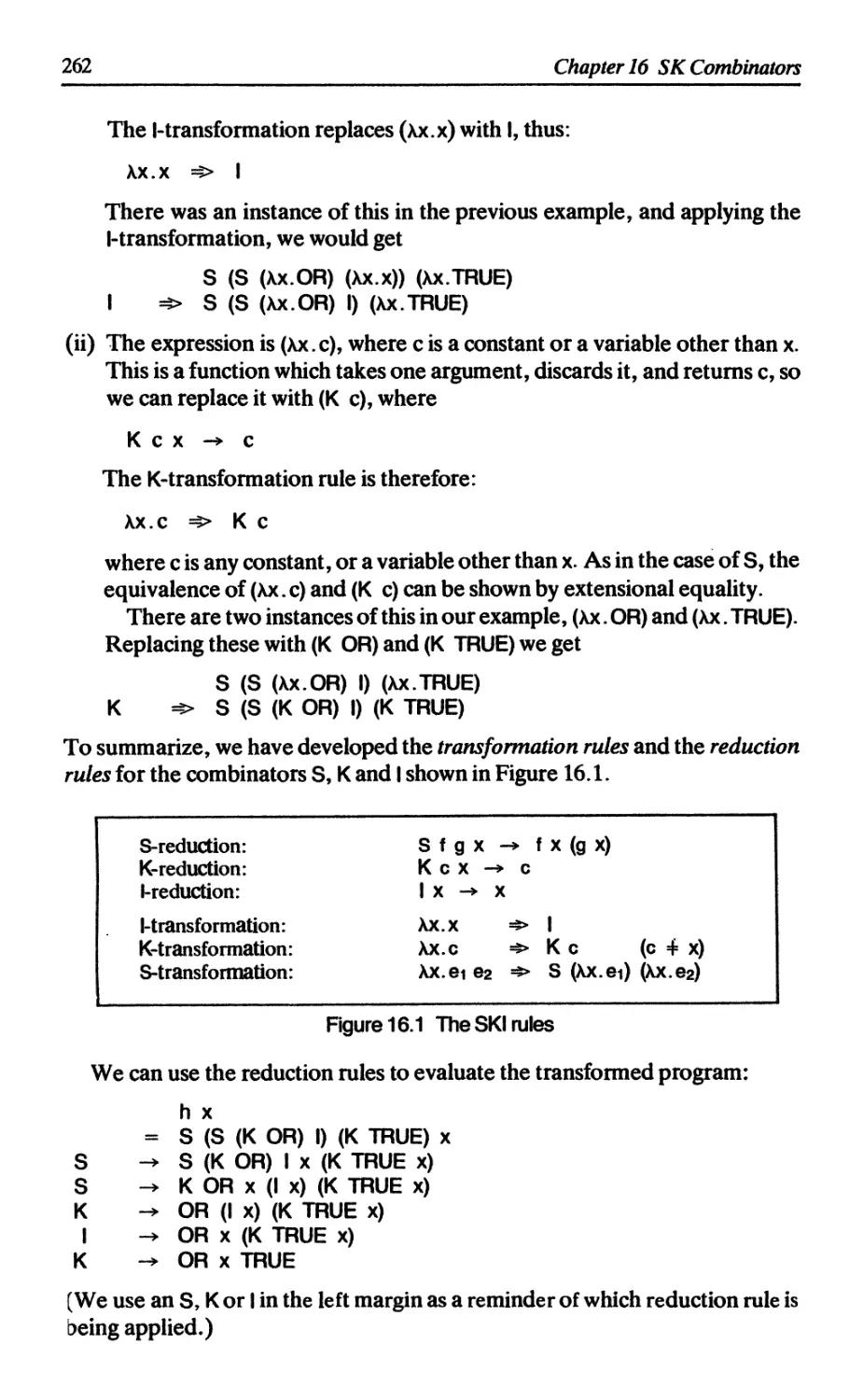
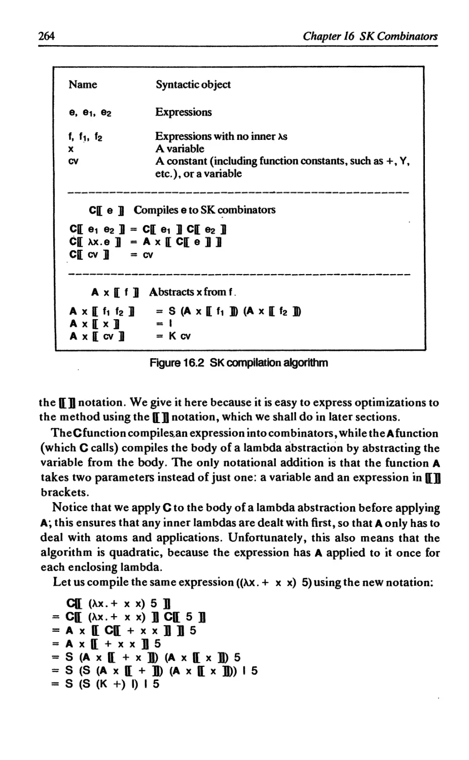
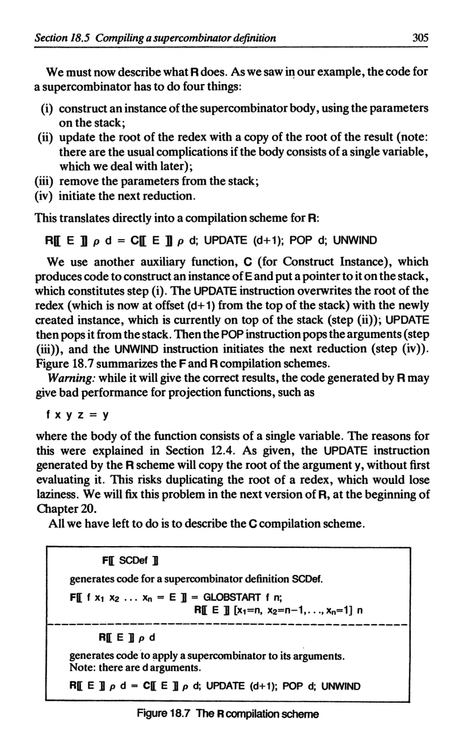
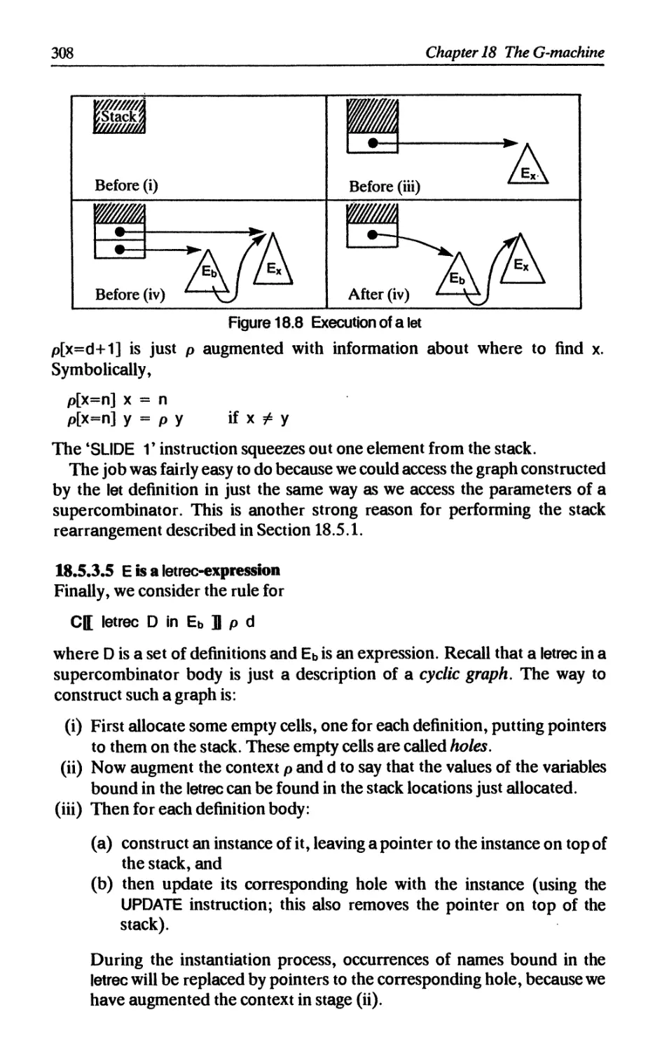
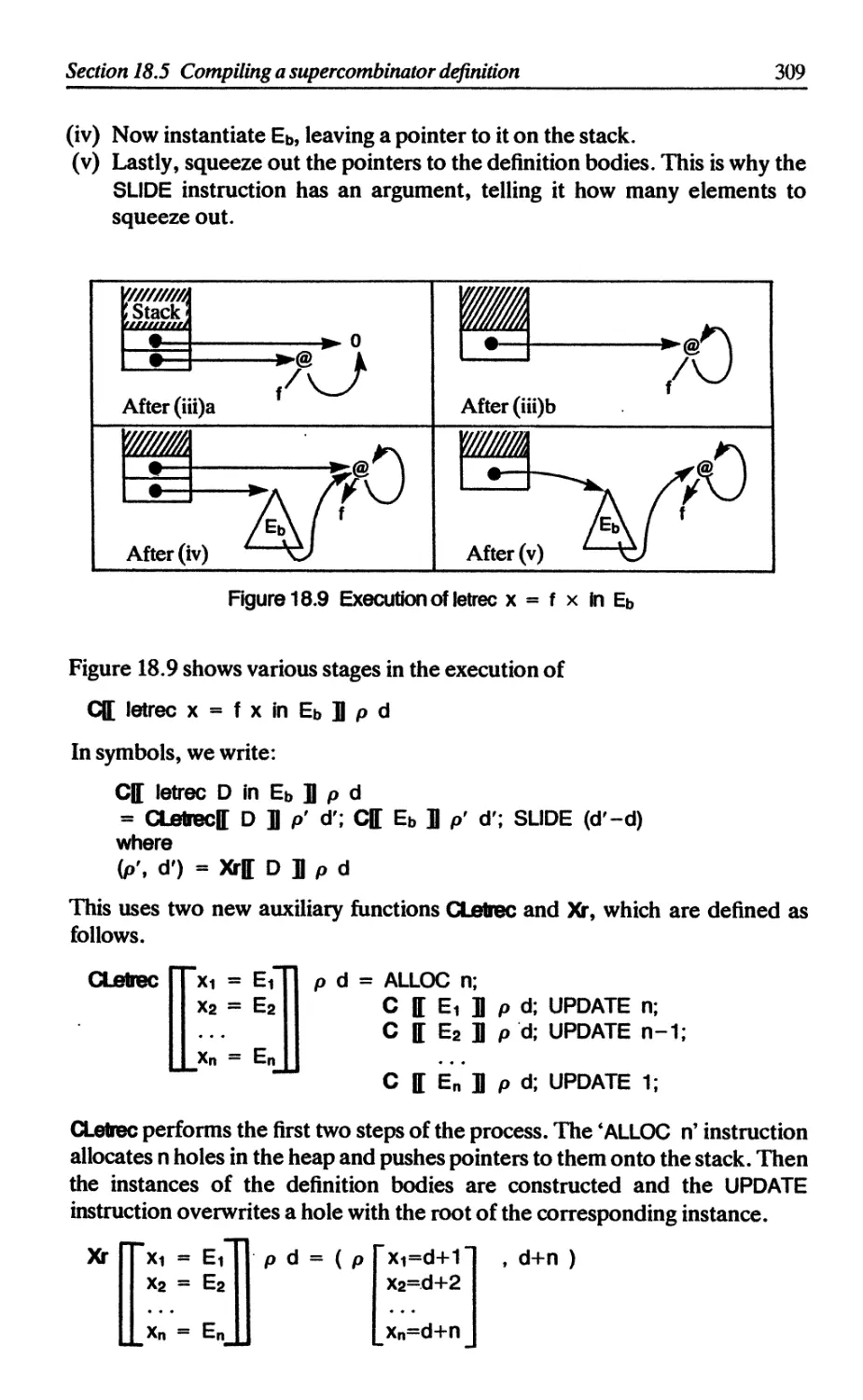
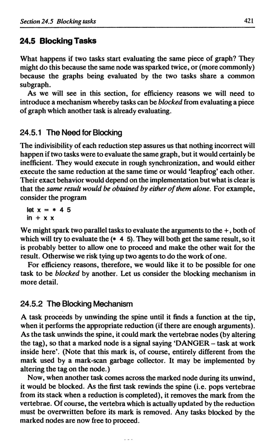
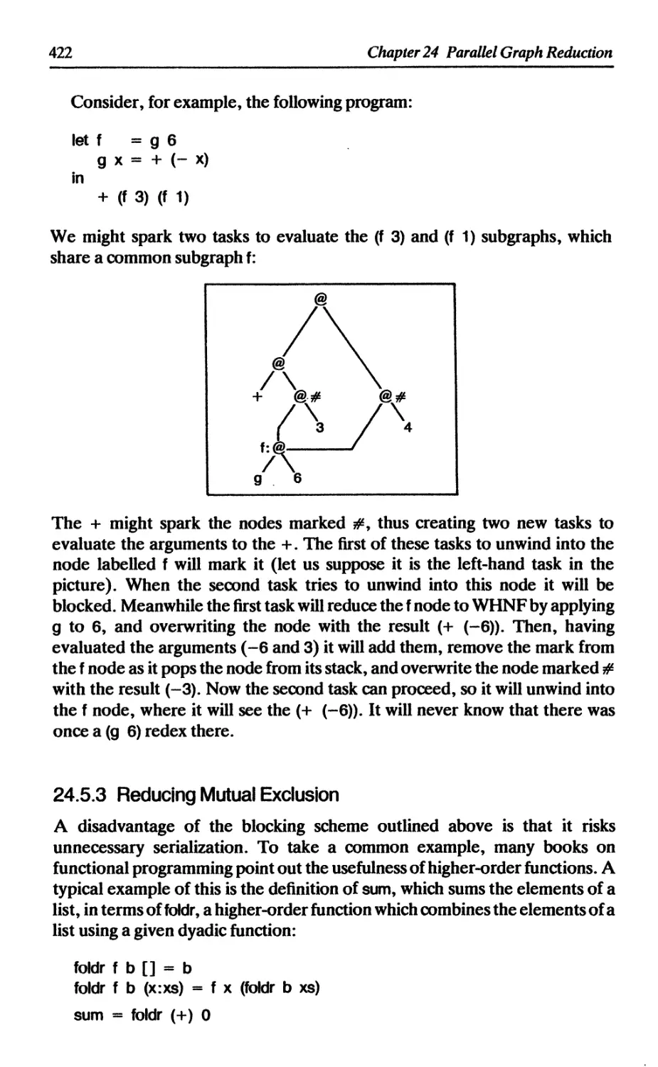
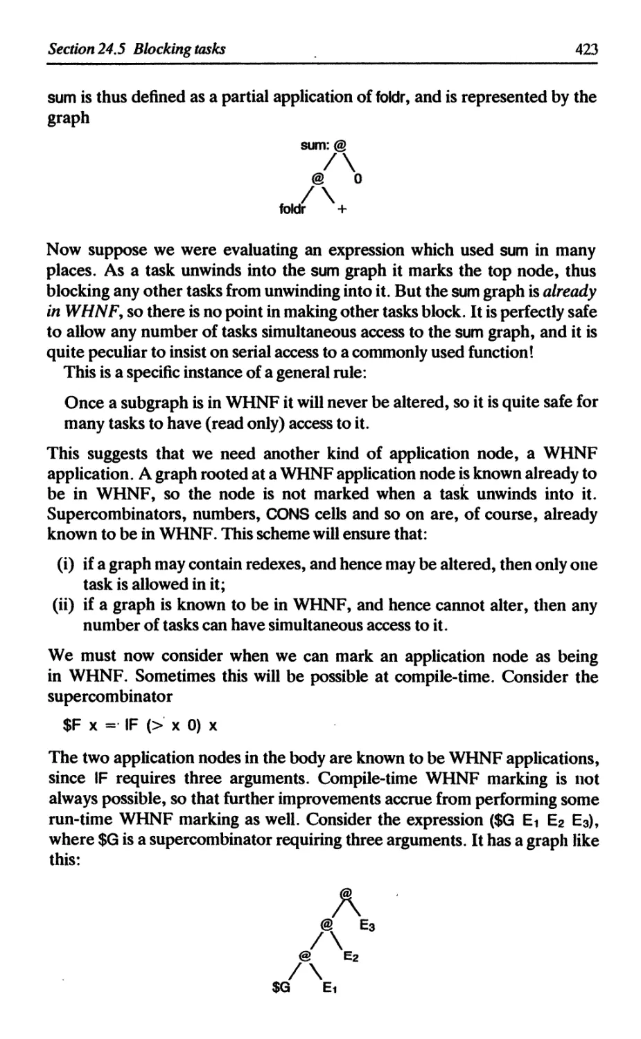
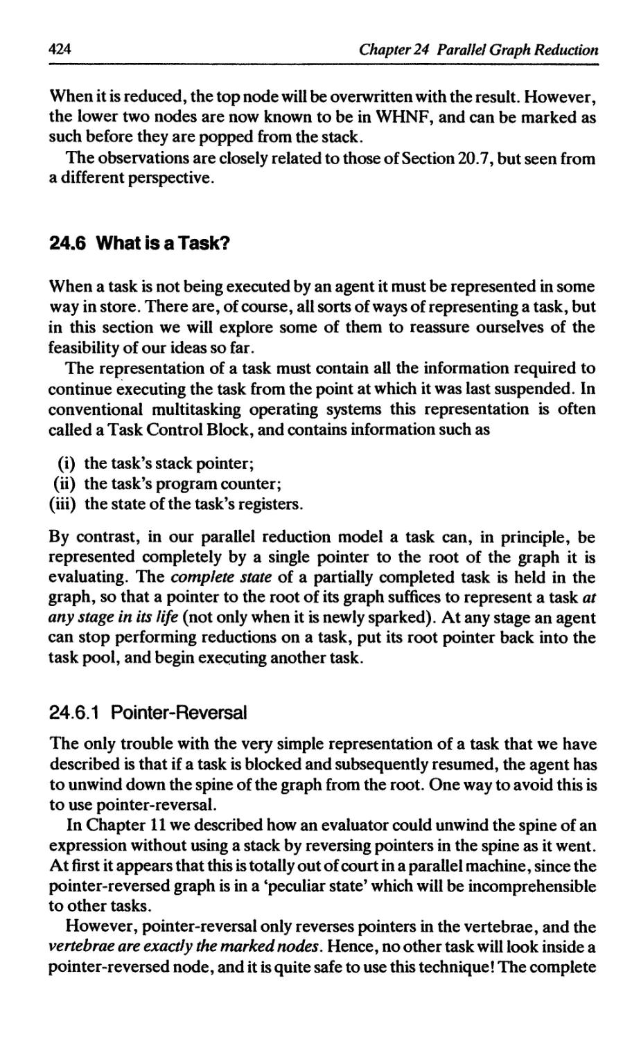
/


Text
Prentice-Hall International
Series in Computer Science
C.A.R. Hoare, Series Editor
BACKHOUSE, R.C., Program Construction and Verification
BACKHOUSE, R.C., Syntax of Programming Languages, Theory and Practice
de BAKKER, J.W., Mathematical Theory of Program Correctness
BJORNER, C, and JONES, C.B., Formal Specification and Software Development
BORNAT, R., Programming from First Principles
CLARK, K.L., and McCABE, F.G., micro-PRO LOG: Programming in Logic
DROMEY, R.G., How to Solve it by Computer
DUNCAN, F., Microprocessor Programming and Software Development
ELDER, J., Construction of Data Processing Software
GOLDSCHLAGER, L., and LISTER, A., Computer Science: A Modern Introduction
HAYES, L., (Editor), Specification Case Studies
HEHNER, E.C.R., The Logic of Programming
HENDERSON, P., Functional Programming: Application and Implementation
HOARE, C.A.R., and SHEPHERDSON, J.C., (Editors), Mathematical Logic and
Programming Languages
INMOS LTD, Occam Programming Manual
JACKSON, M.A., System Development
JOHNSTON, H., Learning to Program
JONES, C.B., Systematic Software Development Using VDM
JONES, G., Programming in Occam
JOSEPH, M., PRASAD, V.R., and NATARAJAN, N., Multiprocessor Operating System
LEW, A., Computer Science: A Mathematical Introduction
MacCALLUM, L, Pascal for the Apple
MacCALLUM, I., UCSD Pascal for the IBM PC
MARTIN, J.J., Data Types and Data Structures
PEYTON JONES, S.L., The Implementation of Functional Programming Languages
POMBERGER, G., Software Engineering and Modula-2
REYNOLDS, J.C., The Craft of Programming
SLOMAN, M., and KRAMER, J., Distributed Systems and Computer Networks
TENNENT, R.D., Principles of Programming Languages
WELSH, J., and ELDER, J., Introduction to Pascal, 2nd Edition
WELSH, J., ELDER, J., and BUSTARD, D., Sequential Program Structures
WELSH, J., and HAY, A., A Model Implementation of Standard Pascal
WELSH, J., and McKEAG, M., Structured System Programming
THE IMPLEMENTATION
OF FUNCTIONAL
PROGRAMMING LANGUAGES
Simon L. Peyton Jones
Department of Computer Science,
University College London
with chapters by
Philip Wadler, Programming Research Group, Oxford
Peter Hancock, Metier Management Systems Ltd
David Turner, University of Kent, Canterbury
PRENTICE HALL
NEW YORK LONDON TORONTO SYDNEY TOKYO
To Dorothy
First published 1987 by
Prentice Hall International (UK) Ltd,
Campus 400, Maylands Avenue, Hemel Hempstead,
Hertfordshire, HP27EZ
A division of
Simon & Schuster International Group
© 1987 Simon L. Peyton Jones (excluding Appendix)
Appendix © David A. Turner
All rights reserved. No part of this publication may be
reproduced, stored in a retrieval system, or transmitted, in any
form, or by any means, electronic, mechanical, photocopying,
recording or otherwise, without the prior permission, in writing,
from the publisher. For permission within the United States of
America contact Prentice Hall Inc., Englewood Cliffs, NJ07632.
Printed and bound in Great Britain by
BPC Wheatons Ltd, Exeter
Library of Congress Cataloging-in-Publication Data
Peyton Jones, Simon L., 1958-
The implementation of functional programming languages.
‘7th May 1986.’
Bibliography: p.
Includes index.
I. Functional programming languages. I. Title.
QA76.7.P495 1987 005.13'3 86-20535
ISBN 0-I3-453333-X
Britisb Library Cataloguing in Publication Data
Peyton Jones, Simon L.
The implementation of functional programming languages -
(Prentice Hall International series in computer science)
I. Electronic digital computers - Programming
I. Title II. Wadler, Philip III. Hancock, Peter
005.1 QA76.6
ISBNO-I3-453333-X
ISBN 0-13-453325-9 Pbk
6 7 8 9 10 98 97 96 95 94
ISBN 0-13-Ч53333-Х
ISBN 0-13-453325-4 PBK
CONTENTS
Preface xvii
1 INTRODUCTION 1
1.1 Assumptions 1
1.2 Part 1: compiling high-level functional languages 2
1.3 Part 11: graph reduction 4
1.4 Part 111: advanced graph reduction 5
References 6
PART I COMPILING HIGH-LEVEL FUNCTIONAL LANGUAGES
2 THE LAMBDA CALCULUS 9
2.1 The syntax of the lambda calculus 9
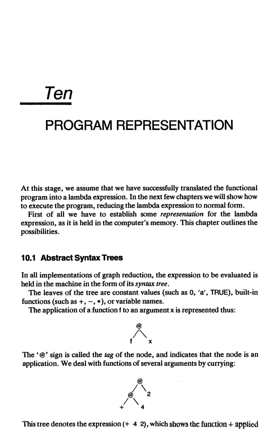
2.1.1 Function application and currying 10
2.1.2 Vse of brackets 11
2.1.3 ^uilbin functions and constants 11
2.1.4 Lambda abstractions 12
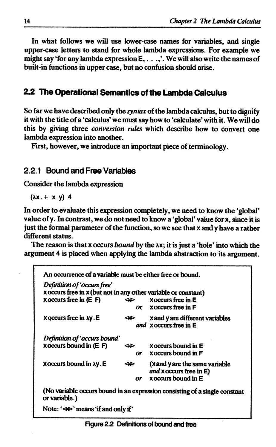
2.1.5 Summary 13
2.2 The operational semantics of the lambda calculus 14
2.2.1 Bound and free variables 14
2.2.2 Beta-conversion 15
2.2.3 Alpha-conversion 18
2.2.4 Eta-conversion 19
2.2.5 Proving interconvertibility 19
2.2.6 The name-capture problem 20
2.2.7 Summary of conversion rules 21
2.3 Reduction order 23
2.3.1 Normal order reduction 24
2.3.2 Optimal reduction orders 25
2.4 Recursive functions 25
2.4.1 Recursive functions and Y 26
2.4.2 Yean be defined as a lambda abstraction 27
vi
Contents
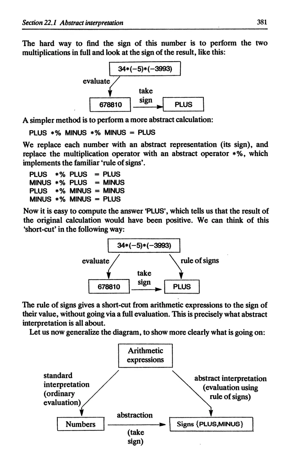
2.5 The denotational semantics of the lambda calculus 28
2.5.1 The Eval function 29
2.5.2 The symbol 1 31
2.5.3 Defining the semantics of built-in functions and constants 31
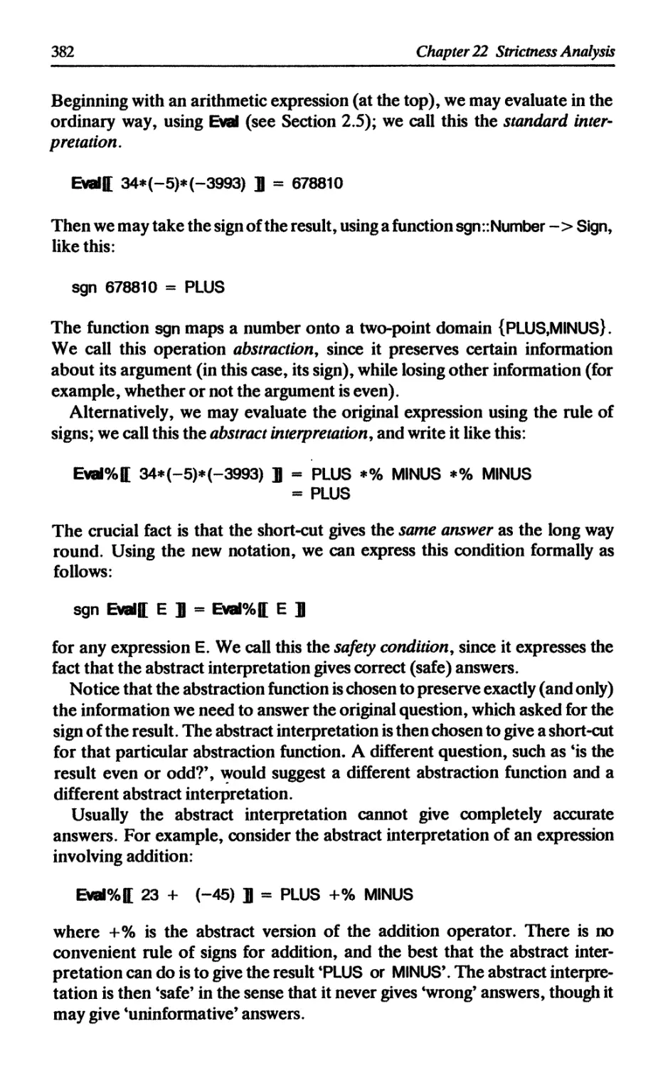
2.5.4 Strictness and laziness 33
2.5.5 The correctness of the conversion rules 34
2.5.6 Equality and convertibility 34
2.6 Summary 35
References 35
3 TRANSLATING A HIGH-LEVEL FUNCTIONAL LANGUAGE
INTO THE LAMBDA CALCULUS 37
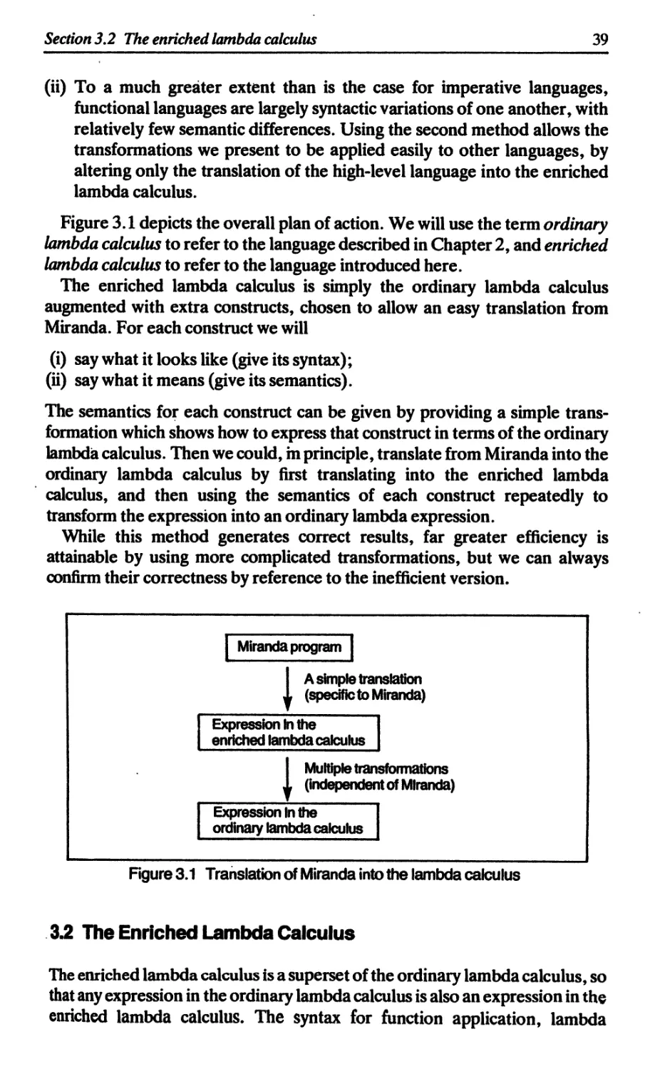
3.1 The overall structure of the translation process 38
3.2 The enriched lambda calculus 39
3.2.1 Simple let-expressions 40
3.2.2 Simple letrec-expressions 42
3.2.3 Pattern-matching let- and letrec-expressions 43
3.2.4 Let(rec)s versus lambda abstractions 43
3.3 Translating Miranda into the enriched lambda calculus 44
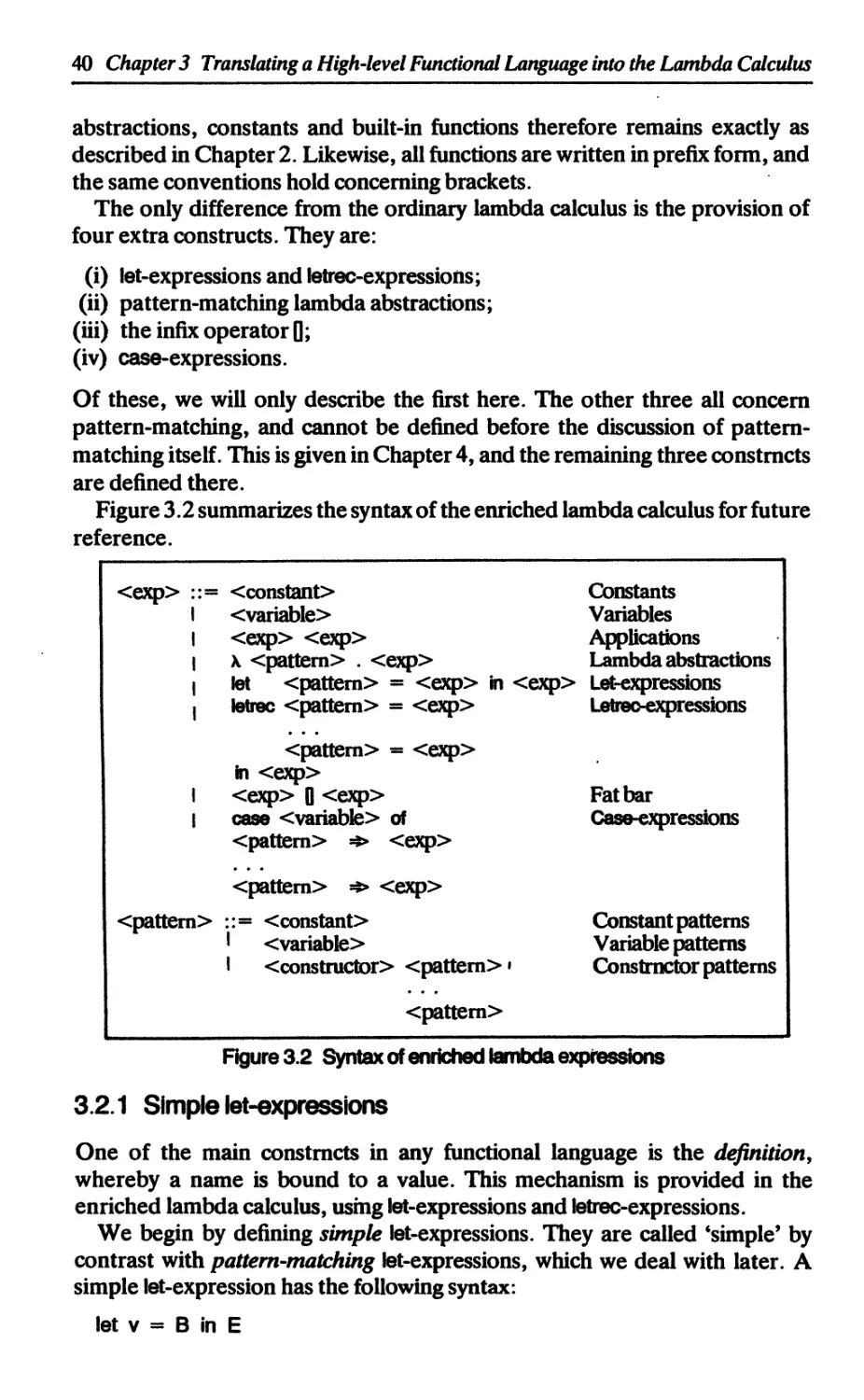
3.4 The ТЕ translation scheme 45
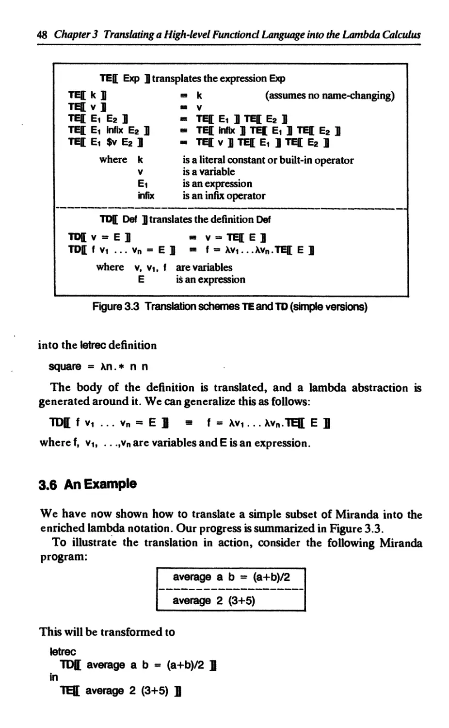
3.4.1 Translating constants 46
3.4.2 Translating variables 46
3.4.3 Translating function applications 46
3.4.4 Translating other forms of expressions 47
3.5 The TO translation scheme 47
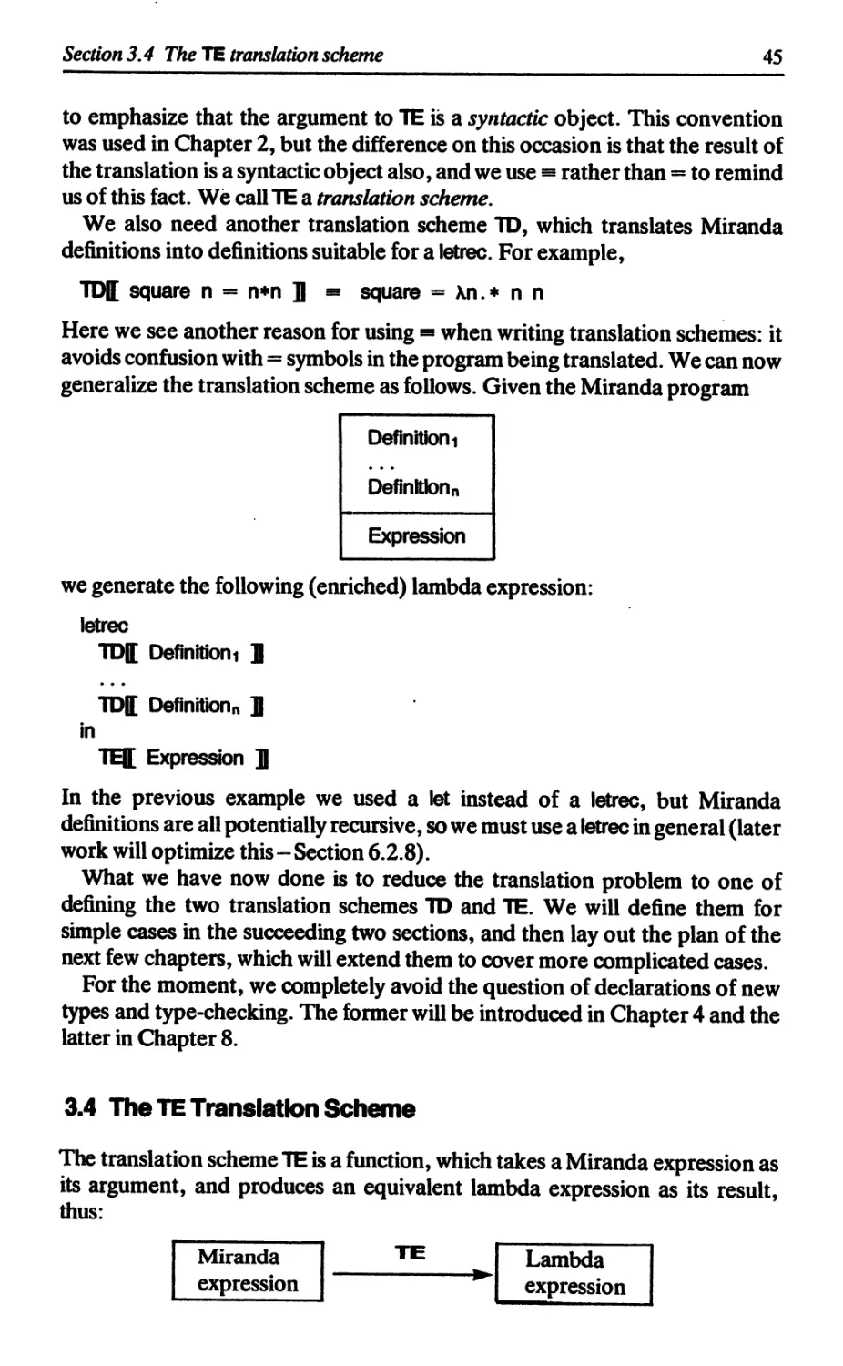
3.5.1 Variable definitions 47
3.5.2 Simple function definitions 47
3.6 An example 48
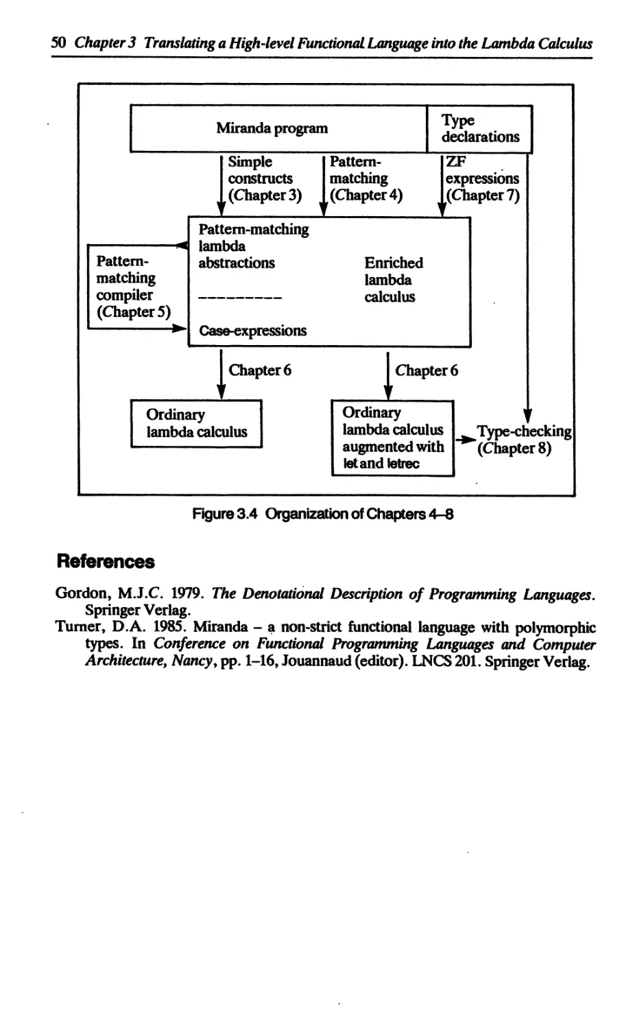
3.7 The organization of Chapters 4-9 49
References 50
4 STRUCTURED TYPES AND THE SEMANTICS OP
PATTERN-MATCHING Simon L Peyton Jones and Philip Wadler 51
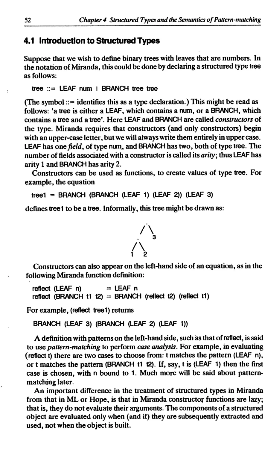
4.1 Introduction to structured types 52
4.1.1 Type variables 53
4.1.2 Special cases 53
4.1.3 General structured types 55
4.1.4 History 56
4.2 Translating Miranda into the enriched lambda calculus 57
4.2.1 Introduction to pattern-matching 57
4.2.2 Patterns 59
4.2.3 Introducing pattern-matching lambda abstractions 60
4.2.4 Multiple equations and failure 61
4.2.5 Multiple argnments 62
Contents
vii
4.2.6 Conditional equations 63
4.2.7 Repeated variables 65
4.2.8 Where-dauses 66
4.2.9 Patterns on the left-hand side of definitions 67
4.2.10 Summary 67
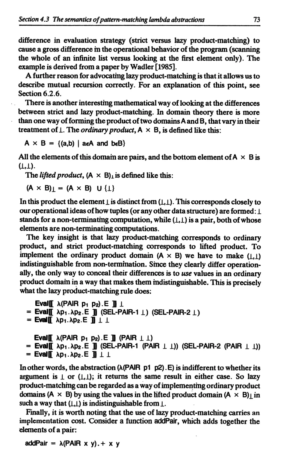
4.3 The semantics of pattern-matching lambda abstractions 67
4.3.1 The semantics of variable patterns 68
4.3.2 The semantics of constant patterns 69
4.3.3 The semantics of sum-constructor patterns 69
4.3.4 The semantics of product-constructor patterns 70
4.3.5 A defence of lazy product-matching 72
4.3.6 Summary 74
4.4 Introducing case-expressions 74
4.5 Summary 76
References 77
5 EFFICIENT COMPILATION OF PATTERN-MATCHING
Philip Wadler 78
5.1 Introduction and examples 78
5.2 The pattern-matching compiler algorithm 81
5.2.1 The function match 81
5.2.2 The variable rule 83
5.2.3 The constructor rule 84
5.2.4 The empty rule 87
5.2.5 An example 88
5.2.6 The mixture rule 88
5.2.7 Completeness 90
5.3 The pattern-matching compiler in Miranda 90
5.3.1 Patterns 90
5.3.2 Expressions 91
5.3.3 Equations 92
5.3.4 Variable names 92
5.3.5 The functions partition and fbldr 92
5.3.6 The function match 93
5.4 Optimizations 94
5.4.1 Case-expressions with default clauses 94
5.4.2 Optimizing expressions containing Q and FAIL 96
5.5 Uniform definitions 98
References 103
5 TRANSFORMING THE ENRICHED LAMBDA CALCULUS 104
6.1 Transforming pattern-matching lambda abstractions 104
6.1.1 Constant patterns 104
6.1.2 Product-constructor patterns 105
6.1.3 Sum-constructor patterns 106
viii
Contents
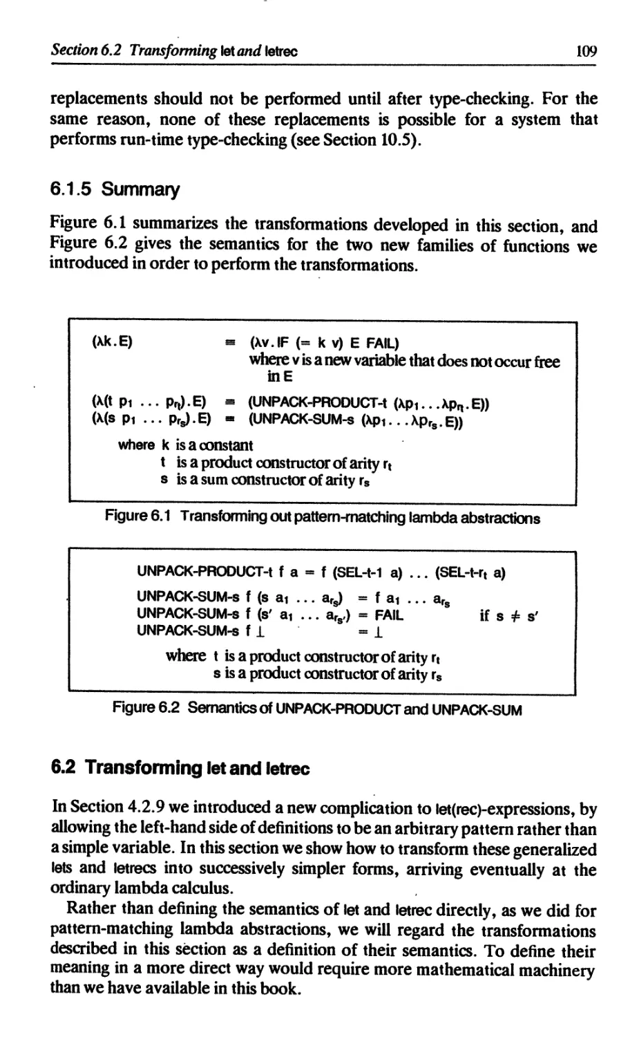
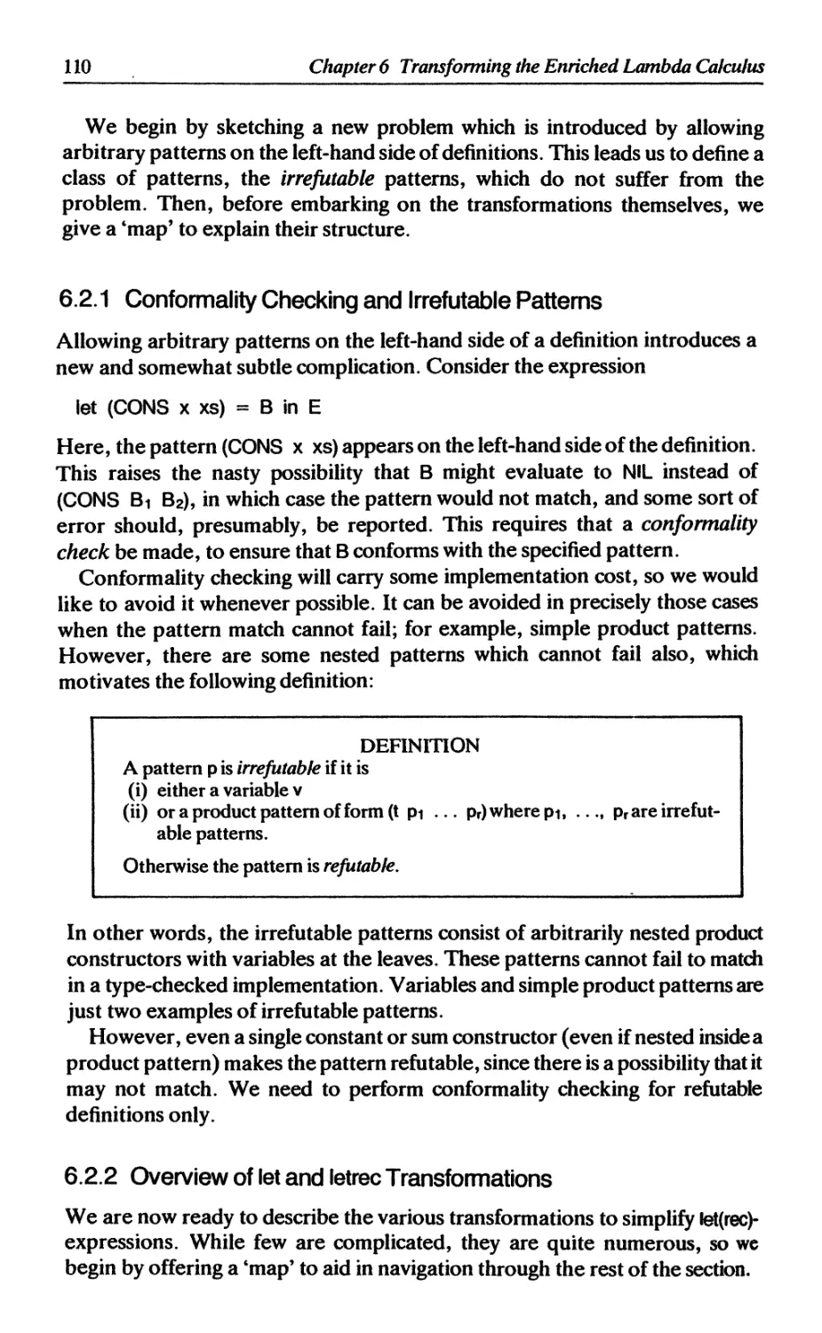
6.1.4 6.1.5 Reducing the number of built-in functions Summary 107 109
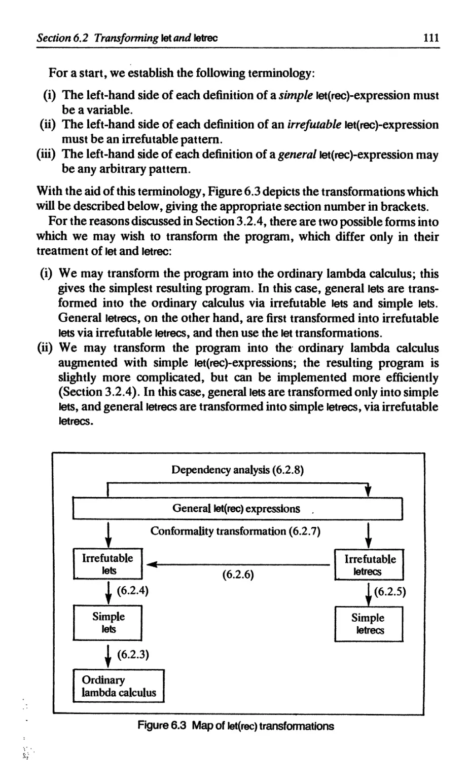
6.2 Transforming let and letrec 109
6.2.1 Conformality checking and irrefutable patterns 110
6.2.2 Overview of let and letrec transformations 110
6.2.3 Transforming simple lets into the ordinary lambda calculus 112
6.2.4 Transforming irrefutable lets into simple lets 112
6.2.5 Transforming irrefutable letrecs into simple letrecs 113
6.2.6 Transforming irrefutable letrecs into irrefutable lets 114
6.2.7 Transforming general let(rec)s into irrefutable let(rec)s 115
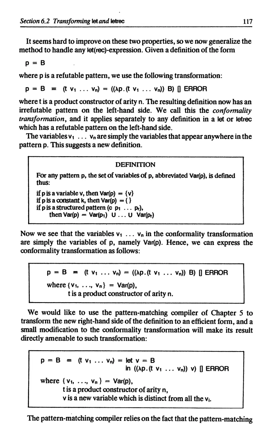
6.2.8 Dependency analysis 118
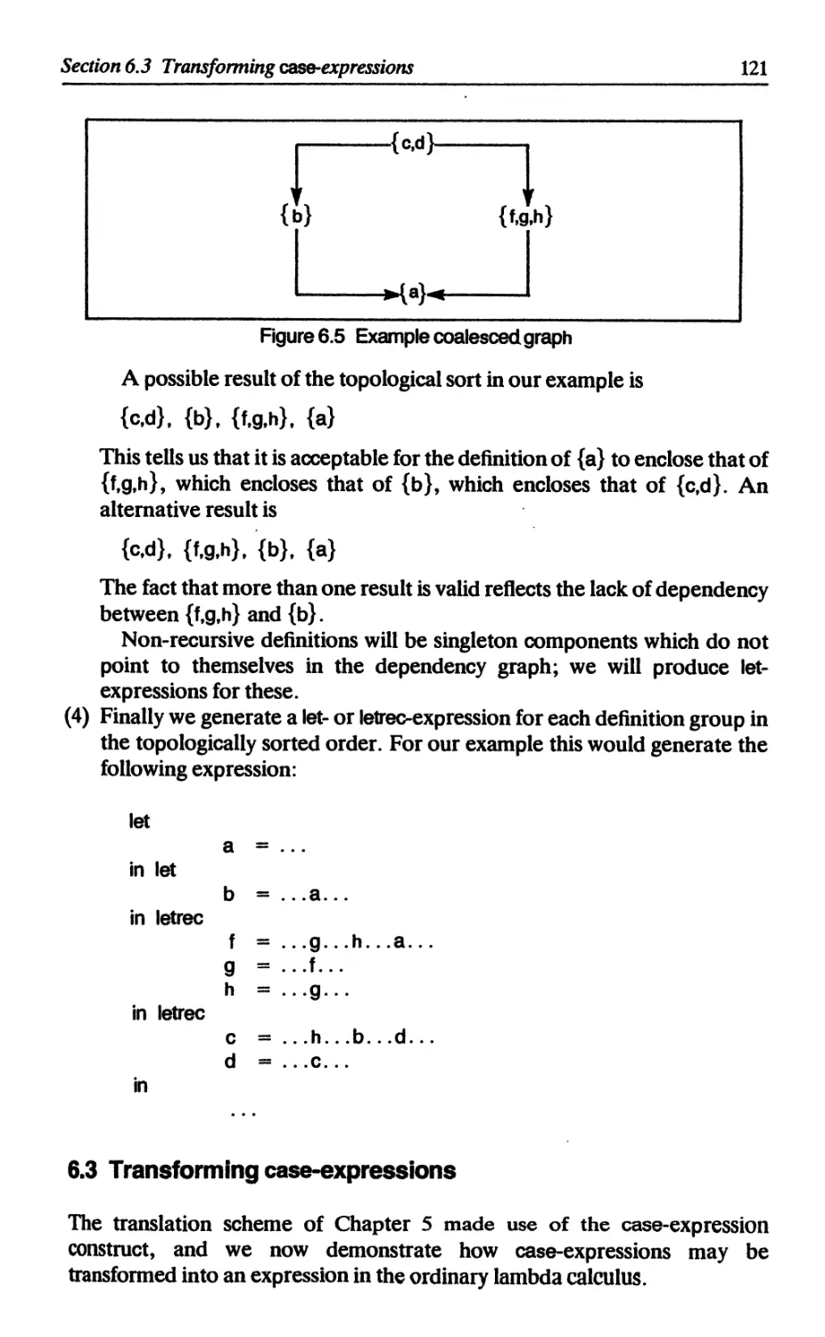
6.3 Transforming case-expressions 121
6.3.1 Case-expressions involving a product type 122
6.3.2 Case-expressions involving a sum type 122
6.3.3 Using a let-expression instead of UNPACK 123
6.3.4 Reducing the number of built-in functions 124
6.4 The П operator and FAIL 125
6.5 Summary 126
References 126
7 LIST COMPREHENSIONS Philip Wadler 127
7.1 Introduction to list comprehensions 127
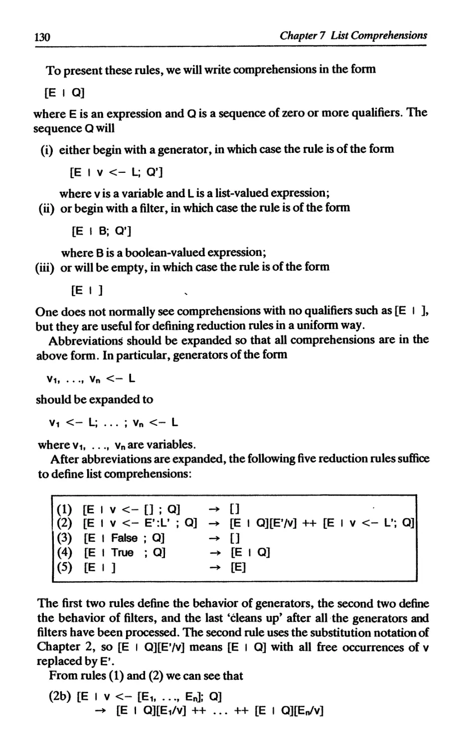
7.2 Reduction rules for list comprehensions 129
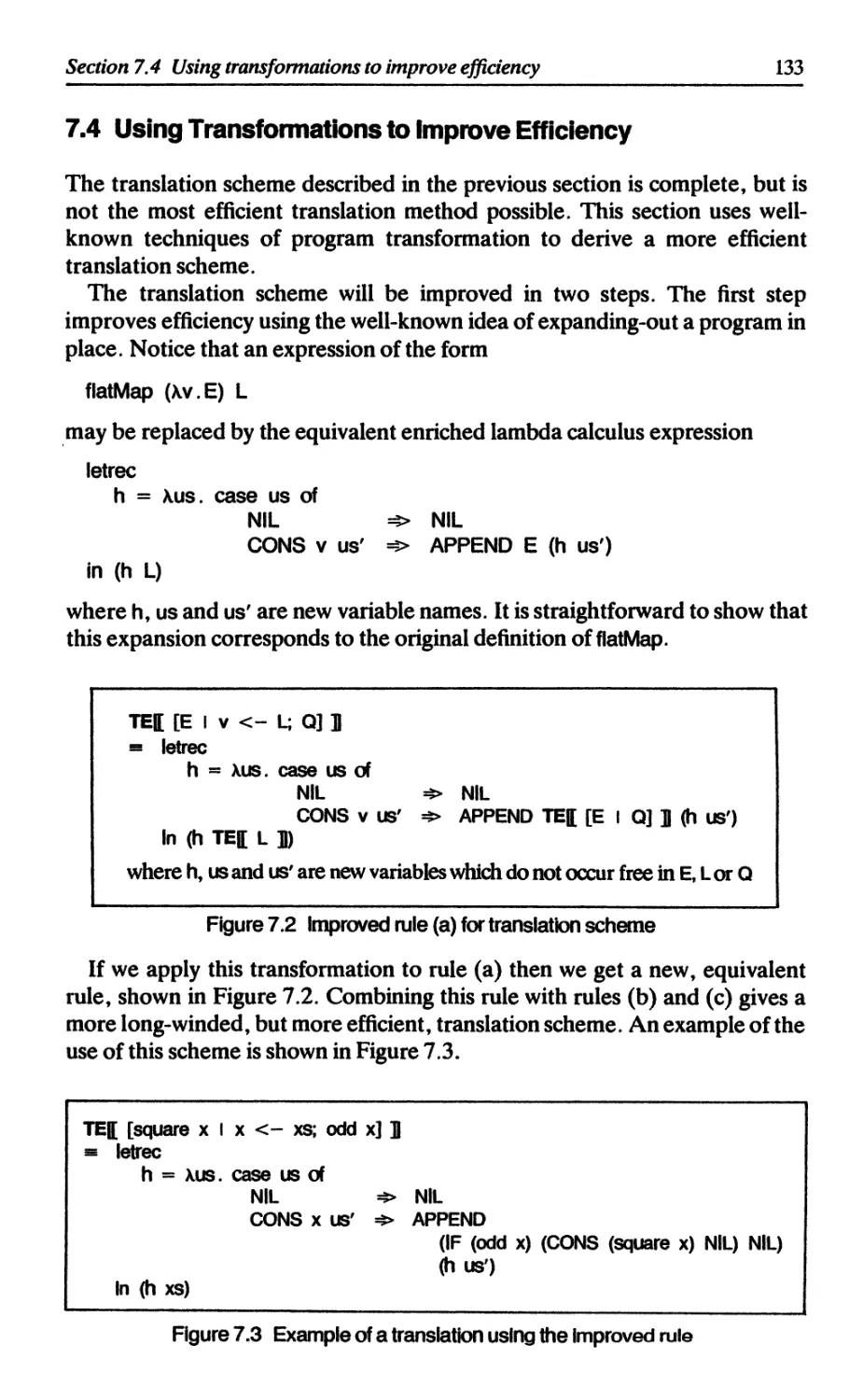
7.3 Translating list comprehensions 132
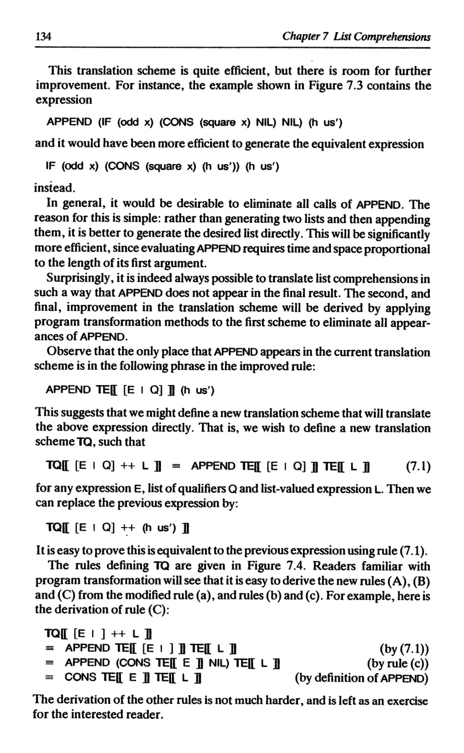
7.4 Using transformations to improve efficiency 133
7.5 Pattern-matching in comprehensions 136
Reference 138
8 POLYMORPHIC TYPE-CHECKING Peter Hancock 139
8.1 Informal notation for types 140
8.1.1 Tuples 140
8.1.2 Lists 141
8.1.3 Structured types 141
8.1.4 Functions 142
8.2 Polymorphism 143
8.2.1 The identity function 143
8.2.2 The length function 144
8.2.3 The composition function 145
8.2.4 The function foldr 146
8.2.5 What polymorphism means 147
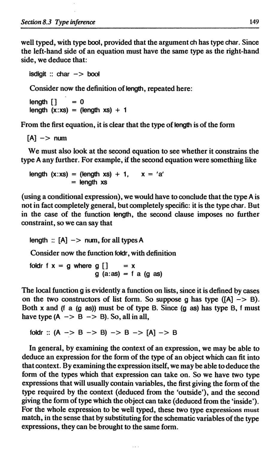
8.3 Type inference 148
8.4 The intermediate language 150
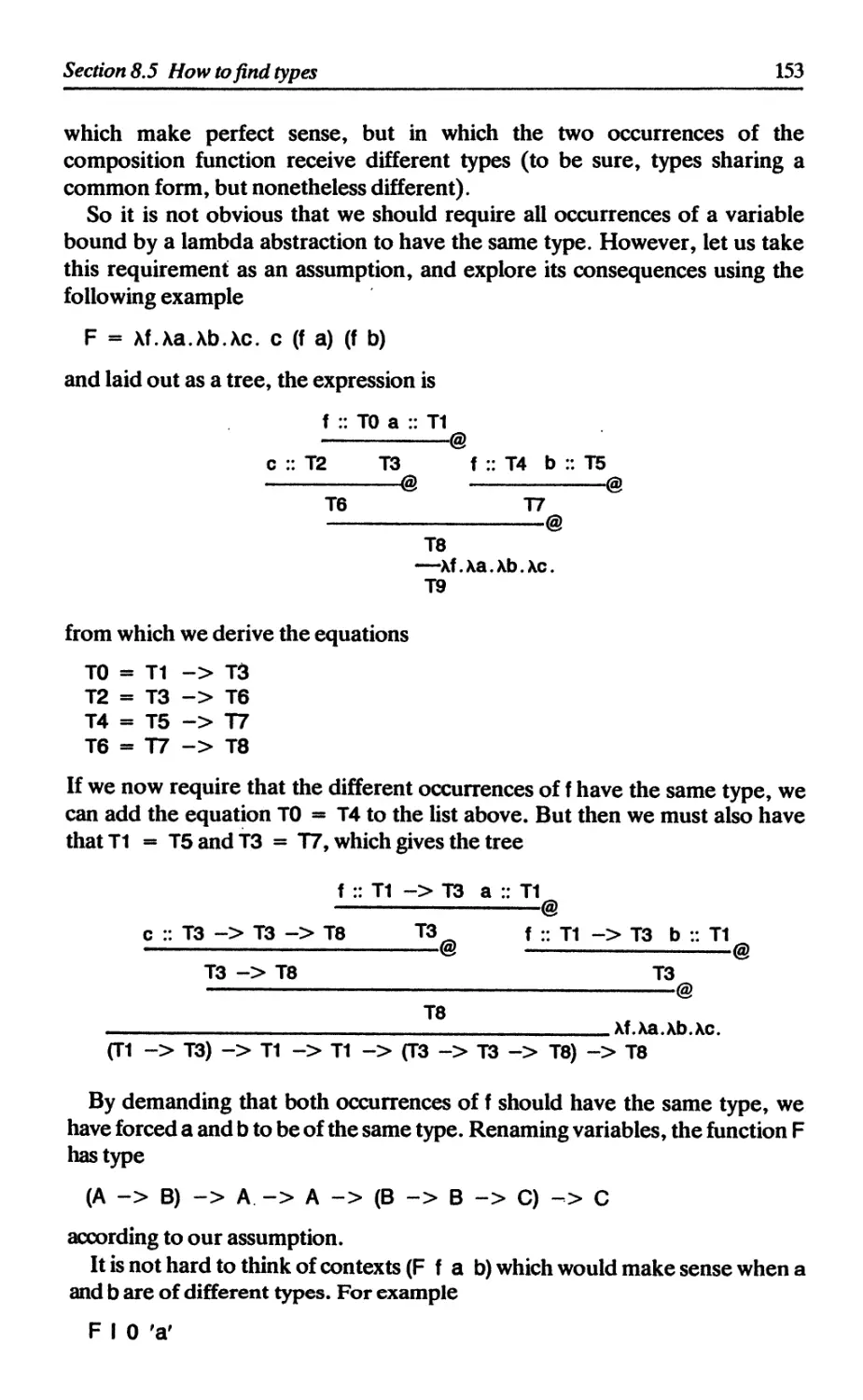
8.5 How to find types 151
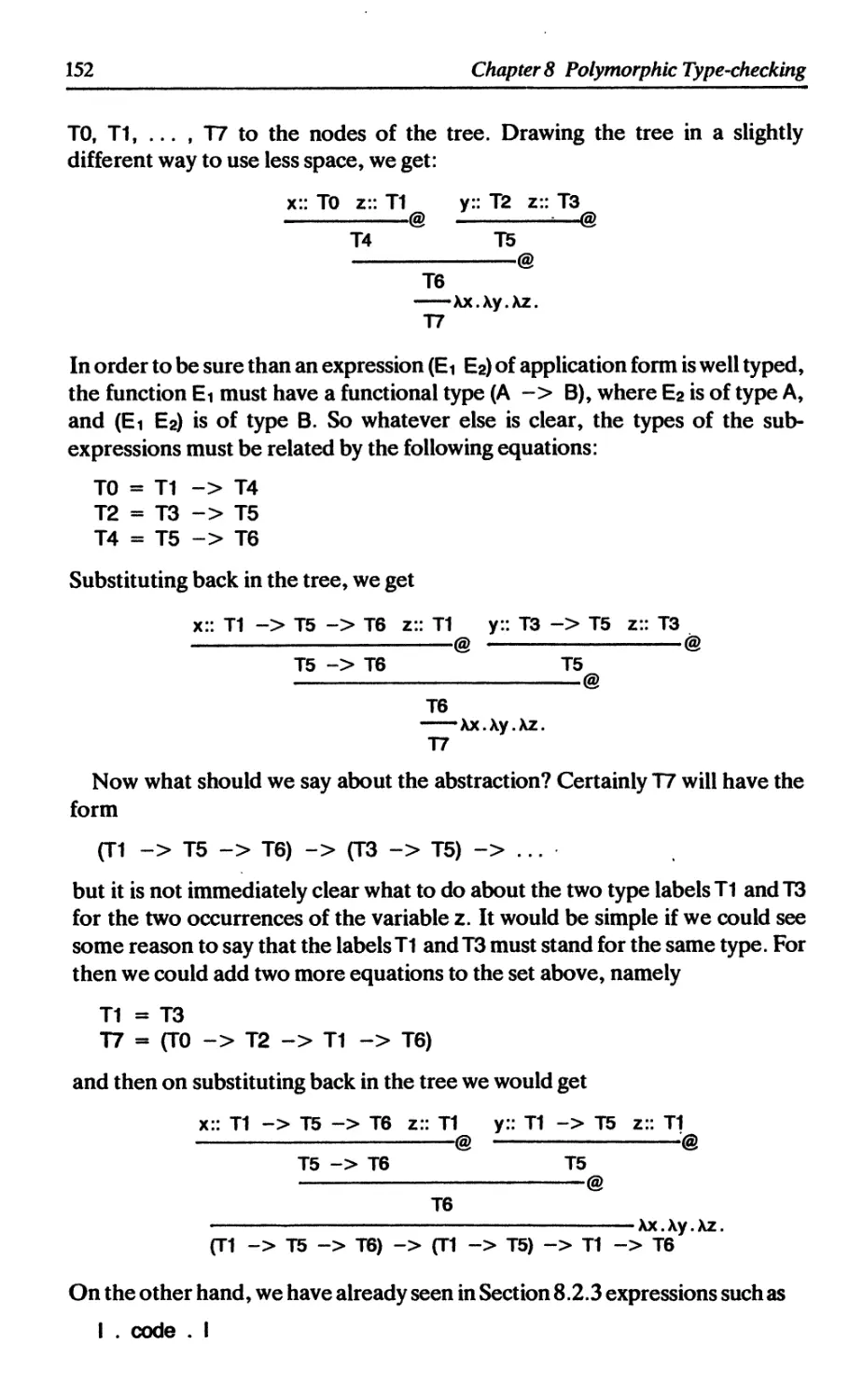
8.5.1 Simple cases, and lambda abstractions 151
8.5.2 A mistyping 154
8.5.3 Top-level lets 155
Contents
ix
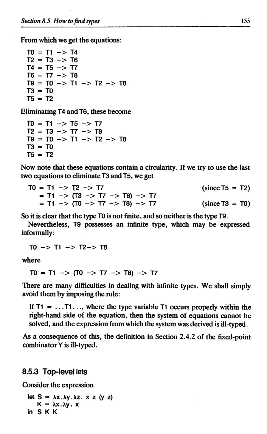
8.5.4 Top-level letrecs 157
8.5.5 Local definitions 159
8.6 Summary of rules for correct typing 160
8.6.1 Rule for applications 160
8.6.2 Rule for lambda abstractions 160
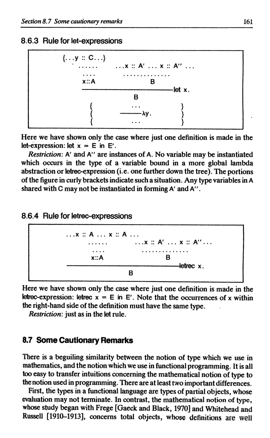
8.6.3 Rule for let-expressions 161
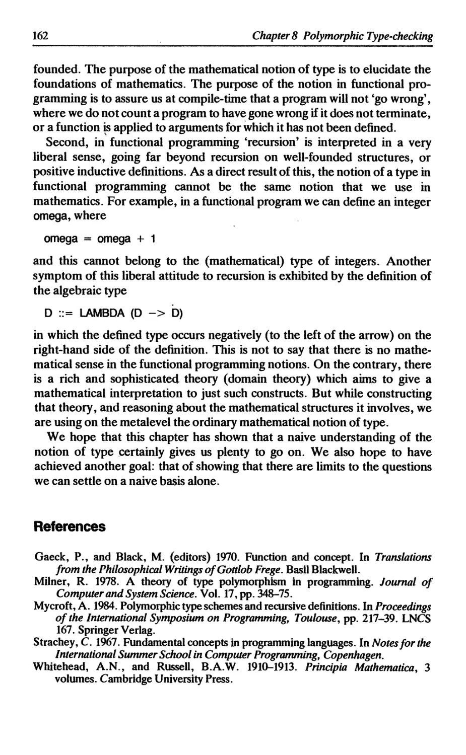
8.6.4 Rule for letreo-expressions 161
8.7 Some cautionary remarks 161
References 162
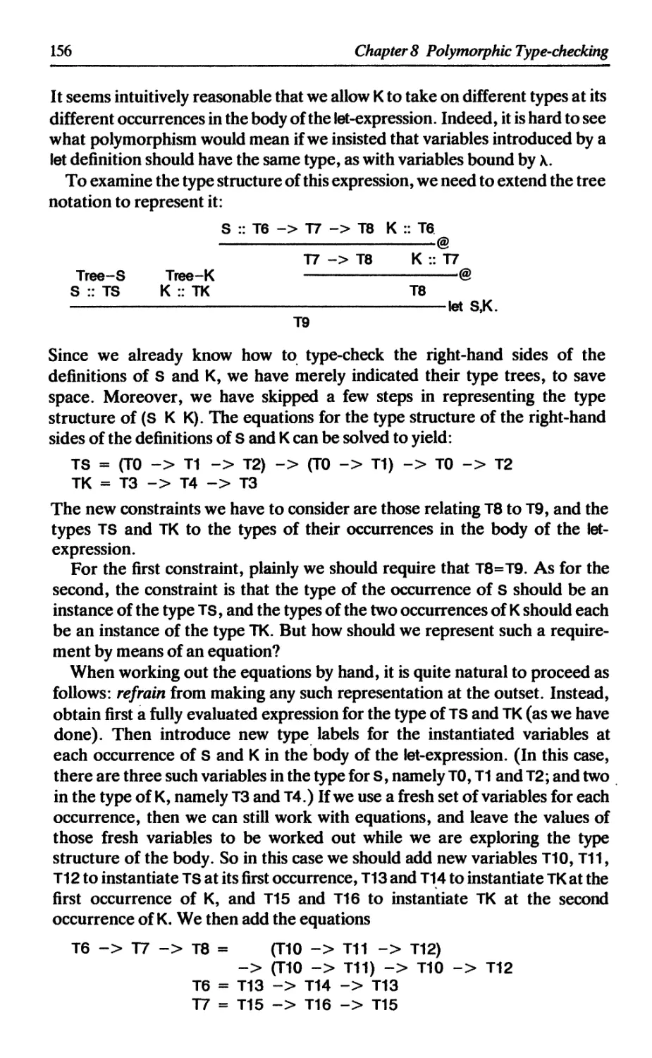
9 A TYPE-CHECKER Peter Hancock 163
9.1 Representation of programs 163
9.2 Representation of type expressions 164
9.3 Success and failure 165
9.4 Solving equations 166
9.4.1 Substitutions 166
9.4.2 Unification 168
9.5 Keeping track of types 171
9.5.1 Method 1: look to the occurrences 171
9.5.2 Method 2: look to the variables 171
9.5.3 Association lists 173
9.6 New variables 175
9.7 The type-checker 176
9.7.1 Type-checking lists of expressions 177
9.7.2 Type-checking variables 177
9.7.3 Type-checking application 178
9.7.4 Type-checking lambda abstractions 179
9.7.5 Type-checking let-expressions 179
9.7.6 Type-checking letreo-expressions 180
References 182
PART II GRAPH REDUCTION
10 PROGRAM REPRESENTATION 185
10.1 Abstract syntax trees 185
10.2 The graph 186
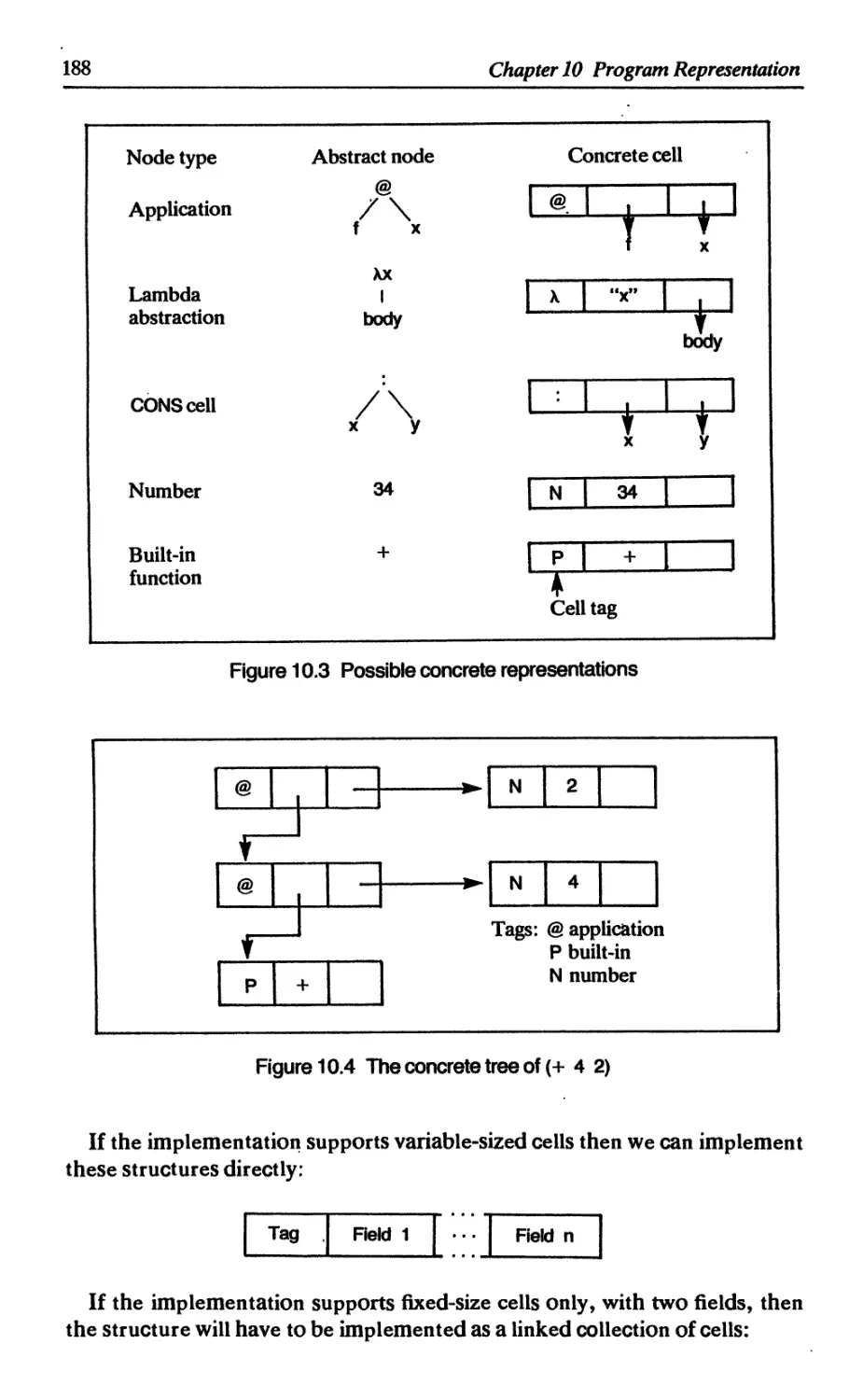
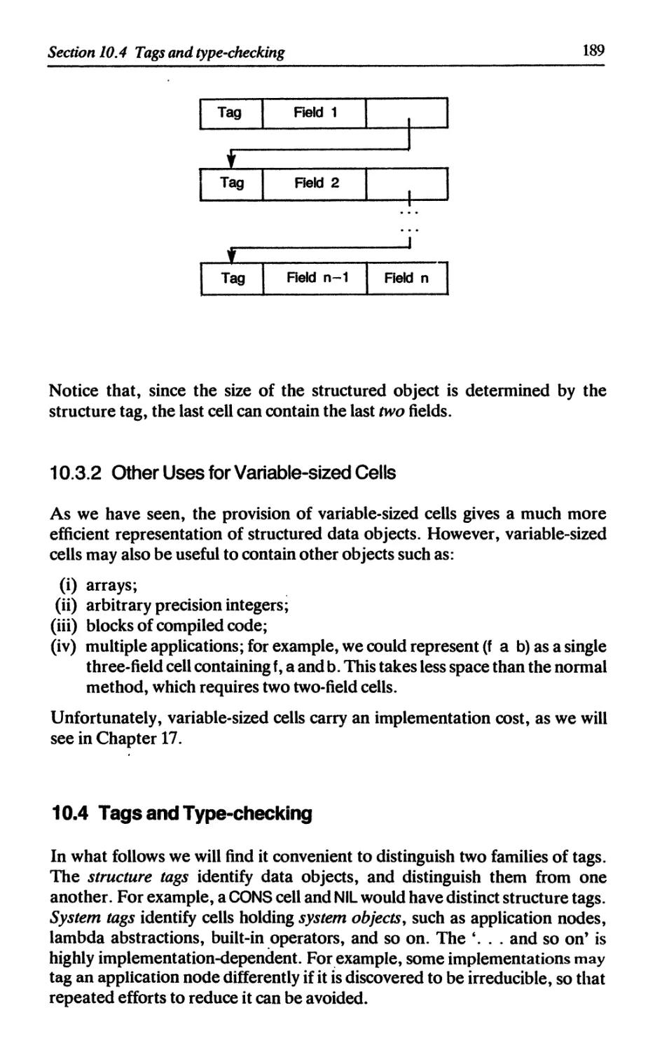
10.3 Concrete representations of the graph 187
10.3.1 Representing structured data 187
10.3.2 Other uses for variable-sized cells 189
10.4 Tags and type-checking 189
10.5 Compile-time versus run-time typing 190
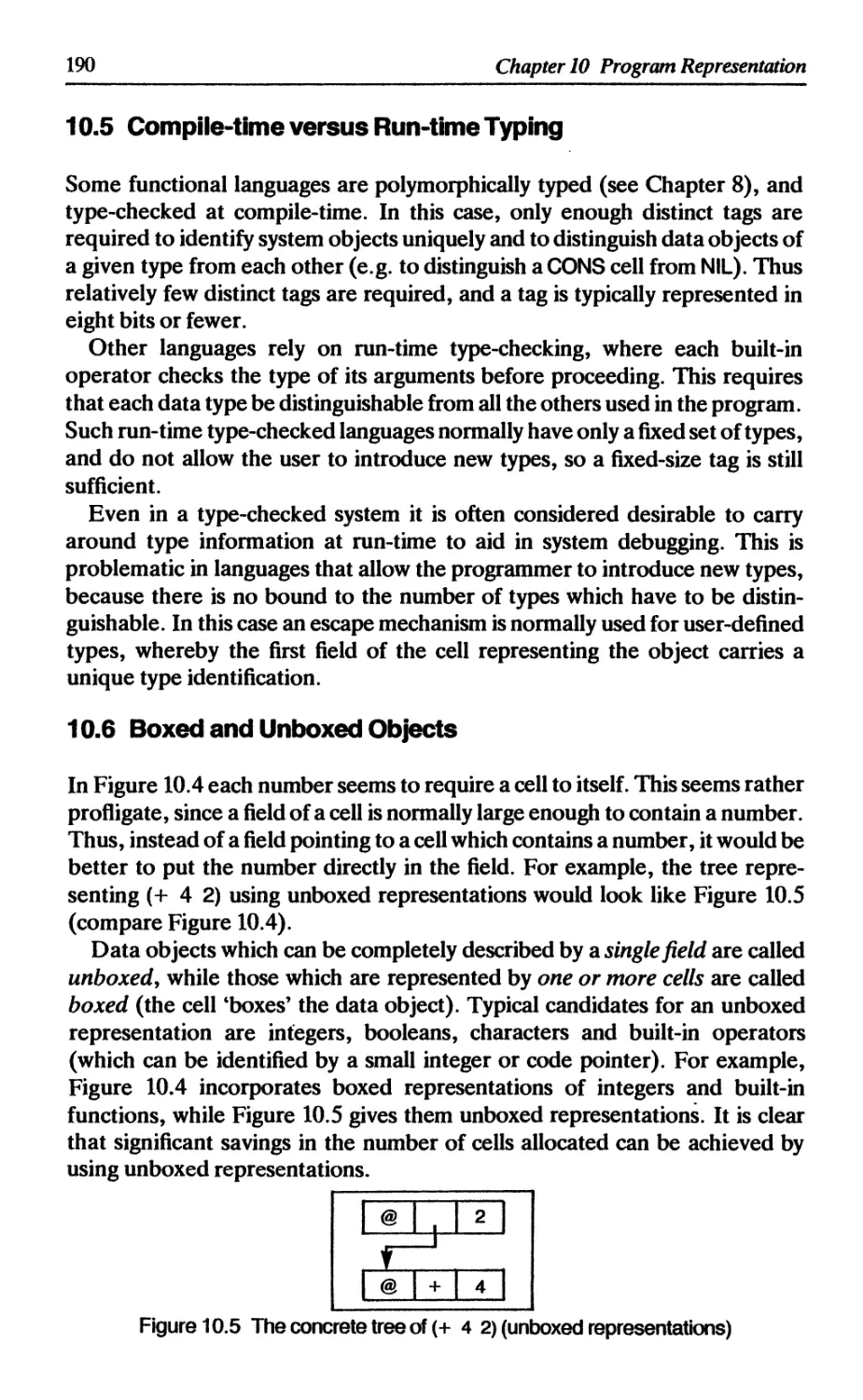
10.6 Boxed and unboxed objects 190
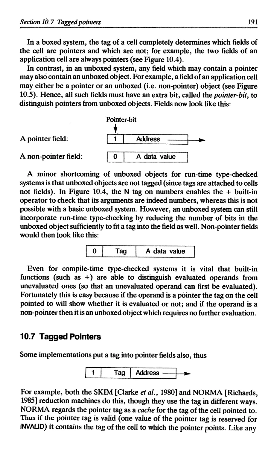
10.7 Tagged pointers 191
10.8 Storage management and the need for garbage collection 192
References 192
X
Contents
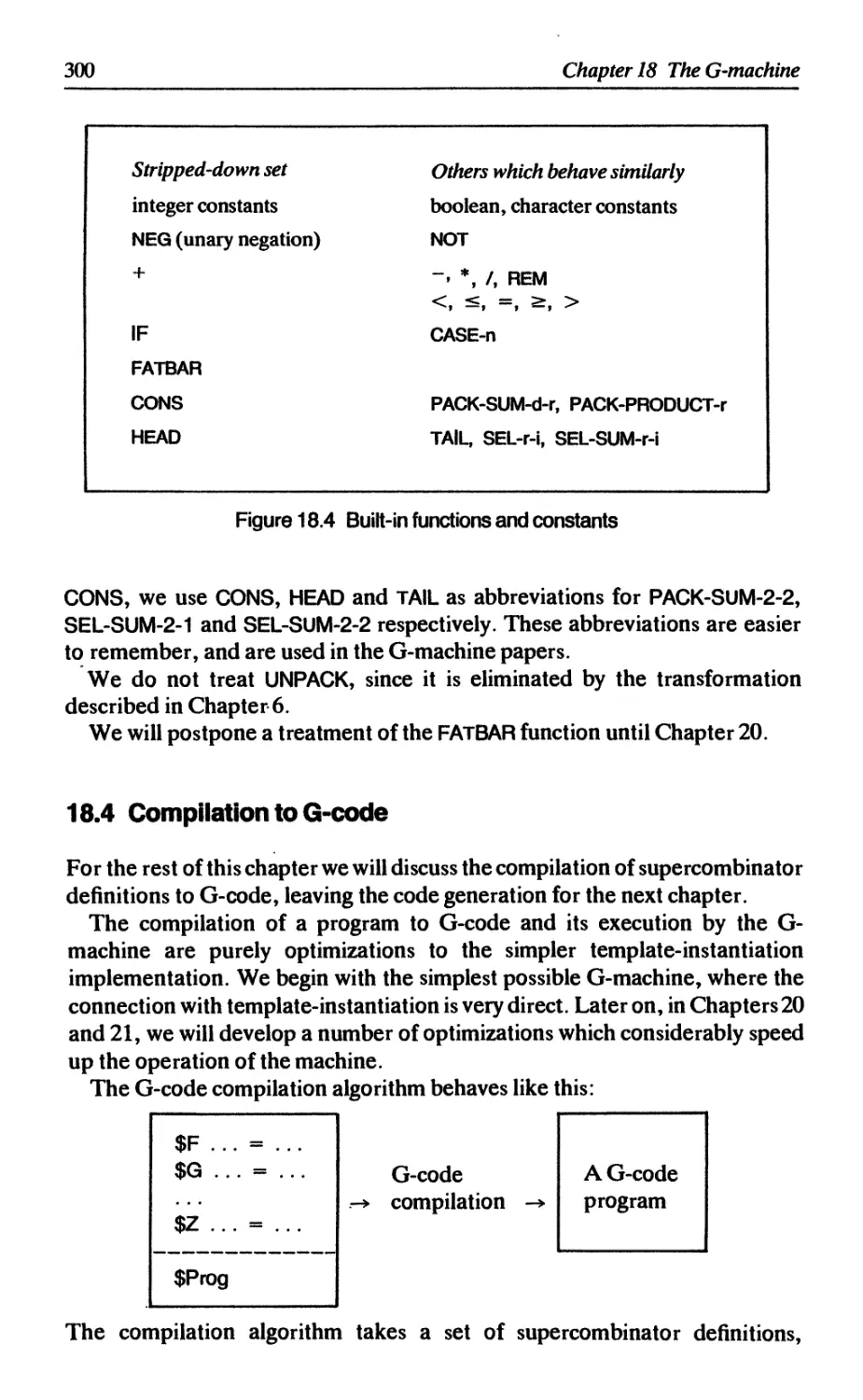
11 SELECTING THE NEXT REDEX 193
11.1 Lazy evaluation 193
11.1.1 The case for lazy evaluation 194
11.1.2 The case against lazy evaluation 194
11.1.3 Normal order reduction 194
11.1.4 Summary 195
11.2 Data constructors, input and output 195
11.2.1 The printing mechanism 196
11.2.2 The input mechanism 197
11.3 Normal forms 197
11.3.1 Weak head normal form 198
11.3.2 Top-level reduction is easier 199
11.3.3 Head normal form 199
11.4 Evaluating arguments of built-in functions 200
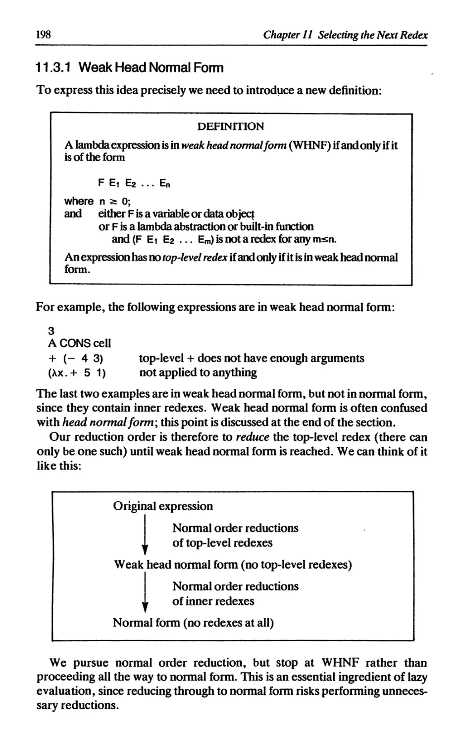
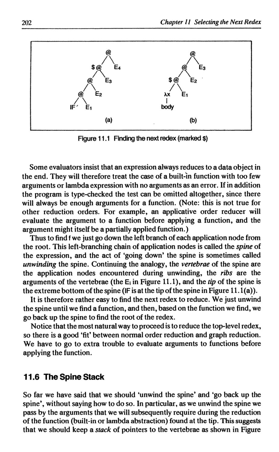
11.5 How to find the next top-level redex 201
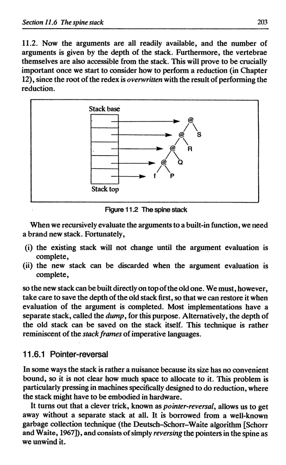
11.6 The spine stack 202
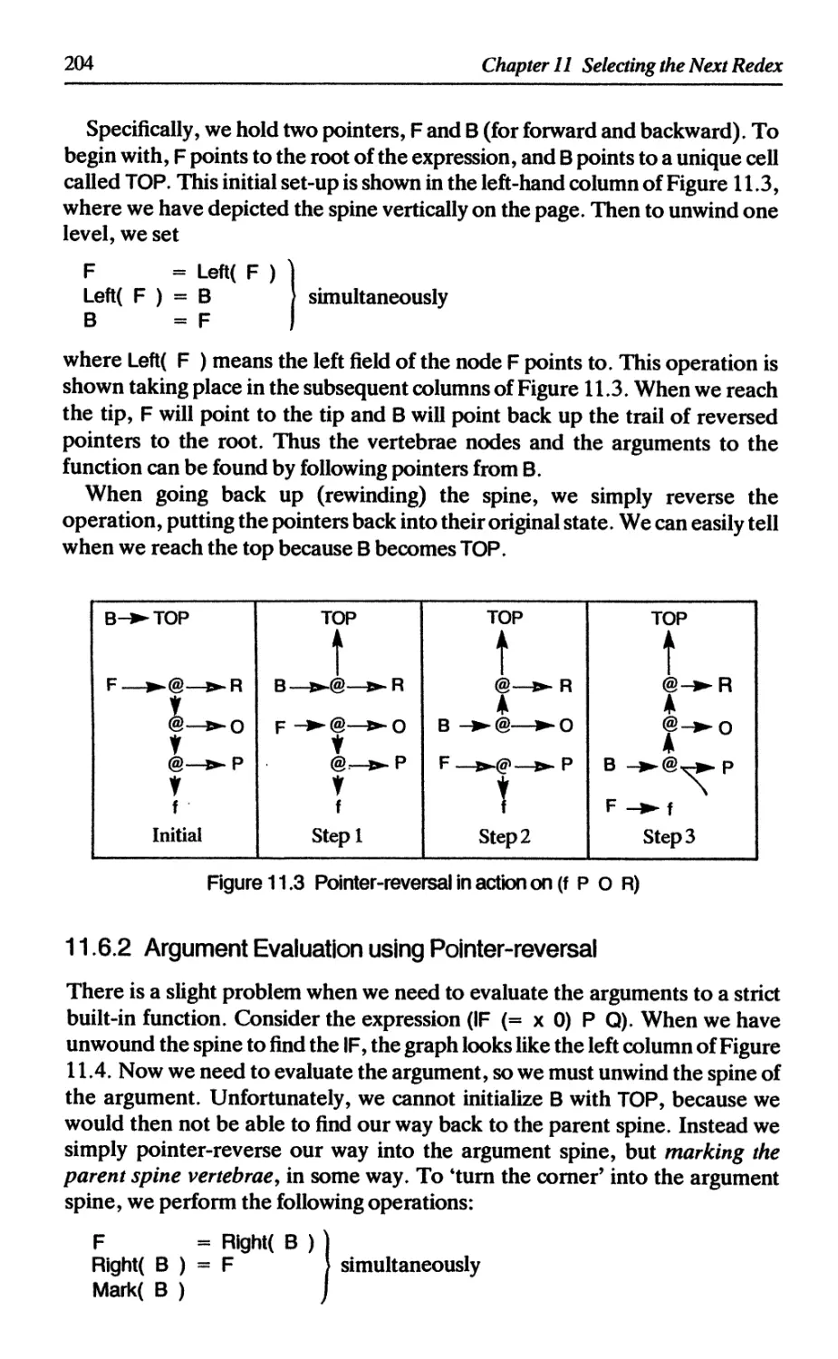
11.6.1 Pointer-reversal 203
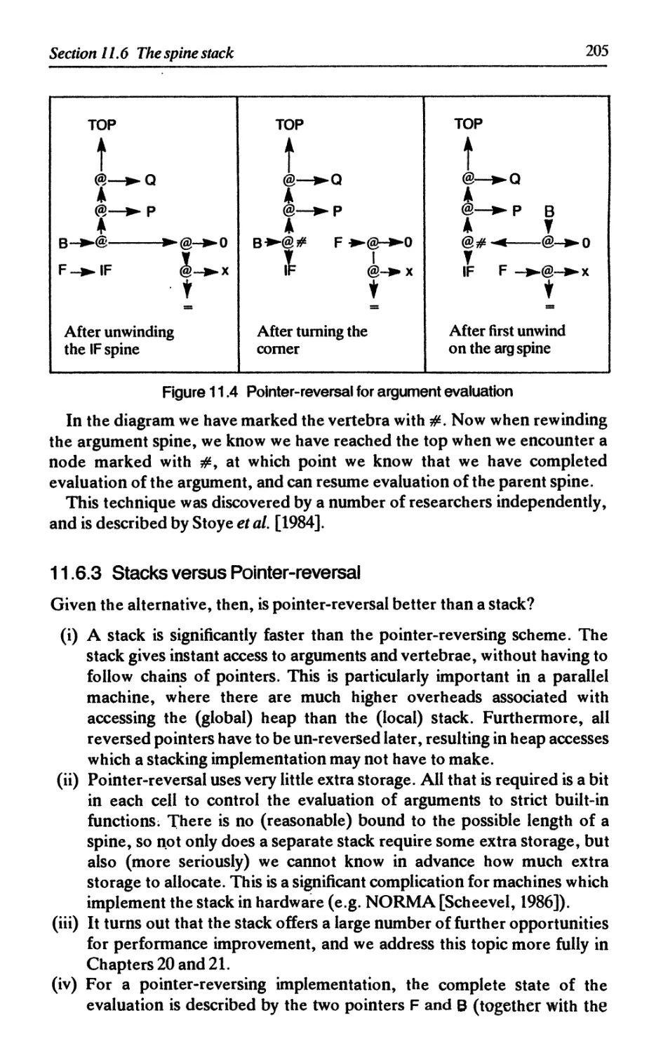
11.6.2 Argument evaluation using pointer-reversal 204
11.6.3 Stacks versus pointer-reversal 205
References 206
12 GRAPH REDUCTION OF LAMBDA EXPRESSIONS 207
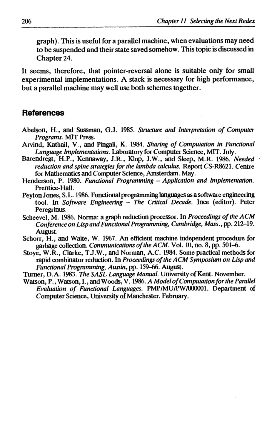
12.1 Reducing a lambda application 207
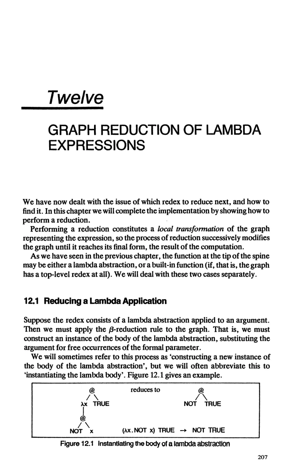
12.1.1 Substituting pointers to the argument 208
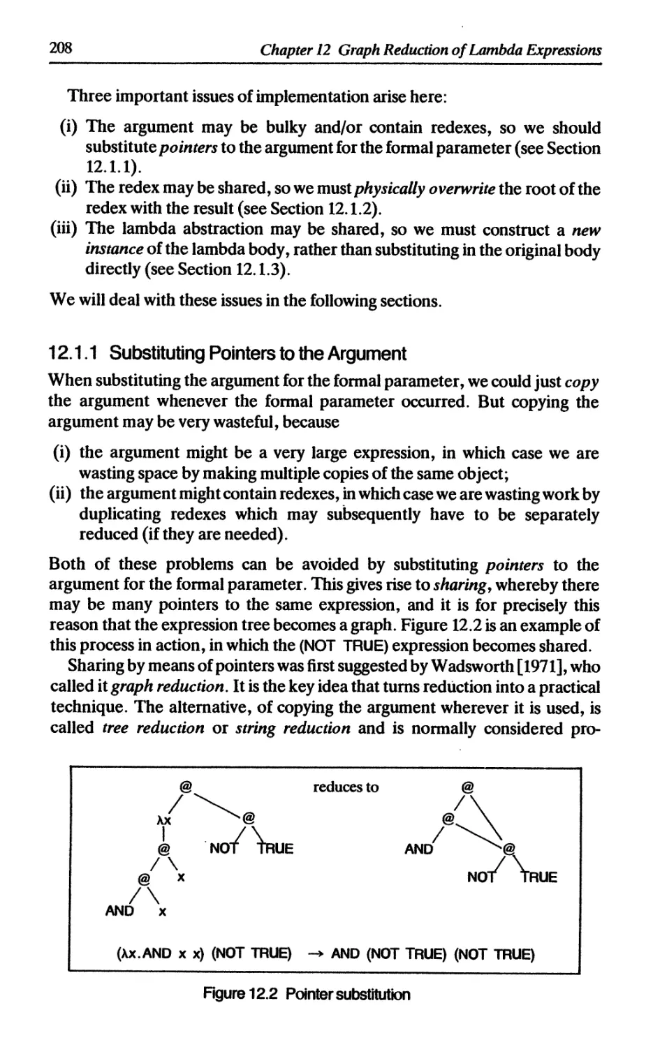
12.1.2 Overwriting the root of the redex 209
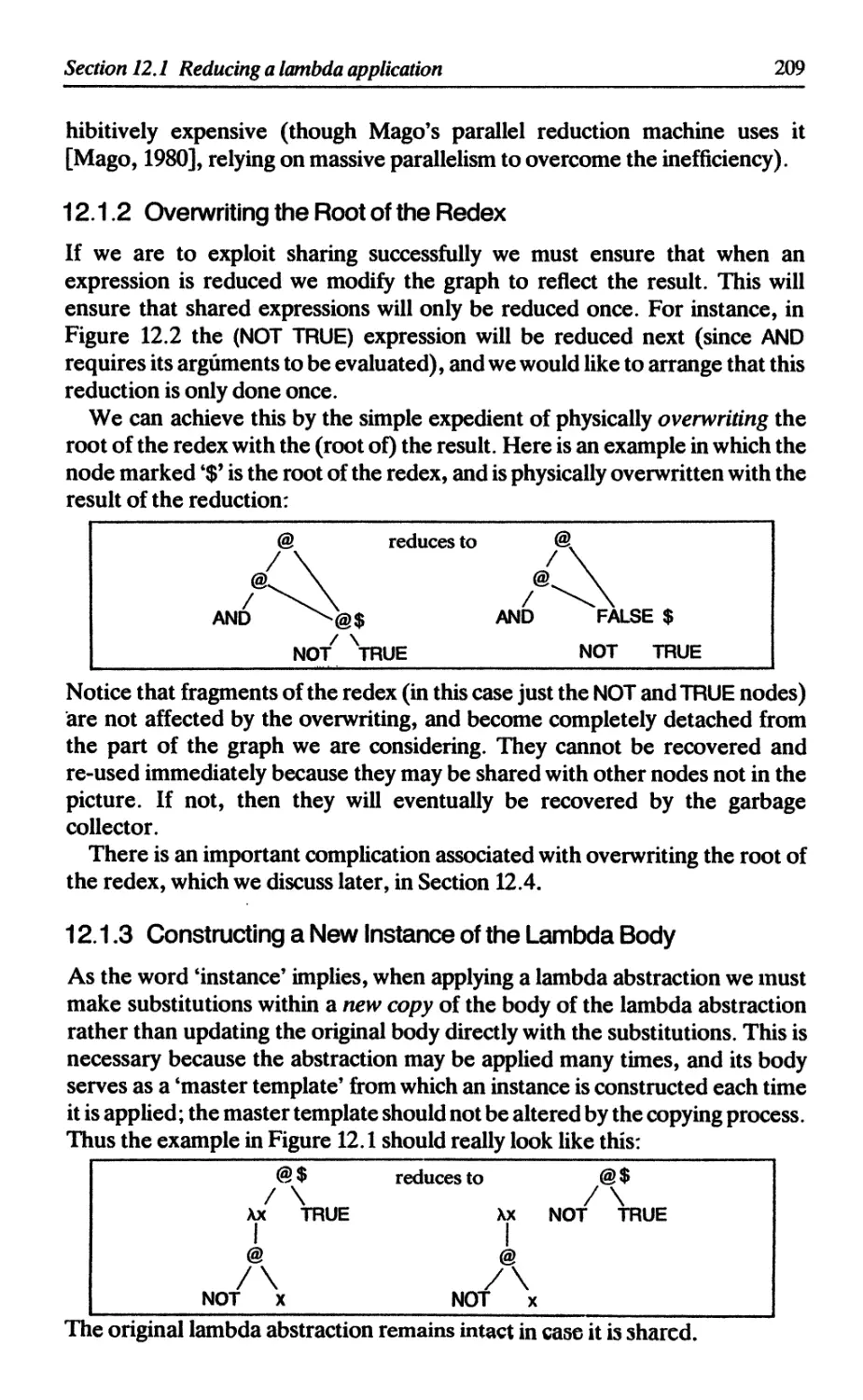
12.1.3 Constructing a new instance of the lambda body 209
12.1.4 Summary 210
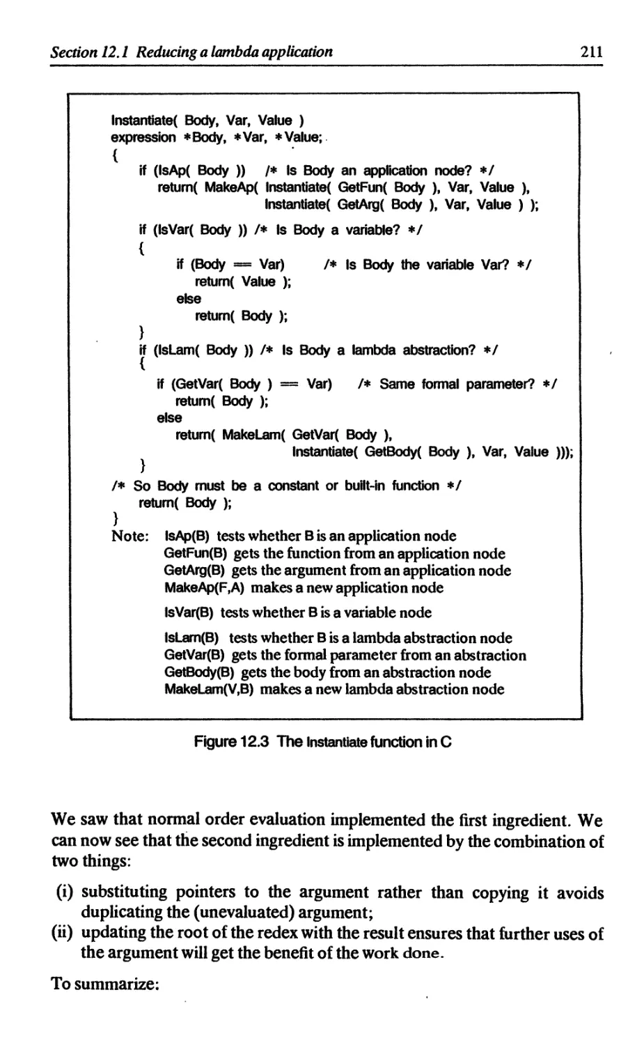
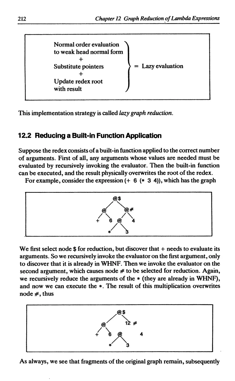
12.2 Reducing a built-in function application 212
12.3 The reduction algorithm so far 213
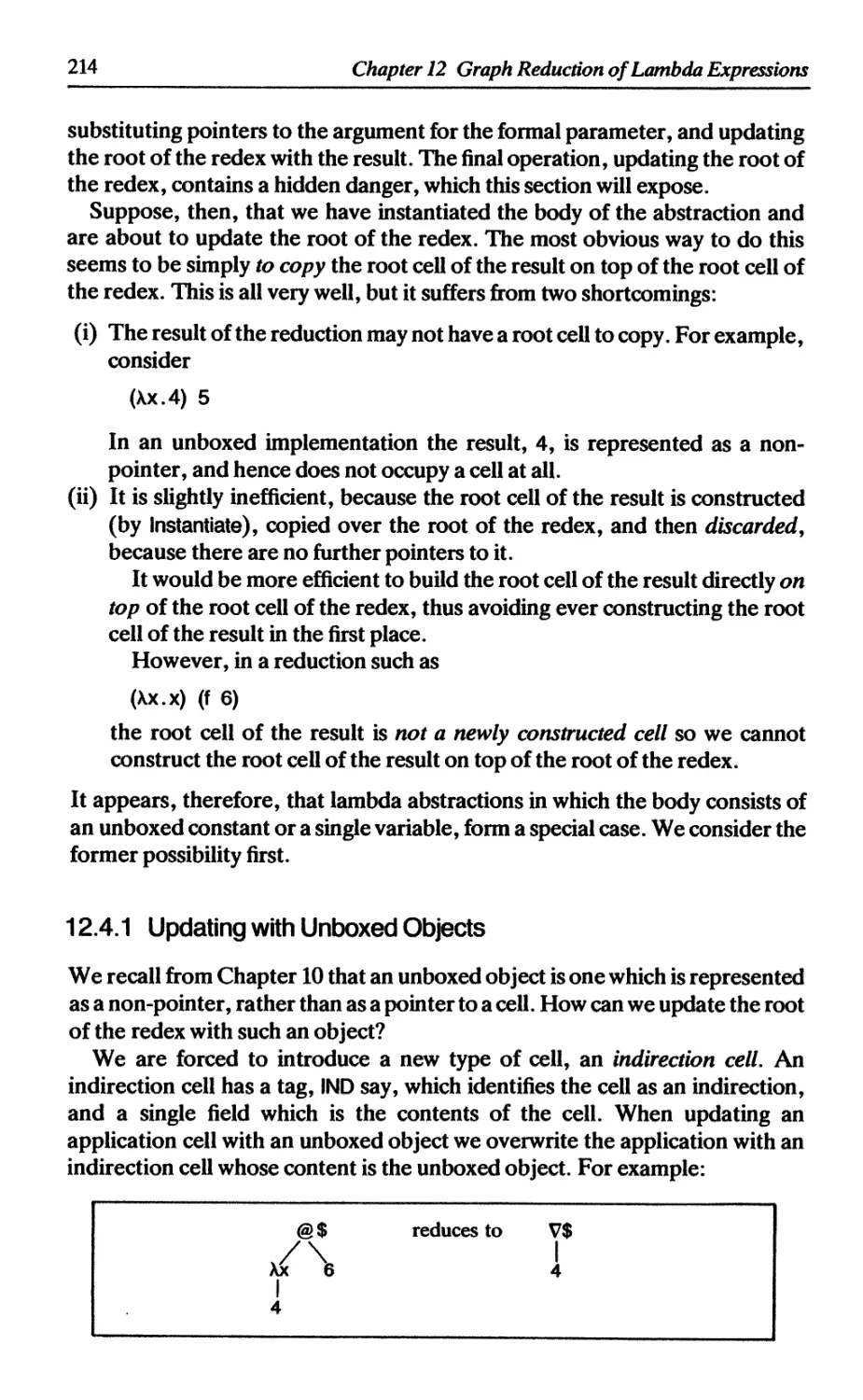
12.4 Indirection nodes 213
12.4.1 Updating with unboxed objects 214
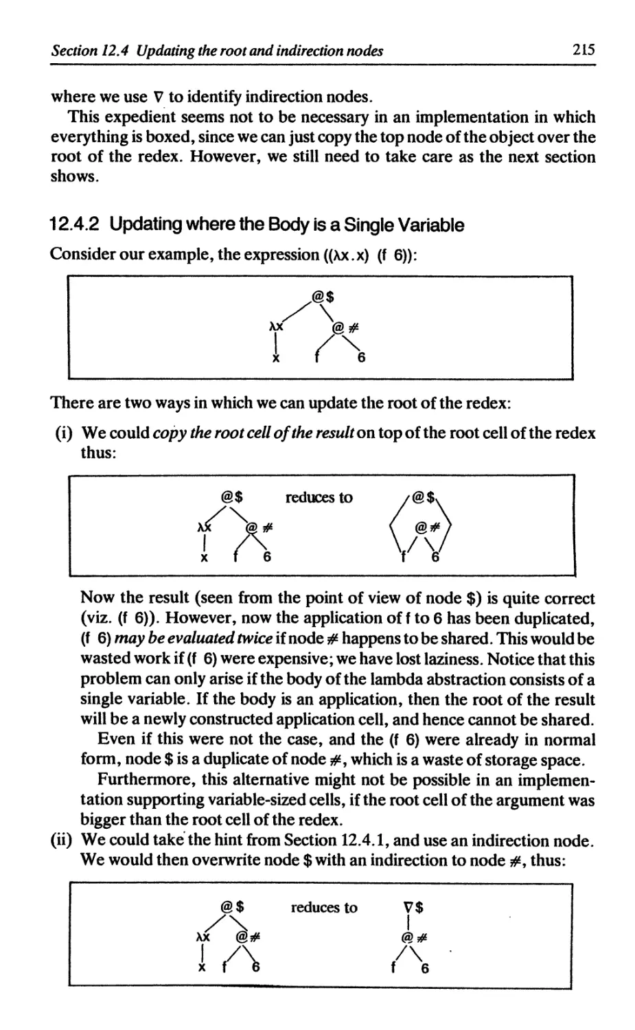
12.4.2 Updating where the body is a single variable 215
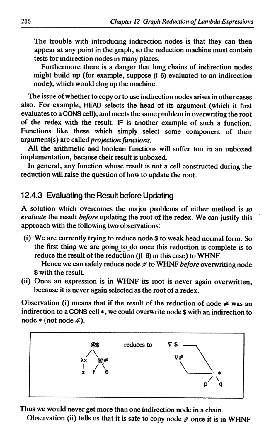
12.4.3 Evaluating the result before updating 216
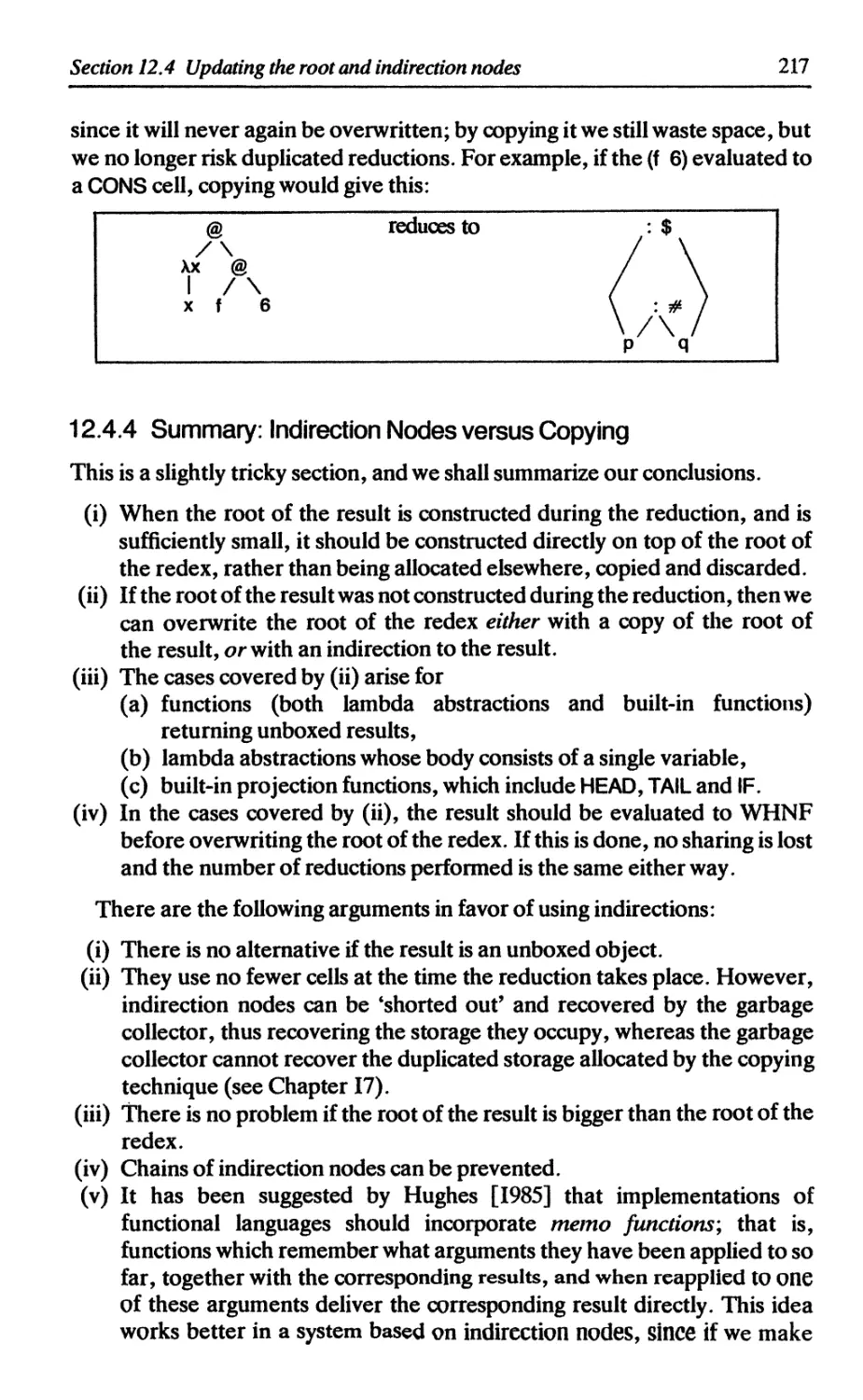
12.4.4 Summary: indirection nodes versus copying 217
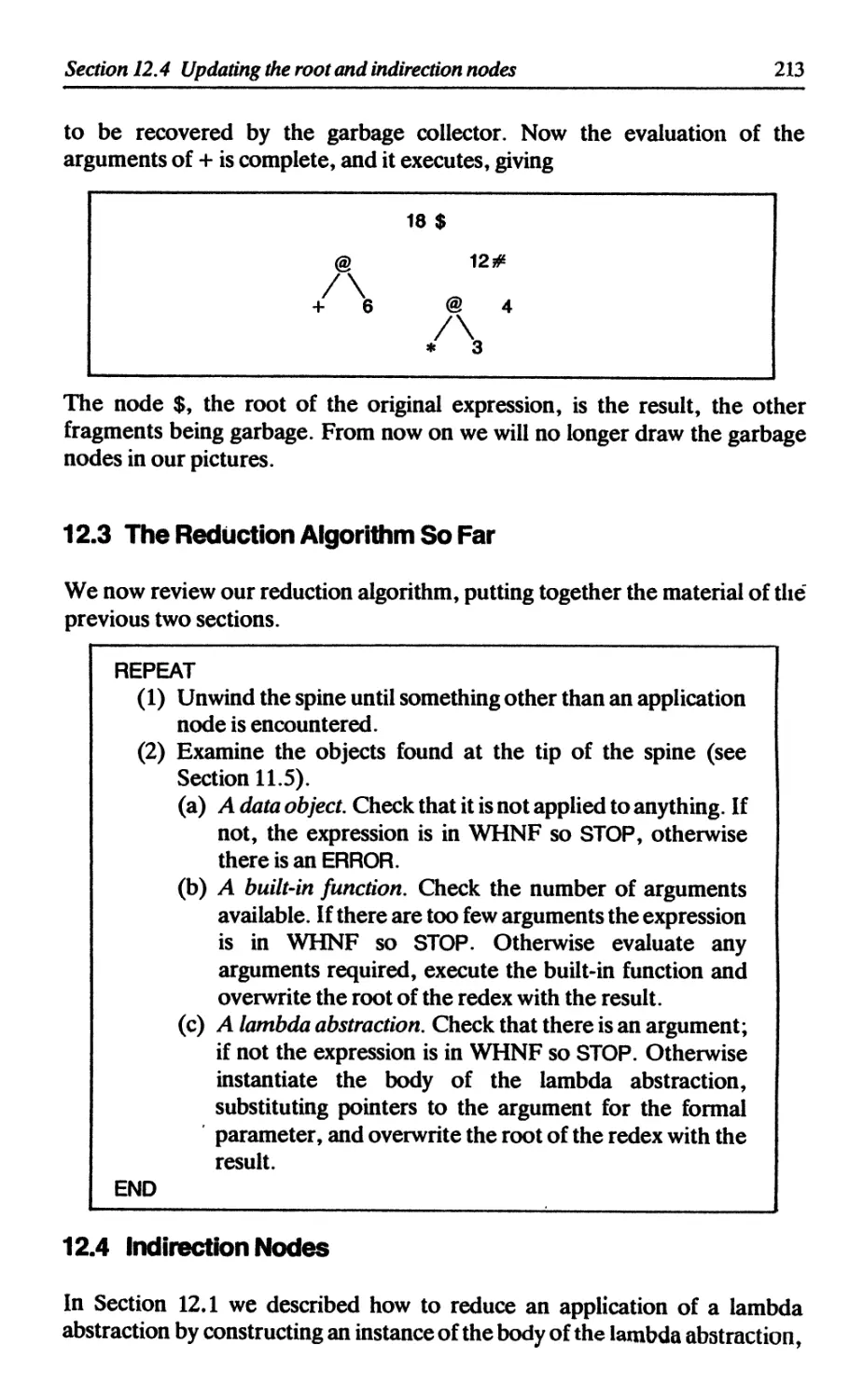
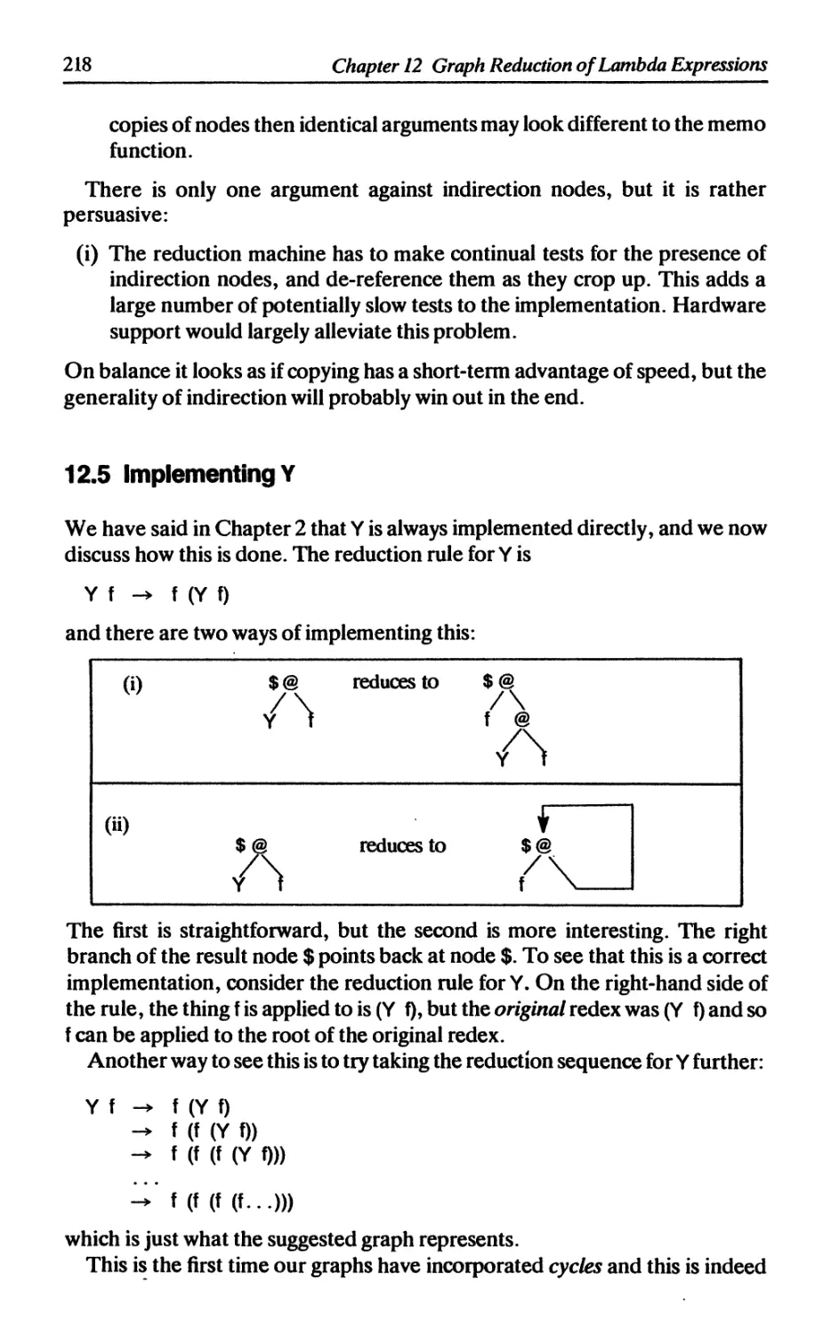
12.5 Implementing Y 218
References 219
13 SUPERCOMBINATORS AND LAMBDA-LIFTING 220
13.1 The idea of compilation 220
13.2 Solving the problem of free variables 222
13.2.1 Supercombinators 223
13.2.2 A supercombinator-based compilation strategy 224
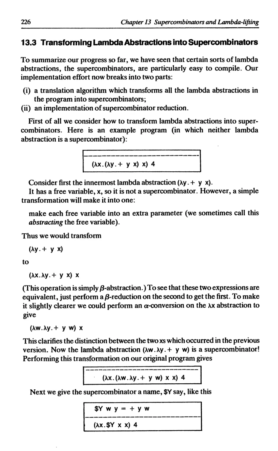
13.3 Transforming lambda abstractions into supercombinators 226
13.3.1 Eliminating redundant parameters 228
13.3.2 Parameter ordering 229
Contents
xi
13.4 Implementing a supercombinator program 230
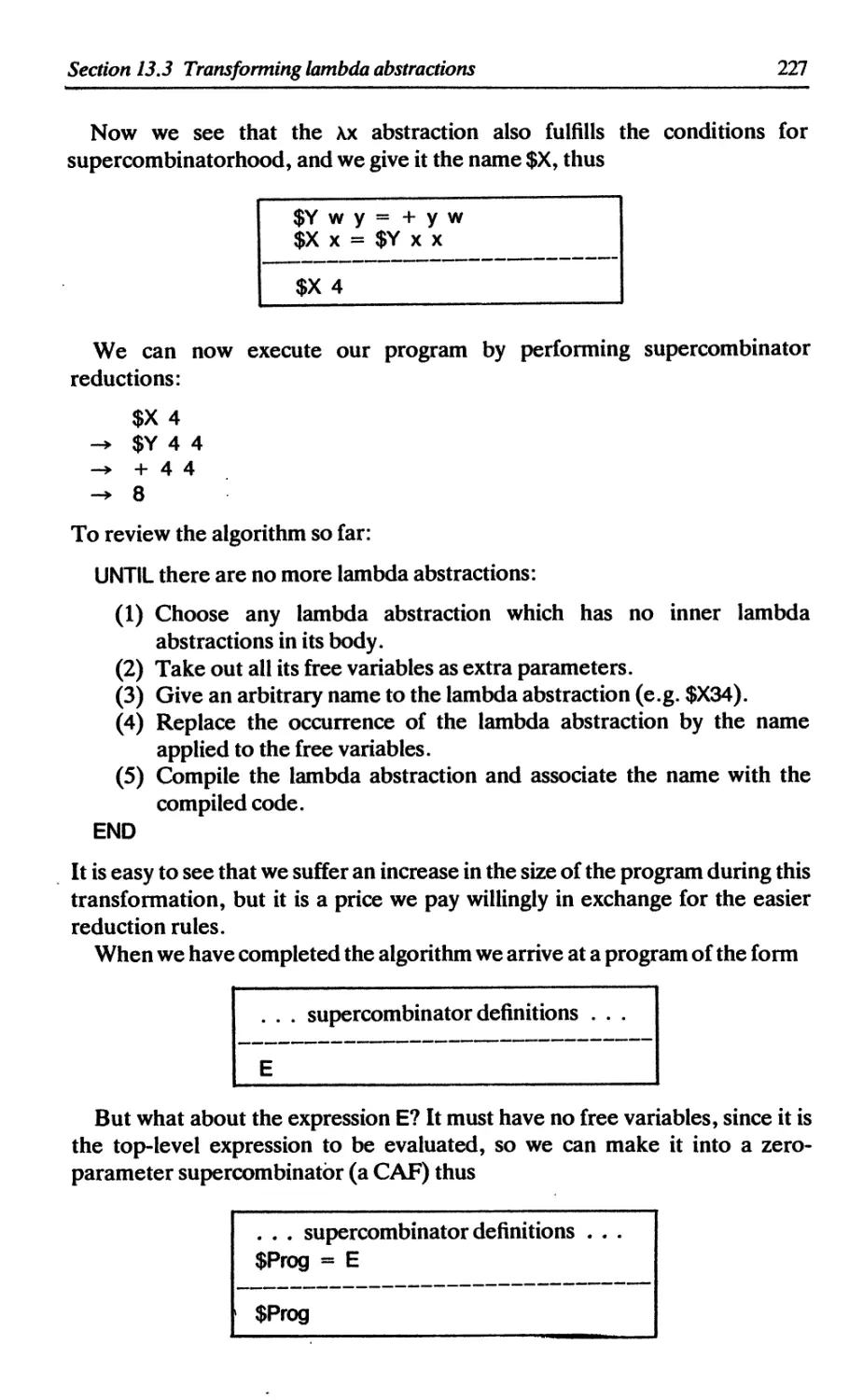
References 231
14 RECURSIVE SUPERCOMBINATORS 232
14.1 Notation 233
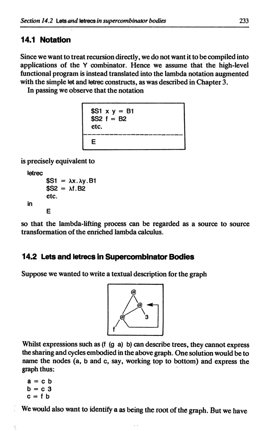
14.2 Lets and letrecs in supercombinator bodies 233
14.3 Lambda-lifting in the presence of letrecs 235
14.4 Generating supercombinators with graphical bodies 236
14.5 An example 236
14.6 Alternative approaches 238
14.7 Compile-time simplifications 240
14.7.1 Compile-time reductions 240
14.7.2 Common subexpression elimination 241
14.7.3 Eliminating redundant lets 241
References 242
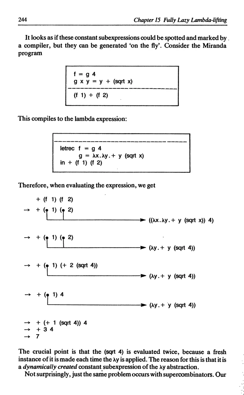
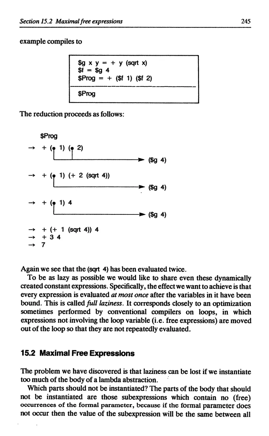
15 FULLY-LAZY LAMBDA-LIFTING 243
15.1 Full laziness 243
15.2 Maximal free expressions 245
15.3 Lambda-lifting using maximal free expressions 247
15.3.1 Modifying the lambda-lifting algorithm 247
15.3.2 Fully lazy lambda-lifting in the presence of letrecs 249
15.4 A larger example 250
15.5 Implementing fully lazy lambda-lifting 252
15.5.1 Identifying the maximal free expressions 252
15.5.2 Lifting CAFs 253
15.5.3 Ordering the parameters 253
15.5.4 Floating out die lets and letrecs 254
15.6 Eliminating redundant full laziness 256
15.6.1 Functions applied to too few arguments 257
15.6.2 Unshared lambda abstractions 258
References 259
16 SKCOMBINATORS 260
16.1 The SK compilation scheme 260
16.1.1 Introducing S, К and I 261
16.1.2 Compilation and implementation 263
16.1.3 Implementations 265
16.1.4 SK combinators perform lazy instantiation 265
16.1.5 I is not necessary 266
16.1.6 History 266
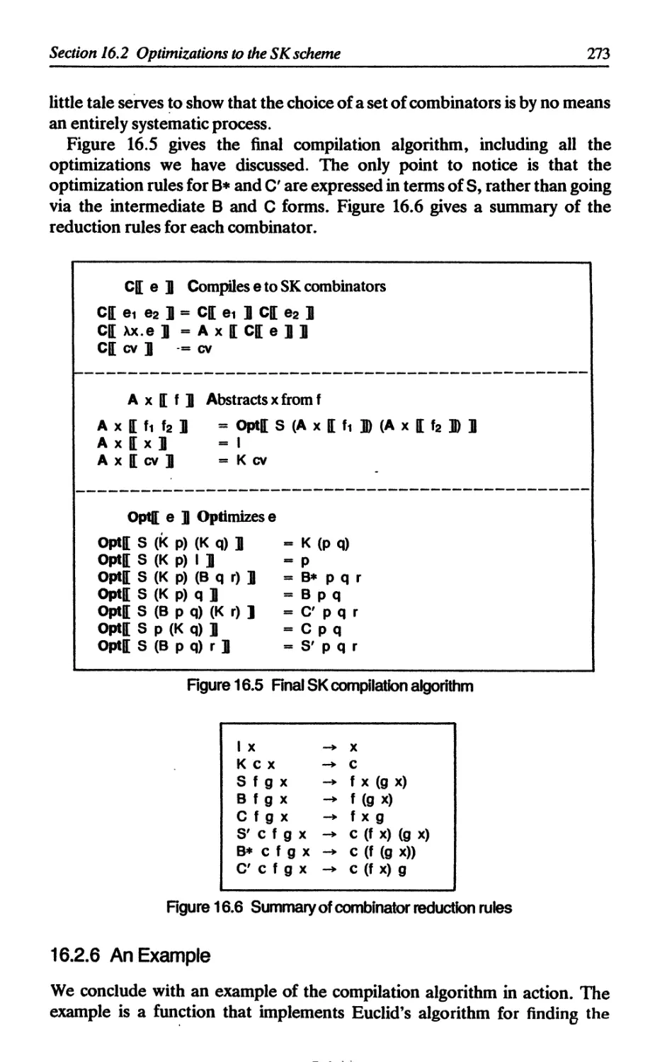
16.2 Optimizations to the SK scheme 267
xii
Contents
16.2.1 К optimization 267
16.2.2 The В combinator 268
16.2.3 TheCcombinator 269
16.2.4 The S' combinator 270
16.2.5 The B' and C combinators 272
16.2.6 An example 273
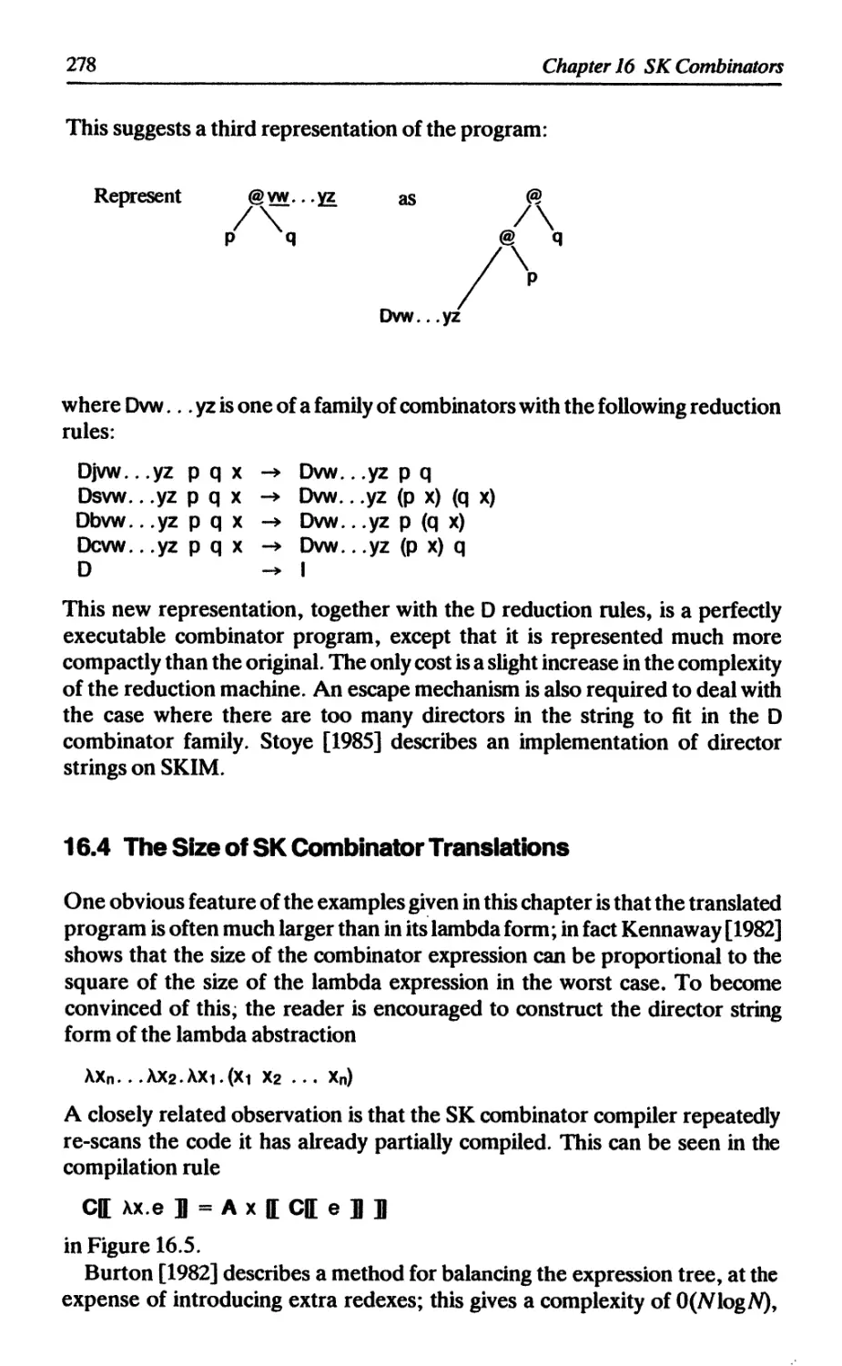
16.3 Director strings 274
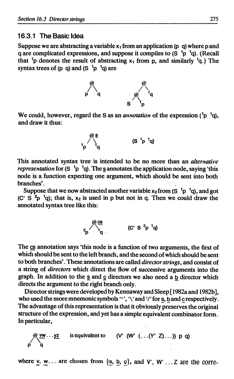
16.3.1 The basic idea 275
16.3.2 Minor refinements 277
16.3.3 Director strings as combinators 277
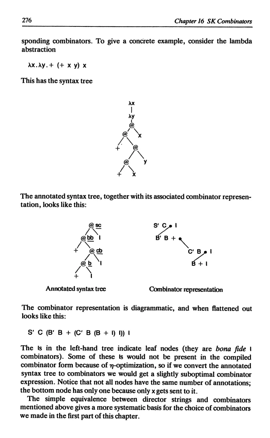
16.4 The size of SK combinator translations 278
16.5 Comparison with supercombinators 279
16.5.1 In favor of SK combinators 279
16.5.2 Against SK combinators 279
References 280
17 STORAGE MANAGEMENT AND GARBAGE COLLECTION 281
17.1 Criteria for assessing a storage manager 281
17.2 A sketch of the standard techniques 282
17.3 Developments in reference-counting 285
17.3.1 Reference-counting garbage collection of cyclic structures 285
17.3.2 One-bit reference-counts 286
17.3.3 Hardware support for reference-counting 286
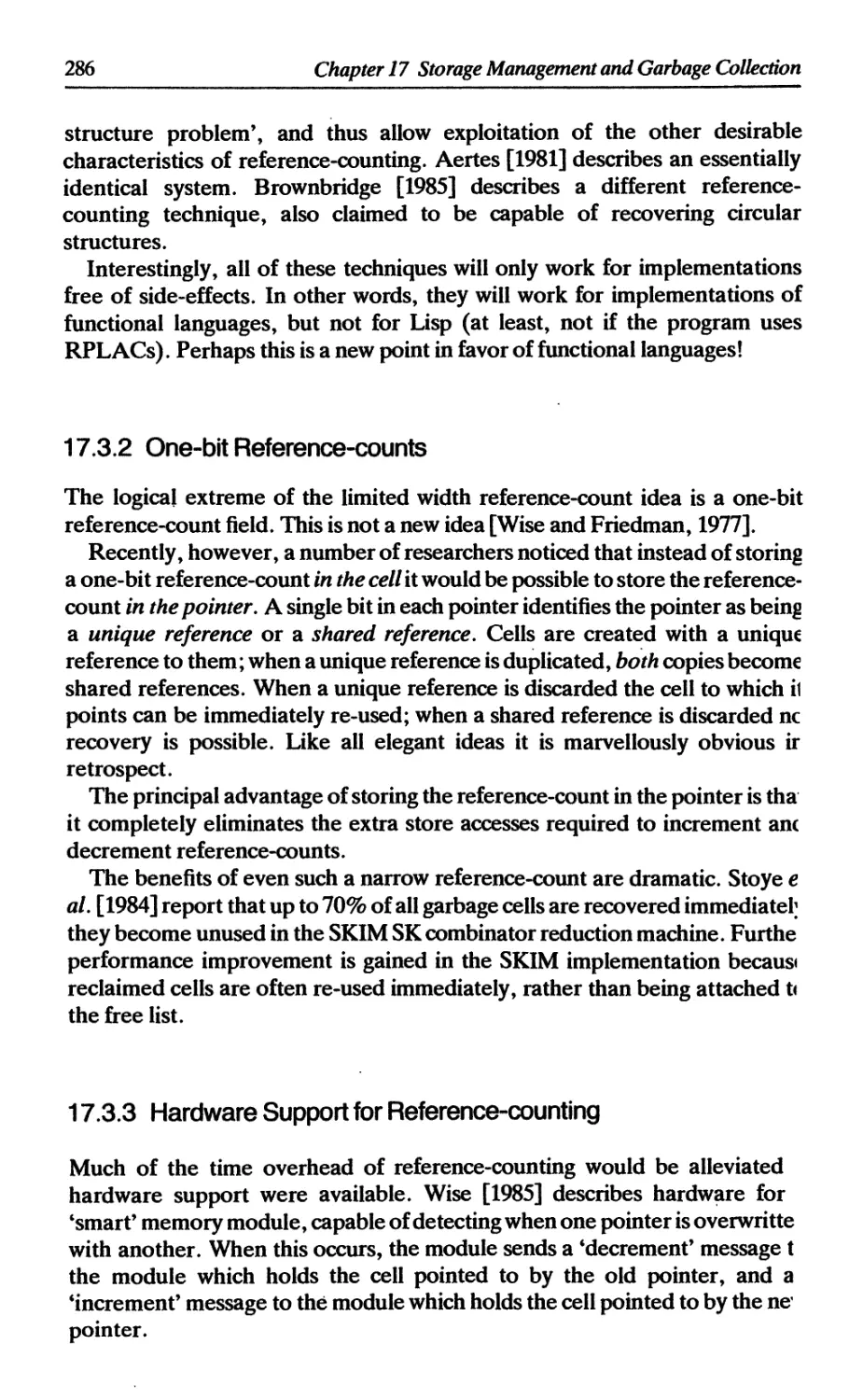
17.4 Shorting out indirection nodes 287
17.5 Exploiting cell lifetimes 287
17.6 Avoiding garbage collection 288
17.7 Garbage collection in distributed systems 288
References 289
PART III ADVANCED GRAPH REDUCTION
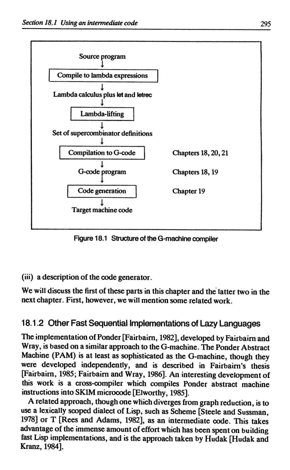
18 THEG-MACHINE 293
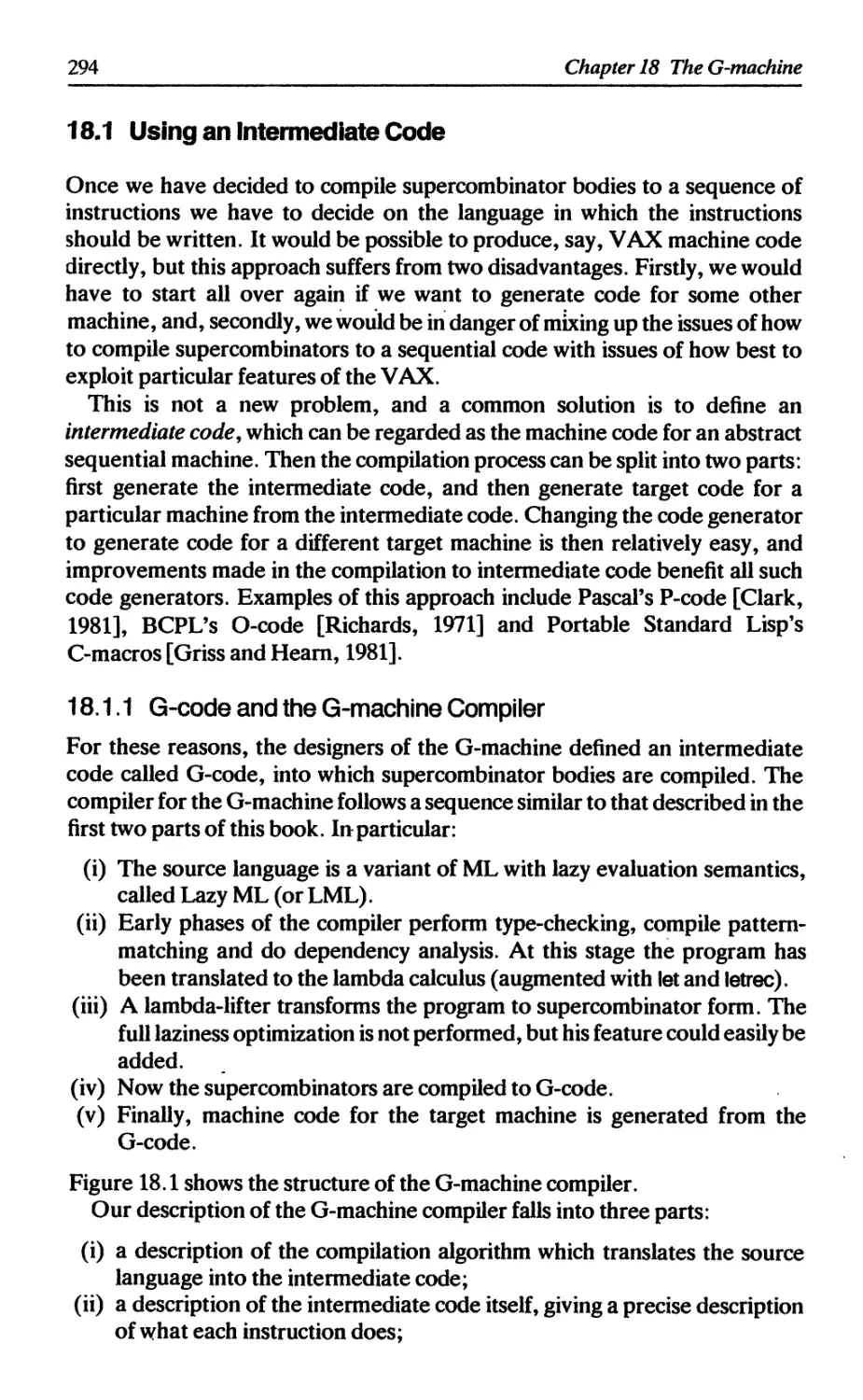
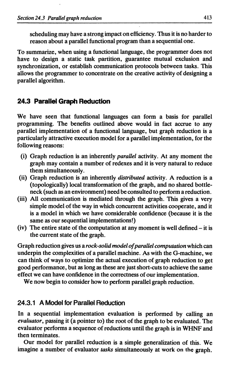
18.1 Using an intermediate code 294
18.1.1 G-code and the G-machine compiler 294
18.1.2 Other fast sequential implementations of lazy languages 295
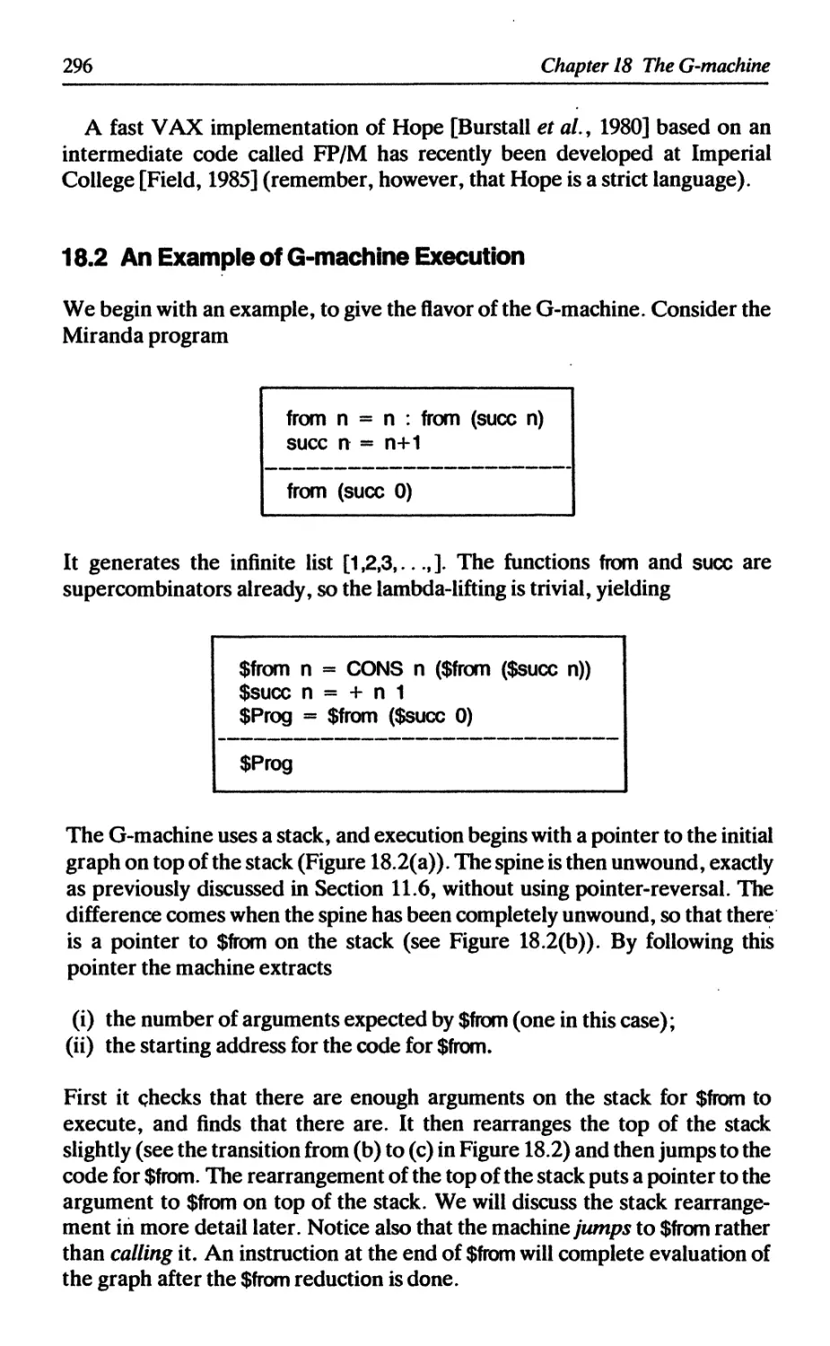
18.2 An example of G-machine execution 296
18.3 The source language for the G-compiler 299
18.4 Compilation to G-code 300
18.5 Compiling a supercombinator definition 301
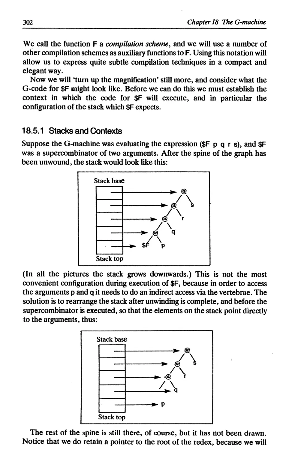
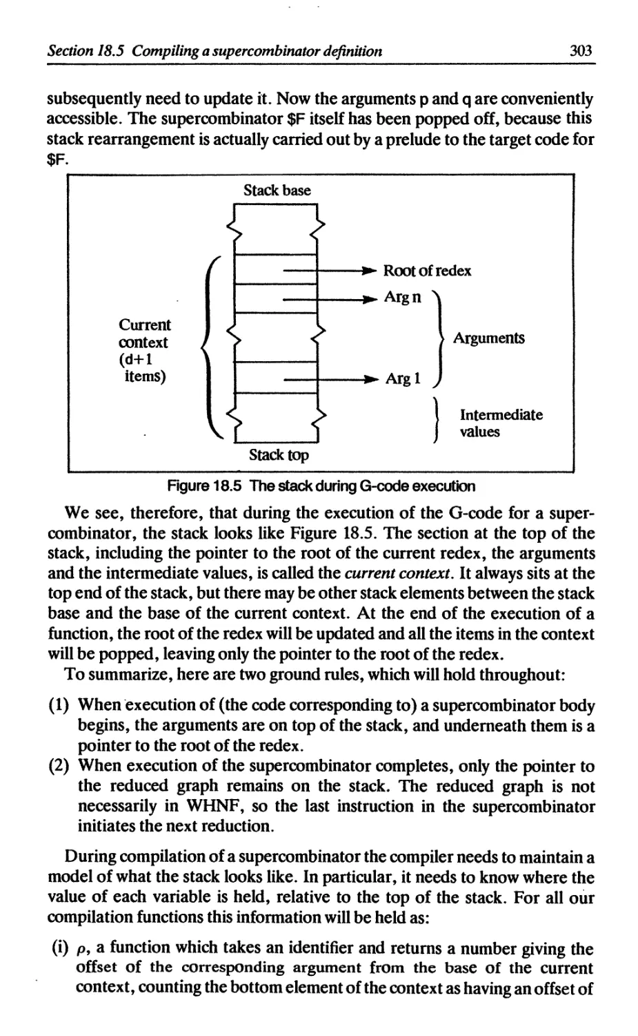
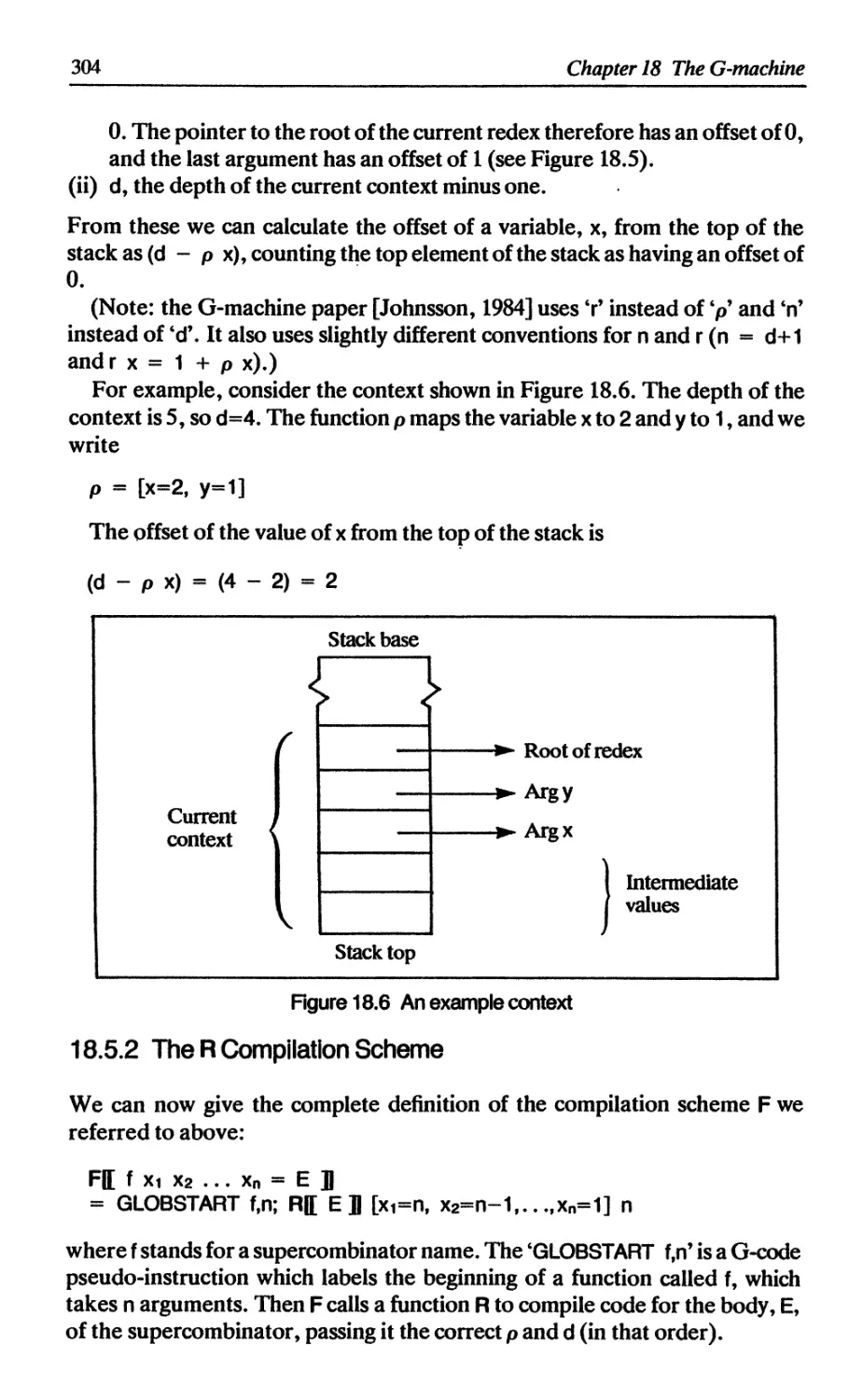
18.5.1 Stacks and contexts 302
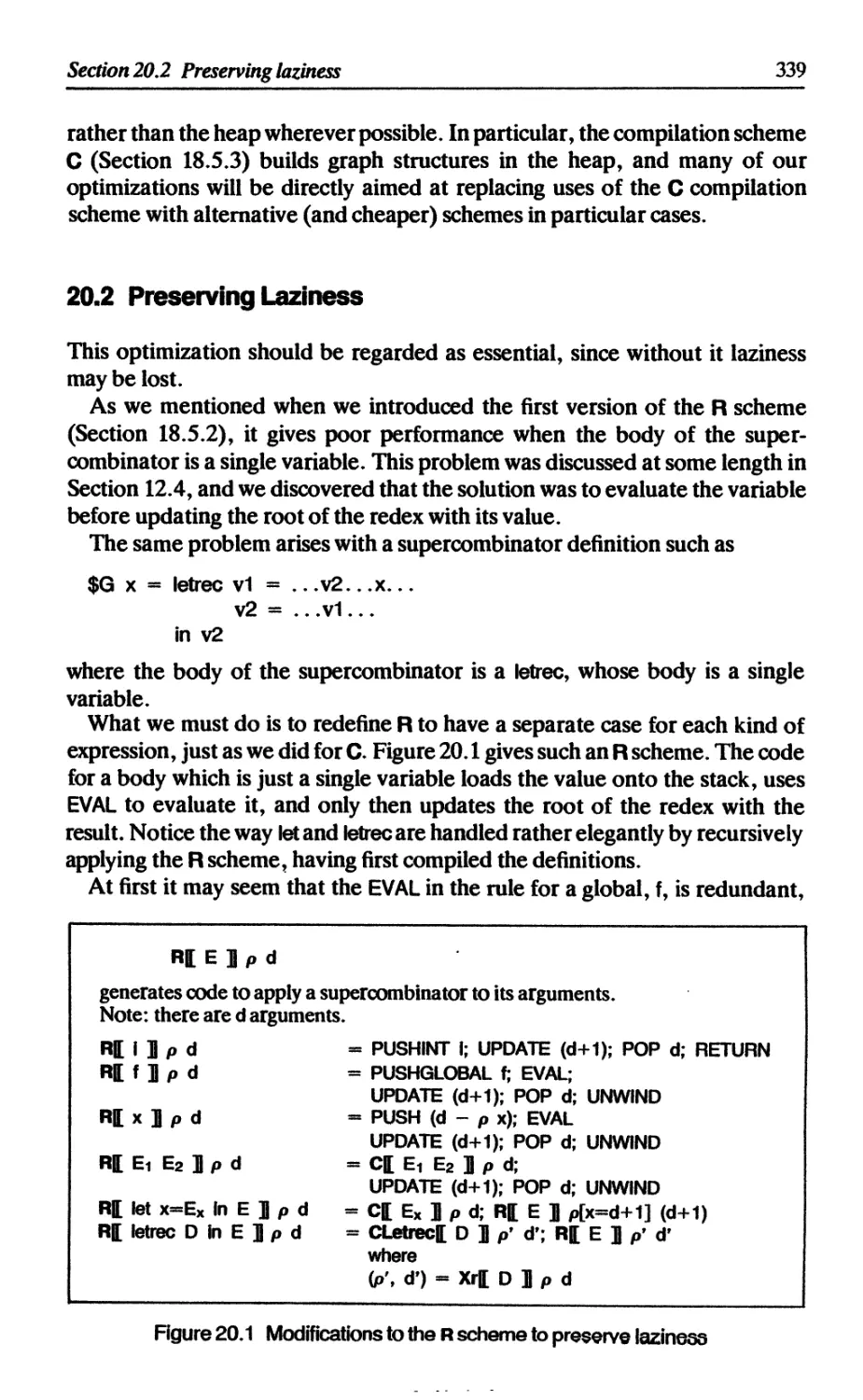
18.5.2 The R compilation scheme 304
18.5.3 The C compilation scheme 306
18.6 Supercombinators with zero arguments 311
18.6.1 Compiling CAFs 311
18.6.2 Garbage collection of CAFs 312
Contents
xiii
18.7 Getting it all together 312
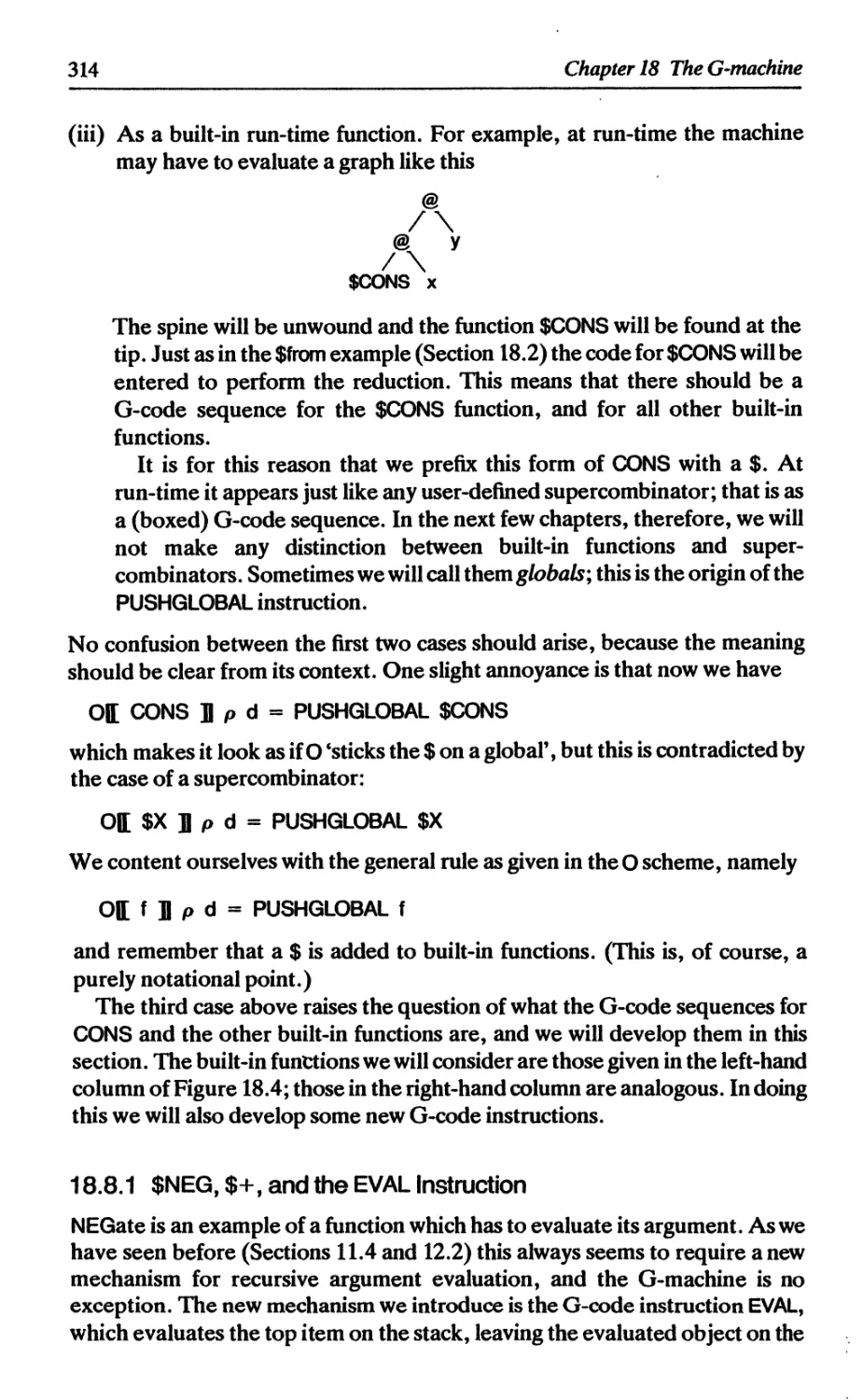
18.8 The built-in functions 313
18.8.1 $NEG, $+, and the EVAL instruction 314
18.8.2 $CONS 316
18.8.3 $HEAD 316
18.8.4 $IF, and the JUMP instruction 317
18.9 Summary 318
References 318
19 G-CODE-DEFINITION AND IMPLEMENTATION 319
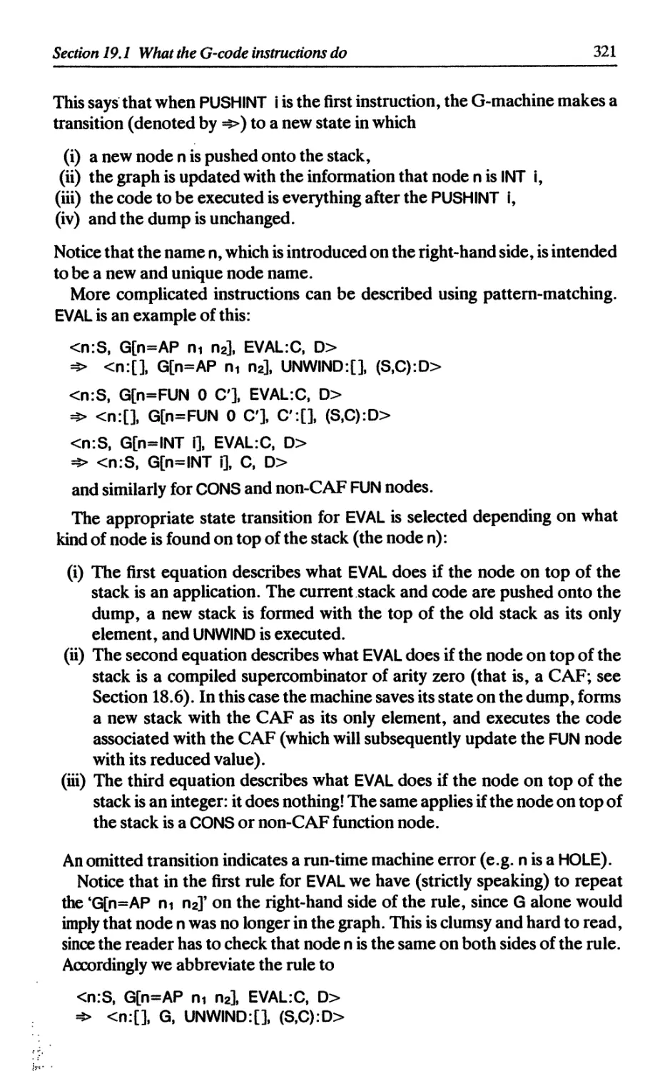
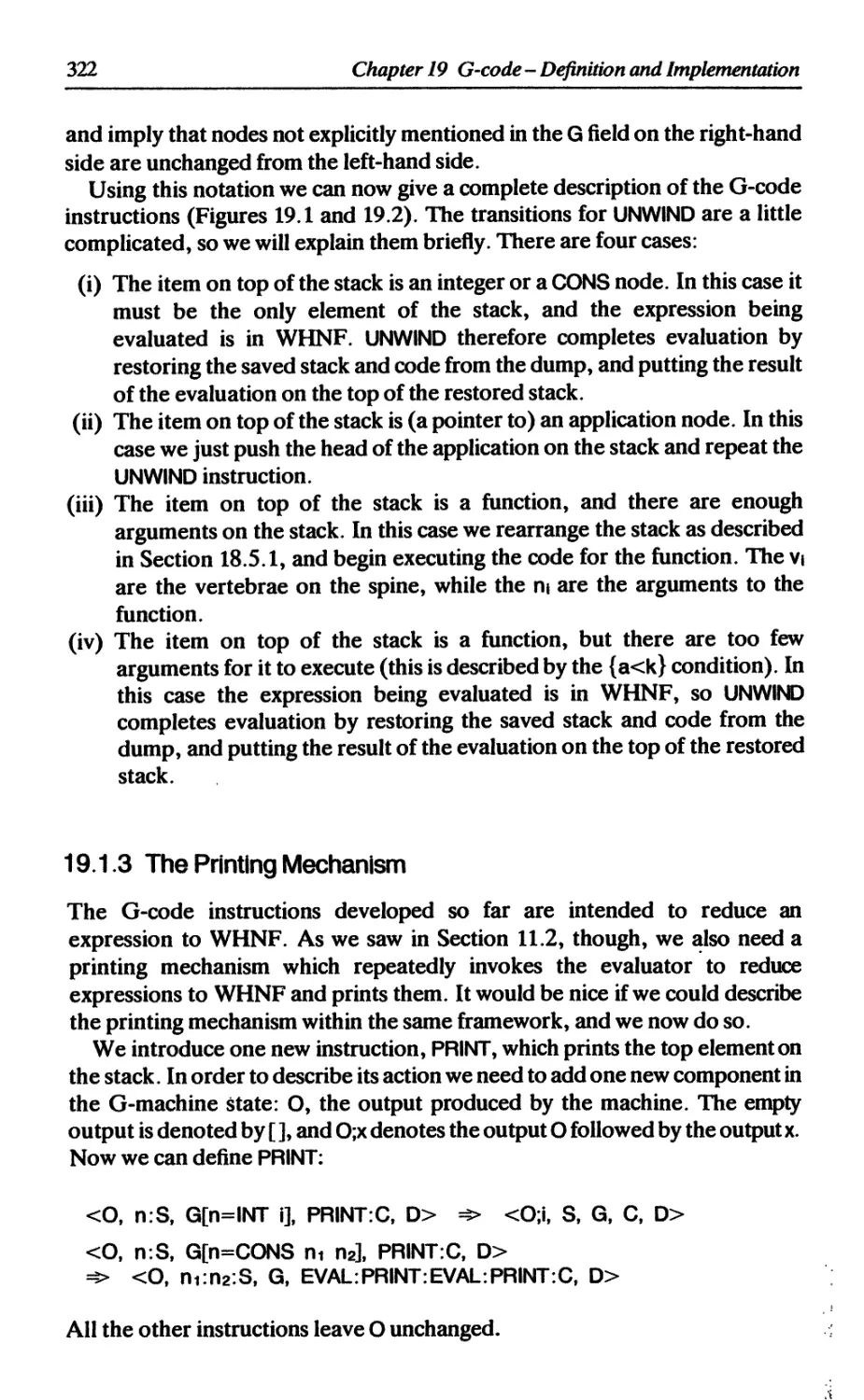
19.1 What the G-code instructions do 319
19.1.1 Notation 320
19.1.2 State transitions for the G-machine 320
19.1.3 The printing mechanism 322
19.1.4 Remarks about G-code 324
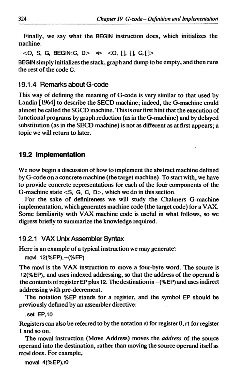
19.2 Implementation 324
19.2.1 VAX Unix assembler syntax 324
19.2.2 The stack representation 325
19.2.3 The graph representation 325
19.2.4 The code representation 326
19.2.5 The dump representation 326
19.3 Target code generation 326
19.3.1 Generating target code from G-code instructions 327
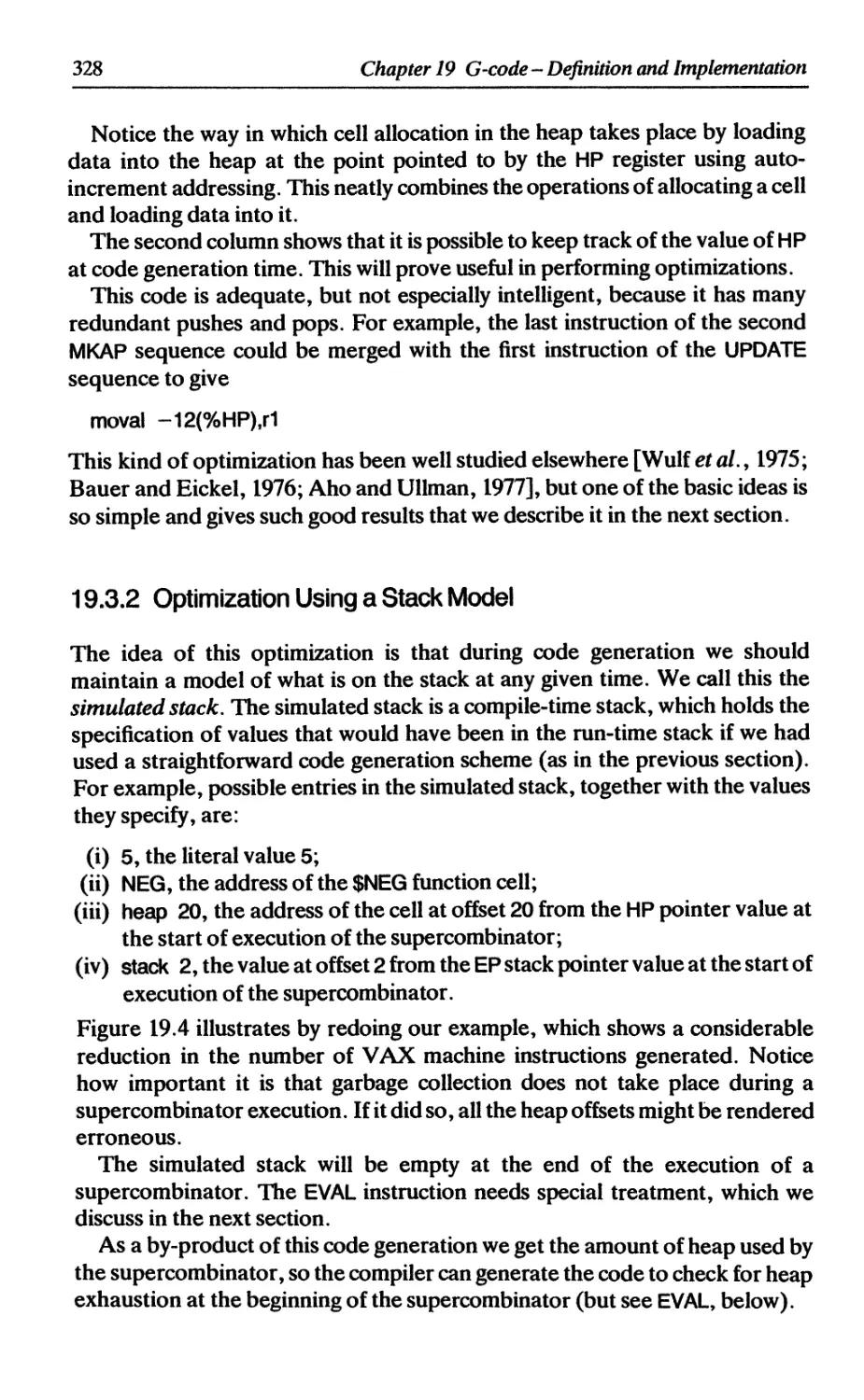
19.3.2 Optimization using a stack model 328
19.3.3 Handling EVALs and JUMPS 329
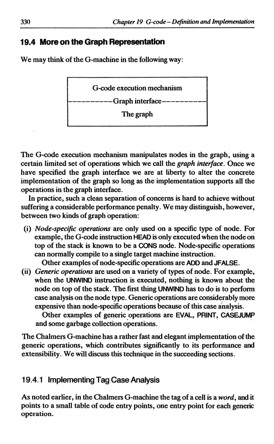
19.4 More on the graph representation 330
19.4.1 Implementing tag case analysis 330
19.4.2 Implementing EVAL 331
19.4.3 Implementing UNWIND 332
19.4.4 Indirection nodes 334
19.4.5 Boxed versus unboxed representations 335
19.4.6 Summary 336
19.5 Getting it all together 336
19.6 Summary 336
References 337
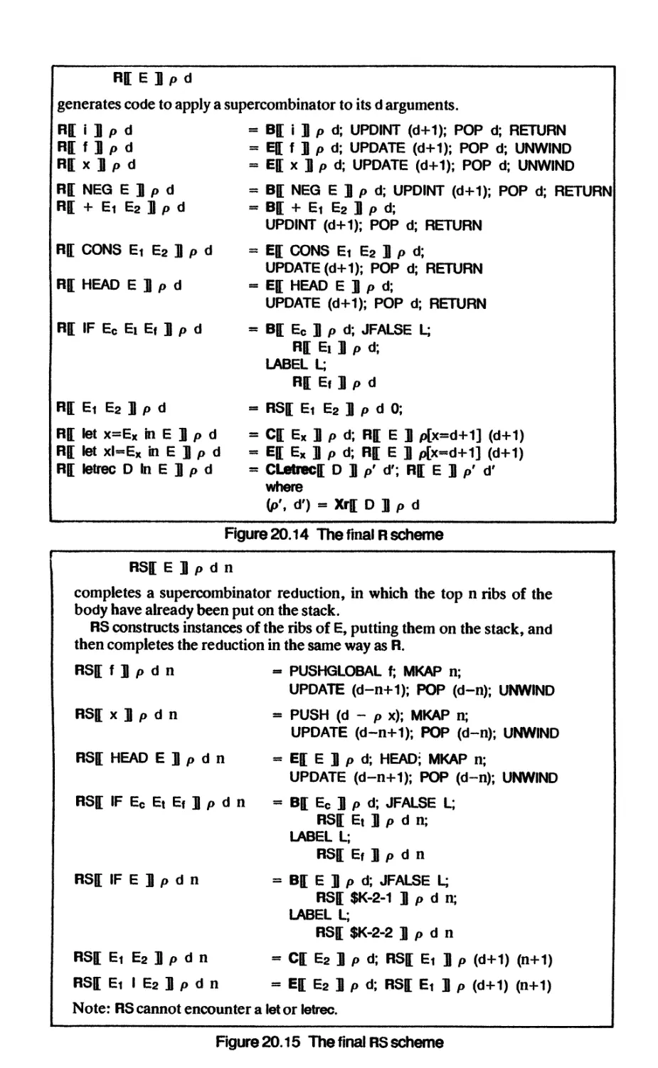
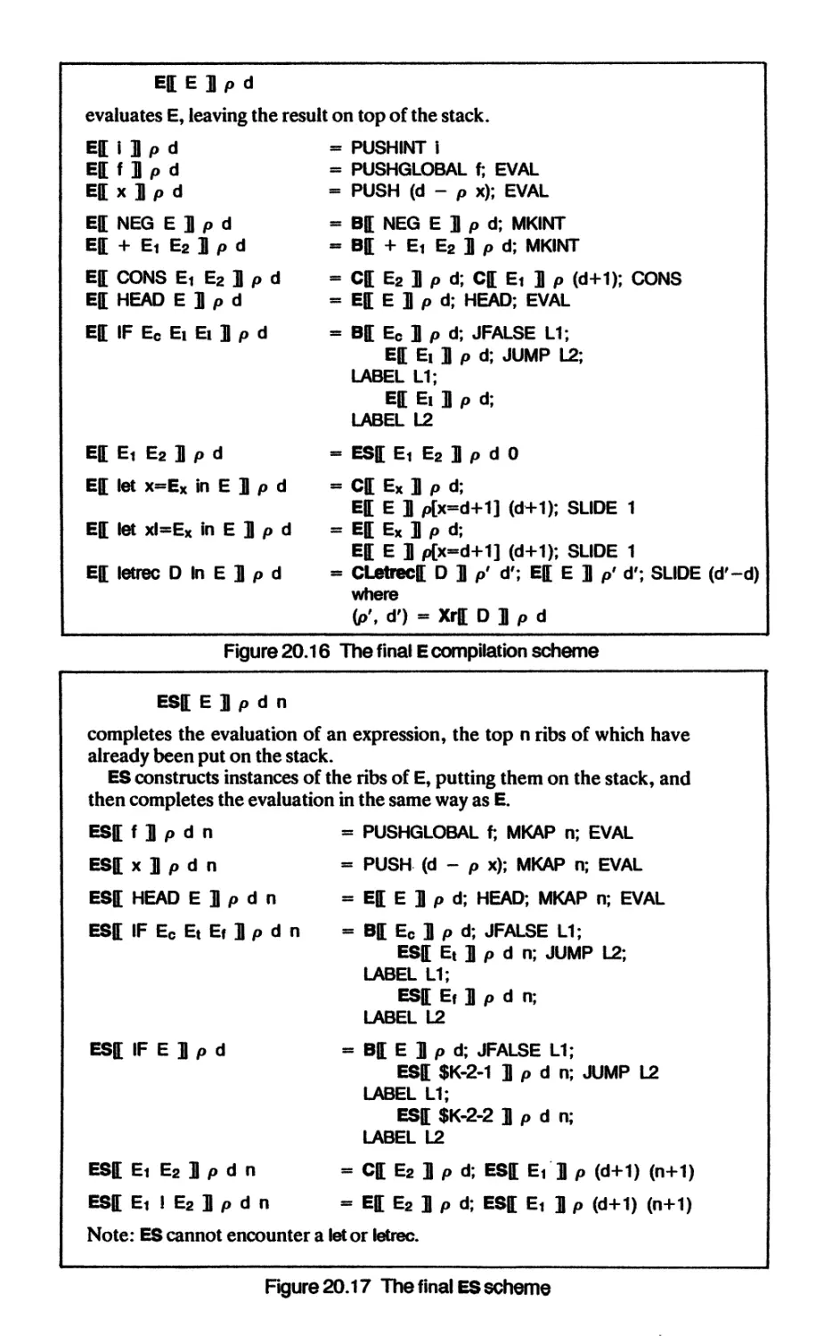
20 OPTIMIZATIONS TO THE G-MACHINE 338
20.1 On not building graphs 338
20.2 Preserving laziness 339
20.3 Direct execution of built-in functions 340
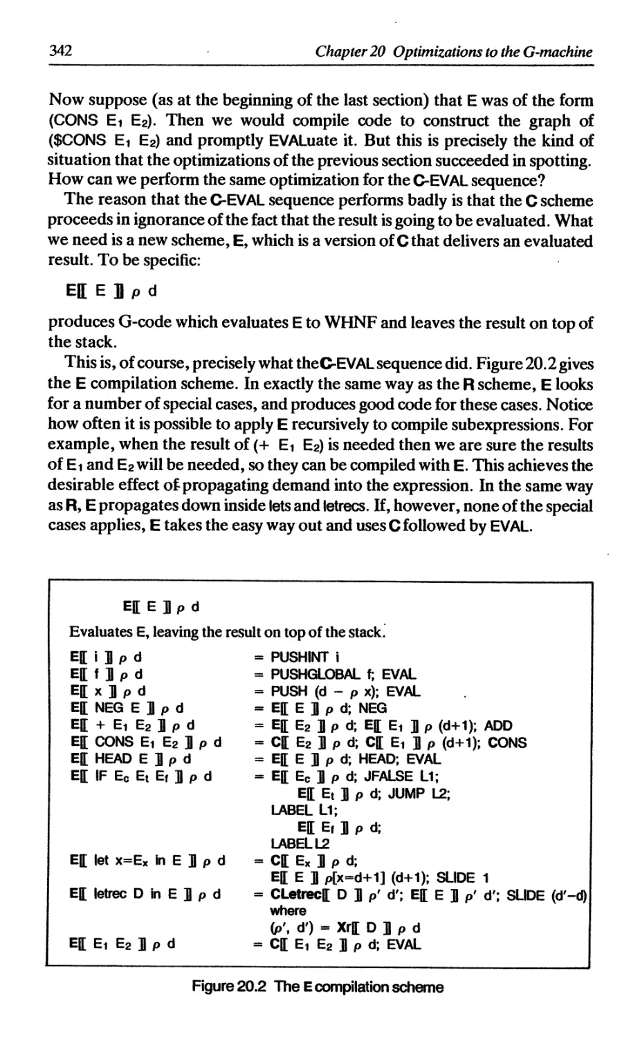
20.3.1 Optimizations to the R scheme 340
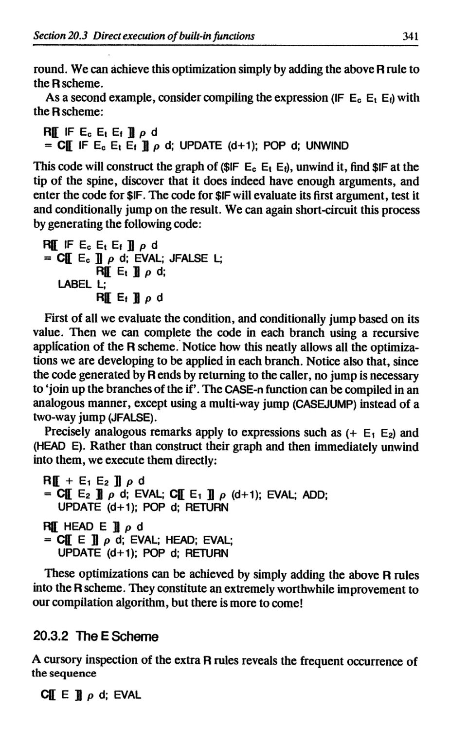
20.3.2 The E scheme 341
20.3.3 The RS and ES schemes 343
20.3.4 17-reduction and lambda-lifting 346
xiv
Contents
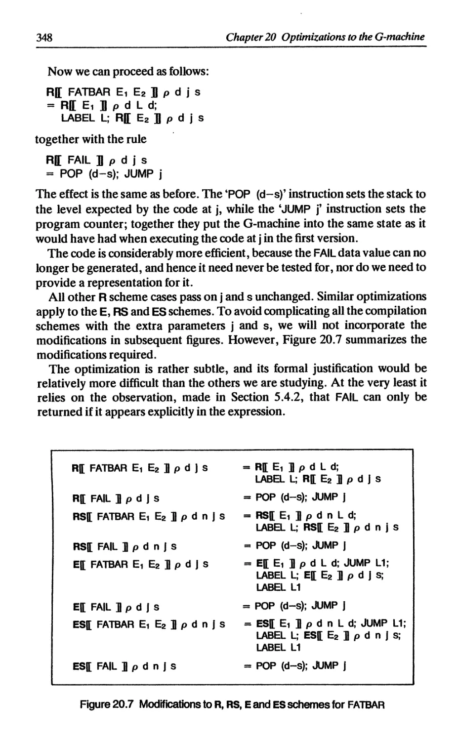
20.4 Compiling FATBAR and FAIL 347
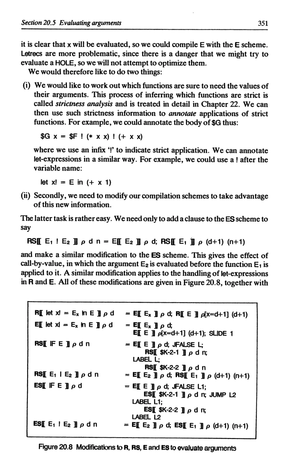
20.5 Evaluating arguments 349
20.5.1 Optimizing partial applications 349
20.5.2 Using global strictness information 350
20.6 Avoiding EVALs 352
20.6.1 Avoiding re-evaluation in a function body 352
20.6.2 Using global strictness information 352
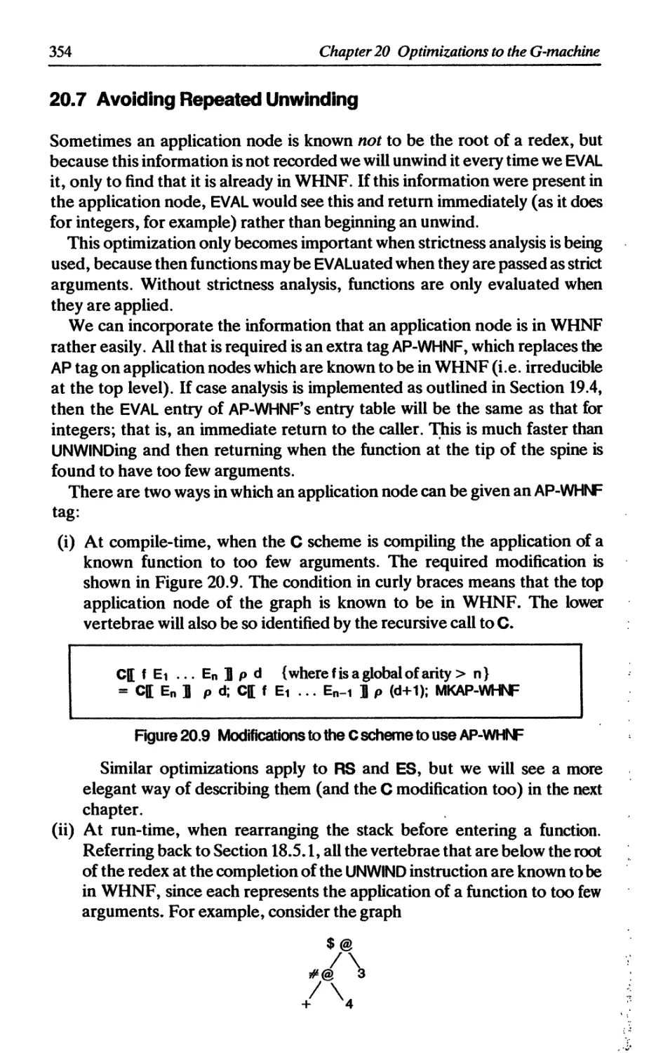
20.7 Avoiding repeated unwinding 354
20.8 Performing some eager evaluation 355
20.9 Manipulating basic values 356
20.10 Peephole optimizations to G-code 360
20.10.1 Combining multiple SLIDES and MKAPs 360
20.10.2 Avoiding redundant EVALs 361
20.10.3 Avoiding allocating the root of the result 361
20.10.4 Unpacking structured objects 362
20.11 Pattern-matching revisited 363
20.12 Summary 363
Reference 366
21 OPTIMIZING GENERALIZED TAIL CALLS Simon L. Peyton
Jones and Thomas Johnsson 367
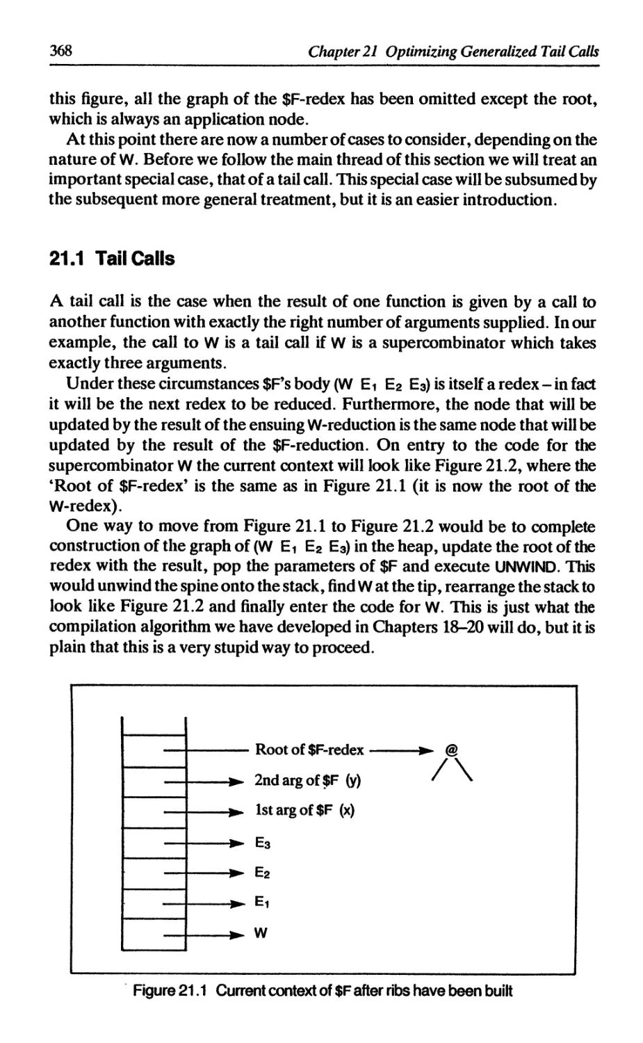
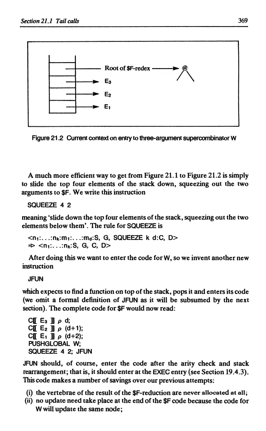
21.1 Tail calls 368
21.2 Generalizing tail calls 371
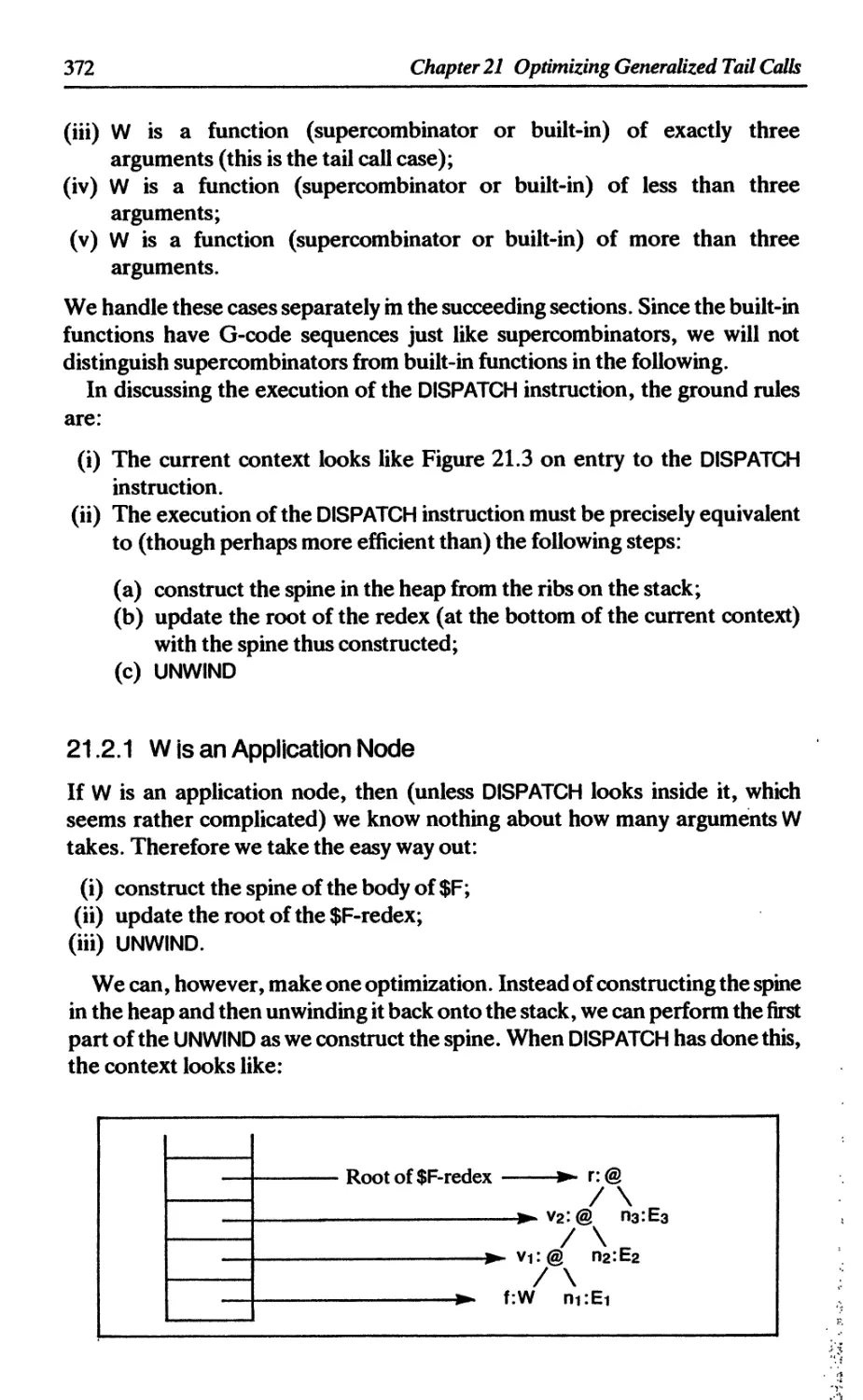
21.2.1 W is an application node 372
21.2.2 W is a supercombinator of zero arguments 373
21.2.3 W is a function of three arguments 373
21.2.4 W is a function of less than three arguments 373
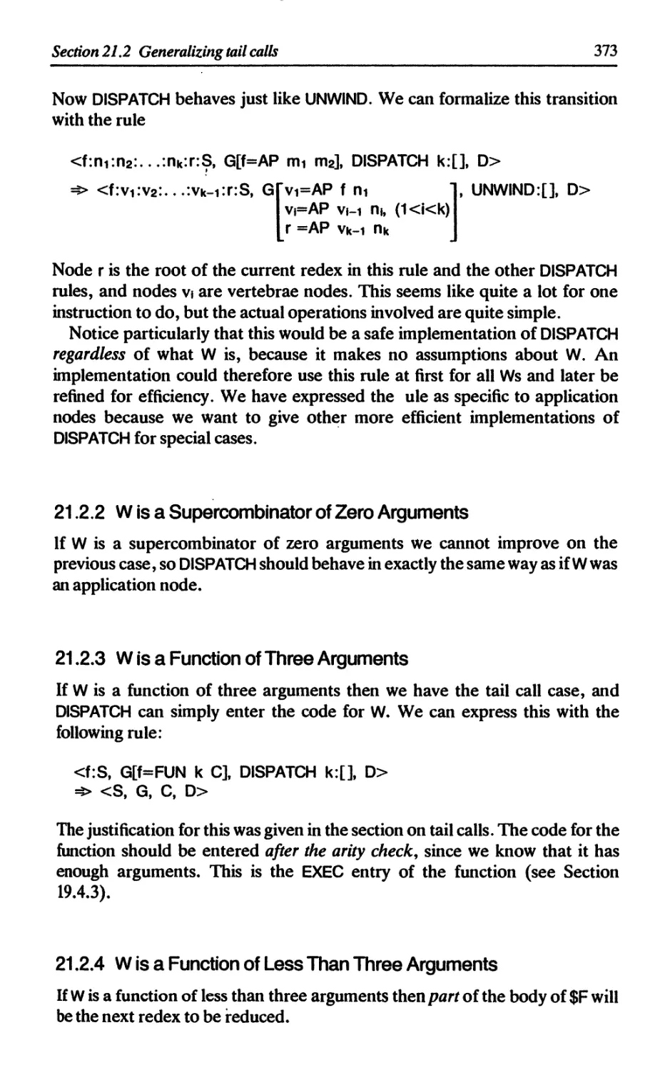
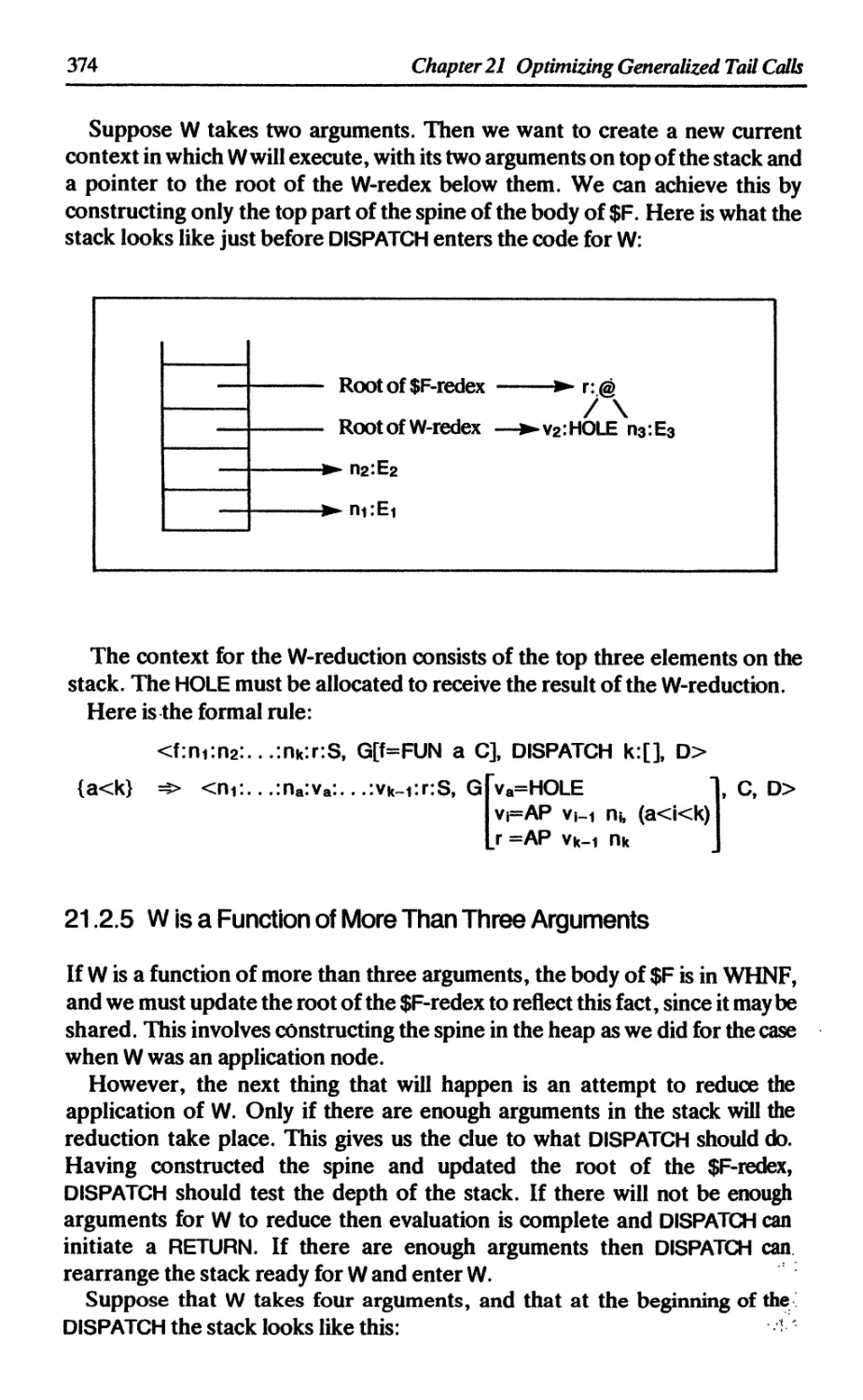
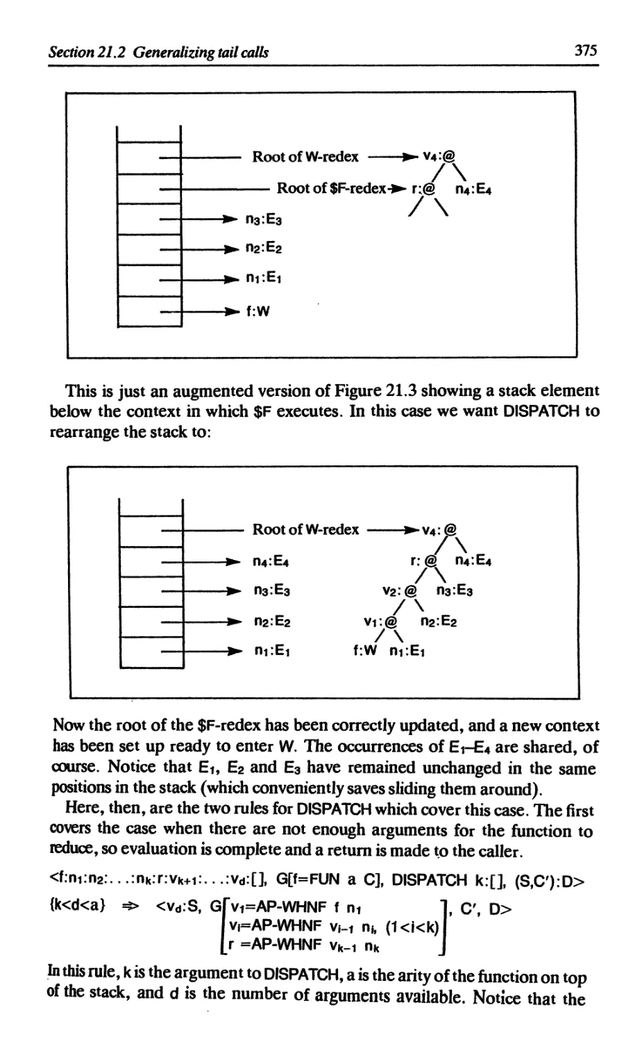
21.2.5 W is a function of more than three arguments 374
21.3 Compilation using DISPATCH 376
21.3.1 Compilation schemes for DISPATCH 376
21.3.2 Compile-time optimization of DISPATCH 376
21.4 Optimizing the E scheme 377
21.5 Comparison with environment-based implementations 378
References 379
22 STRICTNESS ANALYSIS 380
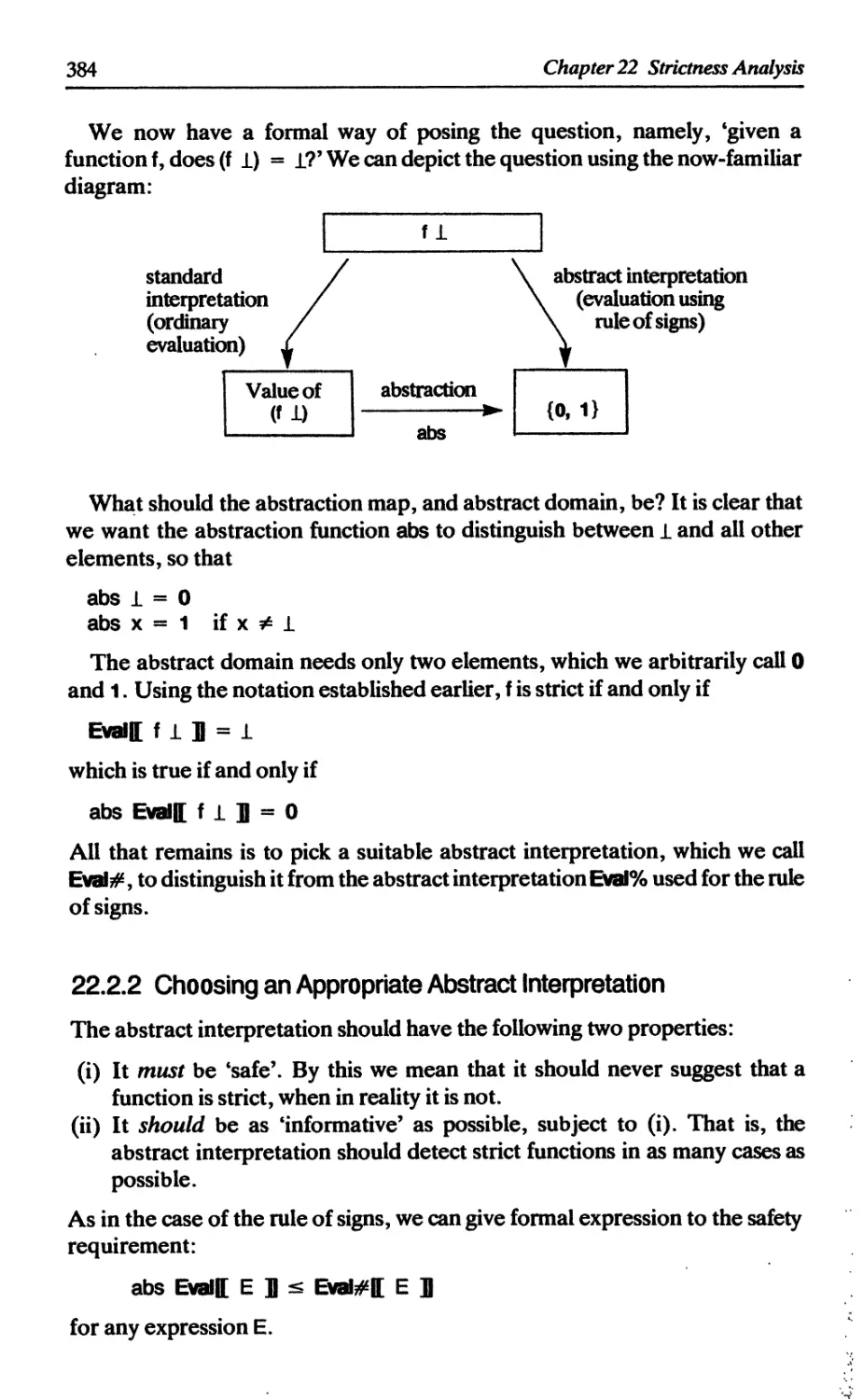
22.1 Abstract interpretation 380
22.1.1 An archetypical example - the rule of signs 380
22.1.2 History and references 383
22.2 Using abstract interpretation to do strictness analysis 383
22.2.1 Formulating the question 383
22.2.2 Choosing an appropriate abstract interpretation 384
22.2.3 Developing f# from f 386
22.2.4 Fitting strictness analysis into the compiler 387
One
INTRODUCTION
This book is about implementing functional programming languages using
Zazy graph reduction, and it divides into three parts.
The first part describes how to translate a high-level functional language
into an intermediate language, called the lambda calculus, including detailed
coverage of pattern-matching and type-checking. The second part begins with
a simple implementation of the lambda calculus, based on graph reduction,
and then develops a number of refinements and alternatives, such as super-
combinators, full laziness and SK combinators. Finally, the third part
describes the G-machine, a sophisticated implementation of graph reduction,
which provides a dramatic increase in performance over the implementations
described earlier.
One of the agreed advantages of functional languages is their semantic
simplicity. This simplicity has considerable payoffs in the book. Over and
over again we are able to make semi-formal arguments for the correctness of
the compilation algorithms, and the whole book has a distinctly mathematical
fiavor - an unusual feature in a book about implementations.
Most of the material to be presented has appeared in the published
literature in some form (though some has not), but mainly in the form of
conference proceedings and isolated papers. References to this work appear
at the end of each chapter.
1.1 Assumptions
This book is about implementations, not languages, so we shall make no
attempt to extol the virtues of functional languages or the functional
programming style. Instead we shall assume that the reader is familiar with
functional programming; those without this familiarity may find it heavy
1
2
Chapter 1 Introduction
going. A brief introduction to functional programming may be found in
Darlington [1984], while Henderson [1980] and Glaser et al. [1984] give more
substantial treatments. Another useful text is Abelson and Sussman [1985]
which describes Scheme, an almost-functional dialect of Lisp..
An encouraging consensus seems to be emerging in the basic features of
high-level functional programming languages, exemplified by languages such
as SASL [Turner, 1976], ML [Gordon et al., 1979], KRC (Turner, 1982],
Hope [Burstall et al., 1980], Ponder [Fairbairn, 1985], LML [Augustsson,
1984], Miranda [Turner, 1985] and Orwell [Wadler, 1985]. However, for the
sake of definiteness, we use the language Miranda as a concrete example
throughout the book (When used as the name of a programming language,
‘Miranda’ is a trademark of Research Software Limited.) A brief intro-
duction to Miranda may be found in the appendix, but no serious attempt is
made to give a tutorial about functional programming in general, or Miranda
in particular. For those familiar with functional programming, however, no
difficulties should arise.
Generally speaking, all the material of the book should apply to the other
functional languages mentioned, with only syntactic changes. The only
exception to this is that we concern ourselves almost exclusively with the
implementation of languages with поп-strict semantics (such as SASL, KRC,
Ponder, LML, Miranda and Orwell). The advantages and disadvantages of
this are discussed in Chapter 11, but it seems that graph reduction is probably
less attractive than the environment-based approach for the implementation
of languages with strict semantics; hence the focus on non-strict languages.
However, some functional languages are strict (ML and Hope, for example),
and while much of the book is still relevant to strict languages, some of the
material would need to be interpreted with care.
The emphasis throughout is on an informal approach, aimed at developing
understanding rather than at formal rigor. It would be an interesting task to
rewrite the book in a formal way, giving watertight proofs of correctness at
each stage.
1.2 Part I: Compiling High-level Functional Languages
It has been widely observed that most functional languages are quite similar to
each other, and differ more in their syntax than their semantics. In order to
simplify our thinking about implementations, the first part of this book shows
how to translate a high-level functional program into an intermediate language
which has a very simple syntax and semantics. Then, in the second and third
parts of the book, we will show how to implement this intermediate language
using graph reduction. Proceeding in this way allows us to describe graph
reduction in considerable detail, but in a way that is not specific to any
particular high-level language.
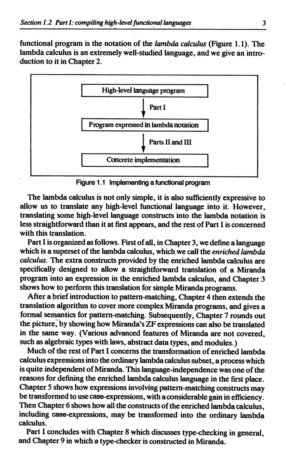
The intermediate language into which we will translate the high-level
Section 1,2 Part I: compiling high-level functional languages
3
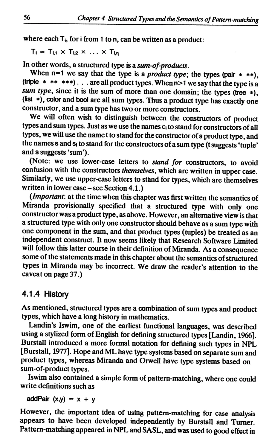
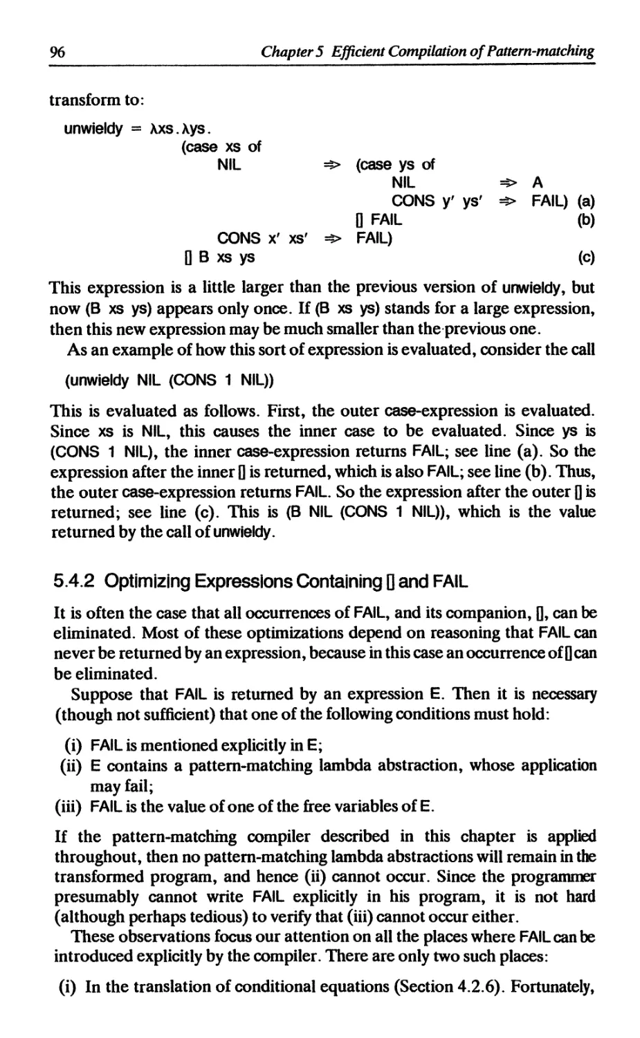
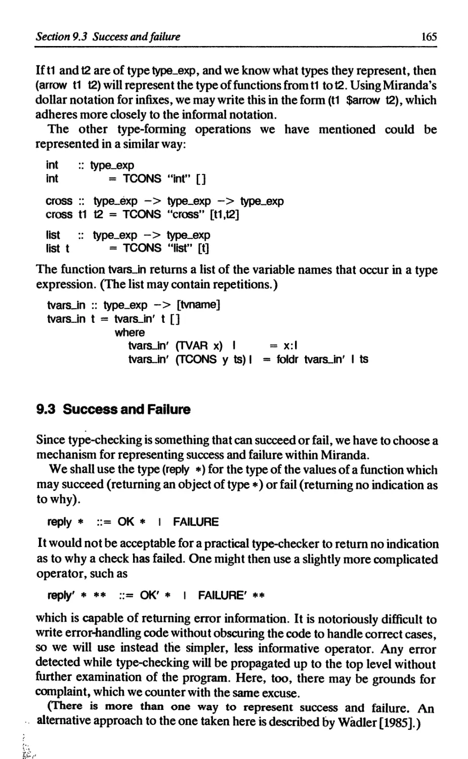
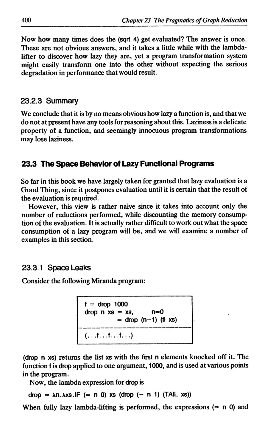
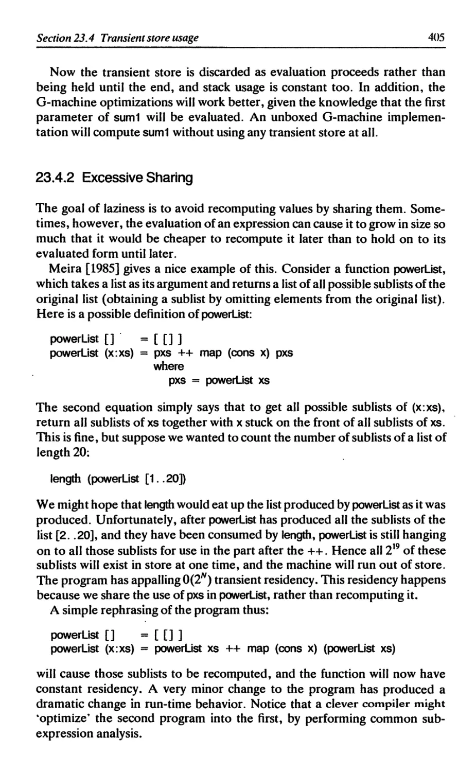
functional program is the notation of the lambda calculus (Figure 1.1). The
lambda calculus is an extremely well-studied language, and we give an intro-
duction to it in Chapter 2.
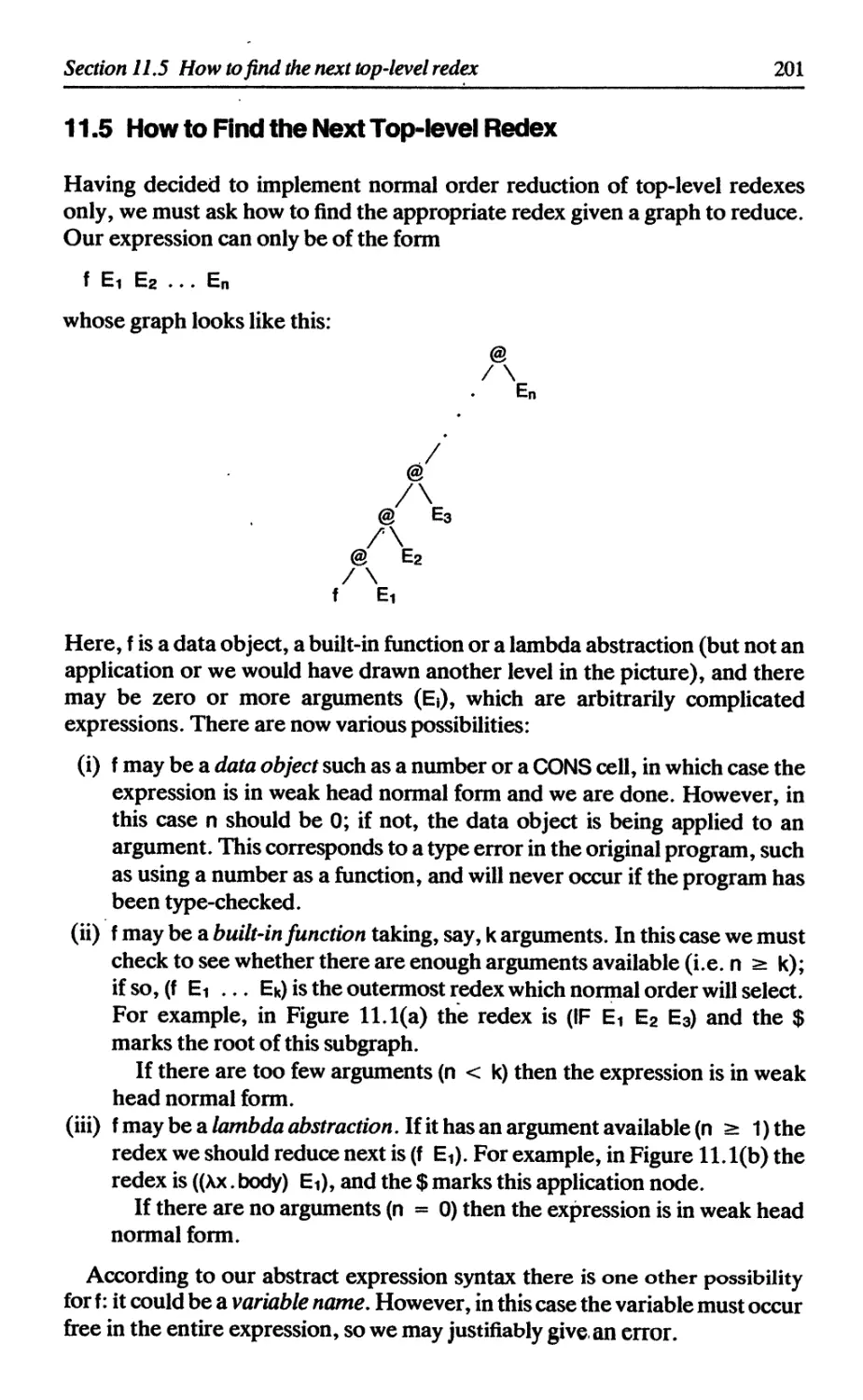
High-level language program
Parti
v
Program expressed in lambda notation
Parts II and III
v
Concrete implementation
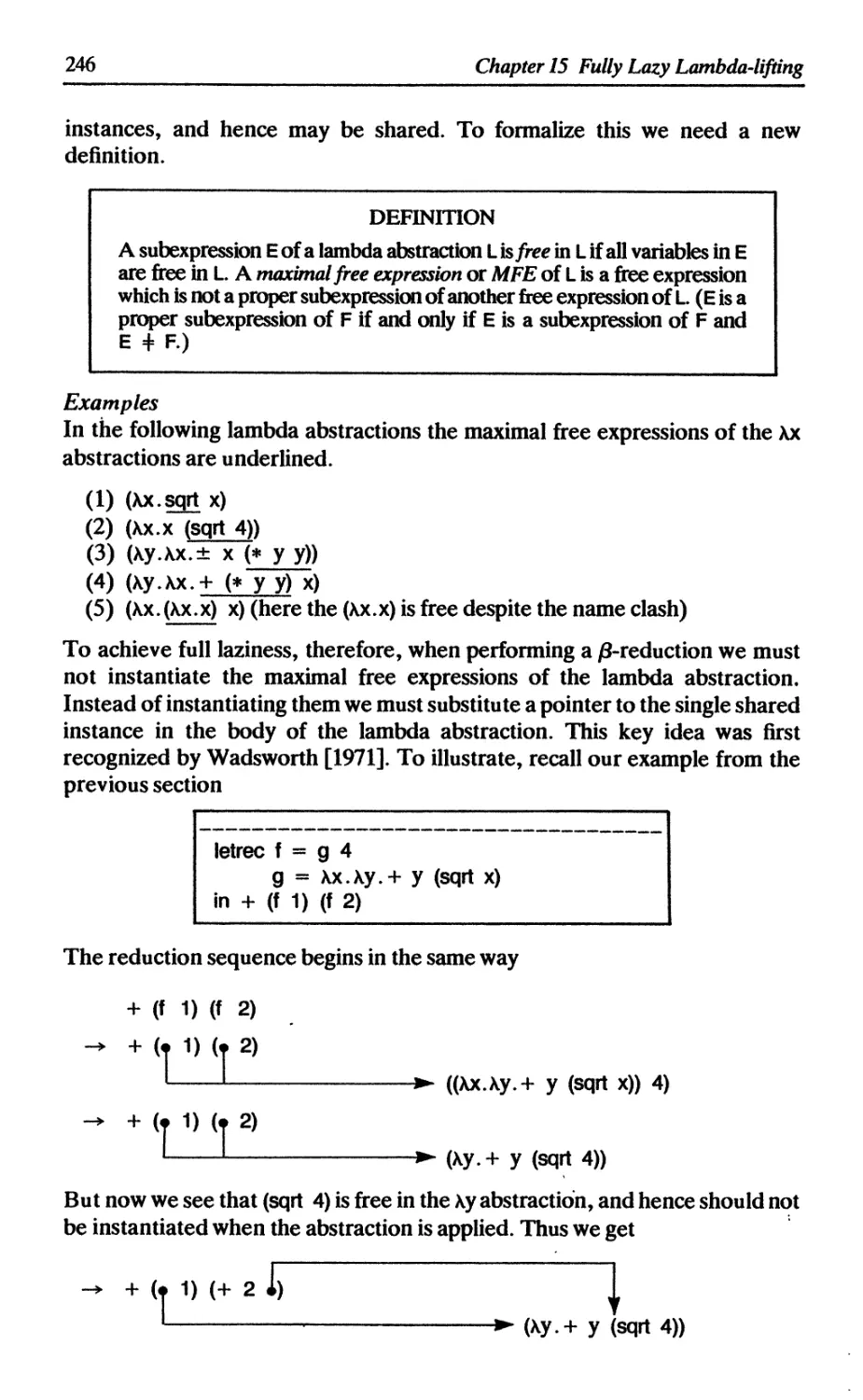
Figure 1.1 Implementing a functional program
The lambda calculus is not only simple, it is also sufficiently expressive to
allow us to translate any high-level functional language into it. However,
translating some high-level language constructs into the lambda notation is
less straightforward than it at first appears, and the rest of Part I is concerned
with this translation.
Part I is organized as follows. First of all, in Chapter 3, we define a language
which is a superset of the lambda calculus, which we call the enriched lambda
calculus. The extra constructs provided by the enriched lambda calculus are
specifically designed to allow a straightforward translation of a Miranda
program into an expression in the enriched lambda calculus, and Chapter 3
shows how to perform this translation for simple Miranda programs.
After a brief introduction to pattern-matching, Chapter 4 then extends the
translation algorithm to cover more complex Miranda programs, and gives a
formal semantics for pattern-matching. Subsequently, Chapter 7 rounds out
the picture, by showing how Miranda's ZF expressions can also be translated
in the same way. (Various advanced features of Miranda are not covered,
such as algebraic types with laws, abstract data types, and modules.)
Much of the rest of Part I concerns the transformation of enriched lambda
calculus expressions into the ordinary lambda calculus subset, a process which
is quite independent of Miranda. This language-independence was one of the
reasons for defining the enriched lambda calculus language in the first place.
Chapter 5 shows how expressions involving pattern-matching constructs may
be transformed to use case-expressions, with a considerable gain in efficiency.
Then Chapter 6 shows how all the constructs of the enriched lambda calculus,
including case-expressions, may be transformed into the ordinary lambda
calculus.
Part I concludes with Chapter 8 which discusses type-checking in general,
and Chapter 9 in which a type-checker is constructed in Miranda.
4
Chapter 1 Introduction
1.3 Part II: Graph Reduction
The rest of the book describes how the lambda calculus may be implemented
using a technique called graph reduction. It is largely independent of the later
chapters in Part I, Chapters 2-4 being the essential prerequisites.
As a foretaste of things to come, we offer the following brief introduction to
graph reduction. Suppose that the function f is defined (in Miranda) like this:
f X = (X + 1) ♦ (X - 1)
This definition specifies that f is a function of a single argument x, which
computes ‘(x + 1) * (x - 1)’. Now suppose that we are required to evaluate
f 4
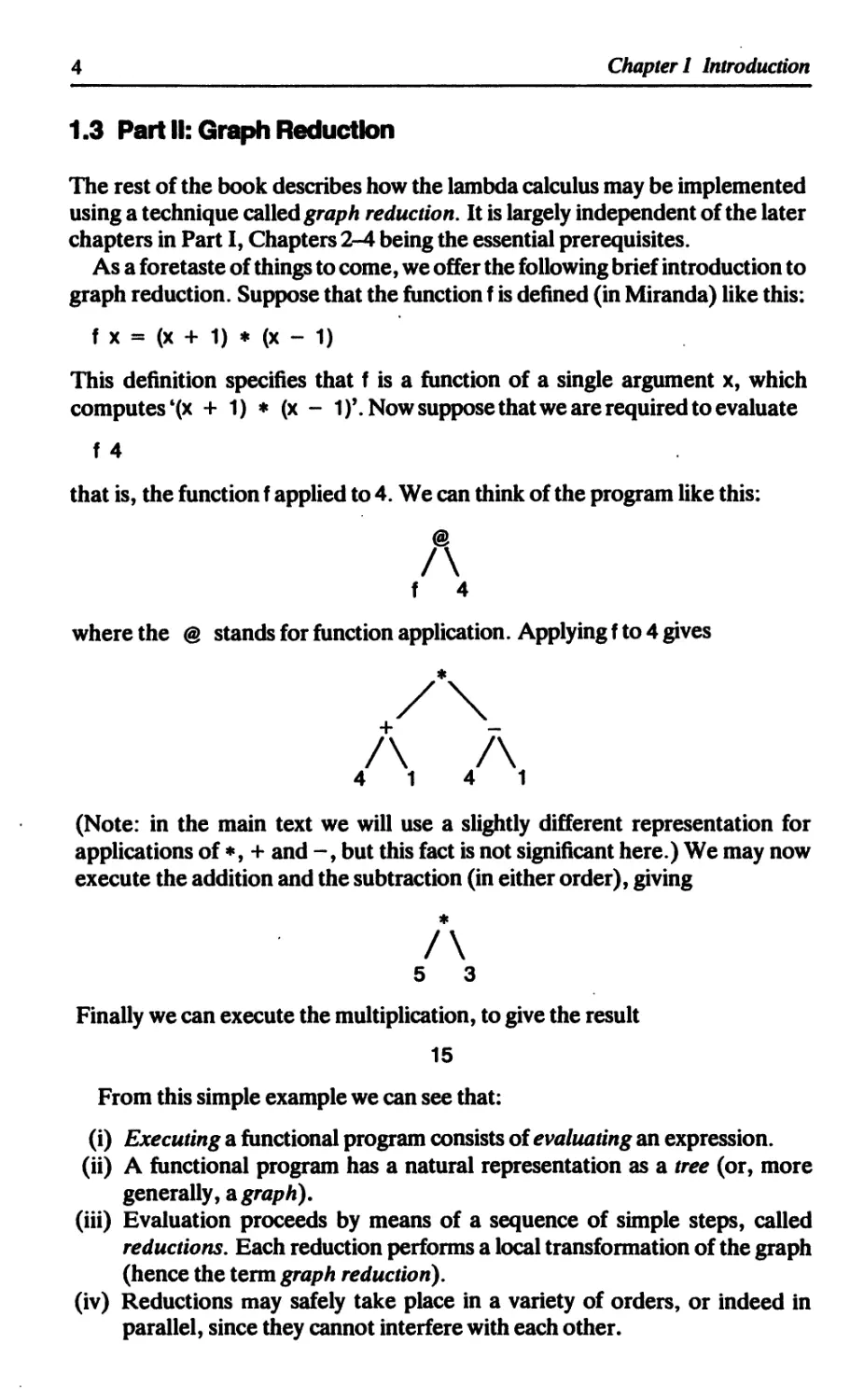
that is, the function f applied to 4. We can think of the program like this:
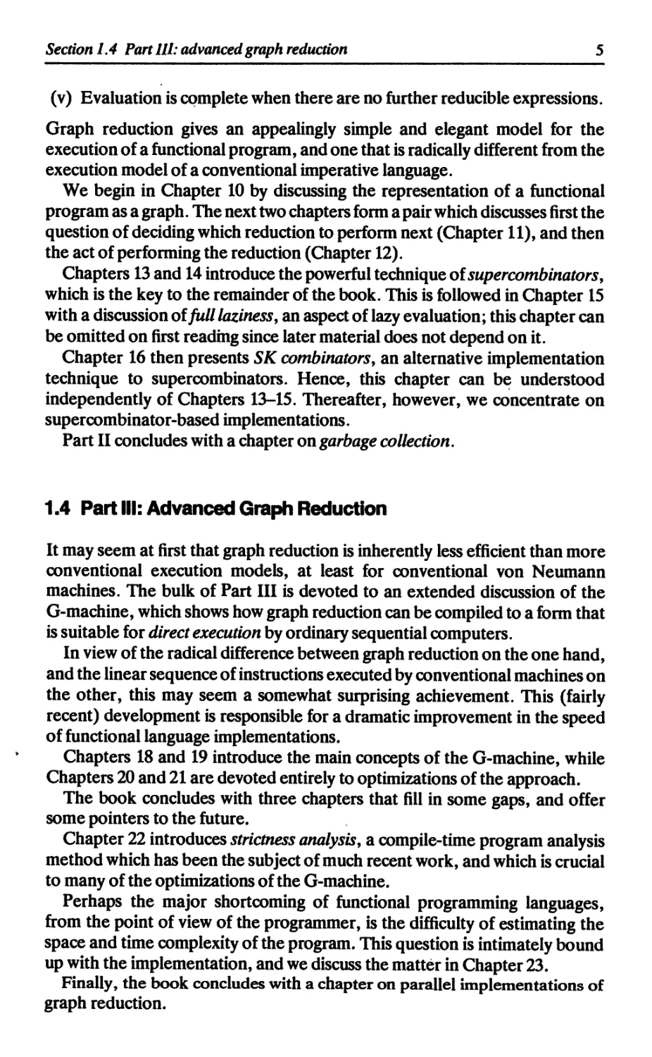
where the @ stands for function application. Applying f to 4 gives
(Note: in the main text we will use a slightly different representation for
applications of *, + and but this fact is not significant here.) We may now
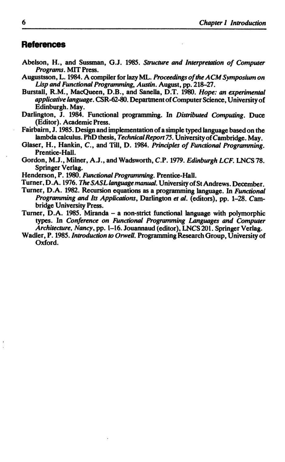
execute the addition and the subtraction (in either order), giving
♦
5 3
Finally we can execute the multiplication, to give the result
15
From this simple example we can see that:
(i) Executing a functional program consists of evaluating an expression.
(ii) A functional program has a natural representation as a tree (or, more
generally, a graph).
(iii) Evaluation proceeds by means of a sequence of simple steps, called
reductions. Each reduction performs a local transformation of the graph
(hence the term graph reduction).
(iv) Reductions may safely take place in a variety of orders, or indeed in
parallel, since they cannot interfere with each other.
Section 1.4 Part 111: advanced graph reduction
5
(v) Evaluation is complete when there are no further reducible expressions.
Graph reduction gives an appealingly simple and elegant model for the
execution of a functional program, and one that is radically different from the
execution model of a conventional imperative language.
We begin in Chapter 10 by discussing the representation of a functional
program as a graph. The next two chapters form a pair which discusses first the
question of deciding which reduction to perform next (Chapter 11), and then
the act of performing the reduction (Chapter 12).
Chapters 13 and 14 introduce the powerful technique of supercombinators,
which is the key to the remainder of the book. This is followed in Chapter 15
with a discussion of full laziness, an aspect of lazy evaluation; this chapter can
be omitted on first reading since later material does not depend on it.
Chapter 16 then presents SK combinators, an alternative implementation
technique to supercombinators. Hence, this chapter can be understood
independently of Chapters 13-15. Thereafter, however, we concentrate on
supercombinator-based implementations.
Part II concludes with a chapter on garbage collection.
1.4 Part III: Advanced Graph Reduction
It may seem at first that graph reduction is inherently less efficient than more
conventional execution models, at least for conventional von Neumann
machines. The bulk of Part III is devoted to an extended discussion of the
G-machine, which shows how graph reduction can be compiled to a form that
is suitable for direct execution by ordinary sequential computers.
In view of the radical difference between graph reduction on the one hand,
and the linear sequence of instructions executed by conventional machines on
the other, this may seem a somewhat surprising achievement. This (fairly
recent) development is responsible for a dramatic improvement in the speed
of functional language implementations.
Chapters 18 and 19 introduce the main concepts of the G-machine, while
Chapters 20 and 21 are devoted entirely to optimizations of the approach.
The book concludes with three chapters that fill in some gaps, and offer
some pointers to the future.
Chapter 22 introduces strictness analysis, a compile-time program analysis
method which has been the subject of much recent work, and which is crucial
to many of the optimizations of the G-machine.
Perhaps the major shortcoming of functional programming languages,
from the point of view of the programmer, is the difficulty of estimating the
space and time complexity of the program. This question is intimately bound
up with the implementation, and we discuss the matter in Chapter 23.
Finally, the book concludes with a chapter on parallel implementations of
graph reduction.
6
Chapter 1 Introduction
References
Abelson, Н.» and Sussman, GJ. 1985. Structure and Interpretation of Computer
Programs. MIT Press.
Augustsson, L. 1984. A compiler for lazy ML. Proceedings of the ACM Symposium on
Lisp and Functional Programming, Austin. August, pp. 218-27.
Burstall, R.M., MacQueen, D.B., and Sanella, D.T. 1980. Hope: an experimental
applicative language. CSR-62-80. Department of Computer Science, University of
Edinburgh. May.
Darlington, J. 1984. Functional programming. In Distributed Computing. Duce
(Editor). Academic Press.
Fairbairn, J. 1985. Design and implementation of a simple typed language based on the
lambda calculus. PhD thesis, Technical Report 75. University of Cambridge. May.
Glaser, H., Hankin, C., and Till, D. 1984. Principles of Functional Programming.
Prentice-Hall.
Gordon, M.J., Milner, A.J., and Wadsworth, C.P. 1979. Edinburgh LCF. LNCS 78.
Springer Verlag.
Henderson, P. 1980. Functional Programming. Prentice-Hall.
Turner, D.A. 1976. The SASL language manual. University of St Andrews. December.
Turner, D.A. 1982. Recursion equations as a programming language. In Functional
Programming and Its Applications, Darlington et al. (editors), pp. 1-28. Cam-
bridge University Press.
Turner, D.A. 1985. Miranda - a non-strict functional language with polymorphic
types. In Conference on Functional Programming Languages and Computer
Architecture, Nancy, pp. 1—16. Jouannaud (editor), LNCS 201. Springer Verlag.
Wadler, P. 1985. Introduction to Orwell. Programming Research Group, University of
Oxford.
Parti
COMPILING HIGH-LEVEL
FUNCTIONAL LANGUAGES
Two
THE LAMBDA CALCULUS
This chapter introduces the lambda calculus, a simple language which will be
used throughout the rest of the book as a bridge between high-level functional
languages and their low-level implementations. The reasons for introducing
the lambda calculus as an intermediate language are:
(i) It is a simple language, with only a few, syntactic constructs, and simple
semantics. These properties make it a good basis for a discussion of
implementations, because an implementation of the lambda calculus only
has to support a few constructs, and the simple semantics allows us to
reason about the correctness of the implementation.
(ii) It is an expressive language, which is sufficiently powerful to express all
functional programs (and indeed, all computable functions). This means
that if we have an implementation of the lambda calculus, we can
implement any other functional language by translating it into the lambda
calculus.
In this chapter we focus on the syntax and semantics of the lambda calculus
itself, before turning our attention to high-level functional languages in the
next chapter.
2.1 The Syntax of the Lambda Calculus
Here is a simple expression in the lambda calculus:
(+4 5)
All function applications m the lambda calculus are written in prefix form, so,
9
10
Chapter 2 The Lambda Calculus
for example, the function + precedes its arguments 4 and 5. A slightly more
complex example, showing the (quite conventional) use of brackets, is
(+ (* 5 6) (* 8 3))
In both examples, the outermost brackets are redundant, but have been
added for clarity (see Section 2.1.2).
From the implementation viewpoint, a functional program should be
thought of as an expression, which is ‘executed’ by evaluating it. Evaluation
proceeds by repeatedly selecting a reducible expression (or redex) and
reducing it. In our last example there are two redexes: (* 5 6) and (* 8 3).
The whole expression (+ (* 5 6) (* 8 3)) is not a redex, since a + needs to be
applied to two numbers before it is reducible. Arbitrarily choosing the first
redex for reduction, we write
(+ (♦ 5 6) (* 8 3)) -* (+ 30 (* 8 3))
where the-* is pronounced‘reduces to’. Now there is only one redex, (* 8 3),
which gives
(+ 30 (* 8 3)) -* (+ 30 24)
This reduction creates a new redex, which we now reduce
(+ 30 24) -* 54
When there are several redexes we have a choice of which one to reduce
first. This issue will be addressed later in this chapter.
2.1.1 Function Application and Currying
In the lambda calculus, function application is so important that it is denoted
by simple juxtaposition; thus we write
f x
to denote ‘the function f applied to the argument x’. How should we express
the application of a function to several arguments? We could use a new
notation, like (f (x,y)), but instead we use a simple and rather ingenious
alternative. To express ‘the sum of 3 and 4’ we write
((+ 3) 4)
The expression (+ 3) denotes the function that adds 3 to its argument. Thus
the whole expression means ‘the function + applied to the argument 3, the
result of which is a function applied to 4’. (In common with all functional
programming languages, the lambda calculus allows a function to return a
function as its result.)
This device allows us to think of all functions as having a single argument
only. It was introduced by Schonfinkel [1924] and extensively used by Curry
[Curry and Feys, 1958]; as a result it is known as currying.
Section 2.1 The syntax of the lambda calculus
11
2.1.2 Use of Brackets
In mathematics it is conventional to omit redundant brackets to avoid
cluttering up expressions. For example, we might omit brackets from the
expression
(ab) + ((2c)/d)
to give
ab + 2с/d
The second expression is easier to read than the first, but there is a danger that
it may be ambiguous. It is rendered unambiguous by establishing conventions
about the precedence of the various functions (for example, multiplication
binds more tightly than addition)..
Sometimes brackets cannot be omitted, as in the expression:
(b + c)la
Similar conventions are usefill when writing down expressions in the
lambda calculus. Consider the expression:
((+ 3) 2)
By establishing the convention that function application associates to the left,
we can write the expression more simply as:
(+ 3 2)
or even
+ 32
We performed some such abbreviations in the examples given earlier. As a
more complicated example, the expression:
((f ((+ 4) 3)) (g x))
is fully bracketed and unambiguous. Following our convention, we may omit
redundant brackets to make the expression easier to read, giving:
f (+ 4 3) (g x)
No further brackets can be omitted. Extra brackets may, of course, be
inserted freely without changing the meaning of the expression; for example
(f (+ 4 3) (g x))
is the same expression again.
2.1.3 Built-in Functions and Constants
In its purest form the lambda calculus does not have built-in functions such as
+, but our intentions are practical and so we extend the pure lambda calculus
with a suitable collection of such built-in functions.
12
Chapter 2 The Lambda Calculus
These include arithmetic functions (such as +, -, *, /) and constants (0, 1,
. . .), logical functions (such as AND, OR, NOT) and constants (TRUE,
FALSE), and character constants (‘a’, ‘b’,...). For example
- 54 1
AND TRUE FALSE -► FALSE
We also include a conditional function, IF, whose behavior is described by the
reduction rules:
IF TRUE Et Ef -+ Et
IF FALSE Et Ef -> Ef
We will initially introduce data constructors into the lambda calculus by
using the built-in functions CONS (short for CONSTRUCT), HEAD and TAIL
(which behave exactly like the Lisp functions CONS, CAR and CDR). The
constructor CONS builds a compound object which can be taken apart with
HEAD and TAIL. We may describe their operation by the following rules:
HEAD (CONS a b) -> a
TAIL (CONS a b) -> b
We also include NIL, the empty list, as a constant. The data constructors will
be discussed at greater length in Chapter 4.
The exact choice of built-m functions is, of course, somewhat arbitrary, and
further ones will be added as the need arises.
2.1.4 Lambda Abstractions
The only functions introduced so far have been the built-in functions (such as
+ and CONS). However, the lambda calculus provides a construct, called a
lambda abstraction, to denote new (non-built-m) functions. A lambda
abstraction is a particular sort of expression which denotes a function. Here is
an example of a lambda abstraction:
(Xx . + x 1)
The X says ‘here comes a function’, and is immediately followed by a variable,
x in this case; then comes a . followed by the body of the function, (+ x1) in
this case. The variable is called the formal parameter, and we say that the X
binds it. You can think of it like this:
(X x . + x 1)
That function of x which adds x to 1
A lambda abstraction always consists of all the four parts mentioned: the X,
the formal parameter, the. and the body.
Section 2.1 The syntax of the lambda calculus
13
A lambda abstraction is rather similar to a function definition in a
conventional language, such as C:
lnc( x )
int x;
{retum( x + 1 );}
The formal parameter of the lambda abstraction corresponds to the formal
parameter of the function, and the body of the abstraction is an expression
rather than a sequence of commands. However, functions in conventional
languages must have a name (such as Inc), whereas lambda abstractions are
"anonymous9 functions.
The body of a lambda abstraction extends as far to the right as possible, so
that in the expression
(Xx.+ x 1) 4
the body of the Xx abstraction is (+ x 1), not just +. As usual, we may add
extra brackets to clarify, thus
(Xx.(+ x 1)) 4
When a lambda abstraction appears in isolation we may write it without any
brackets:
Xx.+ x 1
2.1.5 Summary
We define a lambda expression to be an expression in the lambda calculus, and
Figure 2.1 summarizes the forms which a lambda expression may take. Notice
that a lambda abstraction is not the same as a lambda expression; in fact the
former is a particular instance of the latter.
<exp> : : = <constant> Built-in constants
I <variable> Variable names
I <exp> <exp> Applications
I X <variable> .<exp> Lambda abstractions
This is the abstract syntax of lambda expressions. In order to write down
such an expression in concrete form we use brackets to disambiguate its
structure (see Section 2.1.2).
We will use lower-case letters for variables (e.g. x, f), and upper-case
letters to stand for whole lambda expressions (e.g. M, E).
The choice of constants is rather arbitrary; we assume integers and
booleans (e.g. 4, TRUE), together with built-in functions to manipulate
them (e.g. AND, IF, +). We also assume built-in list-processing functions
(e.g. CONS, HEAD).
Figure 2.1 Syntax of a lambda expression (in BNF)
14
Chapter! The Lambda Calculus
In what follows we will use lower-case names for variables, and single
upper-case letters to stand for whole lambda expressions. For example we
might say ‘for any lambda expression E,. . .,’. We will also write the names of
built-in ftmctions in upper case, but no confusion should arise.
2.2 The Operational Semantics of the Lambda Calculus
So far we have described only the syntax of the lambda calculus, but to dignify
it with the title of a ‘calculus’ we must say how to ‘calculate’ with it. We will do
this by giving three conversion rules which describe how to convert one
lambda expression into another.
First, however, we introduce an important piece of terminology.
2.2.1 Bound and Free Variables
Consider the lambda expression
(Xx.+ x y) 4
In order to evaluate this expression completely, we need to know the ‘global’
value of у. In contrast, we do not need to know a ‘global’ value for x, since it is
just the formal parameter of the function, so we see that x and у have a rather
different status.
The reason is that x occurs bound by the Xx; it is just a ‘hole’ into which the
argument 4 is placed when applying the lambda abstraction to its argument.
An occurrence of a variable must be either free or bound.
Definition of 'occurs free9
x occurs free in x(but not in any other variable or constant)
x occurs free in (E F) < x occurs free in. E or xoccurs free in F
xoccursfree in Xy.E < xand у are different variables and xoccurs free in E
Definition of'occurs bound9 x occurs bound in (E F) < xoccurs bound in E or xoccurs bound in F
xoccurs bound in xy.E < ££> (xand у are the same variable andxoccurs free in E) or xoccurs bound in E
(No variable occurs bound in an expression consisting of a single constant
or variable.)
Note: ‘<=>’ means ‘if and only if’
Figure 2.2 Definitions of bound and free
Section 2,2 The operational semantics of the lambda calculus 15
On the other hand, у is not bound by any X, and so occurs free in the
expression. In general, the value of an expression depends only on the values
of its free variables.
An occurrence of a variable is bound if there is an enclosing lambda
abstraction which binds it, and is free otherwise. For example, x and у occur
bound, but z occurs free in this example:
Xx.+ ((Ху. + у z) 7) x
Notice that the terms ‘bound’ and ‘free’ refer to specific occurrences of the
variable in an expression. This is because a variable may have both a bound
occurrence and a free occurrence in an expression; consider for example
+ x ((Xx.+ x 1) 4)
in which x occurs free (the first time) and bound (the second time). Each
individual occurrence of a variable must be either free or bound.
Figure 2.2 gives formal definitions for ‘free’ and ‘bound’, which cover the
forms of lambda expression given in Figure 2.1 case by case.
2.2.2 Beta-conversion
A lambda abstraction denotes a function, so we must describe how to apply it
to an argument. For example, the expression
(Xx.+ x 1) 4
is the juxtaposition of the lambda abstraction (Xx.+ x 1) and the argument 4,
and hence denotes the application of a certain function, denoted by the
lambda abstraction, to the argument 4. The rule for such function application
is very simple:
The result of applying a lambda abstraction to an argument is an instance of
the body of the lambda abstraction in which (free) occurrences of the
formal parameter in the body are replaced with (copies of) the argument.
Thus the result of applying the lambda abstraction (Xx.+ x 1) to the
argument 4 is
+ 4 1
The (+ 4 1) is an instance of the body (+ x 1) in which occurrences of the
formal parameter, x, are replaced with the argument, 4. We write the
reduction using the arrow as before:
(Xx.+ x 1) 4 -> + 4 1
This operation is called ft-reduction, and much of this book is concerned with
its efficient implementation. We will use a series of examples to show in detail
how ^-reduction works.
16
Chapter 2 The Lambda Calculus
2,2,2,1 Simple examples of beta-reduction
The formal parameter may occur several times in the body:
(Xx.+ x x) 5 -> +55
10
Equally, there may be no occurrences of the formal parameter in the body:
(Xx.3) 5 3
In this case there are no occurrences of the formal parameter (x) for which the
argument (5) should be substituted, so the argument is discarded unused.
The body of a lambda abstraction may consist of another lambda
abstraction:
(Xx.(Xy.~ у x)) 4 5 (Xy.—у 4) 5
- 54
-> 1
Notice that, when constructing an instance of the body of the Xx abstraction,
we copy the entire body including the embedded Xy abstraction (while
substituting for x, of course). Here we see currying in action: the application
of the Xx abstraction returned a function (the Xy abstraction) as its result,
which when applied yielded the result (- 5 4).
We often abbreviate
(Xx.(Xy.E))
to
(Xx.Xy.E)
Functions can be arguments too:
(Xf.f 3) (Xx.+ x 1) —> (xx.+ x 1) 3
-^+3 1
4
An instance of the Xx abstraction is substituted for f wherever f appears in the
body of the Xf abstraction.
2«2«2«2 Naming
Some slight care is needed when formal parameter names are not unique. For
example
(Xx.(Xx.+ (- x 1)) x 3) 9
- > (Xx.+ (- x 1)) 9 3
- » + (- 9 1) 3
- > 11
Notice that we did not substitute for the inner x in the first reduction, because
it was shielded by the enclosing Xx; that is, the inner occurrence of x is not free
in the body of the outer Xx abstraction.
Section 2.2 The operational semantics of the lambda calculus
17
Given a lambda abstraction (Xx.E), how can we identify exactly those
occurrences of x which should be substituted for? It is easy: we should
substitute for those occurrences ofx which are free in E, because, if they are
free in E, then they will be bound by the Xx abstraction (Xx.E). So, when
applying the outer Xx abstraction in the above example, we examine its body
(Xx.+ (- x 1)) x 3
and see that only the second occurrence of x is free, and hence qualifies for
substitution.
This is why the rule given above specified that only the free occurrences of
the formal parameter in the body are to be substituted for. The nesting of the
scope of variables in a block-structured language is closely analogous to this
rule.
Here is another example of the same kind
(Xx.Xy.+ x ((Xx.- x 3) y)) 5 6
(Xy.+ 5 ((Xx.- x 3) y)) 6
-» + 5 ((Xx.- x 3) 6)
+ 5 (- 6 3)
8
Again, the inner x is not substituted for in the first reduction, since it is not free
in the body of the outer Xx abstraction.
2.2.2.3 A larger example
As a larger example, we will demonstrate the somewhat surprising fact that
data constructors can actually be modelled as pure lambda abstractions. We
define CONS, HEAD and TAIL in the following way:
CONS = (Xa.Xb.Xf.f a b)
HEAD = (Xc.c (Xa.Xb.a))
TAIL = (Xc.c (Xa.Xb.b))
These obey the rules for CONS, HEAD and TAIL given in Section 2.1.3. For
example,
HEAD (CONS p q)
= (Xc.c (Xa.Xb.a)) (CONS p q)
-* CONS p q (Xa.Xb.a)
= (Xa.Xb.Xf. f a b) p q (Xa.Xb.a)
-* (Xb.Xf. f p b) q (Xa.Xb.a)
-* (Xf. f p q) (Xa.Xb.a)
-* (Xa.Xb.a) p q
(Xb.p) q
-* P
This means, incidentally, that there is no essential need for the built-in
functions CONS, HEAD and TAIL, and it turns out that all the other built-in
18
Chapter 2 The Lambda Calculus
functions can also be modelled as lambda abstractions. This is rather satis-
fying from a theoretical viewpoint, but all practical implementations support
built-in functions for efficiency reasons.
Z.2.2.4 Conversion, reduction and abstraction
We can use the Д-rule backwards, to introduce new lambda abstractions, thus
+ 41 (Xx.+ x 1) 4
This operation is called ^-abstraction, which we denote with a backwards
reduction arrow W. 0-conversion means Д-reduction or Д-abstraction, and
we denote it with a double-ended arrow W. Thus we write
+ 4 1 у (Xx.+ x 1) 4
The arrow is decorated with ft to distinguish Д-conversion from the other
forms of conversion we will meet shortly. An undecorated reduction arrow
W will stand for one or more Д-reductions, or reductions of the built-in
functions. An undecorated conversion arrow W will stand for zero or more
conversions, of any kind.
Rather than regarding Д-reduction and Д-abstraction as operations, we can
regard Д-conversion as expressing the equivalence of two expressions which
‘look different’ but ‘ought to mean the same’. It turns out that we need two
more rules to satisfy our intuitions about the equivalence of expressions, and
we turn to these rules in the next two sections.
2.2.3 Alpha-conversion
Consider the two lambda abstractions
(Xx.+ x 1)
and
(Xy.+ у 1)
Clearly they ‘ought’ to be equivalent, and а-conversion allows us to change
the name of the formal parameter of any lambda abstraction, so long as we do
so consistently. So
(Xx. + x 1) *-> (Xy.+ у 1)
a,
where the arrow is decorated with an a to specify an «-conversion. The newly
introduced name must not, of course, occur free in the body of the original
lambda abstraction, «-conversion is used solely to eliminate the sort of name
clashes exhibited in the example in the previous section.
Sometimes «-conversion is essential (see Section 2.2.6).
Section 2.2 The operational semantics of the lambda calculus
19
2.2.4 Eta-conversion
One more conversion rule is necessary to express our intuitions about what
lambda abstractions ‘ought’ to be equivalent. Consider the two expressions
(Xx.+ 1 x)
and
(+ 1)
These expressions behave in exactly the same way when applied to an
argument: they add 1 to it. ^-conversion is a rule expressing their equivalence:
(Xx.+ 1 x) «-> (+ 1)
More generally, we can express the ^-conversion rule like this:
(Xx.F x) ++ F
provided x does not occur free in F, and F denotes a function.
The condition that x does not occur free in F prevents false conversions. For
example,
(Xx.+ x x)
is not ^-convertible to
(+ x)
because x occurs free in (+ x). The condition that F denotes a function
prevents other false conversions involving built-in constants; for example:
TRUE
is not ^-convertible to
(Xx.TRUE x)
When the ^-conversion rule is used from left to right it is called reduction.
2.2.5 Proving Interconvertibility
We will quite frequently want to prove the interconvertibility of two lambda
expressions. When the two expressions denote a function such proofs can
become rather tedious, and in this section we will demonstrate a convenient
method that abbreviates the proof without sacrificing rigor.
As an example, consider the two lambda expressions:
IF TRUE ((Xp.p) 3)
and
(Xx.3)
20
Chapter 2 The Lambda Calculus
Both denote the same function, namely the function which always delivers the
result 3 regardless of the value of its argument, and we might hope that they
were interconvertible. This hope is justified, as the following sequence of
conversions shows:
IF TRUE ((Xp.p) 3) у IF TRUE 3
(Xx.lF TRUE 3 x)
(Xx.3)
The final step is the reduction rule for IF.
An alternative method of proving convertibility of expressions denoting
functions, which is often more convenient, is to apply both expressions to an
arbitrary argument, w, say:
IF TRUE ((Xp.p) 3) w (Xx.3) w
(Xp.p) 3 -> 3
3
Hence
(IF TRUE ((Xp.p) 3)) (Xx. 3)
This proof has the advantage that it only uses reduction, and it avoids the
explicit use of ^-conversion. If it is not immediately clear why the final step is
justified, consider the general case, in which we are given two lambda
expressions Fi and F2. If we can show that
Fi w E
and
F2 w -> E
where w is a variable which does not occur free in Fi or F2, and E is some
expression, then we can reason as follows:
Fi у (Xw.Fi w)
(Xw.E)
(XW.F2 w)
F2
and hence Fi F2.
It is not always the case that lambda expressions which ‘ought’ to mean the
same thing are interconvertible, and we will have more to say about this point
in Section 2.5.
2.2.6 The Name-capture Problem
As a warning to the unwary we now give an example to show why the lambda
calculus is trickier than meets the eye. Fortunately, it turns out that none of
Section 2.2 The operational semantics of the lambda calculus
21
our implementations will come across this problem, so this section can safely
be omitted on first reading.
Suppose we define a lambda abstraction TWICE thus:
TWICE = (Xf.Xx.f (f x))
Now consider reducing the expression (TWICE TWICE) using ^-reductions:
TWICE TWICE
= (Xf.Xx.f (f x)) TWICE
-> (Xx.TWICE (TWICE x))
Now there are two j8-redexes, (TWICE x) and (TWICE (TWICE x)), so let us
(arbitrarily) choose the inner one for reduction, first expanding the TWICE to
its lambda abstraction:
= (Xx.TWICE ((Xf.Xx.f (f x)) x))
Now we see the problem. To apply TWICE to x, we must make a new instance
of the body of TWICE (underlined) replacing occurrences of the formal
parameter, f, with the argument, x. But x is already used as a formal parameter
inside the body. It is clearly wrong to reduce to
(Xx.TWICE ((Xf.Xx.f (f x)) x))
-» (Xx.TWICE (Xx.x (x x))) wrong]
because then the x substituted for f would be ‘captured’ by the inner Xx
abstraction. This is called the name-capture problem. One solution is to use
а-conversion to change the name of one of the Xx’s; for instance:
(XX.TWICE ((Xf.Xx.f (f X)) X))
♦j» (Xx.TWICE ((Xf.xy.f (f У)) x))
-> (XX.TWICE (Xy.x (x y))) right]
We conclude:
(i) ^-reduction is only valid provided the free-variables of the argument do
not clash with any formal parameters in th^ body of the lambda
abstraction.
(ii) «-conversion is sometimes necessary to avoid (i).
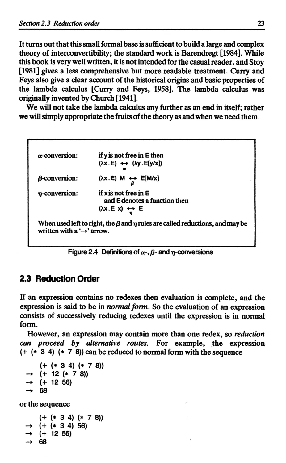
2.2.7 Summary of Conversion Rules
We have now developed three conversion rules which allow us to interconvert
expressions involving lambda abstractions. They are
(i) Name changing, а-conversion allows us to change the name of the formal
parameter of a lambda abstraction, so long as we do so consistently.
(ii) Function application, ^-reduction allows us to apply a lambda abstrac-
tion to an argument, by making a new instance of the body of the
Chapter! The Lambda Calculus
abstraction, substituting the argument for free occurrences of the formal
parameter. Special care needs to be taken when the argument contains
free variables.
(iii) Eliminating redundant lambda abstractions, ^reduction can sometimes
eliminate a lambda abstraction.
Within this framework we may also regard the built-in functions as one more
form of conversion, 8-conversion. For this reason the reduction rules for
built-in functions are sometimes called delta rules.
As we have seen, the application of the conversion rules is not always
straightforward, so it behoves us to give a formal definition of exactly what the
conversion rules are. This requires us to introduce one new piece of notation.
The notation
E[M/x]
means the expression E with M substituted for free occurrences of x.
As a mnemonic, imagine ‘multiplying’ E by M/x, giving M where the x’s
cancel out, so that x[M/x] = M. This notation allows us to express
^-conversion very simply:
(Xx.E) M *-> E[M/x]
p
and it is useful for а-conversion too.
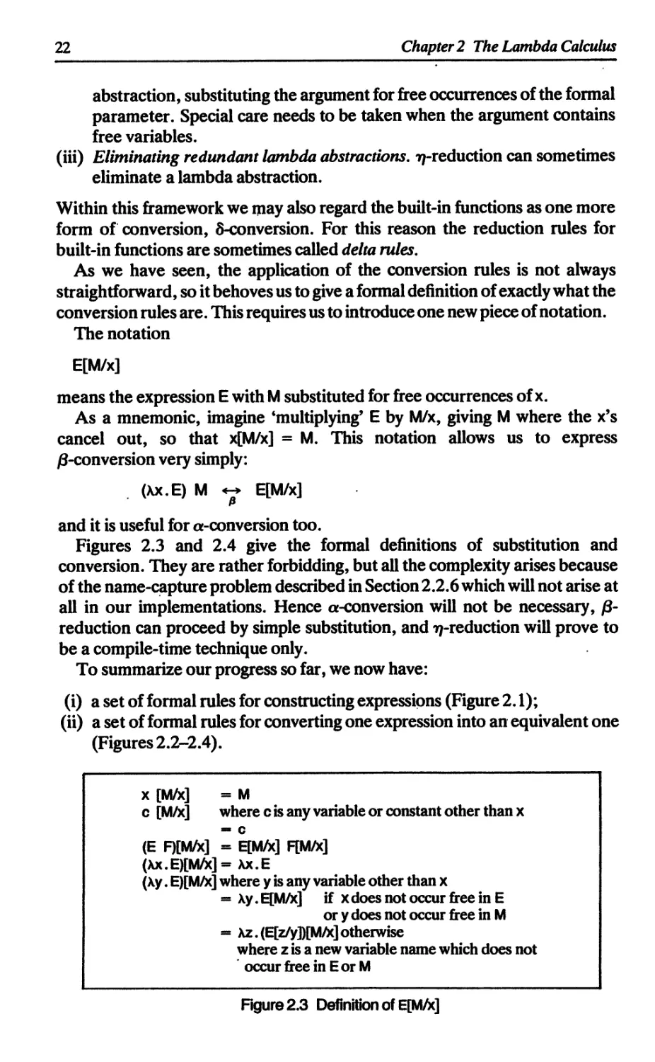
Figures 2.3 and 2.4 give the formal definitions of substitution and
conversion. They are rather forbidding, but all the complexity arises because
of the name-capture problem described in Section 2.2.6 which will not arise at
all in our implementations. Hence а-conversion will not be necessary, Д-
reduction can proceed by simple substitution, and ^-reduction will prove to
be a compile-time technique only.
To summarize our progress so far, we now have:
(i) a set of formal rules for constructing expressions (Figure 2.1);
(ii) a set of formal rules for converting one expression into an equivalent one
(Figures 2.2-2.4).
x [M/x] = M
c [M/x] where c is any variable or constant other than x
« c
(E F)[M/x] = E[M/x] F[M/x]
(Xx.E)[M/x] = Xx.E
(Xy. E)[M/x] where у is any variable other than x
= Xy. E[M/x] if xdoes not occur free in E
or у does not occur free in M
= Xz.(E[z/y])[M/x]otherwise
where z is a new variable name which does not
occur free in E or M
Figure 2.3 Definition of E[M/k]
Section 2.3 Reduction order
23
It turns out that this small formal base is sufficient to build a large and complex
theory of interconvertibility; the standard work is Barendregt [1984]. While
this book is very well written, it is not intended for the casual reader, and Stoy
[1981] gives a less comprehensive but more readable treatment. Curry and
Feys also give a clear account of the historical origins and basic properties of
the lambda calculus [Curry and Feys, 1958]. The lambda calculus was
originally invented by Church [1941].
We will not take the lambda calculus any further as an end in itself; rather
we will simply appropriate the fruits of the theory as and when we need them.
a-conversion: if у is not free in E then (Xx.E) (Xy.E[y/xJ) a
^-conversion: (Xx.E) M E[M/x]
17-conversion: if x is not free in E and E denotes a function then (Xx.E x) E ч
When used left to right, the ft and 17 rules are called reductions, andmay be
written with a arrow.
Figure 2.4 Definitions of a-, /3- and ^-conversions
2.3 Reduction Order
If an expression contains no redexes then evaluation is complete, and the
expression is said to be in normal form. So the evaluation of an expression
consists of successively reducing redexes until the expression is in normal
form.
However, an expression may contain more than one redex, so reduction
can proceed by alternative routes. For example, the expression
(+ (♦ 3 4) (* 7 8)) can be reduced to normal form with the sequence
(+ (* 3 4) (* 7 8))
- > (+ 12 (* 7 8))
- > (+ 12 56)
- > 68
or the sequence
(+ (* 3 4) (* 7 8))
- > (+ (♦ 3 4) 56)
- > (+ 12 56)
- > 68
24
Chapter 2 The Lambda Calculus
Not every expression has a normal form; consider for example
(D D)
where D is (Ax.x x). The evaluation of this expression would not terminate
since (D D) reduces to (D D):
(Ax.x x) (Ax.x x) -» (Ax.x x) (Ax.x x)
-> (Ax.x x) (Ax.x x)
This situation corresponds directly to an imperative program going into an
infinite loop.
Furthermore, some reduction sequences may reach a normal form while
others do not. For example, consider
(Ax.3) (D D)
If we first reduce the application of (Ax. 3) to (D D) (without evaluating (D D))
we get the result 3; but if we first reduce the application of D to D, we just get
(D D) again, and if we keep choosing the (D D) the evaluation will fail to
terminate.
2.3.1 Normal Order Reduction
These complications raise an embarrassing question: can two different
reduction sequences lead to different normal forms? Fortunately the answer
is "no’. This is a consequence of a profound and powerful pair of theorems, the
Church-Rosser Theorems I and ZZ, which save the day.
THEOREM
Church-Rosser Theorem I (CRT I)
IfEi Ег, then there exists an expression E, such that
Ei —» E and Ег —> E
The following corollary is an easy consequence:
Corollary. No expression can be converted to two distinct normal forms
(that is, normal forms that are not «-convertible).
Proof. Suppose that E *-> Ei and E *-> Ег, where Ei and Ег are in normal
form. Then, Ei <-* Ег and, by CRT I, there must exist an expression F,
such that Ei -» F and Ег -» F. But Ei and Ег have no redexes,
so Ei = F = Ег.
Informally, the corollary says that all reduction sequences which terminate
will reach the same result. The second Church-Rosser Theorem concerns a
particular reduction order, called normal order:
Section 2.4 Recursive functions
25
THEOREM
Church-Rosser Theorem II (CRT II)
If Ei -> E2, and E2 is in normal form, then there exists a normal order
reduction sequence from E1 to E2.
This is as much as we can hope for; there is at most one possible result, and
normal order reduction will find it if it exists. Notice that no reduction
sequence can give the ‘wrong’ answer - the worst that can happen is non-
termination.
Normal order reduction specifies that the leftmost outermost redex should
be reduced first.
Thus, in our example above ((Xx.3) (D D)), we would choose the Xx-redex
first, not the (D D). This rule embodies the intuition that arguments to
functions may be discarded, so we should apply the function (Xx. 3) first, rather
than first evaluating the argument (D D).
The shortest proofs of the Church-Rosser Theorem I (which is the harder
one) are in Welch [1975] and Rosser [1982].
2.3.2 Optimal Reduction Orders
While normal order reduction guarantees to find a normal form (if one exists),
it does not guarantee to do so in the fewest possible number of reductions. In
fact, for tree reduction (see Section 12.1.1) it is provably least favorable, but
fortunately for graph reduction (see Section 12.1.1) it seems that normal
order is ‘almost optimal’, and that it probably takes more time to find the
optimal redex than to pursue normal order. Some work has been done on
finding more nearly optimal reduction orders that preserve the desirable
properties of normal order [Levy, 1980].
For SK-combinator reduction (see Chapter 16), normal order graph
reduction has been shown to be optimal. This result, among many others on
graph reduction, is shown in Staples’ series of papers [Staples, 1980a, 1980b,
1980с]. A more accessible treatment of this work is given by Kennaway
[1984].
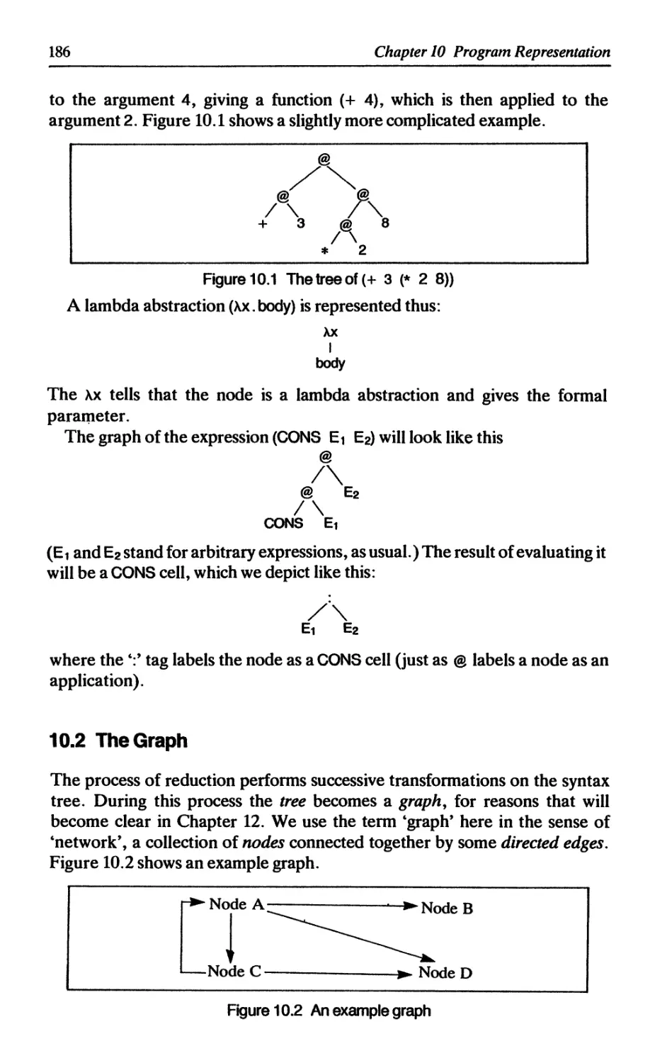
2.4 Recursive Functions
We began by saying that we propose to translate all functional programs into
the lambda calculus. One pervasive feature of all functional programs is
recursion, and this throws the viability of the whole venture into doubt,
because the lambda calculus appears to lack anything corresponding to
recursion.
26
Chapter 2 The Lambda Calculus
In the remainder of this section, therefore, we will show that the lambda
calculus is capable of expressing recursive functions without further exten-
sion. This is quite a remarkable feat, as the reader may verify by trying it
before reading the following sections.
2.4.1 Recursive Functions and Y
Consider the following recursive definition of the factorial function:
FAC = (Xn.lF (= n 0) 1 (♦ n (FAC (- n 1))))
The definition relies on the ability to name a lambda abstraction, and then
to refer to this name inside the lambda abstraction itself. No such construct is
provided by the lambda calculus. The problem is that lambda abstractions are
anonymous functions, so they cannot name (and hence refer to) themselves.
We proceed by simplifying the problem to one in which recursion is
expressed in its purest form. We begin with a recursive definition:
FAC = Xn. (...FAC...)
(We have written parts of the body of the lambda abstraction as ‘...’ to focus
attention on the recursive features alone.)
By performing a ^-abstraction on FAC, we can transform its definition to:
FAC = (Xfac. (Xn. (... fac...))) FAC
We may write this definition in the form:
FAC = H FAC (2.1)
where
H = (Xfac. (Xn. (...fac...)))
The definition of H is quite straightforward. It is an ordinary lambda
abstraction and does not use recursion. The recursion is expressed solely by
definition (2.1).
The definition (2.1) is rather like a mathematical equation. For example, to
solve the mathematical equation
x2 - 2 = x
weseek values of x which satisfy the equation (namely x = — landx = 2).
Similarly, to solve (2.1) we seek a lambda expression for FAC which satisfies
(2.1). As with mathematical equations, there may be more than one solution.
The equation (2.1)
FAC = H FAC
states that when the function H is applied to FAC, the result is FAC. We say that
FAC is a fixed point (or fixpoint) of H. A function may have more than one
Section 2.4 Recursive functions
27
fixed point. For example, both 0 and 1 are fixed points of the function
Xx.* x x
which squares its argument.
To summarize our progress, we now seek a fixed point of H. It is clear that
this can depend on H only, so let us invent (for now) a function Y which takes a
function and delivers a fixed point of the function as its result. Thus Y has the
behavior that
Y H = H (Y H)
and as a result Y is called a fixpoint combinator. Now, if we can produce such a
Y, our problems are over. For we can now give a solution to (2.1), namely
FAC = Y H
which is a non-recursive definition of FAC. To convince ourselves that this
definition of FAC does what is intended, let us compute (FAC 1). We recall the
definitions for FAC and H:
FAC = Y H
H = xfac.An.IF (= n 0) 1 (♦ n (fac (- n 1)))
So
FAC 1
= Y H 1
= H (Y H) 1
= (Xfac.Xn.IF (= n 0) 1 (* n (fac (- n 1)))) (Y H) 1
- > (An.IF (= n 0) 1 (♦ n (Y H (- n 1)))) 1
IF (= 1 0) 1 (• 1 (Y H (- 1 1)))
- > * 1 (Y H 0)
- ♦ 1 (H (Y H) 0)
= * 1 ((Xfac.Xn.IF (= n 0) 1 (♦ n (fac (- n 1)))) (Y H) 0)
- > * 1 ((An.IF (= n 0) 1 (♦ n (Y H (- n 1)))) 0)
- » ♦ 1 (IF (= 0 0) 1 (♦ 0 (Y H (- 0 1))))
->♦11
- » 1
2.4.2 Y Can Be Defined as a Lambda Abstraction
We have shown how to transform a recursive definition of FAC into a non-
recursive one, but we have made use of a mysterious-new function Y. The
property that Y must possess is
Y H = H (Y H)
and this seems to express recursion in its purest form, since we can use it to
express all other recursive functions. Now here comes the magic: Y can be
28
Chapter 2 The Lambda Calculus
defined as a lambda abstraction, without using recursion!
Y = (Xh. (Xx.h (x x)) (Xx.h (x x)))
To see that Y has the required property, let us evaluate
Y H
= (Xh. (Xx.h (x x)) (Xx.h (x x))) H
(Xx.H (x x)) (Xx.H (x x))
H ((Xx.H (x x)) (Xx.H (x x)))
~ H (Y H)
and we are home and dry.
For those interested in polymorphic typing (see Chapter 8), the only respect
in which Y might be considered an ‘improper’ lambda abstraction is that the
subexpression (Xx.h (x x)) does not have a finite type.
The fact that Y can be defined as a lambda abstraction is truly remarkable
from a mathematical point of view. From an implementation point of view,
however, it is rather inefficient to implement Y using its lambda abstraction,
and most implementations provide Y as a built-in function with the reduction
rule
Y H -» H (Y H)
We mentioned above that a function may have more than one fixed point,
so the question arises of which fixed point Y produces. It seems to be the ‘right’
one, in the sense that the reduction sequence of (FAC 1) given above does
mirror our intuitive understanding of recursion, but this is hardly satisfactory
from a mathematical point of view. The answer is to be found in domain
theory, and the solution produced by (Y H) turns out to be the unique least
fixpoint of H [Stoy, 1981], where ‘least’ is used in a technical domain-theoretic
sense.
2.5 The Denotational Semantics of the Lambda Calculus
There are two ways of looking at a function: as an algorithm which will
produce a value given an argument, or as a set of ordered argument-value
pairs.
The first view is ‘dynamic’ or operational, in that it sees a function as a
sequence of operations in time. The second view is ‘static’ or denotational: the
function is regarded as a fixed set of associations between arguments and the
corresponding values.
In the previous three sections we have seen how an expression may be
evaluated by the repeated application of reduction rules. These rules
prescribe purely syntactic transformations on permitted expressions, without
reference to what the expressions ‘mean’; and indeed the lambda calculus can
be regarded as a formal system for manipulating syntactic symbols. Never-
theless, the development of the conversion rules was based on our intuitions
Section 2.5 The denotational semantics of the lambda calculus
29
about abstract functions, and this has, in effect, provided us with an
operational semantics for the lambda calculus. But what reason have we to
suppose that the lambda calculus is an accurate expression of the idea of an
abstract function?
To answer this question requires us to give a denotational semantics for the
lambda calculus. The framework of denotational semantics will be useful in
the rest of the book, so we offer a brief sketch of it in the remainder of this
section.
2.5.1 The Eval Function
The purpose of the denotational semantics of a language is to assign a value to
every expression in that language. An expression is a syntactic object, formed
according to the syntax rules of the language. A value, by contrast, is an
abstract mathematical object, such as ‘the number 5’, or ‘the function which
squares its argument’.
We can therefore express the semantics of a language as a (mathematical)
function, Eval, from expressions to values:
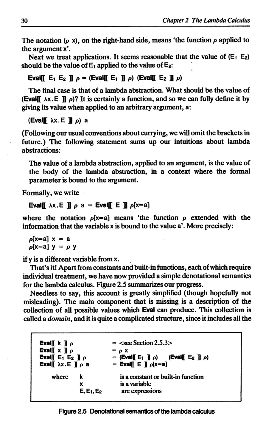
Гс ' Eval ГТ7^
Expressions ----------------► Values
We can now write equations such as
Eval|[ + 3 4 Л = 7
This says ‘the meaning (i.e. value) of the expression (+ 3 4) is the abstract
numerical value 7’. We use bold double square brackets to enclose the
argument to Eval, to emphasize that it is a syntactic object. This convention is
widely used in denotational semantics. We may regard the expression (+ 3 4)
as a representation or denotation of the value 7 (hence the term denotational
semantics).
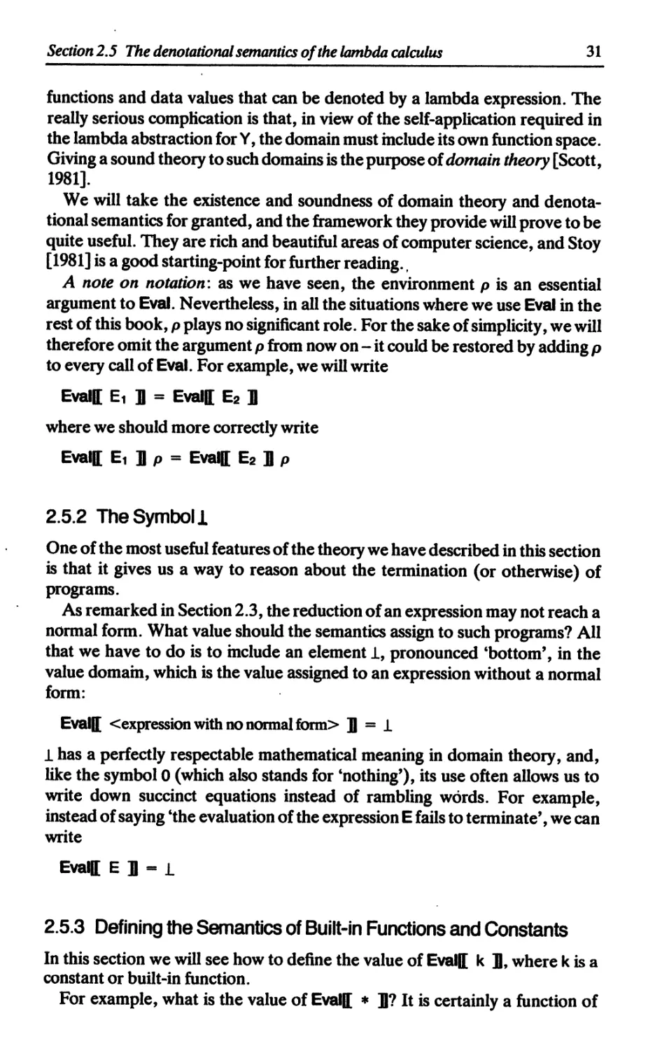
We will now give a very informal development of the Eval function for the
lambda calculus. The task is to give a value for Eval|[ E Д, for every lambda
expression E, and we can proceed by direct reference to the syntax of lambda
expressions (Figure 2.1), which gives the possible forms which E might take.
For the moment we will omit the question of constants and built-in
functions, returning to it in Section 2.5.3. Suppose, then, that E is a variable,
x. What should be the value of
EvalK x Л
where x is a variable? Unfortunately, the value of a variable is given by its
surrounding context, so we cannot tell its value in isolation. We can solve this
problem by giving Eval an extra parameter, p, which gives this contextual
information. The argument p is called an environment, and it is a function
which maps variable names on to their values. Thus
EvalJ x Л p = p x
30
Chapter! The Lambda Calculus
The notation (p x), on the right-hand side, means ‘the function p applied to
the argument x’.
Next we treat applications. It seems reasonable that the value of (Ei Ег)
should be the value of Ei applied to the value of Ег:
Eva® Ei E2 J p = (Eva® Ei J p) (Eva® E2 J p)
The final case is that of a lambda abstraction. What should be the value of
(Eva® Ax. E J p)? It is certainly a function, and so we can fully define it by
giving its value when applied to an arbitrary argument, a:
(Eva® Ax.E J p) a
(Following our usual conventions about currying, we will omit the brackets in
future.) The following statement sums up our intuitions about lambda
abstractions:
The value of a lambda abstraction, applied to an argument, is the value of
the body of the lambda abstraction, in a context where the formal
parameter is bound to the argument.
Formally, we write
Eva® Ax.E J p a = Eva® E J p[x=a]
where the notation p[x=a] means ‘the function p extended with the
information that the variable x is bound to the value a’. More precisely:
p[x=a] x = a
p[x=a] у = p у
if у is a different variable from x.
That’s it! Apart from constants and built-in functions, each of which require
individual treatment, we have now provided a simple denotational semantics
for the lambda calculus. Figure 2.5 summarizes our progress.
Needless to say, this account is greatly simplified (though hopefully not
misleading). The mam component that is missing is a description of the
collection of all possible values which Eval can produce. This collection is
called a domain, and it is quite a complicated structure, since it includes all the
Eva® к J p = <see Section 2.5.3>
Eva® x ] p = P x
Eva® Ei E2 J p « (Eva® Ei ] p) (Eva® E2 ] p)
Eva® Ax.E ] p a = Eva® E ] p[x=a]
where к is a constant or built-in function
X is a variable
E, Ei,E2 are expressions
Figure 2.5 Denotational semantics of the lambda calculus
Section 2.5 The denotational semantics of the lambda calculus
31
functions and data values that can be denoted by a lambda expression. The
really serious complication is that, in view of the self-application required in
the lambda abstraction for Y, the domain must include its own function space.
Giving a sound theory to such domains is the purpose of domain theory [Scott,
1981].
We will take the existence and soundness of domain theory and denota-
tional semantics for granted, and the framework they provide will prove to be
quite useful. They are rich and beautiful areas of computer science, and Stoy
[1981] is a good starting-point for further reading.,
A note on notation: as we have seen, the environment p is an essential
argument to Eval. Nevertheless, in all the situations where we use Eval in the
rest of this book, p plays no significant role. For the sake of simplicity, we will
therefore omit the argument p from now on - it could be restored by adding p
to every call of Eval. For example, we will write
Eval[[ Ei Л = Evall E2 Л
where we should more correctly write
Eval|[ Ei I p = Eval[ E2 Л p
2.5.2 The Symbol 1
One of the most useful features of the theory we have described in this section
is that it gives us a way to reason about the termination (or otherwise) of
programs.
As remarked in Section 2.3, the reduction of an expression may not reach a
normal form. What value should the semantics assign to such programs? All
that we have to do is to include an element 1, pronounced 'bottom’, in the
value domain, which is the value assigned to an expression without a normal
form:
Eval[[ <expression with no normal form> Б = i
1 has a perfectly respectable mathematical meaning in domain theory, and,
like the symbol 0 (which also stands for ‘nothing’), its use often allows us to
write down succinct equations instead of rambling words. For example,
instead of saying ‘the evaluation of the expression E fails to terminate’, we can
write
Eva® E Л - 1
2.5.3 Defining the Semantics of Built-in Functions and Constants
In this section we will see how to define the value of Eval[[ к Л, where к is a
constant or built-in function.
For example, what is the value of Eval[[ * Л? It is certainly a function of
32
Chapter 2 The Lambda Calculus
two arguments, and we can define it by giving the value of this function
applied to arbitrary arguments:
Evald ♦ ] a b = a x b
This gives the meaning of the lambda calculus * in terms of the mathematical
operation of multiplication x. The distinction between the * and x is crucial:
the * is a syntactic expression in the lambda calculus, while x is the abstract
mathematical operation. In the case of multiplication, the mathematical
notation x differs from the program notation ♦, but in the case of addition (for
example) the symbol + is used by both. This is a ready source of confusion,
and we must keep a clear head!
We will use lower-case letters, such as a and b, to stand for values in
semantic equations.
The equation given above is, however, an incomplete specification for ♦.
We must define what * does to each possible argument, including i. The full
set of equations should therefore be:
Evald ♦ ] ab = a x b ifa^landb^l
Evald ♦ ] i b = i
Evald ♦ Л a 1 = 1
The two new equations complete the definition of *, by specifying that if
either argument of * fails to terminate, then so does the application of *.
They are not the only possible set of equations for a multiplication
operator. For example, here are the equations for a more ‘intelligent’
multiplication operator, #:
Evald #]ab = axb if a^iand a^0andb=/=i
Evald # ] 0 b = 0
Evald # J al = 1 if a#=0
Evald # 11 b = 1
These equations imply that # should evaluate its first argument and, if it is
zero, return the result zero without examining the second argument at all;
otherwise it behaves just like *. Using # instead of * would cause the
evaluation of some expressions to terminate when they would not have done
so before.
The point of the example is that the semantic equations for a built-in
function enable us to express subtle variations in its behavior, with a precision
that is hard to achieve by giving reduction rules. The semantic equations for a
function both specify the meaning of the function and imply its operational
behavior (reduction rules).
Strictly speaking we should also provide equations such as
Evald 6 ] = 6
where the ‘6’ on the left-hand side is a lambda expression, and the ‘6’ on the
right-hand side is the abstract mathematical object. Ideally, we should
Section 2.5 The denotational semantics of the lambda calculus
33
distinguish the two kinds of *6’ typographically, but common practice is to
write them in the same way and distinguish them only by context. This applies
to all constants and built-in functions. Thus we write
EvalJ TRUE J = TRUE
Eva® IF J = IF
Eva® + Д = +
and so on.
This is sloppy, but it saves clutter. For example, using this more relaxed
notation, we could write the following semantic equations for the built-in
function IF:
IF TRUE a b = a
IF FALSE a b = b
IF i a b = 1
The use of = and the occurrence of 1 continue to remind us that we are looking
at semantic equations rather than reduction rules.
2.5.4 Strictness and Laziness
We say that a function is stria if it is sure to need the value of its argument.
This is a concept that will arise repeatedly in the book. Can we give a
denotational definition of strictness?
If a function, f, is sure to need the value of its argument, and the evaluation
of the argument will not terminate, then the application of f to the argument
will certainly fail to terminate. This verbose, operational argument suggests
the following concise, denotational, definition of strictness:
DEFINITION
A function f is strict if and only if
fl = i
The definition generalizes easily to functions of several arguments. For
example, if g is a function of three arguments, then g is strict in its second
argument if and only if
g aic = 1
for all values of a and c.
If a function is non-strict, we say that it is lazy. Technically, this is an abuse
of terminology, since lazy evaluation is an implementation technique which
implements non-strict semantics. However, ‘lazy’ is such an evocative term
that it is often used where ‘non-strict’ would be more correct.
34
Chapter 2 The Lambda Calculus
2.5.5 The Correctness of the Conversion Rules
The conversion rules given earlier in this chapter express equivalences
between lambda expressions. It is vital that these equivalences are mirrored in
the denotational world. For example, using а-conversion we may write
(Xx.+ x 1) (Xy.+ у 1)
Our hope is that both of these expressions mean the same thing or, more
precisely, denote the same function, so that
Eval([ Xx.+ x 1 ] = Eval{[ xy.+ у 1 J
In general, we hope that conversion preserves meaning, which we may state
as follows:
Ei «-> Ег
implies
Eval([ Ei 1 = Eval([ Ег 1
In other words, if Ei is convertible to Ег then the meaning of Ei is certainly the
same as the meaning of Ег. (As we will see in the next section, however, the
reverse is not always true.) There is a burden of proof here, to show that the
above statement always holds, given the conversion rules and the semantic
function Eval. We will content ourselves with observing that proof is required,
leaving the hard work to Stoy [1981].
Since the reduction rules (Д-reduction and ^-reduction) are a subset of the
conversion rules, we certainly know that
Ei - Ег
implies
Ei Ег
and hence
Ei - Ег
implies
EvalE Ei 1 = EvalE E2 1
2.5.6 Equality and Convertibility
In the previous section we saw that conversion preserves equality. But is the
reverse true? In particular, does the equality of two expressions imply their
interconvertibility? The answer is ‘no’, as the following example shows.
Consider the two lambda abstractions, which we will call Fi and F2:
Fi = (Xx.+ x x)
F2 = (Xx.* x 2)
Section 2.6 Summary
35
It is clear that Fi cannot be converted into F2 using the conversion rules of the
lambda calculus. To a mathematician, however, a function is a ‘black box’,
and two functions are the same if (and only if) they give the same result for
each possible argument. This sort of equality of functions is called extensional
equality. The function denoted by Fi and that denoted by F2 are certainly
(extensionally) equal, so we may write
EvalE Fi Л = Eva® F2 Л
So Fi and F2 are not interconvertible, but they do denote the same function.
To summarize the main conclusion:
If Ei E2
then Eval[ Ei Л = Eva® E2 Л
but not necessarily the other way around.
We can therefore regard conversion as a weak form of reasoning about the
equality of expressions. It can never cause us to believe that two expressions
are equal when they are not, but it may not allow us to prove the equality of
two expressions which are in fact equal. From this point of view, reduction is a
still weaker form of inference.
2.6 Summary
A working understanding of the lambda calculus will prove extremely useful
for the rest of the book, and in this chapter we have tried to give a compact
summary of the material we will require. The treatment has necessarily been
rather superficial, and the reader is again referred to Stoy [1981] or
Barendregt [1984] for fuller treatments.
References
Barendregt, H.P. 1984. The Lambda Calculus-Its Syntax and Semantics, 2nd edition.
North-Holland.
Church, A. 1941. The Calculi of Lambda Conversion. Princeton University Press.
Curry, H.B., and Feys, R. 1958. Combinatory Logic, Vol. 1. North-Holland.
Kennaway, J.R. 1984. An Outline of Some Results of Staples on Optimal Reduction
Orders in Replacement Systems. CSA/19/1984. School of Information Systems,
University of East Anglia. March.
Levy, J. J. 1980. Optimal reductions in the lambda calculus. In Essays on Combinatory
Logic, pp. 159-92. Hindley and Seldin (editors). Academic Press.
Rosser, J.B. 1982. Highlights of the history of the lambda calculus. Proceedings of the
ACM Symposium on Lisp and Functional Programming, Pittsburgh, pp. 216-25.
August.
Schonfinkel, M. 1924. Uber die Bausteine der mathematischen Logik. Mathematische
Annalen. Vol. 92, pp. 305-16.
Scott, D. 1981. Lectures on a Mathematical Theory of Computation. PRG-19.
Programming Research Group, Oxford. May.
36
Chapter 2 The Lambda Calculus
Staples, J. 1980a. Computation on graph-Кке expressions. Theoretical Computer
Science. Vol. 10, pp. 171-85.
Staples, J. 1980b. Optimal evaluations of graph-like expressions. Theoretical
Computer Science. Vol. 10, pp. 297-316.
Staples, J. 1980c. Speeding up subtree replacement systems. Theoretical Computer
Science. Vol. 11, pp. 39-47.
Stoy, J.E. 1981. Denotational Semantics. МГГ Press.
Welch, P. 1975. Some Notes on the Martin-Lof Proof of the Church Rosser Theorem as
Rediscovered by Park. Computer Lab., University of Kent. October.
Three
TRANSLATING A HIGH-LEVEL
FUNCTIONAL LANGUAGE INTO THE
LAMBDA CALCULUS
In the next few chapters we will describe how to translate a high-level
functional language into the lambda calculus.
We can regard this translation in two ways:
(i) As a description of the semantics of the language, giving the meaning of
each of its constructs in terms of lambda expressions, whose meaning is
well understood. This is precisely the approach taken by denotational
semantics [Gordon, 1979].
(ii) As a step in the implementation of the high-level language, by expressing
all its constructs in terms of the lambda notation.
For the sake of definiteness we use a subset of the language Miranda [Turner,
1985], but the techniques apply to any functional language. An introduction
to Miranda can be found in the Appendix.
Disclaimer
In this book Miranda is used as an example of a modem functional
programming language, to illustrate various points about the imple-
mentation of functional programming languages in general. This book is
not intended to be a source of reference for the definition of Miranda.
Note that:
(i) Miranda has a number of features, both major and minor, which are
not discussed here at all.
(ii) The material about Miranda in this book was based on a prerelease
version of the Miranda system and may therefore be inaccurate by the
time it is published.
The Miranda functional programming system is a product of Research
Software Limited, and a full description of the language and’ its pro-
gramming environment is in preparation by them.
37
38 Chapter 3 Translating a High-level Functional Language into the Lambda Calculus
3.1 The Overall Structure of the Translation Process
Miranda is a powerful, high-level functional language, providing a rich set of
programming constructs. The purpose of the next few chapters is to demon-
strate how some of these constructs can be translated into the lambda
calculus. Specifically, we will discuss structured data types, pattern-matching,
conditional equations and ZF expressions. Miranda includes a number of
other constructs, such as abstract data types and structured data types with
laws, which we will not study in this book.
Even so, the translation we describe is a substantial task, and we begin by
outlining the structure of the translation process.
It might be possible to translate a program directly from Miranda into the
lambda calculus, but this would be an extremely complicated translation, so
we will take a more step-by-step approach. In order to do this, it is convenient
to regard much of the translation as a process of successively transforming one
program into another, until finally the result is a program m the lambda
notation. (We are here using ‘translation’ to suggest a process which takes a
program in one language and produces a program in another, while a
‘transformation’ produces a program in the same language.)
Two ways of organizing the translation then suggest themselves:
(i) We could perform most of the translation by successive transformations
of one Miranda program into another, each transformation performing a
simplification step. We would complete the process by translating the
resulting (simple) Miranda program into the lambda calculus. The idea is
that the earlier transformations would have done all the hard work, so the
final step should consist of tittle more than a change of syntax.
(ii) Alternatively, we could begin the translation by performing a simple
syntactic translation of the Miranda program into an enriched version of
the lambda calculus. This enriched lambda calculus would include the
ordinary lambda calculus as a subset, but would also include extra
constructs, chosen so that the first step consists of little more than a
change of syntax. Then we could do most of the hard work by successivefy
transforming the expression into simpler and simpler forms, until it
becomes an ordinary lambda expression, free from any of the extra
constructs.
Initially, the first method looks more attractive than the second, because it
does not require us to define a new language (the enriched lambda calculus).
However, we choose to follow the second course of action for the following
reasons:
(i) Miranda is designed to be a language for programmers, not compilers,
and it lacks certain features that are desirable for a transformation-based
compiler. (The particular features lacking are lambda abstractions and
the ability to qualify any expression with local definitions. This is not a
criticism of Miranda - it just has a different purpose.)
Section 3.2 The enriched lambda calculus
39
(ii) To a much greater extent than is the case for imperative languages,
functional languages are largely syntactic variations of one another, with
relatively few semantic differences. Using the second method allows the
transformations we present to be applied easily to other languages, by
altering only the translation of the high-level language into the enriched
lambda calculus.
Figure 3.1 depicts the overall plan of action. We will use the term ordinary
lambda calculus to refer to the language described in Chapter 2, and enriched
lambda calculus to refer to the language introduced here.
The enriched lambda calculus is simply the ordinary lambda calculus
augmented with extra constructs, chosen to allow an easy translation from
Miranda. For each construct we will
(i) say what it looks like (give its syntax);
(ii) say what it means (give its semantics).
The semantics for each construct can be given by providing a simple trans-
formation which shows how to express that construct in terms of the ordinary
lambda calculus. Then we could, m principle, translate from Miranda into the
ordinary lambda calculus by first translating into the enriched lambda
calculus, and then using the semantics of each construct repeatedly to
transform the expression into an ordinary lambda expression.
While this method generates correct results, far greater efficiency is
attainable by using more complicated transformations, but we can always
confirm their correctness by reference to the inefficient version.
Miranda program
A simple translation
v (specific to Miranda)
Expression In the
enriched lambda calculus
Multiple transformations
H (independent of Miranda)
Expression In the
ordinary lambda calculus
Figure 3.1 Translation of Miranda into the lambda calculus
3.2 The Enriched Lambda Calculus
The enriched lambda calculus is a superset of the ordinary lambda calculus, so
that any expression in the ordinary lambda calculus is also an expression in the
enriched lambda calculus. The syntax for function application, lambda
40 Chapter 3 Translating a High-level Functional Language into the Lambda Calculus
abstractions, constants and built-in functions therefore remains exactly as
described in Chapter 2. Likewise, all functions are written in prefix form, and
the same conventions hold concerning brackets.
The only difference from the ordinary lambda calculus is the provision of
four extra constructs. They are:
(i) let-expressions and letrec-expressions;
(ii) pattern-matching lambda abstractions;
(iii) the infix operator 0;
(iv) case-expressions.
Of these, we will only describe the first here. The other three all concern
pattern-matching, and cannot be defined before the discussion of pattern-
matching itself. This is given in Chapter 4, and the remaining three constructs
are defined there.
Figure 3.2 summarizes the syntax of the enriched lambda calculus for future
reference.
<exp> <constant> Constants
I I I I I <variable> Variables <exp> <exp> Applications x <pattem> . <exp> Lambda abstractions let <pattem> = <exp> in <exp> Let-expressions letrec <pattem> = <exp> Letrec-expressions
I I <pattem> = <exp> in <exp> <exp> 0 <exp> case <variable> of <pattem> =$> <exp> Fat bar Case-expressions
<pattem> <pattem> =$> <exp> <constant> 1 <variable> 1 <constructor> <pattem>» Constant patterns Variable patterns Constructor patterns
<pattem>
Figure 3.2 Syntax of enriched lambda expressions
3.2.1 Simple let-expressions
One of the main constructs in any functional language is the definition,
whereby a name is bound to a value. This mechanism is provided in the
enriched lambda calculus, using let-expressions and letrec-expressions.
We begin by defining simple let-expressions. They are called ‘simple’ by
contrast with pattern-matching let-expressions, which we deal with later. A
simple let-expression has the following syntax:
let v = В in E
Section 3.2 The enriched lambda calculus
41
where the v is a variable, and В and E are expressions in the (enriched) lambda
notation.
It introduces a definition for a variable v, which binds v to В in E. The
definition is in scope with E but not B. We say that the ‘v = B’ is the
definition of the let, the v is the variable bound by the let, and the В is the
definition body.
For example, consider the following let-expression:
let x = 3 in (* x x)
Intuitively, the value of this expression is found by substituting 3 for x in the
body(* x x), and then evaluating the body, giving the result 9:
let x = 3 In (* x x)
—> .*33
9
A let-expression is an expression like any other, and can be used in the same
way as any other expression. For example,
+ 1 (let x =» 3 In (* x x))
+ 1 (♦ 3 3)
-*+19
10
For the same reason, let-expressions can be nested:
let x = 3 In (let у = 4 In (* x y))
-> let у = 4 in (* 3 y)
* 3 4
-> 12
As a matter of convenience, we also allow ourselves to write multiple
definitions in the same let; thus:
let x - 3
у = 4
in * x у
This expression means precisely the same as the previous one. We define a
let-expression with several definitions to mean the same as the nested set of
let-expressions which defines the same variables in the same order, one per
let-expression. (Syntactically, it would have been possible to specify that
multiple definitions are separated with semicolons, but layout will suffice for
our purposes.)
Earlier in this section we developed an informal reduction rule for let-
expressions. This involved substitution and is very reminiscent of the
^-reduction rule, which also uses substitution. For example, to evaluate
(Xx.* x x) 3
we substitute 3 for x in the body (♦ x x), and then evaluate the body.
42 Chapter 3 Translating a High-level Functional Language into the Lambda Calculus
Generalizing this idea, we can now define the semantics of a simple let-
expression as follows:
(let v = В in E) ((xv.E) B)
(We use the symbol = to denote the equivalence of two expressions.) That
is all that is needed to define its semantics! By repeated application of this
equivalence, we could eliminate all simple let-expressions from an expression,
in favor of lambda abstractions.
3.2.2 Simple letrec-expressions
The syntax of a simple letrec-expression is similar to that of a simple let-
expression:
letrec vi = Ei
V2 = Ег
Vn — En
in
E
where the Vi are variables, and E, Ei,..., En are expressions in the (enriched)
lambda notation. We will sometimes abbreviate ‘letrec-expression’ to ‘letrec’
(and ‘let-expression’ to ‘let’), where no ambiguity arises.
The term ‘letrec’ is short for ‘let recursively’, and it introduces possibly
recursive bindings for a number of variables V|. The difference between lets
and letrecs is that the vi are in scope in the Ei (as well as E) of a letrec. To take an
example, the expression
letrec factorial = Xn.lF (= n 0) 1 (* n (factorial (- n 1)))
in factorial 4
defines a recursive function factorial, and applies it to the argument 4. The
value of the expression is thus 24.
Like let-expressions, letrec-expressions can appear embedded anywhere in
an expression. Unlike let-expressions, however, it is essential to allow
multiple definitions in a letrec-expression, so as to permit mutual recursion.
This is demonstrated by the following example:
letrec f = ... f... g...
g = ...f...
in...
Here, f refers to itself and g, and g refers to f. This cannot be transformed into
a nested pair of letrecs, because then either g would not be in scope in the body
off, or vice versa.
It is easy to provide a semantics for a letrec with only a single definition,
using the Y operator developed in Section 2.4. In particular,
(letrec v = В in E) » (let v = Y (Xv.B) in E)
Section 3.2 The enriched lambda calculus
43
The use of Y renders the definition non-recursive, so we can then use a
let-expression, whose semantics has already been defined.
The case of multiple definitions requires the use of pattern-matching, and
so is postponed until Chapter 6.
3.2.3 Pattern-matching let- and letrec-expressions
We will also allow patterns, as well as variables, to appear on the left-hand side
of definitions in lets and letrecs. We have not yet defined what a pattern is, so
we postpone the topic until Chapter 6. However, a variable is just a simple
form of pattern, so simple let(rec)-expressions are just simple forms of pattern-
matching let(rec)-expressions.
3.2.4 Let(rec)s versus Lambda Abstractions
So far we have regarded the ordinary lambda calculus as the target language,
into which we will transform the program, and (et(rec)-expressions as
intermediate embellishments. However, there are strong efficiency reasons
for including simple let(rec)-expressions in the target language, rather than
transforming them into the ordinary lambda calculus.
Specifically, the transformation of a let-expression
let v = В in E
into the application of a lambda abstraction
(Xv.E) В
is using a sledgehammer (lambda abstraction) to crack a nut (let-expressions).
The lambda abstration (Xv.E) could be applied to many arguments, but it is in
fact only ever applied to one, namely B. The generality of lambda abstraction
is not required, and the special case (that of application to a unique argument)
can be exploited by the more sophisticated compilers described later in this
book.
This issue manifests itself m a number of ways:
(i) Miranda is a polymorphically typed language, and in Chapter 8 we give
an algorithm for type-checking programs. Unfortunately, it is not
possible to type-check the program once it has been transformed into the
ordinary lambda calculus, but the addition of simple let(rec)-expressions
is sufficient to solve the problem.
(ii) In all implementations except the very simplest, let-expressions can be
evaluated very much more efficiently than the corresponding application
of a lambda abstraction. This applies to all the implementations
described from Chapter 14 onwards.
(iii) A related problem is that the transformation of letrec-expressions into
the ordinary lambda calculus compels us to use Y to express recursion
44 Chapter3 Translating a High-level Functional Language into the Lambda Calculus
The resulting expression is not an efficient implementation, and a more
sophisticated compiler may wish to handle recursion in a different way
(see Chapter 14). Keeping the recursion explicit using letrec allows scope
for these optimizations.
To summarize, all our implementations, except the very simplest, will
require the program to be transformed into the ordinary lambda calculus
augmented with simple let(rec)-expressions. This approach makes a dramatic
contribution to the efficiency of the resulting implementations. On the other
hand, little seems to be gained by augmenting the language still further.
3.3 Translating Miranda Into the Enriched Lambda Calculus
A program consists of a set of definitions, together with an expression to be
evaluated. To keep these two components of the program separate we will use
a box, like this:
Set of definitions
Expression to be evaluated
For example, we could compute twice the square of 5 with the following
Miranda program:
square n = n*n
2 * (square 5)
(Note: Miranda is an interactive language, and defines a ‘program’ to be a set
of definitions, while the ‘expression to be evaluated’ is typed by the user. For
the rest of this book, however, we will use ‘program’ to mean ‘a set of
definitions together with an expression to be evaluated’.) Proceeding
informally, we can translate this Miranda program into the enriched lambda
calculus quite easily, to produce the expression
let square = Xn.* n n
In (* 2 (square 5))
We now introduce some notation to help describe the translation process.
Consider the translation of the Miranda expression (2 * (square 5)) into the
lambda expression (♦ 2 (square 5)). We may regard this translation process
as a function ТЕ, which takes the Miranda expression as its input, and
produces the lambda expression as its output. We write the translation like
this:
ТЕД 2 ♦ (square 5) J « ♦ 2 (square 5)
The double square brackets [ 1 are used to enclose the Miranda expression,
Section 3.4 The ТЕ translation scheme
45
to emphasize that the argument to IE is a syntactic object. This convention
was used in Chapter 2, but the difference on this occasion is that the result of
the translation is a syntactic object also, and we use rather than = to remind
us of this fact. We call ТЕ a translation scheme.
We also need another translation scheme TD, which translates Miranda
definitions into definitions suitable for a letrec. For example,
TD|[ square n = n*n Ц square = \n.* n n
Here we see another reason for using = when writing translation schemes: it
avoids confusion with = symbols in the program being translated. We can now
generalize the translation scheme as follows. Given the Miranda program
Definition i
Definttlonn
Expression
we generate the following (enriched) lambda expression:
letrec
TD|[ Definitioni 1
TOff Deflnittonn 1
in
ТЕЦ Expression Б
In the previous example we used a let instead of a letrec, but Miranda
definitions are all potentially recursive, so we must use a letrec in general (later
work will optimize this-Section 6.2.8).
What we have now done is to reduce the translation problem to one of
defining the two translation schemes TD and ТЕ. We will define them for
simple cases in the succeeding two sections, and then lay out the plan of the
next few chapters, which will extend them to cover more complicated cases.
For the moment, we completely avoid the question of declarations of new
types and type-checking. The former will be introduced in Chapter 4 and the
latter in Chapter 8.
3.4 The ТЕ Translation Scheme
The translation scheme ТЕ is a function, which takes a Miranda expression as
its argument, and produces an equivalent lambda expression as its result,
thus:
Miranda ТЕ Lambda
expression expression
46 Chapter3 Translating a High-level Functional Language into the Lambda Calculus
We will describe IE by case analysis, giving a rule for each possible form of a
Miranda expression.
3.4.1 Translating Constants
To translate a constant or built-in function is straightforward, assuming that
the lambda notation into which we are translating supports the same set of
constants. The following rule is ail that is required:
ТЭД к Д « к
where к is a constant or built-in function name (we include ail Miranda’s
operators, and literal constants in this category). Thus, for example
ТЕД 5 fl « 5
ТЕД + J я +
This translation assumes that all the constants and built-in functions have
the same names in the lambda notation. It is straightforward to describe
changes of name, however. For example, the following set of rules for IE
translates the operators + , -, etc. in Miranda into PLUS, MINUS, etc.:
ТЕД + Д = PLUS
ТЕД - J я MINUS
etc.
3.4.2 Translating Variables
An equally simple rule suffices to translate variables:
ТЕД v ] v
where v is a variable (including the names of user-defined.functions and
constructors).
3.4.3 Translating Function Applications
Function application in Miranda is denoted by juxtaposition, thus (f x). The
same syntax is used in the lambda notation, so the rule for translation is
simple:
ТЕД Ei E2 fl - ТЕД Ei 1 Ж E2 Д
where Ei and E2 are arbitrary Miranda expressions. In the case of certain
common operators (such as +, etc.), Miranda provides infix syntax (that is,
the operator is written between its operands). The translation rule to deal
with these constructs is:
ТЕД Ei infix E2 J я ТЕД infix ]] ТЕД Е, Д ТЕД Е2 Д
Section 3.5 TheTD translation scheme 47
where ‘infix’ is an infix operator, and Ei and Ег are arbitrary Miranda
expressions. We must apply IE to ‘infix’ to accomplish any change of name (see
above).
Furthermore, Miranda allows user-defined functions to be used as infix
operators by prefixing their names with $. We can treat this case with the rule
ТЕД Ei $v Ez J г Ж v 1 7E|[ Eil ТЖ Ег 1
3.4.4 Translating Other Forms of Expressions
We shall consider two other forms of Miranda expression, namely
(i) list expressions such as [2,5,1 ];
(ii) ZF expressions.
We will deal with these in Chapters 4 and 7 respectively.
3.5 The TD Translation Scheme
The ID scheme takes a Miranda definition as its argument and produces a
tetrec definition as its result. We will only give a rather simplified TO scheme
here, leaving a more powerful one for later chapters.
There are two cases that we can handle immediately, namely variable
definitions and simple function definitions.
3.5.1 Variable Definitions
Consider the Miranda definition
v = 5*7
It can be translated very easily to
v = ♦ 5 7
All that is required is to translate the body of the definition, using the IE
scheme. In general:
TOff v = E 1 = v = W E I
where v is a variable and E is an expression.
3.5.2 Simple Function Definitions
We have already seen an example of translating a simple function definition,
when we translated the Miranda definition
square n = n*n
48 Chapter 3 Translating a High-level Functionci Language into the Lambda Calculus
TEE Exp J transplates the expression Exp TEE к J » к (assumes no name-changing) TEE v ] «V ТЕЦ Ei E2 J « ТЕЦ Ei J ТЕЦ E2 J ТЕЦ Ei infix E2 J « TE|[ infix J TE|[ Ei J TE|[ E2 J TEE Ei $v E2 ] «TEEv]|TEEEi]|TEEE2]|
where к V Ei infix is a literal constant or built-in operator is a variable is an expression is an infix operator
TDE Def J translates the definition Def
TOE v = E Л TOE f vi ... vn = E J « v = TEE E Л | = f = Xvi.. .XVn.TEE E Л
where v, vi, f E are variables is an expression
Figure 3.3 Translation schemes ТЕ and TD (simple versions)
into the letrec definition
square = Xn.* n n
The body of the definition is translated, and a lambda abstraction is
generated around it. We can generalize this as follows:
TDI f Vi ... vn = E 1 = f = Xvi... Xvn.TE|[ E 1
where f, v1t .. .,vn are variables and E is an expression.
3.6 An Example
We have now shown how to translate a simple subset of Miranda into the
enriched lambda notation. Our progress is summarized in Figure 3.3.
To illustrate the translation in action, consider the following Miranda
program:
average a b = (a+b)/2
average 2 (3+5)
This will be transformed to
letrec
TDJ average a b = (a+b)/2 J
in
ТЕК average 2 (3+5) ]
Section 3.7 The organization of Chapters 4-8
49
Application of tbe rules for ТЕ gives
ТЕК average 2 (3+5) J
= ТЕК average Л ТЕК 2 Л ТЕК 3+5 J
® average 2 (ТЕК + J ТЕК 3 J ТЕК 5 J)
average 2 (+ 3 5)
Similarly, tbe rules for ID give
TDK average a b - (a+b)/2 Л
® average = Xa.Xb.TEK (a+b)/2 Л
® average = Xa.Xb.fTEK / Л ТЕ® a+b Л ТЕК 2 Л)
= average ="Ха.ХЬ.(/ (ТЕК + 1 ТЕК a 1 ТЕК b Л) 2 )
= average - Xa.Xb.(/ (+ a b) 2)
Putting it all together gives the result of tbe translation:
letrec
average = Xa.Xb.(/ (+ a b) 2)
in
average 2 (+ 3 5)
To complete the example, let us transform the expression into tbe ordinary
lambda calculus. Let us suppose that we spot that the letrec may be replaced
with a let, because tbe definition is non-recursive (the method is described in
Chapter 6). Then we can use the semantics of let-expressions to produce tbe
ordinary lambda expression
(Xaverage.(average 2 (+ 3 5))) (Xa.Xb.(/ (+ a b) 2))
You can see why we prefer to write programs in Miranda!
3.7 The Organization of Chapters 4-9
In the interests of simplicity, tbe equations for TD and ТЕ given in Figure 3.3
are far from comprehensive. The rest of Part I of the book is devoted to filling
in the details.
Chapter 4 introduces structured data objects, pattern-matching and
conditional equations, and gives a simple translation into the enriched lambda
calculus. This translation is rather inefficient, and Chapter 5 shows how
pattern-matching can be compiled far more efficiently. Chapter 6 then shows
how to transform all the constructs of the enriched lambda calculus into the
ordinary lambda calculus.
Miranda contains constructs called ZF expressions (also known as list
comprehensions). We discuss their translation in Chapter 7.
Finally, Miranda is a polymorphically typed language, and we have so far
paid no attention to the question of type-checking. This is addressed in
Chapters 8 and 9.
The organization of these chapters is depicted in Figure 3.4.
50 Chapter 3 Translating a High-level Functional Language into the Lambda Calculus
Figure 3.4 Organization of Chapters 4-8
References
Gordon, M.J.C. 1979. The Denotational Description of Programming Languages.
Springer Verlag.
Turner, D.A. 1985. Miranda - a non-strict functional language with polymorphic
types. In Conference on Functional Programming Languages and Computer
Architecture, Nancy, pp. 1-16, Jouannaud (editor). LNCS 201. Springer Verlag.
Four
STRUCTURED TYPES AND THE
SEMANTICS OF
PATTERN-MATCHING
Simon L. Peyton Jones and Philip Wadler
This chapter concerns structured types, a powerful and general mechanism
for defining data types, provided by several functional languages, including
Miranda, ML and Hope. Intimately associated with structured types is a
notational device known as pattern-matching, which is used by such
languages for defining functions.
Section 4.1 gives a general introduction to structured types and pattern-
matching. Section 4.2 begins with a more in-depth look at pattern-matching
and conditional equations, and then introduces two new constructs in the
enriched lambda calculus, 0 and pattern-matching lambda abstractions. Using
these constructs, we then show how to translate a general Miranda function
definition into the enriched lambda calculus. Section 4.3 is devoted to
providing a precise semantics for pattern-matching lambda abstractions.
We conclude m Section 4.4 by defining case-expressions, the last new
construct of the enriched lambda calculus. This clears the way for Chapter 5,
which will show how to transform pattern-matching lambda abstractions into
case-expressions, thus giving a considerable gam m efficiency.
What in this chapter are called ‘structured types’ are called ‘algebraic types’
in Miranda, and ‘free data types’ by some others [Burstall and Gogucn, 1982].
52
Chapter 4 Structured Types and the Semantics of Pattern-matching
4.1 Introduction to Structured Types
Suppose that we wish to define binary trees with leaves that are numbers. In
the notation of Miranda, this could be done by declaring a structured type tree
as follows:
tree ::= LEAF num I BRANCH tree tree
(The symbol identifies this as a type declaration.) This might be read as
follows: ‘a tree is either a LEAF, which contains a num, or a BRANCH, which
contains a tree and a tree’. Here LEAF and BRANCH are called constructors of
the type. Miranda requires that constructors (and only constructors) begin
with an upper-case letter, but we will always write them entirely in upper case.
LEAF has one field, of type num, and BRANCH has two, both of type tree. The
number of fields associated with a constructor is called its arity; thus LEAF has
arity 1 and BRANCH has arity 2.
Constructors can be used as functions, to create values of type tree. For
example, the equation
treel = BRANCH (BRANCH (LEAF 1) (LEAF 2)) (LEAF 3)
defines treel to be a tree. Informally, this tree might be drawn as:
3
Constructors can also appear on the left-hand side of an equation, as in the
following Miranda function definition:
reflect (LEAF n) = LEAF n
reflect (BRANCH t1 t2) = BRANCH (reflect t2) (reflect t1)
For example, (reflect treel) returns
BRANCH (LEAF 3) (BRANCH (LEAF 2) (LEAF 1))
A definition with patterns on the left-hand side, such as that of reflect, is said
to use pattern-matching to perform case analysis. For example, in evaluating
(reflect t) there are two cases to choose from: t matches the pattern (LEAF n),
or t matches the pattern (BRANCH t1 t2). If, say, t is (LEAF 1) then the first
case is chosen, with n bound to 1. Much more will be said about pattern-
matching later.
An important difference in the treatment of structured types in Miranda
from that in ML or Hope, is that in Miranda constructor functions are lazy;
that is, they do not evaluate their arguments. The components of a structured
object are evaluated only when (and if) they are subsequently extracted and
used, not when the object is built.
Section 4,1 Introduction to structured types
53
4.1.1 Type Variables
Type declarations may also contain type variables. For example, the
definition of the type tree above may be rewritten to allow trees with leaves of
any type:
tree ♦ ::= LEAF ♦ I BRANCH (tree ♦) (tree ♦)
Here * is called a generic (or schematic) type variable. The declaration could
be read as follows: ‘a tree of * is either a LEAF, which contains a *, or a
BRANCH which contains a tree of * and a tree of *, for any type
Leaves of any particular tree must all contain values of the same type, but
different trees may have leaves of different types. Examples of trees and their
types are
BRANCH (LEAF 1) (LEAF 2) :: tree num
BRANCH (LEAF ‘a’) (LEAF ‘b’) :: tree char
(The symbol:: is pronounced ‘has type’.) Here, ‘tree’ is called a type-forming
operator, since it takes a type (such as num or char) as an ‘argument’ and
produces a type (respectively, (tree num) or (tree char)).
The repeated use of * on the right-hand side of the type declaration
specifies that the two branches of a tree must be of uniform type. For example,
BRANCH (LEAF 1) (LEAF ‘a’)
is not legal, since it has leaves of mixed type. More will be said about types and
type variables m Chapter 8.
4.1.2 Special Cases
This section shows how three ‘built-in’ types, namely lists, tuples and
enumerated types, can be regarded as instances of general structured types.
4.1X1 Lists
Miranda has a special syntax to denote lists, but lists are just an instance of a
general structured type. Lists could be defined as follows:
list * ::= NIL I CONS * (list *)
This type declaration defines the two new constructors NIL and CONS.
Miranda’s built-in syntax for lists could then be translated to use NIL and
CONS, as follows:
[ ] is translated to NIL
(x:xs) is translated to (CONS x xs).
[x,y,z] is a Miranda abbreviation for (x:y:z;[ ]) and hence is translated to
(CONS x (CONS у (CONS z NIL)))
[*] is translated to (list *)
54
Chapter 4 Structured Types and the Semantics of Pattern-matching
TEff : J - CONS
TEff[]l - NIL
TE[ [Ei, E2, .... En] 1 - CONS TE[ Ei J TE[ [Ez........En] J
TEE (Ei, E2) ] - PAIR TEE Ei ] TEE E2 ]
TEff (E1t E2, Ез) 1 - TRIPLE TEff Ei ] TEE E2 J TEff E3 J
and so on
ТЩ True J
TEE False ]
« TRUE
= FALSE
Figure 4.1 Modifications to the ТЕ scheme for lists, tuples and booleans
(Note: the last example is different from the others, because it describes a
type-expression rather than a value-expression.)
We can conveniently perform this translation when translating from
Miranda into the enriched lambda calqulus; Figure 4.1 gives the required
equations.
Notice that the elements of a list of type (list ♦) must all be of type *, but the
number of elements in a list is not determined by its type. Thus (CONS 2 NIL)
and (CONS 3 (CONS 6 NIL)) are both of type (list num), though they are of
different lengths.
4.1.2.2 Tuples
Miranda also provides special syntax to denote tuples, and these also can be
defined using a structured type. Tuples could be defined as follows:
pair ♦ ♦♦ ::= PAIR ♦ ♦♦
triple * ** ♦♦♦ ::= TRIPLE ♦ ♦♦ ♦♦♦
quadruple * ♦♦ ♦♦♦ ♦♦♦♦ ::= QUADRUPLE * ♦♦ ♦♦♦♦
Notice the difference between ‘pair* and ‘PAIR’: the former is a type-forming
operator, used only m type-expressions, while the latter is the constructor
function of the type, used only in value-expressions.
As with lists, Miranda’s special syntax can be translated as follows:
(x,y) is translated to (Pair x y)
(x,y,z) is translated to (TRIPLE x у z)
and so on.
(♦,♦♦) is translated to (pair ♦ ♦♦)
(*,**,*♦♦) is translated to (triple * *♦ ♦♦*)
Figure 4.1 gives the required equations.
Notice that a tuple may contain elements of mixed type; for example
(3, TRUE) :: PAIR num bool
(‘a’, (3, 2)) :: PAIR char (PAIR num num)
Section 4.1 Introduction to structured types
55
However, the type of a tuple completely determines the number and the types
of its fields. For example, a pair always contains exactly two fields, a triple
contains exactly three fields, and so on.
4.1.2.3 Enumerated types
The type declaration
color ::= VERMILLION I PUCE I LAVENDER
in which each constructor has zero fields, is just like an enumerated type in
Pascal. Thus, we can define the type of boolean values:
bod ::= TRUE I FALSE
The usual functions on booleans can then be defined using pattern-
matching; for example:
if TRUE e1 e2 = e1
if FALSE e1 e2 = e2
Miranda uses the names True’ and ‘False’ for its built-in truth-values.
4.U.4 Summary
Since it is easy to translate ‘built-in’ types like lists and tuples into equivalent
structured types, then any implementation of a functional language that
handles structured types will also handle these ‘built-in’ types for free. This
can greatly simplify an implementation. Instead of implementing several type
mechanisms, one for lists, one for tuples, one for enumerated types, and so
on, we need only implement a single mechanism for structured types, and
translate other types into structured types. Figure 4.1 gives the required
equations.
4.1.3 General Structured Types
In general, the form of a structured type definition is:
T ::= Ci Ti.i ... Ti,f1
I ...
I Cn Tn.1 ... TVn
where the Тц are types and the ci are constructors of arity r<. In the ‘tree’
example above, T was (tree ♦), Ci was LEAF, Tи was num, cz was BRANCH, Тг,!
was (tree ♦), and T« was (tree ♦).
Readers familiar with the mathematical operations for constructing types
will recognize that the general type above can be written as the sum (that is,
discriminated union):
T = Ti + ... + T„
56
Chapter 4 Structured Types and the Semantics of Pattern-matching
where each Tj, for i from 1 to n, can be written as a product:
T| = T|,i X T|,2 X . . . X Ti,q
In other words, a structured type is a sum-of-products.
When n=1 we say that the type is a product type; the types (pair * **),
(triple ♦ ** ***). . . are all product types. When n>1 we say that the type is a
sum type, since it is the sum of more than one domain; the types (tree *),
(list *), color and bool are all sum types. Thus a product type has exactly one
constructor, and a sum type has two or more constructors.
We will often wish to distinguish between the constructors of product
types and sum types. Just as we use the names ci to stand for constructors of all
types, we will use the name t to stand for the constructor of a product type, and
the names s and Si to stand for the constructors of a sum type (t suggests ‘tuple’
and s suggests ‘sum’).
(Note: we use lower-case letters to stand for constructors, to avoid
confusion with the constructors themselves, which are written in upper case.
Similarly, we use upper-case letters to stand for types, which are themselves
written in lower case - see Section 4.1.)
(Important', at the time when this chapter was first written the semantics of
Miranda provisionally specified that a structured type with only one
constructor was a product type, as above. However, an alternative view is that
a structured type with only one constructor should behave as a sum type with
one component in the sum, and that product types (tuples) be treated as an
independent construct. It now seems likely that Research Software Limited
will follow this latter course in their definition of Miranda. As a consequence
some of the statements made in this chapter about the semantics of structured
types in Miranda may be incorrect. We draw the reader’s attention to the
caveat on page 37.)
4.1.4 History
As mentioned, structured types are a combination of sum types and product
types, which have a long history in mathematics.
Landin’s Iswim, one of the earliest functional languages, was described
using a stylized form of English for defining structured types [Landin, 1966].
Burstall introduced a more formal notation for defining such types in NPL
[Burstall, 1977]. Hope and ML have type systems based on separate sum and
product types, whereas Miranda and Orwell have type systems based on
sum-of-product types.
Iswim also contained a simple form of pattern-matching, where one could
write definitions such as
addPair (x,y) = x + у
However, the important idea of using pattern-matching for case analysis
appears to have been developed independently by Burstall and Turner.
Pattern-matching appeared in NPL and SASL, and was used to good effect in
Section 4.2 Translating Miranda into the enriched lambda calculus
57
proofs by structural induction [Burstall, 1969] and program transformation
[Burstall and Darlington, 1977]. It was incorporated into many later
languages such as Hope, KRC, ML, Miranda and Orwell.
4.2 Translating Miranda into the Enriched Lambda Calculus
We must now demonstrate how to translate Miranda function definitions
involving pattern-matching into the enriched lambda calculus. In the process
of doing so we will introduce pattern-matching lambda abstractions and the Q
operator, two of the constructs in the enriched lambda calculus whose
explanation was postponed.
4.2.1 Introduction to Pattern-matching
We begin this section by illustrating some further aspects of pattern-
matching, which have to be handled by an implementation. (Not all the
illustrations should be taken as examples of good programming style. Some
are expressly chosen to demonstrate all the possible nasty things that can
happen!)
Recall the definition of reflect:
reflect (LEAF n) = LEAF n
reflect (BRANCH t1 t2) = BRANCH (reflect t2) (reflect t1)
The terms (LEAF n) and (BRANCH t1 t2) occurring on the left-hand side of
these equations are called patterns. When reflect is applied to an argument, the
argument is first evaluated to see whether it matches the pattern (LEAF n) or
(BRANCH t1 t2). It will certainly match one or the other, because the type-
checker ensures that reflect is only applied to objects of type (tree *), for some
type *. For example, if reflect is applied to an expression which evaluates to
(BRANCH Ei Ег), the second equation is selected, with t1 bound to Ei and t2
bound to Ег.
In the preceding example, the order in which the equations were written
was immaterial, but this is not always the case. Consider the Miranda function
definition
factorial 0 = 1
factorial n = n * factorial (n-1)
The order of the equations in this definition is significant. In the evaluation
of (factorial x), there are two cases to choose from: either x matches 0 (that is, x
evaluates to 0), so the first equation is chosen, or it does not, so the second
case is chosen with n bound to x. The equations are tried out one at a time,
from top to bottom. If they had been written in th© other order then the first
equation would always match. In this situation we say that the patterns
overlap. (As we shall see in Chapter 5, there are good reasons to avoid writing
overlapping patterns, but occasionally they prove useful.)
58
Chapter 4 Structured Types and the Semantics of Pattern-matching
Another point, illustrated by the first factorial equation, is that a pattern
may consist of a literal constant, such as a number or character.
As another example, consider the Miranda function definition
lastElt (x:[J) = x
lastElt (x:xs) = lastElt xs
The function call (lastElt xs) returns the last element of the list xs. Again, the
order of the equations is significant, since the patterns overlap. Furthermore,
the first pattern is an example of a nested pattern, m which the pattern [] is
nested inside the pattern (x:[]). Finally, the equations are not exhaustive,
since neither pattern matches the argument []. If lastElt is applied to [] some
sort of error should be reported.
Pattern-matching can apply to several arguments, as the following Miranda
definition shows:
xor False у = у
xor True False = True
xor True True = False
Another feature of Miranda that is closely connected with pattern*
matching is conditional equations, which control the selection of alternatives
by the use of guards. We could, for example, rewrite the factorial function in
the following way:
factorial n = 1, n=0
= n ♦ factorial (n—1)
A single left*hand side governs several alternatives, which together constitute
the righbhand side. In this case there is only one guard, namely the boolean*
valued expression ‘n=0’, which appears following a comma. Guards are
evaluated one at a time, beginning at the top, and when a guard evaluates to
True, the corresponding alternative expression is selected. The guard may be
omitted in the final righbhand side, giving an ‘otherwise’ case (equivalent to a
guard of True).
The factorial example shows, incidentally, that a constant appearing in a
pattern can easily be eliminated by replacing it with a variable and adding a
guard to the equation instead.
Conditional equations interact with pattern-matching, as demonstrated in
the next example. The function funnyLastElt returns the last element of its
argument list, except that if a negative element is encountered then it is
returned instead:
funnyLastElt (x:xs) = x, x<0
funnyLastElt (x:[]) = x
funnyLastElt (x:xs) = funnyLastElt xs
Pattern*matching proceeds, as usual, from top to bottom; when a left-hand
side matches the argument, the guarded altemative(s) are tried, from top to
bottom. If none of the guards is True, then pattem*matching continues,
Section 4.2 Translating Miranda into the enriched lambda calculus
59
starting with the next equation. Applying funnyLastEH to the list [1,2] would
cause this behavior, since the first equation would match, but the guard fails,
so the second and then third equations are tried.
Finally, variables may be repeated on the left-hand side of an equation. For
example, the function noDups eliminates adjacent duplicate elements in a list:
noDups [] = []
noDups [x] = [x]
noDups (x:x:xs) = noDups (x:xs)
noDups (x:y:ys) = x : noDups (y:ys)
The third equation matches only if the first two elements of the argument list
are equal; the repeated use of x on the left-hand side implies the equality
condition.
We may summarize the features that the implementation must support as
follows:
(i) overlapping patterns;
(ii) constant patterns;
(iii) nested patterns;
(iv) multiple arguments;
(v) non-exhaustive sets of equations;
(vi) conditional equations;
(vii) repeated variables.
Given these complications it is unwise to rely on a purely intuitive under-
standing of what a function definition using pattern-matching means. The rest
of this section and the next is therefore devoted to providing a formal
semantics of pattern-matching.
4.2.2 Patterns
First of all, we will need a precise definition of patterns.
DEFINITION
A pattern pis:
either a variable v,
or a constant k, such as a number, a character, a boolean and soon,
or a constructor pattern, of the form (c pi ... pr) where c is a con-
structor of arityr, and pi, ..., pr are themselves patterns.
All of the variables m a pattern should be distinct.
A pattern of the form (s pi ... pr), where s is a sum constructor, is
called a sum-constructor pattern, or sum pattern. A pattern of the form
(t pi ... pr), where t is a product constructor, is called a product-
constructor pattern, or product pattern.
Note: according to this definition, patterns may not contain repeated
variables, although Miranda allows them to do so. This point is discussed
in Section 4.2.7.
60
Chapter 4 Structured Types and the Semantics of Pattern-matching
Here are some examples of patterns:
x
3
LEAF n
BRANCH (LEAF n) t
CONS x xs written (x:xs) in Miranda
CONS x (CONS 3 NIL) written [x,3] in Miranda
PAIR x 4 written (x,4) in Miranda
The term (PAIR z z) is not a pattern, because it contains a repeated variable.
The term (CONS x) is not a pattern, because the CONS does not have enough
arguments.
Miranda allows patterns with repeated variables, like (PAR z z) but the
patterns defined here do not. This is discussed in Section 4.2.7.
A constructor pattern is simple if it has the form (c v, ... vr), where
Vi, ..., vr are distinct variables. If a constructor pattern is not simple it is
nested.
4.2.3 Introducing Pattern-matching Lambda Abstractions
Up to now we have translated function definitions into the lambda calculus
using the following rule:
TD|[ f Vi ... vn = E J • f = XVi.. .XVn.TEH E 1
where Vi, ..., vn are variables. Temporarily restricting our attention to
functions of a single variable, we could derive the less general rule
TD[[ f v = E J - f = Xv.TEI E J
By analogy, given the function definition
f P - E
(where p is a pattern), it seems plausible to translate it using the rule
TD[[ f p = E 1 » f = Xp.TE|[ E J
This is not quite right yet, because we must remember to translate the
pattern, so that Miranda’s list notation is translated into uses of CONS and NIL
(and likewise for tuples and booleans). Fortunately, the syntax of patterns is a
subset of that of expressions, so we can use the ТЕ scheme.
TD[f p = El = f = ХТЕЦ p J.TEtt E J
For example, consider the Miranda function definition for fst:
fst (x,y) = x
Using the rule above gives:
TDI fst (x,y) = x] « fst= X(PAIR x y).x
Section 4.2 Translating Miranda into the enriched lambda calculus
61
This introduces a new sort of lambda abstraction, a pattern-matching lambda
abstraction, which has the form (Xp. E) where p is a pattern. This leaves us with
two questions:
(i) How can we translate a general Miranda function definition into pattern-
matching lambda abstractions?
(ii) What, exactly, does (Ар. E) mean?
We discuss the first in the remainder of this section, leaving the second for the
next section.
4.2.4 Multiple Equations and Failure
Consider first a Miranda function definition of the form
1 Pi = Ei
1 Рг = Ег
1 Pn ~ En
Intuitively, we expect the semantics to be ‘try the first equation, and if that
fails try the second, and so on’. This introduces the idea that a pattern-match
might fail. Such failure does not necessarily indicate an error, since there
might be a subsequent equation which would match. Hence, we introduce a
new built-in value FAIL, which is returned when a pattern-match fails.
With the aid of this idea, we can translate the definition of 1 into the
following enriched lambda calculus expression:
f = Xx.( ((Xpi'.Ei') x)
D ((Хрг'.Ег') x)
0 ((XPn'.En') x)
0 ERROR)
where x is a new variable name that does not occur free in any Ei, the
expressions Ef are the result of translating the Ei, and the patterns pf are the
result of translating the pi. The new definition of f can be read ‘try to apply
(Xpi'. Ei') to x, and if that succeeds return its result; otherwise try (Хрг'. Ег'),
and so on; if they all fail, return ERROR’.
Here ERROR is meant to be a special value whose evaluation indicates an
error, an event which should never occur.
The function Q is an infix function, whose behavior is described by the
semantic equations:
a Q b - a if a#ianda/=FAIL
FAIL 0 b « b
1 0 b = i
Operationally, Q evaluates its left argument; if the evaluation terminates and
62
Chapter 4 Structured Types and the Semantics of Pattern-matching
yields something other than FAIL, then 0 returns that value (first rule); if it
evaluates to FAIL, Q returns its right argument (second rule); if the evaluation
of the left argument fails to terminate, then so does the application of Q (third
rule).
It is easy to verify that Q is an associative operator, and has identity FAIL. Its
associativity means that we may write expressions such as (Ei 0 Ег 0 Ез)
without ambiguity. It is extremely convenient to write Q between its operands
(that is, infix) but, since all functions are written prefix in the lambda calculus,
we are forced to dignify 0 by making it one of the new constructs of the
enriched lambda calculus. The sole reason for doing so is notational.
As an example of the suggested translation in action, recall the definition of
the reflect function:
reflect (LEAF n) = LEAF n
reflect (BRANCH t1 t2) = BRANCH (reflect t2) (reflect t1)
This would be translated to:
reflect = Xt.( ((x(LEAF n).LEAF n) t)
Q ((X(BRANCH t1 12).BRANCH (reflect 12) (reflect t1)) t)
0 ERROR)
In this case, of course, ERROR can never be returned, since one of the
previous pattern-matches will succeed. This is not always the case, as the
following example shows. Consider the Miranda definition of hd, which
extracts the first element of a list:
hd (x:xs) = x
It would be translated to
hd = Xxs'.(((X(CONS x xs).x) xs') 0 ERROR)
If hd is applied to NIL, then ERROR will be the result. (We have used xs' as the
formal parameter of the lambda abstraction, to avoid confusion with the xs in
the pattern. Technically, however, there would be no problem with using xs,
or any other variable, since hd has no free variables.)
4.2.5 Multiple Arguments
Functions with multiple arguments are easily handled. As we recalled earlier,
the basic approach is to translate a function of several arguments using the
rule
TDK f vi ... vn = E ]| = f = Xvi.. .XVn.TEK E J
Combining this with the approach of the previous section suggests that we
should translate the definition
f pi Рг ... Pm - E
Section 4.2 Translating Miranda into the enriched lambda calculus
63
where ръ •••> pm are patterns, into
f = XV1...Xvm.(((Xpi’...Xpm’.E’) Vi ... Vm) 0 ERROR)
where v,, ..., vm are new variables that do not occur free in E, the pf are the
results of translating the pi, and E’ is the result of translating E. The only new
complication is that we must specify what happens in case of failure. Suppose f
is applied to m arguments, and the first pattern-match fails:
(\pi*.. .Xpm’ .E’) Ei Eg ... Em -> FAIL Eg ... Em
Then we want the whole expression to fail, so we need to add a reduction
rule for FAIL:
FAIL E -* FAIL
Now we can continue reduction:
FAIL Eg E3 ... Em -> FAIL E3 ... Em -* ... -* FAIL
The translation is readily extended for the case when f is defined by several
equations. To see an example of this in action, consider the definition of xor
given above:
xor False у = у
xor True False = True
xor True True = False
Combining the rules of this section and the last allows us to transform this to
(Notice that the arguments are matched from left to right)
xor = Ax.\y.( ((XFALSE.Xy.y) x y)
0 ((XTRUE.XFALSE.TRUE) X y)
0 ((XTRUE.X.TRUE. FALSE) X y)
Q ERROR)
4.2.6 Conditional Equations
Next, we describe how to translate conditional equations into the enriched
lambda calculus. Consider the following Miranda definition:
gcd a b = gcd (a-b) b, a>b
= gcd a (b-a), a<b
= a, a=b
It is easy to see that the right-hand side of this definition could be translated to
(IF (> a b) (gcd (- a b) b)
(IF (< a b) (gcd a (- b a))
(IF (= a b) a FAIL)))
Notice that if all the guards fail, then FAIL is returned by the nested IF
expression. (In the case of gcd this can never occur, and a very clever compiler
might be able to discover this fact and optimize the last IF.) In a more
64
Chapter 4 Structured Types and the Semantics of Pattern-matching
complicated definition, the failure of all the guards would cause the next
equation to be tried (see example below).
Regarding all of an equation after the first = sign as a ‘right-hand side’, we
can now give a new translation scheme, TR, which translates right-hand sides:
TR[ rhs J translates the right-hand side of a definition
TRIT Ab Gl 1 s (IF TE[ Gi J TE[ Ai J
= Аг, G2 (IF TE[ G2 JI TE[ Аг J
IL- An, Gn J| (IF TE[ Gn 1 TE[ An 1 FAIL) ...))
where Aj is an expression and Gi is a boolean-valued expression.
Now we can use TR instead of ТЕ to translate the right-hand sides of
function definitions. As an example, recall the definition of funnyLastElt:
lunnyLastElt (x:xs) = x, x<0
lunnyLastElt (x:[]) = x
funnyLastElt (x:xs) = funnyLastElt xs
We can now translate it to
funnyLastElt = Xv.( ((X(CONS x xs).IF (< x 0) x FAIL) v)
0 ((X(CONS x NIL) .x) v)
О ((X (CONS x xs) .funnyLastElt xs) v)
0 ERROR)
If the first equation matches, but the guard fails, then the IF returns FAIL, and
the next equation is tried.
In Miranda, the final guard Gn may be omitted, which is equivalent to giving
a final guard of True. In this case, the innermost IF is of the form
IF TRUE E1 FAIL
which can be optimized to
Ei
For example, the definition of factorial
factorial n = 1, n=0
= n ♦ factorial (n-1)
would be translated to
factorial = Xv.( ((Xn.lF (= n 0) 1 (♦ n (factorial (- n 1)))) v)
0 ERROR)
This can be simplified further, since the pattern-match cannot fail, and this
special case will be spotted by the transformations of Chapter 5.
Section 4.2 Translating Miranda into the enriched lambda calculus
65
4.2.7 Repeated Variables
It appears at first that it is easy to use a conditional equation to eliminate
repeated variables, by introducing a new variable name to replace one of the
occurrences of the repeated variable, and adding an appropriate equality
condition. For example, we could rewrite the definition of noDups (given in
Section 4.2.1) thus:
noDups [] = []
noDups [x] = [x]
noDups (x:y:ys) = noDups (y:ys), x=y
noDups (x:y:ys) = x : noDups (y:ys)
(The last two equations could now be combined into a conditional equation
with two alternatives.) Unfortunately, this approach occasionally conflicts
with the left-to-right rule originally given for pattern-matching. For example,
given the following definition:
nasty x x True = 1
nasty x у z = 2
consider the evaluation of
nasty bottom 3 False
where the evaluation of bottom fails to terminate (for example, bottom could be
defined by the degenerate equation: bottom = bottom). We might expect that
the evaluation (nasty bottom 3 False) would not terminate, since we will try to
evaluate bottom in order to compare it with 3. However, suppose we trans-
formed the definition of nasty to use a conditional equation:
nasty' x у True = 1, x = у
nasty' x у z = 2
Now, if we evaluate (nasty' bottom 3 False), bottom will match x and 3 will
match y, but the match of True against False will fail, so the second equation
will be tried, and deliver the answer 2. Hence, nasty and nasty' behave
differently, and the transformation is invalid. (Note: nasty and nasty' also
behave differently for expressions such as (nasty 1 2 bottom).)
There is a further complication raised by repeated variables. Consider the
function multi:
multi p q q p = 1
multi p q r s =2
Should we compare the first and fourth arguments, and then compare the
second and third argaments, or the other way around? The order of
comparison is important, because it affects termination; consider
(multi bottom 2 3 4).
This section has shown that repeated variables in a pattern are not as
straightforward as at first appeared (the examples were suggested by Simon
66
Chapter 4 Structured Types and the Semantics of Pattern-matching
Finn of the University of Stirling). To simplify the rest of this chapter we will
therefore side-step these complications, by restricting our attention to a
subset of Miranda which does not allow repeated variables in a pattern. We
lose no expressive power thereby, though we do lose some notational
convenience.
4.2.8 Where-clauses
Miranda allows the right-hand side of a definition to be qualified with a
where-clause. For example,
sumsq x у = xsq + ysq
where
xsq = x*x
ysq = У*У
It is intuitively clear that this could be translated to
sumsq = Xx.Xy.flet xsq = ♦ x x
ysq = ♦ У У
in
(+ xsq ysq))
where we use a let-expression instead of a where-clause. In general, the
definitions in a where-clause may be mutually recursive, so we have to use a
letrec-expression instead. This will be optimized in Section 6.2.8.
Finally, the scope of a where-clause may include a set of alternatives and
guards in a conditional equation:
gcd a b = gcd diff b, a>b
= gcd a (-diff), a<b
= a, a=b
where
diff « a-b
TR[[ rhs Ц translates the right-hand side of a definition
Ai, GiT
= An» Gn
where
Di
letrec TD[ Di Ц
Ж Dm J
in
(IF TEI Gi 1 TEI Ai 1
(IFTEIGn J Ж An 1 FAIL) ...)
If Gn is absent, or True, then the final IF-expression
should be replaced by TEI An 1
where Ai is an expression
Gj is a boolean-valued expression
Di is a definition
Figure 4.2 The final TR translation scheme
Section 4.3 The semantics of pattern-matching lambda abstractions
67
The scope of the definition of diff includes all the alternatives and guards.
Figure 4.2 gives the finalTR translation scheme, which translates right-hand
sides, using a letrec to translate a where-clause.
4.2.9 Patterns on the Left-hand Side of Definitions
So far we have only described how to translate function definitions, but
Miranda also allows a pattern to appear on the left-hand side of a definition.
For example, consider the following Miranda definition:
addPair w = x + у
where (x,y) = w
The product pattern (x,y) appears on the left-hand side of the definition in the
where-clause. It implies that w evaluates to a pair, and it binds the names x and
у to the components of w.
As mentioned in Section 3.2.3, we also allow general patterns to appear on
the left-hand side of definitions in a let(rec). This extension allows us to make a
simple translation of addPair to
addPair = Xw. (letrec (PAIR x y) = w in (+ x y))
The hard work of dealing with patterns on the left-hand side of definitions is
now carried out by transforming this letrec into the ordinary lambda calculus,
which is described in Section 6.2. The modification required to TD is very
simple:
TDK p = R ] s ТЕЦ p ] = TR|[ R J
where p is a pattern and R is a right-hand side.
4.2.10 Summary
We have now completed the development of the translation of a significant
subset of Miranda into the enriched lambda calculus. The final translation
schemes, summarized in Figures 4.2,4.3 and 4.4, look rather forbidding, but
this is because of their generality rather than their complexity.
4.3 The Semantics of Pattern-matching Lambda Abstractions
Having described how to translate from Miranda into a language involving
pattern-matching lambda abstractions, we now give the semantics of pattern-
matching lambda abstractions of the form (Xp.E).
We will do so by devoting a subsection to each form of the pattern, p:
variable, constant, sum-constructor and product-constructor.
68
Chapter 4 Structured Types and the Semantics of Pattern-matching
TEE Exp I translates the expression Exp TEE : J = CONS TEE (] 1 s nil TEE [Ei, E2 En] J ® CONS TEE Ei J TEE [E2 En] J TEE (Ei, E2) J = PAIR TEE Ei J TEE E2 J TEE (Ei, E2, Ез) J » TRIPLE TEE Ei ] TEE E2 ] TEE E3 ] and so on TEE True J = TRUE TEE False J s FALSE TEE к J ® к TEE v J = v TEE Ei E2 J ® TEE Ei J TEE E2 J TEE Ei infix E2 J ® TEE infix J TEE Ei J TEE E2 ]| TEE Ei $v E2 ] ® TEE v ]| TEE El J TEE E2 ]| where к is a literal constant or built-in operator v, V| are variables E, Ei are expressions Infix is an infix operator
Figure 4.3 The final ТЕ translation scheme
TDE Def ] translates the definition Def
TDK p = R ] s TEE P 1 = TRI R J
f pi,i ... Pi.m я Ri T
f Pn,1 .. • pn,m я Rn _
® f = (XVi
Xvm.( ((XTEE pi,i J...XTEE pi,m ]. TRI Ri J) Vi ... vm)
o...
D ((XTEE pn,i ].. .XTEE Pn,m J. TRE Rn JO Vi ... Vm)
П ERROR))
where f is a variable
Vi is a variable not free in any Rj
pi, I is a pattern
R is a right-hand side
Ri is a right-hand side
Figure 4.4 The final TD> translation scheme
4.3.1 The Semantics of Variable Patterns
If the pattern p is a variable v, then the pattern-matching lambda abstraction
(Xp.E) is just an ordinary lambda abstraction (Xv.E), whose semantics have
already been discussed in Section 2.5.
Section 4.3 The semantics of pattern-matching lambda abstractions 69
4.3.2 The Semantics of Constant Patterns
To describe the semantics of constant patterns we must specify the value of
Eval[ Xk.E Л
where к is a constant. Its value is certainly a function, so we can specify it by
giving the value of
Eval[ Xk.E ] a
for any argument a. There are three possibilities: either a is the same as k, or it
is 1, or it is something else. This leads to the following semantic equations:
Evalff Xk.E ] a = Evalff E Ц if a = Evalff к 1
Eval[ Xk.E Л a = FAIL if a Eval[ к Л and a 1
Evall Xk.E Л 1 = 1
The first equation says that if (Xk. E) is applied to something that evaluates to
k, then the result comes from evaluating E. The second equation says that the
result is FAIL if the argument evaluates to anything else, and the third equation
specifies that, if the evaluation of the argument fails to terminate, then so does
the whole application. As usual, these semantic equations specify reduction
rules by implication. Thus, for example
(X1.+ 3 4) 1 -> + 3 4
(X1.+ 3 4) 2 FAIL
It is also possible to regard constants as sum-constructors of arity zero, as
outlined in Section 4.1.2.3, in which case the rules of this section become a
special case of those of the next.
4.3.3 The Semantics of Sum-constructor Patterns
Next, we consider the case of constructor patterns, of the form (s pi ... pr).
Initially we will only consider sum patterns, since product patterns turn out to
require special treatment. Here are the semantic rules for such patterns:
Evalff X(s pi... рг).Е Л (s ai... ar) = Evalff Xpi.. .Хрг.Е Л ai... ar
Eval|[ X(s pi... рг).Е Л (s' ai... ar) = FAIL if s t s'
Evalff X(s pi... pr).E Л i = 1
Operationally, the rules work as follows. To apply (X(s pi ... рг). E) to an
argument A we first evaluate A to find out what sort of object it is. This implies
that if the evaluation of A does not terminate then neither does the application
in question (third rule). (Note: to ‘evaluate A’ we only evaluate it to
constructor form; we do not evaluate its components. They will be evaluated
only if they are extracted and used. This is what it means for constructors to be
lazy.)
If A evaluates to an object built with a constructor other than s, then the
pattern-match fails (second rule). To see how this rule works, consider an
70
Chapter 4 Structured Types and the Semantics of Pattern-matching
application of the lambda abstraction (X(BRANCH t1 t2). BRANCH t2 t1) to
(LEAF 0):
(^(BRANCH t1 t2). BRANCH t2 tl) (LEAF 0) -> FAIL
The application returns FAIL because the constructor in the pattern is different
from that of the argument.
Finally, if A was built with the same constructor as the pattern, then the first
rule applies. To see how this rule works, consider an application of the same
abstraction to a BRANCH:
(X(BRANCH t1 t2).BRANCH t2 t1) (BRANCH (LEAF 0) (LEAF 1))
(Xt1 .Xt2.BRANCH t2 t1) (LEAF 0) (LEAF 1)
-* (Xt2. BRANCH t2 (LEAF 0)) (LEAF 1)
-* BRANCH (LEAF 1) (LEAF 0)
In this case the match succeeds, and 11 and t2 are bound to the components of
the branch with the ordinary Д-reduction rule.
Notice that for constructors of arity zero (r=0) the three rules correspond
exactly to those of the previous section. For example, using the first case of the
xor function gives:
(XFALSE.Xy.y) FALSE TRUE -* (Xy.y) TRUE
-* TRUE
Finally, notice that the rules deal correctly with nested patterns. Consider, for
example, the following application of the first case of the function lastEll to
(CONS 4 (CONS 3 NIL)):
(X(CONS x NIL).x) (CONS 4 (CONS 3 NIL))
- > (Xx.XNlL.x) 4 (CONS 3 NIL) (first rule)
- (XNIL.4) (CONS 3 NIL) (normal Д-rule)
- * FAIL (second rule)
Here, the outer pattern matches but the inner one does not, so the whole
expression returns FAIL.
4.3.4 The Semantics of Product-constructor Patterns
Finally we consider the semantics of matching product patterns. This is an
area in which a rather subtle issue surfaces.
Consider the Miranda functions
zeroAny x =0
zeroLisl [] =0
zeroPair (x,y) = 0
The function zeroAny takes a single argument and returns 0. Miranda’s lazy
semantics clearly means that the argument is not evaluated, so that 0 is
Section 4.3 The semantics of pattern-matching lambda abstractions
71
returned even if the evaluation of the argument is very expensive or non-
terminating:
Evald zeroAny J 1 = 0
We say that zeroAny is lazy since it does not evaluate its argument.
The semantics of the function zeroList has already been described by the
preceding sections. It specifies that zeroList evaluates its argument, and
checks whether it is [ ]. If it is, then zeroList returns 0, otherwise it returns
ERROR. We say that zeroList is strict since it does evaluate its argument:
Evald zeroList 1 i = 1
Should the zeroPair function be lazy or strict? Since the argument is a tuple
there is no point in evaluating it to check that it really is a tuple, as was
required in the case of zeroList, because the check would always succeed
(assuming that the program is type-checked). It would be more in the spirit of
a lazy language to specify that
Evald zeroPair 11 = 0
and the Miranda language specifies this choice. We call this lazy product-
matching. On the other hand, an alternative choice would be to specify that
Evald zeroPair 11 = 1
and we call this strict product-matching.
Notice that there is no ‘right’ or *wrong’ answer; it is simply a question of
making a clear choice of semantics for product-matching. The only ‘wrong’
approach is not to notice that there is a choice to be made (and hence to risk
making different choices in different parts of the implementation, with
unpredictable results).
Nevertheless, we contend that there are persuasive arguments in favor of
the lazy approach. We discuss this issue in the next section, while in the rest of
this section we concentrate on the semantics of lazy product-matching.
We may describe lazy product-matching by the following semantic rule:
Evald X(t pi ... pr).E 1 a = Eval|[ Xpt. . .Xpr.E 1 (SEL-t-1 a)
(SEL-t-г a)
Here SEL4-I is a built-in function which selects the ith field from a structured
object built with constructor t. It may be described by the following semantic
equations:
SEL-t-i (t a> ... ai ... ar) = ai
SEL-t-i 1 =1
Suppose that (Xp. E), where p is a product pattern, is applied to an expression
A. The rule for lazy product-matching postpones the evaluation of the
argument A by binding the names for the components to applications of
SEL-t-i to A, rather than evaluating A and extracting its components directly. If
72
Chapter 4 Structured Types and the Semantics of Pattern-matching
none of the components of A is evaluated, then A will not be evaluated either,
which is the effect we wanted to achieve.
Let us see how this works on zeroPair:
zeroPair - X(PAIR x y).O
Hence,
EvalK zeroPair ] 1
= EvalK x(PAIR x y).O J i
= EvalK Xx.Xy.O J (SEL-PAIR-1 1) (SEL-PAIR-2 1)
= EvalK xy .0 1 (SEL-PAIR-2 1)
= 0
as required.
4.3.5 A Defence of Lazy Product-matching
Consider the Miranda function firsts, which takes a list of numbers, and
returns a pair consisting of the first odd and first even elements of the list:
firsts [] = (0,0)
firsts (x:xs) = combine x (firsts xs)
combine x (od,ev) = (x,ev), odd x
= (od,x), even x
Suppose that we were to use strict product-matching, so that when evaluating
an application (combine Ai Аг) we would first evaluate Аг. Now consider
evaluating (firsts [1.. ]), where [1.. ] is the infinite list of integers starting at 1:
firsts [1..] combine 1 (firsts [2..])
combine 1 (combine 2 (firsts [3. .J)
and so on.
The evaluation of (firsts [1..]) will never terminate. This is hardly satis-
factory, because it is clear that the value of (firsts [1.. ]) should be (1,2).
All is well, however, if we use lazy product-matching. Then, in effect, the
evaluation goes like this:
firsts [1..] combine 1 (firsts [2..])
(1, SEL-PAIR-2 (firsts [2..»
(1, SEL-PAIR-2 (combine 2 (firsts [3..])))
(1, SEL-PAIR-2 (SEL-PAIR-1 (firsts [3..]), 2))
d,2)
Under lazy product-matching, combine does not evaluate its second
argument. Instead it binds od to (SEL-PAIR-1 A) and ev to (SEL-PAIR-2 A),
where A is the argument.
We conclude that lazy product-matching gives significant benefits to the
programmer. The effect is quite subtle: strict product-matching caused the
entire argument list to be scanned even though all the operations on lists are
lazy. One purpose of this section is to point out that it is easy for a subtle
Section 4.3 The semantics of pattern-matching lambda abstractions
73
difference in evaluation strategy (strict versus lazy product-matching) to
cause a gross difference m the operational behavior of the program (scanning
the whole of an infinite list versus looking at the first element only). The
example is derived from a paper by Wadler [1985].
A further reason for advocating lazy product-matching is that it allows us to
describe mutual recursion correctly. For an explanation of this point, see
Section 6.2.6.
There is another interesting mathematical way of looking at the differences
between strict and lazy product-matching. In domain theory there is more
than one way of forming the product of two domains A and B, that vary in their
treatment ofi. The ordinary product, A x B, is defined like this:
A x В = {(a,b) | aeA and beB)
All the elements of this domain are pairs, and the bottom element of A x Bis
(1,1).
The lifted product, (A x B)iis defined like this:
(A x B)i = (A x B) U {1}
In this product the element 1 is distinct from (1,1). This corresponds closely to
our operational ideas of how tuples (or any other data structure) are formed: 1
stands for a non-terminating computation, while (1,1) is a pair, both of whose
elements are non-terminating computations.
The key insight is that lazy product-matching corresponds to ordinary
product, and strict product-matching corresponds to lifted product. To
implement the ordinary product domain (A x B) we have to make (1,1)
indistinguishable from non-termmation. Since they clearly differ operation-
ally, the only way to conceal their differences is to use values in an ordinary
product domain in a way that makes them indistinguishable. This is precisely
what the lazy product-matching rule does;
Eval([ k(PAIR Pi Рг) Е Л 1
= Eval|[ Xpi.kp2.E ]) (SEL-PAIR-1 1) (SEL-PAIR-2 1)
= EvalJ Xpi.\p2.E Л 11
Evald X(PAIR pi p2).E J (PAIR 11)
= Evald Xpi.Xp2.E Л (SEL-PAIR-1 (PAIR 1 1)) (SEL-PAIR-2 (PAIR 1 1))
= Evald Xpi.\p2.E Л 11
In other words, the abstraction (X(PAIR p1 p2).E) is indifferent to whether its
argument is 1 or (1,1); it returns the same result in either case. So lazy
product-matching can be regarded as a way of implementing ordinary product
domains (A x B) by using the values in the hfted product domain (A x B)iin
such a way that (1J.) is indistinguishable from 1.
Finally, it is worth noting that the use of lazy product-matching carries an
implementation cost. Consider a function addPair, which adds together the
elements of a pair:
addPair = X(PAIR xy).+ xy
74
Chapter 4 Structured Types and the Semantics of Pattern-matching
Now, using lazy product-matching, the reduction of (addPair (PAIR 3 4))
goes as follows:
addPair (PAIR 3 4)
= (\(PAIR xy).+ xy) (PAIR 3 4)
-> (Xx.Xy.+ x y) (SEL-PAIR-1 (PAIR 3 4)) (SEL-PAIR-2 (PAIR 3 4))
-> (Xy.+ (SEL-PAIR-1 (PAIR 3 4)) y) (SEL-PAIR-2 (PAIR 3 4))
-> + (SEL-PAIR-1 (PAIR 3 4)) (SEL-PAIR-2 (PAIR 3 4))
-> + 3 (SEL-PAIR-2 (PAIR 3 4))
->+34
-> 7
This takes one reduction to apply the addPair lambda abstraction, and then
two further reductions (subsequently) to reduce the two applications of
SEL-PAIR. Contrast this with the effect of using strict product-matching:
addPair (PAIR 3 4)
== (X(PAIR x y).+ x y) (PAIR 3 4)
- > (Xx.Xy.+ x y) 3 4
- > (Xy.+ 3 y) 4
->+34
- > 7
This uses fewer reductions, since the application of the addPair lambda
abstraction also takes the argument apart. Furthermore, it uses less store
since no temporary applications of SEL-PAIR are constructed. This suggests
that we should use strict product-matching instead of lazy product-matching
wherever this does not affect the semantics.
In the case of addPair, it is clear that the argument will certainly be
evaluated in the end, so it would do no harm to evaluate it at the time of
function application (that is, to use strict product-matching). In general,
whenever a function is strict in an argument (see Section 2.5.4) it is safe to use
strict product-matching for that argument. The process of working out which
functions are strict is called strictness analysis, and is discussed in Chapter 22.
4.3.6 Summary
This section has examined the semantics of pattern-matching in some detail,
because much confusion has surrounded this area in the past. Figure 4.5
summarizes the results of the section. The distinction between strict and lazy
product-matching, and the use of Q and FAIL, are both first described in
Turner's thesis [Turner, 1981], but the present formulation based on
structured types is due to the authors.
4.4 Introducing case-expressions
The transformations in the last section produce remarkably inefficient
programs! The main reason for this is that pattern-matches are attempted,
Section 4.4 Introducing case-expressions
75
testing for FAIL each time, as each equation in the function definition is tried in
turn.
Frequently, however, a single test would suffice to select the appropriate
equation. For example, recall again the reflect function:
reflect (LEAF n) = LEAF n
reflect (BRANCH t1 t2) = BRANCH (reflect t2) (reflect t1)
To apply reflect, it would suffice to test the argument, and select the first or
second right-hand side according to whether it was a LEAF or a BRANCH.
In this section, therefore, we introduce case-expressions, a convenient
construct for describing a particularly simple form of pattern-matching which
has this single-test property. Chapter 5 will then demonstrate how to translate
Miranda function definitions into case-expressions, and Chapter 6 will show
how case-expressions can be transformed into the ordinary lambda calculus.
The net effect will be a significant improvement in the efficiency of the
resulting program.
Case-expressions are a notation for describing a simple form of pattern-
matching. To begin with an example, we may translate the definition of reflect,
using a case-expression, in the following way:
reflect = At.case t of
LEAF n => LEAF n
BRANCH t1 t2 => BRANCH (reflect t2) (reflect t1)
The important points about a case-expression are that the patterns are simple
(that is, not nested) and exhaustive (that is, they cover all constructors of the
type). This makes them particularly simple to implement.
The general form of a case-expression is
case v of
Ci vi,i ... vi,ri => Ei
Cn Vn,1 • • • Vn,rn En
where v is a variable, Ei ... En are expressions, the vy are distinct variables,
and the Ci ... cn are a complete family of constructors from a structured type
declaration. The syntax of case-expressions was defined in Figure 3.2.
Operationally, to evaluate this case-expression, v is first evaluated. Then,
according to what constructor v was built with, the appropriate Ei is selected
and evaluated, with the vy bound to the components of v.
Formally, the construct is defined to be equivalent to
((X(ci vi,i ... vi,ri).Ei) v)
o...
D ((X(Cn Vn.1 ... Vn,m).En) v)
but a case-expression is far more readable!
Intuitively, case-expressions correspond to a multiway jump, whereas the
equivalent expression using 0 corresponds to a sequential‘if.. .then.. .elseif..
76
Chapter 4 Structured Types and the Semantics of Pattern-matching
The semantic equations of (Xp. E) are:
Evald Xk.E J a = Evald E ] if a = Evald к 1 Evald Xk.E ] a « FAIL if a / Evald к J and a 1 Evald Xk.E J i=i Eval|[ X(s Pi ••• Prs) E 1 (s ai ... ars) = Evald Xpi.. .ХрГв.Е I »1 • Evald Ms pi ... prg).E ]| (s' ai ... ar8’) = FAIL if s s' Evald X(s Pi ... PrJ.E Ji =i Eval[ X(i pi ... prt).E ] a = Evald M>i • • Mh-E 1 (SEL-t-1 a) (SEL-i-Tt a) where к is a consiani s is a sum constructor of arity r8 i is a product constructor of arity rt Pi is a pattern E is an expression aj, a are values The SEL-i-l functions are defined as follows: SEL-t-| (t ai ... ai ... ar) » ai SEL-t-l i =1 where t is a product constructor of arity r. The Q operator is defined as follows: a 0 b = a if a land a FAIL FAIL D b = b 1 Db = 1 .. ars
Figure 4.5 Semantics of pattern-matching lambda abstractions and 0
structure. Indeed, the implementation described in Chapters 18-20 will
compile case-expressions and П respectively to precisely such machine code!
4.5 Summary
Structured data types have proved more complicated than at first appeared!
We have discussed the background and semantics of pattern-matching,
showing how to translate a Miranda function definition involving pattern-
matching into the enriched lambda calculus. This required us to define two
new constructs, pattern-matching lambda abstractions and the Q operator,
whose semantics we then defined. To clear the way for a more efficient
translation, we then introduced case-expressions, describing their semantics
in terms of a transformation into the constructs previously described.
The next two chapters complete the pattern-matching story. Chapter 5
References
77
gives a more efficient translation of Miranda function definitions into case-
expressions, and Chapter 6 shows how to transform the new constructs into
the ordinary lambda calculus.
References
Burstall, R.M. 1969. Proving properties of programs by structural induction. The
Computer Journal. Vol. 12, No. 1, pp. 41-8.
Burstall, R.M. 1977. Design considerations for a functional programming language. In
Proceedings Infotech State of the Art Conference, Copenhagen, pp. 54-7.
Burstall, R.M., and Darlington, J. 1977. A transformation system for developing
recursive programs. Journal of the ACM. Vol. 24, No. 1, pp. 44-67.
Burstall, R.M., and Gognen, J.A. 1982. Algebras, Theories, and Freeness: An
Introduction for Computer Scientists. Report CSR-101-82, Dept of Computer
Science, University of Edinburgh. February.
Landin, P. J. 1966. The next 700 programming languages. Communications of the
ACM. Vol. 9, No. 3, pp. 157-64.
Turner, D.A., 1981. Aspects of the implementation of programming languages.
D.Phil. thesis, University of Oxford. February.
Wadler, P. 1985. A Splitting Headache - and Its Cure. Programming Research Group,
Oxford. January.
EFFICIENT COMPILATION OF
PATTERN-MATCHING
Philip Wadler
This chapter shows how to compile function definitions with pattern-matching
into case-expressions that can be efficiently evaluated. Previously, pattern-
matching has been formally defined, and we have seen some examples of
function definitions with pattern-matching.
5.1 Introduction and Examples
We begin by reviewing two examples.
The first example shows pattern-matching on more than one pattern. The
function call (mappairs f xs ys) applies the function f to corresponding pairs
from the lists xs and ys.
mappairs f [] ys = []
mappairs f (x:xs) [] = []
mappairs f (x:xs) (y:ys) = f x у : mappairs f xs ys
For example, (mappairs (+) [1,2] [3,4]) returns [4,6]. The definition given
here specifies that if the argument lists are not the same length, then the
result will be as long as the shorter of the two lists. For example,
(mappairs (+) [1,2] [3,4,5]) also returns [4,6].
The simplest way to think of pattern-matching is as trying to match each
equation in turn. Within each equation, patterns are matched from left to
right. For example, evaluating (mappairs (+) [1,2] [3,4] first matches (+)
against f in the first equation, which succeeds, and then matches [1,2] against
78
Section 5.1 Introduction and examples
79
[], which fails. Then the second equation is tried. Matching (+) against f and
[1,2] against (x:xs) both succeed, but matching [3,4] against [] fails. Finally,
matching in the third equation succeeds, bindingf to (+), x to 1, xs to [2], у to 3,
and ys to [4]. This corresponds exactly to the way pattern-matching was
defined in Chapter 4.
Performing pattern-matching in this way can require a lot of work. The
example above had to examine the list [1,2] three times and the list [3,4] twice.
It seems clear that it should be possible to evaluate this function application in
a more efficient manner that examines each list only once, but still gives the
result prescribed by the semantics. This can be done by transforming the
above definition into an equivalent one using case-expressions:
mappairs
= Xf.Xxs'.Xys'.
case xs' of
NIL => NIL
CONS x xs => case ys' of
NIL => NIL
CONS у ys => CONS (f x y) (mappairs f xs ys)
(Case-expressions were introduced in Section 4.4.) This chapter describes an
algorithm that can automatically translate the first definition into the second.
This algorithm is called the pattern-matching compiler.
The second example shows pattern-matching on a nested pattern. The
function call (nodups xs) removes adjacent duplicate elements from a list xs. It
can be defined as follows:
nodups [] = []
nodups [x] = [x]
nodups (y:x:xs) « nodups (x:xs), у = x
« у : nodups (x.xs), otherwise
(As you would expect, the guard ‘otherwise’ applies if no other guard does.
See Appendix.) For example, (nodups [3,3,1,2,2,2,3]) returns [3,1,2,3]. Note
that the naming need not be consistent: x stands for the first element of the list
in the second equation, and for the second element of the list in the third
equation.
Again, one can apply this definition by matching each equation in turn. For
example, evaluation of (nodups [1,2,3]) will first try to match [1,2,3] against [ ],
which fails. Next, it will try to match [1,2,3] against [x], which also fails.
Finally, it will succeed in matching [1,2,3] against (y: x: xs), binding у to 1, x to 2
and xs to [3]. Again, this corresponds exactly to the semantics in Chapter 4.
As before, this is not very efficient. The list [1,2,3] is examined three times,
and the sublist [2,3] is examined twice (once in the second equation, where it
fails to match [ ], and once in the third equation, where it succeeds in matching
(x.xs)). The pattern-matching compiler can transform this into a form that
80
Chapter5 Efficient Compilation of Pattern-matching
examines the list and the sublist only once:
nodups
= Xxs". case xs" of
NIL => NIL
CONS x' xs' =>
case xs' of
NIL => CONS x' NIL
CONS x xs => IF (= x' x)
(nodups (CONS x xs))
(CONS x' (nodups (CONS x xs)))
(Here x' is the variable that was called x in the second equation and у in the
third.)
The two kinds of pattern-matching, nested patterns and multiple patterns,
are closely related to one another. The pattern-matching compiler discussed
below works uniformly for both.
In the examples above, the patterns on the left-hand sides of the equations
do not overlap. Many people would rewrite the first definition in the form:
mappairs' f [] ys = []
mappairs' f xs [] = []
mappairs' f (x:xs) (y:ys) = f x у : mappairs' f xs ys
In this case, the patterns overlap because both the first and the second
equation match against (mappairs' f [] []).
One reason for preferring mappairs' to mappairs is that it is considered to be
more efficient. Indeed, if the simplest implementation of pattern-matching is
used, matching each equation in turn, then it is slightly less work to match
against xs than to match against (x:xs). However, as we shall see, this
definition may actually be less efficient when the pattern-matching compiler is
used. Some other problems with definitions like mappairs' will be discussed in
Section 5.5.
The remainder of this chapter is organized as follows. Section 5.2 explains
the pattern-matching compiler algorithm. Section 5.3 presents a Miranda
program that implements the algorithm. Section 5.4 describes some optimiza-
tions to the pattern-matching compiler. Section 5.5 discusses a restricted class
of definitions, called uniform definitions, which have useful properties.
Credit for the first published description of a pattern-matching compiler
goes to Augustsson, who used it in the LML compiler [Augustsson, 1985].
Techniques similar to Augustsson’s have been discovered independently by
several researchers, including the authors of the Hope compiler [Burstall et
al., 1980]. The material presented here is derived partly from Augustsson’s
paper and partly from original work by the author (Wadler).
It is also possible to derive the pattern-matching compiler from its
specification using program transformation techniques; see Barrett and
Wadler [1986].
Section 5.2 The pattern-matching compiler algorithm
81
5.2 The Pattern-matching Compiler Algorithm
A Miranda function definition of the form
f Pi.i • • • Pi.n = Ei
f Pm,1 • • • Pm,n = Ещ
can be translated into the enriched lambda calculus definition
f = Xui...Xun. ((Xpu'. ... Xpi.n'.E/) Ui ... un)
0 ...
0 ((^Pm,/. ... Xpm,n'. Em') Uj . . . Un)
0 ERROR
where the Uj are new variables which do not occur free in any Ej, and the ЕГ
and Pi/ are the result of translating the Ei and рц respectively. It was shown
how to do this translation in Chapter 4, using the TD translation scheme.
This section shows how to transform the definition of f into a form which
uses case-expressions, removing all use of pattern-matching lambda abstrac-
tions. The transformation applies to the entire body of the Xui... Xun
abstraction, except that we generalize slightly to allow an arbitrary expression
instead of ERROR.
For the sake of simplicity, we assume that constant patterns have been
replaced by conditional equations, as described in Section 4.2.1.
5.2.1 The Function match
Our goal, then, is to transform an expression of the form
((Xp1t1.. .Xpi,n.Ei) ui ... un)
0- (5.1)
0 ((^Pm,1 • • • • Xpm,n.Em) Ui . . . Un)
0 E
into an equivalent expression which uses case-expressions rather than
pattern-matching lambda abstractions.
The transformation is a bit complicated, and so we will use some new
notation to describe it. Specifically, we will use a function match, which takes
as its arguments the various parts of the input expression, namely the рц, Ej
and Uj, and produces as its output the transformed expression. The function
match is similar to the TD and ТЕ translation schemes introduced in Chapter 3,
except that both its input and its result are enriched lambda calculus expres-
sions. Furthermore, the double square bracket syntax becomes somewhat
cumbersome, so we use a syntax like Miranda instead.
Here, then, is the call to match which we will use to compile the expression
82
Chapter 5 Efficient Compilation of Pattern-matching
(5.1) given above:
match [ub .. un]
[( [Pl.1. • • , Pl.n], El ),
( • • •» Pm,n]> Em )]
E
This call should return an expression equivalent to the expression (5.1), and
we take (5.1) as the definition of match from a semantic point of view. A call of
match takes three arguments: a list of variables, a list of equations and a
default expression. Each equation is a pair, consisting of a list of patterns
(representing the left-hand side of the equation) and an expression (repre-
senting the right-hand side). Notice that the list of variables and each list of
patterns have the same length.
We will also sometimes write calls of match in the form
match us qs E
Here us is the list of argument variables (of length n), and qs is a list of
equations (of length m). Each equation qi inqs has the form (psi, Ej), where psi
is the list of patterns on the left-hand side (of length n) and Ej is the expression
on the right-hand side.
As a running example, we will use the following Miranda function:
demo f [] ys = A f ys
demo f (x:xs) [] = В f x xs
demo f (x:xs) (y:ys) = C f x xs у ys
This function is similar in structure to mappairs, but it has been changed
slightly in order to simplify and clarify the following examples. The right-hand
sides use three unspecified expressions A, В and C.
Translating this into the enriched lambda calculus using TD gives:
demo
= Xu1.Xu2.Xu3. ((Xf.XNlL.Xys.A f ys) Ui U2 u3)
0 ((Xf.X(CONS x xs).XNIL.B f x xs) Ui U2 U3)
0 ((Xf.X(CONS x xs).X(CONS у ys).C f x xs у ys)ui U2 U3)
0 ERROR
where щ, U2, U3 are new variable names which do not occur free in A, BorC.
Now, we transform the definition of demo, by replacing its body with a call of
match:
demo
- Xu1.Xu2.Xu3. match [ui, U2, u3]
[ ( [f, NIL, ys ], (A f ys) ),
( [f, CONS x xs, NIL ], (B f x xs) ),
( [f, CONS x xs, CONS у ys], (C f x xs у ys)) ]
ERROR
The following sections give rules to transform any call of match to an
Section 5.2 The pattern-matching compiler algorithm
83
equivalent case-expression. We begin with rules for simple cases and proceed
to more general cases.
5.2.2 The Variable Rule
In the example above, we have the following call on match:
match [ui, u2, u3]
[ ([f, NIL, ys ], (A f ys) ),
( [f, CONS x xs, NIL ], (B f x xs) ),
( [f, CONS x xs, CONS у ys], (C f x xs у ys) ) ]
ERROR
In this case, the list of patterns in every equation begins with a variable. This
may be reduced to the equivalent call:
match [u2, u3]
[ ( [NIL, ys ], (A ui ys) ),
( [CONS x xs, NIL ], (B ui x xs) ),
( [CONS x xs, CONS у ys], (С щ x xs у ys) ) ]
ERROR
This is derived by removing the first variable, u,, and in each equation
removing the corresponding formal variable, f, and replacing f by u< in the
right-hand side of each equation.
The same method works whenever each equation begins with a variable,
even if each equation begins with a different variable. For example,
match [u2, u3]
[ ( [x, NIL], (B x) ),
( [y, CONS x xs], (С у x xs) ) ]
ERROR
reduces to the call,
match [u3]
[ ( [NIL], (B U2) ),
( [CONS x xs], (C u2 x xs) ) ]
ERROR
(This particular example arises when compiling the definition of nodups.)
In general, if every equation begins with a variable pattern, then the call of
match will have the form:
match (u:us)
[ ( (v^psd, Ei ),
( (Vm.psm), Em ) ]
E
84
Chapter5 Efficient Compilation of Pattern-matching
This can be reduced to the equivalent call:
match us
[ ( psi, Ei[u/vi] ),
( psm, Em[u/Vm] )]
E
where, as usual, E[M/x] means ‘E with M substituted for x’. In order to avoid
too many subscripts, a Miranda-like notation, has been used here; for
example, we write (u:us) instead of [ui, ..un]. The general case corres-
ponds to the first example above, where u is иъ us is [02,03], Vi is f, psi is
[NIL, ys], and so on.
It is not hard to show that the rule is correct, that is, that the two match
expressions are equivalent. This follows from the definition of match and the
semantics of pattern-matching.
5.2.3 The Constructor Rule
The above step has left us with the following call of match:
match [u2, u3]
[ ( [NIL, ys ], (A U1 ys) ),
( [CONS x xs, NIL ], (B u1 x xs) ),
( [CONS x xs, CONS у ys], (C ui x xs у ys) ) ]
ERROR
In this case, the list of patterns in every equation begins with a constructor.
This call is equivalent to the following case-expression:
case U2 of
NIL => match [u3]
[ ( [ys], (А щ ys) ) ]
ERROR
CONS щ u5 =$> match [u4, U5, u3]
[ ( [x, xs, NIL], (B ui x xs) ),
( [x, xs, CONS у ys], (C ui x xs у ys)) ]
ERROR
This call is derived by grouping together all equations that begin with the same
constructor. Within each group, hew variables are introduced corresponding
to each field of the constructor. Thus NIL, which has no fields, requires no new
variables, while CONS, which has two fields, introduces the variables щ and
u5. These new variables are matched against the corresponding subpattemsof
the original patterns.
It may be useful here to look at a second example. In compiling the
definition of a function like nodups, one would encounter the following call of
Section 5.2 The pattern-matching compiler algorithm
85
match:
match [ui]
[ ( [NIL], A ),
( [CONS x NIL], (B x) ),
( [CONS у (CONS x xs)], (С у x xs) ) ]
ERROR
This can be reduced to the equivalent expression:
case и, of
NIL => match []
[ ([]. A ) ]
ERROR
CONS иг из =?> match [иг, из]
[ ([x, NIL], (B x) ),
( [У, CONS x xs], (С у x xs) ) ]
ERROR
Again, NIL introduces no new variables (leaving a call of match with an empty
list of variables), and CONS introduces two new variables, иг and из.
More generally, it may be the case that not all equations beginning with the
same constructor appear next to each other. For example, one might have a
call of match such as:
match [ui]
[ ( [CONS x NIL], (B x) ),
( [NIL], A ),
( [CONS у (CONS x xs)], (С у x xs) ) ]
ERROR
It is always safe to exchange two equations that begin with a different
constructor, so we may rearrange the above to the equivalent call:
match [ui]
[ ( [NIL], A ),
( [CONS x NIL], (B x) ),
( [CONS у (CONS x xs)], (С у x xs) ) ]
ERROR
which may be transformed as before.
It may also be the case that not all constructors appear in the original list of
equations. For example, a function definition such as:
last [x] = x
last (y:(x:xs)) = last (x:xs)
will result in the following call of match:
match [ui]
[ ( [CONS x NIL], x ),
( [CONS у (CONS x xs)], (last (CONS x xs)) ) ]
ERROR
86
Chapter 5 Efficient Compilation of Pattern-matching
This can be reduced to the equivalent expression:
case ui of
NIL => match [] [] ERROR
CONS u2 u3 => match [u2, u3]
[( [x, NIL], x ),
( [y, CONS x xs], (last (CONS x xs)) ) ]
ERROR
The case-expression must still contain a clause for the missing constructor,
and the call of match in this clause will have an empty list of equations. (From
the definition of match, we know that (match [] [] ERROR) is equivalent to
ERROR.)
We now discuss the general rule for reducing a call of match where every
equation begins with a constructor pattern. Say that the constructors are from
a type which has constructors Ci, ..., Ck. Then the equations can be
rearranged into groups of equations qsi, ..., qsk, such that every equation in
group qsi begins with constructor C|. (If there is some constructor ci that begins
no equation, like NIL in the last example above, then the corresponding group
qsi will be empty.) The call of match will then have the form:
match (u:us) (qsi ++ ... ++ qsk) E
where each qs, has the form:
[ ( ((ct ps,i.i):psi.i), Ei,i )
( ((ci PSri,mj):pSi,mj), Eijnj ) ]
(++ is list append.) In this expression we have abbreviated the constructor
pattern (c pi ... pr) to the form (c ps), where ps stands for the list of patterns
[pi, p2, ..., pr]. This call to match is reduced to the case-expression:
case u of
ci us'i =$> match (us'i ++ us) qs'i E
Ck us'к match (us'к ++ us) qs'k E
where each qs'i has the form:
[ ( (ps'i.1 ++ psi.i), Ei,i ),
( (ps'i,mi ++ PSi.mj), E,mj ) ]
Here each us' । is a list of new variables, containing one variable for each field
in Cj.
For instance, in the example at the beginning of this section, qs2 is
[ ( [CONS x xs, NIL ], (B u, x xs) ),
( [CONS x xs, CONS у ys], (C Ui x xs у ys) ) ]
Section 5.2 The pattern-matching compiler algorithm
87
and ег is CONS, ps'aj is[x, xs], ps2,i is [NIL], Ег,1 is (B ui x xs),psz2^is[x, xs],
ps2^is[CONS у ys],andE2^is(C ui x xs у ys). The corresponding qs'2 is
[ ( [x, xs, NIL ], (B ui x xs) ),
( [x, xs, CONS у ys], (C Ui x xs у ys) ) ]
The corresponding list of new variables, us/, is [щ,и5].
This notation is, of necessity, rather clumsy. The reader will be pleased to
discover, in Section 5.3, that this transformation can be written as a functional
program which is more concise and (with experience) easier to read.
Again, the correctness of this rule can be proved using the definition of
match and the semantics of pattern-matching.
5.2.4 The Empty Rule
After repeated application of the rules above, one eventually arrives at a call
of match where the variable list is empty, such as the following:
match []
[ ( [], (A Ui u3) ) ]
ERROR
This reduces to:
(A ui u3)
The correctness of this follows immediately from the definition of match, since
A cannot return FAIL.
In general, the call of match may involve zero, one or more equations. Zero
equations may result if the constructor rule is applied and some constructor of
the type appears in no equations, as in last above. More than one equation can
result if some of the original equations overlap.
Thus, the general form of a call of match with an empty variable list is:
match []
[ ( [1 Ei ),
( [J, Em ) ]
E
where m > 0. From the definition of match, this reduces to
Ei 0 ... D Em 0 E
Further, we can often guarantee that none of Ei, ..., Em can be equal to FAIL.
In this case, the above match expression reduces to Ei if m > 0 and to E if
m = 0. Section 5.4.2 discusses this optimization further.
88
Chapter5 Efficient Compilation of Pattern-matching
5.2.5 An Example
The rules given so far are sufficient to translate the definitions of mappairs and
nodups to the corresponding case-expressions given in the introduction.
Notice that the variable names used in the introduction were chosen for
readability. In practice, the translation algorithm will usually pick new names.
The reader may wish to verify that the rules given above are indeed
sufficient to translate the definition
mappairs f [] ys = []
mappairs f (x:xs) [] = []
mappairs f (x:xs) (y:ys) = f x у : mappairs f xs ys
to the equivalent:
mappairs
= Xu1.Xu2.Xu3.
case U2 of
NIL => NIL
CONS U4 u5 => case из of
NIL => NIL
CONS Ue U7 => CONS (ui U4 ив)
(mappairs Ui U5 u?)
The reader may also wish to check that the function nodups transforms to the
case-expression given in the introduction.
5.2.6 The Mixture Rule
The above rules are sufficient for compiling most function definitions into
case-expressions. However, there is still one case which has not been covered.
This arises when not all equations begin with a variable, and not all equations
begin with a constructor; that is, when there is a mixture of both kinds of
equation. For example, here is an alternative definition of demo (similar in
structure to the alternative definition of mappairs):
demo* f [] ys = A f ys
demo* f xs [] = В f xs
demo* f (x:xs) (y:ys) = C f x xs у ys
Converting this to a match expression and applying the variable rule to
eliminate f results in the following:
match [u2,u3]
[ ( [NIL, ys ], (A ui ys) ),
( [xs, NIL ], (B U1 xs) ),
( [CONS x xs, CONS у ys], (C ui x xs у ys) ) ]
ERROR
Neither the variable rule nor the constructor rule applies to this expression,
because some equations begin with constructors and others with variables.
Section 5.2 The pattern-matching compiler algorithm
89
This is where the third argument to the match function is useful. The above
expression is equivalent to:
match [u2, u3]
[([NIL, ys], (А щ ys))]
( match [u2, u3]
[([xs, NIL], (В щ xs))]
( match [u2, u3]
[([CONS x xs, CONS у ys], (С щ x xs у ys))]
ERROR ))
That is, the equations are broken into groups; first an equation beginning with
a constructor, then one beginning with a variable, and then one beginning
with a constructor again. If the equation in the first call of match fails to match
the arguments then the value of the second call of match is returned. Similarly,
if the equation in the second call does not match then the third call is returned,
and if the equation in the third call does not match then ERROR is returned.
The reader may verify that reducing the three calls of match using the
variable, constructor and base case rules results in the following definition of
demo':
demo'
= Xui.Xu2.Xu3.
case u2 of
NIL => (А щ u3)
CONS щ u5 =>
case u3 of
NIL =£> (B ui u2)
CONS ue u? =>
case u2 of
NIL => ERROR
CONS щ U5 =>
case u3 of
NIL => ERROR
CONS u6 U7 => (C Ui U4 U5 u6 U7)
This involves.four case-expressions. When the second and third arguments
are both non-empty lists then each list is examined twice, as compared with
once for the definition of demo. This confirms the claim made in the
introduction that ‘optimizing’ the definition of mappairs by transforming it
into mappairs' can actually result in worse code.
It may be possible to devise a compilation algorithm that would produce
better code for this case. This could be done by simplifying a case-expression
that appears inside another case-expression for the same variable. This sort of
optimization is straightforward, although it requires considerably more book-
keeping. In this case, mappairs' would compile to the same case-expression as
mappairs, although the compilation process would be rather more
complicated.
90
Chapter 5 Efficient Compilation of Pattern-matching
In general, a call of match where some equations begin with variables and
some with constructors may be transformed as follows. Say we are given a call
of match of the form
match us qs E
The equation list qs may be partitioned into к lists qsi, ..qSk such that
qs = qsi ++ ... ++ qsi<
The partition should be chosen so that each qsj either has every equation
beginning with a variable or every equation beginning with a constructor. (In
the example above, each qsi had length 1, but in general this need not be the
case.) Then the call of match can be reduced to:
match us qsi (match us qs2 ( ... (match us qSk E)...))
It is easy to use the definition of match to show that this rule is correct.
5.2.7 Completeness
With the addition of the mixture rule, it is now possible to reduce any possible
call of match to a case-expression. This can be seen by a simple analysis. Given
a call (match us qs E) then us will be either empty, so the empty rule applies,
or non-empty. If us is non-empty then each equation must have a non-empty
pattern list, which must begin with either a variable or a constructor. If all
equations begin with a variable then the variable rule applies; if all begin with
a constructor then the constructor rule applies; and if some begin with
variables and some with constructors then the mixture rule applies.
Further, define the ‘size’ of an equation list as the sum of the sizes of all the
patterns in the equation list. It can be seen that all four of the rules result in
calls of match with smaller equation lists. This guarantees that the algorithm
must eventually terminate.
5.3 The Pattern-matching Compiler in Miranda
This section presents the transformation algorithm as a functional program in
Miranda.
5.3.1 Patterns
First, it is necessary to give a data type for representing patterns.
pattern VAR variable
I CON constructor [pattern]
variable == [char]
constructor == [char]
Section 5.3 The Miranda pattern-matching compiler
91
For example, (x:xs) is represented by (CON “CONS44 [VAR “x“, VAR “xs“]).
We need two functions on constructor names. The function arity given a
constructor returns its arity, and the function constructors given a constructor
returns a list of all constructors of its type:
arity :: constructor -> num
constructors :: constructor -> [constructor]
For example (arity “NIL44) returns 0, and (arity “CONS44) returns 2. Both
(constructors “NIL44) and (constructors “CONS44) return the list
[“NIL44, “CONS4’].
5.3.2 Expressions
Next, we need a data type for representing expressions:
expression ::= CASE variable [clause]
I FATBAR expression expression
I ...
clause ::= CLAUSE constructor [variable] expression
For example, the case-expression:
case xs of
NIL ==> E,
CONS у ys =$> E2
would be represented by
CASE “xs“
[CLAUSE “NIL44 [] Ei\
CLAUSE “CONS44 [“y’\ “ys”] E2']
where ЕЛ E2' are the representations of the expressions Еь E2. Similarly,
the expression
Ei 0 E2
would be represented by
FATBAR Ei' E2'
The ‘. . .’ in the definition of the type expression stands for other
constructors used to represent other expressions, such as variables,
applications and lambda abstractions. We do not need to know anything
about these other expressions, except that there is a substitution function
defined for them.
subst :: expression -> variable -> variable -> expression
For example, if E represents the expression (f x y), then (subst E “_u1” “x”)
represents the expression (f _u1 y).
92
Chapter5 Efficient Compilation of Pattern-matching
5.3.3 Equations
An equation is a list of patterns paired with an expression:
equation == ([pattern], expression)
We will use the letter q to denote equations, or else write (ps,e).
We need functions to determine if an equation begins with a variable or a
constructor. If it begins with a constructor, we also need a function to return
that constructor.
isVar :: equation -> bool
isVar (VAR v : ps, e) = True
isVar (CON c ps' : ps, e) = False
isCon
isCon q
getCon
getCon (CON c ps' : ps,
:: equation -> bool
= ~ (isVar q)
:: equation -> constructor
e)= c
5.3.4 Variable Names
We need some way of generating the new variable names, u1, u2, and so on.
To do this we introduce a function makeVar that, given a number, returns a
variable name.
makeVar :: num -> variable
makeVar к = “_u” ++ show к
For example, (makeVar 3) returns *_u3’. Here we preface each new variable
name with ‘J to avoid it being confused with any variable already in the
program.
5.3.5 The Functions partition and foldr
The implementation of the mixture rule uses a function called partition. The
call (partition f xs) returns a list [xsi............xsn] such that
xs = xsi ++ ... ++ xsn, and such that f x = f x' for any elements x and x'
in xsi, i from 1 to n, and such that f x f x' for any elements x in xsi and x' in
xsi+i, i from 1 to n-1. For example,
partition odd [1,3,2,4,1] = [ [1,3], [2,4], [1] ]
The function partition is defined as follows:
partition
partition f []
partition f [x]
partition f (x.x'.xs)
:: (* -> **) -> [*] -> [ [*] ]
= []
= [ [x] ]
= tack x (partition f (x':xs)), f x = f x'
= [x] : partition f (x':xs), otherwise
tack x xss
= (x : hd xss) : tl xss
Section 5.3 The Miranda pattern-matching compiler
93
Incidentally, the following definition of tack is not equivalent to the above
definition:
tack x (xs:xss) = (x : xs) : xss
The difference between the two is closely related to the question of strict and
lazy pattern-matching, mentioned in Section 4.3.5 in connection with the
function firsts.
The pattern-matching compiler also uses the standard function foldr. The
function foldr is defined so that
foldr f a [xi, x2, ..., xn] = f xi (f x2 ( ... (f xn a)...))
For example, (foldr (+) 0 xs) returns the sum of the list of numbers xs. The
function foldr is defined by:
foldr :: (* —> ** —> **) —> ** —> [*] —> **
foldr f a [] = a
foldr f a (x:xs) = f x (foldr f a xs)
5.3.6 The Function match
We are now ready to define the function match. Calls of match have the form
(match к us qs def). Here, as in Section 5.2, us represents a list of variables,
qs represents a list of equations and def is a default expression. The argument
к is added to help in generating new variable names; it should be chosen so
that for every i>k, (makeVar i) is a new variable not in us, qs or def.
For example, the initial call to match to compile the definitions of mappairs
would be:
match 3
[”_u1", "_u2”, ”_u3"]
[ ( [VAR "f", CON ’’NIL” [],
VAR "ys” ], Ei ),
( [VAR "f", CON "CONS" [VAR "x", VAR "xs"],
CON "NIL" [] ], E2 ),
( [VAR "f", CON "CONS" [VAR "x", VAR "xs"],
CON "CONS" [VAR "y”, VAR "ys"] ], E3 ) ]
error
where Ei, E2 and E3 represent the three expressions on the right-hand sides of
the equation, and error represents the expression ERROR.
The definition of match can now be derived in a fairly straightforward way
from the description given in Section 5.2. The type of match is:
match :: num -> [variable] -> [equation] -> expression -> expression
The equations for the top-level of match come from the empty rule and the
mixture rule.
match к [] qs def = foldr FATBAR def [e I ([],e) <- qs ]
match к (u:us) qs def
= foldr (matchVarCon к (u:us)) def (partition isVar qs)
94
Chapter 5 Efficient Compilation of Pattern-matching
The function matchVarCon is given a list of equations that either all begin
with a variable or all begin with a constructor. It calls matchVar or matchCon, as
appropriate.
matchVarCon к us qs def
= matchVar к us qs def, isVar (hd qs)
= matchCon к us qs def, isCon (hd qs)
The function matchVar implements the variable rule.
matchVar к (u:us) qs def
= match к us [(ps, subst e u v) I (VAR v : ps, e) <- qs] def
The functions matchCon and matchClause implement the constructor rule.
The call (choose c qs) returns all equations that begin with constructorc.
matchCon к (u:us) qs def
= CASE u [matchClause с к (u:us) (choose c qs) def I c <~ cs]
where
cs = constructors (getCon (hd qs))
matchClause с к (u:us) qs def
= CLAUSE c us' (match (к'4-к)
(us'++us)
[(ps'++ps, e) I (CON c ps' : ps, e) <- qs]
def )
where
k' = arity c
us' = [makeVar (i+k) I i <- [1. .k'] ]
choose c qs = [q I q <- qs; getCon q = c]
This completes the Miranda program for the pattern-matching compiler.
5.4 Optimizations
This section discusses some optimizations to the pattern-matching compiler.
Section 5.4.1 describes an optimization which gives greater efficiency when
compiling overlapping equations. This involves further uses of 0 and FAIL, and
Section 5.4.2 describes how these may often be eliminated.
5.4.1 Case-expressions with Default Clauses
If overlapping equations are allowed, then sometimes the pattern-matching
compiler described above may transform a small set of equations into a
case-expression that is much larger. For example, consider the function
defined by:
unwieldy [] [] = A
unwieldy xs ys = В xs ys
Section 5.4 Optimizations
95
The pattern-matching compiler transforms this into:
unwieldy = Xxs.Xys. case xs of
NIL => case ys of
NIL ==> A
CONS y' ys' =^> В xs ys
CONS x' xs' => В xs ys
Here the expression (B xs ys) appears twice. If (B xs ys) were replaced by
a very large expression, the increase in size caused by the compilation process
could be very significant.
The problem can be avoided by modifying the rules given in Section 5.2 so
that right-hand sides are never duplicated during the compilation process. In
fact, only one rule can cause right-hand sides to be duplicated, the constructor
rule. This rule is modified as follows.
Recall that the constructor rule transforms a call of match of the form:
match (u:us) (qsi ++ ... ++ qs0 E
to a case-expression of the form:
case u of
ci us/ => match (usf ++ us) qsf E
ck us/ =o match (usk' ++ us) qsk' E
where qsi, ..., qsk and qsf, ..., qs/ are as described in Section 5.2.3.
Normally E will be ERROR, but if the mixture rule is used then E may itself
be a match expression containing right-hand sides; it is in this case that
duplication may occur. The modified rule prevents this by using Q and FAIL to
avoid duplicating E.
This is done by replacing the case-expression above with the equivalent
expression:
(case u of
ci usf => match (usf ++ us) qsf FAIL
ck usk' => match (usf ++ us) qsf FAIL)
DE
If we call the old case-expression C, then the new expression is (O' Q E),
where C' is formed by replacing each E in C by FAIL. It is clear that the new
expression is equivalent to the old expression and, as desired, E is not
duplicated by the new rule.
For example, using the new rule, the definition of unwieldy will now
96
Chapter5 Efficient Compilation of Pattern-matching
transform to:
unwieldy = Xxs.Xys.
(case xs of
NIL => (case ys of
NIL => A
CONS y' ys' => FAIL) (a)
0 FAIL (b)
CONS x' xs' => FAIL)
П В xs ys (c)
This expression is a little larger than the previous version of unwieldy, but
now (B xs ys) appears only once. If (B xs ys) stands for a large expression,
then this new expression may be much smaller than the previous one.
As an example of how this sort of expression is evaluated, consider the call
(unwieldy NIL (CONS 1 NIL))
This is evaluated as follows. First, the outer case-expression is evaluated.
Since xs is NIL, this causes the inner case to be evaluated. Since ys is
(CONS 1 NIL), the inner case-expression returns FAIL; see line (a). So the
expression after the inner П is returned, which is also FAIL; see line (b). Thus,
the outer case-expression returns FAIL. So the expression after the outer Q is
returned; see line (c). This is (B NIL (CONS 1 NIL)), which is the value
returned by the call of unwieldy.
5.4.2 Optimizing Expressions Containing 0 and FAIL
It is often the case that all occurrences of FAIL, and its companion, П, can be
eliminated. Most of these optimizations depend on reasoning that FAIL can
never be returned by an expression, because in this case an occurrence of Dean
be eliminated.
Suppose that FAIL is returned by an expression E. Then it is necessary
(though not sufficient) that one of the following conditions must hold:
(i) FAIL is mentioned explicitly in E;
(ii) E contains a pattern-matching lambda abstraction, whose application
may fail;
(iii) FAIL is the value of one of the free variables of E.
If the pattern-matching compiler described in this chapter is applied
throughout, then no pattern-matching lambda abstractions will remain in the
transformed program, and hence (ii) cannot occur. Since the programmer
presumably cannot write FAIL explicitly in his program, it is not hard
(although perhaps tedious) to verify that (iii) cannot occur either.
These observations focus our attention on all the places where FAIL can be
introduced explicitly by the compiler. There are only two such places:
(i) In the translation of conditional equations (Section 4.2.6). Fortunately,
Section 5.4 Optimizations
97
we can easily transform conditional equations to avoid the use of Q and
FAIL, and we show how to do so below.
(ii) In the variant of the pattern-matching compiler described in the last
section, where the introduction of Q and FAIL seems unavoidable. This
problem motivates the discussion in Section 5.5, in which we describe a
restricted class of function definitions that can always be compiled
without using 0 and FAIL.
5.4.2.1 Rules for transforming П and FAIL
We now give some rules for transforming expressions involving Q and FAIL to a
simpler form. In all cases their correctness follows directly from the semantics
ofO.
First, we may eliminate П if FAIL cannot occur on the left:
Ei 0 E2 s Ei
provided that Ei cannot return FAIL.
For example, this rule is used to derive the optimized version of the empty
rule in Section 5.2.4.
Second, we may eliminate П if FAIL definitely occurs on the right or left:
E 0 FAIL s E and FAIL О E s E
For example, these rules can be used to simplify the final definition of unwieldy in
Section 5.4.1.
Third, there is the following useful transformation involving IF:
(IF Ei E2 Ез) 0 E s IF Е1 E2 (Ез 0 E)
provided that neither Ei nor E2 can return FAIL.
This rule will be useful in simplifying conditional equations, which we now
attend to.
5,4'2.2 Eliminating Q and FAIL from conditional equations
The empty rule for match, which was described in Section 5.2.4, resulted in an
expression of the form
Ei П • • • 0 Em П E
Now, the Ei are just the right-hand sides of the original equations. If a
right-hand side consisted of a set of guarded alternatives without a final
‘otherwise’ case, then it will have been translated to the form:
IF Gi Ai (IF,... (IF Gg Ag FAIL) ... )
where g is the number of alternatives (see Section 4.2.6). If there was a final
‘otherwise’ case (that is, a final alternative with no guard, so that the right-
hand side never fails), then it would have been translated to the form:
IF Gi Ai (IF ... (IF Gg_i Ag—i Ag) ... )
98
Chapters Efficient Compilation of Pattern-matching
Notice that Gi and Ai cannot be equal to FAIL, because they are only the
transformed versions of expressions written by the programmer.
If the righbhand side is of the first form, we can use the third rule of the
previous section repeatedly, followed by the second, to give:
(IF Gj Aj (IF ... (IF Gg Ag FAIL) ...))[] E
IF Gi Ai (IF ... (IF Gg Ag E) ... )
If the right-hand side is of the second form, it cannot return FAIL, and so we
can use the first rule of the previous section.
Application of these three rules will eliminate all occurrences of Q and FAIL
in the expression generated by the empty rule, and incidentally thereby give a
worthwhile improvement in efficiency.
5.4.23 Clever compilation
Using these rules, many of the instances of Q and FAIL remaining in a function
definition can be eliminated. Later we will consider compiling an expression
into low-level machine code. When we do this, we will see that it is possible to
compile the remaining expressions involving Q and FAIL in a surprisingly
efficient way, so that Q requires no code at all, and the FAIL simply compiles to
a jump instruction. This is discussed in Section 20.4.
5.5 Uniform Definitions
This section introduces a restricted class of function definitions, called
uniform definitions. There are two motivations for studying this class. First,
uniform definitions avoid certain problems with reasoning about function
definitions that involve pattern-matching. Second, uniform definitions are
easier to compile, and are guaranteed to avoid certain kinds of inefficient
code.
We begin by discussing some problems with reasoning about function
definitions containing pattern-matching. Consider again the alternate
definition of mappairs:
mappairs' f [] ys = []
mappairs' f xs [] = []
mappairs' f (x:xs) (y:ys) = f x у : mappairs' f xs ys
Now, consider evaluation of the expression:
mappairs' (+) bottom []
where the evaluation of bottom would fail to terminate (for example, bottom
could be defined by the degenerate equation bottom = bottom). Matching
against the first equation binds f to (+) and then attempts to match [] against
Section 5.5 Uniform definitions
99
bottom. In order to perform this match it is necessary to evaluate bottom, and
this of course causes the entire expression to fail to terminate.
On the other hand, consider evaluation of:
mappairs' (+) [] bottom
Now matching against the first equation binds f to (+), matching [] against []
succeeds, and then ys is bound to bottom (without evaluating bottom). So the
expression returns [] instead of failing to terminate. This means that the
definition of mappairs' is not as symmetric as it appears.
Further, if the first two equations of mappairs' were written in the opposite
order, the two expressions above would change their meaning: now the first
would return [] and the second would fail to terminate. So even though the
first and second equations have the same right-hand side, the order in which
they are written is important.
The original definition of mappairs has none of these problems:
mappairs f [] ys = []
mappairs f (x:xs) [] = []
mappairs f (x:xs) (y:ys) = f x у : mappairs f xs ys
Now the asymmetry between (mappairs (+) [] bottom) and
(mappairs (+) bottom []) is apparent from the equations. Further, changing
the order of the equations does not change the meaning of the function.
In general, one might expect that whenever the equations do not overlap,
the order in which they are written does not matter. In fact, this is not true.
Consider the definition:
diagonal x True False = 1
diagonal False у True = 2
diagonal True False z =3
The three equations of this definition are non-overlapping, that is, at most one
equation can apply. However, by this definition, the evaluation of:
diagonal bottom True False
would return 1. On the other hand, if the order of equations in the definition
were reversed, so the third equation came first, then the above expression
would fail to terminate. So even though the equations do not overlap, the
order in which they are written is important.
Clearly, it would be useful to have a test that guarantees that the order of
the equations does not matter. We now define the class of uniform definitions,
which have this property. The definition of ‘uniformity’ is designed so that it is
easy to test whether a definition is uniform while applying the pattern-
matching compiler to it.
100
Chapters Efficient Compilation of Pattern-matching
DEFINITION
A set of equations is uniform if one of the following three conditions holds :
(i) either, all equations begin with a variable pattern, and applying the
variable rule (of Section 5.2.2) yields a new set of equations that is
also uniform;
(ii) or, all equations begin with a constructor pattern, and applying the
constructor rule (of Section 5.2.3) yields new sets of equations that
are all also uniform;
(iii) or, all equations have an empty list of patterns, so the empty rule (of
Section 5.2.4) applies, and there is at most one equation in the set.
That is, a set of equations is uniform if it can be compiled without using the
mixture rule (of Section 5.2.6), and if the empty rule is only applied to sets
containing zero or one equations. (It is easy for the reader to check that when
the empty rule is applied to more than one equation, the order is relevant.)
Such equation sets are called ‘uniform’ because all equations must begin the
same way, either with a variable pattern or a constructor pattern, whereas the
mixture rule applies when some equations begin with variable patterns and
some with constructor patterns.
It is not difficult to prove the following:
THEOREM
If a definition is uniform, changing the order of the equations does not
change the meaning of the definition.
The proof is a straightforward induction, and is similar in structure to the
proof of correctness of the pattern-matching compiler that was outlined
(along with its definition) in Section 5.2.
This shows that being uniform is a sufficient condition for the order of the
equations not to matter. It is not a necessary condition, as is shown by the
function dummy:
dummy [] = 1
dummy xs = 1, xs = []
Clearly, dummy is not uniform, but the order of the equations does not matter.
However, the following result shows that being uniform is indeed necessary if
one considers only the left-hand sides:
THEOREM
If the left-hand sides of a definition are such that the order of the equations
does not matter (regardless of the right-hand sides or condition parts of
the equations), the definition is uniform.
Section 5.5 Uniform definitions
101
For example, the order of the equations would matter in dummy if the 1 in the
second equation were changed to a 2. Again, the proof of the theorem is a
straightforward induction. These two theorems give us a simpler way of
characterizing uniform equations, without referring to the pattern-matching
compiler. Namely, a definition is uniform if and only if its left-hand sides are
such that the order of the equations does not matter.
It is also possible to show that every uniform definition is non-overlapping.
The converse is not true: the function diagonal is non-overlapping but is not
uniform. Researchers have often referred to ‘lack of overlapping’ as an
important property, but perhaps they should refer to ‘uniformity’ instead,
since this is the property that guarantees that the order of equations does not
matter.
Uniform equations are related to strongly left-sequential equations as
defined by Hoffman and O’Donnell [1983], which are in turn related to
sequential equations as defined by Huet and Levy [1979].
Notice that although uniform equations are independent of ‘top-to-bottom’
order, they still have a ‘left-to-right’ bias. For example, although the
following definition is uniform:
xor False x = x
xor True False = True
xor True True = False
the same definition with the arguments interchanged is not:
xor' x False = x
xor' False True = True
xor' True True = False
Of course, we can always get around this bias by using extra definitions to
rearrange the arguments. For example, we can define
xor" x у = xor у x
and then xor" is equivalent to xor', and both xor" and xor have uniform
definitions.
The existence of left-to-right bias is due to the semantics of pattern-
matching that we have chosen. A different definition of pattern-matching that
avoids left-to-right bias is possible; see Huet and Levy [1979].
There is a second reason why uniform equations are important: they
are easier to implement. The problems with implementing non-uniform
definitions have been referred to implicitly in previous sections. In summary,
they are as follows:
(i) The resulting case-expressions may examine some variables more than
once (see Section 5.2.6).
(ii) The compiler must use a modified constructor rule to avoid duplicating
the right-hand side of equations (see Section 5.4.1),
102
Chapter 5 Efficient Compilation of Pattern-matching
(iii) The resulting expressions may contain 0 and FAIL. Implementing such
expressions efficiently requires additional simplification rules and/or a
special way of implementing FAIL using jump instructions (see Section
5.4.2).
The result is that the pattern-matching compiler must be significantly more
complicated if it is to deal with non-uniform expressions. Further, the first
point above means that it may be difficult to know how efficient the code
compiled for a non-uniform definition will be.
An issue related to uniformity is the way conditionals are handled. In
languages such as SASL, conditional expressions and where expressions may
appear anywhere in an expression, and the semantics of each is defined
independently. In Miranda, conditions and where clauses are not separate
expressions, but rather must be associated with the right-hand side of
definitions. This increases the power of Miranda, in some ways, but only when
non-uniform definitions are used. Hence, a restriction to uniform equations
would also allow this part of the language to be simplified.
On the other hand, it should be pointed out that non-uniform definitions
are sometimes very convenient. For example, the following definition
reverses lists of length two, and leaves all other lists the same:
reverseTwo [x,y] = [y,x]
reverseTwo xs = xs
The most straightforward way of rewriting this as a uniform definition is much
more long-winded:
reverseTwo [] = []
reverseTwo [x] = [x]
reverseTwo [x,y] = [y,x]
reverseTwo (x:y:z:ws) « x:y:z:ws
In this case, it is easy to see another way of rewriting reverseTwo, but, in
general, rewriting may not be so easy.
Functional language designers have long debated whether or not
definitions with overlapping equations should be allowed in functional
languages. As has been shown, it may be more appropriate to debate the
merits of uniform - as opposed to non-overlapping - equations. Several
arguments in favor of restricting definitions to uniform equations have been
raised here; but it is also true that non-uniform definitions are on occasion
quite convenient. No doubt the debate will continue to be a lively one.
* * *
Acknowledgements: For help with my work on chapters 4, 5 and 7 I would like to
thank the following. Simon Finn made valuable comments, both detailed and deep.
Simon Peyton Jones and I are listed as co-authors only on Chapter 4, but he has
provided as much thoughtful help as a co-author on the other chapters as well. For help
of a very different nature, I thank Catherine Lyons.
This work was performed while on a research fellowship supported by ICL.
References
103
References
Augustsson, L. 1985. Compiling pattern matching. In Conference on Functional
Programming Languages and Computer Architecture, Nancy, pp. 368-81.
Jouannaud (editor), LNCS 201. Springer Verlag.
Barrett, G., and Wadler, P. 1986. Derivation of a Pattern-matching Compiler.
Programming Research Group, Oxford.
Burstall, R.M., MacQueen, D.B., and Sanella, D.T. 1980. HOPE: an experimental
applicative language. In Proceedings of the ACM Lisp Conference. August.
Hoffmann, C.M., and O’Donnell, M.J. 1983. Implementation of an interpreter for
abstract equations. In 10th ACM Symposium on Principles of Programming
Languages, pp. 111—21. ACM.
Huet, G., and Levy, J.J. 1979. Computations in Non-ambiguous Linear Term
Rewriting Systems. INRIA technical report 359.
Six
TRANSFORMING THE ENRICHED
LAMBDA CALCULUS
Having now defined the semantics of pattern-matching, we are in a position to
show how to transform all the constructs of the enriched lambda calculus into
the ordinary lambda calculus.
Section 6.1 shows how to transform pattern-matching lambda abstractions
into the ordinary lambda calculus, while Section 6.2 deals with let- and
letrec-expressions; Sections 6.3 and 6.4 deal with case-expressions and the 0
operator.
6.1 Transforming Pattern-matching Lambda Abstractions
In order to translate Miranda function definitions involving pattern-matching
into the enriched lambda calculus, we had to introduce pattern-matching
lambda abstractions as a new construct. In this section we will show how they
can be transformed into the ordinary lambda calculus. For each form of (Xp. E)
we will give an equivalent form that does not use pattern-matching lambda
abstractions.
In the case when the pattern p is a variable there is nothing to do, because
no pattern-matching is involved. The remaining cases are when the pattern is
a constant, a product-constructor pattern or a sum-constructor pattern. These
are dealt with in the following three subsections.
6.1.1 Constant Patterns
This section shows how to transform a pattern-matching lambda abstraction
(Xk. E), with a constant pattern k, into the ordinary lambda calculus. First of
104
Section 6.1 Transforming pattern-matching lambda abstractions
105
all, we recall the semantics of (Xk.E) from Section 4.3.2:
Eval|[ Xk.E ] a = Eval|[ E ] if a = Ew< к I
Eval[[ Xk.E J a = FAIL if a £ EvalflE к J and a t 1
EvalU Xk.E ] 1 = 1
Operationally, (Xk.E) tests whether its argument is equal to k; if so, it returns
E, if not it returns FAIL. This simple test can be carried out by the built-in IF
function, using the following transformation:
(Xk.E) ® (Xv.IF (= к v) E FAIL)
where v is a new variable which does not occur free in E. It should be clear
(and can be proved, using the semantics of (Xk. E) and the semantics of IF and
=) that these two lambda abstractions have the same meaning, and hence are
equivalent. Notice the way in which we introduce a new Xv abstraction, so that
we can name the argument directly in its body.
As an example, consider the Miranda definition
flip 0 = 1
flip 1 = 0
This will be translated to
flip = Xx.( ((X0.1) x)
0 ((X1.0) x)
0 ERROR)
Now, transforming out the pattern-matching lambda abstractions gives
flip = Xx.( ((Xv.IF (= 0 v) 1 FAIL) x)
0 ((Xv.IF (= 1 v) 0 FAIL) x)
0 ERROR)
It is now easy to verify that
flip 0 1
flip 1 0
flip 2 —► ... —> ERROR
6.1.2 Product-constructor Patterns
Next we consider the case of (Xp.E), where p is the product pattern
(t pi ... pr), and t is a product constructor of arity r. As before, we recall its
semantics (Section 4.3.4):
Eval|[ X(t pi ... pr).E ]| a = Eval|[ Хръ. .xpr.E J (SEL-t-1 a)
(SEL-t-r a)
To implement this semantics, we invent a new function
106
Chapter 6 Transforming the Enriched Lambda Calculus
UNPACK-PRODUCT-t for each product constructor t, and use it in this
transformation:
(X(t pi ... pr).E) ® UNPACK-PRODUCT-t (Xpi.. .Xpr.E)
The idea is that UNPACK-PRODUCT-t takes two arguments, a function and a
structured object, and applies the function to the lazily selected components
of the object. It is defined by the following semantic equation:
UNPACK-PRODUCT-t f a = f (SEL-t-1 a) ... (SEL-t-r a)
It can easily be shown that the transformation is valid, by comparing the
semantics of the expression before and after the transformation.
The right-hand side of the transformation still has pattern-matching lambda
abstractions in it, but they are smaller than the one we began with, and
repeated use of the rules for transforming pattern-matching lambda abstrac-
tions will eliminate them.
As an example, consider the function addPair, which adds together the
elements of a pair:
addPair = X(PAIR xy).+ xy
This will be transformed to
addPair = UNPACK-PRODUCT-PAIR (Xx.Xy.+ x y)
We can check that it gives the right results by reducing (addPair (PAIR 3 4)):
addPair (PAIR 3 4)
= UNPACK-PRODUCT-PAIR (Xx.Xy.+ x y) (PAIR 3 4)
- > (Xx.Xy.+ x y) (SEL-PAIR-1 (PAIR 3 4)) (SEL-PAIR-2 (PAIR 3 4))
- > (Xy.+ (SEL-PAIR-1 (PAIR 3 4)) y) (SEL-PAIR-2 (PAIR 3 4))
- > + (SEL-PAIR-1 (PAIR 3 4)) (SEL-PAIR-2 (PAIR 3 4))
- > + 3 (SEL-PAIR-2 (PAIR 3 4))
- > + 34
- > 7
6.1.3 Sum-constructor Patterns
Finally, consider the case of (Xp. E), where p is a sum pattern (s pi ... pr), and
s is a sum constructor of arity r. The semantics of such lambda abstractions
was derived in Section 4.3.3:
EvalK X(s pi ... pr).E 1 (s ai ... ar) = Eval([ Xpi...Xpr.E Л ai ... ar
EvalK X(s pi ... prj.E Л (s' ai ... ar)= FAIL if s t s'
EvalK X(s pi ... pr).E Л 1 == £
We can make a very similar transformation to the product-constructor case,
leaving all the hard work to a new function UNPACK-SUM-s:
(X(s pi ... pr).E) ® UNPACK-SUM-s (Xpi.. .Xpr.E)
Section 6.1 Transforming pattern-matching lambda abstractions
107
The function UNPACK-SUM-s takes two arguments, a function (in this case
(Xpi... Xpr. E)), and a structured object. It checks whether the object is built
with constructor s: if not, FAIL is returned; if so, UNPACK-SUM-s takes the
object apart and applies the function (its first argument) to its components.
UNPACK-SUM-s is specified by the following semantic equations:
UNPACK-SUM-s f (s ai ... ar) = f ai ... ar
UNPACK-SUM-s f (s' ai ... ar) « FAIL if s s'
UNPACK-SUM-s fl =1
As an example, recall the Miranda definition of reflect:
reflect (LEAF n) = LEAF n
reflect (BRANCH t1 t2) = BRANCH (reflect t2) (reflect t1)
This is translated to:
reflect = Xt.( ((X(LEAF n).LEAF n) t)
0 ((X(BRANCH t1 t2).BRANCH (reflect t2) (reflect t1)) t)
0 ERROR)
Now, applying the transformation gives:
reflect
= Xt.( (UNPACK-SUM-LEAF (Xn.LEAF n) t)
0 (UNPACK-SUM-BRANCH (Xt1. Xt2. BRANCH (reflect t2) (reflect t1)) t)
0 ERROR)
6.1.4 Reducing the Number of Built-in Functions
The trouble with the transformations of the previous section is that they
introduce several functions associated with each constructor. In this section
we discuss the implementation of these functions.
A structured object will be represented by the implementation as an
aggregate, consisting of the component fields together with a structure tag,
which distinguishes objects built by different constructors from each other
(see Section 10.3.1). It is this tag which can be used by UNPACK-SUM-s to
identify the constructor used.
In a type-checked system it is only necessary to distinguish objects from
other objects of the same type, so the structure tag can be a small integer in the
range 1... n (where n is the number of constructors in the type). This means
that, instead of requiring an UNPACK-SUM-s function for each constructor s,
it is only necessary to have a single family of functions UNPACK-SUM-d-rs,
where d is the integer structure tag which is recognized by UNPACK-SUM-d-rs,
and rs is the arity of s. In a similar way, the sum constructor functions can be
replaced with a family of functions PACK-SUM-d-rs, which take rs arguments
and construct an aggregate with rs fields and structure tag d.
We can perform an analogous set of replacements for the functions
associated with product types. UNPACK-PRODUCT-t can be replaced with
108
Chapter 6 Transforming the Enriched Lambda Calculus
UNPACK-PRCDUCT-rt, where rt is the arity of t (there is no need for a structure
tag here, since UNPACK-PRCDUCT does not examine it). Similarly, the
product-constructor functions can be replaced with PACK-PRCDUCT-rt, and
the selector functions SEL-t-i can be replaced with SEL-rrL It is sensible to
keep PACK-SUM and PACK-PRCDUCT distinct because, having no structure
tag, objects of product type may have a different representation from objects
of sum type.
To summarize:
s (a sum-constructor function) is replaced by PACK-SUM-d-rs
UNPACK-SUM-s is replaced by UNPACK-SUM-d-rs
t (a product-constructor function) is replaced by PACK-PRCDUCT-rt
UNPACK-PRCDUCT-t is replaced by UNPACK-PRCDUCT-rt
SEL-t-i iis replaced by SEL-rri
where rs = arity of s,
d — structure tag of s,
rt = arity oft.
For example, assuming that we implement lists with structure tag 1 for NIL
and 2 for CONS, then the following replacements would take place:
PACK-SUM-1-0
PACK-SUM-2-2
UNPACK-SUM-1-0
UNPACK-SUM-2-2
PACK-SUM-1-1
PACK-SUM-2-2
UNPACK-SUM-1-1
UNPACK-SUM-2-2
NIL is replaced by
CONS is replaced by
UNPACK-SUM-NIL is replaced by
UNPACK-SUM-CONS is replaced by
Likewise, if the type tree is declared as before:
tree ::= LEAF num | BRANCH tree tree
and LEAF and BRANCH are assigned structure tags 1 and 2 respectively, the
following replacements would take place:
LEAF is replaced by
BRANCH is replaced by
UNPACK-SUM-LEAF is replaced by
UNPACK-SUM-BRANCH is replaced by
Finally, if the type pair is declared as before:
pair * ** ::= PAIR * **
the following replacements would take place:
PAIR is replaced by
UNPACK-PRODUCT-PAIR is replaced by
SEL-PAIR-1 is replaced by
SEL-PAIR-2 is replaced by
Since functions with different types may be replaced by the same function
(for example, CONS and BRANCH are both replaced by PACK-SUM-2-2), these
PACK-PRODUCT-2
UNPACK-PRODUCT-2
SEL-2-1
SEL-2-2
Section 6.2 Transforming let ши/letrec
109
replacements should not be performed until after type-checking. For the
same reason, none of these replacements is possible for a system that
performs run-time type-checking (see Section 10.5).
6.1.5 Summary
Figure 6.1 summarizes the transformations developed in this section, and
Figure 6.2 gives the semantics for the two new families of functions we
introduced in order to perform the transformations.
(Xk.E) = (Xv.IF (= к v) E FAIL)
where vis a new variable that does not occur free
inE
(X(t pi ... prt). E) - (UNPACK-PRODUCT-t (Xpi... Xpn. E))
(X(s pi ... prs). E) - (UNPACK-SUM-s (Xpi... Xprg. E))
where к is a constant
t is a product constructor of arity n
s is a sum constructor of arity rs
Figure 6. 1 Transforming out pattern-matching lambda abstractions
UNPACK-PRODUCT-t f a = f (SEL-t-1 a) ... (SEL-t-rt a)
UNPACK-SUM-s f (s ai ... ars) = f ai ... а,8
UNPACK-SUM-s f (s' ai ... ars.) = FAIL if s £ s'
UNPACK-SUM-s fl = 1
where t is a product constructor of arity rt
s is a product constructor of arity rs
Figure 6. 2 Semantics of UNPACK-PRODUCT and UNPACK-SUM
6.2 Transforming let and letrec
In Section 4.2.9 we introduced a new complication to let(rec)-expressions, by
allowing the left-hand side of definitions to be an arbitrary pattern rather than
a simple variable. In this seaion we show how to transform these generalized
lets and letrecs into successively simpler forms, arriving eventually at the
ordinary lambda calculus.
Rather than defining the semantics of let and letrec directly, as we did for
pattern-matching lambda abstractions, we will regard the transformations
described in this section as a definition of their semantics. To define their
meaning in a more direct way would require more mathematical machinery
than we have available in this book.
110
Chapter 6 Transforming the Enriched Lambda Calculus
We begin by sketching a new problem which is introduced by allowing
arbitrary patterns on the left-hand side of definitions. This leads us to define a
class of patterns, the irrefutable patterns, which do not suffer from the
problem. Then, before embarking on the transformations themselves, we
give a ‘map’ to explain their structure.
6.2.1 Conformality Checking and Irrefutable Patterns
Allowing arbitrary patterns on the left-hand side of a definition introduces a
new and somewhat subtle complication. Consider the expression
let (CONS x xs) = В in E
Here, the pattern (CONS x xs) appears on the left-hand side of the definition.
This raises the nasty possibility that В might evaluate to NIL instead of
(CONS Bi B2), in which case the pattern would not match, and some sort of
error should, presumably, be reported. This requires that a conformality
check be made, to ensure that В conforms with the specified pattern.
Conformality checking will carry some implementation cost, so we would
like to avoid it whenever possible. It can be avoided in precisely those cases
when the pattern match cannot fail; for example, simple product patterns.
However, there are some nested patterns which cannot fail also, which
motivates the following definition:
DEFINITION
A pattern p is irrefutable if it is
(i) either a variable v
(ii) or a product pattern of form (t pi ... pr) where pi, .... pr are irrefut-
able patterns.
Otherwise the pattern is refutable.
In other words, the irrefutable patterns consist of arbitrarily nested product
constructors with variables at the leaves. These patterns cannot fail to match
in a type-checked implementation. Variables and simple product patterns are
just two examples of irrefutable patterns.
However, even a single constant or sum constructor (even if nested inside a
product pattern) makes the pattern refutable, since there is a possibility that it
may not match. We need to perform conformality checking for refutable
definitions only.
6.2.2 Overview of let and letrec Transformations
We are now ready to describe the various transformations to simplify let(rec)-
expressions. While few are complicated, they are quite numerous, so we
begin by offering a ‘map’ to aid in navigation through the rest of the section.
Section 6.2 Transforming let and letrec
111
For a start, we establish the following terminology:
(i) The left-hand side of each definition of a simple let(rec)-expression must
be a variable.
(ii) The left-hand side of each definition of an irrefutable let(rec)-expression
must be an irrefutable pattern.
(iii) The left-hand side of each definition of a general let(rec)-expression may
be any arbitrary pattern.
With the aid of this terminology, Figure 6.3 depicts the transformations which
will be described below, giving the appropriate section number in brackets.
For the reasons discussed in Section 3.2.4, there are two possible forms into
which we may wish to transform the program, which differ only in their
treatment of let and letrec:
(i) We may transform the program into the ordinary lambda calculus; this
gives the simplest resulting program. In this case, general lets are trans-
formed into the ordinary calculus via irrefutable lets and simple lets.
General letrecs, on the other hand, are first transformed into irrefutable
lets via irrefutable letrecs, and then use the let transformations.
(ii) We may transform the program into the ordinary lambda calculus
augmented with simple let(rec)-expressions; the resulting program is
slightly more complicated, but can be implemented more efficiently
(Section 3.2.4). In this case, general lets are transformed only into simple
lets, and general letrecs are transformed into simple letrecs, via irrefutable
letrecs.
Figure 6.3 Map of let(rec) transformations
112
Chapter 6 Transforming the Enriched Lambda Calculus
Both possibilities are catered for by the transformations shown in Figure 6.3.
In what follows, when considering let-expressions we assume that they
contain only one definition. This gives no loss of generality, since a let-
expression with multiple definitions is trivially equivalent to a nested set of
single-definition let-expressions.
The following sections deal with the transformations depicted in Figure 6.3.
6.2.3 Transforming Simple lets into the Ordinary Lambda Calculus
Once we have arrived at an expression in which all let-expressions are simple,
it is easy to remove them altogether, using the transformation given in Section
3.2Л;____________________________________________________________________
let v - В in E » (Xv.E) В
For example,
let x = 4 in (+ x 6) s (Xx.+ x 6) 4
6.2.4 Transforming Irrefutable lets into Simple lets
Consider the case of an irrefutable let-expression, of the form
let p = В in E
where p is irrefutable. Since the pattern on the left-hand side of the definition
is irrefutable, it must either be a variable or a product pattern. In the former
case there is nothing to do, since the let-expression is already simple. In the
latter case, the let-expression takes the form
let (t pi ... pr) = В in E
where the pi are irrefutable patterns, and В and E are expressions. We can now
make the following transformation:
let (t pi ... pr) = В in E » let v = В
in (let pi = SEL-t-1 v
pr = SEL-t-r v
in E)
where v is a new variable that does not occur free in E.
The pi are bound to selector functions applied to v, which is in turn bound to
B. Repeated application of this transformation will eliminate all non-simple
irrefutable let-expressions.
To take an example, the expression
let (PAIR x у) = В in E
Section 6,2 Transforming let and letrec
113
would be transformed to
let v = В in (let x = SEL-PAIR-1 v
у = SEL-PAIR-2 v
in E)
Notice that if neither x nor у is evaluated in E, then В will not be evaluated
either, so the transformation implements lazy product-matching. Lazy
product-matching is just as much of an advantage here as it was in function
definitions. For example, we could recode the function ‘firsts’ from Section
4.3.5 in the following way:
firsts [] = (0, 0)
firsts (x:xs) = (x, ev), odd x
= (od, x), even x
where
(od, ev) = firsts xs
We would expect this definition to behave just like that of Chapter 4, so that if
lazy product-matching is used for function definitions then it should also be
used for let(rec)-expressions.
(Note: an alternative transformation would have been possible in this
section, namely:
let p = В in E = (Xp.E) В
where p is an irrefutable pattern. From a semantic point of view, this is
entirely equivalent to the transformation used above. However, for the
efficiency reasons outlined in Section 3.2.4, we prefer to stay in the world of
let-expressions as long as possible; hence our choice.)
6.2.5 Transforming Irrefutable letrecs into Simple letrecs
The transformation from a letrec involving only irrefutable definitions into a
simple letrec is very similar to that for let-expressions:
letrec (t pi ... pr) = В я letrec v = В
cother definitions> pi = SEL-t-1 v
in E
pr = SEL-t-r v
cother definitions>
in E
where v is a new variable that does not occur free in E or B.
All the transformed definitions must be in a single letrec, to ensure that
variables in the patterns pj are in scope in B. The ‘cother definitions>’ simply
takes into account the fact that the letrec may contain multiple definitions, and
this transformation should be applied to each of them separately.
114
Chapter 6 Transforming the Enriched Lambda Calculus
Repeated application of the transformation will simplify the pi successively,
until the letrec is simple.
6.2.6 Transforming Irrefutable letrecs into Irrefutable lets
In showing how to eliminate letrec-expressions altogether, we could take as
our starting-point the simple letrec-expressions produced by the transform-
ation described in the preceding section. However, it is slightly more efficient
to start from an earlier stage, the irrefutable letrec-expressions.
First of all, we recall from Section 3.2.2 how to transform a simple letrec
containing only a single definition:
(letrec v = В in E) » (let v = Y (Xv.B) in E)
We simply use the built-in function Y, which was introduced in Section 2.4, to
make the definition non-recursive. Now that the definition is non-recursive,
we can use let instead of letrec, and the job is done.
When there is more than one definition, we apply the following sequence of
two transformations. First of all, we apply the transformation
letrec pi = Bi w letrec (t pi ... pn) = (t Bi ... Bn) in E
Pn =: Bn
in E
where t is a product constructor of arity n.
In other words, we simply package up the right-hand sides into a tuple and
match it against a product pattern on the left-hand side. Furthermore, since
the pi are irrefutable, the pattern (t pi ... pn) is also irrefutable.
Now the letrec contains only a single definition with an irrefutable pattern
on its left-hand side, and we can proceed by analogy with the simple case
described above, using Y. This analogy yields the following transformation:
letrec p = В in E » let p = Y (Xp.B) in E
where p is an irrefutable pattern.
Y is used exactly as before, to make the definition non-recursive. The new
feature is the use of a pattern-matching lambda abstraction, where we used
only a simple lambda abstraction before. The result is a let-expression with an
irrefutable pattern on its left-hand side, which is therefore amenable to the
transformations of Section 6.2.4.
To see this transformation in action, consider the following letrec-
expression:
letrec x = CONS 1 у
у = CONS 2 x
in x
Section 6,2 Transforming let and letrec
115
It defines the infinite list [1,2,1,2,...,]. Applying the first transformation, we
package up the definitions into one:
letrec (PAIR x y) = PAIR (CONS 1 y) (CONS 2 x) in x
Now, applying the second transformation gives:
let (PAIR x y) = Y (X(PAIR x y).PAIR (CONS 1 y) (CONS 2 x)) in x
It is vital that the pattern-matching lambda abstraction should use lazy
product-matching. If it were to use strict product-matching instead, the
expression would yield 1 rather than [1,2,1,2, ...,]. In fact, mutual recursion
cannot be implemented using Y without some form of lazy product-matching.
Using the transformations for let-expressions and pattern-matching lambda
abstractions, we could complete the transformation of the current example as
follows:
(Xv.(Xx.Xy.x) (SEL-PAIR-1 v) (SEL-PAIR-2 v))
(Y (UNPACK-PRODUCT-PAIR (Xx.Xy.PAIR (CONS 1 y) (CONS 2 x))))
This expression is not a pretty sight, but it gives the correct answer (that is, the
infinite list [1,2,1,2,1,2,...,]).
It should be clear from this example that implementing letrec using tuples
carries a run-time cost, both to build the tuple and to take it apart. This is one
of the reasons why more sophisticated implementations implement simple
let(rec)s directly (see Section 3.2.4 and Chapter 14).
6.2.7 Transforming General let(rec)s into Irrefutable iet(rec)s
In Miranda, arbitrary patterns may appear on the left-hand side of a
definition. For example, consider the following Miranda definition of the
function head, which extracts the first element of a list:
head xs = у
where (y:ys) = xs
The pattern (y:ys) appears on the left-hand side of the definition in the
where-clause. But this raises an awkward question: what would happen if the
pattern (y:ys) did not match the result of evaluating xs? In particular, what
would happen if we evaluated (head [])?
It is clearly unacceptable for the system to proceed in ignorance that
anything is wrong, so it is necessary to check that xs matches the pattern,
rather than assume that it always will. This is called the conformality check,
since it checks that xs conforms to the pattern.
Notice that the possibility of a mismatch only arises in the case of refutable
patterns, involving sum-constructor patterns or constants. The irrefutable
patterns, involving variables and product-constructor patterns only, cannot
fail to match (in a type-checked implementation).
The translation into the enriched lambda calculus does not affect the
116
Chapter 6 Transforming the Enriched Lambda Calculus
problem of conformality checking. For example, the definition of head
translates to:
head = Xxs. (letrec (CONS у ys) = xs in y)
The pattern (CONS у ys) is refutable, and may fail to match. The problem
applies equally to lets and letrecs.
Having decided that conformality checking is essential, the next question
is: when is the conformality check performed? There are two possible
answers:
(i) When the evaluation of the entire let(rec)-expression begins.
(ii) On the first occasion when either у or ys is used.
To illustrate the consequences of this choice, consider the (rather
contrived) expression
let (CONS у ys) = NIL in 6
The first answer specifies that the evaluation of this expression should cause
an error, while the second specifies that it should return 6.
In keeping with its lazy approach, the semantics of Miranda specifies the
second of the two answers, and so this property should be inherited by
let(rec)-expressions. How is this to be achieved? The simplest way seems to be
to transform the expression
let (CONS у ys) = В in E
into
let (PAIR у ys) = (((X(CONS у ys).PAIR у ys) В) 0 ERROR) in E
and rely on the transformation of Section 6.2.5 to cope with the simple product
pattem(PAIR у ys). The expression on the right-hand side will evaluate В, check
that it is an object constructed with CONS, take it apart, and construct a pair
cohtaining its two components. These components are then bound to у and ys using
a simple product pattern on the left-hand side.
If it is not an object constructed with CONS, then the application of the
pattern-matching lambda abstraction to В will return FAIL, and Q will return its
second argument, namely ERROR.
There are two points to notice about this transformation:
(i) No conformality check will be made if neither у nor ys is used in E,
because the lazy product-matching ensures that the right-hand side of the
definition is not evaluated unless at least one of the components of the
tuple is used.
(ii) The conformality check is made at most once. The evaluation of у or ys
will cause the evaluation of the right-hand side of the definition, at which
point the conformality check will be made, and the tuple built. Now,
further use of у or ys will simply access the components of this tuple.
Section 6.2 Transforming let and letrec
117
It seems hard to improve on these two properties, so we now generalize the
method to handle any let(rec)-expression. Given a definition of the form
p = В
where p is a refutable pattern, we use the following transformation:
p = В « (t Vi ... vn) = ((Ap.ft Vi ... v„)) В) 0 ERROR
where t is a product constructor of arity n. The resulting definition now has an
irrefutable pattern on the left-hand side. We call this the conformality
transformation, and it applies separately to any definition in a let or letrec
which has a refutable pattern on the left-hand side.
The variables Vi ... vn are simply the variables that appear anywhere in the
pattern p. This suggests a new definition.
DEFINITION
For any pattern p, the set of variables of p, abbreviated Var(p), is defined
thus:
if pis a variable v, then Varfp) = fv)
if p is a constant k, then Varfp) = {}
if p is a structured pattern (c pi ... pr),
then Varfp) = Varfpi) U ... U Varfpr)
Now we see that the variables vi ... vn in the conformality transformation
are simply the variables of p, namely Varfp). Hence, we can express the
conformality transformation as follows:
p = В - ft vi ... vn) = ((Ap.ft v, ... Vn)) В) 0 ERROR
wherefvt, .... vn} = Varfp),
t is a product constructor of arity n.
We would like to use the pattern-matching compiler of Chapter 5 to
transform the new right-hand side of the definition to an efficient form, and a
small modification to the conformality transformation will make its result
directly amenable to such transformation:
p = В = ft vi ... vn) = let v = В
in ((Ap.ft vi ... vn)) v) 0 ERROR
where {v,, ..., vn} = Varfp),
t is a product constructor of arity n,
v is a new variable which is distinct from all the vi.
The pattern-matching compiler relies on the fact that the pattern-matching
118
Chapter 6 Transforming the Enriched Lambda Calculus
lambda abstractions are applied to variables only, which we achieve by
binding В to a new variable v using a let-expression. Now the expression
((xp.(t V1 ... Vn)) v) 0 ERROR
can be transformed by the pattern-matching compiler.
There are some unexpected consequences of the rule that the complete
conformality check is performed whenever any variable from the pattern is
used. For example, consider the following Miranda function definitions:
f1 x = у where у = x
(h:t) = []
f2 x = у where (y,(h:t)) = (x,[])
f3 x = у where (y,z) = (x,[])
(h:t) = z
Given the rules of this section, f1 will behave as the identity function,
ignoring the mismatch between (h:t) and []. The function f3 will behave in the
same way; it binds z to [], but ignores the mismatch between (h:t) and z.
However, f2 will always return ERROR, because when extracting у from the
pair it will perform a conformality check on the whole pattern, and discover
that (h:t) does not match []. Nevertheless, the programmer might be forgiven
for thinking that f1, f2 and f3 should all behave in the same way.
In this section we have given a complete and consistent semantics for
refutable patterns in let(rec)s, which we believe accurately describes the
(current) semantics of this part of Miranda. As we have seen, however, the
semantics gives results which may occasionally be unexpected, which is only
to say that it is not the only possible choice. The examples of unexpected
behavior were suggested by Simon Finn, of the University of Stirling.
6.2.8 Dependency Analysis
The transformation of where-clauses given in Section 4.2.8 does not introduce
any let-expressions. The reason for this is that all definitions in a where-clause
may potentially be mutually recursive, so we assume the worst and generate a
single letrec-expression. Similar remarks apply to the overall scheme
described in Section 3.3.
This is often unnecessarily pessimistic, and in this section we show how to
replace letrecs with lets wherever possible, and how to sort mutually recursive
definitions into minimal groups. For example, consider the following letreo-
expression:
letrec x = fac z
fac = Xn.lF (= n 0) 1 (* n (fac (- n 1)))
z =4
sum = Ax.Xy.IF (= x 0) у (sum (- x 1) (+ у 1))
in sum x z
Section 6,2 Transforming let and letrec
119
An equivalent expression, which exposes more information, would be
let
z = 4
in letrec
sum « Xx.Xy.IF (= x 0) у (sum (- x 1) (+ у 1))
in letrec
fac = Xn.lF (= n 0) 1 (* n (fac (- n 1)))
in let
x = fac z
in
sum x z
In this latter form, the structure of the expression exposes clearly which
definitions depend on each other, and the use of letrec is restricted to the
occasion where it is actually necessary. Even when recursion is being used,
separate groups of recursive definitions are in separate letrecs (so that sum and
fac are in separate letrecs).
This transformation is called dependency analysis, since it sorts definitions
into groups according to the dependency relationships which hold between
them. It is closely related to data flow analysis techniques used in conventional
compilers.
It is highly desirable to perform dependency analysis, for two reasons:
(i) Let-expressions can be implemented considerably more efficiently than
letrec-expressions, so the use of the latter should be avoided unless
recursion is actually present.
(ii) Type-checking may be impossible if dependency analysis is not
performed (see Chapter 8). Furthermore, other steps such as strictness
analysis (see Chapter 22) become considerably more efficient if depen-
dency analysis is performed first.
We will now describe the dependency analysis algorithm in more detail,
using the following example as an illustration:
letrec
a = ...
b = ...a...
c = ...h...b...d...
d = ...c...
f = ...g...h...a...
g = ...f...
h = ...g...
in
The example is a simple letrec, but the algorithm requires only minor
modification to deal with general let(rec)s.
The algorithm divides into four steps, which are performed separately on
each letrec.
120
Chapter 6 Transforming the Enriched Lambda Calculus
(1) For each letrec construct a (directed) graph in which the nodes are the
variables bound by the letrec. There is an arc from one variable, f, to
another variable, g, if g occurs free in the definition of f (i.e. the definition
of f depends directly on g). We call this graph the dependency graph.
Figure 6.4 shows the dependency graph for our example.
(2) Now, two variables x and у are mutually recursive if there is a path (direct
or otherwise) in the dependency graph from x to у and from у to x. But this
is precisely the definition of a strongly connected component of a graph, so
the next phase is to discover the strongly connected components of the
dependency graph. There are a number of standard algorithms for doing
this (see, for example, Aho etal. [1974,1983a] and Dijkstra [1976]).
In our example, the strongly connected components are
{c,d} {f.g.h} {b} {a}
(We put non-recursive variables, such as a and b, in a singleton
component.) Each of the variables in each group depends on the others,
and these are the largest such groups.
(3) Next we need to sort the strongly connected components into dependency
order. In our example above this is to ensure that the let-expression fora
will enclose the let-expression for b. First of all we coalesce each strongly
connected component to a single node, forming a new graph (the
coalesced graph) which is guaranteed to be acyclic. Figure 6.5 shows the
effect of this operation. Now we can perform a topological sort to put
them in dependency order (this is again a standard algorithm [Aho etal.,
1983b]). A topological sort puts the nodes of an acyclic graph into a linear
order such that no node has an arc to an earlier node. Alternatively, a
suitable strongly connected component algorithm (such as those given
above) will produce the components in topologically sorted order, so that
a separate topological sort would not be necessary.
Section 6.3 Transforming case-expressions
121
---------{c.d)----------
▼ T
{b} {f,g,h}
---------Ца}-«----------
Figure 6.5 Example coalesced graph
A possible result of the topological sort in our example is
{c,d}, {b}, {f,g,h}, {a}
This tells us that it is acceptable for the definition of {a} to enclose that of
{f,g,h}, which encloses that of {b}, which encloses that of {c,d}. An
alternative result is
{c,d}, {f,g,h}. {b}, {a}
The fact that more than one result is valid reflects the lack of dependency
between {f,g,h} and {b}.
Non-recursive definitions will be singleton components which do not
point to themselves in the dependency graph; we will produce let-
expressions for these.
(4) Finally we generate a let- or letrec-expression for each definition group in
the topologically sorted order. For our example this would generate the
following expression:
let
a = ...
in let
b = ...a...
in letrec
f = ...g...h...a...
g = ...f...
h = ...g...
in letrec
c = ...h...b...d...
d » ...c...
in
6.3 Transforming case-expressions
The translation scheme of Chapter 5 made use of the case-expression
construct, and we now demonstrate how case-expressions may be
transformed into an expression in the ordinary lambda calculus.
122
Chapter 6 Transforming the Enriched Lambda Calculus
We recall that a case-expression is of the form
case v of
Ci vi,i ... vVl => Ei
Cn Vnj . . . Vn,rn =»> En
where Ci, ..cn are a complete family of constructors of a structured type, v
is a variable and the Ej are expressions.
As usual, there are two possibilities to consider, depending on whether the
constructors in the case-expression are those of a sum type or a product type.
6.3.1 Case-expressions Involving a Product Type
The general case-expression for product types is of the form:
case v of
t vi ... vr => Ei
where t is the constructor of a product type. This case-expression is
degenerate, since there is no need to test v to determine which case to pick, so
we should perform lazy product-matching. We dm therefore use the follow-
ing transformation:
case v of = UNPACK-PRODUCT-t (Xv^. .XVr.EO v
t Vi ... vr => Ei
remembering that UNPACK-PRODUCT works lazily. For example, consider
the following Miranda definition of addPair:
addPair (x,y) = x + у
Translated into the enriched lambda calculus, and transformed into case-
expressions, this becomes
addPair = Xw.(case w of (PAIR x y) => (+ x y))
Now transforming the case-expression gives
addPair = Xw. (UNPACK-PRODUCT-PAIR (Xx.Xy.+ x y) w)
and a final ^-reduction is now available, giving finally
addPair = UNPACK-PRODUCT-PAIR (Xx.Xy.+ x y)
6.3.2 Case-expressions Involving a Sum Type
Now suppose that the constructors are those of a sum type. Then the case-
expression is of the form:
case v of
si vi,i ... vVl => Ei
Sn Vnj . . . Vn,rn En
Section 6.3 Transforming case-expressions 123
where Si, ..sn are the constructors of a sum type T. We can transform this
case-expression using the following transformation:
case v of
Si vij ... vi,n => Ei
Sn Vn,1 • • • Vn,rn => En
» CASE-T v (UNPACK-SUM-Si (Xvv.. AvVl.Ei) v)
(UNPACK-SUM-sn (Xvn,i...Xv„,rn.E„) v)
The function CASE-T, of which there is one for each sum type T, selects one
of its n arguments depending on the constructor used to build its first
argument:
CASE-T (Sj ai ... ar) bi ... bi ... bn = bi
CASE-T 1 bi ... bi ... bn = 1
where T is a sum type. Operationally speaking, CASE-T evaluates its first
argument and returns the argument corresponding to the constructor.
We could use CASE-T to translate the definition of reflect, for which we have
the following case-expression (see Section 4.4):
reflect = At.case t of
LEAF n => LEAF n
BRANCH t1 t2 => BRANCH (reflect t2) (reflect t1)
Applying the transformation gives:
reflect
= Xt.CASE-tree
t
(UNPACK-SUM-LEAF (An.LEAF n) t)
(UNPACK-SUM-BRANCH
(At1.At2. BRANCH (reflect t2) (reflect t1)) t)
This is a more satisfactory definition than the one we produced in Section
6.1.3, because it will execute in fewer reductions, and because no check for
FAIL need be made by CASE-tree. Furthermore, UNPACK-SUM-LEAF is
guaranteed only to be applied to leaves, so it need not check the constructor of
its argument, thus giving a further gain in efficiency. Similar remarks apply to
UNPACK-SUM-BRANCH.
6.3.3 Using a let-expression Instead of UNPACK
The transformations given in the previous sections both introduced a new
lambda abstraction. For all but the simplest implementations, simple let-
expressions can be implemented much more efficiently than lambda
124
Chapter 6 Transforming the Enriched Lambda Calculus
abstractions (Section 3.2.4), so in this section we will see how to transform
case-expressions into simple let-expressions instead.
In the case of a product type, we use the following transformation;
case v of let vi = SEL-t-1 v
t vi ... vr => Ei vr = SEL-t-r v in Ei
This transformation is precisely equivalent to the one given before, as can be
confirmed by transforming the let-expression into lambda abstractions using
the transformation that defines simple let-expressions (Section 3.2.1). The
addPair example would then become
addPair = Xw.(let x = SEL-PAIR-1 w
у = SEL-PAIR-2 w
in (+ x y))
This looks more complicated than the previous version, but it is more
efficient, because addPair can now be applied in fewer reductions.
This idea can be applied to the sum-constructor case as well, by applying the
transformation
case v of
Si vi,i ... vi.ri =£» Ei
Sn Vn,1 . . . Vn.rn En
« CASE-T v (let vi,i = SEL-SUM-Si-1 v
vi,ri = SEL-SUM-Si-ri v
in Ei)
(let vn,i = SEL-SUM-Sn-1 v
vn,rn = SEL-SUM-Sn-Гп v
in En)
The selector function SEL-SUM-s-i selects the ith component of an object built
with the sum constructor s. (Remember that the selector functions SEL-t-i
apply only to objects of product type.) Again, the correctness of this trans-
formation can easily be shown using the equations for CASE-T and the
definition of simple let-expressions.
As before, the transformation seems to increase the complexity of the
expression, but it achieves the important objective of eliminating a lambda
abstraction. The result may run less efficiently on simple implementations,
but it will run much more efficiently on sophisticated implementations (see
Sections 20.10.4 and 20.11).
Section 6.4 The 0 operator and FAIL
125
6.3.4 Reducing the Number of Built-in Functions
The ideas of Section 6.1.4 can be applied to case functions also, to reduce the
number of built-in functions required.
Specifically, CASE-T can be replaced by CASE-n, where n is the number of
constructors for the type T. The integer structure tag of the first argument can
be used directly to select the appropriate one of the other arguments.
Similarly, SEL-SUM-s-i can be replaced with SEL-SUM-r-i, where r is the arity
of s. As before, these replacements should only take place after type-
checking.
As a bonus, the use of let-expressions instead of lambda abstractions has
also avoided the introduction of UNPACK-SUM and UNPACK-PRODUCT. If all
pattern-matching is compiled to case-expressions, then UNPACK-SUM and
UNPACK-PRODUCT do not need to be implemented at all!
The CASE-T function has deliberately been defined to select one of its
arguments (based on the constructor of its first argument), rather than apply
one of its arguments to the components of its first argument. This latter
approach might at first seem more efficient, but there are two reasons for not
taking it:
(i) When performing the replacements described in this section, CASE-T
would have to be replaced by CASE-n-ri-r2.. .-rn, where n is the arity of
the Ith constructor of type T. This seems rather excessive!
(ii) More importantly, it allows us to use let-expressions rather than lambda
abstractions, when transforming case-expressions to the ordinary lambda
calculus.
6.4 The [] Operator and FAIL
Finally, we must transform the Q construct into the ordinary lambda calculus.
This is not difficult, because the Q construct was only syntactic sugar which
allowed us to write П as an infix operator. We therefore use the trans-
formation:
Ei 0 E2 - FATBAR Ei E2
where FATBAR is a built-in function, with the same semantic equations as Д:
FATBAR a b = a if a # FAIL and a i
FATBAR FAIL b = b
FATBAR i b = i
It would be better still to eliminate Q and FAIL from the program altogether,
and optimizations which often succeed in doing this are described in Section
5.4.2. Any remaining occurrences of Q and FAIL can still be compiled sur-
prisingly efficiently by a sophisticated implementation (Section 20.4).
126
Chapter 6 Transforming the Enriched Lambda Calculus
6.5 Summary
In this chapter we have seen how to transform all the constructs of the
enriched lambda calculus into the ordinary lambda calculus, using Y to
express recursion. This is the method we will assume for the early implemen-
tations of Part II.
In addition, we have seen that it is also possible to transform the program
into the ordinary lambda calculus augmented with simple lets and letrecs. This
is essential for type-checking, though it can be transformed into the ordinary
lambda calculus after that, but the use of let and letrec makes it easier for later
parts of the compiler to produce more efficient code. Subsequent implemen-
tations, from Chapter 14 onwards, will therefore use the latter form
exclusively.
References
Aho, A.V., Hopcroft, J.E., and Ullman, D. 1974. The Design and Analysis of
Computer Algorithms, pp. 189—95. Addison Wesley.
Aho, A.V., Hopcroft, J.E., and Ullman, D. 1983a. Data Structures and Algorithms,
pp. 222-6. Addison Wesley.
Aho, A.V., Hopcroft, J.E., and Ullman, D. 1983b. Data Structures and Algorithms,
pp. 221-2. Addison Wesley.
Dijkstra, E.W. 1976. A Discipline of Programming,, pp. 192-200. Prentice Hall.
Seven
LIST COMPREHENSIONS
Philip Wadler
List comprehensions are a syntactic feature of several functional languages,
which, like pattern-matching, can greatly increase the ease with which one
can read and write functional programs. Like pattern-matching, they add no
fundamental new power to the language, and it is easy to translate a program
containing list comprehensions into an equivalent program that does not
contain them.
This chapter is organized as follows. Section 7.1 explains the list compre-
hension notation. Section 7.2 gives a formal semantics of list comprehensions
in terms of reduction rules. Section 7.3 presents a method of translating
comprehensions into the enriched lambda calculus, and Section 7.4 uses
program transformation techniques to improve this method. For simplicity,
Sections 7.2-7.4 do not allow patterns in comprehensions, and the results of
these sections are extended to include patterns in Section 7.5.
7.1 Introduction to List Comprehensions
Set comprehensions were introduced by Burstall in an early version of the
language NPL (which later evolved into Hope, but without set compre-
hensions). List comprehensions were first used by Turner in KRC, where they
were called ZF expressions [Turner, 1982]. List comprehensions have since
been included in several other functional languages, including Miranda and
SASL (in both of which they are called ZF expressions), and Orwell.
(List comprehensions have sometimes been called set abstractions. This
127
128
Chapter 7 List Comprehensions
name is unfortunate, since they operate on lists rather than sets, and since the
word ‘abstraction’ already has too many other meanings.)
List comprehensions are analogous to set comprehensions in Zermelo-
Frankel set theory. An example of a set comprehension in mathematics is
В = {square x I x e A & odd %}
that is, the squares of the odd elements of the set A. For example, if A is
{1,2,3} then В is {1,9}. The corresponding list comprehension in Miranda is
ys = [ square x I x <- xs; odd x ]
The only difference in notation is that the curly braces are changed to square
brackets, the & is changed to a semi-colon, and the symbol e is changed to <-,
which is pronounced ‘drawn from’. A much more important difference is that
the result is a list, not a set. Thus, if xs is [1,2,3] then ys is [1,9] and if xs is [3,2,1 ]
then ys is [9,1].
In general, a list comprehension has the form,
[<expression> I <qualifier>; ...; <qualifier>]
where each <qualifier> is either a generator (such as ‘x <- xs’) or a filter (such
as‘odd x*).
Here are some more examples of list comprehensions. The function cp finds
the Cartesian product of two lists:
cp xs ys = [ (x,y) I x <- xs; у <- ys ]
For example,
cp ['a'.'b'] [1,2,3] = [ ('a',1), ('a',2), ('a',3),
('b',1), ('b',2), ('b',3) ]
Note that the last generator changes most rapidly.
The function pyth returns a list of all Pythagorean triangles with sides of
total length less than n:
pyth n = [ (a,b,c) I a, b, c <- [1..n];
a + b + c <= n;
square a + square b = square c ]
(Here [1.. n] returns the list of numbers from 1 to n, and a generator such as
‘x,y <- zs’ is shorthand for ‘x <- zs; у <- zs’.) This function may be
written a little more efficiently as
pyth n = [ (a,b,c) I a <- [1..n];
b <- [1..n-a];
c <- [1..n-a-b];
square a + square b = square c ]
A later qualifier may refer to a variable defined in an earlier one, but not vice
versa.
The function sort sorts a list into ascending order. The method used is that
Section 7,2 Reduction rules for list comprehensions
129
of quicksort: the list is divided into those elements less than or not less than
the first element, and the two sublists are sorted recursively:
sort [] = []
sort (x:xs) = sort [у I у <- xs; у < x]
++ [x] ++
sort [у I у <- xs; у >= x]
(Here, ++ is list append.)
Patterns may appear to the left of the <- arrow. For example, suppose that
the function zip returns a list of pairs of corresponding elements of a pair of
lists, so that
zip ([1,2,3], [4,5,6]) = [(1,4), (2,5), (3,6)]
Then we can define a function vecAdd for performing vector addition (adding
corresponding elements of two lists) as follows:
vecAdd xs ys « [x+y I (x,y) <- zip (xs,ys)]
The pattern (x,y) appears to the left of a <- arrow. For example,
vecAdd [1,2,3] [4,5,6] = [5,7,9]
It is often convenient to use zip with list comprehensions in this way.
More generally, in a generator ‘p <- L’ the pattern p may be refutable. In
this case, elements of the list L which do not match the pattern are simply
filtered out. The function singletons takes a list of lists and returns the
elements of each list of length one:
singletons xs = [x I [x] <- xs]
For example,
singletons [ [1,2], [5], [], [2] ] = [5, 2]
Here the ‘[x]’ to the left of the arrow is the refutable pattern. The elements
[1,2] and [] do not match the pattern, and so are filtered out.
For simplicity, in Sections 7.2-7.4 we will ignore the fact that a pattern may
appear on the left of the <- arrow, and only deal with variables. The results of
these sections will then be extended to patterns in Section 7.5.
(In Miranda there is a second form of ZF expression, written with curly
braces, which indicates that duplicates should be removed from the result list
and generators should be ‘diagonalized’. This form will not be dealt with
here. There is also another form of generator which we do not cover here.)
7.2 Reduction Rules for List Comprehensions
Just as reduction rules (such as the /З-rule) can be given to define the behavior
of lambda abstractions, so can reduction rules to define the behavior of list
comprehensions be given.
130
Chapter 7 List Comprehensions
To present these rules, we will write comprehensions in the form
[E I Q]
where E is an expression and Q is a sequence of zero or more qualifiers. The
sequence Q will
(i) either begin with a generator, in which case the rule is of the form
[E I v <- L; Q’]
where v is a variable and L is a list-valued expression;
(ii) or begin with a filter, in which case the rule is of the form
[E I B; Q’]
where В is a boolean-valued expression;
(iii) or will be empty, in which case the rule is of the form
[El]
One does not normally see comprehensions with no qualifiers such as [E I ],
but they are useful for defining reduction rules in a uniform way.
Abbreviations should be expanded so that all comprehensions are in the
above form. In particular, generators of the form
Vi, ..., Vn <- L
should be expanded to
Vi <- L; ... ; vn <- L
where Vi, ..., vn are variables.
After abbreviations are expanded, the following five reduction rules suffice
to define list comprehensions:
(1) [E 1 v <- [] ; Q] -> []
(2) [E 1 v <- E’:L’ ; Q] - -> [E 1 Q][E’/v] ++ [E 1 v <- L’; Q]
(3) [E l False ; Q] - []
(4) [E 1 True ; Q] -* [E 1 Q]
(5) [El] * [E]
The first two rules define the behavior of generators, the second two define
the behavior of filters, and the last ‘cleans up’ after all the generators and
filters have been processed. The second rule uses the substitution notation of
Chapter 2, so [E I Q][E’/v] means [E I Q] with all free occurrences of v
replaced by E’.
From rules (1) and (2) we can see that
(2b) [E I v <- [Ei........En]; Q]
-> [E I Q][Ei/v] ++...++ [E I Q][En/v]
Section 7.2 Reduction rules for list comprehensions
131
which may be an easier way to think of the rule for generators. For example,
[square x I x <- [1, 2, 3]; odd x]
- > [square 1 I odd 1] ++ [square 2 l odd 2] ++ [square 3 I odd 3]
(by rules (1) and (2))
- * [square 1 I True] ++ [square 2 I False] ++ [square 3 I True]
(reducing odd)
- * [square 1 !]++[]++ [square 3 I ]
(by rules (3) and (4))
- »• [square 1] ++ [] ++ [square 3]
(by rule (5))
- * [1. 9]
These rules are based upon using append (++) to combine the result lists,
rather than cons (:) as one might expect. This is necessary in order to make it
easy for filters to remove elements (by reducing to the empty list, as with
[square 2 I odd 2] in the example above). It is also necessary for multiple
generators, as in the example below:
cp [’a’.’b’] [1,2,3]
- * [(x,y) I x <- [’a’.’b’]; у <- [1,2,3] ]
(definition of cp)
- * [(’a’.y) I у <- [12,3] ] ++ [(’b’,y) I у <- [1,2,3] ]
(by rules (1) and (2))
- * [(’a’,1) I ] ++ [(’a’,2) I ] ++ [(’a’,3) I ] ++
[(’b’,1) I ] ++ [(’b’2) I ] ++ [(’b’,3) I ]
(by rules (1) and (2) again)
- > [(’a’,1), (’a’2), (’a’,3),
(’b’,1), (’b’2), (’b’,3) ]
(by rule (5))
The careful reader will have noticed that the above examples have ignored
lazy evaluation. A lazy evaluator would begin to reduce the first example as
follows:
[square x I x <- [1, 2, 3]; odd x]
- » [square 1 I odd 1] ++ [square x I x <- [2, 3]; odd x]
(by rule (2))
- » [square 11] ++ [square x I x <- [2, 3]; odd x]
(by rule (4))
- > [square 1] ++ [square x I x <— [2, 3]; odd x]
(by rule (5))
- » 1 : [square x I x <- [2, 3]; odd x]
and so the first element of the result can be returned without examining the
entire input list.
132
Chapter 7 List Comprehensions
7.3 Translating List Comprehensions
The above rules provide a concise definition of list comprehensions. In this
section we will see that a very similar set of rules can be used to translate
Miranda list comprehensions into the enriched lambda calculus.
The translation requires one new function, flatMap. This is defined in
Miranda as follows:
flatMap f [] = []
flatMap f (x:xs) = (f x) ++ (flatMap f xs)
That is, (flatMap f xs) applies a list-valued function f to each element of a list
xs, and then appends all the resulting lists together.
The rules for translation can be expressed by giving some extra rules for the
ТЕ scheme, which was introduced in Chapter 3, and Figure 7.1 gives these
extra rules.
(a) TE[ [E I v <- L; Q] J « flalMap (Xv.TE[ [E I Q] JJ) TE[ L J
(b) TE[ [E I B; Q] J ® IF ТЕЦ В J TE[ [E I Q] J NIL
(с) TE[ [E I ] J « CONS ТЕ[ E J NIL
where E is an expression
В is a boolean-valued expression
L is a list-valued expression
Q is a sequence of гею or more qualifiers
v is a variable
Figure 7.1 Translation scheme for list comprehensions
It is not hard to see that rule (a), together with the definition of flatMap, is
equivalent to rules (1) and (2) of the preceding section. Similarly, rule (b) is
equivalent to rules (3) and (4), and rule (c) is equivalent to rule (5).
Here are two examples, showing how to compile comprehensions like those
used in the examples in the preceding section:
ТЕК [square x I x <- xs; odd x] ]| = flatMap (xx .ТЕК [square x I odd x] Ц) xs я flatMap (xx. IF (odd x) ТЕК [square x I ] J NIL) xs = flatMap (xx.IF (odd x) (CONS (square x) NIL) NIL) xs ТЕК [(x,y) l x <- xs; у <- ys] ]| я flatMap (xx.ТЕК [(x,y) l у <- ys] 1) xs я flatMap (xx.flatMap (xy.TEK [(x,y) 1 ] J) ys) xs я flatMap (xx.flatMap (xy.CONS ТЕК (x,y) 1 NIL) ys) xs = flatMap (xx.flatMap (xy.CONS (PAIR x y) NIL) ys) xs (rule (a)) (rule (b)) (rule (c)) (rule (a)) (rule (a)) (rule(c))
It is left as an exercise for the reader to evaluate the terms above (for some
suitable values of xs and ys) and verify that they return the desired results.
Section 7.4 Using transformations to improve efficiency
133
7.4 Using Transformations to Improve Efficiency
The translation scheme described in the previous section is complete, but is
not the most efficient translation method possible. This section uses well-
known techniques of program transformation to derive a more efficient
translation scheme.
The translation scheme will be improved in two steps. The first step
improves efficiency using the well-known idea of expanding-out a program in
place. Notice that an expression of the form
flatMap (Xv.E) L
may be replaced by the equivalent enriched lambda calculus expression
letrec
h = Xus. case us of
NIL ==> NIL
CONS v us' => APPEND E (h us')
in (h L)
where h, us and us' are new variable names. It is straightforward to show that
this expansion corresponds to the original definition of flatMap.
ТЕЦ [E I v <- L; Q] ])
= letrec
h = Xus. case us of
NIL => NIL
CONS v US' => APPEND ТЕЦ [E I Q] Ц (h US')
In (h ТЕЦ L J)
where h, us and us' are new variables which do not occur free in E, L or Q
Figure 7.2 Improved rule (a) for translation scheme
If we apply this transformation to rule (a) then we get a new, equivalent
rule, shown in Figure 7.2. Combining this rule with rules (b) and (c) gives a
more long-winded, but more efficient, translation scheme. An example of the
use of this scheme is shown in Figure 7.3.
ТЕЦ [square x I x <- xs; odd x] ])
s letrec
h = Xus. case us of
NIL => NIL
CONS x US' => APPEND
(IF (odd x) (CONS (square x) NIL) NIL)
(h US')
In (h xs)
Figure 7.3 Example of a translation using the improved rule
134
Chapter? List Comprehensions
This translation scheme is quite efficient, but there is room for further
improvement. For instance, the example shown in Figure 7.3 contains the
expression
APPEND (IF (odd x) (CONS (square x) NIL) NIL) (h us')
and it would have been more efficient to generate the equivalent expression
IF (odd x) (CONS (square x) (h us')) (h us')
instead.
In general, it would be desirable to eliminate all calls of APPEND. The
reason for this is simple: rather than generating two lists and then appending
them, it is better to generate the desired list directly. This will be significantly
more efficient, since evaluating APPEND requires time and space proportional
to the length of its first argument.
Surprisingly, it is indeed always possible to translate list comprehensions in
such a way that APPEND does not appear in the final result. The second, and
final, improvement in the translation scheme will be derived by applying
program transformation methods to the first scheme to eliminate all appear-
ances of APPEND.
Observe that the only place that APPEND appears in the current translation
scheme is in the following phrase in the improved rule:
APPEND ТЕК [E I Q] Л (h us')
This suggests that we might define a new translation scheme that will translate
the above expression directly. That is, we wish to define a new translation
scheme TQ, such that
так [E I Q] ++ L Б ® APPEND ТЕК [E I Q] J ТЕК L J (7Л)
for any expression E, list of qualifiers Q and list-valued expression L. Then we
can replace the previous expression by :
TQK [E I Q] ++ (h us') Л
It is easy to prove this is equivalent to the previous expression using rule (7.1).
The rules defining TQ are given in Figure 7.4. Readers familiar with
program transformation will see that it is easy to derive the new rules (A), (B)
and (C) from the modified rule (a), and rules (b) and (c). For example, here is
the derivation of rule (C):
TQK [E I ] ++ L Л
APPEND ТЕК [E I ] Л TCK L Л (by (7.1))
= APPEND (CONS ТЕК E Л NIL) ТЕК L Л (by rule (c))
s CONS ТЕК E Л ТЕК L Д (by definition of APPEND)
The derivation of the other rules is not much harder, and is left as an exercise
for the interested reader.
Section 7.4 Using transformations to improve efficiency
135
ТЕЦ [E I Q] ] s TOE [E I Q] ++ [] J
(A) TQE [E I v <- Ц; Q] ++ L2 1
s letrec
h = Xus. case us of
NIL => TEE L2 Л
CQNS v us’ => TQE [E I Q] ++ (h us’) J
in (h TEE Li Д)
(B) TQE [E I B; Q] ++ L ] = IF TEE В J TQE [E I Q] -H- L J TEE L J
(C) TQE [E I ] ++ L J « CONS TEE E J TEE L J
where h, us and us’ are new variables which do not occur free in E, Li, L2 or Q
Figure 7. 4 Optimal translation scheme for list comprehensions
TEE [square x I x <- xs; odd x] J
s letrec
h = Xus. case us of
NIL => NIL
CQNS x us’ => IF (odd x) (CQNS (square x) (h us')) (h us’)
in (h xs)
TEE [(x,y) I x <- xs; у <- ys] 1
« letrec
g = Xus. case us of
NIL => NIL
CQNS x us' =>
letrec
h = Xvs. case vs of
NIL => (g us’)
CQNS у vs’ => CQNS (PAIR x y) (h vs’)
in (h ys)
in (g xs)
Figure 7. 5 Example translations using the optimal scheme
Figure 7.5 shows two examples of the translations produced by the new
scheme. These should be compared with the examples at the end of the
previous section. The reader will see that the new translations are consider-
ably longer, but also considerably more efficient. Indeed, the translations
produced by the new scheme are as good as the best translations one would
make by hand.
More precisely, we can state that the new translation scheme is optimal in
that it performs the minimum number of CONS operations. For a list compre-
hension, this means performing exactly one CONS operation for each element
in the returned list. The old translation scheme performed rather more CONS
136
Chapter 7 List Comprehensions
operations than this, because of the extra CONS operations performed by
APPEND. However, the new scheme is indeed optimal in this sense, as the
reader may verify (informally or by a simple inductive proof).
Although the work here has been presented in an informal style, it is an
excellent example of the power of formal methods. As has been pointed out,
starting from the reduction rules of Section 7.2, one may derive the trans-
lation scheme of Section 7.3 and the improved translation scheme of this
section. None of the transformation steps is particularly difficult. On the other
hand, had formal methods not been used, the development would have been
much more troublesome, and quite possibly the optimal translation scheme
described here would not have been discovered.
7.5 Pattern-matching in Comprehensions
Sections 7.2-7.4 have ignored the fact that in general a pattern rather than a
variable may appear to the left of the <- in a generator. This was done in
order to make the presentation of the material a little simpler. This section
updates the results of the previous sections to allow patterns in generators.
First, we consider the reduction rules that define the semantics of list
comprehensions. Recall that the reduction rules for generators are:
(1) [E I v <- [] ; Q] []
(2) [E I v <- E':L' ; Q] [E I Q][E7v] ++ [E I v <- L'; Q]
To allow for patterns in generators, these are replaced by:
(Г) [E I p <- [] ; Q] []
(2') [E I p <- E':L' ; Q] -> ( ((Xp.[E I Q]) E’) Q [] )
++ [E I p <- L'; Q]
The only changes are that the variable v has been replaced by the pattern p,
and that in the second rule the phrase
[E I Q][E7v]
has been replaced by
((Xp.[E I Q]) E') П []
Thus, instead of substitution we use a pattern-matching lambda abstraction,
as described in Chapter 4. If the pattern does not match then [ ] is returned; so,
as desired, if an element does not match a pattern it is as if it had been filtered
out of the list.
Section 7.5 Pattern-matching in comprehensions
137
Notice that if the pattern p is replaced by a variable v then
((Xv.[E I Q]) E') 0 []
- [E I Q][E7v] 0 []
- [E I Q][E7v]
(by ^-reduction)
(by definition of Q)
so the rule for variables is just a special case of the rule for patterns.
Here is an example using the new reduction rules:
[X I [X] <- [ [1,2], [5], [], [2] ]:]
- (((X[x].[x I ]) [1,2]) 0 [] ) ++
(((A[X].[X I ]) [5]) o □ ) ++
(((A[x].[x I ]) []) 0 [] ) ++
(((X[x].[x I ]) [2]) Q [] )
(by rules (1') and (2'))
(FAIL 0 []) ++ ([5] 0 []) ++ (FAIL 0 []) ++ ([2] 0 [])
(by the rules of pattern-matching and rule (5))
- [] ++ [5] ++ [] ++ [2]
- [5, 2]
(by definition of Q)
which is the desired result» as described in Section 7.1.
The modification to the translation scheme is analogous to the modification
to the reduction rules. The only rule which contains a generator is rule (a):
(a) 1E[ [E I v <- L; Q] I ® flatMap (Xv.IEK [E I Q] Л) ТЕК L Л
For patterns, this is modified to:
(а') "ЛЕЦ [E I p <- L; Q] Л
« flatMap (Xu.(((XTCK Р Л-ТЕК [E I Q] Л) u) 0 NIL )) ТЕК L Л
where u is a new variable which does not occur free in p, E or Q.
Notice that the subexpression
((хтек p Л .тек [E i Q] Л) u) 0 nil
is in exactly the right form to be further translated by the pattern-matching
compiler described in Chapter 5. Moreover, in the case that the pattern p is
just a variable v, applying the pattern-matching compiler to rule (a') will yield
the same result as rule (a), so again the rule for variables is just a special case
of the rule for patterns. Further, just as one can show that rule (a) follows
from rules (1) and (2), one may show that rule (a') follows from rules (Г) and
(2').
Finally, the optimal translation scheme may be generalized in a similar way.
138
Chapter 7 List Comprehensions
The translation rule (A) of Figure 7.4 should be replaced by the rule
(A1) TQ|[ [E I p <- Li; Q] ++ L2 ]|
s letrec
h = Xus. case us of
NIL =s> тец L2 II
CONS u us' =>
( ((XTCff P Il.TQff [E I Q] ++ (h us') B) u)
D (h us') )
in (h ТЕЦ Li Д)
where h, u, us and us' are new variable names which do not occur
free in E, Li, L2orQ.
Again, the central phrase of this rule is in just the right form for further
processing by the pattern-matching compiler, and the rule for variables
emerges as a special case of the rule for patterns. And, again, just as rule (A)
can be derived from rule (a), so rule (A1) can be derived from rule (a1).
Furthermore, the new translation scheme is still optimal, in that it performs
the minimum number of CONS operations.
In short, extending the results of the previous sections to allow patterns in
generators is straightforward; the new rules have the old rules as a special
case; the correctness of the new results may be shown in the same way; and the
efficiency of the translations is unimpaired.
Reference
Turner, D.A. 1982. Recursion equations as a programming language. In Functional
Programming and Its Applications. Darlington et al. (editors). Cambridge
University Press.
Eight
POLYMORPHIC TYPE-CHECKING
Peter Hancock
In common with several other modem programming languages, Miranda
has the property that a programmer need not specify the types of the objects
defined in his program. The compiler can work out those types, if the program
can be consistently typed at all. The part of the compiler that does this is
usually called the ‘type-checker’. It attempts to infer the types of expressions
in the program from their contexts. This kind of type-checking was first
implemented for the language ML, around 1976. The type discipline was first
expounded by Milner [1978].
Whether or not a type-checker requires information from the programmer
to check that a program is well typed, type-checking is of great value in
drawing the programmer’s attention to a variety of errors, from trivial slips in
program entry, to gross logical blunders. It helps us to write robust programs.
Another advantage of type-checking is that it helps to build faster
implementations of programming languages. If a program is passed by the
type-checker, then no type error should occur at run-time, such as the use of
an integer as if it were a function, a boolean as if it were an integer, or a
function as if it were a tuple. In Milner’s words, well-typed expressions do not
‘go wrong’: at run-time we will never misinterpret the representation of an
expression. By omitting run-time checks for such errors, the implementation
of a language can be made simpler and faster. Of course, any implementation
should still provide for diagnosis of its own internal errors.
The purpose of this chapter is to explain in some detail how a type-checker
works. Then, in Chapter 9, we put the ideas into practice by constructing a
type-checker for a simple functional language. The type-checker is con-
structed in Miranda, in the hope that the development of such a functional
program may itself be of some additional interest.
139
140
Chapters Polymorphic Type-checking
Given the informal spirit of this book, and its concentration on setting up
intuitions rather than on attaining impregnable conceptual rigor, it is not
appropriate to proceed ‘from the ground up’. Instead, we shall assume that
the reader already has some understanding of the notion of a type, and wishes
to see how that notion can be applied in practice. Nevertheless, some
cautionary remarks may be in order, and they are made at the end of the
chapter.
This chapter is organized as follows. Section 8.1 reviews some basic
concepts, and notations for types. Section 8.2 illustrates the concept of
polymorphism, using several examples. Section 8.3 shows in an informal way
how types may be inferred from the structure of a definition. Section 8.4 sets
out the language for which we will build a type-checker. Section 8.5 considers
the detailed type structure of expressions in the language, and attempts to
clarify the rules of type inference, which are summarized in Section 8.6.
Section 8.7 contains the cautionary remarks referred to before.
Important note: The type-checker described here is actually somewhat
more liberal than that of the Miranda compiler itself, in that it will succeed in
type-checking some programs which the Miranda compiler would reject. This
difference is explained in Section 8.5.5. The Miranda type-checker is also
considerably more sophisticated than the one we describe here, because it
supports features, such as abstract data types and a module structure, which
are beyond the scope of this book.
8.1 Informal Notation for Types
The types with which we are concerned in functional programming include
ground types such as characters, numbers and booleans, types of tuples, lists
and, of course, functions. To talk about these types, we will use the following
notation. Capital letters will be used for type variables. A type variable A
stands for a type in much the same way that a numerical variable n stands for a
number in mathematics. Lower-case letters will be used for the elements of
types. The notation
a :: A
means that a has type A. For example, 42:: num, 'f' ::char, where num is the
type of numbers, and char is the type of characters. (Note: the notation used
for types in this chapter differs from that of Miranda - in Miranda an upper
case letter cannot stand for a type.)
8.1.1 Tuples
Given types A and B, (A,B) is the type of ordered pairs (a,b) where a:: A, and
b::B. Using Descartes’ terminology, a is the first coordinate of (a,b), and b is
the second. More generally, if n > 2 and Ai,..., An are types, then
Section 8.1 Informal notation for types
141
is the type whose values are of the form of tuples
(ai,..an)
where ai:: Ai,..an:: An. The important points about tuples, so far as typing is
concerned, are:
(i) the coordinates of a tuple need not be of the same type;
(ii) the type of a tuple determines the number of its coordinates (that is, its
dimension), and their types.
8.1.2 Lists
Given a type В, [B] is the type of lists whose entries are of type B. More
specifically, an object of type [B] must be
(i) either the empty list, which is denoted by [];
(ii) or a non-empty list, formed by prefixing an object b::B to a list bs::[B],
which is denoted by b:bs.
If all the successive entries bi,.. .,bk of a finite list are known, we may write
it using the notation
[bi, ..., bk]
The important points about lists, so far as typing is concerned, are:
(i) In contrast with the coordinates of a tuple, all entries of a list must be of
the same type. For example, it would make no sense to form a list in which
the entries were alternately characters and truth values. (We could in fact
define a type of such entities, but they would not be lists.)
(ii) In contrast with the dimension of a tuple, the length of a list is not
determined by its type. Indeed, when programming in a lazy language,
we may operate with infinite lists such as the list of positive integers.
There is no requirement that a list must be built up from the empty list by
a finite number of applications of the prefixing operation (b :bs), or that a
principle of well-founded induction on the structure of lists should be
valid.
8.1.3 Structured Types
Tuple types and list types are both examples of structured types, which were
introduced in Chapter 4. As explained there, in Miranda the general form of a
declaration of an operator for forming structured types is:
name vi ... vk ::= ci tu ... ti,f1
I ...
I Cm tm.1 • • • tm.rm
where m>1, n>0 for 1<i<m, and k>0. Here vi, ..., vk stand for schematic
142
Chapters Polymorphic Type-checking
type variables, which in Miranda have the special form *,**,***, etc. Also,
11,1 tm,rm are type expressions, built up using variables from the list Vi Vk
and names for type-forming operations which are either built-in or declared
elsewhere in the script.
For example, in the type declaration
tree * ::= LEAF * I BRANCH (tree *) (tree *)
Vi is *, Ci is LEAF, and tu is *; C2 is BRANCH, and t^i, t2,2 are both (tree *).
‘tree’ is a type-forming operator since, given a type as ‘argument’, it produces a
type as its ‘result’; for example, (tree char), (tree num), (tree (tree num)). In
this sense, the built-in basic types (such as char, num, bool) are simply type-
forming operators which take no arguments.
A declaration with the form above means that an object of a type
name ti ... t'k
must have one of the constructed forms
Cj X1 ... Xq
where xf.t'y for 1<j<rt, and t'y denotes the result of simultaneously
substituting the type expressions t'i.t'k for the type variables Vi,.. .,Vk in
the type expression ty.
For example here is an object of type (tree char):
BRANCH (LEAF 'a') (LEAF 'b')
In this case, t'i is char; the form of the object is a BRANCH, and Xi is
(LEAF 'a')::tree char, x2 is (LEAF 'b')::tree char.
8.1.4 Functions
Given types A and B, we use the notation:
A -> В
to denote the type of functions f applicable to objects a:: A, whose values (f a)
are of type B.
For example, (char -> num) is the type of integer-valued functions of
characters. The function ‘code’ which maps a character to its ASCII code is of
this type.
(char -> bool) is the type of boolean-valued functions of characters. For
example, the function
isdigit ch = (code '0' <= x) & (x <= code '9')
where x = code ch
is a function of this type.
([char] -> [num]) is the type of functions whose arguments are lists of
characters, and whose values are lists of integers. The function which returns
the list of ASCII codes corresponding to a character list is of this type.
Section 8.2 Polymorphism
143
(Note: in functional programming, we consider a function to belong to a
type (A -> B) even though it is not totally defined on the domain type A. For
example, the partial function which assigns to every even number its successor
has type (num -> num).)
The arrow in the function type notation (A -> B) is considered to be a
right-associative binary operator. So
A -> В -> C
means the same as
A -> (В -> C)
and
(A -> В -> C)
- > (A -> B)
- > A
- > C
means the same as
(A -> (В -> С)) -> ((A -> В) -> (A -> C))
(We shall often lay out a large type expression over several lines, as above.)
The reason we choose -> to be right associative can be seen by considering
a (curried) function f of two arguments a::A and b::B. Then we have:
f :: A -> В -> C
(f a) :: В -> C
(f a b) :: C
If -> were left associative, we would have to write
f :: A -> (В -> C)
which is less convenient, since it uses more brackets.
8.2 Polymorphism
Many of the functions we define in a functional program are to a greater or
lesser degree indifferent to the types of their arguments. This can be
illustrated with a few examples.
8.2.1 The Identity Function
The identity function id, defined by
id x = x
works equally well on arguments of any type. For example, in
id 3 =3
id 'a' = 'a'
144
Chapter8 Polymorphic Type-checking
id (3,'a') = (3,'a')
the function id is used with the types
num -> num
char -> char
(num,char) -> (num,char)
In this sense, id is indifferent to the type of its arguments. However, id always
returns a result of the same type as its argument. We express this by saying
that id is of type A -> A, for all types A.
Sometimes we omit the ‘for all types A’ (the jargon for which is schematic
generality., A is said to be a schematic (or generic) variable). When the
schematic variables are not given explicitly, every type variable is here to be
understood as a schematic variable.
To say that id is of type (A -> A) for all types A means that the name id can
occur in a larger expression in any context suitable for a function whose type is
of that form. When we indicate a form by means of a type expression, we
should say which parts of the expression may vary, by indicating the schematic
variables. To say that a type T is of the form
...A...B...A...C...
where A and В are the schematic variables, is to say that T may be obtained by
substituting certain types TA and ТВ for the schematic variables. In other
words, T is a substitution instance of the indicated type. The types
num -> num
char -> char
(num,char) -> (num,char)
are all substitution instances of the form
A -> A
where it is understood that A is the schematic variable.
For a final example, consider the expression:
id (code (id 'a'))
The first occurrence of id must have type (num -> num), and the second must
have type (char -> char). Since these are both substitution instances of the
type of id, (A -> A), the expression is correctly typed.
Note: What we here call schematic type variables are called in Miranda
generic type variables and written using the special symbols etc. to
distinguish them from ordinary (non-generic) names for types.)
8.2.2 The length Function
The function which returns the length of a list may be defined by the equations
length [] =0
length (x:xs) = (length xs) + 1
Section 8.2 Polymorphism
145
The function length works equally well on any list, regardless of the type of its
entries. For example, in the equations:
length [7,1,4] = 3
length ['7','1','4','z'] = 4
length [(3,'a'),(26,'z')] « 2
length [id,id] = 2
the function is used with the types:
[num] -> num
[char] -> num
[(num,char)] -> num
[(A -> A)] -> num
respectively. We express the type of length by
length :: [A] -> num, for all types A
which conveys that
(i) length is a function;
(ii) its arguments are lists;
(iii) its values are numbers;
(iv) the type of the entries in the argument list does not matter.
8.2.3 The Composition Function
Let us represent the composition of two functions f and g with a right-
associative infix dot, and define
(f . g) x = f (g x)
(We shall write the composition function ‘compose’ when we do not want to
indicate its arguments.) Composition is well defined so long as both its left-
and right-hand arguments are functions, and the type of arguments of its
left-hand argument is the same as the type of values of its right-hand
argument. For example, the following make perfect sense:
(i) decode . succ . code
where succ denotes the successor of an integer. The expression denotes a
function which returns 'b' from 'a', 'c' from 'b', and so on. The composi-
tion function is used here with the type:
(num -> char) -> (char -> num) -> char -> char
at its first occurrence, and with the type:
(num — > num) -> (char -> num) -> char —> num
at its second.
146
Chapter 8 Polymorphic Type-checking
(ii) code . id, and id . code
where id is the identity function discussed above. In these expressions, the
composition function is used with the types:
(char -> num) -> (char -> char) -> char -> num
(num -> num) -> (char -> num) -> char -> num
respectively.
(iii) isdigit . decode
which is the predicate of an integer which is itself the ASCII code of a
decimal digit. Here the composition function is used with type:
(char -> bool) -> (num -> char) -> num -> bool
We can express the constraint on the types of the arguments of compose by
saying:
compose :: (В -> С) -> (A -> В) -> A -> C
where A, В and C are the schematic variables.
8.2.4 The Function foldr
The function foldr may be defined by the equation
foldr f b [] = b
foldr f b (a:as) = f a (foldr f b as)
Again, foldr is to a certain extent indifferent to the types of its arguments. For
example, the following make perfect sense:
(i) foldr plus 0 [7,1,4]
where plus means binary addition. The function foldr is used here with the
type:
(num -> num -> num)
- > num
- > [num]
- > num
(ii) foldr append [] [“str1”,“str2”,“str3”]
Here append is the function which concatenates two lists. The function
foldr is being used here with type:
(string -> string -> string)
- > string
- > [string]
- > string
Section 8.2 Polymorphism
147
(iii) foldr cons [] [5,4,1,4,1]
Here cons x у = x:y. In this expression, foldr is used with the type:
(num -> [num] -> [num])
-> [num] -> [num] -> [num]
In general, foldr may be used in any context which requires a type of the form :
(A -> В -> В)
-> В
-> [A]
-> В
where A and В are the schematic variables.
8.2.5 What Polymorphism Means
Polymorphism is a style of type discipline which seems to have been first
identified by Christopher Strachey [1967]. A programming language has a
polymorphic type discipline if it permits us to define functions which work
uniformly for arguments of different types. For example, in a polymorphic
language, we can define a single function length of type:
[A] -> num
In contrast, a language with a monomorphic type discipline forces the
programmer to define different functions to return the length of a list of
integers, a list of floating point numbers, a list of binary numerical functions,
and so on. Languages such as Pascal and Algol 68 are monomorphic.
Strachey distinguished between ad hoc polymorphism, and parametric
polymorphism. A type discipline exhibits ad hoc polymorphism if it permits
the use of the same expression to denote distinct operations at distinct types,
such as the use of the addition symbol to denote addition of integers,
rationals, real numbers, ordinals, complex numbers, and so on. This char-
acteristic of a language is often now described as the ability to overload
expressions. On the other hand, parametric polymorphism is just poly-
morphism as explained above.
The words polymorphic and monomorphic are also sometimes used to
distinguish between objects whose types are described by expressions with
schematic type variables, and those whose type expressions have none. For
example, the empty list is polymorphic, the functions id, compose, length and
foldr are polymorphic, while the function decode which returns from an
integer the character with that ASCII code is monomorphic.
A polymorphic object may take on different types at different occurrences,
where these different types are substitution instances of the schematic type of
the function. For example, we do not need to have different versions of foldr
for each pair of types that instantiate A and В in the type expression
(A В -> В) -> В -> [A] -> В
148
Chapters Polymorphic Type-checking
or to parameterize foldr with the type variables A and B. Precisely the same
code is executed whatever the types A and В (at least in a naive implemen-
tation of the compiler), and it would be artificial to duplicate that code, or
name it differently for each pair of types.
The terminology is also sometimes (perhaps unfortunately) applied to
types themselves. For example, it is said that foldr possesses a ‘polymorphic’
type, meaning that its type is expressed with schematic variables. (Going by
etymology, ‘polymorphic’ should mean ‘of many forms’, and it is precisely in
order to identify a single form that we use an expression with schematic
variables.)
A polymorphic type discipline was first worked out for the language ML
around 1976, and since then has been incorporated in a number of functional
and imperative languages. In pragmatic terms at least, polymorphism repre-
sents a significant advance over the type disciplines of languages such as
Pascal or Algol 68.
8.3 Type Inference
This type discipline is not only polymorphic; it has the property that the only
places in a program where we have to mention types at all are in the type
definitions themselves. The type-checker is able, as part of a single process,
(i) to determine whether the program is well typed; and
(ii) if the program is well typed, to determine the type of any expression in the
program.
(Of course, to make a program easier to understand we should almost always
accompany a definition with a specification of the type of the defined entity.)
Before delving into the details of type-checking, we should ask ourselves
how we can informally deduce the types of functions given only their defining
equations.
Consider the definition:
Isdigit ch = (code 'O' <= x) & (x <= code '9')
where x « code ch
From the right-hand side of the definition we can see that, if the function is
well defined at all, its value must be a truth-value, since the outermost
operator & (conjunction) produces truth-values. Moreover, the infix operator
<= which supplies its values as arguments to & also produces truth-values. (So
we can see that & is used consistently with its type.) The arguments to <= must
both have the type num, and this is clearly the case for the actual arguments,
namely (code ’O’) and (code ’O’). It follows that x must be a number, and for
this to hold, ch must have type char. So the right-hand side of the definition is
Section 8.3 Type inference
149
well typed, with type bool, provided that the argument ch has type char. Since
the left-hand side of an equation must have the same type as the right-hand
side, we deduce that:
isdigit :: char -> bool
Consider now the definition of length, repeated here:
length [] =0
length (x:xs) = (length xs) + 1
From the first equation, it is clear that the type of length is of the form
[A] -> num
We must also look at the second equation to see whether it constrains the
type A any further. For example, if the second equation were something like
length (x:xs) = (length xs) + 1, x = 'a'
= length xs
(using a conditional expression), we would have to conclude that the type A is
not in fact completely general, but completely specific: it is the type char. But
in the case of the function length, the second clause imposes no further
constraint, so we can say that
length :: [A] -> num, for all types A
Consider now the function foldr, with definition
foldr f x = g where g [] = x
g (a:as) = f a (g as)
The local function g is evidently a function on lists, since it is defined by cases
on the two constructors of list form. So suppose g has type ([A] -> B).
Both x and (f a (g as)) must be of type B. Since (g as) has type B, f must
have type (A -> В -> В). So, all in all,
foldr :: (A -> В ~> В) -> В -> [A] -> В
In general, by examining the context of an expression, we may be able to
deduce an expression for the form of the type of an object which can fit into
that context. By examining the expression itself, we may be able to deduce the
form of the types which that expression can take on. So we have two type
expressions that will usually contain variables, the first giving the form of the
type required by the context (deduced from the ‘outside’), and the second
giving the form of type which the object can take (deduced from the ‘inside’).
For the whole expression to be well typed, these two type expressions must
match, in the sense that by substituting for the schematic variables of the type
expressions, they can be brought to the same form.
150
Chapters Polymorphic Type-checking
8.4 The Intermediate Language
The language for which we will construct a type-checker is the language of the
lambda calculus. We will use the form of that language in which recursion is
expressed using the letrec construct rather than by using the Y combinator.
Briefly, the forms of expression are these:
(i) Variables: x, y, etc.
(ii) Lambda abstractions: Xx. E
(iii) Application: Ei Ег
(iv) Simultaneous definitions (let-expressions):
let xi = Ei
хи = Ek
in E
(v) Mutual recursion (letrec-expressions):
letrec xi = Ei
Xk = Ek
in E
The type-checker should be invoked when the source program has been
brought into this form, and before lambda-lifting, or transformation to a
supercombinator program (see Chapter 13). It is, however, important that
the program is subjected to the dependency analysis referred to in Section 6.2.8
before type-checking. This is for the following reason. If we include in a
letrec-expression a definition whose right-hand side does not ‘really’ depend
on the other names defined in the letrec, we may not be able to type-check the
program at all. (For an explanation of this, see Mycroft [1984].)
The most conspicuous absentee from this list of constructs is anything
corresponding to function definitions by pattern-matching. But as is shown in
Chapters 4-6, we can replace such definitions by using instead built-in case
functions associated with the type-forming operations defined by the
programmer or supplied by the system. The names of these case functions,
and indeed of the associated discriminators and selectors, can be regarded as
the names of variables with predeclared types. Hence they are of no special
interest in the type-checker.
(In the same vein, we might have taken the easy way out in our treatment of
recursion, and used the Y combinator, regarding this as having a priori the
predeclared type
Y :: (A -> A) -> A, for all types A
However, the issues involved in the problem of how a type discipline should
treat recursion are rather subtle. Although the solution we have adopted is in
fact precisely equivalent to adoption of the Y combinator for the expression of
Section 8.5 How to find types
151
recursion, we take the point of view that to do this would be to sweep the
problem under the carpet.)
The type-checking algorithm can still be developed when pattern-matching
is present in the language. Indeed for practical reasons it is better to type-
check while the program is still close to the form in which it was entered, in
order that error messages can refer to program text that the programmer can
recognize.
8.5 How to Find Types
Presumably, when we construct an expression E in a program, we reason to
ourselves that it is well typed. As a product of this reasoning, we are in a
position to say what the type is of any subexpression E' of E. We can, as it
were, label each subexpression with the type which we think it has. When we
enter that expression into the text of our program, that ‘labelling’ has been
lost. It is the job of the type-checker to reason out the type structure of the
expression once again, and to recover the labelling.
If we accept that type-checking is a species of inference, this raises the
question as to what forms of inference we may validly employ in checking the
type of an expression. We shall not go so far as to try to state those forms of
inference explicitly (akin to an exercise in formal logic), but rather by
considering a sufficient variety of examples (as it were, particular syllogisms),
try to work up some confidence that we can tell the difference between right
and wrong inference.
8.5.1 Simple Cases, and Lambda Abstractions
In order to make enough space to expose the type structure of an expression,
let us lay it out as a tree, where at the top we have the variables and constants,
and as we proceed down towards the root, we pass through nodes labelled
with the constructors applied in the formation of the expression. For an
example containing both application and abstraction nodes, take the
expression
(Ax.Ay.Az. x z (y z))
Laid out as a tree this becomes
x z у z
Ax. Ay. Az.
Each node in this tree corresponds to a subexpression of the original
expression, and should therefore possess a type. Assign arbitrary type labels
152
Chapters Polymorphic Type-checking
TO, T1, ... , T7 to the nodes of the tree. Drawing the tree in a slightly
different way to use less space, we get:
x:: TO z:: Т1 у:: T2 z:: T3
--------------@ -------------—@
T4 T5
----------@
T6
----------Xx.Xy.Xz.
T7
In order to be sure than an expression (Ei Ег) of application form is well typed,
the function Ei must have a functional type (A -> B), where Ег is of type A,
and (Ei Ег) is of type B. So whatever else is clear, the types of the sub-
expressions must be related by the following equations:
TO = Т1 -> T4
T2 = ТЗ -> T5
T4 = T5 -> T6
Substituting back in the tree, we get
x:: Т1 -> T5 -> T6 z:: Т1 у:: ТЗ -> T5 z:: T3
---------------------------@ ---------------------@
T5 -> Тб T5
-----------------------------@
T6
----Xx.Xy.Xz.
T7
Now what should we say about the abstraction? Certainly T7 will have the
form
(T1 -> T5 -> T6) -> (ТЗ -> T5) -> ...
but it is not immediately clear what to do about the two type labels T1 and T3
for the two occurrences of the variable z. It would be simple if we could see
some reason to say that the labels T1 and T3 must stand for the same type. For
then we could add two more equations to the set above, namely
T1 = T3
T7 = (TO -> T2 -> T1 -> T6)
and then on substituting back in the tree we would get
x:: T1 -> T5 -> T6 z:: Т1 у:: T1 -> T5 z:: T1
---------------------------@ ---------------------@
T5 -> Тб T5
-----------------------------@
T6
-------------------------------------------Xx.Xy.Xz.
(T1 -> T5 -> T6) -> (Т1 -> T5) -> Т1 -> T6
On the other hand, we have already seen in Section 8.2.3 expressions such as
I . code . I
Section 8.5 How to find types
153
which make perfect sense, but in which the two occurrences of the
composition function receive different types (to be sure, types sharing a
common form, but nonetheless different).
So it is not obvious that we should require all occurrences of a variable
bound by a lambda abstraction to have the same type. However, let us take
this requirement as an assumption, and explore its consequences using the
following example
F = At.ла.ЛЬ.Ac. c (f a) (f b)
and laid out as a tree, the expression is
f :: TO a :: T1
-------------@
c :: T2 T3 f :: T4 b :: T5
-------------@ -------------------@
Тб T7
--------------------@
T8
—xf.xa.xb.xc.
T9
from which we derive the equations
TO = T1 -> T3
T2 = T3 -> T6
T4 = T5 -> T7
T6 = T7 -> T8
If we now require that the different occurrences of f have the same type, we
can add the equation TO » T4 to the list above. But then we must also have
thatTI = T5andT3 = T7, which gives the tree
f :: T1 -> T3 a :: T1
--------------------@
с :: T3 -> T3 -> T8 T3 f :: T1 -> T3 b :: T1
------------------------------@ --------------------------@
T3 -> T8 T3
---------------------------------------------@
T8
__________________________________________________At. ла. Ab. AC.
(Т1 -> T3) -> T1 -> T1 -> (T3 -> T3 -> T8) -> T8
By demanding that both occurrences of f should have the same type, we
have forced a and b to be of the same type. Renaming variables, the function F
has type
(A -> В) -> A -> A -> (В -> В -> С) -> C
according to our assumption.
It is not hard to think of contexts (F f a b) which would make sense when a
and b are of different types. For example
F I 0 'a'
154
Chapters Polymorphic Type-checking
seems to be the function which when applied to a function c of type
(num -> char -> A) returns the value (c 0 'a'). On the other hand,
F code 0 'a' К
would certainly be an error, since it would result in the evaluation of (code 0),
whereas the function code is applicable only to characters. At last we can see
the point of the assumption. In order for an expression to be well typed, it is
not enough that it cannot ‘go wrong’ when evaluated on its own, or in a
particularly favorable context. We have to make sure that it cannot ‘go wrong’
when plugged into any well-typed context.
So we shall require that variables bound in a lambda abstraction receive the
same type at all their occurrences. Without ‘outside knowledge’ of the
arguments to which an abstraction will be applied, we must assume the worst:
all occurrences of a variable bound by the same lambda abstraction must
share the same type.
To sum up, so far we have adopted the following rules:
(i) The function part f of an application (f a) has a function type (A -> V),
where A is the type of the argument part a and V is the type of the
application (f a).
(ii) All occurrences of a X-bound variable must have the same types.
Moreover, when solving a system of equations, we have used the following
rule:
If (T1 -> T2) = (TV -> T2'),thenT1 = T1'andT2 = T2'
(This follows from a more general law which states that if two compound type
expressions are equal, then they must be formed with the same construction,
and their corresponding parts must be equal.)
8.5.2 A Mistyping
Consider the expression
Xn.Xa.Xb. b n (n a b)
(This is sometimes used to define the successor function on natural numbers in
the type-free lambda calculus.) Written as a tree, the expression is;
n :: TO a :: T1
---------------@
b :: T2 n :: ТЗ T4 b :: T5
----------------@ @
Тб--------------T7
--------------------@
T8
--------------------Xn.Xa.Xb.
T9
Section 8.5 How to find types
155
From which we get the equations:
TO = T1 -> T4
T2 = ТЗ -> T6
T4 = T5 -> T7
T6 = T7 -> T8
T9 = TO -> T1 -> T2 -> T8
T3 = TO
T5 = T2
Eliminating T4 and T6, these become
TO = T1 -> T5 -> T7
T2 = ТЗ -> T7 -> T8
T9 = TO -> T1 -> T2 -> T8
T3 = TO
T5 = T2
Now note that these equations contain a circularity. If we try to use the last
two equations to eliminate T3 and T5, we get
TO = T1 -> T2 -> T7 (since T5 = T2)
= T1 -> (ТЗ -> T7 -> T8) -> T7
= T1 -> (TO -> T7 -> T8) -> T7 (since T3 = TO)
So it is clear that the type TO is not finite, and so neither is the type T9.
Nevertheless, T9 possesses an infinite type, which may be expressed
informally:
TO -> T1 -> T2-> T8
where
TO = T1 -> (TO -> T7 -> T8) -> T7
There are many difficulties in dealing with infinite types. We shall simply
avoid them by imposing the rule:
If T1 = .. .T1..., where the type variable T1 occurs properly within the
right-hand side of the equation, then the system of equations cannot be
solved, and the expression from which the system was derived is ill-typed.
As a consequence of this, the definition in Section 2.4.2 of the fixed-point
combinator Y is ill-typed.
8.5.3 Top-level lets
Consider the expression
let S = Xx.Xy.Xz. x z (y z)
К = xx.Xy. x
in S К К
156
Chapters Polymorphic Type-checking
It seems intuitively reasonable that we allow К to take on different types at its
different occurrences in the body of the let-expression. Indeed, it is hard to see
what polymorphism would mean if we insisted that variables introduced by a
let definition should have the same type, as with variables bound by X.
To examine the type structure of this expression, we need to extend the tree
notation to represent it:
S :: T6 -> T7 -> T8 К :: T6
------------------------------@
T7 -> T8 К :: T7
Tree-S Tree-K ----------------------@
S :: TS К :: TK T8
----------------------------------------------------let S,K.
T9
Since we already know how to type-check the right-hand sides of the
definitions of S and K, we have merely indicated their type trees, to save
space. Moreover, we have skipped a few steps in representing the type
structure of (S К K). The equations for the type structure of the right-hand
sides of the definitions of S and К can be solved to yield:
TS = (TO -> T1 -> T2) -> (TO -> T1) -> TO -> T2
TK = T3 -> T4 -> T3
The new constraints we have to consider are those relating T8 to T9, and the
types TS and TK to the types of their occurrences in the body of the let-
expression.
For the first constraint, plainly we should require that T8=T9. As for the
second, the constraint is that the type of the occurrence of S should be an
instance of the type TS, and the types of the two occurrences of К should each
be an instance of the type TK. But how should we represent such a require-
ment by means of an equation?
When working out the equations by hand, it is quite natural to proceed as
follows: refrain from making any such representation at the outset. Instead,
obtain first a fully evaluated expression for the type of TS and TK (as we have
done). Then introduce new type labels for the instantiated variables at
each occurrence of S and К in the body of the let-expression. (In this case,
there are three such variables in the type for S, namely TO, T1 and T2; and two
in the type of K, namely T3 and T4.) If we use a fresh set of variables for each
occurrence, then we can still work with equations, and leave the values of
those fresh variables to be worked out while we are exploring the type
structure of the body. So in this case we should add new variables T10, T11,
T12 to instantiate TS at its first occurrence, T13 and T14 to instantiate TK at the
first occurrence of K, and T15 and T16 to instantiate TK at the second
occurrence of K. We then add the equations
T6 -> T7 —> T8 = (T10 -> T11 -> T12)
-> (T10 -> T11) -> T10 -> T12
Тб = T13 -> T14 -> T13
T7 = T15 -> T16 -> T15
Section 8.5 Howto find types
157
From the first of these we derive:
Тб = T10 -> T11 -> T12
T7 = T10 -> T11
T8 = T10 -> T12
reasoning that if (T1 -> T2) = (TV -> T2'), thenTI = T1'andT2 = T2'.
By the same reasoning, we have
ТЮ = T13 = T12
T11 « T14
ТЮ = T15
T11 = T16 -> T15
which allows us to express the types of the two occurrences of К as
T6 = ТЮ -> (T16 -> T10) -> T10
T7 = ТЮ -> T16 -> T10
and the type of the whole expression as
T9 = T8 = ТЮ -> T10
So the rule we adopt as the type-constraint for let-expressions is that the
types of the occurrences of the defined names in the body must be instances of
the types of the corresponding right-hand sides. The procedure we adopt to
compute those instances is to instantiate the variables in the types of those
right-hand sides with new variables, making a fresh instance for each
occurrence of the defined name in the body of the let. In fact, we shall not in
general be able to instantiate all the type variables, as we shall see shortly.
8.5.4 Top-level letrecs
Turning now to letrecs, it seems clear that a variable introduced by a letrec
definition should be capable of taking on different types in the body of the
program governed by the letrec, just as in the case of let-definitions. So in
letrec f = (...)
in (...f...f...f...)
we expect f to be capable of taking on different types throughout the
expression body. However, there is a new question we must answer. The
variable introduced by a recursive definition can also have many occurrences
in the right-hand side of its definition, as it were ‘while’ it is being defined, as
well as ‘after’. In general, when there are several mutually recursive
definitions, as in
letrec xi = (.. .xi.. .Xi.. .Xk...)
Xk = (...Xi...Xj...Xk...)
in (...xi...Xi...Xj...Xk...)
158
Chapter8 Polymorphic Type-checking
any one of the defined names x, can occur many times in many right-hand
sides, as well as in the body. Should we insist that all these occurrences have
the same type, in the sense of requiring equality to hold between the type
labels for the variable occurrences in the definitions? Or should we treat them
as we treat them in the body, and require only that at each such occurrence,
the type be an instance of the type of the corresponding right-hand side?
Unfortunately, in the nature of things, there is no obvious answer. Never-
theless, to see what the question means, consider the example
letrec Y = (Xf. f (Y f)) in ...
Written out as a tree, the first definition is
Y :: TO f :: T1
--------------@
f :: T2 T3
--------------@
T4
-----------Xf.
Y::T5
The constraints we can write down straight away are these:
T1 = T2
TO = T1 -> T3
T2 = ТЗ -> T4
T5 = T1 -> T4
from which it follows that
TO = (ТЗ -> T4) -> T3
and
T5 = (ТЗ -> T4) -> T4
The question is, should we ask that TO = T5, or only that TO be an instance
of T5? In the former case, the only solution is T5 = ((T4 -> T4) -> T4),
as we would expect of a fixed-point function. On the other hand,
the alternative requires only that T3 be an instance of T4, so again
T5 = ((T4 -> T4) -> T4) is a solution.
We shall adopt the (usual) approach according to which ‘during’ such
definitions all occurrences of the defined variables must share the same type as
the right-hand side of their definitions. On the other hand, ‘after’ the
definitions, the defined variables are polymorphic, and the type of such a
variable can be instantiated differently to satisfy the local constraints on
different occurrences of the variables in the body of the definition. If nothing
else, this approach has at least the merit of simplicity.
Some different approaches to the type-checking of recursive definitions
have been explored by Mycroft [1984]. In some (but not all) of these
approaches the problem of whether an expression is well typed becomes only
semi-decidable.
Section 8.5 How to find types
159
8.5.5 Local Definitions
We have presented type-checking as the search for the solution of a system of
constraints, represented by equations T' = T between type expressions. So
far, we know that when type-checking an expression of let or letrec form, we
should impose the constraint that the types of the occurrences of the defined
variables in the body should equal new instances of the types derived for their
right-hand sides. But just which type variables may be instantiated?
To understand this issue, we have to probe a little into the reason for our
conviction that a defined name can take on different types in the body of its
definition. The reason seems to be this:
An expression (let x = E in E') is well typed just in case the expression
E'[E/x] is well typed, which is the expression obtained by substituting E for
the free occurrences of x in E'.
For each occurrence of x in E', we should be able to instantiate the type
variables in the type tree for E in such a way that it forms a subtree of the type
tree for E'[E/x]. This instantiation is only possible if we do not thereby violate
the law that occurrences of a X-bound variable must have the same type, or the
corresponding law for letrecs.
Consider the expression (Xx.let у = x in у у). By the principle above, this
is well typed just in case (Xx.x x) is well typed, which it blatantly is not. The
problem is that the type expression for у contains (is!) a variable occurring in
the type of a more global X-bound variable. We cannot instantiate that
variable differently at the different occurrences of у in (y y).
Consider the partial expression
Xx.
let I = Xz. z
prxl = Xc. (c x I)
p1 = Xx.Xy. x
p2 = Xx.Xy. у
in ...
Informally, the types of the defined names are
I :: A -> A
prxl :: (X -> (A -> A) -> В) -> В
p1 :: A -> В -> A
p2 :: A -> В -> В
where A and В are schematic variables, and X is the type of x. If we take the
body of the let-expression to be the expression
prxl p1 (prxl p1)
then it cannot be typed. For to satisfy the type constraints of this body, we
would have to instantiate X differently at the different occurrences of prxL On
the other hand, if the body were
prxl p2 (prxl p2)
160
Chapters Polymorphic Type-checking
then the expression is well typed. For the structure of that expression does not
constrain X to be instantiated differently at the different occurrences of prxl.
When we are type-checking the body В of a let or letrec definition, we must
therefore distinguish the type variables in the type derived for a defined name
according to whether they may or may not be differently instantiated at the
various occurrences of the name. Variables of the former kind are those that
do not occur in the type of any constrained variable in the definition of the
name. A constrained variable is one which is a bound variable of a lambda
abstraction enclosing B, or one defined in a letrec-expression enclosing В in
one of its righbhand sides.
This is one of the points at which the type regime of Miranda differs from
that of the type checker described here. The Miranda compiler requires that
all occurrences of a variable bound in a local definition share a single type.
This has the effect that local definitions cannot introduce new polymorphism
into a program. We will not explore the implications of this difference here -
the type checking rules given in this and the following chapter are for a
standard implementation of the Milner type discipline.
We have used the notion of type trees to help elucidate the type structure of
expressions, and guide us towards a sharper view of the rules we use when
constructing and checking the types of expressions. In the next section we
summarize those rules. With luck, the device will have served its purpose, and
we can then consider how to turn our intuitions into algorithms.
8.8 Summary of Rules for Correct Typing
The following rules are intended to describe the local ‘look’ of the type
structure of a well-typed expression. To lighten the notational burden, we
shall sometimes simplify the expression whose type tree is depicted in the
figures. The simplifications are indicated in the commentary.
8.6.1 Rule for Applications
A -> В A
---------------@
в
8.6.2 Rule for Lambda Abstractions
... x :: A ... x :: A ...
В
----------Xx.
A -> В
Note that all occurrences of the variable x bound by the abstraction must have
the same type.
Section 8.7 Some cautionary remarks
161
Here we have shown only the case where just one definition is made in the
let-expression: let x - E in E'.
Restriction'. A! and A" are instances of A. No variable may be instantiated
which occurs in the type of a variable bound in a more global lambda
abstraction or letrec-expression (i.e. one further down the tree). The portions
of the figure in curly brackets indicate such a situation. Any type variables in A
shared with C may not be instantiated in forming A' and A".
8.6.4 Rule for letrec-expressions
.. .x :: A ... x :: A ...
....... .. .x :: A' ... x :: A" ...
x::A В
-----------------------------------------letrec x.
В
Here we have shown only the case where just one definition is made in the
letrec-expression: letrec x = E in E'. Note that the occurrences of x within
the right-hand side of the definition must have the same type.
Restriction', just as in the let rule.
8.7 Some Cautionary Remarks
There is a beguiling similarity between the notion of type which we use in
mathematics, and the notion which we use in functional programming. It is all
too easy to transfer intuitions concerning the mathematical notion of type to
the notion used in programming. There are at least two important differences.
First, the types in a functional language are types of partial objects, whose
evaluation may not terminate. In contrast, the mathematical notion of type,
whose study began with Frege [Gaeck and Black, 1970] and Whitehead and
Russell [1910-1913], concerns total objects, whose definitions are well
162
Chapters Polymorphic Type-checking
founded. The purpose of the mathematical notion of type is to elucidate the
foundations of mathematics. The purpose of the notion in functional pro-
gramming is to assure us at compile-time that a program will not ‘go wrong’,
where we do not count a program to have gone wrong if it does not terminate,
or a function is applied to arguments for which it has not been defined.
Second, in functional programming ‘recursion’ is interpreted in a very
liberal sense, going far beyond recursion on well-founded structures, or
positive inductive definitions. As a direct result of this, the notion of a type in
functional programming cannot be the same notion that we use in
mathematics. For example, in a functional program we can define an integer
omega, where
omega = omega + 1
and this cannot belong to the (mathematical) type of integers. Another
symptom of this liberal attitude to recursion is exhibited by the definition of
the algebraic type
D ::= LAMBDA (D -> D)
in which the defined type occurs negatively (to the left of the arrow) on the
right-hand side of the definition. This is not to say that there is no mathe-
matical sense in the functional programming notions. On the contrary, there
is a rich and sophisticated theory (domain theory) which aims to give a
mathematical interpretation to just such constructs. But while constructing
that theory, and reasoning about the mathematical structures it involves, we
are using on the metalevel the ordinary mathematical notion of type.
We hope that this chapter has shown that a naive understanding of the
notion of type certainly gives us plenty to go on. We also hope to have
achieved another goal: that of showing that there are limits to the questions
we can settle on a naive basis alone.
References
Gaeck, P., and Black, M. (editors) 1970. Function and concept. In Translations
from the Philosophical Writings of Gottlob Frege. Basil Blackwell.
Milner, R. 1978. A theory of type polymorphism in programming. Journal of
Computerand System Science. Vol. 17, pp. 348-75.
Mycroft, A. 1984. Polymorphic type schemes and recursive definitions. In Proceedings
of the International Symposium on Programming, Toulouse, pp. 217-39. LNCS
167. Springer Verlag.
Strachey, C. 1967. Fundamental concepts in programming languages. In Notes for the
International Summer School in Computer Programming, Copenhagen.
Whitehead, A.N., and Russell, B.A.W. 1910-1913. Principia Mathematica, 3
volumes. Cambridge University Press.
Nine
A TYPE-CHECKER
Peter Hancock
In this chapter we will construct a type-checker in Miranda, taking the rules
developed in the previous chapter as the basis for the type discipline.
Sections 9.1 and 9.2 show how the expressions of the intermediate language
and its type expressions can be represented as Miranda data types. Sections
9.3 to 9.6 are concerned with the basic mechanisms of the type-checker, which
is itself defined in Section 9.7.
9.1 Representation of Programs
Since we propose to write a type-checker in Miranda, we will have to
represent the program to be type-checked as a Miranda data structure, which
is passed as an argument to the type-checking function.
The program to be checked will be represented by an object of the
structured type vexp, defined below. Each line of the type definition is derived
directly from the corresponding construct in the concrete syntax.
vname == [char]
vexp ::= VAR vname
I LAMBDA vname vexp
I AP vexp vexp
I LET [vname] [vexp] vexp
I LETREC [vname] [vexp] vexp
In a sense, this type encompasses slightly too much. We shall suppose that the
program is not ‘trivially’ malformed: in a LET or LETREC construct, the list of
variables must have the same length as the list of right-hand sides; the
variable list in a LET or LETREC construct must not be empty, and should
163
164
Chapter 9 A Type-checker
contain no repetitions. Moreover, the free variables in an expression must be
among those associated with predeclared types, either because they are
supplied by the system, or because their types can be deduced from type
definitions in the program. We can assure ourselves that these restrictions are
met in a simple recursive scan through the program.
To understand the representation, let us take for an example the following
trivial program:
let S = Xx.Xy.Xz. x z (y z)
К = Xx.Xy. x
in S К К
Considered as an object in the type vexp, the program becomes:
LET ["S" “K"] [rhs_S, rhs_K] main
where
var.S = VAR “S“
var_K = VAR “K“
var_x = VAR “x“
var.y = VAR "y"
var_z = VAR “z"
main = АР (AP var.S var_K) var_K
rhs_S = plambda ["x".“y".“z“] body_S
rhs_K = plambda [“x“,“y“] body_K
body.S = АР (AP var_x var_z) (AP var.y var_z)
body_K = var_x
plambda vs e = foldr LAMBDA e vs
which the reader may write out without using ‘where* if so inclined.
9.2 Representation of Type Expressions
To construct the type-checker, we will need torepresent type expressions by
Miranda data structures. We need a type for the names of type variables and,
for the moment, we will take this to be the type of lists of characters. (For
technical convenience, we will revise this definition in Section 9.6.)
tvname == [char]
type.exp ::= TVAR tvname
I TCONS [char] [type_exp]
This definition says that a type expression must be either a type variable or a
compound type (such as (A -> B), [A] or (AJB)). We represent such
compound types by the name of the operator (e.g. “arrow" for (A -> B),
“cross’* for (AJB)), and a list of the operands.
Whatever other type-forming operators we have, we will certainly need the
function type operator. So let us define:
arrow :: type.exp -> type.exp -> type_exp
arrow П 12 = TOONS “arrow" Itl Д2]
Section 9,3 Success and failure
165
If t1 and t2 are of type type_exp, and we know what types they represent, then
(arrow t1 t2) will represent the type of functions from t1 to t2. Using Miranda’s
dollar notation for infixes, we may write this in the form (t1 $arrow t2), which
adheres more closely to the informal notation.
The other type-forming operations we have mentioned could be
represented in a similar way:
int :: type_exp
int = TCONS “Int” []
cross :: type_exp -> type_exp -> type__exp
cross t1 t2 = TCONS “cross” [t1,t2]
list :: type_exp -> type_exp
list t = TCONS “list” [t]
The function tvarsJn returns a list of the variable names that occur in a type
expression. (The list may contain repetitions.)
tvarsJn :: type_exp -> [tvname]
tvarsJn t = tvarsJn' t []
where
tvarsJn' (TVAR x) I = x:l
tvarsJn' (TCONS у ts) I = foldr tvarsJn' I ts
9.3 Success and Failure
Since type-checking is something that can succeed or fail, we have to choose a
mechanism for representing success and failure within Miranda.
We shall use the type (reply *) for the type of the values of a function which
may succeed (returning an object of type *) or fail (returning no indication as
to why).
reply * ::= OK * I FAILURE
It would not be acceptable for a practical type-checker to return no indication
as to why a check has failed. One might then use a slightly more complicated
operator, such as
reply' * ** ::= OK' * I FAILURE' **
which is capable of returning error information. It is notoriously difficult to
write error-handling code without obscuring the code to handle correct cases,
so we will use instead the simpler, less informative operator. Any error
detected while type-checking will be propagated up to the top level without
further examination of the program. Here, too, there may be grounds for
complaint, which we counter with the same excuse.
(There is more than one way to represent success and failure. An
alternative approach to the one taken here is described by Wadler [1985].)
166
Chapter 9 A Type-checker
9.4 Solving Equations
Consider type-checking an application (AP e1 e2), where we have worked out
the type t1 for e1 and the type t2 for e2. To do this, we try to ‘solve the
equation’
t1 = t2 -> (TVAR n)
where n is a type variable name that has not been used before. As we have
seen, the structure of an expression gives rise to a system of such equations.
How should we represent solutions of systems of type equations? In
mathematics, the solution of simultaneous equations
«1,1 xXi + «i,2xx2 = &i
«2,1 X*1 + «2,2X*2 = Ь2
is expressed by giving values for each of the unknowns Xi and x2 which satisfy
the equations. Analogously, an alleged solution of a system of type equations
can be expressed as a function from type variables (the unknowns) to type
expressions (their values). The allegation is that the equations are satisfied
when we replace (i.e. substitute) the unknowns by their values under the
function. We therefore take
subst == tvname -> type_exp
to be the type of substitutions. We shall see how to determine whether a set of
equations between type expressions has a solution, and if so how to construct
a substitution that satisfies them. We shall use identifiers such as phi, phi', psi,
as variables over substitutions.
9.4.1 Substitutions
Given a substitution function phi and a type expression te, we define
(sub_type phi te) to be the type expression obtained by performing the phi
substitution on all the type variables in te:
sub_type :: subst -> type_exp -> type_exp
sub_type phi (TVAR tvn) = phi tvn
sub_type phi (TCONS ten ts) = TCONS ten (map (sub_type phi) ts)
Here map is the function that applies a function to each entry in a list:
map :: (* -> **) -> [*] -> [**]
map f [] = []
map f (x:xs) = f x : map f xs
Two substitutions can be composed to give a further substitution:
scomp :: subst -> subst -> subst
scomp sub2 sub1 tvn = sub_type sub2 (sub1 tvn)
Section 9.4 Solving equations
167
The crucial property of scomp is that
sub_type (scomp phi psi) = (sub-type phi) . (sub-type psi)
(Remember that function composition is represented by an infix dot.)
The identity substitution icLsubst has the property that
sub-type icLsubst t = t
for all t::type_exp. It can be defined by:
icLsubst :: subst
icLsubst tvn = TVAR tvn
A delta substitution is one that affects one variable only. We define:
delta :: tvname -> type_exp -> subst
delta tvn t tvn' = t, tvn = tvn'
= TVAR tvn'
Hence, (sub-type (delta tvn t)) is the function that maps a type expression to
one that contains t where before it had (TVAR tvn).
In fact, all the substitutions we need will be built up from the identity
substitution icLsubst by composition on the left with substitutions of delta
form.
In general, a substitution may associate a variable with a value which itself
contains variables. If those variables in turn are given values different from
themselves, then the substitution is not ‘fully worked out’. When we work out
a set of equations
xi = ti; ...; xk = tk
by substituting t, for Xj at all of its occurrences in ti,.. .,tk, we may have to
iterate the substitution many times before the equations stabilize to their final
forms. (Of course, this iterative process does not terminate if there is a
circularity in the equations.) In general, we are interested in obtaining ‘fully
worked out’ substitutions, which do not have to be re-applied. The next
definition is intended to capture what we mean by such a substitution.
A substitution phi is idempotent if
(sub_type phi) . (sub_type phi) = sub-type phi
or equivalently, if (phi $scomp phi) = phi. In other words, if you apply the
substitution twice, you get nothing different the second time. A type
expression t is a fixed point of a substitution phi if
sub-type phi t = t
In particular, if (TVAR x) is a fixed point of phi, then we say that x is unmoved
by phi.
168
Chapter 9 A Type-checker
Note that if phi is idempotent, and phi moves tvn, then
sub_type phi (VAR tvn)
is a fixed point of phi, and hence cannot contain tvn.
9.4.2 Unification
In this section we will show how to construct a substitution which solves a
given set of type equations, using a process called unification.
A system of type equations can be represented by a list of pairs of type
expressions, where each pair (ti,t2) represents the equation
ti = t2
To solve the equations, we have to find a substitution phi which unifies the left-
and right-hand sides of all equations in the system, where phi unifies the pair
(ti,t2) if
sub_type phi ti = sub-type phi t2
If this equation holds, phi is said to be a unifier of й and t2. If phi is a unifier of
each pair in the list representing a set of equations, we may think then of phi as
a simultaneous solution of the equations.
If the substitution phi solves a system of equations, then clearly any
substitution psi' of the form (psi Sscomp phi) is also a solution, but phi will
usually be a more general solution than psi'. A substitution phi is no less
general than a substitution psi if there is a substitution rho such that
psi = rho $scomp phi
If such an equation holds, then psi is said to be an extension of phi.
If we have constructed a solution phi of a system of type equations, and we
have done no more than is necessary to satisfy the equations, we will have a
solution which is maximally general, in the sense that it is no less general than
any other solution.
For an example (in informal terms), consider the type expressions
T1 = (A -> В) -> C
T2 = (В -> A) -> (A -> B)
The substitutions phi1 and phi2, where
phi1 A = B, phi1 С = (В -> B)
phi2 В = A, phi2 0 = (A -> A)
are both unifiers ofT1 andT2. In fact, they are examples of maximally general
unifiers: they each do (one version of) the minimum necessary to makeTI and
T2 equal, so that any other unifier of T1 andT2 is an extension of each of them.
Section 9.4 Solving equations
169
The problem of unification is to find a maximally general idempotent unifier
of a set of pairs of expressions. The method we use is Robinson’s [1965]
unification algorithm. It is convenient when coding the algorithm to concen-
trate on the problem of extending a given substitution, which solves a set of
equations
ti = tf; ... ; t|< = tk'
to one that solves an extended set
ti = tf; ...; tk = tk' ; tk+i = tk+i'
So we shall pose the problem in the following way. Given a pair (t1 ,t2) of type
expressions, and an idempotent substitution phi, our algorithm should return
FAILURE if there is no extension of phi which unifies (ti ,t2), and it should return
(OK psi), where psi is an idempotent unifier of (tbt2) which extends phi. (In
fact, the one we construct will be maximally general among such extensions of
phi.)
The simplest equation we can consider is one of the form
TVAR tvn = t
To handle such cases in the unification algorithm, we will make use of the
following function:
extend :: subst -> tvname -> type_exp -> reply subst
extend phi tvn t = OK phi, t = TVAR tvn
= FAILURE, tvn $in tvarsJn t
= OK ((delta tvn t) $scomp phi)
An expression (extend phi tvn t) will be evaluated only when:
(i) phi is an idempotent substitution (the solution we are trying to extend);
(ii) t is a fixed point of phi;
(iii) tvn is unmoved by phi (tvn does not already have a value under phi).
The value of the expression is either FAILURE, or of the form (OK phi'),
where phi' is an idempotent substitution extending phi, such that
sub_type phi't' = t if t' = TVAR tvn
= subJype phi t' otherwise
In fact, phi' is maximally general among extensions of phi which solve the
equation:
TVAR tvn = t
Note that if phi is idempotent, t is a fixed point of phi and tvn is moved by phi,
then tvn can occur in neither (phi tvn) nor t.
170
Chapter 9 A Type-checker
We can code the unification algorithm as follows:
unify :: subst -> (fype_exp, type.exp) -> reply subst
unify phi ((TVAR tvn),t)
= extend phi tvn phit,
- unify phi (phitvn,phit)
where
phitvn = phi tvn
phit = sub_type phi t
unify phi ((TCONS ten ts),(TVAR tvn))
= unify phi ((TVAR tvn),(TCONS ten ts))
unify phi ((TCONS ten ts),(TCONS ten' ts'))
= unifyl phi (ts $zip ts'), ten = ten'
= FAILURE
phitvn = TVAR tvn
The function zip, which is generally useful, turns a pair of lists into a list of
pairs, whose length is the same as that of the shorter of the lists:
zip :: [*] —> [**] —> [(*,**)]
zip [] xs = []
zip (x:xs) [] = []
zip (x:xs) (y:ys) = (x,y):zip xs ys
The function unifyl is defined such that (unifyl phi pts) constructs a substitution
extending phi which unifies corresponding entries in the list of pairs pts. This
function is also generally useful, so it is defined globally too.
unifyl :: subst -> [(fype_exp,fype_exp)] -> reply subst
unifyl phi eqns = foldr unify' (OK phi) eqns
where
unify' eqn (OK phi) = unify phi eqn
unify' eqn FAILURE = FAILURE
This completes the definition of the unification algorithm.
It is important to see why the unification algorithm terminates. After all, in
the definition above we have defined the value of (unify (TVAR tvn) Qin terms
of (unify phitvn phit) where phitvn == (phi tvn) and phit = (subJype phi t),
which may be very much larger expressions than (TVAR tvn) and t. However,
we only use that clause of the definition in circumstances when tvn cannot
occur in phitvn or phit. Define the solution set of phi to be the set of variables
which occur in an expression (phi tvn'), where tvn' is moved by phi. We can
prove that (unify phi (t1,t2)) terminates, by a nested induction: the outer
induction is on the number of variables in t1 and t2 which are not in the
solution set of phi, and the inner induction is on the combined length of t1 and
t2.
The unification algorithm has many applications other than type-checking.
In particular it is a key algorithm in the implementation of programming
languages such as Prolog.
Section 9.5 Keeping track of types
171
9.5 Keeping Track of Types
When type-checking an expression with free variables, there are two ways to
proceed.
9.5.1 Method 1: Look to the Occurrences
We can find the constraints imposed on the types of the free variables by the
manner in which they occur in the expression. In a complete program, the free
variables must stand for the system’s built-in functions or functions associated
with type definitions. We would then look to see whether the types deduced
for each occurrence of a free variable can be instances of the type supplied a
priori for that variable. When type-checking a lambda abstraction (Xx.E), we
would check that the types deduced for the various occurrences of x within E
can be unified to the same type expression, and we would handle occurrences
of defined variables in the right-hand sides of a letrec-expression in the same
way.
It is quite possible to develop a type-checker along these lines: one is
presented in Damas [1985].
9.5.2 Method 2: Look to the Variables
It is technically rather a nuisance that distinct occurrences of the same variable
in an expression are associated with different type expressions. Is there
something which we can associate with each variable instead?
Suppose we wish to type-check a let-expression. First of all we type-check
the definitions of the let, thus deducing a type for each variable defined by the
let. Then it seems that we could associate each variable with its type, and
proceed to type-check the body of the let-expression. At each occurrence of
one of these defined variables in the body, we should construct an instance of
its associated type, substituting fresh type variables for the schematic
variables in the type (see Section 8.5.3). However, as we discovered in
Section 8.5.5, some of the variables in the type are constrained and should not
be substituted for, and the instantiation mechanism must take account of this.
What is needed, therefore, is to associate with each variable a kind of type
template, in which the schematic variables are distinguished from the non-
schematic variables. Then the template can be instantiated by copying it,
substituting a fresh type variable for each occurrence of a schematic variable
(but copying non-schematic variables unchanged). This type template is
called a type scheme. To summarize:
(i) The schematic type variables in a type scheme associated with a variable
are those that may be freely instantiated to conform with the type
constraints on the various occurrences of that variable.
(ii) All the other (non-schematic) variables in a type scheme are constrained,
172
Chapter 9 A Type-checker
and must not be instantiated when instantiating the type scheme. As we
remarked in Section 9.4, they behave in a similar way to the unknowns of
a mathematical equation. For example, consider the simultaneous
equations
«1,1X*1 + «1,2XX2 = br
«2,1 xxi + a2,2xx2 = b2
We seek values for the unknowns Xi and x2, by solving the equations, but
they must be consistently instantiated, so that Xi stands for the same value
wherever it occurs (and likewise x2).
By analogy, we will refer to the non-schematic variables of a type
scheme as unknowns. They are the type variables whose values we seek
by solving the system of type constraints implied by the structure of an
expression.
(In papers about type-checking, schematic variables are often called generic
variables, and unknowns are called non-generic. We mention this only to
make it easier to link up with the literature, and will not use that terminology
here.)
There is a partial analogy between type schemes and lambda abstractions.
The schematic variables of a type scheme correspond to the formal parameter
of a lambda abstraction, and the unknowns of a type scheme correspond to
the free variables of a lambda abstraction. Applying a lambda abstraction to
an argument involves constructing an instance of its body, substituting the
argument for occurrences of the formal parameter (but copying free variables
unchanged). This is very similar to the process of instantiating a type scheme,
which involves constructing an instance of the type scheme template,
substituting fresh type variables for occurrences of the schematic variables
(but copying unknowns unchanged).
We will represent type schemes by objects of the type
type_scheme SCHEME [tvname] type_exp
A type variable occurring in a type scheme (SCHEME scvs e) is schematic if
its name occurs in the list scvs, otherwise it is an unknown.
unknowns_scheme :: type_scheme -> [tvname]
unknowns_scheme (SCHEME scvs t) = tvarsJn t $bar scvs
where
bar :: [*] -> [*] -> [*]
bar xs ys = [ x <- xs I — (x $in ys) ]
in :: * -> [*] -> bool
in x' [] = False
in x' (x:xs)= True, x = x'
= x' $in xs
Section 9.5 Keeping track of types
173
During the course of type-checking we will have occasion to apply a
substitution to a type scheme, to reflect additional information we have on its
unknowns. When doing this, we should take care that only the unknowns are
affected (remember that the schematic variables function like the formal
parameter of a lambda abstraction, and have only local significance):
sub_scheme :: subst -> type_scheme -> type_scheme
sub_scheme phi (SCHEME scvs t)
= SCHEME scvs (sub_type (exclude phi scvs) t)
where
exclude phi scvs tvn = TVAR tvn, tvn $in scvs
= phi tvn
In Section 2.2.6 we demonstrated the irritating problem of ‘name-capture’,
whereby a free variable of a lambda abstraction could become bound by being
substituted inside another lambda abstraction. There is a similar problem
here with substitution into type schemes. We must take care that the
expression
sub_scheme phi (SCHEME scvs t)
is only evaluated when the schematic variables scvs are distinct from any
variables occurring in the result of applying the substitution phi to any of the
unknowns of t. Otherwise a type variable in the range of the substitution
(which is always an unknown) might surreptitiously be changed into a
schematic variable. The way in which we ensure this is to guarantee that
the names of the schematic type variables in the type scheme are always
distinct from those which can occur in the range of the substitution (which are
always unknowns).
9.5.3 Association Lists
Having decided to associate a type scheme with each free variable in an
expression, rather than a type expression with each occurrence of a free
variable, we now have to decide how this information should be provided to
the type-checker. There are two requirements on the data structure we use:
(i) It should provide a mapping from the free variables of the expression to
type schemes.
(ii) We should be able to determine the range of that mapping.
To understand the second point, consider type-checking (let x=E in E'). We
start by deriving a type t for E, in a type environment
Xi :: tsi, ... , xk :: tsk
which associates a type scheme tsi with each variable xi free in E (the ts, thus
constitute the range of the type environment). In other words, we attempt to
174
Chapter 9 A Type-checker
build a solution phi to the type equations implied by the structure of E, such
that
E :: t provided that xi :: ts/..........Xk :: tek'
where ts/ is the image of tst under the substitution phi. We then form the type
scheme ts to be associated with x when type-checking E', in the extended
environment
xi :: ts/......Xk :: ts/ , x :: ts
The schematic variables of ts are all of the type variables of t except those that
are unknown (non-schematic) in any of the schemes ts/...............ts/. So
whatever data structure we choose to represent the environment of the
type-checker, it should give us ready access to the set of unknowns in its range
(thetsi').
An association list provides us with a suitable data structure.
assocJist * ** == [(*,**)]
Here * stands for the type of keys, and ** for the type of associated values. A
key к is associated with a value v by means of the pair (k,v). The partial
function itself is represented by a list of such associations. We shall use al, аГ,
etc. as variables over association lists.
dom :: assocJist * ** -> [*]
dom al = [ к I (k,v) <- al]
(dom al) returns a list (possibly with duplications) of the keys associated with
values in the list, which is how we shall represent the domain of a partial
function.
val :: assocJist * ** -> * -> **
val al к = hd [ v I (k',v) <- al ; к = к' ]
If к is a key in (dom al), then (val al k) returns the first value in the list which is
associated with k. When using this function, we should be careful to ensure
that the second argument belongs to the domain of the association list.
install al к v = (k,v):al
(install al к v) returns an association list which implements the same partial
function as al, except that the key к is now mapped to the value v.
rng :: assocJist * ** -> [**]
rng al = map (val al) (dom al)
The property which mg is intended to satisfy is that every entry in (rng al) is a
value of (val al).
We shall represent the information passed to the type-checker about the
Section 9.6 New variables
175
types of the free variables of an expression by means of an object of the
following type:
type_env == assocJist vname type_scheme
We shall use gamma, gamma', etc. as variables standing for type environ-
ments. The functions unknowns_scheme and sub_scheme can be extended to
act on type environments, in the obvious way:
unknownsjte :: type_env -> [tvname]
unknowns_te gamma = appendlist (map unknowns_scheme (rng gamma))
appendlist :: [ [*] ] -> [*]
appendlist Ils = foldr (++) [] Ils
sub_te :: subst -> type_env -> type_env
sub_te phi gamma
= [ (x,sub_scheme phi st) I (x,st) <- gamma ]
9.6 New Variables
When type-checking a closed expression, we first assigned a distinct type
variable to each subexpression, and then wrote down equations expressing
the constraints on those variables imposed by the structure of the expression.
When type-checking an expression containing variables defined in a let- or
ietrec-expression, we chose first to work out the schematic types of those
variables (i.e. we checked the definitions first). We then assigned to each
occurrence of such a variable a type expression obtained by substituting new
unknown variables for the schematic variables, using a distinct set of
unknowns for each distinct occurrence.
So we will need a mechanism that enables us to ‘make up’ new type
variables, and guarantees that they are distinct from type variables we may
introduce in the future. There are many ways to provide such a mechanism.
The one we adopt here is to postulate that there is a type name_supply, and
functions
next_name :: name_supply -> tvname
deplete :: name_supply -> name_supply
split :: name_supply -> (name_supply,name_supply)
such that if ns is a name supply, then (next_name ns) is distinct from any name
supplied by (deplete ns), and if (ns0,ns1) = split ns, then any name supplied
from nsO is distinct from any name supplied by ns1. One way to implement
such a type is to (re)define tvname, thus:
tvname == [num]
name_supply == tvname
next_name ns = ns
deplete (n:ns) — (n+2:ns)
split ns = (0:ns,1:ns)
176
Chapter 9 A Type-checker
For example, if we start with the name supply [0], then the names it will supply
are [0], [2], [4],..while the names supplied by splitting the supply into [0,0]
and [1,0] will be [0,0], [2,0], [4,0], ..., and [1,0], [3,0], [5,0], ..., respec-
tively. (The +2 in the definition of deplete is only an artifice to ensure that the
two halves of a split name supply are forever distinct.)
The function narne_sequence returns from a name supply an infinite
sequence of distinct names derived from that supply:
name-sequence :: name_supply -> [tvname]
name-sequence ns = nexLname ns : name_sequence (deplete ns)
In practice, it is probably better to adopt an approach other than the supply
of new variables, according to which variables are named by integers, and the
name supply represented by the name of the next variable to be allocated. The
type-checker would then take the name supply as an argument, and return the
depleted supply as part of its value. We have adopted an approach which
wastes large portions of the variable name space, in order not to encumber the
type-checker code with a further avoidable detail.
9.7 The Type-checker
Finally, we are in a position to define the type-checker. This will take the form
of a function (tc gamma ns e) where
(i) gamma is a type environment, associating type schemes with each of the
free variables of e. When the type-checker is invoked upon a complete
program, this type environment should be initialized to contain
declarations of the types of the built-in system-supplied identifiers.
(ii) ns is a supply of type variable names.
(iii) e is the expression to be checked.
The value returned will be a reply, which in the case of success will return a
pair of the form (phi,t) where
(i)< phi is a substitution defined on the unknown type variables in gamma.
(ii) t is a type derived for the expression e, in the type environment
(sub_te phi gamma). It will in fact be a fixed point ofthe substitution phi.
In other words, if
tc gamma ns e = OK (phi,t)
then e::t can be derived from gamma, provided that each unknown tvn in
gamma has the value given it by phi.
We shall define the function tc by induction on the structure of the
expression, with a different clause for each form which an expression can
take:
Section 9,7 The type-checker
177
-> vexp -> reply (subst, type_exp)
= tevar gamma ns x
= leap gamma ns e1 e2
= tolambda gamma ns x e
= tclet gamma ns xs es e
= toletrec gamma ns xs es e
to :: type_env -> name.supply
to gamma ns (VAR x)
to gamma ns (AP e1 e2)
to gamma ns (LAMBDA x e)
to gamma ns (LET xs es e)
to gamma ns (LETREC xs es e)
We will describe each of these cases in a separate section, beginning at Section
9.7.2. First, however, we define a useful auxiliary function tel.
9.7.1 Type-checking Lists of Expressions
It is convenient to define a function (tel es gamma n) which applies to a list of
expressions es, and will return in the case of success a similar result OK (phi,ts),
where ts is a list of types derived for corresponding components of the list es in
the type environment (sub_te phi gamma), phi embodies all the constraints
on gamma necessary to derive those types simultaneously. The function is
defined from to by the equations:
tel :: type.env -> name_supply -> [vexp] -> reply (subst, [type_exp])
tel gamma ns [] = OK (id_subst,[])
tel gamma ns (e:es) = toll gamma nsO es (to gamma ns1 e)
where (ns0,ns1) = split ns
toll gamma ns es FAILURE = FAILURE
toll gamma ns es (OK (phi,t)) = tcl2 phi t (tel gamma' ns es)
where gamma' = sub_te phi gamma
tcl2 phi t FAILURE = FAILURE
tcl2 phi t (OK (psi,ts)) = OK (psi $scomp phi, (sub_type psi t) : ts)
The substitution can be thought of as built up in two stages. In the first stage,
we type-check each entry in the list, in the type environment ‘seen’ through
the substitutions derived for previous entries. Then in the second stage, we
form the substitution by cumulative composition, and ensure that each type
returned for an expression is a fixed point of the composite substitution.
9.7.2 Type-checking Variables
When type-checking a variable x in a given type environment gamma, with
name supply ns, we look up the type scheme associated with that variable by
gamma. Recall that in a type scheme, a type variable is either schematic, in
which case we substitute a fresh type variable for it, or unknown, in which case
we leave it as it is.
So we return a new instance of the schematic type associated with the
variable, in which the schematic variables have been replaced by fresh type
variables. In this way, the type constraints on different occurrences of a
178
Chapter 9 A Type-checker
variable x can be resolved independently, as indicated by the schematic
variables in the type scheme associated with x.
tcvar :: type_env -> name_supply -> vname
-> reply (subst,type_exp)
tcvar gamma ns x
= OK (id_subst, newinstance ns scheme)
where scheme = val gamma x
where
newinstance :: name_supply -> type_scheme -> type_exp
newinstance ns (SCHEME scvs t)
= sub_type phi t
where al = scvs $zip (name_sequence ns)
phi = aLto_subst al
Here we have built an association list between the schematic variables and
an initial segment of the name sequence built on the given name supply. Such
an association list can be made into a substitution, by means of the function:
al_to_subst :: assocJist tvname tvname -> subst
aLto-_subst al tvn = TVAR (val al tvn), tvn $in (dom al)
= TVAR tvn
9.7.3 Type-checking Application
When type-checking an expression (AP e1 e2) with respect to a type
environment gamma, we first of all try to construct a substitution phi which
solves the type constraints on e1 and e2 together. Suppose that the types t1
and t2 are derived for e1 and e2. We then try to construct an extension of phi
which satisfies the additional constraint
П = t2 -> t'
where t' is a new type variable. We obtain this extension, as usual, by unifying
t1 with t2—> r .
tcap :: type_env -> name_supply -> vexp -> vexp
-> reply (subst,type_exp)
tcap gamma ns e1 e2
= tcapl tvn (tel gamma ns' [e1,e2])
where tvn ® next_name ns
ns' = deplete ns
tcapl tvn FAILURE
= FAILURE
tcapl tvn (OK (phi,[t1 ,t2]))
= tcap2 tvn (unity phi (t1,t2 $arrow (TVAR tvn)))
tcap2 tvn FAILURE = FAILURE
tcap2 tvn (OK phi) = OK (phi, phi tvn)
Section 9.7 The type-checker
179
9.7.4 Type-checking Lambda Abstractions
When type-checking (LAMBDA x e), we know nothing at the outset about the
type of x. So we associate x with a scheme of the form
(SCHEME [] (TVAR tvn)), where tvn is a new type variable. Because this
scheme has no schematic type variables, the various occurrences of the
variable will be assigned the value of the same type variable. This is the formal
counterpart of our decision to insist that all occurrences of the same LAMBDA-
bound variable should have the same type.
tclambda :: type_env -> name_supply -> vname -> vexp
-> reply (subst,type_exp)
tclambda gamma ns x e
= tclambdal tvn (tc gamma' ns' e)
•Where ns' = deplete ns
gamma' = new_bvar (x,tvn) : gamma
tvn - next_name ns
tclambdal tvn FAILURE
= FAILURE
tclambdal tvn (OK (phi,t))
= OK (phi, (phi tvn) $arrow t)
new_bvar (x,tvn) = (x,SCHEME [] (TVAR tvn))
9.7.5 Type-checking let-expressions
When type-checking an expression (LET xs es e), we first of all type-check
the right-hand sides in the list es. We then have to update the environment so
that it associates the appropriate schematic types with the names in the list xs,
and type-check the body e. The details of constructing the ‘appropriate’
schematic types are slightly involved, so we shall hide them in the definition of
a function adcLdecIs.
tclet :: type_env -> name_supply
-> [vname] -> [vexp] -> vexp
-> reply (subst, type.exp)
tclet gamma ns xs es e
= tcletl gamma nsO xs e (tel gamma ns1 es)
where (ns0,ns1) = split ns
tcletl gamma ns xs e FAILURE
= FAILURE
tcletl gamma ns xs e (OK (phi,ts))
= tclet2 phi (tc gamma" ns1 e)
where gamma" = adcLdecIs gamma' nsO xs ts
gamma' = sub_te phi gamma
(ns0,ns1) = split ns
180
Chapter 9 A Type-checker
tclet2 phi FAILURE
= FAILURE
tclet2 phi (OK (phi',t))
= OK (phi' $scomp phi, t)
The purpose of adcLdecIs is to update a type environment gamma so that it
associates schematic types formed from the types ts with the variables xs. The
variables which become schematic variables are those that are not unknowns
in gamma. The definition is slightly complicated by our obligation to ensure
that the names of the schematic variables are distinct from the names of any
unknown variables which can occur in the range of a substitution. We use the
name sequence ns to supply new names for the schematic variables.
add_decls :: type.env -> name_supply
-> [vname] -> [type.exp] -> type.env
add_decls gamma ns xs ts
= (xs $zip schemes) ++ gamma
where schemes = map (genbar unknowns ns) ts
unknowns = unknowns_te gamma
genbar unknowns ns t
= SCHEME (map snd al) t'
where al = scvs $zlp (namejsequence ns)
scvs = (nodups (tvarsJn t)) $bar unknowns
t' = sub_type (aLto_subst al) t
Here snd is a function which projects a pair to its second coordinate. The
projection functions for pairs are defined by
fst :: (*,**) —> *
fst (x,y) = x
snd :: (*,**) —> **
snd (x,y) = у
The function nodups returns a list with the same set of entries as its
argument list, but without duplicates:
nodups :: [*] -> [*]
nodups xs = f [] xs
where
f acc [] = acc
f acc (x:xs) = f acc xs, x $in acc
= f (x:acc) xs
9.7.6 Type-checking letrec-expressions
The definition of the function invoked to type-check expressions
(LETREC xs es e) is rather intricate, as there are many things to do. In
outline, they are these:
Section 9.7 The type-checker
181
(i) Associate new type schemes with the variables xs. These schemes will
have no schematic variables, in accordance with our decision to insist
that all occurrences of a defined name in the right-hand sides of a
recursive definition should have the same type.
(ii) Type-check the right-hand sides. If successful, this will yield a
substitution and a list of types which may be derived for the right-hand
sides if the type environment is constrained by the substitution.
(iii) Unify the types derived for the right-hand sides with the types associated
with the corresponding variables, in the context of that substitution. This
is in accordance with our decision that the right-hand sides of recursive
definitions must receive the same types as occurrences of the corres-
ponding variables. Should the unification succeed, that constraint can be
met.
(iv) We are now in much the same situation as we were in with expressions of
LET form, when the definitions had been processed, and it remained to
type-check the body e, after updating the type environment with
appropriate schematic types.
tcletrec :: type.env -> name_supply
-> [vname] -> [vexp] -> vexp
-> reply (subst, type_exp)
tcletrec gamma ns xs es e
= tcletrecl gamma nsO nbvs e (tel (nbvs ++ gamma) ns1 es)
where (nsO,ns') - split ns
(ns1,ns2) = split ns'
nbvs = newJDvars xs ns2
new_bvars xs ns = map new_bvar (xs $zip (name_sequence ns))
tcletrecl gamma ns nbvs e FAILURE
= FAILURE
tcletrecl gamma ns nbvs e (OK (phi,ts))
= tcletrec2 gamma' ns nbvs' e (unifyl phi (ts $zip ts'))
where ts' = map olcLbvar nbvs'
nbvs' = sub_te phi nbvs
gamma' = sub_te phi gamma
olcLbvar (x,SCHEME [] t) = t
tcletrec2 gamma ns nbvs e FAILURE
- FAILURE
tcletrec2 gamma ns nbvs e (OK phi)
= tclet2 phi (tc gamma" ns1 e)
where ts = map olcLbvar nbvs'
nbvs' . = sub_te phi nbvs
gamma' = sub_te phi gamma
gamma" = adcLdecIs gamma' nsO (map fst nbvs) ts
(ns0,ns1) = split ns
The definition of the type-checker is now complete.
182
Chapter 9 A Type-checker
References
Damas, L. 1985. Type Assignment in Programming Languages. CST-33-35.
Department of Computer Science, University of Edinburgh. April.
Robinson, J.A. 1965. A machine-oriented logic based on the resolution principle.
Journal of the ACM. Vol. 12, no. 1, pp. 23-41.
Wadler, P. 1985. How to replace failure by a list of successes. In Conference on
Functional Programming Languages and Computer Architecture, Nancy.
Jouannaud (editor). LNCS 201. Springer Verlag.
Part II
GRAPH REDUCTION
Ten
PROGRAM REPRESENTATION
At this stage, we assume that we have successfully translated the functional
program into a lambda expression. In the next few chapters we will show how
to execute the program, reducing the lambda expression to normal form.
First of all we have to establish some representation for the lambda
expression, as it is held in the computer’s memory. This chapter outlines the
possibilities.
10.1 Abstract Syntax Trees
In all implementations of graph reduction, the expression to be evaluated is
held in the machine in the form of its syntax tree.
The leaves of the tree are constant values (such as 0, 'a', TRUE), built-in
functions (such as +, -, *), or variable names.
The application of a function f to an argument x is represented thus:
The sign is called the tag Qi the node, and indicates that the node is an
application. We deal with functions of several arguments by currying:
+ 4
This tree denotes the expression (+4 2), which shows the function + applied
186
Chapter 10 Program Representation
to the argument 4, giving a function (+ 4), which is then applied to the
argument 2. Figure 10.1 shows a slightly more complicated example.
Figure 10.1 The tree of (+ 3 (* 2 8))
A lambda abstraction (Xx. body) is represented thus:
Xx
I
body
The Xx tells that the node is a lambda abstraction and gives the formal
parameter.
The graph of the expression (CONS Ei Ег) will look like this
@
@ Ег
CONS Ei
(Ei and E2 stand for arbitrary expressions, as usual.) The result of evaluating it
will be a CONS cell, which we depict like this:
where the ‘:’ tag labels the node as a CONS cell (just as @ labels a node as an
application).
10.2 The Graph
The process of reduction performs successive transformations on the syntax
tree. During this process the tree becomes a graph, for reasons that will
become clear in Chapter 12. We use the term ‘graph’ here in the sense of
‘network’, a collection of nodes connected together by some directed edges.
Figure 10.2 shows an example graph.
Figure 10.2 An example graph
Section 10.3 Concrete representations of the graph
187
A graph differs from a tree in that two edges can point to the same node.
For example, in Figure 10.2 node D is a descendant of nodes A and C (we say
that it is shared). A graph is said to be acyclic if there is no path from a node
back to itself (Figure 10.2 is not acyclic, since there is a path from node A to
itself, via node C). A directed acyclic graph is often abbreviated DAG.
10.3 Concrete Representations of the Graph
The pictures we have shown are still somewhat abstract. In a typical
implementation each node of the tree would be represented by a small
contiguous area of store, called a cell. A cell holds a tag which tells the type of
the cell (application, number, built-in operator, lambda abstraction, CONS
cell, etc.), and two or more fields. The number of fields in a cell varies between
implementations. Many implement fixed-size cells with two fields, but some
have variable-sized cells. This issue is further discussed below. We may draw a
cell thus:
Tag Held 1 Field 2
A field may contain the address of another cell, in which case we say that it
is a pointer, and that it points to the cell. We draw a pointer field like this:
Address----------► Another cell
Alternatively, a field may contain an atomic (non-pointer) data value. We
draw a non-pointer field like this:
A data value
Each node of the abstract syntax tree (or graph) corresponds to a cell of the
concrete representation. The tag on the node goes in the tag field of the cell.
Possible concrete representations for the syntax tree nodes we have met are
given in Figure 10.3, and, using these, our (4- 4 2) tree, for example, would
be represented as in Figure 10.4. Such pictures are rather laborious to draw,
so we will normally use the abstract version.
10.3.1 Representing Structured Data
We recall from Chapter 4 that an implementation of Miranda has to support a
family of constructor functions, of which NIL and CONS are particular
examples. A constructor function builds a structured data object, which is
simply an aggregate of values together with a structure tag to distinguish it
from other constructors of the same data type. Typically the structure tag will
be a small integer, between 1 and the number of constructors of the type (but
see below, where tags and type-checking are discussed).
188
Chapter 10 Program Representation
Figure 10.3 Possible concrete representations
Figure 10.4 The concrete tree of (+ 4 2)
If the implementation supports variable-sized cells then we can implement
these structures directly:
Tag . Reid 1
Field n
If the implementation supports fixed-size cells only, with two fields, then
the structure will have to be implemented as a linked collection of cells:
Section 10.4 Tags and type-checking
189
Notice that, since the size of the structured object is determined by the
structure tag, the last cell can contain the last two fields.
10.3.2 Other Uses for Variable-sized Cells
As we have seen, the provision of variable-sized cells gives a much more
efficient representation of structured data objects. However, variable-sized
cells may also be useful to contain other objects such as:
(i) arrays;
(ii) arbitrary precision integers;
(iii) blocks of compiled code;
(iv) multiple applications; for example, we could represent (f a b) as a single
three-field cell containing f, a and b. This takes less space than the normal
method, which requires two two-field cells.
Unfortunately, variable-sized cells carry an implementation cost, as we will
see in Chapter 17.
10.4 Tags and Type-checking
In what follows we will find it convenient to distinguish two families of tags.
The structure tags identify data objects, and distinguish them from one
another. For example, a CONS cell and NIL would have distinct structure tags.
System tags identify cells holding system objects, such as application nodes,
lambda abstractions, built-in operators, and so on. The ‘. . . and so on’ is
highly implementation-dependent. For example, some implementations may
tag an application node differently if it is discovered to be irreducible, so that
repeated efforts to reduce it can be avoided.
190
Chapter 10 Program Representation
10.5 Compile-time versus Run-time Typing
Some functional languages are polymorphically typed (see Chapter 8), and
type-checked at compile-time. In this case, only enough distinct tags are
required to identify system objects uniquely and to distinguish data objects of
a given type from each other (e.g. to distinguish a CONS cell from NIL). Thus
relatively few distinct tags are required, and a tag is typically represented in
eight bits or fewer.
Other languages rely on run-time type-checking, where each built-in
operator checks the type of its arguments before proceeding. This requires
that each data type be distinguishable from all the others used in the program.
Such run-time type-checked languages normally have only a fixed set of types,
and do not allow the user to introduce new types, so a fixed-size tag is still
sufficient.
Even in a type-checked system it is often considered desirable to cany
around type information at run-time to aid in system debugging. This is
problematic in languages that allow the programmer to introduce new types,
because there is no bound to the number of types which have to be distin-
guishable. In this case an escape mechanism is normally used for user-defined
types, whereby the first field of the cell representing the object canies a
unique type identification.
10.6 Boxed and Unboxed Objects
In Figure 10.4 each number seems to require a cell to itself. This seems rather
profligate, since a field of a cell is normally large enough to contain a number.
Thus, instead of a field pointing to a cell which contains a number, it would be
better to put the number directly in the field. For example, the tree repre-
senting (+ 4 2) using unboxed representations would look like Figure 10.5
(compare Figure 10.4).
Data objects which can be completely described by a single field are called
unboxed, while those which are represented by one or more cells are called
boxed (the cell ‘boxes’ the data object). Typical candidates for an unboxed
representation are integers, booleans, characters and built-in operators
(which can be identified by a small integer or code pointer). For example,
Figure 10.4 incorporates boxed representations of integers and built-in
functions, while Figure 10.5 gives them unboxed representations. It is clear
that significant savings in the number of cells allocated can be achieved by
using unboxed representations.
| @ | | 2 ]
,cz,’......'
| @ | 4- | 4
Figure 10.5 The concrete tree of (4- 4 2) (unboxed representations)
Section 10.7 Tagged pointers
191
In a boxed system, the tag of a cell completely determines which fields of
the cell are pointers and which are not; for example, the two fields of an
application cell are always pointers (see Figure 10.4).
In contrast, in an unboxed system, any field which may contain a pointer
may also contain an unboxed object. For example, a field of an application cell
may either be a pointer or an unboxed (i.e. non-pointer) object (see Figure
10.5). Hence, all such fields must have an extra bit, called the pointer-bit, to
distinguish pointers from unboxed objects. Fields now look like this:
A pointer field:
Pointer-bit
t _________________
| 1 | Address
A non-pointer field:
0 A data value
A minor shortcoming of unboxed objects for run-time type-checked
systems is that unboxed objects are not tagged (since tags are attached to cells
not fields). In Figure 10.4, the N tag on numbers enables the + built-in
operator to check that its arguments are indeed numbers, whereas this is not
possible with a basic unboxed system. However, an unboxed system can still
incorporate run-time type-checking by reducing the number of bits in the
unboxed object sufficiently to fit a tag into the field as well. Non-pointer fields
would then look like this:
0 Tag A data value
Even for compile-time type-checked systems it is vital that built-in
functions (such as +) are able to distinguish evaluated operands from
unevaluated ones (so that an unevaluated operand can first be evaluated).
Fortunately this is easy because if the operand is a pointer the tag on the cell
pointed to will show whether it is evaluated or not; and if the operand is a
non-pointer then it is an unboxed object which requires no further evaluation.
10.7 Tagged Pointers
Some implementations put a tag into pointer fields also, thus
1 Tag Address
For example, both the SKIM [Clarke et al., 1980] and NORMA [Richards,
1985] reduction machines do this, though they use the tag in different ways.
NORMA regards the pointer tag as a cache for the tag of the cell pointed to.
Thus if the pointer tag is valid (one value of the pointer tag is reserved for
INVALID) it contains the tag of the cell to which the pointer points. Like any
192
Chapter 10 Program Representation
cache, this technique should be regarded purely as an optimization of the
ordinary tagged-cell approach.
In SKIM, however, there are no tags on cells at all. The only tags are in the
fields. This has the advantage that a cell now consists of two identical fields
(instead of two identical fields plus a tag), which allows a more uniform
hardware design for SKIM. However, it means that a cell cannot change its
tag; for example, an application cell must remain an application cell, because
it would be impossible to change the tags of all pointers to the cell at once.
This makes reduction slightly more awkward.
In summary, both a pure tagged cell and a pure tagged pointer approach
can adequately support reduction. The tagged cell approach makes reduction
rather easier, but gives rise to a rather less uniform hardware implementation.
The NORMA cacheing approach is more complex still, but may give some
performance improvement.
10.8 Storage Management and the Need for Garbage Collection
As reduction proceeds we will need to build new pieces of graph. In order to
do so we have to allocate new cells. Cells are allocated from a (large) area of
storage called the heap, which is simply an unordered collection of cells. The
term ‘heap’ emphasizes that the physical adjacency of two cells is purely
coincidental; what matters is which cells point to which.
As well as allocating new cells, the reduction process will also discard cells,
or rather it will discard pointers to cells. We must re-use cells whenever
possible, because if we never did so we would soon run out of heap space.
Unfortunately, in a graph there may be many pointers to the same cell, and we
can only re-use a cell when there are no further pointers to it. So long as there
are further pointers to a cell from elsewhere in the graph, it cannot be re-used
because it is still in use. Cells with no pointers to them are said to be garbage.
It is quite tricky to identify garbage cells, and all implementations of
functional languages include a garbage collector whose purpose is to identify
and recycle garbage cells.
The whole activity of cell allocation and garbage collection is called storage
management, and is further discussed in Chapter 17. As we will see there,
fixed-size cells allow for a rather more simple garbage collector than variable-
sized cells.
References
Clarke, T.J.W., Gladstone, P.J.S., Maclean, C., and Norman, A.C. 1980. SKIM-
The SKI reduction machine. Proceedings of the ACM Lisp Conference, Stanford,
Calif. 95044.
Richards, H. 1985. An Overview of Burroughs NORMA, Austin Research Center,
Burroughs Corp., Austin, Texas. January.
Eleven
SELECTING THE NEXT REDEX
When the graph of a functional program has been loaded into a computer, an
evaluator is called to reduce the graph to normal form. It does this by
performing successive reductions on the graph, which involves two distinct
tasks:
(i) selecting the next redex to be reduced;
(ii) reducing it.
In this chapter we shall address the first issue, before turning our attention to
the second issue in the next chapter.
As Section 2.3 has shown, the order in which reductions take place has a
profound effect on the behavior of the program. We begin by discussing the
nature of this effect.
11.1 Lazy Evaluation
In an ordinary imperative language (such as Pascal), arguments to a function
are evaluated before the function is called (call by value). However, it is
possible that the argument thus passed is never used in the body of the
function, so that the work done in evaluating it is wasted. This suggests that a
better scheme might be to postpone the evaluation of the argument until its
value is actually required (call by need). Call by need is in fact rarely
implemented in imperative languages for two main reasons:
(i) The evaluation of an argument may cause some side-effects to take place,
and may produce a result which depends on the side-effects (such as
assignments) of other parts of the program. Hence, the exact time at
which the argument is evaluated is crucial to the correct behavior of the
193
194
Chapter 11 Selecting the Next Redex
program. However, it can be quite tricky to work out exactly when the
argument will first be needed (and hence evaluated).
(ii) Call by need is hard to implement in a stack-based implementation.
In the context of functional languages, call by need is often called lazy
evaluation, since it postpones work until it becomes unavoidable. Conversely,
call by value is often called eager evaluation.
11.1.1 The Case for Lazy Evaluation
In the context of functional programming, there are strong reasons for
providing lazy evaluation in the language.
It adds a new dimension of expressive power to the language, allowing, in
particular, the construction and manipulation of infinite data structures and
streams. A full justification of this point of view is outside the scope of this
book, since it lies in the area of software engineering rather than implemen-
tations, and the reader is referred to Chapter 8 of Henderson’s book [1980],
Section 3.4 of Abelson and Sussman [1985] and the author’s paper [Peyton
Jones, 1986].
Not all functional languages have lazy semantics. For instance, ML and
Hope are strict, while SASL, KRC, LML, Miranda, Orwell and Ponder are
lazy.
11.1.2 The Case Against Lazy Evaluation
There is only one argument against lazy evaluation, but it is a very persuasive
one: the price of lazy evaluation is execution speed. There seems to be no
avoiding this in practice. Faster implementations are possible when the
arguments to functions can be evaluated before the function is applied.
Languages like ML and Hope have strict (call by value) semantics, but
support lazy evaluation where it is explicitly requested by the programmer
(particularly in data constructors). The argument is that the price for lazy
evaluation should only be paid where it is actually required.
11.1.3 Normal Order Reduction
Any implementation of lazy evaluation has two ingredients:
(i) Arguments to functions should be evaluated only when their value is
needed, not when the function is applied.
(ii) Arguments should only be evaluated once; further uses of the argument
within the function should use the value computed the first time. Since the
language is functional we can be sure that this scheme gives the same
result as re-evaluating the argument.
Section 11.2 Data constructors, input and output
195
In a nutshell, arguments should be evaluated at most once and, if possible, not
at all.
Any implementation of a lazy language must somehow support these two
ingredients. We will have to wait until the next chapter before we see how to
support the second ingredient, but the first is rather easy - it is directly
implemented by normal order reduction!
Recall from Section 2.3 that normal order reduction specifies reducing the
leftmost outermost redex first. Given an application of a function to an
argument, the outermost redex is the function application itself, so a normal
order reducer will reduce this prior to reducing the argument to normal form.
For example, in the expression
(Xx.3) <bomb>
where <bomb> does not terminate, normal order chooses to apply the
lambda abstraction (giving the result 3) rather than first evaluating the
argument <bomb>. Hence normal order reduction directly implements the
first ingredient of a lazy evaluator.
In terms of reduction order, strict semantics means reducing the argument
to a lambda expression before reducing the application of the lambda
expression to the argument. This is called applicative order reduction.
As we will see in this chapter, normal order is actually an extremely natural
and easily implemented reduction order, since the rule for identifying the next
redex turns out to be rather simple. Thus graph reduction gives a ‘good fit’
with lazy evaluation.
11.1.4 Summary
There are strong arguments for and against lazy evaluation, but a detailed
discussion of the question is beyond the scope of this book. (The author is,
however, convinced that lazy evaluation is a crucially important feature for
functional programming.)
It seems undeniable, however, that graph reduction is a particularly
effective implementation technique for lazy languages. Since graph reduction
is the subject of this book, we will henceforth restrict our attention to
languages with lazy semantics, implemented using normal order reduction.
Arvind et al. [1984] give a more detailed description of some of these issues.
11.2 Data Constructors, Input and Output
Suppose that the result of evaluating our program is an infinite list. We want
this list to be printed out as it is generated. We certainly do not want to wait
until it has all been evaluated before printing anything, because we would
have to wait forever! Similarly, we do not want the program to evaluate its
196
Chapter ll Selecting the Next Redex
entire input before producing any output. These observations focus our
attention on the mechanisms available for input and output.
Input and output are regarded as side-effects in imperative programming
languages, so functional systems have to take a different view since they do
not support side-effects. The accepted solution is to regard the functional
program as a function from input data to output data:
Input
data
Functional program
^►Output
data
The input data are normally presented to the program as an infinite list of
characters, which might, for example, come from the user’s keyboard. The
output data are the result of applying the program to the input list, and are
normally some kind of data structure which might, for example, be displayed
on the user’s screen.
As well as getting the correct results to the program, however, we also want
it to have ‘nice’ operational behavior, namely that output is printed as soon as
it is available, and that input is not consumed until it is needed. In the next two
sections we discuss how this operational behavior can be achieved, beginning
with the printing mechanism.
11.2.1 The Printing Mechanism
Since we want to print out a data structure as it is generated, we see that the
evaluation of a functional program is driven by the need to print its result, and
that the evaluator is called from the printing program. The printing program
calls the evaluator, and then looks at the root of the result (i.e. the root of the
evaluated graph). If it is a number (or boolean, character, etc.), the printer
prints it and evaluation is complete. If, on the other hand, the result is a data
constructor (such as a CONS cell), the printing program can call the evaluator
successively to evaluate the components of the data structure, printing out the
results as it goes. The whole printing process can be repeated recursively on
the components of the data structure.
Assuming that our functional program always evaluates to a number or a
CONS cell, we might write a pseudo-code printing program like this:
Print( E )
begin
E' :== Evaluate( E )
if (IsNumberf E' )) then Outputf E' )
else begin
Print( Head( E' ) )
Print( Tail( E' ) )
end
end
Section 11.3 Normal forms
197
When Evaluate(E) yields a CONS cell it is vital that its head and tail are not
yet evaluated. If they were evaluated immediately then the entire data
structure would be evaluated before any of it could be printed. This is
achieved by using lazy constructors; that is, constructors that do not evaluate
their arguments.
It has become quite common for printing mechanisms to print the
components of a data constructor one after the other, with no separating
characters. This hides the underlying shape of the data structure, but gives the
functional programmer complete control over the character stream actually
output to the printer. SASL, for example, behaves in this way [Turner, 1983],
though Miranda does not.
So far we have assumed that the result of a program will be printed, but
there is no reason why it should not be put in a file, or fed into some other
program instead. This routing of output would be controlled by the ‘printing
mechanism’, possibly directed by routing information contained in the output
data structure itself.
11.2.2 The Input Mechanism
In order to extract characters from the input list, the program will need to
evaluate the list, element by element. Just as in the case of the printer, it is
vital that the first evaluation does not force evaluation of the entire list,
otherwise the entire input list would have to be evaluated (that is, read in)
before any of it could be used. This would effectively rule out interactive
programs, in which later input data depend on earlier output data.
11.3 Normal Forms
Our consideration of both input and output have led us to the same
conclusion, namely that
evaluating an expression whose result is a CONS cell should not entail
evaluating its head and tail.
This means that we should stop reduction when there may still be some
redexes left in the graph (in the head and the tail). None of these redexes will
be reduced by a normal order reduction scheme until the whole expression
has been evaluated to a CONS cell, because until then there will always be a
top-level redex which normal order will select.
Hence, what we need to do is to pursue normal order reduction, but stop
when there is no top-level redex (even though there may be inner redexes left
in the graph).
198
Chapter 11 Selecting the Next Redex
11.3.1 Weak Head Normal Form
To express this idea precisely we need to introduce a new definition:
DEFINITION
A lambda expression is in weak head normal form (WHNF) if and only if it
is of the form
F Ei E2 ... En
where n > 0;
and either F is a variable or data objecf
or F is a lambda abstraction or built-in function
and(F Ei E2 ... Em) is not a redex for any m<n.
An expression has no top-level redex if and only if it is in weak head normal
form.
For example, the following expressions are in weak head normal form:
3
A CONS cell
+ (- 4 3) top-level + does not have enough arguments
(Xx.+ 5 1) not applied to anything
The last two examples are in weak head normal form, but not in normal form,
since they contain inner redexes. Weak head normal form is often confused
with head normal form; this point is discussed at the end of the section.
Our reduction order is therefore to reduce the top-level redex (there can
only be one such) until weak head normal form is reached. We can think of it
like this:
Original expression
Normal order reductions
,. of top-level redexes
Weak head normal form (no top-level redexes)
Normal order reductions
4 of inner redexes
Normal form (no redexes at all)
We pursue normal order reduction, but stop at WHNF rather than
proceeding all the way to normal form. This is an essential ingredient of lazy
evaluation, since reducing through to normal form risks performing unneces-
sary reductions.
Section 11,3 Normal forms
199
11.3.2 Top-level Reduction is Easier
The result of a functional program never has any free variables. For example,
(+ x 1) is not a valid functional program since it has the free variable x, whose
value is not specified.
Since we only ever reduce the top-level redex, which has no free variables,
it follows that the arguments of the redex have no free variables either. This
means that the name-capture problem described in Section 2.2.6 can never
arise in our implementations, which is a considerable relief. It is also an
essential property if we are to compile our programs (see Chapter 13).
11.3.3 Head Normal Form
Head normal form is often confused with weak head normal form, so it merits
some discussion. The content of this section is, however, largely academic
since for most purposes head normal form is the same as weak head normal
form. Nevertheless, we will stick to the term WHNF for the sake of precision.
DEFINITION
A lambda expression is in head normal form (HNF) if and only if it is of the
form
\Xi.XX2. . .Xxn.(v Mi М2 ... Mm)
where n, m s 0;
v is a variable (x,), a data object, or a built-in function;
and (v Mi М2 ... Mp) is not a redex for any p^m.
Anything in HNF is also in WHNF, but not vice versa. For example, the
following expression is in WHNF but not HNF:
Xx.((Xy.y) 3)
To reach HNF the inner redex should be reduced.
The difference between HNF and WHNF is only significant when the result
is a lambda abstraction, since for data objects and built-in functions they are
identical. For the purists, though, the question is whether we should perhaps
reduce to HNF rather than WHNF. This raises some practical difficulties,
since it will involve performing inner reductions where the argument may
have free variables, so the name-capture problem of Section 2.2.6 comes
back.
Taking this idea further, Barendregt etal, [1986] advocate a reduction order
called innermost spine reduction. This is a modification of normal order which
evaluates the body of a lambda expression before applying it to an argument.
For example
(Xx.((Xy.y) 3)) 4
-> (XX.3) 4
3
200
Chapter 11 Selecting the Next Redex
This is based on the insight that the body of the lambda expression will
subsequently be evaluated anyhow, so we do not risk non-termination by
evaluating it before applying it. Thus Barendregt et al. show that innermost
spine reduction never takes more reductions than normal order, and some-
times takes fewer. As mentioned above, the serious problem with innermost
spine reduction is that it entails performing reduction in the presence of free
variables. From an implementation point of view (only), this objection is so
serious (see Section 11.3.2) that we abandon innermost spine reduction
forthwith.
This view is not universally held; see, for example, Watson et al. [1986].
11.4 Evaluating Arguments of Built-in Functions
Some built-in functions, such as + and HEAD, need to evaluate their
arguments before they can execute. For example, consider
+ (- 4 3) 5
The inner redex (- 4 3) must be evaluated before the + can proceed. We say
that + is strict in both arguments (see Section 2.5.4).
When the evaluator finds that the top-level redex is an application of a
built-in function which evaluates its argument(s), it has to check whether the
appropriate argument(s) are already m WHNF. If they are not, it must
recursively invoke itself to reduce them to WHNF before proceeding with the
application of the function. For example, in the expression
IF (NOT TRUE) f g h
we will select the redex (IF (NOT TRUE) f g) for reduction. Now, the function
IF must evaluate its first argument (only), and that argument is not yet in
WHNF. So the evaluator recursively invokes itself on the (NOT TRUE)
expression, which returns FALSE, at which point the IF can proceed.
As another example, consider
HEAD (CONS 2 NIL)
The outer level redex is the application of HEAD, and HEAD must evaluate its
argument to WHNF (that is, until it is a CONS cell). So the evaluator invokes
itself recursively to evaluate
CONS 2 NIL
This evaluation produces a CONS cell in one reduction, from which HEAD
extracts the result, 2.
To summarize, the evaluator has to invoke itself recursively to evaluate the
arguments of strict built-in functions.
Section 11.5 How to find the next top-level redex
201
11.5 How to Find the Next Top-level Redex
Having decided to implement normal order reduction of top-level redexes
only, we must ask how to find the appropriate redex given a graph to reduce.
Our expression can only be of the form
f Ei E2 ... En
whose graph looks like this:
@
. En
© E2
f Ei
Here, f is a data object, a built-in function or a lambda abstraction (but not an
application or we would have drawn another level in the picture), and there
may be zero or more arguments (Ei), which are arbitrarily complicated
expressions. There are now various possibilities:
(i) f may be a data object such as a number or a CONS cell, in which case the
expression is in weak head normal form and we are done. However, in
this case n should be 0; if not, the data object is being applied to an
argument. This corresponds to a type error in the original program, such
as using a number as a function, and will never occur if the program has
been type-checked.
(ii) f may be a built-in function taking, say, к arguments. In this case we must
check to see whether there are enough arguments available (i.e. n > k);
if so, (f Ei ... Ek) is the outermost redex which normal order will select.
For example, in Figure 11.1(a) the redex is (IF Ei E2 E3) and the $
marks the root of this subgraph.
If there are too few arguments (n < k) then the expression is in weak
head normal form.
(iii) f may be a lambda abstraction. If it has an argument available (n > 1) the
redex we should reduce next is (f Ei). For example, in Figure 11.1(b) the
redex is ((Ax. body) Ei), and the $ marks this application node.
If there are no arguments (n = 0) then the expression is in weak head
normal form.
According to our abstract expression syntax there is one other possibility
for f: it could be a variable name. However, in this case the variable must occur
free in the entire expression, so we may justifiably give an error.
202
Chapter 11 Selecting the Next Redex
Some evaluators insist that an expression always reduces to a data object in
the end. They will therefore treat the case of a built-in function with too few
arguments or lambda expression with no arguments as an error. If in addition
the program is type-checked the test can be omitted altogether, since there
will always be enough arguments for a function. (Note: this is not true for
other reduction orders. For example, an applicative order reducer will
evaluate the argument to a function before applying a function, and the
argument might itself be a partially applied function.)
Thus to find f we just go down the left branch of each application node from
the root. This left-branching chain of application nodes is called the spine of
the expression, and the act of ‘going down’ the spine is sometimes called
unwinding the spine. Continuing the analogy, the vertebrae of the spine are
the application nodes encountered during unwinding, the ribs are the
arguments of the vertebrae (the Ei in Figure 11.1), and the tip of the spine is
the extreme bottom of the spine (IF is at the tip of the spine in Figure 11.1(a)).
It is therefore rather easy to find the next redex to reduce. We just unwind
the spine until we find a function, and then, based on the function we find, we
go back up the spine to find the root of the redex.
Notice that the most natural way to proceed is to reduce the top-level redex,
so there is a good ‘fit’ between normal order reduction and graph reduction.
We have to go to extra trouble to evaluate arguments to functions before
applying the function.
11.6 The Spine Stack
So far we have said that we should ‘unwind the spine’ and ‘go back up the
spine’, without saying how to do so. In particular, as we unwind the spine we
pass by the arguments that we will subsequently require during the reduction
of the function (built-in or lambda abstraction) found at the tip. This suggests
that we should keep a stack of pointers to the vertebrae as shown in Figure
Section 11.6 The spine stack
203
11.2. Now the arguments are all readily available, and the number of
arguments is given by the depth of the stack. Furthermore, the vertebrae
themselves are also accessible from the stack. This will prove to be crucially
important once we start to consider how to perform a reduction (in Chapter
12), since the root of the redex is overwritten with the result of performing the
reduction.
Figure 11.2 The spine stack
When we recursively evaluate the arguments to a built-in function, we need
a brand new stack. Fortunately,
(i) the existing stack will not change until the argument evaluation is
complete,
(ii) the new stack can be discarded when the argument evaluation is
complete,
so the new stack can be built directly on top of the old one. We must, however,
take care to save the depth of the old stack first, so that we can restore it when
evaluation of the argument is completed. Most implementations have a
separate stack, called the dump, for this purpose. Alternatively, the depth of
the old stack can be saved on the stack itself. This technique is rather
reminiscent of the stack frames of imperative languages.
11.6.1 Pointer-reversal
In some ways the stack is rather a nuisance because its size has no convenient
bound, so it is not clear how much space to allocate to it. This problem is
particularly pressing in machines specifically designed to do reduction, where
the stack might have to be embodied in hardware.
It turns out that a clever trick, known as pointer-reversal, allows us to get
away without a separate stack at all. It is borrowed from a well-known
garbage collection technique (the Deutsch-Schorr-Waite algorithm [Schorr
and Waite, 1967]), and consists of simply reversing the pointers in the spine as
we unwind it.
204
Chapter 11 Selecting the Next Redex
Specifically, we hold two pointers, F and В (for forward and backward). To
begin with, F points to the root of the expression, and В points to a unique cell
called TOP. This initial set-up is shown in the left-hand column of Figure 11.3,
where we have depicted the spine vertically on the page. Then to unwind one
level, we set
F = Left( F ) 1
Left( F ) - В J simultaneously
В = F J
where Left( F ) means the left field of the node F points to. This operation is
shown taking place in the subsequent columns of Figure 11.3. When we reach
the tip, F will point to the tip and В will point back up the trail of reversed
pointers to the root. Thus the vertebrae nodes and the arguments to the
function can be found by following pointers from B.
When going back up (rewinding) the spine, we simply reverse the
operation, putting the pointers back into their original state. We can easily tell
when we reach the top because В becomes TOP.
11.6.2 Argument Evaluation using Pointer-reversal
There is a slight problem when we need to evaluate the arguments to a strict
built-in function. Consider the expression (IF (= x 0) P Q). When we have
unwound the spine to find the IF, the graph looks like the left column of Figure
11.4. Now we need to evaluate the argument, so we must unwind the spine of
the argument. Unfortunately, we cannot initialize В with TOP, because we
would then not be able to find our way back to the parent spine. Instead we
simply pointer-reverse our way into the argument spine, but marking the
parent spine vertebrae, in some way. To ‘turn the comer’ into the argument
spine, we perform the following operations:
F « Right( В ) )
Right( В ) = F I simultaneously
Mark( В ) /
Section 11.6 The spine stack
205
In the diagram we have marked the vertebra with #. Now when rewinding
the argument spine, we know we have reached the top when we encounter a
node marked with #, at which point we know that we have completed
evaluation of the argument, and can resume evaluation of the parent spine.
This technique was discovered by a number of researchers independently,
and is described by Stoye et al. [1984].
11.6.3 Stacks versus Pointer-reversal
Given the alternative, then, is pointer-reversal better than a stack?
(i) A stack is significantly faster than the pointer-reversing scheme. The
stack gives instant access to arguments and vertebrae, without having to
follow chains of pointers. This is particularly important in a parallel
machine, where there are much higher overheads associated with
accessing the (global) heap than the (local) stack. Furthermore, all
reversed pointers have to be un-reversed later, resulting in heap accesses
which a stacking implementation may not have to make.
(ii) Pointer-reversal uses very little extra storage. All that is required is a bit
in each cell to control the evaluation of arguments to strict built-in
functions; There is no (reasonable) bound to the possible length of a
spine, so not only does a separate stack require some extra storage, but
also (more seriously) we cannot know in advance how much extra
storage to allocate. This is a significant complication for machines which
implement the stack in hardware (e.g. NORMA [Scheevel, 1986]).
(iii) It turns out that the stack offers a large number of further opportunities
for performance improvement, and we address this topic more fully in
Chapters 20 and 21.
(iv) For a pointer-reversing implementation, the complete state of the
evaluation is described by the two pointers F and В (together with the
206
Chapter 11 Selecting the Next Redex
graph). This is useful for a parallel machine, when evaluations may need
to be suspended and their state saved somehow. This topic is discussed in
Chapter 24.
It seems, therefore, that pointer-reversal alone is suitable only for small
experimental implementations. A stack is necessary for high performance,
but a parallel machine may well use both schemes together.
References
Abelson, H., and Sussman, G.J. 1985. Structure and Interpretation of Computer
Programs. MIT Press.
Arvind, Kathail, V., and Pingali, K. 1984. Sharing of Computation in Functional
Language Implementations. Laboratory for Computer Science, MIT. July.
Barendregt, H.P., Kennaway, J.R., Klop, J.W., and Sleep, M.R. 1986. Needed
reduction and spine strategies for the lambda calculus. Report CS-R8621. Centre
for Mathematics and Computer Science, Amsterdam. May.
Henderson, P. 1980. Functional Programming - Application and Implementation.
Prentice-Hall.
Peyton Jones, S. L. 1986. Functional programming languages as a software engineering
tool. In Software Engineering - The Critical Decade. Ince (editor). Peter
Peregrinus.
Scheevel, M. 1986. Norma: a graph reduction processor. In Proceedings of the ACM
Conference on Lisp and Functional Programming, Cambridge, Mass., pp. 212-19.
August.
Schorr, H., and Waite, W. 1967. An efficient machine independent procedure for
garbage collection. Communications of the ACM. Vol. 10, no. 8, pp. 501-6.
Stoye, W.R., Clarke, T.J.W., and Norman, A.C. 1984. Some practical methods for
rapid combinator reduction. In Proceedings of the ACM Symposium on Lisp and
Functional Programming, Austin, pp. 159-66. August.
Turner, D.A. 1983. The SASL Language Manual. University of Kent. November.
Watson, P., Watson, 1., and Woods, V. 1986. A Model of Computation for the Parallel
Evaluation of Functional Languages. PMP/MU/PW/000001. Department of
Computer Science, University of Manchester. February.
Twelve
GRAPH REDUCTION OF LAMBDA
EXPRESSIONS
We have now dealt with the issue of which redex to reduce next, and how to
find it. In this chapter we will complete the implementation by showing how to
perform a reduction.
Performing a reduction constitutes a local transformation of the graph
representing the expression, so the process of reduction successively modifies
the graph until it reaches its final form, the result of the computation.
As we have seen in the previous chapter, the function at the tip of the spine
may be either a lambda abstraction, or a built-in function (if, that is, the graph
has a top-level redex at all). We will deal with these two cases separately.
12.1 Reducing a Lambda Application
Suppose the redex consists of a lambda abstraction applied to an argument.
Then we must apply the ^-reduction rule to the graph. That is, we must
construct an instance of the body of the lambda abstraction, substituting the
argument for free occurrences of the formal parameter.
We will sometimes refer to this process as ‘constructing a new instance of
the body of the lambda abstraction’, but we will often abbreviate this to
‘instantiating the lambda body’. Figure 12.1 gives an example.
reduces to
Xx 1 TRUE NOT TRUE
I @
NOT X (Xx.NOT x) TRUE -* NOT TRUE
Figure 12.1 Instantiating the body of a lambda abstraction
207
208
Chapter 12 Graph Reduction of Lambda Expressions
Three important issues of implementation arise here:
(i) The argument may be bulky and/or contain redexes, so we should
substitute pointers to the argument for the formal parameter (see Section
12.1.1).
(ii) The redex may be shared, so we must physically overwrite the root of the
redex with the result (see Section 12.1.2).
(iii) The lambda abstraction may be shared, so we must construct a new
instance of the lambda body, rather than substituting in the original body
directly (see Section 12.1.3).
We will deal with these issues in the following sections.
12.1.1 Substituting Pointers to the Argument
When substituting the argument for the formal parameter, we could just copy
the argument whenever the formal parameter occurred. But copying the
argument may be very wasteful, because
(i) the argument might be a very large expression, in which case we are
wasting space by making multiple copies of the same object;
(ii) the argument might contain redexes, in which case we are wasting work by
duplicating redexes which may subsequently have to be separately
reduced (if they are needed).
Both of these problems can be avoided by substituting pointers to the
argument for the formal parameter. This gives rise to sharing, whereby there
may be many pointers to the same expression, and it is for precisely this
reason that the expression tree becomes a graph. Figure 12.2 is an example of
this process in action, in which the (NOT TRUE) expression becomes shared.
Sharing by means of pointers was first suggested by Wadsworth [1971], who
called it graph reduction. It is the key idea that turns reduction into a practical
technique. The alternative, of copying the argument wherever it is used, is
called tree reduction or string reduction and is normally considered pro-
Figure 12.2 Pointer substitution
Section 12.1 Reducing a lambda application
209
hibitively expensive (though Mago’s parallel reduction machine uses it
[Mago, 1980], relying on massive parallelism to overcome the inefficiency).
12.1.2 Overwriting the Root of the Redex
If we are to exploit sharing successfully we must ensure that when an
expression is reduced we modify the graph to reflect the result. This will
ensure that shared expressions will only be reduced once. For instance, in
Figure 12.2 the (NOT TRUE) expression will be reduced next (since AND
requires its arguments to be evaluated), and we would like to arrange that this
reduction is only done once.
We can achieve this by the simple expedient of physically overwriting the
root of the redex with the (root of) the result. Here is an example in which the
node marked ‘$’ is the root of the redex, and is physically overwritten with the
result of the reduction:
Notice that fragments of the redex (in this case just the NOT and TRUE nodes)
are not affected by the overwriting, and become completely detached from
the part of the graph we are considering. They cannot be recovered and
re-used immediately because they may be shared with other nodes not in the
picture. If not, then they will eventually be recovered by the garbage
collector.
There is an important complication associated with overwriting the root of
the redex, which we discuss later, in Section 12.4.
12.1.3 Constructing a New Instance of the Lambda Body
As the word ‘instance’ implies, when applying a lambda abstraction we must
make substitutions within a new copy of the body of the lambda abstraction
rather than updating the original body directly with the substitutions. This is
necessary because the abstraction may be applied many times, and its body
serves as a ‘master template’ from which an instance is constructed each time
it is applied; the master template should not be altered by the copying process.
Thus the example in Figure 12.1 should really look like this:
@ $ reduces to @ $
Xx TRUE Xx NOT \rUE
@ @
NOT X NO"/ x
The original lambda abstraction remains intact in case it is shared.
210
Chapter 12 Graph Reduction of Lambda Expressions
We may describe the instantiation operation by a recursive function
lnstantiate(Body,Var,Value), which copies Body substituting Value for free
occurrences of Var. This function implements precisely the substitution
operation described in Figure 2.3. Specifically:
lnstantiate(Body,Var,Value) constructs Body[Value/Var]
Instantiate proceeds by case-analysis on the root node of Body, and each case is
a direct transcription of the corresponding line of Figure 2.3:
(i) if Body is a variable x and Var = x then return Value (here we substitute
Value for an occurrence of Var),
(ii) //Body is a variable x and Var + x then return Body,
(iii) //Body is a constant or built-in function then return Body,
(iv) if Body is an application (Ei Ег) then return the application
(Instantiate^ 1,Var,Value) Instantiate^,Var,Value)),
(v) if Body is a lambda abstraction Ax.E and Var = x then return Body - the
new lambda abstraction binds Var anew, so no substitutions should occur
inside it, and hence we can avoid instantiating it altogether,
(vi) if Body is a lambda abstraction Ax.E and Var f x then return
Ax. Instantiate^,Var,Value) - we must instantiate the lambda abstraction
in case there are free occurrences of Var inside it.
This case is much simpler than the corresponding rule of Figure 2.3,
because we are assuming that Value has no free variables (see Section
11.3.2).
Figure 12.3 gives a possible definition of Instantiate in the C language.
The instantiation process is simple enough, but it risks copying large
expressions in which Var does not occur free at all, and hence which could be
shared. We could alleviate this by adding a new first clause to the definition of
Instantiate:
//Body does not contain any free occurrences of Var then return Body.
This would, however, be an expensive test to make. We might imagine some
sort of annotation scheme whereby we could precompute such information,
but it is hard to do in general (even Wadsworth did not give an algorithm!).
An implementation which manages to perform this test, or which does
something equivalent, is said to be fully lazy. We discuss full laziness in detail
in Chapter 15, but ignore it until then.
12.1.4 Summary
In the previous chapter we saw that lazy evaluation had two ingredients:
(i) arguments to functions should be evaluated only if needed;
(ii) once evaluated, they should never be re-evaluated.
Section 12.1 Reducing a lambda application
211
Instantiate! Body, Var, Value )
expression *Body, *Var, * Value;
{
if (lsAp( Body )) /* Is Body an application node? */
return! MakeAp( Instantiate! GetFun( Body ), Var, Value ),
Instantiate! GetArg( Body ), Var, Value ) );
if (lsVar( Body )) /* Is Body a variable? */
{
if (Body = Var) /* Is Body the variable Var? */
return! Value );
else
return! Body );
}
H (lsLam( Body )) /* Is Body a lambda abstraction? */
if (GetVar( Body ) = Var) /* Same formal parameter? */
return! Body );
else
return! MakeLam( GetVar( Body ),
Instantiate! GetBody( Body ), Var, Value )));
/♦ So Body must be a constant or built-in function */
return! Body );
}
Note: IsAp(B) tests whether В is an application node
GetFun(B) gets the function from an application node
GetArg(B) gets the argument from an application node
MakeAp(F,A) makes a new application node
lsVar(B) tests whether В is a variable node
IsLam(B) tests whether В is a lambda abstraction node
GetVar(B) gets the formal parameter from an abstraction
GetBody(B) gets the body from an abstraction node
MakeLam(V,B) makes a new lambda abstraction node
Figure 12.3 The Instantiate function in C
We saw that normal order evaluation implemented the first ingredient. We
can now see that the second ingredient is implemented by the combination of
two things:
(i) substituting pointers to the argument rather than copying it avoids
duplicating the (unevaluated) argument;
(ii) updating the root of the redex with the result ensures that further uses of
the argument will get the benefit of the work done.
To summarize;
212
Chapter 12 Graph Reduction of Lambda Expressions
Normal order evaluation
to weak head normal form
Substitute pointers
= Lazy evaluation
Update redex root
with result >
This implementation strategy is called lazy graph reduction.
12.2 Reducing a Built-in Function Application
Suppose the redex consists of a built-in function applied to the correct number
of arguments. First of all, any arguments whose values are needed must be
evaluated by recursively invoking the evaluator. Then the built-in function
can be executed, and the result physically overwrites the root of the redex.
For example, consider the expression (+ 6 (* 3 4)), which has the graph
We first select node $ for reduction, but discover that + needs to evaluate its
arguments. So we recursively invoke the evaluator on the first argument, only
to discover that it is already in WHNF. Then we invoke the evaluator on the
second argument, which causes node # to be selected for reduction. Again,
we recursively reduce the arguments of the * (they are already in WHNF),
and now we can execute the *. The result of this multiplication overwrites
node #, thus
As always, we see that fragments of the original graph remain, subsequently
Section 12.4 Updating the root and indirection nodes
213
to be recovered by the garbage collector. Now the evaluation of the
arguments of + is complete, and it executes, giving
The node $, the root of the original expression, is the result, the other
fragments being garbage. From now on we will no longer draw the garbage
nodes in our pictures.
12.3 The Reduction Algorithm So Far
We now review our reduction algorithm, putting together the material of the'
previous two sections.
REPEAT
(1) Unwind the spine until something other than an application
node is encountered.
(2) Examine the objects found at the tip of the spine (see
Section 11.5).
(a) A data object. Check that it is not applied to anything. If
not, the expression is in WHNF so STOP, otherwise
there is an ERROR.
(b) A built-in function. Check the number of arguments
available. If there are too few arguments the expression
is in WHNF so STOP. Otherwise evaluate any
arguments required, execute the built-in function and
overwrite the root of the redex with the result.
(c) A lambda abstraction. Check that there is an argument;
if not the expression is in WHNF so STOP. Otherwise
instantiate the body of the lambda abstraction,
substituting pointers to the argument for the formal
parameter, and overwrite the root of the redex with the
result.
END
12.4 Indirection Nodes
In Section 12.1 we described how to reduce an application of a lambda
abstraction by constructing an instance of the body of the lambda abstraction,
214
Chapter 12 Graph Reduction of Lambda Expressions
substituting pointers to the argument for the formal parameter, and updating
the root of the redex with the result. The final operation, updating the root of
the redex, contains a hidden danger, which this section will expose.
Suppose, then, that we have instantiated the body of the abstraction and
are about to update the root of the redex. The most obvious way to do this
seems to be simply to copy the root cell of the result on top of the root cell of
the redex. This is all very well, but it suffers from two shortcomings:
(i) The result of the reduction may not have a root cell to copy. For example,
consider
(Xx.4) 5
In an unboxed implementation the result, 4, is represented as a non-
pointer, and hence does not occupy a cell at all.
(ii) It is slightly inefficient, because the root cell of the result is constructed
(by Instantiate), copied over the root of the redex, and then discarded,
because there are no further pointers to it.
It would be more efficient to build the root cell of the result directly on
top of the root cell of the redex, thus avoiding ever constructing the root
cell of the result in the first place.
However, in a reduction such as
(Xx.x) (f 6)
the root cell of the result is not a newly constructed cell so we cannot
construct the root cell of the result on top of the root of the redex.
It appears, therefore, that lambda abstractions in which the body consists of
an unboxed constant or a single variable, form a special case. We consider the
former possibility first.
12.4.1 Updating with Unboxed Objects
We recall from Chapter 10 that an unboxed object is one which is represented
as a non-pointer, rather than as a pointer to a cell. How can we update the root
of the redex with such an object?
We are forced to introduce a new type of cell, an indirection cell. An
indirection cell has a tag, IND say, which identifies the cell as an indirection,
and a single field which is the contents of the cell. When updating an
application cell with an unboxed object we overwrite the application with an
indirection cell whose content is the unboxed object. For example:
@ $ reduces to V$
1 4
1 4
Section 12.4 Updating the root and indirection nodes
215
where we use V to identify indirection nodes.
This expedient seems not to be necessary in an implementation in which
everything is boxed, since we can just copy the top node of the object over the
root of the redex. However, we still need to take care as the next section
shows.
12.4.2 Updating where the Body is a Single Variable
Consider our example, the expression ((Ax.x) (f 6)):
There are two ways in which we can update the root of the redex:
(i) We could copy the root cell of the result on top of the root cell of the redex
thus:
Now the result (seen from the point of view of node $) is quite correct
(viz. (f 6)). However, now the application of f to 6 has been duplicated,
(f 6) may be evaluated twice if node # happens to be shared. This would be
wasted work if (f 6) were expensive; we have lost laziness. Notice that this
problem can only arise if the body of the lambda abstraction consists of a
single variable. If the body is an application, then the root of the result
will be a newly constructed application cell, and hence cannot be shared.
Even if this were not the case, and the (f 6) were already in normal
form, node $ is a duplicate of node #, which is a waste of storage space.
Furthermore, this alternative might not be possible in an implemen-
tation supporting variable-sized cells, if the root cell of the argument was
bigger than the root cell of the redex.
(ii) We could take the hint from Section 12.4.1, and use an indirection node.
We would then overwrite node $ with an indirection to node #, thus:
reduces to v$
1 A A
216
Chapter 12 Graph Reduction of Lambda Expressions
The trouble with introducing indirection nodes is that they can then
appear at any point in the graph, so the reduction machine must contain
tests for indirection nodes in many places.
Furthermore there is a danger that long chains of indirection nodes
might build up (for example, suppose (f 6) evaluated to an indirection
node), which would clog up the machine.
The issue of whether to copy or to use indirection nodes arises in other cases
also. For example, HEAD selects the head of its argument (which it first
evaluates to a CONS cell), and meets the same problem in overwriting the root
of the redex with the result. IF is another example of such a function.
Functions like these which simply select some component of their
argument(s) are called projection functions.
All the arithmetic and boolean functions will suffer too in an unboxed
implementation, because their result is unboxed.
In general, any function whose result is not a cell constructed during the
reduction will raise the question of how to update the root.
12.4.3 Evaluating the Result before Updating
A solution which overcomes the major problems of either method is to
evaluate the result before updating the root of the redex. We can justify this
approach with the following two observations:
(i) We are currently trying to reduce node $ to weak head normal form. So
the first thing we are going todo once this reduction is complete is to
reduce the result of the reduction ((f 6) in this case) to WHNF.
Hence we can safely reduce node # to WHNF before overwriting node
$ with the result.
(ii) Once an expression is in WHNF its root is never again overwritten,
because it is never again selected as the root of a redex.
Observation (i) means that if the result of the reduction of node # was an
indirection to a CONS cell *, we could overwrite node $ with an indirection to
node * (not node #).
Thus we would never get more than one indirection node in a chain.
Observation (ii) tells us that it is safe to copy node # once it is in WHNF
Section 12,4 Updating the root and indirection nodes
217
since it will never again be overwritten; by copying it we still waste space, but
we no longer risk duplicated reductions. For example, if the (f 6) evaluated to
a CONS cell, copying would give this:
@ reduces to : $
/ \ Xx @ 1 / \ X f 6 p q
12.4.4 Summary: Indirection Nodes versus Copying
This is a slightly tricky section, and we shall summarize our conclusions.
(i) When the root of the result is constructed during the reduction, and is
sufficiently small, it should be constructed directly on top of the root of
the redex, rather than being allocated elsewhere, copied and discarded.
(ii) If the root of the result was not constructed during the reduction, then we
can overwrite the root of the redex either with a copy of the root of
the result, or with an indirection to the result.
(iii) The cases covered by (ii) arise for
(a) functions (both lambda abstractions and built-in functions)
returning unboxed results,
(b) lambda abstractions whose body consists of a single variable,
(c) built-in projection functions, which include HEAD, TAIL and IF.
(iv) In the cases covered by (ii), the result should be evaluated to WHNF
before overwriting the root of the redex. If this is done, no sharing is lost
and the number of reductions performed is the same either way.
There are the following arguments in favor of using indirections:
(i) There is no alternative if the result is an unboxed object.
(ii) They use no fewer cells at the time the reduction takes place. However,
indirection nodes can be ‘shorted out’ and recovered by the garbage
collector, thus recovering the storage they occupy, whereas the garbage
collector cannot recover the duplicated storage allocated by the copying
technique (see Chapter 17).
(iii) There is no problem if the root of the result is bigger than the root of the
redex.
(iv) Chains of indirection nodes can be prevented.
(v) It has been suggested by Hughes [1985] that implementations of
functional languages should incorporate memo functions-, that is,
functions which remember what arguments they have been applied to so
far, together with the corresponding results, and when reapplied to one
of these arguments deliver the corresponding result directly. This idea
works better in a system based on indirection nodes, Since if we make
218
Chapter 12 Graph Reduction of Lambda Expressions
copies of nodes then identical arguments may look different to the memo
function.
There is only one argument against indirection nodes, but it is rather
persuasive:
(i) The reduction machine has to make continual tests for the presence of
indirection nodes, and de-reference them as they crop up. This adds a
large number of potentially slow tests to the implementation. Hardware
support would largely alleviate this problem.
On balance it looks as if copying has a short-term advantage of speed, but the
generality of indirection will probably win out in the end.
12.5 Implementing Y
We have said in Chapter 2 that Y is always implemented directly, and we now
discuss how this is done. The reduction rule for Y is
Y f -> f (Y f)
The first is straightforward, but the second is more interesting. The right
branch of the result node $ points back at node $. To see that this is a correct
implementation, consider the reduction rule for Y. On the right-hand side of
the rule, the thing f is applied to is (Y f), but the original redex was (Y f) and so
f can be applied to the root of the original redex.
Another way to see this is to try taking the reduction sequence for Y further:
Y f f (Y f)
f (f (Y f))
f (f (< (Y 0))
f (f (f (f •)))
which is just what the suggested graph represents.
This is the first time our graphs have incorporated cycles and this is indeed
References
219
the only source of cycles in many implementations. This form of Y is therefore
sometimes called cyclic Y or knot-tying Y.
Cyclic graphs give important economies in the use of storage. Using the
acyclic version of Y means that the graph representing (Y f) grows without
limit as each recurrent (Y f) redex is evaluated. In contrast, using a cyclic
version of Y means that (Y f) is represented by a single cell. Hence cyclic
graphs give finite representations of some infinite objects (such as recursive
functions and some infinite data structures).
The principal disadvantage of a cyclic Y is that the presence of cycles
prevents the use of simple reference-counting garbage collection (see Chapter
17).
References
Hughes, R.J.M. 1985. Lazy memo functions. In Proceedings of the I Fl P Conference on
Functional Programming Languages and Computer Architecture, Nancy, pp.
129-46. Jouannaud (editor). LNCS 201. Springer Verlag. September.
Mago, G.A. 1980. A cellular computer architecture for functional programming.
IEEE Computer Society COMPCON, pp. 179-87.
Wadsworth, C.P. 1971. Semantics and pragmatics of the lambda calculus, Chapter 4.
PhD thesis, Oxford.
Thirteen
SUPERCOMBINATORS AND
LAMBDA-LIFTING
Since the operation of constructing an instance of a lambda body while
substituting for the formal parameter is the fundamental operation of our
implementation, we will now consider how to make it more efficient.
In this chapter and the next we will show how to transform a lambda
expression into a form in which the lambda abstractions are particularly easy
to instantiate. These special lambda abstractions are called
supercombinators, and the transformation is called lamb da-lifting. Then, in
Chapter 15, we will show how to enhance the lambda-lifting transformation to
be fully lazy, a property alluded to in Section 12.1.3. The terms
‘supercombinator’ and ‘fully lazy’ were both coined by Hughes, who was the
first to combine full laziness with lambda-lifting [Hughes, 1984].
13.1 The Idea of Compilation
The operation of instantiating the body of a lambda abstraction was called
Instantiate in the previous chapter, and was performed by a recursive tree-walk
over the lambda body. Such an Instantiate operation is rather inefficient for the
following reasons:
(i) at each node of the body, Instantiate has to do a case analysis on the tag of
the node;
(ii) at each variable node Instantiate has to test if the node is the formal
parameter; a similar test has to be made at each lambda node;
(iii) new instances of subexpressions containing no free occurrences of the
formal parameter will be constructed when they could safely and
220
Section 13.1 The idea of compilation
221
beneficially be shared (we discuss this point in more detail in Chapter
15).
A more efficient alternative to this is compilation, whereby we associate
with each lambda body a fixed sequence of instructions which will construct an
instance of the lambda body. Then the operation of instantiating a lambda
body would consist simply of obeying the sequence of instructions associated
with the lambda body.
This instruction sequence can be constructed in advance by a compiler, and
contains implicitly the knowledge about the shape of the body and where the
formal parameter occurs. Hence we would expect the compiled code to run
much faster than the Instantiate method, for just the same reasons that
compiled code runs faster than interpreted code in conventional languages. In
effect, all the tests in Instantiate are made in advance by the compiler.
Furthermore, it turns out that compilation opens up many new avenues for
optimization, which offer considerable further efficiency increases.
Unfortunately, not all lambda abstractions are amenable to compilation in
this way. Consider, for example, the lambda abstraction
Xx.(Xy.- у x)
When we apply the Xx abstraction to an argument, 3 say, we instantiate its
body, thus creating a brand new lambda abstraction (Ху.- у 3).
Furthermore, each application of the Xx abstraction to a different argument
will create a new and different Xy abstraction, thus making a nonsense of our
hope to compile a single fixed code sequence for each lambda abstraction.
The problem is that x occurs free in the body of the xy abstraction, so that
we have to make a new instance of the Xy abstraction whenever x is bound to a
new value by an application of the Xx abstraction. Ln the case of lambda
abstractions which have no free variables there is no problem, and we can
compile a code sequence for it as outlined above.
One way around this problem would be to allow the code sequence to
access the values of the free variables in some way, thus parameterizing the
code sequence on the values of the free variables. This approach leads us to
the SECD machine [Landin, 1964; Henderson, 1980], in which the code
sequence for a lambda abstraction has access to an environment which
contains values for each of the free variables, thus allowing a single code
sequence for each lambda abstraction. It is also the route followed by all
block-structured languages, in which the values of free variables are found by
looking in the appropriate stack frame.
In this book, however, we will study a totally different approach, called
supercombinator graph reduction, which does not require the addition of an
environment to our model of graph reduction. The idea is to transform the
program into an equivalent one in which all the lambda abstractions are
amenable to compilation. This transformation algorithm, which is called
lambda-lifting, is of considerable interest in its own right, and we devote the
222
Chapter 13 Supercombinators and Lambda-lifting
rest of this chapter and the next to it. After this, we spend a chapter discussing
an important optimization to lambda-lifting, called full laziness, and Chapter
16 then digresses to describe an important alternative transformation, into SK
combinators. Finally, the bulk of the third part of the book (Chapters 18-21)
is spent in an extended discussion of how to compile the transformed program
into a linear instruction sequence, and the optimizations which this opens up.
13.2 Solving the Problem of Free Variables
In this section we outline our strategy for dealing with the problem of free
variables. We do so by using a modified form of Д-reduction, in which we may
effectively perform several Д-reductions at once.
Consider our current example
Xx.Xy.- у x
Suppose we applied it to two arguments, thus:
(Xx.Xy.- у x) 3 4
The lambda reducer described in Chapter 12 would proceed like this:
(Xx.Xy. - у x) 3 4
(Xy.— у 3) 4
->-43
There is no reason, however, why we should not perform the Xx and Xy
reductions simultaneously, thus:
(Xx.Xy.- у x) 3 4
->-43
This ‘multi-argument’ reduction entails constructing an instance of the body
(- у x) whilst substituting 3 for free occurrences of x, and 4 for free
occurrences of y. The following observations are crucial:
(i) Much is gained by performing the reductions simultaneously. Firstly,
doing so builds less intermediate structure in the heap, since the inter-
mediate result of the Xx reduction is never constructed. Second (and
more important), no problems are presented by the free occurrence of x
in the Xy abstraction.
(ii) Nothing is lost by performing the Xx and Xy reductions simultaneously.
The result of performing the Xx reduction alone is a Xy abstraction, and
(assuming that we perform normal order reduction until WHNF is
reached) no further work can be done on the Xy abstraction until it is given
another argument.
Hence we may as well wait until both arguments are present and then
perform both reductions at once. This applies even if the application of the
Xx abstraction to a single argument is shared.
Section 13.2 Solving the problem of free variables
223
13.2.1 Supercombinators
What sort of lambda abstractions are amenable to this sort of multi-argument
reduction? Simply lambda abstractions of the form (XX1.XX2.. .Xxn.E). This
motivates a new definition:
DEFINITION
A supercombinator, $s, of arity n is a lambda expression of the form
Axi .Xxg.. .AXn.E
where E is not a lambda abstraction (this just ensures that all the ‘leading
lambdas’ are accounted for by Xi.. .Xn) such that
(i) $S has no free variables,
(ii) any lambda abstraction in E is a supercombinator,
(iii) n > 0; that is, there need be no lambdas at all.
A supercombinator redex consists of the application of a supercombinator
to n arguments, where n is its arity. A supercombinator reduction replaces
a supercombinator redex by an instance of the supercombinator body with
the arguments substituted for free occurrences of the corresponding
formal parameter.
For example,
3
(+ 2 5)
XX.X
XX.+ X 1
XX.+ XX
Xx.Xy. - у X
Xf.f (Xx.+ X x)
are all supercombinators, while the following are not:
Xx.y
xy. - у x
xf.f (Xx.f x 2)
(y occurs free)
(x occurs free)
(inner xx abstraction is not a supercombinator, since f
occurs free)
13.2.1.1 Supercombinators of uou-zero arity
Supercombinators of non-zero arity (that is, having at least one x at the front)
are important because they will be our unit of compilation. Since they have no
free variables (clause (i)) we can compile a fixed code sequence for them.
Furthermore, clause (ii) ensures that any lambda abstractions in the body
have no free variables, and hence do not need to be copied when instantiating
the supercombinator body.
Such a supercombinator is somewhat analogous to a Pascal function which
224
Chapter 13 Supercombinators and Lambda-lifting
takes several (value) parameters, which does not refer to any global variables,
and which has no side-effects.
13.2.1.2 Supercombinators of arity zero and CAFs
A supercombinator of arity zero (that is, having no Xs at the front) is just a
constant expression (remember that it has no free variables). These super-
combinators are often called constant applicative forms or CAFs. For
example,
3
+ 45
+ 3
are all CAFs. The last example makes the point that CAFs can still be
functions.
Since a CAF has no Xs at the front, they are never instantiated. Hence, no
code need be compiled for it, since a single instance of its graph can freely be
shared.
13.2.1.3 Combinators
A ‘supercombinator’ sounds like a special sort of ‘combinator’ and indeed this
is the case:
DEFINITION
A combinator is a lambda expression which contains no occurrences of a
free variable [Barendregt, 1984].
A combinator is a ‘pure’ function in the sense that the value of a combinator
applied to some arguments depends only on the values of the arguments, and
not on any free variables. The term ‘combinator’ has a long pedigree [Curry
and Feys, 1958].
Thus some lambda expressions are combinators, and some combinators are
supercombinators.
13.2.2 A Supercombinator-based Compilation Strategy
If only all the lambda abstractions in our program were supercombinators!
Then it would be easy to compile them all, for the reasons mentioned in the
last section. Real programs, of course, have many lambda abstractions which
are not supercombinators, but it turns out to be relatively straightforward to
transform the program so that it contains only supercombinators. This will be
our strategy, and we embark on the transformation in Section 13.3.
For the sake of clarity we will often give names to supercombinators. These
names are entirely arbitrary, since the lambda abstractions are anonymous,
Section 13.2 Solving the problem of free variables
225
and we will normally begin them with a $ to make them distinctive. Thus we
could write
$XY = Xx.Xy.- у x
but to emphasize their special status further we will write the definition like
this:
$XY x у = - у x
Our strategy is therefore to transform the lambda expression we wish to
compile into:
(i) a set of supercombinator definitions, plus
(ii) an expression to be evaluated.
To emphasize the inseparability of these two components we use a box, just as
we did in the case of Miranda programs (Section 3.3), thus:
Supercombinator definitions
Expression to be evaluated
For example, we could represent the expression
(Xx.Xy.- у x) 3 4
as
$XY x у = - у x
$XY 3 4
A crucial point in the definition of a supercombinator given above is that a
supercombinator reduction only takes place when all the arguments are
present. For example,
($XY 3)
is not a supercombinator redex, and will not be reduced. We can therefore
regard the supercombinator definitions as a set of rewrite rules. A reduction
consists of rewriting an expression which matches the left-hand side of a rule
with an instance of the corresponding right-hand side. Such systems are called
term rewrite systems and have been much studied in their own right
[O’Donnell, 1977; Klop, 1980; Hoffman and O’Donnell, 1982].
226
Chapter 13 Supercombinators and Lambda-lifting
13.3 Transforming Lambda Abstractions into Supercombinators
To summarize our progress so far, we have seen that certain sorts of lambda
abstractions, the supercombinators, are particularly easy to compile. Our
implementation effort now breaks into two parts:
(i) a translation algorithm which transforms all the lambda abstractions in
the program into supercombinators;
(ii) an implementation of supercombinator reduction.
First of all we consider how to transform lambda abstractions into super-
combinators. Here is an example program (in which neither lambda
abstraction is a supercombinator):
(Xx.(Xy.+ у x) x) 4
Consider first the innermost lambda abstraction (Xy. + у x).
It has a free variable, x, so it is not a supercombinator. However, a simple
transformation will make it into one:
make each free variable into an extra parameter (we sometimes call this
abstracting the free variable).
Thus we would transform
(Xy.+ у x)
to
(Xx.Xy. + у x) X
(This operation is simply /^-abstraction.) To see that these two expressions are
equivalent, just perform a ^-reduction on the second to get the first. To make
it slightly clearer we could perform an а-conversion on the Xx abstraction to
give
(Xw.Xy.+ у w) x
This clarifies the distinction between the two xs which occurred in the previous
version. Now the lambda abstraction (Xw.Xy.+ у w) is a supercombinator!
Performing this transformation on our original program gives
(Xx.(Xw.Xy.+ у w) x x) 4
Next we give the supercombinator a name, $Y say, like this
$Y w у = + у w
(Xx.$Y x x) 4
Section 13.3 Transforming lambda abstractions
227
Now we see that the Xx abstraction also fulfills the conditions for
supercombinatorhood, and we give it the name $X, thus
$Y w у = + у w
$X x = $Y x x
$X 4
We can now execute our program by performing supercombinator
reductions:
$X 4
$Y 4 4
+ 44
-> 8
To review the algorithm so far:
UNTIL there are no more lambda abstractions:
(1) Choose any lambda abstraction which has no inner lambda
abstractions in its body.
(2) Take out all its free variables as extra parameters.
(3) Give an arbitrary name to the lambda abstraction (e.g. $X34).
(4) Replace the occurrence of the lambda abstraction by the name
applied to the free variables.
(5) Compile the lambda abstraction and associate the name with the
compiled code.
END
It is easy to see that we suffer an increase in the size of the program during this
transformation, but it is a price we pay willingly in exchange for the easier
reduction rules.
When we have completed the algorithm we arrive at a program of the form
. . . supercombinator definitions . . .
E
But what about the expression E? It must have no free variables, since it is
the top-level expression to be evaluated, so we can make it into a zero-
parameter supercombinator (a CAF) thus
. . . supercombinator definitions . . .
$Prog = E
$Prog
228
Chapter 13 Supercombinators and Lambda-lifting
thus completing the transformation of the program into supercombinators.
So far we have not made any explicit mention of recursion. This topic is so
important that we devote the whole of the next chapter to it.
Following Johnssbn [1985], we call the transformation from lambda
expressions to supercombinators ‘lambda-lifting’ since all the lambda
abstractions are lifted to the top level.
13.3.1 Eliminating Redundant Parameters
In this section and the next we will consider two simple optimizations to the
lambda-lifting algorithm. Consider the expression
Xx.Xy. - у x
It is actually a supercombinator as it stands, but suppose we blindly applied
our algorithm as described above. First we choose the Xy abstraction, noting
that x is free, and transform it to
$Y x у = - у x
Xx.$Y x
(Here we have chosen to use x instead of w as the name of the extra parameter
to the $Y supercombinator. This choice is arbitrary, but we will normally
choose the same name as the free variable being abstracted.) Now dealing
with the Xx abstraction, we get
$Y x у = - у x
$X x = $Y x
$X
. It is clear that we can simplify the definition of $X to
$X = $Y
(This is just T)-reduction, of course.) Having done this we see that $X itself is
redundant, and $X can be replaced wherever it occurs by $Y, giving
$Y x у = - у x
$Y
So there are two optimizations to consider:
(i) Remove redundant parameters from definitions by ^-reduction.
(ii) Where this produces redundant definitions, eliminate them.
Section 13.3 Transforming lambda abstractions
229
These optimizations together exploit supercombinators that appear naturally
in the original program, and sometimes catch other ^-reductions as well.
Caveat: it turns out that, for more sophisticated implementations,
performing such ^-reductions is actually undesirable, unless they succeed in
eliminating a definition, which is always desirable. For a full explanation of
this point, see Section 20.3.4.
13.3.2 Parameter Ordering
When we take out several free variables from a lambda abstraction as extra
parameters the order in which we put them seems rather arbitrary. For
example, consider the program
(...
(XX.XZ.4- у (* X Z))
...)
where the ‘...’ stands for some expression enclosing the Xx abstraction. It
could be transformed to
$S x у z = 4- у (* x z)
(...
(Xx.$S x y)
...)
or alternatively it could be transformed to
$Syxz=4-y(*xz)
(...
(Xx.$S у x)
...)
Both x and у are free, and it does not seem to matter which order we take them
out in. However, let us take the second possibility one stage further, by lifting
the Xx abstraction:
$S у X Z = 4- у (* X z)
$T у x = $S у x
(...
($ту)
- )__________________________
Now we can remove the redundant parameters from the definition of $T, and
230
Chapter 13 Supercombinators and Lambda-lifting
eliminate the definition of $T altogether (since it is the same as $S). This
would not have been possible had we put the extra parameters x and у for $S in
the other order. Hence we should order the free variables, with those bound at
inner levels coming last in the parameter list of the supercombinator.
This suggests that we could associate a lexical level-number with each
lambda abstraction, so that the lexical level-number of a lambda abstraction is
defined to be one more than the number of textually enclosing lambdas (the
experienced reader will recognize these level-numbers as de Bruijn numbers
[de Bruijn, 1972]). For example, consider
(Xx.Xy.+ x (* у у))
The Xx abstraction is at level 1, while the Xy abstraction is at level 2 (since it is
enclosed by a Xx abstraction).
The lexical level of a variable is now defined to be the lexical level of the
lambda abstraction which binds it. If the level of x is less than у we say that x is
freer than y, since it is bound further out.
Constants (including built-in functions such as +, and previously generated
supercombinators) can be regarded as being bound at the top level, and so
should be at level 0. There is, of course, no need to abstract out constants as
extra parameters during lambda-lifting.
To summarize:
(i) The level-number of a lambda abstraction is one more than the number
of lambda abstractions which textually enclose it. If there is none, then
its level-number is 1.
(ii) The level-number of a variable is the level-number of the lambda
abstraction which binds it.
(iii) The level-number of a constant is 0.
It is simple to determine the lexical levels of all variables in a single
tree-walk over the expression. On the way down the tree the level-numbers of
the lambdas are recorded in a sort of environment, while on the way up the
level of each variable is computed, using the environment.
Now to maximize the chances of being able to apply ^-reduction we can
simply sort the extra parameters in increasing order of lexical level.
13.4 Implementing a Supercombinator Program
All the preceding work has shown how to compile our program into a set of
supercombinator definitions. What happens now? We have spoken of the
supercombinators being compiled in some way, but in fact there is a spectrum
of possible implementations:
(i) We could keep the body of the supercombinator as a tree, and instantiate
it using a function similar to Instantiate. This is the supercombinator
equivalent of the lambda reducer in the last chapter, and all the
References
231
mechanisms described in the previous chapters concerning how to find
the next redex, how to perform a reduction, indirection nodes, the stack
and so on are still valid. The only change required is in the implemen-
tation of Instantiate. It is simplified because all lambda abstractions are
known to be supercombinators (which have no free variables, and hence
need never be copied), but is made more complicated because it has to
substitute for several variables at once.
We call this the template-instantiation implementation.
(ii) We could keep the body of the supercombinator as a tree, but held in a
contiguous block of store. Now the instantiation can be done with a
modified block move, which can be implemented much more efficiently
than a tree-walking instantiation. This idea is used by Keller [1985]. It is
possible because supercombinators are constructed once and for all at
compile-time, rather than being generated on the fly at run-time.
(iii) We could compile the body to a linear sequence of instructions which will
create an instance when executed. This is the idea behind the G-machine
[Johnsson, 1984], which we discuss in Chapters 18-21. This is faster still,
and also opens the way to many further optimizations, as we shall see.
The fundamental point is that all we can do with a supercombinator is to apply
it, and hence we are free to choose a representation for the supercombinator
that makes this operation efficient.
References
Barendregt, H.P. 1984. The Lambda Calculus: its syntax and semantics, 2nd edition, p.
24. North-Holland.
Qirry, H.B., and Feys, R. 1958. Combinatory Logic, Vol. 1. North-Holland.
De Bruijn, N.G. 1972. Lambda calculus notation with nameless dummies.
Indagationes Mathematicae. Vol. 34, pp. 381-92.
Henderson, P. 1980. Functional Programming: application and implementation.
Prentice-Hall.
Hoffman, C.M., and O’Donnell, M.J. 1982. Programming with equations. A CM
TOPLAS. Vol. 4, no. 1, pp. 83-112.
Hughes, R.J.M. 1984. The design and implementation of programming languages.
PhD thesis, PRG-40, Programming Research Group, Oxford. September.
Johnsson, T. 1984. Efficient compilation of lazy evaluation. In Proceeding of the ACM
Symposium on Compiler Construction, Montreal, pp. 58-69. June.
Johnsson, T. 1985. Lambda lifting: transforming programs to recursive equations. In
Conference on Functional Programming Languages and Computer Architecture,
Nancy. Jouannaud (editor). LNCS 201. Springer Verlag.
Keller, R.M. 1985. Distributed graph reduction from first principles. Department of
Computer Science, University of Utah.
Klop, J.W. 1980. Combinatory reduction systems. PhD thesis, Mathematisch
Centrum, Amsterdam.
Landin, P.J. 1964. The mechanical evaluation of expressions. Computer Journal. Vol.
6, pp. 308-20.
O’Donnell, M.J. 1977. Computing in Systems Described by Equations. LNCS 58,,
Springer Verlag.
Fourteen
RECURSIVE
SUPERCOMBINATORS
So far we have made no explicit mention of how our lambda-lifter should
handle recursive definitions. One way to do so is to translate all our recursive
definitions into non-recursive ones, using the fixpoint combinator Y, as
described in Chapter 2. This is inefficient and slow for the following reasons:
(i) There is no reason why the supercombinators should not be explicitly
recursive since, unlike lambda abstractions, they have names so they can
refer to themselves. For example
$F x = $G ($F (- x 1)) 0
(ii) To make $F non-recursive using Y would require an auxiliary definition,
thus:
$F = Y $F1
$F1 F x = $G (F (- x 1)) 0
Defining $F in this way will require more reductions than the explicitly
recursive version, since the Y has to be reduced.
(iii) In Chapter 6 the translation into the ordinary lambda calculus of a letrec
involving mutual recursion was handled by first grouping the definitions
into a tuple, and then making this definition non-recursive with Y. Not
only is it annoying to have to introduce tuples to handle mutual recursion
of functions, but it is also very inefficient since the tuple has to be
constructed and then taken apart.
We conclude that explicitly recursive definitions of supercombinators will
give a better performance. We now describe the techniques required to obtain
a set of mutually recursive supercombinator definitions without using Y.
232
Section 14.2 Lets and letrecs in supercombinator bodies
233
14.1 Notation
Since we want to treat recursion directly, we do not want it to be compiled into
applications of the Y combinator. Hence we assume that the high-level
functional program is instead translated into the lambda notation augmented
with the simple let and letrec constructs, as was described in Chapter 3.
In passing we observe that the notation
$S1 x у = B1
$S2 f = B2
etc.
E
is precisely equivalent to
letrec
$S1 = Xx.Xy.B1
$S2 = Xf.B2
etc.
in
E
so that the lambda-lifting process can be regarded as a source to source
transformation of the enriched lambda calculus.
14.2 Lets and letrecs in Supercombinator Bodies
Suppose we wanted to write a textual description for the graph
Whilst expressions such as (f (g a) b) can describe trees, they cannot express
the sharing and cycles embodied in the above graph. One solution would be to
name the nodes (a, b and c, say, working top to bottom) and express the
graph thus:
a = c b
b = c 3
c = f b
We would also want to identify a as being the root of the graph. But we have
234
Chapter 14 Recursive Supercombinators
just reinvented the letrec! The graph can be described by the letrec expression
letrec a = c b
b = c 3
c = f b
in a
This gives us the idea that letrec expressions can be regarded as textual
descriptions of a cyclic graph. Hence a letrec in a supercombinator body can be
regarded as the description of a graphical portion of the supercombinator
body.
Up to now we have considered a supercombinator body to be a tree, and
applying the supercombinator involves constructing a new instance of the
tree. Now we see that allowing letrecs in a supercombinator body allows the
body to be a graphs and applying such a supercombinator involves con-
structing a new instance of this graph. We say that such a supercombinator has
a graphical body.
For example, consider the following supercombinator definition:
$Y f = letrec yf = f yf
in yf
This is a definition of the cyclic version of the familiar Y combinator, whose
body is a graph. When $Y is applied, we make an instance of the graph,
substituting for occurrences of the formal parameter, f. During the
instantiation we must be careful to preserve the cycles of the original graph.
A compiling implementation would compile code which would, when
executed, construct the graph with the appropriate substitutions made. The
way in which this is done is described in Chapter 18.
In a similar way we can allow supercombinator bodies to contain let-
expressions, regarding them as descriptions of (acyclic) graphs. This will
actually save us reductions, because we can now describe directly expressions
such as
let x = 3 in E
where we would previously have translated this to
(Xx.E) 3
which requires a reduction to explicate.
To summarize, we see that
(i) it is quite easy to extend supercombinators to allow them to have bodies
which are general graphs, rather than being restricted to trees;
(ii) graphical supercombinator bodies can easily be described using a letrec
(or a let in the case of acyclic bodies);
(iii) to instantiate a letrec (or let), we simply construct the graph described by
the letrec (or let);
(iv) using graphical bodies can save us reductions.
Section 14.3 Lambda-lifting in the presence of letrecs
235
We now discuss how to transform recursive programs into supercombinators
with graphical bodies.
14.3 Lambda-lifting in the Presence of letrecs
Our lambda-lifting algorithm will work as before, lifting the lambda
abstractions to the top level. No special note need be taken of letrecs; they can
be treated just like any other expression. In particular, lambda-lifting still
applies only to lambda abstractions, not to letrecs as well. Some lambda
abstractions will have letrecs in their bodies, which will give rise to super-
combinators with graphical bodies.
The question arises, however, of what lexical level-number to assign to
variables bound in a letrec.
The variables bound in a letrec will be instantiated when the immediately
(textually) enclosing lambda abstraction is applied to an argument, since that
is when we construct the instance of the letrec, substituting for all the free
variables. Hence the variables bound in a letrec should be given the lexical
level-number of the immediately enclosing lambda abstraction.
What if there is no enclosing lambda abstraction? In this case the natural
level-number for such variables should be 0. But this gives us a hint, since 0 is
the level-number we assign to constants and supercombinators. If there is no
enclosing lambda abstraction, then the definition bodies of the letrec can have
no free variables (other than the variables defined in the letrec); in other words,
they are combinators. All that is needed to turn them into supercombinators
is to lambda-lift them to remove any inner lambdas. Notice that the variables
bound in such level 0 letrecs will not be taken out as free variables because
constants (level 0) are not taken out.
Suppose we have to lambda-lift this program, which computes the infinite
list of 1s.
letrec x = CONS 1 x
in x
The letrec is at level 0, and there are no lambda abstractions, so x is a
supercombinator already, and we get
$x = CONS 1 $x
$x
236
Chapter 14 Recursive Supercombinators
As an example of a recursive function, consider the factorial function:
letrec fac = Xn.lF (= n 0) 1 (* n (fac (- n 1)))
in fac 4
The letrec is at level 0, and there are no lambda abstractions inside the body of
the Xn abstraction. Hence, fac is already a supercombinator and we get
$fac n = IF (= n 0) 1 (* n ($fac (- n 1)))
$Prog = $fac 4
$Prog
14.4 Generating Supercombinators with Graphical Bodies
So far none of our supercombinators has had a graphical body. This occurs
when a letrec has some free variables. Consider, for example, the program
Inf = Xv.(letrec vs - CONS v vs in vs)
Inf 4
(Inf v) returns the infinite list of vs. Again, Inf is at level 0 and contains no inner
lambda abstractions, so it is already a supercombinator, and we get
$lnf v = letrec vs = CONS v vs in vs
$Prog = $lnf 4
$Prog
Notice that the graphical body of the supercombinator preserves the (finite)
cyclic representation of the (infinite) data structure.
14.5 An Example
We shall now work through an example to show the lambda-lifting algorithm
in action. Here is a Miranda program to sum the first 100 integers. It is written
Section 14.5 An example
237
in a slightly odd style in order to demonstrate various aspects of the algorithm:
sumlnts m = sum (count 1)
where
count n = [], n>m
= n : count (n+1)
sum [] =0
sum (n:ns) = n + sum ns
sumlnts 100
Translating this into the enriched lambda calculus gives
letrec
sumlnts
= Xm. letrec
count = Xn.lF (> n m)
NIL
(CONS n (count (+ n 1)))
in
sum (count 1)
sum = Xns.lF (= ns NIL) 0 (+ (HEAD ns) (sum (TAIL ns)))
in
sumlnts 100
(Note: this is not exactly the translation that will be produced by the pattern-
matching compiler described in Chapter 5, but it is a correct translation, and
will suffice for present purposes.) The variables sumlnts and sum are defined at
level 0, but sumlnts has an inner lambda abstraction. This Xn abstraction has
the free variables m and count. We lift them out to generate a super-
combinator, which we arbitrarily name $count, thus
$count count m n = IF (> n m) NIL (CONS n (count (+ n 1)))
letrec
sumlnts
= Xm. letrec
count = $count count m
in
sum (count 1)
sum = Xns.lF (= ns NIL) 0 (+ (HEAD ns) (sum (TAIL ns)))
in
sumlnts 100
238
Chapter 14 Recursive Supercombinators
Now sumlnts and sum have no inner abstractions, and they are at the top
level, so they are supercombinators. Lifting them directly, and adding the
final $Prog supercombinator, gives
$count count m n = IF (> n m) NIL (CONS n (count (+ n 1)))
$sum ns = IF (= ns NIL) 0 (+ (HEAD ns) ($sum (TAIL ns)))
$sumlnts m = letrec count = $count count m
in $sum (count 1)
$Prog = $sumlnts 100
$Prog
We are done.
14.6 Alternative Approaches
।
The technique described earlier is not the only way of lambda-lifting recursive
functions. For example, Johnsson [1985] describes an algorithm which
constructs graphical supercombinator bodies for data structures, but not for
functions.
Briefly, his technique works like this. Suppose we have a program with a
recursive function f containing a free variable v:
(...
letrec f = Xx.(.. .f.. .v...)
in (...f...)
...)
We generate a recursive supercombinator $f from f by abstracting the free
variables (just v in this case) but not f itself. Instead, all uses of f are replaced
with ($f v), including those in the body of $f itself. This yields
$f v x = .. .($f v).. .v...
(...
(...($f v)...)
...)
Section 14.6 Alternative approaches
239
To illustrate the method we will recompile the sumlnts example given
earlier. Recall that we begin with the program
letrec
sumlnts
= Xm. letrec
count = Xn.lF (> n m)
NIL
(CONS n (count (+ n 1)))
in
sum (count 1)
sum = Xns.lF (= ns NIL) 0 (+ (HEAD ns) (sum (TAIL ns)))
in
sumlnts 100
First we lambda-lift the Xn abstraction, abstracting out the free variable m,
but norcount. Instead, we replace all calls to count with ($count m), which gives
$count m n = IF (> n m) NIL (CONS n ($count m (+ n 1)))
letrec
sumlnts
= Xm.sum ($count m 1)
sum = Xns.lF (= ns NIL) 0 (+ (HEAD ns) (sum (TAIL ns)))
in
sumlnts 100
There were two calls to count, one in the body of the Xn abstraction and one in
the definition of sumlnts, both of which were replaced with ($count m). Notice
that this substitution could equally well be carried out using a let-definition to
bind count to ($count m).
Now sumlnts and sum are supercombinators, so we lift them out to give
$count m n = IF (> n m) NIL (CONS n ($count m (+ n 1)))
$sum ns = IF (= ns NIL) 0 (+ (HEAD ns) ($sum (TAIL ns)))
$sumlnts m = sum ($count m 1)
$Prog = $sumlnts 100
$Prog
Notice that (unlike our previous method) no supercombinator has a graphical
body; all the recursion is handled by direct recursion of supercombinators.
However, it turns out that cyclic data structures have to be treated in a
different way, and do require supercombinators with graphical bodies.
240
Chapter 14 Recursive Supercombinators
The new method has one major advantage. In our previous approach the
recursive call to count in the Scount supercombinator was made to a function
passed in as a parameter (called count). In contrast, the new method makes
the recursive call directly to the supercombinator Scount. This means that the
compiler can see which function is being called, and this information can
make the compiled code considerably more efficient (see Chapter 20).
On the other hand, the Scount supercombinator generated by the new
method is larger than that generated by the previous method. It contains an
extra application node (Scount m), and a new instance of this application node
will be constructed on every application of Scount, which will consume more
store.
In the case of mutually recursive functions, it turns out that each function
needs to be passed the free variables of all the other functions in the mutually
recursive set, as well as its own. This involves doing the sort of dependency
analysis described in Section 6.2.8. Furthermore, as mentioned above, data
structures and functions must be treated in different ways by the new method,
which makes the compiler more complicated.
The trade-off between the two techniques is not yet clear.
14.7 Compile-time Simplifications
Once lambda-lifting has been completed there are some simple optimizations
that further improve the lambda-lifted program. These take the form of
compile-time simplifications of the program.
14.7.1 Compile-time Reductions
It may be advantageous to perform certain reductions at compile-time. For
example, consider the definitions
$F x у = + ($G y) x
$G p = * p p
The ($G y) in the body of $F is a redex which will be created every time $F is
applied. We could, however, reduce it at compile-time, giving
$F x у = + (* у у) x
thus performing the $G reduction once and for all at compile-time. This
process is directly analogous to expanding out the code for a procedure call
in-line, a common optimization in conventional compilers. In order to
preserve sharing we should replace the redex with a let-expression:
$G E -> let p = E in * p p
Sometimes we can evaluate subexpressions completely, as in the definition
$H x = + x (* 3 4)
Section 14.7 Compile-time simplifications
241
where we can safely evaluate the (* 3 4) once and for all at compile-time.
This is called constant folding in conventional compiler technology.
The question of exactly which redexes to reduce is not completely straight-
forward, especially in the case of recursive functions, because indiscriminate
use of the technique may cause the code size to increase significantly. The
decision is not clear-cut, because it depends on the relative priorities of speed
and code size. Hudak and Kranz [1984] give an interesting discussion of a
particularly thorough-going use of compile-time reduction.
14.7.2 Common Subexpression Elimination
Sometimes (for clarity) the programmer may write an expression such as
* ($F x) ($F x)
Rather than compute ($F x) twice, we can replace the expression with
let fx = $F x in * fx fx
Identifying common subexpressions may be done by a hashing algorithm
which checks to see if an expression already exists before building a new one.
This simplification seems always to be beneficial, but see Chapter 23 for a
warning about some possible drawbacks.
14.7.3 Eliminating Redundant lets
Sometimes lets of the form
let x = у in E
arise, in which the right-hand side of the definition is a single variable. These
can safely be eliminated by replacing occurrences of x by у in E.
It is also quite common to encounter code in which a variable defined in a let
is used only once in its scope. For example, consider the supercombinator
$sumSq x у = let xsq = * x x
ysq = * У У
in
4- xsq ysq
In this case we may as well substitute the right-hand side of the definition for
the (single) occurrence of the variable, giving
$sumSq x у = 4- (* x x) (* у y)
This is simpler and, it turns out, slightly more efficient. It may be achieved
simply by accumulating information on the number of textually distinct
occurrences of each variable in the body of a let.
242
Chapter 14 Recursive Supercombinators
References
Hudak, P., and Kranz, D. 1984. A combinator based compiler for a functional
language. In Proceedings of the 11th ACM Symposium on Principles of
Programming Languages, pp. 122-32. January.
Johnsson, T. 1985. Lambda-lifting - transforming programs to recursive equations. In
Conference on Functional Programming and Computer Architecture, Nancy, pp.
190-203. Jouannaud (editor). LNCS 201. Springer Verlag.
Fifteen
FULLY LAZY LAMBDA-LIFTING
As we discussed in Chapter 11 our implementations support lazy evaluation.
However, there is one major way in which an implementation based on
lambda-lifting can be made still lazier than the version we have described so
far. The purpose of this chapter is to describe the opportunity and the
modifications required to exploit it.
15.1 Full Laziness
As we remarked in Section 12.1.3, a straightforward implementation of the
template-instantiation procedure risks constructing multiple instances of the
same expression, rather than sharing a single copy of them. This wastes space
because each instance occupies separate storage, and it wastes time because
the instances will be reduced separately. This waste can be arbitrarily large;
for example, the duplicated instances might each separately perform some
large calculation.
The loss of sharing can best be seen using an example. Consider the
function
f = Xy.+ у (sqrt 4)
Whenever this function is applied to an argument we will slavishly construct a
new instance of the subexpression (sqrt 4) in its body, despite the fact that all
instances of the (sqrt 4) reduce to 2. It would be better not to construct a new
instance of such constant subexpressions, but to share a single instance
instead. This can do no harm, since the constant subexpression does not
contain any occurrences of the formal parameter, and hence its value cannot
change between one application and another.
243
244
Chapter 15 Fully Lazy Lambda-lifting
It looks as if these constant subexpressions could be spotted and marked by.
a compiler, but they can be generated ‘on the fly’. Consider the Miranda
program
f = g 4
g x у = у + (sqrt x)
(f 1) + (f 2)
This compiles to the lambda expression:
letrec f = g 4
g = Xx.Xy. + у (sqrt x)
in + (f 1) (f 2)
Therefore, when evaluating the expression, we get
+ (f 1) (f 2)
-* + (? 1) (f 2)
*----1--------------------------► ((Xx.Xy. + у (sqrt x)) 4)
- + (| 1) (| 2)
I----1--------------------------► (Xy.+ у (sqrt 4))
+ (• 1) (+ 2 (sqrt 4))
I-------------------------------► (Xy.+ у (sqrt 4))
- + (• 1) 4
*-------------------------------► (Xy.+ у (sqrt 4))
+ (+ 1 (sqrt 4)) 4
->+34
-> 7
The crucial point is that the (sqrt 4) is evaluated twice, because a fresh
instance of it is made each time the Xy is applied. The reason for this is that it is
a dynamically created constant subexpression of the Xy abstraction.
Not surprisingly, just the same problem occurs with supercombinators. Our
Section 15.2 Maximal free expressions
245
example compiles to
$g x у = + у (sqrt x)
$f = $g 4
$Prog = + ($f 1) ($f 2)
$Prog
The reduction proceeds as follows:
$Prog
-* + (J 1) (f 2)
I-----1-------------------► ($g 4)
-> + (• 1) (+ 2 (sqrt 4))
I-------------------------► ($g 4)
+ (• 1) 4
*------------------------->($g4)
- * + (+ 1 (sqrt 4)) 4
- » + 3 4
- » 7
Again we see that the (sqrt 4) has been evaluated twice.
To be as lazy as possible we would like to share even these dynamically
created constant expressions. Specifically, the effect we want to achieve is that
every expression is evaluated at most once after the variables in it have been
bound. This is called full laziness. It corresponds closely to an optimization
sometimes performed by conventional compilers on loops, in which
expressions not involving the loop variable (i.e. free expressions) are moved
out of the loop so that they are not repeatedly evaluated.
15.2 Maximal Free Expressions
The problem we have discovered is that laziness can be lost if we instantiate
too much of the body of a lambda abstraction.
Which parts should not be instantiated? The parts of the body that should
not be instantiated are those subexpressions which contain no (free)
occurrences of the formal parameter, because if the formal parameter does
not occur then the value of the subexpression will be the same between all
246
Chapter 15 Fully Lazy Lambda-lifting
instances, and hence may be shared. To formalize this we need a new
definition.
DEFINITION
A subexpression E of a lambda abstraction L is free in L if all variables in E
are free in L. A maximal free expression or MFE of L is a free expression
which is not a proper subexpression of another free expression of L. (E is a
proper subexpression of F if and only if E is a subexpression of F and
E + F.)
Examples
In the following lambda abstractions the maximal free expressions of the Xx
abstractions are underlined.
(1) (Xx.sqrt x)
(2) (Xx.x (sqrt 4))
(3) (xy.Xx.± x (* у у))
(4) (xy.Xx.4- (* у у) х)
(5) (Хх.(Хх.х) х) (here the (Xx.x) is free despite the name clash)
To achieve full laziness, therefore, when performing a ^-reduction we must
not instantiate the maximal free expressions of the lambda abstraction.
Instead of instantiating them we must substitute a pointer to the single shared
instance in the body of the lambda abstraction. This key idea was first
recognized by Wadsworth [1971]. To illustrate, recall our example from the
previous section
letrec f = g 4
g = Хх.Ху.ч- у (sqrt x)
in 4- (f 1) (f 2)
The reduction sequence begins in the same way
4- (f 1) (f 2)
+ (• 1) (• 2)
’-----1► ((Xx.Xy.4- у (sqrt x)) 4)
+ (f 1) (f 2)
•-----’---------------------► (Xy.4- у (sqrt 4))
But now we see that (sqrt 4) is free in the Xy abstraction, and hence should not
be instantiated when the abstraction is applied. Thus we get
-* + (f 1) (+ 2 I) 1
♦- (ху.+ У (sqrt 4))
Section 15.3 Lambda-lifting using maximal free expressions
247
The instance contains a pointer back to the (sqrt 4) in the body of the
abstraction.
-* + (J 1) (+ 2 I) v
I-----------------------► (Ay.+ у 2)
- + (f 1) 4
’-----------------------► (Ху.+ у 2)
-»•+(+ 1 Ip* |
2
-> +34
7
Now the (sqrt 4) is only evaluated once, as we had hoped.
15.3 Lambda-lifting using Maximal Free Expressions
In order to achieve full laziness in the lambda reducer of Chapter 12 we
appear to need to identify maximal free expressions dynamically. As we noted
there, this is rather difficult to do efficiently
Fortunately, it turns out that we can modify the lambda-lifting algorithm so
that a straightforward implementation of the resulting supercombinator
program is automatically fully lazy. The algorithm was invented by Hughes
[1984].
15.3.1 Modifying the Lambda-lifting Algorithm
The modification we need is to abstract the maximal free expressions, rather
than free variables, when lambda-lifting a lambda abstraction.
In our running example, the function g has the lambda abstraction
Xx.Xy.+ у (sqrt x)
When doing lambda-lifting on the Xy abstraction, we abstracted x out as an
extra parameter, since it occurs free. Instead we should abstract out the entire
(free) subexpression (sqrt x) as an extra parameter, thus generating the
supercombinator
$g1 sqrtx у = + у sqrtx
The name ‘sqrtx’ is an arbitrary name invented for the extra parameter. We
replace the Xy abstraction with the supercombinator $g1 applied to the
subexpression, thus:
Xx.$g1 (sqrt x)
248
Chapter 15 Fully Lazy Lambda-lifting
Completing the compilation in the normal way gives
$g1 sqrtx у = + у sqrtx
$g x = $g1 (sqrt x)
$f = $g 4
$Prog = + ($f 1) ($f 2)
$Prog
We get an extra supercombinator because we lose an opportunity for
7)-reduction when we take out (sqrt x) as an extra parameter rather than x.
However, in compensation, the execution will be fully lazy, because the uses
of (sqrt x) will be shared. Now we can follow the reduction sequence again:
$Prog
- > + (J 1) (f 2)
I-----------1------------------►(Sg 4)
- + (J 1) (t 2)
I----1... ....... —► ($g1 (sqrt 4))
- > + (♦ 1) (+ 2 I) |
I-----------------------► ($g1 (sqrt 4))
- > + (J 1) (+ 2 I) |
’-----------------------►(Sgl 2)
- * + (J 1) 4
’-----------------------»-($g1 2)
- > + (+ 1 1) 4 |
2
—>+34
7
The (sqrt 4) is shared, and hence only evaluated once.
So to preserve full laziness we should, during lambda-lifting,
abstract out the maximal free expressions (rather than only the free
variables) of a lambda abstraction as extra parameters.
This modification is sufficient to preserve full laziness. We call it fully lazy
lambda-lifting.
One slight optimization is that if a maximal free expression turns out to
have no free variables at all (so it is a CAF), then instead of abstracting it out
as an extra parameter, it can simply be given a name and made into a
Section 15.3 Lambda-lifting using maximal free expressions
249
supercombinator. The name can then be used instead of the expression. This
is illustrated in the next section.
15.3.2 Fully Lazy Lambda-lifting in the Presence of letrecs
As in Chapter 14, our strategy needs to take account of letrecs. Consider the
program
let
f = Xx.letrec fac = Xn.(...)
in + x (fac 1000)
in
+ (f 3) (f 4)
The algorithm of Chapter 14 will compile it to
$fac fac n = (...)
$f x = letrec fac = $fac fac
in + x (fac 1000)
+ ($f 3) ($f 4)
The function fac is defined locally in the body of f, and hence (fac 1000) cannot
be lifted out as a free expression from the body of f. Unfortunately, this means
that (fac 1000) will be recomputed each time $f is applied, so we have lost full
laziness.
The solution is to recognize that the definition of fac does not depend on x.
With this in mind we can ‘float’ the letrec for fac outwards, giving this program
letrec
fac = Xn.(...)
in let
f = Xx.+ x (fac 1000)
in
+ (f 3) (f 4)
Now our fully lazy lambda-lifter will produce a fully lazy program:
$fac n = (...)
$fac1000 = $fac 1000
$f x = + x $fac1000
$Prog = + ($f 3) ($f 4)
$Prog
250
Chapter 15 Fully Lazy Lambda-lifting
This example also illustrates the utility making a maximal constant
expression into a supercombinator ($fac1000 in this case), rather than
abstracting it out as a parameter.
Our strategy now breaks into two phases:
(i) Float out letrec (and let) definitions as far as possible.
(ii) Perform fully lazy lambda-lifting.
How far out can a letrec definition be floated? The value of a variable bound in
a letrec will generally depend on the values of certain free variables. We call
the set of free variables on which a variable x depends, x’s/ree variable set.
Once we know x’s free variable set we can float the definition of x outwards
until the next enclosing lambda abstraction binds one of the variables in the
free variable set.
This step has the additional benefit that definitions which have no free
variables at all will be floated out to the top level, where they will be turned
into supercombinators directly.
15.4 A Larger Example
We shall now work through a larger example to show the lambda-lifting
algorithm with full laziness modifications in action.
The example is the' function •‘foldl’, being iused to add up the numbers
between 1 and 100.
sumlnts n = fold! (+) 0 (count 1 n)
count n m = [], n>m
count n m = n : count (n + 1) m
foldl op base [] = base
fold! op base (x:xs) = fold! op (op base x) xs
sumlnts 100
Translating the example into the enriched lambda calculus, we get
letrec
sumlnts = AnJoldf + 0 (count 1 n)
count = An.Am.IF (> n m) NIL (CONS n (count (+ n 1) m))
foldl
= Лор.Abase.Axs.IF (= xs NIL)
base
(fold! op (op base (HEAD xs)) (TAIL xs))
in sumlnts 100
Section 15.4 A larger example
251
(Note: as before, this is not exactly the translation that would be produced by
the pattern-matching compiler, but it suffices for present purposes.) Applying
the algorithm to foldl,, we choose the innermost lambda abstraction, (Xxs...),
and look for maximal free expressions, which are (foldl op), (op base) and
base. We take these out as extra parameters, p, q and base respectively, giving
$R1 p q base xs = IF (= xs NIL) base (p (q (HEAD xs)) (TAIL xs))
letrec
sumlnts = Xn.foldl + 0 (count 1 n)
count = Xn.Xm.IF (> n m) NIL (CONS n (count (+ n 1) m))
foldl = Xop.Abase.$R1 (foldj op) (op base) base
in
sumlnts 100
Now the innermost lambda abstraction is Abase, and its maximal free
expressions are ($R1 (foldl op)) and op, which we will take out as r and op
respectively, giving
$R1 p q base xs = IF (= xs NIL) base (p (q (HEAD xs)) (TAIL xs))
$R2 r op base - r (op base) base
letrec
sumlnts = Xn.foldl + 0 (count 1 n)
count = xn.Xm.IF (> n m) NIL (CONS n (count (+ n 1) m))
fold! = Xop.$R2 ($R1 (foldl op)) op
in
sumlnts 100
Now all the definitions in the top-level letrec are supercombinators, because
we have lifted out all the inner lambdas, so after lifting out any constant
expressions we can lift them directly to get
Ssumlnts n = SfoldIPIusO ($count1 n)
SfoldIPIusO = $fddi + 0
$count1 = $count 1
$count n m = IF (> n m) NIL (CONS n (Scount (+ n 1) m))
$foldf op = $R2 ($R1 ($foldi op)) op
$Prog = Ssumlnts 100
$R1 p q base xs = IF (= xs NIL) base (p (q (HEAD xs)) (TAIL xs))
$R2 r op base = r (op base) base
$Prog
252 Chapter 15 Fully Lazy Lambda-lifting
Notice that we cannot eliminate the op parameter of SfoldlJ, since it is used
twice on the right-hand side.
15.5 Implementing Fully Lazy Lambda-lifting
We now turn our attention to algorithms for achieving the transformations
required by fully lazy lambda-lifting.
15.5.1 Identifying the Maximal Free Expressions
How can we identify the maximal free expressions of a lambda abstraction?
We can use the concept of lexical level-number introduced in Section 13.3.2,
and compute the lexical level of expressions as well as variables. The lexical
level of an expression should be the maximum of the levels of the free
variables within it. Then when lambda-lifting a lambda abstraction at level n,
we should take out as extra parameters any subexpressions within the body
whose level is less than n.
For example, in the base of the lambda abstraction for g, which is
Xx.Xy.+ у (sqrt x)
the Xx abstraction is at level 1 and the Xy abstraction is at level 2. Hence the
various subexpressions have level-numbers as follows
4- level 0
(4- y) level 2
sqrt level 0
(sqrt x) level 1
(4- у (sqrt x)) level 2
To summarize:
(i) The level-number of a constant is 0.
(ii) The level-number of a variable is the textual nesting depth of the lambda
which binds it.
(iii) The level-number of an application (f x) is the maximum of the level-
numbers of f and x.
Given an expression E, its native lambda abstraction is the enclosing lambda
abstraction whose level-number is the same as that of E. Looking ‘outwards
from E’ it is the first lambda abstraction which binds any variable in E.
All the maximal free expression information can be determined, and
lambda-lifting performed, in a single tree-walk over the expression:
(i) On the way down the tree, the level-number of each lambda abstraction
is recorded.
(ii) On the way up, the level of each expression is computed, using the
environment and the levels of its subexpressions. If it is applied to
another expression with the same level-number, then the two are
Section 15,5 Implementing fully lazy lambda-lifting
253
merged, otherwise they are given new unique names (since they will be
maximal free expressions of distinct lambda abstractions). The merging
is the mechanism whereby free expressions are combined to form
maximal free expressions.
(iii) When a lambda is encountered on the way up, it is transformed into a
supercombinator, and the lambda abstraction is replaced by the super-
combinator applied to the maximal free expressions. The maximal free
expressions are those subexpressions with level-number less than that of
the lambda abstraction, after the merging has taken place.
15.5.2 Lifting CAFs
The maximal constant expressions (level 0) need slightly different treatment.
It would be correct to take them out as extra parameters, but there is an easier
way. We can simply define a new supercombinator of zero arguments to be
the constant expression, and use the name of the supercombinator instead of
the expression. No benefit is obtained, however, by doing this with constant
expressions consisting of a single constant (such as 3 or $F), so they can be left
as they are.
For example, in the expression
Ax.+ 1 x
the (+ 1) is a maximal free expression at level 0, and can be made into a
supercombinator $lnc:
$lnc = + 1
Now the expression becomes
Xx.$lnc x
In this case all that we achieve is the sharing of the (+ 1) graph for each
application of the lambda abstraction, but if the constant expression is itself a
redex (like (+ 1 3), for example) then we also save repeated evaluation of the
redex. There was an example of the utility of this in the $fac1000 super-
combinator of Section 15.3.2. (Note: there is actually a strong case to be made
for not lifting out a constant expression unless it is in fact a redex - see Section
15.6.1.)
15.5.3 Ordering the Parameters
In Section 13.3.2 we put the parameters of a supercombinator in order of
increasing level-number, to maximize the opportunities for 77-reduction. The
same ordering is useful for maximal free expression parameters, for two
reasons.
The first is the same as before. A maximal free expression will often be just
254
Chapter 15 Fully Lazy Lambda-lifting
a single free variable, and in this case, we should still like to have a chance of
^-reduction.
The second reason concerns the size of the MFE. To maximize sharing
(which is the object of the exercise) we should like to make our MFEs as large
as possible.
Suppose we have the lambda abstraction
Ax.(.. .G.. .F.. .E...)
where E, F and G are MFEs of the Ax abstraction, and
level of F < level of G < level of E
It would be best to define the supercombinator
$S f g e x ==
and replace the abstraction with
$S F G E
because then ($S F G) will have a smaller level-number than E, and hence will
be taken out of E’s native lambda abstraction as a single MFE. If we had
arranged the parameters in the reverse order, G and F would have had to be
taken out separately.
This will not affect the amount of computation involved (since ($S F G)
cannot be reducible), but it will mean that there is only one instance of the
($S F G) tree rather than one for each application of E’s native lambda
abstraction. Thus, correctly ordering the parameters should make the
maximal free expressions larger and fewer.
The example in the Section 15.4 showed an example of this optimization in
action. We abstracted (foldl op), (op base) and base from the body of the Axs
abstraction, calling them p, q and base respectively. Though we did not
mention this at the time, we put p first, since (foldl op) is freer than (op base)
and base. This subsequently enabled us to abstract ($R1 (foldl op)) from the
Abase abstraction.
We conclude that ordering the parameters by increasing level-number is
better in both these respects.
15.5.4 Floating Out the lets and letrecs
We recall that to maintain full laziness we must ‘float’ definitions given in lets
and letrecs outwards. In this section we discuss the algorithm in more detail.
Since we will float out all the definitions in a letrec together, we assume that
the dependency analysis described in Chapter 6 has already been performed.
If it were not performed, then a definition might not be floated out as far as
possible, merely because it happened to be defined in the same letrec as a
definition which could not be floated out so far. For the same reason we
assume that lets contain only a single definition.
Section 15.5 Implementing fully lazy lambda-lifting
255
In practice, the algorithm of this section could probably be combined with
the dependency analysis algorithm.
How far out should a let(rec) be floated? We can compute the ‘correct’
level-number of its variables, by computing the level-numbers of their
definition bodies. This level-number is correct in the sense that it identifies the
innermost lambda abstraction on which the definition depends. The let(rec)
should then be floated out until the nearest enclosing lambda abstraction has
this level-number.
This still leaves some freedom in choosing exactly how far out a let(rec) can
be floated. The algorithm which we describe below specifies that:
(i) The immediately enclosing lambda abstraction has the same level-
number as that of the variables bound in the let(rec).
(ii) The let(rec) does not appear in the function position of an application.
(iii) It should be floated out as little as possible subject to the constraints (i)
and (ii).
The second condition rejects expressions such as:
(let v = E in Ei) Ег
in favor of the following equivalent expression, in which the let is floated out
one more stage:
let v = E in (Ei Ег)
(and similarly for letrecs). This has no effect on laziness, but allows an
important simplification in Chapter 20.
The final condition specifies that a let(rec) should be floated out no further
than is necessary to meet the first two conditions. To see why this may be
important, consider the expression
IF E (Xx.let v = F in G) H
where E, F, G and H are arbitrary expressions, and F does not contain x. The
algorithm will transform this to
IF E (let v = F in (Xx.G)) H
A sophisticated implementation may be able to avoid constructing the graph
of H if E turns out to be TRUE, and vice versa (see Chapter 20). If we were to
float the let out further, we would get the expression
let v = F in (IF E (Xx.G) H)
which is less good, because then the graph of F would have to be constructed
whatever value E turned out to have.
We can now outline the algorithm as follows. Working from the outside
inwards, for each let(rec) perform the following steps:
(1) Compute the level-numbers of each definition body. While doing so for
a letrec, assume that the level-number of the variables defined in the
256
Chapter 15 Fully Lazy Lambda-lifting
letrec is zero. The reason for this is that the level-number of a recursive
definition depends only on its free variables, and not on the (as yet
unknown) level-number of the recursive definition itself.
(2) For a letrec, compute the maximum of the level-numbers of the
definitions’ bodies. This is the correct level-number for the variables
bound in the letrec. For lets, the correct level-number is that computed
in Step 1. This level-number should be used for the variables bound in
the let(rec) when processing its body.
(3) Float out the definitions until the next enclosing lambda abstraction has
the same level-number as that of the variables defined in the let(rec),
which was computed in Step 2.
(4) Finally, if the let(rec) now appears in the function position of an
application, continue to float it out until it does not.
Note: if a letrec re-binds a variable that is already in scope, then it cannot be
floated outwards without risk of capturing occurrences of the outer variable.
The solution is to systematically rename one of the variables.
15.6 Eliminating Redundant Full Laziness
The transformations required to achieve full laziness have a price. There are
at least three ways in which we pay:
(i) Supercombinators with many arguments (for all the MFEs) are
generated. This increases the size of the redex and slows down reduction.
(ii) More seriously, more supercombinators may be generated because of
the loss of opportunities for Tj-optimization. To see this, refer back to the
example in Section 15.4, where three combinators were generated for
foldl where one would have sufficed for a non-fully lazy implementation.
More supercombinators mean more reductions.
(iii) Most serious of all, the program is broken up into small fragments,
fragments of the bodies of functions being exported piecemeal. For a
straightforward template-instantiation implementation this is not a
problem, but if the bodies of supercombinators are compiled then many
opportunities for optimization may be lost. This will become clearer in
Chapter 20, but consider for example the lambda abstraction
Xv.Xx.IF (= vO) (+ x 1) (+ x 2)
The non-fully lazy lambda-lifter will generate a single supercombinator:
$R v x = IF (= v 0) (+ x 1) (+ x 2)
An optimizing compiler will produce code for $R which first tests the
value ofv, and then evaluates either the (+ x 1)or(+ x 2), to compute a
Section 15.6 Eliminating redundant full laziness
257
numerical value. No heap will be consumed. A fully lazy lambda-lifter
will produce two combinators:
$S1 if-v-zero x = if-v-zero (+ x 1) (+ x 2)
$S v = $S1 (IF (= v 0))
and will replace the Xv abstraction with $S. The compiler will now have to
generate code for $S1 to construct (+ x V)and(+ x 2) in the heap before
unwinding the spine of the if-v-zero function, about which it now has no
information.
These objections are substantial, but on the other hand full laziness can save
very large amounts of time and space in some cases. Further study reveals,
however, that the fully lazy lambda-lifter often abstracts out an expression
when nothing is gained by so doing. Hence we could improve the trans-
formation by selectively performing ordinary (rather than fully lazy) lambda-
lifting where nothing is gained by the fully lazy method. This section is
therefore devoted to identifying certain situations where fully lazy lambda-
lifting gains nothing, and is based on work by Fairbairn [1985] and Hudak and
Goldberg [1985].
15.6.1 Functions Applied to Too Few Arguments
In the example above, the fully lazy lambda-lifter took out (IF (= v 0))asan
extra parameter. However, IF requires 3 arguments to reduce, so no work is
saved by sharing this expression. More precisely, just as much work would be
saved by taking out (= v 0) as an extra parameter, thus
$T1 v-zero x = IF v-zero (+ x 1) (+ x 2)
$T v = $T1 (= v 0)
and replacing the Xv abstraction with $T. In a straightforward template-
instantiation implementation some space would be saved by taking out the
larger expression (since the application of IF to (= v 0) would only be built
once), but even this is not always true in a compiled implementation (see
Chapter 20).
The conclusion is that no work is saved by abstracting out expressions which
consist of a built-in operator or supercombinator applied to too few
arguments. As the example shows, however, the arguments of the function
may be considered for abstraction.
* This applies equally to constant expressions which might otherwise be
candidates for a new supercombinator definition (see Section 15.5.2). As an
illustration of this, consider the example in Section 15.4, where the $foldlPlusO
and $count1 supercombinators are irreducible; nothing is gained by treating
them as separate supercombinators.
258
Chapter 15 Fully Lazy Lambda-lifting
15.6.2 Unshared Lambda Abstractions
Continuing with the same example, suppose the lambda abstraction under
consideration appeared in a context like this:
let
f = Xv.Xx.IF (= v 0) (+ x 1) (+ x 2)
in
...(f 4 5)...
and suppose that the (f 4 5) is the only use of f. In this case, the partial
application (f 4) cannot be shared, since it is used immediately. Using the $S
combinator fort, the reduction (f 4 5) would go like this:
f 4 5 = $S 4 5
- > $S1 (= 4 0) 5
- > IF (= 4 0) (+ 5 1) (+ 5 2)
->+52
- > 7
Since the partial application cannot be shared, neither can the painstakingly
abstracted expression (=4 0). No sharing would be lost by using the original
$R combinator instead. From this example we can derive a general rule:
given a lambda abstraction Xx.E in a context in which it cannot be shared,
we should not abstract free expressions from E because they will not be
shared. Instead we should abstract only the free variables.
We can justify this rule by observing that free expressions abstracted from E
cannot be shared because:
(i) they are not shared inside E, since they are abstracted from a single place
in E;
(ii) they are not shared outside E, because the whole lambda abstraction Xx. E
is not shared.
The sharing of partial applications is just a specific instance of this general
rule. Notice that for the first time our lambda-lifting strategy becomes context-
dependent. The trick is to work out when a lambda abstraction might be
shared. This is not at all obvious. For a start, it might be passed as an argument
to another function, in which case a complete analysis would involve looking
at the body of that function. More subtly, consider an extension of our
example:
let
f = Xv.Xx.IF (= v 0) (+ x 1) (+ x 2)
g = Xx.Xy. + 1 (f x y)
in
. . .expression not mentioning f. . .
References
259
It does not look as if a partial application of f can be shared. But if a partial
application of g is shared we will abstract (f x) as an MFE from the Xy
abstraction in g, so then the partial application of f is shared.
Discovering information about sharing is potentially very difficult (it seems
to be another application of abstract interpretation ; see Chapter 22), but the
saving grace is that we can give up at any time and assume that a partial
application may be shared. The details are beyond the scope of this book but
Fairbairn [1985] and Hudak and Goldberg [1985] each describe their
algorithms.
References
Fairbairn, J. 1985. The design and implementation of a simple typed language based on
the lambda calculus, pp. 59-60. PhD thesis, Technical Report 75. University of
Cambridge. May.
Hudak, P., and Goldberg, B. 1985. Serial combinators. In Conference on Functional
Programming Languages and Computer Architecture, Nancy, pp. 382-99.
Jouannaud (editor). LNCS 201. Springer Verlag.
Hughes, R.J.M. 1984. The design and implementation of programming languages.
PhD thesis, PRG-40. Programming Research Group, Oxford. September.
Wadsworth, C.P. 1971. Semantics and pragmatics of the lambda calculus, Chapter 4.
PhD thesis, Oxford.
Sixteen
SK COMBINATORS
In this chapter we shall examine another graph reduction technique based on
a fixed set of supercombinators. The most important members of this set are
called S and K; hence the title of this chapter. The idea of having a fixed set of
supercombinators contrasts with the approach previously described, in which
the supercombinator definitions are generated from the program.
The method is appealing because it gives rise to an extremely simple
reduction machine which, in effect, only has to support built-in operators and
needs no template-instantiation mechanism. In addition it turns out that the
implementation is, in a certain sense, lazier than our best efforts so far, but as
we shall see, these benefits are won at a price.
(Note: in this chapter we' shall use lower-case letters to stand for
expressions, to avoid confusion with the combinators, which are written in
upper case.)
16Л The SK Compilation Scheme
Our strategy is to transform the program into one containing only the built-in
operators and constants, together with the combinators S, К and I. These
combinators are described by the reduction rules
S f g x f x (g x)
К x у x
lx x
The motivation for choosing this particular set should become clearer as we
proceed. S, К and I are all supercombinators, since they satisfy the definition
given in Chapter 13, but for the purposes of this chapter, and for compatibility
with other published work, we will use the more general term ‘combinator’.
>60
Section 16.1 The SK compilation scheme
261
16.1.1 Introducing S, К and I
Consider the lambda abstraction Fun, where
Fun = (Xx.ei ©2)
where ©1 and ©2 are arbitrary expressions. Given the reduction rule for S, an
equivalent expression is Fun', where
Fun' = S (Xx.ei) (Хх.ег)
We can demonstrate that Fun and Fun' are equivalent by applying them to the
same argument:
Fun arg = (Xx.ei e2) arg
- > (©i[arg/x]) (e2[arg/x])
Fun' arg = S (Xx.ei) (Xx.e2) arg
- > ((Xx.ei) arg) ((Xx.e2) arg)
- > (©i[arg/x]) (e2[arg/x])
Hence Fun » Fun'by extensional equality.
We call the transformation from Fun to Fun' the S-transformation, and
denote it using a ‘=>’ arrow, in the following way:
Xx.ei ©2 =^> S (Xx.ei) (Хх.ег)
Notice the difference between the arrows *=$>’ and W. Both denote the
transformation of one expression into an equivalent one, but the former
denotes a compile-time transformation and the latter denotes a run-time
reduction.
As an example of the use of the S-transformation, consider the expression
h = Xx.OR x TRUE
Applying the S-transformation twice, we get
Xx.OR x TRUE
S => S (Xx.OR x) (Xx.TRUE)
S => S (S (Xx.OR) (Xx.x)) (Xx.TRUE)
(We use an ‘S’ in the left margin to indicate that the S-transformation rule is
being used.)
As we perform the S-transformation, the Xx gets pushed down one level
each time, because so long as its body is an application we can apply the
S-transformation again. Each time we apply the S-transformation we produce
two new xx abstractions, but with smaller bodies. In the end the body will be
an atomic object, and there are two cases to consider:
(i) The expression is (Xx. x). This is just the identity function, which we call I,
with the definition
I x x
262
Chapter 16 SK Combinators
The l-transformation replaces (Ax.x) with I, thus:
Xx.x => I
There was an instance of this in the previous example, and applying the
^transformation, we would get
S (S (Xx.OR) (Ax.x)) (Ax.TRUE)
I => S (S (Xx.OR) I) (Ax.TRUE)
(ii) The expression is (Ax. c), where c is a constant or a variable other than x.
This is a function which takes one argument, discards it, and returns c, so
we can replace it with (K c), where
К c x -> c
The К-transformation rule is therefore:
Xx.c => К c
where c is any constant, or a variable other than x. As in the case of S, the
equivalence of (Ax. c) and (K c) can be shown by extensional equality.
There are two instances of this in our example, (Ax. OR) and (Ax. TRUE).
Replacing these with (K OR) and (K TRUE) we get
S (S (Xx.OR) I) (Ax.TRUE)
К =?> S (S (К OR) I) (K TRUE)
To summarize, we have developed the transformation rules and the reduction
rules for the combinators S, К and I shown in Figure 16.1.
S-reduction: S f g x -* I x (g x)
K-reduction: К c x - + c
l-reduction: I x X
l-transformation: Ax.x =5> 1
K-transformation: Xx.c ф К c (c + x)
S-trans formation: Ax.ei ег =$> S (Ax.ei) (Ax.ег)
Figure 16.1 The SKI rules
We can use the reduction rules to evaluate the transformed program:
h x
= S (S (K OR) I) (K TRUE) x
S -> S (K OR) I x (K TRUE x)
S -> К OR x (I x) (K TRUE x)
К -> OR (I x) (K TRUE x)
I -> OR x (K TRUE x)
К -> OR x TRUE
(We use an S, К or I in the left margin as a reminder of which reduction rule is
being applied.)
Section 16.1 The SK compilation scheme
263
16.1.2 Compilation and Implementation
The S, К and I transformations together constitute a complete compilation
algorithm (the SK compilation algorithm), which will transform any lambda
expression into an expression involving only S, К, I and constants!
Here, then, is the SK compilation algorithm to compile an expression e:
WHILE e contains a lambda abstraction DO
(1) Choose any innermost lambda abstraction of e.
(2) If its body is an application, apply the S-transformation.
(3) Otherwise its body must be a variable or constant, so apply
the К or I transformation as appropriate.
END
By transforming the innermost lambda abstractions first we ensure that the
body of the chosen lambda abstraction contains no lambdas. This, inciden-
tally, means that we do not run into any а-conversion problems, either during
compilation or evaluation of the combinator expression; a very desirable
property in view of the subtle problems encountered in Chapter 2.
As an example, let us compile the expression ((Xx. + x x) 5).
(Xx.+ x x) 5
S =?> S (Xx.+ x) (Xx.x) 5
S => S (S (Xx.+) (Xx.x)) (Xx.x) 5
I => S (S (Xx. +) I) (Xx.x) 5
I => S (S (Xx.+) I) I 5
К Ф S (S (К +) I) I 5
The successive lines show the state of the expression at successive iterations of
the algorithm’s WHILE loop. To reassure ourselves that the algorithm has
produced an equivalent expression, we can evaluate the result using the
reduction rules for the combinators:
S (S (К +) I) I 5
- * S (К +) I 5 (I 5)
- * К + 5 (I 5) (I 5)
- > + (I 5) (» 5)
- * + 5 (I 5)
-*+55
- * 10
To summarize, we have developed a compilation algorithm which will
compile any expression into an expression involving only S, К, I and constants
(including built-in functions). AU the variables have disappeared! Recursion
may be dealt with using Y, as previously explained in Chapter 6. Y is then
treated as a built-in function by the combinator compilation algorithm.
Figure 16.2 expresses the SK compilation algorithm more formally using
264
Chapter 16 SK Combinators
Name Syntactic object
e, ©1, ©2 Expressions
f, fl, f2 Expressions with no inner Xs
X A variable
cv A constant (including function constants, such as +, Y, etc.), or a variable
C|[ e J Compiles e to SK combinators
C| ei 62 ] = C|[ ©1 J C|[ ©2 JI
CI Xx.e ] = A x I C|[ e J J
CI cv J cv
A x I f Л Abstracts x from f.
A x I fi f2 J = S (A x I fi ® (A x I f2 J)
A x I x J = 1
A x [ cv ]] = Kcv
Figure 16.2 SK compilation algorithm
the КБ notation. We give it here because it is easy to express optimizations to
the method using the ([ Д notation, which we shall do in later sections.
TheCfunction com pile san expression into combinators, while the A function
(which C calls) compiles the body of a lambda abstraction by abstracting the
variable from the body. The only notational addition is that the function A
takes two parameters instead of just one: a variable and an expression in О
brackets.
Notice that we apply C to the body of a lambda abstraction before applying
A; this ensures that any inner lambdas are dealt with first, so that A only has to
deal with atoms and applications. Unfortunately, this also means that the
algorithm is quadratic, because the expression has A applied to it once for
each enclosing lambda.
Let us compile the same expression ((Xx. + x x) 5)using the new notation:
d (Xx.+ xx)5]
= СЦ (Xx. + x x) ]] C[ 5 ]
= A x [[ СЦ + x x Д Д 5
= Ax[ + xx]5
= S(Ax[ + xJ)(Ax|[x]D5
= S (S (A x [ + ]) (A x [ x ])) I 5
= S (S (К +) I) I 5
Section 16.1 The SK compilation scheme
265
16.1.3 Implementations
The combinators S, К, I, etc. are simply particular examples of super-
combinators, so the reduction machine required to execute them is a cut-
down version of the supercombinator reduction machine. The method of
finding the next redex by sliding down the spine, the choice of a spine stack or
pointer reversal, the implementation of Y, the use of indirection nodes, and so
on, all apply exactly as described in Chapter 12. The main differences are that
(i) the combinators are implemented directly as built-in functions by the
reduction machine, rather than indirectly via a general supercombinator
body instantiation mechanism;
(ii) the reduction machine does not need to implement the template-
instantiation mechanism described in Section 12.1, since there are no
lambda abstractions to instantiate.
This means that a graph reducer based on SK reduction is one of the simplest
implementations of graph reduction.
The implementations of Turner’s languages SASL [Turner, 1976] and
Miranda are based on SK combinators, exactly as described above, with some
minor enhancements (especially to assist pattern-matching).
The family of SK combinators can be thought of as the built-in instruction
set of a graph reduction machine, and. thus amenable to direct implemen-
tation in hardware. This idea has been taken up in two machines designed
specifically to implement SK reduction, the Cambridge SKIM machine
[Stoye, 1985 and 1983] and Burroughs’ NORMA machine [Scheevel, 1986].
16.1.4 SK Combinators Perform Lazy Instantiation
A program compiled into SK combinators executes even more lazily than a
supercombinator program. For example, consider the supercombinator
definition
$F x = IF ec ©t ©f
where ef and ©f are textually large expressions. When $F is applied, new
instances of ef and ©f are constructed, despite the fact that one or other will
certainly be discarded. Let us instead compile it using SK combinators:
Xx.lF ©c ©f ©f
S => S (Xx.lF ©c ©0 (Xx.eO
S =*> S (S (Xx.lF ec) (Ax.©fj) (Xx.©0
S => S (S (S (K IF) (Xx.ec)) (Xx.ef)) (Xx.ef)
Suppose that (Xx. ecj compiles to a combinator expression cc, (Xx. ef) compiles
to Cf, and (Xx. ©f) compiles to Cf. Then the whole expression compiles to
S (S (S (K IF) Cc) cf) cf
266
Chapter 16 SK Combinators
When we apply this compiled expression to an argument x, the reduction
sequence begins like this:
S (S (S (K IF) cc) ct) Cf x
S (S (K IF) Cc) Ct x (Cf x)
-> S (K IF) cc x (ct x) (Cf x)
-> К IF x (cc x) (ct x) (Cf x)
IF (Cc x) (Ct X) (Cf X)
Notice that we have not constructed an instance of et or et as we did in the
supercombinator case. Instead we have postponed this instantiation by
building the expressions (ct x) and (Cf x). Only the branch selected by the IF
will be evaluated any further.
The effect of S is to push the argument down one level (only) into the body
of the function. This is advantageous if any parts of the body are discarded.
The price paid for this laziness is the allocation of intermediate nodes to
hold the partially instantiated branches of the IF. For example, the application
node (ct x) would not have been allocated by a supercombinator implemen-
tation. In addition, the reduction steps are rather small. This question is
further discussed at the end of the chapter.
16.1.5 I is Not Necessary
Curiously enough, S and К are sufficient on their own, because the expression
(S К К) is extensionally equal to I :
S К К x
К x (К x)
-> x
Hence I = S К К
I x
x
It is for this reason that this chapter is entitled ‘SK combinators’, rather than
‘SKI combinators’. However, it is only of theoretical interest; all reasonable
implementations include I.
16.1.6 History
This remarkable and counter-intuitive transformation of lambda expressions
into combinators was first developed by Curry and Feys [1958], but was
thought to be of more mathematical than practical interest until David Turner
used it as the basis of an implementation of the functional language SASL
[Turner, 1979a and 1979b]. In these papers he described a number of
optimizations to the basic compilation scheme which we will examine in the
next section.
Section 16.2 Optimizations to the SK scheme
267
16.2 Optimizations to the SK Scheme
The examples given above show that the basic compilation algorithm tends to
produce rather large combinator expressions from quite innocuous-looking
lambda abstractions. In fact, in the form given above it is virtually unusable,
because the combinator expressions become so large, and require so many
reductions to reduce to normal form.
Fortunately there are some optimizations which render the technique quite
practicable, which we will develop in this section. To perform these
optimizations we shall need to introduce five new combinators (В, C, S', B'
and C').
16.2.1 К Optimization
Consider the expression
Xx.+ 1
When we compile it, we get
S (К +) (K 1)
This is very stupid, because x is not used at all in the body of the lambda
abstraction. A far better result would be
К (+ 1)
This optimization is easily achieved, by the optimization rule
S (К p) (K q) ф К (p q)
It is a simple matter to prove the extehsional equality of these expressions:
S (К p) (K q) x К (p q) x
К p x (K q x) -> P q
p (K q x)
p q
Hence S (К p) (K q) = К (p q)
When applied to an argument (K (p q)) requires only one reduction, instead
of three for (S (К p) (K p)), so the optimized version is indeed more efficient.
The effect of applying this rule consistently is that
AxfeJ=Ke if and only if x is not used in e
This property shows that the К optimization is just what is needed to
preserve full laziness. To illustrate this, suppose that f « (Xx.p q), where p
and q do not use x. We can now produce two combinator translations for f,
with and without the К optimization:
f = xx.p q =?> S (К p) (K q) (unoptimized version)
=> К (p q) (optimized version)
268
Chapter 16 SK Combinators
Now if we use the unoptimized version of f, whenever we apply f to a new
argument x, we get
S (К p) (K q) x
-> К p x (K q x)
p (K q x)
p q
and this application of p to q, (p q), is brand new. However, if we use the
optimized version, we get
К (p q) x
p q
and this (p q) is the original shared instance in the (K (p q)) expression. Thus,
not only does it take fewer reductions to get to (p q), but we will only compute
(p q) once; that is, we have a fully lazy implementation.
16.2.2 The В Combinator
Consider the lambda abstraction
\x.~ x
This compiles to
S (K -) I
which wastes time and effort passing x into the left branch (K -) where it is
promptly discarded. What we would like is a version of S which passes x to the
right only; let us call it B. The reduction rule for В is
В f g x f (g x)
The appropriate optimization rule is
S (K p) q => В p q
which says ‘if x is not used in the left branch (as shown by the K), then use В
instead of S’. This rule would optimize our example thus
S (K -) I => В - I
Notice that this optimization saves work at compile-time (because the
resulting program is smaller) and at run-time (because there are fewer
reductions to be done). In fact, this particular example can be optimized
further. The expression
(B p I)
is the same as
P
Section 16.2 Optimizations to the SK scheme
269
For, applying (В p I) to any argument x, we see
В p I x
-> p (I x)
-> p X
So we can use another optimization rule
В p I =$> p
which optimizes our example further:
В - I => -
This is a very good translation for (Xx. - x), which is the same as that
obtained by ^-conversion. In fact the (В p I) optimization is just ^-conversion
in a new guise.
16.2.3 The C Combinator
Just as (B f g x) sends x into g but not f, so it is convenient to have a
combinator C, which sends x into f but not g, thus
C f g x -> f x g
The optimization rule for C is
S p (K q) => C p q
Figure 16.3 summarizes the extra reduction and optimization rules we have
developed so far. The validity of these rules can readily be proved using
extensional equality. For example:
S (K p) q x Bpqx
К p x (q x) -> p (q x)
p (q x)
Hence S (K p) q = В p q
Reduction rules
В f g x -> f (g x)
C f g x f x g
Optimization rules
S (К p) (K q) => К (p q)
S (K p) I => p
S(Kp)q =>Bpq
S p (K q) =>Cpq
Figure 16.3 В, C and К optimizations
270
Chapter 16 SK Combinators
Ax([fB Abstracts x from f
A x I fi f2 U = Opt! S (A x I fi J) (A x I f2 J) J
A x К x ] = I
A x Ц cv J = К cv
Opt|[ e ] Optimizes e
Opt|[ S (К p) (K q) 1 = К (p q)
Opt|[ S (K p) I ] = p
Opt! S (K p) q 1 = В p q
Opt|[ S p (K q) 1 = C p q
Opt|[ S p q J = S p q
Figure 16.4 Modifications to SK compilation algorithm to include В and C
We can formalize the optimizations in the ЦБ notation by introducing a new
function Opt, which optimizes a combinator expression. Figure 16.4 shows the
definition of Opt and a modified version of A which uses it.
Let us apply the new algorithm to the example in Section 16.1.2. We omit
some of the steps, which are rather laborious.
СЦ (Xx.+ x x) 5 Д
= A x [ + x x В 5
= Opttt S (A x [ + x J) I J 5
= Opttt s Opttt s (K +) I в I В 5
= Opttt s + I В 5
= S + I 5
We can now evaluate the expression thus
S + I 5
+ 5 (I 5)
10
The compiled expression is much smaller, and the reduction sequence much
shorter, than before.
16.2.4 The S'Combinator
There remains one major opportunity for improving the code produced by the
compilation algorithm. It occurs when abstracting many variables from an
expression. Suppose we were compiling
Xxn...Xx2.Xxi.p q
where p and q are complicated expressions, which both use xi, x2,.. .,xn. We
define
’₽ = A xi I p ]|
T = A x2 |[ 1p J
and so on.
Section 16.2 Optimizations to the SK scheme
271
Now, we are going to have to abstract xi, x*.. .,xn in turn from (p q). This
gives the following results:
Original expression
First abstraction (xi)
Second abstraction (хг)
Third abstraction (хз)
Fourth abstraction (x4)
P q
S 1p 1q
S (B S *p) *q
S (B S (В (B S) 3p)) 3q
S (B S (В (B S) (В (В (B S)) 4p))) 4q
The size of the expression expands quadratically with the number of variables
abstracted. This happens because the combinators introduced by one
abstraction complicate subsequent abstractions.
We would like to deal with the general problem of abstracting a variable, xi,
from
<combinator expression> p q
where ccombinator expression> contains no variables. At the moment the
abstraction goes like this:
A xi К <combinator expression> p q ]]
= S (B ccombinator expression> 1p) 1q
and it is the fact that we introduce two new combinators (S and B), one of
which is nested, that causes the problem. Suppose we invent a new
combinator, S', with the following optimization rule
S (B x y) z => S' x у z
Now we get a simpler abstraction:
A xi [ ccombinator expression> p q ]]
= S' ccombinator expression> 1p 1q
We must choose the reduction rule for S' to make this optimization valid, so
S' c f g x
== S (В c f) g x (to make optimization valid)
-» В c f x (g x)
-> c (f x) (g x)
which gives us the reduction rule for S', namely
S' c f g x -> c (f x) (g x)
Thus S' is like S, but ‘reaches over’ one extra argument.
Let us see what effect the S' optimization has on multiple abstraction:
Original expression p q
First abstraction (xi) S 1p 1q
Second abstraction (хг) S' S 2p 2q
Third abstraction (хз) S' (S' S) 3p 3q
Fourth abstraction (x4) S' (S' (S' S)) 4p 4q
272
Chapter 16 SK Combinators
Now there is only a linear build-up of combinators as we perform successive
abstractions. This key optimization renders the whole system practicable.
16.2.5 The B' and C' Combinators
Sometimes the variable being abstracted will only be used in p or q, so we need
companion combinators B' and O', with reduction rules
В' c f g x -> c f (g x)
С' c f g x c (f x) g
each of which is like its undashed counterpart, except that it ‘reaches over’
one extra argument. We also need the corresponding optimization rules
В (c f) g => В' c f g
C(Bcf)g => C'cfg
We can, as usual, show the correctness of these rules by showing that the two
sides are extensionally equal, which follows directly from the definitions of
the combinators.
The optimization rule for B' is slightly surprising, since it does not look
quite like the optimization rules for S' and O'. Furthermore, the ‘optimized’
version requires no fewer reductions to evaluate than the ‘unoptimized’
version, and worse still, experiments show that this B' optimization actually
degrades performance!
This seems to have something to do with the B' optimization rule. We gain
nothing when introducting a B', because the sizes of the two graphs are the
same, and we actually lose an opportunity for optimization at an outer level,
because we destroy а (В c f) pattern that might be useful in building an S' or
O'. For example, the expression
С (B (c f) g) h
will become
С (В' c f g) h
if the B' optimization is used, but will become
C' (c f) g h
if not. A different combinator, B*, has been suggested by Mark Sheevel of
Burroughs Corp. It has the reduction rule
Ef* c f g x c (f (g x))
and optimization rule
В с (B f g) => В* c f g
This rule looks more like the optimization rules for S' and O', and experi-
ments show that this B* does indeed give a performance improvement. This
Section 16.2 Optimizations to the SKscheme
273
little tale serves to show that the choice of a set of combinators is by no means
an entirely systematic process.
Figure 16.5 gives the final compilation algorithm, including all the
optimizations we have discussed. The only point to notice is that the
optimization rules for B* and C' are expressed in terms of S, rather than going
via the intermediate В and C forms. Figure 16.6 gives a summary of the
reduction rules for each combinator.
C[ e J Compiles e to SK combinators
СЦ ei eg J = СЦ ei J C[ ег J
CE \x.e J - Ax[C|[e]]
СЦ cv J = cv
A x E f J Abstracts x from f
A X E fl f21 » OptE s (A X E fi JD (A X E f2 JD 3
A x E x 1 =1
A x E cv 3 = К cv
Орф e 3 Optimizes e
OptE S (К p) (K q) J = к (p q)
OptE s (K p) i j = P
OptE s (К p) (B q r) 1 = B* p q r
OptE s (K p) q 1 = В p q
OptE s (B p q) (к r) J = C’ p q r
OptE s p (K q) 1 = C p q
OptE S (B p q) r ] = S' p q r
Figure 16.5 Final SK compilation algorithm
1 X —* X
К C X —* c
S f g x —* f X (0 X)
В f g x —* f (0 X)
C f g x —* f X g
S' c f g x —* c (f x) (g x)
В* c f g x —* c (f (g x))
С' c f g x —* c (f x) g
Figure 16.6 Summary of combinator reduction rules
16.2.6 An Example
We conclude with an example of the compilation algorithm in action. The
example is a function that implements Euclid's algorithm for finding the
274
Chapter 16 SK Combinators
greatest common divisor (gcd) of two integers, a and b, where b<a. In
Miranda, the function is
gcd a b = a, b=0
gcd a b = gcd b (a rem b)
where ‘rem’ is the built-in remainder function. Compiling to lambda
expressions, we get
gcd = Xa.Xb.IF (= 0 b) a (gcd b (REM a b))
This is cheating slightly, because we should have dealt with the recursive call
to gcd using Y, which would give
gcd = Y (Xgcd.Xa.Xb.IF (= 0 b) a (gcd b (REM a b)))
However, the work is laborious enough without doing this, so we shall use
the previous version. Abstracting first b and then a gives
gcd « Xa.Xb.IF (= 0 b) a (gcd b (REM a b))
=> Xa.S (С (B IF (= 0)) a) (S gcd (REM a))
=> S' S (С (B IF (= 0))) (B (S gcd) REM)
We can test this by evaluating (gcd 35 7):
gcd 35 7
= S' S (С (B IF (- 0))) (B (S gcd) REM) 35 7
- > S (С (B IF (= 0)) 35) (B (S gcd) REM 35) 7
- > С (B IF (= 0)) 35 7 (B (S gcd) REM 35 7)
В IF (= 0) 7 35 (B (S gcd) REM 35 7)
IF (= 0 7) 35 (B (S gcd) REM 35 7)
- > IF FALSE 35 (B (S gcd) REM 35 7)
В (S gcd) REM 35 7
- > S gcd (REM 35) 7
- > gcd 7 (REM 35 7)
= S' S (С (B IF (= 0))) (B (S gcd) REM) 7 (REM 35 7)
IF (= 0 (REM 35 7)) 7 (B (S gcd) REM 7 (REM 35 7))
IF (= 0 0) 7 (B (S gcd) REM 7 0)
- > IF TRUE 7 (B (S gcd) REM 7 0)
7
Combinator compilation and reduction is very simple but very laborious - a
task well suited to a computer!
16.3 Director Strings
It seems at first that combinator compilation totally destroys the structure of
the original expression, leaving a tangle of Ss and Ks, but this is not the case.
Gaining insight into the structure of a combinator expression will lead us to a
more efficient implementation.
Section 16,3 Director strings
275
16.3.1 The Basic Idea
Suppose we are abstracting a variable xi from an application (p q) where p and
q are complicated expressions, and suppose it compiles to (S 1p 1q). (Recall
that 1p denotes the result of abstracting xi from p, and similarly 1q.) The
syntax trees of (p q) and (S 1p 1q) are
We could, however, regard the S as an annotation of the expression (1p 1q),
and draw it thus:
@s
(S 1P 1q)
This annotated syntax tree is intended to be no more than an alternative
representation for(S 1p 1q). The s annotates the application node, saying‘this
node is a function expecting one argument, which should be sent into both
branches’.
Suppose that we now abstracted another variable хг from (S 1p 1q), and got
(C' S 2p 1q); that is, хг is used in p but not in q. Then we could draw the
annotated syntax tree like this:
@cs
(C' S 2p 1q)
The cs annotation says ‘this node is a function of two arguments, the first of
which should be sent to the left branch, and the second of which should be sent
to both branches’. These annotations are called director strings, and consist of
a string of directors which direct the flow of successive arguments into the
graph. In addition to the s and c directors we also need a b director which
directs the argument to the right branch only.
Director strings were developed by Kennaway and Sleep [1982a and 1982b],
who used the more mnemonic symbols<A ’, ‘V and 7’ for s, b and c respectively.
The advantage of this representation is that it obviously preserves the original
structure of the expression, and yet has a simple equivalent combinator form.
In particular,
@yw...yz is equivalent to (V' (W' (.. .(Y' Z)...)) p q)
P q
where v, w... are chosen from {i$, b, o}, and V', W'... Z are the СОГГв-
276
Chapter 16 SK Combinators
spending combinators. To give a concrete example, consider the lambda
abstraction
Xx.Xy.4- (+ x y) x
This has the syntax tree
The annotated syntax tree, together with its associated combinator represen-
tation, looks like this:
@sc
@bb I
cb
@b\
+
Annotated syntax tree
Combinator representation
The combinator representation is diagrammatic, and when flattened out
looks like this:
S' С (В' В + (С' В (В + I) I)) I
The Is in the left-hand tree indicate leaf nodes (they are bona fide I
combinators). Some of these Is would not be present in the compiled
combinator form because of ^-optimization, so if we convert the annotated
syntax tree to combinators we would get a slightly suboptimal combinator
expression. Notice that not all nodes have the same number of annotations;
the bottom node has only one because only x gets sent to it.
The simple equivalence between director strings and combinators
mentioned above gives a more systematic basis for the choice of combinators
we made in the first part of this chapter.
Section 16.3 Director strings
277
16.3.2 Minor Refinements
Consider the lambda abstraction
Xx.Xy. + у 1
This does not use x at all, so we need a director which says ‘the argument is not
needed in either branch’. We call this directorj. It can only occur at the root of
a lambda abstraction, because in the rest of the expression the arguments are
only sent where they are needed. Thus the lambda abstraction would have the
annotated tree
@jc
@b 1
Corresponding to the director are the J and J' combinators
J f g x -* f g
J'kfgx -» kfg
Another awkward problem is what to do when given a lambda abstraction
such as
Xx.Xy.3
Here the body is not even an application, so we cannot annotate it. In this case
we use the old К combinator for the Xy abstraction, transforming it to
Xx.K 3
Now the body is an application, so the annotation for x can go as before.
16.3.3 Director Strings as Combinators
We now turn our attention to the implementation of director strings.
So far we have two representations for programs, namely SK combinator
expressions, and syntax trees annotated with directors. To each director there
corresponds exactly one combinator in the combinator representation, each
of which takes a whole node. Since there are only four directors (j, s, b and
c), we could encode each director in two bits. Encoding a string of directors as
a bit-string would give a dramatic decrease in program size over the
combinator representation, since we would need only two bits instead of a
whole node to store each combinator. This would make the program execute
faster, too, since there would be less of it to fetch from store.
278
Chapter 16 SK Combinators
This suggests a third representation of the program:
Represent
@vw.. .yz
P 4
where Dvw... yz is one of a family of combinators with the following reduction
rules:
Djvw.. ,yz p q
Dsvw.. ,yz p q
Dbvw.. .yz p q
Dcvw.. .yz p q
D
x Dvw.
x Dvw.
x Dvw.
x Dvw.
I
.yz p q
.yz (p x) (q x)
.yz p (q x)
.yz (p x) q
This new representation, together with the D reduction rules, is a perfectly
executable combinator program, except that it is represented much more
compactly than the original. The only cost is a slight increase in the complexity
of the reduction machine. An escape mechanism is also required to deal with
the case where there are too many directors in the string to fit in the D
combinator family. Stoye [1985] describes an implementation of director
strings on SKIM.
16.4 The Size of SK Combinator Translations
One obvious feature of the examples given in this chapter is that the translated
program is often much larger than in its lambda form; in fact Kennaway [1982]
shows that the size of the combinator expression can be proportional to the
square of the size of the lambda expression in the worst case. To become
convinced of this, the reader is encouraged to construct the director string
form of the lambda abstraction
AXn. . . ЛХ2. ЛХ1. (Xi X2 ... xn)
A closely related observation is that the SK combinator compiler repeatedly
re-scans the code it has already partially compiled. This can be seen in the
compilation rule
СЦ Лх.е Б = A x J C|[ e Д ]
in Figure 16.5.
Burton [1982] describes a method for balancing the expression tree, at the
expense of introducing extra redexes; this gives a complexity of 0(2Vlog/V),
Section 16.5 Comparison with supercombinators
279
but with a larger constant. Joy et al. [1985] summarize these and other related
results.
By way of comparison, Hughes [1984] shows that the supercombinator
technique has a worst case complexity of O(WlogA), but is typically linear.
To conclude, for a lambda expression of size N, SK combinator compilation
time and code size is worst case O(7V2) and typically O(TVlogTV), while super-
combinator compilation time and code size is worst case 0(7V log N) and
typically linear.
16.5 Comparison with Supercombinators
SK combinators represent one extreme of graph reduction techniques.
Complex reductions are reduced to the composition of many fast, simple
reductions, so the 'grain9 of execution steps is about as small as it can
conceivably be. This is a mixed blessing, and we attempt a summary of the
pros and cons at this point.
16.5.1 In Favor of SK Combinators
(i) A small, fixed set of combinators can be implemented directly in
hardware, thus bypassing a level of interpretation. This is analogous to
moving from machine code to microcode.
(ii) The instantiation of lambda bodies is done lazily, thus avoiding
instantiating sections of graph which are subsequently to be discarded.
(iii) The technique is fully lazy.
(iv) The reduction machine is relatively simple to implement.
16.5.2 Against SK Combinators
(i) The ‘grain’ of execution steps is too small. Since the arguments to a
function are pushed down into its body one level at a time, many
intermediate application nodes are created and almost immediately
taken apart again. This means that an SK combinator reducer consumes
a lot of transient storage, which increases the load on the garbage
collector.
(ii) The translation to combinators is expensive compared with super-
combinator techniques, and the resulting program is larger (see Section
16.4).
(iii) With SK combinators, the larger program increases the number of
storage accesses required, as does the creation and subsequent examina-
tion of intermediate application nodes.
(iv) Any scheme for improving performance using cacheing must operate
with a unit of cacheing of a single node. A supercombinator machine can
280
Chapter 16 SK Combinators
cache whole supercombinator bodies, another consequence of the
coarser grain of supercombinators.
References
Burton, F.W. 1982. A linear space translation of functional programs to Turner
combinators. Information Processing Letters. Vol. 14, no. 5, pp. 202-4.
Curry, H.B., and Feys, R. 1958. Combinatory Logic, Vol. 1. North-Holland.
Hughes, R.J.M. 1984. The design and implementation of programming languages.
PhD thesis, PRG-40. Programming Research Group, Oxford.
Joy, M.S., Rayward-Smith, V.J., and Burton, F.W. 1985. Efficient combinator code.
Computer Languages. Vol. 10, no. 3/4, pp. 211-24.
Kennaway, J.R. 1982. The Complexity of a Translation of Lambda Calculus to
Combinators. Department of Computer Science, University of East Anglia.
Kennaway, J.R., and Sleep, M.R. 1982a. Director Strings as Combinators.
Department of Computer Science, University of East Anglia.
Kennaway, J.R., and Sleep, M.R. 1982b. Counting Director Strings. Department of
Computer Science, University of East Anglia.
Scheevel, M., 1986. Norma: a graph reduction processor. In Proceedings of the ACM
Conference on Lisp and Functional Programming, Cambridge, Mass.,pp. 212-19.
August.
Stoye, W.R. 1983. The SKIM microprogrammer’s guide. Technical Report 31.
University of Cambridge. October.
Stoye, W.R. 1985. The implementation of functional languages using custom
hardware. PhD thesis, Computer Lab., University of Cambridge. May.
Turner, D. A. 1976. SASL Reference Manual. University of St Andrews.
Turner, D.A. 1979a. A new implementation technique for applicative languages.
Software- Practice and Experience. Vol. 9, pp. 31-49.
Turner, D.A. 1979b. Another algorithm for bracket abstraction. Journal of Symbolic
Logic. Vol. 44, no. 2, pp. 67-270.
Seventeen
STORAGE MANAGEMENT AND
GARBAGE COLLECTION
As mentioned in Chapter 16, a graph reducer requires the support of a storage
management system which allocates cells on request, and recovers garbage
cells for subsequent re-use. Storage management and garbage collection is a
subject on which there is a large literature. Cohen [1981] gives an excellent
survey with a comprehensive list of references.
The purpose of this chapter is to sketch the standard algorithms, to give an
assessment of their characteristics, and to make a brief survey of more
recently developed techniques.
17.1 Criteria for Assessing a Storage Manager
When considering a garbage collection technique it is helpful to keep in mind
the criteria against which it should be assessed. The main ones are:
(i) What are its overheads (in space and time)? All garbage collection
systems consume resources, both in the form of per-cell extra storage
requirements and in the CPU cycles taken to perform the collection.
(ii) Does it support compaction? If a storage manager repeatedly allocates,
recovers and re-allocates variable-sized cells, the free storage tends to
become fragmented into many small separate blocks. This can mean that
a cell cannot be allocated because no free block is large enough, even
though the total free storage is adequate. This phenomenon is known as
storage fragmentation [Knuth, 1976], and it can only be avoided by
periodically compacting all the cells together at one end of the address
space, so as to produce a large contiguous free area from which to
282
Chapter 17 Storage Management and Garbage Collection
allocate new cells. Compaction also has a beneficial effect on virtual
memory performance.
(iii) How well does it support a sparsely used heap and virtual memory? There
has been much recent interest in very large persistent heaps. The idea of
persistence is that a functional operating system, for example, could
incorporate a filing system as part of its data structures in a very large
heap, rather than treating the filing system as something external to the
program (an idea first implemented in Multics). In such a system, only a
small fraction of the heap will be in active use at any time, and a virtual
memory system is essential to cache the active portion in fast memory.
(iv) Can it operate on a parallel machine, or in real time? One of the
attractions of functional languages is that they offer a natural way to
exploit the power of parallel architectures (see Chapter 24), which
requires storage managers that are capable of running on such a dis-
tributed system.
Some garbage collection techniques require the computation to be
stopped while garbage collection takes place, leading to an ‘embarrassing
pause’ during which the system appears to do nothing. This is unaccept-
able in real-time applications, and garbage collectors have been
proposed which work in parallel with the useful computation. Such
parallel collectors may also be suitable for parallel architectures.
(v) What is the effect of heap occupancy? The performance of some
algorithms drops sharply when the heap gets full.
(vi) Can it recover cyclic structures?
These issues are all discussed by Cohen.
17.2 A Sketch of the Standard Techniques
There are several well-known garbage collection techniques. Among these
are mark-scan, copying and reference-counting garbage collectors. In this
section we will give a brief sketch of the algorithms and their characteristics.
Cohen [1981] is the reference where no reference is given explicitly.
Mark-scan algorithms operate in two phases. First, all accessible cells are
marked by traversing the entire accessible structure. Then a linear scan
through memory recovers all unmarked cells.
Copying algorithms work by copying the entire accessible structure from
one portion of the address space (from-space) into another (to-space),
thereby leaving all the garbage behind in from-space. Cells being copied into
to-space are placed contiguously, beginning at one end of the space, and
hence when copying is complete there is a contiguous area in to-space from
which new cells can be allocated. When to-space fills up with new cells, the
spaces are flipped (i.e. to-space becomes from-space and vice versa) and the
process is repeated. The algorithm is surprisingly simple, and is well described
in Baker’s classic paper [1978].
Section 17.2 A sketch of the standard techniques
283
Reference-counting relies on keeping an extra field, called the reference-
count, in each cell. The reference-count field holds the number of references
to the cell (i.e. the number of pointers to the cell). This count is incremented
whenever a pointer is duplicated, and decremented whenever a pointer is
discarded. When the reference-count drops to zero the cell must be garbage,
since no other cells point to it.
Against our criteria, the techniques have the following characteristics.
(i) Overheads. A mark-scan collector requires a mark bit in each cell to
indicate that the cell has been visited. In addition it appears at first that
the mark phase will require an auxiliary stack to guide its recursive
tree-walk. Furthermore, the only bound on the size of this stack is the
number of cells in the heap, though this bound would only be attained in
pathological cases. This would be a heavy price to pay, but fortunately
the Deutsch-Schorr-Waite pointer-reversing algorithm [Schorr and
Waite, 1967] reduces the space overheads of the mark phase algorithm to
a single bit per cell (in addition to the mark bit). This algorithm was
explained in a different context in Section 11.6.1.
Copying collectors appear to have a 100% space overhead, but in a
virtual memory system the semi-space that is not in use will be paged out,
so there is very little overhead in fast memory. Even during copying,
activity only takes place at two sites in the target semi-space (to-space),
so only two pages of to-space need to be paged in.
Reference-counting collectors require a reference-count field in every
cell. In principle this field should be as wide as an address, since every cell
in the heap could point to a single cell, but in practice reference-counts
are almost always small. Hybrid systems have therefore been proposed,
which have a limited-width reference-count field. When there are too
many references to a cell and the reference-count field overflows it is set
to a special value meaning ‘infinity’, which is never decremented (so the
cell is then irrecoverable). Cells irrecoverable by reference-counting are
subsequently recovered by an occasional invocation of a mark-scan or
copying collector.
Reference-counting collectors are also somewhat less easy to use.
Great care must be taken in the implementation never to duplicate a
reference without incrementing the reference-count, though this is not,
of course, a criticism of the adequacy of the algorithm itself. More
seriously, many extra storage accesses are required to update the
reference-counts.
(ii) Compaction. Compaction can be combined with the scanning phase of a
mark-scan collector. This is usually done using sliding compaction, in
which cells are slid down to one end of the address space, maintaining
their address order. This means that cells which point to each other will
not normally end up physically adjacent.
A copying collector is inherently compacting, since the cells are Copied
284
Chapter 17 Storage Management and Garbage Collection
into a contiguous area in to-space. Furthermore, it is fairly easy to
arrange that cells that point to one another get copied into physically
adjacent locations, which significantly improves locality and gives
opportunities for extra-compact list representations (cdr-coding)
[Baker, 1978]. This process is sometimes called linearizing since linked
lists get copied into a contiguous linear area of store, and it further
reduces the storage overheads of a copying collector. The improvement
in locality may also give improved paging performance in a virtual
memory system.
Reference-counting does not inherently perform any compaction, but
there is no reason why a compactor could not run concurrently with a
reference-counting garbage collector.
(iii) Sparsely used heap/virtual memory. Mark-scan and copying collectors
visit all accessible cells, not just those in immediate use. In contrast,
reference-counting collectors visit only cells in current use. For heaps in
which only a small fraction of the accessible data is in active use, this
represents a strong advantage for reference-counting.
Without compaction the accessible cells get thinly spread through the
address space, giving appalling paging behavior. The locality-improving
possibilities of copying collectors (or reference-counting plus a copying
compactor), mentioned above, thus make them preferable to sliding
compaction.
(iv) Parallel machines and real-time performance. Since garbage collection
began, researchers have tried to find ways to run garbage collection in
parallel with useful computation, in an endeavor to eliminate the
‘embarrassing pause’. For mark-scan collectors this may be achieved by
arranging that garbage collection is performed by a process (or
processor) in parallel with useful computation. The algorithm is, of
course, more complicated [Steele, 1975; Kung and Wong, 1977; Dijkstra
etal., 1978].
For copying collectors, an ingenious scheme allows the copying
process to take place incrementally, a fixed small amount being
performed whenever a cell is allocated [Baker, 1978]. This scheme
increases the overheads of the useful computation somewhat, in both
time and space, and fails completely if to-space fills up before copying is
completed.
Reference-counting collectors are inherently distributed in time, and
hence need no modification for real-time performance.
(v) Effect of heap occupancy. The performance of mark-scan and copying
collectors degrades sharply as the heap gets full, since all the accessible
data have to be visited in order to recover the few unused cells.
Reference-counting, on the other hand, is unaffected by heap occupancy.
(iv) Cyclic structures. Mark-scan and copying collectors have no problem
with cyclic structures, but reference-counting cannot recover them. The
reason is that when a cell refers to itself it may have a non-zero reference-
Section 17.3 Developments in reference-counting
285
count even though it is not accessible from anywhere else (and hence is
garbage). Recent developments in this area are discussed below.
17.3 Developments in Reference-counting
The overheads of reference-counting, and its inability to recover cyclic
structures, have often led to its dismissal as a garbage collection technique,
except in specialized contexts. However, recent work has made progress
towards alleviating these problems, and the inherently real-time and distri-
buted nature of reference-counting is becoming increasingly attractive as
parallel architectures gain in importance.
17.3.1 Reference-counting Garbage Collection of Cyclic Structures
Hughes [1982] has suggested an extension to the conventional reference-
counting algorithm that would allow it to reclaim circular structures, based on
previous work by Bobrow [1980].
The key idea is simple and elegant. We regard the accessible data in the
heap as a directed graph, and divide this graph into its strongly connected
components. In this context we recall that
(i) a graph is strongly connected if, for any two nodes A and B, there is a path
from A to B, and vice versa;
(ii) a strongly connected component of a graph is a maximal strongly
connected subgraph.
Now, it is clear that
(i) if one node of a strongly connected component is accessible, then all its
nodes are (and vice versa);
(ii) if we coalesce all the nodes in each strongly connected component, then
the resulting derived graph is acyclic.
But now, since the derived graph is acyclic, it is amenable to conventional
reference-counting garbage collection; and when a node of the derived graph
becomes unreferenced, all the nodes of the corresponding strongly connected
component have become unreferenced.
Hughes therefore suggests adding a second reference-count field to each
node, which either contains the shared reference-count for the strongly
connected component of which the node is a part, or is used to point at the
node which does hold the shared reference-count. He gives algorithms for
incrementally maintaining the information about which components are
strongly connected, and shows that they are rather cheap, except where a
strongly connected component is broken up.
It appears that this technique can successfully alleviate the ‘circular data
286
Chapter 17 Storage Management and Garbage Collection
structure problem’, and thus allow exploitation of the other desirable
characteristics of reference-counting. Aertes [1981] describes an essentially
identical system. Brownbridge [1985] describes a different reference-
counting technique, also claimed to be capable of recovering circular
structures.
Interestingly, all of these techniques will only work for implementations
free of side-effects. In other words, they will work for implementations of
functional languages, but not for Lisp (at least, not if the program uses
RPLACs). Perhaps this is a new point in favor of functional languages!
17.3.2 One-bit Reference-counts
The logical extreme of the limited width reference-count idea is a one-bit
reference-count field. This is not a new idea [Wise and Friedman, 1977].
Recently, however, a number of researchers noticed that instead of storing
a one-bit reference-count in the cell it would be possible to store the reference-
count in the pointer. A single bit in each pointer identifies the pointer as being
a unique reference or a shared reference. Cells are created with a unique
reference to them; when a unique reference is duplicated, both copies become
shared references. When a unique reference is discarded the cell to which ii
points can be immediately re-used; when a shared reference is discarded nc
recovery is possible. Like all elegant ideas it is marvellously obvious ir
retrospect.
The principal advantage of storing the reference-count in the pointer is tha
it completely eliminates the extra store accesses required to increment anc
decrement reference-counts.
The benefits of even such a narrow reference-count are dramatic. Stoye e
al. [1984] report that up to 70% of all garbage cells are recovered immediate!;
they become unused in the SKIM SK combinator reduction machine. Furthe
performance improvement is gained in the SKIM implementation because
reclaimed cells are often re-used immediately, rather than being attached t<
the free list.
17.3.3 Hardware Support for Reference-counting
Much of the time overhead of reference-counting would be alleviated
hardware support were available. Wise [1985] describes hardware for
‘smart’ memory module, capable of detecting when one pointer is overwritte
with another. When this occurs, the module sends a ‘decrement’ message t
the module which holds the cell pointed to by the old pointer, and a
‘increment’ message to the module which holds the cell pointed to by the ne
pointer.
Section 17,5 Exploiting cell lifetimes
287
17.4 Shorting out Indirection Nodes
In Chapter 12 we discussed the introduction of indirection nodes to preserve
sharing when updating the root of a redex with its result. This is the only
purpose of indirection nodes, and in all other respects they are a burden on
the implementation, since they take up storage, and have to be ‘jumped over’
when traversing the graph.
It turns out that a rather simple modification to the garbage collector can
‘short out’ all the indirection nodes in a graph, so they are no longer required.
Consider a mark-scan collector. When it reaches an indirection node during
the mark phase, it does not mark the indirection node. Instead it overwrites
the pointer to the indirection node with the contents of the indirection,
effectively shorting it out. Thus:
Since all pointers to indirection nodes will be updated in this way it follows
that the indirection nodes themselves will be unreferenced (and unmarked),
so they can be collected with the rest of the garbage. Not only does this save
store, but it also saves time when following the pointers that have been
updated. A very similar technique will work for a copying collector.
17.5 Exploiting Cell Lifetimes
Another approach recently suggested by Lieberman and Hewitt [1983] is
based on the observation that
The longer a cell has lived,
the longer it is likely to live.
Consider, for example, a heap which includes a filing system. Many files will
be unused for long periods, while data structures that are currently being
processed will have relatively short lifetimes. A conventional copying
collector will copy the entire filing system each time it runs - a very wasteful
activity, since it is unlikely to recover any space from the inactive majority of
the filing system.
Hewitt and Lieberman therefore suggest dividing the address space into
regions of increasing age. Most pointers point backwards in time (that is, if
they cross region boundaries, they will mostly point from younger regions to
older ones). Where pointers point from an older region into a younger one
288
Chapter 17 Storage Management and Garbage Collection
(only update operations can cause this), they are constrained to go via an entry
table associated with the younger region.
Now the youngest region can be garbage-collected independently, using
Baker’s algorithm, so long as we preserve all cells referenced from its entry
table. In general, any region can be garbage-collected without touching any
older information. So all we have to do is to garbage-collect young regions
(where garbage collection will be fruitful) more often than older ones (where
it will be less fruitful, but eventually necessary).
17.6 Avoiding Garbage Collection
Another approach to garbage collection is to try to avoid it altogether. Wadler
[1984] suggests a technique for compiling a certain class of functional program
into a finite state machine with a fixed number of registers and no heap. This, in
effect, performs memory allocation in advance (rather as a conventional
Pascal program has no problem with memory allocation). He calls his
compiler the listless transformer.
The functional programs to which this technique is applicable are, not
surprisingly, those that can be evaluated using bounded internal storage. This
includes, for example, functions that find the length of a list, add up a list,
concatenate or merge two lists, or divide a list into two lists of odd and even
elements. It excludes, however, functions that sort a list, append a list to
itself, or work on tree-shaped data.
Clearly the applicability of the method is limited, but where appropriate it
is extremely effective, since the finite state machine can be made very fast.
Wadler has a working implementation of his listless transformer, written in
KRC.
17.7 Garbage Collection in Distributed Systems
Efforts to develop garbage collectors which work in parallel with useful
computation have gained new impetus with the advent of parallel archi-
tectures, where the problem generalizes to many computation and garbage
collection processes.
Most work has been addressed to architectures with a single large address
space (closely coupled systems), for example Hudak [1983a and 1983b] and
Ben-Ari [1984].
Other efforts have been directed towards loosely coupled systems in which
the heap is distributed between a number of processing elements, and
accessing a cell held by another processing element is recognized as a
relatively expensive operation. Examples include Mohamed-Ali [1984] and
Hughes [1985].
References
289
References
Aerts, J.P.H. 1981. Implementing SASL without Garbage Collection. EUT-Report
81-WSK-05. Eindhoven Univ, of Technology. November.
Baker, H. 1978. List processing in real time on a serial computer. Communications of
the ACM. Vol. 21, no. 4, pp. 280-94.
Ben-Ari, M. 1984. Algorithms for on-the-fly garbage collection. ACM TOPLAS. Vol.
6, no. 3, pp. 333-44.
Bobrow, D.G. 1980. Managing reentrant structures using reference-counts. ACM
TOPLAS. Vol. 2, no. 3, pp. 269-73.
Brownbridge, D. 1985. Cyclic reference-counting for combinator machines. In
Proceedings of the IF IP Conference on Functional Programming and Computer
Architecture, Nancy. September.
Cohen, J. 1981. Garbage collection of linked data structures. ACM Computing Surveys.
Vol. 13, no. 3, pp. 341-67.
Dijkstra, E.W., Lamport, L., Martin, A.J., Scholten, C.S., and Steffens, E.F.M.
1978. On-the-fly garbage collection-an exercise in cooperation. Communications
of the ACM. Vol. 21, no. 11, pp. 966-75.
Hudak, P. 1983a. Distributed Graph Marking. Research report 268, Computer Science
Dept, Yale. January.
Hudak, P. 1983b. Distributed task and memory management. In Proceedings of the
ACM Symposium on Principles of Distributed Computing, pp. 277-89. August.
Hughes, R.J.M. 1982. Reference-counting with Circular Structures in Virtual Memory
Applicative Systems. Programming Research Group, Oxford.
Hughes, R.J.M. 1985. A distributed garbage collection algorithm. In Proceedings ofthe
IFIP Conf, on Functional Programming and Computer Architecture, Nancy, pp.
256-72. Jouannaud (editor). LNCS 201, Springer Verlag. September.
Knuth, D. 1976. The Art of Computer Programming. Vol. 1, Section 2.5. Addison
Wesley.
Kung, H.T., and Wong, S.W. 1977. An Efficient Parallel Garbage Collection System,
and its Correctness Proof. Dept of Comp. Sci., Carnegie-Mellon Univ.
September.
Lieberman, H., and Hewitt, C. 1983. A real time garbage collector based on the
lifetimes of objects. Communications of the ACM. Vol. 26, no. 6, pp. 419-29.
Mohamed-Ali, K.A. 1984. Object oriented storage management and garbage
collection in distributed processing systems. PhD Thesis, report TRITA-CS-8406.
Royal Institute of Technology, Stockholm. December.
Schorr, H., and Waite, W. 1967. An efficient machine independent procedure for
garbage collection. CommunicationsoftheACM. Vol. 10, no. 8, pp. 501-6.
Steele, G.L. 1975. Multiprocessing compactifying garbage collection. Communica-
tions of the ACM. Vol. 18, no. 9, pp. 495-508.
Stoye, W.R., Clarke, T.J.W., and Norman, A.C. 1984. Some practical methods for
rapid combinator reduction. In Proceedings of the ACM Symposium on Lisp and
Functional Programming, Austin, pp. 159-66. August.
Wadler, P. 1984. Listlessness is better than laziness: lazy evaluation and garbage
collection at compile-time. In Proceedings of the ACM Symposium on Lisp and
Functional Programming, Austin, pp. 45-52. August.
Wise, D. 1985. Design for a multiprocessing heap with on-board reference-counting.
In Functional Programming and Computer Architecture, Nancy, pp. 289-304.
Jouannaud (editor). LNCS 201. Springer Verlag.
Wise, D.S., and Friedman, D.P. 1977. The one-bit reference-count. BIT. Vol. 17, no.
3, pp. 351-9.
Partlll
ADVANCED GRAPH REDUCTION
Eighteen
THE G-MACHINE
The heart of any graph reducer is the implementation of function application.
In Chapter 12 we saw that a lambda abstraction can be applied to an argument
by constructing an instance of the body of the abstraction with substitutions
made for occurrences of the formal parameter. Unfortunately, this involved
an inefficient traversal of the tree representing the body of the abstraction,
and the presence of free variables seemed to make a more efficient imple-
mentation rather difficult.
With this in mind, we developed the supercombinator transformation in
Chapter 13, which yielded particularly simple lambda abstractions (the
supercombinators), which had no free variables. This simplified the process of
instantiating the body of such an abstraction, but at the (minor) price of
having to substitute for several variables at once. However, the principal
incentive for developing the supercombinator transformation was the hope of
compiling the body of a supercombinator to a fixed sequence of instructions
which, when executed, would construct an instance of its body.
The payoff comes in this chapter, in which we will examine the G-machine,
an extremely fast implementation of graph reduction based on super-
combinator compilation. The G-machine was developed at the Chalmers
Institute of Technology, Goteborg, Sweden, by Johnsson and Augustsson.
This chapter and the subsequent three chapters draw heavily on the G-
machine papers [Johnsson, 1984; Augustsson, 1984]. Many of the ideas in
these chapters are theirs, and not all of them have appeared in the published
literature.
The development of the G-machine is presented informally, but it would be
an interesting exercise to give a formal proof of its correctness [Lester, 1985].
293
294
Chapter 18 The G-machine
18.1 Using an Intermediate Code
Once we have decided to compile supercombinator bodies to a sequence of
instructions we have to decide on the language in which the instructions
should be written. It would be possible to produce, say, VAX machine code
directly, but this approach suffers from two disadvantages. Firstly, we would
have to start all over again if we want to generate code for some other
machine, and, secondly, we would be in danger of mixing up the issues of how
to compile supercombinators to a sequential code with issues of how best to
exploit particular features of the VAX.
This is not a new problem, and a common solution is to define an
intermediate code, which can be regarded as the machine code for an abstract
sequential machine. Then the compilation process can be split into two parts:
first generate the intermediate code, and then generate target code for a
particular machine from the intermediate code. Changing the code generator
to generate code for a different target machine is then relatively easy, and
improvements made in the compilation to intermediate code benefit all such
code generators. Examples of this approach include Pascal’s P-code [Clark,
1981], BCPL’s О-code [Richards, 1971] and Portable Standard Lisp’s
C-macros [Griss and Hearn, 1981].
18.1.1 G-code and the G-machine Compiler
For these reasons, the designers of the G-machine defined an intermediate
code called G-code, into which supercombinator bodies are compiled. The
compiler for the G-machine follows a sequence similar to that described in the
first two parts of this book. In particular:
(i) The source language is a variant of ML with lazy evaluation semantics,
called Lazy ML (or LML).
(ii) Early phases of the compiler perform type-checking, compile pattern-
matching and do dependency analysis. At this stage the program has
been translated to the lambda calculus (augmented with let and letrec).
(iii) A lambda-lifter transforms the program to supercombinator form. The
full laziness optimization is not performed, but his feature could easily be
added.
(iv) Now the supercombinators are compiled to G-code.
(v) Finally, machine code for the target machine is generated from the
G-code.
Figure 18.1 shows the structure of the G-machine compiler.
Our description of the G-machine compiler falls into three parts:
(i) a description of the compilation algorithm which translates the source
language into the intermediate code;
(ii) a description of the intermediate code itself, giving a precise description
of what each instruction does;
Section 18,1 Using an intermediate code
295
Source program
_______________I________________
Compile to lambda expressions
I
Lambda calculus plus let and letrec
l
Lambda-lifting
I
Set of supercombinator definitions
_______________I____________
Compilation to G-code
G-code program
I
Code generation
I
Target machine code
Chapters 18,20,21
Chapters 18,19
Chapter 19
Figure 18.1 Structure of the G-machine compiler
(iii) a description of the code generator.
We will discuss the first of these parts in this chapter and the latter two in the
next chapter. First, however, we will mention some related work.
18.1.2 Other Fast Sequential Implementations of Lazy Languages
The implementation of Ponder [Fairbairn, 1982], developed by Fairbairn and
Wray, is based on a similar approach to the G-machine. The Ponder Abstract
Machine (PAM) is at least as sophisticated as the G-machine, though they
were developed independently, and is described in Fairbairn’s thesis
[Fairbairn, 1985; Fairbairn and Wray, 1986]. An interesting development of
this work is a cross-compiler which compiles Ponder abstract machine
instructions into SKIM microcode [Elworthy, 1985].
A related approach, though one which diverges from graph reduction, is to
use a lexically scoped dialect of Lisp, such as Scheme [Steele and Sussman,
1978] or T [Rees and Adams, 1982], as an intermediate code. This takes
advantage of the immense amount of effort which has been spent on building
fast Lisp implementations, and is the approach taken by Hudak [Hudak and
Kranz, 1984].
296
Chapter 18 The G-machine
A fast VAX implementation of Hope [Burstall et al., 1980] based on an
intermediate code called FP/M has recently been developed at Imperial
College [Field, 1985] (remember, however, that Hope is a strict language).
18.2 An Example of G-machine Execution
We begin with an example, to give the flavor of the G-machine. Consider the
Miranda program
from n = n : from (succ n)
succ n = n+1
from (succ 0)
It generates the infinite list [1,2,3,...,]. The functions from and succ are
supercombinators already, so the lambda-lifting is trivial, yielding
$from n == CONS n ($from ($succ n))
$succ n = + n 1
$Prog = $from ($succ 0)
$Prog
The G-machine uses a stack, and execution begins with a pointer to the initial
graph on top of the stack (Figure 18.2(a)). The spine is then unwound, exactly
as previously discussed in Section 11.6, without using pointer-reversal. The
difference comes when the spine has been completely unwound, so that there
is a pointer to $from on the stack (see Figure 18.2(b)). By following this
pointer the machine extracts
(i) the number of arguments expected by $from (one in this case);
(ii) the starting address for the code for $from.
First it checks that there are enough arguments on the stack for $from to
execute, and finds that there are. It then rearranges the top of the stack
slightly (see the transition from (b) to (c) in Figure 18.2) and then jumps to the
code for $from. The rearrangement of the top of the stack puts a pointer to the
argument to $from on top of the stack. We will discuss the stack rearrange-
ment in more detail later. Notice also that the machine jumps to $from rather
than calling it. An instruction at the end of $from will complete evaluation of
the graph after the $from reduction is done.
Section 18.2 An example of G-machine execution
297
Strom
Ssucc 0
(b) UNWIND (c) Rearrange stack
(f) MKAP
(d) PUSH 0
(e) PUSHGLOBAL Ssucc
(g) PUSHGLOBAL Strom (h) MKAP
(t) PUSH 1
(j) CONS
(k) UPDATE 2
(1) POP 1
Rgure18.2 Evaluation of (Strom (Ssucc 0))
298
Chapter 18 The G-machine
Control has now passed to $from. A G-machine compiler will produce the
following G-code for $from, which is executed in sequence:
G-code for function $from
PUSH 0; Pushn
PUSHGLOBAL $succ; Push function $succ
MKAP; Construct ($succ n)
PUSHGLOBAL $from; Push function $from
MKAP; Construct ($from ($succ n))
PUSH 1; Pushn
CONS; Construct (n : ($from ($succ n)))
UPDATE 2; Update the root of the redex
POP 1; Pop the parameter n
UNWIND; Initiate next reduction
The execution of $from is shown step by step in Figure 18.2. We can make
several observations by examining the code given above:
(i) At the point of entry, the parameter n is on top of the stack, and a pointer
to the root of the redex is immediately below it (Figure 18.2(c)).
(ii) Items which are not on top of the stack are addressed relative to the top of
the stack, with the top element having offset zero. For example, the
PUSH 1 instruction takes the element next to top in the stack, and pushes
it onto the stack. Stack items cannot be addressed relative to the base of
the stack because a reduction takes place at the tip of the spine, with an
unknown number of vertebrae above. (An alternative would have been
to assume a frame pointer, and relegate offset calculation to code
generation time.)
(iii) Some instructions take their operands from the stack and put their result
on the stack in the manner of a zero address machine. MKAP and CONS
are examples of such instructions.
Apart from the last three instructions, the sequence simply constructs an
instance of the body of $from (see Figure 18.2(1)).
The UPDATE 2 instruction updates the root of the redex with a copy of the
root of the result (there is a slight inefficiency here, since the root of the result
is discarded almost immediately it is constructed; we will address this
efficiency question later). Notice that the G-machine updates the root of the
redex using copying, rather than using indirection nodes (but this is not an
inherent property of the G-machine - see Section 19.4.4).
The POP 1 instruction removes the parameters (only one in this case) from
the stack, leaving a pointer to the reduced graph on top of the stack. Finally
UNWIND examines the tag of the root node of the reduced graph. In this case it
i$ a CONS cell, so evaluation is complete.
This concludes our example, for now. (Note: in order to reduce the number
Section 18.3 The source language for the G-compiler
299
of execution steps, the example contains some optimizations which we will
not study until Chapter 20.)
We will now develop the G-machine in a stepwise fashion, beginning with a
very simple implementation, and developing the compilation algorithm and
the G-code together. First, however, we will specify the language from which
we are compiling.
18.3 The Source Language for the G-compiler
The compilation to G-code begins with a program consisting of a number of
supercombinator definitions of the form
$S Xi x2 ... xn = E
where E is an expression containing no lambdas, but which may contain lets
and letrecs. Figure 18.3 gives a reminder of the syntax of expressions. Notice
<E> <constant>
I <identifier>
I <E> <E>
I let <identifier> = <E> in <E>
I letrec <identifier> - <E>
<identifier> « <E>
in <E>
Figure 18.3 BNF for syntax of expressions
that the left-hand side of a definition in a let or letrec can consist only of a
single variable; local function definitions have been removed by lambda-
lifting. For example,
let f x = + x 1
in E
cannot occur. Notice also that we allow only one definition in a let. Multiple
definitions can be handled by nested lets, and the restriction slightly simplifies
the compiler.
It is worth having a formal description of the syntax, because our compiler
will need to contain a case for each construct. Referring to the syntax enables
us to confirm that all cases have been covered.
To save repetitive work in this chapter we will use a stripped-down set of
built-in functions and constants, shown in Figure 18.4. The stripped-down set
has been chosen to illustrate all the features of the compiler. The operators in
the right-hand column behave exactly like those in the left-hand column.
Assuming that we implement lists with structure tag 1 for NIL and 2 for
300
Chapter 18 The G-machine
Stripped-down set
integer constants
NEG (unary negation)
+
IF
FATBAR
CONS
HEAD
Others which behave similarly
boolean, character constants
NOT
*, /, REM
<, <, =, >
CASE-n
PACK-SUM-d-r, PACK-PRODUCT-r
TAIL, SEL-r-i, SEL-SUM-r-i
Figure 18.4 Built-in functions and constants
CONS, we use CONS, HEAD and TAIL as abbreviations for PACK-SUM-2-2,
SEL-SUM-2-1 and SEL-SUM-2-2 respectively. These abbreviations are easier
to remember, and are used in the G-machine papers.
We do not treat UNPACK, since it is eliminated by the transformation
described in Chapter 6.
We will postpone a treatment of the FATBAR function until Chapter 20.
18.4 Compilation to G-code
For the rest of this chapter we will discuss the compilation of supercombinator
definitions to G-code, leaving the code generation for the next chapter.
The compilation of a program to G-code and its execution by the G-
machine are purely optimizations to the simpler template-instantiation
implementation. We begin with the simplest possible G-machine, where the
connection with template-instantiation is very direct. Later on, in Chapters 20
and 21, we will develop a number of optimizations which considerably speed
up the operation of the machine.
The G-code compilation algorithm behaves like this:
$F ... = ... $G ...=... $Z ... = ... G-code compilation A G-code program
$Prog
The compilation algorithm takes a set of supercombinator definitions,
Section 18,5 Compiling a supercombinator definition
301
together with a distinguished one ($Prog), and produces a G-code program.
The G-code program will consist of the following parts:
(i) A segment of initialization code, which will perform any run-time
initialization necessary.
(ii) A segment of G-code which evaluates the distinguished super-
combinator $Prog and prints its value. This will probably follow
immediately after (i).
(iii) A segment of G-code corresponding to each supercombinator definition.
Each of these will be identified by an initial label.
(iv) Labelled segments of G-code corresponding to each built-in function
(such as + or CONS). This constitutes the run-time library, since it is the
same for all programs.
The code segments for (i) and (ii) can be fairly simple. All we need for (i) is a
G-code instruction BEGIN which labels the beginning of the program and
initializes anything necessary. Then to evaluate $Prog we will first push it onto
the stack (using a G-code instruction PUSHGLOBAL), then evaluate it (using
the EVAL instruction) and then print it (using the PRINT instruction). Here is a
code sequence that could be generated to initialize the system and print $Prog:
BEGIN; Beginning of program
PUSHGLOBAL $Prog; Push $Prog onto stack
EVAL; Evaluate it
PRINT; Print the result
END End of program
We have felt free to invent G-code instructions out of thin air to perform the
steps of the program. We will continue to do this, and will wait until the next
chapter before giving them a more precise meaning. The EVAL instruction is
discussed in Section 18.8.1.
We now turn our attention to (iii), compiling code for supercombinators,
leaving (iv) for Section 18.8.
18.5 Compiling a Supercombinator Definition
We may depict the compilation of a supercombinator definition like this:
$F xi x2 = E ---------------►
G-code
for$F
We can regard the compiler as a function F, which takes a supercombinator
definition as its argument, and returns the compiled G-code as its result. Using
the |[]| notation:
F|£ $F Xi x2 = E ]| = .. .G-code for$F...
302
Chapter 18 The G-machine
We call the function F a compilation scheme, and we will use a number of
other compilation schemes as auxiliary functions to F. Using this notation will
allow us to express quite subtle compilation techniques in a compact and
elegant way.
Now we will ‘turn up the magnification’ still more, and consider what the
G-code for $F might look like. Before we can do this we must establish the
context in which the code for $F will execute, and in particular the
configuration of the stack which $F expects.
18.5.1 Stacks and Contexts
Suppose the G-machine was evaluating the expression ($F p q r s), and $F
was a supercombinator of two arguments. After the spine of the graph has
been unwound, the stack would look like this:
(In all the pictures the stack grows downwards.) This is not the most
convenient configuration during execution of $F, because in order to access
the arguments p and q it needs to do an indirect access via the vertebrae. The
solution is to rearrange the stack after unwinding is complete, and before the
supercombinator is executed, so that the elements on the stack point directly
to the arguments, thus:
The rest of the spine is still there, of course, but it has not been drawn.
Notice that we do retain a pointer to the root of the redex, because we will
Section 18.5 Compiling a supercombinator definition
303
subsequently need to update it. Now the arguments p and q are conveniently
accessible. The supercombinator $F itself has been popped off, because this
stack rearrangement is actually carried out by a prelude to the target code for
We see, therefore, that during the execution of the G-code for a super-
combinator, the stack looks like Figure 18.5. The section at the top of the
stack, including the pointer to the root of the current redex, the arguments
and the intermediate values, is called the current context. It always sits at the
top end of the stack, but there may be other stack elements between the stack
base and the base of the current context. At the end of the execution of a
function, the root of the redex will be updated and all the items in the context
will be popped, leaving only the pointer to the root of the redex.
To summarize, here are two ground rules, which will hold throughout:
(1) When execution of (the code corresponding to) a supercombinator body
begins, the arguments are on top of the stack, and underneath them is a
pointer to the root of the redex.
(2) When execution of the supercombinator completes, only the pointer to
the reduced graph remains on the stack. The reduced graph is not
necessarily in WHNF, so the last instruction in the supercombinator
initiates the next reduction.
During compilation of a supercombinator the compiler needs to maintain a
model of what the stack looks like. In particular, it needs to know where the
value of each variable is held, relative to the top of the stack. For all our
compilation functions this information will be held as:
(i) p, a function which takes an identifier and returns a number giving the
offset of the corresponding argument from the base of the current
context, counting the bottom element of the context as having an offset of
304
Chapter 18 The G-machine
0. The pointer to the root of the current redex therefore has an offset of 0,
and the last argument has an offset of 1 (see Figure 18.5).
(ii) d, the depth of the current context minus one.
From these we can calculate the offset of a variable, x, from the top of the
stack as (d - p x), counting the top element of the stack as having an offset of
0.
(Note: the G-machine paper [Johnsson, 1984] uses ‘r’ instead of ‘p’ and ‘n’
instead of ‘d’. It also uses slightly different conventions for n and r (n ® d+1
and r x = 1 + p x).)
For example, consider the context shown in Figure 18.6. The depth of the
context is 5, so d=4. The function p maps the variable x to 2 and у to 1, and we
write
p = [x=2, y=1]
The offset of the value of x from the top of the stack is
(d - p x) = (4 - 2) = 2
Current
context
Stack top
Figure 18.6 An example context
18.5.2 The R Compilation Scheme
We can now give the complete definition of the compilation scheme F we
referred to above:
FI f X1 X2 ... Xn = E ]J
= GLOBSTART f,n; R[[ E Д [xi=n, X2=n-1,.. .,xn=1] n
where f stands for a supercombinator name. The ‘GLOBSTART f,n’ is a G-code
pseudo-instruction which labels the beginning of a function called f, which
takes n arguments. Then F calls a function R to compile code for the body, E,
of the supercombinator, passing it the correct p and d (in that order).
Section 18.5 Compiling a supercombinator definition
305
We must now describe what R does. As we saw in our example, the code for
a supercombinator has to do four things:
(i) construct an instance of the supercombinator body, using the parameters
on the stack;
(ii) update the root of the redex with a copy of the root of the result (note:
there are the usual complications if the body consists of a single variable,
which we deal with later);
(iii) remove the parameters from the stack;
(iv) initiate the next reduction.
This translates directly into a compilation scheme for R:
R[ E ] p d = C[ E ]p d; UPDATE (d+1); POP d; UNWIND
We use another auxiliary function, C (for Construct Instance), which
produces code to construct an instance of E and put a pointer to it on the stack,
which constitutes step (i). The UPDATE instruction overwrites the root of the
redex (which is now at offset (d+1) from the top of the stack) with the newly
created instance, which is currently on top of the stack (step (ii)); UPDATE
then pops it from the stack. Then the POP instruction pops the arguments (step
(iii)), and the UNWIND instruction initiates the next reduction (step (iv)).
Figure 18.7 summarizes the F and R compilation schemes.
Warning: while it will give the correct results, the code generated by R may
give bad performance for projection functions, such as
f x у z = у
where the body of the function consists of a single variable. The reasons for
this were explained in Section 12.4. As given, the UPDATE instruction
generated by the R scheme will copy the root of the argument y, without first
evaluating it. This risks duplicating the root of a redex, which would lose
laziness. We will fix this problem in the next version of R, at the beginning of
Chapter 20.
All we have left to do is to describe the C compilation scheme.
F(E SCDef ]]
generates code for a supercombinator definition SCDef.
F[fxiX2...Xn = E] = GLOBSTART f n;
RE E Д [xi=n, X2=n-1,..., xn=1] n
RE E Л P d
generates code to apply a supercombinator to its arguments.
Note: there are d arguments.
RE E ] p d = СЕ E ] p d; UPDATE (d+1); POP d; UNWIND
Figure 18.7 The R compilation scheme
306
Chapter 18 The G-machine
18.5.3 The C Compilation Scheme
The C compilation scheme compiles code to construct an instance of an
expression. It is a function with the following behavior:
(i) Arguments', the expression to be compiled, plus p and d, which specify
where the arguments of the supercombinator are to be found in the stack.
(ii) Result', a G-code sequence which, when executed, will construct an
instance of the expression, with pointers to the supercombinator
arguments substituted for occurrences of the corresponding formal
parameters, and leave a pointer to the instance on top of the stack.
To define C fully, we must specify the result of the call
C[ E J p d
for every possible expression E. The expression E can take a number of forms
(see Figure 18.3), and we define C by specifying it separately for each form of
E. The cases are described in the following sections.
18.5.3Л E is a constant
There are actually two cases to consider here. First, suppose E is an integer, i
(or a boolean, or other built-in constant value). All we need do is to push a
pointer to the integer onto the stack (or the integer itself in an unboxed
implementation), an operation which is carried out by the G-code instruction
PUSHINT i
We may write the compilation rule like this:
CK i Б P d = PUSHINT i
Secondly, suppose E is a supercombinator or built-in function, called f. We
must push a pointer to the function onto the stack, using the G-code
instruction
PUSHGLOBAL f
We write the rule in the same way as before:
CK f б P d = PUSHGLOBAL f
18.5.3.2 E is a variable
The next case to consider is that of a variable, x. The value of the variable is in
the stack, at offset (d - p x) from the top, and the G-code instruction
PUSH (d - p x)
will copy this item onto the top of the stack. Hence we may write the rule
CK x ]j p d = PUSH (d - p x)
Section 18.5 Compiling a supercombinator definition
307
18.5.3.3 E is an application
If E is an application (Ei Ег), where Ei and Ег are arbitrary expressions, then
the expression to be constructed is the application of Ei to Ег. It is easy to do
this: first construct an instance of E2 (leaving a pointer to the instance on top of
the stack), then construct an instance of Ei (likewise), then make an
application cell from the top two items on the stack, and leave a pointer to the
application cell on top of the stack. This can be achieved by the following rule:
CIE Ei Ег л P d = СЦ Ег 1 p d; СЦ Ei JI p (d+1); MKAP
Notice that the current context is one deeper during the second call to C, so we
passed it (d+1) instead of d.
MKAP is an instruction which takes the top two items on the stack, pops
them, forms an application node in the heap, and pushes a pointer to this node
onto the stack. If MKAP took its arguments in the other order, we could
construct first Ei and then E2. This might seem to be a more logical order, but
we will see later that it is more convenient to construct E2 first.
18.5.3.4 E is a let-expression
Next, consider the rule for let-expressions
СЦ let x = Ex in Еь JI p d
where x is a variable and Ex, Еь are expressions (we consider only the case of a
single definition). We recall that a let in a supercombinator body is just a way
of describing a graph (with sharing) rather than a tree. We can deal with let in a
very straightforward way.
(i) First we construct an instance of Ex, leaving a pointer to it on the stack.
(ii) Then we augment p to say that x is to be found at offset (d+1) from the
base of the context (which is true, since it is on top of the stack).
(iii) Then we construct an instance of Еь, using the new values of p and d,
leaving a pointer to the instance on top of the stack.
(iv) Now a pointer to the instance of Еь is on top of the stack, and underneath
it is a pointer to the instance of Ex. We no longer want the latter, so we
squeeze it out by sliding down the top element of the stack on top of it.
Figure 18.8 shows the execution of a let after these four stages.
In symbols:
СЦ let x = Ex in Еь 1 p d
= CIE Ex JI p d; СЦ Eb 1 p[x=d+1] (d+1); SLIDE 1
Remembering that p is a function taking a variable as its argument, the
notation ‘pfx=d+1 ]’ means ‘a function which behaves just like p except when it
is applied to x, in which case it delivers the result (d+1)’. In other words,
308
Chapter 18 The G-machine
Figure 18.8 Execution of a let
p[x=d+1] is just p augmented with information about where to find x.
Symbolically,
p[x=n] x = n
p[X=n] у = p у if x У
The ‘SLIDE Г instruction squeezes out one element from the stack.
The job was fairly easy to do because we could access the graph constructed
by the let definition in just the same way as we access the parameters of a
supercombinator. This is another strong reason for performing the stack
rearrangement described in Section 18.5.1.
18.5.3.5 E is a letrec-expression
Finally, we consider the rule for
C|[ letrec D in Еь J p d
where D is a set of definitions and Еь is an expression. Recall that a letrec in a
supercombinator body is just a description of a cyclic graph. The way to
construct such a graph is:
(i) First allocate some empty cells, one for each definition, putting pointers
to them on the stack. These empty cells are called holes.
(ii) Now augment the context p and d to say that the values of the variables
bound in the letrec can be found in the stack locations just allocated.
(iii) Then for each definition body:
(a) construct an instance of it, leaving a pointer to the instance on top of
the stack, and
(b) then update its corresponding hole with the instance (using the
UPDATE instruction; this also removes the pointer on top of the
stack).
During the instantiation process, occurrences of names bound in the
letrec will be replaced by pointers to the corresponding hole, because we
have augmented the context in stage (ii).
Section 18,5 Compiling a supercombinator definition
309
(iv) Now instantiate Еь, leaving a pointer to it on the stack.
(v) Lastly, squeeze out the pointers to the definition bodies. This is why the
SLIDE instruction has an argument, telling it how many elements to
squeeze out.
Figure 18.9 Execution of letrec x = f x in Еь
Figure 18.9 shows various stages in the execution of
СЦ letrec x = fxinEb]|pd
In symbols, we write:
C|[ letrec D in Еь J p d
= CLetrec[[ D ]| p' d'; Cff Еь Л p’ d'; SLIDE (d'-d)
where
(pf, d') = Xr|[ D I p d
This uses two new auxiliary functions CLetrec and Xr, which are defined as
follows.
CLetrec
xi = Ei
X2 = Ег
xn = En
p d = ALLOC n;
С I Ei 1
c [E2]
c 1 En I
p d; UPDATE n;
p d; UPDATE n-1;
p d; UPDATE 1;
CLetrec performs the first two steps of the process. The ‘ALLOC n’ instruction
allocates n holes in the heap and pushes pointers to them onto the stack. Then
the instances of the definition bodies are constructed and the UPDATE
instruction overwrites a hole with the root of the corresponding instance.
Xr ITxi = EiT
Хг = Ег
xn = En
Xi=d+1
X2=d+2
xn=d+n
P d = ( P
, d+n )
310
Chapter 18 The G-machine
Xr just computes the augmented p and the new value of d, returning them as a
pair (p', d'). The [] bracket updates p to include all the new information.
The final ‘SLIDE (d'-d)’ slides down the top element of the stack,
squeezing out the pointers to the Ei.
Warning: there will be a problem if a definition body consists of a single
variable name bound in the same letrec; for example
letrec x = у
у = CONS 1 у
in E
This gives a problem because UPDATE will try to update one hole with
another. However, the definition of x will be removed at an earlier stage in the
compiler, by the optimization of Section 14.7.3, which replaces occurrences
of x by у in E.
C[ E 1 p d
Constructs the graph for an instance of E in a context given by p and d.
It leaves a pointer to the graph on top of the stack.
CI I J p d = PUSHINT I
CI f J p d = PUSHGLOBALf
C|[ x Л p d = PUSH (d - p x)
ci Ei e2 Л p d = C[ E2 ]) p d; C[ El 1 p (d+1); MKAP
CI let x=Ex in E Л P d = C[ Ex J) p
C[ E D p(x=d+1] (d+1); SLIDE 1
CI letrec D in E Л P d = CLetrecf Dip'd'; СЦ E ]) p'd'; SLIDE (d'-d)
where
(p', d') = Xr|[ D J p d
Figure 18.10 The C compilation scheme
CLetrec|[ D J p d
Takes a mutually recursive set of definitions D, constructs an instance of
each body, and leaves the pointers to the instances on top of the stack.
= ALLOC n;
CI Ei J p d; UPDATE n;
CI E2 Л p d; UPDATE n-1;
CI En Л p d; UPDATE 1;
Xr|[ D J p d
Returns a pair (p*. d') which gives the context augmented by the
definitions D.
x2=d+2
XrlFxi = Ei“|] p d = ( p [• xi=d+1 d+n )
x2 = E2
i.xn — En_
- xn=d+n -
Figure 18.11 Auxiliary compilation schemes CLetrec and Xr
Section 18.6 Supercombinators with zero arguments
311
18.5.3.6 Summary
We are done! The C compilation scheme has been described in considerable
detail because the same ideas will be used again and again in what follows. It is
worth some study to ensure that you understand what is going on. Figures
18.10 and 18.11 summarize the C scheme.
18.6 Supercombinators with Zero Arguments
The lambda-lifting algorithm given in earlier chapters may produce some
supercombinators with no arguments. The most obvious example of this is the
$Prog supercombinator.
Such supercombinators are simply constant expressions (sometimes called
constant applicative forms or CAFs), since they have no parameters at all. The
presence of CAFs raises two issues, compilation and garbage collection,
which we now discuss.
18.6.1 Compiling CAFs
How should we compile CAFs? There are two alternatives:
(i) Do not compile them at all. Instead keep them as pieces of graph. Since
they are not functions they will never be copied, so they can be shared
without further ado. This is a perfectly acceptable solution, but it does
mean that the compiled program is a mixture of target machine code and
graph.
(ii) Treat them as supercombinators with zero arguments and compile them
to G-code which will, when executed, construct an instance of their
graph. Since we want to share this graph (and not make repeated copies
of it) the instance should overwrite the compiled code in some way.
This is easily achieved. We allocate a single graph node, tagged as a
function, which holds a pointer to the compiled code. This node is shared
by anyone who uses the supercombinator. When the compiled code
executes, the current context will contain a pointer to that node as its only
element (since there are no arguments), so the node will be updated with
the result, and this update will be seen by anyone else sharing the node.
The F scheme is therefore quite adequate to compile the code for the
body.
The advantage of this is that the compiled program consists almost
entirely of target machine code, plus some individual graph nodes, one
per supercombinator. In the Chalmers G-machine these nodes are
allocated space physically adjacent to the target machine code of the
supercombinator, outside the main heap. Such CAF nodes should not be
in read-only memory, however, since they must be updated after their
code is executed.
312
Chapter 18 The G-machine
18.6.2 Garbage Collection of CAFs
Supercombinators which have one or more arguments need not be garbage-
collected at all, since they cannot grow in size. CAFs, on the other hand, can
grow in size without bound. For example, consider the program:
$from n = CONS n ($from (+ n 1))
$lnts = $from 1
$F x у = .. .$lnts...
$Prog = .. .$F...
$Prog
$lnts is the infinite list of integers, and we would like to recover the space this
list occupies when it is no longer needed. Unfortunately, we will be unable to
reclaim this space if we decide that all supercombinators should not be subject
to garbage collection.
$lnts can be recovered when there are no references to it, directly or
indirectly, from $Prog. However, $Prog may refer to $lnts indirectly, by using
$F which uses $lnts, so we cannot recover $lnts just because $Prog does not
refer to it directly.
The only clean way around this is to associate with each supercombinator
(of any number of arguments, including zero) a list of CAFs to which it refers
directly or indirectly. Then, for mark-scan garbage collection, to mark a
supercombinator of one or more arguments we simply mark all the CAFs in its
associated CAF list. To mark an unreduced CAF we mark its CAF list, while a
reduced CAF is indistinguishable from any other heap structure and is
marked as usual.
Another way to understand this is to see that in a template-instantiating
implementation, the template for $F would refer to that for $lnts. Hence, $lnts
would be reached by the mark phase of garbage collection during the normal
marking traversal of $F. In a compiled implementation, however, the
reference to $lnts is buried in the code for $F, and the CAF list for $F makes
this dependency sufficiently explicit for the garbage collector to understand it.
This technique, or something similar, is essential to prevent ever-
expanding CAFs from filling up the machine.
18.7 Getting it all Together
We can now put all the pieces together to describe how to compile a complete
program. Consider the program:
$F x = NEG x
$Prog = $F 3
$Prog
Section 18.8 The built-in functions
313
(Note: such a program will never be generated by the lambda-lifter due to
17-optimization, but it serves here as the smallest feasible example program.)
This will compile to the following G-code:
BEGIN; PUSHGLOBAL $Prog; EVAL; PRINT; END; Beginning of program Load $Prog Evaluate and print it
GLOBSTART $F, 1; PUSH 0; PUSHGLOBAL $NEG; MKAP; UPDATE 2; POP 1; UNWIND; Beginning of $F (one argument) Pushx Push$NEG Construct ($NEG x) Update the root of the redex Pop the parameter Continue evaluation
GLOBSTART $Prog, 0; PUSHINT 3; PUSHGLOBAL $F; MKAP; UPDATE 1; UNWIND; Beginning of $Prog (no arguments) Push3 Push $F Construct ($F 3) Update the $Prog Continue evaluation
We have now described a complete compilation scheme for compiling a
program into G-code. It is far from optimal, as we will soon see, but even in its
present form it should work faster than a template-instantiation
implementation.
The only mysterious feature of the above code is the function $NEG. It is
one of the built-in functions in the run-time system, and we now describe the
G-code for these functions.
18.8 The Built-in Functions
The names of built-in functions will appear in our implementation in three
distinct ways. For example, CONS can appear in the following ways:
(i) As a (built-in) function in the supercombinator program. For example
$S x у = CONS у x
(ii) As a G-code instruction, which takes the top two elements on the stack,
forms a CONS cell from them, and puts a pointer to the result on top of
the stack (see Section 18.2).
314
Chapter 18 The G-machine
(iii) As a built-in run-time function. For example, at run-time the machine
may have to evaluate a graph like this
/@
/@\ У
$CONS x
The spine will be unwound and the function $CONS will be found at the
tip. Just as in the $from example (Section 18.2) the code for $CONS will be
entered to perform the reduction. This means that there should be a
G-code sequence for the $CONS function, and for all other built-in
functions.
It is for this reason that we prefix this form of CONS with a $. At
run-time it appears just like any user-defined supercombinator; that is as
a (boxed) G-code sequence. In the next few chapters, therefore, we will
not make any distinction between built-in functions and super-
combinators. Sometimes we will call them globals; this is the origin of the
PUSHGLOBAL instruction.
No confusion between the first two cases should arise, because the meaning
should be clear from its context. One slight annoyance is that now we have
O|[ CONS Л p d = PUSHGLOBAL $CONS
which makes it look as if О ‘sticks the $ on a global’, but this is contradicted by
the case of a supercombinator:
O|[ $X J p d = PUSHGLOBAL $X
We content ourselves with the general rule as given in the О scheme, namely
O|[ f Л P d = PUSHGLOBAL f
and remember that a $ is added to built-in functions. (This is, of course, a
purely notational point.)
The third case above raises the question of what the G-code sequences for
CONS and the other built-in functions are, and we will develop them in this
section. The built-in functions we will consider are those given in the left-hand
column of Figure 18.4; those in the right-hand column are analogous. In doing
this we will also develop some new G-code instructions.
18.8.1 $NEG, $+, and the EVAL Instruction
NEGate is an example of a function which has to evaluate its argument. As we
have seen before (Sections 11.4 and 12.2) this always seems to require a new
mechanism for recursive argument evaluation, and the G-machine is no
exception. The new mechanism we introduce is the G-code instruction EVAL,
which evaluates the top item on the stack, leaving the evaluated object on the
Section 18.8 The built-in functions
315
stack. With the aid of this instruction we can give the following sequence for
$NEG:
EVAL; Evaluate the argument
NEG; UPDATE 1; UNWIND; Negate it Update the root of the redex Continue
The code for $+ is similar, complicated only by having to get the appropriate
parameter on top of the stack before calling EVAL:
PUSH 1; EVAL; PUSH 1; EVAL; ADD; UPDATE 3; POP 2; Get second argument Evaluate it Get first argument Evaluate it Add them Update root of redex Pop parameters
UNWIND; Evaluation is complete
The EVAL instruction does the following:
(i) Examines the object on top of the stack. If it is a CONS cell, an integer
(boolean, character), a supercombinator or a built-in function, EVAL
does nothing.
(ii) If it is an application cell, EVAL creates a new stack, pushes the top item of
the old stack, saves the current program counter (which now points to the
instruction after the EVAL), and then executes the UNWIND instruction.
After each reduction an UNWIND instruction is executed. If this UNWIND
discovers that the expression is in WHNF, it restores the old stack and jumps
to the saved return address.
As we saw in Section 11.6, we can build the new stack directly on top of the
old stack. Indeed they can overlap by one item, since the top element of the
old stack is the same as the bottom element of the new stack. We need to save
two items on another stack, called the dump:
(i) the old stack depth, or (equivalently) the old stack pointer;
(ii) the old program counter.
The UNWIND instruction at the end of the code for $NEG or $+ will always
discover that evaluation is complete, because we know that the result of a
negation or addition is an integer. It is wasteful, therefore, for UNWIND to test
the result for being in WHNF. We can encode this information by using a new
instruction, RETURN, instead of UNWIND. RETURN assumes that the
expression being evaluated is now in WHNF, but otherwise behaves just like
UNWIND; that is, it restores the old stack and jumps to the saved program
counter.
316
Chapter 18 The G-machine
The new code for $NEG would therefore be:
EVAL;
NEG;
UPDATE 1;
RETURN;
Evaluate the argument
Negate it
Update the root of the redex
Evaluation is complete
18.8.2 $CONS
When the code for $CONS is entered, the two objects to be CONSed are on top
of the stack, and below them is a pointer to the root of the redex. We can
therefore produce the following code sequence for $CONS:
CONS;
UPDATE 1;
RETURN;
Form the CONS cell
Update the root of the redex
Result guaranteed to be in WHNF
CONS is a G-code instruction which CONSes together the top two items on the
stack, pops them and pushes a pointer to the CONS cell. The CONS cell is then
copied over the root of the redex by UPDATE. The CONS cell cannot be
applied to anything (or the type-checker would have complained), so the
expression being evaluated must now be in WHNF; we can thus use RETURN
instead of UNWIND.
The treatment of $PACK-SUM-d-r is similar, except that we need a new
G-code instruction PACKSUM d,r which constructs a structured data object
with structure tag d and r fields, whose values are found on the stack. CONS is
then equivalent to PACKSUM 2,2. $PACK-PRODUCT-r can be treated
similarly, using a new G-code instruction PACKPRODUCT r. If sum types and
product types are represented in the same way, then a single G-code
instruction would suffice.
18.8.3 $HEAD
$HEAD is a function which evaluates its argument (to WHNF); it expects the
result to be a CONS cell, from which it can extract the head (that is, the first
field). Then, for the reasons we discussed in Section 12.4, it must evaluate the
head of the cell before overwriting the root of the redex with it. Failing to do
this final evaluation would result in the duplication of work.
The code for $HEAD is:
EVAL; Evaluate to WHNF
HEAD; Take its head
EVAL; Evaluate the head
UPDATE 1; Update root of redex
UNWIND; Continue
Notice that we cannot use RETURN at the end, even though the result of the
Section 18.8 The built-in functions
317
HEAD must be in WHNF (since it has been EVALuated). Consider, for
example, the expression
($HEAD E) 3
where E is some expression. Here, $HEAD evaluates E, takes its head,
evaluates it, updates the ($HEAD E) redex and then applies the result to 3.
Evaluation of the whole expression is not complete merely because the result
of the ($HEAD E) reduction is in WHNF.
$TAIL and $SEL-SUM-r-i are precisely analogous to $HEAD, except that we
need a new G-code instruction SELSUM r,i which selects the ith component of
a structured data object of sum type and of size r. Similarly, $SEL-r-i (the
selector functions for product types) requires the introduction of a new
G-code instruction SELPRODUCT r,i. If sum and product types use the same
representation, then only one new G-code instruction is required.
18.8.4 $IF, and the JUMP Instruction
In order to generate code for $IF we need to introduce two jump instructions
(JUMP and JFALSE), and a label pseudo-instruction (LABEL).
The code for $IF is:
PUSH 0; Get first argument
EVAL; Evaluate it
JFALSE L1; Jump to L1 if false
PUSH 1; JUMP L2; Get second argument
LABEL L1; Pseudo-instruction; a label
PUSH 2; Get third argument
LABEL L2; EVAL; Evaluate before overwriting
UPDATE 4; Overwrite root
POP 3; Pop arguments
UNWIND; Continue
(L1 and L2 are unique labels.)
The reason for the last EVAL instruction was mentioned in the previous
section, as was the reason for using UNWIND rather than RETURN.
. In order to implement $CASE-n we need an n-way jump instruction,
CASEJUMP L1,L2,...,Ln
which examines the structure tag of the object on top of the stack, and jumps
to one of n labels depending on its value. Apart from this, its treatment is
identical to $IF, so we will not mention it any further.
318
Chapter 18 The G-machine
18.9 Summary
This chapter has presented the payoff for the hard work earlier in the book.
We have developed:
(i) a compilation algorithm which takes a supercombinator program and
compiles it into G-code;
(ii) G-code sequences for a representative range of built-in functions.
The next chapter completes the picture by giving a precise description of
G-code and a discussion on how to implement it.
References
Augustsson, L. 1984. A compiler for lazy ML. In Proceedings of the ACM Symposium
on Lisp and Functional Programming, Austin, pp. 218-27, August.
Burstall, R.M., MacQueen, D.B., and Sane Ila, D.T. 1980. HOPE: an experimental
applicative language. In Proceedings of the ACM Lisp Conference, pp. 136-43,
August.
Clark, R. (editor) 1981. UCSD P-system and UCSD Pascal Users' Manual, 2nd
edition. Softech Microsystems, San Diego.
Elworthy, D. 1985. Implementing a Ponder cross compiler for the SKIM processor.
Dip. Comp. Sci. Dissertation, Computer Lab., Cambridge. July.
Fairbairn, J. 1982. Ponder and its type system. Technical Report 31. Computer Lab.,
Cambridge. November.
Fairbairn, J. 1985. Design and implementation of a simple typed language based on the
lambda calculus. Technical Report 75. Computer Lab., Cambridge. May.
Fairbairn, J., and Wray, S.C. 1986. Code generation techniques for ftmctional
languages. In Proceedings of the ACM Conference on Lisp and Functional
Programming, Boston, pp. 94-104, August.
Field, A. 1985. The Compilation of FPIM Programs into Conventional Machine Code.
Dept Comp. Sci., Imperial College. June.
Griss, M.L., and Hearn, A.C. 1981. A portable Lisp compiler. Software-Practice and
Experience. Vol. H, pp. 541-605.
Hudak, P., and Kranz, D. 1984. A combinator based compiler for a functional
language. In Proceedings of the 11th ACM Symposium on Principles of
Programming Languages, pp. 122-32, January.
Johnsson, T. 1984. Efficient compilation of lazy evaluation. In Proceedings of the ACM
Conference on Compiler Construction, Montreal, pp. 58-69, June.
Lester, D. 1985. The correctness of a G-machine compiler. MSc dissertation,
Programming Research Group, Oxford. December.
Rees, J. A., and Adams, N.I. 1982. T - a dialect of LISP. In Proceedings of the ACM
Symposium on Lisp and Functional Programming, pp. 114-22, August.
Richards, M. 1971. The portability of the BCPL compiler. Software - Practice and
Experience. Vol. 1, no. 2, pp. 135-46.
Steele, G.L., and Sussman, G.J. 1978. The Revised Report on Scheme. Al Memo 452,
MIT. January.
Nineteen
G-CODE
Definition and Implementation
So far we have described a basic compilation algorithm from super-
combinators into G-code. The next step, code generation, is to compile the
G-code program into target machine code.
The basic idea is that to each G-code instruction there corresponds a simple
sequence of target machine instructions, so that we can generate target code
for a G-code program simply by generating these sequences for each
instruction:
G-code Target machine code
PUSH 3 CTarget code for PUSH 3>
UPDATE 4 CTarget code for UPDATE 4>
Typically the output of the code generator would be a program in the
assembly code of the target machine, which would then be assembled, linked
with any run-time libraries, and run.
In order to perform code generation in this way we need to know:
(i) exactly what each G-code instruction is supposed to do;
(ii) how the various bits of the abstract G-machine are mapped on to the
target machine.
We will address these two issues in order.
19.1 What the G-code Instructions Do
The G-machine is a finite-state machine, with the following components:
(i) S, the stack.
320
Chapter 19 G-code - Definition and Implementation
(ii) G, the graph.
(iii) C, the G-code sequence remaining to be executed.
(iv) D, the dump. This consists of a stack of pairs (S, C), where S is a stack and
C is a code sequence.
Thus the entire state of the G-machine is a 4-tuple <S, G, C, D>. We will
describe the operation of the G-machine by means of state transitions. First,
however, we need some notation for each component of the state.
19.1.1 Notation
A stack whose top item is n is written n: S, where S is a stack. An empty stack is
written [].
A code sequence whose first instruction is I is written I :C, where C is a code
sequence. An empty code sequence is written [].
A dump whose top pair is (S,C) is written (S,C):D, where D is a dump. An
empty dump is written [].
The possible types of nodes in the graph are written like this:
INT i an integer.
CONSni П2 a CONS node.
AP ni П2 an application node.
FUN к C a function (supercombinator or built-in) of к arguments, with
code sequence C.
HOLE a node which is to be filled in later. This is used for constructing
cyclic graphs.
The notation G[n=AP ni П2] stands for a graph in which node n is an
application of ni to П2 (n is just a name for this node). The notation G[n=G n']
stands for a graph in which node n has the same contents as node n' (we will
need this only to describe the UPDATE instruction).
The graph is a logical concept, implemented by the heap. A node in the
logical graph need not necessarily occupy a cell in the physical heap. In the
case of CONS, AP, FUN and HOLE a logical node will indeed occupy a physical
cell, but an INT node (i.e. an integer) will occupy a cell in a boxed implemen-
tation but will not in an unboxed implementation (see Section 10.6).
19.1.2 State Transitions for the G-machine
To illustrate the way in which we can use state transitions to describe the effect
of instructions, consider the instruction PUSHINT i. We can write the
following transition:
<S, G, PUSHINT i:C, D> => <n:S, G[n=INT i], C, D>
Section 19.1 What the G-code instructions do
321
This says that when PUSHINT i is the first instruction, the G-machine makes a
transition (denoted by =>) to a new state in which
(i) a new node n is pushed onto the stack,
(ii) the graph is updated with the information that node n is INT i,
(iii) the code to be executed is everything after the PUSHINT I,
(iv) and the dump is unchanged.
Notice that the name n, which is introduced on the right-hand side, is intended
to be a new and unique node name.
More complicated instructions can be described using pattern-matching.
EVAL is an example of this:
<n:S, G[n=AP m n2], EVAL:C, D>
=^> <n:[], G[n=AP m n2], UNWIND:[], (S,C):D>
<n:S, G[n=FUN 0 O'], EVAL.C, D>
=> <n:[], G[n=FUN 0 O'], C':[], (S,C):D>
<n:S, G[n=INT I], EVAL:C, D>
=3> <n:S, G[n=INT i], C, D>
and similarly for CONS and non-CAF FUN nodes.
The appropriate state transition for EVAL is selected depending on what
kind of node is found on top of the stack (the node n) :
(i) The first equation describes what EVAL does if the node on top of the
stack is an application. The current stack and code are pushed onto the
dump, a new stack is formed with the top of the old stack as its only
element, and UNWIND is executed.
(ii) The second equation describes what EVAL does if the node on top of the
stack is a compiled supercombinator of arity zero (that is, a CAF; see
Section 18.6). In this case the machine saves its state on the dump, forms
a new stack with the CAF as its only element, and executes the code
associated with the CAF (which will subsequently update the FUN node
with its reduced value).
(iii) The third equation describes what EVAL does if the node on top of the
stack is an integer: it does nothing! The same applies if the node on top of
the stack is a CONS or non-CAF function node.
An omitted transition indicates a run-time machine error (e.g. n is a HOLE).
Notice that in the first rule for EVAL we have (strictly speaking) to repeat
the ‘G[n=AP ni n2]’ on the right-hand side of the rule, since G alone would
imply that node n was no longer in the graph. This is clumsy and hard to read,
since the reader has to check that node n is the same on both sides of the rule.
Accordingly we abbreviate the rule to
<n:S, G[n=AP m n2], EVAL.C, D>
=> <n:[], G, UNWIND:[], (S,C):D>
322
Chapter 19 G-code - Definition and Implementation
and imply that nodes not explicitly mentioned in the G field on the right-hand
side are unchanged from the left-hand side.
Using this notation we can now give a complete description of the G-code
instructions (Figures 19.1 and 19.2). The transitions for UNWIND are a little
complicated, so we will explain them briefly. There are four cases:
(i) The item on top of the stack is an integer or a CONS node. In this case it
must be the only element of the stack, and the expression being
evaluated is in WHNF. UNWIND therefore completes evaluation by
restoring the saved stack and code from the dump, and putting the result
of the evaluation on the top of the restored stack.
(ii) The item on top of the stack is (a pointer to) an application node. In this
case we just push the head of the application on the stack and repeat the
UNWIND instruction.
(iii) The item on top of the stack is a function, and there are enough
arguments on the stack. In this case we rearrange the stack as described
in Section 18.5.1, and begin executing the code for the function. The Vi
are the vertebrae on the spine, while the nt are the arguments to the
function.
(iv) The item on top of the stack is a function, but there are too few
arguments for it to execute (this is described by the {a<k} condition). In
this case the expression being evaluated is in WHNF, so UNWIND
completes evaluation by restoring the saved stack and code from the
dump, and putting the result of the evaluation on the top of the restored
stack.
19.1.3 The Printing Mechanism
The G-code instructions developed so far are intended to reduce an
expression to WHNF. As we saw in Section 11.2, though, we also need a
printing mechanism which repeatedly invokes the evaluator to reduce
expressions to WHNF and prints them. It would be nice if we could describe
the printing mechanism within the same framework, and we now do so.
We introduce one new instruction, PRINT, which prints the top element on
the stack. In order to describe its action we need to add one new component in
the G-machine state: O, the output produced by the machine. The empty
output is denoted by [ ], and O;x denotes the output О followed by the output x.
Now we can define PRINT:
<O, n:S, G[n=INT i], PRINT:C, D> => <O;i, S, G, C, D>
<O, n:S, G[n=CONS m n2], PRINT:C, D>
=^> <O, m:n2:S, G, EVAL: PRINT: EVAL: PRINT :C, D>
All the other instructions leave О unchanged.
EVAL <v.S, G[v=AP v’ n], EVAL.C, D>
=> <vz[], G, UNWIND:[], (S,C).D>
<n:S, G[n=FUN 0 C’], EVAL.C, D>
=> <nz[], G, C’z[], (S,C):D>
<n:S, G[n=INT I], EVALzC, D> => <nzS, G, C, D>
and similarly for CONS and non-CAF FUN nodes.
UNWIND <nz[], G[n=INT i], UNWINDz[], (S,C)zD>
=> <nzS, G, C, D>
and similarly for CONS nodes.
<vzS, G[v=AP v’ n], UNWINDz[], D>
=> cv’zv.S, G, UNWINDz[], D>
<VOZV1Z.. .zVkzS, GTvo=FUN к С 1 UNWINDz[], D>
[vi=AP Vi-i пь
=> <nizn2Z.. .znkZVkzS, G, C, D>
<vozviz...zva.[], G[v0=FUN к C’], UNWIND.[], (S,C)zD>
{a<k} => <vazS, G, C, D>
RETURN <v0.viz....VkZ[], G, RETURNz[], (S,C) zD> => <vk:S, G, C, D>
JUMP <S, G, JUMP Lz.. .zLABEL LzC, D> => <S, G, C, D>
JFALSE <nzS, G[n=BOOL true], JFALSE LzC, D> => <S, G, C, D>
<nzS, G[n-BOOL false], JFALSE Lz...zLABEL LzC, D>
=> <S, G, C, D>
Figure 19 .1 G-machine state transitions (control)
PUSH <nozniz.. .znkzS, G, PUSH kzC, D> =$> <nkznoznr... .znk’.S, G, C, D>
PUSHINT <S, G, PUSHINT i.C, D> => <n.S, G[n=INT i], C, D>
PUSHGLOBAL similarly
POP <nizn2Z...znkzS, G, POP k.C, D> => <S, G, C, D>
SLIDE <no:nr... .znk.S, G, SLIDE kzC, D> => <no.S, G, C, D>
UPDATE <nozniz.. .znkzS, G, UPDATE kzC, D> => <niz.. .znkzS, G[nk=G no], C, D>
ALLOC <S, G, ALLOC kzC, D> => <nr.n2Z.. .znkzS, G[ni=HOLE,..., Пк—HOLE], C, D>
HEAD <nzS, G[n=CONS m n2], HEADzC, D> =^> <nizS, G, C, D>
NEG <nzS, G[n=INT I], NEGzC, D> => <n’:S, G[n’=INT (-!)], C, D>
ADD <nizn2zS, G[m=INTii, n2=INT i2], ADDzC, D> => <nzS, G[n=»INT (ii+i2)], C, D>
MKAP <nizn2zS, G, MKAPzC, D> => <nzS, G[n=AP ni пг], C, D>
CONS similarly
Figure 19 .2 G-machine state transitions (stack and data)
324
Chapter 19 G-code - Definition and Implementation
Finally, we say what the BEGIN instruction does, which initializes the
nachine:
<O, S, G, BEGIN:C, D> => <O, [], [], C,[]>
BEGIN simply initializes the stack, graph and dump to be empty, and then runs
the rest of the code C.
19.1.4 Remarks about G-code
This way of defining the meaning of G-code is very similar to that used by
Landin [1964] to describe the SECD machine; indeed, the G-machine could
almost be called the SGCD machine. This is our first hint that the execution of
functional programs by graph reduction (as in the G-machine) and by delayed
substitution (as in the SECD machine) is not as different as at first appears; a
topic we will return to later.
19.2 Implementation
We now begin a discussion of how to implement the abstract machine defined
by G-code on a concrete machine (the target machine). To start with, we have
to provide concrete representations for each of the four components of the
G-machine state <S, G, C, D>, which we do in this section.
For the sake of definiteness we will study the Chalmers G-machine
implementation, which generates machine code (the target code) for a VAX.
Some familiarity with VAX machine code is useful in what follows, so we
digress briefly to summarize the knowledge required.
19.2.1 VAX Unix Assembler Syntax
Here is an example of a typical instruction we may generate’!
movl 12(%EP),-(%EP)
The movl is the VAX instruction to move a four-byte word. The source is
12(%EP), and uses indexed addressing, so that the address of the operand is
the contents of register EP plus 12. The destination is - (% EP) and uses indirect
addressing with pre-decrement.
The notation % EP stands for a register, and the symbol EP should be
previously defined by an assembler directive:
.set EP,10
Registers can also be referred to by the notation rO for register 0, r1 for register
1 and so on.
The moval instruction (Move Address) moves the address of the source
operand into the destination, rather than moving the source operand itself as
movl does. For example,
moval 4(%EP),rO
Section 19.2 Implementation
325
adds 4 to register EP and puts the result in register 0. It can also be used to
move literal constants:
moval 4,r0
loads 4 into rO.
The subroutine call and return instructions are jsb and rsb.
19.2.2 The Stack Representation
The G-machine stack is represented by a data area to hold the stack, together
with a stack pointer held in a register, called EP. The stack grows downwards,
and each element of the stack is a 32-bit VAX word. EP points to the top
element of the stack, so elements can be pushed onto the stack using pre-
decrement of EP, and popped off with post-increment. For example,
movl rO, - (% EP) Push register 0
movl (% EP)+,r0 Pop register 0
As with any stack we must be careful to check for stack overflow. At first it
looks as if we must perform this check (if the target machine’s hardware does
not) on every push. A much cheaper solution is available, however, because
the amount of stack used by a function is totally predictable at compile-time
(apart from EVAL and UNWIND instructions). All we need do is compute the
amount of stack needed by a function (excluding any EVALs or UNWINDS), and
check at the beginning of the function that sufficient stack space is available.
An UNWIND at the end of the function can consume an unpredictable
amount of stack, so it must check for overflow on each push. An EVAL causes
an UNWIND followed by a function call, both of which are now dealt with, so
EVAL need only check for dump overflow.
19.2.3 The Graph Representation
The graph is represented by a large heap area of storage. Each node of the
graph is represented by a cell in the heap. Each cell consists of a tag and one or
more fields. The tag and each field occupy one VAX machine word (four
bytes), and the words constituting a cell are arranged contiguously. A two-
field cell would look like this:
Byte offset _____________
0 Tag
4 Field 1
8 Field 2
It may seem rather wasteful to use four bytes to store a tag, but it gives
considerable uniformity to heap allocation, and offers the opportunity for an
ingenious optimization (see Section 19.4).
326
Chapter 19 G-code - Definition and Implementation
Figure 19.3 Node representations in the G-machine
Boxed representations of basic values are used. The various types of node
are represented as shown in Figure 19.3.
A copying garbage collector is used, so only half the heap area is in use at
any time. Cells are allocated contiguously in the current heap area, and a
register called HP points to the next free word. Cells can then be allocated
simply by incrementing HP; indeed this can be done at the same time as the
contents of the cell are filled in by using the VAX auto-increment instruction.
It appears at first that HP should be checked after each increment to see if
the heap is exhausted (which initiates garbage collection), which would
require an extra instruction for each allocation. Instead, however, the
compiler computes how much heap will be allocated by each super-
combinator, and inserts code at the beginning of the supercombinator to
check that enough heap is available. If not enough is available, garbage
collection is invoked. Hence, during execution of a supercombinator there is
no danger of heap exhaustion, so cells can be allocated with a simple auto-
increment on HP.
19.2.4 The Code Representation
The code is the VAX machine code, together with the program counter.
19.2.5 The Dump Representation
The dump is the VAX system stack, together with its stack pointer held in the
(special) SP register. This stack is addressed in the same way as the other
stack.
19.3 Target Code Generation
Having established concrete representations for the four components of the
G-machine state, we now turn our attention to the task of generating target
code from the G-code instruction sequence. We begin with a simple method,
and then demonstrate a simple but effective optimization technique.
Section 19.3 Target code generation
327
19,3,1 Generating Target Code from G-code Instructions
In this section we will show how to perform simple code generation from
G-code into VAX assembler code.
To each G-code instruction there should correspond a short sequence of
VAX machine instructions. For example, using the representations described
in Section 19,2 for the VAX, we could generate code for the PUSH instruction
like this:
PUSH n movl 4*n(%EP),-(%EP)
The source is 4*n(%EP), and uses indexed addressing to fetch the word 4*n
bytes from the top of the stack, which is pointed to by register EP, We must
multiply n by 4 to get a byte offset (rather than a word offset). The destination
is the top of the stack, and we pre-decrement the stack pointer to push the new
word onto the stack.
As a longer illustration, we will generate code for the function
g f = NEG (f 5)
With our present compilation algorithm this compiles to
PUSHINT 5; PUSH 1; MKAP; PUSHGLOBAL $NEG; MKAP;
UPDATE 2; POP 1; UNWIND
A simple code generation would go like this:
G-code HP VAX assembler code Comments
PUSHINT 5 0 moval L5,-(%EP) Push 5
PUSH 1 movl 4(%EP),-(%EP) Push!
MKAP 4 moval APPLY,(%HP)+ 8 movl (%EP)+,(%HP)+ 12 movl (%EP)+,(%HP)+ moval —12(%HP) ,-(%EP) Tag of apply node to heap Function of apply node (f) Argument of apply node (5) Result on stack (f 5)
PUSHGLOBAL $NEG moval C_NEG,-(%EP) Push NEG
MKAP 16 moval APPLY,(%HP)+ 20 movl (%EP)+,(%HP)+ 24 movl (%EP)+,(%HP)+ moval —12(%HP),-(%EP) Tag of apply node to heap Function of apply ($NEG) Argument of apply (f 5) Result on stack
UPDATE 2 movl (%EP)+,r1 movl 4(%EP),r2 movl (r1)+,(r2)+ movl (r1)+,(r2)+ movl (r1)+,(r2)+ Result in register и Root of redex in гг Copy tag Copy first field Copy second field
POP 1 moval 4(%EP),%EP Decrement stack pointer
APPLY is the tag word for an apply node.
L5is the address of a boxed integer 5.
C_NEG is the address of the NEG function cell.
We will see later how to implement the UNWIND instruction.
328
Chapter 19 G-code - Definition and Implementation
Notice the way in which cell allocation in the heap takes place by loading
data into the heap at the point pointed to by the HP register using auto-
increment addressing. This neatly combines the operations of allocating a cell
and loading data into it.
The second column shows that it is possible to keep track of the value of HP
at code generation time. This will prove useful in performing optimizations.
This code is adequate, but not especially intelligent, because it has many
redundant pushes and pops. For example, the last instruction of the second
MKAP sequence could be merged with the first instruction of the UPDATE
sequence to give
moval -12(%HP),r1
This kind of optimization has been well studied elsewhere [Wulf et al., 1975;
Bauer and Eickel, 1976; Aho and Ullman, 1977], but one of the basic ideas is
so simple and gives such good results that we describe it in the next section.
19.3.2 Optimization Using a Stack Model
The idea of this optimization is that during code generation we should
maintain a model of what is on the stack at any given time. We call this the
simulated stack. The simulated stack is a compile-time stack, which holds the
specification of values that would have been in the run-time stack if we had
used a straightforward code generation scheme (as in the previous section).
For example, possible entries in the simulated stack, together with the values
they specify, are:
(i) 5, the literal value 5;
(ii) NEG, the address of the $NEG function cell;
(iii) heap 20, the address of the cell at offset 20 from the HP pointer value at
the start of execution of the supercombinator;
(iv) stack 2, the value at offset 2 from the EP stack pointer value at the start of
execution of the supercombinator.
Figure 19.4 illustrates by redoing our example, which shows a considerable
reduction in the number of VAX machine instructions generated. Notice
how important it is that garbage collection does not take place during a
supercombinator execution. If it did so, all the heap offsets might be rendered
erroneous.
The simulated stack will be empty at the end of the execution of a
supercombinator. The EVAL instruction needs special treatment, which we
discuss in the next section.
As a by-product of this code generation we get the amount of heap used by
the supercombinator, so the compiler can generate the code to check for heap
exhaustion at the beginning of the supercombinator (but see EVAL, below).
Section 19.3 Target code generation
329
G-code HP VAX assembler code Simulated stack Comments
PUSHINT 5 PUSH 1 MKAP PUSHGLOBAL $NEG MKAP 0 [] 5:[] stack 0:5:[] 4 moval APPLY,(%HP)+ 8 movl 0(%EP),(%HP)+ 5:[] 12 moval l_5,(%HP)+ [] heap 0:[] NEG: heap 0:[] 16 moval APPLY,(%HP)+ 20 moval C_NEG,(%HP)+ heap 0:[] 24 moval -20(%HP),(%HP)+ [] heap 12:[] Begin Push 5 Pushf Tag to heap Fun to heap Arg to heap Result on stack Push NEG Tag to heap Fun to heap Arg to heap Result on stack
UPDATE 2 POP 1 moval -12(%HP),r1 movl 4(%EP),r2 movl (r1)+,(r2)-i- movl (r1)4-,(r2)-i- movl (r1)-i-,(r2)-i- moval 4(%EP),%EP (] Result in и Root in Г2 Copy tag Copy first Copy second Pop arguments
Figure 19.4 Code generation using a simulated stack
19.3.3 Handling EVALs and JUMPs
EVAL is a considerable nuisance because it may cause an arbitrary amount of
computation to occur. This means that the amount of heap consumed has no
simple bound, and garbage collection may occur during such evaluation, thus
completely disrupting the simulated stack and HP.
We can deal with this by treating the segments of code between EVALs
separately, each with its own code to check for heap exhaustion. All stack and
heap offsets in the simulated stack are calculated relative to the values of EP
and HP at the beginning of the segment (not the supercombinator, as stated
above). Furthermore, before EVAL is called, the simulated stack must be
flushed out onto the real stack.
Similar remarks apply to sections of code broken with JUMP instructions. If
there are two different routes leading to a given place in the code then
different amounts of heap may have been allocated along the two routes, and
the contents of the simulated stack may be different. Accordingly, the
simulated stack must be flushed before JUMPS also.
What all this amounts to is that we can generate good code for straight-line
segments of code (‘basic blocks’ in conventional compiler terminology), but
have to take more care when the flow of control can be broken.
330
Chapter 19 G-code - Definition and Implementation
19.4 More on the Graph Representation
We may think of the G-machine in the following way:
G-code execution mechanism
--------------Graph interface------
The graph
The G-code execution mechanism manipulates nodes in the graph, using a
certain limited set of operations which we call the graph interface. Once we
have specified the graph interface we are at liberty to alter the concrete
implementation of the graph so long as the implementation supports all the
operations in the graph interface.
In practice, such a clean separation of concerns is hard to achieve without
suffering a considerable performance penalty. We may distinguish, however,
between two kinds of graph operation:
(i) Node-specific operations are only used on a specific type of node. For
example, the G-code instruction HEAD is only executed when the node on
top of the stack is known to be a CONS node. Node-specific operations
can normally compile to a single target machine instruction.
Other examples of node-specific operations are ADD and JFALSE.
(ii) Generic operations are used on a variety of types of node. For example,
when the UNWIND instruction is executed, nothing is known about the
node on top of the stack. The first thing UNWIND has to do is to perform
case analysis on the node type. Generic operations are considerably more
expensive than node-specific operations because of this case analysis.
Other examples of generic operations are EVAL, PRINT, CASEJUMP
and some garbage collection operations.
The Chalmers G-machine has a rather fast and elegant implementation of the
generic operations, which contributes significantly to its performance and
extensibility. We will discuss this technique in the succeeding sections.
19.4.1 Implementing Tag Case Analysis
As noted earlier, in the Chalmers G-machine the tag of a cell is a word, and it
points to a small table of code entry points, one entry point for each generic
operation.
Section 19.4 More on the graph representation
331
An application node
The APJEVAL code, for example, performs the appropriate operations to
evaluate an application node. Each distinct node type has a different entry
table, so that case analysis on a cell can now be performed simply by jumping
to the appropriate entry of the table pointed to from the tag of the cell.
Naturally, the EVAL entry must occupy the same position in the entry table
for each node type.
19.4.2 Implementing Eval
In this section we will consider the implementation of the EVAL instruction.
This comes in two parts:
(i) the code that is generated in-line for an EVAL G-code instruction;
(ii) the code for the EVAL entry of each tag’s entry table.
First of all, here is the VAX target code which might be generated in-line for
an EVAL G-code instruction:
movl (%EP),rO Top of stack to rO
movl (rO),H Tag to H
jsb *O_Eval(H) Call Eval code
The element on top of the stack is fetched into rO (without popping the stack),
its tag is fetched into r1, and the final instruction is an indexed subroutine call,
where OJEval is the offset of the Eval entry in the entry table. Notice that by
using a jsb instruction we push the return address (the code pointer C) onto
the system stack (the dump D), so that we can return to the instruction
following EVAL when evaluation is complete.
We now consider the Eval code thus entered. Suppose that the cell in
332
Chapter 19 G-code - Definition and Implementation
question is an integer cell (we assume a boxed implementation for the
moment). Then no evaluation need take place, and the code is rather simple:
INT_EVAL: The Eval code for an integer cell.
rsb Return from Eval
The same applies to function cells and CONS cells. Application nodes are a
different story, however. In this case we need to push the current stack S
(implemented by EP) onto the dump D (implemented by the system stack),
and then UNWIND the application.
AP_EVAL The Eval code for an application cell.
<Test for SP stack overflow>
movl %EP,-(SP) Push current stack onto dump
APJJNWIND: Fall through to AP.UNWIND
rO is a copy of top stack element
r1 is its tag
First we save the current stack on the dump, checking first for dump overflow,
and then behave like UNWIND (see next section). Notice that to save the
current stack on the dump we need only save the current stack pointer on the
system stack. Logically, the new stack only contains a single element, which is
the top element of the old stack, so we do not need to alter the stack pointer
itself. The depth of the current stack can be found by comparing the old stack
pointer (found on top of the system stack) with the current stack pointer (in
EP).
19.4.3 Implementing UNWIND
Here is the VAX machine code sequence that might be generated for an
UNWIND G-code instruction:
movl (%EP),rO
movl (rO),r1
jmp *0_Unwind(r1)
Top of stack to rO
Tag to r1
Jump to Unwind code
The element on top of the stack is fetched into rO (without popping the stack),
its tag is fetched into r1, and an indexed jump to the Unwind code is made (not
a jsb).
Now suppose that the cell in question is an application cell. What should the
AP-UNWIND code do? It should simply push the head of the cell on the stack
and UNWIND it again. Remembering that rO points to the cell in question, we
get:
AP_UNWIND:
<Check for EP stack overflow>
The Unwind code for an application cell
movl Head(rO),rO
movl rO,-(%EP)
movl (rO),r1
jmp *0_Unwind(r1)
Get head
Push it
Get tag in r1
Unwind it
Section 19.4 More on the graph representation
333
As noted in Section 19.2.2, we should first check for stack overflow, unless the
machine’s hardware is capable of doing so automatically.
Suppose, instead, that the cell is an integer cell. Then the specification for
UNWIND says that the integer cell must be the only thing on the stack, and we
should return to the caller, restoring the old stack but putting the top element
of the current stack on top of it. Fortunately, it is already in the right place!
Hence, all that is required is the following:
INTJJNWIND: The Unwind code for an integer cell
movl (SP)+,%EP Restore stack pointer
rsb Return to caller
Suppose now that we are unwinding a global function cell. Then the
specification for UNWIND (see Figure 19.1) requires a test to check whether
there are enough arguments on the stack for the function to execute. The
Chalmers G-machine actually uses a separate tag for each function, complete
with a separate entry table (remember that a tag takes a whole word, so there
are plenty of tags available). This means that instead of having code for
FUNJJNWIND we have a piece of code FJJNWIND for each global function F
(supercombinator or built-in function). Suppose that F takes two arguments.
Then the code for FJJNWIND might look like this:
F_Retum: We get here if there are too few args. Return to caller.
movl (SP)+,%EP rsb Restore stack pointer Return to caller
FJJNWIND: Unwind code for function F NB: pointer to FUN node is still on stack
moval 8(%EP),rO cmpl (SP),rO jlss F_Retum rO points to base of context Is this below stack base? Return if too few args Now rearrange the stack
movl 4(%EP),rO movl Tail(rO),(%EP) movl 8(%EP),rO movl Tail(rt)),4(%EP) Top vertebra in rO Push its tail (overwrites FUN pointer) Next vertebra in rO Tail into stack
FJEXEC: Now comes the code for F
The code immediately after FJJNWIND first makes a test to see whether there
are enough arguments. It does so by computing the address of the base of the
context in the stack, assuming that enough arguments are present. In this
case, two arguments and four bytes per stack element give an offset of eight
from the top of the current stack. It then compares this context base address
with the saved stack pointer, found on the dump, which points to the base of
334
Chapter 19 G-code ~ Definition and Implementation
the current stack. If the former is less than the latter, there are too few
arguments, so it jumps to F_Retum where the old stack is restored and the
current evaluation completes with a return to the caller (just as for
INT_UNWIND).
If there are enough arguments, the next four instructions rearrange the
current context ready for the main body of code for F, which begins at
F_EXEC. This entry point will be used in Chapter 21.
A ‘FUN к C’ node is therefore represented as a cell with a tag but no fields.
The tag gives access to the entry points which know about к and C.
19.4.4 Indirection Nodes
A major advantage of this method of implementing generic operations is that
new node types can be added without changing anything except to provide an
entry table for the new node type. As an example of this, we will now describe
how to introduce indirection nodes into the implementation.
Thus far we have described an implementation of the G-machine which
performs the update at the end of a reduction by copying the root of the result
of the reduction over the root of the redex. As we described at length in
Section 12.4, we could instead overwrite the root of the redex with an
indirection to the result. The section also discussed the trade-offs between the
two approaches, but we will now show how some minor and local changes to
our implementation can change the G-machine from using copying to using
indirection nodes.
We need to perform only two changes:
(i) We must introduce a new cell type, an indirection cell, complete with its
entry table. It will only have one field, which contains the indirection
pointer.
(ii) We must change the implementation of the UPDATE instruction.
The only work associated with the first change is to provide target code
sequences for each generic operation. They are all rather easy. For example,
IND-UNWIND - the Unwind code for an indirection cell - looks like this:
movl 4(r0),r0
movl rO,(%EP)
movl (rO),H
jmp *0_Unwind(r1)
Get the indirection pointer
Overwrite top stack element
Get tag
Jump to Unwind code
The overwriting of the stack element ‘shorts out’ the indirection, so that it
does not appear as a vertebra in the stack. The Eval code for an indirection
cell, IND-EVAL, is similarly simple:
movl 4(r0),r0
movl rO,(%EP)
movl (гО),И
jmp *0_Eval(r1)
Get the indirection pointer
Overwrite top stack element
Get tag
Continue Eval
Section 19.4 More on the graph representation
335
The second thing we must do is alter the implementation of UPDATE. Recall
that ‘UPDATE k’ updates the root of the redex, which is pointed to by the kth
element of the stack, with the result, which is on top of the stack. The new
implementation of ‘UPDATE k’ must therefore do three things:
(i) Overwrite the vertebra pointed to from the kth element of the stack with
an indirection node, whose indirection pointer points to the result.
(ii) Overwrite the kth element of the stack to point directly to the result (not
to the indirection node). This is really just an optimization, but ensures
that the result of EVAL is never an indirection cell. This is helpful when,
for example, the result of an EVAL is known to be an integer; in this case it
is a nuisance to have to check for an indirection also.
(iii) Pop the result from the stack.
This gives the following code sequence for the ‘UPDATE d’ G-code
instruction:
r2 points to root of redex
IND tag
Put result into indirection cell
Overwrite vertebra and pop result
movl 4*d(%EP),r2
moval IND,(r2)+
movl (%EP),(r2)
movl (%EP)+,4*d(%EP)
That’s all! In addition, the garbage collection entry point(s) in the indirection
cell entry table can perform the ‘shorting out’ of indirection nodes discussed in
Chapter 17.
19.4.5 Boxed versus Unboxed Representations
The Chalmers G-machine uses boxed representations for all basic values.
There are two reasons for this:
(i) A boxed representation of a basic value has a tag in just the same place as
any other value, so that generic operations can be implemented
uniformly. With unboxed representations generic operations would have
to perform an initial test to separate pointers from non-pointers before
doing case analysis as before.
(ii) An unboxed representation would need to carry around a pointer bit with
each field. This is rather tiresome. On the VAX the pointer bit could
either be packed into the same 32-bit word as the value, or kept in a
separate byte (or word) which was moved around with the value. In the
former case there has to be much stripping off and tacking on of pointer
bits, and integers are restricted to only 31 bits. In the latter case there
have to be two target code ‘move’ instructions instead of one whenever a
value is moved around.
Of course, this problem would go away in a target architecture more
specifically suited to graph reduction.
336
Chapter 19 G-code - Definition and Implementation
19.4.6 Summary
We have seen that the technique of implementing generic operations by using
cell tags as pointers to entry tables gives two main advantages:
(i) it is easy to add new node types (indirection nodes, for example);
(ii) it is fast, because generic operations are implemented uniformly using an
indexed jump.
19.5 Getting it all Together
How does all the code we generate hold together? For a start, the G-code for
each supercombinator begins with a GLOBSTART instruction. This instruction
must generate the following segments of target code:
(i) UNWIND code, which checks the number of arguments and rearranges
the stack;
(ii) GC code, which will depend on the garbage collector;
(iii) the entry table for the supercombinator (the EVAL, PRINT, etc. entries
are the same for all supercombinators);
(iv) the function node itself, which can be allocated at the beginning of the
function code, outside the main heap;
(v) overflow-checking code, which immediately precedes the target code for
the function body, and checks for overflow of stack and heap.
Thus the target code for each function is preceded by some code fragments,
the entry table and the function node. This completes the code generation for
each function.
Finally we must consider what the BEGIN and END G-code instructions do.
The BEGIN instruction is responsible for initializing the whole system. In
particular it must generate target code to
(i) initialize the stack pointer EP;
(ii) initialize the heap (in particular, the heap pointer HP).
In any particular system there will certainly be other initialization tasks to
perform, and the BEGIN instruction is the opportunity to perform them.
The END instruction simply terminates execution of the entire program.
19.6 Summary
In this chapter we have seen how an abstract machine model can provide a
precise description for G-code and a secure basis for code generation.
We have also examined some techniques for generating good code. The
details of good code generation are, however, beyond the scope of this book.
References
337
References
Aho, A. V., and Ullman, J.D. 1977. Principles of Compiler Design. Addison Wesley.
Bauer, F.L., and Eickel, J. 1976. Compiler Construction. Springer Verlag.
Landin, P. J. 1964. The mechanical evaluation of expressions. Computer Journal. Vol.
6, pp. 308-20.
Wulf, W., Johnsson, R.K., Weinstock, C.B., Hobbs, S.O., and Geschke, C.M. 1975.
The Design of an Optimising Compiler. Elsevier.
Twenty
OPTIMIZATIONS TO THE
G-MACHINE
We now give a long sequence of optimizations to the G-code compilation
schemes. In the main they are independent of each other and any combination
of them could be implemented. All of them are based on the idea of compiling
special code to avoid building graphs.
One particular optimization, concerning spine allocation, is so important
that we devote the next chapter to it.
20.1 On Not Building Graphs
The principal reason why implementations of functional languages have the
reputation for being very slow is that they spend a lot of time allocating and
garbage-collecting cells from the heap. A heap provides a very general
storage allocation mechanism, but it is also very expensive. Each cell used
costs us in four ways:
(i) it must be allocated;
(ii) it must be filled with data;
(iii) the data in it will normally subsequently be read;
(iv) the cell must be recovered when it becomes unreferenced.
In contrast, a stack is a much less flexible allocation mechanism, but the store
it allocates is recovered immediately when it becomes unused, and this
recovery is very cheap (decrementing the stack pointer). In addition, because
stacks seldom grow large, it is often possible to implement the stack with
faster technology, so that accessing stack elements is faster than going to the
heap.
A primary objective of our optimizations, then, will be to use the stack
338
Section 20.2 Preserving laziness
339
rather than the heap wherever possible. In particular, the compilation scheme
C (Section 18.5.3) builds graph structures in the heap, and many of our
optimizations will be directly aimed at replacing uses of the C compilation
scheme with alternative (and cheaper) schemes in particular cases.
20.2 Preserving Laziness
This optimization should be regarded as essential, since without it laziness
may be lost.
As we mentioned when we introduced the first version of the R scheme
(Section 18.5.2), it gives poor performance when the body of the super-
combinator is a single variable. This problem was discussed at some length in
Section 12.4, and we discovered that the solution was to evaluate the variable
before updating the root of the redex with its value.
The same problem arises with a supercombinator definition such as
$G x = letrec v1 = .. .v2.. .x...
v2 = ...v1...
in v2
where the body of the supercombinator is a letrec, whose body is a single
variable.
What we must do is to redefine R to have a separate case for each kind of
expression, just as we did for C. Figure 20.1 gives such an R scheme. The code
for a body which is just a single variable loads the value onto the stack, uses
EVAL to evaluate it, and only then updates the root of the redex with the
result. Notice the way let and letrec are handled rather elegantly by recursively
applying the R scheme, having first compiled the definitions.
At first it may seem that the EVAL in the rule for a global, f, is redundant,
R|L E 1 p d
generates code to apply a supercombinator to its arguments.
Note: there are d arguments.
R[ I ] p d » PUSHINT I; UPDATE (d+1); POP d; RETURN
R[ f Ц p d = PUSHGLOBAL f; EVAL; UPDATE (d+1); POP d; UNWIND
R|[ x ] p d - PUSH (d - p x); EVAL UPDATE (d+1); POP d; UNWIND
R[ Ei Ег 1 p d = C|[ Ei E2 1 p d; UPDATE (d+1); POP d; UNWIND
R[ let x=Ex In E Л p d - CI Ex ] p d; R[ E ] p[x=d+1] (d+1)
R[ letrec D in E ] p d = CLetrecH D ] p’ d’; R[ E ] p’d’ where (p', d’) = Xr[ D ] p d
Figure 20.1 Modifications to the R scheme to preserve laziness
340
Chapter 20 Optimizations to the G-machine
since most globals (such as built-in functions, and supercombinators) plainly
do not need to be evaluated. However, the global might be a CAF (a
zero-argument supercombinator), in which case it may be reducible, so the
EVAL is mandatory. There is scope for a simple optimization here, by omitting
the EVAL in non-CAF cases, and it will have a large performance benefit. The
optimization can, however, be carried out by a peephole optimizer (see
Section 20.10), so we do not perform it here.
The other point of interest is that we have used RETURN instead of UNWIND
for the integer case, because we know that the integer cannot be applied to
anything (assuming that the program was type-checked), and hence the
expression being evaluated must now be in WHNF.
20.3 Direct Execution of Built-in Functions
This is probably the next most important optimization we will study, and it
concerns the compilation of expressions such as (P xi xz)when
(i) P is a built-in function;
(ii) all its arguments are present.
In many such cases we will be able to compile far superior code by directly
executing P.
20.3.1 Optimizations to the R Scheme
As our first example, consider compiling (CONS Ei Ег) with the R scheme:
RE CONS Ei E2 1 p d
= Cf CONS Ei Ег Б p d; UPDATE (d+1); POP d; UNWIND
With the present scheme we construct the graph of (SCONS Ei Ег), and then
promptly unwind it. When the unwind completes we will find SCONS at the tip
of the spine, we will discover that it does indeed have enough arguments, and
so we will enter the code for SCONS. This will form a CONS node from its two
arguments and RETURN.
We can short-circuit this completely predictable process by executing the
CONS directly, like this:
Rf CONS Ei E2 ] p d
= Cf E2 1 p d; Cf Ei E p (d+1); CONS;
UPDATE (d+1); POP d; RETURN
We construct the graphs for Ег and Ei, execute the CONS G-code instruction
to form a CONS cell, update the root of the redex and RETURN. This allocates
fewer nodes in the heap, uses fewer G-code instructions, and avoids executing
the code for the $CONS function we developed in Chapter 18. So we win all
Section 20.3 Direct execution of built-in junctions
341
round. We can achieve this optimization simply by adding the above R rule to
the R scheme.
As a second example, consider compiling the expression (IF Ec Et E()with
the R scheme:
RK IF Ec Et Ef Л P d
= СЦ IF Ec Et Ef 1 P d; UPDATE (d+1); POP d; UNWIND
This code will construct the graph of ($IF Ec Et Et), unwind it, find $IF at the
tip of the spine, discover that it does indeed have enough arguments, and
enter the code for $IF. The code for $IF will evaluate its first argument, test it
and conditionally jump on the result. We can again short-circuit this process
by generating the following code:
R|E IF Ec Et Et J p d
= СЦ Ec J p d; EVAL; JFALSE L;
RI Et ]| p d;
LABEL L;
RI Et Л p d
First of all we evaluate the condition, and conditionally jump based on its
value. Then we can complete the code in each branch using a recursive
application of the R scheme. Notice how this neatly allows all the optimiza-
tions we are developing to be applied in each branch. Notice also that, since
the code generated by R ends by returning to the caller, no jump is necessary
to ‘join up the branches of the if’. The CASE-n function can be compiled in an
analogous manner, except using a multi-way jump (CASEJUMP) instead of a
two-way jump (JFALSE).
Precisely analogous remarks apply to expressions such as (+ Ei Ег) and
(HEAD E). Rather than construct their graph and then immediately unwind
into them, we execute them directly:
RI + Ei Ег Л P d
= CI Ег Л P d; EVAL; d Ei Л P (d+1); EVAL; ADD;
UPDATE (d+1); POP d; RETURN
RI HEAD E Л P d
= CI E Л P d; EVAL; HEAD; EVAL;
UPDATE (d+1); POP d; RETURN
These optimizations can be achieved by simply adding the above R rules
into the R scheme. They constitute an extremely worthwhile improvement to
our compilation algorithm, but there is more to come!
20.3.2 The E Scheme
A cursory inspection of the extra R rules reveals the frequent occurrence of
the sequence
CI E Л P d; EVAL
342
Chapter 20 Optimizations to the G-machine
Now suppose (as at the beginning of the last section) that E was of the form
(CONS Ei Ег). Then we would compile code to construct the graph of
(SCONS Ei E2) and promptly EVALuate it. But this is precisely the kind of
situation that the optimizations of the previous section succeeded in spotting.
How can we perform the same optimization for the C-EVAL sequence?
The reason that the C-EVAL sequence performs badly is that the C scheme
proceeds in ignorance of the fact that the result is going to be evaluated. What
we need is a new scheme, E, which is a version of C that delivers an evaluated
result. To be specific:
Eff E J p d
produces G-code which evaluates E to WHNF and leaves the result on top of
the stack.
This is, of course, precisely what theC-EVAL sequence did. Figure 20.2 gives
the E compilation scheme. In exactly the same way as the R scheme, E looks
for a number of special cases, and produces good code for these cases. Notice
how often it is possible to apply E recursively to compile subexpressions. For
example, when the result of (+ Ei Ег) is needed then we are sure the results
of Ei and Ег will be needed, so they can be compiled with E. This achieves the
desirable effect of propagating demand into the expression. In the same way
as R, E propagates down inside lets and letrecs. If, however, none of the special
cases applies, E takes the easy way out and uses C followed by EVAL.
EI E J p d
Evaluates E, leaving the result on top of the stack.
EE i 1 p d EE f 1 p d EE x 1 p d EE NEG E J p d EE + Ei Ег J p d EE CONS Ei Ег 1 p d EE HEAD E 1 p d EE IF Ec Et Ef ]] p d = PUSHINT i = PUSHGLOBAL f; EVAL - PUSH (d - p x); EVAL - EE E 1 p d; NEG = ЕЕ Ег J p d; EE Et J p (d+1); ADD = СЕ Ег 1 p d; CE Et J p (d+1); CONS = EE E J p d; HEAD; EVAL = EE Ec ] p d; JFALSE L1; EE Et 1 p d; JUMP L2; LABEL L1; EE E( J p d; LABELL2
EE let x=Ex In E 1 p d = CE Ex J p d; EE E J p[x=d+1] (d+1); SLIDE 1
EE letrec D in E J p d = CLetrecE D J p'd'; EE E J p'd'; SLIDE (d'-d) where (p', d') - XrE D J p d
EE Et Ег J p d = CE Et Ег ]| p d; EVAL
Figure 20.2 The E compilation scheme
Section 20.3 Direct execution of built-in functions
343
We can now use E by replacing all uses of the C-EVAL sequence in the R
scheme with a call to E (see Figure 20.3). The RI Ei Ег ]J rule is used if none
of the special cases is applicable; it has not changed since Figure 20.1, and is
only put in here as a reminder.
As well as allocating less store and using fewer G-code instructions, these
optimizations have the effect of reducing the number of calls to EVAL. This
means that there will be longer code sequences with no uses of EVAL, which
may mean that an implementation is able to keep things in registers rather
more effectively.
R[ NEG E ] p d = EE E J p d; NEG; UPDATE (d+1); POP d; RETURN
Rf + Ei Ег 1 p d = ЕЕ Ег 1 p d; EE Ei ]] p (d+1); ADD; UPDATE (d+1); POP d; RETURN
RE CONS Ei Ег Л p d = СЕ Ег ]] p d; CE Ei 1 p (d+1); CONS; UPDATE (d+1); POP d; RETURN
R[ HEAD E 1 p d = ЕЕ E Л p d; HEAD; UPDATE (d+1); POP d; RETURN
R[ IF Ec Et Et 1 p d = ЕЕ Ec Л P d; JFALSE L; RE Et Л P d; LABEL L; RE E( Л P d
RE E, Ег J p d = CE Ei Ег Л P d; UPDATE (d+1); POP d; UNWIND
The cases for i, f, x, let and letrec are unchanged.
Figure 20.3 Modifications to the R scheme to optimize known functions
20.3.3 The RS and ES Schemes
There is still one important hole in the new optimizations we have developed
in this section. Consider the expression
(HEAD Ei E2)
We expect Ei to evaluate to a CONS cell, whose head will be a function which
is applied to E2. Let us compile it with the R scheme:
RI HEAD Ei E2 ]J p d
= CI HEAD Ei Ег Л p d; UPDATE (d+1); POP d; UNWIND
We have been unable to take advantage of the optimization of HEAD given
in the preceding sections, because of the second argument E2. This problem
can occur with any built-in function which can deliver a function as its result;
344
Chapter 20 Optimizations to the G-machine
in particular HEAD and IF, together with their analogs SEL-k-i and CASE. What
we would like to generate for the above example is this:
RI HEAD Ei E2 Ц p d
= CI E2 Д p d; EBE Ei Л p (d+1); HEAD; MKAP;
UPDATE (d+1); POP d; UNWIND
Achieving this optimization requires us somehow to apply an R-like
compilation scheme recursively to the (HEAD Ei) subexpression, rather than
just giving up and using C. We call this new compilation scheme RS, and we
want RS to have a rule something like
RSI Ei E2 Д p d = CBE E2 Д p d; RSI Ei Ц p (d+1)
We could then use RS by replacing the Rfl[ Ei E2 Д rule with
RI Ei E2 Ц p d = RSBE Ei E2 Ц p d
(Warning: these rules are not yet correct as they stand here.) With these
/modifications, the compilation of (HEAD Ei E2) would begin thus:
RBE HEAD Ei E2 Л p d
= RSI HEAD Ei E2 Л p d
= ci E2 Д p d; RSI HEAD Ei Л P (d+1)
Now the (HEAD Ei) expression can be picked up with a special case in the RS
scheme.
The RS rule given above causes RS to descend the spine of the expression,
constructing its ribs using C, and putting them on the stack. The question
arises, however, of what RS should do when it reaches the bottom. At this
point, all the ribs of the expression are on the stack, so what RS should do is to
generate an appropriate number of MKAPs to construct the spine of the
expression, update the root of the redex, pop the arguments and UNWIND.
This means that RS must know how many ribs are on the stack, so it needs an
extra parameter, n. The real rule for RS now becomes
RSI Ei E2 Л p d n = CI E2 Л p d; RSI Ei Л P (d+1) (n+1)
It is invoked from the R scheme like this:
RI Ei E2 Л p d = RSI Ei E2 Л p d 0
When it reaches the bottom, RS simply constructs the spine with n MKAPs,
updates the root of the redex, pops the arguments and UNWINDS:
RSI f Л P d n
= PUSHGLOBAL f; MKAP n; UPDATE (d—n+1); POP (d-n); UNWIND
RSI x Л P d n
= PUSH (d - p x); MKAP n; UPDATE (d—n+1); POP (d—n); UNWIND
‘MKAP n’ is an extended version of MKAP, equivalent to n repetitions of
MKAP. The offsets in the UPDATE and POP instructions take into account the
Section 20.3 Direct execution of built-in functions
345
RS[ E J p d n
completes a supercombinator reduction, in which the top n ribs of the body have already been put on the stack. RS constructs instances of the ribs of E, putting them on the stack, and then completes the reduction in the same way as R.
RS[ f ]] p d n = PUSHGLOBAL f; MKAP n; UPDATE (d-n+1); POP (d-n); UNWIND
RS[ x Ц p d n = PUSH (d - P x); MKAP n; UPDATE (d-n+1); POP (d-n); UNWIND
RS[[ HEAD E ]| p d n = E[ E Л P d; HEAD; MKAP n; UPDATE (d-n+1); POP (d-n); UNWIND
RS|[ IF Ec Et Ef Л p d n = Е[ Ec Л P d; JFALSE L1; RS|[ Et Л P d n’» LABEL L1; RS[ Et Л P d n
RS[ Ei Ег Л P d n = С[ Ег Л p d; RS[[ Ei Л P (d+1) (n+1)
Note: RS cannot encounter a let or letrec.
Figure 20.4 The RS compilation scheme
fact that the stack has gained one element as a result of the initial PUSH and
lost n elements as a result of the ‘MKAP n’. No case is needed for an integer,
since the appearance of an integer at this point would mean that it was being
used as a function.
Now we have done the hard work, and Figure 20.4 summarizes the RS
scheme. The occurrence of a let or letrec would cause RS problems, since it
assumes that the n ribs constructed so far occupy successive stack locations.
Fortunately it is easy to ensure that RS can never encounter a let or letrec, by
transforming any expression of the form
(letrec <definitions> in Ei) Ег
into
letrec <definitions> in (Ei Ег)
This is precisely achieved by the algorithm described in Section 15.5.4.
Notice that we do not need special cases for functions such as NEG, + and
CONS, because their result must be a data object, and hence will be caught by
the R scheme.
It may seem that all this is a lot of work to cope with a few unusual cases.
However, it has one other major benefit: it is readily generalized to optimize
supercombinators as well as built-in functions, a subject we tackle in Chapter
21.
346
Chapter 20 Optimizations to the G-machine
Just as optimizing the R scheme provoked us into developing the E scheme,
so the RS scheme has a counterpart, the ES scheme, given in Figure 20.5.
Notice that the structure of the ES scheme is exactly the same as that of the RS
scheme; they differ only in the ESI 1 В an<^ ESI x В cases. Figure 20.6
summarizes the modifications to the R and E schemes to use the new
optimizations.
ESI E ] p d n
completes the evaluation of an expression, the top n ribs of which have
already been put on the stack.
ES constructs instances of the ribs of E, putting them on the stack, and
then completes the evaluation in the same way as E.
ESI f J p d n = PUSHGLOBAL f; MKAP n; EVAL
ES|[ x J p d n = PUSH (d - p x); MKAP n; EVAL
ESI HEAD EJpdn = EI E J p d; HEAD; MKAP n; EVAL
ESI IF Ec Et Ef J p d n = EI Ec J p d; JFALSE L1;
ESI Et 1 p d n; JUMP L2;
LABEL L1;
ESI Ef J p d n
LABEL L2
ESI Ei E2 J p d n = CI E2 1 p d;
ESI Ei J p (d+1) (n+1)
Note: ES cannot encounter a let or letrec.
Figure 20.5 The ES compilation scheme
RI Ei E2 J p d = RSI Ei E2 J p d 0
EI Ei E2 J p d = ESI Ei E2 J p d 0
Figure 20.6 Modifications to R and E to use RS and ES
20.3.4 77-reduction and Lambda-lifting
In Section 13.3.1 we showed how redundant supercombinator parameters
could be eliminated by ^-reduction. For a G-machine implementation, this is
actually undesirable, unless it eliminates a supercombinator definition, which
is always a good thing.
To see why it is undesirable, consider the definition
$F x у = IF Ei E2 у
where Ei and E2 do not use y. Now, it is true that
$F x = IF Ei E2
Section 20.4 Compiling FATBAR and FAIL
347
is an equivalent definition for $F, but it will generate much less efficient
G-code. The reason is that the IF no longer has enough parameters, so R
cannot use the efficient test-and-jump sequence it would have generated for
the previous definition of $F.
This applies quite generally, and means that ^-reduction should only be
performed if it eliminates a whole definition. In fact, the opposite process,
^-abstraction, may be desirable! However, ^-abstraction risks losing full
laziness, and we will not study it further.
A closely related point concerns the lambda-lifting algorithm. The
optimizations described in this section apply to expressions such as
(f Ei Ег ...), where we know what f is. If we do not know what f is, it will
generate less good code. The way in which this tends to occur is:
f x g у = g (+ x y)
that is, when a function is passed in as an argument and then applied.
Unfortunately, fully lazy lambda-lifting results in many such expressions, and
this is the main motivation for eliminating redundant full laziness (see Section
15.6).
20.4 Compiling FATBAR and FAIL
So far we have not made any mention of the built-in function FATBAR, and its
companion value FAIL. In this section we will show a rather subtle
optimization due to Augustsson [1985], which implements them extremely
efficiently.
Suppose we have to compile
RI FATBAR Ei Ег Б p d
First, recall the semantic equations for FATBAR:
FATBAR a b = a if a #= 1 and a FAIL
FATBAR FAIL b = b
FATBAR i b = i
One way to proceed would be to compile Ei with the E scheme, test the result
for FAIL and return Егог Ei accordingly:
RI FATBAR Ei Ег Б p d
= EI Ei Б P d; JFAIL L; UPDATE (d+1); POP d; UNWIND;
LABEL L; RI Ег Б P d;
‘JFAIL L’ tests whether the value on top of the stack is FAIL; if so, it pops the
stack and jumps to L; otherwise it does not pop the stack and does not jump.
A better way is to evaluate Ei with the R scheme, but to jump to the
evaluation o/Ег i/FAIL is encountered. This entails adding two new parameters
to the R scheme, j and s, where j is the label to jump to, and s is the depth of the
current context expected by the code at j.
348
Chapter 20 Optimizations to the G-machine
Now we can proceed as follows:
R|[ FATBAR Ei E2 ] p d j s
= R|E Ei В P d L d;
LABEL L; R|[ E2 В P d j s
together with the rule
R|E FAIL в p d j s
= POP (d-s); JUMP j
The effect is the same as before. The ‘POP (d-s)’ instruction sets the stack to
the level expected by the code at j, while the ‘JUMP j’ instruction sets the
program counter; together they put the G-machine into the same state as it
would have had when executing the code at j in the first version.
The code is considerably more efficient, because the FAIL data value can no
longer be generated, and hence it need never be tested for, nor do we need to
provide a representation for it.
All other R scheme cases pass on j and s unchanged. Similar optimizations
apply to the E, RS and ES schemes. To avoid complicating all the compilation
schemes with the extra parameters j and s, we will not incorporate the
modifications in subsequent figures. However, Figure 20.7 summarizes the
modifications required.
The optimization is rather subtle, and its formal justification would be
relatively more difficult than the others we are studying. At the very least it
relies on the observation, made in Section 5.4.2, that FAIL can only be
returned if it appears explicitly in the expression.
RI FATBAR Ei Ez J p d j S = RI Ei ]] p d L d; LABEL Ц RI Ez ] p d j S
R|[ FAIL ]] p d J s - POP (d-s); JUMP J
RSI FATBAR Ei Ez J p d n J s = RSI Ei 1 p d n L d; LABEL L; RSI Ez J p d n j s
RSI FAIL I p d n I s - POP (d-s); JUMP J
EI FATBAR Ei Ez 1 p d j S - EI Ei 1 p d L d; JUMP L1; LABEL L; EI Ez 1 p d j s; LABEL L1
EI FAIL J p d j S - POP (d-s); JUMP J
ESI FATBAR Ei E2 1 p d n j S = ESI Ei 1 p d n L d; JUMP LI; LABEL L; ESI Ez ]] p d n j s; LABEL L1
ESI FAIL ]] p d n j s = POP (d-s); JUMP j
Figure 20.7 Modifications to R, RS, E and ES schemes for FATBAR
Section 20.5 Evaluating arguments
349
20.5 Evaluating Arguments
Suppose a supercombinator body consists of an expression of the form
(f Ei Ег), where we cannot execute f directly as described in the preceding
section. Then we will compile the following code:
Rtt f Ei Ег Л p d
= C|[ Ег Л p d; C|[ Ei Л p (d+1); PUSHGLOBAL f;
MKAP 2; UPDATE (d+1); POP d; UNWIND
Notice that we have to construct the graph of Ei and Ег. Suppose, however,
that we knew that f would evaluate its first argument. Then we would be safe
to compile Ei with the E scheme (which will evaluate it), thus avoiding
constructing the graph of Ei before subsequently evaluating it.
If we know that f evaluates its first argument we say that f is strict in its first
argument (see Section 2.5.4). The optimizations of this section try to avoid
using C to compile Ei and Ег by using information about the strictness of
functions.
20.5.1 Optimizing Partial Applications
Suppose we are compiling the supercombinator
f x = + (NEG x)
Here the result returned by f is a function which adds (NEG x) to its argument.
With our present compilation schemes we will get
R|[ + (NEG x) П P d (where p=[x=1], d=1)
= PUSH 0; PUSHGLOBAL $NEG; MKAP; PUSHGLOBAL $+; MKAP;
UPDATE 2; POP 1; UNWIND
We cannot apply the Rfl[ + Ei Ег Л optimization of the last section, because
the + is only given one argument.
However, the reason we are evaluating (f x) must be to apply it to
something, and when it is applied to something the first argument of the + will
be evaluated. Hence we could evaluate the first argument straight away,
giving:
RBE + (NEG x) П P d (where p=[x=1], d=1)
= PUSH 0; NEG; PUSHGLOBAL $+; MKAP;
UPDATE 2; POP 1; UNWIND
This is better because it does not construct the graph for ($NEG x). The
general rule is
RflE + E П P d
= EBE E Л P d; PUSHGLOBAL $+; MKAP;
UPDATE (d+1); POP d; UNWIND
350
Chapter 20 Optimizations to the G-machine
This optimization applies to all built-in functions with more than one
argument which evaluate their first argument. In particular, this means +, IF
and their analogs *, etc., and CASE.
In fact, we can do rather better for IF. Consider the function (IF TRUE). It
behaves as follows:
(IF TRUE) Ei E2 Ei
that is, it behaves exactly like the К combinator. What does (IF FALSE)
behave like? Suppose we generalize the К combinator to a family of
combinators K-n-i (where i<n), which have the semantic rule
K-n-i Ei ... Ei ... En = Ei
Then К is the same as K-2-1, and (IF FALSE) behaves like K-2-2. Now we can
use the following rule for IF:
RI IF E J p d
= ЕЦ E Б p d; JFALSE L;
PUSHGLOBAL $K-2-1; UPDATE( d+1); POP d; UNWIND
LABEL L;
PUSHGLOBAL $K-2-2; UPDATE( d+1); POP d; UNWIND
This is better than the previous rule, both because it does not construct the
graph of (IF E), and because it does not subsequently need to inspect the
graph of (IF E). A precisely similar optimization applies to CASE.
The only exception to the statement that the (f x) will eventually be applied
to something is when the result of the whole program is the function (f x),
which we ignore because most implementations insist that the result of the
program is a data object.
The modifications required to the R, RS, E and ES schemes to achieve
these optimizations are given in the next section. The rule for + is omitted,
since it is subsumed by the optimization described in the next section. The rule
for IF is put in the RS and ES schemes to maximize its effectiveness.
20.5.2 Using Global Strictness Information
The optimizations of the previous section rely on special information
concerning the built-in functions. Consider, however, the supercombinators
$F x у = + у x
$G x = $F (* x x) (+ x x)
We can see at a glance that $F will certainly evaluate both its arguments (i.e.
$F is strict in both arguments), so when compiling $G we could use E to
compile the (* x x)andthe(+ x x). Unfortunately, this information is not so
obvious to the compiler.
Similar remarks apply to let-expressions; for example, when evaluating the
expression
let x = E in (+ x 1)
Section 20.5 Evaluating arguments
351
it is clear that x will be evaluated, so we could compile E with the E scheme.
Letrecs are more problematic, since there is a danger that we might try to
evaluate a HOLE, so we will not attempt to optimize them.
We would therefore like to do two things:
(i) We would like to work out which functions are sure to need the values of
their arguments. This process of inferring which functions are strict is
called strictness analysis and is treated in detail in Chapter 22. We can
then use such strictness information to annotate applications of strict
functions. For example, we could annotate the body of $G thus:
$G x = $F I (* x x) I (+ x x)
where we use an infix T to indicate strict application. We can annotate
let-expressions in a similar way. For example, we could use a I after the
variable name:
let x! = E in (+ x 1)
(ii) Secondly, we need to modify our compilation schemes to take advantage
of this new information.
The latter task is rather easy. We need only to add a clause to the ES scheme to
say
RSI Ei I E2 J p d n = E|[ E2 J p d; RS[[ Ei j| p (d+1) (n+1)
and make a similar modification to the ES scheme. This gives the effect of
call-by-value, in which the argument Ег is evaluated before the function Ei is
applied to it. A similar modification applies to the handling of let-expressions
in R and E. All of these modifications are given in Figure 20.8, together with
RI let x! = Ex m E J p d = El Ex 1 p d; RI E J p[x=d+1] (d+1)
Ef let xl = Ex In E J p d - EI Ex J p d; EI E J p[x=d+1] (d+1); SLIDE 1
RSI IF E I p d n = EI E I p d; JFALSE L; RSI SK-2-1 ] p d n; LABEL L; RSI SK-2-2 J p d n
RSI Ei I Ег 1 p d n = EI Ег J p Ct RSI Ei ]] p (d+1) (n+1)
ESI IF E J p d = EI E J p d; JFALSE L1; ESI SK-2-1 ] p d n; JUMP L2 LABEL L1; ESI SK-2-2 J p d a LABEL L2
ESI Ei I Ег J p d n = EI Ег I p d; ESI Ei I p (d+1) (n+1)
Figure 20.8 Modifications to R, RS, E and ES to evaluate arguments
352
Chapter 20 Optimizations to the G-machine
those from the previous section. Notice that partial applications of + (and its
analogs) will be annotated with ! by the strictness analyzer, so this subsumes
the explicit treatment of such partial applications given in the previous
section.
20.6 Avoiding EVALs
EVAL is perhaps the most costly instruction in the G-machine instruction set,
and optimizations that eliminate uses of EVAL are extremely worthwhile. We
will discuss two ways of avoiding EVAL in this section.
20.6.1 Avoiding Re-evaluation in a Function Body
Consider compiling an expression such as (+ x x) with the E scheme. We will
get
E[ + x x ] p d
= PUSH (d - p x); EVAL; PUSH (d + 1 - p x); EVAL; ADD
This is wasteful, because the second EVAL is not necessary-x has already been
evaluated once, so it will now be in WHNF. We would prefer to generate
PUSH (d - p x); EVAL; PUSH (d + 1 - p x); ADD
This can be achieved by keeping track of which variables have been
evaluated, and checking for this when performing the E[ x ] case. From a
conceptual point of view this is very simple, but to write it into our com-
pilation schemes rather destroys their simple structure, so we will content
ourselves with a description of how to do it!
It turns out that it is convenient to keep track of which stack locations are
evaluated, rather than which variables are evaluated. As far as this section
goes there is no benefit from this generalization, but we will need it in the next
section. All that is required is to add an extra parameter, cr, to each
compilation scheme, which gives context information in a similar manner top.
cr is a function which, given an offset from the base of the current context,
returns a flag indicating whether or not that stack location is evaluated.
Furthermore, each compilation scheme must now return two pieces of
information, the code it generates (as before) and a new cr. The new a
returned by a scheme is the same as the cr which was passed to it, except that
the flags on some of the stack locations have been set to indicate that they have
been evaluated.
20.6.2 Using Global Strictness Information
Consider the supercombinator definition
Section 20.6 Avoiding EVALs
353
$F x = IF (= x 0) 0 ($F (- x 1))
$F is clearly strict in x, and the strictness analyzer can spot this. So the
definition as annotated by the strictness analyzer would look like this:
$F x = IF I (= ! x I 0) 0 ($F I (- ! x ! 1))
Hence, when $F is called recursively, its argument is known to be already
evaluated. However, $F does not know that this is always true, so it will go
ahead and call EVAL on its parameter during the calculation of (== x 0).
What we would like is another supercombinator $F_NOEVAL which
behaves just like $F except that it assumes that its argument is evaluated
already. Then we could use $F_NOEVAL for the recursive call, and avoid the
redundant evaluation of x.
$F_NOEVAL is so like $F that it can share much of its code. All that is needed
is to move the EVAL of x to the beginning of the code for $F, and then
$F_NOEVAL can be implemented as an entry point to $F just after this
EVALuation. This suggests that
the code for a supercombinator should begin with EVALs for each argument
in which the supercombinator is strict.
This requires that:
(i) The strictness analyzer annotates supercombinator definitions as well as
application nodes with strictness information. For example, $F might be
annotated:
$F I x = ...
to indicate that $F was strict in x.
(ii) The information that certain arguments had been evaluated is kept in the
context (<r) using the mechanism outlined in the previous section.
Having evaluated x at the beginning, we do not want to re-evaluate it!
(iii) The NOEVAL entry of a function is used when we know that all its strict
arguments are evaluated. The appropriate version of the function can be
selected by RS or ES (in the general case), depending on whether its
arguments are known to be evaluated. On entry to the function, the
arguments are held in the (anonymous) top few stack locations, which is
why <r describes which stack locations are evaluated (rather than which
variables are evaluated). Note: this optimization applies to built-in
functions as well.
Experience with the Ponder compiler suggests that this optimization turns out
to be extremely worthwhile in practice.
A further nice benefit is that, since many EVALs are moved to the beginning
of the code for a function, the main body of code is less broken up with EVALs
(which, remember, are tiresome-see Section 19.3.3).
354
Chapter 20 Optimizations to the G-machine
20.7 Avoiding Repeated Unwinding
Sometimes an application node is known not to be the root of a redex, but
because this information is not recorded we will unwind it every time we EVAL
it, only to find that it is already in WHNF. If this information were present in
the application node, EVAL would see this and return immediately (as it does
for integers, for example) rather than beginning an unwind.
This optimization only becomes important when strictness analysis is being
used, because then functions may be EVALuated when they are passed as strict
arguments. Without strictness analysis, functions are only evaluated when
they are applied.
We can incorporate the information that an application node is in WHNF
rather easily. All that is required is an extra tag AP-WHNF, which replaces the
AP tag on application nodes which are known to be in WHNF (i.e. irreducible
at the top level). If case analysis is implemented as outlined in Section 19.4,
then the EVAL entry of AP-WHNF’s entry table will be the same as that for
integers; that is, an immediate return to the caller. This is much faster than
UNWINDing and then returning when the function at the tip of the spine is
found to have too few arguments.
There are two ways in which an application node can be given an AP-WHNF
tag:
(i) At compile-time, when the C scheme is compiling the application of a
known function to too few arguments. The required modification is
shown in Figure 20.9. The condition in curly braces means that the top
application node of the graph is known to be in WHNF. The lower
vertebrae will also be so identified by the recursive call to C.
СЦ f Ei ... En 1 p d {where f is a global of arity > n}
= CE En 1 p d; CE f Ei ... En-i 1 p (d+1); MKAP-WHNF
Figure 20.9 Modifications to the C scheme to use AP-WHNF
Similar optimizations apply to RS and ES, but we will see a more
elegant way of describing them (and the C modification too) in the next
chapter.
(ii) At run-time, when rearranging the stack before entering a function.
Referring back to Section 18.5.1, all the vertebrae that are below the root
of the redex at the completion of the UNWIND instruction are known to be
in WHNF, since each represents the application of a function to too few
arguments. For example, consider the graph
$ @
+ ^4
Section 20.8 Performing some eager evaluation
355
UNWIND will identify the node labelled $ as the root of the redex, and it
follows that the node labelled # is in WHNF, because it represents the
application of + to one argument only.
The tag on these vertebrae could therefore be changed to АР-WHNF as
they are removed from the stack. We can formally describe this by
modifying one of the clauses describing the UNWIND instruction:
<v0:vi:...:vk:S, Glivo=FUN к С 1, UNWIND:[], D>
[vj=AP Vi-i nj, (1<i<k)J
=£> <П1.-Пг:.. .:nk.’Vk:S, G[vj=AP-WHNF v,-i nj, (1<i<k)], C, D>
For a sequential implementation this modification would make the stack
rearrangement take longer, since the tags of all the vertebrae have to be
changed. Whether it is worth the extra effort depends on the balance
between this cost and the benefits arising from faster EVALs.
20.8 Performing Some Eager Evaluation
Under certain circumstances we may wish to perform a reduction even though
a completely lazy implementation would postpone it. Consider compiling the
expression (CONS Ei Ег) with the C scheme:
CI CONS Ei Ег Л p d
= C[ E2 ] p d; C[ Ei ] p (d+1); PUSHGLOBAL $CONS; MKAP; MKAP
But it is clear that when (and if) evaluated, the expression (CONS Ei Ег)
will simply return a CONS cell, with Off Ei Д in one branch and Off Ег Л in
the other. So it would be much better to construct it directly, with the code:
C|[ CONS Ei Ег ] p d
= СЦ Ег Л p d; Cff Ei Л p (d+1); CONS
The code is shorter and fewer cells are allocated, so we win all round (despite
being less lazy). We can achieve this optimization simply by adding the above
rule to the C compilation scheme.
If we have the information described in the previous section, telling which
variables have been evaluated, we can perform some further optimizations to
С. C is used when we are not sure if an expression will be evaluated or not.
However, consider compiling (+ x 3) with the C scheme in a context where x
has already been evaluated. Our present scheme will produce
C[ + x 3 Л p d
= PUSHINT 3; PUSH (d - p x); PUSHGLOBAL $+; MKAP; MKAP
It would be considerably cheaper to generate
СЦ + x 3 Л P d { x evaluated}
= PUSHINT 3; PUSH (d - p x); ADD
This risks performing an addition which turns out not to be necessary
356
Chapter 20 Optimizations to the G-machine
(because the graph constructed by C may be discarded), but on almost any
conceivable machine it would be cheaper to perform the addition than to
construct the graph. The reason we cannot do this in any old context is that the
evaluation of x might not terminate; but we can safely perform this
optimization in any context where we are sure that x is evaluated. Exactly the
same optimization can be used for any other built-in function. For example,
C|[ HEAD у J p d {у evaluated}
= PUSH (d - p y); HEAD
We would also like to propagate this information upwards. For example,
we would like to arrange that
C|[ + (+ x 5) у J p d {x and у evaluated}
= PUSH (d - p y); PUSHINT 5; PUSH (d - p x); ADD; ADD
To achieve this, we would simply need C to return an extra piece of
information to say when its result was known to be evaluated. But this is
already available to us in the form of cr, which records which stack locations
are evaluated, so the optimization is easily incorporated.
The optimizations in this section depend on the relative costs of performing
certain built-in operations (for example, addition versus heap cell allocation).
As such, they need to be considered carefully with a particular machine in
mind. However, the examples presented here would be worth doing on most
machines. They would not be nearly so attractive if, for example, the +
operator was an arbitrary precision addition function.
20.9 Manipulating Basic Values
Consider the following function definition
f X у = + X (+ у 1)
This will compile to
PUSHINT 1; PUSH 2; ADD; PUSH 1; ADD;
UPDATE 3; POP 2; RETURN
In an implementation which uses a boxed representation of integers (see
Section 10.6) the first ADD will
(i) take two integers (y and 1) out of their boxes,
(ii) add them,
(iii) allocate a new box,
(iv) and put the result in the new box.
The second ADD will promptly take the result out of the box in order to add it
to x. Hence, the allocation of the box and the act of putting the intermediate
result in it were wasted.
Section 20.9 Manipulating basic values
357
Even in an implementation which uses an unboxed representation of
integers some work may have to be done to strip off the pointer bits before
adding, and to add the pointer bit afterwards. This is much less serious than in
the boxed case, but we would like to avoid it even so. For the rest of this
section we will assume a boxed implementation, but everything applies
(though with less weight) to an unboxed implementation.
The inefficiency outlined above arises when we are manipulating basic
values such as integers, characters, booleans and so on. A basic value with no
box is called naked', those enclosed in a box are clothed. For efficiency reasons
we would like to work with naked basic values wherever possible, only
clothing them when unavoidable.
We begin by defining explicit instructions to get naked basic values out of
their boxes and to clothe them again. Thus the instruction GET takes the top
item on the stack out of its box, leaving the result on top of the stack as a naked
basic value. The instruction MKINT wraps an integer box around the top item
on the stack. (In an unboxed implementation, these instructions would strip
off and stick on the pointer bit. A trick that may help is to use a zero pointer bit
for atoms, so that often nothing need be done to stick on the pointer bit.)
We then redefine the instructions which operate on basic values, such as
ADD, so that they operate on naked bit patterns. ADD will now take the top
two words on the stack, treat them as 32-bit integers (or whatever), add them
and put the result back on the stack. Clearly this is outside the hygienic world
of graph reduction, but by the time such integers get back into the heap they
will have been nicely boxed.
How, then, can we compile our programs to use such instructions? We begin
by defining a new compilation scheme B, which is just like E except that it
leaves the result as a naked basic value on the stack. It therefore assumes that
the result is indeed a basic value (and not a function, or a CONS cell, for
example). We can obtain the В scheme by a direct transliteration of the E
scheme (see Figure 20.10, which was prepared by performing minor edits on
Figure 20.2). This assumes that certain G-code instructions, such as JFALSE,
are altered to expect their arguments as naked basic values on the stack; this is
discussed in detail below.
The ‘PUSHBASIC i’ instruction pushes a naked basic value onto the stack,
so one instruction suffices for basic values of all types. If В does not recognize
the expression it is compiling, it evaluates it with E and then GETs the basic
value out of its box.
All that remains is to modify E and R to use B. They will use В in all contexts
where the result is known to be a basic value. Figures 20.11 and 20.12 show the
modifications required to the R and E schemes. Notice the way both R and E
use В to compute the condition of an IF. E uses В to compute the results of all
arithmetic operations, following it with a MKINT to clothe it. Finally, R has an
optimization when the result of the whole supercombinator reduction is
known to be an integer. In this case R uses В to compute the naked integer, and
then uses ‘UPDINT d’ to update the root of the redex with the clothed value.
358
Chapter 20 Optimizations to the G-machine
Bl E ] P d Evaluates E, leaving the result on top of the stack as a naked basic value.
ВЦ i J p d BI NEG E ] p d B[ + Ei Eg J p d ВЦ IF Ec Et Ef J p d BI let x=Ex in E ]) p d BI letrec D in E ]) p d BI E J p d = PUSHBASIC i = BI E J] p d; NEG = BI E2 J p d; BI Et ]| p (d+1); ADD = BI Ec ]p d; JFALSE L1; BI Et J p d; JUMP L2; LABEL L1; BI Ef J p d; LABEL L2 = CI Ex ] p d; BI E JI p[x=d+1] (d+1); SLIDE 1 « CLetrecI D ] p' d'; BI E ]| p' d'; SLIDE (d'-d) where (p', d') = Xrl D J p d = EI E J p d; GET (otherwise)
Figure 20. 10 The В compilation scheme
RI i JI P d RI NEG E ]| p d RI + Ei Ег j p d » B[ i ] p d; UPDINT (d+1); POP d; RETURN « BI NEG E J p d; UPDINT (d+1); POP d; RETURN = BI + Ei Ег J p d; UPDINT (d+1); POP d; RETURN
RI IF Ec Et Ef J p d = BI Ec J p d; JFALSE L; RI Et J p d; LABEL L; RI Ef J p d
Similar modifications apply to the RS scheme.
Figure 20. 11 Modifications to the R scheme to use В
EI NEG E ] p d « BI NEG E ] p d; MKINT
EI + Ei Ег J p d = BI + Ei Ег J p d; MKINT
EI IF Ec Et Ef J p d = BI Ec J p d; JFALSE L1; EI Et J p d; JUMP L2; LABEL L1; EI Ef J p d; LABEL L2
Similar modifications apply to the ES scheme.
Figure 20. 12 Modifications to the E scheme to use В
The extra instructions required are given in Figure 20.13.
The only remaining problem with this optimization concerns garbage
collection. When garbage collection is initiated, the garbage collector has to
traverse all the accessible graph, including that only accessible from the stack.
Section 20.9 Manipulating basic values
359
Note: Redefined instructions are marked with *
GET <n:S, G[n=INT i], GET:C, D> <i:S, G, C, D>
MKINT <i:S, G, MKINTrC, D> => <n:S, G[n=INT i], C, D>
NEG* <i:S, G, NEG:C, D> <-i:S, G, C, D>
ADD* <ir.lz:S, G, ADD:C, D> =»» <ii+ia:S, G, C, D>
JFALSE* <false:S, G, JFALSE L:...: LABEL L:C, D> => <S, G, C, D> <true:S, G, JFALSE L:C, D> => <S, G, C, D>
UPDINT . ,:nk:S, G, UPDINT k:C, D> => <ni:.. .:nk:S, G[nk=INT i], C, D>
Figure 20.13 G-code instructions for basic values
This means that the garbage collector needs to know whether an item in the
stack is a pointer or not. Unfortunately, the stack now contains both naked
and clothed values, and a naked value may be indistinguishable from a
pointer.
There are four possible solutions:
(i) Somehow mark naked values on the stack. This is tantamount to clothing
them.
(ii) Let the garbage collector treat naked basic values as pointers and treat
any structure accidentally accessible from them as in use. This risks the
garbage collector not recovering some store. All ‘pointers’ should also be
checked to see that they point into the heap, in order to avoid memory
protection faults and reduce fruitless ‘pointer’ chasing. This method is
successfully used in the SASL system.
(iii) Use two stacks instead of one, a stack V for naked values and the spine
stack S for clothed values. It is easy to decide, for each instruction, which
stack is referred to. The instructions GET and MKINT transfer values
between stacks in either direction. The trouble with this is that we need
yet another stack.
(iv) Stack naked values on the dump! This is a clever trick, used by the
Chalmers G-machine. It is based on two premises:
(a) The garbage collector does not need to follow pointers from the
dump, since all accessible store can be marked from the spine stack
(or rather all the spine stacks which are sitting on top of each other).
Hence naked values on the dump pose no problem.
(b) At the moments when we want to restore the old stack and code
pointers from the dump, or refer to the old stack pointer to check
whether the present supercombinator has enough arguments, there
are no naked basic values on the dump.
360
Chapter 20 Optimizations to the G-machine
It turns out, therefore, that we can safely combine the V and D stacks, and
this seems altogether the nicest choice. If it is used then the let and letrec
cases of the В scheme should conclude with POP instead of SLIDE,
because the naked value is on the dump, not the S stack.
20.10 Peephole Optimizations to G-code
We now come to some optimizations which can most easily be regarded as
peephole optimizations to the G-code. A peephole optimizer fits between the
G-code compiler and the code generator. It looks at short consecutive
sequences of G-code instructions, and replaces them by some shorter or more
optimal sequence.
20.10.1 Combining Multiple SLIDES and MKAPs
Imagine compiling this expression with the C scheme:
let x = Ex
in letrec у = Ey
x = Ez
in E
The end of the code will be the sequence:
.. .SLIDE 2; SLIDE 1
Clearly these can be combined to the single instruction
.. .SLIDE 3
This sort of optimization is exactly what peephole optimizers are for. We may
describe the optimization like this:
SLIDE ki; SLIDE k2 => (SLIDE ki+k2)
using => to denote the optimization. In a similar way, the C scheme
generates multiple MKAP instructions:
CK Ei E2 E3 ] p d
= CK E3 П p d; C|[ E2 Д p (d+1); CK Ei Л P (d+2); MKAP; MKAP
These MKAP sequences can be combined into an ‘MKAP n’ instruction by the
optimization
MKAP ki; MKAP k2 => MKAP (ki+k2)
where we regard MKAP as equivalent to ‘MKAP Г.
Section 20.10 Peephole optimizations to G-code
361
20.10.2 Avoiding Redundant EVALs
As remarked in Section 20.2, we frequently generate redundant EVALs, in the
sequence
PUSHGLOBAL f; EVAL
The EVAL is redundant if f is a built-in function, or a supercombinator of one
or more arguments, but it is necessary if f is a CAF. The peephole optimizer
can easily eliminate the EVAL if it is redundant:
PUSHGLOBAL f; EVAL => PUSHGLOBAL f (iff is not a CAF)
20.10.3 Avoiding Allocating the Root of the Result
Consider the supercombinator
$F x f = f x
At present we will generate the following G-code for it:
PUSH 0; Pushx
PUSH 2; Pushf
MKAP; Make an application node
UPDATE 3; Update the root of the redex
POP 2; Pop parameters
UNWIND; Continue
In an implementation which uses copying for UPDATE this code is rather
wasteful, since it allocates an application cell with MKAP and then
immediately copies it over the root of the redex, thus discarding the
application cell just allocated. It would be better to construct the root of the
result directly on top of the root of the redex, thus:
PUSH 0; Pushx
PUSH 2; Pushf
UPDAP 4; Build application over root
POP 2; Pop parameters
UNWIND; Continue
The ‘UPDAP 4’ instruction takes the top two items on the stack and, using
them, builds an application node on top of the root of the redex, whose
position in the stack is four from the top. We could modify the RS scheme to
incorporate this optimization by using the following rule:
RS|[ f J p d n = PUSHGLOBAL f; MKAP (n-1);
UPDAP (d-n+2); POP (d-n); UNWIND
and a similar one for RSff x J. Just the same optimization can be made when
the result of the function is a CONS cell (using yet another instruction
362
Chapter 20 Optimizations to the G-machine
UPDCONS). Furthermore the optimization can also be applied to the updates
performed by CLelrec.
We could describe the optimization by modifying the RS and CLelrec
compilation schemes, in the manner indicated above, to generate UPDAP and
UPDCONS instructions. This description has two disadvantages:
(i) It complicates the compilation schemes. In particular, we will have to
introduce a brand new scheme to handle the top level of CLelrec (try it!).
(ii) It is quite a low-level optimization to be allowed to clutter up the
compilation schemes.
Fortunately, we can describe it in quite a different way. All we are really doing
is performing the optimization
MKAP n; UPDATE d => MKAP (n-1); UPDAP (d+1)
which is precisely the sort of thing that a peephole optimizer could spot.
Accordingly, we choose to implement the optimization in the code generator.
There is also the related optimization
CONS n; UPDATE d =?> CONS (n-1); UPDCONS (d+1)
Notice that this description automatically catches cases generated by
CLelrec as well as R, and will also optimize the definition of the SCONS built-in
function (Section 18.8.2).
20.10.4 Unpacking Structured Objects
The compilation of case-expressions, using the optimization described in
Section 6.3.3, resulted in the frequent occurrence of expressions such as
let vi = SEL-SUM-k-1 v
vk = SEL-SUM-k-k v
in E
where v, vi, ..., Vk are variables. If this is compiled by the R scheme in a
context in which v is evaluated, normally by an enclosing CASE function, we
will get the following G-code:
PUSH (d - p v); SELSUM k,1;
PUSH (d+k-1 - p v); SELSUM k,k;
Rf[ E Л p' (d+k)
where p' = p[vi=d+1,.. .,vn=d+k]. (We are assuming here that the
optimization which avoids repeated EVALs described in Section 20.6 is
implemented, so that no EVALs precede the SELSUM instructions; and that the
optimization which performs eager evaluation of applications of SEL-SUM-k-i
described in Section 20.8 is also implemented.)
Section 20.12 Summary
363
This sequence of PUSH/SELSUM instructions simply unpacks v onto the
stack, and hence is readily optimized to:
PUSH (d - p v); UNPACKSUM k;
where ‘UNPACKSUM k’ is a new G-code instruction, which unpacks the top
element on the stack into its к components, placing them on top of the stack.
As before, the optimization can be performed by a peephole optimizer.
Everything in this section applies analogously to product types, reading
SEL-k-iandSELPRODUCT k,i instead of SEL-SUM-k-l and SELSUM k,i.
20.11 Pattern-matching Revisited
The UNPACK peephole optimization presented above puts the finishing touch
to our strategy for compiling pattern-matching. A function which uses
pattern-matching is now compiled to
(i) a code sequence to evaluate the argument;
(ii) a multi-way jump (CASEJUMP), based on the structure tag of the
argument (see Section 18.8.4);
(iii) an unpack instruction, which takes the structure apart, and puts its
components on the stack;
(iv) a code sequence to evaluate the appropriate right-hand side of the
function, in the correct context (namely, free variables accessible in the
stack, and the components of the structure on top of the stack).
It is hard to see how pattern-matching can be compiled more efficiently!
Notice how important the optimization of case-expressions presented in
Section 6.3.3 has proved. There we showed how to transform a case-
expression into a let-expression, without using a lambda abstraction. If the
lambda abstraction had been present, it would have been lambda-lifted, and
we would have generated a separate supercombinator for each right-hand
side of a pattern-matching definition. As it is, we generate a single
supercombinator with far more efficient code.
20.12 Summary
In this chapter we have developed a long sequence of optimizations to the
basic G-machine. It is the possibility of making such optimizations that makes
the G-machine strategy so attractive. What started as an optimization to
improve the efficiency of template instantiation has turned out to offer many
avenues for improved performance. Figures 20.14 and 20.15 give the final
versions of the R and RS schemes, combining all our modifications, while
Figures 20.16 and 20.17 give the final versions of the E and ES schemes.
RI E ]] p d
generates code to apply a supercombinator to its d arguments.
R[ I ] P d RI f J) p d RI x J p d = BI i ]] p d; UPDINT (d+1); POP d; RETURN = EI f ]] p d; UPDATE (d+1); POP d; UNWIND = EI x J p d; UPDATE (d+1); POP d; UNWIND
RI NEG E J p d RI + Ei Eg j p d = BI NEG E J P d; UPDINT (d+1); POP d; RETURN = BI + Ei E2 J p d; UPDINT (d+1); POP d; RETURN
RI CONS Ei E2 J p d RI HEAD E J p d = EI CONS Ei E2 Л p d; UPDATE (d+1); POP d; RETURN = EI HEAD E ] p d; UPDATE (d+1); POP d; RETURN
RI IF Ec Ei Ef J p d = BI Ec J p d; JFALSE L; RI Ei J p d; LABEL L; RI Ef J p d
RI Ei Ег Ц p d = RSI Ei E2 ] p d 0;
RI let x=Ex in E J p d RI let xl-Ex in E J p d RI letrec D In E J p d = CI Ex J p d; RI E J p[x=d+1] (d+1) ~ EI Ex J p d; RI E J p[x=d+1] (d+1) = CLetrecI D ] p' d'; RI E Л p' d' where (p', d') = Xrl D J p d
Figure 20.14 The final R scheme
RSI E ] p d n
completes a supercombinator reduction, in which the top n ribs of the body have already been put on the stack. RS constructs instances of the ribs of E, putting them on the stack, and then completes the reduction in the same way as R.
RSI f J p d n = PUSHGLOBAL f; MKAP n; UPDATE (d-n+1); POP (d-n); UNWIND
RSI x ] p d n = PUSH (d - p x); MKAP n; UPDATE (d-n+1); POP (d-n); UNWIND
RSI HEAD E ] p d n « EI E J p d; HEAD; MKAP n; UPDATE (d-n+1); POP (d-n); UNWIND
RSI IF Ec Et Ef J p d n = BI Ec J p d; JFALSE L; RSI Et ] p d n; LABEL L; RSI Ef Л p d n
RSI IF E ] p d n = BI E Л p d; JFALSE L; RSI SK-2-1 Л P d n; LABEL L; RSI $K-2-2 Л P d n
RSI Ei Ег J p d n = CI E2 Л P d; RSI Ei Л P (d+1) (n+1)
RSI Ei I Ег J p d n = EI Ег Л p d; RSI Ei Л p (d+1) (n+1)
Note: RS cannot encounter a let or letrec.
Figure 20.15 The final RS scheme
E[ E ] p d
evaluates E, leaving the result on top of the stack.
EK 1 J p d EK f 1 p d ЕЦ x J p d = PUSHINT i = PUSHGLOBAL f; EVAL = PUSH (d - P x); EVAL
E|[ NEG E 1 p d EK + Ei Ег 1 p d = BK NEG E 1 p d; MKINT = BK + Ei Ег 1 p d; MKINT
EK CONS Ei Ег JI p d EK HEAD E 1 p d = СК Ег J p d; CK Ei 1 p (d+1); CONS = EK E J p d; HEAD; EVAL
EE IF Ec El Ei ]| P d - BK Ec ]] p d; JFALSE L1; EK Ei 1 p d; JUMP 12; LABEL L1; EK Ei J p d; LABEL L2
EE Ei E2 1 p d - ESK Ei Ег 1 p d 0
EE let x=Ex in E a p d EE let xl=Ex in E a p d EE letrec D In E a p d - CK Ex ]) p d; EK E ]] p[x=d+1] (d+1); SLIDE 1 = EK Ex 1 p d; EK E ]] p[x=d+1] (d+1); SLIDE 1 = CLetrecK DJp' d'; EK E 1 p'd'; SLIDE (d'-d) where (p', d') = XrK D 1 p d
Figure 20.16 The final E compilation scheme
ESI E a p d n
completes the evaluation of an expression, the top n ribs of which have already been put on the stack. ES constructs instances of the ribs of E, putting them on the stack, and then completes the evaluation in the same way as E.
ES|[ f a P d n - PUSHGLOBAL f; MKAP n; EVAL
ES[ x a P d n = PUSH (d - p x); MKAP n; EVAL
ESE HEAD E a P d n = EK E 1 p d; HEAD; MKAP n; EVAL
ESE IF Ec Et Ef 3 P d n = BK Ec 1 p d; JFALSE L1; ESK Et J p d n; JUMP L2; LABEL L1; ESK Ef 1 p d n; LABEL 12
ESE IF E a P d = BK E 1 p d; JFALSE L1; ESK SK-2-1 1 p d n; JUMP L2 LABEL L1; ESK SK-2-2 J p d n; LABEL L2
ESE Ei E2 3 P d n = СК Ег 1 p d; ESK Ei 1 p (d+1) (n+1)
ESE Ei 1 E2 3 P d n = EK Ег 1 p d; ESK Ei J p (d+1) (n+1)
Note: ES cannot encounter a let or letrec.
Figure 20.11 The final es scheme
366
Chapter 20 Optimizations to the G-machine
Reference
Augustsson, L. 1985. Compiling pattern matching. In Conference on Functional
Programming Languages and Computer Architecture, Nancy. Jouannaud
(editor). LNCS 201. Springer Verlag.
Twenty-one
OPTIMIZING GENERALIZED
TAIL CALLS
Simon L. Peyton Jones and Thomas Johnsson
Suppose we are compiling the body of a supercombinator such as
$F x у = W Ei E2 E3
where W is either a supercombinator, or a built-in function, or a variable (only
x or у would be possible in this case). We will produce G-code to build an
instance of the body of $F. However, at the end of this code is an UNWIND
instruction which will unwind the spine of the instance onto the stack. When
we then perform the W-reduction, all the newly allocated vertebrae below the
root of the W-redex will immediately become garbage (note: this is actually a
slight overgeneralization).
This chapter is devoted to techniques designed to avoid allocating
vertebrae that are going to become garbage straight away. During the chapter
we will use the $F supercombinator above as a running example.
Suppose that W was a supercombinator or built-in function. Then the code
for $F would begin as follows:
CI Ез J) p d;
CI E2 J) p (d+1);
CI Ei J) p (d+2);
PUSHGLOBAL W;
(If W was a variable, the only difference is that the last instruction would be a
PUSH instead of a PUSHGLOBAL.) This puts all the ribs on the stack, but does
not construct any vertebrae (which is done subsequently with an ‘MKAP 3’
instruction). After this sequence has executed, the current context looks like
Figure 21.1 (remember that in all our pictures the stack grows downwards). In
367
368
Chapter 21 Optimizing Generalized Tail Calls
this figure, all the graph of the $F-redex has been omitted except the root,
which is always an application node.
At this point there are now a number of cases to consider, depending on the
nature of W. Before we follow the main thread of this section we will treat an
important special case, that of a tail call. This special case will be subsumed by
the subsequent more general treatment, but it is an easier introduction.
21.1 Tail Calls
A tail call is the case when the result of one function is given by a call to
another function with exactly the right number of arguments supplied. In our
example, the call to W is a tail call if W is a supercombinator which takes
exactly three arguments.
Under these circumstances $F’s body (W Ei Ег Ез) is itself a redex-in fact
it will be the next redex to be reduced. Furthermore, the node that will be
updated by the result of the ensuing W-reduction is the same node that will be
updated by the result of the $F-reduction. On entry to the code for the
supercombinator W the current context will look like Figure 21.2, where the
‘Root of $F-redex’ is the same as in Figure 21.1 (it is now the root of the
W-redex).
One way to move from Figure 21.1 to Figure 21.2 would be to complete
construction of the graph of (W Ei E2 E3) in the heap, update the root of the
redex with the result, pop the parameters of $F and execute UNWIND. This
would unwind the spine onto the stack, find W at the tip, rearrange the stack to
look like Figure 21.2 and finally enter the code for W. This is just what the
compilation algorithm we have developed in Chapters 18-20 will do, but it is
plain that this is a very stupid way to proceed.
Figure 21.1 Current context of $F after ribs have been built
Section 21.1 Tail calls
369
A much more efficient way to get from Figure 21.1 to Figure 21.2 is simply
to slide the top four elements of the stack down, squeezing out the two
arguments to $F. We write this instruction
SQUEEZE 4 2
meaning ‘slide down the top four elements of the stack, squeezing out the two
elements below them’. The rule for SQUEEZE is
<ni:.. .:nk‘.mi:.. .:m<i:S, G, SQUEEZE к d:C, D>
=»> <nr....rrikiS, G, C, D>
After doing this we want to enter the code for W, so we invent another new
instruction
JFUN
which expects to find a function on top of the stack, pops it and enters its code
(we omit a formal definition of JFUN as it will be subsumed by the next
section). The complete code for $F would now read:
СЦ Ез J) p d;
СЦ E2 ]J p (d+1);
СЦ Ei ]J p (d+2);
PUSHGLOBAL W;
SQUEEZE 4 2; JFUN
JFUN should, of course, enter the code after the arity check and stack
rearrangement; that is, it should enter at the EXEC entry (see Section 19.4.3).
This code makes a number of savings over our previous attempts:
(i) the vertebrae of the result of the $F-reduction are never allocated at all;
(ii) no update need take place at the end of the $F code because the code for
W will update the same node;
370
Chapter 21 Optimizing Generalized Tail Calls
(iii) the SQUEEZE takes the place of POP in getting rid of the parameters to
$F;
(iv) no UNWIND need take place because it is already done;
(v) no check need be made that W has enough parameters, since we know at
compile-time that it does.
These benefits only obtain, however, if
(i) we know what W is;
(ii) it takes just the right number of arguments.
In the ensuing section we will lift these restrictions.
Tail calls have been well studied in other contexts, and we now discuss
briefly how our new implementation compares with others.
The optimizing of tail calls has been a standard feature in Lisp compilers for
a long time (see Steele [1977], for example). Such compilers exploit the fact
that a tail call to a function W can be replaced by a jump to W, thus saving the
allocation of a new stack frame. A particular effect of this optimization is that
tail recursion (which normally consumes a stack frame for each call) is
transformed into iteration (which operates in constant space).
It is, however, a property of graph reduction that this optimization is
performed automatically [Turner, 1979]! Even the first implementation of
Chapter 18 performs tail recursion in constant stack space, and all our
optimizations preserve this property. The reason for this is that at the end of a
code sequence generated by the R scheme we used UNWIND to continue
evaluation on the same stack, rather than using EVAL which creates a new
stack. (Note: we differ here from the G-machine papers, which use EVAL at
the end of R, at least to begin with.)
While even simple graph reduction implementations can do tail recursion in
constant stack space, they still consume heap. Very many of the heap cells
thus consumed are discarded very soon after they are allocated, and it is the
purpose of the optimization we have described to avoid this turnover of heap
cells.
We make one final observation before proceeding to a more general
treatment of the spine. Consider the function
$H x = IF (- x 0) ($G 3 x) (+ 1 ($H (- x 1)))
where $G is a supercombinator which takes two arguments. The call to $G can
properly be considered a tail call, since once the decision has been taken to
take the ‘then’ branch of the IF, the result of the $H reduction is just ($G 3 x).
Hence we would like our tail call optimizations to propagate into the branches
of an IF.
Complete compilation schemes for tail calls are not given since they are an
easy consequence of the next section.
Section 21.2 Generalizing tail calls
371
21.2 Generalizing Tail Calls
The optimization of the previous section only applied when W was known at
compile-time to be a supercombinator of three arguments. We generalize this
idea for any W by simply replacing the JFUN instruction at the end of the code
for $F given in the previous section with a new instruction
DISPATCH 3
The argument 3 to DISPATCH gives the number of ribs currently on the stack.
The code for $F would then be
CE E3 Ц p d;
CE E2 J p (d+1);
CE Ei 1 p (d+2);
PUSHGLOBAL W;
SQUEEZE 4 2; DISPATCH 3
regardless of what W is (except that the PUSHGLOBAL would be a PUSH if W
was a variable). For the present we will not perform any compile-time analysis
of W; instead, we will simply generate the above code for $F and leave it to the
DISPATCH instruction to sort things out at run-time.
Figure 21.3 Current context on entry to the DISPATCH instruction
Figure 21.3 shows the current context at the moment the DISPATCH
instruction is executed. We annotate the nodes with names using a colon to
make it easier to follow the rules for DISPATCH. For example, the root of the
$F-redex will be r in the rules for DISPATCH.
When the DISPATCH 3 instruction is executed it has to perform case
analysis on the function which is on top of the stack. There are several
possibilities:
(i) W is an application node;
(ii) W is a supercombinator of zero arguments;
372
Chapter 21 Optimizing Generalized Tail Calls
(iii) W is a function (supercombinator or built-in) of exactly three
arguments (this is the tail call case);
(iv) W is a function (supercombinator or built-in) of less than three
arguments;
(v) W is a function (supercombinator or built-in) of more than three
arguments.
We handle these cases separately m the succeeding sections. Since the built-in
functions have G-code sequences just like supercombinators, we will not
distinguish supercombinators from built-in functions in the following.
In discussing the execution of the DISPATCH instruction, the ground rules
are:
(i) The current context looks like Figure 21.3 on entry to the DISPATCH
instruction.
(ii) The execution of the DISPATCH instruction must be precisely equivalent
to (though perhaps more efficient than) the following steps:
(a) construct the spine in the heap from the ribs on the stack;
(b) update the root of the redex (at the bottom of the current context)
with the spine thus constructed;
(c) UNWIND
21.2.1 W is an Application Node
If W is an application node, then (unless DISPATCH looks inside it, which
seems rather complicated) we know nothing about how many arguments W
takes. Therefore we take the easy way out:
(i) construct the spine of the body of $F;
(ii) update the root of the $F-redex;
(iii) UNWIND.
We can, however, make one optimization. Instead of constructing the spine
in the heap and then unwinding it back onto the stack, we can perform the first
part of the UNWIND as we construct the spine. When DISPATCH has done this,
the context looks like:
Section 21.2 Generalizing tail calls
373
Now DISPATCH behaves just like UNWIND. We can formalize this transition
with the rule
<f:nr.n2:...:nk:r:S, G[f=AP rm m2], DISPATCH k:[], D>
=o <f:vi:v2:
:vk-i:r:S, Gfvi=AP f m
vi=AP Vj-i nj, (1<i<k)
r =AP Vk-i nk
, UNWIND:[], D>
Node r is the root of the current redex in this rule and the other DISPATCH
rules, and nodes vj are vertebrae nodes. This seems like quite a lot for one
instruction to do, but the actual operations involved are quite simple.
Notice particularly that this would be a safe implementation of DISPATCH
regardless of what W is, because it makes no assumptions about W. An
implementation could therefore use this rule at first for all Ws and later be
refined for efficiency. We have expressed the ule as specific to application
nodes because we want to give other more efficient implementations of
DISPATCH for special cases.
21.2.2 W is a Supercombinator of Zero Arguments
If W is a supercombinator of zero arguments we cannot improve on the
previous case, so DISPATCH should behave in exactly the same way as if W was
an application node.
21.2.3 W is a Function of Three Arguments
If W is a function of three arguments then we have the tail call case, and
DISPATCH can simply enter the code for W. We can express this with the
following rule:
<f:S, G[f=FUN к C], DISPATCH k:[], D>
=>> <S, G, C, D>
The justification for this was given in the section on tail calls. The code for the
function should be entered after the arity check, since we know that it has
enough arguments. This is the EXEC entry of the function (see Section
19.4.3).
21.2.4 W is a Function of Less Than Three Arguments
If W is a function of less than three arguments then part of the body of $F will
be the next redex to be reduced.
374
Chapter 21 Optimizing Generalized Tail Calls
Suppose W takes two arguments. Then we want to create a new current
context in which W will execute, with its two arguments on top of the stack and
a pointer to the root of the W-redex below them. We can achieve this by
constructing only the top part of the spine of the body of $F. Here is what the
stack looks like just before DISPATCH enters the code for W:
- Rootof$F-redex ------► r:.@
- RootofW-redex —►V2:HOLE П3.Е3
пг’.Ег
m:Ei
The context for the W-reduction consists of the top three elements on the
stack. The HOLE must be allocated to receive the result of the W-reduction.
Here is the formal rule:
<f:nr.n2:.. .:nk:r:S, G[f=FUN a C], DISPATCH k:[], D>
{a<k} =e> <ni
:vk-i:r:S, G va=HOLE
Vj=AP vi-i ns, (a<i<k)
r=AP Vk-i nk
, C, D>
21.2.5 W is a Function of More Than Three Arguments
If W is a function of more than three arguments, the body of $F is in WHNF,
and we must update the root of the $F-redex to reflect this fact, since it maybe
shared. This involves constructing the spine in the heap as we did for the case
when W was an application node.
However, the next thing that will happen is an attempt to reduce the
application of W. Only if there are enough arguments in the stack will the
reduction take place. This gives us the clue to what DISPATCH should do.
Having constructed the spine and updated the root of the $F-redex,
DISPATCH should test the depth of the stack. If there will not be enough
arguments for W to reduce then evaluation is complete and DISPATCH can
initiate a RETURN. If there are enough arguments then DISPATCH can
rearrange the stack ready for W and enter W.
Suppose that W takes four arguments, and that at the beginning of the
DISPATCH the stack looks like this:
Section 21,2 Generalizing tail calls
375
Root of W-redex
V4:@
Root of $F-redex->- г : Ед
Пз:Ез
пг:Е2
nr.Ei
f:W
This is just an augmented version of Figure 21.3 showing a stack element
below the context in which $F executes. In this case we want DISPATCH to
rearrange the stack to:
Root of W-redex
П4.Е4
пз:Ез
пг’Ег
nr.Ei f:W nr.Ei
Now the root of the $F-redex has been correctly updated, and a new context
has been set up ready to enter W. The occurrences of E1-E4 are shared, of
course. Notice that Ei, E2 and E3 have remained unchanged in the same
positions in the stack (which conveniently saves sliding them around).
Here, then, are the two rules for DISPATCH which cover this case. The first
covers the case when there are not enough arguments for the function to
reduce, so evaluation is complete and a return is made to the caller.
<f.ni:n2:...:nk:r:vk+i:...:vd:[], G[f=FUN a C], DISPATCH k:[], (S,C'):D>
{k<d<a} => <Vd.S, G[vi=AP-WHNF f m 1, C', D>
lvi=AP-WHNF Vi-i пь (1<i<k) I
[r =AP-WHNF Vk-! nk J
In this rule, к is the argument to DISPATCH, a is the arity of the function on top
of the stack, and d is the number of arguments available. Notice that the
376
Chapter 21 Optimizing Generalized Tail Calls
vertebrae vi, ...» Vk-i are known to be in WHNF, so we can construct them as
AP-WHNF nodes.
The second rule covers the case when there are enough arguments, and the
rearrangement depicted in the previous diagram takes place, followed by a
jump to the code of the function.
<f:nf.n2:.. .:nk:r:vk+1:.. .:va:S,
G f=FUN a C
vk+i=AP r nk+i
Vi=AP Vi-i m, (k+1<i<a)
, DISPATCH k:[], D>
{k<a} =>
<n<. n2;.. .:nk:nk+i:.. ..ria^Va^S,
G Г AP-WHNF f m
vt==AP-WHNF Vi-i nG (1<i<k)
r=AP-WHNF vk-i nk
,C, D>
21.3 Compilation Using DISPATCH
In this section we discuss the compilation schemes and code generation
necessary to use the DISPATCH instruction.
21.3.1 Compilation Schemes for dispatch
It is rather simple to compile code to use the DISPATCH instruction, by
replacing two rules in the RS scheme (Figure 21.4). This is the reason why we
went to the trouble of developing the RS scheme.
RS|[ x J p d n = PUSH (d-p x); SQUEEZE (n+1) (d-n); DISPATCH n
RS|[ f J p d n = PUSHGLOBAL f; SQUEEZE (n+1) (d-n); DISPATCH П
Figure 21.4 Modifications to the RS scheme to use DISPATCH
21.3.2 Compile-time Optimization of DISPATCH
So far we have assumed that DISPATCH will do all its work at run-time. This is
potentially slow, and sometimes we know what W is at compile-time. We can
easily make use of this information to improve the code we generate.
All that is needed is for the code generator to watch for the sequence
PUSHGLOBAL $H; SQUEEZE p q; DISPATCH к
Now the code generator can do much of the case analysis on $H that would be
done at run-time. For example, it may observe that $H takes exactly к
arguments, in which case we have a tail call and can generate code to jump
directly to the code of $H. This would achieve precisely the effect we obtained
in the section on tail calls. Such a jump should, of course, be to the EXEC entry
of the function, after the arity check and stack rearrangement.
In particular cases we can do even better. For example,
PUSHGLOBAL SCONS; SQUEEZE 3 q; DISPATCH 2
Section 21,4 Optimizing the E scheme
377
can be optimized to
CONS; UPDATE (q+1); POP q; RETURN
This corresponds precisely to the CONS optimization in the R scheme, but
moved to a peephole optimization in the code generator. All the special cases
in R can be moved to the code generator in this way, but this loses
opportunities to use B, so in practice we might wish to use both methods.
The difficult case is when we are confronted with
PUSH n; SQUEEZE p q; DISPATCH к
(that is, a PUSH of a variable). In this case the code generator can do no
compile-time case analysis, so the case analysis must be done at run-time.
Using the case analysis technique outlined in Chapter 19, we would then add a
DISPATCH entry to each tag’s entry table. The VAX target code for
‘DISPATCH 3’ might then be:
moval 3,r2
movl (%EP)+,rO
movl (rO),r1
к is passed to DISPATCH code in r2
Pop function into rO
Tag into r1
jmp *O_Dispatch(r1) Case analysis jump
21.4 Optimizing the E Scheme
The optimizations we have applied to the RS scheme can equally be applied to
the ES scheme. Like the RS scheme, the ES scheme constructs the spine of the
expression and then unwinds into it, so we might hope to use the same
technology to improve it.
Figure 21.5 gives the required modification. First we ALLOCate a HOLE to
contain the result; for the RS scheme this is already present in the form of the
root of the redex. Next we build the ribs using ES, pushing them on the stack.
Finally we use a new G-code instruction, CALL, to finish the job. This CALL at
the end, instead of the SQUEEZE-DISPATCH sequence, is the only difference
between RS and ES.
CALL is very like DISPATCH, except that it first saves the stack and code
pointers in the dump (just as EVAL is very like UNWIND except that it saves the
Modification to the E scheme
ЕЦ Ei E2 ] p d = ALLOC 1; ESI Ei E2 ]p d 0;
Modifications to the ES scheme
ESI x ]] p d n = PUSH (d - p x); CALL n
ESI f J p d n = PUSHGLOBAL f; CALL n
Figure 21.5 Modifications to the E and ES schemes to use CALL
378
Chapter 21 Optimizing Generalized Tail Calls
stack and code pointers first). The rule for CALL is therefore rather straight-
forward:
<f:ni:n2:.. .:nk.*r:S, G, CALL k:C, D>
-> <f:ni:n2:...:nk:r:[], G, DISPATCH k:[], (S,C):D>
Uses of CALL can be optimized by a peephole optimizer in much the same
way as DISPATCH, except that even more opportunities for optimization are
available. For example, the sequence
PUSHGLOBAL $H; CALL к
where $H takes more than к arguments, can be optimized to
PUSHGLOBAL $H; MKAP k; SLIDE 1
Previously, an EVAL would have taken place at the end of the code sequence
EK $H Ei ... Ek ]| p d
(see Figure 20.17). Now, however, the peephole optimizer can spot that no
EVAL is needed, which gives an important improvement to the optimizations
of Section 20.6.
21.5 Comparison with Environment-based implementations
We have concentrated in this chapter on avoiding allocating nodes on the
spine wherever possible. To the extent to which we have been successful,
the G-machine now shows a remarkable similarity to environment-based
implementations.
In this section we will make a brief comparison of our final G-machine with
Cardelli’s Functional Abstract Machine (FAM) [Cardelli, 1983 and 1984].
The FAM is based on delayed substitution in which function application is
carried out not by constructing an instance of the body of the function, but
rather by evaluating the body of the function in an environment in which the
formal parameters are bound to their actual values. The environment is a data
structure which holds the values of all the variables currently in scope. If the
result of evaluating the function is itself a function, then a closure is returned,
which is a pair consisting of
(i) the code of the function;
(ii) the environment in which it should subsequently be executed.
This is the approach of the SECD machine, and the FAM can be considered as
an optimized SECD machine:
(i) The SECD machine code is often implemented by direct interpretation
of the abstract machine code. The FAM has a more powerful abstract
machine code, and is compiled to a target machine code (VAX).
Section 21.5 References
379
(ii) The SECD machine environment is often implemented as a linked list,
and closures as a pair of pointers to the code and to the environment. The
FAM constructs closures as an (2V+l)-tuple, in which the first element
points to the code of the function, and the other N elements are the
values of only those variables that occur free in the function definition.
(iii) The SECD machine stack and dump are often implemented as a linked
list. The FAM uses the target machine stacks, called AS (argument
stack) and RS (return stack) respectively in Cardelli [1984].
Having said this, there is a close correspondence between the FAM and the
G-machine:
(i) The G-machine equivalent to a FAM closure is a piece of graph
consisting of a supercombinator applied to too few arguments. The
arguments give the values of the variables used in the supercombinator
body. It is an easy consequence of the lambda-lifting algorithm that all
the extra arguments to a function produced by lambda-lifting are used
somewhere in the supercombinator body. This corresponds to the fact
that FAM closures only contain variables which may be required in the
function.
(ii) Execution is stack-based for much of the time. Arguments to the current
function are found on the stack. The difference here is that the FAM may
also access free variables in the environment, whereas supercombinators
have no free variables.
(iii) Arguments to be passed to a function are placed in the stack before
calling the function. This is always the case in the FAM and the optimiza-
tions of this chapter mean that it will often be the case in the G-machine.
There are two major differences between the FAM and the G-machine:
(i) The FAM is not lazy. It is to preserve laziness that the G-machine often
has to write the spine out into the heap, rather than always keeping it in
the stack as the FAM does.
(ii) The G-machine is simply an efficient implementation of graph reduction.
As we will see, graph reduction is a much more natural model to support
parallel execution, so a parallel G-machine is probably much easier to
build than a parallel FAM.
References
Cardelli, L. 1983. The functional abstract machine. Polymorphism. Vol. 1, no. 1.
Cardelli, L. 1984. Compiling a functional language. In Proceedings of the ACM
Symposium on Lisp and Functional Programming, Austin, pp. 208-17. August.
Steele, G.L. 1977. Lambda - the ultimate goto. AI Memo 443. MIT Artificial
Intelligence Lab. October.
Turner, D.A. 1979. A new implementation technique for applicative languages.
Software - Practice and Experience. Vol. 9, pp. 31-49,
Twenty-two
STRICTNESS ANALYSIS
In Chapter 20 we saw the usefulness of being able to determine in advance
whether a function would eventually evaluate its argument(s). As we will see
later, in Chapter 24, this information is also useful to determine points at
which parallel evaluation of the program can be begun. In this chapter we will
discuss a method of compile-time analysis, called strictness analysis, which can
determine which arguments a function is sure to evaluate.
The chapter is based on Clack and Peyton Jones [1985].
22.1 Abstract Interpretation
Strictness analysis is one of several compile-time optimizations that can be
achieved through abstract interpretation of the program text.
We begin by giving an informal introduction to abstract interpretation, to
set the framework for the rest of the chapter. In doing so, we try to give an
intuitive grasp of the technique, and inevitably we gloss over several
important theoretical issues. Fortunately, the intuitive approach leads us to a
correct implementation. Unlike the rest of the book, this chapter makes use
of some basic domain theory, including fixed points [Stoy, 1981].
22.1.1 An Archetypical Example: The Rule of Signs
Abstract interpretation is a technique for deducing information about a
program from its text, by executing an abstract version of the program. An
appropriate abstraction is chosen according to what information is wanted.
As an example, suppose we wanted to know the sign of
34 * (-5) * (-3993)
580
Section 22.1 Abstract interpretation
381
The hard way to find the sign of this number is to perform the two
multiplications in full and look at the sign of the result, like this:
A simpler method is to perform a more abstract calculation:
PLUS ♦% MINUS ♦% MINUS = PLUS
We replace each number with an abstract representation (its sign), and
replace the multiplication operator with an abstract operator *%, which
implements the familiar ‘rule of signs’.
PLUS *% PLUS = PLUS
MINUS ♦% PLUS = MINUS
PLUS ♦% MINUS = MINUS
MINUS ♦% MINUS - PLUS
Now it is easy to compute the answer ‘PLUS’, which tells us that the result of
the original calculation would have been positive. We can think of this
‘short-cut’ in the following way:
The rule of signs gives a short-cut from arithmetic expressions to the sign of
their value, without going via a full evaluation. This is precisely what abstract
interpretation is all about.
Let us now generalize the diagram, to show more clearly what is going on:
sign)
382
Chapter 22 Strictness Analysis
Beginning with an arithmetic expression (at the top), we may evaluate in the
ordinary way, using Eval (see Section 2.5); we call this the standard inter-
pretation.
EvalK 34*(—5)*(—3993) J = 678810
Then we may take the sign of the result, using a function sgnnNumber -> Sign,
like this:
sgn 678810 = PLUS
The function sgn maps a number onto a two-point domain {PLUS,MINUS}.
We call this operation abstraction, since it preserves certain information
about its argument (in this case, its sign), while losing other information (for
example, whether or not the argument is even).
Alternatively, we may evaluate the original expression using the rule of
signs; we call this the abstract interpretation, and write it like this:
Eval%K 34*(—5)*(—3993) J = PLUS *% MINUS *% MINUS
= PLUS
The crucial fact is that the short-cut gives the same answer as the long way
round. Using the new notation, we can express this condition formally as
follows:
sgn EvalK E J = Eval%K E Ц
for any expression E. We call this the safety condition, since it expresses the
fact that the abstract interpretation gives correct (safe) answers.
Notice that the abstraction function is chosen to preserve exactly (and only)
the information we need to answer the original question, which asked for the
sign of the result. The abstract interpretation is then chosen to give a short-cut
for that particular abstraction function. A different question, such as ‘is the
result even or odd?’, would suggest a different abstraction function and a
different abstract interpretation.
Usually the abstract interpretation cannot give completely accurate
answers. For example, consider the abstract interpretation of an expression
involving addition:
Eval%K 23 + (-45) J = PLUS +% MINUS
where +% is the abstract version of the addition operator. There is no
convenient rule of signs for addition, and the best that the abstract inter-
pretation can do is to give the result ‘PLUS or MINUS’. The abstract interpre-
tation is then ‘safe’ in the sense that it never gives ‘wrong’ answers, though it
may give ‘uninformative’ answers.
Section 22.2 Using abstract interpretation to do strictness analysis
383
22.1.2 History and References
The pioneers in the field of abstract interpretation were Cousot and Cousot
[1977]. Since then the theory has been extended by Mycroft [1981], whose
doctoral thesis explained how the Cousots’ theory could be applied to
functional languages. In particular, he presented a formal explanation of
strictness analysis, albeit limited to first-order functions and a poor treatment
of data structures. His presentation is primarily theoretical, so we give a
practical exposition of the approach in the following sections.
Since then substantial advances have been made, and the formal basis for
abstract interpretation greatly clarified. Bum, Hankin and Abramsky give an
excellent treatment of the topic, and their paper is strongly recommended
[Burn et al.9 1985]. It addresses all the issues that are glossed over in this
chapter.
22.2 Using Abstract Interpretation to do Strictness Analysis
Abstract interpretation is a general tool, and we choose the abstraction
function and abstract interpretation to be appropriate for the questions we
wish to answer. In this section we will develop an abstract domain and
abstraction mapping which are suitable for strictness analysis.
22.2.1 Formulating the Question
First of all, we must pose the question we wish to answer in a formal way.
Informally, the question is: Moes this function always need the value of its
argument?’ If we were given the answer to this question for all super-
combinators, we could compile better code for the supercombinators
(Chapter 20), or evaluate the argument in parallel (Chapter 24).
Recall from Section 2.5.4 that a function is strict if and only if it always
needs the value of its argument. The formal definition was:
a function f is strict if and only if
f 1 = 1 (22.1)
That is, given a non-terminating argument, f will not terminate. Of course, f
could be failing to terminate for reasons other than trying to evaluate its
argument, but the net result is the same. Certainly if (22.1) holds then it is safe
to evaluate the argument before the call of f (or in parallel with it).
The notion extends naturally to functions of several arguments. For
instance, if g is a function of three arguments (x, у and z) we say that it is strict
inyif
g x 1 z = 1 forany xandz
384
Chapter 22 Strictness Analysis
We now have a formal way of posing the question, namely, ‘given a
function f, does (f 1) = 1?’ We can depict the question using the now-familiar
diagram:
What should the abstraction map, and abstract domain, be? It is clear that
we want the abstraction function abs to distinguish between 1 and all other
elements, so that
abs 1 = 0
abs x = 1 if x # 1
The abstract domain needs only two elements, which we arbitrarily call 0
and 1. Using the notation established earlier, f is strict if and only if
Evalff f 1 ] = 1
which is true if and only if
abs Eval([ f 1 Л = 0
All that remains is to pick a suitable abstract interpretation, which we call
Eval#, to distinguish it from the abstract interpretation Evai% used for the rule
of signs.
22.2.2 Choosing an Appropriate Abstract Interpretation
The abstract interpretation should have the following two properties:
(i) It must be ‘safe’. By this we mean that it should never suggest that a
function is strict, when in reality it is not.
(ii) It should be as ‘informative’ as possible, subject to (i). That is, the
abstract interpretation should detect strict functions in as many cases as
possible.
As in the case of the rule of signs, we can give formal expression to the safety
requirement:
abs EvaJif E Л - EvaJ#I E Л
for any expression E.
Section 22.2 Using abstract interpretation to do strictness analysis
385
This equation says that, if Eval# errs from the ‘right answer’
(abs Eval! E J), then it must always err on the high side. If the right answer
is 1, then Eval# must produce the result 1, since the only alternative is 0,
which is unsafe (this is property (i)). If the right answer is 0, then Eval# can
produce 0 or 1 but we hope that it will produce 0 most of the time, because
that is more informative (this is property (ii)).
To put it another way, it must not be possible to use the short-cut abstract
interpretation to conclude that a function is strict, when in reality it is not.
Hence, the abstract interpretation must only produce the result 0 when the
standard interpretation is guaranteed to produce 1.
It follows that there is a range of possible abstract interpretations, all of
which are safe, but which vary in their informativeness. In the rest of this
section we will use informal arguments to develop a reasonably informative
abstract interpretation Eval#.
For a start, the safety condition means that Eval# should have the following
property:
Eval#! E ] = 0
only if the (ordinary) evaluation of E definitely fails to terminate.
Conversely,
Eval#! E 1 = 1
if the (ordinary) evaluation of E may terminate.
Next, we recall, from the rule of signs example, that
Eval%! 34* (-5)* (-3993) 1 = PLUS *% MINUS *% MINUS
Generalizing from this example, we might suggest the following rules for
Eval%:
Eval%! Ei E2 1 = Eval%! Ei Ц Eval%! E2 Ц
Eval%! * 1 = *%
Eval%! -n ] = MINUS
Eval%! n Л = PLUS
where Ei and E2 are expressions, *% is the abstract version of multiplication,
and n is a number. The first two of these rules are quite general, while the last
two are clearly specific to the rule of signs.
In the case of strictness analysis, we want to evaluate
Eval#! f i 1
Using a similar rule to the first of those given for Eval%, we might proceed as
follows:
Eval#! f i 1 = Eval#! f ]J Eval#! i ]J
386
Chapter 22 Strictness Analysis
Now, certainly Eval#! 1 ]| = 0 (since 1 certainly fails to terminate). Using
this fact, together with a rule similar to the second Eval% rule, gives
Eval#! f i J = Eval#! f II Eval# ! 1 ]|
= f# 0
Remember that we are free to invent whatever rules we like for Etal#, so long
as we can prove that the safety condition holds. We will not do so here, but
Burn et al. [1985] give the formal proofs.
To summarize our progress, for each function f we must first find its abstract
version f#. Having done so, we compute (f# 0), and if the result is 0 then f is
certainly strict. The hope is that computing (f# 0) is very much cheaper than
computing (f 1). It would be hard to do worse, since the latter may fail to
terminate!
22.2.3 Developing f# from f
We will now show how to produce the definition of f# from the definition of f,
using the following example:
f p q r = IF (= p 0) (+ q r) (+ q p)
All we have to do is to take the abstract interpretation of the right-hand side:
f# p q r = Eval#! IF (= P 0) (+ 4 0 (+ Ч P) Л
Using the rules of the previous section repeatedly gives
f# p q r = IF# (=# p 0#) (+# q r) (+# q p)
We have actually used one extra rule, namely
Eval#! v J = v
where v is a variable. Now,
constant# == 1
(since the evaluation of constants always terminates) and hence
f# p q r = IF#(=# p 1) (+# q r) (+# q p)
The net effect is that, to obtain f# from f, we simply replace all constants and
built-in functions in the body of f with their abstract (#) versions. To put this
another way, Eval# gives a denotational semantics for the language, which
differs from the standard semantics only in the interpretation of constants and
built-in functions.
Finally, we must decide what the abstract versions of the built-in functions
actually are. Beginning with the equality function =, we know that
(= Ei Ег) may terminate if (E-i may terminate)
and (E2 may terminate)
Section 22,3 Coping with recursion
387
and hence
=# x у = & x у
where we define & as the boolean AND operator (in the abstract domain).
Similarly we define I as OR. The definition of +# is identical to that of =#.
However, IF# is more interesting. We know that
(IF Ei Ег Ез) may terminate if (Ei may terminate)
and ((E2 may terminate)
or (E3 may terminate))
Thus
IF# x у z = & x (I у z)
(All of these rules are proved in Bum et al,) We can now complete the
definition of f#, thus:
f# p q r = IF# (=# p 1) (+# q r) (+# q p)
= & (& p 1) (I (& q r) (& q p))
= & p (& q (I p r))
At last, we are in a position to discover the strictness of f. For example, to
find whether f is strict in its first parameter, p, we compute
f# 0 1 1 = & 0 (& 1 (I 0 1))
= 0
This tells us that f fails to terminate if p fails to terminate, even if all the other
arguments terminate; so f is strict in p. To discover strictness in q and r, we
compute
f# 1 0 1 = 0 (so f is strict in q)
№110-1 (so f is not strict in r)
22.2.4 Fitting Strictness Analysis Into the Compiler
Everything we have said so far assumes that the functions being analyzed have
no free variables, and indeed it seems rather hard to analyze functions which
do have free variables. Rather than address this problem directly, we can
simply perform strictness analysis after lambda-lifting.
This makes sense in any case, because it is the supercombinator definitions
that we want to annotate for subsequent passes of the compiler, not the
original lambda abstractions.
22.3 Coping with Recursion
There is one fly in the ointment, which is that a user-defined function may be
recursive. To see that we cannot simply execute the # version of the function
normally, consider
f x у = IF (= x 0) у (f (- x 1) y)
388
Chapter 22 Strictness Analysis
The abstract version of f is therefore given by
f# xy = &x(l у (f# X y))
To find out whether f is strict in у we evaluate (f# 1 0), but unfortunately this
evaluation will not terminate. This would be a disaster, because this evaluation
occurs at compile-time, so the compiler would loop. However, it is intuitively
clear that f is strict in y, and we would like the compiler to be able to deduce
this fact.
We will now examine algorithms for dealing with recursion, beginning with
two attempts that turn out to be inadequate.
22.3.1 The First Wrong Way
At first it looks as if we could just assume that recursive calls to f# were strict
in everything. Thus
f# 1 0 = & 1 (I 0 (f# 1 0))
= & 1 (I 0 0)
= o
which is the correct answer. This simple method is, however, easily defeated.
Consider the function
f x у z = if (== у 0) (f 0 1 x) x
The simple method says this function is strict in x and y, whereas it is, of
course, only strict in y. In retrospect this seems obvious, but this mistake was
actually made in two published implementations of Mycroft’s work.
22.3.2 The Second Wrong Way
The reason the first method fails is that it uses a bad approximation to f#. To
see this, observe that the definition of f# is a perfectly good recursive function
definition. Domain theory tells us that the function thus defined is given by the
least upper bound of an ascending sequence of approximations to f# - the
ascending Kleene chain (AKC). For example,
if f# xy z = ...f#. . . (a recursive definition)
then f#oxy z = 0 (zeroth approximation)
f#i x у z = .. .f#0... (first approximation)
f#2 x у z = .. .f#i... (second approximation)
and so on.
Since we are in the abstract two-element domain, there are only a finite
number of functions of three arguments. This sequence must therefore reach
a limit in a finite number of steps. The first method failed because we used the
first approximation only, which may not be the limit. So we must examine
successive approximations until we reach a fixed point, and our problem boils
Section 22.3 Coping with recursion
389
down to deciding when this fixed point has been reached. Notice that the
application of any f#i to any arguments will always terminate.
The second bad method says ‘we have reached a fixed point when the set of
variables in which the approximations are strict remains unchanged from one
approximation to the next’. This copes with the previous counterexample,
because
f#o is strict in { x, y, z}
f#i is strict in {x, у}
f#2 is strict in ( у}
f#3 is strict in {y}
and we conclude that f# itself is strict in у alone. This method is attractive
because it is quite easy to compute the set of strict variables for a function
from its boolean expression. Unfortunately, this is not a genuine check for a
fixed point, as the following counterexample shows:
f x у z p « if (= p 0) (+ x z) (+ (f у 0 0 (- p 1)) (f z z 0 (- p 1)))
The test is better, so the counterexample is more contorted! Working out the
details of this example is left as an exercise. The results are
f#o is strict in { x, y, z, p}
f#i is strict in{x, z, p}
f#2 is strict in {z, p}
f#3 is strict in { z, p }
f#4 is strict in {p}
The second and third approximations are the same, so we might conclude that
the AKC has converged. However, the fourth approximation shows that this
is false. We call such false convergence a plateau, and it is these plateaus that
defeat the second bad method.
22.3.3 The Right Way
The only correct way to find a fixed point is to assure ourselves that
f#n x у z = f#n+i x у z forany x, y, z
This looks like an expensive test to perform, since there are 23 possible
combinations of x, у and z, even in the first-order case. It turns out that in the
worst case the cost of the test must be exponential in the number of arguments
[Hudak and Young, 1986], but in practice it requires considerable contortion
to invent examples with plateaus, so we expect rapid convergence in typical
cases. A promising approach is therefore to develop representations and
heuristics which will perform well in the common cases, and will still give
correct answers (albeit more slowly) in the difficult cases.
This question is discussed at some length in Clack and Peyton Jones [1985].
390
Chapter 22 Strictness Analysis
22.3.4 Order of Analysis and Mutual Recursion
We have described how to find the fixed points of self-recursive definitions,
and we now extend this to cover mutual recursion. Consider the definitions
f x - .. .g.. .f...
gy«...f...g...
Here we cannot fully analyze either function before the other; instead we
must perform the fixed point iterations simultaneously, thus
f#o x == 0 g#o у = 0
f#i x = ...g#0...f#o... g#i у = .f#o...g#o...
f#2 X = .g#v . .. g#2 у = .. Л#1.. .д#1...
It is slightly more efficient (and gives the same result) to use f#i in д#ъ sihce
f#i is now available (assuming we perform each step of the f iteration before
the corresponding д step).
Suppose the definition of a function f involves a function д but not vice
versa, thus
f = ...g...f...
g = ...g...
Then we can safely first analyze g, find the fixed point of g#, and use this
information in the subsequent analysis of f. This can prove very important
when analyzing large systems of equations since finding the fixed point of f and
д simultaneously is much more costly than analyzing д first, and using this
information to analyze f. Unfortunately, functional programmers often write
large collections of equations in a single letrec, so all the equations may
potentially be mutually recursive. This is another reason for performing the
dependency analysis described in Chapter 6, to separate definitions into
minimal mutually recursive sets.
22.4 Extensions to Mycroft’s Work, and Other Work
Mycroft’s original work was restricted to first-order functions and flat
domains (that is, domains without structured data types). Since higher-order
functions and non-fiat domains (providing structured data types, which may
require lazy evaluation) are both important features of functional languages
these restrictions were severe. Fortunately, recent work has extended the
original ideas to cover these areas.
22.4.1 Higher-order Functions
Bum, Hankin and Abramsky [1985] have shown that the techniques
developed to handle first-order functions have a natural extension to the
higher-order case.
Section 22.5 Annotating the program
391
For example, consider
hot g x у = (g (hof (K 0) x (- у 1))) +
(if (= у 0) x (hof I 3 (- у 1)))
where К x у = x
and I x = x
Performing abstraction in a straightforward way, we get
hof# g x у = & (g (hof# (K# 1) x у)) (& у (I x (hof# I# 1 y)))
We need to take some care when looking for a fixed point to ensure that
successive approximations deliver the same result for all values ofg. Since g is
a function, it can take a whole lattice of values (three values in this case: (K 0),
I and (K 1)), and this makes the finding of fixed points even more computa-
tionally expensive. This example is a particularly interesting one, since it turns
out that we have to go to the fourth approximation to find a fixed point.
22.4.2 Non-flat Domains
Strictness analysis of non-fiat domains tells us, for example, when a particular
application of CONS is strict. Knowing this may enable us to generate better
code.
Recent work by Hughes [1985] and Wadler [1985a] offers extensions of
strictness analysis to cover this area.
22.4.3 Other Related Work
Wray [1986] describes a strictness analysis algorithm which, unusually, seems
not to be based on abstract interpretation.
Another compile-time technique, designed to transform list-processing
programs into a highly efficient form, is Wadler’s listless transformer [Wadler,
1984 and 1985b]. The listless transformer is able to compile certain kinds of
list-processing functions into a finite state machine, which runs without
consuming any heap.
22.5 Annotating the Program
The purpose of strictness analysis is to annotate the program for the benefit of
subsequent phases of the compiler. So far in this chapter we have shown how
to derive the abstract version of each supercombinator from its definition. We
now show how to use this information to add annotations to the program.
Suppose that we have produced the abstract versions of each of our
supercombinators. There are two distinct ways in which we can use these
392
Chapter 22 Strictness Analysis
abstract functions to annotate the original (lambda-lifted) program:
(i) We can annotate each supercombinator definition to indicate in which
arguments it is strict. For example, the definition
$F ! xy ! z = . . .bodyof$F. . .
might indicate that $F is strict in x and z, but not in y. (The exclamation
mark is, of course, just an arbitrary symbol chosen to allow us to write a
concrete representation of an annotated definition.)
This kind of annotation was used in the optimizations of Section 20.6.2.
(ii) We can annotate individual application nodes in supercombinator bodies
to indicate strict applications. For example, in the definition
$G p q = .($F I p 3 ! q)...
the application of $F to p is annotated with an infix exclamation mark to
indicate a strict application. The application of ($F p 3) to q is similarly
annotated.
This kind of annotation was used in the optimizations of Section 20.5.2.
At first it appears that the two sorts of annotation give duplicate information,
and indeed they often do so. However, there are situations in which each is
uniquely appropriate.
22.5.1 Annotating Function Definitions
Given a definition for the supercombinator $F, we want to annotate the
definition to indicate the parameters in which it is strict. Using its abstract
interpretation $F#, we can discover this information using the method
described at the end of Section 22.2.3.
Suppose $F takes two arguments. Then in order to find whether $F is strict
in its first argument we simply evaluate
$F# 0 1
If the answer is 0, $F is certainly strict in its first argument. One slight
complication is that the result of $F maybe a function, so that the result of our
abstract evaluation will also be a function. In this case we are interested in
whether the result is the bottom element of the function domain, so we simply
‘feed it 1 s’ until it returns either 0 (in which case $F is strict) or 1 (in which case
it is not). (The bottom element of a function domain is that function which
returns the bottom element of its result domain regardless of its argument.)
For example, suppose $F was defined as
$F x у = + (+ x y)
Then $F# will be
$F# x у = & (& x y)
Section 22.5 Annotating the program
393
We evaluate
$F# 0 1 & (& 0 1)
-> & 0
giving a function. To find out whether this function is bottom, we apply it to 1,
giving
& 0 1 0
so the function is indeed bottom (since it returns 0 no matter how well defined
the argument is). Hence $F is strict in its first argument.
The other complication occurs if an argument to $F is a function. Then,
instead of 0 and 1, we must use the bottom and top of the appropriate function
domain. All of this entails knowing the type of $F, which is perhaps another
motivation for using a typed language.
22.5.2 Annotating Application Nodes
The reason for annotating application nodes is not as clear-cut as the reason
for annotating supercombinator definitions. Consider the definition:
$G x у = у 3 x
and suppose that in the body of another supercombinator there occurred the
expression
...($G E +)...
where E is some complicated expression. Clearly $G is not strict in x, because
the function argument у may not be strict in its second parameter. However,
in this particular application of$G the second argument is +, so E will certainly
be evaluated subsequently. Hence E could be evaluated before the call of $G,
and we could annotate the call thus:
...($G I E I +)...
Doing this is extremely worthwhile, because the optimizations of Section
20.5.2 will then apply, so that we can evaluate E rather than construct a graph
for it.
Fortunately, it is also relatively simple to deduce this annotation. Given an
expression ($G P Q), we can discover whether it is strict in P by evaluating
$G# 0 Q#
and in Q by evaluating
$G# P# 0
(To see that this is formally valid, consider the strictness of the functions
$Dummy1 and $Dummy2, where
$Dummy1 e = $G e Q
$Dummy2 e = $G P e
394
Chapter 22 Strictness Analysis
$Dummy1 is strict in e if and only if the expression ($G P Q) is strict in P, and
similarly for $Dummy2.)
One other point of interest occurs when analyzing a definition such as
$F x у = .. .($G E y)...
where the formal parameters of the definition occur in the subexpression
being analyzed. In order to compute strictness in E we evaluate ($G# 0 y#);
but what value should we use for y#? The analysis we are performing should
hold for any application of $F, so we should use 1 for y#, which reflects our
lack of information about its value. If the type of the parameter is a function,
then we replace occurrences of it with the top of the corresponding abstract
function space.
22.5.3 Why Both Annotations Are Needed
It may now seem that the information provided by annotating application
nodes is always superior to that provided by annotating function definitions,
since the former is able to take advantage of contextual information.
However, there are two reasons why it is important to annotate the function
definition also.
The first is that the optimization of Section 20.6 requires annotations on the
function definition, so that it can compile the best possible code for the
function, which is nevertheless applicable in all possible contexts.
The second reason concerns parallel evaluation, and is explained in Section
24.4.1.
22.5.4 Summary
In summary, we should annotate both the formal parameters of a super-
combinator definition and each application node of a supercombinator body.
These two forms of annotation are complementary, and neither can be
omitted without loss.
Annotation is carried out by performing evaluations in the abstract
domain, using the abstract versions of the supercombinators.
It turns out that precisely the same annotations are needed for parallel
machines (see Chapter 24).
References
Burn, G., Hankin, C.L., and Abramsky, S. 1985. Strictness analysis of higher order
functions. Science of Computer Programming (to appear); also DoC 85/6, Dept
Comp. Sci., Imperial College, London. April.
Clack, C.D., and Peyton Jones, S.L. 1985. Strictness analysis-a practical approach. In
References
395
Conference on Functional Programming and Computer Architecture, Nancy.
pp. 35-49. Jouannaud (editor). LNCS 201. Springer Verlag.
Cousot, P., and Cousot, R. 1977. Abstract interpretation: a unified lattice model for
static analysis of programs by construction or approximation of fixed points. In
Proceedings of the 4th ACM Symposium on Principles of Programming
Languages, Los Angeles, pp. 238-52.
Hudak, P., and Young, J. 1986. Higher order strictness analysis in untyped lambda
calculus. In Proceedings of the 12th ACM Symposium on Principles of
Programming Languages, pp. 97-109, January.
Hughes, R.J.M. 1985. Strictness Detection in Non-flat Domains. Programming
Research Group, Oxford. August.
Mycroft, A. 1981. Abstract interpretation and optimising transformations for
applicative programs. PhD thesis, Dept Computer Science, University of
Edinburgh.
Stoy, J.E. 1981. Denotational Semantics. MIT Press.
Wadler, P. 1984. Listlessness is better than laziness: lazy evaluation and garbage
collection at compile-time. In Proceedings of the ACM Symposium on Lisp and
Functional Programming, Austin, Texas. August.
Wadler, P. 1985a. Strictness Analysis on Non-flat Domains. Programming Research
Group, Oxford. November.
Wadler, P. 1985b. Listlessness is better than laziness 11: composing listless functions.
In Programs as Data Objects, Ganzinger, H., and Jones, N.D. (editors). LNCS
217. Springer Verlag.
Wray, S.C. 1986. Implementation and programming techniques for functional
languages. PhD thesis, University of Cambridge. January.
Twenty-three
THE PRAGMATICS OF GRAPH
REDUCTION
The goal of a programmer is to write programs that are
(i) (absolutely) correct, i.e. they should meet their specification;
(ii) (reasonably) efficient, i.e. they should consume as few machine resources
as possible.
In order to achieve these goals the programmer has to reason about
(i) the meaning of his program, to assure himself that it has the same
meaning as the specification;
(ii) the resource consumption of his program, to assure himself that it will
consume only reasonable resources.
In conventional imperative languages it is relatively hard to reason about the
meaning of a program, because the semantics of the programming language is
generally rather complex. On the other hand, it is normally fairly straight-
forward to reason about the memory space and CPU cycles consumed by a
program, because the programmer has an accurate mental model of how
execution takes place.
A major strength of functional languages is their semantic simplicity, which
makes it much easier to reason about the meaning of a program. This topic has
been well discussed elsewhere (for example Backus [1978], Turner [1981])
and is outside the scope of this book. On the other hand, a major weakness of
functional languages is the difficulty of reasoning about their space and time
behavior, especially the former. In particular, a functional program may have
much worse space-time behavior than the programmer might expect.
This chapter is mainly concerned with a discussion of the various forms in
which this problem occurs, as a warning to the unwary implementor. No good
solutions are yet known to most of these problems; they are very much
396
Section 23.1 The time behavior of functional programs
397
research issues. Meira [1985] takes the efficiency of functional programs as
the main subject of his thesis, and chapter 6 of Stoye’s thesis [Stoye, 1985]
gives a good summary of the area. Both served as major sources for this
chapter.
23.1 The Time Behavior of Functional Programs
Normally we are only concerned with the result of a functional program,
rather than the exact time at which the parts of the result are produced. In the
case of an interactive program, however, we need more control over the order
of evaluation.
We may write interactive functional programs by specifying the program as a
function from a (finite or infinite) list of input characters to a (finite or infinite)
list of output characters. Such finite or infinite lists of data items are often
called streams. We may draw such a system like this:
Keyboard
Functional
program
->► Screen
Suppose we wanted to write a program which repeatedly prompted the user
with
Enter number:
then read a number (17, say) from the input stream, and then output
Result is: 34
where the result is double the input number. We could write the program
using a function double, which takes the input stream as its argument and
produces the output stream as its result:
double inputstream
= “Enter number: ” ++
“Result is: ” ++
numToChars (2*n) ++
double restinput
where
(n, restinput) = charsToNum inputstream
numToChars is a function which takes a number and converts it to a list of
characters. charsToNum takes a list of characters and converts an initial
segment of the list to a number, returning the number and the rest of the list.
The ++ operator is Miranda’s infix list concatenator.
Unfortunately, when we run the program we will get the prompt
Enter number Result is:
The system outputs the result message before reading the number, It does this
398
Chapter 23 The Pragmatics of Graph Reduction
because the result message does not depend on the value of the number; lazy
evaluation has postponed the evaluation of (charsToNum inputstream) until
after the result message has been output.
This is an example of a case when we want some control over the evaluation
order in order to make the program behave correctly in time. In this case there
is a straightforward solution. What is needed is a built-in function seq, with
the behavior
seq 1 у = 1
seq x у = у
Pragmatically,
seq evaluates its first argument, discards it,
and then returns its second argument.
We can now rewrite double, thus:
double inputstream
= “Enter number: ” ++
seq n “Result is: ” ++
numToChars (2*n) ++
double restinput
where
(n, restinput) = charToNum inputstream
Now the ‘Result is:’ message is made to depend on the value of n, so the
message will not be output until n has been evaluated (and hence input).
This is the first example of a situation in which lazy evaluation gives slightly
unexpected results. In this case, however, it is possible to reason about the
order in which results appear in the output stream, so the problem is not
nearly so serious as those which follow.
23.2 The Delicacy of Full Laziness
We have described what it means for an implementation to be lazy or fully
lazy only in very operational terms, and they are difficult concepts to reason
about. Programs that look lazy sometimes turn out not to be for subtle
reasons, and we will see some examples in the following sections.
23.2.1 Ordering of Parameters
We recall the Miranda program from Chapter 15 which we used to develop
the concept of full laziness:
f = g 4
g x у = у + sqrt x
(f 1) + (f 2)
Section 23.2 The delicacy of full laziness
399
Now consider a rather similar program in which g takes its parameters in a
different order:
f у « g у 4
g у x = у + sqrt x
(f 1) + (f 2)
We might hope that the (sqrt 4) would only be computed once, as before,
but it will in fact be computed twice. This is because (sqrt x) is no longer an
MFE of any lambda expression (try it!). This, in turn, is a consequence of the
ordering of the parameters of g.
We might take this as a clue to the compiler to put g’s parameters in the
other order and change all the calls of g appropriately. But suppose the
definition of g was
g x у = sqrt x + sqrt у
Now no order is ‘right’, and its laziness depends on the way it is used. If g is
used many times with its first parameter fixed then all is well, but if it is used
many times with its second parameter fixed we will recompute (sqrt y) each
time.
There is an asymmetry in the laziness of g with respect to different
parameters. The onus is on the programmer to put the parameters to his
functions in the ‘best’ order to maximize laziness.
23.2.2 Full Laziness and Recursion
Consider the following Miranda program (due to William Stoye):
f x0 = 0
f x n = sqrt x + f x (n—1)
f 4 1000
How many times does the (sqrt 4) get evaluated, once or 1000 times? The
answer is 1000 times. Now consider another program, which is plainly
equivalent:
f x = g where g 0 = 0
g n = sqrt x + g (n-1)
f 4 1000
400
Chapter 23 The Pragmatics of Graph Reduction
Now how many times does the (sqrt 4) get evaluated? The answer is once.
These are not obvious answers, and it takes a little while with the lambda-
lifter to discover how lazy they are, yet a program transformation system
might easily transform one into the other without expecting the serious
degradation in performance that would result.
23.2.3 Summary
We conclude that it is by no means obvious how lazy a function is, and that we
do not at present have any tools for reasoning about this. Laziness is a delicate
property of a function, and seemingly innocuous program transformations
may lose laziness.
23.3 The Space Behavior of Lazy Functional Programs
So far in this book we have largely taken for granted that lazy evaluation is a
Good Thing, since it postpones evaluation until it is certain that the result of
the evaluation is required.
However, this view is rather naive since it takes into account only the
number of reductions performed, while discounting the memory consump-
tion of the evaluation. It is actually rather difficult to work out what the space
consumption of a lazy program will be, and we will examine a number of
examples in this section.
23.3.1 Space Leaks
Consider the following Miranda program:
f = drop 1000
drop n xs = xs, n=0
= drop (n—1) (tl xs)
(...f...f...f...)
(drop n xs) returns the list xs with the first n elements knocked off it. The
function f is drop applied to one argument, 1000, and is used at various points
in the program.
Now, the lambda expression for drop is
drop = Xn.Xxs.IF (= n 0) xs (drop (- n 1) (TAIL xs))
When fully lazy lambda-lifting is performed, the expressions (= n 0) and
Section 23,3 The space behavior of lazy functional programs
401
(drop (- n 1)) will be lifted out of the Xxs abstraction, giving two super-
combinators:
$drop n = $L (= n 0) ($drop (- n 1))
$L NO DN1 xs = IF NO xs (DN1 (TAIL xs))
Consider now the value of f:
f = $drop 1000
$L (= 1000 0) ($drop (- 1000 1))
-> $L FALSE ($L (= 999 0) ($drop (- 999 1)))
-> $L FALSE ($L FALSE ($L (= 998 0) ($drop (- 998 1))))
etc.
The second argument to $L can be reduced again and again. Of course, f
alone will never be expanded with successive reductions like this. However,
on the first occasion when f is applied to a list, the ($drop (- 1000 1)) expres-
sion will be reduced, and the result will overwrite the ($drop (- 1000 1))
redex. Also the (= 1000 0) redex will be evaluated, and the result will
overwrite the (= 1000 0) redex. Therefore the graph representing f will grow
in the manner indicated above, until it is 1000 levels deep.
Nothing has gone wrong. The system is simply preserving full laziness. The
next time f is applied to a list, many fewer reductions will have to be done,
because the recursion has been unrolled m advance. This is closely analogous
to the optimization sometimes performed by conventional compilers of loop
unrolling, in which the body of a loop is duplicated as many times as the loop
was to iterate in order to avoid performing a test on each iteration. Sensible
compilers only do this when the number of iterations is small, but our
preoccupation with full laziness has led us to an implementation which unrolls
loops regardless of the extra storage cost incurred.
Our campaign to save reduction steps by full laziness has succeeded, but at
a substantial cost in terms of memory usage. Worse still, it is not at all obvious
from the program that this will happen, nor is there any easy way to reason
about the storage use of such functions.
This unpleasant phenomenon is called a space leak (because memory space
leaks away invisibly) or dragging (because f drags around an unexpectedly
large graph). This memory cost caused by space leaks means that the program
may run out of memory and fail to complete evaluation, but, more insid-
iously, it will also mean that less memory is available for the rest of the
computation, so garbage collection will be more frequent. Thus there is a time
cost associated with memory usage which should ideally be set against the
time saving from saving reduction steps.
No good automatic solutions are known to this problem. One trick that the
programmer can use to avoid it is to define two new functions:
newDrop n xs = newDropI xs n
newDropI xs n = drop n xs
402
Chapter 23 The Pragmatics of Graph Reduction
newDrop has just the same meaning as drop, but it turns out not to be as lazy, so
that it does not have a space leak. This trick is based on the asymmetry in
laziness caused by the order of arguments referred to above, but is hardly
crystal clear! Furthermore, a clever compiler might ‘optimize’ newDrop to
drop, which is certainly a correct transformation (and one that improves
laziness), but will reintroduce the space leak.
23.3.2 Unevaluated Components of Data Structures
Consider the function addHead, where
addHead b (a:xs) = (add b a):xs
add b a = a+b
It just adds something to the first element of a list. Now suppose that addHead
is applied to a list many times, thus:
demo = addHead 1 (addHead 2 (addHead 3 [10,11]))
If evaluated to WHNF, demo will reduce to
[add 1 (add 2 (add 3 10)), 11]
but it will not reduce to
[16, 11]
until the first element of the list is evaluated. Meanwhile the graph
representing
add 1 (add 2 (add 3 10))
is taking up space in the heap. Laziness prohibits the evaluation of this graph
until the value of the first element of the list is needed.
This is a specific instance of a general phenomenon. A less contrived
instance is that of a dictionary or symbol table represented by a tree, which is
updated as data are entered into the dictionary. These updates do not
propagate immediately to the leaves of the tree. Instead an update will be
performed one level at a time, probably in response to the need for a lookup
function to search the tree. Parts of the tree which are not visited by the
lookup function will not have the updates fully performed (quite rightly
according to laziness, since they may never be visited). However, the half-
performed updates take up space in the form of pieces of graph just as the
half-performed addHead did above.
One way to fix this is to have a function which crawls over the tree visiting
every node. In our addHead example we could use seq to give
demo = seq (hd xs) xs
where xs = addHead 1 (addHead 2 (addHead 3 [10,11]))
The seq forces evaluation of the head of the list, before returning the list as
before.
Section 23.4 Transient store usage
403
The same problems apply to this fix as to the others we have discussed. It is
far from obvious when it is good to apply it, it is an extra onus on the
programmer, and it contributes nothing to the meaning of the program.
It would be better if we could perform some kind of automatic analysis
which would discover which components of the data structure will eventually
be needed, and hence which could be evaluated straight away. This is just
strictness analysis in another guise, except that it is a version of strictness
analysis which can 'look inside lists’. It is very much a research issue at the
moment. Furthermore, in the case of a dictionary, the parts of the tree that
are visited are data-dependent, so even a clever strictness analyzer would not
help.
23.3.3 Summary
This section has shown two contrasting ways in which a functional program
may use more store than expected:
(i) By performing reductions and holding on to the result, which is bigger
than the redex.
(ii) By not performing reduction but holding on to the unevaluated graph,
which is bigger than the result.
Notice that one problem is caused by reducing too much and the other is
caused by reducing too little.
23.4 Transient Store Usage
Some functions have a small amount of input data and a small amount of
result data, but nevertheless consume a large amount of store while they
compute their results. The residency of a program at a particular moment is
the size of the graph at that moment, and this section is concerned with
programs which have high transient residency.
Some functions allocate and discard transient store quite rapidly, but if the
function was stopped at any moment there would not be a large amount of
accessible store. Other functions allocate store and do not discard it until the
very end. This behavior is even more undesirable, because just before the
function completes it may be holding a large fraction of the heap. We will look
at some examples of this latter behavior.
23.4.1 Recursion
Consider a function to add up the elements of a list:
sum [] =0
sum (x:xs) = x + sum xs
404
Chapter 23 The Pragmatics of Graph Reduction
This is a nice simple definition, but let us see it in practice:
sum [1,2,3]
-> 1 + sum [2,3]
1 + (2 + (sum [3]))
-> 1 + (2 + (3 + sum []))
1 + (2 + (3 + 0))
1 + (2 + 3)
-> 1 + 5
6
The evaluation consumes transient space linear in the length of the list. (Note:
using an unboxed G-machine implementation this transient space would
actually be on the stack; this is less bad than transient heap space, but still
undesirable.)
This phenomenon is well known to the Lisp community, and any red-
blooded Lisp programmer would never have written the above definition.
Instead he would have used an accumulating parameter:
sum list = sum1 0 list
where
sum1 n [] = n
sum1 n (x:xs) = sum1 (n+x) xs
The definition of sum1 is tail recursive (cf. Chapter 21), and on a Lisp system
will execute in constant space. Unfortunately, many graph reduction imple-
mentations will not execute this in constant space:
sum [1,2,3]
- > sum1 0 [1,2,3]
sum1 (0+1) [2,3]
sum1 ((0+1 )+2) [3]
sum1 (((0+1)+2)+3) []
((0+1)+2)+3
(1+2)+3
3+3
6
Here the first parameter to sum1 grows in size linearly with the length of the
list. Stack usage is also linear in the length of the list.
In this case strictness analysis comes to the rescue, because it can infer that
sum1 will eventually evaluate its first argument, so that its first argument can
safely be evaluated before sum1 is applied. This will produce:
sum [1,2,3]
- > sum1 0 [1,2,3]
sum1 (0+1) [2,3]
- > sum1 1 [2,3]
sum1 (1+2) [3]
- > sum1 3 [3]
etc.
Section 23.4 Transient store usage
405
Now the transient store is discarded as evaluation proceeds rather than
being held until the end, and stack usage is constant too. In addition, the
G-machine optimizations will work better, given the knowledge that the first
parameter of sum1 will be evaluated. An unboxed G-machine implemen-
tation will compute sum1 without using any transient store at all.
23.4.2 Excessive Sharing
The goal of laziness is to avoid recomputing values by sharing them. Some-
times, however, the evaluation of an expression can cause it to grow in size so
much that it would be cheaper to recompute it later than to hold on to its
evaluated form until later.
Meira [1985] gives a nice example of this. Consider a function powerList,
which takes a list as its argument and returns a list of all possible sublists of the
original list (obtaining a sublist by omitting elements from the original list).
Here is a possible definition of powerList:
powerList [] = [ [] ]
powerList (x:xs) = pxs ++ map (cons x) pxs
where
pxs = powerList xs
The second equation simply says that to get all possible sublists of (x:xs),
return all sublists of xs together with x stuck on the front of all sublists of xs.
This is fine, but suppose we wanted to count the number of sublists of a list of
length 20:
length (powerList [1. .20])
We might hope that length would eat up the list produced by powerList as it was
produced. Unfortunately, after powerList has produced all the sublists of the
list [2. .20], and they have been consumed by length, powerList is still hanging
on to all those sublists for use in the part after the ++. Hence all 219 of these
sublists will exist in store at one time, and the machine will run out of store.
The program has appalling 0(2*) transient residency. This residency happens
because we share the use of pxs in powerList, rather than recomputing it.
A simple rephrasing of the program thus:
powerList [] = [ [] ]
powerList (x:xs) = powerList xs ++ map (cons x) (powerList xs)
will cause those sublists to be recomputed, and the function will now have
constant residency. A very minor change to the program has produced a
dramatic change in run-time behavior. Notice that a clever compiler might
‘optimize’ the second program into the first, by performing common sub-
expression analysis.
406
Chapter 23 The Pragmatics of Graph Reduction
23.4.3 Transient Lists
One of the advantages of lazy evaluation is that data are only computed when
needed. For example, in the Miranda program
square n = n*n
sum (map square [1..1000])
the list of integers between 1 and 1000 is squared and added up as it is
generated. The system will not first produce the list of the first 1000 integers,
then square them and then add them up. We may think of it like this:
[1. .1000] >. square sum
In a non-lazy system we would be tempted to write a special version of sum
which squared the elements of the list before adding them, to avoid
generating the intermediate list.
Unfortunately, this nice behavior does not always occur, as Hughes [1984]
points out. Consider the program
average xs = (sum xs) / (length xs)
average (map square [1. .1000])
If we wrote in Pascal, we could write a program which uses bounded space to
compute the average of a list of integers, simply by maintaining a count of how
many integers had been encountered so far and a running total of their
values.
Unfortunately, a conventional functional language implementation will
first evaluate one argument of the division operator and then evaluate the
other. This means that the entire list of integers will reside in memory at once.
It is clear that we would like to evaluate the arguments in parallel and in a
synchronized fashion (notice that the former does not imply the latter).
In the particular example given, it is possible to write a more efficient
version without resorting to parallelism, but the program is rather more
obscure. More seriously, though, Hughes shows that there are simple and
common programs which cannot run in bounded space on any sequential
evaluator.
Another example of the seriousness of this problem is the space complexity
of a straightforward coding of the quicksort algorithm. It turns out that this
has a linear transient space usage on average, but a quadratic transient space
usage in the worst case (the imperative algorithm uses linear space).
Hughes therefore suggests that even on a single processor implementation,
some form of parallelism is desirable if functional programs are to run
Section 23.5 Conclusions
407
efficiently. His proposed solution is to introduce two new built-in functions,
par and synch. The expression
par f x
is semantically equivalent to
f x
but evaluates x in parallel with applying f to x (note: this is slightly different
from Hughes’s definition, for uniformity with the rest of the book). The value
of the expression
synch e
is
e:e
except that e will not be evaluated until both the head and the tail of (synch e)
are required. If, for example, the head is required before the tail, then the
(parallel) process trying to evaluate the head will be suspended until another
process tries to evaluate the tail, at which point both processes continue in
parallel again. In the example given above, two parallel processes to compute
(sum xs) and (length xs) may be resynchronized whenever they consume a
new element of xs.
The way in which these constructs can be used to alleviate the space usage
problem is too complex to describe here, but suffice it to say that the
technique does not alter the program's structure. Even so, putting in the par
and synch constructs in the right place is a subtle business, and if done
incorrectly can cause the program to work less efficiently or even to fail to
terminate.
23.4.4 Summary
In this section, as in the preceding sections, we have seen examples of
programs which are semantically identical, but which have very different
pragmatic behavior.
These differences are not at all obvious to the programmer, and require him
to make subtle changes to the way he writes his program to achieve a good
performance. In addition, a proposed solution to the last problem involves
major alterations to the implementation (synch and par).
23.5 Conclusions
The problems we have discussed in this chapter have a number of common
features:
(i) Seemingly innocuous (and meaning-preserving) changes to a functional
program may have dramatic effects on its run-time behavior.
408
Chapter 23 The Pragmatics of Graph Reduction
(ii) We have no good means of reasoning about run-time behavior so as to
understand how good or bad our programs are.
(iii) In order to reassure himself that his program does not have undesirable
run-time behavior the programmer may have to know a lot about the
particular implementation.
(iv) Even a clever programmer cannot solve all the problems without
extensions to the implementation. Examples are strictness analysis (or
the facility for the programmer to add annotations to indicate strictness)
and parallel execution.
(v) There are as yet no automatic systems for alleviating these effects.
(vi) It is very difficult to tell when undesirable behavior is taking place, except
that the program runs slower than expected. Even this relies on correct
expectations, and gives no help in finding which part of the program is
behaving badly. What is needed here is a good set of debugging tools
which would assist the programmer in finding the ‘hot spots’ in the
program. An example of such a tool in an imperative language is a
profiling tool, which gives a breakdown of how much time is spent in each
subroutine.
We should not get too downhearted! The fact is that most functional programs
run quite satisfactorily. What this chapter has established is an urgent need for
tools to help reason about the space and time behavior of functional
programs. This seems a rather hard problem, and Stoye suggests that efforts
might more profitably be directed to providing better debugging tools with
which to identify the offending part of the program, leaving the programmer
to fix the problem thus identified.
References
Backus, J. 1978. Can programming be liberated from the von Neumann style? A
functional style and its algebra of programs. Communications of the ACM. Vol.
21, no. 8, pp. 613-41.
Hughes, R.J.M. 1984. Parallel Functional Programs use Less Space. Programming
Research Group, Oxford.
Meira, S.R.L. 1985. On the efficiency of applicative algorithms. PhD thesis, Computer
Laboratory, University of Kent, p. 36. March.
Stoye, W. 1985. The implementation of functional languages using custom hardware.
PhD thesis, Computer Lab., University of Cambridge. May.
Turner, D.A. 1981. The semantic elegance of applicative languages. In Proceedings of
the ACM Conference on Functional Languages and Computer Architecture, pp.
85-92. ACM.
Twenty-four
PARALLEL GRAPH REDUCTION
The possibility of parallel execution is often stated as an advantage of
functional languages. In this chapter we will explore this exciting possibility in
greater detail, and attempt to justify it.
Warning: this chapter describes current research work rather than a settled
consensus of opinion. It therefore represents the author’s personal view of the
present state of affairs, and is not a definitive statement.
24.1 The Challenge of Parallelism
Cooperation is expensive, yet it is the only way to get large tasks done quickly.
This lesson is well illustrated by human organizations. Undoubtedly the
most efficient way to get a task done is to assign a single individual to the task.
There comes a time, however, when the sheer volume of work is more than a
single individual can carry out in the required period of time, so he employs
assistants to help him. Inevitably the assistants must be told what to do and
how to do it, and a proportion of the time of all concerned is spent in
communication rather than in doing profitable work.
As the company grows, the overheads of communication can become very
burdensome. The amount of internally generated information grows with the
company, but each individual’s capacity to digest this information remains
fixed. The solution is to partition the work of the company in such a way as to
reduce the amount of interaction required between workers, so that they can
spend more of their time on profitable work and less on communication. This
may be easy if the company is engaged in a number of essentially independent
activities, but it can be very difficult if the company’s activities are highly
interrelated.
A primary challenge facing computer architects is the effective exploitation
410
Chapter 24 Parallel Graph Reduction
of parallelism. Raw processing power is now cheap, through replication of
silicon, but mechanisms for connecting processors together so that they
cooperate to achieve a common goal are hard to build. Inextricably connected
with this challenge is the challenge of programming a parallel machine, and
partitioning the program in a way that minimizes communication.
In specific application areas it may be fairly easy to partition the problem so
as to minimize communication. For example, in a multi-user Unix machine it
is easy to assign a processor to each process awaiting execution. Less trivially,
vector processors such as the Cray-1, or array processors such as the ICL
DAP, have an arrangement of processing elements specifically adapted for
the efficient execution of vector- or array-structured problems.
Programming vector or array processors is, however, a highly skilled and
somewhat arcane art. In order to exploit the parallelism of the machine fully,
the programmer needs an intimate understanding of its workings and of the
workings of the compiler. The investment required to produce such programs
is very large - an investment of 10 man-years’ work or more in a single
program is not unusual-and small program modifications risk destroying the
program’s finely balanced optimizations. Furthermore, such programs are
often extremely complex, not because the task is complex, but in order to
exploit the architecture most effectively.
An alternative approach is to have a number of processing elements
connected together with some kind of network, each independently executing
its own program (an MIMD machine). Such a machine is relatively easy to
build, but gives no clues about how best to program it. The problem of
dividing the task up into concurrent subtasks, programming these subtasks in
a sequential language and arranging the intertask communication is left
entirely to the programmer. Even when the program is written it is hard to be
sure that it is correct, and concurrency gives much scope for transient and
irreproducible bugs which only occur under particular circumstances.
The challenge, then, is to produce a parallel programming system,
including both architecture and a programming methodology, which
(i) is feasible to program (this is the overriding consideration);
(ii) is highly concurrent (this allows us to buy speed with raw processing
power);
(iii) minimizes communication.
24.2 Parallel Functional Programming
24.2.1 The Opportunity for Parallelism
One of the most attractive features of functional programming languages is
that they are not inherently sequential, as conventional imperative languages
are. At any moment there are a number of redexes in the program graph, and
Section 24.2 Parallel functional programming
411
in principle they could all be reduced simultaneously. Thus the hope offered
by functional languages is that
parallel execution of functional programs, through concurrent graph
reduction, may be possible without adding any new language constructs or
detailed program tuning.
If taken without qualification this statement is rather misleading, since it
seems to promise ‘parallelism without tears’, and as we remarked above,
cooperation is always expensive. We can, however, take the statement as
highlighting an opportunity, namely that functional programming offers a
fruitful line of approach to the challenge of parallelism.
The idea of concurrent execution of programs without adding new language
constructs is not new. The Fortran compiler for the Cray-1 vector processor
is designed to spot vectorizable sections of programs written in (almost)
ordinary Fortran. However, as we have remarked already, the effective
use of the Cray relies on the programmer writing his program in such a
way that
(i) it is vectorizable;
(ii) the compiler can spot that it is vectorizable.
We hope that in the case of functional languages the parallelism is more
general, so that the programmer’s task is made easier. First, therefore, we will
discuss the task of writing parallel functional programs.
24.2.2 Writing Parallel Functional Programs
It is tempting to believe that an arbitrary functional program would run much
faster on a parallel graph reduction machine. This comforting belief is quite
erroneous [Clack and Peyton Jones, 1985]. Many functional programs are
essentially sequential (that is, at any moment there are few redexes in the
graph). For example, an insertion sort program cannot insert the next
element into the result until the previous insertion has completed (or at least
partly completed). It is simply unreasonable to expect any old functional
program to run fast on a parallel machine.
In order to achieve good parallel performance the program must contain
algorithmic parallelism. That is, the algorithm must contain gross inherent
parallelism. The most obvious sort of algorithmic parallelism is given by
divide and conquer algorithms, which divide the task at hand into two or more
independent subtasks, solve these independently, and then combine the
results to solve the original task. A standard example of such an algorithm is
quicksort, which splits the set to be sorted into two subsets which can be
sorted independently. Other examples include any kind of search algorithm
(which covers many artificial intelligence applications) and large numerical
computations. Experiments confirm that substantial parallelism is obtainable
[Tighe, 1985; Clack and Peyton Jones, 1985].
412
Chapter 24 Parallel Graph Reduction
It is therefore still the programmer’s responsibility to create an algorithm
which will partition the task at hand into reasonably independent subtasks. It
is unreasonable to expect the machine to do this automatically, since it may
involve major algorithmic changes (such as changing insertion sort to
quicksort).
24.2.3 Writing Parallel Programs is Easier in a Functional Language
Why not program in a conventional language which supports multiple tasks,
such as Ada? There are a number of ways in which writing a parallel program
in a functional language is superior to this:
(i) In conventional languages the partition of the problem into separate
tasks is static and fixed. A task is conceived as a relatively large unit, and
tasks generally cannot be created and deleted dynamically. There will be
relatively few tasks, and the programmer must clearly identify all of them
in his design.
In a functional language the parallelism can be dynamic, and there is
no static division of the problem into tasks. Instead, the programmer
designs an algorithm whose inherent parallelism will enable concurrent
reduction to take place at different places in the graph. The ‘grain’ of
parallelism is therefore smaller and more dynamically adaptable as the
computation proceeds.
(ii) In conventional languages the tasks communicate with each other by
sending messages or making specially protected subroutine calls to each
other. The programmer has to design synchronization and communi-
cation protocols between tasks so that they cooperate correctly and
achieve mutual exclusion where necessary. It is up to the programmer to
ensure that these communication protocols are correct, and failure to do
so can result in a transient malfunction of the program.
In a functional program the synchronization between different
reductions is mediated entirely by the shared graph. A reduction is made
known to the graph by the indivisible operation of overwriting the root of
the redex with the result of the reduction, and no other synchronization
is necessary (though see the next section for efficiency considerations).
(iii) The tasking structure of conventional languages adds a layer of
considerable complexity to the programmer’s model of what is going on.
It is difficult to reason about a multitasking program, because the
programmer has to bear in mind all the possible time orderings in which
execution might take place. The behavior of the program should be
independent of the scheduling of the tasks, but the programmer must
ensure that this is the case.
There are no extra language constructs required to write parallel
functional programs. The result of the program is guaranteed to be
independent of the way in which reductions are scheduled, though this
Section 24.3 Parallel graph reduction
413
scheduling may have a strong impact on efficiency. Thus it is no harder to
reason about a parallel functional program than a sequential one.
To summarize, when using a functional language, the programmer does not
have to design a static task partition, guarantee mutual exclusion and
synchronization, or establish communication protocols between tasks. This
allows the programmer to concentrate on the creative activity of designing a
parallel algorithm.
24.3 Parallel Graph Reduction
We have seen that functional languages can form a basis for parallel
programming. The benefits outlined above would in fact accrue to any
parallel implementation of a functional language, but graph reduction is a
particularly attractive execution model for a parallel implementation, for the
following reasons:
(i) Graph reduction is an inherently parallel activity. At any moment the
graph may contain a number of redexes and it is very natural to reduce
them simultaneously.
(ii) Graph reduction is an inherently distributed activity. A reduction is a
(topologically) local transformation of the graph, and no shared bottle-
neck (such as an environment) need be consulted to perform a reduction.
(iii) All communication is mediated through the graph. This gives a very
simple model of the way in which concurrent activities cooperate, and it
is a model in which we have considerable confidence (because it is the
same as our sequential implementations!)
(iv) The entire state of the computation at any moment is well defined - it is
the current state of the graph.
Graph reduction gives us a rock-solid model of parallel computation which can
underpin the complexities of a parallel machine. As with the G-machine, we
can think of ways to optimize the actual execution of graph reduction to get
good performance, but as long as these are just short-cuts to achieve the same
effect we can have confidence in the correctness of our implementation.
We now begin to consider how to perform parallel graph reduction.
24. 3.1 A Model for Parallel Reduction
In a sequential implementation evaluation is performed by calling an
evaluator, passing it (a pointer to) the root of the graph to be evaluated. The
evaluator performs a sequence of reductions until the graph is in WHNF and
then terminates.
Our model for parallel reduction is a simple generalization of this. We
imagine a number of evaluator tasks simultaneously at work on the graph.
414
Chapter 24 Parallel Graph Reduction
Each evaluator task is busy reducing some particular subgraph to WHNF; the
task terminates when its subgraph reaches WHNF.
During its execution, a task may anticipate that it will require the value of a
certain subgraph at some future time. In this case it may generate a new task
to evaluate the subgraph in parallel by sparking the root node of the subgraph.
(The term ‘sparking’ is intended to convey the idea of ‘setting a match’ to a
subgraph, which ignites a processor evaluation which spreads through the
subgraph autonomously.) The new (child) task will evaluate the graph rooted
at the sparked node to WHNF, concurrently with the continued execution of
the (parent) task that sparked it.
If the parent needs the value of the subgraph before the child has completed
its evaluation, the parent becomes blocked until the child terminates. A task
may also become blocked because a sibling task is evaluating a subgraph
which the two tasks share. Mechanisms for implementing blocking are
discussed below.
Synchronization between tasks is mediated entirely through the graph, so
that the tasks do not communicate directly with each other at all. When
performing a reduction a task overwrites the root of the redex with the result
in a single indivisible operation, so that the reduction appears to all the other
tasks to take place instantaneously. Thus the graph never appears in an
intermediate state.
A task is executed by an agent. Typically an agent will be implemented by a
physical processor. Agents are concrete pieces of hardware (we can point to
one!), whereas a task is a virtual object (a piece of work to be done). An agent
is employed if it is executing a task. An unemployed agent will look for a task
to execute in the task pool which contains all the tasks awaiting execution.
Logically, the machine looks like Figure 24.1. This model raises a number
of issues:
(i) Logical issues, concerning the management of parallelism. The
particular issues we discuss are
(a) When are nodes sparked to create new tasks?
(b) What happens if two tasks start evaluating the same piece of graph?
Figure 24.1 Logical structure of a parallel graph reduction machine
Section 24.4 Sparking tasks
415
(ii) Representational issues, concerning how tasks can be represented inside
the machine.
(iii) Locality issues, concerning how to deploy the resources of the machine
to execute the concurrent tasks, while simultaneously minimizing
communication.
(iv) Architectural issues, concerning the physical architecture of a machine
for performing parallel graph reduction.
We will address these issues in decreasing levels of detail.
24.4 Sparking Tasks
When should a new task be sparked? There are two broad approaches:
(i) Spark a new task to evaluate a subgraph when it is certain that the
subgraph will eventually be evaluated (conservative parallelism). This
ensures that all tasks are doing useful work.
(ii) Spark a new task to evaluate a subgraph when it is possible that the
subgraph will eventually be evaluated (speculative parallelism). This
offers maximum opportunities for parallelism.
We will discuss these alternatives in turn.
24.4.1 Conservative Parallelism
If we insist that we will only spark a task when it is certain that its result will be
needed, then we can initially start only one task, at the root of the whole
graph. This is not very parallel! When can we spark new tasks?
The most obvious place to spark new tasks is to evaluate the arguments of a
strict built-in function. For example, when evaluating
(+ Ei E2)
we could spark tasks to evaluate Ei and E2. It is certain that the values of Ei
and E2 will be needed, so we can safely spark tasks to evaluate them. (Note:
we might choose to spark only one new task, to evaluate Ei say, and allow the
task which is evaluating the whole (+ Ei E2) expression to evaluate E2, since
it has nothing better to do. This is a relatively minor technical consideration,
however.)
Unfortunately, except for numerical analysis programs, this approach is so
conservative that we will obtain little parallelism. Some programs contain no
arithmetic! The idea is, however, easily generalized. Given the application of
a function f to an argument, thus
f E
we are safe to begin parallel evaluation of E if we know that f will need the
416
Chapter 24 Parallel Graph Reduction
value of its argument, that is if f is strict. So here is another application of
strictness analysis (Chapter 22), to identify points at which parallel evaluation
can be started. We can perform strictness analysis, annotate the graph with
information derived thereby, and use these annotations to control the
sparking of new tasks.
24.4.1.1 Strictness annotations
In fact, two forms of annotation are desirable. Consider an application of a
strict supercombinator $F to an argument E, which has a graph looking like
this:
At first sight it looks as if we could annotate in one of two ways:
(i) Annotate the application node to indicate that the argument would be
needed:
@!
(ii) Annotate $F to indicate that it will need its argument:
$R E
Actually we should do both, because either one on its own sometimes fails to
initiate parallelism. Suppose we decided to annotate application nodes only.
Consider the expression
(IF Ec $F $G) E
where $F is strict but $G is not. Parallel evaluation of E cannot be started in
case the result of the IF expression is $G, so the application of the IF expression
to E cannot be annotated as strict. Hence E will not be evaluated in parallel. If,
however, $F was annotated as strict, then after the IF had completed, $F
would be applied to E, and parallel evaluation of E would begin as $F is
applied to E.
On the other hand, suppose that we annotate supercombinators only, not
application nodes, and suppose also that $G in the above example was strict.
Then it would be safe to evaluate E in parallel with evaluating the IF
expression, and it might be highly advantageous to do so (if Ec took a long
time to evaluate, for example). But because we are only annotating super-
combinators, the parallel evaluation of E will not be started until the IF has
completed and either $F or $G is applied to E. A further example of the
Section 24.4 Sparking tasks
417
necessity of annotating application nodes is given by the following example.
Suppose the supercombinator $T is defined thus:
$T x f = f x
Now consider the expression
$T E $F
where $F is strict. $T is not in general strict in its first argument, but in this
context we would be safe to evaluate E in parallel, and we can achieve this by
annotating the ($T E) application node.
We conclude that to maximize opportunities for parallelism we should
annotate both functions and application nodes with strictness information.
These issues are discussed by Hankin etal. [1986].
24.4.2 Speculative Parallelism
In this section we consider relaxing our constraint that a task should only be
sparked if it is certain that its result will be needed, and consider what might
happen if we are more speculative about sparking tasks. This has the
advantage that it increases the opportunities for parallelism.
An extreme example of speculative parallelism is to spark a task for every
node in the graph or, in other words, to regard any redex in the graph as a
candidate for reduction. More conservative regimes are also possible, in
which the arguments to some functions are sparked even though it is not
certain that their result will be required.
24.4.2.1 The dangers of speculation
The danger of such speculative parallelism is that machine resources may be
consumed, evaluating pieces of graph that will eventually be discarded. For
example, consider the expression
IF Ec Et Ee
Only one of the ‘then’ (Et) and ‘else’ (Ee) branches of the IF will be used, and
the speculative evaluation of the other will consume machine resources
uselessly. On the other hand, if the resources are available, we could begin
evaluation of Ec, Et and E© simultaneously, and when the evaluation of Ec was
completed we would have a head start on evaluating the selected branch.
The situation is not unlike a government job creation scheme. If agents are
unemployed then we may as well find some work for them, but there is a
danger that in our eagerness to find them jobs, the work they do may
ultimately prove not to be useful.
This approach has hidden dangers. Suppose the evaluation of Ec would give
the result TRUE after a few reductions, but the evaluation of E© failed to
terminate. Then after we begin concurrent evaluation of Ec, Et and E© there is
a risk that the machine will squander all its resources evaluating E© and never
418
Chapter 24 Parallel Graph Reduction
get around to evaluating Ec! In other words, we must also be careful that we do
not employ so many agents on our job creation scheme that other work that is
required is not done. The machine would not deliver incorrect answers, but it
might take much longer to deliver the correct result.
This suggests that we would need to divide tasks into two classes, vital tasks
and speculative tasks. The results of vital tasks are known to be needed, while
the results of speculative tasks may or may not be needed. Vital tasks should
have a higher priority than speculative tasks, so that only if the machine has
spare resources will speculative tasks be executed. Seen in this light, con-
servative parallelism is simply a regime in which there are no speculative
tasks.
24.4.2.2 Managing speculative tasks
At first, introducing a two-tier priority system seems quite innocuous, but in
fact it poses some significant challenges:
(i) A speculative task may become vital when it is subsequently discovered
that its result is needed. Thus its priority must be upgraded. This is easy
enough, but in addition some (but not all) of the tasks which it has
already sparked must also become vital. Identifying exactly which of
these subtasks must become vital is not easy, especially as they are being
created dynamically.
(ii) A speculative task may be discarded when it is subsequently discovered
that its result is not needed after all. In this case the task must be killed,
since it will otherwise continue to consume machine resources per-
forming useless work. Furthermore, all the tasks it has sparked must also
be killed, unless they are evaluating a piece of graph that is shared, and
whose value is still required. Identifying this collection of subtasks is not
easy either, especially as they might conceivably breed faster than they
can be killed.
Speculative tasks therefore add a considerable resource-management
problem. Nevertheless, some parallel machines are taking this approach
[Hudak, 1984].
24.4.3 Too Little Parallelism
The potential problem with conservative parallelism is the danger that too
little parallelism will be generated to use effectively the parallelism provided
by the implementation.
However, as we remarked earlier, the major source of parallelism in any
program is the algorithmic parallelism introduced by the programmer. This
parallelism is normally of a conservative nature, in the sense that the results
will be required of all the parallel computations which the programmer has in
mind. Hence, sufficient conservative parallelism should be available.
In many functional programs, much of this parallelism is obtained by
Section 24.4 Sparking tasks
419
concurrent evaluation of components of data structures, so some sort of
strictness analysis on non-flat domains is probably essential (see Section
22.4.2).
It is, of course, crucial that algorithmic parallelism is exploited by the
system but, however clever the strictness analyzer is, the programmer will
always fear that it may fail to spot the carefully introduced parallelism in
particular cases. It seems desirable, therefore, that the programmer should be
allowed to annotate the program with strictness information. As a safety
feature the strictness analyzer could issue a warning message if the
programmer annotates a function as strict when the analyzer fails to discover
this.
24.4.4 Too Much Parallelism
The other side of the coin is that, even in a conservative regime, too much
parallelism may be generated. This can raise serious resource-management
problems, since during evaluation a graph often expands before it shrinks.
There is a danger that the entire memory of the machine might become filled
with half-finished computations, none of which could proceed for lack of
space.
For example, consider a program in which a function f returns a list which is
consumed by a function g, which examines the whole list. A clever strictness
analyzer would spot that g used the whole list and, using this information, the
implementation might set off a task to evaluate the whole list concurrently
with its examination by g. Unfortunately, if f runs much faster than g, the
memory of the machine might become filled with the intermediate list.
It seems likely that some kind of control over runaway parallelism of this
kind will be necessary. This is very much a research area, and little experience
has been accumulated so far.
24.4.5 Granularity, and the Problem of Tiny Tasks
In any parallel machine there is some administrative overhead associated with
sparking, executing and completing a task. It is important that this overhead is
small compared with the amount of work that the task does, otherwise the
machine is in danger of spending a large fraction of its resources in task
administration. Hence we must ensure that the tasks we spark are not too
small.
The tasks generated by a divide and conquer program can be thought of as a
tree, in which each node is a task and the descendants of a node are the
subtasks which it sparks.
In a binary tree about half the nodes are leaves, so in a binary divide and
conquer algorithm about half the tasks generated will be ‘leaf tasks’; that is,
tasks which the algorithm does not split into subtasks. For example, in the
420
Chapter 24 Parallel Graph Reduction
case of quicksort the ‘leaf tasks’ might be those which sort a set with only one
element. There is a serious danger that
(i) these‘leaf tasks’will be uneconomically small;
(ii) there will be very many of them (e.g. half, or more, of the total).
If nothing is done about this problem the machine could well become
swamped in a surfeit of tiny tasks. The solution must be to stop sparking
subtasks when the ‘size’ of the problem is small enough. For example, when
quicksort has to sort a set of 10 elements or less, it could avoid sparking
subtasks and do the whole sort in a single task.
This is clearly not an easy decision to make, and is an important issue in
designing parallel machines. At present there seems to be no alternative but
to dump the problem back in the programmer’s lap, but automatic techniques
need to be developed to predict the approximate cost of execution of
subtasks.
The issue of principle is one of granularity. The overheads of tasking begin
to dominate when the ‘grain’ of parallelism has become too fine, which
suggests that we should aim for coarse-grain parallelism even at the expense
of some concurrency. On the other hand, if the grain becomes too coarse
there will be too little concurrency and unemployed agents will be hanging
around with nothing to do. This suggests that some sort of run-time adaptive
system might be effective, in which a task is sparked only if there are
fewer than a given number of tasks in the pool at that time. Ultimately, a
combination of compile-time and run-time techniques will doubtless be used.
Goldberg and Hudak [1985] describe serial combinators, which give the
coarsest grain of parallelism that does not lose concurrency, though, as we
have said, a coarser grain still may be desirable.
24.4.6 Scheduling
In the light of the above discussion, the question of which task an unemployed
agent should execute is rendered rather straightforward. It should execute a
vital task if there is one, or a speculative task otherwise.
Any agent executing a speculative task should, however, keep an eye out
for vital tasks joining the task pool. If this occurs the agent should return the
speculative task to the task pool and begin executing the vital task instead.
In a conservative parallelism regime all tasks are vital, so an unemployed
agent can execute any task in the pool. Furthermore, it can execute the task
until it is complete or blocked, and there is no need to keep an eye on the task
pool. This is another benefit of conservative parallelism.
The choice of exactly which task to execute next may, however, have a
significant impact on the problems of controlling parallelism (Sections 24.4.3-
24.4.5) and of locality (Section 24.7).
Section 24.5 Blocking tasks
421
24.5 Blocking Tasks
What happens if two tasks start evaluating the same piece of graph? They
might do this because the same node was sparked twice, or (more commonly)
because the graphs being evaluated by the two tasks share a common
subgraph.
As we will see in this section, for efficiency reasons we will need to
introduce a mechanism whereby tasks can be blocked from evaluating a piece
of graph which another task is already evaluating.
24.5.1 The Need for Blocking
The indivisibility of each reduction step assures us that nothing incorrect will
happen if two tasks were to evaluate the same graph, but it would certainly be
inefficient. They would execute in rough synchronization, and would either
execute the same reduction at the same time or would ‘leapfrog’ each other.
Their exact behavior would depend on the implementation but what is clear is
that the same result would be obtained by either of them alone. For example,
consider the program
let x = * 4 5
in + x x
We might spark two parallel tasks to evaluate the arguments to the +, both of
which will try to evaluate the (* 4 5). They will both get the same result, so it
is probably better to allow one to proceed and make the other wait for the
result. Otherwise we risk tying up two agents to do the work of one.
For efficiency reasons, therefore, we would like it to be possible for one
task to be blocked by another. Let us consider the blocking mechanism in
more detail.
24.5.2 The Blocking Mechanism
A task proceeds by unwinding the spine until it finds a function at the tip,
when it performs the appropriate reduction (if there are enough arguments).
As the task unwinds the spine, it could mark the vertebrae nodes (by altering
the tag), so that a marked node is a signal saying ‘DANGER - task at work
inside here’. (Note that this mark is, of course, entirely different from the
mark used by a mark-scan garbage collector. It may be implemented by
altering the tag on the node.)
Now, when another task comes across the marked node during its unwind,
it would be blocked. As the first task rewinds the spine (i.e. pops vertebrae
from its stack when a reduction is completed), it removes the mark from the
vertebrae. Of course, the vertebra which is actually updated by the reduction
must be overwritten before its mark is removed. Any tasks blocked by the
marked nodes are now free to proceed.
422
Chapter 24 Parallel Graph Reduction
Consider, for example, the following program:
let f = g 6
g x = + (- x)
in
+ (f 3) (f 1)
We might spark two tasks to evaluate the (f 3) and (f 1) subgraphs, which
share a common subgraph f:
The + might spark the nodes marked #, thus creating two new tasks to
evaluate the arguments to the +. The first of these tasks to unwind into the
node labelled f will mark it (let us suppose it is the left-hand task in the
picture). When the second task tries to unwind into this node it will be
blocked. Meanwhile the first task will reduce the f node to WHNF by applying
g to 6, and overwriting the node with the result (+ (-6)). Then, having
evaluated the arguments (-6 and 3) it will add them, remove the mark from
the f node as it pops the node from its stack, and overwrite the node marked #
with the result (-3). Now the second task can proceed, so it will unwind into
the f node, where it will see the (+ (-6)). It will never know that there was
once a (g 6) redex there.
24.5.3 Reducing Mutual Exclusion
A disadvantage of the blocking scheme outlined above is that it risks
unnecessary serialization. To take a common example, many books on
functional programming point out the usefulness of higher-order functions. A
typical example of this is the definition of sum, which sums the elements of a
list, in terms of foldr, a higher-order function which combines the elements of a
list using a given dyadic function:
foldr f b [] = b
foldr f b (x:xs) = f x (foldr b xs)
sum = foldr (+) 0
Section 24,5 Blocking tasks
423
sum is thus defined as a partial application of foldr, and is represented by the
graph
sum: @
foldr^ +
Now suppose we were evaluating an expression which used sum in many
places. As a task unwinds into the sum graph it marks the top node, thus
blocking any other tasks from unwinding into it. But the sum graph is already
in WHNF, so there is no point in making other tasks block. It is perfectly safe
to allow any number of tasks simultaneous access to the sum graph, and it is
quite peculiar to insist on serial access to a commonly used function!
This is a specific instance of a general rule:
Once a subgraph is in WHNF it will never be altered, so it is quite safe for
many tasks to have (read only) access to it.
This suggests that we need another kind of application node, a WHNF
application. A graph rooted at a WHNF application node is known already to
be in WHNF, so the node is not marked when a task unwinds into it.
Supercombinators, numbers, CONS cells and so on are, of course, already
known to be in WHNF. This scheme will ensure that:
(i) if a graph may contain redexes, and hence may be altered, then only one
task is allowed in it;
(ii) if a graph is known to be in WHNF, and hence cannot alter, then any
number of tasks can have simultaneous access to it.
We must now consider when we can mark an application node as being
in WHNF. Sometimes this will be possible at compile-time. Consider the
supercombinator
$F x = IF (> x 0) x
The two application nodes in the body are known to be WHNF applications,
since IF requires three arguments. Compile-time WHNF marking is not
always possible, so that further improvements accrue from performing some
run-time WHNF marking as well. Consider the expression ($G Ei E2 E3),
where $G is a supercombinator requiring three arguments. It has a graph like
this:
424
Chapter 24 Parallel Graph Reduction
When it is reduced, the top node will be overwritten with the result. However,
the lower two nodes are now known to be in WHNF, and can be marked as
such before they are popped from the stack.
The observations are closely related to those of Section 20.7, but seen from
a different perspective.
24.6 What is a Task?
When a task is not being executed by an agent it must be represented in some
way in store. There are, of course, all sorts of ways of representing a task, but
in this section we will explore some of them to reassure ourselves of the
feasibility of our ideas so far.
The representation of a task must contain all the information required to
continue executing the task from the point at which it was last suspended. In
conventional multitasking operating systems this representation is often
called a Task Control Block, and contains information such as
(i) the task’s stack pointer;
(ii) the task’s program counter;
(iii) the state of the task’s registers.
By contrast, in our parallel reduction model a task can, in principle, be
represented completely by a single pointer to the root of the graph it is
evaluating. The complete state of a partially completed task is held in the
graph, so that a pointer to the root of its graph suffices to represent a task at
any stage in its life (not only when it is newly sparked). At any stage an agent
can stop performing reductions on a task, put its root pointer back into the
task pool, and begin executing another task.
24.6.1 Pointer-Reversal
The only trouble with the very simple representation of a task that we have
described is that if a task is blocked and subsequently resumed, the agent has
to unwind down the spine of the graph from the root. One way to avoid this is
to use pointer-reversal.
In Chapter 11 we described how an evaluator could unwind the spine of an
expression without using a stack by reversing pointers in the spine as it went.
At first it appears that this is totally out of court in a parallel machine, since the
pointer-reversed graph is in a ‘peculiar state’ which will be incomprehensible
to other tasks.
However, pointer-reversal only reverses pointers in the vertebrae, and the
vertebrae are exactly the marked nodes. Hence, no other task will look inside a
pointer-reversed node, and it is quite safe to use this technique! The complete
Section 24.6 What is a task?
425
state of a task would now be represented by two pointers, the forward and
backward pointers. Then when a suspended task is resumed, the forward and
backward pointers are already pointing to the area of the graph which is of
interest.
We have previously understood that pointer-reversal has a hidden cost,
because the pointers have to be re-reversed when rewinding the spine (i.e.
popping nodes from the stack). But even this is no longer necessarily true,
since we have to mark vertebrae as being in WHNF as we pop them, and in a
parallel machine there will probably be little extra cost to re-reverse the
pointers as well. So pointer-reversal may save repeatedly unwinding the spine
each time a task is blocked, and costs very little.
24.6.2 Using a Stack
During the development of the G-machine it became clear that the careful use
of the stack was crucial to a fast implementation of graph reduction. Does the
stack not then form part of the task state? Is it indeed possible to use a
stack-based implementation like the G-machine for a parallel machine?
We recall that the entire G-machine development was simply a sequence of
optimizations to ordinary graph reduction. In effect, part of the state of the
computation is held in the stack for efficiency reasons, but we should be able
to stop execution at any point, and (using information in the stack) fix up the
graph to represent the current state of affairs. If this sounds like a lot of work,
remember that straightforward graph reduction effectively involves flushing
the current state out into the graph at every reduction step, while a parallel
G-machine would, in effect, keep part of the state of the graph in the stack
over a sequence of reduction steps.
There is no reason why this approach should not be combined with the
pointer-reversing idea. They can be used either individually or together.
24.6.3 Reawakening Blocked Tasks
So far we have not discussed what happens to a task when it is blocked. There
are two main alternatives:
(i) We could simply return it to the pool of tasks awaiting execution. In due
course an unemployed agent looking for work will resume execution of
the task. It will very soon encounter the node that blocked it before. If
this node is still marked, the task is blocked again, and is returned to the
pool of tasks, otherwise it can continue to execute normally.
(ii) We could somehow suspend the task, so that it is not considered for
execution by unemployed agents, and reawaken it when the node which
blocked has its mark removed. Reawakening it would consist of putting
it in the pool of tasks awaiting execution.
426
Chapter 24 Parallel Graph Reduction
The first method has the advantage of simplicity, but it is rather inefficient,
since repeated attempts are made to execute a task which is still blocked for
the same reason. Some care would have to be taken to ensure that the
machine did not spend all its time trying to resume blocked tasks, while never
getting around to executing the tasks which would remove the blockage.
In order to implement the second method we would somehow have to
attach the blocked task to the marked node. Then when the mark is taken off
the node, the blocked task can be put back in the task pool. We could achieve
this by adding an extra field to every application node, which pointed to a list
of tasks which should be reawakened when the mark on the node is removed.
This is the approach taken by the ALICE machine (see below).
Attaching an extra field to every application node seems rather wasteful,
since most of them will not have any tasks blocked on them, and an alternative
would be to overwrite the head of the application node with a pointer to a list
of blocked tasks, and to remember the old head in the tail of the list. Some
mechanism would then be required to indicate that there were blocked tasks
queued up on a marked node.
24.7 Locality
All the issues we have discussed so far have been logical issues, concerning the
abstract model of agents reducing a graph. Having fixed the details of the
model we then need to take decisions concerning its physical embodiment.
For the most part we regard a discussion of these physical issues as beyond the
scope of this book, since they are largely technological.
There is, however, one question which straddles the boundary between
these two areas, and which has a pervasive effect on the architecture of the
machine, namely the question of locality.
24.7.1 What is Locality?
Consider the communication within a commercial company. The
organization of the company is intended to enable workers to perform their
tasks by communicating mainly with fellow workers in the same office.
Somewhat less often a worker may need to communicate with someone
further away but in the same building, and less often still he may need to
communicate with a colleague further away. Longer-distance communication
costs more, however, both in time and money, and an excessive proportion
of non-local communication generally indicates an inefficiently organized
company. It is therefore important to achieve predominantly local
communication, a property we call locality of reference.
The idea of locality is well established in conventional computer
architecture. It is an observed property of most programs that they tend to
reference data which have either been referenced in the recent past (temporal
Section 24.7 Locality
427
locality), or which are physically adjacent to recently referenced data
(spatial locality) [Denning, 1972]. A conventional cache exploits locality of
reference (both temporal and spatial) to hold actively used data in fast
memory close to the processor [Smith, 1982].
Functional programs are not so well behaved, since the physical adjacency
of two cells in the heap bears no relation to their logical adjacency, resulting in
a loss of spatial locality. This is, as we now discuss, particularly serious for
parallel machines.
Locality is a statistical property of programs, and the best we can hope to do
is to develop effective heuristics for achieving predominantly local references.
This is at present an area more of speculation than experiment, though some
simulations have been performed [Keller and Lin, 1984; Hudak and
Goldberg, 1985а].
24.7.2 Shared Memory and Distributed Memory
Broadly speaking, a parallel graph reduction machine can be organized in one
of two ways:
(i) In a shared memory machine the graph resides in a large shared memory
system, probably consisting of a number of distinct memory units. The
processors are connected to the memory system by some kind of
communications system and, as the number of processors increases, so
does the transit time of processor-memory transactions through the
communications system.
Hence, adding more processors causes the existing processors to run
more slowly.
(ii) In a distributed memory machine each processor has a local memory unit
attached to it, forming a composite processor/memory unit. The graph is
distributed among these local memory units. Processors access graph
nodes in remote memory units using a communications system which
interconnects all the processor/memory units.
Accessing a local graph node is therefore very much cheaper than
accessing a remote one. If local accesses predominate, then more
processors can be added without slowing down existing processors, a
very desirable property.
There is no reason in principle why accessing a remote graph node in a
distributed memory machine should take any longer than in a shared memory
machine (the communication system needs to be used in either case), and this
is one of the insights of the Rediflow architecture (see below).
We see, therefore, that to be able to add more processors to a machine
without slowing down the existing processors we must
(i) use a distributed memory scheme,
(ii) achieve locality.
428
Chapter 24 Parallel Graph Reduction
It is for this reason that locality plays such a key role in parallel reduction
machine architecture.
24.7.3 Locality versus Concurrency
There is one easy way to achieve perfect locality: execute all tasks and allocate
all cells on a single processor/memory unit! This shows up the tension
between locality and concurrency. When is it best to export a task to another
processor (to maximize concurrency), and when is it best to perform it locally
(to maximize locality)?
We cannot expect any general answers to this question. For particular
programs a good task distribution may suggest itself, and one approach is to
allow the programmer to annotate his program to indicate this [Hudak and
Smith, 1985]. The alternative is to develop effective heuristics for distributing
the tasks through the machine. It seems intuitively plausible that a heavily
loaded processor should export tasks to a lightly loaded neighbor, and this
leads to the idea of load balancing [Keller and Lin, 1984] (also called diffusion
scheduling [Hudak and Goldberg, 1985a]). The idea is that tasks are ‘pushed
away’ from busy processors; in addition it would improve locality if tasks were
‘drawn towards’ memory units to which they have global references.
The granularity of the task is also important, since it is more worthwhile to
export a large computation than a small one.
Much more experience will need to be gained before we can make any
confident assertions about achieving locality in a parallel machine.
24.8 Parallel Reduction Machine Projects
A number of research teams are in the process of building parallel graph
reduction machines. The details of their architecture are beyond the scope of
this book, but we mention some current projects here to serve as a starting-
point for further reading.
The Rediflow project at the University of Utah is a substantial
research program aimed at unifying the ideas of reduction and dataflow in a
single parallel architecture (hence the name) [Keller, 1985]. Rediflow is the
successor to the AMPS (Applicative Multiprocessor System) project [Keller
etal., 1979]. The reduction model is considerably more general (and complex)
than that described in this chapter. The architecture consists of a collection of
processor/memory/switch units, called Xputers, where the switching portion
of the Xputers collectively forms a multistage communications network, over
which the processors communicate using message-passing. Each Xputer is
directly connected to a fixed number of neighboring Xputers, regardless of
the total number of Xputers in the network, so the machine is readily
extensible. The graph is distributed over the memories of the Xputers, so
locality and granularity are major issues.
References
429
ALICE (Applicative Language Idealized Computing Engine) is a parallel
reduction machine based at Imperial College, London [Darlington and
Reeve, 1981]. The reduction model is a slight variant of supercombinator
reduction, but the architecture permits generalizations of the model
to be explored. It is constructed using Inmos Transputers which access
grobally addressable memory using a multistage network switch [Cripps
and Field, 1983]. Locality is not a major issue, since the graph is held
in globally addressable memory. ALICE became operational in February
1986.
As part of the DAPS project (Distributed Applicative Parallel Systems), a
group at Yale University is implementing a parallel graph reduction engine
called Alfalfa [Hudak, 1985]. The parallel reduction model is based on serial
combinators [Hudak and Goldberg, 1985b], a variant of fully lazy super-
combinators. The hardware base is a 128-node Intel Hypercube [Intel, 1985],
a distributed multiprocessor without shared memory, in which processors
communicate using messages. From an abstract point of view, this is riot
unlike the Rediflow architecture, but the research is more closely focused on
purely functional languages. As with Rediflow, the absence of shared
memory means that locality and granularity are major issues.
GRIP (Graph Reduction In Parallel) is a parallel supercombinator graph
reduction machine under construction at University College London [Peyton
Jones et al., 1985; Clack and Peyton Jones, 1986], funded by the UK Alvey
Directorate. In contrast with the other projects described, GRIP is based on a
bus architecture, which places an inherent limit on the achievable parallelism
[Peyton Jones, 1986]. The intention is to deliver significantly better
performance for a given cost than more ambitious designs.
24.9 Summary
We have seen that functional languages are a good medium in which to write
parallel programs, and that graph reduction provides a secure basis for
exploiting the concurrency of a multiprocessor to execute them.
Parallel implementations of functional languages are now beginning to
appear, and the next few years should see the testing in practice of some of the
assertions made in this chapter. It is an exciting field.
References
Clack, C.D., and Peyton Jones, S.L. 1985. Generating Parallelism from Strictness
Analysis. Internal Note 1679, Dept Comp. Sci., University College London.
February.
Qack, C.D., and Peyton Jones, S.L. 1986. The four-stroke reduction engine. In ACM
Conference on Lisp and Functional Programming, Boston, pp. 220-32, August.
Cripps, M.D., and Field, A.J. 1983, An Asynchronous Structure-independent
430
Chapter 24 Parallel Graph Reduction
Switching System with System-level Fault Tolerance, Dept Comp. Sci., Imperial
College, London.
Darlington, J., and Reeve, M. 1981. ALICE - a multiprocessor reduction machine for
the parallel evaluation of applicative languages. In Proceedings of the ACM
Symposium on Functional Languages and Computer Architecture, Portsmouth.
pp. 65-76, October.
Denning, P. J. 1972. On modeling program behavior. In Proceedings ofthe Spring Joint
Computer Conference, 40, pp. 937-44. AFIPS Press.
Goldberg, B., and Hudak, P. 1985. Serial combinators - optimal grains of parallelism.
In Functional Programming Languages and Computer Architecture, pp. 382-99.
LNCS 201. Springer Verlag.
Hankin, C.L., Bum, G.L., and Peyton Jones, S.L. 1986. An approach to safe parallel
combinator reduction. European Symposium on Programming. Robinet, B., and
Wilhelm, R. (editors), pp. 99-110. LNCS 213. Springer Verlag. March.
Hudak, P. 1984. Distributed Applicative Processing Systems. YALEU/DCS/TR-317.
Dept Comp. Sci., Yale. May.
Hudak, P. 1985. Functional Programming on Multiprocessor Architectures - Research
in Progress, Dept Comp. Sci., Yale University. November.
Hudak, P., and Goldberg, B. 1985a. Distributed execution of functional programs
using serial combinators. IEEE Transactions on Computers. Vol. C-34, no. 10.
Hudak, P., and Goldberg, B. 1985b. Serial combinators. In Conference on Functional
Programming and Computer Architecture, Nancy. Jouannaud (editor). LNCS
201. Springer Verlag.
Hudak, P., and Smith, L. 1985. Para-functional Programming - a Paradigm for
Programming Multiprocessor Systems. YALEU/DCS/RR-390. Dept Comp. Sci.,
Yale University. June.
Intel 1985. iPSC User's Guide. Intel Corporation, Order Number 175455-003.
October.
Keller, R.M. 1985. Rediflow Architecture Prospectus. UUCS-85-105. Dept Comp.
Sci., University of Utah. August.
Keller, R.M., and Lin, F.C.H. 1984. Simulated performance of a reduction based
multiprocessor. IEEE Computer. Vol. 17, no. 7, pp. 70-82.
Keller, R.M., Lindstrom, G., and Patil, S. 1979. A loosely-coupled applicative multi-
processing system. In AFIPS Conference Proceedings, pp. 613-22, June.
Peyton Jones, S.L. 1986. Using Futurebus in a fifth generation computer. Micro-
processors and Microsystems. Vol. 10, no. 2.
Peyton Jones, S.L., Clack, C.D., and Salkild, J. 1985. GRIP - a Parallel Graph
Reduction Machine. Dept Comp. Sci., University College London. November.
Smith, A.J. 1982. Cache memories. ACM Computing Surveys. Vol. 14, no. 3, pp.
473-530.
Tighe, S. 1985. A Study of the Parallelism Inherent in Combinator Reduction. Parallel
processing program, MCC, Austin, Texas. August.
Appendix
AN INTRODUCTION TO MIRANDA
David Turner
Miranda is a strongly typed functional language based on higher-order recursion
equations. The basic ideas of Miranda are taken from the earlier languages SASL
[Turner, 1976; Richards, 1984] and KRC [Turner, 1982], with the addition of a type
discipline essentially the same as that of ML [Gordon etal., 1979]. The Miranda system
is a product of Research Software Limited, and is implemented on a variety of
computers, running under the Unix operating system.! A full description of the
language and its programming environment is in preparation. We give here a very brief
introduction to the language, concentrating on those features which are needed to
follow the use of Miranda notation in this book. We omit discussion of a number of
features of the language which are not relevant to the material covered in the book.
Basic ideas
The Miranda programming language is purely functional - there are no side-effects or
imperative features of any kind. A program (actually we don’t call it a program, we call
it a ‘script’) is a collection of equations defining various functions and data structures
which we are interested in computing. Here is a very simple example of a Miranda
script:
z = sq x / sq у
sq n = n * n
x = a + b
у = a - b
a = 10
b = 5
The Miranda system is interactive, and its basic action is to evaluate expressions in
the environment of the current script. So typing z to the system after the above script
had been entered would produce the response 9.
Notice that Miranda scripts have very little by way of excess syntactic baggage -
t Unix is a trademark of AT&T Bell Laboratories; Miranda is a trademark of Research Software
Ltd.
432
Appendix
Miranda is, by design, rather terse. There are no mandatory type declarations,
although (see later) the language is strongly typed. There are no semicolons at the end
of definitions - the parsing algorithm makes intelligent use of layout. Note that the
notation for function application is simply juxtaposition, as in sq x. In the definition of
the sq function, n is a formal parameter - its scope is limited to the equation in which it
occurs (whereas the other names introduced above have the whole script for their
scope).
Certain basic data types are built into the language; these are numbers, characters
and truth values. There are two kinds of built-in data structure, called lists and tuples.
The most commonly used data structure is the list, which in Miranda is written with
square brackets and commas, e.g.:
week_days = [“Mon”,“Tue”, “Wed”, “Thur”, “Fri”]
days « week-days ++ [“Sat”,“Sun”]
In fact a string is just a list of characters, so writing e.g. “Mon” is equivalent to writing
the list ['M','o','n']. Lists may be appended by the ++ operator.
Other useful operations on lists include infix: which prefixes an element to the front
of a list, # which takes the length of a list, and infix I which does subscripting. So, for
example, 0:[1,2,3] has the value [0,1,2,3], #days is 7, and dayslO is “Mon”.
There is also an operator — which does list subtraction. For example
[1,2,3,4,5] — [2,4] is [1,3,5].
There is a shorthand notation using .. for lists whose elements form an arithmetic
series. Here, for example, are definitions of the factorial function, and of a number
result which is the sum of the squares of the odd numbers between 1 and 100 (sum and
product are library functions, which add together and multiply, respectively, the
elements of a list):
fac n = product [1. .n]
result = sum [1,3.. 100]
The elements of a list must all be of the same type. A sequence of elements of mixed
type is called a tuple, and is written using parentheses instead of square brackets. For
example:
employee = (“Jones”,True,False, 39)
Tuples are analogous to records in Pascal (whereas lists are analogous to arrays).
Tuples cannot be subscripted - their elements are extracted by pattern-matching (see
below).
Guarded Equations and Block Structure
An equation can have several alternative right-hand sides distinguished by ‘guards’ (a
guard is a boolean expression written following a comma). So, for example, the
greatest common divisor function can be written:
gcd a b = gcd (a-b) b, a>b
= gcd a (b-a), a<b
= a, a=b
The semantics specifies that the guards are tested in order, from top to bottom, but it is
probably bad style to write code which takes advantage of this. It is best to have a set of
guards which are mutually exclusive, as above, so that the order in which the cases are
written is not relevant. The keyword otherwise may be used as the last guard, indicating
Appendix
433
that this is the case which applies if all the other tests fail. Thus,
f args = rhs1, testl
= rhs2, test2
= rhsN, otherwise
(N.B. Earlier versions of the Miranda compiler permitted the guard to be left off in the
last case - the programs in the main part of this book are written in this older form.)
It is also permitted to introduce local definitions on the right-hand side of a
definition, by means of a where clause. Consider for example the following definition of
a function for solving quadratic equations (it either fails or returns a list of one or two
real roots):
quadsolve a b c = error “complex roots”, delta<0
= [-b/(2*a)], delta=O
= [~b/(2*a) + radlx/(2*a),-b/(2*a) - radix/(2*a)], delta>0
where
delta = b*b - 4*a*c
radix = sqrt delta
Note that the scope of the where clause, if present, is all the right-hand sides associated
with a given left-hand side. Where clauses may occur nested, to arbitrary depth,
allowing Miranda programs to be organized with a nested block structure. Indentation
of inner blocks is compulsory, as layout information is required by the compiler to
determine the correct parse. This is done using Landin’s ‘offside rule’ [Landin, 1966].
Pattern-matching
It is permitted to define a function by giving several alternative equations, dis-
tinguished by the use of different patterns in the formal parameters. This provides
another method of case analysis which is often more elegant than the use of guards.
Here are some simple examples of pattern-matching on lists:
sum [] = 0
sum (a:x) = a + sum x
reverse [] = []
reverse (a:x) - reverse x ++ [a]
The range of possibilities permitted by Miranda in pattern-matching is quite rich - for
example, patterns can be nested, and repeated identifiers can be used to imply equality
of subcomponents. Pattern matching can also be combined with the use of guards. As
an example which shows this, here is a definition of a function for removing adjacent
duplicate elements from a list
no_dups x = x, #x<2
no_dups (a:a:x) = no.dups (a:x)
no.dups (a:b:x) = a : no.dups (b:x), a ~= b
Notice the way in which guards are here used to fully separate the cases, so that the
meaning of the script is not sensitive to the order in which the equations are written. In
fact the semantics of the language specifies that cases are tested in the order written,
but as a general rule it is better to avoid writing code which depends on this (although
this is not always possible without clumsiness).
Accessing the elements of a tuple is also done by pattern-matching. For example, the
selection functions on 2-tuples can be defined thus
fst (a,b) =» a
snd (a,b) = b
434
Appendix
Currying and Higher-order Functions
Miranda is a higher-order language - functions are first class citizens and can be both
passed as parameters and returned as results. Function application is left-associative, so
when we write f x у it is parsed as (f x) y, meaning that the result of applying f to x is a
function, which is then applied to y. So for example if we define the function plus by:
plus x у = x + у
then plus 3 is a function in its own right - it is the function that adds 3 to its argument.
This device, whereby any function of two or more arguments is treated as a higher-
order function, is known as ‘currying’ (after the logician H.B. Curry).
The use of higher-order functions is an important feature of the programming style
made possible by functional languages, and often lends itself to very concise forms of
expression. As a simple example of higher-order programming consider the function
foldr, defined by :
foldr op к [] = к
foldr op к (a:x) = op a (foldr op к x)
All the standard list processing functions can be obtained by partially parameterizing
foldr. Examples:
sum = foldr (+) 0
product - foldr (*) 1
reverse » foldr postfix []
where postfix a x = x ++ [a]
Note that in Miranda an operator can be passed as a parameter, by enclosing it in
parentheses.
Lazy Evaluation
Miranda’s evaluation mechanism is ‘lazy’, in the sense that no subexpression is
evaluated until its value is known to be required. One consequence of this is that it is
possible to define functions which are non-strict (meaning that they are capable of
returning an answer even if one of their arguments is undefined). For example, we can
define a conditional function as follows:
if True x у = x
if False x у » у
and then use it in such situations as if (x=0) 0 (1/x).
The other main consequence of lazy evaluation is that it makes it possible to write
down definitions of infinite data structures. Here are some examples of Miranda
definitions of infinite lists (note that there is a modified form of the .. notation for
endless arithmetic progressions)
ones = 1 : ones
nats - [0..]
odds « [1,3..]
fibs — f 0 1
where f a b = a : f b (a+b)
The last example is the list of all Fibonacci numbers - 0,1,1,2,3,5,8,13 . . . (each
number from the third onwards is the sum of its two predecessors).
The presence of infinite data structures in a programming language is far from being
a mere curiosity - as with higher-order functions it has a strong effect on programming
Appendix
435
style and gives the functional programmer access to a range of programming
possibilities not available to his imperative counterpart.
Infinite lists also provide the means for handling problems of interactive input/
output and communicating processes within a functional framework.
ZF Expressions
ZF expressions (also called list comprehensions) give a concise syntax for a rather
general class of iterations over lists. Tbe notation is adapted from Zermelo Frankel set
theory (whence the name ZF). A simple example of a ZF expression is:
[ n*n I n <- [1. .100] ]
This is a list containing (in order) the squares of all the numbers from 1 to 100. The
above expression would be read aloud as ‘list of all n*n such that n drawn from
[1. .100]’. Note that n is a local variable of the above expression. The variable-binding
construct to the right of the bar is called a ‘generator’ - the ‘<-’ sign denotes that the
variable introduced on its left ranges over all the elements of the list on its right. The
general form of a ZF expression in Miranda is:
[ body I qualifiers ]
where each qualifier is either a generator, of the form var<-exp, or else a filter, which is
a boolean expression used to restrict the ranges of the variables introduced by the
generators. When two or more qualifiers are present they are separated by semicolons.
An example of a ZF expression with two generators is given by the following definition
of a function for returning a list of all the permutations of a given list:
perms [] « [[]]
perms x = [ a:y I a <- x; у <- perms (x—[a]) ]
The use of a filter is shown by the following definition of a function which takes a
number and returns a list of all its factors,
factors n — [ I I i <- [1. .n div 2]; n mod i = 0 ]
ZF notation often allows remarkable conciseness of expression. We give two
examples. Here is a Miranda statement of Hoare’s ‘Quicksort’ algorithm, as a method
of sorting a list:
sort [] = []
sort (a:x) = sort [ b I b <- x; b<=a ] ++ [a] ++ sort [ b I b <- x; b>a ]
Here is a Miranda solution to the eight queens problem. We have to place eight
queens on chess boards so that no queen gives check to any other. Since any solution
must have exactly one queen in each column, a suitable representation for a board is a
list of integers giving the row number of the queen in each successive column. In the
following script the function queens n returns all safe ways to place queens on the first n
columns. A list of all solutions to the eight queens problem is therefore obtained by
printing the value of (queens 8). This example is taken from Turner [1982].
queens 0 » [ [c] ]
queens n = [ q:b I q <- [0. ,7];b <- queens(n-l); safe q b ], n>0
safe q b = and [ ^checks q b i I i <- [0. .#b-1] ]
checks qbi = q=b!i \Z abs(q - b!i)=i+1
It is interesting to note that this is a problem whose solution would have involved
backtracking if it had been programmed in an imperative language. Lazy evaluation
enables us to avoid backtracking, by programming explicitly in terms of a list of all
436
Appendix
solutions, without necessarily incurring the penalty of actually constructing all the
solutions. In fact if we only want the first solution we can print hd (queens 8) and the
remainder of the solution list will not be instantiated. (Note: in the definition of checks,
the infix operator \/ means logical ‘or’.)
Polymorphic Strong Typing
Miranda is strongly typed. That is, every expression and every subexpression has a
type, which can be deduced at compile-time, and any inconsistency in the type structure
of a script results in a compile-time error message. We here briefly summarize
Miranda’s notation for its types.
The three primitive types are called num, bool and char. The type num comprises
integer and floating point numbers (the distinction between integers and floating point
numbers is handled at run-time - this is not regarded as being a type distinction).
If T is type, then [T] is the type of lists whose elements are of type T. For example,
[[1,2],[2,3],[4,5]] is of type [[num]], that is it is a list of lists of numbers.
If TI to Tn are types, then (T1.Tn) is the type of tuples with objects of these types
as components. For example, (True,“hello”,36) is of type (bool,[char],num).
IfT1 and T2 are types, then T1->T2 is the type of a function with arguments in T1 and
results in T2. For example the function sum is of type [num]->num. The function
quadsolve, given earlier, is of type num->num->num->[num]. Note that -> is right-
associative.
Miranda scripts can include type declarations. These are written using:: to mean ‘is
of type’. For example:
sq :: num -> num
sq n = n * n
The type declaration is not necessary, however. The compiler is able to deduce the type
of sq from its defining equation. Miranda scripts often contain type declarations even
though they are not really necessary, since these are useful for documentation (and
they provide an extra check, since the type-checker will complain if the declared type is
inconsistent with the inferred one).
Types can be polymorphic, in the sense of Milner [1978]. This is indicated by using
the symbols * ** *** etc. as an alphabet of generic type variables. For example, the
identity function, defined in the Miranda library as
id x = x
has the following type
id :: * -> *
This means that the identity function has many types, namely all those which can be
obtained by substituting an arbitrary type for the generic type variable, e.g.
num->num, bool->bool, (*->**) -> (*->**) and so on.
We illustrate the Miranda type system by giving types for some of the functions so far
defined in this appendix
fac :: num -> num
sum :: [num] -> num
reverse :: [*] -> [*]
fst :: (*,**) -> *
snd :: (*,**) —> **
foldr :: (*->**->**) -> ♦* -> [*] -> **
perms :: [*] -> [[*]]
queens :: num -> [[num]]
Appendix
437
User-defined Types
The user may introduce new types. This is done by an equation using . For example a
type of labelled binary trees (with numeric labels) would be introduced as follows,
tree Nilt I Node num tree tree
This introduces three new identifiers - tree which is the name of the type, and Nilt and
Node which are the constructors for trees. Nilt is an atomic constructor, while Node takes
three arguments, of the types shown. Here is an example of a tree built using these
constructors:
t1 = Node 7 (Node 3 Nilt Nilt) (Node 4 Nilt Nilt)
Notice that constructors always begin with an upper-case letter (and any identifier
beginning with an upper-case letter is assumed by the compiler to be a constructor).
To analyze an object of user-defined type, we use pattern-matching. For example
here is a definition of a function for taking the mirror image of a tree:
mirror Nilt == Nilt
mirror (Node a x y) = Node a (mirror y) (mirror x)
User-defined types can be polymorphic - this is shown by introducing one or more
generic type variables as parameters of the ::= equation. For example, we can
generalize the definition of tree to allow arbitrary labels, thus:
tree * ::= Nilt l Node * (tree *) (tree *)
this introduces a family of tree types, including tree num, tree bool, tree(char->char)
etc.
The types introduced by ::= definitions are called ‘algebraic types’. Algebraic types
are a very general idea. They include scalar enumeration types, e.g.
color ::= Red I Orange I Yellow I Green I Blue I Indigo I Violet
and also give us a way to do union types, for example:
booLor_num ::= Left bool I Right num
It is interesting to note that all the basic data types of Miranda could be defined from
first principles, using ::= equations. For example here are type definitions for bool,
(natural) numbers and lists,
bool ::= True I False
nat ::= Zero I Sue nat
list * ::= Nil I Cons * (list *)
Having types such as num built in is done for reasons of convenience and efficiency - it
isn’t logically necessary.
It is also possible to associate ‘laws’ with the constructors of an algebraic type, which
are applied whenever an object of the type is built. For example we can associate laws
with the Node constructor of the tree type above, so that trees are always balanced. We
omit discussion of this feature of Miranda here - interested readers will find more
details in the references [Thompson, 1986; Turner, 1985].
In addition to algebraic types as sketched above, there are two other ways in which
the Miranda programmer can introduce new types (these are not discussed in the main
part of this book, but we mention them for completeness). These are:
(i) Type synonyms
The Miranda programmer can introduce a new name for an already existing type. We
438
Appendix
use = for these definitions, to distinguish them from ordinary value definitions. For
example:
string — [char]
matrix — [[num]]
Type synonyms are entirely transparent to the type-checker- it is best to think of them
as macros. It is also possible to introduce synonyms for families of types. This is done by
using generic type symbols as formal parameters, as in
array * = [[*]]
so now, e.g., array num is the same type as matrix.
(ii) Abstract data types
In addition to concrete types, introduced by or == equations, Miranda permits the
definition of abstract types, whose implementation details are ‘hidden’ from the rest of
the program. Abstract data types (and the related idea of free types) become important
in constructing larger pieces of software, which may evolve over time. The way in
which abstract data types are declared in Miranda is one of the innovatory features of
the language - for a partial discussion of this see Turner [1985].
(Note: further information about the Miranda system and its availability for various
computers may be obtained from Research Software Limited, 23 St Augustines Road,
Canterbury, Kent CT1 1XP, UK, or from the following electronic mail address:
mira-request @uk.ac.ukc.)
References
Gordon, M.J., Milner, A.J., and Wadsworth, C.P. 1979. Edinburgh LCF. Springer
Lecture Notes in Computer Science, Vol. 78.
Landin, P.J. 1966. The next 700 programming languages. Communications of the
ACM, Vol. 9, no. 3.
Milner, A.J. 1978. A theory of type polymorphism in programming. Journal of
Computer and System Sciences, Vol. 17.
Richards, H. 1984. An overview of ARC SASL. SIGPLAN Notices, October.
Thompson, S.J. 1986. Laws in Miranda. Proceedings of the 4th ACM International
Conference on LISP and Functional Programming, Boston, Mass, August.
Turner, D.A. 1976. SASL language manual. St Andrews University Technical Report,
December.
Turner, D.A. 1982. Recursion equations as a programming language. In Functional
Programming and its Applications, Darlington et al, (editors). Cambridge
University Press.
Turner, D.A. 1985. Miranda: a non-strict functional language with polymorphic types.
In Proceedings of the IFIP International Conference on Functional Programming
Languages and Computer Architecture, Nancy, Springer Lecture Notes in
Computer Science. LNCS 201.
INDEX
1,31-33,69,71,73,105-109,125,383-6
D, 40,51,57,61,76,94,96,125
«-conversion, 18,21,226,263
^-abstraction, 18,226
^-conversion, 15,18
^-reduction, 15,41,226
^-conversion, 19,20,269
^-reduction, 19,122,228,230,248,253,256,
276
effect on lambda-lifting, 346
A compilation scheme (see compilation
scheme, A)
abstract data type, 438
abstract domain, 383
abstract interpretation, 259,380,382
abstracting a free variable, 226
abstraction, 382
acyclic graph (see graph, acyclic)
ADD, 323
agent, 414,424
algebraic type, 437
Algol68,146
ALICE, 426,429
ALLOC, 309,323
allocation (see storage allocation)
alternative, 58,432
AND, 12
annotation, director string, 275
annotation, strictness (see strictness
annotation)
append, 432
applicative order, 195
AP-WHNF, 354,376,423
argument evaluation (see evaluating
arguments)
arity, 52,223
arity check, 333,373
array, 189
array processor, 410
association list, 173
В combinator, 268
B' combinator, 272
В compilation scheme (see compilation
scheme, B)
basic block, 329
basic value, 357
block move, 231
block-structured language, 221
blocking a task, 414,421
body
of definition, 41
of function, 12
bottom, 31,99
bound, by let(rec)-expression, 41
bound variable (see variable, bound)
boxed representation, 190,320,326,332,
335,356
brackets, 11,40
built-in function, 11,31,17,46,200,212,
313
built-in type, 53
C combinator, 269
C' combinator, 272
C compilation scheme (see compilation
scheme, C)
CLetrec compilation scheme (see compilation
scheme, CLetrec)
cache, 427
CAF (see constant applicative form) '
CALL, 377
call-by-need, 193
call-by-value, 193
case analysis, 52
case-expression, 3,40,50,51,75,79,81,
121
CASEJUMP, 317,341,363
CASE-n, 300,317,341,344,362
CASE-T, 123,125
cdr-codmg, 284
cell, 187,320,325
fixed-size, 187,188,192
variable-size, 187,189,192,215
cell lifetime, 287
character, 432
439
440
Index
character constant, 12
Church-Rosser Theorem 1,24
Church-Rosser Theorem 11,25
closure, 378
clothed value, 357
coalesced graph, 120
code generation, 294,327
combinator, 224
common sub-expression, 241,405
communication, between tasks, 412,426
compaction, 281
compilation, 221
compilation scheme
A, 264
B,357,358
0,264,305,306,339
CLetrec, 309
E,342,365,377
ES,343,365,377
F, 302,304
R,304,339,364
RS,343,364,376
Xr, 309
compile-time reduction, 240
complexity, 5
conditional equations, 58,63
conformality check, 110,115
conformality transformation, 117
CONS, 12,17,53,298,300,316,323,340
constant applicative form, 224,227,248,253,
311,312,321,361
constant sub-expression, 243
constrained variable (see type variable,
constrained)
constructor rule, 84
constructors, 12,52,187,195
lazy, 52,197
context, 303
conversion rules, 14,21,23,34
convertibility, 19,34
coordinate, 140
copying garbage collection, 282
copying root of result, 214,217,334
correctness, 2,138,293,396
Cray-1,410
current context, 303,367
currying, 10,16,185,30,434
cycle (see graph, cyclic)
cyclic graph (see graph, cyclic)
cyclic structure (see graph, cyclic)
cyclic Y, 219
DAP, 410
DAPS, 429
dataflow analysis, 119
de Bruijn number, 230
debugging, 190,408
definition (see let(rec)-expression)
delayed substitution, 378
delta conversion, 22
delta rules, 22
denotation, 29
denotational semantics, 28,37,386
of lambda calculus (see lambda calculus)
dependency analysis, 118,119,150,254,390
dependency graph, 120
Deutsch-Schorr-Waite algorithm, 203,283
diagonalization, 129
diffusion scheduling, 428
directed edge, 186
director, 275
director string, 274
discriminated union, 55
DISPATCH, 371,376
distributed memory, 427
divide and conquer, 411
domain, 30
domain theory, 28,31,162
dragging, 401
dump, 203,315,320,359
dump
G-machine, 320
G-machine representation, 326
ES compilation scheme (see compilation
scheme, E)
eager evaluation, 194,355
efficiency, 73,80,113,115,119,133,221,396
embarrassing pause, 282
empty rule, 87
enriched lambda calculus (see lambda
calculus, enriched)
entry table, 288
enumeration type (see type, enumeration)
environment, 29,31,221,378
equality, 34
equation, 26
equations
conditional, 97
overlapping, 99
sequential, 101
solving, 166
strongly left-sequential, 101
ERROR, 61
Eval, 29,382
EVAL, 314,321,323,329,331,343,352,370,
377
EVAL, avoiding, 361
evaluating arguments, 200,203,349
evaluator, 193,200,202,212,413
EXEC entry, 369,373,376
extension, of substitution, 168
extensional equality, 35,262,269
F compilation scheme (see compilation
scheme, F)
FAIL, 61,69,94,96,125,347
Index
441
failure of pattern-matching, 61 of type-checker, 165 FALSE, 12 FAM (see Functional Abstract Machine) FATBAR, 125,300,347 field, 52,187,325 filter, 128,435 fixed point, 26,28,388 of substitution, 167 fixed-size cells (see cell, fixed size) fixpoint (see fixed point) floating let(rec)s outwards (see let(rec)s, floating) formal methods, 136 formal parameter, 12 FP/M, 296 frame pointer, 298 free occurrence, 17 freer, 230 free variable (see variable, free) free variable set, 250 from-space, 282 full laziness, 5,210,220,245,267,401 delicacy of, 398 effect of recursion, 399 redundant, 256 Functional Abstract Machine, 378 functional programming, parallel, 410 HEAD, 12,17,300,316,323,344 head normal form, 199 heap, 192,325,338 persistent, 282 higher-order function, 390 HNF (see head normal form) hole, 308,351,374 Hope, 2,56,80,194 1 combinator, 260 (-transformation, 262 IF, 12,105,300,317,344 indirection cell, 214 indirection node, 213,217,287,334 infinite data structure, 194,434 infinite list, 195 infinite types, 155 innermost spine reduction, 199 input, 196,197,435 instance, 15,157 of lambda body, 207,220 instantiate function, 210,220,231 instantiation, 210 lazy, 265 intermediate code, 294 intermediate language, 2 irrefutable pattern (see pattern, irrefutable) Iswim, 56
G-code, 294,319 G-machine, 5,231,293 parallel, 424 garbage, 367 garbage collection, 5,281,312,326,328,330, 335,358,401 garbage collector, 192,209,213,217 generator, 128,435 generic operation, 330 generic variable (see type variable, generic) GET, 357 global, 314 GLOBSTART, 304 grain of execution (see granularity) granularity, 279,419,428 graph, 186,233,320 acyclic, 120,187 concrete representation of, 187 cyclic, 218,233,282,285,308 G-machine, 320 G-machine representation, 325,330 graph reduction, 208 lazy, 1,112 parallel, 5,413 supercombinator, 221 graphical body, 234,236 GRIP, 429 ground type, 140 guard, 58,63,432 J combinator, 277 J' combinator, 277 JFAIL, 347 JFALSE, 317,323,341 JFUN, 369 JUMP, 317,323,329 К combinator, 260 К optimization, 267 K-n-i, 350 «-transformation, 262 KRC, 2,127,194 lambda abstraction, 12,13,43 native, 252 pattern-matching, 40,50,57,60,76,104 lambda calculus, 3,9,150 denotational semantics, 28 enriched, 3,39,50,104,133 operational semantics, 14,28 ordinary, 39,50,104, 111 syntax, 9 lambda expression, 13 representation of, 185 lambda-lifting, 150,220,221,228,379,387 context-dependent, 258 effect of ^-reduction, 346 fully lazy, 248
442
Index
laws 437
laziness, 33,215,347,355,379
lazy constructors (see constructors, lazy)
lazy evaluation, 131,194,243,398,406,434
lazy graph reduction, 212
lazy product-matching, 71,72,113,115,116
least upper bound, 388
left-to-right rule, 63,65,101
let (see let-expression)
let-expression, 40,42
compilation of, 307,345
irrefutable, 112
pattern-matching, 67
redundant, 241
simple, 40,112
top-level, 155
let(rec)-expression, 109,234
definitions of, 41,42
floating outwards, 249,250,254
general, 111
irrefutable, 111
simple, 43, 111
letrec (see letrec-expression)
letreoexpression, 40,42
compilation of, 308,345
general, 115
irrefutable, 113,114
pattern-matching, 67
simple, 42
top-level, 157
level number (see lexical level-number)
lexical level-number, 230,235,252,255
lifetime, of cell, 287
linearization, 284
Lisp, 370
list, 53,108,141,432
list comprehension, 127,435
pattern-matching, 136
listless transformer, 288,391
LML, 2,80,194,294
load balancing, 428
locality, 284,415,426
loop unrolling, 401
mark-scan garbage collection, 282
match, 57
match, 81
maximal free expression, 245,246,247
size of, 254
maximally general unifier, 168
memo function, 217
MFE (see maximal free expression)
MIMD machine, 410
Miranda, 2,37,56,102,127,194,197,265,431
mixture rule, 88
MKAP, 298,307,323,360
MKINT, 357
ML, 2,56,139,148,194
monomorphic, 145
mutual exclusion, 422
mutual recursion, 157,232,390
named value, 357
name-capture, 21,173,199,256
native lambda abstraction, 252
NEG, 300,314,323
nested pattern (see pattern, nested)
NIL, 12,53
node, 186,320
non-flat domain, 391
non-generic type variable, 172
non-strict, 33,434
non-strict semantics, 2
NORMA, 191,205,265
normal form, 23,197
normal order, 25,195
NOT, 12
NPL, 56,127
number, 432
occupancy, of heap, 284
occurs bound, 14
occurs free, 14
offside rule, 433
operational semantics, 14
OR, 12
ordinary lambda calculus (see lambda
calculus, ordinary)
Orwell, 2,56,127,194
otherwise, 58,432
output, 196,322,435
overloading, 147
overwriting root of redex (see updating root
of redex)
PACKPRODUCT, 316
PACK-PRODUCT-r, 108,300,316
PACKSUM, 316
PACK-SUM-d-r, 107,300,316
PAIR, 54
par, 407
parallel evaluation, 406
parallel functional programming, 410
parallel graph reduction, 413
parallel reduction machine, 206,209,282,
284,394
parallelism, 409
algorithmic, 411
conservative, 415
dynamic, 412
speculative, 417
parameter order, 229,253,398
parentheses, 11
partial application, 258,349
partial function, 143
partial object, 161
Index
443
Pascal, 146
pattern matching, 3,50,51,52,57,15,150,
433
pattern-matching, compilation, 78,137,362
pattern-matching compiler, 50,78
pattern-matching lambda abstraction (see
lambda abstraction, pattern-matching)
patterns, 43,57,59,129
constant, 69,105
irrefutable, 110
multiple, 80
nested, 58,60,70,80,110
on left-hand side of definition, 67
overlapping, 57
product, 59,69,105
product-constructor, 59
refutable, 110,129
simple, 60
sum, 59,69,106
sum-constmctor, 59
variable, 83
peephole optimization, 340,360,377,378
persistent heap, 282
plateau, 389
pointer, tagged, 191
pointer-bit, 191,357
pointer-reversal, 203,283
m parallel machine, 424
polymorphic typing (see type-checking,
polymorphic)
polymorphism, 139,143
ad hoc, 147
parametric, 147
Ponder, 2,194,295,353
POP, 298,305,323
prefix form, 9,40
PRINT, 322
printing mechanism, 196,322
priority of task, 418
product type (see type, product)
product
lifted, 73
ordinary, 73
program, 44
program transformation, 56,221,400
projection function, 216
proper subexpression, 246
PUSH, 298,306,323
PUSHBASIC, 357
PUSHGLOBAL, 298,306,323
PUSHINT, 306,320,323
qualifier, 128,128,435
R compilation scheme (see compilation
scheme, R)
rearranging top of stack (see stack,
rearranging top of)
RS compilation scheme (see compilation
scheme, RS)
reawakening a task, 425
recursion, 42,43,66,150,162,238,263,387
effect on full laziness, 399
effect on residency, 403
recursive functions, 25
redex, 10
supercombinator, 223
top-level, 198
reduction, 4
compile-time, 240
reduction order, 4,23,193,397
optimal, 25
reduction mle, 129
redundant let-expression, 241
reference count
one bit, 286
shared, 285
reference counting, 219,282,285
refutable pattern (see patterns, refutable)
region, 287
repeated variables, 65
residency, 403,405
RETURN, 315,323,340
rewrite mles, 225
rib, 202
mle of signs, 380,385
mn-time checks, 139
mn-time library, 301,319
run-time type-checking (see type-checking,
mn-time)
S combinator, 260
S' combinator, 270
S-transformation, 261
safety condition, 382,386
SASL, 2,56,102,127,194,197,265,358
scheduling, 420
schematic generality, 144
schematic variable (see type variable,
schematic)
Scheme, 295
script, 431
SECD machine, 221,324,378
SELPRODUCT, 317
SEL-r-i, 108,300,317,344
SELSUM, 317
SEL-SUM-r-l, 125,300,317,362
SEL-SUM-s-l, 124,125
SEL-t-l, 71,76,108
semi-decidable, 158
sequential evaluation, 406
serial combinator, 420,429
serialization, 422
set abstraction, 127
set comprehension, 128
shared memory, 427
sharing, 187,208,233
excessive, 405
444
Index
shorting out indirections, 287,334
simulated stack, 328
SK combinators, 5,260
SK compilation algorithm, 263
SKIM, 191,265,278,286,295
SLIDE, 308,323,360
space leak, 400
sparking a task, 414
spine, 202
spine stack, 202
SQUEEZE, 369
stack, 194,205,302,319,325,338
G-machine, 319
G-machine representation, 325
in parallel machine, 424
rearranging top of, 296,302,322,334,355,
368,374
simulated, 328
spine, 202
stack frame, 203,221,370
standard interpretation, 382
state transition, 320
state of task, 424
storage allocation, 192,338
storage fragmentation, 281
storage management (see also garbage
collection), 192,281
stream, 194,397
strict, 33,200,383
strict product-matching, 71
strictness analysis, 5,74,351,353,380,403,
404,416,419
strictness annotation, 391,416
string, 432
string reduction, 208
strongly connected component, 120,285
structural induction, 56
structure tag, 107,187,189
structured data, 362
structured type (see type, structured)
subscripting, of lists, 432
substitution, 17,41,130,166
substitution instance, 144
substitution
delta, 167
extending, 169
fixed point, 167
idempotent, 167
identity, 167
notation, 22
substitutions, composition of, 166
sum type (see type, sum)
sum-of-products, 56
supercombinator, 5,150,220,223
recursive, 238
supercombinator graph reduction (see graph
reduction, supercombinator)
supercombinator redex, 223
supercombinators, fixed set of, 260
synch, 407
synchronization of tasks, 414,421
syntax tree, 185,275
system tag, 189
T, 295
TD translation scheme (see translation
scheme, TD)
ТЕ translation scheme (see translation
scheme, ТЕ)
tag,185,187,325
TAIL, 12,17,300,317
tail call, 368,373
generalized, 367,371
tail recursion, 370,404
target machine, 324
task, 413
speculative, 418,420
tiny, 419
vital, 418,420
task control block, 424
task pool, 414
template, 210
template instantiation, 231,256,363
term rewrite system, 225
tip of spine, 202
to-space, 282
topological sort, 120
TQ translation scheme (see translation
scheme, TQ)
TR translation scheme (see translation
scheme, TR)
transformation, 39,56
translation, 38
translation scheme, 45
TD, 45,68,81,82
ТЕ, 44,68,81,132
TQ, 134
TR, 64,66
tree, 185,186
TRUE, 12
truth value, 432
tuple, 54,140,432
type
algebraic, 437
boolean, 55
enumeration, 55,437
ground,140
of function, 142
product, 56,122
structured, 51,141
sum, 56,122
union, 437
user-defined, 437
type checker, 176,202
type checking, 3,50,163,109,110,139
polymorphic, 28,436
run-time, 109
type declaration, 52,436
type environment, 173
Index
445
type expressions, 164 type-forming operator, 53,54,142,164 type inference, 149 type labels, 151 type scheme, 171 type synonym, 437 type template, 171 type variable, 53 constrained, 160,171 generic, 53,144,172 non-generic, 172 schematic, 53,144,171 unknown, 172 types, infinite, 155 typing, compile-time, 190 typing, run-time, 190,191 unboxed representation, 190,214,335,404 unification, 168 unification algorithm, 170 unifier, 168 uniform definitions, 98,100 union type, 437 unknowns (see type variable) unmoved variable, 167 UNPACK-PRODUCT-r, 108 UNPACK-PRODUCT-t, 106,122,125 UNPACK-SUM-d-r, 107 UNPACK-SUM-s, 106,123,125 unwind, 202 UNWIND, 298,305,315,322,323,332,370,377 UPDAP, 361 UPDATE, 298,305,323 updating root of redex, 203,208,209,214, 217,298,339,414 UPDCONS, 362 user-defined type, 437 variable pattern (see pattern, variable) variable rule, 83 variable bound, 14,154,159 free, 14,171,222,226 variable-sized cells (see cell, variable-size) VAX, 324 VAX assembler, 324 vector processor, 410 vertebra, of spine, 202 virtual memory, 283,284 weak head normal form, 198,422 well-typed, 151 where clause, 66,118,433 WHNF (see weak head normal form) Xr compilation scheme (see compilation scheme, Xr) Ycombinator, 27,42,43,114,126,150,155, 218,232,263 ZF expression, 3,50,127,435