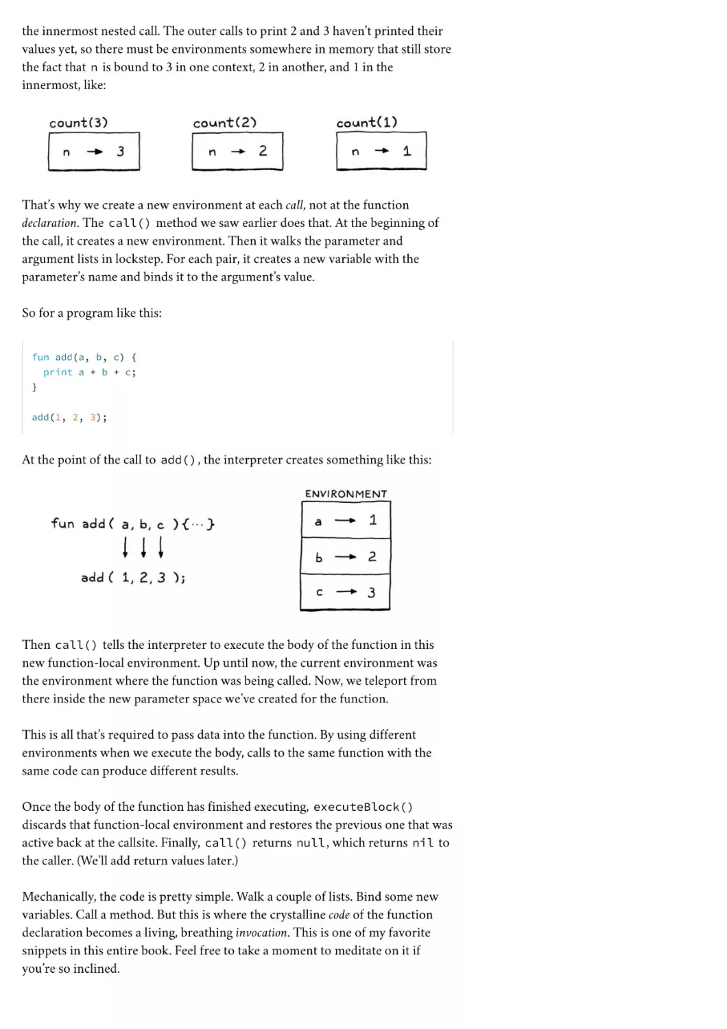
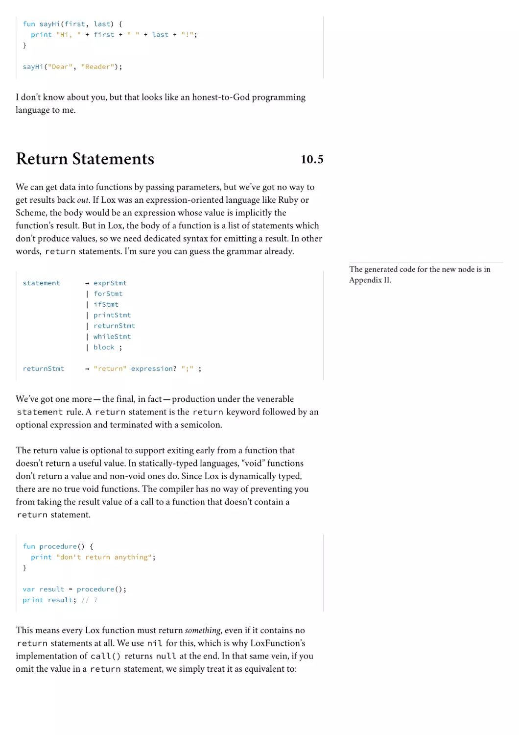
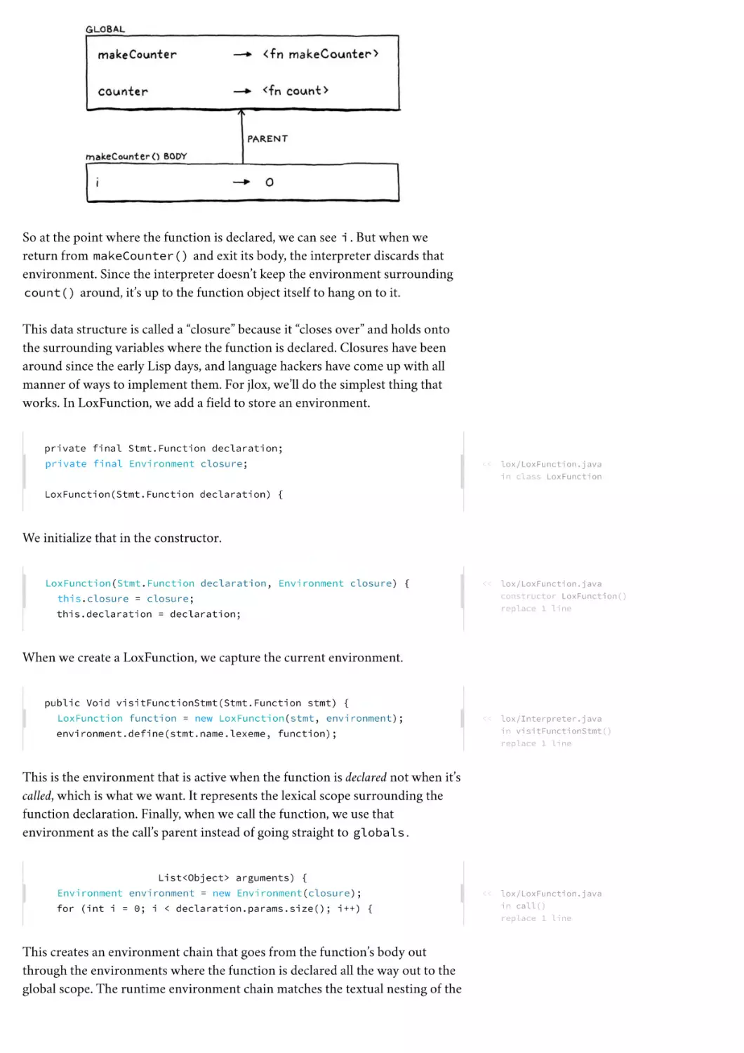
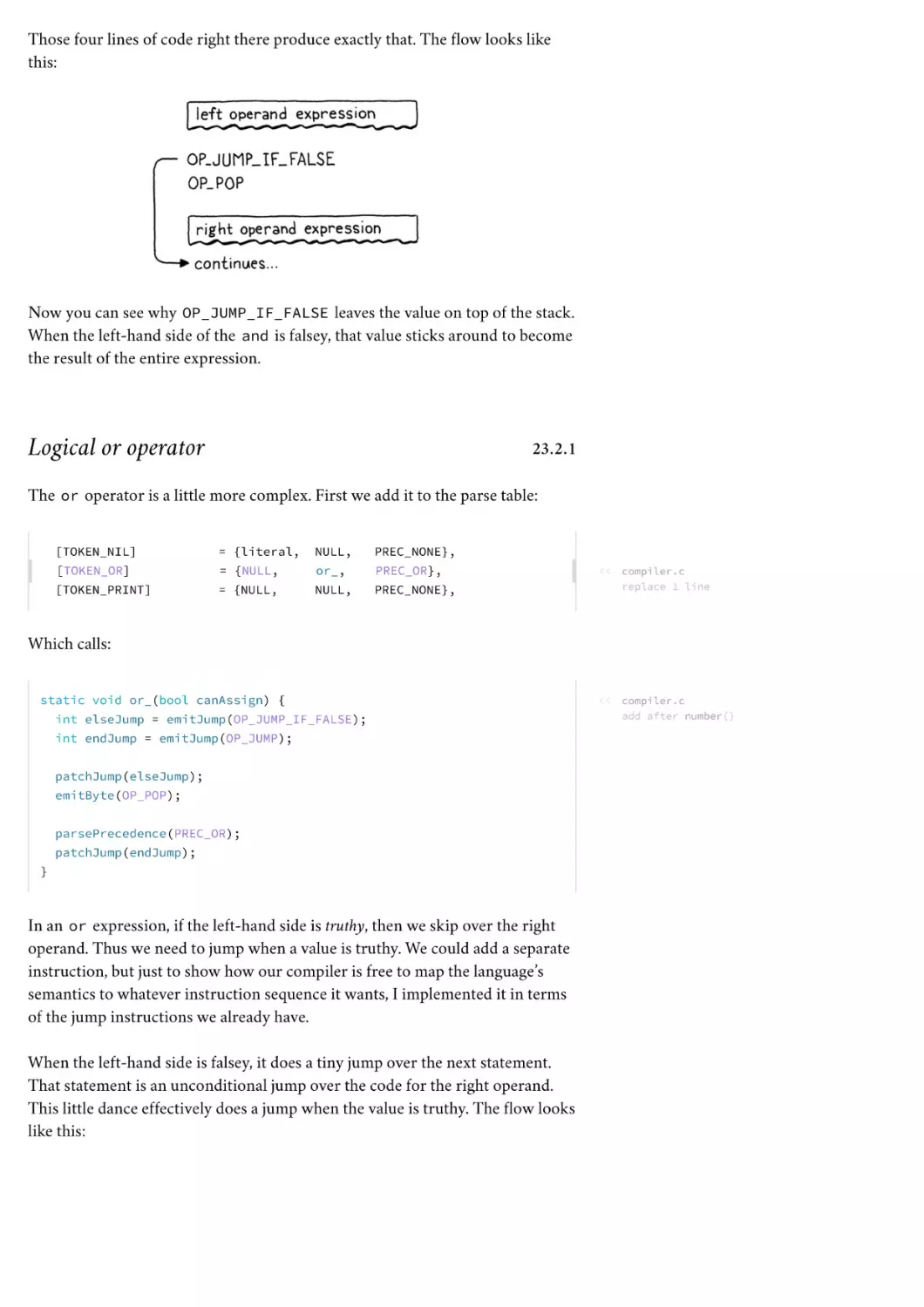
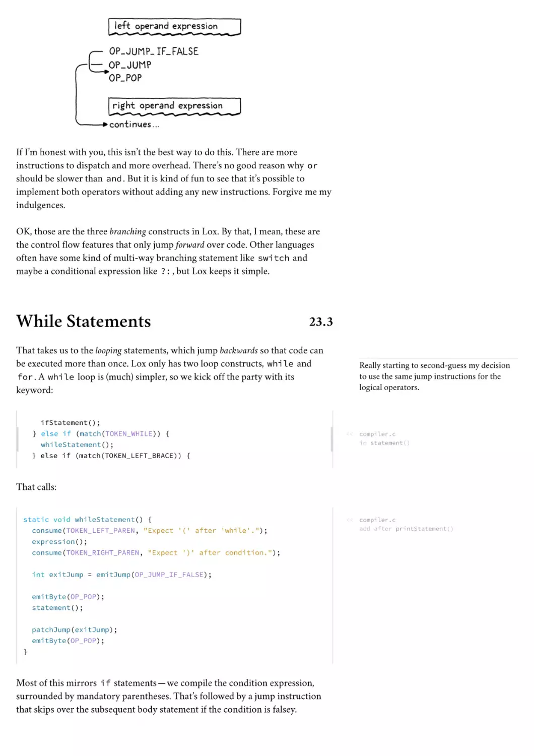
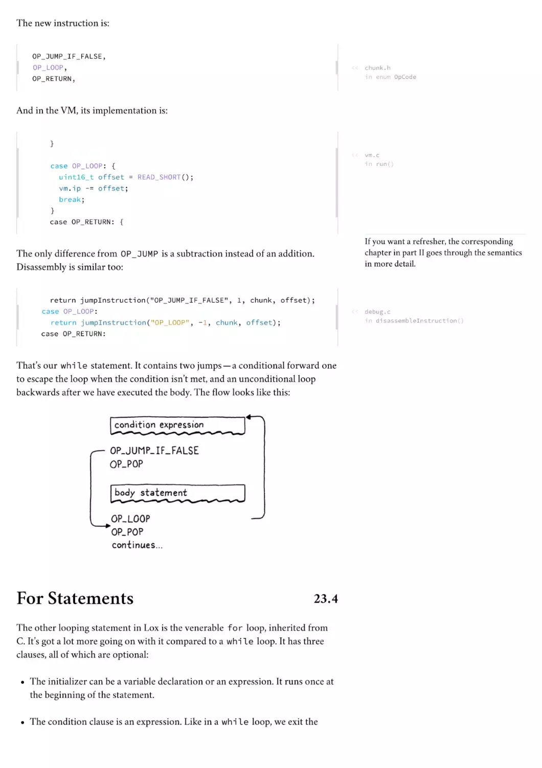
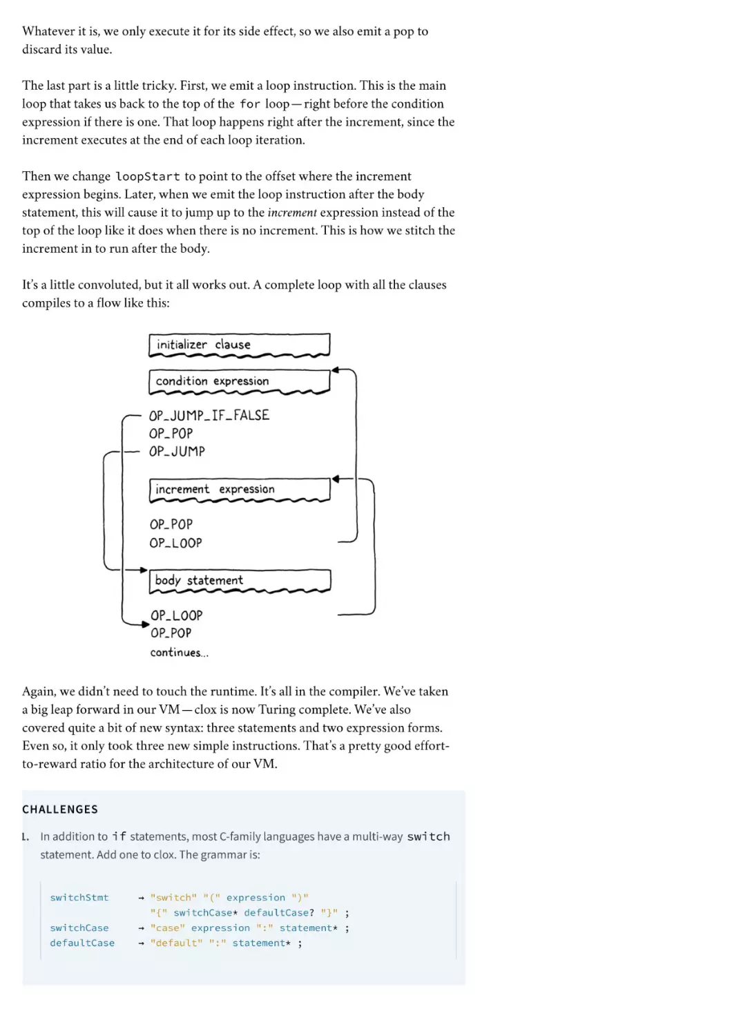
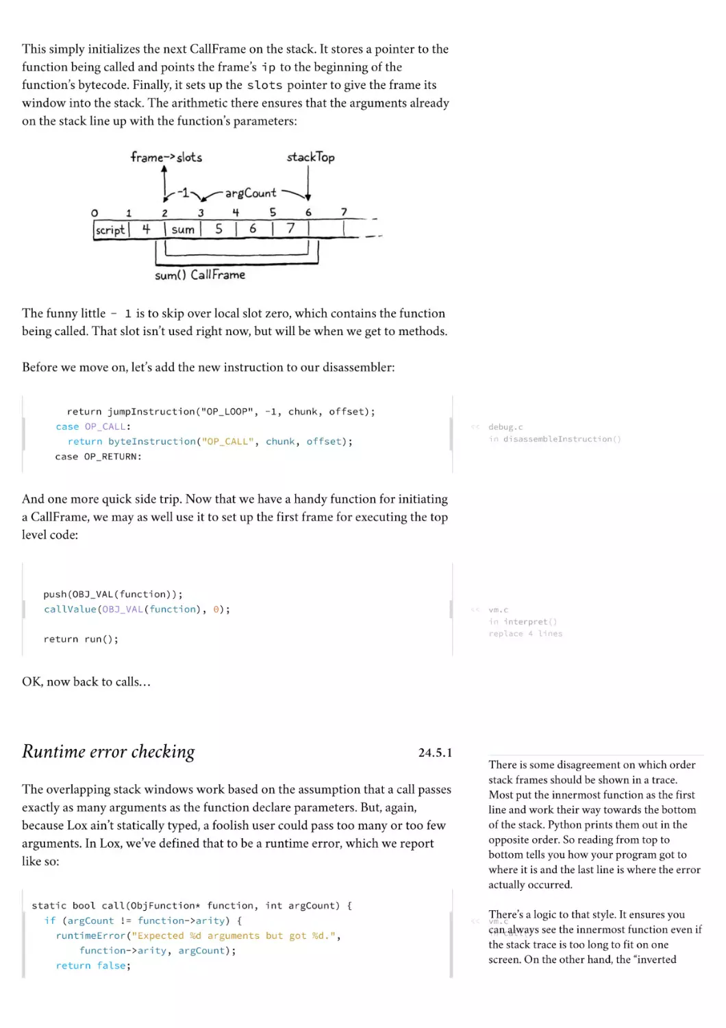
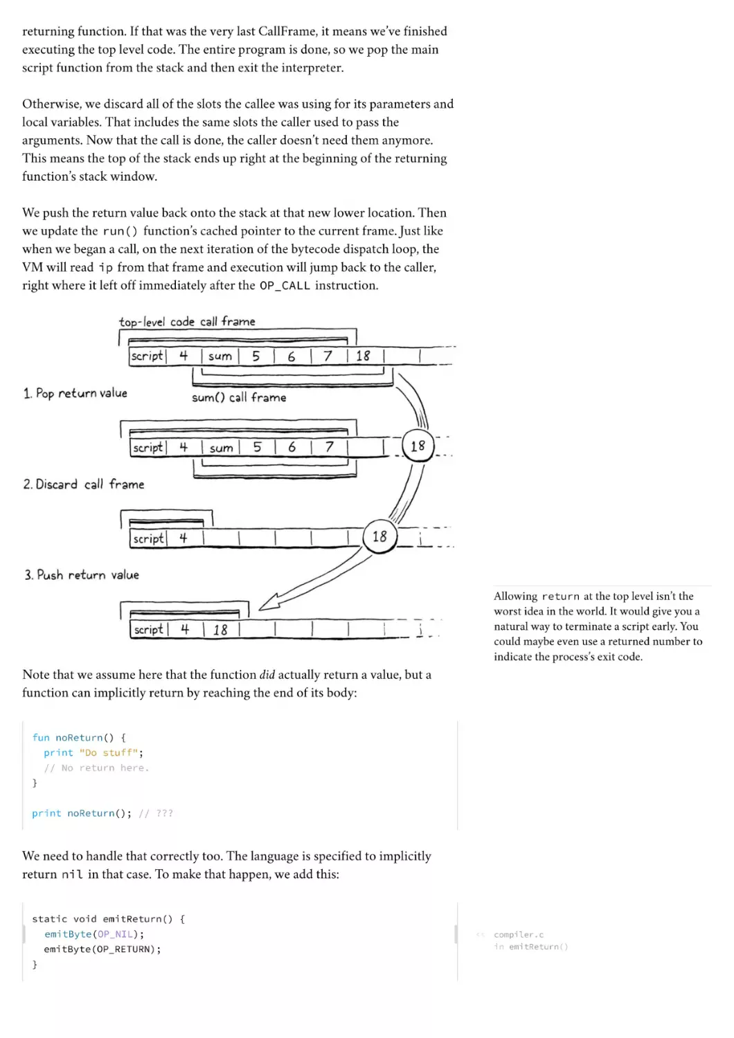
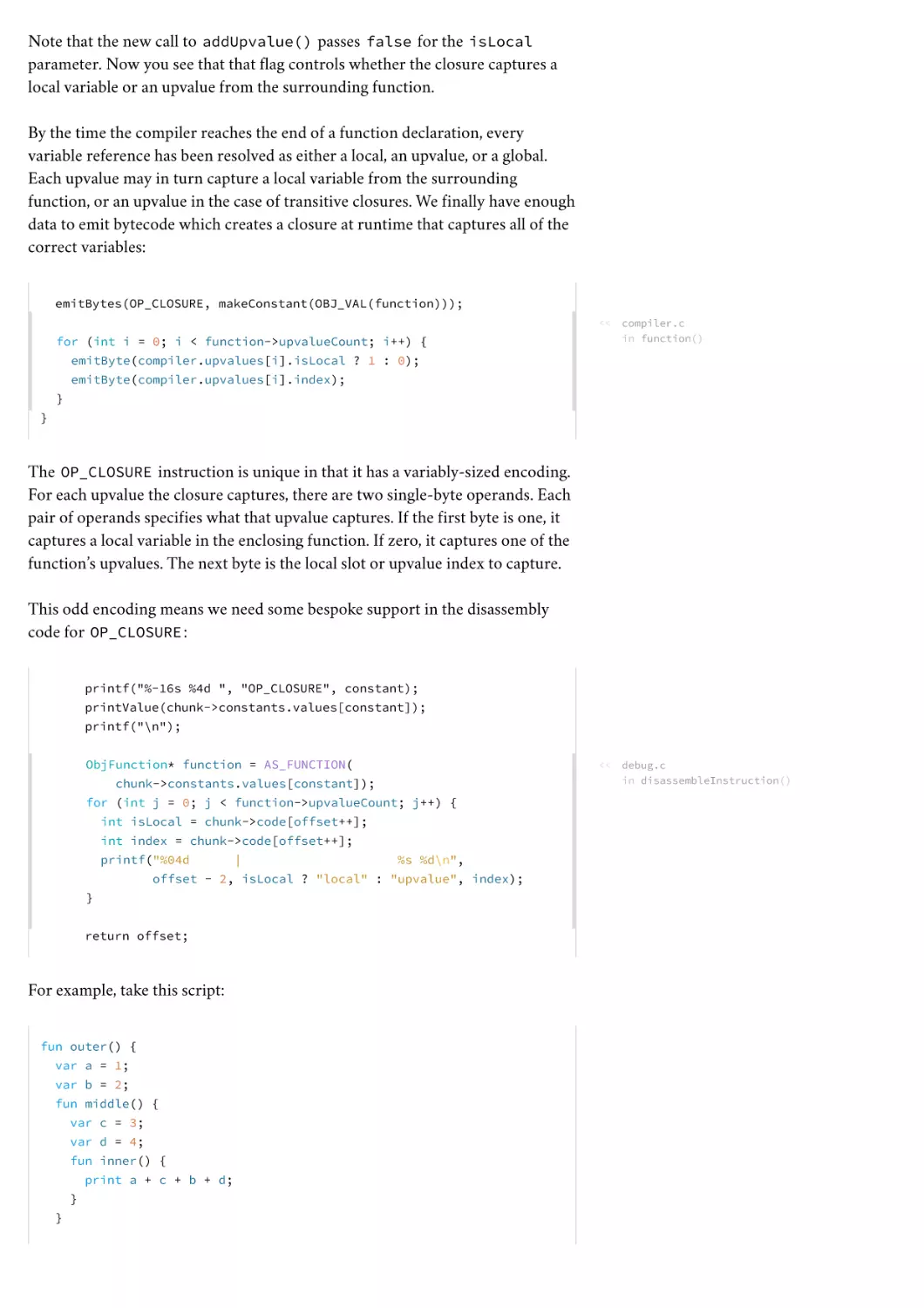
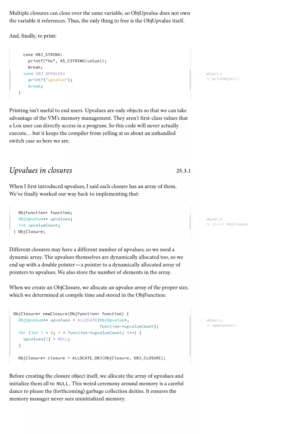
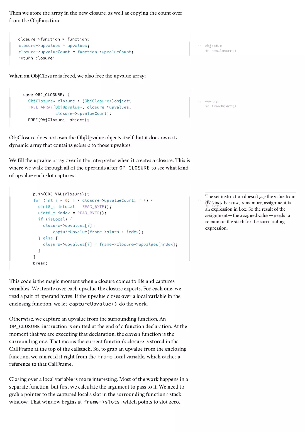
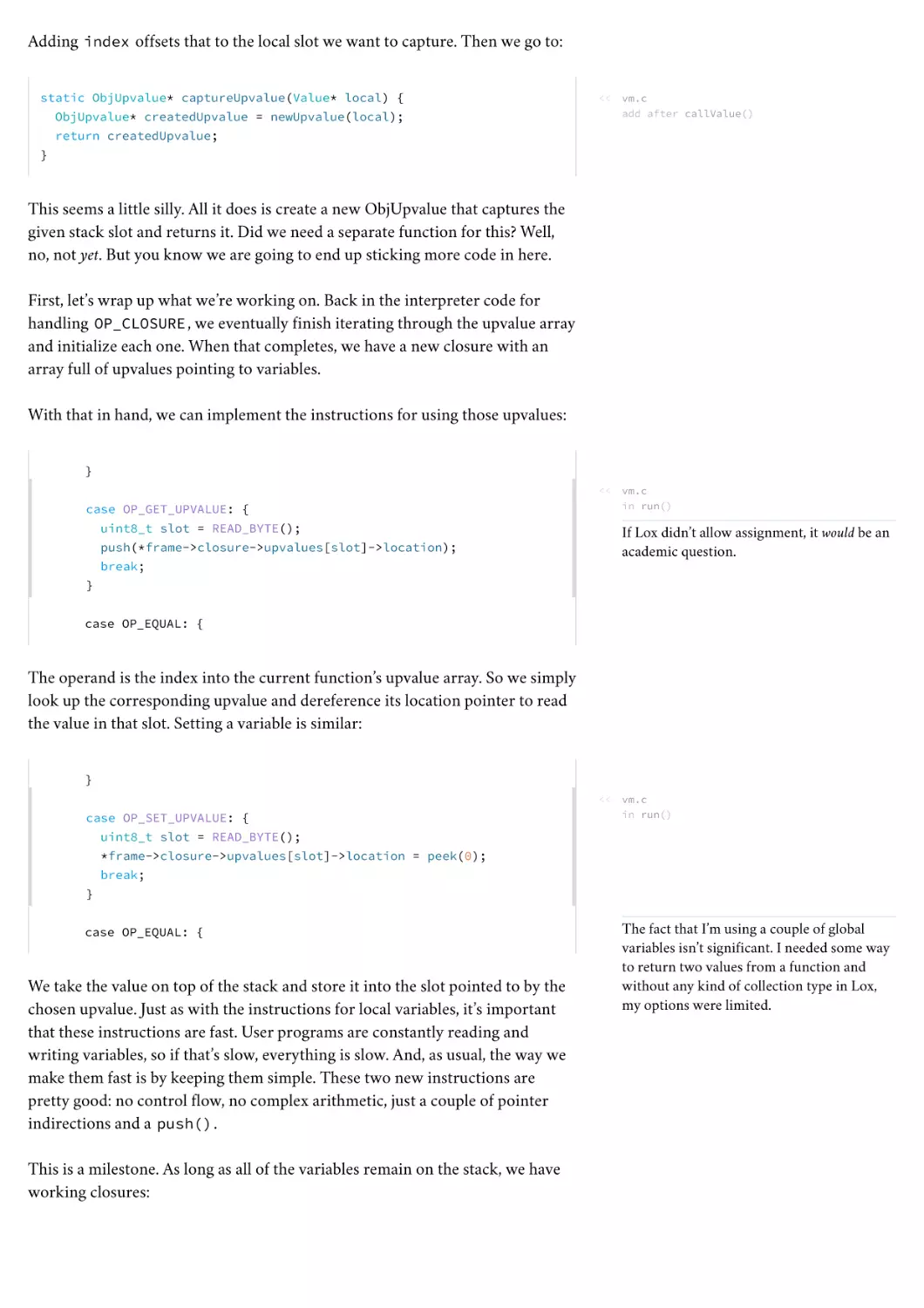
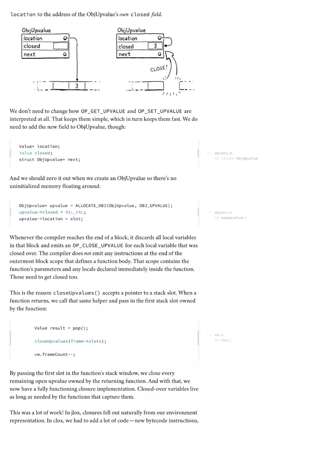
/


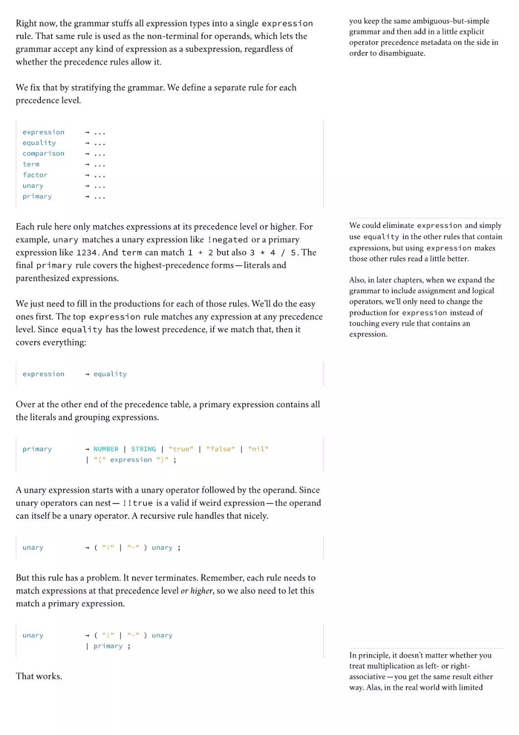


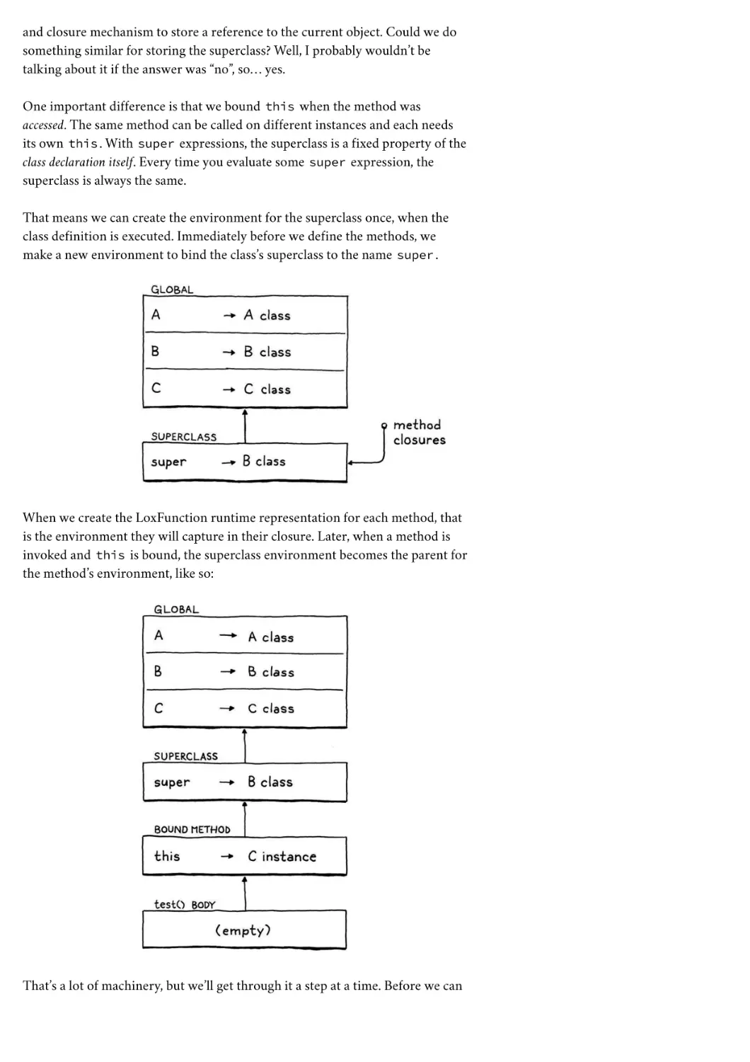

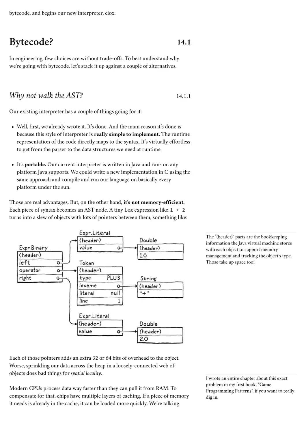
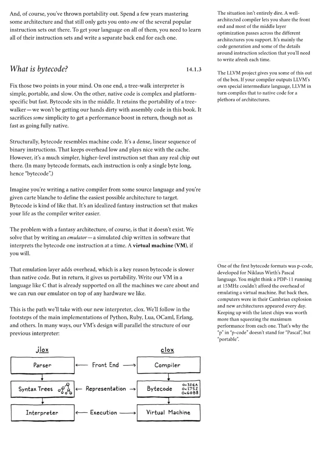


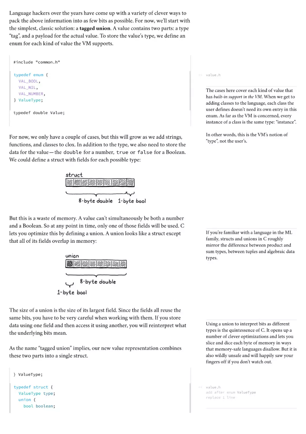
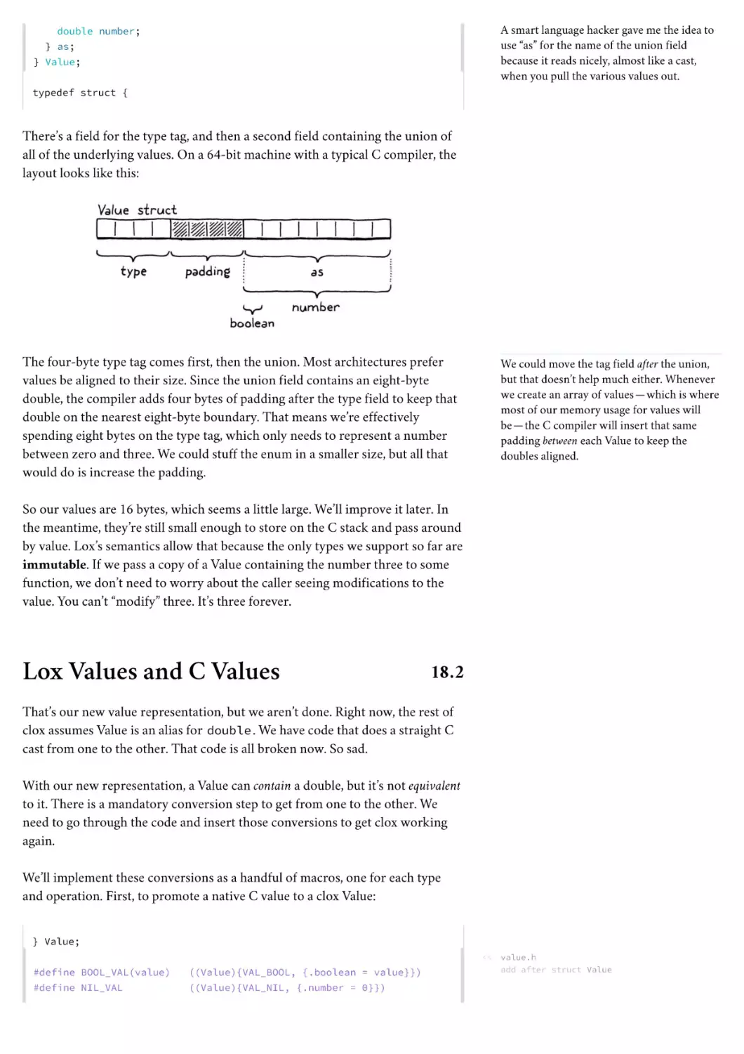
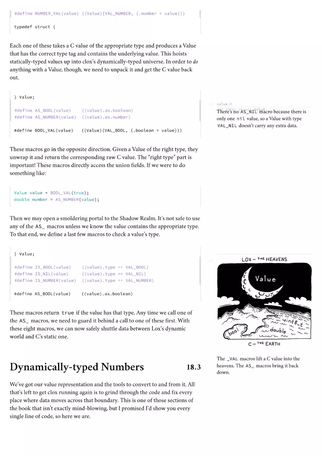


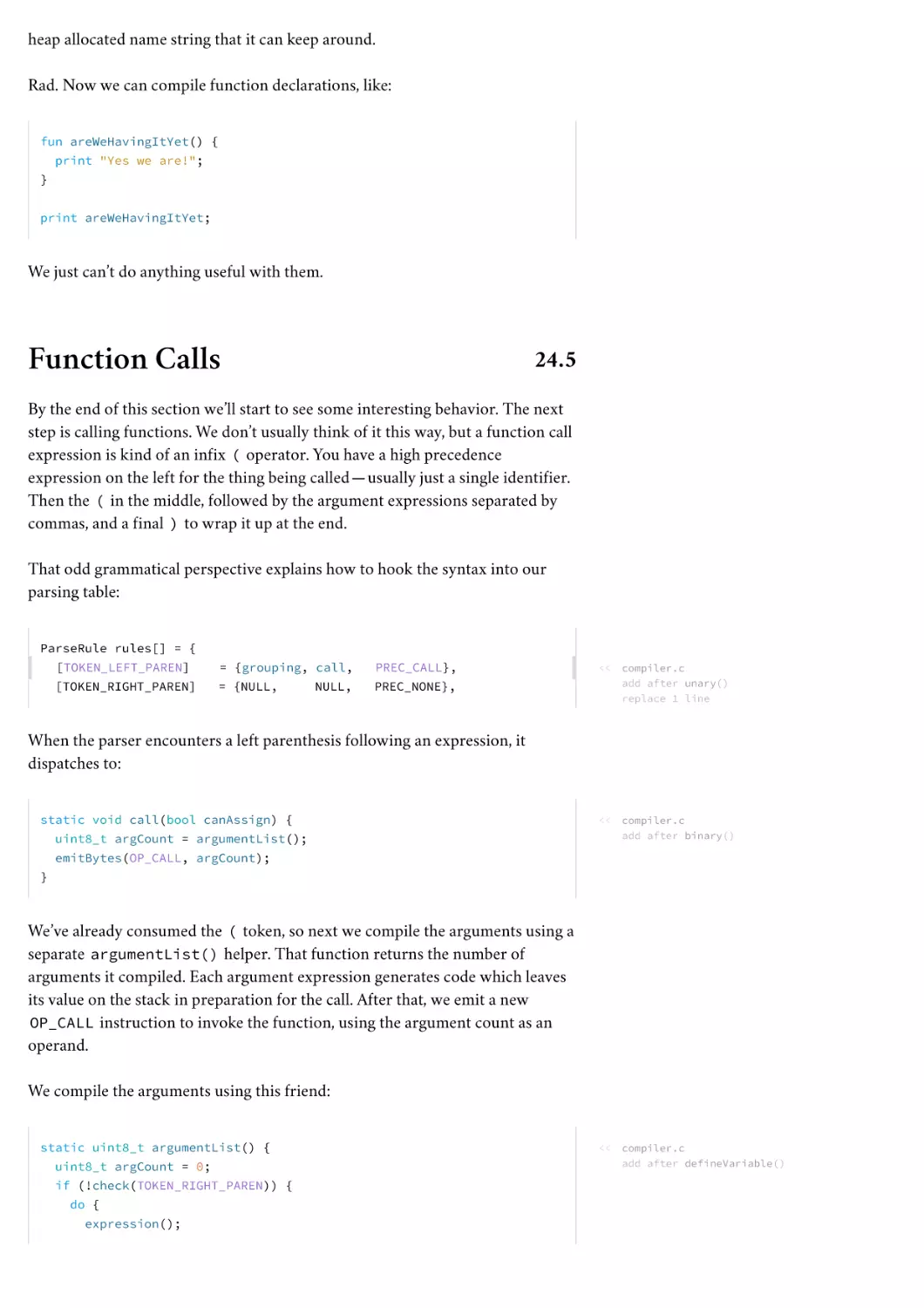


Text
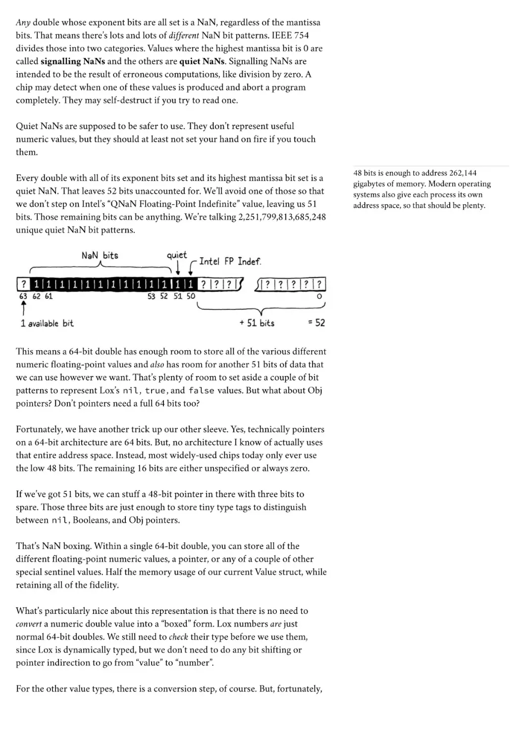
I
WELCOME
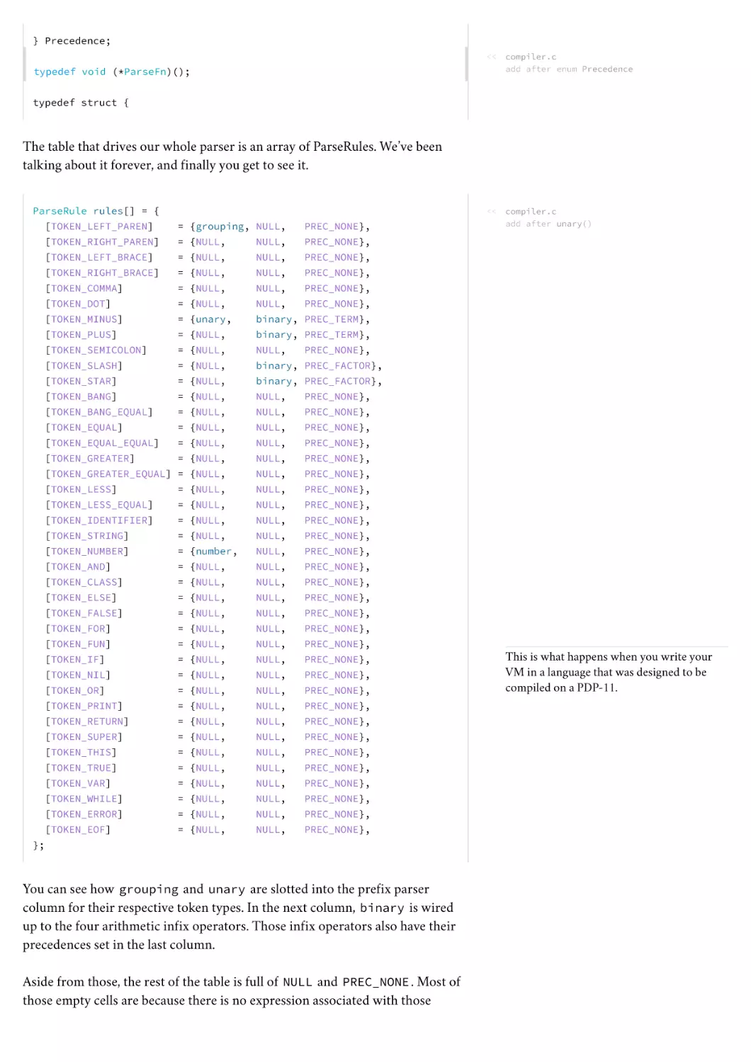
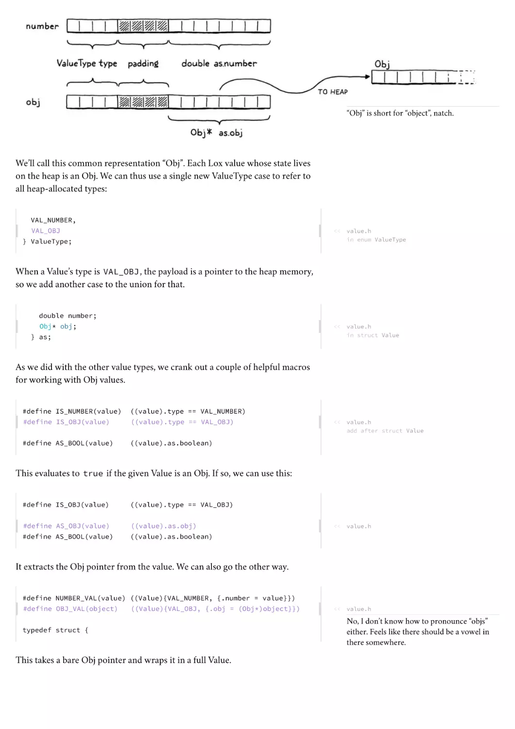
This may be the beginning of a grand adventure. Programming languages
encompass a huge space to explore and play in. Plenty of room for your own
creations to share with others or just enjoy yourself. Brilliant computer
scientists and software engineers have spent entire careers traversing this land
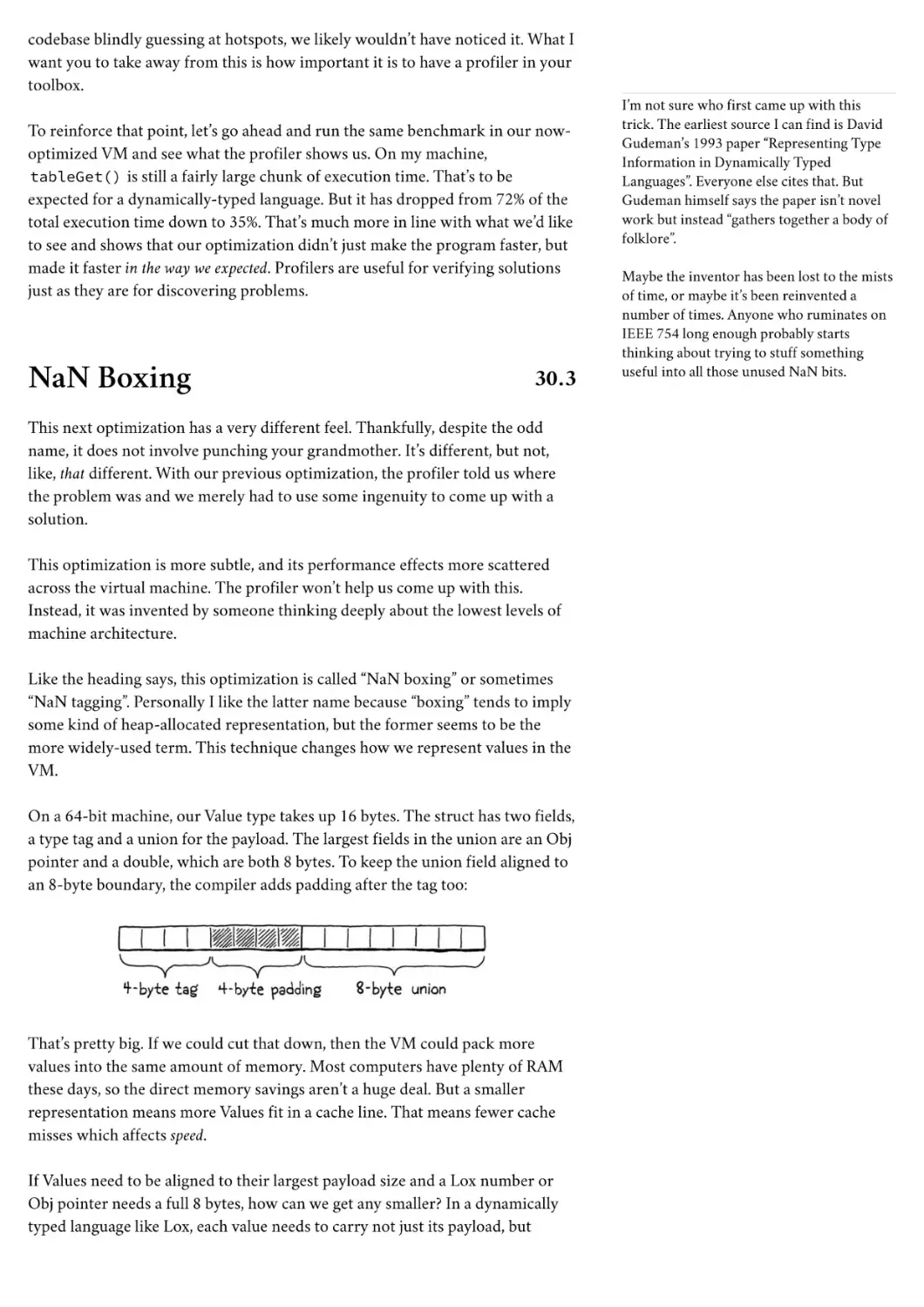
without ever reaching the end. If this book is your first entry into the country,
welcome.
The pages of this book give you a guided tour through some of the world of
languages. But before we strap on our hiking boots and venture out, we should
familiarize ourselves with the territory. The chapters in this part introduce you
to the basic concepts used by programming languages and how they are
organized.
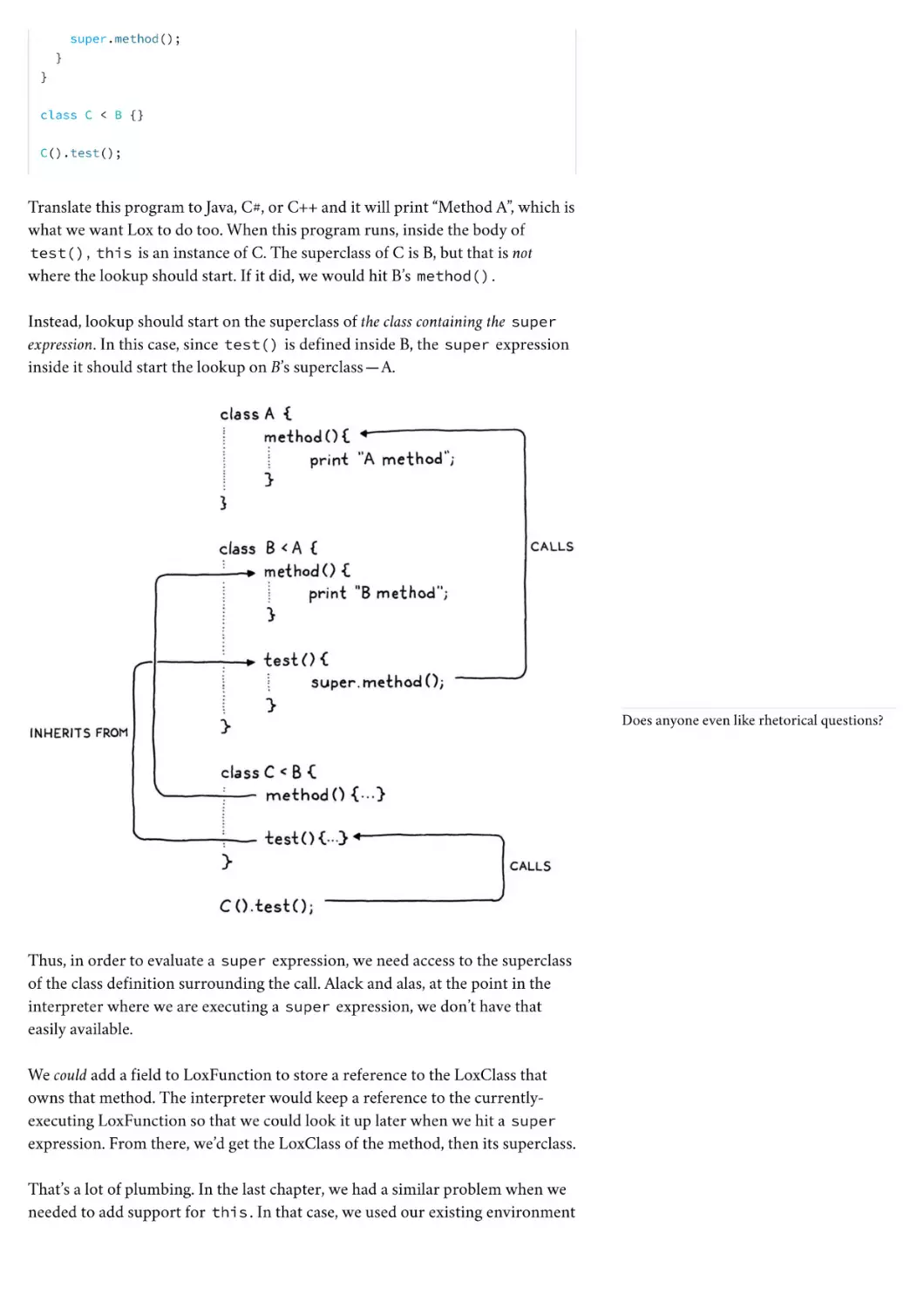
We will also get acquainted with Lox, the language we’ll spend the rest of the
book implementing (twice). Let’s go!
NEXT CHAPTER: “INTRODUCTION” →
Hand-cra!ed by Robert Nystrom — © 2015 – 2020
1
Introduction
“
Fairy tales are more than true: not because they
tell us that dragons exist, but because they tell us
that dragons can be beaten.
”
— Neil Gaiman, Coraline
I’m really excited we’re going on this journey together. This is a book on
implementing interpreters for programming languages. It’s also a book on how
to design a language worth implementing. It’s the book I wish I had when I first
started getting into languages, and it’s the book I’ve been writing in my head for
To my friends and family, sorry I’ve been so
absent-minded!
nearly a decade.
In these pages, we will walk step by step through two complete interpreters for
a full-featured language. I assume this is your first foray into languages, so I’ll
cover each concept and line of code you need to build a complete, usable, fast
language implementation.
In order to cram two full implementations inside one book without it turning
into a doorstop, this text is lighter on theory than others. As we build each piece
of the system, I will introduce the history and concepts behind it. I’ll try to get
you familiar with the lingo so that if you ever find yourself in a cocktail party
full of PL (programming language) researchers, you’ll fit in.
But we’re mostly going to spend our brain juice getting the language up and
running. This is not to say theory isn’t important. Being able to reason precisely
and formally about syntax and semantics is a vital skill when working on a
language. But, personally, I learn best by doing. It’s hard for me to wade through
paragraphs full of abstract concepts and really absorb them. But if I’ve coded
something, run it, and debugged it, then I get it.
That’s my goal for you. I want you to come away with a solid intuition of how a
real language lives and breathes. My hope is that when you read other, more
theoretical books later, the concepts there will firmly stick in your mind,
adhered to this tangible substrate.
Why Learn This Stuff?
1.1
Every introduction to every compiler book seems to have this section. I don’t
know what it is about programming languages that causes such existential
doubt. I don’t think ornithology books worry about justifying their existence.
They assume the reader loves birds and start teaching.
Strangely enough, a situation I have found
myself in multiple times. You wouldn’t
believe how much some of them can drink.
Static type systems in particular require
rigorous formal reasoning. Hacking on a type
system has the same feel as proving a
theorem in mathematics.
It turns out this is no coincidence. In the
early half of last century, Haskell Curry and
William Alvin Howard showed that they are
two sides of the same coin: the CurryHoward isomorphism.
But programming languages are a little different. I suppose it is true that the
odds of any of us creating a broadly successful general-purpose programming
language are slim. The designers of the world’s widely-used languages could fit
in a Volkswagen bus, even without putting the pop-top camper up. If joining
that elite group was the only reason to learn languages, it would be hard to
justify. Fortunately, it isn’t.
Little languages are everywhere
1.1.1
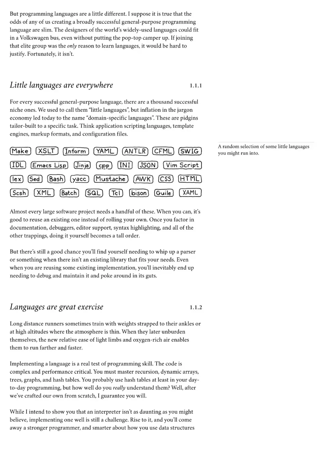
For every successful general-purpose language, there are a thousand successful
niche ones. We used to call them “little languages”, but inflation in the jargon
economy led today to the name “domain-specific languages”. These are pidgins
tailor-built to a specific task. Think application scripting languages, template
engines, markup formats, and configuration files.
A random selection of some little languages
you might run into.
Almost every large software project needs a handful of these. When you can, it’s
good to reuse an existing one instead of rolling your own. Once you factor in
documentation, debuggers, editor support, syntax highlighting, and all of the
other trappings, doing it yourself becomes a tall order.
But there’s still a good chance you’ll find yourself needing to whip up a parser
or something when there isn’t an existing library that fits your needs. Even
when you are reusing some existing implementation, you’ll inevitably end up
needing to debug and maintain it and poke around in its guts.
Languages are great exercise
1.1.2
Long distance runners sometimes train with weights strapped to their ankles or
at high altitudes where the atmosphere is thin. When they later unburden
themselves, the new relative ease of light limbs and oxygen-rich air enables
them to run farther and faster.
Implementing a language is a real test of programming skill. The code is
complex and performance critical. You must master recursion, dynamic arrays,
trees, graphs, and hash tables. You probably use hash tables at least in your dayto-day programming, but how well do you really understand them? Well, after
we’ve crafted our own from scratch, I guarantee you will.
While I intend to show you that an interpreter isn’t as daunting as you might
believe, implementing one well is still a challenge. Rise to it, and you’ll come
away a stronger programmer, and smarter about how you use data structures
and algorithms in your day job.
One more reason
1.1.3
This last reason is hard for me to admit, because it’s so close to my heart. Ever
since I learned to program as a kid, I felt there was something magical about
languages. When I first tapped out BASIC programs one key at a time I couldn’t
conceive how BASIC itself was made.
Later, the mixture of awe and terror on my college friends’ faces when talking
about their compilers class was enough to convince me language hackers were a
different breed of human—some sort of wizards granted privileged access to
arcane arts.
It’s a charming image, but it has a darker side. I didn’t feel like a wizard, so I was
left thinking I lacked some in-born quality necessary to join the cabal. Though
I’ve been fascinated by languages ever since I doodled made up keywords in my
school notebook, it took me decades to muster the courage to try to really learn
them. That “magical” quality, that sense of exclusivity, excluded me.
When I did finally start cobbling together my own little interpreters, I quickly
learned that, of course, there is no magic at all. It’s just code, and the people who
hack on languages are just people.
There are a few techniques you don’t often encounter outside of languages, and
some parts are a little difficult. But not more difficult than other obstacles
you’ve overcome. My hope is that if you’ve felt intimidated by languages, and
this book helps you overcome that fear, maybe I’ll leave you just a tiny bit braver
than you were before.
And, who knows, maybe you will make the next great language. Someone has to.
How the Book is Organized
1.2
This book is broken into three parts. You’re reading the first one now. It’s a
couple of chapters to get you oriented, teach you some of the lingo that
language hackers use, and introduce you to Lox, the language we’ll be
implementing.
Each of the other two parts builds one complete Lox interpreter. Within those
parts, each chapter is structured the same way. The chapter takes a single
language feature, teaches you the concepts behind it, and walks through an
implementation.
It took a good bit of trial and error on my part, but I managed to carve up the
two interpreters into chapter-sized chunks that build on the previous chapters
but require nothing from later ones. From the very first chapter, you’ll have a
working program you can run and play with. With each passing chapter, it
grows increasingly full-featured until you eventually have a complete language.
And one its practitioners don’t hesitate to
play up. Two of the seminal texts on
programming languages feature a dragon and
a wizard on their cover.
Aside from copious, scintillating English prose, chapters have a few other
delightful facets:
The code
1.2.1
We’re about crafting interpreters, so this book contains real code. Every single
line of code needed is included, and each snippet tells you where to insert it in
your ever-growing implementation.
Many other language books and language implementations use tools like Lex
and Yacc, so-called compiler-compilers that automatically generate some of
the source files for an implementation from some higher level description.
There are pros and cons to tools like those, and strong opinions—some might
say religious convictions—on both sides.
Yacc is a tool that takes in a grammar file and
produces a source file for a compiler, so it’s
sort of like a “compiler” that outputs a
compiler, which is where we get the term
“compiler-compiler”.
We will abstain from using them here. I want to ensure there are no dark
corners where magic and confusion can hide, so we’ll write everything by hand.
As you’ll see, it’s not as bad as it sounds and it means you really will understand
Yacc wasn’t the first of its ilk, which is why
it’s named “Yacc”—Yet Another CompilerCompiler. A later similar tool is Bison, named
as a pun on the pronunciation of Yacc like
“yak”.
each line of code and how both interpreters work.
A book has different constraints from the “real world” and so the coding style
here might not always reflect the best way to write maintainable production
software. If I seem a little cavalier about, say, omitting private or declaring a
global variable, understand I do so to keep the code easier on your eyes. The
pages here aren’t as wide as your IDE and every character counts.
Also, the code doesn’t have many comments. That’s because each handful of
lines is surrounded by several paragraphs of honest-to-God prose explaining it.
When you write a book to accompany your program, you are welcome to omit
comments too. Otherwise, you should probably use // a little more than I do.
If you find all of these little self-references
and puns charming and fun, you’ll fit right in
here. If not, well, maybe the language nerd
sense of humor is an acquired taste.
While the book contains every line of code and teaches what each means, it does
not describe the machinery needed to compile and run the interpreter. I assume
you can slap together a makefile or a project in your IDE of choice in order to
get the code to run. Those kinds of instructions get out of date quickly, and I
want this book to age like XO brandy, not backyard hooch.
Snippets
1.2.2
Since the book contains literally every line of code needed for the
implementations, the snippets are quite precise. Also, because I try to keep the
program in a runnable state even when major features are missing, sometimes
we add temporary code that gets replaced in later snippets.
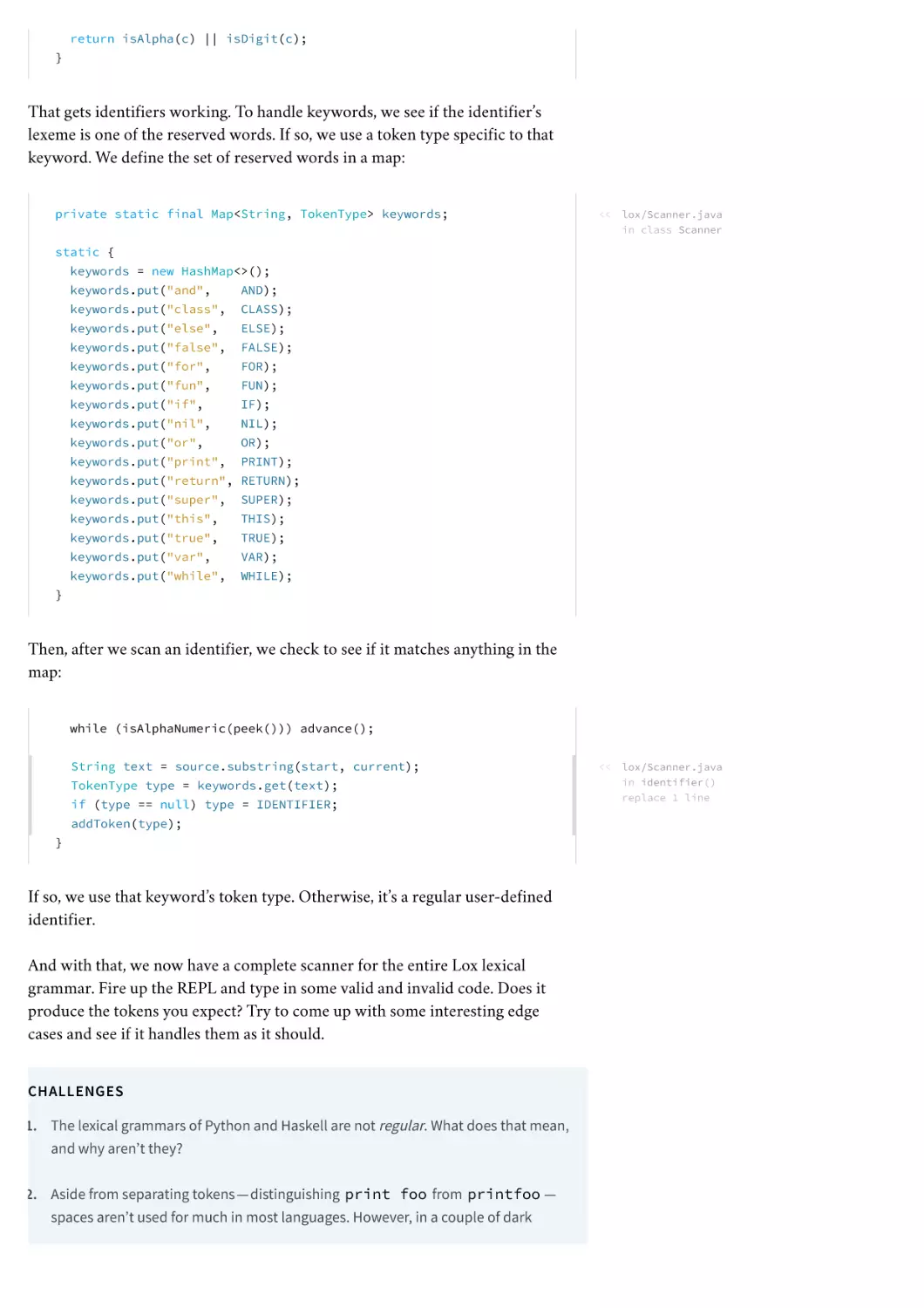
A snippet with all the bells and whistles looks like this:
default:
if (isDigit(c)) {
number();
<<
lox/Scanner.java
in scanToken()
} else {
replace 1 line
Lox.error(line, "Unexpected character.");
}
break;
In the center, you have the new code to add. It may have a few faded out lines
above or below to show where it goes in the existing surrounding code. There is
also a little blurb telling you in which file and where to place the snippet. If that
blurb says “replace _ lines”, there is some existing code between the faded lines
that you need to remove and replace with the new snippet.
Asides
1.2.3
Asides contain biographical sketches, historical background, references to
related topics, and suggestions of other areas to explore. There’s nothing that
you need to know in them to understand later parts of the book, so you can skip
them if you want. I won’t judge you, but I might be a little sad.
Challenges
Well, some asides do, at least. Most of them
are just dumb jokes and amateurish drawings.
1.2.4
Each chapter ends with a few exercises. Unlike textbook problem sets which
tend to review material you already covered, these are to help you learn more
than what’s in the chapter. They force you to step off the guided path and
explore on your own. They will make you research other languages, figure out
how to implement features, or otherwise get you out of your comfort zone.
Vanquish the challenges and you’ll come away with a broader understanding
and possibly a few bumps and scrapes. Or skip them if you want to stay inside
the comfy confines of the tour bus. It’s your book.
Design notes
1.2.5
A word of warning: the challenges often ask
you to make changes to the interpreter you’re
building. You’ll want to implement those in a
copy of your code. The later chapters assume
your interpreter is in a pristine
(“unchallenged”?) state.
Most “programming language” books are strictly programming language
implementation books. They rarely discuss how one might happen to design the
language being implemented. Implementation is fun because it is so precisely
defined. We programmers seem to have an affinity for things that are black and
white, ones and zeroes.
Personally, I think the world only needs so many implementations of
FORTRAN 77. At some point, you find yourself designing a new language. Once
you start playing that game, then the softer, human side of the equation becomes
paramount. Things like what features are easy to learn, how to balance
innovation and familiarity, what syntax is more readable and to whom.
All of that stuff profoundly affects the success of your new language. I want
your language to succeed, so in some chapters I end with a “design note”, a little
essay on some corner of the human aspect of programming languages. I’m no
I know a lot of language hackers whose
careers are based on this. You slide a language
spec under their door, wait a few months,
and code and benchmark results come out.
Hopefully your new language doesn’t
hardcode assumptions about the width of a
punched card into its grammar.
expert on this—I don’t know if anyone really is—so take these with a large
pinch of salt. That should make them tastier food for thought, which is my main
aim.
The First Interpreter
1.3
We’ll write our first interpreter, jlox, in Java. The focus is on concepts. We’ll write
the simplest, cleanest code we can to correctly implement the semantics of the
language. This will get us comfortable with the basic techniques and also hone
our understanding of exactly how the language is supposed to behave.
Java is a great language for this. It’s high level enough that we don’t get
overwhelmed by fiddly implementation details, but it’s still pretty explicit.
Unlike scripting languages, there tends to be less complex machinery hiding
under the hood, and you’ve got static types to see what data structures you’re
working with.
I also chose Java specifically because it is an object-oriented language. That
paradigm swept the programming world in the 90s and is now the dominant
way of thinking for millions of programmers. Odds are good you’re already
used to organizing code into classes and methods, so we’ll keep you in that
comfort zone.
While academic language folks sometimes look down on object-oriented
languages, the reality is that they are widely used even for language work. GCC
and LLVM are written in C++, as are most JavaScript virtual machines. Objectoriented languages are ubiquitous and the tools and compilers for a language are
often written in the same language.
And, finally, Java is hugely popular. That means there’s a good chance you
already know it, so there’s less for you to learn to get going in the book. If you
aren’t that familiar with Java, don’t freak out. I try to stick to a fairly minimal
subset of it. I use the diamond operator from Java 7 to make things a little more
terse, but that’s about it as far as “advanced” features go. If you know another
object-oriented language like C# or C++, you can muddle through.
By the end of part II, we’ll have a simple, readable implementation. What we
won’t have is a fast one. It also takes advantage of the Java virtual machine’s own
runtime facilities. We want to learn how Java itself implements those things.
The Second Interpreter
1.4
So in the next part, we start all over again, but this time in C. C is the perfect
language for understanding how an implementation really works, all the way
down to the bytes in memory and the code flowing through the CPU.
A big reason that we’re using C is so I can show you things C is particularly
good at, but that does mean you’ll need to be pretty comfortable with it. You
don’t have to be the reincarnation of Dennis Ritchie, but you shouldn’t be
A compiler reads files in one language.
translates them, and outputs files in another
language. You can implement a compiler in
any language, including the same language it
compiles, a process called “self-hosting”.
You can’t compile your compiler using itself
yet, but if you have another compiler for your
language written in some other language, you
use that one to compile your compiler once.
Now you can use the compiled version of
your own compiler to compile future
versions of itself and you can discard the
original one compiled from the other
compiler. This is called “bootstrapping” from
the image of pulling yourself up by your own
bootstraps.
spooked by pointers either.
If you aren’t there yet, pick up an introductory book on C and chew through it,
then come back here when you’re done. In return, you’ll come away from this
book an even stronger C programmer. That’s useful given how many language
implementations are written in C: Lua, CPython, and Ruby’s MRI, to name a
few.
In our C interpreter, clox, we are forced to implement for ourselves all the
things Java gave us for free. We’ll write our own dynamic array and hash table.
We’ll decide how objects are represented in memory, and build a garbage
collector to reclaim it.
Our Java implementation was focused on being correct. Now that we have that
down, we’ll turn to also being fast. Our C interpreter will contain a compiler
that translates Lox to an efficient bytecode representation (don’t worry, I’ll get
I pronounce the name like “sea-locks”, but
you can say it “clocks” or even “clochs”, where
you pronounce the “x” like the Greeks do if it
makes you happy.
into what that means soon) which it then executes. This is the same technique
used by implementations of Lua, Python, Ruby, PHP, and many other successful
languages.
We’ll even try our hand at benchmarking and optimization. By the end, we’ll
have a robust, accurate, fast interpreter for our language, able to keep up with
other professional caliber implementations out there. Not bad for one book and
a few thousand lines of code.
CHALLENGES
1. There are at least six domain-specific languages used in the little system I cobbled
together to write and publish this book. What are they?
2. Get a “Hello, world!” program written and running in Java. Set up whatever
Makefiles or IDE projects you need to get it working. If you have a debugger, get
comfortable with it and step through your program as it runs.
3. Do the same thing for C. To get some practice with pointers, define a doubly-linked
list of heap-allocated strings. Write functions to insert, find, and delete items from
it. Test them.
DESIGN NOTE: WHAT’S IN A NAME?
One of the hardest challenges in writing this book was coming up with a name for the
language it implements. I went through pages of candidates before I found one that
worked. As you’ll discover on the first day you start building your own language,
naming is deviously hard. A good name satisfies a few criteria:
1. It isn’t in use. You can run into all sorts of trouble, legal and social, if you
inadvertently step on someone else’s name.
2. It’s easy to pronounce. If things go well, hordes of people will be saying and
writing your language’s name. Anything longer than a couple of syllables or a
handful of letters will annoy them to no end.
Did you think this was just an interpreters
book? It’s a compiler book as well. Two for
the price of one!
3. It’s distinct enough to search for. People will Google your language’s name to
learn about it, so you want a word that’s rare enough that most results point to
your docs. Though, with the amount of AI search engines are packing today, that’s
less of an issue. Still, you won’t be doing your users any favors if you name your
language “for”.
4. It doesn’t have negative connotations across a number of cultures. This is hard to
guard for, but it’s worth considering. The designer of Nimrod ended up renaming
his language to “Nim” because too many people only remember that Bugs Bunny
used “Nimrod” (ironically, actually) as an insult.
If your potential name makes it through that gauntlet, keep it. Don’t get hung up on
trying to find an appellation that captures the quintessence of your language. If the
names of the world’s other successful languages teach us anything, it’s that the name
doesn’t matter much. All you need is a reasonably unique token.
NEXT CHAPTER: “A MAP OF THE TERRITORY” →
Hand-cra!ed by Robert Nystrom — © 2015 – 2020
2
A Map of the Territory
“
You must have a map, no matter how rough.
Otherwise you wander all over the place. In “The
”
Lord of the Rings” I never made anyone go
farther than he could on a given day.
— J.R.R. Tolkien
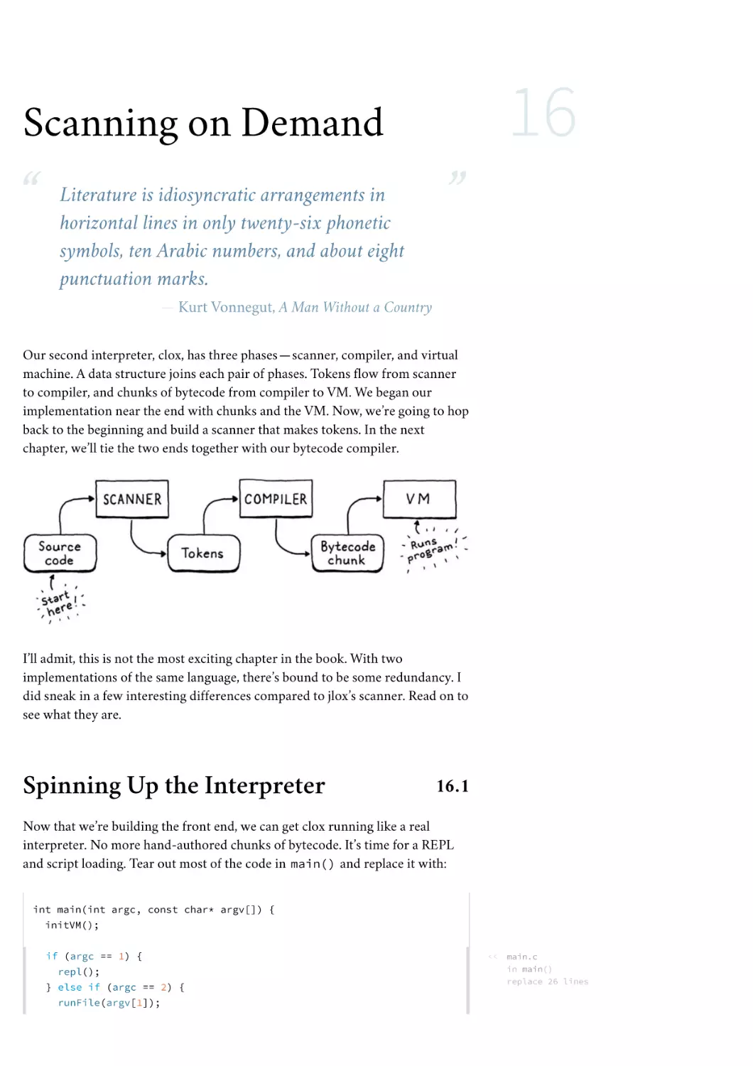
We don’t want to wander all over the place, so before we set off, let’s scan the
territory charted by previous language implementers. It will help us understand
where we are going and alternate routes others take.
First, let me establish a shorthand. Much of this book is about a language’s
implementation, which is distinct from the language itself in some sort of Platonic
ideal form. Things like “stack”, “bytecode”, and “recursive descent”, are nuts and
bolts one particular implementation might use. From the user’s perspective, as
long as the resulting contraption faithfully follows the language’s specification,
it’s all implementation detail.
We’re going to spend a lot of time on those details, so if I have to write
“language implementation” every single time I mention them, I’ll wear my fingers
off. Instead, I’ll use “language” to refer to either a language or an
implementation of it, or both, unless the distinction matters.
The Parts of a Language
2.1
Engineers have been building programming languages since the Dark Ages of
computing. As soon as we could talk to computers, we discovered doing so was
too hard, and we enlisted their help. I find it fascinating that even though
today’s machines are literally a million times faster and have orders of
magnitude more storage, the way we build programming languages is virtually
unchanged.
Though the area explored by language designers is vast, the trails they’ve carved
through it are few. Not every language takes the exact same path—some take a
shortcut or two—but otherwise they are reassuringly similar from Rear
Admiral Grace Hopper’s first COBOL compiler all the way to some hot new
transpile-to-JavaScript language whose “documentation” consists entirely of a
single poorly-edited README in a Git repository somewhere.
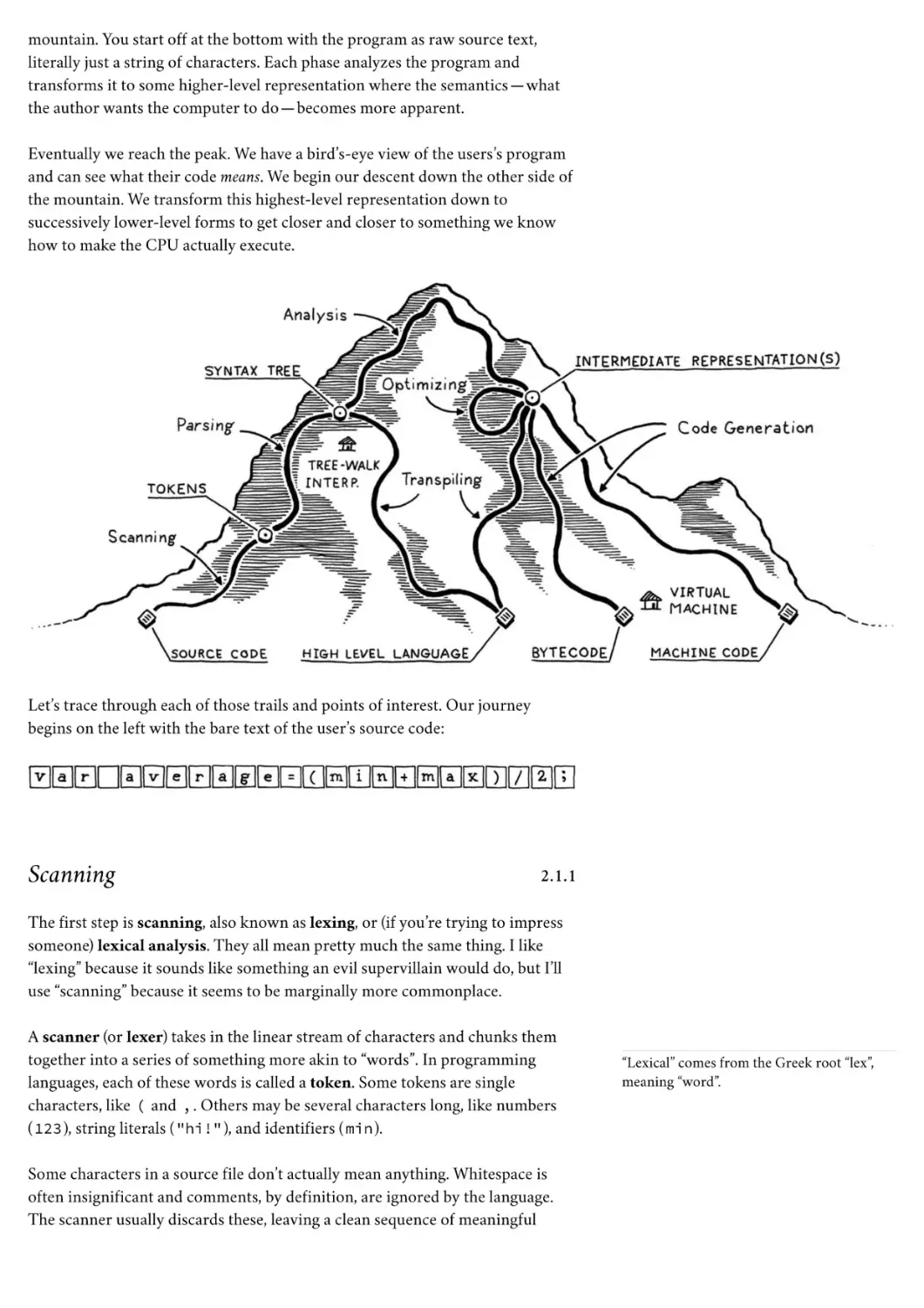
I visualize the network of paths an implementation may choose as climbing a
There are certainly dead ends, sad little culde-sacs of CS papers with zero citations and
now-forgotten optimizations that only made
sense when memory was measured in
individual bytes.
mountain. You start off at the bottom with the program as raw source text,
literally just a string of characters. Each phase analyzes the program and
transforms it to some higher-level representation where the semantics —what
the author wants the computer to do—becomes more apparent.
Eventually we reach the peak. We have a bird’s-eye view of the users’s program
and can see what their code means. We begin our descent down the other side of
the mountain. We transform this highest-level representation down to
successively lower-level forms to get closer and closer to something we know
how to make the CPU actually execute.
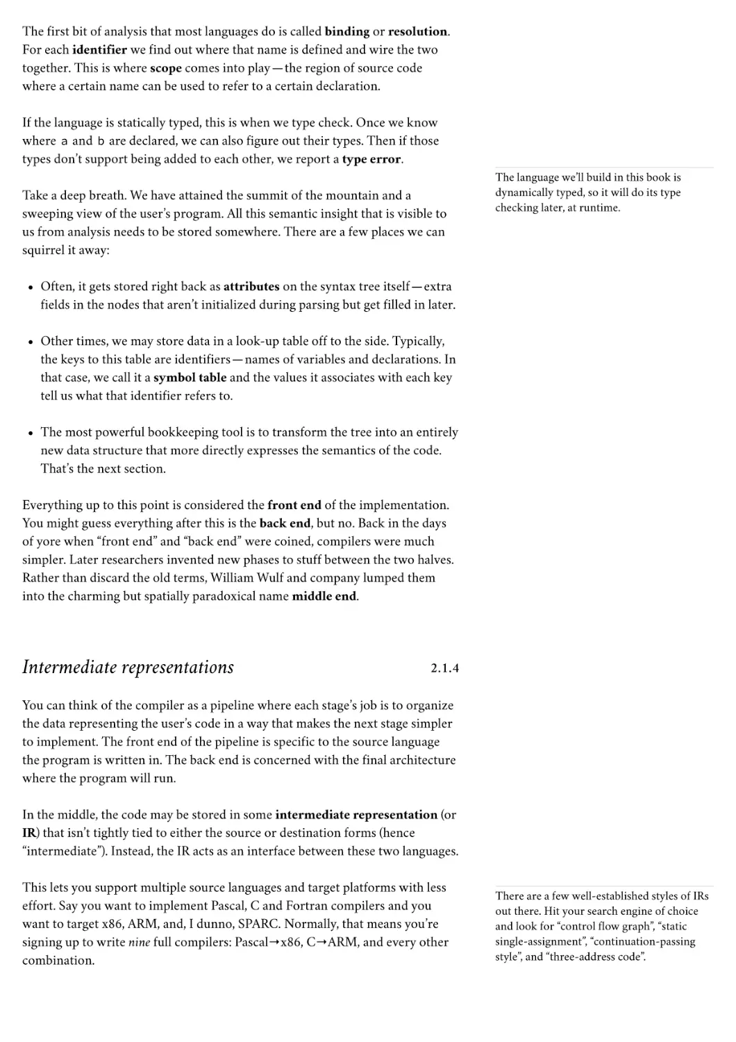
Let’s trace through each of those trails and points of interest. Our journey
begins on the left with the bare text of the user’s source code:
Scanning
2.1.1
The first step is scanning, also known as lexing, or (if you’re trying to impress
someone) lexical analysis. They all mean pretty much the same thing. I like
“lexing” because it sounds like something an evil supervillain would do, but I’ll
use “scanning” because it seems to be marginally more commonplace.
A scanner (or lexer) takes in the linear stream of characters and chunks them
together into a series of something more akin to “words”. In programming
languages, each of these words is called a token. Some tokens are single
characters, like ( and , . Others may be several characters long, like numbers
( 123 ), string literals ( "hi!" ), and identifiers ( min ).
Some characters in a source file don’t actually mean anything. Whitespace is
often insignificant and comments, by definition, are ignored by the language.
The scanner usually discards these, leaving a clean sequence of meaningful
“Lexical” comes from the Greek root “lex”,
meaning “word”.
tokens.
Parsing
2.1.2
The next step is parsing. This is where our syntax gets a grammar—the ability
to compose larger expressions and statements out of smaller parts. Did you ever
diagram sentences in English class? If so, you’ve done what a parser does, except
that English has thousands and thousands of “keywords” and an overflowing
cornucopia of ambiguity. Programming languages are much simpler.
A parser takes the flat sequence of tokens and builds a tree structure that
mirrors the nested nature of the grammar. These trees have a couple of different
names —“parse tree” or “abstract syntax tree”—depending on how close to the
bare syntactic structure of the source language they are. In practice, language
hackers usually call them “syntax trees”, “ASTs”, or often just “trees”.
Parsing has a long, rich history in computer science that is closely tied to the
artificial intelligence community. Many of the techniques used today to parse
programming languages were originally conceived to parse human languages by
AI researchers who were trying to get computers to talk to us.
It turns out human languages are too messy for the rigid grammars those
parsers could handle, but they were a perfect fit for the simpler artificial
grammars of programming languages. Alas, we flawed humans still manage to
use those simple grammars incorrectly, so the parser’s job also includes letting
us know when we do by reporting syntax errors.
Static analysis
2.1.3
The first two stages are pretty similar across all implementations. Now, the
individual characteristics of each language start coming into play. At this point,
we know the syntactic structure of the code—things like which expressions are
nested in which others—but we don’t know much more than that.
In an expression like a + b , we know we are adding a and b , but we don’t
know what those names refer to. Are they local variables? Global? Where are
they defined?
The first bit of analysis that most languages do is called binding or resolution.
For each identifier we find out where that name is defined and wire the two
together. This is where scope comes into play—the region of source code
where a certain name can be used to refer to a certain declaration.
If the language is statically typed, this is when we type check. Once we know
where a and b are declared, we can also figure out their types. Then if those
types don’t support being added to each other, we report a type error.
Take a deep breath. We have attained the summit of the mountain and a
sweeping view of the user’s program. All this semantic insight that is visible to
The language we’ll build in this book is
dynamically typed, so it will do its type
checking later, at runtime.
us from analysis needs to be stored somewhere. There are a few places we can
squirrel it away:
Often, it gets stored right back as attributes on the syntax tree itself—extra
fields in the nodes that aren’t initialized during parsing but get filled in later.
Other times, we may store data in a look-up table off to the side. Typically,
the keys to this table are identifiers—names of variables and declarations. In
that case, we call it a symbol table and the values it associates with each key
tell us what that identifier refers to.
The most powerful bookkeeping tool is to transform the tree into an entirely
new data structure that more directly expresses the semantics of the code.
That’s the next section.
Everything up to this point is considered the front end of the implementation.
You might guess everything after this is the back end, but no. Back in the days
of yore when “front end” and “back end” were coined, compilers were much
simpler. Later researchers invented new phases to stuff between the two halves.
Rather than discard the old terms, William Wulf and company lumped them
into the charming but spatially paradoxical name middle end.
Intermediate representations
2.1.4
You can think of the compiler as a pipeline where each stage’s job is to organize
the data representing the user’s code in a way that makes the next stage simpler
to implement. The front end of the pipeline is specific to the source language
the program is written in. The back end is concerned with the final architecture
where the program will run.
In the middle, the code may be stored in some intermediate representation (or
IR) that isn’t tightly tied to either the source or destination forms (hence
“intermediate”). Instead, the IR acts as an interface between these two languages.
This lets you support multiple source languages and target platforms with less
effort. Say you want to implement Pascal, C and Fortran compilers and you
want to target x86, ARM, and, I dunno, SPARC. Normally, that means you’re
signing up to write nine full compilers: Pascal→x86, C→ARM, and every other
combination.
There are a few well-established styles of IRs
out there. Hit your search engine of choice
and look for “control flow graph”, “static
single-assignment”, “continuation-passing
style”, and “three-address code”.
A shared intermediate representation reduces that dramatically. You write one
front end for each source language that produces the IR. Then one back end for
each target architecture. Now you can mix and match those to get every
combination.
There’s another big reason we might want to transform the code into a form
that makes the semantics more apparent…
Optimization
2.1.5
If you’ve ever wondered how GCC supports
so many crazy languages and architectures,
like Modula-3 on Motorola 68k, now you
know. Language front ends target one of a
handful of IRs, mainly GIMPLE and RTL.
Target backends like the one for 68k then
take those IRs and produce native code.
Once we understand what the user’s program means, we are free to swap it out
with a different program that has the same semantics but implements them more
efficiently—we can optimize it.
A simple example is constant folding: if some expression always evaluates to
the exact same value, we can do the evaluation at compile time and replace the
code for the expression with its result. If the user typed in:
pennyArea = 3.14159 * (0.75 / 2) * (0.75 / 2);
We can do all of that arithmetic in the compiler and change the code to:
pennyArea = 0.4417860938;
Optimization is a huge part of the programming language business. Many
language hackers spend their entire careers here, squeezing every drop of
performance they can out of their compilers to get their benchmarks a fraction
of a percent faster. It can become a sort of obsession.
We’re mostly going to hop over that rathole in this book. Many successful
languages have surprisingly few compile-time optimizations. For example, Lua
and CPython generate relatively unoptimized code, and focus most of their
performance effort on the runtime.
Code generation
2.1.6
We have applied all of the optimizations we can think of to the user’s program.
The last step is converting it to a form the machine can actually run. In other
words generating code (or code gen), where “code” here usually refers to the
kind of primitive assembly-like instructions a CPU runs and not the kind of
“source code” a human might want to read.
Finally, we are in the back end, descending the other side of the mountain.
From here on out, our representation of the code becomes more and more
primitive, like evolution run in reverse, as we get closer to something our
simple-minded machine can understand.
If you can’t resist poking your foot into that
hole, some keywords to get you started are
“constant propagation”, “common
subexpression elimination”, “loop invariant
code motion”, “global value numbering”,
“strength reduction”, “scalar replacement of
aggregates”, “dead code elimination”, and
“loop unrolling”.
We have a decision to make. Do we generate instructions for a real CPU or a
virtual one? If we generate real machine code, we get an executable that the OS
can load directly onto the chip. Native code is lightning fast, but generating it is
a lot of work. Today’s architectures have piles of instructions, complex
pipelines, and enough historical baggage to fill a 747’s luggage bay.
Speaking the chip’s language also means your compiler is tied to a specific
architecture. If your compiler targets x86 machine code, it’s not going to run on
an ARM device. All the way back in the 60s, during the Cambrian explosion of
computer architectures, that lack of portability was a real obstacle.
To get around that, hackers like Martin Richards and Niklaus Wirth, of BCPL
and Pascal fame, respectively, made their compilers produce virtual machine
code. Instead of instructions for some real chip, they produced code for a
For example, the AAD (“ASCII Adjust AX
Before Division”) instruction lets you
perform division, which sounds useful.
Except that instruction takes as operands two
binary-coded decimal digits packed into a
single 16-bit register. When was the last time
you needed BCD on a 16-bit machine?
hypothetical, idealized machine. Wirth called this “p-code” for “portable”, but
today, we generally call it bytecode because each instruction is often a single
byte long.
These synthetic instructions are designed to map a little more closely to the
language’s semantics, and not be so tied to the peculiarities of any one computer
architecture and its accumulated historical cruft. You can think of it like a
dense, binary encoding of the language’s low-level operations.
Virtual machine
2.1.7
If your compiler produces bytecode, your work isn’t over once that’s done.
Since there is no chip that speaks that bytecode, it’s your job to translate. Again,
you have two options. You can write a little mini-compiler for each target
architecture that converts the bytecode to native code for that machine. You still
have to do work for each chip you support, but this last stage is pretty simple
and you get to reuse the rest of the compiler pipeline across all of the machines
you support. You’re basically using your bytecode as an intermediate
representation.
The basic principle here is that the farther
down the pipeline you push the architecturespecific work, the more of the earlier phases
you can share across architectures.
There is a tension, though. Many
optimizations, like register allocation and
instruction selection, work best when they
know the strengths and capabilities of a
specific chip. Figuring out which parts of
your compiler can be shared and which
should be target-specific is an art.
Or you can write a virtual machine (VM), a program that emulates a
hypothetical chip supporting your virtual architecture at runtime. Running
bytecode in a VM is slower than translating it to native code ahead of time
because every instruction must be simulated at runtime each time it executes. In
return, you get simplicity and portability. Implement your VM in, say, C, and
you can run your language on any platform that has a C compiler. This is how
the second interpreter we build in this book works.
Runtime
2.1.8
We have finally hammered the user’s program into a form that we can execute.
The last step is running it. If we compiled it to machine code, we simply tell the
operating system to load the executable and off it goes. If we compiled it to
bytecode, we need to start up the VM and load the program into that.
The term “virtual machine” also refers to a
different kind of abstraction. A system
virtual machine emulates an entire
hardware platform and operating system in
software. This is how you can play Windows
games on your Linux machine, and how
cloud providers give customers the user
experience of controlling their own “server”
without needing to physically allocate
separate computers for each user.
The kind of VMs we’ll talk about in this book
are language virtual machines or process
virtual machines if you want to be
unambiguous.
In both cases, for all but the basest of low-level languages, we usually need some
services that our language provides while the program is running. For example,
if the language automatically manages memory, we need a garbage collector
going in order to reclaim unused bits. If our language supports “instance of”
tests so you can see what kind of object you have, then we need some
representation to keep track of the type of each object during execution.
All of this stuff is going at runtime, so it’s called, appropriately, the runtime. In
a fully compiled language, the code implementing the runtime gets inserted
directly into the resulting executable. In, say, Go, each compiled application has
its own copy of Go’s runtime directly embedded in it. If the language is run
inside an interpreter or VM, then the runtime lives there. This is how most
implementations of languages like Java, Python, and JavaScript work.
Shortcuts and Alternate Routes
2.2
That’s the long path covering every possible phase you might implement. Many
languages do walk the entire route, but there are a few shortcuts and alternate
paths.
Single-pass compilers
2.2.1
Some simple compilers interleave parsing, analysis, and code generation so that
they produce output code directly in the parser, without ever allocating any
syntax trees or other IRs. These single-pass compilers restrict the design of the
language. You have no intermediate data structures to store global information
about the program, and you don’t revisit any previously parsed part of the code.
That means as soon as you see some expression, you need to know enough to
correctly compile it.
Pascal and C were designed around this limitation. At the time, memory was so
precious that a compiler might not even be able to hold an entire source file in
memory, much less the whole program. This is why Pascal’s grammar requires
type declarations to appear first in a block. It’s why in C you can’t call a function
above the code that defines it unless you have an explicit forward declaration
that tells the compiler what it needs to know to generate code for a call to the
later function.
Tree-walk interpreters
2.2.2
Some programming languages begin executing code right after parsing it to an
AST (with maybe a bit of static analysis applied). To run the program, the
interpreter traverses the syntax tree one branch and leaf at a time, evaluating
each node as it goes.
This implementation style is common for student projects and little languages,
but is not widely used for general-purpose languages since it tends to be slow.
Syntax-directed translation is a structured
technique for building these all-at-once
compilers. You associate an action with each
piece of the grammar, usually one that
generates output code. Then, whenever the
parser matches that chunk of syntax, it
executes the action, building up the target
code one rule at a time.
Some people use “interpreter” to mean only these kinds of implementations, but
others define that word more generally, so I’ll use the inarguably explicit “treewalk interpreter” to refer to these. Our first interpreter rolls this way.
Transpilers
2.2.3
A notable exception is early versions of Ruby,
which were tree walkers. At 1.9, the canonical
implementation of Ruby switched from the
original MRI (“Matz’ Ruby Interpreter”) to
Koichi Sasada’s YARV (“Yet Another Ruby
VM”). YARV is a bytecode virtual machine.
Writing a complete back end for a language can be a lot of work. If you have
some existing generic IR to target, you could bolt your front end onto that.
Otherwise, it seems like you’re stuck. But what if you treated some other source
language as if it were an intermediate representation?
You write a front end for your language. Then, in the back end, instead of doing
all the work to lower the semantics to some primitive target language, you
produce a string of valid source code for some other language that’s about as
high level as yours. Then, you use the existing compilation tools for that
language as your escape route off the mountain and down to something you can
execute.
They used to call this a source-to-source compiler or a transcompiler. After
the rise of languages that compile to JavaScript in order to run in the browser,
they’ve affected the hipster sobriquet transpiler.
While the first transcompiler translated one assembly language to another,
today, most transpilers work on higher-level languages. After the viral spread of
UNIX to machines various and sundry, there began a long tradition of
compilers that produced C as their output language. C compilers were available
everywhere UNIX was and produced efficient code, so targeting C was a good
way to get your language running on a lot of architectures.
Web browsers are the “machines” of today, and their “machine code” is
JavaScript, so these days it seems almost every language out there has a compiler
that targets JS since that’s the main way to get your code running in a browser.
The first transcompiler, XLT86, translated
8080 assembly into 8086 assembly. That
might seem straightforward, but keep in
mind the 8080 was an 8-bit chip and the
8086 a 16-bit chip that could use each
register as a pair of 8-bit ones. XLT86 did
data flow analysis to track register usage in
the source program and then efficiently map
it to the register set of the 8086.
It was written by Gary Kildall, a tragic hero
of computer science if there ever was one.
One of the first people to recognize the
promise of microcomputers, he created
PL/M and CP/M, the first high level
language and OS for them.
He was a sea captain, business owner,
licensed pilot, and motorcyclist. A TV host
with the Kris Kristofferson-esque look
sported by dashing bearded dudes in the 80s.
He took on Bill Gates and, like many, lost,
before meeting his end in a biker bar under
mysterious circumstances. He died too
young, but sure as hell lived before he did.
The front end—scanner and parser—of a transpiler looks like other compilers.
Then, if the source language is only a simple syntactic skin over the target
language, it may skip analysis entirely and go straight to outputting the
analogous syntax in the destination language.
JS used to be the only way to execute code in a
browser. Thanks to Web Assembly, compilers
now have a second, lower-level language they
can target that runs on the web.
If the two languages are more semantically different, then you’ll see more of the
typical phases of a full compiler including analysis and possibly even
optimization. Then, when it comes to code generation, instead of outputting
some binary language like machine code, you produce a string of grammatically
correct source (well, destination) code in the target language.
Either way, you then run that resulting code through the output language’s
existing compilation pipeline and you’re good to go.
Just-in-time compilation
2.2.4
This last one is less of a shortcut and more a dangerous alpine scramble best
reserved for experts. The fastest way to execute code is by compiling it to
machine code, but you might not know what architecture your end user’s
machine supports. What to do?
You can do the same thing that the HotSpot JVM, Microsoft’s CLR and most
JavaScript interpreters do. On the end user’s machine, when the program is
loaded—either from source in the case of JS, or platform-independent bytecode
for the JVM and CLR—you compile it to native for the architecture their
computer supports. Naturally enough, this is called just-in-time compilation.
Most hackers just say “JIT”, pronounced like it rhymes with “fit”.
The most sophisticated JITs insert profiling hooks into the generated code to
see which regions are most performance critical and what kind of data is
flowing through them. Then, over time, they will automatically recompile those
hot spots with more advanced optimizations.
Compilers and Interpreters
2.3
This is, of course, exactly where the HotSpot
JVM gets its name.
Now that I’ve stuffed your head with a dictionary’s worth of programming
language jargon, we can finally address a question that’s plagued coders since
time immemorial: “What’s the difference between a compiler and an
interpreter?”
It turns out this is like asking the difference between a fruit and a vegetable.
That seems like a binary either-or choice, but actually “fruit” is a botanical term
and “vegetable” is culinary. One does not strictly imply the negation of the other.
There are fruits that aren’t vegetables (apples) and vegetables that are not fruits
(carrots), but also edible plants that are both fruits and vegetables, like tomatoes.
Peanuts (which are not even nuts) and cereals
like wheat are actually fruit, but I got this
drawing wrong. What can I say, I’m a
software engineer, not a botanist. I should
probably erase the little peanut guy, but he’s
so cute that I can’t bear to.
Now pine nuts, on the other hand, are plantbased foods that are neither fruits nor
vegetables. At least as far as I can tell.
So, back to languages:
Compiling is an implementation technique that involves translating a source
language to some other—usually lower-level —form. When you generate
bytecode or machine code, you are compiling. When you transpile to
another high-level language you are compiling too.
When we say a language implementation “is a compiler”, we mean it
translates source code to some other form but doesn’t execute it. The user
has to take the resulting output and run it themselves.
Conversely, when we say an implementation “is an interpreter”, we mean it
takes in source code and executes it immediately. It runs programs “from
source”.
Like apples and oranges, some implementations are clearly compilers and not
interpreters. GCC and Clang take your C code and compile it to machine code.
An end user runs that executable directly and may never even know which tool
was used to compile it. So those are compilers for C.
In older versions of Matz’ canonical implementation of Ruby, the user ran Ruby
from source. The implementation parsed it and executed it directly by
traversing the syntax tree. No other translation occurred, either internally or in
any user-visible form. So this was definitely an interpreter for Ruby.
But what of CPython? When you run your Python program using it, the code is
parsed and converted to an internal bytecode format, which is then executed
inside the VM. From the user’s perspective, this is clearly an interpreter— they
run their program from source. But if you look under CPython’s scaly skin,
you’ll see that there is definitely some compiling going on.
The answer is that it is both. CPython is an interpreter, and it has a compiler. In
practice, most scripting languages work this way, as you can see:
The Go tool is even more of a horticultural
curiosity. If you run go build , it compiles
your Go source code to machine code and
stops. If you type go run , it does that then
immediately executes the generated
executable.
So go is a compiler (you can use it as a tool to
compile code without running it), is an
interpreter (you can invoke it to immediately
run a program from source), and also has a
compiler (when you use it as an interpreter, it
is still compiling internally).
That overlapping region in the center is where our second interpreter lives too,
since it internally compiles to bytecode. So while this book is nominally about
interpreters, we’ll cover some compilation too.
Our Journey
That’s a lot to take in all at once. Don’t worry. This isn’t the chapter where
2.4
you’re expected to understand all of these pieces and parts. I just want you to
know that they are out there and roughly how they fit together.
This map should serve you well as you explore the territory beyond the guided
path we take in this book. I want to leave you yearning to strike out on your
own and wander all over that mountain.
But, for now, it’s time for our own journey to begin. Tighten your bootlaces,
cinch up your pack, and come along. From here on out, all you need to focus on
is the path in front of you.
CHALLENGES
1. Pick an open source implementation of a language you like. Download the source
code and poke around in it. Try to find the code that implements the scanner and
parser. Are they hand-written, or generated using tools like Lex and Yacc? ( .l or
.y files usually imply the latter.)
2. Just-in-time compilation tends to be the fastest way to implement a dynamicallytyped language, but not all of them use it. What reasons are there to not JIT?
3. Most Lisp implementations that compile to C also contain an interpreter that lets
them execute Lisp code on the fly as well. Why?
NEXT CHAPTER: “THE LOX LANGUAGE” →
Hand-cra!ed by Robert Nystrom — © 2015 – 2020
Henceforth, I promise to tone down the
whole mountain metaphor thing.
3
The Lox Language
“
What nicer thing can you do for somebody than
make them breakfast?
”
— Anthony Bourdain
We’ll spend the rest of this book illuminating every dark and sundry corner of
the Lox language, but it seems cruel to have you immediately start grinding out
code for the interpreter without at least a glimpse of what we’re going to end up
with.
At the same time, I don’t want to drag you through reams of language lawyering
and specification-ese before you get to touch your text editor. So this will be a
gentle, friendly introduction to Lox. It will leave out a lot of details and edge
cases. We’ve got plenty of time for those later.
A tutorial isn’t very fun if you can’t try the
code out yourself. Alas, you don’t have a Lox
interpreter yet, since you haven’t built one!
Fear not. You can use mine.
Hello, Lox
3.1
Your first taste of Lox, the language, that is. I
don’t know if you’ve ever had the cured, coldsmoked salmon before. If not, give it a try
too.
Here’s your very first taste of Lox:
// Your first Lox program!
print "Hello, world!";
As that // line comment and the trailing semicolon imply, Lox’s syntax is a
member of the C family. (There are no parentheses around the string because
print is a built-in statement, and not a library function.)
Now, I won’t claim that C has a great syntax. If we wanted something elegant,
we’d probably mimic Pascal or Smalltalk. If we wanted to go full Scandinavianfurniture-minimalism, we’d do a Scheme. Those all have their virtues.
What C-like syntax has instead is something you’ll find is often more valuable
in a language: familiarity. I know you are already comfortable with that style
because the two languages we’ll be using to implement Lox—Java and C—also
inherit it. Using a similar syntax for Lox gives you one less thing to learn.
A High-Level Language
3.2
While this book ended up bigger than I was hoping, it’s still not big enough to
fit a huge language like Java in it. In order to fit two complete implementations
I’m surely biased, but I think Lox’s syntax is
pretty clean. C’s most egregious grammar
problems are around types. Dennis Ritchie
had this idea called “declaration reflects use”
where variable declarations mirror the
operations you would have to perform on the
variable to get to a value of the base type.
Clever idea, but I don’t think it worked out
great in practice.
Lox doesn’t have static types, so we avoid
that.
of Lox in these pages, Lox itself has to be pretty compact.
When I think of languages that are small but useful, what comes to mind are
high-level “scripting” languages like JavaScript, Scheme, and Lua. Of those
three, Lox looks most like JavaScript, mainly because most C-syntax languages
do. As we’ll learn later, Lox’s approach to scoping hews closely to Scheme. The
C flavor of Lox we’ll build in Part III is heavily indebted to Lua’s clean, efficient
implementation.
Now that JavaScript has taken over the world
and is used to build ginormous applications,
it’s hard to think of it as a “little scripting
language”. But Brendan Eich hacked the first
JS interpreter into Netscape Navigator in ten
days to make buttons animate on web pages.
JavaScript has grown up since then, but it was
once a cute little language.
Lox shares two other aspects with those three languages:
Dynamic typing
3.2.1
Lox is dynamically typed. Variables can store values of any type, and a single
variable can even store values of different types at different times. If you try to
perform an operation on values of the wrong type—say, dividing a number by a
string—then the error is detected and reported at runtime.
There are plenty of reasons to like static types, but they don’t outweigh the
pragmatic reasons to pick dynamic types for Lox. A static type system is a ton of
Because Eich slapped JS together with
roughly the same raw materials and time as
an episode of MacGyver, it has some weird
semantic corners where the duct tape and
paper clips show through. Things like
variable hoisting, dynamically-bound this ,
holes in arrays, and implicit conversions.
I had the luxury of taking my time on Lox, so
it should be a little cleaner.
After all, the two languages we’ll be using to
implement Lox are both statically typed.
work to learn and implement. Skipping it gives you a simpler language and a
shorter book. We’ll get our interpreter up and executing bits of code sooner if
we defer our type checking to runtime.
Automatic memory management
3.2.2
High-level languages exist to eliminate error-prone, low-level drudgery and
what could be more tedious than manually managing the allocation and freeing
of storage? No one rises and greets the morning sun with, “I can’t wait to figure
out the correct place to call free() for every byte of memory I allocate today!”
There are two main techniques for managing memory: reference counting and
tracing garbage collection (usually just called “garbage collection” or “GC”).
Ref counters are much simpler to implement—I think that’s why Perl, PHP, and
Python all started out using them. But, over time, the limitations of ref counting
become too troublesome. All of those languages eventually ended up adding a
In practice, ref counting and tracing are more
ends of a continuum than opposing sides.
Most ref counting systems end up doing
some tracing to handle cycles, and the write
barriers of a generational collector look a bit
like retain calls if you squint.
full tracing GC or at least enough of one to clean up object cycles.
For lots more on this, see “A Unified Theory
of Garbage Collection” (PDF).
Tracing garbage collection has a fearsome reputation. It is a little harrowing
working at the level of raw memory. Debugging a GC can sometimes leave you
seeing hex dumps in your dreams. But, remember, this book is about dispelling
magic and slaying those monsters, so we are going to write our own garbage
collector. I think you’ll find the algorithm is quite simple and a lot of fun to
implement.
Data Types
3.3
In Lox’s little universe, the atoms that make up all matter are the built-in data
types. There are only a few:
Booleans – You can’t code without logic and you can’t logic without Boolean
values. “True” and “false”, the yin and yang of software. Unlike some ancient
languages that repurpose an existing type to represent truth and falsehood,
Lox has a dedicated Boolean type. We may be roughing it on this expedition,
but we aren’t savages.
There are two Boolean values, obviously, and a literal for each one:
true;
Boolean variables are the only data type in
Lox named after a person, George Boole,
which is why “Boolean” is capitalized. He
died in 1864, nearly a century before digital
computers turned his algebra into electricity.
I wonder what he’d think to see his name all
over billions of lines of Java code.
// Not false.
false; // Not *not* false.
Numbers – Lox only has one kind of number: double-precision floating
point. Since floating point numbers can also represent a wide range of
integers, that covers a lot of territory, while keeping things simple.
Full-featured languages have lots of syntax for numbers —hexadecimal,
scientific notation, octal, all sorts of fun stuff. We’ll settle for basic integer
and decimal literals:
1234;
// An integer.
12.34; // A decimal number.
Strings – We’ve already seen one string literal in the first example. Like most
languages, they are enclosed in double quotes:
"I am a string";
"";
// The empty string.
"123"; // This is a string, not a number.
Even that word “character” is a trickster. Is it
ASCII? Unicode? A code point, or a
“grapheme cluster”? How are characters
encoded? Is each character a fixed size, or can
they vary?
As we’ll see when we get to implementing them, there is quite a lot of
complexity hiding in that innocuous sequence of characters.
Nil – There’s one last built-in value who’s never invited to the party but
always seems to show up. It represents “no value”. It’s called “null” in many
other languages. In Lox we spell it nil . (When we get to implementing it,
that will help distinguish when we’re talking about Lox’s nil versus Java or
C’s null .)
There are good arguments for not having a null value in a language since
null pointer errors are the scourge of our industry. If we were doing a
statically-typed language, it would be worth trying to ban it. In a
dynamically-typed one, though, eliminating it is often more annoying than
having it.
Expressions
3.4
If built-in data types and their literals are atoms, then expressions must be the
molecules. Most of these will be familiar.
Arithmetic
3.4.1
Lox features the basic arithmetic operators you know and love from C and
other languages:
add + me;
subtract - me;
multiply * me;
divide / me;
The subexpressions on either side of the operator are operands. Because there
are two of them, these are called binary operators. (It has nothing to do with the
ones-and-zeroes use of “binary”.) Because the operator is fixed in the middle of
the operands, these are also called infix operators as opposed to prefix
operators where the operator comes before and postfix where it follows the
operand.
One arithmetic operator is actually both an infix and a prefix one. The operator can also be used to negate a number:
-negateMe;
All of these operators work on numbers, and it’s an error to pass any other types
to them. The exception is the + operator—you can also pass it two strings to
concatenate them.
Comparison and equality
Moving along, we have a few more operators that always return a Boolean
result. We can compare numbers (and only numbers), using Ye Olde
Comparison Operators:
less < than;
lessThan <= orEqual;
greater > than;
greaterThan >= orEqual;
We can test two values of any kind for equality or inequality:
1 == 2;
// false.
"cat" != "dog"; // true.
Even different types:
3.4.2
There are some operators that have more
than two operands and where the operators
are interleaved between them. The only one
in wide usage is the “conditional” or “ternary”
operator of C and friends:
condition ? thenArm : elseArm;
Some call these mixfix operators. A few
languages let you define your own operators
and control how they are positioned—their
“fixity”.
314 == "pi"; // false.
Values of different types are never equivalent:
123 == "123"; // false.
I’m generally against implicit conversions.
Logical operators
3.4.3
The not operator, a prefix ! , returns false if its operand is true, and vice
versa:
!true;
I also kind of like using words for these since
they are really control flow structures and
not simple operators.
// false.
!false; // true.
The other two logical operators really are control flow constructs in the guise of
expressions. An and expression determines if two values are both true. It
returns the left operand if it’s false, or the right operand otherwise:
true and false; // false.
true and true;
// true.
And an or expression determines if either of two values (or both) are true. It
returns the left operand if it is true and the right operand otherwise:
false or false; // false.
true or false;
// true.
The reason and and or are like control flow structures is because they shortcircuit. Not only does and return the left operand if it is false, it doesn’t even
evaluate the right one in that case. Conversely, (“contrapositively”?) if the left
operand of an or is true, the right is skipped.
Precedence and grouping
3.4.4
All of these operators have the same precedence and associativity that you’d
expect coming from C. (When we get to parsing, we’ll get way more precise
about that.) In cases where the precedence isn’t what you want, you can use ()
to group stuff:
var average = (min + max) / 2;
Since they aren’t very technically interesting, I’ve cut the remainder of the
I used and and or for these instead of &&
and || because Lox doesn’t use & and | for
bitwise operators. It felt weird to introduce
the double-character forms without the
single-character ones.
typical operator menagerie out of our little language. No bitwise, shift, modulo,
or conditional operators. I’m not grading you, but you will get bonus points in
my heart if you augment your own implementation of Lox with them.
Those are the expression forms (except for a couple related to specific features
that we’ll get to later), so let’s move up a level.
Statements
3.5
Now we’re at statements. Where an expression’s main job is to produce a value,
a statement’s job is to produce an effect. Since, by definition, statements don’t
evaluate to a value, to be useful they have to otherwise change the world in
Baking print into the language instead of
just making it a core library function is a
hack. But it’s a useful hack for us: it means our
in-progress interpreter can start producing
output before we’ve implemented all of the
machinery required to define functions, look
them up by name, and call them.
some way—usually modifying some state, reading input, or producing output.
You’ve seen a couple of kinds of statements already. The first one was:
print "Hello, world!";
A print statement evaluates a single expression and displays the result to the
user. You’ve also seen some statements like:
"some expression";
An expression followed by a semicolon ( ; ) promotes the expression to
statement-hood. This is called (imaginatively enough), an expression
statement.
If you want to pack a series of statements where a single one is expected, you
can wrap them up in a block:
This is one of those cases where not having
nil and forcing every variable to be
initialized to some value would be more
annoying than dealing with nil itself.
{
print "One statement.";
print "Two statements.";
}
Can you tell that I tend to work on this book
in the morning before I’ve had anything to
eat?
Blocks also affect scoping, which leads us to the next section…
Variables
3.6
You declare variables using var statements. If you omit the initializer, the
variable’s value defaults to nil :
var imAVariable = "here is my value";
var iAmNil;
Once declared, you can, naturally, access and assign a variable using its name:
We already have and and or for branching,
and we could use recursion to repeat code, so
that’s theoretically sufficient. It would be
pretty awkward to program that way in an
imperative-styled language, though.
var breakfast = "bagels";
print breakfast; // "bagels".
breakfast = "beignets";
print breakfast; // "beignets".
I won’t get into the rules for variable scope here, because we’re going to spend a
surprising amount of time in later chapters mapping every square inch of the
I left do while loops out of Lox because
they aren’t that common and wouldn’t teach
you anything that you won’t already learn
rules. In most cases, it works like you expect coming from C or Java.
Control Flow
Scheme, on the other hand, has no built-in
looping constructs. It does rely on recursion
for repetition. Smalltalk has no built-in
branching constructs, and relies on dynamic
dispatch for selectively executing code.
3.7
from while . Go ahead and add it to your
implementation if it makes you happy. It’s
your party.
It’s hard to write useful programs if you can’t skip some code, or execute some
more than once. That means control flow. In addition to the logical operators
we already covered, Lox lifts three statements straight from C.
An if statement executes one of two statements based on some condition:
if (condition) {
print "yes";
} else {
This is a concession I made because of how
the implementation is split across chapters. A
print "no";
}
A while loop executes the body repeatedly as long as the condition expression
evaluates to true:
var a = 1;
for-in loop needs some sort of dynamic
dispatch in the iterator protocol to handle
different kinds of sequences, but we don’t get
that until after we’re done with control flow.
We could circle back and add for-in loops
later, but I didn’t think doing so would teach
you anything super interesting.
while (a < 10) {
print a;
a = a + 1;
}
Finally, we have for loops:
for (var a = 1; a < 10; a = a + 1) {
print a;
}
This loop does the same thing as the previous while loop. Most modern
languages also have some sort of for-in or foreach loop for explicitly
iterating over various sequence types. In a real language, that’s nicer than the
crude C-style for loop we got here. Lox keeps it basic.
Functions
A function call expression looks the same as it does in C:
3.8
I’ve seen languages that use fn , fun , func ,
and function . I’m still hoping to discover a
funct , functi or functio somewhere.
Speaking of terminology, some staticallytyped languages like C make a distinction
between declaring a function and defining it.
The declaration binds the function’s type to
its name so calls can be type-checked but
does not provide a body. The definition also
fills in the body of the function so that it can
be compiled.
makeBreakfast(bacon, eggs, toast);
Since Lox is dynamically typed, this
distinction isn’t meaningful. A function
declaration fully specifies the function
including its body.
You can also call a function without passing anything to it:
makeBreakfast();
Unlike, say, Ruby, the parentheses are mandatory in this case. If you leave them
off, it doesn’t call the function, it just refers to it.
A language isn’t very fun if you can’t define your own functions. In Lox, you do
that with fun :
fun printSum(a, b) {
See, I told you nil would sneak in when we
weren’t looking.
print a + b;
}
Now’s a good time to clarify some terminology. Some people throw around
“parameter” and “argument” like they are interchangeable and, to many, they
are. We’re going to spend a lot of time splitting the finest of downy hairs around
semantics, so let’s sharpen our words. From here on out:
An argument is an actual value you pass to a function when you call it. So a
function call has an argument list. Sometimes you hear actual parameter
used for these.
A parameter is a variable that holds the value of the argument inside the
body of the function. Thus, a function declaration has a parameter list. Others
call these formal parameters or simply formals.
The body of a function is always a block. Inside it, you can return a value using a
return statement:
fun returnSum(a, b) {
return a + b;
}
If execution reaches the end of the block without hitting a return , it implicitly
returns nil .
Closures
3.8.1
Functions are first class in Lox, which just means they are real values that you
can get a reference to, store in variables, pass around, etc. This works:
fun addPair(a, b) {
return a + b;
}
fun identity(a) {
return a;
}
print identity(addPair)(1, 2); // Prints "3".
Since function declarations are statements, you can declare local functions
inside another function:
Peter J. Landin coined the term. Yes, he
coined damn near half the terms in
programming languages. Most of them came
out of one incredible paper, “The Next 700
Programming Languages”.
fun outerFunction() {
fun localFunction() {
print "I'm local!";
}
localFunction();
}
If you combine local functions, first-class functions, and block scope, you run
into this interesting situation:
fun returnFunction() {
var outside = "outside";
fun inner() {
print outside;
}
return inner;
}
var fn = returnFunction();
fn();
Here, inner() accesses a local variable declared outside of its body in the
surrounding function. Is this kosher? Now that lots of languages have borrowed
this feature from Lisp, you probably know the answer is yes.
For that to work, inner() has to “hold on” to references to any surrounding
variables that it uses so that they stay around even after the outer function has
returned. We call functions that do this closures. These days, the term is often
used for any first-class function, though it’s sort of a misnomer if the function
doesn’t happen to close over any variables.
As you can imagine, implementing these adds some complexity because we can
no longer assume variable scope works strictly like a stack where local variables
evaporate the moment the function returns. We’re going to have a fun time
learning how to make these work and do so efficiently.
Classes
3.9
Since Lox has dynamic typing, lexical (roughly, “block”) scope, and closures, it’s
about halfway to being a functional language. But as you’ll see, it’s also about
In order to implement these kind of
functions, you need to create a data structure
that bundles together the function’s code, and
the surrounding variables it needs. He called
this a “closure” because it “closes over” and
holds onto the variables it needs.
halfway to being an object-oriented language. Both paradigms have a lot going
for them, so I thought it was worth covering some of each.
Since classes have come under fire for not living up to their hype, let me first
explain why I put them into Lox and this book. There are really two questions:
Why might any language want to be object oriented?
3.9.1
Now that object-oriented languages like Java have sold out and only play arena
shows, it’s not cool to like them anymore. Why would anyone make a new
language with objects? Isn’t that like releasing music on 8-track?
It is true that the “all inheritance all the time” binge of the 90s produced some
monstrous class hierarchies, but object-oriented programming is still pretty rad.
Billions of lines of successful code have been written in OOP languages,
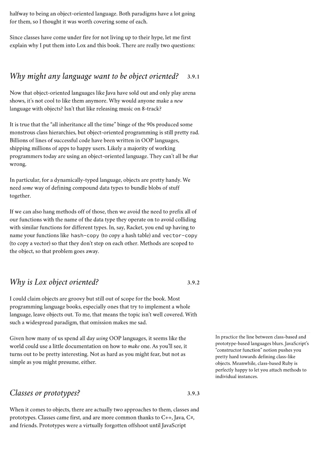
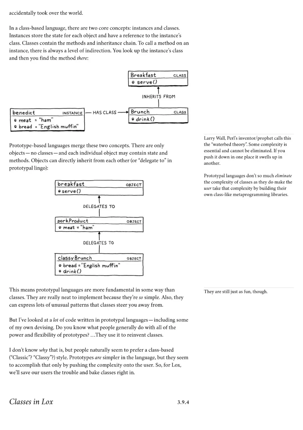
shipping millions of apps to happy users. Likely a majority of working
programmers today are using an object-oriented language. They can’t all be that
wrong.
In particular, for a dynamically-typed language, objects are pretty handy. We
need some way of defining compound data types to bundle blobs of stuff
together.
If we can also hang methods off of those, then we avoid the need to prefix all of
our functions with the name of the data type they operate on to avoid colliding
with similar functions for different types. In, say, Racket, you end up having to
name your functions like hash-copy (to copy a hash table) and vector-copy
(to copy a vector) so that they don’t step on each other. Methods are scoped to
the object, so that problem goes away.
Why is Lox object oriented?
3.9.2
I could claim objects are groovy but still out of scope for the book. Most
programming language books, especially ones that try to implement a whole
language, leave objects out. To me, that means the topic isn’t well covered. With
such a widespread paradigm, that omission makes me sad.
In practice the line between class-based and
prototype-based languages blurs. JavaScript’s
“constructor function” notion pushes you
pretty hard towards defining class-like
objects. Meanwhile, class-based Ruby is
perfectly happy to let you attach methods to
individual instances.
Given how many of us spend all day using OOP languages, it seems like the
world could use a little documentation on how to make one. As you’ll see, it
turns out to be pretty interesting. Not as hard as you might fear, but not as
simple as you might presume, either.
Classes or prototypes?
3.9.3
When it comes to objects, there are actually two approaches to them, classes and
prototypes. Classes came first, and are more common thanks to C++, Java, C#,
and friends. Prototypes were a virtually forgotten offshoot until JavaScript
accidentally took over the world.
In a class-based language, there are two core concepts: instances and classes.
Instances store the state for each object and have a reference to the instance’s
class. Classes contain the methods and inheritance chain. To call a method on an
instance, there is always a level of indirection. You look up the instance’s class
and then you find the method there:
Larry Wall, Perl’s inventor/prophet calls this
the “waterbed theory”. Some complexity is
essential and cannot be eliminated. If you
push it down in one place it swells up in
another.
Prototype-based languages merge these two concepts. There are only
objects—no classes—and each individual object may contain state and
methods. Objects can directly inherit from each other (or “delegate to” in
prototypal lingo):
Prototypal languages don’t so much eliminate
the complexity of classes as they do make the
user take that complexity by building their
own class-like metaprogramming libraries.
This means prototypal languages are more fundamental in some way than
classes. They are really neat to implement because they’re so simple. Also, they
can express lots of unusual patterns that classes steer you away from.
But I’ve looked at a lot of code written in prototypal languages—including some
of my own devising. Do you know what people generally do with all of the
power and flexibility of prototypes? …They use it to reinvent classes.
I don’t know why that is, but people naturally seem to prefer a class-based
(“Classic”? “Classy”?) style. Prototypes are simpler in the language, but they seem
to accomplish that only by pushing the complexity onto the user. So, for Lox,
we’ll save our users the trouble and bake classes right in.
Classes in Lox
3.9.4
They are still just as fun, though.
Enough rationale, let’s see what we actually have. Classes encompass a
constellation of features in most languages. For Lox, I’ve selected what I think
are the brightest stars. You declare a class and its methods like so:
class Breakfast {
cook() {
print "Eggs a-fryin'!";
}
serve(who) {
print "Enjoy your breakfast, " + who + ".";
}
}
The body of a class contains its methods. They look like function declarations
but without the fun keyword. When the class declaration is executed, Lox
creates a class object and stores that in a variable named after the class. Just like
functions, classes are first class in Lox:
// Store it in variables.
var someVariable = Breakfast;
// Pass it to functions.
someFunction(Breakfast);
Next, we need a way to create instances. We could add some sort of new
keyword, but to keep things simple, in Lox the class itself is a factory function
for instances. Call a class like a function and it produces a new instance of itself:
var breakfast = Breakfast();
print breakfast; // "Breakfast instance".
Instantiation and initialization
3.9.5
Classes that only have behavior aren’t super useful. The idea behind objectoriented programming is encapsulating behavior and state together. To do that,
you need fields. Lox, like other dynamically-typed languages, lets you freely add
properties onto objects:
breakfast.meat = "sausage";
breakfast.bread = "sourdough";
Assigning to a field creates it if it doesn’t already exist.
If you want to access a field or method on the current object from within a
method, you use good old this :
Why the < operator? I didn’t feel like
class Breakfast {
serve(who) {
print "Enjoy your " + this.meat + " and " +
introducing a new keyword like extends .
Lox doesn’t use : for anything else so I didn’t
want to reserve that either. Instead, I took a
this.bread + ", " + who + ".";
page from Ruby and used < .
}
// ...
}
Part of encapsulating data within an object is ensuring the object is in a valid
state when it’s created. To do that, you can define an initializer. If your class has
a method named init() , it is called automatically when the object is
constructed. Any parameters passed to the class are forwarded to its initializer:
Lox is different from C++, Java, and C#
which do not inherit constructors, but similar
to Smalltalk and Ruby which do.
class Breakfast {
init(meat, bread) {
this.meat = meat;
this.bread = bread;
}
// ...
}
var baconAndToast = Breakfast("bacon", "toast");
baconAndToast.serve("Dear Reader");
// "Enjoy your bacon and toast, Dear Reader."
Inheritance
3.9.6
Every object-oriented language lets you not only define methods, but reuse
them across multiple classes or objects. For that, Lox supports single
inheritance. When you declare a class, you can specify a class that it inherits
from using a less-than ( < ) operator:
class Brunch < Breakfast {
drink() {
print "How about a Bloody Mary?";
}
}
Here, Brunch is the derived class or subclass, and Breakfast is the base class or
superclass. Every method defined in the superclass is also available to its
subclasses:
var benedict = Brunch("ham", "English muffin");
benedict.serve("Noble Reader");
Even the init() method gets inherited. In practice, the subclass usually wants
to define its own init() method too. But the original one also needs to be
called so that the superclass can maintain its state. We need some way to call a
method on our own instance without hitting our own methods.
As in Java, you use super for that:
If you know any type theory, you’ll notice it’s
not a totally arbitrary choice. Every instance
of a subclass is an instance of its superclass
too, but there may be instances of the
superclass that are not instances of the
subclass. That means, in the universe of
objects, the set of subclass objects is smaller
than the superclass’s set, though type nerds
usually use <: for that relation.
class Brunch < Breakfast {
init(meat, bread, drink) {
super.init(meat, bread);
this.drink = drink;
}
}
That’s about it for object orientation. I tried to keep the feature set minimal. The
structure of the book did force one compromise. Lox is not a pure objectoriented language. In a true OOP language every object is an instance of a class,
even primitive values like numbers and Booleans.
Because we don’t implement classes until well after we start working with the
built-in types, that would have been hard. So values of primitive types aren’t
real objects in the sense of being instances of classes. They don’t have methods
or properties. If I were trying to make Lox a real language for real users, I would
fix that.
The Standard Library
3 . 10
We’re almost done. That’s the whole language, so all that’s left is the “core” or
“standard” library—the set of functionality that is implemented directly in the
interpreter and that all user-defined behavior is built on top of.
This is the saddest part of Lox. Its standard library goes beyond minimalism and
veers close to outright nihilism. For the sample code in the book, we only need
to demonstrate that code is running and doing what it’s supposed to do. For
that, we already have the built-in print statement.
Later, when we start optimizing, we’ll write some benchmarks and see how long
it takes to execute code. That means we need to track time, so we’ll define one
built-in function clock() that returns the number of seconds since the
program started.
And… that’s it. I know, right? It’s embarrassing.
If you wanted to turn Lox into an actual useful language, the very first thing you
should do is flesh this out. String manipulation, trigonometric functions, file
I/O, networking, heck, even reading input from the user would help. But we don’t
need any of that for this book, and adding it wouldn’t teach you anything
interesting, so I left it out.
Don’t worry, we’ll have plenty of exciting stuff in the language itself to keep us
busy.
CHALLENGES
1. Write some sample Lox programs and run them (you can use the implementations
of Lox in my repository). Try to come up with edge case behavior I didn’t specify
here. Does it do what you expect? Why or why not?
2. This informal introduction leaves a lot unspecified. List several open questions you
have about the language’s syntax and semantics. What do you think the answers
should be?
3. Lox is a pretty tiny language. What features do you think it is missing that would
make it annoying to use for real programs? (Aside from the standard library, of
course.)
DESIGN NOTE: EXPRESSIONS AND STATEMENTS
Lox has both expressions and statements. Some languages omit the latter. Instead,
they treat declarations and control flow constructs as expressions too. These
“everything is an expression” languages tend to have functional pedigrees and include
most Lisps, SML, Haskell, Ruby, and Co!eeScript.
To do that, for each “statement-like” construct in the language, you need to decide
what value it evaluates to. Some of those are easy:
An if expression evaluates to the result of whichever branch is chosen. Likewise,
a switch or other multi-way branch evaluates to whichever case is picked.
A variable declaration evaluates to the value of the variable.
A block evaluates to the result of the last expression in the sequence.
Some get a little stranger. What should a loop evaluate to? A while loop in
Co!eeScript evaluates to an array containing each element that the body evaluated to.
That can be handy, or a waste of memory if you don’t need the array.
You also have to decide how these statement-like expressions compose with other
expressions—you have to fit them into the grammar’s precedence table. For example,
Ruby allows:
puts 1 + if true then 2 else 3 end + 4
Is this what you’d expect? Is it what your users expect? How does this a!ect how you
design the syntax for your “statements”? Note that Ruby has an explicit end to tell
when the if expression is complete. Without it, the + 4 would likely be parsed as
part of the else clause.
Turning every statement into an expression forces you to answer a few hairy questions
like that. In return, you eliminate some redundancy. C has both blocks for sequencing
statements, and the comma operator for sequencing expressions. It has both the if
statement and the ?: conditional operator. If everything was an expression in C, you
could unify each of those.
Languages that do away with statements usually also feature implicit returns—a
function automatically returns whatever value its body evaluates to without need for
some explicit return syntax. For small functions and methods, this is really handy. In
fact, many languages that do have statements have added syntax like => to be able to
define functions whose body is the result of evaluating a single expression.
But making all functions work that way can be a little strange. If you aren’t careful,
your function will leak a return value even if you only intend it to produce a side e!ect.
In practice, though, users of these languages don’t find it to be a problem.
For Lox, I gave it statements for prosaic reasons. I picked a C-like syntax for familiarity’s
sake, and trying to take the existing C statement syntax and interpret it like
expressions gets weird pretty fast.
NEXT PART: “A TREE-WALK INTERPRETER” →
Hand-cra"ed by Robert Nystrom — © 2015 – 2020
A TREE-WALK INTERPRETER
With this part, we begin jlox, the first of our two interpreters. Programming
languages are a huge topic with piles of concepts and terminology to cram into
your brain all at once. Programming language theory requires a level of mental
rigor that you probably haven’t had to summon since your last Calculus final.
(Fortunately there isn’t too much theory in this book.)
Implementing an interpreter uses a few architectural tricks and design patterns
uncommon in other kinds of applications, so we’ll be getting used to the
engineering side of things too. Given all of that, we’ll keep the code we have to
write as simple and plain as possible.
In less than two thousand lines of clean Java code, we’ll build a complete
interpreter for Lox that implements every single feature of the language, exactly
as we’ve specified. The first few chapters work front-to-back through the
phases of the interpreter—scanning, parsing, and evaluating code. After that,
we add language features one at a time, growing a simple calculator into a fullfledged scripting language.
NEXT CHAPTER: “SCANNING” →
Hand-cra!ed by Robert Nystrom — © 2015 – 2020
II
4
Scanning
“
Take big bites. Anything worth doing is worth
overdoing.
”
— Robert A. Heinlein, Time Enough for Love
This task has been variously called “scanning”
and “lexing” (short for “lexical analysis”) over
the years. Way back when computers were as
big as Winnebagos but had less memory than
your watch, some people used “scanner” only
to refer to the piece of code that dealt with
reading raw source code characters from disk
and buffering them in memory. Then “lexing”
was the subsequent phase that did useful stuff
with the characters.
The first step in any compiler or interpreter is scanning. The scanner takes in
raw source code as a series of characters and groups it into a series of chunks
we call tokens. These are the meaningful “words” and “punctuation” that make
up the language’s grammar.
Scanning is a good starting point for us too because the code isn’t very
hard —pretty much a switch statement with delusions of grandeur. It will help
us warm up before we tackle some of the more interesting material later. By the
end of this chapter, we’ll have a full-featured, fast scanner that can take any
string of Lox source code and produce the tokens that we’ll feed into the parser
These days, reading a source file into
memory is trivial, so it’s rarely a distinct
phase in the compiler. Because of that, the
two terms are basically interchangeable.
in the next chapter.
The Interpreter Framework
4.1
Since this is our first real chapter, before we get to actually scanning some code,
we need to sketch out the basic shape of our interpreter, jlox. Everything starts
with a class in Java:
package com.craftinginterpreters.lox;
<<
lox/Lox.java
create new file
import java.io.BufferedReader;
import java.io.IOException;
import java.io.InputStreamReader;
import java.nio.charset.Charset;
import java.nio.file.Files;
import java.nio.file.Paths;
import java.util.List;
public class Lox {
public static void main(String[] args) throws IOException {
if (args.length > 1) {
System.out.println("Usage: jlox [script]");
System.exit(64);
} else if (args.length == 1) {
runFile(args[0]);
} else {
runPrompt();
}
}
}
For exit codes, I’m using the conventions
defined in the UNIX “sysexits.h” header. It’s
the closest thing to a standard I could find.
Stick that in a text file, and go get your IDE or Makefile or whatever set up. I’ll
be right here when you’re ready. Good? OK!
Lox is a scripting language, which means it executes directly from source. Our
interpreter supports two ways of running code. If you start jlox from the
command line and give it a path to a file, it reads the file and executes it.
private static void runFile(String path) throws IOException {
<<
lox/Lox.java
add after main()
<<
lox/Lox.java
An interactive prompt
add after runFile()
byte[] bytes = Files.readAllBytes(Paths.get(path));
run(new String(bytes, Charset.defaultCharset()));
}
If you want a more intimate conversation with your interpreter, you can also
run it interactively. Fire up jlox without any arguments, and it drops you into a
prompt where you can enter and execute code one line at a time.
private static void runPrompt() throws IOException {
InputStreamReader input = new InputStreamReader(System.in);
BufferedReader reader = new BufferedReader(input);
for (;;) {
System.out.print("> ");
String line = reader.readLine();
is also called a “REPL”
(pronounced like “rebel” but with a “p”). The
name comes from Lisp where implementing
one is as simple as wrapping a loop around a
few built-in functions:
(print (eval (read)))
if (line == null) break;
run(line);
}
Working outwards from the most nested call,
you Read a line of input, Evaluate it, Print the
result, then Loop and do it all over again.
}
The readLine() function, as the name so helpfully implies, reads a line of
input from the user on the command line and returns the result. To kill an
interactive command-line app, you usually type Control-D. Doing so signals an
“end-of-file” condition to the program. When that happens readLine()
returns null , so we check for that to exit the loop.
Both the prompt and the file runner are thin wrappers around this core
function:
private static void run(String source) {
Scanner scanner = new Scanner(source);
List<Token> tokens = scanner.scanTokens();
// For now, just print the tokens.
for (Token token : tokens) {
System.out.println(token);
}
}
It’s not super useful yet since we haven’t written the interpreter, but baby steps,
you know? Right now, it prints out the tokens our forthcoming scanner will
emit so that we can see if we’re making progress.
<<
lox/Lox.java
add after runPrompt()
Error handling
4.1.1
While we’re setting things up, another key piece of infrastructure is error
handling. Textbooks sometimes gloss over this because it’s more a practical
matter than a formal computer science-y problem. But if you care about making
a language that’s actually usable, then handling errors gracefully is vital.
The tools our language provides for dealing with errors make up a large portion
of its user interface. When the user’s code is working, they aren’t thinking about
our language at all—their headspace is all about their program. It’s usually only
Having said all that, for this interpreter, what
we’ll build is pretty bare bones. I’d love to talk
about interactive debuggers, static analyzers
and other fun stuff, but there’s only so much
ink in the pen.
when things go wrong that they notice our implementation.
When that happens, it’s up to us to give the user all the information they need to
understand what went wrong and guide them gently back to where they are
trying to go. Doing that well means thinking about error handling all through
the implementation of our interpreter, starting now.
static void error(int line, String message) {
report(line, "", message);
}
private static void report(int line, String where,
String message) {
System.err.println(
"[line " + line + "] Error" + where + ": " + message);
hadError = true;
}
This error() function and its report() helper tells the user some syntax
error occurred on a given line. That is really the bare minimum to be able to
claim you even have error reporting. Imagine if you accidentally left a dangling
comma in some function call and the interpreter printed out:
Error: Unexpected "," somewhere in your code. Good luck finding it!
That’s not very helpful. We need to at least point them to the right line. Even
better would be the beginning and end column so they know where in the line.
Even better than that is to show the user the offending line, like:
Error: Unexpected "," in argument list.
15 | function(first, second,);
^-- Here.
I’d love to implement something like that in this book but the honest truth is
that it’s a lot of grungy string munging code. Very useful for users, but not super
fun to read in a book and not very technically interesting. So we’ll stick with
just a line number. In your own interpreters, please do as I say and not as I do.
The primary reason we’re sticking this error reporting function in the main Lox
class is because of that hadError field. It’s defined here:
<<
lox/Lox.java
add after run()
public class Lox {
static boolean hadError = false;
<<
lox/Lox.java
in class Lox
<<
lox/Lox.java
in runFile()
<<
lox/Lox.java
in runPrompt()
We’ll use this to ensure we don’t try to execute code that has a known error.
Also, it lets us exit with a non-zero exit code like a good command line citizen
should.
run(new String(bytes, Charset.defaultCharset()));
// Indicate an error in the exit code.
if (hadError) System.exit(65);
}
We need to reset this flag in the interactive loop. If the user makes a mistake, it
shouldn’t kill their entire session.
run(line);
hadError = false;
}
The other reason I pulled the error reporting out here instead of stuffing it into
the scanner and other phases where the error occurs is to remind you that it’s a
good engineering practice to separate the code that generates the errors from the
code that reports them.
Various phases of the front end will detect errors, but it’s not really their job to
know how to present that to a user. In a full-featured language implementation,
you will likely have multiple ways errors get displayed: on stderr, in an IDE’s
error window, logged to a file, etc. You don’t want that code smeared all over
your scanner and parser.
Ideally, we would have an actual abstraction, some kind of “ErrorReporter”
interface that gets passed to the scanner and parser so that we can swap out
different reporting strategies. For our simple interpreter here, I didn’t do that,
but I did at least move the code for error reporting into a different class.
With some rudimentary error handling in place, our application shell is ready.
Once we have a Scanner class with a scanTokens() method, we can start
running it. Before we get to that, let’s get more precise about what tokens are.
Lexemes and Tokens
Here’s a line of Lox code:
var language = "lox";
Here, var is the keyword for declaring a variable. That three-character
sequence “v-a-r” means something. But if we yank three letters out of the
middle of language , like “g-u-a”, those don’t mean anything on their own.
4.2
I had exactly that when I first implemented
jlox. I ended up tearing it out because it felt
over-engineered for the minimal interpreter
in this book.
That’s what lexical analysis is about. Our job is to scan through the list of
characters and group them together into the smallest sequences that still
represent something. Each of these blobs of characters is called a lexeme. In
that example line of code, the lexemes are:
The lexemes are only the raw substrings of the source code. However, in the
process of grouping character sequences into lexemes, we also stumble upon
some other useful information. When we take the lexeme and bundle it together
with that other data, the result is a token. It includes useful stuff like:
Token type
After all, string comparison ends up looking
at individual characters, and isn’t that the
scanner’s job?
4.2.1
Keywords are part of the shape of the language’s grammar, so the parser often
has code like, “If the next token is while then do…” That means the parser
wants to know not just that it has a lexeme for some identifier, but that it has a
reserved word, and which keyword it is.
The parser could categorize tokens from the raw lexeme by comparing the
strings, but that’s slow and kind of ugly. Instead, at the point that we recognize a
lexeme, we also remember which kind of lexeme it represents. We have a
different type for each keyword, operator, bit of punctuation, and literal type.
package com.craftinginterpreters.lox;
<<
enum TokenType {
// Single-character tokens.
LEFT_PAREN, RIGHT_PAREN, LEFT_BRACE, RIGHT_BRACE,
COMMA, DOT, MINUS, PLUS, SEMICOLON, SLASH, STAR,
// One or two character tokens.
BANG, BANG_EQUAL,
EQUAL, EQUAL_EQUAL,
GREATER, GREATER_EQUAL,
LESS, LESS_EQUAL,
// Literals.
IDENTIFIER, STRING, NUMBER,
// Keywords.
AND, CLASS, ELSE, FALSE, FUN, FOR, IF, NIL, OR,
PRINT, RETURN, SUPER, THIS, TRUE, VAR, WHILE,
EOF
}
Literal value
4.2.2
There are lexemes for literal values—numbers and strings and the like. Since
lox/TokenType.java
create new file
the scanner has to walk each character in the literal to correctly identify it, it
can also convert that textual representation of a value to the living runtime
object that will be used by the interpreter later.
Location information
4.2.3
Back when I was preaching the gospel about error handling, we saw that we
Some token implementations store the
location as two numbers: the offset from the
beginning of the source file to the beginning
of the lexeme, and the length of the lexeme.
The scanner needs to know these anyway, so
there’s no overhead to calculate them.
need to tell users where errors occurred. Tracking that starts here. In our simple
interpreter, we only note which line the token appears on, but more
sophisticated implementations include the column and length too.
We take all of this data and wrap it in a class.
package com.craftinginterpreters.lox;
<<
class Token {
final TokenType type;
final String lexeme;
final Object literal;
final int line;
Token(TokenType type, String lexeme, Object literal, int line) {
An offset can be converted to line and
column positions later by looking back at the
lox/Token.java
source file
create
new and
filecounting the preceding
newlines. That sounds slow, and it is.
However, you only need to do it when you
need to actually display a line and column to the
user. Most tokens never appear in an error
message. For those, the less time you spend
calculating position information ahead of
time, the better.
this.type = type;
this.lexeme = lexeme;
this.literal = literal;
this.line = line;
}
public String toString() {
return type + " " + lexeme + " " + literal;
}
}
Now we have an object with enough structure to be useful for all of the later
phases of the interpreter.
Regular Languages and Expressions
4.3
Now that we know what we’re trying to produce, let’s, well, produce it. The
core of the scanner is a loop. Starting at the first character of the source code, it
figures out what lexeme it belongs to, and consumes it and any following
characters that are part of that lexeme. When it reaches the end of that lexeme,
it emits a token.
Then it loops back and does it again, starting from the very next character in the
source code. It keeps doing that, eating characters and occasionally, uh,
excreting tokens, until it reaches the end of the input.
Lexical analygator.
It pains me to gloss over the theory so much,
especially when it’s as interesting as I think
the Chomsky hierarchy and finite-state
machines are. But the honest truth is other
books cover this better than I could.
Compilers: Principles, Techniques, and Tools
(universally known as “the Dragon Book”) is
the canonical reference.
The part of the loop where we look at a handful of characters to figure out
which kind of lexeme it “matches” may sound familiar. If you know regular
expressions, you might consider defining a regex for each kind of lexeme and
Lex was created by Mike Lesk and Eric
Schmidt. Yes, the same Eric Schmidt who was
executive chairman of Google. I’m not saying
programming languages are a sure-fire path
to wealth and fame, but we can count at least
one mega-billionaire among us.
use those to match characters. For example, Lox has the same rules as C for
identifiers (variable names and the like). This regex matches one:
[a-zA-Z_][a-zA-Z_0-9]*
If you did think of regular expressions, your intuition is a deep one. The rules
that determine how a particular language groups characters into lexemes are
called its lexical grammar. In Lox, as in most programming languages, the rules
of that grammar are simple enough to be classified a regular language. That’s
the same “regular” as in regular expressions.
You very precisely can recognize all of the different lexemes for Lox using
regexes if you want to, and there’s a pile of interesting theory underlying why
that is and what it means. Tools like Lex or Flex are designed expressly to let
you do this—throw a handful of regexes at them, and they give you a complete
scanner back.
I know static imports are considered bad
style by some, but they save me from having
to sprinkle TokenType. all over the scanner
and parser. Forgive me, but every character
counts in a book.
Since our goal is to understand how a scanner does what it does, we won’t be
delegating that task. We’re about hand-crafted goods.
The Scanner Class
4.4
Without further ado, let’s make ourselves a scanner.
package com.craftinginterpreters.lox;
import java.util.ArrayList;
import java.util.HashMap;
import java.util.List;
import java.util.Map;
import static com.craftinginterpreters.lox.TokenType.*;
class Scanner {
private final String source;
private final List<Token> tokens = new ArrayList<>();
Scanner(String source) {
this.source = source;
<<
lox/Scanner.java
create new file
}
}
We store the raw source code as a simple string, and we have a list ready to fill
with tokens we’re going to generate. The aforementioned loop that does that
looks like this:
List<Token> scanTokens() {
<<
lox/Scanner.java
add after Scanner()
<<
lox/Scanner.java
in class Scanner
<<
lox/Scanner.java
add after scanTokens()
while (!isAtEnd()) {
// We are at the beginning of the next lexeme.
start = current;
scanToken();
}
tokens.add(new Token(EOF, "", null, line));
return tokens;
}
The scanner works its way through the source code, adding tokens until it runs
out of characters. Then it appends one final “end of file” token. That isn’t strictly
needed, but it makes our parser a little cleaner.
This loop depends on a couple of fields to keep track of where the scanner is in
the source code.
private final List<Token> tokens = new ArrayList<>();
private int start = 0;
private int current = 0;
private int line = 1;
Scanner(String source) {
The start and current fields are offsets that index into the string. The
start field points to the first character in the lexeme being scanned, and
current points at the character currently being considered. The line field
tracks what source line current is on so we can produce tokens that know
their location.
Then we have one little helper function that tells us if we’ve consumed all the
characters.
private boolean isAtEnd() {
return current >= source.length();
}
Recognizing Lexemes
Wondering why / isn’t in here? Don’t worry,
we’ll get to it.
4.5
Each turn of the loop, we scan a single token. This is the real heart of the
scanner. We’ll start simple. Imagine if every lexeme is only a single character
long. All you need to do is consume the next character and pick a token type for
it. Several lexemes are only a single character in Lox, so let’s start with those.
private void scanToken() {
<<
lox/Scanner.java
add after scanTokens()
<<
lox/Scanner.java
add after isAtEnd()
char c = advance();
switch (c) {
case '(': addToken(LEFT_PAREN); break;
case ')': addToken(RIGHT_PAREN); break;
case '{': addToken(LEFT_BRACE); break;
case '}': addToken(RIGHT_BRACE); break;
case ',': addToken(COMMA); break;
case '.': addToken(DOT); break;
case '-': addToken(MINUS); break;
case '+': addToken(PLUS); break;
case ';': addToken(SEMICOLON); break;
case '*': addToken(STAR); break;
}
}
Again, we need a couple of helper methods.
private char advance() {
current++;
return source.charAt(current - 1);
}
private void addToken(TokenType type) {
addToken(type, null);
}
private void addToken(TokenType type, Object literal) {
String text = source.substring(start, current);
tokens.add(new Token(type, text, literal, line));
}
The advance() method consumes the next character in the source file and
returns it. Where advance() is for input, addToken() is for output. It grabs
the text of the current lexeme and creates a new token for it. We’ll use the other
The code reports each invalid character
separately, so this shotguns the user with a
blast of errors if they accidentally paste a big
blob of weird text. Coalescing a run of invalid
characters into a single error would give a
nicer user experience.
overload to handle tokens with literal values soon.
Lexical errors
4.5.1
Before we get too far in, let’s take a moment to think about errors at the lexical
level. What happens if a user throws a source file containing some characters
Lox doesn’t use, like @#^ at our interpreter? Right now, those characters get
silently discarded. They aren’t used by the Lox language, but that doesn’t mean
the interpreter can pretend they aren’t there. Instead, we report an error.
case '*': addToken(STAR); break;
<<
default:
Lox.error(line, "Unexpected character.");
break;
}
Note that the erroneous character is still consumed by the earlier call to
lox/Scanner.java
in scanToken()
advance() . That’s important so that we don’t get stuck in an infinite loop.
Note also that we keep scanning. There may be other errors later in the program.
It gives our users a better experience if we detect as many of those as possible in
one go. Otherwise, they see one tiny error and fix it, only to have the next error
appear, and so on. Syntax error Whack-a-mole is no fun.
(Don’t worry. Since hadError gets set, we’ll never try to execute any of the
code, even though we keep going and scan the rest of it.)
Operators
4.5.2
We have single-character lexemes working, but that doesn’t cover all of Lox’s
operators. What about ! ? It’s a single character, right? Sometimes, yes, but if the
very next character is an equals sign, then we should instead create a != lexeme.
Note that the ! and = are not two independent operators. You can’t write ! =
in Lox and have it behave like an inequality operator. That’s why we need to
scan != as a single lexeme. Likewise, < , > , and = can all be followed by = to
create the other equality and comparison operators.
For all of these, we need to look at the second character.
case '*': addToken(STAR); break;
case '!':
<<
lox/Scanner.java
in scanToken()
<<
lox/Scanner.java
add after scanToken()
addToken(match('=') ? BANG_EQUAL : BANG);
break;
case '=':
addToken(match('=') ? EQUAL_EQUAL : EQUAL);
break;
case '<':
addToken(match('=') ? LESS_EQUAL : LESS);
break;
case '>':
addToken(match('=') ? GREATER_EQUAL : GREATER);
break;
default:
Those cases use this new method:
private boolean match(char expected) {
if (isAtEnd()) return false;
if (source.charAt(current) != expected) return false;
current++;
return true;
}
It’s like a conditional advance() . We only consume the current character if it’s
what we’re looking for.
Using match() , we recognize these lexemes in two stages. When we reach, for
example, ! , we jump to its switch case. That means we know the lexeme starts
with ! . Then we look at the next character to determine if we’re on a != or
merely a ! .
Longer Lexemes
4.6
We’re still missing one operator, / for division. That character needs a little
special handling because comments begin with a slash too.
Technically, match() is doing lookahead
too. advance() and peek() are the
break;
case '/':
<<
lox/Scanner.java
fundamental
operators and match()
in scanToken()
combines
them.
<<
lox/Scanner.java
add after match()
if (match('/')) {
// A comment goes until the end of the line.
while (peek() != '\n' && !isAtEnd()) advance();
} else {
addToken(SLASH);
}
break;
default:
This is similar to the other two-character operators, except that when we find a
second / , we don’t end the token yet. Instead, we keep consuming characters
until we reach the end of the line.
This is our general strategy for handling longer lexemes. After we detect the
beginning of one, we shunt over to some lexeme-specific code that keeps eating
characters until it sees the end.
We’ve got another helper:
private char peek() {
if (isAtEnd()) return '\0';
return source.charAt(current);
}
It’s sort of like advance() , but doesn’t consume the character. This is called
lookahead. Since it only looks at the current unconsumed character, we have
one character of lookahead. The smaller this number is, generally, the faster the
scanner runs. The rules of the lexical grammar dictate how much lookahead we
need. Fortunately, most languages in wide use only peek one or two characters
ahead.
Comments are lexemes, but they aren’t meaningful, and the parser doesn’t want
to deal with them. So when we reach the end of the comment, we don’t call
addToken() . When we loop back around to start the next lexeme, start gets
reset and the comment’s lexeme disappears in a puff of smoke.
While we’re at it, now’s a good time to skip over those other meaningless
characters: newlines and whitespace.
break;
<<
lox/Scanner.java
in scanToken()
<<
lox/Scanner.java
in scanToken()
<<
lox/Scanner.java
add after scanToken()
case ' ':
case '\r':
case '\t':
// Ignore whitespace.
break;
case '\n':
line++;
break;
default:
Lox.error(line, "Unexpected character.");
When encountering whitespace, we simply go back to the beginning of the scan
loop. That starts a new lexeme after the whitespace character. For newlines, we
do the same thing, but we also increment the line counter. (This is why we used
peek() to find the newline ending a comment instead of match() . We want
that newline to get us here so we can update line .)
Our scanner is getting smarter. It can handle fairly free-form code like:
// this is a comment
(( )){} // grouping stuff
!*+-/=<> <= == // operators
String literals
4.6.1
Now that we’re comfortable with longer lexemes, we’re ready to tackle literals.
We’ll do strings first, since they always begin with a specific character, " :
break;
case '"': string(); break;
default:
That calls:
private void string() {
while (peek() != '"' && !isAtEnd()) {
if (peek() == '\n') line++;
advance();
}
if (isAtEnd()) {
Lox.error(line, "Unterminated string.");
return;
}
// The closing ".
advance();
Since we only look for a digit to start a
number, that means -123 is not a number
literal. Instead, -123 , is an expression that
applies - to the number literal 123 . In
practice, the result is the same, though it has
one interesting edge case if we were to add
method calls on numbers. Consider:
print -123.abs();
// Trim the surrounding quotes.
String value = source.substring(start + 1, current - 1);
This prints -123 because negation has lower
precedence than method calls. We could fix
addToken(STRING, value);
}
that by making - part of the number literal.
But then consider:
Like with comments, we consume characters until we hit the " that ends the
var n = 123;
string. We also gracefully handle running out of input before the string is closed
and report an error for that.
print -n.abs();
This still produces -123 , so now the
language seems inconsistent. No matter what
you do, some case ends up weird.
For no particular reason, Lox supports multi-line strings. There are pros and
cons to that, but prohibiting them was a little more complex than allowing
them, so I left them in. That does mean we also need to update line when we
hit a newline inside a string.
Finally, the last interesting bit is that when we create the token, we also produce
the actual string value that will be used later by the interpreter. Here, that
conversion only requires a substring() to strip off the surrounding quotes.
If Lox supported escape sequences like \n , we’d unescape those here.
Number literals
The Java standard library provides
4.6.2
Character.isDigit() which seems like a
good fit. Alas, that method allows things like
Devanagari digits, fullwidth numbers, and
other funny stuff we don’t want.
All numbers in Lox are floating point at runtime, but it supports both integer
and decimal literals. A number literal is a series of digits optionally followed by
a . and one or more trailing digits:
1234
12.34
We don’t allow a leading or trailing decimal point, so these are both invalid:
.1234
1234.
We could easily support the former, but I left it out to keep things simple. The
latter gets weird if we ever want to allow methods on numbers like
123.sqrt() .
To recognize the beginning of a number lexeme, we look for any digit. It’s kind
of tedious to add cases for every decimal digit, so we’ll stuff it in the default case
instead.
default:
if (isDigit(c)) {
number();
} else {
<<
lox/Scanner.java
in scanToken()
replace 1 line
Lox.error(line, "Unexpected character.");
}
break;
I could have made peek() take a parameter
for the number of characters ahead to look
instead of defining two functions, but that
This relies on this little utility:
private boolean isDigit(char c) {
<<
return c >= '0' && c <= '9';
would allow arbitrarily far lookahead. Only
providing these two functions makes it
clearer to a reader of the code that our
scanner
only looks ahead at most two
lox/Scanner.java
add after peek()
characters.
}
Once we know we are in a number, we branch to a separate method to consume
the rest of the literal, like we do with strings.
private void number() {
<<
while (isDigit(peek())) advance();
lox/Scanner.java
add after scanToken()
// Look for a fractional part.
if (peek() == '.' && isDigit(peekNext())) {
// Consume the "."
advance();
while (isDigit(peek())) advance();
}
addToken(NUMBER,
Double.parseDouble(source.substring(start, current)));
}
We consume as many digits as we find for the integer part of the literal. Then
we look for a fractional part, which is a decimal point ( . ) followed by at least
Consider this nasty bit of C code:
one digit. If we do have a fractional part, again, we consume as many digits as
we can find.
---a;
Is it valid? That depends on how the scanner
splits the lexemes. If the scanner sees it like:
Looking past the decimal point requires a second character of lookahead since
we don’t want to consume the . until we’re sure there is a digit after it. So we
add:
private char peekNext() {
- --a;
<<
if (current + 1 >= source.length()) return '\0';
return source.charAt(current + 1);
}
Then
it could be parsed. But that would
lox/Scanner.java
require
thepeek()
scanner to know about the
add after
grammatical structure of the surrounding
code, which entangles things more than we
want. Instead, the maximal munch rule says
that it is always scanned like:
Finally, we convert the lexeme to its numeric value. Our interpreter uses Java’s
Double type to represent numbers, so we produce a value of that type. We’re
using Java’s own parsing method to convert the lexeme to a real Java double. We
could implement that ourselves, but, honestly, unless you’re trying to cram for
an upcoming programming interview, it’s not worth your time.
The remaining literals are Booleans and nil , but we handle those as keywords,
which gets us to…
Reserved Words and Identifiers
4.7
Our scanner is almost done. The only remaining pieces of the lexical grammar
to implement are identifiers and their close cousins, the reserved words. You
-- -a;
It scans it that way even though doing so
leads to a syntax error later in the parser.
might think we could match keywords like or in the same way we handle
multiple-character operators like <= :
case 'o':
if (peek() == 'r') {
addToken(OR);
}
break;
Consider what would happen if a user named a variable orchid . The scanner
would see the first two letters, or , and immediately emit an or keyword token.
This gets us to an important principle called maximal munch. When two
lexical grammar rules can both match a chunk of code that the scanner is
looking at, whichever one matches the most characters wins.
That rule states that if we can match orchid as an identifier and or as a
keyword, then the former wins. This is also why we tacitly assumed previously
that <= should be scanned as a single <= token and not < followed by = .
Maximal munch means we can’t easily detect a reserved word until we’ve
reached the end of what might instead be an identifier. After all, a reserved
word is an identifier, it’s just one that has been claimed by the language for its
own use. That’s where the term reserved word comes from.
So we begin by assuming any lexeme starting with a letter or underscore is an
identifier.
default:
if (isDigit(c)) {
number();
} else if (isAlpha(c)) {
<<
lox/Scanner.java
in scanToken()
<<
lox/Scanner.java
add after scanToken()
<<
lox/Scanner.java
add after peekNext()
identifier();
} else {
Lox.error(line, "Unexpected character.");
}
The rest of the code lives over here:
private void identifier() {
while (isAlphaNumeric(peek())) advance();
addToken(IDENTIFIER);
}
We define that in terms of these helpers:
private boolean isAlpha(char c) {
return (c >= 'a' && c <= 'z') ||
(c >= 'A' && c <= 'Z') ||
c == '_';
}
private boolean isAlphaNumeric(char c) {
return isAlpha(c) || isDigit(c);
}
That gets identifiers working. To handle keywords, we see if the identifier’s
lexeme is one of the reserved words. If so, we use a token type specific to that
keyword. We define the set of reserved words in a map:
private static final Map<String, TokenType> keywords;
<<
lox/Scanner.java
in class Scanner
<<
lox/Scanner.java
in identifier()
replace 1 line
static {
keywords = new HashMap<>();
keywords.put("and",
AND);
keywords.put("class",
CLASS);
keywords.put("else",
ELSE);
keywords.put("false",
FALSE);
keywords.put("for",
FOR);
keywords.put("fun",
FUN);
keywords.put("if",
IF);
keywords.put("nil",
NIL);
keywords.put("or",
OR);
keywords.put("print",
PRINT);
keywords.put("return", RETURN);
keywords.put("super",
SUPER);
keywords.put("this",
THIS);
keywords.put("true",
TRUE);
keywords.put("var",
VAR);
keywords.put("while",
WHILE);
}
Then, after we scan an identifier, we check to see if it matches anything in the
map:
while (isAlphaNumeric(peek())) advance();
String text = source.substring(start, current);
TokenType type = keywords.get(text);
if (type == null) type = IDENTIFIER;
addToken(type);
}
If so, we use that keyword’s token type. Otherwise, it’s a regular user-defined
identifier.
And with that, we now have a complete scanner for the entire Lox lexical
grammar. Fire up the REPL and type in some valid and invalid code. Does it
produce the tokens you expect? Try to come up with some interesting edge
cases and see if it handles them as it should.
CHALLENGES
1. The lexical grammars of Python and Haskell are not regular. What does that mean,
and why aren’t they?
2. Aside from separating tokens—distinguishing print foo from printfoo —
spaces aren’t used for much in most languages. However, in a couple of dark
corners, a space does a!ect how code is parsed in Co!eeScript, Ruby, and the C
preprocessor. Where and what e!ect does it have in each of those languages?
3. Our scanner here, like most, discards comments and whitespace since those aren’t
needed by the parser. Why might you want to write a scanner that does not discard
those? What would it be useful for?
4. Add support to Lox’s scanner for C-style /* ... */ block comments. Make sure
to handle newlines in them. Consider allowing them to nest. Is adding support for
nesting more work than you expected? Why?
DESIGN NOTE: IMPLICIT SEMICOLONS
Programmers today are spoiled for choice in languages and have gotten picky about
syntax. They want their language to look clean and modern. One bit of syntactic lichen
that almost every new language scrapes o! (and some ancient ones like BASIC never
had) is ; as an explicit statement terminator.
Instead, they treat a newline as a statement terminator where it makes sense to do so.
The “where it makes sense” part is the challenging bit. While most statements are on
their own line, sometimes you need to spread a single statement across a couple of
lines. Those intermingled newlines should not be treated as terminators.
Most of the obvious cases where the newline should be ignored are easy to detect, but
there are a handful of nasty ones:
A return value on the next line:
if (condition) return
"value"
Is “value” the value being returned, or do we have a return statement with no
value followed by an expression statement containing a string literal?
A parenthesized expression on the next line:
func
(parenthesized)
Is this a call to func(parenthesized) , or two expression statements, one for
func and one for a parenthesized expression?
A - on the next line:
first
-second
Is this first - second —an infix subtraction—or two expression statements,
one for first and one to negate second ?
And now you know why Python’s lambda
only allows a single expression body.
In all of these, either treating the newline as a separator or not would both produce
valid code, but possibly not the code the user wants. Across languages, there is an
unsettling variety of rules they use to decide which newlines are separators. Here are a
couple:
Lua completely ignores newlines, but carefully controls its grammar such that no
separator between statements is needed at all in most cases. This is perfectly legit:
a = 1 b = 2
Lua avoids the return problem by requiring a return statement to be the very
last statement in a block. If there is a value a"er return before the keyword
end , it must be for the return . For the other two cases, they allow an explicit ;
and expect users to use that. In practice, that almost never happens because
there’s no point in a parenthesized or unary negation expression statement.
Go handles newlines in the scanner. If a newline appears following one of a handful
of token types that are known to potentially end a statement, the newline is
treated like a semicolon, otherwise it is ignored. The Go team provides a canonical
code formatter, gofmt, and the ecosystem is fervent about its use, which ensures
that idiomatic styled code works well with this simple rule.
Python treats all newlines as significant unless an explicit backslash is used at the
end of a line to continue it to the next line. However, newlines anywhere inside a
pair of brackets ( () , [] , or {} ) are ignored. Idiomatic style strongly prefers the
latter.
This rule works well for Python because it is a highly statement-oriented language.
In particular, Python’s grammar ensures a statement never appears inside an
expression. C does the same, but many other languages which have a “lambda” or
function literal syntax do not.
For example, in JavaScript:
console.log(function() {
statement();
});
Here, the console.log() expression contains a function literal which in turn
contains the statement statement(); .
Python would need a di!erent set of rules for implicitly joining lines if you could
get back into a statement where newlines should become meaningful while still
nested inside brackets.
JavaScript’s “automatic semicolon insertion” rule is the real odd one. Where other
languages assume most newlines are meaningful and only a few should be ignored
in multi-line statements, JS assumes the opposite. It treats all of your newlines as
meaningless whitespace unless it encounters a parse error. If it does, it goes back
and tries turning the previous newline into a semicolon to get something
grammatically valid.
This design note would turn into a design diatribe if I went into complete detail
about how that even works, much less all the various ways that JavaScript’s
“solution” is a bad idea. It’s a mess. JavaScript is the only language I know where
many style guides demand explicit semicolons a"er every statement even though
the language theoretically lets you elide them.
If you’re designing a new language, you almost surely should avoid an explicit
statement terminator. Programmers are creatures of fashion like other humans and
semicolons are as passé as ALL CAPS KEYWORDS. Just make sure you pick a set of
rules that make sense for your language’s particular grammar and idioms. And don’t
do what JavaScript did.
NEXT CHAPTER: “REPRESENTING CODE” →
Hand-cra"ed by Robert Nystrom — © 2015 – 2020
5
Representing Code
“
To dwellers in a wood, almost every species of
tree has its voice as well as its feature.
”
— Thomas Hardy, Under the Greenwood Tree
In the last chapter, we took the raw source code as a string and transformed it
into a slightly higher-level representation: a series of tokens. The parser we’ll
write in the next chapter takes those tokens and transforms them yet again to an
even richer, more complex representation.
Before we can produce that representation, we need to define it. That’s the
subject of this chapter. Along the way, we’ll cover some theory around formal
grammars, feel the difference between functional and object-oriented
programming, go over a couple of design patterns, and do some
metaprogramming.
I was so worried about this being one of the
most boring chapters in the book that I kept
stuffing more fun ideas into it until I ran out
of room.
Before we do all that, let’s focus on the main goal—a representation for code. It
should be simple for the parser to produce and easy for the interpreter to
consume. If you haven’t written a parser or interpreter yet, those requirements
aren’t exactly illuminating. Maybe your intuition can help. What is your brain
doing when you play the part of a human interpreter? How do you mentally
evaluate an arithmetic expression like this:
1 + 2 * 3 - 4
Because you understand the order of operations—the old “Please Excuse My
Dear Aunt Sally” stuff—you know that the multiplication is evaluated before
the addition or subtraction. One way to visualize that precedence is using a tree.
Leaf nodes are numbers, and interior nodes are operators with branches for
each of their operands.
In order to evaluate an arithmetic node, you need to know the numeric values
of its subtrees, so you have to evaluate those first. That means working your
way from the leaves up to the root—a post-order traversal:
A. Starting with the full tree, evaluate the
bottom-most operation, 2 * 3 .
B. Now we can evaluate the + .
C. Next, the - .
D. The final answer.
That’s not to say a tree is the only possible
representation of our code. In Part III, we’ll
generate bytecode, another representation
that isn’t as human friendly but is closer to
the machine.
If I gave you an arithmetic expression, you could draw one of these trees pretty
easily. Given a tree, you can evaluate it without breaking a sweat. So it
intuitively seems like a workable representation of our code is a tree that
matches the grammatical structure—the operator nesting—of the language.
We need to get more precise about what that grammar is then. Like lexical
grammars in the last chapter, there is a long ton of theory around syntactic
grammars. We’re going into that theory a little more than we did when scanning
because it turns out to be a useful tool throughout much of the interpreter. We
start by moving one level up the Chomsky hierarchy…
Context-Free Grammars
5.1
In the last chapter, the formalism we used for defining the lexical
grammar—the rules for how characters get grouped into tokens—was called a
regular language. That was fine for our scanner, which emits a flat sequence of
tokens. But regular languages aren’t powerful enough to handle expressions
which can nest arbitrarily deeply.
We need a bigger hammer, and that hammer is a context-free grammar (CFG).
It’s the next heaviest tool in the toolbox of formal grammars. A formal
grammar takes a set of atomic pieces it calls its “alphabet”. Then it defines a
(usually infinite) set of “strings” that are “in” the grammar. Each string is a
sequence of “letters” in the alphabet.
I’m using all those quotes because the terms get a little confusing as you move
from lexical to syntactic grammars. In our scanner’s grammar, the alphabet
consists of individual characters and the strings are the valid lexemes—roughly
“words”. In the syntactic grammar we’re talking about now, we’re at a different
level of granularity. Now each “letter” in the alphabet is an entire token and a
“string” is a sequence of tokens—an entire expression.
Oof. Maybe a table will help:
Terminology
Lexical grammar
Syntactic grammar
The “alphabet” is…
→
Characters
Tokens
A “string” is…
→
Lexeme or token
Expression
It's implemented by the…
→
Scanner
Parser
A formal grammar’s job is to specify which strings are valid and which aren’t. If
we were defining a grammar for English sentences, “eggs are tasty for breakfast”
would be in the grammar, but “tasty breakfast for are eggs” would probably not.
Rules for grammars
5.1.1
How do we write down a grammar that contains an infinite number of valid
strings? We obviously can’t list them all out. Instead, we create a finite set of
rules. You can think of them as a game that you can “play” in one of two
directions.
If you start with the rules, you can use them to generate strings that are in the
Restricting heads to a single symbol is a
defining feature of context-free grammars.
More powerful formalisms like unrestricted
grammars allow a sequence of symbols in
the head as well as in the body.
grammar. Strings created this way are called derivations because each is
“derived” from the rules of the grammar. In each step of the game, you pick a
rule and follow what it tells you to do. Most of the lingo around formal
grammars comes from playing them in this direction. Rules are called
productions because they produce strings in the grammar.
Each production in a context-free grammar has a head—its name—and a body
which describes what it generates. In its pure form, the body is simply a list of
symbols. Symbols come in two delectable flavors:
A terminal is a letter from the grammar’s alphabet. You can think of it like a
literal value. In the syntactic grammar we’re defining, the terminals are
individual lexemes—tokens coming from the scanner like if or 1234 .
These are called “terminals”, in the sense of an “end point” because they don’t
lead to any further “moves” in the game. You simply produce that one
symbol.
A nonterminal is a named reference to another rule in the grammar. It
means “play that rule and insert whatever it produces here”. In this way, the
grammar composes.
Yes, we need to define a syntax to use for the
rules that define our syntax. Should we
specify that metasyntax too? What notation do
we use for it? It’s languages all the way down!
There is one last refinement: you may have multiple rules with the same name.
When you reach a nonterminal with that name, you are allowed to pick any of
the rules for it, whichever floats your boat.
To make this concrete, we need a way to write down these production rules.
People have been trying to crystallize grammar all the way back to Pāṇini’s
Ashtadhyayi, which codified Sanskrit grammar a mere couple thousand years
ago. Not much progress happened until John Backus and company needed a
notation for specifying ALGOL 58 and came up with Backus-Naur form. Since
then, nearly everyone uses some flavor of BNF, tweaked to their own tastes.
I tried to come up with something clean. Each rule is a name, followed by an
arrow ( → ), followed by a sequence of symbols, and finally ending with a
semicolon ( ; ). Terminals are quoted strings, and nonterminals are lowercase
words.
Using that, here’s a grammar for breakfast menus:
Yes, I really am going to be using breakfast
examples throughout this entire book. Sorry.
breakfast
→ protein "with" breakfast "on the side" ;
breakfast
→ protein ;
breakfast
→ bread ;
protein
→ crispiness "crispy" "bacon" ;
protein
→ "sausage" ;
protein
→ cooked "eggs" ;
crispiness → "really" ;
crispiness → "really" crispiness ;
cooked
→ "scrambled" ;
cooked
→ "poached" ;
cooked
→ "fried" ;
bread
→ "toast" ;
bread
→ "biscuits" ;
bread
→ "English muffin" ;
We can use this grammar to generate random breakfasts. Let’s play a round and
see how it works. By age-old convention, the game starts with the first rule in
the grammar, here breakfast . There are three productions for that, and we
randomly pick the first one. Our resulting string looks like:
protein "with" breakfast "on the side"
We need to expand that first nonterminal, protein , so we pick a production
for that. Let’s pick:
protein → cooked "eggs" ;
Next, we need a production for cooked , and so we pick "poached" . That’s a
terminal, so we add that. Now our string looks like:
"poached" "eggs" "with" breakfast "on the side"
The next non-terminal is breakfast again. The first breakfast production
we chose recursively refers back to the breakfast rule. Recursion like this
usually indicates that the language is context-free instead of regular. In
particular, this kind of nested recursion where the recursive nonterminal has
productions on both sides of it means that it’s not regular.
We could keep picking the first production for breakfast over and over again
yielding all manner of breakfasts like “bacon with sausage with scrambled eggs
with bacon …”. We won’t though. This time we’ll pick bread . There are three
rules for that, each of which contains only a terminal. We’ll pick “English
muffin”.
With that, every nonterminal in the string has been expanded until it finally
contains only terminals and we’re left with:
Imagine that we’ve recursively expanded the
breakfast rule here several times, like
“bacon with bacon with bacon with bacon
…”. In order to complete the string, we’ll need
to add an equal number of “on the side” bits to
the end. Keeping track of that number of
trailing parts is beyond the capabilities of a
simple regular grammar. A regular grammar
can repeat, but it can’t count.
Throw in some ham and Hollandaise, and you’ve got eggs Benedict.
Any time we hit a rule that had multiple productions, we just picked one
arbitrarily. It is this flexibility that allows a short number of grammar rules to
encode a combinatorially larger set of strings. The fact that a rule can refer to
itself—directly or indirectly—kicks it up even more, letting us pack an infinite
number of strings into a finite grammar.
Enhancing our notation
5.1.2
Stuffing an infinite set of strings in a handful of rules is pretty fantastic, but let’s
take it further. Our notation works, but it’s a little tedious. So, like any good
language designer, we’ll sprinkle some syntactic sugar on top. In addition to
terminals and nonterminals, we’ll allow a few other kinds of expressions in the
body of a rule:
Instead of repeating the rule name each time we want to add another
production for it, we’ll allow a series of productions separated by a pipe ( | ):
bread → "toast" | "biscuits" | "English muffin" ;
Further, we’ll allow parentheses for grouping and then allow | within that
to select one from a series of options within the middle of a production:
protein → ( "scrambled" | "poached" | "fried" ) "eggs" ;
Using recursion to support repeated sequences of symbols has a certain
appealing purity, but it’s kind of a chore to make a separate named sub-rule
each time we want to loop. So, we also use a postfix * to allow the previous
symbol or group to be repeated zero or more times.
crispiness → "really" "really"* ;
A postfix + is similar, but requires the preceding production to appear at
least once.
crispiness → "really"+ ;
This is how the Scheme programming
language works. It has no built-in looping
functionality at all. Instead, all repetition is
expressed in terms of recursion.
A postfix ? is for an optional production. The thing before it can appear
zero or one time, but not more.
breakfast → protein ( "with" breakfast "on the side" )? ;
With all of those syntactic niceties, our breakfast grammar condenses down to:
breakfast → protein ( "with" breakfast "on the side" )?
| bread ;
protein
→ "really"+ "crispy" "bacon"
| "sausage"
| ( "scrambled" | "poached" | "fried" ) "eggs" ;
bread
→ "toast" | "biscuits" | "English muffin" ;
Not too bad, I hope. If you’re used to grep or using regular expressions in your
text editor, most of the punctuation should be familiar. The main difference is
that symbols here represent entire tokens, not single characters.
We’ll use this notation throughout the rest of the book to precisely describe
Lox’s grammar. As you work on programming languages, you’ll find contextfree grammars (using this or EBNF or some other notation) help you crystallize
your informal syntax design ideas. They are also a handy medium for
communicating with other language hackers about syntax.
The rules and productions we define for Lox are also our guide to the tree data
structure we’re going to implement to represent code in memory. Before we can
do that, we need an actual grammar for Lox, or at least enough of one for us to
get started.
A Grammar for Lox expressions
5.1.3
In the previous chapter, we did Lox’s entire lexical grammar in one fell swoop.
Every keyword and bit of punctuation is there. The syntactic grammar is larger,
and it would be a real bore to grind through the entire thing before we actually
get our interpreter up and running.
Instead, we’ll crank through a subset of the language in the next couple of
chapters. Once we have that mini-language represented, parsed, and
interpreted, then later chapters will progressively add new features to it,
including the new syntax. For now, we are only going to worry about a handful
of expressions:
Literals – Numbers, strings, Booleans, and nil .
Unary expressions – A prefix ! to perform a logical not, and - to negate a
number.
Binary expressions – The infix arithmetic ( + , - , * , / ) and logic ( == , != ,
If you’re so inclined, try using this grammar
to generate a few expressions like we did
< , <= , > , >= ) operators we know and love.
with the breakfast grammar before. Do the
resulting expressions look right to you? Can
you make it generate anything wrong like
Parentheses – A pair of ( and ) wrapped around an expression.
1 + / 3?
That gives us enough syntax for expressions like:
1 - (2 * 3) < 4 == false
Using our handy dandy new notation, here’s a grammar for those:
expression
→ literal
| unary
| binary
| grouping ;
literal
→ NUMBER | STRING | "true" | "false" | "nil" ;
grouping
→ "(" expression ")" ;
unary
→ ( "-" | "!" ) expression ;
binary
→ expression operator expression ;
operator
→ "==" | "!=" | "<" | "<=" | ">" | ">="
| "+"
| "-"
In particular, we’re defining an abstract
syntax tree (AST). In a parse tree, every
single grammar production becomes a node
in the tree. An AST elides productions that
aren’t needed by later phases.
| "*" | "/" ;
There’s one bit of extra metasyntax here. In addition to quoted strings for
terminals that match exact lexemes, we CAPITALIZE terminals that are a single
lexeme whose text representation may vary. NUMBER is any number literal, and
STRING is any string literal. Later, we’ll do the same for IDENTIFIER .
Tokens aren’t entirely homogeneous either.
Tokens for literals store the value but other
kinds of lexemes don’t need that state. I have
seen scanners that use different classes for
literals and other kinds of lexemes, but I
figured I’d keep things simpler.
This grammar is actually ambiguous, which we’ll see when we get to parsing it.
But it’s good enough for now.
Implementing Syntax Trees
5.2
Finally, we get to write some code. That little expression grammar is our
skeleton. Since the grammar is recursive—note how grouping , unary , and
binary all refer back to expression , our data structure will form a tree.
Since this structure represents the syntax of our language, it’s called a syntax
tree.
Our scanner used a single Token class to represent all kinds of lexemes. To
distinguish the different kinds—think the number 123 versus the string
"123" —we included a simple TokenType enum. Syntax trees are not so
homogeneous. Unary expressions have a single operand, binary expressions
have two, and literals have none.
We could mush that all together into a single Expression class with an arbitrary
list of children. Some compilers do. But I like getting the most out of Java’s type
system. So we’ll define a base class for expressions. Then, for each kind of
expression—each production under expression —we create a subclass that
has fields for the nonterminals specific to that rule. This way, we get a compile
error if we, say, try to access the second operand of a unary expression.
I avoid abbreviations in my code because
they trip up a reader who doesn’t know what
they stand for. But in compilers I’ve looked
at, “Expr” and “Stmt” are so ubiquitous that I
may as well start getting you used to them
now.
Something like this:
package com.craftinginterpreters.lox;
abstract class Expr {
static class Binary extends Expr {
Binary(Expr left, Token operator, Expr right) {
this.left = left;
this.operator = operator;
this.right = right;
}
final Expr left;
final Token operator;
final Expr right;
}
// Other expressions...
}
Expr is the base class that all expression classes inherit from. As you can see
from Binary , the subclasses are nested inside of it. There’s no technical need
for this, but it lets us cram all of the classes into a single Java file.
Disoriented objects
5.2.1
You’ll note that, much like the Token class, there aren’t any methods here. It’s a
dumb structure. Nicely typed, but merely a bag of data. This feels strange in an
object-oriented language like Java. Shouldn’t the class do stuff?
The problem is that these tree classes aren’t owned by any single domain.
Should they have methods for parsing since that’s where the trees are created?
Or interpreting since that’s where they are consumed? Trees span the border
between those territories, which mean they are really owned by neither.
In fact, these types exist to enable the parser and interpreter to communicate.
That lends itself to types that are simply data with no associated behavior. This
style is very natural in functional languages like Lisp and ML where all data is
separate from behavior, but it feels odd in Java.
Picture me doing an awkward robot dance
when you read that. “AU-TO-MATE.”
Functional programming aficionados right now are jumping up to exclaim “See!
Object-oriented languages are a bad fit for an interpreter!” I won’t go that far.
I got the idea of scripting the syntax tree
classes from Jim Hugunin, creator of Jython
and IronPython.
You’ll recall that the scanner itself was admirably suited to object-orientation. It
had all of the mutable state to keep track of where it was in the source code, a
well-defined set of public methods, and a handful of private helpers.
My feeling is that each phase or part of the interpreter works fine in an objectoriented style. It is the data structures that flow between them that are stripped
of behavior.
Metaprogramming the trees
5.2.2
An actual scripting language would be a
better fit for this than Java, but I’m trying not
to throw too many languages at you.
Java can express behavior-less classes, but I wouldn’t say that it’s particularly
great at it. Eleven lines of code to stuff three fields in an object is pretty tedious,
and when we’re all done, we’re going to have 21 of these classes.
I don’t want to waste your time or my ink writing all that down. Really, what is
the essence of each subclass? A name, and a list of typed fields. That’s it. We’re
smart language hackers, right? Let’s automate.
Instead of tediously hand-writing each class definition, field declaration,
constructor, and initializer, we’ll hack together a script that does it for us. It has
a description of each tree type—its name and fields—and it prints out the Java
code needed to define a class with that name and state.
This script is a tiny Java command-line app that generates a file named
“Expr.java”.
package com.craftinginterpreters.tool;
<<
tool/GenerateAst.java
create new file
<<
tool/GenerateAst.java
in main()
import java.io.IOException;
import java.io.PrintWriter;
import java.util.Arrays;
import java.util.List;
public class GenerateAst {
public static void main(String[] args) throws IOException {
if (args.length != 1) {
System.err.println("Usage: generate_ast <output directory>");
System.exit(64);
}
String outputDir = args[0];
}
}
Note that this file is in a different package, .tool instead of .lox . This script
isn’t part of the interpreter itself. It’s a tool we, the people hacking on the
interpreter, run ourselves to generate the syntax tree classes. When it’s done, we
treat “Expr.java” like any other file in the implementation. We are merely
automating how that file gets authored.
To generate the classes, it needs to have some description of each type and its
fields.
String outputDir = args[0];
defineAst(outputDir, "Expr", Arrays.asList(
"Binary
: Expr left, Token operator, Expr right",
"Grouping : Expr expression",
"Literal
: Object value",
"Unary
: Token operator, Expr right"
));
}
For brevity’s sake, I jammed the descriptions of the expression types into
strings. Each is the name of the class followed by : and the list of fields,
separated by commas. Each field has a type and name.
The first thing defineAst() needs to do is output the base Expr class.
private static void defineAst(
<<
String outputDir, String baseName, List<String> types)
throws IOException {
String path = outputDir + "/" + baseName + ".java";
This isn’t the world’s most elegant string
tool/GenerateAst.java
munging
but that’s fine. It only runs on
add after code,
main()
the exact set of class definitions we give it.
Robustness ain’t a priority.
PrintWriter writer = new PrintWriter(path, "UTF-8");
writer.println("package com.craftinginterpreters.lox;");
writer.println();
writer.println("import java.util.List;");
writer.println();
writer.println("abstract class " + baseName + " {");
writer.println("}");
writer.close();
}
When we call this, baseName is “Expr”, which is both the name of the class and
the name of the file it outputs. We pass this as an argument instead of
hardcoding the name because we’ll add a separate family of classes later for
statements.
Inside the base class, we define each subclass.
writer.println("abstract class " + baseName + " {");
// The AST classes.
<<
for (String type : types) {
tool/GenerateAst.java
in defineAst()
String className = type.split(":")[0].trim();
String fields = type.split(":")[1].trim();
defineType(writer, baseName, className, fields);
}
writer.println("}");
That code in turn calls:
private static void defineType(
PrintWriter writer, String baseName,
String className, String fieldList) {
writer.println("
static class " + className + " extends " +
baseName + " {");
// Constructor.
writer.println("
" + className + "(" + fieldList + ") {");
// Store parameters in fields.
String[] fields = fieldList.split(", ");
for (String field : fields) {
String name = field.split(" ")[1];
writer.println("
this." + name + " = " + name + ";");
}
writer.println("
}");
// Fields.
writer.println();
for (String field : fields) {
<<
Appendix II contains the code generated by
tool/GenerateAst.java
this
script defineAst()
once we’ve finished implementing
add after
jlox and defined all of its syntax tree nodes.
writer.println("
final " + field + ";");
}
writer.println("
}");
}
There we go. All of that glorious Java boilerplate is done. It declares each field in
the class body. It defines a constructor for the class with parameters for each
field and initializes them in the body.
Compile and run this Java program now and it blasts out a new “.java” file
containing a few dozen lines of code. That file’s about to get even longer.
Working with Trees
This exact thing is literally called the
“Interpreter pattern” in “Design Patterns:
Elements of Reusable Object-Oriented
Software”.
5.3
Put on your imagination hat for a moment. Even though we aren’t there yet,
consider what the interpreter will do with the syntax trees. Each kind of
expression in Lox behaves differently at runtime. That means the interpreter
needs to select a different chunk of code to handle each expression type. With
tokens, we can simply switch on the TokenType. But we don’t have a “type”
enum for the syntax trees, just a separate Java class for each one.
We could write a long chain of type tests:
if (expr instanceof Expr.Binary) {
// ...
} else if (expr instanceof Expr.Grouping) {
// ...
} else // ...
But all of those sequential type tests are slow. Expression types whose names
are alphabetically later would take longer to execute because they’d fall through
more if cases before finding the right type. That’s not my idea of an elegant
solution.
We have a family of classes and we need to associate a chunk of behavior with
each one. The natural solution in an object-oriented language like Java is to put
that behavior into methods on the classes themselves. We could add an abstract
interpret() method on Expr which each subclass then implements to
interpret itself.
This works alright for tiny projects, but it scales poorly. Like I noted before,
these tree classes span a few domains. At the very least, both the parser and
interpreter will mess with them. As you’ll see later, we need to do name
resolution on them. If our language was statically typed, we’d have a type
checking pass.
If we added instance methods to the expression classes for every one of those
operations, that would smush a bunch of different domains together. That
violates separation of concerns and leads to hard to maintain code.
The Expression Problem
5.3.1
This problem is more fundamental than it may seem at first. We have a handful
of types, and a handful of high level operations like “interpret”. For each pair of
type and operation, we need a specific implementation. Picture a table:
Rows are types, and columns are operations. Each cell represents the unique
piece of code to implement that operation on that type.
An object-oriented language like Java assumes that all of the code in one row
naturally hangs together. It figures all the things you do with a type are likely
related to each other, and the language makes it easy to define them together as
ML, short for “metalanguage” was created by
Robin Milner and friends and forms one of
the main branches in the great programming
language family. Its children include SML,
Caml, OCaml, Haskell, and F#. Even Scala,
Rust, and Swift bear a strong resemblance.
Much like Lisp, it is one of those languages
that is so full of good ideas that language
designers today are still rediscovering them
over forty years later.
methods inside the same class.
This makes it easy to extend the table by adding new rows. Simply define a new
class. No existing code has to be touched. But imagine if you want to add a new
operation —a new column. In Java, that means cracking open each of those
existing classes and adding a method to it.
Functional paradigm languages in the ML family flip that around. There, you
don’t have classes with methods. Types and functions are totally distinct. To
implement an operation for a number of different types, you define a single
function. In the body of that function, you use pattern matching —sort of a typebased switch on steroids—to implement the operation for each type all in one
place.
This makes it trivial to add new operations—simply define another function
that pattern matches on all of the types.
Languages with multimethods, like Common
Lisp’s CLOS, Dylan, and Julia do support
adding both new types and operations easily.
What they typically sacrifice is either static
type checking, or separate compilation.
But, conversely, adding a new type is hard. You have to go back and add a new
case to all of the pattern matches in all of the existing functions.
Each style has a certain “grain” to it. That’s what the paradigm name literally
says—an object-oriented language wants you to orient your code along the rows
of types. A functional language instead encourages you to lump each column’s
worth of code together into functions.
A bunch of smart language nerds noticed that neither style made it easy to add
both rows and columns to the table. They called this difficulty the “expression
problem” because—like we are now —they first ran into it when they were
trying to figure out the best way to model expression syntax tree nodes in a
compiler.
People have thrown all sorts of language features, design patterns and
programming tricks to try to knock that problem down but no perfect language
has finished it off yet. In the meantime, the best we can do is try to pick a
language whose orientation matches the natural architectural seams in the
program we’re writing.
Object-orientation works fine for many parts of our interpreter, but these tree
classes rub against the grain of Java. Fortunately, there’s a design pattern we can
bring to bear on it.
The Visitor pattern
5.3.2
The Visitor pattern is the most widely misunderstood pattern in all of Design
Patterns, which is really saying something when you look at the software
architecture excesses of the past couple of decades.
The trouble starts with terminology. The pattern isn’t about “visiting” and the
“accept” method in it doesn’t conjure up any helpful imagery either. Many think
the pattern has to do with traversing trees, which isn’t the case at all. We are
going to use it on a set of classes that are tree-like, but that’s a coincidence. As
you’ll see, the pattern works as well on a single object.
The Visitor pattern is really about approximating the functional style within an
OOP language. It lets us add new columns to that table easily. We can define all
of the behavior for a new operation on a set of types in one place, without
having to touch the types themselves. It does this the same way we solve almost
every problem in computer science: by adding a layer of indirection.
Before we apply it to our auto-generated Expr classes, let’s walk through a
simpler example. Say we have two kinds of pastries: beignets and crullers.
abstract class Pastry {
}
class Beignet extends Pastry {
}
A beignet (pronounced “ben-yay”, with equal
emphasis on both syllables) is a deep-fried
pastry in the same family as doughnuts.
When the French colonized North America
in the 1700s, they brought beignets with
them. Today, in the US, they are most
strongly associated with the cuisine of New
Orleans.
My preferred way to consume them is fresh
out of the fryer at Café du Monde, piled high
in powdered sugar, and washed down with a
cup of café au lait while I watch tourists
staggering around trying to shake off their
hangover from the previous night’s revelry.
In Design Patterns, both of these methods are
confusingly named visit() , and they rely
on overloading to distinguish them. This
leads some readers to think that the correct
visit method is chosen at runtime based on its
parameter type. That isn’t the case. Unlike
over-riding, over-loading is statically
dispatched at compile time.
Using distinct names for each method makes
the dispatch more obvious, and also shows
you how to apply this pattern in languages
that don’t support overloading.
class Cruller extends Pastry {
}
We want to be able to define new pastry operations—cooking them, eating
them, decorating them, etc.—without having to add a new method to each class
every time. Here’s how we do it. First, we define a separate interface:
interface PastryVisitor {
void visitBeignet(Beignet beignet);
void visitCruller(Cruller cruller);
}
Each operation that can be performed on pastries is a new class that implements
that interface. It has a concrete method for each type of pastry. That keeps the
code for the operation on both types all nestled snugly together in one class.
Given some pastry, how do we route it to the correct method on the visitor
based on its type? Polymorphism to the rescue! We add this method to Pastry:
abstract class Pastry {
abstract void accept(PastryVisitor visitor);
}
Each subclass implements it:
class Beignet extends Pastry {
@Override
void accept(PastryVisitor visitor) {
visitor.visitBeignet(this);
}
}
And:
class Cruller extends Pastry {
@Override
void accept(PastryVisitor visitor) {
visitor.visitCruller(this);
}
}
To perform an operation on a pastry, we call its accept() method and pass in
the visitor for the operation we want to execute. The pastry—the specific
subclass’s overriding implementation of accept() —turns around and calls
the appropriate visit method on the visitor and passes itself to it.
That’s the heart of the trick right there. It lets us use polymorphic dispatch on
the pastry classes to select the appropriate method on the visitor class. In the
table, each pastry class is a row, but if you look at all of the methods for a single
visitor, they form a column.
Another common refinement is an additional
“context” parameter that is passed to the visit
methods and then sent back through as a
parameter to accept() . That lets
operations take an additional parameter. The
visitors we’ll define in the book don’t need
that, so I omitted it.
We added one accept() method to each class, and we can use it for as many
visitors as we want without ever having to touch the pastry classes again. It’s a
clever pattern.
Visitors for expressions
5.3.3
OK, let’s weave it into our expression classes. We’ll also refine the pattern a
little. In the pastry example, the visit and accept() methods don’t return
anything. In practice, visitors often want to define operations that produce
values. But what return type should accept() have? We can’t assume every
visitor class wants to produce the same type, so we’ll use generics to let each
implementation fill in a return type.
First, we define the visitor interface. Again, we nest it inside the base class so
that we can keep everything in one file.
writer.println("abstract class " + baseName + " {");
defineVisitor(writer, baseName, types);
<<
tool/GenerateAst.java
in defineAst()
<<
tool/GenerateAst.java
add after defineAst()
// The AST classes.
That function generates the visitor interface.
private static void defineVisitor(
PrintWriter writer, String baseName, List<String> types) {
writer.println("
interface Visitor<R> {");
for (String type : types) {
String typeName = type.split(":")[0].trim();
writer.println("
R visit" + typeName + baseName + "(" +
typeName + " " + baseName.toLowerCase() + ");");
}
writer.println("
}");
}
Here, we iterate through all of the subclasses and declare a visit method for each
one. When we define new expression types later, this will automatically include
them.
Inside the base class, we define the abstract accept() method.
defineType(writer, baseName, className, fields);
}
<<
tool/GenerateAst.java
in defineAst()
<<
tool/GenerateAst.java
in defineType()
// The base accept() method.
writer.println();
writer.println("
abstract <R> R accept(Visitor<R> visitor);");
writer.println("}");
Finally, each subclass implements that and calls the right visit method for its
own type.
writer.println("
}");
// Visitor pattern.
writer.println();
writer.println("
@Override");
writer.println("
<R> R accept(Visitor<R> visitor) {");
writer.println("
return visitor.visit" +
className + baseName + "(this);");
writer.println("
}");
// Fields.
There we go. Now we can define operations on expressions without having to
muck with the classes or our generator script. Compile and run this generator
script to output an updated “Expr.java” file. It contains a generated Visitor
interface and a set of expression node classes that support the Visitor pattern
using it.
Before we end this rambling chapter, let’s implement that Visitor interface and
see the pattern in action.
A (Not Very) Pretty Printer
5.4
When we debug our parser and interpreter, it’s often useful to look at a parsed
syntax tree and make sure it has the structure we expect. We could inspect it in
the debugger, but that can be a chore.
Instead, we’d like some code that, given a syntax tree, produces an unambiguous
string representation of it. Converting a tree to a string is sort of the opposite of
a parser, and is often called “pretty printing” when the goal is to produce a
string of text that is valid syntax in the source language.
That’s not our goal here. We want the string to very explicitly show the nesting
structure of the tree. A printer that returned 1 + 2 * 3 isn’t super helpful if
what we’re trying to debug is whether operator precedence is handled correctly.
We want to know if the + or * is at the top of the tree.
To that end, the string representation we produce isn’t going to be Lox syntax.
Instead, it will look a lot like, well, Lisp. Each expression is explicitly
parenthesized, and all of its subexpressions and tokens are contained in that.
Given a syntax tree like:
It produces:
(* (- 123) (group 45.67))
Not exactly “pretty”, but it does show the nesting and grouping explicitly. To
implement this, we define a new class.
package com.craftinginterpreters.lox;
<<
lox/AstPrinter.java
create new file
<<
lox/AstPrinter.java
add after print()
class AstPrinter implements Expr.Visitor<String> {
String print(Expr expr) {
return expr.accept(this);
}
}
As you can see, it implements the visitor interface. That means we need visit
methods for each of the expression types we have so far.
return expr.accept(this);
}
@Override
public String visitBinaryExpr(Expr.Binary expr) {
return parenthesize(expr.operator.lexeme,
expr.left, expr.right);
}
@Override
public String visitGroupingExpr(Expr.Grouping expr) {
return parenthesize("group", expr.expression);
}
@Override
public String visitLiteralExpr(Expr.Literal expr) {
if (expr.value == null) return "nil";
return expr.value.toString();
}
@Override
public String visitUnaryExpr(Expr.Unary expr) {
return parenthesize(expr.operator.lexeme, expr.right);
}
}
Literal expressions are easy—they convert the value to a string with a little
check to handle Java’s null standing in for Lox’s nil . The other expressions
have subexpressions, so they use this parenthesize() helper method:
This recursion is also why people think the
Visitor pattern itself has to do with trees.
private String parenthesize(String name, Expr... exprs) {
<<
lox/AstPrinter.java
add after visitUnaryExpr()
<<
lox/AstPrinter.java
add after parenthesize()
StringBuilder builder = new StringBuilder();
builder.append("(").append(name);
for (Expr expr : exprs) {
builder.append(" ");
builder.append(expr.accept(this));
}
builder.append(")");
return builder.toString();
}
It takes a name and a list of subexpressions and wraps them all up in
parentheses, yielding a string like:
(+ 1 2)
Note that it calls accept() on each subexpression and passes in itself. This is
the recursive step that lets us print an entire tree.
We don’t have a parser yet, so it’s hard to see this in action. For now, we’ll hack
together a little main() method that manually instantiates a tree and prints it:
public static void main(String[] args) {
Expr expression = new Expr.Binary(
new Expr.Unary(
new Token(TokenType.MINUS, "-", null, 1),
new Expr.Literal(123)),
new Token(TokenType.STAR, "*", null, 1),
new Expr.Grouping(
new Expr.Literal(45.67)));
System.out.println(new AstPrinter().print(expression));
}
If we did everything right, it prints:
(* (- 123) (group 45.67))
You can go ahead and delete this method. We won’t need it. Also, as we add new
syntax tree types, I won’t bother showing the necessary visit methods for them
in AstPrinter. If you want to (and you want the Java compiler to not yell at you),
go ahead and add them yourself. It will come in handy in the next chapter when
we start parsing Lox code into syntax trees. Or, if you don’t care to maintain
AstPrinter, feel free to delete it. We won’t need it again.
CHALLENGES
1. Earlier, I said that the | , * , and + forms we added to our grammar metasyntax
were just syntactic sugar. Given this grammar:
expr → expr ( "(" ( expr ( "," expr )* )? ")" | "." IDENTIFIER )+
| IDENTIFIER
| NUMBER
Produce a grammar that matches the same language but does not use any of that
notational sugar.
Bonus: What kind of expression does this bit of grammar encode?
2. The Visitor pattern lets you emulate the functional style in an object-oriented
language. Devise a complementary pattern for a functional language. It should let
you bundle all of the operations on one type together and let you define new types
easily.
(SML or Haskell would be ideal for this exercise, but Scheme or another Lisp works
as well.)
3. In Reverse Polish Notation (RPN), the operands to an arithmetic operator are both
placed before the operator, so 1 + 2 becomes 1 2 + . Evaluation proceeds from
le! to right. Numbers are pushed onto an implicit stack. An arithmetic operator
pops the top two numbers, performs the operation, and pushes the result. Thus,
this:
(1 + 2) * (4 - 3)
in RPN becomes:
1 2 + 4 3 - *
Define a visitor class for our syntax tree classes that takes an expression, converts it
to RPN, and returns the resulting string.
NEXT CHAPTER: “PARSING EXPRESSIONS” →
Hand-cra!ed by Robert Nystrom — © 2015 – 2020
6
Parsing Expressions
“
Grammar, which knows how to control even
kings.
”
— Molière
This chapter marks the first major milestone of the book. Many of us have
cobbled together a mishmash of regular expressions and substring operations to
extract some sense out of a pile of text. The code was probably riddled with
bugs and a beast to maintain. Writing a real parser—one with decent errorhandling, a coherent internal structure, and the ability to robustly chew through
a sophisticated syntax—is considered a rare, impressive skill. In this chapter,
you will attain it.
It’s easier than you think, partially because we front-loaded a lot of the hard
work in the last chapter. You already know your way around a formal grammar.
“Parse” comes to English from the Old
French “pars” for “part of speech”. It means to
take a text and map each word to the
grammar of the language. We use it here in
the same sense, except that our language is a
little more modern than Old French.
Like many rites of passage, you’ll probably
find it looks a little smaller, a little less
daunting when it’s behind you than when it
loomed ahead.
You’re familiar with syntax trees, and we have some Java classes to represent
them. The only remaining piece is parsing—transmogrifying a sequence of
tokens into one of those syntax trees.
Some CS textbooks make a big deal out of parsers. In the 60s, computer
scientists—understandably tired of programming in assembly
language—started designing more sophisticated, human-friendly languages like
FORTRAN and ALGOL. Alas, they weren’t very machine-friendly for the
primitive computers of the time.
These pioneers designed languages that they honestly weren’t even sure how to
write compilers for, and then did ground-breaking work inventing parsing and
compiling techniques that could handle these new big languages on those old
tiny machines.
Classic compiler books read like fawning hagiographies of these heroes and
their tools. The cover of “Compilers: Principles, Techniques, and Tools” literally
has a dragon labeled “complexity of compiler design” being slain by a knight
bearing a sword and shield branded “LALR parser generator” and “syntax
directed translation”. They laid it on thick.
A little self-congratulation is well-deserved, but the truth is you don’t need to
know most of that stuff to bang out a high quality parser for a modern machine.
As always, I encourage you to broaden your education and take it in later, but
this book omits the trophy case.
Ambiguity and the Parsing Game
Imagine how harrowing assembly
programming on those old machines must
have been that they considered FORTRAN to
be an improvement.
Ambiguity and the Parsing Game
6.1
In the last chapter, I said you can “play” a context free grammar like a game in
order to generate strings. Parsers play that game in reverse. Given a string—a
series of tokens—we map those tokens to terminals in the grammar to figure
out which rules could have generated that string.
The “could have” part is interesting. It’s entirely possible to create a grammar
that is ambiguous, where different choices of productions can lead to the same
string. When you’re using the grammar to generate strings, that doesn’t matter
much. Once you have the string, who cares how you got to it?
When parsing, ambiguity means the parser may misunderstand the user’s code.
As we parse, we aren’t just determining if the string is valid Lox code, we’re also
tracking which rules match which parts of it so that we know what part of the
language each token belongs to. Here’s the Lox expression grammar we put
together in the last chapter:
expression
→ literal
| unary
| binary
| grouping ;
literal
→ NUMBER | STRING | "true" | "false" | "nil" ;
grouping
→ "(" expression ")" ;
unary
→ ( "-" | "!" ) expression ;
binary
→ expression operator expression ;
operator
→ "==" | "!=" | "<" | "<=" | ">" | ">="
| "+"
| "-"
| "*" | "/" ;
This is a valid string in that grammar:
But there are two ways we could have generated it. One way is:
1. Starting at expression , pick binary .
2. For the left-hand expression , pick NUMBER , and use 6 .
3. For the operator, pick "/" .
4. For the right-hand expression , pick binary again.
5. In that nested binary expression, pick 3 - 1 .
Another is:
1. Starting at expression , pick binary .
2. For the left-hand expression , pick binary again.
3. In that nested binary expression, pick 6 / 3 .
4. Back at the outer binary , for the operator, pick "-" .
5. For the right-hand expression , pick NUMBER , and use 1 .
Those produce the same strings, but not the same syntax trees:
In other words, the grammar allows seeing the expression as (6 / 3) - 1 or
6 / (3 - 1) . The binary rule lets operands nest any which way you want.
That in turn affects the result of evaluating the parsed tree. The way
mathematicians have addressed this ambiguity since blackboards were first
invented is by defining rules for precedence and associativity.
Precedence determines which operator is evaluated first in an expression
containing a mixture of different operators. Precedence rules tell us that we
evaluate the / before the - in the above example. Operators with higher
precedence are evaluated before operators with lower precedence.
Equivalently, higher precedence operators are said to “bind tighter”.
Associativity determines which operator is evaluated first in a series of the
same operator. When an operator is left-associative (think “left-to-right”),
While not common these days, some
languages specify that certain pairs of
operators have no relative precedence. That
makes it a syntax error to mix those
operators in an expression without using
explicit grouping.
Likewise, some operators are nonassociative. That means it’s an error to use
that operator more than once in a sequence.
For example, Perl’s range operator isn’t
associative, so a .. b is OK, but
a .. b .. c is an error.
operators on the left evaluate before those on the right. Since - is leftassociative, this expression:
5 - 3 - 1
is equivalent to:
(5 - 3) - 1
Assignment, on the other hand, is right-associative. This:
a = b = c
is equivalent to:
a = (b = c)
Without well-defined precedence and associativity, an expression that uses
multiple operators is ambiguous—it can be parsed into different syntax trees,
which could in turn evaluate to different results. We’ll fix that in Lox by
applying the same precedence rules as C, going from lowest to highest:
Name
Operators
Associates
Equality
== !=
Left
Comparison
> >= < <=
Left
Term
- +
Left
Factor
/ *
Left
Unary
! -
Right
Instead of baking precedence right into the
grammar rules, some parser generators let
Right now, the grammar stuffs all expression types into a single expression
rule. That same rule is used as the non-terminal for operands, which lets the
grammar accept any kind of expression as a subexpression, regardless of
you keep the same ambiguous-but-simple
grammar and then add in a little explicit
operator precedence metadata on the side in
order to disambiguate.
whether the precedence rules allow it.
We fix that by stratifying the grammar. We define a separate rule for each
precedence level.
expression
→ ...
equality
→ ...
comparison
→ ...
term
→ ...
factor
→ ...
unary
→ ...
primary
→ ...
Each rule here only matches expressions at its precedence level or higher. For
example, unary matches a unary expression like !negated or a primary
expression like 1234 . And term can match 1 + 2 but also 3 * 4 / 5 . The
final primary rule covers the highest-precedence forms—literals and
parenthesized expressions.
We just need to fill in the productions for each of those rules. We’ll do the easy
ones first. The top expression rule matches any expression at any precedence
level. Since equality has the lowest precedence, if we match that, then it
covers everything:
expression
We could eliminate expression and simply
use equality in the other rules that contain
expressions, but using expression makes
those other rules read a little better.
Also, in later chapters, when we expand the
grammar to include assignment and logical
operators, we’ll only need to change the
production for expression instead of
touching every rule that contains an
expression.
→ equality
Over at the other end of the precedence table, a primary expression contains all
the literals and grouping expressions.
primary
→ NUMBER | STRING | "true" | "false" | "nil"
| "(" expression ")" ;
A unary expression starts with a unary operator followed by the operand. Since
unary operators can nest— !!true is a valid if weird expression—the operand
can itself be a unary operator. A recursive rule handles that nicely.
unary
→ ( "!" | "-" ) unary ;
But this rule has a problem. It never terminates. Remember, each rule needs to
match expressions at that precedence level or higher, so we also need to let this
match a primary expression.
unary
→ ( "!" | "-" ) unary
| primary ;
That works.
In principle, it doesn’t matter whether you
treat multiplication as left- or rightassociative—you get the same result either
way. Alas, in the real world with limited
precision, roundoff and overflow mean that
associativity can affect the result of a
sequence of multiplications. Consider:
The remaining rules are all binary operators. We’ll start with the rule for
multiplication and division. Here’s a first try:
factor
→ factor ( "/" | "*" ) unary
print 0.1 * (0.2 * 0.3);
| unary ;
print (0.1 * 0.2) * 0.3;
The rule recurses to match the left operand. That enables the rule to match a
series of multiplication and division expressions like 1 * 2 / 3 . Putting the
recursive production on the left side and unary on the right makes the rule
left-associative and unambiguous.
In languages like Lox that use IEEE 754
double-precision floating-point numbers, the
first evaluates to 0.006 , while the second
yields 0.006000000000000001 .
Sometimes that tiny difference matters. This
is a good place to learn more.
All of this is correct, but the fact that the first nonterminal in the body of the
rule is the same as the head of the rule means this production is left-recursive.
Some parsing techniques, including the one we’re going to use, have trouble
with left recursion. (Recursion elsewhere, like we have in unary and the
indirect recursion for grouping in primary are not a problem.)
There are many grammars you can define that match the same language. The
choice for how to model a particular language is partially a matter of taste and
partially a pragmatic one. This rule is correct, but not optimal for how we
intend to parse it. Instead of a left recursive rule, we’ll use a different one.
factor
→ unary ( ( "/" | "*" ) unary )* ;
We define a factor expression as a flat sequence of multiplications and divisions.
This matches the same syntax as the previous rule, but better mirrors the code
we’ll write to parse Lox. We use the same structure for all of the other binary
operator precedence levels, giving us this complete expression grammar:
expression
→ equality ;
equality
→ comparison ( ( "!=" | "==" ) comparison )* ;
comparison
→ term ( ( ">" | ">=" | "<" | "<=" ) term )* ;
term
→ factor ( ( "-" | "+" ) factor )* ;
factor
→ unary ( ( "/" | "*" ) unary )* ;
unary
→ ( "!" | "-" ) unary
| primary ;
primary
→ NUMBER | STRING | "true" | "false" | "nil"
| "(" expression ")" ;
This grammar is more complex than the one we had before, but in return we
have eliminated the previous one’s ambiguity. It’s just what we need to make a
parser.
Recursive Descent Parsing
6.2
There is a whole pack of parsing techniques whose names are mostly
combinations of “L” and “R” —LL(k), LR(1), LALR—along with more exotic
beasts like parser combinators, Earley parsers, the shunting yard algorithm, and
packrat parsing. For our first interpreter, one technique is more than sufficient:
recursive descent.
It’s called “recursive descent” because it walks
down the grammar. Confusingly, we also use
direction metaphorically when talking about
“high” and “low” precedence, but the
orientation is reversed. In a top-down parser,
you reach the lowest-precedence expressions
first because they may in turn contain
subexpressions of higher precedence.
Recursive descent is the simplest way to build a parser, and doesn’t require
using complex parser generator tools like Yacc, Bison or ANTLR. All you need
is straightforward hand-written code. Don’t be fooled by its simplicity, though.
Recursive descent parsers are fast, robust, and can support sophisticated errorhandling. In fact, GCC, V8 (the JavaScript VM in Chrome), Roslyn (the C#
compiler written in C#) and many other heavyweight production language
implementations use recursive descent. It rocks.
Recursive descent is considered a top-down parser because it starts from the
top or outermost grammar rule (here expression ) and works its way down
into the nested subexpressions before finally reaching the leaves of the syntax
CS people really need to get together and
straighten out their metaphors. Don’t even
get me started on which direction a stack
grows or why trees have their roots on top.
tree. This is in contrast with bottom-up parsers like LR that start with primary
expressions and compose them into larger and larger chunks of syntax.
A recursive descent parser is a literal translation of the grammar’s rules straight
into imperative code. Each rule becomes a function. The body of the rule
translates to code roughly like:
Grammar notation
Code representation
Terminal
Code to match and consume a token
Nonterminal
Call to that rule’s function
|
if or switch statement
* or +
while or for loop
?
if statement
The “recursive” part of recursive descent is because when a grammar rule refers
to itself—directly or indirectly—that translates to a recursive function call.
The parser class
6.2.1
Each grammar rule becomes a method inside this new class.
package com.craftinginterpreters.lox;
<<
lox/Parser.java
create new file
import java.util.List;
import static com.craftinginterpreters.lox.TokenType.*;
class Parser {
private final List<Token> tokens;
private int current = 0;
Parser(List<Token> tokens) {
this.tokens = tokens;
}
}
Like the scanner, the parser consumes a flat input sequence, only now we’re
reading tokens instead of characters. We store the list of tokens and use
current to point to the next token eagerly waiting to be parsed.
This is why left recursion is problematic for
recursive descent. The function for a leftrecursive rule immediately calls itself, which
calls itself again, and so on, until the parser
hits a stack overflow and dies.
We’re going to run straight through the expression grammar now and translate
each rule to Java code. The first rule, expression , simply expands to the
equality rule, so that’s straightforward.
private Expr expression() {
<<
lox/Parser.java
add after Parser()
<<
lox/Parser.java
add after expression()
<<
lox/Parser.java
add after equality()
return equality();
}
Each method for parsing a grammar rule produces a syntax tree for that rule
and returns it to the caller. When the body of the rule contains a
nonterminal—a reference to another rule—we call that other rule’s method.
The rule for equality is a little more complex.
equality
→ comparison ( ( "!=" | "==" ) comparison )* ;
In Java, that becomes:
private Expr equality() {
Expr expr = comparison();
while (match(BANG_EQUAL, EQUAL_EQUAL)) {
Token operator = previous();
Expr right = comparison();
expr = new Expr.Binary(expr, operator, right);
}
return expr;
}
Let’s step through it. The first comparison nonterminal in the body translates
to the first call to comparison() in the method. We take that result and store
it in a local variable.
Then, the ( ... )* loop in the rule maps to a while loop. We need to know
when to exit that loop. We can see that inside the rule, we must first find either
a != or == token. So, if we don’t see one of those, we must be done with the
sequence of equality operators. We express that check using a handy match()
method.
private boolean match(TokenType... types) {
for (TokenType type : types) {
if (check(type)) {
advance();
return true;
}
}
return false;
}
This checks to see if the current token has any of the given types. If so, it
consumes the token and returns true . Otherwise, it returns false and leaves
the current token alone. The match() method is defined in terms of two more
fundamental operations.
private boolean check(TokenType type) {
<<
lox/Parser.java
add after match()
<<
lox/Parser.java
add after check()
<<
lox/Parser.java
add after advance()
if (isAtEnd()) return false;
return peek().type == type;
}
The check() method returns true if the current token is of the given type.
Unlike match() , it never consumes the token, it only looks at it.
private Token advance() {
if (!isAtEnd()) current++;
return previous();
}
The advance() method consumes the current token and returns it, similar to
how our scanner’s corresponding method crawled through characters.
These methods bottom out on the last handful of primitive operations.
private boolean isAtEnd() {
return peek().type == EOF;
}
private Token peek() {
return tokens.get(current);
}
private Token previous() {
return tokens.get(current - 1);
}
isAtEnd() checks if we’ve run out of tokens to parse. peek() returns the
current token we have yet to consume and previous() returns the most
recently consumed token. The latter makes it easier to use match() and then
access the just-matched token.
That’s most of the parsing infrastructure we need. Where were we? Right, so if
we are inside the while loop in equality() , then we know we have found a
!= or == operator and must be parsing an equality expression.
We grab the matched operator token so we can track which kind of equality
expression we have. Then we call comparison() again to parse the right-hand
operand. We combine the operator and its two operands into a new
Expr.Binary syntax tree node, and then loop around. Each iteration, we store
the resulting expression back in the same expr local variable. As we zip
through a sequence of equality expressions, that creates a left-associative nested
tree of binary operator nodes.
Parsing a == b == c == d == e . Each
iteration, we create a new binary expression
using the previous one as the left operand.
If you wanted to do some clever Java 8, you
could create a helper method for parsing a
left-associative series of binary operators
given a list of token types and an operand
method handle to simplify this redundant
code.
The parser falls out of the loop once it hits a token that’s not an equality
operator. Finally, it returns the expression. Note that if the parser never
encounters an equality operator, then it never enters the loop. In that case, the
equality() method effectively calls and returns comparison() . In that way,
this method matches an equality operator or anything of higher precedence.
Moving on to the next rule…
comparison
→ term ( ( ">" | ">=" | "<" | "<=" ) term )* ;
Translated to Java:
private Expr comparison() {
<<
lox/Parser.java
add after equality()
<<
lox/Parser.java
add after comparison()
Expr expr = term();
while (match(GREATER, GREATER_EQUAL, LESS, LESS_EQUAL)) {
Token operator = previous();
Expr right = term();
expr = new Expr.Binary(expr, operator, right);
}
return expr;
}
The grammar rule is virtually identical to equality and so is the
corresponding code. The only differences are the token types for the operators
we match, and the method we call for the operands—now term() instead of
comparison() . The remaining two binary operator rules follow the same
pattern.
In order of precedence, first addition and subtraction:
private Expr term() {
Expr expr = factor();
while (match(MINUS, PLUS)) {
Token operator = previous();
Expr right = factor();
expr = new Expr.Binary(expr, operator, right);
}
return expr;
}
And finally multiplication and division:
private Expr factor() {
<<
lox/Parser.java
The
fact that
the parser
add after
term()
<<
lox/Parser.java
add after factor()
<<
lox/Parser.java
add after unary()
Expr expr = unary();
while (match(SLASH, STAR)) {
Token operator = previous();
looks ahead at
upcoming tokens to decide how to parse puts
recursive descent into the category of
predictive parsers.
Expr right = unary();
expr = new Expr.Binary(expr, operator, right);
}
return expr;
}
That’s all of the binary operators, parsed with the correct precedence and
associativity. We’re crawling up the precedence hierarchy and now we’ve
reached the unary operators.
unary
→ ( "!" | "-" ) unary
| primary ;
The code for this is a little different.
private Expr unary() {
if (match(BANG, MINUS)) {
Token operator = previous();
Expr right = unary();
return new Expr.Unary(operator, right);
}
return primary();
}
Again, we look at the current token to see how to parse. If it’s a ! or - , we must
have a unary expression. In that case, we grab the token, and then recursively
call unary() again to parse the operand. Wrap that all up in a unary expression
syntax tree and we’re done.
Otherwise, we must have reached the highest level of precedence, primary
expressions.
primary
→ NUMBER | STRING | "true" | "false" | "nil"
| "(" expression ")" ;
Most of the cases for the rule are single terminals, so parsing is straightforward.
private Expr primary() {
if (match(FALSE)) return new Expr.Literal(false);
if (match(TRUE)) return new Expr.Literal(true);
if (match(NIL)) return new Expr.Literal(null);
if (match(NUMBER, STRING)) {
return new Expr.Literal(previous().literal);
}
if (match(LEFT_PAREN)) {
Expr expr = expression();
Not yet at least. With the way things are
going in machine learning these days, who
knows what the future will bring?
consume(RIGHT_PAREN, "Expect ')' after expression.");
return new Expr.Grouping(expr);
}
}
The interesting branch is the one for handling parentheses. After we match an
opening ( and parse the expression inside it, we must find a ) token. If we
don’t, that’s an error.
Syntax Errors
6.3
A parser really has two jobs:
1. Given a valid sequence of tokens, produce a corresponding syntax tree.
2. Given an invalid sequence of tokens, detect any errors and tell the user about
their mistakes.
Don’t underestimate how important the second job is! In modern IDEs and
editors, the parser is constantly reparsing code—often while the user is still
editing it—in order to syntax highlight and support things like auto-complete.
That means it will encounter code in incomplete, half-wrong states all the time.
When the user doesn’t realize the syntax is wrong, it is up to the parser to help
guide them back onto the right path. The way it reports errors is a large part of
your language’s user interface. Good syntax error handling is hard. By
definition, the code isn’t in a well-defined state, so there’s no infallible way to
know what the user meant to write. The parser can’t read your mind.
There are a couple of hard requirements for when the parser runs into a syntax
error:
It must detect and report the error. If it doesn’t detect the error and passes
the resulting malformed syntax tree on to the interpreter, all manner of
horrors may be summoned.
It must not crash or hang. Syntax errors are a fact of life and language tools
have to be robust in the face of them. Segfaulting or getting stuck in an
infinite loop isn’t allowed. While the source may not be valid code, it’s still a
valid input to the parser because users use the parser to learn what syntax is
allowed.
Those are the table stakes if you want to get in the parser game at all, but you
really want to raise the ante beyond that. A decent parser should:
Be fast. Computers are thousands of times faster than they were when
parser technology was first invented. The days of needing to optimize your
parser so that it could get through an entire source file during a coffee break
Philosophically speaking, if an error isn’t
detected and the interpreter runs the code, is
it really an error?
are over. But programmer expectations have risen as quickly, if not faster.
They expect their editors to reparse files in milliseconds after every
keystroke.
Report as many distinct errors as there are. Aborting after the first error is
easy to implement, but it’s annoying for users if every time they fix what
they think is the one error in a file, a new one appears. They want to see
them all.
Minimize cascaded errors. Once a single error is found, the parser no longer
really knows what’s going on. It tries to get itself back on track and keep
going, but if it gets confused, it may report a slew of ghost errors that don’t
indicate other real problems in the code. When the first error is fixed, those
phantoms disappear, because they reflect only the parser’s own confusion.
Cascaded errors are annoying because they can scare the user into thinking
their code is in a worse state than it is.
The last two points are in tension. We want to report as many separate errors as
we can, but we don’t want to report ones that are merely side effects of an
earlier one.
The way a parser responds to an error and keeps going to look for later errors is
called error recovery. This was a hot research topic in the 60s. Back then, you’d
hand a stack of punch cards to the secretary and come back the next day to see
if the compiler succeeded. With an iteration loop that slow, you really wanted to
find every single error in your code in one pass.
Today, when parsers complete before you’ve even finished typing, it’s less of an
issue. Simple, fast error recovery is fine.
Panic mode error recovery
6.3.1
Of all the recovery techniques devised in yesteryear, the one that best stood the
test of time is called—somewhat alarmingly—panic mode. As soon as the
parser detects an error, it enters panic mode. It knows at least one token doesn’t
make sense given its current state in the middle of some stack of grammar
productions.
Before it can get back to parsing, it needs to get its state and the sequence of
forthcoming tokens aligned such that the next token does match the rule being
parsed. This process is called synchronization.
To do that, we select some rule in the grammar that will mark the
synchronization point. The parser fixes its parsing state by jumping out of any
nested productions until it gets back to that rule. Then it synchronizes the token
stream by discarding tokens until it reaches one that can appear at that point in
the rule.
Any additional real syntax errors hiding in those discarded tokens aren’t
reported, but it also means that any mistaken cascaded errors that are side
effects of the initial error aren’t falsely reported either, which is a decent trade-
You know you want to push it.
off.
The traditional place in the grammar to synchronize is between statements. We
don’t have those yet, so we won’t actually synchronize in this chapter, but we’ll
get the machinery in place for later.
Entering panic mode
6.3.2
Back before we went on this side trip around error recovery, we were writing
the code to parse a parenthesized expression. After parsing the expression, it
looks for the closing ) by calling consume() . Here, finally, is that method:
private Token consume(TokenType type, String message) {
<<
if (check(type)) return advance();
lox/Parser.java
add after match()
throw error(peek(), message);
}
It’s similar to match() in that it checks to see if the next token is of the
expected type. If so, it consumes it and everything is groovy. If some other
token is there, then we’ve hit an error. We report it by calling this:
private ParseError error(Token token, String message) {
<<
Lox.error(token, message);
Another way to handle common syntax
errors is with error productions. You
augment the grammar with a rule that
successfully matches the erroneous syntax. The
lox/Parser.java
parser
safely parses it but then reports it as an
add after
previous()
error
instead
of producing a syntax tree.
return new ParseError();
}
First, that shows the error to the user by calling:
static void error(Token token, String message) {
<<
if (token.type == TokenType.EOF) {
For example, some languages have a unary +
operator, like +123 , but Lox does not.
Instead of getting confused when the parser
stumbles onto a + at the beginning of an
expression, we could extend the unary rule to
allow it:
lox/Lox.java
add after report()
unary
report(token.line, " at end", message);
→ ( "!" | "-" | "+"
) unary
} else {
| primary ;
report(token.line, " at '" + token.lexeme + "'", message);
}
This lets the parser consume + without
going into panic mode or leaving the parser
in a weird state.
}
This reports an error at a given token. It shows the token’s location and the
Error productions work well because you,
the parser author, know how the code is
wrong and what the user was likely trying to
do. That means you can give a more helpful
message to get the user back on track, like,
“Unary ‘+’ expressions are not supported.”
Mature parsers tend to accumulate error
productions like barnacles since they help
users fix common mistakes.
token itself. This will come in handy later since we use tokens throughout the
interpreter to track locations in code.
After we report the error, the user knows about their mistake, but what does the
parser do next? Back in error() , it creates and returns a ParseError, an
instance of this new class:
class Parser {
private static class ParseError extends RuntimeException {}
<<
lox/Parser.java
nest inside class Parser
private final List<Token> tokens;
I say “probably” because we could hit a
semicolon separating clauses in a for loop.
Our synchronization isn’t perfect, but that’s
OK. We’ve already reported the first error
precisely, so everything after that is kind of
“best effort”.
This is a simple sentinel class we use to unwind the parser. The error()
method returns it instead of throwing because we want to let the calling method
inside the parser decide whether to unwind or not. Some parse errors occur in
places where the parser isn’t likely to get into a weird state and we don’t need to
synchronize. In those places, we simply report the error and keep on truckin’.
For example, Lox limits the number of arguments you can pass to a function. If
you pass too many, the parser needs to report that error, but it can and should
simply keep on parsing the extra arguments instead of freaking out and going
into panic mode.
In our case, though, the syntax error is nasty enough that we want to panic and
synchronize. Discarding tokens is pretty easy, but how do we synchronize the
parser’s own state?
Synchronizing a recursive descent parser
6.3.3
With recursive descent, the parser’s state—which rules it is in the middle of
recognizing—is not stored explicitly in fields. Instead, we use Java’s own call
stack to track what the parser is doing. Each rule in the middle of being parsed
is a call frame on the stack. In order to reset that state, we need to clear out
those call frames.
The natural way to do that in Java is exceptions. When we want to synchronize,
we throw that ParseError object. Higher up in the method for the grammar rule
we are synchronizing to, we’ll catch it. Since we synchronize on statement
boundaries, we’ll catch the exception there. After the exception is caught, the
parser is in the right state. All that’s left is to synchronize the tokens.
We want to discard tokens until we’re right at the beginning of the next
statement. That boundary is pretty easy to spot—it’s one of the main reasons
we picked it. After a semicolon, we’re probably finished with a statement. Most
statements start with a keyword— for , if , return , var , etc. When the next
token is any of those, we’re probably about to start a statement.
This method encapsulates that logic:
private void synchronize() {
advance();
while (!isAtEnd()) {
if (previous().type == SEMICOLON) return;
switch (peek().type) {
case CLASS:
case FUN:
case VAR:
case FOR:
case IF:
case WHILE:
case PRINT:
case RETURN:
return;
<<
lox/Parser.java
add after error()
}
advance();
}
}
It discards tokens until it thinks it found a statement boundary. After catching a
ParseError, we’ll call this and then we are hopefully back in sync. When it
works well, we have discarded tokens that would have likely caused cascaded
errors anyway and now we can parse the rest of the file starting at the next
statement.
Alas, we don’t get to see this method in action, since we don’t have statements
yet. We’ll get to that in a couple of chapters. For now, if an error occurs, we’ll
panic and unwind all the way to the top and stop parsing. Since we can only
parse a single expression anyway, that’s no big loss.
Wiring up the Parser
6.4
We are mostly done parsing expressions now. There is one other place where
we need to add a little error handling. As the parser descends through the
parsing methods for each grammar rule, it eventually hits primary() . If none
of the cases in there match, it means we are sitting on a token that can’t start an
expression. We need to handle that error too.
if (match(LEFT_PAREN)) {
Expr expr = expression();
consume(RIGHT_PAREN, "Expect ')' after expression.");
return new Expr.Grouping(expr);
}
<<
throw error(peek(), "Expect expression.");
lox/Parser.java
in primary()
}
It is possible to define a more complex
grammar than Lox’s that’s difficult to parse
using recursive descent. Predictive parsing
gets tricky when you may need to look ahead
a large number of tokens to figure out what
you’re sitting on.
With that, all that remains in the parser is to define an initial method to kick it
off. That method is called, naturally enough, parse() .
Expr parse() {
try {
return expression();
} catch (ParseError error) {
return null;
}
}
We’ll revisit this method later when we add statements to the language. For
now, it parses a single expression and returns it. We also have some temporary
code to exit out of panic mode. Syntax error recovery is the parser’s job, so we
don’t want the ParseError exception to escape into the rest of the interpreter.
When a syntax error does occur, this method returns null . That’s OK. The
parser promises not to crash or hang on invalid syntax, but it doesn’t promise to
<<
lox/Parser.java
In
most languages
addpractice,
after Parser()
are designed to
avoid that. Even in cases where they aren’t,
you can usually hack around it without too
much pain. If you can parse C++ using
recursive descent—which many C++
compilers do—you can parse anything.
return a usable syntax tree if an error is found. As soon as the parser reports an
error, hadError gets set, and subsequent phases are skipped.
Finally, we can hook up our brand new parser to the main Lox class and try it
out. We still don’t have an interpreter so, for now, we’ll parse to a syntax tree
and then use the AstPrinter class from the last chapter to display it.
Delete the old code to print the scanned tokens and replace it with this:
List<Token> tokens = scanner.scanTokens();
Parser parser = new Parser(tokens);
Expr expression = parser.parse();
// Stop if there was a syntax error.
if (hadError) return;
System.out.println(new AstPrinter().print(expression));
}
Congratulations, you have crossed the threshold! That really is all there is to
hand-writing a parser. We’ll extend the grammar in later chapters with
assignment, statements, and other stuff, but none of that is any more complex
than the binary operators we tackled here.
Fire up the interpreter and type in some expressions. See how it handles
precedence and associativity correctly? Not bad for less than 200 lines of code.
CHALLENGES
1. In C, a block is a statement form that allows you to pack a series of statements
where a single one is expected. The comma operator is an analogous syntax for
expressions. A comma-separated series of expressions can be given where a single
expression is expected (except inside a function call’s argument list). At runtime,
the comma operator evaluates the le! operand and discards the result. Then it
evaluates and returns the right operand.
Add support for comma expressions. Give them the same precedence and
associativity as in C. Write the grammar, and then implement the necessary parsing
code.
2. Likewise, add support for the C-style conditional or “ternary” operator ?: . What
precedence level is allowed between the ? and : ? Is the whole operator le!associative or right-associative?
3. Add error productions to handle each binary operator appearing without a le!hand operand. In other words, detect a binary operator appearing at the beginning
of an expression. Report that as an error, but also parse and discard a right-hand
operand with the appropriate precedence.
DESIGN NOTE: LOGIC VERSUS HISTORY
Let’s say we decide to add bitwise & and | operators to Lox. Where should we put
them in the precedence hierarchy? C—and most languages that follow in C’s
<<
lox/Lox.java
in run()
replace 5 lines
footsteps—place them below == . This is widely considered a mistake because it
means common operations like testing a flag require parentheses:
if (flags & FLAG_MASK == SOME_FLAG) { ... } // Wrong.
if ((flags & FLAG_MASK) == SOME_FLAG) { ... } // Right.
Should we fix this for Lox and put bitwise operators higher up the precedence table
than C does? There are two strategies we can take.
You almost never want to use the result of an == expression as the operand to a
bitwise operator. By making bitwise bind tighter, users don’t need to parenthesize as
o!en. So if we do that, and users assume the precedence is chosen logically to
minimize parentheses, they’re likely to infer it correctly.
This kind of internal consistency makes the language easier to learn because there are
fewer edge cases and exceptions users have to stumble into and then correct. That’s
good, because before users can use our language, they have to load all of that syntax
and semantics into their heads. A simpler, more rational language makes sense.
But, for many users there is an even faster shortcut to getting our language’s ideas into
their wetware— use concepts they already know. Many newcomers to our language
will be coming from some other language or languages. If our language uses some of
the same syntax or semantics as those, there is much less for the user to learn (and
unlearn).
This is particularly helpful with syntax. You may not remember it well today, but way
back when you learned your very first programming language, code probably looked
alien and unapproachable. Only through painstaking e"ort did you learn to read and
accept it. If you design a novel syntax for your new language, you force users to start
that process all over again.
Taking advantage of what users already know is one of the most powerful tools you
can use to ease adoption of your language. It’s almost impossible to overestimate how
valuable this is. But it faces you with a nasty problem: What happens when the thing
the users all know kind of sucks? C’s bitwise operator precedence is a mistake that
doesn’t make sense. But it’s a familiar mistake that millions have already gotten used
to and learned to live with.
Do you stay true to your language’s own internal logic and ignore history? Do you start
from a blank slate and first principles? Or do you weave your language into the rich
tapestry of programming history and give your users a leg up by starting from
something they already know?
There is no perfect answer here, only trade-o"s. You and I are obviously biased
towards liking novel languages, so our natural inclination is to burn the history books
and start our own story.
In practice, it’s o!en better to make the most of what users already know. Getting them
to come to your language requires a big leap. The smaller you can make that chasm,
the more people will be willing to cross it. But you can’t always stick to history, or your
language won’t have anything new and compelling to give people a reason to jump
over.
NEXT CHAPTER: “EVALUATING EXPRESSIONS” →
Hand-cra!ed by Robert Nystrom — © 2015 – 2020
7
Evaluating Expressions
“
You are my creator, but I am your master; Obey!
— Mary Shelley, Frankenstein
”
If you want to properly set the mood for this chapter, try to conjure up a
thunderstorm, one of those swirling tempests that likes to yank open shutters at
the climax of the story. Maybe toss in a few bolts of lightning. In this chapter,
our interpreter will take breath, open its eyes, and execute some code.
A decrepit Victorian mansion is optional, but
adds to the ambiance.
There are all manner of ways that language implementations make a computer
do what the user’s source code commands. They can compile it to machine
code, translate it to another high level language, or reduce it to some bytecode
format for a virtual machine to run. For our first interpreter, though, we are
going to take the simplest, shortest path and execute the syntax tree itself.
Right now, our parser only supports expressions. So, to “execute” code, we will
evaluate the expression and produce a value. For each kind of expression syntax
we can parse—literal, operator, etc.—we need a corresponding chunk of code
that knows how to evaluate that tree and produce a result. That raises two
questions:
1. What kinds of values do we produce?
2. How do we organize those chunks of code?
Taking them on one at a time…
Representing Values
7.1
In Lox, values are created by literals, computed by expressions, and stored in
variables. The user sees these as Lox objects, but they are implemented in the
underlying language our interpreter is written in. That means bridging the
lands of Lox’s dynamic typing and Java’s static types. A variable in Lox can store
a value of any (Lox) type, and can even store values of different types at different
points in time. What Java type might we use to represent that?
Given a Java variable with that static type, we must also be able to determine
which kind of value it holds at runtime. When the interpreter executes a +
operator, it needs to tell if it is adding two numbers or concatenating two
Here, I’m using “value” and “object” pretty
much interchangeably.
Later in the C interpreter we’ll make a slight
distinction between them, but that’s mostly to
have unique terms for two different corners
of the implementation —in-place versus
heap-allocated data. From the user’s
perspective, the terms are synonymous.
strings. Is there a Java type that can hold numbers, strings, Booleans, and more?
Is there one that can tell us what its runtime type is? There is! Good old
java.lang.Object.
In places in the interpreter where we need to store a Lox value, we can use
Object as the type. Java has boxed versions of its primitive types that all subclass
Object, so we can use those for Lox’s built-in types:
Lox type
Java representation
Any Lox value
Object
nil
null
Boolean
Boolean
number
Double
string
String
Given a value of static type Object, we can determine if the runtime value is a
number or a string or whatever using Java’s built-in instanceof operator. In
other words, the JVM’s own object representation conveniently gives us
everything we need to implement Lox’s built-in types. We’ll have to do a little
more work later when we add Lox’s notions of functions, classes, and instances,
but Object and the boxed primitive classes are sufficient for the types we need
right now.
Evaluating Expressions
7.2
Next, we need blobs of code to implement the evaluation logic for each kind of
expression we can parse. We could stuff those into the syntax tree classes
directly in something like an interpret() method. In effect, we could tell
each syntax tree node, “Interpret thyself.” This is the Gang of Four’s Interpreter
design pattern. It’s a neat pattern, but like I mentioned earlier, it gets messy if
we jam all sorts of logic into the tree classes.
Instead, we’re going to reuse our groovy Visitor pattern. In the previous
chapter, we created an AstPrinter class. It took in a syntax tree and recursively
traversed it, building up a string which it ultimately returned. That’s almost
exactly what a real interpreter does, except instead of concatenating strings, it
computes values.
We start with a new class.
Another thing we need to do with values is
manage their memory, and Java does that too.
A handy object representation and a really
nice garbage collector are the main reasons
we’re writing our first interpreter in Java.
package com.craftinginterpreters.lox;
<<
lox/Interpreter.java
create new file
class Interpreter implements Expr.Visitor<Object> {
}
It declares that it’s a visitor. The return type of the visit methods is Object, the
root class that we use to refer to a Lox value in our Java code. To satisfy the
Visitor interface, we need to define visit methods for each of the four
expression tree classes our parser produces. We’ll start with the simplest…
Evaluating literals
7.2.1
The leaves of an expression tree—the atomic bits of syntax that all other
In the next chapter, when we implement
variables, we’ll add identifier expressions,
which are also leaf nodes.
expressions are composed of—are literals. Literals are almost values already,
but the distinction is important. A literal is a bit of syntax that produces a value.
A literal always appears somewhere in the user’s source code. Lots of values are
produced by computation and don’t exist anywhere in the code itself. Those
aren’t literals. A literal comes from the parser’s domain. Values are an
interpreter concept, part of the runtime’s world.
So, much like we converted a literal token into a literal syntax tree node in the
parser, now we convert the literal tree node into a runtime value. That turns out
to be trivial.
@Override
<<
lox/Interpreter.java
in class Interpreter
<<
lox/Interpreter.java
in class Interpreter
public Object visitLiteralExpr(Expr.Literal expr) {
return expr.value;
}
We eagerly produced the runtime value way back during scanning and stuffed it
in the token. The parser took that value and stuck it in the literal tree node, so
to evaluate a literal, we simply pull it back out.
Evaluating parentheses
7.2.2
The next simplest node to evaluate is grouping—the node you get as a result of
using explicit parentheses in an expression.
@Override
public Object visitGroupingExpr(Expr.Grouping expr) {
return evaluate(expr.expression);
}
A grouping node has a reference to an inner node for the expression contained
inside the parentheses. To evaluate the grouping expression itself, we
recursively evaluate that subexpression and return it.
We rely on this helper method which simply sends the expression back into the
Some parsers don’t define tree nodes for
parentheses. Instead, when parsing a
parenthesized expression, they simply return
the node for the inner expression. We do
create a node for parentheses in Lox because
we’ll need it later to correctly handle the lefthand sides of assignment expressions.
interpreter’s visitor implementation:
private Object evaluate(Expr expr) {
<<
lox/Interpreter.java
in class Interpreter
<<
lox/Interpreter.java
add after visitLiteralExpr()
return expr.accept(this);
}
Evaluating unary expressions
7.2.3
Like grouping, unary expressions have a single subexpression that we must
evaluate first. The difference is that the unary expression itself does a little work
afterwards.
@Override
public Object visitUnaryExpr(Expr.Unary expr) {
Object right = evaluate(expr.right);
switch (expr.operator.type) {
case MINUS:
return -(double)right;
}
// Unreachable.
return null;
}
First, we evaluate the operand expression. Then we apply the unary operator
You’re probably wondering what happens if
the cast fails. Fear not, we’ll get into that
soon.
itself to the result of that. There are two different unary expressions, identified
by the type of the operator token.
Shown here is - , which negates the result of the subexpression. The
subexpression must be a number. Since we don’t statically know that in Java, we
cast it before performing the operation. This type cast happens at runtime when
the - is evaluated. That’s the core of what makes a language dynamically typed
right there.
You can start to see how evaluation recursively traverses the tree. We can’t
evaluate the unary operator itself until after we evaluate its operand
subexpression. That means our interpreter is doing a post-order
traversal —each node evaluates its children before doing its own work.
The other unary operator is logical not.
switch (expr.operator.type) {
case BANG:
return !isTruthy(right);
<<
lox/Interpreter.java
in visitUnaryExpr()
case MINUS:
The implementation is simple, but what is this “truthy” thing about? We need to
make a little side trip to one of the great questions of Western philosophy: what
is truth?
In JavaScript, strings are truthy, but empty
strings are not. Arrays are truthy but empty
arrays are… also truthy. The number 0 is
Truthiness and falsiness
falsey, but the string "0" is truthy.
7.2.4
In Python, empty strings are falsey like JS, but
other empty sequences are falsey too.
OK, maybe we’re not going to really get into the universal question, but at least
inside the world of Lox, we need to decide what happens when you use
something other than true or false in a logic operation like ! or any other
place where a Boolean is expected.
In PHP, both the number 0 and the string
"0" are falsey. Most other non-empty
strings are truthy.
We could just say it’s an error because we don’t roll with implicit conversions,
Get all that?
but most dynamically-typed languages aren’t that ascetic. Instead, they take the
universe of values of all types and partition them into two sets, one of which
they define to be “true”, or “truthful”, or (my favorite) “truthy”, and the rest
which are “false” or “falsey”. This partitioning is somewhat arbitrary and gets
weird in a few languages.
Lox follows Ruby’s simple rule: false and nil are falsey and everything else
is truthy. We implement that like so:
private boolean isTruthy(Object object) {
<<
if (object == null) return false;
lox/Interpreter.java
add after visitUnaryExpr()
if (object instanceof Boolean) return (boolean)object;
return true;
}
Evaluating binary operators
7.2.5
Onto the last expression tree class, binary operators. There’s a handful of them,
and we’ll start with the arithmetic ones:
@Override
public Object visitBinaryExpr(Expr.Binary expr) {
Object left = evaluate(expr.left);
Object right = evaluate(expr.right);
<<
Did you notice we pinned down a subtle
corner of the language semantics here? In a
binary expression, we evaluate the operands
in left-to-right order. If those operands have
side effects, that choice is user visible, so this
isn’t
simply an implementation detail.
lox/Interpreter.java
add after evaluate()
If we want our two interpreters to be
consistent (hint: we do), we’ll need to make
sure clox does the same thing.
switch (expr.operator.type) {
case MINUS:
return (double)left - (double)right;
case SLASH:
return (double)left / (double)right;
case STAR:
return (double)left * (double)right;
}
// Unreachable.
return null;
}
I think you can figure out what’s going on here. The main difference from the
unary negation operator is that we have two operands to evaluate.
I left out one arithmetic operator because it’s a little special.
switch (expr.operator.type) {
We could have defined an operator
specifically for string concatenation. That’s
what Perl ( . ), Lua ( .. ), Smalltalk ( , ),
Haskell ( ++ ) and others do.
case MINUS:
return (double)left - (double)right;
case PLUS:
<<
I thought it would make Lox a little more
approachable to use the same syntax as Java,
JavaScript,
Python, and others. This means
lox/Interpreter.java
in
thatvisitBinaryExpr()
the + operator is
if (left instanceof Double && right instanceof Double) {
overloaded to support
both adding numbers and concatenating
return (double)left + (double)right;
}
strings. Even in languages that don’t use +
for strings, they still often overload it for
adding both integers and floating point
numbers.
if (left instanceof String && right instanceof String) {
return (String)left + (String)right;
}
break;
case SLASH:
The + operator can also be used to concatenate two strings. To handle that, we
don’t just assume the operands are a certain type and cast them, we dynamically
check the type and choose the appropriate operation. This is why we need our
object representation to support instanceof .
Next up are the comparison operators.
switch (expr.operator.type) {
case GREATER:
<<
return (double)left > (double)right;
lox/Interpreter.java
in visitBinaryExpr()
case GREATER_EQUAL:
return (double)left >= (double)right;
case LESS:
return (double)left < (double)right;
case LESS_EQUAL:
return (double)left <= (double)right;
case MINUS:
They are basically the same as arithmetic. The only difference is that where the
arithmetic operators produce a value whose type is the same as the operands
(numbers or strings), the comparison operators always produce a Boolean.
Spoiler alert: it’s not.
The last pair of operators are equality.
case BANG_EQUAL: return !isEqual(left, right);
<<
lox/Interpreter.java
in visitBinaryExpr()
<<
lox/Interpreter.java
add after isTruthy()
case EQUAL_EQUAL: return isEqual(left, right);
Unlike the comparison operators which require numbers, the equality operators
support operands of any type, even mixed ones. You can’t ask Lox if 3 is less than
"three" , but you can ask if it’s equal to it.
Like truthiness, the equality logic is hoisted out into a separate method.
private boolean isEqual(Object a, Object b) {
if (a == null && b == null) return true;
if (a == null) return false;
What do you expect this to evaluate to:
return a.equals(b);
}
(0 / 0) == (0 / 0)
According to IEEE 754, which specifies the
This is one of those corners where the details of how we represent Lox objects
in terms of Java matters. We need to correctly implement Lox’s notion of
equality, which may be different from Java’s.
Fortunately, the two are pretty similar. Lox doesn’t do implicit conversions in
equality and Java does not either. We do have to handle nil / null specially so
that we don’t throw a NullPointerException if we try to call equals() on
null . Otherwise, we’re fine. Java’s .equals() method on Boolean, Double,
and String have the behavior we want for Lox.
And that’s it! That’s all the code we need to correctly interpret a valid Lox
expression. But what about an invalid one? In particular, what happens when a
subexpression evaluates to an object of the wrong type for the operation being
performed?
Runtime Errors
7.3
I was cavalier about jamming casts in whenever a subexpression produces an
Object and the operator requires it to be a number or a string. Those casts can
fail. Even though the user’s code is erroneous, if we want to make a usable
language, we are responsible for handling that error gracefully.
behavior of double precision numbers,
dividing a zero by zero gives you the special
NaN (“not a number”) value. Strangely
enough, NaN is not equal to itself.
In Java, the == operator on primitive doubles
preserves that behavior, but the equals()
method on the Double class does not. Lox
uses the latter, so doesn’t follow IEEE. These
kinds of subtle incompatibilities occupy a
dismaying fraction of language implementers’
We could simply not detect or report a type
lives.
error at all. This is what C does if you cast a
pointer to some type that doesn’t match the
data that is actually being pointed to. C gains
flexibility and speed by allowing that, but is
also famously dangerous. Once you
misinterpret bits in memory, all bets are off.
Few modern languages accept unsafe
operations like this. Instead, most are
memory safe and ensure—through a
combination of static and runtime
checks—that a program can never
incorrectly interpret the value stored in a
piece of memory.
It’s time for us to talk about runtime errors. I spilled a lot of ink in the previous
chapters talking about error handling, but those were all syntax or static errors.
Those are detected and reported before any code is executed. Runtime errors
are failures that the language semantics demand we detect and report while the
program is running (hence the name).
Right now, if an operand is the wrong type for the operation being performed,
the Java cast will fail and the JVM will throw a ClassCastException. That
unwinds the whole stack and exits the application, vomiting a Java stack trace
onto the user. That’s probably not what we want. The fact that Lox is
implemented in Java should be a detail hidden from the user. Instead, we want
them to understand that a Lox runtime error occurred, and give them an error
message relevant to our language and their program.
The Java behavior does have one thing going for it, though—it correctly stops
executing any code when the error occurs. Let’s say the user enters some
expression like:
2 * (3 / -"muffin")
You can’t negate a muffin, so we need to report a runtime error at that inner expression. That in turn means we can’t evaluate the / expression since it has
no meaningful right operand. Likewise the * . So when a runtime error occurs
deep in some expression, we need to escape all the way out.
We could print a runtime error and then abort the process and exit the
application entirely. That has a certain melodramatic flair. Sort of the
programming language interpreter equivalent of a mic drop.
I don’t know, man, can you negate a muffin?
Tempting as that is, we should probably do something a little less cataclysmic.
While a runtime error needs to stop evaluating the expression, it shouldn’t kill
the interpreter. If a user is running the REPL and has a typo in a line of code, they
should still be able to keep the session going and enter more code after that.
Detecting runtime errors
7.3.1
Our tree-walk interpreter evaluates nested expressions using recursive method
calls, and we need to unwind out of all of those. Throwing an exception in Java
is a fine way to accomplish that. However, instead of using Java’s own cast
failure, we’ll define a Lox-specific one so that we can handle it how we want.
Before we do the cast, we check the object’s type ourselves. So, for unary - , we
add:
case MINUS:
checkNumberOperand(expr.operator, right);
<<
lox/Interpreter.java
in visitUnaryExpr()
<<
lox/Interpreter.java
add after visitUnaryExpr()
return -(double)right;
The code to check the operand is:
private void checkNumberOperand(Token operator, Object operand) {
if (operand instanceof Double) return;
throw new RuntimeError(operator, "Operand must be a number.");
}
When the check fails, it throws one of these:
package com.craftinginterpreters.lox;
class RuntimeError extends RuntimeException {
final Token token;
RuntimeError(Token token, String message) {
super(message);
this.token = token;
}
}
Unlike the Java cast exception, our class tracks the token that identifies where in
the user’s code the runtime error came from. As with static errors, this helps the
user know where to fix their code.
We need similar checking to the binary operators. Since I promised you every
single line of code needed to implement the interpreters, I’ll run through them
all.
Greater than:
case GREATER:
<<
I admit the name “RuntimeError” is
confusing since Java defines a
RuntimeException class. An annoying thing
about building interpreters is your names
often collide with ones already taken by the
lox/RuntimeError.java
implementation language. Just wait until we
create new file
support Lox classes.
checkNumberOperands(expr.operator, left, right);
<<
lox/Interpreter.java
in visitBinaryExpr()
<<
lox/Interpreter.java
in visitBinaryExpr()
<<
lox/Interpreter.java
in visitBinaryExpr()
<<
lox/Interpreter.java
in visitBinaryExpr()
return (double)left > (double)right;
Greater than or equal to:
case GREATER_EQUAL:
checkNumberOperands(expr.operator, left, right);
return (double)left >= (double)right;
Less than:
case LESS:
checkNumberOperands(expr.operator, left, right);
return (double)left < (double)right;
Less than or equal to:
case LESS_EQUAL:
checkNumberOperands(expr.operator, left, right);
return (double)left <= (double)right;
Subtraction:
case MINUS:
checkNumberOperands(expr.operator, left, right);
<<
return (double)left - (double)right;
Another subtle semantic choice: We evaluate
lox/Interpreter.java
both
operands before checking the type of
in visitBinaryExpr()
either. Imagine we have a function say()
that prints its argument then returns it. In:
Division:
say("left") - say("right");
case SLASH:
checkNumberOperands(expr.operator, left, right);
<<
return (double)left / (double)right;
Multiplication:
Our implementation prints both “left” and
lox/Interpreter.java
“right” before reporting the runtime error.
in visitBinaryExpr()
We could have instead specified that the left
operand is checked before even evaluating
the right.
case STAR:
checkNumberOperands(expr.operator, left, right);
<<
lox/Interpreter.java
in visitBinaryExpr()
<<
lox/Interpreter.java
add after checkNumberOperand()
return (double)left * (double)right;
All of those rely on this validator, which is virtually the same as the unary one.
private void checkNumberOperands(Token operator,
Object left, Object right) {
if (left instanceof Double && right instanceof Double) return;
throw new RuntimeError(operator, "Operands must be numbers.");
}
The last remaining operator, again the odd one out, is addition. Since + is
overloaded for numbers and strings, it already has code to check the types. All
we need to do is fail if neither of the two success cases match.
return (String)left + (String)right;
}
throw new RuntimeError(expr.operator,
<<
lox/Interpreter.java
in visitBinaryExpr()
replace 1 line
<<
lox/Interpreter.java
in class Interpreter
"Operands must be two numbers or two strings.");
case SLASH:
That gets us detecting runtime errors deep in the bowels of the evaluator. The
errors are getting thrown. The next step is to write the code that catches them.
For that, we need to wire up the Interpreter class into the main Lox class that
drives it.
Hooking Up the Interpreter
7.4
The visit methods are sort of the guts of the Interpreter class, where the real
work happens. We need to wrap a skin around them to interface with the rest of
the program. The Interpreter’s public API is simply one method:
void interpret(Expr expression) {
try {
Object value = evaluate(expression);
System.out.println(stringify(value));
} catch (RuntimeError error) {
Lox.runtimeError(error);
}
}
This takes in a syntax tree for an expression and evaluates it. If that succeeds,
evaluate() returns an object for the result value. interpret() converts
that to a string and shows it to the user. To convert a Lox value to a string, we
rely on:
private String stringify(Object object) {
if (object == null) return "nil";
<<
Yet again, we take care of this edge case with
numbers to ensure that jlox and clox work
the same. Handling weird corners of the
lox/Interpreter.java
add
afterlike
isEqual()
language
this will drive you crazy but is
an important part of the job.
if (object instanceof Double) {
String text = object.toString();
if (text.endsWith(".0")) {
text = text.substring(0, text.length() - 2);
}
return text;
}
return object.toString();
}
This is another of those pieces of code like isTruthy() that crosses the
membrane between the user’s view of Lox objects and their internal
representation in Java.
Users rely on these details—either
deliberately or inadvertently—and if the
implementations aren’t consistent, their
program will break when they run it on
different interpreters.
It’s pretty straightforward. Since Lox was designed to be familiar to someone
coming from Java, things like Booleans look the same in both languages. The
two edge cases are nil , which we represent using Java’s null , and numbers.
Lox uses double-precision numbers even for integer values. In that case, they
should print without a decimal point. Since Java has both floating point and
integer types, it wants you to know which one you’re using. It tells you by
adding an explicit .0 to integer-valued doubles. We don’t care about that, so we
hack it off the end.
Reporting runtime errors
7.4.1
If a runtime error is thrown while evaluating the expression, interpret()
catches it. This lets us report the error to the user and then gracefully continue.
All of our existing error reporting code lives in the Lox class, so we put this
method there too.
static void runtimeError(RuntimeError error) {
<<
System.err.println(error.getMessage() +
"\n[line " + error.token.line + "]");
If the user is running the REPL, we don’t care
about tracking runtime errors. After they are
lox/Lox.java
add
after we
error()
reported,
simply loop around and let them
input new code and keep going.
hadRuntimeError = true;
}
We use the token associated with the RuntimeError to tell the user what line of
code was executing when the error occurred. Even better would be to give the
user an entire call stack to show how they got to be executing that code. But we
don’t have function calls yet, so I guess we don’t have to worry about it.
After showing the error, runtimeError() sets this field:
static boolean hadError = false;
static boolean hadRuntimeError = false;
<<
lox/Lox.java
in class Lox
<<
lox/Lox.java
in runFile()
public static void main(String[] args) throws IOException {
That field plays a small but important role.
run(new String(bytes, Charset.defaultCharset()));
// Indicate an error in the exit code.
if (hadError) System.exit(65);
if (hadRuntimeError) System.exit(70);
}
If the user is running a Lox script from a file and a runtime error occurs, we set
an exit code when the process quits to let the calling process know. Not
everyone cares about shell etiquette, but we do.
Running the interpreter
7.4.2
Now that we have an interpreter, the Lox class can start using it.
public class Lox {
private static final Interpreter interpreter = new Interpreter();
<<
lox/Lox.java
in class Lox
<<
lox/Lox.java
in run()
replace 1 line
static boolean hadError = false;
We make the field static so that successive calls to run() inside a REPL session
reuse the same interpreter. That doesn’t make a difference now, but it will later
when the interpreter stores global variables. Those variables should persist
throughout the REPL session.
Finally, we remove the line of temporary code from the last chapter for printing
the syntax tree and replace it with this:
// Stop if there was a syntax error.
if (hadError) return;
interpreter.interpret(expression);
}
We have an entire language pipeline now: scanning, parsing, and execution.
Congratulations, you now have your very own arithmetic calculator.
As you can see, the interpreter is pretty bare bones. But the Interpreter class and
the visitor pattern we’ve set up today form the skeleton that later chapters will
stuff full of interesting guts—variables, functions, etc. Right now, the
interpreter doesn’t do very much, but it’s alive!
CHALLENGES
1. Allowing comparisons on types other than numbers could be useful. The operators
might have a reasonable interpretation for strings. Even comparisons among
mixed types, like 3 < "pancake" could be handy to enable things like ordered
collections of heterogeneous types. Or it could simply lead to bugs and confusion.
Would you extend Lox to support comparing other types? If so, which pairs of types
do you allow and how do you define their ordering? Justify your choices and
compare them to other languages.
2. Many languages define + such that if either operand is a string, the other is
converted to a string and the results are then concatenated. For example,
"scone" + 4 would yield scone4 . Extend the code in
visitBinaryExpr() to support that.
3. What happens right now if you divide a number by zero? What do you think should
happen? Justify your choice. How do other languages you know handle division by
zero and why do they make the choices they do?
Change the implementation in visitBinaryExpr() to detect and report a
runtime error for this case.
DESIGN NOTE: STATIC AND DYNAMIC TYPING
Some languages, like Java, are statically typed which means type errors are detected
and reported at compile time before any code is run. Others, like Lox, are dynamically
typed and defer checking for type errors until runtime right before an operation is
attempted. We tend to consider this a black-and-white choice, but there is actually a
continuum between them.
It turns out even most statically-typed languages do some type checks at runtime. The
type system checks most type rules statically, but inserts runtime checks in the
generated code for other operations.
For example, in Java, the static type system assumes a cast expression will always
safely succeed. A!er you cast some value, you can statically treat it as the destination
type and not get any compile errors. But downcasts can fail, obviously. The only
reason the static checker can presume that casts always succeed without violating the
language’s soundness guarantees is because the cast is checked at runtime and
throws an exception on failure.
A more subtle example is covariant arrays in Java and C#. The static subtyping rules for
arrays allow operations that are not sound. Consider:
Object[] stuff = new Integer[1];
stuff[0] = "not an int!";
This code compiles without any errors. The first line upcasts the Integer array and
stores it in a variable of type Object array. The second line stores a string in one of its
cells. The Object array type statically allows that—strings are Objects—but the actual
Integer array that stuff refers to at runtime should never have a string in it! To avoid
that catastrophe, when you store a value in an array, the JVM does a runtime check to
make sure it’s an allowed type. If not, it throws an ArrayStoreException.
Java could have avoided the need to check this at runtime by disallowing the cast on
the first line. It could make arrays invariant such that an array of Integers is not an
array of Objects. That’s statically sound, but it prohibits common and safe patterns of
code that only read from arrays. Covariance is safe if you never write to the array.
Those patterns were particularly important for usability in Java 1.0 before it supported
generics.
James Gosling and the other Java designers traded o" a little static safety and
performance—those array store checks take time—in return for some flexibility.
There are few modern statically-typed languages that don’t make that trade-o"
somewhere. Even Haskell will let you run code with non-exhaustive matches. If you
find yourself designing a statically-typed language, keep in mind that you can
sometimes give users more flexibility without sacrificing too many of the benefits of
static safety by deferring some type checks until runtime.
On the other hand, a key reason users choose statically-typed languages is because of
the confidence the language gives them that certain kinds of errors can never occur
when their program is run. Defer too many type checks until runtime, and you erode
that confidence.
NEXT CHAPTER: “STATEMENTS AND STATE” →
Hand-cra!ed by Robert Nystrom — © 2015 – 2020
8
Statements and State
“
All my life, my heart has yearned for a thing I
cannot name.
”
— Andre Breton, Mad Love
The interpreter we have so far feels less like programming a real language and
more like punching buttons on a calculator. “Programming” to me means
building up a system out of smaller pieces. We can’t do that yet because we have
no way to bind a name to some data or function. We can’t compose software
without a way to refer to the pieces.
To support bindings, our interpreter needs internal state. When you define a
variable at the beginning of the program and use it at the end, the interpreter
has to hold on to the value of that variable in the meantime. So in this chapter,
we will give our interpreter a brain that can not just process, but remember.
State and statements go hand in hand. Since statements, by definition, don’t
evaluate to a value, they need to do something else to be useful. That something
is called a side effect. It could mean producing user-visible output or modifying
some state in the interpreter that can be detected later. The latter makes them a
great fit for defining variables or other named entities.
In this chapter, we’ll do all of that. We’ll define statements that produce output
( print ) and create state ( var ). We’ll add expressions to access and assign to
variables. Finally, we’ll add blocks and local scope. That’s a lot to stuff into one
chapter, but we’ll chew through it all one bite at a time.
Statements
8.1
You could make a language that treats
variable declarations as expressions that both
create a binding and produce a value, but I’m
not aware of any widely-used languages that
do. Scheme seems like a contender, but note
that after a let expression is evaluated, the
variable it bound is forgotten. The define
syntax is not an expression.
We start by extending Lox’s grammar with statements. They aren’t very
different from expressions. We start with the two simplest kinds:
1. An expression statement lets you place an expression where a statement is
expected. They exist to evaluate expressions that have side effects. You may
not notice them, but you use them all the time in C, Java, and other
languages. Any time you see a function or method call followed by a ; ,
you’re looking at an expression statement.
2. A print statement evaluates an expression and displays the result to the
user. I admit it’s weird to bake printing right into the language instead of
making it a library function. Doing so is a concession to the fact that we’re
Pascal is an outlier. It distinguishes between
procedures and functions. Functions return
values, but procedures cannot. There is a
statement form for calling a procedure, but
functions can only be called where an
expression is expected. There are no
expression statements.
building this interpreter one chapter at a time and want to be able to play
with it before it’s all done. To make print a library function, we’d have to
wait until we had all of the machinery for defining and calling functions
before we could witness any side effects.
New syntax means new grammar rules. In this chapter, we finally gain the
ability to parse an entire Lox script. Since Lox is an imperative, dynamicallytyped language, the “top level” of a script is simply a list of statements. The new
rules are:
program
→ statement* EOF ;
statement
→ exprStmt
| printStmt ;
exprStmt
→ expression ";" ;
printStmt
→ "print" expression ";" ;
The first rule is now program , which is the starting point for the grammar and
represents a complete Lox script or REPL entry. A program is a list of
statements followed by the special “end of file” token. The mandatory end token
ensures the parser consumes the entire input and doesn’t silently ignore
erroneous unconsumed tokens at the end of a script.
Right now, statement only has two cases for the two kinds of statements
we’ve described. We’ll fill in more later in this chapter and in the following ones.
The next step is turning this grammar into something we can store in
memory —syntax trees.
Statement syntax trees
8.1.1
There is no place in the grammar where both an expression and a statement is
allowed. The operands of, say, + are always expressions, never statements. The
body of a while loop is always a statement.
Since the two syntaxes are disjoint, we don’t need a single base class that they all
inherit from. Splitting expressions and statements into separate class
hierarchies enables the Java compiler to help us find dumb mistakes like passing
a statement to a Java method that expects an expression.
I will note with only a modicum of
defensiveness that BASIC and Python have
dedicated print statements and they are
real languages. Granted, Python did remove
their print statement in 3.0…
That means a new base class for statements. As our elders did before us, we will
use the cryptic name “Stmt”. With great foresight, I have designed our little AST
Not really foresight: I wrote all the code for
the book before I sliced it into chapters.
metaprogramming script in anticipation of this. That’s why we passed in “Expr”
as a parameter to defineAst() . Now we add another call to define Stmt and
its subclasses.
"Unary
The generated code for the new nodes is in
Appendix II: Expression statement, Print
statement.
: Token operator, Expr right"
));
<<
tool/GenerateAst.java
in main()
<<
lox/Parser.java
method parse()
replace 7 lines
defineAst(outputDir, "Stmt", Arrays.asList(
"Expression : Expr expression",
"Print
: Expr expression"
));
}
Run the AST generator script and behold the resulting “Stmt.java” file with the
syntax tree classes we need for expression and print statements. Don’t forget
to add the file to your IDE project or makefile or whatever.
Parsing statements
8.1.2
The parser’s parse() method that parses and returns a single expression was a
temporary hack to get the last chapter up and running. Now that our grammar
has the correct starting rule, program , we can turn parse() into the real deal.
List<Stmt> parse() {
List<Stmt> statements = new ArrayList<>();
while (!isAtEnd()) {
statements.add(statement());
}
What about the code we had in here for
catching ParseError exceptions? We’ll put
better parse error handling in place soon
when we add support for additional
statement types.
return statements;
}
This parses a series of statements, as many as it can find until it hits the end of
the input. This is a pretty direct translation of the program rule into recursive
descent style. We must also chant a minor prayer to the Java Verbosity Gods
since we are using ArrayList now.
package com.craftinginterpreters.lox;
import java.util.ArrayList;
<<
lox/Parser.java
<<
lox/Parser.java
add after expression()
import java.util.List;
A program is a list of statements, and we parse one of those statements using
this method:
private Stmt statement() {
if (match(PRINT)) return printStatement();
return expressionStatement();
}
A little bare bones, but we’ll fill it in with more statement types later. We
determine which specific statement rule is matched by looking at the current
token. A print token means it’s obviously a print statement.
If the next token doesn’t look like any known kind of statement, we assume it
must be an expression statement. That’s the typical final fallthrough case when
parsing a statement, since it’s hard to proactively recognize an expression from
its first token.
Each statement kind gets its own method. First print:
private Stmt printStatement() {
<<
lox/Parser.java
add after statement()
<<
lox/Parser.java
add after printStatement()
Expr value = expression();
consume(SEMICOLON, "Expect ';' after value.");
return new Stmt.Print(value);
}
Since we already matched and consumed the print token itself, we don’t need
to do that here. We parse the subsequent expression, consume the terminating
semicolon, and emit the syntax tree.
If we didn’t match a print statement, we must have one of these:
private Stmt expressionStatement() {
Expr expr = expression();
consume(SEMICOLON, "Expect ';' after expression.");
return new Stmt.Expression(expr);
}
Similar to the previous method, we parse an expression followed by a
semicolon. We wrap that Expr in a Stmt of the right type and return it.
Executing statements
8.1.3
We’re running through the previous couple of chapters in microcosm, working
our way through the front end. Our parser can now produce statement syntax
trees, so the next and final step is to interpret them. As in expressions, we use
the Visitor pattern, but we have a new visitor interface, Stmt.Visitor, to
Java doesn’t let you use lowercase “void” as a
generic type argument for obscure reasons
having to do with type erasure and the stack.
Instead, there is a separate “Void” type
specifically for this use. Sort of a “boxed
void”, like “Integer” is for “int”.
implement since statements have their own base class.
We add that to the list of interfaces Interpreter implements.
class Interpreter implements Expr.Visitor<Object>,
Stmt.Visitor<Void> {
void interpret(Expr expression) {
Unlike expressions, statements produce no values, so the return type of the visit
methods is Void, not Object. We have two statement types, and we need a visit
<<
lox/Interpreter.java
replace 1 line
method for each. The easiest is expression statements.
@Override
<<
public Void visitExpressionStmt(Stmt.Expression stmt) {
Appropriately enough, we discard the value
returned by evaluate() by placing that call
inside a Java expression statement.
lox/Interpreter.java
add after evaluate()
evaluate(stmt.expression);
return null;
}
We evaluate the inner expression using our existing evaluate() method and
discard the value. Then we return null . Java requires that to satisfy the special
capitalized Void return type. Weird, but what can you do?
The print statement’s visit method isn’t much different.
@Override
<<
lox/Interpreter.java
add after visitExpressionStmt()
<<
lox/Interpreter.java
method interpret()
replace 8 lines
<<
lox/Interpreter.java
add after evaluate()
<<
lox/Interpreter.java
public Void visitPrintStmt(Stmt.Print stmt) {
Object value = evaluate(stmt.expression);
System.out.println(stringify(value));
return null;
}
Before discarding the expression’s value, we convert it to a string using the
stringify() method we introduced in the last chapter and then dump it to
stdout.
Our interpreter is able to visit statements now, but we have some work to do to
feed them to it. First, modify the old interpret() method in the Interpreter
class to accept a list of statements—in other words, a program.
void interpret(List<Stmt> statements) {
try {
for (Stmt statement : statements) {
execute(statement);
}
} catch (RuntimeError error) {
Lox.runtimeError(error);
}
}
This replaces the old code which took a single expression. The new code relies
on this tiny helper method:
private void execute(Stmt stmt) {
stmt.accept(this);
}
That’s the statement analogue to the evaluate() method we have for
expressions. Since we’re working with lists now, we need to let Java know.
package com.craftinginterpreters.lox;
import java.util.List;
class Interpreter implements Expr.Visitor<Object>,
The main Lox class is still trying to parse a single expression and pass it to the
interpreter. We fix the parsing line like so:
Parser parser = new Parser(tokens);
List<Stmt> statements = parser.parse();
<<
lox/Lox.java
in run()
replace 1 line
<<
lox/Lox.java
in run()
replace 1 line
// Stop if there was a syntax error.
And then replace the call to the interpreter with this:
if (hadError) return;
interpreter.interpret(statements);
}
Basically just plumbing the new syntax through. OK, fire up the interpreter and
give it a try. At this point, it’s worth sketching out a little Lox program in a text
file to run as a script. Something like:
print "one";
print true;
print 2 + 1;
It almost looks like a real program! Note that the REPL too now requires you to
enter a full statement instead of a simple expression. Don’t forget your
semicolons.
Global Variables
8.2
Now that we have statements, we can start working on state. Before we get into
all of the complexity of lexical scoping, we’ll start off with the easiest kind of
variables—globals. We need two new constructs.
1. A variable declaration statement brings a new variable into the world:
var beverage = "espresso";
This creates a new binding that associates a name (here “beverage”) with a
value (here, the string "espresso" ).
2. Once that’s done, a variable expression accesses that binding. When the
identifier “beverage” is used as an expression, it looks up the value bound to
that name and returns it:
print beverage; // "espresso".
Global state gets a bad rap. Sure, lots of global
state—especially mutable state—makes it
hard to maintain large programs. It’s good
software engineering to minimize how much
you use.
But when you’re slapping together a simple
programming language or, heck, even
learning your first language, the flat
simplicity of global variables helps. My first
language was BASIC and, though I outgrew it
eventually, it was nice that I didn’t have to
wrap my head around scoping rules before I
could make a computer do fun stuff.
Later, we’ll add assignment and block scope, but that’s enough to get moving.
Variable syntax
8.2.1
As before, we’ll work through the implementation from front to back, starting
with the syntax. Variable declarations are statements, but they are different
from other statements, and we’re going to split the statement grammar in two
to handle them. That’s because the grammar restricts where some kinds of
statements are allowed.
The clauses in control flow statements—think the then and else branches of an
if statement or the body of a while —are each a single statement. But that
statement is not allowed to be one that declares a name. This is OK:
if (monday) print "Ugh, already?";
In this analogy, a block statement, where you
stuff a series of statements inside a pair of
curly braces, works sort of like parentheses
for expressions. A block statement is itself in
the “higher” precedence level and can be used
anywhere, like in the clauses of an if
statement. But the statements it contains can
be lower precedence. You’re allowed to
declare variables and other names inside the
block. The curlies let you escape back into
the full statement grammar from a place
where only some statements are allowed.
But this is not:
if (monday) var beverage = "espresso";
We could allow the latter, but it’s confusing. What is the scope of that beverage
variable? Does it persist after the if statement? If so, what is its value on days
other than Monday? Does the variable exist at all on those days?
Code like this is weird, so C, Java, and friends all disallow it. It’s as if there are
two levels of “precedence” for statements. Some places where a statement is
allowed—like inside a block or at the top level—allow any kind of statement,
including declarations. Others only allow the “higher” precedence statements
that don’t declare names.
To accommodate the distinction, we add another rule for kinds of statements
that declare names.
program
declaration
→ declaration* EOF ;
→ varDecl
| statement ;
statement
→ exprStmt
| printStmt ;
Declaration statements go under the new declaration rule. Right now, it’s
only variables, but later it will include functions and classes. Any place where a
declaration is allowed also allows non-declaring statements, so the
declaration rule falls through to statement . Obviously, you can declare
stuff at the top level of a script, so program routes to the new rule.
The rule for declaring a variable looks like:
The generated code for the new node is in
Appendix II.
varDecl
→ "var" IDENTIFIER ( "=" expression )? ";" ;
Like most statements, it starts with a leading keyword. In this case, var . Then
an identifier token for the name of the variable being declared, followed by an
optional initializer expression. Finally, we put a bow on it with the semicolon.
To access a variable, we define a new kind of primary expression:
primary
→ "true" | "false" | "nil"
| NUMBER | STRING
The generated code for the new node is in
Appendix II.
| "(" expression ")"
| IDENTIFIER ;
That IDENTIFIER clause matches a single identifier token, which is
understood to be the name of the variable being accessed.
These new grammar rules get their corresponding syntax trees. Over in the AST
generator, we add a new statement tree for a variable declaration:
"Expression : Expr expression",
"Print
: Expr expression",
"Var
: Token name, Expr initializer"
<<
tool/GenerateAst.java
in main()
add “,” to previous line
<<
tool/GenerateAst.java
in main()
add “,” to previous line
<<
lox/Parser.java
));
It stores the name token so we know what it’s declaring, along with the
initializer expression. (If there isn’t an initializer, that field is null .)
Then we add an expression node for accessing a variable:
"Literal
: Object value",
"Unary
: Token operator, Expr right",
"Variable : Token name"
));
It’s simply a wrapper around the token for the variable name. That’s it. As
always, don’t forget to run the AST generator script so that you get updated
“Expr.java” and “Stmt.java” files.
Parsing variables
8.2.2
Before we parse variable statements, we need to shift around some code to
make room for the new declaration rule in the grammar. The top level of a
program is now a list of declarations, so the entrypoint method to the parser
changes.
List<Stmt> parse() {
List<Stmt> statements = new ArrayList<>();
while (!isAtEnd()) {
statements.add(declaration());
in parse()
replace 1 line
}
return statements;
}
That calls this new method:
private Stmt declaration() {
<<
lox/Parser.java
add after expression()
<<
lox/Parser.java
add after printStatement()
try {
if (match(VAR)) return varDeclaration();
return statement();
} catch (ParseError error) {
synchronize();
return null;
}
}
Hey, do you remember way back in that earlier chapter when we put the
infrastructure in place to do error recovery? We are finally ready to hook that
up.
This declaration() method is the method we call repeatedly when parsing a
series of statements in a block or a script, so it’s the right place to synchronize
when the parser goes into panic mode. The whole body of this method is
wrapped in a try block to catch the exception thrown when the parser begins
error recovery. This gets it back to trying to parse the beginning of the next
statement or declaration.
The real parsing happens inside the try block. First, it looks to see if we’re at a
variable declaration by looking for the leading var keyword. If not, it falls
through to the existing statement() method that parses print and
expression statements.
Remember how statement() tries to parse an expression statement if no
other statement matches? And expression() reports a syntax error if it can’t
parse an expression at the current token? That chain of calls ensures we report
an error if a valid declaration or statement isn’t parsed.
When the parser matches a var token, it branches to:
private Stmt varDeclaration() {
Token name = consume(IDENTIFIER, "Expect variable name.");
Expr initializer = null;
if (match(EQUAL)) {
initializer = expression();
}
consume(SEMICOLON, "Expect ';' after variable declaration.");
return new Stmt.Var(name, initializer);
}
As always, the recursive descent code follows the grammar rule. The parser has
I like to imagine the environment literally, as
already matched the var token, so next it requires and consumes an identifier
token for the variable name.
a sylvan wonderland where variables and
values frolic.
Then, if it sees an = token, it knows there is an initializer expression and parses
it. Otherwise, it leaves the initializer null . Finally, it consumes the required
semicolon at the end of the statement. All this gets wrapped in a Stmt.Var syntax
tree node and we’re groovy.
Java calls them maps or hashmaps. Other
languages call them hash tables, dictionaries
(Python and C#), hashes (Ruby and Perl),
tables (Lua), or associative arrays (PHP).
Way back when, they were known as scatter
tables.
Parsing a variable expression is even easier. In primary() , we look for an
identifier token:
return new Expr.Literal(previous().literal);
}
<<
if (match(IDENTIFIER)) {
lox/Parser.java
in primary()
return new Expr.Variable(previous());
}
if (match(LEFT_PAREN)) {
That gives us a working front end for declaring and using variables. All that’s
left is to feed it into the interpreter. Before we get to that, we need to talk about
where variables live in memory.
Environments
8.3
The bindings that associate variables to values need to be stored somewhere.
Ever since the Lisp folks invented parentheses, this data structure has been
called an environment.
You can think of it like a map where the keys are variable names and the values
are the variable’s, uh, values. In fact, that’s how we’ll implement it in Java. We
could stuff that map and the code to manage it right into Interpreter, but since it
forms a nicely delineated concept, we’ll pull it out into its own class.
Start a new file and add:
package com.craftinginterpreters.lox;
import java.util.HashMap;
import java.util.Map;
class Environment {
private final Map<String, Object> values = new HashMap<>();
}
<<
My rule about variables and scoping is,
lox/Environment.java
“When
in doubt,
create new
file do what Scheme does.” The
Scheme folks have probably spent more time
thinking about variable scope than we ever
will—one of the main goals of Scheme was to
introduce lexical scoping to the world—so
it’s hard to go wrong if you follow in their
footsteps.
Scheme allows redefining variables at the top
level.
There’s a Java Map in there to store the bindings. It uses bare strings for the
keys, not tokens. A token represents a unit of code at a specific place in the
source text, but when it comes to looking up variables, all identifier tokens with
the same name should refer to the same variable (ignoring scope for now).
Using the raw string ensures all of those tokens refer to the same map key.
There are two operations we need to support. First, a variable definition binds a
new name to a value.
void define(String name, Object value) {
<<
lox/Environment.java
in class Environment
<<
lox/Environment.java
in class Environment
values.put(name, value);
}
Not exactly brain surgery, but we have made one interesting semantic choice.
When we add the key to the map, we don’t check to see if it’s already present.
That means that this program works:
var a = "before";
print a; // "before".
var a = "after";
print a; // "after".
A variable statement doesn’t just define a new variable, it can also be used to redefine an existing variable. We could choose to make this an error instead. The
user may not intend to redefine an existing variable. (If they did mean to, they
probably would have used assignment, not var .) Making redefinition an error
would help them find that bug.
However, doing so interacts poorly with the REPL. In the middle of a REPL
session, it’s nice to not have to mentally track which variables you’ve already
defined. We could allow redefinition in the REPL but not in scripts, but then
users have to learn two sets of rules, and code copied and pasted from one form
to the other might not work.
So, to keep the two modes consistent, we’ll allow it—at least for global
variables. Once a variable exists, we need a way to look it up.
class Environment {
private final Map<String, Object> values = new HashMap<>();
Object get(Token name) {
if (values.containsKey(name.lexeme)) {
return values.get(name.lexeme);
}
throw new RuntimeError(name,
Granted, this is probably not the most
efficient way to tell if a number is even or
odd (not to mention the bad things that
happen if you pass a non-integer or negative
number to them). Bear with me.
"Undefined variable '" + name.lexeme + "'.");
}
void define(String name, Object value) {
This is a little more semantically interesting. If the variable is found, it simply
Some statically-typed languages like Java and
C# solve this by specifying that the top level
of a program isn’t a sequence of imperative
statements. Instead, a program is a set of
declarations which all come into being
simultaneously. The implementation declares
all of the names before looking at the bodies
of any of the functions.
returns the value bound to it. But what if it’s not? Again, we have a choice.
Make it a syntax error.
Make it a runtime error.
Allow it and return some default value like nil .
Lox is pretty lax, but the last option is a little too permissive to me. Making it a
syntax error—a compile time error—seems like a smart choice. Using an
undefined variable is a bug, and the sooner you detect the mistake, the better.
The problem is that using a variable isn’t the same as referring to it. You can refer
to a variable in a chunk of code without immediately evaluating it if that chunk
of code is wrapped inside a function. If we make it a static error to mention a
variable before it’s been declared, it becomes much harder to define recursive
functions.
We could accommodate single recursion—a function that calls itself—by
declaring the function’s own name before we examine its body. But that doesn’t
help with mutually recursive procedures that call each other. Consider:
fun isOdd(n) {
if (n == 0) return false;
return isEven(n - 1);
}
fun isEven(n) {
if (n == 0) return true;
return isOdd(n - 1);
}
The isEven() function isn’t defined by the time we are looking at the body of
isOdd() where it’s called. If we swap the order of the two functions, then
isOdd() isn’t defined when we’re looking at isEven() ’s body.
Since making it a static error makes recursive declarations too difficult, we’ll
defer the error to runtime. It’s OK to refer to a variable before it’s defined as
long as you don’t evaluate the reference. That lets the program for even and odd
numbers work, but you’d get a runtime error in:
print a;
var a = "too late!";
As with type errors in the expression evaluation code, we report a runtime error
by throwing an exception. The exception contains the variable’s token so we can
tell the user where in their code they messed up.
Interpreting global variables
The Interpreter class gets an instance of the new Environment class.
8.3.1
Older languages like C and Pascal don’t work
like this. Instead, they force you to add
explicit forward declarations to declare a name
before it’s fully defined. That was a
concession to the limited computing power
at the time. They wanted to be able to
compile a source file in one single pass
through the text, so those compilers couldn’t
gather up all of the declarations first before
processing function bodies.
Stmt.Visitor<Void> {
private Environment environment = new Environment();
<<
lox/Interpreter.java
in class Interpreter
<<
lox/Interpreter.java
add after visitPrintStmt()
void interpret(List<Stmt> statements) {
We store it as a field directly in Interpreter so that the variables stay in memory
as long as the interpreter is still running.
We have two new syntax trees, so that’s two new visit methods. The first is for
declaration statements.
@Override
public Void visitVarStmt(Stmt.Var stmt) {
Object value = null;
if (stmt.initializer != null) {
value = evaluate(stmt.initializer);
}
environment.define(stmt.name.lexeme, value);
return null;
}
If the variable has an initializer, we evaluate it. If not, we have another choice to
make. We could have made this a syntax error in the parser by requiring an
initializer. Most languages don’t, though, so it feels a little harsh to do so in Lox.
We could make it a runtime error. We’d let you define an uninitialized variable,
but if you accessed before assigning to it, a runtime error would occur. It’s not a
bad idea, but most dynamically typed languages don’t do that. Instead, we’ll
I find it delightful that the same group of
people who pride themselves on
dispassionate logic are also the ones who
can’t resist emotionally-loaded terms for
their work: “pure”, “side effect”, “lazy”,
“persistent”, “first-class”, “higher-order”.
keep it simple and say that Lox sets a variable to nil if it isn’t explicitly
initialized.
var a;
print a; // "nil".
Thus, if there isn’t an initializer, we set the value to null , which is the Java
representation of Lox’s nil value. Then we tell the environment to bind the
variable to that value.
Next, to evaluate a variable expression.
@Override
public Object visitVariableExpr(Expr.Variable expr) {
return environment.get(expr.name);
}
This simply forwards to the environment which does the heavy lifting to make
sure the variable is defined. With that, we’ve got rudimentary variables working.
Try this out:
var a = 1;
<<
lox/Interpreter.java
add
after
visitUnaryExpr()
In some
other
languages, like
Pascal, Python,
and Go, assignment is a statement.
var b = 2;
print a + b;
We can’t reuse code yet, but we can start to build up programs that reuse data.
The generated code for the new node is in
Appendix II.
Assignment
8.4
It’s possible to create a language that has variables but does not let you
reassign—or mutate—them. Haskell is one example. SML only supports
mutable references and arrays—variables cannot be re-assigned. Rust steers
you away from mutation by requiring a mut modifier to enable assignment.
Mutating a variable is a side effect and, as the name suggests, some language
folks think side effects are dirty or inelegant. Code should be pure math that
produces values—crystalline, unchanging ones—like an act of divine creation.
Not some grubby automaton that beats blobs of data into shape, one imperative
grunt at a time.
Lox is not so austere. Lox is an imperative language, and mutation comes with
the territory. Adding support for assignment doesn’t require much work. Global
variables already support redefinition, so most of the machinery is there now.
Mainly, we’re missing an explicit assignment notation.
Assignment syntax
8.4.1
That little = syntax is more complex than it might seem. Like most C-derived
languages, assignment is an expression and not a statement. As in C, it is the
lowest precedence expression form. That means the rule slots between
expression and equality , the next lowest precedence expression.
expression
assignment
In fact, the names come from assignment
expressions: l-values appear on the left side of
the = in an assignment, and r-values on the
right.
→ assignment ;
→ IDENTIFIER "=" assignment
| equality ;
This says an assignment is either an identifier followed by an = and an
expression for the value, or an equality (and thus any other) expression.
Later, assignment will get more complex when we add property setters on
Since the receiver of a field assignment can
be any expression, and expressions can be as
long as you want to make them, it may take
an unbounded number of tokens of lookahead
objects, like:
instance.field = "value";
to find the = .
The easy part is adding the new syntax tree node.
defineAst(outputDir, "Expr", Arrays.asList(
"Assign
: Token name, Expr value",
"Binary
: Expr left, Token operator, Expr right",
<<
tool/GenerateAst.java
in main()
It has a token for the variable being assigned to, and an expression for the new
value. After you run the AstGenerator to get the new Expr.Assign class, swap
out the body of the parser’s existing expression() method to match the
updated rule.
private Expr expression() {
return assignment();
<<
}
Here is where it gets tricky. A single token lookahead recursive descent parser
can’t see far enough to tell that it’s parsing an assignment until after it has gone
We report an error if the left-hand side isn’t a
lox/Parser.java
valid
assignment target, but we don’t throw it
in expression()
because
parser isn’t in a confused state
replace the
1 line
where we need to go into panic mode and
synchronize.
through the left-hand side and stumbled onto the = . You might wonder why it
even needs to. After all, we don’t know we’re parsing a + expression until after
we’ve finished parsing the left operand.
The difference is that the left-hand side of an assignment isn’t an expression
that evaluates to a value. It’s a sort of pseudo-expression that evaluates to a
“thing” you can assign to. In:
var a = "before";
a = "value";
On the second line, we don’t evaluate a (which would return the string “before”).
We figure out what variable a refers to so we know where to store the righthand side expression’s value. The classic terms for these two constructs are lvalue and r-value. All of the expressions that we’ve seen so far that produce
You can still use this trick even if there are
assignment targets that are not valid
expressions. Define a cover grammar, a
looser grammar that accepts both all of the
valid expression and assignment target
syntaxes. When you hit an = , report an error
if the left-hand side isn’t within the valid
assignment target grammar. Conversely, if
values are r-values. An l-value “evaluates” to a storage location that you can
assign into.
We want the syntax tree to reflect that an l-value isn’t evaluated like a normal
expression. That’s why the Expr.Assign node has a Token for the left-hand side,
not an Expr. The problem is that the parser doesn’t know it’s parsing an l-value
until it hits the = . In a complex l-value, that may occur many tokens later:
you don’t hit an = , report an error if the lefthand side isn’t a valid expression.
makeList().head.next = node;
We only have a single token of lookahead, so what do we do? We use a little
trick, and it looks like this:
private Expr assignment() {
Expr expr = equality();
<<
Do you remember way back in the parsing
chapter when I said we represent
parenthesized expressions in the syntax tree
because we’ll need them later? This is why.
lox/Parser.java
We need
keep track of them so that we can
add
aftertoexpressionStatement()
distinguish between:
if (match(EQUAL)) {
Token equals = previous();
a = 3;
Expr value = assignment();
(a) = 3; // Error.
if (expr instanceof Expr.Variable) {
Token name = ((Expr.Variable)expr).name;
return new Expr.Assign(name, value);
}
error(equals, "Invalid assignment target.");
}
// OK.
return expr;
}
Most of the code for parsing an assignment expression looks similar to the
other binary operators like + . We parse the left-hand side, which can be any
expression of higher precedence. If we find an = , we parse the right-hand side
and then wrap it all up in an assignment expression tree node.
One slight difference from binary operators is that we don’t loop to build up a
sequence of the same operator. Since assignment is right-associative, we instead
recursively call assignment() to parse the right-hand side.
The trick is that right before we create the assignment expression node, we look
at the left-hand side expression and figure out what kind of assignment target it
is. We convert the r-value expression node into an l-value representation.
This trick works because it turns out that every valid assignment target happens
to also be valid syntax as a normal expression. Consider a complex field
assignment like:
newPoint(x + 2, 0).y = 3;
Unlike Python and Ruby, Lox doesn’t do
implicit variable declaration.
The left-hand side of that assignment could also work as a valid expression:
newPoint(x + 2, 0).y;
(Where the first example sets the field, the second gets it.)
This means we can parse the left-hand side as if it were an expression and then
after the fact produce a syntax tree that turns it into an assignment target. If the
left-hand side expression isn’t a valid assignment target, we fail with a syntax
Maybe a little better than that. Unlike some
old BASICs, Lox can handle variable names
longer than two characters
error. That ensures we report an error on code like:
a + b = c;
Right now, the only valid target is a simple variable expression, but we’ll add
fields later. The end result of this trick is an assignment expression tree node
that knows what it is assigning to and has an expression subtree for the value
being assigned. All with only a single token of lookahead and no backtracking.
Assignment semantics
8.4.2
We have a new syntax tree node, so our interpreter gets a new visit method.
@Override
public Object visitAssignExpr(Expr.Assign expr) {
Object value = evaluate(expr.value);
<<
“Lexical” comes from the Greek “lexikos”
which means “related to words”. When we
use it in programming languages, it usually
means a thing you can figure out from source
code itself without having to execute
lox/Interpreter.java
anything.
add after visitVarStmt()
Lexical scope came onto the scene with
environment.assign(expr.name, value);
ALGOL. Earlier languages were often
dynamically scoped. Computer scientists
back then believed dynamic scope was faster
to execute. Today, thanks to early Scheme
hackers, we know that isn’t true. If anything,
it’s the opposite.
return value;
}
For obvious reasons, it’s similar to variable declaration. It evaluates the righthand side to get the value, then stores it in the named variable. Instead of using
define() on Environment, it calls this new method:
void assign(Token name, Object value) {
<<
if (values.containsKey(name.lexeme)) {
values.put(name.lexeme, value);
return;
}
throw new RuntimeError(name,
"Undefined variable '" + name.lexeme + "'.");
}
The key difference between assignment and definition is that assignment is not
allowed to create a new variable. In terms of our implementation, that means it’s
a runtime error if the key doesn’t already exist in the environment’s variable
map.
The last thing the visit() method does is return the assigned value. That’s
because assignment is an expression that can be nested inside other expressions,
like so:
var a = 1;
print a = 2; // "2".
Our interpreter can now create, read, and modify variables. It’s about as
sophisticated as early BASICs. Global variables are simple, but writing a large
program when any two chunks of code can accidentally step on each other’s
state is no fun. We want local variables, which means it’s time for scope.
Scope
8.5
A scope defines a region where a name maps to a certain entity. Multiple scopes
enable the same name to refer to different things in different contexts. In my
house, “Bob” usually refers to me. But maybe in your town you know a different
Bob. Same name, but different dudes based on where you say it.
Lexical scope (or the less commonly heard static scope) is a specific style of
scoping where the text of the program itself shows where a scope begins and
ends. In Lox, as in most modern languages, variables are lexically scoped. When
you see an expression that uses some variable, you can figure out which variable
declaration it refers to just by statically reading the code.
For example:
Dynamic scope for variables lives on in some
corners. Emacs Lisp defaults to dynamic
scope for variables. The binding macro in
Clojure
provides it. The widely-disliked
lox/Environment.java
add
after
get() in JavaScript turns
with
statement
properties on an object into dynamicallyscoped variables.
{
var a = "first";
print a; // "first".
}
{
var a = "second";
print a; // "second".
}
Here, we have two blocks and a variable a is declared in each of them. You and I
can tell just from looking at the code that the use of a in the first print
statement refers to the first a , and the second one refers to the second.
This is in contrast with dynamic scope where you don’t know what a name
refers to until you execute the code. Lox doesn’t have dynamically scoped
variables, but methods and fields on objects are dynamically scoped.
class Saxophone {
play() {
print "Careless Whisper";
}
}
class GolfClub {
play() {
print "Fore!";
}
}
fun playIt(thing) {
thing.play();
}
When playIt() calls thing.play() , we don’t know if we’re about to hear
“Careless Whisper” or “Fore!”. It depends on whether you pass a Saxophone or a
GolfClub to the function, and we don’t know that until runtime.
Scope and environments are close cousins. The former is the theoretical
concept, and the latter machinery implements it. As our interpreter works its
way through code, syntax tree nodes that affect scope will change the
environment. In a C-ish syntax like Lox’s, scope is controlled by curly-braced
blocks. (That’s why we call it block scope.)
{
var a = "in block";
}
print a; // Error! No more "a".
The beginning of a block introduces a new local scope, and that scope ends
when execution passes the closing } . Any variables declared inside the block
disappear.
Nesting and shadowing
8.5.1
A first cut at implementing block scope might work like this:
1. As we visit each statement inside the block, keep track of any variables
declared.
2. After the last statement is executed, tell the environment to delete all of
those variables.
While the interpreter is running, the
environments form a linear list of objects, but
consider the full set of environments created
during the entire execution. An outer scope
may have multiple blocks nested within it,
and each will point to the outer one, giving a
tree-like structure, though only one path
through the tree exists at a time.
The boring name for this is a parent-pointer
tree, but I much prefer the evocative cactus
stack.
That would work for the previous example. But, remember, one motivation for
local scope is encapsulation—a block of code in one corner of the program
shouldn’t interfere with some other one. Check this out:
// How loud?
var volume = 11;
// Silence.
volume = 0;
// Calculate size of 3x4x5 cuboid.
{
var volume = 3 * 4 * 5;
print volume;
}
Look at the block where we calculate the volume of the cuboid using a local
declaration of volume . After the block exits, the interpreter will delete the
global volume variable. That ain’t right. When we exit the block, we should
remove any variables declared inside the block, but if there is a variable with the
same name declared outside of the block, that’s a different variable. It doesn’t get
touched.
When a local variable has the same name as a variable in an enclosing scope, it
shadows the outer one. Code inside the block can’t see it any more—it is
hidden in the “shadow” cast by the inner one—but it’s still there.
When we enter a new block scope, we need to preserve variables defined in
outer scopes so they are still around when we exit the inner block. We do that
by defining a fresh environment for each block containing only the variables
defined in that scope. When we exit the block, we discard its environment and
restore the previous one.
We also need to handle enclosing variables that are not shadowed.
var global = "outside";
{
var local = "inside";
It’s likely faster to iteratively walk the chain,
but I think the recursive solution is prettier.
We’ll do something much faster in clox.
print global + local;
}
Here, global lives in the outer global environment and local is defined
inside the block’s environment. In that print statement, both of those
variables are in scope. In order to find them, the interpreter must search not
only the current innermost environment, but also any enclosing ones.
We implement this by chaining the environments together. Each environment
has a reference to the environment of the immediately enclosing scope. When
we look up a variable, we walk that chain from innermost out until we find the
variable. Starting at the inner scope is how we make local variables shadow
outer ones.
Before we add block syntax to the grammar, we’ll beef up our Environment
class with support for this nesting. First, we give each environment a reference
to its enclosing one.
class Environment {
final Environment enclosing;
<<
private final Map<String, Object> values = new HashMap<>();
The generated code for the new node is in
Appendix II.
This field needs to be initialized, so we add a couple of constructors:
Environment() {
lox/Environment.java
in class Environment
<<
enclosing = null;
}
lox/Environment.java
in class Environment
As always, don’t forget to run
“GenerateAst.java”.
Environment(Environment enclosing) {
this.enclosing = enclosing;
}
The no-argument constructor is for the global scope’s environment, which ends
the chain. The other constructor creates a new local scope nested inside the
given outer one.
We don’t have to touch the define() method—a new variable is always
declared in the current innermost scope. But variable lookup and assignment
work with existing variables and they need to walk the chain to find them. First,
lookup.
return values.get(name.lexeme);
}
<<
lox/Environment.java
if (enclosing != null) return enclosing.get(name);
in get()
throw new RuntimeError(name,
Having block() return the raw list of
statements and leaving it to statement()
to wrap the list in a Stmt.Block looks a little
odd. I did it that way because we’ll reuse
"Undefined variable '" + name.lexeme + "'.");
If the variable isn’t found in this environment, we simply try the enclosing one.
block() later for parsing function bodies
and we don’t want that body wrapped in a
Stmt.Block.
That in turn does the same thing recursively, so this will ultimately walk the
entire chain. If we reach an environment with no enclosing one and still don’t
find the variable, then we give up and report an error as before.
Assignment works the same way.
values.put(name.lexeme, value);
return;
}
if (enclosing != null) {
<<
enclosing.assign(name, value);
lox/Environment.java
in assign()
return;
}
throw new RuntimeError(name,
Again, if the variable isn’t in this environment, it checks the outer one,
recursively.
Block syntax and semantics
8.5.2
Now that Environments nest, we’re ready to add blocks to the language. Behold
the grammar:
statement
Manually changing and restoring a mutable
environment field feels inelegant. Another
classic approach is to explicitly pass the
environment as a parameter to each visit
method. To “change” the environment, you
pass a different one as you recurse down the
tree. You don’t have to restore the old one,
since the new one lives on the Java stack and
is implicitly discarded when the interpreter
returns from the block’s visit method.
→ exprStmt
| printStmt
| block ;
block
→ "{" declaration* "}" ;
A block is a (possibly empty) series of statements or declarations surrounded by
curly braces. A block is itself a statement and can appear anywhere a statement
is allowed. The syntax tree node looks like this:
defineAst(outputDir, "Stmt", Arrays.asList(
"Block
: List<Stmt> statements",
<<
"Expression : Expr expression",
I considered that for jlox, but it’s kind of
tedious and verbose adding an environment
parameter to every single visit method. To
keep the book a little simpler, I went with the
tool/GenerateAst.java
mutable
in
main()field.
It contains the list of statements that are inside the block. Parsing is
straightforward. Like other statements, we detect the beginning of a block by its
leading token—in this case the { . In the statement() method, we add:
if (match(PRINT)) return printStatement();
if (match(LEFT_BRACE)) return new Stmt.Block(block());
<<
lox/Parser.java
in statement()
return expressionStatement();
All the real work happens here:
private List<Stmt> block() {
<<
lox/Parser.java
add after expressionStatement()
<<
lox/Interpreter.java
add after execute()
<<
lox/Interpreter.java
add after execute()
List<Stmt> statements = new ArrayList<>();
while (!check(RIGHT_BRACE) && !isAtEnd()) {
statements.add(declaration());
}
consume(RIGHT_BRACE, "Expect '}' after block.");
return statements;
}
We create an empty list and then parse statements and add them to the list until
we reach the end of the block, marked by the closing } . Note that the loop also
has an explicit check for isAtEnd() . We have to be careful to avoid infinite
loops, even when parsing invalid code. If the user forgot a closing } , the parser
needs to not get stuck.
That’s it for syntax. For semantics, we add another visit method to Interpreter.
@Override
public Void visitBlockStmt(Stmt.Block stmt) {
executeBlock(stmt.statements, new Environment(environment));
return null;
}
To execute a block, we create a new environment for the block’s scope and pass
it off to this other method.
void executeBlock(List<Stmt> statements,
Environment environment) {
Environment previous = this.environment;
try {
this.environment = environment;
for (Stmt statement : statements) {
execute(statement);
}
} finally {
this.environment = previous;
}
}
This new method executes a list of statements in the context of a given
environment. Up until now, the environment field in Interpreter always
pointed to the same environment—the global one. Now, that field represents
the current environment. That’s the environment that corresponds to the
innermost scope containing the code to be executed.
To execute code within a given scope, this method updates the interpreter’s
environment field, visits all of the statements, and then restores the previous
value. As is always good practice in Java, it restores the previous environment
using a finally clause. That way it gets restored even if an exception is thrown.
Surprisingly, that’s all we need to do in order to fully support local variables,
nesting, and shadowing. Go ahead and try this out:
var a = "global a";
var b = "global b";
var c = "global c";
{
var a = "outer a";
var b = "outer b";
{
var a = "inner a";
print a;
print b;
print c;
}
print a;
print b;
print c;
}
print a;
print b;
print c;
Our little interpreter can remember things now. We are inching closer to
something resembling a full-featured programming language.
CHALLENGES
1. The REPL no longer supports entering a single expression and automatically
printing its result value. That’s a drag. Add support to the REPL to let users type in
both statements and expressions. If they enter a statement, execute it. If they enter
an expression, evaluate it and display the result value.
2. Maybe you want Lox to be a little more explicit about variable initialization. Instead
of implicitly initializing variables to nil , make it a runtime error to access a
variable that has not been initialized or assigned to, as in:
// No initializers.
var a;
var b;
a = "assigned";
print a; // OK, was assigned first.
print b; // Error!
3. What does the following program do?
var a = 1;
{
var a = a + 2;
print a;
}
What did you expect it to do? Is it what you think it should do? What does
analogous code in other languages you are familiar with do? What do you think
users will expect this to do?
DESIGN NOTE: IMPLICIT VARIABLE DECLARATION
Lox has distinct syntax for declaring a new variable and assigning to an existing one.
Some languages collapse those to only assignment syntax. Assigning to a non-existent
variable automatically brings it into being. This is called implicit variable declaration
and exists in Python, Ruby, and Co!eeScript, among others. JavaScript has an explicit
syntax to declare variables, but can also create new variables on assignment. Visual
Basic has an option to enable or disable implicit variables.
When the same syntax can assign or create a variable, each language must decide
what happens when it isn’t clear about which behavior the user intends. In particular,
each language must choose how implicit declaration interacts with shadowing, and
which scope an implicitly declared variable goes into.
In Python, assignment always creates a variable in the current function’s scope,
even if there is a variable with the same name declared outside of the function.
Ruby avoids some ambiguity by having di!erent naming rules for local and global
variables. However, blocks (which are more like closures than like “blocks” in C) in
Ruby have their own scope, so it still has the problem. Assignment in Ruby assigns
to an existing variable outside of the current block if there is one with the same
name. Otherwise, it creates a new variable in the current block’s scope.
Co!eeScript, which takes a"er Ruby in many ways, is similar. It explicitly disallows
shadowing by saying that assignment always assigns to a variable in an outer
scope if there is one, all the way up to the outermost global scope. Otherwise, it
creates the variable in the current function scope.
In JavaScript, assignment modifies an existing variable in any enclosing scope, if
found. If not, it implicitly creates a new variable in the global scope.
The main advantage to implicit declaration is simplicity. There’s less syntax and no
“declaration” concept to learn. Users can just start assigning stu! and the language
figures it out.
Older statically-typed languages like C benefit from explicit declaration because they
give the user a place to tell the compiler what type each variable has and how much
storage to allocate for it. In a dynamically-typed, garbage-collected language, that isn’t
really necessary, so you can get away with making declarations implicit. It feels a little
more “scripty”, more “you know what I mean”.
But is that a good idea? Implicit declaration has some problems.
A user may intend to assign to an existing variable, but may have misspelled it. The
interpreter doesn’t know that, so it goes ahead and silently creates some new
variable and the variable the user wanted to assign to still has its old value. This is
particularly heinous in JavaScript where a typo will create a global variable, which
may in turn interfere with other code.
JS, Ruby, and Co!eeScript use the presence of an existing variable with the same
name—even in an outer scope—to determine whether or not an assignment
creates a new variable or assigns to an existing one. That means adding a new
variable in a surrounding scope can change the meaning of existing code. What
was once a local variable may silently turn into an assignment to that new outer
variable.
In Python, you may want to assign to some variable outside of the current function
instead of creating a new variable in the current one, but you can’t.
Over time, the languages I know with implicit variable declaration ended up adding
more features and complexity to deal with these problems.
Implicit declaration of global variables in JavaScript is universally considered a
mistake today. “Strict mode” disables it and makes it a compile error.
Python added a global statement to let you explicitly assign to a global variable
from within a function. Later, as a functional programming style and nested
functions became more popular, they added a similar nonlocal statement to
assign to variables in enclosing functions.
Ruby extended its block syntax to allow declaring certain variables to be explicitly
local to the block even if the same name exists in an outer scope.
Given those, I think the simplicity argument is mostly lost. There is an argument that
implicit declaration is the right default but I personally find that less compelling.
My opinion is that implicit declaration made sense in years past when most scripting
languages were heavily imperative and code was pretty flat. As programmers got more
comfortable with deep nesting, functional programming, and closures, it’s become
much more common to want access to variables in outer scopes. That makes it more
likely that users will run into the tricky cases where it’s not clear whether they intend
their assignment to create a new variable or reuse a surrounding one.
So I prefer explicitly declaring variables, which is why Lox requires it.
NEXT CHAPTER: “CONTROL FLOW” →
Hand-cra"ed by Robert Nystrom — © 2015 – 2020
9
Control Flow
“
Logic, like whiskey, loses its beneficial effect
when taken in too large quantities.
”
— Edward John Moreton Drax Plunkett, Lord Dunsany
Compared to last chapter’s grueling marathon, today is a lighthearted frolic
through a daisy meadow. But while the work is easy, the reward is surprisingly
large.
Right now, our interpreter is little more than a calculator. A Lox program can
only do a fixed amount of work before completing. To make it run twice as long
you have to make the source code twice as lengthy. We’re about to fix that. In
this chapter, our interpreter takes a big step toward the programming language
major leagues: Turing-completeness.
Turing Machines (Briefly)
9.1
In the early part of last century, mathematicians stumbled into a series of
confusing paradoxes that led them to doubt the stability of the foundation they
built their work upon. To address that crisis, they went back to square one.
Starting from a handful of axioms, logic, and set theory, they hoped to rebuild
mathematics on top of an impervious foundation.
They wanted to rigorously answer questions like, “Can all true statements be
proven?”, “Can we compute all functions that we can define?”, or even the more
general question, “What do we mean when we claim a function is
‘computable’?”.
They presumed the answer to the first two questions would be “yes”. All that
remained was to prove it. It turns out that the answer to both is “no” and,
The most famous is Russell’s paradox.
Initially, set theory allowed you to define any
sort of set. If you could describe it in English,
it was valid. Naturally, given mathematicians’
predilection for self reference, sets can
contain other sets. So Russell, rascal that he
was, came up with:
R is the set of all sets that do not contain
themselves.
Does R contain itself? If it doesn’t, then
according to the second half of the definition
it should. But if it does, then it no longer
meets the definition. Cue mind exploding.
astonishingly, the two questions are deeply intertwined. This is a fascinating
corner of mathematics that touches fundamental questions about what brains
are able to do and how the universe works. I can’t do it justice here.
What I do want to note is that in the process of proving that those questions are
false, Alan Turing and Alonzo Church devised a precise answer to the last
question—a definition of what kinds of functions are computable. They each
crafted a tiny system with a minimum set of machinery that is still powerful
enough to compute any of a (very) large class of functions.
They proved the answer to the first question
is “no” by showing that the function that
returns the truth value of a given statement is
not a computable one.
These are now considered the “computable functions”. Turing’s system is called
Turing called his inventions “a-machines” for
a Turing machine. Church’s is the lambda calculus. Both are still widely used
as the basis for models of computation and, in fact, many modern functional
programming languages use the lambda calculus at their core.
“automatic”. He wasn’t so self-aggrandizing to
put his own name on them. Later
mathematicians did that for him. That’s how
you get famous while still retaining some
modesty.
Turing machines have better name recognition—there’s no Hollywood film
about Alonzo Church yet—but the two formalisms are equivalent in power. In
fact, any programming language with some minimal level of expressiveness is
powerful enough to compute any computable function.
You can prove that by writing a simulator for a Turing machine in your
language. Since Turing proved his machine can compute any computable
function, by extension, that means your language can too. All you need to do is
translate the function into a Turing machine, and then run that on your
simulator.
If your language is expressive enough to do that, it’s considered Turingcomplete. Turing machines are pretty dang simple, so it doesn’t take much
power to do this. You basically need arithmetic, a little control flow, and the
ability to allocate and use (theoretically) arbitrary amounts of memory. We’ve
got the first. By the end of this chapter, we’ll have the second.
Conditional Execution
We almost have the third too. You can create
and concatenate strings of arbitrary size, so
you can store unbounded memory. But we
don’t have any way to access parts of a string.
9.2
Enough history, let’s jazz up our language. We can divide control flow roughly
into two kinds:
Conditional or branching control flow is used to not execute some piece of
code. Imperatively, you can think of it as jumping ahead over a region of
code.
Looping control flow executes a chunk of code more than once. It jumps
back so that you can do something again. Since you don’t usually want
infinite loops, it typically has some conditional logic to know when to stop
looping as well.
Branching is simpler, so we’ll start there. C-derived languages have two main
The conditional operator is also called the
conditional execution features, the if statement and the perspicaciously named
“ternary” operator because it’s the only
operator in C that takes three operands.
“conditional” operator ( ?: ). An if statement lets you conditionally execute
statements and the conditional operator lets you conditionally execute
expressions.
For simplicity’s sake, Lox doesn’t have a conditional operator, so let’s get our if
The semicolons in the rules aren’t quoted,
which means they are part of the grammar
metasyntax, not Lox’s syntax. A block does
not have a ; at the end and an if statement
doesn’t either unless the then or else
statement happens to be one that ends in a
semicolon.
statement on. Our statement grammar gets a new production.
statement
→ exprStmt
| ifStmt
| printStmt
| block ;
ifStmt
→ "if" "(" expression ")" statement
( "else" statement )? ;
The generated code for the new node is in
Appendix II.
An if statement has an expression for the condition then a statement to
execute if the condition is truthy. Optionally, it may also have an else keyword
and a statement to execute if the condition is falsey. The syntax tree node has
fields for each of those three pieces.
"Expression : Expr expression",
"If
: Expr condition, Stmt thenBranch," +
<<
tool/GenerateAst.java
in main()
<<
lox/Parser.java
in statement()
" Stmt elseBranch",
"Print
: Expr expression",
Like other statements, the parser recognizes an if statement by the leading if
keyword.
private Stmt statement() {
if (match(IF)) return ifStatement();
if (match(PRINT)) return printStatement();
When it finds one, it calls this new method to parse the rest:
private Stmt ifStatement() {
consume(LEFT_PAREN, "Expect '(' after 'if'.");
Expr condition = expression();
consume(RIGHT_PAREN, "Expect ')' after if condition.");
Stmt thenBranch = statement();
<<
The parentheses around the condition are
only half useful. You need some kind of
delimiter between the condition and the then
statement, otherwise the parser can’t tell
when
it has reached the end of the condition
lox/Parser.java
add after statement()
expression.
But the opening parenthesis after
if doesn’t do anything useful. Dennis
Ritchie put it there so he could use ) as the
ending delimiter without having unbalanced
parentheses.
Stmt elseBranch = null;
if (match(ELSE)) {
elseBranch = statement();
}
return new Stmt.If(condition, thenBranch, elseBranch);
}
As usual, the parsing code hews closely to the grammar. It detects an else clause
by looking for the preceding else keyword. If there isn’t one, the
elseBranch field in the syntax tree is null .
Other languages like Lua and some BASICs
use a keyword like then as the ending
delimiter and don’t have anything before the
condition. Go and Swift instead require the
statement to be a braced block. That lets
them use the { at the beginning of the
statement to tell when the condition is done.
That seemingly innocuous optional else has in fact opened up an ambiguity in
our grammar. Consider:
if (first) if (second) whenTrue(); else whenFalse();
Here’s the riddle: Which if statement does that else clause belong to? This isn’t
just a theoretical question about how we notate our grammar. It actually affects
how the code executes.
If we attach the else to the first if statement, then whenFalse() is called if
first is falsey, regardless of what value second has.
Here, formatting highlights the two ways the
else could be parsed. But note that since
whitespace characters are ignored by the
parser, this is only a guide to the human
reader.
If we attach it to the second if statement, then whenFalse() is only called
if first is truthy and second is falsey.
Since else clauses are optional, and there is no explicit delimiter marking the
end of the if statement, the grammar is ambiguous when you nest ifs in this
way. This classic pitfall of syntax is called the dangling else problem.
It is possible to define a context-free grammar that avoids the ambiguity
directly, but it requires splitting most of the statement rules into pairs, one that
allows an if with an else and one that doesn’t. It’s annoying.
Instead, most languages and parsers avoid the problem in an ad hoc way. No
matter what hack they use to get themselves out of the trouble, they always
choose the same interpretation—the else is bound to the nearest if that
precedes it.
Our parser conveniently does that already. Since ifStatement() eagerly
looks for an else before returning, the innermost call to a nested series will
claim the else clause for itself before returning to the outer if statements.
Syntax in hand, we are ready to interpret.
@Override
public Void visitIfStmt(Stmt.If stmt) {
if (isTruthy(evaluate(stmt.condition))) {
execute(stmt.thenBranch);
} else if (stmt.elseBranch != null) {
execute(stmt.elseBranch);
}
return null;
}
The interpreter implementation is a thin wrapper around the self-same Java
code. It evaluates the condition. If truthy, it executes the then branch.
<<
lox/Interpreter.java
add after visitExpressionStmt()
Otherwise, if there is an else branch, it executes that.
If you compare this code to how the interpreter handles other syntax we’ve
implemented, the part that makes control flow special is that Java if statement.
Most other syntax trees always evaluate their subtrees. Here, we may not
evaluate the then or else statement. If either of those has a side effect, the choice
not to evaluate it becomes user-visible.
Logical Operators
9.3
Since we don’t have the conditional operator, you might think we’re done with
branching, but no. Even without the ternary operator, there are two other
operators that are technically control flow constructs—the logical operators
and and or .
These aren’t like other binary operators because they short-circuit. If, after
evaluating the left operand, we know what the result of the logical expression
must be, we don’t evaluate the right operand. For example:
I’ve always wondered why they don’t have the
same precedence like the various comparison
or equality operators do.
false and sideEffect();
For an and expression to evaluate to something truthy, both operands must be
truthy. We can see as soon as we evaluate the left false operand that that isn’t
going to be the case, so there’s no need to evaluate sideEffect() and it gets
skipped.
This is why we didn’t implement the logical operators with the other binary
operators. Now we’re ready. The two new operators are low in the precedence
table. Similar to || and && in C, they each have their own precedence with or
The syntax doesn’t care that they shortcircuit. That’s a semantic concern.
lower than and . We slot them right between assignment and equality .
expression
assignment
→ assignment ;
→ IDENTIFIER "=" assignment
| logic_or ;
logic_or
→ logic_and ( "or" logic_and )* ;
logic_and
→ equality ( "and" equality )* ;
The generated code for the new node is in
Appendix II.
Instead of falling back to equality , assignment now cascades to
logic_or . The two new rules, logic_or and logic_and , are similar to
other binary operators. Then logic_and calls out to equality for its
operands, and we chain back to the rest of the expression rules.
We could reuse the existing Expr.Binary class for these two new expressions
since they have the same fields. But then visitBinaryExpr() would have to
check to see if the operator is one of the logical operators and use a different
code path to handle the short circuiting. I think it’s cleaner to define a new class
for these operators so that they get their own visit method.
"Literal
: Object value",
"Logical
: Expr left, Token operator, Expr right",
<<
tool/GenerateAst.java
"Unary
in main()
: Token operator, Expr right",
To weave the new expressions into the parser, we first change the parsing code
for assignment to call or() .
private Expr assignment() {
Expr expr = or();
<<
lox/Parser.java
in assignment()
replace 1 line
<<
lox/Parser.java
add after assignment()
<<
lox/Parser.java
add after or()
<<
lox/Interpreter.java
add after visitLiteralExpr()
if (match(EQUAL)) {
The code to parse a series of or expressions mirrors other binary operators.
private Expr or() {
Expr expr = and();
while (match(OR)) {
Token operator = previous();
Expr right = and();
expr = new Expr.Logical(expr, operator, right);
}
return expr;
}
Its operands are the next higher level of precedence, the new and expression.
private Expr and() {
Expr expr = equality();
while (match(AND)) {
Token operator = previous();
Expr right = equality();
expr = new Expr.Logical(expr, operator, right);
}
return expr;
}
That calls equality() for its operands and with that the expression parser is
all tied back together again. We’re ready to interpret.
@Override
public Object visitLogicalExpr(Expr.Logical expr) {
Object left = evaluate(expr.left);
if (expr.operator.type == TokenType.OR) {
if (isTruthy(left)) return left;
} else {
if (!isTruthy(left)) return left;
}
return evaluate(expr.right);
}
If you compare this to the earlier chapter’s visitBinaryExpr() method, you
can see the difference. Here, we evaluate the left operand first. We look at its
value to see if we can short circuit. If not, and only then, do we evaluate the
right operand.
The other interesting piece here is deciding what actual value to return. Since
Lox is dynamically typed, we allow operands of any type and use truthiness to
determine what each operand represents. We apply similar reasoning to the
result. Instead of promising to literally return true or false , a logic operator
merely guarantees it will return a value with appropriate truthiness.
Fortunately, we have values with proper truthiness right at hand—the results of
the operands itself. So we use those. For example:
print "hi" or 2; // "hi".
print nil or "yes"; // "yes".
On the first line, "hi" is truthy, so the or short-circuits and returns that. On
the second line, nil is falsey, so it evaluates and returns the second operand,
"yes" .
That covers all of the branching primitives in Lox. We’re ready to jump ahead to
loops. You see what I did there? Jump. Ahead. Get it? See, it’s like a reference to…
oh, forget it.
While Loops
The generated code for the new node is in
Appendix II.
9.4
Lox features two looping control flow statements, while and for . The while
loop is the simpler one so we’ll start there. Its grammar is the same as in C.
statement
→ exprStmt
| ifStmt
| printStmt
| whileStmt
| block ;
whileStmt
→ "while" "(" expression ")" statement ;
We add another clause to the statement rule that points to the new rule for
while. It takes a while keyword, followed by a parenthesized condition
expression, then a statement for the body. That new grammar rule gets a syntax
tree node.
"Print
: Expr expression",
"Var
: Token name, Expr initializer",
"While
: Expr condition, Stmt body"
));
The node stores the condition and body. Here you can see why it’s nice to have
separate base classes for expressions and statements. The field declarations
make it clear that the condition is an expression and the body is a statement.
<<
tool/GenerateAst.java
in main()
add “,” to previous line
Over in the parser, we follow the same process we used for if statements. First,
we add another case in statement() to detect and match the leading
keyword.
if (match(PRINT)) return printStatement();
if (match(WHILE)) return whileStatement();
<<
lox/Parser.java
in statement()
<<
lox/Parser.java
add after varDeclaration()
if (match(LEFT_BRACE)) return new Stmt.Block(block());
That delegates the real work to this method:
private Stmt whileStatement() {
consume(LEFT_PAREN, "Expect '(' after 'while'.");
Expr condition = expression();
consume(RIGHT_PAREN, "Expect ')' after condition.");
Stmt body = statement();
return new Stmt.While(condition, body);
}
The grammar is dead simple and this is a straight translation of it to Java.
Speaking of translating straight to Java, here’s how we execute the new syntax:
@Override
<<
public Void visitWhileStmt(Stmt.While stmt) {
while (isTruthy(evaluate(stmt.condition))) {
Most modern languages have a higher-level
looping statement for iterating over arbitrary
user-defined sequences. C# has foreach ,
lox/Interpreter.java
add after
visitVarStmt()
Java
has “enhanced
for”, even C++ has rangebased for statements now. Those offer
cleaner syntax than C’s for statement by
implicitly calling into an iteration protocol
that the object being looped over supports.
execute(stmt.body);
}
return null;
}
Like the visit method for if , this visitor uses the corresponding Java feature.
This method isn’t complex, but it makes Lox much more powerful. We can
finally write a program whose running time isn’t strictly bound by the length of
the source code.
For Loops
We’re down to the last control flow construct, Ye Olde C-style for loop. I
probably don’t need to remind you, but it looks like this:
for (var i = 0; i < 10; i = i + 1) print i;
In grammarese, that’s:
statement
→ exprStmt
| forStmt
| ifStmt
| printStmt
| whileStmt
| block ;
9.5
I love those. For Lox, though, we’re limited by
building up the interpreter a chapter at a
time. We don’t have objects and methods yet,
so we have no way of defining an iteration
protocol that the for loop could use. So
we’ll stick with the old school C for loop.
Think of it as “vintage”. The fixie of control
flow statements.
forStmt
→ "for" "(" ( varDecl | exprStmt | ";" )
expression? ";"
expression? ")" statement ;
Inside the parentheses, you have three clauses separated by semicolons:
1. The first clause is the initializer. It is executed exactly once, before anything
else. It’s usually an expression, but for convenience, we also allow a variable
declaration. In that case, the variable is scoped to the rest of the for
loop—the other two clauses and the body.
2. Next is the condition. As in a while loop, this expression controls when to
exit the loop. It’s evaluated once at the beginning of each iteration, including
the first. If the result is truthy, it executes the loop body. Otherwise, it bails.
3. The last clause is the increment. It’s an arbitrary expression that does some
work at the end of each loop iteration. The result of the expression is
discarded, so it must have a side effect to be useful. In practice, it usually
increments a variable.
Any of these clauses can be omitted. Following the three header clauses is a
statement for the body, which is typically a block.
Desugaring
This delightful turn of phrase was coined by
Peter J. Landin in 1964 to describe how some
of the nice expression forms supported by
languages like ALGOL were a sweetener
sprinkled over the more fundamental—but
presumably less palatable—lambda calculus
underneath.
9.5.1
That’s a lot of machinery, but note that none of it does anything you couldn’t do
with the statements we already have. If for loops didn’t support initializer
clauses, you could just put the initializer expression before the for statement.
Without an increment clause, you could simply put the increment expression at
the end of the body yourself.
In other words, Lox doesn’t need for loops, they just make some common code
patterns more pleasant to write. These kinds of features are called syntactic
sugar. For example, the previous for loop could be rewritten like so:
{
var i = 0;
while (i < 10) {
print i;
i = i + 1;
}
}
This script has the exact same semantics as the previous one, though it’s not as
easy on the eyes. Syntactic sugar features like Lox’s for loop make a language
more pleasant and productive to work in. But, especially in sophisticated
language implementations, every language feature that requires back end
support and optimization is expensive.
We can have our cake and eat it too by desugaring. That funny word describes a
Oh, how I wish the accepted term for this was
“caramelization”. Why introduce a metaphor
if you aren’t going to stick with it?
process where the front end takes code using syntax sugar and translates it to a
more primitive form that the back end already knows how to execute.
We’re going to desugar for loops to the while loops and other statements the
interpreter already handles. In our simple interpreter, desugaring really doesn’t
save us much work, but it does give me an excuse to introduce you to the
technique. So, unlike the previous statements, we won’t add a new syntax tree
node. Instead, we go straight to parsing. First, add an import we’ll need soon.
import java.util.ArrayList;
import java.util.Arrays;
<<
lox/Parser.java
<<
lox/Parser.java
in statement()
import java.util.List;
Like every statement, we start parsing a for loop by matching its keyword.
private Stmt statement() {
if (match(FOR)) return forStatement();
if (match(IF)) return ifStatement();
Here is where it gets interesting. The desugaring is going to happen here, so
we’ll build this method a piece at a time, starting with the opening parenthesis
before the clauses.
private Stmt forStatement() {
<<
consume(LEFT_PAREN, "Expect '(' after 'for'.");
In a previous chapter, I said we can split
expression and statement syntax trees into
two separate class hierarchies because there’s
no single place in the grammar that allows
lox/Parser.java
both an expression and a statement. That
add after statement()
wasn’t entirely true, I guess.
// More here...
}
The first clause following that is the initializer.
consume(LEFT_PAREN, "Expect '(' after 'for'.");
Stmt initializer;
if (match(SEMICOLON)) {
initializer = null;
<<
lox/Parser.java
in forStatement()
replace 1 line
} else if (match(VAR)) {
initializer = varDeclaration();
} else {
initializer = expressionStatement();
}
}
If the token following the ( is a semicolon then the initializer has been omitted.
Otherwise, we check for a var keyword to see if it’s a variable declaration. If
neither of those matched, it must be an expression. We parse that and wrap it in
an expression statement so that the initializer is always of type Stmt.
Next up is the condition.
initializer = expressionStatement();
}
Is it just me or does that sound morbid? “All
that remained… was the body.”
<<
lox/Parser.java
in forStatement()
<<
lox/Parser.java
in forStatement()
<<
lox/Parser.java
in forStatement()
<<
lox/Parser.java
in forStatement()
Expr condition = null;
if (!check(SEMICOLON)) {
condition = expression();
}
consume(SEMICOLON, "Expect ';' after loop condition.");
}
Again, we look for a semicolon to see if the clause has been omitted. The last
clause is the increment.
consume(SEMICOLON, "Expect ';' after loop condition.");
Expr increment = null;
if (!check(RIGHT_PAREN)) {
increment = expression();
}
consume(RIGHT_PAREN, "Expect ')' after for clauses.");
}
It’s similar to the condition clause except this one is terminated by the closing
parenthesis. All that remains is the body.
consume(RIGHT_PAREN, "Expect ')' after for clauses.");
Stmt body = statement();
return body;
}
We’ve parsed all of the various pieces of the for loop and the resulting AST
nodes are sitting in a handful of Java local variables. This is where the
desugaring comes in. We take those and use them to synthesize syntax tree
nodes that express the semantics of the for loop, like the hand-desugared
example I showed you earlier.
The code is a little simpler if we work backwards, so we start with the
increment clause.
Stmt body = statement();
if (increment != null) {
body = new Stmt.Block(
Arrays.asList(
body,
new Stmt.Expression(increment)));
}
return body;
The increment, if there is one, executes after the body in each iteration of the
loop. We do that by replacing the body with a little block that contains the
original body followed by an expression statement that evaluates the increment.
}
if (condition == null) condition = new Expr.Literal(true);
<<
lox/Parser.java
in forStatement()
<<
lox/Parser.java
in forStatement()
body = new Stmt.While(condition, body);
return body;
Next, we take the condition and the body and build the loop using a primitive
while loop. If the condition is omitted, we jam in true to make an infinite
loop.
body = new Stmt.While(condition, body);
if (initializer != null) {
body = new Stmt.Block(Arrays.asList(initializer, body));
}
return body;
Finally, if there is an initializer, it runs once before the entire loop. We do that
by, again, replacing the whole statement with a block that runs the initializer
and then executes the loop.
That’s it. Our interpreter now supports C-style for loops and we didn’t have to
touch the Interpreter class at all. Since we desugared to nodes the interpreter
already knows how to visit, there is no more work to do.
Finally, Lox is powerful enough to entertain us, at least for a few minutes. Here’s
a tiny program to print the first 21 elements in the Fibonacci sequence:
var a = 0;
var temp;
for (var b = 1; a < 10000; b = temp + b) {
print a;
temp = a;
a = b;
}
CHALLENGES
1. A few chapters from now, when Lox supports first-class functions and dynamic
dispatch, then we technically won’t need branching statements built into the
language. Show how conditional execution can be implemented in terms of those.
Name a language that uses this technique for its control flow.
2. Likewise, looping can be implemented using those same tools, provided our
interpreter supports an important optimization. What is it, and why is it necessary?
Name a language that uses this technique for iteration.
3. Unlike Lox, most other C-style languages also support break and continue
statements inside loops. Add support for break statements.
The syntax is a break keyword followed by a semicolon. It should be a syntax
error to have a break statement appear outside of any enclosing loop. At
runtime, a break statement causes execution to jump to the end of the nearest
enclosing loop and proceeds from there. Note that the break may be nested
inside other blocks and if statements that also need to be exited.
DESIGN NOTE: SPOONFULS OF SYNTACTIC SUGAR
When you design your own language, you choose how much syntactic sugar to pour
into the grammar. Do you make an unsweetened health food where each semantic
operation maps to a single syntactic unit, or some decadent dessert where every bit of
behavior can be expressed ten di!erent ways? Successful languages inhabit all points
along this continuum.
On the extreme acrid end are those with ruthlessly minimal syntax like Lisp, Forth, and
Smalltalk. Lispers famously claim their language “has no syntax”, while Smalltalkers
proudly show that you can fit the entire grammar on an index card. This tribe has the
philosophy that the language doesn’t need syntactic sugar. Instead, the minimal
syntax and semantics it provides are powerful enough to let library code be as
expressive as if it were part of the language itself.
Near these are languages like C, Lua, and Go. They aim for simplicity and clarity over
minimalism. Some, like Go, deliberately eschew both syntactic sugar and the kind of
syntactic extensibility of the previous category. They want the syntax to get out of the
way of the semantics, so they focus on keeping both the grammar and libraries simple.
Code should be obvious more than beautiful.
Somewhere in the middle you have languages like Java, C# and Python. Eventually
you reach Ruby, C++, Perl, and D—languages which have stu!ed so much syntax into
their grammar, they are running out of punctuation characters on the keyboard.
To some degree, location on the spectrum correlates with age. It’s relatively easy to
add bits of syntactic sugar in later releases. New syntax is a crowd pleaser, and it’s less
likely to break existing programs than mucking with the semantics. Once added, you
can never take it away, so languages tend to sweeten with time. One of the main
benefits of creating a new language from scratch is it gives you an opportunity to
scrape o! those accumulated layers of frosting and start over.
Syntactic sugar has a bad rap among the PL intelligentsia. There’s a real fetish for
minimalism in that crowd. There is some justification for that. Poorly designed,
unneeded syntax raises the cognitive load without adding enough expressiveness to
carry its weight. Since there is always pressure to cram new features into the language,
it takes discipline and a focus on simplicity to avoid bloat. Once you add some syntax,
you’re stuck with it, so it’s smart to be parsimonious.
At the same time, most successful languages do have fairly complex grammars, at least
by the time they are widely used. Programmers spend a ton of time in their language
of choice, and a few niceties here and there really can improve the comfort and
e!iciency of their work.
Striking the right balance—choosing the right level of sweetness for your
language—relies on your own sense of taste.
NEXT CHAPTER: “FUNCTIONS” →
Hand-cra"ed by Robert Nystrom — © 2015 – 2020
10
Functions
“
And that is also the way the human mind
works —by the compounding of old ideas into
new structures that become new ideas that can
”
themselves be used in compounds, and round and
round endlessly, growing ever more remote from
the basic earthbound imagery that is each
language’s soil.
— Douglas R. Hofstadter, I Am a Strange Loop
This chapter marks the culmination of a lot of hard work. The previous
chapters add useful functionality in their own right, but each also supplies a
piece of a puzzle. We’ll take those pieces—expressions, statements, variables,
control flow, and lexical scope—add a couple more, and assemble them all into
support for real user-defined functions and function calls.
Function Calls
10 . 1
You’re certainly familiar with C-style function call syntax, but the grammar is
more subtle than you may realize. Calls are typically to named functions like:
average(1, 2);
But the name of the function being called isn’t actually part of the call syntax.
The thing being called—the callee—can be any expression that evaluates to a
function. (Well, it does have to be a pretty high precedence expression, but
parentheses take care of that.) For example:
getCallback()();
There are two call expressions here. The first pair of parentheses has
getCallback as its callee. But the second call has the entire getCallback()
expression as its callee. It is the parentheses following an expression that
indicate a function call. You can think of a call as sort of like a postfix operator
that starts with ( .
This “operator” has higher precedence than any other operator, even the unary
The name is part of the call syntax in Pascal.
You can only call named functions or
functions stored directly in variables.
The rule uses * to allow matching a series of
ones. So we slot it into the grammar by having the unary rule bubble up to a
calls like fn(1)(2)(3) . Code like that isn’t
common in C-style languages, but it is in the
family of languages derived from ML. There,
the normal way of defining a function that
takes multiple arguments is as a series of
nested functions. Each function takes one
argument and returns a new function. That
function consumes the next argument,
returns yet another function, and so on.
Eventually, once all of the arguments are
consumed, the last function completes the
operation.
new call rule.
unary
→ ( "!" | "-" ) unary | call ;
call
→ primary ( "(" arguments? ")" )* ;
This rule matches a primary expression followed by zero or more function calls.
If there are no parentheses, this parses a bare primary expression. Otherwise,
each call is recognized by a pair of parentheses with an optional list of
arguments inside. The argument list grammar is:
arguments
This style, called currying, after Haskell
Curry (the same guy whose first name graces
that other well-known functional language), is
baked directly into the language syntax so it’s
not as weird looking as it would be here.
→ expression ( "," expression )* ;
This rule requires at least one argument expression, followed by zero or more
other expressions, each preceded by a comma. To handle zero-argument calls,
the call rule itself considers the entire arguments production to be optional.
I admit, this seems more grammatically awkward than you’d expect for the
The generated code for the new node is in
Appendix II.
incredibly common “zero or more comma-separated things” pattern. There are
some sophisticated metasyntaxes that handle this better, but in our EBNF and
many language specs I’ve seen, it is this cumbersome.
Over in our syntax tree generator, we add a new node.
"Binary
: Expr left, Token operator, Expr right",
"Call
: Expr callee, Token paren, List<Expr> arguments",
<<
tool/GenerateAst.java
in main()
<<
lox/Parser.java
in unary()
This code
replace
1 would
line
"Grouping : Expr expression",
It stores the callee expression and a list of expressions for the arguments. It also
stores the token for the closing parenthesis. We’ll use that token’s location when
we report a runtime error caused by a function call.
Crack open the parser. Where unary() used to jump straight to primary() ,
change it to call, well, call() .
return new Expr.Unary(operator, right);
}
return call();
}
Its definition is:
private Expr call() {
Expr expr = primary();
while (true) {
if (match(LEFT_PAREN)) {
expr = finishCall(expr);
} else {
break;
<<
be simpler as
while (match(LEFT_PAREN)) instead of
the silly while (true) and break . Don’t
worry, it will make sense when we expand
the parser later to handle properties on
objects.
lox/Parser.java
add after unary()
}
}
return expr;
}
The code here doesn’t quite line up with the grammar rules. I moved a few
things around to make the code cleaner—one of the luxuries we have with a
hand-written parser. But it’s roughly similar to how we parse infix operators.
First, we parse a primary expression, the “left operand” to the call. Then, each
time we see a ( , we call finishCall() to parse the call expression using the
previously parsed expression as the callee. The returned expression becomes the
new expr and we loop to see if the result is itself called.
The code to parse the argument list is in this helper:
private Expr finishCall(Expr callee) {
<<
List<Expr> arguments = new ArrayList<>();
lox/Parser.java
add after unary()
if (!check(RIGHT_PAREN)) {
do {
arguments.add(expression());
} while (match(COMMA));
}
Token paren = consume(RIGHT_PAREN,
"Expect ')' after arguments.");
return new Expr.Call(callee, paren, arguments);
}
This is more or less the arguments grammar rule translated to code, except
that we also handle the zero-argument case. We check for that case first by
seeing if the next token is ) . If it is, we don’t try to parse any arguments.
Otherwise, we parse an expression, then look for a comma indicating that there
is another argument after that. We keep doing that as long as we find commas
after each expression. When we don’t find a comma, then the argument list
must be done and we consume the expected closing parenthesis. Finally, we
wrap the callee and those arguments up into a call AST node.
Maximum argument counts
10 . 1 . 1
Right now, the loop where we parse arguments has no bound. If you want to call
a function and pass a million arguments to it, the parser would have no problem
with it. Do we want to limit that?
Other languages have various approaches. The C standard says a conforming
implementation has to support at least 127 arguments to a function, but doesn’t
say there’s any upper limit. The Java specification says a method can accept no
more than 255 arguments.
Our Java interpreter for Lox doesn’t really need a limit, but having a maximum
The limit is 254 arguments if the method is
an instance method. That’s because
this —the receiver of the method—works
like an argument that is implicitly passed to
the method, so it claims one of the slots.
number of arguments will simplify our bytecode interpreter in Part III. We
want our two interpreters to be compatible with each other, even in weird
corner cases like this, so we’ll add the same limit to jlox.
do {
if (arguments.size() >= 255) {
<<
error(peek(), "Can't have more than 255 arguments.");
lox/Parser.java
in finishCall()
}
arguments.add(expression());
Note that the code here reports an error if it encounters too many arguments,
but it doesn’t throw the error. Throwing is how we kick into panic mode which
is what we want if the parser is in a confused state and doesn’t know where it is
in the grammar anymore. But here, the parser is still in a perfectly valid state—
it just found too many arguments. So it reports the error and keeps on keepin’
on.
Interpreting function calls
10 . 1 . 2
We don’t have any functions we can call, so it seems weird to start
implementing calls first, but we’ll worry about that when we get there. First, our
interpreter needs a new import.
import java.util.ArrayList;
<<
import java.util.List;
As always, interpretation starts with a new visit method for our new call
expression node.
@Override
public Object visitCallExpr(Expr.Call expr) {
<<
This is another one of those subtle semantic
choices. Since argument expressions may
lox/Interpreter.java
have side effects, the order they are evaluated
could be user visible. Even so, some
languages like Scheme and C don’t specify an
order. This gives compilers freedom to
reorder them for efficiency, but means users
may be unpleasantly surprised if arguments
aren’t evaluated in the order they expect.
lox/Interpreter.java
add after visitBinaryExpr()
Object callee = evaluate(expr.callee);
List<Object> arguments = new ArrayList<>();
for (Expr argument : expr.arguments) {
arguments.add(evaluate(argument));
}
LoxCallable function = (LoxCallable)callee;
return function.call(this, arguments);
}
First, we evaluate the expression for the callee. Typically, this expression is just
an identifier that looks up the function by its name, but it could be anything.
Then we evaluate each of the argument expressions in order and store the
resulting values in a list.
Once we’ve got the callee and the arguments ready, all that remains is to
perform the call. We do that by casting the callee to a LoxCallable and then
invoking a call() method on it. The Java representation of any Lox object
that can be called like a function will implement this interface. That includes
I stuck “Lox” before the name to distinguish
it from the Java standard library’s own
Callable interface. Alas, all the good simple
names are already taken.
user-defined functions, naturally, but also class objects since classes are “called”
to construct new instances. We’ll also use it for one more purpose shortly.
There isn’t too much to this new interface.
package com.craftinginterpreters.lox;
<<
lox/LoxCallable.java
create new file
<<
lox/Interpreter.java
in visitCallExpr()
import java.util.List;
interface LoxCallable {
Object call(Interpreter interpreter, List<Object> arguments);
}
We pass in the interpreter in case the class implementing call() needs it. We
also give it the list of evaluated argument values. The implementer’s job is then
to return the value that the call expression produces.
Call type errors
10 . 1 . 3
Before we get to implementing LoxCallable, we need to make the visit method a
little more robust. It currently ignores a couple of failure modes that we can’t
pretend won’t occur. First, what happens if the callee isn’t actually something
you can call? What if you try to do this:
"totally not a function"();
Strings aren’t callable in Lox. The runtime representation of a Lox string is a
Java string, so when we cast that to LoxCallable, the JVM will throw a
ClassCastException. We don’t want our interpreter to vomit out some nasty
Java stack trace and die. Instead, we need to check the type ourselves first.
}
if (!(callee instanceof LoxCallable)) {
throw new RuntimeError(expr.paren,
"Can only call functions and classes.");
}
LoxCallable function = (LoxCallable)callee;
We still throw an exception, but now we’re throwing our own exception type,
one that the interpreter knows to catch and report gracefully.
Checking arity
10 . 1 . 4
The other problem relates to the function’s arity. Arity is the fancy term for the
number of arguments a function or operation expects. Unary operators have
arity one, binary operators two, etc. With functions, the arity is determined by
the number of parameters it declares.
fun add(a, b, c) {
print a + b + c;
}
This function defines three parameters, a , b , and c , so its arity is three and it
expects three arguments. So what if you try to call it like this:
add(1, 2, 3, 4); // Too many.
add(1, 2);
// Too few.
Different languages take different approaches to this problem. Of course, most
statically-typed languages check this at compile time and refuse to compile the
code if the argument count doesn’t match the function’s arity. JavaScript
discards any extra arguments you pass. If you don’t pass enough, it fills in the
missing parameters with the magic sort-of-like-null-but-not-really value
undefined . Python is stricter. It raises a runtime error if the argument list is
too short or too long.
I think the latter is a better approach. Passing the wrong number of arguments
is almost always a bug, and it’s a mistake I do make in practice. Given that, the
sooner the implementation draws my attention to it, the better. So for Lox, we’ll
take Python’s approach. Before invoking the callable, we check to see if the
argument list’s length matches the callable’s arity.
LoxCallable function = (LoxCallable)callee;
if (arguments.size() != function.arity()) {
<<
throw new RuntimeError(expr.paren, "Expected " +
lox/Interpreter.java
in visitCallExpr()
function.arity() + " arguments but got " +
arguments.size() + ".");
}
return function.call(this, arguments);
That requires a new method on the LoxCallable interface to ask it its arity.
interface LoxCallable {
int arity();
<<
Object call(Interpreter interpreter, List<Object> arguments);
We could push the arity checking into the concrete implementation of call() .
But, since we’ll have multiple classes implementing LoxCallable, that would end
up with redundant validation spread across a few classes. Hoisting it up into the
visit method lets us do it in one place.
Native Functions
10 . 2
We can theoretically call functions, but we have no functions to call. Before we
Curiously, two names for these functions—
“native” and “foreign”—are antonyms. Maybe
it depends on the perspective of the person
choosing the term. If you think of yourself as
“living” within the runtime’s implementation
(in our case, Java) then functions written in
that are “native”. But if you have the mindset
of a user of your language, then the runtime is
lox/LoxCallable.java
implemented
in some other “foreign”
in interface LoxCallable
language.
Or it may be that “native” refers to the
machine code language of the underlying
hardware. In Java, “native” methods are ones
implemented in C or C++ and compiled to
native machine code.
A classic native function almost every
language provides is one to print text to
stdout. In Lox, I made print a built-in
statement so that we could get stuff on screen
in the chapters before this one.
Now that we have functions, we could
simplify the language by tearing out the old
print syntax now and replacing it with a
native function. But that would mean that
examples early in the book wouldn’t run on
the interpreter from later chapters and vice
versa. So, for the book, I’ll leave it alone.
get to user-defined functions, now is a good time to introduce a vital but often
overlooked facet of language implementations—native functions. These are
functions that the interpreter exposes to user code but that are implemented in
the host language (in our case Java), not the language being implemented (Lox).
Sometimes these are called primitives, external functions, or foreign
functions. Since these functions can be called while the user’s program is
If you’re building an interpreter for your own
language, though, you may want to consider
it.
running, they form part of the implementation’s runtime. A lot of programming
language books gloss over these, because they aren’t conceptually interesting.
They’re mostly grunt work.
But when it comes to making your language actually good at doing useful stuff,
the native functions your implementation provides are key. They provide access
to the fundamental services that all programs are defined in terms of. If you
don’t provide native functions to access the file system, a user’s going to have a
hell of a time writing a program that reads and displays a file.
Many languages also allow users to provide their own native functions. The
mechanism for doing so is called a foreign function interface (FFI), native
extension, native interface, or something along those lines. These are nice
because they free the language implementer from providing access to every
single capability the underlying platform supports. We won’t define an FFI for
jlox, but we will add one native function to give you an idea of what it looks like.
Telling time
10 . 2 . 1
When we get to Part III and start working on a much more efficient
implementation of Lox, we’re going to care deeply about performance.
Performance work requires measurement and that in turn means benchmarks.
These are programs that measure the time it takes to exercise some corner of
the interpreter.
We could measure the time it takes to start up the interpreter, run the
benchmark, and exit, but that adds a lot of overhead—JVM startup time, OS
shenanigans, etc. That stuff does matter, of course, but if you’re just trying to
validate an optimization to some piece of the interpreter, you don’t want that
overhead obscuring your results.
A nicer solution is to have the benchmark script itself measure the time elapsed
between two points in the code. To do that, a Lox program needs to be able to
tell time. There’s no way to do that now—you can’t implement a useful clock
“from scratch” without access to the underlying clock on the computer.
So we’ll add clock() , a native function that returns the number of seconds
that have passed since some fixed point in time. The difference between two
successive invocations tells you how much time elapsed between the two calls.
This function is defined in the global scope, so let’s ensure the interpreter has
access to that:
Stmt.Visitor<Void> {
final Environment globals = new Environment();
<<
lox/Interpreter.java
in class Interpreter
replace 1 line
private Environment environment = globals;
void interpret(List<Stmt> statements) {
The environment field in the interpreter changes as we enter and exit local
scopes. It tracks the current environment. This new globals field holds a fixed
reference to the outermost global environment.
When we instantiate an Interpreter, we stuff the native function in that global
scope:
private Environment environment = globals;
Interpreter() {
<<
globals.define("clock", new LoxCallable() {
@Override
public int arity() { return 0; }
In Lox, functions and variables occupy the
same namespace. In Common Lisp, the two
live in their own worlds. A function and
variable with the same name don’t collide. If
you call the name, it looks up the function. If
you
refer to it, it looks up the variable. This
lox/Interpreter.java
in
class
Interpreter
does
require
jumping through some hoops
when you do want to refer to a function as a
first-class value.
Richard P. Gabriel and Kent Pitman coined
the terms “Lisp-1” to refer to languages like
Scheme that put functions and variables in
the same namespace and “Lisp-2” for
languages like Common Lisp that partition
them. Despite being totally opaque, those
names have since stuck. Lox is a Lisp-1.
@Override
public Object call(Interpreter interpreter,
List<Object> arguments) {
return (double)System.currentTimeMillis() / 1000.0;
}
@Override
public String toString() { return "<native fn>"; }
});
}
void interpret(List<Stmt> statements) {
This defines a variable named “clock”. Its value is a Java anonymous class that
implements LoxCallable. The clock() function takes no arguments, so its
arity is zero. The implementation of call() calls the corresponding Java
function and converts the result to a double value in seconds.
If we wanted to add other native functions—reading input from the user,
working with files, etc.—we could add them each as their own anonymous class
that implements LoxCallable. But for the book, this one is really all we need.
A named function declaration isn’t really a
single primitive operation. It’s syntactic sugar
for two distinct steps: (1) creating a new
function object and (2) binding a new
variable to it. If Lox had syntax for
anonymous functions, we wouldn’t need
function declaration statements. You could
just do:
var add = fun (a, b) {
print a + b;
};
Let’s get ourselves out of the function-defining business and let our users take
over…
However, since named functions are the
common case, I went ahead and gave Lox
nice syntax for them.
Function Declarations
10 . 3
We finally get to add a new production to the declaration rule we
introduced back when we added variables. Function declarations, like variables,
bind a new name. That means they are only allowed in places where a
declaration is permitted.
declaration
→ funDecl
| varDecl
| statement ;
Methods are too classy to have fun.
The generated code for the new node is in
Appendix II.
The updated declaration rule references this new rule:
funDecl
→ "fun" function ;
function
→ IDENTIFIER "(" parameters? ")" block ;
The main funDecl rule uses a separate helper rule function . A function
declaration statement is the fun keyword followed by the actual function-y stuff.
When we get to classes, we’ll reuse that function rule for declaring methods.
Those look similar to function declarations, but aren’t preceded by fun .
The function itself is a name followed by the parenthesized parameter list and
the body. The body is always a braced block, using the same grammar rule that
block statements use. The parameter list uses this rule:
parameters
→ IDENTIFIER ( "," IDENTIFIER )* ;
It’s like the earlier arguments rule, except that each parameter is an identifier,
not an expression. That’s a lot of new syntax for the parser to chew through, but
the resulting AST node isn’t too bad.
"Expression : Expr expression",
"Function
: Token name, List<Token> params," +
<<
tool/GenerateAst.java
in main()
<<
lox/Parser.java
in declaration()
<<
lox/Parser.java
add after expressionStatement()
" List<Stmt> body",
"If
: Expr condition, Stmt thenBranch," +
A function node has a name, a list of parameters—their names —and then the
body. We store the body as the list of statements contained inside the curly
braces.
Over in the parser, we weave in the new declaration.
try {
if (match(FUN)) return function("function");
if (match(VAR)) return varDeclaration();
Like other statements, a function is recognized by the leading keyword. When
we encounter fun , we call function . That corresponds to the function
grammar rule since we already matched and consumed the fun keyword. We’ll
build the method up a piece at a time, starting with this:
private Stmt.Function function(String kind) {
Token name = consume(IDENTIFIER, "Expect " + kind + " name.");
}
Right now, it only consumes the identifier token for the function’s name. You
might be wondering about that funny little kind parameter. Just like we reuse
the grammar rule, we’ll reuse the function() method later to parse methods
inside classes. When we do that, we’ll pass in “method” for kind so that the
error messages are specific to the kind of declaration being parsed.
Next, we parse the parameter list and the pair of parentheses wrapped around
it.
Token name = consume(IDENTIFIER, "Expect " + kind + " name.");
consume(LEFT_PAREN, "Expect '(' after " + kind + " name.");
<<
lox/Parser.java
in function()
<<
lox/Parser.java
in function()
List<Token> parameters = new ArrayList<>();
if (!check(RIGHT_PAREN)) {
do {
if (parameters.size() >= 255) {
error(peek(), "Can't have more than 255 parameters.");
}
parameters.add(
consume(IDENTIFIER, "Expect parameter name."));
} while (match(COMMA));
}
consume(RIGHT_PAREN, "Expect ')' after parameters.");
}
This is like the code for handling arguments in a call, except not split out into a
helper method. The outer if statement handles the zero parameter case, and
the inner while loop parses parameters as long as we find commas to separate
them. The result is the list of tokens for each parameter’s name.
Just like we do with arguments to function calls, we validate at parse time that
you don’t exceed the maximum number of parameters a function is allowed to
have.
Finally, we parse the body and wrap it all up in a function node.
consume(RIGHT_PAREN, "Expect ')' after parameters.");
consume(LEFT_BRACE, "Expect '{' before " + kind + " body.");
List<Stmt> body = block();
return new Stmt.Function(name, parameters, body);
}
Note that we consume the { at the beginning of the body here before calling
block() . That’s because block() assumes the brace token has already been
matched. Consuming it here lets us report a more precise error message if the {
isn’t found since we know it’s in the context of a function declaration.
Function Objects
10 . 4
We’ve got some syntax parsed so usually we’re ready to interpret, but first we
need to think about how to represent a Lox function in Java. We need to keep
track of the parameters so that we can bind them to argument values when the
function is called. And, of course, we need to keep around the code for the body
of the function so that we can execute it.
That’s basically what the Stmt.Function class is. Could we just use that? Almost,
but not quite. We also need a class that implements LoxCallable so that we can
call it. We don’t want the runtime phase of the interpreter to bleed into the
front-end’s syntax classes so we don’t want Stmt.Function itself to implement
We’ll dig even deeper into environments in
the next chapter.
that. Instead, we wrap it in a new class.
package com.craftinginterpreters.lox;
<<
lox/LoxFunction.java
create new file
<<
lox/LoxFunction.java
add after LoxFunction()
import java.util.List;
class LoxFunction implements LoxCallable {
private final Stmt.Function declaration;
LoxFunction(Stmt.Function declaration) {
this.declaration = declaration;
}
}
We implement the call() of LoxCallable like so:
@Override
public Object call(Interpreter interpreter,
List<Object> arguments) {
Environment environment = new Environment(interpreter.globals);
for (int i = 0; i < declaration.params.size(); i++) {
environment.define(declaration.params.get(i).lexeme,
arguments.get(i));
}
interpreter.executeBlock(declaration.body, environment);
return null;
}
This handful of lines of code is one of the most fundamental, powerful pieces of
our interpreter. As we saw in the chapter on statements and state, managing
name environments is a core part of a language implementation. Functions are
deeply tied to that.
Core to functions are the idea of parameters, and that a function encapsulates
those parameters—no other code outside of the function can see them. This
means each function gets its own environment where it stores those variables.
Further, this environment must be created dynamically. Each function call gets
its own environment. Otherwise, recursion would break. If there are multiple
calls to the same function in play at the same time, each needs its own
environment, even though they are all calls to the same function.
For example, here’s a convoluted way to count to three:
fun count(n) {
if (n > 1) count(n - 1);
print n;
}
count(3);
Imagine we pause the interpreter right at the point where it’s about to print 1 in
the innermost nested call. The outer calls to print 2 and 3 haven’t printed their
values yet, so there must be environments somewhere in memory that still store
the fact that n is bound to 3 in one context, 2 in another, and 1 in the
innermost, like:
That’s why we create a new environment at each call, not at the function
declaration. The call() method we saw earlier does that. At the beginning of
the call, it creates a new environment. Then it walks the parameter and
argument lists in lockstep. For each pair, it creates a new variable with the
parameter’s name and binds it to the argument’s value.
So for a program like this:
fun add(a, b, c) {
print a + b + c;
}
add(1, 2, 3);
At the point of the call to add() , the interpreter creates something like this:
Then call() tells the interpreter to execute the body of the function in this
new function-local environment. Up until now, the current environment was
the environment where the function was being called. Now, we teleport from
there inside the new parameter space we’ve created for the function.
This is all that’s required to pass data into the function. By using different
environments when we execute the body, calls to the same function with the
same code can produce different results.
Once the body of the function has finished executing, executeBlock()
discards that function-local environment and restores the previous one that was
active back at the callsite. Finally, call() returns null , which returns nil to
the caller. (We’ll add return values later.)
Mechanically, the code is pretty simple. Walk a couple of lists. Bind some new
variables. Call a method. But this is where the crystalline code of the function
declaration becomes a living, breathing invocation. This is one of my favorite
snippets in this entire book. Feel free to take a moment to meditate on it if
you’re so inclined.
Done? OK. Note when we bind the parameters, we assume the parameter and
argument lists have the same length. This is safe because visitCallExpr()
checks the arity before calling call() . It relies on the function reporting its
arity to do that.
@Override
<<
lox/LoxFunction.java
add after LoxFunction()
<<
lox/LoxFunction.java
add after LoxFunction()
public int arity() {
return declaration.params.size();
}
That’s most of our object representation. While we’re in here, we may as well
implement toString() .
@Override
public String toString() {
return "<fn " + declaration.name.lexeme + ">";
}
This gives nicer output if a user decides to print a function value.
fun add(a, b) {
print a + b;
}
print add; // "<fn add>".
Interpreting function declarations
10 . 4 . 1
We’ll come back and refine LoxFunction soon, but that’s enough to get started.
Now we can visit a function declaration:
The Hotel California of data.
@Override
public Void visitFunctionStmt(Stmt.Function stmt) {
LoxFunction function = new LoxFunction(stmt);
environment.define(stmt.name.lexeme, function);
return null;
}
This is similar to how we interpret other literal expressions. We take a function
syntax node—a compile time representation of the function—and convert it to
its runtime representation. Here, that’s a LoxFunction that wraps the syntax
node.
Function declarations are different from other literal nodes in that the
declaration also binds the resulting object to a new variable. So, after creating
the LoxFunction, we create a new binding in the current environment and store
a reference to it there.
With that, we can define and call our own functions all within Lox. Give it a try:
<<
lox/Interpreter.java
add after visitExpressionStmt()
fun sayHi(first, last) {
print "Hi, " + first + " " + last + "!";
}
sayHi("Dear", "Reader");
I don’t know about you, but that looks like an honest-to-God programming
language to me.
Return Statements
10 . 5
We can get data into functions by passing parameters, but we’ve got no way to
get results back out. If Lox was an expression-oriented language like Ruby or
Scheme, the body would be an expression whose value is implicitly the
function’s result. But in Lox, the body of a function is a list of statements which
don’t produce values, so we need dedicated syntax for emitting a result. In other
words, return statements. I’m sure you can guess the grammar already.
statement
→ exprStmt
| forStmt
| ifStmt
| printStmt
| returnStmt
| whileStmt
| block ;
returnStmt
→ "return" expression? ";" ;
We’ve got one more—the final, in fact—production under the venerable
statement rule. A return statement is the return keyword followed by an
optional expression and terminated with a semicolon.
The return value is optional to support exiting early from a function that
doesn’t return a useful value. In statically-typed languages, “void” functions
don’t return a value and non-void ones do. Since Lox is dynamically typed,
there are no true void functions. The compiler has no way of preventing you
from taking the result value of a call to a function that doesn’t contain a
return statement.
fun procedure() {
print "don't return anything";
}
var result = procedure();
print result; // ?
This means every Lox function must return something, even if it contains no
return statements at all. We use nil for this, which is why LoxFunction’s
implementation of call() returns null at the end. In that same vein, if you
omit the value in a return statement, we simply treat it as equivalent to:
The generated code for the new node is in
Appendix II.
return nil;
Over in our AST generator, we add a new node.
"Print
: Expr expression",
"Return
: Token keyword, Expr value",
"Var
: Token name, Expr initializer",
<<
tool/GenerateAst.java
in main()
<<
lox/Parser.java
in statement()
<<
lox/Parser.java
add after printStatement()
It keeps the return keyword token so we can use its location for error
reporting, and the value being returned, if any. We parse it like other statements,
first by recognizing the initial keyword.
if (match(PRINT)) return printStatement();
if (match(RETURN)) return returnStatement();
if (match(WHILE)) return whileStatement();
That branches out to:
private Stmt returnStatement() {
Token keyword = previous();
Expr value = null;
if (!check(SEMICOLON)) {
value = expression();
}
consume(SEMICOLON, "Expect ';' after return value.");
return new Stmt.Return(keyword, value);
}
After snagging the previously-consumed return keyword, we look for a value
expression. Since many different tokens can potentially start an expression, it’s
hard to tell if a return value is present. Instead, we check if it’s absent. Since a
semicolon can’t begin an expression, if the next token is that, we know there
must not be a value.
Returning from calls
10 . 5 . 1
Interpreting a return statement is tricky. You can return from anywhere
within the body of a function, even deeply nested inside other statements. When
the return is executed, the interpreter needs to jump all the way out of whatever
context it’s currently in and cause the function call to complete, like some kind
of jacked up control flow construct.
For example, say we’re running this program and we’re about to execute the
return statement:
fun count(n) {
while (n < 100) {
if (n == 3) return n; // <-print n;
n = n + 1;
}
}
count(1);
For the record, I’m not generally a fan of
using exceptions for control flow. But inside
a heavily recursive tree-walk interpreter, it’s
the way to go. Since our own syntax tree
evaluation is so heavily tied to the Java call
stack, we’re pressed to do some heavyweight
call stack manipulation occasionally, and
exceptions are a handy tool for that.
The Java call stack currently looks roughly like this:
Interpreter.visitReturnStmt()
Interpreter.visitIfStmt()
Interpreter.executeBlock()
Interpreter.visitBlockStmt()
Interpreter.visitWhileStmt()
Interpreter.executeBlock()
LoxFunction.call()
Interpreter.visitCallExpr()
We need to get from the top of the stack all the way back to call() . I don’t
know about you, but to me that sounds like exceptions. When we execute a
return statement, we’ll use an exception to unwind the interpreter past the
visit methods of all of the containing statements back to the code that began
executing the body.
The visit method for our new AST node looks like this:
@Override
<<
public Void visitReturnStmt(Stmt.Return stmt) {
lox/Interpreter.java
add after visitPrintStmt()
Object value = null;
if (stmt.value != null) value = evaluate(stmt.value);
You might notice this is pretty slow.
Obviously, recursion isn’t the most efficient
way to calculate Fibonacci numbers, but as a
micro-benchmark, it does a good job of stress
testing how fast our interpreter implements
function calls.
throw new Return(value);
}
If we have a return value, we evaluate it, otherwise, we use nil . Then we take
that value and wrap it in a custom exception class and throw it.
package com.craftinginterpreters.lox;
class Return extends RuntimeException {
final Object value;
Return(Object value) {
super(null, null, false, false);
this.value = value;
}
}
This class wraps the return value with the accoutrements Java requires for a
runtime exception class. The weird super constructor call with those null s and
false s disables some JVM machinery that we don’t need. Since we’re using
our exception class for control flow and not actual error handling, we don’t
need overhead like stack traces.
We want this to unwind all the way to where the function call began, the
As you can see, the answer is “not very fast”.
That’s OK. Our C interpreter will be faster.
<<
lox/Return.java
create new file
call() method in LoxFunction.
arguments.get(i));
}
try {
<<
interpreter.executeBlock(declaration.body, environment);
} catch (Return returnValue) {
return returnValue.value;
}
return null;
We wrap the call to executeBlock() in a try-catch block. When it catches a
return exception, it pulls out the value and makes that the return value from
call() . If it never catches one of these exceptions, it means the function
reached the end of its body without hitting a return statement. In that case, it
implicitly returns nil .
Let’s try it out. We finally have enough power to support this classic
example—a recursive function to calculate Fibonacci numbers.
fun fib(n) {
if (n <= 1) return n;
return fib(n - 2) + fib(n - 1);
}
for (var i = 0; i < 20; i = i + 1) {
print fib(i);
}
This tiny program exercises almost every language feature we have spent the
past several chapters implementing—expressions, arithmetic, branching,
looping, variables, functions, function calls, parameter binding, and returns.
Local Functions and Closures
10 . 6
Our functions are pretty full-featured, but there is one hole to patch. In fact, it’s
a big enough gap that we’ll spend most of the next chapter sealing it up, but we
can get started here.
LoxFunction’s implementation of call() creates a new environment where it
binds the function’s parameters. When I showed you that code, I glossed over
one important point: What is the parent of that environment?
Right now, it is always globals , the top level global environment. That way, if
an identifier isn’t defined inside the function body itself, the interpreter can
look outside the function in the global scope to find it. In the Fibonacci
example, that’s how the interpreter is able to look up the recursive call to fib
inside the function’s own body— fib is a global variable.
But recall that in Lox, function declarations are allowed anywhere a name can be
lox/LoxFunction.java
in call()
replace 1 line
bound. That includes the top level of a Lox script, but also the inside of blocks
or other functions. Lox supports local functions that are defined inside another
function, or nested inside a block.
Consider this classic example:
fun makeCounter() {
var i = 0;
fun count() {
i = i + 1;
print i;
}
return count;
}
var counter = makeCounter();
counter(); // "1".
counter(); // "2".
Here, count() uses i , which is declared outside of itself in the containing
function makeCounter() . makeCounter() returns a reference to the
count() function and then its own body finishes executing completely.
Meanwhile, the top level code invokes the returned count() function. That
executes the body of count() , which assigns to and reads i , even though the
function where i was defined has already exited.
If you’ve never encountered a language with nested functions before, this might
seem crazy, but users do expect it to work. Alas, if you run it now, you get an
undefined variable error in the call to counter() when the body of count()
tries to look up i . That’s because the environment chain in effect looks like
this:
When we call count() (through the reference to it stored in counter ), we
create a new empty environment for the function body. The parent of that is the
global environment. We lost the environment for makeCounter() where i is
bound.
Let’s go back in time a bit. Here’s what the environment chain looked like right
when we declared count() inside the body of makeCounter() :
“Closure” is yet another term coined by Peter
J. Landin. I assume before he came along that
computer scientists communicated with each
other using only primitive grunts and pawing
hand gestures.
So at the point where the function is declared, we can see i . But when we
return from makeCounter() and exit its body, the interpreter discards that
environment. Since the interpreter doesn’t keep the environment surrounding
count() around, it’s up to the function object itself to hang on to it.
This data structure is called a “closure” because it “closes over” and holds onto
the surrounding variables where the function is declared. Closures have been
around since the early Lisp days, and language hackers have come up with all
manner of ways to implement them. For jlox, we’ll do the simplest thing that
works. In LoxFunction, we add a field to store an environment.
private final Stmt.Function declaration;
private final Environment closure;
<<
lox/LoxFunction.java
in class LoxFunction
<<
lox/LoxFunction.java
constructor LoxFunction()
replace 1 line
<<
lox/Interpreter.java
in visitFunctionStmt()
replace 1 line
<<
lox/LoxFunction.java
in call()
replace 1 line
LoxFunction(Stmt.Function declaration) {
We initialize that in the constructor.
LoxFunction(Stmt.Function declaration, Environment closure) {
this.closure = closure;
this.declaration = declaration;
When we create a LoxFunction, we capture the current environment.
public Void visitFunctionStmt(Stmt.Function stmt) {
LoxFunction function = new LoxFunction(stmt, environment);
environment.define(stmt.name.lexeme, function);
This is the environment that is active when the function is declared not when it’s
called, which is what we want. It represents the lexical scope surrounding the
function declaration. Finally, when we call the function, we use that
environment as the call’s parent instead of going straight to globals .
List<Object> arguments) {
Environment environment = new Environment(closure);
for (int i = 0; i < declaration.params.size(); i++) {
This creates an environment chain that goes from the function’s body out
through the environments where the function is declared all the way out to the
global scope. The runtime environment chain matches the textual nesting of the
source code like we want. The end result when we call that function looks like
this:
Now, as you can see, the interpreter can still find i when it needs to because it’s
in the middle of the environment chain. Try running that makeCounter()
example now. It works!
Functions let us abstract over, reuse, and compose code. Lox is much more
powerful than the rudimentary arithmetic calculator it used to be. Alas, in our
rush to cram closures in, we have let a tiny bit of dynamic scoping leak into the
interpreter. In the next chapter, we will explore more deeply into lexical scope
and close that hole.
CHALLENGES
1. Our interpreter carefully checks that the number of arguments passed to a function
matches the number of parameters it expects. Since this check is done at runtime
on every call, it has a performance cost. Smalltalk implementations don’t have that
problem. Why not?
2. Lox’s function declaration syntax performs two independent operations. It creates
a function and also binds it to a name. This improves usability for the common
case where you do want to associate a name with the function. But in functionalstyled code, you o!en want to create a function to immediately pass it to some
other function or return it. In that case, it doesn’t need a name.
Languages that encourage a functional style usually support anonymous functions
or lambdas—an expression syntax that creates a function without binding it to a
name. Add anonymous function syntax to Lox so that this works:
fun thrice(fn) {
for (var i = 1; i <= 3; i = i + 1) {
fn(i);
}
}
thrice(fun (a) {
print a;
});
// "1".
// "2".
// "3".
How do you handle the tricky case of an anonymous function expression occurring
in an expression statement:
fun () {};
3. Is this program valid?
fun scope(a) {
var a = "local";
}
In other words, are a function’s parameters in the same scope as its local variables,
or in an outer scope? What does Lox do? What about other languages you are
familiar with? What do you think a language should do?
NEXT CHAPTER: “RESOLVING AND BINDING” →
Hand-cra!ed by Robert Nystrom — © 2015 – 2020
11
Resolving and Binding
“
Once in a while you find yourself in an odd
situation. You get into it by degrees and in the
”
most natural way but, when you are right in the
midst of it, you are suddenly astonished and ask
yourself how in the world it all came about.
— Thor Heyerdahl, Kon-Tiki
Oh, no! Our language implementation is taking on water! Way back when we
added variables and blocks, we had scoping nice and tight. But when we later
added closures, a hole opened in our formerly waterproof interpreter. Most real
programs are unlikely to slip through this hole, but as language implementers,
we take a sacred vow to care about correctness even in the deepest, dampest
corners of the semantics.
We will spend this entire chapter exploring that leak, and then carefully
patching it up. In the process, we will gain a more rigorous understanding of
lexical scoping as used by Lox and other languages in the C tradition. We’ll also
get a chance to learn about semantic analysis —a powerful technique for
extracting meaning from the user’s source code without having to run it.
Static Scope
11 . 1
A quick refresher: Lox, like most modern languages, uses lexical scoping. This
means that you can figure out which declaration a variable name refers to just
by reading the text of the program. For example:
var a = "outer";
{
var a = "inner";
print a;
}
Here, we know that the a being printed is the variable declared on the previous
line, and not the global one. Running the program doesn’t—can’t —affect this.
The scope rules are part of the static semantics of the language, which is why
they’re also called static scope.
I haven’t spelled out those scope rules, but now is the time for precision:
This is still nowhere near as precise as a real
language specification. Those docs must be so
explicit that even a Martian or an outright
malicious programmer would be forced to
A variable usage refers to the preceding declaration with the same name in
the innermost scope that encloses the expression where the variable is used.
There’s a lot to unpack in that:
I say “variable usage” instead of “variable expression” to cover both variable
expressions and assignments. Likewise with “expression where the variable
is used”.
implement the correct semantics provided
they followed the letter of the spec.
That exactitude is important when a language
may be implemented by competing
companies who want their product to be
incompatible with the others to lock
customers onto their platform. For this book,
we can thankfully ignore those kinds of
shady shenanigans.
“Preceding” means appearing before in the program text. Given:
var a = "outer";
{
print a;
var a = "inner";
}
Here, the a being printed is the outer one since it appears before the print
statement that uses it. In most cases, in straight line code, the declaration
preceding in text will also precede the usage in time. But that’s not always
true. As we’ll see, functions may defer a chunk of code such that its dynamic
temporal execution no longer mirrors the static textual ordering.
In JavaScript, variables declared using var
are implicitly “hoisted” to the beginning of
the block. Any use of that name in the block
will refer to that variable, even if the use
appears before the declaration. When you
write this in JavaScript:
{
console.log(a);
“Innermost” is there because of our good friend shadowing. There may be
more than one variable with the given name in enclosing scopes, as in:
var a = "value";
}
It behaves like:
var a = "outer";
{
var a = "inner";
{
var a; // Hoist.
print a;
console.log(a);
}
a = "value";
}
Our rule disambiguates this case by saying the innermost scope wins.
Since this rule makes no mention of any runtime behavior, it implies that a
variable expression always refers to the same declaration through the entire
execution of the program. Our interpreter so far mostly implements the rule
That means that in some cases you can read a
variable before its initializer has run—an
annoying source of bugs. The alternate let
syntax for declaring variables was added later
to address this problem.
correctly. But when we added closures, an error snuck in:
var a = "global";
{
fun showA() {
print a;
}
showA();
var a = "block";
showA();
}
Before you type this in and run it, decide what you think it should print.
OK… got it? If you’re familiar with closures in other languages, you’ll expect it
I know, it’s a totally pathological, contrived
program. It’s just weird. No reasonable person
would ever write code like this. Alas, more of
your life than you’d expect will be spent
dealing with bizarro snippets of code like this
if you stay in the programming language
game for long.
to print “global” twice. The first call to showA() should definitely print “global”
since we haven’t even reached the declaration of the inner a yet. And by our
rule that a variable expression always resolves to the same variable, that implies
the second call to showA() should print the same thing.
Alas, it prints:
global
block
Let me stress that this program never reassigns any variable and only contains a
single print statement. Yet, somehow, that print statement for a neverassigned variable prints two different values at different points in time. We
definitely broke something somewhere.
Scopes and mutable environments
11 . 1 . 1
In our interpreter, environments are the dynamic manifestation of static scopes.
The two mostly stay in sync with each other—we create a new environment
when we enter a new scope, and discard it when we leave the scope. There is
one other operation we perform on environments: binding a variable in one.
This is where our bug lies.
Let’s walk through that problematic example and see what the environments
look like at each step. First, we declare a in the global scope:
That gives us a single environment with a single variable in it. Then we enter
the block and execute the declaration of showA() :
We get a new environment for the block. In that, we declare one name showA ,
which is bound to the LoxFunction object we create to represent the function.
That object has a closure field that captures the environment where the
function was declared, so it has a reference back to the environment for the
block.
Now we call showA() :
The interpreter dynamically creates a new environment for the function body
of showA() . It’s empty since that function doesn’t declare any variables. The
parent of that environment is the function’s closure—the outer block
environment.
Inside the body of showA() , we print the value of a . The interpreter looks up
a ’s value by walking the chain of environments. It gets all the way to the global
environment before finding it there and printing "global" . Great.
Next, we declare the second a , this time inside the block:
It’s in the same block—the same scope—as showA() , so it goes into the same
environment, which is also the same environment showA() ’s closure refers to.
This is where it gets interesting. We call showA() again:
We create a new empty environment for the body of showA() again, wire it up
to that closure, and run the body. When the interpreter walks the chain of
environments to find a , it now discovers the new a in the block environment.
Boo.
I chose to implement environments in a way that I hoped would agree with
your informal intuition around scopes. We tend to consider all of the code
within a block as being within the same scope, so our interpreter uses a single
environment to represent that. Each environment is a mutable hash table. When
a new local variable is declared, it gets added to the existing environment for
that scope.
That intuition, like many in life, isn’t quite right. A block is not all actually the
same scope. Consider:
{
var a;
Some languages make this split explicit. In
Scheme and ML, when you declare a local
// 1.
variable using let , you also delineate the
subsequent code where the new variable is in
scope. There is no implicit “rest of the block”.
var b;
// 2.
}
At the first marked line, only a is in scope. At the second line, both a and b are.
If you define a “scope” to be a set of declarations, then those are clearly not the
same scope—they don’t contain the same declarations. It’s like each var
statement splits the block into two separate scopes, the scope before the variable
is declared and the one after, which includes the new variable.
But in our implementation, environments do act like the entire block is one
scope, just a scope that changes over time. Closures do not like that. When a
function is declared, it captures a reference to the current environment. The
function should capture a frozen snapshot of the environment as it existed at the
moment the function was declared. But, instead, in the Java code, it has a reference
to the actual mutable environment object. When a variable is later declared in
the scope that environment corresponds to, the closure sees the new variable,
even though the declaration does not precede the function.
Persistent environments
11 . 1 . 2
There is a style of programming that uses what are called persistent data
structures. Unlike the squishy data structures you’re familiar with in imperative
programming, a persistent data structure can never be directly modified.
Instead, any “modification” to an existing structure produces a brand new object
that contains all of the original data and the new modification. The original is
left unchanged.
If we were to apply that technique to Environment, then every time you
declared a variable it would return a new environment that contained all of the
previously-declared variables along with the one new name. Declaring a
variable would do the implicit “split” where you have an environment before the
variable is declared and one after:
A closure retains a reference to the Environment instance in play when the
function was declared. Since any later declarations in that block would produce
new Environment objects, the closure wouldn’t see the new variables and our
bug would be fixed.
This is a legit way to solve the problem, and it’s the classic way to implement
This sounds like it might waste tons of
memory and time copying the structure for
each operation. In practice, persistent data
structures share most of their data between
the different “copies”.
environments in Scheme interpreters. We could do that for Lox, but it would
mean going back and changing a pile of existing code.
I won’t drag you through that. We’ll keep the way we represent environments
the same. Instead of making the data more statically structured, we’ll bake the
static resolution into the access operation itself.
Semantic Analysis
11 . 2
Our interpreter resolves a variable—tracks down which declaration it refers
to—each and every time the variable expression is evaluated. If that variable is
swaddled inside a loop that runs a thousand times, that variable gets re-resolved
a thousand times.
We know static scope means that a variable usage always resolves to the same
declaration, which can be determined just by looking at the text. Given that,
why are we doing it dynamically every time? Doing so doesn’t just open the hole
that leads to our annoying bug, it’s also needlessly slow.
A better solution is to resolve each variable use once. Write a chunk of code that
inspects the user’s program, finds every variable mentioned, and figures out
which declaration each refers to. This process is an example of a semantic
analysis. Where a parser only tells if a program is grammatically correct—a
syntactic analysis—semantic analysis goes farther and starts to figure out what
pieces of the program actually mean. In this case, our analysis will resolve
variable bindings. We’ll know not just that an expression is a variable, but which
variable it is.
There are a lot of ways we could store the binding between a variable and its
declaration. When we get to the C interpreter for Lox, we’ll have a much more
efficient way of storing and accessing local variables. But for jlox, I want to
minimize the collateral damage we inflict on our existing codebase. I’d hate to
throw out a bunch of mostly-fine code.
Instead, we’ll store the resolution in a way that makes the most out of our
existing Environment class. Recall how the accesses of a are interpreted in the
problematic example:
In the first (correct) evaluation, we look at three environments in the chain
before finding the global declaration of a . Then, when the inner a is later
declared in a block scope, it shadows the global one:
The next look-up walks the chain, finds a in the second environment and stops
there. Each environment corresponds to a single lexical scope where variables
are declared. If we could ensure a variable lookup always walked the same
number of links in the environment chain, that would ensure that it found the
same variable in the same scope every time.
To “resolve” a variable usage, we only need to calculate how many “hops” away
the declared variable will be in the environment chain. The interesting question
is when to do this calculation—or, put differently, where in our interpreter’s
implementation do we stuff the code for it?
Since we’re calculating a static property based on the structure of the source
code, the obvious answer is in the parser. That is the traditional home, and is
where we’ll do it later in clox. It would work here too, but I want an excuse to
show you another technique. We’ll write our resolver as a separate pass.
A variable resolution pass
11 . 2 . 1
After the parser produces the syntax tree, but before the interpreter starts
executing it, we’ll do a single walk over the tree to resolve all of the variables it
contains. Additional passes between parsing and execution are common. If Lox
had static types, we could slide a type checker in there. Optimizations are often
implemented in separate passes like this too. Basically, any work that doesn’t
rely on state that’s only available at runtime can be done in this way.
Our variable resolution pass works like a sort of mini-interpreter. It walks the
tree, visiting each node, but a static analysis is different from a dynamic
execution:
There are no side effects. When the static analysis visits a print statement, it
doesn’t actually print anything. Calls to native functions or other operations
that reach out to the outside world are stubbed out and have no effect.
There is no control flow. Loops are only visited once. Both branches are
visited in if statements. Logic operators are not short-circuited.
A Resolver Class
11 . 3
Like everything in Java, our variable resolution pass is embodied in a class.
Variable resolution touches each node once,
so its performance is O(n) where n is the
number of syntax tree nodes. More
sophisticated analyses may have greater
complexity, but most are carefully designed
to be linear or not far from it. It’s an
embarrassing faux pas if your compiler gets
exponentially slower as the user’s program
grows.
package com.craftinginterpreters.lox;
<<
lox/Resolver.java
create new file
<<
lox/Resolver.java
add after Resolver()
<<
lox/Resolver.java
add after Resolver()
import java.util.HashMap;
import java.util.List;
import java.util.Map;
import java.util.Stack;
class Resolver implements Expr.Visitor<Void>, Stmt.Visitor<Void> {
private final Interpreter interpreter;
Resolver(Interpreter interpreter) {
this.interpreter = interpreter;
}
}
Since the resolver needs to visit every node in the syntax tree, it implements the
visitor abstraction we already have in place. Only a few kinds of nodes are
interesting when it comes to resolving variables:
A block statement introduces a new scope for the statements it contains.
A function declaration introduces a new scope for its body and binds its
parameters in that scope.
A variable declaration adds a new variable to the current scope.
Variable and assignment expressions need to have their variables resolved.
The rest of the nodes don’t do anything special, but we still need to implement
visit methods for them that traverse into their subtrees. Even though a +
expression doesn’t itself have any variables to resolve, either of its operands
might.
Resolving blocks
11 . 3 . 1
We start with blocks since they create the local scopes where all the magic
happens.
@Override
public Void visitBlockStmt(Stmt.Block stmt) {
beginScope();
resolve(stmt.statements);
endScope();
return null;
}
This begins a new scope, traverses into the statements inside the block, and then
discards the scope. The fun stuff lives in those helper methods. We start with
the simple one.
void resolve(List<Stmt> statements) {
for (Stmt statement : statements) {
resolve(statement);
}
}
This walks a list of statements and resolves each one. It in turn calls:
private void resolve(Stmt stmt) {
<<
lox/Resolver.java
add after visitBlockStmt()
<<
lox/Resolver.java
add after resolve(Stmt stmt)
<<
lox/Resolver.java
add after resolve()
<<
lox/Resolver.java
in class Resolver
<<
lox/Resolver.java
add after beginScope()
stmt.accept(this);
}
While we’re at it, let’s add another overload we’ll need later for resolving an
expression.
private void resolve(Expr expr) {
expr.accept(this);
}
These methods are similar to the evaluate() and execute() methods in
Interpreter—they turn around and apply the visitor pattern to the given syntax
tree node.
The real interesting behavior is around scopes. A new block scope is created like
so:
private void beginScope() {
scopes.push(new HashMap<String, Boolean>());
}
Lexical scopes nest in both the interpreter and the resolver. They behave like a
stack. The interpreter implements that stack using a linked list—the chain of
Environment objects. In the resolver, we use an actual Java Stack.
private final Interpreter interpreter;
private final Stack<Map<String, Boolean>> scopes = new Stack<>();
Resolver(Interpreter interpreter) {
This field keeps track of the stack of scopes currently, uh, in scope. Each
element in the stack is a Map representing a single block scope. Keys, as in
Environment, are variable names. The values are Booleans, for a reason I’ll
explain soon.
The scope stack is only used for local block scopes. Variables declared at the top
level in the global scope are not tracked by the resolver since they are more
dynamic in Lox. When resolving a variable, if we can’t find it in the stack of
local scopes, we assume it must be global.
Since scopes are stored in an explicit stack, exiting one is straightforward:
private void endScope() {
scopes.pop();
}
Now we can push and pop a stack of empty scopes. Let’s put some things in
them.
Resolving variable declarations
11 . 3 . 2
Resolving a variable declaration adds a new entry to the current innermost
scope’s map. That seems simple, but there’s a little dance we need to do.
@Override
<<
public Void visitVarStmt(Stmt.Var stmt) {
declare(stmt.name);
if (stmt.initializer != null) {
resolve(stmt.initializer);
}
define(stmt.name);
return null;
}
We split binding into two steps, declaring then defining, in order to handle
funny edge cases like this:
var a = "outer";
{
var a = a;
}
What happens when the initializer for a local variable refers to a variable with
the same name as the variable being declared? We have a few options:
1. Run the initializer, then put the new variable in scope. That means here
the new local a would be initialized with “outer”, the value of the global one.
In other words, the previous declaration desugars to:
var temp = a; // Run the initializer.
var a;
// Declare the variable.
a = temp;
// Initialize it.
2. Put the new variable in scope, then run the initializer. This means you
can observe a variable before it’s initialized, so we need to figure out what
value it would have then. Probably nil . That means the new local a would
be re-initialized to its own implicitly initialized value, nil . Now the
desugaring looks like:
var a; // Define the variable.
a = a; // Run the initializer.
3. Make it an error to reference a variable in its initializer. Have the
interpreter fail either at compile time or runtime if an initializer mentions
lox/Resolver.java
add after visitBlockStmt()
the variable being initialized.
Do either of those first two options look like something a user actually wants?
Shadowing is rare and often an error so initializing a shadowing variable based
on the value of the shadowed one seems unlikely to be deliberate.
The second option is even less useful. The new variable will always have the
value nil . There is never any point in mentioning it by name. You could use an
explicit nil instead.
Since the first two options are likely to mask user errors, we’ll take the third.
Further, we’ll make it a compile error instead of a runtime one. That way, the
user is alerted to the problem before any code is run.
In order to do that, as we visit expressions, we need to know if we’re inside the
initializer for some variable. We do that by splitting binding into two steps. The
first is declaring it.
private void declare(Token name) {
<<
lox/Resolver.java
add after endScope()
<<
lox/Resolver.java
add after declare()
<<
lox/Resolver.java
if (scopes.isEmpty()) return;
Map<String, Boolean> scope = scopes.peek();
scope.put(name.lexeme, false);
}
Declaration adds the variable to the innermost scope so that it shadows any
outer one and so that we know the variable exists. We mark it as “not ready yet”
by binding its name to false in the scope map. The value associated with a key
in the scope map represents whether or not we have finished resolving that
variable’s initializer.
After declaring the variable, we resolve its initializer expression in that same
scope where the new variable now exists but is unavailable. Once the initializer
expression is done, the variable is ready for prime time. We do that by defining
it.
private void define(Token name) {
if (scopes.isEmpty()) return;
scopes.peek().put(name.lexeme, true);
}
We set the variable’s value in the scope map to true to mark it as fully
initialized and available for use. It’s alive!
Resolving variable expressions
11 . 3 . 3
Variable declarations—and function declarations, which we’ll get to— write to
the scope maps. Those maps are read when we resolve variable expressions.
@Override
add after visitVarStmt()
public Void visitVariableExpr(Expr.Variable expr) {
if (!scopes.isEmpty() &&
scopes.peek().get(expr.name.lexeme) == Boolean.FALSE) {
Lox.error(expr.name,
"Can't read local variable in its own initializer.");
}
resolveLocal(expr, expr.name);
return null;
}
First, we check to see if the variable is being accessed inside its own initializer.
This is where the values in the scope map come into play. If the variable exists
in the current scope but its value is false , that means we have declared it but
not yet defined it. We report that error.
After that check, we actually resolve the variable itself using this helper:
private void resolveLocal(Expr expr, Token name) {
<<
lox/Resolver.java
add after define()
<<
lox/Resolver.java
add after visitVarStmt()
for (int i = scopes.size() - 1; i >= 0; i--) {
if (scopes.get(i).containsKey(name.lexeme)) {
interpreter.resolve(expr, scopes.size() - 1 - i);
return;
}
}
}
This looks, for good reason, a lot like the code in Environment for evaluating a
variable. We start at the innermost scope and work outwards, looking in each
map for a matching name. If we find the variable, we resolve it, passing in the
number of scopes between the current innermost scope and the scope where
the variable was found. So, if the variable was found in the current scope, we
pass in 0. If it’s in the immediately enclosing scope, 1. You get the idea.
If we walk through all of the block scopes and never find the variable, we leave
it unresolved and assume it’s global. We’ll get to the implementation of that
resolve() method a little later. For now, let’s keep on cranking through the
other syntax nodes.
Resolving assignment expressions
11 . 3 . 4
The other expression that references a variable is assignment. Resolving one
looks like this:
@Override
public Void visitAssignExpr(Expr.Assign expr) {
resolve(expr.value);
resolveLocal(expr, expr.name);
return null;
}
First, we resolve the expression for the assigned value in case it also contains
references to other variables. Then we use our existing resolveLocal()
method to resolve the variable that’s being assigned to.
Resolving function declarations
11 . 3 . 5
Finally, functions. Functions both bind names and introduce a scope. The name
of the function itself is bound in the surrounding scope where the function is
declared. When we step into the function’s body, we also bind its parameters
into that inner function scope.
@Override
<<
public Void visitFunctionStmt(Stmt.Function stmt) {
lox/Resolver.java
add after visitBlockStmt()
declare(stmt.name);
define(stmt.name);
resolveFunction(stmt);
return null;
}
Similar to visitVariableStmt() , we declare and define the name of the
I did say the book would have every single
line of code for these interpreters. I didn’t say
they’d all be exciting.
function in the current scope. Unlike variables, though, we define the name
eagerly, before resolving the function’s body. This lets a function recursively
refer to itself inside its own body.
Then we resolve the function’s body using this:
private void resolveFunction(Stmt.Function function) {
<<
beginScope();
for (Token param : function.params) {
declare(param);
define(param);
}
resolve(function.body);
endScope();
}
It’s a separate method since we will also use it for resolving Lox methods when
we add classes later. It creates a new scope for the body and then binds variables
for each of the function’s parameters.
Once that’s ready, it resolves the function body in that scope. This is different
from how the interpreter handles function declarations. At runtime declaring a
function doesn’t do anything with the function’s body. The body doesn’t get
touched until later when the function is called. In a static analysis, we
immediately traverse into the body right then and there.
Resolving the other syntax tree nodes
11 . 3 . 6
That covers the interesting corners of the grammars. We handle every place
lox/Resolver.java
add after resolve()
where a variable is declared, read or written, and every place where a scope is
created or destroyed. Even though they aren’t effected by variable resolution,
we also need visit methods for all of the other syntax tree nodes in order to
recurse into their subtrees. Sorry this is boring, but bear with me. We’ll go kind
of “top down” and start with statements.
@Override
<<
lox/Resolver.java
add after visitBlockStmt()
<<
lox/Resolver.java
add after visitFunctionStmt()
<<
lox/Resolver.java
add after visitIfStmt()
<<
lox/Resolver.java
add after visitPrintStmt()
<<
lox/Resolver.java
add after visitVarStmt()
public Void visitExpressionStmt(Stmt.Expression stmt) {
resolve(stmt.expression);
return null;
}
An expression statement contains a single expression to traverse.
@Override
public Void visitIfStmt(Stmt.If stmt) {
resolve(stmt.condition);
resolve(stmt.thenBranch);
if (stmt.elseBranch != null) resolve(stmt.elseBranch);
return null;
}
Here, we can see how resolution is different from interpretation. When we
resolve an if statement, there is no control flow. We resolve the condition and
both branches. Where a dynamic execution only steps into the branch that is run,
a static analysis is conservative—it analyzes any branch that could be run. Since
either one could be reached at runtime, we resolve both.
Moving along…
@Override
public Void visitPrintStmt(Stmt.Print stmt) {
resolve(stmt.expression);
return null;
}
Like expression statements, a print statement contains a single subexpression.
@Override
public Void visitReturnStmt(Stmt.Return stmt) {
if (stmt.value != null) {
resolve(stmt.value);
}
return null;
}
Same deal for return.
@Override
public Void visitWhileStmt(Stmt.While stmt) {
resolve(stmt.condition);
resolve(stmt.body);
return null;
}
As in if statements, with a while statement, we resolve its condition and
resolve the body exactly once.
That covers all the statements. Onto expressions…
@Override
<<
lox/Resolver.java
add after visitAssignExpr()
<<
lox/Resolver.java
add after visitBinaryExpr()
<<
lox/Resolver.java
add after visitCallExpr()
<<
lox/Resolver.java
add after visitGroupingExpr()
public Void visitBinaryExpr(Expr.Binary expr) {
resolve(expr.left);
resolve(expr.right);
return null;
}
Our old friend the binary expression. We traverse into and resolve both
operands.
@Override
public Void visitCallExpr(Expr.Call expr) {
resolve(expr.callee);
for (Expr argument : expr.arguments) {
resolve(argument);
}
return null;
}
Calls are similar—we walk the argument list and resolve them all. The thing
being called is also an expression (usually a variable expression) so that gets
resolved too.
@Override
public Void visitGroupingExpr(Expr.Grouping expr) {
resolve(expr.expression);
return null;
}
Parentheses are easy.
@Override
public Void visitLiteralExpr(Expr.Literal expr) {
return null;
}
I think I’ve heard this map called a “side table”
since it’s a tabular data structure that stores
data separately from the objects it relates to.
But whenever I try to Google for that term, I
get pages about furniture.
Literals are easiest of all. Since a literal expression doesn’t mention any
variables and doesn’t contain any subexpressions, there is no work to do.
@Override
public Void visitLogicalExpr(Expr.Logical expr) {
<<
lox/Resolver.java
add after visitLiteralExpr()
resolve(expr.left);
resolve(expr.right);
Interactive tools like IDEs often
return null;
incrementally reparse and re-resolve parts of
the user’s program. It may be hard to find all
of the bits of state that need recalculating
when they’re hiding in the foliage of the
syntax tree. A benefit of storing this data
outside of the nodes is that it makes it easy to
discard it—simply clear the map.
}
Since a static analysis does no control flow or short-circuiting, logical
expressions are exactly the same as other binary operators.
@Override
<<
lox/Resolver.java
add after visitLogicalExpr()
<<
lox/Interpreter.java
add after execute()
<<
lox/Interpreter.java
in class Interpreter
public Void visitUnaryExpr(Expr.Unary expr) {
resolve(expr.right);
return null;
}
And, finally, the last node. We resolve its one operand. With all of these visit
methods, the Java compiler should be satisfied that Resolver fully implements
Stmt.Visitor and Expr.Visitor. Now is a good time to take a break, have a snack,
maybe a little nap.
Interpreting Resolved Variables
11 . 4
Let’s see what our resolver is good for. Each time it visits a variable, it tells the
interpreter how many scopes there are between the current scope and the scope
where the variable is defined. At runtime, this corresponds exactly to the
number of environments between the current one and the enclosing one where
the interpreter can find the variable’s value. The resolver hands that number to
the interpreter by calling this:
void resolve(Expr expr, int depth) {
locals.put(expr, depth);
}
We want to store the resolution information somewhere so we can use it when
the variable or assignment expression is later executed, but where? One obvious
place is right in the syntax tree node itself. That’s a fine approach, and that’s
where many compilers store the results of analyses like this.
We could do that, but it would require mucking around with our syntax tree
generator. Instead, we’ll take another common approach and store it off to the
side in a map that associates each syntax tree node with its resolved data.
private Environment environment = globals;
private final Map<Expr, Integer> locals = new HashMap<>();
Interpreter() {
You might think we’d need some sort of nested tree structure to avoid getting
confused when there are multiple expressions that reference the same variable,
but each expression node is its own Java object with its own unique identity. A
single monolithic map doesn’t have any trouble keeping them separated.
As usual, using a collection requires us to import a couple of names.
import java.util.ArrayList;
import java.util.HashMap;
<<
lox/Interpreter.java
import java.util.List;
And:
import java.util.List;
import java.util.Map;
<<
class Interpreter implements Expr.Visitor<Object>,
Accessing a resolved variable
11 . 4 . 1
Our interpreter now has access to each variable’s resolved location. Finally, we
get to make use of that. We replace the visit method for variable expressions
with this:
public Object visitVariableExpr(Expr.Variable expr) {
return lookUpVariable(expr.name, expr);
<<
The way the interpreter assumes the variable
is in that map feels like flying blind. The
interpreter code trusts that the resolver did
lox/Interpreter.java
its job and resolved the variable correctly.
This implies a deep coupling between these
two classes. Each line of code in the resolver
that touches a scope must have its exact
match in the interpreter for modifying an
environment.
I felt that coupling first-hand because as I
wrote the code for the book, I ran into a
couple of subtle bugs where the resolver and
interpreter code were slightly out of sync.
Tracking those down was difficult. One tool
to make that easier is to have the interpreter
explicitly assert—using Java’s assert
statements or some other validation
tool—the contract it expects the resolver to
lox/Interpreter.java
have already upheld.
in visitVariableExpr()
replace 1 line
}
That delegates to:
private Object lookUpVariable(Token name, Expr expr) {
<<
lox/Interpreter.java
add after visitVariableExpr()
<<
lox/Environment.java
add after define()
Integer distance = locals.get(expr);
if (distance != null) {
return environment.getAt(distance, name.lexeme);
} else {
return globals.get(name);
}
}
There’s a couple of things going on here. First, we look up the resolved distance
in the map. Remember that we only resolved local variables. Globals are treated
specially and don’t end up in the map (hence the name locals ). So, if we don’t
find the distance in the map, it must be global. In that case, we look it up,
dynamically, directly in the global environment. That throws a runtime error if
the variable isn’t defined.
If we did get a distance, we have a local variable, and we get to take advantage of
the results of our static analysis. Instead of calling get() , we call this new
method on Environment:
Object getAt(int distance, String name) {
return ancestor(distance).values.get(name);
}
The old get() method dynamically walks the chain of enclosing
environments, scouring each one to see if the variable might be hiding in there
somewhere. But now we know exactly which environment in the chain will
have the variable. We reach it using this helper method:
Environment ancestor(int distance) {
<<
lox/Environment.java
add after define()
<<
lox/Interpreter.java
in visitAssignExpr()
replace 1 line
<<
lox/Environment.java
add after getAt()
Environment environment = this;
for (int i = 0; i < distance; i++) {
environment = environment.enclosing;
}
return environment;
}
This walks a fixed number of hops up the parent chain and returns the
environment there. Once we have that, getAt() simply returns the value of
the variable in that environment’s map. It doesn’t even have to check to see if
the variable is there—we know it will be because the resolver already found it
before.
Assigning to a resolved variable
11 . 4 . 2
We can also use a variable by assigning to it. The changes to visiting an
assignment expression are similar.
public Object visitAssignExpr(Expr.Assign expr) {
Object value = evaluate(expr.value);
Integer distance = locals.get(expr);
if (distance != null) {
environment.assignAt(distance, expr.name, value);
} else {
globals.assign(expr.name, value);
}
return value;
Again, we look up the variable’s scope distance. If not found, we assume it’s
global and handle it the same way as before. Otherwise, we call this new
method:
void assignAt(int distance, Token name, Object value) {
ancestor(distance).values.put(name.lexeme, value);
}
As getAt() is to get() , this is to assign() . It walks a fixed number of
environments, and then stuffs the new value in that map.
Those are the only changes to Interpreter. This is why I chose a representation
for our resolved data that was minimally invasive. All of the rest of the nodes
continue working as they did before. Even the code for modifying
environments is unchanged.
Running the resolver
11 . 4 . 3
We do need to actually run the resolver, though. We insert the new pass after the
parser does its magic.
// Stop if there was a syntax error.
if (hadError) return;
Resolver resolver = new Resolver(interpreter);
<<
lox/Lox.java
in run()
<<
lox/Resolver.java
in declare()
resolver.resolve(statements);
interpreter.interpret(statements);
We don’t run the resolver if there are any parse errors. If the code has a syntax
error, it’s never going to run, so there’s little value in resolving it. If the syntax is
clean, we tell the resolver to do its thing. The resolver has a reference to the
interpreter and pokes the resolution data directly into it as it walks over
variables. When the interpreter runs next, it has everything it needs.
At least, that’s true if the resolver succeeds. But what about errors during
resolution?
Resolution Errors
11 . 5
Since we are doing a semantic analysis pass, we have an opportunity to make
Lox’s semantics more precise, and to help users catch bugs early before running
their code. Take a look at this bad boy:
fun bad() {
var a = "first";
var a = "second";
}
We do allow declaring multiple variables with the same name in the global scope,
but doing so in a local scope is probably a mistake. If they knew the variable
already existed, they would assign to it instead of using var . And if they didn’t
know it existed, they probably don’t intend to overwrite the previous one.
We can detect this mistake statically while resolving.
Map<String, Boolean> scope = scopes.peek();
if (scope.containsKey(name.lexeme)) {
Lox.error(name,
"Already variable with this name in this scope.");
}
scope.put(name.lexeme, false);
When we declare a variable in a local scope, we already know the names of
every variable previously declared in that same scope. If we see a collision, we
report an error.
Invalid return errors
11 . 5 . 1
Here’s another nasty little script:
return "at top level";
This executes a return statement but it’s not even inside a function at all. It’s
top level code. I don’t know what the user thinks is going to happen, but I don’t
think we want Lox to allow this.
We can extend the resolver to detect this statically. Much like we track scopes as
we walk the tree, we can track whether or not the code we are currently visiting
is inside a function declaration.
private final Stack<Map<String, Boolean>> scopes = new Stack<>();
private FunctionType currentFunction = FunctionType.NONE;
<<
lox/Resolver.java
in class Resolver
<<
lox/Resolver.java
add after Resolver()
<<
lox/Resolver.java
in visitFunctionStmt()
The choice
of how many
replace
1 line
Resolver(Interpreter interpreter) {
Instead of a bare Boolean, we use this funny enum:
private enum FunctionType {
NONE,
FUNCTION
}
It seems kind of dumb now, but we’ll add a couple more cases to it later and
then it will make more sense. When we resolve a function declaration, we pass
that in.
define(stmt.name);
resolveFunction(stmt, FunctionType.FUNCTION);
return null;
Over in resolveFunction() , we take that parameter and store it in the field
before resolving the body.
private void resolveFunction(
Stmt.Function function, FunctionType type) {
FunctionType enclosingFunction = currentFunction;
currentFunction = type;
beginScope();
We stash the previous value of the field in a local variable first. Remember, Lox
has local functions, so you can nest function declarations arbitrarily deeply. We
need to keep track not just that we’re in a function, but how many we’re in.
We could use an explicit stack of FunctionType values for that, but instead we’ll
piggyback on the JVM. We store the previous value in a local on the Java stack.
<<
different analyses to
lump into a single pass is difficult. Many
small isolated passes, each with their own
responsibility, are simpler to implement and
maintain. However, there is a real runtime
cost to traversing the syntax tree itself, so
bundling multiple analyses into a single pass
lox/Resolver.java
is usually
faster.
method
resolveFunction()
replace 1 line
When we’re done resolving the function body, we restore the field to that value.
endScope();
currentFunction = enclosingFunction;
<<
lox/Resolver.java
in resolveFunction()
<<
lox/Resolver.java
in visitReturnStmt()
<<
lox/Lox.java
in run()
}
Now that we can always tell whether or not we’re inside a function declaration,
we check that when resolving a return statement.
public Void visitReturnStmt(Stmt.Return stmt) {
if (currentFunction == FunctionType.NONE) {
Lox.error(stmt.keyword, "Can't return from top-level code.");
}
if (stmt.value != null) {
Neat, right?
There’s one more piece. Back in the main Lox class that stitches everything
together, we are careful to not run the interpreter if any parse errors are
encountered. That check runs before the resolver so that we don’t try to resolve
syntactically invalid code.
But we also need to skip the interpreter if there are resolution errors, so we add
another check:
resolver.resolve(statements);
// Stop if there was a resolution error.
if (hadError) return;
interpreter.interpret(statements);
You could imagine doing lots of other analysis in here. For example, if we added
break statements to Lox, we probably want to ensure they are only used inside
loops.
We could go farther and report warnings for code that isn’t necessarily wrong
but probably isn’t useful. For example, many IDEs will warn if you have
unreachable code after a return statement, or a local variable whose value is
never read. All of that would be pretty easy to add to our static visiting pass, or
as separate passes.
But, for now, we’ll stick with that limited amount of analysis. The important
part is that we fixed that one weird annoying edge case bug, though it might be
surprising that it took this much work to do it.
CHALLENGES
1. Why is it safe to eagerly define the variable bound to a function’s name when other
variables must wait until a!er they are initialized before they can be used?
2. How do other languages you know handle local variables that refer to the same
name in their initializer, like:
var a = "outer";
{
var a = a;
}
Is it a runtime error? Compile error? Allowed? Do they treat global variables
di"erently? Do you agree with their choices? Justify your answer.
3. Extend the resolver to report an error if a local variable is never used.
4. Our resolver calculates which environment the variable is found in, but it’s still
looked up by name in that map. A more e"icient environment representation
would store local variables in an array and look them up by index.
Extend the resolver to associate a unique index for each local variable declared in a
scope. When resolving a variable access, look up both the scope the variable is in
and its index and store that. In the interpreter, use that to quickly access a variable
by its index instead of using a map.
NEXT CHAPTER: “CLASSES” →
Hand-cra!ed by Robert Nystrom — © 2015 – 2020
12
Classes
“
”
One has no right to love or hate anything if one
has not acquired a thorough knowledge of its
nature. Great love springs from great knowledge
of the beloved object, and if you know it but little
you will be able to love it only a little or not at
all.
— Leonardo da Vinci
We’re eleven chapters in, and the interpreter sitting on your machine is nearly a
complete scripting language. It could use a couple of built-in data structures like
lists and maps, and it certainly needs a core library for file I/O, user input etc.
But the language itself is sufficient. We’ve got a little procedural language in the
same vein as BASIC, Tcl, Scheme (minus macros), and early versions of Python
and Lua.
If this was the 80’s, we’d stop here. But, today, many popular languages support
“object-oriented programming”. Adding that to Lox will give users a familiar set
of tools for writing larger programs. Even if you personally don’t like OOP, this
chapter and the next will help you understand how others design and build
object systems.
OOP and classes
12 . 0 . 1
There are three broad paths to object-oriented programming: classes,
prototypes, and multimethods. Classes came first and are the most popular
style. With the rise of JavaScript (and to a lesser extent Lua), prototypes are
more widely known than they used to be. I’ll talk more about those later. For
Lox, we’re taking the, ahem, classic approach.
Since you’ve written about a thousand lines of Java code with me already, I’m
assuming you don’t need a detailed introduction to object orientation. The main
goal is to bundle data with the code that acts on it. Users do that by declaring a
class that:
1. Exposes a constructor to create and initialize new instances of the class.
2. Provides a way to store and access fields on instances.
If you really hate classes, though, you can skip
these two chapters. They are fairly isolated
from the rest of the book. Personally, I find
it’s good to learn more about the things I
dislike. Things look simple at a distance, but
as I get closer, details emerge and I gain a
more nuanced perspective.
Multimethods are the approach you’re least
likely to be familiar with. I’d love to talk more
about them—I designed a hobby language
around them once and they are super rad—
but there are only so many pages I can fit in.
If you’d like to learn more, take a look at
CLOS (the object system in Common Lisp),
Dylan, Julia, or Perl 6.
3. Defines a set of methods shared by all instances of the class that operate on
the instances’ state.
That’s about as minimal as it gets. Most object-oriented languages, all the way
back to Simula, also do inheritance to reuse behavior across classes. We’ll add
that in the next chapter. Even kicking that out, we still have a lot to get through.
This is a big chapter and everything doesn’t quite come together until we have
all of the above pieces, so gather your stamina.
Class Declarations
12 . 1
It’s like the circle of life, sans Sir Elton John.
Like we do, we’re gonna start with syntax. A class statement introduces a new
name, so it lives in the declaration grammar rule.
declaration
→ classDecl
| funDecl
| varDecl
| statement ;
classDecl
→ "class" IDENTIFIER "{" function* "}" ;
The new classDecl rule relies on the function rule we defined earlier. To
refresh your memory:
function
→ IDENTIFIER "(" parameters? ")" block ;
parameters
→ IDENTIFIER ( "," IDENTIFIER )* ;
Not that I’m trying to say methods aren’t fun
or anything.
In plain English, a class declaration is the class keyword, followed by the
class’s name, then a curly brace body. Inside that body is a list of method
declarations. Unlike function declarations, methods don’t have a leading fun
keyword. Each method is a name, parameter list, and body. Here’s an example:
class Breakfast {
cook() {
print "Eggs a-fryin'!";
}
serve(who) {
print "Enjoy your breakfast, " + who + ".";
}
}
Like most dynamically-typed languages, fields are not explicitly listed in the
class declaration. Instances are loose bags of data and you can freely add fields
to them as you see fit using normal imperative code.
Over in our AST generator, the classDecl grammar rule gets its own
statement node.
"Block
: List<Stmt> statements",
The generated code for the new node is in
Appendix II.
"Class
: Token name, List<Stmt.Function> methods",
<<
tool/GenerateAst.java
in main()
<<
lox/Parser.java
in declaration()
<<
lox/Parser.java
add after declaration()
<<
lox/Resolver.java
add after visitBlockStmt()
"Expression : Expr expression",
It stores the class’s name and the methods inside its body. Methods are
represented by the existing Stmt.Function class that we use for function
declaration AST nodes. That gives us all the bits of state that we need for a
method: name, parameter list, and body.
A class can appear anywhere a named declaration is allowed, triggered by the
leading class keyword.
try {
if (match(CLASS)) return classDeclaration();
if (match(FUN)) return function("function");
That calls out to:
private Stmt classDeclaration() {
Token name = consume(IDENTIFIER, "Expect class name.");
consume(LEFT_BRACE, "Expect '{' before class body.");
List<Stmt.Function> methods = new ArrayList<>();
while (!check(RIGHT_BRACE) && !isAtEnd()) {
methods.add(function("method"));
}
consume(RIGHT_BRACE, "Expect '}' after class body.");
return new Stmt.Class(name, methods);
}
There’s more meat to this than most of the other parsing methods, but it
roughly follows the grammar. We’ve already consumed the class keyword, so
we look for the expected class name next, followed by the opening curly brace.
Once inside the body, we keep parsing method declarations until we hit the
closing brace. Each method declaration is parsed by a call to function() ,
which we defined back in the chapter where functions were introduced.
Like we do in any open-ended loop in the parser, we also check for hitting the
end of the file. That won’t happen in correct code since a class should have a
closing brace at the end, but it ensures the parser doesn’t get stuck in an infinite
loop if the user has a syntax error and forgets to correctly end the class body.
We wrap the name and list of methods into a Stmt.Class node and we’re done.
Previous, we would jump straight into the interpreter, but now we need to
plumb the node through the resolver first.
@Override
public Void visitClassStmt(Stmt.Class stmt) {
declare(stmt.name);
define(stmt.name);
return null;
}
We aren’t going to worry about resolving the methods themselves yet, so for
now all we need to do is declare the class using its name. It’s not common to
declare a class as a local variable, but Lox permits it, so we need to handle it
correctly.
Now we interpret the class declaration:
@Override
<<
lox/Interpreter.java
add after visitBlockStmt()
<<
lox/LoxClass.java
create new file
public Void visitClassStmt(Stmt.Class stmt) {
environment.define(stmt.name.lexeme, null);
LoxClass klass = new LoxClass(stmt.name.lexeme);
environment.assign(stmt.name, klass);
return null;
}
This looks similar to how we execute function declarations. We declare the
class’s name in the current environment. Then we turn the class syntax node into
a LoxClass, the runtime representation of a class. We circle back and store the
class object in the variable we previously declared. That two-stage variable
binding process allows references to the class inside its own methods.
We will refine it throughout the chapter, but the first draft of LoxClass looks
like this:
package com.craftinginterpreters.lox;
import java.util.List;
import java.util.Map;
class LoxClass {
final String name;
LoxClass(String name) {
this.name = name;
}
@Override
public String toString() {
return name;
}
}
Literally a wrapper around a name. We don’t even store the methods yet. Not
super useful, but it does have a toString() method so we can write a trivial
script and test that class objects are actually being parsed and executed:
class DevonshireCream {
serveOn() {
return "Scones";
}
}
print DevonshireCream; // Prints "DevonshireCream".
Creating Instances
In Smalltalk, even classes are created by
calling methods on an existing object, usually
the desired superclass. It’s sort of a turtlesall-the-way down thing. It ultimately bottoms
out on a few magical classes like Object and
Metaclass that the runtime conjures into
being ex nihilo.
12 . 2
We have classes, but they don’t do anything yet. Lox doesn’t have “static”
methods that you can call right on the class itself, so without actual instances,
classes are useless. Thus instances are the next step.
While some syntax and semantics are fairly standard across OOP languages, the
way you create new instances isn’t. Ruby, following Smalltalk, creates instances
by calling a method on the class object itself, a recursively graceful approach.
Some, like C++ and Java have a new keyword dedicated to birthing a new
object. Python has you “call” the class itself like a function. (JavaScript, ever
weird, sort of does both.)
I took a minimal approach with Lox. We already have class objects, and we
already have function calls, so we’ll use call expressions on class objects to
create new instances. It’s as if a class is a factory function that generates
instances of itself. This feels elegant to me, and also spares us the need to
introduce syntax like new . Therefore, we can skip past the front end straight
into the runtime.
Right now, if you try this:
class Bagel {}
Bagel();
You get a runtime error. visitCallExpr() checks to see if the called object
implements LoxCallable and reports an error since LoxClass doesn’t. Not
yet, that is.
import java.util.Map;
class LoxClass implements LoxCallable {
<<
lox/LoxClass.java
replace 1 line
<<
lox/LoxClass.java
add after toString()
final String name;
Implementing that interface requires two methods.
@Override
public Object call(Interpreter interpreter,
List<Object> arguments) {
LoxInstance instance = new LoxInstance(this);
return instance;
}
@Override
public int arity() {
return 0;
}
The interesting one is call() . When you “call” a class, it instantiates a new
LoxInstance for the called class and returns it. The arity() method is how the
interpreter validates that you passed the right number of arguments to a
callable. For now, we’ll say you can’t pass any. When we get to user-defined
constructors, we’ll revisit this.
That leads us to LoxInstance, the runtime representation of an instance of a Lox
class. Again, our first implementation starts small.
package com.craftinginterpreters.lox;
<<
lox/LoxInstance.java
create new file
import java.util.HashMap;
import java.util.Map;
class LoxInstance {
private LoxClass klass;
LoxInstance(LoxClass klass) {
this.klass = klass;
}
@Override
public String toString() {
return klass.name + " instance";
}
}
Like LoxClass, it’s pretty bare bones, but we’re only getting started. If you want
to give it a try, here’s a script to run:
class Bagel {}
var bagel = Bagel();
print bagel; // Prints "Bagel instance".
This program doesn’t do much, but it’s starting to do something.
Properties on Instances
12 . 3
We have instances, so we should make them useful. We’re at a fork in the road.
We could add behavior first—methods—or we could start with state—
properties. We’re going to take the latter because, as we’ll see, the two get
entangled in an interesting way and it will be easier to make sense of them if we
get properties working first.
Allowing code outside of the class to directly
modify an object’s fields goes against the
object-oriented credo that a class encapsulates
state. Some languages take a more principled
stance. In Smalltalk, fields are accessed using
simple identifiers—essentially variables that
are only in scope inside a class’s methods.
Ruby uses @ followed by a name to access a
field in an object. That syntax is only
meaningful inside a method and always
accesses state on the current object.
Lox, for better or worse, isn’t quite so pious
about its OOP faith.
Lox follows JavaScript and Python in how it handles state. Every instance is an
open collection of named values. Methods on the instance’s class can access and
modify properties, but so can outside code. Properties are accessed using a .
syntax.
someObject.someProperty
An expression followed by . and an identifier reads the property with that
name from the object the expression evaluates to. That dot has the same
precedence as the parentheses in a function call expression, so we slot it into the
grammar by replacing the existing call rule with:
The generated code for the new node is in
Appendix II.
call
→ primary ( "(" arguments? ")" | "." IDENTIFIER )* ;
After a primary expression, we allow a series of any mixture of parenthesized
calls and dotted property accesses. “Property access” is a mouthful, so from here
on out, we’ll call these “get expressions”.
Get expressions
12 . 3 . 1
The syntax tree node is:
"Call
: Expr callee, Token paren, List<Expr> arguments",
"Get
: Expr object, Token name",
<<
tool/GenerateAst.java
in main()
<<
lox/Parser.java
in call()
"Grouping : Expr expression",
Following the grammar, the new parsing code goes in our existing call()
method:
while (true) {
if (match(LEFT_PAREN)) {
expr = finishCall(expr);
} else if (match(DOT)) {
Token name = consume(IDENTIFIER,
"Expect property name after '.'.");
expr = new Expr.Get(expr, name);
} else {
break;
}
}
The outer while loop there corresponds to the * in the grammar rule. We zip
along the tokens building up a chain of calls and gets as we find parentheses and
dots, like so:
You can literally see that property dispatch in
Lox is dynamic since we don’t process the
property name during the static resolution
pass.
Instances of the new Expr.Get node feed into the resolver.
@Override
<<
lox/Resolver.java
add after visitCallExpr()
public Void visitGetExpr(Expr.Get expr) {
resolve(expr.object);
return null;
}
OK, not much to that. Since properties are looked up dynamically, they don’t
get resolved. During resolution, we only recurse into the expression to the left
of the dot. The actual property access happens in the interpreter.
@Override
<<
public Object visitGetExpr(Expr.Get expr) {
lox/Interpreter.java
add after visitCallExpr()
Object object = evaluate(expr.object);
if (object instanceof LoxInstance) {
return ((LoxInstance) object).get(expr.name);
}
throw new RuntimeError(expr.name,
"Only instances have properties.");
Doing a hash table lookup for every field
access is fast enough for many language
implementations, but not ideal. High
performance VMs for languages like
JavaScript use sophisticated optimizations
like “hidden classes” to avoid that overhead.
}
First, we evaluate the expression whose property is being accessed. In Lox, only
instances of classes have properties. If the object is some other type like a
number, invoking a getter on it is a runtime error.
Paradoxically, many of the optimizations
invented to make dynamic languages fast rest
on the observation that—even in those
languages—most code is fairly static in terms
of the types of objects it works with and their
fields.
If the object is a LoxInstance, then we ask it to look up the property. It must be
time to give LoxInstance some actual state. A map will do fine.
private LoxClass klass;
private final Map<String, Object> fields = new HashMap<>();
<<
lox/LoxInstance.java
in class LoxInstance
LoxInstance(LoxClass klass) {
Each key in the map is a property name and the corresponding value is the
Ooh, foreshadowing. Spooky!
property’s value. To look up a property on an instance:
Object get(Token name) {
if (fields.containsKey(name.lexeme)) {
return fields.get(name.lexeme);
}
throw new RuntimeError(name,
"Undefined property '" + name.lexeme + "'.");
}
An interesting edge case we need to handle is what happens if the instance
doesn’t have a property with the given name. We could silently return some
dummy value like nil , but my experience with languages like JavaScript is that
this behavior masks bugs more often than it does anything useful. Instead, we’ll
make it a runtime error.
So the first thing we do is see if the instance actually has a field with the given
name. Only then do we return it. Otherwise, we raise an error.
<<
lox/LoxInstance.java
add after LoxInstance()
Note how I switched from talking about “properties” to “fields”. There is a
subtle difference between the two. Fields are named bits of state stored directly
in an instance. Properties are the named, uh, things, that a get expression may
return. Every field is a property, but as we’ll see later, not every property is a
field.
In theory, we can now read properties on objects. But since there’s no way to
actually stuff any state into an instance, there are no fields to access. Before we
can test out reading, we must support writing.
Set expressions
12 . 3 . 2
Setters use the same syntax as getters, except they appear on the left side of an
assignment.
someObject.someProperty = value;
In grammar land, we extend the rule for assignment to allow dotted identifiers
The generated code for the new node is in
Appendix II.
on the left-hand side.
assignment
→ ( call "." )? IDENTIFIER "=" assignment
| logic_or ;
Unlike getters, setters don’t chain. However, the reference to call allows any
high precedence expression before the last dot, including any number of getters,
as in:
Note here that only the last part, the .meat is the setter. The .omelette and
.filling parts are both get expressions.
Like we have two separate AST nodes for variable access and variable
assignment, we need a second setter node to complement our getter node.
"Logical
: Expr left, Token operator, Expr right",
"Set
: Expr object, Token name, Expr value",
"Unary
: Token operator, Expr right",
<<
tool/GenerateAst.java
in main()
In case you don’t remember, the way we handle assignment in the parser is a
little funny. We can’t easily tell that a series of tokens is the left-hand side of an
assignment until we reach the = . Now that our assignment grammar rule has
call on the left side, which can expand to arbitrarily large expressions, that
final = may be many tokens away from the point where we need to know we’re
parsing an assignment.
Instead, the trick we do is to parse the left hand side as a normal expression.
Then, when we stumble onto the equals sign after it, we take the expression we
already parsed and transform it into the correct syntax tree node for the
assignment.
This is another semantic edge case. There are
three distinct operations:
We add another clause to that transformation to handle turning an Expr.Get
expression on the left into the corresponding Expr.Set.
1. Evaluate the object.
return new Expr.Assign(name, value);
} else if (expr instanceof Expr.Get) {
<<
Expr.Get get = (Expr.Get)expr;
3. Evaluate the value.
return new Expr.Set(get.object, get.name, value);
}
The order that those are performed could be
user visible, which means we need to
carefully specify it and ensure our
implementations do these in the same order.
That’s parsing our syntax. We push that node through into the resolver.
@Override
2. Raise a runtime error if it’s not an
class.
lox/Parser.java
instance of a
in assignment()
<<
lox/Resolver.java
add after visitLogicalExpr()
<<
lox/Interpreter.java
add after visitLogicalExpr()
public Void visitSetExpr(Expr.Set expr) {
resolve(expr.value);
resolve(expr.object);
return null;
}
Again, like Expr.Get, the property itself is dynamically evaluated, so there’s
nothing to resolve there. All we need to do is recurse into the two
subexpressions of Expr.Set, the object whose property is being set, and the value
it’s being set to.
That leads us to the interpreter.
@Override
public Object visitSetExpr(Expr.Set expr) {
Object object = evaluate(expr.object);
if (!(object instanceof LoxInstance)) {
throw new RuntimeError(expr.name,
"Only instances have fields.");
}
Object value = evaluate(expr.value);
((LoxInstance)object).set(expr.name, value);
return value;
}
We evaluate the object whose property is being set and check to see if it’s a
LoxInstance. If not, that’s a runtime error. Otherwise, we evaluate the value
being set and store it on the instance. That relies on a new method in
LoxInstance.
void set(Token name, Object value) {
<<
fields.put(name.lexeme, value);
lox/LoxInstance.java
add after get()
}
No real magic here. We stuff the values straight into the Java map where fields
live. Since Lox allows freely creating new fields on instances, there’s no need to
see if the key is already present.
Methods on Classes
12 . 4
You can create instances of classes and stuff data into them, but the class itself
doesn’t really do anything. Instances are just maps and all instances are more or
less the same. To make them feel like instances of classes, we need
behavior—methods.
Our helpful parser already parses method declarations, so we’re good there. We
also don’t need to add any new parser support for method calls. We already have
. (getters) and () (function calls). A “method call” simply chains those together:
That raises an interesting question. What happens when those two expressions
are pulled apart? Assuming that method in this example is a method on the
class of object and not a field on the instance, what should the following piece
of code do?
var m = object.method;
m(argument);
This program “looks up” the method and stores the result—whatever that is —
in a variable and then calls that object later. Is this allowed? Can you treat a
method like it’s a function on the instance?
What about the other direction?
class Box {}
fun notMethod(argument) {
print "called function with " + argument;
A motivating use for this is callbacks. Often,
you want to pass a callback whose body
simply invokes a method on some object.
Being able to lookup the method and pass it
directly saves you the chore of manually
}
declaring a function to wrap it. Compare this:
var box = Box();
box.function = notMethod;
box.function("argument");
This program creates an instance and then stores a function in a field on it.
Then it calls that function using the same syntax as a method call. Does that
work?
fun callback(a, b, c) {
object.method(a, b, c);
}
takeCallback(callback);
Versus this:
takeCallback(object.method);
Different languages have different answers to these questions. One could write
a treatise on it. For Lox, we’ll say the answer to both of these is that, yes, it does
work. We have a couple of reasons to justify that. For the second
example—calling a function stored in a field—we want to support that because
first-class functions are useful and storing them in fields is a perfectly normal
thing to do.
The first example is more obscure. One motivation is that users generally
expect to be able to hoist a subexpression out into a local variable without
changing the meaning of the program. You can take this:
breakfast(omelette.filledWith(cheese), sausage);
And turn it into this:
var eggs = omelette.filledWith(cheese);
breakfast(eggs, sausage);
And it does the same thing. Likewise, since the . and the () in a method call
are two separate expressions, it seems you should be able to hoist the lookup part
into a variable and then call it later. We need to think carefully about what the
thing you get when you look up a method is, and how it behaves, even in weird
cases like:
class Person {
sayName() {
print this.name;
}
}
var jane = Person();
jane.name = "Jane";
var method = jane.sayName;
method(); // ?
If you grab a handle to a method on some instance and call it later, does it
“remember” the instance it was pulled off from? Does this inside the method
still refer to that original object?
Here’s a more pathological example to bend your brain:
I know, imaginative name, right?
class Person {
Storing the function type in a local variable is
pointless right now, but we’ll expand this
code before too long and it will make more
sense.
sayName() {
print this.name;
}
}
var jane = Person();
jane.name = "Jane";
var bill = Person();
bill.name = "Bill";
bill.sayName = jane.sayName;
bill.sayName(); // ?
Does that last line print “Bill” because that’s the instance that we called the
method through, or “Jane” because it’s the instance where we first grabbed the
method?
Equivalent code in Lua and JavaScript would print “Bill”. Those languages don’t
really have a notion of “methods”. Everything is sort of functions-in-fields, so
it’s not clear that jane “owns” sayName any more than bill does.
Lox, though, has real class syntax so we do know which callable things are
methods and which are functions. Thus, like Python, C#, and others, we will
have methods “bind” this to the original instance when the method is first
grabbed. Python calls these “bound methods”.
In practice, that’s usually what you want. If you take a reference to a method on
some object so you can use it as a callback later, you want to remember the
instance it belonged to, even if that callback happens to be stored in a field on
some other object.
OK, that’s a lot of semantics to load into your head. Forget about the edge cases
for a bit. We’ll get back to those. For now, let’s get basic method calls working.
We’re already parsing the method declarations inside the class body, so the next
step is to resolve them.
define(stmt.name);
<<
lox/Resolver.java
in visitClassStmt()
<<
lox/Resolver.java
in enum FunctionType
for (Stmt.Function method : stmt.methods) {
FunctionType declaration = FunctionType.METHOD;
resolveFunction(method, declaration);
}
return null;
We iterate through the methods in the class body and call the
resolveFunction() method we wrote for handling function declarations
already. The only difference is that we pass in a new FunctionType enum value.
NONE,
FUNCTION,
METHOD
}
add “,” to previous line
That’s going to be important when we resolve this expressions. For now,
don’t worry about it. The interesting stuff is in the interpreter.
environment.define(stmt.name.lexeme, null);
<<
Looking for a field first implies that fields
shadow methods, a subtle but important
lox/Interpreter.java
semantic point.
in visitClassStmt()
replace 1 line
Map<String, LoxFunction> methods = new HashMap<>();
for (Stmt.Function method : stmt.methods) {
LoxFunction function = new LoxFunction(method, environment);
methods.put(method.name.lexeme, function);
}
LoxClass klass = new LoxClass(stmt.name.lexeme, methods);
environment.assign(stmt.name, klass);
When we interpret a class declaration statement, we turn the syntactic
representation of the class—its AST node—into its runtime representation.
Now, we need to do that for the methods contained in the class as well. Each
method declaration blossoms into a LoxFunction object.
We take all of those and wrap them up into a map, keyed by the method names.
That gets stored in LoxClass.
final String name;
private final Map<String, LoxFunction> methods;
<<
LoxClass(String name, Map<String, LoxFunction> methods) {
Apologies if you prefer chewy bacon over
lox/LoxClass.java
crunchy. Feel free to adjust the script to your
in class LoxClass
taste.
replace 4 lines
this.name = name;
this.methods = methods;
}
@Override
public String toString() {
Where an instance stores state, the class stores behavior. LoxInstance has its
map of fields, and LoxClass gets a map of methods. Even though methods are
owned by the class, they are still accessed through instances of that class.
Object get(Token name) {
if (fields.containsKey(name.lexeme)) {
return fields.get(name.lexeme);
}
LoxFunction method = klass.findMethod(name.lexeme);
if (method != null) return method;
throw new RuntimeError(name,
"Undefined property '" + name.lexeme + "'.");
When looking up a property on an instance, if we don’t find a matching field,
we look for a method with that name on the instance’s class. If found, we return
that. This is where the distinction between “field” and “property” becomes
meaningful. When accessing a property, you might get a field—a bit of state
stored on the instance—or you could hit a method defined on the instance’s
<<
“I” would have been a great choice, but using
“i” for loop variables predates OOP and goes
all the way back to Fortran. We are victims of
lox/LoxInstance.java
the incidental choices of our forebears.
in get()
class.
The method is looked up using this:
LoxFunction findMethod(String name) {
<<
if (methods.containsKey(name)) {
return methods.get(name);
}
return null;
}
You can probably guess this method is going to get more interesting later. For
now, a simple map lookup on the class’s method table is enough to get us
started. Give it a try:
class Bacon {
eat() {
print "Crunch crunch crunch!";
}
}
Bacon().eat(); // Prints "Crunch crunch crunch!".
This
12 . 5
We can define both behavior and state on objects, but they aren’t tied together
yet. Inside a method, we have no way to access the fields of the “current”
object—the instance that the method was called on—nor can we call other
methods on that same object.
To get at that instance, it needs a name. Smalltalk, Ruby, and Swift use “self”.
Simula, C++, Java, and others use “this”. Python uses “self” by convention, but
you can technically call it whatever you like.
For Lox, since we generally hew to Java-ish style, we’ll go with “this”. Inside a
method body, a this expression evaluates to the instance that the method was
called on. Or, more specifically, since methods are accessed and then invoked as
two steps, it will refer to the object that the method was accessed from.
That makes our job harder. Peep at:
class Egotist {
speak() {
print this;
}
}
var method = Egotist().speak;
method();
lox/LoxClass.java
add after LoxClass()
On the second-to-last line, we grab a reference to the speak() method off an
instance of the class. That returns a function, and that function needs to
remember the instance it was pulled off of so that later, on the last line, it can
still find it when the function is called.
We need to take this at the point that the method is accessed and attach it to
the function somehow so that it stays around as long as we need it to. Hmm… a
way to store some extra data that hangs around a function, eh? That sounds an
awful lot like a closure, doesn’t it?
If we defined this as a sort of hidden variable in an environment that
surrounds the function returned when looking up a method, then uses of this
in the body would be able to find it later. LoxFunction already has the ability to
hold onto a surrounding environment, so we have the machinery we need.
Let’s walk through an example to see how it works:
class Cake {
taste() {
var adjective = "delicious";
print "The " + this.flavor + " cake is " + adjective + "!";
}
}
var cake = Cake();
cake.flavor = "German chocolate";
cake.taste(); // Prints "The German chocolate cake is delicious!".
When we first evaluate the class definition, we create a LoxFunction for
taste() . Its closure is the environment surrounding the class, in this case the
global one. So the LoxFunction we store in the class’s method map looks like so:
When we evaluate the cake.taste get expression, we create a new
environment that binds this to the object the method is accessed from (here,
cake ). Then we make a new LoxFunction with the same code as the original
one but using that new environment as its closure.
The generated code for the new node is in
Appendix II.
This is the LoxFunction that gets returned when evaluating the get expression
for the method name. When that function is later called by a () expression, we
create an environment for the method body as usual.
The parent of the body environment is the environment we created earlier to
bind this to the current object. Thus any use of this inside the body
successfully resolves to that instance.
Reusing our environment code for implementing this also takes care of
interesting cases where methods and functions interact, like:
class Thing {
getCallback() {
fun localFunction() {
print this;
}
return localFunction;
}
}
var callback = Thing().getCallback();
callback();
In, say, JavaScript, it’s common to return a callback from inside a method. That
callback may want to hang onto and retain access to the original object—the
this value—that the method was associated with. Our existing support for
closures and environment chains should do all this correctly.
Let’s code it up. The first step is adding new syntax for this .
"Set
: Expr object, Token name, Expr value",
"This
: Token keyword",
"Unary
: Token operator, Expr right",
<<
tool/GenerateAst.java
in main()
<<
lox/Parser.java
in primary()
<<
lox/Resolver.java
add after visitSetExpr()
<<
lox/Resolver.java
in visitClassStmt()
<<
lox/Resolver.java
in visitClassStmt()
Parsing is simple since it’s a single token which our lexer already recognizes as a
reserved word:
return new Expr.Literal(previous().literal);
}
if (match(THIS)) return new Expr.This(previous());
if (match(IDENTIFIER)) {
You can start to see how this works like a variable when we get to the
resolver.
@Override
public Void visitThisExpr(Expr.This expr) {
resolveLocal(expr, expr.keyword);
return null;
}
We resolve it exactly like any other local variable using “this” as the name for the
“variable”. Of course, that’s not going to work right now, because “this” isn’t
declared in any scope. Let’s fix that over in visitClassStmt() .
define(stmt.name);
beginScope();
scopes.peek().put("this", true);
for (Stmt.Function method : stmt.methods) {
Before we step in and start resolving the method bodies, we push a new scope
and define “this” in it as if it were a variable. Then, when we’re done, we discard
that surrounding scope.
}
endScope();
return null;
Now, whenever a this expression is encountered (at least inside a method) it
will resolve to a “local variable” defined in an implicit scope just outside of the
block for the method body.
The resolver has a new scope for this , so the interpreter needs to create a
corresponding environment for it. Remember, we always have to keep the
resolver’s scope chains and the interpreter’s linked environments in sync with
each other. At runtime, we create the environment after we find the method on
the instance. We replace the previous line of code that simply returned the
method’s LoxFunction with this:
LoxFunction method = klass.findMethod(name.lexeme);
if (method != null) return method.bind(this);
<<
lox/LoxInstance.java
in get()
replace 1 line
<<
lox/LoxFunction.java
add after LoxFunction()
<<
lox/Interpreter.java
add after visitSetExpr()
throw new RuntimeError(name,
"Undefined property '" + name.lexeme + "'.");
Note the new call to bind() . That looks like so:
LoxFunction bind(LoxInstance instance) {
Environment environment = new Environment(closure);
environment.define("this", instance);
return new LoxFunction(declaration, environment);
}
There isn’t much to it. We create a new environment nestled inside the
method’s original closure. Sort of a closure-within-a-closure. When the method
is called, that will become the parent of the method body’s environment.
We declare “this” as a variable in that environment and bind it to the given
instance, the instance that the method is being accessed from. Et voilà, the
returned LoxFunction now carries around its own little persistent world where
“this” is bound to the object.
The remaining task is interpreting those this expressions. Similar to the
resolver, it is the same as interpreting a variable expression.
@Override
public Object visitThisExpr(Expr.This expr) {
return lookUpVariable(expr.keyword, expr);
}
Go ahead and give it a try using that cake example from earlier. With less than
twenty lines of code, our interpreter handles this inside methods even in all of
the weird ways it can interact with nested classes, functions inside methods,
handles to methods, etc.
Invalid uses of this
12 . 5 . 1
Wait a minute. What happens if you try to use this outside of a method? What
about:
print this;
Or:
fun notAMethod() {
print this;
}
There is no instance for this to point to if you’re not in a method. We could
give it some default value like nil or make it a runtime error, but the user has
clearly made a mistake. The sooner they find and fix that mistake, the happier
they’ll be.
A few examples: In Java, even though final
fields must be initialized, it is still possible to
read one before it has been. Exceptions—a
huge, complex feature—were added to C++
mainly as a way to emit errors from
constructors.
Our resolution pass is a fine place to detect this error statically. It already
detects return statements outside of functions. We’ll do something similar for
this . In the vein of our existing FunctionType enum, we define a new
ClassType one.
}
<<
private enum ClassType {
C++’s “placement new” is a rare example
lox/Resolver.java
where the bowels of allocation are laid bare
add after enum FunctionType
for the programmer to prod.
NONE,
CLASS
}
private ClassType currentClass = ClassType.NONE;
void resolve(List<Stmt> statements) {
Yes, it could be a Boolean. When we get to inheritance, it will get a third value,
hence the enum right now. We also add a corresponding field, currentClass .
Its value tells us if we are currently inside a class declaration while traversing
the syntax tree. It starts out NONE which means we aren’t in one.
When we begin to resolve a class declaration, we change that.
public Void visitClassStmt(Stmt.Class stmt) {
ClassType enclosingClass = currentClass;
<<
lox/Resolver.java
in visitClassStmt()
<<
lox/Resolver.java
in visitClassStmt()
currentClass = ClassType.CLASS;
declare(stmt.name);
As with currentFunction , we store the previous value of the field in a local
variable. This lets us piggyback onto the JVM to keep a stack of
currentClass values. That way we don’t lose track of the previous value if
one class nests inside another.
Once the methods have been resolved, we “pop” that stack by restoring the old
value.
endScope();
currentClass = enclosingClass;
return null;
When we resolve a this expression, the currentClass field gives us the bit
of data we need to report an error if the expression doesn’t occur nestled inside
a method body.
public Void visitThisExpr(Expr.This expr) {
if (currentClass == ClassType.NONE) {
<<
Lox.error(expr.keyword,
lox/Resolver.java
in visitThisExpr()
"Can't use 'this' outside of a class.");
return null;
}
resolveLocal(expr, expr.keyword);
That should help users use this correctly and saves us from having to handle
misuse at runtime in the interpreter.
Constructors and Initializers
12 . 6
We can do almost everything with classes now, and as we near the end of the
chapter we find ourselves strangely focused on a beginning. Methods and fields
let us encapsulate state and behavior together so that an object always stays in a
valid configuration. But how do we ensure a brand new object starts in a good
state?
For that, we need constructors. I find them one of the trickiest parts of a
language to design and if you peer closely at most other languages, you’ll see
cracks around object construction where the seams of the design don’t quite fit
together perfectly. Maybe there’s something intrinsically messy about the
moment of birth.
“Constructing” an object is actually a pair of operations:
1. The runtime allocates the memory required for a fresh instance. In most
languages, this operation is at a fundamental level beneath what user code is
able to access.
2. Then a user-provided chunk of code is called which initializes the unformed
object.
The latter is what we tend to think of when we hear “constructor”, but the
language itself has usually done some groundwork for us before we get to that
point. In fact, our Lox interpreter already has that covered when it creates a
new LoxInstance object.
We’ll do the remaining part—user-defined initialization—now. Languages have
a variety of notations for the chunk of code that sets up a new object for a class.
C++, Java, and C# use a method whose name matches the class name. Ruby and
Python call it init() . The latter is nice and short, so we’ll do that.
In LoxClass’s implementation of LoxCallable, we add a few more lines.
Maybe “dislike” is too strong a claim. It’s
reasonable to have the constraints and
resources of your implementation affect the
design of the language. There are only so
many hours in the day and if a cut corner
here or there lets you get more features to
users in less time, it may very well be a net
win for their happiness and productivity. The
trick is figuring out which corners to cut that
won’t cause your users and future self to
curse your short-sightedness.
List<Object> arguments) {
LoxInstance instance = new LoxInstance(this);
LoxFunction initializer = findMethod("init");
<<
lox/LoxClass.java
in call()
<<
lox/LoxClass.java
in arity()
replace 1 line
if (initializer != null) {
initializer.bind(instance).call(interpreter, arguments);
}
return instance;
When a class is called, after the LoxInstance is created, we look for an “init”
method. If we find one, we immediately bind and invoke it just like a normal
method call. The argument list is forwarded along.
That argument list means we also need to tweak how a class declares its arity.
public int arity() {
LoxFunction initializer = findMethod("init");
if (initializer == null) return 0;
return initializer.arity();
}
If there is an initializer, that method’s arity determines how many arguments
you must pass when you call the class itself. We don’t require a class to define an
initializer, though, as a convenience. If you don’t have an initializer, the arity is
still zero.
That’s basically it. Since we bind the init() method before we call it, it has
access to this inside its body. That, along with the arguments passed to the
class, is all you need to be able to set up the new instance however you desire.
Invoking init() directly
12 . 6 . 1
As usual, exploring this new semantic territory rustles up a few weird creatures.
Consider:
class Foo {
init() {
print this;
}
}
var foo = Foo();
print foo.init();
Can you “re-initialize” an object by directly calling its init() method? If you
do, what does it return? A reasonable answer would be nil since that’s what it
appears the body returns.
However—and I generally dislike compromising to satisfy the
implementation—it will make clox’s implementation of constructors much
easier if we say that init() methods always return this , even when directly
called. In order to keep jlox compatible with that, we add a little special case
code in LoxFunction.
return returnValue.value;
}
<<
lox/LoxFunction.java
in call()
<<
lox/LoxFunction.java
in class LoxFunction
replace 1 line
<<
lox/Interpreter.java
in visitFunctionStmt()
replace 1 line
<<
lox/Interpreter.java
in visitClassStmt()
replace 1 line
<<
lox/LoxFunction.java
in bind()
replace 1 line
if (isInitializer) return closure.getAt(0, "this");
return null;
If the function is an initializer, we override the actual return value and forcibly
return this . That relies on a new isInitializer field.
private final Environment closure;
private final boolean isInitializer;
LoxFunction(Stmt.Function declaration, Environment closure,
boolean isInitializer) {
this.isInitializer = isInitializer;
this.closure = closure;
this.declaration = declaration;
We can’t simply see if the name of the LoxFunction is “init” because the user
could have defined a function with that name. In that case, there is no this to
return. To avoid that weird edge case, we’ll directly store whether the
LoxFunction represents an initializer method. That means we need to go back
and fix the few places where we create LoxFunctions.
public Void visitFunctionStmt(Stmt.Function stmt) {
LoxFunction function = new LoxFunction(stmt, environment,
false);
environment.define(stmt.name.lexeme, function);
For actual function declarations, isInitializer is always false. For methods,
we check the name.
for (Stmt.Function method : stmt.methods) {
LoxFunction function = new LoxFunction(method, environment,
method.name.lexeme.equals("init"));
methods.put(method.name.lexeme, function);
And then in bind() where we create the closure that binds this to a method,
we pass along the original method’s value.
environment.define("this", instance);
return new LoxFunction(declaration, environment,
isInitializer);
}
Returning from init()
12 . 6 . 2
We aren’t out of the woods yet. We’ve been assuming that a user-written
initializer doesn’t explicitly return a value because most constructors don’t.
What should happen if a user tries:
class Foo {
init() {
return "something else";
}
}
It’s definitely not going to do what they want, so we may as well make it a static
error. Back in the resolver, we add another case to FunctionType.
FUNCTION,
INITIALIZER,
<<
lox/Resolver.java
in enum FunctionType
<<
lox/Resolver.java
in visitClassStmt()
<<
lox/Resolver.java
in visitReturnStmt()
METHOD
We use the visited method’s name to determine if we’re resolving an initializer
or not.
FunctionType declaration = FunctionType.METHOD;
if (method.name.lexeme.equals("init")) {
declaration = FunctionType.INITIALIZER;
}
resolveFunction(method, declaration);
When we later traverse into a return statement, we check that field and make
it an error to return a value from inside an init() method.
if (stmt.value != null) {
if (currentFunction == FunctionType.INITIALIZER) {
Lox.error(stmt.keyword,
"Can't return a value from an initializer.");
}
resolve(stmt.value);
We’re still not done. We statically disallow returning a value from an initializer,
but you can still use an empty early return :
class Foo {
init() {
return;
}
}
That is actually kind of useful sometimes, so we don’t want to disallow it
entirely. Instead, it should return this instead of nil . That’s an easy fix over
in LoxFunction.
} catch (Return returnValue) {
Including more than a handful by yours truly.
if (isInitializer) return closure.getAt(0, "this");
return returnValue.value;
If we’re in an initializer and execute a return statement, instead of returning
the value (which will always be nil ), we again return this .
Phew! That was a whole list of tasks but our reward is that our little interpreter
has grown an entire programming paradigm. Classes, methods, fields, this ,
and constructors. Our baby language is looking awfully grown-up.
CHALLENGES
1. We have methods on instances, but there is no way to define “static” methods that
can be called directly on the class object itself. Add support for them. Use a class
keyword preceding the method to indicate a static method that hangs o! the class
object:
class Math {
class square(n) {
return n * n;
}
}
print Math.square(3); // Prints "9".
You can solve this however you like, but the “metaclasses” used by Smalltalk and
Ruby are a particularly elegant approach. Hint: Make LoxClass extend LoxInstance
and go from there.
2. Most modern languages support “getters” and “setters”—members on a class that
look like field reads and writes but that actually execute user-defined code. Extend
Lox to support getter methods. These are declared without a parameter list. The
body of the getter is executed when a property with that name is accessed:
class Circle {
init(radius) {
this.radius = radius;
}
area {
return 3.141592653 * this.radius * this.radius;
}
}
var circle = Circle(4);
print circle.area; // Prints roughly "50.2655".
3. Python and JavaScript allow you to freely access an object’s fields from outside of
its own methods. Ruby and Smalltalk encapsulate instance state. Only methods on
the class can access the raw fields, and it is up to the class to decide which state is
exposed. Most statically-typed languages o!er modifiers like private and
public to control which parts of a class are externally accessible on a permember basis.
<<
lox/LoxFunction.java
in call()
What are the trade-o!s between these approaches and why might a language
prefer one or the other?
DESIGN NOTE: PROTOTYPES AND POWER
In this chapter, we introduced two new runtime entities, LoxClass and LoxInstance.
The former is where behavior for objects lives and the latter is for state. What if you
could define methods right on a single object, inside LoxInstance? In that case, we
wouldn’t need LoxClass at all. LoxInstance would be a complete package for defining
the behavior and state of an object.
We’d still want some way to reuse behavior across multiple instances. Since there are
no classes, we’ll let a LoxInstance delegate directly to another LoxInstance to reuse its
fields and methods, sort of like inheritance. The end result is a simpler runtime with
only a single internal construct, LoxInstance.
Users would model their program as a constellation of objects, some of which delegate
to each other to reflect commonality. There are no longer classes. Instead, individual
objects that are delegated to represent “canonical” or “prototypical” objects that
others refine.
That’s where the name “prototypes” comes from for this paradigm. It was invented by
David Ungar and Randall Smith in a language called Self. They came up with it by
starting with Smalltalk and following the above mental exercise to see how much they
could pare it down.
Prototypes were an academic curiosity for a long time, a fascinating one that
generated interesting research but didn’t make a dent in the larger world of
programming. That is until Brendan Eich crammed prototypes into JavaScript which
then promptly took over the world. Many (many) words have been written about
prototypes in JavaScript. Whether that shows that prototypes are brilliant or
confusing—or both!—is an open question.
I won’t get into whether or not I think prototypes are a good idea for a language. I’ve
made languages that are prototypal and class-based, and my opinions of both are
complex. What I want to discuss is the role of simplicity in a language.
Prototypes are simpler than classes—less code for the language implementer to write,
and fewer concepts for the user to learn and understand. Does that make them better?
We language nerds have a tendency to fetishize minimalism. Personally, I think
simplicity is only part of the equation. What we really want to give the user is power,
which I define as:
power = breadth × ease ÷ complexity
None of these are precise numeric measures. I’m using math as analogy here, not
actual quantification.
Breadth is the range of di!erent things the language lets you express. C has a lot of
breadth—it’s been used for everything from operating systems to user applications
to games. Domain-specific languages like AppleScript and Matlab have less
breadth.
Ease is how little e!ort it takes to make the language do what you want. “Usability”
might be another term, though it carries more baggage than I want to bring in.
“Higher-level” languages tend to have more ease than lower-level ones. Most
languages have a “grain” to them where some things feel easier to express than
others.
Complexity is how big the language is (and its runtime, core libraries, tools,
ecosystem, etc.). People talk about how many pages are in a language’s spec, or
how many keywords it has. It’s how much the user has to load into their wetware
before they can be productive in the system. It is the antonym of simplicity.
Reducing complexity does increase power. The smaller the denominator, the larger the
resulting value, so our intuition that simplicity is good is valid. However, when
reducing complexity, we must take care not to sacrifice breadth or ease in the process,
or the total power may go down. Java would be a strictly simpler language if it
removed strings, but it probably wouldn’t handle text manipulation tasks well, nor
would it be as easy to get things done.
The art, then is finding accidental complexity that can be omitted. Language features
and interactions that don’t carry their weight by increasing the breadth or ease of
using the language.
If users want to express their program in terms of categories of objects, then baking
classes into the language increases the ease of doing that, hopefully by a large enough
margin to pay for the added complexity. But if that isn’t how users are using your
language, then by all means leave classes out.
NEXT CHAPTER: “INHERITANCE” →
Hand-cra"ed by Robert Nystrom — © 2015 – 2020
13
Inheritance
“
Once we were blobs in the sea, and then fishes,
and then lizards and rats and then monkeys, and
”
hundreds of things in between. This hand was
once a fin, this hand once had claws! In my
human mouth I have the pointy teeth of a wolf
and the chisel teeth of a rabbit and the grinding
teeth of a cow! Our blood is as salty as the sea we
used to live in! When we’re frightened, the hair
on our skin stands up, just like it did when we
had fur. We are history! Everything we’ve ever
been on the way to becoming us, we still are.
— Terry Pratchett, A Hat Full of Sky
Can you believe it? We’ve reached the last chapter of Part II. We’re almost done
with our first Lox interpreter. The previous chapter was a big ball of
intertwined object-orientation features. I couldn’t separate those from each
other, but I did manage to untangle one piece. In this chapter, we’ll finish off
Lox’s class support by adding inheritance.
Inheritance appears in object-oriented languages all the way back to the first
one, Simula. Early on, Kristen Nygaard and Ole-Johan Dahl noticed
commonalities across classes in the simulation programs they wrote.
You could say all those other languages
inherited it from Simula. Hey-ooo! I’ll, uh, see
myself out.
Inheritance gave them a way to reuse the code for those similar parts.
Superclasses and Subclasses
13 . 1
Given that the concept is “inheritance”, you would hope they would pick a
consistent metaphor and call them “parent” and “child” classes, but that would
be too easy. Way back when, C.A.R. Hoare coined the term “subclass” to refer to
a record type that refines another type. Simula borrowed that term to refer to a
class that inherits from another. I don’t think it was until Smalltalk came along
that someone flipped the Latin prefix to get “superclass” to refer to the other
side of the relationship. From C++, you also hear “base” and “derived” classes.
I’ll mostly stick with “superclass” and “subclass”.
Our first step towards supporting inheritance in Lox is a way to specify a
“Super-” and “sub-” mean “above” and
“below” in Latin, respectively. Picture an
inheritance tree like a family tree with the
root at the top—subclasses are below their
superclasses on the diagram. More generally,
“sub-” refers to things that refine or are
contained by some more general concept. In
zoology, a subclass is a finer categorization of
a larger class of living things.
In set theory, a subset is contained by a larger
superset which has all of the elements of the
subset and possibly more. Set theory and
programming languages directly collide in
type theory. There, you have “supertypes” and
“subtypes”.
superclass when declaring a class. There’s a lot of variety in syntax for this. C++
and C# place a : after the subclass’s name, followed by the superclass name.
Java uses extends instead of the colon. Python puts the superclass(es) in
parentheses after the class name. Simula puts the superclass’s name before the
class keyword.
In statically-typed object-oriented languages,
a subclass is also often a subtype of its
superclass. Say we have a Doughnut
superclass and a BostonCream subclass.
Every BostonCream is also an instance of
Doughnut, but there may be doughnut
objects that are not BostonCreams (like
crullers).
This late in the game, I’d rather not add a new reserved word or token to the
lexer. We don’t have extends or even : , so we’ll follow Ruby and use a lessthan sign ( < ).
class Doughnut {
// General doughnut stuff...
}
Think of a type as the set of all values of that
type. The set of all Doughnut instances
contains the set of all BostonCream instances
since every BostonCream is also a Doughnut.
So BostonCream is a subclass, and a subtype,
and its instances are a subset. It all lines up.
class BostonCream < Doughnut {
// Boston Cream-specific stuff...
}
To work this into the grammar, we add a new optional clause in our existing
classDecl rule.
classDecl
→ "class" IDENTIFIER ( "<" IDENTIFIER )?
"{" function* "}" ;
After the class name, you can have a < followed by the superclass’s name. The
superclass clause is optional because you don’t have to have a superclass. Unlike
some other object-oriented languages like Java, Lox has no root “Object” class
that everything inherits from, so when you omit the superclass clause, the class
has no superclass, not even an implicit one.
We want to capture this new syntax in the class declaration’s AST node.
"Block
"Class
: List<Stmt> statements",
: Token name, Expr.Variable superclass," +
<<
tool/GenerateAst.java
in main()
replace 1 line
<<
lox/Parser.java
in classDeclaration()
" List<Stmt.Function> methods",
"Expression : Expr expression",
You might be surprised that we store the superclass name as an Expr.Variable,
not a Token. The grammar restricts the superclass clause to a single identifier,
but at runtime, that identifier is evaluated as a variable access. Wrapping the
name in an Expr.Variable early on in the parser gives us an object that the
resolver can hang the resolution information off of.
The new parser code follows the grammar directly.
Token name = consume(IDENTIFIER, "Expect class name.");
Expr.Variable superclass = null;
if (match(LESS)) {
consume(IDENTIFIER, "Expect superclass name.");
superclass = new Expr.Variable(previous());
}
consume(LEFT_BRACE, "Expect '{' before class body.");
Once we’ve (possibly) parsed a superclass declaration, we store it in the AST.
consume(RIGHT_BRACE, "Expect '}' after class body.");
return new Stmt.Class(name, superclass, methods);
<<
lox/Parser.java
in classDeclaration()
replace 1 line
<<
lox/Resolver.java
in visitClassStmt()
<<
lox/Resolver.java
in visitClassStmt()
}
If we didn’t parse a superclass clause, the superclass expression will be null .
We’ll have to make sure the later passes check for that. The first of those is the
resolver.
define(stmt.name);
if (stmt.superclass != null) {
resolve(stmt.superclass);
}
beginScope();
The class declaration AST node has a new subexpression, so we traverse into
and resolve that. Since classes are usually declared at the top level, the superclass
name will most likely be a global variable, so this doesn’t usually do anything
useful. However, Lox allows class declarations even inside blocks, so it’s possible
the superclass name refers to a local variable. In that case, we need to make sure
it’s resolved.
Because even well-intentioned programmers sometimes write weird code,
there’s a silly edge case we need to worry about while we’re in here. Take a look
at this:
class Oops < Oops {}
There’s no way this will do anything useful and if we let the runtime try to run
this, it will break the expectation the interpreter has about there not being
cycles in the inheritance chain. The safest thing is to detect this case statically
and report it as an error.
define(stmt.name);
if (stmt.superclass != null &&
stmt.name.lexeme.equals(stmt.superclass.name.lexeme)) {
Lox.error(stmt.superclass.name,
"A class can't inherit from itself.");
}
if (stmt.superclass != null) {
Assuming the code resolves without error, the AST travels to the interpreter.
public Void visitClassStmt(Stmt.Class stmt) {
Object superclass = null;
<<
lox/Interpreter.java
in visitClassStmt()
<<
lox/Interpreter.java
in visitClassStmt()
replace 1 line
<<
lox/LoxClass.java
constructor LoxClass()
replace 1 line
if (stmt.superclass != null) {
superclass = evaluate(stmt.superclass);
if (!(superclass instanceof LoxClass)) {
throw new RuntimeError(stmt.superclass.name,
"Superclass must be a class.");
}
}
environment.define(stmt.name.lexeme, null);
If the class has a superclass expression, we evaluate it. Since that could
potentially evaluate to some other kind of object, we have to check at runtime
that the thing you want to be the superclass is actually a class. Bad things would
happen if we allowed code like:
var NotAClass = "I am totally not a class";
class Subclass < NotAClass {} // ?!
Assuming that check passes, we continue on. Executing a class declaration turns
the syntactic representation of a class—its AST node—into its runtime
representation, a LoxClass object. We need to plumb the superclass through to
that too. We pass the superclass to the constructor.
methods.put(method.name.lexeme, function);
}
LoxClass klass = new LoxClass(stmt.name.lexeme,
(LoxClass)superclass, methods);
environment.assign(stmt.name, klass);
The constructor stores it in a field.
LoxClass(String name, LoxClass superclass,
Map<String, LoxFunction> methods) {
this.superclass = superclass;
this.name = name;
A fancier name for this hand-wavey guideline
is the Liskov substitution principle. Barbara
Liskov introduced it in a keynote during the
formative period of object-oriented
programming.
Which we declare here:
final String name;
final LoxClass superclass;
<<
private final Map<String, LoxFunction> methods;
With that, we can define classes that are subclasses of other classes. Now, what
does having a superclass actually do?
Inheriting Methods
13 . 2
lox/LoxClass.java
in class LoxClass
Inheriting from another class means that everything that’s true of the superclass
should be true, more or less, of the subclass. In statically-typed languages that
carries a lot of implications. The sub-class must also be a sub-type and the
memory layout is controlled so that you can pass an instance of a subclass to a
function expecting a superclass and it can still access the inherited fields
correctly.
Lox is a dynamically-typed language, so our requirements are much simpler.
Basically, it means that if you can call some method on an instance of the
superclass, you should be able to call that method when given an instance of the
subclass. In other words, methods are inherited from the superclass.
This lines up with one of the goals of inheritance—to give users a way to reuse
code across classes. Implementing this in our interpreter is astonishingly easy:
return methods.get(name);
}
if (superclass != null) {
<<
return superclass.findMethod(name);
}
return null;
That’s literally all there is to it. When we are looking up a method on an
instance, if we don’t find it on the instance’s class, we recurse up through the
superclass chain and look there. Give it a try:
class Doughnut {
cook() {
print "Fry until golden brown.";
}
}
class BostonCream < Doughnut {}
BostonCream().cook();
There we go, half of our inheritance features are complete with only three lines
of Java code.
Calling Superclass Methods
13 . 3
In findMethod() we look for a method on the current class before walking up
the superclass chain. If a method with the same name exists in both the subclass
and the superclass, the subclass one takes precedence or overrides the
superclass method. Sort of like how variables in inner scopes shadow outer
ones.
That’s great if the subclass wants to replace some superclass behavior
completely. But, in practice, subclasses often want to refine the superclass’s
behavior. They want to do a little work specific to the subclass, but also execute
lox/LoxClass.java
in findMethod()
the original superclass behavior too.
However, since the subclass has overridden the method, there’s no way to refer
to the original one. If the subclass method tries to call it by name, it will just
recursively hit its own override. We need a way to say “Call this method, but
look for it directly on my superclass and ignore my override”. Java uses super
for this, and we’ll use that same syntax in Lox. Here is an example:
class Doughnut {
cook() {
print "Fry until golden brown.";
}
}
class BostonCream < Doughnut {
cook() {
super.cook();
print "Pipe full of custard and coat with chocolate.";
}
}
BostonCream().cook();
If you run this, it should print:
Fry until golden brown.
Pipe full of custard and coat with chocolate.
We have a new expression form. The super keyword, followed by a dot and an
identifier looks for a method with that name. Unlike calls on this , the search
starts at the superclass.
Syntax
13 . 3 . 1
With this , the keyword works sort of like a magic variable and the expression
is that one lone token. But with super , the subsequent . and property name
are inseparable parts of the super expression. You can’t have a bare super
token all by itself.
print super; // Syntax error.
So the new clause we add to the primary rule in our grammar includes the
property access as well.
primary
→ "true" | "false" | "nil" | "this"
| NUMBER | STRING | IDENTIFIER | "(" expression ")"
| "super" "." IDENTIFIER ;
Typically, a super expression is used for a method call, but, as with regular
methods, the argument list is not part of the expression. Instead, a super call is a
The generated code for the new node is in
Appendix II.
super access followed by a function call. Like other method calls, you can get a
handle to a superclass method and invoke it separately.
var method = super.cook;
method();
So the super expression itself contains only the token for the super keyword
and the name of the method being looked up. The corresponding syntax tree
node is thus:
"Set
: Expr object, Token name, Expr value",
"Super
: Token keyword, Token method",
"This
: Token keyword",
<<
tool/GenerateAst.java
in main()
<<
lox/Parser.java
in primary()
Following the grammar, the new parsing code goes inside our existing
primary() method.
return new Expr.Literal(previous().literal);
}
if (match(SUPER)) {
Token keyword = previous();
consume(DOT, "Expect '.' after 'super'.");
Token method = consume(IDENTIFIER,
"Expect superclass method name.");
return new Expr.Super(keyword, method);
}
if (match(THIS)) return new Expr.This(previous());
A leading super keyword tells us we’ve hit a super expression. After that we
consume the expected . and method name.
Semantics
13 . 3 . 2
Earlier, I said a super expression starts the method lookup from “the
superclass”, but which superclass? The naïve answer is the superclass of this ,
the object the surrounding method was called on. That coincidentally produces
the right behavior in a lot of cases, but that’s not actually correct. Gaze upon:
class A {
method() {
print "Method A";
The execution flow looks something like this
}
}
1. We call test() on an instance of C.
class B < A {
method() {
print "Method B";
}
test() {
2. That enters the test() method
inherited from B. That calls
super.method() .
3. The superclass of B is A, so that chains to
method() on A, and the program prints
“A method”.
super.method();
}
}
class C < B {}
C().test();
Translate this program to Java, C#, or C++ and it will print “Method A”, which is
what we want Lox to do too. When this program runs, inside the body of
test() , this is an instance of C. The superclass of C is B, but that is not
where the lookup should start. If it did, we would hit B’s method() .
Instead, lookup should start on the superclass of the class containing the super
expression. In this case, since test() is defined inside B, the super expression
inside it should start the lookup on B’s superclass—A.
Does anyone even like rhetorical questions?
Thus, in order to evaluate a super expression, we need access to the superclass
of the class definition surrounding the call. Alack and alas, at the point in the
interpreter where we are executing a super expression, we don’t have that
easily available.
We could add a field to LoxFunction to store a reference to the LoxClass that
owns that method. The interpreter would keep a reference to the currentlyexecuting LoxFunction so that we could look it up later when we hit a super
expression. From there, we’d get the LoxClass of the method, then its superclass.
That’s a lot of plumbing. In the last chapter, we had a similar problem when we
needed to add support for this . In that case, we used our existing environment
and closure mechanism to store a reference to the current object. Could we do
something similar for storing the superclass? Well, I probably wouldn’t be
talking about it if the answer was “no”, so… yes.
One important difference is that we bound this when the method was
accessed. The same method can be called on different instances and each needs
its own this . With super expressions, the superclass is a fixed property of the
class declaration itself. Every time you evaluate some super expression, the
superclass is always the same.
That means we can create the environment for the superclass once, when the
class definition is executed. Immediately before we define the methods, we
make a new environment to bind the class’s superclass to the name super .
When we create the LoxFunction runtime representation for each method, that
is the environment they will capture in their closure. Later, when a method is
invoked and this is bound, the superclass environment becomes the parent for
the method’s environment, like so:
That’s a lot of machinery, but we’ll get through it a step at a time. Before we can
get to creating the environment at runtime, we need to handle the
corresponding scope chain in the resolver.
resolve(stmt.superclass);
}
<<
lox/Resolver.java
in visitClassStmt()
<<
lox/Resolver.java
in visitClassStmt()
<<
lox/Resolver.java
add after visitSetExpr()
<<
lox/Interpreter.java
in visitClassStmt()
if (stmt.superclass != null) {
beginScope();
scopes.peek().put("super", true);
}
beginScope();
If the class declaration has a superclass, then we create a new scope surrounding
all of its methods. In that scope, we define the name “super”. Once we’re done
resolving the class’s methods, we discard that scope.
endScope();
if (stmt.superclass != null) endScope();
currentClass = enclosingClass;
It’s a minor optimization, but we only create the superclass environment if the
class actually has a superclass. There’s no point creating it when there isn’t a
superclass since there’d be no superclass to store in it anyway.
With “super” defined in a scope chain, we are able to resolve the super
expression itself.
@Override
public Void visitSuperExpr(Expr.Super expr) {
resolveLocal(expr, expr.keyword);
return null;
}
We resolve the super token exactly as if it were a variable. The resolution
stores the number of hops along the environment chain that the interpreter
needs to walk to find the environment where the superclass is stored.
This code is mirrored in the interpreter. When we evaluate a subclass definition,
we create a new environment.
throw new RuntimeError(stmt.superclass.name,
"Superclass must be a class.");
}
}
environment.define(stmt.name.lexeme, null);
if (stmt.superclass != null) {
environment = new Environment(environment);
environment.define("super", superclass);
}
Map<String, LoxFunction> methods = new HashMap<>();
Inside that environment, we store a reference to the superclass—the actual
LoxClass object for the superclass which we have now that we are in the
runtime. Then we create the LoxFunctions for each method. Those will capture
the current environment—the one where we just bound “super”—as their
closure, holding onto the superclass like we need. Once that’s done, we pop the
environment.
LoxClass klass = new LoxClass(stmt.name.lexeme,
(LoxClass)superclass, methods);
<<
if (superclass != null) {
lox/Interpreter.java
in visitClassStmt()
environment = environment.enclosing;
}
environment.assign(stmt.name, klass);
We’re ready to interpret super expressions themselves. There’s a few moving
Writing a book that includes every single line
of code for a program means I can’t hide the
hacks by leaving them as an “exercise for the
reader”.
parts, so we’ll build this method up in pieces.
@Override
<<
lox/Interpreter.java
add after visitSetExpr()
<<
lox/Interpreter.java
in visitSuperExpr()
public Object visitSuperExpr(Expr.Super expr) {
int distance = locals.get(expr);
LoxClass superclass = (LoxClass)environment.getAt(
distance, "super");
}
First, the work we’ve been leading up to. We look up the surrounding class’s
superclass by looking up “super” in the proper environment.
When we access a method, we also need to bind this to the object the method
is accessed from. In an expression like doughnut.cook , the object is whatever
we get from evaluating doughnut . In a super expression like super.cook ,
the current object is implicitly the same current object that we’re using. In other
words, this . Even though we are looking up the method on the superclass, the
instance is still this .
Unfortunately, inside the super expression, we don’t have a convenient node
for the resolver to hang the number of hops to this on. Fortunately, we do
control the layout of the environment chains. The environment where “this” is
bound is always right inside the environment where we store “super”.
LoxClass superclass = (LoxClass)environment.getAt(
distance, "super");
LoxInstance object = (LoxInstance)environment.getAt(
distance - 1, "this");
}
Offsetting the distance by one looks up “this” in that inner environment. I admit
this isn’t the most elegant code, but it works.
Now we’re ready to look up and bind the method, starting at the superclass.
LoxInstance object = (LoxInstance)environment.getAt(
distance - 1, "this");
<<
lox/Interpreter.java
in visitSuperExpr()
<<
lox/Interpreter.java
in visitSuperExpr()
LoxFunction method = superclass.findMethod(expr.method.lexeme);
return method.bind(object);
}
This is almost exactly like the code for looking up a method of a get expression,
except that we call findMethod() on the superclass instead of on the class of
the current object.
That’s basically it. Except, of course, that we might fail to find the method. So
we check for that too.
LoxFunction method = superclass.findMethod(expr.method.lexeme);
if (method == null) {
throw new RuntimeError(expr.method,
"Undefined property '" + expr.method.lexeme + "'.");
}
return method.bind(object);
}
There you have it! Take that BostonCream example earlier and give it a try.
Assuming you and I did everything right, it should fry it first, then stuff it with
cream.
Invalid uses of super
13 . 3 . 3
As with previous language features, our implementation does the right thing
when the user writes correct code, but we haven’t bulletproofed the intepreter
against bad code. In particular, consider:
class Eclair {
cook() {
super.cook();
print "Pipe full of crème pâtissière.";
}
}
This class has a super expression, but no superclass. At runtime, the code for
evaluating super expressions assumes that “super” was successfully resolved
and will be found in the environment. That’s going to fail here because there is
no surrounding environment for the superclass since there is no superclass. The
JVM will throw an exception and bring our interpreter to its knees.
Heck, there are even simpler broken uses of super:
super.notEvenInAClass();
We could handle errors like these at runtime by checking to see if the look-up of
“super” succeeded. But we can tell statically—just by looking at the source
code—that Eclair has no superclass and thus no super expression will work
inside it. Likewise, in the second example, we know that the super expression
is not even inside a method body.
Even though Lox is dynamically typed, that doesn’t mean we want to defer
everything to runtime. If the user made a mistake, we’d like to help them find it
sooner rather than later. So we’ll report these errors statically, in the resolver.
First, we add a new case to the enum we use to keep track of what kind of class
is surrounding the current code being visited.
NONE,
CLASS,
SUBCLASS
<<
lox/Resolver.java
in enum ClassType
add “,” to previous line
<<
lox/Resolver.java
in visitClassStmt()
<<
lox/Resolver.java
in visitSuperExpr()
}
We’ll use that to distinguish when we’re inside a class that has a superclass
versus one that doesn’t. When we resolve a class declaration, we set that if the
class is a subclass.
if (stmt.superclass != null) {
currentClass = ClassType.SUBCLASS;
resolve(stmt.superclass);
Then, when we resolve a super expression, we check to see that we are
currently inside a scope where that’s allowed.
public Void visitSuperExpr(Expr.Super expr) {
if (currentClass == ClassType.NONE) {
Lox.error(expr.keyword,
"Can't use 'super' outside of a class.");
} else if (currentClass != ClassType.SUBCLASS) {
Lox.error(expr.keyword,
"Can't use 'super' in a class with no superclass.");
}
resolveLocal(expr, expr.keyword);
If not—oopsie!—the user made a mistake.
Conclusion
13 . 4
We made it! That final bit of error-handling is the last chunk of code needed to
complete our Java implementation of Lox. This is a real accomplishment and
one you should be proud of. In the past dozen chapters and a thousand or so
lines of code, we have learned and implemented…
tokens and lexing,
abstract syntax trees,
recursive descent parsing,
prefix and infix expressions,
runtime representation of objects,
interpreting code using the Visitor pattern,
lexical scope,
environment chains for storing variables,
control flow,
functions with parameters,
closures,
static variable resolution and error detection,
classes,
constructors,
fields,
methods,
and finally inheritance.
We did all of that from scratch, with no external dependencies or magic tools.
Just you and I, our respective text editors, a couple of collection classes in the
Java standard library, and the JVM runtime.
This marks the end of Part II, but not the end of the book. Take a break. Maybe
write a few fun Lox programs and run them in your interpreter. (You may want
to add a few more native methods for things like reading user input.) When
you’re refreshed and ready, we’ll embark on our next adventure.
CHALLENGES
1. Lox only supports single inheritance —a class may have a single superclass and
that’s the only way to reuse methods across classes. Other languages have
explored a variety of ways to more freely reuse and share capabilities across
classes: mixins, traits, multiple inheritance, virtual inheritance, extension methods,
etc.
If you were to add some feature along these lines to Lox, which would you pick and
why? If you’re feeling courageous (and you should be at this point), go ahead and
add it.
2. In Lox, as in most other object-oriented languages, when looking up a method, we
start at the bottom of the class hierarchy and work our way up—a subclass’s
method is preferred over a superclass’s. In order to get to the superclass method
from within an overriding method, you use super .
The language BETA takes the opposite approach. When you call a method, it starts
at the top of the class hierarchy and works down. A superclass method wins over a
subclass method. In order to get to the subclass method, the superclass method
can call inner , which is sort of like the inverse of super . It chains to the next
method down the hierarchy.
The superclass method controls when and where the subclass is allowed to refine
its behavior. If the superclass method doesn’t call inner at all, then the subclass
has no way of overriding or modifying the superclass’s behavior.
Take out Lox’s current overriding and super behavior and replace it with BETA’s
semantics. In short:
When calling a method on a class, prefer the method highest on the class’s
inheritance chain.
Inside the body of a method, a call to inner looks for a method with the
same name in the nearest subclass along the inheritance chain between the
class containing the inner and the class of this . If there is no matching
method, the inner call does nothing.
For example:
class Doughnut {
cook() {
print "Fry until golden brown.";
inner();
print "Place in a nice box.";
}
}
class BostonCream < Doughnut {
cook() {
print "Pipe full of custard and coat with chocolate.";
}
}
BostonCream().cook();
This should print:
Fry until golden brown.
Pipe full of custard and coat with chocolate.
Place in a nice box.
3. In the chapter where I introduced Lox, I challenged you to come up with a couple of
features you think the language is missing. Now that you know how to build an
interpreter, implement one of those features.
NEXT PART: “A BYTECODE VIRTUAL MACHINE” →
Hand-cra!ed by Robert Nystrom — © 2015 – 2020
A BYTECODE VIRTUAL MACHINE
Our Java interpreter, jlox, taught us many of the fundamentals of programming
languages, but we still have much to learn. First, if you run any interesting Lox
programs in jlox, you’ll discover it’s achingly slow. The style of interpretation it
uses—walking the AST directly—is good enough for some real-world uses, but
leaves a lot to be desired for a general-purpose scripting language.
Also, we implicitly rely on runtime features of the JVM itself. We take for
granted that things like instanceof in Java work somehow. And we never for a
second worry about memory management because the JVM’s garbage collector
takes care of it for us.
When we were focused on high level concepts, it was fine to gloss over those.
But now that we know our way around an interpreter, it’s time to dig down to
those lower layers and build our own virtual machine from scratch using
nothing more than the C standard library…
NEXT CHAPTER: “CHUNKS OF BYTECODE” →
Hand-cra!ed by Robert Nystrom — © 2015 – 2020
III
14
Chunks of Bytecode
“
If you find that you’re spending almost all your
time on theory, start turning some attention to
”
practical things; it will improve your theories. If
you find that you’re spending almost all your
time on practice, start turning some attention to
theoretical things; it will improve your practice.
— Donald Knuth
We already have ourselves a complete implementation of Lox with jlox, so why
isn’t the book over yet? Part of this is because jlox relies on the JVM to do lots of
things for us. If we want to understand how an interpreter works all the way
down to the metal, we need to build those bits and pieces ourselves.
An even more fundamental reason that jlox isn’t sufficient is that it’s too damn
slow. A tree-walk interpreter is fine for some kinds of high-level, declarative
languages. But for a general-purpose, imperative language—even a “scripting”
language like Lox, it won’t fly. Take this little script:
Of course, our second interpreter relies on
the C standard library for basics like memory
allocation, and the C compiler frees us from
details of the underlying machine code we’re
running it on. Heck, that machine code is
probably implemented in terms of microcode
on the chip. And the C runtime relies on the
operating system to hand out pages of
memory. But we have to stop somewhere if this
book is going to fit on your bookshelf.
fun fib(n) {
if (n < 2) return n;
return fib(n - 1) + fib(n - 2);
}
var before = clock();
print fib(40);
var after = clock();
print after - before;
On my laptop, that takes jlox about 72 seconds to execute. An equivalent C
program finishes in half a second. Our dynamically-typed scripting language is
never going to be as fast as a statically-typed language with manual memory
management, but we don’t need to settle for more than two orders of magnitude
slower.
We could take jlox and run it in a profiler and start tuning and tweaking
hotspots, but that will only get us so far. The execution model—walking the
AST—is fundamentally the wrong design. We can’t micro-optimize that to the
performance we want any more than you can polish an AMC Gremlin into an
SR-71 Blackbird.
We need to rethink the core model. This chapter introduces that model,
This is a comically inefficient way to actually
calculate Fibonacci numbers. Our goal is to
see how fast the interpreter runs, not to see
how fast of a program we can write. A slow
program that does a lot of work—pointless
or not —is a good test case for that.
bytecode, and begins our new interpreter, clox.
Bytecode?
14 . 1
In engineering, few choices are without trade-offs. To best understand why
we’re going with bytecode, let’s stack it up against a couple of alternatives.
Why not walk the AST?
14 . 1 . 1
Our existing interpreter has a couple of things going for it:
Well, first, we already wrote it. It’s done. And the main reason it’s done is
because this style of interpreter is really simple to implement. The runtime
representation of the code directly maps to the syntax. It’s virtually effortless
to get from the parser to the data structures we need at runtime.
It’s portable. Our current interpreter is written in Java and runs on any
platform Java supports. We could write a new implementation in C using the
same approach and compile and run our language on basically every
platform under the sun.
Those are real advantages. But, on the other hand, it’s not memory-efficient.
Each piece of syntax becomes an AST node. A tiny Lox expression like 1 + 2
turns into a slew of objects with lots of pointers between them, something like:
The “(header)” parts are the bookkeeping
information the Java virtual machine stores
with each object to support memory
management and tracking the object’s type.
Those take up space too!
Each of those pointers adds an extra 32 or 64 bits of overhead to the object.
Worse, sprinkling our data across the heap in a loosely-connected web of
objects does bad things for spatial locality.
Modern CPUs process data way faster than they can pull it from RAM. To
compensate for that, chips have multiple layers of caching. If a piece of memory
it needs is already in the cache, it can be loaded more quickly. We’re talking
I wrote an entire chapter about this exact
problem in my first book, “Game
Programming Patterns”, if you want to really
dig in.
upwards of 100 times faster.
How does data get into that cache? The machine speculatively stuffs things in
there for you. Its heuristic is pretty simple. Whenever the CPU reads a bit of
data from RAM, it pulls in a whole little bundle of adjacent bytes and stuffs
them in the cache.
If our program next requests some data close enough to be inside that cache
line, our CPU runs like a well-oiled conveyor belt in a factory. We really want to
take advantage of this. To use the cache effectively, the way we represent code in
memory should be dense and ordered like it’s read.
Now look up at that tree. Those sub-objects could be anywhere. Every step the
tree-walker takes where it follows a reference to a child node may step outside
the bounds of the cache and force the CPU to stall until a new lump of data can
be slurped in from RAM. Just the overhead of those tree nodes with all of their
pointer fields and object headers tends to push objects away from each other
and out of the cache.
Even if the objects happened to be allocated
in sequential memory when the parser first
produced them, after a couple of rounds of
garbage collection—which may move objects
around in memory—there’s no telling where
they’ll be.
Our AST walker has other overhead too around interface dispatch and the
visitor pattern, but the locality issues alone are enough to justify a better code
representation.
Why not compile to native code?
14 . 1 . 2
If you want to go real fast, you want to get all of those layers of indirection out
of the way. Right down to the metal. Machine code. It even sounds fast. “Machine
code.”
Compiling directly to the native instruction set the chip supports is what the
fastest languages do. Targeting native code has been the most efficient option
since way back in the early days when engineers actually hand-wrote programs
in machine code.
If you’ve never written any machine code, or its slightly more human-palatable
cousin assembly code before, I’ll give you the gentlest of introductions. Native
code is a dense series of operations, encoded directly in binary. Each instruction
is between one and a few bytes long, and is almost mind-numbingly low level.
“Move a value from this address to this register.” “Add the integers in these two
registers.” Stuff like that.
The CPU cranks through the instructions, decoding and executing each one in
order. There is no tree structure like our AST, and control flow is handled by
jumping from one point in the code directly to another. No indirection, no
overhead, no unnecessary skipping around or chasing pointers.
Lightning fast, but that performance comes at a cost. First of all, compiling to
native code ain’t easy. Most chips in wide use today have sprawling Byzantine
architectures with heaps of instructions that accreted over decades. They
require sophisticated register allocation, pipelining, and instruction scheduling.
Yes, they actually wrote machine code by
hand. On punched cards. Which, presumably,
they punched with their fists.
And, of course, you’ve thrown portability out. Spend a few years mastering
some architecture and that still only gets you onto one of the several popular
instruction sets out there. To get your language on all of them, you need to learn
all of their instruction sets and write a separate back end for each one.
What is bytecode?
14 . 1 . 3
Fix those two points in your mind. On one end, a tree-walk interpreter is
simple, portable, and slow. On the other, native code is complex and platformspecific but fast. Bytecode sits in the middle. It retains the portability of a treewalker—we won’t be getting our hands dirty with assembly code in this book. It
sacrifices some simplicity to get a performance boost in return, though not as
The situation isn’t entirely dire. A wellarchitected compiler lets you share the front
end and most of the middle layer
optimization passes across the different
architectures you support. It’s mainly the
code generation and some of the details
around instruction selection that you’ll need
to write afresh each time.
The LLVM project gives you some of this out
of the box. If your compiler outputs LLVM’s
own special intermediate language, LLVM in
turn compiles that to native code for a
plethora of architectures.
fast as going fully native.
Structurally, bytecode resembles machine code. It’s a dense, linear sequence of
binary instructions. That keeps overhead low and plays nice with the cache.
However, it’s a much simpler, higher-level instruction set than any real chip out
there. (In many bytecode formats, each instruction is only a single byte long,
hence “bytecode”.)
Imagine you’re writing a native compiler from some source language and you’re
given carte blanche to define the easiest possible architecture to target.
Bytecode is kind of like that. It’s an idealized fantasy instruction set that makes
your life as the compiler writer easier.
The problem with a fantasy architecture, of course, is that it doesn’t exist. We
solve that by writing an emulator—a simulated chip written in software that
interprets the bytecode one instruction at a time. A virtual machine (VM), if
you will.
That emulation layer adds overhead, which is a key reason bytecode is slower
than native code. But in return, it gives us portability. Write our VM in a
language like C that is already supported on all the machines we care about and
we can run our emulator on top of any hardware we like.
This is the path we’ll take with our new interpreter, clox. We’ll follow in the
footsteps of the main implementations of Python, Ruby, Lua, OCaml, Erlang,
and others. In many ways, our VM’s design will parallel the structure of our
previous interpreter:
One of the first bytecode formats was p-code,
developed for Niklaus Wirth’s Pascal
language. You might think a PDP-11 running
at 15MHz couldn’t afford the overhead of
emulating a virtual machine. But back then,
computers were in their Cambrian explosion
and new architectures appeared every day.
Keeping up with the latest chips was worth
more than squeezing the maximum
performance from each one. That’s why the
“p” in “p-code” doesn’t stand for “Pascal”, but
“portable”.
Of course, we won’t implement the phases strictly in order. Like our previous
interpreter, we’ll bounce around, building up the implementation one language
feature at a time. In this chapter, we’ll get the skeleton of the application in place
and the data structures needed to store and represent a chunk of bytecode.
Getting Started
14 . 2
Where else to begin, but at main() ? Fire up your trusty text editor and start
typing.
#include "common.h"
Now is a good time to stretch, maybe crack
your knuckles. A little montage music
wouldn’t hurt either.
<<
main.c
create new file
<<
common.h
create new file
<<
chunk.h
create new file
int main(int argc, const char* argv[]) {
return 0;
}
From this tiny seed, we will grow our entire VM. Since C provides us with so
little, we first need to spend some time amending the soil. Some of that goes
into this header:
#ifndef clox_common_h
#define clox_common_h
#include <stdbool.h>
#include <stddef.h>
#include <stdint.h>
#endif
There are a handful of types and constants we’ll use throughout the interpreter,
and this is a convenient place to put them. For now, it’s the venerable NULL ,
size_t , the nice C99 Boolean bool , and explicit-sized integer
types— uint8_t and friends.
Chunks of Instructions
14 . 3
Next, we need a module to define our code representation. I’ve been using
“chunk” to refer to sequences of bytecode, so let’s make that the official name
for that module.
#ifndef clox_chunk_h
#define clox_chunk_h
#include "common.h"
#endif
In our bytecode format, each instruction has a one-byte operation code
(universally shortened to opcode). That number controls what kind of
instruction we’re dealing with—add, subtract, look up variable, etc. We define
those here:
#include "common.h"
<<
chunk.h
<<
chunk.h
add after enum OpCode
typedef enum {
OP_RETURN,
} OpCode;
#endif
For now, we start with a single instruction, OP_RETURN . When we have a fullfeatured VM, this instruction will mean “return from the current function”. I
admit this isn’t exactly useful yet, but we have to start somewhere, and this is a
particularly simple instruction, for reasons we’ll get to later.
A dynamic array of instructions
14 . 3 . 1
Bytecode is a series of instructions. Eventually, we’ll store some other data along
with the instructions, so let’s go ahead and create a struct to hold it all.
} OpCode;
typedef struct {
uint8_t* code;
} Chunk;
Butter pecan is actually my favorite.
#endif
At the moment, this is simply a wrapper around an array of bytes. Since we
don’t know how big the array needs to be before we start compiling a chunk, it
must be dynamic. Dynamic arrays are one of my favorite data structures. That
sounds like claiming vanilla is my favorite ice cream flavor, but hear me out.
Dynamic arrays provide:
Cache-friendly, dense storage.
Constant-time indexed element lookup.
Constant-time appending to the end of the array.
Those features are exactly why we used dynamic arrays all the time in jlox
under the guise of Java’s ArrayList class. Now that we’re in C, we get to roll our
own. If you’re rusty on dynamic arrays, the idea is pretty simple. In addition to
the array itself, we keep two numbers: the number of elements in the array we
have allocated (“capacity”) and how many of those allocated entries are actually
in use (“count”).
typedef struct {
int count;
int capacity;
<<
chunk.h
in struct Chunk
uint8_t* code;
} Chunk;
When we add an element, if the count is less than the capacity, then there is
already available space in the array. We store the new element right in there and
bump the count:
If we have no spare capacity, then the process is a little more involved:
Copying the existing elements when you
grow the array makes it seem like appending
an element is O(n), not O(1) like I said above.
However, you only need to do this copy step
on some of the appends. Most of the time,
there is already extra capacity, so you don’t
need to copy.
To understand how this works, we need
amortized analysis. That shows us that as
long as we grow the array by a multiple of its
current size, when we average out the cost of
a sequence of appends, each append is O(1).
1. Allocate a new array with more capacity.
2. Copy the existing elements from the old array to the new one.
3. Store the new capacity .
4. Delete the old array.
5. Update code to point to the new array.
6. Store the element in the new array now that there is room.
7. Update the count .
We have our struct ready, so let’s implement the functions to work with it. C
doesn’t have constructors, so we declare a function to initialize a new chunk.
} Chunk;
<<
void initChunk(Chunk* chunk);
#endif
chunk.h
add after struct Chunk
And implement it thusly:
#include <stdlib.h>
<<
chunk.c
create new file
<<
chunk.h
add after initChunk()
<<
chunk.c
add after initChunk()
<<
chunk.c
<<
memory.h
create new file
#include "chunk.h"
void initChunk(Chunk* chunk) {
chunk->count = 0;
chunk->capacity = 0;
chunk->code = NULL;
}
The dynamic array starts off completely empty. We don’t even allocate a raw
array yet. To append a byte to the end of the chunk we use a new function.
void initChunk(Chunk* chunk);
void writeChunk(Chunk* chunk, uint8_t byte);
#endif
This is where the interesting work happens.
void writeChunk(Chunk* chunk, uint8_t byte) {
if (chunk->capacity < chunk->count + 1) {
int oldCapacity = chunk->capacity;
chunk->capacity = GROW_CAPACITY(oldCapacity);
chunk->code = GROW_ARRAY(uint8_t, chunk->code,
oldCapacity, chunk->capacity);
}
chunk->code[chunk->count] = byte;
chunk->count++;
}
The first thing we need to do is see if the current array already has capacity for
the new byte. If it doesn’t, then we first need to grow the array to make room.
(We also hit this case on the very first write when the array is NULL and
capacity is 0.)
To grow the array, first we figure out the new capacity and grow the array to
that size. Both of those lower-level memory operations are defined in a new
module.
#include "chunk.h"
#include "memory.h"
void initChunk(Chunk* chunk) {
This is enough to get us started:
#ifndef clox_memory_h
#define clox_memory_h
#include "common.h"
I picked the number eight somewhat
arbitrarily for the book. Most dynamic array
implementations have a minimum threshold
like this. The right way to pick a value for this
is to profile against real-world usage and see
which constant makes the best performance
trade-off between extra grows versus wasted
space.
#define GROW_CAPACITY(capacity) \
((capacity) < 8 ? 8 : (capacity) * 2)
#endif
This macro calculates a new capacity based on a given current capacity. In order
to get the performance we want, the important part is that it scales based on the
old size. We grow by a factor of two, which is pretty typical. 1.5× is another
common choice.
We also handle the when the current capacity is zero. In that case, we jump
straight to eight elements instead of starting at one. That avoids a little extra
memory churn when the array is very small, at the expense of wasting a few
bytes on very small chunks.
Once we know the desired capacity, we create or grow the array to that size
using GROW_ARRAY() .
#define GROW_CAPACITY(capacity) \
((capacity) < 8 ? 8 : (capacity) * 2)
<<
memory.h
<<
memory.c
create new file
#define GROW_ARRAY(type, pointer, oldCount, newCount) \
(type*)reallocate(pointer, sizeof(type) * (oldCount), \
sizeof(type) * (newCount))
void* reallocate(void* pointer, size_t oldSize, size_t newSize);
#endif
This macro pretties up a function call to reallocate() where the real work
happens. The macro itself takes care of getting the size of the array’s element
type and casting the resulting void* back to a pointer of the right type.
This reallocate() function is the single function we’ll use for all dynamic
memory management in clox—allocating memory, freeing it, and changing the
size of an existing allocation. Routing all of those operations through a single
function will be important later when we add a garbage collector that needs to
keep track of how much memory is in use.
The two size arguments passed to reallocate() control which operation to
perform:
oldSize
newSize
Operation
0
Non‑zero
Allocate new block.
Non‑zero
0
Free allocation.
Non‑zero
Smaller than oldSize
Shrink existing allocation.
Non‑zero
Larger than oldSize
Grow existing allocation.
That sounds like a lot of cases to handle, but here’s the implementation:
#include <stdlib.h>
#include "memory.h"
void* reallocate(void* pointer, size_t oldSize, size_t newSize) {
Since all we passed in was a bare pointer to
the first byte of memory, what does it mean
to “update” the block’s size? Under the hood,
the memory allocator maintains additional
bookkeeping information for each block of
heap-allocated memory, including its size.
if (newSize == 0) {
free(pointer);
return NULL;
}
void* result = realloc(pointer, newSize);
return result;
Given a pointer to some previously-allocated
memory, it can find this bookkeeping
information, which is necessary to be able to
cleanly free it. It’s this size metadata that
}
When newSize is zero, we handle the deallocation case ourselves by calling
free() . Otherwise, we rely on the C standard library’s realloc() function.
realloc() updates.
That function conveniently supports the other three aspects of our policy.
When oldSize is zero, realloc() is equivalent to calling malloc() .
Many implementations of malloc() store
the allocated size in memory right before the
returned address.
The interesting cases are when both oldSize and newSize are not zero.
Those tell realloc() to resize the previously-allocated block. If the new size
is smaller than the existing block of memory, it simply updates the size of the
block and returns the same pointer you gave it. If the new size is larger, it
attempts to grow the existing block of memory.
It can only do that if the memory after that block isn’t already in use. If there
isn’t room to grow the block, realloc() instead allocates a new block of
memory of the desired size, copies over the old bytes, frees the old block, and
then returns a pointer to the new block. Remember, that’s exactly the behavior
we want for our dynamic array.
Because computers are finite lumps of matter and not the perfect mathematical
abstractions computer science theory would have us believe, allocation can fail
if there isn’t enough memory and realloc() will return NULL . We should
handle that.
void* result = realloc(pointer, newSize);
if (result == NULL) exit(1);
<<
memory.c
in reallocate()
<<
chunk.h
add after initChunk()
<<
chunk.c
return result;
There’s not really anything useful that our VM can do if it can’t get the memory
it needs, but we at least detect that and abort the process immediately instead of
returning a NULL pointer and letting it go off the rails later.
OK, we can create new chunks and write instructions to them. Are we done?
Nope! We’re in C now, remember, we have to manage memory ourselves, like
Ye Olden Times, and that means freeing it too.
void initChunk(Chunk* chunk);
void freeChunk(Chunk* chunk);
void writeChunk(Chunk* chunk, uint8_t byte);
The implementation is:
void freeChunk(Chunk* chunk) {
add after initChunk()
FREE_ARRAY(uint8_t, chunk->code, chunk->capacity);
initChunk(chunk);
}
We deallocate all of the memory and then call initChunk() to zero out the
fields leaving the chunk in a well-defined empty state. To free the memory, we
add one more macro.
#define GROW_ARRAY(type, pointer, oldCount, newCount) \
(type*)reallocate(pointer, sizeof(type) * (oldCount), \
sizeof(type) * (newCount))
<<
memory.h
<<
main.c
in main()
#define FREE_ARRAY(type, pointer, oldCount) \
reallocate(pointer, sizeof(type) * (oldCount), 0)
void* reallocate(void* pointer, size_t oldSize, size_t newSize);
Like GROW_ARRAY() , this is a wrapper around a call to reallocate() . This
one frees the memory by passing in zero for the new size. I know, this is a lot of
boring low-level stuff. Don’t worry, we’ll get a lot of use out of these in later
chapters and will get to program at a higher level. Before we can do that,
though, we gotta lay our own foundation.
Disassembling Chunks
14 . 4
Now we have a little module for creating chunks of bytecode. Let’s try it out by
hand-building a sample chunk.
int main(int argc, const char* argv[]) {
Chunk chunk;
initChunk(&chunk);
writeChunk(&chunk, OP_RETURN);
freeChunk(&chunk);
In jlox, our analogous tool was the AstPrinter
class.
return 0;
Don’t forget the include.
#include "common.h"
#include "chunk.h"
<<
main.c
int main(int argc, const char* argv[]) {
Run that and give it a try. Did it work? Uh… who knows? All we’ve done is push
some bytes around in memory. We have no human-friendly way to see what’s
actually inside that chunk we made.
To fix this, we’re going to create a disassembler. An assembler is an old-school
program that takes a file containing human-readable mnemonic names for CPU
instructions like “ADD” and “MULT” and translates them to their binary
machine code equivalent. A dis-assembler goes in the other direction—given a
blob of machine code, it spits out a textual listing of the instructions.
I promise you we won’t be creating this many
new files in later chapters.
We’ll implement something similar. Given a chunk, it will print out all of the
instructions in it. A Lox user won’t use this, but we Lox maintainers will certainly
benefit since it gives us a window into the interpreter’s internal representation
of code.
In main() , after we create the chunk, we pass it to the disassembler.
initChunk(&chunk);
writeChunk(&chunk, OP_RETURN);
<<
main.c
in main()
<<
main.c
<<
debug.h
create new file
<<
debug.c
create new file
disassembleChunk(&chunk, "test chunk");
freeChunk(&chunk);
Again, we whip up yet another module.
#include "chunk.h"
#include "debug.h"
int main(int argc, const char* argv[]) {
Here’s that header:
#ifndef clox_debug_h
#define clox_debug_h
#include "chunk.h"
void disassembleChunk(Chunk* chunk, const char* name);
int disassembleInstruction(Chunk* chunk, int offset);
#endif
In main() , we call disassembleChunk() to disassemble all of the
instructions in the entire chunk. That’s implemented in terms of the other
function, which just disassembles a single instruction. It shows up here in the
header because we’ll call it from the VM in later chapters.
Here’s a start at the implementation file:
#include <stdio.h>
#include "debug.h"
void disassembleChunk(Chunk* chunk, const char* name) {
printf("== %s ==\n", name);
for (int offset = 0; offset < chunk->count;) {
offset = disassembleInstruction(chunk, offset);
}
}
To disassemble a chunk, we print a little header (so we can tell which chunk
we’re looking at) and then crank through the bytecode, disassembling each
instruction. The way we iterate through the code is a little odd. Instead of
incrementing offset in the loop, we let disassembleInstruction() do it
for us. When we call that function, after disassembling the instruction at the
We only have one instruction right now, but
this switch will grow throughout the rest of
the book.
given offset, it returns the offset of the next instruction. This is because, as we’ll
see later, instructions can have different sizes.
The core of the “debug” module is this function:
int disassembleInstruction(Chunk* chunk, int offset) {
<<
debug.c
add after disassembleChunk()
<<
debug.c
add after disassembleChunk()
printf("%04d ", offset);
uint8_t instruction = chunk->code[offset];
switch (instruction) {
case OP_RETURN:
return simpleInstruction("OP_RETURN", offset);
default:
printf("Unknown opcode %d\n", instruction);
return offset + 1;
}
}
First, it prints the byte offset of the given instruction—that tells us where in the
chunk this instruction is. This will be a helpful signpost when we start doing
control flow and jumping around in the bytecode.
Next, it reads a single byte from the bytecode at the given offset. That’s our
opcode. We switch on that. For each kind of instruction, we dispatch to a little
utility function for displaying it. On the off chance that the given byte doesn’t
look like an instruction at all—a bug in our compiler—we print that too. For
the one instruction we do have, OP_RETURN , the display function is:
static int simpleInstruction(const char* name, int offset) {
printf("%s\n", name);
return offset + 1;
}
There isn’t much to a return instruction, so all it does is print the name of the
opcode, then return the next byte offset past this instruction. Other instructions
will have more going on.
If we run our nascent interpreter now, it actually prints something:
== test chunk ==
0000 OP_RETURN
It worked! This is sort of the “Hello, world!” of our code representation. We can
create a chunk, write an instruction to it, and then extract that instruction back
out. Our encoding and decoding of the binary bytecode is working.
Constants
14 . 5
Now that we have a rudimentary chunk structure working, let’s start making it
more useful. We can store code in chunks, but what about data? Many values the
interpreter works with are created at runtime as the result of operations. In:
1 + 2;
The value 3 appears nowhere in the code. However, the literals 1 and 2 do. To
compile that statement to bytecode, we need some sort of instruction that
means “produce a constant” and those literal values need to get stored in the
chunk somewhere. In jlox, the Expr.Literal AST node held the value. We need a
different solution now that we don’t have a syntax tree.
Representing values
14 . 5 . 1
We won’t be running any code in this chapter, but since constants have a foot in
both the static and dynamic worlds of our interpreter, they force us to start
thinking at least a little bit about how our VM should represent values.
For now, we’re going to start as simple as possible—we’ll only support doubleprecision floating point numbers. This will obviously expand over time, so we’ll
set up a new module to give ourselves room to grow.
#ifndef clox_value_h
#define clox_value_h
#include "common.h"
<<
In addition to needing two kinds of constant
instructions—one for immediate values and
one for constants in the constant table—
value.h
immediates also force us to worry about
create new file
alignment, padding, and endianness. Some
architectures aren’t happy if you try to say,
stuff a 4-byte integer at an odd address.
typedef double Value;
#endif
This typedef abstracts how Lox values are concretely represented in C. That
way, we can change that representation without needing to go back and fix
existing code that passes around values.
Back to the question of where to store constants in a chunk. For small fixed-size
values like integers, many instruction sets store the value directly in the code
stream right after the opcode. These are called immediate instructions because
the bits for the value are immediately after the opcode.
That doesn’t work well for large or variable-sized constants like strings. In a
native compiler to machine code, those bigger constants get stored in a separate
“constant data” region in the binary executable. Then, the instruction to load a
constant has an address or offset pointing to where the value is stored in that
section.
Most virtual machines do something similar. For example, the Java Virtual
Machine associates a constant pool with each compiled class. That sounds good
enough for clox to me. Each chunk will carry with it a list of the values that
appear as literals in the program. To keep things simpler, we’ll put all constants
in there, even simple integers.
Defining a new struct and manipulation
functions each time we need a dynamic array
of a different type is a chore. We could cobble
together some preprocessor macros to fake
generics, but that’s overkill for clox. We won’t
need many more of these.
Value arrays
14 . 5 . 2
The constant pool is an array of values. The instruction to load a constant looks
up the value by index in that array. As with our bytecode array, the compiler
doesn’t know how big the array needs to be ahead of time. So, again, we need a
dynamic one. Since C doesn’t have generic data structures, we’ll write another
dynamic array data structure, this time for Value.
typedef double Value;
<<
value.h
typedef struct {
int capacity;
int count;
Value* values;
Fortunately, we don’t need other operations
like insertion and removal.
} ValueArray;
#endif
As with the bytecode array in Chunk, this struct wraps a pointer to an array
along with its allocated capacity and the number of elements in use. We also
need the same three functions to work with value arrays.
} ValueArray;
<<
value.h
add after struct ValueArray
<<
value.c
create new file
<<
value.c
add after initValueArray()
void initValueArray(ValueArray* array);
void writeValueArray(ValueArray* array, Value value);
void freeValueArray(ValueArray* array);
#endif
The implementations will probably give you déjà vu. First, to create a new one:
#include <stdio.h>
#include "memory.h"
#include "value.h"
void initValueArray(ValueArray* array) {
array->values = NULL;
array->capacity = 0;
array->count = 0;
}
Once we have an initialized array, we can start adding values to it.
void writeValueArray(ValueArray* array, Value value) {
if (array->capacity < array->count + 1) {
int oldCapacity = array->capacity;
array->capacity = GROW_CAPACITY(oldCapacity);
array->values = GROW_ARRAY(Value, array->values,
oldCapacity, array->capacity);
}
array->values[array->count] = value;
array->count++;
}
It’s like the circle of life.
The memory-management macros we wrote earlier do let us reuse some of the
logic from the code array, so this isn’t too bad. Finally, to release all memory
used by the array:
void freeValueArray(ValueArray* array) {
<<
value.c
add after writeValueArray()
<<
chunk.h
in struct Chunk
<<
chunk.h
<<
chunk.c
in initChunk()
<<
chunk.c
in freeChunk()
FREE_ARRAY(Value, array->values, array->capacity);
initValueArray(array);
}
Now that we have growable arrays of values, we can add one to Chunk to store
the chunk’s constants.
uint8_t* code;
ValueArray constants;
} Chunk;
Don’t forget the include.
#include "common.h"
#include "value.h"
typedef enum {
Ah, C, and its Stone Age modularity story. Where were we? Right. When we
initialize a new chunk, we initialize its constant list too.
chunk->code = NULL;
initValueArray(&chunk->constants);
}
Likewise, we free the constants when we free the chunk.
FREE_ARRAY(uint8_t, chunk->code, chunk->capacity);
freeValueArray(&chunk->constants);
initChunk(chunk);
Next, we define a convenience method to add a new constant to the chunk. Our
yet-to-be-written compiler could write to the constant array inside Chunk
I’m being vague about what it means to “load”
or “produce” a constant because we haven’t
learned how the virtual machine actually
executes code at runtime yet. For that, you’ll
have to wait until you get to (or skip ahead to,
I suppose) the next chapter.
directly—it’s not like C has private fields or anything—but it’s a little nicer to
add an explicit function.
void writeChunk(Chunk* chunk, uint8_t byte);
int addConstant(Chunk* chunk, Value value);
#endif
Then we implement it.
<<
Bytecode
chunk.h instruction operands are not the
add
sameafter
as thewriteChunk()
operands passed to an arithmetic
operator. You’ll see when we get to
expressions that those operand values are
tracked separately. Instruction operands are a
lower-level notion that modify how the
bytecode instruction itself behaves.
int addConstant(Chunk* chunk, Value value) {
<<
chunk.c
add after writeChunk()
<<
chunk.h
in enum OpCode
writeValueArray(&chunk->constants, value);
return chunk->constants.count - 1;
}
After we add the constant, we return the index where the constant was
appended so that we can locate that same constant later.
Constant instructions
14 . 5 . 3
We can store constants in chunks, but we also need to execute them. In a piece of
code like:
print 1;
print 2;
The compiled chunk needs to not only contain the values 1 and 2, but know
when to produce them so that they are printed in the right order. Thus, we need
an instruction that produces a particular constant.
typedef enum {
OP_CONSTANT,
OP_RETURN,
When the VM executes a constant instruction, it “loads” the constant for use.
This new instruction is a little more complex than OP_RETURN . In the above
example, we load two different constants. A single bare opcode isn’t enough to
know which constant to load.
To handle cases like this, our bytecode—like most others—allows instructions
to have operands. These are stored as binary data immediately after the opcode
in the instruction stream and let us parameterize what the instruction does.
Each opcode determines how many operand bytes it has and what they mean.
For example, a simple operation like “return” may have no operands, where an
instruction for “load local variable” needs an operand to identify which variable
to load. Each time we add a new opcode to clox, we specify what its operands
look like—its instruction format.
In this case, OP_CONSTANT takes a single byte operand that specifies which
constant to load from the chunk’s constant array. Since we don’t have a
compiler yet, we “hand-compile” an instruction in our test chunk.
initChunk(&chunk);
<<
main.c
in main()
<<
debug.c
in disassembleInstruction()
<<
debug.c
add after disassembleChunk()
<<
debug.c
<<
This braindead encoding does do one thing
right: it keeps the line information in a
separate array instead of interleaving it in the
value.h
bytecode itself. Since line information is only
add after freeValueArray()
used when a runtime error occurs, we don’t
want it between the instructions, taking up
int constant = addConstant(&chunk, 1.2);
writeChunk(&chunk, OP_CONSTANT);
writeChunk(&chunk, constant);
writeChunk(&chunk, OP_RETURN);
We add the constant value itself to the chunk’s constant pool. That returns the
index of the constant in the array. Then we write the constant instruction,
starting with its opcode. After that, we write the one-byte constant index
operand. Note that writeChunk() can write opcodes or operands. It’s all raw
bytes as far as that function is concerned.
If we try to run this now, the disassembler is going to yell at us because it
doesn’t know how to decode the new instruction. Let’s fix that.
switch (instruction) {
case OP_CONSTANT:
return constantInstruction("OP_CONSTANT", chunk, offset);
case OP_RETURN:
This instruction has a different instruction format, so we write a new helper
function to disassemble it.
static int constantInstruction(const char* name, Chunk* chunk,
int offset) {
uint8_t constant = chunk->code[offset + 1];
printf("%-16s %4d '", name, constant);
printValue(chunk->constants.values[constant]);
printf("'\n");
}
There’s more going on here. As with OP_RETURN , we print out the name of the
opcode. Then we pull out the constant index from the subsequent byte in the
chunk. We print that index, but that isn’t super useful to us human readers. So
we also look up the actual constant value—since constants are known at
compile-time after all—and display the value itself too.
This requires some way to print a clox Value. That function will live in the
“value” module, so we include that.
#include "debug.h"
#include "value.h"
void disassembleChunk(Chunk* chunk, const char* name) {
Over in that header, we declare:
void freeValueArray(ValueArray* array);
void printValue(Value value);
#endif
precious space in the CPU cache and causing
more cache misses as the interpreter skips
past it to get to the opcodes and operands it
cares about.
And here’s an implementation:
void printValue(Value value) {
<<
value.c
add after freeValueArray()
<<
debug.c
in constantInstruction()
<<
chunk.h
in struct Chunk
printf("%g", value);
}
Magnificent, right? As you can imagine, this is going to get more complex once
we add dynamic typing to Lox and have values of different types.
Back in constantInstruction() , the only remaining piece is the return
value.
printf("'\n");
return offset + 2;
}
Remember that disassembleInstruction() also returns a number to tell
the caller the offset of the beginning of the next instruction. Where OP_RETURN
was only a single byte, OP_CONSTANT is two—one for the opcode and one for
the operand.
Line Information
14 . 6
Chunks contain almost all of the information that the runtime needs from the
user’s source code. It’s kind of crazy to think that we can reduce all of the
different AST classes that we created in jlox down to an array of bytes and an
array of constants. There’s only one piece of data we’re missing. We need it,
even though the user hopes to never see it.
When a runtime error occurs, we show the user the line number of the
offending source code. In jlox, those numbers live in tokens, which we in turn
store in the AST nodes. We need a different solution for clox now that we’ve
ditched syntax trees in favor of bytecode. Given any bytecode instruction, we
need to be able to determine the line of the user’s source program that it was
compiled from.
There are a lot of clever ways we could encode this. I took the absolute simplest
approach I could come up with, even though it’s embarrassingly inefficient with
memory. In the chunk, we store a separate array of integers that parallels the
bytecode. Each number in the array is the line number for the corresponding
byte in the bytecode. When a runtime error occurs, we look up the line number
at the same index as the current instruction’s offset in the code array.
To implement this, we add another array to Chunk.
uint8_t* code;
int* lines;
ValueArray constants;
Since it exactly parallels the bytecode array, we don’t need a separate count or
capacity. Every time we touch the code array, we make a corresponding change
to the line number array, starting with initialization.
chunk->code = NULL;
chunk->lines = NULL;
<<
chunk.c
in initChunk()
<<
chunk.c
in freeChunk()
<<
chunk.h
function writeChunk()
replace 1 line
<<
chunk.c
function writeChunk()
replace 1 line
<<
chunk.c
in writeChunk()
<<
chunk.c
in writeChunk()
<<
main.c
initValueArray(&chunk->constants);
And likewise deallocation:
FREE_ARRAY(uint8_t, chunk->code, chunk->capacity);
FREE_ARRAY(int, chunk->lines, chunk->capacity);
freeValueArray(&chunk->constants);
When we write a byte of code to the chunk, we need to know what source line it
came from, so we add an extra parameter in the declaration of writeChunk() .
void freeChunk(Chunk* chunk);
void writeChunk(Chunk* chunk, uint8_t byte, int line);
int addConstant(Chunk* chunk, Value value);
And in the implementation:
void writeChunk(Chunk* chunk, uint8_t byte, int line) {
if (chunk->capacity < chunk->count + 1) {
When we allocate or grow the code array, we do the same for the line info too.
chunk->code = GROW_ARRAY(uint8_t, chunk->code,
oldCapacity, chunk->capacity);
chunk->lines = GROW_ARRAY(int, chunk->lines,
oldCapacity, chunk->capacity);
}
Finally, we store the line number in the array.
chunk->code[chunk->count] = byte;
chunk->lines[chunk->count] = line;
chunk->count++;
Disassembling line information
14 . 6 . 1
Alright, let’s try this out with our little, uh, artisanal chunk. First, since we
added a new parameter to writeChunk() , we need to fix those calls to pass in
some—arbitrary at this point—line number.
int constant = addConstant(&chunk, 1.2);
writeChunk(&chunk, OP_CONSTANT, 123);
in main()
replace 4 lines
writeChunk(&chunk, constant, 123);
writeChunk(&chunk, OP_RETURN, 123);
disassembleChunk(&chunk, "test chunk");
Once we have a read front end, of course, the compiler will track the current
line as it parses and pass that in.
Now that we have line information for every instruction, let’s put it to good use.
In our disassembler, it’s helpful to show which source line each instruction was
compiled from. That gives us a way to map back to the original code when we’re
trying to figure out what some blob of bytecode is supposed to do. After
printing the offset of the instruction—the number of bytes from the beginning
of the chunk —we show its source line.
int disassembleInstruction(Chunk* chunk, int offset) {
printf("%04d ", offset);
if (offset > 0 &&
<<
chunk->lines[offset] == chunk->lines[offset - 1]) {
printf("
| ");
} else {
printf("%4d ", chunk->lines[offset]);
}
uint8_t instruction = chunk->code[offset];
Bytecode instructions tend to be pretty fine-grained. A single line of source
code often compiles to a whole sequence of instructions. To make that more
visually clear, we show a | for any instruction that comes from the same source
line as the preceding one. The resulting output for our hand-written chunk
looks like:
== test chunk ==
0000
123 OP_CONSTANT
0002
| OP_RETURN
0 '1.2'
We have a three-byte chunk. The first two bytes are a constant instruction that
loads 1.2 from the chunk’s constant pool. The first byte is the OP_CONSTANT
opcode and the second is the index in the constant pool. The third byte (at offset
2) is a single-byte return instruction.
In the remaining chapters, we will flesh this out with lots more kinds of
instructions. But the basic structure is here, and we have everything we need
now to completely represent an executable piece of code at runtime in our
virtual machine. Remember that whole family of AST classes we defined in jlox?
In clox, we’ve reduced that down to three arrays: bytes of code, constant values,
and line information for debugging.
This reduction is a key reason why our new interpreter will be faster than jlox.
You can think of bytecode as a sort of compact serialization of the AST, highly
optimized for how the interpreter will deserialize it in the order it needs as it
executes. In the next chapter, we will see how the virtual machine does exactly
debug.c
in disassembleInstruction()
that.
CHALLENGES
1. Our encoding of line information is hilariously wasteful of memory. Given that a
series of instructions o!en correspond to the same source line, a natural solution is
something akin to run-length encoding of the line numbers.
Devise an encoding that compresses the line information for a series of instructions
on the same line. Change writeChunk() to write this compressed form, and
implement a getLine() function that, given the index of an instruction,
determines the line where the instruction occurs.
Hint: It’s not necessary for getLine() to be particularly e"icient. Since it is only
called when a runtime error occurs, it is well o" the critical path where
performance matters.
2. Because OP_CONSTANT only uses a single byte for its operand, a chunk may only
contain up to 256 di"erent constants. That’s small enough that people writing realworld code will hit that limit. We could use two or more bytes to store the operand,
but that makes every constant instruction take up more space. Most chunks won’t
need that many unique constants, so that wastes space and sacrifices some locality
in the common case to support the rare case.
To balance those two competing aims, many instruction sets feature multiple
instructions that perform the same operation but with operands of di"erent sizes.
Leave our existing one-byte OP_CONSTANT instruction alone, and define a
second OP_CONSTANT_LONG instruction. It stores the operand as a 24-bit
number, which should be plenty.
Implement this function:
void writeConstant(Chunk* chunk, Value value, int line) {
// Implement me...
}
It adds value to chunk ’s constant array and then writes an appropriate
instruction to load the constant. Also add support to the disassembler for
OP_CONSTANT_LONG instructions.
Defining two instructions seems to be the best of both worlds. What sacrifices, if
any, does it force on us?
3. Our reallocate() function relies on the C standard library for dynamic
memory allocation and freeing. malloc() and free() aren’t magic. Find a
couple of open source implementations of them and explain how they work. How
do they keep track of which bytes are allocated and which are free? What is
required to allocate a block of memory? Free it? How do they make that e"icient?
What do they do about fragmentation?
Hardcore mode: Implement reallocate() without calling realloc() ,
malloc() , or free() . You are allowed to call malloc() once, at the
beginning of the interpreter’s execution, to allocate a single big block of memory
which your reallocate() function has access to. It parcels out blobs of
memory from that single region, your own personal heap. It’s your job to define
how it does that.
DESIGN NOTE: TEST YOUR LANGUAGE
We’re almost halfway through the book and one thing we haven’t talked about is
testing your language implementation. That’s not because testing isn’t important. I
can’t possibly stress enough how vital it is to have a good, comprehensive test suite for
your language.
I wrote a test suite for Lox (which you are welcome to use on your own Lox
implementation) before I wrote a single word of this book. Those tests found countless
bugs in my implementations.
Tests are important in all so!ware, but they’re even more important for a
programming language for at least a couple of reasons:
Users expect their programming languages to be rock solid. We are so used to
mature, stable compilers and interpreters that “It’s your code, not the compiler” is
an ingrained part of so!ware culture. If there are bugs in your language
implementation, users will go through the full five stages of grief before they can
figure out what’s going on, and you don’t want to put them through all that.
A language implementation is a deeply interconnected piece of so!ware. Some
codebases are broad and shallow. If the file loading code is broken in your text
editor, it—hopefully!—won’t cause failures in the text rendering on screen.
Language implementations are narrower and deeper, especially the core of the
interpreter that handles the language’s actual semantics. That makes it easy for
subtle bugs to creep in caused by weird interactions between various parts of the
system. It takes good tests to flush those out.
The input to a language implementation is, by design, combinatorial. There are
an infinite number of possible programs a user could write, and your
implementation needs to run them all correctly. You obviously can’t test that
exhaustively, but you need to work hard to cover as much of the input space as you
can.
Language implementations are o!en complex, constantly changing, and full of
optimizations. That leads to gnarly code with lots of dark corners where bugs can
hide.
All of that means you’re gonna want a lot of tests. But what tests? Projects I’ve seen
focus mostly on end-to-end “language tests”. Each test is a program written in the
language along with the output or errors it is expected to produce. Then you have a
test runner that pushes the test program through your language implementation and
validates that it does what it’s supposed to. Writing your tests in the language itself has
a few nice advantages:
The tests aren’t coupled to any particular API or internal architecture decisions of
the implementation. This frees you to reorganize or rewrite parts of your
interpreter or compiler without needing to update a slew of tests.
You can use the same tests for multiple implementations of the language.
Tests can o!en be terse and easy to read and maintain since they are simply scripts
in your language.
It’s not all rosy, though:
End-to-end tests help you determine if there is a bug, but not where the bug is. It
can be harder to figure out where the erroneous code in the implementation is
because all the test tells you is that the right output didn’t appear.
It can be a chore to cra! a valid program that tickles some obscure corner of the
implementation. This is particularly true for highly-optimized compilers where you
may need to write convoluted code to ensure that you end up on just the right
optimization path where a bug may be hiding.
The overhead can be high to fire up the interpreter, parse, compile, and run each
test script. With a big suite of tests—which you do want, remember—that can
mean a lot of time spent waiting for the tests to finish running.
I could go on, but I don’t want this to turn into a sermon. Also, I don’t pretend to be an
expert on how to test languages. I just want you to internalize how important it is that
you test yours. Seriously. Test your language. You’ll thank me for it.
NEXT CHAPTER: “A VIRTUAL MACHINE” →
Hand-cra!ed by Robert Nystrom — © 2015 – 2020
15
A Virtual Machine
“
”
Magicians protect their secrets not because the
secrets are large and important, but because they
are so small and trivial. The wonderful effects
created on stage are often the result of a secret so
absurd that the magician would be embarrassed
to admit that that was how it was done.
— Christopher Priest, The Prestige
We’ve spent a lot of time talking about how to represent a program as a
sequence of bytecode instructions, but it feels like learning biology using only
stuffed dead animals. We know what instructions are in theory, but we’ve never
seen them in action, so it’s hard to really understand what they do. It would be
hard to write a compiler that outputs bytecode when we don’t have a good
understanding of how that bytecode behaves.
So, before we go and build the front end of our new interpreter, we will begin
with the back end—the virtual machine that executes instructions. It breathes
life into the bytecode. Watching the instructions prance around gives us a
clearer picture of how a compiler might translate the user’s source code into a
series of them.
An Instruction Execution Machine
15 . 1
The virtual machine is one part of our interpreter’s internal architecture. You
hand it a chunk of code—literally a Chunk—and it runs it. The code and data
structures for the VM reside in a new module.
#ifndef clox_vm_h
#define clox_vm_h
#include "chunk.h"
typedef struct {
Chunk* chunk;
} VM;
void initVM();
void freeVM();
#endif
<<
vm.h
create new file
As usual, we start simple. The VM will gradually acquire a whole pile of state it
needs to keep track of, so we define a struct now to stuff that all in. Currently,
all we store is the chunk that it executes.
Like we do with most of the data structures we create, we also define functions
to create and tear down a VM. Here’s the implementation:
#include "common.h"
<<
#include "vm.h"
VM vm;
void initVM() {
}
void freeVM() {
}
vm.c
The choice to have
create new file
a static VM instance is a
concession for the book, but not necessarily a
sound engineering choice for a real language
implementation. If you’re building a VM
that’s designed to be embedded in other host
applications, it gives the host more flexibility
if you do explicitly take a VM pointer and
pass it around.
That way, the host app can control when and
where memory for the VM is allocated, run
multiple VMs in parallel, etc.
OK, calling those functions “implementations” is a stretch. We don’t have any
interesting state to initialize or free yet, so the functions are empty. Trust me,
What I’m doing here is a global variable, and
everything bad you’ve heard about global
variables is still true when programming in
the large. But when keeping things small for a
book…
we’ll get there.
The slightly more interesting line here is that declaration of vm . This module is
eventually going to have a slew of functions and it would be a chore to pass
around a pointer to the VM to all of them. Instead, we declare a single global
VM object. We only need one anyway, and this keeps the code in the book a
little lighter on the page.
Before we start pumping fun code into our VM, let’s go ahead and wire it up to
the interpreter’s main entrypoint.
int main(int argc, const char* argv[]) {
initVM();
<<
main.c
in main()
<<
main.c
in main()
<<
main.c
Chunk chunk;
We spin up the VM when the interpreter first starts. Then when we’re about to
exit, we wind it down.
disassembleChunk(&chunk, "test chunk");
freeVM();
freeChunk(&chunk);
One last ceremonial obligation:
#include "debug.h"
#include "vm.h"
int main(int argc, const char* argv[]) {
Now when you run clox, it starts up the VM before it creates that hand-
authored chunk from the last chapter. The VM is ready and waiting, so let’s
teach it to do something.
Executing instructions
15 . 1 . 1
The VM springs into action when we command it to interpret a chunk of
bytecode.
disassembleChunk(&chunk, "test chunk");
interpret(&chunk);
<<
main.c
in main()
<<
vm.h
add after freeVM()
<<
vm.h
add after struct VM
<<
If we were trying to squeeze every ounce of
vm.c
add
after
freeVM()
speed
out of
our bytecode interpreter, we
would store ip in a local variable. It gets
modified so often during execution that we
want the C compiler to keep it in a register.
freeVM();
This function is the main entrypoint into the VM. It’s declared like so:
void freeVM();
InterpretResult interpret(Chunk* chunk);
#endif
The VM runs the chunk and then responds with a value from this enum:
} VM;
typedef enum {
INTERPRET_OK,
INTERPRET_COMPILE_ERROR,
INTERPRET_RUNTIME_ERROR
} InterpretResult;
void initVM();
void freeVM();
We aren’t using the result yet, but when we have a compiler that reports static
errors and a VM that detects runtime errors, the interpreter will use this to
know how to set the exit code of the process.
We’re inching towards some actual implementation.
InterpretResult interpret(Chunk* chunk) {
vm.chunk = chunk;
vm.ip = vm.chunk->code;
return run();
}
First, we store the chunk being executed in the VM. Then we call run() , an
internal helper function that actually runs the bytecode instructions. Between
those two parts is an intriguing line. What is this ip business?
As the VM works its way through the bytecode, it keeps track of where it is—
the location of the instruction currently being executed. We don’t use a local
variable inside run() for this because eventually other functions will need to
access it. Instead, we store it as a field in VM.
x86, x64, and the CLR call it “IP”. 68k,
PowerPC, ARM, p-code, and the JVM call it
“PC”.
typedef struct {
Chunk* chunk;
uint8_t* ip;
<<
} VM;
vm.h
in struct VM
Its type is a byte pointer. We use an actual real C pointer right into the middle of
the bytecode array instead of something like an integer index because it’s faster
to dereference a pointer than look up an element in an array by index.
The name “IP” is traditional, and—unlike many traditional names in CS—
actually makes sense: it’s an instruction pointer. Almost every instruction set
in the world, real and virtual, has a register or variable like this. The other
common name for it is “PC” for “program counter”.
We initialize ip by pointing it at the first byte of code in the chunk. We haven’t
executed that instruction yet, so ip points to the instruction about to be executed.
This will be true during the entire time the VM is running: the IP always points
to the next instruction, not the one currently being handled.
The real fun happens in run ().
static InterpretResult run() {
#define READ_BYTE() (*vm.ip++)
for (;;) {
<<
Or, at least, it will be in a few chapters when it
vm.c
has enough content to be useful. Right now,
add after freeVM()
it’s not exactly a wonder of software
wizardry.
uint8_t instruction;
switch (instruction = READ_BYTE()) {
case OP_RETURN: {
return INTERPRET_OK;
}
}
}
#undef READ_BYTE
}
Note that ip advances as soon as we read the
opcode, before we’ve actually started
executing the instruction. So, again, ip
points to the next byte of code to be used.
This is the single most important function in all of clox, by far. When the
interpreter executes a user’s program, it will spend something like 90% of its
time inside run() . It is the beating heart of the VM.
Despite that dramatic intro, it’s conceptually pretty simple. We have an outer
loop that goes and goes. Each turn through that loop, we read and execute a
single bytecode instruction.
To process an instruction, we first figure out what kind of instruction we’re
dealing with. The READ_BYTE macro reads the byte currently pointed at by ip
and then advances the instruction pointer. The first byte of any instruction is
the opcode. Given a numeric opcode, we need to get to the right C code that
implements that instruction’s semantics. This process is called decoding or
dispatching the instruction.
If you want to learn some of these techniques,
look up “direct threaded code”, “jump table”,
and “computed goto”.
We do that process for every single instruction, every single time one is
executed, so this is the most performance critical part of the entire virtual
machine. Programming language lore is filled with clever techniques to do
bytecode dispatch efficiently, going all the way back to the early days of
computers.
Alas, the fastest solutions require either non-standard extensions to C, or handwritten assembly code. For clox, we’ll keep it simple. Just like our disassembler,
we have a single giant switch statement with a case for each opcode. The body
of each case implements that opcode’s behavior.
So far, we only handle a single instruction, OP_RETURN , and the only thing it
does is exit the loop entirely. Eventually, that instruction will be used to return
from the current Lox function, but we don’t have functions yet, so we’ll
repurpose it temporarily to end the execution.
Let’s go ahead and support our one other instruction.
switch (instruction = READ_BYTE()) {
case OP_CONSTANT: {
<<
vm.c
in run()
<<
vm.c
add to top of file
Value constant = READ_CONSTANT();
printValue(constant);
printf("\n");
break;
}
case OP_RETURN: {
We don’t have enough machinery in place yet to do anything useful with a
constant. For now, we’ll just print it out so we interpreter hackers can see what’s
going on inside our VM. That call to printf() necessitates an include.
#include <stdio.h>
#include "common.h"
Undefining these macros explicitly might
seem needlessly fastidious, but C tends to
punish sloppy users, and the C preprocessor
doubly so.
We also have a new macro to define.
#define READ_BYTE() (*vm.ip++)
#define READ_CONSTANT() (vm.chunk->constants.values[READ_BYTE()])
for (;;) {
READ_CONSTANT() reads the next byte from the bytecode, treats the resulting
number as an index, and looks up the corresponding Value in the chunk’s
constant table. In later chapters, we’ll add a few more instructions with
operands that refer to constants, so we’re setting up this helper macro now.
Like the previous READ_BYTE macro, READ_CONSTANT is only used inside
run() . To make that scoping more explicit, the macro definitions themselves
are confined to that function. We define them at the beginning and—because
we care—undefine them at the end:
<<
vm.c
in run()
#undef READ_BYTE
#undef READ_CONSTANT
<<
vm.c
in run()
<<
common.h
<<
vm.c
in run()
<<
vm.c
}
Execution tracing
15 . 1 . 2
If you run clox now, it executes the chunk we hand-authored in the last chapter
and spits out 1.2 to your terminal. We can see that it’s working, but that’s only
because our implementation of OP_CONSTANT has temporary code to log the
value. Once that instruction is doing what it’s supposed to do and plumbing that
constant along to other operations that want to consume it, the VM will become
a black box. That makes our lives as VM implementers harder.
To help ourselves out, now is a good time to add some diagnostic logging to the
VM like we did with chunks themselves. In fact, we’ll even reuse the same code.
We don’t want this logging enabled all the time—it’s just for us VM hackers, not
Lox users—so first we create a flag to hide it behind.
#include <stdint.h>
#define DEBUG_TRACE_EXECUTION
#endif
When this flag is defined, the VM disassembles and prints each instruction right
before executing it. Where our previous disassembler walked an entire chunk
once, statically, this disassembles instructions dynamically, on the fly.
for (;;) {
#ifdef DEBUG_TRACE_EXECUTION
disassembleInstruction(vm.chunk,
(int)(vm.ip - vm.chunk->code));
#endif
uint8_t instruction;
Since disassembleInstruction() takes an integer byte offset and we store
the current instruction reference as a direct pointer, we first do a little pointer
math to convert ip back to a relative offset from the beginning of the bytecode.
Then we disassemble the instruction that begins at that byte.
As ever, we need to bring in the declaration of the function before we can call it.
#include "common.h"
#include "debug.h"
#include "vm.h"
I know this code isn’t super impressive so far—it’s literally a switch statement
wrapped in a for loop but, believe it or not, this is one of the two major
components of our VM. With this, we can imperatively execute instructions. Its
Yes, I did have to look up “subtrahend” and
simplicity is a virtue—the less work it does, the faster it can do it. Contrast this
with all of the complexity and overhead we had in jlox with the Visitor pattern
for walking the AST.
A Value Stack Manipulator
“minuend” in a dictionary. But aren’t they
delightful words? “Minuend” sounds like a
kind of Elizabethan dance and “subtrahend”
might be some sort of underground
Paleolithic monument.
15 . 2
In addition to imperative side effects, Lox has expressions that produce, modify,
and consume values. Thus, our compiled bytecode needs a way to shuttle values
around between the different instructions that need them. For example, in:
print 3 - 2;
We obviously need instructions for the constants 3 and 2, the print statement,
and the subtraction. But how does the subtraction instruction know that 3 is the
minuend and 2 is the subtrahend? How does the print instruction know to print
the result of that?
To put a finer point on it, look at this thing right here:
fun echo(n) {
print n;
We could have left evaluation order
unspecified and let each implementation
decide. That leaves the door open for
optimizing compilers to reorder arithmetic
expressions for efficiency, even in cases
where the operands have visible side effects.
C and Scheme leave evaluation order
unspecified. Java specifies left-to-right
evaluation like we do for Lox.
return n;
}
print echo(echo(1) + echo(2)) + echo(echo(4) + echo(5));
I wrapped each subexpression in a call to echo() that prints and returns its
argument. That side effect means we can see the exact order of operations.
Don’t worry about the VM for a minute. Think about just the semantics of Lox
itself. The operands to an arithmetic operator obviously need to be evaluated
before we can perform the operation itself. (It’s pretty hard to add a + b if you
don’t know what a and b are.) Also, when we implemented expressions in jlox,
we decided that the left operand must be evaluated before the right.
Here is the syntax tree for the print statement:
I think nailing down stuff like this is
generally better for users. When expressions
are not evaluated in the order users
intuit—possibly in different orders across
different implementations!—it can be a
burning hellscape of pain to figure out what’s
going on.
Given left-to-right evaluation, and the way the expressions are nested, any
correct Lox implementation must print these numbers in this order:
1
// from echo(1)
2
// from echo(2)
3
// from echo(1 + 2)
4
// from echo(4)
5
// from echo(5)
9
// from echo(4 + 5)
12 // from print 3 + 9
Our old jlox interpreter accomplishes this by recursively traversing the AST. It
does a post-order traversal. First it recurses down the left operand branch, then
the right operand, then finally it evaluates the node itself.
After evaluating the left operand, jlox needs to store that result somewhere
temporarily while it’s busy traversing down through the right operand tree. We
used a local variable in Java for that. Our recursive tree-walk interpreter creates
a unique Java call frame for each node being evaluated, so we could have as
many of these local variables as we needed.
In clox, our run() function is not recursive—the nested expression tree is
flattened out into a linear series of instructions. We don’t have the luxury of
using C local variables, so how and where should we store these temporary
values? You can probably guess already, but I want to really drill into this
because it’s an aspect of programming that we take for granted, but we rarely
learn why computers are architected this way.
Let’s do a weird exercise. We’ll walk through the execution of the above
program a step at a time:
On the left are the steps of code. On the right are the values we’re tracking. Each
bar represents a number. It starts when the value is first produced—either a
constant or the result of an addition. The length of the bar tracks when a
previously-produced value needs to be kept around, and it ends when that value
finally gets consumed by an operation.
Hint: it’s in the name of this section, and it’s
how Java and C manage recursive calls to
functions.
As you step through, you see values appear and then later get eaten. The
longest-lived ones are the values produced from the left-hand side of an
addition. Those stick around while we work through the right-hand operand
expression.
In the above diagram, I gave each unique number its own visual column. Let’s be
a little more parsimonious. Once a number is consumed, we allow its column to
be reused for another later value. In other words, we take all of those gaps up
there and fill them in pushing in numbers from the right:
This is also a stack:
There’s some interesting stuff going on here. When we shift everything over,
each number still manages to stay in a single column for its entire life. Also,
there are no gaps left. In other words, whenever a number appears earlier than
another, then it will live at least as long as that second one. The first number to
appear is the last to be consumed. Hmm… last-in, first-out… Why, that’s a stack!
In the second diagram, each time we introduce a number, we push it onto the
stack from the right. When numbers are consumed, they are always popped off
from rightmost to left.
Since the temporary values we need to track naturally have stack-like behavior,
our VM will use a stack to manage them. When an instruction “produces” a
value, it pushes it onto the stack. When it needs to consume one or more values,
Heaps—the data structure, not the memory
management thing —are another. And
Vaughan Pratt’s top-down operator
precedence parsing scheme, which we’ll learn
about in due time.
To take a bit of the sheen off: stack-based
interpreters aren’t a silver bullet. They’re
often adequate, but modern implementations
of the JVM, the CLR, and JavaScript all use
sophisticated just-in-time compilation
pipelines to generate much faster native code
on the fly.
it gets them by popping them off the stack.
The VM’s Stack
15 . 2 . 1
Maybe this doesn’t seem like a revelation, but I love stack-based VMs. When you
first see a magic trick, it feels like something actually magical. But then you
learn how it works—usually some mechanical gimmick or misdirection—and
the sense of wonder evaporates. There are a couple of ideas in computer science
where even after I pulled them apart and learned all the ins and outs, some of
the initial sparkle remained. Stack-based VMs are one of those.
As you’ll see in this chapter, executing instructions in a stack-based VM is dead
If we push the letters of “crepe”—my favorite
stackable breakfast item—onto the stack, in
order, the resulting C array looks like this.
simple. In later chapters, you’ll also discover that compiling a source language to
a stack-based instruction set is a piece of cake. And, yet, this architecture is fast
enough to be used by production language implementations. It almost feels like
cheating at the programming language game.
Alrighty, it’s codin’ time! Here’s the stack:
typedef struct {
Chunk* chunk;
uint8_t* ip;
Value stack[STACK_MAX];
Value* stackTop;
<<
vm.h
in struct VM
} VM;
We implement the stack semantics ourselves on top of a raw C array. The
bottom of the stack—the first value pushed and the last to be popped—is at
element zero in the array, and later pushed values follow it.
Since the stack grows and shrinks as values are pushed and popped, we need to
track where the top of the stack is in the array. As with ip , we use a direct
pointer instead of an integer index since it’s faster to dereference the pointer
than calculate the offset from the index each time we need it.
The pointer points at the array element just past the element containing the top
value on the stack. That seems a little odd, but almost every implementation
does this. It means we can indicate that the stack is empty by pointing at
element zero in the array:
If we pointed to the top element, then for an empty stack we’d need to point at
element -1. That’s undefined in C. As we push values onto the stack…
… stackTop always points just past the last item…
What about when the stack is full, you ask,
Clever Reader? The C standard is one step
ahead of you. It is allowed and well-specified
to have an array pointer that points just past
the end of an array.
I remember it like this: stackTop points to where the next value to be pushed
will go. The maximum number of values we can store on the stack (for now, at
least) is:
#include "chunk.h"
<<
vm.h
<<
vm.h
<<
vm.c
in initVM()
<<
vm.c
add after variable VM
<<
vm.h
add after interpret()
#define STACK_MAX 256
typedef struct {
Giving our VM a fixed stack size means it’s possible for some sequence of
instructions to push too many values and run out of stack space—the classic
“stack overflow”. We could grow the stack dynamically as needed, but for now
we’ll keep it simple. Since VM uses Value, we need to include its declaration.
#include "chunk.h"
#include "value.h"
#define STACK_MAX 256
Now that VM has some interesting state, we get to initialize it.
void initVM() {
resetStack();
}
That uses this helper function:
static void resetStack() {
vm.stackTop = vm.stack;
}
Since the stack array is declared directly inline in the VM struct, we don’t need
to allocate it. We don’t even need to clear the unused cells in the array—we
simply won’t access them until after values have been stored in them. The only
initialization we need is to set stackTop to point to the beginning of the array
to indicate that the stack is empty.
The stack protocol supports two operations:
InterpretResult interpret(Chunk* chunk);
void push(Value value);
Value pop();
#endif
You can push a new value onto the top of the stack, and you can pop the most
recently pushed value back off. Here’s the first function:
void push(Value value) {
<<
vm.c
add after freeVM()
<<
vm.c
add after push()
<<
vm.c
in run()
*vm.stackTop = value;
vm.stackTop++;
}
If you’re rusty on your C pointer syntax and operations, this is a good warm-up.
The first line stores value in the array element at the top of the stack.
Remember, stackTop points just past the last used element, at the next
available one. This stores the value in that slot. Then we increment the pointer
itself to point to the next unused slot in the array now that the previous slot is
occupied.
Popping is the mirror image.
Value pop() {
vm.stackTop--;
return *vm.stackTop;
}
First, we move the stack pointer back to get to the most recent used slot in the
array. Then we look up the value at that index and return it. We don’t need to
explicitly “remove” it from the array—moving stackTop down is enough to
mark that slot as no longer in use.
Stack tracing
15 . 2 . 2
We have a working stack, but it’s hard to see that it’s working. When we start
implementing more complex instructions and compiling and running larger
pieces of code, we’ll end up with a lot of values crammed into that array. It
would make our lives as VM hackers easier if we had some visibility into the
stack.
To that end, whenever we’re tracing execution, we’ll also show the current
contents of the stack before we interpret each instruction.
#ifdef DEBUG_TRACE_EXECUTION
printf("
");
for (Value* slot = vm.stack; slot < vm.stackTop; slot++) {
printf("[ ");
printValue(*slot);
printf(" ]");
}
printf("\n");
disassembleInstruction(vm.chunk,
We loop, printing each value in the array, starting at the first (bottom of the
stack) and ending when we reach the top. This lets us observe the effect of each
instruction on the stack. The output is pretty verbose, but it’s useful when we’re
surgically extracting a nasty bug from the bowels of the interpreter.
Stack in hand, let’s revisit our two instructions. First up:
case OP_CONSTANT: {
Value constant = READ_CONSTANT();
push(constant);
<<
vm.c
in run()
replace 2 lines
<<
vm.c
in run()
<<
chunk.h
in enum OpCode
break;
In the last chapter, I was hand-wavey about how the OP_CONSTANT instruction
“loads” a constant. Now that we have a stack you know what it means to
actually produce a value: it gets pushed onto the stack.
case OP_RETURN: {
printValue(pop());
printf("\n");
return INTERPRET_OK;
Then we make OP_RETURN pop the stack and print the top value before exiting.
When we add support for real functions to clox, we’ll change this code. But, for
now, it gives us a way to get the VM executing simple instruction sequences and
displaying the result.
An Arithmetic Calculator
15 . 3
The heart and soul of our VM are in place now. The bytecode loop dispatches
and executes instructions. The stack grows and shrinks as values flow through
it. The two halves work, but it’s hard to get a feel for how cleverly they interact
with only the two rudimentary instructions we have so far. So let’s teach our
interpreter to do arithmetic.
We’ll start with the simplest arithmetic operation, unary negation:
var a = 1.2;
print -a; // -1.2.
The prefix - operator takes one operand, the value to negate. It produces a
single result. We aren’t fussing with a parser yet, but we can add the bytecode
instruction that the above syntax will compile to.
OP_CONSTANT,
OP_NEGATE,
OP_RETURN,
Lox has some other binary
operators—comparison and equality—but
those don’t produce numbers as a result, so
we aren’t ready for them yet.
We execute it like so:
}
case OP_NEGATE:
case OP_RETURN: {
push(-pop()); break;
<<
vm.c
in run()
The instruction needs a value to operate on which it gets by popping from the
stack. It negates that, then pushes the result back on for later instructions to use.
Doesn’t get much easier than that. We can disassemble it too.
case OP_CONSTANT:
return constantInstruction("OP_CONSTANT", chunk, offset);
case OP_NEGATE:
<<
debug.c
in disassembleInstruction()
<<
main.c
in main()
return simpleInstruction("OP_NEGATE", offset);
case OP_RETURN:
And we can try it out in our test chunk.
writeChunk(&chunk, constant, 123);
writeChunk(&chunk, OP_NEGATE, 123);
writeChunk(&chunk, OP_RETURN, 123);
After loading the constant, but before returning, we execute the negate
instruction. That replaces the constant on the stack with its negation. Then the
return instruction prints that out:
-1.2
Magical!
Binary operators
Did you even know you can pass an operator
as an argument to a macro? Now you do. The
preprocessor doesn’t care that operators
aren’t first class in C. As far as it’s concerned,
it’s all just text tokens.
15 . 3 . 1
I know, you can just feel the temptation to
abuse this, can’t you?
OK, unary operators aren’t that impressive. We still only ever have a single value
on the stack. To really see some depth, we need binary operators. Lox has four
binary arithmetic operators: addition, subtraction, multiplication, and division.
We’ll go ahead and implement them all at the same time.
OP_CONSTANT,
OP_ADD,
<<
chunk.h
in enum OpCode
<<
vm.c
in run()
OP_SUBTRACT,
OP_MULTIPLY,
OP_DIVIDE,
OP_NEGATE,
Back in the bytecode loop, they are executed like this:
}
case OP_ADD:
BINARY_OP(+); break;
case OP_SUBTRACT: BINARY_OP(-); break;
case OP_MULTIPLY: BINARY_OP(*); break;
case OP_DIVIDE:
BINARY_OP(/); break;
case OP_NEGATE:
push(-pop()); break;
The only difference between these four instructions is which underlying C
operator they ultimately use to combine the two operands. Surrounding that
core arithmetic expression is some boilerplate code to pull values off the stack
and push the result. When we later add dynamic typing, that boilerplate will
grow. To avoid repeating that code four times, I wrapped it up in a macro.
#define READ_CONSTANT() (vm.chunk->constants.values[READ_BYTE()])
<<
#define BINARY_OP(op) \
do { \
double b = pop(); \
double a = pop(); \
push(a op b); \
} while (false)
for (;;) {
I admit this is a fairly adventurous use of the C preprocessor. I hesitated to do
this, but you’ll be glad in later chapters when we need to add the type checking
for each operand and stuff. It would be a chore to walk you through the same
code four times.
If you aren’t familiar with the trick already, that outer do while loop probably
looks really weird. This macro needs to expand to a series of statements. To be
careful macro authors, we want to ensure those statements all end up in the
same scope when the macro is expanded. Imagine if you defined:
#define WAKE_UP() makeCoffee(); drinkCoffee();
And then used it like:
if (morning) WAKE_UP();
The intent is to execute both statements of the macro body only if morning is
true. But it expands to:
if (morning) makeCoffee(); drinkCoffee();;
Oops. The if only attaches to the first statement. You might think you could fix
this using a block.
#define WAKE_UP() { makeCoffee(); drinkCoffee(); }
That’s better, but you still risk:
if (morning)
WAKE_UP();
else
sleepIn();
vm.c
in run()
Now you get a compile error on the else because of that trailing ; after the
macro’s block. Using a do while loop in the macro looks funny, but it gives
you a way to contain multiple statements inside a block that also permits a
semicolon at the end.
Where were we? Right, so what the body of that macro does is straightforward.
A binary operator takes two operands, so it pops twice. It performs the
operation on those two values and then pushes the result.
Pay close attention to the order of the two pops. Note that we assign the first
popped operand to b , not a . It looks backwards. When the operands
themselves are calculated, the left is evaluated first, then the right. That means
the left operand gets pushed before the right operand. So the right operand will
be on top of the stack. Thus, the first value we pop is b .
For example, if we compile 3 - 1 , the data flow between the instructions looks
like so:
As we did with the other macros inside run() , we clean up after ourselves at
the end of the function.
#undef READ_CONSTANT
#undef BINARY_OP
<<
vm.c
in run()
<<
debug.c
in disassembleInstruction()
}
Last is disassembler support.
case OP_CONSTANT:
return constantInstruction("OP_CONSTANT", chunk, offset);
case OP_ADD:
return simpleInstruction("OP_ADD", offset);
case OP_SUBTRACT:
return simpleInstruction("OP_SUBTRACT", offset);
case OP_MULTIPLY:
return simpleInstruction("OP_MULTIPLY", offset);
case OP_DIVIDE:
return simpleInstruction("OP_DIVIDE", offset);
case OP_NEGATE:
The arithmetic instruction formats are simple, like OP_RETURN . Even though
the arithmetic operators take operands—which are found on the stack—the
arithmetic bytecode instructions do not.
Let’s put some of our new instructions through their paces by evaluating a
larger expression:
Building on our existing example chunk, here’s the additional instructions we
need to hand-compile that AST to bytecode:
int constant = addConstant(&chunk, 1.2);
writeChunk(&chunk, OP_CONSTANT, 123);
writeChunk(&chunk, constant, 123);
<<
constant = addConstant(&chunk, 3.4);
writeChunk(&chunk, OP_CONSTANT, 123);
writeChunk(&chunk, constant, 123);
writeChunk(&chunk, OP_ADD, 123);
constant = addConstant(&chunk, 5.6);
writeChunk(&chunk, OP_CONSTANT, 123);
writeChunk(&chunk, constant, 123);
writeChunk(&chunk, OP_DIVIDE, 123);
writeChunk(&chunk, OP_NEGATE, 123);
writeChunk(&chunk, OP_RETURN, 123);
The addition goes first. The instruction for the left constant, 1.2, is already
there, so we add another for 3.4. Then we add those two using OP_ADD , leaving
it on the stack. That covers the left side of the division. Next we push the 5.6,
and divide the result of the addition by it. Finally, we negate the result of that.
Note how the output of the OP_ADD implicitly flows into being an operand of
OP_DIVIDE without either instruction being directly coupled to each other.
That’s the magic of the stack. It lets us freely compose instructions without
them needing any complexity or awareness of the data flow. The stack acts like
a shared workspace that they all read from and write to.
In this tiny example chunk, the stack still only gets two values tall, but when we
start compiling Lox source to bytecode, we’ll have chunks that use much more
of the stack. In the meantime, try playing around with this hand-authored
chunk to calculate different nested arithmetic expressions and see how values
flow through the instructions and stack.
main.c
in main()
You may as well get it out of your system now. This is the last chunk we’ll build
by hand. When we next revisit bytecode, we will be writing a compiler to
generate it for us.
Register-based bytecode is a little closer to
the register windows supported by SPARC
chips.
CHALLENGES
1. What bytecode instruction sequences would you generate for the following
expressions:
1 * 2 + 3
1 + 2 * 3
3 - 2 - 1
1 + 2 * 3 - 4 / -5
(Remember that Lox does not have a syntax for negative number literals, so the -5
is negating the number 5.)
2. If we really wanted a minimal instruction set, we could eliminate either
OP_NEGATE or OP_SUBTRACT . Show the bytecode instruction sequence you
would generate for:
4 - 3 * -2
First, without using OP_NEGATE . Then, without using OP_SUBTRACT .
Given the above, do you think it makes sense to have both instructions? Why or
why not? Are there any other redundant instructions you would consider
including?
3. Our VM’s stack has a fixed size, and we don’t check if pushing a value overflows it.
This means the wrong series of instructions could cause our interpreter to crash or
go into undefined behavior. Avoid that by dynamically growing the stack as
needed.
What are the costs and benefits of doing so?
4. To interpret OP_NEGATE , we pop the operand, negate the value, and then push
the result. That’s a simple implementation, but it increments and decrements
stackTop unnecessarily, since the stack ends up the same height in the end. It
might be faster to simply negate the value in place on the stack and leave
stackTop alone. Try that and see if you can measure a performance di!erence.
Are there other instructions where you can do a similar optimization?
DESIGN NOTE: REGISTER-BASED BYTECODE
For the remainder of this book, we’ll meticulously implement an interpreter around a
stack-based bytecode instruction set. There’s another family of bytecode architectures
out there— register-based. Despite the name, these bytecode instructions aren’t quite
as di!icult to work with as the registers in an actual chip like x64. With real hardware
registers, you usually only have a handful for the entire program, so you spend a lot of
The Lua dev team—Roberto Ierusalimschy,
Waldemar Celes, and Luiz Henrique de
Figueiredo—wrote a fantastic paper on this,
one of my all time favorite computer science
papers, “The Implementation of Lua 5.0”
(PDF).
e!ort trying to use them e!iciently and shuttling stu! in and out of them.
In a register-based VM, you still have a stack. Temporary values still get pushed onto it
and popped when no longer needed. The main di!erence is that instructions can read
their inputs from anywhere in the stack and can store their outputs into specific stack
slots.
Take this little Lox script:
var a = 1;
var b = 2;
var c = a + b;
In our stack-based VM, the last statement will get compiled to something like:
load <a>
// Read local variable a and push onto stack.
load <b>
// Read local variable b and push onto stack.
add
// Pop two values, add, push result.
store <c> // Pop value and store in local variable c.
(Don’t worry if you don’t fully understand the load and store instructions yet. We’ll go
over them in much greater detail when we implement variables.) We have four
separate instructions. That means four times through the bytecode interpret loop, four
instructions to decode and dispatch. It’s at least seven bytes of code—four for the
opcodes and another three for the operands identifying which locals to load and store.
Three pushes and three pops. A lot of work!
In a register-based instruction set, instructions can read from and store directly into
local variables. The bytecode for the last statement above looks like:
add <a> <b> <c> // Read values from a and b, add, store in c.
The add instruction is bigger—it has three instruction operands that define where in
the stack it reads its inputs from and writes the result to. But since local variables live
on the stack, it can read directly from a and b and then store the result right into c .
There’s only a single instruction to decode and dispatch, and the whole thing fits in
four bytes. Decoding is more complex because of the additional operands, but it’s still
a net win. There’s no pushing and popping or other stack manipulation.
The main implementation of Lua used to be stack-based. For Lua 5.0, the
implementers switched to a register instruction set and noted a speed improvement.
The amount of improvement, naturally, depends heavily on the details of the language
semantics, specific instruction set, and compiler sophistication, but that should get
your attention.
That raises the obvious question of why I’m going to spend the rest of the book doing a
stack-based bytecode. Register VMs are neat, but they are quite a bit harder to write a
compiler for. For what is likely to be your very first compiler, I wanted to stick with an
instruction set that’s easy to generate and easy to execute. Stack-based bytecode is
marvelously simple.
It’s also much better known in the literature and the community. Even though you may
eventually move to something more advanced, it’s a good common ground to share
with the rest of your language hacker peers.
NEXT CHAPTER: “SCANNING ON DEMAND” →
Hand-cra"ed by Robert Nystrom — © 2015 – 2020
16
Scanning on Demand
“
Literature is idiosyncratic arrangements in
horizontal lines in only twenty-six phonetic
”
symbols, ten Arabic numbers, and about eight
punctuation marks.
— Kurt Vonnegut, A Man Without a Country
Our second interpreter, clox, has three phases—scanner, compiler, and virtual
machine. A data structure joins each pair of phases. Tokens flow from scanner
to compiler, and chunks of bytecode from compiler to VM. We began our
implementation near the end with chunks and the VM. Now, we’re going to hop
back to the beginning and build a scanner that makes tokens. In the next
chapter, we’ll tie the two ends together with our bytecode compiler.
I’ll admit, this is not the most exciting chapter in the book. With two
implementations of the same language, there’s bound to be some redundancy. I
did sneak in a few interesting differences compared to jlox’s scanner. Read on to
see what they are.
Spinning Up the Interpreter
16 . 1
Now that we’re building the front end, we can get clox running like a real
interpreter. No more hand-authored chunks of bytecode. It’s time for a REPL
and script loading. Tear out most of the code in main() and replace it with:
int main(int argc, const char* argv[]) {
initVM();
if (argc == 1) {
repl();
} else if (argc == 2) {
runFile(argv[1]);
<<
main.c
in main()
replace 26 lines
} else {
fprintf(stderr, "Usage: clox [path]\n");
exit(64);
}
freeVM();
return 0;
}
The code tests for one and two arguments,
not zero and one, because the first argument
in argv is always the name of the executable
being run.
If you pass no arguments to the executable, you are dropped into the REPL. A
single command line argument is understood to be the path to a script to run.
We’ll need a few system headers, so let’s get them all out of the way.
#include <stdio.h>
<<
main.c
add to top of file
<<
main.c
#include <stdlib.h>
#include <string.h>
#include "common.h"
Next, we get the REPL up and REPL-ing.
#include "vm.h"
static void repl() {
char line[1024];
for (;;) {
printf("> ");
if (!fgets(line, sizeof(line), stdin)) {
printf("\n");
break;
}
interpret(line);
}
}
A quality REPL handles input that spans multiple lines gracefully and doesn’t
have a hardcoded line length limit. This REPL here is a little more, ahem,
austere, but it’s fine for our purposes.
The real work happens in interpret() . We’ll get to that soon, but first let’s
take care of loading scripts.
static void runFile(const char* path) {
char* source = readFile(path);
InterpretResult result = interpret(source);
free(source);
<<
C asks us not just to manage memory
explicitly, but mentally. We programmers
have
to remember the ownership rules and
main.c
add
after repl() them throughout the
hand-implement
program. Java just does it for us. C++ gives us
tools to encode the policy directly so that the
compiler validates it for us.
if (result == INTERPRET_COMPILE_ERROR) exit(65);
if (result == INTERPRET_RUNTIME_ERROR) exit(70);
}
We read the file and execute the resulting string of Lox source code. Then, based
I like C’s simplicity, but we pay a real price
for it—the language requires us to be more
conscientious.
on the result of that, we set the exit code appropriately because we’re
scrupulous tool builders and care about little details like that.
We also need to free the source code string because readFile() dynamically
allocates it and passes ownership to its caller. That function looks like this:
static char* readFile(const char* path) {
<<
FILE* file = fopen(path, "rb");
main.c
add after repl()
fseek(file, 0L, SEEK_END);
size_t fileSize = ftell(file);
rewind(file);
char* buffer = (char*)malloc(fileSize + 1);
size_t bytesRead = fread(buffer, sizeof(char), fileSize, file);
buffer[bytesRead] = '\0';
fclose(file);
return buffer;
}
Like a lot of C code, it takes more effort than it seems like it should, especially
for a language expressly designed for operating systems. The difficult part is
that we want to allocate a big enough string to read the whole file, but we don’t
know how big the file is until we’ve read it.
Well, that size plus one. Always gotta
remember to make room for the null byte.
The code here is the classic trick to solve that. We open the file, but before
reading it, we seek to the very end using fseek() . Then we call ftell()
which tells us how many bytes we are from the start of the file. Since we seeked
(“sought”?) to the end, that’s the size. We rewind back to the beginning, allocate
a string of that size, and read the whole file in a single batch.
So we’re done, right? Not quite. These function calls, like most calls in the C
standard library, can fail. If this were Java, the failures would be thrown as
exceptions and automatically unwind the stack so we wouldn’t really need to
handle them. In C, if we don’t check for them, they silently get ignored.
This isn’t really a book on good C programming practice, but I hate to
encourage bad style, so let’s go ahead and handle the errors. It’s good for us, like
eating our vegetables or flossing.
Fortunately, we don’t need to do anything particularly clever if a failure occurs.
If we can’t correctly read the user’s script, all we can really do is tell the user and
exit the interpreter gracefully. First of all, we might fail to open the file.
FILE* file = fopen(path, "rb");
if (file == NULL) {
fprintf(stderr, "Could not open file \"%s\".\n", path);
exit(74);
}
fseek(file, 0L, SEEK_END);
This can happen if the file doesn’t exist or the user doesn’t have access to it. It’s
<<
main.c
in readFile()
pretty common—people mistype paths all the time.
This failure is much rarer:
char* buffer = (char*)malloc(fileSize + 1);
if (buffer == NULL) {
<<
fprintf(stderr, "Not enough memory to read \"%s\".\n", path);
main.c
in readFile()
exit(74);
}
size_t bytesRead = fread(buffer, sizeof(char), fileSize, file);
If we can’t even allocate enough memory to read the Lox script, the user’s
probably got bigger problems to worry about, but we should do our best to at
least let them know.
Finally, the read itself may fail.
Even good old printf() can fail. Yup. How
many times have you handled that error?
size_t bytesRead = fread(buffer, sizeof(char), fileSize, file);
if (bytesRead < fileSize) {
<<
main.c
in readFile()
<<
vm.h
function interpret()
replace 1 line
<<
vm.c
function interpret()
replace 4 lines
fprintf(stderr, "Could not read file \"%s\".\n", path);
exit(74);
}
buffer[bytesRead] = '\0';
This is also unlikely. Actually, the calls to fseek() , ftell() , and rewind()
could theoretically fail too, but let’s not go too far off in the weeds, shall we?
Opening the compilation pipeline
16 . 1 . 1
We’ve got ourselves a string of Lox source code, so now we’re ready to set up a
pipeline to scan, compile, and execute it. It’s driven by interpret() . Right
now, that function runs our old hard-coded test chunk. Let’s change it to
something closer to its final incarnation.
void freeVM();
InterpretResult interpret(const char* source);
void push(Value value);
Where before we passed in a Chunk, now we pass in the string of source code.
Here’s the new implementation:
InterpretResult interpret(const char* source) {
compile(source);
return INTERPRET_OK;
}
We won’t build the actual compiler yet in this chapter, but we can start laying out
its structure. It lives in a new module.
#include "common.h"
#include "compiler.h"
<<
vm.c
<<
compiler.h
create new file
<<
compiler.c
create new file
<<
scanner.h
create new file
<<
scanner.c
create new file
#include "debug.h"
For now, the one function in it is declared like so:
#ifndef clox_compiler_h
#define clox_compiler_h
void compile(const char* source);
#endif
That will change, but it gets us going.
#include <stdio.h>
#include "common.h"
#include "compiler.h"
#include "scanner.h"
void compile(const char* source) {
initScanner(source);
}
The first phase of compilation is scanning—the thing we’re doing in this
chapter—so right now all the compiler does is set that up.
The scanner scans
16 . 1 . 2
There’s still a few more feet of scaffolding to stand up before we can start
writing useful code. First, a new header:
#ifndef clox_scanner_h
#define clox_scanner_h
void initScanner(const char* source);
#endif
And its corresponding implementation:
#include <stdio.h>
#include <string.h>
#include "common.h"
#include "scanner.h"
typedef struct {
const char* start;
const char* current;
int line;
Here, we are in the middle of scanning the
identifier bacon . The current character is o
} Scanner;
and the character we most recently
consumed is c .
Scanner scanner;
As our scanner chews through the user’s source code, it tracks how far it’s gone.
Like we did with the VM, we wrap that state in a struct and then create a single
top-level module variable of that type so we don’t have to pass it around all of
the various functions.
There are surprisingly few fields. The start pointer marks the beginning of
the current lexeme being scanned, and current points to the current character
being looked at.
We have a line field to track what line the current lexeme is on for error
reporting. That’s it! We don’t even keep a pointer to the beginning of the source
code string. The scanner works its way through the code once and is done after
that.
Since we have some state, we should initialize it.
void initScanner(const char* source) {
<<
scanner.start = source;
scanner.c
add after variable Scanner
scanner.current = source;
scanner.line = 1;
}
We start at the very first character on the very first line, like a runner crouched
at the starting line.
A Token at a Time
16 . 2
In jlox, when the starting gun went off, the scanner raced ahead and eagerly
scanned the whole program, returning a list of tokens. This would be a
challenge in clox. We’d need some sort of growable array or list to store the
tokens. We’d need to manage allocating and freeing the tokens and the
collection itself. That’s a lot of code, and a lot of memory churn.
At any point in time, the compiler only needs one or two tokens—remember
our grammar only requires a single token of lookahead—so we don’t need to
keep them all around at the same time. Instead, the simplest solution is to not
scan a token until the compiler needs one. When the scanner provides one, it
returns the token by value. It doesn’t need to dynamically allocate anything—it
can just pass tokens around on the C stack.
Unfortunately, we don’t have a compiler yet that can ask the scanner for tokens,
That %.*s in the format string is a neat
feature. Usually, you set the output
precision—the number of characters to
show—by placing a number inside the
format string. Using * instead lets you pass
the precision as an argument. So that
so the scanner will just sit there doing nothing. To kick it into action, we’ll write
printf() call prints the first
some temporary code to drive it.
token.length characters of the string at
token.start . We need to limit the length
like that because the lexeme points into the
original source string and doesn’t have a
terminator
compiler.c at the end.
initScanner(source);
int line = -1;
<<
in compile()
for (;;) {
Token token = scanToken();
if (token.line != line) {
printf("%4d ", token.line);
line = token.line;
} else {
printf("
| ");
}
printf("%2d '%.*s'\n", token.type, token.length, token.start);
if (token.type == TOKEN_EOF) break;
}
Yeah, the raw index of the token type isn’t
exactly human readable, but it’s all C gives us.
}
This loops indefinitely. Each turn through the loop, it scans one token and
prints it. When it reaches a special “end of file” token or an error, it stops. For
example, if we run the interpreter on this program:
print 1 + 2;
It prints out:
1 31 'print'
| 21 '1'
|
7 '+'
| 21 '2'
|
8 ';'
2 39 ''
The first column is the line number, the second is the numeric value of the
token type, and then finally the lexeme. That last empty lexeme on line 2 is the
EOF token.
The goal for the rest of the chapter is to make that blob of code work by
implementing this key function:
void initScanner(const char* source);
Token scanToken();
<<
scanner.h
add after initScanner()
<<
scanner.h
#endif
Each call scans and returns the next token in the source code. A token looks like
this:
#define clox_scanner_h
typedef struct {
TokenType type;
const char* start;
int length;
int line;
} Token;
void initScanner(const char* source);
It’s pretty similar to jlox’s Token class. We have an enum identifying what type
of token it is —number, identifier, + operator, etc. The enum is virtually
identical to the one in jlox, so let’s just hammer out the whole thing.
#ifndef clox_scanner_h
#define clox_scanner_h
<<
scanner.h
typedef enum {
// Single-character tokens.
TOKEN_LEFT_PAREN, TOKEN_RIGHT_PAREN,
TOKEN_LEFT_BRACE, TOKEN_RIGHT_BRACE,
TOKEN_COMMA, TOKEN_DOT, TOKEN_MINUS, TOKEN_PLUS,
TOKEN_SEMICOLON, TOKEN_SLASH, TOKEN_STAR,
// One or two character tokens.
TOKEN_BANG, TOKEN_BANG_EQUAL,
TOKEN_EQUAL, TOKEN_EQUAL_EQUAL,
TOKEN_GREATER, TOKEN_GREATER_EQUAL,
TOKEN_LESS, TOKEN_LESS_EQUAL,
// Literals.
TOKEN_IDENTIFIER, TOKEN_STRING, TOKEN_NUMBER,
// Keywords.
TOKEN_AND, TOKEN_CLASS, TOKEN_ELSE, TOKEN_FALSE,
TOKEN_FOR, TOKEN_FUN, TOKEN_IF, TOKEN_NIL, TOKEN_OR,
TOKEN_PRINT, TOKEN_RETURN, TOKEN_SUPER, TOKEN_THIS,
TOKEN_TRUE, TOKEN_VAR, TOKEN_WHILE,
TOKEN_ERROR,
TOKEN_EOF
} TokenType;
typedef struct {
Aside from prefixing all the names with TOKEN_ (since C tosses enum names in
the top level namespace) the only difference is that extra TOKEN_ERROR type.
What’s that about?
There are only a couple of errors that get detected during scanning:
unterminated strings and unrecognized characters. In jlox, the scanner reports
those itself. In clox, the scanner produces a synthetic “error” token for that error
and passes it over to the compiler. This way, the compiler knows an error
occurred and can kick off error recovery before reporting it.
The novel part in clox’s Token type is how it represents the lexeme. In jlox, each
Token stored the lexeme as its own separate little Java string. If we did that for
clox, we’d have to figure out how to manage the memory for those strings.
That’s especially hard since we pass tokens by value—multiple tokens could
point to the same lexeme string. Ownership gets weird.
I don’t mean to sound flippant. We really do
need to think about and ensure that the
source string, which is created far away over
in the “main” module, has a long enough
lifetime. That’s why runFile() doesn’t free
the string until interpret() finishes
executing the code and returns.
Instead, we use the original source string as our character store. We represent a
lexeme by a pointer to its first character and the number of characters it
contains. This means we don’t need to worry about managing memory for
lexemes at all and we can freely copy tokens around. As long as the main source
code string outlives all of the tokens, everything works fine.
Scanning tokens
16 . 2 . 1
We’re ready to scan some tokens. We’ll work our way up to the complete
implementation, starting with this:
Token scanToken() {
<<
scanner.c
add after initScanner()
<<
scanner.c
add after initScanner()
scanner.start = scanner.current;
if (isAtEnd()) return makeToken(TOKEN_EOF);
return errorToken("Unexpected character.");
}
Since each call to this function scans a complete token, we know we are at the
beginning of a new token when we enter the function. Thus, we set
scanner.start to point to the current character so we remember where the
lexeme we’re about to scan starts.
Then we check to see if we’ve reached the end of the source code. If so, we
return an EOF token and stop. This is a sentinel value that signals to the
compiler to stop asking for more tokens.
If we aren’t at the end, we do some… stuff… to scan the next token. But we
haven’t written that code yet. We’ll get to that soon. If that code doesn’t
successfully scan and return a token, then we reach the end of the function.
That must mean we’re at a character that the scanner can’t recognize, so we
return an error token for that.
This function relies on a couple of helpers, most of which are familiar from jlox.
First up:
static bool isAtEnd() {
return *scanner.current == '\0';
}
This part of the chapter is pretty dry, so
here’s a picture of an axolotl.
We require the source string to be a good null-terminated C string. If the
current character is the null byte, then we’ve reached the end.
To create a token, we have this constructor-like function:
static Token makeToken(TokenType type) {
Token token;
token.type = type;
token.start = scanner.start;
token.length = (int)(scanner.current - scanner.start);
<<
scanner.c
add after isAtEnd()
token.line = scanner.line;
return token;
}
It uses the scanner’s start and current pointers to capture the token’s
lexeme. It sets a couple of other obvious fields then returns the token. It has a
sister function for returning error tokens:
static Token errorToken(const char* message) {
<<
scanner.c
add after makeToken()
<<
scanner.c
in scanToken()
Token token;
token.type = TOKEN_ERROR;
token.start = message;
token.length = (int)strlen(message);
token.line = scanner.line;
return token;
}
The only difference is that the “lexeme” points to the error message string
instead of pointing into the user’s source code. Again, we need to ensure that
the error message sticks around long enough for the compiler to read it. In
practice, we only ever call this function with C string literals. Those are
constant and eternal, so we’re fine.
What we have now is basically a working scanner for a language with an empty
lexical grammar. Since the grammar has no productions, every character is an
error. That’s not exactly a fun language to program in, so let’s fill in the rules.
A Lexical Grammar for Lox
16 . 3
The simplest tokens are only a single character. We recognize those like so:
if (isAtEnd()) return makeToken(TOKEN_EOF);
char c = advance();
switch (c) {
case '(': return makeToken(TOKEN_LEFT_PAREN);
case ')': return makeToken(TOKEN_RIGHT_PAREN);
case '{': return makeToken(TOKEN_LEFT_BRACE);
case '}': return makeToken(TOKEN_RIGHT_BRACE);
case ';': return makeToken(TOKEN_SEMICOLON);
case ',': return makeToken(TOKEN_COMMA);
case '.': return makeToken(TOKEN_DOT);
case '-': return makeToken(TOKEN_MINUS);
case '+': return makeToken(TOKEN_PLUS);
case '/': return makeToken(TOKEN_SLASH);
case '*': return makeToken(TOKEN_STAR);
}
return errorToken("Unexpected character.");
We read the next character from the source code, and then do a straightforward
switch to see if it matches any of Lox’s one-character lexemes. To read the next
character, we use a new helper which consumes the current character and
returns it.
static char advance() {
<<
scanner.c
add after isAtEnd()
<<
scanner.c
in scanToken()
<<
scanner.c
add after advance()
scanner.current++;
return scanner.current[-1];
}
Next up are the two-character punctuation tokens like != and >= . Each of
these also has a corresponding single-character token. That means that when
we see a character like ! , we don’t know if we’re in a ! token or a != until we
look at the next character too. We handle those like so:
case '*': return makeToken(TOKEN_STAR);
case '!':
return makeToken(
match('=') ? TOKEN_BANG_EQUAL : TOKEN_BANG);
case '=':
return makeToken(
match('=') ? TOKEN_EQUAL_EQUAL : TOKEN_EQUAL);
case '<':
return makeToken(
match('=') ? TOKEN_LESS_EQUAL : TOKEN_LESS);
case '>':
return makeToken(
match('=') ? TOKEN_GREATER_EQUAL : TOKEN_GREATER);
}
After consuming the first character, we look for an = . If found, we consume it
and return the corresponding two-character token. Otherwise, we leave the
current character alone (so it can be part of the next token) and return the
appropriate one-character token.
That logic for conditionally consuming the second character lives here:
static bool match(char expected) {
if (isAtEnd()) return false;
if (*scanner.current != expected) return false;
scanner.current++;
return true;
}
If the current character is the desired one, we advance and return true .
Otherwise, we return false to indicate it wasn’t matched.
Now our scanner supports all of the punctuation-like tokens. Before we get to
the longer ones, let’s take a little side trip to handle characters that aren’t part of
a token at all.
Whitespace
16 . 3 . 1
Our scanner needs to handle spaces, tabs, and newlines, but those characters
don’t become part of any token’s lexeme. We could check for those inside the
main character switch in scanToken() but it gets a little tricky to ensure that
the function still correctly finds the next token after the whitespace when you
call it. We’d have to wrap the whole body of the function in a loop or something.
Instead, before starting the token, we shunt off to a separate function.
Token scanToken() {
skipWhitespace();
<<
scanner.c
in scanToken()
<<
scanner.c
add after errorToken()
<<
scanner.c
add after advance()
<<
scanner.c
in skipWhitespace()
scanner.start = scanner.current;
This advances the scanner past any leading whitespace. After this call returns,
we know the very next character is a meaningful one (or we’re at the end of the
source code).
static void skipWhitespace() {
for (;;) {
char c = peek();
switch (c) {
case ' ':
case '\r':
case '\t':
advance();
break;
default:
return;
}
}
}
It’s sort of a separate mini-scanner. It loops, consuming every whitespace
character it encounters. We need to be careful that it does not consume any nonwhitespace characters. To support that, we use this:
static char peek() {
return *scanner.current;
}
This simply returns the current character, but doesn’t consume it. The previous
code handles all the whitespace characters except for newlines.
break;
case '\n':
scanner.line++;
advance();
break;
default:
When we consume one of those, we also bump the current line number.
Comments
16 . 3 . 2
Comments aren’t technically “whitespace”, if you want to get all precise with
your terminology, but as far as Lox is concerned, they may as well be, so we skip
those too.
break;
<<
scanner.c
in skipWhitespace()
<<
scanner.c
add after peek()
case '/':
if (peekNext() == '/') {
// A comment goes until the end of the line.
while (peek() != '\n' && !isAtEnd()) advance();
} else {
return;
}
break;
default:
Comments start with // in Lox, so as with != and friends, we need a second
character of lookahead. However, with != , we still wanted to consume the !
even if the = wasn’t found. Comments are different, if we don’t find a second / ,
then skipWhitespace() needs to not consume the first slash either.
To handle that, we add:
static char peekNext() {
if (isAtEnd()) return '\0';
return scanner.current[1];
}
This is like peek() but for one character past the current one. If the current
character and the next one are both / , we consume them and then any other
characters until the next newline or the end of the source code.
We use peek() to check for the newline but not consume it. That way, the
newline will be the current character on the next turn of the outer loop in
skipWhitespace() and we’ll recognize it and increment scanner.line .
Literal tokens
Number and string tokens are special because they have a runtime value
associated with them. We’ll start with strings because they are easy to
recognize—they always begin with a double quote.
16 . 3 . 3
Doing the lexeme to value conversion in the
compiler does introduce some redundancy.
The work to scan a number literal is awfully
similar to the work required to convert a
sequence of digit characters to a number
value. But there isn’t that much redundancy, it
isn’t in anything performance-critical, and it
match('=') ? TOKEN_GREATER_EQUAL : TOKEN_GREATER);
keeps our scanner simpler.
<<
scanner.c
in scanToken()
<<
scanner.c
add after skipWhitespace()
<<
scanner.c
in scanToken()
<<
scanner.c
add after initScanner()
case '"': return string();
}
That calls a new function.
static Token string() {
while (peek() != '"' && !isAtEnd()) {
if (peek() == '\n') scanner.line++;
advance();
}
if (isAtEnd()) return errorToken("Unterminated string.");
// The closing quote.
advance();
return makeToken(TOKEN_STRING);
}
Similar to jlox, we consume characters until we reach the closing quote. We also
track newlines inside the string literal. (Lox supports multi-line strings.) And, as
ever, we gracefully handle running out of source code before we find the end
quote.
The main change here in clox is something that’s not present. Again, it relates to
memory management. In jlox, the Token class had a field of type Object to store
the runtime value converted from the literal token’s lexeme.
Implementing that in C would require a lot of work. We’d need some sort of
union and type tag to tell whether the token contains a string or double value. If
it’s a string, we’d need to manage the memory for the string’s character array
somehow.
Instead of adding that complexity to the scanner, we defer converting the literal
lexeme to a runtime value until later. In clox, tokens only store the lexeme—the
character sequence exactly as it appears in the user’s source code. Later in the
compiler, we’ll convert that lexeme to a runtime value right when we are ready
to store it in the chunk’s constant table.
Next up, numbers. Instead of adding a switch case for each of the ten digits that
can start a number, we handle them here:
char c = advance();
if (isDigit(c)) return number();
switch (c) {
That uses this obvious utility function:
static bool isDigit(char c) {
return c >= '0' && c <= '9';
}
We finish scanning the number using this:
static Token number() {
<<
while (isDigit(peek())) advance();
scanner.c
add after skipWhitespace()
// Look for a fractional part.
if (peek() == '.' && isDigit(peekNext())) {
// Consume the ".".
advance();
while (isDigit(peek())) advance();
}
return makeToken(TOKEN_NUMBER);
}
It’s virtually identical to jlox’s version except, again, we don’t convert the lexeme
to a double yet.
Identifiers and Keywords
Don’t worry if this is unfamiliar to you.
When we get to building our own hash table
from scratch, we’ll learn all about it in
exquisite detail.
16 . 4
The last batch of tokens are identifiers, both user-defined and reserved. This
section should be fun—the way we recognize keywords in clox is quite different
from how we did it in jlox, and touches on some important data structures.
First, though, we have to scan the lexeme. Names start with a letter or
underscore.
char c = advance();
<<
if (isAlpha(c)) return identifier();
scanner.c
in scanToken()
if (isDigit(c)) return number();
We recognize those using this:
static bool isAlpha(char c) {
<<
Read down each chain of nodes and you’ll see
Lox’s keywords emerge.
scanner.c
add after initScanner()
return (c >= 'a' && c <= 'z') ||
(c >= 'A' && c <= 'Z') ||
c == '_';
}
Once we’ve found an identifier, we scan the rest of it here:
static Token identifier() {
while (isAlpha(peek()) || isDigit(peek())) advance();
return makeToken(identifierType());
}
<<
scanner.c
add after skipWhitespace()
After the first letter, we allow digits too, and we keep consuming alphanumerics
until we run out of them. Then we produce a token with the proper type.
Determining that “proper” type is the unique part of this chapter.
static TokenType identifierType() {
return TOKEN_IDENTIFIER;
<<
scanner.c
add after skipWhitespace()
}
Okay, I guess that’s not very exciting yet. That’s what it looks like if we have no
reserved words at all. How should we go about recognizing keywords? In jlox,
we stuffed them all in a Java Map and looked them up by name. We don’t have
any sort of hash table structure in clox, at least not yet.
A hash table would be overkill anyway. To look up a string in a hash table, we
need to walk the string to calculate its hash code, find the corresponding bucket
in the hash table, and then do a character-by-character equality comparison on
any string it happens to find there.
Let’s say we’ve scanned the identifier “gorgonzola”. How much work should we
need to do to tell if that’s a reserved word? Well, no Lox keyword starts with “g”,
so looking at the first character is enough to definitively answer “no”. That’s a
“Trie” is one of the most confusing names in
CS. Edward Fredkin yanked it out of the
middle of the word “retrieval”, which means
it should be pronounced like “tree”. But, uh,
there is already a pretty important data
structure pronounced “tree” which tries are a
special case of, so unless you never speak of
these things out loud, no one can tell which
one you’re talking about. Thus, people these
days often pronounce it like “try” to avoid the
headache.
lot simpler than a hash table lookup.
What about “cardigan”? We do have a keyword in Lox that starts with “c”: “class”.
But the second character in “cardigan”, “a”, rules that out. What about “forest”?
Since “for” is a keyword, we have to go farther in the string before we can
establish that we don’t have a reserved word. But, in most cases, only a character
or two is enough to tell we’ve got a user-defined name in our hands. We should
be able to recognize that and fail fast.
Here’s a visual representation of that branching character-inspection logic:
This style of diagram is called a syntax
diagram or the more charming railroad
diagram. The latter name is because it looks
something like a switching yard for trains.
Back before Backus-Naur Form was a thing,
this was one of the predominant ways of
documenting a language’s grammar. These
days, we mostly use text, but there’s
something delightful about the official
specification for a textual language relying on
an image.
We start at the root node. If there is a child node whose letter matches the first
character in the lexeme, we move to that node. Then repeat for the next letter in
the lexeme and so on. If at any point the next letter in the lexeme doesn’t match
a child node, then the identifier must not be a keyword and we stop. If we reach
a double-lined box, and we’re at the last character of the lexeme, then we found
a keyword.
This is also how most regular expression
engines in programming languages and text
editors work under the hood. They take your
regex string and convert it to a DFA, which
they then use to match strings.
This tree diagram is an example of a thing called a trie. A trie stores a set of
strings. Most other data structures for storing strings contain the raw character
arrays and then wrap them inside some larger construct that helps you search
faster. A trie is different. Nowhere in the trie will you find a whole string.
Instead, each string the trie “contains” is represented as a path through the tree
of character nodes, as in our traversal above. Nodes that match the last
character in a string have a special marker—the double lined boxes in the
illustration. That way, if your trie contains, say, “banquet” and “ban”, you are
able to tell that it does not contain “banque” —the “e” node won’t have that
marker, while the “n” and “t” nodes will.
Tries are a special case of an even more fundamental data structure: a
deterministic finite automaton (DFA). You might also know these by other
names: finite state machine, or just state machine. State machines are rad.
They end up useful in everything from game programming to implementing
networking protocols.
In a DFA, you have a set of states with transitions between them, forming a graph.
At any point in time, the machine is “in” exactly one state. It gets to other states
by following transitions. When you use a DFA for lexical analysis, each
transition is a character that gets matched from the string. Each state
respresents a set of allowed characters.
Our keyword tree is exactly a DFA that recognizes Lox keywords. But DFAs are
more powerful than simple trees because they can be arbitrary graphs.
Transitions can form cycles between states. That lets you recognize arbitrarily
long strings. For example, here’s a DFA that recognizes number literals:
I’ve collapsed the nodes for the ten digits together to keep it more readable, but
the basic process works the same—you work through the path, entering nodes
whenever you consume a corresponding character in the lexeme. If we were so
inclined, we could construct one big giant DFA that does all of the lexical
analysis for Lox, a single state machine that recognizes and spits out all of the
tokens we need.
However, crafting that mega-DFA by hand would be challenging. That’s why
Lex was created. You give it a simple textual description of your lexical
grammar—a bunch of regular expressions—and it automatically generates a
DFA for you and produces a pile of C code that implements it.
If you want to learn the algorithm to convert
a regular expression into a DFA, the Dragon
Book has you covered.
Simple doesn’t mean dumb. The same
approach is essentially what V8 does, and
that’s currently one of the world’s most
sophisticated, fastest language
implementations.
We won’t go down that road. We already have a perfectly serviceable handrolled scanner. We just need a tiny trie for recognizing keywords. How should
we map that to code?
The absolute simplest solution is to use a switch statement for each node with
cases for each branch. We’ll start with the root node and handle the easy
keywords.
static TokenType identifierType() {
switch (scanner.start[0]) {
<<
case 'a': return checkKeyword(1, 2, "nd", TOKEN_AND);
scanner.c
in identifierType()
case 'c': return checkKeyword(1, 4, "lass", TOKEN_CLASS);
case 'e': return checkKeyword(1, 3, "lse", TOKEN_ELSE);
case 'i': return checkKeyword(1, 1, "f", TOKEN_IF);
case 'n': return checkKeyword(1, 2, "il", TOKEN_NIL);
case 'o': return checkKeyword(1, 1, "r", TOKEN_OR);
case 'p': return checkKeyword(1, 4, "rint", TOKEN_PRINT);
case 'r': return checkKeyword(1, 5, "eturn", TOKEN_RETURN);
case 's': return checkKeyword(1, 4, "uper", TOKEN_SUPER);
case 'v': return checkKeyword(1, 2, "ar", TOKEN_VAR);
case 'w': return checkKeyword(1, 4, "hile", TOKEN_WHILE);
}
return TOKEN_IDENTIFIER;
These are the initial letters that correspond to a single keyword. If we see an “s”,
the only keyword the identifier could possibly be is super . It might not be,
though, so we still need to check the rest of the letters too. In the tree diagram,
this is basically that straight path hanging off the “s”.
We won’t roll a switch for each of those nodes. Instead, we have a utility
function that tests the rest of a potential keyword’s lexeme.
static TokenType checkKeyword(int start, int length,
const char* rest, TokenType type) {
if (scanner.current - scanner.start == start + length &&
memcmp(scanner.start + start, rest, length) == 0) {
return type;
}
return TOKEN_IDENTIFIER;
}
We use this for all of the unbranching paths in the tree. Once we’ve found a
prefix that could only be one possible reserved word, we need to verify two
things. The lexeme must be exactly as long as the keyword. If the first letter is
“s”, the lexeme could still be “sup” or “superb”. And the remaining characters
must match exactly—“supar” isn’t good enough.
If we do have the right number of characters, and they’re the ones we want, then
it’s a keyword, and we return the associated token type. Otherwise, it must be a
normal identifier.
We have a couple of keywords where the tree branches again after the first
letter. If the lexeme starts with “f”, it could be false , for , or fun . So we add
<<
We sometimes fall into the trap of thinking
that performance comes from complicated
data structures, layers of caching, and other
fancy optimizations. But, many times, all
scanner.c
that’s required is to do less work, and I often
add
skipWhitespace()
find after
that writing
the simplest code I can is
sufficient to accomplish that.
another switch for the branches coming off the “f” node.
case 'e': return checkKeyword(1, 3, "lse", TOKEN_ELSE);
case 'f':
<<
scanner.c
in identifierType()
<<
scanner.c
in identifierType()
if (scanner.current - scanner.start > 1) {
switch (scanner.start[1]) {
case 'a': return checkKeyword(2, 3, "lse", TOKEN_FALSE);
case 'o': return checkKeyword(2, 1, "r", TOKEN_FOR);
case 'u': return checkKeyword(2, 1, "n", TOKEN_FUN);
}
}
break;
case 'i': return checkKeyword(1, 1, "f", TOKEN_IF);
Before we switch, we need to check that there even is a second letter. “f” by itself
is a valid identifier too, after all. The other letter that branches is “t”.
case 's': return checkKeyword(1, 4, "uper", TOKEN_SUPER);
case 't':
if (scanner.current - scanner.start > 1) {
switch (scanner.start[1]) {
case 'h': return checkKeyword(2, 2, "is", TOKEN_THIS);
case 'r': return checkKeyword(2, 2, "ue", TOKEN_TRUE);
}
}
break;
case 'v': return checkKeyword(1, 2, "ar", TOKEN_VAR);
That’s it. A couple of nested switch statements. Not only is this code short, but
it’s very very fast. It does the minimum amount of work required to detect a
keyword, and bails out as soon as it can tell the identifier will not be a reserved
one.
And with that, our scanner is complete.
CHALLENGES
1. Many newer languages support string interpolation. Inside a string literal, you have
some sort of special delimiters—most commonly ${ at the beginning and } at
the end. Between those delimiters, any expression can appear. When the string
literal is executed, the inner expression is evaluated, converted to a string, and
then merged with the surrounding string literal.
For example, if Lox supported string interpolation, then this:
var drink = "Tea";
var steep = 4;
var cool = 2;
print "${drink} will be ready in ${steep + cool} minutes.";
Would print:
Tea will be ready in 6 minutes.
What token types would you define to implement a scanner for string
interpolation? What sequence of tokens would you emit for the above string literal?
What tokens would you emit for:
"Nested ${"interpolation?! Are you ${"mad?!"}"}"
Consider looking at other language implementations that support interpolation to
see how they handle it.
2. Several languages use angle brackets for generics and also have a >> right shi!
operator. This led to a classic problem in early versions of C++:
vector<vector<string>> nestedVectors;
This would produce a compile error because the >> was lexed to a single right
shi! token, not two > tokens. Users were forced to avoid this by putting a space
between the closing angle brackets.
Later versions of C++ are smarter and can handle the above code. Java and C#
never had the problem. How do those languages specify and implement this?
3. Many languages, especially later in their evolution, define “contextual keywords”.
These are identifiers that act like reserved words in some contexts but can be
normal user-defined identifiers in others.
For example, await is a keyword inside an async method in C#, but in other
methods, you can use await as your own identifier.
Name a few contextual keywords from other languages, and the context where
they are meaningful. What are the pros and cons of having contextual keywords?
How would you implement them in your language’s front end if you needed to?
NEXT CHAPTER: “COMPILING EXPRESSIONS” →
Hand-cra!ed by Robert Nystrom — © 2015 – 2020
17
Compiling Expressions
“
In the middle of the journey of our life I found
myself within a dark woods where the straight
”
way was lost.
— Dante Alighieri, Inferno
This chapter is exciting for not one, not two, but three reasons. First, it provides
the final segment of our VM’s execution pipeline. Once in place, we can plumb
the user’s source code from scanning all the way through to executing it.
Second, we get to write an actual, honest-to-God compiler. It parses source code
and outputs a low-level series of binary instructions. Sure, it’s bytecode and not
some chip’s native instruction set, but it’s way closer to the metal than jlox was.
We’re about to be real language hackers.
Third and finally, I get to show you one of my absolute favorite algorithms:
Vaughan Pratt’s “top-down operator precedence parsing”. It’s the most elegant
way I know to parse expressions. It gracefully handles prefix operators, postfix,
infix, mixfix, any kind of -fix you got. It deals with precedence and associativity
without breaking a sweat. I love it.
As usual, before we get to the fun stuff, we’ve got some preliminaries to work
through. You have to eat your vegetables before you get dessert. First, let’s ditch
that temporary scaffolding we wrote for testing the scanner and replace it with
something more useful.
InterpretResult interpret(const char* source) {
Bytecode was good enough for Niklaus
Wirth, and no one questions his street cred.
Pratt parsers are a sort of oral tradition in
industry. No compiler or language book I’ve
read teaches them. Academia is very focused
on generated parsers, and Pratt’s technique is
for hand-written ones, so it gets overlooked.
But in production compilers, where handrolled parsers are common, you’d be
surprised how many people know it. Ask
where they learned it, and it’s always, “Oh, I
worked on this compiler years ago and my
coworker said they took it from this old front
end…”
Chunk chunk;
<<
vm.c
in interpret()
replace 2 lines
<<
compiler.h
replace 1 line
<<
compiler.c
function compile()
replace 1 line
<<
compiler.c
in compile()
replace 13 lines
initChunk(&chunk);
if (!compile(source, &chunk)) {
freeChunk(&chunk);
return INTERPRET_COMPILE_ERROR;
}
vm.chunk = &chunk;
vm.ip = vm.chunk->code;
InterpretResult result = run();
freeChunk(&chunk);
return result;
}
We create a new empty chunk and pass it over to the compiler. The compiler
will take the user’s program and fill up the chunk with bytecode. At least, that’s
what it will do if the program doesn’t have any compile errors. If it does
encounter an error, compile() returns false and we discard the unusable
chunk.
Otherwise, we send the completed chunk over to the VM to be executed. When
the VM finishes, we free the chunk and we’re done. As you can see, the
signature to compile() is different now.
#define clox_compiler_h
#include "vm.h"
bool compile(const char* source, Chunk* chunk);
#endif
We pass in the chunk where the compiler will write the code, and then
compile() returns whether or not compilation succeeded. We make the same
change to the signature in the implementation.
#include "scanner.h"
bool compile(const char* source, Chunk* chunk) {
initScanner(source);
That call to initScanner() is the only line that survives this chapter. Rip out
the temporary code we wrote to test the scanner and replace it with these three
lines:
initScanner(source);
advance();
expression();
consume(TOKEN_EOF, "Expect end of expression.");
}
The call to advance() “primes the pump” on the scanner. We’ll see what it
does soon. Then we parse a single expression. We aren’t going to do statements
yet, so that’s the only subset of the grammar we support. We’ll revisit this when
we add statements in a few chapters. After we compile the expression, we
should be at the end of the source code, so we check for the sentinel EOF token.
We’re going to spend the rest of the chapter making this function work,
especially that little expression() call. Normally, we’d dive right into that
function definition and work our way through the implementation from top to
bottom.
This chapter is different. Pratt’s parsing technique is remarkably simple once
you have it all loaded in your head, but it’s a little tricky to break into bite-sized
If this chapter isn’t clicking with you and
you’d like another take on the concepts, I
wrote an article that teaches the same
algorithm but using Java and an objectoriented style: Pratt Parsing: Expression
Parsing Made Easy.
pieces. It’s recursive, of course, which is part of the problem. But it also relies on
a big table of data. As we build up the algorithm, that table grows additional
columns.
I don’t want to revisit 40-something lines of code each time we extend the table.
So we’re going to work our way into the core of the parser from the outside and
cover all of the surrounding bits before we get to the juicy center. This will
require a little more patience and mental scratch space than most chapters, but
it’s the best I could do.
Single-Pass Compilation
17 . 1
A compiler has roughly two jobs. It parses the user’s source code to understand
what it means. Then it takes that knowledge and outputs low-level instructions
that produce the same semantics. Many languages split those two roles into two
separate passes in the implementation. A parser produces an AST—just like jlox
does—and then a code generator traverses the AST and outputs target code.
In clox, we’re taking an old school approach and merging these two passes into
In fact, most sophisticated optimizing
compilers have a heck of a lot more than two
passes. Determining not just what
optimization passes to have, but how to order
them to squeeze the most performance out of
the compiler—since the optimizations often
interact in complex ways—is somewhere
between an “open area of research” and a
“dark art”.
one. Back in the day, language hackers did this because computers literally
didn’t have enough memory to store an entire source file’s AST. We’re doing it
because it keeps our compiler simpler, which is a real asset when programming
in C.
“Single-pass compilers” like we’re going to build don’t work well for all
languages. Since the compiler only has a peephole view into the user’s program
while generating code, the language must be designed such that you don’t need
much surrounding context to understand a piece of syntax. Fortunately, tiny,
dynamically-typed Lox is well-suited to that.
What this means in practical terms is that our “compiler” C module has
functionality you’ll recognize from jlox for parsing—consuming tokens,
matching expected token types, etc. And it also has functions for code gen—
emitting bytecode and adding constants to the destination chunk. (And it means
I’ll use “parsing” and “compiling” interchangeably throughout this and later
chapters.)
We’ll build the parsing and code generation halves first. Then we’ll stitch them
Not that this should come as much of a
surprise. I did design the language specifically
for this book after all.
together with the code in the middle that uses Pratt’s technique to parse Lox’s
particular grammar and output the right bytecode.
Parsing Tokens
17 . 2
First up, the front half of the compiler. This function’s name should sound
familiar.
#include "scanner.h"
<<
compiler.c
<<
compiler.c
static void advance() {
parser.previous = parser.current;
for (;;) {
parser.current = scanToken();
if (parser.current.type != TOKEN_ERROR) break;
errorAtCurrent(parser.current.start);
}
}
Just like in jlox, it steps forward through the token stream. It asks the scanner
for the next token and stores it for later use. Before doing that, it takes the old
current token and stashes that in a previous field. That will come in handy
later so that we can get at the lexeme after we match a token.
The code to read the next token is wrapped in a loop. Remember, clox’s scanner
doesn’t report lexical errors. Instead, it creates special “error tokens” and leaves
it up to the parser to report them. We do that here.
We keep looping, reading tokens and reporting the errors, until we hit a nonerror one or reach the end. That way, the rest of the parser only sees valid
tokens. The current and previous token are stored in this struct:
#include "scanner.h"
typedef struct {
Token current;
Token previous;
} Parser;
Parser parser;
static void advance() {
Like we did in other modules, we have a single global variable of this struct type
so we don’t need to pass the state around from function to function in the
compiler.
Handling syntax errors
17 . 2 . 1
If the scanner hands us an error token, we need to actually tell the user. That
happens using this:
static void errorAtCurrent(const char* message) {
<<
compiler.c
add after variable Parser
<<
compiler.c
add after variable Parser
<<
compiler.c
add after variable Parser
<<
compiler.c
in struct Parser
errorAt(&parser.current, message);
}
We pull the location out of the current token in order to tell the user where the
error occurred and forward it to errorAt() . More often, we’ll report an error
at the location of the token we just consumed, so we give the shorter name to
this other function:
static void error(const char* message) {
errorAt(&parser.previous, message);
}
The actual work happens here:
static void errorAt(Token* token, const char* message) {
fprintf(stderr, "[line %d] Error", token->line);
if (token->type == TOKEN_EOF) {
fprintf(stderr, " at end");
} else if (token->type == TOKEN_ERROR) {
// Nothing.
} else {
fprintf(stderr, " at '%.*s'", token->length, token->start);
}
fprintf(stderr, ": %s\n", message);
parser.hadError = true;
}
First, we print where the error occurred. We try to show the lexeme if it’s
human-readable. Then we print the error message itself. After that, we set this
hadError flag. That records whether any errors occurred during compilation.
This field also lives in the parser struct.
Token previous;
bool hadError;
} Parser;
Earlier I said that compile() should return false if an error occurred. Now
we can make it do that.
consume(TOKEN_EOF, "Expect end of expression.");
return !parser.hadError;
}
I’ve got another flag for error handling to introduce. We want to avoid error
cascades. If the user has a mistake in their code and the parser gets confused
<<
There is setjmp() and longjmp() , but I’d
rather not go there. Those make it too easy to
compiler.c
in
leakcompile()
memory, forget to maintain invariants,
or otherwise have a Very Bad Day.
about where it is in the grammar, we don’t want it to spew out a whole pile of
meaningless knock-on errors after the first one.
We fixed that in jlox using panic mode error recovery. In the Java interpreter,
we threw an exception to unwind out of all of the parser code to a point where
we could skip tokens and resynchronize. We don’t have exceptions in C.
Instead, we’ll do a little smoke and mirrors. We add a flag to track whether we’re
currently in panic mode.
bool hadError;
bool panicMode;
<<
compiler.c
in struct Parser
<<
compiler.c
in errorAt()
<<
compiler.c
in errorAt()
<<
compiler.c
in compile()
<<
compiler.c
} Parser;
When an error occurs, we set it.
static void errorAt(Token* token, const char* message) {
parser.panicMode = true;
fprintf(stderr, "[line %d] Error", token->line);
After that, we go ahead and keep compiling as normal as if the error never
occurred. The bytecode will never get executed, so it’s harmless to keep on
trucking. The trick is that while the panic mode flag is set, we simply suppress
any other errors that get detected.
static void errorAt(Token* token, const char* message) {
if (parser.panicMode) return;
parser.panicMode = true;
There’s a good chance the parser will go off in the weeds, but the user won’t
know because the errors all get swallowed. Panic mode ends when the parser
reaches a synchronization point. For Lox, we chose statement boundaries, so
when we later add those to our compiler, we’ll clear the flag.
These new fields need to be initialized.
initScanner(source);
parser.hadError = false;
parser.panicMode = false;
advance();
And to display the errors, we need a standard header.
#include <stdio.h>
#include <stdlib.h>
#include "common.h"
There’s one last parsing function, another old friend from jlox.
static void consume(TokenType type, const char* message) {
<<
compiler.c
add after advance()
<<
compiler.c
add after consume()
<<
compiler.c
add after variable Parser
if (parser.current.type == type) {
advance();
return;
}
errorAtCurrent(message);
}
It’s similar to advance() in that it reads the next token. But it also validates
that the token has an expected type. If not, it reports an error. This function is
the foundation of most syntax errors in the compiler.
OK, that’s enough on the front end for now.
Emitting Bytecode
17 . 3
After we parse and understand a piece of the user’s program, the next step is to
translate that to a series of bytecode instructions. It starts with the easiest
possible step: appending a single byte to the chunk.
static void emitByte(uint8_t byte) {
writeChunk(currentChunk(), byte, parser.previous.line);
}
It’s hard to believe great things will flow through such a simple function. It
writes the given byte, which may be an opcode or an operand to an instruction.
It sends in the previous token’s line information so that runtime errors are
associated with that line.
The chunk that we’re writing gets passed into compile() , but it needs to make
its way to emitByte() . To do that, we rely on this intermediary function:
Parser parser;
Chunk* compilingChunk;
static Chunk* currentChunk() {
return compilingChunk;
}
static void errorAt(Token* token, const char* message) {
Right now, the chunk pointer is stored in a module level variable like we store
other global state. Later, when we start compiling user-defined functions, the
notion of “current chunk” gets more complicated. To avoid having to go back
and change a lot of code, I encapsulate that logic in the currentChunk()
function.
We initialize this new module variable before we write any bytecode.
bool compile(const char* source, Chunk* chunk) {
initScanner(source);
compilingChunk = chunk;
<<
compiler.c
in compile()
<<
compiler.c
in compile()
<<
compiler.c
add after emitByte()
<<
compiler.c
add after emitByte()
<<
compiler.c
add after emitByte()
parser.hadError = false;
Then, at the very end, when we’re done compiling the chunk, we wrap things
up.
consume(TOKEN_EOF, "Expect end of expression.");
endCompiler();
return !parser.hadError;
That calls this:
static void endCompiler() {
emitReturn();
}
In this chapter, our VM only deals with expressions. When you run clox, it will
parse, compile, and execute a single expression, then print the result. To print
that value, we are temporarily using the OP_RETURN instruction. So we have
the compiler add one of those to the end of the chunk.
static void emitReturn() {
emitByte(OP_RETURN);
}
While we’re here in the back end we may as well make our lives easier.
static void emitBytes(uint8_t byte1, uint8_t byte2) {
emitByte(byte1);
emitByte(byte2);
}
Over time, we’ll have enough cases where we need to write an opcode followed
by a one-byte operand that it’s worth defining this convenience function.
Parsing Prefix Expressions
17 . 4
We’ve assembled our parsing and code generation utility functions. The missing
piece is the code in the middle that connects those together.
The only step in compile() that we have left to implement is this function:
static void expression() {
<<
// What goes here?
compiler.c
add after endCompiler()
}
We aren’t ready to implement every kind of expression in Lox yet. Heck, we
don’t even have Booleans. For this chapter, we’re only going to worry about:
Number literals: 123 .
Parentheses for grouping: (123) .
Unary negation: -123 .
The Four Horsemen of the Arithmetic: + , - , * , / .
As we work through the functions to compile each of those kinds of
expressions, we’ll also assemble the requirements for the table-driven parser
that calls them.
Parsers for tokens
17 . 4 . 1
For now, let’s focus on the Lox expressions that are each only a single token. In
this chapter, that’s just number literals, but there will be more later. Here’s how
we can compile them:
We map each token type to a different kind of expression. We define a function
for each expression that outputs the appropriate bytecode. Then we build an
array of function pointers. The indexes in the array correspond to the
TokenType enum values, and the function at each index is the code to compile
an expression of that token type.
To compile number literals, we store a pointer to the following function at the
TOKEN_NUMBER index in the array.
static void number() {
double value = strtod(parser.previous.start, NULL);
emitConstant(value);
}
We assume the token for the number literal has already been consumed and is
stored in previous . We take that lexeme and use the C standard library to
convert it to a double value. Then we generate the code to load that value using
<<
Yes, that limit is pretty low. If this were a fullsized language implementation, we’d want to
compiler.c
add
endCompiler()
add after
another
instruction like
OP_CONSTANT_16 that stores the index as a
two-byte operand so we can handle more
constants when needed.
The code to support that isn’t particularly
illuminating, so I omitted it from clox, but
you’ll want your VMs to scale to larger
programs.
this function:
static void emitConstant(Value value) {
<<
compiler.c
add after emitReturn()
<<
compiler.c
add after emitReturn()
emitBytes(OP_CONSTANT, makeConstant(value));
}
First, we add the value to the constant table, then we emit an OP_CONSTANT
instruction that pushes it onto the stack at runtime. To insert an entry in the
constant table, we rely on:
static uint8_t makeConstant(Value value) {
int constant = addConstant(currentChunk(), value);
if (constant > UINT8_MAX) {
error("Too many constants in one chunk.");
return 0;
}
return (uint8_t)constant;
}
A Pratt parser isn’t a recursive descent parser,
but it’s still recursive. That’s to be expected
since the grammar itself is recursive.
Most of the work happens in addConstant() , which we defined back in an
earlier chapter. That adds the given value to the end of the chunk’s constant
table and returns its index. The new function’s job is mostly to make sure we
don’t have too many constants. Since the OP_CONSTANT instruction uses a
single byte for the index operand, we can only store and load up to 256
constants in a chunk.
That’s basically all it takes. Provided there is some suitable code that consumes a
TOKEN_NUMBER token, looks up number() in the function pointer array, and
then calls it, we can now compile number literals to bytecode.
Parentheses for grouping
17 . 4 . 2
Our as-yet-imaginary array of parsing function pointers would be great if every
expression was only a single token long. Alas, most are longer. However, many
expressions start with a particular token. We call these prefix expressions. For
example, when we’re parsing an expression and the current token is ( , we
know we must be looking at a parenthesized grouping expression.
It turns out our function pointer array handles those too. The parsing function
for an expression type can consume any additional tokens that it wants to, just
like in a regular recursive descent parser. Here’s how parentheses work:
static void grouping() {
expression();
consume(TOKEN_RIGHT_PAREN, "Expect ')' after expression.");
}
Again, we assume the initial ( has already been consumed. We recursively call
back into expression() to compile the expression between the parentheses,
<<
compiler.c
add after endCompiler()
then parse the closing ) at the end.
As far as the back end is concerned, there’s literally nothing to a grouping
expression. Its sole function is syntactic—it lets you insert a lower precedence
expression where a higher precedence is expected. Thus, it has no runtime
semantics on its own and therefore doesn’t emit any bytecode. The inner call to
expression() takes care of generating bytecode for the expression inside the
parentheses.
Unary negation
17 . 4 . 3
Unary minus is also a prefix expression, so it works with our model too.
static void unary() {
TokenType operatorType = parser.previous.type;
// Compile the operand.
<<
Emitting the OP_NEGATE instruction after
the operands does mean that the current
token when the bytecode is written is not the
- token. That mostly doesn’t matter, except
that we use that token for the line number to
associate with that instruction.
compiler.c
add after number()
This means if you have a multi-line negation
expression, like:
expression();
print // Emit the operator instruction.
true;
switch (operatorType) {
case TOKEN_MINUS: emitByte(OP_NEGATE); break;
default:
return; // Unreachable.
}
}
The leading - token has been consumed and is sitting in parser.previous .
We grab the token type from that to note which unary operator we’re dealing
with. It’s unnecessary right now, but this will make more sense when we use this
same function to compile the ! operator in the next chapter.
As in grouping() , we recursively call expression() to compile the
operand. After that, we emit the bytecode to perform the negation. It might
seem a little weird to write the negate instruction after its operand’s bytecode
since the - appears on the left, but think about it in terms of order of execution:
1. We evaluate the operand first which leaves its value on the stack.
2. Then we pop that value, negate it, and push the result.
So the OP_NEGATE instruction should be emitted last. This is part of the
compiler’s job—parsing the program in the order it appears in the source code
and rearranging it into the order that execution happens.
There is one problem with this code, though. The expression() function it
calls will parse any expression for the operand, regardless of precedence. Once
we add binary operators and other syntax, that will do the wrong thing.
Consider:
-a.b + c;
Then the runtime error will be reported on
the wrong line. Here, it would show the error
on line 2, even though the - is on line 1. A
more robust approach would be to store the
token’s line before compiling the operand
and then pass that into emitByte() , but I
wanted to keep things simple for the book.
Here, the operand to - should be just the a.b expression, not the entire
a.b + c . But if unary() calls expression() , the latter will happily chew
through all of the remaining code including the + . It will erronously treat the as lower precendence than the + .
When parsing the operand to unary - , we need to compile only expressions at a
certain precedence level or higher. In jlox’s recursive descent parser we
accomplished that by calling into the parsing method for the lowest
precendence expression we wanted to allow (in this case, call() ). Each
method for parsing a specific expression also parsed any expressions of higher
precedence too, so that would include the rest of the precedence table.
The parsing functions like number() and unary() here are different. Each
only parses exactly one type of expression. They don’t cascade to include higher
precedence expression types too. We need a different solution, and it looks like
this:
static void parsePrecedence(Precedence precedence) {
<<
compiler.c
add after unary()
<<
compiler.c
add after struct Parser
// What goes here?
}
This function—once we implement it—starts at the current token and parses
any expression at the given precedence level or higher. We have some other
setup to get through before we can write the body of this function, but you can
probably guess that it will use that table of parsing function pointers I’ve been
talking about. For now, don’t worry too much about how it works. In order to
take the “precedence” as a parameter, we define it numerically.
} Parser;
typedef enum {
PREC_NONE,
PREC_ASSIGNMENT,
// =
PREC_OR,
// or
PREC_AND,
// and
PREC_EQUALITY,
// == !=
PREC_COMPARISON,
// < > <= >=
PREC_TERM,
// + -
PREC_FACTOR,
// * /
PREC_UNARY,
// ! -
PREC_CALL,
// . ()
PREC_PRIMARY
} Precedence;
Parser parser;
These are all of Lox’s precedence levels in order from lowest to highest. Since C
implicitly gives successively larger numbers for enums, this means that
PREC_CALL is numerically larger than PREC_UNARY . For example, say the
compiler is sitting on a chunk of code like:
-a.b + c
Not that nesting unary expressions is
particularly useful in Lox. But other
languages let you do it, so we do too.
If we call parsePrecedence(PREC_ASSIGNMENT) , then it will parse the
entire expression because + has higher precedence than assignment. If instead
we call parsePrecedence(PREC_UNARY) , it will compile the -a.b and stop
there. It doesn’t keep going through the + because the addition is lower
precedence than unary operators.
With this function in hand, it’s a snap to fill in the missing body for
expression() .
static void expression() {
parsePrecedence(PREC_ASSIGNMENT);
<<
compiler.c
in expression()
replace 1 line
<<
compiler.c
in unary()
replace 1 line
}
We simply parse the lowest precedence level, which subsumes all of the higher
precedence expressions too. Now, to compile the operand for a unary
expression, we call this new function and limit it to the appropriate level:
// Compile the operand.
parsePrecedence(PREC_UNARY);
// Emit the operator instruction.
We use the unary operator’s own PREC_UNARY precedence to permit nested
unary expressions like !!doubleNegative . Since unary operators have pretty
high precedence, that correctly excludes things like binary operators. Speaking
of which…
Parsing Infix Expressions
17 . 5
Binary operators are different from the previous expressions because they are
infix. With the other expressions, we know what we are parsing from the very
first token. With infix expressions, we don’t know we’re in the middle of a
binary operator until after we’ve parsed its left operand and then stumbled onto
the operator token in the middle.
Here’s an example:
1 + 2
Let’s walk through trying to compile it with what we know so far:
1. We call expression() . That in turn calls
parsePrecedence(PREC_ASSIGNMENT) .
2. That function (once we implement it) sees the leading number token and
recognizes it is parsing a number literal. It hands off control to number() .
3. number() creates a constant, emits an OP_CONSTANT , and returns back to
parsePrecedence() .
Now what? The call to parsePrecedence() should consume the entire
addition expression, so it needs to keep going somehow. Fortunately, the parser
is right where we need it to be. Now that we’ve compiled the leading number
expression, the next token is + . That’s the exact token that
parsePrecedence() needs to detect that we’re in the middle of an infix
expression and to realize that the expression we already compiled is actually an
operand to that.
So this hypothetical array of function pointers doesn’t just list functions to
parse expressions that start with a given token. Instead, it’s a table of function
pointers. One column associates prefix parser functions with token types. The
second column associates infix parser functions with token types.
The function we will use as the infix parser for TOKEN_PLUS , TOKEN_MINUS ,
TOKEN_STAR , and TOKEN_SLASH is this:
static void binary() {
<<
// Remember the operator.
compiler.c
add after endCompiler()
TokenType operatorType = parser.previous.type;
// Compile the right operand.
ParseRule* rule = getRule(operatorType);
parsePrecedence((Precedence)(rule->precedence + 1));
// Emit the operator instruction.
switch (operatorType) {
case TOKEN_PLUS:
emitByte(OP_ADD); break;
case TOKEN_MINUS:
emitByte(OP_SUBTRACT); break;
case TOKEN_STAR:
emitByte(OP_MULTIPLY); break;
case TOKEN_SLASH:
emitByte(OP_DIVIDE); break;
default:
return; // Unreachable.
}
We use one higher level of precedence for the
right operand because the binary operators
are left-associative. Given a series of the same
operator, like:
}
1 + 2 + 3 + 4
When a prefix parser function is called, the leading token has already been
consumed. An infix parser function is even more in medias res—the entire left-
We want to parse it like:
hand operand expression has already been compiled and the subsequent infix
operator consumed.
((1 + 2) + 3) + 4
The fact that the left operand gets compiled first works out fine. It means at
runtime, that code gets executed first. When it runs, the value it produces will
end up on the stack. That’s right where the infix operator is going to need it.
Then we come here to binary() to handle the rest of the arithmetic operators.
This function compiles the right operand, much like how unary() compiles its
own trailing operand. Finally, it emits the bytecode instruction that performs
the binary operation.
When run, the VM will execute the left and right operand code, in that order,
leaving their values on the stack. Then it executes the instruction for the
operator. That pops the two values, computes the operation, and pushes the
result.
The code that probably caught your eye here is that getRule() line. When we
Thus, when parsing the right-hand operand
to the first + , we want to consume the 2 , but
not the rest, so we use one level above + ’s
precedence. But if our operator was rightassociative, this would be wrong. Given:
a = b = c = d
Since assignment is right-associative, we
want to parse it as:
a = (b = (c = d))
To enable that, we would call
parsePrecedence()
with
the same of the
We
don’t need to track the
precedence
precedence
as thestarting
currentwith
operator.
prefix expression
a given token
because all prefix operators in Lox have the
same precedence.
parse the right-hand operand, we again need to worry about precedence. Take
an expression like:
2 * 3 + 4
When we parse the right operand of the * expression, we need to just capture
C’s syntax for function pointer types is so bad
that I always hide it behind a typedef. I
understand the intent behind the syntax—the
whole “declaration reflects use” thing—but I
think it was a failed syntactic experiment.
3 , and not 3 + 4 , because + is lower precedence than * . We could define a
separate function for each binary operator. Each would call
parsePrecedence() and pass in the correct precedence level for its operand.
But that’s kind of tedious. Each binary operator’s right-hand operand
precedence is one level higher than its own. We can look that up dynamically
with this getRule() thing we’ll get to soon. Using that, we call
parsePrecedence() with one level higher than this operator’s level.
This way, we can use a single binary() function for all binary operators even
though they have different precedences.
A Pratt Parser
17 . 6
We now have all of the pieces and parts of the compiler laid out. We have a
function for each grammar production: number() , grouping() , unary() ,
See what I mean about not wanting to revisit
the table each time we needed a new column?
It’s a beast.
and binary() . We still need to implement parsePrecedence() , and
getRule() . We also know we need some table that, given a token type, lets us
find:
If you haven’t seen the [TOKEN_DOT] =
syntax in a C array literal, that is C99’s
designated initializer syntax. It’s clearer than
having to count array indexes by hand.
The function to compile a prefix expression starting with a token of that
type.
The function to compile an infix expression whose left operand is followed
by a token of that type.
The precedence of an infix expression that uses that token as an operator.
We wrap these three properties in a little struct which represents a single row in
the parser table.
} Precedence;
<<
typedef struct {
ParseFn prefix;
ParseFn infix;
Precedence precedence;
} ParseRule;
Parser parser;
That ParseFn type is a simple typedef for a function type that takes no
arguments and returns nothing.
compiler.c
add after enum Precedence
} Precedence;
<<
compiler.c
add after enum Precedence
<<
compiler.c
add after unary()
typedef void (*ParseFn)();
typedef struct {
The table that drives our whole parser is an array of ParseRules. We’ve been
talking about it forever, and finally you get to see it.
ParseRule rules[] = {
= {grouping, NULL,
PREC_NONE},
[TOKEN_RIGHT_PAREN]
= {NULL,
NULL,
PREC_NONE},
[TOKEN_LEFT_BRACE]
= {NULL,
NULL,
PREC_NONE},
[TOKEN_RIGHT_BRACE]
= {NULL,
NULL,
PREC_NONE},
[TOKEN_COMMA]
= {NULL,
NULL,
PREC_NONE},
[TOKEN_DOT]
= {NULL,
NULL,
PREC_NONE},
[TOKEN_MINUS]
= {unary,
binary, PREC_TERM},
[TOKEN_PLUS]
= {NULL,
binary, PREC_TERM},
[TOKEN_SEMICOLON]
= {NULL,
NULL,
[TOKEN_SLASH]
= {NULL,
binary, PREC_FACTOR},
[TOKEN_STAR]
= {NULL,
binary, PREC_FACTOR},
[TOKEN_BANG]
= {NULL,
NULL,
PREC_NONE},
[TOKEN_BANG_EQUAL]
= {NULL,
NULL,
PREC_NONE},
[TOKEN_EQUAL]
= {NULL,
NULL,
PREC_NONE},
[TOKEN_EQUAL_EQUAL]
= {NULL,
NULL,
PREC_NONE},
[TOKEN_GREATER]
= {NULL,
NULL,
PREC_NONE},
[TOKEN_GREATER_EQUAL] = {NULL,
NULL,
PREC_NONE},
[TOKEN_LESS]
= {NULL,
NULL,
PREC_NONE},
[TOKEN_LESS_EQUAL]
= {NULL,
NULL,
PREC_NONE},
[TOKEN_IDENTIFIER]
= {NULL,
NULL,
PREC_NONE},
[TOKEN_STRING]
= {NULL,
NULL,
PREC_NONE},
[TOKEN_NUMBER]
= {number,
NULL,
PREC_NONE},
[TOKEN_AND]
= {NULL,
NULL,
PREC_NONE},
[TOKEN_CLASS]
= {NULL,
NULL,
PREC_NONE},
[TOKEN_ELSE]
= {NULL,
NULL,
PREC_NONE},
[TOKEN_FALSE]
= {NULL,
NULL,
PREC_NONE},
[TOKEN_FOR]
= {NULL,
NULL,
PREC_NONE},
[TOKEN_FUN]
= {NULL,
NULL,
PREC_NONE},
[TOKEN_IF]
= {NULL,
NULL,
PREC_NONE},
[TOKEN_NIL]
= {NULL,
NULL,
PREC_NONE},
[TOKEN_OR]
= {NULL,
NULL,
PREC_NONE},
[TOKEN_PRINT]
= {NULL,
NULL,
PREC_NONE},
[TOKEN_RETURN]
= {NULL,
NULL,
PREC_NONE},
[TOKEN_SUPER]
= {NULL,
NULL,
PREC_NONE},
[TOKEN_THIS]
= {NULL,
NULL,
PREC_NONE},
[TOKEN_TRUE]
= {NULL,
NULL,
PREC_NONE},
[TOKEN_VAR]
= {NULL,
NULL,
PREC_NONE},
[TOKEN_WHILE]
= {NULL,
NULL,
PREC_NONE},
[TOKEN_ERROR]
= {NULL,
NULL,
PREC_NONE},
[TOKEN_EOF]
= {NULL,
NULL,
PREC_NONE},
[TOKEN_LEFT_PAREN]
PREC_NONE},
};
You can see how grouping and unary are slotted into the prefix parser
column for their respective token types. In the next column, binary is wired
up to the four arithmetic infix operators. Those infix operators also have their
precedences set in the last column.
Aside from those, the rest of the table is full of NULL and PREC_NONE . Most of
those empty cells are because there is no expression associated with those
This is what happens when you write your
VM in a language that was designed to be
compiled on a PDP-11.
tokens. You can’t start an expression with, say, else , and } would make for a
pretty confusing infix operator.
But, also, we haven’t filled in the entire grammar yet. In later chapters, as we
add new expression types, some of these slots will get functions in them. One of
the things I like about this approach to parsing is that it makes it very easy to see
which tokens are in use by the grammar and which are available.
Now that we have the table, we are finally ready to write the code that uses it.
This is where our Pratt parser comes to life. The easiest function to define is
getRule() .
static ParseRule* getRule(TokenType type) {
<<
compiler.c
add after parsePrecedence()
<<
compiler.c
add after endCompiler()
<<
compiler.c
in parsePrecedence()
replace 1 line
return &rules[type];
}
It simply returns the rule at the given index. It’s called by binary() to look up
the precedence of the current operator. This function exists solely to handle a
declaration cycle in the C code. binary() is defined before the rules table so
that the table can store a pointer to it. That means the body of binary()
cannot access the table directly.
Instead, we wrap the lookup in a function. That lets us forward declare
getRule() before the definition of binary() , and then define getRule()
after the table. We’ll need a couple of other forward declarations to handle the
fact that our grammar is recursive, so let’s get them all out of the way.
emitReturn();
}
static void expression();
static ParseRule* getRule(TokenType type);
static void parsePrecedence(Precedence precedence);
static void binary() {
If you’re following along and implementing clox yourself, pay close attention to
the little annotations that tell you where to put these code snippets. Don’t
worry, though, if you get it wrong, the C compiler will be happy to tell you.
Parsing with precedence
17 . 6 . 1
Now we’re getting to the fun stuff. The maestro that orchestrates all of the
parsing functions we’ve defined is parsePrecedence() . Let’s start with
parsing prefix expressions.
static void parsePrecedence(Precedence precedence) {
advance();
ParseFn prefixRule = getRule(parser.previous.type)->prefix;
if (prefixRule == NULL) {
error("Expect expression.");
return;
}
prefixRule();
}
The
arrow connects a function to
another function it directly calls. The
arrow shows the table’s pointers to the
parsing functions.
We read the next token and look up the corresponding ParseRule. If there is no
prefix parser then the token must be a syntax error. We report that and return
to the caller.
Otherwise, we call that prefix parse function and let it do its thing. That prefix
parser compiles the rest of the prefix expression, consuming any other tokens it
needs, and returns back here. Infix expressions are where it gets interesting,
since precedence comes into play. The implementation is remarkably simple.
prefixRule();
<<
while (precedence <= getRule(parser.current.type)->precedence) {
advance();
ParseFn infixRule = getRule(parser.previous.type)->infix;
infixRule();
}
}
That’s the whole thing. Really. Here’s how the entire function works: At the
beginning of parsePrecedence() , we look up a prefix parser for the current
token. The first token is always going to belong to some kind of prefix
expression, by definition. It may turn out to be nested as an operand inside one
or more infix expressions, but as you read the code from left to right, the first
token you hit always belongs to a prefix expression.
After parsing that, which may consume more tokens, the prefix expression is
done. Now we look for an infix parser for the next token. If we find one, it
means the prefix expression we already compiled might be an operand for it.
But only if the call to parsePrecedence() has a precedence that is low
enough to permit that infix operator.
If the next token is too low precedence, or isn’t an infix operator at all, we’re
done. We’ve parsed as much expression as we can. Otherwise, we consume the
operator and hand off control to the infix parser we found. It consumes
whatever other tokens it needs (usually the right operand) and returns back to
parsePrecedence() . Then we loop back around and see if the next token is
also a valid infix operator that can take the entire preceding expression as its
operand. We keep looping like that, crunching through infix operators and their
operands until we hit a token that isn’t an infix operator or is too low
precedence and stop.
That’s a lot of prose, but if you really want to mind meld with Vaughan Pratt
and fully understand the algorithm, step through the parser in your debugger as
it works through some expressions. Maybe a picture will help. There’s only a
handful of functions, but they are marvelously intertwined:
compiler.c
in parsePrecedence()
We’ll need to tweak the code in this chapter later to handle assignment. But,
otherwise, what we wrote covers all of our expression compiling needs for the
rest of the book. We’ll plug additional parsing functions into the table when we
add new kinds of expressions, but parsePrecedence() is complete.
Dumping Chunks
17 . 7
While we’re here in the core of our compiler, we should put in some
instrumentation. To help debug the generated bytecode, we’ll add support for
dumping the chunk once the compiler finishes. We had some temporary logging
earlier when we hand-authored the chunk. Now we’ll put in some real code so
that we can enable it whenever we want.
Since this isn’t for end users, we hide it behind a flag.
#include <stdint.h>
#define DEBUG_PRINT_CODE
<<
common.h
<<
compiler.c
in endCompiler()
#define DEBUG_TRACE_EXECUTION
When that flag is defined, we use our existing “debug” module to print out the
chunk’s bytecode.
emitReturn();
#ifdef DEBUG_PRINT_CODE
if (!parser.hadError) {
disassembleChunk(currentChunk(), "code");
}
#endif
}
We only do this if the code was free of errors. After a syntax error, the compiler
keeps on going but it’s in kind of a weird state and might produce broken code.
That’s harmless because it won’t get executed, but we’ll just confuse ourselves if
we try to read it.
Finally, to access disassembleChunk() , we need to include its header.
#include "scanner.h"
<<
#ifdef DEBUG_PRINT_CODE
#include "debug.h"
#endif
typedef struct {
We made it! This was the last major section to install in our VM’s compilation
and execution pipeline. Our interpreter doesn’t look like much, but inside it is
scanning, parsing, compiling to bytecode, and executing.
All of us suffer from the vice of “when all you
compiler.c
have is a hammer, everything looks like a
nail”, but perhaps none so visibly as compiler
people. You wouldn’t believe the breadth of
software problems that miraculously seem to
require a new little language in their solution
as soon as you ask a compiler hacker for help.
Yacc and other compiler-compilers are the
most delightfully recursive example. “Wow,
writing compilers is a chore. I know, let’s
write a compiler to write our compiler for
us.”
Fire up the VM and type in an expression. If we did everything right, it should
calculate and print the result. We now have a very over-engineered arithmetic
calculator. We have a lot of language features to add in the coming chapters, but
the foundation is in place.
CHALLENGES
1. To really understand the parser, you need to see how execution threads through
the interesting parsing functions— parsePrecedence() and the parser
functions stored in the table. Take this (strange) expression:
(-1 + 2) * 3 - -4
Write a trace of how those functions are called. Show the order they are called,
which calls which, and the arguments passed to them.
2. The ParseRule row for TOKEN_MINUS has both prefix and infix function pointers.
That’s because - is both a prefix operator (unary negation) and an infix one
(subtraction).
In the full Lox language, what other tokens can be used in both prefix and infix
positions? What about in C or another language of your choice?
3. You might be wondering about complex “mixfix” expressions that have more than
two operands separated by tokens. C’s conditional or “ternary” operator, ?: is a
widely-known one.
Add support for that operator to the compiler. You don’t have to generate any
bytecode, just show how you would hook it up to the parser and handle the
operands.
DESIGN NOTE: IT’S JUST PARSING
For the record, I don’t claim immunity to this
affliction.
I’m going to make a claim here that will be unpopular with some compiler and
language people. It’s OK if you don’t agree. Personally, I learn more from stronglystated opinions that I disagree with than I do from several pages of qualifiers and
equivocation. My claim is that parsing doesn’t matter.
Over the years, many programming language people, especially in academia, have
gotten really into parsers and taken them very seriously. Initially, it was the compiler
folks who got into compiler-compilers, LALR and other stu! like that. The first half of
the Dragon book is a long love letter to the wonders of parser generators.
Later, the functional programming folks got into parser combinators, packrat parsers
and other sorts of things. Because, obviously, if you give a functional programmer a
problem, the first thing they’ll do is whip out a pocketful of higher-order functions.
Over in math and algorithm analysis land, there is a long legacy of research into
proving time and memory usage for various parsing techniques, transforming parsing
problems into other problems and back, and assigning complexity classes to di!erent
grammars.
At one level, this stu! is important. If you’re implementing a language, you want some
assurance that your parser won’t go exponential and take 7,000 years to parse a weird
edge case in the grammar. Parser theory gives you that bound. As an intellectual
exercise, learning about parsing techniques is also fun and rewarding.
But if your goal is just to implement a language and get it in front of users, almost all of
that stu! doesn’t matter. It’s really easy to get worked up by the enthusiasm of the
people who are into it and think that your front end needs some whiz-bang generated
combinator parser factory thing. I’ve seen people burn tons of time writing and
rewriting their parser using whatever today’s hot library or technique is.
That’s time that doesn’t add any value to your user’s life. If you’re just trying to get
your parser done, pick one of the bog-standard techniques, use it, and move on.
Recursive descent, Pratt parsing, and the popular parser generators like ANTLR or
Bison are all fine.
Take the extra time you saved not rewriting your parsing code and spend it improving
the compile error messages your compiler shows users. Good error handling and
reporting is more valuable to users than almost anything else you can put time into in
the front end.
NEXT CHAPTER: “TYPES OF VALUES” →
Hand-cra"ed by Robert Nystrom — © 2015 – 2020
18
Types of Values
“
”
When you are a Bear of Very Little Brain, and
you Think of Things, you find sometimes that a
Thing which seemed very Thingish inside you is
quite different when it gets out into the open and
has other people looking at it.
— A.A. Milne, Winnie-the-Pooh
The past few chapters were huge, packed full of complex techniques and pages
of code. In this chapter, there’s only one new concept to learn and a scattering
of straightforward code. You’ve earned a respite.
Lox is dynamically typed. A single variable can hold a Boolean, number, or
string at different points in time. At least, that’s the idea. Right now, in clox, all
values are numbers. By the end of the chapter, it will also support Booleans and
nil . While those aren’t super interesting, they force us to figure out how our
value representation can dynamically handle different types.
There is a third category next to statically
typed and dynamically typed: unityped. In
that paradigm, all variables have a single type,
usually a machine register integer. Unityped
languages aren’t common today, but some
Forths and BCPL, the language that inspired
C, worked like this.
As of this moment, clox is unityped.
Tagged Unions
18 . 1
The nice thing about working in C is that we can build our data structures from
the raw bits up. The bad thing is that we have to do that. C doesn’t give you
much for free at compile time and even less at runtime. As far as C is concerned,
the universe is an undifferentiated array of bytes. It’s up to us to decide how
many of those bytes to use and what they mean.
In order to choose a value representation, we need to answer two key questions:
1. How do we represent the type of a value? If you try to, say, multiply a
number by true , we need to detect that error at runtime and report it. In
order to do that, we need to be able to tell what a value’s type is.
2. How do we store the value itself? We need to not only be able to tell that
three is a number, but that it’s different from the number four. I know, seems
obvious, right? But we’re operating at a level where it’s good to spell these
things out.
Since we’re not just designing this language but building it ourselves, when
answering these two questions we also have to keep in mind the implementer’s
eternal goal: how do we do it efficiently?
Language hackers over the years have come up with a variety of clever ways to
pack the above information into as few bits as possible. For now, we’ll start with
the simplest, classic solution: a tagged union. A value contains two parts: a type
“tag”, and a payload for the actual value. To store the value’s type, we define an
enum for each kind of value the VM supports.
#include "common.h"
typedef enum {
<<
value.h
VAL_BOOL,
VAL_NIL,
The cases here cover each kind of value that
has built-in support in the VM. When we get to
adding classes to the language, each class the
user defines doesn’t need its own entry in this
enum. As far as the VM is concerned, every
instance of a class is the same type: “instance”.
VAL_NUMBER,
} ValueType;
typedef double Value;
In other words, this is the VM’s notion of
“type”, not the user’s.
For now, we only have a couple of cases, but this will grow as we add strings,
functions, and classes to clox. In addition to the type, we also need to store the
data for the value—the double for a number, true or false for a Boolean.
We could define a struct with fields for each possible type:
But this is a waste of memory. A value can’t simultaneously be both a number
and a Boolean. So at any point in time, only one of those fields will be used. C
If you’re familiar with a language in the ML
family, structs and unions in C roughly
mirror the difference between product and
sum types, between tuples and algebraic data
types.
lets you optimize this by defining a union. A union looks like a struct except
that all of its fields overlap in memory:
The size of a union is the size of its largest field. Since the fields all reuse the
same bits, you have to be very careful when working with them. If you store
Using a union to interpret bits as different
types is the quintessence of C. It opens up a
number of clever optimizations and lets you
slice and dice each byte of memory in ways
that memory-safe languages disallow. But it is
also wildly unsafe and will happily saw your
fingers off if you don’t watch out.
data using one field and then access it using another, you will reinterpret what
the underlying bits mean.
As the name “tagged union” implies, our new value representation combines
these two parts into a single struct.
} ValueType;
typedef struct {
ValueType type;
union {
bool boolean;
<<
value.h
add after enum ValueType
replace 1 line
double number;
A smart language hacker gave me the idea to
use “as” for the name of the union field
because it reads nicely, almost like a cast,
when you pull the various values out.
} as;
} Value;
typedef struct {
There’s a field for the type tag, and then a second field containing the union of
all of the underlying values. On a 64-bit machine with a typical C compiler, the
layout looks like this:
The four-byte type tag comes first, then the union. Most architectures prefer
values be aligned to their size. Since the union field contains an eight-byte
We could move the tag field after the union,
but that doesn’t help much either. Whenever
we create an array of values—which is where
most of our memory usage for values will
be—the C compiler will insert that same
padding between each Value to keep the
doubles aligned.
double, the compiler adds four bytes of padding after the type field to keep that
double on the nearest eight-byte boundary. That means we’re effectively
spending eight bytes on the type tag, which only needs to represent a number
between zero and three. We could stuff the enum in a smaller size, but all that
would do is increase the padding.
So our values are 16 bytes, which seems a little large. We’ll improve it later. In
the meantime, they’re still small enough to store on the C stack and pass around
by value. Lox’s semantics allow that because the only types we support so far are
immutable. If we pass a copy of a Value containing the number three to some
function, we don’t need to worry about the caller seeing modifications to the
value. You can’t “modify” three. It’s three forever.
Lox Values and C Values
18 . 2
That’s our new value representation, but we aren’t done. Right now, the rest of
clox assumes Value is an alias for double . We have code that does a straight C
cast from one to the other. That code is all broken now. So sad.
With our new representation, a Value can contain a double, but it’s not equivalent
to it. There is a mandatory conversion step to get from one to the other. We
need to go through the code and insert those conversions to get clox working
again.
We’ll implement these conversions as a handful of macros, one for each type
and operation. First, to promote a native C value to a clox Value:
} Value;
<<
#define BOOL_VAL(value)
((Value){VAL_BOOL, {.boolean = value}})
#define NIL_VAL
((Value){VAL_NIL, {.number = 0}})
value.h
add after struct Value
#define NUMBER_VAL(value) ((Value){VAL_NUMBER, {.number = value}})
typedef struct {
Each one of these takes a C value of the appropriate type and produces a Value
that has the correct type tag and contains the underlying value. This hoists
statically-typed values up into clox’s dynamically-typed universe. In order to do
anything with a Value, though, we need to unpack it and get the C value back
out.
} Value;
<<
#define AS_BOOL(value)
((value).as.boolean)
#define AS_NUMBER(value)
((value).as.number)
#define BOOL_VAL(value)
((Value){VAL_BOOL, {.boolean = value}})
value.h
add after struct Value
There’s no AS_NIL macro because there is
only one nil value, so a Value with type
VAL_NIL doesn’t carry any extra data.
These macros go in the opposite direction. Given a Value of the right type, they
unwrap it and return the corresponding raw C value. The “right type” part is
important! These macros directly access the union fields. If we were to do
something like:
Value value = BOOL_VAL(true);
double number = AS_NUMBER(value);
Then we may open a smoldering portal to the Shadow Realm. It’s not safe to use
any of the AS_ macros unless we know the value contains the appropriate type.
To that end, we define a last few macros to check a value’s type.
} Value;
<<
#define IS_BOOL(value)
((value).type == VAL_BOOL)
#define IS_NIL(value)
((value).type == VAL_NIL)
#define IS_NUMBER(value)
((value).type == VAL_NUMBER)
#define AS_BOOL(value)
((value).as.boolean)
value.h
add after struct Value
These macros return true if the value has that type. Any time we call one of
the AS_ macros, we need to guard it behind a call to one of these first. With
these eight macros, we can now safely shuttle data between Lox’s dynamic
world and C’s static one.
The _VAL macros lift a C value into the
Dynamically-typed Numbers
18 . 3
We’ve got our value representation and the tools to convert to and from it. All
that’s left to get clox running again is to grind through the code and fix every
place where data moves across that boundary. This is one of those sections of
the book that isn’t exactly mind-blowing, but I promised I’d show you every
single line of code, so here we are.
heavens. The AS_ macros bring it back
down.
The first values we create are the constants generated when we compile number
literals. After we convert the lexeme to a C double, we simply wrap it in a Value
before storing it in the constant table.
double value = strtod(parser.previous.start, NULL);
emitConstant(NUMBER_VAL(value));
<<
compiler.c
in number()
replace 1 line
<<
value.c
in printValue()
replace 1 line
}
Over in the runtime, we have a function to print values.
void printValue(Value value) {
printf("%g", AS_NUMBER(value));
}
Right before we send the value to printf() , we unwrap it and extract the
double value. We’ll revisit this function shortly to add the other types, but let’s
get our existing code working first.
Unary negation and runtime errors
18 . 3 . 1
The next simplest operation is unary negation. It pops a value off the stack,
negates it, and pushes the result. Now that we have other types of values, we
can’t assume the operand is a number anymore. The user could just as well do:
print -false; // Uh...
We need to handle that gracefully, which means it’s time for runtime errors.
Before performing an operation that requires a certain type, we need to make
sure the value is that type.
For unary negation, the check looks like this:
case OP_DIVIDE:
BINARY_OP(/); break;
case OP_NEGATE:
if (!IS_NUMBER(peek(0))) {
runtimeError("Operand must be a number.");
return INTERPRET_RUNTIME_ERROR;
}
<<
Lox’s approach to error-handling is rather…
spare. All errors are fatal and immediately halt
vm.c
in
therun()
interpreter. There’s no way for user code
replace 1 line
to recover from an error. If Lox were a real
language, this is one of the first things I
would remedy.
push(NUMBER_VAL(-AS_NUMBER(pop())));
break;
case OP_RETURN: {
First, we check to see if the value on top of the stack is a number. If it’s not, we
report the runtime error and stop the interpreter. Otherwise, we keep going.
Only after this validation do we unwrap the operand, negate it, wrap the result
and push it.
To access the value, we use a new little function.
Why not just pop the operand and then
validate it? We could do that. In later
chapters, it will be important to leave
operands on the stack to ensure the garbage
collector can find them if a collection is
triggered in the middle of the operation. I do
the same thing here mostly out of habit.
static Value peek(int distance) {
<<
vm.c
add after pop()
<<
vm.c
add after resetStack()
return vm.stackTop[-1 - distance];
}
It returns a value from the stack but doesn’t pop it. The distance argument is
how far down from the top of the stack to look: zero is the top, one is one slot
down, etc.
We report the runtime error using a new function that we’ll get a lot of mileage
out of over the remainder of the book.
static void runtimeError(const char* format, ...) {
va_list args;
If you are looking for a C tutorial, I love “The
C Programming Language”, usually called
“K&R” in honor of its authors. It’s not
entirely up to date, but the quality of the
writing more than makes up for it.
va_start(args, format);
vfprintf(stderr, format, args);
va_end(args);
fputs("\n", stderr);
size_t instruction = vm.ip - vm.chunk->code - 1;
int line = vm.chunk->lines[instruction];
fprintf(stderr, "[line %d] in script\n", line);
resetStack();
}
You’ve certainly called variadic functions—ones that take a varying number of
arguments—in C before: printf() is one. But you may not have defined your
own. This book isn’t a C tutorial, so I’ll skim over it here, but basically the ...
Just showing the immediate line where the
error occurred doesn’t provide much context.
Better would be a full stack trace. But we
don’t even have functions to call yet, so there
is no call stack to trace.
and va_list stuff let us pass an arbitrary number of arguments to
runtimeError() . It forwards those on to vfprintf() , which is the flavor of
printf() that takes an explicit va_list .
Callers can pass a format string to runtimeError() followed by a number of
arguments, just like they can when calling printf() directly.
runtimeError() then formats and prints those arguments. We won’t take
advantage of that in this chapter, but later chapters will produce formatted
runtime error messages that contain other data.
After we show the hopefully helpful error message, we tell the user which line
of their code was being executed when the error occurred. Since we left the
tokens behind in the compiler, we look up the line in the debug information
compiled into the chunk. If our compiler did its job right, that corresponds to
the line of source code that the bytecode was compiled from.
We look into the chunk’s debug line array using the current bytecode
instruction index minus one. That’s because the interpreter advances past each
instruction before executing it. So, at the point that we call runtimeError() ,
the failed instruction is the previous one.
In order to use va_list and the macros for working with it, we need to bring
in a standard header.
#include <stdarg.h>
<<
vm.c
add to top of file
#include <stdio.h>
With this, our VM can not only do the right thing when you negate numbers
(like it used to before we broke it), but it also gracefully handles erroneous
attempts to negate other types (which we don’t have yet, but still).
Binary arithmetic operators
18 . 3 . 2
We have our runtime error machinery in place now, so fixing the binary
operators is easier even though they’re more complex. We support four binary
operators today: + , - , * , and / . The only difference between them is which
underlying C operator they use. To minimize redundant code between the four
operators, we wrapped up the commonality in a big preprocessor macro that
takes the operator token as a parameter.
That macro seemed like overkill in the last chapter, but we get the benefit from
it today. It lets us add the necessary type checking and conversions in one place.
#define READ_CONSTANT() (vm.chunk->constants.values[READ_BYTE()])
#define BINARY_OP(valueType, op) \
<<
do { \
if (!IS_NUMBER(peek(0)) || !IS_NUMBER(peek(1))) { \
vm.c
in run()
replace 6 lines
runtimeError("Operands must be numbers."); \
return INTERPRET_RUNTIME_ERROR; \
} \
Did you know you can pass macros as
parameters to macros? Now you do!
double b = AS_NUMBER(pop()); \
double a = AS_NUMBER(pop()); \
push(valueType(a op b)); \
} while (false)
for (;;) {
Yeah, I realize that’s a monster of a macro. It’s not what I’d normally consider
good C practice, but let’s roll with it. The changes are similar to what we did for
unary negate. First, we check that the two operands are both numbers. If either
isn’t, we report a runtime error and yank the ejection seat lever.
If the operands are fine, we pop them both and unwrap them. Then we apply
the given operator, wrap the result, and push it back on the stack. Note that we
don’t wrap the result by directly using NUMBER_VAL() . Instead, the wrapper to
use is passed in as a macro parameter. For our existing arithmetic operators, the
result is a number, so we pass in the NUMBER_VAL macro.
}
case OP_ADD:
BINARY_OP(NUMBER_VAL, +); break;
case OP_SUBTRACT: BINARY_OP(NUMBER_VAL, -); break;
case OP_MULTIPLY: BINARY_OP(NUMBER_VAL, *); break;
case OP_DIVIDE:
BINARY_OP(NUMBER_VAL, /); break;
case OP_NEGATE:
Soon, I’ll show you why we made the wrapping macro an argument.
<<
vm.c
in run()
I’m not kidding
replace
4 lines about
dedicated operations
for certain constant values being faster. A
bytecode VM spends much of its execution
time reading and decoding instructions. The
fewer, simpler instructions you need for a
given piece of behavior, the faster it goes.
Two New Types
Short instructions dedicated to common
operations are a classic optimization.
18 . 4
All of our existing clox code is back in working order. Finally, it’s time to add
For example, the Java bytecode instruction
set has dedicated instructions for loading 0.0,
1.0, 2.0, and the integer values from -1
through 5. (This ends up being a vestigial
optimization given that most mature JVMs
now JIT-compile the bytecode to machine
code before execution anyway.)
some new types. We’ve got a running numeric calculator that now does a
number of pointless paranoid runtime type checks. We can represent other
types internally, but there’s no way for a user’s program to ever create a value of
one of those types.
Not until now, that is. We’ll start by adding compiler support for the three new
literals: true , false , and nil . They’re all pretty simple, so we’ll do all three
in a single batch.
With number literals, we had to deal with the fact that there are billions of
possible numeric values. We attended to that by storing the literal’s value in the
chunk’s constant table and emitting a bytecode instruction that simply loaded
that constant. We could do the same thing for the new types. We’d store, say,
true , in the constant table, and use an OP_CONSTANT to read it out.
But given that there are literally only three possible values we need to worry
about with these new types, it’s gratuitous—and slow!—to waste a two-byte
instruction and a constant table entry on them. Instead, we’ll define three
dedicated instructions to push each of these literals on the stack.
OP_CONSTANT,
OP_NIL,
<<
chunk.h
in enum OpCode
<<
compiler.c
replace 1 line
<<
compiler.c
replace 1 line
OP_TRUE,
OP_FALSE,
OP_ADD,
Our scanner already treats true , false , and nil as keywords, so we can skip
right to the parser. With our table-based Pratt parser, we just need to slot parser
functions into the rows associated with those keyword token types. We’ll use
the same function in all three slots. Here:
[TOKEN_ELSE]
= {NULL,
NULL,
[TOKEN_FALSE]
= {literal,
NULL,
PREC_NONE},
PREC_NONE},
[TOKEN_FOR]
= {NULL,
NULL,
PREC_NONE},
[TOKEN_THIS]
= {NULL,
NULL,
PREC_NONE},
[TOKEN_TRUE]
= {literal,
NULL,
PREC_NONE},
[TOKEN_VAR]
= {NULL,
NULL,
PREC_NONE},
[TOKEN_IF]
= {NULL,
NULL,
PREC_NONE},
[TOKEN_NIL]
= {literal,
NULL,
PREC_NONE},
[TOKEN_OR]
= {NULL,
NULL,
PREC_NONE},
Here:
And here:
When the parser encounters false , nil , or true , in prefix position, it calls
<<
We could have used separate parser functions
compiler.c
for each literal and saved ourselves a switch
replace
1 line
but that felt
needlessly verbose to me. I think
it’s mostly a matter of taste.
this new parser function:
static void literal() {
<<
compiler.c
add after binary()
<<
vm.c
in run()
<<
debug.c
in disassembleInstruction()
<<
value.c
in printValue()
replace 1 line
switch (parser.previous.type) {
case TOKEN_FALSE: emitByte(OP_FALSE); break;
case TOKEN_NIL: emitByte(OP_NIL); break;
case TOKEN_TRUE: emitByte(OP_TRUE); break;
default:
return; // Unreachable.
}
}
Since parsePrecedence() has already consumed the keyword token, all we
need to do is output the proper instruction. We figure that out based on the type
of token we parsed. Our front end can now compile Boolean and nil literals to
bytecode. Moving down the execution pipeline, we reach the interpreter.
case OP_CONSTANT: {
Value constant = READ_CONSTANT();
push(constant);
break;
}
case OP_NIL: push(NIL_VAL); break;
case OP_TRUE: push(BOOL_VAL(true)); break;
case OP_FALSE: push(BOOL_VAL(false)); break;
case OP_ADD:
BINARY_OP(NUMBER_VAL, +); break;
This is pretty self-explanatory. Each instruction summons the appropriate value
and pushes it onto the stack. We shouldn’t forget our disassembler either.
case OP_CONSTANT:
return constantInstruction("OP_CONSTANT", chunk, offset);
case OP_NIL:
return simpleInstruction("OP_NIL", offset);
case OP_TRUE:
return simpleInstruction("OP_TRUE", offset);
case OP_FALSE:
return simpleInstruction("OP_FALSE", offset);
case OP_ADD:
With this in place, we can run this Earth-shattering program:
true
Except that when the interpreter tries to print the result, it blows up. We need
to extend printValue() to handle the new types too:
void printValue(Value value) {
switch (value.type) {
case VAL_BOOL:
printf(AS_BOOL(value) ? "true" : "false");
break;
case VAL_NIL: printf("nil"); break;
case VAL_NUMBER: printf("%g", AS_NUMBER(value)); break;
}
}
There we go! Now we have some new types. They just aren’t very useful yet.
Aside from the literals, you can’t really do anything with them. It will be a while
before nil comes into play, but we can start putting Booleans to work in the
logical operators.
Logical not and falsiness
18 . 4 . 1
The simplest logical operator is our old exclamatory friend unary not:
print !true; // "false"
This new operation gets a new instruction.
OP_DIVIDE,
OP_NOT,
<<
chunk.h
in enum OpCode
<<
compiler.c
replace 1 line
OP_NEGATE,
We can reuse the unary() parser function we wrote for unary negation to
compile a not expression. We just need to slot it into the parsing table.
[TOKEN_STAR]
= {NULL,
[TOKEN_BANG]
= {unary,
binary, PREC_FACTOR},
NULL,
PREC_NONE},
[TOKEN_BANG_EQUAL]
= {NULL,
NULL,
PREC_NONE},
Because I knew we were going to do this, the unary() function already has a
switch on the token type to figure out which bytecode instruction to output. We
Now I can’t help but try to figure out what it
would mean to negate other types of values.
merely add another case.
switch (operatorType) {
case TOKEN_BANG: emitByte(OP_NOT); break;
<<
case TOKEN_MINUS: emitByte(OP_NEGATE); break;
nil is probably its own negation, sort of like
a weird pseudo-zero. Negating a string could,
uh, reverse it?
compiler.c
in unary()
default:
return; // Unreachable.
}
That’s it for the front end. Let’s head over to the VM and conjure this
instruction into life.
case OP_DIVIDE:
BINARY_OP(NUMBER_VAL, /); break;
case OP_NOT:
push(BOOL_VAL(isFalsey(pop())));
break;
case OP_NEGATE:
Like our previous unary operator, it pops the one operand, performs the
operation, and pushes the result. And, as we did there, we have to worry about
<<
vm.c
in run()
dynamic typing. Taking the logical not of true is easy, but there’s nothing
preventing an unruly programmer from writing something like this:
print !nil;
For unary minus, we made it an error to negate anything that isn’t a number.
But Lox, like most scripting languages, is more permissive when it comes to !
and other contexts where a Boolean is expected. The rule for how other types
are handled is called “falsiness”, and we implement it here:
static bool isFalsey(Value value) {
<<
return IS_NIL(value) || (IS_BOOL(value) && !AS_BOOL(value));
vm.c
add after peek()
}
Lox follows Ruby in that nil and false are falsey and every other value
behaves like true . We’ve got a new instruction we can generate, so we also
need to be able to un-generate it in the disassembler.
case OP_DIVIDE:
return simpleInstruction("OP_DIVIDE", offset);
case OP_NOT:
<<
return simpleInstruction("OP_NOT", offset);
case OP_NEGATE:
Equality and comparison operators
Is a <= b always the same as !(a > b) ?
According to IEEE 754, all comparison
operators return false when an operand is
NaN. That means NaN <= 1 is false and
debug.c
NaN
> 1 is also false. But our
in
disassembleInstruction()
desugaring
assumes the latter is always the negation of
the former.
For the book, we won’t get hung up on this,
but these kinds of details will matter in your
real language implementations.
18 . 4 . 2
That wasn’t too bad. Let’s keep the momentum going and knock out the
equality and comparison operators too: == , != , < , > , <= , and >= . That covers
all of the operators that return Boolean results except the logical operators and
and or . Since those need to short-circuit—basically do a little control flow —
we aren’t ready for them yet.
Here are the new instructions for those operators:
OP_FALSE,
OP_EQUAL,
OP_GREATER,
OP_LESS,
OP_ADD,
Wait, only three? What about != , <= , and >= ? We could create instructions for
those too. Honestly, the VM would execute faster if we did, so we should do that
if the goal is performance.
But my main goal is to teach you about bytecode compilers. I want you to start
internalizing the idea that the bytecode instructions don’t need to closely follow
the user’s source code. The VM has total freedom to use whatever instruction
set and code sequences it wants as long as they have the right user-visible
behavior.
<<
chunk.h
in enum OpCode
The expression a != b has the same semantics as !(a == b) , so the
compiler is free to compile the former as if it were the latter. Instead of a
dedicated OP_NOT_EQUAL instruction, it can output an OP_EQUAL followed by
an OP_NOT . Likewise, a <= b is the same as !(a > b) and a >= b is
!(a < b) . Thus, we only need three new instructions.
Over in the parser, though, we do have six new operators to slot into the parse
table. We use the same binary() parser function from before. Here’s the row
for != :
[TOKEN_BANG]
= {unary,
NULL,
[TOKEN_BANG_EQUAL]
= {NULL,
binary, PREC_EQUALITY},
PREC_NONE},
[TOKEN_EQUAL]
= {NULL,
NULL,
<<
compiler.c
replace 1 line
<<
compiler.c
replace 5 lines
<<
compiler.c
in binary()
PREC_NONE},
The remaining five operators are a little farther down in the table.
[TOKEN_EQUAL]
= {NULL,
NULL,
[TOKEN_EQUAL_EQUAL]
= {NULL,
binary, PREC_EQUALITY},
[TOKEN_GREATER]
= {NULL,
binary, PREC_COMPARISON},
[TOKEN_GREATER_EQUAL] = {NULL,
binary, PREC_COMPARISON},
= {NULL,
binary, PREC_COMPARISON},
[TOKEN_LESS]
PREC_NONE},
[TOKEN_LESS_EQUAL]
= {NULL,
binary, PREC_COMPARISON},
[TOKEN_IDENTIFIER]
= {NULL,
NULL,
PREC_NONE},
Inside binary() we already have a switch to generate the right bytecode for
each token type. We add cases for the six new operators.
switch (operatorType) {
case TOKEN_BANG_EQUAL:
emitBytes(OP_EQUAL, OP_NOT); break;
case TOKEN_EQUAL_EQUAL:
emitByte(OP_EQUAL); break;
case TOKEN_GREATER:
emitByte(OP_GREATER); break;
case TOKEN_GREATER_EQUAL: emitBytes(OP_LESS, OP_NOT); break;
case TOKEN_LESS:
emitByte(OP_LESS); break;
case TOKEN_LESS_EQUAL:
emitBytes(OP_GREATER, OP_NOT); break;
case TOKEN_PLUS:
emitByte(OP_ADD); break;
The == , < , and > operators output a single instruction. The others output a
pair of instructions, one to evalute the inverse operation, and then an OP_NOT
to flip the result. Six operators for the price of three instructions!
That means over in the VM, our job is simpler. Equality is the most general
operation.
case OP_FALSE: push(BOOL_VAL(false)); break;
<<
case OP_EQUAL: {
Value b = pop();
Value a = pop();
push(BOOL_VAL(valuesEqual(a, b)));
break;
Some languages have “implicit conversions”
where values of different types may be
vm.c
considered equal if one can be converted to
in
therun()
others’ type. For example, the number 0 is
equivalent to the string “0” in JavaScript. This
looseness was a large enough source of pain
that JS added a separate “strict equality”
operator, === .
}
case OP_ADD:
BINARY_OP(NUMBER_VAL, +); break;
PHP considers the strings “1” and “01” to be
equivalent because both can be converted to
equivalent numbers, though the ultimate
You can evaluate == on any pair of objects, even objects of different types.
There’s enough complexity that it makes sense to shunt that logic over to a
reason is because PHP was designed by a
Lovecraftian Eldritch God to destroy the
mind.
separate function. That function always returns a C bool , so we can safely
wrap the result in a BOOL_VAL . The function relates to values, so it lives over in
the “value” module.
} ValueArray;
bool valuesEqual(Value a, Value b);
<<
Most dynamically-typed languages that have
separate integer and floating point number
types consider values of different number
types equal if the numeric values are the same
(so, say, 1.0 is equal to 1), though even that
seemingly innocuous convenience can bite
value.h
the unwary.
add after struct ValueArray
void initValueArray(ValueArray* array);
And here’s the implementation:
bool valuesEqual(Value a, Value b) {
if (a.type != b.type) return false;
switch (a.type) {
case VAL_BOOL:
return AS_BOOL(a) == AS_BOOL(b);
case VAL_NIL:
return true;
case VAL_NUMBER: return AS_NUMBER(a) == AS_NUMBER(b);
default:
return false; // Unreachable.
}
}
First, we check the types. If the values have different types, they are definitely
not equal. Otherwise, we unwrap the two values and compare them directly.
For each value type, we have a separate case that handles comparing the value
itself. Given how similar the cases are, you might wonder why we can’t simply
memcmp() the two Value structs and be done with it. The problem is that
because of padding and different-sized union fields, a value contains unused
bits. C gives no guarantee about what is in those, so it’s possible that two equal
Values actually differ in memory that isn’t used.
(You wouldn’t believe how much pain I went through before learning this fact.)
Anyway, as we add more types to clox, this function will grow new cases. For
now, these three are sufficient. The other comparison operators are easier since
they only work on numbers.
push(BOOL_VAL(valuesEqual(a, b)));
break;
<<
value.c
add after printValue()
}
case OP_GREATER:
BINARY_OP(BOOL_VAL, >); break;
case OP_LESS:
BINARY_OP(BOOL_VAL, <); break;
case OP_ADD:
BINARY_OP(NUMBER_VAL, +); break;
<<
vm.c
in run()
<<
debug.c
in disassembleInstruction()
We already extended the BINARY_OP macro to handle operators that return
non-numeric types. Now we get to use that. We pass in BOOL_VAL since the
result value type is Boolean. Otherwise, it’s no different from plus or minus.
As always, the coda to today’s aria is disassembling the new instructions.
case OP_FALSE:
return simpleInstruction("OP_FALSE", offset);
case OP_EQUAL:
return simpleInstruction("OP_EQUAL", offset);
case OP_GREATER:
return simpleInstruction("OP_GREATER", offset);
case OP_LESS:
return simpleInstruction("OP_LESS", offset);
case OP_ADD:
With that, our numeric calculator has become something closer to a general
expression evaluator. Fire up clox and type in:
!(5 - 4 > 3 * 2 == !nil)
OK, I’ll admit that’s maybe not the most useful expression, but we’re making
progress. We have one missing built-in type with its own literal form: strings.
Those are much more complex because strings can vary in size. That tiny
difference turns out to have implications so large that we give strings their very
own chapter.
CHALLENGES
1. We could reduce our binary operators even further than we did here. Which other
instructions can you eliminate, and how would the compiler cope with their
absence?
2. Conversely, we can improve the speed of our bytecode VM by adding more specific
instructions that correspond to higher-level operations. What instructions would
you define to speed up the kind of user code we added support for in this chapter?
NEXT CHAPTER: “STRINGS” →
Hand-cra!ed by Robert Nystrom — © 2015 – 2020
19
Strings
“
”
“Ah? A small aversion to menial labor?” The
doctor cocked an eyebrow. “Understandable, but
misplaced. One should treasure those hum-drum
tasks that keep the body occupied but leave the
mind and heart unfettered.”
— Tad Williams, The Dragonbone Chair
Our little VM can represent three types of values right now: numbers, Booleans,
and nil . Those types have two important things in common: they’re
immutable and they’re small. Numbers are the largest, and they still fit into two
64-bit words. That’s a small enough price that we can afford to pay it for all
values, even Booleans and nils which don’t need that much space.
Strings, unfortunately, are not so petite. There’s no maximum length for a
string. Even if we were to artificially cap it at some contrived limit like 255
characters, that’s still too much memory to spend on every single value.
We need a way to support values whose size varies, sometimes greatly. This is
exactly what dynamic allocation on the heap is designed for. We can allocate as
many bytes as we need. We get back a pointer that we’ll use to keep track of the
value as it flows through the VM.
Values and Objects
19 . 1
Using the heap for larger, variable-sized values and the stack for smaller atomic
ones leads to a two-level representation. Every Lox value that you can store in a
variable or return from an expression will be a Value. For small fixed-size types
like numbers, the payload is stored directly inside the Value struct itself.
If the object is larger, its data lives on the heap. Then the Value’s payload is a
pointer to that blob of memory. We’ll eventually have a handful of heap-allocated
types in clox: strings, instances, functions, you get the idea. Each type has its
own unique data, but there is also state they all share that our future garbage
collector will use to manage their memory.
UCSD Pascal, one of the first
implementations of Pascal, had this exact
limit. Instead of using a terminating null byte
to indicate the end of the string like C, Pascal
strings start with a length value. Since UCSD
used only a single byte to store the length,
strings couldn’t be any longer than 255
characters.
“Obj” is short for “object”, natch.
We’ll call this common representation “Obj”. Each Lox value whose state lives
on the heap is an Obj. We can thus use a single new ValueType case to refer to
all heap-allocated types:
VAL_NUMBER,
VAL_OBJ
<<
value.h
in enum ValueType
<<
value.h
in struct Value
<<
value.h
add after struct Value
<<
value.h
<<
value.h
} ValueType;
When a Value’s type is VAL_OBJ , the payload is a pointer to the heap memory,
so we add another case to the union for that.
double number;
Obj* obj;
} as;
As we did with the other value types, we crank out a couple of helpful macros
for working with Obj values.
#define IS_NUMBER(value)
((value).type == VAL_NUMBER)
#define IS_OBJ(value)
((value).type == VAL_OBJ)
#define AS_BOOL(value)
((value).as.boolean)
This evaluates to true if the given Value is an Obj. If so, we can use this:
#define IS_OBJ(value)
((value).type == VAL_OBJ)
#define AS_OBJ(value)
((value).as.obj)
#define AS_BOOL(value)
((value).as.boolean)
It extracts the Obj pointer from the value. We can also go the other way.
#define NUMBER_VAL(value) ((Value){VAL_NUMBER, {.number = value}})
#define OBJ_VAL(object)
((Value){VAL_OBJ, {.obj = (Obj*)object}})
typedef struct {
This takes a bare Obj pointer and wraps it in a full Value.
No, I don’t know how to pronounce “objs”
either. Feels like there should be a vowel in
there somewhere.
Struct Inheritance
19 . 2
Every heap-allocated value is an Obj, but Objs are not all the same. For strings,
we need the array of characters. When we get to instances, they will need their
data fields. A function object will need its chunk of bytecode. How do we handle
different payloads and sizes? We can’t use another union like we did for Value
since the sizes are all over the place.
Instead, we’ll use another technique. It’s been around for ages, to the point that
the C specification carves out specific support for it, but I don’t know that it has
a canonical name. It’s an example of type punning, but that term is too broad. In
Ooh, foreshadowing!
the absence of any better ideas, I’ll call it struct inheritance, because it relies on
structs and roughly follows how single-inheritance of state works in objectoriented languages.
Like a tagged union, each Obj starts with a tag field that identifies what kind of
object it is—string, instance, etc. Following that are the payload fields. Instead
of a union with cases for each type, each type is its own separate struct. The
tricky part is how to treat these structs uniformly since C has no concept of
inheritance or polymorphism. I’ll explain that soon, but first lets get the
preliminary stuff out of the way.
The name “Obj” itself refers to a struct that contains the state shared across all
object types. It’s sort of like the “base class” for objects. Because of some cyclic
dependencies between values and objects, we forward-declare it in the “value”
module.
#include "common.h"
typedef struct Obj Obj;
<<
value.h
<<
object.h
create new file
<<
object.h
typedef enum {
And the actual definition is in a new module.
#ifndef clox_object_h
#define clox_object_h
#include "common.h"
#include "value.h"
struct Obj {
ObjType type;
};
#endif
Right now, it only contains the type tag. Shortly, we’ll add some other
bookkeeping information for memory management. The type enum is this:
#include "value.h"
typedef enum {
OBJ_STRING,
} ObjType;
struct Obj {
Obviously, that will be more useful in later chapters after we add more heapallocated types. Since we’ll be accessing these tag types frequently, it’s worth
making a little macro that extracts the object type tag from a given Value.
#include "value.h"
#define OBJ_TYPE(value)
<<
object.h
<<
value.h
<<
object.h
add after struct Obj
(AS_OBJ(value)->type)
typedef enum {
That’s our foundation. Now, let’s build strings on top of it. The payload for
strings is defined in a separate struct. Again we need to forward-declare it.
typedef struct Obj Obj;
typedef struct ObjString ObjString;
typedef enum {
The definition lives alongside Obj.
};
struct ObjString {
Obj obj;
int length;
char* chars;
};
#endif
A string object contains an array of characters. Those are stored in a separate
heap-allocated array so that we only set aside as much room as needed for each
string. We also store the number of bytes in the array. This isn’t strictly
necessary, but lets us tell how much memory is allocated for the string without
walking the character array to find the null terminator.
Because ObjString is an Obj, it also needs the state all Objs share. It
accomplishes that by having its first field be an Obj. C specifies that struct fields
are arranged in memory in the order that they are declared. Also, when you nest
structs, the inner struct’s fields are expanded right in place. So the memory for
Obj and for ObjString looks like this:
The key part of the spec is:
§ 6.7.2.1 13
Within a structure object, the non-bit-field
members and the units in which bit-fields
reside have addresses that increase in the
order in which they are declared. A pointer
to a structure object, suitably converted,
points to its initial member (or if that
member is a bit-field, then to the unit in
which it resides), and vice versa. There
may be unnamed padding within a
structure object, but not at its beginning.
Note how the first bytes of ObjString exactly line up with Obj. This is not a
coincidence—C mandates it. This is designed to enable a clever pattern: You
can take a pointer to a struct and safely convert it to a pointer to its first field
and back.
Given an ObjString* , you can safely cast it to Obj* and then access the
type field from it. Every ObjString “is” an Obj in the OOP sense of “is”. When
we later add other object types, each struct will have an Obj as its first field. Any
code that wants to work with all objects can treat them as base Obj* and ignore
any other fields that may happen to follow.
You can go in the other direction too. Given an Obj* , you can “downcast” it to
an ObjString* . Of course, you need to ensure that the Obj* pointer you have
does point to the obj field of an actual ObjString. Otherwise, you are unsafely
reinterpreting random bits of memory. To detect that such a cast is safe, we add
another macro.
#define OBJ_TYPE(value)
(AS_OBJ(value)->type)
#define IS_STRING(value)
isObjType(value, OBJ_STRING)
<<
object.h
<<
object.h
add after struct ObjString
typedef enum {
It takes a Value, not a raw Obj* because most code in the VM works with
Values. It relies on this inline function:
};
static inline bool isObjType(Value value, ObjType type) {
return IS_OBJ(value) && AS_OBJ(value)->type == type;
}
#endif
Pop quiz: Why not just put the body of this function right in the macro? What’s
different about this one compared to the others? Right, it’s because the body
uses value twice. A macro is expanded by inserting the argument expression
every place the parameter name appears in the body. If a macro uses a
parameter more than once, that expression gets evaluated multiple times.
That’s bad if the expression has side effects. If we put the body of
isObjType() into the macro definition and then you did, say:
IS_STRING(POP())
Then it would pop two values off the stack! Using a function fixes that.
As long as we ensure that we set the type tag correctly whenever we create an
Obj of some type, this macro will tell us when it’s safe to cast a value to a
specific object type. We can do that using these:
#define IS_STRING(value)
isObjType(value, OBJ_STRING)
#define AS_STRING(value)
((ObjString*)AS_OBJ(value))
#define AS_CSTRING(value)
(((ObjString*)AS_OBJ(value))->chars)
<<
object.h
typedef enum {
If Lox supported string escape sequences like
\n , we’d translate those here. Since it
doesn’t, we can take the characters as they
are.
These two macros take a Value that is expected to contain a pointer to a valid
ObjString on the heap. The first one returns the ObjString* pointer. The
second one steps through that to return the character array itself, since that’s
often what we’ll end up needing.
Strings
19 . 3
OK, our VM can now represent string values. It’s time to add strings to the
language itself. As usual, we begin in the front end. The lexer already tokenizes
string literals, so it’s the parser’s turn.
[TOKEN_IDENTIFIER]
= {NULL,
NULL,
[TOKEN_STRING]
= {string,
NULL,
PREC_NONE},
PREC_NONE},
[TOKEN_NUMBER]
= {number,
NULL,
PREC_NONE},
<<
compiler.c
replace 1 line
<<
compiler.c
add after number()
When the parser hits a string token, it calls this parse function:
static void string() {
emitConstant(OBJ_VAL(copyString(parser.previous.start + 1,
parser.previous.length - 2)));
}
This takes the string’s characters directly from the lexeme. The + 1 and - 2
parts trim the leading and trailing quotation marks. It then creates a string
We need to terminate it explicitly ourselves
because the lexeme points at a range of
characters inside the monolithic source string
and isn’t terminated.
object, wraps it in a Value, and stuffs it into the constant table.
To create the string, we use copyString() , which is declared in object.h .
};
ObjString* copyString(const char* chars, int length);
<<
Since ObjString stores the length explicitly,
we could leave the character array
unterminated, but slapping a terminator on
the end costs us only a byte and lets us pass
the character array to C standard library
object.h
functions that expect a terminated string.
add after struct ObjString
static inline bool isObjType(Value value, ObjType type) {
The compiler module needs to include that.
#define clox_compiler_h
#include "object.h"
<<
compiler.h
<<
object.c
create new file
<<
memory.h
#include "vm.h"
Our “object” module gets an implementation file where we define the new
function.
#include <stdio.h>
#include <string.h>
#include "memory.h"
#include "object.h"
#include "value.h"
#include "vm.h"
ObjString* copyString(const char* chars, int length) {
char* heapChars = ALLOCATE(char, length + 1);
memcpy(heapChars, chars, length);
heapChars[length] = '\0';
return allocateString(heapChars, length);
}
First, we allocate a new array on the heap, just big enough for the string’s
characters and the trailing terminator, using this low-level macro that allocates
an array with a given element type and count:
#include "common.h"
#define ALLOCATE(type, count) \
(type*)reallocate(NULL, 0, sizeof(type) * (count))
#define GROW_CAPACITY(capacity) \
Once we have the array, we copy over the characters from the lexeme and
terminate it.
You might wonder why the ObjString can’t just point back to the original
characters in the source string. Some ObjStrings will be created dynamically at
runtime as a result of string operations like concatenation. Those strings
obviously need to dynamically allocate memory for the characters, which means
the string needs to free that memory when it’s no longer needed.
If we had an ObjString for a string literal, and tried to free its character array
which pointed into the original source code string, bad things would happen.
So, for literals, we preemptively copy the characters over to the heap. This way,
every ObjString reliably owns its character array and can free it.
The real work of creating a string object happens in this function:
#include "vm.h"
I admit this chapter has a sea of helper
functions and macros to wade through. I try
to keep the code nicely factored, but that
leads to a scattering of tiny functions. They
will pay off when we reuse them later.
static ObjString* allocateString(char* chars, int length) {
<<
object.c
ObjString* string = ALLOCATE_OBJ(ObjString, OBJ_STRING);
string->length = length;
string->chars = chars;
return string;
}
Don’t get “voilà” confused with “viola”. One
means “there it is” and the other is a string
instrument, the middle child between a violin
and a cello. Yes, I did spend two hours
drawing a viola just to mention that.
It creates a new ObjString on the heap and then initializes its fields. It’s sort of
like a constructor in an OOP language. As such, it first calls the “base class”
constructor to initialize the Obj state, using a new macro.
#include "vm.h"
<<
object.c
<<
object.c
#define ALLOCATE_OBJ(type, objectType) \
(type*)allocateObject(sizeof(type), objectType)
static ObjString* allocateString(char* chars, int length) {
Like the previous macro, this exists mainly to avoid the need to redundantly
cast a void* back to the desired type. The actual functionality is here:
#define ALLOCATE_OBJ(type, objectType) \
(type*)allocateObject(sizeof(type), objectType)
static Obj* allocateObject(size_t size, ObjType type) {
Obj* object = (Obj*)reallocate(NULL, 0, size);
object->type = type;
return object;
}
static ObjString* allocateString(char* chars, int length) {
I told you terminating the string would come
in handy.
It allocates an object of the given size on the heap. Note that the size is not just
the size of Obj itself. The caller passes in the number of bytes so that there is
room for the extra payload fields needed by the specific object type being
created.
Then it initializes the Obj state—right now, that’s just the type tag. This
function returns to allocateString() which finishes initializing the
ObjString fields. Voilà, we can compile and execute string literals.
Operations on Strings
19 . 4
Our fancy strings are there, but they don’t do much of anything yet. A good first
step is to make the existing print code not barf on the new value type.
case VAL_NUMBER: printf("%g", AS_NUMBER(value)); break;
case VAL_OBJ: printObject(value); break;
}
<<
value.c
in printValue()
If the value is a heap-allocated object, it defers to a helper function over in the
“object” module.
void printObject(Value value);
<<
object.h
add after copyString()
<<
object.c
add after copyString()
<<
value.c
in valuesEqual()
The implementation looks like this:
void printObject(Value value) {
switch (OBJ_TYPE(value)) {
case OBJ_STRING:
printf("%s", AS_CSTRING(value));
break;
}
}
We only have a single object type now, but this function will sprout additional
switch cases in later chapters. For string objects, it simply prints the character
array as a C string.
The equality operators also need to gracefully handle strings. Consider:
"string" == "string"
These are two separate string literals. The compiler will make two separate calls
to copyString() , create two distinct ObjString objects and store them as two
constants in the chunk. They are different objects in the heap. But our users
(and thus we) expect strings to have value equality. The above expression should
evaluate to true . That requires a little special support.
case VAL_NUMBER: return AS_NUMBER(a) == AS_NUMBER(b);
case VAL_OBJ: {
ObjString* aString = AS_STRING(a);
ObjString* bString = AS_STRING(b);
return aString->length == bString->length &&
memcmp(aString->chars, bString->chars,
aString->length) == 0;
}
default:
If the two values are both strings, then they are equal if their character arrays
contain the same characters, regardless of whether they are two separate objects
or the exact same one. This does mean that string equality is slower than
equality on other types since it has to walk the whole string. We’ll revise that
later, but this gives us the right semantics for now.
This is more conservative than most
languages. In other languages, if one operand
is a string, the other can be any type and it
will be implicitly converted to a string before
concatenating the two.
Finally, in order to use memcmp() and the new stuff in the “object” module, we
need a couple of includes. Here:
#include <stdio.h>
#include <string.h>
#include "memory.h"
<<
I think that’s a fine feature, but would require
writing
value.c tedious “convert to string” code for
each type, so I left it out of Lox.
And here:
#include <string.h>
#include "object.h"
<<
value.c
<<
vm.c
in run()
replace 1 line
<<
vm.c
add after isFalsey()
#include "memory.h"
Concatenation
19 . 4 . 1
Full-grown languages provide lots of operations for working with strings—
access to individual characters, the string’s length, changing case, splitting,
joining, searching, etc. When you implement your language, you’ll likely want
all that. But for this book, we keep things very minimal.
The only interesting operation we support on strings is + . If you use that
operator on two string objects, it produces a new string that’s a concatenation
of the two operands. Since Lox is dynamically typed, we can’t tell which
behavior is needed at compile time because we don’t know the types of the
operands until runtime. Thus, the OP_ADD instruction dynamically inspects the
operands and chooses the right operation.
case OP_LESS:
BINARY_OP(BOOL_VAL, <); break;
case OP_ADD: {
if (IS_STRING(peek(0)) && IS_STRING(peek(1))) {
concatenate();
} else if (IS_NUMBER(peek(0)) && IS_NUMBER(peek(1))) {
double b = AS_NUMBER(pop());
double a = AS_NUMBER(pop());
push(NUMBER_VAL(a + b));
} else {
runtimeError(
"Operands must be two numbers or two strings.");
return INTERPRET_RUNTIME_ERROR;
}
break;
}
case OP_SUBTRACT: BINARY_OP(NUMBER_VAL, -); break;
If both operands are strings, it concatenates. If they’re both numbers, it adds
them. Any other combination of operand types is a runtime error.
To concatenate strings, we define a new function.
static void concatenate() {
ObjString* b = AS_STRING(pop());
ObjString* a = AS_STRING(pop());
int length = a->length + b->length;
char* chars = ALLOCATE(char, length + 1);
memcpy(chars, a->chars, a->length);
memcpy(chars + a->length, b->chars, b->length);
chars[length] = '\0';
ObjString* result = takeString(chars, length);
push(OBJ_VAL(result));
}
It’s pretty verbose, as C code that works with strings tends to be. First, we
calculate the length of the result string based on the lengths of the operands. We
allocate a character array for the result and then copy the two halves in. As
always, we carefully ensure the string is terminated.
In order to call memcpy() , the VM needs an include.
#include <stdio.h>
#include <string.h>
<<
vm.c
Here’s what the stack looks like after each
instruction:
<<
object.h
add after struct ObjString
<<
object.c
add after allocateString()
#include "common.h"
Finally, we produce an ObjString to contain those characters. This time we use a
new function, takeString() .
};
ObjString* takeString(char* chars, int length);
ObjString* copyString(const char* chars, int length);
void printObject(Value value);
The implementation looks like this:
ObjString* takeString(char* chars, int length) {
return allocateString(chars, length);
}
The previous copyString() function assumes it cannot take ownership of the
characters you pass in. Instead, it conservatively creates a copy of the characters
on the heap that the ObjString can own. That’s the right thing for string literals
where the passed-in characters are in the middle of the source string.
I’ve seen a number of people implement large
swathes of their language before trying to
start on the GC. For the kind of toy programs
you typically run while a language is being
developed, you actually don’t run out of
memory before reaching the end of the
program, so this gets you surprisingly far.
But, for concatenation, we’ve already dynamically allocated a character array on
the heap. Making another copy of that would be redundant (and would mean
concatenate() has to remember to free its copy). Instead, this function
claims ownership of the string you give it.
As usual, stitching this functionality together requires a couple of includes.
#include "debug.h"
#include "object.h"
#include "memory.h"
#include "vm.h"
<<
But that underestimates how hard it is to add
a garbage collector later. The collector must
ensure it can find every bit of memory that is
still being used so that it doesn’t collect live
vm.c
data. There are hundreds of places a language
implementation can squirrel away a reference
to some object. If you don’t find all of them,
you get nightmarish bugs.
I’ve seen language implementations die
Freeing Objects
Freeing Objects
19 . 5
Behold this innocuous-seeming expression:
"st" + "ri" + "ng"
When the compiler chews through this, it allocates an ObjString for each of
those three string literals and stores them in the chunk’s constant table and
generates this bytecode:
0000
OP_CONSTANT
0 "st"
0002
OP_CONSTANT
1 "ri"
0004
OP_ADD
0005
OP_CONSTANT
0007
OP_ADD
0008
OP_RETURN
2 "ng"
The first two instructions push "st" and "ri" onto the stack. Then the
OP_ADD pops those and concatenates them. That dynamically allocates a new
"stri" string on the heap. The VM pushes that and then pushes the "ng"
constant. The last OP_ADD pops "stri" and "ng" , concatenates them, and
pushes the result: "string" . Great, that’s what we expect.
But, wait. What happened to that "stri" string? We dynamically allocated it,
then the VM discarded it after concatenating it with "ng" . We popped it from
the stack and no longer have a reference to it, but we never freed its memory.
We’ve got ourselves a classic memory leak.
Of course, it’s perfectly fine for the Lox program to forget about intermediate
strings and not worry about freeing them. Lox automatically manages memory
on the user’s behalf. The responsibility to manage memory doesn’t disappear.
Instead, it falls on our shoulders as VM implementers.
The full solution is a garbage collector that reclaims unused memory while the
program is running. We’ve got some other stuff to get in place before we’re
ready to tackle that project. Until then, we are living on borrowed time. The
longer we wait to add the collector, the harder it is to do.
Today, we should at least do the bare minimum: avoid leaking memory by
making sure the VM can still find every allocated object even if the Lox
program itself no longer references them. There are many sophisticated
techniques that advanced memory managers use to allocate and track memory
for objects. We’re going to take the simplest practical approach.
We’ll create a linked list that stores every Obj. The VM can traverse that list to
find every single object that has been allocated on the heap, whether or not the
user’s program or the VM’s stack still has a reference to it.
We could define a separate linked list node struct but then we’d have to allocate
those too. Instead, we’ll use an intrusive list—the Obj struct itself will be the
linked list node. Each Obj gets a pointer to the next Obj in the chain.
because it was too hard to get the GC in later.
If your language needs GC, get it working as
soon as you can. It’s a cross-cutting concern
that touches the entire codebase.
struct Obj {
ObjType type;
struct Obj* next;
<<
object.h
in struct Obj
<<
vm.h
in struct VM
<<
vm.c
in initVM()
<<
object.c
in allocateObject()
<<
vm.h
Using
add
after
reallocate()
enum InterpretResult
to free memory
};
The VM stores a pointer to the head of the list.
Value* stackTop;
Obj* objects;
} VM;
When we first initialize the VM, there are no allocated objects.
resetStack();
vm.objects = NULL;
}
Every time we allocate an Obj, we insert it in the list.
object->type = type;
object->next = vm.objects;
vm.objects = object;
return object;
Since this is a singly-linked list, the easiest place to insert it is as the head. That
way, we don’t need to also store a pointer to the tail and keep it updated.
The “object” module is directly using the global vm variable from the “vm”
module, so we need to expose that externally.
} InterpretResult;
extern VM vm;
might
seem pointless. Why not just call free() ?
Later, this will help the VM track how much
memory is still being used. If all allocation
void initVM();
and freeing goes through reallocate() ,
it’s easy to keep a running count of the
number of bytes of allocated memory.
Eventually, the garbage collector will free memory while the VM is still
running. But, even then, there will usually be unused objects still lingering in
memory when the user’s program completes. The VM should free those too.
There’s no sophisticated logic for that. Once the program is done, we can free
every object. We can and should implement that now.
void freeVM() {
freeObjects();
}
That empty function we defined way back when finally does something! It calls
this:
<<
vm.c
in freeVM()
void* reallocate(void* pointer, size_t oldSize, size_t newSize);
void freeObjects();
<<
memory.h
add after reallocate()
<<
memory.c
add after reallocate()
<<
memory.c
add after reallocate()
<<
memory.h
<<
memory.h
#endif
Here’s how we free the objects:
void freeObjects() {
Obj* object = vm.objects;
while (object != NULL) {
Obj* next = object->next;
freeObject(object);
object = next;
}
}
This is a CS 101 textbook implementation of walking a linked list and freeing
its nodes. For each node, we call:
static void freeObject(Obj* object) {
switch (object->type) {
case OBJ_STRING: {
ObjString* string = (ObjString*)object;
FREE_ARRAY(char, string->chars, string->length + 1);
FREE(ObjString, object);
break;
}
}
}
We aren’t only freeing the Obj itself. Since some object types also allocate other
memory that they own, we also need a little type-specific code to handle each
object type’s special needs. Here, that means we free the character array and
then free the ObjString. Those both use one last memory management macro.
(type*)reallocate(NULL, 0, sizeof(type) * (count))
#define FREE(type, pointer) reallocate(pointer, sizeof(type), 0)
#define GROW_CAPACITY(capacity) \
It’s a tiny wrapper around reallocate() that “resizes” an allocation down to
zero bytes.
As usual, we need an include to wire everything together.
#include "common.h"
#include "object.h"
#define ALLOCATE(type, count) \
Then in the implementation file:
It goes without saying that a language that
does not let one discuss Gruyère or Mötley
Crüe is a language not worth using.
#include "memory.h"
#include "vm.h"
<<
memory.c
void* reallocate(void* pointer, size_t oldSize, size_t newSize) {
With this, our VM no longer leaks memory. Like a good C program, it cleans up
its mess before exiting. But it doesn’t free any objects while the VM is running.
Later, when it’s possible to write longer-running Lox programs, the VM will eat
more and more memory as it goes, not relinquishing a single byte until the
entire program is done.
We won’t address that until we’ve added a real garbage collector, but this is a big
step. We now have the infrastructure to support a variety of different kinds of
dynamically-allocated objects. And we’ve used that to add strings to clox, one of
the most-used types in most programming languages. Strings in turn enable us
to build another fundamental data type, especially in dynamic languages: the
venerable hash table. But that’s for the next chapter…
CHALLENGES
1. Each string requires two separate dynamic allocations—one for the ObjString and
a second for the character array. Accessing the characters from a value requires
two pointer indirections, which can be bad for performance. A more e!icient
solution relies on a technique called flexible array members. Use that to store the
ObjString and its character array in a single contiguous allocation.
2. When we create the ObjString for each string literal, we copy the characters onto
the heap. That way, when the string is later freed, we know it is safe to free the
characters too.
This is a simpler approach, but wastes some memory, which might be a problem
on very constrained devices. Instead, we could keep track of which ObjStrings own
their character array and which are “constant strings” that just point back to the
original source string or some other non-freeable location. Add support for this.
3. If Lox was your language, what would you have it do when a user tries to use +
with one string operand and the other some other type? Justify your choice. What
do other languages do?
DESIGN NOTE: STRING ENCODING
In this book, I try not to shy away from the gnarly problems you’ll run into in a real
language implementation. We might not always use the most sophisticated solution—
it’s an intro book a"er all—but I don’t think it’s honest to pretend the problem doesn’t
exist at all. However, I did skirt around one really nasty conundrum: deciding how to
represent strings.
There are two facets to a string encoding:
What is a single “character” in a string? How many di!erent values are there and
what do they represent? The first widely-adopted standard answer to this was
ASCII. It gave you 127 di!erent character values and specified what they were. It
An example of how difficult this problem is
comes from Python. The achingly-long
transition from Python 2 to 3 is painful
mostly because of its changes around string
encoding.
was great… if you only ever cared about English. While it has weird, mostlyforgotten characters like “record separator” and “synchronous idle”, it doesn’t have
a single umlaut, acute, or grave. It can’t represent “jalapeño”, “naïve”, “Gruyère”, or
“Mötley Crüe”.
Next came Unicode. Initially, it supported 16,384 di!erent characters (code points),
which fit nicely in 16 bits with a couple of bits to spare. Later that grew and grew
and now there are well over 100,000 di!erent code points including such vital
(Unicode Character ‘PILE OF POO’,
instruments of human communication as
U+1F4A9 ).
Even that long list of code points is not enough to represent each possible visible
glyph a language might support. To handle that, Unicode also has combining
characters that modify a preceding code point. For example, “a” followed by the
combining character “¨” gives you “ä”. (To make things more confusing Unicode
also has a single code point that looks like “ä”.)
If a user accesses the fourth “character” in “naïve”, do they expect to get back “v”
or “¨”? The former means they are thinking of each code point and its combining
characters as a single unit—what Unicode calls an extended grapheme
cluster—the latter means they are thinking in individual code points. Which do
your users expect?
How is a single unit represented in memory? Most systems using ASCII gave a
single byte to each character and le" the high bit unused. Unicode has a handful of
common encodings. UTF-16 packs most code points into 16 bits. That was great
when every code point fit in that size. When that overflowed, they added surrogate
pairs that use multiple 16-bit code units to represent a single code point. UTF-32 is
the next evolution of UTF-16—it gives a full 32 bits to each and every code point.
UTF-8 is more complex than either of those. It uses a variable number of bytes to
encode a code point. Lower-valued code points fit in fewer bytes. Since each
character may occupy a di!erent number of bytes, you can’t directly index into the
string to find a specific code point. If you want, say, the 10th code point, you don’t
know how many bytes into the string that is without walking and decoding all of
the preceding ones.
Choosing a character representation and encoding involves fundamental trade-o!s.
Like many things in engineering, there’s no perfect solution:
ASCII is memory e!icient and fast, but it kicks non-Latin languages to the side.
UTF-32 is fast and supports the whole Unicode range, but wastes a lot of memory
given that most code points do tend to be in the lower range of values where a full
32 bits aren’t needed.
UTF-8 is memory e!icient and supports the whole Unicode range, but it’s variablelength encoding makes it slow to access arbitrary code points.
UTF-16 is worse than all of them—an ugly consequence of Unicode outgrowing its
earlier 16-bit range. It’s less memory e!icient than UTF-8, but is still a variablelength encoding thanks to surrogate pairs. Avoid it if you can. Alas, if your language
needs to run on or interoperate with the browser, the JVM, or the CLR, you might
be stuck with it, since those all use UTF-16 for their strings and you don’t want to
have to convert every time you pass a string to the underlying system.
One option is to take the maximal approach and do the “rightest” thing. Support all
the Unicode code points. Internally, select an encoding for each string based on its
contents—use ASCII if every code point fits in a byte, UTF-16 if there are no surrogate
pairs, etc. Provide APIs to let users iterate over both code points and extended
grapheme clusters.
This covers all your bases but is really complex. It’s a lot to implement, debug, and
optimize. When serializing strings or interoperating with other systems, you have to
deal with all of the encodings. Users need to understand the two indexing APIs and
know which to use when. This is the approach that newer big languages tend to take
like Perl 6 and Swi".
A simpler compromise is to always encode using UTF-8 and only expose a code pointbased API. For users that want to work with grapheme clusters, let them use a thirdparty library for that. This is less Latin-centric than ASCII but not much more complex.
You lose fast direct indexing by code point, but you can usually live without that or
a!ord to make it O(n) instead of O(1).
If I were designing a big workhorse language for people writing large applications, I’d
probably go with the maximal approach. For my little embedded scripting language
Wren, I went with UTF-8 and code points.
NEXT CHAPTER: “HASH TABLES” →
Hand-cra"ed by Robert Nystrom — © 2015 – 2020
20
Hash Tables
“
”
Hash, x. There is no definition for this
word—nobody knows what hash is.
— Ambrose Bierce, The Unabridged Devil’s Dictionary
Before we can add variables to our burgeoning virtual machine, we need some
way to look up a value given a variable’s name. Later, when we add classes, we’ll
also need a way to store fields on instances. The perfect data structure for these
problems and others is a hash table.
You probably already know what a hash table is, even if you don’t know it by
that name. If you’re a Java programmer, you call them “HashMaps”. C# and
Python users call them “dictionaries”. In C++, it’s an “unordered map”. “Objects”
in JavaScript and “tables” in Lua are hash tables under the hood, which is what
gives them their flexibility.
A hash table, whatever your language calls it, associates a set of keys with a set of
values. Each key/value pair is an entry in the table. Given a key, you can look up
its corresponding value. You can add new key/value pairs and remove entries by
key. If you add a new value for an existing key, it replaces the previous entry.
Hash tables appear in so many languages because they are incredibly powerful.
Much of this power comes from one metric: given a key, a hash table returns the
corresponding value in constant time, regardless of how many keys are in the hash
table.
That’s pretty remarkable when you think about it. Imagine you’ve got a big
stack of business cards and I ask you to find a certain person. The bigger the
pile is, the longer it will take. Even if the pile is nicely sorted and you’ve got the
manual dexterity to do a binary search by hand, you’re still talking O(log n). But
with a hash table, it takes the same time to find that business card when the
stack has ten cards as when it has a million.
An Array of Buckets
20 . 1
A complete, fast hash table has a couple of moving parts. I’ll introduce them one
at a time by working through a couple of toy problems and their solutions.
Eventually, we’ll build up to a data structure that can associate any set of names
with their values.
For now, imagine if Lox was a lot more restricted in variable names. What if a
More specifically, the average-case lookup
time is constant. Worst-case performance can
be, well, worse. In practice, it’s easy to avoid
degenerate behavior and stay on the happy
path.
Stuff all those cards in a Rolodex—does
anyone even remember those things
anymore?—with dividers for each letter and
you improve your speed dramatically. As
we’ll see, that’s not too far from the trick a
hash table uses.
variable’s name could only be a single lowercase letter. How could we very
efficiently represent a set of variable names and their values?
With only 26 possible variables (27 if you consider underscore a “letter”, I guess),
the answer is easy. Declare a fixed-size array with 26 elements. We’ll follow
This limitation isn’t too far-fetched. The
initial versions of BASIC out of Dartmouth
only allowed variable names to be a single
letter followed by one optional digit.
tradition and call each element a “bucket”. Each represents a variable with a
starting at index zero. If there’s a value in the array at some letter’s index, then
that key is present with that value. Otherwise, the bucket is empty and that
key/value pair isn’t in the data structure.
Memory usage is great—just a single reasonably-sized array. There’s some
waste from the empty buckets, but it’s not huge. There’s no overhead for node
pointers, padding, or other stuff you’d get with something like a linked list or
tree.
Performance is even better. Given a variable name—its character—you can
subtract the ASCII value of a and use the result to index directly into the array.
Then you can either lookup the existing value or store a new value directly into
that slot. It doesn’t get much faster than that.
This is sort of our Platonic ideal data structure. Lightning fast, dead simple, and
compact in memory. As we add support for more complex keys, we’ll have to
make some concessions, but this is what we’re aiming for. Even once you add in
hash functions, dynamic resizing, and collision resolution, this is still the core of
every hash table out there—a contiguous array of buckets that you index
directly into.
Load factor and wrapped keys
20 . 1 . 1
Confining Lox to single-letter variables makes our job as implementers easier,
but it’s probably no fun programming in a language that only gives you 26
storage locations. What if we loosened it a little and allowed variables up to
eight characters long?
That’s small enough that we can pack all eight characters into a 64-bit integer
and easily turn the string into a number. We can then use it as an array index.
Or, at least, we could if we could somehow allocate a 295,148 petabyte array.
Memory’s gotten cheaper over time, but not quite that cheap. Even if we could
make an array that big, it would be heinously wasteful. Almost every bucket will
be empty unless users start writing way bigger Lox programs than we’ve
anticipated.
Even though our variable keys cover the full 64-bit numeric range, we clearly
don’t need an array that large. Instead, we’ll allocate an array with enough
capacity for the entries we need, but still some reasonable size. We map the full
64-bit keys down to that smaller range by taking the value modulo the size of
the array.
For example, say we want to store “bagel”. We allocate an array with eight
elements, plenty enough to store it and more later. We treat the key string as a
64-bit integer. On a little-endian machine like Intel, packing those characters
Again, this restriction isn’t so crazy. Early
linkers for C only treated the first six
characters of external identifiers as
meaningful. Everything after that was
ignored. If you’ve ever wondered why the C
standard library is so enamored of
abbreviation—looking at you,
strncmp() —it turns out it wasn’t entirely
because of the small screens (or teletypes!) of
the day.
into a 64-bit word puts the first letter, “b”, ASCII value 98 in the least-significant
byte. We take that integer modulo the array size (8) to fit it in the bounds and
get a bucket index, 2. Then we store the value there as usual.
Using the array size as a modulus lets us map the key’s numeric range down to
fit an array of any size. We can thus control the number of buckets
independently of the key range. That solves our waste problem, but introduces a
new one. Any two variables whose key number has the same remainder when
divided by the array size will end up in the same bucket. Keys can collide. For
example, if we try to add “jam”, it also ends up in bucket 2:
We do have some control of this by tuning the array size. The bigger the array,
the fewer the indexes that get mapped to the same bucket and the fewer the
collisions that are likely to occur. Hash table implementers track this collision
likelihood by measuring the table’s load factor. It’s defined as the number of
entries divided by the number of buckets. So a hash table with five entries and
an array of 16 elements has a load factor of 0.3125. The higher the load factor,
the greater the chance of collisions.
One way we mitigate collisions is by resizing the array. Just like the dynamic
arrays we implemented earlier, we reallocate and grow the hash table’s array as
it fills up. Unlike a regular dynamic array, though, we won’t wait until the array
is full. Instead, we pick a desired load factor and grow the array when it goes
over that.
Collision Resolution
20 . 2
Even with a very low load factor, collisions can still occur. The birthday paradox
tells us that as the number of entries in the hash table increases, the chance of
collision increases very quickly. We can pick a large array size to reduce that,
I’m using powers of two for the array sizes
here, but they don’t need to be. Some styles of
hash table work best with powers of two,
including the one we’ll build in this book.
Others prefer prime number array sizes or
have other rules.
but it’s a losing game. Say we wanted to store a hundred items in a hash table.
To keep the chance of collision below a still-pretty-high 10%, we need an array
with at least 47,015 elements. To get the chance below 1% requires an array
with 492,555 elements, over 4,000 empty buckets for each one in use.
A low load factor can make collisions rarer, but the pigeonhole principle tells us
we can never eliminate them entirely. If you’ve got five pet pigeons and four
holes to put them in, at least one hole is going to end up with more than one
pigeon. With 18,446,744,073,709,551,616 different variable names, any
reasonably-sized array can potentially end up with multiple keys in the same
bucket.
Put these two funny-named mathematical
rules together and you get this observation:
Take a birdhouse containing 365
pigeonholes, and use each pigeon’s birthday
to assign it to a pigeonhole. You’ll need only
about 26 randomly-chosen pigeons before
you get a greater than 50% chance of two
pigeons in the same box.
Thus we still have to handle collisions gracefully when they occur. Users don’t
like it when their programming language can look up variables correctly only
most of the time.
Separate chaining
20 . 2 . 1
Techniques for resolving collisions fall into two broad categories. The first is
separate chaining. Instead of each bucket containing a single entry, we let it
contain a collection of them. In the classic implementation, each bucket points
to a linked list of entries. To look up an entry, you find its bucket and then walk
the list until you find an entry with the matching key.
In catastrophically bad cases where every entry collides in the same bucket, the
data structure degrades into a single unsorted linked list with O(n) lookup. In
practice, it’s easy to avoid that by controlling the load factor and how entries get
scattered across buckets. In typical separate chained hash tables, it’s rare for a
bucket to have more than one or two entries.
Separate chaining is conceptually simple—it’s literally an array of linked lists.
Most operations are straightforward to implement, even deletion which, as we’ll
see, can be a pain. But it’s not a great fit for modern CPUs. It has a lot of
overhead from pointers and tends to scatter little linked list nodes around in
memory which isn’t great for cache usage.
Open addressing
There are a few tricks to optimize this. Many
implementations store the first entry right in
the bucket so that in the common case where
there’s only one, no extra pointer indirection
is needed. You can also make each linked list
node store a few entries to reduce the pointer
overhead.
20 . 2 . 2
It’s called “open” addressing because the entry
The other technique is called “open addressing” or (confusingly) “closed
hashing”. With this technique, all entries live directly in the bucket array, with
one entry per bucket. If two entries collide in the same bucket, we find a
different empty bucket to use instead.
may end up at an address (bucket) outside of
its preferred one. It’s called “closed” hashing
because all of the entries stay inside the array
of buckets.
Storing all entries in a single big contiguous array is great for keeping the
memory representation simple and fast. But it makes all of the operations on
the hash table more complex. When inserting an entry, its bucket may be full,
sending us to look at another bucket. That bucket itself may be occupied and so
on. This process of finding an available bucket is called probing and the order
that you examine buckets is a probe sequence.
There are a number of algorithms for determining which buckets to probe and
how to decide which entry goes in which bucket. There’s been a ton of research
here because even slight tweaks can have a large performance impact. And, on a
data structure as heavily used as hash tables, that performance impact touches a
very large number of real-world programs across a range of hardware
capabilities.
As usual in this book, we’ll pick the simplest one that gets the job done
efficiently. That’s good old linear probing. When looking for an entry, we look
in the first bucket its key maps to. If it’s not in there, we look in the very next
element in the array, and so on. If we reach the end, we wrap back around to the
beginning.
The good thing about linear probing is that it’s cache friendly. Since you walk
the array directly in memory order, it keeps the CPU’s cache lines full and
happy. The bad thing is that it’s prone to clustering. If you have a lot of entries
with numerically similar key values, you can end up with a lot of colliding
overflowing buckets right next to each other.
Compared to separate chaining, open addressing can be harder to wrap your
head around. I think of open addressing as similar to separate chaining except
that the “list” of nodes is threaded through the bucket array itself. Instead of
storing the links between them in pointers, the connections are calculated
implicitly by the order that you look through the buckets.
The tricky part is that more than one of these implicit lists may be interleaved
together. Let’s walk through an example that covers all the interesting cases.
We’ll ignore values for now and just worry about a set of keys. We start with an
empty array of 8 buckets:
We decide to insert “bagel”. The first letter, “b” (ASCII value 98), modulo the
array size (8) puts it in bucket 2:
If you’d like to learn more (and you should,
because some of these are really cool), look
into “double hashing”, “cuckoo hashing”,
“Robin Hood hashing”, and anything those
lead you to.
Next, we insert “jam”. That also wants to go in bucket 2 (106 mod 8 = 2), but that
bucket’s taken. We keep probing to the next bucket. It’s empty, so we put it
there:
We insert “fruit”, which happily lands in bucket 6:
Likewise, “migas” can go in its preferred bucket 5:
When we try to insert “eggs”, it also wants to be in bucket 5. That’s full so we
skip to 6. Bucket 6 is also full. Note that the entry in there is not part of the same
probe sequence. “Fruit” is in its preferred bucket, 6. So the 5 and 6 sequences
have collided and are interleaved. We skip over that and finally put “eggs” in
bucket 7:
We run into a similar problem with “nuts”. It can’t land in 6 like it wants to. Nor
can it go into 7. So we keep going. But we’ve reached the end of the array, so we
wrap back around to 0 and put it there:
In practice, the interleaving turns out to not be much of a problem. Even in
separate chaining, we need to walk the list to check each entry’s key because
multiple keys can reduce to the same bucket. With open addressing, we need to
do that same check, and that also covers the case where you are stepping over
entries that “belong” to a different original bucket.
Hash Functions
20 . 3
We can now build ourselves a reasonably efficient table for storing variable
names up to eight characters long, but that limitation is still annoying. In order
to relax the last constraint, we need a way to take a string of any length and
convert it to a fixed-size integer.
Hash functions are also used for
cryptography. In that domain, “good” has a
much more stringent definition to avoid
exposing details about the data being hashed.
We, thankfully, don’t need to worry about
those concerns for this book.
Finally, we get to the “hash” part of “hash table”. A hash function takes some
larger blob of data and “hashes” it to produce a fixed-size integer whose value
depends on all of the bits of the original data. A good hash function has three
main goals:
1. It must be deterministic. The same input must always hash to the same
number. If the same variable ends up in different buckets at different points
in time, it’s gonna get really hard to find it.
One of the original names for hash tables was
“scatter table” because it takes the entries and
scatters them throughout the array. The word
“hash” came from the idea that a hash
function takes the input data, chops it up, and
tosses it all together into a pile to come up
with a single number from all of those bits.
2. It must be uniform. Given a typical set of inputs, it should produce a wide
and evenly-distributed range of output numbers, with as few clumps or
patterns as possible. We want it to scatter values across the whole numeric
range to minimize collisions and clustering.
3. It must be fast. Every operation on the hash table requires us to hash the key
first. If hashing is slow, it can potentially cancel out the speed of the
underlying array storage.
There is a veritable pile of hash functions out there. Some are old and optimized
for architectures no one uses anymore. Some are designed to be fast, others
cryptographically secure. Some take advantage of vector instructions and cache
sizes for specific chips, others aim to maximize portability.
Who knows, maybe hash functions could
turn out to be your thing too?
There are people out there for whom designing and evaluating hash functions
is, like, their jam. I admire them, but I’m not mathematically astute enough to be
one. So for clox, I picked a simple, well-worn hash function called FNV-1a that’s
served me fine over the years. Consider trying out different ones in your code
and see if they make a difference.
OK, that’s a quick run through of buckets, load factors, open addressing,
collision resolution and hash functions. That’s an awful lot of text and not a lot
of real code. Don’t worry if it still seems vague. Once we’re done coding it up, it
will all click into place.
Building a Hash Table
20 . 4
The great thing about hash tables compared to other classic techniques like
balanced search trees is that the actual data structure is so simple. Ours goes
into a new module:
#ifndef clox_table_h
#define clox_table_h
#include "common.h"
#include "value.h"
<<
table.h
create new file
typedef struct {
int count;
int capacity;
Entry* entries;
} Table;
#endif
A hash table is an array of entries. As in our dynamic array earlier, we keep
track of both the allocated size of the array ( capacity ) and the number of
key/value pairs currently stored in it ( count ). The ratio of count to capacity is
exactly the load factor of the hash table.
Each entry is one of these:
#include "value.h"
<<
typedef struct {
table.h
In clox, we only need to support keys that are
strings. Handling other types of keys doesn’t
add much complexity. As long as you can
reduce an object to a sequence of bits, and
compare two objects for equality, it’s easy to
use as a hash key.
ObjString* key;
Value value;
} Entry;
typedef struct {
It’s a simple key/value pair. Since the key is always a string, we store the
ObjString pointer directly instead of wrapping it in a Value. It’s a little faster
and smaller this way.
To create a new empty hash table, we declare a constructor-like function:
} Table;
void initTable(Table* table);
<<
table.h
add after struct Table
<<
table.c
create new file
#endif
We need a new implementation file to define that. While we’re at it, let’s get all
of the pesky includes out of the way:
#include <stdlib.h>
#include <string.h>
#include "memory.h"
#include "object.h"
#include "table.h"
#include "value.h"
void initTable(Table* table) {
table->count = 0;
table->capacity = 0;
table->entries = NULL;
}
As in our dynamic value array type, a hash table initially starts with zero
capacity and a NULL array. We don’t allocate anything until needed. Assuming
we do eventually allocate something, we need to be able to free it too:
void initTable(Table* table);
void freeTable(Table* table);
<<
table.h
add after initTable()
<<
table.c
add after initTable()
<<
object.h
in struct ObjString
<<
object.c
function allocateString()
replace 1 line
#endif
And its glorious implementation:
void freeTable(Table* table) {
FREE_ARRAY(Entry, table->entries, table->capacity);
initTable(table);
}
Again, it looks just like a dynamic array. In fact, you can think of a hash table as
basically a dynamic array with a really strange policy for inserting items. We
don’t need to check for NULL here since FREE_ARRAY() already handles that
gracefully.
Hashing strings
20 . 4 . 1
Before we can start putting entries in the table, we need to, well, hash them. To
ensure that the entries get distributed uniformly throughout the array, we want
a good hash function that looks at all of the bits of the key string. If it only, say,
looked at the first few characters, then a series of strings that all shared the same
prefix would end up colliding in the same bucket.
On the other hand, walking the entire string to calculate the hash is kind of
slow. We’d lose some of the performance benefit of the hash table if we had to
walk the string every time we looked for a key in the table. So we’ll do the
obvious thing: cache it.
Over in the “object” module in ObjString, we add:
char* chars;
uint32_t hash;
};
Each ObjString stores the hash code for that string. Since strings are immutable
in Lox, we can calculate it once up front and be certain that it will never get
invalidated. Caching it eagerly makes a kind of sense: Allocating the string and
copying its characters over is already an O(n) operation, so it’s a good time to
also do the O(n) calculation of the string’s hash.
Whenever we call the internal function to allocate a string, we pass in its hash
code:
static ObjString* allocateString(char* chars, int length,
uint32_t hash) {
ObjString* string = ALLOCATE_OBJ(ObjString, OBJ_STRING);
That function simply stores the hash in the struct:
string->chars = chars;
string->hash = hash;
<<
object.c
in allocateString()
<<
object.c
in copyString()
<<
object.c
in copyString()
replace 1 line
<<
object.c
in takeString()
replace 1 line
<<
object.c
add after allocateString()
return string;
The fun happens over at the callers. allocateString() is called from two
places: the function that copies a string and the one that takes ownership of an
existing dynamically-allocated string. We’ll start with the first:
ObjString* copyString(const char* chars, int length) {
uint32_t hash = hashString(chars, length);
char* heapChars = ALLOCATE(char, length + 1);
No magic here. We calculate the hash code and then pass it along:
heapChars[length] = '\0';
return allocateString(heapChars, length, hash);
}
The other string function is similar:
ObjString* takeString(char* chars, int length) {
uint32_t hash = hashString(chars, length);
return allocateString(chars, length, hash);
}
The interesting code is over here:
static uint32_t hashString(const char* key, int length) {
uint32_t hash = 2166136261u;
for (int i = 0; i < length; i++) {
hash ^= key[i];
hash *= 16777619;
}
return hash;
}
This is the actual bonafide “hash function” in clox. The algorithm is called
“FNV-1a”, and is the shortest decent hash function I know. Brevity is certainly a
virtue in a book that aims to show you every line of code.
The basic idea is pretty simple and many hash functions follow the same
pattern. You start with some initial hash value, usually a constant with certain
carefully chosen mathematical properties. Then you walk the data to be hashed.
For each byte (or sometimes word), you munge the bits into the hash value
somehow and then mix the resulting bits around some.
What it means to “munge” and “mix” can get pretty sophisticated. Ultimately,
though, the basic goal is uniformity—we want the resulting hash values to be as
widely scattered around the numeric range as possible to avoid collisions and
clustering.
Inserting entries
20 . 4 . 2
Now that string objects know their hash code, we can start putting them into
hash tables:
void freeTable(Table* table);
bool tableSet(Table* table, ObjString* key, Value value);
<<
table.h
add after freeTable()
<<
table.c
add after freeTable()
<<
table.c
Ideal max load
in tableSet()
#endif
This adds the given key/value pair to the given hash table. If an entry for that
key is already present, the new value overwrites the old one. It returns true if a
new entry was added. Here’s the implementation:
bool tableSet(Table* table, ObjString* key, Value value) {
Entry* entry = findEntry(table->entries, table->capacity, key);
bool isNewKey = entry->key == NULL;
if (isNewKey) table->count++;
entry->key = key;
entry->value = value;
return isNewKey;
}
Most of the interesting logic is in findEntry() which we’ll get to soon. That
function’s job is to take a key and figure out which bucket in the array it should
go in. It returns a pointer to that bucket—the Entry in the array.
Once we have that, inserting is straightforward. We update the hash table’s size,
taking care to not increase the count if we overwrote an already-present key.
Then we copy the key and value into the corresponding fields in the entry.
We’re missing a little something here, though. We haven’t actually allocated the
entry array yet. Oops! Before we can insert anything, we need to make sure we
have an array, and that it’s big enough:
bool tableSet(Table* table, ObjString* key, Value value) {
if (table->count + 1 > table->capacity * TABLE_MAX_LOAD) {
int capacity = GROW_CAPACITY(table->capacity);
adjustCapacity(table, capacity);
}
Entry* entry = findEntry(table->entries, table->capacity, key);
factor varies based on the hash
function, collision-handling strategy, and
typical keysets you’ll see. Since a toy language
like Lox doesn’t have “real world” data sets,
it’s hard to optimize this, and I picked 75%
somewhat arbitrarily. When you build your
own hash tables, benchmark and tune this.
This is similar to the code we wrote a while back for growing a dynamic array.
If we don’t have enough capacity to insert an item, we reallocate and grow the
array. The GROW_CAPACITY() macro takes an existing capacity and grows it by
a multiple to ensure that we get amortized constant performance over a series
of inserts.
The interesting difference here is that TABLE_MAX_LOAD constant:
#include "value.h"
#define TABLE_MAX_LOAD 0.75
<<
table.c
<<
table.c
add after freeTable()
void initTable(Table* table) {
This is how we manage the table’s load factor. We don’t grow when the capacity
is completely full. Instead, we grow the array before then, when the array
becomes at least 75% full.
We’ll get to the implementation of adjustCapacity() soon. First, let’s look
at that findEntry() function you’ve been wondering about:
static Entry* findEntry(Entry* entries, int capacity,
ObjString* key) {
uint32_t index = key->hash % capacity;
for (;;) {
Entry* entry = &entries[index];
if (entry->key == key || entry->key == NULL) {
return entry;
}
index = (index + 1) % capacity;
}
}
This function is the real core of the hash table. It’s responsible for taking a key
and an array of buckets and figuring out which bucket the entry belongs in. This
function is also where linear probing and collision handling come into play.
We’ll use it both to find existing entries in the hash table, and to decide where to
insert new ones.
For all that, there isn’t much to it. First, we take the key’s hash code and map it
to the array by taking it modulo the array size. That gives us an index into the
array where, ideally, we’ll be able to find or place the entry.
There are a few cases to check for:
If the key for that entry in the array is NULL , then the bucket is empty. If
we’re using findEntry() to look up something in the hash table, this
means it isn’t there. If we’re using it to insert, it means we’ve found a place to
add it.
If the key in the bucket is equal to the key we’re looking for, then that key is
already present in the table. If we’re doing a look-up, that’s good—we found
It looks like we’re using == to see if two
strings are equal. That doesn’t work, does it?
There could be two copies of the same string
at different places in memory. Fear not,
astute reader. We’ll solve this further on. And,
strangely enough, it’s a hash table that
provides the tool we need.
the key we seek. If we’re doing an insert, this means we’ll be replacing the
value for that key instead of adding a new entry.
Otherwise, the bucket has an entry in it, but with a different key. This is a
collision. In that case, we start probing. That’s what that for loop does. We
start at the bucket where the entry would ideally go. If that bucket is empty
or has the same key, we’re done. Otherwise, we advance to the next
element—this is the linear part of “linear probing” —and check there. If we
go past the end of the array, that second modulo operator wraps us back
around to the beginning.
We exit the loop when we find either an empty bucket or a bucket with the same
key as the one we’re looking for. You might be wondering about an infinite
loop. What if we collide with every bucket? Fortunately, that can’t happen thanks
to our load factor. Because we grow the array as soon as it gets close to being
full, we know there will always be empty buckets.
Once we exit the loop, we return a pointer to the found entry so the caller can
either insert something into it or read from it. Way back in tableSet() , the
function that first kicked this off, it stores the new entry in that bucket and
we’re done.
Allocating and resizing
20 . 4 . 3
Before we can put entries in the hash table, we do need a place to actually store
them. We need to allocate an array of buckets. That happens in this function:
static void adjustCapacity(Table* table, int capacity) {
Entry* entries = ALLOCATE(Entry, capacity);
for (int i = 0; i < capacity; i++) {
entries[i].key = NULL;
entries[i].value = NIL_VAL;
}
table->entries = entries;
table->capacity = capacity;
}
It creates a bucket array with capacity entries. After it allocates the array, it
initializes every element to be an empty bucket and then stores the array (and its
capacity) in the hash table’s main struct. This code is fine for when we insert the
very first entry into the table, and we require the first allocation of the array.
But what about when we already have one and we need to grow it?
Back when we were doing a dynamic array, we could just use realloc() and
let the C standard library copy everything over. That doesn’t work for a hash
table. Remember that to choose the bucket for each entry, we take its hash key
modulo the array size. That means that when the array size changes, entries may
end up in different buckets.
We need to recalculate the buckets for each of the existing entries in the hash
<<
table.c
add after findEntry()
table. That in turn could cause new collisions which we need to resolve. So the
simplest way to handle that is to rebuild the table from scratch by re-inserting
every entry into the new empty array:
entries[i].value = NIL_VAL;
}
<<
table.c
in adjustCapacity()
<<
table.c
in adjustCapacity()
<<
table.h
add after tableSet()
<<
table.c
add after tableSet()
for (int i = 0; i < table->capacity; i++) {
Entry* entry = &table->entries[i];
if (entry->key == NULL) continue;
Entry* dest = findEntry(entries, capacity, entry->key);
dest->key = entry->key;
dest->value = entry->value;
}
table->entries = entries;
We walk through the old array front to back. Any time we find a non-empty
bucket, we insert that entry into the new array. We use findEntry() , passing
in the new array instead of the one currently stored in the Table. (This is why
findEntry() takes a pointer directly to an entry array and not the whole
Table struct. That way, we can pass the new array and capacity before we’ve
stored those in the struct.)
After that’s done, we can release the memory for the old array:
dest->value = entry->value;
}
FREE_ARRAY(Entry, table->entries, table->capacity);
table->entries = entries;
table->capacity = capacity;
}
With that, we have a hash table that we can stuff as many entries into as we like.
It handles overwriting existing keys and growing itself as needed to maintain
the desired load capacity.
While we’re at it, let’s also define a helper function for copying all of the entries
of one hash table into another:
bool tableSet(Table* table, ObjString* key, Value value);
void tableAddAll(Table* from, Table* to);
#endif
We won’t need this until much later when we support method inheritance, but
we may as well implement it now while we’ve got all the hash table stuff fresh in
our minds.
void tableAddAll(Table* from, Table* to) {
for (int i = 0; i < from->capacity; i++) {
Entry* entry = &from->entries[i];
if (entry->key != NULL) {
tableSet(to, entry->key, entry->value);
}
}
}
There’s not much to say about this. It walks the bucket array of the source hash
table. Whenever it finds a non-empty bucket, it adds the entry to the destination
hash table using the tableSet() function we recently defined.
Retrieving values
20 . 4 . 4
Now that our hash table contains some stuff, let’s start pulling things back out.
Given a key, we can look up the corresponding value, if there is one, with this
function:
void freeTable(Table* table);
bool tableGet(Table* table, ObjString* key, Value* value);
<<
table.h
add after freeTable()
<<
if (table->count == 0) return false;
table.c
add after findEntry()
Entry* entry = findEntry(table->entries, table->capacity, key);
With separate chaining, deleting is as simple
as removing a node from a linked list.
bool tableSet(Table* table, ObjString* key, Value value);
You pass in a table and a key. If it finds an entry with that key, it returns true ,
otherwise it returns false . If the entry exists, it stores the resulting value in
the value output parameter.
Since findEntry() already does the hard work, the implementation isn’t too
bad:
bool tableGet(Table* table, ObjString* key, Value* value) {
if (entry->key == NULL) return false;
*value = entry->value;
return true;
}
If the table is completely empty, we definitely won’t find the entry, so we check
for that first. This isn’t just an optimization—it also ensures that we don’t try to
access the bucket array when the array is NULL . Otherwise, we let
findEntry() work its magic. That returns a pointer to a bucket. If the bucket
is empty, which we detect by seeing if the key is NULL , then we didn’t find an
entry with our key. If findEntry() does return a non-empty entry, then that’s
our match. We take the entry’s value and copy it to the output parameter so the
caller can get it. Piece of cake.
Deleting entries
20 . 4 . 5
There is one more fundamental operation a full-featured hash table needs to
support: removing an entry. This seems pretty obvious, if you can add things,
you should be able to un-add them, right? But you’d be surprised how many
tutorials on hash tables omit this.
I could have taken that route too. In fact, we only use deletion in clox in a tiny
edge case in the VM. But if you want to actually understand how to completely
implement a hash table, this feels important. I can sympathize with their desire
to overlook it. As we’ll see, deleting from a hash table that uses open addressing
is tricky.
At least the declaration is simple:
bool tableSet(Table* table, ObjString* key, Value value);
bool tableDelete(Table* table, ObjString* key);
void tableAddAll(Table* from, Table* to);
The obvious approach is to mirror insertion. Use findEntry() to look up the
entry’s bucket. Then clear out the bucket. Done!
In cases where there are no collisions, that works fine. But if a collision has
occurred, then the bucket where the entry lives may be part of one or more
implicit probe sequences. For example, here’s a hash table containing three keys
all with the same preferred bucket, 2:
Remember that when we’re walking a probe sequence to find an entry, we know
we’ve reached the end of a sequence and the entry isn’t present when we hit an
empty bucket. It’s like the probe sequence is a list of entries and an empty entry
terminates that list.
If we delete “biscuit” by simply clearing the entry, then we break that probe
sequence in the middle, leaving the trailing entries orphaned and unreachable.
Sort of like removing a node from a linked list without relinking the pointer
from the previous node to the next one.
If we later try to look for “jam”, we’ll start at “bagel”, stop at the next empty
entry, and never find it:
To solve this, most implementations use a trick called “tombstones”. Instead of
clearing the entry on deletion, we replace it with a special sentinel entry called a
“tombstone”. When we are following a probe sequence during a lookup, and we
hit a tombstone, we don’t treat it like an empty slot and stop iterating. Instead,
we keep going so that deleting an entry doesn’t break any implicit collision
chains and we can still find entries after it:
<<
table.h
add after tableSet()
The code looks like this:
bool tableDelete(Table* table, ObjString* key) {
<<
table.c
add after tableSet()
<<
table.c
in findEntry()
replace 3 lines
if (table->count == 0) return false;
// Find the entry.
Entry* entry = findEntry(table->entries, table->capacity, key);
if (entry->key == NULL) return false;
// Place a tombstone in the entry.
entry->key = NULL;
entry->value = BOOL_VAL(true);
return true;
}
First, we find the bucket containing the entry we want to delete. (If we don’t
find it, there’s nothing to delete, so we bail out.) We replace the entry with a
tombstone. In clox, we use a NULL key and a true value to represent that, but
any representation that can’t be confused with an empty bucket or a valid entry
works.
That’s all we need to do to delete an entry. Simple and fast. But all of the other
operations need to correctly handle tombstones too. A tombstone is a sort of
“half” entry. It has some of the characteristics of a present entry, and some of the
characteristics of an empty one.
When we are following a probe sequence during a lookup, and we hit a
tombstone, we don’t treat it like an empty slot and stop iterating. Instead, we
note it and keep going:
Entry* entry = &entries[index];
if (entry->key == NULL) {
if (IS_NIL(entry->value)) {
// Empty entry.
return tombstone != NULL ? tombstone : entry;
} else {
// We found a tombstone.
if (tombstone == NULL) tombstone = entry;
}
} else if (entry->key == key) {
// We found the key.
return entry;
}
index = (index + 1) % capacity;
The first time we pass a tombstone, we store it in this local variable:
uint32_t index = key->hash % capacity;
Entry* tombstone = NULL;
<<
table.c
in findEntry()
<<
table.c
in tableSet()
replace 1 line
for (;;) {
If we reach a truly empty entry, then the key isn’t present. In that case, if we
have passed a tombstone, we return its bucket instead of the later empty one. If
we’re calling findEntry() in order to insert a node, that lets us treat the
tombstone bucket as empty and reuse it for the new entry.
Reusing tombstone slots automatically like this helps reduce the number of
tombstones wasting space in the bucket array. In typical use cases where there is
a mixture of insertions and deletions, the number of tombstones grows for a
while and then tends to stabilize.
Even so, there’s no guarantee that a large number of deletes won’t cause the
array to be full of tombstones. In the very worst case, we could end up with no
empty buckets. That would be bad because, remember, the only thing
preventing an infinite loop in findEntry() is the assumption that we’ll
eventually hit an empty bucket.
So we need to be thoughtful about how tombstones interact with the table’s
load factor and resizing. The key question is, when calculating the load factor,
should we treat tombstones like full buckets or empty ones?
Counting tombstones
20 . 4 . 6
If we treat tombstones like full buckets, then we may end up with a bigger array
than we probably need because it artificially inflates the load factor. There are
tombstones we could reuse, but they aren’t treated as unused so we end up
growing the array prematurely.
But if we treat tombstones like empty buckets and don’t include them in the load
factor, then we run the risk of ending up with no actual empty buckets to
terminate a lookup. An infinite loop is a much worse problem than a few extra
array slots, so for load factor, we consider tombstones to be full buckets.
That’s why we don’t reduce the count when deleting an entry in the previous
code. The count is no longer the number of entries in the hash table, it’s the
number of entries plus tombstones. That implies that we only increment the
count during insertion if the new entry goes into an entirely empty bucket:
bool isNewKey = entry->key == NULL;
if (isNewKey && IS_NIL(entry->value)) table->count++;
entry->key = key;
If we are replacing a tombstone with a new entry, the bucket has already been
accounted for and the count doesn’t change.
When we resize the array, we allocate a new array and re-insert all of the
existing entries into it. During that process, we don’t copy the tombstones over.
They don’t add any value since we’re rebuilding the probe sequences anyway,
and would just slow down lookups. That means we need to recalculate the
count since it may change during a resize. So we clear it out:
}
table->count = 0;
<<
table.c
in adjustCapacity()
<<
table.c
in adjustCapacity()
for (int i = 0; i < table->capacity; i++) {
Then each time we find a non-tombstone entry, we increment it:
dest->value = entry->value;
table->count++;
}
This means that when we grow the capacity, we may end up with fewer entries
in the resulting larger array because all of the tombstones get discarded. That’s a
little wasteful, but not a huge practical problem.
I find it interesting that much of the work to support deleting entries was in
findEntry() and adjustCapacity() . The actual delete logic is quite
simple and fast. In practice, deletions tend to be rare, so you’d expect a hash
table to do as much work as it can in the delete function and leave the other
In practice, we would first compare the hash
codes of the two strings. That quickly detects
almost all different strings—it wouldn’t be a
very good hash function if it didn’t. But when
the two hashes are the same, we still have to
compare characters to make sure we didn’t
have a hash collision on different strings.
functions alone to keep them faster. With our tombstone approach, deletes are
fast, but lookups get penalized.
I did a little benchmarking to test this out in a few different deletion scenarios. I
was surprised to discover that tombstones did end up being faster overall
compared to doing all the work during deletion to reinsert the affected entries.
But if you think about it, it’s not that the tombstone approach pushes the work
of fully deleting an entry to other operations, it’s more that it makes deleting
lazy. At first, it does the minimal work to turn the entry into a tombstone. That
can cause a penalty when later lookups have to skip over it. But it also allows
that tombstone bucket to be reused by a later insert too. That reuse is a very
efficient way to avoid the cost of rearranging all of the following affected
entries. You basically recycle a node in the chain of probed entries. It’s a neat
trick.
String Interning
20 . 5
We’ve got ourselves a hash table that mostly works, though it has a critical flaw
in its center. Also, we aren’t using it for anything yet. It’s time to address both of
those and in the process learn a classic technique used by interpreters.
The reason the hash table doesn’t totally work is that when findEntry()
checks to see if an existing key matches the one it’s looking for, it uses == to
compare two strings for equality. That only returns true if the two keys are the
I’m guessing “intern” is short for “internal”. I
think the idea is that the language’s runtime
keeps its own “internal” collection of these
strings, whereas other strings could be user
created and floating around in memory.
When you intern a string, you ask it to add
the string to that internal collection and
return a pointer to it.
Languages vary in how much string interning
they do and how it’s exposed to the user. Lua
interns all strings, which is what clox will do
too. Lisp, Scheme, Smalltalk, Ruby and others
have a separate string-like type called
“symbol” that is implicitly interned. (This is
why they say symbols are “faster” in Ruby.)
Java interns constant strings by default, and
provides an API to let you explicitly intern
any string you give it.
exact same string in memory. Two separate strings with the same characters
should be considered equal, but aren’t.
Remember, back when we added strings in the last chapter, we added explicit
support to compare the strings character-by-character in order to get true value
equality. We could do that in findEntry() , but that’s slow.
Instead, we’ll use a technique called “string interning”. The core problem is that
it’s possible to have different strings in memory with the same characters. Those
need to behave like equivalent values even though they are distinct objects.
They’re essentially duplicates, and we have to compare all of their bytes to
detect that.
String interning is a process of deduplication. We create a collection of
“interned” strings. Any string in that collection is guaranteed to be textually
distinct from all others. When you intern a string, you look for a matching
string in the collection. If found, you use that original one. Otherwise, the string
you have is unique, so you add it to the collection.
In this way, you know that each sequence of characters is represented by only
one string in memory. This makes value equality trivial. If two strings point to
the same address in memory, they are obviously the same string and must be
equal. And, because we know strings are unique, if two strings point to different
addresses, they must be distinct strings.
Thus, pointer equality exactly matches value equality. Which in turn means that
our existing == in findEntry() does the right thing. Or, at least, it will once
we intern all the strings. In order to reliably deduplicate all strings, the VM
needs to be able to find every string that’s created. We do that by giving it a hash
table to store them all:
Value* stackTop;
Table strings;
<<
vm.h
in struct VM
<<
vm.h
<<
vm.c
in initVM()
Obj* objects;
As usual, we need an include:
#include "chunk.h"
#include "table.h"
#include "value.h"
When we spin up a new VM, the string table is empty:
vm.objects = NULL;
initTable(&vm.strings);
}
And when we shut down the VM, we clean up any resources used by the table:
void freeVM() {
freeTable(&vm.strings);
<<
vm.c
in freeVM()
<<
object.c
in allocateString()
<<
object.c
in copyString()
<<
object.c
in takeString()
<<
object.c
freeObjects();
Some languages have a separate type or an explicit step to intern a string. For
clox, we’ll automatically intern every one. That means whenever we create a
new unique string, we add it to the table:
string->hash = hash;
tableSet(&vm.strings, string, NIL_VAL);
return string;
We’re using the table more like a hash set than a hash table. The keys are the
strings and those are all we care about, so we just use nil for the values.
This gets a string into the table assuming that it’s unique, but we need to
actually check for duplication before we get here. We do that in the two higherlevel functions that call allocateString() . Here’s one:
uint32_t hash = hashString(chars, length);
ObjString* interned = tableFindString(&vm.strings, chars, length,
hash);
if (interned != NULL) return interned;
char* heapChars = ALLOCATE(char, length + 1);
When copying a string into a new LoxString, we look it up in the string table
first. If we find it, instead of “copying”, we just return a reference to that string.
Otherwise, we fall through, allocate a new string, and store it in the string table.
Taking ownership of a string is a little different:
uint32_t hash = hashString(chars, length);
ObjString* interned = tableFindString(&vm.strings, chars, length,
hash);
if (interned != NULL) {
FREE_ARRAY(char, chars, length + 1);
return interned;
}
return allocateString(chars, length, hash);
Again, we look up the string in the string table first. If we find it, before we
return it, we free the memory for the string that was passed in. Since ownership
is being passed to this function and we no longer need the duplicate string, it’s
up to us to free it.
Before we get to the new function we need to write, there’s one more include:
#include "object.h"
#include "table.h"
#include "value.h"
To look for a string in the table, we can’t use the normal tableGet() function
because that calls findEntry() , which has the exact problem with duplicate
strings that we’re trying to fix right now. Instead, we use this new function:
void tableAddAll(Table* from, Table* to);
ObjString* tableFindString(Table* table, const char* chars,
<<
table.h
add after tableAddAll()
<<
table.c
add after tableAddAll()
int length, uint32_t hash);
#endif
The implementation looks like this:
ObjString* tableFindString(Table* table, const char* chars,
int length, uint32_t hash) {
if (table->count == 0) return NULL;
uint32_t index = hash % table->capacity;
for (;;) {
Entry* entry = &table->entries[index];
if (entry->key == NULL) {
// Stop if we find an empty non-tombstone entry.
if (IS_NIL(entry->value)) return NULL;
} else if (entry->key->length == length &&
entry->key->hash == hash &&
memcmp(entry->key->chars, chars, length) == 0) {
// We found it.
return entry->key;
}
index = (index + 1) % table->capacity;
}
}
It looks like we copy-pasted findEntry() . There is a lot of redundancy, but
also a couple of key differences. First, we pass in the raw character array of the
key we’re looking for instead of an ObjString. At the point that we call this, we
haven’t created an ObjString yet.
Second, when checking to see if we found the key, we look at the actual strings.
First, we see if they have matching lengths and hashes. Those are quick to check
and if they aren’t equal, the strings definitely aren’t the same.
Finally, in case there is a hash collision, we do an actual character-by-character
string comparison. This is the one place in the VM where we actually test
strings for textual equality. We do it here to deduplicate strings and then the rest
of the VM can take for granted that any two strings at different addresses in
memory must have different contents.
In fact, now that we’ve interned all the strings, we can take advantage of it in the
bytecode interpreter. When a user does == on two objects that happen to be
strings, we don’t need to test the characters any more:
Well, at least that wasn’t the only reason they
were created. Whether that was the main
reason is up for debate.
case VAL_NUMBER: return AS_NUMBER(a) == AS_NUMBER(b);
case VAL_OBJ:
return AS_OBJ(a) == AS_OBJ(b);
default:
We’ve added a little overhead when creating strings to intern them. But in
return, at runtime, the equality operator on strings is much faster. With that, we
have a full-featured hash table ready for us to use for tracking variables,
instances, or any other key-value pairs that might show up.
We also sped up testing strings for equality. This is nice for when the user does
== on strings. But it’s even more critical in a dynamically-typed language like
Lox where method calls and instance fields are looked up by name at runtime. If
testing a string for equality is slow, then that means looking up a method by
name is slow. And if that’s slow in your object-oriented language, then everything
is slow.
CHALLENGES
1. In clox, we happen to only need keys that are strings, so the hash table we built is
hardcoded for that key type. If we exposed hash tables to Lox users as a first-class
collection, it would be useful to support di!erent kinds of keys.
Add support for keys of the other primitive types: numbers, Booleans, and nil .
Later, clox will support user-defined classes. If we want to support keys that are
instances of those classes, what kind of complexity does that add?
2. Hash tables have a lot of knobs you can tweak that a!ect their performance. You
decide whether to use separate chaining or open addressing. Depending on which
fork in that road you take, you can tune how many entries are stored in each node,
or the probing strategy you use. You control the hash function, load factor, and
growth rate.
All of this variety wasn’t created just to give CS doctoral candidates something to
publish theses on: each has its uses in the many varied domains and hardware
scenarios where hashing comes into play. Look up a few hash table
implementations in di!erent open source systems, research the choices they
made, and try to figure out why they did things that way.
3. Benchmarking a hash table is notoriously di!icult. A hash table implementation
may perform well with some keysets and poorly with others. It may work well at
small sizes but degrade as it grows, or vice versa. It may choke when deletions are
common, but fly when they aren’t. Creating benchmarks that accurately represent
how your users will use the hash table is a challenge.
Write a handful of di!erent benchmark programs to validate our hash table
implementation. How does the performance vary between them? Why did you
choose the specific test cases you chose?
NEXT CHAPTER: “GLOBAL VARIABLES” →
Hand-cra"ed by Robert Nystrom — © 2015 – 2020
<<
value.c
in valuesEqual()
replace 7 lines
21
Global Variables
“
If only there could be an invention that bottled
up a memory, like scent. And it never faded, and
”
it never got stale. And then, when one wanted it,
the bottle could be uncorked, and it would be like
living the moment all over again.
— Daphne du Maurier, Rebecca
The previous chapter was a long exploration of one big, deep, fundamental
computer science data structure. Heavy on theory and concept. There may have
been some discussion of big-O notation and algorithms. This chapter has fewer
intellectual pretensions. There are no large ideas to learn. Instead, it’s a handful
of straightforward engineering tasks. Once we’ve completed them, our virtual
machine will support variables.
Actually, it will only support global variables. Locals are coming in the next
chapter. In jlox, we managed to cram them both into a single chapter, because
we used the same implementation technique for all variables. We built a chain of
environments, one for each scope, all the way up to the top. That was a simple,
clean way to learn how to manage state.
But it’s also slow. Allocating a new hash table each time you enter a block or call
a function is not the road to a fast VM. Given how much code is concerned with
using variables, if variables go slow, everything goes slow. For clox, we’ll
improve that by using a much more efficient strategy for local variables, but
globals aren’t as easily optimized.
A quick refresher on Lox semantics: Global variables in Lox are “late bound” or
resolved dynamically. This means you can compile a chunk of code that refers
to a global variable before it’s defined. As long as the code doesn’t execute before
the definition happens, everything is fine. In practice, that means you can refer
to later variables inside the body of functions:
fun showVariable() {
print global;
}
var global = "after";
showVariable();
Code like this might seem odd, but it’s handy for defining mutually recursive
functions. It also plays nicer with the REPL. You can write a little function in
This is a common meta-strategy in
sophisticated language implementations.
Often, the same language feature will have
multiple implementation techniques, each
tuned for different use patterns. For example,
JavaScript VMs often have a faster
representation for objects that are used more
like instances of classes compared to other
objects whose set of properties is more freely
modified. C and C++ compilers usually have
a variety of ways to compile switch
statements based on the number of cases and
how densely packed the case values are.
one line, then define the variable it uses in the next.
Local variables work differently. Since a local variable’s declaration always
occurs before it is used, the VM can resolve them at compile time, even in a
simple single-pass compiler. That will let us use a smarter representation for
locals. But that’s for the next chapter. Right now, let’s just worry about globals.
Statements
21 . 1
Variables come into being using variable declarations, which means now is also
the time to add support for statements to our compiler. If you recall, Lox splits
statements into two categories. “Declarations” are those statements that bind a
new name to a value. The other kinds of statements—control flow, print, etc.—
are just called “statements”. We disallow declarations directly inside control
flow statements, like this:
if (monday) var croissant = "yes"; // Error.
Allowing it would raise confusing questions around the scope of the variable.
So, like other languages, we prohibit it syntactically by having a separate
grammar rule for the subset of statements that are allowed inside a control flow
body:
statement
→ exprStmt
| forStmt
| ifStmt
| printStmt
| returnStmt
| whileStmt
| block ;
Then we use a separate rule for the top level of a script and inside a block:
declaration
→ classDecl
| funDecl
| varDecl
| statement ;
The declaration rule contains the statements that declare names, and also
includes statement so that all statements types are allowed. Since block
itself is in statement , you can put declarations inside a control flow construct
by nesting them inside a block.
In this chapter, we’ll only cover a couple of statements and one declaration:
statement
→ exprStmt
| printStmt ;
declaration
→ varDecl
| statement ;
Blocks work sort of like parentheses do for
expressions. A block lets you put the “lower
precedence” declaration statements in places
where only a “higher precedence” nondeclaring statement is allowed.
Up to now, our VM considered a “program” to be a single expression since
that’s all we could parse and compile. In a real Lox program, a script is a
sequence of declarations. We’re ready to support that now:
advance();
<<
compiler.c
in compile()
replace 2 lines
<<
compiler.c
add after expression()
<<
compiler.c
add after declaration()
<<
compiler.c
add after expression()
while (!match(TOKEN_EOF)) {
declaration();
}
endCompiler();
We keep compiling declarations until we hit the end of the source file, using:
static void declaration() {
statement();
}
We’ll get to variable declarations later in the chapter, so, for now, this just
forwards to statement() :
static void statement() {
if (match(TOKEN_PRINT)) {
printStatement();
}
}
Block statements can contain declarations and control flow statements contain
other statements. That means these two functions will eventually be recursive.
We may as well write out the forward declarations now:
static void expression();
static void statement();
static void declaration();
static ParseRule* getRule(TokenType type);
Print statements
21 . 1 . 1
We have two statement types to support. Let’s start with print statements,
which begin, naturally enough, with a print token. We detect that using this
It’s helpers all the way down!
helper function:
static bool match(TokenType type) {
if (!check(type)) return false;
<<
compiler.c
add after consume()
advance();
return true;
}
You may recognize it from jlox. If the current token has the given type, we
This sounds trivial but hand-written parsers
for non-toy languages get pretty big. When
consume the token and return true . Otherwise we leave the token alone and
you have thousands of lines of code, a utility
function that turns two lines into one and
makes the result a little more readable easily
earns its keep.
return false . This helper function is implemented in terms of this other
helper:
static bool check(TokenType type) {
<<
compiler.c
add after consume()
<<
compiler.c
add after expression()
<<
chunk.h
in enum OpCode
return parser.current.type == type;
}
The check() function returns true if the current token has the given type. It
seems a little silly to wrap this in a function, but we’ll use it more later and I
think short verb-named functions like this make the parser easier to read.
If we did match the print token, then we compile the rest of the statement
using:
static void printStatement() {
expression();
consume(TOKEN_SEMICOLON, "Expect ';' after value.");
emitByte(OP_PRINT);
}
A print statement evaluates an expression and prints the result, so we first
parse and compile that expression. The grammar expects a semicolon after that,
so we consume it. Finally, we emit a new instruction to print the result:
OP_NEGATE,
OP_PRINT,
OP_RETURN,
At runtime, we execute this instruction like so:
The stack is one element shorter after an
OP_ADD , so its effect is -1:
break;
<<
case OP_PRINT: {
printValue(pop());
printf("\n");
break;
}
case OP_RETURN: {
At this point, we have already executed the code for the expression and the
result value remains on top of the stack. Now we simply pop it and print it.
Note that we don’t push anything else after that. This is a key difference
between expressions and statements in the VM. Every bytecode instruction has
a stack effect that describes how the instruction modifies the stack. For
example, OP_ADD pops two values and pushes one, leaving the stack one
element smaller than before.
You can also sum the stack effects of a series of instructions. When you add the
stack effects of any series of instructions compiled from an expression, it will
vm.c
in run()
total one. Each expression leaves one result value on the stack.
We’re only one step closer, though. We will
revisit OP_RETURN again when we add
functions. Right now, it exits the entire
interpreter loop.
The bytecode for an entire statement has a total stack effect of zero. Since a
statement produces no values, it ultimately leaves the stack unchanged, though
it of course uses the stack while it’s doing its thing. This is important because
when we get to control flow and looping, a program might execute a long series
of statements. If each statement grew or shrank the stack, it might eventually
overflow or underflow.
While we’re in the interpreter loop, we should delete a bit of code:
case OP_RETURN: {
// Exit interpreter.
<<
vm.c
in run()
replace 2 lines
<<
debug.c
in disassembleInstruction()
<<
compiler.c
in statement()
<<
compiler.c
add after expression()
return INTERPRET_OK;
When the VM only compiled and evaluated a single expression, we had some
temporary code in OP_RETURN to output the value. Now that we have
statements and print , we don’t need that anymore. We’re one step closer to
the complete implementation of clox.
As usual, a new instruction needs support in the disassembler:
return simpleInstruction("OP_NEGATE", offset);
case OP_PRINT:
return simpleInstruction("OP_PRINT", offset);
case OP_RETURN:
That’s our print statement. If you want, give it a whirl:
print 1 + 2;
print 3 * 4;
Exciting!
Expression statements
21 . 1 . 2
Wait until you see the next statement. If we don’t see a print keyword, then we
must be looking at an expression statement:
printStatement();
} else {
expressionStatement();
}
It’s parsed like so:
static void expressionStatement() {
expression();
consume(TOKEN_SEMICOLON, "Expect ';' after expression.");
emitByte(OP_POP);
}
An “expression statement” is simply an expression followed by a semicolon.
They’re how you write an expression in a context where a statement is
expected. Usually, it’s so that you can call a function or evaluate an assignment
for its side effect, like:
brunch = "quiche";
eat(brunch);
Semantically, an expression statement evaluates the expression and discards the
result. The compiler directly encodes that behavior. It emits the code for the
expression, and then an OP_POP instruction:
By my count, 80 of the 149 statements
(~53%), in the version of “compiler.c” that we
have at the end of the chapter are expression
statements.
OP_FALSE,
OP_POP,
<<
chunk.h
in enum OpCode
<<
vm.c
in run()
<<
debug.c
in disassembleInstruction()
OP_EQUAL,
As the name implies, that instruction pops the top value off the stack and
forgets it:
case OP_FALSE: push(BOOL_VAL(false)); break;
case OP_POP: pop(); break;
case OP_EQUAL: {
We can disassemble it too:
return simpleInstruction("OP_FALSE", offset);
case OP_POP:
return simpleInstruction("OP_POP", offset);
case OP_EQUAL:
Expression statements aren’t very useful yet since we can’t create any
expressions that have side effects, but they’ll be essential when we add functions
later. The majority of statements in real-world code in languages like C are
expression statements.
Error synchronization
21 . 1 . 3
While we’re getting this initial work done in the compiler, we can tie off a loose
end we left several chapters back. Like jlox, clox uses panic mode error recovery
to minimize the number of cascaded compile errors that it reports. The
compiler exits panic mode when it reaches a synchronization point. For Lox, we
chose statement boundaries as that point. Now that we have statements, we can
implement synchronization:
statement();
<<
compiler.c
in declaration()
<<
compiler.c
add after printStatement()
if (parser.panicMode) synchronize();
}
If we hit a compile error while parsing the previous statement, we will enter
panic mode. In that case, after the statement, we start synchronizing:
static void synchronize() {
parser.panicMode = false;
while (parser.current.type != TOKEN_EOF) {
if (parser.previous.type == TOKEN_SEMICOLON) return;
switch (parser.current.type) {
I can’t help but imagine a “language fair” like
some country 4H thing. Rows of straw-lined
stalls full of baby languages moo-ing and baaing at each other.
case TOKEN_CLASS:
case TOKEN_FUN:
case TOKEN_VAR:
case TOKEN_FOR:
case TOKEN_IF:
case TOKEN_WHILE:
case TOKEN_PRINT:
case TOKEN_RETURN:
return;
default:
// Do nothing.
;
}
advance();
}
}
We skip tokens indiscriminately until we reach something that looks like a
statement boundary. We recognize the boundary by looking for a preceding
token that can end a statement, like a semicolon. Or we’ll look for a subsequent
token that begins a statement, usually one of the control flow or declaration
keywords.
Variable Declarations
21 . 2
Merely being able to print doesn’t win your language any prizes at the
programming language fair, so let’s move on to something a little more
ambitious and get variables going. There are three operations we need to
support:
Declaring a new variable using a var statement.
Accessing the value of a variable using an identifier expression.
Storing a new value in an existing variable using an assignment expression.
Essentially, the compiler desugars a variable
declaration like:
var a;
into:
We can’t do either of the last two until we have some variables, so we start with
declarations:
var a = nil;
static void declaration() {
if (match(TOKEN_VAR)) {
The code it generates for the former is
identical to what it produces for the latter.
<<
compiler.c
in declaration()
replace 1 line
<<
compiler.c
add after expression()
<<
compiler.c
add after parsePrecedence()
varDeclaration();
} else {
statement();
}
if (parser.panicMode) synchronize();
The placeholder parsing function we sketched out for the declaration grammar
rule has an actual production now. If we match a var token, we jump to:
static void varDeclaration() {
uint8_t global = parseVariable("Expect variable name.");
if (match(TOKEN_EQUAL)) {
expression();
} else {
emitByte(OP_NIL);
}
consume(TOKEN_SEMICOLON,
"Expect ';' after variable declaration.");
defineVariable(global);
}
The keyword is followed by the variable name. That’s compiled by
parseVariable() , which we’ll get to in a second. Then we look for an =
followed by an initializer expression. If the user doesn’t initialize the variable,
the compiler implicitly initializes it to nil by emitting an OP_NIL instruction.
Either way, we expect the statement to be terminated with a semicolon.
There are two new functions here for working with variables and identifiers.
The first one is:
static void parsePrecedence(Precedence precedence);
static uint8_t parseVariable(const char* errorMessage) {
consume(TOKEN_IDENTIFIER, errorMessage);
I know some of these functions seem pretty
pointless right now. But we’ll get more
mileage out of them as we add more language
features for working with names. Function
and class declarations both declare new
variables, and variable and assignment
expressions access them.
return identifierConstant(&parser.previous);
}
It requires the next token to be an identifier token, which it consumes and sends
to:
static void parsePrecedence(Precedence precedence);
static uint8_t identifierConstant(Token* name) {
return makeConstant(OBJ_VAL(copyString(name->start,
name->length)));
}
This function takes the given token and adds its lexeme to the chunk’s constant
table as a string. It then returns the index of that constant in the constant table.
<<
compiler.c
add after parsePrecedence()
Global variables are looked up by name at runtime. That means the VM—the
bytecode interpreter loop—needs access to the name. A whole string is too big
to stuff into the bytecode stream as an operand. Instead, we store the string in
the constant table and the instruction then refers to the name by its index in the
table.
This function returns that index all the way to varDeclaration() which
later hands it over to:
static void defineVariable(uint8_t global) {
<<
emitBytes(OP_DEFINE_GLOBAL, global);
}
Note that we don’t pop the value until after we
add it to the hash table. That ensures the VM
can still find the value if a garbage collection
compiler.c
add
after parseVariable()
is triggered
right in the middle of adding it to
the hash table. That’s a distinct possibility
since the hash table requires dynamic
allocation when it resizes.
This outputs the bytecode instruction that defines the new variable and stores
its initial value. The index of the variable’s name in the constant table is the
instruction’s operand. As usual in a stack-based VM, we emit this instruction
last. At runtime, we execute the code for the variable’s initializer first. That
leaves the value on the stack. Then this instruction takes that and stores it away
for later.
Over in the runtime, we begin with this new instruction:
OP_POP,
OP_DEFINE_GLOBAL,
<<
chunk.h
in enum OpCode
<<
vm.c
in run()
OP_EQUAL,
Thanks to our handy-dandy hash table, the implementation isn’t too hard:
case OP_POP: pop(); break;
case OP_DEFINE_GLOBAL: {
ObjString* name = READ_STRING();
tableSet(&vm.globals, name, peek(0));
pop();
break;
}
case OP_EQUAL: {
We get the name of the variable from the constant table. Then we take the value
from the top of the stack and store it in a hash table with that name as the key.
This code doesn’t check to see if the key is already in the table. Lox is pretty lax
with global variables and lets you redefine them without error. That’s useful in a
REPL session, so the VM supports that by simply overwriting the value if the
key happens to already be in the hash table.
There’s another little helper macro:
#define READ_CONSTANT() (vm.chunk->constants.values[READ_BYTE()])
#define READ_STRING() AS_STRING(READ_CONSTANT())
#define BINARY_OP(valueType, op) \
<<
The process will free everything on exit, but
vm.c
it feels undignified to require the operating
in run()
system to clean up our mess.
It reads a one-byte operand from the bytecode chunk. It treats that as an index
into the chunk’s constant table and returns the string at that index. It doesn’t
check that the value is a string—it just indiscriminately casts it. That’s safe
because the compiler never emits an instruction that refers to a non-string
constant.
Because we care about lexical hygiene, we also undefine this macro at the end of
the interpret function:
#undef READ_CONSTANT
#undef READ_STRING
<<
vm.c
in run()
<<
vm.h
in struct VM
<<
vm.c
in initVM()
<<
vm.c
in freeVM()
<<
debug.c
in disassembleInstruction()
#undef BINARY_OP
I keep saying “the hash table”, but we don’t actually have one yet. We need a
place to store these globals. Since we want them to persist as long as clox is
running, we store them right in the VM:
Value* stackTop;
Table globals;
Table strings;
As we did with the string table, we need to initialize the hash table to a valid
state when the VM boots up:
vm.objects = NULL;
initTable(&vm.globals);
initTable(&vm.strings);
And we should tear it down when we exit:
void freeVM() {
freeTable(&vm.globals);
freeTable(&vm.strings);
As usual, we want to be able to disassemble the new instruction too:
return simpleInstruction("OP_POP", offset);
case OP_DEFINE_GLOBAL:
return constantInstruction("OP_DEFINE_GLOBAL", chunk,
offset);
case OP_EQUAL:
And with that, we can define global variables. Not that users can tell that they’ve
done so, because they can’t actually use them. So let’s fix that next.
Reading Variables
21 . 3
As in every programming language ever, we access a variable’s value using its
name. We hook up identifier tokens to the expression parser here:
[TOKEN_LESS_EQUAL]
= {NULL,
[TOKEN_IDENTIFIER]
= {variable, NULL,
binary, PREC_COMPARISON},
PREC_NONE},
[TOKEN_STRING]
= {string,
PREC_NONE},
NULL,
<<
compiler.c
replace 1 line
<<
compiler.c
add after string()
<<
compiler.c
add after string()
<<
chunk.h
in enum OpCode
That calls:
static void variable() {
namedVariable(parser.previous);
}
Like with declarations, there are a couple of tiny helper functions that seem
pointless now but will become more useful in later chapters. I promise.
static void namedVariable(Token name) {
uint8_t arg = identifierConstant(&name);
emitBytes(OP_GET_GLOBAL, arg);
}
This calls the same identifierConstant() function from before to take the
given identifier token and add its lexeme to the chunk’s constant table as a
string. All that remains is to emit an instruction that loads the global variable
with that name. Here’s the instruction:
OP_POP,
OP_GET_GLOBAL,
OP_DEFINE_GLOBAL,
Over in the bytecode interpreter, the implementation reflects
OP_DEFINE_GLOBAL :
If you recall, assignment was pretty easy in
jlox.
case OP_POP: pop(); break;
<<
case OP_GET_GLOBAL: {
ObjString* name = READ_STRING();
Value value;
if (!tableGet(&vm.globals, name, &value)) {
runtimeError("Undefined variable '%s'.", name->chars);
return INTERPRET_RUNTIME_ERROR;
}
push(value);
break;
}
case OP_DEFINE_GLOBAL: {
We pull the constant table index from the instruction’s operand and get the
variable name. Then we use that as a key to look up the variable’s value in the
globals hash table.
vm.c
in run()
If the key isn’t present in the hash table, it means that global variable has never
been defined. That’s a runtime error in Lox, so we report it and exit the
interpreter loop if that happens. Otherwise, we take the value and push it onto
the stack.
return simpleInstruction("OP_POP", offset);
case OP_GET_GLOBAL:
<<
return constantInstruction("OP_GET_GLOBAL", chunk, offset);
debug.c
in disassembleInstruction()
case OP_DEFINE_GLOBAL:
A little bit of disassembling, and we’re done. Our interpreter is up to running
code like this:
var beverage = "cafe au lait";
var breakfast = "beignets with " + beverage;
print breakfast;
There’s only one operation left…
Assignment
21 . 4
Throughout this book, I’ve tried to keep you on a fairly safe and easy path. I
don’t avoid hard problems, but I try to not make the solutions more complex than
they need to be. Alas, other design choices in our bytecode compiler make
assignment annoying to implement.
Our bytecode VM uses a single-pass compiler. It parses and generates bytecode
on the fly without any intermediate AST. As soon as it recognizes a piece of
syntax, it emits code for it. Assignment doesn’t naturally fit that. Consider:
menu.brunch(sunday).beverage = "mimosa";
In this code, the parser doesn’t realize menu.brunch(sunday).beverage is
the target of an assignment and not a normal expression until it reaches = ,
many tokens after the first menu . By then, the compiler has already emitted
bytecode for the whole thing.
The problem is not as dire as it might seem, though. Look at how the parser sees
that example:
Even though the .beverage part must not be compiled as a get expression,
everything to the left of the . is an expression, with the normal expression
semantics. The menu.brunch(sunday) part can be compiled and executed as
The call to tableSet() stores the value in
the global variable table even if the variable
wasn’t previously defined. That fact is visible
in a REPL session, since it keeps running
even after the runtime error is reported. So
we also take care to delete that zombie value
from the table.
usual.
Fortunately for us, the only semantic differences on the left side of an
assignment appear at the very right-most end of the tokens, immediately
preceding the = . Even though the receiver of a setter may be an arbitrarily long
expression, the part whose behavior differs from a get expression is only the
trailing identifier, which is right before the = . We don’t need much lookahead
to realize beverage should be compiled as a set expression and not a getter.
Variables are even easier since they are just a single bare identifier before an = .
The idea then is that right before compiling an expression that can also be used
as an assignment target, we look for a subsequent = token. If we see one, we
compile it as an assignment or setter instead of a variable access or getter.
We don’t have setters to worry about yet, so all we need to handle is variables:
uint8_t arg = identifierConstant(&name);
<<
if (match(TOKEN_EQUAL)) {
expression();
compiler.c
in namedVariable()
replace 1 line
emitBytes(OP_SET_GLOBAL, arg);
} else {
emitBytes(OP_GET_GLOBAL, arg);
}
}
In the parse function for identifier expressions, we look for a following equals
sign. If we find one, instead of emitting code for a variable access, we compile
the assigned value and then emit an assignment instruction.
That’s the last instruction we need to add in this chapter:
OP_DEFINE_GLOBAL,
OP_SET_GLOBAL,
<<
OP_EQUAL,
As you’d expect, its runtime behavior is similar to defining a new variable:
Wouldn’t it be wild if a * b was a valid
assignment
target, though? You could
chunk.h
imagine
some
in enum OpCodealgebra-like language that tried
to divide the assigned value up in some
reasonable way and distribute it to a and b .
…That’s probably a terrible idea.
}
<<
case OP_SET_GLOBAL: {
ObjString* name = READ_STRING();
if (tableSet(&vm.globals, name, peek(0))) {
tableDelete(&vm.globals, name);
runtimeError("Undefined variable '%s'.", name->chars);
return INTERPRET_RUNTIME_ERROR;
}
break;
}
case OP_EQUAL: {
The main difference is what happens when the key doesn’t already exist in the
globals hash table. If the variable hasn’t been defined yet, it’s a runtime error to
vm.c
in run()
try to assign to it. Lox doesn’t do implicit variable declaration.
The other difference is that setting a variable doesn’t pop the value off the stack.
Remember, assignment is an expression, so it needs to leave that value there in
case the assignment is nested inside some larger expression.
Add a dash of disassembly:
offset);
case OP_SET_GLOBAL:
return constantInstruction("OP_SET_GLOBAL", chunk, offset);
case OP_EQUAL:
So we’re done, right? Well… not quite. We’ve made a mistake! Take a gander at:
a * b = c + d;
According to Lox’s grammar, = has the lowest precedence, so this should be
parsed roughly like:
Obviously, a * b isn’t a valid assignment target, so this should be a syntax
error. But here’s what our parser does:
1. First, parsePrecedence() parses a using the variable() prefix parser.
2. After that, it enters the infix parsing loop.
3. It reaches the * and calls binary() .
4. That recursively calls parsePrecedence() to parse the right-hand
operand.
5. That calls variable() again for parsing b .
6. Inside that call to variable() , it looks for a trailing = . It sees one and thus
parses the rest of the line as an assignment.
In other words, the parser sees the above code like:
We’ve messed up the precedence handling because variable() doesn’t take
into account the precedence of the surrounding expression that contains the
<<
debug.c
in disassembleInstruction()
variable. If the variable happens to be the right-hand side of an infix operator,
or the operand of a unary operator, then that containing expression is too high
precedence to permit the = .
To fix this, variable() should only look for and consume the = if it’s in the
context of a low precedence expression. The code that knows the current
precedence is, logically enough, parsePrecedence() . The variable()
function doesn’t need to know the actual level. It just cares that the precedence
is low enough to allow assignment, so we pass that fact in as a Boolean:
error("Expect expression.");
return;
}
bool canAssign = precedence <= PREC_ASSIGNMENT;
<<
prefixRule(canAssign);
compiler.c
in parsePrecedence()
replace 1 line
while (precedence <= getRule(parser.current.type)->precedence) {
If Lox had arrays and subscript operators like
Since assignment is the lowest precedence expression, the only time we allow an
array[index] then an infix [ would also
allow assignment to support
array[index] = value .
assignment is when parsing an assignment expression or top-level expression
like in an expression statement. That flag makes its way to:
static void variable(bool canAssign) {
<<
compiler.c
function variable()
replace 3 lines
<<
compiler.c
function namedVariable()
replace 1 line
<<
compiler.c
in namedVariable()
replace 1 line
namedVariable(parser.previous, canAssign);
}
Which accepts the parameter:
static void namedVariable(Token name, bool canAssign) {
uint8_t arg = identifierConstant(&name);
And then uses it:
uint8_t arg = identifierConstant(&name);
if (canAssign && match(TOKEN_EQUAL)) {
expression();
That’s a lot of plumbing to get literally one bit of data to the right place in the
compiler, but arrived it has. If the variable is nested inside some expression with
higher precedence, canAssign will be false and this will ignore the = even
if there is one there. Then this returns and eventually makes its way back to
parsePrecedence() .
Then what? What does the compiler do with our broken example from before?
Right now, variable() won’t consume the = so that will be the current
token. It returns back to parsePrecedence() . variable() is a prefix
parser, so then it tries to enter the infix parsing loop. There is no parsing
function associated with = , so it skips that loop.
Then parsePrecedence() silently returns back to the caller. That also isn’t
right. If the = doesn’t get consumed as part of the expression, nothing else is
going to consume it. It’s an error and we should report it:
while (precedence <= getRule(parser.current.type)->precedence) {
advance();
ParseFn infixRule = getRule(parser.previous.type)->infix;
infixRule();
}
<<
compiler.c
in parsePrecedence()
<<
compiler.c
in parsePrecedence()
replace 1 line
<<
compiler.c
add after enum Precedence
replace 1 line
<<
compiler.c
function binary()
replace 1 line
<<
compiler.c
function literal()
replace 1 line
if (canAssign && match(TOKEN_EQUAL)) {
error("Invalid assignment target.");
}
}
With that, the previous bad program correctly gets an error at compile time.
OK, now are we done? Still not quite. See, we’re passing an argument to one of
the parse functions. But those functions are stored in a table of function
pointers, so all of the parse functions need to have the same type. Even though
most parse functions don’t support being used as an assignment target—setters
are the only other one—our friendly C compiler requires them all to accept the
parameter.
So we’re going to finish off this chapter with some grunt work. First, let’s go
ahead and pass the flag to the infix parse functions:
ParseFn infixRule = getRule(parser.previous.type)->infix;
infixRule(canAssign);
}
We’ll need that for setters eventually. Then we’ll fix the typedef for the function
type:
} Precedence;
typedef void (*ParseFn)(bool canAssign);
typedef struct {
And some completely tedious code to accept this parameter in all of our existing
parse functions:
static void binary(bool canAssign) {
// Remember the operator.
And:
static void literal(bool canAssign) {
switch (parser.previous.type) {
And:
static void grouping(bool canAssign) {
<<
compiler.c
function grouping()
replace 1 line
<<
compiler.c
function number()
replace 1 line
<<
compiler.c
function string()
replace 1 line
<<
compiler.c
function unary()
replace 1 line
expression();
And:
static void number(bool canAssign) {
double value = strtod(parser.previous.start, NULL);
And:
static void string(bool canAssign) {
emitConstant(OBJ_VAL(copyString(parser.previous.start + 1,
And, finally:
static void unary(bool canAssign) {
TokenType operatorType = parser.previous.type;
Phew! We’re back to a C program we can compile. Fire it up and now you can
run:
var breakfast = "beignets";
var beverage = "cafe au lait";
breakfast = "beignets with " + beverage;
print breakfast;
It’s starting to look like real code for an actual language!
CHALLENGES
1. The compiler adds a global variable’s name to the constant table as a string every
time an identifier is encountered. It creates a new constant each time, even if that
variable name is already in a previous slot in the constant table. That’s wasteful in
cases where the same variable is referenced multiple times by the same function.
That in turn increases the odds of filling up the constant table and running out of
slots, since we only allow 256 constants in a single chunk.
Optimize this. How does your optimization a!ect the performance of the compiler
compared to the runtime? Is this the right trade-o!?
2. Looking up a global variable by name in a hash table each time it is used is pretty
slow, even with a good hash table. Can you come up with a more e!icient way to
store and access global variables without changing the semantics?
3. When running in the REPL, a user might write a function that references an
unknown global variable. Then, in the next line, they declare the variable. Lox
should handle this gracefully by not reporting an “unknown variable” compile
error when the function is first defined.
But when a user runs a Lox script, the compiler has access to the full text of the
entire program before any code is run. Consider this program:
fun useVar() {
print oops;
}
var ooops = "too many o's!";
Here, we can tell statically that oops will not be defined because there is no
declaration of that global anywhere in the program. Note that useVar() is never
called either, so even though the variable isn’t defined, no runtime error will occur
because it’s never used either.
We could report mistakes like this as compile errors, at least when running from a
script. Do you think we should? Justify your answer. What do other scripting
languages you know do?
NEXT CHAPTER: “LOCAL VARIABLES” →
Hand-cra"ed by Robert Nystrom — © 2015 – 2020
22
Local Variables
“
And as imagination bodies forth
The forms of things unknown, the poet’s pen
”
Turns them to shapes and gives to airy nothing
A local habitation and a name.
— William Shakespeare, A Midsummer Night’s Dream
The last chapter introduced variables to clox, but only of the global variety. In
this chapter, we’ll extend that to support blocks, block scope, and local
variables. In jlox, we managed to pack all of that and globals into one chapter.
There’s probably some dumb “think globally,
act locally” joke here, but I’m struggling to
find it.
For clox, that’s two chapters worth of work partially because, frankly,
everything takes more effort in C.
But an even more important reason is that our approach to local variables will
be quite different from how we implemented globals. Global variables are late
bound in Lox. “Late” in this context means “resolved after compile time”. That’s
good for keeping the compiler simple, but not great for performance. Local
variables are one of the most-used parts of the language. If locals are slow,
everything is slow. So we want a strategy for local variables that’s as efficient as
possible.
Fortunately, lexical scoping is here to help us. As the name implies, lexical scope
means we can resolve a local variable just by looking at the text of the
program—locals are not late bound. Any processing work we do in the compiler
is work we don’t have to do at runtime, so our implementation of local variables
will lean heavily on the compiler.
Representing Local Variables
22 . 1
The nice thing about hacking on a programming language in modern times is
there’s a long lineage of other languages to learn from. So how do C and Java
manage their local variables? Why, on the stack, of course! They typically use
the native stack mechanisms supported by the chip and OS. That’s a little too
low level for us, but inside the virtual world of clox, we have our own stack we
can use.
Right now, we only use it for holding on to temporaries —short-lived blobs of
data that we need to remember while computing an expression. As long as we
don’t get in the way of those, we can stuff our local variables onto the stack too.
This is great for performance. Allocating space for a new local requires only
Function parameters are also heavily used.
They work like local variables too, so we’ll
use the same implementation technique for
them.
incrementing the stackTop pointer and freeing is likewise a decrement.
Accessing a variable from a known stack slot is an indexed array lookup.
We do need to be careful, though. The VM expects the stack to behave like, well,
a stack. We have to be OK with only allocating new locals on the top of the
stack, and we have to accept that we can only discard a local when nothing is
above it on the stack. Also, we need to make sure temporaries don’t interfere.
Conveniently, the design of Lox is in harmony with these constraints. New
locals are always created by declaration statements. Statements don’t nest inside
expressions, so there are never any temporaries on the stack when a statement
begins executing. Blocks are strictly nested. When a block ends, it always takes
the innermost, most recently declared locals with it. Since those are also the
locals that came into scope last, they should be on top of the stack where we
need them.
Step through this example program and watch how the local variables come in
and go out of scope:
This alignment obviously isn’t coincidental. I
designed Lox to be amenable to single-pass
compilation to stack-based bytecode. But I
didn’t have to tweak the language too much
to fit in those restrictions. Most of its design
should feel pretty natural.
This is in large part because the history of
languages is deeply tied to single-pass
compilation and—to a lesser degree—stackbased architectures. Lox’s block scoping
follows a tradition stretching back to BCPL.
As programmers, our intuition of what’s
“normal” in a language is informed even
today by the hardware limitations of
yesteryear.
See how they fit a stack perfectly? It seems that the stack will work for storing
locals at runtime. But we can go further than that. Not only do we know that
they will be on the stack, but we can even pin down precisely where they will be
on the stack. Since the compiler knows exactly which local variables are in
scope at any point in time, it can effectively simulate the stack during
compilation and note where in the stack each variable lives.
We’ll take advantage of this by using these stack offsets as operands for the
bytecode instructions that read and store local variables. This makes working
with locals deliciously fast—as simple as indexing into an array.
There’s a lot of state we need to track in the compiler to make this whole thing
go, so let’s get started there. In jlox, we used a linked chain of “environment”
HashMaps to track what local variables are currently in scope. That’s sort of the
classic, schoolbook way of representing lexical scope. For clox, as usual, we’re
In this chapter, locals live on the bottom of
the stack and are indexed from there. When
we add functions, that scheme gets a little
more complex. Each function needs its own
region of the stack for its parameters and
local variables. But, as we’ll see, that doesn’t
add as much complexity as you might expect.
going a little closer to the metal. All of the state lives in this new struct:
} ParseRule;
<<
typedef struct {
compiler.c
add after struct ParseRule
Local locals[UINT8_COUNT];
int localCount;
int scopeDepth;
} Compiler;
Parser parser;
We’re writing a single pass compiler, so it’s
not like we have too many other options for
how to order them in the array.
We have a simple flat array of all locals that are in scope during each point in the
compilation process. They are ordered in the array in the order that their
declarations appear in the code. Since the instruction operand we’ll use to
encode a local is a single byte, our VM has a hard limit on the number of locals
that can be in scope at once. That means we can also give the locals array a fixed
size:
#define DEBUG_TRACE_EXECUTION
<<
common.h
<<
compiler.c
add after struct ParseRule
#define UINT8_COUNT (UINT8_MAX + 1)
#endif
Back in the Compiler struct, the localCount field tracks how many locals are
in scope—how many of those array slots are in use. We also track the “scope
depth”. This is the number of blocks surrounding the current bit of code we’re
compiling.
Our Java interpreter used a chain of maps to keep each block’s variables
separate from other blocks’. This time, we’ll simply number variables with the
level of nesting where they appear. Zero is the global scope, one is the first toplevel block, two is inside that, you get the idea. We use this to track which block
each local belongs to so that we know which locals to discard when a block
ends.
Each local in the array is one of these:
} ParseRule;
typedef struct {
Token name;
int depth;
} Local;
typedef struct {
We store the name of the variable. When we’re resolving an identifier, we
compare the identifier’s lexeme with each local’s name to find a match. It’s
pretty hard to resolve a variable if you don’t know its name. The depth field
records the scope depth of the block where the local variable was declared.
That’s all the state we need for now.
In particular, if we ever want to use our
compiler in a multi-threaded application,
possibly with multiple compilers running in
parallel, then using a global variable is a bad
idea.
This is a very different representation from what we had in jlox, but it still lets
us answer all of the same questions our compiler needs to ask of the lexical
environment. The next question is how the compiler gets at this state. If we were
principled engineers, we’d give each function in the front end a parameter that
accepts a pointer to a Compiler. We’d create a Compiler at the beginning and
carefully thread it through each function call. But that would mean a lot of
boring changes to the code we already wrote, so here’s a global variable:
Parser parser;
Compiler* current = NULL;
<<
compiler.c
add after variable Parser
<<
compiler.c
add after emitConstant()
<<
compiler.c
in compile()
Chunk* compilingChunk;
Here’s a little function to initialize the compiler:
static void initCompiler(Compiler* compiler) {
compiler->localCount = 0;
compiler->scopeDepth = 0;
current = compiler;
}
When we first start up the VM, we call it to get everything into a clean state:
initScanner(source);
Compiler compiler;
initCompiler(&compiler);
compilingChunk = chunk;
Our compiler has the data it needs, but not the operations on that data. There’s
no way to create and destroy scopes, or add and resolve variables. We’ll add
those as we need them. First, let’s start building some language features.
Block Statements
22 . 2
Before we can have any local variables, we need some local scopes. These come
from two things: function bodies and blocks. Functions are a big chunk of work
that we’ll tackle in a later chapter, so for now we’re only going to do blocks. As
usual, we start with the syntax. The new grammar we’ll introduce is:
statement
→ exprStmt
| printStmt
| block ;
block
→ "{" declaration* "}" ;
Blocks are a kind of statement, so the rule for them goes in the statement
production. The corresponding code to compile one looks like this:
static void statement() {
When you think about it, “block” is a weird
name. Used metaphorically, “block” usually
means a small indivisible unit, but for some
reason, the Algol 60 committee decided to
use it to refer to a compound structure—a
series of statements. It could be worse, I
suppose. Algol 58 called begin and end
“statement parentheses”.
if (match(TOKEN_PRINT)) {
printStatement();
} else if (match(TOKEN_LEFT_BRACE)) {
<<
compiler.c
This function will come in handy later for
in statement()
compiling function bodies.
<<
compiler.c
add after expression()
<<
compiler.c
add after endCompiler()
<<
compiler.c
add after beginScope()
beginScope();
block();
endScope();
} else {
After parsing the initial { , we use this helper function to compile the rest of the
block:
static void block() {
while (!check(TOKEN_RIGHT_BRACE) && !check(TOKEN_EOF)) {
declaration();
}
consume(TOKEN_RIGHT_BRACE, "Expect '}' after block.");
}
It keeps parsing declarations and statements until it hits the closing brace. As we
do with any loop in the parser, we also check for the end of the token stream.
This way, if there’s a malformed program with a missing closing curly, the
compiler doesn’t get stuck in a loop.
Executing a block simply means executing the statements it contains, one after
the other, so there isn’t much to this. The semantically interesting thing blocks
do is create scopes. Before we compile the body of a block, we call this function
to enter a new local scope:
static void beginScope() {
current->scopeDepth++;
}
In order to “create” a scope, all we do is increment the current depth. This is
certainly much faster than jlox which allocated an entire new HashMap for each
one. Given beginScope() , you can probably guess what endScope() does:
static void endScope() {
current->scopeDepth--;
}
That’s it for blocks and scopes—more or less—so we’re ready to stuff some
variables into them.
Declaring Local Variables
22 . 3
Usually we start with parsing here, but our compiler already supports parsing
and compiling variable declarations. We’ve got var statements, identifier
expressions and assignment in there now. It’s just that the compiler assumes all
variables are global. So we don’t need any new parsing support, we just need to
hook up the new scoping semantics to the existing code.
Variable declaration parsing begins in varDeclaration() and relies on a
couple of other functions. First, parseVariable() consumes the identifier
token for the variable name, adds its lexeme to the chunk’s constant table as a
string, and then returns the constant table index where it was added. Then, after
varDeclaration() compiles the initializer, it calls defineVariable() to
emit the bytecode for storing the variable’s value in the global variable hash
table.
Both of those helpers need a few changes to support local variables. In
parseVariable() , we add:
consume(TOKEN_IDENTIFIER, errorMessage);
<<
compiler.c
in parseVariable()
<<
compiler.c
in defineVariable()
declareVariable();
if (current->scopeDepth > 0) return 0;
return identifierConstant(&parser.previous);
First, we “declare” the variable. I’ll get to what that means in a second. After that,
we exit the function if we’re in a local scope. At runtime, locals aren’t looked up
by name. There’s no need to stuff the variable’s name into the constant table so
if the declaration is inside a local scope we return a dummy table index instead.
Over in defineVariable() , we need to emit the code to store a local variable
if we’re in a local scope. It looks like this:
static void defineVariable(uint8_t global) {
if (current->scopeDepth > 0) {
return;
}
emitBytes(OP_DEFINE_GLOBAL, global);
Wait, what? Yup. That’s it. There is no code to create a local variable at runtime.
Think about what state the VM is in. It has already executed the code for the
variable’s initializer (or the implicit nil if the user omitted an initializer), and
that value is sitting right on top of the stack as the only remaining temporary.
We also know that new locals are allocated at the top of the stack… right where
that value already is. Thus, there’s nothing to do. The temporary simply becomes
the local variable. It doesn’t get much more efficient than that.
The code on the left compiles to the sequence
of instructions on the right.
OK, so what’s “declaring” about? Here’s what that does:
static void declareVariable() {
<<
// Global variables are implicitly declared.
compiler.c
add after identifierConstant()
if (current->scopeDepth == 0) return;
Token* name = &parser.previous;
addLocal(*name);
}
This is the point where the compiler records the existence of the variable. We
only do this for locals, so if we’re in the top level global scope, we just bail out.
Because global variables are late bound, the compiler doesn’t keep track of
which declarations for them it has seen.
But for local variables, the compiler does need to remember that the variable
exists. That’s what declaring it does—it adds it to the compiler’s list of variables
in the current scope, using:
static void addLocal(Token name) {
<<
Local* local = ¤t->locals[current->localCount++];
local->name = name;
local->depth = current->scopeDepth;
In case you’re worried about the lifetime of
the string for the variable’s name… The Local
directly stores a copy of the Token struct for
the identifier. Tokens store a pointer to the
first character of their lexeme and the
lexeme’s length. That pointer points into the
compiler.c
original source string for the script or REPL
add after identifierConstant()
entry being compiled.
As long as that string stays around during the
entire compilation process—which it must
since, you know, we’re compiling it—then all
of the tokens pointing into it are fine.
}
This creates a new Local and appends it to the compiler’s array of variables. It
stores the variable’s name and the depth of the scope that owns the variable.
Our implementation is fine for a correct Lox program, but what about invalid
code? Let’s aim to be robust. The first error to handle is not really the user’s
fault, but more a limitation of the VM. The instructions to work with local
variables refer to them by slot index. That index is stored in a single-byte
operand, which means the VM only supports up to 256 local variables in scope
at one time.
If we try to go over that, not only could we not refer to them at runtime, the
compiler would overrwrite its own locals array. Let’s prevent that:
static void addLocal(Token name) {
if (current->localCount == UINT8_COUNT) {
error("Too many local variables in function.");
return;
<<
compiler.c
in addLocal()
}
Interestingly, the Rust programming
language does allow this and idiomatic code
relies on it.
Local* local = ¤t->locals[current->localCount++];
local->name = name;
The next case is trickier. Consider:
{
var a = "first";
var a = "second";
}
At the top level, Lox allows redeclaring a variable with the same name as a
previous declaration because that’s useful for the REPL. But inside a local scope,
that’s a pretty weird thing to do. It’s likely to be a mistake and many languages,
including our own Lox, enshrine that assumption by making this an error.
Note that the above program is different from this one:
{
var a = "outer";
{
var a = "inner";
Don’t worry about that odd depth != -1
part yet. We’ll get to what that’s about later.
}
}
It’s OK to have two variables with the same name in different scopes, even when
the scopes overlap such that both are visible at the same time. That’s shadowing,
and Lox does allow that. It’s only an error to have two variables with the same
name in the same local scope.
We detect that error like so:
Token* name = &parser.previous;
for (int i = current->localCount - 1; i >= 0; i--) {
Local* local = ¤t->locals[i];
<<
compiler.c
in declareVariable()
if (local->depth != -1 && local->depth < current->scopeDepth) {
break;
}
if (identifiersEqual(name, &local->name)) {
error("Already variable with this name in this scope.");
}
}
addLocal(*name);
}
Local variables are appended to the array when they’re declared, which means
the current scope is always at the end of the array. When we declare a new
variable, we start at the end and work backwards looking for an existing
variable with the same name. If we find one in the current scope, we report the
error. Otherwise, if we reach the beginning of the array or a variable owned by
another scope then we know we’ve checked all of the existing variables in the
It would be a nice little optimization if we
could check their hashes, but tokens aren’t
full LoxStrings, so we haven’t calculated their
hashes yet.
scope.
To see if two identifiers are the same we use:
static bool identifiersEqual(Token* a, Token* b) {
<<
compiler.c
add after identifierConstant()
<<
compiler.c
if (a->length != b->length) return false;
return memcmp(a->start, b->start, a->length) == 0;
}
Since we know the lengths of both lexemes, we check that first. That will fail
quickly for many non-equal strings. If the lengths are the same, we check the
characters using memcmp() . To get to memcmp() , we need an include:
#include <stdlib.h>
#include <string.h>
#include "common.h"
With this, we’re able to bring variables into being. But, like ghosts, they linger
on beyond the scope where they are declared. When a block ends, we need to
put them to rest:
current->scopeDepth--;
<<
while (current->localCount > 0 &&
current->locals[current->localCount - 1].depth >
current->scopeDepth) {
emitByte(OP_POP);
current->localCount--;
}
}
When we pop a scope, we walk backwards through the local array looking for
any variables declared at the scope depth we just left. We discard them by
simply decrementing the length of the array.
There is a runtime component to this too. Local variables occupy slots on the
stack. When a local variable goes out of scope, that slot is no longer needed and
should be freed. So, for each variable that we discard, we also emit an OP_POP
instruction to pop it from the stack.
Using Locals
22 . 4
We can now compile and execute local variable declarations. At runtime, their
values are sitting where they should be on the stack. Let’s start using them. We’ll
do both variable access and assignment at the same time since they touch the
same functions in the compiler.
We already have code for getting and setting global variables, and—like good
little software engineers—we want to reuse as much of that existing code as we
can. So we do:
When multiple local variables go out of scope
at once, you get a series of OP_POP
instructions which get interpreted one at a
time. A simple optimization you could add to
your Lox implementation is a specialized
compiler.c
OP_POPN
instruction
in
endScope()
that takes an operand
for the number of slots to pop and pops them
all at once.
static void namedVariable(Token name, bool canAssign) {
uint8_t getOp, setOp;
<<
compiler.c
in namedVariable()
replace 1 line
<<
compiler.c
in namedVariable()
replace 1 line
<<
compiler.c
in namedVariable()
replace 1 line
<<
compiler.c
add after identifiersEqual()
int arg = resolveLocal(current, &name);
if (arg != -1) {
getOp = OP_GET_LOCAL;
setOp = OP_SET_LOCAL;
} else {
arg = identifierConstant(&name);
getOp = OP_GET_GLOBAL;
setOp = OP_SET_GLOBAL;
}
if (canAssign && match(TOKEN_EQUAL)) {
Instead of hardcoding the bytecode instructions emitted for variable access and
assignment, we use a couple of variables. First, we try to find a local variable
with the given name. If we find one, we use the instructions for working with
locals. Otherwise, we assume it’s a global variable and use the existing bytecode
instructions for globals.
A little further down, we use those variables to emit the right instructions. For
assignment:
if (canAssign && match(TOKEN_EQUAL)) {
expression();
emitBytes(setOp, (uint8_t)arg);
} else {
And for access:
emitBytes(setOp, (uint8_t)arg);
} else {
emitBytes(getOp, (uint8_t)arg);
}
The real heart of this chapter, the part where we resolve a local variable, is here:
static int resolveLocal(Compiler* compiler, Token* name) {
for (int i = compiler->localCount - 1; i >= 0; i--) {
Local* local = &compiler->locals[i];
if (identifiersEqual(name, &local->name)) {
return i;
}
}
return -1;
}
For all that, it’s straightforward. We walk the list of locals that are currently in
scope. If one has the same name as the identifier token, the identifier must refer
to that variable. We’ve found it! We walk the array backwards so that we find
the last declared variable with the identifier. That ensures that inner local
variables correctly shadow locals with the same name in surrounding scopes.
At runtime, we load and store locals using the stack slot index, so that’s what the
compiler needs to calculate after it resolves the variable. Whenever a variable is
It seems redundant to push the local’s value
onto the stack since it’s already on the stack
lower down somewhere. The problem is that
the other bytecode instructions only look for
data at the top of the stack. This is the core
aspect that makes our bytecode instruction
set stack-based. Register-based bytecode
instruction sets avoid these pointless stack
juggling instructions at the cost of having
larger instructions with more operands.
declared, we append it to the locals array in Compiler. That means the first local
variable is at index zero, the next one is at index one, and so on. In other words,
the locals array in the compiler has the exact same layout as the VM’s stack will
have at runtime. The variable’s index in the locals array is the same as its stack
slot. How convenient!
If we make it through the whole array without finding a variable with the given
name, it must not be a local. In that case, we return -1 to signal that it wasn’t
found and should be assumed to be a global variable instead.
Our compiler is emitting two new instructions, so let’s get them working. First
is loading a local variable:
OP_POP,
OP_GET_LOCAL,
<<
chunk.h
in enum OpCode
<<
vm.c
in run()
<<
chunk.h
in enum OpCode
<<
vm.c
in run()
OP_GET_GLOBAL,
And its implementation:
case OP_POP: pop(); break;
case OP_GET_LOCAL: {
uint8_t slot = READ_BYTE();
push(vm.stack[slot]);
break;
}
case OP_GET_GLOBAL: {
It takes a single byte operand for the stack slot where the local lives. It loads the
value from that index and then pushes it on top of the stack where later
instructions can find it.
Next is assignment:
OP_GET_LOCAL,
OP_SET_LOCAL,
OP_GET_GLOBAL,
You can probably predict the implementation:
}
case OP_SET_LOCAL: {
uint8_t slot = READ_BYTE();
vm.stack[slot] = peek(0);
break;
}
case OP_GET_GLOBAL: {
Erasing local variable names in the compiler
is a real issue if we ever want to implement a
debugger for our VM. When users step
through code, they expect to see the values of
local variables organized by their names. To
support that, we’d need to output some
additional information that tracks the name
of each local variable at each stack slot.
It takes the assigned value from the top of the stack and stores it in the stack slot
corresponding to the local variable. Note that it doesn’t pop the value from the
stack. Remember, assignment is an expression, and every expression produces a
value. The value of an assignment expression is the assigned value itself, so the
VM just leaves the value on the stack.
Our disassembler is incomplete without support for these two new instructions:
return simpleInstruction("OP_POP", offset);
No, not even Scheme.
case OP_GET_LOCAL:
<<
debug.c
in disassembleInstruction()
<<
debug.c
add after simpleInstruction()
return byteInstruction("OP_GET_LOCAL", chunk, offset);
case OP_SET_LOCAL:
return byteInstruction("OP_SET_LOCAL", chunk, offset);
case OP_GET_GLOBAL:
The compiler compiles local variables to direct slot access. The local variable’s
name never leaves the compiler to make it into the chunk at all. That’s great for
performance, but not so great for introspection. When we disassemble these
instructions, we can’t show the variable’s name like we could with globals.
Instead, we just show the slot number:
static int byteInstruction(const char* name, Chunk* chunk,
int offset) {
uint8_t slot = chunk->code[offset + 1];
printf("%-16s %4d\n", name, slot);
return offset + 2;
}
Another Scope Edge Case
22 . 5
We already sunk some time into handling a couple of weird edge cases around
scopes. We made sure shadowing works correctly. We report an error if two
variables in the same local scope have the same name. For reasons that aren’t
entirely clear to me, variable scoping seems to have a lot of these wrinkles. I’ve
never seen a language where it feels completely elegant.
We’ve got one more edge case to deal with before we end this chapter. Recall
this strange beastie we first met in jlox’s implementation of variable resolution:
{
var a = "outer";
{
var a = a;
}
}
We slayed it then by splitting a variable’s declaration into two phases, and we’ll
do that again here:
As soon as the variable declaration begins—in other words, before its
initializer—the name is declared in the current scope. The variable exists, but in
a special “uninitialized” state. Then we compile the initializer. If at any point in
that expression we resolve an identifier that points back to this variable, we’ll
see that it is not initialized yet and flag it as an error. After we finish compiling
the initializer, we mark the variable as initialized and ready for normal use.
To implement this, when we declare a local, we need to indicate this
“uninitialized” state somehow. We could add a new field, but let’s be a little
more parsimonious with memory. Instead, we’ll set the variable’s scope depth to
a special sentinel value, -1 :
local->name = name;
local->depth = -1;
<<
compiler.c
in addLocal()
replace 1 line
<<
compiler.c
in defineVariable()
}
Later, once the variable’s initializer has been compiled, we mark it initialized:
if (current->scopeDepth > 0) {
markInitialized();
return;
}
That calls:
static void markInitialized() {
<<
current->locals[current->localCount - 1].depth =
current->scopeDepth;
}
You can look at static types as an extreme
example of this trend. A statically-typed
language takes all of the type analysis and
type error handling and sorts it all out during
compilation. Then the runtime doesn’t have
to waste any time checking that values have
the
proper type for their operation. In fact, in
compiler.c
some
statically-typed
languages, you don’t
add after
parseVariable()
even know the type at runtime. The compiler
completely erases any representation of a
value’s type leaving just the bare bits.
So this is really what “declaring” and “defining” a variable means in the compiler.
“Declaring” is when it’s added to the scope, and “defining” is when it becomes
available for use.
When we resolve a reference to a local variable, we check the scope depth to see
if it’s fully defined:
if (identifiersEqual(name, &local->name)) {
if (local->depth == -1) {
error("Can't read local variable in its own initializer.");
}
return i;
If the variable has the sentinel depth, it must be a reference to a variable in its
own initializer, and we report that as an error. And that’s it for this chapter!
We added blocks, local variables, and real, honest-to-God lexical scoping. Given
<<
compiler.c
in resolveLocal()
that we introduced an entirely different runtime representation for variables,
we didn’t have to write a lot of code. The implementation ended up being pretty
clean and efficient.
You’ll notice that almost all of the code we wrote is in the compiler. Over in the
runtime, it’s just two little instructions. You’ll see this as a continuing trend in
clox compared to jlox. One of the biggest hammers in the optimizer’s toolbox is
pulling work forward into the compiler so that you don’t have to do it at
runtime. In this chapter, that meant resolving exactly which stack slot every
local variable occupies. That way, at runtime, no “look up” or resolution needs
to happen.
CHALLENGES
1. Our simple local array makes it easy to calculate the stack slot of each local
variable. But it means that when the compiler resolves a reference to a variable, we
have to do a linear scan through the array.
Come up with something more e!icient. Do you think the additional complexity is
worth it?
2. How do other languages handle code like:
var a = a;
What would you do? Why?
3. Many languages make a distinction between variables that can be reassigned and
those that can’t. In Java, the final modifier prevents you from assigning to a
variable. In JavaScript, a variable declared with let can be assigned but one
declared using const can’t. Swi" treats let as single-assignment and uses var
for assignable variables. Scala and Kotlin use val and var .
Pick a keyword for a single-assignment variable form to add to Lox. Justify your
choice, then implement it. An attempt to assign to a variable declared using your
new keyword should cause a compile error.
4. Extend clox to allow more than 255 local variables to be in scope at a time.
NEXT CHAPTER: “JUMPING BACK AND FORTH” →
Hand-cra"ed by Robert Nystrom — © 2015 – 2020
23
Jumping Back and Forth
“
The order that our mind imagines is like a net,
or like a ladder, built to attain something. But
”
afterward you must throw the ladder away,
because you discover that, even if it was useful, it
was meaningless.
— Umberto Eco, The Name of the Rose
It’s taken a while to get here, but we’re finally ready to add control flow to our
virtual machine. In the tree-walk interpreter we built for jlox, we implemented
Lox’s control flow in terms of Java’s. To execute a Lox if statement, we used a
Java if statement to run the chosen branch. That works, but isn’t entirely
satisfying. By what magic does the JVM or a native CPU implement if
statements? Now that we have our own bytecode VM to hack on, we can
answer that.
When we talk about “control flow”, what are we referring to? By “flow” we mean
the way execution moves through the text of the program. Almost like there is a
little robot inside the computer wandering through our program, executing
each piece of code. Flow is the path that robot takes, and by controlling it, we
drive which pieces of code it executes.
In jlox, the robot’s locus of attention—the current bit of code—was implicit
based on which AST nodes were stored in various Java variables and what Java
code we were in the middle of running. In clox, it is much more explicit. The
VM’s ip field stores the address of the current bytecode instruction. The value
of that field is exactly “where we are” in the program.
Execution proceeds normally by incrementing the ip . But we can mutate that
value however we want to. So in order to implement control flow, all that’s
necessary is to change the ip in more interesting ways. The simplest control
flow construct is an if statement with no else clause:
if (condition) print("condition was truthy");
The VM evaluates the bytecode for the condition expression. If the result is
truthy, then it continues along and executes the print statement in the body.
The interesting case is when the condition is falsey. When that happens,
execution skips over the then branch and proceeds to the next statement.
To skip over a chunk of code, we simply set the ip field to the address of the
bytecode instruction following that code. To conditionally skip over some code,
we need an instruction that looks at the value on top of the stack. If it’s falsey, it
adds a given offset to the ip to jump over a range of instructions. Otherwise, it
does nothing and lets execution proceed to the next instruction as usual.
When we compile to bytecode, the explicit nested block structure of the code
evaporates, leaving only a flat series of instructions behind. Lox is a structured
programming language, but clox bytecode isn’t. The right—or wrong
depending on how you look at it—set of bytecode instructions could jump into
the middle of a block, or from one scope into another.
The VM will happily execute that, even if the result leaves the stack in an
unknown, inconsistent state. So even though the bytecode is unstructured, we’ll
take care to ensure that our compiler only generates clean code that maintains
the same structure and nesting that Lox itself does.
This is exactly how real CPUs behave. Even though we might program them
using higher-level languages that mandate structured control flow, the compiler
lowers that down to raw jumps. At the bottom, it turns out goto is the only real
control flow.
Anyway, I didn’t mean to get all philosophical. The important bit is that if we
have that one conditional jump instruction, that’s enough to implement Lox’s if
statement, as long as it doesn’t have an else clause. So let’s go ahead and get
started with that.
If Statements
23 . 1
This many chapters in, you know the drill. Any new feature starts in the front
end and works its way through the pipeline. An if statement is, well, a
statement, so that’s where we hook it into the parser:
if (match(TOKEN_PRINT)) {
printStatement();
} else if (match(TOKEN_IF)) {
<<
ifStatement();
compiler.c
in statement()
} else if (match(TOKEN_LEFT_BRACE)) {
When we see an if keyword, we hand off compilation to this function:
static void ifStatement() {
consume(TOKEN_LEFT_PAREN, "Expect '(' after 'if'.");
expression();
consume(TOKEN_RIGHT_PAREN, "Expect ')' after condition.");
<<
Have
you ever noticed that the ( after the
compiler.c
add
after expressionStatement()
if keyword
doesn’t actually do anything
useful? The language would be just as
unambiguous and easy to parse without it,
like:
int thenJump = emitJump(OP_JUMP_IF_FALSE);
statement();
patchJump(thenJump);
}
if condition) print("looks weird");
The closing ) is useful because it separates
the condition expression from the body.
Some languages use a then keyword instead.
But the opening ( doesn’t do anything. It’s
just there because unmatched parentheses
look bad to us humans.
First we compile the condition expression, bracketed by parentheses. At
runtime, that will leave the condition value on top of the stack. We’ll use that to
determine whether to execute the then branch or skip it.
Then we emit a new OP_JUMP_IF_FALSE instruction. It has an operand for
The boxes with the torn edges here represent
the blob of bytecode generated by compiling
some sub-clause of a control flow construct.
So the “condition expression” box is all of the
instructions emitted when we compiled that
expression.
how much to offset the ip —how many bytes of code to skip. If the condition is
falsey, it adjusts the ip by that amount. Something like this:
But we have a problem. When we’re writing the OP_JUMP_IF_FALSE
instruction’s operand, how do we know how far to jump? We haven’t compiled
the then branch yet, so we don’t know how much bytecode it contains.
To fix that, we use a classic trick called backpatching. We emit the jump
instruction first with a placeholder offset. We keep track of where that
temporary instruction is. Next, we compile the then body. Once that’s done, we
know how far to jump. So we go back and replace that placeholder offset with
the real one now that we can calculate it. Sort of like sewing a patch onto the
existing fabric of the compiled code.
We encode this trick into two helper functions:
static int emitJump(uint8_t instruction) {
emitByte(instruction);
<<
compiler.c
add after emitBytes()
emitByte(0xff);
emitByte(0xff);
return currentChunk()->count - 2;
}
The first emits a bytecode instruction and writes a placeholder operand for the
jump offset. We pass in the opcode as an argument because later we’ll have two
Some instruction sets have separate “long”
jump instructions that take larger operands
for when you need to jump a greater distance.
different instructions that use this helper. We use two bytes for the jump offset
operand. A 16-bit offset lets us jump over up to 65,536 bytes of code, which
should be plenty for our needs.
The function returns the offset of the emitted instruction in the chunk. After
compiling the then branch, we take that offset and pass it to:
static void patchJump(int offset) {
<<
compiler.c
add after emitConstant()
<<
chunk.h
in enum OpCode
<<
vm.c
in run()
<<
vm.c
in run()
// -2 to adjust for the bytecode for the jump offset itself.
int jump = currentChunk()->count - offset - 2;
if (jump > UINT16_MAX) {
error("Too much code to jump over.");
}
currentChunk()->code[offset] = (jump >> 8) & 0xff;
currentChunk()->code[offset + 1] = jump & 0xff;
}
This goes back into the bytecode and replaces the operand at the given location
with the calculated jump offset. We call patchJump() right before we emit the
next instruction that we want the jump to land on, so it uses the current
bytecode count to determine how far to jump. In the case of an if statement,
that means right after we compile the then branch and before we compile the
next statement.
That’s all we need at compile time. Let’s get the new instruction working:
OP_PRINT,
OP_JUMP_IF_FALSE,
OP_RETURN,
Over in the VM, we interpret it like so:
}
case OP_JUMP_IF_FALSE: {
uint16_t offset = READ_SHORT();
if (isFalsey(peek(0))) vm.ip += offset;
break;
}
case OP_RETURN: {
This is the first instruction we’ve added that takes a 16-bit operand. To read that
from the chunk, we use this new macro:
#define READ_CONSTANT() (vm.chunk->constants.values[READ_BYTE()])
#define READ_SHORT() \
(vm.ip += 2, (uint16_t)((vm.ip[-2] << 8) | vm.ip[-1]))
#define READ_STRING() AS_STRING(READ_CONSTANT())
It yanks the next two bytes from the chunk and builds a 16-bit unsigned integer
out of them. As usual, we clean up our macro when we’re done with it:
I said we wouldn’t use C’s if statement to
implement Lox’s control flow, but we do use
one here to determine whether or not to
offset the instruction pointer. But we aren’t
really using C for control flow. If we wanted
#undef READ_BYTE
#undef READ_SHORT
<<
#undef READ_CONSTANT
After reading the offset, we check the condition value on top of the stack. If it’s
falsey, we apply this jump offset to the ip . Otherwise, we leave it alone and
execution will automatically proceed to the next instruction following the jump
to, we could do the same thing purely
arithmetically. Let’s assume we have a
vm.c
function
in run()
falsey() that takes a Lox Value
and returns 1 if it’s falsey or 0 otherwise.
Then we could implement the jump
instruction like:
case OP_JUMP_IF_FALSE: {
uint16_t offset = READ_SHORT();
instruction.
vm.ip += falsey() * offset;
break;
}
In the case where the condition is falsey, we don’t need to do any other work.
We’ve offset the ip , so when the outer instruction dispatch loop turns again, it
The falsey() function would probably use
some control flow to handle the different
value types, but that’s an implementation
detail of that function and doesn’t affect how
our VM does its own control flow.
will pick up execution at that new instruction, past all of the code in the then
branch.
Note that the jump instruction doesn’t pop the condition value off the stack. So
we aren’t totally done here, since this leaves an extra value floating around on
the stack. We’ll clean that up soon. Ignoring that for the moment, we do have a
working if statement in Lox now, with only one little instruction required to
support it at runtime in the VM.
Else clauses
23 . 1 . 1
An if statement without support for else clauses is like Morticia Addams
without Gomez. So, after we compile the then branch, we look for an else
keyword. If we find one, we compile the else branch:
patchJump(thenJump);
<<
if (match(TOKEN_ELSE)) statement();
}
When the condition is falsey, we’ll jump over the then branch. If there’s an else
branch, the ip will land right at the beginning of its code. But that’s not
enough, though. Here’s the flow that leads to:
If the condition is truthy, we execute the then branch like we want. But after
that, execution rolls right on through into the else branch. Oops! When the
condition is true, after we run the then branch, we need to jump over the else
branch. That way, in either case, we only execute a single branch, like this:
compiler.c
in ifStatement()
To implement that, we need another jump from the end of the then branch:
statement();
int elseJump = emitJump(OP_JUMP);
<<
compiler.c
in ifStatement()
<<
compiler.c
in ifStatement()
<<
chunk.h
in enum OpCode
<<
vm.c
in run()
patchJump(thenJump);
We patch that offset after the end of the else body:
if (match(TOKEN_ELSE)) statement();
patchJump(elseJump);
}
After executing the then branch this jumps to the next statement after the else.
Unlike the other jump, this jump is unconditional. We always take it, so we need
another instruction that expresses that:
OP_PRINT,
OP_JUMP,
OP_JUMP_IF_FALSE,
We interpret it like so:
}
case OP_JUMP: {
uint16_t offset = READ_SHORT();
vm.ip += offset;
break;
}
case OP_JUMP_IF_FALSE: {
Nothing too surprising here—the only difference is that it doesn’t check a
condition and always applies the offset.
We have then and else branches working now, so we’re close. The last bit is to
clean up that condition value we left on the stack. Remember, each statement is
required to have zero stack effect—after the statement is finished executing, the
stack should be as tall as it was before.
We could have the OP_JUMP_IF_FALSE instruction pop the condition itself,
but soon we’ll use that same instruction for the logical operators where we don’t
want the condition popped. Instead, we’ll have the compiler emit a couple of
explicit OP_POP instructions when compiling an if statement. We need to take
care that every execution path through the generated code pops the condition.
When the condition is truthy, we pop it right before the code inside the then
branch:
int thenJump = emitJump(OP_JUMP_IF_FALSE);
emitByte(OP_POP);
<<
compiler.c
in ifStatement()
<<
compiler.c
in ifStatement()
<<
debug.c
in
MydisassembleInstruction()
enduring love of Depeche
statement();
Otherwise, we pop it at the beginning of the else branch:
patchJump(thenJump);
emitByte(OP_POP);
if (match(TOKEN_ELSE)) statement();
This little instruction here also means that every if statement has an implicit
else branch even if the user didn’t write an else clause. In the case where they
left it off, all the branch does is discard the condition value.
The full correct flow looks like this:
If you trace through you can see that it always executes a single branch and
ensures the condition is popped first. All that remains it a little disassembler
support:
return simpleInstruction("OP_PRINT", offset);
case OP_JUMP:
return jumpInstruction("OP_JUMP", 1, chunk, offset);
case OP_JUMP_IF_FALSE:
return jumpInstruction("OP_JUMP_IF_FALSE", 1, chunk, offset);
case OP_RETURN:
notwithstanding.
Mode
These two instructions have a new format with a 16-bit operand, so we add a
new utility function to disassemble them:
static int jumpInstruction(const char* name, int sign,
<<
debug.c
add after byteInstruction()
<<
compiler.c
replace 1 line
<<
compiler.c
add after defineVariable()
Chunk* chunk, int offset) {
uint16_t jump = (uint16_t)(chunk->code[offset + 1] << 8);
jump |= chunk->code[offset + 2];
printf("%-16s %4d -> %d\n", name, offset,
offset + 3 + sign * jump);
return offset + 3;
}
There we go, that’s one complete control flow construct. If this were an 80’s
movie, the montage music would kick in and the rest of the control flow syntax
would take care of itself. Alas, the 80s are long over, so we’ll have to grind it out
ourselves.
Logical Operators
23 . 2
You probably remember this from jlox, but the logical operators and and or
aren’t just another pair of binary operators like + and - . Because they shortcircuit and may not evaluate their right operand depending on the value of the
left one, they work more like control flow expressions.
They’re basically a little variation on an if statement with an else clause. The
easiest way to explain them is to just show you the compiler code and the
control flow it produces in the resulting bytecode. Starting with and , we hook
it into the expression parsing table here:
[TOKEN_NUMBER]
= {number,
NULL,
[TOKEN_AND]
= {NULL,
and_,
PREC_NONE},
PREC_AND},
[TOKEN_CLASS]
= {NULL,
NULL,
PREC_NONE},
That hands off to:
static void and_(bool canAssign) {
int endJump = emitJump(OP_JUMP_IF_FALSE);
emitByte(OP_POP);
parsePrecedence(PREC_AND);
patchJump(endJump);
}
At the point this is called, the left-hand side expression has already been
compiled. That means at runtime, its value will be on top of the stack. If that
value is falsey, then we know the entire and must be false, so we skip the right
operand and leave the left-hand side value as the result of the entire expression.
Otherwise, we discard the left-hand value and the result of the and expression
is the result of evaluating the right operand.
We’ve got plenty of space left in our opcode
range, so we could have separate instructions
for conditional jumps that implicitly pop and
those that don’t, I suppose. But I’m trying to
keep things minimal for the book. In your
bytecode VM, it’s worth exploring adding
more specialized instructions and see how
they affect performance.
Those four lines of code right there produce exactly that. The flow looks like
this:
Now you can see why OP_JUMP_IF_FALSE leaves the value on top of the stack.
When the left-hand side of the and is falsey, that value sticks around to become
the result of the entire expression.
Logical or operator
23 . 2 . 1
The or operator is a little more complex. First we add it to the parse table:
[TOKEN_NIL]
= {literal,
NULL,
[TOKEN_OR]
= {NULL,
or_,
PREC_NONE},
PREC_OR},
[TOKEN_PRINT]
= {NULL,
NULL,
PREC_NONE},
<<
compiler.c
replace 1 line
<<
compiler.c
add after number()
Which calls:
static void or_(bool canAssign) {
int elseJump = emitJump(OP_JUMP_IF_FALSE);
int endJump = emitJump(OP_JUMP);
patchJump(elseJump);
emitByte(OP_POP);
parsePrecedence(PREC_OR);
patchJump(endJump);
}
In an or expression, if the left-hand side is truthy, then we skip over the right
operand. Thus we need to jump when a value is truthy. We could add a separate
instruction, but just to show how our compiler is free to map the language’s
semantics to whatever instruction sequence it wants, I implemented it in terms
of the jump instructions we already have.
When the left-hand side is falsey, it does a tiny jump over the next statement.
That statement is an unconditional jump over the code for the right operand.
This little dance effectively does a jump when the value is truthy. The flow looks
like this:
If I’m honest with you, this isn’t the best way to do this. There are more
instructions to dispatch and more overhead. There’s no good reason why or
should be slower than and . But it is kind of fun to see that it’s possible to
implement both operators without adding any new instructions. Forgive me my
indulgences.
OK, those are the three branching constructs in Lox. By that, I mean, these are
the control flow features that only jump forward over code. Other languages
often have some kind of multi-way branching statement like switch and
maybe a conditional expression like ?: , but Lox keeps it simple.
While Statements
23 . 3
That takes us to the looping statements, which jump backwards so that code can
be executed more than once. Lox only has two loop constructs, while and
Really starting to second-guess my decision
to use the same jump instructions for the
logical operators.
for . A while loop is (much) simpler, so we kick off the party with its
keyword:
ifStatement();
} else if (match(TOKEN_WHILE)) {
<<
compiler.c
in statement()
<<
compiler.c
add after printStatement()
whileStatement();
} else if (match(TOKEN_LEFT_BRACE)) {
That calls:
static void whileStatement() {
consume(TOKEN_LEFT_PAREN, "Expect '(' after 'while'.");
expression();
consume(TOKEN_RIGHT_PAREN, "Expect ')' after condition.");
int exitJump = emitJump(OP_JUMP_IF_FALSE);
emitByte(OP_POP);
statement();
patchJump(exitJump);
emitByte(OP_POP);
}
Most of this mirrors if statements—we compile the condition expression,
surrounded by mandatory parentheses. That’s followed by a jump instruction
that skips over the subsequent body statement if the condition is falsey.
We patch the jump after compiling the body and take care to pop the condition
value from the stack on either path. The only difference from an if statement
is the loop. That looks like this:
statement();
<<
compiler.c
in whileStatement()
<<
compiler.c
in whileStatement()
<<
compiler.c
add after emitBytes()
emitLoop(loopStart);
patchJump(exitJump);
After the body, we call this function to emit a “loop” instruction. That
instruction needs to know how far back to jump. When jumping forward, we
had to emit the instruction in two stages since we didn’t know how far we were
going to jump until after we emitted the jump instruction. We don’t have that
problem now. We’ve already compiled the point in code that we want to jump
back to—it’s right before the condition expression.
All we need to do is capture that location as we compile it:
static void whileStatement() {
int loopStart = currentChunk()->count;
consume(TOKEN_LEFT_PAREN, "Expect '(' after 'while'.");
After executing the body of a while loop, we jump all the way back to before
the condition. That way, we re-evaluate the condition expression on each
iteration. We store chunk’s current instruction count in loopStart to record
the offset in the bytecode right before the condition expression we’re about to
compile. Then we pass that into this helper function:
static void emitLoop(int loopStart) {
emitByte(OP_LOOP);
int offset = currentChunk()->count - loopStart + 2;
if (offset > UINT16_MAX) error("Loop body too large.");
emitByte((offset >> 8) & 0xff);
emitByte(offset & 0xff);
}
It’s a bit like emitJump() and patchJump() combined. It emits a new loop
instruction, which unconditionally jumps backwards by a given offset. Like the
jump instructions, after that we have a 16-bit operand. We calculate the offset
from the instruction we’re currently at to the loopStart point that we want to
jump back to. The + 2 is to take into account the size of the OP_LOOP
instruction’s own operands which we also need to jump over.
From the VM’s perspective, there really is no semantic difference between
OP_LOOP and OP_JUMP . Both just add an offset to the ip . We could have used
a single instruction for both and given it a signed offset operand. But I figured it
was a little easier to sidestep the annoying bit twiddling required to manually
pack a signed 16-bit integer into two bytes, and we’ve got the opcode space
available, so why not use it?
The new instruction is:
OP_JUMP_IF_FALSE,
OP_LOOP,
<<
chunk.h
in enum OpCode
<<
vm.c
in run()
OP_RETURN,
And in the VM, its implementation is:
}
case OP_LOOP: {
uint16_t offset = READ_SHORT();
vm.ip -= offset;
break;
}
case OP_RETURN: {
If you want a refresher, the corresponding
chapter in part II goes through the semantics
in more detail.
The only difference from OP_JUMP is a subtraction instead of an addition.
Disassembly is similar too:
return jumpInstruction("OP_JUMP_IF_FALSE", 1, chunk, offset);
case OP_LOOP:
<<
return jumpInstruction("OP_LOOP", -1, chunk, offset);
case OP_RETURN:
That’s our while statement. It contains two jumps—a conditional forward one
to escape the loop when the condition isn’t met, and an unconditional loop
backwards after we have executed the body. The flow looks like this:
For Statements
23 . 4
The other looping statement in Lox is the venerable for loop, inherited from
C. It’s got a lot more going on with it compared to a while loop. It has three
clauses, all of which are optional:
The initializer can be a variable declaration or an expression. It runs once at
the beginning of the statement.
The condition clause is an expression. Like in a while loop, we exit the
debug.c
in disassembleInstruction()
loop when it evaluates to something falsey.
The increment expression runs once at the end of each loop iteration.
Alas, without return statements, there isn’t
any way to terminate it short of a runtime
error.
In jlox, the parser desugared a for loop to a synthesized AST for a while loop
with some extra stuff before it and at the end of the body. We’ll do something
similiar, though we won’t go through anything like an AST. Instead, our
bytecode compiler will use the jump and loop instructions we already have.
We’ll work our way through the implementation a piece at a time, starting with
the for keyword:
printStatement();
} else if (match(TOKEN_FOR)) {
<<
compiler.c
in statement()
<<
compiler.c
add after expressionStatement()
<<
compiler.c
in forStatement()
replace 1 line
forStatement();
} else if (match(TOKEN_IF)) {
It calls a helper function. If we only supported for loops with empty clauses
like for (;;) , then we could implement it like this:
static void forStatement() {
consume(TOKEN_LEFT_PAREN, "Expect '(' after 'for'.");
consume(TOKEN_SEMICOLON, "Expect ';'.");
int loopStart = currentChunk()->count;
consume(TOKEN_SEMICOLON, "Expect ';'.");
consume(TOKEN_RIGHT_PAREN, "Expect ')' after for clauses.");
statement();
emitLoop(loopStart);
}
There’s a bunch of mandatory punctuation at the top. Then we compile the
body. Like we did for while loops, we record the bytecode offset at the top of
the body and emit a loop to jump back to that point after it. We’ve got a
working implementation of infinite loops now.
Initializer clause
23 . 4 . 1
Now, we’ll add the first clause, the initializer. It only executes once, before the
body, so it’s straightforward:
consume(TOKEN_LEFT_PAREN, "Expect '(' after 'for'.");
if (match(TOKEN_SEMICOLON)) {
// No initializer.
} else if (match(TOKEN_VAR)) {
varDeclaration();
} else {
expressionStatement();
}
int loopStart = currentChunk()->count;
The syntax is a little complex since we allow either a variable declaration or an
expression. We use the presence of the var keyword to tell which we have. For
the expression case, we call expressionStatement() instead of
expression() . That looks for a semicolon, which we need here too, and also
emits an OP_POP instruction to discard the value. We don’t want the initializer
to leave anything on the stack.
If a for statement declares a variable, that variable should be scoped to the
loop body. We ensure that by wrapping the whole statement in a scope:
static void forStatement() {
beginScope();
<<
compiler.c
in forStatement()
<<
compiler.c
in forStatement()
<<
compiler.c
in forStatement()
replace 1 line
consume(TOKEN_LEFT_PAREN, "Expect '(' after 'for'.");
And closing it at the end:
emitLoop(loopStart);
endScope();
}
Condition clause
23 . 4 . 2
Next, is the condition expression that can be used to exit the loop:
int loopStart = currentChunk()->count;
int exitJump = -1;
if (!match(TOKEN_SEMICOLON)) {
expression();
consume(TOKEN_SEMICOLON, "Expect ';' after loop condition.");
// Jump out of the loop if the condition is false.
exitJump = emitJump(OP_JUMP_IF_FALSE);
emitByte(OP_POP); // Condition.
}
consume(TOKEN_RIGHT_PAREN, "Expect ')' after for clauses.");
Since the clause is optional, we need to see if it’s actually present. If the clause is
omitted, the next token must be a semicolon, so we look for that to tell. If there
isn’t a semicolon, there must be a condition expression.
In that case, we compile it. Then, just like with while, we emit a conditional
jump that exits the loop if the condition is falsey. Since the jump leaves the value
on the stack, we pop it before executing the body. That ensures we discard it
when the condition is true.
After the loop body, we need to patch that jump:
emitLoop(loopStart);
<<
compiler.c
in forStatement()
<<
compiler.c
in forStatement()
replace 1 line
if (exitJump != -1) {
patchJump(exitJump);
emitByte(OP_POP); // Condition.
}
endScope();
We only do this when there is a condition clause. If there isn’t, there’s no jump
to patch and no condition to pop.
Increment clause
23 . 4 . 3
I’ve saved the best for last, the increment clause. It’s pretty convoluted. It
appears textually before the body, but executes after it. If we parsed to an AST
and generated code in a separate pass, we could simply traverse into and
compile the for statement AST’s body field before its increment clause.
Unfortunately, we can’t compile the increment clause later, since our compiler
only makes a single pass over the code. Instead, we’ll jump over the increment,
run the body, jump back up to the increment, run it, and then go to the next
iteration.
I know, a little weird, but, hey, it beats manually managing ASTs in memory in
C, right? Here’s the code:
}
if (!match(TOKEN_RIGHT_PAREN)) {
int bodyJump = emitJump(OP_JUMP);
int incrementStart = currentChunk()->count;
expression();
emitByte(OP_POP);
consume(TOKEN_RIGHT_PAREN, "Expect ')' after for clauses.");
emitLoop(loopStart);
loopStart = incrementStart;
patchJump(bodyJump);
}
statement();
Again, it’s optional. Since this is the last clause, when omitted, the next token
will be the closing parenthesis. When an increment is present, we need to
compile it now, but it shouldn’t execute yet. So, first, we emit an unconditional
jump that hops over the increment clause’s code to the body of the loop.
Next, we compile the increment expression itself. This is usually an assignment.
I couldn’t resist the pun. I regret nothing.
Whatever it is, we only execute it for its side effect, so we also emit a pop to
discard its value.
The last part is a little tricky. First, we emit a loop instruction. This is the main
loop that takes us back to the top of the for loop—right before the condition
expression if there is one. That loop happens right after the increment, since the
increment executes at the end of each loop iteration.
Then we change loopStart to point to the offset where the increment
expression begins. Later, when we emit the loop instruction after the body
statement, this will cause it to jump up to the increment expression instead of the
top of the loop like it does when there is no increment. This is how we stitch the
increment in to run after the body.
It’s a little convoluted, but it all works out. A complete loop with all the clauses
compiles to a flow like this:
Again, we didn’t need to touch the runtime. It’s all in the compiler. We’ve taken
a big leap forward in our VM—clox is now Turing complete. We’ve also
covered quite a bit of new syntax: three statements and two expression forms.
Even so, it only took three new simple instructions. That’s a pretty good effortto-reward ratio for the architecture of our VM.
CHALLENGES
1. In addition to if statements, most C-family languages have a multi-way switch
statement. Add one to clox. The grammar is:
switchStmt
→ "switch" "(" expression ")"
switchCase
→ "case" expression ":" statement* ;
defaultCase
→ "default" ":" statement* ;
"{" switchCase* defaultCase? "}" ;
To execute a switch statement, first evaluate the parenthesized switch value
expression. Then walk the cases. For each case, evaluate its value expression. If the
case value is equal to the switch value, execute the statements under the case and
then exit the switch statement. Otherwise, try the next case. If no case matches
and there is a default clause, execute its statements.
To keep things simpler, we’re omitting fallthrough and break statements. Each
case automatically jumps to the end of the switch statement a!er its statements
are done.
2. In jlox, we had a challenge to add support for break statements. This time, let’s
do continue :
continueStmt
→ "continue" ";" ;
A continue statement jumps directly to the top of the nearest enclosing loop,
skipping the rest of the loop body. Inside a for loop, a continue jumps to the
increment clause, if there is one. It’s a compile-time error to have a continue
statement not enclosed in a loop.
Make sure to think about scope. What should happen to local variables declared
inside the body of the loop or in blocks nested inside the loop when a continue
is executed?
3. Control flow constructs have been mostly unchanged since Algol 68. Language
evolution since then has focused on making code more declarative and high level,
so imperative control flow hasn’t gotten much attention.
For fun, try to invent a useful novel control flow feature for Lox. It can be a
refinement of an existing form or something entirely new. In practice, it’s hard to
come up with something useful enough at this low expressiveness level to
outweigh the cost of forcing a user to learn an unfamiliar notation and behavior,
but it’s a good chance to practice your design skills.
DESIGN NOTE: CONSIDERING GOTO HARMFUL
Discovering that all of our beautiful structured control flow in Lox is actually compiled
to raw unstructured jumps is like the moment in Scooby Doo when the monster rips
the mask o" their face. It was goto all along! Except in this case, the monster is under
the mask. We all know goto is evil. But… why?
It is true that you can write outrageously unmaintainable code using goto. But I don’t
think most programmers around today have seen that first hand. It’s been a long time
since that style was common. These days, it’s a boogie man we invoke in scary stories
around the campfire.
The reason we rarely confront that monster in person is because Edsger Dijkstra slayed
it with his famous letter “Goto Considered Harmful”, published in Communications of
the ACM. Debate around structured programming had been fierce for some time with
adherents on both sides, but I think Dijkstra deserves the most credit for e"ectively
ending it. Most new languages today have no unstructured jump statements.
That is, if you can get past Dijkstra’s
insufferable faux-modest self-aggrandizing
writing style:
More recently I discovered why the use of
the go to statement has such disastrous
effects… . At that time I did not attach too
much importance to this discovery; I now
submit my considerations for publication
because in very recent discussions in which
the subject turned up, I have been urged to
do so.
Ah, yet another one of my many discoveries. I
couldn’t even be bothered to write it up until
the clamoring masses begged me to.
A one-and-a-half page letter that almost single-handedly destroyed a language feature
must be pretty impressive stu". If you haven’t read it, I encourage you to do so. It’s a
seminal piece of computer science lore, one of our tribe’s ancestral songs. Also, it’s a
nice short bit of practice for reading academic CS writing, which is a useful skill to
develop.
I’ve read it through a number of times, as well as a few critiques, responses, and
commentaries. I ended up with mixed feelings, at best. At a very high level I’m with
him. His general argument is something like this:
1. As programmers, we write programs—static text—but what we care about is the
actual running program—its dynamic behavior.
2. We’re better at reasoning about static things than dynamic things. (He doesn’t
provide any evidence to support this claim, but I accept it.)
3. Thus, the more we can make the dynamic execution of the program reflect its
textual structure, the better.
This is a good start. Drawing our attention to the separation between the code we
write and the code as it runs inside the machine is an interesting insight. Then he tries
to define a “correspondence” between program text and execution. For someone who
spent literally his entire career advocating greater rigor in programming, his definition
is pretty hand-wavey. He says:
Let us now consider how we can characterize the progress of a process. (You
may think about this question in a very concrete manner: suppose that a
process, considered as a time succession of actions, is stopped a!er an
arbitrary action, what data do we have to fix in order that we can redo the
process until the very same point?)
Imagine it like this. You have two computers with the same program running on the
same exact same inputs—so totally deterministic. You pause one of them at an
arbitrary point in its execution. What data would you need to send to the other
computer to be able to stop it exactly as far along as the first one was?
If your program only allows simple statements like assignment, it’s easy. You just need
to know the point a!er the last statement you executed. Basically a breakpoint, the
ip in our VM, or the line number in an error message.
Adding branching control flow like if and switch doesn’t add any more to this.
Even if the marker points inside a branch, we can still tell where we are.
Once you add function calls, you need something more. You could have paused the
first computer in the middle of a function, but that function may be called from
multiple places. To pause the second machine at exactly the same point in the entire
program’s execution, you need to pause it on the right call to that function.
So you need to know not just the current statement, but, for function calls that haven’t
returned yet, you need to know the locations of the callsites. In other words, a call
stack, though I don’t think that term existed when Dijkstra wrote this. Groovy.
He notes that loops make things harder. If you pause in the middle of a loop body, you
don’t know how many iterations have run. So he says you also need to keep an
iteration count. And, since loops can nest, you need a stack of those (presumably
interleaved with the call stack pointers since you can be in loops in outer calls too).
This is where it gets weird. So we’re really building to something now, and you expect
him to explain how goto breaks all of this. Instead, he just says:
The unbridled use of the go to statement has an immediate consequence that it
becomes terribly hard to find a meaningful set of coordinates in which to
describe the process progress.
He doesn’t prove that this is hard, or say why. He just says it. He does say that one
approach is unsatisfactory:
With the go to statement one can, of course, still describe the progress uniquely
by a counter counting the number of actions performed since program start
(viz. a kind of normalized clock). The di"iculty is that such a coordinate,
although unique, is utterly unhelpful.
But… that’s e"ectively what loop counters do, and he was fine with those. It’s not like
every loop is a simple “for every integer from 0 to 10” incrementing count. Many are
while loops with complex conditionals.
Taking an example close to home, consider the core bytecode execution loop at the
heart of clox. Dijkstra argues that that loop is tractable because we can simply count
how many times the loop has run to reason about its progress. But that loop runs once
for each executed instruction in some user’s compiled Lox program. Does knowing that
it executed 6,201 bytecode instructions really tell us VM maintainers anything edifying
about the state of the interpreter?
In fact, this particular example points to a deeper truth. Böhm and Jacopini proved
that any control flow using goto can be transformed into one using just sequencing,
loops, and branches. Our bytecode interpreter loop is a living example of that proof: it
implements the unstructured control flow of the clox bytecode instruction set without
using any gotos itself.
That seems to o"er a counter-argument to Dijkstra’s claim: you can define a
correspondence for a program using gotos by transforming it to one that doesn’t and
then use the correspondence from that program, which—according to him—is
acceptable because it only uses branches and loops.
But, honestly, my argument here is also weak. I think both of us are basically doing
pretend math and using fake logic to make what should be an empirical, humancentered argument. Dijkstra is right that some code using goto is really bad. Much of
that could and should be turned into clearer code by using structured control flow.
By eliminating goto completely from languages, you’re definitely prevented from
writing bad code using gotos. It may be that forcing users to use structured control
flow and making it an uphill battle to write goto-like code using those constructs is a
net win for all of our productivity.
You could do this without break
statements—themselves a limited goto-ish
construct—by inserting !found && at the
beginning of the condition clause of each
loop.
But I do wonder sometimes if we threw out the baby with the bathwater. In the
absence of goto, we o!en resort to more complex structured patterns. The “switch
inside a loop” is a classic one. Another is using a guard variable to exit out of a series of
nested loops:
// See if the matrix contains a zero.
bool found = false;
for (int x = 0; x < xSize; x++) {
for (int y = 0; y < ySize; y++) {
for (int z = 0; z < zSize; z++) {
if (matrix[x][y][z] == 0) {
printf("found");
found = true;
break;
}
}
if (found) break;
}
if (found) break;
}
Is that really better than:
for (int x = 0; x < xSize; x++) {
for (int y = 0; y < ySize; y++) {
for (int z = 0; z < zSize; z++) {
if (matrix[x][y][z] == 0) {
printf("found");
goto done;
}
}
}
}
done:
I guess what I really don’t like is that we’re making language design and engineering
decisions today based on fear. Few people today have any subtle understanding of the
problems and benefits of goto. Instead, we just think it’s “considered harmful”.
Personally, I’ve never found dogma a good starting place for quality creative work.
NEXT CHAPTER: “CALLS AND FUNCTIONS” →
Hand-cra!ed by Robert Nystrom — © 2015 – 2020
24
Calls and Functions
“
Any problem in computer science can be solved
with another level of indirection. Except for the
”
problem of too many layers of indirection.
— David Wheeler
This chapter is a beast. I try to break features into bite-sized pieces, but
sometimes you gotta swallow the whole meal. Our next task is functions. We
Eating—consumption—is a weird metaphor
for a creative act. But most of the biological
processes that produce “output” are a little
less, ahem, decorous.
could start with only function declarations, but that’s not very useful when you
can’t call them. We could do calls, but there’s nothing to call. And all of the
runtime support needed in the VM to support both of those isn’t very
rewarding if it isn’t hooked up to anything you can see. So we’re going to do it
all. It’s a lot, but we’ll feel good when we’re done.
Function Objects
24 . 1
The most interesting structural change in the VM is around the stack. We
already have a stack for local variables and temporaries, so we’re partway there.
But we have no notion of a call stack. Before we can make much progress, we’ll
have to fix that. But first, let’s write some code. I always feel better once I start
moving. We can’t do much without having some kind of representation for
functions, so we’ll start there. From the VM’s perspective, what is a function?
A function has a body that can be executed, so that means some bytecode. We
could compile the entire program and all of its function declarations into one
big monolithic Chunk. Each function would have a pointer to the first
instruction of its code inside the Chunk.
This is roughly how compilation to native code works where you end up with
one solid blob of machine code. But for our bytecode VM, we can do something
a little higher level. I think a cleaner model is to give each function its own
Chunk. We’ll want some other metadata too, so let’s go ahead and stuff it all in a
struct now:
struct Obj* next;
};
<<
typedef struct {
Obj obj;
int arity;
Chunk chunk;
ObjString* name;
object.h
add after struct Obj
} ObjFunction;
struct ObjString {
Functions are first class in Lox, so they need to be actual Lox objects. Thus
ObjFunction has the same Obj obj header all object types share. The arity
field stores the number of parameters the function expects. Then, in addition to
For some reason, humans don’t seem to find
numeric bytecode offsets particularly
illuminating in crash dumps.
the chunk, we store the function’s name. That will be handy for reporting
readable runtime errors.
This is the first time the “object” module has needed to reference Chunk, so we
get an include:
#include "common.h"
#include "chunk.h"
<<
object.h
<<
object.h
add after struct ObjString
<<
object.c
add after allocateObject()
<<
object.h
in enum ObjType
#include "value.h"
Like we did with the other object types, we need some accessories to make
functions easier to work with in C. Sort of a poor man’s object orientation.
First, we’ll declare a C function to create a new Lox function:
uint32_t hash;
};
ObjFunction* newFunction();
ObjString* takeString(char* chars, int length);
The implementation is over here:
ObjFunction* newFunction() {
ObjFunction* function = ALLOCATE_OBJ(ObjFunction, OBJ_FUNCTION);
function->arity = 0;
function->name = NULL;
initChunk(&function->chunk);
return function;
}
It uses the same procedure we’ve seen to allocate memory and initialize the
object’s header so that the VM knows what type of object it is. Instead of
passing in arguments to initialize the function like we do with other object
types, we set it up in a sort of “blank” state—zero arity, no name, and no code.
That will get filled in later after the function is created.
Since we have a new type of object, we need a new object type in the enum:
typedef enum {
OBJ_FUNCTION,
OBJ_STRING,
} ObjType;
When we’re done with a function object, we must return the bits it borrowed
back to the operating system:
switch (object->type) {
case OBJ_FUNCTION: {
<<
ObjFunction* function = (ObjFunction*)object;
freeChunk(&function->chunk);
memory.c
in freeObject()
We don’t need to explicitly free the function’s
name because it’s an ObjString. That means
we can let the garbage collector manage its
lifetime for us. Or, at least, we’ll be able to
once we implement a garbage collector.
FREE(ObjFunction, object);
break;
}
case OBJ_STRING: {
This switch case is responsible for freeing the ObjFunction itself as well as any
other memory it owns. Functions own their chunk, so we call Chunk’s
destructor-like function.
Lox lets you print any object, and functions are first-class objects, so we need to
handle them too:
switch (OBJ_TYPE(value)) {
case OBJ_FUNCTION:
<<
object.c
in printObject()
<<
object.c
add after copyString()
<<
object.h
<<
object.h
printFunction(AS_FUNCTION(value));
break;
case OBJ_STRING:
This calls out to:
static void printFunction(ObjFunction* function) {
printf("<fn %s>", function->name->chars);
}
Since functions know their name, they may as well say it.
Finally, we have a couple of macros for converting values to functions. First,
make sure your value actually is a function:
#define OBJ_TYPE(value)
(AS_OBJ(value)->type)
#define IS_FUNCTION(value)
isObjType(value, OBJ_FUNCTION)
#define IS_STRING(value)
isObjType(value, OBJ_STRING)
Assuming that returns true, you can then safely cast the Value to an
ObjFunction pointer using:
#define IS_STRING(value)
isObjType(value, OBJ_STRING)
#define AS_FUNCTION(value)
((ObjFunction*)AS_OBJ(value))
#define AS_STRING(value)
((ObjString*)AS_OBJ(value))
With that, our object model knows how to represent functions. I’m feeling
warmed up now. You ready for something a little harder?
Compiling to Function Objects
24 . 2
Right now, our compiler assumes it is always compiling to one single chunk.
With each function’s code living in separate chunks, the compiler needs to
One semantic corner where that analogy
breaks down is global variables. They have
special scoping rules different from local
variables, so in that way, the top level of a
script isn’t like a function body.
switch to the function’s chunk before compiling its body. At the end of the
function body, the compiler needs to return to the previous chunk it was
working with.
That’s fine for code inside function bodies, but what about code that isn’t? The
“top level” of a Lox program is also imperative code and we need a chunk to
compile that into. We can simplify the compiler and VM by placing that top
level code inside an automatically-defined function too. That way, the compiler
is always within some kind of function body, and the VM always runs code by
invoking a function. It’s as if the entire program is wrapped inside an implicit
main() function.
Before we get to user-defined functions, then, let’s do the reorganization to
support that implicit top-level function. It starts with the Compiler struct.
Instead of pointing directly to a Chunk that the compiler writes to, it will
instead have a reference to the function object being built:
typedef struct {
ObjFunction* function;
<<
FunctionType type;
compiler.c
in struct Compiler
Local locals[UINT8_COUNT];
It’s almost like I had a crystal ball that could
see into the future and knew we’d need to
change the code later. But, really, it’s because
I wrote all the code for the book before any
of the text.
We also have a little FunctionType enum. This lets the compiler tell when it’s
compiling top level code versus the body of a function. Most of the compiler
doesn’t care about this—that’s why it’s a useful abstraction—but in one or two
places the distinction is meaningful. We’ll get to one later.
typedef enum {
<<
compiler.c
add after struct Local
<<
compiler.c
function currentChunk()
replace 5 lines
TYPE_FUNCTION,
TYPE_SCRIPT
} FunctionType;
Every place in the compiler that was writing to the Chunk now needs to go
through that function pointer. Fortunately, many chapters ago, we encapsulated
access to the chunk in the currentChunk() function. We only need to fix that
and the rest of the compiler is happy:
Compiler* current = NULL;
static Chunk* currentChunk() {
return ¤t->function->chunk;
}
static void errorAt(Token* token, const char* message) {
The current chunk is always the chunk owned by the function we’re in the
middle of compiling. Next, we need to actually create that function. Previously,
the VM passed a Chunk to the compiler which filled it with code. Instead, the
compiler will create and return a function that contains the compiled top-level
code—which is all we support right now—of the user’s program.
Creating functions at compile time
24 . 2 . 1
We start threading this through in compile() , which is the main entry point
into the compiler:
Compiler compiler;
initCompiler(&compiler, TYPE_SCRIPT);
<<
parser.hadError = false;
I know, it looks dumb to null the function
field only to immediately assign it a value a
few lines later. More garbage collectionrelated paranoia.
There are a bunch of changes in how the compiler is initialized. First, we clear
out the new Compiler fields:
static void initCompiler(Compiler* compiler, FunctionType type) {
compiler.c
in compile()
replace 2 lines
<<
compiler->function = NULL;
compiler->type = type;
compiler.c
function
initCompiler()
We
can create
functions at compile time
replace
1 line
because they
contain only data available at
compile time. The function’s code, name, and
arity are all fixed. When we add closures in
the next chapter, which capture variables at
runtime, the story gets more complex.
compiler->localCount = 0;
Then we allocate a new function object to compile into:
compiler->scopeDepth = 0;
compiler->function = newFunction();
<<
compiler.c
in initCompiler()
<<
compiler.c
in initCompiler()
current = compiler;
This might seem a little strange. A function object is the runtime representation
of a function, but here we are creating it at compile time. The way to think of it
is that a function is similar to string and number literals. It forms a bridge
between the compile time and runtime world. When we get to function
declarations, those really are literals—they are a notation that produces values
of a built-in type. So the compiler creates function objects during compilation.
Then, at runtime, they are simply invoked.
Here is another strange piece of code:
current = compiler;
Local* local = ¤t->locals[current->localCount++];
local->depth = 0;
local->name.start = "";
local->name.length = 0;
}
Remember that the compiler’s locals array keeps track of which stack slots
are associated with which local variables or temporaries. From now on, the
compiler implicitly claims stack slot zero for the VM’s own internal use. We
give it an empty name so that the user can’t write an identifier that refers to it.
I’ll explain what this is about when it becomes useful.
That’s the initialization side. We also need a couple of changes on the other end
when we finish compiling some code:
static ObjFunction* endCompiler() {
<<
compiler.c
function endCompiler()
replace 1 line
<<
compiler.c
in endCompiler()
<<
compiler.c
in endCompiler()
<<
compiler.c
in endCompiler()
replace 1 line
<<
object.c
in printFunction()
emitReturn();
Previously, when interpret() called into the compiler, it passed in a Chunk
to be written to. Now that the compiler creates the function object itself, we
return that function. We grab it from the current compiler:
emitReturn();
ObjFunction* function = current->function;
#ifdef DEBUG_PRINT_CODE
And then return it to compile() :
#endif
return function;
}
Now is a good time to make another tweak in this function. Earlier, we added
some diagnostic code to have the VM dump the disassembled bytecode so we
can debug the compiler. We should fix that now that the generated chunk is
wrapped in a function:
#ifdef DEBUG_PRINT_CODE
if (!parser.hadError) {
disassembleChunk(currentChunk(), function->name != NULL
? function->name->chars : "<script>");
}
#endif
Notice the check in here to see if the function’s name is NULL ? User-defined
functions have names, but the implicit function we create for the top-level code
does not, and we need to handle that gracefully even in our own diagnostic
code. Speaking of which:
static void printFunction(ObjFunction* function) {
if (function->name == NULL) {
printf("<script>");
return;
}
printf("<fn %s>", function->name->chars);
There’s no way for a user to get a reference to the top-level function and try to
print it, but our DEBUG_TRACE_EXECUTION diagnostic code that prints the
entire stack can and does.
Bumping up a level to compile() , we adjust its signature:
#include "vm.h"
ObjFunction* compile(const char* source);
<<
compiler.h
function compile()
replace 1 line
<<
compiler.c
function compile()
replace 1 line
<<
compiler.c
in compile()
replace 2 lines
#endif
Instead of taking a chunk, now it returns a function. Over in the
implementation:
ObjFunction* compile(const char* source) {
initScanner(source);
Finally we get to some actual code. At the very end of the function:
while (!match(TOKEN_EOF)) {
declaration();
}
ObjFunction* function = endCompiler();
return parser.hadError ? NULL : function;
}
We get the function object from the compiler. If there were no compile errors,
we return it. Otherwise, we signal an error by returning NULL . This way, the
VM doesn’t try to execute a function that may contain invalid bytecode.
It’s basically what you’d get if you declared
every local variable in a C program using
static .
Eventually, we will update interpret() to handle the new declaration of
compile() , but first we have some other changes to make.
Call Frames
24 . 3
It’s time for a big conceptual leap. Before we can implement function
declarations and calls, we need to get the VM ready to handle them. There are
two main problems we need to worry about:
Allocating local variables
24 . 3 . 1
The compiler allocates stack slots for local variables. How should that work
when the set of local variables in a program is distributed across multiple
functions?
One option would be to keep them totally separate. Each function would get its
own dedicated set of slots in the VM stack that it would own forever, even when
the function isn’t being called. Each local variable in the entire program would
have a bit of memory in the VM that it keeps to itself.
Fortran avoided this problem by disallowing
recursion entirely. Recursion was considered
an advanced, esoteric feature at the time.
Believe it or not, early programming language implementations worked this
way. The first Fortran compilers statically allocated memory for each variable.
The obvious problem is that it’s really inefficient. Most functions are not in the
middle of being called at any point in time, so sitting on unused memory for
them is wasteful.
The more fundamental problem, though, is recursion. With recursion, you can
be “in” multiple calls of the same function at the same time. Each needs its own
memory for its local variables. In jlox, we solved this by dynamically allocating
memory for an environment each time a function was called or a block entered.
In clox, we don’t want that kind of performance cost on every function call.
Instead, our solution lies somewhere between Fortran’s static allocation and
jlox’s dynamic approach. The value stack in the VM works on the observation
that local variables and temporaries behave in a last-in first-out fashion.
Fortunately for us, that’s still true even when you add function calls into the
mix. Here’s an example:
fun first() {
var a = 1;
second();
var b = 2;
}
fun second() {
var c = 3;
var d = 4;
}
first();
Step through the program and look at which variables are in memory at each
point in time:
As execution flows through the two calls, every local variable obeys the
principle that any variable declared after it will be discarded before the first
variable needs to be. This is true even across calls. We know we’ll be done with
c and d before we are done with a . It seems we should be able to allocate local
variables on the VM’s value stack.
Ideally, we still determine where on the stack each variable will go at compile
time. That keeps the bytecode instructions for working with variables simple
and fast. In the above example, we could imagine doing so in a straightforward
I say “imagine” because the compiler can’t
actually figure this out. Because functions are
first class in Lox, we can’t determine which
functions call which others at compile time.
way, but that doesn’t always work out. Consider:
fun first() {
var a = 1;
second();
var b = 2;
second();
}
fun second() {
var c = 3;
var d = 4;
}
first();
In the first call to second() , c and d would go into slots 1 and 2. But in the
second call, we need to have made room for b , so c and d need to be in slots 2
and 3. Thus the compiler can’t pin down an exact slot for each local variable
across function calls. But within a given function, the relative locations of each
local variable are fixed. Variable d is always in the slot right after c . This is the
key insight.
When a function is called, we don’t know where the top of the stack will be
because it can be called from different contexts. But, wherever that top happens
to be, we do know where all of the function’s local variables will be relative to
that starting point. So, like many problems, we solve our allocation problem
with a level of indirection.
At the beginning of each function call, the VM records the location of the first
slot where that function’s own locals begin. The instructions for working with
local variables access them by a slot index relative to that, instead of relative to
the bottom of the stack like they do today. At compile time, we calculate those
relative slots. At runtime, we convert that relative slot to an absolute stack index
by adding the function call’s starting slot.
It’s as if the function gets a “window” or “frame” within the larger stack where it
can store its locals. The position of the call frame is determined at runtime, but
within and relative to that region, we know where to find things.
The historical name for this recorded location where the function’s locals start
is a “frame pointer” because it points to the beginning of the function’s call
The authors of early Fortran compilers had a
clever trick for implementing return
addresses. Since they didn’t support
recursion, any given function only needed a
single return address at any point in time. So
when a function was called at runtime, the
frame. Sometimes you hear “base pointer”, because it points to the base stack
slot on top of which all of the function’s variables live.
program would modify its own code to change
a jump instruction at the end of the function
to jump back to its caller.
That’s the first piece of data we need to track. Every time we call a function, the
VM determines the first stack slot where that function’s variables begin.
Sometimes the line between genius and
madness is hair thin.
Return addresses
24 . 3 . 2
Right now, the VM works its way through the instruction stream by
incrementing the ip field. The only interesting behavior is around control flow
instructions which offset the ip by larger amounts. Calling a function is pretty
straightforward—simply set ip to point to the first instruction in that
function’s chunk. But what about when the function is done?
The VM needs to return back to the chunk where the function was called from
and resume execution at the instruction immediately after the call. Thus, for
each function call, we need to track where we jump back to when the call
completes. This is called a return address because it’s the address of the
instruction that the VM returns to after the call.
Again, thanks to recursion, there may be multiple return addresses for a single
function, so this is a property of each invocation and not the function itself.
The call stack
24 . 3 . 3
So for each live function invocation—each call that hasn’t returned yet—we
need to track where on the stack that function’s locals begin, and where the
Many Lisp implementations dynamically
allocate stack frames because it simplifies
implementing continuations. With
continuations, function calls do not always
have stack semantics.
caller should resume. We’ll put this, along with some other stuff, in a new struct:
#define STACK_MAX 256
<<
typedef struct {
ObjFunction* function;
uint8_t* ip;
Value* slots;
} CallFrame;
typedef struct {
A CallFrame represents a single ongoing function call. The slots field points
into the VM’s value stack at the first slot that this function can use. I gave it a
plural name because—thanks to C’s weird “pointers are sort of arrays” thing—
we’ll treat it like an array.
The implementation of return addresses is a little different from what I
described above. Instead of storing the return address in the callee’s frame, the
caller stores its own ip . When we return from a function, the VM will jump to
the ip of the caller’s CallFrame and resume from there.
vm.h
I also stuffed a pointer to the function being called in here. We’ll use that to look
up constants and for a few other things.
Each time a function is called, we create one of these structs. We could
dynamically allocate them on the heap, but that’s slow. Function calls are a core
operation, so they need to be as fast as possible. Fortunately, we can make the
same observation we made for variables: function calls have stack semantics. If
It is still possible to overflow the stack if
enough function calls use enough
temporaries in addition to locals. A robust
implementation would guard against this, but
I’m trying to keep things simple.
first() calls second() , the call to second() will complete before
first() does.
So over in the VM, we create an array of these CallFrame structs up front and
treat it as a stack, like we do with the value array:
typedef struct {
CallFrame frames[FRAMES_MAX];
<<
vm.h
in struct VM
replace 2 lines
<<
vm.h
replace 1 line
int frameCount;
Value stack[STACK_MAX];
This array replaces the chunk and ip fields we used to have directly in the
VM. Now each CallFrame has its own ip and its own pointer to the
ObjFunction that it’s executing. From there, we can get to the function’s chunk.
The new frameCount field in the VM stores the current height of the stack—
the number of ongoing function calls. To keep clox simple, the array’s capacity
is fixed. This means, as in many language implementations, there is a maximum
call depth we can handle. For clox, it’s:
#include "value.h"
#define FRAMES_MAX 64
#define STACK_MAX (FRAMES_MAX * UINT8_COUNT)
typedef struct {
We also redefine the value stack’s size in terms of that to make sure we have
plenty of stack slots even in very deep call trees. When the VM starts up, the
CallFrame stack is empty:
vm.stackTop = vm.stack;
vm.frameCount = 0;
<<
}
We could access the current frame by going
through the CallFrame array every time, but
that’s verbose. More importantly, storing the
frame
in a local variable encourages the C
vm.c
compiler
to keep that pointer in a register.
in resetStack()
That speeds up access to the frame’s ip .
There’s no guarantee that the compiler will do
this, but there’s a good chance it will.
The “vm.h” header needs access to ObjFunction, so we need an include:
#define clox_vm_h
#include "object.h"
#include "table.h"
Now we’re ready to move over to the VM’s implementation file. We’ve got some
grunt work ahead of us. We’ve moved ip out of the VM struct and into
<<
vm.h
replace 1 line
CallFrame. We need to fix every line of code in the VM that touches ip to
handle that. Also, the instructions that access local variables by stack slot need
to be updated to do so relative to the current CallFrame’s slots field.
We’ll start at the top and plow through it:
static InterpretResult run() {
CallFrame* frame = &vm.frames[vm.frameCount - 1];
<<
vm.c
in run()
replace 4 lines
<<
vm.c
in run()
replace 1 line
<<
vm.c
in run()
replace 1 line
<<
vm.c
in run()
replace 1 line
#define READ_BYTE() (*frame->ip++)
#define READ_SHORT() \
(frame->ip += 2, \
(uint16_t)((frame->ip[-2] << 8) | frame->ip[-1]))
#define READ_CONSTANT() \
(frame->function->chunk.constants.values[READ_BYTE()])
#define READ_STRING() AS_STRING(READ_CONSTANT())
First, we store the current topmost CallFrame in a local variable inside the main
bytecode execution function. Then we replace the bytecode access macros with
versions that access ip through that variable.
Now onto each instruction that needs a little tender loving care:
case OP_GET_LOCAL: {
uint8_t slot = READ_BYTE();
push(frame->slots[slot]);
break;
Previously, OP_GET_LOCAL read the given local slot directly from the VM’s
stack array, which meant it indexed the slot starting from the bottom of the
stack. Now, it accesses the current frame’s slots array, which means it
accesses the given numbered slot relative to the beginning of that frame.
Setting a local variable works the same way:
case OP_SET_LOCAL: {
uint8_t slot = READ_BYTE();
frame->slots[slot] = peek(0);
break;
The jump instructions used to modify the VM’s ip field. Now, they do the same
for the current frame’s ip :
case OP_JUMP: {
uint16_t offset = READ_SHORT();
frame->ip += offset;
break;
And the conditional jump:
case OP_JUMP_IF_FALSE: {
uint16_t offset = READ_SHORT();
if (isFalsey(peek(0))) frame->ip += offset;
<<
vm.c
in run()
replace 1 line
<<
vm.c
in run()
replace 1 line
<<
vm.c
in run()
replace 2 lines
<<
vm.c
in interpret()
replace 10 lines
break;
And our backwards-jumping loop instruction:
case OP_LOOP: {
uint16_t offset = READ_SHORT();
frame->ip -= offset;
break;
We have some diagnostic code that prints each instruction as it executes to help
us debug our VM. That needs to work with the new structure too:
printf("\n");
disassembleInstruction(&frame->function->chunk,
(int)(frame->ip - frame->function->chunk.code));
#endif
Instead of passing in the VM’s chunk and ip fields, now we read from the
current CallFrame.
You know, that wasn’t too bad, actually. Most instructions just use the macros
so didn’t need to be touched. Next, we jump up a level to the code that calls
run() :
InterpretResult interpret(const char* source) {
ObjFunction* function = compile(source);
if (function == NULL) return INTERPRET_COMPILE_ERROR;
push(OBJ_VAL(function));
CallFrame* frame = &vm.frames[vm.frameCount++];
frame->function = function;
frame->ip = function->chunk.code;
frame->slots = vm.stack;
InterpretResult result = run();
We finally get to wire up our earlier compiler changes to the back end changes
we just made. First, we pass the source code to the compiler. It returns us a new
ObjFunction containing the compiled top-level code. If we get NULL back, it
means there was some compile-time error which the compiler has already
reported. In that case, we bail out since we can’t run anything.
Otherwise, we store the function on the stack and prepare an initial CallFrame
to execute its code. Now you can see why the compiler sets aside stack slot
zero —that stores the function being called. In the new CallFrame, we point to
the function, initialize its ip to point to the beginning of the function’s
bytecode, and set up its stack window to start at the very bottom of the VM’s
value stack.
This gets the interpreter ready to start executing code. After finishing, the VM
used to free the hardcoded chunk. Now that the ObjFunction owns that code,
we don’t need to do that anymore, so the end of interpret() is simply:
Yes, I am proud of myself for this dumb joke,
thank you for asking.
frame->slots = vm.stack;
return run();
<<
vm.c
in interpret()
replace 4 lines
<<
vm.c
in runtimeError()
replace 2 lines
<<
compiler.c
in declaration()
replace 1 line
<<
compiler.c
add after block()
}
The last piece of code referring to the old VM fields is runtimeError() . We’ll
revisit that later in the chapter, but for now, let’s change it to:
fputs("\n", stderr);
CallFrame* frame = &vm.frames[vm.frameCount - 1];
size_t instruction = frame->ip - frame->function->chunk.code - 1;
int line = frame->function->chunk.lines[instruction];
fprintf(stderr, "[line %d] in script\n", line);
Instead of reading the chunk and ip directly from the VM, it pulls those from
the topmost CallFrame on the stack. That should get the function working
again and behaving as it did before.
Assuming we did all of that correctly, we got clox back to a runnable state. Fire
it up and it does… exactly what it did before. We haven’t added any new features
yet, so this is kind of a let down. But all of the infrastructure is there ready for
us now. Let’s take advantage of it.
Function Declarations
24 . 4
Before we can do call expressions, we need something to call, so we’ll do
function declarations first. The fun gets started with a keyword:
static void declaration() {
if (match(TOKEN_FUN)) {
funDeclaration();
} else if (match(TOKEN_VAR)) {
varDeclaration();
That passes off control to:
static void funDeclaration() {
uint8_t global = parseVariable("Expect function name.");
markInitialized();
function(TYPE_FUNCTION);
defineVariable(global);
}
Functions are first class values and a function declaration simply creates and
stores one in a newly-declared variable. So we parse the name just like any other
variable declaration. A function declaration at the top level will bind the
function to a global variable. Inside a block or other function, a function
declaration creates a local variable.
This beginScope() doesn’t have a
corresponding endScope() call. Because we
end Compiler completely when we reach the
end of the function body, there’s no need to
close the lingering outermost scope.
In an earlier chapter, I explained how variables get defined in two stages. This
ensures you can’t access a variable’s value inside the variable’s own initializer.
That would be bad because the variable doesn’t have a value yet.
Functions don’t suffer from this problem. It’s safe for a function to refer to its
own name inside its body. You can’t call the function and execute the body until
after it’s fully defined, so you’ll never see the variable in an uninitialized state.
Practically speaking, it’s useful to allow this in order to support recursive local
functions.
To make that work, we mark the function declaration’s variable initialized as
soon as we compile the name, before we compile the body. That way the name
can be referenced inside the body without generating an error.
We do need one check, though:
static void markInitialized() {
if (current->scopeDepth == 0) return;
<<
Remember that the compiler treats top level
compiler.c
in
markInitialized()
code
as the body of an implicit function, so as
soon as we add any function declarations,
we’re in a world of nested functions.
<<
compiler.c
add after block()
current->locals[current->localCount - 1].depth =
Before, we only called markInitialized() when we already knew we were
in a local scope. Now a top level function declaration will also call this function.
When that happens, there is no local variable to mark initialized—the function
is bound to a global variable.
Next, we compile the function itself—its parameter list and block body. For
that, we use a separate helper function. That helper generates code that leaves
the resulting function object on top of the stack. After that, we call
defineVariable() to store that function back into the variable we declared
for it.
I split out the code to compile the parameters and body because we’ll reuse it
later for parsing method declarations inside classes. Let’s build it incrementally,
starting with this:
static void function(FunctionType type) {
Compiler compiler;
initCompiler(&compiler, type);
beginScope();
// Compile the parameter list.
consume(TOKEN_LEFT_PAREN, "Expect '(' after function name.");
consume(TOKEN_RIGHT_PAREN, "Expect ')' after parameters.");
// The body.
consume(TOKEN_LEFT_BRACE, "Expect '{' before function body.");
block();
// Create the function object.
ObjFunction* function = endCompiler();
emitBytes(OP_CONSTANT, makeConstant(OBJ_VAL(function)));
}
For now, we won’t worry about parameters. We parse an empty pair of
parentheses followed by the body. The body starts with a left curly brace, which
we parse here. Then we call our existing block() function which knows how
to compile the rest of a block including the closing brace.
The interesting parts are the compiler stuff at the top and bottom. The
Compiler struct stores data like which slots are owned by which local variables,
how many blocks of nesting we’re currently in, etc. All of that is specific to a
single function. But now the front end needs to handle compiling multiple
functions nested within each other.
Using the native stack for Compiler structs
does mean our compiler has a practical limit
on how deeply nested function declarations
can be. Go too far and you could overflow the
C stack. If we want the compiler to be more
robust against pathological or even malicious
code—a real concern for tools like JavaScript
VMs—it would be good to have our compiler
artificially limit the amount of function
nesting it permits.
The trick for managing that is to create a separate Compiler for each function
being compiled. When we start compiling a function declaration, we create a
new Compiler on the C stack and initialize it. initCompiler() sets that
Compiler to be the current one. Then, as we compile the body, all of the
functions that emit bytecode write to the chunk owned by the new Compiler’s
function.
After we reach the end of the function’s block body, we call endCompiler() .
That yields the newly compiled function object, which we store as a constant in
the surrounding function’s constant table. But, wait, how do we get back to the
surrounding function? We lost it when initCompiler() overwrote the
current compiler pointer.
We fix that by treating the series of nested Compiler structs as a stack. Unlike
the Value and CallFrame stacks in the VM, we won’t use an array. Instead, we
use a linked list. Each Compiler points back to the Compiler for the function
that encloses it, all the way back to the root Compiler for the top level code:
} FunctionType;
typedef struct Compiler {
<<
compiler.c
add after enum FunctionType
replace 1 line
<<
compiler.c
in initCompiler()
struct Compiler* enclosing;
ObjFunction* function;
Inside the Compiler struct, we can’t reference the Compiler typedef since that
declaration hasn’t finished yet. Instead, we give a name to the struct itself and
use that for the field’s type. C is weird.
When initializing a new Compiler, we capture the about-to-no-longer-becurrent one in that pointer:
static void initCompiler(Compiler* compiler, FunctionType type) {
compiler->enclosing = current;
compiler->function = NULL;
Then when a Compiler finishes, it pops itself off the stack by restoring the
previous compiler as the current one:
? function->name->chars : "<script>");
}
#endif
<<
current = current->enclosing;
return function;
compiler.c
in endCompiler()
Note that we don’t even need to dynamically allocate the Compiler structs. Each
is stored as a local variable in the C stack—either in compile() or
function() . The linked list of Compilers threads through the C stack. The
reason we can get an unbounded number of them is because our compiler uses
recursive descent, so function() ends up calling itself recursively when you
have nested function declarations.
Functions aren’t very useful if you can’t pass arguments to them, so let’s do
parameters next:
We can print them! I guess that’s not very
useful, though.
consume(TOKEN_LEFT_PAREN, "Expect '(' after function name.");
if (!check(TOKEN_RIGHT_PAREN)) {
<<
compiler.c
in function()
<<
compiler.c
in initCompiler()
do {
current->function->arity++;
if (current->function->arity > 255) {
errorAtCurrent("Can't have more than 255 parameters.");
}
uint8_t paramConstant = parseVariable(
"Expect parameter name.");
defineVariable(paramConstant);
} while (match(TOKEN_COMMA));
}
consume(TOKEN_RIGHT_PAREN, "Expect ')' after parameters.");
Semantically, a parameter is simply a local variable declared in the outermost
lexical scope of the function body. We get to use the existing compiler support
for declaring named local variables to parse and compile parameters. Unlike
local variables which have initializers, there’s no code here to initialize the
parameter’s value. We’ll see how they are initialized later when we do argument
passing in function calls.
We also keep track of the function’s arity by counting how many parameters we
parse. The other piece of metadata we store with a function is its name. When
compiling a function declaration, we call initCompiler() right after we
parse the function’s name. That means we can grab the name right then from
the previous token:
current = compiler;
if (type != TYPE_SCRIPT) {
current->function->name = copyString(parser.previous.start,
parser.previous.length);
}
Local* local = ¤t->locals[current->localCount++];
Note that we’re careful to create a copy of the name string. Remember, the
lexeme points directly into the original source code string. That string may get
freed once the code is finished compiling. The function object we create in the
compiler outlives the compiler and persists until runtime. So it needs its own
heap allocated name string that it can keep around.
Rad. Now we can compile function declarations, like:
fun areWeHavingItYet() {
print "Yes we are!";
}
print areWeHavingItYet;
We just can’t do anything useful with them.
Function Calls
24 . 5
By the end of this section we’ll start to see some interesting behavior. The next
step is calling functions. We don’t usually think of it this way, but a function call
expression is kind of an infix ( operator. You have a high precedence
expression on the left for the thing being called—usually just a single identifier.
Then the ( in the middle, followed by the argument expressions separated by
commas, and a final ) to wrap it up at the end.
That odd grammatical perspective explains how to hook the syntax into our
parsing table:
ParseRule rules[] = {
[TOKEN_LEFT_PAREN]
= {grouping, call,
PREC_CALL},
[TOKEN_RIGHT_PAREN]
= {NULL,
PREC_NONE},
NULL,
<<
compiler.c
add after unary()
replace 1 line
<<
compiler.c
add after binary()
<<
compiler.c
add after defineVariable()
When the parser encounters a left parenthesis following an expression, it
dispatches to:
static void call(bool canAssign) {
uint8_t argCount = argumentList();
emitBytes(OP_CALL, argCount);
}
We’ve already consumed the ( token, so next we compile the arguments using a
separate argumentList() helper. That function returns the number of
arguments it compiled. Each argument expression generates code which leaves
its value on the stack in preparation for the call. After that, we emit a new
OP_CALL instruction to invoke the function, using the argument count as an
operand.
We compile the arguments using this friend:
static uint8_t argumentList() {
uint8_t argCount = 0;
if (!check(TOKEN_RIGHT_PAREN)) {
do {
expression();
argCount++;
} while (match(TOKEN_COMMA));
}
consume(TOKEN_RIGHT_PAREN, "Expect ')' after arguments.");
return argCount;
}
That code should look familiar from jlox. We chew through arguments as long
as we find commas after each expression. Once we run out, we consume the
final closing parenthesis and we’re done.
Well, almost. Back in jlox, we added a compile-time check that you don’t pass
more than 255 arguments to a call. At the time, I said that was because clox
would need a similar limit. Now you can see why—since we stuff the argument
count into the bytecode as a single-byte operand, we can only go up to 255. We
need to verify that in this compiler too:
expression();
<<
if (argCount == 255) {
compiler.c
in argumentList()
error("Can't have more than 255 arguments.");
}
Different bytecode VMs and real CPU
architectures have different calling
conventions, which is the specific mechanism
they use to pass arguments, store the return
address, etc. The mechanism I use here is
based on Lua’s clean, fast virtual machine.
argCount++;
That’s the front end. Let’s skip over to the back end, with a quick stop in the
middle to declare the new instruction:
OP_LOOP,
OP_CALL,
OP_RETURN,
Before we get to the implementation, we should think about what the stack
looks like at the point of a call and what we need to do from there. When we
reach the call instruction, we have already executed the expression for the
function being called followed by its arguments. Say our program looks like
this:
fun sum(a, b, c) {
return a + b + c;
}
print 4 + sum(5, 6, 7);
If we pause the VM right on the OP_CALL instruction for that call to sum() ,
the stack looks like this:
Picture this from the perspective of sum() itself. When the compiler compiled
sum() , it automatically allocated slot zero. Then, after that, it allocated local
slots for the parameters a , b , and c , in order. To perform a call to sum() , we
<<
chunk.h
in enum OpCode
need a CallFrame initialized with the function being called and a region of stack
slots that it can use. Then we need to collect the arguments passed to the
function and get them into the corresponding slots for the parameters.
When the VM starts executing the body of sum() , we want its stack window to
look like this:
Do you notice how the argument slots the caller sets up and the parameter slots
the callee needs are both in exactly the right order? How convenient! This is no
Using a switch statement to check a single
type is overkill right now, but will make more
sense later as we add more cases to handle
other callable types.
coincidence. When I talked about each CallFrame having its own window into
the stack, I never said those windows must be disjoint. There’s nothing
preventing us from overlapping them, like this:
The top of the caller’s stack contains the function being called followed by the
arguments in order. We know the caller doesn’t have any other slots above those
in use because any temporaries needed when evaluating argument expressions
have been discarded by now. The bottom of the callee’s stack overlaps so that
the parameter slots exactly line up with where the argument values already live.
This means that we don’t need to do any work to “bind an argument to a
parameter”. There’s no copying values between slots or across environments.
The arguments are already exactly where they need to be. It’s hard to beat that
for performance. Time to implement it:
frame->ip -= offset;
break;
}
<<
case OP_CALL: {
int argCount = READ_BYTE();
if (!callValue(peek(argCount), argCount)) {
return INTERPRET_RUNTIME_ERROR;
}
break;
}
case OP_RETURN: {
We need to know the function being called and the number of arguments
passed to it. We get the latter from the instruction’s operand. That also tells us
vm.c
in run()
where to find the function on the stack since it appears right before the first
operand. We hand that data off to a separate callValue() function. If that
returns false , it means the call caused some sort of runtime error. When that
happens, we abort the interpreter.
If callValue() is successful, there will be a new frame on the CallFrame stack
for the called function. The run() function has its own cached pointer to the
current frame, so we need to update that:
return INTERPRET_RUNTIME_ERROR;
}
frame = &vm.frames[vm.frameCount - 1];
<<
vm.c
in run()
<<
vm.c
add after peek()
<<
vm.c
add after peek()
break;
Since the bytecode dispatch loop reads from that frame variable, when the VM
goes to execute the next instruction, it will read the ip from the newly called
function’s CallFrame and jump to its code. The work for executing that call
begins here:
static bool callValue(Value callee, int argCount) {
if (IS_OBJ(callee)) {
switch (OBJ_TYPE(callee)) {
case OBJ_FUNCTION:
return call(AS_FUNCTION(callee), argCount);
default:
// Non-callable object type.
break;
}
}
runtimeError("Can only call functions and classes.");
return false;
}
There’s more going on here than just initializing a new CallFrame. Because Lox
is dynamically typed, there’s nothing to prevent a user from writing bad code
like:
var notAFunction = 123;
notAFunction();
If that happens, the runtime needs to safely report an error and halt. So the first
thing we do is check the type of the value that we’re trying to call. If it’s not a
function, we error out. Otherwise, the actual call happens here:
static bool call(ObjFunction* function, int argCount) {
CallFrame* frame = &vm.frames[vm.frameCount++];
frame->function = function;
frame->ip = function->chunk.code;
frame->slots = vm.stackTop - argCount - 1;
return true;
}
This simply initializes the next CallFrame on the stack. It stores a pointer to the
function being called and points the frame’s ip to the beginning of the
function’s bytecode. Finally, it sets up the slots pointer to give the frame its
window into the stack. The arithmetic there ensures that the arguments already
on the stack line up with the function’s parameters:
The funny little - 1 is to skip over local slot zero, which contains the function
being called. That slot isn’t used right now, but will be when we get to methods.
Before we move on, let’s add the new instruction to our disassembler:
return jumpInstruction("OP_LOOP", -1, chunk, offset);
case OP_CALL:
<<
debug.c
in disassembleInstruction()
<<
vm.c
in interpret()
replace 4 lines
return byteInstruction("OP_CALL", chunk, offset);
case OP_RETURN:
And one more quick side trip. Now that we have a handy function for initiating
a CallFrame, we may as well use it to set up the first frame for executing the top
level code:
push(OBJ_VAL(function));
callValue(OBJ_VAL(function), 0);
return run();
OK, now back to calls…
Runtime error checking
24 . 5 . 1
There is some disagreement on which order
stack frames should be shown in a trace.
Most put the innermost function as the first
line and work their way towards the bottom
of the stack. Python prints them out in the
opposite order. So reading from top to
bottom tells you how your program got to
where it is and the last line is where the error
actually occurred.
The overlapping stack windows work based on the assumption that a call passes
exactly as many arguments as the function declare parameters. But, again,
because Lox ain’t statically typed, a foolish user could pass too many or too few
arguments. In Lox, we’ve defined that to be a runtime error, which we report
like so:
static bool call(ObjFunction* function, int argCount) {
if (argCount != function->arity) {
runtimeError("Expected %d arguments but got %d.",
function->arity, argCount);
return false;
<<
There’s a logic to that style. It ensures you
vm.c
cancall()
always see the innermost function even if
in
the stack trace is too long to fit on one
screen. On the other hand, the “inverted
}
pyramid” from journalism tells us we should
put the most important information first in a
block of text. In a stack trace, that’s the
function where the error actually occurred.
Most other language implementations do
that.
CallFrame* frame = &vm.frames[vm.frameCount++];
Pretty straightforward. This is why we store the arity of each function inside the
FunctionObj for it.
There’s another error we need to report that’s less to do with the user’s
foolishness than our own. Because the CallFrame array has a fixed size, we need
to ensure a deep call chain doesn’t overflow it:
}
if (vm.frameCount == FRAMES_MAX) {
<<
vm.c
in call()
<<
vm.c
in runtimeError()
replace 4 lines
runtimeError("Stack overflow.");
return false;
}
CallFrame* frame = &vm.frames[vm.frameCount++];
In practice, if a program gets close to this limit, it’s most likely to be a bug in
some runaway recursive code.
Printing stack traces
24 . 5 . 2
While we’re on the subject of runtime errors, let’s spend a little time making
them more useful. Stopping on a runtime error is important to prevent the VM
from crashing and burning in some ill-defined way. But simply aborting doesn’t
help the user fix their code which caused that error.
The classic tool to aid debugging runtime failures is a stack trace—a print out
of each function that was still executing when the program died and where the
execution was at the point that it died. Now that we have a call stack and we’ve
convienently stored each function’s name, we can show that entire stack when a
runtime error disrupts the harmony of the user’s existence. It looks like this:
fputs("\n", stderr);
for (int i = vm.frameCount - 1; i >= 0; i--) {
CallFrame* frame = &vm.frames[i];
ObjFunction* function = frame->function;
// -1 because the IP is sitting on the next instruction to be
// executed.
size_t instruction = frame->ip - function->chunk.code - 1;
fprintf(stderr, "[line %d] in ",
function->chunk.lines[instruction]);
if (function->name == NULL) {
fprintf(stderr, "script\n");
} else {
fprintf(stderr, "%s()\n", function->name->chars);
}
}
resetStack();
After printing the error message itself, we walk the call stack from top (the most
recently called function) to bottom (the top level code). For each frame, we find
the line number that corresponds to the current ip inside that frame’s function.
Then we print that along with the function name.
For example, if you run this broken program:
fun a() { b(); }
fun b() { c(); }
fun c() {
c("too", "many");
}
a();
It prints out:
Expected 0 arguments but got 2.
[line 4] in c()
[line 2] in b()
[line 1] in a()
[line 7] in script
That doesn’t look too bad, does it?
Returning from functions
24 . 5 . 3
We’re getting close. We can call functions and the VM will execute them. But we
can’t return from them yet. We’ve had an OP_RETURN instruction for quite some
time, but it’s always had some kind of temporary code hanging out in it just to
get us out of the bytecode loop. The time has arrived for a real implementation:
case OP_RETURN: {
Value result = pop();
vm.frameCount--;
if (vm.frameCount == 0) {
pop();
return INTERPRET_OK;
}
vm.stackTop = frame->slots;
push(result);
frame = &vm.frames[vm.frameCount - 1];
break;
}
When a function returns a value, that value will be on top of the stack. We’re
about to discard the called function’s entire stack window, so we pop that
return value off and hang on to it. Then we discard the CallFrame for the
<<
vm.c
in run()
replace 2 lines
returning function. If that was the very last CallFrame, it means we’ve finished
executing the top level code. The entire program is done, so we pop the main
script function from the stack and then exit the interpreter.
Otherwise, we discard all of the slots the callee was using for its parameters and
local variables. That includes the same slots the caller used to pass the
arguments. Now that the call is done, the caller doesn’t need them anymore.
This means the top of the stack ends up right at the beginning of the returning
function’s stack window.
We push the return value back onto the stack at that new lower location. Then
we update the run() function’s cached pointer to the current frame. Just like
when we began a call, on the next iteration of the bytecode dispatch loop, the
VM will read ip from that frame and execution will jump back to the caller,
right where it left off immediately after the OP_CALL instruction.
Allowing return at the top level isn’t the
worst idea in the world. It would give you a
natural way to terminate a script early. You
could maybe even use a returned number to
indicate the process’s exit code.
Note that we assume here that the function did actually return a value, but a
function can implicitly return by reaching the end of its body:
fun noReturn() {
print "Do stuff";
// No return here.
}
print noReturn(); // ???
We need to handle that correctly too. The language is specified to implicitly
return nil in that case. To make that happen, we add this:
static void emitReturn() {
emitByte(OP_NIL);
emitByte(OP_RETURN);
}
<<
compiler.c
in emitReturn()
The compiler calls emitReturn() to write the OP_RETURN instruction at the
end of a function body. Now, before that, it emits an instruction to push nil
onto the stack. And with that, we have working function calls! They can even
take parameters! It almost looks like we know what we’re doing here.
Return Statements
24 . 6
If you want a function that returns something other than the implicit nil , you
need a return statement:
ifStatement();
} else if (match(TOKEN_RETURN)) {
<<
compiler.c
in statement()
<<
compiler.c
add after printStatement()
returnStatement();
} else if (match(TOKEN_WHILE)) {
That relies on:
static void returnStatement() {
if (match(TOKEN_SEMICOLON)) {
emitReturn();
} else {
expression();
consume(TOKEN_SEMICOLON, "Expect ';' after return value.");
emitByte(OP_RETURN);
}
}
The return value expression is optional, so the parser looks for a semicolon
token to tell if a value was provided. If there is no return value, the statement
implicitly returns nil . We implement that by calling emitReturn() , which
implicitly emits an OP_NIL instruction. Otherwise, we compile the return value
expression and return it with an OP_RETURN instruction.
This is the same OP_RETURN instruction we’ve already implemented—we don’t
need any new runtime code. This is quite a difference from jlox. There, we had
to use exceptions to unwind the stack when a return statement was executed.
That was because you could return from deep inside some nested blocks. Since
jlox recursively walks the AST, that means there’s a bunch of Java method calls
we need to escape out of.
Our bytecode compiler flattens that all out. We do recursive descent during
parsing, but at runtime, the VM’s bytecode dispatch loop is completely flat.
There is no recursion going on at the C level at all. So returning, even from
within some nested blocks, is as straightforward as returning from the end of
the function’s body.
We’re not totally done, though. The new return statement gives us a new
compile error to worry about. Returns are useful for returning from functions
but the top level of a Lox program is imperative code too. You shouldn’t be able
to return from there:
return "What?!";
We’ve specified that it’s a compile error to have a return statement outside of
any function:
static void returnStatement() {
if (current->type == TYPE_SCRIPT) {
<<
error("Can't return from top-level code.");
}
if (match(TOKEN_SEMICOLON)) {
This is one of the reasons we added that FunctionType enum to the compiler.
Native Functions
24 . 7
Our VM is getting more powerful. We’ve got functions, calls, parameters,
returns. You can define lots of different functions that can call each other in
interesting ways. But, ultimately, they can’t really do anything. The only user
visible thing a Lox program can do, regardless of its complexity, is print. To add
more capabilities, we need to expose them to the user.
A programming language implementation reaches out and touches the material
world through native functions. If you want to be able to write programs that
check the time, read user input, or access the file system, we need to add native
functions—callable from Lox but implemented in C—that expose those
capabilities.
At the language level, Lox is fairly complete—it’s got closures, classes,
inheritance, and other fun stuff. One reason it feels like a toy language is
because it has almost no native capabilities. We could turn it into a real language
by adding a long list of them.
However, grinding through a pile of OS operations isn’t actually very
educational. Once you’ve seen how to bind one piece of C code to Lox, you get
the idea. But you do need to see one, and even a single native function requires
us to build out all the machinery for interfacing Lox with C. So we’ll go through
that and do all the hard work. Then, when that’s done, we’ll add one tiny native
function just to prove that it works.
The reason we need new machinery is because, from the implementation’s
perspective, native functions are different from Lox functions. When they are
called, they don’t push a CallFrame, because there’s no bytecode code for that
frame to point to. They have no bytecode chunk. Instead, they somehow
reference a piece of native C code.
We handle this in clox by defining native functions as an entirely different
object type:
} ObjFunction;
compiler.c
in returnStatement()
<<
object.h
add after struct ObjFunction
<<
object.h
add after newFunction()
<<
object.c
add after newFunction()
typedef Value (*NativeFn)(int argCount, Value* args);
typedef struct {
Obj obj;
NativeFn function;
} ObjNative;
struct ObjString {
The representation is simpler than ObjFunction—merely an Obj header and a
pointer to the C function that implements the native behavior. The native
function takes the argument count and a pointer to the first argument on the
stack. It accesses the arguments through that pointer. Once it’s done, it returns
the result value.
As always, a new object type carries some accoutrements with it. To create an
ObjNative, we declare a constructor-like function:
ObjFunction* newFunction();
ObjNative* newNative(NativeFn function);
ObjString* takeString(char* chars, int length);
And an implementation:
ObjNative* newNative(NativeFn function) {
ObjNative* native = ALLOCATE_OBJ(ObjNative, OBJ_NATIVE);
native->function = function;
return native;
}
The constructor takes a C function pointer to wrap in an ObjNative. It sets up
the object header and stores the function. For the header, we need a new object
type:
Don’t worry if you didn’t follow all that. It
will make a lot more sense once we get
around to implementing the GC.
typedef enum {
OBJ_FUNCTION,
OBJ_NATIVE,
<<
object.h
in enum ObjType
<<
memory.c
in freeObject()
OBJ_STRING,
} ObjType;
The VM also needs to know how to deallocate a native function object:
FREE(ObjFunction, object);
break;
}
case OBJ_NATIVE:
FREE(ObjNative, object);
break;
case OBJ_STRING: {
There isn’t much here since ObjNative doesn’t own any extra memory. The
other capability all Lox objects support is being printed:
printFunction(AS_FUNCTION(value));
break;
case OBJ_NATIVE:
<<
object.c
in printObject()
<<
object.h
printf("<native fn>");
break;
case OBJ_STRING:
In order to support dynamic typing, we have a macro to see if a value is a native
function:
#define IS_FUNCTION(value)
isObjType(value, OBJ_FUNCTION)
#define IS_NATIVE(value)
isObjType(value, OBJ_NATIVE)
#define IS_STRING(value)
isObjType(value, OBJ_STRING)
Assuming that returns true, this macro extracts the C function pointer from a
Value representing a native function:
#define AS_FUNCTION(value)
((ObjFunction*)AS_OBJ(value))
#define AS_NATIVE(value) \
<<
(((ObjNative*)AS_OBJ(value))->function)
#define AS_STRING(value)
((ObjString*)AS_OBJ(value))
It’s a little slower than a comparable Ruby
object.h
program run in Ruby 2.4.3p205, and about 3x
faster than one run in Python 3.7.3. And we
still have a lot of simple optimizations we can
do in our VM.
All of this baggage lets the VM treat native functions like any other object. You
can store them in variables, pass them around, throw them birthday parties, etc.
Of course, the operation we actually care about is calling them—using one as
the left-hand operand in a call expression.
Over in callValue() we add another type case:
case OBJ_FUNCTION:
return call(AS_FUNCTION(callee), argCount);
<<
case OBJ_NATIVE: {
NativeFn native = AS_NATIVE(callee);
Value result = native(argCount, vm.stackTop - argCount);
vm.stackTop -= argCount + 1;
push(result);
return true;
}
default:
If the object being called is a native function, we invoke the C function right
then and there. There’s no need to muck with CallFrames or anything. We just
hand off to C, get the result and stuff it back in the stack. This makes native
functions as fast as we can get.
With this, users should be able to call native functions, but there aren’t any to
call. Without something like a foreign function interface, users can’t define their
own native functions. That’s our job as VM implementers. We’ll start with a
vm.c
in callValue()
helper to define a new native function exposed to Lox programs:
static void defineNative(const char* name, NativeFn function) {
<<
vm.c
add after runtimeError()
<<
vm.c
add after variable VM
<<
vm.c
in initVM()
<<
vm.c
push(OBJ_VAL(copyString(name, (int)strlen(name))));
push(OBJ_VAL(newNative(function)));
tableSet(&vm.globals, AS_STRING(vm.stack[0]), vm.stack[1]);
pop();
pop();
}
It takes a pointer to a C function and the name it will be known as in Lox. We
wrap the function in an ObjNative and then store that in a global variable with
the given name.
You’re probably wondering why we push and pop the name and function on the
stack. That looks weird, right? This is the kind of stuff you have to worry about
when garbage collection gets involved. Both copyString() and
newNative() dynamically allocate memory. That means once we have a GC,
they can potentially trigger a collection. If that happens, we need to ensure the
collector knows we’re not done with the name and ObjFunction so that it
doesn’t free them out from under us. Storing them on the value stack
accomplishes that.
It feels silly, but after all of that work, we’re only going to add one little native
function:
static Value clockNative(int argCount, Value* args) {
return NUMBER_VAL((double)clock() / CLOCKS_PER_SEC);
}
This returns the elapsed time since the program started running, in seconds. It’s
handy for benchmarking Lox programs. In Lox, we’ll name it clock() :
initTable(&vm.strings);
defineNative("clock", clockNative);
}
To get to the C standard library clock() function, the “vm” module needs an
include:
#include <string.h>
#include <time.h>
#include "common.h"
That was a lot of material to work through, but we did it! Type this in and try it
out:
fun fib(n) {
if (n < 2) return n;
return fib(n - 2) + fib(n - 1);
}
var start = clock();
print fib(35);
print clock() - start;
We can write a really inefficient recursive Fibonacci function. Even better, we
can measure just how inefficient it is. This is, of course, not the smartest way to
calculate a Fibonacci number. But it is a good way to stress test a language
implementation’s support for function calls. On my machine, running this in
clox is about five times faster than in jlox. That’s quite an improvement.
CHALLENGES
1. Reading and writing the ip field is one of the most frequent operations inside the
bytecode loop. Right now, we access it through a pointer to the current CallFrame.
That requires a pointer indirection which may force the CPU to bypass the cache
and hit main memory. That can be a real performance sink.
Ideally, we’d keep the ip in a native CPU register. C doesn’t let us require that
without dropping into inline assembly, but we can structure the code to encourage
the compiler to make that optimization. If we store the ip directly in a C local
variable and mark it register , there’s a good chance the C compiler will accede
to our polite request.
This does mean we need to be careful to load and store the local ip back into the
correct CallFrame when starting and ending function calls. Implement this
optimization. Write a couple of benchmarks and see how it a!ects the
performance. Do you think the extra code complexity is worth it?
2. Native function calls are fast in part because we don’t validate that the call passes
as many arguments as the function expects. We really should, or an incorrect call to
a native function without enough arguments could cause the function to read
uninitialized memory. Add arity checking.
3. Right now, there’s no way for a native function to signal a runtime error. In a real
implementation, this is something we’d need to support because native functions
live in the statically-typed world of C but are called from dynamically-typed Lox
land. If a user, say, tries to pass a string to sin() , that native function needs to
report a runtime error.
Extend the native function system to support that. How does this capability a!ect
the performance of native calls?
4. Add some more native functions to do things you find useful. Write some programs
using those. What did you add? How do they a!ect the feel of the language and
how practical it is?
NEXT CHAPTER: “CLOSURES” →
Hand-cra"ed by Robert Nystrom — © 2015 – 2020
25
Closures
“
As the man said, for every complex problem
there’s a simple solution, and it’s wrong.
”
— Umberto Eco, Foucault’s Pendulum
Thanks to our diligent labor in the last chapter, we have a virtual machine with
working functions. What it lacks is closures. Aside from global variables, which
are their own breed of animal, a function has no way to reference a variable
declared outside of its own body:
var x = "global";
fun outer() {
var x = "outer";
fun inner() {
print x;
}
inner();
}
outer();
Run this example now and it prints “global”. It’s supposed to print “outer”. To fix
this, we need to include the entire lexical scope of all surrounding functions
when resolving a variable.
This problem is harder in clox than it was in jlox because our bytecode VM
stores locals on a stack. We used a stack because I claimed locals have stack
semantics—variables are discarded in the reverse order that they are created.
But with closures, that’s only mostly true:
fun makeClosure() {
var local = "local";
fun closure() {
print local;
}
return closure;
}
var closure = makeClosure();
closure();
The outer function makeClosure() declares a variable, local . It also creates
an inner function, closure() that captures that variable. Then
makeClosure() returns a reference to that function. Since the closure escapes
while holding onto the local variable, local must outlive the function call
where it was created.
Oh no, it’s escaping!
We could solve this problem by dynamically allocating memory for all local
variables. That’s what jlox does by putting everything in those Environment
There is a reason that C and Java use the
stack for their local variables, after all.
objects that float around in Java’s heap. But we don’t want to. Using a stack is
really fast. Most local variables are not captured by closures and do have stack
semantics. It would suck to make all of those slower for the benefit of the rare
local that is captured.
This means a more complex approach than we used in our Java interpreter.
Because some locals have very different lifetimes, we will have two
implementation strategies. For locals that aren’t used in closures, we’ll keep
them just as they are on the stack. When a local is captured by a closure, we’ll
adopt another solution that lifts them onto the heap where they can live as long
as needed.
Closures have been around since the early Lisp days when bytes of memory and
CPU cycles were more precious than emeralds. Over the intervening decades,
Search for “closure conversion” or “lambda
lifting” to start exploring.
hackers devised all manner of ways to compile closures to optimized runtime
representations. Some are more efficient but require a more complex
compilation process than we could easily retrofit into clox.
The technique I explain here comes from the design of the Lua VM. It is fast,
parsimonious with memory, and relatively little code to implement. Even more
impressive, it fits naturally into the single-pass compilers clox and Lua both use.
It is somewhat intricate, though. It might take a while before all the pieces click
together in your mind. We’ll build them one step at a time and I’ll try to
introduce the concepts in stages.
Closure Objects
25 . 1
Our VM represents functions at runtime using ObjFunction. These objects are
created by the front end during compilation. At runtime, all the VM does is load
the function object from a constant table and bind it to a name. There is no
operation to “create” a function at runtime. Much like string and number
literals, they are instantiated purely at compile time.
That made sense because all of the data that composes a function is known at
compile time: the chunk of bytecode compiled from the function’s body, and
some constants. Once we introduce closures, though, that representation is no
longer sufficient. Take a gander at:
fun makeClosure(value) {
fun closure() {
print value;
}
return closure;
}
var doughnut = makeClosure("doughnut");
var bagel = makeClosure("bagel");
doughnut();
bagel();
In other words, a function declaration in Lox
is a kind of literal—a piece of syntax that
defines a constant value of a built in type.
The makeClosure() function defines and returns a function. We call it twice
and get two closures back. They are created by the same nested function
declaration, but close over different values. When we call the two closures, each
prints a different string. That implies we need some runtime representation for
a closure that captures the local variables surrounding the function as they exist
when the function declaration is executed.
The Lua implementation refers to the raw
function object containing the bytecode as a
“prototype”, which is a great word to describe
this, except that word also gets overloaded to
refer to prototypal inheritance.
We’ll work our way up to capturing variables, but a good first step is defining
that object representation. Our existing ObjFunction type represents the “raw”
compile-time state of a function declaration, since all closures created from a
single declaration share the same code and constants. At runtime, when we
execute a function declaration, we wrap the ObjFunction in a new ObjClosure
structure. The latter has a reference to the underlying bare function along with
runtime state for the variables the function closes over.
We’ll wrap every function in an ObjClosure, even if the function doesn’t
actually close over and capture any surrounding local variables. This is a little
wasteful, but it simplifies the VM because we can always assume that the
function we’re calling is an ObjClosure. That new struct starts out like this:
typedef struct {
<<
object.h
add after struct ObjString
<<
object.h
add after struct ObjClosure
<<
object.c
add after allocateObject()
Obj obj;
ObjFunction* function;
} ObjClosure;
Right now, it simply points to an ObjFunction and adds the necessary object
header stuff. Grinding through the usual ceremony for adding a new object type
to clox, we declare a C function to create a new closure:
} ObjClosure;
ObjClosure* newClosure(ObjFunction* function);
ObjFunction* newFunction();
Then implement it:
ObjClosure* newClosure(ObjFunction* function) {
ObjClosure* closure = ALLOCATE_OBJ(ObjClosure, OBJ_CLOSURE);
closure->function = function;
return closure;
}
It takes a pointer to the ObjFunction it wraps. It also initializes the type field to
a new type:
typedef enum {
OBJ_CLOSURE,
<<
object.h
in enum ObjType
<<
memory.c
in freeObject()
OBJ_FUNCTION,
And when we’re done with a closure, we release its memory:
switch (object->type) {
case OBJ_CLOSURE: {
FREE(ObjClosure, object);
break;
}
case OBJ_FUNCTION: {
Perhaps I should have defined a macro to
make it easier to generate these macros.
Maybe that would be a little too meta.
We only free the ObjClosure itself, not the ObjFunction. That’s because the
closure doesn’t own the function. There may be multiple closures that all
reference the same function, and none of them claims any special privilege over
it. We can’t free the ObjFunction until all objects referencing it are gone—
including even the surrounding function whose constant table contains it.
Tracking that sounds tricky, and it is! That’s why we’ll write a garbage collector
soon to manage it for us.
We also have the usual macros for checking a value’s type:
#define OBJ_TYPE(value)
(AS_OBJ(value)->type)
#define IS_CLOSURE(value)
isObjType(value, OBJ_CLOSURE)
#define IS_FUNCTION(value)
isObjType(value, OBJ_FUNCTION)
<<
object.h
<<
object.h
<<
object.c
in printObject()
And to cast a value:
#define IS_STRING(value)
isObjType(value, OBJ_STRING)
#define AS_CLOSURE(value)
((ObjClosure*)AS_OBJ(value))
#define AS_FUNCTION(value)
((ObjFunction*)AS_OBJ(value))
Closures are first-class objects, so you can print them:
switch (OBJ_TYPE(value)) {
case OBJ_CLOSURE:
printFunction(AS_CLOSURE(value)->function);
break;
case OBJ_FUNCTION:
They display exactly as ObjFunction does. From the user’s perspective, the
difference between ObjFunction and ObjClosure is purely a hidden
implementation detail. With that out of the way, we have a working but empty
representation for closures.
Compiling to closure objects
25 . 1 . 1
We have closure objects but our VM never creates them. The next step is getting
the compiler to emit instructions to tell the runtime when to create a new
ObjClosure to wrap a given ObjFunction. This happens right at the end of a
function declaration:
ObjFunction* function = endCompiler();
emitBytes(OP_CLOSURE, makeConstant(OBJ_VAL(function)));
<<
compiler.c
in function()
replace 1 line
<<
chunk.h
in enum OpCode
<<
debug.c
in disassembleInstruction()
}
Before, the final bytecode for a declaration was a single OP_CONSTANT
instruction to load the compiled function from the surrounding function’s
constant table and push it onto the stack. Now we have a new instruction:
OP_CALL,
OP_CLOSURE,
OP_RETURN,
Like OP_CONSTANT , it takes a single operand that represents a constant table
index for the function. But when we get over to the runtime implementation,
we do something more interesting.
First, let’s be diligent VM hackers and slot in disassembler support for it:
return jumpInstruction("OP_LOOP", -1, chunk, offset);
case OP_CALL:
return byteInstruction("OP_CALL", chunk, offset);
case OP_CLOSURE: {
offset++;
uint8_t constant = chunk->code[offset++];
printf("%-16s %4d ", "OP_CLOSURE", constant);
printValue(chunk->constants.values[constant]);
printf("\n");
return offset;
}
case OP_RETURN:
There’s more going on here than we usually have in the disassembler. By the
end of the chapter, you’ll discover that OP_CLOSURE is quite an unusual
instruction. It’s straightforward right now—just a single byte operand—but
we’ll be adding to it. This code here anticipates that future.
Interpreting function declarations
25 . 1 . 2
Most of the work we need to do is in the runtime. We have to handle the new
instruction, naturally. But we also need to touch every piece of code in the VM
that works with ObjFunction and change it to use ObjClosure instead—
function calls, call frames, etc. We’ll start with the instruction, though:
}
case OP_CLOSURE: {
<<
ObjFunction* function = AS_FUNCTION(READ_CONSTANT());
vm.c
in run()
ObjClosure* closure = newClosure(function);
push(OBJ_VAL(closure));
break;
}
We don’t want any naked functions
wandering around the VM! What would the
neighbors say?
case OP_RETURN: {
Like the OP_CONSTANT instruction we used before, first we load the compiled
function from the constant table. The difference now is that we wrap that
function in a new ObjClosure and push the result onto the stack.
Once you have a closure, you’ll eventually want to call it:
switch (OBJ_TYPE(callee)) {
case OBJ_CLOSURE:
<<
vm.c
in callValue()
replace 2 lines
<<
vm.c
function call()
replace 1 line
<<
vm.c
in call()
replace 3 lines
<<
vm.c
in call()
replace 2 lines
return call(AS_CLOSURE(callee), argCount);
We remove the code for calling objects whose type is OBJ_FUNCTION . Since we
wrap all functions in ObjClosures, the runtime will never try to invoke a bare
ObjFunction anymore. Those objects only live in constant tables and get
immediately wrapped in closures before anything else sees them.
We replace the old code with very similar code for calling a closure instead. The
only difference is the type of object we pass to call() . The real changes are
over in that function. First, we update its signature:
static bool call(ObjClosure* closure, int argCount) {
if (argCount != function->arity) {
Then, in the body, we need to fix everything that referenced the function to
handle the fact that we’ve introduced a layer of indirection. First, the arity
checking:
static bool call(ObjClosure* closure, int argCount) {
if (argCount != closure->function->arity) {
runtimeError("Expected %d arguments but got %d.",
closure->function->arity, argCount);
return false;
The only change is that we unwrap the closure to get to the underlying
function. The next thing call() does is create a new CallFrame. We change
that to store the closure in the CallFrame and get the bytecode pointer from the
closure’s function:
CallFrame* frame = &vm.frames[vm.frameCount++];
frame->closure = closure;
frame->ip = closure->function->chunk.code;
frame->slots = vm.stackTop - argCount - 1;
This necessitates changing the declaration of CallFrame too:
typedef struct {
ObjClosure* closure;
<<
vm.h
in struct CallFrame
replace 1 line
<<
vm.c
in run()
replace 2 lines
uint8_t* ip;
That change triggers a few other cascading changes. Every place in the VM that
accessed CallFrame’s function needs to use a closure instead. First, the macro
for reading a constant from the current function’s constant table:
(uint16_t)((frame->ip[-2] << 8) | frame->ip[-1]))
#define READ_CONSTANT() \
(frame->closure->function->chunk.constants.values[READ_BYTE()])
#define READ_STRING() AS_STRING(READ_CONSTANT())
When DEBUG_TRACE_EXECUTION is enabled, it needs to get to the chunk from
the closure:
printf("\n");
disassembleInstruction(&frame->closure->function->chunk,
<<
(int)(frame->ip - frame->closure->function->chunk.code));
#endif
Likewise, when reporting a runtime error:
The code looks a little silly because we still
push the original ObjFunction onto the stack.
Then we pop it after creating the closure,
vm.c
only
to then push the closure. Why put the
in run()
ObjFunction
on there at all? As usual, when
replace
2 lines
you see weird stack stuff going on, it’s to keep
the forthcoming garbage collector aware of
some heap-allocated objects.
CallFrame* frame = &vm.frames[i];
ObjFunction* function = frame->closure->function;
<<
vm.c
in runtimeError()
replace 1 line
<<
vm.c
in interpret()
replace 1 line
// -1 because the IP is sitting on the next instruction to be
Almost there. The last piece is the blob of code that sets up the very first
CallFrame to begin executing the top level code for a Lox script:
ObjFunction* function = compile(source);
if (function == NULL) return INTERPRET_COMPILE_ERROR;
push(OBJ_VAL(function));
ObjClosure* closure = newClosure(function);
pop();
push(OBJ_VAL(closure));
callValue(OBJ_VAL(closure), 0);
return run();
The compiler still returns a raw ObjFunction when compiling a script. That’s
fine, but it means we need to wrap it in an ObjClosure here before the VM can
execute it.
We are back to a working interpreter. The user can’t tell any difference, but the
compiler now generates code to produce a closure for each function
declaration. The VM then handles executing those closures. That’s the boring
stuff out of the way. Now we’re ready to make these closures actually do
something.
Upvalues
25 . 2
Our existing instructions for reading and writing local variables are limited to a
single function’s stack window. Locals from a surrounding function are outside
of the inner function’s window. We’re going to need some new instructions.
The easiest approach might be an instruction that takes a relative stack slot
offset that can reach before the current function’s window. That would work if
closed-over variables were always on the stack. But as we saw earlier, these
variables sometimes outlive the function where they are declared. That means
they won’t always be on the stack.
The next easiest approach then would be to take any local variable that gets
closed over and have it always live on the heap. When the local variable
declaration in the surrounding function is executed, the VM allocates memory
for it dynamically. That way it can live as long as needed.
This would be a fine approach if clox didn’t have a single-pass compiler. But
that restriction we chose in our implementation makes things harder. Take a
look at this example:
fun outer() {
var x = 1;
// (1)
x = 2;
// (2)
fun inner() { // (3)
print x;
}
inner();
}
Here, the compiler compiles the declaration of x at (1) and emits code for the
assignment at (2) . It does that before reaching the declaration of inner() at
(3) and discovering that x is in fact closed over. We don’t have an easy way to
go back and fix that already-emitted code to treat x specially. Instead, we want
a solution that allows a closed over variable to live on the stack exactly like a
normal local variable until the point that is closed over.
Fortunately, thanks to the Lua dev team, we have a solution. We use a level of
indirection that they call an upvalue. An upvalue refers to a local variable in an
enclosing function. Every closure maintains an array of upvalues, one for each
surrounding local variable that the closure uses.
The upvalue points back into the stack to where the variable it captured lives.
When the closure needs to access a closed-over variable, it goes through the
corresponding upvalue to reach it. When a function declaration is first executed
and we create a closure for it, the VM creates the array of upvalues and wires
them up to “capture” the surrounding local variables that the closure needs.
For example, if we throw this program at clox:
{
var a = 3;
fun f() {
print a;
}
}
The compiler and runtime will conspire together to build up a set of objects in
memory like this:
That might look overwhelming, but fear not. We’ll work our way through it.
The important part is that upvalues serve as the level of indirection we need to
continue to find a captured local variable even after it moves off the stack. But
before we get to all that, let’s focus on compiling captured variables.
Compiling upvalues
25 . 2 . 1
As usual, we want to do as much work as possible during compilation to keep
execution simple and fast. Since local variables are lexically scoped in Lox, we
have enough knowledge at compile time to resolve which surrounding local
variables a function accesses and where those locals are declared. That in turn
means we know how many upvalues a closure needs, which variables they
capture, and which stack slots contain those variables in the declaring function’s
stack window.
Currently, when the compiler resolves an identifier, it walks the block scopes
for the current function from innermost to outermost. If we don’t find the
variable in that function, we assume the variable must be a global variable. We
don’t consider the local scopes of enclosing functions—they get skipped right
over. The first change then is inserting a resolution step for those outer local
scopes:
if (arg != -1) {
getOp = OP_GET_LOCAL;
setOp = OP_SET_LOCAL;
} else if ((arg = resolveUpvalue(current, &name)) != -1) {
getOp = OP_GET_UPVALUE;
setOp = OP_SET_UPVALUE;
} else {
<<
compiler.c
in namedVariable()
This new resolveUpvalue() function looks for a local variable declared in
any of the surrounding functions. If it finds one, it returns an “upvalue index”
It might end up being an entirely undefined
variable and not even global. But in Lox, we
don’t detect that error until runtime, so from
the compiler’s perspective, it’s “hopefully
global.”
for that variable. (We’ll get into what that means later.) Otherwise, it returns -1
to indicate the variable wasn’t found. If it was found, we use these two new
instructions for reading or writing to the variable through its upvalue:
OP_SET_GLOBAL,
OP_GET_UPVALUE,
<<
chunk.h
in enum OpCode
<<
compiler.c
add after resolveLocal()
OP_SET_UPVALUE,
OP_EQUAL,
We’re implementing this sort of top-down, so I’ll show you how these work at
runtime soon. The part to focus on now is how the compiler actually resolves
the identifier:
static int resolveUpvalue(Compiler* compiler, Token* name) {
if (compiler->enclosing == NULL) return -1;
int local = resolveLocal(compiler->enclosing, name);
if (local != -1) {
return addUpvalue(compiler, (uint8_t)local, true);
}
return -1;
}
We call this after failing to resolve a local variable in the current function’s
scope, so we know the variable isn’t in the current compiler. Recall that
Compiler stores a pointer to the Compiler for the enclosing function and these
pointers form a linked chain that goes all the way to the root Compiler for the
top-level code. Thus, if the enclosing Compiler is NULL , we know we’ve
reached the outermost function without finding a local variable. The variable
must be global so we return -1.
Otherwise, we try to resolve the identifier as a local variable in the enclosing
compiler. In other words, we look for it right outside the current function. For
example:
Like constants and function arity, the upvalue
count is another one of those little pieces of
data that forms the bridge between the
compiler and runtime.
fun outer() {
var x = 1;
fun inner() {
print x; // (1)
}
inner();
}
When compiling the identifier expression at (1) , resolveUpvalue() looks
for a local variable x declared in outer() . If found—like it is in this
example—then we’ve successfully resolved the variable. We create an upvalue
so that the inner function can access the variable through that. The upvalue is
created here:
static int addUpvalue(Compiler* compiler, uint8_t index,
<<
compiler.c
add after resolveLocal()
bool isLocal) {
int upvalueCount = compiler->function->upvalueCount;
compiler->upvalues[upvalueCount].isLocal = isLocal;
compiler->upvalues[upvalueCount].index = index;
return compiler->function->upvalueCount++;
}
The compiler keeps an array of upvalue structures to track the closed-over
identifiers that it has resolved in the body of each function. Remember how the
compiler’s Local array mirrors the stack slot indexes where locals live at
runtime? This new upvalue array works the same way. The indexes in the
compiler’s array match the indexes where upvalues will live in the ObjClosure
at runtime.
This function adds a new upvalue to that array. It also keeps track of the
number of upvalues the function uses. It stores that count directly in the
ObjFunction itself because we’ll also need that number for use at runtime.
The index field tracks the closed-over local variable’s slot index. That way the
compiler knows which variable in the enclosing function needs to be captured.
We’ll circle back to what that isLocal field is for before too long. Finally,
addUpvalue() returns the index of the created upvalue in the function’s
upvalue list. That index becomes the operand to the OP_GET_UPVALUE and
OP_SET_UPVALUE instructions.
That’s the basic idea for resolving upvalues, but the function isn’t fully baked. A
closure may reference the same variable in a surrounding function multiple
times. In that case, we don’t want to waste time and memory creating a separate
upvalue for each identifier expression. To fix that, before we add a new upvalue,
we first check to see if the function already has an upvalue that closes over that
variable:
int upvalueCount = compiler->function->upvalueCount;
<<
compiler.c
in addUpvalue()
<<
object.h
in struct ObjFunction
for (int i = 0; i < upvalueCount; i++) {
Upvalue* upvalue = &compiler->upvalues[i];
if (upvalue->index == index && upvalue->isLocal == isLocal) {
return i;
}
}
compiler->upvalues[upvalueCount].isLocal = isLocal;
If we find an upvalue in the array whose slot index matches the one we’re
adding, we just return that upvalue index and reuse it. Otherwise, we fall
through and add the new upvalue.
These two functions access and modify a bunch of new state, so let’s define that.
First, we add the upvalue count to ObjFunction:
int arity;
int upvalueCount;
Chunk chunk;
We’re conscientious C programmers, so we zero-initialize that when an
ObjFunction is first allocated:
function->arity = 0;
function->upvalueCount = 0;
<<
object.c
in newFunction()
<<
compiler.c
in struct Compiler
<<
compiler.c
in addUpvalue()
<<
compiler.c
add after struct Local
function->name = NULL;
In the compiler, we add a field for the upvalue array:
int localCount;
Upvalue upvalues[UINT8_COUNT];
int scopeDepth;
For simplicity, I gave it a fixed size. The OP_GET_UPVALUE and
OP_SET_UPVALUE instructions encode an upvalue index using a single byte
operand, so there’s a restriction on how many upvalues a function can have—
how many unique variables it can close over. Given that, we can afford a static
array that large. We also need to make sure the compiler doesn’t overflow that
limit:
if (upvalue->index == index && upvalue->isLocal == isLocal) {
return i;
}
}
if (upvalueCount == UINT8_COUNT) {
error("Too many closure variables in function.");
return 0;
}
compiler->upvalues[upvalueCount].isLocal = isLocal;
Finally, the Upvalue struct type itself:
typedef struct {
uint8_t index;
bool isLocal;
} Upvalue;
The index field stores which local slot the upvalue is capturing. The isLocal
field deserves its own section, which we’ll get to next.
Flattening upvalues
25 . 2 . 2
In the example I showed before, the closure is accessing a variable declared in
the immediately enclosing function. Lox also supports accessing local variables
declared in any enclosing scope, as in:
fun outer() {
var x = 1;
fun middle() {
fun inner() {
print x;
}
}
}
Here, we’re accessing x in inner() . That variable is defined not in middle() ,
but all the way out in outer() . We need to handle cases like this too. You might
think that this isn’t much harder since the variable will simply be somewhere
farther down on the stack. But consider this devious example:
fun outer() {
var x = "value";
fun middle() {
fun inner() {
print x;
}
print "create inner closure";
return inner;
}
print "return from outer";
return middle;
}
var mid = outer();
var in = mid();
in();
When you run this, it should print:
return from outer
create inner closure
value
I know, it’s convoluted. The important part is that outer() —where x is
declared—returns and pops all of its variables off the stack before the
declaration of inner() executes. So, at the point in time that we create the
closure for inner() , x is already off the stack.
Here, I traced out the execution flow for you:
See how x is popped (1) before it is captured (2) and then later accessed (3)? We
really have two problems:
The other base case, of course, is if there is no
enclosing function. In that case, the variable
can’t be resolved lexically and is treated as
global.
1. We need to resolve local variables that are declared in surrounding functions
beyond the immediately enclosing one.
2. We need to be able to capture variables that have already left the stack.
Fortunately, we’re in the middle of adding upvalues to the VM, and upvalues are
explicitly designed for tracking variables that have escaped the stack. So, in a
clever bit of self-reference, we can use upvalues to allow upvalues to capture
variables declared outside of the immediately surrounding function.
The solution is to allow a closure to capture either a local variable or an existing
upvalue in the enclosing function. If a deeply nested function references a local
variable declared several hops away, we’ll thread it through all of the
intermediate functions by having each function capture an upvalue for the next
function to grab.
In the above example, middle() captures the local variable x in the
immediately enclosing function outer() and stores it in its own upvalue. It
does this even though middle() itself doesn’t reference x . Then, when the
declaration of inner() executes, its closure grabs the upvalue from middle()
that captured x . A function only ever captures—either a local or
upvalue—from the immediately surrounding function, which is guaranteed to
still be around at the point that the inner function declaration executes.
In order to implement this, resolveUpvalue() becomes recursive:
Each recursive call to resolveUpvalue()
walks out one level of function nesting. So an
inner recursive call refers to an outer nested
declaration. The innermost recursive call to
resolveUpvalue() that finds the local
variable will be for the outermost function, just
inside the enclosing function where that
variable is actually declared.
if (local != -1) {
return addUpvalue(compiler, (uint8_t)local, true);
}
<<
int upvalue = resolveUpvalue(compiler->enclosing, name);
if (upvalue != -1) {
return addUpvalue(compiler, (uint8_t)upvalue, false);
}
return -1;
It’s only another three lines of code, but I found this function really challenging
to get right the first time. This in spite of the fact that I wasn’t inventing
anything new, just porting the concept over from Lua. Most recursive functions
either do all their work before the recursive call (a pre-order traversal, or “on the
way down”), or they do all the work after the recursive call (a post-order traversal,
or “on the way back up”). This function does both. The recursive call is right in
the middle.
We’ll walk through it slowly. First, we look for a matching local variable in the
enclosing function. If we find one, we capture that local and return. That’s the
base case.
Otherwise, we look for a local variable beyond the immediately enclosing
function. We do that by recursively calling resolveUpvalue() on the
enclosing compiler, not the current one. This series of resolveUpvalue() calls
works its way along the chain of nested compilers until it hits one of the base
cases—either it finds an actual local variable to capture or it runs out of
compilers.
Assuming a local variable is found, the mostly deeply nested call to
resolveUpvalue() captures it as a local and returns the upvalue index. That
returns to the next call for the inner function declaration. That call captures the
upvalue from the surrounding function, and so on. As each nested call to
resolveUpvalue() returns, we drill back down into the innermost function
declaration where the identifier we are resolving appears. At each step along the
way, we add an upvalue to the intervening function and pass the resulting
upvalue index down to the next call.
It might help to walk through the original example when resolving x :
compiler.c
in resolveUpvalue()
Note that the new call to addUpvalue() passes false for the isLocal
parameter. Now you see that that flag controls whether the closure captures a
local variable or an upvalue from the surrounding function.
By the time the compiler reaches the end of a function declaration, every
variable reference has been resolved as either a local, an upvalue, or a global.
Each upvalue may in turn capture a local variable from the surrounding
function, or an upvalue in the case of transitive closures. We finally have enough
data to emit bytecode which creates a closure at runtime that captures all of the
correct variables:
emitBytes(OP_CLOSURE, makeConstant(OBJ_VAL(function)));
<<
compiler.c
in function()
<<
debug.c
in disassembleInstruction()
for (int i = 0; i < function->upvalueCount; i++) {
emitByte(compiler.upvalues[i].isLocal ? 1 : 0);
emitByte(compiler.upvalues[i].index);
}
}
The OP_CLOSURE instruction is unique in that it has a variably-sized encoding.
For each upvalue the closure captures, there are two single-byte operands. Each
pair of operands specifies what that upvalue captures. If the first byte is one, it
captures a local variable in the enclosing function. If zero, it captures one of the
function’s upvalues. The next byte is the local slot or upvalue index to capture.
This odd encoding means we need some bespoke support in the disassembly
code for OP_CLOSURE :
printf("%-16s %4d ", "OP_CLOSURE", constant);
printValue(chunk->constants.values[constant]);
printf("\n");
ObjFunction* function = AS_FUNCTION(
chunk->constants.values[constant]);
for (int j = 0; j < function->upvalueCount; j++) {
int isLocal = chunk->code[offset++];
int index = chunk->code[offset++];
printf("%04d
|
%s %d\n",
offset - 2, isLocal ? "local" : "upvalue", index);
}
return offset;
For example, take this script:
fun outer() {
var a = 1;
var b = 2;
fun middle() {
var c = 3;
var d = 4;
fun inner() {
print a + c + b + d;
}
}
}
If we disassemble the instruction that creates the closure for inner() it prints:
0004
9 OP_CLOSURE
2 <fn inner>
0006
|
upvalue 0
0008
|
local 1
0010
|
upvalue 1
0012
|
local 2
We have two other, simpler instructions to add disassembler support for:
case OP_SET_GLOBAL:
return constantInstruction("OP_SET_GLOBAL", chunk, offset);
case OP_GET_UPVALUE:
<<
debug.c
in disassembleInstruction()
<<
debug.c
<<
object.h
add after struct ObjString
return byteInstruction("OP_GET_UPVALUE", chunk, offset);
case OP_SET_UPVALUE:
return byteInstruction("OP_SET_UPVALUE", chunk, offset);
case OP_EQUAL:
These both have a single byte operand, so there’s nothing exciting going on. We
do need to add an include so the debug module can get to AS_FUNCTION() :
#include "debug.h"
#include "object.h"
#include "value.h"
With that, our compiler is where we want it. For each function declaration, it
outputs an OP_CLOSURE instruction followed by a series of operand byte pairs
for each upvalue it needs to capture at runtime. It’s time to hop over to that side
of the VM and get things running.
Upvalue Objects
25 . 3
Each OP_CLOSURE instruction is now followed by the series of bytes that
specify the upvalues the ObjClosure should own. Before we process those
operands, we need a runtime representation for upvalues:
typedef struct ObjUpvalue {
Obj obj;
Value* location;
} ObjUpvalue;
We know upvalues must manage closed-over variables that no longer live on the
stack, which implies some amount of dynamic allocation. The easiest way to do
that in our VM is by building on the object system we already have. That way,
when we implement a garbage collector in the next chapter, the GC can manage
memory for upvalues too.
Thus, our runtime upvalue structure is an ObjUpvalue with the typical Obj
header field. Following that is a location field that points to the closed-over
variable. Note that this is a pointer to a Value, not a Value itself. It’s a reference to
a variable, not a value. This is important because it means that when we assign to
the variable the upvalue captures, we’re assigning to the actual variable, not a
copy. For example:
fun outer() {
var x = "before";
fun inner() {
x = "assigned";
}
inner();
print x;
}
outer();
This program should print “assigned” even though the closure assigns to x and
the surrounding function accesses it.
Because upvalues are objects, we’ve got all the usual object machinery. A
constructor-like function:
ObjString* copyString(const char* chars, int length);
ObjUpvalue* newUpvalue(Value* slot);
<<
void printObject(Value value);
It takes the address of the slot where the closed-over variable lives. Here is the
Storing the upvalue count in the closure is
redundant because the ObjFunction that the
ObjClosure references also keeps that count.
As usual, this weird code is to appease the
object.h
GC. The collector may need to know an
add after copyString()
ObjClosure’s upvalue array size after the
closure’s corresponding ObjFunction has
already been freed.
implementation:
ObjUpvalue* newUpvalue(Value* slot) {
<<
object.c
add after copyString()
<<
object.h
in enum ObjType
<<
memory.c
in freeObject()
ObjUpvalue* upvalue = ALLOCATE_OBJ(ObjUpvalue, OBJ_UPVALUE);
upvalue->location = slot;
return upvalue;
}
We simply initialize the object and store the pointer. That requires a new object
type:
OBJ_STRING,
OBJ_UPVALUE
} ObjType;
And on the back side, a destructor-like function:
FREE(ObjString, object);
break;
}
case OBJ_UPVALUE:
FREE(ObjUpvalue, object);
break;
}
Multiple closures can close over the same variable, so ObjUpvalue does not own
the variable it references. Thus, the only thing to free is the ObjUpvalue itself.
And, finally, to print:
case OBJ_STRING:
printf("%s", AS_CSTRING(value));
break;
case OBJ_UPVALUE:
<<
object.c
in printObject()
<<
object.h
in struct ObjClosure
<<
object.c
in newClosure()
printf("upvalue");
break;
}
Printing isn’t useful to end users. Upvalues are only objects so that we can take
advantage of the VM’s memory management. They aren’t first-class values that
a Lox user can directly access in a program. So this code will never actually
execute… but it keeps the compiler from yelling at us about an unhandled
switch case so here we are.
Upvalues in closures
25 . 3 . 1
When I first introduced upvalues, I said each closure has an array of them.
We’ve finally worked our way back to implementing that:
ObjFunction* function;
ObjUpvalue** upvalues;
int upvalueCount;
} ObjClosure;
Different closures may have a different number of upvalues, so we need a
dynamic array. The upvalues themselves are dynamically allocated too, so we
end up with a double pointer—a pointer to a dynamically allocated array of
pointers to upvalues. We also store the number of elements in the array.
When we create an ObjClosure, we allocate an upvalue array of the proper size,
which we determined at compile time and stored in the ObjFunction:
ObjClosure* newClosure(ObjFunction* function) {
ObjUpvalue** upvalues = ALLOCATE(ObjUpvalue*,
function->upvalueCount);
for (int i = 0; i < function->upvalueCount; i++) {
upvalues[i] = NULL;
}
ObjClosure* closure = ALLOCATE_OBJ(ObjClosure, OBJ_CLOSURE);
Before creating the closure object itself, we allocate the array of upvalues and
initialize them all to NULL . This weird ceremony around memory is a careful
dance to please the (forthcoming) garbage collection deities. It ensures the
memory manager never sees uninitialized memory.
Then we store the array in the new closure, as well as copying the count over
from the ObjFunction:
closure->function = function;
closure->upvalues = upvalues;
<<
object.c
in newClosure()
<<
memory.c
in freeObject()
closure->upvalueCount = function->upvalueCount;
return closure;
When an ObjClosure is freed, we also free the upvalue array:
case OBJ_CLOSURE: {
ObjClosure* closure = (ObjClosure*)object;
FREE_ARRAY(ObjUpvalue*, closure->upvalues,
closure->upvalueCount);
FREE(ObjClosure, object);
ObjClosure does not own the ObjUpvalue objects itself, but it does own its
dynamic array that contains pointers to those upvalues.
We fill the upvalue array over in the interpreter when it creates a closure. This is
where we walk through all of the operands after OP_CLOSURE to see what kind
of upvalue each slot captures:
push(OBJ_VAL(closure));
for (int i = 0; i < closure->upvalueCount; i++) {
uint8_t isLocal = READ_BYTE();
uint8_t index = READ_BYTE();
if (isLocal) {
closure->upvalues[i] =
captureUpvalue(frame->slots + index);
} else {
closure->upvalues[i] = frame->closure->upvalues[index];
}
}
break;
This code is the magic moment when a closure comes to life and captures
variables. We iterate over each upvalue the closure expects. For each one, we
read a pair of operand bytes. If the upvalue closes over a local variable in the
enclosing function, we let captureUpvalue() do the work.
Otherwise, we capture an upvalue from the surrounding function. An
OP_CLOSURE instruction is emitted at the end of a function declaration. At the
moment that we are executing that declaration, the current function is the
surrounding one. That means the current function’s closure is stored in the
CallFrame at the top of the callstack. So, to grab an upvalue from the enclosing
function, we can read it right from the frame local variable, which caches a
reference to that CallFrame.
Closing over a local variable is more interesting. Most of the work happens in a
separate function, but first we calculate the argument to pass to it. We need to
grab a pointer to the captured local’s slot in the surrounding function’s stack
window. That window begins at frame->slots , which points to slot zero.
<<
The set instruction doesn’t pop the value from
vm.c
the stack because, remember, assignment is
in run()
an expression in Lox. So the result of the
assignment—the assigned value—needs to
remain on the stack for the surrounding
expression.
Adding index offsets that to the local slot we want to capture. Then we go to:
static ObjUpvalue* captureUpvalue(Value* local) {
<<
vm.c
add after callValue()
<<
vm.c
in run()
ObjUpvalue* createdUpvalue = newUpvalue(local);
return createdUpvalue;
}
This seems a little silly. All it does is create a new ObjUpvalue that captures the
given stack slot and returns it. Did we need a separate function for this? Well,
no, not yet. But you know we are going to end up sticking more code in here.
First, let’s wrap up what we’re working on. Back in the interpreter code for
handling OP_CLOSURE , we eventually finish iterating through the upvalue array
and initialize each one. When that completes, we have a new closure with an
array full of upvalues pointing to variables.
With that in hand, we can implement the instructions for using those upvalues:
}
case OP_GET_UPVALUE: {
uint8_t slot = READ_BYTE();
If Lox didn’t allow assignment, it would be an
academic question.
push(*frame->closure->upvalues[slot]->location);
break;
}
case OP_EQUAL: {
The operand is the index into the current function’s upvalue array. So we simply
look up the corresponding upvalue and dereference its location pointer to read
the value in that slot. Setting a variable is similar:
}
<<
case OP_SET_UPVALUE: {
vm.c
in run()
uint8_t slot = READ_BYTE();
*frame->closure->upvalues[slot]->location = peek(0);
break;
}
case OP_EQUAL: {
We take the value on top of the stack and store it into the slot pointed to by the
chosen upvalue. Just as with the instructions for local variables, it’s important
that these instructions are fast. User programs are constantly reading and
writing variables, so if that’s slow, everything is slow. And, as usual, the way we
make them fast is by keeping them simple. These two new instructions are
pretty good: no control flow, no complex arithmetic, just a couple of pointer
indirections and a push() .
This is a milestone. As long as all of the variables remain on the stack, we have
working closures:
The fact that I’m using a couple of global
variables isn’t significant. I needed some way
to return two values from a function and
without any kind of collection type in Lox,
my options were limited.
fun outer() {
var x = "outside";
fun inner() {
print x;
}
inner();
}
outer();
Run this and it correctly prints “outside”.
Closed Upvalues
25 . 4
Of course, a key feature of closures is that they hold onto the variable as long as
needed, even after the function that declares the variable has returned. Here’s
another example that should work:
fun outer() {
var x = "outside";
fun inner() {
print x;
}
return inner;
}
var closure = outer();
closure();
But if you run it right now… who knows what it does? At runtime, it will end up
reading from a stack slot that no longer contains the closed-over variable. Like
I’ve mentioned a few times, the crux of the issue is that variables in closures
don’t have stack semantics. That means we’ve got to hoist them off the stack
when the function where they were declared returns. This final section of the
chapter does that.
Values and variables
25 . 4 . 1
By “after” here, I mean in the lexical or
textual sense—code past the } for the block
containing the declaration of the closed-over
variable.
Before we get to writing code, I want to dig into an important semantic point.
Does a closure close over a value or a variable? This isn’t purely an academic
question. I’m not just splitting hairs. Consider:
var globalSet;
var globalGet;
fun main() {
var a = "initial";
fun set() { a = "updated"; }
fun get() { print a; }
The compiler doesn’t pop parameters and
locals declared immediately inside the body
of a function. We’ll handle those too, in the
runtime.
globalSet = set;
globalGet = get;
}
main();
globalSet();
globalGet();
The outer main() function creates two closures and stores them in global
variables so that they outlive the execution of main() itself. Both of those
closures capture the same variable. The first closure assigns a new value to it
and the second closure reads the variable.
What does the call to globalGet() print? If closures capture values then each
closure gets its own copy of a with the value that a had at the point in time that
the closure’s function declaration executed. The call to globalSet() will
modify set() ’s copy of a , but get() ’s copy will be unaffected. Thus, the call
to globalGet() will print “initial”.
If closures close over variables, then get() and set() will both
capture—reference—the same mutable variable. When set() changes a , it
changes the same a that get() reads from. There is only one a . That in turn
implies the call to globalGet() will print “updated”.
Which is it? The answer for Lox and most other languages I know with closures
is the latter. Closures capture variables. You can think of them as capturing the
place the value lives. This is important to keep in mind as we deal with closedover variables that are no longer on the stack. When a variable moves to the
heap, we need to ensure that all closures capturing that variable retain a
reference to its one new location. That way, when the variable is mutated, all
closures see the change.
Closing upvalues
25 . 4 . 2
We know that local variables always start out on the stack. This is faster, and
lets our single-pass compiler emit code before it discovers the variable has been
captured. We also know that closed-over variables need to move to the heap if
the closure outlives the function where the captured variable is declared.
Following Lua, we’ll use open upvalue to refer to an upvalue that points to a
local variable still on the stack. When a variable moves to the heap, we are
closing the upvalue and the result is, naturally, a closed upvalue. The two
questions we need to answer are:
1. Where on the heap does the closed-over variable go?
2. When do we close the upvalue?
The answer to the first question is easy. We already have a convenient object on
the heap that represents a reference to a variable—ObjUpvalue itself. The
closed-over variable will move into a new field right inside the ObjUpvalue
struct. That way we don’t need to do any additional heap allocation to close an
Later in the book, it will become possible for
a user to capture this variable. Just building
some anticipation here.
upvalue.
The second question is straightforward too. As long as the variable is on the
stack, there may be code that refers to it there and that code must work
correctly. So the logical time to hoist the variable to the heap is as late as
possible. If we move the local variable right when it goes out of scope, we are
certain that no code after that point will try to access it from the stack. After the
variable is out of scope, the compiler will have reported an error if any code
tried to use it.
The compiler already emits an OP_POP instruction when a local variable goes
out of scope. If a variable is captured by a closure, we will instead emit a
different instruction to hoist that variable out of the stack and into its
corresponding upvalue. To do that, the compiler needs to know which locals are
closed over.
The compiler already maintains an array of Upvalue structs for each local
variable in the function to track exactly that state. That array is good for
answering “Which variables does this closure use?” But it’s poorly suited for
answering, “Does any function capture this local variable?” In particular, once
the Compiler for some closure has finished, the Compiler for the enclosing
The VM does share upvalues if one closure
captures an upvalue from a surrounding
function. The nested case works correctly.
But if two sibling closures capture the same
local variable, they each create a separate
ObjUpvalue.
function whose variable has been captured no longer has access to any of the
upvalue state.
In other words, the compiler maintains pointers from upvalues to the locals
they capture, but not in the other direction. So we first need to add some extra
tracking inside the existing Local struct so that we can tell if a given local is
captured by a closure:
int depth;
bool isCaptured;
<<
} Local;
compiler.c
in struct Local
This field is true if the local is captured by any later nested function
declaration. Initially, all locals are not captured:
local->depth = -1;
local->isCaptured = false;
<<
}
Closures are frequently invoked inside hot
loops. Think about the closures passed to
typical higher-order functions on collections
like map() and filter() . That should be
compiler.c
in
fast.addLocal()
But the function declaration that creates
the closure only happens once and is usually
outside of the loop.
Likewise, the special “slot zero local” that the compiler implicitly declares:
local->depth = 0;
local->isCaptured = false;
<<
compiler.c
in initCompiler()
<<
compiler.c
local->name.start = "";
When resolving an identifier, if we end up creating an upvalue for a local
variable, we mark it as captured:
if (local != -1) {
compiler->enclosing->locals[local].isCaptured = true;
in resolveUpvalue()
return addUpvalue(compiler, (uint8_t)local, true);
Now, at the end of a block scope when the compiler emits code to free the stack
slots for the locals, we can tell which ones need to get hoisted onto the heap.
We’ll use a new instruction for that:
while (current->localCount > 0 &&
current->locals[current->localCount - 1].depth >
current->scopeDepth) {
if (current->locals[current->localCount - 1].isCaptured) {
<<
compiler.c
in endScope()
replace 1 line
<<
chunk.h
in enum OpCode
<<
debug.c
in disassembleInstruction()
emitByte(OP_CLOSE_UPVALUE);
} else {
emitByte(OP_POP);
}
current->localCount--;
}
The instruction requires no operand. We know that the variable will always be
right on top of the stack at the point that this instruction executes. We declare
the instruction:
OP_CLOSURE,
OP_CLOSE_UPVALUE,
OP_RETURN,
And add trivial disassembler support for it:
}
case OP_CLOSE_UPVALUE:
return simpleInstruction("OP_CLOSE_UPVALUE", offset);
case OP_RETURN:
Excellent. Now the generated bytecode tells the runtime exactly when each
captured local variable must move to the heap. Better, it only does so for the
locals that are used by a closure and need this special treatment. This aligns with
our general performance goal that we only want users to pay for functionality
that they use. Variables that aren’t used by closures live and die entirely on the
stack just as they did before.
Tracking open upvalues
25 . 4 . 3
Let’s move over to the runtime side. Before we can interpret
OP_CLOSE_UPVALUE instructions, we have an issue to resolve. Earlier, when I
talked about whether closures capture variables or values, I said it was
important that if multiple closures access the same variable that they end up
with a reference to the exact same storage location in memory. That way if one
closure writes to the variable, the other closure sees the change.
Right now, if two closures capture the same local variable, the VM creates a
separate Upvalue for each one. That breaks that sharing. When we move the
variable off the stack, if we move it into only one of the upvalues, the other
upvalue will have an orphaned value.
To fix that, whenever the VM needs an upvalue that captures a particular local
variable slot, we will first search for an existing upvalue pointing to that slot. If
found, we reuse that. The challenge is that all of the previously created upvalues
are squirreled away inside the upvalue arrays of the various closures. Those
closures could be anywhere in the VM’s memory.
The first step is to give the VM its own list of all open upvalues that point to
variables still on the stack. Searching a list each time the VM needs an upvalue
sounds like it might be slow, but in practice, it’s not bad. The number of
variables on the stack that actually get closed over tends to be small. And
function declarations that create closures are rarely on performance critical
It’s a singly-linked list. It’s not like we have
any other choice than to start at the head and
go forward from there.
execution paths in the user’s program.
Even better, we can order the list of open upvalues by the stack slot index they
point to. The common case is that a slot has not already been captured—sharing
variables between closures is uncommon—and closures tend to capture locals
near the top of the stack. If we store the open upvalue array in stack slot order,
as soon as we step past the slot where the local we’re capturing lives, we know it
won’t be found. When that local is near the top of the stack, we can exit the loop
pretty early.
Maintaining a sorted list requires inserting elements in the middle efficiently.
That suggests using a linked list instead of a dynamic array. Since we defined
the ObjUpvalue struct ourselves, the easiest implementation is an intrusive list
that puts the next pointer right inside the ObjUpvalue struct itself:
Value* location;
struct ObjUpvalue* next;
<<
object.h
in struct ObjUpvalue
<<
object.c
in newUpvalue()
<<
vm.h
in struct VM
} ObjUpvalue;
When we allocate an upvalue, it is not attached to any list yet so the link is
NULL :
upvalue->location = slot;
upvalue->next = NULL;
return upvalue;
The VM owns the list, so the head pointer goes right inside the main VM struct:
Table strings;
ObjUpvalue* openUpvalues;
Obj* objects;
} VM;
The list starts out empty:
vm.frameCount = 0;
vm.openUpvalues = NULL;
<<
}
vm.c
in resetStack()
There is a shorter implementation that
handles updating either the head pointer or
Starting with the first upvalue pointed to by the VM, each open upvalue points
the previous upvalue’s next pointer
uniformly by using a pointer to a pointer, but
that kind of code confuses almost everyone
who hasn’t reached some Zen master level of
pointer expertise. I went with the basic if
statement approach.
to the next open upvalue that references a local variable farther down the stack.
For example, this script:
{
var a = 1;
fun f() {
print a;
}
var b = 2;
fun g() {
print b;
}
var c = 3;
fun h() {
print c;
}
}
Should produce a series of linked upvalues like so:
Whenever we close over a local variable, before creating a new upvalue, we look
for an existing one in the list:
static ObjUpvalue* captureUpvalue(Value* local) {
ObjUpvalue* prevUpvalue = NULL;
ObjUpvalue* upvalue = vm.openUpvalues;
while (upvalue != NULL && upvalue->location > local) {
prevUpvalue = upvalue;
upvalue = upvalue->next;
}
if (upvalue != NULL && upvalue->location == local) {
return upvalue;
}
ObjUpvalue* createdUpvalue = newUpvalue(local);
We start at the head of the list, which is the upvalue closest to the top of the
stack. We walk through the list, using a little pointer comparison to iterate past
<<
vm.c
in captureUpvalue()
I’m not praising myself here. This is all the
Lua dev team’s innovation.
every upvalue pointing to slots above the one we’re looking for. While we do
that, we keep track of the preceding upvalue on the list. We’ll need to update
that node’s next pointer if we end up inserting a node after it.
There are three ways we can exit the loop:
1. The local slot we stopped at is the slot we’re looking for. We found an
existing upvalue capturing the variable, so we reuse that upvalue.
2. We ran out of upvalues to search. When upvalue is NULL , it means every
open upvalue in the list points to locals above the slot we’re looking for, or
(more likely) the upvalue list is empty. Either way, we didn’t find an upvalue
for our slot.
3. We found an upvalue whose local slot is below the one we’re looking for.
Since the list is sorted, that means we’ve gone past the slot we are closing
over and thus there must not be an existing upvalue for it.
In the first case, we’re done and we’ve returned. Otherwise, we need to create a
new upvalue for our local slot and insert it into the list at the right location:
ObjUpvalue* createdUpvalue = newUpvalue(local);
createdUpvalue->next = upvalue;
<<
vm.c
in captureUpvalue()
if (prevUpvalue == NULL) {
vm.openUpvalues = createdUpvalue;
} else {
prevUpvalue->next = createdUpvalue;
}
return createdUpvalue;
The current incarnation of this function already creates the upvalue, so we only
need to add code to insert it in the list. We exited the list traversal by either
going past the end of the list, or by stopping on the first upvalue whose stack
slot is below the one we’re looking for. In either case, that means we need to
insert the new upvalue before upvalue (which may be NULL if we hit the end of
the list).
As you may have learned in Data Structures 101, to insert a node into a linked
list, you set the next pointer of the previous node to point to your new one.
We have been conveniently keeping track of that preceding node as we walked
the list. We also need to handle the special case where we are inserting a new
upvalue at the head of the list, in which case the “next” pointer is the VM’s head
pointer.
With this updated function, the VM now ensures that there is only ever a single
ObjUpvalue for any given local slot. If two closures capture the same variable,
they will get the same upvalue. We’re ready to move those upvalues off the stack
now.
There’s nothing preventing us from closing the
outermost function scope in the compiler
and emitting OP_POP and
OP_CLOSE_UPVALUE instructions. Doing so
was just unnecessary because the runtime
discards all of the stack slots used by the
function implicitly when it pops the call
frame.
Closing upvalues at runtime
25 . 4 . 4
The compiler helpfully emits an OP_CLOSE_UPVALUE instruction to tell the
VM exactly when a local variable should be hoisted onto the heap. Executing
that is the interpreter’s responsibility:
}
case OP_CLOSE_UPVALUE:
<<
vm.c
in run()
<<
vm.c
add after captureUpvalue()
closeUpvalues(vm.stackTop - 1);
pop();
break;
case OP_RETURN: {
When we reach that instruction, the variable we are hoisting is right on top of
the stack. We call a helper function, passing the address of that stack slot. That
function is responsible for closing the upvalue and moving the local from the
stack to the heap. After that, the VM is free to discard the stack slot, which it
does by calling pop() .
The fun stuff happens here:
static void closeUpvalues(Value* last) {
while (vm.openUpvalues != NULL &&
vm.openUpvalues->location >= last) {
ObjUpvalue* upvalue = vm.openUpvalues;
upvalue->closed = *upvalue->location;
upvalue->location = &upvalue->closed;
vm.openUpvalues = upvalue->next;
}
}
This function takes a pointer to a stack slot. It closes every open upvalue it can
find that points to that slot or any slot above it on the stack. Right now, we only
pass a pointer to the top slot on the stack, so the “or above it” part doesn’t come
into play, but it will soon.
To do this, we walk the VM’s list of open upvalues, again from top to bottom. If
an upvalue’s location points into the range of slots we’re closing, we close the
upvalue. Otherwise, once we reach an upvalue outside of the range, we know
the rest will be too so we stop iterating.
The way an upvalue gets closed is pretty cool. First, we copy the variable’s value
into the closed field in the ObjUpvalue. That’s where closed-over variables
live on the heap. The OP_GET_UPVALUE and OP_SET_UPVALUE instructions
need to look for the variable there after it’s been moved. We could add some
conditional logic in the interpreter code for those instructions to check some
flag for whether the upvalue is open or closed.
But there is already a level of indirection in play—those instructions
dereference the location pointer to get to the variable’s value. When the
variable moves from the stack to the closed field, we simply update that
location to the address of the ObjUpvalue’s own closed field.
We don’t need to change how OP_GET_UPVALUE and OP_SET_UPVALUE are
interpreted at all. That keeps them simple, which in turn keeps them fast. We do
need to add the new field to ObjUpvalue, though:
Value* location;
Value closed;
<<
object.h
in struct ObjUpvalue
<<
object.c
in newUpvalue()
<<
vm.c
in run()
struct ObjUpvalue* next;
And we should zero it out when we create an ObjUpvalue so there’s no
uninitialized memory floating around:
ObjUpvalue* upvalue = ALLOCATE_OBJ(ObjUpvalue, OBJ_UPVALUE);
upvalue->closed = NIL_VAL;
upvalue->location = slot;
Whenever the compiler reaches the end of a block, it discards all local variables
in that block and emits an OP_CLOSE_UPVALUE for each local variable that was
closed over. The compiler does not emit any instructions at the end of the
outermost block scope that defines a function body. That scope contains the
function’s parameters and any locals declared immediately inside the function.
Those need to get closed too.
This is the reason closeUpvalues() accepts a pointer to a stack slot. When a
function returns, we call that same helper and pass in the first stack slot owned
by the function:
Value result = pop();
closeUpvalues(frame->slots);
vm.frameCount--;
By passing the first slot in the function’s stack window, we close every
remaining open upvalue owned by the returning function. And with that, we
now have a fully functioning closure implementation. Closed-over variables live
as long as needed by the functions that capture them.
This was a lot of work! In jlox, closures fell out naturally from our environment
representation. In clox, we had to add a lot of code—new bytecode instructions,
more data structures in the compiler, and new runtime objects. The VM very
much treats variables in closures as different from other variables.
There is a rationale for that. In terms of implementation complexity, jlox gave
us closures “for free”. But in terms of performance, jlox’s closures are anything
but. By allocating all environments on the heap, jlox pays a significant
performance price for all local variables, even the majority which are never
captured by closures.
With clox, we have a more complex system, but that allows us to tailor the
implementation to fit the two use patterns we observe for local variables. For
most variables which do have stack semantics, we allocate them entirely on the
stack which is simple and fast. Then, for the few local variables where that
doesn’t work, we have a second slower path we can opt in to as needed.
Fortunately, users don’t perceive the complexity. From their perspective, local
variables in Lox are simple and uniform. The language itself is as simple as jlox’s
implementation. But under the hood, clox is watching what the user does and
optimizing for their specific uses. As your language implementations grow in
sophistication, you’ll find yourself doing this more. A large fraction of
“optimization” is about adding special case code that detects certain usage
patterns and provides a custom-build faster path for code that fits that pattern.
We have lexical scoping fully working in clox now, which is a major milestone.
And, now that we have functions and variables with complex lifetimes, we also
have a lot of objects floating around in clox’s heap, with a web of pointers
stringing them together. The next step is figuring out how to manage that
memory so that we can free some of those objects when they’re no longer
needed.
You’re wondering how three enters the
picture? After the second iteration, i++ is
executed, which increments i to three.
CHALLENGES
That’s what causes i <= 2 to evaluate to
false and end the loop. If i never reached
three, the loop would run forever.
1. Wrapping every ObjFunction in an ObjClosure introduces a level of indirection that
has a performance cost. That cost isn’t necessary for functions that do not close
over any variables, but it does let the runtime treat all calls uniformly.
Change clox to only wrap functions in ObjClosures that need upvalues. How does
the code complexity and performance compare to always wrapping functions?
Take care to benchmark programs that do and do not use closures. How should
you weight the importance of each benchmark? If one gets slower and one faster,
how do you decide what trade-o! to make to choose an implementation strategy?
2. Read the design note below. I’ll wait. Now, how do you think Lox should behave?
Change the implementation to create a new variable for each loop iteration.
3. A famous koan teaches us that “objects are a poor man’s closure” (and vice versa).
Our VM doesn’t support objects yet, but now that we have closures we can
approximate them. Using closures, write a Lox program that expresses twodimensional vector “objects”. It should:
Define a “constructor” function to create a new vector with the given x and y
coordinates.
Provide “methods” to access the x and y coordinates of values returned from
that constructor.
Define an addition “method” that adds two vectors and produces a third.
DESIGN NOTE: CLOSING OVER THE LOOP VARIABLE
Closures capture variables. When two closures capture the same variable, they share a
reference to the same underlying storage location. This fact is visible when new values
are assigned to the variable. Obviously, if two closures capture di!erent variables,
there is no sharing:
var globalOne;
var globalTwo;
fun main() {
{
var a = "one";
fun one() {
print a;
}
globalOne = one;
}
{
var a = "two";
fun two() {
print a;
}
globalTwo = two;
}
}
main();
globalOne();
globalTwo();
This prints “one” then “two”. In this example, it’s pretty clear that the two a variables
are di!erent. But it’s not always so obvious. Consider:
var globalOne;
var globalTwo;
fun main() {
for (var a = 1; a <= 2; a = a + 1) {
fun closure() {
print a;
}
if (globalOne == nil) {
globalOne = closure;
} else {
globalTwo = closure;
}
}
}
main();
globalOne();
globalTwo();
The code is convoluted because Lox has no collection types. The important part is that
the main() function does two iterations of a for loop. Each time through the loop,
it creates a closure that captures the loop variable. It stores the first closure in
globalOne and the second in globalTwo .
There are definitely two di!erent closures. Do they close over two di!erent variables?
Is there only one a for the entire duration of the loop, or does each iteration get its
own distinct a variable?
The script here is strange and contrived, but this does show up in real code in
languages that aren’t as minimal as clox. Here’s a JavaScript example:
var closures = [];
for (var i = 1; i <= 2; i++) {
closures.push(function () { console.log(i); });
}
closures[0]();
closures[1]();
Does this print “1” then “2”, or does it print “3” twice? You may be surprised to hear
that it prints “3” twice. In this JavaScript program, there is only a single i variable
whose lifetime includes all iterations of the loop, including the final exit.
If you’re familiar with JavaScript, you probably know that variables declared using
var are implicitly hoisted to the surrounding function or top level scope. It’s as if you
really wrote:
var closures = [];
var i;
for (i = 1; i <= 2; i++) {
closures.push(function () { console.log(i); });
}
closures[0]();
closures[1]();
At that point, it’s clearer that there is only a single i . Now consider if you change the
program to use the newer let keyword:
var closures = [];
for (let i = 1; i <= 2; i++) {
closures.push(function () { console.log(i); });
}
closures[0]();
closures[1]();
Does this new program behave the same? Nope. In this case, it prints “1” then “2”.
Each closure gets its own i . That’s sort of strange when you think about it. The
increment clause is i++ . That looks very much like it is assigning to and mutating an
existing variable, not creating a new one.
Let’s try some other languages. Here’s Python:
closures = []
for i in range(1, 3):
closures.append(lambda: print(i))
closures[0]()
closures[1]()
Python doesn’t really have block scope. Variables are implicitly declared and are
automatically scoped to the surrounding function. Kind of like hoisting in JS, now that
I think about it. So both closures capture the same variable. Unlike C, though, we don’t
exit the loop by incrementing i past the last value, so this prints “2” twice.
What about Ruby? Ruby has two typical ways to iterate numerically. Here’s the classic
imperative style:
closures = []
for i in 1..2 do
closures << lambda { puts i }
end
closures[0].call
closures[1].call
This, like Python, prints “2” twice. But the more idiomatic Ruby style is using a higherorder each() method on range objects:
closures = []
(1..2).each do |i|
closures << lambda { puts i }
end
closures[0].call
closures[1].call
If you’re not familiar with Ruby, the do |i| ... end part is basically a closure that
gets created and passed to the each() method. The |i| is the parameter signature
for the closure. The each() method invokes that closure twice, passing in 1 for i the
first time and 2 the second time.
In this case, the “loop variable” is really a function parameter. And, since each iteration
of the loop is a separate invocation of the function, those are definitely separate
variables for each call. So this prints “1” then “2”.
If a language has a higher-level iterator-based looping structure like foreach in C#,
Java’s “enhanced for”, for-of in JavaScript, for-in in Dart, etc. then I think it’s
natural to the reader to have each iteration create a new variable. The code looks like a
new variable because the loop header looks like a variable declaration. And there’s no
increment expression that looks like it’s mutating that variable to advance to the next
step.
If you dig around StackOverflow and other places, you find evidence that this is what
users expect because they are very surprised when they don’t get it. In particular, C#
originally did not create a new loop variable for each iteration of a foreach loop.
This was such a frequent source of user confusion that they took the very rare step of
shipping a breaking change to the language. In C# 5, each iteration creates a fresh
variable.
Old C-style for loops are harder. The increment clause really does look like mutation.
That implies there is a single variable that’s getting updated each step. But it’s almost
never useful for each iteration to share a loop variable. The only time you can even
detect this is when closures capture it. And it’s rarely helpful to have a closure that
references a variable whose value is whatever value caused you to exit the loop.
The pragmatically useful answer is probably to do what JavaScript does with let in
for loops. Make it look like mutation but actually create a new variable each time
because that’s what users want. It is kind of weird when you think about it, though.
NEXT CHAPTER: “GARBAGE COLLECTION” →
Hand-cra"ed by Robert Nystrom — © 2015 – 2020
26
Garbage Collection
“
”
I wanna, I wanna,
I wanna, I wanna,
I wanna be trash.
— The Whip, Trash
We say Lox is a “high-level” language because it frees programmers from
worrying about details irrelevant to the problem they’re solving. The user
becomes an executive giving the machine abstract goals and letting the lowly
computer figure out how to get there.
Dynamic memory allocation is a perfect candidate for automation. It’s
necessary for a working program, tedious to do by hand, and yet still errorprone. The inevitable mistakes can be catastrophic, leading to crashes, memory
corruption or security violations. It’s the kind of risky-yet-boring work that
machines excel at over humans.
This is why Lox is a “managed” language, which means that the language
implementation manages memory allocation and freeing on the user’s behalf.
When a user performs an operation that requires some dynamic memory, the
VM automatically allocates it. The programmer never worries about
deallocating anything. As long as they use a piece of memory, the machine
ensures that memory is still there.
Lox provides the illusion that the computer has an infinite amount of memory.
Users can allocate and allocate and allocate and never once think about where
all these bytes are coming from. Of course, computers do not yet have infinite
memory. So the way managed languages maintain this illusion is by going
behind the programmer’s back and reclaiming memory that the program no
longer needs. The component that does this is called a garbage collector.
Reachability
26 . 0 . 1
Recycling would really be a better metaphor
for this. The GC doesn’t throw away the
memory, it reclaims it to be reused for new
data. But managed languages are older than
Earth Day, so the inventors went with the
analogy they knew.
This raises a surprisingly difficult question: how does a VM tell what memory is
not needed? Memory is only needed if it is read in the future, but short of having
a time machine, how can an implementation tell what code the program will
execute and which data it will use? Spoiler alert: VMs cannot travel into the
future. Instead, the language makes a conservative approximation: it considers a
piece of memory to still be in use if it could possibly be read in the future.
That sounds too conservative. Couldn’t any bit of memory potentially be read?
I’m using “conservative” in the general sense.
There is such a thing as a “conservative
garbage collector” which means something
more specific. All garbage collectors are
Actually, no, at least not in a memory-safe language like Lox. Here’s an example:
var a = "first value";
“conservative” in that they keep memory alive
if it could be accessed instead of having a
Magic 8-Ball that lets them more precisely
know what data will be accessed.
a = "updated";
// GC here.
print a;
Say we run the GC after the assignment has completed on the second line. The
string “first value” is still sitting in memory, but there is no way for the user’s
program to ever get to it. Once a got reassigned, the program lost any reference
to that string. We can safely free it. A value is reachable if there is some way for
A conservative GC is a special kind of
collector that considers any piece of memory
to be a pointer if the value in there looks like
it could be an address. This is in contrast to a
precise GC —which is what we’ll
implement—that knows exactly which words
in memory are pointers and which store
other kinds of values like numbers or strings.
a user program to reference it.
Many values can be directly accessed by the VM. Take a look at:
var global = "string";
{
var local = "another";
print global + local;
}
Pause the program right after the two strings have been concatenated but before
the print statement has executed. The VM can reach "string" by looking
through the global variable table and finding the entry for global . It can find
"another" by walking the value stack and hitting the slot for the local variable
local . It can even find the concatenated string "stringanother" since that
temporary value is also sitting on the VM’s stack at the point when we paused
our program.
All of these values are called roots. A root is any object that the VM can reach
directly without going through a reference in some other object. Most roots are
global variables or on the stack, but as we’ll see, there are a couple of other
places the VM stores references to objects that it can find.
Other values can be found by going through a reference inside another value.
Fields on instances of classes are the most obvious case, but we don’t have those
yet. Even without those, our VM still has indirect references. Consider:
fun makeClosure() {
var a = "data";
fun f() { print a; }
return f;
}
var closure = makeClosure();
// GC here.
closure();
Say we pause the program on the marked line and run the garbage collector.
When the collector is done and the program resumes, it will call the closure,
which will in turn print "data" . So the collector needs to not free that string.
But here’s what the stack looks like when we pause the program:
We’ll get there soon, though!
The "data" string is nowhere on it. It has already been hoisted off the stack
and moved into the closed upvalue that the closure uses. The closure itself is on
the stack. But to get to the string, we need to trace through the closure and its
upvalue array. Since it is possible for the user’s program to do that, all of these
indirectly accessible objects are also considered reachable.
This gives us an inductive definition of reachability:
All roots are reachable.
Any object referred to from a reachable object is itself reachable.
These are the values that are still “live” and need to stay in memory. Any value
that doesn’t meet this definition is fair game for the collector to reap. That
recursive pair of rules hints at a recursive algorithm we can use to free up
unneeded memory:
1. Starting with the roots, traverse through object references to find the full set
of reachable objects.
2. Free all objects not in that set.
Many different garbage collection algorithms are in use today, but they all
roughly follow that same structure. Some may interleave the steps or mix them,
but the three fundamental operations are there. They mostly differ in how they
perform each step.
Mark-Sweep Garbage Collection
If you want to explore other GC algorithms,
“The Garbage Collection Handbook” is the
canonical reference. For a large book on such
a deep, narrow topic, it is quite enjoyable to
read. Or perhaps I have a strange idea of fun.
26 . 1
The first managed language was Lisp, the second “high level” language to be
invented, right after Fortran. John McCarthy considered using manual memory
management or reference counting, but eventually settled on (and coined)
garbage collection—once the program was out of memory it would go back and
find unused storage it could reclaim.
In John McCarthy’s “History of Lisp”, he
notes: “Once we decided on garbage
collection, its actual implementation could be
postponed, because only toy examples were
being done.” Our choice to procrastinate
adding the GC to clox follows in the footsteps
of giants.
He designed the very first, simplest garbage collection algorithm, called markand-sweep or just mark-sweep. Its description fits in three short paragraphs in
the initial paper on Lisp. Despite its age and simplicity, the same fundamental
algorithm underlies many modern memory managers. Some corners of CS
seem to be timeless.
As the name implies, mark-sweep works in two phases:
A tracing garbage collector is any algorithm
that traces through the graph of object
references. This is in contrast with reference
counting which has a different strategy for
tracking the reachable objects.
Marking – We start with the roots and traverse or trace through all of the
objects those roots refer to. This is a classic graph traversal of all of the
reachable objects. Each time we visit an object, we mark it in some way.
(Implementations differ in how they record the mark.)
Sweeping – Once the mark phase completes, every reachable object in the
heap is marked. That means any unmarked object is unreachable and ripe for
reclamation. We go through all the unmarked objects and free each one.
It looks something like this:
That’s what we’re gonna implement. Whenever we decide it’s time to reclaim
some bytes, we’ll trace everything and mark all the reachable objects, free what
didn’t get marked, and then resume the user’s program.
Collecting garbage
26 . 1 . 1
Of course, we’ll end up adding a bunch of
helper functions too.
This entire chapter is about implementing one function:
void* reallocate(void* pointer, size_t oldSize, size_t newSize);
void collectGarbage();
<<
memory.h
add after reallocate()
<<
memory.c
add after freeObject()
void freeObjects();
We’ll work our way up to a full implementation starting with this empty shell:
void collectGarbage() {
}
The first question you might ask is, “When does this function get called?” It
turns out that’s a subtle question that we’ll spend some time on later in the
chapter. For now we’ll sidestep the issue and build ourselves a handy diagnostic
tool in the process:
#define DEBUG_TRACE_EXECUTION
<<
common.h
<<
memory.c
in reallocate()
#define DEBUG_STRESS_GC
#define UINT8_COUNT (UINT8_MAX + 1)
We’ll add an optional “stress test” mode for the garbage collector. When this flag
is defined, the GC runs as often as it possibly can. This is, obviously, horrendous
for performance. But it’s great for flushing out memory management bugs that
only occur when a GC is triggered at just the right moment. If every moment
triggers a GC, you’re likely to hit it.
void* reallocate(void* pointer, size_t oldSize, size_t newSize) {
if (newSize > oldSize) {
#ifdef DEBUG_STRESS_GC
collectGarbage();
#endif
}
if (newSize == 0) {
More sophisticated collectors might run on a
separate thread or interleaved periodically
during program execution—often at function
call boundaries or when a backwards jump
occurs.
Whenever we call reallocate() to acquire more memory, we force a
collection to run. The if check is because reallocate() is also called to free
or shrink an allocation. We don’t want to trigger a GC for that—in particular
because the GC itself will call reallocate() to free memory.
Collecting right before allocation is the classic way to wire a GC into a VM.
You’re already calling into the memory manager, so it’s an easy place to hook in
the code. Also, allocation is the only time when you really need some freed up
memory, so that you can reuse it. If you don’t use allocation to trigger a GC, you
have to make sure every possible place in code where you can loop and allocate
memory also has a way to trigger the collector. Otherwise, the VM can get into
a starved state where it needs more memory but never collects any.
Debug logging
26 . 1 . 2
While we’re on the subject of diagnostics, let’s put some more in. A real
challenge I’ve found with garbage collectors is that they are opaque. We’ve been
running lots of Lox programs just fine without any GC at all so far. Once we
add one, how do we tell if it’s doing anything useful? Can we only tell if we
write programs that plow through acres of memory? How do we debug that?
An easy way to shine a light into the GC’s inner workings is with some logging:
#define DEBUG_STRESS_GC
#define DEBUG_LOG_GC
<<
common.h
#define UINT8_COUNT (UINT8_MAX + 1)
When this is enabled, clox prints information to the console when it does
something with dynamic memory. We need a couple of includes:
#include "vm.h"
<<
memory.c
<<
memory.c
in collectGarbage()
<<
memory.c
in collectGarbage()
<<
object.c
in allocateObject()
<<
memory.c
in freeObject()
#ifdef DEBUG_LOG_GC
#include <stdio.h>
#include "debug.h"
#endif
void* reallocate(void* pointer, size_t oldSize, size_t newSize) {
We don’t have a collector yet, but we can start putting in some of the logging
now. We’ll want to know when a collection run starts:
void collectGarbage() {
#ifdef DEBUG_LOG_GC
printf("-- gc begin\n");
#endif
}
void freeObjects() {
Eventually we will log some other operations during the collection, so we’ll also
want to know when the show’s over:
printf("-- gc begin\n");
#endif
#ifdef DEBUG_LOG_GC
printf("-- gc end\n");
#endif
}
We don’t have any code for the collector yet, but we do have functions for
allocating and freeing, so we can instrument those now:
vm.objects = object;
#ifdef DEBUG_LOG_GC
printf("%p allocate %ld for %d\n", (void*)object, size, type);
#endif
return object;
And at the end of an object’s lifespan:
static void freeObject(Obj* object) {
#ifdef DEBUG_LOG_GC
printf("%p free type %d\n", (void*)object, object->type);
#endif
switch (object->type) {
With these two flags, we should be able to see that we’re making progress as we
work through the rest of the chapter.
Marking the Roots
26 . 2
Objects are scattered across the heap like stars in the inky night sky. A reference
from one object to another forms a connection and these constellations are the
graph that the mark phase traverses. Marking begins at the roots:
#ifdef DEBUG_LOG_GC
printf("-- gc begin\n");
#endif
<<
memory.c
in collectGarbage()
<<
memory.c
add after freeObject()
<<
memory.h
add after reallocate()
<<
memory.c
add after reallocate()
<<
memory.h
add after reallocate()
markRoots();
#ifdef DEBUG_LOG_GC
Most roots are local variables or temporaries sitting right in the VM’s stack, so
we start by walking that:
static void markRoots() {
for (Value* slot = vm.stack; slot < vm.stackTop; slot++) {
markValue(*slot);
}
}
To mark a Lox value, we use this new function:
void* reallocate(void* pointer, size_t oldSize, size_t newSize);
void markValue(Value value);
void collectGarbage();
Its implementation is:
void markValue(Value value) {
if (!IS_OBJ(value)) return;
markObject(AS_OBJ(value));
}
Some Lox values—numbers, Booleans, and nil —are stored directly inline in
Value and require no heap allocation. The garbage collector doesn’t need to
worry about them at all, so the first thing we do is ensure that the value is an
actual heap object. If so, the real work happens in this function:
void* reallocate(void* pointer, size_t oldSize, size_t newSize);
void markObject(Obj* object);
void markValue(Value value);
Which is defined here:
void markObject(Obj* object) {
<<
memory.c
add after reallocate()
<<
object.h
in struct Obj
<<
object.c
in allocateObject()
<<
memory.c
in markObject()
<<
memory.c
in markRoots()
if (object == NULL) return;
object->isMarked = true;
}
The NULL check is unnecessary when called from markValue() . A Lox Value
that is some kind of Obj type will always have a valid pointer. But later we will
call this function directly from other code and in some of those places, the
object being pointed to is optional.
Assuming we do have a valid object, we mark it by setting a flag. That new field
lives in the Obj header struct all objects share:
ObjType type;
bool isMarked;
struct Obj* next;
Every new object begins life unmarked because we haven’t determined if it is
reachable or not yet:
object->type = type;
object->isMarked = false;
object->next = vm.objects;
Before we go any farther, let’s add some logging to markObject() :
void markObject(Obj* object) {
if (object == NULL) return;
#ifdef DEBUG_LOG_GC
printf("%p mark ", (void*)object);
printValue(OBJ_VAL(object));
printf("\n");
#endif
object->isMarked = true;
Marking the stack covers local variables and temporaries. The other main
source of roots are the global variables:
markValue(*slot);
}
markTable(&vm.globals);
}
Those live in a hash table owned by the VM, so we’ll declare another helper
function for marking all of the objects in a table:
ObjString* tableFindString(Table* table, const char* chars,
int length, uint32_t hash);
void markTable(Table* table);
<<
table.h
add after tableFindString()
<<
table.c
add after tableFindString()
<<
memory.c
in markRoots()
<<
memory.c
in markRoots()
#endif
We implement that in the “table” module:
void markTable(Table* table) {
for (int i = 0; i < table->capacity; i++) {
Entry* entry = &table->entries[i];
markObject((Obj*)entry->key);
markValue(entry->value);
}
}
Pretty straightforward. We walk the entry array. For each one, we mark its
value. We also mark the key strings for each entry since the GC manages those
strings too.
Less obvious roots
26 . 2 . 1
Those cover the roots that we typically think of—the values that are obviously
reachable because they’re stored in variables the user’s program can see. But the
VM has a few of its own hidey holes where it squirrels away references to values
that it directly accesses.
Most function call state lives in the value stack, but the VM maintains a separate
stack of CallFrames. Each CallFrame contains a pointer to the closure being
called. The VM uses those pointers to access constants and upvalues, so those
closures need to be kept around too:
}
for (int i = 0; i < vm.frameCount; i++) {
markObject((Obj*)vm.frames[i].closure);
}
markTable(&vm.globals);
Speaking of upvalues, the open upvalue list is another set of values that the VM
can directly reach:
for (int i = 0; i < vm.frameCount; i++) {
markObject((Obj*)vm.frames[i].closure);
}
for (ObjUpvalue* upvalue = vm.openUpvalues;
upvalue != NULL;
upvalue = upvalue->next) {
markObject((Obj*)upvalue);
}
markTable(&vm.globals);
Remember also that a collection can begin during any allocation. Those
allocations don’t just happen while the user’s program is running. The compiler
itself periodically grabs memory from the heap for literals and the constant
table. If the GC runs while we’re in the middle of compiling, then any values the
compiler directly accesses need to be treated as roots too.
To keep the compiler module cleanly separated from the rest of the VM, we’ll do
that in a separate function:
markTable(&vm.globals);
markCompilerRoots();
<<
memory.c
in markRoots()
<<
compiler.h
add after compile()
<<
memory.c
<<
compiler.c
add after compile()
}
It’s declared here:
ObjFunction* compile(const char* source);
void markCompilerRoots();
#endif
Which means the “memory” module needs an include:
#include <stdlib.h>
#include "compiler.h"
#include "memory.h"
And the definition is over in the “compiler” module:
void markCompilerRoots() {
Compiler* compiler = current;
while (compiler != NULL) {
I slotted this chapter into the book right here
specifically because we now have closures
which give us interesting objects for the
garbage collector to process.
markObject((Obj*)compiler->function);
compiler = compiler->enclosing;
}
}
Fortunately, the compiler doesn’t have too many values that it hangs onto. The
only object it uses is the ObjFunction it is compiling into. Since function
declarations can nest, the compiler has a linked list of those and we walk the
whole list.
Since the “compiler” module is calling markObject() , it also needs an include:
#include "compiler.h"
#include "memory.h"
#include "scanner.h"
Those are all the roots. After running this, every object that the VM—runtime
and compiler—can get to without going through some other object has its mark
<<
I say “mostly” because some garbage
collectors move objects in the order that they
are visited, so traversal order determines
which objects end up adjacent in memory.
That impacts performance because the CPU
uses locality to determine which memory to
preload into the caches.
compiler.c
Even when traversal order does matter, it’s
not clear which order is best. It’s very difficult
to determine which order objects will be used
in the future, so it’s hard for the GC to know
bit set.
which order will help performance.
Tracing Object References
Advanced garbage collection algorithms
often add other colors to the abstraction. I’ve
seen multiple shades of gray and even purple
in some designs. My puce-chartreusefuchsia-malachite collector paper was, alas,
not accepted for publication.
26 . 3
The next step in the marking process is tracing through the graph of references
between objects to find the indirectly reachable values. We don’t have instances
with fields yet, so there aren’t many objects that contain references, but we do
have some. In particular, ObjClosure has the list of ObjUpvalues it closes over as
well as a reference to the raw ObjFunction that it wraps. ObjFunction in turn
has a constant table containing references to all of the literals created in the
function’s body. This is enough to build a fairly complex web of objects for our
collector to crawl through.
Now it’s time to implement that traversal. We can go breadth-first, depth-first,
or some other order. Since we just need to find the set of all reachable objects,
the order we visit them mostly doesn’t matter.
The tri-color abstraction
26 . 3 . 1
As the collector wanders through the graph of objects, we need to make sure it
doesn’t lose track of where it is or get stuck going in circles. This is particularly
a concern for advanced implementations like incremental GCs that interleave
marking with running pieces of the user’s program. The collector needs to be
able to pause and then pick up where it left off later.
To help us soft-brained humans reason about this complex process, VM hackers
came up with a metaphor called the tri-color abstraction. Each object has a
conceptual “color” that tracks what state the object is in and what work is left to
do.
White
– At the beginning of a garbage collection, every object is white.
This color means we have not reached or processed the object at all.
Gray
– During marking, when we first reach an object, we darken it gray.
This color means we know it is reachable and should not be collected. But
we have not yet traced through it to see what other objects it references. In
graph algorithm terms, this is the worklist—the set of objects we know about
but haven’t processed yet.
Black
– When we take a gray object and mark all of the objects it
references, we then turn it black. This color means the mark phase is done
with that object.
In terms of that abstraction, the marking process now looks like this:
1. Start off with all objects white.
2. Find all the roots and mark them gray.
Note that at every step of this process no
black node ever points to a white node. This
property is called the tri-color invariant.
The traversal process maintains this invariant
to ensure that no reachable object is ever
collected.
3. As long as there are still gray objects:
1. Pick a gray object. Turn any white objects that the object mentions to
gray.
2. Mark the original gray object black.
I find it helps to visualize this. You have a web of objects with references
between them. Initially, they are all little white dots. Off to the side are some
incoming edges from the VM that point to the roots. Those roots turn gray.
Then each gray object’s siblings turn gray while the object itself turns black. The
full effect is a gray wavefront that passes through the graph, leaving a field of
reachable black objects behind it. Unreachable objects are not touched by the
wavefront and stay white.
At the end, you’re left with a sea of reached black objects sprinkled with islands
of white objects that can be swept up and freed. Once the unreachable objects
are freed, the remaining objects—all black —are reset to white for the next
garbage collection cycle.
A worklist for gray objects
26 . 3 . 2
In our implementation we have already marked the roots. They’re all gray. The
next step is to start picking them and traversing their references. But we don’t
have any easy way to find them. We set a field on the object, but that’s it. We
don’t want to have to traverse the entire object list looking for objects with that
field set.
Instead, we’ll create a separate worklist to keep track of all of the gray objects.
When an object turns gray—in addition to setting the mark field—we’ll also
add it to the worklist:
object->isMarked = true;
<<
if (vm.grayCapacity < vm.grayCount + 1) {
vm.grayCapacity = GROW_CAPACITY(vm.grayCapacity);
vm.grayStack = realloc(vm.grayStack,
sizeof(Obj*) * vm.grayCapacity);
}
vm.grayStack[vm.grayCount++] = object;
}
We could use any kind of data structure that lets us put items in and take them
memory.c
in markObject()
out easily. I picked a stack because that’s the simplest to implement with a
To be more robust, we can allocate a “rainy
day fund” block of memory when we start the
VM. If the gray stack allocation fails, we free
the rainy day block and try again. That may
give us enough wiggle room on the heap to
create the gray stack, finish the GC, and free
up more memory.
dynamic array in C. It works mostly like other dynamic arrays we’ve built in
Lox, except note that it calls the system realloc() function and not our own
reallocate() wrapper. The memory for the gray stack itself is not managed
by the garbage collector. We don’t want growing the gray stack during a GC to
cause the GC to recursively start a new GC. That could tear a hole in the spacetime continuum.
We’ll manage its memory ourselves, explicitly. The VM owns the gray stack:
Obj* objects;
int grayCount;
<<
vm.h
in struct VM
<<
vm.c
in initVM()
<<
memory.c
in freeObjects()
<<
memory.c
in markObject()
int grayCapacity;
Obj** grayStack;
} VM;
It starts out empty:
vm.objects = NULL;
vm.grayCount = 0;
vm.grayCapacity = 0;
vm.grayStack = NULL;
initTable(&vm.globals);
And we need to free it when the VM shuts down:
object = next;
}
free(vm.grayStack);
}
We take full responsibility for this array. That includes allocation failure. If we
can’t create or grow the gray stack, then we can’t finish the garbage collection.
This is bad news for the VM, but fortunately rare since the gray stack tends to
be pretty small. It would be nice to do something more graceful, but to keep the
code in this book simple, we just abort.
vm.grayStack = realloc(vm.grayStack,
sizeof(Obj*) * vm.grayCapacity);
if (vm.grayStack == NULL) exit(1);
}
Processing gray objects
26 . 3 . 3
OK, now when we’re done marking the roots we have both set a bunch of fields
and filled our work list with objects to chew through. It’s time for the next
An easy optimization we could do in
markObject() is to skip adding strings and
native functions to the gray stack at all since
we know they don’t need to be processed.
Instead, they can darken from white straight
to black.
phase:
markRoots();
traceReferences();
<<
You may rightly wonder why we have the
isMarked field at all. All in good time,
memory.c
friend.
in collectGarbage()
#ifdef DEBUG_LOG_GC
Here’s the implementation:
static void traceReferences() {
<<
memory.c
add after markRoots()
<<
memory.c
add after markValue()
<<
memory.c
in blackenObject()
while (vm.grayCount > 0) {
Obj* object = vm.grayStack[--vm.grayCount];
blackenObject(object);
}
}
It’s as close to that textual algorithm as you can get. Until the stack empties, we
keep pulling out gray objects, traversing their references, and then marking
them black. Traversing an object’s references may turn up new white objects
that get marked gray and added to the stack. So this function swings back and
forth between turning white objects gray and gray objects black, gradually
advancing the entire wavefront forward.
Here’s where we traverse a single object’s references:
static void blackenObject(Obj* object) {
switch (object->type) {
case OBJ_NATIVE:
case OBJ_STRING:
break;
}
}
Each object kind has different fields that might reference other objects, so we
need a specific blob of code for each type. We start with the easy ones—strings
and native function objects contain no outgoing references so there is nothing
to traverse.
Note that we don’t set any state in the traversed object itself. There is no direct
encoding of “black” in the object’s state. A black object is any object whose
isMarked field is set and that is no longer in the gray stack.
Now let’s start adding in the other object types. The simplest is upvalues:
static void blackenObject(Obj* object) {
switch (object->type) {
case OBJ_UPVALUE:
markValue(((ObjUpvalue*)object)->closed);
break;
case OBJ_NATIVE:
When an upvalue is closed, it contains a reference to the closed-over value.
Since the value is no longer on the stack, we need to make sure we trace the
reference to it from the upvalue.
Next are functions:
switch (object->type) {
case OBJ_FUNCTION: {
<<
memory.c
in blackenObject()
<<
memory.c
add after markValue()
<<
memory.c
in blackenObject()
<<
memory.c
in blackenObject()
ObjFunction* function = (ObjFunction*)object;
markObject((Obj*)function->name);
markArray(&function->chunk.constants);
break;
}
case OBJ_UPVALUE:
Each function has a reference to an ObjString containing the function’s name.
More importantly, the function has a constant table packed full of references to
other objects. We trace all of those using this helper:
static void markArray(ValueArray* array) {
for (int i = 0; i < array->count; i++) {
markValue(array->values[i]);
}
}
The last object type we have now—we’ll add more in later chapters—is
closures:
switch (object->type) {
case OBJ_CLOSURE: {
ObjClosure* closure = (ObjClosure*)object;
markObject((Obj*)closure->function);
for (int i = 0; i < closure->upvalueCount; i++) {
markObject((Obj*)closure->upvalues[i]);
}
break;
}
case OBJ_FUNCTION: {
Each closure has a reference to the bare function it wraps, as well as an array of
pointers to the upvalues it captures.
That’s the basic mechanism for processing a gray object, but there are two loose
ends to tie off. First, some logging:
static void blackenObject(Obj* object) {
#ifdef DEBUG_LOG_GC
printf("%p blacken ", (void*)object);
printValue(OBJ_VAL(object));
printf("\n");
#endif
switch (object->type) {
This way, we can watch the tracing percolate through the object graph.
Speaking of which, note that I said graph. References between objects are
directed, but that doesn’t mean they’re acyclic! It’s entirely possible to have
cycles of objects. When that happens, we need to ensure our collector doesn’t
get stuck in an infinite loop as it continually re-adds the same series of objects
to the gray stack.
The fix is easy:
if (object == NULL) return;
if (object->isMarked) return;
<<
memory.c
in markObject()
<<
memory.c
in collectGarbage()
<<
memory.c
add after traceReferences()
#ifdef DEBUG_LOG_GC
If the object is already marked, we don’t mark it again and thus don’t add it to
the gray stack. This ensures that an already-gray object is not redundantly
added and that a black object is not inadvertently turned back to gray. In other
words, it keeps the wavefront moving forward through the white objects.
Sweeping Unused Objects
26 . 4
When the loop in traceReferences() exits, we have processed all the objects
we could get our hands on. The gray stack is empty and every object in the heap
is either black or white. The black objects are reachable and we want to hang on
to them. Anything still white never got touched by the trace and is thus garbage.
All that’s left is to reclaim them:
traceReferences();
sweep();
#ifdef DEBUG_LOG_GC
All of the logic lives in one function:
static void sweep() {
Obj* previous = NULL;
Obj* object = vm.objects;
while (object != NULL) {
if (object->isMarked) {
previous = object;
object = object->next;
} else {
Obj* unreached = object;
object = object->next;
if (previous != NULL) {
previous->next = object;
} else {
vm.objects = object;
}
freeObject(unreached);
}
}
}
I know that’s kind of a lot of code and pointer shenanigans but there isn’t much
to it once you work through it. The outer while loop walks the linked list of
every object in the heap, checking their mark bits. If an object is unmarked
(white), we unlink it from the list and free it using the freeObject() function
we already wrote.
This can be a real problem. Java does not
intern all strings, but it does intern string
literals. It also provides an API to add strings
to the string table. For many years, the
capacity of that table was fixed and strings
added to it could never be removed. If users
weren’t careful about their use of
String.intern() they could run out of
memory and crash.
Most of the other code in here deals with the fact that removing a node from a
singly-linked list is cumbersome. We have to continuously remember the
previous node so we can unlink its next pointer, and we have to handle the edge
case where we are freeing the first node. But, otherwise, it’s pretty simple—
delete every node in a linked list that doesn’t have a bit set in it.
Ruby had a similar problem for years where
symbols—interned string-like values —were
not garbage collected. Both eventually
enabled the GC to collect these strings.
There’s one little addition:
if (object->isMarked) {
object->isMarked = false;
<<
previous = object;
After sweep() completes, the only remaining objects are the live black ones
with their mark bits set. That’s correct, but when the next collection cycle starts,
we need every object to be white. So whenever we reach a black object, we go
ahead and clear the bit now in anticipation of the next run.
Weak references and the string pool
26 . 4 . 1
We are almost done collecting. There is one remaining corner of the VM that
has some unusual requirements around memory. Recall that when we added
strings to clox we made the VM intern them all. That means the VM has a hash
table containing a pointer to every single string in the heap. The VM uses this to
memory.c
in sweep()
de-duplicate strings.
During the mark phase, we deliberately did not treat the VM’s string table as a
source of roots. If we had, no string would ever be collected. The string table
would grow and grow and never yield a single byte of memory back to the
operating system. That would be bad.
At the same time, if we do let the GC free strings, then the VM’s string table will
be left with dangling pointers to freed memory. That would be even worse.
The string table is special and we need special support for it. In particular, it
needs a special kind of reference. The table should be able to refer to a string,
but that link should not be considered a root when determining reachability.
That implies that the referenced object can be freed. When that happens, the
dangling reference must be fixed too, sort of like a magic self-clearing pointer.
This particular set of semantics comes up frequently enough that it has a name:
a weak reference.
We have already implicitly implemented half of the string table’s unique
behavior by virtue of the fact that we don’t traverse it during marking. That
means it doesn’t force strings to be reachable. The remaining piece is clearing
out any dangling pointers for strings that are freed.
To remove references to unreachable strings, we need to know which strings are
unreachable. We don’t know that until after the mark phase has completed. But
we can’t wait until after the sweep phase is done because by then the
objects—and their mark bits—are no longer around to check. So the right time
is exactly between the marking and sweeping phases:
traceReferences();
tableRemoveWhite(&vm.strings);
<<
memory.c
in collectGarbage()
<<
table.h
add after tableFindString()
<<
table.c
add after tableFindString()
sweep();
The logic for removing the about-to-be-deleted strings exists in a new function
in the “table” module:
ObjString* tableFindString(Table* table, const char* chars,
int length, uint32_t hash);
void tableRemoveWhite(Table* table);
void markTable(Table* table);
The implementation is here:
void tableRemoveWhite(Table* table) {
for (int i = 0; i < table->capacity; i++) {
Entry* entry = &table->entries[i];
if (entry->key != NULL && !entry->key->obj.isMarked) {
tableDelete(table, entry->key);
}
}
}
We walk every entry in the table. The string intern table only uses the key of
each entry—it’s basically a hash set not a hash map. If the key string object’s
mark bit is not set, then it is a white object that is moments from being swept
away. We delete it from the hash table first and thus ensure we won’t see any
dangling pointers.
When to Collect
Well, not exactly 100%. It did still put the
allocated objects into a linked list, so there
was some tiny overhead for setting those
pointers.
26 . 5
We have a fully functioning mark-sweep garbage collector now. When the stress
testing flag is enabled, it gets called all the time, and with the logging enabled
too we can watch it do its thing and see that it is indeed reclaiming memory.
But, when the stress testing flag is off, it never runs at all. It’s time to decide
when the collector should be invoked during normal program execution.
As far as I can tell, this question is poorly answered by the literature. When
garbage collectors were first invented, computers had a tiny, fixed amount of
memory. Many of the early GC papers assume that you set aside a few thousand
words of memory—in other words, most of it—and invoke the collector
whenever you run out. Simple.
Modern machines have gigs of physical RAM, hidden behind the operating
system’s even larger virtual memory abstraction, which is shared among a slew
of other programs all fighting for their chunk of memory. The operating system
will let your program request as much as it wants and then page in and out from
the disc when physical memory gets full. You never really “run out” of memory,
you just get slower and slower.
Latency and throughput
The bar represents the execution of a
program, divided into time spent running
user code and time spent in the GC. The size
of the largest single slice of time running the
GC is the latency. The size of all of the user
code slices added up is the throughput.
26 . 5 . 1
It no longer makes sense to wait until you “have to”, to run the GC, so we need a
more subtle timing strategy. To reason about this more precisely, it’s time to
introduce two fundamental numbers used when measuring a memory
manager’s performance: throughput and latency.
Every managed language pays a performance price compared to explicit, userauthored deallocation. The time spent actually freeing memory is the same, but
the GC spends cycles figuring out which memory to free. That is time not spent
running the user’s code and doing useful work. In our implementation, that’s
the entirety of the mark phase. The goal of a sophisticated garbage collector is
doing garbage collection work. Say you run a clox program for ten seconds
and it spends a second of that inside collectGarbage() . That means the
If each person represents a thread, then an
obvious optimization is to have separate
threads running garbage collection, giving
you a concurrent garbage collector. In other
words, hire some dishwashers to clean while
others bake. This is how very sophisticated
GCs work because it does let the bakers—the
worker threads—keep running user code
with little interruption.
throughput is 90%—it spent 90% of the time running the program and 10%
on GC overhead.
However, coordination is required. You don’t
to minimize that overhead.
There are two key metrics we can use to understand that cost better:
Throughput is the total fraction of time spent running user code versus
Throughput is the most fundamental measure because it tracks the total cost
of collection overhead. All else being equal, you want to maximize
throughput. Up until this chapter, clox had no GC at all and thus 100%
throughput. That’s pretty hard to beat. Of course, it came at the slight
expense of potentially running out of memory and crashing if the user’s
program ran long enough. You can look at the goal of a GC as fixing that
“glitch” while sacrificing as little throughput as possible.
want a dishwasher grabbing a bowl out of a
baker’s hands! This coordination adds
overhead and a lot of complexity. Concurrent
collectors are fast, but challenging to
implement correctly.
Clearly the baking analogy is going to my
head.
Latency is the longest continuous chunk of time where the user’s program is
completely paused while garbage collection happens. It’s a measure of how
“chunky” the collector is. Latency is an entirely different metric than
throughput.
Consider two runs of a clox program that both take ten seconds. In the first
run, the GC kicks in once and spends a solid second in
collectGarbage() in one massive collection. In the second run, the GC
gets invoked five times, each for a fifth of a second. The total amount of time
spent collecting is still a second, so the throughput is 90% in both cases. But
in the second run, the latency is only 1/5th of a second, five times less than
in the first.
If you like analogies, imagine your program is a bakery selling fresh-baked
bread to customers. Throughput is the total number of warm, crusty baguettes
you can serve to customers in a single day. Latency is how long the unluckiest
customer has to wait in line before they get served.
Running the garbage collector is like shutting down the bakery temporarily to
go through all of the dishes, sort out the dirty from the clean, and then wash the
used ones. In our analogy, we don’t have dedicated dishwashers, so while this is
going on, no baking is happening. The baker is washing up.
Selling fewer loaves of bread a day is bad, and making any particular customer
sit and wait while you clean all the dishes is too. The goal is to maximize
throughput and minimize latency, but there is no free lunch, even inside a
bakery. Garbage collectors make different trade-offs between how much
throughput they sacrifice and latency they tolerate.
Being able to make these trade-offs is useful because different user programs
An incremental garbage collector can do a
little collection, then run some user code,
then collect a little more, and so on.
have different needs. An overnight batch job that is generating a report from a
terabyte of data just needs to get as much work done as fast as possible.
Throughput is queen. Meanwhile, an app running on a user’s smartphone needs
to always respond immediately to user input so that dragging on the screen feels
buttery smooth. The app can’t freeze for a few seconds while the GC mucks
around in the heap.
As a garbage collector author, you control some of the trade-off between
throughput and latency by your choice of collection algorithm. But even within
a single algorithm, we have a lot of control over how frequently the collector
runs.
Our collector is a “stop-the-world” GC which means the user’s program is
paused until the entire garbage collection process has completed. If we wait a
long time before we run the collector, then a large number of dead objects will
accumulate. That leads to a very long pause while the collector runs and thus
high latency. So, clearly, we want to run the collector really frequently.
But every time the collector runs, it spends some time visiting live objects. That
doesn’t really do anything useful (aside from ensuring that they don’t incorrectly
get deleted). Time visiting live objects is time not freeing memory and also time
not running user code. If you run the GC really frequently, then the user’s
program doesn’t have enough time to even generate new garbage for the VM to
collect. The VM will spend all of its time obsessively revisiting the same set of
live objects over and over, and throughput suffers. So, clearly, we want to run
the collector really in-frequently.
In fact, we want something in the middle, and the frequency of when the
collector runs is one of our main knobs for tuning the trade-off between latency
and throughput.
Self-adjusting heap
26 . 5 . 2
We want our GC to run frequently enough to minimize latency but infrequently
enough to maintain decent throughput. But how do we find the balance
between these when we have no idea how much memory the user’s program
needs and how often it allocates? We could pawn the problem onto the user and
force them to pick by exposing GC tuning parameters. Many VMs do this. But
if we, the GC authors, don’t know how to tune it well, odds are good most users
won’t either. They deserve a reasonable default behavior.
I’ll be honest with you, this is not my area of expertise. I’ve talked to a number
of professional GC hackers—this is something you can build an entire career
on—and read a lot of the literature, and all of the answers I got were… vague.
The strategy I ended up picking is common, pretty simple, and (I hope!) good
enough for most uses.
The idea is that the collector frequency automatically adjusts based on the live
size of the heap. We track the total number of bytes of managed memory that
the VM has allocated. When it goes above some threshold, we trigger a GC.
After that, we note how many bytes of memory remain—how many were not
A challenge with learning garbage collectors
is that it’s very hard to discover the best
practices in an isolated lab environment. You
don’t see how a collector actually performs
unless you run it on the kind of large, messy
real-world programs it is actually intended
for. It’s like tuning a rally car—you need to
take it out on the course.
freed. Then we adjust the threshold to some value larger than that.
The result is that as the amount of live memory increases, we collect less
frequently in order to avoid sacrificing throughput by re-traversing the growing
pile of live objects. As the amount of live memory goes down, we collect more
frequently so that we don’t lose too much latency by waiting too long.
The implementation requires two new bookkeeping fields in the VM:
ObjUpvalue* openUpvalues;
<<
vm.h
in struct VM
<<
vm.c
in initVM()
<<
memory.c
in reallocate()
<<
memory.c
in reallocate()
size_t bytesAllocated;
size_t nextGC;
Obj* objects;
The first is a running total of the number of bytes of managed memory the VM
has allocated. The second is the threshold that triggers the next collection. We
initialize them when the VM starts up:
vm.objects = NULL;
vm.bytesAllocated = 0;
vm.nextGC = 1024 * 1024;
vm.grayCount = 0;
The starting threshold here is arbitrary. It’s similar to the initial capacity we
picked for our various dynamic arrays. The goal is to not trigger the first few
GCs too quickly but also to not wait too long. If we had some real-world Lox
programs, we could profile those to tune this. But since all we have is toy
programs, I just picked a number.
Every time we allocate or free some memory, we adjust the counter by that
delta:
void* reallocate(void* pointer, size_t oldSize, size_t newSize) {
vm.bytesAllocated += newSize - oldSize;
if (newSize > oldSize) {
When the total crosses the limit, we run the collector:
if (newSize > oldSize) {
#ifdef DEBUG_STRESS_GC
collectGarbage();
#endif
if (vm.bytesAllocated > vm.nextGC) {
collectGarbage();
}
}
Now, finally, our garbage collector actually does something when the user runs
a program without our hidden diagnostic flag enabled. The sweep phase frees
objects by calling reallocate() , which lowers the value of
bytesAllocated , so after the collection completes we know how many live
bytes remain. We adjust the threshold of the next GC based on that:
sweep();
<<
vm.nextGC = vm.bytesAllocated * GC_HEAP_GROW_FACTOR;
memory.c
in collectGarbage()
#ifdef DEBUG_LOG_GC
The threshold is a multiple of the heap size. This way, as the amount of memory
the program uses grows, the threshold moves farther out to limit the total time
spent re-traversing the larger live set. Like other numbers in this chapter, the
scaling factor is basically arbitrary:
#endif
<<
#define GC_HEAP_GROW_FACTOR 2
void* reallocate(void* pointer, size_t oldSize, size_t newSize) {
Our GC can’t find addresses in the C stack,
but many can. Conservative garbage
collectors look all through memory,
including the native stack. The most wellknown of this variety is the Boehm–Demers–
Weiser garbage collector, usually just called
memory.c
the “Boehm collector”. (The shortest path to
fame in CS is a last name that’s alphabetically
early so that it shows up first in sorted lists of
names.)
Many precise GCs walk the C stack too. Even
those have to be careful about pointers to live
objects that exist only in CPU registers.
You’d want to tune this in your implementation once you had some real
programs to benchmark it on. Right now, we can at least log some of the
statistics that we have. We capture the heap size before the collection:
printf("-- gc begin\n");
size_t before = vm.bytesAllocated;
<<
memory.c
in collectGarbage()
<<
memory.c
in collectGarbage()
#endif
And then print the results at the end:
printf("-- gc end\n");
printf("
collected %ld bytes (from %ld to %ld) next at %ld\n",
before - vm.bytesAllocated, before, vm.bytesAllocated,
vm.nextGC);
#endif
This way we can see how much the garbage collector accomplished while it ran.
Garbage Collection Bugs
26 . 6
In theory, we are all done now. We have a GC. It kicks in periodically, collects
what it can, and leaves the rest. If this were a typical textbook, we would wipe
the dust from our hands and bask in the soft glow of the flawless marble edifice
we have created.
But I aim to teach you not just the theory of programming languages but the
sometimes painful reality. I am going to roll over a rotten log and show you the
nasty bugs that live under it, and garbage collector bugs really are some of the
grossest invertebrates out there.
The collector’s job is to free dead objects and preserve live ones. Mistakes are
easy to make in both directions. If the VM fails to free objects that aren’t
needed, it slowly leaks memory. If it frees an object that is in use, the user’s
program can access invalid memory. These failures often don’t immediately
cause a crash, which makes it harder for us to trace backwards in time to find
the bug.
This is made harder by the fact that we don’t know when the collector will run.
Any call that eventually allocates some memory is a place in the VM where a
collection could happen. It’s like musical chairs. At any point, the GC might stop
the music. Every single heap-allocated object that we want to keep needs to find
a chair quickly—get marked as a root or stored as a reference in some other
object—before the sweep phase comes to kick it out of the game.
How is it possible for the VM to use an object later that the GC itself doesn’t
see? How can the VM find it? The most common answer is through a pointer
stored in some local variable on the C stack. The GC walks the VM’s value and
CallFrame stacks, but the C stack is hidden to it.
In previous chapters, we wrote seemingly pointless code that pushed an object
onto the VM’s value stack, did a little work, and then popped it right back off.
Most times, I said this was for the GC’s benefit. Now you see why. The code
between pushing and popping potentially allocates memory and thus can
trigger a GC. We had to make sure the object was on the value stack so that the
collector’s mark phase would find it and keep it alive.
I wrote the entire clox implementation before splitting it into chapters and
writing the prose, so I had plenty of time to find all of these corners and flush
out most of these bugs. The stress testing code we put in at the beginning of this
chapter and a pretty good test suite were very helpful.
But I only fixed most of them. I left a couple in because I want to give you a hint
of what it’s like to encounter these bugs in the wild. If you enable the stress test
flag and run some toy Lox programs, you can probably stumble onto a few. Give
it a try and see if you can fix any yourself.
You are very likely to hit the first bug. The constant table each chunk owns is a
dynamic array. When the compiler adds a new constant to the current
function’s table, that array may need to grow. The constant itself may also be
some heap-allocated object like a string or a nested function.
The new object being added to the constant table is passed to addConstant() .
At that moment, the object can only be found in the parameter to that function
on the C stack. That function appends the object to the constant table. If the
table doesn’t have enough capacity and needs to grow, it calls reallocate() .
That in turn triggers a GC, which fails to mark the new constant object and thus
sweeps it right before we have a chance to add it to the table. Crash.
The fix, as you’ve seen in other places, is to push the constant onto the stack
temporarily:
int addConstant(Chunk* chunk, Value value) {
push(value);
<<
chunk.c
in addConstant()
<<
chunk.c
in addConstant()
<<
chunk.c
<<
object.c
in allocateString()
<<
object.c
in allocateString()
writeValueArray(&chunk->constants, value);
Once the constant table contains the object, we pop it off the stack:
writeValueArray(&chunk->constants, value);
pop();
return chunk->constants.count - 1;
When the GC is marking roots, it walks the chain of compilers and marks each
of their functions, so the new constant is reachable now. We do need an include
to call into the VM from the “chunk” module:
#include "memory.h"
#include "vm.h"
void initChunk(Chunk* chunk) {
Here’s another similar one. All strings are interned in clox so whenever we
create a new string we also add it to the intern table. You can see where this is
going. Since the string is brand new, it isn’t reachable anywhere. And resizing
the string pool can trigger a collection. Again, we go ahead and stash the string
on the stack first:
string->hash = hash;
push(OBJ_VAL(string));
tableSet(&vm.strings, string, NIL_VAL);
And then pop it back off once it’s safely nestled in the table:
tableSet(&vm.strings, string, NIL_VAL);
pop();
return string;
This ensures the string is safe while the table is being resized. Once it survives
that, allocateString() will return it to some caller which can then take
responsibility for ensuring the string is still reachable before the next heap
allocation occurs.
One last example: Over in the interpreter, the OP_ADD instruction can be used
to concatenate two strings. As it does with numbers, it pops the two operands
from the stack, computes the result, and pushes that new value back onto the
stack. For numbers that’s perfectly safe.
But concatenating two strings requires allocating a new character array on the
heap, which can in turn trigger a GC. Since we’ve already popped the operand
strings by that point, they can potentially be missed by the mark phase and get
swept away. Instead of popping them off the stack eagerly, we peek them:
static void concatenate() {
ObjString* b = AS_STRING(peek(0));
<<
ObjString* a = AS_STRING(peek(1));
Nurseries are also usually managed using a
copying collector which is faster at allocating
vm.c
and freeing objects than a mark-sweep
in concatenate()
collector.2 lines
replace
int length = a->length + b->length;
That way, they are still hanging out on the stack when we create the result
string. Once that’s done, we can safely pop them off and replace them with the
result:
ObjString* result = takeString(chars, length);
pop();
pop();
push(OBJ_VAL(result));
Those were all pretty easy, especially because I showed you where the fix was. In
practice, finding them is the hard part. All you see is an object that should be
there but isn’t. It’s not like other bugs where you’re looking for the code that
causes some problem. You’re looking for the absence of code which fails to
prevent a problem, and that’s a much harder search.
But, for now at least, you can rest easy. As far as I know, we’ve found all of the
collection bugs in clox and now we have a working, robust, self-tuning marksweep garbage collector.
CHALLENGES
1. The Obj header struct at the top of each object now has three fields: type ,
isMarked , and next . How much memory do those take up (on your machine)?
Can you come up with something more compact? Is there a runtime cost to doing
so?
2. When the sweep phase traverses a live object, it clears the isMarked field to
prepare it for the next collection cycle. Can you come up with a more e!icient
approach?
3. Mark-sweep is only one of a variety of garbage collection algorithms out there.
Explore those by replacing or augmenting the current collector with another one.
Good candidates to consider are reference counting, Cheney’s algorithm, or the
Lisp 2 mark-compact algorithm.
DESIGN NOTE: GENERATIONAL COLLECTORS
A collector loses throughput if it spends a long time re-visiting objects that are still
alive. But it can increase latency if it avoids collecting and accumulates a large pile of
garbage to wade through. If only there were some way to tell which objects were likely
to be long-lived and which weren’t. Then the GC could avoid revisiting the long-lived
ones as o"en and clean up the ephemeral ones more frequently.
Spoiler alert: there kind of is. Many years ago, GC researchers gathered metrics on the
lifetime of objects in real-world running programs. They tracked every object when it
was allocated and eventually when it was no longer needed and then graphed out how
<<
vm.c
in concatenate()
long objects tended to live.
They discovered something they called the generational hypothesis, or the much less
tactful term infant mortality. Their observation was that most objects are very shortlived but once they survive beyond a certain age, they tend to stick around quite a long
time. The longer an object has lived, the longer it likely will continue to live. This
observation is powerful because it gave them a handle on how to partition objects into
groups that benefit from frequent collections and those that don’t.
They designed a technique called generational garbage collection. It works like this:
Every time a new object is allocated, it goes into a special relatively small region of the
heap called the nursery. Since objects tend to die young, the garbage collector is
invoked frequently over the objects just in this region.
Each time the GC runs over the nursery is called a generation. Any objects that are no
longer needed get freed. Those that survive are now considered one generation older,
and the GC tracks this for each object. If an object survives a certain number of
generations—o"en just a single collection—it gets tenured. At this point, it is copied
out of the nursery into a much larger heap region for long-lived objects. The garbage
collector runs over that region too, but much less frequently since odds are good that
most of those objects will still be alive.
Generational collectors are a beautiful marriage of empirical data—the observation
that object lifetimes are not evenly distributed—and clever algorithm design that
takes advantage of that fact. They’re also conceptually quite simple. You can think of
one as just two separately tuned GCs and a pretty simple policy for moving objects
from one to the other.
NEXT CHAPTER: “CLASSES AND INSTANCES” →
Hand-cra"ed by Robert Nystrom — © 2015 – 2020
27
Classes and Instances
“
Caring too much for objects can destroy you.
Only—if you care for a thing enough, it takes on
”
a life of its own, doesn’t it? And isn’t the whole
point of things—beautiful things—that they
connect you to some larger beauty?
— Donna Tartt, The Goldfinch
People who have strong opinions about
object-oriented programming—read
“everyone” —tend to assume OOP means
some very specific list of language features,
but really there’s a whole space to explore
and each language has its own ingredients
and recipes.
The last area left to implement in clox is object-oriented programming. OOP is
a bundle of intertwined features: classes, instances, fields, methods, initializers,
and inheritance. Using relatively high-level Java, we packed all that into two
chapters. Now that we’re coding in C, which feels like building a model of the
Eiffel tower out of toothpicks, we’ll devote three chapters to covering the same
territory. This makes for a leisurely stroll through the implementation. After
strenuous chapters like closures and the garbage collector, you have earned a
rest. In fact, the book should be easy from here on out.
Self has objects but no classes. CLOS has
methods but doesn’t attach them to specific
classes. C++ initially had no runtime
polymorphism—no virtual methods. Python
has multiple inheritance, but Java does not.
Ruby attaches methods to classes, but you can
also define methods on a single object.
In this chapter, we cover the first three features: classes, instances, and fields.
This is the stateful side of object orientation. Then in the next two chapters, we
will hang behavior and code reuse off of those objects.
Class Objects
27 . 1
In a class-based object-oriented language, everything begins with classes. They
define what sorts of objects exist in the program and are the factories used to
produce new instances. Going bottom-up, we’ll start with their runtime
representation and then hook that into the language.
By this point, we’re well-acquainted with the process of adding a new object
type to the VM. We start with a struct:
} ObjClosure;
<<
typedef struct {
Obj obj;
ObjString* name;
} ObjClass;
ObjClosure* newClosure(ObjFunction* function);
object.h
add after struct ObjClosure
After the Obj header, we store the class’s name. This isn’t strictly needed for the
user’s program, but it lets us show the name at runtime for things like stack
traces.
The new type needs a corresponding case in the ObjType enum:
typedef enum {
OBJ_CLASS,
<<
object.h
in enum ObjType
<<
object.h
<<
object.h
<<
object.h
add after struct ObjClass
<<
object.c
add after allocateObject()
OBJ_CLOSURE,
And that type gets a corresponding pair of macros. First, for testing an object’s
type:
#define OBJ_TYPE(value)
(AS_OBJ(value)->type)
#define IS_CLASS(value)
isObjType(value, OBJ_CLASS)
#define IS_CLOSURE(value)
isObjType(value, OBJ_CLOSURE)
And then for casting a Value to an ObjClass pointer:
#define IS_STRING(value)
isObjType(value, OBJ_STRING)
#define AS_CLASS(value)
((ObjClass*)AS_OBJ(value))
#define AS_CLOSURE(value)
((ObjClosure*)AS_OBJ(value))
The VM creates new class objects using this function:
} ObjClass;
ObjClass* newClass(ObjString* name);
ObjClosure* newClosure(ObjFunction* function);
The implementation lives over here:
ObjClass* newClass(ObjString* name) {
ObjClass* klass = ALLOCATE_OBJ(ObjClass, OBJ_CLASS);
klass->name = name;
return klass;
I named the variable “klass” not just to give
the VM a zany preschool “kidz korner” feel.
While “class” is not a reserved word in C, it is
in C++, and you can compile clox as either.
}
Pretty much all boilerplate. It takes in the class’s name as a string and stores it.
Every time the user declares a new class, the VM will create a new one of these
ObjClass structs to represent it.
The braces here are pointless now, but will be
useful in the next chapter when we add some
more code to the switch case.
When the VM no longer needs a class, it frees it like so:
switch (object->type) {
case OBJ_CLASS: {
FREE(ObjClass, object);
break;
}
<<
memory.c
in freeObject()
case OBJ_CLOSURE: {
We have a memory manager now, so we also need to support tracing through
class objects:
switch (object->type) {
case OBJ_CLASS: {
<<
memory.c
in blackenObject()
<<
object.c
in printObject()
<<
compiler.c
in declaration()
replace 1 line
<<
compiler.c
add after function()
ObjClass* klass = (ObjClass*)object;
markObject((Obj*)klass->name);
break;
}
case OBJ_CLOSURE: {
When the GC reaches a class object, we mark its name to keep that string alive
too.
The last operation the VM can perform on a class is printing it:
switch (OBJ_TYPE(value)) {
case OBJ_CLASS:
printf("%s", AS_CLASS(value)->name->chars);
break;
case OBJ_CLOSURE:
A class simply prints its own name.
Class Declarations
27 . 2
Runtime representation in hand, we are ready to add support for classes to the
language. As usual, we start in the parser:
static void declaration() {
if (match(TOKEN_CLASS)) {
classDeclaration();
} else if (match(TOKEN_FUN)) {
funDeclaration();
Class declarations are statements and the parser recognizes one by the leading
class keyword. The rest of the compilation happens over here:
static void classDeclaration() {
consume(TOKEN_IDENTIFIER, "Expect class name.");
uint8_t nameConstant = identifierConstant(&parser.previous);
declareVariable();
emitBytes(OP_CLASS, nameConstant);
defineVariable(nameConstant);
consume(TOKEN_LEFT_BRACE, "Expect '{' before class body.");
consume(TOKEN_RIGHT_BRACE, "Expect '}' after class body.");
}
We could have made class declarations be
expressions instead of statements. Then users
would have to explicitly bind the class to a
variable themselves like:
var Pie = class Pie {}
Immediately after the class keyword is the class’s name. We take that
identifier and add it to the surrounding function’s constant table as a string. As
Sort of like lambda functions but for classes.
But since we generally want classes to be
named anyway, it makes sense to treat them
as declarations.
you just saw, printing a class shows its name, so the compiler needs to stuff the
name string somewhere that the runtime can find. The constant table is the way
to do that.
The class’s name is also used to bind the class object to a variable of the same
name. So we declare a variable with that identifier right after consuming its
token.
Next, we emit a new instruction to actually create the class object at runtime.
That instruction takes the constant table index of the class’s name as an
operand.
After that, but before compiling the body of the class, we define the variable for
the class’s name. Declaring the variable adds it to the scope but recall from a
previous chapter that we can’t use the variable until it’s defined. For classes, we
define the variable before the body. That way, users can refer to the containing
class inside the bodies of methods. That’s useful for things like factory methods.
Finally, we compile the body. We don’t have methods yet, so right now it’s
simply an empty pair of braces. Lox doesn’t require fields to be declared in the
class, so we’re done with the body—and the parser—for now.
The compiler is emitting a new instruction, so let’s define that:
OP_RETURN,
OP_CLASS,
<<
chunk.h
in enum OpCode
<<
debug.c
in disassembleInstruction()
} OpCode;
And add it to the disassembler:
case OP_RETURN:
return simpleInstruction("OP_RETURN", offset);
case OP_CLASS:
return constantInstruction("OP_CLASS", chunk, offset);
default:
For such a large-seeming feature, the interpreter support is easy:
frame = &vm.frames[vm.frameCount - 1];
break;
}
<<
case OP_CLASS:
push(OBJ_VAL(newClass(READ_STRING())));
break;
}
We load the string for the class’s name from the constant table and pass that to
newClass() . That creates a new class object with the given name. We push
“Local” classes—classes declared inside the
body of a function or block, are an unusual
concept. Many languages don’t allow them at
all. But since Lox is a dynamically-typed
scripting language, it treats the top level of a
vm.c
in
run() and the bodies of functions and
program
blocks uniformly. Classes are just another
kind of declaration and since you can declare
variables and functions inside blocks, you can
declare classes in there too.
that onto the stack and we’re good. If the class is bound to a global variable, then
the compiler’s call to defineVariable() will emit code to store that object
from the stack into the global variable table. Otherwise, it’s right where it needs
to be on the stack for a new local variable.
There you have it, our VM supports classes now. You can run this:
class Brioche {}
print Brioche;
Unfortunately, printing is about all you can do with classes, so next is making
them more useful.
Instances of Classes
27 . 3
Classes serve two main purposes in a language:
Being able to freely add fields to an object at
runtime is a big practical difference between
most dynamic and static languages.
Statically-typed languages usually require
fields to be explicitly declared. This way, the
compiler knows exactly what fields each
instance has. It can use that to determine the
precise amount of memory needed for each
instance and the offsets in that memory
where each field can be found.
1. They are how you create new instances. Sometimes this involves a new
keyword, other times it’s a method call on the class object, but you usually
mention the class by name somehow to get a new instance.
2. They contain methods. These define how all instances of the class behave.
We won’t get to methods until the next chapter, so for now we will only worry
about the first part. Before classes can create instances, we need a
representation for them:
} ObjClass;
<<
typedef struct {
Obj obj;
ObjClass* klass;
Table fields;
} ObjInstance;
ObjClass* newClass(ObjString* name);
Each instance has a pointer to the class that it is an instance of. Instances know
their class. We won’t use this much in this chapter, but it will become critical
when we add methods.
More important to this chapter is how instances store their state. Lox lets users
freely add fields to an instance at runtime. This means we need a storage
mechanism that can grow. We could use a dynamic array, but we also want to
look up fields by name as quickly as possible. There’s a data structure that’s just
perfect for quickly accessing a set of values by name and—even more
conveniently—we’ve already implemented it. Each instance stores its fields
using a hash table.
We only need to add an include and we’ve got it:
In Lox and other dynamic languages,
accessing a field is usually a hash table
lookup. Constant time, but still pretty
heavyweight. In a language like C++,
object.h
accessing
field isObjClass
as fast as offsetting a
add after astruct
pointer by an integer constant.
#include "chunk.h"
#include "table.h"
<<
object.h
<<
object.h
in enum ObjType
#include "value.h"
This new struct gets a new object type:
OBJ_FUNCTION,
OBJ_INSTANCE,
OBJ_NATIVE,
I want to slow down a bit here because Lox’s notion of “type” and the VM’s
implementation notion of type brush against each other in ways that can be
confusing. Inside the C code that makes clox, there are a number of different
types of Obj—ObjString, ObjClosure, etc. Each has its own internal
representation and semantics.
In the Lox language, users can define their own classes—say Cake and Pie—and
then create instances of those classes. From the user’s perspective, an instance of
Cake is a different “type” of object than an instance of Pie. But, from the VM’s
perspective every class the user defines is simply another value of type ObjClass.
Likewise, each instance in the user’s program, no matter what class it is an
instance of, is an ObjInstance. That one VM object type covers instances of all
classes. The two worlds map to each other something like this:
Got it? OK, back to the implementation. We also get our usual macros:
#define IS_FUNCTION(value)
isObjType(value, OBJ_FUNCTION)
#define IS_INSTANCE(value)
isObjType(value, OBJ_INSTANCE)
#define IS_NATIVE(value)
isObjType(value, OBJ_NATIVE)
<<
object.h
<<
object.h
<<
object.h
add after newFunction()
<<
object.c
add after newFunction()
<<
memory.c
in freeObject()
And:
#define AS_FUNCTION(value)
((ObjFunction*)AS_OBJ(value))
#define AS_INSTANCE(value)
((ObjInstance*)AS_OBJ(value))
#define AS_NATIVE(value) \
Since fields are added after the instance is created, the “constructor” function
only needs to know the class:
ObjFunction* newFunction();
ObjInstance* newInstance(ObjClass* klass);
ObjNative* newNative(NativeFn function);
We implement that function here:
ObjInstance* newInstance(ObjClass* klass) {
ObjInstance* instance = ALLOCATE_OBJ(ObjInstance, OBJ_INSTANCE);
instance->klass = klass;
initTable(&instance->fields);
return instance;
}
We store a reference to the instance’s class. Then we initialize the field table to
an empty hash table. A new baby object is born!
At the sadder end of the instance’s lifespan, it gets freed:
FREE(ObjFunction, object);
break;
}
case OBJ_INSTANCE: {
ObjInstance* instance = (ObjInstance*)object;
freeTable(&instance->fields);
FREE(ObjInstance, object);
break;
}
case OBJ_NATIVE:
The instance owns its field table so when freeing the instance, we also free the
table.
Speaking of memory management, we also need to support instances in the
garbage collector:
markArray(&function->chunk.constants);
break;
}
case OBJ_INSTANCE: {
<<
memory.c
Most
object-oriented languages let a class
in blackenObject()
define some sort of toString() method
that lets the class specify how its instances are
converted to a string and printed. If Lox was
less of a toy language, I would want to
support that too.
ObjInstance* instance = (ObjInstance*)object;
markObject((Obj*)instance->klass);
markTable(&instance->fields);
break;
}
case OBJ_UPVALUE:
If the instance is alive, we need to keep its class around. Also, we need to keep
every object referenced by the instance’s fields. Most live objects that are not
roots are reachable because some instance references the object in a field.
Fortunately, we already have a nice markTable() function to make tracing
them easy.
Less critical but still important is printing:
case OBJ_FUNCTION:
printFunction(AS_FUNCTION(value));
break;
case OBJ_INSTANCE:
<<
object.c
We
ignore any arguments
in printObject()
<<
vm.c
in callValue()
printf("%s instance",
AS_INSTANCE(value)->klass->name->chars);
break;
passed to the call
for now. We’ll revisit this in the next chapter
when we add support for initializers.
case OBJ_NATIVE:
An instance prints its name followed by “instance”. (The “instance” part is
mainly so that classes and instances don’t print the same.)
The real fun happens over in the interpreter. Lox has no special new keyword.
The way to create an instance of a class is to invoke the class itself as if it were a
function. The runtime already supports function calls and it checks the type of
object being called to make sure the user doesn’t try to invoke a number or
other invalid type.
We extend that with a new valid case:
switch (OBJ_TYPE(callee)) {
case OBJ_CLASS: {
ObjClass* klass = AS_CLASS(callee);
vm.stackTop[-argCount - 1] = OBJ_VAL(newInstance(klass));
return true;
}
case OBJ_CLOSURE:
If the value being called—the object that results when evaluating the expression
to the left of the opening parenthesis—is a class, then we treat it as a
constructor call. We create a new instance of the called class and store the result
in the stack.
We’re one step farther. Now we can define classes and create instances of them:
class Brioche {}
print Brioche();
I say “sort of” because the right-hand side
after the . is not an expression, but a single
identifier whose semantics are handled by the
get or set expression itself. It’s really closer to
a postfix expression.
Note the parentheses after Brioche on the second line now. This prints
“Brioche instance”.
Get and Set Expressions
27 . 4
Our object representation for instances can already store state, so all that
remains is exposing that functionality to the user. Fields are accessed and
modified using get and set expressions. Not one to break with tradition, Lox
uses the classic “dot” syntax:
The compiler uses “property” instead of
“field” here because remember Lox also lets
you use dot syntax to access a method
without calling it. “Property” is the general
term we use to refer to any named entity you
can access on an instance. Fields are the
subset of properties that are backed by the
instance’s state.
eclair.filling = "pastry creme";
print eclair.filling;
The period—full stop for my English friends—works sort of like an infix
operator. There is an expression to the left that is evaluated first and produces
an instance. After that is the . followed by a field name. Since there is a
preceding operand, we hook this into the parse table as an infix expression:
[TOKEN_COMMA]
= {NULL,
NULL,
PREC_NONE},
[TOKEN_DOT]
= {NULL,
dot,
PREC_CALL},
[TOKEN_MINUS]
= {unary,
binary, PREC_TERM},
<<
compiler.c
replace 1 line
<<
compiler.c
add after call()
As in other languages, the . operator binds tightly, with precedence as high as
the parentheses in a function call. After the parser consumes the dot token, it
dispatches to:
static void dot(bool canAssign) {
consume(TOKEN_IDENTIFIER, "Expect property name after '.'.");
uint8_t name = identifierConstant(&parser.previous);
if (canAssign && match(TOKEN_EQUAL)) {
expression();
emitBytes(OP_SET_PROPERTY, name);
} else {
emitBytes(OP_GET_PROPERTY, name);
}
}
The parser expects to find a property name immediately after the dot. We load
that token’s lexeme into the constant table as a string so that the name is
available at runtime.
We have two new expression forms—getters and setters—that this one
function handles. If we see an equals sign after the field name, it must be a set
expression that is assigning to a field. But we don’t always allow an equals sign
after the field to be compiled. Consider:
a + b.c = 3
You can’t set a non-field property, so I
suppose that instruction could have been
OP_SET_FIELD , but I thought it looked
nicer to be consistent with the get
instruction.
This is syntactically invalid according to Lox’s grammar, which means our Lox
implementation is obligated to detect and report the error. If dot() silently
parsed the = 3 part, we would incorrectly interpret the code as if the user had
written:
a + (b.c = 3)
The problem is that the = side of a set expression has much lower precedence
than the . part. The parser may call dot() in a context that is too high
precedence to permit a setter to appear. To avoid incorrectly allowing that, we
only parse and compile the equals part when canAssign is true. If an equals
token appears when canAssign is false, dot() leaves it alone and returns. In
that case, the compiler will eventually unwind up to parsePrecedence()
which stops at the unexpected = still sitting as the next token and reports an
error.
If we found an = in a context where it is allowed, then we compile the righthand expression being stored in the field. After that, we emit a new
OP_SET_PROPERTY instruction. That takes a single operand for the index of
the property name in the constant table. If we didn’t compile a set expression,
we assume it’s a getter and emit an OP_GET_PROPERTY instruction, which also
takes an operand for the property name.
Now is a good time to define these two new instructions:
OP_SET_UPVALUE,
OP_GET_PROPERTY,
<<
chunk.h
in enum OpCode
<<
debug.c
in disassembleInstruction()
OP_SET_PROPERTY,
OP_EQUAL,
And add support for disassembling them:
return byteInstruction("OP_SET_UPVALUE", chunk, offset);
case OP_GET_PROPERTY:
return constantInstruction("OP_GET_PROPERTY", chunk, offset);
case OP_SET_PROPERTY:
return constantInstruction("OP_SET_PROPERTY", chunk, offset);
case OP_EQUAL:
Interpreting getter and setter expressions
27 . 4 . 1
Sliding over to the runtime, we’ll start with get expressions since those are a
little simpler:
*frame->closure->upvalues[slot]->location = peek(0);
break;
}
<<
case OP_GET_PROPERTY: {
ObjInstance* instance = AS_INSTANCE(peek(0));
Lox could support adding fields to values of
other types. It’s our language and we can do
what we want. But it’s likely a bad idea. It
significantly complicates the implementation
in
ways that hurt performance—for example
vm.c
in
run()
string
interning gets a lot harder.
ObjString* name = READ_STRING();
Also, it raises gnarly semantic questions
around the equality and identity of values. If I
attach a field to the number 3 , does the result
of 1 + 2 have that field as well? If so, how
does the implementation track that? If not,
are those two resulting “threes” still
considered equal?
Value value;
if (tableGet(&instance->fields, name, &value)) {
pop(); // Instance.
push(value);
break;
}
}
case OP_EQUAL: {
When the interpreter reaches this instruction, the expression to the left of the .
has already been executed and the resulting instance is on top of the stack. We
read the field name from the constant pool and look it up in the instance’s field
table. If the hash table contains an entry with that name, we pop the instance
and push the entry’s value as the result.
Of course, the field might not exist. In Lox, we’ve defined that to be a runtime
error. So we add a check for that and abort if it happens:
push(value);
break;
}
<<
runtimeError("Undefined property '%s'.", name->chars);
vm.c
in run()
return INTERPRET_RUNTIME_ERROR;
}
case OP_EQUAL: {
There is another failure mode to handle which you’ve probably noticed. The
above code assumes the expression to the left of the dot did evaluate to an
ObjInstance. But there’s nothing preventing a user from writing:
var obj = "not an instance";
print obj.field;
The user’s program is wrong, but the VM still has to handle it with some grace.
Right now, it will misinterpret the bits of the ObjString as an ObjInstance and, I
don’t know, catch on fire or something definitely not graceful.
In Lox, only instances are allowed to have fields. You can’t stuff a field onto a
string or number. So we need to check that the value is an instance before
accessing any fields on it:
The stack operations go like this:
case OP_GET_PROPERTY: {
if (!IS_INSTANCE(peek(0))) {
runtimeError("Only instances have properties.");
return INTERPRET_RUNTIME_ERROR;
}
ObjInstance* instance = AS_INSTANCE(peek(0));
<<
vm.c
in run()
If the value on the stack isn’t an instance, we report a runtime error and safely
exit.
Of course, get expressions are not very useful when no instances have any fields.
For that we need setters:
runtimeError("Undefined property '%s'.", name->chars);
return INTERPRET_RUNTIME_ERROR;
}
<<
vm.c
in run()
<<
vm.c
in run()
case OP_SET_PROPERTY: {
ObjInstance* instance = AS_INSTANCE(peek(1));
tableSet(&instance->fields, READ_STRING(), peek(0));
Value value = pop();
pop();
push(value);
break;
}
case OP_EQUAL: {
This is a little more complex than OP_GET_PROPERTY . On top of the stack, we
first have the instance whose field is being set and then above that is the value to
be stored in the instance’s field. Like before, we read the instruction’s operand
and find the field name string. Using that, we store the value on top of the stack
into the instance’s field table.
After that is a little stack juggling. We pop the stored value off, then pop the
instance, and finally push the value back on. In other words, we remove the
second element from the stack while leaving the top alone. A setter is itself an
expression whose result is the assigned value, so we need to leave that value on
the stack. Here’s what I mean:
class Toast {}
var toast = Toast();
print toast.jam = "grape"; // Prints "grape".
Unlike when reading a field, we don’t need to worry about the hash table not
containing the field. A setter implicitly creates the field if needed. We do need to
handle the user incorrectly trying to store a field on a value that isn’t an
instance:
case OP_SET_PROPERTY: {
if (!IS_INSTANCE(peek(1))) {
runtimeError("Only instances have fields.");
return INTERPRET_RUNTIME_ERROR;
}
ObjInstance* instance = AS_INSTANCE(peek(1));
Exactly like with get expressions, we check the value’s type and report a
runtime error if it’s invalid. And, with that, the stateful side of Lox’s support for
object-oriented programming is in place. Give it a try:
class Pair {}
var pair = Pair();
pair.first = 1;
pair.second = 2;
print pair.first + pair.second; // 3.
This doesn’t really feel very object-oriented. It’s more like a strange dynamicallytyped variant of C where objects are loose struct-like bags of data. Sort of a
dynamic procedural language. But this is a big step in expressiveness. Our Lox
implementation now lets users freely aggregate data into bigger units. In the
next chapter, we will breathe life into those inert blobs.
CHALLENGES
1. Trying to access a non-existent field on an object immediately aborts the entire VM.
The user has no way to recover from this runtime error, nor is there any way to see
if a field exists before trying to access it. It’s up to the user to ensure on their own
that only valid fields are read.
How do other dynamically-typed languages handle missing fields? What do you
think Lox should do? Implement your solution.
2. Fields are accessed at runtime by their string name. But that name must always
appear directly in the source code as an identifier token. A user program cannot
imperatively build a string value and then use that as the name of a field. Do you
think they should be able to? Devise a language feature that enables that and
implement it.
3. Conversely, Lox o!ers no way to remove a field from an instance. You can set a
field’s value to nil , but the entry in the hash table is still there. How do other
languages handle this? Choose and implement a strategy for Lox.
4. Because fields are accessed by name at runtime, working with instance state is
slow. It’s technically a constant-time operation —thanks, hash tables—but the
constant factors are relatively large. This is a major component of why dynamic
languages are slower than statically-typed ones.
How do sophisticated implementations of dynamically-typed languages cope with
and optimize this?
NEXT CHAPTER: “METHODS AND INITIALIZERS” →
Hand-cra"ed by Robert Nystrom — © 2015 – 2020
28
Methods and Initializers
“
”
When you are on the dancefloor, there is nothing
to do but dance.
— Umberto Eco, The Mysterious Flame of Queen Loana
It is time for our virtual machine to bring its nascent objects to life with
behavior. That means methods and method calls. And, since they are a special
kind of method, we will include initializers too.
All of this is familiar territory from our previous jlox interpreter. What’s new in
this second trip is an important optimization we will implement to make
method calls over seven times faster than our baseline performance. But before
we get to that fun, we gotta get the basic stuff working.
Method Declarations
28 . 1
We can’t optimize method calls before we have method calls, and we can’t call
methods without having methods to call, so we’ll start with declarations.
Representing methods
28 . 1 . 1
We usually start in the compiler, but let’s knock the object model out first this
time. The runtime representation for methods in clox is similar to jlox. Each
class stores a hash table of methods. Keys are method names and each value is
an ObjClosure for the body of the method:
typedef struct {
Obj obj;
ObjString* name;
Table methods;
<<
object.h
in struct ObjClass
<<
object.c
in newClass()
} ObjClass;
A brand new class begins with an empty method table:
klass->name = name;
initTable(&klass->methods);
return klass;
The ObjClass struct owns the memory for this table, so when the memory
manager deallocates a class, the table should be freed too:
case OBJ_CLASS: {
ObjClass* klass = (ObjClass*)object;
<<
memory.c
in freeObject()
<<
memory.c
in blackenObject()
<<
compiler.c
in classDeclaration()
freeTable(&klass->methods);
FREE(ObjClass, object);
Speaking of memory managers, the GC needs to trace through classes into the
method table. If a class is still reachable (likely through some instance), then all
of its methods certainly need to stick around too:
markObject((Obj*)klass->name);
markTable(&klass->methods);
break;
We use the existing markTable() function which traces through the key
strings and value in each table entry.
Storing a class’s methods is pretty familiar coming from jlox. The different part
is how that table gets populated. Our previous interpreter had access to the
entire AST node for the class declaration and all of the methods it contains. At
runtime, the interpreter simply walked that list of declarations.
Now every piece of information the compiler wants to shunt over to the
runtime has to squeeze through the interface of a flat series of bytecode
instructions. How do we take a class declaration, which can contain an
arbitrarily large set of methods, and represent it as bytecode? It’s time to move
to the compiler…
Compiling method declarations
28 . 1 . 2
The last chapter left us with a compiler that parses classes but only allows an
empty body. We expand that to compile a series of method declarations
between the braces:
consume(TOKEN_LEFT_BRACE, "Expect '{' before class body.");
while (!check(TOKEN_RIGHT_BRACE) && !check(TOKEN_EOF)) {
method();
}
consume(TOKEN_RIGHT_BRACE, "Expect '}' after class body.");
Lox doesn’t have field declarations, so anything before the closing brace that
ends a class body must be a method. We stop compiling methods when we hit
that final curly or if we reach the end of the file. The latter check ensures our
compiler doesn’t get stuck in an infinite loop if the user accidentally forgets the
closing brace.
Before we dig into the implementation of method() , let’s think about how it
might work. The problem is that a class may declare any number of methods
and somehow the runtime needs to look up and bind all of them. Packing all of
We used a similar technique for closures. The
OP_CLOSURE instruction needs to know the
type and index for each captured upvalue. We
that information into a single OP_CLASS instruction would be a challenge.
encoded that using a series of pseudoinstructions following the main
Instead, our bytecode representation of a class declaration will split creating a
class and its methods into a series of instructions. The compiler already emits an
OP_CLOSURE instruction—basically a
variable number of operands. The VM
processed all of those extra bytes in a loop
OP_CLASS instruction that creates a new empty ObjClass object. Then it emits
instructions to store the class in a variable with its name.
when interpreting the OP_CLOSURE
instruction.
Now, for each method declaration, we emit a new OP_METHOD instruction that
Here our approach is a little different because
from the VM’s perspective, each instruction
to define a method is a separate standalone
operation. Either approach would work. I
chose this one for methods because it doesn’t
require us to know the number of methods
when emitting the first OP_CLASS
instruction.
adds a single method to that class. When all of the OP_METHOD instructions
have executed, we’re left with a fully formed class. While the user sees a class
declaration as a single atomic operation, the VM implements it as a series of
mutations.
To define a new method, the VM needs three things:
1. The name of the method.
2. The closure for the method body.
3. The class to bind the method to.
We’ll incrementally write the compiler code to see how those all get through to
the runtime, starting with this:
static void method() {
<<
compiler.c
add after function()
<<
compiler.c
in method()
consume(TOKEN_IDENTIFIER, "Expect method name.");
uint8_t constant = identifierConstant(&parser.previous);
emitBytes(OP_METHOD, constant);
}
Like OP_GET_PROPERTY and other instructions that need names at runtime,
the compiler adds the method name token’s lexeme to the constant table, getting
back a table index. Then we emit an OP_METHOD instruction with that index as
the operand. That’s the name. Next is the method body:
uint8_t constant = identifierConstant(&parser.previous);
FunctionType type = TYPE_FUNCTION;
function(type);
emitBytes(OP_METHOD, constant);
We use the same function() helper that we use to compile function
declarations. That utility function compiles the subsequent parameter list and
function body. Then it emits the code to create an ObjClosure and leave it on
top of the stack. At runtime, the VM will find the closure there.
Last is the class to bind the method to. Where can the VM find that?
Unfortunately, by the time we reach the OP_METHOD instruction, we don’t
know where it is. It could be on the stack, if the user declared the class in a local
scope. But a top-level class declaration ends up with the ObjClass in the global
variable table.
Fear not. The compiler does know the name of the class. We can capture it right
after we consume its token:
If Lox only supported declaring classes at the
top level, the VM could assume that any class
could be found by looking it up directly from
the global variable table. Alas, because we
support local classes, we need to handle that
case too.
consume(TOKEN_IDENTIFIER, "Expect class name.");
Token className = parser.previous;
<<
uint8_t nameConstant = identifierConstant(&parser.previous);
And we know that no other declaration with that name could possibly shadow
it. So we do the easy fix. Before we start binding methods, we emit whatever
code is necessary to load the class back on top of the stack:
defineVariable(nameConstant);
namedVariable(className, false);
<<
consume(TOKEN_LEFT_BRACE, "Expect '{' before class body.");
compiler.c
in classDeclaration()
The preceding call to defineVariable()
pops the class, so it seems silly to call
namedVariable() to load it right back
onto the stack. Why not simply leave it on the
stack in the first place? We could, but in the
next chapter we will insert code between
these two calls to support inheritance. At that
point, it will be simpler if the class isn’t
sitting around on the stack.
compiler.c
in classDeclaration()
Right before compiling the class body, we call namedVariable() . That helper
function generates code to load a variable with the given name onto the stack.
Then we compile the methods.
This means that when we execute each OP_METHOD instruction, the top of the
stack is the closure for the method with the class right under it. Once we’ve
reached the end of the methods, we no longer need the class and pop it off the
stack:
consume(TOKEN_RIGHT_BRACE, "Expect '}' after class body.");
emitByte(OP_POP);
}
static void funDeclaration() {
Putting all of that together, here is a class declaration to throw at the compiler:
class Brunch {
bacon() {}
eggs() {}
}
It generates the following bytecode instructions and at runtime this is what we
want the stack to do:
<<
compiler.c
in classDeclaration()
All that remains is for us to implement the runtime half of that illustration.
Executing method declarations
28 . 1 . 3
First we define the opcode:
OP_CLASS,
OP_METHOD
<<
} OpCode;
chunk.h
in enum OpCode
We disassemble it like other instructions that have string constant operands:
case OP_CLASS:
return constantInstruction("OP_CLASS", chunk, offset);
case OP_METHOD:
<<
return constantInstruction("OP_METHOD", chunk, offset);
default:
And over in the interpreter, we add a new case too:
The VM trusts that the instructions it
executes are valid because the only way to get
debug.c
code
to the bytecode interpreter is by going
in disassembleInstruction()
through clox’s own compiler. Many bytecode
VMs like the JVM and CPython support
executing bytecode that has been compiled
separately. That leads to a different security
story. Maliciously crafted bytecode could
crash the VM or worse.
break;
<<
To
prevent that, the JVM does a bytecode
vm.c
verification
pass before it executes any loaded
in run()
code. CPython says it’s up to the user to
ensure any bytecode they run is safe.
<<
vm.c
add after closeUpvalues()
case OP_METHOD:
defineMethod(READ_STRING());
break;
}
There, we read the method name from the constant table and then pass it here:
static void defineMethod(ObjString* name) {
Value method = peek(0);
ObjClass* klass = AS_CLASS(peek(1));
tableSet(&klass->methods, name, method);
pop();
}
The method closure is on top of the stack, above the class it will be bound to.
We read those two stack slots and store the closure in the class’s method table.
Then we pop the closure since we’re done with it.
Note that we don’t do any runtime type checking on the closure or class object.
That AS_CLASS() call is safe because the compiler itself generated the code
that causes the class to be in that stack slot. The VM trusts its own compiler.
After the series of OP_METHOD instructions is done and the OP_POP has
popped the class, we will have a nicely populated class ready to start doing
things. Next is pulling those methods back out.
Method References
28 . 2
Most of the time, methods are accessed and immediately called, leading to this
familiar syntax:
instance.method(argument);
But remember in Lox and some other languages those two steps are distinct and
can be separated:
var closure = instance.method;
closure(argument);
Since users can separate the operations, we have to implement them separately.
The first step is using our existing dotted property syntax to access a method
defined on the instance’s class. That should return some kind of object that the
user can then call like a function.
The obvious approach is to look up the method in the class’s method table and
return the ObjClosure associated with that name. But we also need to
remember that when you access a method, this gets bound to the instance the
method was accessed from. Here’s the example from when we added methods
to jlox:
class Person {
sayName() {
print this.name;
}
}
var jane = Person();
jane.name = "Jane";
var method = jane.sayName;
method(); // ?
I took the name “bound method” from
CPython. Python behaves similar to Lox here
and I used its implementation for inspiration.
This should print “Jane”, so the object returned by .sayName somehow needs
to remember the instance when it later gets called. In jlox, we implemented that
“memory” using the interpreter’s existing heap-allocated Environment class,
which handled all variable storage.
Our bytecode VM has a more complex architecture for storing state. Local
variables and temporaries are on the stack, globals are in a hash table, and
variables in closures use upvalues. That necessitates a somewhat more complex
solution for tracking a method’s receiver in clox, and a new runtime type.
Bound methods
28 . 2 . 1
When the user executes a method access, we’ll find the closure for that method
and wrap it in a new “bound method” object that tracks the instance that the
method was accessed from. This bound object can be called later like a function.
When invoked, the VM will do some shenanigans to wire up this to point to
the receiver inside the method’s body.
Here’s the new object type:
} ObjInstance;
typedef struct {
<<
object.h
add after struct ObjInstance
<<
object.h
in enum ObjType
<<
object.h
Obj obj;
Value receiver;
ObjClosure* method;
} ObjBoundMethod;
ObjClass* newClass(ObjString* name);
It wraps the receiver and the method closure together. The receiver’s type is
Value even though methods can only be called on ObjInstances. Since the VM
doesn’t care what kind of receiver it has anyway, using Value means we don’t
have to keep converting the pointer back to a Value when it gets passed to more
general functions.
The new struct implies the usual boilerplate you’re used to by now. A new case
in the object type enum:
typedef enum {
OBJ_BOUND_METHOD,
OBJ_CLASS,
A macro to check a value’s type:
#define OBJ_TYPE(value)
(AS_OBJ(value)->type)
#define IS_BOUND_METHOD(value) isObjType(value, OBJ_BOUND_METHOD)
#define IS_CLASS(value)
isObjType(value, OBJ_CLASS)
Another to cast the value to an ObjBoundMethod pointer:
#define IS_STRING(value)
isObjType(value, OBJ_STRING)
#define AS_BOUND_METHOD(value) ((ObjBoundMethod*)AS_OBJ(value))
#define AS_CLASS(value)
<<
object.h
<<
Tracing the method closure isn’t really
necessary. The receiver is an ObjInstance
which has a pointer to its ObjClass, which
object.h
has
table struct
for all of
the methods. But it feels
add aafter
ObjBoundMethod
dubious to me in some vague way to have
ObjBoundMethod rely on that.
((ObjClass*)AS_OBJ(value))
A function to create a new ObjBoundMethod:
} ObjBoundMethod;
ObjBoundMethod* newBoundMethod(Value receiver,
ObjClosure* method);
ObjClass* newClass(ObjString* name);
And an implementation here:
ObjBoundMethod* newBoundMethod(Value receiver,
<<
object.c
add after allocateObject()
<<
memory.c
in freeObject()
<<
memory.c
in blackenObject()
ObjClosure* method) {
ObjBoundMethod* bound = ALLOCATE_OBJ(ObjBoundMethod,
OBJ_BOUND_METHOD);
bound->receiver = receiver;
bound->method = method;
return bound;
}
The constructor-like function simply stores the given closure and receiver.
When the bound method is no longer needed, we free it:
switch (object->type) {
case OBJ_BOUND_METHOD:
FREE(ObjBoundMethod, object);
break;
case OBJ_CLASS: {
The bound method has a couple of references, but it doesn’t own them, so it
frees nothing but itself. However, those references do get traced by the garbage
collector:
switch (object->type) {
case OBJ_BOUND_METHOD: {
ObjBoundMethod* bound = (ObjBoundMethod*)object;
markValue(bound->receiver);
markObject((Obj*)bound->method);
break;
}
case OBJ_CLASS: {
This ensures that a handle to a method keeps the receiver around in memory so
that this can still find the object when you invoke the handle later. We also
trace the method closure.
The last operation all objects support is printing:
break;
case OBJ_BOUND_METHOD:
<<
printFunction(AS_BOUND_METHOD(value)->method->function);
object.c
in printObject()
break;
case OBJ_CLOSURE:
A bound method prints exactly the same way as a function. From the user’s
perspective, a bound method is a function. It’s an object they can call. We don’t
expose that the VM implements bound methods using a different object type.
Put on your party hat because we just reached a little milestone.
ObjBoundMethod is the very last runtime type to add to clox. You’ve written
your last IS_ and AS_ macros. We’re only a few chapters from the end of the
book and we’re getting close to a complete VM.
Accessing methods
28 . 2 . 2
Let’s get our new object type doing something. Methods are accessed using the
same “dot” property syntax we implemented in the last chapter. The compiler
already parses the right expressions and emits OP_GET_PROPERTY instructions
for them. The only changes we need to make are in the runtime.
When a property access instruction executes, the instance is on top of the stack.
The instruction’s job is to find a field or method with the given name and
replace the top of the stack with the accessed property.
The interpreter already handles fields, so we simply extend the
OP_GET_PROPERTY case with another section:
Given this script:
pop(); // Instance.
push(value);
class Brunch {
break;
eggs() {}
}
}
if (!bindMethod(instance->klass, name)) {
return INTERPRET_RUNTIME_ERROR;
}
<<
vm.c
var
brunch = Brunch();
in
run()
replace
2 lines
var eggs
= brunch.eggs;
break;
}
We insert this after the code to look up a field on the receiver instance. Fields
take priority over and shadow methods, so we look for a field first. If the
instance does not have a field with the given property name, then the name may
refer to a method.
We take the instance’s class and pass it to a new bindMethod() helper. If the
function finds a method, it places the method on the stack and returns true .
Otherwise it returns false to indicate a method with that name couldn’t be
found. Since the name also wasn’t a field, that means we have a runtime error,
The illustration shows what happens when
the VM executes the bindMethod() call for
this brunch.eggs expression.
A bound method is a first class value, so they
can store it in variables, pass it to functions,
and otherwise do “value”-y stuff with it.
which aborts the interpreter.
Here is the good stuff:
static bool bindMethod(ObjClass* klass, ObjString* name) {
<<
Value method;
vm.c
add after callValue()
if (!tableGet(&klass->methods, name, &method)) {
runtimeError("Undefined property '%s'.", name->chars);
return false;
}
ObjBoundMethod* bound = newBoundMethod(peek(0),
AS_CLOSURE(method));
pop();
push(OBJ_VAL(bound));
return true;
}
First we look for a method with the given name in the class’s method table. If
we don’t find one, we report a runtime error and bail out. Otherwise, we take
the method and wrap it in a new ObjBoundMethod. We grab the receiver from
its home on top of the stack. Finally, we pop the instance and replace the top of
the stack with the bound method.
Calling methods
28 . 2 . 3
The user can declare methods on classes, access them on instances, and get
bound methods onto the stack. They just can’t do anything useful with those
bound method objects. The operation we’re missing is calling them. Calls are
implemented in callValue() , so we add a case there for the new object type:
The underscore at the end of the name of the
switch (OBJ_TYPE(callee)) {
case OBJ_BOUND_METHOD: {
ObjBoundMethod* bound = AS_BOUND_METHOD(callee);
return call(bound->method, argCount);
}
case OBJ_CLASS: {
<<
parser function is because this is a reserved
word in C++ and we support compiling clox
as C++.
vm.c
in callValue()
We pull the raw closure back out of the ObjBoundMethod and use the existing
call() helper to begin an invocation of that closure by pushing a CallFrame
for it onto the call stack. That’s all it takes to be able to run this Lox program:
class Scone {
topping(first, second) {
print "scone with " + first + " and " + second;
}
}
var scone = Scone();
scone.topping("berries", "cream");
That’s three big steps. We can declare, access, and invoke methods. But
something is missing. We went to all that trouble to wrap the method closure in
an object that binds the receiver, but when we invoke the method here, we don’t
use that receiver at all.
This
28 . 3
The reason bound methods need to keep hold of the receiver is so that it can be
accessed inside the body of the method. Lox exposes a method’s receiver
through this expressions. The lexer already treats this as a special token
type, so the first step is wiring that token up in the parse table:
[TOKEN_SUPER]
= {NULL,
NULL,
[TOKEN_THIS]
= {this_,
NULL,
PREC_NONE},
PREC_NONE},
[TOKEN_TRUE]
= {literal,
NULL,
PREC_NONE},
<<
compiler.c
replace 1 line
<<
compiler.c
add after variable()
When the parser encounters a this in prefix position, it dispatches to:
static void this_(bool canAssign) {
variable(false);
}
We’ll apply the same implementation technique for this in clox that we used
in jlox. We treat this as a lexically-scoped local variable whose value gets
magically initialized. Compiling it like a local variable means we get a lot of
behavior for free. In particular, closures inside a method that reference this
will do the right thing and capture the receiver in an upvalue.
When the parser function is called, the this token has just been consumed and
is stored as the previous token. We call our existing variable() function
which compiles identifier expressions as variable accesses. It takes a single
Boolean parameter for whether the compiler should look for a following =
operator and parse a setter. You can’t assign to this , so we pass false to
disallow that.
The variable() function doesn’t care that this has its own token type and
isn’t an identifier. It is happy to treat the lexeme “this” as if it were a variable
name and then look it up using the existing scope resolution machinery. Right
now, that lookup will fail because we never declared a variable whose name is
“this”. It’s time to think about where the receiver should live in memory.
At least until they get captured by closures, clox stores every local variable on
the VM’s stack. The compiler keeps track of which slots in the function’s stack
window are owned by which local variables. If you recall, the compiler sets
aside stack slot zero by declaring a local variable whose name is an empty
string.
For function calls, that slot ends up holding the function being called. Since the
slot has no name, the function body never accesses it. You can guess where this
is going. For method calls, we can repurpose that slot to store the receiver. Slot
zero will store the instance that this is bound to. In order to compile this
expressions, the compiler simply needs to give the right name to that local
variable:
local->isCaptured = false;
if (type != TYPE_FUNCTION) {
<<
compiler.c
in initCompiler()
replace 2 lines
<<
compiler.c
in enum FunctionType
local->name.start = "this";
local->name.length = 4;
} else {
local->name.start = "";
local->name.length = 0;
}
}
We only want to do this for methods. Function declarations don’t have a this .
And, in fact, they must not declare a variable named “this”, so that if you write a
this expression inside a function declaration which is itself inside a method,
the this correctly resolves to the outer method’s receiver:
class Nested {
method() {
fun function() {
print this;
}
function();
}
}
Nested().method();
This program should print “Nested instance”. To decide what name to give to
local slot zero, the compiler needs to know whether it’s compiling a function or
method declaration, so we add a new case to our FunctionType enum to
distinguish methods:
TYPE_FUNCTION,
TYPE_METHOD,
TYPE_SCRIPT
When we compile a method, we use that type:
uint8_t constant = identifierConstant(&parser.previous);
FunctionType type = TYPE_METHOD;
<<
compiler.c
in method()
replace 1 line
<<
vm.c
in callValue()
function(type);
Now we can correctly compile references to the special “this” variable and the
compiler will emit the right OP_GET_LOCAL instructions to access it. Closures
can even capture this and store the receiver in upvalues. Pretty cool.
Except that at runtime, the receiver isn’t actually in slot zero. The interpreter
isn’t holding up its end of the bargain yet. Here is the fix:
case OBJ_BOUND_METHOD: {
ObjBoundMethod* bound = AS_BOUND_METHOD(callee);
vm.stackTop[-argCount - 1] = bound->receiver;
return call(bound->method, argCount);
}
When a method is called, the top of the stack contains all of the arguments and
then just under those is the closure of the called method. That’s where slot zero
in the new CallFrame will be. This line of code inserts the receiver into that slot.
For example, given a method call like:
scone.topping("berries", "cream");
We calculate the slot to store the receiver like so:
The -argCount skips past the arguments and the - 1 adjusts for the fact that
stackTop points just past the last used stack slot.
Misusing this
28 . 3 . 1
Now our VM correctly supports users correctly using this , but we also need to
make sure it properly handles users mis-using this . Lox says it is a compile
error for a this expression to appear outside of the body of a method. These
two wrong uses should be caught by the compiler:
print this; // At top level.
fun notMethod() {
print this; // In a function.
}
So how does the compiler know if it’s inside a method? The obvious answer is
to look at the FunctionType of the current Compiler. We did just add an enum
case there to treat methods specially. However, that wouldn’t correctly handle
code like the earlier example where you are inside a function which is itself
nested inside a method.
We could try to resolve “this” and then report an error if it wasn’t found in any
of the surrounding lexical scopes. That would work, but would require us to
shuffle around a bunch of code since right now the code for resolving a variable
implicitly considers it a global access if no declaration is found.
In the next chapter, we will need information about the nearest enclosing class.
If we had that, we could use it here to determine if we are inside a method. So
we may as well make our future self’s life a little easier and put that machinery
in place now:
Compiler* current = NULL;
<<
compiler.c
add after variable Parser
<<
compiler.c
add after struct Compiler
ClassCompiler* currentClass = NULL;
static Chunk* currentChunk() {
This module variable points to a struct representing the current innermost class
being compiled. The new type looks like this:
} Compiler;
typedef struct ClassCompiler {
struct ClassCompiler* enclosing;
Token name;
Of course, Lox does let outside code directly
access and modify an instance’s fields
without going through its methods. This is
unlike Ruby and Smalltalk which completely
encapsulate state inside objects. Our toy
scripting language, alas, isn’t so principled.
} ClassCompiler;
Parser parser;
Right now we store only the class’s name. We also keep a pointer to the
ClassCompiler for the enclosing class, if any. Nesting a class declaration inside a
method in some other class is an uncommon thing to do, but Lox supports it.
Just like the Compiler struct, this means ClassCompiler forms a linked list from
the current innermost class being compiled out through all of the enclosing
classes.
If we aren’t inside any class declaration at all, the module variable
currentClass is NULL . When the compiler begins compiling a class, it pushes
a new ClassCompiler onto that implict linked stack:
It’s like the initializer is implicitly wrapped in
a bundle of code like:
fun create(klass) {
defineVariable(nameConstant);
ClassCompiler classCompiler;
var obj = newInstance(klass);
obj.init();
<<
compiler.c
return obj;
in
} classDeclaration()
classCompiler.name = parser.previous;
classCompiler.enclosing = currentClass;
currentClass = &classCompiler;
Note how the value returned by init() is
discarded.
namedVariable(className, false);
The memory for the ClassCompiler struct lives right on the C stack, a handy
capability we get by writing our compiler using recursive descent. At the end of
the class body, we pop that compiler off the stack and restore the enclosing one:
emitByte(OP_POP);
<<
compiler.c
in classDeclaration()
<<
compiler.c
in this_()
currentClass = currentClass->enclosing;
}
When an outermost class body ends, enclosing will be NULL , so this resets
currentClass to NULL . Thus to see if we are inside a class—and thus inside a
method—we simply check that module variable:
static void this_(bool canAssign) {
if (currentClass == NULL) {
error("Can't use 'this' outside of a class.");
return;
}
variable(false);
With that, this outside of a class is correctly forbidden. Now our methods
really feel like methods in the object-oriented sense. Accessing the receiver lets
them affect the instance you called the method on. We’re getting there!
Instance Initializers
28 . 4
The reason object-oriented languages tie state and behavior together—one of
the core tenets of the paradigm—is to ensure that objects are always in a valid,
meaningful state. When the only way to touch an object’s state is through its
methods, the methods can make sure nothing goes awry. But that presumes the
object is already in a proper state. What about when it’s first created?
Object-oriented languages ensure that brand new objects are properly set up
through constructors, which both produce a new instance and initialize its state.
In Lox, the runtime allocates new raw instances, and a class may declare an
initializer to set up any fields. Initializers work mostly like normal methods,
with a few tweaks:
1. The runtime automatically invokes the initializer method whenever an
instance of a class is created.
2. The caller that constructs an instance always gets the instance back after the
initializer finishes, regardless of what the initializer function itself returns.
The initializer method doesn’t need to explicitly return this .
3. In fact, an initializer is prohibited from returning any value at all since the
value would never be seen anyway.
Now that we support methods, to add initializers, we merely need to implement
those three special rules. We’ll go in order.
Invoking initializers
28 . 4 . 1
First, automatically calling init() on new instances:
vm.stackTop[-argCount - 1] = OBJ_VAL(newInstance(klass));
Value initializer;
if (tableGet(&klass->methods, vm.initString,
&initializer)) {
return call(AS_CLOSURE(initializer), argCount);
}
return true;
After the runtime allocates the new instance, we look for an init() method
on the class. If we find one, we initiate a call to it. This pushes a new CallFrame
for the initializer’s closure. Say we run this program:
class Brunch {
init(food, drink) {}
}
Brunch("eggs", "coffee");
When the VM executes the call to Brunch() , it goes like this:
Any arguments passed to the class when we called it are still sitting on the stack
above the instance. The new CallFrame for the init() method shares that
stack window so those arguments implictly get forwarded to the initializer.
Lox doesn’t require a class to define an initializer. If omitted, the runtime
simply returns the new uninitialized instance. However, if there is no init()
method, then it doesn’t make any sense to pass arguments to the class when
creating the instance. We make that an error:
<<
vm.c
in callValue()
&initializer)) {
return call(AS_CLOSURE(initializer), argCount);
} else if (argCount != 0) {
<<
vm.c
in callValue()
<<
vm.h
in struct VM
<<
vm.c
in initVM()
<<
memory.c
in markRoots()
<<
vm.c
in initVM()
runtimeError("Expected 0 arguments but got %d.",
argCount);
return false;
}
It’s as if a class without an initializer gets a default one like:
init() {}
When the class does provide an initializer, we also need to ensure that the
expected number of arguments passed match the initializer’s arity. Fortunately,
the call() helper does that for us already.
To call the initializer, the runtime looks up the init() method by name. We
want that to be fast since it happens every time an instance is constructed. That
means it would be good to take advantage of the string interning we’ve already
implemented. To do that, the VM creates an ObjString for “init” and reuses it.
The string lives right in the VM struct:
Table strings;
ObjString* initString;
ObjUpvalue* openUpvalues;
We create and intern the string when the VM boots up:
initTable(&vm.strings);
vm.initString = copyString("init", 4);
defineNative("clock", clockNative);
We want it to stick around, so the GC considers it a root:
markCompilerRoots();
markObject((Obj*)vm.initString);
}
Look carefully. See any bug waiting to happen? No? It’s a subtle one. The
garbage collector now reads vm.initString . That variable gets initialized by
the result of calling copyString() . But that function itself allocates memory,
which can trigger a GC. If the collector ran at just the wrong time, it would read
vm.initString before it had been initialized. So, first we zero the field out:
initTable(&vm.strings);
vm.initString = NULL;
vm.initString = copyString("init", 4);
We forget the string pointer when the VM shuts down since the next line will
free it:
freeTable(&vm.strings);
vm.initString = NULL;
<<
vm.c
in freeVM()
<<
compiler.c
in method()
freeObjects();
OK, that lets us call initializers.
Initializer return values
28 . 4 . 2
The next step is ensuring that constructing an instance of a class with an
initializer always returns the new instance and not nil or whatever the body of
the initializer returns. Right now, if a class defines an initializer, then when an
instance is constructed, the VM pushes a call to that initializer onto the
CallFrame stack. Then it just keeps on trucking.
The user’s invocation on the class to create the instance will complete whenever
that initializer method returns and will leave on the stack whatever value the
initializer puts there. That means that unless the user takes care to put
return this; at the end of the initializer, no instance will come out. Not
very helpful.
To fix this, whenever the front end compiles an initializer method, it will emit
different bytecode at the end of the body to return this from the method
instead of the usual implicit nil most functions return. In order to do that, the
compiler needs to actually know when it is compiling an initializer. We detect
that by checking to see if the name of the method we’re compiling is “init”:
FunctionType type = TYPE_METHOD;
if (parser.previous.length == 4 &&
memcmp(parser.previous.start, "init", 4) == 0) {
type = TYPE_INITIALIZER;
I acknowledge that “floppy disk” may no
longer be a useful size reference for current
generations of programmers. Maybe I should
have said “a few tweets” or something.
}
function(type);
We define a new function type to distinguish initializers from other methods:
TYPE_FUNCTION,
TYPE_INITIALIZER,
<<
TYPE_METHOD,
compiler.c
in enum FunctionType
Whenever the compiler emits the implicit return at the end of a body, we check
the type to decide whether to insert the initializer-specific behavior:
static void emitReturn() {
if (current->type == TYPE_INITIALIZER) {
emitBytes(OP_GET_LOCAL, 0);
} else {
<<
Recognizing that a few specific bytecode
instructions often occur one after the other
and creating a new single instruction—called
a superinstruction—that fuses those into
compiler.c
one operation is a classic optimization
in emitReturn()
technique in bytecode VMs.
replace 1 line
emitByte(OP_NIL);
One of the largest performance drains in a
bytecode interpreter is the overhead of
decoding and dispatching each instruction.
Fusing several instructions into one
eliminates some of that.
}
emitByte(OP_RETURN);
In an initializer, instead of pushing nil onto the stack before returning, we
load slot zero, which contains the instance. This emitReturn() function is
The challenge is determining which
instruction sequences are common enough to
benefit from this optimization. Every new
superinstruction claims an opcode for its
own use and there are only so many of those
to go around. Add too many and you’ll need a
larger encoding for opcodes which then
increases code size and makes decoding all
instructions slower.
also called when compiling a return statement without a value, so this also
correctly handles cases where the user does an early return inside the initializer.
Incorrect returns in initializers
28 . 4 . 3
The last step, the last item in our list of special features of initializers, is making
it an error to try to return anything else from an initializer. Now that the
compiler tracks the method type, this is straightforward:
if (match(TOKEN_SEMICOLON)) {
emitReturn();
} else {
if (current->type == TYPE_INITIALIZER) {
<<
error("Can't return a value from an initializer.");
}
expression();
We report an error if a return statement in an initializer has a value. We still
go ahead and compile the value afterwards so that the compiler doesn’t get
confused by the trailing expression and report a bunch of cascaded errors.
Aside from inheritance, which we’ll get to soon, we now have a fairly fullfeatured class system working in clox:
class CoffeeMaker {
init(coffee) {
this.coffee = coffee;
}
brew() {
print "Enjoy your cup of " + this.coffee;
// No reusing the grounds!
this.coffee = nil;
}
}
var maker = CoffeeMaker("coffee and chicory");
maker.brew();
Pretty fancy for a C program that would fit on an old floppy disk.
Optimized Invocations
28 . 5
compiler.c
in returnStatement()
Our VM correctly implements the language’s semantics for method calls and
initializers. We could stop here. But the main reason we are building an entire
second implementation of Lox from scratch is to execute faster than our old
Java interpreter. Right now, method calls even in clox are slow.
Lox’s semantics define a method invocation as two operations—accessing the
method and then calling the result. Our VM must support those as separate
operations because the user can separate them. You can access a method without
calling it and then invoke the bound method later. Nothing we’ve implemented
so far is unnecessary.
But always executing those as separate operations has a significant cost. Every
single time a Lox program accesses and invokes a method, the runtime heapallocates a new ObjBoundMethod, initializes its fields, then pulls them right
back out. Later, the GC has to spend time freeing all of those ephemeral bound
methods.
Most of the time, a Lox program accesses a method and then immediately calls
it. The bound method is created by one bytecode instruction and then
consumed by the very next one. In fact, it’s so immediate that the compiler can
even textually see that it’s happening—a dotted property access followed by an
opening parenthesis is most likely a method call.
Since we can recognize this pair of operations at compile time, we have the
opportunity to emit a new special instruction that performs an optimized
method call. We start in the function that compiles dotted property expressions:
if (canAssign && match(TOKEN_EQUAL)) {
expression();
emitBytes(OP_SET_PROPERTY, name);
} else if (match(TOKEN_LEFT_PAREN)) {
<<
compiler.c
in dot()
<<
chunk.h
in enum OpCode
uint8_t argCount = argumentList();
emitBytes(OP_INVOKE, name);
emitByte(argCount);
} else {
After the compiler has parsed the property name, we look for a left parenthesis.
If we match one, we switch to a new code path. There, we compile the argument
list exactly like we do when compiling a call expression. Then we emit a single
new OP_INVOKE instruction. It takes two operands:
1. The index of the property name in the constant table.
2. The number of arguments passed to the method.
In other words, this single instruction combines the operands of the
OP_GET_PROPERTY and OP_CALL instructions it replaces, in that order. It
really is a fusion of those two instructions. Let’s define it:
OP_CALL,
OP_INVOKE,
OP_CLOSURE,
And add it to the disassembler:
case OP_CALL:
return byteInstruction("OP_CALL", chunk, offset);
case OP_INVOKE:
<<
return invokeInstruction("OP_INVOKE", chunk, offset);
As you can guess by now, we split this code
into a separate function because we’re going
debug.c
to
reuse it later—in this case
in disassembleInstruction()
for super calls.
case OP_CLOSURE: {
This is a new, special, instruction format, so it needs a little custom disassembly
logic:
static int invokeInstruction(const char* name, Chunk* chunk,
<<
int offset) {
debug.c
add after constantInstruction()
uint8_t constant = chunk->code[offset + 1];
uint8_t argCount = chunk->code[offset + 2];
printf("%-16s (%d args) %4d '", name, argCount, constant);
printValue(chunk->constants.values[constant]);
printf("'\n");
return offset + 3;
}
We read the two operands and then print out both the method name and the
argument count. Over in the interpreter’s bytecode dispatch loop is where the
This is a key reason why we use stack slot
zero to store the receiver—it’s how the caller
already organizes the stack for a method call.
An efficient calling convention is an
important part of a bytecode VM’s
performance story.
real action begins:
frame = &vm.frames[vm.frameCount - 1];
break;
}
case OP_INVOKE: {
<<
ObjString* method = READ_STRING();
vm.c
in run()
int argCount = READ_BYTE();
if (!invoke(method, argCount)) {
return INTERPRET_RUNTIME_ERROR;
}
frame = &vm.frames[vm.frameCount - 1];
We shouldn’t pat ourselves on the back too
firmly. This performance improvement is
relative to our own unoptimized method call
implementation which was quite slow. Doing
a heap allocation for every single method call
isn’t going to win any races.
break;
}
case OP_CLOSURE: {
Most of the work happens in invoke() , which we’ll get to. Here, we look up
the method name from the first operand and then read the argument count
operand. Then we hand off to invoke() to do the heavy lifting. That function
returns true if the invocation succeeds. As usual, a false return means a
runtime error occurred. We check for that here and abort the interpreter if
disaster struck.
Finally, assuming the invocation succeeded, then there is a new CallFrame on
the stack, so we refresh our cached copy of the current frame in frame .
The interesting work happens here:
static bool invoke(ObjString* name, int argCount) {
Value receiver = peek(argCount);
ObjInstance* instance = AS_INSTANCE(receiver);
<<
There are cases where users may be satisfied
when a program sometimes returns the
wrong answer in return for running
significantly faster or with a better bound on
the performance. These are the field of
Monte Carlo algorithms. For some use
cases, this is a good trade-off.
vm.c
add after callValue()
The important part, though, is that the user is
return invokeFromClass(instance->klass, name, argCount);
choosing to apply one of these algorithms. We
language implementers can’t unilaterally
decide to sacrifice their program’s
correctness.
}
First we grab the receiver off the stack. The arguments passed to the method are
above it on the stack, so we peek that many slots down. Then it’s a simple
matter to cast the object to an instance and invoke the method on it.
That does assume the object is an instance. As with OP_GET_PROPERTY
instructions, we also need to handle the case where a user incorrectly tries to
call a method on a value of the wrong type:
Value receiver = peek(argCount);
<<
vm.c
in invoke()
<<
vm.c
add after callValue()
if (!IS_INSTANCE(receiver)) {
runtimeError("Only instances have methods.");
return false;
}
ObjInstance* instance = AS_INSTANCE(receiver);
That’s a runtime error, so we report that and bail out. Otherwise, we get the
instance’s class and jump over to this other new utility function:
static bool invokeFromClass(ObjClass* klass, ObjString* name,
int argCount) {
Value method;
if (!tableGet(&klass->methods, name, &method)) {
runtimeError("Undefined property '%s'.", name->chars);
return false;
}
return call(AS_CLOSURE(method), argCount);
}
This function combines the logic of how the VM implements
OP_GET_PROPERTY and OP_CALL instructions, in that order. First we look up
the method by name in the class’s method table. If we don’t find one, we report
that runtime error and exit.
Otherwise, we take the method’s closure and push a call to it onto the
CallFrame stack. We don’t need to heap allocate and initialize an
ObjBoundMethod. In fact, we don’t even need to juggle anything on the stack.
The receiver and method arguments are already right where they need to be.
If you fire up the VM and run a little program that calls methods now, you
should see the exact same behavior as before. But, if we did our job right, the
performance should be much improved. I wrote a little micro-benchmark that
does a batch of 10,000 method calls. Then it tests how many of these batches it
can execute in 10 seconds. On my computer, without the new OP_INVOKE
instruction, it got through 1,089 batches. With this new optimization, it finished
8,324 batches in the same time. That’s 7.6 times faster, which is a huge
improvement when it comes to programming language optimization.
As language designers, our role is very
different. If we do control the language itself,
we may sometimes choose to restrict or
change the language in ways that enable
optimizations. Users want expressive
languages, but they also want fast
implementations. Sometimes it is good
language design to sacrifice a little power if
you can give them perf in return.
Invoking fields
28 . 5 . 1
The fundamental creed of optimization is: “Thou shalt not break correctness.”
Users like it when a language implementation gives them an answer faster, but
only if it’s the right answer. Alas, our implementation of faster method
invocations fails to uphold that tenet:
class Oops {
init() {
fun f() {
print "not a method";
}
this.field = f;
}
}
var oops = Oops();
oops.field();
The last line looks like a method call. The compiler thinks that it is and dutifully
emits an OP_INVOKE instruction for it. However, it’s not. What is actually
happening is a field access that returns a function which then gets called. Right
now, instead of executing that correctly, our VM reports a runtime error when
it can’t find a method named “field”.
Earlier, when we implemented OP_GET_PROPERTY , we handled both field and
method accesses. To squash this new bug, we need to do the same thing for
OP_INVOKE :
ObjInstance* instance = AS_INSTANCE(receiver);
<<
Value value;
if (tableGet(&instance->fields, name, &value)) {
vm.stackTop[-argCount - 1] = value;
return callValue(value, argCount);
}
return invokeFromClass(instance->klass, name, argCount);
Pretty simple fix. Before looking up a method on the instance’s class, we look
for a field with the same name. If we find a field, then we store it on the stack in
place of the receiver, under the argument list. This is how OP_GET_PROPERTY
behaves since the latter instruction executes before a subsequent parenthesized
list of arguments has been evaluated.
vm.c
in invoke()
Then we try to call that field’s value like the callable that it hopefully is. The
callValue() helper will check the value’s type and call it as appropriate or
report a runtime error if the field’s value isn’t a callable type like a closure.
That’s all it takes to make our optimization fully safe. We do sacrifice a little
performance, unfortunately. But that’s the price you have to pay sometimes. You
occasionally get frustrated by optimizations you could do if only the language
wouldn’t allow some annoying corner case. But, as language implementers, we
have to play the game we’re given.
The code we wrote here follows a typical pattern in optimization:
1. Recognize a common operation or sequence of operations that is
performance critical. In this case, it is a property access followed by a call.
2. Add an optimized implementation of that pattern. That’s our OP_INVOKE
instruction.
3. Before the optimization kicks in, guard it with some conditional logic that
validates that the pattern actually applies. If it does, stay on the fast path.
Otherwise, fall back to a slower but more robust unoptimized behavior.
Here, that means checking that we are actually calling a method and not
accessing a field.
As your language work moves from getting the implementation working at all
to getting it to work faster, you will find yourself spending more and more time
looking for patterns like this and adding guarded optimizations for them. Fulltime VM engineers spend much of their careers in this loop.
But we can stop here for now. With this, clox now supports most of the features
of object-oriented programming language, and with respectable performance.
In particular, this is a big advantage of
dynamically-typed languages. A static
language requires you to learn two
languages—the runtime semantics and the
static type system—before you can get to the
point where you are making the computer do
stuff. Dynamic languages only require you to
learn the former.
Eventually, programs get big enough that the
value of static analysis pays for the effort to
learn that second static language, but the
value proposition isn’t as obvious at the
outset.
CHALLENGES
1. The hash table lookup to find a class’s init() method is constant time, but still
fairly slow. Implement something faster. Write a benchmark and measure the
performance di!erence.
2. In a dynamically-typed language like Lox, a single callsite may invoke a variety of
methods on a number of classes throughout a program’s execution. Even so, in
practice, most of the time a callsite ends up calling the exact same method on the
exact same class for the duration of the run. Most calls are actually not
polymorphic even if the language says they can be.
How do advanced language implementations optimize based on that observation?
3. When interpreting an OP_INVOKE instruction, the VM has to do two hash table
lookups. First, it looks for a field that could shadow a method and only if that fails
does it look for a method. The former check is rarely useful—most fields do not
contain functions. But it is necessary because the language says fields and
methods are accessed using the same syntax and fields shadow methods.
That is a language choice that a!ects the performance of our implementation. Was
A related concept in psychology is
idiosyncracy credit, the idea that other
people in society grant you a finite amount of
deviations from social norms. You earn credit
by fitting in and doing in-group things,
which you can then spend on oddball
it the right choice? If Lox were your language, what would you do?
DESIGN NOTE: NOVELTY BUDGET
I still remember the first time I wrote a tiny BASIC program on a TRS-80 and made a
computer do something it hadn’t done before. It felt like a superpower. The first time I
cobbled together just enough of a parser and interpreter to let me write a tiny program
in my own language that made a computer do a thing was like some sort of higherorder meta-superpower. It was and remains a wonderful feeling.
I realized I could design a language that looked and behaved however I chose. It was
like I’d been going to a private school that required uniforms my whole life and then
one day transferred to a public school where I could wear whatever I wanted. I don’t
need to use curly braces for blocks? I can use something other than an equals sign for
assignment? I can do objects without classes? Multiple inheritance and multimethods?
A dynamic language that overloads statically, by arity?
Naturally, I took that freedom and ran with it. I made the weirdest, most arbitrary
language design decisions. Apostrophes for generics. No commas between arguments.
Overload resolution that can fail at runtime. I did things di!erently just for di!erence’s
sake.
This is a very fun experience that I highly recommend. We need more weird, avantgarde programming languages. I want to see more art languages. I still make oddball
toy languages for fun sometimes.
However, if your goal is success where “success” is defined as a large number of users,
then your priorities must be di!erent. In that case, your primary goal is to have your
language loaded into the brains of as many people as possible. That’s really hard. It
takes a lot of human e!ort to move a language’s syntax and semantics from a
computer into trillions of neurons.
Programmers are naturally conservative with their time and cautious about what
languages are worth uploading into their wetware. They don’t want to waste their time
on a language that ends up not being useful to them. As a language designer, your goal
is thus to give them as much language power as you can with as little required learning
as possible.
One natural approach is simplicity. The fewer concepts and features your language
has, the less total volume of stu! there is to learn. This is one of the reasons minimal
scripting languages o"en find success even though they aren’t as powerful as the big
industrial languages—they are easier to get started with, and once they are in
someone’s brain, the user wants to keep using them.
The problem with simplicity is that simply cutting features o"en sacrifices power and
expressiveness. There is an art to finding features that punch above their weight, but
o"en minimal languages simply do less.
There is another path that avoids much of that problem. The trick is to realize that a
user doesn’t have to load your entire language into their head, just the part they don’t
already have in there. As I mentioned in an earlier design note, learning is about
transferring the delta between what they already know and what they need to know.
activities that might otherwise raise
eyebrows. In other words, demonstrating
that you are “one of the good ones” gives you
license to raise your freak flag, but only so
far.
Many potential users of your language already know some other programming
language. Any features your language shares with that language are essentially “free”
when it comes to learning. It’s already in their head, they just have to recognize that
your language does the same thing.
In other words, familiarity is another key tool to lower the adoption cost of your
language. Of course, if you fully maximize that attribute, the end result is a language
that is completely identical to some existing one. That’s not a recipe for success
because at that point there’s no incentive for users to switch to your language at all.
So you do need to provide some compelling di!erences. Some things your language
can do that other languages can’t or at least can’t do as well. I believe this is one of the
fundamental balancing acts of language design: similarity to other languages lowers
learning cost, while divergence raises the compelling advantages.
I think of this balancing act in terms of a novelty budget, or as Steve Klabnik calls it, a
“strangeness budget”. Users have a low threshold for the total amount of new stu!
they are willing to accept to learn a new language. Exceed that and they won’t show
up.
Anytime you add something new to your language that other languages don’t have, or
anytime your language does something other languages do in a di!erent way, you
spend some of that budget. That’s OK—you need to spend it to make your language
compelling. But your goal is to spend it wisely. For each feature or di!erence, ask
yourself how much compelling power it adds to your language and then evaluate
critically whether it pays its way. Is the change so valuable that it is worth blowing
some of your novelty budget?
In practice, I find this means that you end up being pretty conservative with syntax and
more adventurous with semantics. As fun as it is to put on a new change of clothes,
swapping out curly braces with some other block delimiter is very unlikely to add
much real power to the language, but it does spend some novelty. It’s hard for syntax
di!erences to carry their weight.
On the other hand, new semantics can significantly increase the power of the
language. Multimethods, mixins, traits, reflection, dependent types, runtime
metaprogramming, etc. can radically level up what a user can do with the language.
Alas, being conservative like this is not as fun as just changing everything. But it’s up to
you to decide whether you want to chase mainstream success or not in the first place.
We don’t all need to be radio-friendly pop bands. If you want your language to be like
free jazz or drone metal and are happy with the proportionally smaller (but likely more
devoted) audience size, go for it.
NEXT CHAPTER: “SUPERCLASSES” →
Hand-cra"ed by Robert Nystrom — © 2015 – 2020
29
Superclasses
“
You can choose your friends but you sho’ can’t
choose your family, an’ they’re still kin to you no
”
matter whether you acknowledge ‘em or not, and
it makes you look right silly when you don’t.
— Harper Lee, To Kill a Mockingbird
This is the very last chapter where we add new functionality to our VM. We’ve
packed almost the entire Lox language in there already. All that remains is
inheriting methods and calling superclass methods. We have another chapter
after this one, but it introduces no new behavior. It only makes existing stuff
faster. Make it to the end of this one, and you’ll have a complete Lox
implementation.
Some of the material in this chapter will remind you of jlox. The way we resolve
super calls is pretty much the same, though viewed through clox’s more
complex mechanism for storing state on the stack. But we have an entirely
different, much faster, way of handling inherited method calls this time around.
Inheriting Methods
29 . 1
We’ll kick things off with method inheritance since it’s the simpler piece. To
refresh your memory, Lox inheritance syntax looks like this:
class Doughnut {
cook() {
print "Dunk in the fryer.";
}
}
class Cruller < Doughnut {
finish() {
print "Glaze with icing";
}
}
Here, the Cruller class inherits from Doughnut and thus instances of Cruller
inherit the cook() method. I don’t know why I’m belaboring this. You know
how inheritance works. Let’s start compiling the new syntax:
currentClass = &classCompiler;
That “only” should not imply that making
stuff faster isn’t important! After all, the
whole purpose of our entire second virtual
machine is better performance over jlox. You
could argue that all of the past fifteen
chapters are “optimization”.
if (match(TOKEN_LESS)) {
<<
compiler.c
in classDeclaration()
<<
compiler.c
in classDeclaration()
consume(TOKEN_IDENTIFIER, "Expect superclass name.");
variable(false);
namedVariable(className, false);
emitByte(OP_INHERIT);
}
namedVariable(className, false);
After we compile the class name, if the next token is a < then we found a
superclass clause. We consume the superclass’s identifier token, then call
variable() . That function takes the previously consumed token, treats it as a
variable reference, and emits code to load the variable’s value. In other words, it
looks up the superclass by name and pushes it onto the stack.
After that, we call namedVariable() to load the subclass doing the inheriting
onto the stack, followed by an OP_INHERIT instruction. That instruction wires
up the superclass to the new subclass. In the last chapter, we defined an
OP_METHOD instruction to mutate an existing class object by adding a method
to its method table. This is similar—the OP_INHERIT instruction takes an
existing class and applies the effect of inheritance to it.
In the previous example, when the compiler works through this bit of syntax:
class Cruller < Doughnut {
The result is this bytecode:
Before we implement the new OP_INHERIT instruction, we have an edge case
to detect:
variable(false);
if (identifiersEqual(&className, &parser.previous)) {
error("A class can't inherit from itself.");
}
namedVariable(className, false);
Interestingly, with the way we implement
method inheritance, I don’t think allowing
cycles would actually cause any problems in
clox. It wouldn’t do anything useful, but I
don’t think it would cause a crash or infinite
loop.
A class cannot be its own superclass. Unless you have access to a deranged
nuclear physicist and a very heavily modified DeLorean, you cannot inherit
from yourself.
Executing inheritance
29 . 1 . 1
Now onto the new instruction:
OP_CLASS,
OP_INHERIT,
<<
chunk.h
in enum OpCode
<<
debug.c
in disassembleInstruction()
<<
vm.c
in run()
OP_METHOD
There are no operands to worry about. The two values we need—superclass
and subclass—are both found on the stack. That means disassembling is easy:
return constantInstruction("OP_CLASS", chunk, offset);
case OP_INHERIT:
return simpleInstruction("OP_INHERIT", offset);
case OP_METHOD:
The interpreter is where the action happens:
break;
case OP_INHERIT: {
Value superclass = peek(1);
ObjClass* subclass = AS_CLASS(peek(0));
tableAddAll(&AS_CLASS(superclass)->methods,
&subclass->methods);
pop(); // Subclass.
break;
}
case OP_METHOD:
The top of the stack contains the superclass with the subclass on top. We grab
both of those and then do the inherit-y bit. This is where clox takes a different
path than jlox. In our first interpreter, each subclass stored a reference to its
superclass. When a method was accessed, if we didn’t find it in the subclass’s
method table, we recursed through the inheritance chain looking at each
ancestor’s method table until we found it.
For example, calling cook() on an instance of Cruller sends the VM on this
journey:
Well, two hash table lookups, I guess. Because
first we have to make sure a field on the
instance doesn’t shadow the method.
That’s a lot of work to perform during method invocation time. It’s slow and,
worse, the farther an inherited method is up the ancestor chain, the slower it
gets. Not a great performance story.
The new approach is much faster. When the subclass is declared, we copy all of
the inherited class’s methods down into the subclass’s own method table. Later,
when calling a method, any method inherited from a superclass will be found
right in the subclass’s own method table. There is no extra runtime work
needed for inheritance at all. By the time the class is declared, the work is done.
This means inherited method calls are exactly as fast as normal method calls—a
single hash table lookup.
As you can imagine, changing the set of
methods a class defines imperatively at
runtime can make it hard to reason about a
program. It is a very powerful tool, but also a
dangerous tool.
Those who find this tool maybe a little too
dangerous gave it the unbecoming name
“monkey patching”, or the even less decorous
“duck punching”.
I’ve sometimes heard this technique called “copy-down inheritance”. It’s simple
and fast, but, like most optimizations, you only get to use it under certain
constraints. It works in Lox because Lox classes are closed. Once a class
declaration is finished executing, the set of methods for that class can never
change.
In languages like Ruby, Python, and JavaScript, it’s possible to crack open an
existing class and jam some new methods into it or even remove them. That
would break our optimization because if those modifications happened to a
superclass after the subclass declaration executed, the subclass would not pick
up those changes. That breaks a user’s expectation that inheritance always
reflects the current state of the superclass.
Fortunately for us (but not for users who like the feature, I guess), Lox doesn’t
let you patch monkeys or punch ducks, so we can safely apply this optimization.
What about method overrides? Won’t copying the superclass’s methods into the
subclass’s method table clash with the subclass’s own methods? Fortunately, no.
We emit the OP_INHERIT after the OP_CLASS instruction that creates the
subclass but before any method declarations and OP_METHOD instructions have
been compiled. At the point that we copy the superclass’s methods down, the
subclass’s method table is empty. Any methods the subclass overrides will
overwrite those inherited entries in the table.
Invalid superclasses
29 . 1 . 2
Our implementation is simple and fast, which is just the way I like my VM code.
But it’s not robust. Nothing prevents a user from inheriting from an object that
isn’t a class at all:
var NotClass = "So not a class";
class OhNo < NotClass {}
Obviously, no self-respecting programmer would write that, but we have to
guard against potential Lox users who have no self respect. A simple runtime
check fixes that:
Value superclass = peek(1);
if (!IS_CLASS(superclass)) {
<<
runtimeError("Superclass must be a class.");
vm.c
in run()
return INTERPRET_RUNTIME_ERROR;
}
“May” might not be a strong enough word.
Presumably the method has been overridden.
Otherwise, why are you bothering to use
super instead of just calling it directly?
ObjClass* subclass = AS_CLASS(peek(0));
tableAddAll(&AS_CLASS(superclass)->methods,
If the value we loaded from the identifier in the superclass clause isn’t an
ObjClass, we report a runtime error to let the user know what we think of them
and their code.
Storing Superclasses
29 . 2
Did you notice that when we added method inheritance we didn’t actually add
any reference from a subclass to its superclass? After we copy the inherited
methods over, we forget the superclass entirely. We don’t need to keep a handle
on the superclass, so we don’t.
That won’t be sufficient to support super calls. Since a subclass may override
the superclass method, we need to be able to get our hands on superclass
method tables. Before we get to mechanism, I want to refresh your memory on
how super calls are statically resolved.
Back in the halcyon days of jlox, I showed you this tricky example to explain the
way super calls are dispatched:
class A {
method() {
print "A method";
}
}
class B < A {
method() {
print "B method";
}
test() {
super.method();
}
}
class C < B {}
C().test();
Inside the body of the test() method, this is an instance of C. If super calls
were resolved relative to the superclass of the receiver then we would look in C’s
superclass, B. But super calls are resolved relative to the superclass of the
surrounding class where the super call occurs. In this case, we are in B’s test()
method, so the superclass is A and the program should print “A method”.
This means that super calls are not resolved dynamically based on the runtime
instance. The superclass used to look up the method is a static—practically
lexical—property of where the call occurs. When we added inheritance to jlox,
we took advantage of that static aspect by storing the superclass in the same
Environment structure we used for all lexical scopes. Almost as if the
interpreter saw the above program like:
class A {
method() {
print "A method";
}
}
var Bs_super = A;
class B < A {
method() {
print "B method";
}
test() {
runtimeSuperCall(Bs_super, "method");
}
}
var Cs_super = B;
class C < B {}
C().test();
Each subclass gets a hidden variable storing a reference to its superclass.
Whenever we need to perform a super call, we find the superclass in that
variable and tell the runtime to start looking for methods there.
We’ll take the same path with clox. The difference is that instead of jlox’s heapallocated Environment class, we have the bytecode VM’s value stack and
upvalue system. The machinery is a little different, but the overall effect is the
same.
A superclass local variable
29 . 2 . 1
Over in the front end, compiling the superclass clause emits bytecode that loads
the superclass onto the stack. Instead of leaving that slot as a temporary, we
create a new scope and make it a local variable:
}
beginScope();
<<
addLocal(syntheticToken("super"));
I say “constant string” because tokens don’t
do any memory management of their lexeme.
If we tried to use a heap-allocated string for
this, we’d end up leaking memory because it
never gets freed. But the memory for C string
literals lives in the executable’s constant data
section and never needs to be freed, so we’re
fine.
compiler.c
in classDeclaration()
defineVariable(0);
namedVariable(className, false);
emitByte(OP_INHERIT);
Creating a new lexical scope ensures that if we declare two classes in the same
scope, each has a different local slot to store its superclass. Since we always
name this variable “super”, if we didn’t make a scope for each subclass, the
variables would collide.
We name the variable “super” for the same reason we use “this” as the name of
the hidden local variable that this expressions resolve to: “super” is a reserved
word, which guarantees the compiler’s hidden variable won’t collide with a
user-defined one.
The difference is that when compiling this expressions, we conveniently have
a token sitting around whose lexeme is “this”. We aren’t so lucky here. Instead,
we add a little helper function to create a synthetic token for the given constant
string:
static Token syntheticToken(const char* text) {
<<
compiler.c
add after variable()
<<
compiler.c
in classDeclaration()
Token token;
token.start = text;
token.length = (int)strlen(text);
return token;
}
Since we opened a local scope for the superclass variable, we need to close it:
emitByte(OP_POP);
if (classCompiler.hasSuperclass) {
endScope();
}
currentClass = currentClass->enclosing;
We pop the scope and discard the “super” variable after compiling the class body
and its methods. That way, the variable is accessible in all of the methods of the
subclass. It’s a somewhat pointless optimization, but we only create the scope if
there is a superclass clause. Thus we need to only close the scope if there is one.
To track that, we could declare a little local variable in classDeclaration() .
But soon other functions in the compiler will need to know whether the
surrounding class is a subclass or not. So we may as well give our future selves a
hand and store this fact as a field in the ClassCompiler now:
typedef struct ClassCompiler {
struct ClassCompiler* enclosing;
Token name;
bool hasSuperclass;
<<
} ClassCompiler;
compiler.c
in struct ClassCompiler
When we first initialize a ClassCompiler, we assume it is not a subclass:
This is it, friend. The very last entry you’ll
add to the parsing table.
classCompiler.name = parser.previous;
classCompiler.hasSuperclass = false;
<<
compiler.c
in classDeclaration()
<<
compiler.c
in classDeclaration()
classCompiler.enclosing = currentClass;
Then, if we see a superclass clause, we know we are compiling a subclass:
emitByte(OP_INHERIT);
classCompiler.hasSuperclass = true;
}
This machinery gives us a mechanism at runtime to access the superclass object
of the surrounding subclass from within any of the subclass’s methods—simply
emit code to load the variable named “super”. That variable is a local outside of
the method body, but our existing upvalue support enables the VM to capture
Hypothetical question: If a bare super token
was an expression, what kind of object would
it evaluate to?
that local inside the body of the method or even in functions nested inside that
method.
Super Calls
29 . 3
With that runtime support in place, we are ready to implement super calls. As
usual, we go front to back, starting with the new syntax. A super call begins,
naturally enough, with the super keyword:
[TOKEN_RETURN]
= {NULL,
NULL,
[TOKEN_SUPER]
= {super_,
NULL,
PREC_NONE},
PREC_NONE},
[TOKEN_THIS]
= {this_,
NULL,
PREC_NONE},
<<
compiler.c
replace 1 line
<<
compiler.c
add after syntheticToken()
When the expression parser lands on a super token, control jumps to a new
parsing function which starts off like so:
static void super_(bool canAssign) {
consume(TOKEN_DOT, "Expect '.' after 'super'.");
consume(TOKEN_IDENTIFIER, "Expect superclass method name.");
uint8_t name = identifierConstant(&parser.previous);
}
This is pretty different from how we compiled this expressions. Unlike this ,
a super token is not a standalone expression. Instead, the dot and method
name following it are inseparable parts of the syntax. However, the
parenthesized argument list is separate. As with normal method access, Lox
supports getting a reference to a superclass method as a closure without
invoking it:
class A {
method() {
print "A";
}
}
class B < A {
method() {
var closure = super.method;
closure(); // Prints "A".
}
}
In other words, Lox doesn’t really have super call expressions, it has super access
expressions, which you can choose to immediately invoke if you want. So when
the compiler hits a super token, we consume the subsequent . token and then
look for a method name. Methods are looked up dynamically, so we use
identifierConstant() to take the lexeme of the method name token and
store it in the constant table just like we do for property access expressions.
Here is what the compiler does after consuming those tokens:
uint8_t name = identifierConstant(&parser.previous);
<<
namedVariable(syntheticToken("this"), false);
namedVariable(syntheticToken("super"), false);
emitBytes(OP_GET_SUPER, name);
}
In order to access a superclass method on the current instance, the runtime needs
both the receiver and the superclass of the surrounding method’s class. The first
namedVariable() call generates code to look up the current receiver stored
in the hidden variable “this” and push it onto the stack. The second
namedVariable() call emits code to look up the superclass from its “super”
variable and push that on top.
Finally, we emit a new OP_GET_SUPER instruction with an operand for the
constant table index of the method named. That’s a lot to hold in your head. To
make it tangible, consider this example program:
class Doughnut {
cook() {
print "Dunk in the fryer.";
compiler.c
in super_()
this.finish("sprinkles");
}
finish(ingredient) {
print "Finish with " + ingredient;
}
}
class Cruller < Doughnut {
finish(ingredient) {
// No sprinkles, always icing.
super.finish("icing");
}
}
The bytecode emitted for the super.finish("icing") expression looks and
works like this:
The first three instructions give the runtime access to the three pieces of
information it needs to perform the super access:
1. The first instruction loads the instance onto the stack.
2. The second instruction loads the superclass where the method is resolved.
3. Then the new OP_GET_SUPER instuction encodes the name of the method
to access as an operand.
The remaining instructions are the normal bytecode for executing an argument
list and calling a function.
We’re almost ready to implement the new OP_GET_SUPER instruction in the
interpreter. But before we do, the compiler has some errors it is responsible for
reporting:
static void super_(bool canAssign) {
if (currentClass == NULL) {
error("Can't use 'super' outside of a class.");
} else if (!currentClass->hasSuperclass) {
error("Can't use 'super' in a class with no superclass.");
}
consume(TOKEN_DOT, "Expect '.' after 'super'.");
A super call is only meaningful inside the body of a method (or in a function
nested inside a method), and only inside the method of a class that has a
<<
compiler.c
in super_()
superclass. We detect both of these cases using the value of currentClass . If
that’s NULL or points to a class with no superclass, we report those errors.
Executing super accesses
29 . 3 . 1
Assuming the user didn’t put a super expression where it’s not allowed, their
code passes from the compiler over to the runtime. We’ve got ourselves a new
instruction:
OP_SET_PROPERTY,
OP_GET_SUPER,
<<
OP_EQUAL,
We disassemble it like other opcodes that take a constant table index operand:
return constantInstruction("OP_SET_PROPERTY", chunk, offset);
case OP_GET_SUPER:
<<
return constantInstruction("OP_GET_SUPER", chunk, offset);
case OP_EQUAL:
Another difference compared to
OP_GET_PROPERTY is that we don’t try to
look for a shadowing field first. Fields are not
chunk.h
inherited
so super expressions always
in
enum OpCode
resolve to methods.
If Lox were a prototype-based language that
used delegation instead of inheritance, then
instead of one class inheriting from another
class, instances would inherit from (“delegate
to”)
other instances. In that case, fields can be
debug.c
inherited
and we would need to check for
in disassembleInstruction()
them here.
You might anticipate something harder, but interpreting the new instruction is
similar to executing a normal property access:
}
<<
case OP_GET_SUPER: {
ObjString* name = READ_STRING();
ObjClass* superclass = AS_CLASS(pop());
if (!bindMethod(superclass, name)) {
return INTERPRET_RUNTIME_ERROR;
}
break;
}
case OP_EQUAL: {
As with properties, we read the method name from the constant table. Then we
pass that to bindMethod() which looks up the method in the given class’s
method table and creates an ObjBoundMethod to bundle the resulting closure
to the current instance.
The key difference is which class we pass to bindMethod() . With a normal
property access, we use the ObjInstances’s own class, which gives us the
dynamic dispatch we want. For a super call, we don’t use the instance’s class.
Instead, we use the statically resolved superclass of the containing class, which
the compiler has conveniently ensured is sitting on top of the stack waiting for
us.
We pop that superclass and pass it to bindMethod() , which correctly skips
over any overriding methods in any of the subclasses between that superclass
and the instance’s own class. It also correctly includes any methods inherited by
vm.c
in run()
the superclass from any of its superclasses.
The rest of the behavior is the same. Popping the superclass leaves the instance
at the top of the stack. When bindMethod() succeeds, it pops the instance and
pushes the new bound method. Otherwise, it reports a runtime error and
returns false . In that case, we abort the interpreter.
Faster super calls
This is a particularly super superinstruction, if
you get what I’m saying. I… I’m sorry for this
terrible joke.
29 . 3 . 2
We have superclass method accesses working now. And since the returned
object is an ObjBoundMethod that you can then invoke, we’ve got super calls
working too. Just like last chapter, we’ve reached a point where our VM has the
complete correct semantics.
But, also like last chapter, it’s pretty slow. Again, we’re heap allocating an
ObjBoundMethod for each super call even though most of the time the very
next instruction is an OP_CALL that immediately unpacks that bound method,
invokes it, and then discards it. In fact, this is even more likely to be true for
super calls than for regular method calls. At least with method calls there is a
chance that the user is actually invoking a function stored in a field. With super
calls, you’re always looking up a method. The only question is whether you
invoke it immediately or not.
The compiler can certainly answer that question for itself if it sees a left
parenthesis after the superclass method name, so we’ll go ahead and perform
the same optimization we did for method calls. Take out the two lines of code
that load the superclass and emit OP_GET_SUPER and replace them with this:
namedVariable(syntheticToken("this"), false);
if (match(TOKEN_LEFT_PAREN)) {
uint8_t argCount = argumentList();
namedVariable(syntheticToken("super"), false);
emitBytes(OP_SUPER_INVOKE, name);
emitByte(argCount);
} else {
namedVariable(syntheticToken("super"), false);
emitBytes(OP_GET_SUPER, name);
}
}
Now before we emit anything, we look for a parenthesized argument list. If we
find one, we compile that. Then we load the superclass. After that, we emit a
new OP_SUPER_INVOKE instruction. This superinstruction combines the
behavior of OP_GET_SUPER and OP_CALL , so it takes two operands: the
constant table index of the method name to lookup and the number of
arguments to pass to it.
Otherwise, if we don’t find a ( , we continue to compile the expression as a
super access like we did before and emit an OP_GET_SUPER .
Drifting down the compilation pipeline, our first stop is a new instruction:
<<
compiler.c
in super_()
replace 2 lines
OP_INVOKE,
OP_SUPER_INVOKE,
<<
chunk.h
in enum OpCode
<<
debug.c
in disassembleInstruction()
<<
vm.c
in run()
OP_CLOSURE,
And just past that, its disassembler support:
return invokeInstruction("OP_INVOKE", chunk, offset);
case OP_SUPER_INVOKE:
return invokeInstruction("OP_SUPER_INVOKE", chunk, offset);
case OP_CLOSURE: {
A super invocation instruction has the same set of operands as OP_INVOKE , so
we reuse the same helper to disassemble it. Finally, the pipeline dumps us into
the interpreter:
}
case OP_SUPER_INVOKE: {
ObjString* method = READ_STRING();
int argCount = READ_BYTE();
ObjClass* superclass = AS_CLASS(pop());
if (!invokeFromClass(superclass, method, argCount)) {
return INTERPRET_RUNTIME_ERROR;
}
frame = &vm.frames[vm.frameCount - 1];
break;
}
case OP_CLOSURE: {
This handful of code is basically our implementation of OP_INVOKE mixed
together with a dash of OP_GET_SUPER . There are some differences in how the
stack is organized, though. With an unoptimized super call, the superclass is
popped and replaced by the ObjBoundMethod for the resolved function before
the arguments to the call are executed. This ensures that by the time the
OP_CALL is executed, the bound method is under the argument list, where the
runtime expects it to be for a closure call.
With our optimized instructions, things are shuffled a bit:
Now resolving the superclass method is part of the invocation, so the arguments
need to already be on the stack at the point that we look up the method. This
means the superclass object is on top of the arguments.
Aside from that, the behavior is roughly the same as an OP_GET_SUPER
followed by an OP_CALL . First, we pull out the method name and argument
count operands. Then we pop the superclass off the top of the stack so that we
can look up the method in its method table. This conveniently leaves the stack
set up just right for a method call.
We pass the superclass, method name, and argument count to our existing
invokeFromClass() function. That function looks up the given method on
the given class and attempts to create a call to it with the given arity. If a method
could not be found, it returns false and we bail out of the interpreter.
Otherwise, invokeFromClass() pushes a new CallFrame onto the call stack
for the method’s closure. That invalidates the interpreter’s cached CallFrame
pointer, so we refresh frame .
A Complete Virtual Machine
29 . 4
Take a look back at what we’ve created. By my count, we wrote around 2,500
lines of fairly clean, straightforward C. That little program contains a complete
implementation of the—quite high-level! —Lox language with a whole
precedence table full of expression types and a suite of control flow statements.
We implemented variables, functions, closures, classes, fields, methods, and
inheritance.
Even more impressive, our implementation is portable to any platform with a C
compiler, and is fast enough for real-world production use. We have a singlepass bytecode compiler, a tight virtual machine interpreter for our internal
instruction set, compact object representations, a stack for storing variables
without heap allocation, and a precise garbage collector.
If you go out and start poking around in the implementations of Lua, Python, or
Ruby, you will be surprised by how much of it now looks familiar to you. You
have seriously leveled up your knowledge of how programming languages
work, which in turn gives you a deeper understanding of programming itself.
It’s like you used to be a race car driver and now you can pop the hood and
repair the engine too.
You can stop here if you like. The two implementations of Lox you have are
complete and full-featured. You built the car and can drive it wherever you want
now. But if you are looking to have more fun tuning and tweaking for even
greater performance out on the track, there is one more chapter. We don’t add
any new capabilities, but we roll in a couple of classic optimizations to squeeze
even more perf out. If that sounds fun, keep reading…
CHALLENGES
1. A tenet of object-oriented programming is that a class should ensure new objects
are in a valid state. In Lox, that means defining an initializer that populates the
instance’s fields. Inheritance complicates invariants because the instance must be
in a valid state according to all of the classes in the object’s inheritance chain.
The easy part is remembering to call super.init() in each subclass’s init()
method. The harder part is fields. There is nothing preventing two classes in the
inheritance chain from accidentally claiming the same field name. When this
happens, they will step on each other’s fields and possibly leave you with an
instance in a broken state.
If Lox was your language, how would you address this, if at all? If you would change
the language, implement your change.
2. Our copy-down inheritance optimization is only valid because Lox does not permit
you to modify a class’s methods a!er its declaration. This means we don’t have to
worry about the copied methods in the subclass getting out of sync with later
changes to the superclass.
Other languages like Ruby do allow classes to be modified a!er the fact. How do
implementations of languages like that support class modification while keeping
method resolution e"icient?
3. In the jlox chapter on inheritance, we had a challenge to implement the BETA
language’s approach to method overriding. Solve the challenge again, but this time
in clox. Here’s the description of the previous challenge:
In Lox, as in most other object-oriented languages, when looking up a method, we
start at the bottom of the class hierarchy and work our way up—a subclass’s
method is preferred over a superclass’s. In order to get to the superclass method
from within an overriding method, you use super .
The language BETA takes the opposite approach. When you call a method, it starts
at the top of the class hierarchy and works down. A superclass method wins over a
subclass method. In order to get to the subclass method, the superclass method
can call inner , which is sort of like the inverse of super . It chains to the next
method down the hierarchy.
The superclass method controls when and where the subclass is allowed to refine
its behavior. If the superclass method doesn’t call inner at all, then the subclass
has no way of overriding or modifying the superclass’s behavior.
Take out Lox’s current overriding and super behavior and replace it with BETA’s
semantics. In short:
When calling a method on a class, prefer the method highest on the class’s
inheritance chain.
Inside the body of a method, a call to inner looks for a method with the
same name in the nearest subclass along the inheritance chain between the
class containing the inner and the class of this . If there is no matching
method, the inner call does nothing.
For example:
class Doughnut {
cook() {
print "Fry until golden brown.";
inner();
print "Place in a nice box.";
}
}
class BostonCream < Doughnut {
cook() {
print "Pipe full of custard and coat with chocolate.";
}
}
BostonCream().cook();
This should print:
Fry until golden brown.
Pipe full of custard and coat with chocolate.
Place in a nice box.
Since clox is about not just implementing Lox, but doing so with good
performance, this time around try to solve the challenge with an eye towards
e"iciency.
NEXT CHAPTER: “OPTIMIZATION” →
Hand-cra!ed by Robert Nystrom — © 2015 – 2020
30
Optimization
“
”
The evening’s the best part of the day. You’ve
done your day’s work. Now you can put your
feet up and enjoy it.
— Kazuo Ishiguro, The Remains of the Day
If I still lived in New Orleans, I’d call this chapter a lagniappe—a little something
extra given for free to a customer. You’ve got a whole book and a complete
virtual machine already, but I want you to have some more fun hacking on
clox—this time purely for performance. We’ll apply two very different
optimizations to our virtual machine. In the process, you’ll get a feel for
measuring and improving the performance of a language implementation or
any program, really.
Measuring Performance
30 . 1
Optimization means taking a working application and improving its
performance along any number of axes. In contrast with other programming, it
doesn’t aim to change what the program does, instead, it reduces the number of
resources it takes to do so. We usually assume optimization is for runtime
speed. That tends to be the main metric we optimize, but it’s often important to
reduce memory usage, startup time, persistent storage size, or network
bandwidth. All physical resources have some cost—even if the cost is mostly in
wasted human time—so optimization work often pays off.
There was a time in the early days of computing that a skilled programmer
could hold the entire hardware architecture and compiler pipeline in their head
and understand a program’s performance just by thinking real hard. Those days
are long gone, separated from the present by microcode, cache lines, branch
prediction, deep compiler pipelines, and mammoth instruction sets. We like to
pretend C is a “low level” language, but the stack of technology between
printf("Hello, world!"); and a greeting appearing on screen is now
miles tall.
Optimization today is an empirical science. Our program is a border collie
sprinting through the hardware’s obstacle course. If we want her to reach the
end faster, we can’t just sit and ruminate on canine physiology until
enlightenment strikes. Instead, we need to observe her performance, see where
she stumbles, and then find faster paths for her to take.
Much of that process is particular to one dog on one obstacle course. When we
write optimizations for our virtual machine, we also can’t assume that we will
make all Lox programs run faster on all hardware. Different Lox programs
stress different areas of the VM, and different architectures have their own
strengths and weaknesses.
Benchmarks
30 . 1 . 1
When we add new functionality, we validate correctness by writing tests—Lox
programs that use a feature and validate the VM’s behavior. Tests pin down
semantics and ensure we don’t break existing features when we add new ones.
We have similar needs when it comes to performance:
1. How do we validate that an optimization does improve performance and by
how much?
2. How do we ensure that other unrelated changes don’t regress performance?
The Lox programs we write to accomplish those goals are benchmarks. These
are carefully crafted programs that stress some part of the language
implementation. They measure not what the program does, but how long it takes
to do it.
Most benchmarks measure running time.
But, of course, you’ll eventually find yourself
needing to write benchmarks that measure
memory allocation, how much time is spent
in the garbage collector, start-up time, etc.
By measuring the performance of a benchmark before and after a change, you
can see what your change does. When you land an optimization, all of the tests
should behave exactly the same as they did before, but hopefully the
benchmarks run faster.
Once you have an entire suite of benchmarks, you can measure not just that an
optimization changes performance, but on which kinds of code. Often you’ll
find that some benchmarks get faster while others get slower. Then you have to
make hard decisions about what kinds of code your language implementation
optimizes for.
The suite of benchmarks you choose to write is a key part of that decision. In
the same way that your tests encode your choices around what correct behavior
looks like, your benchmarks are the embodiment of your priorities when it
comes to performance. They will guide which optimizations you implement, so
choose your benchmarks carefully and don’t forget to periodically reflect on
whether they are helping you reach your larger goals.
Benchmarking is a subtle art. Like tests, you need to balance not overfitting to
your implementation while ensuring that the benchmark does actually tickle
the code paths that you care about. When you measure performance, you need
to compensate for variance caused by CPU throttling, caching, and other weird
hardware and operating system quirks. I won’t give you a whole sermon here,
but treat benchmarking as its own skill that improves with practice.
Profiling
30 . 1 . 2
In the early proliferation of JavaScript VMs,
the first widely-used benchmark suite was
SunSpider from WebKit. During the browser
wars, marketing folks used SunSpider results
to claim their browser was fastest. That
highly incentivized VM hackers to optimize
to those benchmarks.
Unfortunately, SunSpider programs often
didn’t match real-world JavaScript. They
were mostly microbenchmarks—tiny toy
programs that completed quickly. Those
benchmarks penalize complex just-in-time
compilers that start off slower but get much
faster once the JIT has had enough time to
optimize and re-compile hot code paths. This
put VM hackers in the unfortunate position
of having to choose between making the
SunSpider numbers get better, or actually
optimizing the kinds of programs real users
ran.
Google’s V8 team responded by sharing their
Octane benchmark suite, which was closer to
real-world code at the time. Years later, as
JavaScript use patterns continued to evolve,
even Octane outlived its usefulness. Expect
that your benchmarks will evolve as your
language’s ecosystem does.
OK, so you’ve got a few benchmarks now. You want to make them go faster.
Now what? First of all, let’s assume you’ve done all the obvious easy work. You
are using the right algorithms and data structures—or, at least, you aren’t using
ones that are aggressively wrong. I don’t consider using a hash table instead of a
linear search through a huge unsorted array “optimization” so much as “good
Remember, the ultimate goal is to make user
programs faster, and benchmarks are only a
proxy for that.
software engineering”.
Since the hardware is too complex to reason about our program’s performance
from first principles, we have to go out into the field. That means profiling. A
profiler, if you’ve never used one, is a tool that runs your program and tracks
hardware resource use as the code executes. Simple ones show you how much
time was spent in each function in your program. Sophisticated ones log data
cache misses, instruction cache misses, branch mispredictions, memory
allocations, and all sorts of other metrics.
There are many profilers out there for various operating systems and languages.
On whatever platform you program, it is worth getting familiar with a decent
profiler. You don’t need to be a master. I have learned things within minutes of
throwing a program at a profiler that would have taken me days to discover on
my own through trial and error. Profilers are wonderful, magical tools.
Faster Hash Table Probing
30 . 2
Enough pontificating, let’s get some performance charts going up and to the
right. The first optimization we’ll do, it turns out, is about the tiniest possible
change we could make to our VM. There’s a lot of scaffolding around the
change we’ll have to deal with, but the main optimization itself is pint-sized.
When I first got the bytecode virtual machine that clox is descended from
working, I did what any self-respecting VM hacker would do. I cobbled
together a couple of benchmarks, fired up a profiler, and ran those scripts
through my interpreter. In a dynamically-typed language like Lox, a large
fraction of user code is field accesses and method calls, so one of my
benchmarks looked something like this:
class Zoo {
init() {
this.aardvark = 1;
this.baboon
= 1;
this.cat
= 1;
this.donkey
= 1;
this.elephant = 1;
this.fox
= 1;
}
ant()
{ return this.aardvark; }
banana() { return this.baboon; }
tuna()
{ return this.cat; }
hay()
{ return this.donkey; }
grass()
{ return this.elephant; }
mouse()
{ return this.fox; }
}
var zoo = Zoo();
“Your program” here means the Lox VM itself
running some other Lox program. We are
trying to optimize clox, not the user’s Lox
script. Of course, the choice of which Lox
program to load into our VM will highly
affect which parts of clox get stressed, which
is why benchmarks are so important.
A profiler won’t show us how much time is
spent in each Lox function in the script being
run. We’d have to write our own “Lox
profiler” to do that, which is slightly out of
scope for this book.
var sum = 0;
Another thing this benchmark is careful to do
is use the result of the code it executes. By
calculating a rolling sum and printing the
result, we ensure the VM must execute all that
Lox code. This is an important habit. Unlike
our simple Lox VM, many compilers do
aggressive dead code elimination and are
smart enough to discard a computation
whose result is never used.
var start = clock();
while (sum < 100000000) {
sum = sum + zoo.ant()
+ zoo.banana()
+ zoo.tuna()
+ zoo.hay()
+ zoo.grass()
+ zoo.mouse();
}
Many a programming language hacker has
been impressed by the blazing performance
of a VM on some benchmark, only to realize
that it’s because the compiler optimized the
entire benchmark program away to nothing.
print clock() - start;
print sum;
If you’ve never seen a benchmark before, this might seem ludicrous. What is
going on here? The program itself doesn’t intend to do anything useful. What it
does do is call a bunch of methods and access a bunch of fields since those are
the parts of the language we’re interested in. Fields and methods live in hash
tables, so it takes care to populate at least a few interesting keys in those tables.
That is all wrapped in a big loop to ensure our profiler has enough execution
time to dig in and see where the cycles are going.
Before I tell you what my profiler showed me, spend a minute taking a few
guesses. Where in clox’s codebase do you think the VM spent most of its time?
Is there any code we’ve written in previous chapters that you suspect is
particularly slow?
Here’s what I found: Naturally, the function with the greatest inclusive time is
run() . (Inclusive time means the total time spent in some function and all
other functions it calls—the total time between when you enter the function
and when it returns.) Since run() is the main bytecode execution loop, it
drives everything.
Inside run() , there are small chunks of time sprinkled in various cases in the
bytecode switch for common instructions like OP_POP , OP_RETURN , and
OP_ADD . The big heavy instructions are OP_GET_GLOBAL with 17% of the
execution time, OP_GET_PROPERTY at 12%, and OP_INVOKE which takes a
whopping 42% of the total running time.
So we’ve got three hotspots to optimize? Actually, no. Because it turns out those
three instructions spend almost all of their time inside calls to the same
function: tableGet() . That function claims a whole 72% of the execution
time (again, inclusive). Now, in a dynamically-typed language, we expect to
spend a fair bit of time looking stuff up in hash tables—it’s sort of the price of
dynamism. But, still, wow.
Slow key wrapping
30 . 2 . 1
If you take a look at tableGet() , you’ll see it’s mostly a wrapper around a call
to findEntry() where the actual hash table lookup happens. To refresh your
memory, here it is in full:
If you really want to benchmark hash table
performance, you should use many tables of
different sizes. The six keys we add to each
table here aren’t even enough to get over our
hash table’s eight-element minimum
threshold. But I didn’t want to throw an
enormous benchmark script at you. Feel free
to add more critters and treats if you like.
static Entry* findEntry(Entry* entries, int capacity,
ObjString* key) {
uint32_t index = key->hash % capacity;
Entry* tombstone = NULL;
for (;;) {
Entry* entry = &entries[index];
if (entry->key == NULL) {
if (IS_NIL(entry->value)) {
// Empty entry.
return tombstone != NULL ? tombstone : entry;
} else {
// We found a tombstone.
if (tombstone == NULL) tombstone = entry;
}
} else if (entry->key == key) {
// We found the key.
return entry;
}
index = (index + 1) % capacity;
}
}
When running that previous benchmark —on my machine, at least—the VM
spends 70% of the total execution time on one line in this function. Any guesses
as to which one? No? It’s this:
uint32_t index = key->hash % capacity;
That pointer dereference isn’t the problem. It’s the little % . It turns out the
modulo operator is really slow. Much slower than other arithmetic operators.
Can we do something better?
In the general case, it’s really hard to re-implement a fundamental arithmetic
operator in user code in a way that’s faster than what the CPU itself can do.
After all, our C code ultimately compiles down to the CPU’s own arithmetic
operations. If there were tricks we could use to go faster, the chip would already
be using them.
However, we can take advantage of the fact that we know more about our
problem than the CPU does. We use modulo here to take a key string’s hash
code and wrap it to fit within the bounds of the table’s entry array. That array
starts out at eight elements and grows by a factor of two each time. We
know —and the CPU and C compiler do not—that our table’s size is always a
power of two.
Because we’re clever bit twiddlers, we know a faster way to calculate the
remainder of a number modulo a power of two: masking. Let’s say we want to
calculate 229 modulo 64. The answer is 37, which is not particularly apparent in
decimal, but is clearer when you view those numbers in binary:
Its sister operation, division, is equally slow.
On the left side of the illustration, notice how the result (37) is simply the
dividend (229) with the highest two bits shaved off? Those two highest bits are
the bits at or to the left of the divisor’s single 1 bit.
On the right side, we get the same result by taking 229 and bitwise and-ing it
with 63, which is one less than our original power of two divisor. Subtracting
one from a power of two gives you a series of 1 bits. That is exactly the mask we
need in order to strip out those two leftmost bits.
In other words, you can calculate a number modulo any power of two by simply
and-ing it with that power of two minus one. I’m not enough of a
mathematician to prove to you that this works, but if you think it through, it
should make sense. We can replace that slow modulo operator with a fast
subtraction followed by a very fast bitwise and. We simply change the offending
line of code to:
uint32_t index = key->hash & (capacity - 1);
Honestly, the code is clearer if we rename the
field to capacityMask . But doing so means
a slew of very uninteresting code changes to
drag you through, so in the interest of
expedience, I left the name alone.
We can go farther. The result of (capacity - 1) changes infrequently, only
when the table grows or shrinks. Instead of performing the subtraction on each
hash table lookup, we can cache the result and reuse it. In fact, if we cache the
mask used to wrap a hash key into the table size, we don’t even need to store the
capacity since we can easily calculate that by incrementing the mask.
Instead of storing the entry array capacity in Table, we’ll directly store the bit
mask. We’ll keep the same capacity field but its meaning and value are now
different. It now stores the mask and its value is always one less than the size of
the entry array.
With that interpretation, to wrap a key, we simply apply the mask:
ObjString* key) {
uint32_t index = key->hash & capacity;
Entry* tombstone = NULL;
CPUs love bitwise operators, so it’s hard to improve on that.
Our linear probing search may need to wrap around the end of the array, so
there is another modulo in findEntry() to update:
// We found the key.
return entry;
}
<<
table.c
in findEntry()
replace 1 line
index = (index + 1) & capacity;
<<
table.c
in findEntry()
replace 1 line
<<
table.c
in adjustCapacity()
replace 1 line
<<
table.c
in adjustCapacity()
replace 1 line
<<
table.c
in adjustCapacity()
replace 1 line
<<
table.c
in adjustCapacity()
replace 1 line
<<
table.c
}
This line didn’t show up in the profile since most searches don’t wrap. Before
we can try out these changes and see how they affect the performance, we have
to fix every piece of code that uses the capacity field and update it to work
with the new value it represents. This is going to be kind of a chore. Sorry.
Hash table changes
30 . 2 . 2
There are a few changes to make in adjustCapacity() . First, when we
allocate the new array, we calculate the size from the mask:
static void adjustCapacity(Table* table, int capacity) {
Entry* entries = ALLOCATE(Entry, capacity + 1);
for (int i = 0; i < capacity; i++) {
Then we iterate over the array to initialize the empty entries:
Entry* entries = ALLOCATE(Entry, capacity + 1);
for (int i = 0; i <= capacity; i++) {
entries[i].key = NULL;
The difference here is that the < checking to exit the loop has become a <= .
table->count = 0;
for (int i = 0; i <= table->capacity; i++) {
Entry* entry = &table->entries[i];
When we free the old array, the garbage collector wants to track how many
bytes are released:
table->count++;
}
FREE_ARRAY(Entry, table->entries, table->capacity + 1);
table->entries = entries;
There’s going to be a lot of + 1 and <= in this section. This is fertile ground for
subtle off-by-one bugs, so we should tread carefully to ensure we don’t get
stung.
Moving up the abstraction stack, we get to the main hash table operations that
call adjustCapacity() and findEntry() . When we grow the array before
inserting a new entry into it, we need to calculate the capacity:
bool tableSet(Table* table, ObjString* key, Value value) {
if (table->count + 1 > (table->capacity + 1) * TABLE_MAX_LOAD) {
in tableSet()
replace 2 lines
int capacity = GROW_CAPACITY(table->capacity + 1) - 1;
adjustCapacity(table, capacity);
All the way at the beginning, when we first initialize the field:
table->count = 0;
table->capacity = -1;
<<
table.c
in initTable()
replace 1 line
<<
table.c
in tableAddAll()
replace 1 line
<<
table.c
in tableFindString()
replace 1 line
<<
table.c
in tableFindString()
replace 1 line
table->entries = NULL;
As you’ve seen, when we need to calculate the actual array size from the
capacity field we get that by adding one. When the hash table is empty, the
size is zero, so initializing capacity to -1 correctly yields zero when we
increment it.
When copying all of the entries from one hash table to another, we iterate over
the source table’s array:
void tableAddAll(Table* from, Table* to) {
for (int i = 0; i <= from->capacity; i++) {
Entry* entry = &from->entries[i];
That’s another < to <= change.
The findEntry() function has a sister function, tableFindString() that
does a hash table lookup for interning strings. We need to make the same
changes there that we made in findEntry() . We use capacity as a mask
when wrapping the string’s hash key:
ObjString* tableFindString(Table* table, const char* chars,
int length, uint32_t hash) {
if (table->count == 0) return NULL;
uint32_t index = hash & table->capacity;
for (;;) {
And also when the linear probing wraps around:
return entry->key;
}
index = (index + 1) & table->capacity;
}
These are actual optimizations. This function is only called when interning
strings, which wasn’t heavily stressed by our benchmark. But a Lox program
that created lots of strings might noticeably benefit from this change.
Memory manager changes
30 . 2 . 3
There are a few places in the memory management code where we access a hash
table’s capacity. First, using a <= in the loop when we mark all of the entries in
a table:
void markTable(Table* table) {
for (int i = 0; i <= table->capacity; i++) {
<<
Entry* entry = &table->entries[i];
And another one in the loop to remove unmarked entries from the string table:
void tableRemoveWhite(Table* table) {
for (int i = 0; i <= table->capacity; i++) {
<<
Entry* entry = &table->entries[i];
Finally, the garbage collector tracks the amount of memory freed, so it needs an
accurate count of the entry array size:
table.c
Our original benchmark fixed the amount of
in markTable()
work and then measured the time. Changing
replace 1 line
the script to count how many batches of calls
it can do in ten seconds fixes the time and
measures the work. For performance
comparisons, I like that style of benchmark
because the reported number represents
speed. You can directly compare the numbers
table.c
before and after an optimization. When
in tableRemoveWhite()
measuring
execution time, you have to do a
replace
1 line
little arithmetic to get to a good relative
measure of performance.
void freeTable(Table* table) {
FREE_ARRAY(Entry, table->entries, table->capacity + 1);
initTable(table);
That’s our last + 1 ! That was a lot of plumbing just to turn a couple of %
operators into a & .
Let’s see if it was worth it. I tweaked that zoological benchmark to count how
many batches of 10,000 calls it can run in ten seconds. More batches equals
faster performance. On my machine using the unoptimized code, the
benchmark gets through 3,192 batches. With this optimization, that jumps to
6,249.
That’s almost exactly twice as much work in the same amount of time. We made
the VM twice as fast (usual caveat: on this benchmark). That is a massive win
when it comes to optimization. Usually you feel good if you can claw a few
percentage points here or there. Since methods, fields, and global variables are
so prevalent in Lox programs, this tiny optimization improves performance
across the board. Almost every Lox program benefits.
Now, the point of this section is not that the modulo operator is profoundly evil
and you should stamp it out of every program you ever write. Nor is it that
micro-optimization is a vital engineering skill. It’s rare that a performance
problem has such a narrow, effective solution. We got lucky.
The point is that we didn’t know that the modulo operator was a performance
drain until our profiler told us so. If we had wandered around our VM’s
<<
table.c
in freeTable()
replace 1 line
codebase blindly guessing at hotspots, we likely wouldn’t have noticed it. What I
want you to take away from this is how important it is to have a profiler in your
toolbox.
To reinforce that point, let’s go ahead and run the same benchmark in our nowoptimized VM and see what the profiler shows us. On my machine,
tableGet() is still a fairly large chunk of execution time. That’s to be
expected for a dynamically-typed language. But it has dropped from 72% of the
total execution time down to 35%. That’s much more in line with what we’d like
to see and shows that our optimization didn’t just make the program faster, but
made it faster in the way we expected. Profilers are useful for verifying solutions
just as they are for discovering problems.
NaN Boxing
30 . 3
This next optimization has a very different feel. Thankfully, despite the odd
name, it does not involve punching your grandmother. It’s different, but not,
like, that different. With our previous optimization, the profiler told us where
the problem was and we merely had to use some ingenuity to come up with a
solution.
This optimization is more subtle, and its performance effects more scattered
across the virtual machine. The profiler won’t help us come up with this.
Instead, it was invented by someone thinking deeply about the lowest levels of
machine architecture.
Like the heading says, this optimization is called “NaN boxing” or sometimes
“NaN tagging”. Personally I like the latter name because “boxing” tends to imply
some kind of heap-allocated representation, but the former seems to be the
more widely-used term. This technique changes how we represent values in the
VM.
On a 64-bit machine, our Value type takes up 16 bytes. The struct has two fields,
a type tag and a union for the payload. The largest fields in the union are an Obj
pointer and a double, which are both 8 bytes. To keep the union field aligned to
an 8-byte boundary, the compiler adds padding after the tag too:
That’s pretty big. If we could cut that down, then the VM could pack more
values into the same amount of memory. Most computers have plenty of RAM
these days, so the direct memory savings aren’t a huge deal. But a smaller
representation means more Values fit in a cache line. That means fewer cache
misses which affects speed.
If Values need to be aligned to their largest payload size and a Lox number or
Obj pointer needs a full 8 bytes, how can we get any smaller? In a dynamically
typed language like Lox, each value needs to carry not just its payload, but
I’m not sure who first came up with this
trick. The earliest source I can find is David
Gudeman’s 1993 paper “Representing Type
Information in Dynamically Typed
Languages”. Everyone else cites that. But
Gudeman himself says the paper isn’t novel
work but instead “gathers together a body of
folklore”.
Maybe the inventor has been lost to the mists
of time, or maybe it’s been reinvented a
number of times. Anyone who ruminates on
IEEE 754 long enough probably starts
thinking about trying to stuff something
useful into all those unused NaN bits.
enough additional information to determine the value’s type at runtime. If a Lox
number is already using the full 8 bytes, where could we squirrel away a couple
of extra bits to tell the runtime “this is a number”?
That’s a lot of hyphens for one sentence.
This is one of the perennial problems for dynamic language hackers. It
particularly bugs them because statically-typed languages don’t generally have
this problem. The type of each value is known at compile time, so no extra
memory is needed at runtime to track it. When your C compiler compiles a 32bit int, the resulting variable gets exactly 32 bits of storage.
Dynamic language folks hate losing ground to the static camp, so they’ve come
up with a number of very clever ways to pack type information and a payload
into a small number of bits. NaN boxing is one of those. It’s a particularly good
fit for languages like JavaScript and Lua where all numbers are double-precision
floating point. Lox is in that same boat.
What is (and is not) a number?
30 . 3 . 1
Before we start optimizing, we need to really understand how our friend the
CPU represents floating-point numbers. Almost all machines today use the
same scheme, encoded in the venerable scroll IEEE 754, known to mortals as
Since the sign bit is always present even if the
number is zero, that implies that “positive
zero” and “negative zero” have different bit
representations and, indeed, IEEE 754 does
distinguish those.
the “IEEE Standard for Floating-Point Arithmetic”.
In the eyes of your computer, a 64-bit double-precision IEEE floating-point
number looks like this:
Starting from the right, the first 52 bits are the fraction, mantissa, or
significand bits. They represent the significant digits of the number, as a
binary integer.
Next to that are 11 exponent bits. These tell you how far the mantissa is
shifted away from the decimal (well, binary) point.
The highest bit is the sign bit and indicates whether the number is positive
or negative.
I know that’s a little vague, but this chapter isn’t a deep dive on floating-point
representation. If you want to know how the exponent and mantissa play
together, there are already better explanations out there than I could write.
The important part for our purposes is that the spec carves out a special case
exponent. When all of the exponent bits are set, then instead of just
representing a really big number, the value has a different meaning. These
values are “not a number” (hence, “NaN”) values. They represent concepts like
infinity or the result of division by zero.
I don’t know if any CPUs actually do trap
signalling NaNs and abort. The spec just says
they could.
Any double whose exponent bits are all set is a NaN, regardless of the mantissa
bits. That means there’s lots and lots of different NaN bit patterns. IEEE 754
divides those into two categories. Values where the highest mantissa bit is 0 are
called signalling NaNs and the others are quiet NaNs. Signalling NaNs are
intended to be the result of erroneous computations, like division by zero. A
chip may detect when one of these values is produced and abort a program
completely. They may self-destruct if you try to read one.
Quiet NaNs are supposed to be safer to use. They don’t represent useful
numeric values, but they should at least not set your hand on fire if you touch
them.
Every double with all of its exponent bits set and its highest mantissa bit set is a
quiet NaN. That leaves 52 bits unaccounted for. We’ll avoid one of those so that
we don’t step on Intel’s “QNaN Floating-Point Indefinite” value, leaving us 51
bits. Those remaining bits can be anything. We’re talking 2,251,799,813,685,248
unique quiet NaN bit patterns.
This means a 64-bit double has enough room to store all of the various different
numeric floating-point values and also has room for another 51 bits of data that
we can use however we want. That’s plenty of room to set aside a couple of bit
patterns to represent Lox’s nil , true , and false values. But what about Obj
pointers? Don’t pointers need a full 64 bits too?
Fortunately, we have another trick up our other sleeve. Yes, technically pointers
on a 64-bit architecture are 64 bits. But, no architecture I know of actually uses
that entire address space. Instead, most widely-used chips today only ever use
the low 48 bits. The remaining 16 bits are either unspecified or always zero.
If we’ve got 51 bits, we can stuff a 48-bit pointer in there with three bits to
spare. Those three bits are just enough to store tiny type tags to distinguish
between nil , Booleans, and Obj pointers.
That’s NaN boxing. Within a single 64-bit double, you can store all of the
different floating-point numeric values, a pointer, or any of a couple of other
special sentinel values. Half the memory usage of our current Value struct, while
retaining all of the fidelity.
What’s particularly nice about this representation is that there is no need to
convert a numeric double value into a “boxed” form. Lox numbers are just
normal 64-bit doubles. We still need to check their type before we use them,
since Lox is dynamically typed, but we don’t need to do any bit shifting or
pointer indirection to go from “value” to “number”.
For the other value types, there is a conversion step, of course. But, fortunately,
48 bits is enough to address 262,144
gigabytes of memory. Modern operating
systems also give each process its own
address space, so that should be plenty.
our VM hides all of the mechanism to go from values to raw types behind a
handful of macros. Rewrite those to implement NaN boxing and the rest of the
VM should just work.
Conditional support
30 . 3 . 2
I know the details of this new representation aren’t clear in your head yet. Don’t
worry, they will crystallize as we work through the implementation. Before we
get to that, we’re going to put some compile-time scaffolding in place.
For our previous optimization, we rewrote the previous slow code and called it
done. This one is a little different. NaN boxing relies on some very low-level
details of how a chip represents floating-point numbers and pointers. It probably
works on most CPUs you’re likely to encounter, but you can never be totally
sure.
It would suck if our VM completely lost support for an architecture just because
of its value representation. To avoid that, we’ll maintain support for both the old
tagged union implementation of Value and the new NaN-boxed form. We select
which representation we want at compile time using this flag:
#include <stdint.h>
#define NAN_BOXING
<<
common.h
#define DEBUG_PRINT_CODE
If that’s defined, the VM uses the new form. Otherwise, it reverts to the old
style. The few pieces of code that care about the details of the value
representation—mainly the handful of macros for wrapping and unwrapping
Values—vary based on whether this flag is set. The rest of the VM can continue
along its merry way.
Most of the work happens in the “value” module where we add a section for the
new type:
typedef struct ObjString ObjString;
#ifdef NAN_BOXING
typedef uint64_t Value;
#else
typedef enum {
When NaN boxing is enabled, the actual type of a Value is a flat unsigned 64-bit
integer. We could use double instead which would make the macros for dealing
with Lox numbers a little simpler. But all of the other macros need to do bitwise
operations and uint64_t is a much friendlier type for that. Outside of this
module, the rest of the VM doesn’t really care one way or the other.
<<
Spec authors don’t like type punning because
it makes optimization harder. A key
optimization technique is reordering
instructions to fill the CPU’s execution
pipelines.
A compiler can only reorder code
value.h
when doing so doesn’t have a user visible
effect, obviously.
Pointers make that harder. If two pointers
point to the same value, then a write through
one and a read through the other cannot be
reordered. But what about two pointers of
different types? If those could point to the
same object then basically any two pointers
could be aliases to the same value. That
drastically limits the amount of code the
compiler is free to rearrange.
To avoid that, compilers want to assume
strict aliasing—pointers of incompatible
Before we start re-implementing those macros, we close the #else branch of
the #ifdef at the end of the definitions for the old representation:
#define OBJ_VAL(object)
types cannot point to the same value. Type
punning, by nature, breaks that assumption.
((Value){VAL_OBJ, {.obj = (Obj*)object}})
<<
value.h
#endif
typedef struct {
Our remaining task is simply to fill in that first #ifdef section with new
implementations of all the stuff already in the #else side. We’ll work through
it one value type at a time, from easiest to hardest.
Numbers
30 . 3 . 3
We’ll start with numbers since they have the most direct representation under
NaN boxing. To “convert” a C double to a NaN-boxed clox Value, we don’t need
to touch a single bit—the representation is exactly the same. But we do need to
convince our C compiler of that fact, which we made harder by defining Value
to be uint64_t.
We need to get the compiler to take a set of bits that it thinks are a double and
On the off chance you find yourself with a
compiler that does not optimize this away,
try this trick instead:
use those same bits as a uint64_t, or vice versa—called type punning. C and
C++ programmers have been doing this since the days of bell bottoms and 8-
double valueToNum(Value value) {
union {
tracks, but the language specifications have hesitated to say which of the many
ways to do this is officially sanctioned.
uint64_t bits;
double num;
} data;
I know one way to convert a double to Value and back that I believe is
supported by both the C and C++ specs. Unfortunately, it doesn’t fit in a single
data.bits = value;
return data.num;
}
expression, so the conversion macros have to call out to helper functions. Here’s
the first macro:
typedef uint64_t Value;
<<
value.h
<<
value.h
#define NUMBER_VAL(num) numToValue(num)
#else
That macro passes the double to:
#define NUMBER_VAL(num) numToValue(num)
static inline Value numToValue(double num) {
Value value;
memcpy(&value, &num, sizeof(double));
return value;
}
#else
I know, weird, right? The way to treat a series of bytes as having a different type
without changing their value at all is memcpy() ? This looks horrendously slow.
Create a local variable. Pass its address to the operating system through a syscall
to copy a few bytes. Then return the result, which is the exact same bytes as the
input.
Fortunately, because this is the supported idiom for type punning, most
compilers recognize the pattern and optimize away the memcpy() entirely.
“Unwrapping” a Lox number is the mirror image:
typedef uint64_t Value;
#define AS_NUMBER(value)
<<
value.h
<<
value.h
valueToNum(value)
#define NUMBER_VAL(num) numToValue(num)
That macro calls this function:
#define NUMBER_VAL(num) numToValue(num)
static inline double valueToNum(Value value) {
double num;
memcpy(&num, &value, sizeof(Value));
return num;
}
Pretty certain, but not strictly guaranteed. As
far as I know, there is nothing preventing a
CPU from producing a NaN value as the
result of some operation whose bit
representation collides with ones we have
claimed. But in my tests across a number of
architectures, I haven’t seen it happen.
static inline Value numToValue(double num) {
It works exactly the same except we swap the types. Again, the compiler will
eliminate all of it. Even though those calls to memcpy() will disappear, we still
need to show the compiler which memcpy() we’re calling so we also need an
include:
#define clox_value_h
<<
value.h
<<
value.h
#include <string.h>
#include "common.h"
That was a lot of code to ultimately do nothing but silence the C type checker.
Doing a runtime type test on a Lox number is a little more interesting. If all we
have are exactly the bits for a double, how do we tell that it is a double?
It’s time to get bit twiddling:
typedef uint64_t Value;
#define IS_NUMBER(value)
(((value) & QNAN) != QNAN)
#define AS_NUMBER(value)
valueToNum(value)
We know that every Value that is not a number will use a special quiet NaN
representation. And we presume we have correctly avoided any of the
meaningful NaN representations that may actually be produced by doing
arithmetic on numbers.
If the double has all of its NaN bits set, and the quiet NaN bit set, and one more
for good measure, we can be pretty certain it is one of the bit patterns we
ourselves have set aside for other types. To check that, we mask out all of the
bits except for our set of quiet NaN bits. If all of those bits are set, it must be a
NaN-boxed value of some other Lox type.
The set of quiet NaN bits are declared like this:
#ifdef NAN_BOXING
#define QNAN
<<
value.h
<<
value.h
((uint64_t)0x7ffc000000000000)
typedef uint64_t Value;
It would be nice if C supported binary literals. But if you do the conversion,
you’ll see that value is the same as:
This is exactly all of the exponent bits, plus the quiet NaN bit, plus one extra to
dodge that Intel value.
Nil, true, and false
30 . 3 . 4
The next type to handle is nil . That’s pretty simple since there’s only one nil
value and thus we only need a single bit pattern to represent it. There are two
other singleton values, the two Booleans true and false . This calls for three
unique bit patterns.
Two bits gives us four different combinations, which is plenty. We claim the two
lowest bits of our unused mantissa space as a “type tag” to determine which of
these three singleton values we’re looking at. The three type tags are defined
like so:
#define QNAN
#define TAG_NIL
((uint64_t)0x7ffc000000000000)
1 // 01.
#define TAG_FALSE 2 // 10.
#define TAG_TRUE
3 // 11.
typedef uint64_t Value;
Our representation of nil is thus all of the bits required to define our quiet
NaN representation along with the nil type tag bits:
In code, that’s:
#define AS_NUMBER(value)
#define NIL_VAL
valueToNum(value)
((Value)(uint64_t)(QNAN | TAG_NIL))
<<
value.h
<<
value.h
<<
value.h
<<
value.h
#define NUMBER_VAL(num) numToValue(num)
We simply bitwise or the quiet NaN bits and the type tag, and then do a little
cast dance to teach the C compiler what we want those bits to mean.
Since nil has only a single bit representation, we can use equality on uint64_t
to see if a Value is nil :
typedef uint64_t Value;
#define IS_NIL(value)
((value) == NIL_VAL)
#define IS_NUMBER(value)
(((value) & QNAN) != QNAN)
You can guess how we define the true and false values:
#define AS_NUMBER(value)
valueToNum(value)
#define FALSE_VAL
((Value)(uint64_t)(QNAN | TAG_FALSE))
#define TRUE_VAL
((Value)(uint64_t)(QNAN | TAG_TRUE))
#define NIL_VAL
((Value)(uint64_t)(QNAN | TAG_NIL))
The bits look like this:
To convert a C bool into a Lox Boolean, we rely on these two singleton values
and the good old conditional operator:
#define AS_NUMBER(value)
valueToNum(value)
#define BOOL_VAL(b)
((b) ? TRUE_VAL : FALSE_VAL)
#define FALSE_VAL
((Value)(uint64_t)(QNAN | TAG_FALSE))
There’s probably a more clever bitwise way to do this, but my hunch is that the
compiler can figure one out faster than I can. Going the other direction is
simpler:
#define IS_NUMBER(value)
(((value) & QNAN) != QNAN)
#define AS_BOOL(value)
((value) == TRUE_VAL)
#define AS_NUMBER(value)
valueToNum(value)
<<
Since we know there are exactly two Boolean bit representations in Lox—
unlike in C where any non-zero value can be considered “true” —if it ain’t
true , it must be false . This macro does assume you only call it on a Value
that you know is a Lox Boolean. To check that, there’s one more macro:
We actually could use the lowest bits to store
the
type tag even when the value is an Obj
value.h
pointer. That’s because Obj pointers are
always aligned to an 8-byte boundary since
Obj contains a 64-bit field. That in turn
implies that the three lowest bits of an Obj
pointer will always be zero. We could store
whatever we wanted in there and just mask it
off before dereferencing the pointer.
This is another value representation
optimization called “pointer tagging”.
typedef uint64_t Value;
#define IS_BOOL(value)
(((value) | 1) == TRUE_VAL)
#define IS_NIL(value)
((value) == NIL_VAL)
<<
value.h
That looks a little strange. A more obvious macro would look like:
#define IS_BOOL(v) ((v) == TRUE_VAL || (v) == FALSE_VAL)
Unfortunately, that’s not safe. The expansion mentions v twice which means if
that expression has any side effects, they will be executed twice. We could have
the macro call out to a separate function, but, ugh, what a chore.
Instead, we bitwise or a 1 onto the value to merge the only two valid Boolean bit
patterns. That leaves three potential states the value could be in:
1. It was FALSE_VAL and has now been converted to TRUE_VAL .
2. It was TRUE_VAL and the | 1 did nothing and it’s still TRUE_VAL .
I try to follow the letter of the law when it
comes to the code in this book, so this
paragraph is dubious. There comes a point
when optimizing where you push the
boundary of not just what the spec says you
can do but what a real compiler and chip let
you get away with.
3. It’s some other non-Boolean value.
At that point, we can simply compare the result to TRUE_VAL to see if we’re in
the first two states or the third.
Objects
30 . 3 . 5
The last value type is the hardest. Unlike the singleton values, there are billions
of different pointer values we need to box inside a NaN. This means we need
both some kind of tag to indicate that these particular NaNs are Obj pointers
and we need room for the addresses themselves.
The tag bits we used for the singleton values are in the region where I decided
to store the pointer itself, so we can’t easily use a different bit there to indicate
that the value is an object reference. However, there is another bit we aren’t
using. Since all our NaN values are not numbers—it’s right there in the name—
the sign bit isn’t used for anything. We’ll go ahead and use that as the type tag
for objects. If one of our quiet NaNs has its sign bit set, then it’s an Obj pointer.
Otherwise, it must be one of the previous singleton values.
There are risks when stepping outside of the
spec, but there are rewards in that lawless
territory too. It’s up to you to decide if the
gains are worth it.
If the sign bit is set, then the remaining low bits store the pointer to the Obj:
To convert a raw Obj pointer to a Value, we simply take the pointer and set all
of the quiet NaN bits and the sign bit:
#define NUMBER_VAL(num) numToValue(num)
#define OBJ_VAL(obj) \
<<
value.h
<<
value.h
<<
value.h
<<
value.h
(Value)(SIGN_BIT | QNAN | (uint64_t)(uintptr_t)(obj))
static inline double valueToNum(Value value) {
The pointer itself is a full 64 bits and, in principle, it could thus overlap with
some of those quiet NaN and sign bits. But in practice, at least on the
architectures I’ve tested, everything above the 48-th bit in a pointer is always
zero. There’s a lot of casting going on here, which I’ve found is necessary to
satisfy some of the pickiest C compilers, but the end result is just munging some
bits together.
We define the sign bit like so:
#ifdef NAN_BOXING
#define SIGN_BIT ((uint64_t)0x8000000000000000)
#define QNAN
((uint64_t)0x7ffc000000000000)
To get the Obj pointer back out, we simply mask off all of those extra bits:
#define AS_NUMBER(value)
valueToNum(value)
#define AS_OBJ(value) \
((Obj*)(uintptr_t)((value) & ~(SIGN_BIT | QNAN)))
#define BOOL_VAL(b)
((b) ? TRUE_VAL : FALSE_VAL)
The tilde ( ~ ), if you haven’t done enough bit munging to encounter it before, is
bitwise not. It toggles all ones and zeroes in its operand. By masking the value
with the bitwise negation of the quiet NaN and sign bits, we clear those bits and
let the pointer bits remain.
One last macro:
#define IS_NUMBER(value)
(((value) & QNAN) != QNAN)
#define IS_OBJ(value) \
(((value) & (QNAN | SIGN_BIT)) == (QNAN | SIGN_BIT))
#define AS_BOOL(value)
((value) == TRUE_VAL)
A Value storing an Obj pointer has its sign bit set, but so does any negative
number. To tell if a Value is an Obj pointer, we need to check that both the sign
bit and all of the quiet NaN bits are set. This is similar to how we detect the type
of the singleton values except this time we use the sign bit as the tag.
Value functions
30 . 3 . 6
The rest of the VM usually goes through the macros when working with Values,
so we are almost done. However, there are a couple of functions in the “value”
module that peek inside the otherwise black box of Value and work with its
encoding directly. We need to fix those too.
The first is printValue() . It has separate code for each value type. We no
longer have an explicit type enum we can switch on so instead we use a series of
type tests to handle each kind of value:
void printValue(Value value) {
#ifdef NAN_BOXING
<<
if (IS_BOOL(value)) {
value.c
in printValue()
printf(AS_BOOL(value) ? "true" : "false");
} else if (IS_NIL(value)) {
printf("nil");
} else if (IS_NUMBER(value)) {
printf("%g", AS_NUMBER(value));
} else if (IS_OBJ(value)) {
printObject(value);
}
#else
switch (value.type) {
This is technically a tiny bit slower than a switch, but compared to the overhead
of actually writing to a stream, it’s negligible.
In fact, jlox gets NaN equality wrong. Java
does the right thing when you compare
We still support the original tagged union representation, so we keep the old
code and enclose it in the #else conditional section:
primitive doubles using == , but not if you
box those to Double or Object and compare
them using equals() , which is how jlox
implements equality.
}
#endif
<<
value.c
in printValue()
<<
value.c
in valuesEqual()
}
The other operation is testing two values for equality:
bool valuesEqual(Value a, Value b) {
#ifdef NAN_BOXING
return a == b;
#else
if (a.type != b.type) return false;
It doesn’t get much simpler than that! If the two bit representations are
identical, the values are equal. That does the right thing for the singleton values
since each has a unique bit representation and they are only equal to themselves.
It also does the right thing for Obj pointers, since objects use identity for
equality—two Obj references are only equal if they point to the exact same
object.
It’s mostly correct for numbers too. Most floating-point numbers with different
bit representations are distinct numeric values. Alas, IEEE 754 contains a
pothole to trip us up. For reasons that aren’t entirely clear to me, the spec
When doing profiling work, you almost
always want to profile an optimized “release”
build of your program since that reflects the
performance story your end users
experience. Compiler optimizations like
inlining can dramatically affect which parts
of the code are performance hotspots. Handoptimizing a debug build risks sending you
off “fixing” problems that the optimizing
compiler will already solve for you.
mandates that NaN values are not equal to themselves. This isn’t a problem for
the special quiet NaNs that we are using for our own purposes. But it’s possible
to produce a “real” arithmetic NaN in Lox and if we want to correctly
implement IEEE 754 numbers then the resulting value is not supposed to be
equal to itself. More concretely:
var nan = 0/0;
print nan == nan;
Make sure you don’t accidentally benchmark
and optimize your debug build. I seem to
make that mistake at least once a year.
IEEE 754 says this program is supposed to print “false”. It does the right thing
with our old tagged union representation because the VAL_NUMBER case applies
== to two values that the C compiler knows are doubles. Thus the compiler
generates the right CPU instruction to perform an IEEE floating-point equality.
Our new representation breaks that by defining Value to be a uint64_t. If we
want to be fully compliant with IEEE 754, we need to handle this case:
#ifdef NAN_BOXING
if (IS_NUMBER(a) && IS_NUMBER(b)) {
<<
value.c
in valuesEqual()
<<
value.c
in valuesEqual()
return AS_NUMBER(a) == AS_NUMBER(b);
}
return a == b;
I know, it’s weird. And there is a performance cost to doing this type test every
time we check two Lox values for equality. If we are willing to sacrifice a little
compatibility—who really cares if NaN is not equal to itself?—we could leave
this off. I’ll leave it up to you to decide how pedantic you want to be.
Finally, we close the conditional compilation section around the old
implementation:
}
#endif
}
And that’s it. This optimization is complete, as is our clox virtual machine. That
was the last line of new code in the book.
Evaluating performance
30 . 3 . 7
The code is done, but we still need to figure out if we actually made anything
better with these changes. Evaluating an optimization like this is very different
from the previous one. There, we had a clear hotspot visible in the profiler. We
fixed that part of the code and could instantly see the hotspot get faster.
The effects of changing the value representation are more diffused. The macros
are expanded in place wherever they are used, so the performance changes are
spread across the codebase in a way that’s hard for many profilers to track well,
especially in an optimized build.
We also can’t easily reason about the effects of our change. We’ve made values
smaller, which reduces cache misses all across the VM. But the actual real-world
performance effect of that change is highly dependent on the memory use of the
Lox program being run. A tiny Lox microbenchmark may not have enough
values scattered around in memory for the effect to be noticeable, and even
things like the addresses handed out to us by the C memory allocator can
impact the results.
If we did our job right, basically everything gets a little faster, especially on
larger, more complex Lox programs. But it is possible that the extra bitwise
operations we do when NaN-boxing values nullifies the gains from the better
memory use. Doing performance work like this is unnerving because you can’t
easily prove that you’ve made the VM better. You can’t point to a single
This goes for other domains too. I don’t think
there’s a single topic I’ve learned in
programming—or even outside of
programming—that I haven’t ended up
finding useful in other areas. One of my
favorite aspects of software engineering is
how much it rewards those with eclectic
interests.
surgically targeted microbenchmark and say, “There, see?”
Instead, what we really need is a suite of larger benchmarks. Ideally, they would
be distilled from real-world applications —not that such a thing exists for a toy
language like Lox. Then we can measure the aggregate performance changes
across all of those. I did my best to cobble together a handful of larger Lox
programs. On my machine, the new value representation seems to make
I like Cooper and Torczon’s “Engineering a
Compiler” for this. Appel’s “Modern
Compiler Implementation” is also well
regarded.
everything roughly 10% faster across the board.
That’s not a huge improvement, especially compared to the profound effect of
making hash table lookups faster. I added this optimization in large part
because it’s a good example of a certain kind of performance work you may
experience, and, honestly, because I think it’s technically really cool. It might
not be the first thing I reached for if I were seriously trying to make clox faster.
There is probably other lower-hanging fruit.
But, if you find yourself working on a program where all of the easy wins have
been taken, then at some point you may want to think about tuning your value
representation. This chapter has hopefully shined a light on some of the options
you have in that area.
Where to Next
30 . 4
We’ll stop here with the Lox language and our two interpreters. We could tinker
on it forever, adding new language features and clever speed improvements.
But, for this book, I think we’ve reached a natural place to call our work
complete. I won’t rehash everything we’ve learned in the past many pages. You
were there with me and you remember. Instead, I’d like to take a minute to talk
about where you might go from here. What is the next step in your
programming language journey?
The text of this book is copyrighted to me,
but the code and the implementations of jlox
and clox use the very permissive MIT license.
You are more than welcome to take either of
those interpreters and do whatever you want
with them. Go to town.
If you make significant changes to the
language, it would be good to also change the
name, mostly to avoid confusing people
Most of you probably won’t spend a significant part of your career working in
compilers or interpreters. It’s a pretty small slice of the computer science pie,
and an even smaller segment of software engineering in industry. That’s OK.
Even if you never work on a compiler again in your life, you will certainly use
one, and I hope this book has equipped you with a better understanding of how
the programming languages you use are designed and implemented.
You have also learned a handful of important, fundamental data structures, and
gotten some practice doing low-level profiling and optimization work. That
kind of expertise is helpful no matter what domain you program in.
I also hope I gave you a new way of looking at and solving problems. Even if
you never work on a language again, you may be surprised to discover how
many programming problems can be seen as language-like. Maybe that report
generator you need to write can be modeled as a series of stack-based
“instructions” that the generator “executes”. That user interface you need to
render looks an awful lot like traversing an AST.
If you do want to go further down the programming language rabbit hole, here
are some suggestions for which branches in the tunnel to explore:
Our simple single-pass bytecode compiler pushed us towards mostly
runtime optimization. In a mature language implementation, compile-time
optimization is generally more important, and the field of compiler
optimizations is incredibly rich. Grab a classic compilers book, and rebuild
the front end of clox or jlox to be a sophisticated compilation pipeline with
some interesting intermediate representations and optimization passes.
Dynamic typing will place some restrictions on how far you can go, but
there is still a lot you can do. Or maybe you want to take a big leap and add
static types and a type checker to Lox. That will certainly give your front end
a lot more to chew on.
In this book, I aim to be correct, but not particularly rigorous. My goal is
mostly to give you an intuition and a feel for doing language work. If you like
more precision, then the whole world of programming language academia is
waiting for you. Languages and compilers have been studied formally since
before we even had computers, so there is no shortage of books and papers
on parser theory, type systems, semantics, and formal logic. Going down this
path will also teach you how to read CS papers, which is a valuable skill in its
own right.
Or, if you just really enjoy hacking on and making languages, you can take
Lox and turn it into your own plaything. Change the syntax to something
that delights your eye. Add missing features or remove ones you don’t like.
Jam new optimizations in there.
Eventually you may get to a point where you have something you think
others could use as well. That gets you into the very distinct world of
programming language popularity. Expect to spend a ton of time writing
documentation, example programs, tools, and useful libraries. The field is
crowded with languages vying for users. To thrive in that space you’ll have to
put on your marketing hat and sell. Not everyone enjoys that kind of public-
about what “Lox” refers to.
facing work, but if you do, it can be incredibly gratifying to see people use
your language to express themselves.
Or maybe this book has satisfied your craving and you’ll stop here. Whichever
way you go, or don’t go, there is one lesson I hope to lodge in your heart. Like I
was, you may have initially been intimidated by programming languages. But in
these chapters, you’ve seen that even really challenging material can be tackled
by us mortals if we get our hands dirty and take it a step at a time. If you can
handle compilers and interpreters, you can do that with anything you put your
mind to.
CHALLENGES
Assigning homework on the last day of school seems cruel but if you really want
something to do during your summer vacation:
1. Fire up your profiler, run a couple of benchmarks, and look for other hotspots in
the VM. Do you see anything in the runtime that you can improve?
2. Many strings in real-world user programs are small, o!en only a character or two.
This is less of a concern in clox because we intern strings, but most VMs don’t. For
those that don’t, heap-allocating a tiny character array for each of those little
strings and then representing the value as a pointer to that array is wasteful. O!en
the pointer is larger than the string’s characters. A classic trick is to have a separate
value representation for small strings that stores the characters inline in the value.
Starting from clox’s original tagged union representation, implement that
optimization. Write a couple of relevant benchmarks and see if it helps.
3. Reflect back on your experience with this book. What parts of it worked well for
you? What didn’t? Was it easier for you to learn bottom-up or top-down? Did the
illustrations help or distract? Did the analogies clarify or confuse?
The more you understand your personal learning style, the more e"ectively you
can upload knowledge into your head. You can specifically target material that
teaches the way you learn best.
NEXT PART: “BACKMATTER” →
Hand-cra!ed by Robert Nystrom — © 2015 – 2020
BACKMATTER
You’ve reached the end of the book! There are two pieces of supplementary
material you may find helpful:
Appendix I contains a complete grammar for Lox, all in one place.
Appendix II shows the Java classes produced by the AST generator we use
for jlox.
NEXT CHAPTER: “APPENDIX I” →
Hand-cra!ed by Robert Nystrom — © 2015 – 2020
A1
Appendix I
Here is a complete grammar for Lox. The chapters that introduce each part of
the language include the grammar rules there, but this collects them all into one
place.
Syntax Grammar
A1 . 1
The syntactic grammar is used to parse the linear sequence of tokens into the
nested syntax tree structure. It starts with the first rule that matches an entire
Lox program (or a single REPL entry):
program
→ declaration* EOF ;
Declarations
A1 . 1 . 1
A program is a series of declarations, which are the statements that bind new
identifiers or any of the other statement types:
declaration
→ classDecl
| funDecl
| varDecl
| statement ;
classDecl
→ "class" IDENTIFIER ( "<" IDENTIFIER )?
funDecl
→ "fun" function ;
varDecl
→ "var" IDENTIFIER ( "=" expression )? ";" ;
"{" function* "}" ;
Statements
A1 . 1 . 2
The remaining statement rules produce side effects, but do not introduce
bindings:
statement
→ exprStmt
| forStmt
| ifStmt
| printStmt
| returnStmt
| whileStmt
| block ;
exprStmt
→ expression ";" ;
forStmt
→ "for" "(" ( varDecl | exprStmt | ";" )
expression? ";"
expression? ")" statement ;
ifStmt
→ "if" "(" expression ")" statement
printStmt
→ "print" expression ";" ;
( "else" statement )? ;
returnStmt
→ "return" expression? ";" ;
whileStmt
→ "while" "(" expression ")" statement ;
block
→ "{" declaration* "}" ;
Note that block is a statement rule, but is also used as a nonterminal in a
couple of other rules for things like function bodies.
Expressions
A1 . 1 . 3
Expressions produce values. Lox has a number of unary and binary operators
with different levels of precedence. Some grammars for languages do not
directly encode the precedence relationships and specify that elsewhere. Here,
we use a separate rule for each precedence level to make it explicit:
expression
assignment
→ assignment ;
→ ( call "." )? IDENTIFIER "=" assignment
| logic_or ;
logic_or
→ logic_and ( "or" logic_and )* ;
logic_and
→ equality ( "and" equality )* ;
equality
→ comparison ( ( "!=" | "==" ) comparison )* ;
comparison
→ term ( ( ">" | ">=" | "<" | "<=" ) term )* ;
term
→ factor ( ( "-" | "+" ) factor )* ;
factor
→ unary ( ( "/" | "*" ) unary )* ;
unary
→ ( "!" | "-" ) unary | call ;
call
→ primary ( "(" arguments? ")" | "." IDENTIFIER )* ;
primary
→ "true" | "false" | "nil" | "this"
| NUMBER | STRING | IDENTIFIER | "(" expression ")"
| "super" "." IDENTIFIER ;
Utility Rules
A1 . 1 . 4
In order to keep the above rules a little cleaner, some of the grammar is split out
into a few reused helper rules:
function
→ IDENTIFIER "(" parameters? ")" block ;
parameters
→ IDENTIFIER ( "," IDENTIFIER )* ;
arguments
→ expression ( "," expression )* ;
Lexical Grammar
Lexical Grammar
A1 . 2
The lexical grammar is used by the scanner to group characters into tokens.
Where the syntax is context free, the lexical grammar is regular—note that
there are no recursive rules.
NUMBER
→ DIGIT+ ( "." DIGIT+ )? ;
STRING
→ "\"" <any char except "\"">* "\"" ;
IDENTIFIER
→ ALPHA ( ALPHA | DIGIT )* ;
ALPHA
→ "a" ... "z" | "A" ... "Z" | "_" ;
DIGIT
→ "0" ... "9" ;
NEXT CHAPTER: “APPENDIX II” →
Hand-cra!ed by Robert Nystrom — © 2015 – 2020
A2
Appendix II
For your edification, here is the code produced by the little script we built to
automate generating the syntax tree classes for jlox.
Expressions
A2 . 1
Expressions are the first syntax tree nodes we see, introduced in “Representing
Code”. The main Expr class defines the visitor interface used to dispatch against
the specific expression types, and contains the other expression subclasses as
nested classes:
package com.craftinginterpreters.lox;
<<
lox/Expr.java
create new file
<<
lox/Expr.java
nest inside class Expr
import java.util.List;
abstract class Expr {
interface Visitor<R> {
R visitAssignExpr(Assign expr);
R visitBinaryExpr(Binary expr);
R visitCallExpr(Call expr);
R visitGetExpr(Get expr);
R visitGroupingExpr(Grouping expr);
R visitLiteralExpr(Literal expr);
R visitLogicalExpr(Logical expr);
R visitSetExpr(Set expr);
R visitSuperExpr(Super expr);
R visitThisExpr(This expr);
R visitUnaryExpr(Unary expr);
R visitVariableExpr(Variable expr);
}
// Nested Expr classes here...
abstract <R> R accept(Visitor<R> visitor);
}
Assign expression
A2 . 1 . 1
Variable assignment is introduced in “Statements and State”:
static class Assign extends Expr {
Assign(Token name, Expr value) {
this.name = name;
this.value = value;
}
@Override
<R> R accept(Visitor<R> visitor) {
return visitor.visitAssignExpr(this);
}
final Token name;
final Expr value;
}
Binary expression
A2 . 1 . 2
Binary operators are introduced in “Representing Code”:
static class Binary extends Expr {
<<
lox/Expr.java
nest inside class Expr
<<
lox/Expr.java
nest inside class Expr
Binary(Expr left, Token operator, Expr right) {
this.left = left;
this.operator = operator;
this.right = right;
}
@Override
<R> R accept(Visitor<R> visitor) {
return visitor.visitBinaryExpr(this);
}
final Expr left;
final Token operator;
final Expr right;
}
Call expression
A2 . 1 . 3
Function call expressions are introduced in “Functions”:
static class Call extends Expr {
Call(Expr callee, Token paren, List<Expr> arguments) {
this.callee = callee;
this.paren = paren;
this.arguments = arguments;
}
@Override
<R> R accept(Visitor<R> visitor) {
return visitor.visitCallExpr(this);
}
final Expr callee;
final Token paren;
final List<Expr> arguments;
}
Get expression
A2 . 1 . 4
Property access, or “get” expressions are introduced in “Classes”:
static class Get extends Expr {
<<
lox/Expr.java
nest inside class Expr
<<
lox/Expr.java
nest inside class Expr
<<
lox/Expr.java
nest inside class Expr
Get(Expr object, Token name) {
this.object = object;
this.name = name;
}
@Override
<R> R accept(Visitor<R> visitor) {
return visitor.visitGetExpr(this);
}
final Expr object;
final Token name;
}
Grouping expression
A2 . 1 . 5
Using parentheses to group expressions is introduced in “Representing Code”:
static class Grouping extends Expr {
Grouping(Expr expression) {
this.expression = expression;
}
@Override
<R> R accept(Visitor<R> visitor) {
return visitor.visitGroupingExpr(this);
}
final Expr expression;
}
Literal expression
A2 . 1 . 6
Literal value expressions are introduced in “Representing Code”:
static class Literal extends Expr {
Literal(Object value) {
this.value = value;
}
@Override
<R> R accept(Visitor<R> visitor) {
return visitor.visitLiteralExpr(this);
}
final Object value;
}
Logical expression
A2 . 1 . 7
The logical and and or operators are introduced in “Control Flow”:
static class Logical extends Expr {
<<
lox/Expr.java
nest inside class Expr
<<
lox/Expr.java
nest inside class Expr
<<
lox/Expr.java
nest inside class Expr
Logical(Expr left, Token operator, Expr right) {
this.left = left;
this.operator = operator;
this.right = right;
}
@Override
<R> R accept(Visitor<R> visitor) {
return visitor.visitLogicalExpr(this);
}
final Expr left;
final Token operator;
final Expr right;
}
Set expression
A2 . 1 . 8
Property assignment, or “set” expressions are introduced in “Classes”:
static class Set extends Expr {
Set(Expr object, Token name, Expr value) {
this.object = object;
this.name = name;
this.value = value;
}
@Override
<R> R accept(Visitor<R> visitor) {
return visitor.visitSetExpr(this);
}
final Expr object;
final Token name;
final Expr value;
}
Super expression
A2 . 1 . 9
The super expression is introduced in “Inheritance”:
static class Super extends Expr {
Super(Token keyword, Token method) {
this.keyword = keyword;
this.method = method;
}
@Override
<R> R accept(Visitor<R> visitor) {
return visitor.visitSuperExpr(this);
}
final Token keyword;
final Token method;
}
This expression
A2 . 1 . 10
The this expression is introduced in “Classes”:
static class This extends Expr {
<<
lox/Expr.java
nest inside class Expr
<<
lox/Expr.java
nest inside class Expr
<<
lox/Expr.java
nest inside class Expr
This(Token keyword) {
this.keyword = keyword;
}
@Override
<R> R accept(Visitor<R> visitor) {
return visitor.visitThisExpr(this);
}
final Token keyword;
}
Unary expression
A2 . 1 . 11
Unary operators are introduced in “Representing Code”:
static class Unary extends Expr {
Unary(Token operator, Expr right) {
this.operator = operator;
this.right = right;
}
@Override
<R> R accept(Visitor<R> visitor) {
return visitor.visitUnaryExpr(this);
}
final Token operator;
final Expr right;
}
Variable expression
A2 . 1 . 12
Variable access expressions are introduced in “Statements and State”:
static class Variable extends Expr {
Variable(Token name) {
this.name = name;
}
@Override
<R> R accept(Visitor<R> visitor) {
return visitor.visitVariableExpr(this);
}
final Token name;
}
Statements
A2 . 2
Statements form a second hierarchy of syntax tree nodes independent of
expressions. We add the first couple of them in “Statements and State”.
package com.craftinginterpreters.lox;
<<
lox/Stmt.java
create new file
<<
lox/Stmt.java
nest inside class Stmt
import java.util.List;
abstract class Stmt {
interface Visitor<R> {
R visitBlockStmt(Block stmt);
R visitClassStmt(Class stmt);
R visitExpressionStmt(Expression stmt);
R visitFunctionStmt(Function stmt);
R visitIfStmt(If stmt);
R visitPrintStmt(Print stmt);
R visitReturnStmt(Return stmt);
R visitVarStmt(Var stmt);
R visitWhileStmt(While stmt);
}
// Nested Stmt classes here...
abstract <R> R accept(Visitor<R> visitor);
}
Block statement
A2 . 2 . 1
The curly-braced block statement that defines a local scope is introduced in
“Statements and State”:
static class Block extends Stmt {
Block(List<Stmt> statements) {
this.statements = statements;
}
@Override
<R> R accept(Visitor<R> visitor) {
return visitor.visitBlockStmt(this);
}
final List<Stmt> statements;
}
Class statement
A2 . 2 . 2
Class declaration is introduced in, unsurprisingly, “Classes”:
static class Class extends Stmt {
<<
lox/Stmt.java
nest inside class Stmt
<<
lox/Stmt.java
nest inside class Stmt
<<
lox/Stmt.java
nest inside class Stmt
Class(Token name,
Expr.Variable superclass,
List<Stmt.Function> methods) {
this.name = name;
this.superclass = superclass;
this.methods = methods;
}
@Override
<R> R accept(Visitor<R> visitor) {
return visitor.visitClassStmt(this);
}
final Token name;
final Expr.Variable superclass;
final List<Stmt.Function> methods;
}
Expression statement
A2 . 2 . 3
The expression statement is introduced in “Statements and State”:
static class Expression extends Stmt {
Expression(Expr expression) {
this.expression = expression;
}
@Override
<R> R accept(Visitor<R> visitor) {
return visitor.visitExpressionStmt(this);
}
final Expr expression;
}
Function statement
A2 . 2 . 4
Function declaration is introduced in, you guessed it, “Functions”:
static class Function extends Stmt {
Function(Token name, List<Token> params, List<Stmt> body) {
this.name = name;
this.params = params;
this.body = body;
}
@Override
<R> R accept(Visitor<R> visitor) {
return visitor.visitFunctionStmt(this);
}
final Token name;
final List<Token> params;
final List<Stmt> body;
}
If statement
A2 . 2 . 5
The if statement is introduced in “Control Flow”:
static class If extends Stmt {
<<
lox/Stmt.java
nest inside class Stmt
<<
lox/Stmt.java
nest inside class Stmt
If(Expr condition, Stmt thenBranch, Stmt elseBranch) {
this.condition = condition;
this.thenBranch = thenBranch;
this.elseBranch = elseBranch;
}
@Override
<R> R accept(Visitor<R> visitor) {
return visitor.visitIfStmt(this);
}
final Expr condition;
final Stmt thenBranch;
final Stmt elseBranch;
}
Print statement
A2 . 2 . 6
The print statement is introduced in “Statements and State”:
static class Print extends Stmt {
Print(Expr expression) {
this.expression = expression;
}
@Override
<R> R accept(Visitor<R> visitor) {
return visitor.visitPrintStmt(this);
}
final Expr expression;
}
Return statement
A2 . 2 . 7
You need a function to return from, so return statements are introduced in
“Functions”:
static class Return extends Stmt {
<<
lox/Stmt.java
nest inside class Stmt
<<
lox/Stmt.java
nest inside class Stmt
<<
lox/Stmt.java
nest inside class Stmt
Return(Token keyword, Expr value) {
this.keyword = keyword;
this.value = value;
}
@Override
<R> R accept(Visitor<R> visitor) {
return visitor.visitReturnStmt(this);
}
final Token keyword;
final Expr value;
}
Variable statement
A2 . 2 . 8
Variable declaration is introduced in “Statements and State”:
static class Var extends Stmt {
Var(Token name, Expr initializer) {
this.name = name;
this.initializer = initializer;
}
@Override
<R> R accept(Visitor<R> visitor) {
return visitor.visitVarStmt(this);
}
final Token name;
final Expr initializer;
}
While statement
A2 . 2 . 9
The while statement is introduced in “Control Flow”:
static class While extends Stmt {
While(Expr condition, Stmt body) {
this.condition = condition;
this.body = body;
}
@Override
<R> R accept(Visitor<R> visitor) {
return visitor.visitWhileStmt(this);
}
final Expr condition;
final Stmt body;
}
Hand-cra!ed by Robert Nystrom — © 2015 – 2020