/


Author: Shapiro A.H.
Tags: physics mathematical physics thermodynamics dynamics ronald press publisher compressible fluid flow
Year: 1954


Text
Ascher H. Shapiro is Professor of Mechanical
Engineering at the Massachusetts Institute of Technology where he
received his S.B. and his Sc.D. For various periods he served
on the Subcommittee on Turbines, the Subcommittee on
Internal Flow, and the Subcommittee on Compressors and
Turbines of the National Advisory Committee for
Aeronautics, Beginning with the Lexington Project he has been
associated with studies of the use of nuclear energy for
aircraft propulsion. An inventor and a consulting engineer for
many industrial firms, Professor Shapiro is a Fellow of the
American Academy of Arts and Sciences.
The Dynamics
and Thermodynamics of
COMPRESSIBLE FLUID
FLOW
By
ASCHER H. SHAPIRO
Professor of Mechanical Engineering
Massachusetts Institute of Technology
In Two Volumes
VOLU ME II
THE RONALD PRESS COMPANY i NEW YORK
Copyright, 1954, by
The Ronald Press Company
All Rights Reserved
The text of this publication or any part
thereof may not be reproduced in any
manner whatsoever without permission in
writing from the publisher.
IOmp
Library of Congress Catalog Card Number: 53-8869
PRINTED IN THE UNITED STATES OF AMERICA
To
SYLVIA
who gave meaning to this effort
PREFACE
During the past two decades a rapid growth of interest in the motion
of compressible fluids has accompanied developments in high-speed
flight, jet engines, rockets, ballistics, combustion, gas turbines, ram jets
and other novel propulsive mechanisms, heat transfer at high speeds,
and blast-wave phenomena. My purpose in writing this book is to make
available to students, engineers, and applied physicists a work on
compressible fluid motion which would be suitable as an introductory text
in the subject as well as a reference work for some of its more advanced
phases. The choice of subject matter has not been dictated by any
particular field of engineering, but rather includes topics of interest to
aeronautical engineers, mechanical engineers, chemical engineers,
applied mechanicians, and applied physicists.
In selecting material from the vast literature of the field the basic
objective has been to make the book of practical value for engineering
purposes. To achieve this aim, I have followed the philosophy that the
most practical approach to the subject of compressible fluid mechanics
is one which combines theoretical analysis, clear physical reasoning, and
empirical results, each leaning on the other for mutual support and
advancement, and the whole being greater than the sum of the parts.
The analytical developments of this book comprise two types of
treatments: those leading to design methods and those leading to exemplary
methods. The design methods are direct and rapid, and easily applied
to a variety of problems. Therefore, they are suited for use in the
engineering office. The discussions of these design methods are detailed and
illustrative examples are often given. The exemplary methods, on the
other hand, comprise those theoretical analyses which are time
consuming, which generally require mathematical invention, and which are not
easily applied to a variety of problems. Such methods are primarily of
value for yielding detailed answers to a small number of typical
problems. Although they are not in themselves suitable for the engineering
office, the examples which they permit to be worked out often provide
important information about the behavior of fluids in typical situations.
Thus they serve as guides to the designer in solving the many complex
problems where even the so-called design methods are not sufficient.
The treatment of exemplary methods in this book usually consists of a
brief outline of the method, together with a presentation of those results
obtained by the method which illuminate significant questions concern-
-ri PREFACE
ing fluid motion and which help to form the vital "feel" so desired by
designers.
In keeping with the spirit of the several foregoing remarks, all
the important results of the book have been reduced to the form
of convenient charts and tables. Unless otherwise specified, the
charts and tables are for a perfect gas with a ratio of specific heats (k)
of 1.4.
In those parts of the book dealing with fundamentals, emphasis is
placed on the introduction of new concepts in an unambiguous manner,
on securing a clear physical understanding before the undertaking of an
analysis, on the rigorous application of physical laws, and on showing
fruitful avenues of approach in analytical thinking. The remaining part
of the work proceeds at a more rapid pace befitting the technical
maturity of advanced students and professionals.
The work is organized in eight parts. Part I sets forth the basic
concepts and principles of fluid dynamics and thermodynamics from which
the remainder of the book proceeds and also introduces some
fundamental concepts peculiar to compressible flows. In Part II is a
discussion of problems accessible by the most simple picture of fluid motion
—the one-dimensional analysis. Part III constitutes a summary of the
basic ideas and concepts necessary for the succeeding chapters on two-
and three-dimensional flow. Parts IV, V, and VI then present in order
comprehensive surveys of subsonic flows, of supersonic flows (including
hypersonic flow), and of mixed subsonic-supersonic flows. In Part VII
is an exposition of unsteady one-dimensional flows. Part VIII is an
examination of the viscous and heat conduction effects in laminar and
turbulent boundary layers, and of the interaction between shock waves
and boundary layers. For those readers not already familiar with it,
the mathematical theory of characteristic curves is briefly developed in
Appendix A. Appendix B is a collection of tables which facilitate the
numerical solution of problems.
The "References and Selected Bibliography" at the end of each
chapter will, it is hoped, be a helpful guide for further study of the
voluminous subject. Apart from specific references cited in each chapter, the
lists include general references appropriate to the subject matter of each
chapter. The choice of references has been based primarily on clarity,
on completeness, and on the desirability of an English text, rather than
on historical priority.
My first acknowledgment is to Professor Joseph H. Keenan, to whom
I owe my first interest in the subject, and who, as teacher, friend, and
colleague, has been a source of inspiration and encouragement.
In an intangible yet real way I am indebted to my students, who have
made teaching a satisfying experience, and to my friends and colleagues
PREFACE vii
at the Massachusetts Institute of Technology who contributed the
climate of constructive criticism so conducive to creative effort.
Many individuals and organizations have been cooperative in
supplying me with helpful material and I hope that I have not failed to
acknowledge any of these at the appropriate place in the text. The
National Advisory Committee for Aeronautics and the M.I.T. Gas Turbine
Laboratory have been especially helpful along these lines.
I was fortunate in being able to place responsibility for the important
work of the drawings in the competent hands of Mr. Percy H. Lund,
who, with Miss Prudence Santoro, has been most cooperative in this
regard.
For help with the final revision and checking of the manuscript I wish
to give thanks to Dr. Bruce D. Gavril and Dr. Ralph A. Burton.
Finally, but by no means least, I must express a word of appreciation
to Sylvia, and to young Peter, Mardi, and Bunny, who, one and all,
made it possible for me to escape from the office into the somewhat less
trying atmosphere of the home, and there to carry this work forward
to its completion.
Ascher H. Shapiro
Arlington, Mass.
CONTENTS
VOLUME II
Part V. Supersonic Flow (Continued)
chapter page
17 Axially Symmetric Supersonic Flow . . . 651
Exact Solution for Flow Past a Cone. Linear Theory for Slender
Bodies of Revolution. Method of Characteristics. Miscellaneous
Experimental Results.
18 Supersonic Flow Past Wings of Finite Span . . 703
Preliminary Considerations of Finite Wings. Sweptback Wings.
Similarity Rule for Supersonic Wings. The Method of
Supersonic Source and Doublet Distributions. The Method of Conical
Fields. Typical Theoretical Results for Finite Wings.
Comparison of Theory with Experiment.
19 Hypersonic Flow ....... 745
Similarity Laws for Hypersonic Flow. Oblique Shock Relations
for Hypersonic Flow. Simple-Wave Expansion Relations for
Hypersonic Flow. Hypersonic Performance of Two-Dimensional
Profiles. Hypersonic Performance of Bodies of Revolution.
Experimental Results.
Part VI. Mixed Flow
20 The Hodograph Method for Mixed Subsonic-Supersonic
Flow 773
Equations of the Hodograph Method. Source-Vortex Flow.
Compressible Flow with 180° Turn. The Limit Line. Solution
of Hodograph Equations by Hypergeometric Functions.
21 Transonic Flow 800
The Transonic Similarity Law. Applications of the Transonic
Similarity Law. Flow in Throat of Converging-Diverging Nozzle.
Relaxation Method. Transonic Flow Past a Wavy Wall. Flow
at Mach Number Unity. Slopes of Force Coefficients at M«, = 1,
Transonic Flow Past Wedge Nose.
ix
x CONTENTS
chapter page
22 Drag and Lift at Transonic Speeds .... 857
Experimental Validity of Transonic Similarity Law.
Characteristics of Wing Profiles. Characteristics of Wings. Transonic
Drag of Bodies of Revolution. Detached Shocks. Theoretical
Consideration of Transonic Flow Without Shocks. Interaction
Between Boundary Layer and Shock Wave.
Part VII. Unsteady Motion in One Dimension
23 Unsteady Wave Motion of Small Amplitude . . 907
Equations of Motion. Waves of Small Amplitude. Simplified
Physical Analysis of Pressure Pulse. Characteristic Curves.
Application of Theory. Development of Wave Forms. Effects
of Gradual Changes in Area.
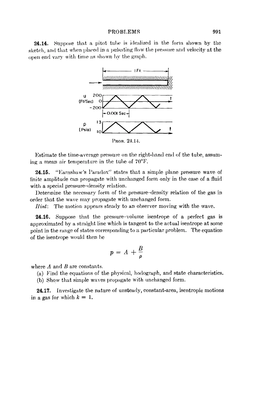
24 Unsteady, One-Dimensional, Continuous Flow . 930
Extension of Linearized Theory. Method of Characteristics.
Simple Waves. Waves of Both Families. Unit Operations and
Boundary Conditions. Unsteady, One-Dimensional Flow with
Area Change, Friction, and Heat Transfer or Combustion.
Remarks on Details of Working Out the Method of
Characteristics. Some Examples.
25 Unsteady, One-Dimensional Shock Waves . . 992
Analysis in Terms of Stationary Shock Formulas. Analysis of
Moving Shocks. The Shock Tube—Riemann's Problem. Weak
Shock Waves. Modified Calculation Procedure for Weak Shocks.
End Conditions and Interaction Effects for Strong Shocks.
Comparison Between Experimental and Theoretical Results.
Part VIII. Flow of Real Gases with Viscosity and
Heat Conductivity
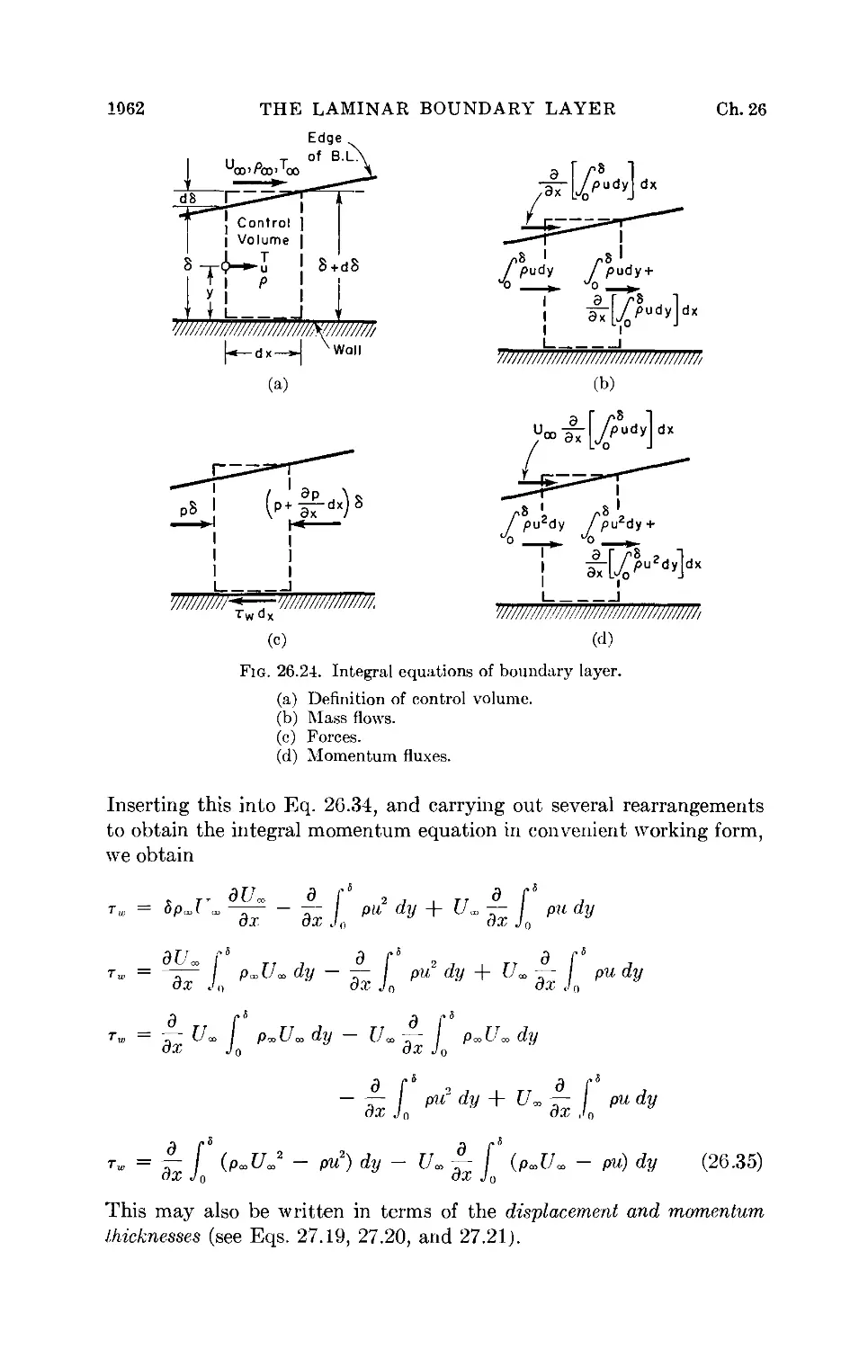
26 The Laminar Boundary Layer ..... 1033
Differential Equations of the Laminar Boundary Layer. Flow
With Prandtl Number Unity. Flow With Arbitrary Prandtl
Number. Integral Equations of the Laminar Boundary Layer.
Laminar Boundary Layer for Axi-Symmetric Flow. Experimental
Results for Laminar Boundary Layers. Stability of the Laminar
Boundary Layer.
27 The Turbulent Boundary Layer .... 1080
Differential Equations of the Turbulent Boundary Layer.
Integral Equations of the Turbulent Boundary Layer. Analyses of
Recovery Factor, Skin Friction, and Heat Transfer for Turbulent
Flow Past a Flat Plate with Turbulent Prandtl Number of Unity.
Theoretical and Experimental Results for Skin Friction on Flat
Plates. Recovery Factor for Turbulent Flow. Turbulent
Boundary Layer on Bodies of Revolution.
CONTENTS xi
chapter page
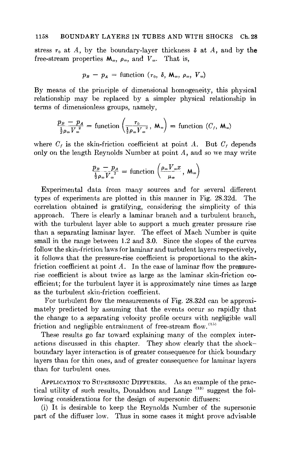
28 Boundary Layers in Tubes and in the Presence of Shock
Waves 1130
Flow in Tubes. Shock-Boundary Layer Interactions in
Supersonic Flow. Shock-Boundary Layer Interactions in Transonic
Flow. Normal Shocks in Ducts. Boundary-Layer Separation
Produced by Shock Waves.
Index for Volumes I and IX ...... 1161
PART V
SUPERSONIC FLOW (Continued)
Chapter 17
AXIALLY SYMMETRIC SUPERSONIC FLOW
17.1. Introductory Remarks
Important practical examples of axially symmetric supersonic flow
are (i) the flow past the fuselages of supersonic aircraft, rockets, and
ram jets, (ii) the flow past projectiles, and (iii) internal flow in ducts,
nozzles, and diffusers of round cross section.
Even though there are only two space coordinates in an axially
symmetric flow, the mathematical problems prove to be more difficult
than for two-dimensional flow because an axi-symmetric flow is
essentially a space flow, whereas a two-dimensional flow is essentially a plane
flow. Likewise, the physical natures of the two types of flows are quite
different.
The important analytical methods which have been developed and
which are outlined in this chapter are (i) the classical Taylor-Maccoll
exact solution for the flow past a cone, (ii) the approximate linearized
theory, first proposed by von Karman and Moore, and based on the
elementary solution for an infinitesimal "source" in a uniform, parallel
supersonic flow, and (iii) the method of characteristics, a procedure for
stepwise construction applicable to any flow pattern, time permitting
its use.
These analyses are based on the assumption of a frictionless, steady
flow, isentropic along each streamline. The flow is taken to be axi-
symmetric. In some cases, the flow is assumed irrotational, but in
others it is necessary to take account of the vorticity in the fluid.
A final section in the chapter summarizes some typical experimental
results.
Hypersonic Similarity Law. In Chapter 19 there is derived a
hypersonic similarity law for flow with small perturbations at high supersonic
speeds. The law is applicable when the hypersonic similarity parameter
K = Mmr (r = thickness ratio) is of the order of magnitude of unity
or larger. It states that for a given class of affinely related axi-symmetric
bodies the distribution of CvfaJ on the surface depends only on the
parameter K.
This result is relevant to the present chapter because various
investigations (see Chapter 19) have shown that the similarity law often
prevails at Mach Numbers which are usually considered to be super-
651
652
AXIALLY SYMMETRIC SUPERSONIC FLOW
Ch. 17
sonic rather than hypersonic. In the present chapter several methods
are presented for determining the pressure distribution on bodies of
revolution. For the range in which the similarity law is valid, it is
necessary to carry out these calculations (which are often tedious)
only for a few values of McT. Then the similarity law gives, with little
effort, the pressure distributions on members of the particular family
of affinely related shapes investigated for all combinations of M<» and
t falling within the range of validity of the law.
NOMENCLATURE
c speed of sound
C,, pressure coefficient
F see Eq. 17.34; also fineness
ratio
G see Eq. 17.34
i "\/— 1
K similarity parameter, M^ =
hhJF
k ratio of specific heats
M Mach Number
n direction normal to streamline
p pressure
Q source strength; also see Eq.
17.34a
r radius in spherical coordinates;
also radius in cylindrical
coordinates
R see Eq. 17.11; also radius in
spherical coordinates; also
radius to surface of axi-
symmetric body
s entropy per unit mass
S cross-sectional area of axi-
symmetric body in plane
normal to axis of symmetry
u ^-component of perturbation
velocity
f/oo free-stream velocity
v r-component of perturbation
velocity
V velocity
I'maI maximum velocity for adia-
batic flow
V
x, y, z
a
S
6
p
a
( )i
( )2
( ),
( )r
( )„
( )0
( )<»
( )/.;
vector velocity
Cartesian coordinates
Mach angle
semi-angle of cone; thickness
ratio of body of revolution
flow direction
^-coordinate of source
mass density
shock angle
thickness ratio; t = l/F
perturbation velocity
potential
velocity potential
angle in spherical coordinates
signifies conditions upstream
of conical shock
signifies conditions
downstream of conical shock
signifies conditions at surface
of cone
signifies component in r-di-
rection
signifies component in
co-direction
signifies stagnation state
signifies free-stream
conditions
signifies conditions on
characteristic curves
Art. 17.2
SOLUTION FOR PLOW PAST A CONE
653
17.2. Exact Solution for Flow Past a Cone
In plane supersonic flow a class of simple-wave solutions (Prandtl-
Meyer flow, Chapter 15) was found, defined by the property that the
two velocity components should be functions of each other. In the
corresponding flow pattern all stream properties are uniform on straight
lines in the physical plane, and these straight lines are identical with
the Mach lines. If a simple-wave flow pattern denned by the same
property is sought for an axi-symmetric flow, it is found again that all
stream properties are uniform on straight lines in the physical plane.
These lines are no longer the Mach lines, however, and the solution
requires that these straight lines pass through a common point. Thus,
because of the axial symmetry, all stream properties are constant on
cones having a common vertex. The resulting flow pattern is in fact a
special variety of the general class of conical flows discussed in Chapter
18.
General Nature of Flow Pattern. The type of simple-wave flow
outlined above could be bounded only by a cone. By assuming that fluid
properties are constant on cones having a common vertex, therefore,
we obtain the flow pattern past a cone (Fig. 17.1a). The practical
Line of Constant
Streamline
Stream Properties j'l0
Shock Cone
(a)
Fig. 17.1. Flow past cone.
(a) Shock cone and typical streamline.
(b) Hodograph image of streamline.
importance of this flow pattern is not limited to cones, however, since
the solutions for a cone will be applicable to the region near the tip of
any sharp-nosed body of revolution.
A continuous variation of fluid properties from free-stream conditions,
654 AXIALLY SYMMETRIC SUPERSONIC FLOW Ch. 17
Pi and Vi, to the surface of the cone, conditions p, and V„ proves to
be impossible. <3) A shock is therefore necessary. But, since the flow
downstream of the shock is by assumption conical, it follows that the
shock itself must be conical and of uniform strength, and must be
attached to the tip of the cone.
Consider a typical streamline (Fig. 17.1a) and its image in the hodo-
graph plane (Fig. 17.1b). Across the shock cone there is a discontinuous
change in direction and velocity from 1 to 2; points 1 and 2 therefore
lie on a common hodograph shock polar originating at point 1. Between
2 and s is a region of conical flow in which all stream properties vary
continuously, the streamline reaching point s on the surface of the
cone only in infinite distance. The velocity vector to point s in the
hodograph plane makes the cone semi-angle h with the axis. A typical
point P, with its corresponding angle wP is shown, together with its
image point in the hodograph plane. All stream properties are constant
on the cone wP, and hodograph point P is the image of the entire cone
wP. Likewise, the line 1-2-P-s is the hodograph image of all streamlines.
Since all streamlines experience the same entropy jump across the shock,
the flow between the shock and the cone is isentropic and irrotational.
Governing Physical Equations. Let us use spherical coordinates r and
a, with corresponding velocity components Vr and Fo (see Fig. 17.2a).
Then, considering the toroidal-shaped control volume of Fig. 17.2b,
for which the in-going mass flows are indicated, the equation of
continuity states that the net outflux of mass is zero:
— (27rpF,r2-<ia>-sin w) dr + —- (2wpV<lr-dr-sin «) dw = 0
or aw
Simplifying, and noting that all stream properties are independent of r,
i.e., d/dr = 0 and d/dw = d/doi, we have
2PVr + P7U cot co + p ^ + VB ^ = 0 (17.1)
Now, considering the velocity components of Fig. 17.2c, the
condition of irrotationality is introduced by setting the circulation around
the boundary of the control volume equal to zero:
•XT 7 I I T7" I u ' W 7 1 / i 7 \ 7
VT dr + I Va + —— dr \(r -\- dr) do.
~ [Vr + ~ dw) dr - Vjr dw = 0
which reduces to
V. = ^~ (17.2)
Art. 17.2 SOLUTION FOR FLOW PAST A CONE
655
Euler's equation, the velocity of sound, and the energy equation are,
respectively,
dp = -pVdV = -P(Vr dVr + Vu dVa) (17.3)
dp/dp = c2 (17.4)
(17.5)
pVudr(2Trr sinoi)
Fig. 17.2. Analysis of cone flow.
(a) Nomenclature.
(b) Continuity equation.
(c) Equation of irrotationality.
Combining Eqs. 17.3, 17.4, and 17.5 to eliminate the pressure, we
get
4
whence
dp
p
k
2
1
k - 1 ,
2 (
Vr dVr 4
' max
V 2
' max
- Va dV«
- V2
V2) dp
T } P
656 AXIALLY SYMMETRIC SUPERSONIC FLOW Ch. 17
Inserting this expression into Eq. 17.1, and rearranging, we obtain
(27, + Va cot co + ^)(VmJ - VJ - V>)
But, from Eq. 17.2,
T, dVr , dV« d2Vr
Vu = -;— , whence —— = —r-r
aco aco aco
With these it is now possible to eliminate terms in V' a from Eq. 17.6.
Thus we obtain, after rearrangement, an ordinary, nonlinear differential
equation of second order for Vr in terms of co:
d2Vr \~k + 1 fdVr\' k-l,T, , Tr2J *- l.-".coto,
+ (fc - l)F,(^max2 - Vr2) = 0 (17.7)
The integration of this equation was first done by Busemann (3)
with a clever graphical construction in the hodograph plane, and
subsequently by Taylor and Maccoll (4) by straightforward numerical
integration. Let us consider the latter method first.
Numerical Integration of Taylor and Maccoll. The general procedure for
arriving at solutions to Eq. 17.7 is indicated by the following schedule of
operations:
(i) Select a value of 8 (cone angle) and of (VT/Vm%x)., corresponding to the
Mach Number at the cone surface.
(ii) Begin with co = 5, at which Vr = {VT)H and Fo = 0.
(iii) Integrate Eq. (17.7) stepwise, for small steps in co, by replacing the
differential equation by a finite-difference equation.
(iv) Having found the value of Fr/Fmax corresponding to each value of co,
Vu/Vme,x niay be found by differentiation, using Eq. 17.2.
(v) The final step is to determine the appropriate shock angle a and free-
stream velocity Fi/F,nax. This is done by cut-and-try. For each value of co
during the integration there is a corresponding flow angle 6 and Mach Number
M. Corresponding to each point of the integration the downstream Mach
Number of a shock having a shock angle <r = co and turning angle 6 is compared with
the Mach Number M of the integration. When these two Mach Numbers are
found to be alike, the limit of integration has been reached and the correct shock
strength has been found.
(vi) From the shock tables the approach Mach Number Mi may then be
found. Flow properties in the conical-flow region are finally computed by using
Art. 17.2 SOLUTION FOR FLOW PAST A CONE 657
the shock relations for the shock, the isentropic relations for the conical-flow
region, and the values of Vr/VmtLX and Va/Vm!LX as functions of co found by the
previous integration.
Graphical Construction of Busemann. A geometrical solution to the
cone equations, leading to apple curves analogous to the hodograph
shock polars for plane shocks, is due to Busemann. <3) The governing
equations must first be put into a form involving only the hodograph
variables V and 8.
Hodograph Equations. From the geometry of Fig. 17.2a,
Vr = V cos (w - 8); Va = - Fsin (co - 8) (17.8)
or, differentiating with respect to co,
dVr „(, de\ . . . dV . .. /1f7nx
-^ = — V 1 — 3- sin (w — 8) + -j- cos (co — 6) (17.9a)
fflo; \ dw/ uco
^ = - v(l - ^) cos (« - 8) - ^ sin (co - 6) (17.9b)
aco \ do>/ dw
From Eqs. 17.2 and 17.8, however,
dV
^ = 7. = - y sm (c - 0) (17.9c)
When this is substituted into Eq. 17.9a, we obtain
= (17 9d)
dco Ftan(co - 8) \u .ya)
Eliminating dd/du from Eq. 17.9b, and substituting the expressions for
Vr, Vu, dVr/dw, and dV^/doo given by Eqs. 17.8, 17.9b, and 17.9c into
Eq. 17.6, we get, after rearrangement,
Jr . . . sin 8
7 sin (w — 8) -.
j_ sin co
do, _ 2 F2 sin2 (<o- Q)
- 1)(F_2 - F2)
The geometrical relations for two neighboring points, P and P', on
the same streamline in the hodograph plane are shown in Fig. 17.3.
From Eq. 17.9d, it is evident that the tangent to the hodograph
streamline makes the angle (co — 8) with the normal to the velocity vector.
From the geometry of the figure, this may be interpreted as meaning
that the vector change in velocity, dV, must be normal to the line of
constant co. This result might have been reached on physical grounds
since (i) the cones of constant co are surfaces of constant pressure,
(ii) the velocity gradient is normal to these cones, and therefore (iii)
the vector change in V must lie normal to the line of constant co.
658
AXIALLY SYMMETRIC SUPERSONIC FLOW
Ch.17
Also seen from Fig. 17.3 is that the normal to the hodograph
streamline makes the angle o> with the axis. This is illustrated further in Fig.
17.1b.
Center of Curvature of
Streamline Hodograph
-do)/
t
/
<
/
d
f
>
/
/
/
/
\
f
/
Hodograph
s/ Streamline
of
v/
/^dai
<
><*
ai-dw 6
Fig. 17.3. Geometry of hodograph Fig. 17.4. Graphical aid to construc-
streamline. tion of hodograph streamline.
If R is the radius of curvature of the hodograph streamline at point
P, then, from Fig. 17.3,
R = _
sin (w — 6) du
which, when combined with Eq. 17.10, gives
R =
sina>
1 -
2F2sin2(to - 6)
(k - l)(VmJ - V2)
1 -
2h2
(17.12)
(fc - D(VmJ - V2)
where q and h are defined by Eq. 17.12 and have the geometrical
significance shown by Fig. 17.4.
Graphical Solution. The graphical construction of the solution
now begins with the choice of free-stream Mach Number M! and shock-
wave angle a, thus defining points 1 and 2 of the hodograph shock
polar (Fig. 17.5) as well as the velocity V2 and streamline angle 02 at
the beginning of the region of conical flow. Using Eq. 17.12 and the
graphical construction of Fig. 17.4, the radius of curvature R2 of the
hodograph streamline at point 2 is computed and the corresponding
center of curvature 2' is laid off graphically. A short arc 2-3 is then
drawn with the radius jR2 about the center 2', thus giving, at least
approximately, point 3 on the hodograph streamline. Using the fluid
properties at 3 together with Eq. 17.12, the value of R3 is found, and
another short arc laid off with radius R3 about the center 3'. This
procedure is continued until the normal to the hodograph streamline
passes through the origin, thus indicating that the surface of the cone
has been reached, since Figr. 17.1a shows that 0, = to, = 5.
SOLUTION FOR FLOW PAST A CONE
uis=Bs-B w$ a i
Fig. 17.5. Graphical construction of cone flow.
Point s on the hodograph streamline is thus established and yields
the velocity at the surface of the cone, together with the cone angle 5
corresponding to the initially chosen values of Mi and a. The physical
streamlines may also be drawn inasmuch as the streamline direction 6
is known for each polar angle w.
If the procedure outlined above is repeated for the same value of M1;
but with different values of shock angle a, a corresponding point s is
found for each such angle, giving a family of solutions for cones of various
angles S in a stream of fixed Mach Number M[. The locus of such
points s forms the type of curve shown in Fig. 17.6, aptly named by
Busemann an apple curve.
M,= 1.50
Pos
01
0
0.94V^\
0.94lY\.
= O.93V/
c*
\
\
<*^\ 20 \
\TNiP.9998
Curves of
^'Constant
\
(«)-9)
Fig. 17.6. Apple curves for flow past cone with Mi = 1.50 (after Hantzsche and Wendt).
Apple Curves. Fig. 17.6 t5) shows a typical apple curve, for
M[ = 1.50. Several hodograph streamlines are shown, corresponding
to different cone angles. The stagnation-pressure ratio across the shock
for each such cone angle is also indicated. For convenience in graphical
660
AXIALLY SYMMETRIC SUPERSONIC FLOW
Ch. 17
construction, lines of constant (co — 0) are shown, the apple curve itself
being such a curve with the value zero for (co — 6).
Charts and Tables for Flow Past Cones. The graphical construction
is obviously limited in accuracy. Accordingly, the apple curves are
useful primarily for showing general orders of magnitude and for
comparative and illustrative purposes.
0.7
0.6
0.5
0.4
0.3
0.2
O.I
0
/
<
\
\
\
\
\
V
V
\
V
\
A
\
s.
\
\
\
\
5"
\
\
\
\
\
\
1
\
\
\
\
sj
\
N
o^j-'v
1
M,
S
P,
r-
h
41
---
50°
!-.-.
4.0
3.0
2.0 —
1.0
-M
i
/
>
S
M.
s-
nin
t
or 8^
i
ox
*—
0
r i
n°
—
—
-40°-
-—
*s
■^
M,
1.0
2.0
(b)
M,
(c)
3.0
4.0
Fig. 17.7. Theoretical results for flow past cone.
(a) Shock angle versus approach Mach Number, with cone angle as parameter.
(b) Ratio of surface pressure to free-stream pressure versus freo-stream Mach
Number, with cone angle as parameter.
(c) Surface Mach Number versus free-stream Much Number, with cone angle
as parameter.
Art. 17.2
SOLUTION FOR PLOW PAST A CONE
661
Kopal (6) has prepared extensive tables of theoretical results, based
on the integration of Eq. 17.7 by means of a differential analyser.
Many of these results have been put into convenient graphical form
in Reference 7. Small-scale charts showing the most important practical
results are given in Figs. 17.7a to 17.7f.
48
40
32
24
0,5° )0.
16
Shock Wove Detochec
"From Both Cone ■
.And Wedae ..iS
—
)
t
n
L
t
•"■■•
/
\/
Bi
4\
Shock Wove Attac
ro Nose Of Cone
t Not To Wedae _J
S
T
- c
y
led
0"-
hock Wave Attache
o Nose Of Both
00-"
2.0
3.0
4.0
M,
(d)
1.2
I.I
_ 1.0
o 0.9
° 0.8
2 0.5
■o
£0.4
a>
| 0.3
o°0.2
O.I
0
1.5 2.0 2.5 3.0 3.5 40
M. . or M,
(e)
/
/
A
A
■'1 '
\
**«
/
T
\
*»>
-Shock Wave Detache
s
v
—•.
-M, »- -
~-
<
4
S
i
0°
r
8
30" "
20° _
>~| |~
15° -
10°
1.0
2.0
3.0
4.0
(f)
Fig. 17.7. (Continued)
(d) Ratio of surface stagnation pressure to free-stream stagnation pressure,
with cone angle as parameter.
(e) Regions of shock attachment and detachment for cone and wedge.
(f) Pressure-drag coefficient based on projected frontal area.
662 AXIALLY SYMMETRIC SUPERSONIC FLOW Ch. 17
Special Features of Flow Past Cones. It may be noted from the
apple curves, Fig. 17.6, that for each value of M! there is a maximum
value of 5 for which there exists a solution to conical flow; and,
conversely, for each value of 8, there is a minimum Mi. Furthermore, for
a given M1; and for a cone angle less than 8max, there appear to be two
possible solutions. Similar results were obtained in Chapter 16 for
wedges.
Strong and Weak Solutions. The strong solution, i.e., the solution
with the larger shock angle, is never observed in photographs of flow
past cones. In practice the cone is never infinite. Since the flow
behind the "strong" shock is always subsonic, and since a subsonic
flow cannot have conical properties, it is impossible for the "strong"
solution to exist physically. The occurrence of the weak solution is
possible with finite cones in supersonic flow because cutting off the
downstream part of the cone cannot affect the upstream flow.
In Fig. 17.7, accordingly, only curves for the weak solution are
presented, and these are all bounded by a line labeled "Mimio or 5max,"
beyond which the shock is detached.
Attached and Detached Shocks. Fig. 17.7e shows the regions of
attached and detached shocks for cones, together with the corresponding
regions for two-dimensional wedges. For a given Mach Number
cones may have considerably larger angles than wedges before
detachment occurs.
Pressure Drag. The wave-drag coefficient of conical tips, based on
frontal projected area, is shown in Fig. 17.7f. It may be seen that
supersonic aircraft and projectiles must have sharp noses if the wave
drag is not to be excessive.
Comparison of Cones with Wedges. As compared with two-
dimensional wedges, cones produce less disturbance in the flow because
the flow may deviate from a conelike obstacle in three dimensions,
whereas for a wedgelike obstacle the deviation can be in only two
dimensions. For equal cone and wedge angles, therefore, the surface
pressure rise and shock angle are greater for wedges. Thus, a wedge
of given angle is a more sensitive instrument than a cone for determining
the Mach Number of a stream by measuring the Mach angle or pressure
rise; but, on the other hand, cones of larger angle than wedges may be
used with a given Mach Number.
Use of Cone for Supersonic Diffusion. Inspection of Fig. 17.6
shows that there are many instances where the flow between the shock
cone and the solid cone passes from supersonic speeds to subsonic
speeds without shocks. Streamlines and Mach lines for such a case are
illustrated in Fig. 17.8a. That this actually occurs in practice has
Art. 17.3 LINEAR THEORY FOR SLENDER BODIES 663
Shock M=l
/ Mach /
/ /"Lines'/
MroM.3l / __ —T
2
(b)
Fig. 17.8. (a) Typical streamlines and Mach lines for cone flow.
(b) Application of flow past cone to design of supersonic inlet.
been confirmed by experiment, thus providing a direct refutation to
the idea that passage from supersonic to subsonic speeds must necessarily
be accompanied by shocks. This result also suggests the use of
supersonic diffusers like that of Fig. 17.8b, where a portion of the supersonic
deceleration occurs without losses downstream of the shock.
Comparison with Experiment. Photographs of the waves attached to
cones (29) verify beautifully the theory as here outlined. Corresponding
measurements of the shock angle are shown in Fig. 17.9e and are seen
to agree almost perfectly with the analytical predictions. The measured
pressure coefficient at the surface of the cone is also in good accord
with the theory provided that the pressure taps are sufficiently far
from the vertex to avoid the distorting effects of boundary layers.
Since the effects produced by cones can be so accurately predicted,
cone-shaped probes are often used for measuring the local Mach Number
of a supersonic stream.
Flow Past Yawing Cones. The important aerodynamic features of
supersonic flow past yawing cones, such as yaw angle of shock, drag
coefficient, and lift coefficient, have been calculated in great detail by
Kopal based on theories by Stone. Both the theory and the results
are too extensive to be given here, and the reader is referred to
References 8 and 9 for details.
17.3. Linear Theory for Slender Bodies of Revolution
Although, by the method of characteristics, it is possible to work
out exactly the frictionless supersonic flow pattern for any body of
664 AXIALLY SYMMETRIC SUPERSONIC FLOW Ch. 17
80
70
60
50 —
40
30.
\
8 = 1
M,
\
Theory
0 Experiment
1
*^
»»^
—
1.0
1.2
1.4 1.6
M,
(e)
1.8
2.0
Fig. 17.9. Experimental results for cones (after Maecoll).
(a) Shadowgraph, Mi = 1.794. Shock is attached.
(b) Shadowgraph, Mi = 1.576. Shock is attached but has larger angle than
in (a). Note Mach lines produced by slight roughnesses on the surface.
(c) Shadowgraph, Mi = 1.160. The Mach Number is too low to permit of
conical flow. The shock is not conical and is about to detach from the nose.
(d) Shadowgraph, Mi = 1.090. Shock is detached and curved. Flow is
subsonic behind shock as far as the sharp corner at the shoulder of the
projectile.
(e) Comparison of measured wave angles with theoretical results.
Art. 17.3 LINEAR THEORY FOR SLENDER BODIES 665
revolution, the exact method is laborious and does not give answers in
analytical form, but rather requires each case to be worked out
individually on a numerical basis. The method of small perturbations, <10)
on the other hand, yields only approximate results, but has the great
advantage of being an analytic method, so that formulas showing the
effects of the different variables entering into a problem may readily
be obtained.
Linearized Equations of Motion. We shall assume that a slender body
of revolution is placed in an otherwise uniform, parallel supersonic
flow with properties M,,,, p«,, ?/„, etc. The axis of the body is parallel
to the free-stream direction, and hence there is complete axial symmetry.
The body is furthermore assumed to be very slender, so that the
perturbations from the free-stream velocity are very small compared with
the free-stream velocity. By writing the velocity potential as
$ = Uax + <p
where <p is the perturbation velocity potential, the derivatives of which
give the perturbation velocity components u, v, and w, and by following
the line of argument employed for two-dimensional flow (Chapter 10),
the equation for the velocity potential in three dimensions is reduced
to the following linear differential equation for the perturbation velocity
potential:
* ~ M~) e? + W + * - ° (17-13)
The local pressure coefficient has the approximate linearized form
c"~ ~2Th,= 'ulai (17-14)
Compressible Sources and Sinks. For incompressible flow it is well
known that the flow pattern around a body of revolution may be
synthesized by imagining sources and sinks to be placed on the axis of
the body. The linearized method for supersonic flow is based on an
extension of this concept.
Incompressible Source. When the flow is incompressible, M. = 0,
and Eq. 17.13 becomes
dV , d2tp . d2(p , _ .
d? + a? + a? = ° (17'15a)
A particular solution of Eq. 17.15a is
(17J5b)
666 AXIALLY SYMMETRIC SUPERSONIC FLOW Ch. 17
where Q is a constant and R is the radius from the origin. That this
is indeed a solution may be verified by direct differentiation and
substitution. The equipotential lines are concentric spheres around the
origin and hence the streamlines are straight radial lines and represent
the flow from a point source or sink placed at the origin. The radial
velocity is
R ~ 3D ~~
dR
and thus Q is seen to represent the strength of the source in terms of
the volume rate of flow issuing from the source. The source velocities
and potential lines are shown in Fig. 17.10a.
Subsonic Source. When M<,,< 1, we rearrange Eq. 17.13 in the form
(17.16a)
By comparing this with Eq. 17.15, we immediately see that a particular
solution is
(17.16b)
which may be rearranged in the form
y V , ,
i -\j w**v Wr=4eQ/iw<p/ (i7.i6c)
The equipotential lines of this subsonic compressible source are ellipsoids
of revolution. Both the equipotential lines and the perturbation
streamlines are as shown in Fig. 17.10b.
Supersonic Source. WhenM» > 1, we write Eq. 17.13 in the form
32 t2 -,2
^ + KT^- + aiiVKT^lr " ( 7a)
^i y
where i = V — 1. By analogy with Eq. 17.15, a particular solution is
which may be rearranged in the form
x N2 ' ■■ X2
(17.17c)
Art. 17.3
LINEAR THEORY FOR SLENDER BODIES
667
From this it is evident that the equipotential lines of the supersonic
compressible source are hyperboloids of revolution in the upstream and
downstream Mach cones (Fig. 17.10c). Or course, only the part of
the flow pattern lying in the downstream Mach cone is physically
Fig. 17.10. Equipotential lines and perturbation streamlines for point source.
(a) Incompressible.
(b) Subsonic.
(c) Supersonic.
significant. In Fig. 17.10c only the perturbation streamlines for this
region are shown.
It must be emphasized that Eqs. 17.16 and 17.17 do not truly represent
source flows, but acquire this title in a conceptual sense because of
the formal analogy with Eq. 17.15. The important result is that
Eqs. 17.16b and 17.17b represent elementary solutions of the differential
equation. Likewise, Fig. 17.10 shows only the perturbation
streamlines; the true streamlines are nearly straight parallel lines and are
668
AXIALLY SYMMETRIC SUPERSONIC FLOW Ch. 17
found by adding vectorially the perturbation velocity at each point to
the free-stream velocity.
Superposition of Sources. Since Eq. 17.13 is linear, and since Eq.
17.17b is an elementary solution to Eq. 17.13, we may construct more
complex solutions of Eq. 17.13 merely by adding together the velocity
potentials for several sources or sinks. This is most conveniently done
by imagining the sources and sinks to be continuously distributed
along the axis of the body.
Fig. 17.11. Nomenclature for Karm&n-Moore theory.
Referring to the meridian plane of Fig. 17.11, let £ represent the
x-coordinate of an elementary source lying on the axis of the body, and
let the sharp nose of the body be at x = 0. The strength of the
distributed source per unit length is called /(£); thus the strength of the
elementary source lying between £ and £ + d£ is /(£) d£. Now let us
consider the potential at the point P(x, r), owing to the source of strength
/(£)d£ at the location (£, 0). By comparison with the expression of
Eq. 17.17b for the potential of a source at the origin, we may write
4*- V(x - £)2 -
/3 =
- 1
for the potential in question. Now the total potential at P(x, r) is
due to all the sources lying between £ = 0 and £ = x — fir; these limits
are chosen because the sources cannot begin upstream of the tip of the
body, and because the effect of a given element of source is felt only in
the Mach cone downstream of the source.* Thus, the perturbation
potential at P(x, r), may be written
<p{x, r) = /
J 0
- £)2 - /3V
(17.18)
*Mathematically, the upper limit of integration may be interpreted as the limiting
value of { for which the integrand of Eq. 17.18 is real.
Art. 17.3
LINEAR THEORY FOR SLENDER BODIES
669
This is a definite integral from which £ vanishes after the integration
is performed. Our problem now is to determine the form of /(£) which
will give us the flow pattern for a body of selected shape.
It is necessary to calculate the perturbation velocity components.
Omitting the algebraic steps, we get
u — — = / ——
ox Jo 4ir
dip fz ' /'
V = * = "Jo 1
(x - £)2 - 0V
V(x - ?)2 -
(17.19)
(17.20)
where v is now taken to be the perturbation velocity component in the
r-direction, and /'(£) denotes d[f{£)]/d$. It should be mentioned
here that in taking the derivatives of Eq. 17.18 due account must be
taken of the fact that the upper limit of integration is a variable.
Uoo+u
Fig. 17.12/vBoundary condition at surface.
Source Distribution. Referring to Fig. 17.12, the boundary condition
at the body may be written
dx W.» + u)T.R.
Furthermore, if, as assumed, the body is very slender, we may write
W,«(x-Q; ffix«x
With the help of Eq. 17.20, therefore, the boundary condition may be
written approximately
= _ j_ r mik = l_ r
V. A 4T/J, ±*\]Jtx Jo
This may be immediately integrated to give
d]k = _JW_
dx
670 AXIALLY SYMMETRIC SUPERSONIC FLOW Ch. 17
where the lower limit of integration is found by setting /(0) = 0, since
if the source strength did not start with zero at the tip there would
be a blunt leading edge and consequently a detached shock wave.
The analysis is, therefore, limited to slender bodies with pointed tips.
Inasmuch as the foregoing equation is valid, within the assumptions, for
all values of x, we may write it in the form
dRj. = -/($)
or,
/(£) = -^UmR^ = -217.^ (17-21)
where S( = tR2, and represents the cross-sectional area of the body.
Eq. 17.21 thus gives the desired function /(£) corresponding to a body
of given shape.
Working Formulas. Finally, substituting Eq. 17.21 into Eqs. 17.19,
17.20, and 17.14, we get the following working formulas for the method:
' ^T ^ —r^=^-=F=, (17 -22)
u(x, r) = - — --/ .-— ^= ^ (17.23)
J 2ir d£ V( ?)" SV
Cp(x, r) = f! ~^ -, ^,—= (17.25)
Jo t df V(x - ^)2 - /TV2
For axi-symmetric bodies of arbitrary shape, these equations can
always be solved by graphical or numerical differentiation and
integration. This procedure is of course fairly lengthy, since the integrations
must be repeated for each set of values of x and r where the pressure
coefficient is desired, but nevertheless the method for arbitrary bodies
is considerably more rapid than the method of characteristics. A
modification of the calculation method outlined here, using a finite
number of sources and sinks, is outlined in Reference 11, and reduces
the labor of calculation considerably.
For axi-symmetric bodies having shapes which can be described by
simple functions, the working equations can be integrated to give
analytic solutions in closed form. Two such examples will now be
discussed.
Flow Past a Cone. It is of special interest to apply the linear theory
to flow past a cone, because the exact solution for this case was found
Art. 17.3 LINEAR THEORY FOR SLENDER BODIES 671
in Art. 17.2, and thus it is possible to estimate the accuracy of the
linear theory by comparison.
Using the nomenclature of Fig. 17.1a and assuming, within the
approximations of the linear theory, that tan 5=5, we have
S( = irff; dSJdi = 2tt52£; cfSJd? = 2tt52
We are particularly interested in the pressure coefficient at the surface
of the cone. Substituting into Eq. 17.25, setting r = R, and carrying
out the integration, we obtain
V(x - &2 - 01? x + Vx - p2r2
But /3R « x, and hence, to the degree of approximation of the method,
Cp. = -252 In g = 252 In —,=!== (17.26)
Fig. 17.13 indicates the type of agreement which may be expected
from the first-order theory. From Fig. 17.13a it appears that the error
in calculating Cv, is very small for cone semi-vertex angles up to about
10°, but for larger angles the error becomes very large. A generalized
comparison is shown in Fig. 17.13b <ii) in terms of the hypersonic
similarity parameter discussed in Chapter 19. The close grouping of
the several curves for the different cone angles illustrates the utility of
working with this parameter. From this chart it may be—seen that,
with semi-vertex angles \ip to 15°, the first-order theory is accurate
within 10 per cent as long as M, tan 5 is less than 0.3.
Flow Past a Parabolic Body of Revolution. Consider the flow past a
body of revolution Clli) with the meridian curve
R = ^-(l- 4x2)
where the body extends from x = —0.5 to x = +0.5, F is the length-
diameter ratio, and the maximum diameter is l/F. Substituting into
Eq. 17.25, and noting that the lower limit of integration is now —0.5,
there results for the surface pressure coefficient,
Cvs = |, |[12x2 - 1 + W2R2} cosh"
+ 6[(x + 0.5) - 4x]yfijc~+ 0.5)2 - (32R2\ (17.27)
This equation is plotted in Fig. 17.14 for a length-diameter ratio of
10 at Meo = 1.4. For comparison there are shown also the pressure
672
AXIALLY SYMMETRIC SUPERSONIC FLOW
Ch.17
.30
.20
P.
.10
0
—
— First Order _
— Second Order
— Exact
CPs
.80
.60
.40
i
.20
0
- ■
I 2 3 4 5 6 7
M.
I
(a)
-60
Similarity Parameter, K = 2M,tanS
(b)
Fig. 17.13. (a) Calculated surface pressure coefficient on cone versus free-stream
Mach Number according to (i) first-order (Karman-Moore) theory, (ii) second-order
(Van Dyke) theory, and (iii) exact (Taylor-Maccoll) theory.
(b) Accuracy of several approximate procedures for calculating surface pressure
coefficient on oone, correlated by means of hypersonic similarity parameter (after
Khret).
Art. 17.3
LINEAR THEORY FOR SLENDER BODIES
673
Fineness Rotio = m
distributions over the same body for incompressible flow and over a
two-dimensional body with the same profile for Mro = 1.4.
For incompressible flow over the body of revolution the pressure
distribution is symmetrical fore and aft, and there is no drag. For
supersonic flow, on the other hand, the pressures acting on the rearward
half of the body are generally lower
than those acting over the forward
half, and there is a resultant wave
drag.
For two-dimensional supersonic
flow over the same profile (ignoring
vorticity), the surface pressure
depends only on the local slope and
continually decreases. Because of
the pressure recovery near the tail
of the axi-symmetric body, the
-0.4
Fig. 17.14. Comparison of pressure
distributions on two- and
three-dimensional bodies having parabolic contours
(after Jones),
wave drag in three-dimensional
flow is smaller than in two-dimensional flow. Within the approximations
of the linear theory, no wake is left by this profile in two-dimensional
flow, whereas for the body of revolution there is a wake which extends
to infinity.
Fig. 17.15 illustrates the difference in wave drag (based on maximum
0 7
o
f 0.6
O
c
o
£ 0.5
c
o
1 0.4
O
CO
u° 0.3
c
;g 0.2
0 1 0.2
Thickness Ratio
Fig. 17.15. Comparison of pressure
1
(
Moc
/
/
•
) '
J
1
1
4
t
/
j
I
1
~T_
"wo-
Dimensional
7
y
/
Body of
Revolution
/
/
0
-O.I
-0.2
0.08
R
0.04
O,A Experimental
——^— Linear Theory
I I I l__
>" Ogival—-(«Cylindrical*kOgival»
/
\
Body Shape
u
"■V
0.2 0.4 0.6 0.8 1.0
X
Fig. 17.16. Comparison of measured
drags of two- and three-dimensional pressure distribution on A-4 missile at
bodies having parabolic contours (after Mo, = 1.87 with results of linear theory
Jones).
(after Thompson).
674
AXIALLY SYMMETRIC SUPERSONIC PLOW
Ch. 17
frontal area) between a wing section of parabolic profile and a fuselage of
parabolic profile. The difference in magnitudes is striking. Although
the wave drag of the wing increases with the first power of thickness
ratio, whereas that of the fuselage increases as the square of the
thickness ratio, this does not reverse the relative magnitudes for practicable
thickness ratios.
Comparison of Linear Theory with Measured Pressure Distribution
on Projectile. Fig. 17.16 shows how the pressure distribution calculated
by the linearized theory <u) compares with the experimental pressure
distribution on a typical projectile shape. It is seen that the linear
theory gives a fair approximation to the measured results. The method
of characteristics (11) gives somewhat better agreement.
Projectiles of Minimum Wave Drag. Because the linear theory gives
results in analytic form, it may be used to solve such variational
problems as the determination of projectile shapes for fixed length and
volume having minimum wave drag. <13> The shape of such a projectile
is illustrated in Fig. 17.17.
Open-Nosed Bodies of Revolution. The linearized theory outlined
here may also be extended to open-nosed bodies, such as ram-jet
fuselages. For details the reader is referred to References 14 and 15.
1.0
D =
(if
m cD = f
08
06
0.4
r
r mox
0.2
- N
-
-
-
I
\
1
1
\
1
1
I
V
0.5
1.0
Fig. 17.17. Shapes of bodies of revolution of minimum pressure drag under various
restraints (after Jones).
I. Body with minimum pressure drag for given length and volume.
II. Body with minimum pressure drag for given length and diameter.
III. Body with minimum pressure drag for given diameter and volume.
Art. 17.3 LINEAR THEORY FOR SLENDER BODIES 675
Inclined Bodies of Revolution. For an extension of the linear theory
to inclined bodies of revolution, the reader is referred to References 16
and 30.
Second-Order Theory. The results of this article are based on the
linear, or first-order terms in the equation of motion. A significant
improvement in the method, taking account of second-order terms, has
been developed by Van Dyke. <30>
Although the numerical calculations required are not lengthy, the
analytical formulation of the method is too lengthy to be given here,
and the reader is referred to Reference 30 for full details of the analysis
and of convenient calculation procedures based on specially prepared
tables.
The degree of accuracy to be expected from the second-order theory is
illustrated by Fig. 17.13. The second-order theory is markedly superior
to the first-order theory, and, for values of Mj tan 8 less than 0.5, is
in almost perfect agreement with the exact solution.
Comparison of Several Approximate Methods. Ehret <33> has made
an illuminating comparison of various approximate methods of solution
(requiring calculation times of a few hours) with the exact method of
characteristics (requiring calculation times of a few weeks). Each of
the approximate methods turns out to be fairly accurate in a certain
range of the similarity parameter K, and very inaccurate in other
ranges of K.
The various approximate methods considered for determining the
surface pressure distribution include
(i) The first-order theory discussed in Art. 17.3.
(ii) The second-order theory of Van Dyke referred to above.
(iii) The tangent-cone method, using the exact solutions for cones
whose slopes correspond to the local slopes of the body surface.
(iv) The conical-shock-expansion theory of Eggers and Savin, <34>
based on the observation that the equations for the variation of surface
Mach Number with surface slope downstream of the vertex of a pointed
body of revolution are approximately the same as the Prandtl-Meyer
equations for two-dimensional flow when K is greater than unity.
(v) The Newtonian theory of corpuscular flow (see Chapter 19)
based on the assumption that the nose shock wave lies very near to the
body surface, a condition which becomes valid as M, —» °°. This
assumption leads to the results that the component of velocity normal
to the surface is destroyed and that the tangential component is
unaltered; it is then readily shown from momentum considerations that the
surface pressure coefficient is given by 2 sin2 S.
Fig. 17.18a shows a comparison of the computed surface pressure
distributions for a tangent-ogive body of revolution with a fineness
676
AXIALLY SYMMETRIC SUPERSONIC FLOW
Ch.17
ratio of 6 at Mi = 3, corresponding to a value of the similarity parameter
of K = 0.5. The accuracy of each approximate method is seen to vary
considerably along the length of the body.
A summary of the errors in computing the pressure drag coefficient
by the several approximate
methods, found by carrying out detailed
calculations for a variety of typical
bodies of revolution, is shown in
Fig. 17.18b. The first-order theory
and second-order theory are seen
to be most accurate for values of K
less than 0.8. For values of K
Conical-shock-
expansion Theory
Method of
Characteristics
Linearized,
Theory
o Second-order _
Theory
Newtonian
-.04 -
-.06
0 20 40 60 80 100
Longitudinal Coordinate, Percent Length
(a)
Similarity Parameter,K
(b)
Fig. 17.18. Accuracy of various approximate methods for computing surface
pressure distribution on bodies of revolution (after Ehret).
(a) Comparison of approximate methods with exact method of characteristics
for tangent-ogive body with Mi = 3, F = 6, K = 0.5.
(b) Zones of error in pressure drag coefficient for various typical body shapes.
greater than about 1.6, however, the conical-shock-expansion theory,
the Newtonian theory, and the tangent-cone method are the most
accurate. It should be noted, however, that Fig. 17.18b is not a good
guide for estimating the error in local surface pressure coefficients, as
is evident from Fig. 17.18a.
17.4. Method of Characteristics
Because the governing differential equation is hyperbolic in nature,
the method of characteristics may be used for the exact stepwise
numerical calculation of axi-symmetric supersonic flows.
Characteristic Equations for Axi-Symmetric Irrotational Flow. When
the flow is axi-symmetric, steady, and irrotational, the differential
Art. 17.4
METHOD OF CHARACTERISTICS
677
equation for the complete velocity potential, in terms of cylindrical
coordinates x and r (Fig. 17.19), is (see Chapter 9):
where
and
C2 = Co2 -
(17.27)
(17.28)
(17.29)
Following the procedure of
Appendix A, we note, by
comparison of Eq. 17.27 with Eq.
A.ll, and using the symbol r in
place of y, that the coefficients of
the latter equation are, in this
instance: A = c2 — u2;B = — uv;
C = c - v2;D = -c2v/r.
Substituting these into Eqs. A. 17 and _, ,_,„ _, , .
, „_ , ,, r ii • !•«■ F1G- 17-19. Relation between stream-
A.18, we get the following differ- lines and characteristics.
ential equations for the
characteristic curves of Eq. 17.27:
n-Choracteristic
{Left-running
Mach Line)
I/a
/
/
/
My,
A
ov
u
\
\
V S
\
(8-a)
I-Characteristic
(Right-running
V" Mach Line)
\
1
(9+a)
dr\ _ — uv
.dx/,.,i
cVu+v2-c2
2
\du/r_ir
C — U
uv ± c s/u + v2 - c2
(17.30a)
c - v
c — v r
where the upper sign refers to family /, and the lower sign to family //.
These equations are more convenient to handle when written in terms
of the velocity components V and 6 (Fig. 17.19). Setting
u = V cos 6; v = Fsin 8
and noting that sin a = c/V, Eqs. 17.30 and 17.31 are transformed into
(dr/dx),,u = tan (0 T a) (17.30b)
V\dd
= =Ftan a H :—-.
sin a tan a sin 0 1 / dr\
( )
sin (6 =F a) r \dd/, u
(17.32)
The curves of Eq. 17.30b are projections on the physical plane of
curves lying in the <p, x, r-surface representing the solution to Eq. 17.27.
Likewise, the curves of Eq. 17.32 are the corresponding projections on
the hodograph plane of the corresponding curves lying in the <p, u,
^-surface representing the solution to Eq. 17.27. Thus, the simultaneous
678
AXIALLY SYMMETRIC SUPERSONIC PLOW
Ch.17
solution of the ordinary differential equations of Eqs. 17.30b and 17.32
for given initial conditions is equivalent to solving the original partial
differential equation, Eq. 17.27.
Eqs. 17.30b and 17.32 are seen to be similar to the corresponding
expressions for two-dimensional flow except for the presence of the
last term in Eq. 17.32. From Eq. 17.30b and Fig. 17.19 it is evident
that the physical characteristics of family / are the right-running Mach
lines and those of family II are the left-running Mach lines.
Since Eqs. 17.30b and 17.32 each contain terms in both velocity and
physical coordinates, it is necessary that they be solved simultaneously.
That is, both the physical and hodograph characteristics must be
constructed at the same time. This is in contrast to the two-dimensional
problem, where the last term of Eq. 17.32 is absent, thus making it
possible to construct the hodograph characteristics independently of
the physical characteristics.
Calculation Procedure. To construct the two families of
characteristic curves in the physical and hodograph planes, we replace the system
of continuous characteristic curves by a system of straight-line chords
connecting the intersection points of the two curves of the two families.
Of course the accuracy of this procedure depends on the fineness of the
net which is chosen. Corresponding to the replacement of a continuous
curve by a series of chords, we replace Eqs. 17.30b and 17.32 by finite-
difference equations.
Unit Process. The unit step of the entire procedure may be summed
up thus: Given in Fig. 17.20 the locations of two points 1 and 2 in
Fig. 17.20. Unit process of characteristics method.
both the physical and hodograph planes; to find the location in both
planes of a point 3 lying at the intersection of the two characteristics
passing through points 1 and 2.
As a first approximation, we may assume the average fluid properties
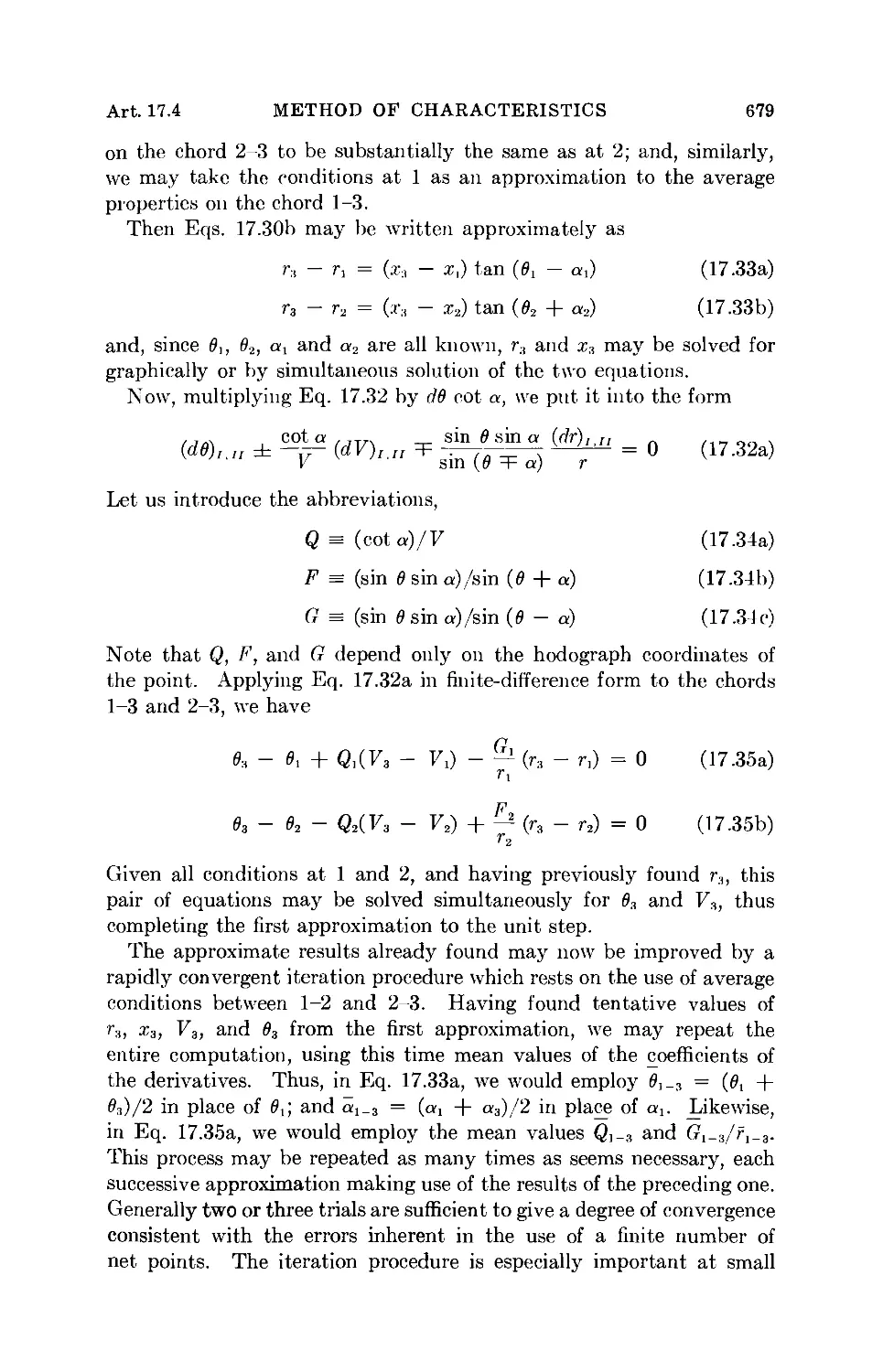
Art. 17.4 METHOD OF CHARACTERISTICS 679
on the chord 2-3 to be substantially the same as at 2; and, similarly,
we may take the conditions at 1 as an approximation to the average
properties on the chord 1-3.
Then Eqs. 17.30b may be written approximately as
r3 - r, = (x:1 - x,) tan {6l - a,) (17.33a)
rs - r2 = (x3 - x2) tan (02 + a2) (17.33b)
and, since 0,, 02, «i and a2 are all known, r3 and x3 may be solved for
graphically or by simultaneous solution of the two equations.
Now, multiplying Eq. 17.32 by dd cot a, we put it into the form
f ,, =F |f^ ^ = 0 (17.32a)
Let us introduce the abbreviations,
Q = (cota)/F (17.34a)
F = (sin 0 sin a)/sin (0 + a) (17.34b)
G = (sin 6 sin a)/sin (0 - a) (17.34c)
Note that Q, F, and G depend only on the hodograph coordinates of
the point. Applying Eq. 17.32a in finite-difference form to the chords
1-3 and 2-3, we have
9,-9,+ Q,(7, - 70 - — (r, - r,) = 0 (17.35a)
03 - 02 - Q2CF3 - 72) + ^ (r, - r2) = 0 (17.35b)
^2
Given all conditions at 1 and 2, and having previously found ra, this
pair of equations may be solved simultaneously for 03 and F3, thus
completing the first approximation to the unit step.
The approximate results already found may now be improved by a
rapidly convergent iteration procedure which rests on the use of average
conditions between 1-2 and 2-3. Having found tentative values of
r3, %a, F3, and 03 from the first approximation, we may repeat the
entire computation, using this time mean values of the coefficients of
the derivatives. Thus, in Eq. 17.33a, we would employ 0,_3 = (0t +
83)/2 in place of 9X; and a?^ = («i + a3)/2 in place of a^. likewise,
in Eq. 17.35a, we would employ the mean values Q,_3 and Gi-3/fi_3.
This process may be repeated as many times as seems necessary, each
successive approximation making use of the results of the preceding one.
Generally two or three trials are sufficient to give a degree of convergence
consistent with the errors inherent in the use of a finite number of
net points. The iteration procedure is especially important at small
680 AXIALLY SYMMETRIC SUPERSONIC FLOW Ch. 17
Mach Numbers. Although the improvement in accuracy obtained by-
iteration appears to be small for each new point determined, it must be
remembered that the conditions at a newly determined point become
the initial conditions for the next succeeding point, so that small errors
are cumulative and may in the end become quite large.
Point on Axis of Symmetry. When a point such as 2 lies on the
axis of symmetry, then r, and 02 are simultaneously zero, and F2/r2
is indeterminate. Its limiting form may be found, remembering that
we are working along the chord 2-3, as
.. sin 02 sin a2 ,. sin 0, sin a2
lim .—t- ; = lim —. ; —. : r
r.^o t2 sin (02 + a2) r2(cos 02 sin a2 + sin 02 cos a2)
.. sin 62 ,. (dd\ ^ 03
= lim = lim I -r) ^ —
r2 \dr/,T n
and with this form Eq. 17.35b may be solved directly.
If point 3, i.e., the point to be found, lies on the axis of symmetry,
so that r3 = 0 and 03 = 0, no difficulties arise, as either of Eqs. 17.35
may be solved immediately for V3.
Point on Solid Boundary. When point 3 lies on a solid boundary,
03 is known from the slope of the boundary, and point 3 in the physical
plane is found from the intersection of the boundary curve with one
of the characteristic curves. Thus the appropriate equation of Eqs.
17.35 is used for finding V3 at such a boundary point.
Point on Constant-Pressure Boundary. When point 3 lies on the
boundary of a free jet, where the pressure and velocity are known,
point 3 in the physical plane is found from the intersection of one of
the characteristics with the jet boundary. Thus the appropriate
equation of Eqs. 17.35 is used for finding 03 at such a free-boundary
point.
There is of course a great similarity between the calculations described
here and those described in Chapter 15 for two-dimensional flow.
The discussions in that chapter relative to initial-value situations,
numerical versus graphical procedures, field method versus net method,
organization of the numerical solution, etc., are all applicable here.
Example of Method. Fig. 17.21 shows the results of an example <19> describing
the flow at Mach Number 2.047 past a conical-nosed body. The conical nose,
with a semi-vertex angle of 30°, is joined at point 1 (x = 3) by a circular arc of
radius 10 in the meridian plane.
The flow in the neighborhood of the tip is found from the results of the exact
Taylor-Maccoll method for a cone, thus establishing the fluid properties on the
cones marked 30°, 40°, 45°, and on the downstream side of the shock cone 47.4°.
Art. 17.4
METHOD OF CHARACTERISTICS
681
12 3 4 5 6 7 8
x
Fig. 17.21. Example of construction of characteristics net (after Cronvich).
All fluid properties are constant on these lines up to the intersection of the
//-characteristic originating at point 1. In passing, it may be noted that even
with a sharp-nosed body not having a conical tip, the exact cone solution is
applicable in a limited region near the nose, and is always used to get a set of
initial values downstream of the shock for use with the method of characteristics.
Point 2 is located by applying Eqs. 17.33b and 17.35b to the chord 1-2, and
finding the intersection of the latter with the line marked 40°. Of course the
fluid properties at 2 are known from the cone solution. Points 4 and 7 are located
similarly.
Point 3 is found by applying Eqs. 17.33a and 17.35a to the chord 2-3, and
finding the intersection of this chord with the surface of the body. The iteration
procedure is necessary here, since V3 is at first not known, and 03 is known only
after the location of point 3 is found. The dashed chord 2-3 represents the first
approximation, whereas the solid chord 2-3" represents the third approximation.
Similar notation is used for the remainder of the characteristics net.
Point 5 is now found from points 3 and 4, this being a direct application of the
unit process previously described. Proceeding in this way, the flow in the entire
region 1-7-10 is established.
Downstream of this region the flow is no longer irrotational, because the Mach
waves originating at the body weaken the shock where they intersect the latter,
and the curvature of the shock in turn produces entropy variations which make
the flow rotational.
Often, however, the vorticity created by curvature in the shock wave is small,
and a good approximation is obtained by continuing the calculation beyond 7-10
with the assumption that the flow remains irrotational. Using this assumption,
682 AXIALLY SYMMETRIC SUPERSONIC FLOW Ch. 17
we must now construct the curved portion of the shock simultaneously with the
characteristics net.
By straight-line interpolation we choose arbitrarily an intermediate point 7a
on the /-characteristic 7-8'. The point 11' on the downstream side of the shock
wave is now found by satisfying simultaneously Eqs. 17.33b and 17.35b for the
chord 7a-ll, and the oblique shock equations for the direction of 7-11, and the
changes in flow properties across the shock at point 11. To accomplish this
solution requires the use of the iteration procedure. The position chosen for
point 7a is seen to determine the length 7a-ll' along the curved part of the shock
wave. By continuing this procedure the entire flow downstream of the curved
shock and of the line 7-10 may be calculated.
Graphical Method of de Haller. An ingenious graphical method,
using in part the two-dimensional hodograph characteristics, has been
described by de Haller. <23) Eq. 17.32 may be rearranged in the form
(dV)I,II = ~— [=F(dO)i.,i + (SO)/.//]
COL OL
(17.36a)
where, by definition,
If the flow were two-dimensional, the term 59 would be zero, and Eq.
17.36a would be the equation of the familiar two-dimensional epicycloid
hodograph characteristics (Chapter 15). Referring to Fig. 17.22, we
may thus obtain a first approximation to point 3 lying at the intersection
of the characteristics passing through the known points 1 and 2 by
using the simple graphical construction for the two-dimensional
characteristics. The next step is to bring in the correction term 50 owing to
the three-dimensional nature of the flow. Having established point 3
approximately, 801 and 80u may be calculated approximately from
Eq. 17.36b. Then, because of the form of Eq. 17.36a, we may determine
SV by laying out 86 along the two-dimensional hodograph characteristics.
Thus, in Fig. 17.22a, we lay off the angle 80r from point 1 along either
of the two-dimensional characteristics passing through 1, thus
establishing point 4, and then, by swinging an arc through 4, we determine
point 5. The distance 1-5 then represents 8Vt. Similarly we construct
the chord 2-7 representing &Vn. We now complete the hodograph
construction by finding the corrected point 3' at the intersection of
the two-dimensional characteristics passing through points 5 and 7.
Finally, the corrected physical point 3' (Fig. 17.22b) is found by laying
off 2-3' at the corresponding mean value of (6 + a), and 1-3' at the
corresponding mean value of (0 — a).
Art. 17.4
METHOD OF CHARACTERISTICS
c*
683
(b) (c)
Fig. 17.22. De Haller's graphical method of characteristics.
(a) Hodograph plane.
(b) Physical plane.
(c) Graphical aid to construction.
Fig. 17.22c illustrates a graphical construction for 8drI. Draw the
velocity vector through point 2, and extend it backward to point P.
Draw the normal 3-.V. Then, from the geometry of the figure,
sin 6
= P - 2
dr = 2 - 3 sin (8 + a) = 3 ^ sin (8 + a)
sin a
so that, comparing with Eq. 17.36b,
(86) a =
3 - JV
P - 2
(17.37)
A similar construction may be used for <507.
The accuracy of the method is illustrated in Fig. 17.22, showing,
for a spherical source beginning at the sonic speed, the hodograph
684 AXIALLY SYMMETRIC SUPERSONIC FLOW Ch. 17
diagram (Fig. 17.23a), the physical plane with Mach waves (Fig.
17.23b), and a chart of M* versus location in nozzle (Fig. 17.23c).
This chart shows excellent agreement between the stepwise results of
the method of characteristics and the exact one-dimensional formula
c*
\l 3 5 7 9 11 13 15 19
2 4 6 8 1012 16 u
(a) (b)
18 " Method of Char
M*
1.4
1.0
Exact Solution
rlr*
Fig. 17.23. Application of de Haller's method to point source flow.
(a) Hodograph plane.
(b) Physical plane, showing Mach lines.
(c) Comparison of characteristics solution with exact solution.
for isentropic flow. Note that, because of the symmetry of the flow
from a point source, it was necessary to investigate only the region of
flow in a cone of small vertex angle.
Further applications of the method to flow past a cone and to the
design of axi-symmetric nozzles are given in Reference 23.
Flow with Rotation. Most supersonic flow patterns with axial
symmetry have curved shock waves in important regions of the flow, and
hence it is necessary to take account of vorticity in the flow more often
than is the case with two-dimensional flow.
Using methods similar to that worked out for two-dimensional
rotational flow in Chapter 16, the differential equations of the
characteristics are found to be (see References 1, 17, and 20 for details)
(dr/dx)i,n = tan (0 =F a) (17.38)
. cot a
y (dV)i,a =F sm (e T \ r ± pi (ds)uu = 0
(17.39)
where R is the gas constant and s is the entropy.
The physical characteristics are, as usual, the Mach lines of the flow.
The equation for the hodograph characteristics is similar to that foi
irrotational flow, except for the addition of the last term, involving the
change in entropy (ds) along the characteristics. In the case undei
Art. 17.4
METHOD OF CHARACTERISTICS
685
consideration, for which the stagnation enthalpy is assumed the same
everywhere, the entropy remains constant on each streamline, but
varies from streamline to streamline. This suggests that we write
(ds),.,, = (ds/dn)(dn)r,n
where n is distance normal to the
streamline. For the wave of
family //, the geometry of Fig.
17.24 shows that
dnn = ——
sin a
(dr)r
sin (0 + a)
and there is a similar relation for
(rfn)7. Thus, the last term of Eq.
17.39 may be written
(S+a)
Fig. 17.24. Nomenclature for
characteristics method in rotational flow.
Sin a COS a
Rk sin (0 =F a)
If the variation of entropy normal to the streamlines is not large, we
may, from the geometry of Fig. 17.24, write further
ds
dn
s, - s2
~ X2)
Sin
sin i
cos (92 + «2) v 3 u cos (0, - a,)
With the help of these expressions, Eqs. 17.38 and 17.39 may be solved
in finite-difference form in a manner similar to that already described
for irrotational flow.
Example of Flow Past Projectile. As an example of the results
obtained by the method of characteristics, Fig. 17.25b shows the pressure
distribution obtained at Mra = 3.24 on the surface of the German
rocket projectile of Fig. 17.25a. <18) In this particular case there is
little error in the calculations as the result of ignoring vorticity behind
the curved shock wave. Similar calculations at M= = 8, however,
show that vorticity cannot be ignored in the latter case. Fig. 17.25c
shows, for the same body, a comparison of the calculated pressure
distributions at three different Mach Numbers. The agreement between
the calculated and measured pressure distributions, shown by Fig.
17.25d, is seen to be quite good.
Example of Flow Past Double-Cone Body. (18) The wave pattern
and some of the streamlines for the flow at M<» = 1.587 past a body
composed of two cones, back to back, is shown in Fig. 17.26a. The
corresponding velocity distribution is shown in Fig. 17.26b. The
"small mesh" is that of Fig. 17.26a, while the results labeled "large
686
AXIALLY SYMMETRIC SUPERSONIC PLOW
Ch. 17
mesh" were based on about one-third as many mesh points. There is
very little difference in the two sets of calculations except very near
the trailing edge.
At the sharp corner near the middle of the body, the flow in the
immediate neighborhood of the corner is given exactly by the two-
2 3 4 5 6
Calibers
(b)
0.25
°'°
A4 Rocket
Ma, = 1.86
o Measured
^°j ^——Method of Characteristics
1
J L
0 12 3 4 5 6 7 8
Calibers
(d)
Fig. 17.25. Flow past A-4 rocket (after Isenberg).
(a) Profile.
(b) Theoretical pressure distribution at M^, = 3.24, as found by method of
characteristics. Pressure distribution found by Van Dyke's approximate
second-order theory is in almost perfect agreement with curves of this
chart.
(c) Theoretical pressure distributions, as found by method of characteristics,
for several Mach Numbers.
(d) Comparison of measured with theoretical pressure distributions.
Art. 17.4
METHOD OF CHARACTERISTICS
687
dimensional relations for Prandtl-Meyer flow. In this small region
changes in radius are negligible compared with the radius itself, and
thus the flow may be considered plane. This is a situation frequently
encountered with axi-symmetric flow.
Example of External Flow Around Open-Nosed Body. (20) The wave
pattern for the external flow past an open-nosed body, such as a ram
jet, is illustrated in Fig. 17.27a, and the corresponding streamline
pattern is shown in Fig. 17.27b. The latter figure also indicates that
the calculated shock wave shape is in excellent agreement with the
observed shape. The corresponding pressure distribution is shown in
Fig. 17.27c.
Shock Wove—.
Streomlme
■Streamline
1.7
1.6
1.5
1.4
1.3
1.2
I.I
Undistu
Flow
1
1
bed
Conical
_Flow_
K
^A>,
1
o
«l oo = l-5
Large
Small
AvS
87
Mesh
Mesh"
\
b
0.5
0.6
0.7
x/i
0.8
0.9
1.0
(b)
Pig. 17.26. Flow past double-cone body (after Isenberg).
(a.) Streamlines and Mach lines.
(b) Pressure distributions as found by fine mesh and coarse mesh.
688
AXIALLY SYMMETRIC SUPERSONIC FLOW
Ch.17
Body of
Revolution
A
(a)
1.2
I.I
8
o.
1.0
o Experimental
— Theoretical
(b)
».v Method of
^^■^^ Chora cteristics
Linearized
Theory
(c)
Fig. 17.27. External flow past open-nosed body (after Ferri).
(a) Characteristics net.
(b) Streamlines and shock wave.
(c) Surface pressure distribution.
Example of Internal Flow for Open-Nosed Body. (20> The wave
pattern and streamlines for the internal flow near the entrance of a
supersonic inlet of revolution are shown in Figs. 17.28a and b. It is
found that the shock originating at the lip i.s strengthened as it moves
toward the center line, and, as a result, beyond a certain point the flow
is subsonic behind the shock. The extent of subsonic flow for M» = 1.6
is shown in Fig. 17.28c as a function of the lip angle.
Note that the internal and external flows of Figs. 17.27 and 17.28
may be calculated independently of each other as long as the shocks are
attached to the lip of the inlet.
Example of Axially Symmetric Body with Low Pressure Drag. <20)
Fig. 17.29 shows the wave pattern and streamlines for the flow through a
body of revolution consisting of a central plug and a surrounding
cylinder. This body is designed so that no waves are produced
externally to the body, and, therefore, the body has only the small amount
of pressure drag occasioned by the shock attached to the 10°-inlet cone.
Indeed, this drag could be reduced to zero if the plug were properly
Art. 17.4
METHOD OF CHARACTERISTICS
689
Subsonic /
Flow \/
0 5 10 15
Angle of Internal Cone, S, Deg
(c)
Fig. 17.28. Internal flow through open-nosed body (after Ferri).
(a) Characteristics net.
(b) Streamlines and shock wave.
(c) Extent of subsonic flow behind shock.
tapered to zero angle at the inlet. This flow arrangement will be
recognized as similar to the Busemann biplane for two-dimensional
flow.
Supersonic Inlets. For air-breathing propulsion engines at
supersonic speeds, it is very important to have supersonic diffusers of high
efficiency, and, because of the shape of supersonic aircraft and missiles,
it is often convenient to make such diffusers axi-symmetric. A
converging-diverging passage, such as is discussed in Chapter 5, comes to
690 AXIALLY SYMMETRIC SUPERSONIC FLOW
Ch.17
M = 1.09
Fig. 17.29. Axi-symmetrio body with low pressure drag (after Ferri).
(a) Mach lines and streamlines for forward half.
(b) Mach lines and streamlines for aft half.
mind as the first possibility, but Oswatitsch (28) has proposed a type of
diffuser with a central plug which has the advantages of providing
more usable volume in an aircraft and withal a better efficiency. Figs.
17.8b and 17.29 show inlet diffusers based on this general idea.
In Fig. 17.30 are shown several additional types proposed by
Oswatitsch. Fig. 17.30a shows a diffuser with one conical oblique shock and
one weak normal shock. The cone may have a rather large included
angle, and yet the conical shock is rather weak: at the same time the
Art. 17.4
METHOD OF CHARACTERISTICS
691
O.S.,
O.S.
O.S.
O.S.
(b) \ (c)
Fig. 17.30. Oblique shock supersonic inlets (after Oswatitsch).
O.S.: Oblique shock.
N.S.: Normal shock.
efficient compression downstream of the conical shock reduces the
Mach Number to the point where the losses across the normal shock
are very small. An extension of this scheme is shown in Fig. 17.30b,
where two oblique shocks precede the normal shock. A variant of
the latter scheme is illustrated in Fig. 17.30c, where the second oblique
shock is generated at the outer rim of the annular intake.
In Fig. 17.31 the efficiency of single-shock conical diffusers <35) like
that of Fig. 17.8b is compared with that of other types. The conical-
i.o
0.8
0.6
0.4
0.2
' lo.a
1
A)
Fig. 17.31. Efficiency of single-shock diffusers for k = 1.4 (after Lukasiewicz).
Curves 1: Normal shock followed by subsonic diffuser of indicated efficiency.
Curve 2: Oblique or conical shock with sonic velocity behind shock, followed
by isentropic subsonic compression.
Curve 3: Conical shock with sonic velocity at cone surface, followed by
isentropic subsonic compression.
Curve 4: One-dimensional, fixed-geometry, converging-diverging diffuser with
maximum allowable contraction for starting, followed by isentropic
subsonic compression.
692
AXIALLY SYMMETRIC SUPERSONIC PLOW
Ch.17
1.0
0.8
0.6
0.4
0.2
3
Moo
Fig. 17.32. Pressure recovery of multi-shock two-dimensional diffusers for k = 1.4.
There are n oblique shocks, each with the same stagnation-pressure ratio. Following
the last shock, where the Mach Number is 1.6, the stream is further decelerated by a
normal shock and then by an isentropic subsonic compression (after Lukasiewicz).
\
\
Normal
^\
^ 1
\
\
Shock '
"With Isentropic
Subsonic Compres
|
\
\
\
sion
n = oo
\n = 3
\n=l
^—
1.0 1.5 2.0 2.5 3.0 3.5 4.0 4.5 5.0
Fig. 17.33. Relation between diffuser efficiency and stagnation-pressure ratio,
for k = 1.4. Based on formulas of Chapter 5, leading to
+ Idiff
k
' k-1
+
Art. 17.4
METHOD OF CHARACTERISTICS
693
shock diffuser is seen to be considerably more efficient than a normal-
shock diffuser, and is comparable in efficiency with the optimum design
of a fixed-geometry, converging-diverging one-dimensional diffuser.
Two practical points to be kept in mind here are (i) the ready
adaptability of the plug-type diffuser for variable-geometry applications, and
(ii) the frequent need for boundary-layer control in order to prevent
the desired flow configuration from being ruined by shock-boundary
layer interactions.
The increase in efficiency realizable by substituting a number of
weak shocks for a single strong shock is not easily calculated for a
plug-type diffuser. Some notion of this improvement may be gained,
however, by carrying out the corresponding (and comparatively simple)
calculations for a two-dimensional diffuser with a series of oblique
shocks. As seen from Fig. 17.32, there is considerable improvement in
going from 1 to 2 or 3 shocks, especially at high Mach Numbers.
(d)
Mass Flow Entering Diffuser
Fig. 17.34. Operation of plug-type diffuser with constant approach conditions but
variable discharge pressure.
(a) Optimum conditions. Maximum mass flow and high pressure recovery.
(b) Discharge pressure too low. High mass flow but low pressure recovery.
(c) Discharge pressure too high. High pressure recovery but low mass flow.
(d) Corresponding curve of pressure recovery versus mass flow.
It may be noted that the performance is expressed in terms of diffuser
efficiency (see Chapter 5) in Fig. 17.31, whereas in Fig. 17.32 it is
expressed in terms of stagnation-pressure recovery. Since both these
measures of performance are used frequently, there is given in Fig.
17.33 a chart for passing quickly from one to the other.
Fig. 17.34 shows the typical performance of a plug-type diffuser at
constant approach Mach Number when the discharge pressure of the
694
AXIALLY SYMMETRIC SUPERSONIC FLOW
Ch.17
diffuser is varied (for example, by means of a throttle valve or by the
operation of an engine downstream of the diffuser). Fig. 17.34a
represents the design condition, with the maximum mass flow entering the
diffuser, and with a high efficiency because the normal shock is at the
minimum area. When the back pressure is too low, as in Fig. 17.34b,
the flow is still the maximum, but the normal shock occurs at a higher
Mach Number, thus producing a larger loss in stagnation pressure.
When the back pressure is too high, a normal shock stands ahead of
the cowl lip and allows some flow to spill over the cowl lip (Fig. 17.34c),
thus reducing the mass rate of flow. The curve of pressure recovery
versus mass flow (Fig. 17.34d) is composed of a nearly horizontal part,
corresponding to spillage operatiou with a nearly normal shock, and a
vertical portion, corresponding to operation with a swallowed normal
shock and with the maximum possible mass rate of flow.
10
0.9
0.8
0.7
0.6
o
•
a
X
D
Degrees
8
25
30
30
30
30
a
36
46
46
42
42
One —dimensi,
Converging-diverging
Diffusers with _
Swallowed Shocks
(Experimental Performance)
1.3
1.4
1.5
1.6
1.7
1.6
1.9
2.0
2.1
Fig. 17.35. Experimental performance of plug-type diffusers with several cowl
designs. Comparison with theoretical performance and with experimental
performance of normal shock, converging-diverging diffusers (after Ferri and Nucci).
Fig. 17.35 <36) shows experimental values of pressure recovery for
the optimum conditions of operation (point a of Fig. 17.34d) as a
function of free-stream Mach Number for several diffusers of the type
shown in Fig. 17.34. The measured efficiency is considerably higher
than the values attainable with fixed-geometry normal-shock diffusers.
One reason for the comparatively high "theoretical" performance is
the neglect of viscosity in the theoretical analysis, but it is clear that
the measured performance generally follows the theoretical curve.
Supersonic Nozzle Design. The design of an axi-symmetric nozzle
to produce a uniform, parallel, supersonic flow is somewhat different
from the design of a two-dimensional nozzle.
Referring to Fig. 17.36, suppose that along the line AB near the
throat the distribution of the velocity vector is known. Several points
Art. 17.4 METHOD OF CHARACTERISTICS 695
B D
Fig. 17.36. Design of nozzle for parallel, supersonic flow.
on this line are chosen as starting points for the characteristics net.
The wall is curved outward from point A for some distance, in a manner
at the disposal of the designer. The characteristics net is then
constructed step wise in the region downstream oi AB and bounded by the
wall on one side and by the center line of symmetry on the other.
This procedure is continued until the design Mach Number of the nozzle
is reached along the axis. Let the point at which it is reached be called
D, and let C be the point on the wall lying on the same characteristic
as point D.
The entire flow pattern is thus far known in the region A-C-D-B.
The wall contour A-C was selected arbitrarily, but beyond C the wall
must be so shaped as to give the desired uniform parallel flow at exit.
The Mach line extending downstream from D must be straight because
it bounds the uniform, parallel flow of the test section, and so it may be
drawn in. Along this line several points are chosen as the end points
of /-characteristics. If E is one of these points, then a point such as
G may be found from the known data at F and E. Proceeding in this
way the characteristics net is constructed in the region above the
characteristic C-D and the characteristic D-E-H. Once the
characteristics are drawn, the velocity is known at each point, and so the
streamlines may be drawn.
The particular streamline of interest is the one passing through C,
for this gives the desired nozzle contour, C-H, to produce a uniform,
parallel flow at exit. To find this boundary streamline requires, in
general, an interpolation for the stream direction 6 between the net
points. As a check on accuracy, the area ratio found by this construction
may be compared with the exact area ratio based on one-dimensional
isentropic flow.
An approximate analytical method for determining nozzle contours is
given in Reference 22.
696
AXIALLY SYMMETRIC SUPERSONIC FLOW
Ch. 17
Rapid Approximate Method for Pressure Distribution on Circular-
Arc Ogives/37' By examining the results of exact applications of the
method of characteristics to a large number of examples, Zienkiewicz<37)
discovered an empirical rule which greatly reduces the labor of
computing the surface pressure distribution on the nose portion of a body
of revolution having a circular-arc ogive for a nose. Comparing the
actual pressure distribution with that for two-dimensional Prandtl-
Meyer flow (which is easily calculated as in Chapter 15) over the same
profile, it was found that
pn - p = X(pn - p«)
where X remains virtually constant along a given ogive at a given
free-stream Mach Number; pn is the pressure at the nose just
downstream of the attached shock in axi-symmetric flow; p is the local
pressure at point P on the surface in axi-symmetric flow; and pt is the
local pressure at P for a two-dimensional simple-wave expansion from
pn at the nose. The table below shows how X depends on the free-
stream Mach Number Mo, upstream of the nose shock and on the
fineness ratio L/D of the nose (L is the axial length of the circular-arc
ogive from the tip to where it becomes tangent to the cylindrical portion
of the body, and D is the diameter where this tangency occurs).
L/D
2 0
2 5
3.0
3 5. . .
4.0
4.5
5.0
5 5
6 0. ...
6.5
7 0
Mco
1.5
0.748
.713
1.6
0.820
.775
.738
1.8
0.869
.817
.781
.750
2.0
0.914
.861
.821
.786
.762
2.5
0.942
.906
.870
.840
.813
.795
3.0
0.962
.928
.899
.870
.845
.826
.810
3.5
0.968
.938
.911
.887
.864
.844
827
.814
17.5. Miscellaneous Experimental Results
In this article we present some experimental results for practical
problems not easily accessible to analysis.
Static Pressure Probes. <24> Typical results of an experimental
investigation of the static pressure on probes having spherical and conical
heads are shown in Fig. 17,37. After some 10 diameters downstream
Art. 17.5 MISCELLANEOUS EXPERIMENTAL RESULTS
697
x/D
0af*£.;.-A:.:::j l^yyA ^yyy^Ky^yy^y,
t^...•■;.;. .V. ..^-f.;.^^^- -
*fci|--...-.v..j (.v.:.;.;.|[:.:.:.:.v.:.v.v.:.:.:.:.:.:.v.
mmd
0
/
10
s—
2C
1.0
0.9
0.8
0.7
0.6
0.5
Fig. 17.37. Static pressure at various distances aft of nose of static pressure probe
(after Cronvich).
of the tip the static pressure is within one or 2 per cent of free-stream
pressure for either type of probe. This instrument is, therefore, useful
for measuring static pressures in a supersonic stream. Extensive data
are given in Reference 24.
Drag of Projectiles. (25> Typical measurements of the drag of
projectiles are shown in Fig. 17.38. The drag coefficient is seen to decrease
E 12
E 13
0.16
0.14
0.12
0.10
0.08
0.06,
<
EI3
k
•^,
-*^
——
■—^
—
1.0 1.2 ■ 1.4 1.6 1.8 2.0 2.2 2.4 2.6
(a) (b)
Fig. 17.38. Drag of projectiles (after Charters).
(a) Projectile shapes.
(b) Drag coefficient versus Mach Number.
with Mach Number, but the rate of decrease is small at high Mach
Numbers. The drag coefficient at supersonic speeds is generally far
greater than that at subsonic speeds.
Base Pressure on Projectiles. <3132) Most supersonic projectiles,
missiles, and aircraft have a flat base, either circular or annular. The
pressures on this base contribute in either a positive or negative way
to the drag of the body.
(a) Schlieren photograph of
cone-cylinder at Mo, = 2.33, with turbulent
boundary layer on cylindrical part of
projectile (Ballistic Research
Laboratories, Aberdeen).
(b) Nomenclature.
(c) Summary of measurements of base
pressure versus Mach Number (after
Kurzweg).
0.3
0.2
0.1
A -APL-JHU
. I Spinning
likl Projectiles
k Atmospheric
fRonge-B.R.L.
Laminar Boundary Layer
1 " \!in? r Turbulent Boundary Layer
(c)
Fig. 17.39. Base pressure on projectiles.
698
Art. 17.5 MISCELLANEOUS EXPERIMENTAL RESULTS 699
Using the nomenclature of Fig. 17.39b, the base drag is defined as
where Ab is the area of the flat base on which the base pressure pn acts.
Fig. 17.39a is a typical schlieren photograph of the flow near the
base of a projectile. Near the end of the cylindrical portion the surface
pressure is not very different from pra. As the flow leaves the projectile
it expands around the edge in a Prandtl-Meyer expansion. The base
pressure is therefore smaller than pra and, consequently, the base drag
is positive. When a jet issues from the rear end (as in a rocket) the
situation may of course be different.
Fig. 17.39c is a summary of many tests on cone-cylinder projectiles.
In a general way the base drag is seen to increase with Mach Number,
but the base drag coefficient (2D,,.,>,,/A-pm Moo2.-!,,) decreases with Mach
Number.
The nature of the boundary-layer flow at the aft end of the cylinder
is found by experiment to be all-important in the determination of the
base pressure. The effects of variations in Reynolds Number are
extremely large for a laminar boundary layer, but are quite small for a
fully developed turbulent layer. It is accordingly difficult to predict
the base drag with good accuracy unless it is known that the boundary
layer is turbulent.
When the Reynolds Number is increased, the Mach Number being
maintained constant, the base pressure decreases as long as the boundary
layer is laminar. As the Reynolds Number reaches the point where
transition to turbulence occurs, the base pressure rises, thus reducing
the base drag. At very high Reynolds Numbers pB/p*> is nearly
independent of Reynolds Number. From Fig. 17.39c it may be seen that the
base pressure for a turbulent boundary layer lies between the maximum
and minimum values which are attained with a laminar boundary layer.
Apart from the effects mentioned above, other aspects of the
experimental measurements may be summarized as follows: U2>
(i) Large changes in surface temperature can significantly alter
the base pressure,
(ii) The effect of body shape is great for length-diameter ratios
less than about 4 but is small for length-diameter ratios
greater than about 6.
(iii) The presence of tail fins can considerably change the base drag.
REFERENCES AND SELECTED BIBLIOGRAPHY
1. Ferbi, A. Elements of Aerodynamics of Supersonic Flows. New York: The
Macmillan Co., 1949.
2. Sauek, R. Introduction to Theoretical Gas Dynamics. Ann Arbor: J. W. Edwards,
1947.
700 AXIALLY SYMMETRIC SUPERSONIC FLOW Ch. 17
3. Busemann, A. Drucke auf Kegelformige Spitzen bei Bewegung mit Uberschall-
geschwindigkeit, Z.a.M.M., Vol. 9 (1929), p. 496.
4. Taylor, G. I., and Maccoll, J. W. The Air Pressure on a Cone Moving at High
Speed, Proc. Roy. Soc. (A), Vol. 139 (1933), p. 278.
5. Hantzsche, W., and Wendt, H. Cones in Supersonic Flow, NACA Tech. Memo.,
No. 1157 (1947).
6. Kopal, Z. Tables of Supersonic Flow Around Cones, M.I.T. Center of Analysis,
Tech. Report No. 1, M.I.T., 1947.
7. Dailey, C. L., and Wood, F. C. Computation Curves for Compressible Fluid
Problems. New York: John Wiley & Sons, Inc., 1949.
8. Kopal, Z. Tables of Supersonic Flows Around Yawing Cones, M.I.T. Center of
Analysis, Tech. Report No. 3, M.I.T., 1947.
9. Kopal, Z. Supersonic Flow Around Cones of Large Yaw, M.I.T. Center of
Analysis, Tech. Report No. 5, M.I.T., 1947.
10. von Karman, T., and Moore, N. B. The Resistance of Slender Bodies Moving
with Supersonic Velocities with Special Reference to Projectiles, Trans.
A.S.M.E., Vol. 54 (1932), pp. 303-10.
11. Thompson, J. R. A Rapid Graphical Method for Computing the Pressure
Distribution at Supersonic Speeds on a Slender Body of Revolution, NACA
Tech. Note, No. 1768 (1949).
12. Jones, R. T., and Margolis, K. Flow Over a Slender Body of Revolution at
Supersonic Velocities, NACA Tech. Note, No. 1768 (1949).
13. Sears, W. R. On Projectiles of Minimum Wave Drag, Quarterly App. Math.,
Vol. 4, No. 4 (1947), p. 361.
14. Ludloff, H. F., and Reiche, F. Linearized Treatment of Supersonic Flow
Through Ducts, Jour. Aero. Sci., Vol. 16, No. 1 (1949), p. 5.
15. Moore, F. Linearized Supersonic Axially Symmetric Flow About Open-Nosed
Bodies Obtained by Use of Stream Function, NACA Tech. Note, No. 2116
(1950).
16. Laitone, E. V. The Linearized Subsonic and Supersonic Flow About Inclined
Slender Bodies of Revolution, Jour. Aero. Sci., Vol. 14, No. 11 (1947), p. 631.
17. Isenberg, J. S., and Lin, C. C. The Method of Characteristics in Compressible
Flow, Part I (Steady Supersonic Flow), Air Materiel Command Report, No.
F-TR-1173A-ND (Dec, 1947).
18. Isenberg, J. S. The Method of Characteristics in Compressible Flow, Part IB
(Numerical Examples), Air Materiel Command Report, No. F-TR-1173C-ND
(Dec, 1947).
19. Cronvich, L. L. A Numerical-Graphical Method of Characteristics for Axially
Symmetric Isentropic Flow, Jour. Aero. Sci., Vol. 15, No. 3 (1948), p. 155.
20. Ferri, A. Application of the Method of Characteristics to Supersonic Rotational
Flow, NACA Tech. Note, No. 1135 (1946).
21. Ferri, A. The Method of Characteristics for the Determination of Supersonic
Flow Over Bodies of Revolution at Small Angles of Attack, NACA Tech. Note,
No. 1809 (1949).
22. Foelsch, K. The Analytic Design of an Axially Symmetric Laval Nozzle for a
Parallel and Uniform Jet, Jour. Aero. Sci., Vol. 16, No. 3 (1949), p. 161.
23. de Haller, P. The Application of a Graphic Method to Some Dynamic
Problems in Gases, Sulzer Technical Review, No. 1 (1945), p. 6.
24. Cronvich, L. L. Pressure Distributions Over a Cylinder with Conical or
Hemispherical Head, Report No. CM-528 of the Applied Physics Lab. of Johns
Hopkins Univ., 1949.
25. Charters, A. C. Some Ballistic Contributions to Aerodynamics, Jour. Aero. Sci.,
Vol. 14, No. 3 (1947), p. 155.
26. Hill, F. K. Base Pressure at Supersonic Velocities, Jour. Aero. Sci., Vol. 17,
No. 3 (1950), p. 185.
27. Heberle, J. W., Wood, G. P., and Gooderum, P. B. Data on Shape and
Location of Detached Shock Waves on Cones and Spheres, NACA Tech. Note, No.
2000 (1950).
Art. 17.5 PROBLEMS 701
28. Oswatitsch, K. Pressure Recovery for Missiles with Reaction Propulsion at
High Supersonic Speeds, NACA Tech. Memo., No. 1140 (1947).
29. Maccoll, J. W. The Conical Shock Wave Formed by a Cone Moving at a High
Speed, Proc. Roy. Soc. (A), Vol. 159 (1937), p. 459.
30. Van Dyke, M. D. First- and Second-Order Theory of Supersonic Flow Past
Bodies of Revolution, Jour. Aero. Sci., Vol. 18, No. 3 (1951), p. 161. See also:
Van Dyke, M. D. Practical Calculation of Second-Order Supersonic Flow
Past Nonlifting Bodies of Revolution, NACA Tech. Note, No. 2744 (1952).
See also; Van Dyke, M. D. A Study of Second-Order Supersonic Flow
Theory, NACA Report, No. 1081 (1952).
31. Kurzweo, H. H. Interrelationship Between Boundary Layer and Base Pressure,
Jour. Aero. Set., Vol. 18, No. 11 (1951), p. 743.
32. Chapman, D. R. Note on Base Pressure Measurements, Jour. Aero. Sci., Vol.
17, No. 12 (1950), p. 812.
33. Ehret, D. M. Accuracy of Approximate Methods for Predicting Pressure on
Pointed Nonlifting Bodies of Revolution in Supersonic Flow, NACA Tech.
Note, No. 2704 (1952).
34. Egoerk, A. J., Jr., and Savin, R. C. Approximate Methods for Calculating the
Flow About Nonlifting Bodies of Revolution at High Supersonic Speeds,
NACA Tech. Note, No. 2579 (1951).
35. Lukasiewicz, J. Supersonic Diffusers, British A.R.C., R & M No. 2501 (1952).
36. Ferri, A., and Nucci, L. M. Preliminary Investigation of a New Type of
Supersonic Inlet, NACA Tech. Note, No. 2286 (1951).
37. Zienkiewicz, H. K. A Method for Calculating Pressure Distributions on
Circular Arc Ogives at Zero Incidence at Supersonic Speeds, Using the
Prandtl-Meyer Flow Relations, British A.R.C., C. P. No. 114 (1953).
PROBLEMS
17.1. Demonstrate, for the axi-symmetric flow past a cone, that the
condition of irrotationality is dVr/(h> = Va. Employ a geometrical interpretation
based on the facts that (i) the pressure is constant on rays emanating from the
origin, and (ii) the vector change in velocity is in the direction of the pressure
gradient.
17.2. Demonstrate by simple physical reasoning that the type of flow typified
by plane flow past a wedge, i.e., with all changes in stream properties occurring
exclusively across the oblique shock, is impossible for flow past a cone.
17.3. Demonstrate that, for the region of flow between a conical shock wave
and a cone, the hodograph of the streamline has the differential equation
/ ^ dvV
d\ , , (dv\ [U+Vdu]
1 + ) \/
17.4. Demonstrate that in an axi-symmetric supersonic flow, if the x- and
r-components of velooity are unique functions of each other, then the only
possible flow pattern is one in which the surfaces of constant fluid properties are cones
having a common vertex.
17.5. Investigate the supersonic flow past a cone for isothermal flow (k = 1)
and demonstrate that
-r^y— = cos (co - 5)
702 AXIALLY SYMMETRIC SUPERSONIC FLOW Ch. 17
Determine the shape of the streamlines, and other properties of the flow
pattern.
17.6. Find, for a cone, a relation between the surface pressure coefficient,
Cp, and the drag coefficient based on the base area of the cone.
17.7. (a) Find the equation of the perturbation streamlines in the x, y-
meridian plane for a "supersonic source" place in a uniform, parallel stream.
Demonstrate that these perturbation streamlines are equilateral hyperbolas for
M» = a/2.
(b) Determine the pressure coefficient produced by the source at each point
on the streamline, and express the pressure coefficient in terms of the j-coordinate
of the streamline.
17.8. Investigate the shape of the streamlines for the linearized solution of
flow past a cone, and compare with the exact solution.
Show that for this approximate solution all fluid properties are uniform on
cones having a common vertex.
17.9. Using the linearized theory, determine the surface pressure distribution
and the wave-drag coefficient for a body with fineness ratio 10 at speed Mo = \/2
having the form
R . x
^— = sin ir —
17.10. Determine the pressure distribution on the body of Fig. 17.25a by
the linearized theory, and compare the results with Fig. 17.25b.
17.11. Develop the characteristic equations for axi-symmetric, irrotational
flow, assuming that the perturbation velocities are sufficiently small to make the
linearized equations applicable.
Chapter 18
SUPERSONIC FLOW PAST WINGS OF FINITE SPAN
18.1. Introductory Remarks
In Chapters 14, 15, and 16 it was shown how two-dimensional
supersonic flows past any profile could be solved with relative ease. The
methods presented there lead to the aerodynamic properties of untapered
wings of infinite span having rectangular planforms.
In all practical situations, however, we must deal with wings of
finite span, and so it is important to understand the effects produced
by the ends of such wings. Furthermore, it is of interest to determine
whether the aerodynamic properties of supersonic wings may be
improved or controlled through changes in planform effected through
sweepback or sweepforward of the leading and trailing edges, or of
raking the wing tip.
In this chapter we shall outline the methods available for treating
such problems, and shall summarize those results of greatest practical
importance.
Because of the great mathematical difficulties attached to three-
dimensional flows, it is necessary, except in the discussion of the infinite
sweptback wing, to employ the method of small perturbations. This
is tantamount to the assumption that the wing is very thin in one of the
directions lateral to the flow, and, correspondingly, that only first-order
changes in all fluid properties are significant. As supersonic wings
must be thin in order to escape the penalty of large drag, the restriction
to small perturbations is not necessarily of .serious consequence.
In addition to neglecting second-order perturbations, we shall ignore
viscous effects and shall assume the flow irrotational and isentropic.
The net consequence of making these assumptions is that for most
aerodynamically desirable wings we get a good approximation to the
pressure distribution at the wing surface unless the boundary layer
either separates or exhibits rapid rates of growth.
The significance and validity of the non-viscous theory are examined
in the final part of the chapter through a comparison with experimental
results.
703
704
FLOW PAST WINGS OP FINITE SPAN
Ch. 18
NOMENCLATURE
a angle of attack
M aspect ratio
b span; also chord wise position
of maximum thickness
position
c speed of sound
d see Figs. 18.17a and 18.19a
Cv pressure coefficient
CL lift coefficient
CD pressure drag coefficient
Cf skin-friction coefficient
Cd. tot sum of coefficients of pressure
drag and skin friction
D drag
e see Figs. 18.17a and 18.19a
L lift
I chord
M Mach Number
n X//8
p pressure
q intensity of source
distribution; also conical-flow
parameter (Eq. 18.32)
r radius in cylindrical
coordinates
61 real part of a complex
variable
s transformed (/-variable (see
Eq. 18.35)
t thickness of wing; also \y/x
u, v, w Cartesian velocity
components
x, y,z
«-
5
V
e
X
A
h
fX
£
T
<P
$
free-stream velocity
Cartesian coordinates
free-stream Mach angle
thickness ratio
^-coordinate of source
cylindrical coordinate
tan A
sweepback angle of leading
edge
sweepback angle of mid-
chord line
(x/2) - A
x-coordinate of source
slope of surface in y, 2-plane
perturbation velocity
potential
defined by Eq. 18.38
( )a> signifies free-stream
conditions; also signifies
aerodynamic properties of un-
swept wing of infinite span
( )„ signifies component normal
to leading edge
( ), signifies component
tangential to leading edge
( )e signifies equivalent
two-dimensional, for swept wing
18.2. Preliminary Considerations of Finite Wings
Certain rules useful to the understanding of finite wings may be
derived from our general knowledge of the behavior of supersonic flows
and of flows with small perturbations.
Regions of Two-Dimensional Flow on Finite Wings. Because of the
rule that in supersonic flow a disturbance is felt only within the Mach
cone extending downstream from the source of disturbance, certain
portions of finite wings behave as though they were in a two-dimensional
flow. To illustrate this point, consider (Fig. 18.1a) a wing of infinite
span with a thin profile at a small angle of incidence. Any disturbances
Art. 18.2
PRELIMINARY CONSIDERATIONS
705
(f)
Fig. 18.1. Illustrates regions where two-dimensional flow prevails on
three-dimensional wings. Shaded zones signify two-dimensional flow.
produced in the regions E-A-C-G or B-F-H-D cannot influence the
flow in A-B-D-C. Therefore, if the infinite wing is cut along A-C
and B-D, and if all except the finite wing A-B-D-C is removed, this
finite wing will produce the same two-dimensional flow that it would
if it were part of an infinite wing. The downwash pattern behind the
wing, however, will not be completely two-dimensional.
By applying the same reasoning to the other planforms of Fig. 18.1,
706 PLOW PAST WINGS OF FINITE SPAN Ch. 18
it may be shown that two-dimensional flow exists in those regions
which are shaded.
When the wing is unswept, but the wing ends are raked inside the
Mach cones emanating from the ends of the leading edge, as in Fig.
18.1b, the flow over the entire planform is two-dimensional. The
downwash in the plane of the wing, however, is two-dimensional only
in the region J-K-L. With an unswept wing having its ends within
the tip Mach cones, as in Fig. 18.1c, the flow is two-dimensional except
within the tip Mach cones.
If a wing of infinite span were swept back, the flow past it would
appear two-dimensional to an observer moving along the span at such
a speed that in the observer's coordinate system the oncoming flow
was normal to the spanwise direction. Such a wing may be calculated
by the methods of two-dimensional flow, using the simple corrections
outlined in Art. 18.3. With this in mind, it follows that the arrowhead
wing of Fig. 18. Id will have two-dimensional flow except within the tip
Mach cones and the Mach cone originating at the forward point. If
the leading edges of such a wing were swept behind the Mach line from
the forward point, however, as in Fig. 18. le, no part of the flow would
be two-dimensional.
The shaded portions of Fig. 18.1 indicate only those portions in the
plane of the wing where the flow is two-dimensional. To determine
which portions of the flow away from the wing surface are
two-dimensional, it must be recalled that the disturbances of the wing tips, etc.,
are propagated within the Mach cones.
From these considerations it is clear that, for a given wing planform,
whether or not an element of the wing surface has two-dimensional or
three-dimensional flow over it depends in part on the free-stream Mach
Number.
Supersonic and Subsonic Leading and Trailing Edges. Consider a
swept wing of infinite span, as in Fig. 18.2. The free-stream velocity
Ua may be resolved into components along the span (£/„,) and normal
to the span (£/„„). An observer moving along the span with the uniform
speed [/„( sees a two-dimensional flow with the free-stream velocity
£/„„ past an unswept wing. Whether this equivalent two-dimensional
flow is supersonic or subsonic depends on whether (/„„ is, respectively,
greater or less than c«,. Since cro = [/„ sin aa, and [/„„ = Um sin /*, it
follows that
Moon = C/»n/c« = sin m/sui <*„
Hence the equivalent two-dimensional flow is supersonic if n exceeds
the Mach angle (Fig. 18.2a) but is subsonic if n is less than <*„ (Fig.
18.2b). In the former case we say that the leading edge is supersonic,
and in the latter that it is subsonic. Identical considerations apply to
Art. 18.2
PRELIMINARY CONSIDERATIONS
707
Mach
Line
(b)
Fig. 18.2. Swept leading edges.
(a) Supersonic leading edge ([/„„ > cm).
(b) Subsonic leading edge (f ran < cm).
the trailing edge. Thus, in Fig. 18. Id both the leading and trailing
edges are supersonic, whereas in Fig. 18.le both the leading and trailing
edges are subsonic.
The significance of the natures of the leading and trailing edges may
be illustrated by considering the details of the mechanism by which
lift is produced on a flat plate of infinite span. Fig. 18.3 shows schem-
Leading-
Edge
"Suction"\
Force }
Normal-Force
Distribution
(a) - (b)
Fig. 18.3. Chordwise distribution of pressure force on flat plate at angle of attack.
(a) Subsonic.
(b) Supersonic.
atically the lift distributions over the chord of such a wing in subsonic
and supersonic flow.
In the starting instant of subsonic flow, the motion around the wing
is both irrotational and without circulation, and hence produces no
lift. However, this flow has infinite velocity around the sharp trailing
edge, and, as a result of viscosity, no matter how small the latter may
be, the flow separates near the trailing edge and produces a vortex.
In accordance with Kelvin's Theorem, the shedding of this "starting
vortex" has as a reaction the production of circulation around the profile,
708 FLOW PAST WINGS OF FINITE SPAN Ch. 18
the magnitude of the circulation being determined by the Kutta-
Joukowski condition that the rearward stagnation point be at the
trailing edge. From this it follows that the fluid pressures acting on
the upper and lower surfaces of the airfoil at the trailing edge are equal,
and the trailing-edge lift per unit area is zero (Fig. 18.3a).
In supersonic flow the trailing-edge lift per unit area, in consequence
of the rule of forbidden signals, need not be zero. Indeed, since in
supersonic simple-wave flow the local pressure depends only on the local
inclination of the surface, the lift distribution of the flat plate is constant
over the chord (Fig. 18.3b).
Near the leading edge in incompressible flow the lift per unit area
tends toward infinity, in accordance with the infinite fluid velocity at
the sharp corner. It may be argued that this infinite velocity necessarily
leads to boundary-layer separation. This difficulty is eliminated,
however, by allowing a small rounding of the leading edge, a change
which does not alter the essential character of the flow over most of the
profile. The very low pressures at the leading edge produce a "suction
force" which cancels the drag component of the normal force, and
leads to zero net drag, skin friction excepted (d'Alembert's Paradox).
In supersonic flow, this "suction force" is not present, and there results
an "induced drag due to lift."
We may summarize the foregoing considerations as follows: (i)
supersonic leading and trailing edges have finite lift loadings, (ii) a
subsonic leading edge tends to have a very high lift loading and a
negative drag force, and (iii) a sharp subsonic trailing edge has zero
lift loading.
Fig. 18.4. Wing planform having leading and trailing edges with partially
supersonic and partially subsonic flow.
AB, supersonic leading edge.
BC, subsonic leading edge.
CD, subsonic trailing edge.
DE, supersonic trailing edge.
Consider the arbitrary planform of Fig. 18.4. The curve A-B is called
a supersonic leading edge because the flow in this neighborhood is like
that near the leading edge of a supersonic normal wing with infinite
span. For like reasons, the line D-E is called a supersonic trailing edge.
Art. 18.3
SWEPTBACK WINGS
709
The boundary B-C, on the other hand, is called a subsonic leading
edge because the velocity component normal to the edge is less than the
sonic speed, and the flow is typically subsonic in character. Between
C and D the boundary is called a subsonic trailing edge. Note that
disturbances propagated from points along C-D cover part of the
planform, and thus the flow can adjust itself so as to satisfy the Kutta-
Joukowski condition at the trailing edge.
A practical rule which follows from these considerations is that the
portion of the boundary of the planform which constitutes a subsonic
leading edge should have a rounded nose so as to avoid a large form
drag owing to separation at the leading edge. Conversely, supersonic
leading edges should be sharp so as to avoid the large pressure drags
associated with detached shock waves.
With planforms of general shape, the simultaneous presence of portions
having both supersonic and
subsonic properties leads
understandably to analytical problems of
considerable difficulty.
Incidence
Camber
(c)
Composite
Profile
Superposition of Effects. Since
we are considering flows with
small perturbations, the
governing equations are linear. Thus it
is possible to study separately
the effects of thickness, camber,
and angle of incidence, and to
determine by linear addition the
flow pattern for a combination of
these effects. Thus, the
perturbation pressure distribution on
the profile of Fig. 18.5d may be found by adding the perturbation
pressure distributions for the flows of Figs. 18.5a, b, and c.
Fig. 18.5. Illustrating linear
superposition of effects of incidence, thickness, and
camber.
18.3. Sweptback Wings
We shall now investigate the properties of infinite sweptback wings,
but it is important to remember that the results we obtain are applicable
also to such cases as the shaded areas of Fig. 18. Id.
Two separate cases may be distinguished, corresponding to Figs.
18.2a and b. In the latter case, where the leading edge is swept behind
the Mach line, the flow normal to the leading edge is subsonic, and that
part of the flow pattern not influenced by viscosity will behave as
though the flow were subsonic. This problem was treated in detail in
Art. 13.7, and will not be discussed here.
710
FLOW PAST WINGS OF FINITE SPAN
Ch. 18
The former case, where the leading edge is swept ahead of the Mach
line, has a supersonic normal component of velocity, and is the subject
of our present attention.
Equivalent Two-Dimensional Flow. Consider a wing of infinite span
swept at an angle A and set at an angle of attack a (Fig. 18.6). We
(c)
Fig. 18.6. Analysis of infinite sweptback wing.
(a) View in plane of wing.
(b) View in plane parallel to direction of flight.
(c) View in plane normal to leading edge.
may resolve the free-stream Mach Number Me into three components:
(i) the Mach Number M. cos A cos a in the plane of the wing and
normal to the leading edge, (ii) the velocity M, sin a normal to the
plane of the wing, and (iii) the velocity M. sin A cos a in the plane of
the wing and tangential to the leading edge. To an observer moving
along the span with the last-named tangential speed, the flow appears
two-dimensional, and may be so treated (except for the boundary-layer
flow). Let us use the subscript e to denote quantities seen by the
moving observer. With the help of Fig. 18.6c, we may write
M«,e =
sin a)2 + (M^ cos a cos A)2 = M» y/l — sin3 A cos2 a
(18.1)
Mra sin a , tan a ,1O o.
a. = arc tan 77-TrrTTrTT = »re tan T7TT (18-2)
cos a cos A
—1-= -A_
/ cos A cos A
cos A
(18.3)
where 5 is the thickness ratio in the plane parallel to U*. Since the
lift is not changed by the observer's motion, we may write
I.
L
^;-'(/ cos A)(6/cos A)
Art. 18.3 SWEPTBACK WINGS 711
With the help of Eq. 18.1, we obtain, therefore,
CL = CU/VU/MJ2 = CLr{\ - sin2 A cos2 a) (18.4)
Since, for the present, we are ignoring viscous drag, the tangential
component of velocity does not contribute to the drag, and the pressure
drag is normal to the leading edge. Thus, if I) is the total pressure
drag, the component of this in the Mro direction is only D cos A.
Accordingly, we write
^ D cos A „ __ D
' l>e =
" ~ k , ' " ~~ k
~ J0=M«, Ib — pcoMrar"(/ cos A)(6/cos A)
or
Cn = CD. cos A(Mcoe/Mj;! = C,u cos A(l — sinL> A cos2 a) (18.5)
Calculation of Properties of Swept Wing. These equations take exact
account of the geometrical relationships and are correct even for large
angles of attack. For any given profile shape with given values of
Me, A, a, and 5, the corresponding values of M^,, a,, and 8e may be
found from Eqs. 18.1 to 18.3. The corresponding force coefficients
CLt and CDe may then be found from two-dimensional theory. Finally,
the values of CL and C,, for the swept wing, based on the free-stream
velocity and direction, may be calculated from Eqs. 18.4 and 18.5.
Effect of Skin Friction. Since the skin friction depends primarily on
the free-stream velocity and direction, the total drag coefficient may be
found merely by adding the skin-friction coefficient, Cf, to the pressure
drag coefficient:
Cfl.toi = CD + Cf (18.6)
Approximate Formulas for Small Angles of Attack. When the angle
of attack is small, we may write
cos a = 1; tan a = a; tan"1 ae = at
Then Eqs. 18.1 and 18.2 may be written, with good accuracy, as
M»e = M,, cos A (18.7)
ae = a/cos A (18.8)
Similarly, Eqs. 18.4, 18.5, and 18.6 become
CL ^ CLe cos2 A (18.9)
Cn.tot = CDe cosJ A + Cf (18.10)
712 FLOW PAST WINGS OF FINITE SPAN Ch. 18
Thin Profiles at Small Angle of Attack. If, in addition to the
assumption of small angles of attack, we assume that the profile is thin, the
linearized theory of Chapter 14 yields
CLe = _J^— CDe = -7=Jr= (a.' + K82)
V Me, - 1 VM., - 1
where the coefficient K depends only on the thickness distribution of
the profile as seen in a plane normal to the leading edge.
Combining these relations with Eqs. 18.7 to 18.10, we get
„ 4 cos A /,n n\
CL = ,—T? ; a (18.11)
'" J cos2 A - 1
4 cos A 2 4 cos3 A 2 ,
„ cos A — 1 vMco cos A — 1
A plot of Eq. 18.11 shows that the lift-curve slope dCL/da increases
with sweepback angle A for all values of M.^. Thus there is actually a
gain from sweepback on this score.
The first term on the right-hand side of Eq. 18.12 represents the
induced drag due to lift. It may be seen by comparison with Eq. 18.11
that this part of the drag increases in proportion to the lift.
The second term on the right-hand side of Eq. 18.12 represents the
wave drag due to thickness. This term was intentionally left in terms
of 8e rather than 8 because structural considerations would dictate that
8, be kept more nearly constant than 5 as the sweepback A was changed.
With 8, constant, the thickness drag at first decreases as the sweepback
is increased, but when the leading edge begins to approach the Mach
line (i.e., M«, cos A —> 1) the thickness drag begins to rise.
Diamond Profile. Another important result may be simply
illustrated by taking the case of a symmetrical double-wedge profile with
no skin friction, in which case Cf = 0 and K = 1. Then, by setting
equal to zero the derivative d(D/L)/da, we get
_ cos A
nIn = ~28~7
a' = 8e cos A
c ' =
cos2 A - 1
where a' and CL' are respectively the incidence and lift coefficient at
the condition of maximum lift-drag ratio. These relations show that
sweepback increases the maximum lift-drag ratio but that this condition
occurs at a smaller angle of attack and, within the restrictions of the
paragraph which follows, at a slightly smaller lift coefficient.
Art. 18.3
SWEPTBACK WINGS
713
Fig. 18.7. Effect of sweepback on lift-
curve slope of wing with double-wedge
profile (after Ivey and Bowen, NACA).
0.08
0.07
0.06
0.05
0.04
0.03
0.02
0.01
0
|M00
X 1
Double
a
8
.
Wedge
= 0°
e=0.05
--'
4
0 10 20 30 40 50 60
A,Degrees
0.08 0.16 0.24 0.32 0.40 0.48
Section Lift Coefficient, C[_
0.08 0.16 0.24 0.32 0.40 0.48
Section Lift Coefficient, CL
3
i- 2
1
L
w
III
\
f
\
A
(Deg)
60
(
—45
6^30
^15
= 4
0.08 0.16 0.24 0.32 0.40 0.48
Section Lift Coefficient, CL
0.08 0.16 0.24 0.32 0.40 0.48
Section Lift Coefficient, CL
Fig. 18.8. Effect of sweepback on lift drag ratio of wing with double-wedge profile
(after Ivey and Bowen, NACA).
714 FLOW PAST WINGS OP FINITE SPAN Ch. 18
It should be noted that Eqs. 18.11 and 18.12 are valid only within
the approximations of the linear theory, and that they are further
restricted to combinations of A and M« such that the leading-edge
shock wave is attached.
Typical Effect of Sweepback. The foregoing discussion is amplified
by the illustrative curves of Figs. 18.7 and 18.8. These curves give a
more accurate picture than is provided by the linear theory, inasmuch
as they are based upon (i) the exact geometrical relations of Eqs. 18.1
to 18.5; (ii) the calculation of the pressure drag for a 10% symmetrical
double wedge, using the exact expansion wave and shock theory for a
frictionless fluid; and (iii) a skin-friction coefficient of 0.006.
Sweepback is seen to yield substantial improvements in performance.
18.4. Similarity Rule for Supersonic Wings
In Chapter 13 we discussed Gothert's rule for linearized flow, by
means of which the flow pattern around any wing in subsonic flow could
be related to the incompressible flow past an affinely related wing.
Using the same approach we shall now derive a rule by which the flow
pattern around any thin wing at small incidence in a supersonic flow
may be related to the flow past an affinely related wing at Mra = y/2.
Similarity Transformation. For supersonic flow with only small
perturbations from a uniform, parallel flow along the z-axis, the equation
of the perturbation velocity potential (Eq. 13.1) is
~p e? + W+ a? " ( 3a)
where
/3 = VmT^T (18.13b)
We now introduce the transformation
x' = x; y' = 0y; z' = fc; <p'(x', y', z') s p2<p{x, y, z) (18.14)
In terms of these variables Eq. 18.13a takes the form
-% + w + % - ° (lfU5)
It may be further verified by the methods of Chapter 13 that the
boundary conditions of the original How at infinity and at the profile
surface give, in the transformed flow, uniform parallel flow at infinity
together with flow past a new profile whose ordinates are related to
that of the original profile by Eq. 18.14.
A comparison of Eq. 18.13a with Eq. 18.15 shows that the latter is
Art. 18.4 SIMILARITY RULE FOR SUPERSONIC WINGS 715
the same as the equation of the perturbation potential <p when M» = \/2.
From Eq. 18.14 it may also be seen that the flow <p'(x', y', z') refers to
a body all of whose lateral dimensions are greater by the factor /? than
the corresponding dimensions of the original body.
The linearized pressure coefficients at corresponding points in the
two flows are related by
Cp ~ ~ U. dx' ~ ~ Uj dx - (* C> (18-16)
where CJ may be thought of as the pressure coefficient at Ma =
for a body whose lateral dimensions are fi times larger than the
corresponding lateral dimensions of the body whose corresponding pressure
coefficient is Cv at Mach Number M» = s/2.
Similarity Rule. If 5, JR, and a denote respectively the thickness
ratio, aspect ratio, and incidence, and I, t, and b denote respectively the
characteristic body dimensions in the x-, y-, and 2-directions, the
similarity rule may be expressed symbolically in the form
(^)/,f«,M,i/i,j/t.j/i (18.17)
Within the assumptions of the linear theory, the pressure coefficient
for supersonic flow is proportional to either the angle of attack or the
thickness ratio if these two variables are changed simultaneously and
in proportion to each other. Applying this rule to the right-hand side
of Eq. 18.17, we may obtain the more useful form
(P)/,a,fiJR,z/l,t//t,M/b (18.18)
which states that the pressure coefficient at a given point for flow at M»
past a given wing is greater by the factor 1//3 than the pressure coefficient
at a corresponding point for flow at Mach Number \/2 past a wing which
is alike in all respects except that its aspect ratio is greater by the factor /?
than that of the original wing.
By integration, the lift coefficients will accordingly be related by
(C)V,a,l3JR (18.19)
Identical rules will hold for the moment coefficient and the pressure drag
coefficient.
The forms of these rules yield a further rule, namely: the linearized
theory for supersonic wings must depend on Mm and M in such a way
that these variables always appear in the combination VMro2 — 1 jr .
716
FLOW PAST WINGS OF FINITE SPAN
Ch. 18
Geometrical Interpretation. The similarity rules are essentially
the result of dimensional reasoning.
Fig. 18.9. Illustrating that the
proportion of two-dimensional flow depends on
the factor jr -\/M
- l.
b
b - ":—
They also have a geometric
interpretation inasmuch as a constant
value of v M»2 — 1 ^ for affine-
ly related wings signifies that the
geometrical relationship between
the Mach cones and the wing
surface remains constant. For
example, referring to the
rectangular planform of Fig. 18.9, the
fraction of the span at the
trailing edge for which
two-dimensional flow exists is given by
21
- 1
j - 1
As a result of Eq. 18.19, it is sufficient to solve ^for the supersonic
flow past thin wings for the special case M. = V 2, after which the
general result is obtained by replacing the term JR., wherever it appears,
by the term -\/M«,2 — 1 JR.
18.5. The Method of Supersonic Source and Doublet Distributions
In Chapter 17 it was shown that an elementary solution to the
linearized differential equation, Eq. 18.13, is that corresponding to a supersonic
source, and that by a distribution of such sources along the axis of
symmetry the flow patterns past bodies of revolution might be
established.
By distributing sources on the planform of a thin finite wing lying
in the x, ?/-plane, it is possible similarly to calculate the flow past wings
having symmetry about the z-axis at zero angle of attack. Such a
calculation leads to a determination of the thickness drag. (5)
A further extension of this principle is to distribute in the plane of
the wing supersonic doublets. Such a distribution has the same effect as
a circulation around the wing and gives rise to a lifting force. By
means of an appropriate doublet distribution the lift and the drag due
to lift of finite wings at an angle of attack may be calculated. <6)
The calculation of the pressure distribution for wings at angles of
incidence is much more tedious than that for wings at zero incidence.
Moreover, the method of conical fields is often better adapted to the
lift problem. Accordingly, we shall discuss here only the method of
source distributions.
Art. 18.5
SUPERSONIC SOURCE DISTRIBUTIONS
717
Supersonic Source Distribution. Suppose that the profile lies in the
x, ?/-plane, that the free-stream velocity (/„ is in the ^-direction, and
that the profile is very thin in the z-direction. Then, within the
approximations of the linear theory, the boundary condition at the profile
may be written
T = w/U«, = vJU* (18.20)
where t is the slope of the profile measured in the y, z-plane. Since
the airfoil is assumed to be very thin, Eq. 18.20 may be evaluated
approximately in the plane 2 = 0.
Elementary Source
Of Strength qdfdij
(x.y.z)
tarr'/3
Fig. 18.10. Elementary source q
at the coordinates (£, y\, 0).
i di\ Fig. 18.11. Only those source elements
q dj' d-n' lying forward of the hyperbola
|i, i/i contribute to the potential at P.
Referring to Fig. 18.10, consider.an elementary source in the x, ?y-plane,
and let the x- and ^-coordinates of the source be £ and 77, respectively.
If q is the strength of the source per unit area, the infinitesimal
perturbation potential at the point (x, y, z) owing to the infinitesimal source
at (£, 77, 0) is, according to Art. 17.3, given by
dtp — y-=r=--
dt)
(18.21)
where q is in general a function of £ and j?. To find the 2-component of
velocity at (x, y, z) owing to this source element, we compute
This shows that the w-velocity due to this source element is zero
everywhere in the x, ?/-plane except on the area ri£ dr\. That is, it is
everywhere zero when z = 0 except where (x — £) is small compared with
d% and (y — r?) is small compared with dy, and in this region it is
indeterminate. Hence, to find the w-velocity at £, rj we must subdivide
d£ dr) into smaller elements and sum the effects of these elements at a
point P lying slightly above rf£ d-q (Fig. 18.11) and then allow z to
718
PLOW PAST WINGS OF FINITE SPAN
Ch. 18
approach zero. However, only those elements of d£ dr\ which lie in the
forward Mach cone extending from P(x, y, z) should be included. This
forward Mach cone intersects d% d-q in a hyperbola with coordinates
r?i and £,. The equation of the hyperbola may be shown to be
(a; - £,)2 = 02[(y - t,,)2 + z2\
The potential at P owing to a constant source intensity q over d% di\
may thus be written
/.Z-0Z r*+Vi
= ~q d?
J a •> —ti.
dr,'
V(x -
- v?
Note that the limits of integration, defined by the forward Mach cone,
are also such as to include only the regions where the radical in the
integrand has real values.
By integrating and inserting the indicated limits it may be shown (5)
that
<P = —— {x - (32 - a)
and, therefore,
w = d<p/dz = irq; q = w/v (18.22)
This result remains valid as z —>• 0 and a ~^> x. Previously we found
that there is no contribution to w at z = 0 except from the source
element directly at the point in question, and thus it follows that Eq.
18.22 gives the total w-velocity at the point £, t\. In other words, the
w-component of velocity at the surface depends only on the local source
intensity. The u- and v-components of velocity, on the other hand,
x = -y ton A = -y X
Fig. 18.12. Single-wedge delta with subsonic leading edge.
(a) Illustrates nomenclature.
(b) Potential at P is the sum of the potentials produced by the source
distributions in the three-shaded regions.
Art. 18.5 SUPERSONIC SOURCE DISTRIBUTIONS 719
are affected by all source elements lying in the Mach cones upstream
of the point in question.
Application to Simple Delta Wing with Subsonic Leading Edge. Let
us consider a delta wing (point foremost) with constant q over the
surface. From Eq. 18.22, therefore, w is also constant at the surface.
Since this source distribution gives complete symmetry about z, these
conditions yield a wedge-shaped profile in the 2-plane (Fig. 18.12a).
Referring to Fig. 18.12b, the potential at P is the sum of the potentials
owing to the source elements in the three shaded areas. Remembering
that q is constant, and using Eqs. 18.21 and 18.22, we may write,
assuming that \ > 8
-0 nx-fity-,)
<p(x, y, 0) = -- / dv f(a, r,) dk
-y .X-/Hy-V)
-- / dv M, r,) d$
T Jo J\i
-~ dv /ft, ,) df (18.23)
IT Jy Jx,
where
/({, v) = [(x - tf - p\y - r,fVn (18.23a)
and, from the geometry of the figure,
Py — x j x + By
Omitting the details of the integration <r>) the important end result
is that
u = -= - ^ isvhicosh"' ^-f^f1 (18-24a)
wnich holds for values
0 < t < 1; n > 1 (18.24b)
where the symbols t and n are denned by
n = \/B (18.25a)
t = \y/x (18.25b)
Note that, for n > 1, the leading edge is swept behind the Mach line,
and the leading edge is subsonic; while, for n < 1, the leading edge is
supersonic. The variable t is constant on straight lines through the
vertex, and is zero on the axis and unity on the leading edge. Eq.
18.24b signifies that Eq. 18.24a is valid in the region occupied by the
wing.
720 FLOW PAST WINGS OF FINITE SPAN Ch. 18
It is seen from Eq. 18.24a that <px) and hence
Cv ^ -W17.
is constant along straight lines through the vertex.
By means of a similar analysis, the following additional result is
obtained for the flow between the Mach line and the leading edge,
at z = 0:
When
1 < t < n; n > 1 (18.26a)
then
^ h~1 ^ (18'26b)
Recalling that the wing has no effect ahead of the Mach lines
emanating from the apex (i.e., for t > n), it is evident that Eqs. 18.24a and
18.26b give the entire pressure distribution in the plane of the wing.
y
Fig. 18.13. Single-wedge delta with
supersonic leading edge.
Simple Delta Wing with
Supersonic Leading Edge. In this
case, for which the leading edge
is supersonic (Fig. 18.13), we
have X < (3, or n < 1. Two-
dimensional flow exists at any
point in Region I (n < t < 1) by
virtue of the reasoning of Art.
18.3. Using the analysis for an
infinite sweptback wing, the
incremental velocity in Region I
may be shown to have the
constant value
w
for
u = <px = , -,
/3V1 - n
n < t < 1; n < 1
(18.27a)
(18.27b)
For a point P(x, y) lying behind the Mach line, the incremental
velocity may be thought of as the sum of (i) that of Eq. 18.27a,
corresponding to an infinite swept wing, plus (ii) that due to a source
distribution of magnitude (—w/r) in Region II. When the infinitely
swept wing is cut off along OB to form the delta wing, Region II is
the only part of the cutoff portion which affects conditions at P. By
adding the source distribution { — w/if) in Region II to the source
distribution (w/t) of the infinitely swept wing, the net effect is to make
the flow in Region II identical with the undisturbed free-stream flow,
Art. 18.5 SUPERSONIC SOURCE DISTRIBUTIONS
721
thus yielding the desired boundary condition. Carrying through the
details of this calculation, it is found that <5)
u = <px = —
O O.I 0.2 0.3 0.4 0.5 0.6 0.7 0.8 0.9 1.0
tsXy/x
Fig. 18.] 4. Pressure-eooffinient narameter for single-wedge delta (after Puckett).
722
FLOW PAST WINGS OF FINITE SPAN
Ch. 18
Pressure Distribution for Single-Wedge Deltas. It is convenient to
form the parameter
U
w
(18.29)
ton"'\2
for it will be noted from Eqs. 18.24 to 18.28 that this parameter depends
only on t and n. Fig. 18.14 shows how this pressure-coefficient
parameter varies with the location parameter t for various values of the shape
parameter n.
For supersonic leading edges in < 1), the pressure is constant in
the region between the leading edge and the Mach line (n < t < 1),
and falls off to lower values in the region between the Mach line and
the axis (0 < t < n). An interesting result when n < 1 is obtained by
integrating the pressure over the entire surface (between t = 0 and
t = 1), for it turns out that this
integral is independent of n; from which
it is concluded that the pressure
drag of a single-wedge delta is
independent of sweepback angle
provided that the leading edge is
supersonic.
For subsonic leading edges (n > 1),
the pressure distribution is like that
of a subsonic flow, which is to be
expected on physical grounds.
Drag of Double-Wedge Delta
Wing. The single-wedge deltas thus
far discussed are of no practical use,
since they have blunt trailing edges.
However, by the principle of
superposition of elementary solutions for
the linear theory, the pressure
coefficients of Fig. 18.14 may be used for
calculating the drag of a double-
wedge delta (Fig. 18.15). The
calculation is most easily carried out by
imagining that the complete wing is
the sum of (i) a single-wedge delta
(profile B-D-F-F'-D') with vertex
at B and with constant slope tx; and (ii) a single-wedge delta (profile
G—F-F') with vertex at G and constant slope ( — tx + t2), where r2
is a negative number. In region B-D-C (see planform) the source
strength is
Fig. 18.15. Double-wedge delta wing.
Art. 18.5 SUPERSONIC SOURCE DISTRIBUTIONS 723
while in region D-C'-C (see planform) the source strength is
q = — = -) =
Thus the boundary conditions are satisfied over the entire planform.
The detailed calculations (ll5> are too lengthy to be given here, but
the results are of practical interest. When the Mach line lies behind
both the leading edge and the maximum-thickness line, the pressure
drag coefficient is given in Fig. 18.16a. <5>
When the Mach line lies ahead of the maximum-thickness line or
ahead of both the maximum-thickness line and the leading edge, the
pressure drag coefficient is given by Fig. 18.16b. <o> In both charts
the curve nx = 0, corresponding to two-dimensional flow for a wing
of infinite span, is inserted for comparison.
It may be seen from Figs. 18.16a and 18.16b that the thickness drag
coefficient of the delta wing is larger than that of a two-dimensional
wing if the leading edge is supersonic. By sweeping the leading edge
well behind the Mach line and by simultaneously putting the point of
O.I 0.2 0.3 0.4 0.5 0.6 0.7 0.8 0.9
Fig. 18.16(a). Thickness drag of double-wedge delta—supersonic leading edge and
supersonic line of maximum thickness (after Puckett^
724
FLOW PAST WINGS OF FINITE SPAN
Ch. 18
O.I 0.2 0.3 0.4 0.5 0.6 0.7 0.8 0.9
Fig. 18.16(b). Thickness drag of double-wedge delta—subsonic line of maximum
thickness (after Puckett).
maximum thickness far enough forward so that the line of maximum
thickness is also behind the Mach line, very substantial decreases in
pressure drag may be obtained as compared with the two-dimensional
wing, unless viscous effects act to produce considerable changes in
pressure distribution.
Corresponding results for wings with biconvex sections are given in
Reference 17.
Art. 18.5 SUPERSONIC SOURCE DISTRIBUTIONS 725
Sweptback Arrowhead Wings. The method of approach outlined
previously may be extended to such planforms as that of Fig. 18.17a.
where the complete solution is found by superposing three constant
source distributions: one in the area A-D-E, the second in the area
B-D-E, and the third in the area C-D-E. If the profile is not made up
of straight line segments, as, for example, in the case of a biconvex
profile, similar results may be obtained <17) by superposing an infinite
number of source distributions, each of which is constant in a triangular
region; the chord wise rate of change of total source intensity is then
proportional to the rate of change of slope of the profile.
The thickness drag of planforms for which both the leading and trailing
edges are swept <8> is shown in Figs. 18.17b, c, and d. Fig. 18.17b gives
the same results as Figs. 18.16a and 18.16b in a form which brings out
clearly the importance of having the location of maximum thickness
close to the leading edge. Fig. 18.17c, by comparison with the previous
figure, shows the effect of sweeping the trailing edge, and illustrates
that in the range where the delta wing has less drag than the two-
dimensional wing, sweeping the trailing edge reduces the thickness
drag still further. The same result is shown even more strikingly in
Fig. 18.17d.
Arrowhead Wing with Constant Chord. The arrowhead wing with
constant chord of Fig. 18.18a is analyzed by superposing source
distributions in triangles with sides parallel to the leading edge. The
first triangle begins at the leading edge and has a source intensity to
produce the slope of the profile at the leading edge. An infinitesimal
distance behind the leading edge, an infinitesimal source distribution
(which is in fact negative) is superposed, of such magnitude as to produce
the necessary changes in profile slope; and so on, until the trailing edge
is reached. The details of this calculation have been carried through
in Reference 7 for a biconvex profile of 10% thickness ratio (normal to
leading edge), at M^ = V2, with 60°-sweepback. Fig. 18.18b shows
the pressure distribution at various stations along the span. On the
axis of symmetry the pressure distribution is that of a two-dimensional
supersonic wing, for reasons of symmetry. At spanwise distances
greater than two chord lengths, the pressure distribution is very much
like that of a subsonic flow, corresponding approximately to an infinitely
swept wing with subsonic leading edge. Fig. 18.18c shows how the
drag coefficient drops very rapidly in the spanwise direction,
demonstrating that the thickness drag may be drastically reduced by sharp
sweepback.
Systematic Representation of Pressure Drag of Swept Wings.
Lawrence il8) has made a comprehensive survey of the various source-type
solutions for the pressure (wave) drag of thin, nonlifting wings, and has
726
PLOW PAST WINGS OF FINITE SPAN
■y.
Ch. 18
CD/8
0 0.2 0.4 0.6 0.8 1.0 1.2 1.4 1.6 1.8 2.0
l/n, = ^Mqo2 - I/tan A =/3/X,
Fig. 18.17. Arrowhead wings with double-wedge profile at zero incidence (after
Puckett and Stewart).
(a) Nomenclature.
(b) Thickness drag for e = 0.
(c) Thickness drag for e = 0.5.
(d) Thickness drag for 6 = 0.2.
(See opposite page.)
wo Dimensional Double Wedge
0.2 0.4 0.6 0.8 1.0 1.2 1.4 1.6 1.8 2.0
l/n, = fA£- I/tan A =
(c)
•16
Two Dimensional Double Wedge
0.6 0.8 1.0 1.2 1-4 '-6 1-8 2.0
Fig. 18.17. (Continued)
728
FLOW PAST WINGS OF FINITE SPAN
Ch. 18
Fig. 18.18. Arrowhead wing with constant chord, biconvex profile, and subsonic
leading edge (after Jones).
(a) Planform.
(b) Pressure distribution at various spanwise stations.
(c) Thickness drag coefficient at various spanwise stations.
digested them in a series of charts of uniform style which facilitate
practical computations and which make comparisons easy. The wings
are all assumed to have straight leading and trailing edges, straight
maximum-thickness lines, and the same dimensionless airfoil profile in
each chordwise plane. Fig. 18.19a shows the nomenclature employed
and the applicable geometrical relationships.
The various solutions in the literature have been rearranged so that
they are in the form
SI
= f(
M
o2 - 1, M tan A., y, b, profile)
On each chart of Fig. 18.19 the profile shape and the values of y
(taper ratio) and of b (chordwise position of maximum thickness) are
maintained constant, and CD/jRd2 is plotted against M \/h\J — 1 for
constant values of JR tan Ai. The latter depends only on y and e,
Art. 18.6 THE METHOD OF CONICAL FIELDS 729
and therefore a curve of constant JR tan Ai represents a family of wings
having a constant ratio of tip chord to root chord and a constant ratio
of root chord to the effective distance d from the apex A to the projected
tip B (note that e is negative if C lies aft of B). For a given wing the
curves of Fig. 18.19 are basically curves of CD versus vM.! — 1.
The values of y and b for the various charts permit comparisons
showing the effects of taper ratio and of the position of maximum
thickness. Of the charts presented, all but Fig. 18.19h are for double-wedge
profiles, and the latter is for a biconvex parabolic arc profile.
Computation of Lift by Doublet Distributions. For methods by which
the lift of finite wings may be calculated in terms of the velocity potential
produced by a doublet distribution in the plane of the wing, the reader
is referred to References 1 and 8.
18.6. The Method of Conical Fields
One of the interesting features of the flow past a cone (Chapter 17)
is its "conical" nature—all flow properties are uniform on cones having
their vertexes at the vertex of the solid cone. In Art. 18.5, it was seen
further that with delta wings at zero incidence the surface pressure is
uniform on straight lines passing through the apex of the delta.
Busemann (9) conceived the general idea of the conical field, that is,
a flow in which all fluid properties are uniform on rays through a common
vertex. The only irrotational flow fitting this specification exactly is
the supersonic flow past a cone. However, conical fields are also
applicable to the perturbation fluid properties of a linearized supersonic
flow provided that the boundary conditions in these perturbation
properties satisfy the conical condition. This can hardly be the case
for subsonic flows because the boundary conditions to infinity influence
the flow. However, in supersonic flow disturbances are propagated only
in the downstream Mach cone, and thus conical fields in limited regions
have practical significance.
Regions of Conical Flow. To illustrate this concept, consider the
three wing planforms of Fig. 18.20, all of which have flat-plate profiles
at an angle of incidence. The regions of conical flow on each planform
are filled by dashed straight lines passing through a common vertex.
The delta of Fig. 18.20a, with leading edges swept behind the Mach
lines, has boundary conditions of the conical type, and thus may be
treated by the method of conical fields. Likewise, the portion of the
tip of the rectangular wing of Fig. 18.20b lying within the Mach cone
may be treated by the method of conical fields because it has a conical
boundary condition. The polygonal planform of Fig. 18.20c has three
regions of conical flow with separate vertexes; in the regions where the
730
FLOW PAST WINGS OF FINITE SPAN
Ch. 18
c = I -(£/d); -I* e£l
/R = (spon)2/Plonform area
ton A, /tonA = (l + e)/2
2
3"1 &
tan A X, /RtanA
(a)
l-e l+y
0 12 3 4 5 6 7
(b)
Cp
1.0
0.8
0.6
0.4
0.2
O.I
-a
— —
TUns
J)
3
—J~
y
*~—
. *
-Dimer
wept
r-
/
y
^^
isiona
— 5,
-T
/
/
A
M
_L
/
4
s^
& tan A|
2
Double Wedge
y=0.2
b»0.5
0 1 2 3 4 5 6 7
(d)
Pig. 18J9. (See opposite page.)
Art. 18.6
THE METHOD OF CONICAL FIELDS
731
0.8
0.6
0.4
0.2
O.I
N Two-Dimensio
^Xunswept
7
/
/
/
1
(-
/
/
'
1
i
/
/
y
nal
Mco
1
1
/
Dou
r
b
<
/
\
'>«tanAl
2
ble Wedge
- 1.0
-0.3
0 I 2 3 4 5 6 7
7g)
Fig. 18.19. Systematic presentation of wave drag of thin, nonlifting wings having
straight leading and trailing edges and the same dimensionless profile in all chordwise
planes (after Lawrence).
(a) Nomenclature and geometrical relationships. Note that e is negative if
C lies aft of B.
(b), (c), (d), (e), (f), (g) Wings with double-wedge profiles,
(h) Wings with biconvex parabolic arc profile.
732
FLOW PAST WINGS OF FINITE SPAN
Ch. 18
Mach /
Line\ S
Macn
Line
^s-—-— -
§>
—. -s
\
(b)
Mach/
Line/
(c) (d)
Fig. 18.20. Dashed lines indicate zones of conical flow.
conical flows overlap, the perturbation velocities may be added because
of the linear nature of the flow. Regions A have flows corresponding to
two-dimensional, infinitely swept wings. In Fig. 18.20d, showing a
wing of rectangular planform, it is to be noted that regions B are not
conical because the conical boundary conditions corresponding to the
Mach lines leaving the leading-edge tips end where these Mach lines
cross the opposite wing tips.
Equations of Conical Field. With the origin placed at the vertex of
the conical field (Fig. 18.21), and with the free-stream flow in the
.r-direction, the linearized equation for the perturbation potential
may be written as
dx~2 + dy~2
(18.29)
Differentiating partially with respect to x, and noting that u = d<p/dx,
we get
(d/dx){dv/dy) = (d/dy)/(dv/dx) = (d/dy)(du/dy), etc.,
dy2 ' dz
= 0
(18.30)
Art. 18.6 THE METHOD OF CONICAL FIELDS 733
From this it is evident that a solution of Eq. 18.29 for ip(x, y, z) is also
a solution for u{x, y, z). Similarly it may be shown to be also a solution
for v(x, y, z), w(x, y, z), and C,,(x, y, z).
It is convenient to work in the cylindrical coordinate system r, 8, x
(Fig. 18.21), in terms of which Eq. 18.29 becomes
ip.oip.laip.loip » ,,„ _>x
Following the treatment of Reference 10, we introduce a conical
coordinate system in terms of the variable q, denned by
^ r VM,2 - 1 = tan^
a; tan««,
Note that g is constant on coaxial cones with vertexes at the origin,
and that it has the value zero on the x-axis and the value unity on the
Mach cone. Considering <p to be a
function of q, d, and x, we get, by
of variables,
fj = & (18.33b)
Fig. 18.21. Cylindrical coordinate dip q .
~ iPx — ~~ <Pv \ 1
system. Qx X
Taking second derivatives in like manner, and substituting into Eq.
18.31, we find
(1 - (?)*„ + ~q (1 - 2q2)^ + 4j <pee + 2qxipat - x\xx = 0
As explained previously, a similar equation may be written for u,
with which it is more convenient to work because the boundary
conditions in u are relatively simple. Then, using the fact that in conical
flows u does not depend on x, but only on q and 6, the equation reduces to
(1 - g>N + - (1 - 2q2)ua + \ ue) = 0 (18.34)
Transformation of Chaplygin. A fortunate transformation, attributed
to Chaplygin,
734 FLOW PAST WINGS OF FINITE SPAN Ch. 18
transforms Eq. 18.34 into the familiar Laplace equation in the polar
coordinates s and 8:
«.. + -«. + Ku,, = 0 (18.36)
s s
Note that the transformation given by Eq. 18.35 yields real values
of s only when 0 < q < 1, that is, only within the Mach cone. Within
this region, therefore, solutions of elliptical type may be expected.
Outside the Mach cone, Eq. 18.35 gives meaningless results, and the
method of characteristics must be used.
Solution by Means of Functions of a Complex Variable. Either the
real or imaginary part of any analytic function of the complex variable
se'9 will satisfy Eq. 18.36. Thus, within the Mach cone, the problem
may be reduced to that of finding the real part of an analytic function
u = (R[./V)] (18.37)
such that u, as given by this relation, satisfies the boundary conditions
on the Mach cone (s = 1) and also on the surfaces of bodies lying within
the Mach cone.
Assuming that the required function of Eq. 18.37 may be found, it
remains to find the other velocity components. This is done by first
integrating to find <p. Because of the conical nature of the flow, the
potential <p must be expressible in the form
<p = x-$(q, 0) (18.38)
Combining this with Eq. 18.33c, we get
u = — = * — (7$,, = — q I
dx dq \q
Then, integrating at constant 6, and using Eq. 18.38 again, we find
= -xq\ ~idq+ g(d) (18.39)
where the integration is performed with constant 6, and g(6) is an
arbitrary function of 6.
The radial component of velocity, denoted by v, is next found from
Eqs. 18.33a and 18.39 as
which becomes, after integration by parts,
v = -fi[j' ^ + («)„., + </(*)] (18.40)
Art. 18.7
TYPICAL THEORETICAL RESULTS
735
The tangential component of velocity, denoted by w, may also be
found from Eqs. 18.33b and 18.39 as
1 dtp p d<p
W = r~d~6 = ~xqJ~O = ~^
dq
+ O'(0)
(18.41)
The details of applying the method are too laborious to be given
here; for these the reader is referred to References 8 through 13.
18.7. Typical Theoretical Results for Finite Wings
We shall now summarize some important theoretical results of a
practical nature found with the methods of this chapter, and drawn
from References 3, 6, 8, 9, 11, 12, 14, and 15.
Rectangular Wings. Because of the assumed linearity of the
perturbation velocities, the effects due to thickness and due to incidence may be
treated separately, and then superposed for the complete wing.
For the rectangular wing of finite span (Fig. 18.22a), the flow is
1.5
i.o
0.5
Equal
Areas
0.5 1.0
tan p
tan ago
(b)
1.5
2.0
Fig. 18.22. Rectangular wing of finite span at zero incidence (after Bonney).
(a) Configuration near tip.
(b) Pressure distribution near tip.
(c) Effect of aspect ratio on thickness drag.
1.0
0.8
a 0.6
o
1
-
-
/
1
1
1
1
1
I
1
1
J
/
-
-
1
0 0.2 0.4 0.6 0.8 1.0
Fin. 18.23. Rectangular flat plate of finite span at angle of attack (after Bonney).
(a) Configuration near tip.
(b) Pressure distribution near tip.
(c) Three-dimensional view of lift distribution.
(d) Superposition of three pressure coefficients in the region where both regions
of conical flow overlap the two-dimensional flow. For this purpose a value
of Cp/Cja, of 0.7, say, on one of the radial lines is best thought of as the sum
of (i) 1.0, corresponding to the two-dimensional flow, and (ii) —0.3,
corresponding to the effects of the conical flow near the tip.
(e) Effect of aspect ratio on lift coefficient.
(f) Effect of aspect ratio on center of pressure.
736
Art. 18.7 TYPICAL THEORETICAL RESULTS 737
two-dimensional except for the portions of the wing tips lying within
the Mach cones generated at the tips of the leading edge. Within
these tip regions the perturbation velocities are conical.
Thickness Drag. Assuming no interaction between the tip Mach
cones, the spanwise distribution of pressure coefficient at a fixed chord
position is shown in Fig. 18.22b for a symmetrical profile at zero
incidence. At the outboard tip, the pressure coefficient is exactly one-half
the two-dimensional value (CE»), while at the Mach line it is equal to
the two-dimensional value. In between, the variation of Cv is such
that the average value over the tip area is exactly equal to Cv«>.
Consequently, the thickness drag is independent of aspect ratio, and is
given by the two-dimensional value, as long as m \/Moo2 — 1 > 2.
When M a/mo2 — 1 < 2, the conical fields from the two tips cross,
and the superposition of effects is such that the total thickness drag
is not changed until m\/fiAj — 1 < 1, after which there is a reduction
as compared with the two-dimensional value, as shown in Fig. 18.22c.
Lift and Induced Drag. The spanwise pressure distribution in the
tip region for an inclined plate with zero thickness is shown in Fig.
18.23b. It is seen that the flow around the tip reduces the pressure
coefficient (and the lift intensity) there to zero, and that Cp takes on
the two-dimensional value at the Mach line. Because of the symmetry
of the curve, the average value of Cv at any chordwise station for the
part of the span lying within the tip region is exactly half the two-
dimensional value. Consequently the coefficients of lift and induced
drag for the tip triangle are half the corresponding two-dimensional
values, and the center of pressure of the tip triangle is at 2/3 chord.
Fig. 18.23c shows a three-dimensional perspective of the lift
distribution when the tip triangles do not intersect. When the tip triangles
do intersect the pressure coefficient of the two-dimensional flow is
added to the pressure-loss coefficients of the two conical flows at a
point in the region of intersection to give the pressure coefficient at
the point in question. This procedure is valid of course only to the
point where the Mach line from one tip intersects the other tips, i.e.,
only for m\ZtoJ — 1 > 1. Lines of constant pressure coefficient for
this limiting case are shown, based on the superposition principle, in
Fig. 18.23d. _This diagram is universally valid for any value of I less
than bs/~f^J — 1, because in supersonic flow a reduction in chord
obtained by cutting off the downstream part of the chord cannot affect
the upstream pressure distribution. If the chord is made larger than the
limiting value of Fig. 18.23d, the pressure distribution over the added
region is difficult to predict, but it is likely that the amount of additional
lift obtained is negligible or perhaps even negative.
When these considerations are applied to wings of various aspect
738
FLOW PAST WINGS OF FINITE SPAN
Ch. 18
ratios, the ratio of lift coefficient to the two-dimensional Cico takes the
form of Fig. 18.23e, while the center of pressure is as shown in Fig.
18.23f. The reduction in lift owing to tip loss is small until
JR \/Ms,2 — 1 is less than 5. The effect of tip loss is to move the center
of pressure slightly forward.
Lift of Straight Wing with Raked Tips. When the leading and trailing
edges are normal to M«, and when the tip is raked within the Mach
cone so that it is a subsonic trailing edge, as in Fig. 18.24, the spanwise
distribution of pressure coefficient (owing to angle of attack) along a
line such as A-A is as shown in Fig. 18.23b. From this it follows that
the average value of Cp/Cpa in the tip region is 0.50. With this rule
Edge
Spanwise Position on Trailing Edge
Fig. 18.24. Rectangular flat plate with Fig. 18.25. Rectangular flat plate with
raked tip lying within Mach cone. supersonic raked tip.
it is easy to determine the lift coefficient and center of pressure for
wings with such tips.
When the wing has the shape of Fig. 18.25, with raked tips outside
the Mach cone and acting as supersonic leading edges, three types of
regions may be identified: (i) Region I, with two-dimensional, uniform
flow, (ii) Region II, with conical flow, and (iii) Region III with the
uniform, parallel flow typical of infinite sweptback wings. The span-
wise pressure distribution is as shown in the diagram. When integrated,
this curve leads to the surprising results that the lift coefficient and
induced drag coefficient are the same as if the wing were subject to the
uniform pressure distribution of an infinite-span airfoil. This
conclusion applies also when the regions of conical flow overlap to any extent
whatsoever.
Lift of Delta with Supersonic Leading Edge. The forward-pointing
triangle, Fig. 18.26d, is a special case of Fig. 18.25. Thus, the thin
Art. 18.7
TYPICAL THEORETICAL RESULTS
739
Mpch ^_^.. .
Lmes ^ 2aoo^ ' Mm
(c) (d)
Fig. 18.26. Several planforms with symmetry about fore-and-aft diagonal.
delta wing with supersonic leading edge has the same CL as an infinite-
span airfoil, and has its center of pressure 2/3 of the chord aft of the
apex.
Lift of Thin Quadrilateral Wings with Supersonic Leading and Trailing
Edges. Consider thin quadrilaterals which are symmetrical about a
diagonal in the direction of flow, and with supersonic leading and trailing
edges. Various possibilities are shown in Fig. 18.26. Then, if we define
cos t = tan ara/tan y.
the lift coefficient, as compared with the two-dimensional lift coefficient,
is given by <l2)
CL _ 2 e2 sin 2et — et sin 2e2
CL.o -k sin «2 sin 2«! — sin ^ sin 2e2
Reference 12 also gives expressions for the center of pressure.
Lift of Thin Diamond Planform with Supersonic Leading and Trailing
Edges. A special case of Fig. 18.26c occurs when ^ = n2, in which case
the planform is diamond-shaped. The main results are given in the
740
FLOW PAST WINGS OP FINITE SPAN
Ch. 18
following table, where xo.v. is the distance aft of the leading apex to
the center of pressure: (12)
tan yu/tan <*„
Cl/Cl,
X..../J
1.000
0.849
0.467
1.556
0.912
0.479
2.000
0.938
0.484
CO
1.000
0.500
It is seen that there is little difference between such a diamond and a
wing of infinite span.
Lift of Delta Wings.
2.0
1.6
1.2
08
0.4
0.4
/
A
P-OA
A
\
/—
-0.8
s '
-
0.4 0.8 1.2 1.6 2.0 2.4
VM<x>- I/tan A
The lift of thin delta wings having the plan-
form of Fig. 18.17a is shown in Fig.
18.27. For values of the abscissa
greater than 1, i.e., for supersonic
leading edges, the curves
represent graphically the formula given
previously for symmetrical
quadrilateral planforms.
On comparing with Fig. 18.8c it
is seen that planforms with e = 0.5
and Vm»2 - 1/tan A ^ 0.6 are
°f practical interest because, as
compared with the two-dimension-
Fig. 18.27. Effect of sweepback on lift-
curve slope of arrowhead wing of Fig. al case, there is a large decrease in
( d S
p
18.17a (after Puckett and Stewart).
thickness drag with little loss of lift.
"4
/
y;.
/—
Ackeret
Theory (4R=oo) ^^^^»
J
'mw
!^ —-
Fig. 18.28. Lifting properties of three planforms (after Jones).
Art. 18.8 COMPARISON OP THEORY WITH EXPERIMENT
741
Comparison of Wing Planforms. Fig. 18.28 (15) shows a comparison
between the lift-curve slopes of three planforms. For Mm ^ 1.4, the
rectangular wing gives the highest CL for M < 3. Between 3 < jr < 6,
the delta with straight trailing edge gives the highest CL; and, for
JR > 6, the arrowhead delta has the highest dCL/da.
A further comparison between these three planforms is shown in
Fig. 18.29. Induced drag of throe planforms (after Jones).
Fig. 18.29, <15) where it is seen that there are significant differences in
induced drag due to lift, the delta arrowhead showing the least induced
drag, and the rectangular wing the most.
18.8. Comparison of Theory with Experiment
A systematic comparison of the foregoing theoretical predictions with
experimental results is given in Reference 1(5, from which the following
results are drawn.
Lift-Curve Slope. Fig. 18.30 shows that the linear theories predict
remarkably well the effect of aspect ratio on the lift-curve slope of
unswept wings. Similarly good agreement is indicated in Fig. 18.31 for
the effect of sweep angle on lift-curve slope, except where the Mach
line is nearly coincident with the leading edge.
Center of Pressure. As might be expected, the linear theory gave
erroneous results as to the center-of-pressure location, and is not reliable
for this purpose (the experimental results are not shown here).
742
0.10
0.08
dCL/da, 006
Per Deg.
0.04
0.02
0
FLOW PAST WINGS OF FINITE SPAN
Sweepforword
YTheory and
Experiment Coincide —
Moo = )
Experiment
Linear Theory
2
a
O.IO
0.08
0.06
0.04
0.02
0
Ch. 18
Sweepback
a, = 1.53; /R= 4
Experiment
Linear Theory
2 3 4 5 6
Aspect Rotio,/R
Fig. 18.30. Comparison of experiment
and theory for lift-curve slope of un-
swept wings (after Vincenti).
-60 -40 -20 0 20 40 60
Sweep Angle at Midchord, Ai.Deg.
Fig. 18.31. Comparison of experiment
and theory for lift-curve slope of swept
wings (after Vincenti).
Thickness Drag. The effect of sweep angle on the thickness plus
skin-friction drag is shown in Fig. 18.32. Over most of the range the
difference between the measured CD and that computed by the linear
theory is consistent with a turbulent skin-friction coefficient of about
0.006. In the region where the flow normal to the leading edge is
transonic the linear theory, as might be expected, overestimates the pressure
drag.
An unexpected result is shown in Fig. 18.33. For double-wedge
delta wings with subsonic leading edges the linear theory suggests that
the thickness drag may be considerably reduced by placing the line of
Sweepforward -
-Sweepback
-60 -40 -20 0 20 40 60
Sweep Angle at Midchord, Ax, Deg.
Fig. 18.32. Thickness plus
skin-friction drag as a function of sweep angle
(after Vincenti).
/JTurbulent
Friction\T.heoretica|
Laminar/Total Drag
Theoretical
Pressure Drag
(Linear Theory)
0 20 40 60 80 100
Position of Maximum Thickness, % Chord
Fig. 18.33. Thickness plus
skin-friction drag as a function of position of
maximum thickness (after Vincenti).
maximum thickness near the leading edge. In the experiments the
effect was found to be opposite, and it was established in various ways
that the difference was due to a change in skin-friction coefficient. The
reduction in pressure drag when the line of maximum thickness is far
forward is brought about by a rise in pressure over the surface aft of
this line. This apparently causes the boundary layer in this region to
become turbulent, and thus increases the skin-friction drag to such an
extent that the total drag is increased rather than decreased.
Art. 18.8 COMPARISON OF THEORY WITH EXPERIMENT
743
Induced Drag. The induced drag for a delta wing with a subsonic
leading edge and with several profiles is shown in Fig. 18.34. Two
curves based on the linear theory are shown: (i) the lower line includes
the leading-edge auction connected with the extremely high negative
pressure at a subsonic leading edge; (ii) the upper line omits the "leading-
edge suction" on the grounds that in practice it would not exist because
of boundary-layer separation. It is seen that the profiles with sharp
Experiment
.05
i.O4
.03
.02
.01
= 1.53
Linear Theory
- L.E. Suction: -\y
Omitted -
- Included
O.I
0.4
Fig. 18.34. Effect of radius of
subsonic leading edge on pressure drag due
to lift (after Vincenti).
L
"D"
t
-l
Mco =
v
y
.53
\LE Radius =
1/4% Chord
O.I
0.2 0.3 0.4
Fig. 18.35. Effect of radius of
subsonic leading edge on lift-drag ratio
(after Vincenti).
leading edges have induced drags which agree well with the upper
curve, while the profile with the rounded leading edge achieves part of
the leading-edge suction and thereby has a lower drag.
Finally, the experimental results of Fig. 18.34 are replotted in Fig.
18.35 and show convincingly that it is desirable to have a slight rounding
of the leading edge when the leading edge is subsonic. A different set
of experiments, not shown here, demonstrated that it was equally
bad to round the leading edge if the latter were supersonic.
REFERENCES AND SELECTED BIBLIOGRAPHY
1. Ferri, A. Elements of Aerodynamics of Supersonic Flows. New York: The
Macmillan Co., 1949.
2. Bonney, E. A. Engineering Supersonic Aerodynamics. New York: McGraw-
Hill Book Co., Inc., 1950.
3. von KarmXn, T. Supersonic Aerodynamics—Principles and Applications, Jour.
Aero. Sci., Vol. 14, No. 7 (1947),'p. 373.
4. Ivey, H. R., and Bowen, E. N., Jr. Theoretical Supersonic Lift and Drag
Characteristics of Symmetrical Wedge-Shape-Airfoil Sections as Affected by
Sweepback Outside the Mach Cone, NACA Tech. Note, No. 1223 (1947).
5. Puckett, A. E. Supersonic Wave Drag of Thin Airfoils, Jour. Aero. Sd., Vol. 13,
No. 9 (1946), p. 475.
6. Lighthill, M. J. The Supersonic Theory of Wings of Finite Span, British A.R.C.
R& M No. 2001 (1944).
7. Jones, R. T. Thin Oblique Airfoils at Supersonic Speeds, NACA Tech. Note,
No. 1107 (1946).
744 FLOW PAST WINGS OF FINITE SPAN Ch. 18
8. PtiOKETT, A. E., and Stewart, H. J. Aerodynamic Performance of Delta Wings
at Supersonic Speeds, Jour. Aero. Sci., Vol. 14, No. 10 (1947), p. 567.
9. Buskmann, A. Infinitesimale Kegele Uberschallstromung, Schriften den deutschen
Akademie der Luftfahrtforschung, 7B (1943), p. 105.
10. Hayes, W. D. Linearized Theory of Conical Supersonic Flow with Application
to Triangular Wings, North American Aviation Co. Report NA-46-818 (.1946).
11. Stewart, II. J. The Lift of a Delta Wing at Supersonic Speeds, Quarterly A pp.
Math., Vol. 4, No. 3 (1946), p. 246.
12. Snow, R. M. Aerodynamics of Thin Quadrilateral Wings at Supersonic Speeds,
Quarterly App. Math., Vol. 5, No. 4 (1948), p. 417.
13. Beskin, L. Supersonic Flow Past Airfoil Tips, Jour. App. Mech., Paper No.
48-A-23.
14. Bonney, E. A. Aerodynamic Characteristics of Rectangular Wings at Supersonic
Speeds, Jour. Aero. Sci., Vol. 14, No. 2 (1947), p. 111.
15. Jones, R. T. Estimated Lift-Drag Ratios at Supersonic Speed, NACA Tech.
Note, No. 1350 (1947).
16. Vincenti, W. G. Comparison Between Theory and Experiment for Wings at
Supersonic Speeds, NACA Tech. Note, No. 2100 (1950).
17. Beane, B. The Characteristics of Supersonic Wings Having Biconvex Sections,
Jour. Aero. Sci., Vol. 18, No. 1 (1951), p. 7.
18. Lawrence, T. Charts of the Wave Drag of Wings at Zero Lift, British A.K.C.
Tech. Rept., C.P. No. 110 (1953).
Chapter 19
HYPERSONIC FLOW
19.1. Introductory Remarks
The various exact theories for supersonic flow which have been
discussed previously are of course applicable at large Mach Numbers
as well as small. However, when the Mach Number is very large, the
flow exhibits a special behavior which is worth studying separately.
It is then called hypersonic flow. A more precise definition of
hypersonic flow will be given later.
It may be recalled that the linearized equations for the velocity
potential are not valid for very large Mach Numbers, thus making
invalid for hypersonic flow the Ackeret approximation for
two-dimensional profiles (Chapter 14) and the source-sink method of Karman and
Moore for bodies of revolution (Chapter 17). Indeed, it will be seen
that for hypersonic flow the pressure coefficient varies nonlinearly with
thickness ratio and angle of incidence, as compared with the familiar
linear laws for thin two-dimensional bodies at moderate supersonic
speeds.
The principal applications of the theory of hypersonic flow are, at
present, to the flight of rockets and guided missiles at very high speeds.
Often such flight is feasible only at very high altitudes where the air
density is relatively small and the drag is not prohibitive. Hence
hypersonic flow may sometimes occur under conditions for which the
fluid may no longer be treated as a continuum. Such flows lie in the
so-called realm of "super-aerodynamics," for which kinetic theory
rather than continuum dynamics must be employed for analysis.
Having made these precautionary remarks, we shall confine our
attention to a study of hypersonic flows from the continuum viewpoint.
Some of the general features of hypersonic flow may be grasped from
a qualitative examination of the exact relations for isentropic flow,
Prandtl-Meyer flow, and oblique shock waves. When the Mach Number
is very large, the speed is very near the maximum speed corresponding to
the stagnation temperature. If the flow is disturbed by a body the
speed of the fluid remains almost unchanged, but the local speed of sound
undergoes large changes. The Mach angle is extremely small, and hence
the Mach waves tend to follow the surface of the body. Likewise,
oblique shock waves make a very small angle with the flow and thus
745
746
HYPERSONIC FLOW
Ch. 19
tend also to follow the surface of the body. Referring to the flat plate
at incidence (Fig. 19.1a) these considerations give rise to the concept of a
hypersonic boundary layer near the surface; within this layer there is
confined all the fluid which has been affected by the presence of the
body. The similarity with the viscous boundary layer is obvious.
Mm»l
Prandtl - Meyer
Expansion
Hypersonic
Boundary Layer
Shock
P-M Exp
"Shock ^~
(a)
o
> o
0
o
o
w
o
o
0
0
o
o
*£?
o
m
o
o
o
HP
0
0
o
O O 0
Vacuum
(b)
Fig. 19.1. (n) Hypersonic boundary layer.
(b) Newton's corpuscular theory of fluid dynamics.
Since the pressure rise across the shock at high M is very much larger
than the pressure decrease across the Prandtl-Meyer expansion, as an
approximation it may be assumed that there is a vacuum on the upper
side of the plate. On the lower side the oblique shock nearly coincides
with the plate surface. Therefore the flow of Fig. 19.1a conforms
approximately to Newton's corpuscular theory of fluid dynamics, which
for the flat plate gives the flow of Fig. 19.1b. From momentum
considerations alone, and assuming that the magnitude of the fluid velocity
is substantially unchanged, Newton's theory yields CL = 2 sin2 a and
CD = 2 sin3 a, where a is the angle of incidence.
Since exact methods are in fact available for hypersonic flow in the
form of the method of characteristics, the main discussion of this
chapter will center around similarity laws for hypersonic flow. These
laws (i) illustrate general rules of behavior of such flows, (ii) permit
the most general extension of analytical results, and (iii) may be used
for correlating and extending experimental data at hypersonic speeds.
In order to arrive at similarity laws of reasonably simple form, it will
be necessary to assume that there are only small perturbations from a
uniform, parallel flow. This is not a serious restriction because at
hypersonic speeds the drag of a thick body is so enormous that only
thin bodies are of practical interest.
Art. 19.2
SIMILARITY LAWS
747
NOMENCLATURE
angle of attack
speed of sound
pressure coefficient
pressure coefficient of shock
lift coefficient
drag coefficient
similarity function for CD
function of f and rj (Eq. 19.6)
dimensionless thickness
distribution
ratio of specific heats
hypersonic similarity parameter,
a
c
Cp
Cvs
C/,
CD
D
f
h
k
K
Ks similarity parameter for shock,
M,0S
Ke similarity parameter for simple-
wave expansion, M,0,,
I chord
£ similarity function for CL
M Mach Number
3TC similarity function for Cx
p pressure
(P similarity function for Cv
(P, see Eq. 19.24
t maximum thickness
u, v Cartesian velocity components
[/„ free-stream velocity
x, y Cartesian coordinates
5 thickness ratio
v y/t
9, deflection angle across shock
9e deflection angle of simple-wave
expansion
£ x/l
a shock angle
<p perturbation velocity potential
co angle of turn through a wave;
positive for compressions,
negative for expansions
( )„ signifies free-stream conditions
( )0 signifies stagnation state
( )i signifies condition before shock
( )2 signifies condition after shock
( )i signifies conditions at beginning
of simple-wave expansion
19.2. Similarity Laws for Hypersonic Flow (1 7)
We shall derive the similarity law for two-dimensional flow in detail
and shall subsequently state the analogous forms for axi-symmetric
flow and for wings of finite span.
Approximate Differential Equation for Hypersonic Flow. Consider a
two-dimensional, irrotational motion past a thin profile. If the stream
is initially uniform and parallel, and is of magnitude £/„ in the ^-direction,
the exact expression for the perturbation velocity potential <p is, as
shown in Chapter 10, given by
' 2« ^ "ll^ 2
c dx dy \ c
where the velocity components are
u = L
i dip
+ ~;
dx
dip
~
dy
(19.1)
(19.2)
748 HYPERSONIC FLOW Ch. 19
and the local speed of sound is related to the free-stream speed of sound
by
= cj -
For hypersonic flow over a thin profile, the speeds cw, d<p/dx, and
dtp/dy are all small compared with Ua. Keeping this in mind when
substituting Eqs. 19.2 and 19.3 into Eq. 19.1, and retaining only terms
of first order in ca/Ua, etc., we obtain
d (
dy dx dy
Affine Transformation. Tsien (1) has shown that Eq. 19.4 can be put
into a form which relates the flows about afnnely connected profiles if
the coordinate transformations
are employed, where I is the chord and S is the thickness ratio of the
profile. Note that the t\ parameter represents a magnification of the
coordinate normal to the surface of the body, thus making it possible
to investigate more easily the velocity variation in the hypersonic
boundary layer. The nondimensional form employed for the velocity
potential (p is
<P - —Jit, v) (19-6)
Substituting Eqs. 19.5 and 19.6 into Eq. 19.4 by the usual
mathematical methods for interchange of variables, and assuming (i) that
52 <K 1, and (ii) that the product M»5 is at least of the order of magnitude
of unity, the resulting equation when small-order terms are neglected is
Ail.(l !_ fM *)£ , 24fJ!
)2 U/ J dv2 ~ (M-8) d? + 2 av a«
(19.7)
The boundary conditions are:
Art. 19.2 SIMILARITY LAWS 749
at profile surface: (^) = UaSh^) (19.8b)
where the function h(£) represents the ratio of the local surface slope
to the thickness ratio 5. Note that h(£) depends only on the form of
the thickness distribution of a family of affinely related profiles and not
on the thickness ratio itself. In terms of the transformed variables
£, t\, and /, these boundary conditions become:
ati= -«,: ^- = 0;^ = 0 (19.9a)
at profile surface: (fM = Hij82h(£) (19.9b)
Similarity Rule. By examination of the forms of Eqs. 19.7 and 19.9
the following similarity rule may be seen to hold for hypersonic flow:
If a series of profiles having the same thickness distribution but
different thickness ratios are placed in flows of different Mach Numbers
such that the product M»S is the same for all the profiles, then the flow
patterns are similar in the sense that they are governed by the same
function /(£, 77). This is true because the functions /(£, 77) for the various
profiles are determined by the same differential equation (Eq. 19.7)
and the same boundary conditions (Eqs. 19.9). From this it follows
further that the function /(£, 77) depends only on the ratio of specific
heats k, the hypersonic similarity parameter K, and the thickness
distribution #>(£)•
The product M^S is called the hypersonic similarity parameter and
is represented by the symbol K = M«,5.
In arriving at Eq. 19.7 it was assumed that K is at least of the order
of magnitude of unity. We may now define hypersonic flow more
precisely as a supersonic flow with small perturbations for which M»5
is of the order of unity or greater.
Force Coefficients. From the exact isentropic relations we may obtain
k-lu2+ ,,*
1L_-'- "1 +
-*/<*-!>
This, together with Eqs. 19.2, 19.3, 19.5, and 19.6, is now substituted
into the formula for the pressure coefficient,
750 HYPERSONIC PLOW Ch. 19
After expanding the resultant expression for Cv in a power series and
discarding higher-order terms according to the assumptions previously
made, we obtain for the pressure coefficient corresponding to a given
thickness distribution h(!j),
Cp = 52(P(K, k, f, „) = -L K2(P(K, k, $, „) (19.10a)
tv\m
where the function (P( K, k, £, rf) is given by
(19.10b)
But it has already been shown that /(£, t;) depends only on k, K,
and h{£). Accordingly, for profiles having the same thickness
distribution (and whose camber and angle of attack are proportional to 8),
the quantities CJb2 and C,, M<»2 are functions only of the single
parameter K, provided of course that the pressure coefficients are all evaluated
at the same values of £ and 77 and that gases with the same ratio of
specific heats are used.
Within the approximations of thin-profile theory the lift, drag, and
moment coefficients of a family of affinely related profiles are therefore
expressible concisely as
CL = \£> C,, dx = 52£(K, fc) = 7^-2 K2£(K, k) (19.11)
\£> Cv^dx = 53XK, k) = -rf-5 K2£>(K, fc) (19.12)
I J (IX Mod
Cot = 4 & Cpx dx = 523TC(K, k) = tK K23TC(K, k) (19.13)
L J Ma,
where the functions £,, 3D, and 371 depend, for a given thickness
distribution, only on k and K. These rules show that when air flows hyper-
sonically past different profiles having the same thickness distribution,
with the camber and angle of attack being made proportional to S,
the quantities CL/b'\ CL Mj, CD/S3, CD M.3, Cro/52, and C^ M»2 are
all functions of the single parameter McS.
Illustration of Similarity Law. The meaning of the similarity laws as stated
above may be clarified by means of a specific example.
Suppose that a symmetrical profile with thickness ratio S = 0.10 is tested at
M,»i = 5 and angle of attack ax = 5°; the measurements yield corresponding
values of CLl and Cm.
What conclusions can we draw concerning the performance of a geometrically
similar profile with thickness ratio d2 = 0.05? In order to apply the similarity
Art. 19.2 SIMILARITY LAWS 751
law, we must set MciSi = M^^, and hence information concerning the second
profile can be drawn from the data for the first profile only at M»2 = 10. In
addition, the two profiles will be affinely related only if a2/di = 82/5i; hence we
must also set a2 = 2.5°.
Eqs. 19.11 and 19.12 accordingly state that the lift and drag coefficients
corresponding to 82 = 0.05, M«,2 = 10, and a2 = 2.5° are related to those corresponding
to 5i = 0.10, Mooi = 5, and a, = 5° by the ratios
CM/CL1 = (52/5,)2 = 1/4
CD2/CDl = (5,/SO3 = 1/8
Infinite Mach Number. When Mra becomes infinite, K also becomes
infinite. The functions (P, £, 3D, and SflZ then are independent of the
thickness ratio 5. Consequently it is concluded from Eqs. 19.10, 19.11,
19.12, and 19.13 that, at infinite Mach Number, Cv varies as <52, CL varies
as 82, CD varies as <53, and C^ varies as 82.
This result conforms with Newton's corpuscular theory of fluid
dynamics.
Comparison with Ackeret Linearized Theory. The linearized theory
for supersonic flow past thin profiles (Chapter 14) shows that, for affinely
related profiles,
For hypersonic flow, M^,2 » 1, and thus these may be written
It is seen that these agree with Eqs. 19.11 and 19.12 if we set £ = 1/ K
and 3D = 1/ K. The rules of the linear theory therefore fit into the
hypersonic similarity laws. The latter are more general, however,
inasmuch as they apply to very high supersonic speeds whereas the
Ackeret theory does not.
Similarity Law for Bodies of Revolution. Clp7) By following the
procedure outlined above for two-dimensional flows, the hypersonic
similarity parameter for axi-symmetric flow is found also to be K = M.,,5.
The similarity laws for the pressure coefficient and drag coefficient
(referred to the maximum cross-sectional area of the body) are
Cp = 52(P(K, k, Q = ~2 K2(P(K, k, Q (19.14)
C» = 522D(K, jfc) = --»- K22D(K, k) (19.15)
Moo
752 HYPERSONIC FLOW Ch. 19
Corresponding results for inclined bodies of revolution are presented
in References 6 and 7.
Similarity Laws for Wings of Finite Span. <S) Following the same line
of reasoning as for two-dimensional flow, the following similarity rules
may be shown to apply to affinely related wings of finite span, where it
is to be understood that the affinity relations require the camber, angle
of incidence, and aspect ratio all to vary in proportion to &:
Cv = 52<P(K, fc) = Ak2(P(K, k) (19.16)
Moo
CL = «2£(K, fc) = ~-2 K2£(K, fc) (19.17)
CD = 83£>(K, fc) = t~iK:'s(K, fc) (19.18)
Cx = 523IT(K, fc) = ^K231l(K, fc) (19.19)
The pressure coefficients are to be compared, of course, at corresponding
points of the affinely related wings under consideration.
If the aspect ratio is of the order of magnitude of unity or greater,
the tip Mach cones cover a negligibly small fraction of the planform
area. Consequently the flow may with good accuracy be treated as
two-dimensional.
Rotational Flows. An important conclusion reached by Hayes <2) is
that the hypersonic similarity laws as given above apply to flows with
rotation as well as to irrotational flows. This is especially significant
because of the large entropy increases which occur across oblique
shocks at hypersonic speeds.
Combined Supersonic-Hypersonic Similarity Law.<13> It has been
shown on page 751 that the small-disturbance theories of supersonic
flow and hypersonic flow yield equivalent results for plane flow at very
high Mach Numbers. Van Dyke <1(> has shown that the two small-
disturbance theories may be artificially combined for three-dimensional
as well as plane flows merely by reinterpreting the solutions of the
hypersonic theory. In brief, the foregoing hypersonic similarity laws
of Eqs. 19.10, 19.11, 19.12, 19.13, 19.14, 19.15, 19.16, 19.17, 19.l8^and
19.19 are modified by replacing M^ wherever it occurs by V^Mi — 1.
Thus the similarity parameter would become K == -\/mJ — 1 5, and
Eq. 19.10a, for example, would take the form
Cv = 52(P(K, fc, $, i,) = -/t#—7 (P(K, fc, {, u)
Art. 19.3 OBLIQUE SHOCK RELATIONS 753
It is evident that these modified forms are virtually equivalent to the
original hypersonic forms as Mro grows large. What Van Dyke has
shown is that the modified forms embrace the similarity laws of
supersonic flow with small disturbances (see Chapter 14, for example), and
yield a single correlation rule valid from the upper limit of the transonic
range up to and including hypersonic flows.
Optimum Use of Hypersonic Small-Disturbance Theory for Large
Disturbances.<13) The error in hypersonic small-disturbance theory
is only of order S2, as compared with order 5 for supersonic linearized
theory and 52/3 for transonic small-disturbance theory. Hence the
need to correct for higher order terms in the thickness ratio is less in
the hypersonic range than at lower speeds. Nevertheless, the accuracy
of hypersonic small-disturbance theory can be strikingly improved
simply by interpreting its results in conformity with the Newtonian
corpuscular (or impact) theory. The latter assumes that fluid particles
striking the surface of a body lose the normal component of their
free-stream momentum, with the result that the surface Cp is
proportional to the square of the sine of the streamwise inclination. This
suggests that the pressure distribution predicted by hypersonic small-
disturbance theory might best be extrapolated to thick shapes by
assuming a sine-squared variation. Van Dyke (13) has shown that
this is indeed true. For example, the surface Cp for cones of semi-
vertex angle 7 is much better correlated at high values of 7 if one plots
C,,/sin2 7 vs. Mro tan 7 instead of Cp/tan2 7 vs. Mm tan 7. It has also
been shown by Van Dyke that the accuracy of correlating lift forces
at hypersonic speeds may be increased manyfold by this interpretation
of the similarity law.
19.3. Oblique Shock Relations for Hypersonic Flow
Starting with the exact shock relations of Chapter 16, we shall find
special relations for large values of the initial Mach Number Mi and
small values of the turning angle 6,. These special formulas will be
useful for working out the pressure distributions over thin airfoils and
fuselages in hypersonic flow. <14)
Exact Shock Equations. The pressure ratio across the shock, in
terms of the shock angle a, is
P2 ^fc ■■ ! • ! k 1
— = -,—;—r Mi sin <r — ~7—;—7
Pi k + ] k + 1
Previously we have found the pressure coefficient to be given by
whence I =1 + kJf c» (19-20a)
754 HYPERSONIC FLOW Ch. 19
Thus, the pressure coefficient for the shock, Cpa, is
sin2 * - *b) (19-20b)
Now, the relation between shock angle, turning angle, and initial
Mach Number for an oblique shock may be written
1 .2 fc + 1 sin q- sin 6,
Sm °
Mi2 ~ Sm ° 2 cos (a - 0.)
Combining this with the preceding relation, we get, after some
trigonometric rearrangement,
= M -
| CJ cos2 <r = M - ^J sin2 <x tan2 6S (19.21)
Similarity Form of Shock Relations. Eqs. 19.20 and 19.21 are exact.
We now introduce assumptions consistent with the assumptions of
large M,. and small 0,. These assumptions require Cv, to be small
compared with unity and a and 0S to be small also in the sense that cos u = 1
and tan 0S ^ 0S. Inserting these approximations into Eq. 19.21, and
using Eq. 19.20b, we get
2 „ 2 -2 „ i[ k + 1 „ , 1
i CJ = 8,2 sin2 c = 8>[^-f^ Cvs + ~) (19.22)
We now put this into a form suggested by the hypersonic similarity
relations. The thickness ratio of an oblique shock is represented by
the turning angle 0S, and the hypersonic similarity parameter by
Ks = Mi0s. Accordingly we postulate that
Cp. = e,2(?s(K,, k); Ks = M,0S (19.23)
where (P, is the form of the function for the special geometry of an
oblique shock. Eliminating Cv, and M[ from Eq. 19.22 with the help of
Eq. 19.23 and the definition of K8, we obtain
3\2 - (fc + 1)<P. - ~ = 0
The only valid solution to this quadratic is
because only the positive sign before the radical gives a positive value
for (P..
Art. 19.4 SIMPLE-WAVE EXPANSION RELATIONS 755
Similarly, the Mach Number M2 after the shock may, on the basis
of the same approximations, be shown to be given by
Limiting Case of Infinite Mach Number. When M! becomes infinite,
Ks —>oo; and thus Eqs. 19.23 and 19.24 take the form
C.->(& + 1R2 (19.26)
Considering the flat plate of Fig. 19.1a, and assuming zero pressure on
the upper surface (the validity of this assumption is proved later), the
lift and drag coefficients are seen to be
CL^(k + 1)6,2; C^C.6. = (k + 1)6.* (19.27)
where d, in this case is equal to the angle of incidence. These results,
if we set k = 1, are in accord with Newton's corpuscular theory for
small angles of incidence.
Considering a symmetrical profile of finite thickness at zero incidence,
the Ackeret linear theory indicates that the pressure drag varies with
Mach Number according to CD ^ {'/VM.2 — 1, which suggests that
the pressure drag coefficient tends to vanish at very high Mach Numbers.
Eq. 19.27, however, shows that this is not so, and that the pressure drag
coefficient tends rather to reach a limiting finite value as Mro increases
indefinitely.
As Mt tends to infinity, Eq. 19.25, together with Eqs. 19.23 and
19.26, show that
\/k(k
(19.28)
Hence, for small values of 6,, M2 is also large compared with unity
when Mi is very large.
19.4. Simple-Wave Expansion Relations for Hypersonic Flow <4)
The flow over the surface of thin two-dimensional profiles may be
approximated by a simple-wave expansion. This expansion starts
either with the free-stream conditions or with the conditions which
follow an oblique shock attached to the leading edge. In either case
the starting Mach Number for the simple-wave flow is very large
(see Eq. 19.28) compared with unity, and grows even larger during the
expansion.
756
HYPERSONIC FLOW
Ch. 19
According to the exact relations of Chapter 15, the turning angle 6e
of a simple-wave expansion may be written
9. =
arc tan
— arc tan
| Vm? - i)
— (arc tan -\/M2 — 1 — arc tan a/M;2 — T)
(19.29)
where M is the local Mach Number, and M; is the Mach Number at
the beginning of the expansion. For hypersonic flow, we may employ
the approximations
VM^"! ^ M; Vm7^-~L ^ M;
Making these substitutions, and expanding Eq. 19.29 in an infinite
series, we obtain
3 Lu -
m,3
(19.30)
The pressure ratio for the expansion may be taken approximately as
2. =
Pi
1 -
1 -
k
r
k
—
2
—
2
1
1
M,2
M2
m
(19.31)
Substituting M as found from Eq. 19.31 into Eq. 19.30, we find
Since M; is very large compared with unity, we shall retain only the
first term on the right-hand side. Then, since the appropriate
hypersonic similarity parameter for the expansion is
Ke = M<0.
we get
(19.33)
(19.34a)
Art. 19.5 TWO-DIMENSIONAL PROFILES 757
and
2 (19-34b)
Note that when Ke becomes equal to 2/(fc — 1), the local pressure goes
to zero, thus indicating that the local Mach Number has become
infinite. If the surface of the profile curves still further so that K,
exceeds this limiting value, the flow can deflect no further, and there
exists a cavitated region near the profile. Accordingly, Eq. 19.34 is
valid if Ke < 2/(k — 1), but for larger values of Ke it must be assumed
that p = 0, at least within the postulate of a continuum.
19.5. Hypersonic Performance of Two-Dimensional Profiles
The force and moment coefficients for a thin profile are found by
first determining the pressure coefficient at each point on the surface
and then integrating over the entire profile according to Eqs. 19.11 to
19.13.
To illustrate the procedure, we shall suppose that the angle of incidence
of a given profile is such that there is no leading-edge shock for the
upper surface. In that case there must necessarily be a leading-edge
shock for the lower surface. The free-stream conditions are denoted
by M» and p*,.
Pressure Coefficient on Upper Surface with No Leading-Edge Shock.
For the upper surface the relations of Art. 19.4 may be applied
directly, provided that M, = Mo,, p, = pa, and that 8e is interpreted
as the angle between the free-stream direction and the local tangent
to the surface. Then, using Eq. 19.34 and the definition of the pressure
coefficient, we obtain, for the upper surface,
" fcM«
If the similarity parameter for the entire profile is K = M»5, where
5 is the thickness ratio and it is understood that for affinely related
profiles the angle of attack and camber are proportional to S, the
foregoing expression may be written as
758 HYPERSONIC FLOW Oh. 19
Pressure Coefficient on Lower Surface with Leading-Edge Shock.
To determine Cv for the lower surface, we first find conditions just
behind the leading-edge shock by using the relations of Art. 19.3 with
M! = Ma, px = pa, M2 = M,, p2 = pi, and with d, taken as the angle
between the free-stream direction and the tangent to the surface at
the leading edge. From these relations it is possible to find p, and M;
as the starting conditions for the simple-wave expansion on the lower
surface.
The next step is to employ the relations of Art. 19.4 for the simple-
wave flow, using the values of p, and M, downstream of the shock, and
taking de as the angle between the tangent to the surface at the leading
edge and the local tangent to the surface.
For the local pressure coefficient, we form
C --2_f-2-_ A -
Cp ~ k^J W V ~ fcM2 \Pi Pl
We then substitute for p/p, according to Eq. 19.34, for p2/pi according
to Eqs. 19.20a and 19.23, and introduce K = M^.5. Thus we obtain
Detailed considerations for a family of affinely related profiles having
a particular ratio of angle of incidence to thickness ratio show that
Ks and Ke are uniquely related to K. The right-hand sides of Eqs.
19.35 and 19.36 may therefore be evaluated in terms of K, k, and a/8.
Integrations of the type of Eqs. 19.11, 19.12, and 19.13 may then be
carried out in terms of the dimensionless parameters £ and ?j. For given
values of K and of a; 8 the calculations lead to numerical values of CL/82,
C,,/8\ and Cx/8'\ Full details of the calculation procedure are given
in convenient form in Reference 4. We shall now examine some typical
results of the calculations.
Flat Plate Airfoil. If a is the angle of attack, then K = M«,a. Then,
for the upper surface, Eq. 19.35 is applicable, with 8 = a, and Ke = K.
For the lower surface, Eq. 19.3(5 is applicable, with 8 = a and K, = K.
By making these substitutions we obtain
CL _ CD _ fc+ 1 , (k + lV , 4
a*~ a3' 2 + +
except that when K > 2/(/c — 1) the last term becomes simply 2/fc K2.
Fig. 19.2 shows in solid lines CL and C,,/a versus angle of incidence
Art. 19.5
TWO-DIMENSIONAL PROFILES
759
for Me from 3to <», as computed from this formula. For finite values
of Me, the lift curve starts as a straight line, but rapidly becomes
parabolic. As Me becomes very large, however, it is seen that CL —>
Ackeret
Hypersonic
0.16
0 — Degrees
Fig. 19.2. Lift and drag of flat plat
Fig. 19.3. Lift of single-wedge profile
Solid curves indicate hypersonic theory; (after Linnell).
dashed curves indicate linear theory of
supersonic flow (after Linnell).
(fc + l)a2, indicating an exactly parabolic relation. The point of
transition from a linear relation approaches the origin as M^ approaches
infinity.
The dashed curves of Fig. 19^sho\Y_the results of the Ackeret linear
theory [CL = CD/a = 4/v/McoL~-~T]. At M«, = 3, the Ackeret
theory begins to underestimate the forces by an appreciable amount,
and for larger M^ the Ackeret theory is increasingly inaccurate.
The uppermost curve shows for comparison the lift coefficient in
incompressible flow [Ch = 2ira].
Profiles with Thickness. Fig. 19.3 shows in generalized form the lift
curve of a single-wedge profile with a flat bottom. The curves on this
chart are similar to those of Fig. 19.2, since, for a particular value of 8,
they may be regarded as plots of CL versus a for constant M«,. These
generalized curves may also be used for finding the effects of 8 and of
M*. on the lift coefficient.
760
HYPERSONIC FLOW
Ch. 19
Fig. 19.4 is a comparison between the lift-drag polars of (i) the
double-wedge profile, (ii) the single-wedge profile, and (iii) the single
circular-arc profile. For large values of K, i.e., for hypersonic flow,
the single-wedge shows the best performance, and the double-wedge
the worst. This may be explained as follows. In hypersonic flow the
algebraic pressure rise across a shock of given turning angle is very
much greater than across an expansion wave of equal turning angle.
The aerodynamic forces are, therefore, influenced mostly by the
pressures on those surfaces upstream of which the flow has passed through
a shock. It is always desirable, therefore, to operate with angles of
attack sufficiently large to avoid a leading-edge shock on the upper
(b)
8*
240
40
20
11
\\
160
80
(c) c/83
Pig. 19.4. Lift-drag polars of double- Fig. 19.5. Pressure coefficient for oblique
wedge, single-wedge, and single-convex shocks and for Prandtl-Meyer waves. "Sec-
profile (after Linnell). ond-order" refers to first two terms in Eq.
19.38b; "first-order" refers to first term in
Eq. 19.38b (after Dorranee).
surface of the profile, for otherwise there is a loss of lift owing to the
positive CB on the upper surface. Assuming that this condition is met,
the contribution of the upper surface to the lift is increasingly negligible
as M« increases. Since most of the lift is, therefore, furnished by the
lower surface, it follows that expansions on the lower surface reduce
Art. 19.6 BODIES OF REVOLUTION 761
the lift and are undesirable. Consequently, the best profiles in
hypersonic flow have flat lower surfaces.
Approximate Method of Calculation by Expanding the Pressure
Coefficient as a Power Series in the Similarity Parameter. The calculation
procedure outlined previously loses in simplicity because the regions of
compression and of expansion must be treated separately, and thus it
is not possible to obtain closed formulas for the profile force coefficients.
By introducing a small approximation, this difficulty is removed, as
explained below. (12)
Let co be the angle of turn through a wave, taken as positive for
compressions and negative for expansions. Then
a, = co; K, = M^
6e = —wj K, = —MjW
Using this nomenclature, Eq. 19.24 is expanded as a power series in
K», thus yielding
% = |- + ^4^ + (ktJ)2 K. + [Order]K/ + • • • (19.38a)
co K, Z lo
Similarly, Eq. 19.34b is expanded as a power series in Ke, thus yielding
% = ~ + ^4^ + ^T^ K, + [Order]K2, + • • • (19.38b)
co K, Z b
It is evident that these equations are identical up through the second
term. Furthermore, the third terms differ by only 10 per cent for
K < 1.66. The approximation adopted here is to assume that Eq.
19.38b applies to compressions as well as to expansions. The accuracy
of the method is shown in Fig. 19.5 to be excellent.
With this approximation, analytical formulas for two-dimensional
profiles may be worked out in a manner exactly like that of the linear
Ackeret theory (Chapter 14). Dorrance <12) gives these in simple
tabular form for virtually every profile shape. For example, the
properties of the symmetrical double-wedge in hypersonic flow are given by
CL r>
19.6. Hypersonic Performance of Bodies of Revolution
A careful appraisal of the hypersonic similarity law has been carried
out in References 5 and 8, based on comparisons with exact solutions
762
HYPERSONIC FLOW
Ch. 19
tor the pressure distributions on cylindrical bodies having either a
conical nose or an ogival nose. The fineness ratio F of such bodies is
for the present purpose denned as the ratio of the length of the nose
section to the maximum diameter of the nose section. The appropriate
hypersonic similarity parameter is K = M^/F. The exact solutions,
all of which are for zero angle of attack, were found by the method of
characteristics together with the Taylor-Maccoll solution for a cone.
40 60 80 100 120 140 160
Longitudinal Coordinate, Percent Nose Length
(a)
4.4 r
4.0-
3.6
o 3.2
C
o
<-> 2.8
8 2.4
0.8
0.4
0
0 _
0 0.4 0.8 1.2 1.6 2-0 2.4 2.8 3.2 36
180 200
(
Sem
-one
i-Ve
rtex
o 5°
o 10°
x 15°
a 20°
J
A
kfk+O
8 '
J
k
(l
x •
U
y
(b)
Fig. 19.6. Pressure distribution plotted according to hypersonic similarity law
(after Ehret et at).
(a) Three ogive-cylinders with K = 1.
(b) Five cones with different vertex angles.
Art. 19.6
BODIES OF REVOLUTION
763
Correlation of Pressure Distributions. Fig. 19.6a shows the pressure
distributions on three ogive cylinders of different fineness ratios but at
such Mach Numbers that K = 1 for all three. The agreement in the
three pressure distributions is striking, thus illustrating the utility and
accuracy of the similarity concept.
Correlation of Vertex Pressure Coefficient. Fig. 19.6b indicates that
the pressure coefficients for cones are well correlated by the K parameter
over a wide range of fineness ratios and Mach Numbers. An
approximate formula for the cone may be found as follows. If Me is very
large, and if we assume the turning angle across the conical shock to be
equal to the semi-vertex angle of the cone, 9, Eq. 19.26 yields
Furthermore, for small vertex angles,
F ^ 1/20
It follows, therefore, that
(19.39a)
V - p.
Kk + 1)
8
(19.39b)
This formula is represented by a dashed line in Fig. 19.6b.
Range of Applicability of Similarity Law. Using curves like those of
Fig. 19.6 as a guide, Ehret et al. <5) and Rossow <8> have constructed
12 r:.,,.v.:.!.w.w.
10
6
K=2-
K= I
12
10
.':-:::::v: $£■:■>:■:■:■
||:|p
1
| K = 2
r
|/
/
ubtful
yyyyy.V:'■>-■'■-■■ -
^■ymXY-Y
y/
: = o.5-
ftpplica
■immBB.
/
)iiity|l
(a)
0 2 4 6
Nose Fineness Ratio,F
(b)
2 4 6 8 10 12
Nose Fineness Ratio, F
Fig. 19.7. Range of applicability of similarity law (after Ehret et al.).
(a) Cone-cylinders.
(b) Ogive-cylinders.
764
HYPERSONIC FLOW
Ch. 19
Fig. 19.1, in which is shown the range of variables for which the
hypersonic similarity law is valid in the sense that it will predict the pressure
coefficient on the body with an error not exceeding 5 per cent. The
range of applicability is astonishingly large, considering the nature of
the assumptions underlying the similarity law.
Generalized Pressure Distribution on Ogive-Cylinder Bodies. Fig.
19.8, based on crossplots of a number of exact solutions of the flow for
representative values of K, may be used for determining the pressure
distribution over any ogive cylinder falling within the range of the
hypersonic similarity law. Fig. 19.8a refers to the ogival nose section,
and Fig. 19.8b to the cylindrical section. This generalized chart is in
excellent agreement with individual cases worked out by the method of
characteristics.
Similar generalized curves are presented in Reference 8 for cone-
cylinder bodies.
When applied to the German V-2 missile, the theoretical
generalization of Fig. 19.8 leads to excellent agreement with wind tunnel
measurements, as shown by Fig. 19.9.
6.0
5.0
4.0
3.0
i
. 2.0
r ,.o
0.8
0.4
0
-0.4
0
-O.I
-0.2
-0.3.
Longitudinal Coordinate, Percent Nose Length
c
L
0)0
give
ole
honge
f
cole ■
<
*•*
/,
■■■••"
/
s
*>>
^
■■••
;—
°a
>,
1 ll
/
—-
-
**•
s
X
/
s
s
**•
/
/
/
/
/
/
*
-—iC
^—20
*—40
-—60
^-70
-■—80
^-90
-^100
<
to
(b)Cy
a
t
1
indr
W
1
ca
F
ti
1
'0.4 Q8 1.2 1.6
Similarity Parameter.K
-160
£™
no
100
2.0
Fig. 19.8. Generalized charts for
pressure distribution on cylinders with
ogival nose, taking account of vorticity
behind curved shock (after Rossow).
1.0
0.8
°6
&
V
K
f
FlQL
xper
\
re 19.8 X
mental
\
0.2
"020 100 180
Longitudinal Coordinate, Percent Nose Length
Fig. 19.9. Comparison of generalized
results of Fig. 19.8 with experimental
pressure distribution on German V-2
rocket at Ma, = 2.47 (nose-fineness ratio
F = 3.50).
Effects of Nose-Fineness Ratio and Mach Number on Pressure
Distribution. The curves of Fig. 19.8, which seem to be quite reliable, are
replotted in Fig. 19.10 to show the effects of fineness ratio and Mach
Art. 19.6
6
5
84
Q.
\ -a
8
a.
i 2
a.
I
0
-I
V
\9
<6
co--i;
\
— —
a. :. i
BODIES OF REVOLUTION
6
5
8'
a.
765
0 20 40 60 80 100 120 140 160
8
CL
\
12
i
\
\
' Mo
IS
o- 6
0
0 20 40 60 80 100 120 140 160
Longitudinal Coordinate,
Percent Nose Length
Longitudinal Coordinate,
Percent Nose Length
(a) (b)
Fig. 19.10. Pressure distribution on ogive-cylinders (after Ehret et al.).
(a) Nose-fineness ratio = 6.0, showing effect of Mach Number.
(b) Me = 6.0, showing effect of nose-fineness ratio.
Number on the pressure distribution of ogive-cylinders. From this
figure it is concluded that: (i) As either the Mach Number or bluntness
is increased, the pressure coefficient at the vertex is increased, (ii) The
pressure coefficient goes to zero at approximately 75 per cent of nose
length for all values of F and M«. (iii) The negative pressure coefficient
on the cylinder increases in magnitude with increasing Mach Number or
bluntness. (iv) With increasing Mach Number or bluntness the rate of
pressure recovery along the cylinder decreases. The last-named item
is important for the design of static-pressure probes.
The pressure distributions on ogives were found <5) to give straight
lines when plotted as log p versus per cent of nose length, provided that
K exceeds 0.5. Thus, for an ogival nose, an empirical law for the surface
pressure is
pZ = \p~) t l°mi'/l) (19.40a)
where x is distance aft of the vertex, I is the length of the nose, {p/p^)verlex
is the pressure ratio at the vertex as given by tables of the exact solution
for a cone tangent to the vertex, and m has the following values,
dependent only on K:
0
-0
.5
.25
0.
-0.
7
36
1.
-0.
0
55
1
-0
.5
.86
2.
-1.
0
17
A simpler but more approximate expression is
- 0.75J
(19.40b)
766
HYPERSONIC FLOW
Ch. 19
2.0
12
Nose Drag Coefficients. The drag coefficients of cone-cylinders and
ogival cylinders, based on the maximum frontal area, and as found by
integration of the exact pressure
distribution, are plotted in Fig. 19.11
according to the similarity form
suggested by Eq. 19.15. It was
found that within the unshaded
zones of Fig. 19.7 the
hypersonic similarity law permits the
drag coefficient for each type of
body to be correlated by a single
curve. The curve for cones is of
course identical with the curve
of Fig. 19.6b.
-tjcvl
0 8
04 -
0.4
-
^*
Ogive
-Cyl
nder-
"one-
-Cylin
der
0.8
1.2
1.6
2.0
Fig. 19.11. Nose drag coefficients for
cone-cylinders and ogive-cylinders (after
Rossowj.
Approximate Pressure Distribution for Bodies of Revolution. C13>
An approximate but extremely simple method of estimating the pressure
distribution on pointed bodies has been advanced by Eggers and by
Zienkiewicz. This "cone-expansion" method consists in applying the
two-dimensional Prandtl-Meyer relations behind the tip of a pointed
body. Thus, for a body of revolution, the surface pressure and Mach
Number at the tip are taken from the solution for a cone, and the
subsequent surface pressure distribution is calculated according to a
two-dimensional simple-wave expansion. This approximation yields
surprising accuracy at high Mach Numbers. At lower Mach Numbers,
Zienkiewicz has obtained good accuracy by introducing certain empirical
factors (see Chapter 17, page 696).
19.7. Experimental Results
Wings. The experimental lift and drag characteristics at Mm = 6.9
of a delta wing and of a rectangular wing with m. = 1, both having
double-wedge profiles, are shown in Fig. 19.12. <!>)
All the theoretical curves of this figure are based on two-dimensional
flow, an assumption which is justified because the region of three-
dimensional flow is so small at Mm = 6.9. In the case of the delta wing
the two-dimensional flow is appropriately corrected (as described in
Chapter 18) for the sweptback leading edges.
Fig. 19.12a shows clearly the nonlinear nature of the lift-curve slope
although the linear theory is surprisingly adequate up to angles of
attack of 5°.
Only the pressure drag is included in Fig. 19.12b. The agreement
with theory is, consequently, good at large angles of attack but poor at
low angles. If a skin-friction drag coefficient of 0.0028 (corresponding
Art. 19.7
EXPERIMENTAL RESULTS
767
to laminar flow at the test Reynolds Number) is added to the theoretical
pressure drag, the total is in good agreement with the measurements at
both low and high angles of attack.
A similar result is shown in Fig. 19.12c. The experimental lift-drag
ratio based on the measured pressure distribution is in good accord with
the inviscid theory. The experimental force measurements agree with
the theory, however, only when the skin-friction coefficient is added to
the latter.
Shock Angles on Cones. Fig. 19.13 <10> illustrates strikingly the rule
of thumb that at hypersonic speeds the flow affected by a body lies
within a hypersonic boundary layer.
0.48
0.20
0.16
0.12
CD
0.08
0.04
0
Ch
Th
oracte
eory
ristics
Hypersonic —
Theory
/
A
D
i
4 8 12 16 20 24
a,Deg
(b)
oPressuresjExperimenta|
□ Force Jv°lues
-*—i
t Force-
Flat Plate, Cf
\jnviscid,Two-Dimensional,
Characteristics Theory
Two-Dimensional,
Characteristics Theory,
with Cf = 0.0028
' i' '
16
24
a,Deg
(c)
Fig. 19.12. Experimental lift and drag of wings with double-wedge profiles and with
delta and square planforms (Me = 6.9) (after McLellan).
(a) Lift coefficient.
(b) Drag coefficient.
(c) Lift-drag ratio.
768
HYPERSONIC FLOW
Ch.19
Fig. 19.13. Shadowgraph of flow past 60° cone (included tingle) ;it M,, = (i.7.
Note that nose shock is straight up to the point where it is intersected by the first
Mach wave from the shoulder (after Soule and Sabol).
34
7.0
8.0
Fig. 19.14. Experimental and theoretical shock wave angles for cones. Curves
indicate theoretical solutions. Points indicate shock angle measured from
shadowgraphs; the number next to each point shows the semi-angle of the cone (after Soule
and Sabol).
Art. 19.7
EXPERIMENTAL RESULTS
769
Measurements of shock angles from shadowgraphs like Fig. 19.13
yield values which differ from the theoretical values by only a small
fraction of one degree, as shown by Fig. 19.14. <10)
Pressure Distribution on Cone-Cylinder. Fig. 19.15 (9> shows
generally good agreement between the theoretical and measured pressure
distributions on a cone-cylinder of 20° included angle at M« = 6.9.
1.2
p-pa
pa>
-1
0
1
1 ■
2
10"
r
I8
1
—O—-o—<>. ——
— — —Theory
o Experiment
0.8
0.4
Moo
—e>—
*b£% c
0
10
Fig. 19.15. Experimental and theoret- Fig. 19.16. Drag coefficient of cone-
ical pressure distributions on cone-cylin- cylinder (based on frontal area) versus
der at Me = 6.9 (after McLellan). Mach Number (after Stevens).
Drag of Cone-Cylinder. The drag curve of a cone-cylinder is seen
from Fig. 19.16 to level off at hypersonic speeds. (11) The value at
very high Mach Numbers is about half the value of unity predicted by
the Newtonian corpuscular theory.
Sphere at Hypersonic Speeds. Fig. 19.17 is a schlieren picture of the
flow past a sphere at a Mach Number of 12.1. Despite the bluntness
of the sphere, the bow shock is nearly attached. Also of interest is the
Fig. 19.17. Schlieren photograph of flow past sphere at Moo = 12.1 (New Mexico
School of Mines).
770 HYPERSONIC FLOW Ch. 19
highly turbulent wake. Between the wake and the bow shock wave is
a zone containing curious but unexplained striations.
REFERENCES AND SELECTED BIBLIOGRAPHY
1. Tsien, H. S. Similarity Laws of Hypersonic Flows, Jour, Math, and Phys., Vol.
25, No. 3 (1946), p. 247.
2. Hayes, W. D. On Hypersonic Similitude, Quarterly App. Math., Vol. 5, No 1.
(1947), p. 105.
3. Falkovich, S. V. Two-Dimensional Motion of a Gas at Large Supersonic
Velocities, NACA Tech. Memo., No. 1239 (1949).
4. Linnell, R. D. Two-Dimensional Airfoils in Hypersonic Flows, Jour. Aero. Sci.,
Vol. 16, No. 1 (1949), p. 22.
5. Ehret, D. M., Rossow, V. J., and Stevens, V. I. An Analysis of the
Applicability of the Hypersonic Similarity Law to the Study of Flow About Bodies of
Revolution at Zero Angle of Attack, NACA Tech. Note, No. 2250 (1950).
6. Neice, S. E., and Ehret, D. M. Similarity Laws for Slender Bodies of
Revolution in Hypersonic Flows, Jour. Aero. Sci., Vol. 18, No. 8 (1951), p. 527.
7. Hamaker, F. M., Neice, S. E., and Eggeks, A. J., Jr. The Similarity Law for
Hypersonic Flow About Slender Three-Dimensional Shapes, NACA Tech.
Note, No. 2443 (1951).
8. Rossow, V. J. Applicability of the Hypersonic Similarity Rule to Pressure
Distributions Which Include the Effects of Rotation for Bodies of Revolution at
Zero Angle of Attack, NACA Tech. Note, No. 2399 (1951).
9. McLellan, C. M. Exploratory Investigation of Wings and Bodies at M = 6.9,
Jour. Aero. Sci., Vol. 18, No. 10 (1951), p. 641.
10. Soule, H. V., and Sabol, A. P. Development and Preliminary Investigation of a
Method of Obtaining Hypersonic Aerodvnamic Data by Firing Models
Through Highly Cooled Gases, NACA Tech. Note, No. 2120 (1950).
11. Stevens, V. I. Hypersonic Research Facilities at the Ames Aeronautical
Laboratory, Jour. App. Phys., Vol. 21 (1950), p. 1150.
12. Dorrance, W. H. Two-Dimensional Airfoils at Moderate Hypersonic Velocities,
Jour. Aero. Sci., Vol. 19, No. 9 (1952), p. 593.
13. Van Dyke, M. D. Applications of Hypersonic Small-Disturbance Theory,
Jour. Aero. Sci., Vol. 21, No. 3 (1954), p. 179.
14. Fraenkel, L. E. Curves for Estimating the Wave Drag of Some Bodies of
Revolution, Based on Exact and Approximate Theories, British A.R.C., Tech.
Rep. C.P. No. 136 (1953).
15. Eggers, A. J., Jr., Syvertson, C. A., and Kraus, S. A Study of Inviscid Flow
About Airfoils at High Supersonic Speeds, NACA Report, No. 1123 (1953).
PART VI
MIXED FLOW
Chapter 20
THE HODOGRAPH METHOD FOR MIXED
SUBSONIC-SUPERSONIC FLOW
20.1. Introductory Remarks
Because of the profound differences between subsonic and supersonic
flows, both mathematical and physical, some early investigators doubted
whether steady mixed flows (i.e., flows containing both subsonic and
supersonic regions) could exist stably. It is now known that these
doubts were ill-founded, since we have many illustrations, both
experimental and analytical, of mixed steady flows.
In practice it seems relatively easy to obtain a smooth and continuous
transition from subsonic to supersonic speeds, the simplest example
being the converging-diverging nozzle. The reverse process, that is, a
smooth and continuous transition from supersonic to subsonic speeds,
has proved extremely difficult to realize. Indeed, deceleration through
the speed of sound is, with a few exceptions, invariably accompanied
by shock waves with their attendant losses and boundary-layer
disturbances.
In this chapter we shall investigate by the hodograph method certain
mixed flow patterns which are interesting as illustrations of the general
features of mixed flows. In addition, some of the questions concerning
the possible existence of shockless transition from supersonic to
subsonic speeds will be discussed, in particular as they relate to the so-
called limit line.
The hodograph method is particularly well adapted to the study of
mixed flows. Because of the linearity of the hodograph equations a
few elementary solutions may be superposed to yield more complex
solutions.
Many of the practical problems of high-speed flight are related to
mixed flows. Flight in the important range of Mach Numbers between
0.75 and 1.3 is certain to involve regions of both supersonic and
subsonic flow. Similar problems exist in the design of compressors and
turbines and indeed often represent the chief limitations on performance.
In these several cases the reduction of the large drag which usually
occurs at transonic speeds represents one of the fruitful avenues of
research.
The analyses of this chapter are based on the assumptions of two-
773
774
THE HODOGRAPH METHOD
Ch. 20
dimensional, steady, irrotational, isentropic motion of a perfect gas.
No assumptions as to small perturbations are made, however, and the
results are exact within the foregoing premises. This is in distinction
to the manner in which the hodograph method was applied in Chapter
11, where the use of the "tangent-gas" approximation led to the
Karman-Tsien method for subsonic flow.
Additional material relevant to the subject matter of this chapter
may be found in Chapter 21.
NOMENCLATURE
a
c
J
k
I
L
M
M*
n
P
Q
r
R
s
t
fluid acceleration
speed of sound
function of y (see p. 778)
ratio of specific heats
etc. constants of integration
characteristic length
dimension
function of y (see Eq.
20.18)
Mach Number
V/c*
a constant
a function of Tr
volume flow at density p,,;
also a function of 6
radius of curvature of
streamline; also see Eq.
20.10
distance along streamline
time
u, v
V
w
x, y
a
y
r
e
p
V
+
( )o
()*
( )*
Cartesian velocity
components
velocity
mass rate of flow
Cartesian coordinates
Mach angle
(p/Po)'/5
circulation
flow direction
mass density
velocity potential
stream function
signifies stagnation
condition
signifies condition where
M = 1
signifies "along a
streamline"
20.2. Equations of the Hodograph Method
The point of view of the hodograph method was given in Chapter 11,
together with the derivation of the hodograph equations.
Differential Equation. It may be recalled that V and 6, the polar
velocity coordinates, are taken as independent variables, and either the
stream function \p or the potential function <p as dependent variable.
The resulting differential equation in terms of \p is
I2'
I!
c2
= 0
(20.1a)
where
Art. 20.2 EQUATIONS OF THE HODOGRAPH METHOD 775
2 V2
= c02 - -~ V2 (20.1b)
If c2 is eliminated from these equations, we get
I
l-
(20.1c)
Calculation Procedure. Mathematically, it is necessary to find
functions ^(F, 6) which satisfy Eq. 20.1c. Assuming that some such function
has been found, the physical streamlines and pressure distribution may
then be computed as described below.
Since 4>(V, 6) is assumed known, the derivatives \f/v and \f/e may be
calculated. Next, the following relations, derived in Chapter 11, are
used for finding <pv and <pe as functions of V and 6 (note that po/p depends
only on V/c0):
<ps = ^ VW, <Pv = -~ Tr
p p V
The following formulas, also derived in Chapter 11, are then employed
for finding x,, xv, ye, and yv as functions of V and 6:
cos 9 p0 sin 6 . .
xv = ~y- ipv - — -y- ypv (20.3a)
cos 0 p0 sin 6 . . ,
x, = —y— <p, y- ft (20.3 b)
sin 6 pn cos 6 . „ .
VV = —y- <PV + y— 4>V (2O.3C)
sin 9 pn cos 9 . ,.
2/8 = -Tr- >P<> H fT~ ^« (20.3 d)
K p V
Having these four derivatives, x and y may by integration be expressed
in terms of V and 6. Since ^ is known originally in terms of V and 9,
it follows that the physical streamlines and velocity distribution are
also known.
Superposition of Solutions. Eq. 20.1c is linear in the dependent
variable \]/. Hence, if ^(F, 6) and ^2(V, 6) are each solutions to the
differential equation, it follows that A^ + A2\j/2 is also a solution,
Ai and A2 being arbitrary constants. This makes it possible by linear
superposition to construct complex solutions from elementary solutions,
the elementary solutions being weighted according to the factors Ax
and A2. The linearity extends to the remaining equations of the method,
776 THE HODOGRAPH METHOD Ch. 20
for it will be noted that Eqs. 20.2 and 20.3 are all linear in the dependent
variables. Therefore, if the functions z,(F, 9), x2(V, B), y,(V, 6), and
y2(V, 6) correspond to the original solutions ^, and \p2, the functions
(AtXi + A2x2) and (A^j, + A2y2) correspond to the combined solution
A^xf/i + A2\f/2. Note, however, that the linear superposition is
allowable only when ip, x, and y are expressed in terms of the hodograph
coordinates V and 6.
20.3. Source-Vortex Flow
As a simple example of the hodograph method, we shall consider the
combination of a line source (or sink) with a potential vortex. This
flow is of practical importance in the diffusers of centrifugal compressors,
is of potential importance as a possibly efficient form of supersonic
diffuser, and approximates the flow in vortex-type dust collectors.
Source Flow. Although the relations for the compressible line source
or sink are easily found from one-dimensional considerations, the very
simplicity of this flow makes it an instructive example of the procedure
used in the hodograph method.
Integration of Equations. Let us seek a particular solution of
Eq. 20.1c in which \p depends on 6 only. Then \pv = iw = 0, and the
differential equation reduces to
t» = d^/dd2 = 0
The general solution to this is ^ = K^d + K2, where K^ and K2 are
constants of integration. The streamlines are lines of constant flow
direction and must therefore be straight lines passing through the
origin.
Differentiation of this solution yields \f/e = Klw Then Eq. 20.2 yields
<pe = 0; <pv = —A\ — -^
Substituting these into Eq. 20.3b, and integrating with respect to 6
at constant V, we obtain
Po sin 0 „ po cos 6 .
Xe = —Ki y~; X = A, y h J{ V)
Differentiating the latter expression with respect to V, and recalling
that d(Po/p)/dV = (po/p)(F/c2), we get
„ Po cos 6 „ po cos 6 . ,,
Xv = —ill 772~ + ili T~ -T J
p V p C
Art. 20.3
SOURCE-VORTEX PLOW
777
Comparing this expression with the expression for xv which is found
when <py and \pv are substituted into Eq. 20.3a, we see that f'(V) = 0.
It follows that f(V) — K3, and, finally, that
X = Kl
pa cos 6
Similarly, integration of Eqs. 20.3c and 20.3d yields
T, p0 sin 6 . „
y = K1-~ir + Ki
The constants K2, K3, and Kt merely involve displacements of the
entire streamline pattern in the hodograph and physical planes. Since
such shifts are unimportant, we set these constants equal to zero.
Streamline Pattern. By dividing the expression for x by that for y,
it may be seen that lines of constant flow direction 8 are also lines of
constant x/y. But the latter are radial lines through the origin, and
the former were previously shown to be lines of constant f. Therefore
the physical streamlines are those of a two-dimensional source or sink.
For reasons which are evident from the final solution we let K,
have the value {p*/pa)c*r*, where r* is the radius where the Mach
Number is unity. Then, since the radial distance in the physical plane
is r = vi! + y2, the foregoing expressions for x and y may be combined
to give
r_
\
\
c
I
/
/
/
3 i
X
* E -
0.5
I 1.5 2.0 2.5
(a)
(b)
Fig. 20.1. Two-dimensional source or sink.
(a) Radius versus dimensionless speed.
(b) Physical flow pattern.
778 THE HODOGRAPH METHOD Ch. 20
This may be recognized as the continuity equation, since r/r*
represents the isentropic area ratio A/A* for a line source or sink.
Limit Line. Fig. 20.1a shows r/r* as a function of the local Mach
Number, and indicates that the source-sink flow cannot exist inside
the radius r*. In other words, there is a forbidden region to the flow.
Outside the limit line formed by the radius r*, the streamlines are radial
lines (Fig. 20.1b), and the field of flow may be regarded as two-sheeted,
with the two sheets joined on r* as a branch line; one sheet has only
supersonic flow, and the other only subsonic flow. This is of course the
mathematical interpretation of the solution; physically it is absurd,
since at a given physical location there can be instantaneously only one
value of the velocity vector, pressure, density, etc. Only one sheet of
the plane at a time is acceptable for physical reasons. This means
that in a source or sink flow the velocity may be either subsonic or
supersonic, but not both. In order for the flow to pass from subsonic
to supersonic speeds, or vice versa, the passage must therefore be
converging-diverging.
Fluid Acceleration. Another interesting feature of this flow which
we shall later investigate in more general form is the particle acceleration
along a streamline in the neighborhood of the limit line. The
acceleration of a fluid particle in the streamline direction r is
dr dr/dV p* c*r
from which it is seen that the particle acceleration is infinite at the
limit line.
Vortex Flow. Let us now seek a particular solution of Eq. 20.1c in
which \p depends on V only. Then \//g = tee = 0, and the differential
equation becomes
This ordinary differential equation cannot be integrated in closed form
except for certain values of it. Fortunately a closed solution is possible
for k = 1.4. It may be shown to be
$ = KJ + K2
where J is a function of the dimensionless velocity V/c0:
Art. 20.3 SOURCE-VORTEX FLOW
From this and Eqs. 20.2 it may be shown that
779
O
Po 5
Y
P
Then, substituting these into Eqs. 20.3, we find
sin 6
xv = —
Vv = K,
M V
cos 8
— K cos 0
2 , 3^9 — "-l T,-
Ve =
sin 8
Integrating these, and omitting unessential additive constants, we
get x and y in terms of V and 6:
x = K1
sin 8
y =
cos 9
Letting K^ = r*c*, where r* is the radius corresponding to M = 1,
we may rewrite these in the form
x_
1
sin 6 V _ cos 8 r
V/c*' r* = Vic*' r* ~ V/c*
Previously it was shown that the streamlines of this flow are lines of
constant velocity. Xow it is seen that the lines of constant velocity
are also concentric circles in the physical plane. It follows, therefore,
\
\
4
* £
0.5
1.0 1.5 2.0
M*
2.5
(a) (b)
Fig. 20.2. Compressible potential vortex.
(a) Radius versus dimensionless speed.
(b) Physical flow pattern.
780 THE HODOGRAPH METHOD Ch. 20
that the physical streamlines are concentric circles. It may also be
seen that the velocity variation is that of a potential vortex, i.e., Vr is
constant.
The essential features of the flow pattern are illustrated in Fig. 20.2.
The only peculiarity in this flow is that there is a minimum radius
corresponding to the maximum possible velocity:
Inside of rmin there is an absolute vacuum, at least within the assumptions
of this analysis. It should be remembered, however, that near rmin the
assumption of a continuous fluid breaks down, and so the solution is
not valid in this neighborhood.
Source-Vortex. We are now ready to examine the source-vortex or
sink-vortex. For this it is convenient to express the constants of the
elementary flows in a somewhat different form.
Source Flow. For the line source we may write, from continuity,
p*c*r* = w = p0Q
where w is the mass rate of flow generated per unit length of source, and Q
is the corresponding volume rate of flow at the density p0. Then the
several results for the source flow may be expressed as follows:
* = £ 8 (20.4)
Q_ cos 9 = _Q_ sin 6> Q ]__
* ~ 2tc0 (p/Po)(F/co); V ~ 2tc0 (p/poW/co)' T ~ 2xc0 (p/po)(F/co)
(20.5)
Vortex Flow. For the vortex flow we note that 2irr*c* = T, where
F is the circulation for any closed curve enclosing the origin. Then
the formulas for the line vortex may be written as
(20.6)
r_ sin e r cos e r l
X ~ 2tc (V/cY V ~
2xc0 (V/co); r - 2ttc0 (V/c0)
Superposition op Source and Vortex. The constants Q and r
may respectively be regarded as the strengths of the source and vortex.
A convenient measure of the strength of the combined flow is ~\/Q2 + r2,
and either the ratio Q/T or T/Q may be taken to represent the relative
Art. 20.3 SOURCE-VORTEX FLOW 781
strengths of the source and vortex. We therefore combine the
elementary solutions in the following manner':
which may be rearranged in the form
h (t/q)2 Vi + (Q/r)2
and
_ Q cos 9 _T_ sin 0
X ~ 2ttc0 (p/Po)(F/co) + 2«o (V/cQ)
which may be rearranged in the form
2-irCn cos 9 , sin 9
Kpo/\Co
Similarly, we obtain
2irc0 sin 9 cos 9 . , .
y = / \/TA r- , ,. ~ 77X-T=== (20.9b)
Construction of Streamlines. To plot a physical streamline for
selected values of Q and V, a value of <p is chosen and corresponding
pairs of values of V/c0 and 6 are solved for from Eq. 20.8. These are
then substituted into Eq. 20.9 to determine corresponding values of
x and y on the streamline.
Fig. 20.3a shows a typical streamline of the compressible vortex-
source. The physical plane is mathematically covered twice by the
streamline pattern, but of course only one set of streamlines at a time
is physically allowable. A limit line, within which there is no flow, is
present. At the limit line (rmin) the two superimposed streamlines
meet in a cusp. The minimum radius rmin lies inside of the radius r*
where M = 1. One set of physical streamlines is purely supersonic,
whereas the other set has both subsonic and supersonic portions.
It may be shown that at the limit line the fluid acceleration is infinite
and that the component of velocity in the radial direction is equal to
the local sound velocity. In consequence of the latter fact, one Mach
782
THE HODOGRAPH METHOD
Ch.20
line at the cusp is tangent to the limit line, a result which we shall
prove more generally in Art. 20.5.
The streamline pattern as a whole is rotationally symmetric, as may
be seen from the complete diagram of the physical streamlines (Fig.
20.3b).
IT
it
If
\\\\ Q
I
V
t^V05
\
lr°
0 /I/Ill
I
1 ^
0.5
0.2 s
/
/
m
7L
\'
/
/I
__ Limit
Line
2.8
2.4
2.0
1.6
1.2
0.8
04
0.2 0.6 1.0 14 1.8 2.2
M*
(C)
Fig. 20.3. Compressible source-vortex.
(a) Typical streamline.
(b) Complete streamline pattern.
(c) Radius versus dimensionless speed for various strengths of source and
vortex.
Art. 20.4
COMPRESSIBLE FLOW WITH 180°-TURN
783
It is striking that in this flow pattern a deceleration from supersonic
speeds to subsonic speeds is possible without shocks. This is of potential
significance for supersonic diffusers and centrifugal compressors.
Quantitative Results. The relation between radius and M* for
various strength ratios Q/T is shown in Fig. 20.3c. This shows that
Q/T must be small compared with unity in order to have smooth
deceleration from high supersonic speeds.
Additional features of this flow are summarized in Fig. 20.3d, where,
for various values of Q/T, there are plotted (i) the critical radius
parameter R*, (ii) the minimum radius parameter RmiD, (iii) Rmin/R*, and
(iv) the values of M* and M corresponding to the minimum radius.
20.4. Compressible Flow with 180°-Turn
Ringleb (I> has explored a simple yet highly instructive example of
mixed flow which we shall study in detail.
Product-Type Solution of Differential Equations. A standard method
for finding solutions to partial differential equations is to seek product-
type solutions which reduce the problem to that of solving ordinary
Vortex
Source ■
0.01
(d)
Fig. 20.3. (Continued)
(d) Parameters at limit line and at sonic line.
784 THE HODOGRAPH METHOD Ch. 20
differential equations. Accordingly, we seek solutions to Eq. 20.1c
of the form
(20.11)
where P is a function only of V, and Q is a function only of 6. Then,
in the usual notation, where P' = dP/dV, P" = d2P/dV2, etc., we have
iv = QP'; ivy = QP"; *„ = PQ"
Substituting these into Eq. 20.1c, and rearranging, we get
_ k - 1 y2 _ ^zlll
r
i Hlf P , Hlf
2 Co2 X 2 c02
Now, since V and 6 are independent, this equation may be satisfied for
all values of V and 6 only if
Q"/Q = -n2 (20.12)
k - 1 V2 _ k - 3 V2
9 r 2 P" 9 /■ 2 P'
V2 f i2. i— i v — - n2 O(\ n1)
v , , , t,2 p ^ v , , , „! p ~ " ^u.io;
1 ~ 2 c,1 ' 2 c0"
where n2 is an arbitrary constant.
Eq. 20.12 is the differential equation of simple harmonic motion, and
its general solution may be written as
Q(0) = Kr sinnd + K2 cosnd (20.14)
Eq. 20.13 may be solved by analysis in a few special cases, but in
general it must be solved through numerical integration or with a
differential analyzer.
Ringleb's Example. A particular solution of Eq. 20.13, when n = 1,
is P = 1/V. That this is indeed a solution may be verified by direct
substitution into Eq. 20.13.
We shall investigate the particular case for which, corresponding to
n= 1,
f = ^ysind (20.15)
where I is any characteristic length dimension, and c,,2l is used in place
of K for the sake of dimensional homogeneity.
Integration of Streamlines. Differentiating Eq. 20.15, we obtain
\pv = -~2 sin 0; f, = ^- cos q
Art. 20.4 COMPRESSIBLE PLOW WITH 180°-TURN 785
Substituting these into Eqs. 20.2, we get
<Pv = ~c0 I — y?2 [ 1 ~ —2 ] cos 0; <po = —c02l — -^ sin 0
P V \ c I p V
Inserting these into Eqs. 20.3, and simplifying, there is obtained
2/ p0 / cos 20 cos2 0\ ,
xv = Co t — I ^3 1 77~2~J (20.16a)
2t Po Sill Zv /orv -i />i \
a;« = —c0 ( ^2~ (20.16b)
p V
2, p0 / sin 20 sin 0 cos 0\ ,o_ , _ .
Vv = Co t — I ^73— H f?~2 ) (zu.loc)
p \ V Vc I
2 p0 cos 20 ,
w9 = Co l 7}2~~ (20.16d)
P *
With the help of Eq. 20.16b, we may now write
x = [ x9d6 + f(V) =C-±±P± ^Lfi + /(F)
Differentiating this with respect to V (and noting that pn/p depends
upon V), we get
Comparison of this with Eq. 20.16a indicates that
OjJ /•/ / tt\ Co I Po 1
JT7 ~ J \") ~ O „ TA-2
rfF J K ' 2 p Vc2
Integrating, and ignoring an unimportant additive constant of
integration, we write
/(F) = ~pr I Tr 2 == n L (20.17)
z J p Vc &
where the integral L is found by expressing c2/c2 and pn/p in terms of
F. Eq. 20.17 is integrable in closed form only for special values of k.
For k = 1.4, L has the value
V
w
(20.18)
786
THE HODOGRAPH METHOD
Ch. 20
Inserting Eq. 20.17 into the previous expression for x, we have
;J (20.19a)
f = lL7(t)cos9 + L
By means of similar integrations we get, ignoring immaterial additive
constants,
U. _ I Po
I 2 p
Eqs. 20.19, together with Eq. 20.15, are the parametric equations
of the streamlines in terms of d and V/c0. By eliminating 6 between
Eq. 20.15 and Eqs. 20.19 we get a useful pair of parametric equations
of the streamlines in terms of ^ and V/cn:
sin
(20.19b)
1 Po (c_l_
2 p \V2
_ poCjl±
p Vcnl
lc0
(20.20a)
(20.20b)
The Incompressible Case. Since these results are rather complex,
it is helpful to begin by analyzing them for the limiting case of
incompressible flow. For this we set p = p0, and we note that L becomes
an unimportant constant which may be omitted without altering the
shape of the flow pattern. Then Eqs. 20.20 become
x
J
- 2
l2c0
/ V {* I
?
where c0 is now interpreted as some reference velocity, since it was
originally introduced merely as a dimensional constant.
To find the shape of the streamlines, we eliminate V/cn from this
pair of equations, and thus obtain
(20.22)
Similarly, by eliminating ^//col
from Eqs. 20.21, we get the
equation of the lines of constant
velocity, and thus of constant
pressure:
(20.23)
Fig. 20.4. Incompressible flow around
the edge of a plate.
Art. 20.4 COMPRESSIBLE FLOW WITH 180°-TURN 787
The streamlines, according to Eq. 20.22, are confocal parabolas,
symmetrical with respect to the x-axis. Therefore the flow pattern is
that of a 180°-turn around a semi-infinite plane lying along the .r-axis
(Fig. 20.4). Inspection of Eq. 20.23 shows that the lines of constant
pressure are circles concentric with the origin, also as shown in Fig.
20.4. It is evident from Eq. 20.15 that on any given streamline, either
for compressible or incompressible flow, the maximum speed is reached
when 6 = ±x/2. For reasons of symmetry, this condition must occur
on the x-axis. At the edge of the plate the velocity is, of course,
infinite for the incompressible case.
The Compressible Case. For compressible flow the streamlines may
be plotted from Eqs. 20.20. For any selected value of the streamline
constant if>/lc0 the corresponding values of x/l and y/l at various points
on the streamline may be computed by choosing various values of the
parameter V/cn.
For small values of ^/Zc0 the maximum Mach Number on the
streamline is so small that the flow is essentially incompressible, and such
streamlines are virtually identical with those of Fig. 20.4. See, for
example, the streamline labeled 300 in Fig. 20.5a. Eq. 20.15 shows
that the hodograph streamlines are circles all tangent to the horizontal
axis at the origin. As seen from Fig. 20.5b, the streamline 300 is
everywhere subsonic.
As \f//lc0 increases parts of the flow become supersonic. The
streamlines become flattened near their apex, in accordance with the area-
ratio requirements for isentropic flow.
The streamline 550 has a point of infinite acceleration (Fig. 20.5c)
at V/c0 = 1.2, and reaches a maximum speed of V/c0 = 1.67.
All streamlines with ip/col larger than 550 show a peculiar behavior.
For example, considering the streamline 650, the behavior is regular
as the streamline approaches the edge until point F is reached, at
which point the acceleration becomes infinite. The streamline then
doubles back on itself until, at point G, there is again an infinite
acceleration and a cusp, and the streamline for the second time doubles back
on itself. The loci of the cusp points (such as F and G) for various
streamlines form the limit line of this flow. To the right of the limit
line three flow planes are superposed and are branched at the limit
curves. Of course only one such flow plane at a time is physically
possible.
Limit Line. To learn more about the limit line in this case, it is
helpful to compute the curvature of the streamlines, for at the cusps
the streamlines have infinite curvature. With the help of Eqs. 20.21,
788
THE HODOGRAPH METHOD
Ch.20
(a)
Mrnax^—
Gj
(1/
r,
EX /
FKX\\
1
y
^550
^400
30O.
v/c*
1—■^
T
Nasties
\ V
m
1 u/c*'
(b) (c)
Fig. 20.5. Compressible flow around the edge of a plate (after Ringleb).
(a) Streamlines and limit line.
(b) Streamlines and limit line in hodograph plane.
(c) Velocity distribution on several streamlines of (a).
Art. 20.4 COMPRESSIBLE FLOW WITH 180°-TURN 789
we may compute the radius of curvature, R, of the physical
streamlines, as
l_ l(d2y/dx2)t
R [1 + (dy/dx)+']"a
JdV _d_ [dy/dVl
\dx dVLd/dVj
I" (dy/dV) 21
L + \dx/dv)t J
P Cn
°c2 L1 U Ifcj J
Co2
V2
At the limit line the denominator of this expression is zero, and the
"limit-line condition" may be expressed as
Eliminating c2 with the help of the energy equation,
= Co» -
we get
(vY jfe + 1 (KY
W " 2 W
/. /J- _1_ 1 /7,. \
# .. ... i\/< \i/ ■^
\Cq/
as the value of V/c0 at the limit line for a streamline with a given value
of yp/lc0. It is evident that this expression is real only when
\ 4
that is, only when
!°>fc^T (=1.667forfc=1.4)
Eq. 20.15 shows, however, that lcn/\p is also the maximum value of
V/c0 on the streamline. We conclude, therefore, that no difficulties
in the flow arise on any streamline for which the maximum speed is
less than 1.67c0 (corresponding to a maximum local Mach Number of
2.50).
Historically, this example had an important influence on the thinking
of investigators in this field. The experimental facts until recently
seemed to indicate that when a stream flowing over a curved surface
790 THE HODOGRAPH METHOD Ch. ?0
became supersonic locally the deceleration to subsonic speeds was
always accompanied by shocks. The example given here shows at
least that there is no natural law forbidding the efficient deceleration of
supersonic flows.
20.5. The Limit Line
The examples of the vortex-source and of the Ringleb 180°-turn both
contain the remarkable feature of the limit line. In both cases the
streamlines are cusped at the limit line and turn back upon themselves;
and, moreover, the fluid acceleration and pressure gradient are each
infinite at the limit line. If the Mach lines of these flows were to be
drawn, it would be found that the Mach lines of one family intersect
and have an envelope, the envelope being the limit line itself. From
this it follows that the component of velocity normal to the limit line
is equal to the local speed of sound.
Many other examples of particular solutions to the equations of
motion containing limit lines are to be found in the literature, and all
exhibit the features outlined above. A particularly revealing example
was touched upon in Chapter 15, and will now be discussed from a
different point of view because it illuminates in a simple manner the
typical behavior of streamlines in the vicinity of a limit line.
Compression Prandtl-Meyer Flow. Consider the two-dimensional
supersonic flow past the concave wall of Fig. 20.6a. The influence of
the wall is propagated along straight left-running Mach lines, on each
of which all stream properties are uniform. Near the wall a streamline
such as AB is quite regular, and is a transformation of the wall
streamline. At a considerable distance from the wall, however, the Mach
lines cross and form an envelope. A typical streamline far from the
wall, such as CDEF, has two cusps and doubles back upon itself twice.
Between the two branches of the limit line the flow plane is covered
thrice with streamlines. Clearly the flow depicted in Fig. 20.6a must
in practice be modified beyond the limit line. The nature of this
modification is suggested by the fact that at the beginning of the limit
line the spacing between successive Mach lines goes to zero, and thus
the velocity gradient along a streamline becomes infinite. Viscous and
heat conduction effects must, consequently, come into play and so
the flow near the limit line cannot in fact be irrotational. Schlieren
photographs of flows like that of Fig. 20.6a show that shock waves
appear approximately in the position of the envelope of the shock waves.
A still more pronounced example, where it is well known that shocks
appear, is that of Fig. 20.6b, in which the entire turning of the wall is
concentrated at a sharp bend. The dotted streamline is based on the
assumption of isentropic flow, for which the simple-wave (Prandtl-
Art. 20.5
THE LIMIT LINE
791
Meyer) solution is applicable. This leads to two cusps, at A and B, on
each streamline. In practice it is well known that the actual streamline
undergoes a sharp turn across an oblique shock which lies somewhat
upstream of the first cusp in the Prandtl-Meyer streamline.
Criterion of Limit Line. We shall now define the limit line as the
locus of points in the flow where the fluid acceleration is infinite, and
we shall proceed to determine a criterion for the appearance of a limit
line.
The fluid particle acceleration along a streamline may be written,
Envelope of
Moch Waves
(Limit Line)
Hypothetical
Prondtl -Meyer
Streamline
Fig. 20.6. Formation of limit lines in compressive Prandtl-Meyer flow
(a) Wall with continuous curvature.
(b) Wall with sharp bend.
792 THE HODOGRAPH METHOD Ch. 20
using the symbol D/dt for the substantial derivative and s for distance
along the streamline, as
*
(
\dt + tMpt
Or, since (Ds/dt)$ = V, and (dip/ds)^ = V, it may also be written as
In order to find the conditions for which (dV/dip)^ might be infinite,
we write the following relations, based on the assumptions that ip and
\[/ are continuous functions of V and 6:
dip = <pv dV + <pe dd (20.26a)
d$ = tv dV + <pe dd (20.26b)
Regarding these as a pair of simultaneous equations in dV and dd, and
solving for dV, we obtain
\pg dip — (Pff d\J/
from which it follows that
(dj) = h h (2o27)
\dip I $ iprYe — VeYv o(tp, YJ/dyV, d)
where the denominator is the Jacobian of Eqs. 20.26. Referring back to
Eq. 20.25, we see that the fluid acceleration becomes infinite either
when this Jacobian vanishes or when \j/e becomes infinite. The former
possibility proves to be the one of greater significance. Setting the
Jacobian equal to zero, and employing Eqs. 20.2 for <pv and <pe, we get
as the criterion of the limit line that
(1 - M2)^92 + FW = 0 (20.28)
Inspection of this equation shows that under no circumstances may
it be satisfied unless M > 1, that is, unless the flow is supersonic. Limit
lines may occur, therefore, only in supersonic regions of the flow.
Behavior of Streamlines Near the Limit Line. To prove that cusps in
the streamlines appear at the limit line, let us consider an arbitrary
increment ds along the streamline. Along the streamline, ds = dip/V,
and d\p = 0, and so we may write
_ (dv\ — (dp \ dV.
~~ ~ = ~vL v
Art. 20.5 THE LIMIT LINE
Combining this with Eq. 20.25, we get
, VdV
ds =
793
(20.29)
This shows that, when the fluid acceleration becomes infinite, ds goes
to zero. If successive increments dV of the same sign are chosen along
a streamline, it is evident that
ds generally changes sign when
the streamline reaches the limit
line. Accordingly, a cusp is
formed at the limit line.
The curvature of the
streamlines also becomes infinite at the
limit line. To prove this, we
may note from the graphical
construction of Fig. 20.7 that
the streamline radius of
curvature is R = (ds/dd)}. This may
be rewritten as Fig. 20.7. Geometry of streamline.
dV
dfl
dV\ 1 (djp_\ (dV_
Comparing this with Eq. 20.25, we see that
dd
(20.30)
The radius of curvature therefore goes to zero as the acceleration
becomes infinite, thus indicating either a sharp corner or a cusp in the
streamline at the limit line. But it is known that, except at singular
points, a sharp bend in the streamline can occur only with oblique
shocks. Since the latter are not allowable in the present analysis of
continuous flows, it follows that the physical streamline must have a
cusp at the limit line. A more detailed proof of this point is given in
Reference 4.
Limit Line in Hodograph Plane. The criterion of the limit line,
Eq. 20.28, may be rewritten in the form
1 - M2 FVr2 L W/d7).J
Eliminating (d\///dV)e with the help of the mathematical relation
(«) {%) © = -1
794 THE HODOGRAPH METHOD
it may be shown that
1 frlV\
1 ()
V \dd L
Ch. 20
1
The left-hand side of this relation has a simple geometric meaning
in the hodograph plane. As seen from Fig. 20.8a, the left-hand side
dfl
y
,(
#^
g i//(Streomline)
Direction of
Velocity Vector
Normal to
Streamline
Characteristic
.^ Direction
StreamlineJI of
-Direction of
\Mach Line
(a)
(b)
Fig. 20.8. At the limit line the hodograph streamline is tangent to the hodograph
ohsiraeteristic.
represents the tangent of the angle fi between the velocity vector and
the normal to the hodograph streamline.
By definition, however,
1
Vm2
= = tan a
- 1
where a is the local Mach angle. Therefore it follows that /3 = ±a.
But the Mach angle is, geometrically, the angle between the velocity
vector and the normal to the two-dimensional hodograph characteristic.
Therefore, as shown in Fig. 20.8b, at a point on the hodograph limit line
the hodograph streamline is locally
tangent to the hodograph
characteristic of one family.
If the limit line exists,
therefore, its hodograph image is
defined by the locus of points where
the hodograph characteristics of
one family are tangent to the
hodograph streamlines. This
result is illustrated in Fig. 20.5b
for Ringleb's example. In the source flow of Fig. 20.1 the hodograph
streamlines are radial lines which are tangent to the hodograph
characteristics at M = 1; as shown previously, the sonic line is in this
case also the limit line. Fig. 20.9 shows the relation between the
streamlines, characteristics, and limit line in the hodograph plane for
the vortex-source of Fig. 20.3.
Charocteristic
Fig. 20.9. Hodograph streamline for the
flow of Fig. 20.3.
Art. 20.5 THE LIMIT LINE 795
It appears from these considerations, therefore, that if solutions to
the hodograph equation (Eq. 20.1) are found for which the hodograph
streamlines are nowhere tangent to the hodograph characteristics, then
limit lines cannot appear in the physical flow.
Limit Line as Envelope of Mach Waves. The physical characteristics
for two-dimensional, irrotational, supersonic flow were shown in Chapter
15 to be defined by the differential equation
(c2 - ii){dy)2 - 2uv dy dx + (c2 - v2)(dx)2 = 0 (20.31)
Since x and y are assumed to be continuous functions of V and 6, we
may write
dx = xv dV + xe dd; dy = yv dV + ye dd
Substituting in these relations the expressions for xv, xe, yv, and ye
given by Eqs. 20.3, dx and dy may each be expressed in terms of 6, V,
dd, dV, and the derivatives <pV) <p9, \f/v, <A«- When these expressions for
dx and dy are placed in Eq. 20.31, and when <pv and <pe are further
eliminated by means of Eq. 20.2, the transformed equations of the
physical characteristics are obtained in the form
[V\d6)2 - (M2 - l)(dV)2][V2tv2 + (1 - M2)*,2] = 0
The term in the second set of square brackets is seen, by comparison
with Eq. 20.28, to be equal to zero at the hodograph limit line. This
means that an element of the hodograph limit line, when transferred to
the physical plane, will have its slope equal to that of one family of
Mach waves.
The question now arises whether the hodograph limit line is identical
with a hodograph characteristic. It may be proved <4'5) that the
limiting hodograph can never be a characteristic in the hodograph plane.
In the physical plane, therefore, the limiting line cannot be a Mach
line. But, as shown before, the limit line is everywhere tangent to one
family of Mach lines. It is concluded, therefore, that the physical
limit line must be the envelope of one family of Mach waves.
This geometric property, with its simple physical interpretation, is
illustrated in Fig. 20.6a.
Since the physical limit line is tangent to a Mach line, and since the
component of velocity normal to the Mach line is equal to the local speed
of sound, it follows further that at the limit line the component of
velocity normal to the limit line is equal to the local speed of sound
(see Fig. 20.3a).
Forbidden Regions of the Flow. Having discovered the possibility of
limit lines in the flow, we now inquire as to whether the flow up to the
796
THE HODOGRAPH METHOD
Ch.20
limit line may be employed and joined at that line to another flow
pattern.
One type of joining of the two flows would be by means of a shock
discontinuity. However, the limit line makes the Mach angle with the
velocity vector, whereas the angle of an oblique shock is larger than
the Mach angle. On these elementary grounds it is seen that the original
flow cannot be continued across a shock at the limit line.
As to the possibility of joining a new solution at the limit line without
discontinuities, the argument is lengthy, but it has been shown <4'5>
that this cannot be done.
The region beyond the limit line is therefore truly forbidden within
the limits of these statements. If physical flow boundaries
corresponding to two streamlines of the theoretical flow are constructed up to the
limit line, and then continued beyond the limit line, it is therefore to
be expected that the flow will differ from the theoretical flow even
before the limit line is reached. Whether shocks then appear, or whether
no steady-state flow pattern is then possible, cannot be stated in general.
Axially Symmetric and Three-Dimensional Flows. All the theorems
proved in this section concerning limit lines have been generalized by
Tsien <5> and shown to be valid also for axially symmetric flows and for
three-dimensional flows in terms of limiting surfaces, stream surfaces,
and characteristic surfaces.
Geometric Interpretation of Limit-Line Occurrence. The potential,
steady motion of a gas is governed by the continuity equation, Euler's
equations, and the condition of
irrotationality. Each of these
has a geometrical interpretation.
For example, consider the
mixed flow over the curved surface
of Fig. 20.10, with an embedded
supersonic region present. For
the flow to be irrotational there
is a tendency for the streamlines
nearer the wall to have more
curvature than those far from
the wall. However, in following
a stream, tube continuity requires
the spacing between two adjacent
streamlines to decrease as the
sonic line is approached and subsequently to increase in the supersonic
region until the peak Mach Number on the streamline is reached. This
requirement tends to make the streamlines flatter as the wall is
approached.
Fig. 20.10. Supersonic zone near a curved
surface.
Art. 20.5 THE LIMIT LINE 797
These two geometric demands on the streamlines, one based on
continuity and the other based on irrotationality, can sometimes act
oppositely and even be incompatible. If so, one of the physical
requirements must be relaxed, which means that either (i) the flow becomes
unsteady, or (ii) viscous effects appear in the form of shock waves.
Physical Interpretation of the Limit Line. To evaluate what might
ensue when a limit line appears in a theoretical solution, we must
re-examine the fundamental assumptions of the solution. These
assumptions are (i) steady flow (ii) irrotationality, (iii) zero viscous
and heat conduction effects. One possibility is that no steady-state
flow patterns are possible, in which case the first assumption would
fail. A second possibility is that shock waves appear, which would
make the latter two assumptions invalid.
In the case of supersonic flow past a concave corner, Fig. 20.(5b,
it is known that the theoretical flow pattern having limit lines is
replaced by a steady flow with an oblique shock wave. This shows that
in at least one case the assumption of irrotationality fails. The original
solution is, in this case, valid up to the shock wave.
If the theoretical flow is replaced by an unsteady-state flow, no part
of the steady theoretical solution is, of course, valid.
Upper and Lower Critical Mach Numbers. Shock waves cannot
appear in subsonic regions of the flow. For bodies immersed in a
flowing stream the lower critical Mach Number is therefore defined as the
minimum free-stream Mach Number for which the sonic velocity is
first reached somewhere in the flow field.
If limit lines appear in the irrotational flow past a body, the evidence
is strong that either steady or moving shock waves will appear in the
flow pattern. The imminence of a limit line may also produce large
adverse pressure gradients in the viscous boundary layer and, because
of thickening or separation of the latter, may effect changes in the
irrotational flow which bring the limit-line phenomenon even nearer.
Therefore the free-stream Mach Number at which the limit line first
appears in the irrotational flow may be regarded as an upper critical
Mach Number.
Tsien (5) has suggested that the actual critical Mach Number for the
appearance of shock waves and compressibility burble must lie between
the limits of these two critical Mach Numbers.
Limit Lines for Flow Past Given Profiles. All the previous discussions
of the limit line referred to solutions of the equations of motion which are
regular in the hodograph plane but exhibit irregularities in the physical
plane. In many ways this is an unsatisfactory approach, since we are
very much more interested in whether limit lines can appear in the flow
798
THE HODOGRAPH METHOD
Ch. 20
past a given profile than we are in whether completely regular physical
streamlines are obtained from particular solutions of the hodograph
equations.
This problem will be discussed more fully in Chapter 22.
20.6. Solution of Hodograph Equations by
Hypergeometric Functions
As a result of the linearity of Eqs. 20.1, and the existence of product-
type solutions as shown by Eqs. 20.11, 20.12, 20.13, and 20.14, the
general solution of the hodograph differential equation may be expressed
as
[Pn(V)][An cos/10 + B,,sin nd]
(20.32)
where P,,(V) is the solution to Eq. 20.13 corresponding to a specific
value of n, and An and B,, are constants to be determined by the
boundaries of the flow.
For incompressible flow the differential equation of the function P
is (since c,, = »)
V'P" + VP' - nP = 0 (20.33)
It may be verified by substitution that the solution to this equation is
1\ = V
(a) (b)
Fig. 20.11. Two-dimensional doublet (after Ringleb).
(a) Incompressible flow.
(b) Compressible generalization of (a).
Art. 20.6 SOLUTION BY HYPERGEOMETRIC FUNCTIONS 799
The general solution to the hodograph equations for incompressible
flow may accordingly be written
'/'ucomp = ZV"(An cos nd + Bn sin riff) (20.34)
The streamline patterns defined by Eq. 20.34 are those of well-known
elementary solutions for incompressible potential flow. They may also
be regarded as the limiting forms of the streamline patterns
corresponding to Eq. 20.32 as the Mach Number goes to zero. Unfortunately, the
physical streamlines thus found alter in shape as the Mach Number
changes, and so this attack on the problem does not provide a convenient
method for determining the effect of Mach Number on a profile of given
shape.
The compressible generalization of a doublet was found in this way
by Ringleb (1) by setting all the constants An and Bn equal to zero,
except Ai/2 = 1. This leads to the flow pattern of Fig. 20.11, which is
seen to have a limit line when the fluid is compressible.
More general methods for obtaining solutions like that of Eq. 20.32
involve the use of hypergeometric functions. For details of this method
the reader is referred to References 6, 8, and 9.
REFERENCES AND SELECTED BIBLIOGRAPHY
1. Ringleb, F. Exakte Losungen der Differentialgleichungen einer adiabatischen
Gasstromung, Z.a.M.M., Vol. 20, No. 4 (1940), pp. 185-08.
2. Kraft, H., and Dibblk, C. (S. Some Two-Dimensional Adiabatic Compressible
Flow Patterns, Jour. Aero. Sri., Vol. 11, No. 4 (1944), p. 283.
3. von Karman, T. Compressibility Effects in Aerodynamics, Jour. Aero. Sci.t
Vol. 8, No. 9 (1941), p. 337.
4. Dalitz, R. H. Some Mathematical Aspects of Compressible Flow, Australian
Council for Aeronautics Report, ACA-20 (194(i).
5. Tsien, H. S. The "Limiting Line" in Mixed Subsonic and Supersonic Flow of
Compressible Fluids, NACA Tech. Note, No. 9(il (1944).
6. Garrick, I. K., and Kaplan, C. On the Flow of a Compressible Fluid by the
Hodograph Method: II—Fundamental Set of Particular Flow Solutions of the
Chaplygin Differential Equation, NACA Tech. Rep., No. 790 (1944).
7. Tsien, H. S., and Kuo, Y. H. Two-Dimensional Irrotational Mixed Subsonic and
Supersonic Flow of a Compressible Fluid and the Upper Critical Mach Number,
NACA Tech. Note, No. 995 (1946).
8. Huckel, Vera. Tables of Hypergeometric Functions for Use in Compressible-
Flow Theory, NACA Tech. Note, No. 1716 (1948).
9. Lighthiu., M. J. The Hodograph Transformation in Trans-sonic Flow, Proc.
Roy. Soc. (A), Vol. 191 (1947), p. 323; Vol. 191 (1947), p. 341; Vol. 191 (1947),
p. 352; Vol. 192 (1947), p. 135.
Chapter 21
TRANSONIC FLOW
21.1. Introductory Remarks
The term transonic implies flows with speeds near the local speed of
sound. Such flows may be either subsonic or supersonic, or, more
commonly, may contain both subsonic and supersonic regions.
Both the theoretical and the experimental approaches to such problems
are difficult. The theoretical treatment owes its difficulties to the
different nature of the mathematical solutions for subsonic flows (elliptical
solutions) and for supersonic flows (hyperbolic solutions). Experimental
investigations in wind tunnels are handicapped by the undue influence
caused by the boundaries of the wind tunnel stream (either walls or the
free surface of a jet) near Mach Number unity, thus tending to make
wind tunnel tests unreliable. Recent trends point toward the use of
porous or slotted test-section walls as a means of overcoming such
difficulties, the objective being to produce a condition midway between
that of wave reflection in like sense from a fixed wall and reflection in
unlike sense from a constant-pressure boundary.
The extreme lateral influence produced by an obstacle in a stream
near Mach Number unity is illustrated by an examination of the
linearized equation for two-dimensional flow with small perturbations:
(1-AO^ + ^ = 0 (21.1)
dx dy
where u" and v" are the perturbation velocities. This shows that when
Mo, = 1, dv"'/dy = 0, and, therefore, that v" depends only on x. In
other words, the disturbance produced by the body is propagated
laterally with undiminished strength, as shown in Fig. 21.1. This
result is in accord with the solutions for subsonic and supersonic flow
past a wavy wall derived previously in Chapters 10 and 14. Since the
curvature of the streamlines remains finite as y increases, it follows
that infinite pressure differences can exist between the surface of the
body and points at great lateral distances from the body.
Of course this picture of the flow is not physically plausible. Equally
implausible are other results of the linear theory, such as that (i) the
drag in an inviscid fluid is zero for M» slightly less than unity, but
infinite for M«, slightly greater than unity, and (ii) the lift coefficient is
800
Art. 21.1
INTRODUCTORY REMARKS
801
infinite at Mach Number unity. The answer to these seeming
paradoxes is that one of the assumptions of the theory of small perturbations
underlying Eq. 21.1 is invalid for transonic flow; that assumption is
that the local velocity is not close to the local speed of sound.
Despite the imperfection of the theory underlying Fig. 21.1, it is surely
indicative that at Mach Number
unity the influence of boundaries
very far from the obstacle may
not be negligible. This effect, as
suggested before, renders
difficult the interpretation of wind
tunnel data.
In this chapter we shall
consider a number of analytical
methods of studying transonic
flows and shall discuss some typi-
Fig. 21.1. Flow past thin profile at
Mco = 1, as predicted by linearized theory
of supersonic flow.
cal theoretical results from the
point of view of their practical
significance. The study of
transonic flow will be rounded out in Chapter 22 by an examination of
experimental results and by a theoretical consideration of the possibility
of obtaining transonic flows without shocks.
In proportion to its importance, the understanding of transonic flows
is smaller than for any other phase of high-speed compressible flow.
Much work therefore remains to be done in this field.
Additional material relevant to the subject matter of the present
chapter may be found in Chapter 22.
NOMENCLATURE
a
On, o2, a4, • • •
M
b
h, bs, ■•'
c
cv
Co
cL
3D
f
angle of attack
coefficients of power
series (Eq. 21.67)
aspect ratio
span of wing
coefficients of power
series (Eq. 21.67)
speed of sound
pressure coefficient
drag coefficient
lift coefficient
moment coefficient
similarity function for
Co
ratio of nozzle height
h
k
K
K'
to height at throat;
also transformed
velocity potential (Eq.
21.11)
ratio of slope of profile
to thickness ratio
ratio of specific heats
transonic similarity pa^
rameter for
two-dimensional flow (Eqs
21.14a and 21.17)
transonic similarity
parameter for axi-sym-
metric flow (Eq.
21.23)
802
TRANSONIC FLOW
Ch.21
NOMENCLATURE—Continued
K"
I
£
to, n
M
M*
arc
p
(P
R
t
U, V, W
u',v'
u", v"
U, V
V
transonic similarity
parameter for
three-dimensional flow (Eq.
21.26)
chord
similarity function for
CL
exponents (Eq. 21.10)
Mach Number
V/c*
similarity function for
C
U31!
pressure
similarity function for
radius of curvature of
nozzle wall
thickness of profile
Cartesian velocity
components
perturbation velocity
components from a
condition of uniform,
parallel flow at speed
c*
perturbation velocity
components from a
condition of uniform,
parallel flow at speed
l'a>
u'/c* and v'/c*,
respectively
free-stream velocity
velocity
maximum velocity for
adiabatic flow
w
x, y,z
S
f
V
9
I
P
<j
$
<P
*
()-
()*
()i
()2
Oo
()s
()8h
Op-m
mass rate of flow
Cartesian coordinates
thickness ratio; also
turning angle
transformed z-coordi-
nate
transformed
^-coordinate
flow direction
transformed x-coordi-
nate
mass density
shock angle
velocity potential
perturbation velocity
potential (Eq. 21.5)
stream function
signifies free-stream
conditions
signifies sonic
conditions
signifies state upstream
of shock or at
beginning of simple-wave
expansion
signifies state
downstream of shock
signifies isentropic
stagnation state
signifies sonic point on
wall
refers to oblique shock
refers to simple-wave
expansion
21.2. The Transonic Similarity Law
The Prandtl-Glauert rule for subsonic flow and the Ackeret small-
perturbation method for supersonic flow, both of which are based on
Eq. 21.1, may be thought of as similarity rules connecting the
performance of affinely related thin profiles at different free-stream Mach
Numbers. Although these rules fail near Mach Number unity because
of the invalidity of Eq. 21.1, it is possible to construct analogous rules
Art. 21.2 THE TRANSONIC SIMILARITY LAW 803
for transonic flow, based on the premise that all velocities are in the
neighborhood of the critical velocity. The transonic similarity law
which is thus found is, like the hypersonic similarity law, of considerable
use (i) for extrapolation of experimental data beyond the range of
measured variables, and (ii) for reaching generalizations concerning
the flow behavior at transonic speeds.
General Remarks Concerning Similarity Laws. All the similarity laws
outlined in this book, namely, those for subsonic, transonic, supersonic,
and hypersonic flows with small perturbations, may be considered as
forms of dimensional analysis.
In its most general form dimensional analysis constitutes a recognition
that when two different physical experiments are described by identical
differential equations and that when the experiments are such as to give
identical boundary conditions for the differential equations, then the
solutions of the equations must be identical.
Consider, for example, the well-known case of incompressible, steady
flow under the action of viscous stresses, pressure gradients, and inertia
effects. By rearranging the governing Navier-Stokes equations so that
the variables are dimensionless lengths (based on some reference length),
dimensionless velocity components (based on some reference velocity),
and dimensionless pressures (based on the reference velocity and on the
fluid density), it is found that the differential equations are identical in
form for different flows provided that the latter have equal Reynolds
Numbers. If, in addition, the different flows considered have boundaries
which are geometrically similar, the boundary conditions (expressed in
the dimensionless variables) are identical. Accordingly, the solutions
of the equations are identical for the flows past geometrically similar
bodies at the same Reynolds Number, and, therefore, the dimensionless
velocity distribution, dimensionless pressure distribution, and
dimensionless shear stress distribution are respectively equal for the flows
considered.
The type of similitude discussed in the foregoing paragraph is one
based on geometrically similar models. The several similarity rules
discussed in this book for inviscid, compressible flow illustrate a form
of similitude which is sometimes called the theory of distorted models.
That is, the similarity laws relate flows at different Mach Numbers
past bodies which are not geometrically similar but which are rather
affinely related by means of lateral contractions or elongations. The
similarity laws take such a form because the differential equations and
boundary conditions can be made identical for flows with different
Mach Numbers only when the physical boundaries are related by certain
stretching factors.
Spreiter <23) has formulated a generalized version of the transonic rule
804 TRANSONIC FLOW Ch.21
which shows that, properly interpreted, it includes the similarity rules
for subsonic and supersonic (but not hypersonic) flow.
We shall now derive in detail the transonic similarity law for two-
dimensional flow past thin profiles. Subsequently we shall briefly
consider axi-symmetric flow and flow past wings of finite span.
Approximate Differential Equation for Transonic Flow.
Two-dimensional, steady, irrotational, isentropic motions may be described by
the exact differential equation (Eqs. 9.34 and 9.35)
(c2 - «2) f - 2uvd^ + (c2 - v2) £■ = 0 (21.2a)
dx dy dy
c2 = ^±ic*>_^V+/) (21.2b)
where u and v are the respective velocity components along x and y.
Assumptions. We suppose that we are dealing with thin profiles
placed in an otherwise uniform stream at transonic speed. This leads
us to assume (i) that there are only small perturbations from the free-
stream velocity Ua, and (ii) that the fluid velocity is near the local
sound velocity, and, therefore, near the critical sound velocity.
Mathematically, these assumptions may be stated in the forms
(c* - t/«,)/c* « 1
(c* - u)/c* « 1
v/c* « 1
Perturbations About the Critical Velocity. These assumptions
suggest that for transonic flow the appropriate perturbation velocity
is (c* — u), i.e., the deviation from the critical speed. In subsonic and
supersonic flow, it may be recalled parenthetically, the appropriate
perturbation velocity was the deviation from [/„. We therefore develop
the coefficients of Eq. 21.2a in terms of (c* — u), etc., employing Eq.
21.2b for c2. Dropping quadratic terms of quantities small compared
with unity, according to the assumptions stated above, we obtain
(u*
- u)(-c* +u + 2c*) -
v
= ~ ^p (c* - u)2 + (k + l)(c* - u)c* - --=^ v2
^(k + l)c*(c* - u) (21.3a)
Art. 21.2 THE TRANSONIC SIMILARITY LAW 805
wo = —v(c* — u) + vc* ^ vc* (21.3b)
c2 - v2 = ^^c*2 - ^-=^ (u2 + t,2) - z;2
= ~(c*2 -u^-^^v' + c*2
^ c*2 + (A; - l)c*(c* - u) (21.3c)
Substituting these into Eq. 21.2a, we get the approximate equation
-(*+l)(M-C*)!-2,g + c*g = 0 (21.4a)
where the term (A; — l)c*(c* — u)(dv/dy) has been neglected in
comparison with the remaining terms because, in transonic flow, the small
lateral decay of disturbances causes dv/dy to be of smaller order than
du/dx (see, for example, Eq. 21.1).
Perturbation Velocity Potential. We now introduce the total
velocity potential $ as the sum of two parts: (i) c*x, representing a
uniform parallel flow at the critical speed, and (ii) (1 — M«,*V,
representing the perturbation potential:
$ = c*x + (1 - Mc*V; M«* = Um/c* (21.5)
Then
u = d$/dx = c* + (1 - ^*)(d<p/dx) =c* +u' (21.6a)
v = d$/dy = (1 - M^X&p/cfy) = v', etc. (21.6b)
Substituting these derivatives into Eq. 21.4a, we obtain
-(jfe + 1)(1 - M-*) & ft - 2(1 - M.*) & /*- + c* ft = 0
dx dx dy dx dy By
(21.7)
Boundary Conditions. The boundary condition at infinity requires
that the velocity components there be u = Ua and v = 0. From Eqs.
21.6, therefore,
at * = »=±»: W**=« (21.8)
[ = 0
Referring to Fig. 21.2, let I and t be respectively the chord and
maximum thickness of the profile, and let 5 = t/l be the thickness ratio.
Also, let h represent the ratio of the local surface slope to the thickness
ratio. Then the local slope of the surface may be expressed as
{dy/dx)B,,i = Sh
806
TRANSONIC FLOW
Ch.21
where it is understood that h is a nondimensional function of the dimen-
sionless abscissa x/l. The boundary condition at the surface of the body,
assuming that the flow follows the contour, is, within the assumption
of small perturbations,
- = -* - aft
u c*
u
h" t/l
Surf. 1 / dy\
t
n
It
-—ton"1
(dy/dx
--—
'Surface
>•
Fig. 21.2. Nomenclature.
Then, using Eq. 21.0b, and noting that this boundary condition may be
evaluated on the x-axis because the profile is assumed very thin (this
approximation is appraised later), we may write
at
(1 -
lo < x/l <
dy
= c*Sh
(21.9)
Transonic Differential Equation. Employing the nomenclature
of Eqs. 21.fi, where the primed quantities signify perturbations from a
uniform, parallel flow with speed c*, Eq. 21.4a may alternatively be
written in the form
n i i\ / 5m' , , du' * dv' n
(k + 1)m' -t- + 2v' c* — = 0
dx dy dy
Now u' and v' are of the same order and are very much less than c*.
However, because the lateral decay of disturbances is so small at
transonic speeds, dv'/dy and du'/dy are considerably smaller than du'/dx.
Then, considering the orders of magnitudes of the products in this
equation, it is seen that the second term is negligible compared with the
remaining terms. Therefore the differential equation for transonic flow
with small perturbations may be written as
ii i iw du * dv n
(k + 1)m c* — = 0
dx dy
(21.4b)
This equation, which is seen to be essentially nonlinear, is justified
in a different manner in connection with Eq. 21.15a.
Art. 21.2 THE TRANSONIC SIMILARITY LAW 807
Derivation of Similarity Conditions. Despite the relative simplicity
of Eq. 21.7, explicit solutions cannot easily be obtained. As in the case
of subsonic flow, supersonic flow, and hypersonic flow, therefore, we
attempt to extract information from the equations of motion without
actually solving them. This is done by transforming the governing
differential equation in such a way as to point to similarity laws. Such
a similarity law gives the solution for a whole class of related bodies
at related conditions if the solution for only one of these bodies at one
set of conditions is known.
Transformed Variables. We now seek a similarity rule which will
relate the pressure distributions on arfinely related profiles of different
thickness ratios and operating at different transonic Mach Numbers.
That is, we try to find a form of the equations which will involve only a
single parameter of the thickness ratio and Mach Number, rather than
these two variables separately.
Accordingly, we introduce the nondimensional coordinates
f = x/l (21.10a)
i, = (y/l)(k + l)-"a- (21.10b)
where m and n are exponents to be determined in such a way that both
the governing differential equation and its boundary conditions contain
the same combined parameter of thickness ratio and M<»*. We further
suppose that the perturbation potential <p depends on the dimensionless
coordinates according to the nondimensional form
<P = fc*/(S, v) (21.11)
Transformed Differential Equation. Now we transform from
the x, ?/-system of coordinates to the £, ^-system by means of the usual
mathematical forms:
§<£ = dvdJL = * ^/
dx d£ dx d£
(\
dx dx ~ \d£ dx) dx ~ I df
A. §JE _ (A. §v) dv _ c* d2/
by dx ~ \dv dx) dy ~ l(k + 1)T dri d£
dtp _ d<p drj _ c* d£
dy ~ d-q dy ~ (k + 1)™5" dv
dy dy ~ \dv dy) dy ~ l(k + \)2mt' dr,2
808 TRANSONIC FLOW Ch. 21
Substituting these into Eq. 21.7, and simplifying, we obtain
-ft + o-o - «„♦)*■■ |9 + % = 2(1 - «„•) % J£
(21.12)
Transformed Boundary Conditions. Applying the transformation
relations to the boundary conditions of Eqs. 21.8 and 21.9, we obtain:
at $ = „= ±»: \dfm = -1 (21.13a)
[df/dr, = 0
at r, = 0; 0 < { < 1: g = iJ~1~^- W.&] (21.13b)
Karman Transonic Similarity Parameter. Now, comparing the
first term of Eq. 21.12 with Eq. 21.13b, we see that a parameter common
to the differential equation and the boundary condition, and involving
(1 — Mo,*), (k + 1), and 5, may be constructed if we set
2m + 1 = -m; m = -1/3
2n = -{n +1); n = -1/3
The parameter so defined is the Karman transonic similarity -parameter,
and is denoted by 2K:
Ih -t- i\1/3
2K = i—-1) (1 - M.*)S~2/3 (21.14a)
Equation 21.10b must now be written as
V = (y/Ql(k + l)8)U3 (21.14b)
The differential equation, Eq. 21.12, and the boundary conditions,
Eqs. 21.13, when written in terms of K have the forms
9lf d/ d2f 1 d2f . ^-i/a .2/3 9/ d2f . .
~2KaF^ + (2)T75V-4K(A; + 1) 5 ^J^k { ]
at ^ = rj = ±c°: df/d% = -1; d//a»j = 0 (21.16a)
at r, = 0; 0 < f < 1: 2K J^ = ^ fc(Q (21.16b)
Order op Magnitude of K. In order to formulate a transonic
similarity rule, it is necessary to assume that 5 and M»* are of such
Art. 21.2 THE TRANSONIC SIMILARITY LAW 809
magnitudes that the parameter K is not greater in order of magnitude
than unity. This assumption is not very stringent inasmuch as for
most practical cases it follows from the assumptions previously made.
Since, for thin profiles, S is at least one order of magnitude less than
unity, the last term of Eq. 21.15a may be ignored compared with the
first two terms. Accordingly, the equation may be written as
(2L15b)
provided that K is not large compared with unity.
Transonic Similarity Law. Equations 21.15b and 21.16 do not
contain M* and 8 explicitly, but rather only in terms of the transonic
similarity parameter, K. Inspection of these equations leads to the
transonic similarity law:
If a series of affine bodies having the same dimensionless thickness
distribution h(%) are placed in flows of different free-stream Mach
Number and different values of k, such that the parameter K remains
constant, then the flow patterns are similar in the sense that the same
function /(£, 77) describes the several flows. For affinely related
profiles, it is to be understood that the camber and the angle of incidence
are adjusted in proportion to 5.
Alternate Form of Transonic Similarity Parameter.! Thus far
K has been expressed in terms of M»*. For a more useful expression in
terms of M», we form
U U c
1 _ Moo* = 1 - ~ = 1 - — ~
C* C« C*
fWithin the approximations of transonic theory, several forms of the transonic
similarity law may be devised, all of them being equivalent at M^ = 1 but differing
somewhat at Mach Numbers above and below unity. Spreiter(26) has shown that
the most satisfactory form, from the point of view of agreeing with experiments and
with exact theoretical solutions, is slightly different from the one presented in this
chapter. In Spreiter's formulation, the transonic similarity parameter, instead of
Eq. 21.17, is given by
., _ 1 - Ml
and the similarity laws are identical with Eqs. 21.19, 21.20, 21.21, 21.22, 21.23,
21.24, 21.25, 21.30, 21.31, and 21.32, provided that the term (k + 1) is everywhere
replaced by (k +
810 TRANSONIC FLOW Ch. 21
Then, using Eq. 21.2b, we obtain ca/c* in terms of (M« — 1):
2 _ ~"~ ,.*2 ~ 77 2
Using the binomial theorem, this is expanded in terms of (M,» — 1).
Retaining only first-order terms, we get
Substituting this into the previous expression, we obtain, if terms up
to (1 — M«,) are retained,
Therefore the transonic similarity parameter (Eq. 21.14a) may be
written as
K = 1 ~ M°° . 1 ~ M-2 col 171
Note that this parameter includes not only the effects of M,, and 5, as
originally intended, but also the effect of the specific-heat ratio k.
Force Coefficients. Without actually obtaining solutions to Eq.
21.15b, several useful conclusions may be drawn concerning the forces
on airfoils in the transonic range.
Pressure Coefficient. With the assumptions of small
perturbations and of transonic flow, the pressure coefficient may be written as
We have previously found that
Art. 21.2 THE TRANSONIC SIMILARITY LAW 811
Noting that f/»/c* = M^*, and that M.* ^ 1, we obtain
Cv - -2(1 - M.*) % = -^ (1 - M.) | (21.18)
The solution /(£, rj) to the governing differential relations, Eqs. 21.15b
and 21.16, depends only on h and K. That is, it depends only on the
thickness distribution of the particular family of affinely related profiles
under consideration and on the value of the transonic similarity
parameter K under consideration. The derivative d//df therefore depends
only on the profile shape, on K, and on the dimensionless coordinates
£, 7j of the point considered. The pressure coefficient may, therefore,
be expressed implicitly as
t2 (P(K' *' v) = [(k +51)/2]1/3 K(P(K' *' "} (2L19)
where (P is a function only of the arguments K, £, r), and the form of
the function (P is determined by the dimensionless thickness distribution
of the family of profiles.
Example of Transonic Similarity Rule. To illustrate the meaning
of Eq. 21.19, suppose that a profile of 5% thickness has a peak negative
pressure coefficient of 0.3 at M^ = 0.95. Then, at M^ = 0.90, an
affinely-related profile with S = 0.141 would be transonically similar,
inasmuch as K is then the same for both profiles. From Eq. 21.19 it
follows further that the function (P has the same numerical magnitude
for both profiles, whence it is concluded that the peak negative pressure
coefficient of the second profile is 0.6.
Lift Coefficient. The lift coefficient is found by integrating the
vertical component of the pressure coefficient around the contour of the
profile. With the help of Eq. 21.19, and assuming the profile to be
very thin, we may write
\ = t <P Cp dx = <b Cp dH =
[(* + D/2]1
1 - Mo, £(K)
+ D/2 K
(21.20)
Moment Coefficient. Similarly, the moment coefficient is given
approximately by
Cm = j2 j> Cpx dx =
3Tt(K)
K
812 TRANSONIC FLOW Ch.21
Pressure Drag Coefficient. The pressure drag coefficient is found
by integrating the horizontal component of the pressure coefficient
around the contour of the airfoil. We may therefore write,
approximately,
~ [(ft + 1)/2]1/3 "w [(ft
In all these expressions the functions £, 3TC, and 3D are functions
only of the parameter K and of the dimensionless thickness distribution
of the family of profiles.
Flow at Ma. = 1. When M. = 1, the parameter K is zero
irrespective of the thickness ratio. Hence the functions £, 3TC, and 3D depend
on the thickness distribution but not on the thickness ratio. Therefore
it follows that at Mach Number unity the lift and moment coefficients of
affinely similar profiles vary as 52/3, whereas the pressure drag coefficient
varies as 55/3. Thus the drag-lift ratio at the sonic speed is proportional
to 8. The importance of using thin profiles for transonic speeds is
therefore obvious.
Axially Symmetric Flow. By means of an analysis similar to that
for plane flows (1> a transonic similarity law may be derived for such
axi-symmetric flows as that past a projectile or fuselage at zero yaw.
The similarity parameter for this case is
K'-2ifw (21-23)
and the pressure coefficient and pressure drag coefficient are, using
notation similar to that employed previously, given implicitly by
(2L24)
(21-25)
At Mach Number unity, where K = 0 irrespective of the thickness
ratio, it is seen that the pressure drag coefficient varies as the square
of the thickness ratio. For affine bodies of fixed length, the total drag
then varies as the fourth power of the maximum diameter, thus
emphasizing the importance of slenderness in order to avoid excessive drag.
Wings of Finite Span. Let us consider now the transonic flow past
affine wings of finite span, with chord I, thickness t, and span h. The
Art. 21.2 THE TRANSONIC SIMILARITY LAW 813
span lies in the ^-direction. Then the dimensionless coordinates
corresponding to Eq. 21.10 are
i = x/l; , = |(A+1)1/V/S; f = ?(*+l)1/V/a
where the exponents 1/3 are entered immediately because of the previous
results for plane flow. The perturbation velocity potential takes the
form
<P = fc*/ft, V, t)
and Eq. 21.15b, with the inclusion of the third dimension, becomes
The boundary conditions are the same as for plane flow, but the slope
function of course depends not only on £ but also on the spanwise
location f.
As a result of these considerations, which are entirely parallel to
those for plane flow, it may be shown that the transonic similarity
parameter is
(21-26)
In comparing pressure coefficients by means of Eq. 21.18, the profiles
must be affinely related at corresponding values of f and must at
corresponding values of f have the camber and angle of incidence adjusted
in proportion to the thickness ratio, 8. In addition, the aspect ratios
must also be related according to the coordinate transformation. This
requires that
from which it is seen that, in order to make comparisons at corresponding
values of f and z/b, the m must be made proportional to [(k + 1)5]~1/3.
To state the transonic similarity rule concretely, let us suppose that
there are two wings 1 and 2 with affinely related profiles and which
operate at such Mach Numbers and incidence and with such aspect
ratios that
1 - Mo,, 1 - M«,2
i = a2/S2
JR i JR 2
rTTsTT75 = [(fc2 + i)l
(21.27)
814 TRANSONIC FLOW Ch. 21
Then it fpllows from the similarity law that, at corresponding points,
2=. _ (Si)"3(h±l)1" _ i - Mm, fc2 + i
cp2~\U U. + i/ -I^7a~/c7TT (2L28)
This rule may be stated succinctly as
v ,, -2/3
(2i-29)
Integrating the pressure coefficient over the surface of the wing, and
assuming that the surface pressure coefficient for thin profiles may be
evaluated at -q = 0, it may be shown that the force coefficients of tran-
sonically similar wings are expressible as
LClW5;«(* + 1)>/"S'/» = ,i , iy73 £(K' ) = I, I I Zp~' (21.30)
/t , iy/3 JH-I.N ; — , . .
Flows with Rotation. The transonic similarity law as derived above
is based on the assumption of potential flow, thus barring from
consideration regions having vorticity. It is well known, however, that shocks
usually occur in transonic flow. On the other hand, these shocks are
in regions of only slightly supersonic flow where the entropy change
across the shock is negligible. Moreover, the shocks usually are only
slightly curved, and, therefore, the variations in entropy from one
streamline to the next are very small. The vorticity induced by curved
shocks in transonic flow does not, therefore, significantly affect the
transonic similarity laws.
Under certain conditions, on the other hand, the effects of viscosity,
which are usually confined to thin boundary layers, may be greatly
exaggerated by shock waves owing to the well-known phenomenon of
interaction between shock waves and boundary layers. Whether or
not the transonic similarity laws then hold depends in part, consequently,
on the degree to which the character of the shock-boundary layer
interaction is altered by the changes in M,, and 5 required for transonic
similarity.
Effect of Violating Boundary Conditions on Validity of Transonic
Similarity Law. The Prandtl-Glauert rule for subsonic flow, it may be
recalled, is based on an approximate application of the boundary
Art. 21.3 APPLICATIONS OF THE SIMILARITY LAW 815
condition at the profile; that is, it is applied not at the surface of the
profile but rather on the x-axis. Historically, this at first led to
fortuitously correct results for plane flow, but to quite erroneous results
for axi-symmetric flow. The significance of this approximation was not
explored until some twenty years after the statement of the rule.
Plane Flow. A similar approximation of the boundary condition
underlies the transonic similarity law, and the question naturally arises
to what degree this assumption is justified. This question has been
investigated for plane flow <4) by an iteration procedure combining the
features of the Prandtl-Glauert and Rayleigh-Janzen methods (Chapter
12), wherein the total velocity potential is expressed as a power .series
in a parameter which contains S, M^, and k. Without going into details
here, the significant results of this study may be stated as follows:
(i) As 5 —» 0 and M,, —> 1 simultaneously, the exact solution to
the flow may be expressed in terms of a series involving a
single parameter, that parameter being the transonic similarity
parameter K.
(ii) A comparison of the exact with the approximate boundary
condition shows that the approximation is justified for plane
transonic flow.
(iii) For transonic flow with small perturbations the limiting form
of an exact solution of the governing differential equations is
the same as the solution of the limiting form (Eq. 21.15b) of
the differential equation. This conclusion leads to a
comparatively convenient method of working out series solutions.
Axi-Symmetric Flow. A similar investigation for axi-symmetric
transonic flow <s) led to the following results:
(i) For regions of the flow field not close to the body, the
similarity law of Eqs. 21.23 to 21.25 applies approximately.
(ii) In the neighborhood of the body, a similarity law exists only
if the body is extremely slender, and in this case involves a
different similarity parameter, namely,
J = S2log [V2 5(1 - M.)]
21.3. Applications of the Transonic Similarity Law
We shall now consider several practical applications of the transonic
similarity law.
Oblique Shocks. "' All the oblique shock relations of Chapter 16 are
valid so long as the approach flow is supersonic. However, for shocks
with Mt nearly equal to unity, the transonic similarity law suggests that
816 TRANSONIC FLOW Ch. 21
the exact shock relations may be put into an explicit algebraic form
which brings out clearly the way in which the physical variables depend
upon each other.
Exact Shock Relations. For transonic flow through an oblique
shock, with approach Mach Number A^ and turning angle 8, a
convenient and appropriate form of the similarity parameter defined by
Eq. 21.17 is
K |M:\T K.h>0 (21.33)
If o- is the shock angle, and subscripts 1 and 2 denote, respectively,
conditions upstream of and downstream of the shock, the exact shock
relations of Chapter 16 may be written as
frth^^'-v+i (21-34)
tan (o- - 5) _ k- 1
tan <r ~ k + 1 + k + 1 M,2 sin2 a
The pressure coefficient of the shock is defined as
_ _E
2a _ i ) ^__ (2? _
— M — >i.2\ —
p, / /fM, \p,
With Eqs. 21.34 and 21.36 it is possible to eliminate a and
from Eq. 21.35. The latter may then be shown to be
Transonic Similarity Form of Shock Relations. We now
attempt to modify this exact relation to an approximate form
corresponding to the transonic similarity law. If such a form exists, then it may
be written according to Eq. 21.19 as
To find the function (PBh(KBi,) for the shock, we note first that, since
M, is near unity and since 8 is assumed small, Eq. 21.33 may be
expressed approximately as the series
1 /k 4- 1 \2Ai
jp = 1 - 2K8h(^Y^ 8) + ■■• (2L39)
Substituting Cv from Eq. 21.38 and 1/M,2 from Eq. 21.39 into Eq.
21.37, and approximating tan 8 as 8, the exact relation of Eq. 21.37
Art. 21.3 APPLICATIONS OF THE SIMILARITY LAW 817
may be shown to have the following approximate form when only the
lowest order terms are retained:
(^) (21.40)
The fact that M1; 8, and k do not appear explicitly here indicates the
validity of the concept of transonic similarity.
The character of the roots of this cubic equation may be shown to
depend on the algebraic sign of the quantity
(i) Positive Values of E. If E is positive, there are two complex roots
and one real root. The complex roots are physically meaningless, and
the real root is negative. The latter corresponds to a rarefaction
discontinuity, and may also be dismissed as physically impossible.
Therefore, positive values of E are of no interest.
(ii) Zero Value of E; Limiting Case of Attached Shock. When E is
zero, we obtain the minimum value of K,h which is physically meaningful,
namely
(K3h)min = (27/32)1/3 = 0.945 (21.41a)
There are three roots, of which two are identical, thus giving two
distinct roots, of which only one is positive and thus physically possible:
(<P»h)sra.I = 24/3 = 2.502 (21.41b)
The minimum value of 0.945 for Ksh corresponds to the maximum value
of 8 for a given M, (or to a minimum value of M! for a given 8) for
which there is a solution to the oblique shock relations. It corresponds,
therefore, to the limiting case of an attached shock. Thus we obtain the
beautifully simple result that, for M, near unity, and k = 1.4,
5m« ^ 0.908(M, - 1)3/2 (21.42)
(Hi) Negative Values of E. For negative values of E, corresponding
to values of Kah greater than (Ksh)min, there are two physically meaningful
roots, corresponding to the weak and strong shocks for given values of
M[ and 8. These roots are, respectively,
(21.43)
(21.44)
where
cost = a/^^-3 (21.45)
818
TRANSONIC FLOW
Ch.21
It will be recalled that the strong shock is usually met with only when
there are detached shock waves, and that the weak shock otherwise
seems to occur in practice, except for confined flows in ducts.
An algebraic approximation to Eq. 21.43 is <3) given by
, L
(U1048 0.06250
(21.46)
5 10 20 50 IOO
Fig. 21.3. Transonic similarity functions for oblique shock (after Tsien and Baron).
The function (P8h(Ksh) is plotted in Fig. 21.3 for both the weak and
strong shock.
Mach Number Downstream of Shock. In connection with the
calculation of the flow past thin, sharp airfoils at slightly supersonic
speeds, it is necessary to know the Mach Number after the shock.
Since we are dealing with shocks for which (M! — 1) is small compared
with unity, and since the entropy increase across the shock is of third
order in (M, — 1), no great error is involved in using the isentropic
relations for this purpose. With this assumption the pressure ratio
across the shock may be written as
Pi
fc-1
l+~2—
1 1=1
1 + ~^ M2!
A; - 1
k
i
(M,2 - 1)
.1 + |-=4 (M22 - 1)
k
k-l
Noting that both (M/ — 1) and (M22 — 1) are small compared with
unity, this expression may be expanded by the binomial theorem and
substituted into Eq. 21.3(5. Neglecting higher-order terms, we obtain
Art. 21.3 APPLICATIONS OF THE SIMILARITY LAW 819
Using this to eliminate Cv from Eq. 21.38, we get the desired relation
for M2:
M22 -
7=1-^ (21.47)
"•1 1 ^sh
The curve of (M/ - 1)/(M,2 - 1) in Fig. 21.3 is for a weak shock.
It is calculated by combining Eq. 21.47 with Eqs. 21.43 and 21.45.
Condition of Sonic Flow Downstream of Shock. Eq. 21.47 allows
us immediately to determine when the downstream flow is exactly sonic,
for, if we set M2 = 1, we get
(Pah* = 2K3h* (21.48)
where the asterisk denotes sonic conditions downstream of the shock.
If Eq. 21.40 is divided by Kgh3, there is obtained
J- = (^(2 - ^
Combining this with Eq. 21.48, we obtain the interesting result that
Kah* = 1; (P9h* = 2 (21.49)
This result applies only to the weak shock, for with a strong shock M2
is always less than unity. Therefore we may say that, if Kah < 1, the
flow after a weak shock is subsonic; whereas, if K,h > 1, the flow after
a weak shock is supersonic.
Prandtl-Meyer Expansion. l3) Just as the oblique shock relations
may be put into transonic similarity form, so may the exact relations
for a simple-wave expansion be put into transonic similarity form when
it is assumed that M is near unity and that the turning angles are small.
Exact Relations. Letting V denote the local velocity, and 6 the
streamline direction, the relation between V and 8 in a simple-wave
expansion (Chapter 15) is given by
- 1 dv = Vde
where dd is taken as always positive for an expansion. Eliminating
dV by means of Euler's equation,
dp = -pVdV
we obtain
M = - WW -7=?= d6 (21.50)
pj WW vm - 1
where subscript 1 denotes conditions at the beginning of the turn.
For a perfect gas, we may write
d2 = /cp,/p,; pJvi = k/cS (21.51)
820 TRANSONIC FLOW Ch. 21
The energy equation for adiabatic flow may be written in terms of c
andF,
c2 + ^f1 V2 = Cl2 + ^ F,2
and, eliminating c2 by means of the isentropic relation between c2 and
p, we may form
Noting further that
Eq. 21.52 may be put in the form
Ml/(~) * ~ F^T (2L53)
The pressure coefficient of the turn is defined as
... R = l+J^L.Cp (2i.54)
Now, substituting Eqs. 21.51, 21.52, 21.53, and 21.54 into Eq. 21.50,
and using the isentropic laws, we may arrive at the following exact
differential relation connecting Cp and 6:
Transonic Similarity Form of Expansion Formula. Our next
task is to find an approximate form of this equation fitting into the
form of the transonic similarity relation. The latter is appropriately
written for a simple-wave expansion as
02/3 M 2 — 1 <?
c»= i(k + i)/2p (P--m(Kp-m) = ~ir+T K"p!f (2L56)
where
Art. 21.3 APPLICATIONS OF THE SIMILARITY LAW 821
Expanding the right-hand terms of Eq. 21.55 in a power series of Cv,
and retaining only the leading terms on the assumptions that both Cv
and (M^ — 1) are small compared with unity, it may be shown that
Next, using Eqs. 21.56 and 21.57, we form
dCj, _ dCv rfKp-M
de ~ rfKp_M de
= [7m,2 - 1\ _d_ (<P,-m)J M,2 - 1 /_ 2 V3Y
|_\ k+ 1 /dKp.M \Kp_m/J (k+l\2/3\ 3 /
L2j
Eliminating dCJdd by means of Eq. 21.58, and simplifying with the
help of Eqs. 21.56 and 21.57, we get
1 ., ,,/2 d
oKp-m ^ 1jT I /- 7- (21.59;
6 rfKp-M \Kp.M/ V2 — (Pp-M. Kp-M
This is an ordinary differential equation between (PP_M and KP_M,
which, when integrated, yields
3/2
i R
+
The constant of integration, B, is evaluated by noting that when
6 = 0, Cv is also zero since there is no turning of the stream.
Correspondingly, when Kp_M = <», (PP_M = 0, whence B = (2)3/2. Thus, we
finally get
(Pp.m = 2Kp.M - [(2Kp.M):l/2 + 3]2/3 (21.60)
One case of special interest is a Prandtl-Meyer expansion beginning
with M, - 1. Then, from Eq. 21.57, KP^M = 0, and Eqs. 21.60 and
21.56 show that
(C) = (2L61)
This indicates that in transonic flow Cp is nonlinear with 8, as contrasted
with the linear result of the small-perturbation theory for supersonic
flow (C,, = 20/Vm,2 — 1). Note also that the latter relation would
822
TRANSONIC FLOW
Ch. 21
indicate that Cp becomes infinite in the neighborhood of the sonic
speed, whereas Eq. 21.61 proves that this is far from true.
The pressure function for Prandtl-Meyer flow, as given by Eq. 21.60,
is plotted in Fig. 21.4.
10
0.5
0.2
O.I
X
\
„
N
— —
1
M2-l ]
M
2 i
' -
s
s
s
•*
1
1
1 1
M, /
Ml
■1
-
//
s
O.I 0.2
0.5 I
2 5
KP-M
10 20
50 100
Fio. 21.4. Transonic, similarity functions for simple-wave expansion (after Tsien
and Baron).
By recalling that Eq. 21.47 for the Mach Number downstream of a
shock was based on the assumption of isentropic flow, it is immediately
evident that the same relation holds for Prandtl-Meyer flow. Then,
with the help of Eq. 21.(50, we get
M, — I Np-M
L Kp-M J
(21.62)
This relation is also plotted in Fig. 21.4.
Flat-Plate Airfoil. l3> We may now easily find the aerodynamic
characteristics of a flat plate at a small angle of incidence, a (Fig. 21.5a).
Applying the oblique shock theory to the lower surface and the Prandtl-
Meyer theory to the upper surface, and noting that for this case
K — K,h — KP_M —
9.\-—-a
Art. 21.3 APPLICATIONS OF THE SIMILARITY LAW
823
K ^____. .._^_.
/ P-M
Shock
/IK)
05
0 2
5 10 20 50 100
K
(1))
Transonic Theory —
K ' 0 945
(c)
Fig. 21.5. Transonic, flow over flat plate (after Tsien and Baron).
(a) Nomenclature.
(b) Lift function versus similarity parameter.
(c) Effect of Mach Number on force characteristics.
(d) Effect of angle of incidence on force characteristics.
we get
C,=j
i -j it
— CPoppor) dx =
si \ dy ,
— w,,,,,,) ~t~ dx =
— C \r dr =
£(K) = <P.h -
fc + 1
2 x'/:!
fc + 1
a5/:t£(K)
£(K)
2/3
(21.63)
(21.64)
(21.65)
t Jo
where
(21.66)
The function £(K) in Eq. 21.66 is evaluated by means of Figs. 21.3
and 21.4, and is plotted in Fig. 21.5b, thus giving a generalized
representation of the force coefficients. To give a better picture of the
824
TRANSONIC FLOW
Ch. 21
aerodynamic characteristics, the curve of Fig. 21.5b is used together
with Eqs. 21.63 to 21.65 for constructing a chart of CL versus Mo, at
constant incidence (Fig. 21.5c) and a chart of CL versus a at constant
Mach Number (Fig. 21.5d). For comparative purposes, these charts
show also the results of the Ackeret linear theory. It is seen that for
very small incidence the lift-curve slope agrees well with the linear
theory. As the incidence increases, however, the lift-curve slope does
not remain constant but instead increases very rapidly, and the pre-
, 04
0.3
0.2
04
0.3
0.2
O.I
0
0.03
Co
0.02
0.01
y
/
/
.11
/
1.3
0 1
1
K3 =0.945-
V..o.
A
r
\
A
\\
\
\
\
\
s
——..
0
*" c
8°
r-7—.
6°
3°
1.0
1.2
(b)
(c)
i
II
: U-^
1.16
1
3
y
/
y
0.15
0.10
0.05
—"—
-—
1
^^1
w
16
1
3 —
■
(d)
(e)
Fig. 21.6. Transonic flow over single wedge with « = 3° (after Tsien and Baron).
(a) Nomenclature.
(b) Lift coefficient versus Mach Number.
(c) Lift coefficient versus incidence.
(d) Drag coefficient versus incidence.
(e) Moment coefficient versus incidence.
Art. 21.3
APPLICATIONS OF THE SIMILARITY LAW
825
dieted lift is always greater than the lift given by the linear theory, at
least up to the point where the oblique shock on the lower surface
detaches itself.
Asymmetric Wedge Airfoil. <3> The results of the oblique shock
theory and the Prandtl-Meyer theory may easily be applied to find
the section force characteristics of any profile for which the flow near
the surface is composed of oblique shocks and simple-wave expansions.
For example, considering the asymmetric double wedge of Fig. 21.6a,
the shock theory may be used for finding Cv in regions 1 and 3 and the
Mach Number in region 1; then the Prandtl-Meyer theory gives Cv in
region 2. Integrating the pressure coefficient over the surface gives
the several force coefficients.
Generalized lift, drag, and moment similarity curves have been thus
computed (3> for the profile of Fig. 21.6a. The aerodynamic properties of
a profile with thickness are illustrated in the charts of Fig. 21.6 for the
particular profile with e = 3°.
Fig. 21.6b shows that for small incidence, CL increases slightly with
an increase in M^, whereas at large incidence CL decreases as M<»
increases. The latter trend is of course familiar for supersonic flow.
Fig. 21.6c shows that whereas the lift curve is linear at high transonic
(a)
i.o
0.9
0.8
0.7
1.2
,3<
i...
1.0,
0.05
Thickness Rotio.S
(b)
O.I
--^
- k
1
L-k
l.li
b
1.0
0.9
0.8
0.9
0.05
Thickness Ratio.S
(c)
O.I
c
(a)
N
k =
1.4
0.05
Thickness Rotio, S
(b)
O.I
1.13
=3
Ee
Fig. 21.7. Transonic flow past Kaplan
(cusped) profile (after Kaplan).
(a) Profile shape.
(b) Lower critical Mach Number.
(c) Critical value of transonic
similarity parameter.
°'7O " 0.05 0.1
Thickness Ratio, S
(c)
Fig. 21.8. Transonic flow past
elliptical profile (after Kaplan).
(a) Profile shape.
(b) Lower critical Mach Number.
(c) Critical value of transonic
similarity oarameter.
826
TRANSONIC PLOW
Ch.21
Mach Numbers (as might be expected from the linearized theory of
supersonic flow), for M^ of about 1.1 it is strongly concave upward.
The curves of CD versus a (Fig. 21.6d) at first decrease to a minimum
at about a ^ 1.5°, after which they increase. For supersonic flow with
small perturbations, it may be recalled in contrast that the drag is the
sum of two parts: (i) a constant portion due to thickness, and (ii) an
"induced drag due to lift" which varies with the square of a.
Critical Mach Number for Subsonic Flow. Kaplan (2! , by means of
series expansions, has computed the lower critical Mach Number
(corresponding to the first appearance of local supersonic zones) for
the cusped profile of Fig. 21.7 and the elliptical profile of Fig. 21.8.
The curves show the computed value of Mco or versus thickness ratio 8,
and the corresponding "critical" value Kcr of the transonic similarity
parameter versus S.
It is seen that as 5 —> 0, M«, or —> 1, thus making the flow near the
lower critical Mach Number fit well with the assumptions of transonic
similarity. Accordingly, the curve of Kcr is quite flat for small values
of 6, and the limiting value of Kcr as S —> 0 is independent of specific-
heat ratio, all in accordance with the law of transonic similarity.
From Figs. 21.7 and 21.8 it may be concluded that the lower critical
Mach Number for transonic flow past thin profiles can be computed
approximately by the rough rule that Kcr ^ 1.
21.4. Flow in Throat of Converging-Diverging Nozzle
Some of the earliest attempts to study mixed subsonic and supersonic
flows near the sound velocity were formulated by means of power
series solutions to the equations of
motion, and were applied
particularly to the flow in the throat of a
converging-diverging nozzle.
Apart from the instructive value of
such results, they are of practical
utility in the design of supersonic
nozzles for wind tunnels.
f
f=l
Solution by Power Series. (6>
Referring to Fig. 21.9, let the
nozzle axis lie along x, and let the flow
be two-dimensional, with the y-
axis at the narrowest cross section.
The shape of the nozzle is given by y = f(x) where / denotes the ratio of
the half-height to the half-height at the throat. It is convenient to make
the half-height at the throat equal to unity.
Fig. 21.9. Throat of nozzle.
u(x,
v(x,
V) =
V) =
\
i*o ~T~
1
2~\a
1
' 3!
hy
+
■i ■
J_
aty*
+ •••
Art. 21.4 CONVERGING-DIVERGING NOZZLE 827
It is assumed that the velocity components u and v may be expressed
as power series in y, with the coefficients of the series depending upon x.
Since the flow is symmetrical about the z-axis, the series for u must
contain only even powers of y, whereas that for v must contain only
odd powers. We therefore formulate the expressions
(21.67)
where the coefficients a and b are functions of x. Our task now is to
determine these coefficients so that the flow satisfies the governing
physical relations.
Equation of Irrotationality. Since the flow is assumed irrota-
tional, it is necessary that
du/dy = dv/dx
and, using Eq. 21.67, this results in
a2y + ^aiy3 = h'y + ^b/y3
where V — db/dx. Since this relation must prevail for all values of y,
the coefficients of like powers of y must be equal. Hence
a2 = W; at = b3' (21.68)
Equation of Continuity. For isentropic, two-dimensional, irrota-
tional flow, the equation of continuity may be written in the form
(Chapter 9)
/ 2 2n du du . . 2 2\ dv .
(c ~ u) 2uv — + (c - v) — = 0
dx dy dy
where
2 *C A / -it 2 tt-2\
Taking derivatives of Eq. 21.67, substituting these into the continuity
relation, and equating the terms independent of y, there results
7» I I
17 2 K -\- I 2
k _ 1
6. = ^^ ^— oo' (21 -69)
Boundary Condition. At the wall of the nozzle, the condition that
the gas follows the wall may be written in the form
Vf/uf = dy/dx = df/dx = f
828 TRANSONIC FLOW Ch. 21
where u, and vf denote the velocity components at the wall. When this
condition is combined with Eqs. 21.67, we obtain
bj + I 6s/3 = f'(a0 + \ a2f + ± b3'f) (21.70)
Now, suppose that the nozzle contour is given, that is to say, f(x)
and the derivative fix) are known. Then, if ao(x) were known
(corresponding to the velocity distribution on the x-axis) it would be possible
(i) to compute bi(x) from Eq. 21.69; (ii) to compute a.2{x) from Eq.
21.68a; (iii) to integrate Eq. 21.70 numerically and thus find b:i(x); and
(iv) to determine a4(x) from Eq. 21.68b. With all the coefficients of
Eqs. 21.67 known the entire flow pattern is determined, at least to the
fourth power in y.
Conservation of Total Mass Flow. In order to determine an(x),
it is necessary to satisfy the equation of continuity for the entire flow
passing through any section of the nozzle. This conservation principle
may be written
up dy = w = constant
Jo
where
£
T 2
The details of the calculation procedure, including the introduction of
many approximations in order to get rapid convergence, are described
in Reference 6.
Typical Results. Two general types of steady flow without shocks
through a converging passage are possible. As is well known from one-
dimensional considerations, the flow may be symmetrical about the
minimum cross section with subsonic velocities on both sides; or it may
be asymmetrical, with subsonic speed on one side and supersonic speed
on the other side of the throat.
Symmetric Solution. Fig. 21.10 shows curves of constant speed for
the symmetric solution of a plane nozzle with a hyperbolic wall, the
radius of curvature of the wall at the throat being five times the throat
half-height. The maximum speed reached on the wall is greater than
that reached on the center line, and in Fig. 21.10b there is a sizable
supersonic zone near the wall even though from a one-dimensional viewpoint the
flow is entirely subsonic. As in the one-dimensional case, there are an
infinite number of continuous, symmetrical solutions, each with a
different maximum Mach Number in the throat. Corresponding to the
choking effect in one-dimensional flow, there is a limit to this maximum
Art. 21.4
CONVERGING-DIVERGING NOZZLE
829
Kic 21.10. Contours of constant speed for symmetric, flow through throat of two-
dimensional nozzle. Wall contour is hyperbolic; the wall radius of curvature at the
throat is five times the throat half-height (after Oswatitsch and Rothstein).
(a) Low Mach Number at throat.
(b) Maximum Mach Number for which continuous solution is possible.
2 NI.3 \l.4 M.5 I 1.6
Fig. 21.11. Contours of constant speed for asymmetric flow through throat of
nozzle. Wall contour is hyperbolic; the wall radius of curvature is five times the throat
half-height (after Oswatitsch and Rothstein).
(a) Two-dimensional flow.
(b) Axi-symmetric flow.
830 TRANSONIC FLOW Ch.21
Mach Number for which such continuous, symmetrical flows are possible.
The limiting case of symmetrical flow is shown in Fig. 21.10b.
Asymmetric Solution. The asymmetric case is illustrated in Fig.
21.11 for both plane flow and axi-symmetric flow. The sonic speed is
reached at the wall upstream of the throat, and at the center line
downstream of the throat. Fig. 21.11 shows also how far from accurate
the one-dimensional solution is, especially at high supersonic speeds.
As in the case of one-dimensional flow, however, there is a single unique
flow pattern for continuous, asymmetrical flow. In other words,
downstream of the throat the Mach Number at a given point is uniquely
determined by the geometry if no shocks are present.
Approximate Solution for Shape of Sonic Line. By combining the
concept of a series solution with the concept of a special form of the
differential equation for transonic flow, Sauer <7) has succeeded in
obtaining approximate but general rules for the shape of the sonic line
in a nozzle when the flow passes from subsonic to supersonic speeds.
Approximate Differential Equation. Let us define u and v by
J = i + «; J = * (21-7D
where u and v, which are assumed to be small compared with unity for
transonic flow with small perturbations, represent dimensionless
disturbance velocities from a condition of uniform, parallel flow at
the sonic speed. With this notation, Eq. 21.4b has the form
Series Formulation. Following the line of thought underlying
Eqs. 21.67, the perturbation velocity potential corresponding to the
disturbance velocities u and v is now written in the form
~^ = /„(*) + y'fa(x) + y\f<(x) + ■■■
By differentiation, the dimensionless perturbation velocities are then
found to be
*= h fx = u + ifu + ViU> + ■ ■ ■ (2L73a)
where the primes signify differentiation with respect to x. Taking the
derivatives dii/dx and dv/dy in Eqs. 21.73, substituting these into
Art. 21.4
CONVERGING-DIVERGING NOZZLE
831
Eq. 21.72, and equating coefficients of like powers of y, we obtain the
following relations among the coefficients:
2/2 = (k + l)/,,7o"
12/4 = (fc+ !)(/„'/," + /„"/,')
(21.74a)
(21.74b)
Now /„' represents, according to Eq. 21.73a, the velocity distribution
on the a;-axis. For a short distance along the axis, the velocity on the
axis may be approximated by a straight line. Restricting our considera-
(a)
Fig. 21.12. Throat of nozzle.
(a) Nomenclature for sonic line.
(b) Curvature of wall.
tions to the neighborhood of the sonic line, and setting x = 0 where
the sonic line crosses the z-axis (Fig. 21.12a), we write, accordingly,
(21.75a)
Jo — |MWJ»-o = \ ,!„
\(1X
where (du/dx)0 denotes the velocity gradient on the axis near x = 0.
Then, from Eqs. 21.74, we may evaluate the remaining coefficients as
The velocity distribution, Eqs. 21.73, may now be expressed as
(du
u =
dx/o
2
l~\ 2
6
(21.76a)
(21.76b)
832 TRANSONIC FLOW Ch. 21
Sonic Line. To obtain the equation of the sonic line, we first set
down the definition of the sonic line as
u2 + v2 = c*2; or (1 + uf + f = 1
Within the assumptions of the present theory, this may be
approximated by u ~ 0, and thus we get from Eq. 21.76a,
k+l(du\^ (2177)
where the asterisk denotes the sonic condition, and Fig. 21.12 illustrates
the notation. The sonic curve is, therefore, a parabola, and its curvature
on the x-axis may be shown to be given by
1.78)
*Y
(dx*/dy*
We next wish to relate the location of the sonic curve to the throat
section of the nozzle, signified by point S on the wall. Since vs = 0,
we find from Eq. 21.7Gb that
6
and we note from Fig. 21.12 that ( — xs) is the maximum distance of
the sonic line downstream of the throat.
To find where the sound speed is first reached on the wall, we note
that at the wall near the throat it is a good approximation to write
y* = ■</«. Using this approximation, Eqs. 21.77 and 21.79 may be
combined to yield
xs - **„... = —-- (f )ys2 = 2(-x,) (21.80)
The wall curvature near the throat is evaluated, employing the
approximate geometry of Fig. 21.12b, as
Rs — dx
Then, using Eq. 21.76b, we get
£-*+«©."'■-£(£).»• (21-81)
Sonic-Line Parameters for Given Nozzle Shape. Thus far we
have thought in terms of the velocity distribution on the axis, (du/dx)n,
as being known. In practice, however, it is the shape of the nozzle
Art. 21.4
CONVERGING-DIVERGING NOZZLE
833
which is known. If we regard the nozzle shape near the throat as being
defined by ys and Rs, Eqs. 21.78 through 21.81 may be inverted to
give the following sonic-line parameters in terms of nozzle shape:
(21.82a)
(21.82 b)
1
k + 1 ys
XS -
9 Rs
(21.82c)
The sonic line is a parabola determined by Eq. 21.77 in conjunction
with Eq. 21.82a.
Axi-Symmetric Nozzles. Similar considerations for axi-symmetric
nozzles <7) lead to the following results:
(21.83a)
(21.83b)
(21.83c)
(21.83 d)
2 R8
k + 1 ys
%s
k + 1 ys
32 Rs
Comparison of Plane and Axi-
Symmetric Nozzles. The
relative contours of the sonic line for
plane and axi-symmetric nozzles
having the same profile are shown
in Fig. 21.13, in accordance with
the comparative values in Eqs.
21.82 and Eqs. 21.83, respectively.
Note that the rate of velocity
increase on the axis for the round
nozzle is V 2 times greater than
that for the flat nozzle, which is
the same result as would be given
by a one-dimensional analysis.
,00^
Sonic Line
y (Round Nozzle)
Fio. 21.13. Comparison of sonic lines in
plane and axi-symmetric nozzles having
same wall contours (after Sauer).
Comparison with Exact Results. The accuracy of the approximate
formulas may be checked against the more exact results of Fig. 21.11a
834
TRANSONIC FLOW
Ch. 21
and 21.11b, where Rs/Vs = 5. The comparison, which follows, shows
the approximation formulas to be quite accurate.
Flat Round
Exact Approx. Exact Approx.
[-jt^-t I 0.27 0.29 0.37 0.41
Ld(x/ys)Jo
(~xs)/ys 0.12 0.12 0.14 0.12
(zs - z*w.u)/2/s 0.23 0.23 0.12 0.12
Application to Wind Tunnel Design. An important practical
application of these results is to the design of supersonic nozzles for
wind tunnels. In using the method of characteristics, it is necessary
to begin the calculations at an initial line in the supersonic region on
which the velocity is known. The results in Reference 6 (typified by
Fig. 21.11) give such information for hyperbolic contours near the
throat, and those of References 8 and 9 for several other contours. The
approximate formulas of Eqs. 21.82 and 21.83 may be employed for
contours near the throat when the exact solution is not known.
Transition from Purely Subsonic Flow to Subsonic-Supersonic Flow.
The one-dimensional theory of the way in which the flow in a
converging-diverging nozzle changes
from a purely subsonic flow
(symmetrical solution) to a subsonic-
supersonic flow without
discontinuities (asymmetric solution) is
summarized in Fig. 21.14. For
high exhaust pressures, the flow is
subsonic throughout and the
passage behaves like a conventional
venturi. As the exhaust pressure
is reduced, the speeds increase but
there are no changes in the general
character of the flow until the
speed of sound is reached in the
throat. Further reductions in ex-
Fig. 21.14. One-dimensional theory of
development of supersonic flow in nozzle.
haust pressure cause a normal
shock to grow and to proceed
downstream; a typical pattern
comprises subsonic flow to the throat, supersonic flow between the throat
and the shock, and subsonic flow downstream of the shock. When the
exhaust pressure is sufficiently low, all the flow downstream of the throat
is supersonic, corresponding to the unique asymmetrical solution.
Taking account of two-dimensional effects, Fig. 21.10b shows a
Art. 21.4
CONVERGING-DIVERGING NOZZLE
835
typical continuous symmetrical solution with the highest local Mach
Number for which such a solution is possible. Similarly, Fig. 21.11a
shows the unique continuous asymmetrical solution for the same nozzle.
There is no hint from these two patterns as to how the transition from
one to the other takes place. It has been suggested by Emmons <10)
Fig. 21.15. Two-dimensional effects in development of supersonic flow through
nozzle. Shaded zones are supersonic, and dashed lines are sonic lines (after Emmons).
(a) Lowest back pressure for which continuous venturi-type flow is possible.
Note supersonic zones,
(b, c, d) Shocks appear, grow, and move downstream as back pressure is
reduced. Condition (d) is similar to one-dimensional flow,
(e) Shock-free flow through entire nozzle.
that the intermediate stages are as sketched in Fig. 21.15, where sketches
(a) and (e) indicate the continuous solutions already discussed. Sketch
(d) indicates a phase which is very similar to the one-dimensional flow of
Fig. 21.14, but sketches (b) and (c) incorporate essentially
two-dimensional effects, indicating as they do the initiation of a shock on the wall
near the end of the supersonic zone, and the growth of this shock until
it extends across the entire passage.
836 TRANSONIC FLOW Ch. 21
In attempting to study the transition phases analytically, it is to be
expected that any mathematically continuous solution would involve
limit lines and the overlapping of streamlines. This would of course
lead to physical discontinuities in the form of shocks. Consequently,
to obtain analytical solutions to the transition problem requires that
viscous terms be retained in the equations of motion, and this probably
leads to hopeless difficulties unless numerical solutions are sought with
the aid of high-speed computing machines.
Apart from the last-named possibility, the only way in which
combined subsonic-supersonic flows containing shocks can be handled is
through the use of numerical relaxation methods, with the shock treated
as a discontinuity. This method is discussed in the next article together
with its application to the transition flow in a nozzle.
21.5. Relaxation Method
The relaxation method (U) is unique in that it may be used not only
for obtaining theoretical solutions to incompressible, subsonic,
transonic, supersonic, or hypersonic flow, or to combined fields of flow,
with given physical boundaries, but it allows solutions to be obtained
even when there are shocks in the flow. It is based on finding numerical
solutions to the equations of motion. Consequently, it requires a
great deal of labor, and individual solutions are obtained rather than
general solutions or families of particular solutions. Therefore, the
method is not suitable as a tool for making design calculations. Its
importance lies rather in yielding exemplary solutions to typical cases,
thus giving the designer a general understanding or "feel" for the
important features of typical flow patterns.
Equations of Motion. To obtain a systematic method for arriving at
numerical solutions, we put the equations of motion into finite-difference
form.
Assuming that we are dealing with plane, steady, isentropic, and
irrotational flow, the equation of continuity,
is identically satisfied through the use of the stream function ^, defined
by
Pa dy p0 dx
where p0 is the stagnation density. Since we are dealing with an
irrotational flow, we may write
Art. 21.5
RELAXATION METHOD
837
dv du _
dx dy
Differentiating the velocity components, and inserting the derivatives
into the equation of irrotationality, we obtain
Po
-j = 0
Pol
(21.84)
Equations of Motion in Finite-Difference Form. Let us imagine the
x, //-plane (Fig. 21.1(5) to be covered by a square grid with spacing h.
If a certain flow pattern \p —
tix, //) satisfied Eq. 21.84, there
would be a value of t
corresponding to each net point of the grid,
and these values would be so
related as to satisfy Eq. 21.84 in
every small region of the flow.
This condition may be expressed
approximately in finite-difference
o
o
o
o
o
o
o
o
o
o
o
3
o
o
o
o
<r
m
4
«
0
2
o
o
o
o
*
1
o
o
o
o
o
o
O l.
K
o
o o
o o
0 O
O-i-O
olo
o o
o
o
■—>•*
o
o
0
0
o
o
o
o
o
o
o
o
o
o
o
o
o
o
o
o
o
o
o
o
Fig. 21.10. Square grid used for
relaxation method.
form by relating the value to at a
point 0 to the values of tu t-2,
t-i, and ti at the surrounding
net points. The relevant derivatives may be written in the following
finite-difference forms:
ti — to
h
tl —
>«*&
to —
h2
*» = h
— 2/j
'" ~ tl] _ (to - tz
h \ h
(In
(In p Pn), = ,
- (In p 'p(1);!
(In p'p,),, =
2h
(In p ■>„)., - (In p'p,,).,
2h '
h2
When these ai'e introduced into Eq. 21.84, we get the finite-difference
form of the differential equation,
h + *2 + t, + t> - H« - lit, - i«[(ln p/po)! - (In P/Po):i]
- lit, ~ <A2)[(ln p/po), - (In p/pa).2\ = 0 (21.85a)
838 TRANSONIC FLOW Ch. 21
The density ratio, p/p0, is connected with the local speed and thus
with the local derivatives of the stream function, inasmuch as
(\ 2
—) (tyx -}- \^M)
There are many important details in using the relaxation method,
described fully in References 10 and 11. A brief outline of the method of
attack to indicate its potentialities and limitations is given below.
Incompressible Flow. To illustrate the approach, suppose to begin
with that the flow were incompressible. Then Eq. 21.85a would take
the simple form
^i + 1A2 + ^3 + ^4 — 4^o = 0 (21.85b)
To obtain a solution for flow past given boundaries, the values of \}/
are first guessed at each point of the net, based on the known boundary
conditions and on the computer's judgment and intuition. Then it is
seen whether Eq. 21.85b is satisfied at every net point. In general,
the right-hand side of Eq. 21.85b will not equal zero for any point, and
its magnitude is termed the residual. The residual is a measure of the
amount by which the differential equation, \f/zx + ipyu = 0, is violated
at each point with the assumed distribution of ^. The residuals are
then "relaxed" by systematically adjusting the values of \fs at each
point in such a manner as to reduce the residuals. When all the residuals
have been completely relaxed, the distribution of \p represents a solution
to the Laplace equation with the assumed boundary conditions.
Compressible Flow. With compressible irrotational flow, the
situation differs from incompressible flow through the presence of the last
two terms in Eq. 21.85a. While these terms generally do not vary
greatly throughout the field of flow, they enormously complicate the
otherwise simple pattern of calculations. This suggests that these terms
need be calculated accurately only a few times during the relaxation
procedure, and that between such accurate calculations they be taken
as constant in order to hasten the calculations.
Rotational Flow. Although the method has been outlined for
irrotational flow, it may easily be extended to rotational flow lln, an extension
which is important when there are curved shock waves in the flow.
Shock Waves. It sometimes happens that when there are regions of
both subsonic and supersonic flow it is impossible to relax all the residuals
in the field of flow. This result signifies that there is no steady,
continuous flow with the assumed boundary conditions, and it is probably
equivalent to the appearance of limit lines in analytical solutions.
Experiment results then suggest that shocks will be present.
Art. 21.5
RELAXATION METHOD
839
When this situation occurs, the relaxation solution is modified by
assuming a location and shape for the shock wave. The shock line is
then treated as a boundary in the flow, and the relaxation method is
employed to solve for the flow patterns upstream and downstream of the
shock. When this has been done, the correctness of the assumed shock
is tested by seeing whether the flow conditions on the two sides of the
discontinuity satisfy the oblique shock relations. If they do not, the
shock shape and location are modified and the procedure repeated
until both the relaxation equation and the shock relations are
everywhere satisfied. Note that when shocks are present, the problem is in
part one of determining the location of an initially unknown boundary.
Application to Two-Dimensional Nozzle with Hyperbolic Walls. We
now return to the question of how the flow in the throat section of a
nozzle develops as the exhaust pressure is reduced. This problem has
been worked out in detail <10> by the relaxation method.
The continuous solutions are substantially the same as those of Figs.
21.10 and 21.11. What is of interest here is the typical solution with
Compressible Streamlines
Incompressible Streamlines
W///////////////////////////W
Fig. 21.17. Flow in two-dimensional nozzle with hyperbolic wall contour. The
zone of supersonic flow near the throat wall is terminated by a shook (after Emmons).
shock waves of Fig. 21.17. Two facts are striking: (i) the shock wave
curves upstream, and (ii) the shock first originates upstream of the
M = 1 line of the supersonic zone of the highest-speed, continuous,
symmetrical solution, which suggests that the shock may appear quite
suddenly with a finite length.
Aside from these unexpected results, the development of the shock
wave, as summarized in Fig. 21.18 for the relaxation solutions, is in
accord with the speculations of Fig. 21.15. However, photographs of
the flow through a nozzle of the shape under consideration here (wall
radius of curvature at throat is about twice the half-height) show shock
patterns somewhat different from those of Fig. 21.18. This suggests
that the viscous boundary layer and the shock-boundary layer inter-
840
TRANSONIC FLOW
Ch.21
action are very important, especially in the sensitive zone near M = 1.
A final point of interest is the actual amount of mass flow through the
nozzle as compared with the amount which would be determined from
one-dimensional isentropic theory in conjunction with measurements of
Fig. 21.18. Development of zone of
supersonic flow and of terminating shock as
back pressure is reduced. Nozzle is two-
dimensional, with hyperbolic wall contour
(after limmons).
W7/MM/7/M77M7W/77/7M77777777/7J7IMM7/7/^
the upstream stagnation pressure and of the wall static pressure at
the throat. This comparison is shown in Fig. 21.19. The actual flow,
even disregarding friction, is as much as 5 per cent less than that
predicted by one-dimensional calculations, and the choking flow is about
0.6
One-Dimensional
Theory
Relaxation
Method
Fig. 21.19. Mass flow through two-
dimensional nozzle with hyperbolic wall
contour (radius of curvature at throat is
about twice the throat height from axis
of symmetry to wall). Solid curve shows
flow computed by relaxation method,
taking account of two-dimensional
effects. Dashed curve is based on
assumption of one-dimensional flow at the
throat. Left-hand end of each curve
represents choking condition (after
Emmons).
0.7 per cent less than that predicted by one-dimensional theory. These
figures, of course, would vary according to the shape of the nozzle.
Transonic Flow Past Two-Dimensional Profiles. Another application
of the relaxation method to transonic flow with shock waves, it may be
recalled, was discussed in Chapter 12 in connection with the flow past
a symmetrical airfoil.
Art. 21.6
TRANSONIC PLOW PAST A WAVY WALL
841
'Moo-Poo
21.6. Transonic Flow Past a Wavy Wall
In Chapters 10 and 14, respectively, the subsonic and supersonic
flows along a wavy wall (Fig. 21.20) were studied with the aim of
observing some general features of
subsonic and supersonic flow.
These linearized solutions
have been extended to transonic
flow <13', where the nonlinear
terms are essential, by using the
Prandtl-Busemann method
(Chapter 12) of expanding the
velocity potential in a power
series of the thickness ratio. The mathematical details are too lengthy
to be given here, but the results are of practical interest.
The maximum velocity in the flow occurs at the crest of the wall
(x = 0), and the minimum at the trough (x = 180°). The pressure
distribution at the wall, expressed in transonic similarity fashion, is
Fig. 21.20. Nomenclature for flow past
wave-shaped wall.
-2.4
3
Q.
w
2.4
/
/
/
\
s
s
\
r
\
0(
It X
/
•o)
-120
0 120
x, Deg
280
Fig. 21.21. Pressure distribution on wave-shaped wall of Fig. 21.20, expressed in
transonic similarity fashion, for critical case where the maximum Mach Number in
the flow is unity. The pressure coefficient is referred to the free-stream conditions p^
and Moj (after Kaplan).
shown in Fig. 21.21 for the special case where the Mach Number on
the wall at x = 0 is exactly unity. This condition corresponds to the
maximum free-stream Mach Number for which the flow is everywhere
subsonic.
The form of the results shows that the pressure coefficient at the
wall is proportional to the 2/3-power of the thickness ratio. Sample
calculations show that the disturbance produced by the wall at transonic
speeds is very considerable. For example, if the wall has a thickness
ratio (2a/I) of only 0.01, Fig. 21.21 leads to the conclusion that the
critical condition is reached at the wall when M^ ~ 0.91 and that the
peak negative pressure coefficient is then approximately 0.17.
842
TRANSONIC FLOW
Ch.21
21.7. Flow at Mach Number Unity
As might be expected, the analytical determination of flow patterns
when M» is exactly unity involves formidable difficulties. Several
specific examples have been worked out, however, and although the
calculations are too lengthy to be given here, the results are very
instructive. Moreover, they may be extended to values of Mro above
and below unity by the method of Art. 21.8.
1.0
0.8
Cp 0.6
0.4
0.2
0
-0.2
-0.4
-0.6
-0.8
0.12
0.10
Co
0.08
006,
\
V
Mar>
8 = 0.10
(a)
0 20 40 60 80
% Position of Moximum Thickness
(c)
\
\\
\ v-^
V v ■
\ ^
\
1
^= ■ — 1 —— — ' — ^=~ .-i ~i
Percent Chord
100
(b)
Fig. 21.22. Two-dimensional profiles of 10%thickness ratio having different
positions of maximum thickness and affinely related cusped noses. The rear part of each
profile is shaped so as to give minimum total pressure drag at Mod = 1 (after Guderley).
(a) Profile shapes.
(b) Pressure distributions for M^, = 1.
(c) Total pressure drag versus position of maximum thickness, for Mco = 1.
Art. 21.7
FLOW AT MACH NUMBER UNITY
843
Drag of Two-Dimensional Symmetrical Profiles. (14> Fig. 21.22a
shows a series of profiles which have affinely related noses, and, for each
nose, a rear portion such as to give minimum pressure drag. The
corresponding pressure distributions are given in Fig. 21.22b, and the
drag coefficient (referred to the chord) is shown in Fig. 21.22c as a
function of the position of maximum thickness.
Minimum pressure drag is obtained with the profile whose maximum
thickness is at about 50% chord.
Perhaps the most interesting and important feature of these results
is that at transonic speeds with thin profiles there is a finite pressure
drag which, although considerable in magnitude, is nonetheless not
nearly so large as would be predicted by extrapolating subsonic or
supersonic theories into the transonic range.
Two-Dimensional Profiles with Wedge-Shaped Nose. (15) The
pressure distribution over the nose of a profile having a wedge-shaped fore
portion is shown in transonic similarity form in Fig. 21.23. With such
a profile the sonic line in the flow
field must start at the sharp
shoulders of the profile, at which
point there is a Prandtl-Meyer
corner flow starting with Mach
Number unity. Thus it is possi-
ble to establish the pressure
distribution over the fore portion
without considering the shape of
the aft portion of the profile.
Because of the Prandtl-Meyer
corner flow, the pressure
coefficient passes discontinuously
cpe-2/3
Fig. 21.23. Pressure distribution at
Mo; = 1 over wedge-shaped nose
terminated by sharp-corner shoulders (after
GuJerley and Yoshihara).
through zero at the shoulder (see
Fig. 21.24b).
The shapes and pressure
distributions for three profiles of
10% thickness ratio and with
wedge-shaped noses are shown in
Figs. 21.24a and b. One of the profiles is the conventional double-wedge
or diamond, and, for comparison, there are two other profiles with rear
parts such as to give minimum total pressure drag.
The drag coefficients of 10% profiles with wedge noses and rear
parts of minimum drag are shown in Fig. 21.24c as functions of the
position of maximum thickness. For comparison, this chart shows
also the pressure drag of the diamond profile and of the cusped-nose
profiles of Fig. 21.22. From the chart it is again observed that the
844 TRANSONIC FLOW
Profile A with Rear Part of Minimum Drag
0.6
Ch. 21
Diamond Profile
-0.8r
I Double-wedge
_O6Ls=o.io
-0.4
-0.2
C.
Theory —
(Guderley and
Yoshihara)
Experiment
o Upper Surface
a Lower Surface
0.4
0.2
Diamond Profile
Profile A
Profile B
Profile B with Rear Part of Minimum Drag VP
(a) 0
-0.2
-0.4
-0.6
Moo=l; 8 = 0.10
100
Percent Chord
(b)
20 40 60 80 100
0.090
0.088
0.086
0084
0.082
0080
i
\
0
r
c;
^
? Profi
*»•
s
Dnd
e
1.0
0.1
* Wedge Nose Profiles
^^
;d
Mos
-^
i i
40% 50% _ 60%
Percent Chord Position of Maximum Thickness
(d) (c)
Fig. 21.24. Flow at Mo = 1 past profiles with wedge-shaped noses and sharp-corner
shoulders (after Guderley and Yoshihara).
(a) Profile shapes.
(b) Theoretical pressure distributions on profiles of (a).
(c) Theoretical pressure drag coefficient versus position of maximum thickness
when rear part is such as to give minimum total pressure drag. Also shown
is result for diamond profile and cusped-nose profiles of Fig. 21.22.
(d) Comparison of theoretical and experimental pressure distribution on 10%
double-wedge at M^ = 1 (after Habel and Henderson).
Art. 21.7
FLOW AT MACH NUMBER UNITY
845
pressure drag is a minimum when the maximum thickness is at about
50% chord. Although the cusped-nose profile has a lower drag than
the wedge-shaped profile, an important conclusion to be drawn from
Fig. 21.24c is that at MOT = 1 the pressure drag is not very sensitive to
profile shape.
Experimental measurements <"" on a 10% double-wedge profile at
M« = 1 (Fig. 21.24d) are in good accord with the theory, especially
over the forward half of the profile. Viscous effects are undoubtedly
significant in a .small region aft of the shoulder.
Lift of Symmetrical Double Wedge. <24) The theoretical lift-curve
slope at zero lift and Mm = 1 is shown by the following table to decrease
as the thickness ratio increases:
8 0.04 0.05 0.06 0.07 0.08 0.09 0.10
W(,',/ita)..,, 7.24 6.76 6.35 6.02 5.76 5.53 5.35
Of further interest is that the lift-curve slope at zero lift does not vary
with Mach Number at Mra = 1, i.e.,
= 0
For the range of supersonic speeds in which the shock is attached,
(dCr./<la),,-<i decreases rapidly as M, increases (as illustrated strikingly
--—
—■—=^
Cl
a tanfl
Cd
a2 tan9
4.0 4.4 4.8 5.2 5.6 6.0
(b)
Fig. 21.25. Flow at Me = 1 past family of flat-plate sweptback wings (after
Heaslet, Lomax, and Spreiter).
(a) Planform.
(b) Lift and induced drag versus planform parameter.
846
TRANSONIC FLOW
Ch.21
by the linear supersonic theory). It follows that the lift-curve slope
must undergo rapid alterations in the range of Mach Numbers from
unity to that for shock attachment, particularly because the lift-curve
slope at the point of shock attachment is considerably greater than at
M«, = 1.
Lift and Drag of Flat-Plate, Sweptback Wing. <1B) The lift and
induced drag coefficients of the family of sweptback wings shown in
Fig. 21.25a are summarized in Fig. 21.25b.
All other things remaining unchanged, the lift is proportional to angle
of incidence, a, and the induced drag to a2, as in supersonic flow. Note
that the values of C,Ja tan 6 and C,,/az tan d for the sweptback wing
are always less than for the triangular wing (for which M tan 6 = 4).
21.8. Slopes of Force Coefficients at M,, = 1
By a simple and intuitive consideration <17) it is possible to determine
the slopes of the several curves of force coefficient versus Mach Number
at Mro = 1.
Pressure Distribution on Body is Independent of Mo near Mach
Number Unity. For supersonic free-stream Mach Numbers slightly
greater than unity, a detached shock stands ahead of the body (Fig.
Horizontal Slope
at Moo= I-
M< I
i Detached
U-"Shock Wave
MP
\
(a)
(b)
Fig. 21.26. Flow past body when M^ ^ 1.
(a) Detached shock wave is nearly normal and stands far ahead of body.
(b) Local fluid properties do not change with M^, when Mco = 1.
21.26a). As M» decreases and approaches unity, the detached shock
becomes very nearly normal and stands very far ahead of the body
and, in addition, the Mach Number just downstream of the normal
shock is barely below unity. Indeed, according to the familiar Prandtl
formula, the Mach Number downstream of a weak normal shock is as
Art. 21.8 SLOPES OF FORCE COEFFICIENTS 847
much below unity as the approach Mach Number is above unity.
When M. is slightly greater than unity, the flow far ahead of the body
(but downstream of the shock wave) is uniform and slightly subsonic.
Consequently the flow pattern near the body for subsonic flow with
Mo a little less than unity is the same as that for supersonic flow with
Mo, slightly greater than unity. Hence, if M denotes the local Mach
Number at some particular point for a free-stream Mach Number of
Mro, the curve of M versus Me should have a horizontal slope at M^, = 1
(Fig. 21.26b). This conclusion may be expressed as
(dM/dMooV.-i -» 0 (21.86)
Variation of Cv with Moo. Neglecting entropy changes, and assuming
flow with small perturbations, we may employ for the pressure coefficient
the relation preceding Eq. 21.47. If Cv is the local pressure coefficient
corresponding to the local Mach Number M and the free-stream Mach
Number Mo,, we may write,
By differentiation of Eq. 21.87 we obtain
dCv _ 2
dMoo k +
When Moo —* 1, Eq. 21.86 is applicable, and thus we obtain the
surprisingly simple result that
This may be put into the transonic similarity form suggested by
Eq. 21.19, by means of a simple rearrangement based on the definition
of K:
i\1/3l
a\ s2/3 I o / J I o / s2/:f «'-/'
L±±\"\ f*±lY/s J
82/3 \ 2 / I \ 2 )
rfK I ( _ ?_
2U+ 1
= -2 (21.89)
Flow with Large Perturbations. If the flow is isentropic but has
appreciable perturbations, then the relation following Eq. 21.46 must
be used for determining the pressure coefficient. In this case it may be
shown that
©-ibfi-ibTi^- (2L90)
848 TRANSONIC FLOW Ch. 21
Often the value of Cp at Mm = 1 is large enough so that the last term
of Eq. 21.90 must be taken into account.
Lift Coefficient. The value of CL is found by integration of Cv with
respect to the chord,
CL = (Cvl - CJ d[-
where the subscripts I and u refer respectively to the lower and upper
surfaces. Differentiating this expression with respect to M,,, and
evaluating the results at M» = 1, we have
dCj\ = f1 fdC^ _ d('^\ Jx
dMm/M,.i io VfiMco riM^/M. i \l
Writing the integrand in the form given by Eq. 21.90, and carrying out
the indicated integration, we obtain
Drag Coefficient at Zero Lift. Assuming that we are dealing with
profiles symmetrical about the chord line, the pressure drag coefficient
at zero lift is most conveniently expressed as the sum of two parts:
(i) CD, for the forward part, i.e., the part forward of the position of
maximum thickness, and (ii) CDr for the rear part.
For the forward part we may write
=
where the integration is carried out over the forward surface.
Differentiating with respect to M», substituting Eq. 21.90 for the integrand,
and integrating, we get
4m. (21.92a)
,., fc + 1 " k + 1 "
For the rear part we obtain, in similar fashion,
Addition of these two equations yields, for the entire profile,
r-kh^^ (2U)2c)
Curves of Force Coefficients. Eqs. 21.88, 21.90, 21.91, and 21.92
serve as useful guides for fairing in and extrapolating experimental
Art. 21.8
SLOPES OF FORCE COEFFICIENTS
849
p and CL
results. One immediate result of interest is that although thin profiles
with equal thickness ratios may have different values of CL at M«, = 1,
the slopes of the curves of CL versus M^, are nearly the same for these
different profiles.
Another interesting and important result for thin profiles which is
evident from Eqs. 21.88 and 21.91 is that the curves of Cv and CL
are all rising with Mach Xumber at M. = 1. Since it is known that at
supersonic speeds the values of CB
and CL decrease as M. increases,
it follows that there must be a
peak in the curves at a value of
M^ somewhat in excess of unity,
as suggested by Fig. 21.27. This
conclusion is generally confirmed
by experimental data, although
shock wave-boundary layer
interactions can sometimes modify
it.
The pressure drag coefficient
for zero lift, on the other hand, is
shown by Eq. 21.92c to decrease
with Mach Xumber in the
vicinity of Mach Xumber unity.
Accordingly the curve of CD (zero-
lift pressure drag) versus Mm must peak at a value slightly less than unity,
as suggested by Fig. 21.27.
Implications for Wind-Tunnel Testing. The difficulties of making
wind tunnel tests near Mach Xumber unity have already been
elaborated. By using the results outlined in this article the need for such
tests may be partially eliminated. If tests are performed at Mach
Numbers both above and below the troublesome range near Mach
Number unity, the performance in the latter range may be estimated
with the help of Eqs. 21.90, 21.91, and 21.92, together with similar
formulas which may be derived for three-dimensional flows.
Application to Biconvex Profile. Fig. 21.28 shows the application of
these ideas to a 12% biconvex profile. <19) Pressure distributions on the
surface were measured for subsonic Mach Numbers up to 0.94 and for
supersonic Mach Numbers of 1.29 and 1.42. Integration of the surface
pressures yielded the data points of the chart, in which the separate
drags of the forward and rear portions are shown in addition to the
total drag. The drag coefficient for values of M«, between 0.96 and 1.20
was interpolated for by assuming a constant surface pressure distribution
in this range. This constant pressure distribution was taken as the
Fig. 21.27. Maxima in curves of Cp and
Cl occur at supersonic free-stream Mach
Number. Maximum for CD occurs for
M^ < 1.
850
TRANSONIC PLOW
Ch. 21
mean of that for M» = 0.94 and that for M., = 1.42, a procedure entailing
little error because the two latter distributions were so nearly alike.
The drag curves interpolated in this manner (shown by dashed lines)
were faired into the experimental curves. For values of M» greater
than 1.42 the experimental curves were faired into curves calculated
0.12
0.10
0.08
0.06
0.04
0.02
0.6 0.7 0.8 0.9 1.0 I.I
M > I
' 1
I
1
\
./
---
x
0
-o
—6
- —O
I i
-Co ]
- Cor ?■ Experiment
-CDfJ
- Prandtl-Meyer Flowl
-dM/dMoo^O /
1
1-
Theory
—► M > 1
•4-
—>- M > 1
1
"f
—*-M > 1
"■• •■«■-J
12
Moo
1.3
1.4
1.5 1.6
1.7
1.8
Fig. 21.28. Drag coefficient versus M^, for 12% biconvex circular-arc profile,
illustrating interpolation in the transonic range by means of the assumption that
(d/rf),, = 0 (after Bryson).
by means of oblique shock theory and simple-wave theory. The latter
curves begin at M« = 1.58, corresponding to the point where the flow
behind the attached shock is exactly sonic.
The interpolation procedure in the transonic range is seen to give a
fairly consistent picture. As predicted by Eq. 21.92a, Cm reaches a
maximum at supersonic speeds, whereas CDr and CD have maxima at
subsonic speeds. The curve of CD has a slightly negative slope as it
passes through Mach Number unity (Eq. 21.92c). Up to Mach Number
unity the fore drag is small compared with the rear drag, but in the
range of fully supersonic flow (M» > 1.58) the fore drag constitutes
about two-thirds of the total.
21.9. Transonic Flow Past Wedge Nose
In Art. 21.7 results were presented for the flow at M» = 1 past a
profile having a wedge-shaped nose terminated by sharp-corner
shoulders. For such profiles, it was pointed out, the pressure distribution on
the wedge must, in the absence of viscous effects, be independent of
the shape of the profile aft of the shoulders.
The problem of flow at high subsonic speeds past a wedge-shaped
Art.
21.9
2
TRANSONIC FLOW PAST WEDGE NOSE
851
M0o>l (Shock Detached)
M00>l (Shock Attached)
[(k-H)S]"3_
y
095 ^
0.70^
005^
fr
;!==
^=
Shock
p=^
Detacht
1/
-/■[■«»
f
Shock
^1 =
0
Attached
Shock
02 0.4 0.6 0.8 1.0
(a)
-2
-3 -2
(b)
-I 0
..2_,
2/3
.5/3
N
Yt 28
'
/
/
/
|/
Shock
\ u/" Attachment
M > 1
:ollowi
Shock
ig
-3
-2
-I
M'-l
2/3
(C)
Fig. 21.29. Theoretical results at surface of wedge-shaped nose terminated by
sharp-corner shoulders (after Bryson). Results are compiled from following
references:
Range Investigator Reference
Me < 1 Cole 20
Me = 1 Guderley and Yoshihara 15
Me > 1, detached shock Vincenti and Wagoner 18
Mod > 1, attached shock Tsien and Baron 3
(a) Chordwise distribution of Mach Number for various free-stream Mach
Numbers.
(b) Variation of local Mach Number with free-stream Mach Number for
various chordwise stations.
(c) Pressure drag coefficient versus free-stream Mach Number.
852 TRANSONIC FLOW Ch. 21
nose has been explored analytically by Cole <20) and, at supersonic
speeds with detached shocks, by Vincenti and Wagoner. <18) For
supersonic speeds with attached shocks, the method of Tsien and
Baron (Art. 21.3) has already been discussed.
By combining the results of the several investigations mentioned
above, Bryson ll9) has given a picture of the theoretical flow past a
wedge-shaped nose for the entire transonic region. The results are
presented in Fig. 21.29 in generalized forms consistent with the
transonic similarity laws.
Fig. 21.29a shows that at low subsonic Mach Numbers the distribution
of Mach Number on the surface is typically that of a subsonic flow,
with a stagnation point at the apex. At sufficiently high supersonic
Mach Numbers, the leading-edge shock is attached, and the Mach
Number is constant on the surface. In the range of low supersonic
Mach Numbers there is a detached shock and the flow near the surface
is essentially subsonic in character. For flow with no shocks and also
for flow with a detached shock the flow becomes sonic at the sharp
shoulder. It may be noted for reference purposes that the parameter
on the curves is 1.19 at the point of shock attachment, and is 1.26 when
the flow downstream of the attached shock is exactly sonic. The change
from completely subsonic flow to supersonic flow with an attached
shock is seen to be gradual in character, and no such phenomenon as a
"sonic barrier" is present. The curves for M« < 1 and for M» > 1 are
very closely grouped in the neighborhood of Meo = 1, thus substantiating
our previous conclusion that (rfM/dMco)M_,l = 0.
The latter result is even more strikingly evident from Fig. 21.29b,
where the local Mach Number is plotted against free-stream Mach
Number for various stations on the wedge.
The integrated pressure drag coefficient, based on the length I, is
shown in Fig. 21.29c as a function of free-stream Mach Number. The
curve is in accord with the rule expressed by Eq. 21.92a, and has a
shape like that of the curve of Cp versus M. (Fig. 21.27).
These theoretical results are compared with experimental
measurements in Chapter 22.
REFERENCES AND SELECTED BIBLIOGRAPHY
1. von Karman, T. Similarity Law of Transonic Flow, Jour. !\falh. and Pht/s.,
Vol. 26 (1947), p. 182.
2. Kaplan, C. On Similarity Rules for Transonic Flows, NACA Tech. Note, No.
1527 (1948).
3. Tsien, H. S., and Baron, J. R. Airfoils in Slightly Supersonic Flow, Jour. Aero.
Sci., Vol. 16, No. 1 (1949), p. 55.
4. Perl, W., and Klein, M. M. Theoretical Investigation and Application of
Transonic Similarity Law for Two-Dimensional Flow, NACA Tech. Note, No.
2191 (1950).
Ch.21 PROBLEMS 853
5. Perl, W., and Klein, M. M. Theoretical Investigation of Transonic Similarity
for Bodies of Revolution, NACA Tech. Note, No. 2239 (1950).
6. Oswatitsch, K., and Rothstein, W. Flow Pattern in a Converging-Diverging
, Nozzle, NACA Tech. Memo., No. 1215 (1949).
7. Sauer, R. General Characteristics of the Flow Through Nozzles at Near Critical
Speeds, NACA Tech. Memo., No. 1147 (1947).
8. 'Meyer, T. Uber zweidimensional Bewegungsvorgange in einem Gas, das mit
Uberschallgeschwindigkeit stromt, Forschung a. d. Geb. d. Ing., 62 (1908).
9. Baylor, G. I. The Flow of Air at High Speeds Past Curved Surfaces, British
A.R.C., R & M No. 1381 (1930).
10. Emmons, H. W. The Theoretical Flow of a Frictionless, Adiabatic, Perfect Gas
Inside of a Two-Dimensional Hyperbolic Nozzle, NACA Tech. Note, No. 1003
(1946).
11. Emmons, H. W. The Numerical Solution of Compressible Fluid Flow Problems,
NACA Tech. Note, No. 932 (1944).
12. Emmo.ns, H. W. Flow of a Compressible Fluid Past a Symmetrical Airfoil in a
Wind Tunnel and in Free Air, NACA Tech. Note, No. 1746 (1948).
13. Kaplan*, C. On a Solution of the Nonlinear Differential Equation for Transonic
Flow Past a Wave-Shaped Wall, NACA Tech. Note, No. 2383 (1951).
14. Guderley, K. G. Singularities at the Sonic Velocity, U.S. Air Force Technical
Report, F-TR-1171-ND (1948).
15. Guderley, G., and Yoshihara, H. The Flow Over a Wedge Profile at Mach
Number One, Jour. Aero. Sci., Vol. 17, No. 11 (1950), p. 723.
16. Heaslet, M. A., Lomax, H., and Spreiter, J. R. Linearized Compressible-Flow
Theory for Sonic Flight Speeds, NACA Tech. Note, No. 1824 (1949).
17. Liepmann, II. W., and Bryson, A. E., Jr. Transonic Flow Past Wedge Sections,
Jour. Aero. Sci., Vol. 17, No. 12 (1950), p. 745.
18. Vincenti, W. G., and Wagoner, C. B. Transonic Flow Past a Wedge Profile
with Detached Bow Wave—General Analytical Method and Final Calculated
Results, NACA Tech. Note, No. 2339 (1951).
19. Bryson, A. E., Jr. An Experimental Investigation of Transonic Flow Past Two-
Dimensional Wedge and Circular-Arc Sections Using a Mach-Zehnder
Interferometer, NACA Tech. Note, No. 2560 (1951).
20. Cole, J. D. Drag of a Finite Wedge at High Subsonic Speeds, Jour. Math, and
Phi/s., Vol. 30, No. 2 (1951), p. 79.
21. Habel, L. W., and Henderson, J. H. Preliminary Investigation of Airfoil
Characteristics in the Langley Annular Transonic Tunnel, NACA R.M., No.
L50E18 (1950).
22. Griffith, W. Shock-Tube Studies of Transonic Flow Over Wedge Profiles,
Jour. Aero. Sci., Vol. 19, No. 4 (1952), p. 249.
23. Spreiter, J. R. On the Application of Transonic Similarity Rules, NACA Tech.
Note, No. 2726 (1952).
24. Guderley, G., and Yoshihara, H. Two-Dimensional Unsymmetric Flow
Patterns at Mach Number 1, Jour. Aero. Sci., Vol. 20, No. 11 (1953), p. 757.
25. Spreiter, J. 11. On Alternative Forms for the Basic Equations of Transonic
Flow Theory, Jour. Aero. Sci., Vol. 21, No. 1 (1954), p. 70.
PROBLEMS
21.1. The two-dimensional transonic similarity rule of Eq. 21.19 states that,
at corresponding points of the flow past affinely related profiles operating with
the same values of K, C,, is proportional to 8~ /(k + 1)
(a) Show that the corresponding points are not at geometrically similar
locations, but are rather connected by the rules that
x n - x n- tiu - «^(A±I£!
•Cl/l-l — -l2/t2, /, — j, 4/3/7, , 1\l/3
854 TRANSONIC FLOW Ch. 21
where I is the chord, t is the maximum thickness, and subscripts 1 and 2 refer to
affine profiles which are transonically similar.
(b) Compare the corresponding locations for the cases where M^i = 0.95 and
Mm2 = 0.90.
(c) What do you conclude from the above formulas regarding the comparison
of lift and drag coefficients for the profile?
(d) Determine what is meant by corresponding points in the transonic
similarity rule for wings of finite span.
21.2. Suppose experimental data were available giving the lift and drag
coefficients versus Mach Number for a 10% profile in the transonic range.
Explain how you would derive from these data curves showing CL and CD versus
Me for a 5% profile in the transonic range.
21.3. Demonstrate that if CP -—- K~3/2, then Eq. 21.19 leads to the same
conclusions as the linearized theory of supersonic flow.
What is the significance, if any, of this?
21.4. (a) Using the exact results for oblique shock waves, plot, for the shock
corresponding to the limiting case of shock attachment, K versus wedge angle
and initial Mach Number. Determine the range of Mach Numbers and wedge
angles for which the transonic similarity law is accurate to within 5 per cent in
this respect.
(b) Carry out a corresponding inquiry for the value of K corresponding to
sonic velocity downstream of the shock.
21.5. (a) Using the results of the exact oblique shock relations, plot
(k + tyCJitAi — 1) versus K for several values of 5, where Cv is the pressure
coefficient across the shock, 5 is the turning angle, and ML is the approach Mach
Number. From this chart, construct a chart of ML versus 5 which indicates the
range of parameters for which the transonic similarity law can be relied upon
with an error in CD of not more than 5 per cent.
(b) Derive a similar range of parameters for transonic flow past a cone.
21.6. Formulate expressions for Prandtl-Meyer compressions based on the
assumptions of transonic similarity.
21.7. Employing the exact equations for a Prandtl-Meyer expansion
beginning with M = 1, plot the exact value of
r WL±J)/2r!
°» (30)2/3
versus 8 for such an expansion, and compare this exact result with the value of
(—1) predicted by the transonic similarity theory. Determine the range of
values of 6 and M for which the approximate theory predicts Cv within 5 per cent.
21.8. (a) Consider the supersonic flow past a cone of half-angle 5 at the
minimum free-stream Mach Number, Mi,min, for which the shock remains
attached. Plot (Mlmin — 1) versus h1 in radians, and show that this curve
approaches a straight line as Mi,mill approaches unity.
Ch.21 PROBLEMS 855
(b) Explain this in terms of the transonic similarity law.
(c) Determine the value of the transonic similarity parameter corresponding
to shock detachment. Compare with the value of —0.945 for the
two-dimensional similarity parameter in the case of shock detachment for the flow past a
wedge.
21.9. (a) Compare the laws of variation of lift and drag coefficients with
thickness ratio for two-dimensional flow in the subsonic, transonic, supersonic,
and hypersonic regimes.
(b) Make similar comparisons for the drag of slender bodies of revolution in
the four regimes.
(c) Repeat the comparisons to show the effects of maximum thickness on total
lift and drag for bodies of fixed length.
21.10. Consider a flat-plate profile operating at an angle of incidence of 5°.
Neglecting viscous effects, plot CL, CD, and C.M versus M^ for this profile over a
range of speeds from incompressible to hypersonic flow. Plot also CV, CV, and
CV versus M«,, where the primed coefficients are based on c rather than on Va.
21.11. Consider a slender body of revolution of fineness ratio 20 and having
a parabolic profile in the meridian plane, with a sharp nose and tail. Neglecting
viscous effects, plot CD versus Me over a range of speeds from incompressible to
hypersonic flow. Plot also CD' versus M«, where CD' is based on ca rather than
on yro, as a measure of total drag.
21.12. Demonstrate that the Mach Number at the wall of a nozzle throat is
approximately
21.13. Demonstrate that, within the approximations of transonic flow with
small perturbations, the physical characteristics are defined by
dy - + /
(A; + 1)m'
where u' is the perturbation speed in the z-direction, referred to c*.
When are the characteristics real and when are they imaginary?
Determine the corresponding differential equation for the hodograph
characteristics expressed in terms of u' and v', and also in terms of the polar velocity
coordinates corresponding to u' and v'.
21.14. By interchanging dependent and independent variables, show that the
transonic perturbation equation (Eq. 21.72) and the equation of irrotationality
take the respective hodograph forms
dx _ dy ^
dv du
856 TRANSONIC FLOW Ch. 21
Note that these equations are linear, and that, after elimination of x by
differentiation, there is obtained the Tricomi equation:
(k + 1) g = fj
dv du
21.15. Show that if the flow is isentropic, but has perturbations which are not
necessarily small, the variation of C,, with M» at the condition where the latter
is unity is given by Eq. 21.90.
Using this result, investigate the shape of the curve of Cv versus Mo, near
Mach Number unity.
21.16. Show that the equation of the hodograph shock polar for transonic
flow is given approximately by
where ut is equal to (("i — <■*),'<■* and l\ is the velocity approaching the shock.
From this find the transonic similarity forms of the conditions for a detached
shock and for sonic flow behind the shock, as expressed by Eqs. 21.41 and 21.49.
21.17. Show that the results of the linearized supersonic theory for flow past
a wedge of turning angle 5 may be put into the following transonic similarity
form:
(k +
52/3
C _ /[
Chapter 22
DRAG AND LIFT AT TRANSONIC SPEEDS
22.1. Introductory Remarks
In the preceding two chapters various theoretical considerations
concerning mixed flows and transonic flows were outlined.
In this chapter we shall concern ourselves principally with outlining
typical experimental results at transonic speeds. Apart from the
intrinsic value of experimental data, such data serve to illuminate the
various analytical approaches, and thus make it possible to plan future
experiments more intelligently. The experiments will be discussed
with this in mind.
Because of the great lateral influence of profiles at transonic speeds,
models must be made extremely small compared with the wind tunnel
in which they are tested, and this introduces great experimental
difficulties. Consequently, the body of data at transonic speeds is considerably
smaller and less reliable than at either subsonic or supersonic speeds.
In recent years, fortunately, sufficient experimental results at transonic
speeds have become available to indicate the principal features of the
flow past profiles, three-dimensional wings, and bodies of revolution.
These will be outlined.
Experimentally, the drag coefficient at transonic speeds is higher
than at either subsonic or supersonic speeds. We shall discuss some
of the theoretical thinking on the question of whether such high drags
are in fact unavoidable or whether they may be eliminated by proper
design.
Finally, we shall examine the main features of the shock-boundary
layer interaction at transonic speeds. This interaction often plays such
a major part in determining the flow pattern, especially at transonic
speeds, that even a discussion of "potential" transonic flow can scarcely
omit considerations of this effect.
857
858
DRAG AND LIFT AT TRANSONIC SPEEDS
Ch.22
NOMENCLATURE
A cross-sectional area for flow
c* critical sound velocity
CD drag coefficient
CL lift coefficient
Cv pressure coefficient
D drag
h height of supersonic zone
k ratio of specific heats
I chord
L lift; also see Fig. 22.27
M Mach Number
M,* V/c* at surface
Mcr lower critical Mw
p pressure
u' perturbation velocity in x-direc-
tion, referred to Ua
Ua free-stream velocity
V velocity
x, y Cartesian coordinates
a, Mach angle at surface
- 1
thickness ratio; also wedge semi-
angle
see Fig. 22.27
turning angle
flow direction at surface
mass density
shock angle
( )=> signifies free-stream conditions
( )0 signifies stagnation state
( ),q signifies point of intersection of
sonic line with detached shock
( )sb signifies sonic point on body
22.2. Experimental Validity of Transonic Similarity Law
We shall now discuss several systematic collections of experimental
data which will serve to indicate the reliability with which experimental
data may be extended through the use of the similarity law. In addition,
the measured data are of interest for themselves.
Flow Past Biconvex Circular Arc Profiles. n> The results of wind
tunnel measurements made at transonic speeds past biconvex profiles
are shown in Fig. 22.1.
In Fig. 22.1b is shown, for a 6% profile, the way in which the Mach
Number Ms above the point of maximum thickness decays with
increasing distance y/l from the profile. Examination of the faired curves
shows that the lateral influence of the profile (as measured by the
distance y/l required for M,, to approach M») increases as Me approaches
unity, thus verifying in this respect the predictions of the crude
linearized theory.
Similar results are given in Fig. 22.1c for a 12% profile. In addition
to the experimental points on this chart, there are shown four predicted
curves, corresponding to 5 = 0.12, which are derived by the similarity
law from the faired curves of Fig. 22.1b for 5 = 0.06. These are derived
by the argument which follows. If the similarity parameter K,, is
defined in terms of a point (x = 1/2, y = y) having a local MB, then
Cvy = 0 if the latter is referred to pv and M,,. It follows from Eq. 21.19
that for fixed values of Ku and £ there can be only one value of j?. We
Art. 22.2
TRANSONIC SIMILARITY LAW
859
are considering here only points for which £ = 0.5. Then, if 8l = 0.06
and <52 = 0.12, it follows from Kqs. 21.17 and 21.14b that if
then
For each curve of Fig. 22.1b, pairs of values of MB, and (y/l)l may be
selected; then, using the formulas given immediately above, the cor-
Jf = (£)"" = (2)1" = 1.260
1.15,
1.05
VI,
'y
C.95
0.85
1.20
1.10
1.00
0.90
0.80
v^
s=o.c
1
Faired
s^Curves A
6
Experimental
0 Ma,'0.954
a 1^00=0.936
— » Mnj-0.914 —
L'Mco'0.889
■^>—n.
"^—^~
-"- i»
™ -0
1 ■ v
- .a
0.8
0.6
h.
04
o8=o.06lExperimentali
'•8=O.I2j
8 =0.12, Computed
by Similarity Law
from Curve for
8 = 0.06
40
100 120
0}
1.00
I.I 0
1.20
60 80
y/J, Percent M max
(c) (d)
Fig. 22.1. Flow past biconvex profile (after Liepmann, Ashkenas, and Cole).
(a) Nomenclature.
(b) Lateral decay of local Mach Number for 5 = 0.06.
(c) Lateral decay of local Mach Number for 5 = 0.12. Curves are computed
by applying similarity law to faired curves of (b).
(d) Height of supersonic zone.
860
DRAG AND LIFT AT TRANSONIC SPEEDS
Ch.22
1.0
08
M
0.6
0.4
0.2
vShock
06
0.4
0.657
0.792 -/- 0.705 —
!///- ! I 0.824 0.762
0.860
(b)
Incompre
with Prar
Correctio
•
ssible Solution .'
dtl-Glauert r
n \
/
/
c
c
/ Obliq
\'\ Shoe
^ x Theo
y°
S = 7.5°
x/I=O
3 Exper
: Guder
iment
ley
1 Vincenti
dM-n „♦ u -i
dMoo
ue
k
ry
Theory
*
0.2
0.4 0.6
0.8
1.0
M,
1.2
1.4
1.6
1.8
GO
(C)
Fig. 22.2. Experimental results for flow past wedge-shaped nose (after Liepmann
and Bryson).
(a) Nomenclature.
(b) Surface Mach Number versus per cent chord.
(c) Surface Mach Number versus free-stream Mach Number, at x/l = 0.5.
Art. 22.2
TRANSONIC SIMILARITY LAW
861
0.10
0.08
0.06
0.04
0 02
-
o 7^° Wedge
1 Vincenti
Cole
a Guderley
Eq. 21.92a
j Exper
• Theorj
merit
f
/
/
/
t
T -
Shock
>-M >l
"V
/
Theory
0.5 0.6 0.7 0.8 0.9 1.0 I.I
1.2
1.3 1.4
01)
0
o
A
. ___
— —
8.
l0°o
72
4-°
10°
7i°
1
> Experiment
J
]
>Shock Theory
Equation 21.92 a
-1.0
1.0
2.0
3.0
(e)
Fig. 22.2 (.Continued)
(d) Drag coefficient versus M^ for 5 = 7.5°. Vertical lines through data points
indicate experimental accuracy.
(e) Transonic similarity correlation of Cn with Mm. Vertical lines through
data points indicate experimental accuracy.
862 DRAG AND LIFT AT TRANSONIC SPEEDS Ch.22
responding pairs of values for <52 = 0.12 may be computed. In this
way the curves of Fig. 22.1c are drawn. The appropriate value of Mo,
is attached to each curve by using the same calculation procedure
and by noting that M,, —> Mm as y —» °°.
From Fig. 22.1c it is evident that in this instance the transonic
similarity law is quite good except for values of Mro very close to unity.
The discrepancies are in part due to interference between the model
and the tunnel walls; this interference is especially pronounced near
Mro equal to unity, and, moreover, tends to make M= a somewhat
ambiguous quantity. If the computed curves of Fig. 22.1c are thought
of as representing the decay of M beginning with some particular
value of M,,,nx at the point of maximum thickness, then only the shapes
of the curves are important, and in this respect the agreement with
the experimental data for 8 = 0.12 is seen to be good.
A further check on the transonic .similarity law, based on the same
data, is illustrated by Fig. 22.Id, where the height of the supersonic
zone is plotted against Mmav, the latter being the surface Mach Number
at mid-chord. Apart from the experimental results for 8 = 0.06 and
5 = 0.12, there is shown also the predicted result for 8 = 0.12, based
on a combination of the transonic similarity law with the experimental
data for 8 = 0.0(5. The similarity law states that if
,nav,2 S.2
then
= ^f) = 1.260
In this case the predictions of the similarity law are in remarkable
agreement with the measurements.
Flow Past Wedge-Shaped Nose. !2) Figs. 22.2b, c, d, e show the results
of measurements on a wedge-nose of the shape shown in Fig. 22.2a, and
may be compared with Fig. 21.29. Since the Mach Number at the
shoulder corner must be unity as long as Me is less than the value
required for an attached shock at the nose, the pressure distribution
over the wedge-shaped nose is, in this range of Mm, independent of the
shape of the afterbody, provided of course that boundary-layer effects
are negligible.
The distribution of Mach Number along the wedge surface is shown
in Fig. 22.2b. For high Mach Numbers, there is an attached shock,
and the Mach Number on the surface is constant except for the influence
of the marked changes in boundary-layer thickness near the apex and
near the shoulder, changes which are felt to a considerable distance
along the wedge. As Mm decreases, the Mach Number distribution
changes slowly and regularly until it takes the typical subsonic form.
Art. 22.2 TRANSONIC SIMILARITY LAW 863
Note that because of the rounding effect of the boundary layer at
the corner, the Mach Number at the corner is considerably different
from unity, even for the flows with detached shock. These results are
in good agreement with Fig. 21.29a, except in the vicinity of the corner.
Fig. 22.2b reveals that over the range of MM from 0.82 to 1.2, the
distribution of Mach Number on the wedge is almost independent of
Mco, thus confirming the theoretical prediction of Art. 21.8 that
(dM/dM»)M. = 1 = 0.
The same result is shown even more clearly in Fig. 22.2c, where M
is cross-plotted versus Mo, at mid-chord [x/l = 0.50) for 5 = 7.5°.
Besides indicating that dM/rfM« = 0 over a surprisingly wide range of
values of M«, in the neighborhood of unity, this chart shows a number
of interesting comparisons with theory (see also Fig. 21.29b). In the
low range of M^, there is shown the incompressible theory corrected by
the Prandtl-Glauert rule. At M. = 1, there is shown the theoretical
result of Guderley ''" together with the theoretical prediction that
(dM/rfMoo)Mn,,, = 0. In the low supersonic range are shown the
theoretical predictions of Vincenti and Wagoner; l4> these are shown as
horizontal bars, the upper end corresponding to the approximation
that Cv = —2u'/c* and the lower to Cp = —2u'/Ua (these two methods
of calculating C,, are equally correct within the approximations of the
transonic theory). When Mra is high enough so that a shock is attached
to the nose, the oblique shock theory is used for finding M versus Mm.
In sum, the experimental data of Fig. 22.2c are in excellent accord
with the theories for the several ranges of Mach Number shown. At a
given point on the wedge M at first increases almost linearly with Mm
in the low subsonic range; in the transonic range M remains nearly
constant; and in the supersonic range M again increases with Mm.
By integrating the measured pressure coefficients over the surface
of the wedge, the drag of the no.se of the wedge up to the shoulder may
be found, and may be reckoned as a drag coefficient based on the chord
length I:
CD = 2 tan 5 I Cv d(x/l)
The measured drag coefficients as so found are plotted versus Mm in
Fig. 22.2d for 8 = 7.5°. As in the previous chart, there are shown also
(i) the theoretical drag based on oblique shock theory for values of
Me large enough to yield an attached nose shock; (ii) the theoretical
drag for slightly supersonic speeds with detached shock, shown as a
range corresponding to the two different definitions of CB; (iii) the
theoretical drag at Ma, = 1 as computed by Guderley and Yoshihara; <5'
(iv) the theoretical drag slope at M» = 1 based on Eq. 21.92a; and
(v) the theoretical drag for subsonic speeds as computed by Cole, <(l>
and also given as a range of values corresponding to the two definitions
864
DRAG AND LIFT AT TRANSONIC SPEEDS
Ch.22
of Cv. The agreement between the various theories and the
measurements is generally good. It is seen that the pressure drag coefficient
rises rapidly with SAa at high subsonic Mach Numbers and reaches a
maximum at M« = 1.2 to 1.3, after which it decreases, at first quite
rapidly and then more slowly, as is usual in the supersonic range.
The data of Fig. 22.2d, together with similar data for two other
wedge angles, are replotted in Fig. 22.2e according to the form of the
transonic similarity law. It is seen that the similarity principle is quite
successful in bringing all the data within a rather narrow band,
notwithstanding that the range of wedge angles makes the assumption of
NACA 0012-64
NACA 0012-34
NACA 2312
NACA 2412
U.S.N.P.S. 3, 10 Percent
(a)
0.20
O.io :
c 0.05
i
—««
O
~* 0.02
0.01
s
ON AC/
.ONAC/
aNAC,
• USN
eries
\0000
^0000
^2300
4 2400
PS
1
Moo^.94
Slope
K
' i
-6
-3
f
I
4
4
rv
/
*
1
*
y
f t
V
■cjV—
/
0.01 0.02
0.05 0.10 0.20
8
(b)
Fio. 22.3. Minimum drag of several families of affinely related profiles at Me = 0.94
(after Ferri).
(a) Typical profiles of the five families.
(b) C,> versus thickness ratio. Dashed lines indicate transonic similarity law
for Mo, = 1.
Art. 22.2
TRANSONIC SIMILARITY LAW
865
small perturbations somewhat questionable. The agreement with the
theoretical curve of Fig. 21.29 is also seen to be fairly good.*
Effect of Thickness on Drag near Mach Number Unity. <8) Fig. 22.3b
shows the minimum drag coefficient as a function of thickness ratio for
several families of affine profiles at tAm = 0.94, typical profiles in these
families being shown in Fig. 22.3a. Presumably the minimum drag is
principally pressure drag plus a certain amount of skin-friction drag.
0.05
0.04
0.03
0.02
0.01
0
lco<
1
^—-
1
12%/
/
0.3
0.2
I-M.
0.1
0.3
1.6
1.4
1.2
1.0
0.8
I-Mqo
3 2/3
0.6
0.4
0.2
Fig. 22.4. Measured drag of rectangular and sweptback wings (aspect ratio = 3.25)
having same profiles in streamwise direction. Insert charts show Cn versus (1 — Meo)
for each planform and with profile thicknesses of 9 per cent and 12 per cent. (NACA
0-0009-1.1-30 and NACA 0-0012-1.1-30.) Large chart shows plots of same data
(with skin-friction drag deducted from total drag) in transonic similarity form (after
Ackeret, Degen, and Rott).
*Note added in proof. As indicated in the footnote on page 809, the transonic
similarity law is most successful if, in Eqs. 21.17 through 21.32, the term (k + 1)
is replaced by (k + l)Mco2. When the experimental results of Fig. 22.2e are replotted
with the modified variables [{k + DM1'3^^'3 and (M^2 - l)/[(fc + l)^'!]'",
it is found(31) that the data points do indeed lie much closer to a single curve, thus
signifying that the modified variables provide a better correlation. Moreover, the
theoretical curve of Fig. 21.29, when the coordinate variables are^replaced by the
modified forms, is in nearly perfect agreement with the modified experimental results.
866 DRAG AND LIFT AT TRANSONIC SPEEDS Ch. 22
According to the transonic similarity law, at Mro = 1 the pressure drag
coefficient should, in the absence of boundary-layer separation, vary
as 55/3. It is seen from the chart that this rule fits the data quite well
even at M^ = 0.94 for the uncambered profiles. For the cambered
profiles the agreement is not so good, possibly because boundary-layer
separation due to shocks or adverse pressure gradients is more likely to
occur with a cambered section in consequence of the higher local Mach
Numbers reached for a given free-stream Maeh Number.
Pressure Drag of Wings at Zero Lift. <2K) Fig. 22.4 shows the results
of drag measurements at high subsonic speeds on two wings having
uncambered subsonic profiles. The insert charts show plainly that the
onset of drag rise owing to compressibility effects may be delayed by
using thin profiles or by employing the sweepback principle.
The same data (except with the skin-friction drag subtracted from
the total drag) are plotted in the large chart in terms of the transonic
similarity groups. For each planform the points for the two thickness
ratios fall on a common curve and provide a striking confirmation of the
transonic similarity principle. This is especially gratifying because the
similarity law does not strictly apply to wings of fixed planform, but
requires, rather, adjustments in aspect ratio as well as in thickness ratio.
22.3. Characteristics of Wing Profiles
We shall now discuss some typical experimental data which illustrate
the behavior of wing sections in the transonic range.
Flow Patterns. <7) Fig. 22.5 shows typical flow patterns for an airfoil
passing through the transonic range.
The diagram for M^ = 0.70 represents a condition beyond the critical
Mach Number Mcr at which the local Mach Number first reaches unity.
There is a small zone of supersonic flow. If M^ is only slightly greater
than Mcr, no shocks are observed. For values of M«, appreciably greater
than Mcr, however, the supersonic zone is usually terminated by a
lambda shock. Later we shall discuss whether the supersonic zone
can be traversed smoothly without shocks.
As M«, increases, the lambda shock moves rearward and the local
supersonic zone increases rapidly in much the same manner as near
the throat of a nozzle. Ultimately the shock becomes so strong that,
as a result of a shock-boundary lajrer interaction, boundary-layer
separation occurs somewhat upstream of the main shock, as illustrated
for Mco = 0.90. This gives rise to shock stall, evidenced by a rapid
decrease in C,, with increasing M». Basically, both shock stall and the
old-fashioned stall at low speeds (owing to excessively large angles of
CHARACTERISTICS OF WING PROFILES
867
...l-r-J JL
Fig. 22.5. Schematic representation of flow patterns for subsonic profiles in
transonic range. Dashed lines represent boundary between subsonic and supersonic
regions, heavy lines indicate shocks, and wavy lines indicate wakes and separated
boundary layers (after Becker).
incidence) are due to the same physical phenomenon, namely, boundary-
layer separation caused by excessive adverse pressure gradients.
Further increases in Mco, as illustrated in the sketch for M«, = 0.95,
cause the shock to move to the rear of the profile and to become stronger.
The flow over the surface is now predominantly supersonic, except near
the nose. Since boundary-layer separation occurs so far aft, the lift
coefficient increases again, but at the same time there is a further
increase of drag.
When the flow is slightly supersonic, as illustrated for M«, = 1.05, the
flow over the surface is again predominantly supersonic except for a
small region near the nose. As discussed in the previous chapter, the
flow near the profile for Meo = 1.05 is substantially the same as for
Mco = 0.95 except for the detached shock well ahead of the profile in
the former case.
The sketch for M^ = 1.30 illustrates a typical pattern just prior to
attachment of the leading-edge shock. Except for the fact that the
shock is detached and that there is a small subsonic region near the
nose, the flow pattern is similar to that for supersonic flow past sharp-
edged profiles. The comparatively high pressures (corresponding to
868
DRAG AND LIFT AT TRANSONIC SPEEDS
Ch.22
subsonic flow) acting on the nose, as compared with the low pressures
(corresponding to supersonic flow) acting on the rearward portion of
the profile, lead to a significant pressure drag.
Some of these effects, together with similar effects for supersonic-type
profiles, are shown in the schlieren photographs of Fig. 22.6.
Subsonic
Transonic
Supersonic
Fio. 22.6. Schlieren photographs of flows at subsonic, transonic, and supersonic
speeds past a typical subsonical profile (rounded nose, moderate thickness) and a
typical supersonic profile (sharp nose, small thickness). Table below summarizes
main features (courtesy NACA).
Subsonic Transonic
Shocks None Lambda-type
Flow Steady Fluctuating
Boundary layer Thin Thick
Wake Small Large and violent
Supersonic
Bow and trailing edge
Steady
Thin'
Small
Pressure Distribution. (7> The influence of Mach Number on pressure
distribution in the transonic region is illustrated by Fig. 22.7, which
indicates also the corresponding changes in CL and Cn . It is instructive
to compare these measurements with the patterns of Figs. 22.5 and 22.6.
For subcritical speeds, as illustrated by the curves for M,,, = 0.29
and M«, = 0.59, there is observed the usual increase in Cp with Mm,
corresponding approximately to the Prandtl-Glauert and Karman-Tsien
rules.
The chart for M«, = 0.74 shows, at about 45% chord on the upper
surface, a sudden increase in Cp from a value corresponding to super-
Art. 22.3
CHARACTERISTICS OF WING PROFILES
869
sonic flow to a value corresponding to subsonic flow. This indicates
that there is a sizable supersonic zone terminated by a strong shock.
At this Mach Number there are seen to be no unduly large adverse
effects on the lift and drag coefficients.
For Mo = 0.88, the pressure distribution shows that the flow over
0.3 0.5 0.7
-1.6
-0.8
0.4
_E.
(\ M
lf\\ ^o
/ A/
CO
59
29
0.5
x/t
I.C
1.0
0.4
M0o= 0.88
/
0.5
x/4
1.0
Fi<i. 22.7. lOffcct of Meo on pressure distribution :uid lift and drag coefficients of
subsonic profile (NACA 23012 at 1.6° angle of attack). M,.r is the lower critical Mach
Number (after Becker).
most of the profile is .supersonic, with shocks near the trailing edge.
Beyond the point where M = 1 is reached on the surface, the pressure
decreases in the direction of flow, which of course is typical of supersonic
flow over a convex surface.
By comparing the pressure distributions for the several Mach
Numbers, it is seen that beyond the lower critical Mach Number the pressures
870
DRAG AND LIFT AT TRANSONIC SPEEDS
Ch.22
on the forward portions of the profile are increased relative to the
pressures over the rearward portions, thus explaining the large increase
of CD at Mach Numbers beyond Mcr. The area enclosed by the curves
of Cp for the upper and lower surface increases as Me increases from
0.59 to 0.74, and leads to a corresponding increase in CL, whereas in
going from Mo, = 0.74 to Me = 0.88 there is a marked decrease in the
area, corresponding to a large loss in lift coefficient.
Effects of Thickness Ratio. <7) Affine Profiles Operating with
Same Cl. Fig. 22.8 shows the aerodynamic characteristics with chang-
Co
0.10
0.08
0.06
0.04
0.02
n
CL = 0.2
0
NACA Airfoil
0012-34
\J j
n
/
0006-34 I
Mcr
Mcr
4
1
1
\
/
/
/
/
\
i
a, Deg
CL =0.20
.s
0.4 06 0.8 10
0.04
«/4
-004
04
06
0.8
1.0
0.4
Fig. 22.8. Effect of thickness ratio on aerodynamic properties of affine profiles
operating with same Cr, (after Becker).
ing Mach Number of two affine profiles, having 6% and 12% thickness
ratios, which operate with the same lift coefficients. Although the 6%
profile has a smaller lower-critical Mach Number, it has a larger shock-
stall Mach Number. Moreover, the thinner profile has smaller
undesirable changes in force characteristics after shock stall. These
results demonstrate that the critical Mach Number represents only
the lower limit of where transonic effects might begin. It is otherwise
unrelated to the "force-break" Mach Number and to airfoil behavior
beyond the shock stall. The drag coefficient of the 6% profile at
Art. 22.3
CHARACTERISTICS OF WING PROFILES
871
Mo = 1 is about three times as large as at Meo = 0; for the 12% profile
the corresponding drag ratio is about eight.
Minimum Drag of Affine Profiles. Typical curves of minimum
drag coefficient versus thickness ratio (Fig. 22.9) show that at low Mach
o.oi 6
0.014
0.0 12
o.oio
0.008
8
-? 0.006
0.004
0.002
c
[
\
1
s
3 0.06
: 0.09
• 0.12
\ 0. 15
7 0. 15
1 0. 18
Pb.
1
J
t
j
f
f
/
>
f
f
i
j
f
i
0
006 008 010 012 014 016
S
(a)
-0.12 -0.08 -0.04 0 0.04
Moo"Mook
(b)
Fig. 22.9. (a) Effect of thickness ratio on minimum drag coefficient of affine
profiles (after Becker).
(b) Semi-empirical correlation of pressure drag of NACA 4-digit series un-
cambered profiles (after Nitzberg and Crandall).
Numbers the minimum drag is insensitive to thickness ratio. At
high Mach Numbers, however, beginning at about the shock-stall
Mach Number, the effect of thickness ratio becomes pronounced.
Near Mra equal to unity, indeed, both the transonic similarity rule and
the experimental data show a very strong influence of the form
CD min ^ (5O/3. For purely supersonic flow, it will be recalled that
CD min ^ S2, and therefore a smooth transition in the effect of thickness
ratio from transonic speeds to supersonic speeds may be expected.
Semi-Empirical Correlation of Pressure Drag. Nitzberg and
Crandall <30) have shown that the pressure drag of families of profiles
may be correlated by plotting the ratio of pressure drag to free-stream
stagnation pressure (po») against an empirically determined free-stream
Mach Number (M^). Such a correlation is shown in Fig. 22.9b, for
which the value of M,»t was taken to be the value of M» at which the
872
DRAG AND LIFT AT TRANSONIC SPEEDS
Ch.22
20
l6
modified drag coefficient had a value of 0.008. The pressure drags
plotted in this chart were found by subtracting the skin-friction drag
from the measured total drag.
Correlations approximately as good as that of Fig. 22.9b were obtained
for the same family of profiles
28' 1 1 1 1—i—i 1—i—i at various angles of attack and
also for several families of cam-
■m I \ IV >, I I I I I I I bered profiles.
I \ \TvL I Mro | | I |
Lift-Drag Ratio of Affine
Profiles. Fig. 22.10 shows
typical effects of thickness ratio on
the maximum lift-drag ratio of
affine profiles operating with
various values of M.. For the low
Mach Numbers there is a modest
reduction in (L/D)mtiK as the
result of increases in 8. As M«,
increases there is at first a
significant reduction in (L//))„,„ for
thick profiles. As M= increases still
further, the thinner profiles also
suffer serious losses in (L/D)max.
These results are explained by
the fact that shock stall occurs
first on the thicker profiles as the
result of the higher peak negative
pressure cofficients for such profiles.
It is obvious that, to have reasonable values of (///Z))raax in the
transonic range, thin profiles must perforce be employed.
Effects of Camber. <7) Fig. 22.11 shows the aerodynamic
characteristics with changing Mach Number of two profiles which are alike except
for camber, and which operate with the same lift coefficients. The
symmetrical profile has a somewhat higher force-break Mach Number.
More important, however, the uncambered section has much smaller
undesirable changes in incidence and moment coefficient after shock stall.
These results are further illuminated by the data in Fig. 22.12. For
the same lift coefficient, the symmetrical section must operate with a
higher incidence, and thus, as shown in Fig. 22.12a, the symmetrical
section has a high suction peak near the nose, while the cambered
section has a relatively flat pressure distribution. With this particular
pair of profiles, the symmetrical section has the lower critical Mach
Number. Nevertheless, as shown in Fig. 22.12b, it has a higher shock-
stall Mach Number.
o
0.06
\
\
s
\
\
\
\
\
\
1 i '
NACA 2300
Series Profiles
-«^0.65
p-
\o.70
N
).75
\
3.80
L
^0.85
C
J.94
\
—-_
s
—
0.09
0.12
0.15
Fig. 22.10. Effect of thickness ratio
on maximum lift-drag ratio of affinely
related profiles (after Ferri).
Art. 22.3 CHARACTERISTICS OF WING PROFILES
4
873
—— 2% Camber
•——- 0% Camber
CL= 0.20
0.06
0.04
0.02
a,Deg
—■ —'
.
MCr
--. 1
(X
1/ '
I Mcr
0.04
0.4
Fig. 22.11. Effect of camber on aerodynamic properties of two profiles with same
thickness distribution (after Becker).
The mechanism underlying these observations is explained by Fig.
22.12c, which is sketched from a schlieren photograph. It is seen that
the uncambered profile develops sonic regions and shocks near the
nose at low Mm. Thin boundary layers do not separate easily, however,
and thus there are no significant adverse effects until Me is exceeded
by a considerable amount. The flow pattern for the cambered profile
(Fig. 22.12d), on the other hand, indicates considerable boundary-layer
separation because shocks first occur over the rearward portions of the
profile where the boundary layer is relatively thick and hence easily
susceptible to separation. Thus, with the cambered profile, the Mach
Number of shock stall is only slightly greater than Mcr.
Low-Drag Profiles. This description of the flow also explains the
behavior of high-critical-speed and low-drag types of airfoils when
operating over a wide range of CL (Fig. 22.13). For operation near
the design CL, the force-breaks occur shortly after Mor is exceeded.
For operation with CL considerably different from the design value,
high suction peaks appear near the nose, the flow pattern is as illustrated
in Fig. 22.12c, and shock stall does not occur until Meo is very much
larger than Mcr.
874
-0.8
-0.6
DRAG AND LIFT AT TRANSONIC SPEEDS
0,4
Ch.22
0.4 0.6 0.8 1.0
NACA 0009-64/
(Uncambered)
0 0.2 0.4 0.6 0.8 1.0
NACA 0009-64
CL = 0.27, a = 2°
NACA 16-209
CL=004, a = 0°
Ny 0.83 = Moocr+ 0.05
(c) (d)
Fig. 22.12. Comparison of cambered with uncambered profiles (after Becker).
(a) Pressure distributions for CL = 0.20 and M,» = 0.30.
(b) CL versus Mm at constant incidence.
(c) Flow pattern for uncambered profile.
(d) Flow pattern for cambered profile.
Empirical Rule for Mach Number of Drag Divergence. The
same mechanism also explains in a less precise way the empirical
observation <9) that the Mach Number of drag divergence is substantially the
same as the Mach Number at which sonic speed is reached on the airfoil
"crest"; the latter being defined as the chordwise station where the
airfoil surface is tangent to the free-stream direction. Since the value
of Mco for which sonic velocity is reached on the airfoil crest can be
approximated by using the Prandtl-Glauert rule in conjunction with
the low-speed pressure distribution, this correlation affords a simple
means of estimating the drag-divergence Mach Number. For
moderately thick profiles, the method as so outlined predicts with fairly good
accuracy the drag-divergence Mach Number of profiles having diverse
shapes and a wide range of thickness ratios.
Art. 22.3
CHARACTERISTICS OF WING PROFILES
875
and the 70%
upper surface.
Empirical Correlation for Shock Stall. Still another empirical
result which is partly explainable by the same mechanism is the
remarkable correlation (11) shown in Fig. 22.14 between the Mach Number
of shock stall and the angle e between the flight direction and a line
passing through the trailing edge
station on the
This correlation
is based both on flight tests and
wind tunnel tests, and includes
profiles of varying camber and
thickness ratio. In connection
with flight tests, transonic
separation appears to have associated
with it unsteady effects which may
limit the speed to which the pilot
dare take an aircraft. These
unsteady effects are felt in the form of
shaking of the airframe and severe
buffeting of the control surfaces.
0.9
0.8
0.7
0.6
0.5
0.4
0.3
0.2
O.I
...
•
t
Drag- Bre
Lift - Bre
Dra
t
Crit
g-Br
\
\
cal y
>ak
Brea
■^
\
A
(Mi = l) ^
\
k —
\
s
, ) 3C0 \ '
0 \"5m ) ~
(^-Design CL
i i
-0.6 -0.4 -0.2 0 0.2 0.4 0.6 0.8
Effect of Camber on
Maximum Lift-Drag Ratio. The
effects of camber on the maximum
lift-drag ratio obtainable with a
family of profiles of variable camber
but constant thickness are illus-
strated by Fig. 22.15. For low Mach Numbers, the percentage camber
for (L/Z))mas varies approximately linearly with the required CL. As
Me increases, the optimum camber rapidly decreases, especially for large
CL. Above Mor the optimum camber drops rapidly to zero and remains
Fig. 22.13. Critical, drag-break, and
lift-break Mach Numbers for typical
low-drag profile (design Cl = 0.20)
operating with various values of CL
(after Becker).
28
24
x 20
ff 16
S 12
L ne Throu
—a— and 70% -
M
cP
gh Trailing Edge
Chord Position^
1
o
0.5
0.6
0.7 0.8
for Shock Stoll
0.9
1.0
Fig. 22.14. Empirical correlation for
Mach Number of shock stall (after Out-
man and Lambert).
!r. 2
——
CL=0.6
0.4
.
n ?
——.
r
\
\
0.3
0.4
0.5
0.6
0.7
0.8
Fin. 22.15. Per cent camber required
to obtain maximum lift-drag ratio (after
Becker).
876 DRAG AND LIFT AT TRANSONIC SPEEDS Ch. 22
there, whence it is concluded that transonic profiles should have virtually
zero camber.
Optimum Profiles for Transonic Speeds. Becker, <7> on the basis of
the type of data discussed above, suggests that the optimum profile
for the high subsonic range should have the following properties:
(i) No camber
(ii) Maximum thickness near 50% chord
(iii) Thickness ratio and trailing-edge included angle as small as
strength considerations permit
(iv) Small but finite leading-edge radius
With the exception of the leading-edge radius, these specifications
are also suitable for purely supersonic flow. With regard to the low
supersonic range, there is no reason to believe that a sharp leading
edge offers any advantage over the rounded leading edge as long as
there are detached shocks, and so it is likely that the specifications
outlined above are also suitable for the supersonic portion of the
transonic range.
The following symmetrical profiles, or thinner profiles with the same
thickness distribution, are suggested by Becker as approximating the
foregoing specifications:
NACA 0009-44
NACA 65-009
NACA 65A-009
22.4. Characteristics of Wings
Effect of Mach Number. <12> Typical performance characteristics in
transonic flow are shown in Fig. 22.16 for a wing of aspect ratio 6.4.
The major changes in force coefficients are seen to occur between
Mro = 0.8 and Me = 1. Beyond the latter value the boundary-layer
separation effects which appear in transonic flow are no longer present
(see Fig. 22.5), and the performance begins to take on a typically
supersonic character.
For C'L = 0, the maximum drag coefficient is about 9 times the low-
speed drag coefficient; for CL = 0.4, on the other hand, the corresponding
ratio is only about 6.
Between Mcr and M^ = 0.9, the lift coefficient for a given incidence
decreases with increasing Mach Number. Above M^ = 0.9, however,
and probably as the result of increasing boundary-layer reattachment,
the lift coefficient increases for a short time with increasing Mach
CHARACTERISTICS OF WINGS
8°
877
Fir,. 22.16. Performance data, for wing
of aspect ratio 6.4 (after Weaver).
(a) C/> versus M^ for fixed values of
C,,.
(b) Angle of incidence versus Mro for
fixed values of CL.
(a)
O.I 0.2 0.3 0.4 0.5 0.6 0.7
0.10
(b)
0.5 0.6 0.7 0.8 0.9 1.0
Fig. 22.17. Effect of aspect ratio on lift-
22 lg Effect of a ratio
drag polar (after Stack and Lindsey). minimum drag coefficient at low and
(a) Low subsonic Mach Number. high Mach Numbers (after Stack and
(b) High subsonic Mach Number. Lindsey).
878
DRAG AND LIFT AT TRANSONIC SPEEDS
Ch.22
Number. Beyond Mro ^ 1.0, CL again begins to decrease with increasing
Mach Number, which is typical of supersonic flow.
Effect of Aspect Ratio. "" As a result of the induced drag associated
with the trailing vortices of a finite wing, wings of large aspect ratio
are desirable for superior aerodynamic performance at moderate
subsonic speeds (Fig. 22.17a).
These trailing vortices are associated with the freedom of the air to
flow span wise. This freedom constitutes a three-dimensional "relieving"
effect in the sense that the wing produces smaller disturbances in the
flow. With high values of Mo, therefore, the local Mach Numbers on
the wing are not so high as for a wing of infinite aspect ratio. Thus,
as illustrated by Fig. 22.17b, there is a reversal in trend beyond the
critical Mach Number, and, for high values of M», wings of small
aspect ratio have a more desirable lift-drag polar.
For minimum drag at low Mach Numbers, wings of large aspect
ratio should be used. At high Mach Numbers, however, Fig. 22.18
shows that wings of low aspect ratio have decidedly less drag.
Moreover, the drag-break Mach Number is seen to be significantly higher
for wings of low aspect ratio.
0.08
0.07
0.06
0.05
0.04
0.03
0.02
0.01
0.06
0.04
0.02
.30°
45°-
Sweepback
Angle
As
CL=0
pect Ratio
1 n
\
/
//
III
A
U
n
6.4
^<
3.7
-3.0-
1
-0.2
0.2
0.4
0.6
Fig. 22.19. Effect of sweepback on
lift-drag polar of wings of fixed aspect
ratio, all operating at M^ = 0.925, and all
having NACA 65-110 profile in planes
normal to leading edge (after Adler).
0.7 0.8 0.9 1.0 I.I
Moo
Fig. 22.20. Effects of sweepback and
aspect ratio on zero-lift drag coefficient
of wings (after Weaver).
Effect of Sweepback. In Chapter 13 it was shown that the flow past
a sweptback wing might be thought of as the sum of (i) a spanwise
flow along the wing, which does not affect the pressure distribution
but does influence the boundary layer; and (ii) a flow normal to the
Art. 22.5
DRAG OF BODIES OF REVOLUTION
879
wing, which, apart from viscous effects, controls the pressure distribution.
Thus, neglecting viscosity, the effective Mach Number of the flow is
based on the normal component of velocity and is therefore less than
M«. Hence it is to be expected that compressibility effects will be
delayed by sweeping back the wing. The data of Fig. 22.19 <14) confirm
this conclusion, and show that significant improvements in the lift-drag
polar may be obtained at transonic speeds by means of a moderate
amount of sweepback.
Still another striking demonstration of the reductions in transonic
drag attainable through either sweepback or a decrease in aspect ratio
is shown by Fig. 22.20, tl2) which shows curves of zero-lift drag coefficient
versus Mm for several wings of different sweepback and different aspect
ratio. A decrease in maximum zero-lift drag coefficient is seen to go
hand in hand with an increase in the Mach Number of drag-break and
with an increase in the Mach Number at which the maximum zero-lift
drag coefficient occurs. During the experiments it was also observed
that the transonic flow over the wings became steadier as the sweepback
angle was increased, thus implying a lesser amount of boundary-layer
separation.
060
22.5. Transonic Drag of Bodies of Revolution
High-Speed Aircraft. The drag coefficient of a typical aircraft
fuselage designed for high-speed flight is seen from Fig. 22.21 "^ to remain
almost unaffected by Mach
Number until about M» ^ 0.95, after
which the drag rises sharply and
reaches a maximum at Me = 1.05.
The maximum drag coefficient is
about three times the low-speed
drag coefficient. That the Mach
Number of drag rise is so high
compared with wing sections is
explained (Chapter 13) by the fact
that three-dimensional objects
allow the air flow to flow past the
body with less disturbance, thus
tending to reduce the peak local
Mach Number for a given free-stream Mach Number.
P-80 Fuselage
Fineness Ratio =9.6
Flo 22 2L Drag
(after Weaver).
of P-80 fuselage
Projectiles. The drag curves for several projectiles (Fig. 22.22)
indicate that fineness ratio and bluntness of the nose are the important
factors at supersonic speeds and through the transonic range. The
bluntness of the base is known to be the controlling factor at low sub-
m
1.2
0.8
0.4
i
— i
— i
m
■ E
(a) (b)
Fig. 22.22. Drug of projectiles (after Crunz).
120'
100°
80° —
60°
(a) (b)
Fig. 22.23. Supersonic How past spheres.
(a) Schlieren photograph (Applied Physics Lab.).
(b) Separation point versus Ma.ch Number (after Charters).
880
Moo
V.
^" ~Y~ "To
V
^—
Art. 22.6 DETACHED SHOCKS 881
sonic speeds. For the bluntest projectile shown, the maximum drag
coefficient is about 3.5 times the low-speed value, whereas for the least
blunt projectile the corresponding ratio is only 2.5. All the projectiles
show peak drag coefficients at Mm = 1.2.
Spheres. The drag coefficient of spheres at high speeds (15> is seen
from Fig. 13.12 to begin a sharp rise at Mro = 0.6, and reaches its peak
at the comparatively high value of M^, = 1.75, after which there is
only a slight reduction in CD in the supersonic range. The peak value
of drag coefficient is about twice the low-speed value, while the value at
M.,, = 1 is about 70 per cent greater than the low-speed value.
A detached bow wave (Fig. 22.23a) stands ahead of the sphere when
M^ > 1. Near the point of maximum thickness the boundary layer
separates from the body and a large turbulent wake is formed. Fig.
22.23b shows that through the transonic range the point of boundary-
layer separation shifts from the forward half of the sphere to the aft
half. This is doubtless a result of the change in pressure distribution,
near the point of maximum thickness, from a typically subsonic
distribution to a typically supersonic distribution.
22.6. Detached Shocks
Mixed flow patterns are always encountered when detached bow
waves stand ahead of a body. The resulting flow patterns are therefore
extremely complex and difficult to study analytically.
Transition from Flow with Attached Shock to Flow with Detached
Shock. In a supersonic flow past a body having a given nose angle,
there may be an attached shock if the Mach Number is sufficiently
high, but, for sufficiently low Mach Numbers, there is always a detached
bow wave. It is pertinent to ask, therefore, whether the transition
from one type of flow to the other is continuous, or whether for an
infinitesimal change of Mach Number there is a finite change in flow
pattern. This question has been answered by Guderley, <o) and by
Busemann, "'' who have shown that the transition is indeed continuous.
Typical wave patterns for the flow at various Mach Numbers past a
wedge attached to a straight-sided profile are shown in Fig. 22.24a,
and the corresponding shock polar diagrams are shown in Fig. 22.24b.
In sketch 1, the free-stream Mach Number is sufficiently high so that
there is a solution at 1' on the shock polar. The flow downstream
of the shock is uniform and supersonic, and the oblique shock remains
straight up to the point where it is intersected by the first Mach wave
of the Prandtl-Meyer flow originating at the shoulder.
With a lower Mach Number (sketch 2), the flow behind the shock
near the tip is subsonic. Now it is known that in incompressible flow
882
DRAG AND LIFT AT TRANSONIC SPEEDS
Ch.22
the velocity at the convex corner of the shoulder is infinite. If a
subsonic compressible flow approaches the corner, on the other hand,
the velocity at the corner must be at least sonic. But the only length
dimension in the flow is the distance from the nose to the shoulder,
and the distance of the shock
forward of the nose must depend
on this dimension. Since the
shoulder could not influence the
flow upstream of the sonic line if
the latter stood in front of the
shoulder, it is a plausible
conclusion that the sonic line for sketch 2
must begin at the shoulder. The
flow behind the shock accelerates
as it approaches the sonic line.
Hence the shock must change in
strength and be curved in such a
way that the flow behind the shock
is exactly sonic where the shock
meets the sonic line (point 2").
Fig. 22.24. Process of shock detachment from nose of wedge (after Guderley and
Busemann).
(a) Successive stages as Mod decreases (ch denotes Mach line, $.1. denotes sonic
line, and tan denotes tangent to shock at nose).
(b) Hodograph diagrams corresponding to various stages of (a).
In sketch 2 the shock is perfectly straight near the tip and the shock
curvature increases with distance from the tip up to the point where
the shock meets the sonic line.
With further decreases in Mach Number the main change is that
(sketch 3) the shock wave has curvature over the entire length between
the tip and sonic line. When the limiting Mach Number for shock
attachment is reached (sketch 4), the curvature of the wave at the tip
becomes infinite.
Art. 22.6
DETACHED SHOCKS
883
Expansion "I Mach
CompressionJ Lines _
■ Streamline
■Sonic Line (M = l) /A I
• Shock Waves
Characteristics
Shock Polar
VooA*
(b)
Fig. 22.25. Supersonic flow past double-wedge profile with detached shock (after
Vincenti and Wagoner).
(a) Physical plane.
(b) Hodograph plane.
Thus, even before detachment occurs (sketch 5), the point of
maximum curvature on the shock wave has shifted to the tip, and the
transition to the detached shock occurs quite naturally and without
discontinuities.
The hodograph and physical diagrams for the flow past a double-
wedge profile with a detached shock wave are illustrated in Fig. 22.25.
Shock
OO (b)
Fio. 22.20. Location of sonic point on body.
(a) Body with gradual curvature.
(b) Body with sharp shoulders.
884
DRAG AND LIFT AT TRANSONIC SPEEDS
Ch.22
Approximate Method of Locating Detached Shock Waves. The exact
determination of the shape and location of detached shock waves is
most laborious, and it is doubtful whether exact methods can ever
lead to simple formulas showing the effect of Mach Number and body
shape. Moeckel <18) has devised an approximate method which has
the desirable property of yielding a single relation between free-stream
Mach Number and distance of the shock wave from the sonic point on
the body.
One of the assumptions of the method is that the sonic line may be
approximated as a straight line. For bodies with sharp shoulders, the
sonic line must begin at the shoulder (Fig. 22.26b). For gradually
curved bodies (Fig. 22.26a), it has been shown <17' 18) that the sonic
point (SB) on the body is approximately at the point where, depending
on whether the flow is two-dimensional or axi-symmetric, the contour is
inclined, respectively, at the
maximum wedge angle or the
maximum cone angle for a shock at the
given free-stream Mach Number.
Detached shock waves are
normal to the free-stream direction on
the axis of sj'mmetry, and are
asymptotic to the free-stream
Mach lines at great distances from
Fig. 22.27. Nomenclature for approxi- the axis of symmetry. Hence it
mate analysis of shock location. seems plausible that the shape of
the wave may be approximated by
a hyperbola (Fig. 22.27). We therefore postulate that the equation of
the shock is
py = Vxr-
(22.1)
where /3 = \/M^2 — 1 and x0 is the location of the vertex of the wave.
With this shape of wave, the shock angle is given by
= tan a =
+
(22.2)
Using subscript S to denote conditions at the intersection of the wave
with the sonic line, the coordinates of S are found from this relation
and Eq. 22.1 to be given by
Xn COt as
- COt2
(22.3a)
V fi~ — cot"
(22.3 b)
<rs
Art. 22.6 DETACHED SHOCKS 885
Using ySB as a reference dimension, the dimensionless distance to
point S is found from Eq. 22.3b as
J^ (22.4)
y,n y/p- _ cot- Cg ySB
Solving for xn/ySB, and eliminating xs by means of Eq. 22.1, we find
the dimensionless distance to the vertex of the wave to be
aZTT^l (22.5)
Vsb Vsb
The quantity we wish to establish is the distance from the wave
vertex to the sonic point on the body, expressed in the dimensionless
form L/i/sH- From Fig. 22.27, it is evident that
Vsn Vhh Vsn
and
+(
Van V.1H \y.sn
Now, combining these with Eqs. 22.4 and 22.5, we get
— = -^- [/32 tan a-,, - ^ V/^TanVT-T + tan v] - tan r, (22.6)
y.iH y.iR
As <t,s. is the shock angle for which the flow downstream of the wave
is exactly sonic, the right-hand side of Eq. 22.6 depends, apart from
Me,,, only on ij and i/s/Usb- To determine the latter quantities we
apply the continuity equation to the fluid that crosses the sonic line,
using the approximation that the average stagnation pressure for this
flow is that existing along the streamline representing the mass centroid
of the flow crossing the sonic line. Using subscript c to denote the
centroid streamline, it follows that, for plane flow, yr — y,s/2, whereas,
for axi-symmetric flow, y,. = 2//,s/3. The shock angle <rc corresponding
to the centroid streamline may then be found by combining Eqs. 22.2
and 22.3a and inserting the appropriate value of ;/,.//y.s:
tan ar = V-7- (H ~ i -~) " 1 (22-7)
\cot" <ts \yj /8 \_\yj J
Having a,, and M», the stagnation pressure ratio pOe/Pn~ may be found
from the obliciue shock tables, where pOr is the isentropic stagnation
pressure on the centroid streamline downstream of the shock. Then,
signifying by A ,s the cross-sectional area offered by the sonic line, the
continuity equation may be written approximately as
A
886
DRAG AND LIFT AT TRANSONIC SPEEDS
Ch.22
where (A/A*)iaen is the area ratio for isentropic flow at the Mach
Number Mo.
Employing the approximations that the sonic line is straight, and
that it is normal to the local flow direction, Eq. 22.8 may, for plane
flow, be put into the form
(22.9a)
VSB
The corresponding result for axi-symmetric flow is
(22.9b)
To determine 17, we use the assumption that the sonic line is normal
to the mean inclination of the velocity vector. At point S, the flow
direction is 6,, the turning angle
for a shock whose downstream
condition is exactly sonic. At
point SB, by assumption, the flow
direction is 5max, the maximum
possible turning angle for the given
M». Therefore, on the average,
V *=
(22.10)
The calculation procedure is as
follows, assuming a given Mra and
a given body shape:
(i) 13, es, SmM, (A*/A);,,,n, as are
found for the given M^,; (ii) ySB is
determined from the body shape
and 5mnx; (iii) ac is determined from
Eq. 22.7, and then, from the
oblique-shock relations, po«/Po« is
determined; (iv) r; is determined
from Eq. 22.10; (v) ys/ySB is
computed from Eq. 22.9; (vi) L/ySB
is finally computed from Eq. 22.6.
In addition, the shock wave shape
may be plotted from Eq. 22.1,
and the sonic line may be drawn
at the angle ij.
An interesting feature of the method is that it indicates the shape of
the nose upstream of the sonic point to be relatively unimportant in
determining the shock shape and location.
Fio. 22.28. Shape of shock line and
sonic line for flow past cone, sphere, and
projectile. Comparison between theory
and experiment. Each body is in such
a position that the vertex of the shock is
at the origin of coordinates (after
Moeckel).
Art. 22.6
DETACHED SHOCKS
887
Experiments on Detached Shocks. The shapes of the shock and sonic
line for Mo = 1.7 as determined by this method are shown in Fig. 22.28,
together with corresponding experimental data for a cone, a sphere,
and a projectile at the same M». To make comparisons easy, the vertex
of the wave is placed at the origin in each case. Considering the nature
of the approximations in the theory, the agreement with experiment
is, by and large, satisfactory, and indicates at least that the method
predicts accurately the main features of the flow.
Further comparisons of the approximate theory with experimental
results are shown in Fig. 22.29 in terms of the distance of the vertex of
the wave from the body, for a variety of body shapes. From Fig. 22.29a
1.5
i.o
0.6
1.0
1.0 1.4 1.8 2.2 2.6 3.0 3.4 38
\!
o
\
Moo
Theoretical
/ 1
(in)
- o 1/4
□ 1/2
" A 1
Sphere
D
s
i
15
1.9
(b)
The
\«
\^
\
\
>
1
\
( \ !
jreticalv
g
~~ KM
/ 1 d
i i
'd
(in.)
o 1/4
d 9/16
• 3/4
a 9/16
, 3/4
t- 9/16
« 1/4
sr ■ 1/2
«
9
(deg)
35
35
35
45
45
6C
90
90 ~
I
1.5
1.9
(c)
Fig. 22.29. Shock detachment distance versus Mach Number. Solid curves
represent Moeckel's approximate theory.
(a) Various two-dimensional and three-dimensional shapes (after Moeckel).
(b) Spheres (after Heberle, Wood, and Gooderum).
(c) Cones (after Heberle, Wood, and Gooderum).
it is evident that shocks stand considerably farther ahead of two-
dimensional profiles than they do ahead of bodies of revolution. The
theory seems to fit plane flow and axi-symmetric flow equally well,
but appears to lose accuracy in the transonic range. It is significant
that the data for cones of widely different vertex angle fall on a single
curve in Fig. 22.29c, for this bears out the contention that the shape of
DRAG AND LIFT AT TRANSONIC SPEEDS
Ch. 22
Via. 22.30. Sehlieren photograph of flow past a cylinder with a spherical nose
(Applied Physics Lab.).
the body upstream of the sonic point plays a secondary role m
determining the location of the shock wave.
A typical schlieren photograph of a detached shock is shown in
Fig. 22.30 (see also Fig. 22.2-3).
22.7. Theoretical Consideration of Transonic Flow
Without Shocks
We have already seen .several theoretical examples of subsonic-
transonic flows having local zones of supersonic flow for which, ignoring
viscous effects, there is a smooth shock-free deceleration of the
streamlines from the supersonic zone to the subsonic region aft ot the body.
As illustrations, refer to (i) the flow past a bump (Fig. 12.7), (ii) the
flow at the throat of a nozzle (Fig. 21.10), and (iii) Kingleb's 180°-flow
(Fig. 20.5).
In practice it is always observed that shocks appear on profiles
Art. 22.7 TRANSONIC FLOW WITHOUT SHOCKS 889
after a sizable local supersonic zone has appeared, with a consequent
sharp rise in drag. It is of great practical importance, therefore, to
ask why these shocks arise and whether it might not be possible to
design profiles which could have local speeds greatly in excess of the
sonic speed and yet be free of shocks. The answers to these questions
are not fully known, but we shall discuss several points which seem
relevant.
Nature of Supersonic Zone. Fig. 22.31a shows a typical supersonic
zone, free of shocks, attached to a thin profile at high subsonic Mach
Number. Employing the concept that the Mach lines are waves
across which the fluid properties change, the left-running Mach lines
are seen to be expansion waves, and the right-running Mach lines to be
compression waves.
That the wave pattern must be of this nature may be proved by
considering a very short segment of the sonic line (Fig. 22.31b), at one
point of which wave .1 ends and wave B begins. Wave B may be
regarded as the reflection of wave .1. The pressure on the sonic line
is constant because the velocity there is constant, and hence the reflection
of wave *-l is as from a surface of constant pressure, i.e., it is in unlike
sense. If wave A is a rarefaction, wave B must therefore be a
compression; but if .1 is a compression, B must be a rarefaction. However,
in crossing the sonic line from the supersonic side to the subsonic side,
the velocity decreases and thus the pressure must increase, whence it
follows that the pressure in region 2 must be less than the sonic pressure
which exists m regions 1 and 3. This can be so only if wave A is a
rarefaction and wave B a compression, as illustrated in the hodograph
diagram (Fig. 22.31c).
Thus we conclude that the leaves incident em the sonic line must be
expansions, and those reflected from the sonic. line must be compressions.
This is true even when the supersonic zone is terminated by a shock,
as in Fig. 22.3Id. The conclusion is not necessarily true, however,
for those left-running waves which end on the shock.
Another conclusion which is immediately evident from Figs. 22.31b
and 22.31c is that as one travels along the sonic line so that the supersonic
zone lies to the right, the velocity vector turns monolonicalhj in the clockwise
direction.
A more important practical result follows from the consideration
that the left-running expansion waves originate at the profile and may
be thought of as the reflections at the solid surface of the right-running
compression waves which begin at the sonic line. Xow a compression
wave is reflected from a straight solid boundary as a compression wave,
and is reflected as a rarefaction wave only if the boundary is sufficiently
convex. We conclude, therefore, that if the downstream-running charac-
890
DRAG AND LIFT AT TRANSONIC SPEEDS
Ch.22
Sonic Line
Expansion Waves
Compression Waves
Right-Running
Mach Waves
Left - Running
Mach Waves
(b)
C"
\ Characteristics
\
(c)
M =
M00>l
Shock
Last Wave
Incident on
Sonic Line
(d)
Fig. 22.31. Flow with embedded supersonic zone.
(a) Typical flow pattern.
(b) Conditions at a point on the sonic line.
(c) Hodograph diagram for (b).
(d) Termination of supersonic zone by shock.
Art. 22.7
TRANSONIC FLOW WITHOUT SHOCKS
891
teristics originating from a portion of the profile end on the sonic line
rather than on a shock, then that portion of the profile must be convex.
And if the supersonic zone is not terminated by a shock, the entire
portion of the profile adjacent to the supersonic zone must be convex.
By the same argument, if even a short segment of the profile adjacent
to the supersonic zone is straight-sided or concave, a shock will be
formed as the result of the coalescence of the compression waves
reflected from or generated by this segment.
By putting these arguments into analytical form, it has been shown(20)
that the criterion for the supersonic zone to be terminated smoothly
without shocks is that
where subscript s denotes conditions at the surface of the profile adjacent
to the supersonic zone, 0, is the stream direction, Ms* = VJc*, and
a, is the Mach angle.
This criterion has been applied to the flow past a Kaplan bump
and to the flow past a wavy wall, and it has been found that the
conditions under which irrotational flow for these two examples becomes
impossible do indeed agree with the criterion stated above.
Symmetrical
Detached Shock
(f Ml
Asymmetrical
(c)
Fig. 22.32. Transition from symmetrical flow without pressure drag to asymmetric
flow with pressure drag.
Change from Symmetric Flow to Asymmetric Flow. Consider a
profile symmetrical about both the x- and ?/-axes and having sharp leading
and trailing edges (Fig. 22.32). At high subsonic speeds, there is a
local supersonic zone (Fig. 22.32a), the details of which are as shown in
Fig. 22.3a, but the flow pattern is completely symmetrical, and there
892 DRAG AND LIFT AT TRANSONIC SPEEDS Ch.22
is no pressure drag. At sufficiently high supersonic speeds (Fig. 22.32c),
the entire flow is supersonic, there are oblique shocks carrying momentum
to infinity, the flow pattern is definitely asymmetric, and there is a
finite pressure drag even for a fluid without viscosity. For M^ near
unity, whether slightly below or slightly above, the flow pattern near
the profile (apart from boundary-layer effects) is as shown in Fig. 22.32b,
representing an intermediate phase between the symmetric and
asymmetric flows. This transition from a symmetric to an asymmetric flow
should be compared with the similar transition which occurs at a nozzle
throat (Art. 21.4).
Assuming now that Me < 1, it is of great practical interest to
determine why and how the symmetric flow without drag passes over into
the flow with drag in which there is a supersonic zone terminated
by a shock. For, if this were known, it might be possible to design
profiles for which pressure drag could be avoided up to a Mach Number
of unity.
When the symmetrical solution of Fig. 22.31a is extended to slightly
higher free-stream Mach Numbers, it is found that the rarefaction
waves at the forward end tend to form an envelope, as do the
compression waves at the aft end of the supersonic zone. Such an envelope
constitutes a limit line and indicates that a discontinuity must be
formed. Now a stationary rarefaction discontinuity is impossible, since
it is well known that a rarefaction shock, if formed momentarily,
cannot persist in a steady way, but rather, with the passage of time,
decays into a continuous wave. This thought suggests that, as Mra
increases, the steady symmetric flow becomes impossible because shocks
are formed through the coalition of compression waves and because
unsteady effects are introduced through the tendency of rarefaction
waves to spread out.
There is in fact considerable experimental evidence to the effect that
flows like that of Fig. 22.32b are unsteady. A series of schlieren pictures
of what is ostensibly the same flow often show, near the profile, a
number of shock and expansion waves whose positions are different
from picture to picture. These possibly are waves traveling with and
against the general direction of flow. It is also observed that the shock
which terminates a supersonic zone extends upstream from the profile,
thus supporting the supposition that the shock is formed by the coalition
of compression waves originating at the sonic line.
Sears <21) has pointed out that three effects have at various times
been advanced to explain the discrepancy between the observed Mach
Numbers at which shocks appear on profiles and the relatively higher
Mach Numbers at which it would appear from potential theory that
shock-free flow is possible. These effects are (i) the effects of viscosity,
(ii) the possible nonexistence of neighboring flows, and (iii) the possible
Art. 22.7
TRANSONIC FLOW WITHOUT SHOCKS
893
nonexistence of steady flow or the possible instability of steady flows.
These will now be discussed.
Viscous Effects. One of the effects of viscosity is to increase the
displacement thickness of the boundary layer, thus altering the effective
contour of the profile. An increasing displacement thickness in a
supersonic zone changes the slope of the profile in a manner the effect
of which is to generate incremental compression waves (or to weaken
l''i<i. 22.33. Kffect of boundary layer on transonic potential flow. Dashed lines
are expansion waves; solid lines compression waves (after Busemann).
(a) Without boundary layer.
(b) With boundary layer (B.L.) of increasing displacement thickness.
the rarefaction waves) at the contour. As illustrated by Fig. 22.33,
this may lead to the coalescence of compression waves into a shock
which destroys the potential nature of the flow.
If this were the only effect of viscosity, it would appear that the shock-
free character of the flow could be readily re-established merely by
changing the shape of the profile to take account of the boundary-layer
displacement thickness.
However, as pointed out by Liepmann (1) and others, there may be,
in supersonic boundary layers, a kind of instability which is illustrated
by the flat-plate flow of Fig. 22.34a. Suppose that normally the
displacement thickness is substantially constant and that the flow outside
the boundary layer is at uniform pressure and Mach Number. Then
• Expansion
/ / Waves
v/imnmmm7n7mrmmmm/immmmmiiimimimiimmiimmi.
Displacement T -^ s^/
Thickness of B.L loisplacement Thickness<«^__ _
(a)
(b)
Fig. 22.34. Possible instability of boundary layer in supersonic flow (after
Liepmann).
(a) Catastrophic thickening with creation of detached shock.
(b) Catastrophic thinning followed by terminal shock.
894 DRAG AND LIFT AT TRANSONIC SPEEDS Ch.22
imagine that at some point, say A, the thickness accidentally increases
owing to a disturbance. A compression wave is generated there owing
to the resulting convexity of the effective contour. This wave produces
a pressure rise in the direction of flow, which in turn produces a further
thickening of the boundary layer. Thus there may exist a self-exciting
chain of events which leads to a catastrophic thickening of the boundary
layer and to a shock wave. A similar argument would indicate also
the possibility of a catastrophic thinning of the boundary layer,
terminated ultimately by a shock (Fig. 22.34b).
It is an experimental fact, however, that neither of the instabilities
mentioned above are observed on flat plates. Very likely the reason is
that a slight bump in the boundary layer generates, in addition to the
compression wave on the upstream side, a compensating rarefaction
wave on the downstream side. It would appear, however, that the
type of instability illustrated by Fig. 22.34a might be much more
probable over the aft portion of the supersonic zone of Fig. 22.32a
because of the adverse pressure gradient which already exists in this
region. As M» increases, the adverse pressure gradient associated with
the potential flow solution increases very rapidly, which is a different
way of saying that the compression waves originating at the sonic line
tend to become very closely spaced. Now, with sufficiently adverse
pressure gradients, a reverse flow occurs near the wall inside the
boundary layer, and the ensuing separation aggravates the type of instability
of Fig. 22.34a. Thus it is conceivable that, at Mach Numbers for
which potential flow is still possible, an accidental thickening of the
boundary layer in the region of adverse pressure gradient might produce
a catastrophic change to a flow with shock waves. The latter flow
would appear to be more stable than the original flow, because the
intense pressure gradient produced by the shock wave creates an
upstream thickening of the boundary layer which "feeds" the shock wave
and which could not easily be altered by a small disturbance. An
essential feature of this line of thought is the interaction between the
boundary layer, the shock wave, and the main flow, which we shall
discuss more fully in Art. 22.8.
Uniqueness of Profile for Flow Without Shocks. It seems possible
that there may be certain unique profiles which allow of steady potential
flow at very high subsonic Mach Numbers, and that there are no
neighboring solutions to the flow in the sense that the slightest alteration
of the original unique shape immediately leads to a flow with shocks.
If this were true, it would mean that shock-free flow at very high
subsonic Mach Numbers is in practice impossible, for no amount of
manufacturing precision could possibly avoid deviations from a
mathematically unique contour.
Art. 22.7 TRANSONIC FLOW WITHOUT SHOCKS 895
Such a situation may indeed arise in channel flow, as can be seen by
considering the flow on one side of the line of symmetry of a reversed
Laval nozzle (Fig. 22.35) which smoothly decelerates a parallel,
supersonic flow through the sonic velocity. Suppose that the contour is
Fig. 22.35. Two-dimensional diffuser designed for shock-free deceleration.
Infinitesimal compression wave produced inadvertently at A propagates along original
Mach lines and forms finite shock near throat (after Busemann).
correctly designed by the method of characteristics to decelerate the
initially parallel flow smoothly without shocks; this is the reverse of
designing a nozzle for uniform, parallel, supersonic flow. Now imagine
that at point A there is a very small error in the actual contour employed
for the passage. The effects of such a perturbation can be superposed
on the original design, and thus the actual flow may be thought of as
the design flow pattern plus the incremental flow pattern produced by
the disturbance at A. Since we are dealing with a small perturbation,
the effects of the disturbance will be propagated as pressure waves
along the Mach lines of the original flow, as illustrated by the sketch.
From the small-perturbation theory for two-dimensional supersonic
flow (Chapter 14),
dp = ± — JL--~= 86
Vm2 i
where 8p and 88 are the changes in pressure and flow direction across
a wave, and M is the local Mach Number. Assuming that the wave
originating at A is a compression wave, it will each time be reflected
as a compression, the value of \5d\ being the same for every wave of
the system. Since the waves are inclined at the local Mach angle to
the flow, it is clear that they become infinitely numerous near the throat.
Furthermore, the pressure rise across the wave becomes larger as M —» 1.
From these considerations, it follows that a finite shock forms near the
throat. Thus, although there are many contours which could decelerate
the flow past the sonic line without shocks, such contours are unique
in that the slightest alteration at a typical point A leads to cumulative
and violent changes further downstream. Mathematically, the solutions
for potential flow do not have neighboring solutions.
In passing, it is of interest to note that similar considerations when
896
DRAG AND LIFT AT TRANSONIC SPEEDS
Ch.22
applied to an accelerating supersonic passage indicate no such difficulties,
but show rather that the effects of accidental alterations in contour
decay as they pass downstream. Measurements on supersonic nozzles
verify closely the computed potential flow pattern, the minor deviations
being explained entirely by the difficulties in estimating exactly the
boundary-layer growth. However, reversed nozzles (diffusers) have
never been observed to operate without shocks.
These arguments have been extended to transonic flow over a profile
by Busemann. l22) Suppose that there exists a symmetrical supersonic
Flow
Sonic Line
Fig. 22.36. Amimulat.ion of disturbances near oxit corner of supersonic zone (after
Busemann).
zone without shocks past a certain profile (Fig. 22.36) and that at
point A a small alteration is made in the contour. This change is
propagated along a Mach "alley" which leads downstream to the sonic
line, from which it is reflected down another Mach "alley," and so on,
until the exit corner is reached. But, because the local Mach Number
approaches unity, the perturbation waves become infinitely crowded
near the exit corner. Moreover, the pressure increment across the
disturbance wave becomes larger as the latter zigzags downstream.
Thus there is a tendency for a shock to occur near the exit corner, and
for the potential flow to be destroyed. Here again, profiles for smooth
transonic flow, if they exist, are unique and without neighboring
solutions, inasmuch as the slightest alteration in contour leads to large
changes in flow pattern.
There is one questionable feature, however, of this line of reasoning.
The flow upstream of point A is in fact affected by the disturbance at
A, because the disturbance reaches the sonic line at points such as B,
and, once in the subsonic region, the disturbance may work its way
Art. 22.7
TRANSONIC FLOW WITHOUT SHOCKS
897
upstream and make itself felt throughout the entire field of flow. Thus
there exists the possibility, improbable as it may appear to be, that the
signals escaping from the sonic line at a typical point B re-enter the
supersonic region at points such as C and act to cancel the original
disturbance to an extent sufficient to avoid irregularities at the exit
corner.
Stability of Flows with Imbedded Supersonic Zones. Kuo <25> has
investigated analytically the dynamic stability of shock-free, steady,
transonic flow by the usual method of inquiring as to the time history
of disturbances which may accidentally appear in the originally steady
flow. If the original steady motion is stable, the disturbances will die
out; but, if it is unstable, the disturbances will amplify and eventually
become shock waves, with a consequent production of drag.
Without going into the details of calculation, the conclusions reached
by Kuo are as follows:
(i) Downstream-moving pressure pulses propagate with unchanged
strength, irrespective of the curvature of the surface or of whether the
Shock
Pio. 22.37. Interaction between shock wave and boundary layer in transonic flow.
(a) Laminar boundary layer.
(b) Turbulent boundary layer.
898 DRAG AND LIFT AT TRANSONIC SPEEDS Ch. 22
steady flow is accelerating or decelerating. If they are initially weak,
they remain weak. Thus they cannot lead to instability.
(ii) In decelerating transonic flow over a convex surface, an upstream-
propagating compression pulse grows continuously by consuming the
kinetic energy of the steady flow, ultimately becoming so strong as to
change drastically the nature of the flow pattern. Upstream-propagating
expansion pulses in decelerating transonic flow over a convex surface,
however, decay and are ultimately dissipated.
(iii) In accelerating transonic flow over any shape of surface, both
compression and expansion pulses propagating upstream decay as time
progresses and thus cannot lead to instability.
Since imbedded supersonic zones without shocks can exist only
adjacent to convex surfaces, it follows from point (ii) that such flows
are unstable.
Whether these conclusions are entirely correct for real flows is not
yet known, as it is an established experimental fact that finite
supersonic zones without appreciable shocks do exist over convex profiles.
The discrepancy noted here is perhaps explainable in terms of whether
the maximum amplitude of pulse which is formed can be measured,
or in terms of the behavior of the boundary layer under the action of a
pressure pulse.
22.8. Interaction Between Boundary Layer and Shock Wave
The discussion of transonic flow could hardly be complete without
mention of the interaction between boundary layers and shock waves.
Regardless of the exact mechanism by which shocks are first formed in
a transonic flow, it is firmly established by experiment that, once such
shocks do appear, their interaction with the boundary layer exerts a
considerable magnifying influence on changes in flow pattern,
particularly when the boundary layer is laminar and thick.
Typical transonic flows with shocks are sketched in Figs. 22.37 and
schlieren photographs are shown in Fig. 22.39. Additional schlieren
photographs are presented in Chapter 28.
The main shock seen in Fig. 22.37 is generated through the coalescence
of right-running compression waves which originate at the sonic line.
As this shock enters the boundary layer near the profile, it tends to
produce extraordinary adverse pressure gradients, but these are
considerably softened by upstream and downstream propagation in the
boundary layer.
Laminar Boundary Layer. Within a laminar boundary layer (Figs.
22.37a, 22.39a, and 22.39c), the influence of the shock extends far
upstream. The rising pressure in the boundary layer causes the latter to
thicken, and this thickening in turn generates compression waves which
Art. 22.8
BOUNDARY LAYER AND SHOCK WAVE
899
propagate along the Mach lines into the main stream. The thickened
boundary layer, which often is separated for sufficiently strong shocks,
cannot have within itself large longitudinal pressure gradients. It may
be thought of as a comparatively stagnant air mass which cushions the
surface from the main flow and thus "softens" the shock. When the
main shock is incident on this comparatively stagnant layer, the shock
reflects approximately as from a constant-pressure surface, that is,
it reflects as a Prandtl-Meyer expansion wave. The latter usually
turns the stream to< far toward the solid surface, and the subsequent
turning of the stream to the direction of the surface initiates
compression waves which coalesce into a weak shock.
Turbulent Boundary Layer. With a turbulent boundary layer (Figs.
22.37b, 22.39b and 22.39d), somewhat similar effects are observed
except that the influence of the shock on the pressure distribution and
the reflected wave pattern is very much less, for two reasons: (i) the
thickness of the subsonic layer is very much less for a turbulent boundary
layer than for a laminar layer of the same displacement thickness, and
thus the effects of the adverse pressure gradient are propagated
upstream to a correspondingly lesser extent; (ii) the ability of a turbulent
boundary layer to transmit momentum from the main stream into the
slow-moving layers near the wall makes the turbulent layer much less
sensitive than the laminar boundary layer to adverse pressure gradients.
The schlieren photographs show in striking fashion that, for a given
Mach Number, the character of the potential flow depends strongly on
whether the boundary layer is laminar or turbulent. It is of interest
to speculate on the appearance of
the potential flow if viscous effects
were altogether absent.
Presumably the flow would then be more
like that with a turbulent layer
than with a laminar layer because
the former is considerably less
sensitive to pressure gradients.
1.2
i.o —
0.8
0.6
/
/
Laminar \
Turbulent
\
20
40 60
% Chord
80 100
Effect on Pressure Distribution.
The difference in surface Mach
Number which results from the
two different types of interaction
is illustrated in Fig. 22.38. ll) In
the particular test shown, the
influence of the shock begins to be felt at about 50% chord in the case of
the laminar boundary layer. With a turbulent boundary layer the
influence of the shock does not begin until about 65% chord. As a
result of the difference in pressure distributions for the two curves of
Fig. 22.38. Surface Mach Number
distribution on 12% thick biconvex,
circular-arc profile at Mro = 0.889 (after
Liepmann, Ashkenas, and Cole).
Fig. 22.39. Schlicren photographs of shock-boundary layer interactior
flow. Region shown in photographs is near trailing edge of 12% biconve:
profile. Flow is from left to right. Schlioron knife-ixlge is parallel to f-
(after H. W. Liepmann). (Continued on following page).
900
(ii) Laminar boundary layer,
(h) Turbulent, boundary layer, Mra = 0.84.
(c) Laminar boundary layer, M,, = 0.90.
(d) Turbulent boundary layer, M^ = 0.90.
90]
902 DRAG AND LIFT AT TRANSONIC SPEEDS Ch. 22
Fig. 22.38, the pressure drag is less for the flow with turbulent boundary
layer.
REFERENCES AND SELECTED BIBLIOGRAPHY
1. Liepmann, H. W., Ashkenas, H., and Cole, J. D. Experiments in Transonic
Flow, U.S. Air Force Technical Report, No. 5667 (1948).
2. Liepmann, H. W., and Beyson, A. E., Jr. Transonic Flow Past Wedge Sections,
Jour. Aero. Set., Vol. 17, No. 12 (1950), p. 745.
3. Guderley, G. Considerations of the Structure of Mixed Subsonic and
Supersonic Flow Patterns, AMC Wright Field Technical Report, No. F-TR-2168-
ND (1947).
4. Vincenti, W. G., and Wagoner, C. B. Transonic Flow Past a Wedge Profile
with Detached Bow Wave—General Analytical Method and Final Calculated
Results, NACA Tech. Note, No. 2339 (1951).
5. Guderley, G., and Yoshihara, H. The Flow Over a Wedge Profile at Mach
Number One, U.S. Air Force Technical Report, No. 5783 (1949).
6. Cole, J. D. Drag of a Finite Wedge at High Subsonic Speeds, Jour. Math, and
Phys., Vol. 30, No. 2 (1951), p. 79.
7. Becker, J. V. Characteristics of Wing Sections at Transonic Speeds, NACA-
University Conference on Aerodynamics (1948).
8. Ferri, A. Completed Tabulation in the United States of Tests of 24 Airfoils at
High Mach Numbers, NACA Wartime Report, L-143 (1945).
9. Nitzberg, G. E., and Crandall, S. A Study of Flow Changes Associated with
Airfoil Drag Rise at Supercritical Speeds, NACA Tech. Note, No. 1813 (1949).
10. Linusey, W. F., Daley, B. N., and Humphreys, M. D. The Flow and Force
Characteristics of Supersonic Airfoils at High Subsonic Speeds, NACA Tech.
Note, No. 1211 (1947).
11. Outman, V., and Lambert, A. A. Transonic Separation, Jour. Aero. Sci., Vol. 15,
No. 11 (1948), p. 071.
12. Weaver, J. II. A Method of Wind-Tunnel Testing Through the Transonic
Range, Jour. Aero. Sci., Vol. 15, No. 1 (1948), p. 28.
13. Stack, J., and Lindsey, W. F. Characteristics of Low-Aspect-Ratio Wings at
Supercritical Mach Numbers, NACA Tech. Note, No. 1665 (1948).
14. Adler, A. A. Effects of Combinations of Aspect Ratio and Sweepback at High
Subsonic Mach Numbers, NACA RM, No. L7C24 (1947).
15. Charters, A. C, and Thomas, R. N. The Aerodynamic Performance of Small
Spheres from Subsonic to High Supersonic Velocities, Jour. Aero. Sci., Vol. 12,
No. 4 (1945), p. 468.
16. Prandtl, L., Poschl, T., and Ewai.d, P. P. The Physics of Solids and Fluids.
2d ed. London: Blackie & Son, 1936.
17. Busemann, A. A Review of Analytical Methods for the Treatment of Flows
with Detached Shocks, NACA Tech. Note, No. 1858 (1949).
18. Moeckel, W. E. Approximate Method for Predicting Form and Location of
Detached Shock Waves Ahead of Plane or Axially Symmetric Bodies, NACA
Tech. Note, No. 1921 (1949).
19. Hebkri-e, J. W., Wood, G. P., and Goooerum, P. B. Data on Shape and
Location of Detached Shock Waves on Cones and Spheres, NACA Tech. Note,
No. 2000 (1950).
20. Nikolskii, A. A., and Tagenov, G. I. Gas Motion in a Local Supersonic Region
and Conditions of Potential-Flow Breakdown, NACA Tech. Memo, No. 1213
(1949).
21. Sears, W. R. Transonic Potential Flow of a Compressible Fluid, Jour. App.
Phys., Vol. 21 (1950), p. 771.
22. Busemann, A. The Drag Problem at High Subsonic Speeds, Jour. Aero. Sci.,
Vol. 16, No. 6 (1949), p. 337.
REFERENCES AND SELECTED BIBLIOGRAPHY 903
23. Guderlby, G. New Aspects of Transonic Flow Theory, Technical Data Digest,
Air Materiel Command, Vol. 12, No. 9 (1947).
24. Franks, F. I. On the Formation of Shock Waves in Subsonic Flows with Local
Supersonic Velocities, NACA Tech. Memo., No. 1215 (L950).
25. Kuo, Y. H. On the Stability of Two-Dimensional Smooth Transonic Flows,
Jour. Aero. Set., Vol. 18, No. 1 (1951), p. 1.
26. Ackeret, J., Fblbmann, F., and Rott, N. Investigations of Compression
Shocks and Boundary Layers in Gases Moving at High Speed, NACA Tech.
Memo., No. 1113 (1947). '
27. Bryson, A. E., Jr. An Experimental Investigation of Transonic Flow Past
Two-Dimensional Wedge and Circular-Arc Sections Using a Mach-Zehnder
Interferometer, NACA Tech. Note, No. 2560 (1951).
28. Ackeret, J., Degkn, M., and Rott, N. Investigations on Wings With and
Without Sweepback at High Subsonic Speeds, NACA Tech. Memo., No. 1320
(1951).
29. Johnston, G. W. An Investigation of the Flow About Cones and Wedges at and
Beyond the Critical Angle, UTIA Report, No. 24 (1952), Univ. of Toronto.
30. Nitzberg, G. E., and Crandall, S. M. Comparative Examination of Some
Measurements of Airfoil Section Lift and Drag at Supercritical Speeds,
NACA Tech. Note, No. 2825 (1952).
31. Si'reiter, J. R. On Alternative Forms for the Basic Equations of Transonic
Flow Theory, Jour. Aero. Set., Vol. 21, No. 1 (1954), p. 70.
PART VII
UNSTEADY MOTION IN ONE DIMENSION
Chapter 23
UNSTEADY WAVE MOTION OF SMALL AMPLITUDE
23.1. Introductory Remarks
In most engineering problems the flow pattern may be considered
steady, or at least quasi-steady, yet there are many instances where
the unsteady features of the fluid motion play a dominant role.
Perhaps the best-known example of unsteady gas motion is the field
of acoustics, the propagation of sound in the form of very small pressure
disturbances through a gas. The analytical methods of acoustics are
highly developed, but are applicable only to disturbances of small
amplitude. In this and succeeding chapters we shall concern ourselves
with problems of unsteady, one-dimensional motion with waves of
large amplitude. Chapters 23 and 24 are devoted to continuous motions
while Chapter 25 deals with motions in which shock discontinuities are
present.
The consideration of unsteady flow enters into all transient processes,
as, for example, the behavior of a gas turbine plant under a suddenly
changing load. In certain kinds of power plants, such as the high-speed
reciprocating engine or the Holzwarth explosion turbine, the unsteady
motions in the ducts of the machine are an integral part of the power
cycle. It is also well known that by "tuning" the inlet and exhaust
ducts of high-speed piston engines, it is often possible to improve the
volumetric efficiency and mean effective pressure. Finally, we may
mention certain "wave engines" whose very functioning depends on
unsteady flow processes, namely, (i) the Comprex, and (ii) the
intermittent-jet engine of the V-l "buzz-bomb."
In this chapter we shall set down the physical equations describing
problems of this nature, and we shall introduce some of the important
concepts and methods of representation with the help of a simplified
linear theory.
To avoid mathematical difficulties, it will be necessary to make a
number of simplifying assumptions. First of all, it will be assumed that
the flow is geometrically one-dimensional, implying that all fluid
properties are uniform over each cross section of the passage, and that
changes in cross-sectional area take place very slowly.
The viscosity and thermal conductivity of the gas will be neglected.
This means that all parts of the gas are related through the isentropic
907
908
UNSTEADY WAVE MOTION
Ch.23
relations unless shocks of changing strength (curved shocks in time-
distance coordinates) appear.
When normal shocks of constant strength are present, the methods
we shall develop are valid on either side of the shock. When the shocks
are of varying strength they produce unequal changes of entropy for
different fluid particles. Often the entropy variations on either side
of such a curved shock are negligible, but on occasion it is necessary to
employ more complex methods to take account of these entropy
variations. Such methods are described in Chapter 24; in the present chapter
we shall assume the flow to be isentropic.
As in the analysis of steady-flow problems, we shall assume that the
equation of state is that of a perfect gas, that gravity effects are negligible
and that the fluid may be treated as a continuum.
A
c
k
L
M
V
R
s
t
T
u
area
speed of sound
ratio of specific heats
length
Mach Number
pressure
gas constant
entropy per unit mass
time
absolute temperature
velocity in z-direction
NOMENCLATURE
V
X
P
<P
$
$
Df
velocity
Cartesian coordinate
density
perturbation velocity potential
velocity potential
auxiliary velocity potential
signifies mean properties
signifies a perturbation from a
time-mean property
23.2. Equations of Motion
Consider the one-dimensional, unsteady, shock-free flow through the
control surface of Fig. 23.1. The physical properties tabulated refer
to a given instant of time.
Conservation of Mass. The continuity equation states that the net
mass rate of flow out of the control surface is equal to the rate of decrease
of mass within the control surface. At a given instant, the mass flow
into the left-hand side of the control volume is pAu, and the mass within
the control volume is pA dx. Hence we write
d(pAu) , _ j
dx c
(23.1)
Expanding this, and noting that the cross-sectional area A depends
only on the space coordinate x, we get
dp dp du dA/dx .
Art. 23.2
EQUATIONS OF MOTION
909
Dynamic Equation. The momentum theorem as applied to a control
surface states that the net force acting on the fluid within the control
surface is equal to the time rate of change of momentum within the
control surface plus the excess of the outgoing momentum flux over the
incoming momentum flux. This may be written
pA + V dA -
dA
or, after simplification,
Expanding the right-hand side, and
subtracting from it Eq. 23.2, we get
This is Euler's equation for
unsteady motion. The right-hand
side is the substantial derivative of
velocity with respect to time, that
is, the acceleration of a fluid
particle of fixed identity.
— (pA dxu) + — (pAu2) dx
at ox
pU d . . .
Isentropic Pressure-Density Relation.
same entropy, we may write
Fig. 23.1. Flow through control surface.
Since all fluid states have the
(dp /dp), = dp I dp = c2
so that
p dx
1 dp dp
p dp dx
p dx
(23.4a)
(23.4b)
Velocity Potential. We now define a velocity potential $(z, t) through
the relation
u = d$/dx =
(23.5)
It should be noted that we are entirely free to do this—no restrictions
such as the irrotationality condition of two-dimensional and three-
dimensional flow are applicable here. The main reason for introducing
$ is that the resulting equations then bear a formal resemblance to those
of steady two-dimensional and axi-symmetric motion, and useful
parallels may be drawn.
910 UNSTEADY WAVE MOTION Ch.23
Substituting Eqs. 23.4b and 23.5 into Eq. 23.3, we get
*,« + *,*„ + - ~ = °
p dx
Multiplying each term by dx and integrating with respect to x at
constant time (note that the constant of integration will be a function
of t), we find
*, +¥+ f-dp = f{t) (23.6)
^ J p. P
where p0 is a reference density.
Thennodynamic Properties. The isentropic relation, the equation of
state, and the expression for the sound velocity, are, respectively,
p/pk = constant; p/pT = constant; c =
These may be expressed in the convenient differential forms
dp _ 1 dp _ 1 dT _ 2 dc
p~kp~k-\T~k-lc { '
We may now evaluate the integral in Eq. 23.6 as
/ C , Z / , C — Co
— dp = / c dc = —. —
JPo p k — 1 Jro k — 1
and Eq. 23.6 accordingly becomes
To eliminate the density terms in Eq. 23.2, we differentiate Eq. 23.6
with respect to x and then again with respect to t. Thus we get
p dx
*«« + *,**« + " ~ = fit)
p at
Solving for dp/dx and dp/dt and inserting these into Eq. 23.2, we obtain
(c2 - $/)$„ - 2$^, - *„ + c2 -^- ^ = -/'«) (23.9)
We may now eliminate the function f(t) by defining the auxiliary
velocity potential
$ = $ - / f(t) dt
f fit)
Art. 23.3 WAVES OF SMALL AMPLITUDE 911
from which
u = $, = $,; $„ = <£>«; $,, = <£*,
*« = *<
By inserting these into Eqs. 23.5, 23.6, and 23.9, we obtain identical
equations in terms of the derivatives of $ except that neither the
function f(t) nor its derivatives appear in the governing Eqs. 23.5, 23.6, and
23.9 when these are written in terms of $. From this we conclude that
f(t) was immaterial to the problem to begin with, and may arbitrarily
be set equal to zero.
Governing Differential Equations. Setting f(t) = 0, we obtain the
following set of governing differential equations:
2 2 k
c»
- 1
2
$2
U = d<&/dx =
/ - (k - 1)*, = c,,2
)$„ — 2"l>I<i>I, — $,,
+ c2
2
(t-1
= 0
(23.5)
(23.8)
(23.9)
Eq. 23.9 (with c2 expressed by Eq. 23.8) is strongly nonlinear and
always hyperbolic in form. For the latter reason we may expect that
the solutions will be mathematically similar to those of steady, two-
dimensional (either plane or axi-symmetric), supersonic flow. In the
discussions which follow notice should be taken of the similarities
between steady, two-dimensional, supersonic flow, and unsteady, one-
dimensional motion.
23.3. Waves of Small Amplitude
Many qualitative features of nonlinear, unsteady motion, as well as
the method of calculation, may most easily be appreciated by restricting
the discussion at first to the case where there are only small
perturbations from a condition of steady flow. Also, to simplify the approach,
we shall consider a tube of constant cross-sectional area (dA/dx = 0).
Then the flow pattern may be thought of as a steady flow, having
properties u, p, c, and p which are independent of x and t, on which is
superposed a perturbation motion with incremental properties 8n,
8p, 5c, and 8p.
Perturbation Properties. According to the assumption of small
perturbations we may write
u = u + 8u; p = p + 8p; c = c + Sc; p = p + Sp (23.10)
912 UNSTEADY WAVE MOTION Ch. 23
The velocity potential is likewise written as the sum of the potential
due to the steady motion plus the perturbation potential <p,
$ = ux + <p
The derivatives of $ are then given by
** = u + <px ; $xl = v?x, ; <f>, = <pt
The expression for $x indicates that
5m = d<p/dx = <px (23.11a)
Substituting c and u from Eq. 23.10 into Eq. 23.8, and then
subtracting from the resulting expression the steady-flow version of Eq.
23.8, we get
2c 5c = ~{k - 1)m Su - (k - l)<p, (23.11b)
Linearized Equation. Substituting the foregoing into Eq. 23.9 (with
dA/dx = 0), and assuming that the squares and products of perturbation
terms are negligible and that u is not close to c, we obtain the differential
equation for small perturbations,
(c2 - M2V« - 2Hpxt - <p>, = 0 (23.12)
General Solution. Since the coefficients of Eq. 23.12 are constant,
the equation is linear, and particular solutions may be linearly
superposed to give new solutions.
The equation is of the form of the wave equation, and has the general
solution
<p = f,[x - (« + c)t] + ft[x - (w - c)t] (23.13)
where /i and /2 are arbitrary functions of their respective arguments.
That Eq. 23.13 is indeed the general solution may be verified by taking
derivatives and finding that Eq. 23.12 is identically satisfied by the
arbitrary functions /, and f2.
The arbitrariness and superposability of the functions /t and f2
produce (as in the case of steady, supersonic flow) a great simplification,
for flow patterns may be constructed by choosing the forms of these
functions at will. In acoustics it is customary to express the solution
as the sum of Fourier series in the arguments of /, and /?, the coefficients
of the series being determined by the initial conditions and the boundary
conditions. However, as we shall see presently, it is often more
convenient to synthesize solutions in terms of the "waves" which propagate
along the lines of constant fx and /2.
Path Lines and Physical Characteristics. By analogy with steady,
two-dimensional motion, we shall call the £,<-plane the physical plane.
Art. 23.3
WAVES OF SMALL AMPLITUDE
913
Referring to Fig. 23.2, the various events which occur at different
times at a fixed location in the duct are found by following a vertical
line; the variations of fluid properties in the duct at a given instant of
time are found by following a
horizontal line.
The path line, or the time-space
trajectory of a fluid particle of
fixed identity, is denned by the
relation
= u
path 1 ine
Fig. 23.2 shows the path lines
corresponding to the main velocity u.
The path lines are analogous to the
streamlines of a steady flow.
Lines of constant fi and f2 are
, i ■ .1 . j. i Fig. 23.2. Physical plane, showing path
represented in the ^-diagram by Hnes and Mach[ines. P
two families of parallel straight
lines designated respectively, by the symbols / and //, according to the
relations
dx
\dt.
= u ± c
(23.14)
the upper sign referring to the symbol / and the lower to the symbol //.
We shall see presently that the perturbation properties are propagated
along these lines and that they are analogous to the Mach waves
(characteristic curves) of steady, two-dimensional flow.
Simple Wave. The linearity of Eq. 23.13 allows us to superpose
elementary solutions. Let us consider, therefore, an elementary
solution for which the function f2 is constant throughout the x, i-plane.
The resultant flow is called a simple wave.
From Eqs. 23.11 and 23.13 we obtain, for the perturbation velocity
in such a simple wave,
Su = <px = //
where the prime designates differentiation with respect to the argument
of /,. Differentiating Eq. 23.13 with respect to t, and using the
expression above, we obtain
¥>« = -(« + c)// = -(u + c) Su (23.15)
Eliminating <p, by means of Eq. 23.11b, we obtain
bu/j, ~ 2
(23.16a)
914 UNSTEADY WAVE MOTION Ch. 23
the subscript II indicating (by convention) that we are considering
changes of state for a process in which the function /2 is everywhere
constant.
For a simple wave with /,. set equal to a constant we would obtain,
similarly,
' 8c\ fc - 1
2
(23.16b)
From these results we see that in a simple wave for which /2 is
everywhere constant, the perturbation velocity and sound velocity associated
with a certain function /, (and, from Eq. 23.7, all stream properties)
are constant along lines on which the argument of /, is constant. Thus
the lines on which the arguments of /, and f2 are constant may be
thought of as the lines along which disturbances are propagated. These
lines are therefore commonly spoken of as waves.
Referring to Eq. 23.14, the propagation speed of these waves,
{dx/dt)IIh is seen to be the speed of sound relative to the moving fluid.
Waves of family / travel rightward relative to the fluid, and waves of
family // travel leftward relative to the fluid.
Using Eqs. 23.7 and 23.16, the pressure perturbation produced by
a wave is found to be given by
f) =T £(««),.„ (23.17)
V ' i.n c
where it is to be noted again that the subscript / in Eqs. 23.16 and
23.17 corresponds to a wave with subscript // in Eq. 23.14, and vice
versa. The justification for this seemingly irrational procedure is
given later but for the present it suffices to point out that the choice
of subscripts is merely a convention and is therefore arbitrary.
Calculation Procedure. Usually it is not possible to work out
practical problems in terms of analytic forms of the functions /, and f2.
Instead, an approximate stepwise procedure is employed, in which
the x,t-p\a,ne is imagined to be covered by a finite number of / and //
lines. The approximation involves a replacement of the continuous
variation of bu, 5c and h-p in the £,<-plane by a pattern in which these
perturbation properties are assumed to be constant in each of the
quadrilaterals, or fields, formed by the net of / and // lines. Changes
in fluid properties are then assumed to occur only across the lines
bounding the fields. That is, a fluid particle is assumed to undergo
changes in 8u, 5c, and dp only when it is crossed by either a left-moving
or right-moving pressure wave. Fig. 23.3 illustrates how a continuous
wave may be represented approximately in such a way as to make it
amenable to this type of stepwise procedure.
Art. 23.3
WAVES OP SMALL AMPLITUDE
915
Wave at t.
We may now dispense with the velocity potential as a device for
actual calculations, retaining only the result (Eqs. 23.13 and 23.14)
that the equation of the velocity potential may be satisfied by
constructing a net of left-running and right-running pressure pulses which
respectively propagate leftward and right-
ward with the speed c relative to
the fluid. Since each pressure
pulse may be thought of as a
special type of simple wave across
which a small discontinuity occurs,
Eqs. 23.16 and 23.17 may be used
for determining the changes of 5c
and 8p corresponding to the
particular difference of Su between
adjacent fields.
Fig. 23.3. Replacement of continuous
wave by step wise wave.
Four Basic Pressure Pulses.
Flow patterns may be synthesized
in terms of four elementary types
of pressure pulses, depending on
whether they are of family / (right-
running) or of family // (left-running), and on whether they are
compressions or rarefactions. In a rarefaction (expansion) wave, the fluid
over which the wave passes undergoes a reduction in pressure; the
opposite is true for a compression (condensation) wave.
The four elementary types of waves are illustrated in Fig. 23.4. In
Figs. 23.4a, b, c, d are shown the physical planes together with typical
wave forms at a given instant of time.
The corresponding changes in fluid properties are represented in
the u,c-state plane of Fig. 23.4e. It may be noted that on the w,c-plane
the states on the two sides of a left-running pressure pulse lie on a
straight line of slope — (k — l)/2; the states on the two sides of a right-
running pulse lie on a straight line of slope (k — l)/2. According to
Eq. 23.17 a similar representation may be made on a p,w-plane, the
slopes of the lines of state change then being equal to =F/cp/c.
Summary of Rules of Calculation. The /, //-system of
identification for the two families of waves has been adopted so as to conform to
the usual practice in the theory of characteristic curves (Art. 23.5).
The seeming inconsistency of the notation is explained by the fact
that Eq. 23.14 applies along a wave of a given family, whereas Eqs.
23.16 and 23.17 apply across the wave of the given family (and therefore
along a wave of the opposite family). The rules of calculation may,
without reference to the /, //-system of subscripts, be summarized in
the following way:
916
UNSTEADY WAVE MOTION
Ch.23
/»—8p,8u, 8c
Wave at ta
: 8c, = 0
(a)
(-)
t
Wave at ta
. 8p, 8u, 8c
('■>)
8u-
Wave at ta
(e)
Pig. 23.4. Four elementary pressure pulses.
(a) Right-running compression. (d) Left-running rarefaction.
(b) Right-running rarefaction. (e) Representation of changes in state on
(c) Left-running compression. M,oplane.
Art. 23.4 PHYSICAL ANALYSIS OF PRESSURE PULSE 917
Right-Running Waves.
dx
~rr = u + c along the wave
8c = ——— 5u across the wave
Left-Running Waves.
dx
37 = u — c along the wave
8c = — 8u across the wave
The values of Sp, 8p, and 8T may be computed from the corresponding
value of 5c by means of Eq. 23.7.
Bending of Path Lines. Examination of the path lines for the four
elementary waves of Fig. 23.4 yields the rules that (i) in a rarefaction
the path lines bend away from the wave front, and (ii) in a compression
the path lines bend toward the wave front.
23.4. Simplified Physical Analysis of Pressure Pulse
The results of the preceding article may be found, in a manner which
emphasizes physical rather than mathematical considerations, by
considering the effects produced by a pressure pulse propagating through
a constant-area duct.
Referring to Fig. 23.5a, suppose that the fluid is generally moving
y///////////////////////////////////////////////////////////////. ■1///////1////////1//////////11////////////1/////////1/////1////1
(a) (b)
Fig. 23.5. Moving pressure pulse.
(a) Actual flow.
(b) Coordinate system in which pulse appears stationary.
at the speed u, with properties p, p~, and c. A pressure pulse of
amplitude 8p is generated somewhere upstream and moves down the tube
with the velocity Vw. By imposing on the entire flow pattern a uniform
velocity Vw to the left, the wave front becomes stationary and the
steady-flow relations may be applied to the flow pattern of Fig. 23.5b.
918 UNSTEADY WAVE MOTION Ch.23
Conservation of Mass. The continuity equation is
(p + Sp)(u + 5u - Vw) = p(u - VJ)
or,
p 5u + {u - Vw) bp = 0
Dynamic Equation. The Euler equation may be written for the
steady flow of Fig. 23.5b as
5p = —p(u— Vu) bu
Working Formulas. Eliminating Su from this pair of equations, we
obtain
Vw = u ± -Vbp/Sp = u ± c
This result shows that the pressure wave moves with the sound
velocity relative to the fluid, either with or against the direction of
principal flow.
The Euler equation may now be written as
Then, with the help of the isentropic (Eq. 23.7), we get
5c = =b—^— 5w
These results are equivalent to those obtained previously in the
form of Eqs. 23.14, 23.16, and 23.17. The upper sign in each case
refers to a right-running wave and the lower to a left-running wave.
23.5. Characteristic Curves
Let us now investigate Eq. 23.12 in the light of the theory of
characteristics (Appendix A). Comparing Eq. A. 11 with Eq. 23.12 (see also
Art. 24.3), we obtain for the coefficients of Eq. A. 11 (with t taken as y),
A = c - u2; B = -u; C = -1; D = 0
Since B2 — AC equals c2, and the latter is always positive, it follows
that the equations of unsteady motion are always hyperbolic in type.
Physical Characteristics. Equation A. 17 gives, for the characteristic
curves in the physical plane,
dt\ —u ± Vu2 + c2 - u -u±c 1
(dt
\dx
.dx/l,ir c2 — u2 (c + w)(c — u) (u ± c)
Art. 23.6 APPLICATION OF THEORY 919
Thus the physical characteristics are identical with the lines on which
the arguments of fl and /2 are constant. They are "propagated"
through the duct with the speed ±c relative to the fluid, and thus the
characteristics are identified as the lines along which pressure waves
are propagated.
Hodograph Characteristics. From Eq. A. 18 we get, for the hodograph
(tpx, <p,) characteristics,
\dipx/1,a \d SuJi,a
Comparison with the expression for the physical characteristics shows
that the hodograph characteristics form two families of parallel lines
which are mutually orthogonal to the respective physical characteristics
of the opposite family. Integrating this expression, and setting equal
to zero the immaterial constant of integration, we obtain
((P,/Su)i,n = — (w ± c)
State Characteristics. To find the characteristics in the w,c-state
plane, we first find from Eq. 23.11b that
jte _ A: — 1
8u ~ 2c Y + 5m,
Inserting this into the previous expression for {<Pi/8u)Ijn, and
simplifying, we get
5c\ _ k - 1
which is identical with Eq. 23.16, and indicates that in the state plane
the characteristics for a gas with k = 1.4 are two families of straight
lines with slopes T0.2 (Fig. 23.4e).
23.6. Application of Theory
If only waves of small amplitudes were of interest; the characteristics
method described here, requiring step wise numerical calculations, would
not be of great value because analytical methods (Fourier analysis)
are available from the theory of sound. However, our ultimate aim
is to make calculations for waves of finite amplitude, for which analytical
methods are usually not available. It is therefore worth while to pursue
further the application of the method of characteristics to the linearized
theory because the method illustrates the concepts and techniques we
shall later use, and also because it is a useful preliminary for obtaining
quick estimates of what to expect from a more exact solution for waves
of large amplitude.
920
UNSTEADY WAVE MOTION
Ch.23
Example. Let us consider the problem illustrated by Fig. 23.6. A
tube, open at one end and closed at the other, is divided by a partition
across which a small pressure difference exists initially. The partition
is suddenly broken, and we wish to determine how the velocity, pressure,
density, etc., subsequently vary with time for each location in the tube.
Since the gas is initially at rest, we may set u = 0. For simplicity,
let us suppose that there is an initial temperature difference of such a
magnitude that the entropy is the same on both sides of the membrane.
Then we may locate, at t = 0, points 1 and 2 in the u, c-diagram to
ct
L
f
©
©
W///////////////////////////////A
P-P,
P-P,
P-P,
P-P,
P-P,
P-P,
P-P,
11 = 0.75)
x/L
U/L =
n
LJ
0
c/c'
1.004
1.000
0.996
-
-oe
_
i
2
ct/L
I
i
4 6
2,14 .n
i i .,
-0.02
-0.01
0
u/c
001
0.02
Fig. 23.6. Solution for the problem of the bursting of a diaphragm which separates
region 1 (high pressure) from region 2 (low pressure).
Art. 23.6 APPLICATION OF THEORY 921
represent the states in gas regions 1 and 2. For convenience, we denote
the gas properties in region 1, corresponding to atmospheric pressure,
by p, c, etc.
Numerical Solution. When the partition is broken, there is a
discontinuity of pressure which cannot persist, and pressure waves are
accordingly propagated from the discontinuity in both directions.
Part of the gas in zone 3, between the two waves, is compressed by the
right-moving compression wave of family /, and another part is rarefied
by the left-moving rarefaction wave of family //. But, since all the
gas in zone 3 is at uniform pressure and velocity, we find from Eq. 23.17
that
(Pa - Pi)/P = fc(W:t - Wi)/C
(p3 — V^.'P = — fr(«s — 1*2)/c
Adding and then subtracting this pair of equations, and noting that
u2 = Hi = 0, we may solve for p:i and u3 in the forms
pJP = 2 (P> 'P + V*'fi>
/ (! /P)
From Eq. 23.16, we find similarly that
k — 1 ii:i C-.1 c2 fc — 1 ?43
fi, _ 1 _ k_^_ 1m,. <± _c_i _ J_
c 2 c ' c c
To make the problem more specific, let us suppose that u3/c = 0.01.
Then the initial pressure difference required to impart this velocity is,
for k = 1.4,
= 2k~ = 0.028; ^ = 1.028
c p
Furthermore
p3/p = 0.5(1.000 + 1.028) = 1.014
and
c3/c = 1.002; c2/c = 1.004
Graphical Solution. These same results might be found
graphically by using the simple geometrical properties of the w,c-diagram as
given by Eq. 23.16 and illustrated in Fig. 23.4e. On this diagram the
characteristics are straight lines with slopes =F0.2. Regions 1 and 3
lie on the same //-characteristic, and regions 2 and 3 lie on the same
/-characteristic. The intersection defines the location of point 3 in
922 UNSTEADY WAVE MOTION Ch.23
the state plane. Given u3/c = 0.01, the values of c3/c and c2/c may be
read graphically, and the corresponding pressures found from the
isentropic relation, Eq. 23.7.
Reflection of Wave from Solid Surface. When the left-running wave
which separates region 2 from region 3 strikes the solid end of the tube,
it must be reflected, for otherwise the gas would lose contact with the
wall. If the reflected wave leaves the gas in a state denoted by 5, then
this state is defined, first, by the fact that w5 = 0 (since the gas is in
contact with a stationary wall), and secondly, by the fact that states
3 and 5 lie on the same //-characteristic;. Thus, point 5 may be located
on the diagram, and from the latter we read
c6/c = 1.000; m5/c = 0
The same result might be found of course from Eq. 23.16a,
c 2 c 2 c
while from Eq. 23.17,
^ = _o.OO2; cjc = 1.000
()
p c
pjp = 1.014 - 0.014 = 1.000
The reflected wave, like the incident wave, is a rarefaction. We
therefore draw the general conclusion that waves are reflected from
stationary end walls in like sense. Furthermore, for waves of small
amplitude, the reflected and incident waves are of equal strength.
Reflection of Wave from Open End. For the present we shall make
the simplifying assumption that dynamic effects near the tube opening
may be ignored and that the pressure at the open end is always
atmospheric. Then the right-traveling wave between regions 1 and 3 must
be reflected at the open end in order to preserve atmospheric pressure
at this end. From the condition that states 3 and 4 lie on a
/-characteristic, and that p4 = pu or c4 = cu point 4 may be located in the
u,c-diagram, and we find graphically that
ujc = 0.02; cjc = 1.000; pjp = 1.000
A.s in the previous calculations, the same results might also have been
obtained from Eqs. 23.16 and 23.17.
In this case the incident wave is a compression and the reflected
wave is a rarefaction. Hence we conclude that waves are reflected from
a constant-pressure end in unlike sense. For waves of small amplitude,
the incident and reflected waves are of equal strength.
Art. 23.6 APPLICATION OF THEORY 923
Intersection of Waves. We next investigate the crossing of waves,
that is, we calculate conditions in region 6. States 6 and 5 lie on the
same /-characteristic, and states 6 and 4 lie on the same //-characteristic.
Point 6 may therefore be located in the M,c-diagram, and we read
directly that
ujc = 0.01; c6/c = 0.998; p6/p = 0.986
The general rule for the intersection of two waves may be found by
applying Eq. 23.16. Thus
k - 1 , ,
k - 1 , .
Cn — Ct = —-— (?/„ — M4)
Adding and then subtracting, we get, after simplification, the desired
results in the forms
_ Cr> ~^~ c* i ^ ~ ^ Ur< ~ ui
c +
+ it* . 2 c, —
U* ~ 2 + k - 1 2
By comparing the fluid states in regions 3, 4, 5, and 6, we may conclude
that intersecting waves of small amplitude do not influence each other.
For example, the differences in pressure and velocity between regions
3 and 4 on the one hand, and between 5 and 6 on the other hand, are
alike. Thus, to each wave may be assigned a certain strength as to
pressure and velocity changes, and this strength is not altered when the
wave crosses a wave of opposite family.
Complete Solution. By repeated application of the reasoning
described in the previous paragraphs, the course of the process may be
completely analyzed in terms of the pressure waves. Fig. 23.6 shows
the locus of positions of the various waves on the physical diagram,
rarefaction waves being denoted by dashed lines and compression waves
by solid lines. It will be noted that, at ct/L = 4, the states in the tube
are the same as at the beginning of the process, and the entire process
begins again. Thus the period, or the time for a complete cycle of
events to occur, is 4L/c.
If it is desired to know the pressure distribution, say, at various
times, this may easily be found by drawing horizontal lines in the
x,/-diagram and consulting the it,c-diagram for the fluid properties in
each region of the tube. Fig. 23.6 shows the pressure distribution along
the tube at several values of ct/L. It is of interest that the process
924
UNSTEADY WAVE MOTION
Ch.23
"overshoots," that is, at ct/L = 2 the pressure on the closed end is
below atmospheric by the amount by which it was originally above
atmospheric. This is similar to the so-called "Kadenacy effect" which
may be used for improving the performance of high-speed piston engines
by "tuning" the inlet and exhaust ducts.
The variation of pressure at a fixed location may be found by following
a vertical line on the x,i-diagram and referring to the w,c-diagram for
the fluid properties at each instant of time. Fig. 23.6 shows the pressure
variation at the left-hand end of the tube as a function of time.
In this example the field method was used. That is, the z^-diagram
was divided into several fields separated by characteristics, with all
fluid properties uniform in each field, and changes in properties
occurring only across the characteristics. Sometimes it is more convenient
to employ the lattice-point method, in which the fluid properties are
found at the lattice points of the characteristics mesh in the x,t-pl&ne.
A*B
23.7. Development of Wave Forms
The term wave form, or wave shape, refers to the instantaneous curve
of some fluid property, usually the pressure, as a function of longitudinal
distance.
A wave of any shape may be thought of as a succession of pulses
which, taken together, form the complete wave. If the entire wave is
of small amplitude, then, according to Eq. 23.14, all parts of a wave
traveling in only one direction
travel at the same speed.
Therefore, since each part of such a
simple wave can neither overtake
nor be overtaken by other parts
of the same wave, the wave form
must remain unchanged Avith the
passage of time. This rule is
illustrated by Fig. 23.7 for the
times ti and t2 for both right-
traveling and left-traveling
simple Avaves. As was shown in Art.
5.6, and as we shall see later,
when the amplitudes are not van-
ishingly small the nonlinearities
in the motion require (i) that
compression Avaves become steeper and ultimately form shocks, and
(ii) that rarefaction Avaves become less steep.
Since, for small amplitudes, crossing Avaves do not influence each
other, the pressure disturbances due to tAvo Avaves traveling in opposite
Fig. 23.7. Development of wave form.
Wave A is originally a right-traveling
simple wave. Wave B is originally a left-
traveling simple wave.
Art. 23.8 GRADUAL CHANGES IN AREA 925
directions may be added linearly. This rule is also illustrated in Fig.
23.7 for the time t3.
23.8. Effects of Gradual Changes in Area
Some of the effects due to changes in cross-sectional area may be
seen by considering the case where there are small perturbations in
fluid properties u', c', p, etc., superposed on the steady-state conditions
u, c, p, etc., and where the rate of change of cross-sectional area,
d(ln A)/dx, is also of perturbation magnitude.
Analytical Formulation. The main stream conditions u, c, p are now
assumed to be functions of x but not of t. Writing
u = u + u'; c = c + c'; p = p + p'; p = p + p'; $ = $ + v
and substituting these into Eq. 23.9, it may be shown that
(c2 - u)<f>zx - 2wpxl - Vll =0 (23.18)
where this simplified form is obtained by
(i) Omitting squares and products of perturbation terms
(ii) Using the steady-state relation, du/u = —(1/1 — M2) dA/A
(iii) Writing Eq. 23.9 in terms of the steady-state quantities
c, u, <p, etc., with all time derivatives set equal to zero
Carrying out similar operations for Eq. 23.8, it may be shown that
2
from which, by differentiation, we may obtain
f-f = ~ ^T^ (- + l- T*) (23-19)
du 2 \c c du I
Characteristic Curves. Applying the characteristics theory of
Appendix A to Eqs. 23.18 and 23.19, it may be shown that
f^) = - -~ (23.20)
.0X11,il M ± C
ldjp\
\du /i.ii
l±c) (23.21)
T'l -^ 'T1 (23"22)
.du 11.n *
926
UNSTEADY WAVE MOTION
Ch.23
Introducing the critical sound velocity of the steady flow, c*, and
using the adiabatic steady-state relation of Chapter 4 between c/c*
and M, we get, for the physical characteristics,
+
2 / M± 1
The slope of the path line is found in dimensionless terms as
1 dt =
c u
(23.20a)
(23-23)
1
0
;
1
0
-1
•..._ Path>.
V-00
/^
X
\
X
Fi«. 23.8. Path linos and pressure waves in a duct of slowly changing cross section.
Accelerating Flow. In Fig. 23.8 the physical characteristics and path
lines, as calculated by these equations, are shown for an accelerating
flow. Considering only simple waves, and examining the change of
spacing with respect to time between characteristics of a single family,
PROBLEMS 927
we conclude that, in an accelerating flow, (i) waves which move
downstream relative to the fluid (family /) become less steep, and (ii) waves
which move upstream relative to the fluid (family //) also become
less steep. The amplitude of a simple wave appears to be constant
according to this analysis; if the rate of area change is not vanishingly
small, however, a more exact analysis indicates that a simple wave of
small amplitude decreases in amplitude if the wave broadens, and
increases in amplitude if the wave steepens.
Decelerating Flow. By considering in a similar manner a gradually
decelerating flow, it is concluded that simple waves in a decelerating
flow, whether moving upstream or downstream relative to the fluid,
tend to steepen.
Conclusions. In Chapter 5, it was shown that in a constant-area duct
finite compression waves steepen and finite expansion waves broaden
at a time rate proportional to the square of the wave slope. Combining
this effect with the effect due to area change, we conclude that
(i) Compression waves always steepen in a decelerating flow and
tend toward shocks,
(ii) Rarefaction waves always become less steep in an accelerating
flow,
(iii) Compression waves in an accelerating flow, and expansion
waves in a decelerating flow, may either steepen or broaden,
depending upon the relative magnitudes of the wave slope and
of the acceleration (or deceleration).
PROBLEMS
23.1. In using the lattice-point method for solving problems, the basic
operation is to solve for the location and fluid properties of a point 3, given data as to
Prob. 23.1.
the location and fluid properties at two other points 1 and 2, assuming that points
1 and 3 lie on a common /-characteristic and that 2 and 3 lie on a common
//-characteristic.
928 UNSTEADY WAVE MOTION Ch.23
Show that this basic operation for constant-area duets with small perturbations
may be carried out with the following formulas:
if — c" , u + r u — c
u — c . , u + c
r
~ C2
Ms ~ 2 + k - 1: 2
Derive a similar formula for p:1.
Illustrate the relations for r:! and m3 geometrically on the ?/,c-diagram.
23.2. A oonstant-area tube 10 ft in length is closed at the left-hand end and is
separated from the atmosphere at the right-hand end by a paper diaphragm.
Initially the pressure and temperature in the tube are lo psia and 70°F. The
atmosphere is at 12.7 psia.
The diaphragm is suddenly broken.
(a) Show the pressure at the left-hand as a function of time.
(b) What is the "period" for the process?
(c) What is the maximum velocity attained by a fluid particle?
23.3. A tube 10 ft in length is closed by pistons at both ends and contains air
at 100 psia and 70°F. The left-hand piston is sinusoidally pushed inward 0.1 ft
during a time of 0.01 second, is then sinusoidally pulled outward the same
distance in an equal time, and finally remains at rest.
(a) Assuming that the right-hand piston is stationary, plot the pressures on
the two pistons as a function of time for one complete period.
(b) Describe the motion which the right-hand piston must possess if there are
to be no reflections of the pressure waves originating at the left-hand piston.
(c) Describe the motion of the right-hand piston if the pressure on the latter
remains constant. For this case plot the pressures and velocities at the two
piston faces for one complete period.
23.4. A tube 10 ft long is closed at both ends and contains air at a mean
temperature of 70°F and a mean pressure of 100 psia.
At one instant of time the pressure and temperature are uniform throughout
the tube; at the same instant the fluid velocity at the center of the tube is
20 ft/sec, and varies linearly to zero at the two ends.
Find the variation with time of pressure and velocity at the two ends and at
the middle of the tube for a complete cycle.
23.5. A tube 10 ft long is closed at both ends and contains air which at a
given instant of time is completely at rest. At the same instant the pressure
varies linearly from 100 psia at the left-hand end to 110 psia at the right-hand;
PROBLEMS 929
the temperature at the center of the tube is 70°F at this instant and varies isen-
tropically with the pressure.
Find the variation with time of the pressure and velocity at the two ends and
at the center of the tube for a complete cycle.
23.6. Suppose that a pitot tube is idealized in the -orm shown by the sketch,
and that when placed in a pulsating flow the pressure and velocity at the open
end vary with time as shown in the graph. The mean temperature in the tube
is 70°F.
Estimate the time-average pressure on the right-hand end of the tube.
Valve
(D ■-*■
A
— (
B
C
Valve
D -
© —
/////////A
Pkob. 23.6. Prob. 23.7.
23.7. The three sketches show in a highly idealized fashion the charging
process in a positive displacement machine.
In sketch A the air is flowing through the constant-area passage in steady flow.
In sketch B the left-hand valve has been abruptly closed, and a pressure wave
is traveling toward the open end.
In sketch C the right-hand valve has been closed just as the pressure wave
reaches the open end.
(a) Assuming that 7, = 200 ft/sec, 7\ = 70°F, and p, = 14.0 psia, find p2 in
the most accurate way, and compare your answer with the results of the linear
theory.
(b) Assuming that Vi is very small compared with ct find a simple approximate
formula for pa/pOi in terms of Vt/cu where p,,, is the isentropic stagnation density
corresponding to the steady flow entering the cylinder. Note that when p2 is
greater than p0,, the cylinder is "supercharged" in the sense that it contains a
larger mass of air than would be contained in a like volume of air at the inlet
stagnation conditions.
23.8. A gas with k = 1.4 flows steadily in a pipe at a Mach Number of 0.10.
The end of the pipe is instantaneously closed by a valve, and a compression
wave therefore propagates back into the gas. Calculate, by means of the linear
theory, the percentage changes in pressure, temperature, and density produced
by the wave. Compare these approximate answers with the exact answers
obtained by treating the wave as a normal shock.
Chapter 24
UNSTEADY, ONE-DIMENSIONAL, CONTINUOUS
FLOW
24.1. Introductory Remarks
In the introduction to the preceding chapter the practical reasons
for studying unsteady motion were outlined, and the implications of
the assumptions of isentropic, frictionless, and one-dimensional flow
were discussed. Some of the features of unsteady flow were then
discussed from the standpoint of a linearized theory based on the
assumption of small perturbations.
For many problems the assumption of small perturbations leads to
excessively large errors, and, moreover, fails to predict certain important
qualitative features, such as the tendency for compression waves to
steepen into shock waves. The intermittent pulse jet, the Comprex,
internal ballistics, and the inlet and exhaust manifolds of high-speed
reciprocating machinery are examples of practical applications where
the nonlinearities of large-amplitude waves are important.
In this chapter we shall therefore consider unsteady flow without
the restriction of small perturbations. At first we shall restrict the
study to constant-area ducts and shall suppose the flow to be one-
dimensional in a geometric sense. Also, all fluid particles will be assumed
to have the same entropy, friction will be ignored, the fluid will be
taken as a perfect gas, and the implications of a fluid continuum will
be accepted.
Later in the chapter, we shall discuss the effects of area change,
friction, and entropy variations.
Finally, some specific examples and comparisons of experiment with
theory are presented.
930
Art. 24.1
INTRODUCTORY REMARKS
931
NOMENCLATURE
A
c
c.
cv
D
I
F
k
KT
M
P
q
R
area
velocity of sound
specific heat at constant
volume
specific heat at constant
pressure
diameter
friction coefficient
wall friction term (Eq. 24.43)
ratio of specific heats
Kn constants of integration
(Eqs. 24.10)
Mach Number
pressure
rate of heat transfer per unit
mass of fluid and per unit
time
gas constant
s
t
T
u
X
p
$
I, II
T)
( )o
()*
entropy per unit mass
time
absolute temperature
velocity in x-direction
Cartesian coordinate
mass density
wall shearing stress
velocity potential
characteristic coordinates
(Eq. 24.17)
signifies the average value of
a property in two adjoining
fields
signifies an arbitrary
reference state
signifies state where M = 1
Summary of Governing Equations for Constant-Area, Isentropic
Motion. Under these conditions, the motion is governed by Eqs. 23.5,
23.8, and 23.9 (with dA/dx set equal to zero), which we write here for
easy reference:
(c2-
c2 = c02 - ~
- (k -
2*,*,, - *,, = 0
h — 1
2 "' -A- 2
= c0 --2~«
u =
(24.1)
(k - 1)*,
(24.2)
(24.3)
where $ is the velocity potential, the space derivative of which gives
the velocity of fluid particles, and c0 is the value of the sound velocity
at the conditions u = 0 and $, = 0. The value of $< (as shown in
Chapter 23) may arbitrarily be set equal to zero at any desired condition,
i.e., for any specific combination of u and c.
We work with the dependent state variables u and c as functions of
the independent space variables x and t. Such fluid properties as pressure
and density are then related to the sound velocity through the isentropic
relations, namely,
r0
W
2
(24.4)
932 UNSTEADY, ONE-DIMENSIONAL FLOW Ch.24
24.2. Extension of Linearized Theory
Let us introduce the methods of treating nonlinear motion by means
of an extension of the physical concepts underlying the theory of
propagation of small pressure pulses in a moving stream, as outlined previously
in Art. 23.4. There we saw that if there are small pressure pulses
propagating downstream and upstream in an otherwise uniform stream
characterized by the fluid properties u and c, the pulses propagate at
the speed
=u±e (24-5)
and the changes in fluid properties across the pulse are given by
5c = ±^y^ 5m (24.6)
where the upper and lower signs refer respectively to waves traveling
rightward and leftward relative to the fluid.
Now let us drop the assumption of small perturbations, and let us
suppose instead that there are large variations of u and c in space and
time. For such flows we may think of pressure waves of large amplitude
being propagated in both directions along the duct. However, these
large pressure waves may also be thought of as a succession of small
pressure pulses which, when superposed on each other, form the complete
wave of large amplitude. The justification for this procedure lies
in the hyperbolic nature of the governing equations, thereby permitting
discontinuities in the derivatives of u, c, and p on the characteristic
curves. Thus regions which are analytically different may be joined
along the characteristics. Or, from a different viewpoint, the
arbitrariness of the functions ft and /2 in Eq. 23.13 means that the velocity
potential may undergo arbitrary jumps across the lines on which /t
and /2 are constant, these lines being recognized as the lines in the
£,£-plane along which small pressure pulses are propagated.
Across one of the small pulses forming a large wave there are only
small changes in u and c compared with the values of u and c themselves
in the small regions or fields in each of which u and c are assumed to be
constant. The changes in u and c from field to field are assumed to
occur across the small pressure pulses which divide the fields from each
other.
Our task then is to construct the wave pattern in the x,<-plane and
to determine the values of u and c (and thus of all fluid properties) in
each field, given suitable initial data for each problem. The waves are
constructed with the slope given by Eq. 24.5, where the symbols u
and c are now taken to represent the average values of u and c in the
Art. 24.3 METHOD OF CHARACTERISTICS 933
two regions which the pressure pulse (or wave) separates, the appropriate
sign to be used depending upon whether the wave is right-traveling or
left-traveling. Likewise, the changes in u and c which occur from field to
field across each wave are found from Eq. 24.6, the appropriate sign
again being chosen according to the direction of the wave. Thus, the
wave pattern may be constructed step by step from the initial data
and boundary conditions for each problem.
Since the values of u and c vary throughout the x,£-plane, the lines
representing the waves (that is, the characteristics, or Mach lines) will,
according to Eq. 24.5, be curved and in general not parallel. This is
in contrast to the small-amplitude waves of the preceding chapter,
which were represented in the .r,^-plane by two families of parallel
straight lines.
With regard to the fluid properties, Eq. 24.6 indicates that the changes
in fluid properties may conveniently be traced on a ?t,c-diagram on
which the two families of parallel straight lines represented by
c =F —-— u = constant
are drawn. The nodal points of this mesh represent the fluid properties
in each of the x,t-ti.e\ds, and the changes in u and c between fields are
found by passing from one nodal point to another along one of the
straight lines of the mesh.
A detailed example illustrating this field method of solution is given
in Art. 24.5.
24.3. Method of Characteristics
The results of the preceding article may be obtained more rigorously
through the application of the theory of characteristics, as outlined in
Appendix A. There it is shown that if a differential equation has the
form
A*« + 25*,« + C*(1 = 0
where A, B, and C are functions of x, t, $,, and $,, then the
characteristic curves are defined by the ordinary differential equations
dj\ _ B ± ^B* ~ AC'■ (d$>) = _ B ^ ^B2 - AC
dxl,.n A ' xd^Ju, C
Characteristic Curves. Referring to Eq. 24.1, we see that in the
present case the coefficients are
A = c - m2; B = -u; C = -1
934 UNSTEADY, ONE-DIMENSIONAL FLOW Ch.24
The characteristic curves are therefore defined by
dt\ = _[ fdt\
) )
dx) i u + c' \dx)a u — c
-3—J = ~(w —c); -7- = -(m + c) (24.8)
du 11 \du I a
We note that the characteristics are real for all problems of isentropic,
non-steady motion in straight ducts of constant area. Remembering
that the characteristics are lines of possible discontinuities in the
derivatives of u and of c, we see from Eq. 24.7 that the propagation
speed, dx/dt, of such discontinuities is given by u ± c. This means
that the velocity of propagation relative to the fluid itself is the local
sound velocity, c. Interpreting the discontinuity lines as waves, the
plus sign indicates a wave traveling to the right, and the minus sign
a wave traveling to the left, each with respect to a fluid particle
(assuming that x is positive toward the right). Thus, the waves of family /
are right-running waves and those of family // are left-running waves.
By analogy with two-dimensional, steady, supersonic flow, these waves
are sometimes spoken of as Mach waves.
Also by analogy, the £,<-plane for brevity will be referred to as the
physical plane, and the w,$,-plane will be referred to as the hodograph
plane. The w,c-plane, which we shall find even more useful than the
hodograph plane, will be called the state plane.
Inspection of Eqs. 24.7 and 24.8 shows that the physical
characteristics are mutually orthogonal to the hodograph characteristics of the
opposite family, a fact which permits a simple geometrical construction.
Furthermore, since c depends only on u and <£,, the equations of the
hodograph characteristics may be found in a fixed form for all problems
by integration of Eq. 24.8 after c has been eliminated with the help
of Eq. 24.2.
State Characteristics. The determination of the hodograph
characteristics is simpler if we first find the characteristics in the state plane.
Differentiating Eq. 24.2 with respect to w, we get
rfc ^_= 1 / d$,
du ~ 2c" V + dv
Then, eliminating d^,/du with the help of Eq. 24.8, we obtain for the
state characteristics,
\ - k ~ l (dc) - + *L=li C24Q1
,du)i ~ ~ ~2~' [duJn - + 2 (24-9)
We therefore have the remarkably simple result that the
characteristics in the state plane are two families of parallel straight lines with
Art. 24.3
METHOD OF CHARACTERISTICS
935
slopes =F(/c — l)/2. These lines, moreover, are uniquely determined
in the sense that they are independent of the particular example under
consideration. The physical characteristics, on the other hand, form a
different network for each example.
Upon integration of Eq. 24.9, and dividing by c0 to get dimensionless
ratios, we obtain the equations of the state characteristics in the form
k - 1
fC X.
Co
(24.10)
where K, and Kn are the respective constants of integration. The
w,c-characteristics are shown in Fig. 24.1, on which the indexes / and
II are related to the constants Kt and Kn by Eq. 24.17.
i ZZ
■'500-5*.
—.
—.
I ■—
'000^.
-—
I ~~
-500-5:
—-
^000
S3
m
8
m
5~S
e
c/
I
oo "X,
Co
i
m
a
1
&
g§
i
—
——
—-■
*—■
——
-5 -4 -3 -2 -I 0
U/Co= *xAo
Fia. 24.1. State characteristics for k = 1.4.
Hodograph Characteristics. The hodograph characteristics are now
found by eliminating c from Eq. 24.10 with the help of Eq. 24.2.
After rearrangement, we obtain the dimensionless form
c«
k + 1 - 2f-7^
\ Cp .
(k + \)(k - 1)
t + tCT" (24-n)
From the form of this equation it may be seen that the u,
$,-characteristics are congruent parabolas with their axes parallel to the $,-axis
(Fig. 24.2). Thus, both families of parabolas may be constructed
rapidly with the help of a single template.
936
UNSTEADY, ONE-DIMENSIONAL FLOW
Ch.24
Vertexes of Hodograph Characteristics. The vertexes of the
parabolas, according to Eq. 24.11, are at the coordinates
k+ 1 -2 ^
Co
(k + l)(ft - 1) '
- ±—-—■■ I——1 (24.12)
Eliminating i^/./f from this pair of equations, the locus of vertexes
becomes
(24.13)
* - 1
— 1) L\Co/™,
Fig. 24.2. Hodograph clitiructeristics for k = 1.4.
Art. 24.3 METHOD OF CHARACTERISTICS 937
which shows that the line of vertexes is itself a parabola with its axis
lying along the $,-axis. Now, by eliminating $,/c02 from Eq. 24.13
with the help of Eq. 24.2, we find that
= 4-) (24.14)
which shows that at the vertexes of the hodograph characteristic
parabolas the speed of the fluid and the local speed of sound are identical.
In the u,e-plane th;s condition is represented by ±45°-lines drawn
through the origin.
Envelope of Hodograph Characteristics. The system of u,$t-
characteristic parabolas given by Eq. 24.11 has an envelope which is
found by taking the partial derivatives (in Eq. 24.11) of $, with respect
to Kt and Kn and setting these equal to zero. Thus, on the envelope,
Using this relation to eliminate KIiU from Eq. 24.11, we obtain, for
the equation of the envelope,
(24.15b)
Thus, the envelope, like the line of vertexes, is a parabola with its
axis along the $,-axis. Its vertex is located at $,/c02 = l/(/e — 1) = 2.5
for air. In the next paragraph it is shown that along the envelope the
temperature and pressure of the gas are zero.
Lines of Constant Thermodynamic Properties. The lines of
constant sound velocity are, through the isentropic relations, also lines
of constant temperature and pressure. To find the equations of these
lines, we rearrange Eq. 24.2 in the form
c02 *-l " I©2 ^
Lines of constant c/c0, and hence of constant T/To and p/p0, are
therefore congruent parabolas in the m,$,-plane, with their axes lying along
the $,-axis, and with their vertexes lying at $,/c02 = [1 — (c/c0)2]/
(k — 1). By comparing Eq. 24.16 with Eq. 24.15, we see that the
envelope of characteristic parabolas is the line of zero sound velocity,
zero temperature, and zero pressure. Thus, although the hodograph
characteristics extend beyond the point of tangency to the envelope,
the portions lying beyond the point of tangency refer to negative gas
temperatures on the absolute scale and are, consequently, physically
938 UNSTEADY, ONE-DIMENSIONAL PLOW Ch. 24
unrealizable. Only the parts of the characteristic parabolas extending
from each vertex to the envelope are of physical significance.
In the w,c-plane, states of constant sound velocity, temperature,
and pressure lie on horizontal lines. Since the absolute temperature
is zero at the line c/cn = 0, the parts of the characteristics lying below
this line are physically meaningless.
Characteristic Coordinates. The constants K, and Kr[ may be
considered as characteristic coordinates, since each of them defines a
particular characteristic curve. To obtain numbers of convenient
size, however, we define a new set of characteristic coordinates I and
// in terms of K, and Ku, respectively, by the following relations:
/ = 5Oo(l + --); II = 5Oo(l + —) (24.17)
Using these to eliminate KT and KTI from Eq. 24.10, we obtain the
equations of the state characteristics in the form
By first adding and then subtracting this pair of equations, we get
the useful relations
£ = l±M _ , . u _2_ iWZ
c0 1000 'co A- - 1 1000 l ;
from which the speed of sound and fluid velocity may be calculated
from values of the characteristic coordinates / and //.
The hodograph equations of the characteristics, line of vertexes,
envelope curve, and curves of constant thermodynamic properties may
easily be found in terms of the characteristic coordinates / and // by
using Eq. 24.17 in conjunction with Eqs. 24.11, 24.12, 24.15, and 24.16.
Fig. 24.1 shows the characteristic curves in the state plane as found
from Eq. 24.18. In the case of air, for which k = 1.4, these curves are
straight lines with slopes =F0.2. Fig. 24.2 is a working chart of
hodograph characteristics for k = 1.4.
Geometrical Constructions. Some useful geometrical relationships
are illustrated in Fig. 24.3, in which the characteristic curves in the
neighborhood of a point P are shown in the physical, hodograph, and
state planes. The same point P is also shown in Figs. 24.1 and 24.2.
Relations Between Physical and Hodograph Planes.
Between the physical and hodograph planes there exist the reciprocal
orthogonality relationships (Eqs. 24.7 and 24.8) which require that
the physical characteristics be normal to the hodograph characteristics
Art. 24.3
METHOD OF CHARACTERISTICS
939
of the opposite family. For example, Fig. 24.3 shows how the x,t-cha,r-
acteristic of family I is constructed normal to the u,$,-characteristic
of family //, and how the physical //-characteristic is constructed
normal to the hodograph /-characteristic.
In addition, Fig. 24.3 shows how the direction of the path line, i.e.,
the direction of motion of the fluid particle at point P, is found by
(utc)/c0 (u-c)/c0
Fig. 24.3. Determination of the slope of the path line and of the characteristics at
a point in the physical plane by means of graphical constructions at the image point
in the hodograph and state planes.
constructing in the hodograph plane a line from the origin to point /.
Point / lies vertically above P and lies above the horizontal axis by a
distance corresponding to unit magnitude of u/c0. The reader may
verify that this construction satisfies the equation of a particle following
the path line, namely,
dx
dt
= u;
dx
u/c0
Relations Between Physical and State Planes. The physical
characteristics may also be constructed geometrically with the help
of the fixed state characteristics of Fig. 24.1. Referring to the w,c-char-
acteristics diagram of Fig. 24.3, there are first drawn the straight lines
u = c and u = — c. Then, from the point P, horizontal lines are struck
to give points a and b. Next, vertical lines are dropped from a and b
to the horizontal axis, thus giving points d and e. Point / is found
(as above) by projecting P vertically on the horizontal line lying above
940 UNSTEADY, ONE-DIMENSIONAL FLOW Ch.24
the horizontal axis by an amount equal to unity on the scale of u/c0.
The line d-f gives the slope of the /-characteristic in the x,<-diagram;
and the line e-f gives the direction of the //-characteristic in the
£,<-diagram. It may be verified that the construction described here
satisfies Eq. 24.7.
The line from the origin through point / in the w,c-diagram gives
the direction of the path line in the physical plane, as was shown
previously.
The constructions given here are of course valid only when the
scales of the z,<-diagram are laid out so that a unit increment in x
corresponds in length to a unit increment in t. If this is not so, the
construction must be suitably adjusted.
In comparing the two graphical constructions described above, we
note that fewer steps are required when using the hodograph diagram,
although this method is likely to be less accurate because of the difficulty
of drawing tangents accurately. The state diagram has the great
advantage that any portion of it may be quickly and accurately drawn
to any desired scale, whereas the hodograph diagram is troublesome to
construct accurately. On the whole, the hodograph characteristics are
advantageous for illustrative purposes, and the state characteristics are
preferable for accurate graphical constructions.
24.4. Simple Waves
Proceeding from the elementary to the complex, we may distinguish
three classes of flow patterns:
(i) Steady-state flows, in which there are no pressure waves, and in
which u and c have constant values throughout the entire physical
plane. This case, which is in a sense trivial for our present purposes,
is doubly degenerate, since any arbitrary area of the physical plane is
mapped as a single point in the state plane.
(ii) Simple-wave flows, in which either right-traveling or left-traveling
pressure waves, but not both, are present. This case, for which the
physically significant physical characteristics are straight lines on
which all properties are constant, is singly degenerate, since an area of
the physical plane is mapped as a single line in the state plane (these
features are proved below).
(iii) Double-wave flows, in which there are both right-traveling and
left-traveling waves, and in which an area of the physical plane maps
as an area in the state plane.
Generation of Simple Wave. The manner in which a simple wave
may be physically originated is illustrated by Fig. 2-i.4c. With the gas
to the right of the piston originally at rest, the piston gradually acceler-
Art. 24.4
SIMPLE WAVES
941
ates leftward. We may imagine the motion of the piston as being
approximated by a series of sudden changes in velocity with a constant-
velocity interval between each pair of impulsive accelerations; this is
equivalent to replacing the continuous x,t "piston curve" by a series of
6'
1
-1.0
o—
1
-0.8
t
—SL /
10001 ^i^
fi
7*
1
-0.6 -0.4
u/c0
-0:2
*t
r
\
\
(e) (d)
Fig. 24.4. Left-traveling simple rarefaction wave.
(a) Hodograph diagram. (c) Physical plane.
(b) State diagram. (d) Centered wave.
straight-line chords. Using the physical concept of pressure pulses, a
rarefaction wave will propagate rightward into the gas each time the
piston changes velocity. These pressure pulses are represented as
physical /-characteristics. Since the fluid undergoes changes in u and
c only as it is influenced by the successive pressure waves, the fluid
properties must be constant along /-characteristics and hence, according
942 UNSTEADY, ONE-DIMENSIONAL FLOW Ch.24
to Eq. 24.7, the physical /-characteristics must be straight lines which
are represented as single points in the state and hodograph planes.
Furthermore, the fluid properties change only across the
/-characteristics, that is, while following a //-characteristic. Therefore, all states
are mapped in the hodograph and state planes on a single
//-characteristic.
Definition of Simple Wave by Method of Characteristics. From a
more rigorous analytical point of view, we shall define a zone of simple
waves as one in which the fluid properties u and c are not independent
but are, rather, functions of each other. From Eq. 24.2, therefore, it
follows that $2 and $, are uniquely related. With this condition we
may write
dx dx d$,' dt dt d$x dx d$x
where the last equation is found by employing the mathematical identity
that $,x = $xl.
Inserting these expressions for $xx and $,, into Eq. 24.1, we find
that the term $x, vanishes, and thus we obtain
Solving this quadratic for d$,/d$x, and simplifying, we get
^1 - _r$^F A = -(u =F )
d$x
Now this expression is identical with the equation of the hodograph
characteristic (Eq. 24.8), and therefore we conclude without further
calculation that the series of states in a zone of simple waves is mapped
on one of the hodograph characteristic parabolas of Fig. 24.2. It is to
be noted that only the plus or minus sign in the above expression, but
not both, is applicable in a region of simple waves, since otherwise u
and c would not be uniquely related.
Because of the relation between c, $,, and $x given by Eq. 24.2, and
the fact that the states in a region of simple waves are mapped on
one $x,$,-characteristic, it follows that the states in such a region are
mapped also on one of the state characteristics of Fig. 24.1.
We now investigate the nature of the motion in the physical plane
for a region of simple waves. Making use of the mathematical identity
$*! = $(*, we write
d$i _ dx d$x _ dt d$x
c?$x 3$( 3$,
dx dx
Art. 24.4 SIMPLE WAVES 943
Then, since $x is a function only of $, in a region of simple waves,
we put this in the form
¥t d$x _ d<S>t/dt
dx
But, since
cM>, = (d&./dx) dx + (d$,/dt) dt
the slope of a line of constant <£, in the physical plane is given by
' dt\
and thus we see that in a region of simple waves
'dt\ 1 1
This shows that a line of constant u (since u is a function only of <£,)
in the physical plane is normal to the characteristic of one family in the
hodograph plane. From this orthogonality relation, and also by
comparing the above expression with Eq. 24.7, we see that lines of constant
$,, u, and c are characteristics of one family in the physical plane.
Moreover, since the slope of the physical characteristic depends only
on u and c, the appropriate family of physical characteristics in a region
of simple waves are straight lines. An examination of the signs of
d$Jd$, and of (dt/dx)cimsl $, in a region of simple waves shows that if
all states are mapped on a hodograph or state characteristic of family /,
then the fluid properties are constant on straight-line physical
characteristics of family //, and vice versa.
Summary of Simple Wave. To sum up, in a region of simple waves,
the fluid properties u and c lie on a single state characteristic, and the
lines of constant fluid properties in the physical plane are straight
lines which coincide with the physical characteristics of the opposite
family.
By pursuing this type of reasoning, two important rules may be
proved:
(i) If along some portion of a physical characteristic the values of
u and c are constant, then the regions adjacent to this section
must be either steady-flow or simple-wave in type.
(ii) If in some physical region the flow is steady, then in the
adjacent regions the flow must be of the simple-wave variety.
944 UNSTEADY, ONE-DIMENSIONAL FLOW Ch.24
Example. Returning now to the example of Fig. 24.4, we note that
the first rarefaction wave produced by the piston's motion is propagated
to the right with the speed of sound, c0, of the "dead" or undisturbed
gas. Since the dead region is one of steady flow, we conclude from rule
(ii) of the preceding paragraph that the flow in the disturbed region
is of the simple-wave type. Or we might reach the same conclusion by
arguing that there is no physical agency for initiating left-traveling
waves. As the initial condition of the gas is described by the properties
u/c, = 0; c/c() = 1
it follows from Eq. 24.18 that at state 1 the characteristic coordinates are
/, = 1000; //, = 1000
Since the piston motion produces rarefactions, and since the gas at
the face of the piston travels with the piston speed (which is negative),
inspection of Figs. 24.1 and 24.2 shows that all states must lie on the
characteristic 1000//. This might have been deducted also by noting
that the rarefaction waves can proceed only to the right, and, since
these waves are the physical /-characteristics, they are all normal to
one of the hodograph //-characteristics, in this case the characteristic
1000//. Assuming that the piston curve of Fig. 24.4c is given, several
points along it are selected, and, from the corresponding slopes, the
image points of the gas adjacent to the piston are located in Figs. 24.4a
and 24.4b. The construction of Fig. 24.3 may be used for this purpose.
From each of the points 1 to 6 the corresponding /-characteristic is
drawn, again by using either of the constructions shown in Fig. 24.3.
Along each of these characteristics, which might be considered as
rarefaction lines or as elements of a continuous rarefaction wave, the
fluid properties u and c are constant and may be found from the piston
speed together with either Fig. 24.4b or Eq. 24.18b. Thus the entire
flow pattern is established, since the temperature and pressure depend
only on c. Along any rarefaction line the gas speed is the same as the
piston speed. Hence the path lines of fluid particles are transformations
of the piston curve, and are found by transferring the slopes of the
piston curve out along the physical /-characteristics, and by drawing
integral curves tangent to these slopes.
As an example of the method, the slope at point 3 of the piston curve shows that
the piston speed there (and hence the speed of the gas next to the piston) is
dx _ (u\ _ us _ „ .
From Eq. 24.18b, with //3 = 1000 and k= 1.4, we find that
-J =^ = 0.92
Art. 24.4 SIMPLE WAVES 945
and, therefore, from the isentropic relations,
Pa/Pi = (C3/C1)* ' = 0.56
T3/T, = fe/c,)2 = 0.846
Next, using Eq. 24.18a, we find that h = 920. Also, Eq. 24.16 yields
($i/co)s = 0.304. The slope of the rarefaction wave emanating from point 3 is
found from Eq. 24.7a to be
A)/ 3 \Cf)/3
The straight line 920/ in Fig. 24.4c may be laid off with this slope, or either of the
graphical constructions shown in Fig. 24.3 may be employed.
In Fig. 24.4c the region covered by the characteristics emanating
from points 1 to 6 is one of simple waves and is singly degenerate, since
points lying on straight lines in this region all have the same fluid
properties. The dead region below 1000/ and the region of steady
flow to the left of 800/ are also zones of simple waves, but are doubly
degenerate, for in each of these areas the fluid properties u and c are
constant. The preceding statements illustrate the role of the
characteristics as lines of possible discontinuities in the derivatives of u and
c along which different types of motions may be patched. In this case
the characteristic 1000/ joins a region of simple rarefaction waves
to a region where the gas is at rest; and the characteristic 800/ joins a
region of simple rarefaction waves to a region in which there exists a
state of uniform motion and pressure.
Centered Simple Wave. The waves in Fig. 24.4c are noncentered.
Corresponding to the Prandtl-Meyer corner flow in a steady, two-
dimensional motion, we may conceive of a centered simple-wave motion
in which the piston velocity is altered instantaneously. The flow
pattern, which is shown in Fig. 24.4d, is found in the same way as that
of Fig. 24.4c except that the piston curve 1-6 has shrunk to a point.
The pattern of Fig. 24.4d is one of centered simple waves. Although
this particular case is not practical because the piston has infinite
acceleration, a motion of the piston along one of the path lines of Fig.
24.4d would involve finite accelerations and at the same time would
produce a motion with centered simple waves.
Formulas for Simple Wave. Certain analytical relations which apply
to simple waves will now be derived. Using Eq. 24.9, we find by
integration that the relation between u and c in a simple wave is
946
UNSTEADY, ONE-DIMENSIONAL FLOW
Ch.24
where the upper and lower signs refer respectively to right-traveling
and left-traveling simple waves, and where the subscript 1 refers to
conditions at the beginning of the wave. From Eq. 24.4, the temperature
and pressure are then given by
= 1±
Ik
'- - (T - \
!i W L
c,
R
V
= I k_-J. lu_ _ Ui
2 \c, c
2 it
(24.21)
(24.22)
If, as in many cases, the wave starts in a gas which is at rest, we
would have ux = 0. Then the foregoing relations reduce to
- = 1
c,
k - 1 u
2 c,
fc - 1 wV
k -\ uY-1
h ~~~2~ c,
(24.23)
(24.24)
(24.25)
In the last expression the exponent is equal to 7 for k = 1.4, which
implies that relatively small piston speeds produce relatively large
pressure changes.
Escape Speed. It is evident from Eqs. 24.20 and 24.23 that in a
simple rarefaction wave the absolute magnitude of u/cn cannot exceed
a certain value, for otherwise the sound velocity would become negative,
which is physically meaningless. For simple waves starting from rest,
Fio. 24.5. Complete! simple rarefaction wave starting with stagnant gas and ending
at escape speed.
Art. 24.4 SIMPLE WAVES 947
Eq. 24.23 with c/cx = 0 shows that the maximum absolute value of
u/c0, corresponding to zero pressure and temperature, is given by
I (u/c)m« I = 2/(k - 1) (24.26)
Thus, for fc = 1.4, the maximum gas speed, or the escape speed, is five
times the sound velocity in the initially undisturbed gas. If the piston
in Figs. 24.4c and 24.4d were to attain a velocity greater than this,
the gas would be unable to follow the piston. The gas nearest the piston
would travel at the escape speed, and there would be a cavitation
region near the piston in which there would be no gas whatsoever.
According to Eq. 24.7, the rarefaction wave in the region where the
gas travels at the escape speed would also propagate at the escape speed
and thus the path line would coincide with the rarefaction line. Fig.
24.5 illustrates the type of motion which arises when the piston speed
exceeds the escape speed of the gas.
The above considerations are of course based on the treatment of the
gas as a continuum, and they are accordingly not valid at very low
pressures, for then the continuum treatment would have to be replaced
by a kinetic theory treatment.
Path Lines in a Simple Wave.
As pointed out previously, the path line of a particle, in the case of simple
waves, may be found graphically by transforming the piston curve in such a way
that the path line and the piston curve have equal slopes at the points of
intersection with a given rarefaction line. Although the equation of the path line may
be found analytically for an arbitrary piston curve given in analytical form, the
development is complex and will therefore not be given here. However, for
centered simple waves, the equation of the path line may be found rather simply and
is derived in the following paragraphs.
Referring to Fig. 24.4d, point B, with coordinates zH and ta, is the center of
the wave system. Point P is the location of a particle on a given path line at the
time t and distance x. Since the line connecting P and B is a /-characteristic,
we find from Eq. 24.7 that
' dt\ t - tb
\dx) i x — xB u + c
or, using the relation between u/c0 and c/c0 given by Eq. 24.23, we get
t - tB_ = 1— = l_— (24.27)
X — XB ^L i £_ ii fc + I U_
Co Co Z Cq
The path line is denned through the equation u = dx/dt. Introducing this,
we find that
c I^lJjl = 1
0 x — xB , i fc + 1 dx
2c0 d<
948 UNSTEADY, ONE-DIMENSIONAL FLOW Ch.24
or, rearranging,
dx 2 \{x - xB) - co(t - tB)~]
i = Y^J I f^TB J
(24'28)
To facilitate the integration of Eq. 24.28, we define the auxiliary variable
from which
= (x - xB) - ~-n~ (t- („)
IV 1
di; __ dx _ _2co_
dt~ dt ~ k - 1
Replacing terms in x in Eq. 24.28 by terms in £, we get after rearrangement,
4£ _ 2 dt
£ ~ k + It - tB
Integrating, and reverting to £ as a variable, we find that
x- xB = (t- tB)[K(t - tB)^ - £%J (24.29)
where K is a constant of integration which is now evaluated by noting that, at
the beginning of the motion of the particle now at P, Eq. 24.27 may be written
as
— XB
where x, and i, give the coordinates of the fluid particle when it is influenced by
the first rarefaction wave. Inserting this relation into Eq. 24.29, the constant K
may be evaluated, and we finally obtain the equation of the path line as
(24.30)
This is valid, of course, only in the region between rarefaction lines 1 and 6 in
Fig. 24.4d.
For centered rarefactions proceeding to very low pressures, the term co(t — tB)
becomes very large compared with (Xi — xB), in which case the motion of the
gas in the low-pressure region may be described approximately by
-x" = -
Expressions similar to Eqs. 24.30 and 24.31 may be obtained for left-traveling
simple waves, such as would be generated in a gas region to the left of the piston.
Four Classes of Simple Waves. We may distinguish four types of
simple waves, depending on whether they are right-traveling or left-
Art. 24.4
SIMPLE WAVES
949
traveling, and on whether they are rarefactions or compressions. The
four types are illustrated in Fig. 24.6. Note that in compressions the
path line bends toward the wave line; in rarefactions, away from the wave
line.
-»-u
(o)
(b) (O (d)
Fig. 24.6. Four classes of simple waves.
(a) Right-traveling rarefaction. (c) Left-traveling rarefaction.
(b) Right-traveling compression. (d) Left-traveling compression.
Change in Form of a Simple Wave. The wave form at a given instant
is defined as the curve of some fluid property (usually p or u) against x,
and is therefore found by tracing the course of pressure, say, on a
horizontal line of the z,£-diagram. With simple waves, fluid properties
are constant on each physical characteristic. Reference to Fig. 24.6
shows that in simple rarefactions the characteristics diverge as time
progresses, while with simple compressions the characteristics converge.
Thus, the rarefaction part of a simple wave always broadens, while the
compression part always steepens, as illustrated by Fig. 24.8 for a
right-traveling wave. The compression part of the wave ultimately
forms a vertical tangent. In the x,<-plane this condition corresponds
to the intersection of the characteristics and to the formation of an
envelope of characteristics, as illustrated by Fig. 24.7. Clearly this
type of flow is no longer possible after the characteristics intersect,
because at given values of t and x there would be several possible values
of u and c. The difficulty is resolved by the appearance of a
discontinuous compression shock, the entropy increase across which invalidates
one of the assumptions of the simple-wave theory. It is interesting to
950
UNSTEADY, ONE-DIMENSIONAL FLOW
Ch.24
note that the envelope of physical characteristics is a limit line such
as is found also for steady, plane, supersonic flow.
Changes in wave form such as those described here are observed in
gravity waves near an ocean beach. However, surface "compression"
Fig. 24.7. Formation of a limit-line en- Fig. 24.8. Development of wave form
velope by the coalescence of compression for right-traveling simple wave. Upper
waves. diagram shows wave form at three
successive times. Compression portion of
wave steepens; rarefaction portion
broadens.
waves cannot only steepen to a vertical tangent, but can "break,"
thus forming a surf.
A simple physical explanation of the change in wave form may be
given with the help of the concept of pressure pulses. Referring to
Fig. 24.7, suppose that the motion is produced by a right-traveling
piston which initiates pressure pulses each time it undergoes an increase
in velocity. Now each pressure pulse travels with the local speed of
sound relative to the fluid in which it is moving. But the fluid nearest
the piston has the largest velocity and also the highest temperature.
Hence the pressure pulses nearer the piston travel most rapidly, and,
therefore overtake the pressure pulses farthest from the piston. Thus
the wave becomes progressively steeper. Similar arguments apply to
the broadening of a rarefaction wave. (See also Art. 5.6.)
By carrying through the same reasoning mathematically, we obtain further
information of value. Let us consider the instantaneous slope of the velocity
curve at a given point, du/dx, to be a measure of the wave form. Then we wish
to investigate how the slope du/dx changes with respect to time for the given
point on the wave, that is, while following the wave. In other words, we wish to
calculate [(d/dt)(du/dx)]w^ve.
Since du/dx depends on both x and t, we may write
Art. 24.4 SIMPLE WAVES 951
Jdu\ d (du\ ,, . d (du\
d\d-x)=dt \dx)M+to ydx
or,
d 3m\ 3 (du) (dx\ d\ , ,
It dx)wave = dt\d~x) + \1t)wm dx2 (24'32)
We may also write the mathematical identity
(d,'dt)(du/dx) = {d/dx){du/dt)
In addition, the dynamic equation, Eq. 23.3, yields
du _ du 1[dp
dt dx p dx
However, since the flow is isentropic, we find, with the help of Eq. 23.7, that
15p_l1rfg3p_c^5p_ 2 dc^
p dx p dp dx p dx k — 1 dx
Also, since we are considering a simple wave, in which c is a function of u, we
obtain, with the help of Eq. 24.9,
dc _ dc du k — 1 du
dx ~ du dx ~ 2 3x
and, therefore,
du du __ du , . du
~ = — u — =F c -- = —(u±c) —
dt dx dx dx
Differentiating this with respect to x and using the previous relation for dc/dx,
we get
d (du\ , . d1u du (du dc
dx \dtl dx dx \dx dx
. d'u k + 1 (duY
= — («■ ± r) ---3 — -■■-— I-—]
dx 2 \3x/
Finally, inserting this expression for (d/dx)(dit/dt) and V]q. 24.7 for (dx/dt),,^,,
into Eq. 24.32, we obtain the simple result that
(D*
Reference to Fig. 24.0 shows that in simple rarefactions du/dx is always
positive, while in simple compressions du/dx is always negative. Since, according to
the form of Eq. 24.33, the slope always decreases algebraically as time progresses,
it follows that the absolute magnitude of the slope decreases for a simple
rarefaction and increases for a simple compression wave. Therefore, rarefaction waves
progressively broaden whereas compression waves progressively steepen and thus
tend to form compression shocks.
952
UNSTEADY, ONE-DIMENSIONAL PLOW
Ch.24
The time history of the wave slope may be found by separating variables in
Eq. 24.33 and integrating. Thus we get, after rearrangement,
du
= 1
1
(24.34)
dx V \_(du/dx)0 ^ 2
where (du/dx)0 is the slope of a given part of the wave at zero time. The varia-
Rarefactions
> 0
1-00 j -CO I -GO"*
Fig. 24.9. Slope of simple wave versus time.
tion with time of the wave slope du/dx is shown in Fig. 24.9 for various initial
values of the slope.
To find the time required for the wave to approach a condition of incipient
shock, we set du/dx equal to infinity in Eq. 24.34. Thus we obtain
(k'+"i)(du/dx)o
(24.35)
24.5. Waves of Both Families
In general, pressure waves of both families are present in a flow
pattern. Such problems may be solved by noting that the characteristic
curves are not only lines of possible discontinuities in the derivatives
of the fluid properties, but also satisfy the equations of motion.
Therefore, by constructing the characteristics nets for given initial conditions,
we find a solution in the sense that at each physical point x, t all the
fluid properties it, r, p, etc., are known. Since, for the isentropic,
constant-area case, the hodograph and state characteristics are already
known for all problems, we need construct for each problem only the
physical characteristics net. Because of the simple geometrical
relationships between the physical, hodograph, and state characteristics,
this construction may be carried out in a purely graphical way. Or,
as will be discussed later, purely numerical methods may be used in the
interest of accuracy.
Art. 24.5
WAVES OF BOTH FAMILIES
953
A stepwise solution is employed. For this purpose the curvilinear
characteristics net is replaced by a net of straight-line chords. Therefore
the characteristic curves which are used for calculation must be spaced
closely enough so that linear interpolation is tolerable.
Basic Step in Construction of Characteristics Net. In general, the
fundamental operation of the method of characteristics is to find the
location of a third point from given data at two other points. Repeated
application of this step yields the complete characteristics net.
For example, suppose that (Fig. 24.10a) all properties (u, c, x, t) are
9001
10001
(a)
850 HN
900 n^
/*\
Direction
of 2-3,
\ \
Direction
of 1-3 j
/
~^\950I
\975
"V^ 1000 I
N \ U/Co
(c)
Fig. 24.10. Determination of location and properties at point 3 from known
location and properties at points 1 and 2 on the characteristics passing through 1 and 2.
(a) Physical plane.
(b) State plane.
(c) Hodograph plane.
954
UNSTEADY, ONE-DIMENSIONAL FLOW
Ch.24
(a)
-06 -05 -0.4 -0.3 -0.2 -O.I
0.7
O.I
Fig. 24.11. Example showing construction of characteristics nets.
(a) Physical plane.
(b) State plane.
(c) Hodograph plane.
Art. 24.5 WAVES OP BOTH FAMILIES 955
known at a pair of typical points (1 and 2) of the physical characteristics
net. Since u and c are known, the image points (1', 2', 1", 2") may be
located in the hodograph and state planes. Point 3 lies on the
characteristic of family / passing through point 1, and also lies on the
characteristic of family // passing through point 2; hence points 3' and 3"
may be located in Figs. 24.10b and 24.10c. The direction of the physical
characteristic 950/ between points 1 and 3 may be found by either of
the graphical methods shown in Fig. 24.3. It is important to note,
however, that the direction of 950/ is taken to correspond to the mean
of the fluid properties between points 1 and 3, thus improving the
accuracy of the stepwise method. Similar considerations apply to the
direction of the physical characteristics 850// between points 2 and 3.
Having constructed the direction of 950/ through point 1 and of 850//
through point 2, the location of point 3 in the physical plane is then
uniquely determined at the intersection of 950/ and 850//. By carrying
out similar constructions, the complete flow pattern may be determined
in step-by-step fashion.
Example. An example will best show how this unit operation is used in
repeated fashion to solve practical problems. Let us consider the motion of gas
within a cylinder which is closed at one end and which has a movable piston at
the other end. (Fig. 24.11a). The gas and the piston are initially at rest. The
piston then moves to the left with uniform acceleration until the value of u/c0 for
the piston is —0.5, after which the piston moves with constant speed. These
specifications define the piston curve of Fig. 24.11a.
Fig. 24.11 shows two methods of solution: (i) the lattice-point method, and
(ii) the field method. For the present we shall consider only the lattice-point
method, in which case the solid characteristics net and the numbered circles of
Fig. 24.11a are applicable. The dashed characteristics and the lettered squares
pertain to the field method and will be discussed later.
Lattice-Point Method. In keeping with the stepwise nature of the solution,
points 1 to 6 are located on the piston curve, corresponding to increments of
piston speed of 0.1rn. Since the gas is initially at rest, the motion of the piston
generates first of all a simple ware of the type previously discussed in connection
with Fig. 24.4. The image points 1' to 6' are located in the state plane of Fig.
24.11b, and the directions of the characteristics of family / emanating from
points 1 to 6 are found in the manner shown in Fig. 24.4.
Point 7 is located at the intersection of 1000/ with the end of the cylinder, and
indicates the time at which the motion of the piston is first felt at the fixed wall.
To locate point 8, we draw the characteristic 1000/7 through point 7 with a
direction corresponding to the mean fluid property between points 7 and 8 (note
that the properties at 8 are the same as those at 2), using the construction of
Fig. 24.10. Points 9, 10, 11, and 12, and the connecting segments of 1000/7,
are found in similar fashion. The direction of 100077 beyond point 12 is drawn
to correspond to the fluid properties at point 12, since the region bej'ond the
line 12-27 is one of simple waves.
956 UNSTEADY, ONE-DIMENSIONAL FLOW Ch.24
Point 13 lies on the characteristic 9807 passing through point 8. Moreover,
the fluid at 13 is in contact with a stationary wall and is therefore at rest. These
facts permit 13' to be located in the state plane. The physical characteristic
9807 between 8 and 13 is drawn to correspond to the mean fluid properties
between 8 and 13.
Point 14 lies on the characteristic 9607 passing through 9 and on the
characteristic 98077 passing through 13. Thus point 14' may be located in the
w,c-plane. Next, the direction of the physical characteristic 9607 is drawn through
point 9 on the basis of the mean fluid properties between 9 and 14, and the
direction of the physical characteristic 98077 is drawn through 13 on the basis of the
mean fluid properties between 9 and 13. The intersection of these two physical
characteristics gives the location of point 14. The same procedure is used for
locating point 15 from data at 10 and 14; point 16 from data at 11 and 15; and
point 17 from data at 12 and 16.
We note that conditions at points 13 to 17 have been found from data at
points 7 to 12, together with the physical conditions that the gas speed is zero
at the stationary wall. In the same way the conditions at points 18 to 21 may
be obtained from the newly found data at points 13 to 17. Then, again in the
same way, the conditions at points 22 to 24 may be obtained from the newly
found data at points 18 to 21. By following this process, the fluid motion is
determined completely in the characteristic semiquadrilateral 7-12-27.
The region to the left of the characteristic line 12-27 is one of simple waves,
since in this region all the states are mapped on the hodograph characteristic
9007. In this region the physical characteristics of family 77 appear as straight
lines, and all fluid properties are constant along each of these lines.
We may summarize the general nature of the flow pattern as follows:
(i) The dead region 1-7-0 is a doubly degenerate region of steady flow.
(ii) The region 1-6-12-7 is a singly degenerate region of simple waves.
(iii) The region 7-12-27 is one with waves of both families.
(iv) The region to the left of 6-12 is a doubly degenerate region of steady
flow.
(v) The region to the left of 12-27 is a singly degenerate region of simple
waves.
(vi) The simple expansion wave emanating from the piston along 1-6 is
reflected at the end of the cylinder, and the reflected waves, which are
of family 77, interact with the incident waves, which are of family 7,
before the former pass into the region to the left of 12-27. The
expansion waves are reflected from the stationary solid boundary in like
sense, i.e., as expansion waves.
Using Figs. 24.11a and 24.11b conjointly, together with the isentropic relations
between c, p, and T, the speed, temperature, and pressure of a fluid particle at
any value of x and t may be determined. Furthermore, since the particle speed
determines the direction of the path line in the x, i-plane, the path line of any
fluid particle may be constructed in the physical plane. The temperature or
pressure distribution in the cylinder at a given time may be found by drawing
in Fig. 24.11a a horizontal line corresponding to the selected time. Or, if the
Art. 24.5 WAVES OF BOTH FAMILIES 957
history of the temperature or pressure at a certain location is desired, a vertical
line is drawn at the specified location.
Field Method of Solution. To illustrate the field method of solution, let us
again consider the example of Fig. 24.1 la. A dashed characteristics net has been
interpolated midway between the solid characteristics net of the lattice-point
solution. In the field method we imagine that a region of continuously varying
fluid properties in the physical plane is, for purposes of stepwise calculation,
broken into a large number of small regions in each of which the fluid properties
are assumed constant. For example, we consider the characteristic quadrilateral
n-q-p-m surrounding lattice point 20 to be a field of constant fluid properties,
and denote it field 20. This is done throughout the entire physical plane, with
the result that the physical plane is divided into a large number of dashed
characteristic quadrilaterals, in each of which the fluid properties are constant, so
that each physical field maps as a single point in the state and hodograph planes.
A fluid particle in the cylinder undergoes changes in velocity and pressure only
when it goes from one field to another, i.e., only when it crosses a characteristic,
or, in physical terms, only when it is crossed by a pressure wave.
To carry out the solution by the field method, we begin by replacing the piston
curve by several straight-line segments along each of which the piston speed is
taken to be constant. In this case the segments are 1-a, a-b, b-c, and so on.
The mean conditions for the segment a-b are represented by point 2, and so
forth. Each time the piston changes its speed, a small wave is propagated into
the gas. Thus, from 1 to a the piston is stationary, and there are no effects. At
point a the piston speed changes to the value corresponding to point 2, and an
expansion wave emanates from a. This wave divides field 1 from field 2, and
its direction is therefore taken at the mean of the fluid properties between fields
1 and 2. Thus the wave a-f, corresponding to the characteristic 990/, may be
drawn. The waves 970/, 950/, 930/, and 910/ are drawn on the basis of similar
considerations.
A particle near the end of the cylinder acquires a velocity to the left when the
wave a-f reaches the particle. From continuity considerations, however, a
particle at the dead end of the cylinder must remain motionless. Hence, there
must be a reflected wave at point / which reduces the particle velocity to zero.
The reflected wave travels to the left relative to the gas and is consequently of
family //. To obtain the direction of the reflected wave f-g, we first note that
field 13 may be reached from field 8 (or 2) along a characteristic of family /, and
also that the particle velocity is zero in field 13. Thus, point 13' is located in
Fig. 24.11b, and the wave f-g, which is also the characteristic 990//, is drawn
with a direction corresponding to the mean of the fluid properties of fields 8 and
13. The intersection of the direction lines b-g and f-g establishes point g.
Next, we note that field 14 may be reached from field 13 along a characteristic
of family //, and from field 9 (or 3) along a characteristic of family /. This
allows us to locate point 14' in the «,c-plane. Then drawing the direction lines
c-h and g-h by one of the methods previously described, point h is located.
Following the same procedure, we locate points i and j, after which the next row
of points, k, I, m, n is determined, and so on, until the entire physical plane
is covered by a characteristics net. We note that the field method involves
958
UNSTEADY, ONE-DIMENSIONAL FLOW
Ch.24
determining, point by point, the corners of the fields, and that the loci of these
corners form the dashed characteristics net.
As in the case of two-dimensional, steady, supersonic flow, the lattice-point
method illustrates the role of the characteristics as solution curves of the
differential equation, while the field method illustrates the role of the characteristics
as possible lines of discontinuity in the derivatives of fluid properties.
24.6. Unit Operations and Boundary Conditions
It has already been seen that problems in unsteady motion may be
solved by constructing the characteristics nets in the physical and state
planes. The construction of a complete net usually requires the
repeated application of certain typical steps in the interior of the duct
and of certain typical steps representing the boundary conditions at the
ends of the duct. We shall now classify these various unit processes
out of which complex solutions are synthesized, and shall show how
they are applied.
The field method will be employed. That is, we shall imagine the
x,t-pla,ne to be divided into small fields in each of which all fluid
properties are constant, and changes in fluid properties will be assumed to
take place only across the waves or characteristics separating the
various fields.
Intersection of Waves. The most common unit process in the interior
of the duct is the intersection of two waves traveling in opposite
directions. Referring to Fig. 24.12, suppose that the fluid properties (i.e.,
Col
.• Path
x/L
Fro. 24.12. Intersection of waves.
u/c0
u and c) are known in field 1, and that waves a and b advance into this
region. Assuming that the strength of wave a in terms of the ratio
c2/ci is known, point 2' may be located on the state diagram, since
fields 1 and 2 lie on a common //-characteristic. Also, the direction of
Art.24.fi
BOUNDARY CONDITIONS
959
wave a may be drawn corresponding to the mean properties between
1' and 2'. IJkewi.se, if the strength of wave b is known, point 3' may
be located, and the direction of wave 6 determined.
Fields 3 and 4 lie on a common //-characteristic, and fields 2 and 4
lie on a common /-characteristic. Hence point 4' may be located in
the M,oplane, and the fluid properties in Held 4 are thus determined.
The direction of wave d is determined from the mean of the properties
at 2' and 4'; and that of wave c from the mean of the properties at 3'
and 4'.
In passing through each other, the waves are curved, or refracted.
Therefore, the characteristics usually form a curvilinear net. The
sense of a wave, that is, whether compression or rarefaction, is not
altered as it passes through a wave of the opposite; family.
The repeated application of this unit process has already been
illustrated in Fig. 24.11.
Reflection of Wave from Stationary Wall. In many problems we have
a tube closed at one end, and we must apply the boundary condition
that at all times u = 0 at the closed end.
Referring to Fig. 24.13, suppose that wave a, of known strength,
advances into region 1 near the wall. From the assumed known
conditions in region 1 and the strength
of wave a, points 1' and 2' may
be located in the state plane. As
the velocity in field 2 is not zero,
there must be a reflected wave b
to preserve the condition of zero
speed at the wall.
Since fields 2 and 3 lie on a
common /-characteristic, and
since u3 = 0, point 3' may be
located in the w,c-diagram, thus de-
Path -^
x/L
Fig. 24.13.
closed end.
Reflection of wave from
fining completely the fluid
properties in field 3. Wave b is drawn
with the direction corresponding to the mean properties between 2'
and 3'.
In this example both waves a and b are compressions. If wave a
had been a rarefaction, wave b would likewise have been a rarefaction.
Therefore we conclude that waves are reflected from a stationary wall in
like sense.
This unit process has previously been illustrated in Fig. 24.11.
Reflection from Moving Piston. Sometimes, as in the cylinder of a
reciprocating machine, or as in the bore of a rifle, waves are reflected
960
UNSTEADY, ONE-DIMENSIONAL FLOW
Ch.24
from a moving piston. Here we apply the boundary condition that
the fluid at the face of the piston must have the same speed as the
piston.
Referring to Fig. 24.14a, suppose that the piston curve is given, and
that wave a of known strength is incident on the piston. Assuming
X/L
(a) (b)
Fig. 24.14. Reflection of wave from moving boundary.
(c)
that the state in field 1 is known, points 1' and 2' may be located in the
state plane (Fig. 24.14b).
In accordance with the stepwise nature of the characteristics method,
the continuous piston curve is replaced by a series of straight-line chords.
Usually it is convenient to place the break in the stepwise piston curve
at the point where the incident wave a strikes the piston, as shown in
Fig. 24.14a.
Since the velocity in field 3 must be identical with the known piston
speed at the boundary of field 3, and also since fields 3 and 2 lie on a
common /-characteristic, we may locate point 3' in the state plane and
thus determine all fluid properties in field 3. Wave b is drawn with
the direction corresponding to the mean properties between 2' and 3'.
The reflected wave b may be either a rarefaction, a compression, or
of zero strength, depending on whether the piston speed bounding
field 3 is respectively greater than, less than, or equal to the fluid
velocity in field 2.
If the stepwise piston curve undergoes a change in slope at a point
where there is no incident wave, the boundary conditions require that
a new wave be propagated into the gas from the point where the piston
changes in velocity.
Fig. 24.14c illustrates the reflection of a simple wave and the initiation
of a new wave from a moving piston.
Outflow Through Open End of Duct. In such applications as the
inlet and exhaust ducts of reciprocating machines and the exhaust
pipe of the intermittent-jet engine, one end of the duct is open to a
large exhaust region, and there may be either outflow or inflow at the
Art. 24.6
BOUNDARY CONDITIONS
961
open end. An exact analysis of this process must take account of the
unsteady motions in the exhaust region, but this is so difficult that it
is common instead to employ plausible approximations for the boundary
conditions at the open end. It will be convenient to discuss separately
outflow and inflow at the open end.
Subsonic Outflow. With outflow through the open end, we shall
assume that the pressure at the end is equal to pe, the pressure in the
exhaust region, provided that the flow at the end is subsonic. According
to a theory of Helmholtz, the inertia of the fluid outside the duct exit
may be taken account of approximately by adding to the duct an
equivalent length ird/8, where d is the duct diameter.
Referring to Fig. 24.15, suppose that the state is known for field 1
near the duct end and that wave a of known strength approaches the
open end. Points 1' and 2' may accordingly be located in the state
diagram.
• Path
x/L
u/c0
/ pe
Fig. 24.15. Reflection of wave from open end when Mach Number in exit plane is
less than unity.
In field 1 the pressure is pe. In order to preserve this pressure at
the open end, wave b must be reflected and must be of such strength
that the pressure in field 3 is also pe. From the isentropic relation
between p and c, it follows that c:i = cx. Also, since fields 2 and 3 lie
on a common /-characteristic, point 3' may be located in the state
diagram, and thus all fluid properties in field 3 are determined. Wave b
has a direction corresponding to the mean properties between 2' and 3'.
Since wave a is a compression and wave b is a rarefaction, we conclude
that a wave is reflected from a constant-pressure end in unlike sense.
962
UNSTEADY, ONE-DIMENSIONAL FLOW
Ch.24
Sonic Outflow. If, with the assumption that the exit pressure is
pe, it is found that u > c at the open end, the construction would fail
because wave b would then be propagated outside the duct, and the
assumption of a one-dimension geometry would have to be abandoned.
In order to make the one-dimensional approach workable, we assume
that at the open end the fluid velocity cannot exceed the sonic speed.
How large an error this entails for typical cases is not known.
The boundary conditions for outflow at an open end are then: (i) the
pressure at the open end is pe, provided that u < c; (ii) if assumption
(i) gives u > c, we replace it by the assumption that u = c at the open
end.
Cot
L
©-KD
(p
u
/■
)"
y
'//////////////////////////////////,,,„ „.
u/co
7////////////////////////////////////A p
//A
Fig. 24.16. lloflcction of wave from open end when pressure in exit plane is greater
than pressure in exhaust space.
To illustrate the case of reflection from an open end with outflow
and with u = c, Fig. 24. Hi shows compression wave a of given strength
advancing into field 1 where all fluid properties are given and where,
in addition, u, = c, and p, > p,,. Points 1' and 2' may, from the given
data, be located in the v, odiagram. Wave b must be reflected and
must be of proper strength to insure that u = c at the open end. From
the latter condition, and from the condition that fields 2 and 3 lie on a
common /-characteristic, point 3' is located in the state diagram.
Now, in the limit where an infinitely fine characteristics net is employed,
points 2' and 3' must, by assumption, coincide. Hence, in practical
applications we suppose that the properties in field 2 are those of state
3', and from this it follows that wave b is propagate.! directly upward
in the physical plane.
Art. 24.6
BOUNDARY CONDITIONS
963
Inflow Through Open End of Duct. When there is flow into the open
end of the duct from a large and relatively stagnant atmosphere, a
workable approximation is to assume that the flow from the atmosphere
into the duct may be treated as though it were quasi-steady at each
instant of time. This is equivalent to assuming that, when the rate of
change of cross-sectional area is very large, the term du/dt is negligible
compared with the term u du/dx in the Euler equation, and that similar
approximations are applicable in the continuity equation.
Steady-State Ellipse. With the assumption of quasi-steady flow
from the reservoir to the duct inlet plane, we may write the energy
equation of steady flow as
Tr = 7\ + Ul2/2c7,
where subscript r denotes stagnation conditions in the reservoir, and
subscript i denotes the duct inlet plane. Eliminating T in favor of c
through the relation c = y/kRT, and dividing by c0 to obtain dimen-
sionless ratios, we obtain the equation of the steady-state ellipse,
k - 1
(24.36)
For a fixed value of c0 corresponding to the unsteady flow in the duct,
and for a fixed value of cr corresponding to stagnation conditions in
the reservoir, Eq. 24.30 defines an ellipse on which must lie all states
at the duct inlet.
Steady-State
Ellipse
_™™™™™™_ U/C°
'/////////////////////////////, (a) (b)
Fig. 24.17. Reflection of wave from open end at which there is an inflow.
Example. Fig. 24.17 shows inflow to state 1 at the open end of a duct, with
rarefaction wave a approaching the open end. Point 1' lies on the particular
steady-state ellipse defined by cr/cn, and point 2' may be located from the given
strength of wave a.
964 UNSTEADY, ONE-DIMENSIONAL FLOW Ch.24
Wave b must be reflected in order to preserve the condition that all inflow
states at the duct inlet must lie on the ellipse. Using this boundary condition,
together with the further condition that fields 2 and 3 lie on a common
//-characteristic, point 3' may be located in the state plane, and thus all fluid properties
in field 3 may be determined. The direction of wave b is determined from the
mean properties between 2' and 3'.
Considering the slope of the steady-state ellipse, it may be shown that the
reflection is in unlike sense, provided that the flow is subsonic at the inlet.
As in the preceding example, the procedure described here is limited by the
condition that the inflow velocity at the open end shall not exceed the sonic
velocity, unless there is a converging-diverging nozzle at the inflow end.
Outflow Through Nozzle at Open End. Occasionally (as in the inlet
duct of reciprocating machines), the open end of the duct is terminated
by a nozzle or its equivalent.
When there is outflow through the nozzle, we apply boundary
conditions similar to those used for outflow through an open end discharging
into a large atmosphere at the pressure pe, namely: (i) the pressure at
the nozzle exit is pn provided that u < c at the exit; (ii) if assumption
(i) leads to u > c, we use instead the boundary condition that u = c
at the nozzle exit.
The nozzle is assumed to be so short that (for the flow through the
nozzle) (i) the term dn/dt is negligible compared with u du/dx in the
Euler equation, and (ii) similar assumptions apply to the derivatives
in the continuity equation. Then we may treat the flow in the nozzle
as quasi-steady. That is, the steady-state equations may be written
for each instant of time.
Referring to Fig. 24.18a, we write the energy equation of steady
flow as a generalization of Eq. 24.36,
^J = (^J + *-=Ll (^J (24.37)
where the subscript s refers to the instantaneous quasi-steady-state
adiabatic stagnation condition in the nozzle. At any one instant of
time, both states y and z lie on the particular ellipse defined by Eq. 24.37.
Construction of Auxiliary Area-Ratio Curves. According to
the boundary conditions previously mentioned, point z' in the state
plane lies either on the horizontal line pz = pe or on the 45° line uz = cz.
To illustrate, suppose that state z lies at the known point z/ (Fig. 2i.l8).
The corresponding location of y,' on the steady-state ellipse passing
through Zi is found by writing the continuity equation between sections
y and z and by using the isentropic relation (Eq. 24.4),
Az PvUu (CyY^U, m om
~r~ = = I — I (Z4.O0)
Av pz uz \cj uz
Art. 24.6
BOUNDARY CONDITIONS
965
W/7////////////
Pe
c
Co
(
1
—.
z,'
/
/■
-u =
'Ay
/
c
=Const /
'Steady-State
Ellipses
u/c0
(a)
1.00
O.I
0.2
0.3
0.5
0.6
0.7
0.4
Uy/Ce
(b)
Fig. 24.18. Boundary conditions for outflow through a nozzle.
(a) States y/ and z/ correspond to subsonic flow in exit plane. States y% and
z% correspond to sonic flow in exit plane.
(b) Universal chart of auxiliary area-ratio curves (pe and ce are, respectively,
the density and speed of sound at the pressure pe and at the entropy of
state y). The portion below the sonic steady-state ellipse is for subsonic
outflow, with uz < cz and p2 = pe; the portion above is for sonic outflow,
with m2 = cz and ps > pe (after Jenny).
966 UNSTEADY, ONE-DIMENSIONAL FLOW Ch.24
Since Az/Ay is known from the geometry of the nozzle, and since wZl
and cZl are assumed to be known, Eqs. 24.37 and 24.38 may be solved
simultaneously for «Bl and cBl.
It is convenient to carry out these calculations with the methods of
Chapter 4, which may be outlined as follows: (i) Given uz and cZ) calculate
M, = ujc,. (ii) From the isentropic tables at this M.,, find AJA*,
uju*, and cjcs. (iii) Knowing A,/A,,, calculate AJA*. (iv) With
this A,,/A*, from the isentropic tables find MB and the corresponding
values of uju* and cjc,. (v) Finally, calculate u,, and cu. When this
is done for a number of points z' lying on the assumed
boundary-condition curve, the corresponding points // define a curve corresponding
to the particular area ratio AJA,,. Having constructed this curve
beforehand, point iji is found at the intersection of this curve with
the steady-state ellipse passing through z,'.
It should be noted that for each value of pr there is a family of such
curves, each corresponding to a particular value of .1, .!„. By working
with dimensionless ratios, however, one universal family of area-ratio
curves on the w,c-plane may be constructed, each curve of the family
being applicable to a particular value of AJA „. If extensive calculations
are to be made, it is well to prepare such a set of universal curves
beforehand. Fig. 24.18b shows convenient forms of these curves for
k = 1.4. '■'■"' These are derived by writing (as in Chapter 4) the
steady-state equations of energy and continuity together with the
isentropic relations between sections // and z, thus giving (for subsonic
outflow)
k - 1
IP*
[fef'-'k
For sonic outflow, the back pressure pe has no effect on the flow, and the
steady-flow equations then show that, for a given area ratio, uu and c,,
are proportional to each other. Accordingly, above the sonic steady-
state ellipse the curves of constant AJA,, are straight lines passing
through the origin.
Kxamfi.e. To illustrate these ideas, suppose that in Figs. 24.19a and 24.19b
compression wave a of known strength advances into field 1 of known state, and
that there is subsonic flow at the nozzle exit. Points 1' and 2' may, fmm the
given data, be located in the state plane. Point \z', representing the state at the
nozzle outlet corresponding to state 1' at the nozzle inlet, lies at the intersection
of the horizontal line pe with the steady-state ellipse through point 1'.
For the given area ratio of the nozzle and the given values of <■„ and /;,, the
curve marked AJAU = const may be constructed with the hoh> of Fig. 24.) 8b.
Art. 24.6
BOUNDARY CONDITIONS
967
To satisfy the boundary conditions, it will usually be necessary for wave b to be
reflected at section y. Point 3' lies on the curve AJ Au = const, and, furthermore,
points 2' and 3' lie on a common /-characteristic. Hence point 3' may be located
in the state plane, and all fluid propei-ties in field 3 may be determined. Point
l^ ; N>ath
X/L
'/////////////////////////////A p
(a)
(b)
(c)
Fir,. 24.19. Reflection of wave from an end at which there is outflow through a
nozzle.
(a) Physical plane.
(b) State plane for condition of subsonic flow in exit plane.
(c) State plane for condition of sonic flow in exit plane.
3z', representing the state at the nozzle exit, lies at the intersection of the steady-
state ellipse through point 3' with the line p,,.
The corresponding construction for sonic flow at the exit is illustrated in Fig.
24.19c.
The nozzle may be considered as either a partially open or partially closed
end, the limiting cases being (i) closed end for A./A,, = 0; (ii) open end for
A./A,, = 1. The incident wave a may consequently be reflected in like sense,
or in unlike sense, or may be canceled entirely, depending upon the area ratio
and on the state in field 1. These various possibilities can easily be illustrated by
reference to the ?/, r-diagram of Fig. 24.18.
Inflow Through Nozzles. When there is inflow to the nozzle of Fig.
24.10, methods similar to those outlined above are applicable, the
nozzle (or diffuser) being treated as a part of the quasi-steady-state
flow from the atmosphere (or reservoir) to the duct. Universal area-
ratio curves representing the boundary conditions for waves incident
on section // are shown in Fig. 24.20. <!i'0>
Change in Cross-Sectional Area. In some problems two tubes of
different cross-sectional area may be joined together by a short transition
piece. The flow in the transition may then, as an approximation, be
treated as quasi-steady in character and we may replace the actual flow
by a model in which there is a sudden change in cross section. The
analysis of this process may also be used for studying unsteady motion
in ducts of varying size if the actual duct is, for computation purposes,
968 UNSTEADY, ONE-DIMENSIONAL FLOW Ch.24
uy/ce
-1.0 -0.9 -OB -0.7 -0.6 -0.5 -0.4 -0.3 -0.2 -0.1
0.98
0.96
0.94
0.92
0.4 -
0.3 -
0.90
0.88
086
0.84
Fio. 24.20. Universal chart (k = 1.4) of auxiliary area-ratio curves for determining
boundary conditions at section y in the case of inflow to the nozzle of Fig. 24.18a
(after Jenny).
replaced by an approximately equivalent duct composed of sections of
constant-area duct joined by discontinuities in area.
Example of Subsonic Flow. Referring to the subsonic flow of
Fig. 24.21a, suppose that compression wave a is incident on a cross
section where there is a sudden decrease of area. Given the state in
R.eflected I Transmitted
u/cf
(a)
(b)
Fio. 24.21. Reflection and transmit tal of wave at change in cross section (subsonic
flow).
Art. 24.6
BOUNDARY CONDITIONS
969
field 1 and the area ratio across the area discontinuity, the state in
field 2 may be found with the help of the steady-flow isentropic tables.
Thus, points 1/ and 2', which lie on a common steady-state ellipse, may
be located in the state plane (Fig. 24.21b). From the strength of
wave a, point 3' may also be located in the state plane.
To satisfy the quasi-steady conditions at the discontinuity, there
must in general be a reflected wave b and a transmitted wave c. State
5' lies somewhere on the //-characteristic passing through 2'. For
each point on this characteristic we may determine from the steady-
flow isentropic tables a corresponding point which refers to the left-hand
side of the area discontinuity, and in this way curve A-B may be
constructed. Point 4' lies on the curve A-B, and, in addition, lies on
the /-characteristic passing through 3'. Hence, point 4' may be located
in the state plane. Then point 5' is located at the intersection of the
steady-state ellipse passing through 4' with the //-characteristic passing
through 2'.
Fig. 24.21c illustrates how a simple compression wave is in part
transmitted and in part reflected at an area discontinuity.
Example of Supersonic Flow. When the flow is supersonic, the
situation is different because the reflected wave then travels in the
x/L
^///////////////////////////////
u/cn
I1/////////////////////////////////
Fig. 24.22. Transmission and reflection of wave at change in cross section
(supersonic flow).
downstream direction, and it is not necessary to construct the line
A-B. The construction for this case is illustrated in Fig. 24.22.
Temperature Discontinuity. In many problems of practical
importance waves are incident on the interface between two slugs of gas
which are at different temperature.
For example, either low- or high-temperature gases may be drawn
970
UNSTEADY, ONE-DIMENSIONAL FLOW
Ch. 24
in at the open end of a duct. Or, as in the V-l buzz-bomb, a slug of
combustible gas adjacent to another slug of incombustible gas suddenly
explodes, producing a temperature discontinuity at the interface. Or,
when a shock interacts with a continuous wave, the shock strength
changes continuously and produces different entropy augmentations for
different fluid particles; the resulting continuous entropy variation may
as an approximation be replaced in stepwise fashion by regions of
constant entropy joined by entropy discontinuities. In all these cases,
the fluid pressure and velocity must be respectively equal on the two
sides of a gas discontinuity in a constant-area duct. Therefore, whether
the adjacent slugs of gas are unlike at the interface because of
combustion, or because of entropy variations, or because one of the slugs has
been taken from the atmosphere, the nature of the discontinuity is the
same: it is a temperature discontinuity.
(b)
x/L
Cold (y) ||^ Hot(z)
Contact Line
(a)
Reflected
Wave/
.^Incident
• Wave
: Transmitted
; Wave
x/L
uz/coy
(d)
(c)
Fin. 24.23. Transmission and reflection of a wave at a contact discontinuity.
Fig. 24.23a shows compression wave a approaching a temperature
discontinuity. The cold gas is denoted by subscript // and the hot gas
by z. The temperature discontinuity, which we shall call a contact line,
moves with the interface of the two fluids and is therefore a path line.
It is convenient to represent the states on the two sides of the
discontinuity on separate state diagrams, but with the same normalizing factor,
cOy, for obtaining dimensionless ratios. If the abscissa and ordinate
of the dimensionless physical plane are taken as x/L and cOut/L, the
graphical constructions of Fig. 24.3 remain valid provided that they
are carried out with the respective state planes (Figs. 24.23b and c)
corresponding to gases y and z.
Fields \y and \z have the same pressure and speed, but different
Art. 24.6 BOUNDARY CONDITIONS 971
values of c. Assuming that the states are known in these fields, we
may locate the state points \y' and \z'. Also, if the strength of wave a
is given, point 2y' may be located in the state plane.
To satisfy the boundary conditions across a contact line, it is generally
necessary to have both a reflected wave h and a transmitted wave c.
These must be of such strength as to satisfy the contact conditions at
the discontinuity, namely:
and Usy/Coy = U3'/Co" (24.39)
Pto/Pu = P3z/Pu
But, s\nce the isentropic relation is valid on each side of the contact
line, the latter condition may be written
iky 2/fc,
(c/d,)*'-1 - (c./O*'"1 (24.40a)
Or, ii" the specific-heat ratios are alike,
c3»/ci» = c3,/clz (24.40b)
Ear,. 24.39 and 24.40, together with the additional facts that 2y' and
Sy' lie on a common /-characteristic, and \z' and 3z' lie on a common
//-characteristic, serve to locate points 3y' and 3z' in the state plane.
Algebraic Solution. To solve this problem algebraically, we write
the characteristics equations as
2
j, C2y)
2 ,
(
^ _ 1 i, — C32)
Comuining these with Eqs. 24.39 and 24.40b, we get
c2,) -
2 v "
^21// o V^ls ""2
^ J/ \ l>lzl
Ci, + C2b
1+5i. k~ !
These give the fluid properties in field Sy and 3z in terms of the known
properties in fields \z and 2y.
Fig. 24.23d illustrates the transmission and partial reflection of a
simple compression wave at a contact discontinuity.
972
UNSTEADY, ONE-DIMENSIONAL FLOW
Ch.24
24.7. Unsteady, One-Dimensional Flow with Area Change,
Friction, and Heat Transfer or Combustion
We shall now develop a calculation procedure based on the method
of characteristics and suitable for solving problems of unsteady motion
in a duct of slowly varying area when wall friction and changes in
temperature owing to heat transfer or combustion must be taken into
account. <D|6)
Governing Equations. The governing physical laws may be written
for the flow through the control surface of Fig. 24.24. The flow is
assumed to be one-dimensional at
each value of x. This requires that
d(ln A)/dx be small compared
with unity, i.e., the cross-sectionai
area must change only gradually
with distance. The effects of wall
friction and of heat conduction
from the walls are in essence not
one-dimensional, but a
one-dimensional model (using the appropriate
Fig. 24.24. Control surface.
mean quantities) is employed
order to simplify the analysis.
Continuity. The principle of conservation of mass may be expressed
£
(PuA)dx = -ft
or, after simplification, by
6p , du . §_p pu (LA_ _
dt dx dx A dx
Momentum. We shall assume that the effects of friction are expressed
in terms of the conventional pipe friction coefficient / defined by
(24.41)
where t,,. is the wall shearing stress.
The momentum theorem may then be written as
d d 4 pH~ d do
— — (pA) dx + p — dx — f — irD dx = — (pAu dx) + — (pAu) dx
dx dx '2 dt dx
Expanding this equation, and subtracting from it Eq. 24.41, we obtain
^ + ^ + 1^ + F = 0 (24.42)
where F is a wall-friction term defined by
Art. 24.7 AREA CHANGE, FRICTION, HEAT TRANSFER 973
The factor u/\u\ being introduced in order to guarantee that the fric-
tional force shall always act opposite to the direction of motion.
Energy. We shall let q represent the rate of heat transfer per unit
time and per unit mass of fluid. The heat transfer may either be through
the walls or be the result of longitudinal heat conduction. In the
event of combustion, we replace the actual process of chemical reaction
by an approximately equivalent process in which there is no chemical
reaction but, rather, a heat transfer equal in magnitude to the constant-
volume heat of combustion of the actual process.
The First Law of Thermodynamics may accordingly be written
= j-t [(P
qpA dx = j-t [(PA dx)(c.T + £)]+£
where the internal energy per unit mass is written as c,T for a perfect
gas with constant specific heats. Expanding this relation, and
subtracting from it the continuity equation, we get
-j. \c,T + —I = q ~ ~ — (Au)
dt\ 2 / p dx pA dx
where D/dt = (d/dt) + (w) (d/dx) represents the substantial (or material)
derivative.
The term dp/dx may be eliminated from the foregoing expression by
means of Eq. 24.42, thus leaving
Now, from the perfect-gas laws,
C"1 ' PR~ k- 1 P
and therefore, after differentiation by parts, we obtain
"Ml L_ [(& + u&) _ v (ap dp\l
dt ~ (fc - l)p l\dt ^ dx) p \dt ^ dx)\
The term d(Au)/dx may be evaluated with the help of the continuity
equation as
dx ~ p\dt+U dx.
Substituting this relation and the one preceding it into Eq. 24.44 and
simplifying, we obtain the energy equation in the form
-£ + »£-«■&+«£) (2«5»
974 UNSTEADY, ONE-DIMENSIONAL FLOW Ch.24
Entropy. The entropy change may be evaluated from the thermo-
dynamic relation
T ds =
or
p 1 dp k p ,
-i^ds = . —- ~- - 7 - . -2 dp
pR k - 1 p k — \ p
Since p and p are to be evaluated while following a particle of fixed
identity (for which u dt = dx), we may replace dp and dp by
Substituting these into the relation for ds, and combining the resulting
expression with Eq. 24.45, we obtain
up -\- n
(rfs)path = —^— {dt)mth (24 .to)
which applies while following a fluid particle.
At this point it is convenient to derive a special relation for later use.
The pressure may be thought of as a function of the sound speed and
entropy, and thus we may write
* - (I). *+(S). *
From the isentropic relation (Eq. 24.4) between p and c we find that
dp\ _ 2k p
~dc). ~ ¥^1 c
From the thermodynamics relation T ds = cv dT — dp/p, we get, upon
noting that c depends only on T,
(I), - -><■
Combining these with Eq. 24.46, we obtain
(dp)P.th = r^T 2 (<*c)p.t>. - p(uF + ?)W0p.tb (24.47)
Characteristic Curves. The characteristic curves are defined as curves
on which the derivatives of the fluid properties are indeterminate and
may, therefore, undergo arbitrary discontinuities. The derivatives in
question are, in the present case, du/dx, du/dt, dp/dx, dp/dt, dp/dx,
Art. 24.7 AREA CHANGE, FRICTION, HEAT TRANSFER
975
and dp/dt. In order to find under what conditions these derivatives
may be discontinuous, we set down the following array of six
simultaneous equations. The first three of those equations express
mathematically the conditions that the properties themselves (i.e., u, p, and
p) vary continuously with x and t; the last three equations are,
respectively, those of continuity (Eq. 24.41), momentum (Eq. 24.42), and
energy (Eq. 24.45).
du du
+dxdx+dtdt
= du
= dp
, du
dt = dp
dp pu dA
dt
dx
+
du 1. dp
dt p dx
= -F
'If
These may be regarded as six simultaneous equations with the six
derivatives as unknowns. Solving for one of the derivatives, say
du/-)x, we obtain, in determinant notation,
du
dx
du
dp
dp
pu dA
~A~~dx
-F
(k - \)p(uF + q)
dx
0
0
P
u
0
dt
0
0
0
1
0
dt
0
0
0
1
0
0
dx
0
0
1/p
u
0
dx
0
0
1/p
u
0
dt
0
0
0
1
0
dt
0
0
0
1
0
0
dx
u
0
-MC2
0
0
dx
u
0
—u<?
0
0
dt
I
0
-c2
0
0
dt
1
0
_6.2
(24.48)
976 UNSTEADY, ONE-DIMENSIONAL FLOW Ch.24
Physical Characteristics. The condition that du/dx be
indeterminate is that the denominator of Eq. 24.48 be equal to zero. Since
du/dx is in general finite, it is necessary that the numerator also be
equal to zero. By setting the two determinants of Eq. 24.48 equal to
zero we therefore obtain the differential equations of the characteristic
curves. It should be noted that to obtain these, it is sufficient to follow
this procedure for any one of the six derivatives in the system of
simultaneous equations.
Setting the denominator equal to zero, and simplifying, we get the
roots
dx\
~) =u±c (Mach Lines) (24.49)
dr
~ = u (Path Lines) (24.50)
Equation 24.49 is already familiar, and signifies that discontinuities
in the derivatives may occur on lines which travel either rightward or
leftward with the local speed of sound relative to the fluid. This is the
same as saying that disturbances are propagated on such lines. Note
that area change, friction, and heat transfer have no influence on this
result.
Eq. 24.50 did not previously appear when we considered isentropic
motions. For the more general type of unsteady motion we are
considering here, Eq. 24.50 indicates that the trajectories of the fluid
particles themselves may be the loci of discontinuities. Physically,
this means that frictional and heat transfer effects act on individual
fluid particles, and, since these effects may be varied arbitrarily, the
path lines are characteristic curves on which the entropy or temperature
gradients may have discontinuities.
State Characteristics. Setting the numerator of Eq. 24.48 equal
to zero, expanding the determinant, and eliminating dx by means of
Eqs. 24.49, we obtain the following expression for the differential
equations of the Mach lines in terms of the state coordinates p and u:
iff \ _ (dp)i.n _ cu eL4 ...
pc A dx
± (k - 1) - {dt)j,n - F 1 =F (k - 1) - (di)r.n (24.51)
It has been found more convenient to work with the c,w-charac-
teristics. To this end we form
Art. 24.7 AREA CHANGE, FRICTION, HEAT TRANSFER 977
dP) =dp, (dx\ dp=dp dp
dt/r,n dt^\dtl,,,,dx dt ^ K ' dx
dt ' ~ dx ■" " dx dt ' \dt/DBtbdx ±Cdx
Cfx
In similar manner it may be shown that
(dc\ __ fdc\ dc
W/,,/ ~ WI>ath ^ C dx
By combining these relations with Eq. 24.47 we may obtain
_2_t_
dp) 2k p (dc\ _ d /, c*~T\
-f j = i 7 t, j =F pc — I In I — p(uF + q)
At)i,a k — 1 c \dt),,n y dx \ p ) H'
Insertion of this into Eq. 24.51 yields, after simplification, the state
characteristics in the form
(du)i,n = T ^ _ ^ (<fc)/.jj
-r -T- ± fc a - f 1 T- +rr In (d<)/ // (24.52)
A dx c \ c) k dx V p /J
The last term of this expression is related to the lengthwise
distribution of entropy, as may be seen by noting that for a perfect gas,
ln™
R ~ V
For isentropic motion in the absence of area change, friction, and heat
transfer, Eq. 24.52 becomes identical with Eq. 24.9.
Numerical Solutions. Eq. 24.52 contains terms which depend upon t
and x as well as upon c and u. Consequently it is not possible (as it
was for isentropic motions) to integrate the state characteristics in a
universal form applicable to all problems. Instead, the net of state
characteristics is different for each physical problem, and it must be
constructed simultaneously with the physical Mach net by means of a
stepwise iterative procedure. At the same time that the state and
physical characteristics nets are under construction, it is necessary to
integrate Eq. 24.47 stepwise along the path lines. This not only
provides useful information concerning the pressure at each value of x and
t but also leads to the determination of the last term in Eq. 24.52.
Iterative stepwise procedures of the type necessary here have already
978
UNSTEADY, ONE-DIMENSIONAL FLOW
Ch.24
been outlined in connection with similar problems in Chapters 15 and
17 and are also discussed in Appendix A.
Graphical Method of Solution. (5'6> The iterative procedure
described above may be carried out more rapidly with the help of a semi-
graphical method. For this purpose we write Eq. 24.52 in the finite-
difference form
k - 1
(Ac)r,n
+ {AuA)1M + (Aw,)/,// + {AuF),,u + (Am.,)/,77
where AuA, AuQ, etc., represent respectively the terms in Eq. 24.52
connected with the effects of (i) area change; (ii) heat transfer or
combustion; (iii) wall friction; and (iv) longitudinal entropy gradients
owing to heat transfer or combustion, to wall friction, to nonuniform
starting conditions, to the introduction of hot or cold gas, or to the
passage of variable-strength shocks through the gas. For example,
/ a \ _^ cm dA . A .
(AuA)i.n = =F 7^-00/,//
where the coefficient of (At)Ilr is evaluated at its mean value over the
interval.
The basic step in the construction of the characteristics nets is this:
Given data (m, c, x, t) at two points 1 and 2, it is necessary to find similar
data at the intersection point 3 of the two characteristics passing
through points 1 and 2. Repeated application of this step, given
suitable initial data, leads to the construction of the complete nets in
the two planes.
Fig. 24.25 illustrates the procedure. It is assumed that A is known
as a function of x and that (l/A)(dA/dx) is accordingly known at each
value of x. It is further assumed that the values of F and q are known
X U
Fin. 24.25. Semi-graphical method of constructing characteristics nets.
Art. 24.8 WORKING OUT METHOD OF CHARACTERISTICS 979
in the neighborhood of the particular locations (x, t) and states (u, p, c)
under consideration. It is also assumed that Eq. 24.47 has been inte~
grated on several path lines as far as the current stage of the calculations
permits, and that the ^-derivative in the expression for Am, is therefore
known in the neighborhoods of points 1 and 2. The method may be
outlined as follows:
(i) A crude first approximation to point 3 in the state plane is found
by ignoring the terms AuA, AuQ, AuF, and Am,. It is then only necessary
to find the intersections of the lines passing through points 1 and 2
with the slopes =F(fc — l)/2, respectively.
(ii) Using the mean values of m,_3 and c,_3 between 1 and 3, the
physical /-characteristic is drawn through point 1 with the slope
m,_3 + c,_3. Similarly, the physical //-characteristic is drawn through
point 2 with the slope Ui_2 — Cj_2. The intersection of these two
lines establishes a first approximation to point 3 in the physical plane,
and yields tentative values of (Af)/,//-
(iii) The values of (AuA)r, (Am,)/, (Auf),, and (Am,)/ are calculated
from Eq. 24.52 and the given data, the coefficient of (dt)r in each case
being taken at the mean conditions between points 1 and 3. The sum
of these values, S(Am)7, is then laid off horizontally (and algebraically)
from point 1, thus yielding point la. Similarly, 2(Am)// is calculated
and laid off horizontally from point 2, thus giving point 2a. Straight
lines with slopes =F(fc — l)/2 are then drawn through points la and 2a,
respectively. Their intersection at point 3' gives a second, and better,
approximation to the desired point. The construction outlined here
satisfies Eq. 24.52.
(iv) Using the mean values of u and c between 1 and 3', and between
2 and 3', point 3' is established in the physical plane as an improvement
over point 3.
(v) Steps (iii) and (iv) are repeated with the values at 1, 2, and 3',
and lead to the establishment of point 3" (a still better approximation)
in the state and physical planes. This iterative procedure is continued
until satisfactory convergence is obtained.
24.8. Remarks on Details of Working Out the
Method of Characteristics
Graphical Versus Numerical Procedures. For the actual working out
of problems, three procedures are possible, namely: (i) purely graphical,
(ii) purely numerical, and (iii) a combination of graphical and numerical
methods. The choice of these will depend on the type of problem, on
the accuracy desired, on the importance of speed, on the number of
problems of a given type to be worked out, and on the skills of the
computer.
980 UNSTEADY, ONE-DIMENSIONAL FLOW Ch.24
Graphical Method. The purely graphical procedure derives from
the geometric properties illustrated by Fig. 24.4. Such problems as
those shown in Figs. 24.5 and 24.11 may be worked out rapidly on the
drafting board without making any numerical calculations whatsoever,
using either the lattice-point or the field method.
As a guide to the essential physical features of a process, and for
illustrative purposes, the graphical representations are indispensable
even where numerical methods are made the basis for the design
calculations. Where great accuracy is essential, however, the inherent
limitations in this respect of graphical techniques leaves the numerical
approach as the only acceptable alternative for design purposes.
Numerical Method. The purely numerical procedure is based on a
stepwise integration of the differential equations of the characteristics
by the method of finite differences.
It will be recalled that the unit operation in working out the
characteristics nets, using either the lattice-point or field approach, is the
calculation of data (u, c, t, x) at a point 3 from similar data, previously
found or initially given, at points 1 and 2 which lie on the two
characteristics passing through the point 3. We shall outline the numerical
procedure for the case of constant-area, isentropic flow.
Referring to Fig. 24.10a, and assuming that at points 1 and 2 we know
the values of u, c, x, and t, we find from an integration of Eq. 24.9 that
c3
Co
c3
Co
Ci
Co
c2
Co
k
K
—
2
2
1
I
u
Co
These may be regarded as a pair of simultaneous equations in the
variables c3/c0 and u3/c0. Solving for these, we obtain
(24.53)
( + A + ^ (
2 \c0 cj 4 \c0 c
= t ) + I
7 = FT7 t - t) + I (? + i
Cn ft J \Cn Cn/ Z \Cit to
Since, by supposition, the right-hand sides of these equations are
known, we may solve for the values of u and c at point 3. It remains
to find the values of x and t at point 3. This is done by integrating
Eqs. 24.7 approximately, making the assumption that over a short
interval the values of u and c may be taken to be constant at their
respective mean values. Thus we obtain
Art. 24.8 WORKING OUT METHOD OP CHARACTERISTICS 981
- Xl = ( +
\ C(, Co /
where Ui_z is the average value of u between points 1 and 3, and similarly
for Ci-3. The values of Ci_3 and u{_3 may be computed after Eqs.
24.53 and 24.54 have been solved for u3 and c3.
Regarding the relations above as a pair of simultaneous equations
in x3 and cnt3, and solving for these variables, we finally get
. Co Cp /L \ Co Co / J V Co C
Cp / L V Co Co
,Ci-i1 /w2_3 C2_3
C2_3
Co Co / V c0 c0 / (24.55)
Cots—
_
M2-3
The values of x3 and co<3 may now be calculated from Eqs. 24.55 and
24.56, and therefore all the required data at point 3 are known.
Referring to Fig. 24.11a, it will be noted that the numerical procedure
is directly applicable to determining a point such as 20 irom data at
16 and 19; or to determining a point such as n from data at j and m.
In certain cases, however, a point is determined not at the intersection
of two characteristics, but rather at the intersection of a characteristic
with one of the boundaries of the problem. The numerical procedure
is then modified accordingly and is completely analogous to the graphical
solution. For example, point 13 is found by analytical geometry at
the intersection of 980/ passing through point 8 and the line representing
the dead end of the cylinder passing through point 7. Similar
techniques may be worked out for the various unit operations outlined in
Art. 24.6.
Organization of Calculations. The accuracy of the final results
depends not only on the accuracy of the individual steps in constructing
the characteristics, but also on the fineness of the characteristics net.
Here again no general rules may be laid down which apply to all
situations. As in similar finite-difference procedures, however, the final
criterion of whether the net is sufficiently detailed to yield a certain
accuracy is to rework the problem with ever finer nets until it is clear
that further refinement is not necessary. Naturally, after a number of
982
UNSTEADY, ONE-DIMENSIONAL FLOW
Ch.24
examples have been worked, the judgment of the computer is a good
guide in this respect.
From these remarks and the nature of the characteristics method it
is clear that much can be gained in the way of accuracy and time by
considering in advance the best procedures for each problem and by
laying out an organization form for the various steps. Through
ingenious planning, the actual calculations may be reduced to a few
simple, repetitive operations which allow final results to be obtained
quite rapidly. In Chapter 15, for example, there are shown computation
forms and work sheets which expedite the application of the method of
characteristics to problems of two-dimensional, supersonic flow. Similar
computation forms and work sheets may be devised for the types of
problems under discussion here.
It has been found convenient to work with dimensionless forms of
the equations. For this purpose, x may be normalized with respect to
some length parameter L of the problem, u and c may be normalized
with respect to some reference value c0 of the speed of sound, t may be
normalized with respect to L/c0, A may be normalized with respect to
L2 and so on. The advantages of employing dimensionless ratios are
that (i) the numerical values have convenient sizes, and (ii) each solution
in dimensionless form may quickly be converted into many other
solutions in dimensional form.
Analogy Between One-Dimensional, Unsteady Motion and Two-
Dimensional, Steady, Supersonic Flow. "' We have already noted
several similarities between the type of problem discussed in this chapter
and the supersonic, steady flow problems of Chapters 15 and 17. The
analogies may be conveniently summarized by means of a table:
Unsteady One-Dimensional
Physical coordinates: x and t
Hodograph coordinates: u and <J><
State coordinates: u and c
Supersonic and subsonic speeds
Flow through cylindrical pipes
Flow through pipe of changing area
Infinitesimal pressure pulses
Path lines
Isentropic flow
Nonisentropic flow
Steady Two-Dimensional
Physical coordinates: x and y
Hodograph coordinates: a and v
State coordinates: u and c
Exclusively supersonic speeds
Plane flow
Axi-sytnmetric flow
Mach waves
Streamlines
Irrotational isentropic flow
Flow with rotation
Initial-Value Theorems. In Appendix A and in Chapters 14 and 15
there are discussions of the initial-value theorem and its corollaries for
quasi-linear, second order, partial differential equations of hyperbolic
type with two independent variables. Without going into details, it
will be remarked that these discussions are entirely applicable to
problems of unsteady, one-dimensional motion. Of particular interest
-
-
-
-
-
1
I \
X
L"
1 1
t
L
\
1
6-i
5-
4-
3-
2-
|
6
\
55_Js
44\^:
67
1 57
56 A—-- "
\ \ 47
^^^^^
69
59
49
A
1.00
0.90
0.80
(b)
1'iii. 24.26. Calculated results for starting of How from reservoir (after de Haller).
(a) Physical plane. Diagram at left shows variation of velocity with time at
left-hand and right-hand ends of pipe.
(b) State diagram. Note that c/c0 scale is 5 times as large as u/ca scale, so
that (for k = 1.4) state characteristics are ±45° lines. c0 is the speed of
sound in the initially stagnant gas.
983
984
UNSTEADY, ONE-DIMENSIONAL FLOW
Ch.24
Cylinder
D = 40 m m
(a)
Fig. 24.27. Theoretical and experimental results for model of duct at discharge of
a four-stroke reciprocating engine. Valve rotates at 225 rpm (after Jenny).
(a) Calculated characteristics and path lines in x, <-plane (ignoring friction).
The ordinate (() is expressed in degrees of rotation of the port.
Compression waves are shown by solid lines; rarefaction waves by dashed lines.
Path lines are shown by short dashed lines. The upper left-hand diagram
shows the port area as a function of time. At t = 0, the air in the tube is
stagnant, with the pressure j»0, and the pressure in the cylinder is 4Ap0.
(b) State diagram corresponding to (a), again ignoring friction.
(c) Comparison of calculated and measured pressure-time history at five
stations. The calculated curves are based on charts similar to those of
(a) and (b) except that friction is taken into account. Parts (a) and (b)
are shown without the effects of friction for the sake of clarity in the
diagrams. The agreement of theory with experiment when friction is ignored
is only slightly less good than shown here.
(See opposite page.)
Time
Fig. 24.27. (Continued)
Time
(c)
985
986 UNSTEADY, ONE-DIMENSIONAL FLOW Ch. 24
are the results concerning (i) the regions where, for given types of
initial data, the characteristics nets may be constructed; (ii) the
concept of regions of influence; (iii) the concept of domains of dependence;
and (iv) the propagation of disturbances in the solution along the physical
characteristics.
24.9. Some Examples
Development of Discharge from Reservoir. Fig. 24.26 <2) shows the
results of applying the method of characteristics to the calculation of
the way in which a high-pressure gas begins to discharge through a
tube from a reservoir. The left-hand end of the tube is open to a
reservoir of constant pressure. Initially, the right-hand end is closed by a
valve and the gas in the system is stagnant. At I = 0 the valve is
suddenly opened, thus exposing the right-hand end to a region of very
low pressure.
When the valve is opened, a simple rarefaction wave travels leftward
into the duct. The front of the wave is at the state u = 0, c = c,>;
the rear is at the sonic condition, u/c0 = c/c0 = 2/(/o + 1) = 0.833.
When the left-running rarefaction waves reach the left-hand end they
are reflected as compressions, the boundary condition at x/L = 0
lying on the steady-state ellipse. Since the pressure in exhaust region
is assumed to be very low, the boundary condition at x/L = 1 always
lies on the sonic line, u/cn = c/cu.
From the steady-state solution it is known that at t = °° the flow
in the pipe is uniform, with u*/c0 = c*/c0 = \/2/(k + 1) = 0.905.
It may be seen from Fig. 24.26 that this condition is approximated with
a value of cot/L of about 5. At the right-hand end the steady-state
sonic speed is attained with a value of cot/L of only about 2 (this
corresponds to the time required for a sound wave to travel the distance
1L at the speed c0).
Discharge Duct of Four-Stroke Engine. Fig. 24.27 (5i6) shows the
calculated and measured time history of the events in the discharge
duct of a four-stroke reciprocating engine. At the left-hand end is a
rotating valve simulating the discharge port of the engine. At the
right-hand end is a nozzle to simulate the nozzles of a blow-down
turbine attached to the exhaust of the engine.
The agreement of the calculated with the measured pressure
variations at several points in the duct (Fig. 24.27c) is seen to be remarkably
good.
REFERENCES AND SELECTED BIBLIOGRAPHY
1. Coukant, R., and Fhiedrichs, K. O. Supersonic Flow and Shock Waves. New
York: Interscience Publishers, Inc., 1948.
PROBLEMS 987
2. db Haller, P. The Application of a Graphic Method to some Dynamics Problems
in Gases, Sulzer Technical Review, No. 1 (J915), p. 6.
3. Roberts, R. C., and Lin, C. C. The Method of Characteristics in Compressible
Flow, Part II (Unsteady Flow), Air Materiel Command Report, No. F-TR-
1173D-ND (1947).
4. Sauer, R. Theory of the Xonstationary Gas Flow, Part I, Laminar Steady Gas
Waves, Air Materiel Command Translation, No. F-TS-763-RE (1946).
5. Jkmny, 1']. Herechnungen und M odellversuche iiber Druckwellen Grosser Amplituden
in Auspuff-Leitungen, Doctoral dissertation, E.T.H., Zurich, Amaba-Druck,
Basel, 1949.
6. Jenny, E. Unidimensional Transient Flow with Consideration of Friction, Heat
Transfer, and Change of Section, The Brown Boveri Review, Vol. 37, No. 11
(1950), p. 447.
7. Gudeklby, G. Nonstationary Gas Flow in Thin Pipes of Variable Cross-Section,
NACA Tech. Memo., No. 1196 (1948).
8. Hess, R. V. Study of Unsteady Flow Disturbances of Large and Small Amplitudes
Moving Through Supersonic or Subsonic Steady Flows, NACA Tech. Note,
No. 1878 (1949).
PROBLEMS
24.1. Draw to scale on a dimensionless physical plane (cnt/L versus x/L) the
characteristics lines and the path lines for the twelve possible cases corresponding
to c/c0 = 0.5, 1.0, 2.0, and u/cn = 0, 0.5, 1.0, 2.0.
For each of these cases illustrate on the physical plane and on the u, c-diagram
the changes in fluid velocity and in slopes of the characteristics and path lines
for (a) right-traveling compression waves, (b) left-traveling compression waves.
24.2. Consider simple right-traveling waves in which properties at the
forward end are denoted by subscript 1 and properties at the rear are denoted by
subscript 2.
Demonstrate by means of binomial expansions the following approximate
formulas which are useful for calculating simple waves of moderate amplitude:
C2 = Ci + (U2 — lh)
. . . u2 — w, , 3 — k (u2 —
P2 =
Derive similar formulas for simple left-traveling waves.
24.3. Consider a simple wave, the front end of which propagates into
stagnant gas.
Show that the ratios of fluid properties at the front end to those at the rear end
of the wave may be expressed in terms of the Mach Number at the rear end
through the formulas
1 _ (T\l _ (vP „ 1
Tj W iTifc-l«
988 UNSTEADY, ONE-DIMENSIONAL PLOW Ch. 24
where the upper sign refers to right-traveling waves, and subscript 1 denotes
conditions in the stagnant gas.
24.4. Consider a simple rarefaction wave at the front end of which is stagnant
air and the back end of which is moving at Mach Number unity. Find the ratio
of the pressure at the back end to the pressure at the front end.
24.5. It is desired to investigate the importance of the nonlinearities of sound
waves in the audible range of frequencies.
As one approach to this problem, suppose that a note of 5000 cycles per second
is generated by a vibrating diaphragm at one end of a long tube. Assuming that
the generated wave is sinusoidal in form, and neglecting reflections from the
other end of the tube, plot versus sound intensity (decibels) the distance from the
diaphragm at which the wave form becomes saw-toothed, that is, the distance at
which shock waves are formed. Carry out the calculations over a range from
60 decibels to 160 decibels.
What conclusions do you reach from the results?
24.6. A tube 10 ft long containing air is closed at one end and is open to the
atmosphere (14.7 psia) at the other end. At one instant of time the pressure and
temperature are uniform throughout the tube, with respective values of 14.7 psia
and 70°P\ At the same instant the fluid velocity varies linearly from zero at the
closed end to 500 ft/sec at the open end.
Find the variation with time of pressure and velocity at the center and ends of
the tube for a total duration of 0.05 sec. Determine whether the states in the
tube are cyclically repetitive or whether compression shocks are formed.
24.7. It is desired to estimate the time required for steady-state conditions
to be reached after starting the flow in a long tube supplied from a constant-
pressure reservoir.
Referring to the sketch, assume that initially the end of the tube is closed and
that the air is at rest through the system. The end of the tube is suddenly opened
to an atmosphere at 20 psia. Estimate the time required for the pressure and
velocity at all sections of the tube to arrive within one per cent of their respective
steady-state values, for initial pressures of (a) 100 psia, and (b) 25 psia.
Assume that the pressure in the reservoir does not change during the process,
and that friction may be neglected. The tube is 10 ft long.
///////////////////#////// Shut-off
'/////////////////mm/mmX W,
W/rm//m/i/m/////mrmwi
70°F
W77/M/JMJMM, .„„ „,.,„„„„„„„„„„]$
f, 20 Psia WMMMMM.
___J W valve y
W/////ff//////////m//i ''////////////////////////A
Prob. 24.7. Prob. 24.8.
24.8. It is desired to investigate the time history of the shutting down of an
initially steady flow.
Assume that initially air flows from the reservoir (p = 20 psia, t = 100°F)
PROBLEMS
989
through a tube 10 ft long without friction, and that it exhausts through a
completely open valve to an atmosphere at 15 psia.
The valve is shut in a time of 0.01 sec. During this period, treat the valve as a
nozzle whose cross-sectional area decreases linearly with time.
Estimate the time required for the velocity at all points in the tube to be
reduced to one per cent of its initial value.
24.9. To investigate the importance of unsteady gas motions in the cylinder
of a high-speed reciprocating engine, consider the simple model of a piston
traveling in simple harmonic motion in a closed cylinder.
Suppose that initially the piston is at its outermost position and that there is
stagnant air in the cylinder at 20 psia and 100°F. The piston then commences its
simple harmonic motion.
Assume that the ratio of maximum to minimum cylinder volumes is 10:1,
that the average piston speed is 100 ft/sec (an unusually high value), and that
the air processes are isentropic.
Plot the pressure on the cylinder head as a function of time, taking account of
the unsteady gas motions.
Compare these results with the result obtained from the common assumption
that the air is static and that the pressure and volume in the cylinder vary
isentropically.
>Gas Projectile
i
y////]///////,
40
10
W/7T///////////////,
■ 500"-
Prob. 24.9.
Profs. 24.10.
24.10. The sketch shows a simplified model of an artillery rifle at the moment
after the powder charge is assumed to explode instantaneously and to be
converted into gas at 40,000 psi and 6000°F.
To simplify the calculations, assume that at the instant shown by the sketch
everything is stationary and that the gas has the properties of air. The
projectile has a density of 400 lbm/ft3. During the acceleration of the projectile, ignore
the pressure waves on the right-hand side of the projectile.
Estimate the muzzle velocity of the projectile, taking account of the unsteady
motion of the burned gas.
Compare your result with the muzzle velocity calculated on the basis that the
burned gas is stationary and uniform in properties during the process and that
the gas pressure varies isentropically with its volume.
24.11. The sketch shows a piston in a tube of varying cross section with a
closed end. For purposes of calculation the tube is replaced by two constant-
area sections joined by a discontinuity in area. The larger tube is 10 per cent
greater in cross-sectional area than the smaller.
Initially the piston is at rest, and the enclosed air is also at rest, with a pressure
990
UNSTEADY, ONE-DIMENSIONAL FLOW
Ch.24
of 100 psia and temperature of 100°F. The piston accelerates to the left at the
rate of 100 ft/sec2 for a time of 0.001 sec and then decelerates at the same rate
until it is stationary again, after which it remains stationary.
I I
\- 5 ft j- 5ft.
Prob. 24.11.
Plot versus time, for a duration of 0.05 sec, the pressure and velocity at the
piston face, at the closed end, and at the center of the tube.
24.12. One of the processes of the Comprex is illustrated schematically in the
sketch.
Air is initially at rest at uniform conditions of 80 psia, 600°F, in a tube 3 ft long.
The right-hand shut-off plate is instantaneously opened.
V////////////////M
Phob. 24.12.
Find the pressure and velocity distribution in the tube (a) when the first part
of the rarefaction wave reaches the left-hand shut-off plate, and (b) when the last
part of the rarefaction wave reaches the left-hand shut-off plate.
24.13. One of the processes of the Comprex is illustrated schematically in
the sketch.
Air flows in a tube (say, 3 ft long) between two reservoirs at 100 psia. At one
instant of time there are two slugs of air in the tube, one at 70°F and the other at
600°F, but the entire mass of air moves with a uniform speed of 500 ft/sec.
y//////////////////
hut-off
///////////
'/////////////////A
'Mil
Prob. 24.13.
IVhen the interface is one ft from the left-hand end, the left-hand end is
instantaneously closed by the shut-off plate.
Find the velocity and pressure distribution when the interface reaches the
right-hand end.
PROBLEMS 991
24.14. Suppose that a pitot tube is idealized in the form shown by the
sketch, and that when placed in a pulsating flow the pressure and velocity at the
open end vary with time as shown by the graph.
l Ft.
U 200
(Ft/Sec) 0
-200
7\ 7\
p
(Psio) l0
Uo.OOl Sec-|
13
\/ N/
Prob. 24.14.
Estimate the time-average pressure on the right-hand end of the tube,
assuming a mean air temperature in the tube of 70°F.
24.15. "Earnshaw's Paradox" states that a simple plane pressure wave of
finite amplitude can propagate with unchanged form only in the case of a fluid
with a special pressure-density relation.
Determine the necessary form of the pressure-density relation of the gas in
order that the wave may propagate with unchanged form.
Hint: The motion appears steady to an observer moving with the wave.
24.16. Suppose that the pressure-volume isentrope of a perfect gas is
approximated by a straight line which is tangent to the actual isentrope at some
point in the range of states corresponding to a particular problem. The equation
of the isentrope would then be
where A and B are constants.
(a) Find the equations of the physical, hodograph, and state characteristics.
(b) Show that simple waves propagate with unchanged form.
24.17. Investigate the nature of unsteady, constant-area, isentropic motions
in a gas for which k = 1.
Chapter 25
UNSTEADY, ONE-DIMENSIONAL, SHOCK WAVES
25.1. Introductory Remarks
In the preceding chapter it was found that continuous compression
waves continuously steepen and that ultimately a vertical tangent
forms at some point of the wave, after which the type of flow postulated
is no longer physically possible. When this occurs, it can mean only
that one or more of the underlying assumptions break down.
The type of flow referred to is based on (i) the continuity equation,
(ii) the dynamic equation, and (iii) the assumption that each fluid
particle undergoes only isentropic changes in state. Of these three
premises, the only one which can reasonably be abandoned is the last.
In other words, when the limit line, or envelope of the physical
characteristics, is first reached, we must seek solutions in which entropy
increases may occur. How such entropy changes come about is explained
below.
As the wave steepens toward a vertical tangent, the longitudinal
velocity and temperature gradients approach infinity. Hence, no
matter how small the coefficients of viscosity and thermal conductivity,
longitudinal viscous stresses and longitudinal heat conduction, which
have hitherto been assumed negligible, must ultimately become of the
same order of magnitude as the other terms in the dynamic and energy
equations. Accordingly, the type of flow originally assumed is severely
modified. The vertical tangent to the wave is never formed in fact,
because of the "spreading" or "smoothing-out" effects of viscosity
and heat conduction. Instead, a zone of rapidly changing fluid
properties is formed, within which viscous stresses and heat conduction play
controlling roles. As time progresses, more and more of the compression
wave merges into this zone, thus increasing the amplitude of the pressure
change within the zone. Ultimately the entire compression wave is
coalesced into a zone so thin that viscosity and heat conduction are
significant for the complete wave and the wave subsequently propagates
with unchanged form. The part of the wave with a nearly vertical
tangent is called a shock wave, compression shock, or shock front. It
is plain that the existence of viscous stresses and heat transfer within
the zone of the shock wave leads in general to nonisentropic changes
of state for a fluid particle.
992
Art. 25.1 INTRODUCTORY REMARKS 993
Within the shock wave all fluid properties change continuously. A
complete analysis should recognize this state of affairs and the viscous
and heat conduction effects which go with it. Only under greatly
simplifying assumptions, however, and only with considerable
mathematical complexity, can the conditions within the shock wave be solved
for.
From a practical point of view, on the other hand, it is almost never
necessary to take account of conditions within the shock wave.
Theoretical analyses <8) (Chapter 5) indicate that the shock-wave thickness
is of the order of only a few mean free molecular path lengths.
Experiments with x-ray reflection confirm the theory, and spark photographs
show the shock waves as lines so thin that their widths cannot be
measured. As a result of this happy circumstance we may assume for
purposes of calculation that the shock wave is so thin that it may be
replaced by a simple model in which all fluid properties change dis-
continuously across a mathematical line. This line will henceforth
be called the shock wave.
In making calculations according to this model of the shock, we
need consider only conditions fore and aft of the shook wave. Although
viscous stresses and heat transfer are significant within the wave, and
in fact determine the form of the wave, the change from the initial to
the final conditions of the discontinuity may be treated as occurring
without external friction and heat transfer, because the shock zone is
so thin that heat transfer and friction from bodies external to the gas
stream (such as the walls of a duct) are negligibly small.
In this chapter we shall consider one-dimensional shock discontinuities
which, in general, are not stationary. After discussing the general
relations governing moving shocks we shall see how many of the
calculations may be simplified when we are dealing with weak shocks.
The reflections of shock waves from the ends of a duct will be
investigated, as will the interactions of shocks with each other and with
continuous waves. The passage of shocks through regions of changing
cross-sectional area and through zones of varying entropy will also be
discussed.
Additional material relevant to the subject matter of this chapter
may be found in Chapters 3, 5, 23, and 24.
994
UNSTEADY, ONE-DIMENSIONAL SHOCK WAVES Ch. 25
NOMENCLATURE
c
c*
Cv
h
k
M
M*
V
R
T
t
u
V
speed of sound
critical speed of sound for
steady, adiabatic flow
specific heat at constant pressure
specific heat at constant volume
enthalpy per unit mass
ratio of specific heats
Mach Number
V/c*
pressure
gas constant
temperature
time
speed in x-direction
speed
W
X
P
( ),
()i
()»
[0]
speed of shock relative to gas
into which it propagates
longitudinal coordinate
mass density
signifies conditions upstream oi
stationary shock
signifies conditions downstream
of stationary shock
signifies conditions on front side
of moving shock
signifies conditions on back side
of moving shock
signifies "terms of the order of"
25.2. Analysis in Terms of Stationary Shock Formulas
In the special case where a shock of constant strength (i.e., constant
pressure rise) travels into a region of constant fluid properties, the
shock will travel with constant speed and all fluid properties aft of the
shock will be constant. Therefore, by imagining that the observer
travels with the uniform linear speed of the shock, the phenomenon
may be reduced to one of steady flow. The one-dimensional shock
relations of Chapter 5 may accordingly be applied directly in the new
system of coordinates.
In the more general case where the shock is of variable strength and
is traveling into a region of variable fluid properties, the shock will
travel with variable speed and the fluid properties aft of the shock will
also be variable from instant to instant. At first sight it might appear,
therefore, that the phenomenon could not be reduced to one of steady
flow. However, we recall that the shock zone may with good accuracy
be treated as a discontinuity. Hence, if the observer moves with the
shock, and if the continuity, momentum, and energy equations are
written for a control surface which encloses only the shock, the unsteady-
flow terms pertaining to the time rates of change of mass, momentum,
and internal plus kinetic energy within the control volume are equal
to zero. From this it follows that the steady-flow relations are applicable
to the states on the two sides of the variable shock.
We conclude, therefore, that the flow through a shock discontinuity
may be considered as quasi-steady (i.e., it may be treated as though it
were steady at each instant of time) in terms of the properties seen by
an observer to whom the shock is stationary. The steady-flow normal
Art. 25.2 STATIONARY SHOCK FORMULAS 995
shock relations of Chapter 5 may therefore be applied in terms of a
coordinate system which moves with the shock.
Stationary Shock Formulas. For the coordinate system moving
with the shock let us (as in Chapter 5) denote the state of the gas
moving toward the shock by subscript x, and the state of the gas moving
away from the shock by subscript y. The important formulas of
Chapter 5, relating the fluid properties on the two sides of a stationary
shock, are summarized below for convenient reference.
Mv2 = —r- L (25.1)
* ~ 1 M^ - ]
VXVK = c*- (25.2)
V
Vr
V
) -
fc+'l'
Tv V
k + 1
2
K k
2
+ 1
(AH
w
- I)2
2k M2 1^
- 1 * /
2
The graphs or tables (Appendix B) representing these formulas,
with M, as the independent argument, may conveniently be employed
for numerical calculations.
It will be recalled that, as a consequence of the second law of
thermodynamics, the gas enters the shock with a speed which is supersonic
relative to the shock, and that it leaves with a speed which is subsonic
relative to the shock. As the gas crosses the shock, the speed relative
to the shock decreases in absolute magnitude, and the pressure,
temperature, density, and sound velocity all increase.
Moving Shocks. Now let us consider the moving shock. The front
side of the shock is denned as the side into which a gas particle enters,
and the back side as that from which a gas particle leaves. Let us
denote by subscript 1 conditions on the front side, and by subscript 2
conditions on the back side. Then state 1 of the moving shock
corresponds to state x of the stationary shock and, likewise, states 2 and
y correspond. As in the case of continuous waves, there are two families
of shocks: (i) right-traveling shocks, which travel right ward relative to
996
UNSTEADY, ONE-DIMENSIONAL SHOCK WAVES Ch. 25
the gas, and (ii) left-traveling shocks, which travel leftward relative to
the gas. By our previous definitions, therefore, the front of a right-
traveling shock is always on the right-hand side of the shock line, and
the front of a left-traveling shock is always on the left-hand side of the
shock line.
Let us denote the velocity of the shock relative to the gas into which
it moves (i.e., the gas in state 1) by ±TF, where W is always a positive
number. The upper sign represents right-traveling waves and the
lower sign left-traveling waves.
Right-Traveling Shock. A right-traveling shock is shown in Fig.
25.1a. According to our convention the gas on the front side of the
t k
Path
Line
®
*
u
o
CO
'■■••-, ®
ront
u.
Shock
W
7///////////////////////M///////////////////////////////
(a) (b)
Fig. 25.1. Right-traveling shock.
(a) Moving shock in stationary coordinate system.
(b) Stationary shock in moving coordinate system.
shock, into which the shock moves, is denoted by state 1; and the gas
on the back side, over which the shock has passed, by state 2. The
velocity of the moving shock is then (ux + W), and, since W is always
positive, it is clear that the shock overtakes the gas in region 1. Now
we imagine that the observer moves with the shock. This is equivalent
to adding the velocity ( — ux — W) to all the velocities in Fig. 25.1a,
and leads to the flow pattern of Fig. 25.1b, with the shock stationary.
Left-Traveling Shock. In Fig. 25.2 a similar coordinate
transformation is shown for a left-traveling shock. Here the gas into which
the shock travels is on the left of the shock, and the speed of the shock
is («! — W). Since W is always positive, this result is in accord with
the convention that the gas in state 1 travels into the shock.
Art. 25.2
STATIONARY SHOCK FORMULAS
997
Transformation of Stationary Shock Formulas. Such thermo-
dynamic properties as the pressure, temperature, density, and sound
velocity are not influenced by the motion of the observer. Hence,
Pi = p,; p2 = p*
J- I 1 x! ±2 1 y
Pi ~ Px'i P2 = Py
C\ = cx; c2 = Cy
(25.6)
(25.7)
(25.8)
(25.9)
i Path
ine
Line
Shock
y//////////////////////////////////////////////////////////,
W
(a) (b)
Fig. 25.2. Left-traveling shock.
(a) Moving shock in stationary coordinate system.
(b) Stationary shock in moving coordinate system.
Letting V represent the gas speed for the steady-flow picture, reference
to Figs. 25.1b and 25.2b leads to the following transformation formulas
in respect to velocities:
1\ = IF
V, = W ± (u, - u2)
(25.10a)
(25.10b)
where the upper sign refers to right-traveling waves. Then the steady-
flow Mach Numbers may be expressed in terms of the moving-shock
variables by the relations
c,
W
c,
IF
— u2)
C-2
(25.11a)
(25.11b)
998 UNSTEADY, ONE-DIMENSIONAL SHOCK WAVES Ch. 25
Using the transformation formulas of Eqs. 25.6 to 25.11, numerical
calculations for moving shocks may now easily be carried out with the
help of the one-dimensional, normal shock tables.
Example. As an illustration, suppose that we are given the fluid properties in
state 1 as
«! = 200 ft/sec; cx = 1000 ft/sec; V\ = 10 psia
and that a right-traveling shock with a speed of 2200 ft 'see travels into region 1.
What are the corresponding fluid properties in state 2?
Since we are given w, + W = 2200, it follows that W = 2000. Hence,
Mx = W/c, = 2000/1000 = 2. Now, from Table B.3, with k = 1.4 and
Mx = 2.0, we find
M, = 0.577; pu/px = 4.500; VjY, = 2.667; TjT, = 1.688
Then
/^ = 1000 -s/17688 = 1300 ft/sec
p2 = 10(4.50) = 45.0 psia
V W
-f = 2.667 = r—— ; .'. u2 = 1450 ft/sec
I' „ IK + «i — u2
As a check, using Eq. 25.11b,
2000 + 200 - 1450
M, = —b = 0.o77
Anotlier situation that often arises in practical problems is that the conditions
in state 1 and the pressure ratio across the shock are given. For the given
pressure ratio, there may be found from the tables the values of Mx, M,,, p,,/pj,
TJTIt etc. Then W may be found from Eq. 25.11a, and u2 from Eq. 25.10b.
The remaining fluid properties may be found as in the preceding example.
Shock Configurations. It should be noted that u, and u, are to be
treated as algebraic quantities which may be either positive or negative,
but that W is always a positive number. Keeping this in mind, it is
possible to show that there are seven different configurations for either
right-traveling or left-traveling shocks.
Considering for the present only right-traveling shocks, Fig. 25.1
shows two configurations. The remaining configurations are easily
found by following the rule that during a coordinate transformation
the shock path and particle paths all rotate in the same direction,
although not by the same amount; they are illustrated in Fig. 25.3.
In Fig. 25.3a the gas in front of the shock is at rest, and the gas
behind the shock follows the shock. This situation would obtain if a
piston were suddenly accelerated rightward into a stagnant gas.
Art. 25.2
STATIONARY SHOCK FORMULAS
999
In Fig. 25.3b the gas in front of the shock is traveling to the left,
and the gas behind the shock is stationary. This situation would
obtain if a gas traveling leftward were suddenly brought to rest at a
closed end.
In Fig. 25.3c the gas particles on the two sides of the shock
discontinuity travel in opposite directions.
In Fig. 25.3d the gas moves
leftward on both sides of the shock,
but the shock moves right ward.
In Fig. 25.3e the gas moves
leftward on both sides of the shock
and the latter, too, moves
leftward. In other words, the shock
moves to the left in absolute
coordinates, although according to our
definition it is a right-traveling
shock relative to the gas.
Similar considerations apply to
left-traveling shocks.
Interaction of Shocks with
Continuous Waves. Let is now see
how the shock speed compares with
the speed of propagation of small
pressure waves in the gas before
and after the shock. First
considering right-traveling shocks, we
recall that m, + IF is the shock
speed, Mi + Ci is the propagation speed of small disturbances in the gas
before the shock, and <(._> + r, is the propagation speed of small
disturbances in the gas behind the shock. Now, since Mx is always greater
than unity, it follows from Eq. 25.11a that
W > c,
or, adding ux to both sides, that
m, + W > ux + d (25.12)
Furthermore, MB is always less than unity, and hence, from Eq. 25.11b,
W + W, — U-2 < C2
or,
Fig. 25.3. Some flow
for right-traveling shocks.
configurations
u2 + c2
(25.13)
1000 UNSTEADY, ONE-DIMENSIONAL SHOCK WAVES Ch. 25
What do these equations mean? Eq. 25.12 shows that the shock
travels faster than small pressure waves in the gas ahead of the shock,
and Eq. 25.13 shows that the shock travels slower than small pressure
waves in the gas behind the shock. By pursuing similar arguments,
the same conclusions would be obtained for left-traveling shocks.
Thus we reach the general rule that shock waves always overtake continuous
waves of the same family in the region ahead of the shock, and are always
overtaken by continuous waves of the same family in the region behind the
shock.
These results are illustrated in Figs. 25.1 and 25.2, which show the
relative directions of the physical characteristics (corresponding to the
paths of propagation of small pressure waves) in the regions ahead of
and behind the shock.
If the shock overtakes a continuous compression wave of the same
family, the continuous wave is gradually absorbed into the shock
wave and the latter grows stronger. On the other hand, if the shock
overtakes a continuous rarefaction wave of the same family the two
tend to cancel each other, the rarefaction wave gradually disappearing
and the shock wave gradually weakening.
If the shock is overtaken by a continuous compression wave of the
same family, the two coalesce, the continuous wave gradually
disappearing as the shock wave grows stronger. On the other hand, if the
shock is overtaken by a continuous rarefaction wave of the same family,
the two tend to cancel each other, the rarefaction wave gradually
disappearing and the shock wave gradually weakening.
25.3. Analysis of Moving Shocks
In the preceding article it was shown how the changes across moving
shocks may be calculated with the familiar formulas, tables, and graphs
for one-dimensional, steady, normal shocks. Often it is desirable to
have relations which apply directly to moving shocks, especially where
graphical methods are being employed. Let us, therefore, derive
such relations and see what graphical methods may be developed. The
ratio W/ci, that is, Mx, will be used as the independent variable.
Derivation of Formulas. We begin by writing the governing physical
equations in terms of the notation of Figs. 25.1 and 25.2.
Continuity: PlW = p2[W ± (m, - u2)] (25.14)
Momentum: p, + PlW2 = p2 + p.2[W ± («, - u2)f (25.15)
Energy: A, + f = h2 + ^-(f - ^ (25.16)
Art. 25.3 ANALYSIS OF MOVING SHOCKS 1001
Perfect Gas: h2 - hs = cv(T2 - T,) (25.17a)
cp — c, = R; cjc, = k (25.17b)
c = kRT (25.17c)
p = PRT = pc2/k (25.17d)
As in our previous analyses, the upper sign always refers to right-
traveling waves and the lower sign to left-traveling waves.
From Eqs. 25.17a, 25.17b, and 25.17c, we get
1 2 2
Substituting this relation into Eq. 25.16 and simplifying, we obtain
c22 - c,2 = - ~~ (m, - m2)[(m, - u2) ± 2W] (25.18)
Elimination of p2 from Eq. 25.15 with the value found from Eq.
25.14 yields, after rearrangement,
p, - Vi = ±PiW(ul - u2) (25.19)
Writing p in terms of p and c according to Eq. 25.17d, and eliminating
p2 with the help of Eq. 25.14, Eq. 25.19 may be reduced to
W
2 '' 9 .i-rrr/ *
Cl TT±(mi - u2) C* = ± kW{u' ~ Ui)
Solving for c22, and substituting the resulting expression into Eq. 25.18,
we obtain an expression for the velocity change in the form
Substituting this value for w2 — us into Eq. 25.18 and simplifying,
we get
= 1 + 7f^ I *M*2 - ^7 - (* - 1)] (25-21)
2(fc - 1)
(k + I)
Eliminating u2 — m, from Eqs. 25.20 and Eq. 25.14, we obtain for
the density ratio
P2 1 l (25.22)
1 k +1L \w) J l ~ k +1 v - m,s
1002
UNSTEADY, ONE-DIMENSIONAL SHOCK WAVES Ch. 25
Setting Eq. 25.20 into Eq. 25.19, and making use of Eq. 25.17d, we
find the pressure ratio to be given by
Vx
+ 1
7 ^ -1=1 +
k + 1
(AC - 1) (25.23)
100
80
60
50
40
30
20
10
/
/
1
I
1
1
y
/
/A
I
U|
/
/
/
/
/
f
/
V
/
c,
/
p2/
/
Pi
/
1
/
l
1
/
/
t
/
r
Eqs. 25.20 to 25.23, which
completely describe moving shocks,
are plotted in Fig. 25.4. Only
values of Mx greater than unity are
shown, in accordance with the
entropy requirement that the gas
entering the shock must be
traveling at supersonic speed relative to
the shock. The curves of Fig. 25.4
are very convenient for solving
such numerical problems as the one
worked out in the preceding article.
Indeed, by setting m, = ^FW, the
chart may be used for handling the
special case of stationary shocks.
Very
2
5 6
10
Fig. 25.4. Working chart for moving
shocks (k — 1.4).
(c
Ml
J
P2
Pi
?2
Pi
— ±A;
2A-(fc
iU
2k
2
+
- 1
1
W
1 d
l)(
i)2 V
AfV
tfV
6 for air)
>
Strong Shocks. When
M/ » 1, it is evident from Eq.
25.23 that p2/Pi is very large, or,
in other words, that the shock is
very strong.
Assuming that unity is
negligible compared with M/, Eqs. 25.20
to 25.23 may be reduced to the
following approximate but simple
forms:
(25.24)
(25.25)
(25.26)
(25.27)
Thus, for strong shocks the pressure ratio varies in proportion to
the sauare of the Mach Number W/clt the velocity change increases
Art, 25.3 ANALYSIS OF MOVING SHOCKS 1003
in direct proportion to W/cu the density ratio remains approximately-
constant with a value of about 6, and the ratio of sonic speeds is directly
proportional to W/cx.
As a practical example, consider a strong shock wave advancing into
stationary air, in which case the absolute wave speed is W. Then
Eqs. 25.24 and 25.27 show that the gas behind the wave travels
approximately with the speed of the wave and that the wave speed is larger
than the speed of sound in the stationary gas by a factor equal
approximately to the square root of the pressure ratio. In a detonation wave
with a pressure ratio of, say, 100, the wave speed and the gas speed
behind the wave would be of the order of ten times the speed of sound in
the undisturbed gas.
Very Weak Shocks. Turning now to the case of very weak shocks,
Eq. 25.23 shows that the criterion in this respect is that M* be near
unity, or, mathematically, that (Mx — 1) « 1. Making this assumption,
Eqs. 25.20 to 25.23 take the following approximate forms:
^T^ = ± fr^TT (M* - D (25.28a)
^Y *= 1 + ^T^T1 (M, - 1) (25.29a)
- = 1 + r^rr (M* ~ !) (25.31a)
p, K -j- I
Now, employing the notation that
c2 Ci + Ac 1 Ac
— = = 1 H , etc.
C, Ci d
these may be put in the form
Aw/c, SS , 4; , (Mx - 1) (25.28b)
^ ^J^f1 (M, - 1) (25.29b)
Ap/p, ^ -.-^-r (Mx - 1) (25.30b)
AP/Pl ^ fc-~- (M, - 1) (25.31b)
1004 UNSTEADY, ONE-DIMENSIONAL SHOCK WAVES Ch. 25
From the last set of equations we obtain
Am 2 ' Am d Ap
By comparison of these with the results of the linearized analysis of
Chapter 23 and with the characteristics analysis of Chapter 24, we draw
the conclusion that very weak shock waves are approximately equivalent
to continuous, isentropic compression waves.
As a practical example, consider a weak shock wave advancing into stationary-
air, in which case the absolute wave speed is W. Then Eqs. 25.28b and 25.30b
may be put in the form
Ap _ 4fc W - c, _ 4
These indicate (i) that the percentage by which the wave speed exceeds the sound
speed is approximately half the percentage pressure rise through the wave, and (ii)
that the gas speed behind the wave is approximately twice as large as the excess
of wave speed over sound speed. A shock wave with a 10 per cent pressure rise
travels about 4 per cent faster than a sound wave; with a sound speed of, say,
1000 ft/sec, the gas behind such a shock would have a speed of about 70 ft/sec.
Graphical Shock Polars. For simple waves we found it convenient
to map the series of states through the wave on the u,c-state diagram,
and we learned that all states in a simple wave map on a single state
characteristic. Let us represent in a similar manner the states fore
and aft of a moving shock on the M,c-diagram. By analogy with the
hodograph shock-polar representation of two-dimensional, steady,
oblique shocks, the M,c-chart for moving shocks is called the w,c-shock
polar.
Form of Shock Polars. The relations denning the M,c-shock polars
are Eqs. 25.20 and 25.21, where Mx appears as a parameter. For
arbitrarily selected values of Mx there may be calculated the
corresponding values of (m2/ci) — (wi/ci) and of c2/cl. The resulting curve (Fig.
25.5), on which the values of Mx are marked, is a dimensionless and
generalized form of the shock polar.
In any specific case, with given values of ux and Ci before the shock,
the general curve of Fig. 25.5 may be replotted (by appropriate changes
in the horizontal and vertical scales) in terms of u2 and c2, as in Fig.
25.6. The intersection of the two branches of the curve represents the
conditions before the shock, denned by ux and cu The right-hand
branch represents all states (in terms of u2 and c2) which may be reached
from state 1 through a right-traveling shock, and the value of Mx at
each such state 2 represents the dimensionless relative shock speed,
W/c1. Similarly, the left-hand branch represents states which may be
reached from state 1 across a left-traveling shock.
Art. 25.3
ANALYSIS OF MOVING SHOCKS
100J
Construction of Families of Shock Polars. For graphical
purposes it is desirable to have a chart like Fig. 25.6 with a great many
shock polars on it. Since each shock polar is defined by given values
of m, and Ci, it is evident that the number of shock polars is doubly
Fig. 25.5. Generalized ?i,c-shock polar Fig. 25.6. Shock polar for specific
(k = 1.4). values of u{ and c{.
infinite. However, Eqs. 25.20 and 25.21 show that if we consider
shock polars having the same value of c,, a change in tt, produces an
equal change in u2. Hence all shock polars for a given c, may be
generated by horizontally sliding the shock polar for ux = 0 until the apex
of the shock polar is at the proper value of u,. Therefore, if the shock
polars for u{ = 0 and different values of cx are drawn on a single sheet,
the shock polars for other values of ux may easily be found by sliding
this master sheet under a sheet of tracing paper.
With regard to the effect of d on the individual shock polars, Eq.
25.21 shows that for a given value of MT, c2 is proportional to c,. For
the same value of Mx, furthermore, w2 (with u, = 0) is also proportional
to d. Therefore the ratio of c2 to u2 (with ut = 0) depends only on Mx.
Lines of constant Mx are therefore radial lines passing through the
origin. With these rules it is easy to draw the family of shock polars
with ux — 0, provided that there has first been drawn a single shock
polar for a specific value of Ci.
The rules outlined above permit all shock polars to be drawn from a
single master shock polar.
Properties of Shock Polars. Since the individual shock polars
which cover the u,c-plane are transformations of the generalized shock
polar of Fig. 25.5, we may use the latter curve for studying the properties
of all shock polars.
First of all, we note that the branches of the curves extending below
the point of intersection of the two branches correspond to values of
Mx less than unity, and therefore are physically not real. To find the
1006
UNSTEADY, ONE-DIMENSIONAL SHOCK WAVES Ch. 2.0
slope of the curves at their intersection, that is, at M, = 1, we
differentiate Eqs. 25.20 and 25.21 with respect to Mx, and thus we obtain
d{c2/cx)
k - 1
This shows that for M, equal to unity, corresponding to very weak
shocks, the shock polar has the same slope as the u,c-characteristic
(Arts. 24.2 and 24.3). By differentiating further, we find that
from which we conclude that the shock polar is identical with the
characteristic curve (see Fig. 25.11) up to terms of second order in
(u2 — Ui)- I]1 other words, weak shocks may, for calculation purposes,
be treated as continuous, simple, compression waves.
For very strong shocks differentiation of Eqs. 25.20 and 25.21, with
M* —> oo, yields
rffe/c.) .1 . , IW^V (= o.53 for air)
Therefore the dimensionless shock polar is asymptotic to a line with
slope ±0.53 for k = 1.4.
120
100
80
60
40
20
2
3
4
y
Mx
V
y
8s
J
/
/
/
y
IC
7
Fig. 25.7. Generalized p, M-shock polar (k = 1.4).
Art. 25.4 THE SHOCK TUBE—RIEMANN'S PROBLEM
1007
The m,p-Shock Polars. Whenever shocks are involved, entropy
increases occur, and there is a possibility of forming contact surfaces
between adjacent slugs of gas having different temperatures, as
previously mentioned in Chapter 24. The masses of gas adjacent to each
other at the contact line have equal velocities aid pressures. For this
reason, it is often convenient for graphical purposes to employ the
w,p-shock polars rather than the w,c-shock polars described above.
The generalized M,p-shock polar is denned parametrically by Eqs.
25.20 and 25.23, and is plotted in Fig. 25.7. Individual shock polars,
corresponding to specific values of ux and pM may be generated from a
master shock polar in the same way as was described for the w,c-shock
polars.
D i o phrag m
W//////////////////////////////////////////////////////////M
25.4. The Shock Tube—Riemann's Problem
As an example of the foregoing discussions, let us consider one of the
problems which stimulated the researches of the great mathematician,
Riemann, into the properties of
nonlinear partial differential
equations.
A long tube (Fig. 25.8) is
initially divided into two parts by a
diaphragm, on the left-hand side
of which there is high-pressure
stagnant gas, and on the right-
hand side of which there is low-
pressure stagnant gas. The
temperatures, and hence the sound
velocities, are alike for states 1
and 3. When the diaphragm is
broken, a right-traveling shock
propagates into gas 1, and a left-
traveling rarefaction wave
travels into gas 3. Denoting the state
rs\ High
^ Pressure
(Q)t = O
Rarefaction
®j i j'j ©
(b)t = t,
.«f\ ^
''^^\—
Low
Pressure
f/f/f//
Contact
Line
'////////////////
©
w
W/////////M
■A
Shock
/////////////////////
IW,
4
©
"m"""">>
©
—tl
(C)
Fir,. 25.8. The shock tube.
(a) Flow pattern at { = 0.
(b) Flow pattern at t = tu
(c) Physical plane, showing shock
wave, rarefaction wave, contact
discontinuity, and path lines.
after the shock by 2, and the state
after the rarefaction wave by 4,
it is evident that p2 = p4 and
u2 = ut . However, since there is no entropy change between 3 and 4,
and since there is an entropy increase across the shock from 1 to 2, the
temperatures in zones 2 and 4 are not alike. A contact discontinuity
therefore separates the two adjacent slugs of gas which have been
respectively accelerated by the shock wave and rarefaction wave.
It will be noted that this problem is the extension to large
amplitudes of the first part of the linearized example of Art. 23.6.
1008 UNSTEADY, ONE-DIMENSIONAL SHOCK WAVES Ch. 25
The process described here is one around which simple experiments
may be devised for making measurements on shock waves and
rarefaction waves. <7"'12) The experimental apparatus is usually called a
shock tube. It may also be used as a simple wind tunnel because there
are locations where the flow is uniform and supersonic for finite periods
of time. Additional subjects accessible to study by the shock tube
include the structure of shock fronts, wave interactions, wave diffraction
and refraction, shock loading of structures, measurement of speed of
sound, relaxation phenomena, flame propagation, chemical reaction
kinetics, and atomic physics of nonequilibrium states.
We shall show how numerical results may be obtained by three
methods: (i) by using the steady, normal shock tables; (ii) by employing
analytical shock relations; and (iii) by employing the ?t,p-shock polar.
The problem is to find p,/p2, u2/c,, and W/cx as functions of P\/p3.
Solution with Normal Shock Tables. Select an arbitrary value of
Mj. = W/cx. From the shock tables, find py/px = p2/pi', 1\/TX =
7\,/7\; and Mv = (W - u2)/c2. Then, since T2/T, = (c2/c,)2, calculate
u^/cx. But u2/ct = w4/c3. Therefore, from the simple-wave relation,
Eq. 24.25, calculate p4/p3 = p2/p-,i- Finally, compute pi/p3 =
(Pi/PaXpa/Ps)- By repeating these calculations for several values of
M,, the problem is solved.
Analytical Solution. From Eqs. 25.20 and 25.23 for a right-traveling
shock, with Ux = 0, we have
m2 2 V
Cx k + I c
~ = 1 + ITT K?)2 ~ M (25.32b)
Eliminating W/ct from this pair of equations, we obtain
(25.32c)
Now, for the simple left-traveling rarefaction wave with w3 = 0,
Eq. 24.23 yields
c - k-lV c> (25-32d)
Introducing the isentropic relation between c and p, this becomes
/t-i"
u4 2 | , _ Ipi)
* - l L \p.
Art. 25.4
THE SHOCK TUBE—RIEMANN'S PROBLEM
1009
However, since m4 = u2, c3 — cu and p4 = p2, we may rearrange this
in the form
i-l *-
u2
k - 1
1 - ^ ^
•P
(25.32e)
Equating the expressions for u2/ci in Eqs. 25.32c and 25.32e, and
solving for pjp3, we get
Pi = Pi
Pa P2
1 -
fc - 1
— — 1
fc + 1
2k
(25.32f)
From this we may find pjp2 for any value of pjp3. Then, using
Eq. 25.32c, u2/c, may be found; and, from E(j. 25.32b, W/cy may be
found.
Small Pressure Difference. This analysis lends itself to exploring
the two possible extreme conditions. At one extreme, Pi/p3 is almost
unity, and the waves are of small amplitude. Then, by expanding
Eq. 25.32f by the binomial theorem, with the assumption that
[(p2 — pO/pJ « 1, it may be shown that
Pi P2 1
= and p3 — p2=p2 — pi
P2 T>3
The latter result is seen to agree with the linearized theory (Art. 23.6).
Large Pressure Difference. At the other extreme, suppose that
Pi/p3 approaches zero. Now p2/Pi may become very large, but p2/p3
can never become less than zero. Since Eq. 25.32f may also be written as
P? =
P3
2k
k~\
1 -
k - 1
2fc
it is evident that as p.t/Pi approaches infinity, p2/pi approaches a finite
maximum value found by setting p2/p3 equal to zero in this expression.
Thus we find that
k{k + 1)
k
{k - I)2 ' jfe - 1
Inserting this into Eq. 25.32b, we obtain
1 k + 1 , 1
+ 4
2k - 1
k±^ +4
1010
UNSTEADY, ONE-DIMENSIONAL SHOCK WAVES Ch. 25
For k = 1.4, the numerical values are
(P2'Pi)m« = 44.1; (WVc,),^ = 6.16
Since Pi/ps = 0 and p2/pi is finite, it follows that pjp3 = 0. In
addition, Eq. 25.32e yields
(u /ci)ra« = (ujc ) = - = 5 00
2/ max 4/ I/max ]c — \
and we conclude that when the pressure ratio across the diaphragm is
infinite, the shock wave is of finite strength, and the rarefaction wave
accelerates the gas to the escape speed.
Graphical Solution with u,p-Shock Polar. Corresponding to given
conditions at state 1, we may draw the shock polar for a right-traveling
wave (Fig. 25.9).
In Chapter 24 we discussed the
w,c-state characteristics. Since u
and p are uniquely related in isen-
tropic flow, it is clear that we may
equally well work with the
characteristics in the u,p-plane. The u,p I-
characteristic passing through state
3 may therefore be drawn.
States 2 and 1 lie on a common
right-traveling shock polar, states
0.5
I-Characteristic
I-Characteristic
2'A
0.1
0.05
I fvRight Shock :
Polar
0.01
0
M
u
-"
*s
/
W/c,-
u /cr
m
K
,-c4
c,
p /r
\
,\
1
}—
3
f
X
1
—
■*■
Vj
U4-C4
cl
\
-\:
"f
1
0.01
0.05 O.I
0.5 1.0
u u
Fig. 25.9. Representation of shock-tube
process on u,p- and w,odiagrams.
Fig. 25.10. Theoretical results for
shock tube (k = 1.4).
3 and 4 lie on a common /-characteristic, and states 2 and 4 have equal
values of u and p. Hence, the intersection of the two curves on the
M,p-diagram yields the solution to our problem.
Working Charts for Shock Tube. Fig. 25.10 shows in convenient form
the theoretical results to the shock-tube problem, as found by any of
the three methods described above.
The curve of («4 — c^/ci, representing the absolute propagation
speed of the rear part of the rarefaction wave, shows that, when
Pi/?>3 > 0.097, the rear part of the wave travels to the left. When
Pi/p3 < 0.097, however, it travels to the right (relative to the tube).
Art. 25.5 WEAK SHOCK WAVES 1011
For p-i/p3 = 0.097, the rear part of the wave remains at a fixed cross
section of the tube.
25.5. Weak Shock Waves
We shall now discuss weak shocks in more detail, and show how the
calculation procedure for weak shocks may be greatly simplified.
In Chapter 5 it was proved that the entropy increase across a normal
shock is of the third order in shock strength, thus indicating that little
error is involved in employing the isentropic relations for the changes
in state across weak shocks.
Essentially the same results were obtained in a different way in
Art. 25.3, where it was shown that the relations between Ac, Am, Ap,
and Ap in a weak shock are identical with those for isentropic waves of
small amplitude. It was also shown that the u, c-shock polar and
u, c-characteristic have equal first and second derivatives, and differ
only in the third derivative d3c/du3, thus indicating that the shock
relations and simple-wave relations are identical up to terms of second
order in the shock strength.
Polynomial Expansions of Shock Relations in Terms of Shock
Strength. It is useful to carry this approach further and to compare
directly the shock-wave relations and simple-wave relations in terms
of the wave strength. We recall that the strength of a wave may be
expressed in any of several ways—for example, in terms of the pressure
ratio across the wave, the density ratio across the wave, or the change
in gas speed across the wave. For the present purpose, it is convenient
to employ the last-named measure of wave strength.
We return to Eqs. 25.20, 25.21, and 25.23, therefore, and expand
the shock relations in terms of (u2 — Ui). Omitting the detailed
calculations, the main results may be summarized as
c2 - Cl = ±^=^ (u2 - «0 + • • • [O](«* - «i)3 (25.33a)
u2 =F JJ.TT1 fc) = (Mi ^ yiTJ ci) + • ■ • [O](u2 - Ulf (25.33b)
= I l h M2 - Ml , fc(fc + 1) U2 -
(25.33c)
Ul ±W = ^ ±A)_^J^±^) + ... [0](u2 - Ml)2 (25.33 d)
where [0] signifies "terms of the order of."
1012 UNSTEADY, ONE-DIMENSIONAL SHOCK WAVES Ch.25
Polynomial Expansions for Simple Waves. By expanding Eqs. 24.9
and 24.4 we may obtain the following analogous relations for simple
waves (see Problem 24.2):
C - c, = ± —^ (u2 - «,) (25.34a)
2 2
u2 =F ~, c2 = «, T -. r- d (25.34b)
k — 1 fc — 1
Jh = 1 , k lh - Ml , k(k
P d
Pi d 4 \ c,
+ • • ■ [O](M2 ~ "') (25.34c)
Comparison of Shock with Simple Wave. By comparing Eq. 25.34a
with Eq. 25.33a, and Eq. 25.34c with Eq. 25.33c, we observe that the
velocity and pressure changes across shocks and across simple waves are
identical up to (and including) terms in the second order of shock
strength.
Eqs. 25.33b and 25.34b show, furthermore, that if terms in the third
order of shock strength are ignored, then the magnitude of the
appropriate characteristic coordinate (i.e., the coordinate / or //) is
unchanged in a shock wave.
From Eq. 25.33d we see that, if terms in the second order of shock
strength are negligible, the speed of the shock is the arithmetic mean
between the propagation speeds of infinitesimal waves before and after
the shock.
From all this we conclude that, for calculation purposes, weak shocks
may be treated as though they were continuous compression waves.
The accuracy of this approximation is especially good in respect to the
velocity and pressure changes, and somewhat less good in respect to
the wave propagation speed.
Numerical Example. Let us test the approximate method of calculation
against the example which was worked out by the exact method in Art. 25.2.
The initial data are
m, = 200 ft/sec; d = 1000 ft/sec; m + W = 2200 ft/sec
From Eq. 25.33d, w2 + c2 = 3200
From Eq. 25.33a, r2 - 1000 = 0.2(«2 - 200)
Solving this pair of equations simultaneously, we get
m2 = 1867 ft/sec; c2 = 1333 ft/sec
Art. 25.5 WEAK SHOCK WAVES 1013
The isentropic relation yields
P2/P1 = (c2/c,fhnk-"= (1.333)7 = 7.5
The exact solution gave, in comparison,
u2 = 1450; c2 = 1300; p2/Pl = 4.5
Thus, there is an error of 67 per cent in pressure ratio, an error of 33 per cent
in (m2 — «i), and an error of 11 per cent in (e2 — r,).
A Second Example. The foregoing is rather an extreme example, since a
shock with a pressure ratio of 4.5 could scarcely be called a weak shock. Let us
try a second example with the following initial data:
Ul = 200; fi = 1000; h, + W = 1700; W/cx = 1.50
The results of the calculations are shown in the following table:
M2
c2
Pt/Pl
Uz — Mi
C2 — Ci
Approximate
1033
1167
2.94
833
167
Exact
895
1150
2.46
695
150
Percentage
Error
20
20
11
For still weaker shocks the errors shown here would decrease very rapidly.
For example, by reducing W/cx to about 1.2, all the errors would be one per cent
or less. It should also be noticed that we are comparing shocks and simple
compressions on the basis of Eq. 25.33d, which is valid only up to terms in first order
of wave strength. If we were to compare on the basis of equal pressure ratio,
say, the agreement would be considerably better in both examples.
Graphical Comparison of Shock Wave with Simple Compression Wave.
The approximate method of calculation may be compared with the
exact method in a different way by plotting on the same diagram the
«,c-shock polar and w,c-characteristic curve. This has been done in
Fig. 25.11, on which the values of the pressure ratio across the wave
have been marked for both the shock polar and the characteristic curve.
Comparing a shock wave and a simple compression wave of equal
pressure ratio, Fig. 25.11 shows that both the change in gas velocity
and in sound velocity are greater for the shock than for the simple
compression. For pressure ratios of the order of 2, however, there is
scarcely any difference between the two curves.
The type of comparison described above is summarized by Fig. 25.12,
in which the relative wave speed and the changes in gas velocity and
sound velocity are compared for shock waves and simple compression
waves having equal pressure ratios. Note that W for the simple wave
is denned as (ct + c2)/2.
From this chart we see that, if the allowable error incurred by using
1014
UNSTEADY, ONE-DIMENSIONAL SHOCK WAVES Ch. 25
the simple-wave relations rather than the exact shock relations is one
per cent, then (i) the maximum pressure ratio for computing the change
in gas speed is about 2.5, (ii) the maximum pressure ratio for computing
the change in sound velocity is about 1.4, and (iii) the maximum pres-
5
1
0
2
/ci
10
P2
y
P2
/P< s
l00v
8<Js/
60^,
^100
1.0
0.9
0.8 -
0.7 -
0.6
-^'"■'sin,
,
pie Wov
(uz~ui'shock
fW)Simple Wave
""'Shock
pie Wa
<c2-c'>Shock
i
1—-.
s
1
/e ~"~~"
<
\
>
\
>
S
S
\
S
s
s
-2
2 4 6 8 10
P2/p,
c Fig. 25.12. Comparison of results
obtained by means of exact shock relations
Fig. 25.11. Comparison of shock polar with results obtained by treating shock as
and characteristic curve (A- = 1.4). isentropic wave (A- = 1.4).
sure ratio for computing the relative wave speed is about 1.45. These
figures are a guide for deciding whether the approximate method of
calculation is satisfactory in a particular problem.
25.6. Modified Calculation Procedure for Weak Shocks
The results obtained in the preceding article suggest a greatly
simplified procedure when dealing with weak shocks. We simply ignore
the entropy increase across the weak shock as being negligible. Then
we may use the simple-wave relations for the shock, with the absolute
shock speed computed as the arithmetic mean of the absolute wave
speeds before and after the shock. Since the flow is considered as
isentropic, all the methods and unit processes of Chapter 24 may be
used if we regard the shock wave as an isentropic pressure wave. No
contact discontinuities are produced by traveling weak shocks of varying
strength, because entropy changes are ignored completely.
By this means the treatment of weak shocks may be made an integral
part of the treatment of continuous waves outlined in Chapter 24.
There is one essential difference, however, which is worth mentioning.
If the stepwise methods for calculating continuous waves are re-examined,
Art. 25.6 CALCULATION PROCEDURE FOR WEAK SHOCKS
1015
it will be seen that, for purposes of computation, we lumped a continuous
wave into a number of isentropic discontinuities, and assumed that
the discontinuity (or wave) traveled at the mean of the absolute wave
speeds in the regions ahead of and behind the discontinuity. This is
exactly what we propose to do with a weak shock wave. However,
the process may be made as exact as we wish in the case of continuous
waves, merely by increasing the number and decreasing the strength
of the imaginary discontinuities. The weak shock, on the other hand,
is a true discontinuity, and the error in treating it with the isentropic
relations can be eliminated only by using instead the exact shock-wave
relations. A weak shock may not be divided into several weaker
discontinuities, for the essence of the shock is that it is a discontinuity
of fixed strength.
When dealing with weak shocks by the isentropic methods of Chapter
24, the field method is usually more convenient than the lattice-point
method.
Formation of Shock Wave. As an example of the approximate
treatment of weak shocks, consider the formation of a shock wave by a
piston traveling into a mass of gas initially at rest (Fig. 25.13).
t '
Characteristic
Fi<;. 25.13. Coalescence of a continuous compression wave into a shook.
Using the field method, we replace the piston curve by a series of
straight chords, and we suppose that a compression wavelet is
originated each time the piston undergoes a change in speed. Then the
states in fields 1, 2, 3, 4, and 5 may be identified through their image
points on the u,c /-characteristic, and the slopes of the waves a, b, c,
and d may be drawn, all according to the methods of Chapter 24.
When wavelets a and b merge, they form a small compression shock,
shown as line e, across which the state changes from 1 to 3. The slope of
wave e is drawn with the value of (« + c) corresponding to the mean
conditions between points 1' and 3'. If the points in the ?t,c-plane
are equally spaced, wave e, propagates at the speed u2 + c2.
Next, when wavelet c merges with shock e, the two combine to form
1016
UNSTEADY, ONE-DIMENSIONAL SHOCK WAVES Ch. 25
wave /, which is stronger than shock e. Wave / propagates at a speed
corresponding to the mean value of (u + c) for states 1' and 4'.
As successive wavelets merge with the shock, the latter becomes
stronger (in terms of pressure rise) and propagates at an increasingly-
higher speed. Naturally, the accuracy of the procedure suggested here
decreases as the shock strength increases.
Shock Interacting with Continuous Waves Traveling in Same
Direction. In Art. 25.2 it was shown that shock waves always tend to interact
with continuous waves of the same family. In the examples which
follow, compression wavelets are shown as thin solid lines, expansion
wavelets as dashed lines, and shock waves as heavy solid lines.
Shock Overtaking Expansion. Fig. 25.14a shows a shock wave
overtaking an expansion wave. The shock and the expansion gradually
t '
Fir,. 25.1 [. (a) Shock overtaking continuous rarefaction wave,
(h) Shock overtaking continuous compression wave.
cancel each other, and each grows weaker. In this example the shock
was assumed to be stronger than the rarefaction. After sufficient time,
therefore, the rarefaction disappears completely, and there remains a
shock which is weaker than the original shock.
Art. 25.6 CALCULATION PROCEDURE FOR WEAK SHOCKS
1017
Shock Overtaking Compression. Fig. 25.14b shows a shock
overtaking a continuous compression wave. The continuous wave is
absorbed into the shock, and the latter gradually grows stronger.
Ultimately the continuous wave disappears and there remains only a shock
which is stronger than the original shock.
Rarefaction Overtaking Shock. Fig. 25.15a shows a shock being
overtaken by a continuous rarefaction. The two gradually cancel each
(a)
4
, 5
I- Characteristic
(b)
Fig. 25.15. (a) Shock being overtaken by continuous rarefaction wave,
(b) Shock being overtaken by continuous compression wave.
other and the shock becomes weaker. In this example the rarefaction
is stronger than the shock. If the limiting solution where the rarefaction
wave is broken up into an infinite number of steps is considered, it will
be seen that ultimately the shock completely disappears, and only a
portion of the original rarefaction wave remains.
Compression Overtaking Shock. Fig. 25.15b shows a shock being
overtaken by a continuous compression wave. The compression
wavelets gradually merge into and strengthen the shock wave, until
finally only the shock remains.
Shock Interacting with Continuous Waves Traveling in Opposite
Direction. As a further example of the approximate method, Fig.
25.16a shows a right-traveling shock interacting with a left-traveling
rarefaction wave. The graphical solution to this problem shows that
the shock is refracted in a continuous way as it crosses the rarefaction,
1018
UNSTEADY, ONE-DIMENSIONAL SHOCK WAVES Ch.25
and that the rarefaction is refracted suddenly as it crosses the shock.
Speaking in terms of pressure ratios, the shock wave is strengthened
and the rarefaction wave is weakened as a result of the interaction.
Fig. 25.1Gb shows a right-traveling shock interacting with a left-
Fig. 25.16. (a) Interaction of right-traveling shock with left-traveling simple-wave
rarefaotion. (b) Interaction of right-traveling shock with left-traveling simple-wave
compression.
traveling continuous compression wave. The refraction effects are
similar to those of Fig. 25.16a. In this example, however, both the
shock and the continuous compression are weakened as a result of the
interaction.
25.7. End Conditions and Interaction Effects for Strong Shocks
When strong shocks occur, the substantial entropy changes that go
with them make the approximate method of the preceding article
inaccurate. It is then necessary to carry out computations based on
the exact shock relations. Several methods of calculation based on
these exact relations for the instantaneous changes across a single
shock were outlined in Arts. 25.2 and 25.3.
We shall now discuss the extension of these methods to such unit
processes as (i) the reflections of shocks from the ends of a pipe, and
(ii) the interaction of shocks with other shocks, with continuous waves,
Art. 25.7
END CONDITIONS AND INTERACTIONS
1019
with contact discontinuities, and with area discontinuities. The
general line of attack in handling these various unit processes will be
seen to be similar to the methods of Chapter 24, except that now we are
dealing with finite discontinuities whereas previously small
discontinuities were introduced fictitiously as part of the calculation procedure.
The field method will be employed throughout. Although the methods of
procedure will be illustrated graphically, it is to be understood that
equivalent algebraic methods are often more desirable.
Reflection of Shock from Closed End. Referring to Fig. 25.17,
suppose that a right-traveling shock is incident on the closed end of a tube.
Left
Shock
Polar
Right
Shock
Polar
Frc. 25.17. Reflection of shock from closed end.
When shock A reaches the closed end, shock B must be reflected in order
to preserve the condition that the gas adjacent to the wall is at rest.
Graphical Solution. Assuming that the strength of shock A is
known, that is, that pu p2, c,, c2, and u2 are known, the conditions in
region 3 may be worked out by several methods. Graphically, we
first draw the shock polar connecting states 1' and 2' (Fig. 25.17).
Next we draw the left-traveling shock polar for shock B with its apex
starting at point 2'. Where shock polar B crosses the c-axis determines
the location of state 3'.
Numerical Solution. To illustrate the numerical method of computation,
let us assume the following initial data:
Wl = 0; d = 1000; WA = 2000; », + WA = 2000; p, = 100
Then MXjl = WJcx = 2.0. From Eqs. 25.20, 25.21, and 25.23 we may find
u2 = 1250, c2 = 1299, p2 = 450
1020 UNSTEADY, ONE-DIMENSIONAL SHOCK WAVES Ch. 25
Next, writing Eq. 25.20 for the left-traveling shock B, with m3 = 0, we get
MXJ! = 1.71. Then WH = N\XBc2 = 2220. The absolute propagation speed of
wave B is then
Ui-WB = 1299 - 2220 = -920
as compared with the absolute propagation speed of wave A of 2000. This shows'
that the angle of reflection, a3, is less than the angle of incidence, a,. Substituting
the value of MJB into Eq. 25.23, we obtain p3 = 1460.
From the point of view of pressure ratio, this example shows that the incident
wave is stronger than the reflected wave, the pressure ratios being 4.50 and 3.24,
respectively. From another point of view, however, the reflected wave B is
stronger insofar as the pressure rise across B is 1010 as compared with 350 for the
pressure rise across A.
Analysis of Relative Strengths of Incident and Reflected
Waves. These results for the pressure relations across the shock system
may be worked out analytically. Writing Eq. 25.20 for the incident and
reflected shocks, and noting that (u2 — w0 = — (u3 — u2), we get
But Eq. 25.21 gives cjc2 in terms of M^. Hence MXB may be found in
terms of Mx^. Using Eq. 25.23, we write
p, k + 1 v " p2 k + 1
Since Mxi) is in terms of MXil, it follows that p3/p2 may be found also in
terms of hAXA. But MXJ depends only on p2/pi, and hence p3/p2 may
be expressed directly in terms of p2/pi-
Omitting the detailed calculations outlined above, it may be shown
that
, „ k - l\ £2 _ k — 1
J--L1/<n 7- I 1
= fc + 1/ Pl + 1 ^ 35)
P2 K — 1 Pi \ 1
k + 1 Pl "*"
For very strong incident shocks, p2/pi goes to infinity. The pressure
ratio across the reflected shock reaches a limiting value, however, givei\
by
) ^ (=8forfc=1.4)
To compare the pressure rises across the incident and reflected shocks,
we form the expression
Art. 25.7 END CONDITIONS AND INTERACTIONS
1021
P* _P* Pj< P? _ P? & /El _ A
— P2 _ Pi Pj_ _ Vi Pi Pi _ Pi \P2 I
Pi Pi Pi
Substituting for p3/p2 with the help of Eq. 25.35, and simplifying, we get
fc-f 1
P2 - Pi
(25.36)
fc + 1
As the pressure ratio of the incident shock becomes very large, the
above expression approaches the limit
(P3 ~ PA
2k
k - 1
(= 7forfc = 1.4)
from which it follows that for strong shock systems, the pressure rise
across the reflected shock is very much larger than that across the
incident shock.
For very weak incident shocks, pjp2 approaches unity, and
P2 - Pi
1
thus showing that for weak shock systems the incident and reflected
shocks have equal pressure rises. This agrees, of course, with the results
of the linearized theory for waves of small amplitude.
Reflection of Shock from Open End at Constant Pressure. In Fig.
25.18, right-traveling shock A is incident on the open end of the pipe,
t p
I-Char.
Right
Shock
Polar
t c
. Shock
I Polar
u '///////I//////////////////////////
'//////////////////////////I
Fig. 25.18. Reflection of shock from Fig. 25.19. Reflection of shock from
constant-pressure end. moving piston.
at which point the pressure is assumed to be constant. Assuming that
the state before the shock and the strength of the shock are known,
points 1' and 2' may be located in the w,p-diagram.
1022
UNSTEADY, ONE-DIMENSIONAL SHOCK WAVES Ch. 25
To satisfy the condition of constant pressure at the open end, an
expansion wave must be reflected at the open end at the instant when
wave A is incident. This expansion wave must be continuous, and
therefore isentropic, since a discontinuous expansion is barred out by
the second law of thermodynamics. Furthermore, the rarefaction wave
must be centered, for it is only in this way that the pressure rise across
shock A can be instantaneously canceled by a corresponding pressure
drop across expansion wave B. Noting that states 2' and 3' lie on a
common /-characteristic, and that p2 = p-,, state 3' may be located.
Thus all properties of the reflected wave may be calculated.
Reflection of Shock from Moving Piston. Certain problems contain a
unit process which involves the incidence of a shock wave on a moving
piston or its equivalent. Fig. 25.19 shows, for example, shock A
incident on an accelerating piston. The piston curve is represented by a
series of chords, and, with the field method, it is convenient to locate
the points of sudden change in piston speed at the points where the
waves are incident.
Given states 1' and 2', and the piston motion, the reflected wave is
determined by the condition that the gas speed in field 3 must be equal to
the piston speed adjacent to field 3. If this piston speed is less than u2,
the reflected wave must be a compression shock, and states 2' and 3'
must lie on a left-traveling shock polar originating at 2' and terminating
at u-i = (dx/dt)viaUm; this situation is illustrated in Fig. 25.19. On the
other hand, if the piston speed adjacent to zone 3 were greater than u2,
the reflected wave would be a centered rarefaction, and states 3' and 2'
would lie on a common /-characteristic.
X U U
Fie 25.20. Intersection of shocks of opposite families.
Crossing of Shocks. Fig. 25.20 shows right-traveling shock A meeting
left-traveling shock B, with both shocks traveling into field 1 where,
for this example, the gas is assumed to be stagnant. Assuming that
the respective strengths of shocks A and B are given, states 1', 2', and
3' may be located in the v,p- and ?.t,c-diagrams with the help of the
shock polar curves.
Art. 25.7
END CONDITIONS AND INTERACTIONS
1023
The strengths of the two refracted shocks, C and ]), are determined
by the simultaneous conditions that p., = p-, and m, = ur,. The ?*,p-shock
polar diagram is most convenient for this calculation. In general, the
entropy change of a gas particle passing through shocks A and C will be
different from the entropy change of a gas particle passing through
shocks B and I). Since fields 4 and 5 have the same pressure but different
entropies, they will have different temperatures, as illustrated by the
w,c-diagram. A contact line, therefore, separates fields 4 and 5.
For the special ca;- ; where shocks .1 and B are of equal strength,
complete symmetry exists, the contact line vanishes, and the problem
is equivalent to the reflections of a shock from a solid boundary (see
Fig. 25.17).
Shock Overtaking Shock. We have previously seen (Art. 25.2) that
an infinitesimal wave always overtakes a shock moving in the same
direction. Furthermore, a shock wave always travels faster than an
infinitesimal wave passing through the same medium into which the
shock propagates. From these two facts it follows that when two
shocks travel in the same direction, the rearward shock always overtakes
the forward shock. We may also reach the same conclusion by noting
that a shock travels at subsonic speed relative to the gas behind it, and at
supersonic speed relative to the gas ahead of it.
I-Characteristic
Kiri. 25.21. Intersection of shocks of same family.
Fig. 25.21 shows, for example, shock B overtaking shock A. Assuming
that the gas in field 1 is at rest, and that the strengths of shocks A and
B are given, states 1', 2', and 3' may be located in the u,p-diagram
with the help of the appropriate shock polars.
The events which occur after the two shocks meet are determined
by the condition that gas particles passing respectively to the left and
right of the junction point must ultimately have the same pressure
and speed. For this condition to prevail it is necessary that there be,
in general, a transmitted shock C and a reflected, centered rarefaction
wave D. (1) Because of the different entropy changes for gas particles
1024
UNSTEADY, ONE-DIMENSIONAL SHOCK WAVES Ch. 25
passing respectively to the left and to the right of the junction point,
a contact line separates fields 4 and 5. The solution to the problem is
mo.st easily carried out graphically with the help of the M,p-shock
polars and M,p-characteristics. A trial-and-error procedure is necessary
if numerical solutions are desired.
Shock Wave Incident on Contact Discontinuity. We have seen in this
chapter and in the preceding one that there are numerous ways in which
contact surfaces, separating slugs of gas with different temperatures
but equal speeds and pressures, may arise.
To illustrate the calculation procedure for a shock wave incident
on such a contact surface, Fig. 25.22 shows shock wave A propagating
t
x u
Fin. 25.22. Shock incident on contact discontinuity.
into field 1 where the gas is at rest. Adjacent to gas 1 is gas 2, also at
rest, but with a different temperature and sound speed. The
interaction of the incident shock with the contact line results, in general,
in a transmitted wave and a reflected wave. The nature and strength
of these waves will depend on whether the sound speed in field 2 is
greater or less than that in field 1, and on the strength of the incident
shock. <u The solution to the problem is determined by the conditions
that pA = p5 and u4 = m5. Here again the «,p-shock polars and
w,p-characteristics provide the most rapid means of solution.
Fig. 25.22 illustrates the process when c2 > cx. In this case both
the transmitted wave B and reflected wave C are shock waves.
For the case where c2 < cu two possibilities exist: (i) the transmitted
wave is a shock, and the reflected wave is a centered rarefaction, and
(ii) the transmitted wave is a centered rarefaction, and the reflected
wave is a shock. Although there are no simple rules for predicting
which of these alternatives will occur, it appears that possibility (i) is
generally associated with relatively weak incident shocks and relatively
small values of c2/cu and that possibility (ii) is generally associated
with relatively strong incident shocks and with the condition that
c/c, > 2/(/c + 1).
Art. 25.7
END CONDITIONS AND INTERACTIONS
1025
Development of Strong Shock from Continuous Compression Wave.
We have noted previously the tendency for continuous compression
waves to develop into shock waves. To investigate the outcome of
such a development, let us consider (Fig. 25.23) a right-traveling
Fig. 25.23. Development of strong shock from continuous compression wave.
compression wave A which, for simplicity, is assumed to be centered
at point P. It is evident that a solution with compression shock B
alone emanating from point P is physically impossible, for such a
solution would mean that two neighboring gas particles passing on
opposite sides of P, one of which was accelerated by wave A and the
other of which was accelerated to the same speed by shock B, would
arrive at different pressures.
Reference to Fig. 25.11 shows that, for the same initial state, the
w,p-shock polar lies lower than the w,p-characteristic. With this in
mind, a consideration of various wave configurations centered at point
P indicates that centered rarefaction wave C, of opposite family to the
original compression wave A, must be reflected at point P. This is the
only solution which gives equal speeds and pressures in fields 3 and 4.
Because of the entropy increase through the shock, the temperature
in field 4 must be greater than that in field 3, and a contact surface is
accordingly generated. The pressure rise across shock B may be shown
to be less than that across compression wave A.
To generalize the foregoing argument, suppose now that the original
compression wave A were n on centered. By extending our analysis to
this case, we may show that the shock wave is formed in a continuous
manner and that reflected rarefaction waves are also generated as the
shock gathers strength. No distinct contact surfaces appear, but
instead the region behind the shock is one of constantly varying entropy.
By imagining this region to be approximated by strips of constant
entropy, with the entropy changes lumped along the contact lines
dividing the strips, we may show further that the region behind the
shock must have continuous waves of both families because the reflected
1026
UNSTEADY, ONE-DIMENSIONAL SHOCK WAVES Ch. 25
rarefactions originating at the curved shock are in turn partly reflected
at the contact lines.
Interaction of Shocks with Continuous Waves. In Art. 25.6 we
discussed approximate but simple methods for studying the interaction of
continuous waves with weak compression shocks. We shall now see
how very much more complex is the interaction of a continuous wave
with a strong compression shock.
Six possible configurations may occur. A shock may overtake either
a continuous compression wave or a continuous rarefaction wave
traveling in the same direction; it may be overtaken either by a
continuous compression or a continuous rarefaction traveling in the same
direction; or it may cross a continuous compression or rarefaction wave
traveling in the opposite direction. Let us, by way of illustrating the
line of attack for such problems, examine the case of a shock being
overtaken by a continuous rarefaction wave.
Referring to Fig. 25.24, suppose that right-traveling, strong shock
A is overtaken by right-traveling,
rarefaction wave B. The
interaction begins at point 1. Following
the type of reasoning employed
previously, we may show that the
shock is propagated from point 1 to
point 2 with diminished strength,
that the first portion of the
rarefaction is partially reflected to
point 3, and that a contact surface
originates at point 1. A similar
process occurs when the second
portion of the rarefaction wave
meets the partially weakened
shock wave at point 2. The
remaining parts of the wave diagram
are constructed by using the unit processes of (i) interaction of
continuous waves (as at point 3) and (ii) interaction of a continuous wave
with a contact line (as at point 4).
The reflected wave system is usually much weaker than the original
shock and original rarefaction. Furthermore, the waves originating at
the contact lines are usually much weaker than the main reflected waves.
Interaction of a Shock Wave with an Area Discontinuity. In Art.
24.6 we discussed the concept of quasi-steady flow through a short
section of duct of rapidly changing area, that is, a flow where du/dt
could be ignored compared to u du/dx and where dp/dt could be ignored
compared to a dp/d.v, thus rendering the steady-state equations valid for
\
\
Overtaking ^v
Rarefaction >
B< ' _^--
\
\
f
\
\
\
\i
\ /
S4
"•' /
\L-
-/ \#
0>s<JL - /
'-\ /
-^>,
'/^
Fig. 25.24. Strong shock overtaken
by continuous rarefaction wave.
Art. 25.8 EXPERIMENTAL AND THEORETICAL RESULTS
1027
each instant of time. Also, we have seen how the analysis of flow at an
area discontinuity could be employed for stepwise calculations in the
case of a duct of gradually varying area.
The analysis of a shock wave incident on an area discontinuity is very
similar to the analysis in Art. 24.6 of a continuous wave incident on an
area discontinuity. The main points of difference are that (i) the
w,c-shock polars and w,c-characteristics are used in combination,
rather than the w,c-characteristics alone, and (ii) a contact surface is
formed at the area discontinuity. The incident shock is transmitted
in modified form, and either a shock wave or a centered rarefaction is
reflected from the area discontinuity.
Compression Wove
or Shock
Rarefaction Wave
Contact Line
(1.912 I-
11118
(a) Theoretical wave pattern.
(b) Comparison between measured and
theoretical pressure-time histories
at x = 24.
(c) Comparison between measured and
theoretical pressure ratios across
first shock wave (see Fig. 25.8 for
nomenclature).
2.0
1.8
1.6
1.4
1.2
1.0
— A
3 IV
naly
easu
tical
red
L.
1.0
1.4
1.8
P3/P1
2.2
2.6
(c)
2.0
£ 1.5
1.0 -
...1
— Analytical
""Measured
r
4 5 6 7 8 9
Time, Milliseconds
(b)
10 II
12
Pig. 25.25. Results of shock-tube experiment (after Huber, Fitton, and Delpino).
1028 UNSTEADY, ONE-DIMENSIONAL SHOCK WAVES Ch. 25
25.8. Comparison Between Experimental and Theoretical Results
As an illustration of the synthesis of many of the unit processes already
discussed, Fig. 25.25 shows analytical and experimental results for a
shock tube experiment.<7>
Fig. 25.25a is the theoretical wave pattern for an initial pressure
ratio of 2.0. By means of a piezo-crystal 24 in. to the right of the
diaphragm, the static pressure at that location was measured as a
function of time. How the measured pressure variation compares with
the theoretical is shown in Fig. 25.25b. The pressure ratio across the
shock, as a function of the original pressure ratio across the diaphragm,
was also inferred from the measurements, and is compared with the
theoretical solution in Fig. 25.25c (see Fig. 25.8 for nomenclature).
The agreement between theory and experiment is seen to be adequate
for most engineering calculations.
Experimental studies of many shock tube phenomena are described
by Glass et aVi2)
REFERENCES AND SELECTED BIBLIOGRAPHY
1. Courant, R., and Friedrichs, K. O. Supersonic Flow and Shock Waves. New
York: Interscience Publishers, Inc., 1948.
2. Sauer, R. Theory of Nonstationary Gas Flow, Part II, Plane Gas Waves with
Compression Shocks, Air Materiel Command Translation, No. F-TS-758-RE
(1946).
3. Roberts, R. C, and Lin, C. C. The Method of Characteristics in Compressible
Flow, Part II (Unsteady Flow), Air Materiel Command Report, No. F-TR-
1173-ND (1947).
4. Kantrowitz, A. The Formation and Stability of Normal Shock Waves in
Channel Flows, NACA Tech. Note, No. 1225 (1947).
5. Shultz-Grunow, F. Gas-Dynamic Investigations of the Pulse-Jet Tube, Parts
I and II, NACA Tech. Memo., No. 1131 (1947).
6. Hess, R. V. Study of Unsteady Flow Disturbances of Large and Small
Amplitudes Moving Through Supersonic or Subsonic Steady Flows, NACA Tech.
Note, No. 1878 (May 1949).
7. Huber, P. W., Fitton, C. E., Jr., and Delpino, F. Experimental Investigation
of Moving Pressure Disturbances and Shock Waves and Correlation with
One-Dimensional Unsteady-Flow Theory, NACA Tech. Note, No. 1903 (1949).
8. Taylor, G. I., and Maccoll, J. W. The Mechanics of Compressible Fluids,
Division H, Vol. 3, of Aerodynamic Tl^eory, edited by W. F. Durand. Berlin:
Julius Springer, 1934.
9. Sauer, R. Theory of the Nonstationary Gas Flow, Part IV, Plane Gas Flow with
Friction, Heat Transfer, and Temperature Differences, Air Materiel
Command Translation, No. F-TS-949-RE (1947).
10. Donaldson, C. duP., and Sullivan, R. D. The Effect of Wall Friction on the
Strength of Shock Waves in Tubes and Hydraulic Jumps in Channels, NACA
Tech. Note, No. 1942 (1949).
11. Resler, E. L., Lin, S. C, and Kantrowitz, A. The Production of High
Temperature Gases in Shock Tubes. Jour. App. Phys., Vol. 23, No. 12 (1952),
p. 1390.
12. Glass, I. I., Martin, W., and Patterson, G. N. A Theoretical and
Experimental Study of the Shock Tube. UTIA Report No. 2, Institute of Aero-
physics, Univ. of Toronto, 1953.
PROBLEMS 1029
PROBLEMS
25.1. A right-traveling shock with a pressure ratio of 4.50 travels into a
region where ct = 1000 ft/sec. For values of u^ of +1000, 0, -500, -1250,
— 1500, —2000, and —3000 ft/sec, calculate the shock speed, the speed of the
gas at the back of the shock, and the speeds of propagation of small
right-traveling pressure pulses in front of and behind the shock. Plot to scale the lines
representing these various speeds on a chart of cxt versus x.
25.2. A shock wave is formed in a tube of initially stagnant air (state 1) by
the sudden acceleration of a piston to the speed uP.
Find an algebraic relation between the dimensionless shock speed, W/ct, and
the dimensionless piston speed, uP/cl. Determine the limiting forms of this
relation as uP/cx goes to infinity and as iip/cy goes to zero. Plot W/ci against
u?/c, on log-log paper for values of the latter between 0.1 and 100.
25.3. Consider the reflection of a strong shock from an open end at constant
pressure. Find analytically the relation between the velocity change across the
incident shock and the velocity change across the reflected rarefaction.
25.4. A right-traveling shock of pressure ratio 2.0 crosses a left-traveling
shock of pressure ratio 4.0. Both shocks propagate into stagnant air at 70°F and
10 psia. Calculate the pressure, temperature, gas speed, and wave speed for all
the zones around the point of interaction, using (a) the approximate treatment
for weak shocks, and (b) the exact method for strong shocks.
25.5. A right-traveling shock of pressure ratio 2.0 is overtaken by a second
right-traveling shock of pressure ratio 2.0. The first shock propagates into
stagnant air at 70°F and 10 psia. Calculate the pressure, temperature, gas speed,
and wave speed for all the zones around the point of interaction, using (a) the
approximate treatment for weak shocks, and (b) the exact method for strong
shocks.
25.6. Air is initially stagnant in a long tube at 70°F and one atm. A piston is
instantaneously accelerated rightward to a speed of 200 ft/sec, and continues at
that speed for a distance of one ft. It is then instantaneously decelerated to
zero speed, and subsequently remains motionless. Work out the wave pattern in
the .ri-diagrani, showing gas pressures, gas temperatures, gas speeds, and wave
speeds, up to the point where the pressure ratio across the shock wave has been
reduced to 25 per cent of its original value, using (a) the approximate treatment
for weak shocks, and (b) the exact treatment for strong shocks.
25.7. Consider a variation of Riemann's shock-tube problem, in which the
high pressure on one side of the diaphragm is produced by the uniform explosion
of a combustible mixture.
(a) Referring to Fig. 25.8, and letting T3 and ps represent, respectively, the
temperature and pressure in the completely burned gas at the instant the
diaphragm ruptures, find p2/Pi as a function of p3/pi and Ta/Tlt assuming that
h = kz-
(b) Find the special form of the above relation when the initial pressures and
temperatures are connected through the isentropic relation T-JTX = (p3/pi) <A"1)A,
1030 UNSTEADY, ONE-DIMENSIONAL SHOCK WAVES Ch. 25
25.8. A very long tube is closed at one end. Between the closed end and a
diaphragm one ft away is a combustible mixture. On the other side of the
diaphragm is air at 70cF and one atm. The combustible mixture is exploded. When
combustion is complete the gas is at 3000°F and 5 atm. At this instant the
diaphragm shatters. Assuming that the burned gas has the same gas constants as
air, plot the pressure distribution on the closed end for a period of 0.01 sec.
25.9. A shock tube 10 ft long is closed at both ends and has a diaphragm
midway between the two ends. Initially the air on both sides is at 70°F. The
pressures are initially 1.0 atm and 3.0 atm. The diaphragm is then broken.
Work out the wave pattern in the x, i-plane up to the time when the original
shock wave has been reflected once from each end. Show in each zone the
pressure, temperature, and gas speed, and show the absolute speed of each wave.
PART VIII
FLOW OF REAL GASES WITH VISCOSITY AND
HEAT CONDUCTIVITY
Chapter 26
THE LAMINAR BOUNDARY LAYER
26.1. Introductory Remarks
Most of the analytical discussions in this book have been based on
the hypothesis of a perfect fluid without viscosity and without heat
conductivity. The usefulness of this hypothesis proceeds from the
premise implied in the term boundary layer, namely, that the viscous
terms in the momentum and energy equations and the heat-conduction
terms in the energy equation are, respectively, negligible compared
with the remaining terms in those equations, except for the narrow
regions near solid boundaries where the velocity and temperature
gradients are of necessity so large as not to be negligible. In brief, for
practical purposes, and assuming that the Reynolds Number of the
flow is large compared with unity, viscous and heat conduction effects
may be thought of as being confined to thin boundary layers near
solid surfaces (or at the interface between streams of different speeds),
and may be ignored elsewhere.
This point of view has been of the greatest practical utility, for it
permits the field of flow for a given problem to be treated in two parts:
(i) the potential flow outside the boundary layer, where viscous stresses
are negligible compared with inertia stresses; and (ii) the thin boundary
layer, where viscous stresses are of the same order of magnitude as
inertia stresses, but the flow geometry is comparatively simple. For
purely subsonic flows, the presence of a boundary layer on a body
influences the potential flow only in a secondary way (unless reverse
flow and separation occur) through an alteration in the effective
boundaries of the potential flow by the amount of the boundary-layer
displacement thickness. The potential flow, on the other hand, establishes
the longitudinal pressure distribution for the boundary layer, and thereby
plays a controlling role in the behavior and formation of the boundary
layer.
When shocks appear in the field of flow, they may produce such large
changes in boundary-layer flow as to have a first-order effect on the
potential flow. This effect in turn influences the boundary layer, and
thus there may be a considerable interaction between the potential
flow, the shock wave, and the boundary layer.
The purpose of this chapter and of the two chapters which follow is
1033
1034
THE LAMINAR BOUNDARY LAYER
Ch.26
to round out the understanding of high-speed flows by investigating
the most important features of compressible boundary layers. In this
chapter we shall introduce some fundamental concepts and shall give
primary attention to the laminar boundary layer.
NOMENCLATURE
cv specific heat at constant pressure
Cr local skin-friction coefficient
CD integrated skin-friction
coefficient
C/i local Stanton Number
h enthalpy per unit mass
3C film coefficient of heat transfer
k ratio of specific heats
L a characteristic length dimension
M Mach Number
n exponent in fi *-"■> T"
Nu Nusselt Number
p pressure
Pr Prandtl Number
q heat transfer per unit time and
per unit area
r radius in cylindrical coordinates
R radius of curvature
Rey Reynolds Number
(R recovery factor
T absolute temperature
Taw adiabatic wall temperature
Ta stagnation temperature
u, v velocity components in x- and
{/-directions, respectively
t/ro velocity outside boundary layer
x curvilinear coordinate along
surface
y curvilinear coordinate normal to
surface
S boundary-layer thickness
8T thickness of thermal boundary
layer
8U thickness of velocity boundary
layer
f (See Eq. 26.28)
X coefficient of thermal
conductivity
ix coefficient of viscosity
p mass density
r shear stress
ip stream function
( )„ signifies conditions at edge of
boundary layer
( ),„ signifies conditions at wall
( ) signifies dimensionless variable
(see Eq. 26.22)
[0] signifies "of the order of
magnitude of"
Simultaneous Action of Friction and Heat Transfer. The frictional
behavior of a boundary layer, even when it flows over a completely
insulated wall, is always, to a greater or lesser extent, affected by heat
transfer between fluid layers within the boundary layer. Viscous
stresses within the boundary layer do shearing work on fluid particles.
This shearing work tends to alter the temperatures of the fluid particles,
and such variations in temperature not only lead to heat conduction
but also produce changes in viscosity and density. Since the velocity
distribution in the boundary layer depends on the density and
viscosity distributions, as well as on the shear stress distribution, it follows
that the skin-friction coefficient is in part controlled by heat transfer
within the boundary layer.
For the flow of most liquids and of gases at low Mach Numbers
Art. 26.1
INTRODUCTORY REMARKS
1035
past an insulated body, such heat transfers are relatively unimportant,
inasmuch as the internal heat transfers within the boundary layer
are then of the same order as the viscous shearing work, and the latter
is not large except at high Mach Numbers. In the case of liquids having
coefficients of viscosity very sensitive to temperature, however, or in
the case of gases at high speed, the effect is quite marked, and the
analysis of the boundary layer must proceed not only from momentum
considerations but from energy considerations as well.
To illustrate this train of thought, consider the high-speed boundary-
layer flow next to a flat wall insulated against heat transfer. The outer
layers of fluid do viscous shearing work on the inner layers, and,
consequently, the internal energy and temperature of the fluid in the inner
layers tend to rise. If there were no heat conduction whatsoever, the
inner layers and the wall would become progressively hotter. On the
other hand, the temperature gradients created by the viscous shearing
work lead to a conduction of heat away from the wall which ultimately
counterbalances the effects of the shearing work. The resulting steady-
y'
T
Thermol
Boundary
Layer
Thickness
i
W///////////////////M
nsulated Wall'
U
Tooo = 2C^ + To°
Too
u|,/2Cp
Temp.
Profile
\
W//////I///////////////////
'uw
\3y /0
I//////////////!//////////////////////'.
1 Temperature
*i
Temperature
,T(y) for
Insulated Plate
(b)
W////////////////////////M/M
Tw for Taw Tw for
Cold Plate Hot Plate
(c)
Fig. 26.1. Thermal boundary layer.
(a) Temperature distribution near insulated wall.
(b) Distribution of temperature and stagnation temperature near insulated
wall.
(c) Effect of heating and cooling on temperature distribution.
1036 THE LAMINAR BOUNDARY LAYER Ch. 26
state temperature distribution is illustrated in Fig. 26.1a. The adiabatic
wall temperature Taw is greater than the free-stream temperature Ta.
Moreover, the temperature gradient at the wall is zero, in accordance
with the Fourier equation of heat conduction in the j/-direction together
with the assumption of zero heat flux at the wall,
9 = -X fy ^"D
where X denotes the coefficient of thermal conductivity.
In gases the adiabatic wall temperature is always less than the free-
stream stagnation temperature Taa>. For practical computations it is
convenient to define a quantity known as the recovery factor which is a
measure of the fraction of the local free-stream dynamic-temperature
rise, Uj/2cp, recovered at the wall:
2 \T
01 ~ U:/2cr ~ To. - r. " (fc -
If the entire plate is adiabatic, energy considerations dictate that the
mean stagnation temperature with respect to mass flow must be equal
to T0oo. Since the wall temperature is less than TOa, it follows that the
distribution of stagnation temperature within the boundary layer must
be of the form shown in Fig. 26.1b, with some portion of the boundary
layer having a stagnation temperature greater than To«,-
When the wall is uninsulated, the temperature distributions in the
boundary layer for heating and cooling of the stream are as shown
schematically in Fig. 26.1c, the slopes of the curves at the wall being
established by Eq. 26.1.
The important conclusion from these preliminary considerations is
that the analysis of the high-speed compressible boundary layer must
take into account the viscous shearing work and heat conduction effects
within the boundary layer.
In gases the density varies inversely with the temperature, and the
coefficients of viscosity and thermal conductivity vary approximately
in proportion to the three-fourths power of the temperature. This
observation leads to the conclusion that at high speeds the consideration
of the variation of m and X with temperature is of the same order of
importance as the consideration of compressibility effects.
26.2. Differential Equations of the Laminar Boundary Layer
The most fundamental and the surest way of arriving at the differential
equations of the compressible laminar boundary layer is to derive first
the exact differential equations representing (i) the continuity equation,
(ii) the momentum (Xavier-Stokes) equation, and (iii) the energy
Art. 2G.2
DIFFERENTIAL EQUATIONS
1037
equation, and then to simplify these equations by bringing in the order-
of-magnitude assumptions which are collectively known as the
"boundary-layer approximations." This procedure (see Reference 1, for
example) is too lengthy for our present purposes, and we shall proceed
instead by first making the boundary-layer approximations and then
deriving the simplified differential equations with the aid of these
approximations.
Boundary-Layer Assumptions. Referring to the curved wall of Fig.
26.2, and using x and y to denote
curvilinear coordinates along and
normal to the wall, with
corresponding velocity components u and v, the
basic boundary-layer
approximations may be listed as follows:
(i) The effects of viscosity are
confined to a narrow region close to
the wall, and thus the boundary-
Ia3rer thickness 5 is very small
compared with the distance from the
stagnation point x. Considering only
orders of magnitude, it follows from a consideration of the streamline
slope that
v/u = [O]8/x
where [0] signifies "of the order of magnitude of." By assumption,
8/x « 1, and thus it follows that the component of velocity normal to
the plate is very small compared with the component along the plate,
and that the boundary-layer flow is almost parallel to the wall.
(ii) The inertia forces and viscous forces within the boundary layer
are of comparable magnitudes. Thus, considering again only orders of
magnitude,
du ,„, d / du
pUdx=[°]dy{»dy.
R = Radius of
Curvature
Fig. 26.2. Nomenclature. Note that
Poo and Uca are the local properties
outside the boundary layer, and are in
general functions of x.
or
giving
X
2
8
X
[0]
[0]
u,
82
M
f>Ua
,X
[0]
1
VRey
It follows from this that 5 is proportional to vi, and thus it is seen that
assumption (i) cannot be satisfied near the stagnation point, since the
boundary layer thickens in parabolic fashion. More strictly, to make
assumption (i) valid, we assume further that we limit our analysis to
1038
THE LAMINAR BOUNDARY LAYER
Ch.26
regions where the Reynolds Number (pUax/n) is large compared with
unity.
(iii) The radius of curvature of the wall, R, is at least of the same
order of magnitude as x. The significance of this is seen by writing the
leading terms in the momentum equation for the y-direction as
or
Now if x/R is of order of magnitude unity or less, it follows that
(Ap)hAJpUj is not greater in order of magnitude than S/x. In that
case the pressure within the boundary layer at any value of x scarcely
differs from the pressure at the edge of the boundary layer at the same
value of x, and we are justified for practical purposes in assuming that
the pressure within the boundary layer varies only in the z-direction.
This leads to two important conclusions: (i) the pressure within the
boundary layer is established by the potential flow outside the boundary
layer, and (ii) the approximate momentum equation in the ^-direction
takes the trivial form dp/dy = 0. The latter conclusion would not be
correct, however, in the vicinity of a sharp concave corner, or near an
extremely slender body of revolution.
(iv) The velocity and temperature gradients in the ^-direction are
much smaller than in the ^-direction. From this it follows that the
viscous shear stresses associated with the term du/dx and the heat
conduction associated with the term dT/dx may be respectively ignored
/>vdx
I
I Control
pudy I Volume
Streomlines
pudy
— (/>udy)dx
pvdx
Fig. 26.3. Control volume for analy- Fig. 26.4. Mass flows through control
sis of boundary layer. surface.
Art. 26.2
DIFFERENTIAL EQUATIONS
1039
compared with the corresponding effects embodied in the terms du/dy
and dT/dy.
We shall now derive the laminar boundary-layer equations for a
two-dimensional steady flow in rectangular Cartesian coordinates,
making use of the stated approximations. Within ■'■hese-approximations,
however, the equations are also valid for the curvilinear coordinates of
Fig. 26.2. In deriving the three governing physical equations, we
shall consider the flow through the infinitesimal control volume of
Fig. 26.3, with unit width normal to the paper.
Continuity Equation. The mass flows entering and leaving the
control volume are indicated in Fig. 26.4, from which the condition that
the net mass efflux is zero becomes
a (pB) + a
= 0
(26.3)
There are no simplifications possible from the boundary-layer
approximations.
Momentum Equation. As stated above, the momentum equation in
the y-direction, within the boundary-layer approximations, may be
written as
dp/dy = 0 (26.4)
/>u2dy
/>vudx
(b)
Fig. 26.5. Illustrates momentum equation.
(a) Forces acting on fluid within control volume.
(b) Momentum fluxes in x-direction through control surface.
Fig. 26.5a shows the forces acting instantaneously in the ^-direction
on the fluid within the control volume (body forces are assumed
negligible). The z-components of momentum fluxes entering and leaving
the control volume are shown in Fig. 26.5b. We now set the net force
1040
THE LAMINAR BOUNDARY LAYER
Ch.26
acting on the control volume in the x-direction equal to the net increase
of momentum flux in the x-direction. Thus we obtain
dp
f
d
= «| - (pu)
d . .
— (pv)
du
die
du
'dy
From the continuity equation, Eq. 26.3, the term in brackets on the
right-hand side is exactly zero, and so we get the dynamic equation
in the form
du , du dp d ( du\ , .
PU a" + PO — = " £ + . U r- (26.5)
dx
dy \ dy.
Energy Equation. The energy equation for steady flow through a
control volume states that the net efflux of enthalpy plus kinetic energy
aT
dy
I
Control
Volume
I J .dJL-
-Xfldx
(b)
9u . 3 f 3u J 1
-r— dx + -r— u/i -r— dx
3y ^9y [ 3y J
dy
Fig. 2G.6. Illustrates energy equation.
(a) Fluxes of enthalpy and kinetic energy through control surface.
(b) Heat conduction through control surface.
(c) Rates of shearing work.
Art. 26.2 DIFFERENTIAL EQUATIONS 1041
is equal to the net rate of heat transfer into the control volume plus
the net rate of shear work into the control volume.
Fig. 26.6a shows the fluxes of enthalpy plus kinetic energy into and
out of the control volume. The rates of heat conduction across the
control surface are shown in Fig. 26.6b, the conduction in the ^-direction
being omitted because dT/dx is assumed small compared with dT/dy.
The term "shaft work" which is referred to in thermodynamics texts
in connection with the steady-flow energy equation comprises work
done by shearing forces at the control surface when the material at the
control surface is in motion in the direction of these forces. At the
lower surface of the control volume the fluid within the control volume
exerts on the fluid outside the control volume a force -fi(du/dy)dx in
the x-direction, and the fluid on which this force is exerted moves with
the speed u in the x-direction. At this boundary the fluid within the
control volume therefore delivers shear work to the surroundings at
the rate un(du/dy)dx. Similarly, the fluid within the control volume
receives shear work from the surroundings at the upper boundary at
the rate indicated in the sketch.
The net outgoing flux of enthalpy and kinetic energy per unit area
dx dy is seen to be
d t Yi. i w* + A . d f ^ a. u* +
- (Pu)[h + -g—j + Yy (Pv)[h + -g—
Expansion of these terms yields
3x [h + -2-j + pV3y
and comparison with the continuity equation then shows that the term
in square brackets is exactly zero.
We shall suppose that the enthalpy is a function only of temperature.
This assumption, together with the perfect gas law p = pRT, leads to
the thermodynamic relation
dh = cpdT; dh/dx = cn(dT/dx); etc.
Using the foregoing results, the energy equation may now be written
in the form
l" dT d (u2 + v2\] I" 37' d (u2 + v2Y\
PT> Jx + dx r y-J J + pvb ¥ + aj \—2-) J
1042 THE LAMINAR BOUNDARY LAYER Ch. 26
Energy Equation for Constant cp. A form of the energy equation
which is illuminating is found by assuming that cp is constant, i.e.,
independent of T. Using the approximation that v/u <JC 1, we set
1 o = J H ^ = 1 + y~
4Vp AVp
and from this we obtain
du d u (bTn dT
U — = — 7T = Cp I —
dy dy 2 \ dy
Eq. 26.6, after division by cp, then takes the form,
dTn , dTn d
dx t "" dy ~ dy V* dy ) T dy LVPr 7" dy] (26>7)
where Pr = cPn/\ is the Prandtl Number. This form of the energy
equation refers primarily to the variation in stagnation temperature,
and indicates besides that the Prandtl Number must be reproduced in
order to obtain similarity between model and prototype experiments.
Energy Equation for Variable cp. A third form of the energy
equation is obtained by combining it with the momentum equation.
Multiplying Eq. 26.5 by u, and rearranging, we obtain
pu --
dx
u2 .
d
dy
u2 _
2
= -
Subtracting this expression from
may both be
tions, we get
pm
dropped
dT
'" dx
in
pvcp
dp
~Udx
dp
~ub~x
U dy V by)
+ dyV
bu\
by)
Eq. 26.6, and noting
and
b v2
vTy2
accordance with the
dT
by -'
dx
d (x
' by\X
\byl
that the terms
boundary-layer assump-
Ty) + "'
(f ^
This equation, which is valid for variable cp, X, and n, is the most
commonly used form of the energy equation for the laminar boundary layer.
Mathematically, the problem of the laminar boundary layer may
now be summarized as that of finding the simultaneous solution to
Eqs. 26.3, 26.4, 26.5, and 26.8 for given wall conditions, for a given
longitudinal pressure distribution p(x), and for a gas with specified
thermodynamic properties.
Art. 26.3 FLOW WITH PRANDTL NUMBER UNITY 1043
26.3. Flow with Prandtl Number Unity
Because of the large temperature variations which may exist within
a high-speed boundary layer, consideration must be given to the
variations with y and x of cv, y., X and Pr. For gases, the variation with
pressure of these fluid properties is so small as not to be important for
our present purpose. The variations of cp and Pr with temperature
are known to be small, and are therefore not usually taken into account
in boundary-layer calculations except at very high Mach Numbers.
However, ju and X, which are proportional to each other for constant
cT and Pr, are strong functions of temperature, and this dependency has
a correspondingly significant influence on boundary-layer behavior.
Simplified Energy Equation. The Prandtl Number for gases is always
less than unity, and is in the general neighborhood of 0.75. Examination
of Eq. 26.7 shows that the energy equation is considerably simplified
when the Prandtl Number is unity. Since this value does in fact agree
approximately with the actual Prandtl Numbers for gases, we shall in
this article assume that Pr = 1. Thus we may easily obtain some
important practical results.
The special form of the energy equation we shall now consider is
dTn dfn d ( dT0\
pu — h pv — = — I n — I (26.9)
dx dy dy \ dy / y
Adiabatic Flow. Obviously Eq. 26.9 is satisfied when To is
everywhere constant, and therefore a particular solution is
2
11
To = T + — = constant
2c?
The value of the constant is found by noting that the stagnation
temperature at the edge of the boundary layer is that of the adiabatic
potential flow. Hence
2
To = T + %- = To» (26.10)
Since u = 0 at the wall, it follows from Eq. 26.10 that the wall
temperature is constant and equal to the free-stream stagnation temperature.
Furthermore, the heat flux through the boundary layer in the ^-direction
is found from the Fourier equation and Eq. 26.10 to be given by
ar u du
from which we reach the conclusion that at the wall, where u = 0,
the heat flux is also zero. Elsewhere, however, heat flows from the wall
toward the edge of the boundary layer.
1044 THE LAMINAR BOUNDARY LAYER Ch. 26
Conclusions. To summarize, we have found that when a gas with
Prandtl Number unity flows past an insulated wall, either with or
without a longitudinal pressure gradient, the stagnation temperature
is constant throughout the boundary layer. The adiabatic wall
temperature Taw is then equal to the free-stream stagnation temperature
TOa. According to Eq. 26.2, moreover, the recovery factor is unity.
Physical Interpretation. A physical interpretation of this result
may be reached from energy considerations by noting that the
stagnation temperature can be constant throughout the boundary layer
only when the rate of heat transfer crossing a surface in the fluid is
exactly balanced by the rate of shear work crossing the same surface
in the opposite direction. Referring to Fig. 26.6, this requirement
may be stated as
. dT du d /wn
Rearranging, and assuming cv and Pr to be constant, we may restate
this as
f \t + (Pr) f 1 = 0
dy L 2c,J
which yields a constant stagnation temperature only when Pr = 1.
Thus we may say in a crude way that (i) the Prandtl Number partially
controls the ratio of viscous shear work to thermal heat conduction;
and (ii) when the Prandtl Number is unity and the plate is insulated,
this ratio is unity, and so the stagnation temperature is constant
everywhere. A parallel argument would also lead us to the conclusion that,
for a Prandtl Number of less than unity, the recovery factor is likewise
less than unity, a conclusion which will shortly be verified.
The results obtained above indicate that the temperature reached
by an insulated body in a high-speed gas stream is much closer to the
free-stream stagnation temperature than to the free-stream static
temperature. This conclusion has obvious and important practical
implications in respect (i) to the surface temperatures of high-speed
aircraft, rockets, and projectiles, (ii) to the problem of aircraft-cabin
cooling at high speeds, (iii) to the surface temperatures of the blades
and nozzle passages in steam and gas turbines, (iv) to the problem of
thermometry at high Mach Numbers, and (v) to the temperature of
the walls of high-speed wind tunnels. It explains also why the real
obstacle to flight at extreme speeds is a "thermal barrier" rather than
a "sonic barrier."
Flow with Zero Pressure Gradient and Constant Wall Temperature.
Thus far we have not restricted the discussion to flows with zero pressure
Art. 26.3 FLOW WITH PRANDTL NUMBER UNITY 1045
gradients. To make further progress without introducing great
analytical complexity, it is necessary to make this additional assumption.
We shall therefore consider the flow along a flat plate which lies parallel
to the gas stream. With the assumption that dp/dx = 0, Eq. 2(5.5
becomes
du , du d ( du\ , , „ .
pit t- + pv — = — m — I (2().oa)
d.r dy dy \ dy/
Particular Solution for Constant Wall Temperature. A
comparison between Eqs. 26.5a and 26.9 now shows that they can be
reduced to the same equation if
where a and b are constants to be found from the boundary conditions.
By using this special relation between temperature and velocity, the
energy equation is automatically satisfied when the momentum equation
is satisfied. The relation requires that the wall temperature be constant,
inasmuch as u = 0 at the wall.
The resulting physical situation is entirely plausible, since if we have
uniform flow along a plate of constant temperature, there is no length
dimension to the problem and one should expect similarity in the
flow patterns at all values of x. One aspect of this anticipated similarity
is that points in the boundary layer having the same velocity should
also have the same temperature. This results, incidentally, in the
viscous boundary layer and the thermal boundary layer having equal
thicknesses.
These considerations indicate that we are considering a particular
solution to the governing equations, a solution which corresponds to
the flow past a flat plate (which may be either heated or cooled) having
constant wall temperature.
Temperature-Velocity Relationship. The constants a and b are
evaluated by noting from the boundary conditions that
To = TOa, when u = £/„
To = T,,. when u = 0
Thus we get, for the distribution of stagnation temperature,
U.
1046 THE LAMINAR BOUNDARY LAYER Ch. 26
Introducing the definition To = T + (u2/2cv) into Eq. 26.11, the
distribution of temperature may be found as
= (Too. - T,,) ~- - --— MjrJjf) (26.12)
Heat Flux. The heat flux in the ^-direction (positive when away
from the plate) may now be computed from Eqs. 26.1 and 26.12 as
A du [T T -4- (k
In the absence of separation the velocity always increases as y increases.
Hence, du/dy > 0, and the direction of heat transfer accordingly depends
only on the sign of the quantity within the square brackets. When
Tw exceeds TOa>, it is seen from the foregoing equation that the heat
flux at all points within the boundary layer is away from the plate,
corresponding to the curve marked "hot plate" in Fig. 26.1c. When
Tw is less than TOaJ, on the other hand, there may under certain
circumstances be a heat flux away from the plate at some points in the boundary
layer even though at the plate itself heat flows from the gas to the plate;
this state of affairs corresponds to the curve marked "cold plate" in
Fig. 26.1c.
We now eliminate du/dy in the foregoing equation by employing the
relation t = n{du/dy), and, furthermore, we make use of the assumption
that Pr = cPn/\ = 1. Thus we get
for any point in the boundary layer. Of greatest importance is the heat
flux at the wall (qw), which is found by setting u = 0, thus leading to
qn, = cv j*- (T. - To.) = cvjf- (T,,. - Tau) (20.13)
where on the right-hand side we have made use of the fact that TOa, = Taw
when Pr = 1.
Definition of Film Coeeticient of Heat Transfer. The
important conclusion to be drawn from Eq. 26.13 is that the direction of
heat flow at the plate surface depends not on the difference between
the wall temperature and the free-stream temperature (Tw — T«,),
but rather on the difference between the wall temperature and the
adiabatic wall temperature. This suggests that in defining a film
Art. 26.3 FLOW WITH PRANDTL NUMBER UNITY 1047
coefficient of heat transfer, 3C, for compressible fluids, the appropriate
temperature differential is (Tw — Taw). Hence, we define
Reynolds Analogy Between Friction and Heat Transfer. We
introduce further the local skin-friction coefficient based on the local
free-stream properties,
C/"" w/7 (26-15)
Eq. 26.13 may then be written as
where CH is the Stanton Number.
This result is recognized as being identical with the familiar Reynolds
analogy between friction and heat transfer for incompressible flow.
We therefore conclude that, at least for Pr = 1, the Reynolds analogy
is valid also for compressible flow if 3C is defined as in Eq. 26.14.
By writing the identity
,, 3C Kx Xco m» Nu..
(
where Nu signifies the dimensionless Nusselt Number (3Cx/\), we get,
upon noting again that Pr = 1 for the present case,
^ (26.17)
as another form of the friction-heat transfer analogy.
Dimensionless Coefficients Based on Wall Properties. For
some purposes it is more fundamental to base the several dimensionless
coefficients on the fluid properties p, X and ^ taken at the local wall
temperature, and denoted respectively by pw, X,,,, and /*„. Defining
Cfm - 1-%^; Nu, ^ f^. R s B^L, (26.18)
and beginning again with Eq. 26.13, we obtain
C. - --^jj- = ^; Nu,,, = ^ • Rey,,. (26.19)
The results obtained thus far, although of interest and practical
importance, are based only on the connection between the temperature
1048 THE LAMINAR BOUNDARY LAYER Ch. 26
and velocity profiles (Eq. 26.11). To arrive at the velocity and
temperature distributions and at the skin-friction coefficient, it is now
necessary to integrate Eqs. 26.5a and 26.3.<2'4>
Stream Function. The latter equation, i.e., conservation of mass, is
identically satisfied if we introduce a stream function \p(x, y), the
derivatives of which yield
Pco diP Pea d\L ,_„ rtrt.
u = — —^-j v = — — -r- (26.20)
p ay p ox
Transformation of von Mises. We now transform from x and y
as independent variables to x and i^/a transformation first employed
by von Mises for incompressible flow and one which leads to important
simplifications in the momentum equation. The basic relations i'or this
interchange of variables are
A) _
A\ _ W
.dx), ~ Wr/.W/, ' V.r/,,W/,
Applying these transformations to Eq. 26.5a, there results
. du _ d ( .. P
[fM I (26.21)
ox dy/ \ pm dip/
where the partial derivatives are to be taken with x and \p as independent
variables.
Introduction of Dimensionless Variables. We now generalize
the above equation by introducing the nondimensional variables
u = itl\« f = T;i\
l^*:L ^ ^ "■■■'"- (26.22)
p = P/Po> if* = ^■'V/Xco/vPo./Peo
rjt rn >rn i i "" ' |i !
The temperature-velocity relation of Eq. 26.12 become.s, in terms of
these dimensionless quantities,
f - f,,. = ('/'„. - f,,)u - 1<L~L M.¥ (26.23)
Furthermore, since the pressure is constant through the boundary
layer, it follows from the perfect gas law p = pRT that pf = 1.
Art. 2G.3 FLOW WITH PRANDTL NUMBER UNITY 1049
Introduction of ApproximatI': Temperature-Viscosity Law. We
now assume that the viscosity-temperature relation for a gas may be
written
, = T (2(5.24)
The kinetic theory of gases predicts that n = 1/2, but experimental
data for air indicate that n = 0.70 is a better value.
Introducing the foregoing relations, Eq. 20.21 becomes
(20.25)
The shear stress may be written, with the help of the first
transformation formula, as
(du\ pu ( du\
t = ^Ty),= " P: UW,
We now form the dimensionless skin-friction coefficient, and we introduce
the dimensionless variables of Eqs. 20.22 together with the relation
~pf = l. Thus we obtain
,v=
(20.20)
Special Results When Viscosity is Proportional to
Temperature. Before going further with the solution for the velocity profile, we
shall pause to reach a simple but important conclusion based on the
assumption that the temperature-viscosity relation is approximately
satisfied by setting n = 1. We then observe that Eq. 20.25 no longer
depends in any way on the density. Therefore, the well-known solution
of Blasius, in the form u(£, ip) for incompressible flow <u must be
equally valid for compressible flow. If this_is true, then it follows from
Eq. 20.20 that the magnitude of Cfa^Reya is independent of Mach
Number, and that it must therefore be equal to the Blasius value,
0.004.
With n = 1 (i.e., pu = constant), it is equally true that Cfw\/Reyw =
0.004. This is perhaps the preferable form, since we shall see presently
that (when n ^ 1) the influence of Mach Number is minimized if one
bases the fluid properties on wall temperature rather than on free-
stream temperature.
If p. varied directly with T, the foregoing considerations show that
the skin-friction coefficient would be independent of Mach Number,
and, according to Eqs. 20.17 and 20.19, that the Nusselt Number would
be likewise independent of Mach Number, Since p. ^ 77076 is a fairly
accurate representation of the viscosity-temperature law, we would
1050 THE LAMINAR BOUNDARY LAYER Ch. 26
expect that the skin-friction coefficient and Nusselt Number would
depend on Mach Number, but only in a weak way. Later we shall
see that this is true.
Reduction to Ordinary Differential Equation. We now return
to the problem of solving Eq. 26.25 for the velocity distribution. This
is a partial differential equation, but since it is to be expected that there
will be similarity of velocity profiles at different values of x, we seek a
combined variable in \p and x which will reduce the partial differential
equation to an ordinary differential equation. Accordingly, we postulate
that u is a function only of f, where the latter is defined arbitrarily by
r = t°zh
where a and b are pure numbers to be determined in such manner that
Eq. 26.25 may be expressed in terms of f as the single independent
variable. Substituting into Eq. 26.25, we get
rff dx \d\j/' d{
which gives
By setting a = 1, and noting that x and f are independent, this may
be reduced to
_i du _26 d I~ffm-\ du
Then, by setting b = —1/2, we succeed in eliminating x altogether, and
thus we obtain an ordinary differential equation,
Idu _ d_ ( fn^ du\
"2 rff " df \uT as) (26-27)
where the variable f is now given by
Procedure for Finding Velocity Profile. The nonlinear
equation Eq. 26.27 may be solved by successive approximations. The first
approximation «(f) is conveniently assumed as the incompressible
solution of Blasius. Then, since T(£) for the first approximation may
be found from Eq. 26.23 for a given Tw, the term uT"'1 may be computed
in first approximation. If we let
Art. 26.3 FLOW WITH PRANDTL NUMBER UNITY 1051
Eq. 26.27 may be written
_(f
~2 df ~ df V df
By formally applying the standard methods for solving ordinary
nonlinear differential equations, the solution of this is found to be
(assuming the boundary condition that f = 0 when u = 0),
fr F
u = K j df (26.29a)
Jo J
where
F s exp (- ^ ^) (26.29b)
and K is a constant of integration to be determined from the boundary
condition that
u = {/„ when y = m, i.e., when ^ = ro
which, in dimensionless variables, is
u — \ when f = oo
Applying this boundary condition to Eq. 26.29a, we get
jdi (26.29c)
Having found /(f) in first approximation, F(f) may be found from
Eq. 26.29b by simple quadrature. The constant K may then be found
from Eq. 26.29c by simple quadrature, and finally #(f) may be found
from Eq. 26.29a by simple quadrature. Thus we obtain what may be
regarded as the second approximation. By repeating the calculation
procedure with the second approximation as a starting point, a third
approximation may be computed, and so on, until the desired accuracy
has been obtained (in Reference 2 the third or fourth approximation is
stated to give satisfactory accuracy).
Having computed «(f) with acceptable accuracy, T(f) is computed
from Eq. 26.23, and then the skin-friction coefficient is computed from
which is found by combining Eq. 26.26 with Eq. 26.28. The Nusselt
Number may be found for a given Reynolds Number from Eq. 26.19.
It finally remains only to determine the ^-coordinate corresponding
to a given value of u. At constant x,
1052 THE LAMINAR BOUNDARY LAYER
or, using Eqs. 26.28 and 26.20a,
Oh. 26
This is now rearranged in dimensionless form and integrated between
y = 0, f = 0 and y = y, f = f, thus giving
y
T
o U '
(26.31)
where the integral is found by quadrature.
In reviewing the analysis, it is observed that (i) n is a parameter
chosen to fit the experimental viscosity-temperature relationship,
(ii) fy, = Tw/Ta is an independent parameter which is constant for
the entire plate, (iii) Rey« = V7p^Uax/n*, is the dimensionless
distance coordinate along the plate, and (iv) the //-coordinate is represented
by the dimensionless similarity parameter (/ V'U^p^/^x = (///x)_V/Rey»,
all fluid properties being constant on parabolas for which y/ \/x is
constant.
Theoretical Results. Typical velocity and temperature profiles
for an insulated plate <3) are shown in Fig. 26.7. The velocity profile
10 =
1.0
08
=> 0.6
= 0.4
0.2
0
1
!/
w
/1
/,
is*
L
/i
/
/
^8
'To^Mco
24
32
0
8 16 24 32 40
(a)
(b)
Fig. 26.7. Temperature and velocity profiles for flow past insulated plate, with
Pr = 1 and n = 0.76 (after Karman and Tsien).
becomes nearly linear at about M» ^ 5, and at higher Mach Numbers
develops a point of inflection. Evidently at high Mach Numbers the
assumption of a linear velocity profile is fairly accurate. For a given
free-stream Reynolds Number, the thickness of the boundary layer
increases significantly with increasing M«,. At high free-stream Mach
Numbers, the adiabatic wall temperature may reach serious proportions.
For example, with Ta = 500°R and M» = 10, the adiabatic wall
temperature reaches the staggering figure of 10,500°R.
Typical velocity and temperature profiles for a "cold plate," with
Ty,/'Tn = 1/4, are shown in Fig. 26.8. The boundary-layer thickness
Art. 26.3 FLOW WITH PEANDTL NUMBER UNITY
6
5 —(yH—I—KH—I—I—I i.o
0.8
^0.6
2 W—1^-1^—I- - f -r PVH 1 0.4
' PTi~n^~i—I—n 02
0
0 4 8 12 16
(a)
1053
1
.—
\
,= 10
v
_
V
f
X
4 8
_y
(b)
12
Fig. 26.8. Temperature and velocity profiles for flow past cold plate,
l/4; pr = it and n = 0.76 (after Karman and Tsien).
is seen to be smaller than for the insulated plate, especially at high
Mach Numbers. It is interesting to note that with M» = 10, the
maximum temperature in the boundary layer is almost six times as
large as the free-stream temperature, even though the gas stream is
being cooled by the wall.
The effects of compressibility and of cooling on the skin-friction
coefficient and on the Xusselt
Number are shown in Fig. 26.9.
For the insulated wall, an
increase in Moo from 0
(incompressible flow) to 10 changes the value
of CVcVReyl from 0.664 to
0.487, which is a 30 per cent
reduction. Thus it appears that
the laminar skin-friction
coefficient depends only weakly on Mm.
In the range of subsonic speeds,
i.o
0.9,
Insulatedy
Plote
■Tw
1
4
->*
1 1
■~-
10
Fig. 26.9. Effect of Mo on local skin-
friction coefficient and on local Nusselt
Number for flow past flat plate, with
Pr = 1 and n — 0.76 (after Karman and
Tsien).
the variation of Cf owing to M^
is negligible for most practical
applications.
Fig. 26.9 shows that cooling of the stream tends to increase the
skin-friction coefficient and the Nusselt Number, but this again is
not a very large effect.
Theoretical Results in Terms of Properties at the Wall
Temperature. Since the principal viscous and heat conduction effects
occur immediately adjacent to the wall, it might be argued that it is
more appropriate to base the fluid properties on the wall temperature
rather than on the free-stream temperature.
As shown in Fig. 26.10 for the adiabatic wall, when the parameters
1054
THE LAMINAR BOUNDARY LAYER
Ch.26
are evaluated in this way the velocity profiles show but little dependence
on Mach Number (compare with Fig. 26.7b). The profiles are practically
independent of M^ in the inner half of the boundary layer, and only
begin to deviate from each other in the outer half.
i.o
0.8
0.6
i
0.4
0.2
/
/
/
/
= io-y
//
f
lnsu
— n =
Pr =
ated P
0.76
1
ate
1.6
3.2
4.8
0.8
0.7
0.6——.»
0.5
0.4
, '
Adiaba
tic Wai
(q=ok
10
Fig. 26.10. Velocity profiles plotted in
similarity form, with fluid properties
based on wall temperature. Insulated
flat plate, with Pr = 1 and n = 0.76
(after Hantzsche and Wendt).
Fig. 26.11. Theoretical skin friction
and heat transfer for flow past flat plate,
with Pr = 1 and n = 0.76. Fluid
properties based on wall temperature.
A similar modification of Fig. 26.8b, for T,,/Ta = 1/4, produces the
same result—the velocity profiles group together in a narrow band.
As to the skin-friction coefficient and Nusselt Number, use of the
various definitions previously set forth yields
and modification of Fig. 26.9 according to this formula then leads to
Fig. 26.11. For adiabatic flow there is less than 6 per cent change in
Cfw \/Rey,,. over the range of M^ from 0 to 10.
These results, and other results cited later lead to the approximate
rule that the velocity profile, skin-friction coefficient, and Nusselt
Number are all approximately independent of Mach Number up to
MOT = 5 if all fluid properties in the dimensionless parameters are
evaluated at the wall temperature. By empirical fitting o|_ theoretical
results, it has been found (14) that the curve of C/ V^ey' is for all
practical purposes independent of Mach Number up to very high
values of M^ if the fluid properties p', /j.', and X' on which C/ and Rey'
are based are taken at a temperature T' defined by
T'
= 1 + 0.032M»2 + 0.58 [^r
Art- 2G.3
FLOW WITH PRANDTL NUMBER UNITY
1055
Integrated Drag Coefficient. It should be noted that the average
drag coefficient for one side of the plate, from x = 0 to x = x, is given by
dx
r,,,dx
T T
and, .since C, ^ l/\/x, it follows that
fr,,,dx
1 T T 2 X .' it
9 pm('ra x
and
^ Dv
= 2C,W VRey.
Effect of Viscosity Variation. The effects of the variation of
viscosity with temperature on the local skin-friction and heat transfer
coefficients are shown in Fig. 20.12. <S) It is seen, as demonstrated
earlier, that with Pr = 1 and n ^ T, the coefficients are independent
of M,». However, with a viscosity-temperature relationship more akin
to that of real gases, say n = 0.8, the coefficients decrease as the result
of compressibility^ On the other_hand, if Fig. 26.12 is replotted in
terms of Clw\/Reyw and Nu»/\/Rey», it is found that all the curves
are very nearly horizontal, illustrating again the rule that the
incompressible flow formulas are approximately correct for compressible
flow if in the latter case the fluid properties are based on the temperature
at the wall.
Effect of Pressure Gradient. Howarth <1"> has investigated the effects
of an adverse pressure gradient on the separation of a laminar boundary
layer, based on the assumptions that (i) Pr = 1, (ii) /* ^ T, and (iii) the
1.0
0.5
■—
Pr= 1, n * t
PrM, n = 0.8
""* Pr = l, n = 0.5
Adiabotic Plate
t n
10
Fig. 26.12. Effect of
viscosity-temperature law on theoretical skin friction for
flow past flat plate (after Hantzsche and
Wendt).
Fig. 26.13. Effect of Mach Number
on point of separation of laminar
boundary layer in adverse pressure gradient
(after Howarth).
1056
THE LAMINAR BOUNDARY LAYER
Ch.26
main-stream velocity Ua decreases linearly with distance from one
leading edge, i.e.,
[/„ = UJ - (dl.L/dx)x
where (dU^/dx) is a constant, and UJ is the main-stream velocity
at the beginning of the plate. The results are shown in Fig. 26.13,
where x, denotes the distance to the point of laminar separation and
Ma,, denotes the local free-stream Mach Number where separation
occurs.
At high Mach Numbers the boundary layer is not able to support
so large a deceleration as at low Mach Numbers, according to Fig. 26.13.
26.4. Flow with Arbitrary Prandtl Number
When the Prandtl Number is not unity, the governing physical
relations, Eqs. 26.3, 26.4, 26.5, and 26.8, can be integrated only with
difficulty, and then only by
iterative methods, by numerical
integration, or with the help of a
differential analyzer. The details
of such calculations are too
lengthy to be set out here, but
we shall summarize the most
important results.
Flow Past Insulated Flat
Plate. Recovery Factor. The
recovery factor (R for flow with
0.4
0.8
zero pressure gradient
is
Fig. 26.14. Recovery factor for flow past
flat plate (after Eramons and Brainerd).
shown in Fig. 26.14 as a function
of Pr and M^ when jx is constant
through the boundary layer. It
is seen that the recovery factor
varies almost exactly as the
square root of the Prandtl Number and is almost independent of Mach
Number, and hence for thin laminar layers we may assume for practical
purposes that
Si ^ VPr (26.32)
In Reference 9 it is confirmed that this rule is also accurate when
account is taken of the viscosity variation through the boundary layer.
Velocity and Temperature Profiles. Fig. 26.15 <6) shows that
as the Prandtl Number increases the velocity boundary layer increases
in thickness but the thermal boundary-layer thickness decreases. With
Pr = 1, the two thicknesses are alike. In the range of Pr from 0.5 to 1.0,
Art. 26.4 FLOW WITH ARBITRARY PRANDTL NUMBER
1057
within which all gases lie, the velocity profiles are substantially
independent of Prandtl Number. Within the same range the temperature
profiles are also substantially identical when normalized with respect
to the wall temperature, but of course the latter increases with Pr
according to the rule that (R = \/Pr.
1.0
0.8
0.6
0.4
0.2
0
Fig. 26.
Insulated
Brainerd)
Pr
0
/
25
/a
f
<?'
0.733
-1.0 -
kl.2
(a)
10
1.2
1.0
0.8
0.6
0.4
0.2
0
\\
Pr= 1.20
/ 1.00 "
/> 0.733
>^0.25
—
4
h
(1))
10
15. Effect, of Prandtl Number on shape of velocity and temperature profiles,
plate, with (k — l)tom2 = 10 and constant viscosity (after Emmons and
When the velocity profiles are plotted as in Fig. 26.16 with kinematic
viscosity based on the wall temperature, <S) the effects of variations in
Pr and M^ are insignificant near the plate and make themselves felt
only in the outer half of the boundary layer. With this method of
correlation the difference between the profiles for M,, = 0 and M» = °°
is surprisingly small and would be negligible up to M,,, ~ 3. At low
Mach Numbers the velocity profile is approximately parabolic, whereas
at supersonic Mach Numbers it is approximately linear. The effect of
Pr is small at high Mach Numbers.
i.o
0.5
(any Pr)
-
-
-
----
Adi
Dbatic Plate
^~T0-76
Pr = 1
1733
k
Fig. 26.16. Effect of Prandtl Number
on velocity profiles when represented in
similarity form, with properties based on
wall temperature. Insulated plate with
n = 1 (after Hantzsche and Wendt).
Fig. 20.17. Effect of Prandtl Number
on skin-friction coefficient. Flat plate
with n = 0.76 (after Emmons and
Brainerd).
1058
THE LAMINAR BOUNDARY LAYER
Ch.26
Skin-Friction Coefficient. The effect of Prandtl Number on the
skin-friction coefficient (7) is seen from Fig. 26.17 to be almost negligible.
The curve for Pr = 0.733 may be closely represented by
I = 1.328 - 0.0217M«,3/2
20
—.
2
12
N
^=20
S
V
\
\
\
40
60
80
£0
(b)
80
(c)
Fig. 26.18. Insulated plate, with Pr = 0.75 and Sutherland law of viscosity
jTco = 0.505) (after van Driest).
(a) Velocity profiles.
(b) Temperature profiles.
(c) Mach Number profiles.
20
16
L l2
r0D 8
4
>
/
,—
<»
-——.
oS
\
s
\
\
)
N
10
20
30
40
(b)
Fig. 26.19. Cold flat plate, with Tw/Tai = 0.25, Pr = 0.75 and Sutherland law of
viscosity (S/T^ = 0.505) (after van Driest).
(a) Velocity profiles.
(b) Temperature profiles.
Art. 26.4 FLOW WITH ARBITRARY PRANDTL NUMBER
1059
Flow Past Heated or Cooled Flat Plate. The viscosity-temperature
relation which best fits experimental data over the range between
-250°F and 3250°F is the Sutherland law,
Tm + S
~T + S
'+£
T/Tr.
where the ratio S/T^ is empirically taken as 0.505. Using this law,
van Driest <J) has worked out by a method due to Crocco an extensive
i.o
0.8
_u_0.6
U°°0.4
0.2
M^O/
y
L--2O^
10
20
30
40
20
16
L12
roo 8
4
0
/
s
rMco=2"o-*
^8
\
s
\
\
s
s
S
\
0
10
20
30
40
(a)
Fig. 26.20. Hot flat plate, with TW/TQO = 6, Pr =
viscosity (S/T^ = 0.505) (after van Driest).
(a) Velocity profiles.
(b) Temperature profiles.
(b)
0.75 and Sutherland law of
set of solutions for the laminar boundary-layer flow over a flat plate,
based on Pr = 0.75. Some typical results are summarized here.
The velocity, temperature, and Mach Number profiles are shown in
Fig. 26.18 for the insulated plate over the range of free-stream Mach
Numbers from 0 to 20. There is a remarkable difference between the
velocity distributions and the Mach Number distributions.
When the stream is cooled by the plate at such a rate that
Tw/Tv, = 1/4, the velocity and temperature profiles are as shown in
100
80
60
40
20
0
a
=—=
= y
as
0 995
1nsulated
00 / / /
1=5
Plated
0.7
0.6
0.5
8 0-4
0.3
0.2
^Tw/T
--.
InsL
30 = 0.25
late
1 2
=^
1
ass
20
0
20
Fig. 26.21. Thickness of laminar
boundary layer on flat plate, based on
Pr = 0.75 and Sutherland viscosity law
= 0.505) (after van Driest).'
Fig. 26.22. Skin friction on flat plate,
based on Pr = 0.75 and Sutherland
viscosity law (S/^co = 0.505) (after van
Driest).
1060
THE LAMINAR BOUNDARY LAYER
Ch.26
Fig. 26.19. On comparing this figure with Fig. 26.18, it is seen that
the chief effect of reducing Tw is on the temperature distribution.
When the stream is heated (or cooled) by the plate at such a rate
that Tw/Te> = 6.0, the velocity and temperature profiles are as given
in Fig. 26.20. When M^, is less than about 5.5, the stream is heated,
whereas when Mro is greater than about 5.5, the stream is cooled.
According to Fig. 26.21, the boundary-layer thickness on an insulated
plate increases quite rapidly with Mach Number. In addition, heating
of the stream can cause marked increases in thickness whereas cooling
can cause significant decreases in thickness. In terms of the parameter
(S/x) vReyTO, based on kinematic viscosity at the wall, however, the
changes in boundary-layer thickness owing to variations in M» and
cooling rate are very much smaller than those shown in Fig. 26.21.
The local skin-friction coefficient
is shown as a function of Mach
Number in Fig. 26.22 for the
adiabatic plate and for various
ratios Tw/T^ Here again,
although C/co V Rey^ depends
considerably on both Tw/Ta and Mm,
a similar plot of Cfw vReyro
shows only minor dependency.
Finally, the local heat transfer
coefficient is shown in Fig. 26.23
as a function of M« and Tu/T*,.
The curves of this chart are very
similar to those of Fig. 26.22, and indeed the theoretical results follow
closely the empirical rule that
Ins
ulat
1 ^
Vl/
?d Plate
6
/
T
20
Fig. 26.23. Heat transfer for fiat plate,
based on Pr = 0.75 and Sutherland
viscosity law (S/Too = 0.505) (after van
Driest).
Nu.
(26.33)
Except at high Mach Numbers, the results given in Reference 9 and
summarized here agree well with the simpler results based on the law
a — r076 with Pr = 1.
26.5. Integral Equations of the Laminar Boundary Layer
As in the case of incompressible flow, the most powerful method for
solving practical boundary-layer problems, especially when pressure
gradients are present, is the so-called integral method.
In obtaining exact solutions to the boundary-layer equations, we
begin with the differential equations representing the governing physical
laws, and therefore the resulting solutions satisfy these physical laws
in the small, i.e., at every point of the flow field.
Art. 26.5 INTEGRAL EQUATIONS 1061
With integral methods, however, we do not attempt to satisfy the
physical laws in the small, but only in the large. That is, we require
only that the physical laws be satisfied for the boundary-layer flow as
a whole. Such an approach, of course, cannot be expected to give
exact information concerning local temperatures, velocities, etc. Indeed,
to apply the method it is necessary to make "plausible" assumptions,
guided by the exact differential equations and boundary conditions, as
to the shapes of the velocity and temperature profiles. On the other
hand, the integral method does furnish fairly accurate information
concerning such gross quantities as the skin-friction coefficient, heat
transfer coefficient, and boundary-layer thickness.
Let 8U represent the thickness of the velocity boundary layer, defined
as the distance from the solid boundary to the point where u = Ua.
Note that [/„ is taken as the local free-stream velocity outside the
boundary layer, and that in general it may depend on x. Similarly,
let 8T be the thickness of the thermal boundary layer. Now 8a and 8T
will usually be different from each other, and we therefore denote the
larger of the two by 5, the latter representing the distance from the
surface beyond which there are no further changes in both velocity and
temperature.
Integral Momentum Equation. Referring to Fig. 26.24a, 5 represents
the boundary-layer thickness at a local value of x in the sense stated
immediately above, and the control volume has its upper boundary
parallel to the wall and outside the edge of the boundary layer. The
mass flows entering and leaving the control volume are shown in Fig.
26.24b, where the flow entering the part of the control surface outside
the boundary layer is found from the condition that for steady flow
the net mass efflux is zero. The forces acting on the fluid within the
control volume are indicated in Fig. 26.24c, and the momentum fluxes
entering and leaving are shown in Fig. 26.24d.
Equating the net force of Fig. 26.24c to the net outgoing momentum
flux of Fig. 26.24d, we obtain
dp d fS 2 d fS
— t,,, — 8 — = — / pu dy — Uco — / pu dy (26.34)
where the integrals are taken at constant x, and the upper limit of
integration is a function of x.
Since the flow outside the boundary layer is without friction, Euler's
equation expresses the pressure gradient as
dp _ _ ,. dlh,
dx p"L"'dx
1062
THE LAMINAR BOUNDARY LAYER
Ch.26
/ ^>udy / />udy +
W//////////////////////////W//////////
|~-dx-*| \Wall
(a)
dx
(b)
- -1
'///////////« . '/////////////7M,
i"wdx
(c)
(d)
Fig. 26.24. Integral equations of boundary layer.
(a) Definition of control volume.
(b) Mass flows.
(c) Forces.
(d) Momentum fluxes.
Inserting this into Eq. 26.34, and carrying out several rearrangements
to obtain the integral momentum equation in convenient working form,
we obtain
rw = SpJ^^ ~ J- [
dx dx Jn
U"dx]0 pudy
d f 2
d f
d~xl pudy
'ail ^ dy+u~aiL pudy
T" = h t
aiL
-pu) dy (26-35)
This may also be written in terms of the displacement and momentum
thicknesses (see Eqs. 27.19, 27.20, and 27.21).
Art. 26.5
INTEGRAL EQUATIONS
1063
Integral Energy Equation. Fig. 26.25 shows the rate of heat transfer
and fluxes of stagnation enthalpy crossing the control surface under
consideration, the rate of shearing work being zero. Equating the net
rate of heat transfer to the net outgoing flux of stagnation enthalpy,
we get
qw = xz \ pucvT0 dy - c,pTna — / pu dy
OX J o OX c' o
This may be arranged in a form similar to that of the momentum
equation:
zp{puT0 — pcoCAoT'oco) dy — cpTOa, — / (pu — p^U^) dy
(26.36)
where
To = T + ~
(26.37a)
(26.37b)
An alternate form of the integral energy
equation, in terms of the stagnation-temperature dx
thickness, is given by Eqs. 27.23 and 27.24. ,, „„ o_ ,,, . ,
' fe J l l<ir, 26.25. Illustrates
integral energy equation.
Velocity and Temperature Profiles. We now
assume that the velocity distribution at any value of x is given by
m/C/co = /,.(*//5») for 0 < y < Sn
u/Um = 1 lor y > Su
The choice of the function /„(///<>„) is partly arbitrary, but the actual
shape of the velocity profile is restricted within rather narrow limits
by making the function satisfy the following physical conditions derived
from the boundary conditions and the differential equations of motion.
(i) At y = Su, the velocity profile must merge smoothly with the
inviscid main-stream flow. Thus, for y/8u = 1,
U = Ua,
At the edge of the boundary layer, where y = 8U, the last term in
Eq. 26.5 must vanish, because by definition the edge of the boundary
layer is the location where viscous forces become negligible. Neglecting
the variation of viscosity at this point, we get du/dy = 0. By differ-
1064 THE LAMINAR BOUNDARY LAYER Ch. 26
entiating Eq. 26.5 successively with respect to y, and applying the
foregoing reasoning to each of the resulting equations, we get
du/dy = d2u/dy2 = d\/dy3 = ■■■ =0
(ii) At y = 0, the fluid is in contact with the wall, and therefore
u = 0. Furthermore, since v = 0 at y = 0, Eq. 26.5 gives
du\] _ dp
dy \M dy/X-a
and further conditions may be obtained by successively differentiating
Eq. 26.5 with respect to y and setting y = u = v = 0.
Similarly, the temperature distribution is taken as
1
l!r = frl^f) for 0 < y < hT
1 \O/
T
— = 1 for y > 8T
The function fT is selected arbitrarily (usually as a polynomial) but
is constrained to satisfy the following requirements based on the
boundary conditions and on the energy equation (Eq. 26.8) in differential
form:
(i) When y = ST,
T = ?'„
dT/dy = Sl'T/dy- = ■■■ =0
(ii) When y = 0,
T = T,,.
The local density in the boundary layer depends only on the local
pressure and temperature. Assuming that the potential flow outside
of the boundary layer is known to begin with, it is clear that the local
p depends on the functions /„ and fT and on the supposedly known
variation of free-stream properties.
Method of Solution. Having chosen the forms of the functions
/„ and fT involving the unknowns Su and 8T, they are substituted into
the right-hand sides of Eqs. 26.35 and 26.36. The left-hand sides of
these equations are now expressed in terms of 8U, 8T, Ua, and Ta through
the relations
Art. 26.5
INTEGRAL EQUATIONS
dyh-o
<!„■ = -
1065
(26.38a)
(26.38b)
Eqs. 26.35 and 26.36, after the definite integrals are evaluated, yield
two first-order ordinary differential equations for 5U and oT- These
are then solved simultaneously to give 5U and ST as functions of x.
From this there follow the velocity and temperature profiles at each
value of x. Eqs. 26.38 then yield r,,, and qa as functions of x, thus
completing the solution to the problem.
The calculation procedure outlined above is similar to the well-known
Pohlhausen method for incompressible flow, except that both the
velocity and thermal boundary layers must be solved for, resulting in
laborious computations. A great simplification may be obtained,
however, by assuming that the temperature distribution is represented
by Eq. 26.12. Such an assumption will not lead to large errors unless
there are present large pressure gradients, or extremely high Mach
Numbers, or very high rates of heat transfer.
The use of Eq. 26.12 in effect connects the temperature distribution
with the velocity distribution, and makes the energy equation (Eq.
26.36) superfluous. Nor is 8T any longer a variable, since the thicknesses
Su and 8T are automatically alike.
Consequently, only the
momentum equation need be solved for
5U, and the procedure is then
very similar to that of
Pohlhausen.
Detailed elaborations of the
integral method are given in
References 3, 26, 36, 39, and 43
along the lines of Pohlhausen's
procedure for incompressible flow,
together with extensions of the
integral method to flow past
bodies of revolution and to turbu-
d0.04
s"003
10.02
30.01
Experiment
Colculated by
Integral Method "
NACA 66,2-420 Profile _
55% Chord,Variable Reynolds No.
0.8
SO 0.2 0.4 0.6
Approach Moch Number
Fig. 26.26. Comparison of theoretical
and experimental boundary-layer
thickness at 55%-chord point of NACA 66,
2-420 profile. Tests were conducted so
that Reynolds Number increased as
Mach Number increased (after Allen and
Nitzberg).
lent flows. The work of Libby
et al. (36> is especially illuminating
and useful in showing the degree of accuracy obtainable by using
different forms of polynomials for the velocity distribution.
As an illustration of the type of results to be expected by the integral
method, Fig. 26.26 shows (i) the measured boundary-layer thickness
at a fixed station on an airfoil profile as the approach velocity is
increased, and (ii) the corresponding calculated values based on the
1066 THE LAMINAR BOUNDARY LAYER Ch. 26
integral method and on the assumptions that 8U = dT and that Eq.
26.12 is valid. The agreement is seen to be adequate for engineering
purposes. It is to be noted that Fig. 20.2G does not indicate the effects
of Mach Number alone, since the Reynolds Number was simultaneously
varied.
For flat plates it is shown in Reference 36 that the skin-friction and
heat transfer coefficients found by the integral method are in excellent
accord with the results shown in Figs. 26.22 and 26.23.
The influence of pressure gradients is illustrated by the results of
calculations'4"' for the mean skin-friction coefficients of biconvex
airfoils in supersonic flow. Over the range of approach Mach Numbers
from 1.5 to 4.0 the increase in mean skin-friction coefficient over that
for a flat plate varies approximately linearly with the thickness ratio.
When the latter is 0.05, the increase is 30% at an approach Mach
Number of 1.5; 24% at 2.0; 22% at 2.5, 3.0, and 3.5; and 23% at 4.0.
26.6. Laminar Boundary Layer for Axi-Symmetric Flow
Although, for thin boundary layers on the outside of bodies of
revolution or on the inside of nozzles and ducts, the equations of motion and
of energy are the same as for plane flow, the continuity equation takes
a different form, and thus the results of boundary-layer calculations
for plane flow cannot be directly transferred to axi-symmetric flow
except for the special case where the radius of the wall is unchanging.
Differential Equations. Let us signify by r the radius in cylindrical
coordinates, by x the curvilinear distance along the profile in a meridian
plane, and by y the distance normal to the profile. Then r at the body
surface is a function only of x for axi-symmetric flow. If we assume
further that within the boundary layer r is small compared with x,
and that the boundary-layer thickness is small compared with r
(assumptions which may fail near the front and back of a body of revolution),
then the dynamic and energy equations as expressed by Eqs. 26.4,
26.5, and 26.8 are valid for axi-symmetric flow. The continuity equation,
however, assumes the form
£ {pUr) + dy {pVr) = ° (26-39)
We shall go no further with this approach except to point out that
Mangier <12) has devised a set of transformations which reduces the
equations of axi-symmetric boundary-layer flow to those of plane
boundary-layer flow. Consequently there is no essential difference
between obtaining solutions to the boundary-layer equations in the
two cases, the chief difficulty being that of taking pressure gradients
into account.
Art. 26.7 EXPERIMENTAL RESULTS 1067
A special application of this is worth mentioning here. For
supersonic flow past a cone with an attached shock, the surface pressure and
velocity are constant along the cone. Thus this case bears a simple
relation to the boundary layer on a flat plate. Based on free-stream
properties just outside the boundary layer (not upstream of the conical
shock), and for equal Reynolds Numbers in the same sense, the analysis
yields for the local and average skin-friction coefficients, respectively,
(C/)oone/(C/)plate = V 3
(CB)conc/(CD)plate = 2/V3
Eqs. 26.17 and 26.33 show that similar rules apply to the coefficient
of heat transfer.
Integral Equations. Since pressure gradients are usually significant
in axi-symmetric flow, the integral method of boundary-layer
calculation is the most powerful for practical use.
By considering the fluxes of mass, momentum, and stagnation
enthalpy into and out of a ring-shaped control volume the cross section
of which has dimensions dx and 5, the momentum and energy equations
corresponding to Eqs. 26.35 and 26.36 become, respectively,
r,,.r = j- f' (p.I/.2 - pu2)r dy-U.^-f (p.U. - pu)r dy
OX ,'n OX Jq
J,,r = v^ I c,,(puT0 - p«,UJTOa)rdy - cpT0«, — I (pu - pa
OX ,'o OX Jo
(26.41)
where r here denotes the radius at the body surface.
The remarks in Art. 26.5 as to the choice of velocity and temperature
profiles and of the method for reaching solutions are all applicable as
well here.
Practical details of the calculation method are given in References
15 and 3.
26.7. Experimental Results for Laminar Boundary Layers
We shall now discuss some typical experimental results which illustrate
the degree of validity of the theoretical analyses of the laminar boundary
layer.
Velocity Profiles. (I6) Fig. 26.27 shows a generally good agreement
between the measured and theoretical velocity profiles on an insulated
flat plate at M» = 2.06. The significant discrepancies are that (i) the
measured boundary-layer thickness is somewhat greater than the
1068
THE LAMINAR BOUNDARY LAYER
Ch.26
theoretical, and (ii) the measured velocity gradient at the wall is
appreciably greater than the theoretical. These discrepancies are perhaps
partly explainable by the fact that in supersonic flow there are always
interactions at the leading edge between the boundary layer and a
leading-edge shock (see Fig. 26.28), thus giving rise to an initial
distortion in the boundary layer not
taken account of in the theory.
(See also discussion of Fig. 26.29.)
The measured velocity profile
of Fig. 26.27 was determined by
means of interferograms like those
of Fig. 26.28.
Experimental
Theoretical for
Laminar Boundary
Layer
8 10 12
14
Fig. 26.27. Comparison of theoretical
and experimental velocity profiles in
laminar boundary layer on insulated flat
plate, with M^ = 2.06 and Reyco = 0.39
X 106 (after Blue).
Skin-Friction Coefficient. Using
a small floating dynamometer for
measuring directly the local
viscous stress on a flat plate, Coles ('n>
has determined the laminar skin-
friction coefficient at M^ = 2.6
(Fig. 26.29). The experimental
data in the laminar zone are seen
to lie about 5 per cent above the
theoretical results of Fig. 26.22.
If the density or total-pressure
profile at several stations on a flat
plate is respectively measured in-
terferometrically or by impact
tube traverses, the integrated skin-friction coefficient between the
leading edge and the measuring station may be computed approximately
from the momentum theorem. Measurements of these types <I6i38) at
Mco = 2.0 generally yield drag coefficients from 10 to 50 per cent greater
than the theoretical values. For a number of reasons, however, these
measurements are inherently less reliable than those found with the
floating-element technique, and Fig. 26.29 may therefore be regarded as
indicative of the accuracy of the theory. In particular, Blue and Low l37)
have shown that the size of the impact tube influences the observed
skin-friction coefficient. From a series of tests made with different
sizes of impact tube it was possible to determine by extrapolation the
skin-friction coefficient for a probe of vanishingly small size. The
extrapolated skin-friction coefficients thus found are in substantially
perfect agreement with the theoretical values of skin-friction coefficient.
Experimental skin-friction coefficients for a hot plate <21) at M» = 2.40
over a range of Tw/Ta from 2.0 to 2.8, based on measured velocity
profiles, lie about 35 per cent above the theoretical values.
Art. 26.7
EXPERIMENTAL RESULTS
1069
(a) Entire plate.
(b) Enlarged view of boundary layer.
1070
THE LAMiNAR BOUNDARY LAYER
Ch.26
6 8 10
Fig. 26.29. Comparison of theoretical and experimental skin-friction coefficients
on flat plate at M^ = 2.6 (after Coles).
Recovery Factor. Air at normal temperatures has a Prandtl Number
of 0.72. The laminar recovery factor is theoretically "\/0.72, or 0.85,
and is substantially independent of Me, except for very high values of
Subsonic Speeds.
0.90
0.85
0.80
0.75
/<-
T°°
'oo
„
— Mean
~ Experimental-
Curve
1 H
5(IOf 10
The recovery factor measured at subsonic speeds
for axial flow along wires ll7)
shows excellent agreement with the
theoretical value (Fig. 26.30) up
to Rey« =5X 10°, at which point
transition to turbulent flow would
normally be expected to occur. In
the turbulent range the recovery
factor seems to approach a value
of about 0.90.
5(IOf
Fig. 26.30. Measured recovery factor
at subsonic speeds for flow parallel to long
wires (after Eckert and Weise).
Supersonic Speeds. At
supersonic speeds, recovery factors on
cones having an attached shock <28)
are given in Fig. 26.31, based on local conditions at the surface of the
cone. Within the scatter of the data, the results are substantially
independent of Mach Number, of cone_angle, and of Reynolds Number,
and agree well with the expression V Pr.
Art. 26.7
EXPERIMENTAL RESULTS
1071
A survey of additional data on laminar recovery factors (compiled
in part by J. Kayeu>)) is given below.
Data on Recovery Factor for Laminar Boundary Layer
Author
Wimbrow
Stalder, Rubesin,
and Tendeland*
liber
des Clers and
Stcrnberg
Slack
Stine and Scherrer
Ladenburg and
Bershader
Mackay and
Nagamatsu
Reference
25, 32
18
28
33
34
35
38
44
Geometry
Cone (20°)
Cone (20°)
Paraboloid
Flat plate
Cones
Cone (10°)
Flat Plate
Cone
Flat Plate
Cone (20°)
10° Rey,o
0.7-5
0.7-3
0.5-5
0.2-1
0.006-0.5
0.1-1.3
0.15 3
0.2-1.3
0.45
0.02-0.5
Mo,
2.0
1.5
2.0
2.4
0.88-4.65
1.4-3.4
2.4
2.0-3.8
2.35
4.9**
(R
0.855 ±.008
O.845±.OO8
O.855±.OO8
O.881±.OO7
O.845±.OO8
O.851±.OO7
0.884±.006
0.845
0.860±.005
0.844±.008
*See Fig. 27.15.
**V/rV~ = 0.837; VpZ = 0.873
For bodies of revolution (cones and paraboloid) the measured recovery
factors are in close agreement with the theoretical value of \/Pr when
the latter is evaluated at the adiabatic wall temperature. The recovery
factor for flat plates is some 3 to 4 per cent greater than the theoretical
value, for reasons which are not clear.
There is no evidence of any dependence of the laminar recovery
factor on Reynolds Number or on the Mach Number up to values of
the latter of 4.
Circular Cylinders at Subsonic Speeds. Fig. 26.32 shows the
results of temperature-recovery measurements <17) on the surface of
circular cylinders at subsonic speeds. The recovery factor based on
the approach velocity and temperature to the cylinder and on the local
adiabatic wall temperature, shown as a solid line in Fig. 26.32b, varies
from unity at the leading edge to approximately zero at the trailing
edge (the sharp break at d = 90° is due to separation of the flow).
The dashed line shows the local recovery factor in the sense we have
1072
THE LAMINAR BOUNDARY LAYER
Ch.26
thus far been using, that is, based on the local Ta,v and on the local value
of [/„ and Ta at the edge of the boundary layer. This recovery factor,
denoted by (R, is remarkably independent of 9 up to the point of flow
separation, and agrees with the theoretical value of \/?r. From this
result we draw the important conclusion that negative pressure gradients
have virtually no effect on the local recovery factor so long as the latter
is based on the local conditions at the edge of the boundary layer.
Fig. 26.32c, showing the recovery factor at a fixed station on the cylinder,
shows (R to be substantially independent of the approach Mach Number
i.o
0.9
ft 0.8
0.7
0.6
■O-tx
o n
Total Cone
Angle
O 10°
d2O°
7 40°
i60°
0 80°
Local Mach
Number
1.51 to 4.63
1.42 to 4.22
1.20 to 3.28
0.88 to 2.48
1.12 to 1.76
4 6
IOJ
6 8
(Rey)v
(a)
1.0
0.9
0.8
0.7
0.6
O r.
v (
. . .?
JO"
n rV0
V
0 C
Total
O 10°
v 40°
0 80°
Cone Angle
D 20°
A 60°
(b)
Fig. 26.31. Measured recovery factors on cones with attached shock. Note that
i the Mach Number at the surface of the cone for in viscid flow (after Eber).
(a) Effect of Reynolds Number.
(b) Effect of Mach Number.
Art. 26.7
U°,M°,T°
1.0
0.9
0.8
0.7
0.6
uoo.Mcx>.Too
Ob
8
70°
EXPERIMENTAL RESULTS
1.0
0.8
0.6
0.4
0.2 —
1073
0.4
'aw~
u°2/;
T° ^
uao/2
\
0.6 0.8
M"
(c)
1.0
80
6, Degrees
(b)
160
Fig. 26.32. Measured recovery factors at surface of circular cylinder for subsonic
speeds (after Eckert and Weise).
(a) Nomenclature.
(b) Recovery factors based on approach conditions and on local conditions,
M° = 0.53.
(c) Effect of approach Mach Number.
Nuu
10'
_ocol Mach Number
OI.42 D2.26
V2.90 A 3.70
O4.22
• H
eat Flow
out of C
one
A
■52V
^°
/Rej
w
6 10
105
Reyw
I06
Fig. 26.33. Measured local heat transfer coefficient at surface of cones with
attached shocks. Solid curve shows theoretical value (after Eber).
1074
THE LAMINAR BOUNDARY LAYER
Ch.26
up to values of the latter near unity, corresponding to local Mach
Numbers well in excess of unity.
Heat-Transfer Coefficients. The measured local heat-transfer
coefficients for supersonic flow past cones with attached shocks are shown in
Fig. 26.33 for a range of Reynolds and Mach Numbers. <28)
Based on the previously mentioned correction factor \/3 between
supersonic cones and flat plates, using Pr = 0.72 for air, and evaluating
C/OJ VReycs for flat plates from Fig. 26.22, it may be found from Eq.
26.33 that
M°=I49
This value is shown in Fig. 26.33 as a solid line and is seen to be in
excellent agreement with the data.
Heat transfer measurements for supersonic flow with attached shocks
past bodies of revolution having parabolic profiles in a meridian plane (20)
are shown in dimensionless form in
Fig. 26.34. The interpretation of
the results is complicated by two
opposing effects: (i) Near the front
of the body, the flow is
essentially cone-like, and theoretically
NuVVRey,, = 0.51. Near the
back, however, the radius is nearly
constant and thus_the flat-plate
formula Nu0O/V/Reyco = 0.30
should apply, (ii) Because of the
negative pressure gradient, the
boundary layer tends to decrease
in thickness, thus increasing the
temperature gradients and tending
Nu,
0.8
0.4
"V
1
-+-
\"heor
I
1
f
y
|
1
-I
for
-J,
I
—o
Cones
I
-0-
N"oo.
1
I
0.51
1
0.2
0.4 0.6
x/t
0.8
1.0
Fig. 20.34. Measured local heat,
transfer coefficient at surface of parabolic nose
with attached shock (after Wimbrow and
Seherrer).
to increase the rate of heat
transfer. In the figure the dashed
line shows the theoretical value for a cone, and the remarkable
agreement of this with the experimental data indicates that the effects
mentioned above tend effectively to cancel each other. From this
follows the rule of thumb that heat transfer over the fore portions of
bodies of revolution at .supersonic speeds may be predicted
approximately by means of the cone formula,
Art. 26.8
STABILITY
1075
Disturbance Velocity = f(yje'a(x-y
26.8. Stability of the Laminar Boundary Layer
It is well established, both experimentally and theoretically, that a
laminar boundary layer may become turbulent at high Reynolds
Numbers because the steady flow is dynamically unstable to small
disturbances above a certain
critical Reynolds Number.
Accidental unsteady disturbances
which appear in the flow (Toll-
mien-Schlichting waves) are self-
excited, and these initially
infinitesimal disturbances amplify to
the point where the steady laminar
motion is destroyed. A typical
theoretical curve of neutral
stability to infinitesimal disturbances
is shown schematically in Fig. Rey0
Neutrally Stable:
Real Part of y= 0
Stable
Reynolds Number
Fig. 26.35. Typical
curve.
neutral stability
26.35. This curve has been fully
verified experimentally for low-
speed flow over an insulated flat
plate, and we now query as to the effects of compressibility and heat
transfer on this type of instability.
Effect of Mach Number. Theoretical calculations of Lees l22) indicate
that the laminar boundary layer becomes less stable as the free-stream
Mach Number is increased (Fig. 26.36a). In this respect it is important
to note that the minimum critical Rey», defined as in Fig. 26.35, merely
marks the onset of possible amplification of infinitesimal disturbances
in the boundary layer, and does not directly indicate the Reynolds
Number of transition at which the disturbances have multiplied non-
linearly to the point where the flow is turbulent. For flat plates, the
Reynolds Number of transition is usually about an order of magnitude
larger than the minimum critical Reynolds Number.
Effect of Heat Transfer. Lees found further (Fig. 26.36b) that cooling
of the stream leads to substantial increases in stability, while heating
of the stream has an opposite effect. If the wall is maintained below
a certain temperature, indicated in Fig. 26.36c by (Tm/Ta)atable, the
boundary layer is stable at any Reynolds Number, and transition would
presumably never occur if large-amplitude disturbances were initially
absent.*
*Note added in proof: Recent unpublished work by C. C. Lin shows that the results
of Fig. 26.36c apply only to two-dimensional disturbances, and that at high Mach
Numbers the boundary layer is less stable to three-dimensional disturbances than
to two-dimensional ones; at subsonic Mach Numbers the reverse is true.
1076
THE LAMINAR BOUNDARY LAYER
Ch.26
60,000
§
IT
8 40,000
o
E 20,000
£
S I 0,000
Insulated
Flat Plate
0.4 0.8 1.2 1.6
(a)
10s
10'
I0
\
\
\
Flat
Moo =
Pr =
Dlate
0.70
.rAdia
\
8 4
s 3
0.7 0.8 0.9 I.O I.I I.2
Flat
Pr =
=late
Unsta
High
w
ble at
Reyoo
/
T' 1
t /,
V
^ Stable at
any Rey^
//
(b)
(C)
Fig. 26.36. Stability of flat-plate laminar flow for two-dimensional disturbances
(after Lees).
(a) Effect of M^.
(b) Effect of heat transfer.
(c) Region of stability at any Reynolds Number.
Experimental Results. The destabilizing effects of a hot surface and
the stabilizing effects of a cold surface have been verified
qualitatively (2324) by experiments at supersonic speeds with cones. These
experiments showed that transition to turbulence occurred earlier as
the cone temperature was raised, and occurred later as the cone
temperature was reduced.
For supersonic flow on a flat plate, the measured destabilizing effect
of surface heating (">u is shown quantitatively in Fig. 26.37 and
illustrates again the powerful influence of this factor. Additional
experimental data are given in Art. 27.7.
Art. 26.8 STABILITY
3.2
2.8
2.4
2.0
Fig. 26.37. Effect of wall temperature °
on transition of laminar boundary layer 8
(after Hi^gins and Pappas). i
1077
1.2
0.8
0.4
\
\
Flat P
" Mco=2
Taw/T
\n
N
late
.40
oo = 2-04
\
d Start of Transition
o End of Transition
si
^^
1
2.0 2.2 2.4 2.6 28 3.0
REFERENCES AND SELECTED BIBLIOGRAPHY
1. Goldstein, S. Modern Developments in Fluid Mechanics. Vol. 2. London:
Clarendon Press (Oxford), 1938, Chapters 14, 15.
2. von Karman, T., and Tsien, H. S. Boundary Layer in Compressible Fluids,
Jour. Aero. Sci., Vol. 5 (1938), p. 227.
3. Kalikhman, L. E. Heat Transmission in the Boundary Layer, NACA Tech.
Memo., No. 1229 (1949).
4. Chapman, D. R. Laminar Mixing of a Compressible Fluid, NACA Report,
No. 958 (1950).
5. Eckert, E., and Drewitz, O. The Heat Transfer to a Plate in Flow at High
Speed, NACA Tech. Memo., No. 1045 (1943).
6. Emmons, H. W., and Brainbrd, J. G. Temperature Effects in a Laminar
Compressible-Fluid Boundary Layer Along a Flat Plate, Jour. App. Mech., Trans.
A.S.M.E., Vol. 63 (1941), p. A-105.
7. Emmons, H. W., and Brainerd, J. G. Effect of Variable Viscosity on Boundary
Layers, with a Discussion of Drag Measurements, Jour. App. Mech., Trans.
A.S.M.E., Vol. 64 (1942), p. A-l.
8. Hantzsche, W., and Wendt, H. Integration der laminaren Grenzschicht der
ebenen Platte mit und ohne Warmeubergang, Luftfahrtforschung, Bericht 139
(October, 1941).
9. Van Driest, E. R. Investigation of the Laminar Boundary Layer in
Compressible Fluids Using the Crocco Method, NACA Tech. Note, No. 2597 (1952).
10. Howarth, L. Concerning the Effects of Compressibility on Laminar Boundary
Layers, Proc. Roy. Soc. (A), Vol. 194 (1948), p. 16.
11. Allen, H. J., and Nitzbrrg, G. E. The Effect of Compressibility on the Growth
of the Laminar Boundary Layer on Low-Drag Wings and Bodies, NACA
Tech. Note, No. 1255 (1947).
12. Mangler, W. Zusammenhang zwischen ebenen un^ rotations symmetrischen
Grenzschichten in kompressiblen Flussigkeiten, Z.a.M.M., Vol. 28 (1948), p. 7.
13. Hantzsche, W., and Wendt, H. Die laminare Grenzschicht bei einem mit
Uberschallgeschwindigkeit angestromten nichtangestallten Kreiskegel, Jahr-
buch 1941 der deulschen Luftfahrtforschung, Sect I (1941), p. 76.
1078 THE LAMINAR BOUNDARY LAYER Ch.26
14. Johnson, H. A., and Rubesix, M. W. Aerodynamic Heating and Convective
Heat Transfer—Summary of Literature Survey, Trans. A.S.M.E., Vol. 71
(1949), p. 447.
15. Schekber, R. The Effects of Aerodynamic Heating and Heat Transfer on the
Surface Temperature of a Body of Revolution in Steady Supersonic Flight,
NACA Tech. Note, Xo. 1300 (1947).
16. Blue, R. E. Interferometer Corrections and Measurements of Laminar
Boundary Layers in Supersonic Stream, NACA Tech. Note, Xo. 2110 (1950).
17. Eckebt, E., and Weise, W. Measurement of Temperature Distribution on the
Surface of Unheated Bodies in High-Velocity How, Forxchung a. d. Geb. d. Ing.,
Vol. 13 (1942), p. 226.
18. Staldeb, J. R., Rubesin, M. W., and Tendeland, T. A Determination of the
Laminar-, Transitional-, and Turbulent-Boundary-Layer
Temperature-Recovery Factors on a Flat Plate in Supersonic Flow, NACA Tech. Note, Xo.
2077 (1950).
19. Scherreb, R., and Gowen, F. E. Comparison of Theoretical and Experimental
Heat Transfer on a Cooled 20°-Cone with a Laminar Boundary Layer at a
Mach Xumber of 2.02, Ar.4CA Tech. Note, Xo. 2087 (1950).
20. Wimbrow, W. R., and Scherreb, R. Laminar-Boundary-Layer Heat-Transfer
Characteristics of a Body of Revolution with a Pressure Gradient at
Supersonic Speeds, NACA Tech. Note, Xo. 2148 (1950).
21. Higgins, R. W., and Pappas, C. C. An Experimental Investigation of the Effect
of Surface Heating on Boundarv-Layer Transition on a Flat Plate in
Supersonic Flow, NACA Tech. Note, Xo. 2351 (1951).
22. Lees, L. The Stability of the Laminar Boundary Layer in a Compressible Fluid,
NACA Tech. Note', Xo. 1360 (1947).
23. Schereeb, It., Wimbrow W. R., and Gowen, F. E. Heat-Transfer and
Boundary-Layer Transition on a Heated 20°-Cone at a Mach Number of 1.53,
NACA R.M., Xo. A8L28 (1949).
24. Scherree, It. Boundary-Layer Transition on a Cooled 20°-Cone at Mach
Numbers of 1.5 and 2.0, NACA Tech. Note, Xo. 2131 (1950).
25. Wimbrow, W. It. Experimental Investigation of Temperature Recovery Factors
on Bodies of Revolution at Supersonic Speeds, NACA Tech. Note, Xo. 1975
(1949).
26. Low, G. M. Simplified Method for Calculation of Compressible Laminar
Boundary Layer with Arbitrary Free-Stream Pressure Gradient, NACA Tech. Note,
Xo. 2531 (1951).
27. Klunkeb, E. B., and McLean, F. E. Laminar Friction and Heat Transfer at
Mach Numbers from 1 to 10, NACA Tech. Note, No. 2499 (1951).
28. Ebeb, G. R. Recent Investigation of Temperature Recovery and Heat
Transmission on Cones and Cylinders in Axial Flow in the N.O.L. Aeroballistics
Wind Tunnel, Jour. Aero. Set., Vol. 19, No. 1 (1952), p. 1.
29. Young, G. B. W., and Janssen, E. The Compressible Boundary Layer, Jour.
Aero. Sci., Vol. 19, No. 4 (1952), p. 229.
30. Schuchting, II. Grenzschicht-Theorie. Karlsruhe: Verlag G. Braun, 1951.
31. Coles, D. Direct Measurement of Supersonic Skin Friction, Jour. Aero. Sci.,
Vol. 17, Xo. 10 (1952), p. 717.
32. Scherree, R. Comparison of Theoretical and Experimental Heat-Transfer
Characteristics of Bodies of Revolution at Supersonic Speeds, NACA Tech.
Rep., Xo. 1055 (1951).
33. des Clers, B., and Sternbero, J. On Boundary-Layer Temperature Recovery
Factors, Jour. Aero. Sci., Vol. 19, No. 9 (1952), p.' 645.
34. Slack, E. G. Experimental Investigation of Heat Transfer Through Laminar
and Turbulent Boundary Layers on a Cooled Flat Plate at a Mach Number of
2.4, NACA Tech. Note, No. 2686 (1952).
35. Stine, H. A., and Schebeer, It. Experimental Investigation of the Turbulent-
Boundary-Laver Temperature-Recovery Factor on Bodies of Revolution at
Mach Numbers from 2.0 to 3.8, NACA Tech. Note, No. 2664 (1952).
Ch. 26 REFERENCES AND SELECTED BIBLIOGRAPHY 1079
36. Libby, P. A., Morduchow, M., and Bloom, M. Critical Study of Integra]
Methods in Compressible Laminar Boundary Layers, NACA Tech. Note,
No. 2655 (1952).
37. Blue, R. E., and Low, G. M. Factors Affecting Laminar Boundary Layer
Measurements in a Supersonic Stream, NACA Tech. Note, No. 2891 (1953).
38. Ladenburg, R., and Bebshadee, D. Optical Studies of Boundary Layer
Phenomena on a Flat Plate at Mach Number 2.35, Princeton University Report,
NR061-020 (December, 1952).
39. Libby, P. A., and Mohduchow, M. Method for Calculation of Compressible
Laminar Boundary Layer with Axial Pressure Gradient and Heat Transfer,
NACA Tech. Note, No. 3157 (1954).
40. Sohlichting, H. Zur Berechnung der laminaren Reibungsschicht bei tlber-
schallgeschwindigkeit, Braunschweigischen Wissenschaftlichen Gesellschaft,
Vol. 3 (1951), p. 239.
41. O'Donnell, R. M. Experimental Investigation at a Mach Number of 2.41
of Average Skin-Friction Coefficients and Velocity Profiles for Laminar and
Turbulent Boundary Layers and an Assessment of Probe Effects, NACA
Tech. Note, No. 3122 (1954).
42. Boison, J. C. Mean Skin-Friction Coefficients for Biconvex Airfoils in
Supersonic Flow, Jour. Aero. Sci., Vol. 20, No. 11 (1953), p. 787.
43. Beckwith, I. E. Heat Transfer and Skin Friction by an Integral Method in
the Compressible Laminar Boundary Layer with a Streamwise Pressure
Gradient, NACA Tech. Note, No. 3005 (1953).
44. Mackay, D. S., and Nagamatsu, H. T. Laminar Boundary-Layer Temperature
Recovery Factor on a Cone at Nominal Mach Number Six, Jour. Aero. Sci.,
Vol. 21,'No. 1 (1954), p. 65.
45. Kaye, J. Survey of Friction Coefficients, Recovery Factors, and Heat-Transfer
Coefficients for Supersonic Flow, Jour. Aero. Sci., Vol. 21, No. 2 (1954).
Chapter 27
THE TURBULENT BOUNDARY LAYER
27.1. Introductory Remarks
In by far the greatest number of practical applications the boundary-
layer is turbulent rather than laminar. Or, more precisely, the bulk of
the boundary layer is turbulent, with a thin laminar sublayer near the
wall.
The essential difference between laminar and turbulent flows lies in
the relative steadiness of the two types of flows. In a steady laminar
flow, the macroscopic fluid properties and velocity at each and every
point are truly constant with respect to time. Therefore the
streamlines have constant shapes, and the fluid flows in "lamina," or in sheets
which do not intermingle. Strictly, it is a contradiction in terms to
speak of a "steady, turbulent flow," but the phrase is used to denote
a turbulent flow which is steady in the mean. That is, at each point
of such a flow the fluid properties and velocity may fluctuate wildly,
but, when averaged over time periods comprising many cyclic
fluctuations, the time-mean properties and velocity are constant with respect
to time. In a steady laminar flow only the convective acceleration of
the fluid (e.g., u du/dx) is significant, whereas in a steady turbulent
flow the time-varying acceleration du/dt may be very much larger
than the convective acceleration.
As a result of the rapid fluctuations in velocity at each point in a
turbulent flow, the instantaneous streamlines have a highly irregular
and jagged appearance. Moreover, the instantaneous streamlines
change in form from instant to instant. This leads to a macroscopic
intermingling, or transport, of fluid between different time-mean
streamlines. Blobs of fluid when transported in this way tend to retain for a
short period the time-mean velocity and temperature corresponding to
the location from which they migrated. In the new location to which
they are transported by turbulent fluctuations, there may be a very
different time-mean velocity and temperature. Physically, then,
turbulence acts to magnify enormously the local, instantaneous gradients
of velocity and temperature, and thus it greatly augments the viscous
stresses and rate of heat conduction acting in the fluid. The most
important practical consequence of this is that the skin-friction and
heat transfer coefficients for a turbulent boundary layer are several
1080
Art. 27.1
INTRODUCTORY REMARKS
1081
NOMENCLATURE
C, specific heat at constant
pressure
CD integrated skin-friction
coefficient
C; local skin-friction coefficient
CH Stanton Number (Kq. 27.17c)
3C film coefficient of heat transfer
(Eq. 27.17b)
K mixing-length constant (Eq.
27.60)
I mixing length
M Mach Number
N exponent for turbulent velocity
profile (Eq. 27.25)
Nu Nusselt Number (Eq. 27.17c)
p pressure
Pr Prandtl Number
q rate of heat transfer per unit
area
Si See Eq. 27.54b.
(R recovery factor
Rey Reynolds Number
t time
T temperature
To adiabatic stagnation
temperature
u, v velocity components in x- and
^-directions
u+ dimensionless friction velocity
(Eq. 27.27a)
£/«, velocity at edge of boundary
layer
x, y curvilinear coordinates along
and normal to wall
;/+ dimensionless friction length
(Eq. 27.27b)
F stagnation-temperature
thickness (Eq. 27.24)
8 boundary-layer thickness
8* displacement thickness (Eq.
27.19a)
e eddy viscosity
6 momentum thickness (Eq.
27.19b)
k eddy heat conductivity
X coefficient of thermal
conductivity
H coefficient of viscosity
p mass density
t shear stress
( ) signifies time-mean of quantity
( )' signifies instantaneous
deviation from time-mean
( ),„ signifies conditions at wall
( )„ signifies conditions at edge of
boundary layer
( ),- signifies interface between
laminar sublayer and turbulent
layer
( )n signifies conditions at (T^ ■+-
Tw)/2
1082 THE TURBULENT BOUNDARY LAYER Ch. 27
orders of magnitude larger than the corresponding values for a laminar
boundary layer at the same Reynolds Number.
Although turbulent flows are of greater practical significance than
laminar flows, they are less well understood theoretically, and are less
amenable to analytical prediction. This situation stems from the great
unsteadiness of turbulent flows. The exceedingly complex character
of such flows not only makes the mathematical description extremely
awkward, but makes an exact analytical development almost hopeless.
To make the analysis of turbulent flows manageable, it is usual to write
the governing equations in terms of the time-mean fluid properties as
though the flow were in fact steady, and then to add certain terms
(such as the Reynolds stress) which represent, at least crudely, the
influence of the unsteadiness on the time-mean flow field. It is usually
necessary, in addition, to introduce a certain amount of empirical
information (such as the measured shape of turbulent mean velocity
profiles) in order to arrive at useful "theoretical" results.
In this chapter we shall first introduce some of the basic concepts
useful for treating turbulent motions, after which we shall outline some
of the principal analytical approaches to turbulent flows, and finally
we shall summarize the most significant experimental information
concerning turbulent flows at high Mach Numbers.
27.2. Differential Equations of the Turbulent Boundary
Layer «■»
We shall now set down the differential equations for two-dimensional,
turbulent flow. The derivation of these equations is substantially
identical with the derivation in Art. 2fi.2 of the corresponding equations
for laminar flow, except that it is essential to introduce the terms
connected with the unsteady nature of the motion.
Continuity Equation. Taking account of the rate of change of mass
within the control volume of Fig. 26.4, the principle of conservation
of mass may be written as
Definition of Time-Mean Properties and of Fluctuating Components.
The fluctuating nature of turbulent motion suggests that the
instantaneous value of each fluid property may be considered as the sum of
two parts: (i) a mean value which varies slowly with time, if at all; and
Art. 27.2
DIFFERENTIAL EQUATIONS
1083
(ii) a fluctuating component which is a function of time. We therefore
define
u = u + u'; pu s pu + (pu)'
v = v + v'; pv = ~pv + (pv)'
P = p + p'
(27.2)
where the bar over a symbol denotes the slowly varying temporal mean
value of the quantity, and the prime denotes the instantaneous deviation
from the mean value.
Tf t denotes time, then, by definition,
w
1 f'*
= 7i / u dt, etc.
t Jo
where t* is large compared with the period of the fluctuations. From
the latter relation and Eq. 27.2 it follows that the time average of any
fluctuating component is zero, e.g.,
u = 0. It may also be shown from
the definition of a mean property
that
du 3
dx dx
du
dx
etc.
''.L.
Figure 27.1 shows graphically the Fig. 27.1. Typical time variation of
meaning of u and u'. fluid ProPRrty in a turbulent flow.
Continuity Equation in Time-Mean Form. Substituting Eqs.
27.2 into Eq. 27.1, we obtain
w
m
Now, taking the time mean of this equation, and noting that
etc-
we obtain the continuity equation in the form
(27.3)
1084 THE TURBULENT BOUNDARY LAYER Ch. 27
By definition, however,
pu = (p + p)(u + it) = pu+ pu + up' + p'u - pu + p'u . 4
'pv = (p + p'){v + v) = pv + pv' + vp + p'v' = pv + p'v
and so the continuity equation may be written as
The first three terms of Eq. 27.5 are recognized as the form which
Eq. 27.1 would take if there were no turbulent fluctuations, and would
be the form which one would write down for the continuity equation
if one observed only the time-mean flow properties p, u, etc., and took no
account of the unsteadiness in the flow. The terms p'u' and p'v'
represent, therefore, apparent flows in the x- and ^-directions, respectively.
These must be added to the time-mean flows pu and pv when one
wishes to treat a turbulent flow in terms of time-mean properties.
Momentum Equation. Using the control volume of Fig. 26.5,
denoting by ryz the shear stress acting on a y-face in the x-direction, and
taking account of the rate of change of momentum within the control
volume, the momentum equation in the x-direction may be written as
2\ , 3 , . dp dry
Jt dx{fM) + dy{f>m) = -£ dy
In analogous fashion to Eqs. 27.2, we define
p = p + p'\ tvx = tvx + TJ
These, together with Eqs. 27.2, are now substituted into the momentum
equation, and the time average of the latter is taken, thus yielding
— (p u + p'u) + — [pu u + (pu)'u] + — [pv u + (pv)'u]
Differentiating by parts the product terms containing u in this
expression, three terms may be eliminated with the help of Eq. 27.3, and thus
there is obtained
.du , du . du
dp , drv
(27-7)
Art. 27.2 DIFFERENTIAL EQUATIONS 1085
We now simplify this greatly by assuming that:
(i) The boundary layer is very thin, and hence
WV«(PS)V
(ii) The flow is steady in the mean, and hence
d -7-7 n du
-Pu = 0; - = 0
(iii) The time-mean viscous stress, which is shown by experience
to be small compared with (pv)'u , may be approximated by
(du . dv\ (du dv\ . , du7 , '. dv7 _ du
T« = »[dj + dx) = lx\dy + dx) + * 3^ + * te=»aH
With these assumptions, Eq. 27.7 reduces to
du , du dp , d ( du\ , d r '
^d-x+^dy^-i + dy^dyj + dy [~
Reynolds Stress. If we considered only the time-mean properties
of the flow, and disregarded the turbulent fluctuations, we would write
the momentum equation in the form of Eq. 26.5, except that all the
symbols would be barred. But Eq. 27.8 shows that we would then be
omitting the term containing [ — (pv)'u'], a term which arises from the
unsteadiness of the flow, and which has the same effect in the
momentum equation as the mean viscous stress p, du/dy.
The term [ — {pv)'u} is the generalization for compressible flow of
the well-known Reynolds stress, or turbulent stress, for incompressible
flow, and is analogous to the apparent mass flow in Eq. 27.5. It should
be recognized that the Reynolds stress is not a stress at all, but is rather
the time-mean of the z-momentum flux crossing a surface aligned
normal to the ^-direction. It is called an apparent shear stress only by
analogy between Eq. 27.8 and Eq. 26.5. More precisely, however, it
represents a momentum-exchange term which must be introduced to
take account of the unsteadiness of the flow when the momentum
equation is written in terms of the time-mean flow properties.
For thin, steady, turbulent boundary layers, the momentum equation
in the y-direction reduces, as in laminar motion, to
dp/dy = 0 (27.9)
Energy Equation. The corresponding formulation for the energy
equation is very lengthy in its details. Van Driest <2) has shown that,
1086 THE TURBULENT BOUNDARY LAYER Ch. 27
based on assumptions analogous to those underlying Eq. 27.8, the
time-mean energy equation may be written as
_ df . _ dT .dp . d (-df\ . (duY
+ j-y [-cj^yf7] - WY fy (27.10)
If we took no account of the unsteadiness of the flow, the energy
equation would be written in terms of time-mean properties simply by
copying Eq. 26.8 with bars over each symbol. It is evident from Eq.
27.10 that we would then be omitting the last two terms, both of which
are connected with the unsteadiness of the flow, and both of which are
in fact much larger than the two terms preceding them. By comparison
of terms, it is evident that the term [cv(pv)'T'} is in_the_nature of an
apparent heat flux in the time-mean motion, and [ — [pv)'u], as in Eq.
27.8, is an apparent shear stress in the time-mean motion.
Turbulent Exchange Coefficients. For convenience in practical
computations, a turbulent exchange coefficient for momentum, or eddy viscosity,
t, is often denned by
?turb=-WV = eg (27.11)
Although t is formally analogous to the coefficient of viscosity n, the
two are essentially different in that the latter is a fluid property whereas
the former depends on the dynamics of the flow. In a turbulent flow
e/n is very large compared with unity, and therefore the viscous term
is usually omitted from Eqs. 27.8 and 27.10.
Similarly, we define a turbulent exchange coefficient for temperature,
or eddy heat conductivity, k, by formal analogy with the Fourier equation,
r\rp
-gtUrb = -cv{pv)'T' = kj- (27.12)
Here again, the molecular heat conductivity X is a fluid property
connected only with the thermodynamic state of the fluid, whereas the
eddy conductivity e is controlled primarily by the nature of the fluid
motion. The ratio k/\ is of the same order of magnitude as the ratio
e/n, i.e., both are very much larger than unity, and therefore the heat
conduction and viscous terms are usually dropped from Eq. 27.10.
Prandtl Mixing Length. The simplest formulation of the turbulent
shear stress having any physical interpretation is that of Prandtl,
who argued that the turbulent fluctuations u' and T' are chiefly the
result of a lateral migration of a small fluid mass over some average
Art. 27.2
DIFFERENTIAL EQUATIONS
1087
mixing length I, and that the fluid mass approximately retains its identity
and properties during the migration. According to this concept the
turbulent fluctuation at the new location is chiefly the result of the
difference in time-mean properties between the old and the new locations.
Referring to Fig. 27.2, if a
particle migrates from A to B,
Prandtl's argument indicates that
u' ^
^ (27.13a)
dy
and, similarly, that
T ^ I ~
dy
(27.13b)
Fig. 27.2. Illustrates
hypothesis.
mixing-length
The mixing length I is the same in
both equations because it is usually
assumed that the mechanisms for transport of velocity and temperature
are identical.
Substituting Eqs. 27.13 into Eqs. 27.11 and 27.12, we get
-{pvfl
—cJpiY'i
From these it follows
du
dy = i
df
*y = K
further
du
ay ;
df
dy '
that
c,,(/k
whence 6 =
whence k =
= 1
-{pvfl
—cp(pv)'l
(27.14)
Turbulent Prandtl Number. By analogy with the ratio cv/x/\,
the ratio cve/K is called the turbulent Prandtl Number. We see from
Eq. 27.14 that the mixing-length theory of Prandtl predicts a turbulent
Prandtl Number of unity.
The physical model on which this result is based is so oversimplified
that the result can at best be regarded as indicating the order of
magnitude, rather than the actual value, of the turbulent Prandtl Number.
For one thing, temperature is a scalar quantity, but velocity is a vector.
The temperature of a migrating fluid particle may be conserved if the
migration is rapid, but its momentum is generally not conserved because
there are usually pressure gradients in any non-steady flow.
An analysis of the results of many different types of experiments with
turbulent flows has led to the remarkable conclusion U) that the
turbulent Prandtl Number is substantially independent of the value of
the laminar Prandtl Number and is also substantially independent of
1088 THE TURBULENT BOUNDARY LAYER Ch. 27
the type of experiment. These various experiments indicate that,
within a margin of ±10 per cent,
(Pr)t,,rb = cpe/K ^ 0.70 (27.15)
For most practical purposes, therefore, the laminar and turbulent
Prandtl Numbers for air may be assumed identical.
Differential Equations with Exchange Coefficients. When the
definitions of e and k, as given by Eqs. 27.11 and 27.12, are inserted into
Eqs. 27.8 and 27.10, the time-mean equations of continuity, momentum,
and energy for a thin, steady, turbulent boundary layer may be
summarized as follows:
Jr ^ + dy W = ° (27.16a)
du , du dp , d I . . du\ .„_ , „. .
0 = fy (27.16c)
_ dT . — df . dp , d f, ,rs
pucv~ + Pvcv-y = u- + ~ [_(« + X)
-J + (« +
(27.16d)
These bear a formal resemblance to Eqs. 26.3, 26.5, 26.4, and 26.8,
respectively, pertaining to steady laminar flow. Since p. and X are
respectively so small compared with e and k for turbulent flows, they
are usually omitted from the equations.
Flow with Prandtl Number Unity. In gases both the laminar and
turbulent Prandtl Numbers are in the vicinity of 0.7. This is sufficiently
close to unity to make it of practical interest to investigate the special
but simple case where both the turbulent boundary layer and laminar
sublayer are assumed to have Prandtl Numbers of unity. The results
of such an analysis are presumably good approximations except when
there are large temperature differentials in the boundary layer.
Eqs. 27.16 are completely similar to the corresponding equations for
steady, laminar flow. Moreover, the boundary conditions at the wall
and at the edge of the boundary layer are the same as for laminar flow.
Consequently all the results of Art. 26.3 (up through Eq. 26.19) for
laminar flow with Prandtl Number unity are also applicable to the
time-mean properties of a turbulent flow with Prandtl Number unity.
The principal conclusions applicable to turbulent flows are summarized
below.
Art. 27.3 INTEGRAL EQUATIONS 1089
Flow Past Insulated Surface. If the wall is insulated, the
stagnation temperature is constant throughout the boundary layer. This
result is independent of the pressure gradient.
The adiabatic wall temperature is therefore equal to the free-stream
stagnation temperature, and the recovery factor is unity.
Flow Past Flat Plate at Constant Temperature. If the wall is
not insulated, but is instead at constant temperature, and if there are
no longitudinal pressure gradients, then we may conclude that:
(i) The time-mean temperature distribution in the boundary layer
is uniquely determined by the time-mean velocity distribution,
as given by Eq. 26.12.
(ii) The film coefficient of heat transfer, 3C, is most appropriately
denned in terms of the difference between the wall temperature
and the adiabatic wall temperature, as in Eq. 26.14.
(iii) Reynolds' analogy between friction and heat transfer, as given
by Eqs. 26.16, 26.17, and 26.19, is valid.
The foregoing conclusion may be written as
T - T. = (To- - TJ -±- - *-f± tAjT»(jff (27.17a)
x - !' (27.17b)
!rj
27.3. Integral Equations of the Turbulent Boundary Layer
Because the exact analysis of turbulent flows is so difficult, the
integral methods of calculation play an even more important role than
in the investigation of laminar flows. In what follows we shall consider
only flows which are steady in the mean.
Momentum Equation. The analysis which leads to Eq. 26.34 is
correct for turbulent flows (assuming that the symbols in that equation
represent instantaneous values of the quantities) provided that we
add to the right-hand side the term
5 It {PU)
1090 THE TURBULENT BOUNDARY LAYER Ch. 27
representing the time-rate of change of rc-momentum within the control
volume of Fig. 26.24. However, we may write
-(pu) =jt{Pu) =-(pu) + ~(pu)
and, since we have specified that the flow is steady in the mean, the
time-mean of this term vanishes.
When we take the time-mean of the right-hand side of Eq. 26.34,
there appear under the integrals such fluctuation terms asw'2, p'u', and
p'u'1. However, these double and triple correlations are to be integrated
across the boundary layer, and it is a plausible assumption that, although
these terms may be large locally, when integrated over a large surface
they will tend to cancel themselves out. Employing this assumption,
the time-mean momentum equation in integral form may be written
o I _ .2
- TV - 5 f = ~ pu' dy - U» t- pudy (27.18)
OX OX ,'o OX J (f
This may now be put into the form of Eq. 26.35, or, alternatively,
we shall derive a somewhat different form which is often convenient
for practical computations.
Since the pressure within the boundary layer is established by the
free-stream pressure, the pressure gradient may be eliminated with
the help of Euler's equation written for the inviscid flow at the edge of
the boundary layer. Thus
op/ox = — pv.U m
' dx
where p^ and (/„ are the local free-stream properties at the edge of the
boundary layer. We now insert this into Eq. 27.18 and perform the
algebraic rearrangements shown below:
df/co d f6 _2, T. d fs
rm = opaLi „ ~~~— — — I p u dy + L co r~ / p u dy
f'' - -(TJ
Jo
d /'S dU f°
+ -.— f/» / pu dy — -— / p
dx Jn dx J,,
u
_ df/co jj
Displacement and Momentum Thicknesses. We now introduce
the definitions of the displacement thickness 5* and the momentum
thickness d as
Art. 27.3
INTEGRAL EQUATIONS
6*
5
( / \
I'
1091
(27.19a)
(27.19b)
Physically, the displacement thickness is a measure of the deficiency
in mass flow through the boundary layer as a result of the stream,
having been slowed down by friction. Since Eq. 27.19a may be put in
the form
/ pudy = Pa,L\{5 - 6*)
it is evident from Fig. 27.3 that 5* represents the outward displacement
of a streamline outside the boundary layer to make space for the rela-
/Streamline
Edge of B.L.
Pudy
Fig. 27.3. Displacement thickness.
tively low-speed boundary-layer flow. From another point of view,
the displacement thickness is the amount by which the walls should
be displaced so that, by leaving sufficient room for the boundary-layer
flow, the inviscid flow may not be affected by the thickening of the
boundary layer.
The momentum thickness has an analogous significance. It represents
the thickness of the free-stream flow necessary to make up the deficiency
in momentum flux within the boundary layer.
With these definitions of 5* and 6, the momentum equation may be
written as
which, when expanded, may be rearranged to give
T,,.
dx
By means of the isentropic relations,
dUa 1 dpn
dx pm dx
M«
(27.20)
1 +
M.
1092 THE TURBULENT BOUNDARY LAYER Ch. 27
Eq. 27.20 may be put in the form
(27.21)
Energy Equation. By employing the same arguments which underlie
the derivations of Eqs. 27.18, 27.20, and 27.21, a form of the energy
equation analogous to Eq. 26.36 may be derived, namely,
tw dd
P^UJ ~ dx '
(2-
M.(l 4
.*
2) +
- 1
o
5*
e
dM,
dx
cv{p u To - p*UJTB.) dy - cpT0. f- (pit- p.tf.) dy
OX Jo O% J0
(27.22)
Stagnation-Temperature Thickness. Sinee TnJ> is assumed to be
independent of x, Eq. 27.22 may be rearranged in the form
where V is the stagnation-temperature thickness, denned, analogously
to the momentum thickness, by
I ■ /: it ih - o <i)
The thickness F is a measure of the amount of free-stream flow required
to account for the deficiency (or excess) of stagnation-temperature
flux in the boundary layer.
As in the case of the laminar boundary layer, the 8 referred to in
Eqs. 27.19 and 27.24 is the thickness of the velocity boundary layer
or the thermal boundary layer, whichever is the greater.
If the turbulent and laminar Prandtl Numbers are assumed to be
unity, and if it is also assumed that with small pressure gradients the
connection between velocity and temperature distributions given by
Eq. 27.17a remains valid, then the thicknesses of the velocity and
thermal boundary layers will be alike. In that case there is no need
for Eq. 27.24, inasmuch as a solution for the velocity boundary layer
immediately yields (through Eq. 27.17a) a solution for the thermal
boundary layer. Although this procedure is often used for the sake of
simplicity in calculation, it should be recognized that it is likely to be
of only mediocre accuracy for the pressure gradients which are present
in practical problems.
Velocity Profile in Turbulent Boundary Layer. To apply the
momentum integral analysis, it is necessary to choose a shape for the
Art. 27.3
INTEGRAL EQUATIONS
1093
velocity profile. Lacking extensive experimental data in compressible
flows, the usual custom is to employ the empirically determined power
law for incompressible flow,14'5'61 namely,
£=dr c^
where N is a constant whose value depends primarily on the Reynolds
Number of the flow. The value of N varies from N = 5 (Rey ^ 105)
to about N = 10 (Rey = 10"). Often a mean value of 7 is chosen for N.
Fortunately the values of 5*/d and 5/6 are insensitive to the exact
shape of the velocity profile. The following table <37) shows the values
of these ratios as a function of free-stream Mach Number, based on a
value of N = 7 in Eq. 27.25, and also based on the assumption that
the stagnation enthalpy is constant throughout the boundary layer.
A
0
0.2
0
0
0
1
1
1
1
1
2
2
2
2
2
3
3
.4
.6
.8
.0
.2
.4
.6
.8
.0
.2
.4
.6
.8
.0
2
5
1
1
1
1
1
1
1
2
2
2
3
3
3
4
4
5
5
*/9
.286
304
.358
.447
.573
.734
.930
.163
.430
.733
.071
.444
.852
.294
.770
.284
831
d/e
10.286
10.314
10.399
10.540
10.735
10.984
11.282
11.634
12.031
12.475
12.963
13.494
14.067
14.680
15.328
16.023
16.752
A
3
3
3
4
4
4
4
4
5
5
5
5
5
.4
.6
.8
.0
.2
.4
.6
.8
.0
.2
.4
.6
.8
6.0
6
6
6
.2
.4
.6
d*/e
6
7
7
413
029
680
8.365
9
9
085
839
10.627
11
12
13
14
15
16
17
18
19
20
451
308
200
126
091
082
112
175
273
400
a
17
18
19
20
20
21
22
23
24
25
27
28
29.
30.
31.
33
34.
/»
517
319
157
030
938
881
858
869
914
993
105
259
431
644
889
168
471
Mco
6.8
7.0
7.2
7.4
7.6
7.8
8 0
8.2
8.4
8.6
8.8
9.0
9.2
9.4
9.6
9.8
10.0
d
21
22
24
25
26
27
29
30
32
33
35
36
38
*/e
573
775
010
279
584
922
295
702
144
620
130
675
254
39.867
41
43
44
515
197
914
35
37
38
40
41
43
44
46
47
49
51
52
54
56
58
59
61
5/0
825
.205
.615
.059
.536
.046
.589
.165
.774
.416
.091
799
.539
.313
.119
.959
832
Wilson, l37) using Eq. 27.21 in conjunction with Eq. 27.G8 and the
table above, has given a simple method for determining boundary-
layer growth under conditions of a favorable pressure gradient.
Experiments on the boundary-layer growth in a supersonic wind-tunnel
nozzle shows the method to be sufficiently accurate for most purposes.
Laminar Sublayer. The velocity profile of Kq. 27.25 is of course
applicable only to the turbulent portion of the boundary layer. Since
the laminar sublayer is very thin, it is a good approximation, at least
for small pressure gradients, to assume a linear velocity profile in this
region. Thus we write
— = -^ (27.26)
u, v
1094
THE TURBULENT BOUNDARY LAYER
Ch.27
where the subscript i denotes the interface between the laminar sublayer
and the turbulent layer.
The complete velocity profile corresponding to these assumptions is
shown in Fig. 27.4. It is seen to
Edge have a discontinuity in slope at the
Uoo
ofBi interface.
Velocity at Interface. In
order to complete the
quantitative description of the velocity
profile, it is necessary to know the
velocity at the interface.
For incompressible flow, von
Kantian'4'0' has reasoned from
physical considerations that, in the
laminar sublayer very close to the
wall, the relation between the
velocity distribution, the wall shear
stress, and the fluid properties p
and n should be nearly independent
of conditions far from the wall. This postulate has been confirmed by
experiment. It states that, near the wall, u = u(y, r,,,, pw, nw). Applying
dimensional analysis to this relation, we conclude that a dimensionless
friction velocity, defined by
(27.,27'a)
T«,/P« U
should be a function only of a dimensionless friction length, defined by
y _ ypJU fcZ
Fig. 27.4. Velocity profile in
turbulent boundary layer.
y = —7
(27.27b)
Having assumed a linear profile in the laminar sublayer, we may
write the shear stress at the wall as
(du\ u u{
\dy/n M y M y,
Combining this with Eqs. 27.27, we get the universal velocity profile
of the laminar sublayer,
ii+ = y* (27.28)
At the interface, experimental data for incompressible flow <5) show
that
«.-" = 2/,f ^ 11.5 (27.29a)
Art. 27.3 INTEGRAL EQUATIONS 1095
and that the dimensionless slope on the turbulent side of the interface is
= °-218 (2
rb
For incompressible flow, p and n are constant through the boundary
layer. For compressible flow, on the other hand, they are not constant.
However, since the laminar sublayer is confined to a narrow low-speed
region near the wall, it seems reasonable to assume that the
incompressible formulas of Eqs. 27.27, 27.28, and 27.29 will be applicable as
well to compressible flow provided that p and /* are evaluated at the
wall temperature, or possibly at some mean temperature in the laminar
sublayer.
Calculated Velocity Profiles in Turbulent Layer. Apart from
assuming the empirical power-law velocity distribution of Eq. 27.25,
it is possible to calculate the velocity profile in the turbulent zone by
(i) employing either the empirical mixing-length expression of Prandtl
(Eq. 27.49), or that of von Karman (Eq. 27.51); and (ii) assuming the
law of variation of rturb through the turbulent boundary layer. This
procedure will be discussed in Art. 27.4.
Skin-Friction Law. In applying the integral momentum method of
Eq. 27.21, evaluation of the right-hand side depends of course on the
velocity and temperature profiles and on the streamwise variation of
free-stream Mach Number.
To evaluate the left-hand side, either (i) a set of empirical rules such
as are embodied in Eqs. 27.27, 27.28, and 27.29 must be employed
together with hypotheses concerning the variation of mixing length and
Reynolds stress in the turbulent layer, or (ii) an empirical friction law
for turbulent flow must be used.
Along the latter lines, Falkner (TI has given, for flat plates, the
following low-speed law which is probably reliable also for favorable and for
moderately adverse pressure gradients:
0.0131
(2
In the case of compressible flow on insulated flat plates, Tucker <K> has
shown by comparison with experiment that the same law applies at
high speeds provided that p and /x are evaluated at the arithmetic mean
temperature between the wall and free stream, T,im = (Tw -f- T«,)/2.
The law may then be written as
1 r rw 0.013100131 .
jj2 1/7
pamu„ (UvX/vnJ Reya
1096 THE TURBULENT BOUNDARY LAYER Ch. 27
The various semi-empirical lines of attack for turbulent flow, all of
which represent a judicious mixture of experiment, analysis, and physical
intuition, are best explained through specific applications (Arts. 27.4
and 27.5).
27.4. Analyses of Recovery Factor, Skin Friction, and
Heat Transfer for Turbulent Flow Past a Flat Plate with
Turbulent Prandtl Number of Unity
Because of the absence of pressure gradients, the flat plate aligned
parallel to the flow is by far the simplest case to analyze. It is therefore
the logical starting point for illustrating analytical methods.
Nearly all available analytical methods for the turbulent,
compressible boundary layer are based on the assumption that the turbulent
Prandtl Number is unity. This is partly because it was for many years
thought that the mechanism of turbulent mixing demanded that the
turbulent exchange coefficients for temperature and velocity be alike,
although there are abundant data "' that the turbulent Prandtl Number
is about 0.7; and partly because the analysis is greatly simplified, indeed
made manageable, through the assumption that(Pr)turb = 1. In this
article we shall proceed on the latter assumption.
Velocity and Temperature Distributions in Laminar Sublayer. <9>
Since the laminar sublayer is very thin, Eq. 27.26 is used for the velocity
distribution therein. The velocity distribution may then conveniently
be expressed in terms of the wall shear stress as
(dll\ Ui U (nTi\\
T,c = M«l^/ = V-w — = M«. ~~ (27.31)
p \dy)v,0 Vi y
For the temperature distribution, we begin by writing the energy
equation, Eq. 26.8,
dT , dT d A dT\ , (du\
pUC7, ~~ + pVCv — = — I A — - I + ju( — I
dx ay dy \ ayl \ayl
The left-hand side of this equation represents physically the time rate
of enthalpy increase of a fluid particle. Compared with the terms on
the right-hand side, which represent the net heat flux and net rate of
delivery of shear work to the fluid particle, the left-hand side is very
small for particles near the wall. By setting the left-hand side equal
to zero, therefore, we are assuming in effect that the laminar sublayer
is so thin that virtually all the heat transfer and shear work is
transmitted across the layer, with only a negligible portion going to increase
the enthalpy of the gas passing through the layer itself. Making this
assumption, we have
Art. 27.4 TURBULENT FLOW PAST A FLAT PLATE 1097
TURBULENT
~ (
FLOW
' dT)
\ ay''
PAST
■4- JdU
A
V
1
FLAT
- 0
PLATE
or, assuming X and n constant through the thin sublayer, and employing
Eq. 27.31, we get
f (X. £) + „>)' = 0
dy \ dyl * \nJ
Multiplying by dy and integrating at constant x, between limits of
y = 0 and y = y, we obtain
[dT (dT\ 1 , r,,.2
\_dy \dy/v,oJ m«.
But, since the heat flux at the wall is given by
(dT\
the previous expression may be rearranged to give
ar _ _ q,,. _ jr,,r_
dy ~ X,, m«-X,,- ?y
Integrating once again with respect to // at constant x, between the
same limits as before, there is obtained a parabolic distribution of
temperature in the laminar sublayer,
T - Tw = - ^ y - ^'-- if (27.32)
By taking the derivative of this expression, and evaluating the
derivative at the interface i, we obtain, for later reference,
X, ^\J' (27'33)
Also for later reference, we express Eq. 27.32 in terms of conditions
at the interface, and we replace y{ in favor of w, by means of Eq. 27.31.
Thus we obtain
T, = 7\,. -3±?}Ui-*y£ (27.34)
where Pr denotes the laminar Prandtl Number cp/j.m/Xw.
Velocity and Temperature Distribution in Turbulent Layer. (9) Since
the turbulent Prandtl Number is assumed as unity, Crocco's linear
relation between the stagnation temperature and velocity, expressed
1098 THE TURBULENT BOUNDARY LAYER Ch. 27
by the formula follow ing Eq. 20.5a, is valid within the turbulent layer
and at the two "edges" of the turbulent layer. Therefore we may write
cvT0 = au + b
cpTOa> = aU«, + b
cpToi = aui + b
Subtracting the third of these from the first, and the third from the
second, and then dividing one of the resulting equations by the other,
the constants a and b may be eliminated, thus leaving
f,, - Tai = y™!^- (u ~ u.) (27.35)
Taking the derivative of this expression, and evaluating the derivative
at the interface, we get
df,\ Tna - Tn,
However, from the definition of stagnation temperature, we may
obtain the relation
dT,\ _ (df\ ( d a2) _ (df\ Ui (du)
Elimination of (dTa/dy)i from Eqs. 27.36 and 27.37 now yields
+ Tfttl (27.38)
c,, ]_(du '<3/y),Jturh
where the subscript "turb" is used here to denote that the derivatives
are evaluated on the turbulent side of the interface.
Although, for simplicity in calculation, we allow a discontinuity in
the slopes of the velocity and temperature profiles at the interface
(Fig. 27.4), there can be no discontinuity in the shear stress r,- and the
heat flux qt. We therefore equate the turbulent value of the stress rt
with the corresponding laminar value. Thus, using Eq. 27.31, we get
[(du\ 1 [(du\ 1 iu QQ
Ti = t, 7 = m» V/ = M«- ~ = rw (27.39a)
Similarly, we equate the turbulent heat flux qt with the laminar heat
flux g,. With the aid of Eq. 27.33, we get
=9.+^y, (27.39b)
In order to evaluate the rightmost term of Eq. 27.38, we divide
Art. 27.4 TURBULENT FLOW PAST A FLAT PLATE 1099
Eq. 27.39b by Eq. 27.39a. Noting that (Pr)turb = c^e,-/*,- = 1, and
employing Eq. 27.31, we obtain, after simplification,
Substitution of Eq. 27.40 into Eq. 27.38 then yields an interesting
relation between the wall heat flux and wall shear stress in terms of
the temperatures and velocities at the edge of the turbulent layer,
r,r " U~ - «,- £/.-«( ' 2(t/_ - m.)
We may eliminate T, from this expression with the help of Eq. 27.34.
Thus we obtain after rearrangement and simplification,
_ rJ _
Recovery Factor. <14) When the plate is insulated against heat
transfer, qw = 0, and the wall temperature becomes the adiabatic wall
temperature, Taw. Making these substitutions in Eq. 27.41, it is found
after rearrangement that
61 - hfrt= x -(1 - Pr)fe) (27-42)
Now Ui/Ua is not accurately known for compressible flow, and is
indeed not found unambiguously from experimental data in any case
because the data do not obligingly follow exactly the simplified model
of Fig. 27.4. However, we may set bounds upon (R by noting that
Mi/f/oo cannot be greater than one or less than zero, thus yielding
respectively that (R may not be less than Pr or greater than unity.
A somewhat more revealing approach is to suppose that Eq. 27.29a
is valid for compressible flow when the properties are evaluated at the
wall temperature. Employing Eq. 27.27a, there is thus found
which, when inserted into Eq. 27.42, yields
<R = 1 - 66(1 - Pr)CV» (27.43)
This relation is plotted in Fig. 27.5 for air (Pr = 0.72) over the range
of Cfw associated with turbulent flow. In evaluating this result, it
should be recalled that if the laminar Prandtl Number were also taken
as unity, (R would be unity. Therefore, the departure of (R from unity
1100
THE TURBULENT BOUNDARY LAYER
Ch.27
1.00
ft
shown in Fig. 27.5 is associated with the laminar Prandtl Number of
0.72. For turbulent Prandtl Numbers less than unity, the theoretical
values of (R would presumably be less than those shown in Fig. 27.5.
This is in accord with experimental data, which show recovery factors
in turbulent flow to be about 0.88-
0.90, and which show a variation
with Cfw opposite to that of Eq.
27.43. Hence we conclude that
Eq. 27.43 represents, at best,
orders of magnitude and that it
probably gives an upper limit to
the recovery factor.
Reynolds' Analogy. By
substituting the value of «</ £/„ from Eq.
27.42 into Eq. 27.41, we get
0.90
0.80
0.008
Fig. 27.5. Theoretical recovery factor
for flow with (Pr)turb = 1.
2. _ c,(r. - r.) - cv(Taw -
tw Ua - (1 - Pr)w,
- Tav)
- (1 - Pr)w,
— (27.44)
This demonstrates clearly, as in the case of laminar flow, that the
appropriate temperature differential for reckoning the heat transfer coefficient
3C is the excess of the wall temperature over the adiabatic wall
temperature. Hence we define
3C =
T — T
J- w 1 aw
(27.45)
Introducing the definitions of Stanton Number and of skin-friction
coefficient, namely,
X,
X
cJ,pwUa,
we may put Eq. 27.44 into the dimensionless form
Wfoo Li,,,, U.O
1 - (1 - Pr) f-
(27.46)
This may be recognized as being identical in form with the Reynolds'
analogy for turbulent incompressible flow based on the same assumption
that (Pr)turb = 1. It differs from the incompressible result, however,
insofar as uJU^ may be a function of Mach Number. Employing
Eq. 27.28 as an approximation for Ui/Ua in compressible flow, we get
Art.27.4 TURBULENT PLOW PAST A FLAT PLATE 1101
1 — (1 — Pr)(11.5)
'
Taking Pr = 0.72 for air, and using for illustrative purposes a typical
value of C!w ^ 0.003 for turbulent flow, we obtain CH ^ C//1.75 as a
representative result relating the friction and heat transfer coefficients
according to the assumptions underlying the present theory.
Turbulent Shear Stress According to Karman's Hypothesis of
Mechanical Similitude. a "'' In order to arrive at specific results concerning
skin friction, heat transfer, and boundary-layer thickness, it is necessary
to introduce one or more semi-empirical assumptions as to events
within the turbulent layer. We shall set down here the basic concepts
and definitions underlying the formulation of von Karman, a formulation
which has proved successful for incompressible flow.
Further Development of Mixing-Length Concept. Expanding
Eq. 27.11 for the turbulent shear stress, we have
= -{pv)'u = -[pv — pv]u'
= — [jo v + p'v + v'p + p'v' — pv]u'
_ " 7 ~1~1 , ~~1~J 7
= —v pu — pv u -f- pv u
Now, in a thin boundary layer, v = 0. If we further ignore the triple
correlation, we get the same result as for incompressible flow, namely,
7turb = -pwV (27.48)
The correlation coefficient between vl and v' is defined as
— U V
and hence, in terms of f, we have
Eq. 27.13a, based on the mixing-length concept, may be written
more precisely in the form
where I is now constant with respect to time.
Considerations of continuity demand that W2 be connected with
VV2 because a turbulent fluctuation at some point giving rise to a
certain v' must simultaneously have a comparable value of u', for other-
1102 THE TURBULENT BOUNDARY LAYER Ch. 27
wise mass would not be conserved. Assuming with Prandtl that V/!
is proportional to V u'2, and drawing both the factor of proportionality
and the correlation coefficient f into the mixing length I (inasmuch as
the latter must in any event be determined experimentally), we obtain
(27.49)
where I2 is written rather than I in order to maintain dimensional
homogeneity, and the equation is written in such a form as to preserve
the correct relationship between the signs of f turb and du/dy.
Karman's Hypothesis of Mechanical Similitude. The mean
velocity about any point ?A in the boundary layer may be expanded in
a Taylor's series. Thus
, . d2u{y - y,)2 ,
^ + ip"^—+
Now the essential idea of Karman's hypothesis of mechanical similitude
is that there must be similarity between the large-scale turbulence
(connected with the first derivative) and the small-scale turbulence
(connected with the higher derivatives). Therefore the ratio of
successive terms in this series must be independent of location, and hence
du
where y is assumed to be a "universal" dimensionless constant.
Representing (y — yt) by the mixing length I, we get
7 0
d u
u/dy
(27.50)
and Eq. 27.49 accordingly becomes
_ 2 (du/dy) .
Tt"'b = py (dW)5 ( }
Lacking better information, it is usually assumed that the turbulent
shear stress is constant throughout the boundary layer, although it is
very well known that it goes to zero at the outer edge. The practical
justification for the assumption lies largely in the general agreement
of theory with experiment. Apparently the error in the assumption is
substantially canceled by opposite errors on account of the assumption
that 7 is a constant. Using the assumption of constant turbulent
shear stress we may write
Art. 27.4 TURBULENT FLOW PAST A FLAT PLATE 1103
|^p (27.51b)
where y for incompressible flow has been determined empirically to be
about 0.40.
Skjn-Fkiction Based on the Karman Hypothesis. Introducing
the dimensionless velocity u* and the dimensionless length y+ of Eqs.
27.27 into Eq. 27.51b, we get an ordinary differential equation between
u+ and y+,
(£vJdyJL _ * jl ,27 -2x
(du+/dyy ~ y p., (27-o2}
The density ratio is equal to the inverse of the temperature ratio,
inasmuch as the pressure is constant across the boundary layer. Hence,
p/Pw = TJT
Now, eliminating a and b from the three equations preceding Eq. 27.35,
we may form
— (T — T \
T — T - I — — Ifo — JJ 1
Expanding the left-hand side of this expression by means of the definition
of stagnation temperature, and eliminating the first bracket on the
right-hand side through a combination of Eqs. 27.38 and 27.40, we get
We now insert the value of Tro given by this expression into Eq. 27.41,
and thus we obtain a relation between the local velocity and local
temperature in the turbulent boundary layer,
it - T\ -
— = : n ST^ (27-53)
tw u — (1 — Pr)Ui
At the outer edge of the layer, this is seen to agree with Eq. 27.41.
The ratio T/Tw is now formed from Eq. 27.53. In terms of the
dimensionless quantities already defined, and employing Eq. 27.27a for
u,- +, we get
Y = l ~ Qu+ - n-50 ~ Pr)l
Tw , , k - 1
1 + —^—
[u+2 - 132.2(1 - Pr)] (27.54a)
1104 THE TURBULENT BOUNDARY LAYER Ch. 27
where Q. is a dimensionless heat transfer quantity defined by
(27.54b)
By employing the definitions of Cfa and C/«, together with the
Reynolds' analogy in the form of Eq. 27.40, we may also express 3. as
X
-1
1
- 11
T,
T
.5(1
- +
—
T,
Pr)
CO
„
fc -
2
A;
7/2J
1 2
CO
— 1 2
2
(132.2)(1 - Pr) ^
(27.54c)
When p/pw in Eq. 27.52 is replaced by 7^,/T as given by Eqs. 27.54,
there is obtained an ordinary nonlinear differential equation of second
order between u* and y+, with M^, Pr, Cfw, and T,ta,/Tw as constants
or parameters. The two necessary boundary conditions for this equation
are expressed by Eqs. 27.29. That is,
when y+ = 11.5,
u+ = 11.5
du+/dy* = 0.218
In principle, therefore, it is possible by integration to obtain solutions
to the differential equation. The solutions are of the general form
u = u\y+, M_, Pr, Cfr,
(27.55)
In practice, the integration of Eq. 27.52 is quite awkward. It usually
must be effected numerically, by series expansions, or by means of
other approximate methods. (9101112)
Writing the definition of momentum thickness (Eq. 27.19b) in the
form
Jo
— 7=- 1 -
U
dy
and introducing into this expression the dimensionless variables of
Eqs. 27.27 and 27.54, we may obtain a convenient expression for the
displacement-thickness Reynolds Number,
1
(27.56)
Assuming that the relation of Eq. 27.55 has been found in one way or
another, and noting again that Tw/T is given by Eqs. 27.54, it follows
Art. 27.4 TURBULENT PLOW PAST A FLAT PLATE 1105
that Eq. 27.56 may be integrated (usually by quadrature). Thus we
may obtain a result of the general form
^^ = function (M., Pr, Clw, TOa,/Tw) (27.57)
In carrying out the integration indicated in Eq. 27.56 it is customary
to employ the relations which apply to the turbulent layer, and to carry
the integration all the way to the wall (y = 0). This introduces an
error because incorrect relations are being used for the laminar sublayer.
However, since the sublayer is so thin, the error is very small, and the
approximation is justified through the simplification which it affords.
One of the virtues of the integral method is that it does allow
simplifications of this sort.
Next we note that, for a flat plate with zero pressure gradient, the
momentum equation (Eq. 27.21) may be written as
d6
Pcot/co dX
d
Now, using the definition of Cfw and the relation p^/pw = Tw/Ta,!
this may be rearranged and integrated to give
■If, \ jXW / fly,
dCf
dCfw (27.58)
where the lower limit of integration is obtained by noting that, when
x = 0, the boundary layer has zero thickness, and that the velocity
gradient and skin-friction coefficient are accordingly infinite. The term
on the right-hand side is found by differentiation of Eq. 27.57, keeping
Moo, Pr, and T0co/Tw all constant. The right-hand side, upon integration,
is a function only of M<», Pr, Cfw, and T0co/Tw. The left-hand side is
the value of the length Reynolds Number (based on wall properties)
corresponding to the value of Cfw on the right-hand side.
The integration of Eq. 27.58 therefore yields the desired relation
between skin-friction coefficient and Reynolds Number, in the general
form
Cfw = function [^^) Mco, Pr, p=J (27.59)
1106 THE TURBULENT BOUNDARY LAYER Ch. 27
The corresponding heat-transfer coefficient may then easily be found
from Eq. 27.47.
Skin Friction Based on the Prandtl Mixing-Length Hypothesis. (13)
Beginning again with Eq. 27.49 for the turbulent shear stress, a
somewhat different formulation for determining the skin friction is that
based on Prandtl's hypothesis concerning the mixing length I. This
length must be zero at the wall and must, at least initially, increase as
y increases. The simplest possible variation of I with y satisfying this
requirement is the linear relation
I = Ky (27.60)
where K is a "universal" constant, which, for incompressible flow,
has the experimentally determined value of about 0.4.
As in Eq. 27.51, we assume that f turb is constant across the boundary
layer, with the value tw. The chief justification, as before, is that for
incompressible flow the results fit well with experiment. Then Eq.
27.49 becomes
da _ J^ f^. 1
dy~ K\ p y
Introducing into this the definitions of n+ and y+ as given by Eqs. 21.27,
and the definition of Cfm, we get the differential equation of the velocity
profile in dimensionless form, namely,
This ordinary differential equation, based on the Prandtl hypothesis,
corresponds to Eq. 27.52, based on the Karman hypothesis. However,
Eq. 27.61 is of first order, and only one boundary condition may be
used. In order to assure the correct value of r,,,, we employ for the
boundary condition the values at the interface:
when y+ = 11.5, then u+ = 11.5 (27.62)
The procedure for solving Eq. 27.61 is exactly parallel to that for
solving Eq. 27.52, the same expression for p~/pw being applicable to
both cases. Carrying out the necessary quadratures, the results for
skin-friction and heat transfer coefficients, based on the Prandtl
formulation, will be of the general form indicated by Eqs. 27.59 and 27.47.
The calculation procedure outlined for obtaining Eq. 27.59 is of course
exceedingly laborious for the formulations of both Karman and Prandtl.
For details the reader is referred to References 9 through 13. Some
typical results of the theoretical calculations are given in the next
article, together with a comparison with experimental results.
Art. 27.5
SKIN FRICTION ON FLAT PLATES
1107
27.5. Theoretical and Experimental Results for Skin Friction on
Flat Plates
Incompressible Drag Coefficient. For the purpose of later
comparison, Fig. 27.6 shows the theoretical curves of drag coefficient versus
Reynolds Number for adiabatic, incompressible flow, as determined by
the mixing-length formulations of Karman and of Prandtl. Experi-
o.oio
0.008
0.006
Cdc
0.004
0.002
0.001
-a
■a
^ Prnnritl - Rrh
•a
f
lichting
1
a
s
:
<s
:
I06
I07
I08
10s
Fig. 27.6. Theoretical integrated drag coefficients for incompressible flow on flat
plate (Me = 0, Tv/Tv, — 1), based on turbulent formulations of von Karman (dashed
curve) and of Prandtl (solid curve):
Karman:
0.242
log i
Rey«,)
Prandtl: C7
0.472
(logic Reyoo)2
mental results for incompressible flow are in good agreement with both
theoretical curves, which differ from each other only by about 4 per cent.
It is to be noted that the ordinate of Fig. 27.6 is the integrated drag
coefficient, COq0, based on the assumption that the flow is turbulent
from x = 0 to x = x, and referring to the total drag force acting on
one surface of the plate. The relation between CDco and Cfa is then
H
From this it follows that
dx
dx
dx (27-63)
(27.64a)
(-' fla
d Reycc
(27.64b)
1108 THE TURBULENT BOUNDARY LAYER Ch. 27
Hence, given a curve or formula of In CDa> versus In Reyro, the variation
of local skin-friction coefficient with Reyra may be found by differentiation
as indicated by Eq. 27.64b. The second term in the bracket of Eq.
27.64b is especially easy to evaluate from the slope of the curve of
CDa versus Rey,* when plotted on log-log paper. For example, the
average slope in Fig. 27.6 is about —1/6; therefore the value of C/co is
approximately 5/6 of the value of CDa.
Adiabatic Skin-Friction Coefficient Found by Applying Falkner's
Incompressible Formula at Appropriate Reference Temperature. For the
laminar boundary layer it will be recalled that the relation between
skin-friction coefficient and Reynolds Number is nearly independent
of Mach Number when properties are evaluated at the wall
temperature, i.e., when Cfw is related to Rey^. This suggests that a similar
correlation might be valid in turbulent flow, when the fluid properties
are expressed at some reference temperature TT. Then CfT, denoting the
skin-friction coefficient evaluated at the temperature TT, is given by
Now, assuming Eq. 27.30a as a reasonably good approximation for
the low-speed skin-friction formula which has the additional virtue of
simplicity of form, the assumption that the same formula applies at
high speeds at the reference temperature T, may be expressed as
C,T = 0:
Combining the two equations, we get
Since the viscosity ratio appears to the one-seventh power, almost any
reasonable approximation relating /z to T will be satisfactory, and so
we assume the simple relation
which is in rough accord with experiment. Thus we obtain
(27.65a)
Reference Temperature Assumed Equal to Wall Temperature.
If we take Tr to be the wall temperature, Tw, as suggested originally by
von Karman, and if we further assume a recovery factor of unity
(Tw = roo>), then we get, for the insulated plate,
Art. 27.5
SKIN FRICTION ON FLAT PLATES
C%(Reyo,)'/7 = 0.0262/
1109
(27.65b)
1 +
2
This is plotted as the lowermost curve of Fig. 27.7. As we shall see
later, the curve marked "Frankl and Voishel" is in best agreement
Fronkl and Voishel
Falkner's Law with Tw as Ref. Temp
Falkner's Law with Tam as Ref. Temp
M
00
Fig. 27.7. Effect of Mach Number on drag coefficient of insulated flat plate at
Reyc = 7(10)6 (after Rubesin, Maydew, and Vargas).
with experiment. Fig. 27.7 therefore shows that, by using Tw as a
reference temperature, the effects of compressibility on skin-friction
coefficient are overestimated.
Reference Temperature Assumed as Mean of Tw and T^. A
more successful approach <8> is to assume the reference temperature to
be Tam, the arithmetic mean between T'„ and Ta. Again assuming a
recovery factor of unity, we may write
2T,,
and thus the effect of M. on skin friction is indicated by
C/<o(Rey»)1/7 = 0.0262
(27.65c)
(login Rey.)2'3s(l
1110 THE TURBULENT BOUNDARY LAYER Ch. 27
This is plotted as one of the intermediate curves of Fig. 27.7, and is seen
to be in almost perfect agreement with the curve marked "Frankl and
Voishel" up to M» = 4, beyond which the calculations for the latter
curve have not been carried. Thus Eq. 27.65c is a convenient semi-
empirical rule showing the effect of Mach Number on skin friction in
turbulent, adiabatic flow.
Adiabatic Skin-Friction Coefficient Based on Karman's Mixing-Length
Formulation. The curve marked "Frankl and Voishel" in Fig. 27.7 is
based on the extension <1012) of Karman's mixing-length hypothesis to
compressible flow. The results of the calculations, which have so far
been carried out only for the insulated plate, are in numerical form,
but are fitted with an accuracy of ±2 per cent by the following formulas
in the range 0 < M= < 4:
(27.6fia)
c,. = rDj i - i—Hr—) (27.66b)
\ loglf, ReyJ
It is seen that the effects of Rey^, and M. are entirely separate, at
least in the range of applicability of this formula. That is, the influence
of M«, does not depend on the Reynolds Number, and, conversely, the
influence of Rey«, does not depend on the Mach Number.
Skin-Friction Coefficient Based on Prandtl's Mixing-Length Formula.
Results of the form of Eq. 27.59, based on Eq. 27.61 as a starting point,
have been computed by van Driest,"" based on a Prandtl Number
of unity, but covering the case of the cold plate as well as of the adiabatic
plate. The results are in the form
JL242. (sin"1 a + sin"1 0)
A VcDa, VTJTa
= log,0 (Reyro CDJ) - X-^~ lQg10 ~ (27.67a)
-^p (sin"1 a + sin- /3)Cn.
(27.67b)
^f25 (sin"1 a + sin"1 $) + 2 VVV VT,C,/Ta
where
Art. 27.5 SKIN FRICTION ON FLAT PLATES 1111
f i. i
A 2 I o= K * . . 2
t~ ' —9
i +^r^M» - i
B
(27.67c)
and n is the exponent in the temperature-viscosity relation n ^ 71".
The uppermost curve of Fig. 27.7 shows the effect of M» on drag
coefficient as found by these formulas for the case of the adiabatic
plate. By comparing with the "Frankl and Voishel" curve, it is seen
that this calculation method tends to underestimate slightly the effects
of compressibility on the frictional drag.
Experimental Adiabatic Skin-Friction Coefficient at High Mach
Numbers. In comparing experimental data with the theoretical results, it is
necessary to make corrections on account of the flow not being turbulent
over the entire length of the plate. The experimental results given
below have accordingly been corrected to a form where they apply to a
hypothetical adiabatic plate having turbulent flow over its entire length.
As these corrections are based on a number of assumptions which are
difficult to verify, the results cannot be expected to have the accuracy
of the initial data from which they are derived.
Total Drag Coefficient. Fig. 27.8a (12> shows, for M» = 2.5,
a comparison between the measured curve of total drag coefficient
versus Reynolds Number and the theoretical curve corresponding to
the extension ""' of Frankl and VoisheFs method (!l> based on the
Karman similarity formulation. The agreement is seen to be generally
excellent, except in the range of low Rey^, where so much of the plate is
covered by laminar flow that considerable errors are incurred when the
results are corrected to the equivalent all-turbulent flow. The
agreement between theory and experiment is confirmed by the data of
O'Doiniell/4'"
Fig. 27.8b <12) shows, in the range of high Reynolds Numbers, a
comparison between the measured variation of CDa with M,,, (based on
the data of References 11, 12, 3"), and 3(>) and the corresponding variation
based on the extension of the Frankl and Voishel theory mentioned
previously. Here again the theory is seen to give satisfactory agreement
with experiment up to the highest measured MM of 3.6. The
experiments of Chapman and Kester u>> demonstrated two additional facts:
(i) Moderate variations in lengthwise pressure distribution, such as
might be associated with thin airfoils or bodies of revolution, have no
appreciable effect on the average skin friction, (ii) With cylindrical
1112
THE TURBULENT BOUNDARY LAYER
Ch. 27
bodies of revolution, the average skin-friction coefficient is substantially-
independent of nose shape and fineness ratio.
Wilson <n) has also extended Karman's turbulent skin-friction
formulation to compressible flow, using approximations for the numerical
0.004
0.003
0002
■ ,
1—-—.
O Measured
- Frankl and
~-o—.
Voishel
TT-—
——.
I06
I07
(a)
Fig. 27.8. Comparison of experimental
and theoretical drag coefficients for
insulated flat plate.
(a) Effect of ReyaD at M^ = 2.25.
(b) Effect of Me at constant Reyco.
1.0 r—a;
-A Chapman a Kester(Cylinder)
V Brinich a Diacoms (Flat Plate)
(b)
calculation somewhat different from those of References 9 and 12, and
introducing the recovery factor in a semi-empirical fashion to bring the
theory into closer agreement with experiment. The result of the
calculations is given by
0.242 sin"' VA . f A-B
lo& Y
where
k - 1
A =
B=
1 +
(27.68a)
(27.68b)
2
This formula, in which the effects of M« and Rey^ are intermixed, is
plotted in Fig. 27.9 in terms of a modified Cl>a} and a modified Rey«,
Art. 27.5
SKIN FRICTION ON FLAT PLATES
111ft
the modification factors being functions of M, which respectively
multiply C;>,» and Reyco. On the same chart are plotted experimental data
for Ma, between 1.58 and 2.5. The theoretical curve is in accord with
measurements within the experimental scatter of the data.
0.010
0.001
■a---
i
-—.
R7r
• 1.66!
□ 1.7 1"
D 1.89'
V
T
1
| N> M M M
1)0"
12
I8(
50
3
7
7
3
3
3
-
A =
B =
~2~ ivioo
l + ^Ma
>
u
■r
-f
2
3
-P
'1
—
. 2
"oo
10'
10"'
(sin
A B
1.768
Fig. 27.9. Comparison of experimental data with Wilson's formula for turbulent
flow on insulated flat plate. Numbers in legend show values of M^,. Theoretical
curve is based on (R = 0.88 (after Wilson).
Monaghan <33> has derived in a semi-empirical manner an interpolation
formula for the integrated skin-friction coefficient. The interpolation
formula, which is approximate but more convenient for numerical
calculations, states that
Vat
CDw = 0.46
(sin
A
[(
iogl0 y
A
■Rey.
(27.68c)
inhere A is defined by Eq. 27.68b.
Local Skin-Friction Coefficient. Fig. 27.10a shows the results of
direct measurements of the local skin friction in the turbulent range by
means of the floating-element dynamometer technique.(30) The data
in the fully developed turbulent zone are in good agreement with the
theoretical values of Eq. 27.66b. The effect of Mach Number on the
local skin-friction coefficient is shown in Fig. 27.10b. According to
Eqs. 27.66, the theoretical effect of M. is the same for Cf and CD. The
close agreement of the mean curve of Fig. 27.10b with the curve of Fig.
27.8b is therefore additional confirmation of the extended Frankl and
Voishel theory.
1114
THE TURBULENT BOUNDARY LAYER
Ch. 27
From Figs. 27.7 to 27.10 it may be concluded that the semi-empirical
theories based on the mixing-length formulations of Karman and of
Prandtl, and that based on the extension of low-speed data through
the use of the reference temperature Tam, all predict correctly the general
4.
o
o
o
0.8
0.6
0.4
*—■—.
^Theoretic o
s ===
Turbul
—
;nt, M
0
n
— —
o \
-Th
— ° 6
D ,—- —
soretical Lami
cal Turbulent,
~
-■-°^q
iar, 1^00=0
c
L
Moo=O-
■ .
> X = 5.5
3 X = 13"
\ X = 24
■ ■
0.2
0.4 0.6 0.8 I
6 8 10
Reyoo/106
Fig. 27.10. Local skin-friction
coefficient on flat plate (after Coles).
(a) C/co versus Reynolds Number for
Mo, = 3.7. Dashed curve
represents Eqs. 27.06.
(b) Effect of Mach Number on local
skin-friction coefficient, with
Reyco = 8(10)".
1.0
0.8
0.6
8 0.4
0.2
\
Reyco=8(IO)6
0 1 2 3 4 5
Moo
(b)
variation of CD« with M., and that the formulation of Karman, as
developed in References 9, 11, and 12, gives the best agreement with
experiment up to Mm = 4.
A somewhat different approach to the problem of extending incom-
Art. 27.5
SKIN FRICTION ON FLAT PLATES
1115
pressible friction data to compressible flows, formulated by
Donaldson,120' also agrees well with the data of Reference 11.
Velocity and Stagnation-Temperature Profiles for Adiabatic Plate.
Fig. 27.11a shows a typical measured velocity profile <n> for supersonic
flow at high Reynolds Numbers. Also shown is the theoretical velocity
profile based on the integration <lu of Eq. 27.52. It is rather surprising
16
10
o
—. The
Exp
u
Dry
;ri ment
= 0.742
[A
i
2
/
6 -
80
60 -
40
20
0.2
0.4
0.6
0.8
1.0
c
\
i
o
o
1
CO
o
o
o
0.9
1.0
To/To
(a)
(h)
Fig. 27.11. (a) Theoretical and measured velocity profiles for turbulent flow on
insulated flat plate, with M^ = 1.999 and Cfw = 0.00264 (after Wilson), (b)
Stagnation-temperature profile on insulated flat plate with Mco = 2.28 (after van Driest).
that the theory predicts the drag coefficient (Figs. 27.8, 27.9, and 27.10)
so well when there is a substantial discrepancy between the measured
and theoretical velocity profiles. This is strong evidence that there are
mutually compensating errors in the theory.
Fig. 27.11a indicates additionally that at high Reynolds Numbers the
compressible, turbulent velocity profile follows approximately a l/9th
power law. At Reynolds Numbers near 106, a l/7th power law fits
the data.<40)
The measured stagnation-temperature profile for an insulated plate
shown in Fig. 27.11b <12> is of interest inasmuch as it verifies the
prediction that, even though there is no heat transfer to or from the plate,
■o 6
i8 4
o
1
1
mm
:
i
""■—a.
I.C
)
rn
j
7
■■
m,
■a
/_
0
a
■
= 2.0 T
T
/
__ /
CO
o
r
7*°
/
m
■Ma
*m*
■»■
■■
■■■
!!■
■a.
4.2
aa
m
■
mm
--
m a
■■ ■
s ;
■■ ■
I06
10'
IOH
10*
106
(a)
4
8 2
Q
O
in-3
8
6
5
5
a
:
T
/
w
00
1.0
A
mm
m.
a.
2.0 Tw
Too
= 30
^- = 4.2
'oo
-■ ■■
•-• mm,
— -
-—.
mmmm
>K=
■^
mm~
•m
•m,
-a
-a
=
••
5 I07
(h)
5 108
5 I09
— ro
oi o o
^^uJ Tw/TcD
0.26
0.24
O M =
1
1 °°
,v
\\Moo
\\\
k
m
0
= 1
= 2
= 3
\Moo
^$
5
^^00 =
3
o o o o o (Por Co )
ui o> ^j a> id w
I i mI'I'I'. Jill"" I'ljl'l" ImjI'I" Rpw
I l"llllllj "!M'l!l[ "i|lili|"ITi|iiii| "eyoo
o o o 6 6 (For Cf ^
Reference Line
11111 ii1111 ii1111 ii 1111
10 15 20 25
(c)
0.242(sin-|g + ;
AVTw/Toq
(d)
Art. 27.6 RECOVERY FACTOR FOR TURBULENT FLOW 1117
the stagnation temperature in the boundary layer is at some points
greater than both the wall temperature and the free-stream temperature.
Skin Friction and Heat Transfer for the Nonadiabatic Plate. The
theoretical results of van Dreist, (l3> based on the Prandtl mixing-
length hypothesis (see Eqs. 27.67), are of special interest because they
show how the skin-friction and heat transfer coefficients are affected
by heat transfer from the free stream to the plate.
For example, referring to Fig. 27.12a, which shows the local
coefficients C/oo and C,ta for Mra = 4, it is noted that the condition
Tw/T^ = 4.2 corresponds to the adiabatic plate. Extrapolating the
curves to T,,,/Tm = 0, corresponding to the maximum possible heat
transfer to the plate, it is seen that when the plate receives heat at the
maximum possible rate, the skin-friction and heat transfer coefficients
are of the order of 40 to 50 per cent greater than for the insulated plate.
Fig. 27.12b shows similar results for the integrated drag coefficient, CDc0.
Convenient nomographic charts'"1 for rapidly solving Eqs. 27.67 are
given in Figs. 27.12c and 27.12d.
Slack,(2K) in tests on a flat plate at M» = 2.4, measured values of
C/zco in the turbulent zone which agree with van Driest's theory within
the accuracy of the experimental data.
27.6. Recovery Factor for Turbulent Flow
For the purpose of calculating drag and heat transfer it is possible
to assume without excessive error that the Prandtl Number is unity,
especially when the Mach Number is not very large and when the heat
flux is not large. On the other hand, it is essential to take note of the
deviation of Pr from unity when it is desired to reckon accurately the
adiabatic. wall temperature. This is obviously of great practical
importance for estimating the adiabatic skin temperature at very high
Mach Numbers, for high skin temperatures represent one of the trouble-
Fin. 27.12. Theoretical skin friction and heat transfer for flat plate at M^ = 4,
based on 61 — 1. Curves for 'l\./l'm = 4.2 correspond to insulated plate (after van
Driest).
(a) Local skin-friction coefficient and Stanton Number.
(b) Integrated drag coefficient.
(c) and (d) Graphical solution of Eqs. 27.67 for local and integrated
skin-friction coefficients (after Martin). Procedure for use of charts: (i) For given
values of Me and Tw/T^, find auxiliary parameter 4> from Fig. 27.12c.
(ii) In Fig. 27.12d, pass straight line through given value of 7'U,/71CO and
given value of Reyco (on the scale corresponding to C/=o or CDco, as desired),
and find intersection with "reference line." (iii) Pass straight line through
point on reference line and value of i/-, and find value of C/iX> or CDoo on
"skin-friction coefficient" scale.
1118 THE TURBULENT BOUNDARY LAYER Ch. 27
some practical problems in high-speed flight. Furthermore, accurate
estimates of the recovery factor are necessary for calculations of heat
transfer rates at high Mo, since the definition of the heat transfer
coefficient involves the adiabatic wall temperature.
Experimental data at low speeds <3> show that, in a variety of different
types of turbulent flow, the turbulent Prandtl Number is substantially
constant and is in the vicinity of 0.7. This is fortunate, as many gases
of practical interest have laminar Prandtl Numbers of the same order
of magnitude, and so it is possible to simplify the analytical approach
by assuming, with reasonable accuracy, that the Prandtl Number is
uniform throughout the boundary layer.
Analytical Estimate of Recovery Factor for Flat Plates.(15) We shall
calculate approximately the recovery factor for turbulent flow by
introducing some arbitrary but physically plausible assumptions.
From the definition of recovery factor, Eq. 26.2, we have
T h — l
-y- = 1 + (R —^~ M.
For flow with Pr = 1, whether laminar or turbulent, the recovery
factor is unity, and the temperature ratio in the boundary layer is
connected uniquely with the square of the velocity ratio, as given by
Eq. 26.12 with Tw = Tna>. This equation may then be rewritten as
(27.69)
Postulated Relation Between Velocity and Temperature.
When the flow is turbulent and Pr is constant but less than unity, it is
plausible to suppose that the temperature ratio will again be a function
only of the square of the velocity ratio. However, a difficulty arises
here because 5T, the thickness of the thermal boundary layer, is greater
than du, the thickness of the velocity boundary layer. That is, although
«/£/» becomes unity when y = Su, T/Ta does not become unity until
y = 8T. We may take care of this difficulty by supposing that if the
velocity ratio is given by some function of y/5u, say
then any dependence of the temperature ratio on y will be in terms of
the square of the same function of y/5T, i.e., in terms of
Art. 27.6 RECOVERY FACTOR FOR TURBULENT FLOW 1119
__ Now, when y = 0, g = 0, and T = Ta,,,. Furthermore, when y = ST,
T = Tm. Putting together these boundary conditions with the
assumption regarding the connection between T/Ta and (u/UJ)2, and keeping
in mind that the definition of (ft must be satisfied when y = 0, we
postulate by comparison with Eq. 27.09 the following relation for
^-= 1 +((, ■ m.uj 1 - (/ f- (27.71)
Ratio of Velocity Thickness to Thermal Thickness. We next
obtain a relation between 5u/8r, Pr, and (R by using Eq. 27.71 together
with the energy equation. Eq. 27.71 may be rearranged by multiplying
through by Ta, giving
f - T«, = ^
We next form, from the definition of stagnation temperature,
=t'{+-4)]4-4)]} «
Differentiating this twice with respect to y, and evaluating the result
at y = 0 (at which point we note that .9 = 0 inasmuch as u = 0), we
obtain after some calculation,
<dy i v-o
From Eq. 27.70, however,
- —
and so the preceding equation becomes
(a2f0
(27.72b)
Introducing the energy equation in the form of Eq. 26.7, but
remembering that we are now dealing with a turbulent flow for which the
"total viscosity" of the mean flow is /x + t, we write (see also Eq. 27.16d)
. dT0 . dfa d , , ,dfn , d
^"to + ~pv^y = aj {» + e) ^7 + aj
1120 THE TURBULENT BOUNDARY LAYER Oh. 27
We now evaluate this_at the wall, where y = 0, u = 0, v = 0, and
where, furthermore, dT/dy = 0 (since the plate is insulated). The
term dTn/dy is evaluated at the wall by noting that
I _^_ I i_ = —— -I- I — —— = 0
U>y \2r,J,, J ~ la?/. „ "*" \r7) oV,,.,, ~
Substituting 71 = 7',, — (u2/'2cl,) into the energy equation, carrying out
the indicated differentiations, and employing the foregoing boundary
conditions at the wall, we finally get the simple result
'<fT,\ 1 - Pr fdu
,, , (27.73)
Comparison of this with Eq. 27.72b leads immediately to the desired
relation, namely
8U /Pr
Note that for laminar flow, where (R = \/Pr, Eq. 27.74 yields 8u/8r =
Integral Energy Equation. We now write the energy equation
in integral form for the flows
i_£ontroi_yoiurne£^__<>_=_=— entering and leaving the control
Mm t j e"^^>^Z o-r= volume of Fig. 27.13. In terms
10(10 |^2^~Vel > BL- J &u t of tjie stagnatjon temperature,
Insulated Plate ^ we have
Fio. 27.13. Control volume for applica- f"
tion of integral energy equation. I pUCv(Tn — TOc») dy = 0
•'0
which, in the light of Eq. 27.74, may also be written as
^'!/Pr f f- cJT0 - Ta.) d(f) = 0 (27.75)
Now p/Pa> = Tm/T, and the latter is expressed by Eq. 27.71.
Furthermore, u/Ua, is given by Eq. 27.70, and c,,(T0 — TOa>) by Eq. 27.72a.
Substituting these into Eq. 27.75, we get
tKt)-° (2776)
So far, nothing has been said concerning the form of the function g.
However, as indicated by the experimental results of Figs. 27.10 and
27.11a, the assumption of the power-law variation of Eq. 27.25 is
accurate as well as simple. We therefore assume that
Art. 27.6 RECOVERY FACTOR FOR TURBULENT FLOW
1121
I/AT
= !?'
8.
(27.77a)
and, taking note of Eq. 27.74, that
Substituting these into Eq. 27.76, there is finally obtained
1 + <R
(27.78)
Approximate Formula for Recovery Factor. Evaluation of this
definite integral at constant (R, Pr and N then yields the recovery
factor as a function of the Prandtl Number and of the velocity-profile
parameter N. The integral cannot be evaluated in closed form, but
is found instead by iteration. For Pr = 0.7, the results of the
calculations are represented by Fig.
27.14.
The following formula"'' fits
the results to within ± 1 per cent:
0.88
0.86
^ (pr)
(27.79)
0.84
0.82
-R
<^
for
1
M
rs
1 1 1
9
-7"
-5
*■■»»
■—
10
Fio. 27.14. Theoretical recovery factor
for turbulent boundary layer with laminar
and turbulent Prandtl Numbers of 0.70
(after Tucker and Maslin).
For incompressible flow at very
high Reynolds Numbers, for
which ,/V is very large compared
with unity, Eq. 27.79 leads to the
oft-quoted formula for turbulent
flow, (R ^ S/Pr. For smaller
values of N, corresponding to smaller Reynolds Numbers, the theoretical
recovery factor is also smaller.
It is seen from Fig. 27.14 that the turbulent recovery factor is higher
than the laminar recovery factor at Mach Numbers less than 10, but
that at higher Mach Numbers the turbulent recovery factor predicted
by this theory decreases to a value less than the laminar recovery factor.
For Mach Numbers between zero and two, the variation of (R for
turbulent flow is so small as to be almost negligible.
Measured Recovery Factor for Flat Plates. <16> Fig. 27.15 shows
measured recovery factors for both laminar and turbulent flow at
M» = 2.4. In the laminar range, as observed in the previous chapter,
the measured recovery factors are in excess of the theoretical value,
1122
THE TURBULENT BOUNDARY LAYER
Ch.27
\/Pr. In the turbulent range, the comparison is difficult to make
because of uncertainty as to the values of Pr and N to be inserted in
the theoretical formula, but, using Pr = 0.72 and values of N of both
5 and 7, which seem appropriate for the given range of Rey«,, the theory
is in fairly good agreement with experiment.
1 1 I I I
Range of
Experimental Data
I 1
0.84
2(10)
Rey0
Fig. 27.15. Measured recovery factor for flat plate,
sin, and Tendeland).
= 2.4 (after Stalder, Rube-
It is seen from Fig. 27.15 that the turbulent recovery factor decreases
as the Reynolds Number increases. This indicates a defect in the theory,
for, as Rey increases, N also increases, and Fig. 27.14 then predicts an
increase in recovery factor.
It is of considerable practical consequence that the value of (R in
Thermocouple Support
Vents
Outer Shield
Inner Shield
Thermocouple Junction
(a)
1.00
0.98
Vent Area/Entrance Area
q
o
= 0.625
Vent
Vent Areo
o Mm=l.5O
1.0 ' 1.2 1.4 1.6 1.8 ZO
(b)
1.00
0.98
WrcmceArec'0-625 ° 1^=2.01
1
2 4 6 8 10
Angle of Inclination, Deg
(c)
Fig. 27.16. Stagnation-temperature probe (after Goldstein and Scherrer).
(a) Construction.
(b) Effect of Mo, at zero angle of attack, for optimum ratio of vent, area to
entrance area of 0.625.
(c) Effect of angle of attack, with same dimensions as in (b).
Art. 27.6 RECOVERY FACTOR FOR TURBULENT FLOW
1123
the transition zone is greater than that for either laminar or turbulent
flow.
Measured Recovery Factors for Turbulent Flow for Miscellaneous
Shapes. We summarize here experimental results on recovery factors
for a variety of shapes. The following table (based in part on a
compilation by J. Kaye{:i9)) gives a concise comparison:
Data ox Recovery Factors for Turbulent Boundary Layer
Author
Wimbrow
Stalder, Rubesin, and
Tendeland
Hilton
des Clers and
Sternberg
Slack
Stine and Scherrer
Eckert and Weise
Eber
Eber
Ladenburg and
Bershader
Reference
17, 26
16
18
27
28
29
19
20
20
32
Geometry
Cone (20°)
Paraboloid
Paraboloid
Flat plate
Ogive-cylinder
Ogive-cylinder
Cone (10°)
Flat plate
10° Cone
40° Cone-cylinder
Wire, axis normal
to flow-
Wire, axis normal
to flow-
Stagnation point
of disk normal
to flow
Flat plate
Mac
2.0
1.5
2.0
2.4
2.0
1.73
1.4-3.4
2.4
2.0-3.8
2.0-3.8
0-1
1.2
1.85
2.5
3.2
1.5
2.0
2.5
3.0
2.35
(R
0.885±.008
0.902 ±.005
0.894±.008
0.884-.807
O.88O±.OO4
O.882±.OO3
0.882+.007
0.906
0.882±.008
O.885±.O11
0.84-0.87
0.83
0.89
0.91
0.91
0.96
0.97
0.98
0.98
0.892±.005
Except for the wire and the disk, both of which are bluff bodies, all
the recovery factors lie within the range 0.88 to 0.91. Curiously, the
middle of this range is nearly exactly the cube root of the Prandtl
Number.
Stagnation-Temperature Probes. Since it is almost impossible to
measure static temperatures directly, it is more practical to measure
1124 THE TURBULENT BOUNDARY LAYER Ch. 27
either a combination of (i) stagnation temperature and Mach Number,
or (ii) adiabatic wall temperature and Mach Number. However, the
latter method requires, for calculating the static temperature, an
accurate knowledge of the recovery factor. Since the latter is seldom
accurately known over a wide range of M» and Rey, the scheme of
measuring stagnation temperature is the most practical.
To measure the stagnation temperature, one must bring the gas to
rest adiabatically, and must place the temperature probe in a low-
velocity region. A typical method for doing this <21) is illustrated in
Fig. 27.16a. The gas is first decelerated in a diverging duct and is
then brought to rest on a sphere, the thermocouple being placed just
in front of the stagnation point of the sphere. Heat transfer by radiation
and conduction is minimized through the use of a double shield and by
venting some gas continually through ports, the amount of vent area
being a compromise between the desire to maintain low speeds within
the probe and the desire to maintain good heat transfer rates within
the probe.
Fig. 27.16b, which refers to a probe of this type with an optimum
ratio of vent area to entrance area, indicates that, for supersonic free-
stream velocities, the recovery factor is substantially independent of
Mo, and departs from unity by only about 0.8 per cent. It is seen
further from Fig. 27.16c that the calibration of this probe is nearly
independent of inclination to the flow direction up to values of
inclination of 9°.
27.7. Turbulent Boundary Layer on Bodies of Revolution
The integral methods of calculation may be extended to boundary
layers on bodies of revolution with little additional difficulty. In the
case of flow past a cylinder, with the boundary-layer thickness small
compared to the radius of the cylinder, the boundary-layer behavior
and the relations governing the boundary layer may be expected to be
substantially the same as for a plane boundary layer having the same
pressure gradient. For bodies which are not cylindrical, or in cases
where the boundary-layer thickness is not negligible compared with the
radius of the body of revolution, the boundary-layer relations are
different from those for plane flow because of the presence of terms
containing r (radius in cylindrical coordinates) in the continuity and
momentum equations.
Cone with Attached Shock. The effects of changes in the radius r can
be most readily investigated by considering supersonic flow past a
cone with an attached shock, for in this case there is no longitudinal
pressure gradient at the surface of the cone.
Art. 27.7
BODIES OF REVOLUTION
1125
Laminar Flow. It may be recalled (Chapter 26) that the local
values of C/co and _of CHa, for .laminar flow may be found by merely
multiplying by V 3 the corresponding values for a flat plate at the
same value of Reyffl. Now the values of C/0O and Cffco for laminar flow
vary in proportion to 1/vRey*,. Therefore the similarity rule may be
stated in the alternative form that the cone values of Cfa and CHa at a
given Rey,, are respectively the same as the flat-plate values of Cfa>
and CHa> at a Reynolds Number one-third as large as the value of
for the cone.
Turbulent Flow. Van Driest/23' by extending the momentum
integral method to the case of a cone, and using Prandtl's formulation
of the turbulent shear stress, has derived an analogous similarity rule
for turbulent flow. He has shown that, for the same values of Me
(outside the boundary layer) and of TIa,/77co, the cone values of Cfa
and CHa, at a given Rey^ are respectively the same as the flat-plate
values of C/co and CHas at a Reynolds Number one-half as large as the
value of Reyo, for the cone.
In turbulent flow Fig. 27.9 and Eq. 27.64b show that Cfa, and C,fa
vary approximately as Reyco"0'2. Accordingly the rule stated above
o" 1.05
o~ 1.00
X
Moo=0 '°/
0
1.0
0.9
0.8
0.7
1.10 ";
o
o
— 1.05 ^
O
1.00°
0.01
O.I
(a)
0.5
Fig. 27.17. Turbulent boundary layer on insulated circular cylinder with no
pressure gradient. Notation: r denotes radius of cylinder; ( )PL signifies value of quantity
for S/r -» 0, i. e., for flat plate (after Eckert).
(a) Boundary-layer thickness, local skin-friction coefficient, and integrated
skin-friction coefficient.
(b) Displacement thickness.
1126
THE TURBULENT BOUNDARY LAYER
Ch. 27
may be stated approximately in the alternative form that, for the same
values of M«, Tw/Tm, and Rey», the values of Cfa> and C//O5 for the cone
are approximately 15 per cent larger than the corresponding values
for the flat plate.
Cylindrical Body of Revolution with Zero Pressure Gradient. The
effect of the lateral curvature of the boundary layer has been
investigated with the help of the integral momentum method by Eckert <24)
for the simple case of a circular cylinder aligned parallel to the flow,
the longitudinal pressure gradient being zero.
Fig. 27.17 shows the results of the calculations in a form where the
boundary-layer parameters are compared with the corresponding
parameters for a flat plate at the same Rey,. The results for 8/r = 0 are of
course identical with those for the flat plate.
For values of 8/r of the order of 0.01, there are virtually no deviations
from the flat-plate values. Even when 5 is 10 per cent of r the deviations
are negligible for most practical purposes. For very thick boundary
layers, i.e., when 8 ^ r, the growth of the boundary layer is considerably
less rapid than on a flat plate, but the skin-friction coefficients are
nevertheless only a few per cent greater than for the flat plate.
Experimental Results. Recovery Factor. Des Clers and Stern-
berg l27> have made measurements of the surface temperature of
10°-cones at supersonic speeds in the laminar, transitional, and turbulent
0.90
0.84
Rey^/IO6
Fig. 27.18. Recovery factor for 10°-cone at M» = 2.18 (at surface). The Reynolds
Number is measured along the surface from the tip of the cone (after des Clers and
Sternberg).
ranges. Fig. 27.18 shows that the recovery factor rises smoothly from
the laminar value to a value slightly greater than the fully developed
turbulent value, then settles down to the turbulent value, which in the
case shown was 0.881.
Heat Transfer. Fig. 27.19 shows the results of Eber(23) for the
local heat transfer coefficients on cones in the turbulent and transition
ranges of Reynolds Numbers. The solid lines indicate the theoretical
turbulent and laminar curves, based on the analyses of this and the
preceding chapters for the case where Tw = Taw.
Art. 27.7
BODIES OF REVOLUTION
1127
Apart from the effect of the direction of heat transfer on the Reynolds
Number of transition, there is an effect of Tw/Te, on the relation between
Nu, Rey, and Pr. This effect is unfortunately in the direction opposite
to that predicted by Fig. 27.12. The general orders of magnitude of
the data are seen, however, to be in agreement with the theoretical
curves.
Transition. As already mentioned, the direction of heat transfer
produces substantial changes in the Reynolds Number of transition.
This effect is shown even more strikingly by Fig. 27.20. These data
10'
-Nu = 0.295 ReyPr
(Laminar)
4-
a Heat Flow from Air to Surface
O Heat Flow from Surface to Air
I05
10°
10'
(Rey)
Tr
Fio. 27.19. Heat transfer for cone-
cylinder at Me = 2.87. The subscript
( )r,, signifies that the fluid properties
are evaluated at the adiabatic wall
temperature (after Eber).
(Rey)w
Q
6
w
2
n5
■-^ l
•V4__J—»
D Heat Flow from Air to Surface
. fl Insulated Surface
^ O Heat Flow from Surface to Air
D\
\°o
Fig. 27.20. Effect of heating and
cooling on Reynolds Number of transition at
Mo, = 2.87 (after Eber).
tend to confirm the results of the calculations of Lees concerning the
stability of the laminar boundary layer—namely, that heat flux to
the wall is stabilizing and heat flux away from the wall is destabilizing.
The influence of heat transfer increases as the initial turbulence
level decreases, i.e., as the transition becomes more and more due to
Tollmien-Schlichting waves. "K> For example, in tests at MOT = 1.61
with a parabolic body of revolution having an adiabatic Reynolds
Number of transition of 11(10)'', an increase to 26(10)6 was achieved
with (Tw - r,,u,)/TUa, = -0.1, and a decrease to 3(10)6 with
(Tu. — Taw)/Tum = 0.3. In free-flight tests of a cone on a missile, a
value of 90(10)° was achieved.
1128 THE TURBULENT BOUNDARY LAYER Ch. 27
REFERENCES AND SELECTED BIBLIOGRAPHY
1. Goldstein, S. (ed.). Modern Developments in Fluid Dynamics. London:
Clarendon Press (Oxford), 1938.
2. Van Driest, E. R. Turbulent Boundary Layer in Compressible Fluids, Jour.
Aero. Sci., Vol. 18, No. 3 (1951), p. 145.
3. Forstall, W., Jr., and Shapiro, A. H. Momentum and Mass Transfer in
Coaxial Gas Jets, Jour. App. Mech., Vol. 17, No. 4 (1950), p. 399.
4. von Karman, T. Turbulence and Skin Friction, Jour. Aero. Set., Vol. 1, No. 1
(1934), p. 1.
5. von Karman, T. Mechanical Similitude and Turbulence, NACA Tech. Memo.,
No. 611 (1931).
(5. Prandtl, L., and Tiet.iens, O. G. Applied Hydro- and Aeromechanics. New
York: McGraw-Hill Book Co., Inc., 1934.
7. Falkner, V. N. A New Law for Calculating Drag, Aircraft Engineering, Vol. 15,
No. 109 (1943), p. 65.
8. Tuckkr, M. Approximate Calculation of Turbulent Boundary-Layer
Development in Compressible Flow, NACA Tech. Note., No. 2337 (1951).
9. Franks, F. Heat Transfer in the Turbulent Boundary Layer of a Compressible
Gas at High Speeds, and Frankl, F., and Voishel, V. Friction in the
Turbulent Boundary Layer of a Compressible Gas at High Speeds, NACA Tech.
Memo., No. 1032 (1942).
10. Frankl, F., and Voishel, V. Turbulent Friction in the Boundary Layer of a
Flat Plate in a Two-Dimensional Compressible Flow at High Speeds, NACA
Tech. Memo., No. 1053 (1943).
11. Wilson, R. E. Turbulent Boundary-Layer Characteristics at Supersonic Speeds
—Theory and Experiment, Jour. Aero. Sci., Vol. 17, No. 9 (1950), p. 585.
12. Rubesin, M. W., Matubw, R. C, and Varga, S. A. An Analytical and
Experimental Investigation of the Skin Friction of the Turbulent Boundary Layer
on a Flat Plate at Supersonic Speeds, NACA Tech. Note, No. 2305 (1951)'.
13. Van Driest, E. R. Turbulent Boundary Layer in Compressible Fluids, Jour.
Aero. Sci., Vol. 18, No. 3 (1951), p. 145.
14. Donaldson, C. duP. Some Considerations of Aerodynamic Heating, NACA-
Vniversitii Conference on Aerodynamics, NACA (1948).
15. Tucker, M., and Maslin, S. H. Turbulent Boundary-Layer Temperature
Recoverv Factors in Two-Dimensional Supersonic Flow, NACA Tech. Note,
No. 2296 (1951).
Hi. Stalder, J. R., Rubesin, M. W., and Tendeland, T. A Determination of the
Laminar-, Transitional-, and Turbulent-Boundary-Layer
Temperature-Recovery Factors on a Flat Plate in Supersonic Flow, NACA Tech. Note, No.
2077 (1950).
17. Wimbrow, W. R. Experimental Investigation of Temperature Recovery Factors
on Bodies of Revolution at Supersonic Speeds, NACA 'Tech. Note, No. 1975
(1949).
18. Hilton, W. F. Wind-Tunnel Tests for Temperature Recovery Factors at
Supersonic Velocities, Jour. Aero. Sci., Vol. 18, No. 2 (1951), p. 97.
19. Eckert, E., and Weise, W. The Temperature of Unheated Bodies in a High-
Speed Gas Stream, NACA Tech. Memo., No. 1000 (1941).
20. Johnson, H. A., and Rubiosin, M. W. Aerodynamic Heating and Convective
Heat Transfer—Summary of Literature Survey, Trans. A.S.M.E., Vol. 71,
No. 5 (1949), p. 447.
21. Goldstein, D. L., and Scherrer, R. Design and Calibration of a
Total-Temperature Probe for Use at Supersonic Speeds, NACA Tech. Note, No. 1885 (1949).
22. Eber, (!. R. Recent Investigation of Temperature Recovery and Heat
Transmission on Cones and Cylinders in Axial Flow in the N.O.L. Aeroballistics
Wind Tunnel, Jour. Aero. Sci., Vol. 19, No. 1 (1952), p. 1.
23. Van Dhikst, 1']. R. Turbulent Boundary Layer on a Cone in a Supersonic Flow
at Zero Angle of Attack, Jour. Aero. Sci.,'\U>\. 19, No. 1 (1952), p. 55.
Ch. 27 REFERENCES AND SELECTED BIBLIOGRAPHY 1129
24. Eckiokt, H. V. Simplified Treatment of the Turbulent Boundary Layer Along a
Cylinder in Compressible Flow, Jour. Aero. Sr.L, Vol. li), No. 1 (1952), p. 23.
25. Donaldson, C. duP. On the Form of the Turbulent Skin-Friction Law and Its
Extension to Compressible Flows, NACA Tech. Note, No. 2692 (1952).
26. Schbrrbr, R. Comparison of Theoretical and Experimental Heat-Transfer
Characteristics of Bodies of Revolution at Supersonic Speeds, NACA Tech.
Rep., No. 1055 (1951).
27. des Clers, B., and Ster.vbero, J. On Boundary-Layer Temperature Recovery
Factors, Jour. Aero. Sri., Vol. 19, No. 9 (1952), p. 645.
28. Slack, E. G. Experimental Investigation of Heat Transfer Through Laminar
and Turbulent Boundary Layers on a Cooled Flat Plate at a Mach Number
of 2.4, NACA Tech. Note, No. 2680 (1952).
29. Sti.ve, II. A., and Sciikrrer, R. Experimental Investigation of the Turbulent-
Boundary-Layer Temperature-Recoverv Factor on Bodies of Revolution at
Mach Numbers from 2.0 to 3.8, NACA Tech. Note, No. 2664 (1952).
30. Coles, D. Direct Measurement of Supersonic Skin Friction, Jour. Aero. Set.,
Vol. 19, No. 10 (1952), p. 717.
31. Monaghan, R. J. A Review and Assessment of Various Formulae for Turbulent
Skin Friction in Compressible Flow, Roi/al Aircraft Establishment Tech. Note
Aero., No. 2182 (1952).
32. Ladenburg, R., and Bershader, D. Optical Studies of Boundary Layer
Phenomena on a Flat Plate at Mach Number 2.35, Princeton University Report,
NR061-020 (1952).
33. Monaghan, R. J. Further Comments on "Turbulent Boundary-Layer
Characteristics at Supersonic Speeds," Jour. Aero. Sci., Vol. 20, No. 2 (1953), p. 142.
34. Martin, J. J. Graphical Solution for "Turbulent Boundary Layer in
Compressible Fluids," Jour. Aero. Sci., Vol. 20, No. 2 (1953), p.'147.
35. Chapman, D. R., and Kester, R. H. Measurements of Turbulent Skin Friction
on Cylinders in Axial Flow at Subsonic and Supersonic Velocities, Jour. Aero.
Sct"., Vol. 20, No. 7 (1953), p. 142.
36. Brinich, P. F., and Diaconis, N. S. Boundary-Layer Development and Skin
Friction at Mach Number 3.05, NACA Tech. Note, No. 2742 (1952).
37. Wilson, R. E. Turbulent Boundary Layer Growth with Favorable Static
Pressure Gradient at Supersonic Speeds, Proceedings of the Second Midwestern
Conference on Fluid Mechanics, The Ohio State University (1952).
38. Czarnecki, K. R., and Sinclair, R. Factors Affecting Transition at
Supersonic Speeds, NACA Research Memo., No. RM L53I18a (1953).
39. Kaye, J. Survey of Friction Coefficients, Recovery Factors, and Heat-Transfer
Coefficients for Supersonic Flow, Jour. Aero. Sci., Vol. 21, No. 2 (1954), p. 117.
40. O'Donnell, R. M. Experimental Investigation at a Mach Number of 2.41
of Average Skin-Friction Coefficients and Velocity Profiles for Laminar and
Turbulent Boundary Layers and an Assessment of Probe Effects, NACA
Tech. Note, No. 3122 (1954).
Chapter 28
BOUNDARY LAYERS IN TUBES AND IN THE
PRESENCE OF SHOCK WAVES
28.1. Introductory Remarks
In this chapter we shall round out the discussion of boundary layers
in high-speed flow by considering two separate but important aspects
of the subject: (i) flow in tubes, and (ii) the interaction between boundary
layers and shock waves.
The subject of flow in tubes with friction and heat transfer was
treated in Chapters 6, 7, and 8 from the one-dimensional point of
view, in terms of certain average fluid properties (V, T, p, etc.) at each
cross section. Friction and heat transfer are governed, however, by
phenomena which are in essence not one-dimensional. A better
understanding can be acquired, and the friction and heat transfer coefficients
can be predicted analytically, only by considering the details of the
boundary layer near the tube walls. It is appropriate, therefore, to
reconsider the subject of internal flow after having studied, in the
previous two chapters, the principal features of boundary layers in
high-speed flow.
Some of the peculiar phenomena which appear near regions where
both shock waves and boundary layers are present have already been
mentioned briefly at several points in this book. In this chapter we
shall discuss this important practical subject, the shock-boundary
layer interaction, from a more unified point of view.
28.2. Flow in Tubes
Although the mechanism of friction and heat transfer in tubes is
associated with the radial variation of properties, it is convenient for
practical calculations to express all results, both experimental and
theoretical, in terms of the one-dimensional average properties V, T,
p, p, p0, To, etc., as defined in Chapters 4 through 8. Thus, in what
follows, V represents the "average velocity," T the "average
temperature," etc., at a given section of the pipe, and so on, the averages being
found by treating the flow as completely one-dimensional. The pipe
friction coefficient / is defined in Chapter 6.
1130
Art. 28.2
FLOW IN TUBES
1131
I I
, Karman - Nikurodse;
j= = -0.8 + 2 Log(O(Rey(/4f)
Friction Coefficient for Adiabatic, Subsonic, Turbulent Flow. By
applying the Karman mixing-length hypothesis (Eqs. 27.50 and 27.51)
to the case of turbulent compressible flow in a pipe, with the boundary
layer filling the pipe, Deissler <2) has shown theoretically that the
effects of compressibility, up to M = 1, are almost negligible with
regard to the relationship
between friction factor and
Reynolds Number. At a pipe
Reynolds Number of G000, the theo- ,000 f
retical effect is imperceptible up
to M ^ 1, whereas at a pipe
Reynolds Number of about
300,000 the pipe friction factor at
M ^ 1.7 is only about 5 per cent
less than at M = 0.
These theoretical results have
been fully confirmed by
experiments for subsonic flow up to ReyD/io5
M = 1, the principal conclusion
being that the incompressible
friction formulas are applicable
Experiments .
— {Keenan S Neuman)-
uptoM = 1. u'"'4) For example,
Fig. 28.1. Average apparent friction
coefficient for subsonic flow in long tubes.
The Mach Number in the tube varied from
0.3 near the inlet to 1.0 near the exit. The
Reynolds Number is based on the average
one-dimensional properties (after Keenan
and Neumann).
Fig. 28.1, u> based on
measurements in long tubes at Mach
Numbers up to unity, shows the
measured friction coefficient to agree with the well-known Karman-
Nikuradse formula for incompressible flow, within the accuracy of the
experiments.
Friction Coefficient for Adiabatic, Supersonic Flow. In supersonic
flow the maximum L/D of pipe allowable before choking occurs is so
small that in practice the flow never really approaches the fully developed
condition. This difficulty is enhanced at supersonic speeds because
the rates of change of all fluid properties are so large that, even with a
boundary layer filling the pipe, the model of a fully developed flow
would be inaccurate. For these reasons, the pipe friction factor
computed from experimental tests by means of the one-dimensional formulas
is called an apparent friction coefficient, inasmuch as it includes not only
the effects of shearing stress at the wall, but also changes in momentum
flux owing to alterations in shape of the velocity profile.
Laminar Flow Near Inlet. The boundary-layer flow near the
inlet of a tube, where the boundary-layer thickness is small compared
with the pipe radius, is more like the flow over a flat plate than like the
flow in a pipe. Therefore, assuming that the flow enters the tube
1132 BOUNDARY LAYERS IN TUBES AND WITH SHOCKS Ch. 28
smoothly and with little turbulence, the boundary layer may be
expected to be laminar, irrespective of the value of ReyD (diameter
Reynolds Number), up to values of Reyx (length Reynolds Number) of
about 106, the latter figure representing the Reynolds Number of
transition for a fiat plate.
Dimensional reasoning shows that both Reyx and Reyo are significant
parameters near the tube entrance. When the boundary layer is thin
and laminar, however, it may be further shown that the only parameter
governing the flow, apart of course from M1; is the combination
(a) (b)
Fig. 28.2. Thin laminar boundary layer at tube inlet.
(a) Actual flow.
(b) Approximate model.
Reyx/ReyD2. Referring to Fig. 28.2a, the flow near the inlet may be
thought of as the combination of a viscous boundary layer and an
isentropic core. The growth of the boundary layer reduces the cross-
sectional area available for the core flow. In subsonic flow this reduction
in area causes the Mach Number to increase and the pressure to fall;
in supersonic flow the effects are just opposite. If we regard the pressure
gradients as arising because of the reduction in the cross-sectional area
of a stream-tube in the isentropic core, then the main physical effects
may be explained in terms of the roughly analogous flow of Fig. 28.2b.
Here there is isentropic flow in a tube of decreasing area, the diameter
reduction being proportional to the displacement thickness 5* of the
boundary-layer flow of Fig. 28.2a. Since the flow of Fig. 28.2b is
governed by pressure forces and inertia forces, together with
compressibility effects, we may write the physical equation
(Pi -p) = *>(O, 5*, Pu VilCl)
By the principles of dimensional analysis, this physical equation may
be expressed in the simpler form
2P1' i
, S*/D)
But, in a laminar boundary layer on a fiat plate,
o 1
x VRey^
Ait. 28.2
and hence
Therefore
FLOW IN TUBES
1133
D x D
y^ ReY»
ey*
o
Pi - p _ I M
Rey,>
which was to be proved.
Toong <n> has carried out lengthy theoretical calculations for the
type of flow under consideration, starting with the differential equations
of motion, and using methods similar to those of Chapter 26. The
0.5
O.I
0.01
0.002
p
-P
/2 />, V,2
P-P,
/2^
2
II
for M, = 0--c
,.Jm, = 2.0-
/
<
'I
*
M, = 2.8-
/ /
/ .
/
/
f
/
/
/
f
0.
.01
0.010
0.060
.001
10,000
_ ReyD =40,000
-
-
2.8^5^
1,000,000
100,000
2\/Reyx/ReyD Reyx
(ay (b)
Fig. 28.3. Theoretical effects of thin laminar boundary layer near inlet of insulated
tube. Reynolds Number is based on properties at section 1 (after Toong).
(a) Pressure changes.
(b) Mean integrated apparent friction coefficient.
results are shown in Fig. 28.3. In Fig. 28.3a the results are in the form
suggested by the foregoing physical equation. To make these results
applicable to the one-dimensional analyses of Chapter 6 they may
be converted to the form of Fig. 28.3b, which is for the specific ReyD
of 40,000. The ordinate is the mean integrated apparent friction
coefficient between x = 0 and x = x, denned by
7
f dx
where / is the local apparent friction coefficient. On the basis of other
analyses it may be expected that the curve of / is nearly independent
1134 BOUNDARY LAYERS IN TUBES AND WITH SHOCKS Ch. 28
of Mi for values of the latter between 0 and 1. It may be seen from
Fig. 28.3b, therefore, that the values of / for supersonic flow are of
the order of half those for subsonic flow. This difference may be in
part explained by the difference in the sign of the pressure gradient for
subsonic flow and for supersonic flow; and in part by the fact that at
supersonic speeds there is a considerable difference in temperature
between the wall (where viscosity
is most important) and at section
1 (the fluid properties of which
are employed in the Reynolds
Number).
These theoretical results are
compared with the experimental
results at supersonic speeds in
Fig. 28.4. It may be seen that
there is fairly good agreement
between theory and experiment up
to values of Reyr of about 106, at
which point transition may be
expected to occur. Above this
0.24
0.20 -
0.16 -
F-0-12
poi
0.08 ■
0.04
Symbol ReyD
D 0.26(1
o 0.64(1
o 1.01(1
v 1.35(1
• 2.30(1
■ 5.00(1
3)"
Of
•
Theoretica
1
!
i
f
n
4 6 8 10
20
40 80
Fig. 28.4. Comparison of measured
pressure distributions with theoretical
results of Fig. 28.3a for laminar boundary
layer, M, = 2.8 (after Toong).
value of Reyx there are marked
and seemingly chaotic variations in the pressure gradients. Some
reasons for this behavior are discussed below.
Flow Downstream of Transition Point. Theoretical calculations
show that near the inlet of a tube the apparent friction coefficient is
dependent on the rate of development of the velocity profile to as
great a degree as it is on the rate of change of true skin-friction coefficient.
During the transition of the boundary layer from a laminar flow to a
turbulent flow, the rapid change from one velocity profile to another
profile which is distinctly different in shape may therefore be expected
to have radical effects on the apparent friction coefficient.
After the boundary layer has become completely turbulent some
degree of order is probably restored to the variation of / with Rey,,
but it may be expected that both Reyx and ReyD are individually
important.
The foregoing considerations indicate that in general there is no
way of correlating frictional effects on the basis of a one-dimensional
approach. Unfortunately, any other approach is too cumbersome for
everyday calculations.
Experimental Results. Typical experimental results <3) are
summarized in Fig. 28.5 for tests in which M varied from about 2.5 at the
tube inlet to about unity at the exit (x/D = 30). Each shaded zone
shows the range of experimental data, found with several tubes and
Art. 28.2
PLOW IN TUBES
1135
nozzles, for a given ReyD. There is evidently a zone of laminar flow
and a zone of turbulent flow, the dividing line being, approximately,
Rey^ = 101'. The negative apparent friction coefficients are most
likely associated with a transition from a laminar to a turbulent
boundary layer.
The general order of magnitude of the apparent friction factor is
0.006
0.004
f 0.002-
-0.002
10'
10'
Fig. 28.5. Ranges of local apparent friction coefficients measured for flow in
insulated tubes with Mi = 2.5 (after Kaye, Keenan, and Shoulberg).
comparable with that of subsonic flow, but the spread of data, for
reasons given previously, is very wide.
The integrated apparent friction coefficients, representing the average
value over a length of tube extending to about 30 or 40 diameters, of
course shows much less spread. (1) For approximate calculations, an
average value of the integrated coefficient of about iW)025 may be
used for reasonably long tubes.
Recovery Factor for Subsonic Flow. <5) Measurements near the end
of a long insulated tube, with Mach Numbers ranging from about 0.3
0.95
0.90
0.85
0.80
Fig. 28.6. Measured recovery factors for tests in which M varied from 2.5 at tube
inlet to 1.0 at tube exit (after Kaye, Keenan, and Shoulberg).
1136 BOUNDARY LAYERS IN TUBES AND WITH SHOCKS Ch. 28
to 1.0, and Reynolds Numbers in the range 25,000 to 35,000, indicate
recovery factors (reckoned in terms of the difference between adiabatic
wall temperature and one-dimensional average stream temperature) in
the range between 0.87 and 0.91. This is generally in agreement with
measurements of turbulent recovery factors on flat plates.
Recovery Factor for Supersonic Flow. <3> Fig. 28.6 shows the
variation with distance along the tube of the measured recovery factor for
four different Reynolds Numbers, with the Mach Number varying from
2.5 to 1.0 along the length of the tube. These recovery factors are, as
before, defined in terms of the one-dimensional model,
(R =
Tnw - T
V2/2c,,
The lack of correlation of the experimental data, and the relatively
wide variation in (R, are indications that the one-dimensional model
is too simple to draw together a variety of experimental data in
meaningful relation to each other.
Selection of Appropriate Temperature Differential for Definition of
Heat Transfer Coefficients. It will be recalled that the definition of the
heat transfer coefficient .1C for compressible flow is arbitrary
insofar as the choice of temperature
differential is concerned. There
are three simple possibilities in
the choice of this differential for
pipe flow:
(i) Tw — Tn, the excess of
the wall temperature
over the
one-dimensional stagnation
temperature.
(ii) Tw — 7',,,,,, the excess of
the wall temperature
over the adiabatic wall
temperature.
(iii) Tw - T, the excess of
the wall temperature
over the
one-dimensional static
temperature.
o
o
\
\
\
Q
rU Bos
/Tw"
Tw-
Ji*
d on'.
TOW
——o—
T
_ -tr-
20
40
60
80 100
Fig. 28.7. Effect of choice of reference
temperature difference on variation of
Stanton Number with rate of heat transfer.
Rey» = 24,500 (after McAdams, Nicolai,
and Keenan).
The theoretical arguments of Chapters 26 and 27 indicated that the
second of these is the most appropriate inasmuch as it should lead to
the simplest correlations. This is confirmed by the measurements <u)
Art. 28.2
FLOW IN TUBES
1131
on heat transfer rates for subsonic flow (from M = 0.5 to M = 1) in
a long tube. As shown by Fig. 28.7, corresponding to tests at a fixed
Eeynolds Number, the dimensionless Stanton Number (5tC/ccpF) is
independent of the rate of heat transfer only when X. is based on the
difference between Tw and Taw. Therefore the most convenient definition
of SO. is given by
no - 1
31 = t - T
Heat Transfer in Subsonic Flow. C4) Experiments involving
simultaneous heat transfer and friction, with the Mach Number varying
4f
0.003
0.002
0.001
O Experiments of Lelchuck
— Reynolds Analogy
— — Mean Experimental Curve
2.0
2.2
1000
7f
vCp
Fig. 28.8. Results of experiments involving combined friction and heat transfer at
subsonic speeds, with M varying between 0 and 1 (after Lelchuk).
along the length cf the tube, are shown by Fig. 28.8 to be in good
agreement with Reynolds' analogy, iSfus indicating that the latter
does not depend strongly on compressibility or on the rate of heat flux.
The experimental heat transfer data are shown separately in Fig.
28.9. Also shown on this chart is the predicted relation between the
Nusselt Number and the product of Rey and Pr, found by employing
the Reynolds' analogy. For Reynolds Numbers up to 100,000, the
400 -
f/D
- = Nu
200
O Experiments of Lelchuk
— Nu = 0.0364 (Rey-Pr)0'75
(Reynolds Analogy)
300
Fig. 28.9. Measurements of heat transfer in pipes with Mach Numbers varying
between 0 and 1 (after Lelchuk).
1138 BOUNDARY LAYERS IN TUBES AND WITH SHOCKS Ch. 28
pipe friction coefficient for incompressible flow may be accurately
represented by
/ ^ 0.079 Rey"° 25
The Reynolds' analogy yields
-^- = { = 0.039.5 Rey"0-25
pvcv I
which may be rearranged in the form
_3C_ _ X.D _ji A_ _ Nlu 0.0395
PVcp ~ A ' pVl)'cvlx ~ ReyPr ~ Rey'»-2r>
This may also be written as
Nu = 0.039.-)(ReyPr)0"(Pr)°-2S
or, using Pr = 0.72 for air, as
Nu = 0.0364(ReyPr)° "
This formula, which is plotted in Fig. 28.9, is seen to be in excellent
agreement with the experimental results.
28.3. Shock-Boundary Layer Interactions in Supersonic Flow
In many problems of fluid dynamics it is possible to ignore viscous
effects everywhere except in a thin layer adjacent to solid boundaries.
Because the fluid is brought to rest at the boundary, however, the viscous
stresses in the equation of motion are inevitably of the same order as
the inertia stresses. Hence, they cannot be neglected in the
aforementioned thin layer. This concept leads to a model of the flow past
solid boundaries, invented by Prandtl, in which the pressure distribution
is initially calculated as though the fluid were without viscosity and
heat conduction, and subsequently the viscous effects at the wall are
computed by boundary-layer theory.
Unless separation occurs, or unless there are extraordinary pressure
gradients, the potential flow external to the boundary layer is
substantially independent of the boundary-layer flow, except insofar as the
potential flow streamlines are displaced outward from the wall owing
to the displacement thickness of the boundary layer. This effect,
however, is often negligible. The boundary-layer flow, on the other
hand, depends strongly on the longitudinal pressure distribution
established by the potential flow.
Shock waves, like boundary layers, are semi-discontinuities in which
viscosity and heat conduction play a controlling role, the major difference
being that the shock wave is considerably thinner than an ordinary
Art. 28.3 SHOCK INTERACTIONS IN SUPERSONIC FLOW 1139
boundary layer, and therefore it creates prodigious pressure gradients.
When shock waves appear in the neighborhood of solid boundaries,
they tend to impose such large pressure gradients on the boundary
layer that the latter is necessarily distorted to a considerable extent.
These effects on the boundary layer are, moreover, propagated both
upstream and downstream through the subsonic portion of the boundary
layer. The consequent changes in the boundary layer flow
simultaneously act in such a manner as to propagate compression and
expansion waves into the external flow. These in turn tend to change
the original shock pattern. Thus there is likely to be a mutual
interaction of considerable extent between the boundary layer flow and the
external flow.
We shall consider in this article three examples of such interactions:
(i) the reflection of oblique shocks from a boundary layer on a flat
plate, (ii) the generation of shocks in a concave corner, and (iii) the
generation of shocks at the leading edge of a wedge.
Reflection of Oblique Shock from Flat Plate. To best appreciate the
effect of a boundary layer on the shock reflection, it is well first to
review the types of reflection which occur in the total absence of
boundary layers. If the turning angle through the shock is not too
large, or if the initial Mach Number is not too small, regular reflection
Vortex
Sheet
W/IMMIM///MJM1//////M//////////////////////1
Wall
(a)
Incident
Shock
'/MMM/I///////////////////////////////////////////////,
Won
(b)
Reflected
Prandtl-Meyer
Expansion
Constant-Pressure
Boundary, and also
Streamline
(c)
Fig. 28.10. Shock reflection in the absence of boundary layer.
(a) Regular reflection from plane wall.
(b) Mach reflection from plane wall.
(c) Reflection from constant-pressure boundary.
1140 BOUNDARY LAYERS IN TUBES AND WITH SHOCKS Ch. 28
(Fig. 28.10a) occurs when a shock is incident on a plane wall; the reflected
wave is an oblique shock having the same turning angle as the incident
shock. For either excessively large turning angles or excessively small
initial Mach Numbers, regular reflection is impossible (for reasons
given in Chapter 16), and "Mach reflection" occurs, as illustrated by
Fig. 28.10b. In this case there is a triple-shock intersection, with a
surface of discontinuity proceeding from the triple point, and the
lower leg is necessarily normal at the wall. When a shock is incident
on a free boundary at constant pressure (Fig. 28.10c) it reflects in
unlike sense. That is, the reflected wave is a Prandtl-Meyer expansion,
Shock.
/ Expansion Wave
/ / Shock,
--Turb. B. L.
© S 5 O 3 5 s
S £> d) 3 o> 3 d
"■Separated Zone
(a)
Incident
(b)
.Turt>:B.L-> jf
,^-Turb. B.L.
VSeporated
Zone
(c)
Fin. 28.11. Typira! features observed in reflection of shook from walls with
boundary layers.
(a) Laminar boundary layer.
(b) Turbulent boundary layer.
(c) Turbulent boundary layer with separated zone.
Art. 28.3 SHOCK INTERACTIONS IN SUPERSONIC PLOW 1141
the pressure change across the expansion being equal and opposite to
the pressure change across the incident shock.
Laminar Boundary Layer. Several typical features observed in
experiments where an oblique shock is incident on a laminar boundary
layer are illustrated schematically in Fig. 28.11a. The regular reflection
of Fig. 28.10a would impose on the boundary-layer flow pressure
gradients which the latter could not negotiate. Therefore, a completely
different pattern is established in which the pressure begins to rise in
the boundary layer considerably upstream of the point of incidence of
the shock. This pressure rise in turn leads to a thickening of the
boundary layer, and the resulting streamline curvature generates
compression wavelets which merge into a "reflected shock" whose apparent
origin is upstream of the original point of incidence. If the adverse
pressure gradient upstream of the point of incidence is sufficiently
large, the boundary layer may even separate, thus augmenting the
strength of the first reflected shock. The latter has the additional
effect of modifying the incident shock at the point of intersection of the
two. Since the motions in the separated zone are relatively small, it
may be regarded approximately as a region of constant pressure.
Consequently, the incident shock, as in Fig. 28.10c, reflects from this
zone as a Prandtl-Meyer expansion. The latter turns the flow toward
the plate again, producing reattachment of the boundary layer. Often
the turning angle through the expansion wave is so large that the flow
tends to go into the plate, land the subsequent adjustment of flow
direction to the direction of the plate generates a second "reflected
shock" whose apparent origin is well downstream of the original point
of incidence. The boundary layer often becomes turbulent immediately
downstream of this second reflected shock.
Turbulent Boundary Layek. For our present purpose, the most
significant difference between a laminar and a turbulent boundary
layer is that, as a result of momentum being transferred into the layer
by turbulent exchange, the turbulent layer is much better able to
negotiate adverse pressure gradients. The interaction between the
shock and boundary layer (Fig. 28.11b) is consequently much smaller
than in the case of the laminar boundary layer. There is a moderate
thickening of the boundary layer, with some wavelets generated
upstream of and some downstream of the point of incidence. However,
the extent of upstream and downstream influence is relatively small,
and so the reflection of a shock from a turbulent layer may be regarded
as corresponding closely to the regular reflection of Fig. 28.10a.
Fig. 28.11c shows another form of reflection sometimes observed with
a turbulent boundary layer, especially when there is a slight separation
of the boundary-layer flow. The separation gives rise to a "reflected"
1142 BOUNDARY LAYERS IN TUBES AND WITH SHOCKS Ch. 28
1.8
1.6
p
Prv
1,4
1.2
1.0
Theor. Value
Regular
Reflection
A«-Lam. 8=6°
Reyx = 120,000
-Turb. 8 = 6°
shock which originates upstream of the point of incidence, and the
shock pattern then takes on a bifurcated form immediately adjacent
to the boundary layer.
Experimental Results. Fig. 28.12 <S) shows typical pressure
distributions at the wall for shocks reflecting from laminar and turbulent
layers. In the latter case, the
2-01 ' ' ' pressure rise is quite rapid,
corresponding approximately to the
instantaneous pressure rise of
regular reflection. For laminar flow,
the pressure begins to rise well
upstream of the point of
incidence, and there follows a length
of nearly constant pressure,
signifying flow separation. The
largest part of the pressure rise
occurs just downstream of the
point of incidence, and there
follows a pressure decrease
associated with the Prandtl-Meyer
expansion. Fig. 28.12 (which
should be compared with the
wave patterns of Fig. 28.11)
shows also that the extent of
laminar boundary-layer
disturbance grows as the boundary-layer
thickness is increased; that is, the extent of disturbance increases as the
Reynolds Number for a given position on the flat plate is decreased.
Photographs of Flow Patterns. Schlieren photographs of the
reflection from a laminar layer are shown in Fig. 28.13. It may be seen
that the entire flow pattern is quite sensitive to the thickness of the
boundary layer.
The reflection from a turbulent layer (Fig. 28.14a), on the other
hand, occurs with scarcely any disturbance of the boundary layer.
Fig. 28.14b shows a number of interesting effects which are described
in the caption to the figure.
Fig. 28.15 shows the results of an interferometric study of the reflection
from a laminar layer. This figure should be compared with Figs. 28.11a
and 28.13.
An example of Mach reflection from a turbulent boundary layer is
shown in Fig. 28.16.
Generation of Shock in Concave Corner. Since the flow in the
neighborhood of a concave corner is composed of a layer of subsonic flow on
0 I 2
Distance from Point of
Shock Incidence, Inches
Fig. 28.12. Measured pressure
distributions on a plane wall near the point of
incidence of an oblique shock with turning
angle h and Much Number 2.06 (after
Harry, Shapiro, and Neumann).
Fir,. 28.13. Schlieren photographs of oblique shock (0° turning angle) incident on
flat plate with laminar boundary layer, M:o = 2.0G. Numbers below photographs
indicate distance from leading edge, in inches (after Barry, Shapiro, and Neumann).
(a) Reyx = 120,000 at point of incidence.
(b) Rey* = 2(10,000 at point of incidence.
(c) Reyc = 030,000 at point of incidence.
114.".
1144 BOUNDARY LAYERS IN TUBES AND WITH SHOCKS Ch.28
Fig. 28.14a. Schlieren photograph of oblique shock (6° turning angle) incident on
fiat plate with turbulent boundary layer, Mm = 2.06. Boundary layer made turbulent
by means of wire trip near leading edge of plate (after Barry, Shapiro, and Neumann).
Fit;. 28.141). Composite srhlieren and inierl'eromelei1 photograph ol How past two-
dimensional flat plate with semi-circular nose, lvisily seen are (lie detached bow
wave, the boundary-layer separation and its subsequent reattaehment near the nose,
and the shock-turbulent boundary layer interactions on the plate and tunnel walls.
The oblique shocks originating from the tunnel walls upstream of the plate are
generated by the boundary-layer separation where the detached bow wave is incident on
the tunnel walls. Note the vortex sheet generated at (he intersection of the bow shock
with the oblique shock generated at the wall (after Ladenburg and BershaderJ.
Art. 28.3 SHOCK INTERACTIONS IN SUPERSONIC FLOW 1145
l"
1.5"
Fig. 28.15. Interferometric study of oblique shook (3° turning angle) incident on
flat plate with laminar boundary layer, M^ = 2.0G. Upper part of figure shows inter-
ferogram. Lower part shows contours of constant density found from analysis of
interferogram, the numbers on the curves representing the ratio of the local density to
the free-stream density upstream of the incident shock (after Barry, Shapiro, and
Neumann).
top of which is a layer of supersonic flow, it is well to begin by considering
the individual features of the two types of flow. For simplicity, we
shall at first ignore viscous effects. With a purely supersonic flow, all
streamlines undergo equal turning angles across an oblique shock
originating at the corner (Fig. 28.17a). With a purely subsonic inviscid
flow, on the other hand, the corner is a stagnation point, and the
streamlines are approximately hyperbolas which approach the two wall
directions asymptotically (Fig. 28.17b).
The actual generation of a shock at a corner must have some aspects
of both patterns discussed above, together with additional effects owing
to viscosity in the boundary layer.
Typical wave patterns for laminar and turbulent layers are shown in
Fig. 28.18, and the corresponding wall-pressure distributions are shown
1146 BOUNDARY LAYERS IN TUBES AND WITH SHOCKS Ch. 28
(-0
Fig. 28.16. Schlieren photographs of Mach reflection from turbulent layer, flow
left to right (after Liepmann, Roshko, and Dhawan).
(a) Knife edge parallel to flow.
(b) Knife edge normal to flow.
Art. 28.3 SHOCK INTERACTIONS IN SUPERSONIC PLOW
1147
in Fig. 28.19. <12) For both types of layers the apparent origin of the
shock is upstream of the corner itself, the shock is formed from the
coalescence of compression wavelets generated in a region of pressure
rise and consequent boundary-layer thickening, and there is a net
increase in boundary-layer thickness. The flattening of the pressure-
distribution curve for the laminar layer just before the curve rises
sharply upward is an indication of a separated region near the wall
where the pressure is nearly uniform.
Schlieren photographs ""'' corresponding to the pressure distributions
of Fig. 28.19 are shown in Figs. 28.20a and 28.20b. Fig. 28.20b shows
evidence of a small separated region and indicates also that the boundary
layer becomes turbulent a short distance downstream of the corner.
Flow
(a) i. hi
Fig. 28.17. Effect of concave corner in inviscid iiow.
(a) Supersonic.
(b) Subsonic.
Shock,
Separated Zone
(a)
Shock
Flow
(b)
Fig. 28.18. Typical features observed in
generation of shock in concave corner.
(a) Laminar.
(b) Turbulent.
M<x>= 1-55
8 = 10°
Reyx = 900,000
Lorn. B.L
Disfance Downstream
of Corner
Fig. 28.19. Measured
surface pressure
distributions in neighborhood of
concave corner (after Liep-
mann, Roshko, and Dha-
vvan).
1148 BOUNDARY LAYERS IN TUBES AND WITH SHOCKS Ch. 28
The thickening of the laminar layer (Fig. 28.20b) is seen to be markedly
^h^r^^if^ner/^ the —n pomt
moves well upstream of the corner and there is a large separated=,
The total turning of the stream occurs in two phases, (i) a turning
produced by the Lck generated at the point of "^^^
subsequent turning produced by the corner ^fJ^Xdlter-
which the separation point is located upstream of the come is dete
mined bv the requirement that the maximum pressure rise supportable
Fig. 28.20. Schlieren photographs of generation of shock in concave corner. Flow
left to right.
(a) Turbulent layer, Moo = 1.55, for experiment of Fig. 28.19 (after Liepmann,
(b, Silat? M^'l.55, for experiment of Fig. 28.19 (after Liepmann,
(c) SSlCS 1.56, with large turning angle (Institute of Aero-
physics, University of Toronto).
Art. 28.3 SHOCK INTERACTIONS IN SUPERSONIC PLOW
1149
by the boundary layer must be equal to the pressure rise produced by
the shock which is generated as a result of the separation of the layer.
Generation of Shock by Wedge. The wedge is usually thought of as a
shape giving a "clean" flow pattern with a single shock (Fig. 28.21a),
Fig. 28.21. Effect of boundary layer near leading edge of wedge.
(a) Flow without viscosity.
(b) Flow with viscosity.
(c) Flow with viscosity near leading edge of flat plate.
and surface pressures on the wedge are often used for measuring stream
direction and Mach Number.
However, there is a boundary layer on the wedge which also extends
slightly ahead of the apex, and this boundary layer produces strong
streamline curvatures near the apex. Consequently, the flow pattern
and pressure distribution immediately adjacent to the apex are anything
but simple. Fig. 28.21b shows features sometimes observed in such
flows. The shock tends to be strongly curved near the apex, and is
asymptotically weakened to the theoretical shock strength corresponding
to Fig. 28.21a by means of expansion wavelets generated by the
streamline curvature associated with formation of a viscous layer. In using
llfiO BOUNDARY LAYERS IN TUBES AND WITH SHOCKS Ch. 28
the: wedge for making measurements, therefore, it is important not to
place pressure taps too near the apex.
For similar reasons, the leading edge of a flat plate aligned with the
flow generates a curved shock which is weakened by expansion wavelets
until only a Mach wave remains (Fig. 28.21c).
28.4. Shock-Boundary Layer Interactions in Transonic Flow
In Chapter 22 we discussed the question of whether the appearance
of shocks in transonic flow over a curved surface was initiated by viscous
effects in the boundary layer, or whether the shocks would appear even
in an inviscid fluid. Whatever the reason for their appearance, it is
now well established by experiment that, when the shocks do appear,
the entire flow pattern is sensitive to viscous effects as the result of an
interaction between the shock waves and the boundary layer.
Laminar Boundary Layer. Fig. 28.22 shows a typical flow pattern for
slightly supersonic flow over a curved surface. There is considerable
Main
Shock
*-■!
Shock
Separated Zone
Fig. 28.22. Interaction of shock and laminar boundary layer on profile in transonic
flow (after Becker, XACA).
(a) Schlieren photograph.
(b) Schematic flow pattern.
resemblance between this pattern and the corresponding pattern for a
shock incident on a flat plate, except that in the present case the shock
is of undetermined origin and strength. The main incident shock is
right running; i.e., it seems to originate at the sonic line, and it is nearly
normal. Thickening of the boundary layer upstream of the point of
incidence of the main shock generates compression wavelets which
end on the main shock, giving a typical lambda -pattern. As a result of
Art. 28.4 SHOCK INTERACTIONS IN TRANSONIC FLOW
1151
M= 1.106 1.141
1.195
.204
1.223
1.303
Fir;. 28.23. iSchlicren photographs showing effort of Much Number on shock-
laminar boundary layer interaction near curved profile in transonic flow. Reynolds
Number at shock = 1.3(10)6. Alach Number for each flow pattern refers to a point
on profile just upstream of first shock. Flow left to right. In upper series of
photographs the; knife edge is normal to flow; in lower series it is parallel to flow (after
Ackerof, Feldmann, and Rott).
i
Fig. 28.24. Schlieren photograph showing interaction of shock and turbulent
boundary layer near trailing edge of profile in transonic flow. Flow left to right
(after Liepmann).
M -- 1.12
= 1.26
M = 1.31
Fio. 28.25. Schlieren photographs showing effect of Mach Number on interaction
between shock and turbulent boundary layer on profile in transonic flow. Reynolds
Number at shock = 2.7(10)6. Mach Number for each flow pattern refers to a point
on profile just upstream of shock. Flow left to right. In upper series of photographs
the knife edge is normal to the flow; in lower series it is parallel (after Ackeret,
Feldmann, and Rott).
Rey/lO6= 1.3
M = 1.22
Fig 28 26 Schlieren photographs showing effect of Reynolds Number on flow
pattern in transonic flow. Mach Number for each flow pattern refers to a point on
profile just upstream of first shock. Flow left to right. In upper series of
photographs the knife edge is normal to the flow; in lower series it is parallel (after Ackeret,
Feldmann, and Rott).
Art. 28.5 NORMAL SHOCKS IN DUCTS 1153
separation of the boundary layer, a "deadwater" zone is formed, and
the main shock reflects from this region as a Prandtl-Meyer expansion.
In the subsequent adjustment of the stream to the direction of the
surface, compression wavelets are generated. There is a considerable
net thickening of the boundary layer as the result of the interaction.
The effects on the pattern of variations in Mach Number, while the
Reynolds Number is held constant, are illustrated in Fig. 28.23. (6)
For very low supersonic Mach Numbers, there is a series of shocks
followed by rarefactions. As the Mach Number increases, the number
of such shocks is reduced until finally only one remains. A further
increase in Mach Number tends to make all the waves stronger and of
greater extent.
Turbulent Boundary Layer. Fig. 28.24 shows a typical interaction of
a shock with a turbulent boundary layer. The shock is seen to be nearly
normal, and the effect on the boundary layer to be not large.
As the Mach Number is increased, with Reynolds Number held
constant, Fig. 28.25 <6> shows that there is no change in the nature of
the flow pattern, but rather a strengthening and lengthening of the
shock. The latter effects are due most likely to the nature of the external
flow rather than to viscous effects.
Effect of Reynolds Number. Fig. 28.26 gives striking confirmation of
the importance of viscous effects in transonic flow. The series of
photographs was taken at substantially constant Mach Number, and
over a range of Reynolds Numbers for which the boundary layer
changed from laminar to turbulent. The flow pattern is seen to change
slowly from that corresponding to a laminar layer to that corresponding
to a turbulent layer. Since turbulent layers are less susceptible than
laminar layers to modification by adverse pressure gradients, it is
plausible to suppose that the flow pattern with the turbulent layer
resembles the more closely of the two the pattern which would be
obtained with an inviscid fluid.
28.5. Normal Shocks in Ducts
Normal shocks produce pressure gradients considerably greater than
those produced by oblique shocks, and so the shock-boundary layer
interaction is understandably intensified when normal shocks are present.
When a "normal" shock is introduced into a duct by controlling the
back pressure, it is found to assume one of several possible configurations.
If the boundary layer in quite thin, there exists a single nearly normal
shock over most of the duct, with bifurcated ends as the result of
boundary layer separation, illustrated by Fig. 28.27a. With a thicker
boundary layer (Fig. 28.27b), there is a series of such bifurcated normal
1154 BOUNDARY LAYERS IN TUBES AND WITH SHOCKS Ch. 28
V////////////////////////////////W///////////////////////////.
(a)
(b)
(c)
Fie. 28.27. Normal shocks in tubes.
(a) Thin boundary layer.
(b), (c) Thick boundary layers.
shocks, with the normal segment growing progressively shorter, until
finally the stream is entirely subsonic and the duct cross section is
ultimately refilled by the stream as the result of turbulent mixing. For still
thicker boundary layers (Fig. 28.27c), the normal parts of the multiple
shocks disappear altogether because of the great boundary-layer
separation, and the "normal" shock extends over a great distance.
Pressure Distribution. From
^
these flow patterns one would
hardly expect the pressure at the
wall to rise abruptly. Typical
measured pressure distribution
curves '" for various positions of
a "normal" shock in a tube are
shown in Fig. 28.28. The
pressure rises almost linearly through
the shock pattern, then bends
over to a maximum, after which
the pressure begins to fall as the
result of pipe friction.
Length of Shock. Fig. 28.29b
shows how the length of a normal
shock in a duct varies with
distance from the inlet,tln> the
various terms being defined in Fig.
28.29a. At M = 2.05, the length
of the shock region approaches
asymptotically a distance of about eight duct diameters as the boundary-
layer thickness becomes very large. Additional data '" for ducts with
very thick boundary layers are shown in Fig. 28.29c. These data show
40
Fir.. 28.28. Surface pressure distribution
caused by normal shock in duct (after
Neumann and Lust work).
Art. 28.5
1155
NORMAL SHOCKS IN DUCTS
12 3 4
Moch Number Preceding ShocK
(c)
20
M = 2.05
f
/
/
V
I 5
I 0
y
The
No
/
oret
'(r\a\
/
col f
Shoe
/
/
fv
or
/
j
(b)
12 3 4
Mach Number Preceding Shock
(d)
Fig. 28.29. Measured parameters for normal shock in duct (after Neumann and
Lustwerk).
(a) Nomenclature.
(b) Effect of boundary-layer thickness on shock length.
(c) Effect of Mach Number on shock length (with thick boundary layer).
(d) Comparison of measured with theoretical pressure rise.
the L/D of the shock to vary from about 8 at M = 1.8 to about 13 at
M = 4.2.
Pressure Rise Through Shock. We have just seen that the normal
shock in a duct may extend over many duct diameters because of
boundary-layer separation and that it may have a very different appearance
from a true normal shock. However, when the governing physical
equations of the normal shock are reviewed, and when we also remember
that the skin-friction forces in a separated boundary layer are very
small, it is to be expected that the over-all rise in pressure through
Normal Shock Followed
By 100%-Eff'y
Subsonic Diffuser
1156 BOUNDARY LAYERS IN TUBES AND WITH SHOCKS Ch. 28
the shock should be substantially the same as for the idealized normal
discontinuity. Experimental data ['" confirm this reasoning (Fig.
28.29d).
Supersonic Diffusers. An understanding of the actual
configurations of normal shocks in ducts
proves to be of considerable
practical significance. For example,
Fig. 28.30 <9) shows how normal-
shock diffusers may be improved
in efficiency by providing a
sufficient length of constant-area duct
in which the "normal" shock may
occur. Without this length, the
stream does not fill the cross
section as it enters the diverging
subsonic diffuser. This may either
produce inefficient subsonic
diffusion, or it may produce locally a
supersonic stream of even higher
Mach Number than the one which
originally entered the diffuser.
Fig. 28.31 shows the complicated nature of the flow in the converging
portion of a supersonic diffuser.
Normal Shock
Followed By
90%-Eff'y
1.5 2.0
Mach. No. Entering Diffuser
2.5
Fig. 28.30. Improvement of supersonic
diffuser efficiency by incorporating a
constant-diameter section of sufficient length
to allow the normal shock to be completed
(after Neumann and Lustwerk).
Fig. 28.31. Schlieren photograph of flow in converging portion of supersonic diffuser.
Flow left to right (Krenkel, M.I.T. Gas Turbine Laboratory).
28.6. Boundary-Layer Separation Produced by Shock Waves
Many of the shock-boundary layer interactions for the different
configurations discussed in this chapter display a common feature,
namely, a separation of the boundary layer as a result of the pressure
rise across a shock which is generated because of the separation itself
(Fig. 28.32a). Examples include (i) the generation of such a separation
and shock upstream of the point of incidence of an oblique shock of the
other family, as in Figs. 28.11a and 28.11c; (ii) a similar generation at
Art. 28.6 SEPARATION PRODUCED BY SHOCK WAVES
1157
the bifurcated base of a normal shock, as in Fig. 28.16, Fig. 28.27, and
Fig. 28.29a; and (iii) a similar generation upstream of a large corner
angle in the wall, as in Fig. 28.20c.
Critical Pressure Rise for Separation. Donaldson and Lange <13)
have correlated the pressure rise at such a separation point by means of
parameters based on the following physical argument. Assuming that
... .-r
■-e-C
1/2 /fcVffl
IO4
(a)
(b)
(c)
"——
1.4
\/Reyoo
y
""""°--q-~«° o?
•
O
»«w to
4
.5
X Re*co/5
Laminar B. L.
Turbulen
3 Covered
3.0 for
'•
t B. L.
Range from 1.2
Data Shown
10s
IOe
10'
IO8
(d)
Fig. 28.32. Pressure rise across shock required to separate boundary layer (after
Donaldson).
(a) Schematic sketch of flow pattern, showing separated zone.
(b) Definition of pressure rise for laminar layer.
(c) Definition of pressure rise for turbulent layer.
(d) Correlation of experimental data for many different experiments.
the boundary layer upstream of the pressure rise (point A of Fig.
28.32a) is either a laminar or turbulent layer such as prevails in a zero
pressure gradient, a consideration of the physical phenomena (viscous,
pressure, and inertia effects) between point A and the point of separation
B indicate that the pressure rise should be controlled by the wall shear
1158 BOUNDARY LAYERS IN TUBES AND WITH SHOCKS Ch.28
stress To at A, by the boundary-layer thickness S at A, and by the
free-stream properties M^,, po, and Va. That is,
Vb — Pa = function (r0, 8, Mro, pro, Va)
By means of the principle of dimensional homogeneity, this physical
relationship may be replaced by a simpler physical relationship in
terms of dimensionless groups, namely,
T^t^t = function {^~F^» M») = function (Cf, M,)
2P«K, \2PcoKc0 /
where Cf is the skin-friction coefficient at point A. But Cf depends
only on the length Reynolds Number at point A, and so we may write
= function
Experimental data from many sources and for several different
types of experiments are plotted in this manner in Fig. 28.32d. The
correlation obtained is gratifying, considering the simplicity of this
approach. There is clearly a laminar branch and a turbulent branch,
with the turbulent layer able to support a much greater pressure rise
than a separating laminar layer. The effect of Mach Number is quite
small in the range between 1.2 and 3.0. Since the slopes of the curves
follow the skin-friction laws for laminar and turbulent layers respectively,
it follows that the pressure-rise coefficient is proportional to the skin-
friction coefficient at point A. In the case of laminar flow the pressure-
rise coefficient is about twice as large as the laminar skin-friction
coefficient; for the turbulent layer it is approximately nine times as large
as the turbulent skin-friction coefficient.
For turbulent flow the measurements of Fig. 28.32d can be
approximately predicted by assuming that the events occur so rapidly that
the change to a separating velocity profile occurs with negligible wall
friction and negligible entrainment of free-stream flow."'1'
These results go far toward explaining many of the complex
interactions discussed in this chapter. They show clearly that the shock-
boundary layer interaction is of greater consequence for thick boundary
layers than for thin ones, and of greater consequence for laminar layers
than for turbulent ones.
Application to Supersonic Diffusers. As an example of the
practical utility of such results, Donaldson and Lange C13) suggest the
following considerations for the design of supersonic diffusers:
(i) It is desirable to keep the Reynolds Number of the supersonic
part of the diffuser low. Thus in some cases it might prove advisable
Art. 28.6 SEPARATION PRODUCED BY SHOCK WAVES 1159
to replace a single large diffuser by an assembly in parallel of several
small short diffusers of the same shape.
(ii) Artificial transition (by boundary-layer trips or vortex
generators) may be useful unless the Reynolds Number is so low that the
laminar layer will tolerate almost as large a pressure rise as a turbulent
layer.
(iii) When compression waves are generated at a curved wall, it is
desirable to keep the total pressure rise less than the critical value,
and to impinge the coalesced wave on another surface at as low a
Reynolds Number as possible.
(iv) Unless the supersonic Mach Number entering the normal shock
in the diffuser is very low, the critical pressure rise of even a turbulent
layer will be exceeded.
REFERENCES AND SELECTED BIBLIOGRAPHY
1. Keenan, J. II., and Neumann, E. P. Measurements of Friction in a Pipe for
Subsonic and Supersonic Flow of Air, Jour. App. Mech., Vol. 13 (1946), p. A91.
2. Deissler, It. G. Analytical and Experimental Investigation of Adiabatic
Turbulent Flow in Smooth Tubes, NACA Tech. Note, No. 2138 (1950).
3. Kaye, J., Keenan, J. H., and Shoulbebg, It. H. Measurement of Recovery
Factors and Friction Coefficients for Supersonic Flow of Air in a Tube,
presented at General Discussion on Heat Transmission in London, September,
1951.
4. Lelchuk, V. L. Heat Transfer and Hydraulic Flow Resistance for Streams of
High Velocity, NACA Tech. Memo., No. 1054 (1943).
5. McAdams, W. H., Nicolai, L. A., and Keenan, J. H. Measurements of
Recovery Factors and Coefficients of Heat Transfer in a Tube for Subsonic Flow
of Air, Trans. Amer. Inst. of Chem. Eng., Vol. 42, Nos. 5-6 (1946), p. 907.
6. Ackeret, J., Feldmann, F., and Rott, N. Investigations of Compression
Shocks and Boundary Layers in Gases Moving at High Speed, NACA Tech.
Memo., No. 1113 (1947).
7. Liepmann, H. W. The Interaction Between Boundary Layer and Shock Waves
in Transonic Flow, Jour. Aero. Sci., Vol. 13, No. 12 (1946), p. 623.
8. Barry, F. W., Shapiro, A. II., and Neumann, E. P. The Interaction of Shock
Waves with Boundary Layers on a Flat Surface, Jour. Aero. Sci., Vol. 18,
No. 4 (1951), p. 229.
9. Neumann, E. P., and Lustwerk, F. Supersonic Diffusers for Wind Tunnels,
Jour. App. Mech., Vol. 16, No. 2 (1949), p. 195.
10. Lustwkrk, F. The Influence of Boundary Layer on the "Normal" Shock
Configuration, Meteor Report, No. 61 (1950), M.I.T. Guided Missiles Program.
11. Toong, T. Y. The Laminar Boundary Layer of a Steady, Compressible Flow in the
Entrance Region of a Tube, Sc.D. Thesis, Dept. of Mech. Eng., Mass. Inst. of
Tech., Cambridge, 1952.
12. Liepmann, II. W., Roshko, A., and Dhawan, S. On Reflection of Shock Waves
from Boundary Layers, NACA Tech. Note, No. 2334 (1951).
13. Donaldson, C. duP., and Lange, R. H. Study of the Pressure Rise Across Shock
Waves Required to Separate Laminar and Turbulent Boundary Layers,
NACA Tech. Note, No. 2770 (1952).
14. Lee, J. D. The Influence of High Adverse Pressure Gradients on Boundary
Layers in Supersonic Flow, UTIA Report, No. 21 (1952), Univ. of Toronto.
15. Tyler, It. D., and Shapiro, A. H. Pressure Rise Required for Separation in
Interaction Between Turbulent Boundary Layer and Shock Wave, Jour.
Aero. S<i., Vol. 20, No. 12 (1953), p. 858.
INDEX
(Volume I—pages 1 to iiJ,7. Volume 11—ixiyen 6J,9 to 1159.)
Absolute temperature scale, 32
Accelerating flows, 507
Acoustics, 48
Action, zone of, 500
Adiabatic ellipse, 58-59
Adiabatic flow
critical velocity for, 79-81
dimensionless velocity M* of, 81-82
energy equation of. 80-81
flow per unit area of, 82
maximum velocity for, 79-81
one-dimensional, 160-78
of perfect gas, 78-82
at constant area, 162-73
stagnation-temperature ratio for, 80
Adiabatic process
definition of, 29
entropy change for, 34
Adiabatic wall
temperature. 211-12. 1036
turbulent flow past. 1089
Affine transformation. 319
Air, properties of, 612
Airfoils; see also Profiles; Wings
biconvex, 568, 849, 858
camber effects in transonic flow, 872
completely symmetrical. 574
double-wedge, 444, 446, 568
flow patterns in transonic flow, 866
lift-drag polars of. 446, 571
lift-drag ratio in transonic flow. 872
low-drag in transonic flow. 874
optimum for transonic flow, 876
pressure drag in transonic flow. 871
shock-characteristic theory of, 566
skin-friction drag of, 1066
subsonic
pressure distributions for, 379-81
at supersonic speeds. 571
thickness of, 384-87
in wind tunnel, 378
without stagnation prints; see
Bump
supersonic
aerodynamically optimum. 575
biplane, 579
center of pressure of, 444, 446, 574
downwash of. 576
drag of, 442, 446, 572
experimental data for, 447-48
flow past, 501
induced drag of, 442
lift of, 441, 445, 472
lift-drag polar of, 446
lift-drag ratio of, 443
linearized theory of. 440-49
of minimum thickness drag, 575
moment of. 444. 572
performance of, 445
pressure drag of, 442
second-order theory of, 571-78
shape of, 571
skin-friction drag of, 443
theory vs. experiment, 575
thickness drag of, 443; see also
Pressure drag
traihng-edge flow of, 584
two-dimensional, 567-80
types of, 575
wake of, 578
wave drag of, 443
thickness effects in transonic flow, 870
thin, supersonic flow for, 427
in transonic flow. 812. 822-25, 840,
842-50. 858, 865, 866. 870-78. 888,
894; see also Transonic flow
transonic similarity law for, 825
triangular profile, 574
two-dimensional, 567-80
uniqueness in transonic flow, 894
Analogue techniques. 289
Angular velocity, 269
Apparent friction coefficient, 1131. 1135
Apparent heat flux, in turbulent flow.
1086
Apparent mass flow, in turbulent flow.
1084
Apple curve, 659
Area change
flow with, 219-55
unsteady flow with, 972
Area change and friction, flow with.
241-42
Area discontinuity, interaction with
moving shock. 1026
Area ratio, for isentropic flow, 85-86
Arrowhead wing
of constant chord, 725
sweptback, 725
Aspect ratio
effect on compressibility, 400, 411-
15
effects in transonic flow, 878
generalized correlation of. 422
Atmosphere, properties of, 612
Atomic explosion. 211
1161
1162
INDEX
Attached shocks
for cone, 662
for wedge, 662
Axially symmetric body of low pressure
drag, 688
AxiaHy symmetric boundary Ja.yer; sec
Boundary layer
Axially symmetric flow, 291, 294-95,
299, 596
conical-shock-expansion theory for,
675
hypersonic, 761-66
hypersonic similarity law for, 751
laminar boundary layer of. 1066-67;
see also Laminar boundary layer,
axi-symmetrie
Mangier transformation for. 1066
method of characteristics for, 676-96;
see also Method of
characteristics
graphical, 682-84
with rotation, 684; see also Rotation;
Vorticity
supersonic, 651-702
approximate method for, 696
Karman-Moore theory of. 668-76;
see also Karman-Moore theory
linear theory for, 663-76; sec also
Linearized theory
second-order theory of. 675; see
also Second-order theory
tangent-cone method for, 675
transonic similarity law of. 812; see
also Transonic similarity law
Ballistics, 49
Barotropic fluid, 278
Barrier
sonic, 1044
thermal, 1044
Base pressure, 697
Bend, concave, 583
Bernoulli constant, 276
Bernoulli's equation. 276, 278
Biconvex airfoil, 568; see also Airfoils
in transonic flow, 849, 858
Biplane, supersonic, 455, 579
Body
free, 11
isolated, 11
Body forces, 18
Body of revolution; see Revolution,
body of
Bomb, drag of, 408; see also Drag;
Revolution, body of
Borda re-entrant orifice, 111
Boundary layer, 10, 265-66, 282. 379;
see also Laminar boundary layer;
Turbulent boundary layer
assumptions of, 1037
axi-symmetric, 1066-67
differential equations of, 1066
integral equations of, 1067
Mangier transformation for, 1066
concept of, 1033
continuity equation of, 1039
differential equations of, 1036-43,
1082-89
displacement thickness of, 266, 1062,
1090
energy equation of. 1040, 1085
friction and heat transfer in, 1034
integral energy equation of, 1063,
1092
integral equations of, 1089-96
integral method for, 1060-66
velocity and temperature profiles
of. 1063
integral momentum equation of,
1061. 1089
interaction with potential flow, 1033
and interaction with shocks. 135-37,
266. 381-82, 580-84. 897-902. 1033,
1138-50; .sec also Shock-boundary
layer interaction
laminar. 1033-77; see also Laminar
boundary layer
momentum equation of, 1039. 10S4
momentum thickness of. 1062, 1090
possible instability in supersonic flow.
893
and pressure distribution, 308
recovery factor for, 1117-24; see also
Recovery factor
on flat plate. 1122
separation of. 379, 380, 415
pressure rise for shock interaction,
1157
produced by shock wave, 1156-59
stability of. effect of heat transfer on,
1127'
stagnation-temperature thickness of.
1063. 1092
temperature, 1061
temperature distribution in, 1035
thermal, 1035. 1061
transition of, effect of heat transfer
on, 1127
in transonic Row, 893
in tube flow, 1130-38; see also Ducts;
Pipe; Tube
turbulent. 1080-1129; see also
Turbulent boundary layer
on body of revolution. 1124-27
velocity. '1061
velocity and temperature profiles of.
1063
viscous shear work in, 1034
Boundary of system. 11
Bump, flow past. 350, 372-74. 826
Burning, slow, 207-11
Busemann solution for cone, 657-60
Camber
in subsonic flow, 384-87
in transonic flow, 872
(Volume I—pages 1 to fi-',7j
INDEX
1163
Cancellation of waves, 450, 452, 493;
see also Wave
Cauchy-Riemann equations, 351
Cavitation, 475
Center of pressure, of supersonic
airfoils, 446, 572; see also Airfoils
Centered simple wave, 945; see also
Simple waves; Wave
Centered waves, 474, 945; see also
Corner flow; Prandtl-Meyer wave;
Simple waves
streamlines of. 525
Chapman-Jouguet rule, 210-11
Characteristic coordinates, 478, 938; see
also Method of characteristics
Characteristic curves, 482-86, 598, 677,
918, 925. 933, 974; see also Method
of characteristics
for axi-symmetric flow with rotation,
684
equations of, 602
geometry of. 938
hodograph. 599. 678
initial-value theorem of. 603-6
method of constructing, 603-6
orthogonality relation for, 485. 603
physical. 599, 678
properties of, 601
and shocks, 601
as solutions, 601
Characteristic function
series expression of, 561
table of, 632
Characteristic net. construction of. 953;
sec also Method of characteristics
Characteristic quadrilateral. 498. 499
Characteristics, 933; see also
Hodograph characteristic; Method of
characteristics
hodograph. 467-68, 478. 485, 678. 684,
919, 935; see also Hodograph
characteristic; Hodograph
characteristic curves
table of. 468
working chart of. 467
method of, 462-523; see also
Characteristic curves; Method of
characteristics
illustrative example of, 479, 486-89,
680
rules for using, 478
unit processes for, 492-94, 678-82
physical, 484. 678, 684, 912, 918, 976
physical significance of, 499
state, 919. 934, 976
theory of, 482-91, 595-608
Chemical reaction, flow with, 206-11,
219-55; see also Simple 7VChange
Choking. 234-36, 257
due to heating, 192-93, 201-3. 205
due to Simple 7VChange, 192-93,
201-3, 205
in explosion wave, 210-11
frictional, 162, 170-78
for isentropic flow, 89-94
for isothermal flow, 183
rules of, 235-36
thermal, 192-93, 201-3, 205
Circular-arc profile, in subsonic flow,
375; see also Airfoils
Circular cylinder
recovery factor for, 1071
in subsonic flow, 367
in free jet, 368; see also Subsonic
wind tunnel; Wind tunnel,
subsonic
in wind tunnel, 357-58, 367
Circulation, 267-69, 278-80, 284
Clausius, inequality of, 32
Coefficient
of discharge; see Discharge coefficient
of friction; see Drag; Friction
coefficient; Skin-friction coefficient
of heat transfer, 212-13, 1046; see
also Boundary layer; Heat
transfer
for turbulent boundary layer, 1089;
see also Turbulent boundary
layer
influence; see Influence coefficients
pressure; see Pressure coefficient
Combustion
choking in, 198, 201-2; see also
Choking
example of, 197-98
flow with, 206-11; see also Simple 7V
Change
unsteady flow with, 972
Combustion chamber, 219
Complete simple wave, 945
Compressibility burble, 326, 384
effect of aspect ratio on, 400
Compressibility of liquid, 69
Compressible flow
classification of, 58-59
hypersonic, 59; see also Hypersonic
flow
subsonic, 59; see also Subsonic flow
supersonic. 59; see also Supersonic
flow
transonic, 59; see also Transonic flow
Compressible source and sink, 665-68
Compression shock; see Shocks
Compression wave
development to shock, 1025
steepening of, 127-31, 915; see also
Wave
Compressor, interference in, 315
Compressor cascades, 427, 462
supersonic, 505
Comprex, 907
Concave bend, 583
Condensation
flow with, 219-55
moisture, flow with; see Simple JV
Change
(Volume II—pages 61)9 to 1159.)
1164
INDEX
Condensation—Continued
shock, moisture, 203-5
Conduction of heat, Fourier law of, 36;
see also Heat transfer
Conductivity, thermal, definition of, 36
Cone
apple curve for, 659
attached shocks for, 662
Busemann solution for. 657-60
charts for supersonic flow. 660-62
compared with wedge. 662
comparison of theories for. 672-76
detached shock for, 662. 886. 887
experimental results for, 663-64
heat transfer for, 1067, 1073. 1125,
1126
in hypersonic flow, 763, 767
hypersonic similarity for. 672
laminar boundary layer on. 1067. 1125
Mach, 706
Newtonian theory for. 672
pressure drag of. 662
recovery factor for, 1070-71. 1126
turbulent. 1123
second-order theory for. 672-76
skin friction on, 1067, 1125
strong solution for, 662
in supersonic flow. 653-63. 670-71
in supersonic inlet. 662-63
tables for supersonic flow. 661
Taylor-Maceoll solution for, 656-57
transition of laminar boundary layer
on. 1076
turbulent boundary layer on, 1124
weak solution for, 662
yawing. 663
Cone-cylinder, in hypersonic flow, 769
Cone-expansion method. 766
Configuration of moving shocks. 998;
fiee also Moving shocks; Shocks
Conical field. 729
method of. 716. 729-35
Conical flow. 653
Conical-shock-expansion theory, 675
Conservation of mass; see also
Continuity equation
principle of. 12
for control volume. 13
Contact discontinuity. 970; see also
Slip line; Vortex sheet
shock incident on, 1024
Continuity equation, 14. 283-84; see
also Conservation of mass
in cylindrical coordinates. 290
in spherical coordinates. 299
in steady flow. 15
for turbulent flow. 1082
time-mean, 1083
Continuum
concept of, 4. 23
domain of, 56-58
Euler's description of, 11
Lagrange's description of. 11
limitations of, 56-58
mathematical description of, 10
properties of, 5, 35
Control surface, 12
Control volume. 12
First Law of thermodynamics for,
39
Second Law of thermodynamics for,
40
Converging-diverging nozzle
operating characteristics of, 139-43;
see also Nozzle
with varying pressure ratio, 93-94
Converging nozzle
discharge coefficient of, 93; see aho
Nozzle
as flow meter, 93
as flow regulator, 93
with varying pressure ratio. 91-93
Cooling, flow with; see Simple 7V
Change
Corner
flow, supersonic. 463-64; see ako
Prandtl-Meyer wave; Simple
waves; Centered waves
generation of shock in. 1142
Corpuscular flow, Newtonian theory of.
675
Corpuscular theory, Newton's, 746,
753, 755
Correlation coefficient, 1101; see also
Turbulent flow
Critical Mach Number, 874; see also
Lower critical Mach Number
lower, 797
in transonic similarity form. 826;
see aho Transonic similarity law
upper. 797; see also Limit line
Critical point. 258
Critical pressure ratio, 76; see also
Nozzle
Critical speed. 79-81
Critical state. 83
Critical velocity, in adiabatic flow, 79-
81
Crocco's temperature-velocity
relationship, 1097; see also Boundary
layer
Crocco's theorem, 281-82
Crossing of moving shocks; see also
Moving shocks; Shocks
Crossing of waves; see Intersection of
waves; Wave
Curved shocks, 549, 559-61, 908; see
also Shocks
Curved wall, supersonic flow past, 464
Curves, characteristic. 598: see also
Characteristic curves; Method of
characteristics
Cusped profile, lower critical Mach
Number of, 826; see also Bump
Cycle, 24
First Law for a. 28
(Volume I—pages 1 to
INDEX
1165
Cylinder, recovery factor for, turbulent,
1123
d'Alembert's Paradox, 449, 708
d'Arcy's formula, 189
Decelerating flows. 507
Deflagration. 207-11
Delta wing
lift of, 738
supersonic, 719-24 ?
Dependence, domain of, 499'
Detached shocks. 548. 881-88; see also
Shocks
for cone. 662
location of. 884-88
shape of, 886
for wedge, 662
Detonation, 207-11
Detonation wave. 219
Diffuser
isentropic flow in. 73
oblique-shock. 566. 691
supersonic. 143-152. 651. 689-94. 1156,
1158; see also Inlet, supersonic
of air-breathing engines. 147-51,
689-94
allowable contraction for. 144-51
devices for starting of. 147
efficiency of. 151-52. 691-92
of fixed geometry. 143-52
friction in, 147
limiting contraction ratio of, 149
one-dimensional, 143-52
operating conditions of. 146-47
overspeeding of, 150
plug type, 691
special problems of. 143-44
starting of, 144-51
of variable geometry, 147-52, 693
for wind tunnels, 144-47; see also
Wind tunnel
Dimensional analysis, 315
of inviscid flow, 308-9
Dimensions, of dynamical quantities,
20
Direction index, 450
Discharge coefficient
of Borda orifice. Ill
of nozzle, 99-100
of orifice, 359
of sharp-edged orifice, 100
Discharge duct, unsteady flow in, 986;
see also Unsteady flow
Discharge from reservoir, starting of,
986; see also Unsteady flow
Discontinuity
contact, shock incident on, 1024
surface of; see Contact
discontinuity; Slip line; Vortex sheets
temperature. 969; see also
Discontinuity, surface of
Disk, recovery factor for, turbulent,
1123
(Volume II—vanes 6iS to 11S9.J
Displacement thickness, 266. 1062, 1090
Distorted models. 315
theory of, 803
Disturbances, propagation of, 499; see
also Mach wave; Shocks; Wave
Domain of dependence, 499
Domain of influence, 499
Double-cone body, supersonic flow
past, 685
Double wedge
lift-drag ratio of, 446
supersonic flow past, 444, 568
Doublet
compressible, 798
supersonic, 716
Doublet distributions, for calculation of
lift, 729
Downwash of supersonic airfoil. 576;
see also Wake
Drag. 449; see also Airfoils; Drag
coefficient; Induced drag; Pressure
drag; Skin friction; Thickness
drag; Wave drag
of airfoils, 442. 446. 572. 757-61, 1066
in hypersonic flow, 757-61
in supersonic flow. 443
and aspect, ratio, 401
axi-symmetric body of low, 688
base pressure. 697
of bomb, 408
of cone. 662
of cone-cylinder, 769
of flat plate; see also Boundary layer;
Laminar boundary layer;
Turbulent boundary layer
frictional, 1107-17
normal to stream. 360
in hypersonic flow, 766
induced. 442
due to lift, 708
of wings, 412
internal, flow with, 219-55
and Mach Number, 383
at Mach Number unity, 843
nose, 766
and oblique shocks, 569
pressure, 442, 549; -see also Induced
drag; Pressure drag; Thickness
drag; Wave drag
of parabolic bodies, 673
of swept wings. 725-29
of projectiles, 697
projectiles of minimum, 674
skin friction
effect of pressure gradient on. 1066
on flat plate, 1059
of spheres. 410
for subsonic flow. 386
of supersonic airfoils, 442, 446, 572
thickness, 443
in transonic flow, 846-50
wave, 443
Drag-break, 875
1166
INDEX
Drag coefficient, 163, 379; see also
Drag; Friction coefficient; Skin
friction coefficient
relation to skin-friction coefficient,
1107
Drag divergence, 874
Mach Number of, 384-87
Duct
flow in; see also Pipe, flow in; Tube,
flow in
fed by converging-diverging nozzle,
175-78
fed by converging nozzle, 173-75
with friction, 159-86
isothermal, 178-83; see also
Isothermal flow in ducts
shock-boundary layer interaction
in, 1153-56
with varying pressure ratio, 173-78
Eddy heat conductivity, 1086; see also
Turbulent boundary layer;
Turbulent flow
Eddy thermal conductivity, 1086; see
also Turbulent boundary layer;
Turbulent flow
Eddy viscosity, 1086; sec also Shear
stress, apparent; Reynolds stress;
Turbulent boundary layer;
Turbulent flow
Efficiency
of nozzle, 98-99, 110; see also Xozzle
of supersonic diffuser. 151-52; see
also Diffuser
thermal, of heat engines, 29
Ejector, 219
Elbow
for accelerated flow, 359-60
supersonic, 504
Ellipse
adiabatic, 58-59
steady-state, 962
Ellipsoid
subsonic flow past. 398-401
Ellipsoid of revolution
lower critical Mach Number of, 407
subsonic flow past, 405
Elliptic cylinder
lift of, 376
lower critical Mach Number of. 407,
826
subsonic flow past. 354-56. 358. 369
Elliptic differential equation, 429,
600
Energy
internal, 27
for perfect gas, 41
U, for pure substance, 35
kinetic, 36
flux of, 39
potential, 36
Energy effects, flow with; see Simple
TVChange
Energy equation
integral, 1063, 1092
in kinematic form, 80-81
for steady flow, 39-40
for turbulent boundary layer, 1085
Engine
heat, 29
intermittent-jet, 907
wave, 907
Enthalpy
definition of, 36
flux of. 39
of perfect gas, 41, 43
stagnation, 75
Entropy
definition of, 33
evaluation of, 34
increase of
principle of, 34
in shock, 119-20
in weak shock. 125
of perfect, gas, 43
Equal-temperature process, 25
Equality of temperature, 24
Equation of continuity; see Continuity
equation
Equations of motion. 265-97
Euler's, 273-78; see also Euler's
equations
linearized, 428; see also Linearized
theory
Equipotential lines
for flow past circular cylinder, 297
and streamlines, 295-97
Escape speed, 946
Euler, method of, 11
Euler's equations
in Cartesian coordinates, 273-75
integration of
for irrotational flow, 277-78
along a streamline, 275-77
in streamline coordinates, 281
Evaporation, flow with. 219-55; see
also Simple 7VChange
Exchange coefficients, turbulent, 1086;
see <iho Turbulent boundary layer;
Turbulent flow
Exchanger, heat; see Heat exchanger
Expansion wave, 915; see also Wave
spreading of, 128-31
Explosion
atomic, 211
hydrocarbon, 206-7
Explosion waves, 206-11
Fanno line, 114-15, 160-61, 192, 240
equation of, 155
table of, 626
Field, conical. 729
method of, 729-35
Field method, 491, 924, 933, 957; see
also Method of characteristics
Fields in supersonic flow, 477
(Volume I—pages ] to 61t1.)
INDEX
1167
Film coefficient of heat transfer. 212-
13, 1046; see <tU<> Heat transfer
Finite wings, lift of, 735-41; sec (duo
Lift; Wings
First Law of thermodynamics, 26
for control volume, 37-3!)
for a cycle, 28
First-order theory; .sec. Linearized
theory
Flame front, 219
propagation speed of, 207, 209-11
Flat plate
friction on; see (duo Boundary layer;
Laminar boundary Ia3'er;
Turbulent boundary layer
friction drag on. 1059
heat transfer for. 1060. 1066; see also
Boundary layer; Heat transfer;
Laminar boundary layer;
Turbulent boundary layer
turbulent, 1096-1107, 1103, 1106
in hypersonic; flow, 758
Karnn'urs mixing-length formulation
for, 1110
laminar boundary layer on, 1056-60
laminar skin friction on, 1057
nonadiabatic, turbulent skin friction
and heat transfer, 1117
normal to subsonic stream, 360
Prandtl's mixing-length formulation
for, 1110
recovery factor for, 1071, 1099
laminar, 1122
turbulent, 1096-1107, 1118-23
reflection of shock from, 1139
shock-boundary layer interaction on,
1139
skin friction on, 1066, 1068
turbulent, 1095-1117
stagnation-temperature profile on,
turbulent, 1115
subsonic flow past, 448, 707
supersonic flow past, 444, 448, 707
lift-drag ratio of, 446
transition of laminar boundary layer
on. 1076
in transonic flow, 822-25
turbulent boundary layer on, 1089
turbulent skin friction on, 1109, 1110
experimental, 1111
velocity profile on, turbulent, 1115
Fliegner's formula, 85
Flow; see also One-dimensional flow
accelerating, 507
adiabatic; see Adiabatic flow
decelerating, 507
irrotational; see Irrotational motion
isentropic; see Isentropic flow
mass rate of, 14
one-dimensional
adiabatic, 160-78; see also
Friction, one-dimensional flow with,
adiabatic
with friction, 159-86; see also
Friction, one-dimensional flow
with
potent ial; see Potential flow
rotational; see Rotation; Rotational
flow; Vortieity
Flow coefficient, of nozzle, 99-100; see
also Discharge coefficient
Flow per unit area
isentropic, 84-85
maximum, 85
Flow with friction; see Friction, one-
dimensional flow with
Flow with waves of one family; see
Corner flow; Prandtl-Meyer flow;
Simple waves
Fluid
barotropic, 278
definition of. 3
homogeneous, 278
inviseid, 10
Newtonian, 10
perfect, 10, 1033
Fluid curve, 269
Fluid line. 269
Fluid rotation, 269-73; see also
Rotation; Vorticity
Flux
of enthalpy, 39
of kinetic energy, 39
of mass, 14
of moment of momentum, 20
of momentum, 17
Force, units of, 20-21
Force break, 383-84
Force-divergence Mach Number, 384-87
Forces
body, 18
surface, 18
types of, 18
Fourier law of heat conduction, 36.
1086; see also Heat transfer
Frankl and Voishel method for
turbulent skin friction, 1109
Free jet, 368
Friction; see also Drag; Drag
coefficient; Pressure drag; Skin friction
one-dimensional flow with
adiabatic. 159-86, 219-55; see aho
Fanno line
choking effects in, 170-78; see also
Choking
curves for, 169
example of, 169-70
formula for, 166-69
isothermal, 178-83; see also
Isothermal flow in ducts
laminar, 189; see also Laminar
boundary layer; Laminar flow
limiting duct length for, 170-71;
see also Choking
in long ducts, 173-78
of perfect gas, 162-73
(Volume II—pages 649 to 1159.)
1168
INDEX
Friction—Continued
tables for, 169, 626
unsteady, 972; see also Unsteady
flow
simple, 159-78; nee also Fanno line;
Friction, one-dimensional flow with
in tube flow, 1130-38
Friction and area change, flow with,
241-42
Friction coefficient; see also Drag
coefficient; Skin friction coefficient
apparent, 1131, 1135
definition of, 163
experimental, 184-86
for subsonic flow, 184-85
for supersonic flow, 185-86
for tube flow, 1131-35
Friction factor; see Friction coefficient
Friction and heat transfer
in boundary layer. 1034
flow with, 242-55
Reynolds analogy for, 1047
Friction length, 1094
Friction velocity, 1094
Frict ional effects on gas flow; see.
Friction, one-dimensional flow with
Frictional flow, table of, 626
Frictional heating. 211-12; see also
Boundary layer
Frictional shear work, 1034; see also
Boundary layer
Frictionless flow, dimensional analysis
of, 308-9
Fuselage
of minimum drag, 674
in supersonic flow, 651
transonic drag of, 879
Gas, perfect.; see Perfect gas
Gas constant, definition of, 41
and molecular weight, 41
universal, 41
Gas constants, relations among, 42
Gas dynamics, 49
Generation of shock in concave corner,
1142
Generation of wave, 449, 463. 493
Geometry of moving shocks. 998
Gladstone-Dale equation, 63
Gothert's rule, 316-21. 336
for bodies of revolution, 402-5
for one-dimensional flow, 331-32
for spheres, 409
for sweptback wings, 416
for three-dimensional flow, 394-99
for two-dimensional passages, 330-32
for wind tunnels, 327-30
for wings, 410
Green's theorem, 268-69
Heat
definition of, 27
mechanical equivalent of,
28
in reversible processes, 33
specific, 36
of perfect gas, 42
Heat conduction, Fourier law of, 36
Heat conductivity
coefficient of. 1086
eddy, 1086; sec also Turbulent
boundary layer; Turbulent flow
molecular, 1086
Heat engines, 29
thermal efficiency of, 29
Heat exchanger, 214-55; see also Heat
transfer
approximate method for low Mach
Numbers, 249-51
with constant heat flux, 246-47, 251-
52
with constant wall temperature, 243-
51
graphical integration for. 244-48
in nuclear reactor, 252-55
numerical integration for, 244-48
Heat flow
apparent, in turbulent flow. 1086;
see also Heat transfer; Turbulent
boundary layer; Turbulent flow
in laminar boundary layer, 1046
Heat transfer; see also Heat exchanger
for bodies of revolution. 1074
coefficient of. 212-13. 1046
choice of definition for. 1136
for turbulent boundary layer, 1089
for turbulent flow, 1100
for cone. 1067, 1125, 1126
effect on stability of laminar
boundary layer, 1075
experimental correlation of. 213
on flat plate, 1060. 1066
turbulent. 1096-1107. 1117
flow with. 219-55; see also Simple
To-Change
in laminar boundary layer, 1053.
1060, 1066, 1074
Reynolds' analogy for. 1100
in tube flow, 1130-38
unsteady flow with. 972
Heat transfer and friction
in boundary layer, 1034; see also
Boundary layer
flow with, 242-55
Reynolds' analogy for, 1047
Heating
flow with, see Simple To-Change
frictional, 211-12
Hodograph characteristic, 468. 478, 485.
678, 684, 919, 935
related to shock polar, 552
Hodograph characteristic curves, 599
Hodograph characteristic function, 467
chart of, 467
table of, 468, 632
Hodograph coordinates, 338
Hodograph equations, 338-41
(Volume I—pages 1 to
INDEX
1169
Hodograph method, 288, 336, 773
Hodograph plane, 336, 465, 934
equation of stream function in, 341
Hodograph shock polars, 542, 552
Hodograph streamlines, 336-37
and physical streamlines, 336-37, 341
Holzwarth turbine, 907
Homogeneous fluid. 278
Hyperbolic differential equation, 429.
600
Hypergeometric functions, 798
Hypersonic boundary layer, 746
Hypersonic flow, 59, 745-70
axi-symmetric, 761-66
cone-cylinder in, 769
cones in, 763, 767
corpuscular theory of, 746, 753
experimental results for, 766-70
with large disturbances. 753
oblique shock relations of, 753-55
past ogive-cylinders. 763-65
Prandtl-Meyer expansion in, 755-57
simple wave in, 755-57
for two-dimensional profiles. 757-61
wings in, 766
Hypersonic similaritv law, 651-52, 747-
53
for axi-symmetric flow, 751
combined with supersonic. 752
for finite wings. 752
for plane flow, 750
range of, applicability of. 763
for supersonic flow, 751
Hypersonic similarity parameter, 651,
749
Impulse function
definition of, 86
for isentropic flow. 86-87
Impulse turbine blade. 504
Inclined body of revolution, 675
Incompressible flow
Bernoulli's equation for, 278
flat-plate drag coefficient for, 1107
similarity law for. 321-22
square network for. 297
velocity potential for, 289
Index of refraction, 63
Induced drag, 442; see also Drag;
Pressure drag
due to lift, 708
of wings, 412
Influence
domain of, 499
range of, 500
Influence coefficients. 226-31
table of, 228. 231, 237-38, 630
Initial-value theorem
for hyperbolic equations, 603-6. 982
for supersonic flow, 497-500, 603-6
Injector, 219
Inlet, supersonic, 506. 689-94; see also
Diffuser, supersonic
with cone plug. 662-63
efficiency of, 691-92
of fixed geometry, 148-51
limiting contraction ratio for, 149
overspeeding of, 150
starting of, 147-51
of variable geometry, 150-51, 693
Insulated wall, turbulent flow past. 1089
Integral energy equation, 1063, 1092
Integral equations, for axi-symmetric
boundary layer, 1067
Integral method
for axi-svmmctric boundary layer,
1067
for boundary layer, 1060-66
calculation procedure for, 1064-66
example of, 1065
heat transfer by. 1066
skin-friction coefficient by, 1066
for turbulent boundary layer, 1089-96
velocity and temperature profiles for.
1063
Integral momentum equation, 1061
Integral surface. 598
Interface of laminar sublayer, 1094
Interference in wind tunnel, 315, 335.
403; see also Wind tunnel
Interference pressure coefficient, 329
Interferogram
evaluation of. 62-65
fringe-displacement. 63-65
infinite-fringe, 61-63
Interferometer, 60-65
Intermittent-jet engine, 907
Internal energy, 27
of perfect gas, 41, 43
(/, for pure substance, 35
Intersection of oblique shocks, 553-59;
see also Shocks; Wave
of same family. 558
Intersection of waves, 450, 453, 494, 922.
958; see also Wave
Inviscid flow, dimensional analysis of,
308-9
Inviscid fluid, definition of, 10
Irveversibility, 30
and perpetual motion, 31
and Second Law, 31
Irrotational flow; see Irrotational
motion
Irrotational motion, 266, 267-73, 280.
282, 284, 286
in axially symmetric flow, 294
in cylindrical coordinates, 290
example of, 271-73
in spherical coordinates, 299
Isentropic flow
applications of, 73
charts for, 87
choking in. 89-94; see also Choking
of compressible liquid, 11
with deviations from perfect gas
laws, 95-97
(Volume II -ptiiiex fi^fl In 1U,9.)
1170
INDEX
Isentropic flow—Continued
in diffuser, 73; see also Diffuser
formulas in powers of Mach Number,
95
general features of, 74-78
illustrative example of, 88
for low Mach Numbers, 94-95
Mach Number relations for, 83-86
in nozzle, 73; see also Nozzle
one-dimensional, 74-78, 239
of perfect gas, 83-88
in stream tube, 73
tables for, 88, 614
with van der Waals gas, 96-97
with variable specific heat, 96-97
Isentropic process
enthalpy change in, 43
of perfect gas, 43
Isentropic stagnation pressure, 75
Isentropic stagnation state. 83
Isothermal flow in ducts, 178-83
charts for, 181
choking effects for, 183
formulas for, 180-81
at low Mach Number, 182-83
variation of fluid properties for, 179—
80
Jet
contraction ratio of, 358-59
free, 368
overexpanded, 454, 565
turbine nozzle, 566
underexpanded, 454, 479-81, 501
Joukowski profile
lift of, 370
lower critical Mach Number of, 370
in subsonic flow, 369
Joule's constant, 28
Kadenacy effect, 924
Karman hypothesis of mechanical
similitude, 1101
Karman mixing length formulation,
1110
Karman-Moore theory
for body of revolution, 668-76; see
also Linearized theory
parabolic, 671-74
for cone, 670-71
Karman-Tsien coordinate correction
formula, 353
Karman-Tsien method, 344r51
for flow with circulation, 357
with polygonal approximation, 357
profile correction for, 351-56
Karman-Tsien pressure correction
formula, 323, 327, 341; see also Kar-
man-Tsien rule
Karman-Tsien rule, 370, 374, 375
accuracy of. 349-50
chart for, 348
comparison with experiment, 350
comparison with Prandtl-Glauert
rule, 349
Kelvin temperature scale, 32
Kelvin's theorem, 278-80, 282
Kinetic energy, 36
flux of, 39
Lagrange, method of, 11
Laitone's modification of Prandtl-
Glauert rule, 324-27
Lambda shock, 381, 866
Laminar boundary layer, 1033-77; see
also Boundary layer
for adiabatic wall, 1043; see also Flat
plate
for arbitrary Prandtl Number, 1056-
60
axi-symmetric, 1066-67; see also Axi-
ally symmetric flow
integral equations of, 1067
Mangier transformation for, 1066
on cone, 1067, 1125
for constant wall temperature, 1044-
56
differential equations of, 1036-43
effect of heat transfer on, 1058-59
effect of Prandtl Number on, 1057
effect of pressure gradient on, 1055
effects of viscosity variation on, 1055
experimental, results for, 1067-74
heat transfer in, 1045, 1053, 1060,
1066, 1074
on insulated flat plate, 1052, 1054,
1055, 1056-58
integral equations of, 1060-66
integral method for, 1060-66
calculation procedure of, 1064-66
example of, 1065
and interaction with shocks, 1141,
1150; see nho Shock-boundary
layer interaction
Mach Number profile in, 1058
Nusselt Number for, 1053; see also
Heat transfer
for Prandtl Number unity, 1043-56
recovery factor for, 1056, 1070, 1122;
see also Recovery factor
summary of, 1071
results based on wall properties, 1053
Reynolds analogy for, 1047; see also
Reynolds analogy
skin friction in 1053, 1057-60, 1066,
1068; see also Skin friction
stability of, 1127; see also Stability,
boundary layer
temperature profile in, 1052-54, 1056-
60, 1096
temperature-velocity relationship in,
1045
temperature-viscosity relationship in,
linear, 1049
theoretical results for, 1052-60
thickness of, 1059
(Volume I—pages 1 to 6J/7.)
INDEX
1171
transition of
effect of heat transfer on, 1127
effect of wall temperature on, 1076
in transonic flow. 900
velocity profile in, 1052-54, 1056-60,
1067, 1096
von Mises transformation for, 1048
for zero pressure gradient, 1044-56
Laminar flow, compared with
turbulent, 1080
Laminar sublayer, 1080, 1093
interface of, 1094
Laplace's equation. 289, 294, 297
Lattice-point method, 491, 924, 955;
see also Method of characteristics
Layer, boundary; see Boundary layer;
Laminar boundary layer;
Turbulent boundary layer
Leading edge
subsonic, 706
suction force on, 708
supersonic, 706
swept, 707
Length
friction, 1094
mixing, 1101
units of, 20-21
Lift; see also Airfoils; Wings
calculation by doublet distribution,
729
of finite wings, 735-41
in hypersonic flow, 766
at Mach Number unity, 845
of profile in hypersonic flow, 757-
61
of supersonic airfoils, 441, 445, 472,
572; see also Airfoils; Lift
coefficient
in transonic flow, 846-50
Lift-break, 875
Lift coefficient; see also Airfoils; Lift;
Wings
of circular-arc profile, 375
Gothert's rule for, 321
and Mach Number, 315. 326, 376. 383
Prandtl-Glauert rule for, 322-23
for subsonic flow, 385
of supersonic airfoils, 441, 445, 472
Lift-curve slope, effect of Mach
Number on, 326
Lift-divergence Mach Number, 384-87
Lift-drag polar
of subsonic profiles in supersonic
flow, 571
of supersonic profile, 446
Lift-drag ratio
of supersonic airfoil, 443
in transonic flow, 872
Limit line, 540, 773, 778, 787, 790. 950,
992; see also Critical Mach
Number, upper
Linear differential equation, 288, 289
Linearized theory; see also Gothert's
(Volume II—pages 6Jt9 to 115!).)
rule; Karman-Moore theory;
Prandtl-Glauert rule
assumptions of, 308
axi-symmetric
comparison of theory and
experiment, 674
supersonic, 663-76; see also
Karman-Moore theory
for cone, 670-71
for parabolic body of revolution. 671-
74
pressure coefficient in, 309-10
and second-order theory, 561-63
subsonic, 303
supersonic, 426-56
for bodies of revolution, 663-76
compared with experiment, 447-48
general solution for, 429
geometrical interpretation of, 434-
37
modified, 463, 477
and shock theory. 553
for three-dimensional subsonic flow,
394-99
Liquid
change in wave shape for, 131
shock wave in, 155
Low-drag profile in transonic flow, 874
Lower critical Mach Number, 348, 349,
797
of bump. 372-74
of circular-arc profile, 375
of circular cylinder, 367
of circular cylinder in wind tunnel,
358. 368
of ellipsoid, 398-400
of ellipsoid of revolution. 407
of elliptic cylinder. 358, 369, 407
of Joukowski profile, 370
of profile, 387
of sphere, 409
and sweepback, 418
Mach angle, 54, 432
Mach cone, 51-54, 706
Mach line, 463, 484, 499, 678, 684, 976;
see also Mach wave
Mach Number
constant, flow with, 241-42
definition of, 54
influence of independent variables
on, 233
lower critical; see Lower critical
Mach Number
profile, in laminar boundary layer,
1058
relation to M*, 81-82
as similarity parameter, 56
Mach quadrilateral. 477, 498
Mach reflection, 555-57, 1140, 1146
Mach wave, 601; see also Mach line;
Pressure wave; Wave
compared with oblique shock, 531
1172
INDEX
Mach wave—Continued
four basic types of. 436
interaction with oblique shock, 541
loft-running. 432, 678
as limit of oblique shock, 551
pressure-deflection relation for, 435
right-running, 433, 678
Mangier transformation for axi-sym-
mctric boundary layer. 1066
Mass
conservation of; see Conservation of
mass; Continuity equation
flux of. 14
units of, 20-21
Mass flow, apparent, in turbulent flow,
1084; see also Turbulent boundary
layer; Turbulent flow-
Mass flow parameter, for adiabatic
flow, 82
Mass rate of flow, 14
Maximum velocity, for adiabatic flow,
79-81
Mean effective pressure. 907
Mechanical equivalent of heat. 28
Mechanical similitude, Karman's
hypothesis of, 1101
Method of characteristics, 462-528; see
also Characteristic curves;
Characteristics, method of
for axi-symmetric flow, 676-96; see
also Axially symmetric flow
with rotation, 684
compared with experiment. 514
details of working. 979-82
graphical. 494, 682-84
graphical vs. numerical procedures.
979
grid size vs. accuracy of, 497, 685
illustrative example of,'479, 486-89,
680
initial-value theorem of, 497-500,
603-6
numerical, 494-97, 603
for rotational flow. 516-23
rules for using, 478
and shock theory, 553
theory of, 595-608
unit processes for, 492-94, 495. 678-
82
for unsteady flow, 972
Minimum critical Reynolds Number,
1075
Missiles
of minimum drag, 674
in supersonic flow, 651
Mixed flow, 773, 881; see also
Transonic flow
Mixing
flow with, 239; see also Simple gas
injection
one-dimensional flow with, 219-55
Mixing length, constant for, 1106
Karman's formulation of, 1110
Prandtl's formulation of, 1086, 1106
1110
turbulent. 1101
Models, distorted, 315
Moisture condensation, flow with, 219-
55; see also Simple 7VChange
Moisture condensation shock, 203-5
Moment coefficient
effect of Mach Number on, 315, 383
Prandtl-Glauert rule for, 322-23
of supersonic airfoils, 444, 572
Moment of momentum
flux of, 20
theorem of, 19
Moment of supersonic airfoils, 572; see
also Airfoils; Moment coefficient
Momentum, flux of, 17
Momentum boundary layer; see
Velocity boundary layer
Momentum equation
integral, 1061, 1089
for turbulent boundary layer, 1084
Momentum theorem, 16
for moving reference frames. 18
working form of, 17
Momentum thickness, 1062, 1090
Motion
equations of; see Equations of
motion
irrotational; see Irrotational motion
perpetual, of second kind. 29
Moving shocks, 995; see also Shocks;
Unsteady
flowchart for, 1002
crossing of, 1022
development from continuous
compression, 1025
end conditions for, 1018-27
formulas for, 1000
graphical shock polars for, 1004
incident on contact discontinuity,
1024
interaction with area discontinuity,
1026
interaction with continuous waves.
1016-18. 1026
interaction effects for. 1018-27
mutual overtaking of. 1023
reflection from closed end. 1019
reflection from open end, 1021
reflection from piston, 1022
very strong. 1002
very weak, 1003
weak, 1011-14
approximate calculation of, 1014—
18
Newtonian fluid, definition of, 10
Newton's corpuscular theory, 672-76.
746. 753, 755; see also Hypersonic
flow
Newton's second law; see Euler's
equations
(Volume I—pages 1 to RJ/7.)
INDEX
1173
Nonlinear differential equation. 288
Normal shock. 112-54, 199-200; see also
Shocks; Wave
curves for, 122
development of, 125-31, 131-32
direction of. 120-21
in ducts, 135-37, 583
interaction with boundary layer.
1153-56
with energy effects, 203-11
entropy increase in, 119-20
example of. 123
formation of. 125-31
formulas for. 118-20
governing equations of, 114-16
impossibility of rarefaction, 120-21
interaction with boundary layer. 135-
37, 583
in liquid. 155
moving, 137-39; see also Moving
shocks
in perfect gas. 116-22
Prandtl's equation of. 118
Rankine-Hugoniot equation of, 121-
22
stagnation-pressure loss in. 119
strength of. 123-24
tables for. 123. 621
thickness of, 131-34
transformed from oblique shock, 530;
■tee also Shocks, oblique
of vanishing strength. 124
velocity of 124
weak. '123-25
Normal shock wave; see Normal shock;
Wave
Normal stresses. 18
work done by. 38
Nozzle; nee alno Isentropic flow
asymmetric flow in throat of, 830
converging
discharge coefficient of. 93
as flow meter, 93
as flow regulator. 93
with varying pressure ratio. 91-93
converging-diverging
flow in throat of, 839-40
operating characteristics of. 139-
43
with varying pressure ratio, 93-94
discharge coefficient of. 99-100
efficiency of, 98-99, 110
flow in throat of. 826-36
isentropic flow in, 73
overexpanded. 454. 565
performance of. 98-100
rocket. 219
shape of sonic line in. 830-34
sharp-cornered. 412
supersonic
axi-symmetric, 694
sonic line in, 834
two-dimensional. 507-16
supersonic flow in, 651
supersonic wind tunnel, 427, 507-16.
694, 834
symmetric flow in throat of, 828
transition from subsonic to subsonic-
supersonic flow. 834
turbine, 566
underexpanded, 454, 479-81, 501
velocity coefficient of, 99
wind tunnel. 502
Nuclear reactor, 219
heat transfer in. 252-55
Nusselt Number, 213, 1047; see also
Boundary layer; Heat transfer
for laminar boundary layer, 1053
Oblique shocks. 529-84; see also Shocks
approximate treatment of. 552
charts for, 536-38
compared with Maeh waves, 531; sec
also Wave
crossing of, 555
crossing slip line, 561, 592
curved. 549. 559-61
detached. 548
equations of, 532-39
formation of, 540, 563
formulas for, 535
generation at concave bend, 583
geometry of, 539-41
in hypersonic flow, 753-55
hypersonic similarity law for, 754
impossibility of rarefaction. 539
interaction with shocks. 541
interaction with waves. 541. 559, 563
intersection of. 553-59
limit of as Mach wave, 551
maximum deflection for. 548, 586
minimum Mach Number for, 548
nearly normal, 550
Prandtl relation for. 534
Rankine-Hugoniot law for. 533
reflection of. 553-59; .see nlno
Reflection
from boundary layer, 582
from flat plate. 1139
from free boundary, 554
from wall, 554
and Second Law of thermodynamics.
539
series solution of, 562
sonic flow after, 550, 586
streamline turning in, 539
strong. 544-48
tables for, 536
transformed from normal shock, 530
transonic similarity law for, 815-19
and wave drag, 569
weak, 544-48, 551-53. 587
Ogive-cylinder
in hypersonic flow, 763-65
turbulent recovery factor for, 1123
One-dimensional approximation, 73-74
(Volume II—pages 6J,9 to 1159.)
1174
INDEX
One-dimensional flow; see also Flow
with area change. 219-55; see also
Isentropic flow
with chemical reaction, 219-55; see
also Simple 7VChange
with evaporation or condensation.
219-55; see also Simple T0-Change
with friction, 159-86; see also
Boundary layer; Fanno line;
Friction, flow with
with friction and area change. 241-42
with friction and heat transfer, 242-
55; see also Heat exchanger
general method of solution, 236-37
Gothert's rule for, 331-32
with heat transfer. 219-55; see aho
Heat transfer; Simple 7VChange
influence coefficients of. 237-38
influence of independent variables
on. 232-36
with internal drag. 219-55
with mixing, 219-55
simple types of, 238-41
table for, 239
transition through sonic speed, 235-
36
unsteady, 596; see also Unsteady
flow
with wall friction, 219-55; see also
Boundaiy layer; Duct; Tube
Open-nosed body
external supersonic flow past. 687
internal supersonic flow in, 688
of revolution, 674
Optical methods, 59-68
comparison of, 59-60
Optimum airfoils, supersonic, 575
Orifice, discharge coefficient of, 100,
359
Orthogonal network of equipotential
and streamlines, 296-97
Overexpanded nozzle, 454, 565
Overtaking of moving shock, 1023
Parabolic bodies
comparison of incompressible and
supersonic flow, 673
comparison of two- and
throe-dimensional flow, 673
Parabolic differential equation, 600
Paraboloid
recovery factor for, 1071
turbulent, 1123
Patching curves, 482, 601
Path lines, 912, 976; see also Unsteady
flow
Perfect fluid, 1033
definition of, 10
Perfect gas
adiabatic flow of. 78-82
change in wave shape for, 131
constants of, 42
definition of, 41
enthalpy of, 41, 42
entropy of, 43
equation of state of. 41
flow of, adiabatic constant-area, 162—
73
internal cnergj' of, 41, 43
isentropic flow of. 83-88
isentropic1 process in. 43
normal shock in. 116-22
ratio of specific heats of. 42
shock thickness in. 133-34
specific heats of, 42
velocity of sound in, 47
Perpetual motion
and irreversibility, 31
of record kind. 29
Perturbation potential. 305, 428
Perturbation velocities. 305
Perturbations, small, method of, 303;
see also Linearized theory
Physical characteristic curves. 484. 599,
'678. 684. 912. 918. 976; see also
Method of characteristics;
Unsteady flow
Physical plane. 912. 934
Pipes, flow in; see Ducts, flow in;
Tube, flow in
shock-boundary layer interaction in,
1153-56
Pitot tube
subsonic, 94-95, 154
supersonic, 153-54
Plate, flat; see Flat plate
Pohlhausen method. 1C65
Polars, shock; see Shock polars
Potential, velocity; see also Velocity
potential
perturbation, 305. 426, 428
Potential energy. 36
Potential flow. 265-66
interaction with boundary layer, 1033
Potential motion, 286
Potential vortex, 271-73
Pound of force, definition of. 20-21
Pound of mass, definition of. 20-21
Prandtl-Glauert method. 370-72
Prandtl-Glauert rule. 321-24, 336, 370,
375, 376, 383. 400
comparison with experiment, 326-27
comparison with Karman-Tsien rule,
349
and drag, 383 '
Laitone's modification of. 324-26
for wind tunnels. 327-30
Prandtl-Meyer expansion
in hypersonic flow. 755-57
transonic similarity law for, 819-22
Prandtl-Meyer flow; see Centered
waves; Corner flow; Prandtl-Meyer
wave; Simple waves
Prandtl-Meyer wave. 463-64, 539
impossibility of, in concave corner,
540
(Volume I—pages 1 to 647.)
INDEX
1175
Prandtl mixing length, 1086, 1106, 1110
Prandtl Number, 1042
laminar, 1087
as similarity parameter, 56
turbulent, 1087
PrandtPs equation
for normal shock, 118
for oblique shock, 534
Pressure
base, 697
center of; see Center of pressure
mean effective, 907
stagnation, 75
total, 75; see also Isenlropic
stagnation pressure; Stagnation pressure
Pressure coefficient. 107. 309
dimensional analysis of. 308-9
effect of Mach Number on. 309, 314-
15, 327
for elliptic cylinder, 369
Gothert's rule for, 320
interference. 329
Karman-Tsien rule for. 347
lateral decay of. 314
linearized, 309-10, 428
Prandtl-Glauert rule for. 322-23
for small perturbations, 428
Pressure distribution
and boundary layer, 308
and Mach Number. 327
for subsonic airfoils. 379-81
on subsonic flat plate. 707
for supersonic airfoils, 571
on supersonic flat plate, 707
in transonic flow. 846-50
on wing profiles, 379-81
Pressure drag, 442; see also Drag;
Induced drag; Thickness drag
of airfoils in supersonic flow, 442
of airfoils in transonic flow, 871
of cone, 662
nose, 766
and oblique shocks, 569
of parabolic bodies. 673
projectiles of minimum, 674
of swept, wings. 725-2!)
Pressure gradient, effect on laminar
boundary layer. 1055
effect on skin friction. 1066
in tube flow. 1131-35
Pressure index. 450
Pressure probe, static, 696
Pressure pulses, 915
Pressure ratio, critical, 76
Pressure stresses, work done by. 38
Pressure wave, 433. 463; sec also Mach
wave; Shocks; Unsteady flow;
Wave
Probe, stagnation-temperature. 1123
Process, adiabatic; .see Adiabatic
process
definition of, 24
equal-temperature, 25
irreversible, 30
reversible, 30
Profiles; see also Airfoils
biconvex, in transonic flow, 849, 858
drag in transonic flow, 865
hypersonic performance of, 757-61
at Mach Number unity, 842^6
in transonic flow, 840, 866-76
Projectiles
detached shock for, 886, 887
drag of, 697
in transonic flow, 879
of minimum wave drag, 674
in supersonic flow, 651, 685
Prolate spheroid, subsonic flow past, 406
Propagation of disturbances, 499; see
also Pressure wave; Wave
Properties, thermodynamic, units of,
37
Property
specific value of, 35
of a system, 24
per unit mass. 35
Pulse, pressure, 915
Pure substance, definition of, 34
internal energy of, 35-36
Quasi-linear equation, 597
Ram jet, 219
combustion in. 201-2
in supersonic flow, 651
Rankine-Hugoniot curve, 125; see also
Shocks
Rankine-Hugoniot equation, 121-22.
533, 552
Rankine temperature scale, 32
Rarefaction wave, 915; see also
Unsteady flow; Wave
Rarefaction wave, spreading of, 128-31
Rayleigh-Janzen method, 336, 365-67.
371
for spheres, 409
Rayleigh line. 115-16. 191-93, 240
equation of. 155
table of. 62S
Rayleigh pitot-tube formula, 153-54
Reactor, nuclear. 219
Reciprocating engines, unsteady motion
in. 907
unsteady flow in ducts of, 986
Recovery factor, 211-13, 1036; see also
Boundary layer; Laminar
boundary layer; Laminar flow; Turbulent
boundary layer; Turbulent flow
for circular cylinder, 1071
for cone. 1070-71, 1126
effect of Mach Number on, 1071
effect of Reynolds Number on, 1071
for flat plate, 1056, 1071, 1096-1107,
1118-23
for laminar boundary layer, 1070
for paraboloid, 1071
(Volume II—pages 6.}9 to 1159.)
1176
INDEX
Recovery factor—Continued
for tube flow, 1135-36
turbulent
for cone, 1123
for cone-cylinder, 1123
for disk normal to flow, 1123
experimental summary of, 1123
for flat plate, 1123
for ogive-cylinder, 1123
for paraboloid, 1123
for wire normal to flow, 1123
for wire parallel to flow. 1123
for turbulent boundary laver, 1099
for turbulent flow. 1117-24 "
for wire, 1070
Rectangular wing, 735; sec also Wings
Reference temperature, 1108
Reflection
Mach. 555-57; see also Shocks
of moving shock
from closed end. 1019; sec also
Moving shocks
from open end. 1021
from piston. 1022
of oblique shock. 553-59; see also
Oblique shocks
from boundary layer. 582
from free boundary, 493. 554
from wall. 554
regular. 555
of wave. 922. 959-72; see also
Unsteady flow; Wave; Wave
reflection
from free boundary. 450. 452
from surface of discontinuity. 461
from wall. 450. 451. 493
Refraction, index of. 63
Regular reflection. 555
Relaxation method. 297, 336, 377-79.
836-41
Relief effect, three-dimensional, 399,
400. 414. 416
Reservoir, starting of discharge from.
986
Reversibility, 30
Revolution
body of; sec also Axially symmetric
'flow
disturbance of, 402
drag of. 408
experimental results for, 404, 407
Gothert's rule for, 402-5
heat transfer for. 1074
in hypersonic flow, 761-66
inclined, 675
Karman-Moore theory for, 668-
76
in linearized supersonic flow, 663-
76
open-nosed, 674
parabolic, 671-74
pressure coefficient for, 402
pressure distribution on, 766
recovery factor for, 1123
subsonic flow past, 401-10
supersonic flow past, 663-76
thin. 405-6
transonic drag of, 879-81
turbulent boundary layer on. 1124-
27
ellipsoid of, subsonic flow past, 405
Reynolds' analogy, 213, 243, 1047
for turbulent boundary layer, 1100
for turbulent flow, 1089
Reynolds Number
minimum critical. 1075
of shock wave, 132-34
as similarity parameter, 56
of supersonic wind tunnel. 103-4
Reynolds stress, 1081. 1085
Reynolds stress. Karman's formulation
of. 1101
Ringleb flow, 783
Rocket motor, thrust of, 100-3
Rocket nozzle, 219; see also Nozzle
Rocket in supersonic flow, 651
Rotation. 267. 269-71; see also Vor-
ticity
axi-symmetric flow with, 684
flow with; see Rotational flow
in streamline coordinates. 280-81
supersonic flow with, 516-23
and thermodynamic properties 280-
82
Rotational flow. 266 271. 282 516-
23
Saddle point; see Critical point
Schheren method. 59-60. 65-67
analysis of, 66-67
Second Law of thermodynamics, 30
in analytical form. 34
for control volume. 40
corollaries of. 31
and irreversibility. 31
Second-order theory
for axi-symmetric supersonic flow.
675
coefficients of. 562
table of, 633
compared with experiment, 575
supersonic 561-63. 571-78
Separation of boundary layer. 379, 380.
415; see also Shock-boundary layer
interaction
pressure rise in shock interaction.
1157
produced by shock wave. 1156-59
Shadowgraph! 59-60. 67-68
Shaft work. 39
Sharp-cornered nozzle, 512
experiments on. 514
Shear deformation, rate of, 270-71
Shear stress, 18
apparent, 1085
definition of, 9
(Volume I—pages 1 to 6'}7J
INDEX
1177
Reynolds. 1085
turbulent. 1085
Karman's formulation of, 1101
Shear stresses, work done by, 38. 1034
Shear work, 38-39
in boundary layer, 1034
Shock-boundary layer interaction, 507,
576, 580-84
in concave corner. 1142
effect of Mach Number on. 1151-53
effect of Reynolds Number on, 1153
laminar, 1141, 1150
for normal shocks in ducts, 1153-56
at nose of wedge. 1149
pressure rise for separation, 1157
for reflection of oblique shock, 1139
separation in, 1156-59
in supersonic flow. 1138-50
in transonic flow. 1150-53
turbulent, 1141. 1153
Shock-characteristic theory. 575
for airfoils, 566
Shock polars. 542-44; see also Moving
shocks; Shocks; Unsteady flow
hodograph, 542. 552
and characteristic curve, 552
pressure-deflection, 544
unsteady flow, 1004
Shock stall, 866
correlation of. 875
Shock tube. 1007-11
comparison of theory and
experiment, 1027
Shock wave, 992; see Normal shock;
Oblique shocks; Shocks; Wave
normal; see Normal shock
oblique; see Oblique shocks
Shocks. 266; see aho Normal shock;
Oblique shocks; Wave
analysis of, 994-1007
attached
for cone, 662
for wedge, 662
attachment of. 881
back side of, 995
change from detached to attached.
881
and characteristics, 601
compared with simple wave, 1012-
1014
configuration of. 998
curved, 282, 549, 559-61, 908
detached, 548, 881-88
for cone, 662
location of, 884-88
shape of, 886
for wedge, 662
development of, 125-32
direction of, 116
as discontinuities, 112
dissipative effects in, 131-32
entropy increase of, 119-20
for weak shock. 124-25
explosion, 206-11
formal ion of. 125-31, 1015
front side of, 995
geometry of. 99S
impossibility of rarefaction, 120-21
interaction of
with boundary layer, 135-37 266
381-82, 580-84, 897-902, 1033; sec
aho Shock-boundary layer
interaction
with continuous waves, 999, 1016-
18; .see also Wave
lambda. 381. 866
left traveling, 995
moisture condensation, 203-5; see
alsa Simple T,,-Change
moving. 137-39, 994-1007; see also
Moving shock
approximate calculation of 1014—
18
chart for, 1002
crossing of, 1022
development from continuous
compression. 1025
end conditions for, 1018-27
formulas for, 1000
incident on contact discontinuity,
1024
interaction effects for, 1018-27
interaction with area discontinuity,
1026
interaction with continuous waves.
1016-18, 1026
overtaken by shocks. 1023
reflection from closed end. 1019
reflection from open end. 1021
reflection from piston, 1022
shock polars for, 1004
very strong, 1002
very weak, 1003
weak, 1011-14
normal; see Normal shock
oblique, 529-84; see aho Oblique
shocks
Reynolds Number of, 132-34
right-traveling, 995
strength of, 123-24, 551
swallowing of, 145-51; see also Dif-
fuser. supersonic
thickness of, 112, 131-34
in perfect gas, 133-34
table for. 133-34
for weak shocks, 133
in unsteady flow, 992-1027
variation of fluid properties within
134
velocity of. 48
and wave drag. 569
weak, 1011-14
Silence, zone of, 500
Similarity laws, 303. 315-17; see also
Gothert's rule; Hypersonic
similarity law; Prandtl-Glauert rule;
(Volume II—pages 6J,9 to 1159.)
1178
INDEX
Similarity laws—Continued
Subsonic similarity law; Supersonic
similarity law: Transonic similarity
law
combined supersonic-hypersonic, 752
for flow far from profile. 324
general remarks on. 803
hypersonic, 651-52, 747-53
for axi-symmetric flow, 751
for finite wings. 752
for plane flow, 750
range of applicability of, 763
for supersonic flow, 751
for incompressible flow, 321-22
subsonic, 303-32
compared with experiment. 326-27
for one-dimensional flow. 331-32
for two-dimensional passages. 330-
32
for wind tunnels. 327-30. 335
for supersonic wings. 714-16
transonic, 802
for axi-symmetric flow. 812
for flow with rotation, 814
for plane flow. 808-12
for wings, 812
for two-dimensional subsonic flow,
Gothert's, 315-21
Laitone's. 324-26
Prandtl-Glauert. 321-24
summary of, 323
for wings, 410-15
Similarity parameters. 54-56
hypersonic, 651, 749
transonic, 808
Simple Area Change; see Isentropic
flow
Simple friction; nee Friction, onc-
dimensional flow with
Simple gas injection. 239-41
Simple heating; sec Simple 7VChange
Simple 7VChange, 190-211, 239
chart for, 196
choking due to. 192-93. 201-3
example of, 197-98
formulas for, 195-96
of perfect gas, 193-203
tables for, 196, 628
variations of fluid properties in,
198-99
Simple types of flow, 238-41
table of, 239
Simple wave flow; see Simple waves
Simple waves, 431, 464, 489-91. 602.
606-8, 913, 940-52; see also
Centered waves; Corner flow; Method
of characteristics; Prandtl-Meyer
wave
calculation rules of, 467
cavitation in, 475
centered; see Centered waves
change in form of, 948
compared with shock, 1012-14
complete, 474, 475, 946
definition of, 940
exact solution for, 465-77
examples of, 468, 470, 944
features of, 471
flow, axi-symmetric. 653
four classes of, 948
generation of, 940
hodograph of, 607
in hypersonic flow, 755-57
left-running. 472
patching of, 608
path lines in. 947
in physical plane, 607
right-running, 473
streamlines of, 475-77
tables for, 468
transonic similarity law for, 819-22
Skin friction
of airfoils. 1066
on cone, 1067
effect of pressure gradient on. 1066
on flat plate
incompressible turbulent, 1107
turbulent. 1096-1117
in laminar boundary layer, 1057-60,
1068
turbulent
based on Karman's mixing-length
formulation, 1110
based on Prandtl's mixing-length
formulation, 1110
effect of Mach Number on, 1109
Frank 1 and Voishel method for.
1109
by reference temperature
hypothesis. 1108
Skin-friction coefficient. 379; see also
Friction coefficient; Drag
coefficient ; Skin friction
for circular cylinder parallel to flow,
1126
for cone, 1125
by integral method, 1066
integrated. 1107
for laminar boundary layer, 1053
relations to drag coefficient, 1107
for tube flow, 1131-35
Skin-friction drag of airfoils, 443, 1066;
see also Drag
Skin-friction law for turbulent flow,
1095
Slender bodies, flow past; see
Linearized theory
Slip line. 519, 544, 555
crossed by oblique shocks, 561, 592
Slow burning, 207-11
Slug, definition of, 20-21
and pound force, 21
and pound mass, 21
Small perturbations; see Linearized
theory
Sonic barrier, 852 1044
(Volume I—pages 1 to 61,7.)
INDEX
1179
Sonic line in nozzle, 830-34
Sonic point
passage through. 258
stability of, 260
special conditions at, 255
Sound, velocity of, 45-49; see also
Velocity of sound
in air, 48
in incompressible fluid, 48
in liquid, 69
in perfect gas, 47
transition through, 235-36
Source
compressible, 665-68
incompressible, 665
subsonic, 666
supersonic, 666
superposition of, 668
Source distribution, supersonic, method
of, 716-29
Source flow, 776
Source-vortex flow, 776, 780
Sources and sinks, method of, 401
Specific heat
definition of, 36
of perfect gas, 42
Speed, escape, 946
flame propagation, 207, 209-11
Speed of sound; see Velocity of sound;
Sound, velocity of
Spheres
detached shock for, 886, 887
drag of, 410
subsonic flow past. 409-10
in transonic flow, 881
Spherical coordinate system. 299
Stability, boundary layer, 1075-76
effect of heat transfer on. 1075,
1127
effect of Mach Number on,
1075
Stagnation enthalpy, 75
Stagnation pressure, 75
loss of, in normal shock, 119
Stagnation state, 83
Stagnation temperature. 79
measurement of, 1123
Stagnation-temperature probe, 1123
Stagnation-temperature profile on
turbulent flat plate, 1115
Stagnation-temperature ratio, 80
Stagnation-temperature thickness,
1063, 1092
Stagnation velocity of sound, 79-81
Stall, shock, 866
correlation of, 875
Stanton number, 1047
Starting vortex, 707
State, change of, 24
equation of, for perfect gas, 41
equilibrium, 40
nonequilibrium, 40
of a system, 24
State cli&rauteristics, 919, 934, 976
State plane, 934
Static pressure probe, 696
Steady flow
continuity equation for, 15
definition of, 11
energy equation of, 39-40
one-dimensional, 15
Steady-state ellipse, 962
Stokes' theorem, 269
Stream function, 1048
for axially symmetric flow, 294
definition of, 291792
differential equations of, 291-92
equation of
for incompressible flow, 293
in Cartesian coordinates, 292-94
in cylindrical coordinates, 294-95
in hodograph plane, 341
physical meaning of, 292
of plane source, 299
and velocity potential, 295-97
Stream tube, isentropic flow in, 73
Streamline coordinates, 280
Streamline curvature method, 387-91
Streamlines
and equipotential lines, 295-97
for flow past circular cylinder, 297
hodograph, 336-37, 341
Strength of shock, 123-24, 551
Stress
apparent shear, 1085
Mohr's circle of, 9
normal, 18
work done by, 38
Reynolds, 1085
Karman's formulation of, 1101
shear, 9, 18
work done by, 38
state of, 9
hydrostatic, 9
in inviscid fluid, 9
in viscous fluid, 9
surface, 18
turbulent. 1085
viscous. 18
Strong solution for cone, 662
Sublayer, laminar, 1080, 1093
interface of, 1094
Subsonic flow, 59
in accelerating elbow, 359-60
for airfoil in wind tunnel, 378
angle of attack in, 410-34
for bodies of revolution, 401-10
drag of, 408
for bump, 372-74
for circular arc profile, 375
for circular cylinder, 367
in free jet, 368
in wind tunnel, 357-58, 367
compared with supersonic, 76-78
429, 448, 500
(Volume II—pages 6'f9 to 1159.)
1180
INDEX
Subsonic flow—Continued
effect of camber in. 384-87
effect of Maeh Number on flow far
from profile, 324
effect of thickness in. 384-87
for ellipsoids. 398-401
for elliptic cylinder. 354-56. 369
at angle of attack, 358, 376
experimental results for, 326-27. 350,
379-87
for flat plate normal to stream, 360
influence of compressibility in, 400
for Joukowski profile, 369
Karman-Tsien method for, 344-60
lift coefficient for. 376
pressure distributions in. 379-81
similarity laws for. 303-32
for spheres, 409-10
for sweptback wings; .see Sweptback
wings
for thin bodies of revolution, 405-6
three-dimensional, 394-99
wind tunnel corrections for. 327-30
for wings. 410-15
generalized correlation of, 422
Subsonic leading edge, 706
Subsonic pitot-tube. 154
Subsonic source. 666
Subsonic-supersonic Sow, 773
Subsonic trailing edge, 706
Subsonic wind tunnel, airfoils in. 357.
368, 378
Substance, pure
definition of, 34
internal energy of. 35-36
Suction force, loading edge. 708
Suction pressure, at nose of airfoil,
449
Super-aerodynamics. 745
Superposition of effects. 709
Superposition of solutions, 289
Superposition of sources. 668
Supersaturation. 203
Supersonic airfoils, optimum. 575; see
Airfoils, supersonic; Wings,
supersonic
Supersonic biplane. 579
Supersonic diffuser; see Diffuser,
supersonic
Supersonic doublet. 716
Supersonic flow. 59
axi-symmetric. 651-702
Karman-Moore theory of, 668-76
linear theory for. 663-76
compared with subsonic. 76-78, 429,
448, 500
in duct with friction. 104-5
Karman's rules of, 51
linearized, 427-56
general solution for. 429
method of characteristics for, 482-91
parabolic body of revolution in, 671—
74
compared with incompressible flow.
673
compared with plane flow, 673
past cones, 653-63; 670-71; see also
Cone
yawing, 663
with rotation. 516-23
with small perturbations. 427-56
Supersonic inlet; see Diffuser,
supersonic; Inlet, supersonic
Supersonic leading edge, 706
Supersonic nozzle, 426.. 507-16, 694; see
also Supersonic flow
axi-symmctric, 694
two-dimensional, 507-16
Supersonic pitot tube, 153-54
Supersonic similarity law, combined
with hypersonic. 752
Supersonic source. 666. 716
superposition of. 668
Supersonic source distribution, method
of, 716-29
Supersonic-subsonic flow, 773
Supersonic trailing edge. 706
Supersonic wind tunnel, 459, 502
Supersonic zones
in transonic flow. 889
stability of, 897
Surface
control, 12
integral, 598
Surface forces, definition of, 18
Surface of discontinuity; see Slip line;
Vortex sheets
Surface stresses. 18
Surroundings, definition of. 11
Sutherland viscosity law. 1059
Sweepback, effects in transonic flow,
878; see also Sweptback wings
Swept leading edge, 707
Sweptbaek wings
arrowhead. 725
compressibility effects for, 417
drag of, 421
experimental results for. 419-22
generalized correlation of, 422
Gothert's rule for. 416
lift of, 420, 421
lower critical Mach Number of,
418
pressure drag of, 725-29
subsonic flow past, 415-22
in supersonic flow, 709-14
System
boundary of. 11
definition of, 11
property of, 24
state of, 24
Tangent-cone method, 675
Tangent gas, 336
definition of. 342
limitations of, 343-44
(Volume I—pages 1 to 6.J7J
INDEX
1181
polygonal extension of, 357
properties of. 342-43
Tangent-gas approximation, 341-44
Taylor-Maccoll solution for cone. 656-
57
Temperature
absolute scale of, 32
adiabatic wall, 211-12. 1036
equality of. 24
ratio of stagnaiion to static. 80
reference, 1108
scale of, 24
stagnation, 79
measurement of, 1123
total, 79
Temperature boundary layer. 1061
Temperature discontinuity. 969
Temperature distribution in boundary
layer, 1035; see also Temperature
profile
Temperature profile, 1063
in laminar boundary layer, 1052-54.
1056-60
in laminar sublayer, 1096
in turbulent boundary layer, 1097
Temperature recovery factor; see
Recovery factor
Temperature sea'-:
absolute, 32
Kelvin. 32
Rankine, 32
Temperature-entiopy diagram. 34
Temperature-velocity relationship in
laminar boundary layer. 1045
Temperature-viscosity law, 1049
Temporal mean value in turbulent
flow, 1083
Thermal barrier, 1044
Thermal boundary layer, 1061
Thermal choking, 192-93, 201-3, 205
Thermal conductivity
coefficient of, 1086
definition of, 36
eddy, 1086
molecular. 1086
Thermal efficiency of heat engines, 29
Thermodynamic properties, units of.
37
Thermodynamics
First Law of. 26
for a cycle, 28
laws of
for irrotational Hctionless flow,
284
of nonequilibrium states, 40
Second Law of, 30
in analytical form, 34
for control volume, 40
corollaries of, 31
Zeroth law of, 25
Thickness, boundary layer, 1090
displacement
of boundary layer. 266. 1062. 1090
effects of
in subsonic flow, 384-87
in transonic flow, 865. 870
of laminar boundary layer, 1059
momentum. 1062, 1090*
stagnation-temperature. 1063, 1092
Thickness drag, 443, 575
Thickness ratio, effects of
in subsonic flow, 384-87
in transonic flow, 870
Thickness of normal shock, 112
Thin airfoil, supersonic flow past, 434,
see oho Linearized theory
Thin bodies, flow past; see Linearized
theory
Thomson's theorem, 278-80, 282
Three-dimensional flow. supersonic,
past wings, 703-43
Three-dimensional relief effect, 399,
400, 414, 416
Thrust of rocket motor, 100-3
Time, units of, 20-21
Time-mean properties, 1083
Tollmien-Sehlichting waves, 1075
Total pressure, 75
Total temperature, 79
Trailing edge
subsonic. 706
supersonic. 706
flow at, 584
Trajectory, time-space, 913
Transformation, affine. 319
Transient processes. 907
Transition of boundary layer
effect of heat transfer on. 1127
effect of wall temperature on.
1076
Transition through speed of sound, 235-
36
Transmission of waves, 960-72
Transonic differential equation, 806
Transonic flow, 59, 378, 773, 800
airfoil camber effects in. 872
airfoil lift-drag in, 872
airfoil pressure drag in, 871
airfoil thickness effects in. 870
airfoils in. 812, 822-25. 840, 842-50,
858, 865, 866, 870-78, 888, 894
approximate equation of, 804
aspect ratio effects in, 878
biconvex profile in, 849, 858
bodies of revolution in. 879-81
boundary layer in, 893
camber in, 872
change from symmetrical to
asymmetrical pattern. 891
drag vs. Mach Number in, 848
drag of wings in. 866
flat plate in. 822-25
fuselage drag in, 879
lift vs. Mach Number in, 848
low-drag airfoils for, 874
(Volume II—pages 6.J.9 to 1159.)
1182
INDEX
Transonic flow—Continued
at Mach Number unity, 812, 842-46,
846-50
in nozzle throat, 826-36
optimum profiles for, 876
profile drag in, 865
projectile drag in, 879
shock-boundary layer interaction in,
897-902, 1150-53
shockfree, 888
stability of, 897
uniqueness of profile, 894
spheres in, 881
stability of imbedded supersonic zone
in, 897
supersonic zones in, 889
sweepback effects in, 878
thickness effects in, 865, 870
two-dimensional profiles in, 840
uniqueness of profile in, 894
viscous effects in, 893
wavy wall in, 841
wedge nose in, 850, 862
wind tunnel tests for, 849
wings in, 876-79
Transonic similarity law, 802
for airfoils, 825
applications of, 815-26
for axi-symmetric flow, 812
for critical Mach Number, 826
experimental validity of, 858-66
for flat plate, 822-25
for flow with rotation, 814
for oblique shocks, 815-19
for plane flow, 808-12
for Prandtl-Meyer expansion, 819-22
validity of, 814
for wedge airfoil, 825
for wings, 812
Transonic similarity parameter, 808
Transonic wind tunnel, 800
Tricomi equation, 856
Tube
flow in, 1130-38; see also Ducts, flow
in
heat transfer for, 1136-38
recovery factor for, ■1135—36
friction coefficient for, 1131-35
subsonic turbulent, 1131
supersonic, 1131
shock, 1007-11
comparison of theory and
experiment, 1027
shock-boundary layer interaction in,
1153-56
"Tuning" of ducts, 907
Turbine, blade cascades of, 427
impulse blade of, 504
interference in, 315
nozzle jet of, 566
Turbulent boundary layer, 1080-1129;
see also Boundary layer; Turbulent
flow
based on Karman's mixing-length
formulation, 1110
based on Prandtl's mixing-length
formulation, 1110
on body of revolution, 1124-27
on circular cylinder parallel to flow,
1126
coefficient of heat transfer for, 1089
on cone, 1124
on constant-temperature plate, 1089
continuity equation for, 1082
Croeco's velocity-temperature
relationship for, 1097
differential equations of, 1082-89
in terms of exchange coefficients,
1088
displacement thickness of, 1090
energy equation of, 1085
on flat plate, 1089, 1096-1107
skin friction for, 1107-17
for flow past insulated wall, 1089
Frank! and Voishel method for,
1109
friction length of, 1094
friction velocity of, 1094
growth of, 1093
heat transfer for, 1096-1107, 1103,
1106
heat transfer coefficient for, 1100
incompressible, 1107
integral energy equation of, 1092
integral equations of, 1089-96
integral method for, 1089-96
integral momentum equation of,
1089
and interaction with shocks, 1141,
1153; see also Shock-boundary
layer interaction
interface of, 1094
Karman's hypothesis of mechanical
similitude for, 1101
laminar sublayer of, 1080. 1093
mixing length for, 1101, 1106
momentum equation of, 1084
momentum thickness of, 1090
on nonadiabatic flat plate, 1117
for Prandtl Number unity, 1088
recovery factor for, 1096-1107, 1117-
24
Reynolds' analogy for, 1089, 1100
skin friction for, 1095, 1096, 1103, 1106,
1107-17
skin friction for, experimental, 1111
stagnation-temperature profile for,
1115
temperature profile in, 1097
temporal mean value in, 1083
thickness ratios for, 1093
time-mean continuity equation of,
1083
in transonic flow, 901
for turbulent Prandtl Number of
unity, 1096-1107
(Volume I—pages 1 to 647.)
INDEX
1183
velocity profile in, 1092, 1094, 1097,
1115
calculated, 1095
universal, 1094
universal mixing-length constant for,
1106
Turbulent exchange coefficients, 1086
Turbulent flow; see also Turbulent
boundary layer
apparent heat flux in, 1086
apparent mass flow in, 1084
apparent shear stress in, 1085
compared with laminar, 1080
continuity equation for, 1082
correlation coefficient for, 1101
exchange coefficients for, 1086
fluctuating components of, 1083
heat flux in, apparent, 1086
physical description of, 1080
Prandtl mixing length of, 1086
recovery factor for; nee also
Recovery factor
experimental summary of, 1123
Reynolds stress in, 1085
"steady," 1080
time-mean properties of, 1082
Turbulent Prandtl Number, 1087
Turbulent shear stress, Karman's
formulation of, 1101
Turn, 180°, 783
Two-dimensional airfoils; see Airfoils,
two-dimensional
Two-dimensional passages, subsonic
similarity rule for, 338-32
Two-dimensional profile in hypersonic
flow, 757-61
Underexpanded jet, 454, 479-81, 501
Underexpanded nozzle, 454, 479-81,
501
Unit processes, for waves, 450, 492-94
Units of dynamic quantities, 20^21
Units of thermodynamic quantities, 37
Universal velocity profile, 1094
Unsteady flow
accelerating, 926
with area change, 925
characteristic curves for, 918
decelerating, 926
equations of motion for, 908-11
example of, 919, 986
governing equations of, 931
linearized theory of, 931
method of characteristics for, 972
shock waves in, 992-1027
of small amplitude, 911-17
Unsteady one-dimensional flow, 596
Upper critical Mach Number, 797
for bump, 372-74
definition of, 372
Velocity
critical, 79-81
dimensionless, M*, 81-82
flame propagation, 207, 209-11
fluid, 6
friction, 1094
line integral of, 267
maximum, for adiabatic flow, 79-81
perturbation, 305
of shock wave, 48
of sound, 45-49
in air, 48
in incompressible fluid, 48
in liquid, 69
passage through, 258
stability of, 260
in perfect gas, 47
special conditions at, 255
stagnation, 79-81
transition through, 235-36
Velocity boundary layer, 1061
Velocity plane, 465
Velocity potential, 909, 931
definition of, 285
equation of, 284-91
for axially symmetric flow, 291
in Cartesian coordinates, 286-89
in cylindrical coordinates, 289-91
for incompressible flow, 289
linearized. 304-8
mathematical features of, 288
in polar coordinates, 291
solution of, 288
for two-dimensional flow, 289
of line vortex, 299
lines of; .sec Equipotential lines
perturbation. 305, 426, 428
and stream function, 295-97
Velocity profile, 1063
on flat plate, turbulent, 1115
in laminar boundary layer, 1052-54,
1056T60, 1067
in laminar sublayer, 1096
power law for, 1092
in turbulent boundary layer, 1092,
1094, 1097
calculated, 1095
universal, 1094
Velocity-temperature relationship in
laminar boundary layer, 1045
Viscosity
coefficient of, 9, 1086
eddy, 1086
effects of, in design, 506
variation with temperature, 1049
Viscosity law, Sutherland, 1059
Viscosity variation, effects on laminar
boundary layer, 1055
Viscous stresses, 18
Volume, control, 12
Volumetric efficiency, 907
von Mises transformation for boundary
layer, 1048
Vortex
potential, 271-73
(Volume II—pages 649 to 1159.)
J184
INDEX
Vortex—Continued
starting. 707
Vortex flow, 778
Vortex sheets, 519, 544. 555
Vortex-source flow, 776. 780
Vorticily; nee- also Rotation
axi-symmetric flow with, 684
error in ignoring. 685
Wake
of supersonic airfoils, 578
wave system in, 578
Wake losses, effect of Mach Number
on. 383
Wall
curved, supersonic flow past, 464
wave-shaped, flow past, 310-15
Wall properties, boundary layer results
for, 1053
Wave, 912, 914; see also Mach wave;
Pressure1 wave; Shocks
of both families. 477-89. 952-58
calculation rules for, 915
cancellation of. 450. 452. 493
centered; -see ('entered waves
compression, 915
steepening of. 127-31
detonation, 219
development of, 158
analysis of, 128-31
expansion. 915
spreading of, 128-31
explosion. 206-11
generation of. 449, 463, 493
interaction with moving shocks, 1026
interaction with oblique shocks, 559
intersection with wave, 450, 453, 494,
922, 958
left-running, 465
lumped, 449
Mach; .see Mach wave
normal shock, 112-54; .see also
Normal shock
of one family. 431 •
physical analysis of. 917 I
rarefaction. 915
spreading of. 128-31
reflection of, 922. 959-72
from free boundary. 450, 452, 493
from surface of discontinuity, 461
from wall, 450, 451, 493
right-running, 467
shock
with energy effects.* 203-11
oblique, 529-84; .see also Oblique
shocks
thickness of, 131-34
velocity of, 48
simple, 913, 940-52; .see also Simple
wave
of small amplitude. 911-17
steepness of, rate of change of, 158
transmission of, 960-72
(Volume I-
of two families. 477-89
unit processes for, 450, 492-94
Wave drag, 443; see also Drag;
Induced drag; Pressure drag;
Thickness drag
of cone, 662
and oblique shocks, 569
projectiles of minimum, 674
of supersonic airfoils. 443
Wave engines, 907
Wave (Kiuation, 429. 912
Wave form, development of, 924
Wave reflection. 959-72
from area transition. 967
from inflow nozzle. 967
from inlet, 962
from moving piston, 959
from open end, 960
from outflow nozzle, 963
from stationary wall, 959
from temperature discontinuity, 969
Wave shape, change in. 130-31
Wave-shaped wall
subsonic flow past. 310-15
supersonic flow past, 438-40
transonic flow past, 811
Weak shock. 551-53
entropy change in. 124-25, 552
moving. 1011-14
approximate calculation of, 1014-18
Weak shock waves, 123-25. 551-53
Weak solution for cone. 662
Wedge
attached shocks for. 662
compared with cone. 662
detached shocks for, 662
double
lift-drag ratio of. 446
supersonic flow past. 437, 444, 568
shock-boundary layer interaction
near nose of. 1149
single. 448
Wedge nose, in transonic fiow, 850, 862
Wilson line. 204
Wind tunnel
airfoil in. 378
corrections for. 327-30
interference in, 315, 335, 403
nozzle, sonic line in, 834
subsonic, airfoils in, 378
supersonic, 459. 462. 502
nozzles for, 507-16. 834
performance of, 152
sonic line in. 834
transonic. 800, 849
Wing tips, 706
Wings; nee also Airfoils
arrowhead, of constant chord. 725
aspect ratio effects in transonic flow.
8 TO
to
comparison of planforms, 741
comparison of theory and
experiment, 741-43
panes 1 to 6J,7.)
INDEX
1185
delta
lift of, 738
supersonic, 719-24
diamond planform. 739
drag of. in transonic flow, 866
effect of aspect ratio on, 411-15
experimental results for, 412-15
finite, lift of, 735-41
lift-curve slope for. 411-12
regions of two-dimensional flow in,
704
similarity rule for, 714-16
subsonic flow past. 410-15
in supersonic ilow, 703-43
generalized correlation of. 422
in hypersonic flow, 766
hypersonic similarity law for, 752
induced drag of. 412
lift of. generalized correlation of,
422
lift-curve slope of. 425
quadrilateral, 739
rectangular, 735
supersonic; we nlno Airfoils,
supersonic
similarity rule for, 714-16
sweepback effects in transonic flow.
878
sweptback; see also Sweptback
wings
arrowhead, 725
pressure drag of, 725-29
in supersonic flow, 709-14
in transonic flow, 876-79
transonic similarity law of, 812
Wire
recovery factor for, 1070
turbulent, 1123
Work
definition of, 25
done by normal stresses, 38
done by shear stresses, 38
measurement of, 26
recognition of, 25
shaft, 38-39
shear, 38-39
Yawing cone, 663
Zeroth law of thermodynamics, 25
Zone of action, 500
Zone of silence, 500
(Volume II—payes 6J/9 to 1J5S.J