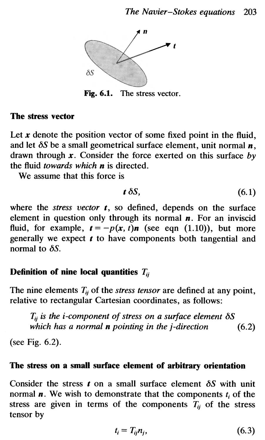
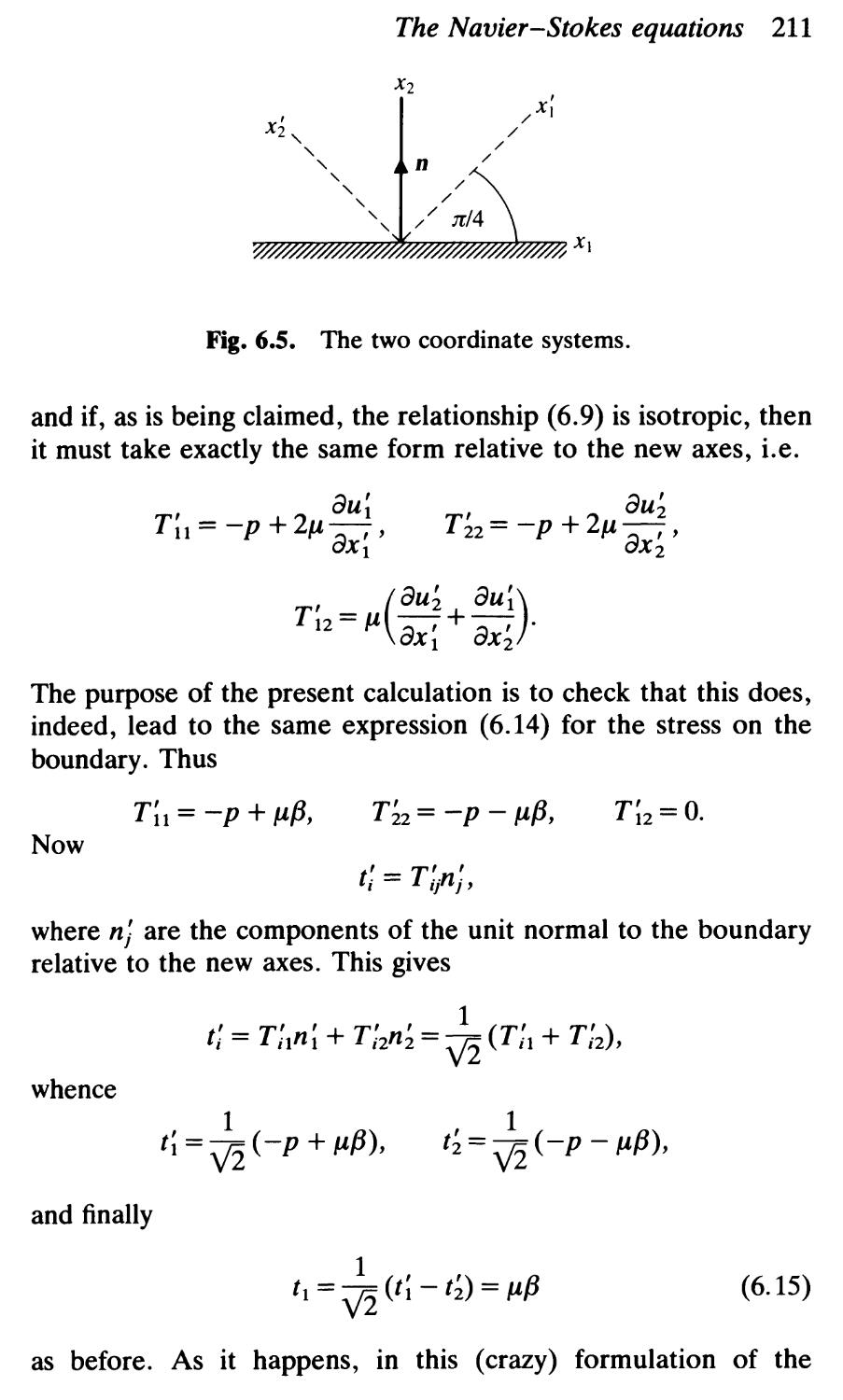
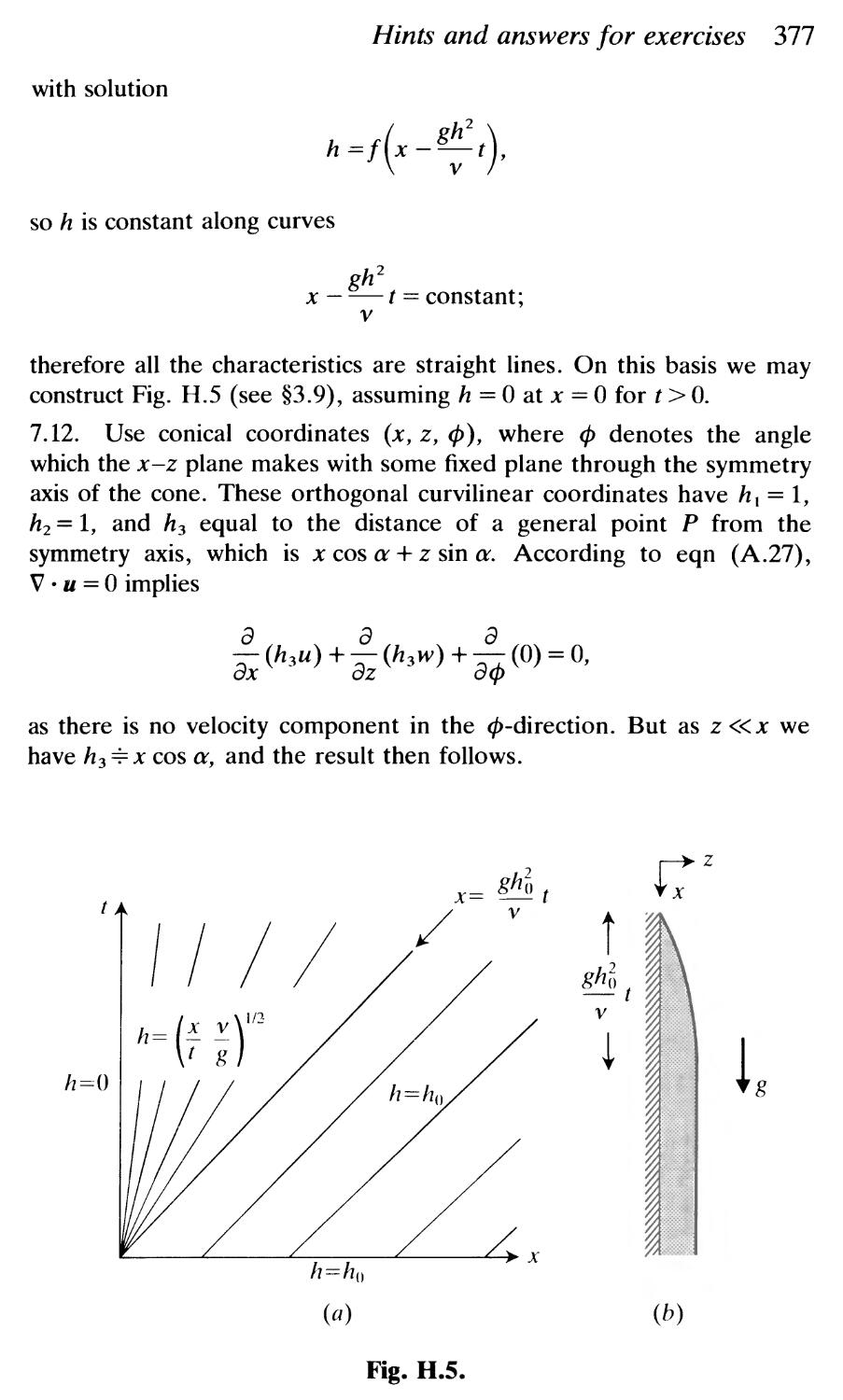
/


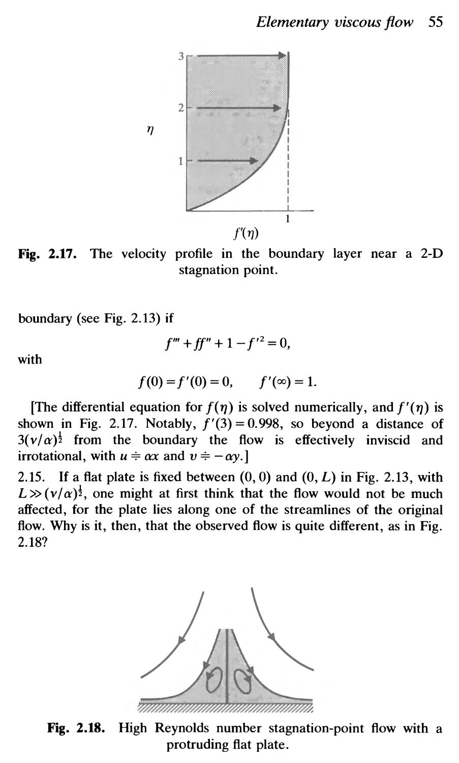


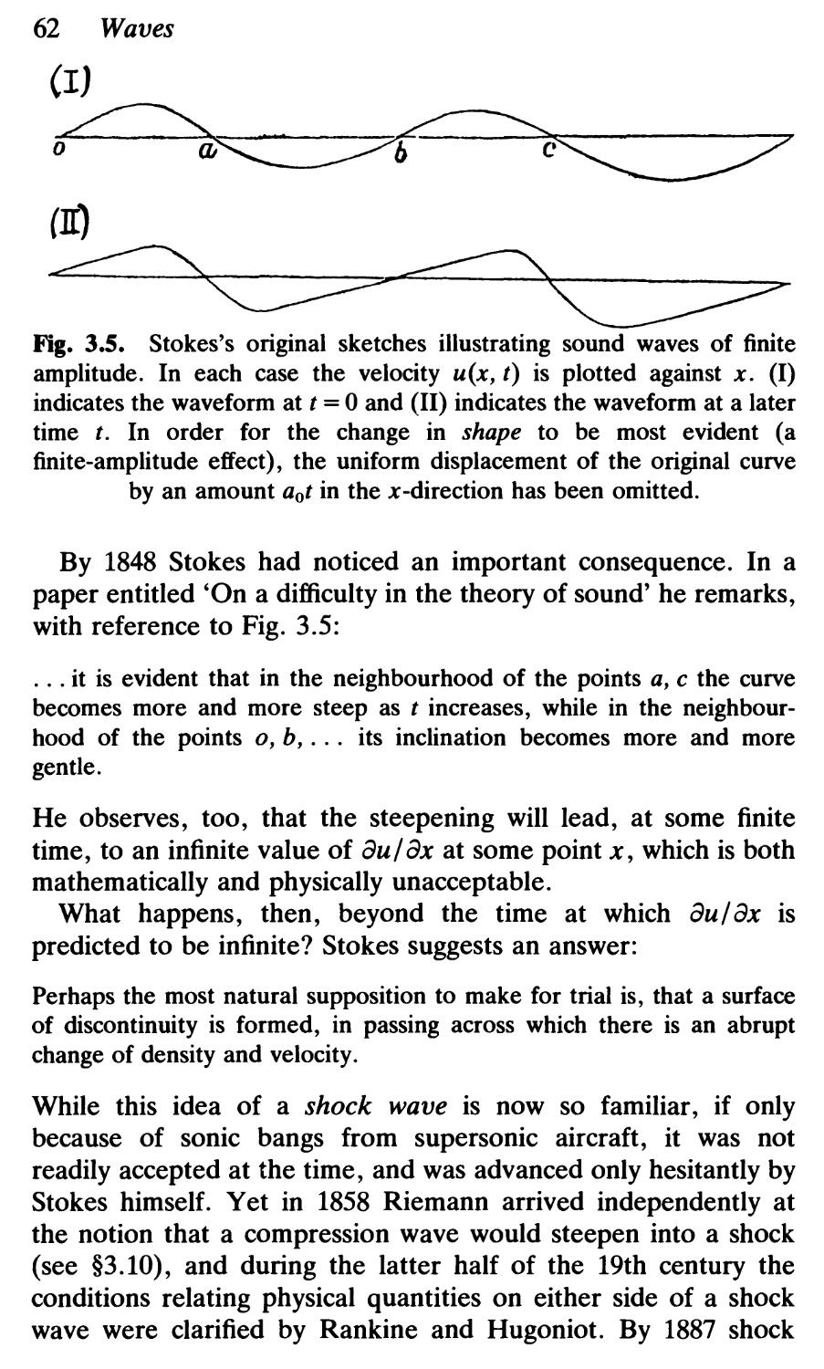


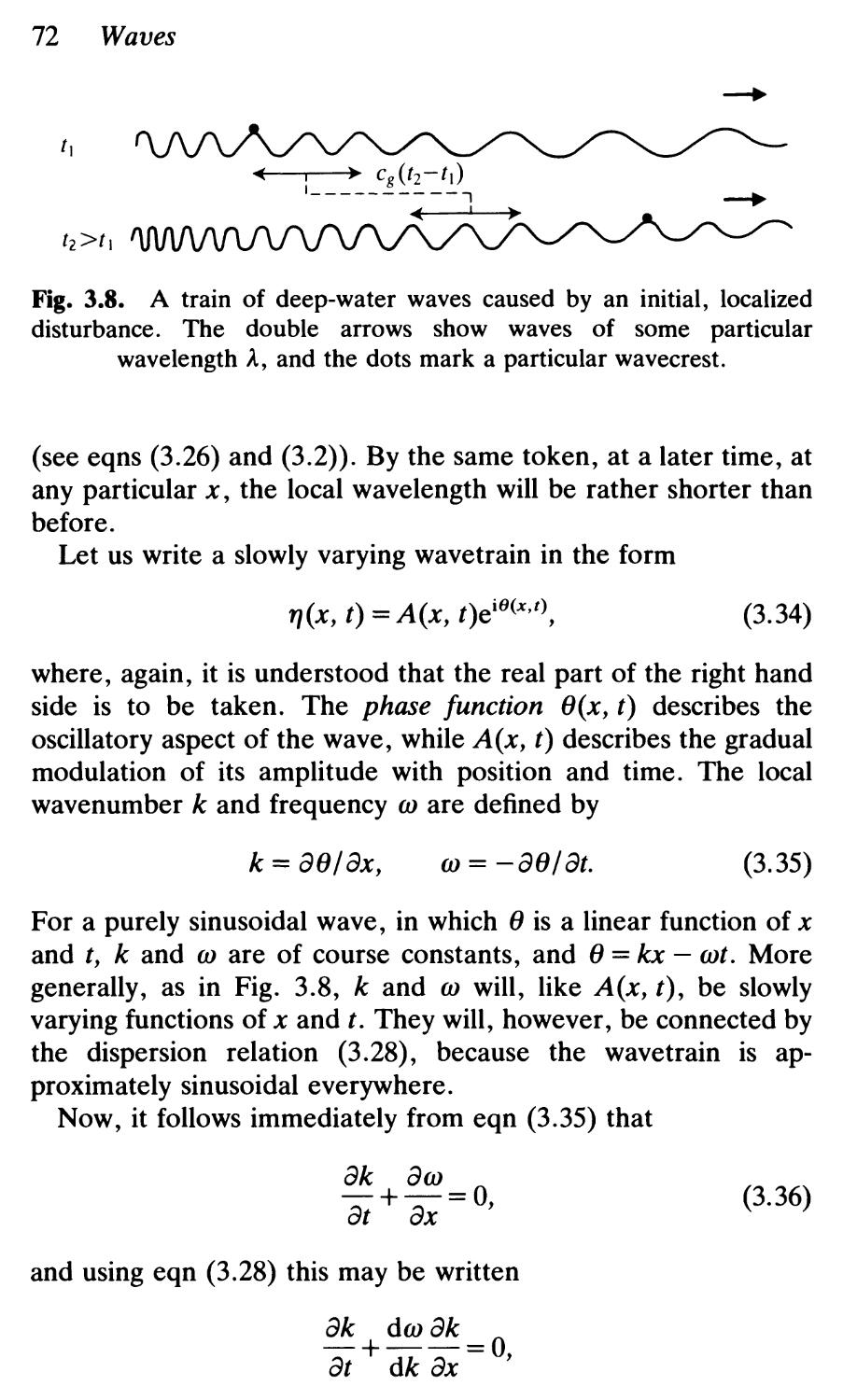


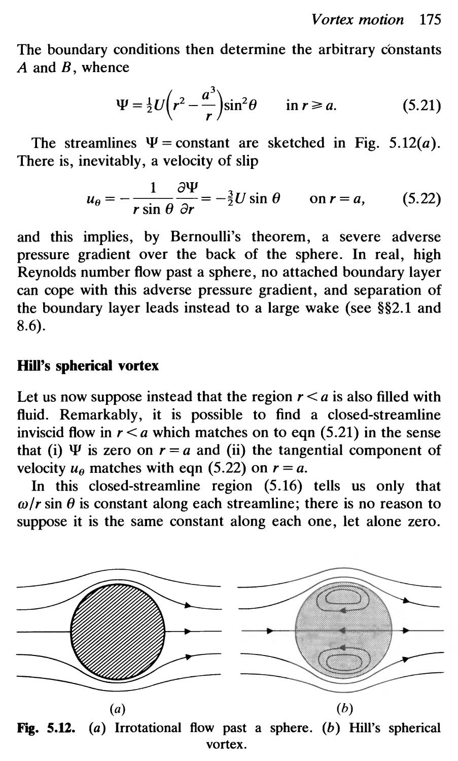


Text
Oxford Applied Mathematics
and Computing Science Series
Oxford Applied Mathematics
and Computing Science Series
I. Anderson: A First Course in COlnbinatorial Mathematics (Second Edition)
D. W. Jordan and P. Smith: Nonlinear Ordinary Differential Equations
(Second Edition)
D. S. Jones: Elementary Information Theory
B. Carre: Graphs and Networks
A. J. Davies: The Finite Element Method
W. E. Williams: Partial Different ial Equations
R. G. Garside: The Architecture of Digital Cornputers
J. C. Newby: Mathematics for the Biological Sciences
G. D. Smith: Numerical Solution of Partial DUferential Equations (Third
Edit ion)
J. R. Ullmann: A Pascal Datahase Book
S. Barnett and R. G. CalTICron: lntroduction to Mathel11aticaL Control Theory
(Second Edition)
A. B. Tayler: Mathematical Models in Applied Mechanics
R. Hill: A First Course in Coding Theory
P. Baxandall and H. Liebeck: Vector Calculus
D. C. Ince: An Introduction to Discrete Mathematics and Formal System
Specification
P. Thomas, H. Robinson, and J. EmITIs: Abstract Data Types: Their
Specification, Representation, and Use
D. R. Bland: Waue Theory and Applications
R. P. Whittington: Database Systems Engineering
J. J. Modi: Parallel Algorithms and Matrix Computation
P. Gibbins: Logic with Prolog
W. L. Wood: Practical Time-stepping Schemes
D. J. Acheson: Elementary Fluid Dynamics
L. M. Hocking: Optimal Control: An Introduction to the Theory with
Applications
S. Barnett: Matrices: Methods and Applications
P. Grindrod: Patterns and Waves: The Theory and Applications of Reaction-
Diffusion Equations
O. Pretzel: Error-Correcting Codes and Finite Fields
D. J. ACHESON
Jesus College, Oxford
Elementary Fluid
Dynamics
@J CLARENDON PRESS · OXFORD
OXFORD
UNIVERSITY PRESS
Great Clarendon Street, Oxford OX2 6DP
Oxford University Press is a department of the University of Oxford.
It furthers the University's objective of excellence in research, scholarship,
and education by publishing worldwide in
Oxford New York
Auckland Cape Town Dar es Salaam Hong Kong Karachi
Kuala Lumpur Madrid Melbourne Mexico City Nairobi
New Delhi Shanghai Taipei Toronto
With offices in
Argentina Austria Brazil Chile Czech Republic France Greece
Guatemala Hungary Italy Japan South Korea Poland Portugal
Singapore Switzerland Thailand Turkey Ukraine Vietnam
Published in the United States
by Oxford University Press Inc., New York
@ D. J. Acheson 1990
The moral rights of the author have been asserted
Database right Oxford University Press (maker)
First published 1990
Reprinted 1990, 1992, 1994
1995, 1996, 1998, 2000, 2001, 2003 (twice, once with correction), 2005
All rights reserved. No part of this publication may be reproduced,
stored in a retrieval system, or transmitted, in any form or by any means,
without the prior permission in writing of Oxford University Press,
or as expressly permitted by law, or under terms agreed with the appropriate
reprographics rights organization. Enquiries concerning reproduction
outside the scope of the above should be sent to the Rights Department,
Oxford University Press, at the address above.
You must not circulate this book in any other binding or cover
and you must impose this same condition on any acquirer.
A catalogue record for this book is available from the British Library
Library of Congress Cataloging in Publication Data
Acheson, D. J.
Elementary, fluid dYnamics/D. J. Acheson.
p. cm.-( Oxford applied mathematics and computing science series)
1. Fluid dYnamics. I. Title. II. Series.
TA357.A276 1990
532-dc20 89-22947 CIP
ISBN 0 19 859679 0 (Pbk)
Printed in Great Britain
on acid-free paper by
BiddIes Ltd., King's LYnn, Norfolk
Preface
This book is an introduction to fluid dynamics for students of
applied mathematics, physics, and engineering. The main
mathematical requirements are the vector calculus and simple
methods for solving differential equations. Exercises are pro-
vided at the end of each chapter, and extensive hints and
answers are offered at the end of the book. In order to indicate
how the text is organized it is first necessary to say a little
about the subject itself.
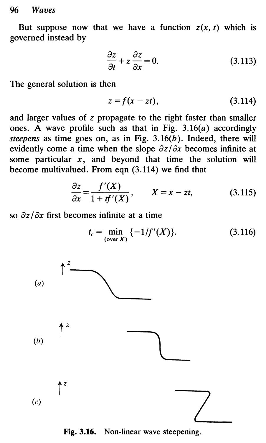
It is a matter of common experience that some fluids are more
viscous than others. No reader will be surprised to learn that the
'coefficient of viscosity' 1J is much greater for syrup than it is for
water. Many fluids, such as water and air, hardly seem to be
viscous at all. It is natural, then, to construct a theory based on
the concept of an inviscid fluid, i.e. one for which 1J is precisely
zero. This is how the subject first developed, and this is how we
begin, in Chapter 1.
Yet inviscid theory has its dangers. Careful analysis of the
equations of motion for a viscous fluid shows that strange things
can happen in the limit 1J 0, so that a fluid with very small
viscosity may behave quite differently to a (hypothetical) fluid
with no viscosity at all. For this reason an elementary account of
viscous flow appears very early in the book, in Chapter 2. The
aim there, particularly in 2.1 and 2.2, is to introduce some of
the key ideas as simply as possible. In order to do this the viscous
flow equations are merely stated; their derivation from first
principles appears later.
While inviscid theory has to be used with caution there are
major areas of fluid dynamics in which it is extremely successful,
and one of these is wave motion (Chapter 3). Another is flow
past a thin wing (Chapter 4), provided that the wing makes only
a small angle of incidence with the oncoming stream. Inviscid
vi Preface
theory has a further role in the study of vortex motion (Chapter
5), which turns out to be central to much of fluid dynamics,
largely through the elegant theorems of Kelvin and Helmholtz.
In Chapter 6 we establish the equations of viscous flow from
first principles, although some readers may wish to consult this
chapter quite early. In Chapter 7 we explore very viscous flow,
i.e. the case in which /.l is large (in some appropriate sense). The
flow problems here have some novel features and are the object
of much current research. We return to fluids of low viscosity in
Chapter 8, focusing on thin 'boundary layers', where viscous
effects are of crucial importance, no matter how small /.l happens
to be. In the final chapter we examine the instability of fluid flow,
which, together with boundary layer separation, gives rise to
some of the deepest and most challenging problems in the
subject.
I am extremely grateful to all the students who have tried out
successive drafts of this book. I would also like to thank Brooke
Benjamin, David Crighton, Raymond Hide, Tom Mullin, Hilary
Ockendon, John Ockendon, Norman Riley, John Roe, Alan
Tayler, and Robert Terrill for their comments on various
chapters.
Finally, I take the opportunity to acknowledge all the help I
received, when I was first learning the subject, from Raymond
Hide at the Meteorological Office and from Norman Riley,
Michael Glauert, and others at the University of East Anglia.
Jesus College, Oxford
April 1989
D. J. A.
Contents
1 INTRODUCTION 1
1.1 An experiment 1
1.2 Some preliminary ideas 2
1.3 Equations of motion for an ideal fluid 6
1.4 Vorticity: irrotational flow 10
1.5 The vorticity equation 16
1.6 Steady flow past a fixed wing 18
1.7 Concluding remarks 22
Exercises 23
2 ELEMENTARY VISCOUS FLOW 26
2.1 Introduction 26
2.2 The equations of viscous flow 30
2.3 Some simple viscous flows: the diffusion of vorticity 33
2.4 Flow with circular streamlines 42
2.5 The convection and diffusion of vorticity 48
Exercises 50
3 W A V E S 56
3.1 Introduction 56
3.2 Surface waves on deep water 65
3.3 Dispersion: group velocity 69
3.4 Surface tension effects: capillary waves 74
3.5 Effects of finite depth 78
3.6 Sound waves 79
3.7 Supersonic flow past a thin aerofoil 82
3.8 Internal gravity waves 86
3.9 Finite-amplitude waves in shallow water 89
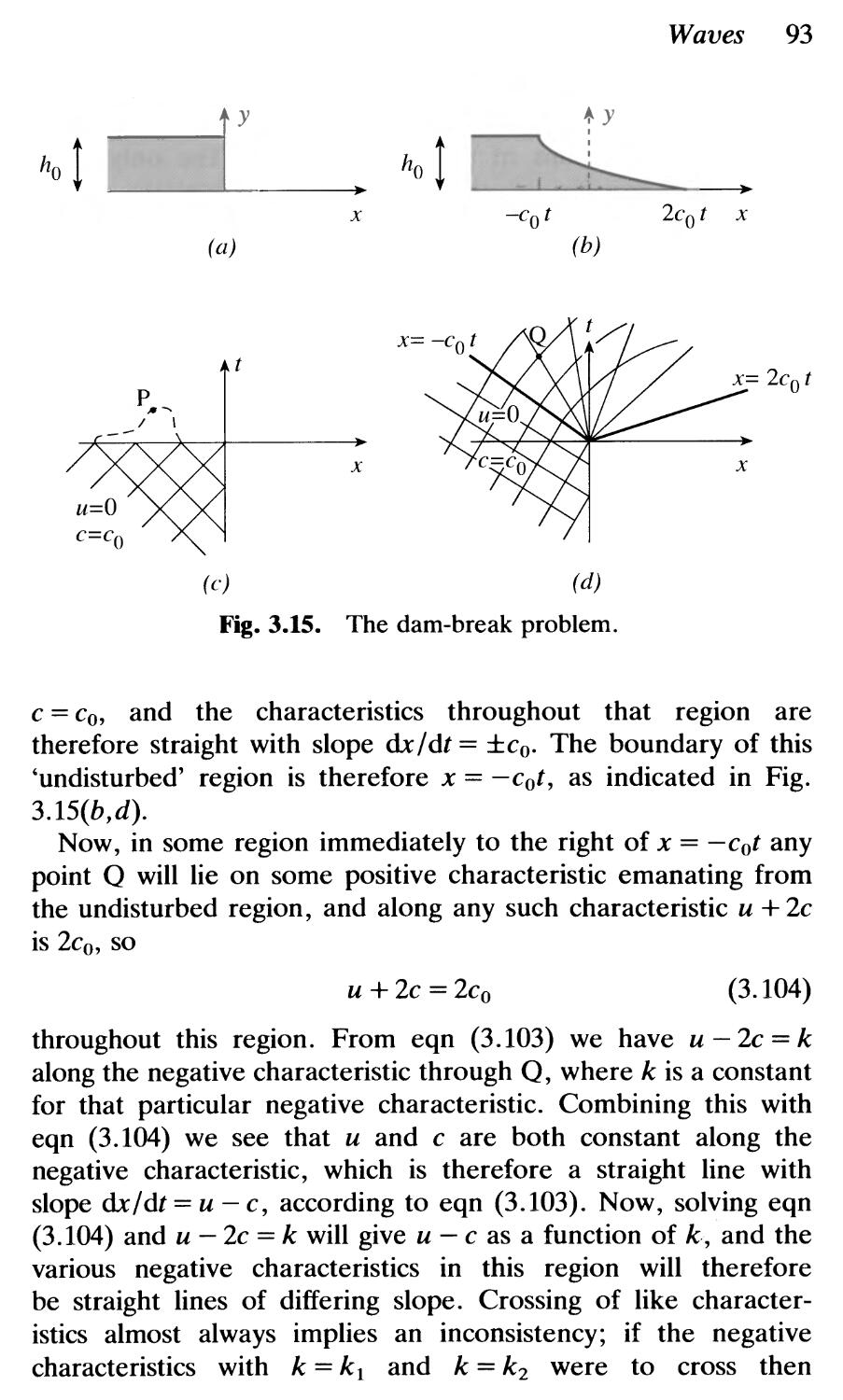
3.10 Hydraulic jumps and shock waves 100
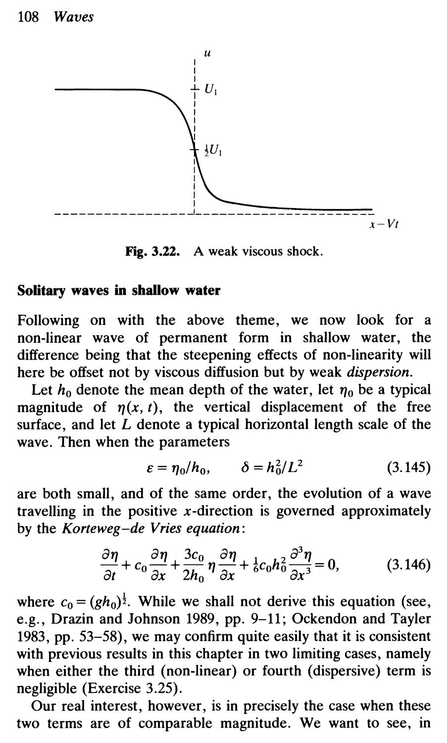
3.11 Viscous shocks and solitary waves 106
Exercises 111
Vlll Contents
4 CLASSICAL AEROFOIL THEORY 120
4.1 Introduction 120
4.2 Velocity potential and stream function 122
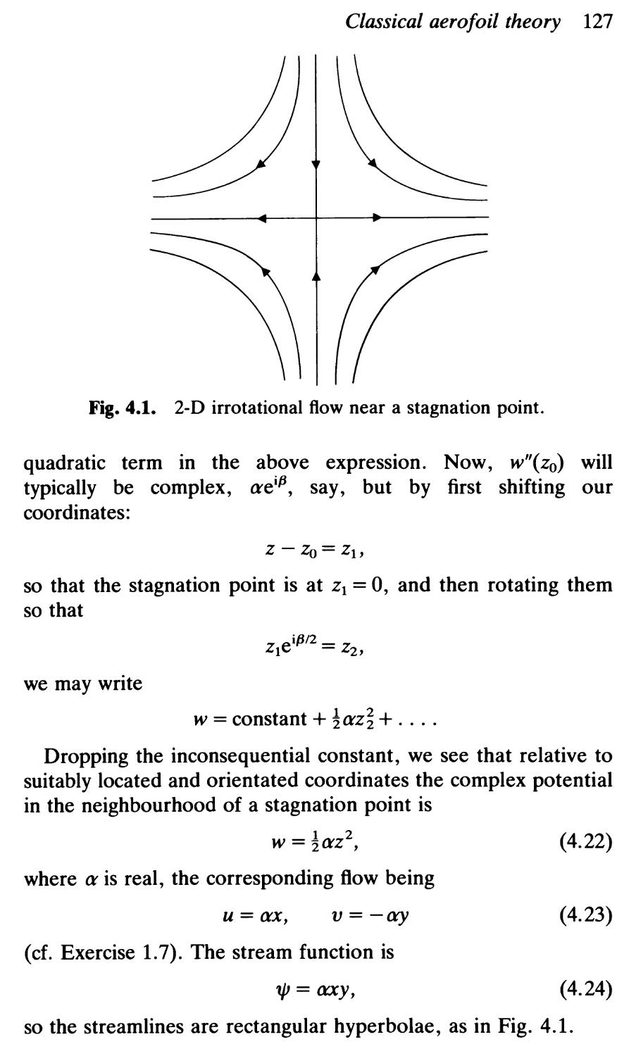
4.3 The complex potential 124
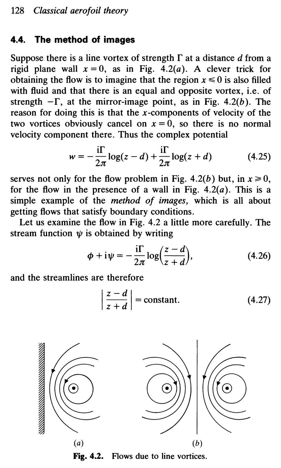
4.4 The method of images 128
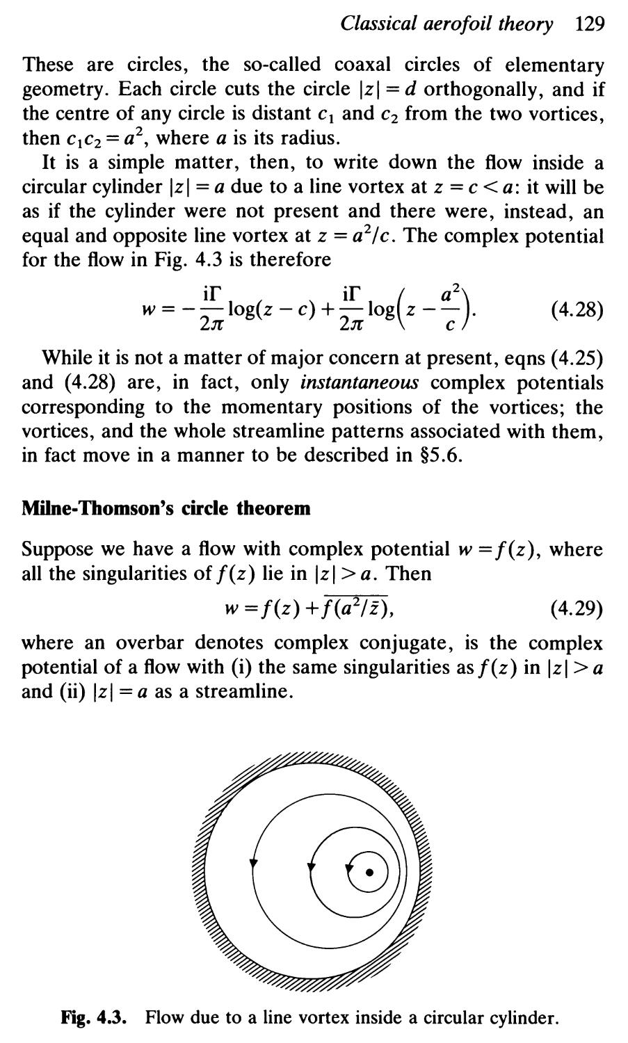
4.5 Irrotational flow past a circular cylinder 130
4.6 Conformal mapping 134
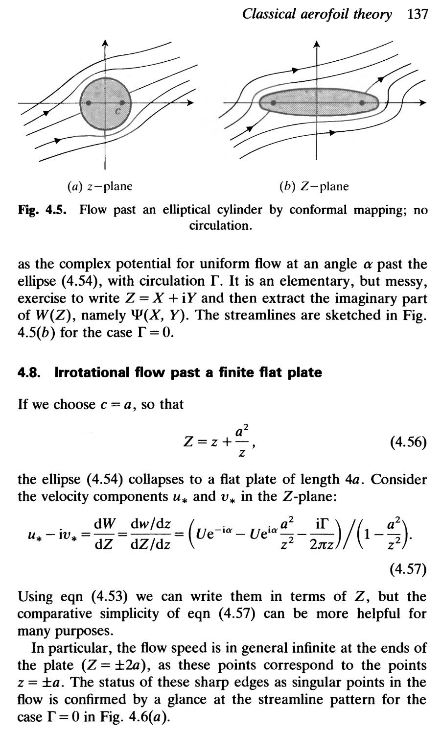
4.7 Irrotational flow past an elliptical cylinder 136
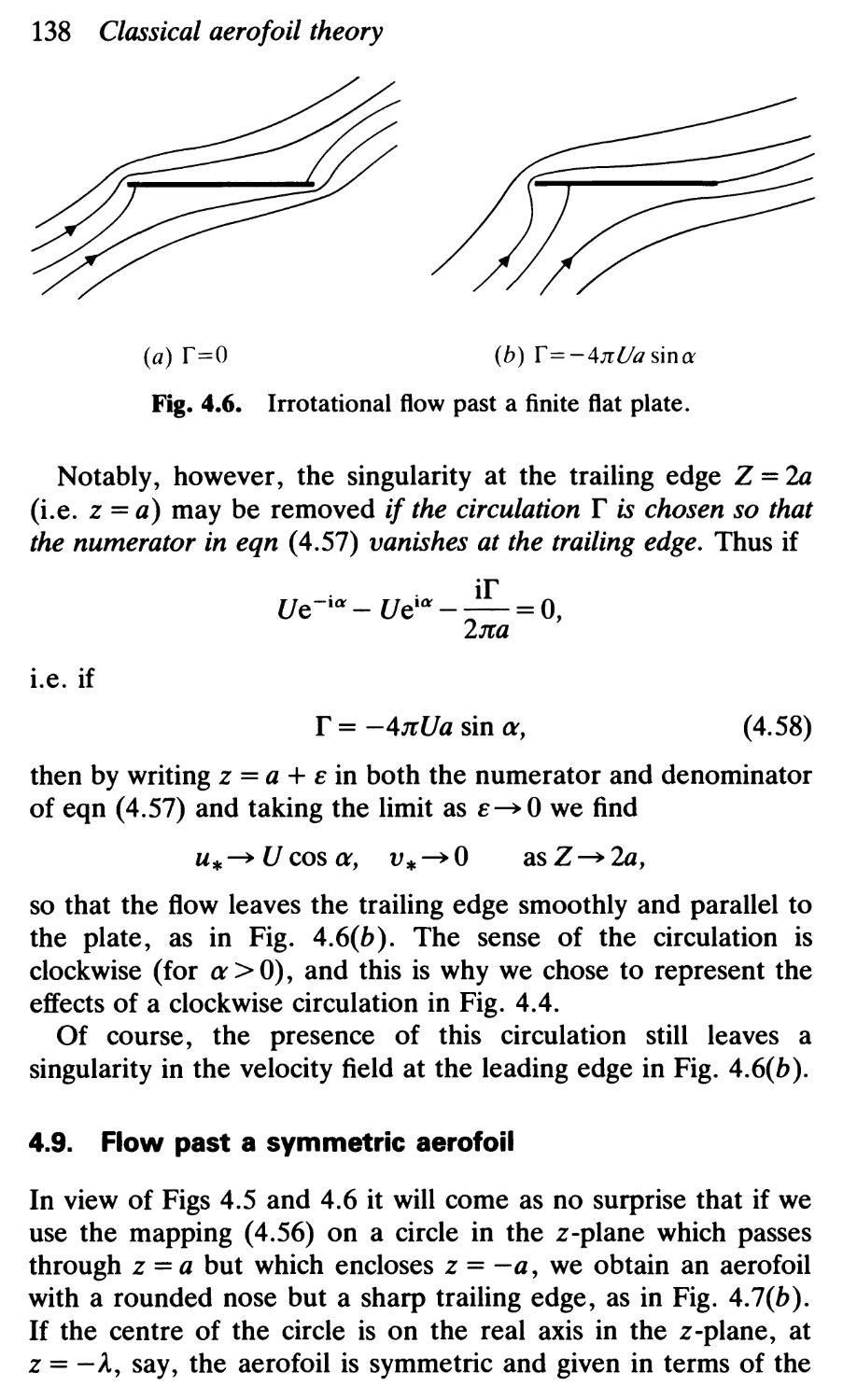
4.8 Irrotational flow past a finite flat plate 137
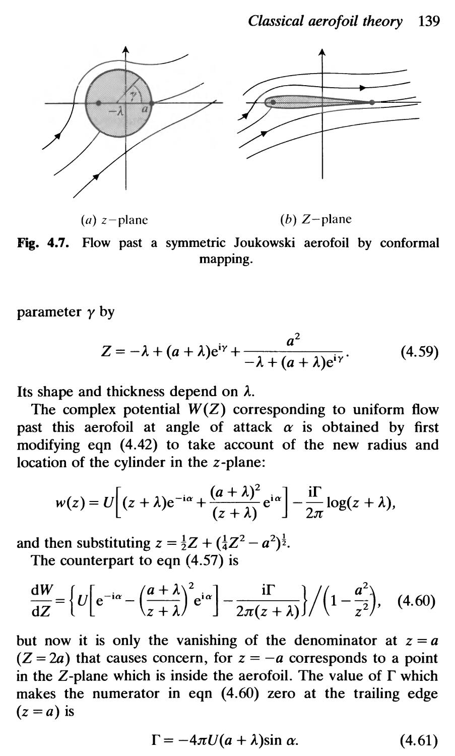
4.9 Flow past a symmetric aerofoil 138
4.10 The forces involved: Blasius's theorem 140
4.11 The Kutta-Joukowski Lift Theorem 143
4.12 Lift: the deflection of the airstream 145
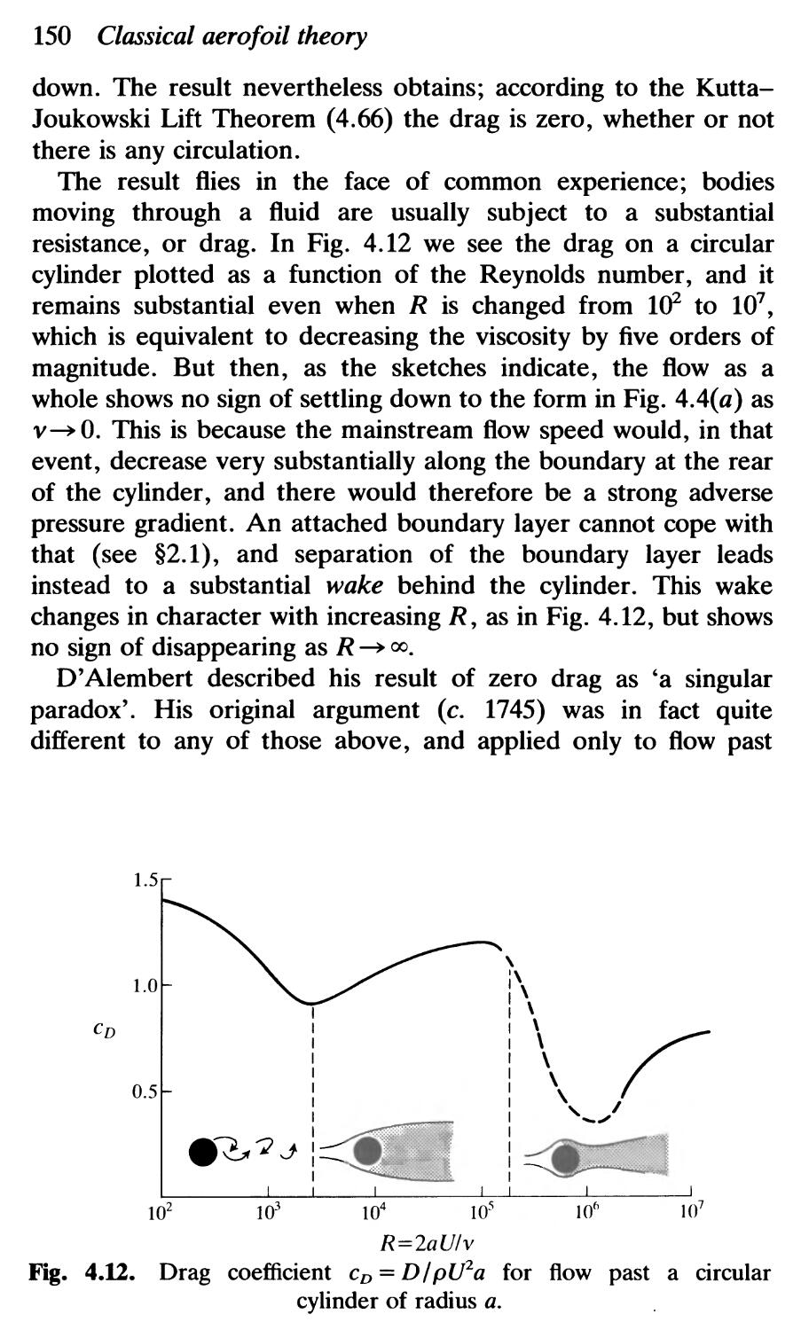
4.13 D'Alembert's paradox 147
Exercises 151
5 VORTEX MOTION 157
5.1 Kelvin's circulation theorem 157
5.2 The persistence of irrotational flow 161
5.3 The Helmholtz vortex theorems 162
5.4 Vortex rings 168
5.5 Axisymmetric flow 172
5.6 Motion of a vortex pair 177
5.7 Vortices in flow past a circular cylinder 178
5.8 Instability of vortex patterns 184
5.9 A steady viscous vortex maintained by a secondary flow 187
5.10 Viscous vortices: the Prandtl-Batchelor theorem 189
Exercises 191
6 THE NA VIER-STOKES EQUATIONS 201
6.1 Introduction 201
6.2 The stress tensor 202
6.3 Cauchy's equation of motion 205
6.4 A Newtonian viscous fluid: the Navier-Stokes equations 207
6.5 Viscous dissipation of energy 216
Exercises 217
Contents IX
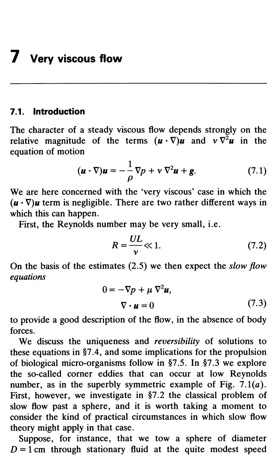
7 VERY VISCOUS FLOW 221
7.1 Introduction 221
7.2 Low Reynolds number flow past a sphere 223
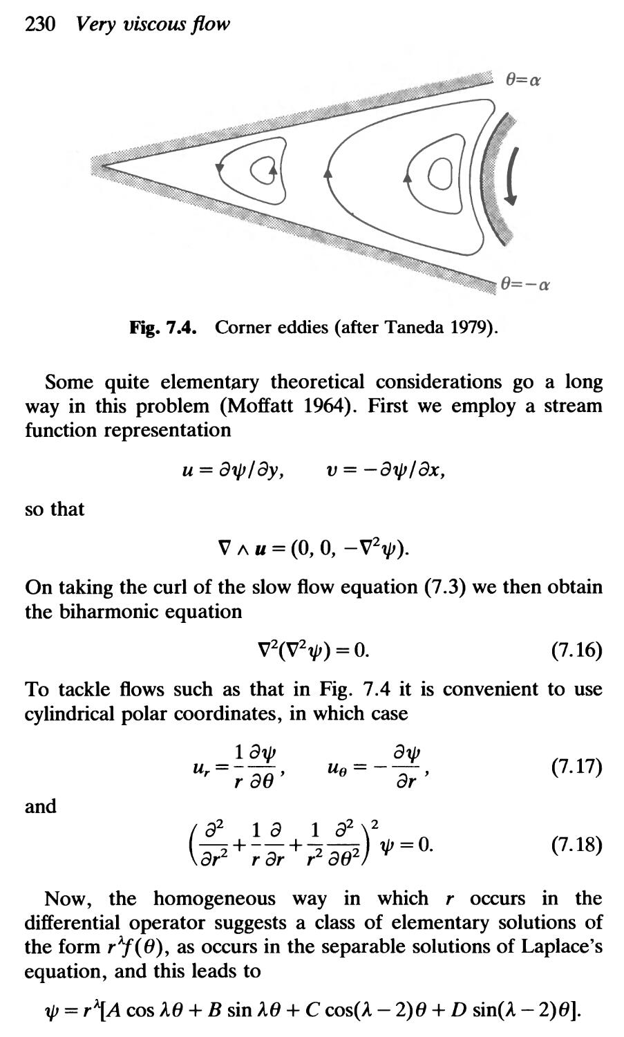
7.3 Corner eddies 229
7.4 Uniqueness and reversibility of slow flows 233
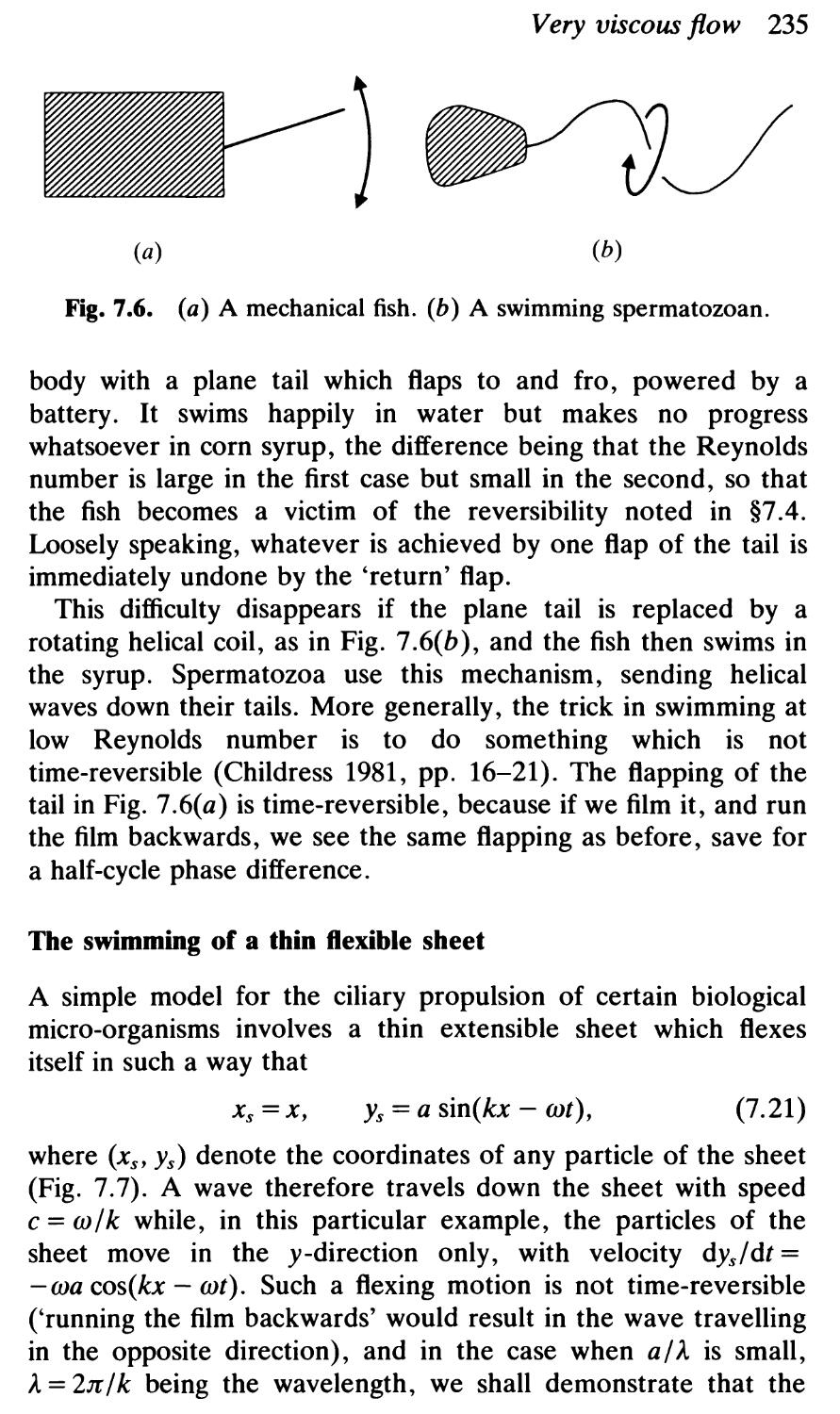
7.5 Swimming at low Reynolds number 234
7.6 Flow in a thin film 238
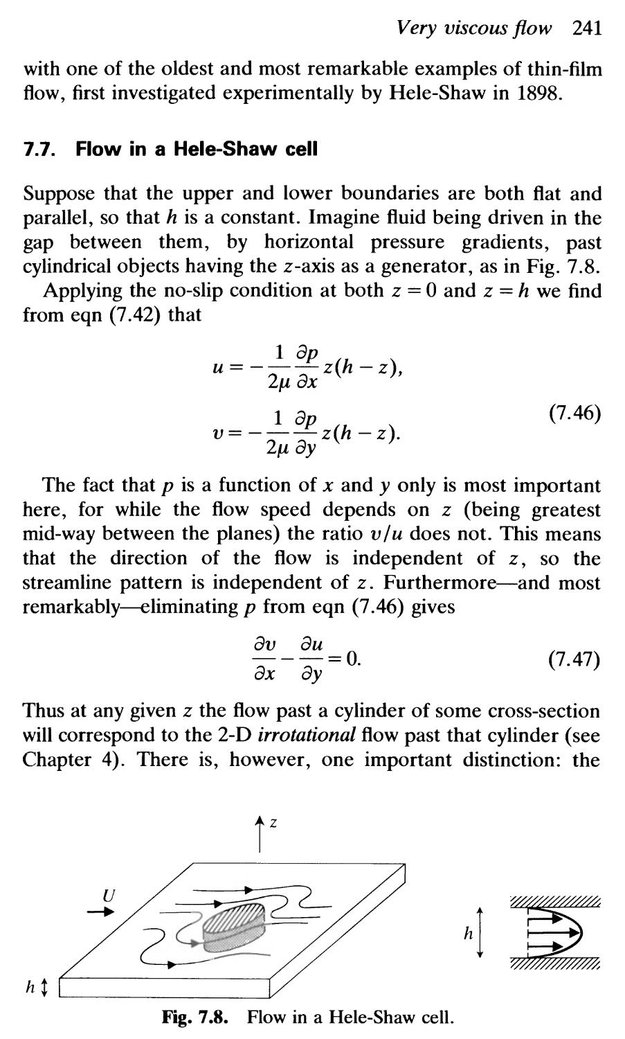
7.7 Flow in a Hele-Shaw cell 241
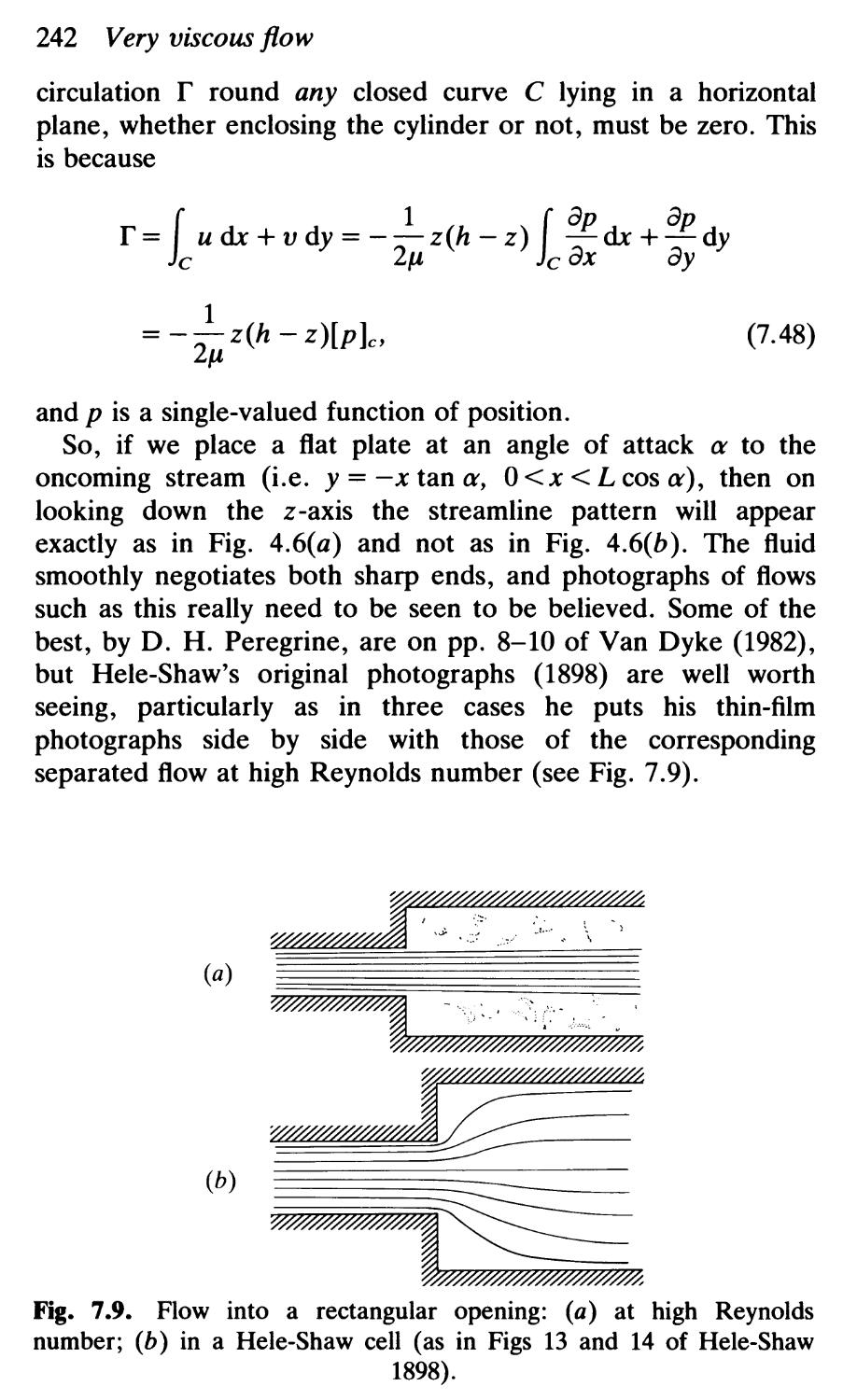
7.8 An adhesive problem 243
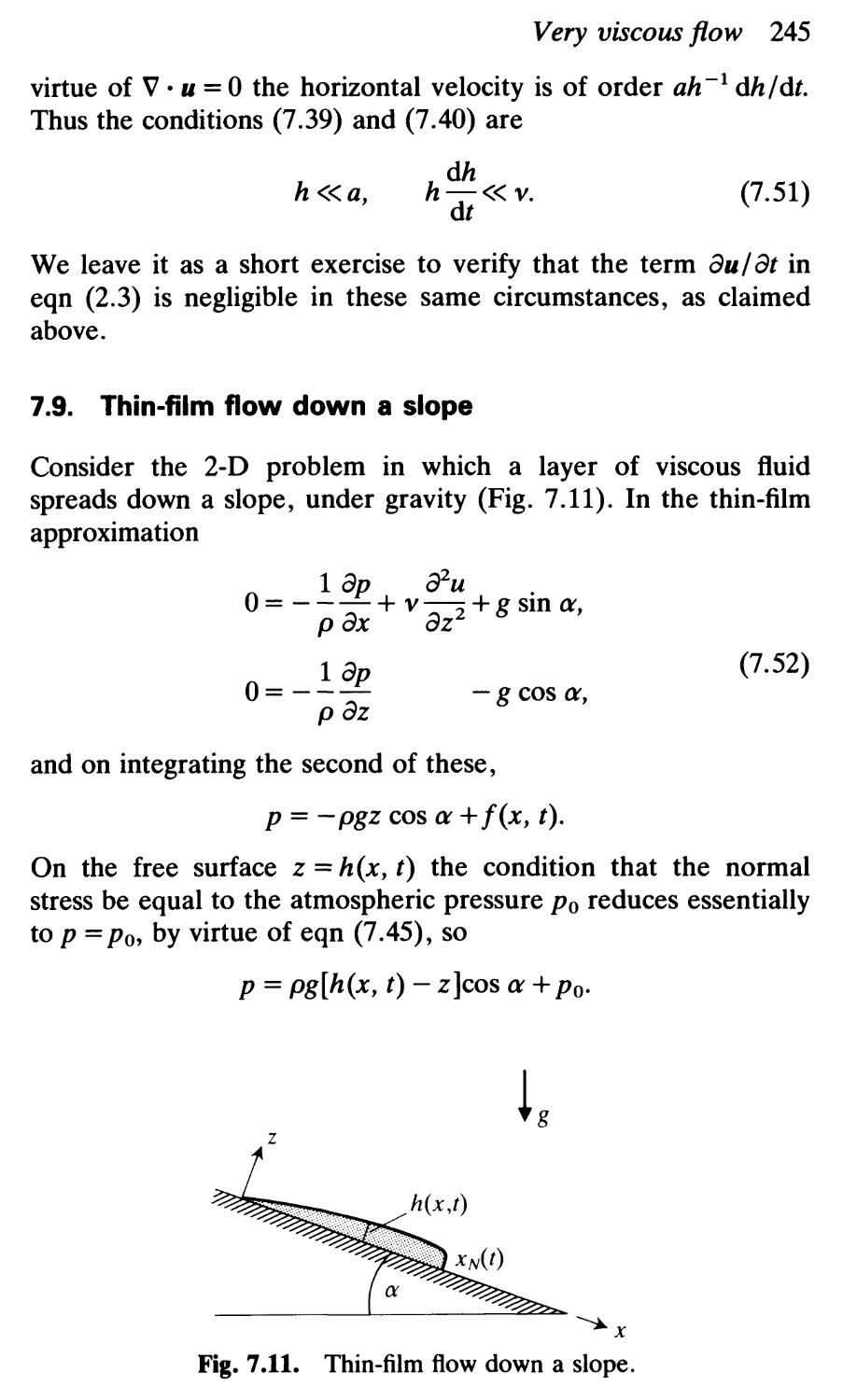
7.9 Thin-film flow down a slope 245
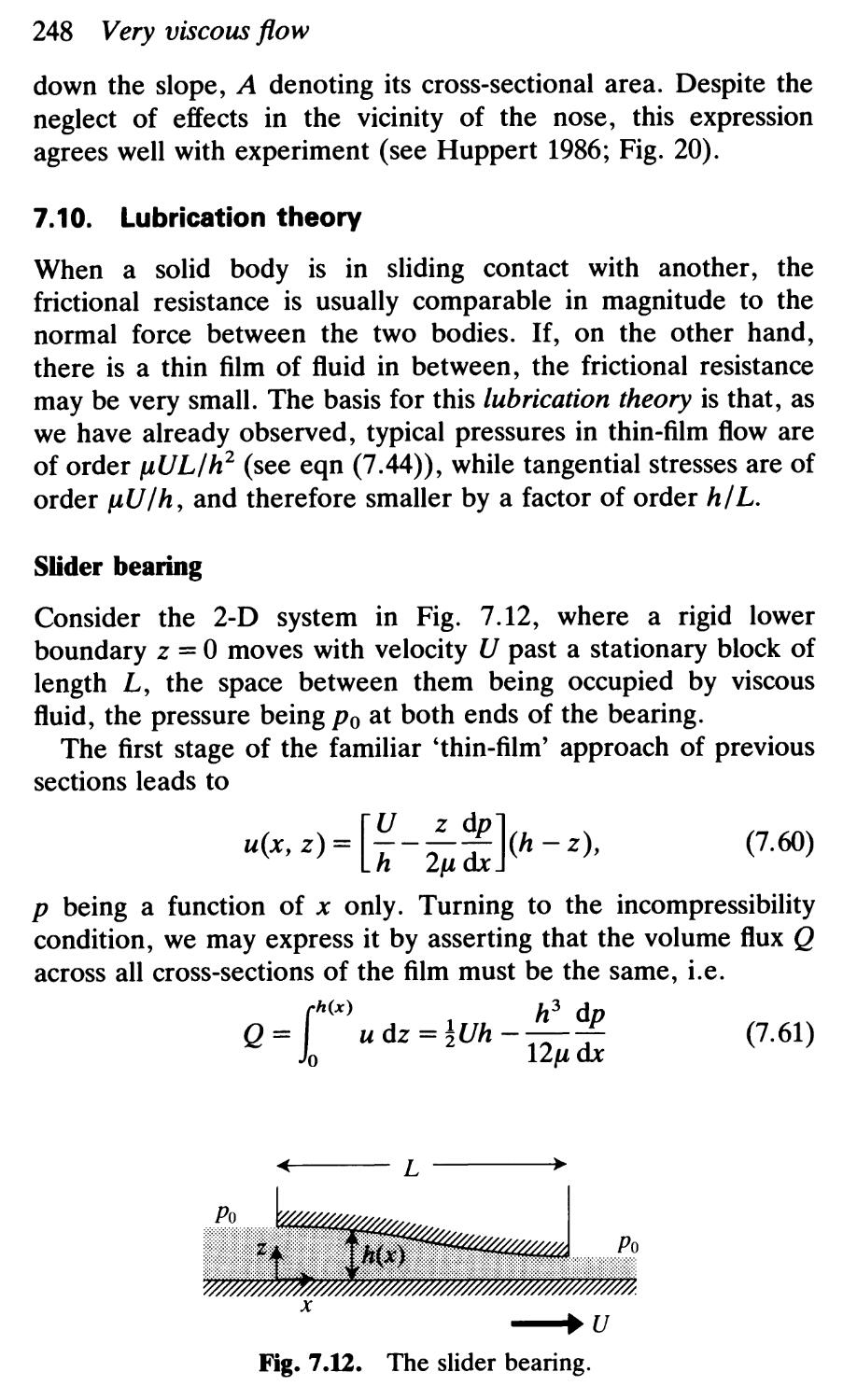
7.10 Lubrication theory 248
Exercises 251
8 BOUNDARY LA YERS 260
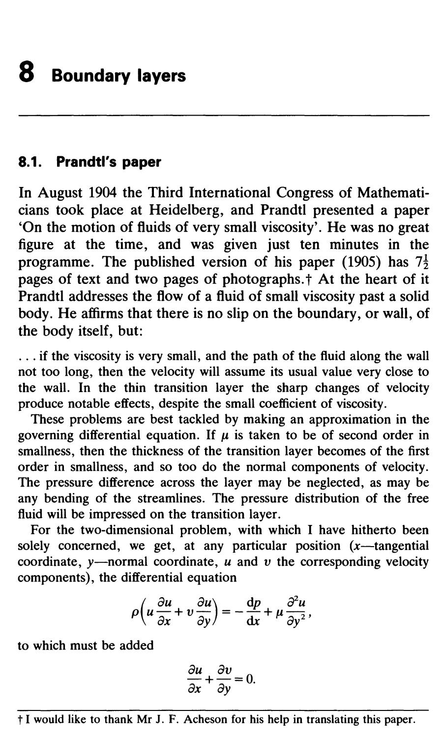
8.1 Prandtl's paper 260
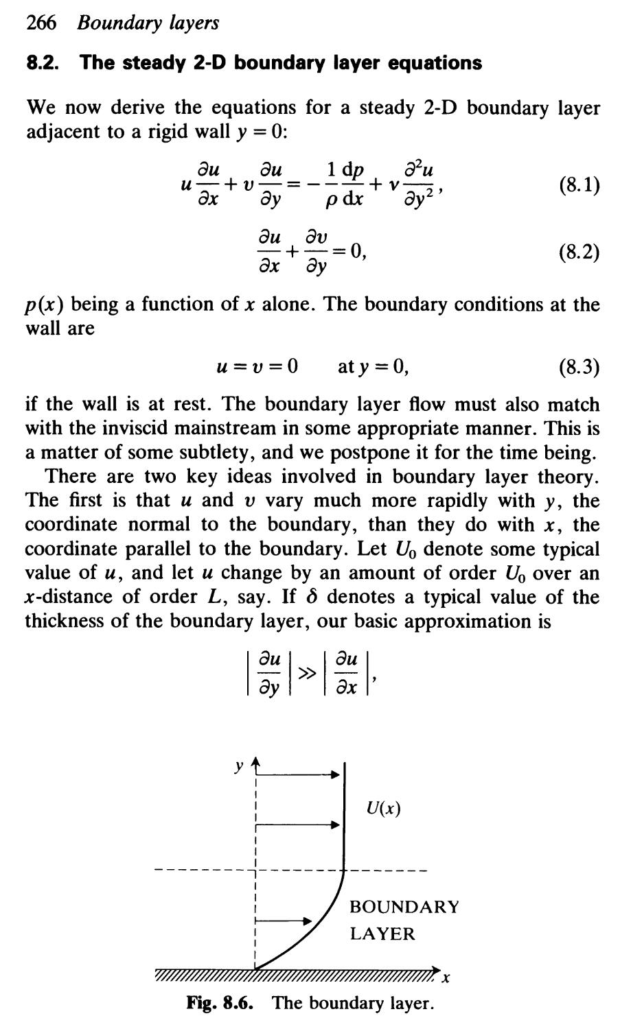
8.2 The steady 2-D boundary layer equations 266
8.3 The boundary layer on a flat plate 271
8.4 High Reynolds number flow in a converging channel 275
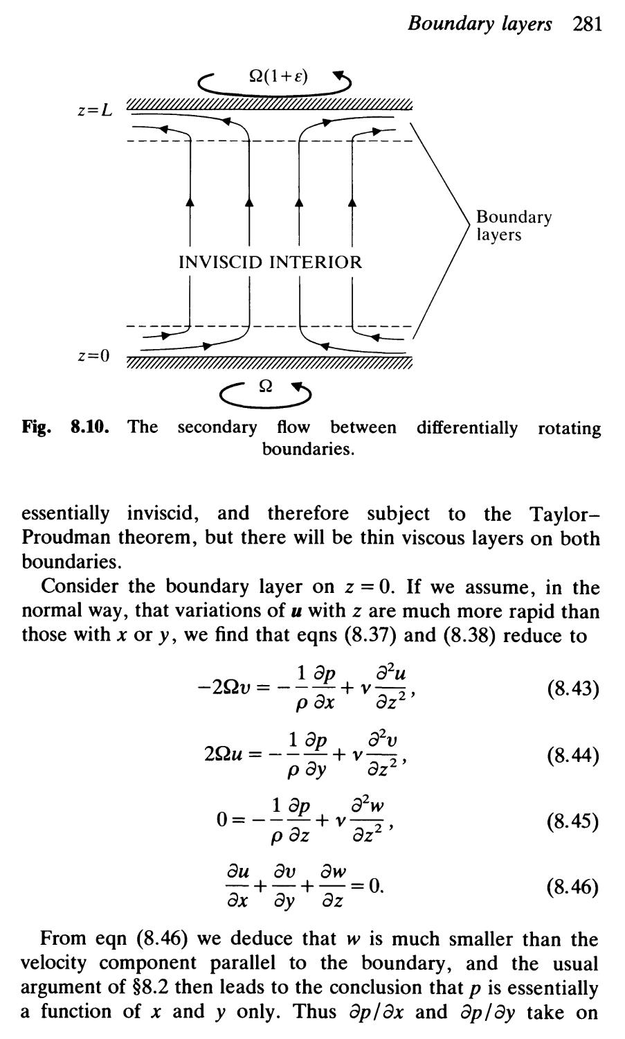
8.5 Rotating flows controlled by boundary layers 278
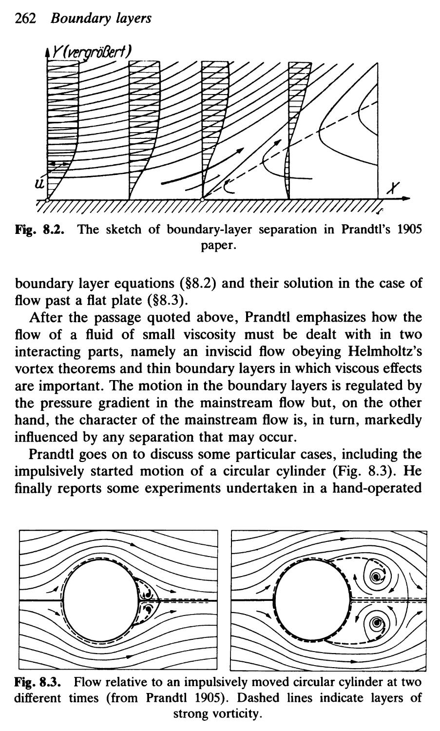
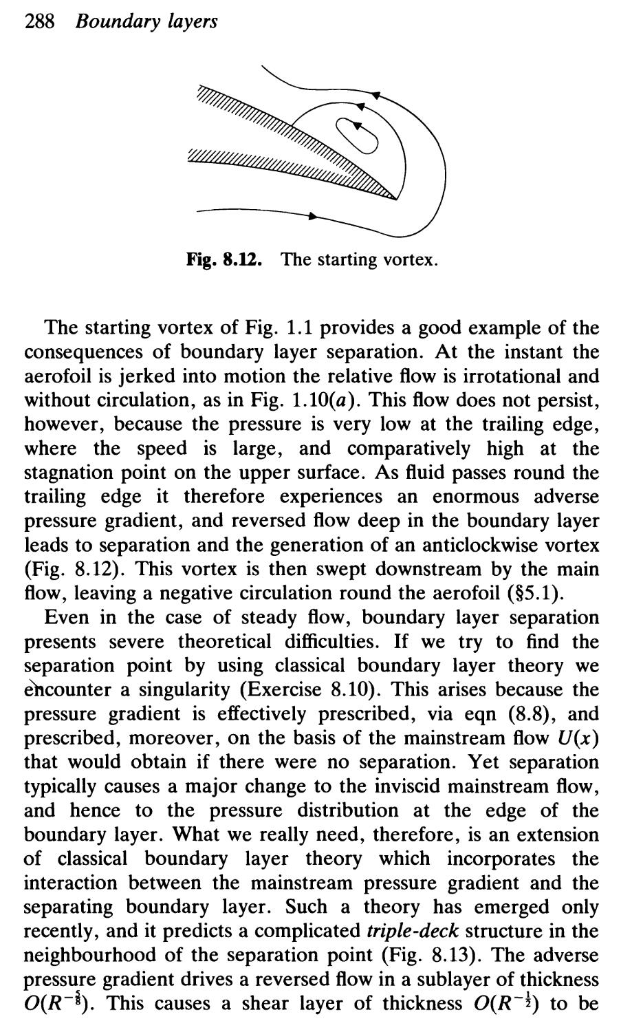
8.6 Boundary layer separation 287
Exercises 291
9 INST ABILITY 300
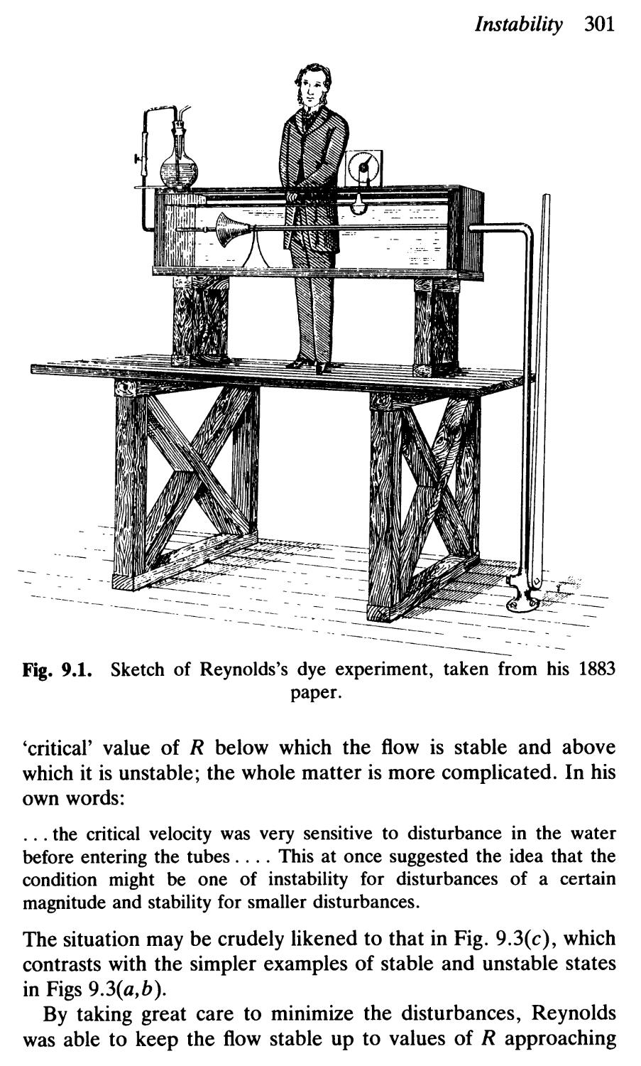
9.1 The Reynolds experiment 300
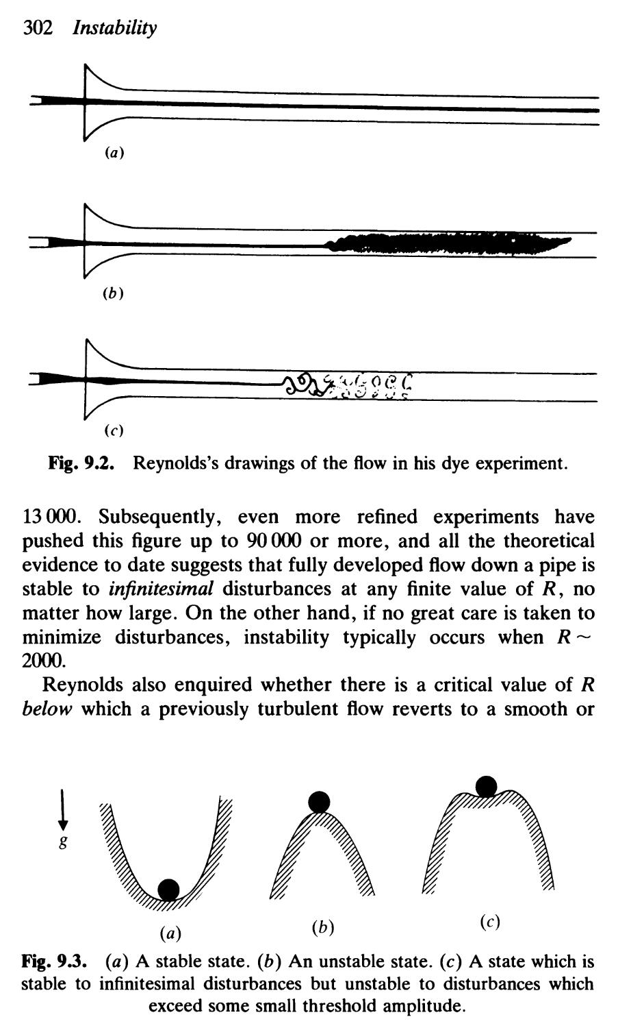
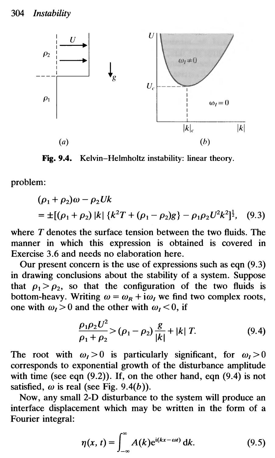
9.2 Kelvin-Helmholtz instability 303
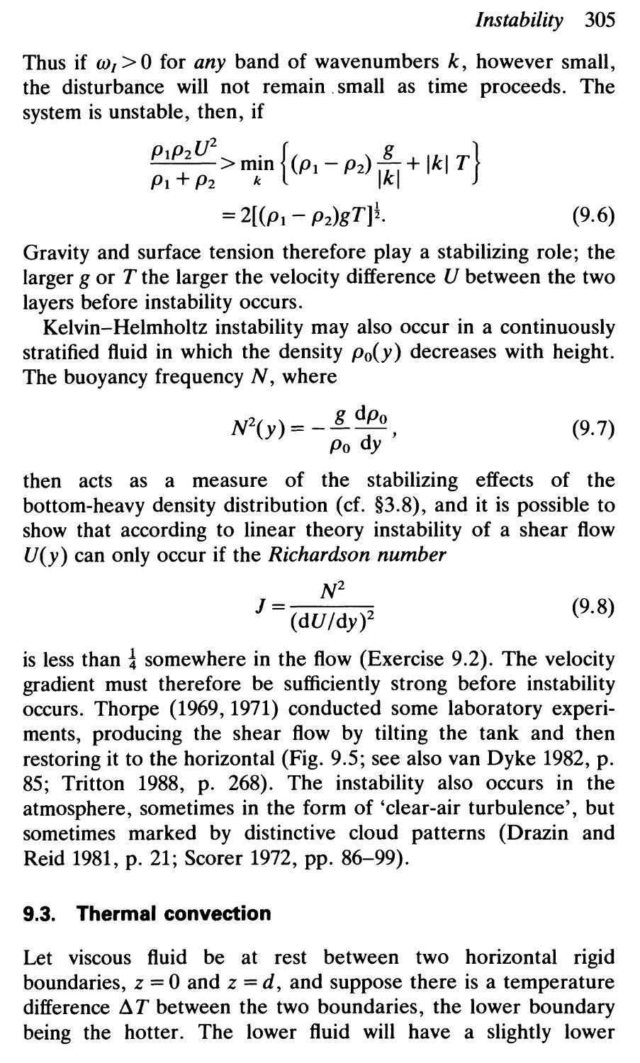
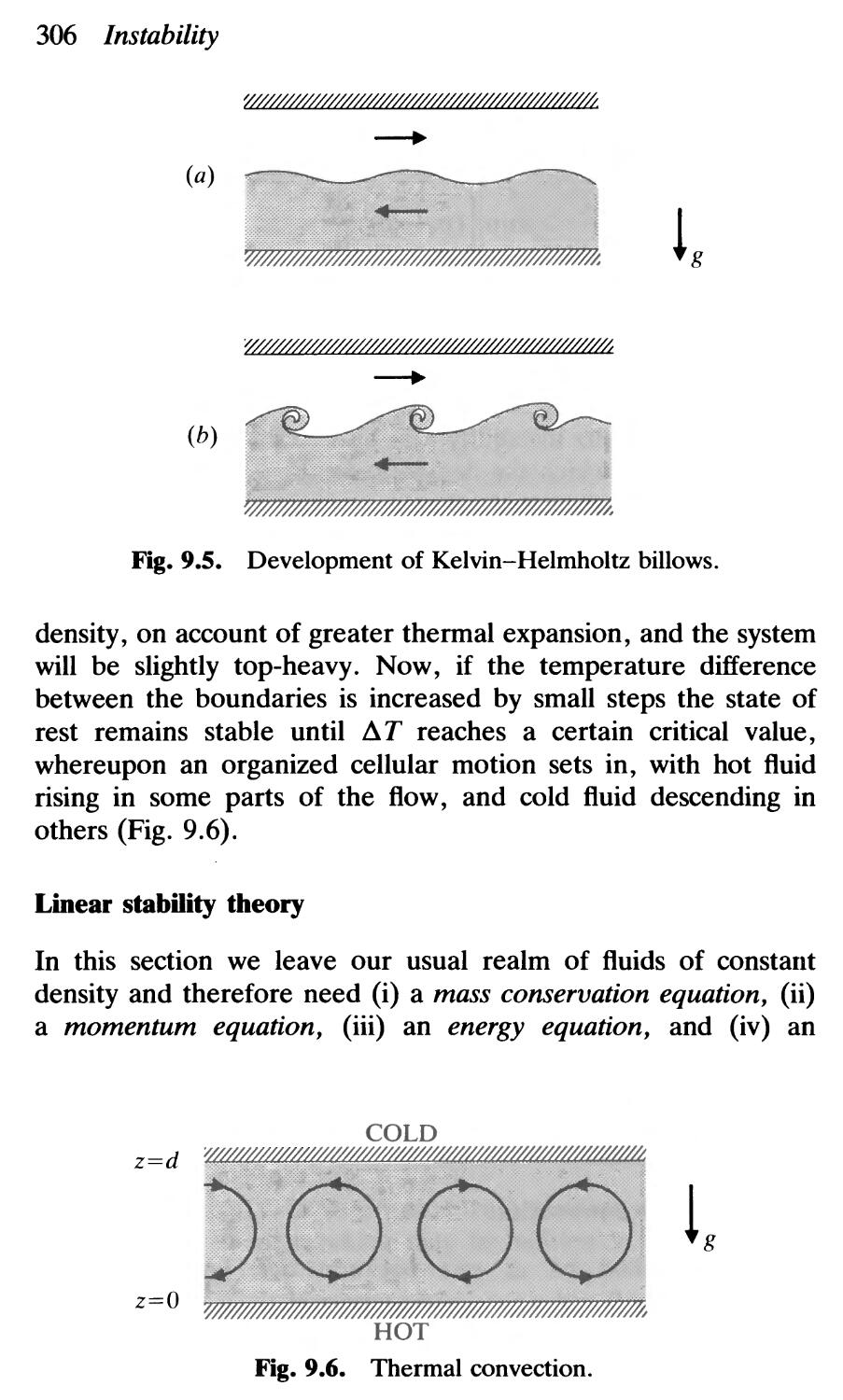
9.3 Thermal convection 305
9.4 Centrifugal instability 313
9.5 Instability of parallel shear flow 320
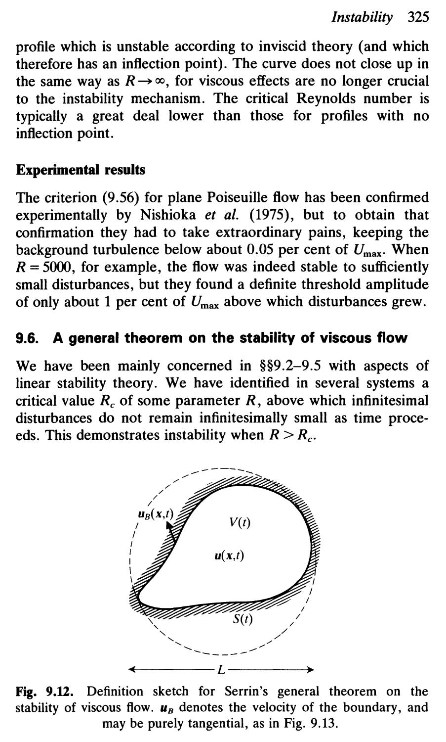
9.6 A general theorem on the stability of viscous flow 325
9.7 Uniqueness and non-uniqueness of steady viscous flow 330
9.8 Instability, chaos, and turbulence 334
9.9 Instability at very low Reynolds number 341
Exercises 343
APPENDIX 348
HINTS AND ANSWERS FOR EXERCISES 356
BIBLIOGRAPHY 384
INDEX 390
1 Introduction
1.1. An experiment
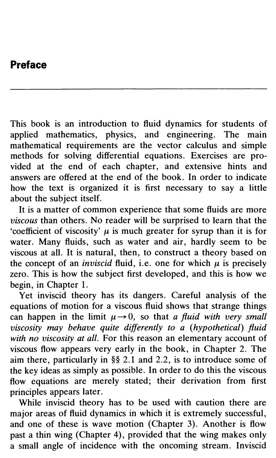
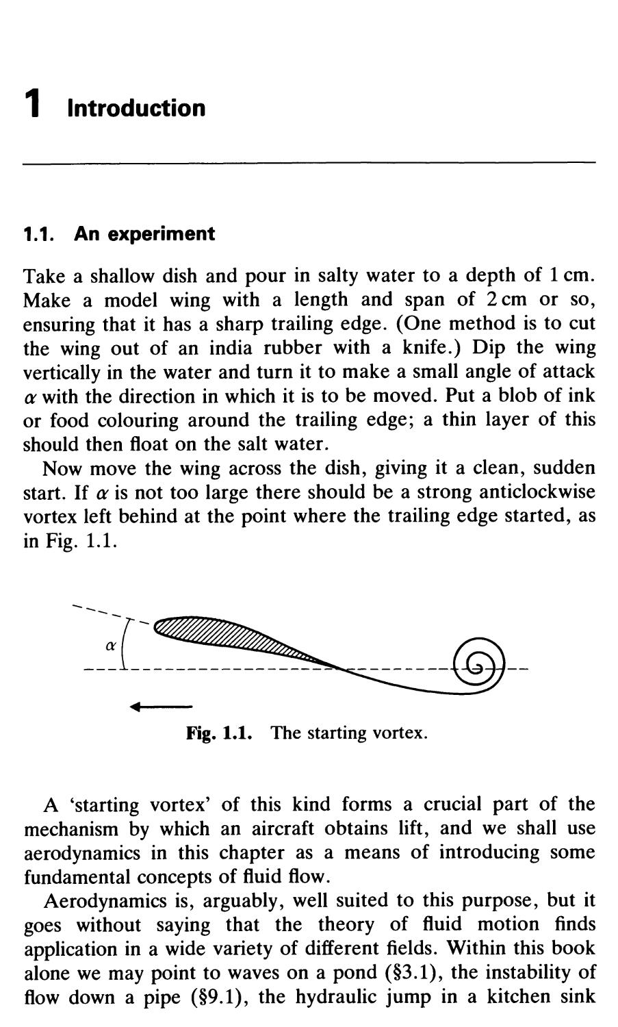
Take a shallow dish and pour in salty water to a depth of 1 cm.
Make a model wing with a length and span of 2 cm or so,
ensuring that it has a sharp trailing edge. (One method is to cut
the wing out of an india rubber with a knife.) Dip the wing
vertically in the water and turn it to make a small angle of attack
a with the direction in which it is to be moved. Put a blob of ink
or food colouring around the trailing edge; a thin layer of this
should then float on the salt water.
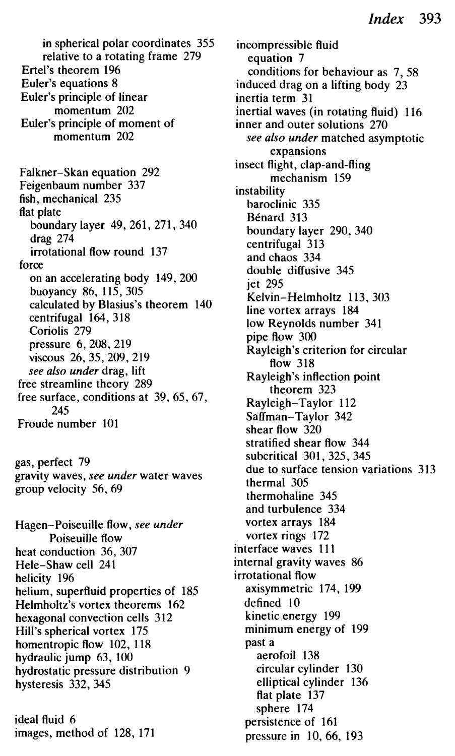
Now move the wing across the dish, giving it a clean, sudden
start. If a is not too large there should be a strong anticlockwise
vortex left behind at the point where the trailing edge started, as
in Fig. 1.1.
1_ __ @ __
Fig. 1.1. The starting vortex.
A 'starting vortex' of this kind forms a crucial part of the
mechanism by which an aircraft obtains lift, and we shall use
aerodynamics in this chapter as a means of introducing some
fundamental concepts of fluid flow.
Aerodynamics is, arguably, well suited to this purpose, but it
goes without saying that the theory of fluid motion finds
application in a wide variety of different fields. Within this book
alone we may point to waves on a pond ( 3.1), the instability of
flow down a pipe ( 9.1), the hydraulic jump in a kitchen sink
2 Introduction
( 3.10), the interaction of two smoke rings ( 5.4), the jet stream
in the atmosphere ( 9.8), the motion of quantum vortices in
liquid helium ( 5.8), the flow of volcanic lava ( 7.9), the
swimming of biological micro-organisms ( 7 .5), and the spin-
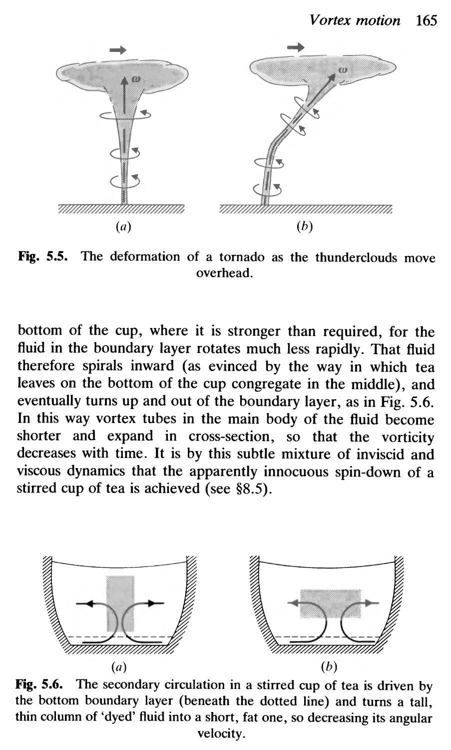
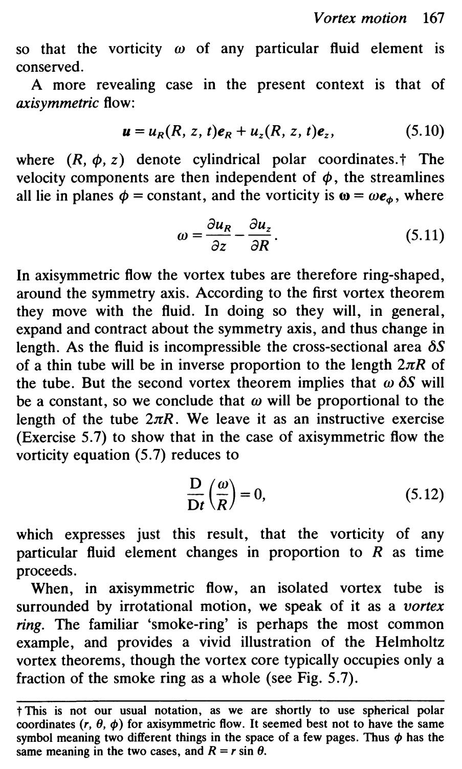
down of a stirred cup of tea ( 8.5) as examples of the breadth
and diversity of the subject.
1.2. Some preliminary ideas
The usual way of describing a fluid flow IS by means of an
expression
u = u(x, t)
(1.1)
for the flow velocity u at any point x and at any time t. This tells
us what all elements of the fluid are doing at any time; finding
eqn (1.1) is usually the main task.
In general we must expect this task to be quite difficult. Let us
take Cartesian coordinates, for example, and denote the three
components of u by u, v, and w. Then eqn (1.1) is a convenient
shorthand for
u = u(x, y, z, t),
v = v(x, y, z, t),
w = w(x, y, z, t).
There are, however, special classes of flow which have simplify-
ing features.
A steady flow is one for which
au
at = 0,
(1.2)
so that u depends on x alone. At any fixed point in space the
speed and direction of flow are both constant.
A two-dimensional (2-D) flow is of the form
u = (u(x, y, t), v(x, y, t), 0],
(1.3)
so that u is independent of one spatial coordinate (here selected
to be z) and has no component in that direction.
A two-dimensional steady flow is thus of the form
u = (u(x, y), v(x, y), 0].
(1.4)
Introduction 3
These are idealizations. No real flow can be exactly two-
dimensional, but in the case of flow past a fixed wing of long span
and uniform cross-section we might reasonably expect a close
approximation to 2-D flow, except near the wing-tips.
Before exploring such a flow more closely it is useful to
introduce the concept of a streamline. This is, at any particular
time t, a curve which has the same direction as u(x, t) at each
point. Mathematically, then, a streamline x = x(s), y = y(s),
z = z(s) is obtained by solving
dx/ds dy/ds dz/ds
(1.5)
u v w
at a particular time t.
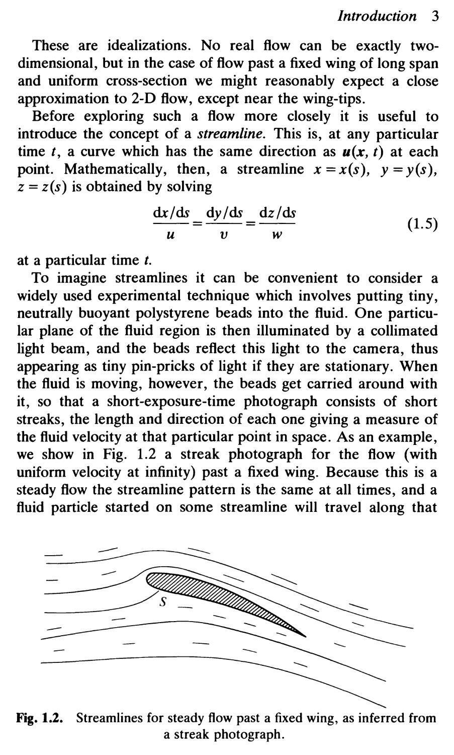
To imagine streamlines it can be convenient to consider a
widely used experimental technique which involves putting tiny,
neutrally buoyant polystyrene beads into the fluid. One particu-
lar plane of the fluid region is then illuminated by a collimated
light beam, and the beads reflect this light to the camera, thus
appearing as tiny pin-pricks of light if they are stationary. When
the fluid is moving, however, the beads get carried around with
it, so that a short-exposure-time photograph consists of short
streaks, the length and direction of each one giving a measure of
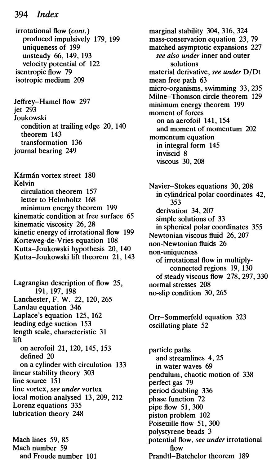
the fluid velocity at that particular point in space. As an example,
we show in Fig. 1.2 a streak photograph for the flow (with
uniform velocity at infinity) past a fixed wing. Because this is a
steady flow the streamline pattern is the same at all times, and a
fluid particle started on some streamline will travel along that
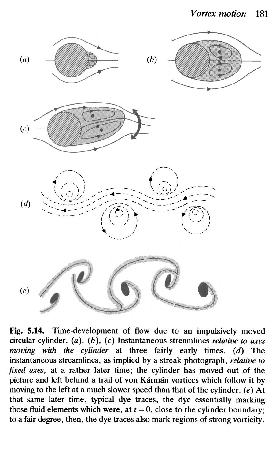
Fig. 1.2. Streamlines for steady flow past a fixed wing, as inferred from
a streak photograph.
4 Introduction
streamline as time proceeds. (In an unsteady flow, on the other
hand, streamlines and particle paths are usually quite different;
see Exercise 1.8.)
It is evident from Fig. 1.2 that even though the flow is steady,
so that u is constant at a point fixed in space, u changes as we
follow any particular fluid element. In particular--changes in
direction of flow aside-an element riding over the top of the
wing first speeds up and then slows down again.
Rate of change 'following the fluid'
This notion is of fundamental importance in fluid dynamics.
Let f(x, y, z, t) denote some quantity of interest in the fluid
motion. It could, for example, be one component of the velocity
u, or it could be the density p. Note first that at I at means the
rate of change of t at fixed x, y, and z, i.e. at a fixed position in
space.
In contrast, the rate of change of f 'following the fluid', which
we denote by Of lOt, is
Of d
Ot = dt f(x(t), y(t), z(t), t],
where x(t), y(t), and z(t) are understood to change with time at
the local flow velocity u:
dxldt=u, dyldt=v, dzldt=w,
so as to 'follow the fluid'. A simple application of the chain rule
gIves
Of afdx afdy atdz at
-=--+--+--+-
Ot ax dt ay dt az dt at '
whence
Of at af af at
-=-+u-+v-+w-
Ot at ax ay az '
I.e.
Of at
- = - + (u · V)f.
Ot at
(1.6)
By applying eqn (1.6) to the velocity components u, v, and w
in turn it follows, in particular, that the acceleration of the fluid
Introduction 5
element at x is
Du au
-=-+ (u. V)u.
Dt at
(1.7)
As an immediate check on eqn (1.7) consider fluid in uniform
rotation with angular velocity Q, so that
u = -Qy,
v = Qx,
w =0.
Now auf at is zero, because the flow is steady, but
(u. V)u = (-Qy + Qx )(-QY, Qx, 0)
= _Q2(X, y, 0).
This is just as expected; it represents the familiar centrifugal
acceleration Q 2 r towards the rotation axis.
According to eqn (1.6) in any steady flow the rate of change of
I following a fluid element is (u · V)/, and it is quite easy to see
why this should be so. Let e s denote a unit vector which is always
parallel to the streamlines and in the same sense as the flow.
Then
al
u · VI = lul e s · VI = lul as '
where s denotes distance along a streamline. Now, ai/as is the
rate of change of I with distance along a streamline, so
multiplying it by the flow speed lul evidently gives the rate of
change with time as we follow a fluid element along that
streamline.
The equation
(u.V)/=O,
(1.8)
which arises at some important stages in the following theory,
thus implies that I is constant along a streamline. It should be
emphasized that eqn (1.8) offers no information at all about
whether I might be a different constant on different streamlines.
Suppose, for instance, that the flow is everywhere in the
x-direction, so that eqn (1.8) reduces to ai/ax = o. This equation
says that I is independent of x, but it contains no implication
about how I might depend on y, z, or t.
6 Introduction
Likewise, the equation
Df =0
Dt '
(1.9)
which also arises in the following theory, implies that f is a
constant for a particular fluid element, and this follows directly
from the definition of Df /Dt above. It does not preclude
different elements having different values of f; it just implies that
each such element will retain whatever value of f it started with.
Finally, it is worth remarking that there will be occasions on
which we wish to follow not just an infinitesimal fluid element
but a finite blob consisting always of the same fluid particles.
Such a blob, which will of course deform as it moves about, is
typically called a 'material' volume in the literature, but we shall
freely describe it instead as 'dyed', with the understanding, of
course, that no diffusion of this imaginary dye is envisaged. Such
terminology can become rather colourful, but if it evokes a sharp
mental picture of a moving and deforming blob of fluid, as
opposed to some region fixed in space, it serves its purpose.
1.3. Equations of motion for an ideal fluid
In this text we define an ideal fluid as one with the following
properties:
(i) It is incompressible, so that no 'dyed' blob of fluid can
change in volume as it moves.
(ii) The density p (Le. the mass per unit volume) is a constant,
the same for all fluid elements and for all time t.
(iii) The force exerted across a geometrical surface element
n S within the fluid is
pn S,
(1.10)
where p(x, y, z, t) is a scalar function, independent of the
normal n, called the pressure. (To be more precise, eqn
(1.10) is the force exerted on the fluid into which n is
pointing by the fluid on the other side of S.)
There is, of course, no such thing in practice as an ideal fluid.
All fluids are to some extent compressible, and all fluids are to
Introduction 7
some extent viscous, so that adjacent fluid elements exert both
normal and tangential forces on one another across their
common interface. For the time being, however, we explore
some consequences of the assumptions (i)-(iii).
To examine the implications of (i), consider a fixed closed
surface S drawn in the fluid, with unit outward normal n. Fluid
will be entering the enclosed region V at some places on S, and
leaving it at others. The velocity component along the outward
normal is u · n, so the volume of fluid leaving through a small
surface element DS in unit time is u · n DS. The net volume rate
at which fluid is leaving V is therefore
L u · n dS.
But this must plainly be zero for an incompressible fluid, and on
using the divergence theorem we find that
Iv V · u dV = O.
Now, this must be true for all regions V within the fluid.
Suppose, then, that V · u is greater than zero at some point in the
fluid. Assuming that it is continuous, V. u will be greater than
zero in some small sphere around that point, and by taking V to
be such a sphere we violate the above equation. The same
applies if V · u is negative at some point. We thus conclude that
V. u =0 (1.11)
everywhere in the fluid.
This incompressibility condition is an important constraint on
the velocity field u in virtually the whole of this book. t
To examine the implications of (iii) consider a surface S
enclosing a 'dyed' blob of fluid. The force exerted by the
surrounding fluid across any surface element DS is, by hypothe-
sis, given by eqn (1.10), so that the net force exerted on the dyed
blob is
- Lpn dS = - Iv Vp dV,
t Air is, of course, highly compressible, but it can behave like an incompressible
fluid if the flow speed is much smaller than the speed of sound (see p. 58).
8 Introduction
where we have used the identity (A.14)-see the Appendix (the
negative sign arises because n points out of S). Now, provided
that Vp is continuous it will be almost constant over a small blob
of fluid of volume 6V. The net force on such a small blob due to
the pressure of the surrounding fluid will therefore be -Vp 6V.
Euler's equations of motion
We are now in a position to apply the principle of linear
momentum to a small 'dyed' blob of fluid of volume 6V.
Allowing for the presence of a gravitational body force per unit
mass g, the total force on the blob is
(-Vp + pg) 6V.
This force must be equal to the product of the blob's mass (which
is conserved) and its acceleration, i.e. to
Du
P 6V-.
Dt
We thus obtain
Du 1
Dt = - p Vp + g,
(1.12)
v · u = 0,
as the basic equations of motion for an ideal fluid. They are
known as Euler's equations, and written out in full they become
au au au au 1 ap
-+u-+v-+w-= ---
at ax ay az p ax '
av av av av 1 ap
-+u-+v-+w-= ---
at ax ay az p ay ,
aw aw aw aw 1 ap
-+u-+v-+w-=----g
at ax ay az p az '
au av aw
-+-+-=0
ax ay az '
Introduction 9
i.e. four scalar equations for four unknowns: u, v, w, and p. In
dealing with the gravitational term we have momentarily taken
the z-axis vertically upward, setting g = (0, 0, -g).
Now, the gravitational force, being conservative, can be
written as the gradient of a potential:
g = -Vx.
(1.13)
(In the above case, X=gz.) Using the expression (1.7) for the
fluid acceleration we may rewrite eqn (1.12) in the formt
au ( p )
at + (u · V)u = - v p + x ,
where we have used the assumption that p IS constant.
Furthermore, it can be helpful to use the identity
(u · V)u = (V A u) A u + V(!u 2 )
to cast the momentum equation into the form
au ( p )
- + (V A u) A U = -V - + !u 2 + x .
at p
(1.14)
The BemouUi streamline theorem
If the flow is steady, eqn (1.14) reduces to
(VAU)AU=-VH,
where
H = p + !u 2 + X.
P
(1.15)
On taking the dot product with U we obtain
(U · V)H = 0,
(1.16)
t The way in which p / P + X appears as a combination is significant; there will be
many circumstances in this book in which gravity simply modifies the pressure
distribution in the fluid and does nothing to change the velocity u. Thus when we
speak occasionally of 'ignoring' gravity, or of gravitational body forces being
'absent', what we often mean is that separate allowance may be made for gravity
simply by subtracting PX from the pressure field. This is emphatically not the
case, however, if there is a free surface-as with water waves in Chapter 3---or if
P is not constant-as in 3.8 and 9.3.
10 Introduction
so
If an ideal fluid is in steady flow,
then H is constant along a streamline.
In the absence of gravity it follows that p + !pu 2 is constant along
a streamline in steady flow.
The above theorem says nothing about H being the same
constant on different streamlines, only that it remains constant
along each one. There is, however, one important circumstance
in which H is constant throughout the whole flow field, and this
now follows.
DEFINITION. An irrotational flow is one for which
V A U = O.
(1.17)
The BemouUi theorem for irrotational flow
If the flow is steady and irrotational, then eqn (1.14) reduces to
V H = 0, so H is independent of x, y, and z, as well as t. Thus
If an ideal fluid is in steady irrotational flow,
then H is constant throughout the whole flow field.
Whether this result is of any value rests, evidently, on whether
irrotational flows are of any real interest in practice. We address
this matter in the next section.
1.4. Vorticity: irrotational flow
The vorticity (J) is defined as
(J) = V A U,
(1.18)
and it is a concept of central importance in fluid dynamics. The
vorticity is, by definition, zero for an irrotational flow.
We consider vorticity first in the context of two-dimensional
flow, for if
U = [u(x, y, t), v(x, y, t), 0]
then (J) is (0, 0, £0), where
av au
£0=---
ax ay .
(1.19)
Introduction 11
Interpretation of vorticity in 2-D ftow
Consider two short fluid line elements AB and AC which are
perpendicular at a certain instant, as in Fig. 1.3. Note that the
y-component of velocity at B exceeds that at A by
av
v(x + Dx, y, t) - v(x, y, t) : - Dx,
ax
so that av / ax represents the instantaneous angular velocity of
the fluid line element AB. Likewise, auf ay represents the
instantaneous angular velocity (in the opposite sense) of the line
element AC. Thus at any point of the flow field
1 l ( aV au )
-0)-- ---
2 - 2 ax ay
represents the average angular velocity of two short fluid line
elements that happen, at that instant, to be mutually perpendicu-
lar. In this precise sense the vorticity 0) acts as a measure of the
local rotation, or spin, of fluid elements.
We emphasize that vorticity has nothing directly to do with any
global rotation of the fluid. Take, for example, the shear flow of
ov
a- by
Yt '
C --+ CU b
(Jy y
by
bx
(1V
t ox {jx
--+ ou bx
B ox
A
Fig. 1.3. Sketch for the interpretation of vorticity in 2-D flow. The
velocity components shown are relative to the fluid particle at A.
12 Introduction
C L -+ L C
A B A B
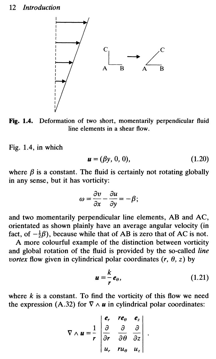
Fig. 1.4. Deformation of two short, momentarily perpendicular fluid
line elements in a shear flow.
Fig. 1.4, in which
U = (Py, 0, 0),
( 1.20)
where P is a constant. The fluid is certainly not rotating globally
in any sense, but it has vorticity:
av au
OJ = ax - ay = - f3;
and two momentarily perpendicular line elements, AB and AC,
orientated as shown plainly have an average angular velocity (in
fact, of -!P), because while that of AB is zero that of AC is not.
A more colourful example of the distinction between vorticity
and global rotation of the fluid is provided by the so-called line
vortex flow given in cylindrical polar coordinates (r, (J, z) by
k
U = - ee,
r
(1.21 )
where k is a constant. To find the vorticity of this flow we need
the expression (A.32) for V A U in cylindrical polar coordinates:
e r ree e z
1 a a a
VAU=- - - -
r ar a(J az
U r rUe U z
Introduction 13
Plainly, then, the vorticity is zero except at r = 0, where neither u
nor V A U is defined. Thus although the fluid is clearly rotating in
a global sense the flow is in fact irrotational, since V A U = 0,
except on the axis. This is quite understandable if we consider
two momentarily perpendicular fluid line elements, AB and AC,
at (J = 0 in Fig. 1.5. Clearly AC is rotating in an anticlockwise
sense, because it will continue to lie along the circular streamline
as time proceeds, but AB is rotating clockwise because of the
decrease of Ue with r in eqn (1.21). This particular fall-off of Ue
with r is, apparently, just the correct one-neither too slow nor
too rapid-to ensure that AB has an equal and opposite angular
velocity to AC at the instant they are perpendicular, so that their
average angular velocity is zero.
We keep emphasizing the instantaneous nature of this
conclusion about zero average angular velocity because two fluid
line elements such as AB and AC in Fig. 1.5 will not remain
perpendicular as they get carried about by the flow, and as soon
as this happens we have no cause to conclude from the
irrotationality of the flow that their average angular velocity
should any longer be zero.
Fig. 1.5. The fate of a small square fluid element in a line vortex flow.
The size of the element has been greatly exaggerated for the sake of
clarity; an unfortunate consequence is that B does not look as if it is
following a circular path.
14 Introduction
- -
'+
I \
+ -}.
\ I
\ /
" /
" ./
-- --
... ..... ...
. :l:
::1.1 11 ,"'iY I
;: ;;;;;;:;:i. :.1[ ! : : : :::: : ::::.. :jj:
:::-:--- I
I
I
I
(a) ueocl.
r
(b)
/ .- -...
I \
I \
+ +-
\ I
\ /
" /
'- ..--/
( c) Uo oc r
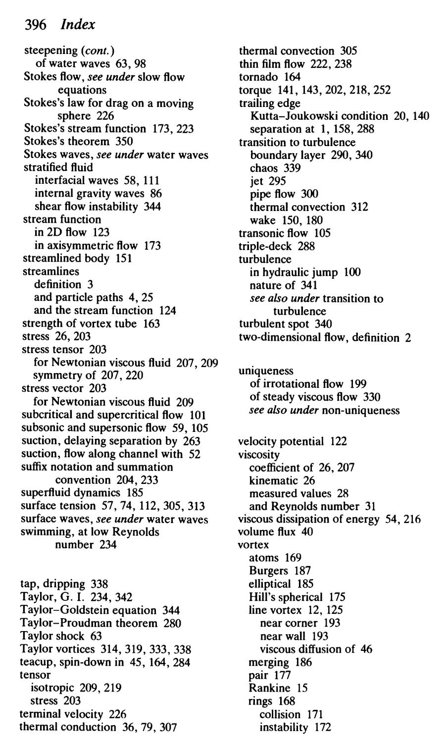
Fig. 1.6. A crude 'vorticity meter' (b), and its behaviour when
immersed in a line vortex flow (a) and a uniformly rotating flow (c).
What we have sketched in Fig. 1.6(a), then, is not what
happens to two momentarily dyed fluid elements, AB and AC, as
they get swept round but what would happen if we were to
immerse in the fluid a small 'vorticity meter' consisting of two
short, rigid vanes fixed at right angles to each other, as in Fig.
1.6(b). We have marked one tip of one of the vanes, and in Fig.
1.6(a) we see that this device would not rotate in this particular
(line vortex) flow, even though its axis would of course get swept
round on a circular streamline. This behaviour may be seen in
the bath by observing closely the strong vortex that may occur as
the water goes down the plug-hole. The azimuthal velocity Ue
varies roughly as r- 1 over a fair distance from the axis, and a
crude but simple vorticity meter which serves the purpose
consists of a pair of short wooden line elements shaved off a
matchstick, seHotaped together at right angles and floated on the
surface.
However, if such a vorticity meter were to be inserted in the
Introduction 15
flow
u = Qreo,
(1. 22)
Q being a constant, the result would of course be as in Fig.
1.6( c), because the device would get carried around just as if it
were embedded in a rigid body. Its angular velocity would
evidently be Q, the same as the uniform angular velocity of the
fluid as a whole, and the vorticity of the flow is therefore
(0, 0, 2Q), as may be confirmed by direct calculation of V 1\ U.
By putting the two flows in Fig. 1.6 together in the following
way:
{ Qr,
U(J = Qr a2 ,
r<a,
r>a,
U r = U z = 0,
(1. 23)
we obtain a so-called 'Rankine vortex', which serves as a simple
model for a real vortex such as that in Fig. 1.1. Real vortices are
typically characterized by fairly small vortex 'cores' in which, by
definition, the vorticity is concentrated, while outside the core
the flow is essentially irrotational. The core is not usually exactly
circular, of course; nor is the vorticity usually uniform within it.
In these two respects the Rankine vortex of Fig. 1.7 is only an
idealized model.
We have now said a fair amount about vorticity, albeit strictly
UfJ
w
Qa
2Q
a
r
a
r
(a) (b)
Fig. 1.7. Distribution of (a) azimuthal velocity Ue and (b) vorticity OJ in
a Rankine vortex.
16 Introduction
--- --- ---- ----
----- --+
.-r- ---- ..................
-- / - ----- --
..-"-- .................. .................
-- + _..------------+ ----- ---
-- ..- ----- + ................-........................
.--...-------- ...............................
---
--
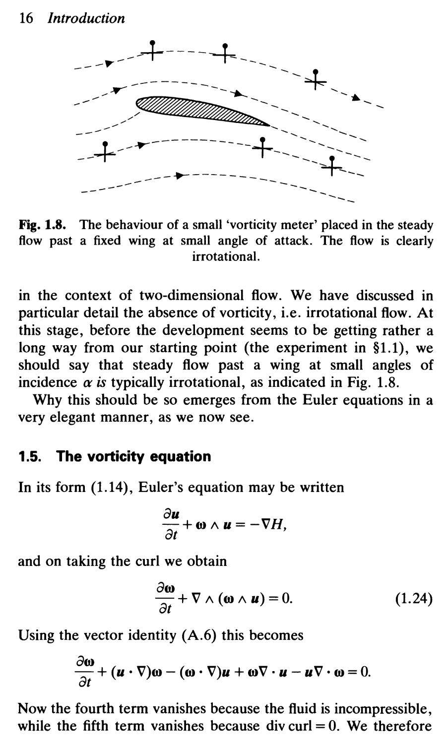
Fig. 1.8. The behaviour of a small 'vorticity meter' placed in the steady
flow past a fixed wing at small angle of attack. The flow is clearly
irrotational.
in the context of two-dimensional flow. We have discussed in
particular detail the absence of vorticity, i.e. irrotational flow. At
this stage, before the development seems to be getting rather a
long way from our starting point (the experiment in 1.1), we
should say that steady flow past a wing at small angles of
incidence a is typically irrotational, as indicated in Fig. 1.8.
Why this should be so emerges from the Euler equations in a
very elegant manner, as we now see.
1.5. The vorticity equation
In its form (1.14), Euler's equation may be written
au
-+rol\u=-VH
at '
and on taking the curl we obtain
aro
at + V 1\ (ro 1\ u) = o.
(1.24 )
Using the vector identity (A.6) this becomes
aro
at + (u · V)ro - (ro · V)u + ro V · u - u V · ro = o.
Now the fourth term vanishes because the fluid is incompressible,
while the fifth term vanishes because div curl = O. We therefore
Introduction 17
have
aro
at + (u · V)ro = (ro · V)u,
or, alternatively,
Oro
- = (ro · V)u.
Ot
(1. 25)
This vorticity equation is extremely valuable. Note that the
pressure has been eliminated; eqn (1.25) involves only u and ro,
which are, of course, related by
ro = V 1\ u.
In particular, if the flow is two-dimensional, so that
u = (u(x, y, t), v(x, y, t), 0]
(1. 26)
and
ro = (0, 0, w),
then
au
(ro · V)u = w - = o.
az
It then follows that
OW =o
Ot '
(1.27)
and we thus conclude, referring back to eqn (1.9), that
In the two-dimensional flow of an ideal fluid subject to
a conservative body force g the vorticity w of each
individual fluid element is conserved. (1.28)
This result has important applications, which we discuss in
Chapter 5. In the particular case of steady flow, eqn (1.27)
reduces to
(u · V)w = 0 (1.29)
and consequently
In the steady, two-dimensional flow of an ideal fluid
subject to a conservative body force g the vorticity
w is constant along a streamline. (1.30)
18 Introduction
This, then, is the reason why the steady flow in Fig. 1.8 is
irrotational. Note first that there are no regions of closed
streamlines in the flow; all the streamlines can be traced back to
x = -00. Now, the vorticity is constant along each one, and hence
equal on each one to whatever it is on that particular streamline
at x = -00. As the flow is uniform at x = -00 the vorticity is zero
on all streamlines there. Hence it is zero throughout the flow
field in Fig. 1.8.
1.6. Steady flow past a fixed wing
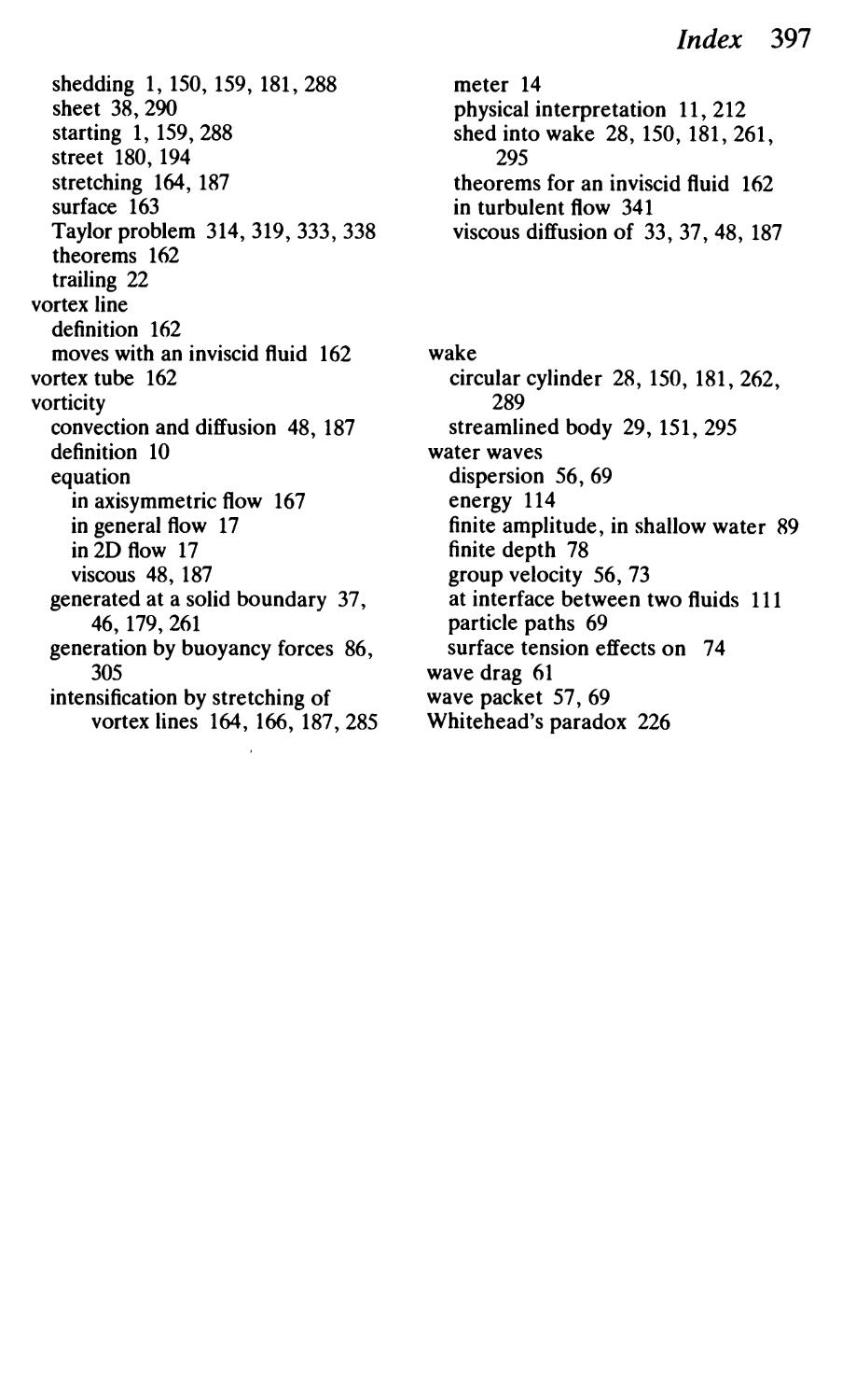
In Fig. 1.9 we show typical measured pressure distributions on
the upper and lower surfaces of a fixed wing in steady flow. The
pressures on the upper surface are substantially lower than the
free-stream value poo, while those on the lower surface are a little
higher than pooo In fact, then, the wing gets most of its lift from a
suction effect on its upper surface 0
But why is it that the pressures above the wing are less than
those below? Well, because the flow is irrotational, the Bernoulli
theorem tells us that p + !pu 2 is constant throughout the flow.
Explaining the pressure differences, and hence the lift on the
1
LOWER SURFACE
P-Poo
w U2
o
-1
-2
U
--+
---
Fig. 1.9. Typical pressure distribution on a wing in steady flow.
Introduction 19
wing, thus reduces to explaining why (as in Fig. 1.2) the flow
speeds above the wing are greater than those below.
Let us first dispose of one bogus explanation that occasionally
appears, namely that the air on the top of the wing flows faster
'because it has farther to go'. There are many woolly aspects to
this argument, but it seems to turn principally on the notion that
two neighbouring fluid elements, after parting to go their
separate ways round the wing, meet up again at the trailing edge,
and this is demonstrably false (see Fig. 2.4).
The right way forward to an explanation of the higher flow
speeds above the wing is in terms of the concept of circulation.
Circulation
Let C be some closed curve lying in the fluid region. Then the
circulation r round C is defined as
r = Ie u · <Ix.
(1.31)
At first sight, perhaps, there cannot be any circulation in an
irrotational flow, for Stokes's theorem gives
Ie u · <Ix = L (V 1\ u) · n dS,
and an irrotational flow is, by definition, one for which V 1\ U is
zero. But such an argument holds only if the closed curve C in
question can be spanned by a surface S which lies wholly in the
region of irrotational flow. Thus in the two-dimensional context
of Fig. 1.8, for example, for which eqn (1.32) reduces to
r = L u dx + v dy = f ( av - au ) dx dy, (1.33)
c s ax ay
(1.32)
it is true that r must be zero for any closed curve C not enclosing
the wing, but the argument fails for any closed curve that does
enclose the wing. The most that can be said about such circuits is
that they all have the same value of r (Exercise 1.6).
Circulation round a wing is permissible, then, in a steady
irrotational flow; but the question still arises as to why there
should be any, and, in particular, why it should be negative,
corresponding to larger flow speeds above the wing than below.
20 Introduction
The Kutta-Joukowski hypothesis
In the case of a wing with a sharp trailing edge, one good reason
for non-zero circulation r is that there would otherwise be a
singularity in the velocity field. The irrotational flow past a wing
with r = 0 is sketched in Fig. 1.10(a), but the velocity is infinite
at the trailing edge where, loosely speaking, the fluid is having a
hard time turning the corner. We show in Chapter 4 that only for
one value of the circulation, r K say, is the flow speed finite at the
trailing edge, as in Fig. 1.10(b). It is natural to hope that this
particular irrotational flow will correspond to the steady flow that
is actually observed; this is the Kutta-loukowski hypothesis.
This hypothesis is inevitably somewhat ad hoc, resting as it
does on the unsatisfactory state of affairs that would otherwise
arise because of the sharp trailing edge. (How are we to decide
between all the different irrotational flows if the trailing edge is
not sharp?) It is, nonetheless, one of the key steps in the
development of aerodynamics, and gives results which are in
excellent accord with experiment, as we shall shortly see.
The critical value r K depends, naturally, on the flow speed at
infinity U and on the size, shape, and orientation of the wing. In
Chapter 4 we show that if the wing is thin and symmetrical, of
length L, making an angle a' with the oncoming stream, then
r K : -nUL sin a'.
(1. 34)
Lift
According to ideal flow theory, the drag on the wing (the force
parallel to the oncoming stream) is zero, but the lift (the force
Wg
...._....:.:.:.:.:.:::::::;:::;::::::.::.:::::{: : :{: ::=:::::::.:.:...... ...............:.........:::::::.::::.:......
(a) (b)
Fig. 1.10. Irrotational flow past a fixed wing with (a) r = 0 and (b)
r = r K < O.
Introduction 21
perpendicular to the stream) is
It = - pur.
(1.35)
This Kutta-Joukowski Lift Theorem is proved in 4.11.
That negative r should give positive lift is entirely natural; we
have argued as much in the preceding sections. As a precise
theorem, however, eqn (1.35) is rather extraordinary, as it holds
for irrotational flow (uniform at infinity) past a two-dimensional
body of any size or shape; It depends on the size and shape of
the body only inasmuch as r does. For the thin symmetrical wing
of Fig. 1.10(b), for example, with r as in eqn (1.34) by the
Kutta-Joukowski condition, the lift is
It : 1CpU 2 L sin a'. (1.36)
Agreement with experiment is good provided that a' is only a
few degrees (Fig. 1.11) . Thereafter the measured lift falls
dramatically and diverges substantially from the predictions of
inviscid theory, for reasons to be discussed later. The angle a' at
which this divergence begins may be anywhere between about 6°
and 12°, depending on the shape of the wing (see, e.g.,
Nakayama 1988, pp. 76-80).
Accounting for the flow past a wing at small angles of attack a'
is nevertheless one of the great, and practically important,
successes of ideal-flow theory.
f£
Inviscid
theory
.
.
Experiment
a
Fig. 1.11. Lift on a symmetric aerofoil.
22 Introduction
1.7. Concluding remarks
In this chapter we have introduced some of the basic concepts of
fluid dynamics and, at the same time, given some indication of
how they figure in one particular branch of the subject, namely
aerodynamics. Our treatment of this branch has inevitably been
sketchy.
We have, for instance, focused wholly on 2-D aerodynamics,
yet any real wing, no matter how long, has ends, and important
new phenomena then arise. The circulation round a circuit such
as C in Fig. 1.12(a) is essentially that predicted by the 2-D theory
(i.e. eqn (1.34)), but plainly the flow cannot be everywhere
irrotational, because C can now be spanned by a surface S which
lies wholly in the fluid. Indeed, from Stokes's theorem (1.32) we
deduce that there must be a positive flux of vorticity out of S,
and this is in practice observed as a concentrated trailing vortex
emanating from the wing-tip as shown. The higher the lift (and
G uuu uuuuu
(a)
(b)
- 0
z
(c)
Fig. 1.12. Trailing vortices: (a) definition sketch for application of
Stokes's theorem; (b) view from some distance ahead of the aircraft; (c)
the original drawing from Lanchester's Aerodynamics (1907).
Introduction 23
therefore the circulation), the stronger the trailing vortices.
Furthermore, the presence of these trailing vortices results in a
drag on the wing, even on ideal flow theory, for as they lengthen
they contain more and more kinetic energy, and creating all this
kinetic energy takes work.
But even within a purely two-dimensional framework we have
left some key questions unanswered. We indicated how the
Kutta-Joukowski hypothesis provides a rational, although ad
hoc, basis for deciding the circulation round an aerofoil in steady
flight, and we have noted that this gives good agreement with
experiment. Yet we have given no account of the dynamical
processes by which that circulation is generated when the aerofoil
starts from a state of rest. It arises, in fact, in response to the
'starting vortex' in 1.1, but why this should be so is far from
obvious, and rests on one of the deepest theorems in the subject
( 5.1).
Again, the sceptical reader may even be asking: 'But what is
all this business about a starting vortex? If the aerofoil and fluid
are initially at rest, the vorticity OJ is initially zero for each fluid
element. By eqn (1.27) it remains zero for each fluid element,
even when the aerofoil has been started into motion. Therefore
there should not be a starting vortex.'
This is a legitimate conclusion---on the basis of ideal flow
theory. While that theory accounts well for the steady flow past
an aerofoil, the explanation of how that flow became established
involves viscous effects in a crucial way.
If this provokes the response: 'But air isn't very viscous, is it?',
the answer is, 'No, in some sense air is hardly viscous at all' . Yet,
as we shall see, viscous effects are sufficiently subtle that the
shedding of the vortex in 1.1, while being an essentially viscous
process, would occur no matter how small the viscosity of the
fluid happened to be.
Exercises
1.1. Whether a fluid is incompressible or not, each element must
conserve its mass as it moves. Consider the rate of mass flow through a
fixed closed surface S drawn in the fluid, and use an argument similar to
that on p. 7 to show that this conservation of mass implies
ap
at + V · (pu) = 0, (1.37)
24 Introduction
where p(x, t) denotes the (variable) density of the fluid. Show too that
this equation may alternatively be written
Dp
Dt + pV · u = O.
It follows that if V. u = 0, then DplDt = O. What does this mean,
exactly, and does it make sense?
1.2. An ideal fluid is rotating under gravity g with constant angular
velocity Q, so that relative to fixed Cartesian axes u = (-Qy, Qx, 0).
We wish to find the surfaces of constant pressure, and hence the surface
of a uniformly rotating bucket of water (which will be at atmospheric
pressure) .
'By Bernoulli,' pip + U2 + gz is constant, so the constant pressure
surfaces are
(1.38 )
Q2
Z = constant - 2g (x 2 + y2).
But this means that the surface of a rotating bucket of water is at its
highest in the middle. What is wrong?
Write down the Euler equations in component form, integrate them
directly to find the pressure p, and hence obtain the correct shape for
the free surface.
1.3. Find the pressure p both inside and outside the core of the
Rankine vortex (1.23). Show that the pressure at r = 0 is lower than that
at r = 00 by an amount pQ 2 a 2 (hence the very low pressure in the centre
of a tornado). Deduce that if there is a free surface to the fluid and
gravity is acting, then the surface at r = 0 is a depth Q 2 a 2 I g below the
surface at r = 00 (hence the dimples in a cup of tea accompanying the
vortices that are shed by the edges of the spoon).
1.4. Take the Euler equation for an incompressible fluid of constant
density, cast it into an appropriate form, and perform suitable
operations on it to obtain the energy equation:
L !pu 2 dV = - L (p' + !pu 2 )u. n dS,
where V is the region enclosed by a fixed closed surface S drawn in the
fluid, and p' denotes p + PX, the non-hydrostatic part of the pressure
field.
1.5. For an inviscid fluid we have Euler's equation
au 1 2 1
at + ro 1\ u + V(2 U ) = - p Vp - Vx,
Introduction 25
and, whether or not the fluid is incompressible, we also have
conservation of mass (Exercise 1.1):
Dp
-+ pV. u =0.
Dt
Show that
( : ) = ( : . v)u - v G ) A Vp.
(1.39)
Deduce that, if p is a function of palone, the vorticity equation is
exactly as in the incompressible, constant density case, except that ro is
replaced by ro/ p.
1.6. Show that the circulation is the same round all simple closed
circuits enclosing the wing in Fig. 1.8. (Hint: sketch two such circuits,
and then make a construction so as to create a single closed circuit that
does not enclose the wing.)
1.7. Sketch the streamlines for the flow
U = ax,
v = -ay,
w=o
,
where a' is a positive constant.
Let the concentration of some pollutant in the fluid be
c(x, y, t) = f3x 2 ye- at ,
for y > 0, where f3 is a constant. Does the pollutant concentration for
any particular fluid element change with time?
An alternative way of describing any flow is to specify the position x
of each fluid element at time t in terms of the position X of that element
at time t = O. For the above flow this 'Lagrangian' description is
x =Xe at ,
y = Ye- at ,
z =z.
Verify by direct calculation that
( ax ) = u
at x '
( au ) Du
- --
at x Dt
in this particular case. Why are these results true in general?
Write c as a function of X, Y, and t.
1.8. Consider the unsteady flow
U = Uo,
v = kt,
w =0,
where Uo and k are positive constants. Show that the streamlines are
straight lines, and sketch them at two different times. Also show that
any fluid particle follows a parabolic path as time proceeds.
2 Elementary viscous flow
2.1. Introduction
Steady flow past a fixed aerofoil may seem at first to be wholly
accounted for by inviscid flow theory. The streamline pattern
seems right, and so does the velocity field. In particular, the fluid
in contact with the aerofoil appears to slip along the boundary in
just the manner predicted by inviscid theory. Yet close inspection
reveals that there is in fact no such slip. Instead there is a very
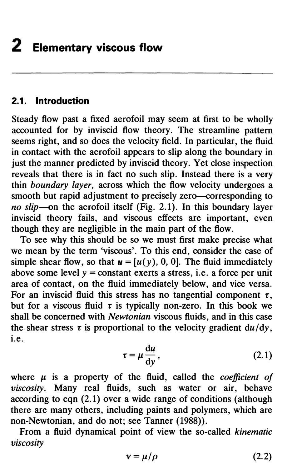
thin boundary layer, across which the flow velocity undergoes a
smooth but rapid adjustment to precisely zero--corresponding to
no slip-on the aerofoil itself (Fig. 2.1). In this boundary layer
inviscid theory fails, and viscous effects are important, even
though they are negligible in the main part of the flow.
To see why this should be so we must first make precise what
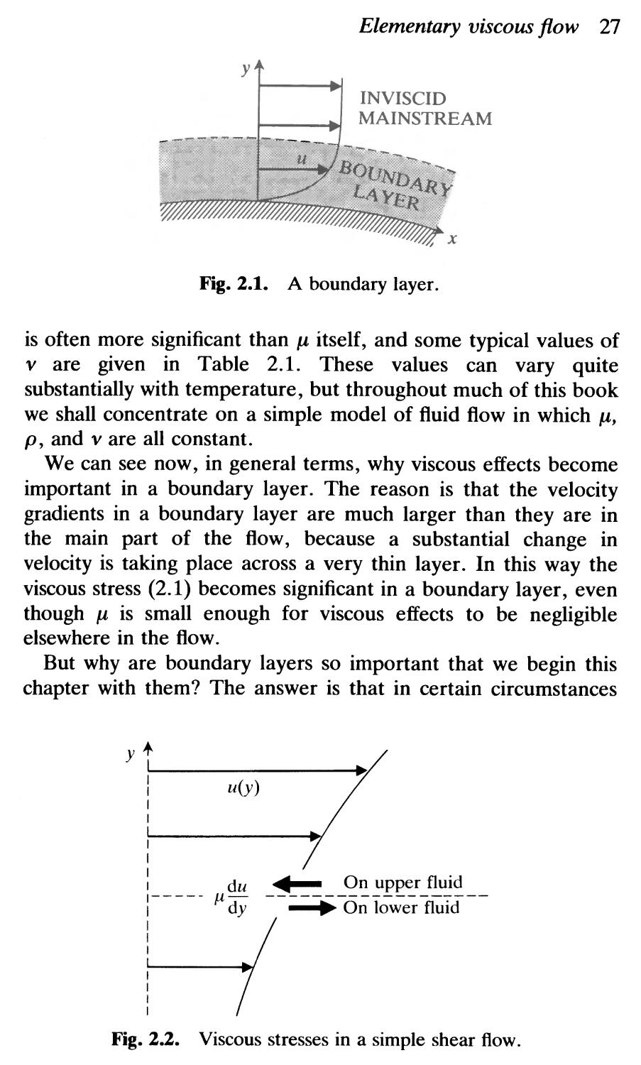
we mean by the term 'viscous'. To this end, consider the case of
simple shear flow, so that u = [u(y), 0, 0]. The fluid immediately
above some level y = constant exerts a stress, i.e. a force per unit
area of contact, on the fluid immediately below, and vice versa.
For an inviscid fluid this stress has no tangential component 1:,
but for a viscous fluid 1: is typically non-zero. In this book we
shall be concerned with Newtonian viscous fluids, and in this case
the shear stress 1: is proportional to the velocity gradient du/dy,
I.e.
du
T = JL d y , (2. 1 )
where IJ is a property of the fluid, called the coefficient of
viscosity. Many real fluids, such as water or air, behave
according to eqn (2.1) over a wide range of conditions (although
there are many others, including paints and polymers, which are
non-Newtonian, and do not; see Tanner (1988».
From a fluid dynamical point of view the so-called kinematic
viscosity
v = IJ/ P
(2.2)
Elementary viscous flow 27
y
INVISCID
MAINSTREAM
,t:; I;itl ;t:i : ill"
Fig. 2.1. A boundary layer.
is often more significant than Jl itself, and some typical values of
v are given in Table 2.1. These values can vary quite
substantially with temperature, but throughout much of this book
we shall concentrate on a simple model of fluid flow in which Jl,
p, and v are all constant.
We can see now, in general terms, why viscous effects become
important in a boundary layer. The reason is that the velocity
gradients in a boundary layer are much larger than they are in
the main part of the flow, because a substantial change in
velocity is taking place across a very thin layer. In this way the
viscous stress (2.1) becomes significant in a boundary layer, even
though Jl is small enough for viscous effects to be negligible
elsewhere in the flow.
But why are boundary layers so important that we begin this
chapter with them? The answer is that in certain circumstances
y+
I
I u(y)
I
1
I
I
I
I du
1----- Il-
I dy
I
I
I
+- On upper fluid
-------------------
. On lower fluid
Fig. 2.2. Viscous stresses in a simple shear flow.
28 Elementary viscous flow
Table 2.1. Kinematic viscosity v (cm 2 S-I) at 15°C.
Water
Air
Olive oil
Glycerine
Golden syrup/treacle
0.01
0.15
1.0
18
-1200
(fJ. = 0.01 c.g.s. units)
(fJ. = 0.0002 c.g.s. units)
( v - 200 at 27°C)
they may separate from the boundary, thus causing the whole flow
of a low-viscosity fluid to be quite different to that predicted by
inviscid theory.
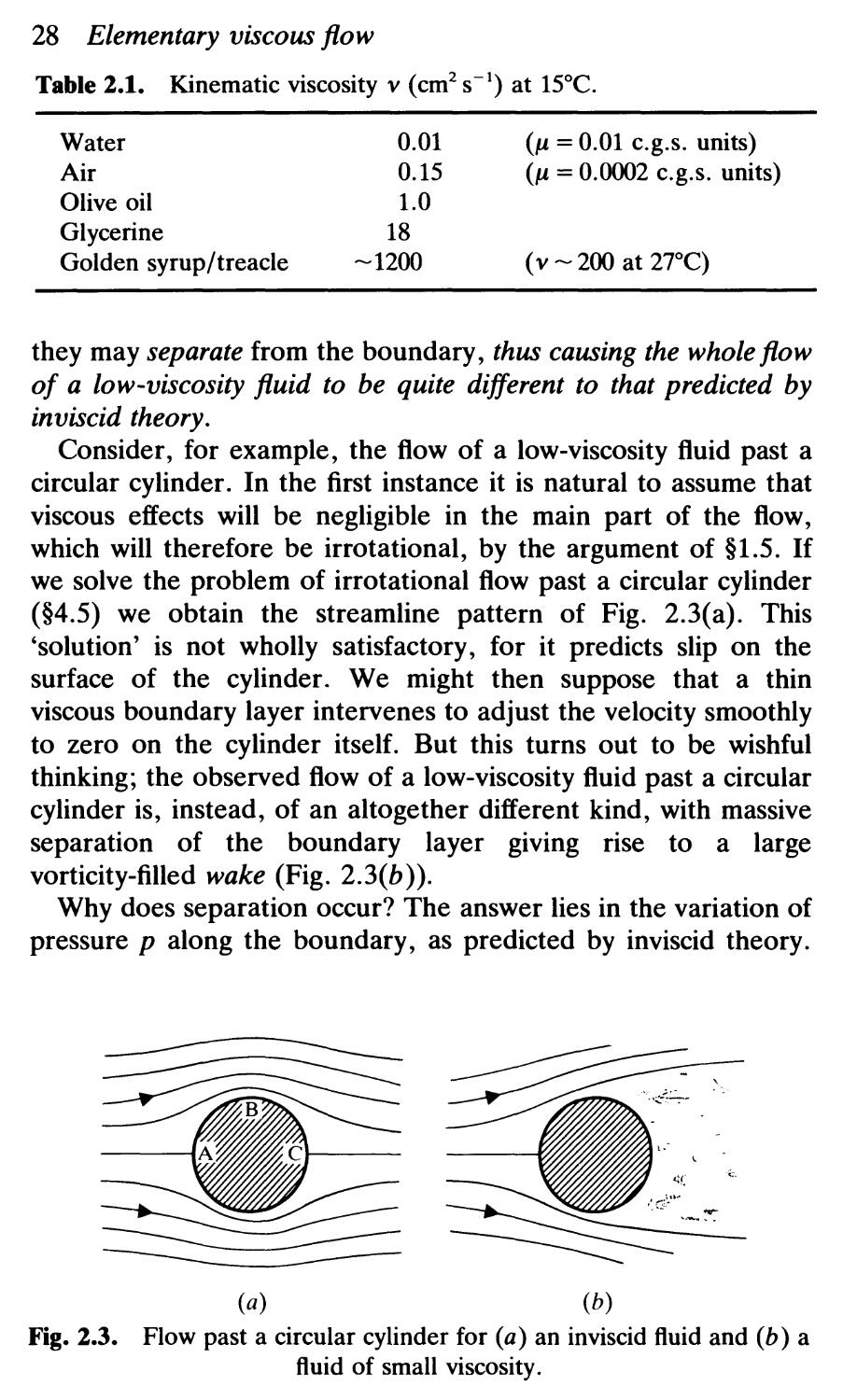
Consider, for example, the flow of a low-viscosity fluid past a
circular cylinder. In the first instance it is natural to assume that
viscous effects will be negligible in the main part of the flow,
which will therefore be irrotational, by the argument of 1.5. If
we solve the problem of irrotational flow past a circular cylinder
( 4.5) we obtain the streamline pattern of Fig. 2.3(a). This
'solution' is not wholly satisfactory, for it predicts slip on the
surface of the cylinder. We might then suppose that a thin
viscous boundary layer intervenes to adjust the velocity smoothly
to zero on the cylinder itself. But this turns out to be wishful
thinking; the observed flow of a low-viscosity fluid past a circular
cylinder is, instead, of an altogether different kind, with massive
separation of the boundary layer giving rise to a large
vorticity-filled wake (Fig. 2.3(b)).
Why does separation occur? The answer lies in the variation of
pressure p along the boundary, as predicted by inviscid theory.
------
-
-:.
(a) (b)
Fig. 2.3. Flow past a circular cylinder for (a) an inviscid fluid and (b) a
fluid of small viscosity.
Elementary viscous flow 29
J o"Joo .
1 :-'---"._ -":'-------'------"'-"-'---':':::::::.:::.:.:.:.:...-.-.
l .'...........................:.:.:............... ---.. .... -............-
-... ...... ....... ... ...;..........-.-.:.:.:.:.:.... - .
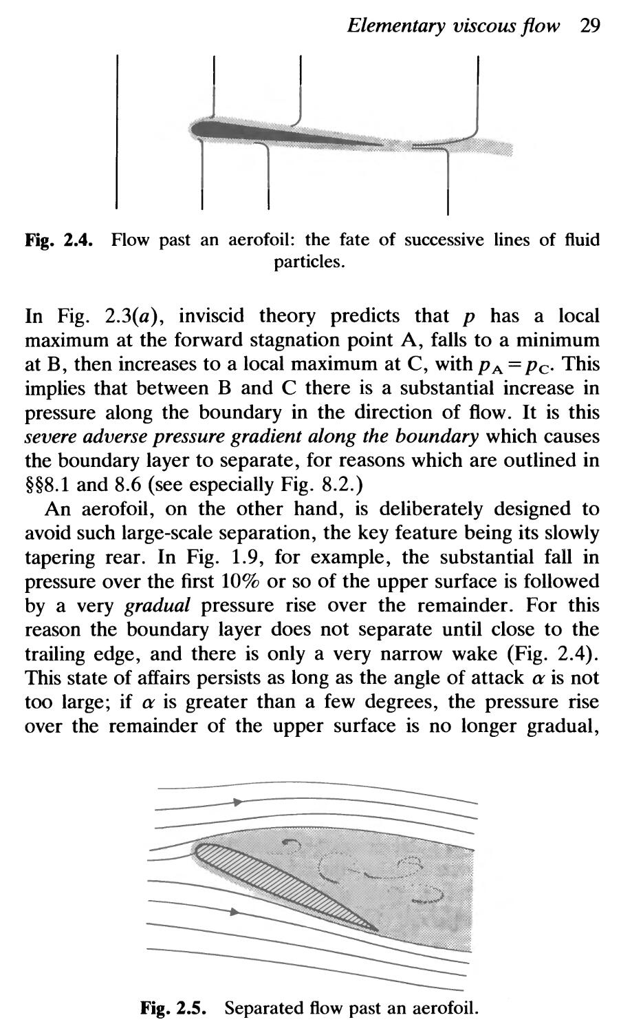
Fig. 2.4. Flow past an aerofoil: the fate of successive lines of fluid
particles.
In Fig. 2.3(a), inviscid theory predicts that p has a local
maximum at the forward stagnation point A, falls to a minimum
at B, then increases to a local maximum at C, with p A = Pc. This
implies that between Band C there is a substantial increase in
pressure along the boundary in the direction of flow. It is this
severe adverse pressure gradient along the boundary which causes
the boundary layer to separate, for reasons which are outlined in
8.1 and 8.6 (see especially Fig. 8.2.)
An aerofoil, on the other hand, is deliberately designed to
avoid such large-scale separation, the key feature being its slowly
tapering rear. In Fig. 1.9, for example, the substantial fall in
pressure over the first 10% or so of the upper surface is followed
by a very gradual pressure rise over the remainder. For this
reason the boundary layer does not separate until close to the
trailing edge, and there is only a very narrow wake (Fig. 2.4).
This state of affairs persists as long as the angle of attack a is not
too large; if a is greater than a few degrees, the pressure rise
over the remainder of the upper surface is no longer gradual,
-=-----
-----
------
Fig. 2.5. Separated flow past an aerofoil.
30 Elementary viscous flow
large-scale separation takes place, and the aerofoil is said to be
stalled, as in Fig. 2.5. This is the explanation for the sudden drop
in lift in Fig. 1.11.
The most important overall message of this introduction is that
the behaviour of a fluid of small viscosity IJ may, on account of
boundary layer separation, be completely different to that of a
(hypothetical) fluid of no viscosity at all. From a mathematical
point of view, what happens in the limit IJ--+ 0 may be quite
different to what happens when IJ = o.
2.2. The equations of viscous flow
So far we have considered the motion of fluids of small viscosity.
Yet there is more to the subject than this, including the opposite
extreme of very viscous flow (Chapter 7). It is time, then, to take
a more balanced-if brief-look at viscous flow as a whole.
The Navier-Stokes equations
Suppose that we have an incompressible Newtonian fluid of
constant density p and constant viscosity IJ. Its motion is
governed by the Navier-Stokes equationst
au 1
at + (u · V)u = - p Vp + vV 2 u + g,
V · u = o.
(2.3)
These differ from the Euler equations (1.12) by virtue of the
viscous term vV 2 u, where V 2 denotes the Laplace operator
/ ax 2 + a 2 / ay2 + a 2 / az 2 .
The no-slip condition
Observations of real (i.e. viscous) fluid flow reveal that both
normal and tangential components of fluid velocity at a rigid
boundary must be equal to those of the boundary itself. Thus if
the boundary is at rest, u = 0 there. The condition on the
tangential component of velocity is known as the no-slip
condition, and it holds for a fluid of any viscosity v =#= 0, no
matter how small v may be.
t The Navier-Stokes equations are derived from first principles in Chapter 6.
Elementary viscous flow 31
The Reynolds number
Consider a viscous fluid in motion, and let U denote a typical
flow speed. Furthermore, let L denote a characteristic length
scale of the flow. This is all somewhat subjective, but in dealing
with the spin-down of a stirred cup of tea, for instance, 4 cm and
5 em S-1 would be reasonable choices for Land U, while 10 m
and 100 m S-1 would not. Having thus chosen a value for Land
for U we may form the quantity
R= UL
,
v
(2.4)
which is a pure number known as a Reynolds number.
To see why R should be important, note that derivatives of the
velocity components, such as aul ax, will typically be of order
U I L-assuming, that is, that the components of u change by
amounts of order U over distances of order L. Typically, these
derivatives will themselves change by amounts of order U I Lover
distances of order L, so second derivatives such as a 2 ul ax 2 will
be of order U I L 2. In this way we obtain the following order of
magnitude estimates for two of the terms in eqn (2.3):
inertia term: I(u. V)ul = O(U 2 IL),
viscous term: IvV 2 ul = O(vUIL 2 ).
(2.5)
Provided that these are correct we deduce that
li ertia terml = O ( U2 I L ) = O(R).
IVISCOUS terml vU I L 2
The Reynolds number is important, then, because it can give a
rough indication of the relative magnitudes of two key terms in
the equations of motion (2.3). It is not surprising, therefore, that
high Reynolds number flows and low Reynolds number flows
have quite different general characteristics.
(2.6)
High Reynolds number flow
The case R » 1 corresponds to what we have hitherto called the
motion of a fluid of small viscosity. Equation (2.6) suggests that
viscous effects should on the whole be negligible, and flow past a
32 Elementary viscous flow
thin aerofoil at small angle of attack provides just one example
where this is indeed the case. Even then, however, viscous effects
become important in thin boundary layers, where the unusually
large velocity gradients make the viscous term much larger than
the estimate in eqn (2.5). We show in 8.1 and 8.2 that the
typical thickness D of such a boundary layer is given by
D/ L = O(R-!).
(2.7)
The larger the Reynolds number, then, the thinner the boundary
layer.
A large Reynolds number is necessary for inviscid theory to
apply over most of the flow field, but it is not sufficient. As we
have seen, boundary layer separation can lead to a quite different
state of affairs. A further complication at high Reynolds number
is that steady flows are often unstable to small disturbances, and
may, as a result, become turbulent. It was in fact in this context
that Reynolds first employed the dimensionless parameter that
now bears his name (see 9.1).
Low Reynolds number flow
Consider a laboratory experiment in which golden syrup occupies
the gap between two circular cylinders, the inner one rotating
and the outer one at rest. For reasonable rotation rates of the
inner cylinder the Reynolds number might be in the region of
10- 2 or so; it will certainly be much less than 1. At such Reynolds
numbers there is no sign of turbulence, and the flow is extremely
well ordered.
The flow is so well ordered, in fact, that if the rotation of the
(a)
(b)
(c)
(d)
(e)
Fig. 2.6. The reversibility of a very viscous flow.
Elementary viscous flow 33
inner cylinder is stopped after a few revolutions, and the inner
cylinder is then rotated back through the correct number of turns
to its original position, a dyed blob of syrup, which has been
greatly sheared in the meantime, will return almost exactly to its
original configuration as a concentrated blob (Fig. 2.6).
This near reversibility is characteristic of low Reynolds number
flows, and helps account, in fact, for the unusual swimming
techniques that are adopted by certain biological micro-
organisms such as the Spermatozoa ( 7.5).
2.3. Some simple viscous flows: the diffusion of vorticity
We now turn to some elementary exact solutions of the
Navier-Stokes equations. There is, in addition, a major theme
running through 2.3 and 2.4, and that theme is the viscous
diffusion of vorticity, an important mechanism which was wholly
absent in Chapter 1, where v was zero.
Plane paraDel shear ftow
Suppose that a viscous fluid is moving so that relative to some set
of rectangular Cartesian coordinates
u = [u(y, t), 0, 0].
(2.8)
Such a flow is termed a plane parallel shear flow. It automatically
satisfies V · u = 0, as u is independent of x, and in the absence of
gravityt the Navier-Stokes equations (2.3) become, in component
form :
au 1 ap cYu
-=---+v-
at p ax ay2 '
ap _ ap _ 0
ay - az - .
The pressure p is thus a function of x and t only. But from eqn
(2.9) ap / ax is equal to the difference between two terms which
are independent of x. Thus ap / ax must be a function of t alone.
As we shall see shortly, there are important circumstances in
which this fact enables us to deduce that ap / ax must be zero.
(2.9)
t See footnote on p. 9.
34 Elementary viscous flow
First, however, it is instructive to see how eqn (2.9) may be
obtained by a simple and direct application of the expression
(2.1) .
An ad hoc derivation of the equations of motion for a viscous
fluid in plane paraDel shear flow
First note that in the absence of viscous forces the corresponding
Euler equation
au ap
p-= --
at ax
(2.10)
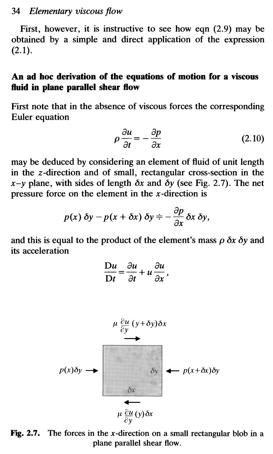
may be deduced by considering an element of fluid of unit length
in the z-direction and of small, rectangular cross-section in the
x-y plane, with sides of length x and y (see Fig. 2.7). The net
pressure force on the element in the x-direction is
ap
p(x) y - p(x + x) y : - - x by,
ax
and this is equal to the product of the element's mass p x y and
its acceleration
Du au au
-=-+u-
Dt at ax '
II AU (y+c5y)c5x
oy
-+
r"""'i], p(x+bx)by
i,illlilfl 'lll
11 AU (y) c5x
oy
Fig. 2.7. The forces in the x-direction on a small rectangular blob in a
plane parallel shear flow.
p(x)c5y --.
Elementary viscous flow 35
which reduces simply to auf at because u is independent of x.
In a similar manner we may use eqn (2.1) to deduce that
viscous forces on the top and bottom of the element give rise to a
net contribution in the x-direction of
au au u
Jl- x - Jl- x : Jl a 2 x y,
ay y+6y ay y y
whence eqn (2.10) becomes modified to
au ap a 2 u
p at = - ax + II. ay2 '
(2.11 )
i.e. to eqn (2.9).
This equation is, of course, valid only for a very restricted class
of flows, but the brevity of the above derivation does have its
merits. In particular, it brings out rather clearly, via eqns (2.1)
and (2.11), why the viscous term in the equation of motion (2.3)
involves the second derivatives of the velocity field.
The flow due to an impulsively moved plane boundary
Suppose that viscous fluid lies at rest in the region 0 < y < 00 and
suppose that at t = 0 the rigid boundary y = 0 is suddenly jerked
into motion in the x-direction with constant speed U. By virtue
of the no-slip condition the fluid elements in contact with the
boundary will immediately move with velocity U . We wish to
find how the rest of the fluid responds.
It is natural to look for a flow of the form (2.8), and eqn (2.9)
then applies. We assume that the flow is being driven only by the
motion of the boundary, Le. not by any externally applied
pressure gradient. This experimental consideration corresponds
to asserting that the pressures at x = :i:oo are equal, and as ap / ax
is independent of x (so that p is a linear function of x) it follows
that ap / ax is zero.
The velocity u(y, t) thus satisfies the classical one-dimensional
diffusion equation
au a 2 u
-=v-
at ay 2 '
together with the initial condition
(2.12)
u(y, 0) = 0,
y>O,
36 Elementary viscous flow
and the boundary conditions
u(O, t) = U, t > 0,
u(oo, t) = 0, t > O.
This whole problem is in fact identical with the problem of the
spreading of heat through a thermally conducting solid when its
boundary temperature is suddenly raised from zero to some
constant.
We may proceed most easily, on this occasion, by seeking a
similarity solution. We postpone a more rational discussion of
this method until 8.3; for the time being we simply observe that
the equation is unchanged by the transformation of variables
y ay, t crt, a being a constant. This suggests the possibility
that there are solutions to eqn (2.12) which are functions of y and
t simply through the single combination y / t!, for this 'similarity'
variable would itself be unchanged by such a transformation.
Inspection of eqn (2.12) suggests that it may be more convenient
still to take y /( vt)! as the similarity variable. Thus if we try
u=f(TJ), whereTJ=y/(vt)!, (2.13)
so that
au , aTJ , y
at = f (TJ) at = -f (TJ) 2v!t '
au aTJ 1
_ a =f'(TJ)- a =f'(TJ) I t 1 ' etc.,
Y Y v 2 2
we obtain, from eqn (2.12),
f" + !TJf' = O.
Integrating,
f' = Be-,,2 /4 ,
whence
f = A + B r e- s2/4 ds,
where A and B are constants of integration, to be determined
from the initial and boundary conditions. By virtue of eqn (2.13)
these reduce to
f(oo) = 0,
f(O) = U,
Elementary viscous flow 37
so that
u = u[ 1- ! r e- S2 / 4 ds] (2.14)
is the solution of the problem, where 1] = y / ( vt )!.
The simple form of the initial and boundary conditions was
essential to the success of the method. The underlying reason lies
in the nature of the similarity solution (2.14) itself. As its name
implies, the velocity profiles u(y) are, at different times, all
geometrically similar. At time tIthe velocity u is a function of
y /( VtI)!; at a later time t 2 the velocity u is the same function of
y / ( vt 2 )!. All that happens as time goes on is that the velocity
profile becomes stretched out, as indicated in Fig. 2.8. We would
not expect this to be the case if, for instance, an upper boundary
were present, and the solution is, indeed, not then of similarity
form (see eqn (2.21».
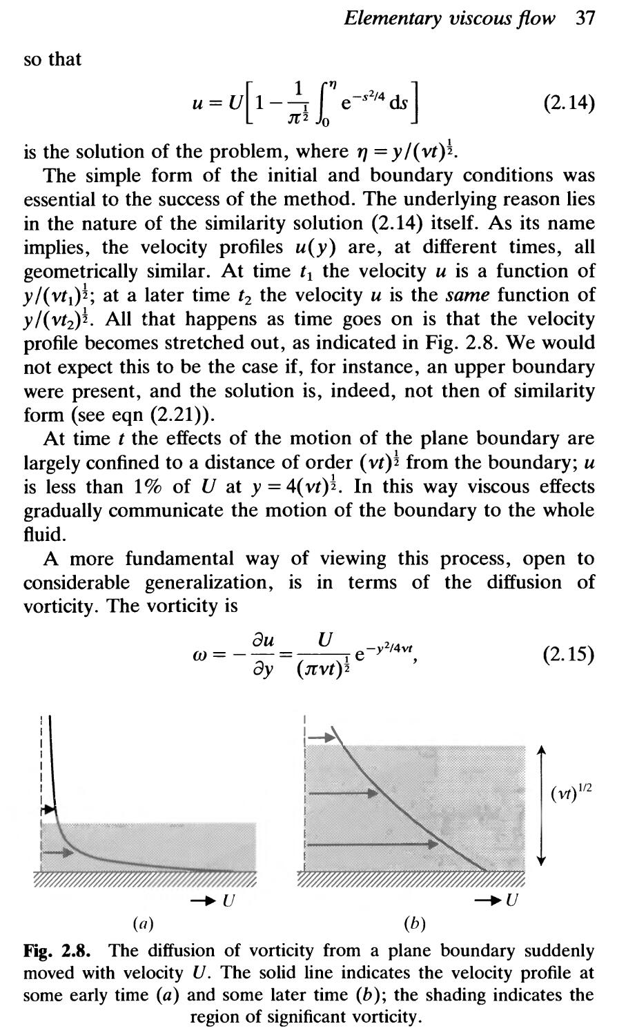
At time t the effects of the motion of the plane boundary are
largely confined to a distance of order (vt)! from the boundary; u
is less than 1 % of U at y = 4( vt)!. In this way viscous effects
gradually communicate the motion of the boundary to the whole
fluid.
A more fundamental way of viewing this process, open to
considerable generalization, is in terms of the diffusion of
vorticity. The vorticity is
(J) = - au = U 1 e- y2 / 4vt
ay (Jl'vt)z '
(2.15)
I
I
I
I
t . .:.:.:.: .''''''''' :.:.:...'.(.:.....:.....:.:.
f:
I ;:.. .. . ... . ....
. .
. . .... ...................................................
. "0" ......... ......................................................................................................
. .0. .................................
. ..- ................-................
.0. .................................
.....................................
.....................................
-.-.................................
..... ...........................
.... ............................
..... ...........................
................-................
.................................
.................................
.................................
.................................
.................................
.................................
................-................
............. ........... .,.
............ ..............
............ ...........-...
......... ....................
.......... .....................
. .....................................
. . .....................................
. ..................................... 1/2
... . ................................. ...
.... ....... p ..) .{::I,'{I)I ! ; 1 (11)
: !:, .tt:; :!:tJli!
A
-+u
(a) (b)
Fig. 2.8. The diffusion of vorticity from a plane boundary suddenly
moved with velocity U. The solid line indicates the velocity profile at
some early time (a) and some later time (b); the shading indicates the
region of significant vorticity.
38 Elementary viscous flow
and this is exponentially small beyond a distance of order (vt)!
from the boundary. The spreading of vorticity by viscous action
thus smooths out what was, initially, a vortex sheet, i.e. an
infinite concentration of vorticity at the boundary (y = 0, t 0)
with none elsewhere (y > 0, t 0).
Finally we may state these broad conclusions in a slightly
different way. Vorticity diffuses a distance of order (vt)! in time
t. Equivalently, the time taken for vorticity to diffuse a distance of
order L is of the order
viscous diffusion time = O(L 2 /v). (2.16)
Steady flow under gravity down an inclined plane
This next solution of the Navier-Stokes equations serves to make
one or two elementary points about technique.
It may be argued that the key step in solving any flow problem,
having decided on a sensible coordinate system, is to decide the
number of independent variables (e.g. x, y, z, t) on which u
depends, and the rule is 'the fewer, the better'.
In the present problem u is zero on y = 0 (see Fig. 2.9), by
virtue of the no-slip condition, so u must depend on y. In the
absence of any a priori reason why u needs to depend on
apything else we examine the possibility that there is a
two-dimensional steady flow solution 10 which u =
[u(y), v(y), 0].
Now, it is only common sense in any problem to turn to the
incompressibility condition at an early stage, for of the two
!g
::
:J
--------------
Fig. 2.9. Steady flow of a viscous fluid down an inclined plane.
Elementary viscous flow 39
equations (2.3) it is by far the simpler. In the present instance it
tells us immediately that
dv/dy = 0,
i.e. that v is a constant. But v = 0 on y = 0, so v is zero
everywhere.
Substituting u = [u(y), 0, 0] into the momentum equation
(2.3), with the gravitational body force included, we obtain
1 ap d 2 u
0= ---+ v-+ g sin a,
p ax dy2
o = _.!. ap
pay
(2.17)
- g cos £1'.
Integrating the second of these we find
p = -pgy cos £1'+ f(x),
where f (x) is an arbitrary function of x.
Now, the free surface must be y = h, where h is a constant,
because all the streamlines are parallel to the plane. At this free
surface the tangential stress must be zero and the pressure p must
be equal to atmospheric pressure Po (see Exercise 6.3), so
du
p = Po and J.l- = 0
dy
by virtue of eqn (2.1). Consequently,
p - Po = pg(h - y)cos a,
.hence ap / ax is zero. Equation (2.17) then reduces to
d 2 u .
V dy2 = -g sIn a,
at y = h,
(2.18)
and we may easily integrate this twice, applying the boundary
conditions
u = 0 at y = 0,
du
J.l- = 0 at y = h,
dy
to obtain
u = y (2h - y)sin £1'.
2v
(2.19)
40 Elementary viscous flow
The velocity profile is therefore parabolic, as shown in Fig. 2.9.
The volume flux down the plane, per unit length in the
z-direction, is
L h gh3
Q= udy=-sina.
o 3v
Another example of vorticity ditfusion
Consider the problem in Fig. 2.10, in which a lower rigid
boundary y = 0 is suddenly moved with speed U, while an upper
rigid boundary to the fluid, y = h, is held at rest. As in an earlier
subsection, we argue that u = [u(y, t), 0, 0] will satisfy eqn
(2.12):
au a 2 u
-=v-
at ay2 '
subject to the initial condition
(2.20)
u(y, 0) = 0,
O<y<h;
but this time the boundary conditions will be
u(O, t) = U, t > 0,
u(h, t) = 0, t > O.
The equation is homogeneous, but the boundary conditions
are not. Before using the method of separation of variables and
"/
"/
I
I} ;;;i;::: t;;: i::;i:; ;;;:;;:::r::: :;::::::::: : ::: tttt I r??jIII {If:.:.:j!
=1:::' .--
:::::: -J ::::'_ ---_ -
f: t i:\: -- -
1r i.---'--
= ::. 1 .:.:.:.: _ _ _ . - __
1:-1'---
::::.: 1-:.':::::
1 L}\::;:::-::---- - - - - - - --
'1 t-
1 !
:1tj':"':':
h
/.
--+u -+u
(a) t« h 2 /v (b) t 2h2/v
Fig. 2.10. Flow between two rigid boundaries, one suddenly moved
with speed U and one held fixed. Shading indicates regions of significant
vorticity.
Elementary viscous flow 41
Fourier series we therefore reformulate the problem by first
seeking a steady solution that satisfies the boundary conditions;
this is clearly U(1- y/h). We therefore write
u=U(1-y/h)+UI,
where
aU I a2UI
-=v-
at ay2 '
uI(y,0)=-U(1-y/h), O<y<h,
ul(O,t)=O, t>O, ul(h,t)=O, t>O.
The boundary conditions are now homogeneous. By the
method of separation of variables we find that the functions
exp( -n 2 :Jr2vt/ h 2 )sin(n:JrY / h), n = 1, 2, . . . .
all satisfy the equation for UI and the boundary conditions for UI
at y = 0, h. None of these individually satisfies the initial
condition for UI, but by writing
00
UI = L An exp( -n 2 :Jr2vt/ h 2 )sin(n:JrY / h),
n=l
we may use Fourier theory to determine the An such that
00
L An sin(n:Jry/h) = -U(1- y/h)
n=l
in 0 < y < h,
thus satisfying the initial condition. In this way we find
2 L h
An=- h 0 U(1-y/h)sin(mry/h)dy=-2U/mr,
and the solution is therefore
2U 00 1
u(y, t) = U(1- y/h) - - L - exp( -n 2 :Jr 2 vt/h 2 )sin(n:Jry/h).
:Jr n=l n
(2.21 )
The main feature of this solution is that for times t;;::: h 2 / v (cf.
eqn (2.16» the flow has almost reached its steady state, as in Fig.
2.10(b), and the vorticity is almost distributed uniformly
throughout the fluid.
42 Elementary viscous flow
2.4. Flow with circular streamlines
The Navier-Stokes equations are
au 1
at + (u · V)u = - p Vp + vV 2 u,
V · U = 0,
and when written out in cylindrical polar coordinates they
become
au,
- + ( u · V ) u
at '
u
r
= _.! ap + V ( V 2 u _ U, _ aU 8 )
p ar ',2,2 ao
aU8 U,U8 1 ap ( 2 2 au, U 8 )
-+ (u. V)U8 +- = ---+ v V U8 +----
at r pr ao ,2 ao ,2
(2.22)
1 ap 2
= ---+ vV u
p az z,
au z
- + ( u · V ) u
at z
1 a 1 aU8 au z
--(ru )+--+-=0
, ar ' r ao az '
where
a U8 a a
( u · V ) = u - + - - + u -
, ar r ao z az '
l a ( a ) 1 a 2 a 2
v 2 =-- r- +--+-
r ar ar r 2 ao 2 az 2 '
(see eqn (A.35».
Note the 'extra' terms that arise; the r-component of (u · V)u is
not (u · V)u" for instance, but (u · V)u, - u /, instead. This kind
of thing occurs because u = u,e, + U8e8 + uze z , and some of the
unit vectors involved change with 0:
ae,
ao = e8,
ae8
ao = -en
ae z = 0
ao '
(2.23)
(see eqn (A.29». When (u. V)u and v V 2 u are expanded
carefully using these expressions they may be seen to yield eqn
(2.22).
Elementary viscous flow 43
Taking explicit account of the change in direction of unit
vectors may alternatively be avoided by use of the identities
(U · V)U = (V A U) A U + V(!U 2 ),
V 2 U=V(V.U)-V A(V AU).
For this purpose we recall
(2.24)
(2.25)
e r ree e z
1 a
VAU=-
r ar
a a
ao az
(2. 26)
U r rUe U z
(see Exercise 2.13).
The Merential equation for circular flow
Consider solutions to the Navier-Stokes equations of the form
U = ue(r, t)ee,
(2.27)
so that the streamlines are circular. The incompressibility
condition V. U = 0 is automatically satisfied for any flow of the
form (2.27).
Rather than use the remaining equations in the ready-made
form (2.22) it is instructive to derive them, for the flow (2.27),
using the expressions (2.23). Thus
Ue a u ae e u
(u · V)u = -;: ao [ue(r, t)ee] = -;: ao = - -; en (2.28)
while
( a 2 1a 1 a 2 a 2 )
vV 2 u-= v ---Z+--+2 +---Z [ue(r-, t)ee],
ar r ar r ao az
and
1 a 2 1 a ( aee ) -1 a Ue
r 2 ao 2 [Ueee] = r 2 ao Ue ao = r 2 ao (uee r ) = - r2 ee,
so
2 ( a2ue 1 aUe Ue )
vV U = v -+---- ee.
ar 2 r ar r 2
(2.29)
44 Elementary viscous flow
When u = u8(r, t)e8 the Navier-Stokes equations therefore
reduce to
u 1 ap
---
r p ar '
aU8 = _ ap + V ( cfuo + ! auo _ u o )
at pr ao ar 2 r ar r 2 '
o = _.! ap
paz'
as we might have deduced more quickly from eqn (2.22).
Now, U8 is a function of rand t only, so from the second
equation the same must be true of ap/ao, so ap/ao = P(r, t),
say. Integrating:
p = P(r, t)O + f(r, t),
as ap/ az = O. We conclude that P(r, t) = 0, for otherwise p
would be a multivalued function of position (different at 0 = 0
and at 0 = 2Jr, say). Thus
aU8 = V ( a2uo + ! auo _ u o ) (2.30)
at ar 2 r ar r 2
is the evolution equation for a viscous flow with u = u8(r, t)e8'
Steady flow between rotating cylinders
For steady flow we have
2 d2U8 dU8
r dr 2 + r dr - U8 = 0,
with general solution
B
U8 =Ar +-.
r
(2.31 )
If the fluid occupies the gap rl r r2 between two circular
cylinders which rotate with angular velocities Ql and Q2, then we
may apply the no-slip condition at each cylinder to obtain
Q2r - Ql r i (Ql - Q2)rir
A = 2 2 ' B = 2 2 ' (2.32)
r2- r l r2- r l
Elementary viscous flow 45
The most interesting thing about this flow is the manner in
which it becomes unstable if Ql is too large, so that superbly
regular and axisymmetric Taylor vortices appear (see 9.4,
especially Fig. 9.8).
Spin-down in an infinitely long circular cylinder
Suppose viscous fluid occupies the region r a within a circular
cylinder of radius a, and suppose that both cylinder and fluid are
initially rotating with uniform angular velocity Q, so that
Uo = Qr,
r a,
t = O.
Suppose that the cylinder is then suddenly brought to rest. We
need to solve
auo = V ( a2ue + ! aUe _ Ue )
at ar 2 r ar r 2
with the above initial condition and the boundary condition
U(J = 0 at r = a, t > O.
The problem may be tackled in a Fourier-series type manner,
as for eqn (2.21), but the separable solutions now involve Bessel
functions, and
J 1 (A n rla) ( 2 v t )
ue(r, t)= -2Qa L.J A (A) exp -A n "2 ·
n=1 nJO n a
(2.33)
Here An denote the positive values of A at which J 1 (A) = 0, and J k
denotes the Bessel function of order k. All the terms of the series
decay rapidly with t; the one that survives longest is the first one,
and Al : 3.83. The 'spin-down' process is therefore well under
way in a time of order a 2 /vAi, i.e. in the classic viscous diffusion
time (2.16).
If we apply this to a stirred cup of tea, with a = 4 cm and
v = 10- 2 cm 2 S-1 for water, we obtain a 'spin-down' time of about
2 minutes. This is much too long; casual observation suggests
that U(J drops to about lie of its original value in about 15 s. The
discrepancy arises because straightforward diffusion of (negative)
vorticity from the side walls is not the key process by which a
stirred cup of tea comes to rest; the bottom of the cup-wholly
absent in the present model-plays a crucial role (see Fig. 5.6.)
46 Elementary viscous flow
(a)
(b)
Fig. 2.11. 'Spin-down' in an infinitely long circular cylinder. Initially
there is vorticity 2Q everywhere, but negative vorticity diffuses inward
from the stationary boundary r = a, so that the (shaded) region of
significant vorticity shrinks with time.
Viscous decay of a line vortex
The line vortex
ro
u =- 2 eo,
nr
(2.34)
where ro is a constant, has zero vorticity in r > 0 but infinite
vorticity at r = O. In a viscous fluid, then, this flow does not
persist; the vorticity diffuses outward as time goes on.
To examine this process it is convenient to take the circulation
r(r, t) = 2nruo(r, t)
(2.35)
as the dependent variable of the problem. In place of eqn (2.30)
we then obtain
ar _ ( a 2 r 1 ar )
--v ----
at ar 2 r ar .
The initial condition is
(2.36)
r(r, 0) = Fo.
We require U o finite at r = 0 at any later time, so
r(o, t) = 0, t > O.
Elementary viscous flow 47
This problem is very similar to that in which a plane rigid
boundary is jerked into motion (see eqn (2.14»; we leave it as an
exercise to seek, as in that case, a similarity solution in which
r=f(1]),
where 1] = r/( vt)!.
In this way we may discover that
r = ro(l - e-r2/4vt),
so
r
- (1 - -r 2 /4vt )
U(J - 2 e .
Jtr
(2.37)
At distances greater than about (4vt)! from the axis the
circulation is almost unaltered, because very little vorticity has
yet diffused that far out. At small distances from the axis,
however, where r« (4vt) , the flow is no longer remotely
irrotational; indeed
. ro
U(J . - r
8Jtvt
for
1
r« (4vt)2,
(2.38)
which corresponds to almost uniform rotation with angular
velocity r o/8Jtvt. The intensity of the vortex thus decreases with
time as the 'core' spreads radially outward (Fig. 2.12).
(a)
(b)
Fig. 2.12. The viscous diffusion of a vortex.
48 Elementary viscous flow
2.5. The convection and diffusion of vorticity
If we take the curl of the momentum equation (2.3) we obtain
aro
- + (u · V)ro = (ro · V)u + v V 2 ro,
at
(2.39)
(cf. eqn (1.25)), and in the case of a 2-D flow this reduces to
aw ( a2 w a 2 W )
-+ (u. V)w = v -+- . (2.40)
at ax 2 ay2
In Chapter 1 we set the viscosity v to zero from the outset; w
was then conserved by individual fluid elements in 2-D flow.
Changes in w at a particular point in space took place only by the
convection of vorticity from elsewhere in the fluid, and this
process is represented by the second term in eqn (2.40). In 2.3
and 2.4, on the other hand, we looked at some simple viscous
flow problems in which the term (u. V)w happened to be
identically zero; in other words, we isolated diffusion of vorticity
as a mechanism, this being represented by the third term in eqn
(2.40) .
In general, there is both diffusion and convection of vorticity in
a viscous fluid flow, and we end this chapter with two examples.
2-D flow near a stagnation point
The main features of this exact solution of the Navier-Stokes
equations (Exercise 2.14) are as follows. First, there is an inviscid
'mainstream' flow
u = ax,
v = -ay,
(2.41 )
where a is a positive constant. This fails to satisfy the no-slip
condition at the rigid boundary y = 0, but the mainstream flow
speed a Ix I increases with distance Ix I along the boundary. By
Bernoulli's theorem, the mainstream pressure p decreases with
distance along the boundary in the flow direction (Fig. 2.13), so
we may hope for a thin, unseparated boundary layer which
adjusts the velocity to satisfy the no-slip condition (see 2.1).
This is indeed the case, as Exercise 2.14 shows, and the boundary
layer, in which all the vorticity is concentrated, has thickness
Elementary viscous flow 49
Y I \
Low
High Low
JC l ;;;jJJ)!
x
Low
1 O( v/a) 1/2
Fig. 2.13. Flow towards a 2-D stagnation point.
D = O(v/a)!. In this boundary layer there is a steady state
balance between the viscous diffusion of vorticity from the wall
and the convection of vorticity towards the wall by the flow. Thus
if v decreases the diffusive effect is weakened, while if a
increases the convective effect is enhanced; in either case the
boundary layer becomes thinner.
High Reynolds number flow past a flat plate
In uniform flow past a flat plate with a leading edge, as in Fig. 2.14,
there is no flow component convecting vorticity towards the plate
to counter the diffusion of vorticity from it, so the boundary layer
becomes progressively thicker with downstream distance x. (In
less formal terms, the layers of fluid closest to the centreline are
the first to be slowed down as they pass the leading edge,
and they in turn gradually slow down the layers of fluid which are
further away.)
y
--. .
A'..: ::%:% :=::::::::::;:::-::\::::"
: :::::::
..........
1-( r
--+u
--+
............. .......
"<@] jJgli;;!;;i;il;I,I;,ji;;iii!ii;iilll
-....;. -: _......::LU\i(iltJLtUL\fU\IE<J\ltII
--+
Fig. 2.14. The boundary layer on a flat plate.
50 Elementary viscous flow
We may estimate the boundary layer thickness by a simple
argument based on the related problem in which the flat plate is
instead suddenly pulled to the left, with speed V, through fluid
which was previously at rest. From Fig. 2.8 we infer that at time t
after the plate is moved vorticity will have diffused out a distance
of order (vt)!. But by this time the leading edge of the plate will
have moved a distance x = Vt to the left. It follows that at
distance x downstream from the leading edge there will be
significant vorticity a distance of order
'- (vx/ V)! (2.42)
from the plate, but not beyond.
This crude estimate for the growth of the boundary layer with
downstream distance x in Fig. 2.14 is indeed confirmed by the
appropriate solution of the boundary layer equations (see 8.3).
For a plate of finite length L the thickness (2.42) is in keeping
with the claim (2.7) and is small compared with L at all points of
the plate if R = VL/v» 1.
Exercises
2.1. Give an order of magnitude estimate of the Reynolds number for:
(i) flow past the wing of a jumbo jet at 150 m s -1 (roughly half the
speed of sound);
(ii) the experiment in 1.1 with, say, L = 2 cm and U = 5 cm S-I;
(iii) a thick layer of golden syrup draining off a spoon;
(iv) a spermatozoan with tail length of 10- 3 cm sWimming at
10- 2 cm S-1 in water.
Give an order of magnitude estimate of the thickness of the
boundary layer in case (i).
2.2. The problem of 2-D steady viscous flow past a circular cylinder of
radius a involves finding a velocity field u = [u(x, y), v(x, y), 0] which
satisfies
1
(u. V)u = --Vp + vV 2 u,
P
V.u=O
,
together with the boundary conditions
u = 0 on x 2 + y2 = a 2 ;
U (U 0 0) asx 2 +y 2 ao .
, ,
Elementary viscous flow 51
Rewrite this problem in dimensionless form by using the dimensionless
variables
x' = x/a,
u' = u/V,
p'=p/pV z
in places of x, u, and p. Without attempting to solve the problem, show
that the streamline pattern can depend on v, a, and V only in the
combination R = Va/v, so that flows at equal Reynolds numbers are
geometrically similar.
2.3. (i) Viscous fluid flows between two stationary rigid boundaries
y = r.h under a constant pressure gradient P = -dp/dx. Show that
P
u = 2p. (h 2 - y2),
v = w = O.
(ii) Viscous fluid flows down a pipe of circular cross-section r = a
under a constant pressure gradient P = -dp/dz. Show that
P
U = - ( a Z - rZ )
z 4/-l '
U r = Ue = o.
[These are called Poiseuille flows (Fig. 2.15), after the physician who
first studied (ii) in connection with blood flow. Their instability at high
Reynolds number constitutes one of the most important problems of
fluid dynamics (see 9.1).]
2.4. Two incompressible viscous fluids of the same density p flow, one
on top of the other, down an inclined plane making an angle a with the
horizontal. Their viscosities are /-It and /-lz, the lower fluid is of depth ht
and the upper fluid is of depth h z . Show that
t Z ] g sIn a
ut(Y) = [(ht + hz)y - zy ,
v t
so that the velocity of the lower fluid U t (y) is dependent on the depth
hz, but not the viscosity, of the upper fluid. Why is this?
I
, .
i
High I .... Low
P ... P
: . .
__m m mmm___
Fig. 2.15. Poiseuille flow.
52 Elementary viscous flow
2.5. Viscous fluid is at rest in a two-dimensional channel between two
stationary rigid walls y = i:.h. For t 0 a constant pressure gradient
P = -dp/dx is imposed. Show that u(y, t) satisfies
au a 2 u P
-= v-+-
at ay2 p ,
and give suitable initial and boundary conditions. Find u(y, t) in the
form of a Fourier series, and show that the flow approximates to steady
channel flow when t» h 2 /v.
2.6. Viscous fluid flows between two rigid boundaries y = 0, y = h, the
lower boundary moving in the x-direction with constant speed U, the
upper boundary being at rest. The boundaries are porous, and the
vertical velocity v is -Vo at each one, V o being a given constant (so that
there is an imposed flow across the system). Show that the resulting flow
IS
( e -voy/v - e -Voh/V )
u=U
l-e- voh / v '
v = -V o .
Show that the horizontal velocity profile u(y) is as in Fig. 2.16, so that
when voh / v is large the down flow V o confines the vorticity to a very thin
layer adjacent to y = O.
[This is probably the mathematically simplest example of a steady
boundary layer, but it is untypical in that the boundary layer thickness is
proportional to v, rather than to v! (see eqn (2.7)).]
2.7. Incompressible fluid occupies the space 0 < y < 00 above a plane
rigid boundary y = 0 which oscillates to and fro in the x-direction with
velocity U cos wt. Show that the velocity field u = [u(y, t), 0, 0] satisfies
au a 2 u
-=v-
at ay2
t Vo
o
y=h
7
o
y=O
h
U
.Vo u-+
(a)
(h)
Fig. 2.16. Wall-driven channel flow with (a) V o = 0 and (b) voh/v» 1.
Elementary viscous flow 53
(there being no applied pressure gradient), and by seeking a solution of
the form
U = [f(y )e iOJ 1,
where denotes 'real part of, show that
u(y, t) = Ue- ky cos(ky - wt),
where k = (wI2v)t
Sketch the velocity profile at some time t, and note that there is hardly
any motion beyond a distance of order (v I w)! from the boundary.
2.8. A circular cylinder of radius a rotates with constant angular
velocity Q in a viscous fluid. Show that the line vortex flow
Qa 2
u =-ee,
r
r ;?; a,
is an exact solution of the equations and boundary conditions. Describe
roughly how the vorticity changes with time when the cylinder is
suddenly started into rotation with angular velocity Q from a state of
rest. Likewise, discuss the case in which an outer cylinder r = b is
simultaneously given an angular velocity Qa 2 I b 2 .
2.9. A viscous flow is generated in r;?; a by a circular cylinder r = a
which rotates with constant angular velocity Q. There is also a radial
inflow which results from a uniform suction on the (porous) cylinder, so
that U r = -U on r = a. Show that
U r = -Ualr
for r ;?; a,
and that
d 2 u(J dUe
r 2 -+ ( R+1 ) r-+ ( R-1 ) u =0
dr 2 dr e,
where R = Ual v.
Show that if R < 2 there is just one solution of this equation which
satisfies the no-slip condition on r = a and has finite circulation
r = 2nru e at infinity, but that if R > 2 there are many such solutions.
2.10. Show that, as claimed in eqn (2.37), a line vortex of strength r 0
decays by viscous diffusion in the following manner:
r 0 (1 -r2/4v )
U =- -e
e 2 .
nr
Calculate and sketch the vorticity as a function of r at two different
times.
54 Elementary viscous flow
2.11. Viscous fluid occupies the region 0 < z < h between two rigid
boundaries z = 0 and z = h. The lower boundary is at rest, the upper
boundary rotates with constant angular velocity Q about the z-axis.
Show that a steady solution of the full Navier-Stokes equations of the
form
U = u9(r, z)e9
is not possible, so that any rotary motion u9(r, z) in this system must be
accompanied by a secondary flow (un U z * 0).
2.12. Viscous fluid is inside an infinitely long circular cylinder r = a
which is rotating with angular velocity Q, so that U 9 = Qr for r a. The
cylinder is suddenly brought to rest at t = O. Rewrite the evolution
equation (2.30) in the form
aU9 =! ( r aU9 ) _ VU 9
at r ar ar r 2 ,
and thereby show that
dE 2v
-+-E O
dt a 2 ,
where
E =! f ru dr,
which is proportional to the kinetic energy of the flow. Hence show that
E O as t oo.
[This may seem a little pointless, given that the exact solution (2.33) is
available, but the above approach is in fact of very general value, and
provides the basis for the proof, in 9. 7, of an important uniqueness
theorem. ]
2.13. Re-derive the results (2.28) and (2.29) by the alternative route
involving eqns (2.24), (2.25), and (2.26).
2.14. Consider in y ;;0; 0 the 2-D flow
U = axf' ( 17 ),
v = -( vll') f( 17),
where
17 = (ll'/v) y.
Show that it is an exact solution of the Navier-Stokes equations which
(i) satisfies the boundary conditions at the stationary rigid boundary
y = 0 and (ii) takes the asymptotic form U --., ax, v --., - ay far from the
Elementary viscous flow 55
3 :-:.-- - - - ------------. "' :
...... ..... ..... .......... ....
....... ...... ...... .......... .....
....... ..... ..... .......... ....
.............,............ -
........ .....
2 ::};::: - -:-;-;-:---:.:- -.. . - -..._.:.:......:::.:::._.... ::.: : JI[ I
I
I
.... ........ - I
I
I
I
I
I
I
I
1
f'( 1])
Fig. 2.17. The velocity profile in the boundary layer near a 2-D
stagnation point.
boundary (see Fig. 2.13) if
f'" + ff" + 1 - f,2 = 0,
with
f(O) = f'(O) = 0,
f'(oo) = 1.
[The differential equation for f( 1]) is solved numerically, and f' (1]) is
shown in Fig. 2.17. Notably, f'(3) = 0.998, so beyond a distance of
3( v / a)! from the boundary the flow is effectively inviscid and
irrotational, with u : ax and v : - ay. ]
2.15. If a flat plate is fixed between (0,0) and (0, L) in Fig. 2.13, with
L » (v / a) , one might at first think that the flow would not be much
affected, for the plate lies along one of the streamlines of the original
flow. Why is it, then, that the observed flow is quite different, as in Fig.
2.18?
Fig. 2.18. High Reynolds number stagnation-point flow with a
protruding flat plate.
3 Waves
3.1. Introduction
When a group of waves moves across the surface of a pond, each
particular wavecrest travels faster than the group as a whole, and
eventually passes through it. Thus new crests are continually
being created at the back of the group while old crests are
continually disappearing at the front. Suppose, for instance, that
a snapshot of the wavetrain reveals ten crests, as in Fig. 3.1. A
stationary observer at some fixed x will count substantially more
than ten crests as the whole wavetrain passes by.
The reason for this curious behaviour is that water waves are
dispersive, i.e. the different Fourier components that make up a
general disturbance propagate at different speeds, depending on
their wavelength. We show in fact, in 3.2, that a simple
harmonic surface wave described by
TJ = A cos(kx - wt),
(3.1)
where k and ware both positive, has a wave speed
1
C = w/k = (g/k)2
(3.2)
so that waves of longer wavelength A = 2n / k travel faster.
(Contrast this with small amplitude waves on a stretched string,
where all disturbances travel at a speed determined wholly by the
tension in the string and its mass per unit length.) We show
further, in 3.3, that while each individual wavecrest in Fig. 3.1
travels with speed c, the velocity of travel of the group as a
whole is the so-called 'group velocity'
dw
c g = dk .
(3.3)
According to eqn (3.2) the frequency is given by
1
W = (gk)2
(3.4)
Waves 57
Y
Y=1J(x,t) -+
. ...................
...-.-. .......--.............---------- - ..
...._._ .......................................6
....... .............----.......................
..................--...................---.....--.
.. .... ..............-------...............---...........
- -- .... .............................-----..-............
. .. . ... ......----.......................--.--....................-.
. .. ::::::..-_ ::: ...........:::::::::::::::::::::::::::::::.:::::::::::.":::::::::0-::::::::::::::::::::::::::::::::::::::::::::::::::::::::::::::.
. .. ::::::::::::::. .:::::::::::::::::::::::::::::::::::::::::::::::::::::::::::::::::::::::::::::::::::::::.:::::::::.::::::::: : :::::::::::::::::::::::::::::::::::::::::::::::::::::::
. ... ........ ...................................................................................
- . ........ ...................................................................................
......... ..............................................................
........ ..............................................................
.. ...... ..............................................................
............... ...........................................
............... ...........................................
- - - --- ....-..............- ......................
........" ............................ ............................................
:.:::::=::::::;::::::=::::::::::::::::=::=:::=:::::::::::::::::::::::::::::::::::::::::::::::::::
......................................................
:: :." ....... ....... . ......... :::.:.:. .::.............. ........... ......... .... .... .:.... .:.:;:;:;:.: :..::;: ; ; ; :;;;;;;; : ;; = : i ;: : ; : : : : i : : : ;
Fig. 3.1. A group of surface waves on deep water.
!g
so the group velocity is
c g = !(g / k)! = !c. (3.5)
Thus in the case of surface waves on (deep) water, individual
wavecrests travel twice as fast as the group as a whole, and this is
why they may be seen to be continually appearing at the back of
the group and disappearing at the front.
The dispersive property of water waves is fundamental. It is
responsible, for example, for the complicated wave pattern
behind a moving ship (Fig. 3.2(a». For very short waves, surface
tension effects make the dispersion properties even more
complicated ( 3.4). If, for example, water flows past a fishing
line, the stationary wave pattern contains both upstream and
downstream disturbances (Fig. 3.2(b ».
We obtain a still broader class of wave if we consider
disturbances to the interface between two fluids. If the lower
fluid has density PI and the upper fluid has density P2 < PI, then
(a)
(b)
Fig. 3.2. Stationary wave patterns in (a) flow past a ship and (b) flow
past a fishing line.
58 Waves
in place of eqn (3.2) we find
c 2 = g ( PI - P2 )
k PI + P2
(Exercise 3.2). Buoyancy, i.e. the action of gravity on density
differences, is here seen to be the mechanism responsible for the
waves. We may view (3.2) as an extreme case, with P2 = O. If, on
the other hand, the densities PI and P2 are almost equal-as
would be the case with a layer of fresh water overlying a layer of
salty water-then the wave speed c is much reduced.
A rather different kind of wave can arise if the density of a
fluid decreases continuously with height. Buoyancy forces are
again responsible, but now internal gravity waves travel through
the main body of the fluid, and possess some surprising
properties, as we see in 3.8.
But buoyancy is not, of course, the only mechanism that
enables a fluid to support wave motion. Another is compres-
sibility, which permits the propagation of sound waves. We show
in 3.6 that small-amplitude sound waves propagate through a
gas at the speed of sound:
1
ao = (YPol PO)2, (3.7)
(3.6)
where Po and Po denote the background pressure and density
respectively, while Y is a constant for the gas in question,
approximately 1.4 for air. The most notable feature of eqn (3.7),
given all the remarks above, is that it is independent of the
wavelength of the waves. Sound waves are therefore non-
dispersive.
In fact, eqn (3.7) also reveals why, elsewhere in the text, we so
readily treat aerodynamic problems using incompressible flow
theory. Isn't air compressible? It is, of course, but it may
nevertheless be that, in a particular motion, the air is not being
much compressed. By virtue of eqn (3.7) we may write the
background pressure Po as poa 1 y. By inspection of the equations
of motion, however, it is evident that the pressure fluctuations PI
within the gas associated with the fluid motion are of order P o U 2 ,
where U is a typical flow speed. Provided, therefore, that
U 2 «a , the fractional change in pressure wrought by the fluid
motion will be small, and will result in little expansion or
compression of fluid elements. For this reason incompressible
Waves 59
flow theory is aerodynamically useful, provided that the flow
speed is much smaller than the speed of sound.
The above argument is borne out by the analysis in 3.7 of 2-D
compressible flow past a thin aerofoil. Such a flow may be
written in the form
alfJ
u=U+-
ax '
alfJ
v=-
ay ,
(3.8)
where the velocity potential lfJ for the small disturbance to the
uniform flow U satisfies
(1 _ M 2 ) a 2 <j> + a 2 <j> = 0
ax 2 ay2 '
(3.9)
the Mach number M being defined as the ratio of the speed of
the free stream to the speed of sound:
M = U/ao.
(3.10)
Now, if M 2 is small compared with 1, then eqn (3.9) is
approximately Laplace's equation, which is exactly the equation
that arises if we treat the fluid as incompressible, as may be seen
by substituting eqn (3.8) directly into V · u = O. In fact, provided
that M 2 < 1, it is possible to infer certain properties of the flow
from those of the corresponding incompressible flow by exploit-
ing the change of variable X = (1 - M 2 ) - x. In this way it may be
shown, for example, that for a steady, unseparated and subsonic
flow past a thin aerofoil
lift = liftincompressible/ (1 - M 2 ) ,
drag = O.
(3.11)
It follows, too, that at subsonic speeds there is some disturbance
to the oncoming flow at all distances from the aerofoil, even
though that disturbance will be very small when the distance is
large.
At supersonic speeds, however, the situation is quite different.
The flow past a thin aerofoil when M 2 > 1 is as indicated in Fig.
3.3( b); there is no disturbance whatever to the oncoming stream
except between the Mach lines extending from the ends of the
aerofoil. These make an angle
a = sin- 1 (1/ M)
(3.12)
60 Waves
D
/ /
/ ----, /
/ /
/ . /
."",,-
/ /
A //////////// /B
, '
, '
,
..-..
, ,
, ,
F
A7
------
"
(a) M 2 <1
,
'\
E
(b) M 2 > 1
Fig. 3.3. Subsonic and supersonic flow past a thin symmetrical aerofoil
at zero incidence.
with the uniform stream, and until an approaching parcel of air
reaches the leading Mach line it is totally unaffected by the
aerofoil's presence.
The reason for this may be appreciated in elementary terms by
reference to Fig. 3.4. Imagine the fluid to be at rest at infinity,
and a body moving through it to the left, from A to A'. In
moving a small distance U 6t to the left of A it generates a sound
wave which, after time t, will have radiated to the position shown
in Fig. 3.4(a). This generation of sound waves continues all along
the path from A to A'. Now, provided that U < ao the motion of
the body clearly makes itself felt ahead of A', and, most
-
-
-
-
-
(a) M 2 <1
Fig. 3.4. Acoustic radiation by a body moving (a) subsonically and (b)
supersonically.
( b) M 2 > 1
"
Waves 61
significantly, throughout the entire fluid as t 00. But contrast
this case with the supersonic case in Fig. 3.4(b), where A' plainly
lies outside the region affected by the initial sound wave; indeed,
the disturbances resulting from each infinitesimal part of the
body's motion are all confined to a wedge of angle a' defined by
eqn (3.12).
The final major distinction between subsonic and supersonic
flow concerns the drag on the body. For M 2 < 1 the drag is
precisely zero according to inviscid theory (see eqn (3.11», but
for M 2 > 1 it is not. In the case of a thin symmetric aerofoil,
length L, at zero incidence, the drag is
2p o U 2 l L , 2
D = (M 2 -I)! 0 [f (x)] dx,
for M 2 > 1,
(3.13)
where y = f(x) denotes the shape of the upper surface (see 3.7).
It arises because of the sound wave energy which the aerofoil
radiates to infinity between the Mach lines in Fig. 3.3(b). (The
ship and the fishing line in Fig. 3.2 experience a similar wave
drag, but the dispersive property of water waves makes the
corresponding theory more difficult.)
The above theory breaks down when M is very close to 1, but
there is nonetheless a clear indication from both (3.11) and
(3.13) that the aerofoil will then be subject to exceptionally large
aerodynamic forces. This is indeed the case, and it was the
destructive effect of these forces that led at one time to the
notion of a 'sound barrier'.
Waves of finite ampHtude
The formula (3.7) for the speed of small-amplitude sound waves
was first given by Laplace, in a paper published in 1816. Even at
that time there had already been one theoretical study of sound
waves of arbitrary amplitude, at least in the 1-D case, with
u = [u(x, t), 0, 0]. This analysis, by Poisson, was based on an
inappropriate thermodynamic assumption (constant tempera-
ture), but it suggested correctly that, for a disturbance travelling
in the positive x-direction, larger values of u travel faster than
smaller values, the difference being negligible only in the
small-amplitude limit (u 0).
62 Waves
(1)
-
o (b - b c .--/
(1[)
.
Fig. 3.5. Stokes's original sketches illustrating sound waves of finite
amplitude. In each case the velocity u(x, t) is plotted against x. (I)
indicates the waveform at t = 0 and (II) indicates the waveform at a later
time t. In order for the change in shape to be most evident (a
finite-amplitude effect), the uniform displacement of the original curve
by an amount aot in the x-direction has been omitted.
By 1848 Stokes had noticed an important consequence. In a
paper entitled 'On a difficulty in the theory of sound' he remarks,
with reference to Fig. 3.5:
. . . it is evident that in the neighbourhood of the points a, c the curve
becomes more and more steep as t increases, while in the neighbour-
hood of the points 0, b, . .. its inclination becomes more and more
gentle.
He observes, too, that the steepening will lead, at some finite
time, to an infinite value of auf ax at some point x, which is both
mathematically and physically unacceptable.
What happens, then, beyond the time at which auf ax is
predicted to be infinite? Stokes suggests an answer:
Perhaps the most natural supposition to make for trial is, that a surface
of discontinuity is formed, in passing across which there is an abrupt
change of density and velocity.
While this idea of a shock wave is now so familiar, if only
because of sonic bangs from supersonic aircraft, it was not
readily accepted at the time, and was advanced only hesitantly by
Stokes himself. Yet in 1858 Riemann arrived independently at
the notion that a compression wave would steepen into a shock
(see 3.10), and during the latter half of the 19th century the
conditions relating physical quantities on either side of a shock
wave were clarified by Rankine and Hugoniot. By 1887 shock
Waves 63
waves were to be seen in some of Mach's ingenious experiments
(see in particular the photograph that serves as frontispiece to
van Dyke (1982) and which appears as Fig. 22 of Reichenbach
(1983) ).
Stokes recognized that when auf ax becomes very large the
neglect of viscosity may cease to be justified:
Suppose now that a surface of discontinuity is very nearly formed, that is
to say, that in the neighbourhood of a certain surface there is a very
rapid change of density and velocity. It may be easily shown, that in
such a case the rapid condensation or rarefaction implies a rapid sliding
motion of the fluid; and this rapid sliding motion would call into playa
considerable tangential force, the effect of which would be to check the
relative motion of the parts of the fluid. It appears, then, almost certain
that the internal friction would effectually prevent the formation of a
surface of discontinuity, and even render the motion continuous again if
it were for an instant discontinuous.
The limiting effect of viscosity does indeed give rise to a region of
very rapid change, as opposed to a discontinuity, as Rayleigh and
Taylor eventually showed in 1910. There is no telling, however,
whether Stokes had any idea how thin such a region can be; a
strong shock is in fact typically no thicker than the mean free
path of the constituent gas molecules, and provides one well
known instance where our whole treatment of the fluid as a
continuous medium breaks down.
Early in the 19th century it was recognized that surface waves
of finite amplitude in shallow water have a similar capacity to
steepen. The consequence can in fact be something remarkably
analogous to a shock wave, namely a hydraulic jump. This is a
sudden change in water level-the bore on the River Severn
being a well known example-with turbulent dissipation of
energy in the jump itself being typically the limiting mechanism
that prevents the occurrence of an actual discontinuity.
But in the case of surface waves on water there is another
mechanism that can counteract finite-amplitude wave steepening,
namely dispersion. The outstanding example of this came to light
as the result of a chance observation by Russell on the
Edinburgh-Glasgow canal in 1834:
I happened to be engaged in observing the motion of a vessel at a high
velocity, when it was suddenly stopped, and a violent and tumultuous
64 Waves
agitation among the little undulations which the vessel had formed
around it attracted my notice. The water in various masses was observed
gathering in a heap of a well-defined form around the centre of the
length of the vessel. This accumulated mass, raising at last to a pointed
crest, began to rush forward with considerable velocity towards the prow
of the boat, and then passed away before it altogether, and, retaining its
form, appeared to roll forward alone along the surface of the quiescent
fluid, a large, solitary, progressive wave. I immediately left the vessel,
and attempted to follow this wave on foot, but finding its motion too
rapid, I got instantly on horseback and overtook it in a few minutes,
when I found it pursuing its solitary path with a uniform velocity along
the surface of the fluid. After having followed it for more than a mile, I
found it subside gradually, until at length it was lost among the windings
of the channel.
By 1844, when Russell reported this phenomenon to a meeting
of the British Association for the Advancement of Science, he
had produced such 'solitary waves' in the laboratory by
dropping weights at one end of a water channel (Fig. 3.6), and he
had also constructed an empirical formula for their wave speed.
The matter was taken up by others, notably by Korteweg and de
Vries (1895), and a solitary wave is now understood to arise from
a precise balance between the steepening effects of finite
amplitude and the smoothing effects of dispersion.
The Great JIT{J;Ve of Trl17LSlatioru
11
(0)
I )g ': ,
. ' ,::,;.'f, j
· i 1b
A 4
, : . :.,.,
I
I
I
!
.A.
1 . 'Z: £ tL - .
. ,: -':I', of:....
. :.: 7.;.:#,: ': :;
.A.
Fig. 3.6. Russell's original sketches of the generation of a solitary
,
.
-=--
-':::;.:..;.:.- :- .----
wave.
Waves 65
In the second part of this chapter ( 3.9-3.11) we give a brief
account of all the finite-amplitude phenomena that have just
been mentioned, and in discussing the interaction of two solitary
waves in 3.11 we touch on one of the most unexpected
developments of modern wave theory.
3.2. Surface waves on deep water
Let us investigate two-dimensional water waves, with
u = [u(x, y, t), v(x, y, t), 0],
and suppose that the fluid motion is irrotational, so that
av au
- - - = o.
ax ay
This would certainly be the case if, for example, the fluid were
initially at rest. The vorticity of each fluid element would then be
zero at t = 0, and would remain zero by virtue of the 2-D
vorticity equation (1.27), provided viscous effects were negli-
gible. The above condition implies the existence of a velocity
potential cp(x, y, t) such that
u=a4J/ax, v=a4J/ay (3.14)
(see 4.2). By virtue of the incompressibility condition V. u = 0
this velocity potential cp will satisfy Laplace's equation
a 2 4J a 2 4J
-+-=0 (3.15)
ax 2 ay2 .
The fluid motion will arise from a deformation of the water
surface, which is of major interest. We denote the equation of
this free surface, as in Fig. 3.1, by
y = TJ(x, t).
(3.16)
Kinematic condition at the free surface
Fluid particles on the surface must remain on the surface, as may
be seen by imagining all the surface particles being marked with
dye at some instant. If we define the quantity F(x, y, t) =
y - TJ(x, t) we may then claim that F(x, y, t) remains constant (in
66 Waves
fact, zero) for any particular particle on the free surface. It
follows that DF /Dt = 0 on the free surface, i.e.
aF
- + (u · V)F = 0
at
on y = 1](x, t).
(3.17)
Now
aF = _ a1]
at at '
aF a1]
u-= -u-,
ax ax
aF
v-=v
ay ,
so eqn (3.17) is equivalent to
a1] a1]
-+u-=v
at ax
on y = 1](x, t).
(3.18)
There are two special cases in which we can check this. If the
free surface stays horizontal, then a1]/ ax = 0, so v = d1]/dt,
which is obviously correct. If, on the other hand, the free surface
is stationary, so that 1] = 1](x) and a1]/ at = 0, then eqn (3.18)
reduces to v/u = d1]/dx. This implies that the slope of the
streamlines at y = 1] (x) is equal to the slope of the free surface,
as it should be in this particular case.
BemoulH's equation for unsteady irrotational flow
Let us return for a moment to Euler's equation (1.14). If the flow
is irrotational, so that u=Vcp (see eqn (4.3», the second term
vanishes, and we are left with
a ( p 1 2 )
at v ljJ = - v p + '2" + x ,
where X = gy in the present context. Integration gives
acp + P + 1u 2 + X = G ( t )
at p 2 ,
where G(t) is an arbitrary function of time alone, which may in
fact be chosen at our convenience, as it corresponds to adding a
function of time alone to cp, and this makes no difference
whatever to the flow velocity u = V cpo
Equation (3.19) is a direct extension to unsteady irrotational
flow of the second Bernoulli result in 1.3.
(3.19)
Waves 67
The pressure condition at the free surface
We are assuming that the fluid is inviscid, so the condition at the
free surface is simply that the pressure P is equal to atmospheric
pressure Po at y = TJ(x, t). For practical purposes Po may be taken
to be constant. By choosing G(t) in a convenient manner, then,
the pressure condition may be written
alj)
at + !(u 2 + v 2 ) + g7J = 0
on Y = TJ(x, t).
(3.20 )
SmaU-amplitude waves: 'linearization' of the surface conditions
We shall now suppose that both the free surface displacement
TJ(x, t) and the associated fluid velocities u, v are small, in a
sense to be made precise later. On this basis we will 'linearize'
the problem by neglecting quadratic (and higher) terms in small
quantities. In this way eqn (3.18) simplifies at once to
v(x, TJ, t) = aTJI at.
Furthermore, on expanding the left-hand side in a Taylor series,
av
v(x, 0, t) + 7J ay (x, 0, t) + · · · ,
and again neglecting quadratic (and higher) terms, we obtain
v(x, 0, t) = aTJI at. By virtue of eqn (3.14) this becomes
alj)1 ay = aTJ I at on y = O. (3.21)
A similar treatment of the pressure condition, eqn (3.20), gives
alj)
at + gTJ = 0
on y = O.
(3.22)
Dispersion relation
Let us now seek a sinusoidal travelling wave solution, so that the
free surface is
TJ = A cos(kx - wt),
(3.23)
where A is the amplitude of the surface displacement, w is the
frequency, and k is the wavenumber.
68 Waves
Inspection of eqns (3.21) and (3.22) suggests that the
corresponding velocity potential <p(x, y, t) will be of the form
<p = I(y)sin(kx - wt).
Now <p satisfies Laplace's equation (3.15), Le.
a2<p az<p
ax2 + ay2 = 0,
(3.24)
so I(y) must satisfy
I" - k 2 1 = 0,
the general solution of which is
1= Ce ky + De- ky .
We may take k > 0, without loss of generality. If the water is of
infinite depth we must then choose D = 0 in order that the
velocity be bounded as y -+ -00. Thus
<p = Ce ky sin(kx - wt).
Substituting this, together with eqn (3.23), into the free surface
conditions (3.21) and (3.22), we obtain
Ck = Aw, -Coo + gA = 0,
so
<I> = AkW e ky sin(kx - wt),
(3.25)
and, most importantly,
00 2 = gk.
(3.26)
This dispersion relation between 00 and k is the key result. It
takes the form 00 2 = g Ikl if no restriction is placed on the sign
of k.
Exact meaning of 'small amplitude'
The approximation of 'small amplitude' invites the practical
question of small compared with what?
In eqn (3.18) we neglected the term u aT} / ax compared with
the term v. Equations (3.14) and (3.25) show u and v to be of
Waves 69
the same order of magnitude, Aw. The approximation made in
eqn (3.18) is thus essentially that the slope of the free surface is
small, Le. that the surface displacement is small compared with
the wavelength of the waves.
Turning to eqn (3.20), we observe that u 2 + v 2 is of order
A 2W 2 = A 2 g k, and that this is negligible compared with grJ if Ak
is small. Again, therefore, the condition is that A be small
compared with the wavelength A = 2n / k.
Particle paths
The velocity components are, from eqns (3.14) and (3.25):
u = Awe ky cos(kx - wt), v = Awe ky sin(kx - wt).
Assuming that any particle departs only a small amount (x', y')
from its mean position (i, y) we may therefore find its position as
a function of time by integrating
dx' / dt = A we ky cos( ki - wt), dy , / dt = A we ky sin( ki - wt);
whence
x' = -Ae ky sin(ki - wt), y' = Ae ky cos(ki - wt). (3.27)
Particle paths are therefore circular, and the radius of the circles,
Ae kY , decreases exponentially with depth, as do the fluid
velocities themselves. Virtually all the energy of a surface water
wave is contained within half a wavelength below the surface.
3.3. Dispersion: group velocity
Suppose we have a system that supports wave propagation, the
dispersion relation being
w = w(k).
The group velocity is defined as
dw
c g = dk '
(3.28)
(3.29)
and in a dispersive system c g depends on k. This group velocity
has several important properties:
(i) It is the velocity at which an isolated wave packet travels as
a whole (Fig. 3.7(a».
70 Waves
(H) In the aftermath of some messy, localized, initial distur-
bance (such as dropping a stone into a pond) it is the
velocity at which you must travel if you wish to continually
see waves of the same wavelength 21f/k (Fig. 3.8).
(Hi) It is the velocity at which energy is transported by waves of
wavelength 21f / k.
We now elaborate a little on each of these interpretations of
group velocity.
Motion of a wave packet
Let us represent a general disturbance in the form of the Fourier
integral
,,(x, t) = f"" a (k)ei(kx-wt) dk,
(3. 30)
it being understood that the real part of the right-hand side is to
be taken. If the disturbance in question has the form of a single
wave packet of almost constant wavenumber ko, and if the
amplitude of the wave packet varies slowly with x, so that the
packet contains a large number of crests, then the amplitude
distribution of the various Fourier components will be such that
la(k)1 is very small except when k is very near to ko (see Fig. 3.7
and Exercise 3.11). Now, when k is near to ko,
w(k) : w(ko) + (k - ko)c g ,
(3.31 )
la(k)1
17
-+C g
ko k
(a) (b)
Fig. 3.7. A single, slowly varying wave packet and its spectrum.
Waves 71
where
dw
c =-
g dk
(3.32)
k=k o
In the case of a slowly modulated wave packet, then, we
should be able to replace w(k) in eqn (3.30) by eqn (3.31), the
idea being that for values of k not close to ko, where eqn (3.31)
fails, la(k)1 will be so small that it makes no odds to the value of
the integral. We thus find
17(X, t) : ei[koX-w(ko)t) J:oo a(k)ei(k-ko)(x-cgl) dk.
(3.33)
Note that we have extracted a term representing a pure harmonic
wave of wavenumber ko, and that what remains is a function of x
and t only through the particular combination x - cgt. This
shows, then, that the envelope of the wave in Fig. 3.7(a), and
hence the packet as a whole, moves with the group velocity
(3.32).
How might such a packet be generated? One might use a
wavemaker which oscillates at a single frequency wo, first
increasing its amplitude slowly from zero, up to some maximum
value, and then bringing it slowly down to zero again. Most of
the wave energy would then be concentrated in a narrow band of
wavenumbers around k = ko, where ko would be calculated in
terms of Wo from the dispersion relation (3.28), which we
presume to be known for the system in question.
Large-time response to a localized disturbance
Now imagine waves being set up in some far more natural, but
messy, way-by some 2-D equivalent, perhaps, of a stone
dropping into a pond. The early response of the system will be
very complicated, but after a sufficiently long time the different
Fourier components will have greatly dispersed. There will then
be a slowly modulated wavetrain which is approximately
sinusoidal everywhere, but with a local wavenumber k(x, t) and
frequency w(x, t) which change gradually with x and t. In the
case of surface waves on deep water, for example, we would
expect that at any particular time the wavelength A will gradually
increase with x, as in Fig. 3.8, for long waves propagate faster
72 Waves
-+
t l
. I ) C g (1 2 -1 1 )
1________ __.,
. I
-+
t2>11
Fig. 3.8. A train of deep-water waves caused by an initial, localized
disturbance. The double arrows show waves of some particular
wavelength A, and the dots mark a particular wavecrest.
(see eqns (3.26) and (3.2)). By the same token, at a later time, at
any particular x, the local wavelength will be rather shorter than
before.
Let us write a slowly varying wavetrain in the form
1J(x, t) = A(x, t)e i8 (x,t>,
(3. 34)
where, again, it is understood that the real part of the right hand
side is to be taken. The phase function e(x, t) describes the
oscillatory aspect of the wave, while A(x, t) describes the gradual
modulation of its amplitude with position and time. The local
wavenumber k and frequency ware defined by
k = ae/ax,
w = -ae/ at.
(3.35)
For a purely sinusoidal wave, in which e is a linear function of x
and t, k and ware of course constants, and e = kx - wt. More
generally, as in Fig. 3.8, k and w will, like A(x, t), be slowly
varying functions of x and t. They will, however, be connected by
the dispersion relation (3.28), because the wavetrain is ap-
proximately sinusoidal everywhere.
Now, it follows immediately from eqn (3.35) that
ak aw
at + ax = 0,
(3.36)
and using eqn (3.28) this may be written
ak + dw ak = 0
at dk ax '
Waves 73
I.e.
ak ak
-+c (k)-=O.
at g ax
(3.37)
Just as the operator a/ at + u a/ ax signifies differentiation with
respect to time as we move with speed u (see eqn (1.6», so eqn
(3.37) means that k(x, t) is constant for an observer moving with
the group velocity cg(k), as was claimed earlier. An alternative,
more formal, way of deducing this is to treat eqn (3.37) as a
first-order partial differential equation with implicit solution
k = f[x - cg(k)t],
(3.38)
where f is an arbitrary function to be determined by the initial
conditions (cf. eqn (3.114». Plainly k remains constant if
x - cg(k)t does.
Example: surface waves on deep water
Suppose there is some localized initial disturbance, so that waves
are sent out in both directions, those propagating to the right
having dispersion relation
1
W = (gk)2,
(3.39)
with k > O. Now, to continue to see waves of some particular
wavenumber k at large times after the initial disturbance we must
move with velocity
C g = dw/dk = !(g/k)!.
In other words, the wave train will be locally sinusoidal with
wavenumber k in the neighbourhood of a distance
x=ct
g
(3.40)
from the initial disturbance region. Thus at any particular (large)
x and t the local wavenumber is
k = gt 2 /4x 2 .
According to eqn (3.39) the local frequency will be
w = gt/2x
(3.41)
so
ao/ ax = gt 2 /4x2,
-ao/ at = gt/2x.
74 Waves
The local phase function is therefore
gt 2
O ( x t ) = --+ E
, 4x'
where E is a constant, and by eqn (3.34) the free surface
displacement is
1J(x, t) = A(x, t)e- i (gt 2 /4X-E). (3.42)
The amplitude A(x, t) must, of course, depend on the details of
how the waves are being generated (see Lamb 1932, p. 398, for
an example).
Note from eqn (3.41) that the local wavelength A is of order
x 2 / gt 2 , and that the change in A over a distance 6x is therefore of
order x x / gt 2 . The change in A over a distance of one
wavelength is therefore of order XA/ gt 2 , and the fractional change
over such a distance is of order x/gt 2 . This must obviously be
small if the wavetrain is to be locally sinusoidal, as assumed, so
the key requirement for the preceding theory is
gt 2 /x » 1. (3.43)
At any particular x this expression tells us how long we must wait
before the various Fourier components have dispersed
sufficiently for the wavetrain to be locally sinusoidal.
Energy is transported at the group velocity
In one particular circumstance, that of a single, slowly modulated
wave packet (Fig. 3.7(a)), this is rather obvious; the packet is
where all the energy is, the packet moves as a whole with the
group velocity, therefore so does the energy.
It is the case, however, that a perfectly sinusoidal wave of fixed
wavenumber k and frequency 0) also transports energy not at the
crest speed 0) / k but at the group velocity defined by dO) / dk. This
is a general result, valid for any dispersive wave system (Lighthill
1978, pp. 254-260), although we confine ourselves here to
demonstrating it by means of an example (Exercise 3.12).
3.4. Surface tension effects: capillary waves
Imagine a line drawn parallel to the wave crests in the surface of
the water. On the surface particles either side of that line there
Waves 75
will be a surface tension force T, per unit length of line, directed
tangentially to the surface. The vertical component of this force
will therefore be T arJ / as, where s denotes distance along the
surface, but for small wave amplitudes this will be approximately
T arJ / ax. A small portion of surface of length Dx will experience
surface tension forces at both its ends, so the net upward force
on it will be
an an . a2n
T a: x+lix - T a: x -;- T ax' ox.
This gives a net upward force per unit area of surface of
T rJ / ax 2 , and this must be balanced by the difference between
the atmospheric pressure Po and the pressure p in the fluid just
below the surface, so that
a 2 rJ
Po-P = T ax 2 aty = rJ(x, t).
Using eqn (3.19) and linearizing we obtain, in place of eqn
(3.22):
acp T a 2 rJ
-+grJ---=O aty=O. (3.44)
at p ax 2
The analysis leading to eqn (3.26) may then be re-worked to
obtain the new dispersion relation. Alternatively, we may note
by inspection of eqn (3.44) that, as we are looking for solutions
of the form rJ = A cos(kx - lOt), the result must be obtainable by
replacing g in the previous theory by g + Tk2/ p. Either way:
Tk 3
w 2 =gk+-, (3.45)
p
C = ( + y (3.46)
and
g + 3Tk 2 /p
c g = 2(gk + Tk 3 / P )! . (3.47)
The importance of surface tension IS measured by the
parameter
[/= Tk 2 /pg. (3.48)
76 Waves
For surface waves on water, g = 1 when the wavelength is about
1.7 cm. If the wavelength is much longer than this, the effects of
surface tension are negligible. If, on the other hand, the
wavelength is much smaller, so that g is large, the waves are
essentially capillary waves, dominated by the effects of surface
tension:
w 2 = Tk 3 / p,
1
c=(Tk/p)z,
c g = c.
(3.49)
For capillary waves, short waves propagate fastest, and the group
velocity exceeds the phase velocity, so crests move backward
through a wave packet as it moves along as a whole.
Capillary waves are produced when raindrops fall on a pond,
and as short waves travel faster the wavelength decreases with
radius at any particular time, as in Fig. 3.9(a). This is in marked
contrast to the disturbance produced by dropping a large stone
into a pond (Fig. 3.9(b », where the effects of gravity
predominate, on account of the longer wavelengths involved, so
that long waves travel faster (see the photographs in Crapper
1984, pp. 110-115).
The differences between capillary and gravity waves are again
in evidence in the steady streaming past a 2-D obstacle (Fig.
3.10). Each wavecrest is at rest, but relative to still water it is
travelling upstream with crest (or phase) speed c = U. Now, an
important feature of eqn (3.46) is that it implies a minimum
phase speed of
. 1 1
c mm =(4gT/p)4 fork=(pg/T)z (3.50)
(a)
(b)
Fig. 3.9. Wave patterns produced by (a) a raindrop and (b) a large
stone falling into a pond.
Waves 77
. . - - ....
......-. ,". ......
..........--
:.:.:. .° 0 "0' :::::: ,".::: ..:::_ :.::.__::::::.:.:. ::::::::::0::: ::::.::::;;: : :;:::::::::::::::: : : :::.::: : ::::::::::::: .:.:.:::;
u
Obstacle
Fig. 3.10. Stationary waves generated by uniform flow, speed U, past a
submerged obstacle.
(see Fig. 3.11). If U<c min , then there are no steady waves
generated by the obstacle, but if U> c min there are two values of
k for which c = U. The smaller represents a gravity wave, the
corresponding group velocity is less that c, and the energy of this
relatively long-wavelength disturbance is thus carried down-
stream of the obstacle. The larger value of k represents a
capillary wave, the corresponding group velocity is greater than
c, and the energy of this relatively short -wavelength disturbance
is therefore carried upstream of the obstacle, where it is rather
quickly dissipated by viscous effects, on account of the short
wavelength (Fig. 3.10). Nevertheless, these upstream waves may
be readily observed, and by extending the above ideas to two
dimensions one can account for the wave pattern set up by the
fishing line in Fig. 3.2(b). (There are, again, excellent photo-
graphs of this on pp. 131-132 of Crapper 1984.)
c
Capillary
waves
Gravity
waves
,.
-
-
-
......-
/'
/'
/'
./
./
./
./
./
\ ,/
v/
/'
/ ......
/ '........
I --_
/
I
I
---
---
----
A=2n/k
Fig. 3.11. The phase speed c for capillary-gravity waves.
78 Waves
3.5. Effects of finite depth
Let us now neglect surface tension, but suppose instead that the
fluid is bounded below by a rigid plane y = -h, so that
a<j> = 0
ay
aty = -h.
A simple re-working of the analysis in 3.2 (Exercise 3.1) shows
that in place of eqn (3.26) we have the dispersion relation
OJ2 = gk tanh(kh).
The phase speed c = OJ / k is thus given by
(3.51)
c 2 = g tanh(kh),
k
(3.52)
and is sketched in Fig. 3.12. We note, in particular, that the
phase speed cannot exceed Viii, and this is in fact true of the
group velocit s well, so no small-amplitude disturbance travels
faster than V gh in water of uniform depth h.
If kh is large, Le. h »A, then tanh(kh) : 1 and
c 2 : g/k,
(3.53)
as in the case of infinite depth. In fact, h has only to be greater
than about iA for eqn (3.53) to provide a good approximation to
the phase speed.
At the other extreme, however, of shallow water, i.e.
h « A/21r, we have tanh( kh) : kh, so the dispersion relation
(gh) 112 ______________________
c
lOh A
Fig. 3.12. Phase speed c of gravity waves in water of uniform depth h.
Waves 79
(3.52) becomes
c 2 : gh. (3.54)
Notably, c is independent of k in this limit. Thus gravity waves in
shallow water are non-dispersive, and a small-amplitude wave
propagating in one direction will do so, whatever its form,
without change of shape. This is highly significant, not least
because it gives shallow-water waves something in common with
sound waves, which we now discuss.
3.6. Sound waves
We now investigate, albeit briefly, the waves that result from the
compressibility of a fluid. While the equation V. u = 0 holds
throughout most of this book, it does not hold here.
Euler's equation (1.12), which is a statement about the rate of
change of momentum of fluid elements, holds as before:
p( ; + u · Vu) = -Vp, (3.55)
although p(x, t) is of course now one of the variables, like p and
u. Individual fluid elements must still conserve their mass, so by
Exercise 1.1 we have
ap
at + V · (pu) = O.
(3.56)
Finally, if we are dealing with a perfect gas, and if heat
conduction within the gas is so slow as to be negligible, then
D
- (pp-Y) = 0 (3.57)
Dt '
where y denotes the 'ratio of specific heats', which is very nearly
1.4 for air at normal temperatures and pressures. This last
equation expresses the fact that the entropy, which is propor-
tional to log(pp-Y), is conserved by individual fluid elements. t
t Here we are taking a short-cut through the relevant thermodynamics (see
Batchelor 1967, pp. 20-45). The equation of state for a perfect gas is p = pRT,
where R is the gas constant and T the absolute temperature. Note that with p
proportional to p Y for a fluid element, T is proportional to p Y-l, so a fluid
element becomes hotter when it is compressed, as will be well known to anyone
who has used a bicycle pump. Where does this thermal energy come from? Not
by conduction from neighbouring elements, by hypothesis, but from work done
by the pressure forces of the surrounding fluid in compressing the element in
question.
80 Waves
Small-amplitude sound waves
Let the undisturbed state be one of rest, with constant pressure
Po and constant density Po. This state is a trivial exact solution of
eqns (3.55)-(3.57).
Now let the system be slightly disturbed, so that
U=Ut, P=Po+Pt, P=Po+Pt. (3.58)
We intend to linearize the equations by neglecting quadratic and
higher order terms in the perturbation variables Ut, Ph and Pt.
As pp- Y stays constant for each fluid element, and was originally
PoPaY for each such element, pp- Y is PoPaY everywhere. Thus
(Po + Pt)(Po + Pt)-Y = PoPaY,
I.e.
(1 + ;J (1 + = rY = 1
and therefore
(1 + ;J ( 1- Y l + . . .) = 1.
On neglecting higher order terms we obtain
Pt/Po= YPt/Po,
and on defining
1
ao = (YPo/ PO)2
we may write the relation between Pt and Pt as
Pt = a Pt.
(3.59)
(3.60)
Turning to eqn (3.55) we see that this equation reduces upon
linearization to
aUt
P0at= -VPt,
while eqn (3.56) likewise becomes
apt
at + PoV. Ut = o.
(3.61)
(3.62)
Waves 81
An effective way of dealing with these linearized equations,
which have constant coefficients, is to take the divergence of eqn
(3.61), and so obtain
a 2
Po- V. Ul = -v Pb
at
then use eqn (3.62) to eliminate V · Ub and finally use eqn (3.60)
to eliminate Pl. The result is
a 2 p 1 2V 2
at 2 = ao PI'
(3.63)
so that the perturbation pressure-and, in fact, any of the other
perturbation variables-satisfies the classical 3-D wave equation.
For one-dimensional waves, with PI = PI (x, t), we have
a 2 Pl 2 a 2 Pl
--a-
at 2 - 0 ax 2 '
(3.64)
with general solution
PI = f(x - aot) + g(x + aot),
the first/second term corresponding to a wave propagating to the
right/left with speed ao and without change of shape. Sound
waves are therefore non-dispersive, and the speed of sound is ao,
given by eqn (3.59), which is approximately 340 m S-l for air at
20°C and normal atmospheric pressure.
For spherically symmetric waves, with PI = Pl(r, t), eqn (3.63)
reduces to
a 2 Pl = a2 o ! ( r2 aPl )
at 2 r 2 ar ar' (3.65)
which would be more difficult but for the happy circumstance
that the substitution PI = r-lh(r, t) leads to
a 2 h a 2 h
2
--a-
at 2 - 0 ar 2 '
which is the same as eqn (3.64). It follows that
1
PI = - [F(r - aot) + G(r + aot)]
r
(3.66)
82 Waves
is the general solution to eqn (3.65). If the fluid domain extends
to infinity, and the source of the sound is in some neighbourhood
of the origin, we shall want to impose a radiation condition that
there be no wave coming in from infinity. The solution will then
be of the form
1
Pt = - F(r - aot),
r
corresponding to an outward-propagating wave. The decrease of
amplitude with distance from the source, which is a purely
geometrical effect, is of course a matter of common experience.
3.7. Supersonic flow past a thin aerofoil
Consider now steady 2-D compressible flow past an aerofoil, as
in Fig. 3.3, and suppose that the aerofoil only causes a slight
disturbance to the uniform flow U, with correspondingly small
changes to the pressure Po and density Po. We propose to write
u=[U+Ut,Vt,O],
P=Po+Pt,
P = Po + Pt (3.67)
in the steady versions of (3.55)-(3.57) and then neglect quadratic
and higher order terms in the variables Ut, Vt, Pt, and Pt.
Turning first to the steady version of eqn (3.57), we see that pp- Y
is constant along a streamline. Provided that all the streamlines
of the flow come from x = -00 it follows that pp- Y is everywhere
equal to its upstream value PoPa Y . The same few steps leading to
eqn (3.60) then apply here also, so that
Pt = a Pt.
(3.68)
Turning to the steady version of eqn (3.55), the x-component
of the left-hand side is
(Po + Pt) [ (U + UI) + VI ] ( U + Ut),
ax ay
and this is equal to
[ aUt aUt ]
(Po + Pt) (U + Ut) - + Vt -
ax ay
Waves 83
as U is a constant. On expanding this expression we note that the
only term linear in the perturbation variables is PoU aUt/ax, so
U aUt _ apt
Po ax - - ax .
Similarly,
U aVt apt
P ----
o ax - ay.
Cross-differentiation gives
U ( aVt _ aUt ) _
Po ax ax ay - 0,
so the vorticity is independent of x. But it is zero far upstream
and far downstream, where the flow is uniform, so it is zero
everywhere. We can therefore introduce a velocity potential
cp(x, y) such that
acp
Ut = ax '
acp
Vt = ay ,
(3. 69)
and it then follows that
acp
Pt = -PoU-.
ax
(3. 70)
We now turn to the steady version of eqn (3.56), i.e.
pV.u+u.Vp=O,
which is
apt apt
(Po + Pt)V. Ut + (U + Ut)-+ Vt-= 0,
ax ay
as U and Po are constants. On linearization this equation
becomes
( aU} aVt ) U apt 0
Po -+- + -=.
ax ay ax
If we substitute for U} and Vt from eqn (3.69) and for Pt from
84 Waves
eqn (3.68), the result is
( a2l/> a2l/» U apt
Po ax2 + ay2 + a ax = O.
Finally, if we substitute for Pt from eqn (3.70), we obtain
a 2 l/> a 2 l/>
(1-M 2 )--Z+- a 2 =0,
ax y
as claimed in eqn (3.9), where
M = U / ao
(3.71 )
(3. 72)
is the Mach number for the flow.
Consider now, for simplicity, flow past a thin symmetric
aerofoil at zero incidence to the stream, as in Fig. 3.3. Let its
upper surface be y = f (x ), for 0 < x < L. The flow there must be
tangential to the surface, so
Vt =f'(x)
U+Ut
Equation (3.71) will describe the disturbance (Ut, Vt) to the
uniform flow U only if it is small compared with U, so what we
mean by a 'thin' aerofoil in the present context is
ony=f(x), O<x<L.
If'(x)1 « 1;
(3.73)
this is a key requirement of the theory. As Ut, Vb and If'(x)1 are
all small, the boundary condition above reduces, after quadrati-
cally small terms have been neglected, to
Vt[x,f(x)] = Uf'(x),
o < x < L.
When the left-hand side is expanded in a Taylor series,
VI [x, 0+] + f(x) aVl [x, 0+] . . . = Uf'(x),
ay
O<x < L,
the boundary condition reduces further to
al/>/ay = Uf'(x)
ony = 0+,
O<x<L, (3.74)
because f(x) and avt/ay are both small. There is, of course, a
similar condition for the underside of the aerofoil on y = 0-.
Waves 85
M 2 > 1: the streamline pattern
For supersonic flow, eqn (3.71) has precisely the form of the 1-D
wave equation (3.64), so the general solution is
l/J = F(x - By) + G(x + By),
(3. 75)
where
B = (M 2 -1)!.
(3. 76)
The lines x - By = constant, x + By = constant are the Mach
lines of the flow, and l/J will be zero upstream of the leading
Mach lines AC and AE in Fig. 3.3(b), for reasons explained in
3.1. We ensure the continuity of l/J across AC by specifying
0= F(O) + G(2x),
so G must be a constant. There is no loss of generality in taking
G to be zero, and downstream of AC we then have
l/J = F(x - By),
with F(O) = O.
To satisfy the boundary condition (3.74) we require
-BF'(x) = Uf'(x),
0< x < L,
so
U
F(x) = - B f(x) + c,
O<x<L,
where c is a constant. But with f(O) = 0, as in Fig. 3.3, we must
choose c = 0, in order that F(O) = O. Thus
U
l/J = - B f(x - By)
for y > 0, 0 < x - By < L. (3. 77)
Similarly,
U
l/J = --f(x + By)
B
for y < 0, 0 < x + By < L.
Along the Mach lines BD and BF in Fig. 3.3( b), l/J is therefore
zero again, because f(L) = 0, and downstream of them the flow
is undisturbed.
86 Waves
One outstanding feature of eqn (3.77) is that it implies
VI = Uf'(x - By)
for y > 0, 0 < x - By < L, (3.78)
so that in the region between the Mach lines AC and BD the
slope of the streamlines (vII U in the linearized theory) is
f'(x - By), which is constant along lines x - By = constant.
Thus, in between the leading and trailing Mach lines each
streamline has exactly the same shape as that of the wing, as in
Fig.3.3(b).
3.8. Internal gravity waves
Let us return now to the motion of an incompressible fluid. Even
in the absence of a free surface, buoyancy forces can give rise to
internal gravity waves if different fluid elements contain different
concentrations of salt (say) and so have different densities. This
happens in the oceans, and can be arranged quite easily in the
laboratory. We suppose that the stratification of the fluid is such
that the density Po(y) decreases with height y in some prescribed
way when the fluid is at rest, the more salty water being further
down, so that p (y) < O. The corresponding hydrostatic pressure
distribution po(y) will be given by
dpo
o = - dy - Pogo
(3. 79)
Suppose now that the fluid is slightly disturbed from this state.
Each element conserves its mass, its volume, and hence its
density, so the governing equations are
p[ + (u · V)u] = -Vp + pg,
ap
- + (u · V)p = 0
at
(3.80)
V.u=O
,
(see Exercise 1.1). Suppose, in addition, that the motion IS
two-dimensional and of small amplitude. We may then write
u = [UI(X, y, t), VI (x, y, t), 0],
P = po(Y) + PI (x, y, t), p = Po(Y) + Pt(x, y, t),
Waves 87
and on substituting in eqn (3.80) and neglecting quadratically
small terms in Ut, Vt, Pt, and Pt we obtain
aUt apt
Po at = - ax '
aUt + aVt = 0
ax ay ,
aVt apt
P°at= - ay - Ptg,
apt dpo - 0
at + v. dy - ·
(3.81 )
Now, some of the coefficients of these linear equations, namely
Po and dpol dy, are functions of y. In looking at one particular
Fourier mode we must therefore write
V t = Vt (y )ei(kx-rot),
(3.82)
together with similar expressions for U t, P t, and Pt (the real part
being understood). Substitution in eqn (3.81) leads to
POWUt = kpt, poiwvt = P + Ptg,
. '" '" dpo 0
-IWPt + Vt - = ,
dy
where a dash denotes differentiation with respect
eliminating all variables except Vt(Y) we obtain
, ( N2 )
"''' + Po "" + k 2 - - 1 '" = 0
Vt Vt 2 Vt ,
Po W
. k '" '" , 0
I Ut + Vt = ,
(3.83)
to y. On
(3.84)
where the buoyancy frequency N is defined by
N 2 = _ dpo .
Po dy
For simplicity, suppose now that Po decreases exponentially
with height, so that Po ex e- yIH . The buoyancy frequency Nand
the coefficients in eqn (3.84) are then constant, and we may
easily solve the equation to obtain wave-like solutions for Vt of
the form
v ex eY /2H e i (kx+ly-rot)
t ,
where
N 2 k 2
w 2 =
( k2 + [2 + )
4H 2
(3.85)
(3.86)
(3.87)
88 Waves
Using eqn (3.86) and the last of eqns (3.83) we see that
P ex: e -yI2H e i(kx+l y -wt).
1 ,
(3. 88)
it is usually these density variations that are most conveniently
observed in laboratory experiments, by the same 'Schlieren'
technique that is used to visualize shock waves in supersonic flow
(see Fig. 3.21).
The 2-D propagation of these internal gravity waves is, of
course, anisotropic; in the dispersion relation (3.87) w depends
on k and I in quite different ways. This leads to some rather
surprising results, as we now see.
It is frequently the case in practice that the wavelength
A = 21r/(k 2 + 12)! is small compared with the scale height H of the
basic density distribution, and eqn (3.87) is then approximately
N 2 k 2
0)2 = (k 2 + [2)" (3.89)
Now consider not a single sinusoidal wave but a slowly
modulated 2-D wave packet, as in Fig. 3.13. A natural extension
of the argument following eqn (3.30) shows that the packet as a
whole propagates with the group velocity
( aw aw )
c g = ak ' al '
(3.90)
!g
y
'Crests'
/" --
(/
/ ,acket
x
Fig. 3.13. Propagation of a 2-D packet of internal gravity waves; the
'crests' denote lines of constant phase kx + ly - wt.
Waves 89
and by differentiating eqn (3.89) we find
wi
c g = (k2 + P)k (I, -k).
(3.91 )
This result is surprising. Suppose, for instance, that w, k, and I
are all positive in eqn (3.86). The lines of constant phase,
kx + Iy - wt = constant, are orientated as in Fig. 3.13, and as
time proceeds these 'crests' move in the direction (k, I), Le. to
the right and upward. Plainly, however, the group velocity (3.91)
is perpendicular to this direction and, moreover, has a vertically
downward component. The packet as a whole, then, moves in
the direction of the large arrow, while the individual 'crests'
move sideways through it. While such behaviour may seem
extraordinary, it is a clear prediction of the theory and has been
well confirmed by experiment.
3.9. Finite-amplitude waves in shallow water
The rest of this chapter is concerned with non-linear waves, Le.
waves of finite amplitude.
We return first to 2-D surface waves, taking a flat bottom at
y = 0 and a free surface y = h(x, t). We shall not assume that the
amplitude of the waves is small compared with the depth-so
linearized theory does not apply (see Exercise 3.1)-but we shall
assume that if ho is some typical value of h(x, t) and L is a typical
horizontal length scale of the wave, then
ho « L.
(3. 92)
This is the basis of the so-called shallow-water approximation.
Now, the full 2-D equations are
au au au 1 ap
-+u-+v-= ---
at ax ay p ax '
(3.93)
av av av 1 ap
-+u-+v-=----g
at ax ay p ay ,
au av
- + - = o.
ax ay
In the shallow-water approximation we neglect the vertical
component of acceleration Dv /Dt in comparison with g in eqn
(3. 94)
(3.95)
90 Waves
g
Y _ ; (X )
'0
II( L )
Fig. 3.14. Shallow-water waves.
(3.94); we verify this simplification a posteriori. The vertical
pressure distribution is therefore essentially hydrostatic:
ap/ay = -pg.
On integrating and applying the condition p = Po at y = h(x, t)
we obtain
p = Po - pg[y - h(x, t)).
Substituting this into eqn (3.93) gives
Du ah
-= -g-.
Dt ax
This equation implies that the rate of change of u for any
particular fluid element is independent of y. Thus, if u is
independent of y initially, it will remain independent of y for all
t. The above equation then simplifies to
au au ah
-+ u-= -g- (3.96)
at ax ax '
where u and h are functions of x and t only.
A second equation linking these quantities may be obtained by
first integrating eqn (3.95) with respect to y:
au
v = - ax y + f(x, t),
and then imposing the condition v = 0 at y = 0, which gives
f(x, t) = O. We then invoke the kinematic condition (3.18) at the
free surface:
ah ah
v=-+u-
at ax
at y = h(x, t),
Waves 91
whence
ah ah au
-+u-+h-=O.
at ax ax
(3.97)
Before casting the shallow-water equations (3.96) and (3.97)
into a more revealing form we should justify the neglect of the
term Dv/Dt in eqn (3.94). Comparing the second and third terms
in eqn (3.96) we infer that typical values of u are of order (gh o )!,
and on comparing the first term with either of the others we then
infer that L/(gh o )! is a typical time scale on which events occur in
this theory. These estimates are plainly in keeping with all the
terms of eqn (3.97) being of the same order. Turning to eqn
(3.95), we infer that v is small compared with u, of order
(gho)!ho/ L. In eqn (3.94), then, we find that all three terms that
make up Dv /Dt are of order gh / L 2 . They are therefore small
compared with g-as assumed-by virtue of the shallow-water
hypothesis (3.92).
It is now helpful to introduce the new variable
c(x, t) == (gh)! (3.98)
in place of h(x, t). Then eqns (3.96) and (3.97) become
au au ac
-+u-+2c-=0
at ax ax '
a a au
at (2c) + u ax (2c) + c ax = o.
Adding and subtracting these equations gives
[ + (u + C) ] (u + 2c) = 0,
at ax
[ + (u - c) ] (u - 2c) = o.
at ax
(3. 99)
(3.100)
These partial differential equations lend themselves to treat-
ment by the method of characteristics. Consider first eqn (3.99),
and let us define parametrically a characteristic curve x = x(s),
t = t(s) in the x-t plane, starting at some point (xo, to), and such
that
dt/ds = 1,
dx/ds=u+c.
(3.101 )
92 Waves
We make this particular choice so that we may write eqn (3.99)
in the form
( dt a dx a )
--+-- (u+2c)=0
ds at ds ax '
whence, by the chain rule,
d
- (u + 2c) = o.
ds
(3.102)
Equation (3.99) thus reduces to the simple statement that u + 2c
is a constant along characteristic curves defined by eqn (3.101).
A similar argument can be applied to eqn (3.100), and the
outcome is that
u f: 2c is constant along 'positive' /'negative'
characteristic curves defined by dx/dt = u f: c. (3.103)
We do not know in advance what these characteristic curves will
look like, of course, for we do not yet know how u and c depend
on x and t; that is what we are trying to find.
The flow caused by a dam break
Suppose that water of uniform depth ho is contained at rest in
x < 0 by a dam at x = 0, and that at t = 0 this dam suddenly
breaks. We wish to use shallow-water theory to find the
subsequent flow and, in particular, the subsequent shape of the
free surface.
Consider first the region x < 0, t < O. The fluid is at rest, so
u = 0, and c is a constant, Co = (gh o )1. According to eqn (3.103)
the characteristics are therefore straight lines dx / dt = f:co, as
indicated in Fig. 3 .15( c).
Now consider a point P in x < 0, t > 0 such that it is the
intersection of a positive and a negative characteristic emanating
from the region x < 0, t < O. We cannot assume in advance that
these two characteristics remain straight as they emerge from
t < 0; we simply observe that u + 2c = 2co along the positive
characteristic and u - 2c = - 2co along the negative one, by eqn
(3.103). Thus u = 0 and c = Co at their point of intersection P.
Throughout the region composed of such points, then, u = 0 and
Waves 93
y .y
I
ho ! ho ! I
I
. --.
x -cot 2c o t x
(a) (b)
x
t
p
.......
/ \
c=c o
(c) (d)
Fig. 3.15. The dam-break problem.
c = co, and the characteristics throughout that region are
therefore straight with slope dx/dt = :f:co. The boundary of this
'undisturbed' region is therefore x = -cot, as indicated in Fig.
3.15(b,d).
Now, in some region immediately to the right of x = -cot any
point Q will lie on some positive characteristic emanating from
the undisturbed region, and along any such characteristic u + 2c
is 2co, so
u + 2c = 2co
(3.104)
throughout this region. From eqn (3.103) we have u - 2c = k
along the negative characteristic through Q, where k is a constant
for that particular negative characteristic. Combining this with
eqn (3.104) we see that u and c are both constant along the
negative characteristic, which is therefore a straight line with
slope dx/dt = u - c, according to eqn (3.103). Now, solving eqn
(3.104) and u - 2c = k will give u - c as a function of k., and the
various negative characteristics in this region will therefore
be straight lines of differing slope. Crossing of like character-
istics almost always implies an inconsistency; if the negative
characteristics with k = k 1 and k = k 2 were to cross then
94 Waves
u - 2c would need to be both k 1 and k 2 at that particular
point in the x-t plane, yet u and c must in general be
single-valued functions of position and time. The only place
where such crossing of characteristics is appropriate in the
present problem is at x = 0, t = 0, on account of the initial
discontinuity in the water level at x = O. We conclude that the
negative characteristics must be straight lines passing through the
origin, so forming a centred fan, as in Fig. 3.15(d).
We may now deduce u and c in the region occupied by this
fan. The negative characteristics dx / dt = u - c, being straight
lines through the origin, may be written
u-c=x/t,
and using eqn (3.104), which is valid throughout the region, we
deduce that
c = 1 ( 2c - )
3 0 t'
u = (co + ). (3.105, 3.106)
Now, c = (gh)!, so c cannot be negative, and the limit of the fan
is therefore x = 2c o t. The shape of the free surface is thus given,
as in Fig. 3.15(b), by
h(x, t) = h o ,
1 [ X ] 2
h(x, t) = 9g 2(gh o )! - t '
h(x, t) = 0,
x < -cot,
-cot < x < 2c o t.
(3.107)
x > 2c o t.
Non-Hoear wave distortion
We may view what is going on in Fig. 3.15 as a smoothing out of
the initial discontinuity in h(x, t), but the physical mechanism
achieving this smoothing is certainly not the dispersion of 3.3; it
is, instead, a finite-amplitude mechanism, and we may obtain
further insight into it as follows.
In the region -cot < x < 2c o t we have u + 2c = 2co, so eqn
(3.99) is satisfied. If we substitute for u in eqn (3.100) we obtain
ac ac
- + (2co - 3c) - = o.
at ax
Waves 95
It is convenient to write
z = 3c - 2co
(3.108)
so that
az _ z az = o.
at ax
(3.109)
This equation is sufficiently interesting that it is worth leaving
our particular problem for a moment and considering eqn (3.109)
on its own merits. Its general solution is
z = F(x + zt), (3.110)
where F( ) is an arbitrary differentiable function of = x + zt,
although this is only an implicit solution for z(x, t), as z(x, t)
occurs in the argument of the function F . We may verify that eqn
(3.110) satisfies eqn (3.109) by differentiating:
az = F'(l;) ( az t + Z )
at at'
I.e.
az zF'( )
--
at 1-tF'( ).
Similarly,
az F'( )
--
ax 1-tF'( )'
(3.111)
(3.112)
and in this way eqn (3.109) is plainly satisfied.
Now let us consider, at t = 0, some particular value of z. It will
occur at some particular value of x. If, at a time t later, we want
to find that same value of z again, we will clearly find it at a value
of x that leaves the argument of F unchanged, i.e. at a value of x
less than the original by an amount zt. We may say, then, that
any particular value of z propagates to the left with speed z. The
crux of the matter here is that larger values of z propagate faster.
Consider, then, what is happening in Fig. 3.15(b). A moment
after the dam breaks h(x, t) is a strongly decreasing function of
x. Now, larger values of z propagate to the left faster; by eqn
(3.108) the same is true of c, and hence of h(x, t). This, then, is
the reason that the free surface smooths out as time proceeds in
this particular case.
96 Waves
But suppose now that we have a function z(x, t) which IS
governed instead by
az az
-+z-=O.
at ax
(3.113)
The general solution is then
z = f(x - zt),
(3.114)
and larger values of z propagate to the right faster than smaller
ones. A wave profile such as that in Fig. 3.16(a) accordingly
steepens as time goes on, as in Fig. 3 .16( b ). Indeed, there will
evidently come a time when the slope az / ax becomes infinite at
some particular x, and beyond that time the solution will
become multivalued. From eqn (3.114) we find that
az
--
ax
f'(X)
1 + tf'(X) ,
x = x - zt,
(3.115)
so az / ax first becomes infinite at a time
t c = min {-1/f'(X)}.
(over X)
(3.116)
t Z
'\
(a)
t z
L
(b)
t z
(c)
Fig. 3.16. Non-linear wave steepening.
Waves 97
This critical time is determined, not surprisingly, by the steepest
negative slope of the initial profile. Another instructive way of
viewing eqn (3.116) is in terms of the first crossing of
characteristics (Exercise 3.19).
The formation of a bore
Suppose that fluid of uniform depth ho is contained at rest in
x > 0 by a vertical plate, and that at t = 0 the plate is started into
motion in the positive x-direction with speed U = at, where ll'is a
constant. We may again use the method of characteristics, and an
identical argument to that in the dam break problem leads to the
conclusion that there is no disturbance at all ahead of the point
x = cot (see Fig. 3.18).
Our attention switches to the region ! at 2 < X < cot. (The
implied restriction t < 2co/ ll' will not, in fact, concern us; the
solution breaks down well before this.) Now, some neighbour-
hood of x = cot will be penetrated by negative characteristics
-+ U=ctt
h .. ........... ................. .......
. ".-- ..... .' ..-................. ................................. ..............
:: :I;:2jj ; :!j, :::::!!s'lil ' ;',!!!!! fo!' !IIIIII\lilll
Plate
x
h b
..... .
..... .... . .'. ............... .....,.
...................................................................................-....
.0. ............ ..' .0_. .
o. ............. ._ ..... ..
... ............ .00 .0.. .
............................ ......... ............................................ ..........................................
.............. ..... ....................... .....................
. ....................... ............................................
. ........................ .............................................
.............................................................................
..............................................................................
.............................................................................
. . ....... ......................................................................
.. .- ...... .....................................................................
. ....... ......................................................................
, """ , ,i.>;.,.;,
...................................... .........................................................................................................................................................................)
cot
x
-+
hillllll IIIIIII,;1
cot
Fig. 3.17. The formation of a bore.
x
98 Waves
t
x
Fig. 3.18. The characteristic diagram.
from the undisturbed region, and throughout that neighbourhood
u - 2c = -2co,
(3.117)
by eqn (3.103). Substituting into eqn (3.99) we find
au ( 3U ) au
at + 2 + Co ax = o.
This is similar to eqn (3.113) and has general solution
u = [x - ( u + co)t].
(3.118)
(3.119)
We expect u, at any particular time, to decrease from a
maximum value of U at the plate to a minimum of zero at
x = cot, and it is fairly evident, then, that conditions prevail for
the kind of non-linear steepening shown in Fig. 3.16.
In any event, we may determine the function by applying
the boundary condition at the plate, for u = at at x = !at 2 , so
that
at = (-at2 - cot), t O.
Writing S = - at 2 - cot we deduce that
(s) =![ -co + (c - 4as)!], S 0,
the positive sign of the square root being taken because 0,
by virtue of eqn (3.120). So
2u = -co + [c - 4a{x - ( u + co)t} ]!,
(3.120)
Waves 99
and rearranging this as an explicit expressIon for u(x, t) we
obtain
2u = -(co - at) + [(co - at)2 - 4a(x - cot)]!. (3.121)
Using eqn (3.117) we find that
c = Co - (co - at) + [(co - at)2 - 4a(x - cot)]!. (3.122)
In this way c decreases with x, at any given time, from a value of
Co +!at at the plate to its undisturbed value Co at x = cot.
Finally,
ac a 2 1
ax = - 2 [(co - 2 at ) - 4a(x - c o t)]-2,
and this first becomes infinite at x = cot at a time
2co
t e = 3£1' .
(3.123)
At this particular time c is co at x = ! at 2 , so the height at the
plate is ho. We have tried to indicate all these conclusions in
Fig. 3.17.
The above treatment was slightly different to that used in the
dam break problem in that we chose not to highlight the role
played by the characteristics. One may, instead, use eqn (3.117)
to show that the positive characteristic through any point
(1atI, t l ) of the 'plate' curve in Fig. 3.18 has u = at 1 and
c = Co + !at l everywhere along it, and is therefore the straight
line
x - 1atI = (co + atl)(t - tl).
By solving this equation for t l one may obtain eqns (3.121) and
(3.122). Furthermore, the slope dx/dt = Co + at1 of these
characteristics increases with t., as shown in Fig. 3.18, so they
cross, and the first crossing of two such characteristics occurs at
the time t e given by eqn (3.123), the two characteristics in
question coming from t l = 0 and t 1 = 0+. We leave all this as an
exercIse.
Beyond the time t e given by (3.123), Fig. 3.16(c) indicates that
c(x, t) becomes a multivalued function of x. By virtue of eqn
(3.117) this would mean u(x, t) becoming a multivalued function
of x also, which is physically impossible, so our model breaks
100 Waves
down at t = t c . In reality, the wavefront for t > t c will take the
form of a fairly sudden change in water level known as a bore.
The term hydraulic jump is also used, particularly when the
position of the change in water level is fixed relative to the
observer.
3.10. Hydraulic jumps and shock waves
A hydraulic jump may be produced quite simply by first tilting a
tray of shallow water, then quickly returning the tray to the
horizontal. More easily still, one can turn on a kitchen tap. The
water in the sink splays radially outwards in a thin layer, but at a
certain radius, depending on the rate of flow, the height of this
thin layer suddenly increases.
In the latter case the jump is stationary relative to the
observer, and that is how we shall view it in the following
analysis (Fig. 3.19). Across the jump:
(i) mass is conserved;
(ii) there is no loss of momentum, other than that caused by
the difference in pressure on the two sides of the jump;
(iii) there is a loss of energy, owing to turbulence at the jump
itself, which dissipates the lost energy as heat.
The first two of these statements imply
U1h 1 = U 2 h 2 ,
1 h 2 h U 2 - 1 h 2 h U 2
2g 1 + 1 1 - 2g 2 + 2 2-
(3.124)
(3.125)
!g
C
:.}"'::';.:.:.:" ':'1:' :){ .. ::: ....... ..... ...... ...... :
OJ ::.... (.
.................... ..... t: :.:
.:::::::::::::::::::::::::::::::::::::':':'0 0 : .:. . . I
.'. .::: ttmf II IIII II:::tJ t; :':':':"':':':'. .:.:...:.:.: t:f '":"",:,:,,..:.: '1 :::::::::-:. :r:':::::::::::::.. ..:'::::::'
UI I)jfJJII;;; $j
:II:
A . D
Fig. 3.19. A hydraulic jump.
Waves 101
[To see how eqn (3.125) comes about, consider the net force in
the downstream direction on some dyed fluid that momentarily
occupies some control region ABCDA; that net force is equal to
the rate of change of momentum of the dyed fluid. Now, the
momentum within the control region is not changing with time,
so the rate of change of momentum of the dyed fluid is the rate
at which momentum is being swept through CD minus the rate at
which it is being swept through AB. Now, these cross-sections
are taken either side of the jump, where the flow is uniform, so
the pressure is hydrostatic. Taking atmospheric pressure as zero
for simplicity, the net pressure force on AB is therefore
ft p dy = ft pg(h 1 - y) dy = !pght.
A similar calculation gives !pgh for the force in the upstream
direction on CD, so the net force in the downstream direction is
!pg(hi - h ). The rate at which mass is being swept through CD
is ph 2 U 2 , so the rate at which momentum is being swept through
CD is ph 2 U . The rate at which it is being swept through AB is
phlUi, and eqn (3.125) then follows.]
At this point it is helpful to introduce the Froude number
F = U I(gh ) , (3.126)
i.e. the ratio of the flow speed to the speed of small-amplitude
surface waves in shallow water. This dimensionless parameter
has a role comparable with that of the Mach number in
compressible flow, and similar terminology is in common use: a
flow with F < 1 is termed subcritical, while a flow with F > 1 is
termed supercritical.
Now, a little algebra with eqns (3.124) and (3.125) gives the
following expressions for the Froude numbers upstream and
downstream of the jump:
Fi = uil gh l = (hI + h 2 )h 2 /2hi, F = U I gh 2 = (hI + h2)hI/2h .
(3.127)
We finally use the third physical consideration, that of energy.
The rate of loss of energy in the jump is
pgU 1 ( h _ h ) 3
4h 2 2 I,
(3.128)
102 Waves
(Exercise 3.20), and this must be positive, so
h z > hl.
(3.129)
This accounts for the way the water level leaps up, not down, at
a hydraulic jump. Further, it implies via eqn (3.127) that
fi> 1
and
F2 < 1,
(3.130)
so that a hydraulic Jump changes a supercritical flow into a
subcritical one.
Unsteady I-D gas dynamics
We now describe some remarkable similarities between
shallow-water theory and gas dynamics.
According to eqn (3.57), the quantity pp-Y remains constant
for each element of the gas. Consequently, if the gas is initially at
rest with constant pressure Po and density Po, then pp-Y remains
constant everywhere throughout the subsequent motion, and the
flow is said to be homentropic. In 1-D homentropic flow, with
u = (u(x, t), 0, 0], the governing equations reduce to
[ +(u+a) ](u+ Y l )=O,
(3.131)
[ i+(u-a) ]( u- 2a ) =0,
at ax y - 1
where the variable a(x, t) is defined in terms of p(x, t) and
p(x, t) by
(3.132)
a = (yplp)!
(3.133)
(Exercise 3.22).
The similarity between these equations and the shallow-water
equations (3.99) and (3.100) is immediately evident, and
elementary solutions may again be found in certain special cases.
The problem corresponding to that in Fig. 3.17, for instance,
involves a piston being moved with speed U = at into a long tube
containing gas at rest with sound speed ao = ( YPol Po)!. A similar
analysis shows that between the piston and the undisturbed gas
Waves 103
there is a region of 'simple wave flow' in which
2a 2ao
u- =-
y-1 y-1
(3.134)
(cf. eqn (3.117», so
au au
- + [!(y + 1)u + ao] - = 0,
at ax
(3.135)
by virtue of eqn (3.131). The general solution of eqn (3.135) is
u = F[x - {!( y + 1)u + ao}t], (3.136)
so larger values of u propagate faster in the positive x-direction.
At early times the distribution of u with x looks something like
Fig. 3.16(a), but at later times the waveform steepens up,
eventually to the state in Fig. 3.16(b) where au/ax becomes
infinite at a certain value of x. This happens at a time
t c = 2a o /(Y + l)lX in the particular problem under consideration.
Equation (3.135) breaks down at that time, so that we never
reach the physically absurd situation in Fig. 3.16( c) where u(x, t)
is a multivalued function of x. Instead, a shock, i.e. a
discontinuity in u, p, and p, forms at the point of breakdown and
then propagates down the tube.
Normal shock waves
The analysis of a shock that is normal to the oncoming stream
has much in common with that of a hydraulic jump. Again, it is
simplest to adopt a frame of reference in which the shock is at
rest (Fig. 3.20), and the various quantities on the two sides of the
VI
.
---+ V 2 VI
P2 PI
P2 PI
M I >1 M 2 1
Fig. 3.20. Flow through a normal shock.
104 Waves
shock are then related by the Rankine-Hugoniot equations
PtUt = P2 U 2,
Pt + ptUi = P2 + P2U ,
2 2
lu 2 + at _lU 2 + a2
2 t 1 -2 2 l '
Y- Y-
where ai = YPtl Pt and a = YP 2 1 P2' The first of these expresses
conservation of mass, while the second is a statement that no
momentum is lost in the shock, as may be established by an
argument similar to that which gave eqn (3.125). The third
equation says that no energy is lost in the shock (cf. Exercise
3.21).
There is a final physical statement to be made. According to
the Second Law of Thermodynamics, entropy must not decrease
across the shock, and as entropy is proportional to log(pp- Y ) it
follows that
(3.137)
P 2 1 P t (p 2 1 Pt) Y. (3.138)
After a great deal of algebra with eqns (3.137) and (3.138) one
can deduce, in particular, the results displayed in Fig. 3.20:
(i) the flow into a normal shock is supersonic;
(ii) the flow out of a normal shock is subsonic;
(iii) both the pressure and density increase as the fluid passes
through the shock.
Again, then, the analogy with the corresponding results (3.129)
and (3.130) in shallow-water theory is quite strong.
High-speed flow past an aerofoil
We looked at the linearized theory for supersonic flow past a thin
aerofoil in 3.7; we now look briefly at the more complicated
flow fields that can arise when linearized theory is not valid (Fig.
3.21). Oblique shocks play an important role in deflecting the
airstream. While the flow ahead of an oblique shock must be
supersonic, the flow behind it may be subsonic or supersonic, as
is evident from Fig. 3.21, and in this respect oblique shocks differ
significantly from normal shocks.
Waves 105
It is as well to emphasize that with substantial variations of
flow speed, pressure and density now present the Mach number
M = VIa
(3.139)
will vary significantly with position, it being understood that U
1
here denotes the local flow speed and a = (yp I p)2 denotes the
(a) M <Mc
M<l
-------
------
M<l
M<l
(b) Mc<Moo<l
(c)l<M <M: M>l
M>l
/
/
I
/
M>l
(d) M( < Mx
Fig. 3.21. Regimes of flow past a sharp-nosed aerofoil: (a) subsonic,
(b) lower transonic, (c) upper transonic, and (d) supersonic.
106 Waves
local speed of small-amplitude sound waves. The free stream
Mach number Moo = U oo / a oo is, however, a prescribed quantity,
and when this is sufficiently larger than 1 the flow is supersonic
everywhere, as in Fig. 3.21(d). Oblique shocks extend from the
sharp leading and trailing edges and provide sudden deflections
of the airstream. In the limit of a thin aerofoil these shocks
weaken and assume equal angles sin-l(M l) to the free stream;
in this way we recover Fig. 3.3(b).
Oblique shocks, however orientated, cannot turn a stream
through more than a certain angle lJ max , which depends on the
Mach number M 1 ahead of the shock. For a perfect gas with
y = 1.4 this angle is small when M 1 just exceeds 1, it rises to 23°
for M 1 = 2, and it tends to about 46° as M 1 ---+ 00. For any given
aerofoil with a sharp leading edge, then, there is a range
1 < Moo < M; for which no shock extending from the leading edge
is capable of turning the airstream through the required angle. In
this range Fig. 3.21(d) does not apply and we have instead the
situation in Fig. 3.21(c), where a detached bow shock reduces
the oncoming stream to a subsonic state, so allowing it to pass
around the leading edge. The stream eventually becomes
supersonic again, but in a smooth manner, as indicated by the
dotted lines.
There is also a range Me < Moo < 1 in which the flow is subsonic
far upstream but becomes supersonic as the air accelerates past
the aerofoil. The flow then reverts to a subsonic state via a
shock. Only if Moo is below some critical Mach number Me is the
flow subsonic everywhere and free of shocks, as in Fig. 3.21(a).
Both Me and M; depend on the shape of the aerofoil.
Our remarks about the maximum angle through which an
oblique shock can turn a supersonic stream imply, of course, that
supersonic flow past a body with a blunt leading edge never
assumes the form in Fig. 3.21(d); it always has a detached bow
shock when Moo> 1.
3.11. Viscous shocks and solitary waves
In the last few sections we have seen how non-linear wave-
steepening mechanisms exist both in shallow-water theory and in
gas dynamics. We now discuss two different mechanisms which
can exactly offset this wave steepening, so permitting finite
amplitude waves to propagate without change of shape.
Waves 107
Weak viscous shocks
So far we have treated a shock as a genuine discontinuity. In
practice a shock has a finite structure, although its thickness may
be extremely small. One obvious limiting mechanism which
comes into playas au / ax becomes large is viscosity, and it can be
shown that for a weak viscous shock propagating in the positive
x-direction into gas at rest the velocity u(x, t) satisfies Burgers'
equation
au 1 au _ z azu
- +{z(y+1)u+a o }- a -jV a z
at x x
(3.140)
(see, e.g., Ockendon and Tayler 1983, p. 88). Here v may be
written as /J/ Po, as changes in density are assumed to be small,
and we are treating /J as a constant. When v = 0 the equation
reduces to eqn (3.135).
The real value of Burgers' equation is as an evolution
equation, which enables us to see how a finite shock structure
emerges from some initial conditions as time goes on. For the
time being, however, we simply seek a solution to eqn (3.140) in
the form of a travelling wave
u = f(x - Vt),
(3.141)
such that u Vb say, as x - Vt -00 and u 0 as x - Vt +00.
We then find (Exercise 3.24) that such a solution may be written
VI
u(x t) =
, 1 + exp{(x - Vt)/ L\} ,
(3.142)
where the shock speed is
V = ao + ( y + 1) VI
and the shock thickness is
(3.143)
V
A _
u - 3 .
(y + 1)V I
In this way a rapid but smooth transition between u = VI and
u = 0 is effected.
Note that the shock thickness is proportional to v, so that
when v is small the shock wave is very thin.
(3.144)
108 Waves
u
I
I
I
I
I
I
---------------- ----------------------
x-Vt
I
I
I
...L U 1
I
I
I
I
I
I
Fig. 3.22. A weak viscous shock.
Solitary waves in shallow water
Following on with the above theme, we now look for a
non-linear wave of permanent form in shallow water, the
difference being that the steepening effects of non-linearity will
here be offset not by viscous diffusion but by weak dispersion.
Let ho denote the mean depth of the water, let ""0 be a typical
magnitude of ".,(x, t), the vertical displacement of the free
surface, and let L denote a typical horizontal length scale of the
wave. Then when the parameters
E = ""0/ ho,
D = h / L 2
(3.145)
are both small, and of the same order, the evolution of a wave
travelling in the positive x-direction is governed approximately
by the Korteweg-de Vries equation:
a"., a"., 3co a"., 1 2 a 3 ".,
-+C -+-t1-+-C h -=0 ( 3146 )
at 0 ax 2ho.' ax 6 0 0 ax 3' .
where Co = (gh o )!. While we shall not derive this equation (see,
e.g., Drazin and Johnson 1989, pp. 9-11; Ockendon and Tayler
1983, pp. 53-58), we may confirm quite easily that it is consistent
with previous results in this chapter in two limiting cases, namely
when either the third (non-linear) or fourth (dispersive) term is
negligible (Exercise 3.25).
Our real interest, however, is in precisely the case when these
two terms are of comparable magnitude. We want to see, in
Waves 109
particular, whether the two physical effects can exactly offset
each other so as to give a finite-amplitude wave of permanent
shape. We accordingly seek a solution to eqn (3.146) of the form
1] = f(x - Vt), where f and its derivatives are assumed to vanish
as x - Vt :1:00. In this way we obtain
3co
( c - V ) I.f' + _ fj r.f' + Ic h 2 f '" = 0
o 'J 2ho J 6 0 0 ,
and on integrating once and applying the boundary conditions we
find
3c o
( c - V ) I.f + _ f 2 + Ic h 2 / " = 0
o 'J 4ho 6 0 0 .
We may then multiply by f', integrate again, and use the
boundary conditions once more to obtain
where a = 2ho( - 1 ).
On taking the square root of both sides we may then separate
variables and integrate, most easily by the substitution f =
a sech 2 p. In this way we find that
1] = a sech2[(3a/4h )!(x - Vt)], (3.147)
ih f'2 = (a - f)f2
where
v = co( 1 + 2 ) '
The maximum height of the wave, a, is a free parameter in the
theory, but eqn (3.146) only holds if both E and 6 in eqn (3.145)
are small, so eqns (3.147) and (3.148) only hold if a «ho. The
(3.148)
:
. .. ... --.... ......
....: ... ... :: .: .:::.:.:.: f i::::0 L::::::....'7fm tj:: ?::::ji
...... :.:.:.......:.:.:.:-:-
... ...........
..................
....................................
..................
............................
. . . . . . . . . . .. ... . . . . . . . . . . . . . . . . . . . . . . . . . . . . . . . . . . . . . . . . . .. .
.....-.. .. -- ..._--.-....-............................ ...
-.....".- ..- ... .....................--.......---.-..... .-."
,..
:.
x-Vt
Fig. 3.23. A solitary wave.
110 Waves
t
/ /
/\ ---+
L
//// /
r
/
// /
/ / III I
,.. -..
/
/
Fig. 3.24. Collision of two solitary waves.
wave has the form shown in Fig. 3.23, and propagates without
change of shape at a speed just above the speed of infinitesimal
waves Co.
According to eqn (3.148), larger-amplitude solitary waves
travel faster. In Fig. 3.24, then, one solitary wave catches up with
the other. There is a period of complicated interaction, but
eventually both solitary waves emerge completely unscathed (see
Drazin and Johnson 1989, especially pp. 1-22 and their Fig. 4.3).
There is nevertheless one crucial piece of evidence that a
non-linear interaction must have taken place: in arriving at any
particular position x the large-amplitude wave is slightly early
and the small-amplitude wave is slightly late.
Solitary waves which retain their identity upon collision are
called solitons. Twenty years ago their discovery caused some-
thing of astir, and solitons have subsequently had a large impact
on various branches of modern physics.
Waves 111
Exercises
3.1. Modify the analysis of 3.2 to establish the dispersion relation
(3.52) ,
g
C Z = k tanh(kh),
for surface waves on water of uniform depth h.
In what precise sense must the surface displacement be small for the
validity of the analysis? Find and sketch the particle paths.
3.2. Modify the analysis of 3.2 to establish the dispersion relation
(3.6),
z g ( PI - Pz )
c = IkI PI + pz '
for waves on the interface between two fluids, the upper fluid being of
density pz and the lower being of density PI> Pz.
3.3. Fluid of density pz lies on top of another of density PI > pz, both
fluids being confined between plane vertical boundaries at x = 0 and
x = a (see Fig. 3.25). The surface tension between the fluids is T. (We
avoid consideration of capillary effects at the moving lines of contact
between the fluid interface and the vertical boundaries.)
Derive the linearized boundary conditions to be satisfied at y = 0, and
write down also the boundary conditions to be satisfied by the velocity
potentials at x = 0 and x = a. Hence show that the normal modes of
oscillation of the system have
Nnx
TJ(x, t) = AN COS - cos( wNt + EN),
a
N = 1, 2, . . . ,
I . liill ' 1
f;: ,lltliill"l
y = 0 . U;::::' .. ::':L£: r .::::.:::>..::.:: ......:.:.:.:.::::
.....P . . . . . .. . . . . . : . . . :. . :. . :: . : . :::
....g..
!g
./
x=o
x=a
Fig. 3.25. Interfacial oscillations in a tank.
112 Waves
where
NJr [ N2Jr2 J
(Pt + P2)W =-;; (Pt - P2)g + T7 .
Suppose that the fluids and the interface are initially at rest, with
TJ = TJo(x) at t = O. Explain why, for t 0,
00 N JrX
TJ(x, t) = L AN COS - cos wNt,
N=t a
where
2 L a NJrx
A N =- TJo(x)cos-dx.
a 0 a
3.4. Rayleigh- Taylor instability. Suppose that the upper fluid in Fig.
3.25 is the heavier, so that P2 > Pt. Use the results of Exercise 3.3 to
show that a small initial disturbance TJo(x) will not remain small as time
proceeds, so that the system is unstable, if
Jr2
(P2 - Pt)g >2 T.
a
[Surface tension essentially stabilizes the system against short-
wavelength disturbances, and the geometry puts an upper limit on the
wavelength. For water overlying air, the above criterion amounts
roughly to a > 9 mm, which explains why water can be retained in an
inverted glass if the mouth of the glass is covered by a fine-meshed
gauze.]
3.5. Water flows steadily with speed U over a corrugated bed
y = - h + E COS kx, where E« h, so that there is a time-independent
disturbance TJ(x) to the free surface, which would be at y = 0 but for the
corrugations. By writing
all>
u=U+-
ax '
all>
v=-
ay ,
where lI>(x, y) denotes the velocity potential of the disturbance to the
uniform flow, show that the linearized boundary conditions are
U dTJ = all>
dx ay'
all>
U-+gTJ =0
ax
ony = 0,
all> k . kx
-= -U ESln
ay
ony=-h,
Waves 113
and hence find 7J (x). Deduce that crests on the free surface occur
immediately above troughs on the bed if
U 2 < f tanh(kh),
but that if this inequality is reversed the crests on the surface overlie the
crests on the bed.
3.6. Kelvin-Helmholtz instability. One deep layer of inviscid fluid,
density P2, flows with uniform speed U over another deep layer of
density PI > P2 which is at rest. If the interface is
7J(x, t) = Aei(kx-wt),
where the real part of the right-hand side is understood, show that
(PI + P2)W 2 - 2p2 Ukw + P2 U2k2 -Ikl [k 2 T + (PI - P2)g] = O.
Deduce that the system is unstable if
U 2 > 2 ( .! + .! ) [(PI - P2)gT]t
PI P2
[Note that both surface tension and gravity are needed to stop the
instability. In the absence of one of them there will be instability for any
U, however small, for disturbance wavelengths which are sufficiently
long (in the case g = 0) or sufficiently short (in the case T = 0). ]
3.7. When a stone is dropped into a deep pond, waves are eventually
observed only beyond a central region of calm water which expands in
radius with time (see Fig. 3.9). Furthermore, the wavelength just
beyond this calm region is constant, about 4.5 cm.
Use 2-D plane wave theory, including both gravity and surface
tension, to account broadly for these observations, and obtain an
estimate for the speed at which the calm region expands.
[g : 9.81 m S-2; P = 10 3 kgm m-\ T : 0.074 N m- I .]
3.8. Surface waves generated by a mid-Atlantic storm arrive at the
British coast with period 15 seconds. A day later the period of the waves
arriving has dropped to 12.5 seconds. Roughly how far away did the
storm occur?
3.9. A ripple tank is a device for simulating certain aspects of sound
propagation (see Lighthill 1978, pp. 41-50, for some excellent
photographs). It consists of a shallow layer of water in a glass-bottomed
container, and is illuminated from below in such a way that images of
the surface waves are thrown onto a screen. The waves have a slight
tendency to disperse, on account of the small depth (see 3.5) and on
114 Waves
account of surface tension ( 3.4). Show that by choosing the depth h
such that
h = (3T / pg) : 0.5 cm,
these two dispersive agencies almost cancel each other, so that the wave
speed is approximately 22 cm s -1 for all but the shortest wavelengths.
3.10. Show that when plane capillary waves have dispersed sufficiently
to be locally sinusoidal,
. { 4pX3 }
TJ(x, t) -:- A(x, t)cos 27Tt 2 + E ,
where E is a constant and A(x, t) is a slowly varying amplitude factor
which will depend on the details of how the waves were generated. How
does the local wavelength change with time as we move along with one
particular crest?
Explain why, at any particular x, the above expression for TJ(x, t)
cannot be a good description of events if t is too large.
3.11. Consider the disturbance (3.30) at t = 0:
7/(x, 0) = f a(k)e;kx dk,
and suppose that
a(k) = aoe- O (k-k o )2,
where ao, ko, and a are constants. Show that
TJ(x, 0) = ao(1'C/ a)!e-x2/40eikOX,
the real part being understood. Sketch this Gaussian wave packet TJ(x, 0)
and show that if it contains a large number of crests then a(k) is small
except for values of k very close to ko.
3.12. Calculate the total energy (per unit length in the z-direction) in
one wavelength of a deep water wave:
E = p I. xo+ A f '1 U2 + v 2 dy dx + I. xo+ A 1 '1 pgy dy dx,
Xo -00 Xo 0
where the first term denotes the kinetic energy and the second the
potential energy. Deduce that the average wave energy per unit length
in the x-direction is E = pgA 2 , where A is the amplitude of the free
surface displacement (3.23).
Explain why at any fixed point the pressure perturbation caused by
the presence of the waves is PI = - p acp / at. Calculate
i Plu dy,
Waves 115
which is the rate at which those pressure perturbations do work on a
section x = constant in the fluid, and deduce that the average rate at
which energy is transferred across a vertical cross-section is F = lpgA 2C ,
where C = ro / k . Thus verify in this particular case that the energy
propagation velocity, defined as FIE, is the same as the group velocity
c g , defined by eqn (3.29).
[Hint: the upper limit 7J may be replaced by zero to the level of
approximation required, except in the expression for the potential
energy. ]
3.13. An inviscid, perfect gas is contained in a rigid sphere of radius L.
Show that the natural frequencies of spherically symmetric oscillations of
the gas are given by
tan( roLl ao) = roLl ao.
3.14. Show that the drag on the upper surface of the thin aerofoil in
3. 7 is approximately
f Pt(x, O)f'(x) dx,
and hence derive the expression (3.13).
3.15. Suppose that H» (k 2 + 1 2 )-! in eqn (3.86) so that the actual (i.e.
real) vertical velocity is essentially
v. = A cos(kx + Iy - rot),
say, where A is a constant. Use eqn (3.81) to find corresponding
expressions for u. and P..
The mean fluxes of energy in the x and y directions are P.U. and P1V.
respectively, where an overbar denotes an average over one period (cf.
Exercise 3.12). Show that
( _ _ ) POA2 ro / ( )
P.U., P.V. = 2k 2 k I, -k ,
and confirm that this is in the same direction and sense as the group
velocity (3.91).
3.16. Consider a circular cylinder oscillating to and fro,.. with small
amplitude and frequency ro, in a direction normal to its axis. If it is
immersed in a compressible fluid, sound waves propagate outwards in all
directions.
Suppose, instead, that it is immersed with its axis horizontal in a
stratified fluid having buoyancy frequency N. Suppose too that its radius
is small compared with H, the scale height of the basic density
variations. It is then found that disturbances to the basic density field are
116 Waves
significant only in two planes extending from the cylinder, provided that
w < N. Both planes make an angle a with the vertical, so forming a St
Andrews cross (see Lighthill 1978, p. 314; and Tritton 1988, p. 212).
Explain why this should be, and find an expression for a in terms of w
and N.
What happens when w > N?
3.17. Waves in a rotating fluid. Suppose an inviscid incompressible fluid
is rotating uniformly with angular velocity Q, and take Cartesian axes
fixed in a frame rotating with that angular velocity. We show in 8.5 that
the evolution of a small velocity field U I relative to those rotating axes is
governed by
aU I 1
-+2Q /\ U = --V p
at I pI'
V.UI=O,
where P I denotes a so-called 'reduced pressure'.
Write out these equations in Cartesian components, taking Q =
(0, 0, Q), and by eliminating u l , VI, and WI show that
[ a2 ( a2 a 2 a 2 ) a2 ]
- -+-+- +4Q2- P =0
at 2 ax 2 ay2 az 2 az2 I .
Hence show that plane waves with
PI \X. el(kx+ly+mz-wl)
are possible provided that
4Q 2 m 2
w 2 =
k 2 + 1 2 + m 2 ,
and deduce that the group velocity of a packet of such waves is
perpendicular to the wavenumber vector" = (k, I, m).
Show too that if rand z denote appropriate cylindrical polar
coordinates then axisymmetric disturbances of the form
PI = PI(r, z)e IW1 ,
satisfy
a 2 PI +! apI _ ( 4Q2 _ 1 ) a2PI = o.
ar 2 r ar w 2 az 2
[I am grateful to C. Jones, N. Mottram, and N. Wright for pointing
out a serious error in the original version of this problem.]
3.18. Water of depth ho lies at rest in the region x < 0, and there is a
vertical plate at x = O. At t = 0 the plate is moved into the region x > 0
with uniform speed V < 2c o , where c = gho.
Waves 117
Use an analysis similar to that for the dam break problem to show
that:
(i)
(ii)
(iii)
c =C o
in x < -cot;
c = (2co - x/t) in -cot <x < ( V - co)t;
c=co-!V in( V-co)t<x<Vt;
so that the free surface takes the form indicated in Fig. 3.26.
[Hint: look at (i) and (iii) first, using very similar arguments to those
in the text, and assume-and verify later-that the positive characteris-
tics from region (i) reach the curve x = Vt in the x-t plane, so that
u + 2c = 2c o there.]
3.19. Consider the equation
az az
-+z-=O
at ax '
with initial condition z = g(x) at t = O. Show that the characteristic curve
through the point (xo, 0) in the (x, t) plane is given by
x - g(xo)t = xo,
and sketch several such characteristics in the two cases (i) g'(x) > 0 for
all x and (ii) g'(x) < 0 for all x.
In the latter case, show that characteristics from (xo, 0) and
(xo + Dxo, 0) intersect at a time
t c = -l/g'(xo),
so that the first such intersection takes place as in eqn (3.116).
3.20. Explain why, in 2-D flow, the flux of energy across a vertical
section of height h (x) is
;g; = f (p + pU2 + pgy)u dy,
and show that the flux of energy across such a section upstream of the
Co
+-
y
-.v
v-Co
. - . . . . - . . .
..... -- .. .......
. .....- .............. ..............
.. ..... ............. ....-........
. ...... .............. ....---......-
.................. .... ................
........--........ ..... ...............
..- -- .....-.-.-_.-..... .... .-.....-.....
.......0 .... ..... .. ...........
-..... .... .... . ............
........0 .... ..... ..............
........................-...........-...........
... .... ................................................
____ - .0 .... .................. ..... ......................
.... .. ..... ................. .... ......................
.... . .. .... .................. ..... ......................
.- -. -. ... ... . --. _..- - .-..
,
x
Fig. 3.26. A variant of the dam-break problem.
118 Waves
hydraulic jump in Fig. 3.19 is
pgUthi + pUiUtht.
Hence deduce that energy is lost in a hydraulic jump at a rate
pgU t ( h _ h ) 3
4h 2 2 t.
3.21. Suppose a perfect gas is in steady, homentropic, and irrotational
flow, so that pp-Y is a constant throughout the flow field and V A " = O.
Prove that
yp t 2
( Y _ l)p + 2" = constant.
3.22. A perfect gas is in unsteady, 1-D homentropic flow, so that
" = [u(x, t), 0, 0] and pp - Y is a constant throughout the flow field. Show
that the momentum equation and the mass conservation equation reduce
to
p ( au + u au ) = _ ap
at ax ax '
ap a
-+- (p u ) = 0
at ax '
and show also that these may be recast in the form
au au 2a aa
-+u-+--=O
at ax y - 1 ax '
2 ( aa aa ) au
- -+u- +a-=O
y - 1 at ax ax '
where a 2 = yp/ p. Hence obtain the evolution equations (3.131) and
(3.132).
3.23. A perfect gas has been set into 1-D unsteady simple wave flow in
such a way that
au au
-+ { (y+ l)u +ao}-=O,
at ax
(see eqn (3.135», and
u(x, 0) = U[l- tanh(x/ L)],
where U and L are constants. Sketch u(x, 0), sketch how u(x, t) will
evolve, and show that the solution breaks down at a time 4L/(y + l)U.
3.24. Seek a travelling wave solution
u = !(;),
; = x - Vt
Waves 119
to Burgers' equation (3.140), together with the conditions
[( -00) = VI'
[(00) = 0,
as in Fig. 3.22. Hence establish the expression (3.143) for the shock
speed, together with the equation
(y + 1)([ - V I )[ = vf'.
Integrate this, and show that expressions (3.142) and (3.144) follow, if
we choose our origin for S such that [(0) = !V I .
3.25. (i) Show that if the third, non-linear, term in the Korteweg-de
Vries equation (3.146) may be neglected then the equation admits a
simple harmonic wave solution with 1] = A cos(kx - wt), provided that
wi k = co(l - k2h ).
Show also that this is in keeping with the exact dispersion relation (3.51)
for waves of infinitesimal amplitude, when that is expanded to second
order for small kho.
(ii) Consider the shallow-water equations (3.99) and (3.100) in the
case of a right-travelling simple wave flow into water of depth ho at rest,
so that u - 2c = - 2c o . Show that
ac ac
- + ( 3c - 2c ) - = 0
at 0 ax '
and show too that if h = ho + 1], where 1]« ho, this equation is in
keeping with the Korteweg-de Vries equation (3.146) when the fourth,
dispersive, term is neglected.
4 Classical aerofoil theory
4.1. Introduction
Let us begin by noting some of the key events in the early days of
aerodynamics.
1894 F. W. Lanchester presents a paper, 'The soaring of
birds and the possibilities of mechanical flight', to a meeting of
the Birmingham Natural History and Philosophical Society. It
contains the elements of the circulation theory of lift, but not in
conventional terms.
1897 Lanchester submits a written version of his paper for
publication by the Physical Society. It is rejected.
1901 The Wright brothers encounter failure with their first
attempts at glider design. One of them is heard to mutter that
'nobody will fly for a thousand years'.
1902 Kutta publishes a short paper, 'Lifting forces in flowing
fluids'. It contains the solution for 2-D irrotational flow past a
circular arc, with circulation round the surface and a finite
velocity at the trailing edge (Exercise 4.8). The connection
between circulation and lift is recognized, though not in the form
of the general theorem (1.35).
1903 17 December: The Wright brothers achieve their first
powered flight. It lasts for 12 seconds, although they improve on
this later the same day.
1904 Prandtl presents his paper on boundary layers to the
Third International Congress of Mathematicians at Heidelberg
(see 8.1).
1906 Joukowski publishes the lift theorem (1.35):
If an irrotational two-dimensional fluid current, having at infinity the
velocity Voo, surrounds any closed contour on which the circulation of
velocity is f, the force of the aerodynamic pressure acts on this contour
in a direction perpendicular to the velocity and has the value
L' = poo Voof.
Classical aerofoil theory 121
The direction of this force is found by causing to rotate through a right
angle the vector V oo around its origin, in an inverse direction to that of
the circulation.
1907 Lanchester publishes his Aerodynamics, although some
of the most important results in the book date from as early as
1892. He was certainly years ahead of everyone else in
recognizing the inevitability, and the importance, of trailing
vortices from the tip of a wing of finite length ( 1.7).
A list like this is a concise way of presenting some of the facts,
but it can be misleading, for the events within it were, at the
time, almost wholly unconnected. Thus Lanchester, Kutta, and
Joukowski came to their various conclusions about aerodynamics
quite independently, and Wilbur Wright, had he known, would
probably not have had much time for any of them. He and his
brother relied greatly on their own experimental work on
wind-tunnel flows past aerofoils of various shapes, but as late as
1909 he wrote to Lanchester:
. . . I note such differences of information, theory, and even ideals, as to
make it quite out of the question to reach common ground. . . , so I
think it will save me much time if I follow my usual plan and let the
truth make itself apparent in actual practice.
Our first aim in this chapter is to establish that for uniform
irrotational flow past an aerofoil with a sharp trailing edge there
is just one value of the circulation r for which the velocity is
finite everywhere (Kutta-Joukowski condition). In particular, we
seek to show that in the case of a thin symmetrical aerofoil of
length L making an angle of attack it' with the oncoming stream
the value r is given by
r = -nUL sin it'.
(4.1)
We set about doing this by first solving the comparatively easy
problem of irrotational flow past a circular cylinder, and then
using the method of conformal mapping to infer the irrotational
flow past 2-D objects of more wing-like cross-section.
We must add one important warning before we start. The
present chapter is full of irrotational flows which involve slip at
rigid boundaries. While any particular flow may well serve a
quite different purpose, it will represent correctly the motion of a
viscous fluid at high Reynolds number only if the slip velocity can
122 Classical aerofoil theory
be adjusted to zero successfully, by a viscous boundary layer,
without separation. Rough guidelines on whether or not separa-
tion will occur have already been presented in 2.1.
4.2. Velocity potential and stream function
The velocity potential
The velocity potential cp is something that exists only if
V A U = 0; it is defined at any point P by
4J = 1: u · dx (4.2)
where 0 is some arbitrary fixed point. In a simply connected
fluid region cp is independent of the path between 0 and P, and
thus a single-valued function of position (Exercise 4.1.) Partial
differentiation of eqn (4.2) gives
u=Vcp, (4.3)
and the vector identity (A.2) at once confirms that this flow is
irrotational, as desired.
This representation of an irrotational flow, eqn (4.3), is valid
also in multiply connected fluid regions, but the integral in eqn
(4.2) may then depend on the path from 0 to P, in which case cp
will be a multivalued function of position. In this case, it is worth
noting at once that the circulation round any closed curve C in
the flow is given by
r = Tc u · dx = { V 4J · dx = [4J]c,
(4.4)
where the last expression denotes the change (if any) in cp after
one circuit round C (see eqn (A.12)).
Let us take some examples. The uniform flow U = (U, 0, 0) has
velocity potential cp = Ux (plus an insignificant arbitrary con-
stant, which has no effect on the flow (4.3)). The stagnation point
flow of Exercise 1.7:
u = ax,
v = -ay,
w=O
is irrotational, and writing
acp/ ax = ax,
acp/ay = -ay,
acp/az=o
Classical aerofoil theory 123
we may integrate to obtain
cp = !a(x2 _ y2).
In both these cases cp is a single-valued function of position;
there is therefore no circulation round any closed circuit lying in
the flow domain.
Now take the line vortex flow (1.21):
k
u = - e(J ,
r
which is an irrotational flow except at the origin, where it is not
defined. To meet this difficulty, consider the flow domain to be
r a, which is not simply connected, for there are now some
closed curves (i.e. those which enclose r = a) which cannot be
shrunk to a point without leaving the flow domain. To find the
velocity potential we integrate
acp = 0 ! acp = k
ar ' r ao r
acp = 0
az '
and thus obtain
cp = kO,
which is a multivalued function of position. As we go round any
circuit not enclosing r = a it is clear that 0, and hence cp, will
return, at the end of that circuit, to its original value. There is
therefore no circulation round such a circuit. But as we go round
any closed curve which winds once round the cylinder r = a, 0
increases by 21f, and the circulation round such a circuit will
therefore be r = 21fk. Thus all circuits which wind once round
the cylinder have the same circulation (cf. Exercise 1.6).
The stream function
This is a useful device for representing flows which are
incompressible and two-dimensional. The essential idea is to
write
a1jJ a1jJ
u = ay , v = - ax ' (4.5)
thus automatically satisfying the 2-D incompressibility condition
au + av = o.
ax ay (4.6)
124 Classical aerofoil theory
That such a function 1jJ(x, y, t) may be found can be shown by a
similar argument to that used above (Exercise 4.1).
An important property of 1jJ follows immediately from eqn
(4.5), for
a1jJ a1jJ a1jJ a1jJ a1jJ a1jJ
(u. V)1jJ = u-+ v-=-----=O, (4.7)
ax ay ay ax ax ay
so 1jJ is constant along a streamline. This gives an effective way of
finding the streamlines for a 2-D incompressible flow; if we can
just find 1jJ(x, y, t) the equations for the streamlines can be
written down immediately.
A useful way of viewing the representation (4.5) is as
u=V/\(1jJk),
(4.8)
where k is the unit vector in the z-direction. It provides, in
particular, a way of obtaining the plane polar counterparts to eqn
(4.5). Regarding 1jJ instead as a function of r, 0, and t, we obtain
at once
1a1jJ
u =--
r r ao '
a1jJ
u ---
o - ar'
(4.9)
and such a flow automatically satisfies the 2-D incompressibility
condition in plane polar coordinates:
1 a 1 auo
; ar (ru r ) +; ao = 0
( 4.10)
(see eqn (A.35)).
4.3. The complex potential
Suppose now that we have a flow which is (i) two-dimensional,
(ii) incompressible, and (iii) irrotational. Then the velocity field
can be represented by both eqns (4.3) and (4.5), so that
acp a1jJ
u----
- ax - ay ,
_ acp _ atjJ
v-----
ay ax .
(4.11 )
The second of the equations in each pair constitute the well
known Cauchy-Riemann equations of complex variable theory,
and provided that the partial derivatives in eqn (4.11) are
Classical aerofoil theory 125
continuous it follows that
w = cp + i1jJ (4.12)
is an analytic function of the complex variable z = x + iy
(Priestley 1985, pp. 16,184). We call w(z) the complex potential.
One of the most important properties of a 2-D incompressible,
irrotational flow is that its velocity potential and stream function
both satisfy Laplace's equation, so
a 2 cp a 2 cp
-+-=0 (4.13)
ax 2 ay2
and
(j1jJ + (j1jJ = 0
ax 2 ay2 '
as may be seen directly from eqn (4.11).
The velocity components u and v are directly related to
dw / dz, which is most conveniently calculated as follows:
dw acp . a1jJ .
-=-+1-= u -IV.
dz ax ax
( 4.14)
(4.15)
(Note the negative sign.) The flow speed at any point is therefore
2 2 1 dw
q=(u +V )2= dz . (4.16)
We now consider a number of examples.
Uniform ftow at an angle It' to the x-axis
Here
u = U cos It',
so dw/dz = Ue- icx , and therefore
w = Uze- icx .
V = U sin It',
( 4.17)
Line vortex
We may write this flow as
r
u=- 2 eo,
1fr
( 4.18)
126 Classical aerofoil theory
where f is the circulation round any simple circuit enclosing the
vortex, and we already know from the previous section that
4> = fO /21(.
( 4.19)
Using eqn (4.9) we may also write
! a1/J = 0
r ao '
_ a1/J =
ar 21fr '
whence
f
1/J = - 21f log r.
Thus
. f ( 0 . I ) if ( . )
4> + 11/J = _ 2 - 1 og r = - - log r + 10 ,
1f 21f
and the complex potential for a line vortex at the ongln IS
therefore
if
w = - 21f logz.
(4.20)
By the same token, the complex potential for a line vortex at
z = Zo IS
if
w = - 21f log(z - zo).
(4.21)
2-D irrotational flow near a stagnation point
If the complex potential w(z) is analytic in some region it will
possess a Taylor series expansion in the neighbourhood of any
point Zo in that region (Priestley 1985, p. 69), i.e.
w(z) = w(zo) + (z - zo)w'(zo) + !(z - ZO)2W"(ZO) +. . . .
Now, the first term is an inconsequential constant which makes
no difference to dw / dz, and if z = Zo is a stagnation point for the
flow, then w'(zo) = 0, by virtue of eqn (4.15). Unless w"(zo) also
happens to be zero, it follows that the flow in the immediate
neighbourhood of the stagnation point will be determined by the
Classical aerofoil theory 127
Fig. 4.1. 2-D irrotational flow near a stagnation point.
quadratic term in the above expression. Now, w"(zo) will
typically be complex, lXe ifj , say, but by first shifting our
coordinates:
Z - Zo = Zl,
so that the stagnation point is at Zl = 0, and then rotating them
so that
Zle ifj / Z = Zz,
we may write
w = constant + !lXZ + . . . .
Dropping the inconsequential constant, we see that relative to
suitably located and orientated coordinates the complex potential
in the neighbourhood of a stagnation point is
w = !lXZZ,
( 4.22)
where lX is real, the corresponding flow being
( 4. 23)
U=lXX, v=-ay
( cf. Exercise 1.7). The stream function is
1/1 = axy,
(4.24)
so the streamlines are rectangular hyperbolae, as in Fig. 4.1.
128 Classical aerofoil theory
4.4. The method of images
Suppose there is a line vortex of strength f at a distance d from a
rigid plane wall x = 0, as in Fig. 4.2(a). A clever trick for
obtaining the flow is to imagine that the region x 0 is also filled
with fluid and that there is an equal and opposite vortex, Le. of
strength -f, at the mirror-image point, as in Fig. 4.2(b). The
reason for doing this is that the x-components of velocity of the
two vortices obviously cancel on x = 0, so there is no normal
velocity component there. Thus the complex potential
if if
w = - 21r log(z - d) + 21r log(z + d) (4.25)
serves not only for the flow problem in Fig. 4.2(b) but, in x 0,
for the flow in the presence of a wall in Fig. 4.2( a). This is a
simple example of the method of images, which is all about
getting flows that satisfy boundary conditions.
Let us examine the flow in Fig. 4.2 a little more carefully. The
stream function 1jJ is obtained by writing
. if ( z - d )
cp + 11jJ = - 21r log z + d '
( 4.26)
and the streamlines are therefore
z-d
d = constant.
z+
(4.27)
%;
(a) (b)
Fig. 4.2. Flows due to line vortices.
Classical aerofoil theory 129
These are circles, the so-called coaxal circles of elementary
geometry. Each circle cuts the circle Iz I = d orthogonally, and if
the centre of any circle is distant Cl and C2 from the two vortices,
then Cl C2 = a 2 , where a is its radius.
It is a simple matter, then, to write down the flow inside a
circular cylinder Izl = a due to a line vortex at z = C < a: it will be
as if the cylinder were not present and there were, instead, an
equal and opposite line vortex at z = a 2 / c. The complex potential
for the flow in Fig. 4.3 is therefore
ir ir ( a2 )
w=--log(z-c)+-log z-- .
21r 21r C
( 4.28)
While it is not a matter of major concern at present, eqns (4.25)
and (4.28) are, in fact, only instantaneous complex potentials
corresponding to the momentary positions of the vortices; the
vortices, and the whole streamline patterns associated with them,
in fact move in a manner to be described in 5.6.
Milne- Thomson's circle theorem
Suppose we have a flow with complex potential w = f(z), where
all the singularities of f(z) lie in I z I > a. Then
w = f(z) + f(a 2 /i), (4.29)
where an overbar denotes complex conjugate, is the complex
potential of a flow with (i) the same singularities asf(z) in Izl >a
and (ii) Izl = a as a streamline.
Fig. 4.3. Flow due to a line vortex inside a circular cylinder.
130 Classical aerofoil theory
The last property makes the circle theorem a sort of automated
method of images for circular boundaries. To prove it, note first
that as all the singularities of f(z) are in Iz I > a, all those of
f(a 2 /i) are in la 2 /il > a, i.e. in Izl < a. Second, on the circle
itself we have zi = a 2 , so
w = f(z) + f(z) on Izl = a. (4.30)
Thus w is real on Izl = a, so 1/J = 0 there, so Izl = a is a
streamline.
An elementary application of the circle theorem follows in the
next section.
4.5. Irrotational flow past a circular cylinder
Consider irrotational flow, uniform with speed U at infinity, past
a fixed circular cylinder Iz I = a. If the stream is parallel to the
x-axis the complex potential for the undisturbed flow is
f(z) = Uz, which has a singularity only at infinity. Applying the
circle theorem we find
f(a 2 /i) = Ua 2 /i,
f(a 2 /i) = Ua 2 /z,
so
w(z) = u(z + :2 )
(4.31)
is the complex potential of an irrotational flow, uniform at
infinity, having Izl = a as a streamline.
It is not the only irrotational flow satisfying these conditions;
we may plainly superimpose a line vortex flow of arbitrary
strength r to give
w(z) = U ( z + a 2 ) _ ir log z (4.32)
z 2n
as the complex potential of a more general irrotational flow
having no normal velocity at Izl = a, yet being uniform, with
speed U, at infinity.
Nevertheless, consider first the case (4.31) in which there is no
circulation round the cylinder. Putting z = re i8 we find that
4J = u(r + a r 2 )cos 8 (4.33)
Classical aerofoil theory 131
and
1/J = u(r - a r 2 )Sin e,
( 4. 34 )
whencet
U, = u( 1 - :: )COS e,
Uo = - u( 1 + :: )sin e. (4.35)
The flow is symmetric fore and aft of the cylinder, and some of
the streamlines are sketched in Fig. 4.4(a).
There is evidently slip on the cylinder-according to this
irrotational flow theory, at any rate-for
U8 = -2U sin 8
at r = a.
( 4.36)
In discussing this it is convenient to use instead Us = - U8, which
is positive, and s = (1f - 8)a, which is the distance along the top
of the cylinder from the forward stagnation point. Thus
Us = 2U sin ,
a
(4.37)
and
du s 2 U s
-=-cos-.
ds a a
The slip velocity therefore rises from zero at the front stagnation
point to a maximum of 2U at 8 = 1f/2; it then decreases again to
zero at the rear stagnation point.
When there is circulation r round the cylinder, as In eqn
(4.32), the velocity components are
U, = u( 1 - :: )cos e,
( a2 ) r
U8 = - U 1 + - sin 8 + - .
r 2 21fr
(4.38)
Anticipating the applications to aerofoil theory that lie ahead, we
have taken r to be negative in Fig. 4.4, so that the superimposed
circulatory flow is clockwise. The character of the streamline
t We do not, of course, need the full apparatus of complex variable theory and
circle theorem to establish this particular result; there is a much simpler way
(Exercise 4.4).
132 Classical aerofoil theory
(a) B=O
(c) B=2
(b) B<2
t Lift
= - pur
(d) B>2
Fig. 4.4. Irrotational flows past a circular cylinder.
pattern depends crucially on the parameter
B = -r/2nUa,
(4.39)
which is then positive.
One notable feature of the flow that changes with B is the
location of the stagnation points. When B < 2 there are two of
them, both located on the cylinder r = a, at sin (J = -!B. They
therefore move round as B is increased and coalesce when B = 2
at (J = 3n /2. When B > 2 there is only one stagnation point, and
it lies off the cylinder at
= B + ( B2 _ I ) !
a 2 4 '
3n
(J=-
2'
(4.40)
This stagnation point thus moves further and further away from
the cylinder as B increases, and the region of closed streamlines
adjacent to the cylinder becomes steadily larger.
The net force on the cylinder may be calculated from the
pressure distribution on r = a. As the cylinder is a streamline,
Classical aerofoil theory 133
and the motion is steady, Bernoulli's theorem gives
p + !pu 2 = constant on r = a,
whence
p = constant - 2U 2 sin 2 (J + ur sin (J
p 1ra
This pressure distribution is symmetric fore and aft of the
cylinder (Le. unchanged by the transformation (J 1r - (J), so
any net force must be perpendicular to the oncoming stream.
The force on a small element a d(J of the cylinder is pa d(J (per
unit length in the z-direction). The y-component of this force is
-pa sin (J d(J, and there is therefore a net force on the cylinder
of
on r = a.
P f1t (2U 2 sin 2 0 - : sin o)a sin 0 dO = -pur (4.41)
in the y-direction, in keeping with the far more general
Kutta-Joukowski Lift Theorem of 4.11.
There is positive 'lift', then, if r < 0, and it is easy to see why
this should be so, as we have already observed in 1.6. On top of
the cylinder in Fig. 4.4 the circulatory flow reinforces the
oncoming stream (if r < 0), leading to high speeds and low
pressures. Beneath the cylinder the circulatory flow opposes the
oncoming stream, leading to low speeds-as evinced by the
stagnation points-and high pressures.
Before proceeding further we should emphasize again that we
are currently using the irrotational flows in Fig. 4.4 purely as a
mathematical device for the calculation of irrotational flows past
a thin aerofoil. We are deferring, in particular, all question of
whether the flows of Fig. 4.4 are themselves observable for a real
(i.e. viscous) fluid, whether at high Reynolds number or
otherwise (see 5.7 and 8.6, cf. 7.7).
For what follows it is convenient, in fact, to take the oncoming
stream at an angle (t' to the x-axis. The complex potential of the
undisturbed flow is Uze- ilX , by virtue of eqn (4.17). Applying the
circle theorem and superposing a line vortex flow of strength r
then gives
2 . r
( . a . ) I
w(z)=U ze-llX+-e llX --logz
z 21r
(4.42)
134 Classical aerofoil theory
as our starting point, and this corresponds to the flows of Fig. 4.4
turned anticlockwise through an angle a.
4.6. Conformal mapping
Let w(z) be the complex potential of some 2-D irrotational flow
in the z-plane, with w = cp + i1jJ. Suppose now that we choose
Z = f(z)
(4.43)
as some analytic function of z, with an inverse
z = F(Z)
which is an analytic function of Z. Then
W(Z) = w{F(Z)}
( 4.44 )
(4.45)
is an analytic function of Z. Now write
Z = X + iY
and split W(Z) into its real and imaginary parts:
W(Z) = <I>(X, Y) + i\ll(X, Y).
(4.46)
( 4.47)
As W is an analytic function of Z, <I> and \II satisfy the
Cauchy-Riemann equations, and it follows that the two
functions
u*(X, y)=a<l>/ax=a\ll/ay,
v*(X, Y) = a<l>/ay= -a\ll/ax,
( 4.48)
represent the velocity components of an irrotational, incompres-
sible flow in the Z-plane.
Further, because W(Z) and w(z) take the same value at
corresponding points of the two planes (i.e. points related by
eqns (4.43) or (4.44)) it follows that \II and 1jJ are the same at
corresponding points. Thus streamlines are mapped into
streamlines. In particular, a fixed rigid boundary in the z-plane,
which is necessarily a streamline, gets mapped into a streamline
in the Z-plane, which could accordingly be viewed as a rigid
boundary for the flow in the Z-plane. The key question, then, is:
Given flow past a circular cylinder in the z-plane (see eqn (4.42)),
can we choose the mapping (4.43) so as to obtain in the Z-plane
uniform flow past a more wing-like shape?
Classical aerofoil theory 135
What happens to the circulation round a closed circuit is
important in this connection. Evidently and cp are the same at
corresponding points of the two planes, and it follows that if we
go once round some closed circuit of the z-plane and obtain
some consequent change in cp, we will obtain the same change in
<I> on going once round the corresponding circuit in the Z-plane.
Appealing to eqn (4.4), then, we see that the circulations round
two uch corresponding circuits must be the same.
What happens to the flow at infinity is also of importance.
Plainly
dW dw/dz
-
dZ dZ/dz'
(4.49)
so
u* - iv* = (u - iv)/f'(z).
( 4. 50)
If we want to map uniform flow past some object into the same
uniform flow past another object we must therefore choose f(z)
such thatf'(z) 1 as Izl oo.
One last general observation concerns a strictly local property
of conformal mapping which gives the method its name. Take
some point Zo in the z-plane, with a corresponding point Zo in
the Z-plane, and let f(n)(zo) be the first non-vanishing derivative
of the function f(z) at zoo Typically, n will be 1, but there will be
occasions in what follows when f'(zo) = 0 but f"(zo) * 0, in which
case n = 2. Let Dz denote a small element in the z-plane,
originating at z = Zo, and let 6Z denote the corresponding
element in the Z-plane, originating at Z = Zoo By expanding f(z)
in a Taylor series we find that
tJZ = (tJzt f(n)(zo) + O(tJzt+ 1 ,
n!
To first order in small quantities, then,
arg( 6Z) = n arg( 6z) + arg{f(n)(zo)},
and it follows that if 6z 1 and 6z 2 denote two small elements in the
z-plane, both originating at Zo, then
arg(6Z 2 ) - arg(6Z 1 ) = n[arg(6z 2 ) - arg(6z 1 )].
(4.51 )
Thus when two short intersecting elements in the z-plane are
mapped into two short intersecting elements in the Z-plane, the
136 Classical aerofoil theory
angle between them is multiplied by n. Usually, n = 1, and such
angles are preserved. The shape of a small figure in the z-plane
(e.g. a small parallelogram) is then preserved by the mapping-
hence the name 'conformal'.
A very effective transformation for our purposes is the
Joukowski transformation,
c 2
Z=z+-
,
z
(4.52)
and we shall exploit the fact that f' (:i:c) = 0 but f"(:i:c) =/:= 0, so
that angles between two short line elements which intersect at
either z = c or z = -c are doubled by the transformation. The
inverse of eqn (4.52) is
z =!Z + (lZ 2 - C2) , (4.53)
although we have to take steps to pin down the meaning of this,
for there are branch points at Z = :i:2c. In all that follows we
shall (i) cut the Z-plane along the real axis between Z = -2c and
Z = 2c, which stops eqn (4.53) from being multivalued, and (ii)
interpret (lZ 2 - C2) as meaning that branch of the function
which behaves like !Z (as opposed to -!Z) as IZI---+ 00, which
ensures that z '- Z when IZI is large.
4.7. Irrotational flow past an elliptical cylinder
Consider the effect of the Joukowski transformation (4.52) on
the circle z = ae iB , where 0 c a. Plainly
X + iY = (a + :2 )COS 0 + i( a - :) sin 0,
so the circle is mapped into the ellipse
X2 y2
+ = 1 (4.54)
(a + c 2 /a)2 (a - c 2 /a)2
in the Z-plane (see Fig. 4.5).
Substituting eqn (4.53) into eqn (4.42) we thus obtain
2
W(Z) = Ue-ia[!Z + (lZ 2 - C2) ] + Ueia [!Z - (lZ 2 - C2) ]
c 2
if 1 1 2 2 1
- -log[zZ + (4Z - c )2]
21r
( 4.55)
Classical aerofoil theory 137
........ .-.-........
..-_...-...... .....-.....-. .
. ...... ........ 0.._..
.00- ....... ....... .....0_..
. .... ----.. ..-..... .... ....
... ........... ..... -....................-
- ... ........... .... .--...--.-..........-_.
... ........-.. -. .......-. ... ..--
.. ..........._ -0 ....___. __ ._.___
- .... -............. ......... ... ......
. - . - - . . - - . - . - . . . . . . . . . . .. .. - . . . . - . - . . . - - - - - - - -
.................... ...............-... .
. _................. ........_-..-.--.-
............-...... -...................
................... ....................
------.-......... . - .'---.---.-
-.- ..---.-...- ...........
. ........... .. ..-.......-
....... .. --.-.. ...
...-.- . .. -....-..
(a) z-plane
(b) Z-plane
Fig. 4.5. Flow past an elliptical cylinder by conformal mapping; no
circulation.
as the complex potential for uniform flow at an angle a past the
ellipse (4.54), with circulation r. It is an elementary, but messy,
exercise to write Z = X + iY and then extract the imaginary part
of W(Z), namely 'P(X, Y). The streamlines are sketched in Fig.
4.5(b) for the case r = o.
4.8. Irrotational flow past a finite flat plate
If we choose c = a, so that
a 2
Z=z+-
,
z
(4.56)
the ellipse (4.54) collapses to a flat plate of length 4a. Consider
the velocity components u* and v* in the Z-plane:
. dW dw /dz ( -ia ia a 2 ir )/( a2 )
u* -IV* = dZ = dZ/dz = Ue - Ue Z2 - 2nz 1- Z2 .
(4.57)
Using eqn (4.53) we can write them in terms of Z, but the
comparative simplicity of eqn (4.57) can be more helpful for
many purposes.
In particular, the flow speed is in general infinite at the ends of
the plate (Z = :I:2a), as these points correspond to the points
z = :I:a. The status of these sharp edges as singular points in the
flow is confirmed by a glance at the streamline pattern for the
case r = 0 in Fig. 4.6(a).
138 Classical aerofoil theory
(a) f=O
(b) f=-4nUasina
Fig. 4.6. Irrotational flow past a finite flat plate.
Notably, however, the singularity at the trailing edge Z = 2a
(i.e. z = a) may be removed if the circulation f is chosen so that
the numerator in eqn (4.57) vanishes at the trailing edge. Thus if
. . if
Ue- 1lX - Ue 1lX - - = 0,
2Jta
i. e. if
f = -4JtUa sin £1',
( 4.58)
then by writing z = a + E in both the numerator and denominator
of eqn (4.57) and taking the limit as E 0 we find
u* UCoS£1', v* O
asZ 2a,
so that the flow leaves the trailing edge smoothly and parallel to
the plate, as in Fig. 4.6(b). The sense of the circulation is
clockwise (for £1' > 0), and this is why we chose to represent the
effects of a clockwise circulation in Fig. 4.4.
Of course, the presence of this circulation still leaves a
singularity in the velocity field at the leading edge in Fig. 4.6(b).
4.9. Flow past a symmetric aerofoil
In view of Figs 4.5 and 4.6 it will come as no surprise that if we
use the mapping (4.56) on a circle in the z-plane which passes
through z = a but which encloses z = -a, we obtain an aerofoil
with a rounded nose but a sharp trailing edge, as in Fig. 4.7(b).
If the centre of the circle is on the real axis in the z -plane, at
z = -A, say, the aerofoil is symmetric and given in terms of the
Classical aerofoil theory 139
----::.
A-:
J -- - 1-a
.. It ..
/
/
(a) z-plane (b) Z-plane
Fig. 4.7. Flow past a symmetric J oukowski aerofoil by conformal
mapping.
parameter y by
2
Z = - A + (a + A )e iY + At). .
- + a + A e 1Y
(4.59)
Its shape and thickness depend on A.
The complex potential W(Z) corresponding to uniform flow
past this aerofoil at angle of attack it' is obtained by first
modifying eqn (4.42) to take account of the new radius and
location of the cylinder in the z-plane:
[ . (a + A)2 . ] ir
w(z) = U (z + A)e- I '" + (z + A) e ' ''' - 2Jr log(z + A),
and then substituting z = !Z + (!Z2 - a 2 )!.
The counterpart to eqn (4.57) is
:; = {u[ e- i '" - (;: rei"'] - 2Jr( r+ A) }/ (1- :; ),
but now it is only the vanishing of the denominator at z = a
(Z = 2a) that causes concern, for z = -a corresponds to a point
in the Z-plane which is inside the aerofoil. The value of r which
makes the numerator in eqn (4.60) zero at the trailing edge
(z = a) is
(4.60)
r = -4nU(a + A)sin it'.
(4.61)
140 Classical aerofoil theory
The flow is then smooth and free of singularities everywhere, as
shown in Fig. 4.7(b), and this is an example of the Kutta-
loukowski condition at work.
When A« a the aerofoil described by eqn (4.59) is thin and
symmetric, with length approximately 4a and maximum thickness
3v'3A. By neglecting A in comparison with a in eqn (4.61) we
obtain the classic expression (4.1).
4.10. The forces involved: Blasius's theorem
Let there be a steady flow with complex potential w(z) about
some fixed body which has as its boundary the closed contour C,
as in Fig. 4.8. If F x 'and F yare the components of the net force (per
unit length) on the body, then
. 1. 1 ( dw ) 2 d
Ex - IFy = 'lIP J c dz z.
This is Blasius's theorem.
To prove it, let s denote arc length along C, and let (J denote
the angle made with the x-axis by the tangent to C. Then the
force (per unit length) on a small element 8s of the boundary is
(-sin (J, cos (J)p 8s, so
DF'x - i DFy = -p(sin (J + i cos (J) Ds = -pie- iB Ds.
(4.62)
y
Fx
x
Fig. 4.8. Definition sketch for proof of Blasius's theorem.
Classical aerofoil theory 141
Now, C is a streamline for the flow, so
u = q cos 8, v = q sin 8 on C,
where q = (u 2 + v 2 )!, so
dw .0
dz = u - iv = qe -Ion C.
Using Bernoulli's equation we may write
F'x - i F'y = (! pq 2 - k )ie -iO s,
where k is a constant, and substituting for q we find
{)Ex - i {)F'y = !iP( :: ) 2 e i6 {)s - ki( {)x - i {)y).
Now, e iO s = z. On integrating round the closed contour C
the final term disappears and we obtain eqn (4.62).
In a similar way we may establish a formula for .N, the
moment about the origin of the forces on the body:
K= Reat part of [ -!pfc z( :: r dZ] (4.63)
(see Exercise 4.5).
We now consider two examples.
Uniform flow past a circular cylinder
We have, of course, already calculated the net force in this case
by direct integration of the pressure distribution in 4.5.
Nevertheless, the complex potential is, in the case it' = 0:
( a2 ) ir
w = U z +- --logz,
z 2n
so applying Blasius's theorem:
Ex - iF = !ip 1, [ U ( l _ a 2 ) _ ] 2 dz.
Y J c Z2 2nz
When the integrand is expanded only the z -1 term gIves a
contribution to the integral. The coefficient of that term is
142 Classical aerofoil theory
-iur/n, so a simple application of the residue calculus gives
F'x - iF;, = !ip · 23li · ( - iC: ) = ipUr.
Thus
=o,
F;, = -pur,
(4.64)
as found previously.
Uniform flow past an elUpticai cyUnder
Consider for simplicity the case when there is no circulation, as
in Fig. 4.5(b). By the Kutta-Joukowski Lift Theorem ( 4.11)
there will be no net force on the ellipse, but there will in general
be a torque about the origin given by eqn (4.63), i.e.
ReaIPartof [ -!P,(. Z( 2 dZ].
1:1hPse Z
Now, the expression (4.55) for W in terms of Z = z + c 2 /z is
quite complicated, even in the case r = O. It is more sensible,
then, to write
dW dw dz
- --
-
dZ dz dZ
and change the variable of integration from Z to z, so calculating
Real part of [ -!P,( Z ( d d W ) 2 d dZ dZ ] .
zl=a Z Z
Now, when r = 0,
( . a 2 . )
w = U ze-1Q' + --; elQ' ,
so the torque on the ellipse is the real part of
f ( C2 )( . a 2 . ) 2 ( C2 ) -1
-!pU 2 z + - e-1Q' - 2 elQ' 1- 2 dz.
Izl=a Z Z Z
The integrand has poles at -c, 0, and c, all within the contour
(as 0 < c < a). Expanding the whole integrand in a Laurent series
valid for Iz I > c, and therefore valid on the integration contour,
Classical aerofoil theory 143
we obtain
( C2 ) ( -2iQ' 2a 2 a 4 2iQ' ) ( C2 c 4 )
z + e - Z2 + Z4 e 1 + Z2 + Z4 + . .. .
The coefficient of z -1 is
c 2 e -2iQ' _ 2a 2 + c2e -2iQ',
and the torque on the ellipse is therefore the real part of
-1PU 2 . 21ri . (2c 2 e- 2i Q' - 2a 2 ),
I.e.
.H = -21rpU 2 C 2 sin 2lX. (4.65)
For the flow in Fig. 4.5(b) the torque is negative, i.e. clockwise.
More generally, it is such as to tend to align the ellipse so that it
is broadside-on to the stream.
4.11. The Kutta-Joukowski Lift Theorem
Consider steady flow past a two-dimensional body, the cross-
section of which is some simple closed curve C, as in Fig. 4.9.
Let the flow be uniform at infinity, with speed U in the
x-direction, and let the circulation round the body be r. Then
=o,
F'y = -pur.
(4.66)
To prove this theorem, first choose the origin 0 so that it lies
inside the body. Then, assuming the flow to be free of
singularities, dw / dz will be an analytic function of z in the flow
domain and can be expanded in a Laurent series valid for
R < Izi < 00, where R is the radius of the smallest circle centred
on 0 which encloses the body. Furthermore, the form of this
series must be
dw at a2
- d =U+-+2+...
z z z
(4.67)
because the flow is uniform, speed U, at infinity.
Now, we stated Blasius's theorem in the form of an integral
(4.62) taken round the contour C of the body, but if the flow is
free of singularities we may, by a cross-cut argument and use of
Cauchy's theorem, take the integral equally well round any
simple closed contour C' which surrounds the body. In
144 Classical aerofoil theory
---+
-
u
./
,/
/
/
/
I
/ -pur
I
I
I
I
I
\
\
\
\
\
\
"-
"
"'-
.......
'-
........
.
/
/
/
/
/
,/
./
--
c'
Fig. 4.9. Definition sketch for proof of the Kutta-Joukowski Lift
Theorem.
particular, if we take it round a contour C', such as that in Fig.
4.9, which lies wholly in the region Izl >R, we may use eqn
(4.67) to write
. 1. t ( a 1 az ) z
F'x - IF;, = 2IP U + - + 2 + . .. dz.
C' z z
On expanding the integrand only the z-t term contributes to the
integral, and with residue 2Ual at z = 0 this gives
F'x - iF;, = !ip . 2.rri. 2Ua t = -2.rrpUat. (4.68)
To find at, use eqn (4.67) to write
2 . t dw
.rrIat = - dz,
c,dz
where C' lies wholly in Iz I > R . We may then appeal again to
Cauchy's theorem and a cross-cut argument to justify taking the
integral round C instead of C', as dw /dz is analytic in the whole
of the flow region. Thus
. ,( dw .
2.1lla 1 = Y c dz dz = [w]c = [tJ> + 11/1 ]c.
But C is a streamline, so the change in 1jJ after one journey round
C is zero. The change in cp, on the other hand, is simply r, the
Classical aerofoil theory 145
circulation round the body (see eqn (4.4)). Thus
2nial = r, (4.69)
and substituting this in eqn (4.68) establishes the theorem, eqn
( 4.66).
4.12. Lift: the deflection of the airstream
Notwithstanding the importance of circulation, the Kutta-
Joukowski condition, and the theorem of 4.11, an aerofoil
obtains lift essentially by imparting downward momentum to the
oncoming airstream. In the case of a single aerofoil in an infinite
expanse of fluid this elementary truth is disguised, perhaps, by
the way that the deflection of the airstream tends to zero at
infinity. But in uniform flow past an infinite array of aerofoils, as
in Fig. 4.10, there is a finite deflection of the airstream at infinity,
so that the downward momentum flux is more readily apparent.
Moreover, the deflection is related in a most instructive way to
both the circulation and the lift. For this reason, it is worth
exploring, and to do this we first need a reformulation of the
equation of motion.
The steady momentum equation in integral form
For steady flow, and in the absence of body forces, Euler's
equation (1.12) reduces to
p(u · V)u = -Vp,
and using a suffix notation and the summation convention this
may be written
au; ap
PUj-= --.
ax- ax-
} I
Let us integrate this over some fixed region V which is enclosed
by a fixed surface S, so that fluid is flowing in through some parts
of S and out at others. Then the left-hand side becomes
J. au- J. a f
PUj dV = P - (uju;) dV = pUju;nj dS
v aXj v aXj S
= L p(u · n)u; dS,
146 Classical aerofoil theory
the first equation holding because aUj/ aXj = V · u = 0, and the
second holding by virtue of eqn (A.18). Thus
L p(u · n)u; dS = _ 1 ap dV = - L pn; dS,
s vax; s
where we have used eqn (A.15). In vector terms, then,
-LpndS= Lpu(uon)dS.
(4.70)
Now, pu is the momentum per unit volume of a fluid element,
and (u · n) 6S is the volume rate at which fluid is leaving a small
portion 6S of the surface S, so the right-hand side represents the
rate at which momentum is getting carried out of S. The
equation states, then, that the total force on S is equal to the rate
at which momentum is carried out of S.
Flow past a stack of aerofoils
Let the (identical) aerofoils be a distance d apart, as in Fig. 4.10.
Consider the flow in and out of the control surface ABCDA,
where AB and DC are portions of identical streamlines a distance
d apart, AD being far upstream, where the velocity is (U, 0), and
BC being far downstream, where we assume the velocity to be
o
I
I
-+ dl
U I
I
I
A
.
I
L V2
B
U2
Fig. 4.10. Flow past a stack of aerofoils.
Classical aerofoil theory 147
uniform again, but equal to (U2, V2). Now, because the fluid is
incompressible the volume flux across AD must be equal to that
across BC, so Ud = U2d, and therefore
U2 = U.
( 4. 71)
We now apply the result (4.70) to the fixed region S which lies
within ABCDA but excludes the aerofoil. If the lift on the
aerofoil is Fy there is a vertical component of force - Fy on S.
(There is no other y-component to the first term in eqn (4.70),
for those at BC and DA are zero and those at AB and CD
cancel, because at any given x the pressures on AB and CD will
be the same, as the flow repeats periodically in the y-direction.)
There is no flux of momentum across either AB or CD, for they
are streamlines, and there is no flux of vertical momentum across
AD. Vertical momentum is, however, flowing out of BC at a rate
pV2Ud (per unit length in the z-direction). Equating this to the
force exerted on S by the aerofoil, we have
Fy = - pUv2d. (4.72)
In this way we see clearly how the lift is related to the
deflection of the airstream; a downward deflection (V2 < 0)
corresponds to positive lift. Moreover, it is clear, too, how the
circulation is related to this deflection, and hence to the lift itself,
for the circulation round ABCDA is
r = V2d,
( 4. 73)
as the contribution from DA is zero and those from AB and CD
cancel. Thus
Fy = -pur,
(4.74)
so that the Kutta-Joukowski result for a single aerofoil in fact
holds in this rather different situation also.
4.13. D'Alembert's paradox
Consider the steady flow of an ideal fluid around a 3-D body
which is placed in a long straight channel of uniform cross-section
(Fig. 4.11). Let us apply eqn (4.70) to the fixed region bounded
by the obstacle, two fixed cross-sections S} and S2, and the
channel walls. The net force in the downstream direction on the
148 Classical aerofoil theory
I \ I \
I \ I \
PII \ " \ p-,
f\ #+ D t\"-
I 1-1-+
U I \ 5 I \ , U2
\ II \ 52 I
\ I \ I
\ I \ I
\ I \ I
Fig. 4.11. Definition sketch for D' Alembert's paradox.
boundary of this region is
1. PI dS - 1. P2 dS - D,
Sl
where D is the drag exerted by the fluid on the obstacle.
According to eqn (4.70), this net force is equal to the
downstream component of the flux of momentum out of the
region, which is
p 1. u dS - p 1. uI dS,
Sl
where UI and U2 are the velocity components parallel to the
channel walls at Sl and S2. Thus
D = 1. (PI + pui) dS - 1. (P2 + pu ) dS.
Sl
(4.75)
Now let us assume that the flow is uniform with speed U o far
upstream, so that the pressure is a constant, Po, there. Let us
assume that conditions far downstream are similarly uniform;
then considerations of mass flow show that the speed must again
be U o far downstream, as the cross-sectional area of the channel
has not changed. Applying the Bernoulli streamline theorem
(1.16) to a streamline that runs along the channel walls from
x = -00 to x = +00 we find that the uniform pressure far
downstream must again be Po.
If, then, we let the cross-sections Sl and S2 in Fig. 4.11 recede
to infinity in the upstream and downstream directions, we see
that the two competing integrals in eqn (4.75) tend to the same
Classical aerofoil theory 149
limit, and we therefore deduce that
D =0.
( 4. 76)
This is one of several ways of presenting D'Alembert's paradox,
namely that steady, uniform flow of an ideal fluid past a fixed
body gives no drag on the body.
Another instructive way of viewing this result is as follows.
Consider a finite rigid body which has as its boundary a simple
closed surface S, and suppose that it is immersed in an infinite
expanse of ideal fluid, the entire system being initially at rest.
Suppose that the body now moves with speed U(t) in the
negative x-direction. The resulting flow is necessarily irrotational
( 5.2), and it is, at any instant, unique (Exercise 5.24),
determined entirely by the instantaneous normal component of
velocity at the surface of the body. Indeed, at any instant the
kinetic energy T(t) of the fluid is proportional to the square of
U(t), the constant of proportionality being simply a function of
the shape and size of the body (see, e. g., Exercise 5.27) . Now, if
D is the drag exerted on the body (i.e. the force opposite to the
direction of U(t)), then the rate at which the fluid does work on
the body is - D U. Equivalently, the body does work on the fluid
at a rate D U, and the only way this energy can appear, in the
present circumstances, t is as the kinetic energy of the fluid. So
DU = dT Idt.
( 4. 77)
There is therefore a drag on the body during the starting process,
because the body needs to do work to set up all the kinetic
energy of the fluid. But suppose that after a certain time the
translational velocity U is held constant. D is then zero,
according to eqn (4.77), because the kinetic energy of the fluid
remains constant (although it is redistributed, of course, in a
rather trivial way, as the whole streamline pattern shifts to follow
the body).
The above energy argument can be adapted quite easily for
2-D flow past a 2-D object, provided that there is no circulation;
if there is circulation round the object the kinetic energy T is
typically infinite, and the argument based on eqn (4.77) breaks
t Equation (4.77) does not hold for a viscous fluid, because this energy can then
be dissipated ( 6.5). Nor does it hold when water waves or sound waves are
present, because they can radiate energy to infinity (see, e.g., 3. 7).
150 Classical aerofoil theory
down. The result nevertheless obtains; according to the Kutta-
10ukowski Lift Theorem (4.66) the drag is zero, whether or not
there is any circulation.
The result flies in the face of common experience; bodies
moving through a fluid are usually subject to a substantial
resistance, or drag. In Fig. 4.12 we see the drag on a circular
cylinder plotted as a function of the Reynolds number, and it
remains substantial even when R is changed from lW to 10 7 ,
which is equivalent to decreasing the viscosity by five orders of
magnitude. But then, as the sketches indicate, the flow as a
whole shows no sign of settling down to the form in Fig. 4.4(a) as
v O. This is because the mainstream flow speed would, in that
event, decrease very substantially along the boundary at the rear
of the cylinder, and there would therefore be a strong adverse
pressure gradient. An attached boundary layer cannot cope with
that (see 2.1), and separation of the boundary layer leads
instead to a substantial wake behind the cylinder. This wake
changes in character with increasing R, as in Fig. 4.12, but shows
no sign of disappearing as R 00.
D' Alembert described his result of zero drag as 'a singular
paradox' . His original argument (c. 1745) was in fact quite
different to any of those above, and applied only to flow past
1.5
. n7
'-" j - _.::::::::::::.:.:.:.:.:.:.:.:.:.:...:
\
1\
\
\
\r-
\ I
'-",",
1.0
CD
0.5
.........
.......... ::
,
. .
.:.......
10 2
10 3
10 4
10 5
10 6
10 7
R=2aU/v
Fig. 4.12. Drag coefficient CD = D / pU 2 a for flow past a circular
cylinder of radius a.
Classical aerofoil theory 151
bodies, such as a sphere, that have fore-aft symmetry (see Exercise
5.26). Such an appeal to symmetry is unnecessary, and Euler
came across the full 'paradox' quite independently. His argument
involved consideration of the balance of momentum, but it
differed significantly from the first argument presented above,
not least because the concept of internal pressure p was not
secure at the time (see 6.1).
Lighthill (1986) argues that 'D'Alembert's paradox' might
better be designated 'D' Alembert's theorem', for if only a body
is designed so as to avoid the kind of boundary layer separation
evident in Fig. 4.12, then very low drag forces may indeed be
achieved. The key feature in this respect is a long, slowly
tapering rear to the body-as with an aerofoil-for this typically
implies a very weak adverse pressure gradient at the rear of the
body, enabling the boundary layer to remain attached. For flow
past such a 'streamlined' body CD is typically O( R -!) as R 00
(see eqn (8.24)).
Exercises
4.1. (i) Show that in a simply connected region of irrotational fluid
motion the integral (4.2) is independent of the path between 0 and P.
(ii) Show that in a simply connected region of two-dimensional,
incompressible fluid motion the integral
1/1 = f u dy - v dx
is independent of the path between 0 and P, and hence serves as a
definition of the stream function.
4.2. The velocity field
Q
U r = 2nr '
U8 = 0,
where Q is a constant, is called a line source flow if Q > 0 and a line sink
if Q < O. Show that it is irrotational and that it satisfies V · u = 0, save at
r = 0, where it is not defined. Find the velocity potential and the stream
function, and show that the complex potential is
Q
w=-logz.
2n
152 Classical aerofoil theory
:&
Fig. 4.13. Irrotational flow due to a line source near a wall.
Observe that the stream function is a multivalued function of position.
Why does this not contradict part (ii) of Exercise 4.1?
Fluid occupies the region x 0, and there is a plane rigid boundary at
x = o. Find the complex potential for the flow due to a line source at
z = d > 0, and show that the pressure at x = 0 decreases to a minimum at
Iyl = d and thereafter increases with Iyl.
[Any attempt to reproduce the flow of Fig. 4.13 at high Reynolds
number would be fraught with difficulties. A viscous boundary layer
would be present, to satisfy the no-slip condition, but for I y I > d the
substantial adverse pressure gradient along the boundary would make
separation inevitable (see 2.1). More fundamentally still, there are
considerable practical difficulties in producing a line source, as opposed
to a line sink, at high Reynolds number. These are more easily seen by
considering the corresponding 3-D problem; a point sink can be
simulated quite well by sucking at a small tube inserted in the fluid, but
blowing down such a tube produces not a point source but a highly
directional and usually turbulent jet (see, e.g. Lighthill 1986, pp.
100-103). The streamline pattern in Fig. 4.13 may nevertheless be
observed in a Hele-Shaw cell ( 7.7), although viscous effects are then
paramount throughout the whole flow, so the pressure distribution is not
given by Bernoulli's equation.]
4.3. An irrotational 2-D flow has stream function 1jJ = A(x - c)y,
where A and c are constants. A circular cylinder of radius a is
introduced, its centre being at the origin. Find the complex potential,
and hence the stream function, of the resulting flow. Use Blasius's
theorem (4.62) to calculate the force exerted on the cylinder.
Classical aerofoil theory 153
4.4. Show that the problem of irrotational flow past a circular cylinder
may be formulated in terms of the velocity potential 4>(r, 0) as follows:
a 2 4> 1 a4> 1 a 2 4>
-+--+--=0
ar 2 r ar r 2 a0 2 ,
with
4> -- Ur cos 0 as r 00,
a4>/ ar = 0 on r = a,
and obtain the solution (4.33) by using the method of separation of
variables.
When there is circulation round the cylinder, derive eqn (4.40), and
confirm that the stagnation points vary in position with the parameter B
in the manner of Fig. 4.4.
4.5. Establish the expression (4.63) for the moment, J{, of forces on a
body in irrotational flow, using an argument similar to that for Blasius's
theorem.
4.6. By writing z = a + £ in eqn (4.57) and taking the limit £ 0 check
that the choice of circulation (4.58) does indeed lead to a finite velocity
at the trailing edge.
4.7. According to eqns (4.1) and (4.66), the force on a thin symmetric
aerofoil with a sharp trailing edge is
.P = npU 2 L sin it
in a direction perpendicular to the uniform stream. This amounts to a
component !£ cos it perpendicular to the aerofoil and a component
.P sin it parallel to the aerofoil, directed towards the leading edge. This
latter component is, at first sight, rather curious; it might be thought that
the net effect of a pressure distribution on a thin symmetric aerofoil
should be almost normal to the aerofoil. That it is not is due to leading
edge suction, i.e. a severe drop in pressure in the immediate vicinity of
the rounded leading edge, this pressure drop being sufficient to make
itself felt despite the small thickness of the wing on which it acts.
To see evidence of this, consider the extreme case of flow past a flat
plate with circulation, as in Fig. 4.6(b) or Fig. 4.15. First, use eqns
(4.56) and (4.57), on z = ae i8 , with r chosen according to eqn (4.58), to
show that the flow speed on the plate is
( 1 - S ) ! I
U cos it 1: 1 + s sin it ,
where the upper/lower sign corresponds to the upper/lower side of the
plate, and s denotes X /2a, which therefore runs between -1 at the
leading edge and + 1 at the trailing edge.
154 Classical aerofoil theory
Show that the corresponding pressure distributions are
[ ( 1 - S ) ( 1 - S ) ! ]
p(s) = p(l) - !pU 2 1 + s sin 2 £1' 1: 2 1 + s sin a cos a ,
(see Fig. 4.14). Note that there is a (negative) pressure singularity at the
leading edge, whereas if the leading edge were rounded this pressure
drop would be finite.
As far as the force component normal to the plate is concerned, note
that the pressure difference across the plate is
( 1 - S ) !
PD = 2pU 2 1 + s sin a cos a.
This too has a singularity at the leading edge, but it is integrable. Show
that
J:PD dX = :£cos a,
in keeping with the Kutta-Joukowski Lift Theorem.
Finally, show that eqn (4.65) holds even if there is circulation r round
the ellipse, and then take the case c = a to show that the torque on a flat
plate about the origin is - 5£a cos a, i.e. as if the whole lift force 5£ were
6
2
LOWER SURFACE
p(s)-p(l)
pU 2 sin a
4
o -1
-2
o
s
-4
-6
UPPER SURFACE
-8
-10
-12
-14
-16
a= 10°
Fig. 4.14. Theoretical pressure distribution on a flat plate at a 10° angle
of attack.
Classical aerofoil theory 155
Fig. 4.15. The torque on a flat plate in uniform flow is as if the lift 5£
were concentrated at a point one-quarter of the way along the plate
from the leading edge.
applied at a point one-quarter of the way along the plate, as indicated in
Fig. 4.15.
[The fact that this point is independent of ll' is of practical value, and
makes for smooth control of an aircraft.]
4.8. Show that the 10ukowski transformation Z = z + a 2 / z can be
written in the form
Z - 2a ( z - a ) 2
Z+2a = z+a '
so that, in particular,
arg(Z - 2a) - arg(Z + 2a) = 2[arg(z - a) - arg(z + a)].
Consider the circle in the z-plane which passes through z = -a and
z = a and has centre ia cot fJ. Show that the above transformation takes
it into a circular arc between Z = - 2a and Z = 2a, with subtended angle
2fJ (Fig. 4.16). Obtain an expression for the complex potential in the
Z-plane, when the flow is uniform, speed U, and parallel to the real
axis. Show that the velocity will be finite at both the leading and trailing
edges if
r = -4TCUa cot fJ.
[This exceptional circumstance arises only when the undisturbed flow
is parallel to the chord line of the arc.]
4.9. Provided that !'(zo) =# 0, points in the neighbourhood of z = Zo are
mapped by Z = !(z), according to Taylor's theorem, in such a way that
Z - Zo = !'(zo)(z - zo) + O(z - ZO)2,
156 Classical aerofoil theory
z-plane
Z-plane
/
/
/
/
/ ,/
/ // {3
/ /'
///
/ f3 / \
/
\
\
\
...... ,
{3 .................... \
............ \
......
2a
a
Fig. 4.16. Generation of a circular arc by a Joukowski transformation.
where Zo = !(zo). Use this to show that a line source of strength Q at
z = Zo is mapped into a line source of strength Q at Z = Zo, provided
that !'(zo) =1= O.
Fluid occupies the region between two plane rigid boundaries at
y = :i:b, and there is a line source of strength Q at z = O. Find the
complex potential w(z) for the flow
(i) by the method of images,
(ii) by using the mapping Z = eQ'Z with a suitably chosen a > O.
4.10. Use the momentum equation in its integral form (4.70) to show
that there is a non-zero drag
Fx = pr 2 /2d
on each of the aerofoils in Fig. 4.10.
Is this at odds with the Kutta-Joukowski Lift Theorem (4.66)?
5 Vortex motion
5.1. Kelvin's circulation theorem
THEOREM. Let an in viscid, incompressible fluid of constant
density be in motion in the presence of a conservative body force
g = -V X per unit mass. Let C(t) denote a closed circuit that
consists of the same fluid particles as time proceeds (Fig. 5.1).
Then the circulation
r= L u.dx
C(t)
round C(t) is independent of time.
(5.1)
Proof We appeal to the following lemma:
L u. dx = L Du . dx (5.2)
dt C(t) C(t) Dt
(Exercise 5.2). Then, by Euler's equation (1.12),
df = - L V ( P + X ) · dx = - [ P + X ] ,
dt C(t) P P C
where the last term denotes the change in p / P + X on going once
round C (see eqn (A.12)). But this change is zero, as p, p, and X
are all single-valued functions of position. This proves the
theorem.
Notes on the theorem
(a) C denotes a 'dyed' circuit, composed of the same fluid
particles as time proceeds; the result is not true in general if
C is a closed curve fixed in space.
(b) The conditions of incompressibility and constant density are
not essential: Kelvin established his result subject to weaker
restrictions (Exercise 5.4).
158 Vortex motion
-;
/ .
. /
/ ,
/ .
. /
/ .
. /
L. C(tz)
Fig. 5.1. Definition sketch for Kelvin's theorem, showing eight fluid
particles along a 'dyed' circuit C at time t b and their positions at time t 2 .
( c) The theorem does not require the fluid region to be simply
connected, i.e. it does not require the dyed circuit C to be
spann able by a surface S lying wholly in the fluid.
(d) The inviscid equations of motion enter the proof only in
helping to evaluate a line integral round C , so if viscous
forces happened to be important elsewhere in the flow, i.e.
off the curve C, this would not affect the conclusion that r
remains constant round C.
The generation of lift on an aerofoil
We mentioned in 1.1 how the shedding of a starting vortex is
essential to the generation of lift on an aerofoil, and we now
investigate why this should be so.
Consider the situation at a time t after the start. Vorticity and
viscous forces will be confined to (i) a thin boundary layer on the
aerofoil, (ii) a thin wake, and (iii) the rolled-up 'core' of the
starting vortex, as indicated by the shading in Fig. 5.2. Consider
now a dyed circuit abcda which is large enough to have been
clear of all these regions since the start of the motion. As the
original state was one of rest the circulation round that circuit
was originally zero. By Kelvin's circulation theorem, then, the
circulation round that circuit will still be zero at time t (see
especially note (d) above). Thus if we sketch in a line aec-an
Vortex motion 159
d
t:..
I
I
I
I
I
I
I
-. Ie
b
. .. . ; . .. .
...... J"":.;.;.:.. .;:;:. :;.;..: _.......
I
I
I
a
Fig. 5.2. The generation of circulation by means of vortex shedding.
instantaneous line in space at time t such that the curve aecda
encloses the aerofoil but not the wake or the starting vortex-
then the circulation round aecda must be equal and opposite to
that round abcea.
What happens, then, as the aerofoil starts to move, is that
positive vorticity is shed in the form of a starting vortex. By
Stokes's theorem,
L (J)' n dS = L u · dx,
this gives a positive circulation round abcea. This in turn implies,
by the preceding argument, a negative circulation round aecda,
and this circulation is very evident in some classic photographs
taken by Prandtl and Tietjens (see, e.g., Batchelor 1967, Plate
13). The vortex shedding continues until the circulation round
the aerofoil is sufficient to make the main, irrotational flow
smooth at the trailing edge, as in Fig. 1.10(b), at which stage no
further net vorticity is shed into the wake from the boundary
layers on the upper and lower surfaces of the aerofoil. Thereafter
the aerofoil retains its final 'Kutta-Joukowski' value of the
circulation.
A novel mechanism of lift generation for hovering insects
An exotic variation on the above theme was discovered by
Weis-Fogh (1973, 1975) in the hovering motions of the tiny
chalcid wasp Encarsia formosa (wing chord --0.2 mm). This
insect claps its wings together, then flings them open about a
160 Vortex motion
.......
(a)
(b)
(c)
...o.....................: ...... 0.000
.. :::,::. '::::::;:;,::::::::.:r:.:::::::::;::;.:.;..o.o.ooo.. ::
IIIIIIIIItt:::; : jj! J ii .::;::::! !J!!jjjjjil!lil!liiIIJIIIII :;;!!!lilili!!: : : ::: ::::: ::: ::::::::: ::: :::::::.:L.t:....::...::...r:....................;.;. ;.;.;.;.;.:.;.'.'. ...;.;.;....... .'.W.W ;.w.....w. ,'. w................ow .w.w ...........::
Fig. 5.3. The Weis-Fogh mechanism of lift generation. The first three
sketches give a 2-D model of (a) the 'clap', (b) the 'fling', and (c) the
parting of the wings. The remaining sketches (after Dalton 1977) show
the mechanism in practice, and the final sketch indicates also the flow
associated with the vortex (not shown) that extends, in a circular arc,
between the wing tips (cf. Fig. 1.12).
horizontal line of contact, so that air has to rush in to fill the gap
(Fig. 5.3(b )). Then it moves its wings apart, by which time each
one has acquired during the 'fling' movement a circulation of the
correct sign to give lift in the subsequent motion.
In practice, viscous effects are important, especially in causing
large leading-edge separation vortices (see the excellent photo-
graphs in Spedding and Maxworthy 1986). Nevertheless, one
remarkable feature of this novel lift generation mechanism is that
it could work, in principle, in a strictly inviscid fluid (Lighthill
1973). In this sense it differs markedly from the conventional
method for lift generation which we have just discussed, for that
relies in an essential way on viscous effects for boundary layer
formation, separation at the trailing edge, and consequent vortex
shedding. In the Weis-Fogh mechanism the circulation round one
wing essentially acts as the starting vortex for the other.
At first sight, perhaps, Kelvin's circulation theorem does not
permit the situation in Fig. 5.3(c) for a strictly inviscid fluid: if
one views the circuits there as dyed circuits then the circulations
round them must have remained constant. Yet one cannot claim
that those circulations are zero, even if the fluid were wholly at
Vortex motion 161
rest at stage (a), for neither dyed circuit at stage (c) was a closed
circuit at stage (b), an unusual circumstance that arises only
because the topology of the fluid domain has changed in the
meantime.
The word 'meantime' gives, in fact, rather too leisurely an
impression; Encarsia formosa goes through the sequence in Fig.
5.3 roughly 400 times a second.
5.2. The persistence of irrotational flow
Let an inviscid, incompressible fluid of constant density move in
the presence of a conservative body force. Then if a portion of
the fluid is initially in irrotational motion, that portion will always
be in irrotational motion.
To prove this Cauchy-Lagrange theorem suppose that the
vorticity (J) = V 1\ U were not identically zero throughout that
portion of fluid at a later time. By virtue of Stokes's theorem:
L u · dx = L ro · n dS,
and it would then be possible to select some small closed dyed
circuit around which the circulation would be non-zero. But this
would violate Kelvin's circulation theorem, because the circula-
tion round such a circuit must initially have been zero, on
account of Stokes's theorem and the fact that (J) was initially
zero. Our initial assumption must therefore be false. This
completes the proof.
For 2-D flows the result is obvious from the vorticity equation
(1.27); if OJ is zero for a portion of the fluid at t = 0 then,
according to eqn (1.27), OJ remains zero for each fluid element
constituting that portion for all time t. But in three dimensions
the result is not obvious from eqn (1.25), and it is here that the
theorem comes into its own. (Although it is of course quite
evident that if (J) is everywhere zero at t = 0 then (J) = 0
everywhere for all t is one solution of eqn (1.25).)
Irrotational flows are important, then, even in three dimen-
sions. The velocity field can then be written as
U = V 4>,
(5.3)
and 4> will be a single-valued function of position when the flow
162 Vortex motion
region is simply connected (see 4.2). [In other circumstances-
as, for example, with the irrotational part of the flow due to a
vortex ring (Fig. 5. 7( b»-4> may be multivalued.] As the fluid is
incompressible, V. U = 0, so 4> satisfies Laplace's equation
V 2 4> = o.
(5.4)
The general theory of irrotational flow is a classical and
important part of fluid dynamics, and we explore something of it
in Exercises 5.23-5.29. We should emphasize, however, that
much of the present chapter is concerned with fluid motions in
which the vorticity is not zero, in which case there is no such
thing as a velocity potential 4> and u cannot be written in the
form (5.3).
5.3. The Helmholtz vortex theorems
A vortex line is, at any particular time t, a curve which has the
same direction as the vorticity vector
ro=VI\U
(5.5)
at each point. Mathematically, then, a vortex line x =x(s),
y = y(s), z = z(s), is obtained by solving
dx/ds dy/ds dz/ds
W x
W y
W z
at a particular time t.
The vortex lines which pass through some simple closed curve
in space are said to form the boundary of a vortex tube (Fig.
5.4(a».
Suppose now that we have an in viscid, incompressible fluid of
constant density moving in the presence of a conservative body
force (so that Kelvin's circulation theorem applies). Then
(1) The fluid elements that lie on a vortex line at some instant
continue to lie on a vortex line, i.e. vortex lines 'move with
the fluid'.
An immediate consequence of this is that vortex tubes move with
the fluid in a like manner.
Vortex motion 163
t- D
la "
" s-: u,-, fu,
. . '.:.:. :;'::: : ? \ g:::;; i : : : : }f r {r :??::::: : :::::::: ::::"
(a)
Fig. 5.4. (a) A vortex tube. (b) A vortex surface.
(b)
(2) The quantity
r=L(J)ondS
is the same for all cross-sections S of a vortex tube.
Furthermore, r is independent of time.
(5.6)
The quantity r is therefore a conserved property of the tube as a
whole, called the strength of the tube.
Proof of (1). We first define a vortex surface as a surface such
that (J) is tangent to the surface at every point (Fig. 5.4(b)). The
proof proceeds by viewing the vortex line, in its initial
configuration, as the intersection of two vortex surfaces. Mark
the particles which occupy one of the vortex surfaces, at t = 0,
with dye. Consider a closed circuit C made up of a particular set
of dyed particles and spanned by a portion S* of the vortex
surface. At t = 0 the circulation round C is zero, for by Stokes's
theorem
L U 0 dr = L (J) 0 n dS,
c s.
and (J). n is zero on S*. Now, as time proceeds the dyed sheet of
fluid will deform, but the circulation round C will remain zero,
by Kelvin's circulation theorem. This being so for all circuits such
as C it follows, by using Stokes's theorem again, that (J) · n will
remain zero at all points of the dyed sheet of fluid. That sheet
therefore remains a vortex surface as time proceeds. The proof is
164 Vortex motion
completed by noting that the intersection of two such dyed sheets
therefore remains the intersection of two vortex surfaces, i.e. it
remains a vortex line.
Proof of (2). The statement that r is independent of the
cross-section S has nothing to do with the equations of motion,
but is simply a consequence of the fact that the vorticity
(J) = V 1\ U is divergence-free (Exercise 5.5). The statement that r
is independent of time follows on considering a circuit, such as
C 1 in Fig. 5.4(a), composed of fluid particles which lie on the
wall of the vortex tube and encircle it. By Stokes's theorem, r is
the circulation round C}, and by Kelvin's circulation theorem this
remains constant as time proceeds.
It is instructive to consider the particular case of a thin vortex
tube in which (J) is virtually constant across any particular
cross-section. In that case r is essentially just the product OJ 6S,
where 6S is the normal cross-section of the tube. But 6S is also
the normal cross-section of the fluid continually occupying the
tube, and as the fluid must conserve its volume 6S will vary
inversely with the length I of a small section of the tube. Thus the
vorticity OJ varies in proportion to I; stretching of vortex tubes by
the fluid motion intensifies the local vorticity.
In a tornado, for example, the strong thermal updraughts into
the thunderclouds overhead produce intense stretching of vortex
tubes, and hence the potentially devastating rotary motions
observed. The funnel cloud serves, in fact, as a direct marker of
the vortex tube, rather than the air occupying it, because it
essentially marks regions of very low pressure (where the air
rapidly expands and condenses), and these in turn are located in
the core of the vortex, where all the vorticity is concentrated (see
Exercise 1.3). Thus when the thunderclouds move on, and the
funnel cloud tips over in the manner of Fig. 5.5, we have a vivid
illustration of Helmholtz's first vortex theorem at work.
In contrast, it is the shortening of vortex tubes that is
responsible for the gradual 'spin-down' of a stirred cup of tea
(Fig. 5.6). The main body of the fluid is essentially inviscid and in
rapid rotation, the centrifugal force being (almost) balanced by a
radially inward pressure gradient. This pressure gradient also
imposes itself throughout the thin viscous boundary layer on the
Vortex motion 165
(a)
(b)
Fig. 5.5. The deformation of a tornado as the thunderclouds move
overhead.
bottom of the cup, where it is stronger than required, for the
fluid in the boundary layer rotates much less rapidly. That fluid
therefore spirals inward (as evinced by the way in which tea
leaves on the bottom of the cup congregate in the middle), and
eventually turns up and out of the boundary layer, as in Fig. 5.6.
In this way vortex tubes in the main body of the fluid become
shorter and expand in cross-section, so that the vorticity
decreases with time. It is by this subtle mixture of inviscid and
viscous dynamics that the apparently innocuous spin-down of a
stirred cup of tea is achieved (see 8.5).
o
. -: -:
:.
.:
.
:jj::: :..::::::;;;;;;?! !!!iiiiiiiiiiiIjJ?j: !
ii::::)i\:::.:-: _:\:) ;:.-_:-.::::::t!
........
-?:
- --- ----- -- --
(a) (b)
Fig. 5.6. The secondary circulation in a stirred cup of tea is driven by
the bottom boundary layer (beneath the dotted line) and turns a tall,
thin column of 'dyed' fluid into a short, fat one, so decreasing its angular
velocity.
166 Vortex motion
The Helmholtz vortex theorems and the vorticity equation
The vortex theorems above were first given by Helmholtz in
1858, but Kelvin did not obtain and publish his circulation
theorem until 1867. It goes without saying, then, that Helmholtz
took a different route; he appealed directly to the vorticity
equation (1.25):
Dm
Dt = (m · V)u.
(5.7)
We will not give his actual argument here,t but consider instead
the relationship between eqn (5.7) and the vortex theorems in
some simple specific cases.
It is possible, for instance, to see by inspection of eqn (5.7)
how stretching the fluid that lies along a vortex line leads to an
intensification of the local vorticity field. Suppose, for example,
that the vortex lines are almost in the z-direction, as in Fig. 5.5(a),
so that m : wk and
Dm au
- ...:. 00 -
Dt. az .
The z-component of this equation gives
Dw ...:... aw
Dt -;- 00 az '
and the vorticity of a particular fluid element therefore increases
with time if aw / az > 0, Le. if the instantaneous vertical velocity
increases with z. Such is the case, of course, if fluid elements are
being stretched in the vertical direction, whereas if they were
being carried up or down without any vertical stretching or
squashing, w would be independent of z.
A particularly simple case is that of 2-D flow. Vortex tubes are
aligned with the z-axis, and w = O. There is no stretching of
vortex tubes, and
(5.8)
Dw
Dt = 0,
(5.9)
t It in fact contains a flaw, which may however be corrected (see, e.g. Lamb
1932, p. 206; Rosenhead 1963, pp. 122-123).
Vortex motion 167
so that the vorticity w of any particular fluid element IS
conserved.
A more revealing case in the present context IS that of
axisymmetric flow:
U = uR(R, z, t)eR + uz(R, z, t)e z ,
(5.10)
where (R, cp, z) denote cylindrical polar coordinates.t The
velocity components are then independent of cp, the streamlines
all lie in planes cp = constant, and the vorticity is (J) = weep, where
aUR au z
w=---
az aR ·
(5.11)
In axisymmetric flow the vortex tubes are therefore ring-shaped,
around the symmetry axis. According to the first vortex theorem
they move with the fluid. In doing so they will, in general,
expand and contract about the symmetry axis, and thus change in
length. As the fluid is incompressible the cross-sectional area 6S
of a thin tube will be in inverse proportion to the length 2nR of
the tube. But the second vortex theorem implies that w 6S will
be a constant, so we conclude that w will be proportional to the
length of the tube 2nR . We leave it as an instructive exercise
(Exercise 5.7) to show that in the case of axisymmetric flow the
vorticity equation (5.7) reduces to
( w ) = 0
Dt R '
(5.12)
which expresses just this result, that the vorticity of any
particular fluid element changes in proportion to R as time
proceeds.
When, in axisymmetric flow, an isolated vortex tube is
surrounded by irrotational motion, we speak of it as a vortex
ring. The familiar 'smoke-ring' is perhaps the most common
example, and provides a vivid illustration of the Helmholtz
vortex theorems, though the vortex core typically occupies only a
fraction of the smoke ring as a whole (see Fig. 5.7).
t This is not our usual notation, as we are shortly to use spherical polar
coordinates (r, 8, 4» for axisymmetric flow. It seemed best not to have the same
symbol meaning two different things in the space of a few pages. Thus 4> has the
same meaning in the two cases, and R = r sin 8.
168 Vortex motion
.---.--
...
.
(b)
Fig. 5.7. Flow due to a vortex ring (a) relative to a fixed frame and (b)
relative to a frame moving with the vortex core. Shading denotes smoke,
in the case of a smoke ring, while the vortex core is indicated by the
black dots.
5.4. Vortex rings
We showed in 5.1 how Kelvin's circulation theorem plays a key
part in the mechanism by which an aircraft obtains lift at
take-off. While this is one of the theorem's most elegant and
significant applications, it is not of course what Kelvin had in
mind in 1867. What he did have in mind is quite extraordinary,
but clear enough from the following:
Jan. 22, 1867.
My DEAR HELMHOLTZ-I have allowed too long a time to pass
without thanking you for your kind letter .... Just now, ...
Wirbelbewegungen have displaced everything else, since a few days ago
Tait showed me in Edinburgh a magnificent way of producing them.
Take one side (or the lid) off a box (any old packing-box will serve)
and cut a large hole in the opposite side. Stop the open side loosely
with a piece of cloth, and strike the middle of the cloth with your hand.
If you leave anything smoking in the box, you will see a magnificent
ring shot out by every blow. A piece of burning phosphorus gives very
good smoke for the purpose; but I think nitric acid with pieces of zinc
thrown into it, in the bottom of the box, and cloth wet with ammonia, or
a large open dish of ammonia beside it, will answer better. The nitrite of
ammonia makes fine white clouds in the air, which, I think, will be less
Vortex motion 169
pungent and disagreeable than the smoke from the phosphorus. We
sometimes can make one ring shoot through another, illustrating
perfectly your description; when one ring passes near another, each is
much disturbed, and is seen to be in a state of violent vibration for a few
seconds, till it settles again into its circular form. The accuracy of the
circular form of the whole ring, and the fineness and roundness of
the section, are beautifully seen. If you try it, you will easily make rings
of a foot in diameter and an inch or so in section, and be able to follow
them and see the constituent rotary motion. The vibrations make a
beautiful subject for mathematical work. The solution for the lon-
gitudinal vibration of a straight vortex column comes out easily enough.
The absolute permanence of the rotation, and the unchangeable relation
you have proved between it and the portion of the fluid once acquiring
such motion in a perfect fluid, shows that if there is a perfect fluid all
through space, constituting the substance of all matter, a vortex-ring
would be as permanent as the solid hard atoms assumed by Lucretius
and his followers (and predecessors) to account for the permanent
properties of bodies (as gold, lead, etc.) and the differences of their
characters. Thus, if two vortex-rings were once created in a perfect fluid,
passing through one another like links of a chain, they never could come
into collision, or break one another, they would form an indestructible
atom; every variety of combinations might exist. Thus a long chain of
vortex-rings, or three rings, each running through each of the other,
would give each very characteristic reactions upon other such kinetic
atoms.
This atomic theory, t 40 years ahead of that of Niels Bohr, was
no speculative sideline to Kelvin's hydrodynamic researches at
the time; it was the main impetus behind them, and in the
opening sentence of his 1867 paper he more or less says as much.
One hundred and twenty years later, vortex rings still exercise
a certain fascination, although more modest and less dangerous
ways of producing them are perhaps to be recommended. All
that is needed is some arrangement for discharging smoke
through a circular hole in a plane rigid boundary, where
separation of the boundary layer can take place and be followed
by the rolling up of the consequent vortex sheet (Fig. 5.9). Any
simple apparatus which achieves this will suffice; I employ a
syringe of the kind commonly used to squeeze icing on to cakes.
t Atiyah (1988) observes that one particular notion in this theory-that of using
topology as a source of stability-may be said to have surfaced again in modern
physics, albeit in a different guise.
170 Vortex motion
Fig. 5.8. Kelvin's sketches of knotted and linked vortex rings, the basis
for his 'vortex atom' theory of matter.
A satisfactory procedure, having detached the nozzle itself, is as
follows. Push the piston fully in, then puff cigar smoke through
the circular hole while rapidly withdrawing the piston, so that the
smoke is sucked into the syringe. As soon as the piston is fully
withdrawn, put a hand over the hole to keep the smoke in. Allow
a few moments for the motions inside to die down, and then
generate vortex rings by holding the cylinder horizontally and
giving the piston short, sharp taps. Each ring should travel a foot
or so while maintaining its form, provided that the surrounding
air is fairly still.
Helmholtz considered vortex rings in his 1858 paper, and after
deducing that rings of smaller radius travel faster, went on:
We can. .. see how two ring- formed vortex filaments having the
same axis would mutually affect each other, since each, in addition to its
proper motion, has that of its elements of fluid as produced by the
other . . .
"""""""""' ..'
...................
.....
. . . .
. ...
. .
. ..
. ....
. . .... .
. . ...
. . . .
. ..0 . .
. . .. .. .
. . ..... .
. ..... .
. .. . .
. . . . .
. .. .
. . . .
. ....
. . . .
. .
. .
.. .
... ..
.... .-
-/fi u i)
..... ..
.... ..
.. .
. .
. "..
.' .' ", "
. . .
" ......0 "
. . .' . ' .... . .. .
. .....
:. -: :....-: .:
. . ..... .
"0 ',.........
. . .
. .
. .
." . ....
. ...
Fig. 5.9. Generation of a vortex ring by the discharge of fluid through
a circular hole.
Vortex motion 171
If they have equal radii and equal and opposite angular velocities,
they will approach each other and widen one another; so that finally,
when they are very near each other, their velocity of approach becomes
smaller and smaller, and their rate of widening faster and faster. If they
are perfectly symmetrical, the velocity of fluid elements midway between
them parallel to the axis is zero. Here, then, we might imagine a rigid
plane to be inserted, which would not disturb the motion, and so obtain
the case of a vortex-ring which encounters a fixed plane.
The last sentence is, of course, an interesting example of the
method of images, while in saying earlier 'they will approach
each other and widen one another' Helmholtz is applying his first
vortex theorem.
He considers, too, the case when the vortex rings are travelling
in the same direction. On the same basis he deduces:
. . . the foremost widens and travels more slowly, the pursuer shrinks
and travels faster, till finally, if their velocities are not too different, it
overtakes the first and penetrates it. Then the same game goes on in the
opposite order, so that the rings pass through each other alternately.
Good photographs of this 'leap-frogging' phenomenon may be
found in Yamada and Matsui (1978), in Oshima (1978) and on p.
46 of van Dyke (1982). In practice, of course, viscous effects act
to stop such leap-frogging from continuing indefinitely; indeed
they have profound effects, more generally, on the behaviour of
real vortex rings (Maxworthy 1972).
Kelvin was of course well aware that real vortex rings do not,
on account of viscous effects, wholly retain their identity in the
manner indicated by Helmholtz's vortex theorems. One never-
theless wonders, given his hopes for the theory of vortex
atoms, what he would have made of an experiment by Oshima
and Asaka (1975) in which a red vortex ring and a yellow vortex
ring (in water) collide at a certain angle. The rings merge, then
break up again into two separate rings, each half yellow and half
red. The way in which they do this is indicated in Fig. 5.10. In (a)
the vortex rings are coming towards us, but they are also
approaching one another. In (b) they collide, and after a
distortion (c) of the resulting (single) vortex ring two separate
rings are formed (d). These come towards us but move apart in a
plane at right angles to the plane of approach. Oshima and
Asaka provide excellent photographs of this collision process,
and further photographs and analysis may be found in Fohl and
Turner (1975).
172 Vortex motion
(a)
(b)
(d) (c)
Fig. 5.10. The collision of two viscous vortex rings.
Even within the framework of strictly in viscid theory there are
subtle aspects of vortex rings which have taken a long time to
emerge. Kelvin himself expressed the view that 'the known
phenomena of... smoke rings... convinces. . . us . . . that the
steady configuration. . . is stable', and J. J. Thomson purported
to demonstrate as much in his 1883 essay, A treatise on vortex
motion. But Widnall and Tsai (1977) have carried out a more
accurate calculation, and have shown that a vortex ring is in fact
unstable, even according to ideal flow theory. The instability
takes the form of bending waves around the perimeter, and these
grow in amplitude as time proceeds (Fig. 5.11).
5.5. Axisymmetric flow
The uniform motion of a vortex ring-let alone its instability-
presents theoretical difficulties, but there is one particular
circumstance in which it is quite easy to calculate the self-induced
motion of an isolated, axisymmetric patch of vorticity. Before
doing this we introduce one or two concepts that are of more
general value for axisymmetric flow.
Vortex motion 173
(a) 1=1)
(b) 1=1 2 >t 1
Fig. 5.11. The instability of a vortex ring.
The Stokes stream function
For incompressible flow in two dimensions the stream function
representation (4.8) ensures that V. u = 0 is automatically
satisfied. It is natural to enquire, then, whether for axisymmetric
incompressible flow a representation of the form u = V A (1J1' ecp)
exists, 1jJ' being a function of R, z, and t only.
This is indeed the case, but a minor inconvenience is that 1jJ'
turns out to be not constant along streamlines, but inversely
proportional to R. We therefore write instead
u=v/\( ; e ),
(5.13)
or, in spherical polars,
u = V A ( ': () e ) ,
r sin
(5.14)
whence
1 a'll
U r = r 2 sin e ae '
1 a'll
U(J = -
r sin e ar '
(5.15)
'II being a function of r, 0, and t only. We may verify
immediately that
a'll U(J a'll
(u. V)\II = ur-+--=O.
ar r a 0
Thus the Stokes stream function \II, defined by eqn (5.15), IS
constant along streamlines.
174 Vortex motion
Irrotational Bow past a sphere
In steady axisymmetric flow the vorticity equation (5.12) reduces
to
(u · V) ( (J ) = 0,
r sIn
( 5.16)
so that OJ / r sin e is constant along streamlines. Consider, then,
uniform inviscid flow past a rigid sphere r = a. If there are no
closed streamlines in the flow, i.e. if all streamlines originate at
infinity, where OJ is zero, then OJ is zero everywhere in r > a, so
the flow is irrotational.
Now, the vorticity in axisymmetric flow is (J) = OJet/>, where
1 a 1 aUr
OJ = -- (ru(J) ---
r ar r ae '
(5.17)
and this may be expressed in terms of the Stokes stream function
as follows:
1 [ '11 sin e a ( 1 a'l1 )]
OJ = r sin e ar 2 + r 2 ae sin e ae .
(5.18)
Thus, for irrotational flow past a sphere, we wish to solve
qt + sin (J a ( 1 a'l1 ) = 0 (5.19)
ar 2 r 2 ae sin e ae .
in r a, subject to '11 = 0 on r = a and
U r --- U cos e, U(J --- - U sin e
as r ---+ 00,
which, on using eqn (5.15), means
'11--- Ur2 sin 2 e as r---+ 00.
(5.20)
This last condition suggests trying a separable solution of the
form '11 = f(r)sin 2 e, and this is indeed possible if
f" - 2{ = 0,
r
i. e . if
B
f = Ar 2 + - .
r
Vortex motion 175
The boundary conditions then determine the arbitrary constants
A and B, whence
'II = 1 u (r 2 - a; )Sin 2 0
in r a.
(5.21)
The streamlines W = constant are sketched in Fig. 5.12(a).
There is, inevitably, a velocity of slip
1 aw 3 .
u(J = - = - 2 U sIn (J
r sin (J ar
on r = a,
( 5.22)
and this implies, by Bernoulli's theorem, a severe adverse
pressure gradient over the back of the sphere. In real, high
Reynolds number flow past a sphere, no attached boundary layer
can cope with this adverse pressure gradient, and separation of
the boundary layer leads instead to a large wake (see 2.1 and
8.6).
Hill's spherical vortex
Let us now suppose instead that the region r < a is also filled with
fluid. Remarkably, it is possible to find a closed-streamline
inviscid flow in r < a which matches on to eqn (5.21) in the sense
that (i) W is zero on r = a and (ii) the tangential component of
velocity U(J matches with eqn (5.22) on r = a.
In this closed-streamline region (5.16) tells us only that
wlr sin (J is constant along each streamline; there is no reason to
suppose it is the same constant along each one, let alone zero.
(a) (b)
Fig. 5.12. (a) Irrotational flow past a sphere. (b) Hill's spherical
vortex.
176 Vortex motion
The most we can claim, then, is that
OJ
. (J = C('P)
r SIn
in r a,
where the function c('P) is at this stage unknown. Using eqn
(5.18) this implies that
a 2 'P sin (J a ( 1 a'll ) 2 . 2
ar 2 + r 2 a(J sin (J a(J = -c('P)r SIn (J
(5.23)
is r a, and c('P) is to be determined as part of the solution (if,
indeed, such a solution exists).
Now, in order that UB matches with eqn (5.22) on r = a we
need
a'll
- = Ua sin 2 (J
ar
and this suggests trying 'II = g(r)sin 2 (J in eqn (5.23). The
left-hand side is then a function of r times sin 2 (J, and the form of
the right-hand side then shows that c('P) will need to be a
constant, c, if eqn (5.23) is to reduce to an ordinary differential
equation for g(r). The function g(r) then emerges as
on r = a,
(5.24)
B
g(r) = Ar 2 + - - 1 cr4.
r
We must choose B = 0 to keep u finite at r = 0, and A must then
be chosen so that'll = 0 on r = a. Finally, eqn (5.24) implies that
c = -15U /2a 2 , so
qt = - ur2( 1 - :: )Sin 2 8
in r a.
(5.25)
The corresponding streamlines are sketched in Fig. 5.12(b).
The circulation round these streamlines varies from one to the
other, of course, because the flow in r a has vorticity, but the
circulation round the perimeter of a full hemispherical cross-
section is, by Stokes's theorem,
r max = in f wrdrd8=c in f r 2 sin8drd8=-5Ua.
Vortex motion 177
Equivalently, a Hill spherical vortex will travel through station-
ary fluid with uniform speed r max/5a, distinguished from an
ordinary smoke ring by the absence of a hole and by the way in
which the vorticity is spread throughout the whole of the closed
streamline region (cf. Fig. 5.7(b )).
5.6. Motion of a vortex pair
We now explore some aspects of 2-D vortex motion. Consider,
for instance, the vortex pair of Fig. 5.13(a), and suppose that the
core of each vortex, where all the vorticity is concentrated, is
quite small. The fluid momentarily occupying one of the vortex
cores will be swept downwards by the flow due to the other
vortex, and by eqn (5.9) that fluid will retain its vorticity, so the
vortex itself will be swept downwards. The two vortices therefore
move down together, maintaining their relative positions. It is
possible to observe this at airports by watching the trailing
vortices from the wing-tips of departing aircraft (see Fig.
1.12(b)).
To make these ideas more specific we treat each vortex as a line
vortex which moves at the local flow velocity due to everything
other than itself. If the vortices are of strength rand - r, distance
2d apart, then each will induce a downward flow r/4nd at the
"- \ / /
,,\\/ /
............
"- I / /
" /
- , I
/ I " \ \ \ I/'" "-
{ I @ \ I I ( ((i) ) I
\ , \ /
,,"- / 111\\,,-
--_//..
./ / \,"-
-
"'-.. "
-
"
"
/
/
....... ./
./'
(b)
(a)
Fig. 5.13. Flow due to a vortex pair relative to (a) a fixed frame and
(b) a frame moving with the vortices.
178 Vortex motion
position momentarily occupied by the other, so the pair itself,
and the whole instantaneous streamline pattern, will move
downwards at this speed.
We may alternatively view the motion from a frame in which
the vortices are fixed. This in turn is equivalent to superimposing
a uniform upward flow with speed f/4nd, i.e. just that required
to hold the vortices at rest. The complex potential for the
resulting flow is clearly
ifz if if
w = --- -log(z - d) +-log(z + d),
4nd 2n 2n
( 5.26)
the first term representing the uniform upward flow, and the
others representing the flows due to the two vortices. To confirm
that the vortex at z = d may indeed remain stationary in this
situation we calculate the contribution to dw / dz at z = d from
everything but the vortex at z = d itself. Thus if (U, V) denotes
the translational velocity of the vortex at z = d then
. [ d { -ifZ if }]
U -IV = dz 4n:d + 2n: log(z + d) z=d
[ -if if ]
= 4n:d + 2n:(z + d) z=d = O.
The stream function for the flow (5.26) is
fx f z - d
1jJ = -- - - log
4nd 2n z + d
f [ X { (X - d)2 + y2 }]
= - 4n: d + log (x + d)2 + y2 ·
The streamlines are sketched in Fig. 5 .13(b ). If the fluid in the
closed streamline region were dyed, an observer in the original
frame would see this dyed fluid moving downward as a coherent
entity, without change of shape. This is by no means unexpected,
of course, as we are now dealing with a 2-D counterpart to the
vortex ring of Fig. 5.7.
(5.27)
5.7. Vortices in flow past a circular cylinder
Let a circular cylinder of radius a be initially at rest in a fluid of
kinematic viscosity v. Suppose that it is suddenly translated with
Vortex motion 179
speed U perpendicular to its axIS, and suppose too that the
Reynolds number
R = 2aU
v
( 5. 28)
is somewhere in the region of 200 or so. With the simple home
apparatus of 1.1 this might be achieved, for example, with the
refill from a ballpoint pen (radius -2 mm) and a towing speed U
of about 5 cm S-l.
The initial phase: almost irrotational flow
According to inviscid theory the response of the fluid to the
motion of the cylinder will be determined by the vorticity
equation (5.9):
Dw =O
Dt '
which says that the vorticity of each individual fluid element is
conserved. Each has zero vorticity initially, as the fluid is at rest.
Each element therefore continues to have zero vorticity and the
subsequent flow is irrotational.
Consider now the real, viscous situation. During a very short
initial phase, which is over by the time the cylinder has moved a
distance comparable to its radius, the flow relative to the cylinder
is indeed predominantly irrotational, as in Fig. 4.4(a). There is
intense vorticity in the rapidly thickening boundary layer on the
cylinder, but despite the large adverse pressure gradient at the
rear of the cylinder there simply has not yet been time for
separation to occur, and the vorticity in the boundary layer has
not therefore found its way into the main flow.
During this initial phase irrotational flow theory plays a major
role by determining the velocity at the edge of the boundary
layer. This is important, for in impulsively started flows of this
kind reversed flow in the boundary layer first occurs at the place
where the velocity at the edge of the boundary layer decreases
most rapidly with distance along the boundary. In the case of a
circular cylinder, this place is the rear stagnation point, so this is
where reversed flow first occurs (Fig. 5.14(a)).
180 Vortex motion
Flow at a later stage: the von Karman vortex street
Thereafter the flow diverges substantially from that predicted by
irrotational flow theory. The two attached eddies behind the
cylinder grow in size, as in Fig. 5.14(b). At a later time still the
flow ceases to be symmetric about the centreline (Fig. 5.14(c»
and, even more strangely, it ceases to be steady relative to the
cylinder, even though the flow at infinity (relative to the cylinder)
is constant. Instead, the flow settles into an unsteady but highly
structured form in which vortices are shed alternately from the
two sides of the cylinder, so giving the remarkable von Karman
vortex street of Fig. 5.14(d, e).
Von Karman's interest in the phenomenon stemmed from
about 1911, when he was a graduate assistant in Prandtl's
laboratory in Gottingen. He tells of those early days in his
Aerodynamics (1954):
. . . Prandtl had a doctoral candidate, Karl Hiemenz, to whom he gave
the task of constructing a water channel in which he could observe the
separation of the flow behind a cylinder. The object was to check
experimentally the separation point calculated by means of the
boundary-layer theory. For this purpose, it was first necessary to know
the pressure distribution around the cylinder in a steady flow. Much to
his surprise, Hiemenz found that the flow in his channel oscillated
violently.
When he reported this to Prandtl, the latter told him: 'Obviously your
cylinder is not circular.'
However, even after very careful machining of the cylinder, the flow
continued to oscillate. Then Hiemenz was told that possibly the channel
was not symmetric, and he started to adjust it.
I was not concerned with this problem, but every morning when I
came in the laboratory I asked him, 'Herr Hiemenz, is the flow steady
now?'
He answered very sadly, 'It always oscillates.'
It must be said that this picture of events is valid for a certain
range of Reynolds numbers only. Thus at R = 2000 the wake is
essentially turbulent, with only traces of the periodic structure of
Fig. 5.14(d, e). At R = 30, on the other hand, the wake develops
into two symmetrically disposed vortices which remain attached
as time proceeds, much as in Fig. 5.14(b). There are many
Vortex motion 181
(a)
(b)
(c)
(d)
..-- / .......
" ......... / \
/" +
... \ - \
.... - \ /...,\ I
I (/ '\ J I ,... - - -
\ I _ \ / .........----- ',\)// /- .......
" , \ I....) 1/ ./ ...-..... - - _.................. ...........:::::- /......... _ - -............
, -.... ...., - /...... ......... ......... - - - ......... - - - - .. -
......... -- - /'..-- -............. .........-
......... .......---- .,,/ /' /--......... ......... ---- /"
......... ...-.,,/ / ......."......... ......... /:::.,'
......... - ...... - -../ / / r \ , - - - - / /(-, \ \
-.... - -- - I f '- J I . ,. f ..." I \
I \ I I I \-../
\ ,-/ I \ I
/ '........._....../
......... ./
/ ......
..
... ...
. ...:=:.-:.:.:.....;....
(e)
Fig. 5.14. Time-development of flow due to an impulsively moved
circular cylinder. (a), (b), (c) Instantaneous streamlines relative to axes
moving with the cylinder at three fairly early times. (d) The
instantaneous streamlines, as implied by a streak photograph, relative to
fixed axes, at a rather later time; the cylinder has moved out of the
picture and left behind a trail of von Karman vortices which follow it by
moving to the left at a much slower speed than that of the cylinder. (e) At
that same later time, typical dye traces, the dye essentially marking
those fluid elements which were, at t = 0, close to the cylinder boundary;
to a fair degree, then, the dye traces also mark regions of strong vorticity.
182 Vortex motion
excellent photographs in the literature of these attached vortices
(Coutanceau and Bouard 1977; van Dyke 1982, pp. 28-30), the
early evolution of the wake at rather higher Reynolds number
(Prandtl and Tietjens 1934, pp. 279-280; Bouard and Coutan-
ceau 1980; van Dyke 1982, pp. 36-37; Perry et ale 1982; Loc and
Bouard 1985), the subsequent von Karman vortex street (Gold-
stein 1938, p. 552; Rouse 1946, p. 241; Rosenhead 1963, opp. p.
105; Batchelor 1967, plate 2; van Dyke 1982, pp. 4-5, 56-57;
Perry et ale 1982, opp. p. 90; Tritton 1988, pp. 25-26), and the
turbulent wake that occurs instead at still higher Reynolds
number (van Dyke 1982, p. 31; Tritton 1988, p. 30).
The von Karman vortex street: a simple model
We now model a fully formed vortex street (Fig. 5.14(d, e)) by
one set of line vortices of strength r at z = na, and another set of
strength - r at z = (n + !)a + ib, with n = 0, ::I: 1, ::1:2. . . (see Fig.
5.15). As in 5.6 we assume that each line vortex moves at the
local flow velocity due to everything other than itself, this being a
crude substitute for having finite patches of vorticity which move
according to eqn (5.9).
Consider any vortex. The local flow velocity due to the others
in the same row is zero, because their contributions cancel in
pairs. The y-components of velocity due to those in the other
row also cancel in pairs, but the x-components reinforce each
other to give a certain velocity V to the left (if r > 0). This
velocity is common to all the vortices, so the whole array moves
to the left at this speed, while maintaining its form.
.
.
.
.
i
b
1
.
.
.
.
"'--JI
'-.JI
.
a
)
Fig. 5.15. Line vortex representation of a von Karman vortex street.
Vortex motion 183
To find V, let us calculate dw / dz at, say, z = !a + ib, where w
is the complex potential due to the whole of the bottom row. The
complex potential due to the member of that row at z = na may
be written as
if
- 2lr log(z - na),
but we note, as a preliminary, that an equally good repre-
sentation of this particular flow is
if ( z )
- - log 1 - - ,
2lr na
(n * 0),
for the two differ only by an additive constant, which makes no
difference to the resulting flow. The complex potential due to the
whole of the bottom row can therefore be written
if -1 z if if 00 z
w = -- L 10g ( 1-- ) --logz -- L 10g ( 1-- )
2lr -00 na 2lr 2lr 1 na
Of [ 00 2 ]
= - log z IT ( 1- 2 )
2lr n = 1 n a
= _ ir log ( sin lrZ ) + constant,
2lr a
where we have used an identity drawn from complex variable
theory (e.g. Carrier et ale 1966, p. 97). Thus
(5.29)
dw = _ if c ot ( lrZ ) ,
dz 2a a
whence
dw = jf tan ( ilrb ) = _.!. tanh ( lrb ) .
dz z= a+ib 2a a 2a a
The whole vortex street therefore moves to the left with speed
f ( lrb )
V =-tanh - .
2a a
( 5. 30)
This accounts for why the von Karman vortices in Fig. 5.14(d)
give chase to the cylinder, and why, relative to the cylinder, they
are not swept downstream at quite the free stream speed U.
184 Vortex motion
5.8. Instability of vortex patterns
Von Karman went on to consider what happens if the vortices in
Fig. 5.15 are slightly displaced from their correct positions. He
showed that such displacements do not remain small as time
proceeds, so that the basic configuration is unstable, except in
the case
1rb
cosh - = V2,
a
i. e. b / a : O. 281 ,
(5.31)
when his analysis revealed no instability. The relevance or
otherwise of this special value of b / a to real vortex streets has
caused much consternation over the years, the issue being
clouded by the subsequent discovery that the system is more
weakly unstable even in the case (5.31).
Another classical problem involves the stability of n line
vortices spaced regularly around the circumference of a circle of
radius a. Now, it is obvious that two vortices of strength r,
placed a distance 2a apart, will rotate about the mid-point of the
line joining them with angular velocity r / 41ra 2 , because each
induces a velocity r /41ra perpendicular to that line at the position
occupied by the other (Fig. 5.16(a)). More generally, it can be
shown that n equal line vortices can maintain themselves in a
circular array by rotating with angular velocity
r
Q = (n - 1) 4 2 ' (5.32)
1ra
where r denotes the circulation around any one such vortex
--- -----......... - -e-
/- ........ .JY /" .........
"- ,/ ........
/' "'- / " "
/ '\ / "-
\
/ \ / \ / \
/ 1\ / \ / --. 1
I I 1 \ / '\
I I I I \
. . . , . I
\ \ I \ /
\ I \ \ "- ......_../ I
\ / \ / \ I
'\ / "- / \ /
"- / , / .
"- ./ 'a. ./ /'
"- ..... /' ........ ./
-- - - ..-' - --- - - -e--
(a) (b) (c)
Fig. 5.16. Stable rotating configurations of 2, 6, and 11 line vortices.
Vortex motion 185
(Exercise 5.14). The stability of this motion was first investigated
in 1883 by J. J. Thomson, who later discovered the electron. He
concluded that the motion was stable when n < 7 and unstable
when n 7, but the case n = 7 was subsequently shown to be
neutrally stable by Havelock in 1931. It is chastening to find this
apparently academic problem having very real application, nigh
on a century after Thomson's analysis, to superfluid
hydrodynamics. t In liquid helium, at temperatures extremely
close to absolute zero, unusual line vortices are observed, each
with a circulation r which is quantized and equal to hIm, where
h is Planck's constant and m is the mass of the 4He II atom.
These vortices can be observed rotating in various types of array
(e.g. Fig. 5.16(c)), but, notably, only in the singly circular arrays
of Fig. 5.16(a, b) if n < 7, as the stability results would suggest
(see the photograph in Yarmchuk et ale (1979) and Table II of
Campbell and Ziff (1979)).
We turn now to the evolution of finite patches of concentrated
vorticity. An early example was provided by Kirchhoff in 1876,
who showed that an elliptical patch of uniform vorticity OJ will
rotate with angular velocity
ab
Q= (a+bfw,
(5.33 )
where a and b denote the semi-axes of the elliptical region (see
Lamb 1932, p. 232). Some years later, in 1893, Love showed that
this simple motion is unstable if b I a is greater than 3 or less than
1, and the subsequent evolution of such a vortex has been
investigated by Dritschel 1986 (see especially his Figs 12-14).
A circular array of n finite patches of vorticity-a sort of
smeared-out version of Fig. 5.16(a, b)-turns out to be unstable
even when n < 7, if the patches are big enough, the critical size
being larger for smaller values of n (Dritschel 1985, see especially
his Fig. 2 and 7).
We remarked above that the classical von Karman vortex
street is stable for just one spacing ratio b I a = 0.281, at least
according to linear theory (exemplified by Exercise 5.13). If the
t This field seems to provide a wealth of other exotic applications of classical,
strictly inviscid, flow theory (see Roberts and Donnelly 1974, especially pp.
184-186, 196-199, 210-211; also Donnelly 1988).
186 Vortex motion
vortices have small but finite cross-sectional area A, there
remains just one spacing ratio for which the street is stable on
linear theory, this ratio being close to the von Karman value and
only weakly dependent on the small parameter A/a 2 (Meiron et
ale 1984). This hard-earned result was somewhat unexpected (but
see the survey of the whole problem in the introduction to
Jimenez (1987)).
The evolution of a continuous 2-D distribution of vorticity
av au
w=---
ax ay
is of course governed by the vorticity equation (5.9)
aw aw aw
at + U ax + v ay = 0,
(5. 34 )
together with
au + av = o.
ax ay
Now, eqn (5.34) implies that w is conserved for an individual
fluid element, and the incompressibility condition (5.35) implies
that the element's cross-sectional area in the x-y plane is
conserved, so
(5.35)
f W dS = constant,
the integral being taken over the whole plane of the flow. There
are other relationships of this kind:
( 5.36)
f xw dS = constant,
f yw dS = constant
(5.37)
(see Batchelor (1967, p. 528), and see Exercise 5.15 for the
equivalent result for line vortices), and such conserved quantities
provide valuable constraints on how distributions of vorticity can
evolve.
A particularly interesting case is that of vortex merging.
Suppose that, at t = 0, two circular patches of uniform and equal
vorticity, each of radius R, have centres a distance d apart. Then
if d/ R is greater than about 3.5 the (deformed) patches end up
Vortex motion 187
rotating about a common centre, much as do two line vortices of
equal strength (Fig. 5.16(a ». But if d/ R is less than 3.5 the
vortex patches quickly merge, and to satisfy the conservation
laws they do this by wrapping around each other with
irrotationally moving fluid entrained between them like the jam
in a Swiss roll (Aref (1983), and see also the outstanding
photographs of a computer simulation of this process by Seren et
al., in Reed (1987».
While two nearby like-signed vortices tend to merge in this
way, two nearby patches of vorticity of opposite sign stand a
chance of escaping from the vicinity of other such patches,
essentially as a lone vortex pair. An interesting example of this
occurs in the work of Cattaneo and Hughes (1988; see especially
their Figs 6 and 8). This behaviour has also been observed in the
truly remarkable soap-film experiments of Couder and Basdevant
(1986). By towing a cylinder through a soap film they produce
some extraordinary phenomena which are, presumably, lurking
in the 2-D equations of motion, but which are usually obscured
in more conventional experiments by an assortment of 3-D
instabilities (see especially their Figs 3 and 7).
5.9. A steady viscous vortex maintained by a secondary
flow
The Helmholtz vortex theorems are about the convection of
vortex lines with the fluid and the intensification of vorticity
when vortex lines are stretched. In a viscous fluid there is also
diffusion of vorticity (see 2.3-2.5), and the three processes
correspond, respectively, to the second, third, and fourth terms
in the vorticity equation (2.39):
aro
- + (u · V)ro = (ro · V)u + vV 2 ro. (5.38)
at
There is one exact solution of the Navier-Stokes equations-
known as the Burgers vortex-which involves all three processes.
It is essentially the vortex of Fig. 2.12, but with the radially
outward diffusion of vorticity countered by a secondary flow (Fig.
5.17) which (i) sweeps the vorticity back towards the axis and (ii)
intensifies the vorticity by stretching fluid elements in the
z-direction. The result is a steady, rather than decaying, vortex
188 Vortex motion
Fig. 5.17. The Burgers vortex.
of the form
U r = -!ar,
U z = az,
r
u(J = - (1 - e-ar2/4V) (5.39)
2nr
(Exercise 5.19), where a> 0 and r are constants. The velocity
profile is sketched in Fig. 5.18.
The vorticity
ar 2 /4
ro=-e- ar v e (5.40)
4nv z
is concentrated in a vortex core of radius of order (v / lY)!, which
is smaller for small viscosity fluids and for strong secondary
flows, as one would expect.
The Burgers vortex provides an excellent example of a balance
between convection, intensification and diffusion of vorticity, and
it is easy to show that without diffusion (v = 0) the secondary
flow makes the vortex stronger and stronger as time proceeds
(Exercise 5.18).
The Burgers vortex is, unfortunately, untypical of real vortices
in one important respect; the radius of the core is firmly linked to
the strength of the secondary flow (via a), but the magnitude of
the rotary flow is not-r and a are both free parameters in eqn
(5.39). This is essentially because there are no rigid boundaries.
For real vortices the presence of rigid boundaries plays a crucial
part by coupling the magnitudes of the rotary and secondary
flows (see 8.5.)
Vortex motion 189
Ufl
234 5
(a/4v) 1/2 r
Fig. 5.18. The variation of Ue with r in a Burgers vortex.
5.10. Viscous vortices: the Prandtl-Batchelor theorem
In the 2-D, steady motion of an inviscid fluid, the equation for
the vorticity (J) = wk reduces to
(u.V)w=O,
(see eqn (1.29», so that w is constant along any streamline. We
may write, then,
(J) = [0, 0, w( 1jJ)],
(5.41)
the stream function 1jJ being constant along streamlines, as
implied by its definition:
u=a1jJ/ay, v=-a1jJ/ax
(see eqns (4.5) and (4.7». The representation (5.41) emphasizes
how w may well be a different constant on different streamlines.
In some cases, as in Fig. 1.8, w can be determined everywhere
without much more ado. In the case of Fig. 1.8, all streamlines
can be traced back far upstream, where the vorticity is zero. It
follows immediately that the vorticity is zero everywhere.
190 Vortex motion
What happens, however, if there is a region of closed
streamlines in the flow?
As long as we consider wholly inviscid theory there is in fact
nothing we can say about how OJ might vary from one streamline
to another in such a region. We are, however, as usual, only
interested in inviscid theory insofar as it may describe the
behaviour of a real fluid in tlte limit v--+ 0, and for the steady
flow of a fluid of non-zero (but constant) viscosity v it is the case
that
Ie (V A (I) · dx = 0,
where C is any closed streamline (Exercise 5.20).
It is important to note that this integral constraint is exact, and
holds for any non-zero v, however small. Now, in the limit
v--+ 0, eqn (5.41) holds and
(5.42)
( aOJ aOJ ) , ( a1jJ a1jJ )
V A (0, 0, w) = ay ' - ax ' 0 = w (1/1) ay ' - ax ' 0 ·
Combining this with eqn (5.42) we obtain
w'(1/1) Ie u.dx=O,
(5.43 )
the function OJ' ( 1jJ) being taken outside the integral because 1jJ is
a constant on the streamline C. The line integral is of course the
circulation round the closed streamline C, and will be zero only
in exceptional cases; in a typical closed streamline region (such as
either of the two eddies in Fig. 5.14(b)) the flow will be in the
same sense all round C. So OJ' ( 1jJ ) is zero, and this is the
Prandtl-Batchelor theorem: in steady, 2-D viscous flow the
vorticity is constant throughout any region of closed streamlines
in the limit v --+ o.
The computations by Fornberg (1985) of steady flow past a
circular cylinder provide a recent example of the theorem at
work. These computations give two attached eddies in the wake
of the cylinder, so that there are two regions of closed
streamlines. Such flows are unstable at high Reynolds number,
but they are nevertheless of some interest and importance. In
particular, the vorticity in each closed streamline region becomes
Vortex motion 191
progressively more uniform as the Reynolds number R increases,
and at R = 600 it looks very uniform indeed (see Fornberg's
Fig. 9).
Exercises
5.1. Let a closed circuit C of fluid particles be given, at t = 0, by
x = (a coss, a sins, 0),
o s < 21r,
so that each value of s between 0 and 21r corresponds to a particular
fluid particle. Let C(t) be given subsequently by
x=(acoss +aatsins, a sins, 0), 0 s<21r.
Find the velocity u(s, t) of each fluid particle, and show that the
particles s = 0 and s = 1r remain at rest. Find the acceleration of
each fluid particle, show that
u = (ay, 0, 0),
and sketch how the shape of C(t) changes with time.
Now, by definition,
r = f u . dx = 1 2 .1f U . ax ds.
JC(t) 0 as
Calculate the last integral explicitly at time t, confirming that it IS
independent of t, in accord with Kelvin's circulation theorem.
5.2. Let C(t) denote a closed circuit composed of the same fluid
particles as time proceeds. Then
d 1 1 Du
- u · dx = - · dx.
dt C(t) C(t) Dt
To prove this, let x = x(s, t) be a parametric representation of C(t), so
that each fluid particle has, throughout the motion, a particular value of
s lying between, say, 0 and 1. Then
d 1 d 1 1 ax 1 1 a ( ax )
- u.dx=- u.-ds= - u.- ds
dt C(t) dt 0 as 0 at as '
(5.44)
where a/ at denotes differentiation with respect to t holding s constant, s
being the variable of integration and the limits on s being fixed.
Continue the analysis to establish the result, eqn (5.2).
5.3. Let an ideal fluid be in 2-D motion. By virtue of eqn (5.9) the
vorticity (J) of any fluid element is conserved. The fluid element must
192 Vortex motion
also conserve its volume, and because it is not being stretched in the
z -direction its cross-sectional area S in the x - y plane must therefore be
conserved. It follows that the integral
I wdS
taken over a dyed cross-section S in the x-y plane, must be independent
of time. By Stokes's theorem, or by Green's theorem in the plane
(A.24), it follows that f, the circulation round the dyed circuit which
forms the perimeter of S, must also be independent of time.
This is in some respects a nice way of seeing how Kelvin's circulation
theorem comes about. It is, however, a wholly 2-D argument, and that
theorem is certainly not restricted to 2-D flows. What is the other
serious limitation to the above point of view?
5.4. Show that if we relax the assumptions of incompressibility and
constant density in 5.1 then
df f 1 flap
dt = JC(t) - P vp · dx = JC(t) - p as ds.
A barotropic fluid is one for which the pressure p is a function only of
the density p, so that p = [(p). Kelvin's circulation theorem holds for
such a fluid; apply Stokes's theorem to the first integral above to give
one demonstration of this. What unnecessary assumption is involved in
this argument? Construct an alternative proof based on the second
in tegral above.
Use Exercise 1.5 to show that the vorticity equation for a barotropic
fluid is
t ( : ) = : · Vu, (5.45)
and note that this is just the vorticity equation (5.7), but with ro/ p in
place of ro.
As Kelvin's circulation theorem holds, eqn (5.6) is independent of
time for a barotropic fluid. Modify the thin vortex-tube argument
following the proof of (2) in 5.3 to show that for a barotropic fluid it is
ro/ p, rather than ro, that varies in proportion to I, the length of a small
section of the tube.
5.5. Prove that the quantity (5.6) is, at any time, the same for all
cross-sections of a vortex tube.
5.6. Show that if a(x, t) is any suitably smooth vector field and
(t) = fa. dx,
JC(t)
Vortex motion 193
where C(t) is a circuit consisting of the same fluid particles as time
proceeds, then
d<€ 1 { aa }
- = - + (V 1\ a) 1\ U · dx.
dt C(t) at
5.7. Use eqn (5.10) to show that the vorticity equation (5.7) reduces,
in the case of axisymmetric flow, to eqn (5.12):
J; ) = O.
5.8. Inviscid fluid occupies the region x 0, y 0 bounded by two
rigid boundaries x = 0, y = o. Its motion results wholly from the
presence of a line vortex, which itself moves according to the Helmholtz
vortex theorems. Show that the path taken by the vortex is
1 1
- + - = constant.
x2 y2
When an aircraft takes off, the two vortices that trail from its wing-tips
( 1.7) are observed to move downwards under each other's influence
and then to move further apart as they approach the ground. Why is
this?
5.9. A Bernoulli theorem for unsteady irrotational flow. Use the
momentum equation for an ideal fluid in the form (1.14) to show that for
an irrotational flow:
acp + E + 1u 2 + X = F ( t )
at p 2 ,
where <I> is the velocity potential and F(t) is a function of time alone.
(Note, too, that F(t) may be taken to be zero if desired, for its presence
is equivalent to adding f F(tt) dt t to the velocity potential <1>, which is of
no consequence, the velocity field being u = V <1>.)
5.10. Inviscid fluid occupies the region x 0, and there is a plane rigid
boundary at x = O. A line vortex of strength f is at (d, Yo). Explain why
the instantaneous complex potential is
if ( d . ) if ( d . )
w = - 21r log z - - lYo + 21r log z + - lYo ,
and why the vortex moves downward, parallel to the boundary, in such
a way that
dyo/ dt = - f /41rd.
194 Vortex motion
Consider, for simplicity, the motion when Yo = o. Show that at that
instant
rd
v = - and
Jl(y2 + d 2 )
a<jJ = _
at
r 2
4Jl2(y2 + d 2 )
on x = 0,
and hence use Exercise 5.9 to calculate the net force
roo p dy
exerted on the wall x = o.
What would the force on the wall be if the vortex were somehow fixed
at (d, O)?
[This raises questions about the forces involved on the fluid in the core
of a vortex when it moves in accord with Helmholtz's theorems, and
Lamb (1932, p. 222) makes some interesting observations on the
matter. ]
5.11. Consider a symmetric vortex street in which one set of line
vortices of strength r is at Z = na and the other set, of strength - r, is at
Z = na + ib. Show that the whole array may, in principle, maintain its
form by moving to the left with speed
r ( Jlb )
V = 2a coth .
[This configuration is, however, unstable according to linear theory
for all values of the spacing ratio b / a; there is no exceptional value
corresponding to eqn (5.31). It is still not entirely clear whether this is of
any significance in connection with the observed asymmetry of real von
Karman vortex streets, particularly as symmetric streets have, it seems,
been observed, albeit under somewhat artificial circumstances (see
Taneda 1965; Figs 8a and 9).]
5.12. Suppose that there is, in y 0, the irrotational flow
u = -ax,
v = It}',
where a is a positive constant, and let there be a plane rigid boundary at
y = o. Suppose, in addition, there are two line vortices, one of strength
- r at Z = Zt(t) and the other of strength r at Z = Z2(t), where Z = x + iy.
Write down the instantaneous complex potential for the whole flow by
the method of images and, by letting the vortices move with the fluid
Vortex motion 195
according to Helmholtz's first vortex theorem, show that
dit = _ if [ 1 _ 1 + 1 ] _ az
dt 21C Zt - Zz Zt - i z Zt - it b
di z if [ 1 1 1 ]
-=- - + - az
dt 2n Zz - Zt Zz - it Zz - i z z,
(5.46)
where an overbar denotes the complex conjugate.
Verify that the vortices may remain at rest at
Zt = d( -1 + i), Zz = d(l + i),
where d Z = f/8na (see Fig. 5.19(b )).
[This system, when rotated clockwise through 90°, may be regarded as
a simple model for the attached vortices in Fig. 5.14(a, b).]
5.13. Investigate the stability of the vortex configuration in Fig. 5.19(b)
as follows. Introduce dimensionless variables
Z;=Zt/ d ,
Z = zz/d,
t' = 4a1,
and rewrite eqn (5.46) accordingly. Then disturb the vortices slightly,
so that
Z; = -1 + i + Et(t),
z =l+i+Ez(t),
where Et(t) and Ez(t) are complex variables with moduli which are
small compared to 1. Expand the right-hand sides of eqn (5.46)
binomially for small IE tl and I Ezl, and retain only terms of first order in
small quantities to obtain
4£1 = -i(Ez - Et) + !(Et - Ez) - Et,
4£z = i(E 1 - Ez) + !(Ez - Et) - Ez,
where the dot denotes differentiation with respect to t'.
(a) (b)
Fig. 5.19. Irrotational flow away from a stagnation point (a) without
and (b) with 'attached' vortices.
196 Vortex motion
By introducing suitable new dependent variables in place of £1 and £2,
or otherwise, solve these equations, and thus show that the vortex
configuration is unstable, in that any small initial difference in the
y-displacements of the two vortices will grow exponentially with time.
[An analysis of this kind with a cylindrical, rather than plane
boundary was first carried out by Foppl in 1913, with similar result, and
it was the basis for an early theory of how the asymmetry in the
downstream positions of the two vortices in Fig. 5.14(c) might come
about. ]
5.14. Establish that an array of n line vortices of strength f, spaced
equally around a circle of radius a, can rotate with angular velocity
f
Q=(n-1)-.
4.7t'a 2
5.15. Let there be line vortices of strength f k at Z = Zk, where
k = 1, 2, . . . , n, each moving under the influence of all the others. Show
that if the sth vortex has coordinates (xs, Ys), then
dx s _ i dys = - i i r k .
dt dt 2.7t' k=1 Zs - Zk
k-:#s
Hence show that E:=1 fsxs and E:=1 fsys are both constant.
5.16. The helicity of a blob of fluid is defined as
L U · fI) d V,
where the integral is taken over the volume of the blob. Using
Reynolds's transport theorem (6.6a) we find that the rate of change of
the helicity of a dyed blob of incompressible fluid is
1 D (u · ro) d v.
v Dt
Show that if ro · n = 0 on S, the boundary of V, then the helicity of the
blob is conserved.
[The helicity of two closed vortex tubes is crucially dependent on
whether or not they are linked (Moffatt 1969), and its conservation is
then related to the immutability, by virtue of the Helmholtz theorems,
of the linkage between such tubes, which led Kelvin to his theory of
vortex atoms (see Fig. 5.8).]
5.17. Ertel's theorem (1942). Consider the vorticity equation in its form
( 1. 24) :
aro
at + V 1\ (ro 1\ u) = o.
Vortex motion 197
Take the scalar product with VA, where A(X, t) is any scalar function of
position and time that we care to choose, and then use vector identities
to show that
D DA
- «(J) · V A) = «(J) · V) - .
Dt Dt
Hence deduce that if A(X, t) is any scalar quantity which is conserved by
individual fluid elements, then (J) · V A is likewise conserved.
[This is actually a special case of the theorem, which is not restricted
to incompressible fluids of constant density.]
5.18. An intensifying vortex. Consider the flow
x = e-!at[ X cos{ (eat - 1)} - Y Sin{ (eat - 1)}].
y = e-!a{ y COS{ (eat -1)} + X Sin{ (eat -1)}].
z = Zeat,
where (x, y, z) denotes the position at time t of the fluid particle that
was, at t = 0, at (X, Y, Z) (see Exercise 1.7). Show that
u = (-!ax - Qye at , -!ay + Qxe at , Q'z)
and
(J) = (0, 0, 2Qe at ).
Verify that V. u = o. Show too that the inviscid vorticity equation (5.7)
is satisfied, and note how it describes the rate of change of the vorticity
in terms of the stretching of the vortex lines resulting from the increase
of w with z.
Briefly describe the above flow.
5.19. The Burgers vortex. Seek an exact, steady solution to the
Navier-Stokes equations of the form
u = -!are r + ufJ(r)efJ + Q'ze v
where Q' is a positive constant. Note that (J) = we z , where
1 d
w = -- d (rufJ).
r r
Verify that V. u = 0, and show that the equations of motion imply
1 dw
-"2Q'rw = v dr .
198 Vortex motion
Deduce that
- J:... ( 1 _ - c:w 2 /4V\
Ue _ 2 e h
Hr
where r is an arbitrary constant.
5.20. Steady viscous flow with closed streamlines. The steady momen-
tum equation for an incompressible viscous fluid of constant density p is
(u. V)u = -V(p/p) + vV 2 u.
Rewrite the first and last terms by means of suitable vector identities,
and then integrate both sides round a closed streamline C to show that
v L (V 1\ (J)) · <Ix = 0,
where ro = V /\ u.
5.21. Cauchy's vorticity formula (1815). Let a fluid particle be at
position X at t = 0, and let the vorticity there be roo at t = O. Let the
subsequent motion of the fluid particle be described by x = x(X, t) as,
for example, in Exercise 5.18. (This description will have a unique
inverse X = X(x, t).) Let the vorticity of the fluid at x, the position of
the particle at time t, be roo Then Cauchy proved that ro is related to roo
by
ax-
,
Wi = wO j ax. '
J
i = 1, 2, 3,
where x = (Xl' X2, X3), X = (Xl' X 2 , X 3 ), and summation over j = 1, 2, 3
is understood, by virtue of the repeated suffix.
Confirm, first, that this formula holds in the particular case of
Exercise 5.18, and then prove that it holds in general.
[One way is to use Ertel's theorem (Exercise 5.17) on three scalar
quantities that are rather trivially constant following a particular fluid
element; this gives roo in terms of ro, which then has to be inverted.]
5.22. Alternative proof of the laws of vortex motion. Let X =X(s)
denote a line of dyed particles in the fluid, at t = 0, s denoting distance
along the line at that time, and suppose that the line is also a vortex line.
Use Cauchy's vorticity formula (Exercise 5.21) to show that the dyed
particles continue to lie on a vortex line. Investigate, too, the magnitude
of the vorticity, lrol, in the neighbourhood of any particular dyed
segment, showing that lrol increases with time in proportion to the length
of that segment.
Vortex motion 199
MisceUaneous exercises on irrotational flow
5.23. Ideal fluid moves irrotationally in a simply connected region V
bounded by a closed surface S, so that u = V </J, where </J is the velocity
potential. Show that
V 2 </J = 0,
and that the kinetic energy
T=!p L u 2 dV
can therefore be written in the form
1 1. a</J
T=2P </J-dS.
s an
5.24. Uniqueness of irrotational flow. Ideal fluid moves in a bounded
simply connected region V, and the normal component of velocity u · n
is given (as f(x, t), say) at each point of the boundary of V. Show that
there is at most one irrotational flow in V which satisfies the boundary
condition.
[This explains why such flows cannot, typically, satisfy a no-slip
condition as well. The theorem may, in addition, be extended to
encompass unbounded simply connected regions of irrotational flow, as
in the case of a sphere moving through a fluid at rest at infinity.]
5.25. Kelvin's minimum energy theorem. Consider the various smooth
velocity fields u(x, t) in a simply connected region V that satisfy (i)
V · u = 0 and (ii) the condition u · n = f(x, t) on S, the boundary of V.
(We suspend, then, for the present, all consideration of whether or not
the velocity fields would be dynamically possible.) Show that the
(unique) irrotational flow has less kinetic energy than any of the others.
5.26. In 5.5 the problem of irrotational flow past a rigid sphere was
formulated, and solved, in terms of the Stokes stream function \P.
Re-work the problem in terms of the velocity potential </J, which satisfies
the axisymmetric version of Laplace's equation (5.4), i.e.
! ( r 2 a</J ) + 1 ( sin 0 a</J ) = 0
r 2 ar ar r 2 sin 0 ao ao .
Check that the 'slip velocity' on the sphere is eqn (5.22), as before.
Show that the pressure distribution on the sphere is symmetric, fore and
aft, so that the drag on the sphere is zero.
5.27. A sphere of radius a moves in a straight line with speed U(t)
through inviscid incompressible fluid which is at rest at infinity. Explain
200 Vortex motion
why, at the instant the sphere passes the origin,
acp
ar = U(t)cos (J on r = a,
where rand (J are spherical polar coordinates, the polar axis «(J = 0)
being in the direction in which the sphere is moving. Show that at the
instant in question
U (t)a 3
cp = - 2r 2 cos (J.
Calculate the kinetic energy of the instantaneous fluid motion, and
show, by considering the rate of working of the sphere on the fluid, that
the sphere experiences a drag force
1 dU
D=-M-
2 dt'
where M denotes the mass of liquid displaced by the sphere.
5.28. Two plane rigid boundaries (J = f:Qt are rotating with equal and
opposite angular velocities Q, and there is inviscid fluid in the region
between them, 0 < r < 00, -Qt < (J < Qt. The flow is irrotational, so a
velocity potential cp(r, (J, t) exists which satisfies the 2-D version of eqn
(5.4) in cylindrical polar coordinates, i.e.
:r (r : ) + :2 ;; = o.
Use the method of separation of variables to find the velocity potential
cp(r, (J, t), and then use eqn (4.9) to find the stream function 1jJ(r, (J, t).
Sketch the streamlines at time t. Find the pressure p on the boundaries
as a function of rand t.
Show that the whole solution breaks down when the angle between
the boundaries increases to 1f, but that until that time the origin is a
stagnation point for the flow.
[This last result is of practical significance in connexion with the 'fling'
in Fig. 5.3.]
5.29. Ideal fluid occupies the gap a < r < b between two infinitely long
cylinders, which are fixed. The irrotational flow between them is
r
u=-e
2 (J1
1fr
where r is a constant. 'As there is no normal velocity on either bounding
surface, r = a or r = b, we find from the last result in Exercise 5.23 that
the kinetic energy is zero.' This is evidently absurd. Explain the fallacy,
and show how to use the last result in Exercise 5.23 correctly to give the
kinetic energy of the flow.
6 The Navier-Stokes equations
6.1 Introduction
In Book II of the Principia (1687) Newton writes:
SECTION IX
The circular motion of fluids
HYPOTHESIS
The resistance arising from the want of lubricity in the parts of a fluid is,
other things being equal, proportional to the velocity with which the
parts of the fluid are separated from one another.
PROPOSITION LI. THEOREM XXXIX
If a solid cylinder infinitely long, in an uniform and infinite fluid, revolves
with an uniform motion about an axis given in position, and the fluid be
forced round by only this impulse of the cylinder, and every part of the
fluid continues uniformly in its motion: I say, that the periodic times of
the parts of the fluid are as their distances from the axis of the cylinder.
This is the essence of what Newton has to say about viscous flow.
The hypothesis, of course, gets the subject off to a good start,
but it is contained and applied wholly within a section on the
circular motion of fluids, and it is immediately followed by a
proposition which is false; the final statement implies that U(J is
independent of r, whereas the correct conclusion, on the basis of
Newton's own hypothesis, is that U(J is inversely proportional to r
(see Exercise 2.8). This error gives one small indication of how
rudimentary fluid mechanics was at the time, even in the hands
of a great master.
Indeed, setting viscous effects aside for a moment, it was not
until about 1743, when John Bernoulli published his Hydraulica,
that the concept of internal pressure was used with clarity and
confidence in the study of moving fluids. Furthermore, in spite of
all Newton's work, the full generality of the basic principles of
202 The Navier-Stokes equations
mechanics did not emerge until 1752, when Euler advanced
The principle of linear momentum: the total force on a
body is equal to the rate of change of the total
momentum of the body,
with the clear understanding that the term 'body' might be
applied to each and every part of a continuous medium such as a
fluid or elastic solid. In 1755 Euler combined this with the
concept of internal pressure to obtain his equations of motion for
an inviscid fluid (1.12), the achievement being all the greater
because he was having to formulate the calculus of partial
derivatives as he went along. It was Euler, too, who put forward
in 1775
The principle of moment of momentum: the total
torque on a body about some fixed point is equal to
the rate of change of the moment of momentum of the
body about that same point.
He recognized this at the time as an equally general, but quite
independent, law of mechanics (see Truesdell 1968).
The next key steps were taken in 1822, when Cauchy
introduced the concept of the stress tensor, and combined it with
Euler's laws of mechanics to construct a general theoretical
framework for the motion of any continuous medium. To study,
say, a Newtonian viscous fluid it became necessary only to add
the appropriate constitutive relation describing its physical
properties. Yet it was not until 1845, a full 158 years after the
Principia, that Stokes extended Newton's original hypothesis in a
wholly rational way to obtain that constitutive relation, so
deriving what we now term the Navier-Stokes equations. t
6.2. The stress tensor
In this section and the next we describe Cauchy's theory. While
we use freely the term 'fluid' in what follows, the formalism
applies equally well to any continuous deformable medium.
t In recognition of the fact that N avier obtained the correct equations of motion
(rather earlier than Stokes), but by making assumptions about the molecular basis
of viscous effects which have not stood the test of time.
The Navier-Stokes equations 203
t
Fig. 6.1. The stress vector.
The stress vector
Let x denote the position vector of some fixed point in the fluid,
and let DS be a small geometrical surface element, unit normal n,
drawn through x. Consider the force exerted on this surface by
the fluid towards which n is directed.
We assume that this force is
IDS,
(6.1)
where the stress vector I, so defined, depends on the surface
element in question only through its normal n. For an inviscid
fluid, for example, 1= -p(x, t)n (see eqn (1.10)), but more
generally we expect I to have components both tangential and
normal to DS.
Definition of nine local quantities T;j
The nine elements T;j of the stress tensor are defined at any point,
relative to rectangular Cartesian coordinates, as follows:
T;j is the i-component of stress on a surface element DS
which has a normal n pointing in the j-direction (6.2)
(see Fig. 6.2).
The stress on a small surface element of arbitrary orientation
Consider the stress I on a small surface element DS with unit
normal n. We wish to demonstrate that the components t; of the
stress are given in terms of the components T;j of the stress
tensor by
(. = ];.n.
I IJ J'
(6.3)
204 The Navier-Stokes equations
T 31
T 21
Tl1
el
Fig. 6.2. Three components of the stress tensor 7;j.
where summation over j = 1, 2, 3 is understood by virtue of the
repeated suffix.
To do this we take DS to be the large face of the tetrahedron in
Fig. 6.3, and apply the principle of linear momentum to the fluid
that momentarily occupies the tetrahedron. Consider the i-
component of force on the fluid element. That exerted by the
surrounding fluid on the main face is t i DS. The i-component of
stress exerted by the surrounding fluid on the face which is
. e3
I
I
- -- ..
e2
/
/
J' e,
/
Fig. 6.3. Definition sketch for the proof of eqn (6.3).
The Navier-Stokes equations 205
normal to el is - T;1, because the normal n to that surface is
pointing in the -el direction, according to the conventions
established above in the definition of the stress vector and stress
tensor. Now, the area of the face which is normal to el is, by
vector algebra or elementary geometry, nl 6S, where n denotes
the unit outward normal to the large face. The i-component of
force on the face which is normal to el is therefore - T;lnl 6S. A
similar argument holds for the remaining two faces. The
i-component of the force exerted on the element by the sur-
rounding fluid is therefore
(t; - T;jnj) 6S,
summation over j being understood.
This force, together with a body force pg 6V, will be equal to
the mass p 6V of the element multiplied by its (finite)
acceleration. Now let the linear dimension L of the tetrahedron
tend to zero, while maintaining the orientation n of its large
surface. As 6V is proportional to L 3 and 6S is proportional to L 2 ,
it follows that t; = T;jnj, as claimed above.
6.3. Cauchy's equation of motion
Having developed the notion of the stress tensor, Cauchy
obtained the general equation of motion for any continuous
medium:
Du. aT..
p =---9..+pg;. (6.4)
Dt aXj
To establish this we consider the ith component of force
exerted, by the surrounding fluid, on some dyed blob of fluid
with surface S. This is
1 1 l aT..
t. dS = T..n. dS = ---.!1 dV
I IJ J a '
s S v 'Xj
where we have used eqn (6.3) together with the divergence
theorem. If we consider a small blob of fluid, then, aT;j/ aXj will
be almost constant throughout it, and the surrounding fluid will
exert on it a force having an i-component which is aT;j/ aXj
multiplied by the volume of the blob 6 V. If there is also a body
force g per unit mass, equating the total force on the small blob
(6.5)
206 The Navier-Stokes equations
to the rate of change of its momentum gives eqn (6.4), bearing in
mind that the mass p 6V of the blob is conserved.
Reynolds's transport theorem
This theorem is about rates of change of volume integrals over
finite 'dyed' blobs of fluid, and it provides, in particular, a
pleasing alternative derivation of eqn (6.4). The theorem states
that
r G dV = r ( OG + G V · U ) dV,
dt JV(t) JV(t) Ot
where G(x, t) is any scalar or vector function and V(t) denotes
the region of space occupied by a finite, deforming blob of fluid.
A strict proof of this result may be found in Exercise 6.13. For
the present we simply cast it into a different and more obvious
form by writing G = pF. Then it follows that for any function
F(x, t):
(6.6a)
d f. f. OF
- FpdV= -pdV
dt V(t) V(t) Ot
(see Exercise 6.5). This is no surprise; the rate of change of the
quantity Fp 6V following a small element 6V is OF lOt
multiplied by p 6V, because the mass p 6V of any particular
element is conserved.
( 6. 6b)
Alternative derivation of Cauchy's equation
The principle of linear momentum, applied to a finite blob of
dyed fluid, gives
r PUi dV = L ti dS + r pgi dV
dt JV(t) S(t) JV(t)
and on applying Reynolds's transport theorem (6.6b) to the
left-hand side and eqn (6.5) to the right we obtain
f. ( ou. aT.. )
p - --.!l_ pg; dV = o.
V(t) Ot aXj
This being true for arbitrary V(t) we deduce-provided that the
The Navier-Stokes equations 207
integrand is continuous-that eqn (6.4) must hold, the argument
being exactly the same as that leading to eqn (1.11).
Summary
The development so far is valid for any continuous medium, and:
(i) the stress components t; on a surface element with normal n
may be written
f. = T..n.
I I}}
(6.7)
where T;j are the elements of a stress tensor;
(ii) the principle of linear momentum takes the form
Du. aT..
I I}
p-=-+ pg;.
Dt aXj
It is also the case, in fact, that the principle of moment of
momentum ( 6.1) implies
(6.8)
T.. = T..
I} }I ,
save in circumstances which, from a practical point of view, are
most exceptional (see Exercise 6.14).
What we do not know at this stage, and what we cannot
possibly know without deciding what kind of deformable medium
we are working with, is how to calculate the elements T;j.
6.4. A Newtonian viscous fluid: the Navier-Stokes
equations
We now restrict attention to an incompressible fluid, for which
V · u = 0,
and at this point it is possible to take
( au. au- )
T.- = - p 6.. + u ---1 + --!
I} I} r a a
x- x.
I }
(6.9)
as the constitutive relation defining an incompressible, New-
tonian viscous fluid of viscosity J-t. Notably, the stress tensor is
symmetric, i.e. T;j = 1];. In view of this symmetry, eqn (6.9)
208 The Navier-Stokes equations
amounts to six, rather than nine equations:
aU1
1;1 = -p + 2Jl.-,
ax 1
aU3
133 = -p + 2Jl.- a '
X3
T = ( au 1 + aU 3 )
31 Jl. a a '
X3 Xl
aU2
1;2 = -p + 2Jl.- a '
X2
_ ( aU3 au 2 )
1;3 - Jl. _ a + _ a '
X2 X3
T _ ( au2 aU1 )
112 - Jl. - + - .
aX1 aX2
The physical significance of the quantity p, called the pressure, is
simply that -p is the mean of the three normal stresses at a
point, Le.
p = -1(1;1 + 1;2 + 133)
(see Fig. 6.2).
On substituting eqn (6.9) into Cauchy's equation of motion we
obtain, in the case of constant viscosity Jl.,
Du; ap a ( aUj au; )
P-=--+Jl.- -+- +pg.
Dt ax. ax. ax. ax- I
I ] I ]
ap a ( aU- ) a2u-
= - - + Jl. - -.J. + Jl. ----i + pg;.
ax. ax. ax. ax.
I I ] ]
But
a 2 a 2 a 2 a 2
-=-+-+-
axJ ax I ax ax '
and for an incompressible fluid
aUj/ aXj = V · u = 0,
whence the Navier-Stokes equations
Du
p- = -Vp + pg + Jl. V 2 u,
Dt
(6.10)
V.u=O
,
(6.11 )
as claimed in eqn (2.3).
Using the vector identity (A.10) we may rewrite eqn (6.10) as
Du
p Dt = -Vp + pg - Jl.V 1\ (V 1\ u)
( 6.12)
The Navier-Stokes equations 209
and this can be more convenient when working in non-Cartesian
coordinate systems.
We also observe that on combining eqns (6.7) and (6.9) the
stress vector may be written
t = -pn + Jl[2(n · V)u + n A (V AU)].
We leave the proof as an exercise (Exercise 6.1).
(6.13)
Where does eqn (6.9) come from?
Stokes (1845) deduced eqn (6.9) from three elementary hypoth-
eses. On writing T;j = -P ;j + Tg these amount essentially to:
(i) each Tg should be a linear function of the velocity
gradients aUt/ ax t, aUt/ aX2, etc.;
(ii) each Tg should vanish if the flow involves no deformation
of fluid elements;
(iii) the relationship between Tg and the velocity gradients
should be isotropic, as the physical properties of the fluid
are assumed to show no preferred direction.
We do not pursue the argument in detail here (see Exercise
6.11), but try instead to indicate by example how eqn (6.9)
conforms to each of the above hypotheses. With regard to (i),
which is the most natural extension of Newton's original
proposal, there is little to do beyond observe that in eqn (6.9) the
quantities Tg are indeed linear functions of the quantities
au;/ aXj.
With regard to (ii), consider first a fluid element in 2-D flow,
as in Fig. 6.4, where we have displayed the velocity components
of the fluid particles at Band C relative to those of the particle at
A. Plainly, the distance between the particles at A and B is
momentarily increasing with time if aUt/ ax t > 0 and decreasing if
aut/aXt <0. Thus the terms 2Jl aUt/aXt and 2Jl aU2/aX2 in the
2-D version of eqn (6.9) have a simple physical interpretation in
terms of the stretching (or shrinking) of fluid elements, and they
vanish if the fluid is moving without deformation. Similarly, we
see that the fluid line element AB is momentarily rotating with
angular velocity aU2/ ax t, while the fluid line element AC is
rotating with angular velocity - aUt/ aX2. The angle between AB
210 The Navier-Stokes equations
OUz
tJxz
uXz
L aUt
-;:::- vXz
oXz
c 11111:1
::::::::::;:::::::;:::::::::::::::::::;:::::::::::::::::::::;:::::::::::::::::::::::::::::;:::::::;:::;::::: oUz
:::::::::::::::::::::::::::::::::::::::::::::::::::::::::::::::::::::::::::::::::::::::::::::::::::::::::::: - UX}
:;:::;:::::::;::::::::;:::::::::;::::::::;:::;::::;;::;;::::::::;:::;:::::::;:::::::::::::::::::;::::::::::: ax
IfltljllillliJI C aUI bx
A B ox]]
Fig. 6.4. Velocity components at two points of a fluid element, relative
to those at A.
and AC is therefore momentarily decreasing with time at a
rate auz/ aX 1 + aUl/ axz. The so-called 'shear stress' term
J-l( auz/ aXl + aUl/ axz) in the 2-D version of eqn (6.9) therefore
also has a simple physical interpretation, and again vanishes if
the fluid is moving without deformation. We say more about (ii)
in the subsection which follows.
With regard to (iii) let us consider the simple example of a 2-D
shear flow
Ul = fjxz,
Uz=O
over a rigid plane boundary Xz = O. In this case
111 = -p,
1;z = -p,
l1z = J-lfj.
The tangential stress on the boundary is
t l = l1 j n j = l1znz = T IZ = J-lfj.
( 6.14)
Note that the terms 2J-l aUl/ aXl and 2J-l auz/ axz are zero.
But suppose that, somewhat perversely, we carry out the
whole calculation of the tangential stress on the boundary not
with reference to the obvious coordinate system but with
reference to the coordinates x ,x; shown in Fig. 6.5 instead. The
velocity components relative to these coordinates are
, fj ( ' ' )
Ul = 2 Xl + Xz ,
, fj ( ' ' )
Uz = - 2 Xl + Xz ,
The Navier-Stokes equations 211
X2
x'
2,
,
,
"
,
"
"
"
,
XI
/
/
/
/
n
Xl
y
/
/
/ / HI4
Fig. 6.5. The two coordinate systems.
and if, as is being claimed, the relationship (6.9) is isotropic, then
it must take exactly the same form relative to the new axes, i.e.
, au;
Tll = -p + 2J-l---;,
ax 1
, au
T 22 = -p + 2J-l---;,
aX2
, ( au au )
T 12 = J-l ---; + ---; .
ax 1 aX2
The purpose of the present calculation is to check that this does,
indeed, lead to the same expression (6.14) for the stress on the
boundary. Thus
T;1 = -P + J-lf3,
T 2 = -P - J-lf3,
T 2 = o.
Now
, T "
t. = ..n.
I I} J'
where n; are the components of the unit normal to the boundary
relative to the new axes. This gives
, T ' , T " 1 (T ' T ' )
t i = il n 1 + i2 n 2 = V2 i 1 + i2,
whence
t; = ( -p + J.lfJ),
t = (-p - J.lfJ),
and finally
1 , ' )
t 1 = V2 (t 1 - t 2 = J.lfJ
(6.15)
as before. As it happens, in this (crazy) formulation of the
212 The Navier-Stokes equations
problem the 'shear stress' T 2 is actually zero, and eqn (6.15)
originates wholly from the terms 2J.l au / ax and 2J.l au / ax .
The general deformation of a fluid element
We now look more deeply at (ii), and at this point it is useful to
define the rate-of -strain tensor
_ 1 ( au; au j )
e..- 2 -+-
I} '
ax. ax.
} I
( 6.16)
in which case the constitutive relation for an incompressible
Newtonian viscous fluid is
1'.. = - p 6.. + 2 u e..
lj lj r lj'
( 6.17)
In the foregoing discussion we have provided some evidence that
e;j vanishes if there is no deformation of fluid elements. We now
explore this notion further.
Let the fluid velocity at some fixed point be Up. By Taylor's
theorem the velocity at a point Q a small distance s from Pis,
to first order in s,
UQ = Up + (s · V)u,
( 6.18)
the derivatives in this expression being evaluated at P. We are
interested in how uQ depends, locally, on s, and the key to this
lies in rewriting eqn (6.18) as
UQ = Up + !(V 1\ u) 1\ s + !Vs(e;js;sj)' (6.19)
where V 1\ U and e;j are evaluated at P (Exercise 6.7). Here V s
denotes the operator ek a/ aSk, i.e. the V operator with respect to
the variable s.
Now, the term !(V 1\ u) 1\ S is of the form '0 1\ x' and
uo
./
./
U P !,,/.#;
p
Fig. 6.6. Definition sketch for eqn (6.18).
The Navier-Stokes equations 213
represents a local rigid-body rotation with angular velocity
!(V 1\ u). Thus the vorticity V 1\ U (or, more precisely, one half of
it) acts as a measure of the extent to which a fluid element is
spinning, just as we observed in 1.4 in a strictly 2-D context.
To see that the term !Vs(e;js;sj) represents a pure straining
motion, i.e. one involving stretching/squashing in mutually
perpendicular directions but no overall rotation, note first that it
denotes a vector field which is everywhere normal to surfaces of
constant e;js;sj. To picture these surfaces consider first a simple
2-D example in which
u = (aXt, - aX2, 0).
( 6.20)
In this case
e..= (
I]
o
o
)
-a
o
(which is untypical, in that e;j is the same, no matter which Xp we
choose), and
e..s.s. = ( S t
I] I ]
S2 S3{
= a(si - s ).
o
)(::)
-a
o
Thus the cross-sections of surfaces of constant e;js;sj are, in this
case, as in Fig. 6.7. More generally, we note that as e;j is
Fig. 6.7. Surfaces of constant e;js;sj in a pure straining motion.
214 The Navier-Stokes equations
symmetric principal axes can always be found with respect to
which it is diagonal, and with respect to those axes the quantity
ejjsjsj IS
, '2 + ' '2 + ' '2
ellS I e2 2 e3JS3 .
Together with the incompressibility condition (e l + e 2 + e 3 = 0)
this implies that surfaces of constant e;js;sj are hyperboloids, and
the associated motions are accordingly simple 3-D equivalents of
the kind shown in Fig. 6.7.
Thus eqn (6.19) does indeed decompose the flow in the
neighbourhood of any point P into a pure translation (first term),
a rotary flow involving no deformation (second term) and a flow
involving deformation but no rotation (third term).
Finding the components of the stress vector t in cylindrical or
spherical polar coordinates
If we are solving a flow problem in cylindrical or spherical polar
coordinates we need a quick and effective way of calculating the
stress vector t.
Consider, for example, the flow
u = uo(r)eo
between two rotating cylinders, as in eqn (2.31). One way of
obtaining the stress t at any point on the inner cylinder is to use
the expression (6.13), as in Exercise 6.4. This method is quite
effective, although the calculation of (n. V)u requires careful
attention to how the unit base vectors change with position, as
Exercise 6.9 shows.
An alternative way of obtaining to, say, is to pick some
particular point of the inner cylinder and set up Cartesian axes
coincident with the unit vectors e r , eo, and e z at that point. Then
we want t 2 , i.e.
t 2 = T 2j nj = 121nl + T 22 n 2 + T 23 n 3,
for which
to = Tornr + Toono + Tozn z
(6.21)
is no more than an alternative notation. In the present instance
The Navier-Stokes equations 215
n =e r , and on using eqn (6.17):
t(J = T(Jr = T,.(J = 2Jle r (J.
To find er(J we may turn to eqn (A.36), and as U r = 0 on the
cylinder we obtain
d ( U(J )
t(J = Jlr dr -;: ,
as in Exercise 6.4.
This is effective, but it requires some understanding of where
expressions such as eqn (A.36) come from. To this end, note that
aU2 aUt
2e r (J = 2et2 = - + - = (et · V)(u · e2) + (e2 · V)(u · et)
ax t aX2
= [(et · V)u] · e2 + [(e2 · V)u] · et,
( 6.22)
the final step following because (in marked contrast to e r , e(J, e z )
the unit vectors et, e2, and e3 are all constant. Thus
2e r(J = [( e r · V)u] · e (J + [( e(J · V)u] · e r
= [ :r (u,e, + u(Je(J + uze z )] · e(J
+ [; :0 (u,e, + u(Je(J + uzez)] · e,.
( 6.23)
Now, the unit vectors e r and e(J change with e according to eqn
(A.29), so
aU(J 1 [ aUr aU(J au z ]
2e r (J = ar +; ae e r + ure(J + ae e(J - u(Je r + ae e z · e r
aU(J 1 aUr U(J
=-+----
ar r ae r
= r!... ( U(J ) +! aUr
ar r r ae '
which is the last of the expressions (A.36).
216 The Navier-Stokes equations
6.5. Viscous dissipation of energy
Consider the kinetic energy
T =! Iv PUT dV (6.24)
of a dyed blob of fluid V with surface S. The rate of change of T
IS
dT f Du;
d(= J v Ui Dt P dV,
(see eqn (6.6b)), and by virtue of Cauchy's equation (6.4) we
may rewrite this as
d T I. I. a]';.
-= pu;g;dV+ u; dV.
dt v v aXj
( 6.25)
Now,
I. a]';. I. a I. au.
u. dV= - ( u.],;. ) dV- ]';.---2dV
I a a I IJ IJ a '
v Xj v Xj v Xj
and
I. ( u.]';. ) dV = 1. u.]';.n. dS = 1. u.[. dS
a I IJ I IJ J I I ,
V Xj S S
where we have used eqn (6.3) and the divergence theorem
(A.13). Furthermore,
au; 1 ( au; au j ) 1 ( au; au j )
]';.- = 2 ]';.- + ]';.- = 2]';. - +-
IJ ax. IJ ax. Jl ax. IJ ax- ax.
J J I J I
as (i) summation over i = 1, 2, 3 and j = 1, 2, 3 is understood,
and (ii) T;j is symmetric. Using the relation (6.9) for an
incompressible Newtonian viscous fluid, together with V. u = 0,
we see that
Tau; 1 ( au; aU j ) 2 2 2
1.;.-=2JJ -+- = JJe..
IJ ax- ax- ax. IJ
J J I
(see eqn (6.16)). Thus
dT = ( pu. g dV + ( t. u dS - 2Jl ( e dV.
dt J v J s J v
(6.26)
The Navier-Stokes equations 217
The first term on the right-hand side represents the rate of
decrease of potential energy of the 'dyed' fluid, while the second
term represents the rate at which the surrounding fluid is doing
work on the dyed fluid via the surface stresses t. Not all this goes
into increasing the kinetic energy of the dyed fluid; viscous
stresses within the blob are evidently dissipating energy at a rate
2Jlet (6.27)
per unit volume which, written out in full, is
2Jl(eil + e 2 + e 3 + 2e 3 + 2e 1 + 2ei2).
This viscous dissipation of energy is zero only if e;j = 0 for all i
and j, i.e. if there is no deformation of fluid elements.
Exercises
6.1. We may deduce from eqns (6.7) and (6.9) that
( au- au- )
t i = - pn i + 1Jnj --.!. + -1 .
ax- ax-
J I
Show that this identical to
t = -pn + 1J[2(n · V)u + n /\ (V /\ u)],
by expanding this expression using the suffix notation and the
summation convention.
6.2. Use eqn (6.13) and various vector identities to show that the net
force exerted on a finite blob of fluid by the surrounding fluid is
L tdS = L (-Vp + fJ. V 2 u) dV,
where S is the surface of the blob and V the region occupied by the blob.
Deduce that if the blob is small the net force on it, excluding gravity, is
-Vp + 1J V 2 u per unit volume, in agreement with eqn (6.10).
6.3. Verify that in the case of a simple shear flow
u = [u(y), 0, 0]
eqn (6.13) reduces, when n = (0, 1, 0), to
t = [fJ. :; , - p, 0 ].
6.4. Show that in the case of a purely rotary flow
u = uo(r)eo
218 The Navier-Stokes equations
eqn (6.13) reduces, when n = e r , to
d ( U8 )
t = -per + Jl.r dr e8,
and note that the second term vanishes in the case of uniform rotation,
U 8 ex: r, for there is then no deformation of fluid elements.
Use this result to calculate the torque exerted on the inner cylinder by
the flow (2.31) and (2.32).
6.5. Use Reynolds's transport theorem (6.6a) to provide an alternative
derivation of the conservation of mass equation
Dp
-+pV.u=O
Dt
(cf. Exercise 1.1). Then use this equation to deduce eqn (6.6b) from eqn
( 6. 6a ) .
6.6. Show that the terms Jl.( au j / ax; + au;/ ax j ) of the stress tensor (6.9)
are zero for the uniformly rotating flow u = (I 1\ X, (I being a constant
vector.
6.7. Expand eqn (6.19) using the suffix notation and summation
convention:
UQ = Up + ! [( e; 1\ a au ) /\ s + ek (ei1SiS j ) ]
X; as k
etc., to show that eqn (6.19) is equivalent to eqn (6.18).
6.8. Separate the shear flow u = (f3X2' 0, 0) of Fig. 1.4 into its local (i)
translation, (ii) rotation, and (iii) pure straining parts, using eqn (6.19).
Find the directions of the principal axes of e;j, and verify that this
decomposition of the flow can be represented schematically as in Fig.
6.8.
1'/- "). /- -, JI -+/- .... " --+
"-
/ I \ / \
/ \ I I \
I \
/ + J -
\ \ \ /
'('- / / \ /
- , / , /
II' '- /" .... -
Fig. 6.8. The decomposition of a uniform shear flow.
The Navier-Stokes equations 219
6.9. Consider a 2-D viscous flow
U = ur(r, lJ)e n
as might occur in a converging or diverging channel (see, e.g. Exercise
7.6). Use both methods described at the end of 6.4 to show that the
stress exerted by the fluid in lJ > 0 on that in lJ < 0 is
Jl. aUr ( 2Jl.Ur )
t=--e + - p +- e
r alJ r r e.
[Note that the normal component of stress is not due to the pressure p
alone. ]
6.10. Verify by direct calculation the expression for eeq, in the spherical
polar formulae (A.44).
6.11. If T is a linear function of en, e 12 , etc., then we may write
T = C.. k/ e k/
'J 'J .
It is shown in books on tensor analysis (e.g. Bourne and Kendall 1977,
8.3) that the most general fourth-order isotropic tensor is of the form
COO k/ = A6..6 k / + B6. k 6. / + C6. / 6. k
'J 'J 'J , J'
where A, B, and C are scalars. Use this to show that
Tg = )..ekk 6 ;j + 2Jl.e;J'
where).. and Jl. are scalars.
Show that if p is defined, as in 6.4, so that
p = -IT,,,
then
( 2 ( au, au J )
T,} = - P + 3P.V · u)6;} + p. ax} + ax; ,
which reduces to eqn (6.9) when the fluid is incompressible.
[With a compressible fluid some care is needed in distinguishing
between the mechanical pressure, defined above, and the thermo-
dynamic pressure (see Batchelor 1967, p. 154).]
6.12. Observe that if a flow u is irrotational, the viscous term is zero in
the equation of motion (6.12).
Consider now the flow
Qa 2
u = - ee,
r
r a,
driven by a rotating cylinder at r = a, as in Exercise 2.8. 'The flow is
irrotational in r a; therefore the viscous term is zero; therefore the
viscous forces are zero; and so the torque on the cylinder is zero.' But it
is not. What is wrong with the argument?
220 The Navier-Stokes equations
6.13. Let x =x(X, t) denote some fluid motion, as in Exercises 1.7,
5.18, and 5.21, and let J denote the determinant
aX t aXt aXt
- - -
aX t aX 2 aX 3
J= aX 2 aX2 aX2
- - -
aX t aX 2 aX 3
aX 3 aX3 aX3
- - -
aX t aX 2 aX 3
Establish Euler's identity
DJ IDt = J V · u,
and use this to give a proof of Reynolds's transport theorem (6.6a).
6.14. If we apply the principle of moment of momentum ( 6.1) to a
finite 'dyed' blob of some continuous medium occupying a region V (t)
we obtaint
d d 1 x A. pu dV = 1 x A. t dS + 1 x A. pg dV.
t V(t) S(t) V(t)
Use Reynolds's transport theorem, together with eqns (6.7) and (6.8), to
write this in the form
l aT. 1
Xkek A. ---3.. e, d V = Xkek A. T;jnje; dS
V(t) aXj S(t)
where summation over 1, 2, 3 is implied for i, j, and k. Re-cast this
equation into the form
ek A. e, 1 T;k dV = 0,
V(t)
and hence deduce that, subject to the proviso in the footnote,
T.=T.
l} I' ,
i.e. the stress tensor must be symmetric, whatever the nature of the
deformable medium in question. (This famous requirement, to which eqn
(6.9) conforms, is due to Cauchy.)
t There is a proviso here, namely that the net torque on the blob is due simply to
the moment of the stresses t on its surface and the moment of the body force g
per unit mass. This is very generally the case, but there are exotic exceptions, as
when the medium consists of a suspension of ferromagnetic particles, each being
subject to the torque of an applied magnetic field (see Chap. 8 of Rosensweig
1985).
7 Very viscous flow
7.1. Introduction
The character of a steady viscous flow depends strongly on the
relative magnitude of the terms (u. V)u and v V 2 u in the
equation of motion
1
(u · V)u = - - Vp + v V 2 u + g. (7.1)
p
We are here concerned with the 'very viscous' case in which the
(u · V)u term is negligible. There are two rather different ways in
which this can happen.
First, the Reynolds number may be very small, i.e.
UL
R=-«1.
v
(7.2)
On the basis of the estimates (2.5) we then expect the slow flow
equations
0= -Vp + JJ V 2 u,
V.u=O
(7.3)
to provide a good description of the flow, in the absence of body
forces.
We discuss the uniqueness and reversibility of solutions to
these equations in 7 .4, and some implications for the propulsion
of biological micro-organisms follow in 7.5. In 7.3 we explore
the so-called corner eddies that can occur at low Reynolds
number, as in the superbly symmetric example of Fig. 7.1(a).
First, however, we investigate in 7.2 the classical problem of
slow flow past a sphere, and it is worth taking a moment to
consider the kind of practical circumstances in which slow flow
theory might apply in that case.
Suppose, for instance, that we tow a sphere of diameter
D = 1 cm through stationary fluid at the quite modest speed
222 Very viscous flow
ppmp.mp.pm.......
................................. -0 ..._..............................
................................ .............. ...............................
.,-,-
................ . IB . . 8& ... .. .. . .. ..... .............
............... ..... ... - .. .. .... .... -....._-....
.............. '0' o. .... ... .. .... ..... ............
:=:=:=:=:=:=::::::::':::.::::::=:::::".::::: .::."::::}:":::::=: ::::::::o:::::::,:::o}::..-,:::;:::::::::.-::,::::::=:::=:::::
..... ......... .......... .... .... ... .... .......... ....
.... .......... _....... .... "-0' ......... .......... ...
o ............ ..._._.. _.... ...._ ....... ......_..... .
.............. ..... ..... ...... ....-. .............
:: : :tt J fff ::::::::::::::: : :: : ::: tf ::::;:;:;:;:;:::: rtt t: : f;:
!g
(a) (b)
Fig. 7.1. Two very viscous flows: (a) flow at low Reynolds number past
a square block on a plate; (b) a thin film of syrup on the outside of a
rotating cylinder.
U=2cms- 1 . Then according to Table 2.1 the Reynolds number
UD/v will be about 200 for water, 2 for olive oil, 0.1 for
glycerine, and 0.002 for golden syrup. Now, if we move the
sphere at a speed of only 0.2 cm S-I, all these values will be
reduced by a factor of 10,. but they are still not spectacularly
small. Our point, then, is that while Reynolds numbers of order
10 8 or 10 9 are not at all uncommon in nature, to get a genuinely
small Reynolds number takes a bit more effort.
A second, quite different, way in which the (u · V)u term may
be negligible in eqn (7.1) involves motion in a thin film of liquid,
and in this case the 'conventional' Reynolds number need not be
small. The key idea is, instead, that the velocity gradients across
the film are so strong, on account of its small thickness, that
viscous forces predominate. Thus if L denotes the length of the
film, and h a typical thickness, the term (u · V)u turns out to be
negligible if
h 2 V
-«-
L 2 UL'
(7.4)
as we show in 7.6. The resulting thin-film equations are even
simpler than eqn (7.3), and provide the opportunity of tackling
some problems which would otherwise be unapproachable by
elementary analysis. One example will be well known to patrons
of Dutch pancake houses: if you dip a wooden spoon into syrup,
withdraw it, and hold it horizontal, you can prevent the syrup
Very viscous flow 223
from draining off the handle by rotating the spoon (Fig. 7.1(b».
Moffatt (1977) used thin-film theory to show that there is a
steady flow solution if
gli 2
U>2.014-,
v
(7.5)
where Ii is the mean thickness of the film. If the peripheral speed
U of the handle is below this critical value there is no steady
solution, and the liquid slowly drains off.
In the second half of this chapter we look at a number of
thin-film flows of this kind, one of the most notable being that in
a Hele-Shaw cell ( 7.7). In this quite elementary apparatus it is
possible to simulate many 2-D irrotational flow patterns that
would, on account of boundary layer separation, be wholly
unobservable at high Reynolds number.
7.2. Low Reynolds number flow past a sphere
We now seek a solution to the slow flow equations (7.3) for
uniform flow past a sphere, and using appropriate spherical polar
coordinates we therefore want an axisymmetric flow
U = [ur(r, 0), uB(r, 0), 0].
We may automatically satisfy V. U = 0 by introducing a Stokes
stream function 'II(r, 0) such that
1 a'll
U r = r 2 sin 0 a 0 '
1 a'll
UB = - -
r sin 0 ar
(7.6)
(cf. 5.5). Then
V 1\ U = [ 0, 0, - .1 E 2 q.r ] ,
r sIn 0
where E 2 denotes the differential operator
2 a 2 sin 0 a ( 1 a )
E = ar 2 + r 2 a 0 sin 0 a 0 .
Writing eqn (7.3) in the form
Vp = -Jl.V 1\ (V 1\ u),
224 Very viscous flow
(see eqn (6.12» we obtain
ap =
ar
JJ £2\11
r 2 sin e a e '
! ap = - JJ £2\11
r ae r sin e ar '
and eliminating the pressure by cross-differentiation we find that
£2(£2\11) = 0, i.e.
[ a2 sin e a ( 1 a ) ] 2
-+ - '1'=0
ar 2 r 2 ae sin e ae .
(7.7)
The boundary conditions are
a\ll 1 a\ll
-=--=0
ar r ae
together with the condition that as r --+ 00 the flow becomes
uniform with speed U:
U r --- U cos e and Uo --- - U sin e as r --+ 00.
This infinity condition may be written
\II --- ! Ur 2 sin 2 e as r --+ 00,
on r = a,
which suggests trying a solution to eqn (7.7) of the form
\II = f(r)sin 2 e.
This turns out to be possible provided that
( d2 2 ) 2
--- f =0.
dr 2 r 2
Fig. 7.2. Low Reynolds number flow past a sphere.
Very viscous flow 225
This equation is homogeneous in r and has solutions of the form
rQ' provided that
[( £1' - 2)( £1' - 3) - 2][ £1'( £1' - 1) - 2] = 0,
so that
A
f(r) = - + Br + Cr z + Dr 4 ,
r
where A, B, C, and D are arbitrary constants. The condition of
uniform flow at infinity implies that C =!U and D = O. The
constants A and B are then determined by applying the boundary
conditions on r = a, which reduce to f(a) = f'(a) = O. We thus
find that
\II = u( Zr 2 + a; - 3ar )sin 2 8.
(7.8)
The streamlines are symmetric fore and aft of the sphere (Fig.
7.2).
A quantity of major interest is the drag D on the sphere. By
computing £zW = Uar-l sin z 8 and then integrating the equa-
tions above for the pressure p we obtain
J JJUa
p=poo-z-Zcos8,
r
where poo denotes the pressure as r 00. The stress components
on the sphere are
aU r
t r = 1',.r = - p + 2JJ ar '
a ( UO ) J.l aU r
to = 1',.0 = J.lr ar --; +;- a8 '
tcp = 1',.cp = 0,
(see eqn (A.44) and 6.4). Having found W, we may calculate U r ,
and Uo, and hence
J.lU
t r = -poo + -cos 8,
a
J J.lU . 8
to = - Z - sIn .
a
226 Very viscous flow
By symmetry we expect the net force on the sphere to be in the
direction of the uniform stream, and the appropriate component
of the stress vector is
t = t r COS 0 - t(J sin 0 = -poo COS 0 + f..t U .
a
The drag on the sphere is therefore
D = fJt L Jt ta 2 sin 0 dO dq, = 6Jrf..tUa.
Laboratory experiments confirm the approximate validity of
this formula at low Reynolds number R = Va/v. One such
experiment involves dropping a steel ball into a pot of glycerine;
the ball accelerates downwards until it reaches a terminal velocity
V r such that the viscous drag exactly balances the (buoyancy-
reduced) effect of gravity:
(7.9)
61rJ,lV r a = 11ra 3 (ps p here - Pftuid)g.
Further considerations
The above theory, due to Stokes (1851), is not without its
problems. Stokes himself knew that a similar analysis for 2-D
flow past a circular cylinder does not work (Exercise 7.4). Later,
in 1889, Whitehead attempted to improve on Stokes's theory for
flow past a sphere by taking account of the (u. V)u term as a
small correction, but his 'correction' to the flow inevitably
became unbounded as r 00.
In 1910 Oseen identified the source of the difficulty. The basis
for the neglect of the (u · V)u term at low Reynolds number lies
in eqn (2.6), where the ratio of I(u · V)ul to Iv V 2 ul is estimated
to be of order V L/ v. But L here denotes the characteristic
length scale of the flow, i. e. a typical distance over which u
changes by an amount of order V. Now, in the immediate
vicinity of the sphere, L will be of order a, so if the Reynolds
number based on the radius of the sphere R = Va/v is small,
then the term (u · V)u will certainly be negligible in that vicinity.
The trouble is that the further we go from the sphere, the larger
L becomes, for the flow becomes more and more uniform.
Inevitably, then, sufficiently far from the sphere the neglect of
Very viscous flow 227
the (u · V)u term becomes unjustified, and the basis for using eqn
(7.3) as an approximation breaks down. Compare this with what
often happens in flow problems at high Reynolds number; the
viscous terms are small throughout most of the flow but
inevitably become important in boundary layers, where velocity
gradients are untypically high. Here the viscous terms are
assumed to be large, but inevitably cease to dominate in regions
of the flow where velocity gradients are untypically low.
Oseen provided an ingenious (partial) resolution of the
difficulty, but it was not until 1957 that Proudman and Pearson
thoroughly clarified the whole issue by using the method of
matched asymptotic expansions, which subsequently proved to be
one of the most effective techniques in theoretical fluid
mechanics. We provide here only the briefest sketch of this
work, hoping simply to convey some idea of what the 'matching'
entails. For this purpose it is helpful to work with dimensionless
variables
r'=rla,
u' = ulU,
'1" = '1'1 Ua 2 ,
(7.10)
based on the sphere radius a and the speed at infinity U. Then,
dropping primes in what follows, substitution of eqn (7.6) into
the full Navier-Stokes equations gives, on eliminating the
pressure p:
2 2 R ( aw a a'l' a a'l' 2 a'l' ) 2
E (E '1') = r 2 sin e ae ar - ar ae + 2 cot e ar -; ae E '1',
(7. 11 )
where
R = Ualv.
(7.12)
It is emphasized that eqn (7.11) as it stands is exact; if we neglect
the terms on the right-hand side, on the grounds that R is small,
we recover eqn (7.7).
Proudman and Pearson obtained the solution to eqn (7.11) in
two parts. Near the sphere they found
'I' : (r -If sinZO[ (1 + R)( 2 +;) - iR( 2 +; + r I z )COs 0 ].
(7.13)
More precisely, this is the sum of the first two terms (O( 1) and
228 Very viscous flow
O(R)) in an asymptotic expansion for'll that is valid in the limit
R --+ 0 with r fixed. If we just take the very first term we have
'II : 1(r -1)2(2 + ;)sin 2 8 = 1( 2r 2 +; - 3r )Sin 2 8,
i.e. Stokes's solution (7.8). The more accurate representation in
eqn (7.13) permits a more accurate calculation of the drag on the
sphere:
D : 6:JrIJUa(1 + R).
Far away from the sphere, Proudman and Pearson found that
r 2 1
'II ...:... 1 sin 2 8 - - ( 1 + cos 8 )[ 1 - e- r.(I-cos 8) ] ( 7.14 )
. 2 R2 2 R '
where
r* = Rr,
(7.15)
r of course denoting the dimensionless distance from the origin
(i.e. r' in eqn (7.10)). More precisely, eqn (7.14) is the sum of
the first two terms (O(R- 2 ) and O(R- 1 )) in an asymptotic
expansion for 'II that is valid in the limit R --+ 0 with r * fixed.
Thus by 'far away' from the sphere we mean at a distance of
order R -lor greater as R --+ o.
The precise sense in which the two solutions (7.13) and (7.14)
'match' is as follows. Suppose we take eqn (7.13), rewrite it in
terms of the scaled variable r *, and then expand the result for
small R, keeping r* fixed. We obtain
r; . 2 [ 3R ]
'II : sIn 8 2 + 4R(1 - cos 8) - - ,
4R r*
on keeping just the first two terms (O(R- 2 ) and O(R- 1 )). By the
same token-and the symmetry here is to be noted-we take eqn
(7.14), rewrite it in terms of the original (but dimensionless)
variable r, and then expand the result for small R, keeping r
fixed. The result is
'II : : Sin 2 8[ 2 + 3R(1 - cos 8) - ;],
again on keeping just the first two terms. In view of eqn (7.15)
the two expressions just obtained are identical. This gives some
Very viscous flow 229
idea, perhaps, of how the two solutions, each valid in an
appropriate region of the flow field, 'match' with one another.
7.3. Corner eddies
We have already seen in Fig. 7.1(a) an example of 2-D slow flow
past a symmetric obstacle in which eddies occur symmetrically
fore and aft of the body. Another example, of a uniform shear
flow over a ridge in the form of a circular arc, is shown in Fig.
7.3. Why do these low Reynolds number eddies occur?
The answer appears to lie in the corners; if the internal angle is
not too small, i.e. marginally less than 180°, as in Fig. 7 .3(a),
then a simple flow in and out of each corner is possible, but if the
corner angle falls below 146.3°, as in Fig. 7 .3(b) (where it is 90°),
then a simple flow of that kind is not possible, and corner eddies
occur instead. Indeed, as we probe deeper and deeper into each
corner we find, in theory, not just one eddy but an infinite
sequence of nested, alternately rotating eddies. The scale in Fig.
7.3(b) is too small to show more than the first of each sequence;
we sketch in Fig. 7.4 an example where two eddies may be seen.
The flow is driven by the rotating cylinder on the right; the
Reynolds number based on the peripheral speed of the cylinder
and the length of the wedge is 0.17. Theoretically, each eddy is
1000 times weaker than the next; even with a 90-minute exposure
time the experiment in Fig. 7.4 (by Taneda 1979) failed to detect
the third eddy.
(a)
.. ---- -----
.... ""
;::;:;:;::;:;::.;::.;.:.;.;.;.;.;.;.;.: .;.;;.;;. .;.; ;.;.;.;.;.;.;.;.;.;.;.;.;.;.;.;.;.;.;.;.;:;:;:::: .:.: .:.:.:.:.:.:.:.:.:.:.:.:.:.:.:...:...:...:...:..-:-. .........w.........:...:::.. ... {::::.-.:::::::::::::::::::::::::::::::::::::::: :::.::::. : : ::. -:.:.:::.:::::. .-:.......::;} :
(b)
.
........----......................-................
. - .... ..... ...-.- ... .
.0.0 .._. ._.__. _.... . _ .
..... .:.:.:.:.:.:.:.:.:.:.:.:.:::.:.:::.:.:.:.:.:.:.:.:.:.:.:.:.:.:.:.:.:.:.:.:.:.:::.:.:::.:.:.:::.:.:.:.:.:.:.:.:.:.:.:.:.:::.:.:.:::::.:::
Fig. 7.3. Simple shear flow over circular bumps at low Reynolds
number (after Higdon 1985).
230 Very viscous flow
(}=a
.": ':: .
@ :...::.. { .:.
O :tr
- .:.
::::: ;.
\,
Fig. 7.4. Corner eddies (after Taneda 1979).
Some quite elementary theoretical considerations go a long
way in this problem (Moffatt 1964). First we employ a stream
function representation
U = a1jJ/ ay,
v = -a1jJ/ax,
so that
V 1\ U = (0, 0, - V 2 1jJ ).
On taking the curl of the slow flow equation (7.3) we then obtain
the biharmonic equation
V 2 (V 2 1jJ) = o.
(7.16)
To tackle flows such as that in Fig. 7.4 it is convenient to use
cylindrical polar coordinates, in which case
1 a1jJ
U =--
r r ao '
a1jJ
U(J = - ar '
(7.17)
and
( a2 1 a 1 a 2 ) 2
-+--+-- 1jJ=0
ar 2 r ar r 2 ao 2 .
(7.18)
Now, the homogeneous way in which r occurs in the
differential operator suggests a class of elementary solutions of
the form rAf( 0), as occurs in the separable solutions of Laplace's
equation, and this leads to
1jJ = rA[A cos)..,o + B sin)..,O + C cos(l - 2)0 + D sin(l - 2)0].
Very viscous flow 231
For flows such as that in Fig. 7.4 we want U r to change sign when
o changes sign. As U r = r- 1 a1jJ/ao we therefore choose B = D =
o in the above expression and concentrate on
1jJ = rA[A cos AO + C COS(A - 2)0].
This is a stream function satisfying eqn (7.18) for any value of A,
but the boundary conditions U r = U(J = 0 on 0 = :t: a demand that
A cos All' + C COS(A - 2)£1' = 0,
AA sin All' + C(A - 2)sin(A - 2)£1' = 0,
and these imply that
A tan All' = (A - 2)tan(A - 2)£1'.
With a little manipulation this may instead be written in the form
SIn x sin 2£1'
-=-
x 2£1' '
(7.19)
where x denotes 2(A - 1) a. Given a, this particular form allows
us to easily extract information about the roots A.
The main issue is whether or not there are real roots A. For,
consider U(J as a function of r on the centre line 0 = O. It varies
with r essentially as r A - 1 . If A is real and greater than unity then
U(J is zero at r = 0 and of one sign for r > 0, so the flow is of the
simple form shown in Fig. 7.3(a), in and out of the corner. But if
A = p + iq the solutions r'l( 0) will be complex, and as eqn (7.18)
is linear their real and imaginary parts will individually satisfy the
equation. If we look at the real part, then, we find on the
centreline 0 = 0 that
U(J = 9A[cr A - 1 ] = 9A[C'-p-l+iq] = 9A[crP-leiqlogr],
where c is some complex constant. Thus U(J will be of the form
dr P - 1 cos(q log r + E),
where d and E are real. Clearly U(J now changes sign with r;
indeed, it changes sign with increasing rapidity as r--+ 0, because
log r--+ -00 as r--+ O. This behavour is clearly indicative of the
infinite sequence of eddies described above.
Returning to eqn (7.19), then, we plot (sinx)/x against x (Fig.
7.5). For given a we find any real roots x = 2(A - 1)£1' as follows.
232 Very viscous flow
1.0
o
x
c::
.-
r/}
----
0.217 --------- -----------------------
-0.217
Fig. 7.5. Graph for determining the critical angle below which corner
eddies occur.
Fix 2a- such that 0 < 2a- < 2n, and use the graph to read off the
corresponding value of sin 2a- /2a-; call it 9JJ, say. Then use the
graph again to find the value(s) of x for which (sinx)/x is -9JJ.
This can always be done for the larger values of 2a- in the
range-and certainly when 2a- > n-but there comes a point
when this can no longer be done, and at that point (sin 2a-)/2a- is
minus the value of (sinx)/x at the first (and deepest) minimum in
Fig. 7.5, that value being -0.2172. The angle 2a- in question thus
turns out to be
2a-c : 146.3°;
(7.20)
for corner angles less than this A is necessarily complex, and
corner eddies occur.
The foregoing analysis is, of course, an entirely local one; we
have paid scant attention to the mechanism (such as the roller in
Fig. 7.4) that actually drives the flow, the hope being that,
sufficiently far into the corner, this will not matter too much.
Eddies certainly arise in all sorts of 2-D slow flows with sharp
corners of angle less than 146.3° (Hasimoto and Sano 1980).
Very viscous flow 233
7.4. Uniqueness and reversibility of slow flows
Let there be viscous fluid in some region V which is bounded by
a closed surface S. Let u be given as u = UB(X), say, on S. Then
there is at most one solution of the slow flow equations (7.3)
which satisfies that boundary condition.
To prove this, suppose there is another flow, u*, which also
satisfies the slow flow equations (with corresponding pressure
field p*) and has u* = UB(X) on S. Consider the 'difference flow'
v = u* - U and corresponding 'difference pressure' P = p* - p.
By hypothesis, v is not identically zero in V.
As the slow flow equations are linear we obtain, on
subtraction,
o = - V P + Jl. V 2 v, V · V = 0,
with v = 0 on S. In component form these equations become
o = - ap + J.l. a 2 v; av; = 0
ax. ax? ' ax. '
I ] I
where we are using the suffix notation and the summation
convention (see, e.g., Bourne and Kenda111977). Multiplying the
first of these equations by V; (which is equivalent to taking the
dot product with v) we obtain
a a 2 v-
o = - - (Pv;) + Jl.V; ---i: '
ax- ax-
I ]
because av;/ ax; = O. Integrating over V and using the divergence
theorem (A.13) gives
1. L azv-
0=- Pv;n; dS + Jl. v;---i: dV.
s v aXj
The first term vanishes, as v = 0 on S. Thus
L [ a ( av. ) ( av- ) 2 ]
Jl. - v.---! - ---! dV = 0
v aXj I aXj aXj .
Using the divergence theorem again:
1. avo L ( av. ) 2
Jl. V; ---! nj dS - Jl. ---! dV = O.
s aXj v aXj
The first term again vanishes, as v = 0 on S. Thus
Iv (av;/ aXj) 2 dV = O.
234 Very viscous flow
The integrand here consists of the sum of nine terms, because
summation over both i = 1, 2, 3 and j = 1, 2, 3 is understood.
Each one of these terms will be positive unless it is zero. To
avoid violating the equation, then, av;/ aXj must be zero for all i
and j, so v is a constant. But v is zero on S, so v is identically
zero in V. This contradicts the original hypothesis that u and u *
are different, and therefore that hypothesis is false. This
completes the proof.
ReversibHity
Let us take UB to be some particular function.A(x) on S. Let the
unique velocity field satisfying eqn (7.3) and the boundary
condition be u}(x), and let p}(x) denote the corresponding
pressure field, which is determined to within an inconsequential
additive constant. Suppose we then change the boundary
condition to UB = -.A(x) instead. It is obvious by inspection of
the slow flow equations (7.3) that -Ut(x) constitutes a solution to
this 'reversed' problem-the associated pressure field being
c - p}(x), where c is a constant- but by invoking the uniqueness
theorem we see it to be the only solution. Thus, inasmuch as the
slow flow equations hold, 'reversed' boundary conditions lead to
reversed flow.
This, then, is the explanation for the unusual behaviour in the
concentric cylinder experiment of Fig. 2.6, though it has to be
said that with more general boundary geometries it is typically
the case that only some particles of a very viscous fluid return
almost to their original position in this way (see the excellent
photographs in Chaiken et al. 1986 and in Ottino 1989a). The
reason that other particles do not is that their paths are
extremely sensitive to tiny disturbances, and it is of course never
possible in practice to exactly reverse the boundary conditions.
7.5. Swimming at low Reynolds number
One of the more exotic experiments in fluid dynamics involves a
mechanical fisht (Fig. 7.6(a)). The fish consists of a cylindrical
t This experiment, and the one in Fig. 2.6, can be seen in the film Low Reynolds
Number Flows by G. I. Taylor, one of an excellent series produced in the U.S.A.
in the 1960s by the National Committee for Fluid Mechanics Films. (See Drazin
and Reid 1981, p. 515 or Tritton 1988, p. 498 for further details.)
Very viscous flow 235
()J
(a)
(b)
Fig. 7.6. (a) A mechanical fish. (b) A swimming spermatozoan.
body with a plane tail which flaps to and fro, powered by a
battery. It swims happily in water but makes no progress
whatsoever in corn syrup, the difference being that the Reynolds
number is large in the first case but small in the second, so that
the fish becomes a victim of the reversibility noted in 7 .4.
Loosely speaking, whatever is achieved by one flap of the tail is
immediately undone by the 'return' flap.
This difficulty disappears if the plane tail is replaced by a
rotating helical coil, as in Fig. 7 .6( b), and the fish then swims in
the syrup. Spermatozoa use this mechanism, sending helical
waves down their tails. More generally, the trick in swimming at
low Reynolds number is to do something which is not
time-reversible (Childress 1981, pp. 16-21). The flapping of the
tail in Fig. 7 .6(a) is time-reversible, because if we film it, and run
the film backwards, we see the same flapping as before, save for
a half-cycle phase difference.
The swimming of a thin flexible sheet
A simple model for the ciliary propulsion of certain biological
micro-organisms involves a thin extensible sheet which flexes
itself in such a way that
Xs = x, Ys = a sin(kx - rot), (7.21)
where (xs, Ys) denote the coordinates of any particle of the sheet
(Fig. 7.7). A wave therefore travels down the sheet with speed
c = ro / k while, in this particular example, the particles of the
sheet move in the y-direction only, with velocity dYs/dt =
-roa cos(kx - rot). Such a flexing motion is not time-reversible
('running the film backwards' would result in the wave travelling
in the opposite direction), and in the case when a/A is small,
A = 2Jt/k being the wavelength, we shall demonstrate that the
236 Very viscous flow
u
2=.
x
c
-....
Ys
Fig. 7.7. The mean flow generated, at low Reynolds number, by a
flexible sheet.
oscillatory flexing of the sheet induces not only an oscillatory
flow, but also a steady flow component
U = 2.1l2(a/ A)2C
(7.22 )
in the x-direction. Viewed from a different frame, then, the sheet
swims to the left, at speed U, through fluid which is, on average,
at rest.
We first introduce a stream function 1IJ such that
u = a1lJ/ay,
v = - a1lJ / ax,
(7.23 )
and need to solve the slow flow equation
( a2 a 2 ) 2
-+- 1IJ=0
ax 2 ay2
(see eqn (7.16» subject to the condition U = Us on the sheet:
(7.24 )
a1lJ/ay=0 }
a1lJ/ax = roa cos(kx - rot)
ony = a sin(kx - rot), (7.25)
together with suitable conditions as y 00. Now, t appears only
in the boundary conditions as a parameter. For convenience we
solve the problem at t = 0; the flow at any other time can be
obtained simply by replacing kx in our solution by kx - rot.
It is convenient to introduce non-dimensional variables
x' = kx
,
y' = ky,
1IJ' = k1lJ / roa,
(7.26)
and if we make these substitutions in eqns (7.24) and (7.25), and
Very viscous flow 237
then drop primes to simplify the notation, we have
( a2 az ) 2
-Z + -Z 1J1 = 0,
ax ay
(7.27)
with
a1jJ / ay = 0 }
a1jJ / ax = cos x
ony = E sin x
(7. 28)
as our non-dimensional formulation of the problem, where
E = ka.
(7.29)
We now make the assumption that E is small, and expand
a1jJ / ay and a1jJ / ax in eqn (7.28) in a Taylor series about y = 0:
a1jJ . a 2 1jJ
+ E SIn x --z + . . . = 0,
ay y=o ay y=o
a1jJ . a 2 1jJ
+ E sIn x + . . . = cos x.
ax y=o ay ax y=o
(7.30)
Next we seek a solution in powers of E:
1jJ = 1jJt + E1jJ2 + E 2 1jJ3 . . . ,
(7.31)
where the 1jJn are independent of E. By substituting eqn (7.31)
into eqn (7.27) and the boundary conditions (7.30) and equating
coefficients of successive powers of E to zero, we obtain a
succession of problems for the 1jJn, each depending on the
solutions to the earlier ones. Thus the problem for 1jJt is
( az a 2 ) 2
ox 2 + oy2 tpl = 0,
a1jJ}/ ay = 0, a1jJ}/ ax = cos x on y = 0,
the problem for 1jJ2 is
( a2 a 2 ) 2
ox 2 + oy2 tp2 = 0,
a1jJ2 + a21jJ} . 0 a1jJ2 + a 2 1jJ} . 0
- sIn x = , - sIn x =
ay ay2 ax ay ax
(7.32)
(7. 33)
any = 0,
and so on. As far as the first problem is concerned, solutions of
238 Very viscous flow
the biharmonic equation with the correct x-dependence are
1J11 = [(A + By)e- Y + (C + Dy)eY]sinx,
but we must have C = D = 0 in order that the velocity be
bounded as y 00, and the boundary conditions then give
1J11 = (1 + y)e -Y sin x. (7.34)
Turning to the problem for 1jJ2, the boundary conditions (7.33)
become
a1J12/ ay = sin 2 x, a1jJ2/ ax = 0 on y = O. (7.35)
We rewrite sin 2 x as !(1 - cos 2x), which forces not only a
contribution (E + Fy)e -2y cos 2x but also a contribution in-
dependent of x. The most general solution of the biharmonic
equation which is a function of y alone is A y 3 + B y 2 + Cy + D,
and in order that the velocity be bounded as y 00 we must have
A = B = O. The additive constant D is of no significance and may
be set equal to zero, and on adjusting E, F, and C to fit the
boundary conditions (7.35) we obtain
1J12 = !y - !ye- 2y cos 2x. (7.36)
Combining eqns (7.31), (7.34), and (7.36):
a1J1/ay = -ye- Y sin x + E[! + (y - !)e- 2Y cos2x] +. . ., (7.37)
but we need to remember that all variables here should really
have primes (which were dropped), and on turning back to eqn
(7.26) we find that the actual, dimensional, horizontal flow
velocity is therefore
u = a1jJ/ay = -Ewye- ky sin(kx - lOt)
+ E 2 C[! + (ky - !)e- 2ky cos 2(kx - lOt)] + . . .. (7.38)
The steady term, !E 2 C, is precisely eqn (7.22).
7.6. Flow in a thin film
Let viscous fluid be in steady flow between two rigid boundaries
z = 0 and z = h(x, y). Let U be a typical horizontal flow speed
and let L be a typical horizontal length scale of the flow.
Suppose, in addition, that
h « L.
(7. 39)
Very viscous flow 239
Now, the no-slip condition must be satisfied at z = 0 and z = h,
so u will change by an amount of order U over a z-distance of
order h. Thus au/az will be of order U/h, and likewise a 2 u/az 2
will be of order U/h 2 . The horizontal gradients of u, on the other
hand, will be much weaker; auf ax will be of order U / Land
u/ax2 will be of order U/L 2 . In view of eqn (7.39), then, the
viscous term in the equation of motion (7.1) may be well
approximated as follows:
a 2 u
V 2 .
v U "7 v az 2 '
We now ask in what circumstances this term greatly exceeds
the term (u · V)u in eqn (7.1). Order of magnitude estimates of
the components of the two terms are as follows:
U 2 ( h )
( u · V ) u -.. - 1 1 -
L "L'
a 2 u vU ( h )
v az 2 -.. h 2 1, 1, L '
the z-components being smaller than the others because the
incompressibility condition
au av aw
-+-+-=0
ax ay az
implies that aw / az is of order U / L and hence that w is of order
Uhf L. These estimates show that the term (u. V)u may be
neglected if
UL ( h ) 2
--;- L « 1.
This, together with eqn (7.39), forms the basis of thin film theory,
which will occupy the remainder of this chapter. We note, in
particular, how the conventional Reynolds number UL/v need
not be small. Indeed, UL/v is often quite large in practice; the
condition (7.40) can still be met, so that viscous forces
predominate, provided that h/ L is small enough.
The reduction of the Navier-Stokes equations under eqns
(7.39) and (7.40) is dramatic; with the term (u · V)u absent and
(7.40 )
240 Very viscous flow
the term v V 2 u greatly simplified, the equations become, in the
absence of body forces:
ap _ a 2 u
ax - IJ az 2 '
ap _ a 2 v
ay - IJ az 2 '
ap _ a 2 w
az - IJ az 2 '
au + av + aw = o.
ax ay az
Furthermore, because w is smaller than the horizontal flow speed
by a factor of order hi L, it follows from these equations that
ap I az is much smaller than the horizontal pressure gradients.
Thus p is, to a first approximation, a function of x and y alone.
This means that the first two equations may be trivially
integrated with respect to z (a most unusual circumstance) to
gIve
(7.41)
1 ap
u = - - Z2 + Az + B,
2IJ ax
v = dp Z2 + Cz + D,
2IJ ay
where ap I ax, ap I ay, A, B, C, and D are all functions of x and y
only.
A final point worth noting concerns the stress tensor
(7.42)
( au. au. )
1'.. = - p 6.. + H --! + --1
I] I] r- a a .
x. x.
] I
(7.43)
We infer from eqn (7.41) that
p = O(/lULlh 2 ),
(7.44)
and note that the largest of the second group of terms in eqn
(7.43) is of order IJUlh. Thus in a thin-film flow (h «L)
T;j : - p6;j,
(7.45)
and tangential stresses at a rigid boundary are small compared
with normal stresses.
In the next few sections the simplifications of thin-film theory
allow us to tackle some problems that would otherwise be quite
formidable. While some of the studies are quite recent, we begin
Very viscous flow 241
with one of the oldest and most remarkable examples of thin-film
flow, first investigated experimentally by Hele-Shaw in 1898.
7.7. Flow in a Hele-Shaw cell
Suppose that the upper and lower boundaries are both flat and
parallel, so that h is a constant. Imagine fluid being driven in the
gap between them, by horizontal pressure gradients, past
cylindrical objects having the z-axis as a generator, as in Fig. 7.8.
Applying the no-slip condition at both z = 0 and z = h we find
from eqn (7.42) that
1 ap
u=---z(h-z)
2/vl ax '
1 ap
v= ---z(h -z).
2/vl ay
(7.46)
The fact that p is a function of x and y only is most important
here, for while the flow speed depends on z (being greatest
mid-way between the planes) the ratio v / u does not. This means
that the direction of the flow is independent of z, so the
streamline pattern is independent of z. Furthermore-and most
remarkably-eliminating p from eqn (7.46) gives
av au
- - - = o.
ax ay
(7.47)
Thus at any given z the flow past a cylinder of some cross-section
will correspond to the 2-D irrotational flow past that cylinder (see
Chapter 4). There is, however, one important distinction: the
jZ
L
...:.J_
U .....
. - - .
. ...- . ...
..- ..-.". ....
--
hI
m:
I .
h
Fig. 7.8. Flow in a Hele-Shaw cell.
242 Very viscous flow
circulation r round any closed curve C lying in a horizontal
plane, whether enclosing the cylinder or not, must be zero. This
is because
L 1 L ap ap
r= u dx + v dy = --z(h - z) -dx +-dy
c 2J.l c ax ay
1
= - 2/l z(h - z)[p]c,
(7.48 )
and p is a single-valued function of position.
So, if we place a flat plate at an angle of attack a to the
oncoming stream (i.e. y=-xtana, O<x<Lcosa), then on
looking down the z-axis the streamline pattern will appear
exactly as in Fig. 4.6(a) and not as in Fig. 4.6(b). The fluid
smoothly negotiates both sharp ends, and photographs of flows
such as this really need to be seen to be believed. Some of the
best, by D. H. Peregrine, are on pp. 8-10 of Van Dyke (1982),
but Hele-Shaw's original photographs (1898) are well worth
seeing, particularly as in three cases he puts his thin-film
photographs side by side with those of the corresponding
separated flow at high Reynolds number (see Fig. 7.9).
'," :". "
o '.... . .::-: ... ... - .' \
(a)
" , : , ",.'- : ....
:) ,,_ 0,_, ; ;' . !,.'
.. ,.::....... 10'
jk-
:::::=..----
(b)
Fig. 7.9. Flow into a rectangular opening: (a) at high Reynolds
number; (b) in a Hele-Shaw cell (as in Figs 13 and 14 of Hele-Shaw
1898).
Very viscous flow 243
7.8. An adhesive problem
It is a matter of common experience that it takes a large force F
to pull a disc of radius a away from a rigid plane, if the two are
separated by a thin film of viscous liquid (Fig. 7.10).
In view of the changing thickness h(t) we anticipate an
unsteady flow
U = ur(r, Z, t)e r + uz(r, z, t)e z ,
though we assume that the terms (u. V)u and auf at are both
negligible in the equation of motion (2.3), so that the
unsteadiness enters the problem only through the changing
boundary conditions. (We shall verify this a posteriori.) We infer
from eqn (7.41) that in the thin-film approximation
ap _ a 2 u r
ar - Jl az 2 '
p being a function of rand t only. Integrating twice with respect
to z, and applying the no-slip condition U r = 0 at z = 0 and at
z = h(t), we obtain
1 ap
ur=--z(z -h).
2Jl ar
The incompressibility condition V · u = 0 here takes the form
1 a au z
-- (ru r ) +-= O.
r ar az
Substituting for u r , integrating with respect to z, and applying
Ft
. -... .....-...-.-... ..-...-...-...-..-............-.-...........-...-...-...-.-...........--. - - .:.:
:-: ..___ .:-:.: .'.'. .'. ...........:....::: .....::: h(t)
Uu . ;;l
.... ......,. .--." .. ....... - ........ ..... .......-.-_.............
'/
Fig. 7.10. Pulling a circular disc away from a rigid plane.
244 Very viscous flow
the boundary condition U z = 0 on z = 0 gives
U z = _ ( r ap )( z3 _ hZ2 ) .
2Jlr ar ar 3 2
The boundary condition U z = dh/dt at z = h(t) then implies
( r ap ) = 12Jlrdh
ar ar h 3 dt.
(7.49)
Integrating,
ap 6Jlrdh C(t)
-=--+-
ar h 3 dt r'
but we must choose C(t) = 0 to prevent a singularity at r = O. A
further integration gives
3 Jl dh 2
P = h 3 dt r + D(t).
Now, in view of eqn (7.45), we must have p equal to Po,
atmospheric pressure, at r = a, so
3 Jl dh 2 2
P - Po = h 3 dt (r - a ).
Furthermore, the upward force exerted by the fluid on the disc is
essentially
L 2 .1f L a 3.1l Jla 4 dh
(p - p ) rdrdO= ----
o 0 0 2 h 3 dt.
This is negative, of course, if dh/dt > 0; it then represents a
suction force which makes the disc adhere to the plane. This
force
3.1l Jla 4 dh
---
2 h 3 dt
(7.50)
is clearly very large indeed if h is very small.
Finally, we need to go back and think more carefully about the
conditions under which the thin-film equations are valid. The
given parameters at any time t in this problem are essentially a,
h, dh / dt, and v. The vertical velocity is of order dh / dt, and by
Very viscous flow 245
virtue of V · u = 0 the horizontal velocity is of order ah- 1 dh/dt.
Thus the conditions (7.39) and (7.40) are
dh
h -« v.
dt
h « a,
(7.51 )
We leave it as a short exercise to verify that the term auf at in
eqn (2.3) is negligible in these same circumstances, as claimed
above.
7.9. Thin-film flow down a slope
Consider the 2-D problem in which a layer of viscous fluid
spreads down a slope, under gravity (Fig. 7.11). In the thin-film
approximation
1 ap a 2 u
0= ---+ v-+g sin a'
p ax az 2 '
1 ap
o = - - - - g COS a',
paz
(7.52 )
and on integrating the second of these,
p = -pgz COS a' + f(x, t).
On the free surface z = h(x, t) the condition that the normal
stress be equal to the atmospheric pressure Po reduces essentially
to p = Po, by virtue of eqn (7.45), so
p = pg[h(x, t) - z ]cos a' + Po.
!g
z
-"x
Fig. 7.11. Thin-film flow down a slope.
246 Very viscous flow
The condition that the tangential stress be zero at the free
surface reduces, in the thin-film approximation, to
au
/-l-=o
az
on z = h(x, t).
(7.53)
The equation of motion becomes
a'lu . ah
v az 2 = -g sin a + g ax cos a.
(7.54 )
Now, ah / ax is small, by virtue of the thin-film approximation, so
unless a is very small (or zero-see Exercise 7.13) the last term
may be neglected, and
a 2 u .
v az 2 = -g sin a.
This is easily integrated, and on applying eqn (7.53) together
with the no-slip condition on z = 0 we find
gSlna (h 12 )
U = Z - 2Z .
V
(7.55)
The incompressibility condition now gives
aw
az
au
---=
ax
g sin aah
v ax z,
and on integration and application of the boundary condition
w = 0 at z = 0 we find
g sin a ah 2
w = - -z .
2v ax
The final consideration is the purely kinematic condition at
the free surface (see eqn (3.18)), namely
ah ah
w=-+u-
at ax
on z = h(x, t).
Now, eqn (7.55) shows that u =gh 2 sin a/2v on z =h(x, t), so
_ g sin a ah h 2 = ah + gh 2 sin a ah .
2 v ax at 2 v ax
Very viscous flow 247
The evolution equation for h(x, t) is therefore
ah + g sin a' h 2 ah = o.
at v ax
(7.56)
The solution of this equation is
h = t(x - g s a h 2 t),
where f is an arbitrary function of a single variable, so any
particular value of h propagates down the slope with speed
gh 2 sin a'/v. Larger values of h therefore travel faster (cf.
finite-amplitude shallow-water wave theory in 3.9, especially
Fig. 3.16).
Consider now the evolution of a finite 2-D blob of liquid, so
that at any time t it occupies the region 0 < x < XN(t), where XN(t)
denotes the position of the 'nose' of the blob (Fig. 7.11). As
larger values of h travel faster, the back of the blob will acquire a
gentler slope as time goes on, while the front will steepen. Now,
in practice, surface tension effects are important at the nose and
tend to counteract such steepening. In fact, Huppert (1986) finds
that nose effects can be largely ignored in determining the
spreading of the blob as a whole. As time goes on, the main part
of the blob approaches the following simple similarity solution of
eqn (7.56):
( v ) x!
h = g sin a t! '
(7.57)
more or less regardless of the initial conditions (see Exercise
7.10). On coupling this with the condition that the volume of the
blob as a whole must be conserved,
L XN( t)
o h(x, t) dx = A,
(7. 58)
we obtain
( ) ( 9A 2g sin a' ) ! 1
XN t = t 3
4v
(7.59)
as the expression for the eventual rate at which the blob spreads
248 Very viscous flow
down the slope, A denoting its cross-sectional area. Despite the
neglect of effects in the vicinity of the nose, this expression
agrees well with experiment (see Huppert 1986; Fig. 20).
7.10. Lubrication theory
When a solid body is in sliding contact with another, the
frictional resistance is usually comparable in magnitude to the
normal force between the two bodies. If, on the other hand,
there is a thin film of fluid in between, the frictional resistance
may be very small. The basis for this lubrication theory is that, as
we have already observed, typical pressures in thin-film flow are
of order p,UL/h 2 (see eqn (7.44)), while tangential stresses are of
order p,U/h, and therefore smaller by a factor of order h/L.
Slider bearing
Consider the 2-D system in Fig. 7.12, where a rigid lower
boundary z = 0 moves with velocity U past a stationary block of
length L, the space between them being occupied by viscous
fluid, the pressure being Po at both ends of the bearing.
The first stage of the familiar 'thin-film' approach of previous
sections leads to
U(X'Z)=[ - 2:: ](h-Z)' (7.60)
p being a function of x only. Turning to the incompressibility
condition, we may express it by asserting that the volume flux Q
across all cross-sections of the film must be the same, Le.
L h(X) h3 dp
Q= udz=!Uh---
o 12p, dx
(7.61)
.t( L )
o
i !!I; I;II !I'Jji;il:;ii!1 iiinniIirI:i. 1
x
U
Fig. 7.12. The slider bearing.
Very viscous flow 249
must be independent of x. Rewriting this as an expression for
dp/dx we may then integrate to obtain
P - Po L x 1 L x 1
6f.l = U 0 h 2 (s} ds - 2Q 0 h 3 (s} ds,
bearing in mind that P = Po at x = O. But P is also equal to Po at
x = L, and thus
L L 1 / L L 1
Q = U 0 h 2 (s} ds 2 0 h 3 (s} ds.
In the special case of a plane slider bearing, with h (x) varying
linearly between the values hI at x = 0 and h 2 at x = L, it turns
out that Q = Uh l h 2 /(h l + h 2 ), and hence that
(7.62)
P -Po
6JlUL
(hI - h)(h 2 - h)
(h - hI)h 2
(7.63)
As h (x) lies between h I and h 2 it is clear that p will be greater
than Po throughout the film, so there will be a net upward force
on the block to support a load, if h 2 < hI, i. e. if the width of
the lubricating layer decreases in the direction of flow, as in
Fig. 7.12.
Flow between eccentric rotating cytinders
A related problem involves flow in the narrow gap between a
fixed outer cylinder r = a(l + E) and a slightly smaller, off-set,
inner cylinder of radius a which rotates with peripheral velocity
U (see Fig. 7.13). This is a simple model for an axle rotating in
its housing.
Some elementary geometry shows that the width of the gap
between the two (circular) cylinders is approximately
h( 8) = aE(l - A cos 8).
(7.64)
The small parameter E acts as a measure of the smallness of the
gap, while the parameter A may be taken between 0 and 1 and
acts as a measure of the eccentricity of the two cylinders. With
A = !, for example, the gap is substantially smaller at 8 = 0 than
at 8 = 1r, as is the case in Fig. 7.13. With A = 1 the cylinders
touch at 8 = 0; with A = 0 they are coaxial.
250 Very viscous flow
Fig. 7.13. Flow between eccentric rotating cylinders, with A in excess
of the critical value (7.70).
As the gap is small, curvature effects may essentially be
neglected, and the analysis above for a plane slider bearing can
be used simply by replacing x by a(J. Thus eqn (7.60) converts
directly into
[ U z d P ]
Ue = h - 2t.ta dO (h - z),
(7.65)
where z denotes distance across the gap, measured radially
outwards from the inner cylinder. Likewise, eqn (7.61) converts
to
h 3 dp
Q = !Uh - 12t.ta dO '
As Q is constant this may be integrated to find p, and the
condition that p be the same at 0 = 0 as at 0 = 2Jr gives an
expression equivalent to eqn (7.62), the integrals being between
o and 2Jr. Knowing h(O) = aE(l- A, cos 0), the two integrals may
be evaluated (most easily by contour integration and the residue
calculus), and the result is an explicit expression for Q:
(7.66)
( 1- A,2 )
Q = UaE 2 + A,2 .
(7.67)
A quantity of practical interest is the net force on, say, the
inner cylinder. Now h ( 0) is an even function of 0, so dp / dO is
Very viscous flow 251
also, by virtue of eqn (7.66), and p itself is therefore an odd
function of O. There is therefore no 'horizontal' force on the
inner cylinder in Fig. 7.13; the 'upward' force is in fact
121rJJUA
F = ,,2(1 _ A,z)!(2 + A,z) · (7.68)
The factor (1 - A2)! in the denominator implies that the
eccentricity parameter A can, in principle, adjust itself so as to
permit any external load on the inner cylinder, however large.
Returning to the flow itself, it is easy to show from eqns (7.66)
and (7.67) that dp / dO is positive at 0 = 1r, so that there is an
adverse pressure gradient in some neighbourhood of that angle,
and consequently the possibility of reversed flow near the
stationary outer cylinder. That this does, indeed, occur can be
seen by using eqns (7.65), (7.66), and (7.67) to calculate the
velocity gradient aU(J/ az on the outer cylinder:
aU(J 2UaEA [ 4A2 - 1 ]
az z=h = h 2 A,(2 + A,2) - cos (J ·
(7.69)
It is then a simple matter to show that if
A> !(Y13 - 3) : 0.30
(7. 70)
there is a range of (J for which aU(J / az is positive at z = h,
corresponding to reversed flow in the neighbourhood of the outer
cylinder (see Fig. 7.13).
In practical lubrication theory this particular feature is
overshadowed by other complications, but it is of some relevance
to the arguments at the beginning of 8.6, and it has been clearly
observed in experiments with very viscous fluids between offset
rotating cylinders (see Chaiken et ale 1986, Fig. 3; also Aref 1986,
Fig. 5 and Ottino 1989b, Fig. 7.4).
Exercises
7.1. Viscous fluid is contained between two rigid boundaries, z = 0 and
z = h. The lower plane is at rest, the upper plane rotates about a vertical
axis with constant angular velocity Q. The Reynolds number R = Qh 2 /v
is small, so that the slow flow equations (7.3) provide a good
approximation to the resulting flow. Use 2.4 to write these equations in
252 Very viscous flow
cylindrical polar coordinates, and show that they admit a purely rotary
flow solution u = uo(r, z )eo provided that
( :2 +; :r - :2 + :2 )U9 = O.
(7.71)
Write down the boundary conditions which Uo must satisfy at z = 0 and
z = h. Hence seek a solution of the form Uo = r/(z). Show that the
O-component of stress, to, on the upper plane is -/JQr/h.
Suppose instead that both upper and lower boundaries are horizontal
discs of radius a. If end effects are neglected, show that the external
torque on the upper disc needed to sustain the flow is
a 4
T = !""'uQ-
2. II 'r h.
7.2. A rigid sphere of radius a is immersed in an infinite expanse of
viscous fluid. The sphere rotates with constant angular velocity Q. The
Reynolds number R = Qa 2 /v is small, so that the slow flow equations
Vp = -/JV 1\ (V 1\ u),
V.u=o
apply (see eqns (7.3) and (6.12)). Using spherical polar coordinates
(r, 0, ljJ) with 0 = 0 as the rotation axis, show that a purely rotary flow
u = uq, (r, O)eq, is possible provided that
a 2 1a [ 1 a . ]
2 (ruq,) + -i) 7f} a n (uq, sin 0) = O.
ar r au sin u u
(7.72)
(This is, of course, just eqn (7.71) written in terms of different
coordinates; uq, here means the same thing as Uo in Exercise 7.1.)
Write down the boundary conditions which uq, must satisfy at r = a
and as r 00, and hence seek an appropriate solution to eqn (7.72), thus
finding
Qa 3
uq, = sin O.
r
Show that the ljJ-component of stress on r = a is tq, = -3/JQ sin 0, and
deduce that the torque needed to maintain the rotation of the sphere is
T = 81r/JQa3.
[In practice, in both the above situations there will be a small
secondary circulation, of order R, in addition to the rotary flow. In the
case of Exercise 7.1 we have already seen that the full N avier-Stokes
equations do not admit a purely rotary flow solution (Exercise 2.11).]
Very viscous flow 253
7.3. Consider uniform slow flow past a spherical bubble of radius a by
modifying the analysis of 7.2 accordingly, i.e. by replacing the no-slip
condition on r = a by the condition of no tangential stress (t e = 0) on
r = a. Show, in particular, that
'II = !U(r 2 - ar)sin 2 0
and that the normal component of stress on r = a is t r = 3J.lUa- 1 cos o.
Hence show that the drag on the bubble is
D = 4:rcJ.lUa
in the direction of the free stream (cf. eqn (7.9)).
[A similar but rather more involved problem is the uniform slow flow
past a spherical drop of different fluid, of viscosity il, say. This involves
solving the slow flow equations separately outside and inside r = a, with
U r = 0 at r = a, and tangential stresses continuous at r = a. The drag on
the drop is
( J.l + il )
D = 4:rcJ.lUa _ ;
J.l+J.l
the limit {l/ J.l 0 gives the 'bubble' result, while the limit il/ J.l 00 gives
a drag identical to that for a rigid sphere (see eqn (7.9)).]
7.4. Consider uniform slow flow past a circular cylinder, and show that
the problem reduces to
( az 1 a 1 az ) 2
-+--+-- 1jJ=0
ar 2 r ar r 2 a0 2 ,
with a1jJ/ ar = a1jJ/ ao = 0 on r = a and
1jJ -.. Ur sin 0
as r 00.
Show that seeking a solution of the form 1jJ = f(r)sin 0 leads to
1/J = [ Ar 3 + Br log r + Cr + ]Sin (J
(7.73)
and thus fails, in that for no choice of the arbitrary constants can all the
boundary conditions be satisfied.
[There is, as stated in 7 .2, no solution of any form to the problem as
posed, but this takes rather more proving. Proudman and Pearson
(1957) show that the equivalent dimensionless expression to eqn (7.13)
in the neighbourhood of the cylinder r = 1 is
1/J : [(rlOg r - !r + ;r )sin (J ]/[ log( ) - y + !].
254 Very viscous flow
where y is Euler's constant:
. [ 11 1 1 ] . 0
y = hm 1 + 2 + 3 . . . + - - og n -:- .58.
n---+ oo n
Thus 1/1 is of the form (7.73) at moderate distances from the cylinder,
but after applying the boundary conditions on the cylinder the remaining
constants in eqn (7.73) cannot be obtained by appealing directly to the
boundary condition at infinity; they have to be obtained by matching the
partial solution so obtained to one valid far from the cylinder, as
indicated in the text.]
7.5. Two infinite plates, B = :i: Qt, are hinged together at r = 0 and are
moving apart with angular velocities :i:Q as in Fig. 7.14. Between them
the space - Qt < B < Qt, 0 < r < 00 is filled with viscous fluid. Write
down the boundary conditions satisfied by U r and U B at B = :i: Qt, and
hence write down boundary conditions for the stream function
1/1(r, B, t).
Assuming that the slow flow equations apply, show that
( a'2 1 a 1 a 2 ) 2
ar 2 + ar + r 2 aB 2 1/1 = 0,
and solve this equation, subject to the boundary conditions, to obtain
1 2 ( sin 2B - 2B cos 2Qt )
1/1 = -2 Qr sin 2Qt _ 2Qt cos 2Qt . (7.74)
......
.0
Fig. 7.14. Slow flow in an opening wedge.
Very viscous flow 255
Show that when 2Qt = 1r /2 the instantaneous streamlines are rectangular
hyperbolae.
Use the above expression for 1jJ to give rough order of magnitude
estimates for the terms auf at, (u · V)u and v V 2 u in the full equations of
motion. Deduce that the slow flow equations only provide a good
approximation if
Qr 2 /v« 1,
so that no matter how large the viscosity those equations must become
invalid if r is sufficiently large.
[Note that eqn (7.74) blows up when the angle between the walls
satisfies tan 2Qt = 2Qt, i.e. when 2Qt : 257.45°. Moffatt and Duffy
(1980) demonstrate that for greater angles than this the simple flow
solution (7.74) will, in practice, be irrelevant, and the real flow will
depend, inter alia, on the manner in which the plates are hinged in the
neighbourhood of r = O. They do this by investigating an ingenious
composite problem which embraces both this exercise and Exercise 7.6.]
7.6. Consider 2-D flow into a convergent channel, -a < 8 < a, the
fluid being extracted through a narrow gap between the walls at r = O.
Seek a solution to the slow flow equations and the boundary conditions
in which the streamlines are purely radial. Show that
C
U r = - (cos 28 - cos 2a),
r
where C is a constant, and show that the slow flow equations are
approximately valid if C / v « 1.
Deduce that for 2a < 180° the flow is radially inward everywhere (if
C < 0), but that for 2a > 180° the flow is radially inward in some places
and radially outward in others.
7.7. Consider the 2-D problem of flow in a corner, as in 7.3, but
suppose that two counter-rotating rollers generate the flow far from the
corner, so that it is appropriate instead to focus on solutions of eqn
(7.18) in which U r is an even function of 8, thus:
1jJ = r1B sin)"8 + D sin()., - 2)8].
Show that the boundary conditions imply, in place of eqn (7.19):
sIn x sin 2a
--
x 2a'
where x denotes 2()" - l)a. Use Fig. 7.5 to deduce that corner eddies
occur if 2a < 159°.
256 Very viscous flow
7.8. Suppose that the extensible sheet in 7.5 is engaged instead in a
worm-like squirming motion, so that in place of eqn (7.21):
Xs = Xo + a sin(kx o - wt),
Ys = 0,
where Xo is the mean position of any particular particle of the sheet.
Show that this induces a steady flow component
U = -2Jr 2 (a/ A)2C
in the x-direction, i.e. in the opposite direction to eqn (7.22).
[Examples exist among micro-organisms of both type of propulsion
(Childress 1981, p. 67), in opposite senses for a given direction of the
body wave, just as slow-flow theory predicts.]
7.9. Viscous fluid occupies the 2-D region 0 < r < a, 0 < (J < £1'(t)
between two flat plates, (J = 0 and (J = £1'(t), the plates being hinged
along the line r = O. If a is very small, use thin-film theory to show that
( r 3 d P ) = 12 Jl rd£1' ,
dr dr £1'3 dt
and deduce that the fluid exerts a torque
3 Jla 2 d£1'
2 £1'3 dt
on the upper plate, in a sense such as to oppose opening of the gap.
7.10. Verify that eqn (7.57) is a solution of eqn (7.56):
ah + g sin a h 2 ah = O.
at v ax
Disregarding effects at the nose, obtain an exact expression for h(x, t)
when, at t = 0, h = f3x for 0 < x < L, where f3 is a positive constant.
Then show that h(x, t) takes the form (7.57) as t 00.
7.11. A plate is drawn out of a bath and held vertically to allow the
thin film of liquid to drain off. If the film is initially of uniform thickness
ho show that
( V ) ! x!
h(x, t) = -
g t2
h 2
for 0 < x < gO t,
v
=h o
gh
for x > - t,
v
where x denotes distance downward from the upper edge of the plate.
Very viscous flow 257
7.12. Consider the axisymmetric version of the problem in 7.9, i.e.
thin-film flow down the outside of a cone, its vertex upward. Let x
denote distance down the surface from the vertex, let z denote the
coordinate normal to the surface of the cone, and let u and w denote the
corresponding velocity components. Then, according to thin-film theory,
the only modification to the 2-D analysis of 7.9 is in respect of
conservation of volume, i.e. the incompressibility condition. Explain, in
particular, why auf ax + awl az = 0 is replaced by
1 a aw
ax (xu) + az = 0
in the thin-film approximation.
Show that in place of eqn (7.56) we have
ah + g sin a a (xh 3 ) = 0,
at 3vx ax
where a is the angle made with the horizontal by a line of steepest
descent down the cone. By following the approach of 7.9 deduce that
the nose of a fixed amount of fluid eventually progresses down the cone
. I 1
at a rate proportIon a to t 5.
[I am grateful to Professor H. E. Huppert for pointing out a serious
error in the original version of this problem.]
7.13. Modify the analysis of 7.9 to deal with the 2-D spreading of a
thin layer of viscous fluid on a horizontal plate, and show that the height
h(x, t) of the free surface evolves according to
ah = ( h 3 ah ) .
at 3vax ax
(7.75)
Show, too, that the equivalent axisymmetric problem, for the
spreading of a thin circular drop on a horizontal plate, gives rise to the
equation
ah = ! ( rh 3 ah ) .
at 3 v r ar ar
(7.76)
[Solving either of these subject to initial conditions is more difficult
than solving eqn (7.56), but some remarkable 'waiting-time' solutions
have recently been found, in which a viscous drop spends some time
adjusting its shape before increasing its area of contact with the plate
(Tayler 1986, pp. 193-197).]
7.14. Consider the large-time axisymmetric spreading of a thin viscous
drop on a horizontal surface by looking for a similarity solution to eqn
258 Very viscous flow
(7.76) of the form
h(r, t) = f(t)F(7J),
where 7J = r / k(t).
Let rN(t) denote the radius of the drop at time t, and let TJN = rN(t)/ k(t).
In contrast to flow down a slope, effects at the nose are most important
here, so we insist that h is zero at r = rN(t), i.e.
F(7JN) =0.
Consequently, TJN is a constant. Use this fact, together with the fact that
the volume Y of the drop must remain constant, to show that f(t) is
proportional to the inverse square of k(t). By substitution in eqn (7.76)
deduce that k( t) = etl, where e is a constant which is at our disposal.
Show that on choosing
k(t) = (gy3/3v)ltl
the differential equation for F( 7J) is
(7JF3 F')' + (7J2 F' + 27JF) = O.
Integrate this, subject to suitable conditions, to find F( 7J) and hence
determine
( 210 ) .
7JN = 3 4 Jr3 : 0.894,
so that
rN(t) = 0.894(gy 3 /3v)ltl.
[The agreement with experiment is good (Huppert 1982; see in
particular his Fig. 6). In a later paper, Huppert (1986) relates these
results to the spreading of volcanic lava, and discusses several other
interesting applications of fluid dynamics to geological problems.]
7.15. A viscous layer of small thickness h(8) is on the outside of a
circular cylinder which rotates with peripheral speed U about a
horizontal axis (Fig. 7.1(b )). We wish to find the minimum value of U
for which such a steady solution exists.
Explain why, according to thin-film theory,
u
v - = g cos 8
az 2 '
with
u = U on z = O.
,
au/az = 0 on z = h(8),
where z denotes distance normal to the cylinder, and u( 8, z) is the
Very viscous flow 259
velocity of the fluid in the B-direction. Solve the equation, and
calculate the volume flux
l h(6)
Q= 0 udz
across any section B = constant. Explain why Q must be a constant, and
show that
1 1 gQ2
H2 - H 3 = 3vU 3 cos B,
where H( B) = Uh( B)/ Q. Deduce that there is no satisfactory solution
for H( B) unless
gQ2/3vU 3 iT ,
and show that when this inequality is satisfied, h( B) is as in Fig. 7 .1(b),
i.e. largest when B = 0 and smallest when B = 1r.
In the limiting case, H( B) satisfies
1 1 4
H 2 - H 3 = 27 cos B,
and it is then found numerically that
l 21f
o H( B) dB = 6.641.
Use this to show that a steady solution is possible only if
U 2.014(gh 2 /v),
as claimed in eqn (7.5).
7.16. Work through the lubrication theory of 7.10, establishing eqns
(7.63) and (7.70), and the earlier results on which they depend.
7.17. The Hele-Shaw flow (7.46) is, at any constant z, identical to the
irrotational 2-D flow (without circulation) past the obstacle in question,
and such a flow involves a certain slip velocity on the obstacle itself. Yet
there can be no such slip, as the fluid is viscous, and this implies that eqn
(7.46) cannot properly represent the flow in some region adjacent to the
obstacle.
Give an order of magnitude estimate of the thickness of this (highly
unusual) 'boundary layer' adjacent to the obstacle.
8 Boundary layers
8.1. Prandtl's paper
In August 1904 the Third International Congress of Mathemati-
cians took place at Heidelberg, and Prandtl presented a paper
'On the motion of fluids of very small viscosity'. He was no great
figure at the time, and was given just ten minutes in the
programme. The published version of his paper (1905) has 7!
pages of text and two pages of photographs. t At the heart of it
Prandtl addresses the flow of a fluid of small viscosity past a solid
body. He affirms that there is no slip on the boundary, or wall, of
the body itself, but:
. . . if the viscosity is very small, and the path of the fluid along the wall
not too long, then the velocity will assume its usual value very close to
the wall. In the thin transition layer the sharp changes of velocity
produce notable effects, despite the small coefficient of viscosity.
These problems are best tackled by making an approximation in the
governing differential equation. If J.l is taken to be of second order in
smallness, then the thickness of the transition layer becomes of the first
order in smallness, and so too do the normal components of velocity.
The pressure difference across the layer may be neglected, as may be
any bending of the streamlines. The pressure distribution of the free
fluid will be impressed on the transition layer.
For the two-dimensional problem, with which I have hitherto been
solely concerned, we get, at any particular position (x-tangential
coordinate, y-normal coordinate, u and v the corresponding velocity
components), the differential equation
( au au ) dp a 2 u
p u-+v- =--+J.l-
ax ay dx ay2'
to which must be added
au av
- + - = o.
ax ay
t I would like to thank Mr J. F. Acheson for his help in translating this paper.
Boundary layers 261
Let us assume that, as is usual, dp / dx is given as a function of x, and,
further, that the velocity u is given as a function of y at some initial
value of x. Then we can determine numerically, from each u, the
associated au/ax, and with one of the known algorithms we can then
proceed, step by step, in the x-direction. A difficulty exists, however, in
various singularities which appear on the fixed boundary. The simplest
case of the flow situations under discussion is that of water streaming
along a thin flat plate. Here a reduction in variables is possible; we can
write u = f(y /x ). By numerical integration of the resulting differential
equation we obtain an expression for th e drag
D = 1.1 x b V llplu
(b breadth, I length of the plate, Uo velocity of the undisturbed water
relative to the plate). The velocity profile is shown in [Fig. 8.1].
For practical purposes the most important result of these investiga-
tions is that in certain cases, and at a point wholly determined by the
external conditions, the flow separates from the wall [Fig. 8.2]. A fluid
layer which is set into rotation by friction at the wall thus pushes itself
out into the free fluid where, in causing a complete transformation of the
motion, it plays the same role as a Helmholtz surface of discontinuity. A
change in the coefficient of viscosity Il produces a change in the
thickness of the vortex layer (this thickness being proportional to
V(1l1/ pu», but everything else remains unchanged, so that one may, if
one so wishes, take the limit 1l---+ 0 and still obtain the same flow picture.
Separation can only occur if there is an increase in pressure along the
wall in the direction of the stream . . .
The amount of insight packed into this part of Prandtl's paper
is staggering, and much of the present chapter will be spent filling
in the details, particularly with regard to the derivation of the
u
y
VI
Fig. 8.1. Prandtl's diagram of the velocity profile in the boundary layer
on a flat plate.
262 Boundary layers
y
Fig. 8.2. The sketch of boundary-layer separation in Prandtl's 1905
paper.
boundary layer equations ( 8.2) and their solution in the case of
flow past a flat plate ( 8.3).
After the passage quoted above, Prandtl emphasizes how the
flow of a fluid of small viscosity must be dealt with in two
interacting parts, namely an inviscid flow obeying Helmholtz's
vortex theorems and thin boundary layers in which viscous effects
are important. The motion in the boundary layers is regulated by
the pressure gradient in the mainstream flow but, on the other
hand, the character of the mainstream flow is, in turn, markedly
influenced by any separation that may occur.
Prandtl goes on to discuss some particular cases, including the
impulsively started motion of a circular cylinder (Fig. 8.3). He
finally reports some experiments undertaken in a hand-operated
Fig. 8.3. Flow relative to an impulsively moved circular cylinder at two
different times (from Prandtl 1905). Dashed lines indicate layers of
strong vorticity.
Boundary layers 263
.....
I I r I C _.
I I I I . ...,.- - -... -'-,
I I I t - 0-' "- :::\ - ... ·
. ,
'"" ....y/}. -..I.Jr f "
I If: .. "- ... ,, "'--
I tit '-- -. ---' -
I I
Fig. 8.4. Prandtl's hand-operated flow tank.
water tank (Fig. 8.4). These include flow past a wall, flow past a
circular arc at zero incidence, and flow past a circular cylinder. In
the last case he demonstrates that even a very small amount of
suction into a slit on one side of the cylinder is enough to prevent
separation of the boundary layer on that side (Fig. 8.5). He
notes, too, a most interesting consequence of this, because 'the
speed must decrease in the broadening aperture through which
the water flows, and therefore the pressure must rise'. A
substantial adverse pressure gradient will therefore be impressed
on the boundary layer on the corresponding side wall of the tank
.
/\
( '\ ....,.,
!- . <t...;> '\f- \ .
..)./ < (",r Jj' :>oi:!.
W/h
Fig. 8.5. Sketch of the final photograph in Prandtl's paper.
' \,' < :; :.l \ :;}
"" ,':' :,: '. .1'.:
264 Boundary layers
(uppermost in Fig. 8.5), and accordingly that boundary layer
must be expected to separate. Such separation is indeed observed
(Fig. 8.5), and on this successful note the paper ends. t
For all its fundamental insights, the paper was scarcely an
overnight success, and several years were to pass before Prandtl's
work became widely known outside Germany, let alone fully
appreciated.
Prior to 1900, ideal flow theory and viscous flow theory had
more or less gone their separate ways. On the inviscid side there
had been the great papers of Euler (1755) on the fundamental
equations, of Helmholtz (1858) on vortex motion and of Kelvin
(1869) on the circulation theorem. There had been success, too,
in accounting for many of the most important properties of water
waves and sound waves. There was no doubt, then, that inviscid
flow theory had its value. On the other hand, it was well known
that uniform flow past a 'bluff' body-such as a circular
cylinder-bore little resemblance at the rear of the body to the
predictions of inviscid flow theory.
Viscous flow theory effectively began with the pioneering paper
of Stokes (1845), who not only laid down the equations of motion
but obtained many of the elementary exact solutions that are to
be found in Chapter 2. He followed this with another important
paper (1851) on what we would now call low Reynolds number
flow ( 7.2), and when Hele-Shaw performed his remarkable
experiments with irrotational streamline patterns (1898; see 7.7)
it was Stokes again who produced the relevant viscous theory.
The other pioneering work of the time was by Reynolds, notably
his beautiful experiments in 1883 on transition in flow down a
pipe ( 9.1).
Yet a major problem remained: that of accounting for the
motion of a fluid of small viscosity past a solid body. Prandtl was
not alone, of course, in addressing the matter. As early as 1872
Froude had conducted experiments on the drag on a thin flat
plate towed through still water, and had attributed that drag to
t Prandtl's paper is not exclusively concerned with boundary layers; its subject is
the motion of a fluid with very small viscosity. He points out, quite early in the
paper, a wholly different way in which small viscosity can be significant, namely
through its cumulative effect, over a long time interval, in a region of closed
streamlines (see 5.10).
Boundary layers 265
the layers of fluid in intense shear near the plate. He had
found, too, that the drag varied not in proportion to the length I
of the plate, but at a slower rate. Lanchester later proposed,
independently of Prandtl, that the drag should be proportional to
f.l1l2U /2. He also discussed separation, and affirmed correctly that
on a rotating cylinder in a uniform stream separation would be
delayed on one side and hastened on the other. He published all
this and much more, in his Aerodynamics of 1907, although just
how much earlier the work was done is not entirely c.lear.
If, nigh on a hundred years later, the concept of a boundary
layer and its separation seem to have been a long time in the
making, it is worth recalling that there were at least two factors
which clouded the issue at the time. First, there was substantial
uncertainty about whether the correct boundary condition was
one of no slip. It is one thing to find Stokes unsure about the
matter on pp. 96-99 of his 1845 paper, but it is quite another to
find this uncertainty continuing right up to the turn of the
century, with some investigators convinced of the no-slip
condition only in the case of slow flow (see Goldstein 1969, and
pp. 676-680 of Goldstein 1938). Second, it was known that when
ideal flow theory predicts a negative value of the absolute
pressure at any point in a liquid, the formation of bubbles of
vapour, known as cavitation, may be expected. Thus when
irrotational flow past sharp corners (e.g. Fig. 4.6(a» bore little
resemblance to the actual flow of real liquids such as water, there
seemed to be a ready explanation: ideal flow theory implies an
infinite speed at the corner, and by Bernoulli's theorem this
means an infinitely negative pressure. The onset of cavitation will
prevent such a singularity occurring but, in so doing, will give
rise to a different and 'separated' flow (see, e.g., Batchelor 1967,
pp. 497-506). In an essay on pp. 1-5 of Rosenhead (1963),
Lighthill emphasizes how this obscured the possibility that there
might be a quite different (viscous) explanation for flow
separation, one which would obtain, indeed, for liquids or gases
and whether the rigid boundary was sharp-cornered or smooth.
It was this quite different explanation, along with so much
else, that Prandtl was eventually. to squeeze into just a few
pages in 1904.
266 Boundary layers
8.2. The steady 2-D boundary layer equations
We now derive the equations for a steady 2-D boundary layer
adjacent to a rigid wall y = 0:
au au 1 dp a 2 u
u-+v-=---+v-
ax ay p dx ay2'
(8.1)
au + au = 0,
ax ay
p(x) being a function of x alone. The boundary conditions at the
wall are
(8.2)
u=v=O
at y = 0,
(8.3)
if the wall is at rest. The boundary layer flow must also match
with the inviscid mainstream in some appropriate manner. This is
a matter of some subtlety, and we postpone it for the time being.
There are two key ideas involved in boundary layer theory.
The first is that u and v vary much more rapidly with y, the
coordinate normal to the boundary, than they do with x, the
coordinate parallel to the boundary. Let U o denote some typical
value of u, and let u change by an amount of order U o over an
x-distance of order L, say. If {) denotes a typical value of the
thickness of the boundary layer, our basic approximation is
au
ay
au
»
ax '
y t
I
I
I
I
I
I
I
I
--------,-------
I
I
I
I
I
I
I
U(x)
.
BOUNDARY
LAYER
; x
Fig. 8.6. The boundary layer.
Boundary layers 267
and this amounts, by making an order of magnitude estimate of
each term, to V o /6» Vol L, i.e.
6 « L. (8.4)
Now, the exact 2-D equations are
u au + v au = _.! ap + V ( a 2 u + a 2 u )
ax ay p ax ax 2 ay2'
u av + v av = _.! ap + V ( a 2 v + a 2 v ) (8.5)
ax ay p ay ax 2 ay2'
au + av = o.
ax ay
It follows at once from the last of these that av I ay is of order
Vol L, and as v is zero at y = 0 it follows that v is of order Uo I L
in the boundary layer. Thus v is much smaller than u. On
viewing the first two equations as expressions for ap I ax and
ap I ay respectively it then follows that
ap « ap
ay ax '
which means that in the boundary layer p is, to a first
approximation, a function of x alone. This justifies the use of
dpldx, rather than aplax, in eqn (8.1), and bears out Prandtl's
remark that 'the pressure distribution of the free fluid will be
impressed on the transition layer'. But the most dramatic
simplification of eqn (8.5) arises on account of the following
estimates:
a 2 u ( Uo )
ax 2 = 0 L 2 '
a 2 u = O ( Vo )
ay2 6 2 .
(8.6)
In view of eqn (8.4) the term a 2 ul ax 2 is negligible compared with
the term a 2 ul ay2, and with this major simplification of eqn (8.5)
we complete our derivation of eqn (8.1).
The other key idea involved in boundary layer theory is that
the rapid variation of u with Y should be just sufficient to prevent
the viscous term from being negligible, notwithstanding the small
coefficient of viscosity v . We may at once use this consideration
268 Boundary layers
to obtain an order of magnitude estimate of the boundary layer
thickness. Both non-linear terms on the left-hand side of eqn
(8.1) are of order U /L, and in order that the viscous term be of
comparable magnitude we require that
U vU o
-,"",,-,-
L 6 2 '
I.e.
{) = O(R-!)
L .
(8.7)
The basic hypothesis (8.4) is evidently correct if the Reynolds
number R = UoL/v is large; the whole procedure is then
self-consistent, and may indeed be put on a more formal basis
(Exercise 8.1).
Equation (8.1) is also valid in the case of a curved boundary,
provided that x denotes distance along the boundary and y
distance normal to it. This may be demonstrated by writing the
full Navier-Stokes equations in a suitable system of curvilinear
coordinates (x, y); the argument is much as before, save that
ap / ay is then comparable in magnitude with ap / ax, for a
substantial pressure gradient in the y-direction is required to
balance the centrifugal effect of the flow round the curved
surface (Rosenhead 1963, pp. 201-203; Goldstein 1938, pp.
119-120). It is still the case that within the boundary layer p is
essentially a function of x alone, for although the two pressure
gradients are comparable, actual changes in p across the
boundary layer are still much smaller, by a factor O( 6/ L), than
changes in p along the boundary, simply because the boundary
la yer is so thin.
To actually determine the pressure distribution p(x), suppose
that U(x) denotes the slip velocity that would arise, at y = 0, if
the fluid were (mistakenly) treated as being entirely inviscid. The
velocity at the 'edge' of the boundary layer in Fig. 8.6 will be
almost equal to U(x), and by Bernoulli's theorem p + !pU 2 will
be constant along a streamline at the edge of the boundary layer.
It follows that
1 dp _ U dU.
- pdx - dx '
(8.8)
Boundary layers 269
thus if U(x) increases with x the pressure p(x) decreases, and
vIce versa.
We must finally address the matter of how to ensure a 'match'
between the flow velocity in the boundary layer and that in the
inviscid mainstream. In the sections which follow we shall, to this
end, impose on the boundary layer flow the condition
U--+ U(x)
as y / D --+ 00,
(8.9)
D denoting a typical measure of the boundary layer thickness,
proportional to v!. Note that the limiting process here is
y / y! --+ 00, not y --+ 00, which would correspond to rocketing out of
the laboratory and into the heavens. This important distinction
may become clearer with the following elementary example.
An elementary differential equation with a 'boundary layer'
Consider the following problem for a function u(y):
EU" + u' = 1.
,
U(O) = 0, u(l) = 2,
(8.10)
where E denotes a small positive constant. The exact solution is
easily shown to be
1 - e- ylE
U = Y + 1 _ e-lIE.
(8.11)
y
E
o
2
u
Fig. 8.7. The solution to eqn (8.10) for small E.
270 Boundary layers
Now, e- lle is extremely small, and so is e-y/e, for O<y < 1,
unless y is of order E. The solution may therefore be
approximated, in two parts, by a 'mainstream'
UM = Y + 1,
and a 'boundary layer' adjacent to y = 0 with thickness of order
E:
UBL = 1 - e- ylE .
These two expressions represent particular limits of the full,
exact solution (8.11), the first being obtained by letting E 0 at
fixed y, and the second being obtained by letting E 0 with y / E
fixed. Notably,
lim UBL = lim UM,
y / e-+ oo y-+O
and this is the equivalent statement to eqn (8.9) in this
elementary example.
It is instructive to take the analogy further by returning to eqn
(8.10) and proceeding on an approximate basis from the outset,
exploiting the fact that E is small. If we neglect the term EU"
entirely, on this basis, we obtain
U = 1,
i. e. Uo = Y + c,
and on making this satisfy the condition uo(l) = 2 we obtain an
'outer' solution,
UO(y) = y + 1.
This procedure thus far is comparable with treating a high
Reynolds number flow as being entirely inviscid; the small
parameter E multiplies the highest derivative in the equation, and
by ignoring that term we lower the order of the system and are
unable to satisfy all the boundary conditions. Here an 'inner'
solution, or boundary layer, is needed near y = 0, in order to
satisfy the boundary condition there. We may recognize
variations of U in this boundary layer to be much more rapid than
those elsewhere by changing the independent variable in eqn
(8.10) to
Y = y / E.
Boundary layers 271
With this scaling the previously negligible second derivative
regains its importance:
1 d 2 u 1 du
E--+--=l
E 2 dy 2 EdY ,
so that to a first approximation the inner solution U i satisfies
d 2 u; + du; = o.
dy 2 dY
This is the equivalent of the boundary layer equation (8.1), in
our simple example (and cf. Exercise 8.1). On making the inner
solution satisfy the boundary condition u(O) = 0 we obtain
U i = A(l- e- Y ),
and the matching condition
lim Ui = lim Uo
Y ---+ 00 y---+ 0
determines that A = 1. Thus
as E 0 for fixed y,
as E 0 for fixed y / E,
in keeping with our deductions from the exact solution (8.11).
{ y + 1
u= 1-e- Y'E
8.3. The boundary layer on a flat plate
On inviscid theory a uniform stream approaching a flat plate at
zero angle of incidence is unaffected by the presence of the plate,
so U(x) is a constant. The boundary layer equations then reduce
to
au au u
u-+v-=v-
ax ay ay2 '
au + av = O.
ax ay
(8.12)
(8.13)
We seek a similarity solution in which u is some function of the
single variable
TJ = Y /g(x).
(8.14)
272 Boundary layers
This implies that the velocity profile at any distance x from the
leading edge will be just a 'stretched out' version of the velocity
profile at any other distance x, as in Fig. 2.14; this is a natural
assumption if, as we shall suppose, the plate is semi-infinite, from
x = 0 to x = 00. We here take the similarity method of 2.3 a little
further by not attempting to guess the function g(x) in advance;
we show instead how it can be left to emerge in a rational way as
the calculation proceeds.
We first satisfy eqn (8.13) by introducing a stream function
1jJ(x, y) such that
u = a1jJ / ay, v = - a1jJ / ax. (8.15)
If we write u in the form u = Uh(TJ) we may integrate to obtain
1jJ = Ug(x) r h(s) ds + k(x).
But we want the plate itself to be a streamline, so that tjJ = 0,
say, at TJ = 0; so k(x) = O. It is then more convenient to write tjJ
in the form
1jJ = Ug(x )f( TJ),
withf(O) = 0,
(8.16)
whence
u = Uf'(TJ)
(8. 17)
and
v = - atjJ = _ U ( g'f + gf' a TJ )
ax ax
= -U(g'f - f'g')
= U( TJf' - f)g'.
(8.18)
Here, of course, f' denotes f'(TJ), but g' denotes g'(x). On
substituting for u and v in eqn (8.12) we obtain
- U 2 f'f" L g' + U 2 ( rif' - f)g' f" = vU f'" ,
g2 g g2
which simplifies to
u '
f'" + gg !f" = O.
v
Boundary layers 273
Our aim is, of course, to obtain an ordinary differential
equation for f as a function of 1] . We must therefore choose
gg'-which would otherwise be a function of x-to be a constant.
Clearly the choice of v / U for this constant is convenient in that it
rids the equation of all parameters of the problem, and
integrating gg' = v / U gives
vx
1 9 2 = - + d
2 U '
where d is an arbitrary constant. Now, if g vanishes for some
value of x, certain flow quantities such as
au/ay = Uf"/g
become singular. We clearly expect some such behaviour at the
leading edge, if only because on y = 0 the velocity suddenly
changes from U in x < 0 to zero in x > O. We therefore choose
d = 0 to ensure that any such behaviour occurs at the leading
1
edge. Thus g(x) = (2vx/ U)2 and, to sum up, we have found that
1
1/1 = (2vUx )2f( 1]),
y
where rJ = (2vx/U)! '
(8.19)
and
f'" + ff" = O. (8.20)
This equation must be supplemented by the boundary conditions
f(O) = f'(O) = 0,
f'(oo) = 1.
(8.21 )
The first of these stems from eqn (8.18), the second from eqn
(8.17), and the third from the fact that u must tend to U, the
mainstream value, as we leave the boundary layer (cf. eqn (8.9)).
The boundary value problem (8.20), (8.21) has to be solved
numerically, and the results are shown in Fig. 8.8. The ratio u/U
is 0.97 at 1] = 3 and 0.999936 at 1] = 5. According to eqn (8.19),
therefore, the boundary layer thickness 6 is such that
(j = o( t (8.22)
as indicated in Fig. 2.14. As the boundary layer thickens the
horizontal stress on the plate
( au av ) au ( U ) !
t x = IJ - + - = IJ - = IJU - f"(O) (8.23)
ay ax y=o ay y=o 2vx
274 Boundary layers
17
4
1
3
2
1
u/U
Fig. 8.8. The velocity profile in the boundary layer on a flat plate.
decreases with x. (Here we have used eqns (6.7) and (6.9), with,
of course, n = (0, 1, 0).)
Application of the theory to a finite flat plate of length L
It is natural to hope that the above similarity solution will hold
reasonably well for a finite plate of length L, even if behaviour of
a different kind must be expected near and beyond the trailing
edge. Taking into account both the top and the bottom of the
plate, we obtain for the drag
D = 2 LL t x dx = 2V2!"(O)pU 2 LR-!, (8.24)
where R = UL/v. Thus D is proportional to L!, rather than to L,
because the velocity gradients at the plate decrease with x,
corresponding to the thickening of the boundary layer. The drag
is proportional to v!, and vanishes as v O. The numerical value
of ["(0) is 0.4696.
The agreement between boundary layer theory and experiment
is very good, both in respect of the expression (8.24) for the drag
and in respect of the details of the velocity profile. This
agreement does break down, however, if the Reynolds number is
Boundary layers 275
very high, for the boundary layer then becomes unstable and
turbulent flow ensues. The critical value of R at which this
happens can be anywhere between about 10 5 and 3 x 10 6 ,
depending on the level of turbulence in the oncoming stream.
8.4. High Reynolds number flow in a
converging channel
We now consider high Reynolds number flow between two plane
walls, y = 0 and y = x tan a-, there being a narrow slit at the
origin through which fluid is extracted (in the case of inflow) or
injected (in the case of outflow). The low Reynolds number
limit is discussed in Exercise 7.6; here we proceed on the
assumption that the flow divides into an essentially inviscid
mainstream with thin viscous boundary layers on the walls, as in
Fig. 8.9.
It is natural to look first for a mainstream flow which is purely
radial, i.e. u = ur(r, O)e r ; we leave it as an exercise to show that
the inviscid equations of motion then demand that
Q
u = - - en
r
where Q is a constant, positive in the case of inflow.
We now analyse the boundary layer on y = O. For this purpose,
then,
U(x) = - Q/x,
(8.25)
y
z
x
Fig. 8.9. Flow in a converging channel at high Reynolds number.
--
276 Boundary layers
and eqns (8.1) and (8.8) give
au au Q2 a 2 u
u-+ v-= --+ v-. (8.26)
ax ay x 3 ay2
Following the approach of 8.3 we try a similarity solution in
which
u = _ 1 1 !'(11),
x
y
where 11 = g(x) ·
The choice is, of course, guided by the mainstream boundary
condition, and we shall require
in the case of inflow,
in the case of outflow.
f'(oo) = { 1
-1
With the assumed form of solution
a 2 u IQlf'"
v-= -v--
ay2 x g2'
and we see at once that the only chance of converting eqn (8.26)
into an ordinary differential equation for f( 1/) is if g(x) is
proportional to x. The choice
g(x) = v!x/IQI!
begins to clear eqn (8.26) of the parameters of the problem, for
the right-hand side is then
- Q: (1 + /,,').
x
Now, with
u = -lQI!'(l1)
x
and
1
IQI"2y
t1 = -
., -'
v 2 X
(8.27)
the stream function 1jJ is -v! IQI! f(1/), and hence
1 1
a1jJ IQI2 v 2
V = - ax = - x 1/f',
which satisfies v = 0 on y = O. Substituting into eqn (8.26) we
obtain
f,2 = 1 + f"'.
Boundary layers 277
The no-slip condition u = 0 on y = 0 is satisfied provided that
f'(O) = O.
We see that this problem is, in fact, just a second-order
problem in F( 1]) = f' (1]):
F" + 1 - F 2 = 0,
(8.28 )
subject to
F(O) = 0
and
F(oo)= { 1
-1
for inflow
for outflow.
(8.29)
The case of inflow: F ( (0) = 1
We may multiply eqn (8.28) by F' and integrate once to obtain
!F,2 + F -lF 3 = constant.
Now F(oo) = 1, and we may easily deduce that F'(oo) = 0, so
!F,2 + F - iF 3 = 1.
This may be written
F,2 = 1(1 - F)2(2 + F),
which calls for the substitution 2 + F = G 2 , whence
1
G' = V6 (3 - G 2 ).
The further substitution G = V3 tanh H leads to
, 1
H =:i: V2 '
so
F= -2+3tanh 2 ( V2 + c),
(8. 30)
where C is an arbitrary constant. This expression satisfies
F(oo) = 1, but to satisfy F(O) = 0 we need to choose C such that
tanh C = :i: ( )! , i. e. C : :i: 1. 14.
The two possible choices for C correspond to two different
kinds of velocity profile in the boundary layer. The first case,
278 Boundary layers
C = 1.14, corresponds to the kind of profile anticipated in Fig.
8.9, and this is what is typically observed in experiments
(Goldstein 1938, p. 371). The second case, with C = -1.14,
involves reversed flow close to the wall in the boundary layer.
We have here, then, an example of non-uniqueness of flow at
high Reynolds number (see 9.7); indeed, the non-uniqueness of
high Reynolds number flow in a converging channel is far greater
than a boundary layer treatment of the problem suggests (see
Exercise 8.7).
As in Fig. 8.8, the ratio u/ U becomes very close to 1 within an
0(1) distance,., from the boundary, so, according to eqn (8.27),
the boundary layer thickness is
1
Vi
6- IQ1 ! x.
This decreases as x decreases, i.e. as the mainstream flow (8.25)
increases. If the angle (}' is 0(1) the condition that the boundary
layers be thin is
(8.31)
Q/v»1,
and this is the opposite extreme to that in Exercise 7.6.
(8.32)
The case of outftow: F (00) = -1
It is possible to show that there is no solution of the boundary
layer equations in this case; the whole supposition that the flow
divides into an inviscid mainstream and thin viscous boundary
layers is false (see Exercises 8.6 and 8.7).
8.5. Rotating flows controlled by boundary layers
In their most passive form, boundary layers simply effect a
smooth transition between a given mainstream flow and no-slip
at the boundary. There are occasions, however, when boundary
layers exert a controlling influence on the flow as a whole, and
one case amenable to elementary analysis arises when a fluid is
almost, but not quite, in a state of uniform rotation.
Suppose, for instance, that viscous fluid occupies the space
between two rigid boundaries z = 0 and z = L, the lower
boundary rotating about the z-axis with angular velocity Q, the
Boundary layers 279
upper boundary rotating about the same axis with angular
velocity Q(l + E), where E is small. Between z = 0 and z = L the
fluid must somehow achieve ,the slight change in angular velocity
implied by the boundary conditions. If the Reynolds number
R = QL 2 /v (8.33)
is large, we expect thin viscous layers on both boundaries and an
essentially inviscid 'interior' flow in between. But what happens
in the inviscid interior? The flow there is certainly not known in
advance; it is, instead, largely controlled by the boundary layers.
Almost-uniform rotation: the basic equations
If a fluid is almost rotating with some uniform angular velocity 0
it is convenient to write down the Navier-Stokes equations
relative to a frame of reference which rotates at that angular
velocity:
au 1
- + (u · V)u + 20 A U + 0 A (0 A x) = - - Vp + v V 2 u,
at p (8.34)
V · u = o.
Here u denotes the fluid velocity relative to the rotating frame,
and auf at denotes the rate of change of u at a fixed position x in
that frame. The familiar expression for the acceleration (first two
terms) has been augmented by a Coriolis (third) term and a
centrifugal (fourth) term in the normal way, as in elementary
particle mechanics (e.g. Smith and Smith 1968, Chapter 8). In
fact the vector identity
o A (0 AX) = -V[!(O AX)2]
(8.35)
(0 being constant) enables us to clear away the centrifugal term
by defining a 'reduced pressure'
PR = P - !p(O A X)2. (8.36)
We shall not continue with the suffix, but will understand P to
denote reduced pressure in all that follows.
Weare interested in relative flows u which are weak compared
to the basic rotation of the system as a whole. If we let U denote
a typical value of lul, and let L denote a typical length scale of
280 Boundary layers
the flow, the dimensionless parameter U /QL will therefore be
small (of order E in the specific problem mentioned above). Now,
I(u. V)ul = O(U 2 /L)
and
12" /\ ul = O(QU),
and we now assume that U /QL is so small that the term (u · V)u
may be neglected in comparison with the Coriolis term 2" /\ u.
The equations governing the small departure u from a state of
uniform rotation with angular velocity " are then
au 1
- + 2" /\ U = - - V p .+ V V 2 u
& p ,
v · u = o.
(8.37)
(8.38)
Within this framework we consider the flow at large Reynolds
number R = QL 2 / v, and assume the main part of that flow to be
essentially inviscid.
Steady, inviscid ftow
Let us take Cartesian coordinates (x, y, z) fixed in the rotating
frame with the z-axis parallel to the rotation axis, so that
"= (0, 0, Q). We deduce from eqns (8.37) and (8.38) that a
steady, inviscid flow UI = (Ub Vb WI) satisfies
1 apI
-2QvI= ---
p ax '
2Qu = _.! apI
I a '
p y
(8.39, 8.40)
0= _.! apI
p az '
aUI + aVI + aWI =o.
ax ay az
(8.41, 8.42)
Clearly PI is independent of z. It follows immediately from eqns
(8.39) and (8.40) that UI and VI are independent of z also.
Moreover, on substituting eqns (8.39) and (8.40) into (8.42) we
see that aWI/ az = O. It follows that UI is independent of z. This
far-reaching result is known as the Taylor-Proudman theorem.
Ekman boundary layers
Let us now turn to the particular problem of steady flow between
two differentially rotating rigid boundaries at z = 0 and z = L
(Fig. 8.10). If R is large, the flow in the 'interior' will be
Boundary layers 281
C Q(l+ /
z = L W///////////// / //////////////////h ///////h
INVISCID INTERIOR
-- ---- ---- --- -
Boundary
I aye rs
z=o
CQ
Fig. 8.10. The secondary flow between differentially rotating
boundaries.
essentially inviscid, and therefore subject to the Taylor-
Proudman theorem, but there will be thin viscous layers on both
boundaries.
Consider the boundary layer on z = O. If we assume, in the
normal way, that variations of u with z are much more rapid than
those with x or y, we find that eqns (8.37) and (8.38) reduce to
1 ap a 2 u
-2Qv = ---+ y- (8.43)
p ax az 2 ,
1 ap a 2 v
2Qu = ---+ y- (8.44)
p ay az 2 ,
1 ap a 2 w
0= ---+ y- (8.45)
p az az 2 ,
au av aw
-+-+-=0.
ax ay az
(8.46)
From eqn (8.46) we deduce that w is much smaller than the
velocity component parallel to the boundary, and the usual
argument of 8.2 then leads to the conclusion that p is essentially
a function of x and y only. Thus ap / ax and ap / ay take on
282 Boundary layers
throughout the boundary layer their inviscid 'interior' values,
which are given in terms of the interior flow components UI(X, y),
VI(X, y) by eqns (8.39) and (8.40). The boundary layer equations
then become
azU
-2Q(v - VI) = v-z'
az
azv
2Q(u - UI) = v-z'
az
(8.47)
(8. 48)
and these can be integrated immediately. An effective way of
doing this is to multiply the second equation by i (= H ) and
add the result to the first, whence
aZI .
v -Z = 2Ql/,
az
where
1= U - UI(X, y) + i[v - VI(X, y)].
The general solution is
I = Ae -(l+i)z. + Be(l+i)z.,
where
1
z* = (Q/V)2Z,
and A and B are arbitrary functions of x and y. To match with
the interior flow we require 1---+0 as z* ---+ 00, so B = O. As the
rigid boundary z = 0 is at rest in the rotating frame, we require
U = V = 0 there, so
1= -(UI + iVI)e-(l+i)z.,
which implies
U = UI - e-z.(ul cos z* + VI sin z*), (8.49)
V = VI - e- z .( VI cos z* - UI sin z*). (8.50)
At the 'edge' of this Ekman boundary layer, where the flow
matches with that in the interior, there is a small, but highly
significant, z-component of velocity. To see this, note that
( Q ) ! aw = aw = _ ( au + av )
v az* az ax ay
= ( aVI _ aUI ) e-Z. sin z* _ ( aUI + aVI ) (l_ e-z. cos z*).
ax ay ax ay
Boundary layers 283
Now, the final term vanishes, by virtue of eqns (8.39) and (8.40),
so on integrating with respect to z* from z* = 0 to z* = 00 we find
the value of W at the edge of the Ekman layer to be
1 ( V ) ! ( aVI aUI )
WE(X, y) = 2 Q ax - ay ·
(8.51 )
This expression may be written
WE(X, y) = !( V /Q)!WI'
where WI is the z-component of the vorticity of the interior flow.
If the boundary is rotating with angular velocity QB relative to
the rotating frame, the above expression generalizes to
WE(X, y) = (v/Q)!(!WI - QB). (8.52)
We leave this as a simple exercise. Similarly, if QT denotes the
angular velocity of a rigid upper boundary z = L relative to the
rotating frame, then there is a small z-component of velocity up
into the boundary layer on z = L of
WE(X, y) = (v/Q)!(QT - !WI). (8.53)
Determination of the 'interior' flow
We are now in a position to use what we know of the Ekman
layers in Fig. 8.10 to determine the flow in the inviscid interior of
the fluid. The argument is beautifully simple: the components UI,
VI, and WI are all independent of z, by the Taylor-Proudman
theorem, so WI = aVI/ ax - aUI/ ay and WI are independent of z.
The expressions (8.52) and (8.53), valid at the top of the lower
boundary layer and the bottom of the upper boundary layer
respectively, must therefore match. So
!WI - QB = QT - !w/J
(8.54)
I.e.
WI = QB + QT.
In the case of Fig. 8.10, with QB = 0 and QT = QE, this gives
lIh = aVj _ aUj = QE.
ax ay
At this point it IS convenient to switch to cylindrical polar
284 Boundary layers
coordinates, and on assuming that the velocity field is axisym-
metric we find
1 d
-- d (ruBI) = QE.
r r
The solution of this which is finite at r = 0 is
UBI = !QEr,
so the fluid in the interior rotates at an angular velocity which is
the mean of those of the two boundaries. This behaviour is a
direct result of the influence of the top and bottom boundary
layers.
The solution in the interior is completed by returning to eqn
(8.51) to obtain
1 ( ) 1
uzI = 2 vQ 2E,
and then turning to the incompressibility condition
! (rUrf) + aUzf = 0
r ar az
in the interior, which gives Url = O. The secondary flow in the
interior is therefore purely in the z-direction (Fig. 8.10).
(8.55)
Unsteady flow: 'spin-down'
Consider now a related but unsteady problem in which two
boundaries, at z = :f:!L, and the fluid between them, initially
rotate with angular velocity Q(l + E). Suppose that at t = 0
the angular velocity of the boundaries is reduced to Q. We wish
to find the manner in which the fluid spins down to its new state
of uniform rotation with angular velocity Q. The time scale on
which this happens is of particular interest.
Now, Ekman layers form quickly on both boundaries, within a
time of order Q-l. In between them there is an essentially
inviscid interior flow in which the main rotary component,
represented by UI and VI, is independent of z, while the small
z-component WI is not. In fact, early in the spin-down process the
interior is essentially still rotating with angular velocity Q(l + E),
and according to eqns (8.52) and (8.53) WI is therefore positive at
the top of the lower layer and negative at the bottom of the
Boundary layers 285
Q
z= L
h
z=-!L
'/
Q
Fig. 8.11. The secondary flow during spin-down between two plane
boundaries.
upper layer. This means that a tall, thin column of 'dyed' fluid in
the interior is turned into a shorter, fatter one by the secondary
flow as time proceeds (Fig. 8.11). The column has to conserve its
angular momentum, as the interior flow is inviscid, so its angular
velocity decreases with time. This is the essence of the spin-down
process.
To quantify the above ideas, first eliminate the pressure
between
aUI _ 2Qv = _.!. apI
at I p ax '
aVI + 2Qu = _.!. apI
at I p ay ,
and then use V · UI = 0 to obtain the vorticity equation
( aVI _ aUI ) = 2Q aWl .
at ax ay az
In the present circumstances aWI/ az is negative, vortex lines
(which are essentially in the z-direction) are being compressed,
and the vorticity in the interior is decreasing with time, as we
have already argued. This behaviour in the inviscid interior is, of
(8.56)
(8.57)
(8.58)
286 Boundary layers
course, an excellent illustration of the Helmholtz vortex
theorems ( 5.3).
Now, because UI and VI are independent of z we may integrate
eqn (8.58) between the top of the lower boundary layer and the
bottom of the upper boundary layer to obtain essentially
L aWl = 2 Q [ w ] .
at I
The z-component of velocity at the top of the lower boundary
layer is
(V/Q)!!Wb (8.59)
by eqn (8.51), as the boundary is at rest in the rotating frame.
There is an equal and opposite velocity component at the bottom
of the upper boundary layer, so
aWl 1
L at = -2(QV)2WI.
(8.60)
Integrating with respect to t we obtain
WI = Ae -tIT,
where the 'spin-down time' T is given by
L
T = 2(Qv)! ·
Here A (x, y) is an arbitrary function of x and y, but on applying
the initial condition WI = 2QE at t = 0 (corresponding to rotation
of the interior fluid with angular velocity Q E, relative to the
rotating frame) we find
(8.61)
WI = 2QEe- tIT .
As in the subsection above we now switch to cylindrical polar
coordinates and assume axisymmetry. Thus
1 a
-- ( ru ) = 2QEe- tIT
a BI ,
r r
and the solution which is finite at r = 0 is
UBI = EQre- tIT .
(8.62)
Boundary layers 287
This is the main result, for it displays how the excess rotation of
the interior fluid decreases as time proceeds.
The solution is completed by turning to eqn (8.58) to obtain WI
and then to eqn (8.55) to obtain the radial flow Url. The results
are
U = E ( QV ) ! !.... e -tiT
rl L'
lZ T
WI = -2E(QV)2 - e- tl (8.63)
L .
The streamlines of this weak secondary flow are the solutions of
dz WI
---
dr Url
i.e. r 2 z = constant, as in Fig. 8.11.
The above analysis, and eqn (8.62) in particular, is valid for
small decreases in rotation rate only; we cannot otherwise justify
the neglect of the term (u · V)u compared to the term 20 A U in
eqn (8.34). Nevertheless, the mechanism by which a stirred cup
of tea comes to rest is, essentially, that described above (see
5.3), and the time scale is, roughly, that emerging from the
above theory, i.e. eqn (8.61). Typical values, e.g. L = 4 cm,
v = 10- 2 cm 2 s -1, and Q = 21f, lead us to expect significant
changes in angular velocity within 10 seconds or so, in accord
with casual observation. More serious experimental confirmation
of eqn (8.62), within the limits of its validity, may be found in
Fig. 1 of Greenspan and Howard (1963).
8.6. Boundary layer separation
We observed in 2.1 how a viscous boundary layer cannot, in
general, subsist on a stationary rigid boundary if the pressure at
the edge of the boundary layer increases substantially in the
direction of flow. The reason is that the adverse pressure
gradient, being the same at all levels in the boundary layer
( 8.2), is usually sufficient to cause reversed flow close to the
boundary, where the fluid moves sluggishly on account of the
no-slip condition. t The way in which this reversed flow can lead
to separation of the boundary layer as a whole is indicated in
Prandtl's famous sketch (Fig. 8.2).
t This kind of flow reversal driven by an adverse pressure gradient also occurs in
the much simpler thin-film situation of Fig. 7.13.
288 Boundary layers
Fig. 8.12. The starting vortex.
The starting vortex of Fig. 1.1 provides a good example of the
consequences of boundary layer separation. At the instant the
aerofoil is jerked into motion the relative flow is irrotational and
without circulation, as in Fig. 1.10(a). This flow does not persist,
however, because the pressure is very low at the trailing edge,
where the speed is large, and comparatively high at the
stagnation point on the upper surface. As fluid passes round the
trailing edge it therefore experiences an enormous adverse
pressure gradient, and reversed flow deep in the boundary layer
leads to separation and the generation of an anticlockwise vortex
(Fig. 8.12). This vortex is then swept downstream by the main
flow, leaving a negative circulation round the aerofoil ( 5.1).
Even in the case of steady flow, boundary layer separation
presents severe theoretical difficulties. If we try to find the
separation point by using classical boundary layer theory we
encounter a singularity (Exercise 8.10). This arises because the
pressure gradient is effectively prescribed, via eqn (8.8), and
prescribed, moreover, on the basis of the mainstream flow U(x)
that would obtain if there were no separation. Yet separation
typically causes a major change to the inviscid mainstream flow,
and hence to the pressure distribution at the edge of the
boundary layer. What we really need, therefore, is an extension
of classical boundary layer theory which incorporates the
interaction between the mainstream pressure gradient and the
separating boundary layer. Such a theory has emerged only
recently, and it predicts a complicated triple-deck structure in the
neighbourhood of the separation point (Fig. 8.13). The adverse
pressure gradient drives a reversed flow in a sublayer of thickness
O(R-i). This causes a shear layer of thickness O(R-!) to be
Boundary layers 289
,........-;
---
---
---
R - 3/8
--
--
---
--
R - 3/8
UPPER DECK
---
---
---
---
R - 5/8
0(
R - 3/H
)
Fig. 8.13. Sketch of the triple-deck structure in the neighbourhood of a
separation point on a rigid boundary.
pushed out into the mainstream, and this in turn modifies the
adverse pressure gradient. This interaction between the main-
stream pressure gradient and the O(R-i) sublayer takes place on
a length scale of order R-i around the separation point, which is
large compared to the boundary layer thickness but small
compared to the 0(1) scale of the main flow (Smith 1977;
Stewartson 1981).
In the case of large-scale separation there remains the
question: 'What form does the inviscid, mainstream flow take in
the limit R oo?'. For flow past a circular cylinder, for instance,
the answer is certainly not the inviscid flow of Fig. 4.4(a). In fact,
the only inviscid flow which can, apparently, accommodate the
triple-deck structure in the neighbourhood of the separation
point is one of the 'free-streamline' flows discovered by Kirchhoff
in 1869 (see Smith 1979; Stewartson 1981). In this flow a
streamline leaves the cylinder at an angle of approximately 55°
from the forward stagnation point and divides the flow into two
parts, an irrotational mainstream flow and a large stagnant wake
in which the pressure p is a constant. The pressure is continuous
across the dividing streamline, but the velocity is not. The free
290 Boundary layers
u=O
p = constant
Fig. 8.14. Kirchhoff inviscid, free-streamline flow past a circular
cylinder.
streamline is therefore a vortex sheet, t and it constitutes the
limit, as R 00, of the breakaway shear layer indicated in Fig.
8.13.
In practice, high Reynolds number flow past a circular cylinder
is unsteady. This unsteadiness may take the form of von Karman
vortex shedding ( 5.7), but at larger values of Rother
complications arise, one being the sudden drop in drag-known
as the drag crisis-at R '"- 10 5 . This happens because the
boundary layer becomes turbulent ahead of the separation point,
and the consequent exchange of momentum between different
levels in the boundary layer helps to keep the deeper fluid going,
thus postponing the onset of reversed flow. As R increases in this
range the separation point shifts from the front to the rear of the
cylinder, leading to a narrower wake and a decrease in the drag
(see Fig. 4.12).
In a striking experiment on flow past a sphere, Prandtl showed
that when R is a little too low for the drag crisis to occur
naturally it can be provoked by fixing a thin wire hoop to the
sphere at about 80° from the forward stagnation point, so
'tripping' the boundary layer into turbulence. Separation duly
occurs on the rear portion of the sphere, and good photographs
of this can be found in Goldstein (1938, p. 73), Batchelor (1967,
plate 11), or van Dyke (1982, pp. 34-35). This artificial
inducement of the drag crisis is exploited in cricket by seam
t This is what Prandtl is referring to, on p. 261, when he speaks of 'a Helmholtz
surface of discontinuity'.
Boundary layers 291
bowlers, and in golf, where the dimples on the ball serve a
similar purpose to Prandtl's trip wire.
Exercises
8.1. Rewrite the exact 2- D equations of motion In terms of the
non-dimensional and scaled variables
x
x' =-
L'
, y
y = R-!L '
u
u'=-
U o '
v
v'-
- R-!U o '
, p
p = pU '
where R = UoL/v. By taking the limit R 00 with fixed u', au' / ax',
etc., derive the boundary layer equations in their non-dimensional and
scaled form:
au' au' ap' a 2 u'
u'-+v'-=--+-
ax' ay' ax' ay,2 ,
ap'
0=--
ay' ,
au ' av '
- + - = o.
ax ' ay ,
8.2. Consider the boundary layer near the forward stagnation point on
some 2-D body, such as a circular cylinder (see Fig. 8.14). The
mainstream flow at the edge of the boundary layer is U (x) = ax, where x
denotes distance along the boundary measured from the stagnation point
and a is a positive constant (see eqn (4.23». Seek a similarity solution of
the boundary layer equations in which
u(x, y) = axf'( 1]),
where 1] = y /g(x),
and deduce that g(x) must be a constant. By choosing that constant as
( v / a) show that the problem can be reduced to
fIll + ff" + 1 - f,2 = 0
subject to
f(O) = ['(0) = 0,
['(00) = 1.
[Note that the boundary layer is of constant thickness, O(v/ a) , and
that this flow is in fact an exact solution of the Navier-Stokes equations
(see Exercise 2.14 and Fig. 2.13).
The corresponding problem at a rear stagnation point has [' (00) = -1.
There is no solution to the boundary layer equations, which is in keeping
with the idea that the flow given by eqn (4.35) cannot be reconciled
with the no-slip condition on the rear of the cylinder by a steady
boundary layer. Proving this non-existence is, however, more difficult
than in Exercise 8.6 (see Rosenhead 1963, p. 251 for references).]
292 Boundary layers
8.3. Consider a general similarity solution
1/J = F(x )/( 11),
11 = Y /g(x)
to the boundary layer equations (8.1) and (8.2), where 1/J denotes the
stream function. Show that the mainstream condition (8.9) demands that
F(x) = cU(x)g(x), where c is a constant, and then, for convenience,
choose c to be 1. Show that substitution in the boundary layer equations
leads to
1,2 - ( 1 + E. g' ) ff" = 1 + vf'" ,
U' g g2U'
where a prime denotes differentiation with respect to the
appropriate single variable in each case. Deduce that a similarity
solution is only possible if
either
U(x) <X (x - xo)m
or
U(x) ex eMC
where xo, m, and a are constants.
In the case
U(x) = Axm, A> 0,
show that g(x) is proportional to x!(1-m), and show that choosing
[ 2v ] !
g(x) = (m + 1)Ax m - 1
leads to
f'" + ff" + m 2 : 1 (1- 1'2) =0,
subject to
1(0) = 1'(0) = 0,
1'(00) = 1.
Verify that flow past a flat plate ( 8.3) and flow near a forward
stagnation point (Exercise 8.2) are special cases of these Falkner-Skan
equations.
[It is possible to show that if m 0, so that the flow speed U(x) is
increasing with x, then the problem for I( 11) has a unique solution. The
velocity profile for each such m is qualitatively similar to that in Fig. 8.8.
If m is less than zero, so that the flow speed U (x) is decreasing with x,
there are two solutions for 1(11), provided that m is not less than
-0.0904. One has a velocity profile of the 'normal' kind, with
o < I' ( 11 ) < 1, but the other has a region of reversed flow near the
boundary. If m is less than -0.0904 there are no 'normal' solutions, so
Boundary layers 293
Fig. 8.15. Irrotational flow past a wedge (0 m 1).
only a very weak deceleration of the mainstream flow is needed to make
reversed flow inevitable in the boundary layer. Indeed, in the more
extreme case of m = -1 we have already seen ( 8.4) that there are no
solutions of the boundary layer equations at all if, as we have been
assuming here, A> O.
In discussing these Falkner-Skan equations we have not laid much
emphasis on how the mainstream flows U(x) rxx m might arise in practice,
but one possibility, for m 0, is indicated in Fig. 8.15.]
8.4. A two-dimensional jet emerges from a narrow slit in a wall into
fluid which is at rest. If the jet is thin, so that u varies much more rapidly
across the jet than along it (Fig. 8.16), the arguments of boundary layer
y
Fig. 8.16. A thin 2-D jet.
294 Boundary layers
theory apply and
au au u
u-+v-=v-
ax ay ay2
(8.64)
in the jet. (The pressure gradient is zero in the jet because it is zero in
the stationary fluid outside; cf. eqn (8.8).) The boundary conditions are
that u 0 as we leave the jet and auf ay = 0 at y = 0, as the motion is
symmetrical about the x -axis.
By integrating eqn (8.64) across the jet, show that
1 00 a 1 00 a [ a ] 00
u dy + v dy = v
-00 ax -00 ay ay -00
and hence that
M = p L u 2 dy = constant.
(8.65)
Seek a similarity solution for the stream function
1JJ = F(x )/( 17),
where 17 = Y / g(x),
and show first that
F(x) = (3M /2p )! [g(x )]!
(8.66)
if we set
f [f'(f/W df/ = .
(8.67)
(The choice of is arbitrary, but it keeps the numerical factors relatively
simple in what follows.) Then use the jet equation (8.64) to deduce that
g(x) must be proportional to x .
Show that the particular choice
g(x) = (3xv) (2p/3M)!
leads to the problem
f'" + ff" + 1'2 = 0
subject to
[(0) = 1"(0) = 0,
1'(00) = o.
Integrate twice to obtain
I' + tf2 = constant
Boundary layers 295
and deduce that f = 2A tanh(A 1]). Then use eqn (8.67) to determine A,
and show that
t ( 3M2 ) ! 2 t
U = 2 4 Vp 2 X sech (21]).
Give a rough estimate of the width of the jet at a distance x from the
slit, and deduce a condition involving M / p, v, and x which must be
satisfied for the above boundary-layer-type treatment to be valid.
[It is possible to investigate an axisymmetric jet emerging from a small
hole in a wall in a similar manner (Goldstein 1938, pp. 147-148;
Rosenhead 1963, pp. 452-455; Schlichting 1979, pp. 230-234). Using
cylindrical polar coordinates, the momentum flux
M = 21rp r ru; dr
is independent of z, the distance from the hole, and the width of the jet
is of order z / (M / pv 2 )!, so the boundary-layer-type treatment is valid
only if M / pv 2 » 1.
This axisymmetric jet is in fact a limiting case (for large M / pv 2 ) of an
exact, jet-like solution of the full Navier-Stokes equations (Rosenhead
1963, pp. 150-155; Batchelor 1967, pp. 205-211). At the opposite
extreme, M / pv 2 « 1, the jet is very broad, and its Stokes stream
function is, in spherical polar coordinates,
M .
\II = - r sln 2 0,
81rJ-l
which is a solution of the slow flow equations (see 7.2).
In practice, jets become unstable and turbulent at much lower
Reynolds numbers than do boundary layers. Furthermore, the 'solu-
tions' above for the jet emerging from a hole in a wall do not, of course,
satisfy the no-slip condition on the wall. This matter has been put to
right only quite recently, with interesting consequences for the flow
outside the jet, particularly at lower Reynolds numbers (Schneider 1981,
1985; Zauner 1985, especially pp. 115 and 116).]
8.5. Consider the flow downstream of a 2-D streamlined body at high
Reynolds number, so that there is a thin wake in which u varies much
more rapidly with y than with downstream distance x. Suppose, too, that
we are sufficiently far from the body that the flow velocity has nearly
returned to its original (constant) value U, so that U = U + Uh where Ut
is small (and negative). Show that in these circumstances the momentum
equation approximates to
aUt a 2 u t
U-=v-.
ax ay2
296 Boundary layers
Deduce that
L U t dy = constant.
Seek a similarity solution
U t = F(x )/( 1]),
1]=y/g(x),
so obtaining
A _ U y 2/4vx
U t = 1 e ,
X2
where A is a constant (which may be related to the drag on the body;
see Batchelor 1967, pp. 348-352). Sketch the velocity profiles at two
different downstream distances x.
8.6. Prove that the differential equation (8.28) has no real solution for
F( 1]) satisfying F(O) = 0 and F( (0) = -1.
8.7. Consider 2-D flow in a diverging channel, -a- < 0 < a-, 0 < r < 00.
To satisfy V · u = 0 any purely radial flow must take the form
U r = F( O)/r,
Uo = O.
Let Ib denote F(O), and define a Reynolds number
R = a-Ib/v.
Writing 1] = 0/ a- and F( 0) = Ibl (1]), show that the N avier-Stokes
equations and the boundary conditions are satisfied if
I'" + 2a-Rtf' + 4a- 2 /' = 0,
1(-1) =/(1) =0,
1(0) = 1.
(8.68)
(8.69)
and
Suppose now that we consider only velocity profiles which are
symmetric about the centre line 0 = 0, so that I is an even function of 1],
and
1'(0) = O.
(8.70)
Deduce that
where
1,2 = (1 - 1)[ a-R(/2 + I) + 4 1 + c],
c = [/'(1)]2 0
is an arbitrary constant.
Suppose further that of these symmetric velocity profiles we now
consider only those which involve pure outflow and are fastest on the
Boundary layers 297
centreline, so that R > 0 and f > 0 for -1 < 'TJ < 1, as in Fig. 8.17(a).
Show that in this case
i t df
o (1 - f)![ £1'R(f2 + f) + 4£1' 2 f + c]! = 1,
which in principle determines c;:::= 0 in terms of a and R. Hence show
that there can be no such solution if
i t df 2 1
o f!(l - F)! < (JaR)2,
i . e . if
£1'R > 10.31.
(8.71 )
Show too that there can be no such solution if
a > :Jr /2,
(8.72)
no matter what the value of R > O. Relate these results to those of
Exercises 7.6 and 8.6.
[When R is large there are many different solutions of the kind
sketched in Fig. 8.17(b). The width of each 'peak' is of order R-!, i.e.
the classical boundary layer thickness, and in this way viscous effects
remain important throughout the whole flow. Extensive discussions of
these 'Jeffery-Hamel' flows may be found in Goldstein (1938, pp.
105-110), Rosenhead (1963, pp. 144-150), and Batchelor (1967, pp.
294-302). A more recent discussion of the whole problem, including
instability and the importance of asymmetric solutions at higher
Reynolds numbers, may be found in Sobey and Drazin (1986).]
I II III
, 1 11 1111
(a) (b)
Fig. 8.17. Two possible flows in a divergent channel.
298 Boundary layers
8.8. Viscous fluid occupies the region above a plane rigid boundary
z = 0 which is rotating with angular velocity Q. Verify that there is a
similarity solution to the N avier-Stokes equations of the form
U r = Qrf( ),
U(J = Qrg( ),
= z(Q/v) ,
U z = (vQ) h( ),
where
if
1 2 + hi' - g2 = I",
2/g + hg' = g",
2/+h'=0,
the boundary conditions being
I = 0, g = 1, h = 0
I O, g O
at = 0,
as OO.
[This classical problem was first investigated by von Karman in 1921.
From the numerical solution in Fig. 8.18 we see that variations in I, g,
and h take place effectively in a distance of order 1, Le. in a boundary
layer of thickness O( v / Q) . There is a significant radially outward
secondary flow in this boundary layer, and to compensate for this fluid is
sucked down from above, into the boundary layer, so that as 00, h
tends not to zero but to -0.88, i.e.
1
uz -0.88(vQ)2 asz oo
(cf. the Ekman layers in 8.5).
When there is an upper, rigid boundary at z = L the Reynolds number
R = QL 2 /v enters the problem. In 8.5 we examined the case when R is
large and the two boundaries rotate at almost the same angular velocity.
The case when the upper boundary is at rest is much more difficult,
o
4.5
Fig. 8.18. Numerical solution of the single-disc von Karman problem.
Boundary layers 299
though the similarity equations for J, g, and h still hold, with
J = g = h = 0 at ; = R! as the upper boundary condition. This problem
caused some excitement in the early 1950s when two well known figures
in fluid dynamics came to different conclusions about the nature of the
flow at high Reynolds number. Stewartson argued that there would be a
thin boundary layer on the lower (rotating) disc, and more or less
stationary fluid elsewhere, while Batchelor argued that there would be
thin boundary layers on both discs, with an essentially inviscid, rotating
core of fluid between them. In 1968 Mellor, Chapple, and Stokes found
computer solutions of both kinds, and more beside, for Reynolds
numbers R greater than about 200. This is a good example of
non-uniqueness of solution to the Navier-Stokes equations (cf. 9.7),
and an extensive survey of the von Karman problem by Zandbergen
and Dijkstra (1987) contains many others.]
8.9. Use eqns (8.1)-(8.3) to show that
l . f dp > 0 h u I 0
dx t en ---z >.
ay y=o
Consider the flow in Fig. 8.2 upstream of the point at which auf ay is
zero at the wall, and use the above result, together with eqn (8.8), to
explain why, with the mainstream velocity U(x) decreasing with x, the
velocity profile in the boundary layer must have an inflection point.
8.10. Use eqns (8.1)-(8.3) to consider the flow in the immediate
neighbourhood of the point x = Xs at which auf ay is zero at the wall.
Show, in particular, that according to those equations
au I 1
- ex (xs - X)2
ay y =0
when x is close to X n provided that (a 4 u/ a y 4)ly=0 is finite and non-zero
at x = Xs.
[This square-root singularity is a consequence of treating the
mainstream pressure gradient dp / dx as a prescribed quantity, instead of
using triple-deck theory (Fig. 8.13) to let it respond to what is happening
in the boundary layer near x = xs.]
9 Instability
9.1. The Reynolds experiment
In his classic paper on the instability of flow down a pIpe
Reynolds (1883) writes:
The . . . experiments were made on three tubes . . . . The diameters of
these were nearly 1 inch, ! inch and inch. They were all about 4 feet 6
inches long, and fitted with trumpet mouthpieces, so that water might
enter without disturbance. The water was drawn through the tubes out
of a large glass tank [Fig. 9.1] , in which the tubes were immersed,
arrangements being made so that a streak or streaks of highly coloured
water entered the tubes with the clear water.
The general results were as follows:
(1) When the velocities were sufficiently low, the streak of colour
extended in a beautiful straight line through the tube [Fig. 9.2(a)].
(2) If the water in the tank had not quite settled to rest, at
sufficiently low velocities, the streak would shift about the tube, but
there was no appearance of sinuosity.
(3) As the velocity was increased by small stages, at some point in
the tube, always at a considerable distance from the trumpet or intake,
the colour band would all at once mix up with the surrounding water,
and fill the rest of the tube with a mass of coloured water [Fig. 9.2(b )].
Any increase in the velocity caused the point of break down to approach
the trumpet, but with no velocities that were tried did it reach this. On
viewing the tube by the light of an electric spark, the mass of colour
resolved itself into a mass of more or less distinct curls, showing eddies
[Fig. 9. 2( c) ] .
To quantify these results Reynolds used the now familiar
dimensionless parameter
Ud
R=-
,
v
(9.1)
with U denoting, in this context, the mean velocity of the water
down the tube and d denoting the diameter of the tube.
Reynolds made it quite clear, however, that there is no single
Instability 301
--
-
------
----
-- ----
------
--- -------= -. - - --
Fig. 9.1. Sketch of Reynolds's dye experiment, taken from his 1883
paper.
'critical' value of R below which the flow is stable and above
which it is unstable; the whole matter is more complicated. In his
own words:
. . . the critical velocity was very sensitive to disturbance in the water
before entering the tubes . . . . This at once suggested the idea that the
condition might be one of instability for disturbances of a certain
magnitude and stability for smaller disturbances.
The situation may be crudely likened to that in Fig. 9.3(c), which
contrasts with the simpler examples of stable and unstable states
in Figs 9.3(a,b).
By taking great care to minimize the disturbances, Reynolds
was able to keep the flow stable up to values of R approaching
302 Instability
[::
(a)
t:=
(b)
.
..' .:; <? <? C
, t...' v ,;, , ' t'
(c)
Fig. 9.2. Reynolds's drawings of the flow in his dye experiment.
13 000. Subsequently, even more refined experiments have
pushed this figure up to 90000 or more, and all the theoretical
evidence to date suggests that fully developed flow down a pipe is
stable to infinitesimal disturbances at any finite value of R, no
matter how large. On the other hand, if no great care is taken to
minimize disturbances, instability typically occurs when R '"-
2000.
Reynolds also enquired whether there is a critical value of R
below which a previously turbulent flow reverts to a smooth or
g
(a)
Fig. 9.3. (a) A stable state. (b) An unstable state. (c) A state which is
stable to infinitesimal disturbances but unstable to disturbances which
exceed some small threshold amplitude.
(b)
(c)
Instability 303
'laminar' form. His dye technique was of course useless for this
purpose, and he measured instead the pressure gradient P
needed to drive the flow. For turbulent flow he found P ex: Vl. 7 ,
but the dependence changed to P ex: V, in accord with the laminar
flow theory of Exercise 2.3, when R was reduced below about
2000 .
Reynolds's original apparatus still stands in the hydraulics
laboratory of the Engineering Department at Manchester
University. Recently, Johannesen and Lowe used it to obtain
some excellent photographs of the phenomena in Fig. 9.2 (see
Fig. 103 in van Dyke 1982). In accord with the above ideas,
vibration from the heavy traffic on the streets of Manchester now
makes the critical value of R substantially lower than the value of
13 000 obtained by Reynolds himself in the horse-and-cart days
of 100 years ago.
9.2. Kelvin-Helmholtz instability
The natural first step in examining the stability of any system is
to consider infinitesimal disturbances, so that all terms in the
equations involving products of small perturbations may be
neglected. This makes analysis simpler, although in fluid
dynamics the resulting linear stability theory may still be difficult.
In 9.2-9.5 we focus largely on this kind of theory, keeping
firmly in mind the lesson from 9.1 that there may also be
instabilities that arise only if a certain threshold disturbance
amplitude is exceeded.
The particular example of Kelvin-Helmholtz instability serves
to illustrate some of the key ideas of linear theory. Let one deep
layer of inviscid fluid, density P2, flow with uniform speed V over
another deep layer of density PI which is at rest, as in Fig. 9.4.
Consider a small travelling-wave disturbance so that the
interface, y = TJ(x, t), has the form
TJ(X, t) = Aei(kx-wt),
(9.2)
the real part of the right-hand side being understood. By
studying the associated small-amplitude motions, neglecting all
quadratically small terms, we find a dispersion relation for OJ as a
function of the wavenumber k and the parameters of the
304 Instability
U U
..
P2
.. !g
PI
(OI#Q
0),=0
Ikl c Ikl
(a) (b)
Fig. 9.4. Kelvin-Helmholtz instability: linear theory.
problem:
(PI + pz)w - pzUk
= :i:[(PI + pz) Ikl {kZT + (PI - pz)g} - PIPzUZkZ] , (9.3)
where T denotes the surface tension between the two fluids. The
manner in which this expression is obtained is covered in
Exercise 3.6 and needs no elaboration here.
Our present concern is the use of expressions such as eqn (9.3)
in drawing conclusions about the stability of a system. Suppose
that PI > pz, so that the configuration of the two fluids is
bottom-heavy. Writing W = W R + iWI we find two complex roots,
one with WI> 0 and the other with WI < 0, if
PIPZ U Z g
> (PI - pz) - Ikl + Ikl T.
PI + pz
(9.4)
The root with WI> 0 is particularly significant, for WI > 0
corresponds to exponential growth of the disturbance amplitude
with time (see eqn (9.2)). If, on the other hand, eqn (9.4) is not
satisfied, W is real (see Fig. 9.4(b )).
Now, any small 2-D disturbance to the system will produce an
interface displacement which may be written in the form of a
Fourier integral:
1J(X, t) = f", A (k)ei(kx-rot) dk.
(9.5)
Instability 305
Thus if WI> 0 for any band of wavenumbers k, however small,
the disturbance will not remain. small as time proceeds. The
system is unstable, then, if
PtP2 U2 > min { (PI - P2) I g kl + Ikl T }
PI + P2 k
1
= 2[(PI - P2)gT]2. (9.6)
Gravity and surface tension therefore playa stabilizing role; the
larger g or T the larger the velocity difference U between the two
layers before instability occurs.
Kelvin-Helmholtz instability may also occur in a continuously
stratified fluid in which the density Po(y) decreases with height.
The buoyancy frequency N, where
N 2 (y) = _ d p o ,
Po dy
(9.7)
then acts as a measure of the stabilizing effects of the
bottom-heavy density distribution (cf. 3.8), and it is possible to
show that according to linear theory instability of a shear flow
U(y) can only occur if the Richardson number
N 2
J=(dU/dy)2 (9.8)
is less than somewhere in the flow (Exercise 9.2). The velocity
gradient must therefore be sufficiently strong before instability
occurs. Thorpe (1969, 1971) conducted some laboratory experi-
ments, producing the shear flow by tilting the tank and then
restoring it to the horizontal (Fig. 9.5; see also van Dyke 1982, p.
85; Tritton 1988, p. 268). The instability also occurs in the
atmosphere, sometimes in the form of 'clear-air turbulence', but
sometimes marked by distinctive cloud patterns (Drazin and
Reid 1981, p. 21; Scorer 1972, pp. 86-99).
9.3. Thermal convection
Let viscous fluid be at rest between two horizontal rigid
boundaries, z = 0 and z = d, and suppose there is a temperature
difference T between the two boundaries, the lower boundary
being the hotter. The lower fluid will have a slightly lower
306 Instability
W/////////////////////////////////////////////////M.
--+
(a)
- ..-.............
...---...-........
._..0_____.0. ._.__ _ __ ____ __.. .___._._ ____
............ .......... .... ..... ....._-.-...-...
.--.--...... .......... ..... ..... ...............
.....____._._._.___.__. ___._._.. ---0.- .._..
........................ .......... ..... -.0.
........................ ......... ...... .....
fIi IIIII I! :;: ;:::...;; ;; I :::. .. . -:::;;:::;;;:.:.:.: . ;:':':': .:.
:\ : ::: :: ::: :;:::::.: .:.: ':". ;:::::; ::::: : :::
':"W));;;;;;$j)$ ;W;;;;;;;;;h
!g
W/////////////////////////////////////////////&
--+
(b)
!1!j!I! ! : I! II!!!I![ !!! :;;:! ! ! ! ! ! ! I! ::::: !: : ;: .":: : : ;':: : - . ::::: : :: . =: .'
: : r ffrt. -:} t {:.:-:.:.: .:.:::..t =:: ::=::::=::.: :=:::=:::..
W////////////J/ /l////l/////J///////////////////p,....-------d . p------- ---. -. -------- -'d'-' . - -- - .. -. - . - - -.....
Fig. 9.5. Development of Kelvin-Helmholtz billows.
density, on account of greater thermal expansion, and the system
will be slightly top-heavy. Now, if the temperature difference
between the boundaries is increased by small steps the state of
rest remains stable until t! T reaches a certain critical value,
whereupon an organized cellular motion sets in, with hot fluid
rising in some parts of the flow, and cold fluid descending in
others (Fig. 9.6).
Linear stability theory
In this section we leave our usual realm of fluids of constant
density and therefore need (i) a mass conservation equation, (ii)
a momentum equation, (iii) an energy equation, and (iv) an
z=O
COLD
wjjjjjji//i/////////////////////////////////////////l// /lJ///l/a
HOT
Fig. 9.6. Thermal convection.
!g
z=d
Instability 307
equation of state, expressing how the density of the fluid depends
on temperature and pressure. These equations are in general
extremely complicated, but in dealing with the instability of a
layer of viscous liquid heated from below many simplifying
approximations may be made.
First, the density of a liquid varies slightly with temperature
but only minutely with pressure, so we may take as our equation
of state
p = p[l - (T - t)],
(9.9)
where p is the density of the fluid at temperature t, and
denotes the volume coefficient of thermal expansion. As the
variation of p is so slight, the mass conservation equation (1.38)
reduces essentially to
v · u = 0,
(9.10)
and if the viscosity is assumed to be constant, independent of
temperature, the momentum equation takes the form
Du
p-= -Vp + pv V 2 u + pg.
Dt
(9.11)
Finally, the energy equation may be taken to be
aT + u . VT = K V 2 T
at '
(9.12)
K denoting the thermal diffusivity of the fluid (i.e. the thermal
conductivity divided by the product of the density and the
specific heat). In the case of no motion, eqn (9.12) reduces to the
classic equation of heat conduction in a solid. Equation (9.12)
states, then, that the heat of a moving blob of fluid changes only
as a result of the conduction of heat into that blob from the
surrounding fluid; all other sources and sinks of energy (e.g.
work done on the blob by stresses exerted by the surrounding
fluid, dissipation of energy by viscosity) are neglected.
Now, in the undisturbed state of no motion the temperature
10( z) must satisfy eqn (9.12), so that
O _ d2
- K dz 2 .
308 Instability
It follows that
z
To(z) = Ii - d AT,
(9.13)
where Ii denotes the temperature of the lower boundary.
Accordingly,
Po(z) = p[l- a{To(z) - t}],
(9.14)
and the basic hydrostatic pressure distribution may be calculated
from
dpo
0=- dz - Po(z)g.
(9.15)
In this state the fluid remains still and conducts heat upward as if
it were a conducting solid.
Now disturb the system slightly, writing
T = To(z) + Tt,
P = Po(z) + PI'
P = Po(z) + PI'
U = Ul,
(9.16)
where the variables Tt, PI' PI' and Ul, all functions of x, y, z,
and t, are assumed small. Then linearization of eqns (9.9)-(9.12)
gIves
PI = -apTt,
v · Ul = 0,
(9.17,9.18)
aUI 2
P0-af = -Vpl + PoV V Ul + PIg,
aT I dTo V 2
-+Wl-=K 1;.
at dz
If we finally replace Po(z) in the third equation by p, on the
grounds that variations in density are small, we obtain a set of
linear equations with constant coefficients.
We next obtain, by elimination, an equation for the vertical
component of velocity WI alone. Taking the curl of eqn (9.19)
gives, on using eqn (9.17):
( - VV 2 )V /\"1 = -a(V'lJ.) /\g.
(9.19)
(9. 20)
Instability 309
Taking the curl again gives, on using eqns (A.6) and (A.10):
( - v V 2 ) V2Ul = a[(g. V) V11 - g V 2 11],
and on taking the z-component and recognizing that g = (0, 0,
- g) the result is
( - V V 2 ) V2Wl = a g ( ::2 + :2 )11.
On using eqn (9.20) we finally obtain
(9.21)
( a 2 )( a 2 ) 2 d10 ( a2 a 2 )
-- vV --KV V WI = -ag- -+- WI.
at at dz ax 2 ay2
(9.22 )
Now, derivatives with respect to x and y enter this equation
only in the combination a 2 / ax 2 + a 2 / ay2; there is no preferred
horizontal direction in the problem. This permits separable
solutions of the form
WI = W(z)f(x, y)e st (9.23)
provided that a 2 f / ax 2 + a 2 f / ay2 is a constant multiple of f, i.e.
a 2 f a 2 f
-+-+a 2 f=0, (9.24)
ax 2 ay2
say. Then substitution of eqn (9.23) into eqn (9.22) gives
[ V(02 - a 2 ) - S ][ K(02 - a 2 ) - S ](0 2 - a 2 ) W = ag ; a 2 W,
(9.25)
where D denotes d/dz. We thus have a sixth-order ordinary
differential equation for W with constant coefficients.
The boundary conditions are UI = VI = WI = 1i = 0 at both
z = 0 and z = d. The first two imply that both aUI/ ax and aVI/ ay
are zero at z = 0 and z = d, and in view of eqn (9.18) this means
that aWI/ az is also zero. As 1i is zero there, so too is the
right-hand side of eqn (9.21), and in view of eqns (9.23) and
(9.24) it follows that
[V(D2 - a 2 ) - s ](D 2 - a 2 )W = 0 at z = 0, d.
310 Instability
As W = DW = 0 at the boundaries this may, on expansion, be
simplified, and the full set of boundary conditions is then
W = DW = D 4 W - (2a 2 +s/v)D 2 W = 0
at z = 0, d. (9.26)
Together with eqn (9.25) this gives a sixth-order eigenvalue
problem for s.
What happens next is straightforward enough in principle, but
greatly complicated in practice by the awkward boundary
conditions (9.26). To bring out the key ideas we shall apply
instead the alternative conditions
W = D 2 W =D 4 W =0
at z = 0 and z = d,
which happen to arise in the artificial problem of thermal
instability between two boundaries which are stress-free. These
conditions loosely resemble eqn (9.26) and have the great merit
that suitable eigenfunctions of eqn (9.25) satisfying them may be
obtained immediately by inspection:
W = sin(N1fz/d),
N = 1, 2, 3, . . . .
The corresponding eigenvalues s are therefore given by
(s + va;)(s + Ka;)a; + ag ; a 2 = 0,
with
N 2 1f2
a; = a 2 + d 2 .
Solving for s, we obtain
s = -!(v + K)a;:I:: [l(v + K)2a + { a g d T ;; - vKa } r.
where we have substituted for d /dz using eqn (9.13). It is easy
to show that if T > 0 the contents of the square root are always
positive, so s is real, and the question then is whether either of
the roots has s > 0, corresponding to exponential growth of the
disturbance with time (see eqn (9.23)). The answer, evidently, is
that the root with the plus sign will give s > 0 if
ag T >! ( 2 N 2 1f2 ) 3
d 2a+ d 2.
VK a
Instability 311
Now, a is not some parameter of the problem, but simply an
unknown constant related to the horizontal length scale of the
disturbance via eqn (9.24). Therefore instability occurs as soon as
the left-hand side of the above inequality exceeds the minimum
of the right-hand side with respect to both a and N. Clearly
N = 1, and by differentiation we find that the minimum with
respect to a 2 occurs when
a = a c = 1r/Y2d.
Introducing the Rayleigh number
= ag !1Td 3
,
VK
(9. 27)
we see that g/i > 271r 4 / 4 is the criterion for instability, in this
somewhat artificial case of stress-free boundaries. This was in
fact the case solved by Lord Rayleigh (1916a); as he surmised, it
captures the essentials of the problem.
The corresponding calculation with the boundary conditions
(9.26) was not carried out until rather later. The result is that
instability between two rigid plane boundaries occurs when
PIi > 1708.
There is a correspondingly different value for a c , namely 3.1/d.
The criterion above reveals how the various parameters of the
system playa part in determining the stability of the basic state.
Viscosity plays a stabilizing role; the larger the value of v, the
larger the temperature difference T needed before convection
sets in.
Stability to finite-amplitude disturbances
We have just answered the question: 'Is there a critical value of
T above which infinitesimal disturbances do not remain
infinitesimal as t--. oo?'. There is also, as always, the quite
different question: 'Is there a critical value of T below which
the energy of any disturbance tends to zero as t--. oo?'.
In this particular (idealized) system the answer is yes, and that
second critical value is the same as the first; if the Rayleigh
number is less than 1708 then disturbances of arbitrary initial
312 Instability
magnitude die out as t 00, whereupon the initial state of rest is
restored (see, e.g., Drazin and Reid 1981, p. 464). In this
respect the whole matter of stability is much simpler and more
clear-cut than in the case of pipe flow (see 9.1).
Experimental results
Good agreement has been found between the measured value of
the critical Rayleigh number and the theoretical prediction of
1708. But this is, just about, the extent to which linear theory
accounts for the observations. According to such a theory
infinitesimal disturbances grow exponentially with time when
@l > @lc; in practice the non-linear terms in the equations of
motion quickly cease to be small and bring the exponential
growth to a halt. In this manner a state of steady convection is
reached, the vigour of which depends on @l- @lc. We emphasize
again that linear theory has nothing to say about this.
Nor does linear theory have anything to say about the pattern
of convection when viewed from above, even when @l is only
very slightly above @lc; all it yields is a critical value of a, thus
fixing the general scale of the horizontal variations in the slightly
supercritical case but leaving a whole multitude of possibilities
for f(x, y) satisfying eqn (9.24). In practice both 2-D rolls (Fig.
9.7(a» and hexagonal cells (Fig. 9.7(b» are quite common (van
Dyke 1982, pp. 82-83), but as @l is increased well beyond 1708
the initial state of steady convection may itself become unstable,
leading to a different steady convection pattern. This in turn will
typically become unstable at a still higher value of @l, leading
t
t
.
t t
+
(a) (b)
Fig. 9.7. Thermal convection viewed from above: (a) rolls; (b)
hexagons.
Instability 313
perhaps to a time-dependent motion. The precise sequence of
events as t1A increases depends critically on a variety of factors,
including the value of the Prandtl number v / K, the variation of
viscosity Jl, with temperature, and the presence of side-wall
boundaries. Some idea of these developments, along with some
excellent photographs, may be found in Turner (1973, pp.
207-226), Busse (1985), Craik (1985, pp. 258-272), and Tritton
(1988, pp. 366-370).
Further complications arise if the upper surface of the fluid is
free. It is now known, for instance, that the beautiful hexagonal
cells observed by Benard in 1900, which prompted Rayleigh to
develop the above theory, were in fact driven by an altogether
different mechanism involving the variation of surface tension
with temperature.
To perform an elementary experiment (although many of the
above complicating factors will be at work) we may follow the
advice of Drazin and Reid (1981, p. 64): 'Pour corn oil in a clean
frying pan (Le. skillet), so that there is a layer of oil about 2 mm
deep. Heat the bottom of the pan gently and uniformly. To
visualize the instability, drop in a little powder (cocoa serves
well). Sprinkling powder on the surface reveals the polygonal
pattern of the steady cells. The movement of individual particles
of powder may be seen, with rising near the centre of a cell and
falling near the sides.'
9.4. Centrifugal instability
Let viscous fluid occupy the gap between two circular cylinders,
the inner one having radius r1 and angular velocity Q1, the outer
one having radius r2 and angular velocity Q2. The purely rotary
flow
B
Uo(r) = Ar + - ,
r
(9.28)
where
Q2r - Q1 r i
A= 2 2 '
r2 - r1
(Q1 - Q2)rir
B= 2 2 '
r2 - r1
(9.29)
is an exact solution of the Navier-Stokes equations satisfying the
no slip condition on the cylinders (see eqn (2.31».
314 Instability
+-d
' . . --............ "' fZ
. . ................ -0"
..... ............................. ........ rJ
:::::::. .00::::::::::::::::::::.. : ::::::::::: I
.0. .. ....
..... - .....
...... ...... --....
....... ,_. ......
....... .. ......
........ ..........
....... ...........
.......... .............
............ ............
............. .............
...........................
.........................
.......................... .
............. . ..........
............. . ..........
......--.. . ..........
-..-.. .. ........
...... . .......
....- ........
.... . ... . . ......
..... ...... ......
...... ........... -......
..... ............ .......
..... ............. ......
.... . ........... -.....
.0. . ........... .....
...... .' ......................... ......... A
... .............. ...
.. - ............ . ...
.. ............... ...
... ................ ...
R t ::.:I I@fffIt.: r Ii '/
. ...................
.. .................. ....
... -................ ....
.. .............. .....
. . ............ -....
.. .............. .....
.... . ............ . ...
.... ............ ....
..... ........... .. ...
..... . . . ....-
...... . . -...
.....- .. ....-
...... . ... ........
..... . .........
....... -........
......... ..........-
lit
...................... ......
III
!j! !.. ! !
'/ t ... :::::::::::::::{....:'.:1/
. ... - .
.. . . .
: :::- .... . -:.;... .-.. :.::
. ..... .... .-. ..-....
-.......-.-: ... ...-.-... :
. . ..... - . -
. ...... .
. ......
. ...... ......
. ... . ... .
.. . .-
::. . '.-- .. -. '-. :
- . ..
.' -'
. ..
\/. :.:./(:::::}\:.:. . . : A
\ . ::: ::\\\ \\\ \\\\\\\\\\\\!\!; i:.<. .'..
... . . .
.. . ..
;\:: ;::.::;;:;:. ::.::.:\:::::;\:;;;; . /
. -- - -...
. .. .
. .. -
.. .......
!ilif:. .
: ... '- ...- .-.. ..
{ [i ":::::."::':-:.::::::::::.:':'::::::"':
. ..-.- ....
;;;I!: ! :t J
::::::: :/.:.:::.:::.:....:::.::::::::::.:.
t::::::.:.::: ::t{:):::. :;::::::::: ;; i
Fig. 9.8. Taylor vortices
Taylor (1923) investigated the stability of this flow to
infinitesimal axisymmetric disturbances, and we present below a
simplified version of his theory. If the two cylinders rotate in the
same sense, so that Ql > 0 and Qz > 0, say, then instability is
predicted if the angular velocity of the inner cylinder exceeds
some critical value depending on Qz, rl' rz, and v (see eqns
(9.41) and (9.42)). The ensuing motion consists of counter-
rotating Taylor vortices superimposed on a predominantly rotary
flow (Fig. 9.8). According to linear theory the magnitude of this
secondary flow increases exponentially with time, but non-linear
terms eventually cease to be negligible and bring this growth to a
halt, so that a steady state is reached, the strength of the Taylor
vortices depending on the amount by which Ql exceeds the
critical value (Stuart 1986).
Linear stability theory
We first write
u = [u;, U(J(r) + u , u;],
(9.30 )
where u;, u , and u; are small functions of r, Z, and t. Likewise,
we write p = po(r) + p'(r, z, t). Substituting into eqn (2.22) and
Instability 315
neglecting quadratically small terms we obtain
au;
at
_ 2UBU = _.!. ap' + V ( V 2 u' _ U; )
r p ar r r 2 '
au , dUB u;U B
-+u -+ =
at r dr r
( ' )
2' UB
V V U B - r 2 '
at
1 ap'
- --- + vV 2 u;,
p az
(9.31)
au'
z
1 a , au;
-- a (rur)+- a =0,
r r z
where
a 2 1a a 2
V 2 =-+--+-.
ar 2 r ar az 2
Let us make the further simplifying assumption that there is a
narrow gap between the two cylinders, so that d = r2 - rl «rl.
Then
cfu; = O ( U; )
ar 2 d 2 '
! au; = O ( u; ) ,
r ar rl d
u; = O ( U; ) (9.32)
r 2 r '
and so on. As a result we may write
( _ V V 2 ) u' _ 2U B U' = _.!. ap'
at r r B p ar '
( a - 2 ) , ,
at - v V UB + 2AU r = 0,
(9.33)
( - V V 2 ) U'
at Z
1 ap'
---
-
p az '
au' au '
+ =o
ar az '
where
_ a 2 a 2
V 2 -- + -
- ar 2 az 2 .
We may eliminate p' and u; between the first, third, and fourth
316 Instability
of these to obtain
( _ V -2 ) V -2 , = 2 Uo a2u
a v U r a 2 ·
t r z
(9. 34)
Now seek normal mode solutions to eqns (9.33) and (9.34),
writing
u; = f1l[ ur(r )cos nze st ],
u = f1l[uo(r)cos nze st ],
(9.35)
so that
[v(D 2 - n 2 ) - s ]uo = 2Au n
[v(D 2 - n 2 ) - s ](D 2 - n 2 )u r = 2 VB n 2 uB'
r
(9. 36)
(9.37)
where D denotes dl dr. The boundary conditions are u; = u =
u; = 0 at r = rl, r2, and the first and last of these give
u = Du = 0
r r
at r = r}, r2.
In view of these conditions, and eqn (9.37), the condition on u
gIves
D 4 u r - (2n 2 + slv)D 2 u r = 0 at r = r}, r2.
Now, the coefficients of eqns (9.36) and (9.37) are constant,
save for the factor Uolr, which is the angular velocity of the fluid
at any radius r, as given by eqn (9.28). If the cylinders rotate at
significantly different angular velocities this will certainly not be
constant across the gap, but suppose now that Q} and Q2 are
almost equal. It would then seem reasonable to replace Uolr in
eqn (9.37) by either one of them, or by their average, Q, say. In
that case, eliminating Uo gives
[v(D 2 - n 2 ) - s ]2(D2 - n 2 )u r = 4AQn 2 u r .
(9.38)
Let us now assume that instability takes place in a non-
oscillatory manner, i.e. by one of the eigenvalues s changing
from a negative to a positive value. To obtain the marginal state
we therefore set s = 0 in the above equations, and on introducing
x = (r - r})ld,
a=nd
,
(9.39)
Instability 317
the problem reduces to
( d2 ) 3
2 A 2A
dx 2 - a U r = -Ta U r ,
subject to
d A d 4 A d 2 A
A U r U r 2 U r 0
U r = dx = dx 4 - 2a dx 2 =
where the Taylor number T may be written
at x = 0, 1,
(9.40)
2 2 - 3
T = 2(Ql r l - Q2 r 2)Qd
v 2 rl '
(9.41)
on making use of the narrow gap approximation (rl + r2 : 2rl).
For a given dimensionless axial wavenumber a there will be
non-trivial solutions u r to the problem (9.40) only for certain
discrete values of T, and there will be some least eigenvalue
1i(a) corresponding to each particular a. We seek the minimum
of these least eigenvalues 1i( a) over all values of a.
Now, remarkably, the problem (9.40) is mathematically
identical to that of thermal instability (set s = 0 in eqns (9.25)
and (9.26)), and
T > 1708
(9.42)
thus emerges as the criterion for the centrifugal instability of flow
in the narrow gap between two rotating cylinders (see eqn
(9.28)). Likewise, the critical value of n is approximately 3.1/d.
The streamlines of the secondary flow take the form shown in
Fig. 9.8; the radial flow is periodic in the z-direction with period
2:re/n (see eqn (9.35)), so the height of the cells is
H = :re/n = nd/3.1.
(9.43)
They are therefore almost square in cross-section.
While the final steps in the above analysis are only valid for the
case Ql almost equal to Q2, it turns out that eqns (9.41) and
(9.42) give a remarkably good approximation to the instability
criterion more generally, so long as Ql and Q2 are of the same
sIgn.
If we take Ql and Q2 positive, for convenience, the criterion
clearly points to the importance of Qr 2 decreasing with r if
318 Instability
instability is to occur; this decrease has to be sufficient, evidently,
to overcome the stabilizing effects of viscosity.
Inviscid theory: the Rayleigh criterion
We may gain some physical insight into why a decrease of Qr 2 is
important to the instability mechanism by the following wholly
inviscid argument due to von Karman.
Inviscid rotary flow with velocity U(J(r) need not, of course, be
of the form (9.28), but in the steady state we must nonetheless
have
U 1 dpo
-- ---
-
r pdr'
(9.44)
Le. the centrifugal force at any radius r must be balanced by a
radially inward pressure gradient. Now, if a ring of fluid at radius
rl with circumferential velocity U t is displaced to r2 (>rt), where
the local speed of the fluid is U 2 , it will, in the absence of viscous
forces, conserve its angular momentum. It will therefore acquire
a new velocity U such that rt U t = r2 U , as its mass will be
conserved. But the prevailing inward pressure gradient at r2 is
just that required to hold in place a ring rotating with speed U 2 .
If U 2 > U this pressure gradient will, according to eqn (9.44),
be too small to offset the centrifugal force of the displaced ring,
which will move further out; if U 2 < U it will be more than
sufficient, and the displaced ring will be forced back towards its
original position. There should therefore be instability if
Uiri > U r and stability if Uiri < U r , and on substituting
U = Qr we deduce that a necessary and sufficient condition for
stability to axisymmetric disturbances is that
d
- (Qr 2 )2 0
dr
(9.45)
throughout the flow. This criterion was in fact first obtained by a
different (energy) argument by Lord Rayleigh (1916b), and may
also be established by an elegant piece of inviscid stability
analysis (Exercise 9.1).
Instability 319
Experimental results
Taylor (1923) carried out some experiments, increasing the
angular velocity Q} of the inner cylinder by small amounts until
the vortices appeared. He found excellent agreement between
that measured value of Q} and the critical value predicted by his
linear stability theory. This was something of a breakthrough,
for, to quote from the introduction to his paper:
. . . A great many attempts have been made to discover some
mathematical representation of fluid instability, but so far they have
been unsuccessful in every case. . . . Indeed, Orr remarks. . . 'It would
seem improbable that any sharp criterion for stability of fluid motion will
ever be arrived at mathematically'.
Orr may have been pessimistic, but the instability of fluid
motion continues, to this day, to pose formidable problems.
Moreover, the flow between rotating cylinders remains an
extraordinarily rich subject for research, and many other aspects
of the problem have come to light since Taylor's original study.
It is important to recognize, for example, that with any
realistic conditions at the ends of the apparatus the purely rotary
flow (9.28) will not be an exact solution of the problem, even
when Q} is very small. In the case of stationary rigid boundaries
at z = 0 and z = L, say, eqn (9.28) fails to satisfy the no-slip
condition at either end, and even at very small values of Ql the
(modified) rotary flow is then accompanied by a weak secondary
circulation. In an attempt to minimize such end-effects Taylor
used cylinders that were 90 cm long, while in one set of
experiments the gap width d = '2 -'1 was only 0.235 cm.
Subsequent experiments with long cylinders have confirmed that
as Q} is increased from zero in small steps there is indeed a very
rapid development of the vortices as Ql approaches and moves
through the critical value corresponding to the instability of the
'infinite-cylinder' flow (9.28). That development is nevertheless
an essentially smooth process, and the vortices can be seen
spreading from the two ends of the apparatus until they link up
to form a continuous chain, as in Fig. 9.8. Furthermore, the end
conditions play a crucial part in determining the precise number,
and sense of spin, of the vortices that are observed as Ql is
gradually increased through this quasi-critical range. More
significantly still, it is possible, by the use of more exotic
320 Instability
'switch-on' procedures than a gradual increase in Q}, to produce
many different steady Taylor vortex flows satisfying the same
steady boundary conditions, and in such cases the ends of the
apparatus again play an essential role in determining what is
actually observed, even if the apparatus is very long (see 9.7
and Benjamin and Mullin 1982).
A quite different complication arises from the possibility of
time-dependent wavy vortex flows (Fig. 9.9). Suppose that Ql is
increased in small steps beyond the stage at which the
axisymmetric Taylor vortices make their appearance. Then at
some critical value of Ql those vortices become unstable to
O-dependent disturbances, and take on the appearance of waves
which travel round the apparatus. Non-uniqueness is again in
evidence; by different switch-on procedures it is possible to
produce several different wavy vortex flows at a single,
sufficiently large, value of Ql (Coles 1965).
Extensive reviews of the whole complicated problem have
been given by Di Prima and Swinney (1985) and by Stuart
(1986). Some excellent photographs of both steady and wavy
vortices may be found in Joseph (1976, p. 131), van Dyke (1982,
pp. 76-77), Thompson (1982, p. 139), Craik (1985, p. 247),
Tritton (1988, p. 259), and, not least, in Taylor's original paper.
9.5. Instability of parallel shear flow
The inviscid theory
Consider the two-dimensional flow of an inviscid fluid between
two flat plates y = - Land y = L. The basic equations are
au au au 1 ap
-+u-+v-= ---
at ax ay p ax '
av av av 1 ap
-+u-+v-= ---
at ax ay p ay ,
au av
ax + ay = o.
The parallel shear flow
"0 = [U (y ), 0, 0]
(9.46)
Instability 321
Fig. 9.9. Wavy Taylor vortices.
is an exact solution of these equations for any U(y). The
corresponding pressure is constant, Po.
Let us now consider the linear stability of this flow to
two-dimensional disturbances, writing
u = [U(y) + Ut, Vt, 0],
where Ut and Vt are small functions of x, y, and t. Similarly, we
write Pt for the perturbation to the pressure field. Then putting
these expressions into the equations and linearizing we have
aUt aUt , 1 apt
-+U-+Vt U =---
at ax p ax '
aVt + u aVt
at ax
1 apt
= - p ay ,
aUt aVt
-+-=0
ax ay ,
where a prime denotes differentiation with respect to y.
y== - L
Fig. 9.10. An inviscid shear flow.
y==L
322 Instability
The above equations have coefficients which depend on y
alone. We therefore explore modes of the form
Vt = [v(y )ei(kx-wt)], (9.47)
with similar expressions for Ut and Pt. In this way we obtain
1
-i(w - Uk)u + U'v = --ikp,
p
1
-i(w-Uk)v =--p',
p
iku + v' = O.
On eliminating fi and u we find
( k U" )
v" + - k 2 V = 0,
w-Uk
(9. 48)
subject to
v=O
aty = r.L,
(9.49)
as our eigenvalue problem for w.
At first sight, perhaps, we may proceed no further unless we
take special cases, settling on particular velocity profiles U(y)
and then solving the eigenvalue problem numerically in each
case. We may, however, obtain a sufficient condition for stability
by a clever argument due to Lord Rayleigh (1880).
Take eqn (9.48), multiply it by V, the complex conjugate of V,
and integrate between - Land L to obtain
f L f L ( k U" )
vv"dy+ _ k -e IvI 2 dy=O.
-L -L w U
(9.50)
The merit of this manoeuvre is that we can obviously say
something definite about I v1 2 , even without solving for v: it is
greater than or equal to zero. Now, it is true that the first integral
in eqn (9.50) looks troublesome, but on integrating by parts we
obtain
f L f L ( k U" )
[V'V] L- Iv'1 2 dy+ _ -k 2 IvI 2 dy=0.
-L -L w Uk
The first term vanishes, because v is zero at y = r.L, and so
Instability 323
therefore is fJ. Now let us write OJ = OJR + iOJ/, so that
- LLL lu'1 2 dy + LLL [ (COR ::: f/)kU" - k2] lul 2 dy = O. (9.51)
The real and imaginary parts of the left-hand side must
individually be zero, and the imaginary part yields
f L U" 101 2
co/k -L lco _ Ukl2 dy = O.
(9.52)
Let us suppose, then, that there is at least one mode which has
(fJ/ > 0, corresponding to exponential growth of the amplitude
with time. According to eqn (9.52) this is impossible unless
U"(y) changes sign somewhere in the interval, for otherwise the
integral cannot vanish. This gives us the following:
Rayleigh's Inflection Point Theorem. A necessary condition for
the linear instability of an inviscid shear flow U(y) is that U"(y)
should change sign somewhere in the flow.
Note that the presence of an inflection point in the velocity
profile is a necessary condition for instability to infinitesimal
disturbances; there is no claim here that any velocity profile with
an inflection point is unstable.
The viscous theory
If the fluid is viscous, the above analysis may easily be modified
as far as eqn (9.48) to give
iv( {p"" - 2k2{P" + k 4 {P) + (Uk - OJ)( {p" - k 2 {P) - U"k{P = O.
(9.53)
instead. Here the velocity perturbations Ut, V t have been written
in terms of a perturbation stream function:
UI = a1jJ / ay,
VI = -a1jJ/ ax,
and
1jJ = [ {p(y )ei(kx-wt»).
The boundary conditions now include no slip; the basic flow
324 Instability
U(y) must satisfy this, and so must the perturbations, so
1P=1P'=o
at y = f:.L.
(9.54)
In the case of plane Poiseuille flow, for which
U(y) = U max ( 1- i: ),
(9.55)
(see Exercise 2.3), the fourth-order eigenvalue problem consist-
ing of eqns (9.53) and (9.54) leads to a curve of marginal stability
as shown in Fig. 9.11(a), so instability occurs for some band of
wavenumbers k if
R = UmaxL/ v > 5772.
(9.56)
Now this is interesting, for according to a strictly inviscid
theory the velocity profile (9.55) should be stable, as it has no
point of inflection. Viscosity therefore plays a dual role: eqn
(9.56) shows it to be stabilizing, in the sense that the critical
velocity increases with v; yet if v were precisely zero there would
be no instability at all. Figure 9.11(a) displays the sense in which
the inviscid and viscous theories agree, after a fashion, as R -+ 00,
for the width of the band of unstable wavenumbers k tends to
zero in that limit.
For comparison, we show in Fig. 9.11(b) a typical marginal-
stability curve, according to the viscous theory, for a velocity
k
w/<o
,...--
/ -....-....
/ ......."....... b
/ -'-
f
I
I
I
1\
: \
I \ I
I" I
I '--.J
I ,---
I I
---
--------
5772 R
Fig. 9.11. Marginal stability curves for (a) plane Poiseuille flow and (b)
a typical velocity profile having an inflection point.
Instability 325
profile which is unstable according to inviscid theory (and which
therefore has an inflection point). The curve does not close up in
the same way as R 00, for viscous effects are no longer crucial
to the instability mechanism. The critical Reynolds number is
typically a great deal lower than those for profiles with no
inflection point.
Experimental results
The criterion (9.56) for plane Poiseuille flow has been confirmed
experimentally by Nishioka et ale (1975), but to obtain that
confirmation they had to take extraordinary pains, keeping the
background turbulence below about 0.05 per cent of Umaxo When
R = 5000, for example, the flow was indeed stable to sufficiently
small disturbances, but they found a definite threshold amplitude
of only about 1 per cent of U max above which disturbances grew.
9.6. A general theorem on the stability of viscous flow
We have been mainly concerned in 902-9.5 with aspects of
linear stability theory. We have identified in several systems a
critical value Rc of some parameter R, above which infinitesimal
disturbances do not remain infinitesimally small as time proce-
eds. This demonstrates instability when R > Rco
-- -----
""--------
.
L
)
Fig. 9.12. Definition sketch for Serrin's general theorem on the
stability of viscous flow. UB denotes the velocity of the boundary, and
may be purely tangential, as in Fig. 9.13.
326 Instability
To pronounce confidently that a system is stable, on the other
hand, we need to know the fate of finite-amplitude, as well as
infinitesimal disturbances, and we now prove a general theorem
due to Serrin (1959):
THEOREM. Let incompressible viscous fluid occupy a region
V(t) which may be enclosed within a sphere of diameter L. Let
there be a solution u(x, t) to the Navier-Stokes equations in V(t)
satisfying the boundary condition u = UB(X, t) on S(t), the
boundary of V(t). Let UM be an upper bound to lul in V(t) for all
time t. Let there be another solution u*(x, t) which satisfies the
same boundary condition, but suppose that u and u* satisfy
different initial conditions at t = O. Then the kinetic energy of the
'difference flow' v = u* - u satisfies
oe(uL-3.1f2v2/L2)t/v,
(9.57)
where o is its initial value. Thus if
uML "' /
R=-<.7ry3
v
(9.58)
then -+ 0 as t-+ 00, and the flow u is stable.
To prove the theorem we consider the difference motion
v = u* - u
(9.59)
which has the property that
v =0
on S(t),
(9.60)
because u and u* satisfy the same boundary conditions. Define a
'kinetic energy' based on the difference motion
=!p L v2dV.
V(t)
(9.61)
The analysis proceeds by exploiting the following expression for
the rate of change of :
1 d L [ avo ( avo ) 2 ]
--= vou.-v dV
P dt v (t) ax j } I ax j .
(9.62)
Instability 327
Proof of eqn (9.62)
Both u and u* are solutions of the Navier-Stokes equations, so
au 1
at + (u · V)u = - p Vp + v V 2 u,
au* 1
- + (u* · V)u* = - - Vp* + v VZu*.
at p
Subtracting, and writing u* = u + v, we have
av
- + (v · V)u + (u* · V)v = -VP + v VZv,
at
where P = (p* - p)/ p. In suffix notation this becomes
av; au; * av; ap azv;
-+v.-+u. -=--+V-
at 1 ax. 1 ax. ax. ax '
1 1 I 1
where the summation convention is understood. Multiplying by
V; gIves
a 1 z _ au; * av; ap cf2V;
_ a ( zv;)--V;Vj- a -V;Uj _ a -v;- a +vv;- a Z.
t x. x. x. X.
1 1 I 1
We now try to write as much of this as possible in divergence
form:
a 1 z a [ 1 Z * av; ]
- (z v. ) =- -v.v.u.-- z v.u. -V.P+Vv.-
at I ax. I 1 I I 1 1 I ax.
1 1
av; aVj 1 z aut aVj ( av; ) Z
+-v.u.+v.-u.+ v.-+-P-V -
a l' ' a I Z l a a a .
x. x. x. x. X.
1 1 1 1 1
The middle three of the last five terms vanish, for V. u =
V · u* = V · v = O. On integrating over V(t) and applying the
divergence theorem we have
1 a 1 z - 1. [ 1 z * aVi ]
- (zv ) dV - -ViVjU; - ZViUj - VjP + VVi- nj dS
V(t) at S(t) aXj
1. [ avo ( av. ) Z ]
+ ---! VjUi - v ---! d V.
V(t) aXj aXj
328 Instability
But v = 0 on S(t), so the surface integral is zero. Furthermore,
Reynolds's transport theorem (6.6a) may be written in the form
L Gdv= L aG d v+ L GUndS,
dt V(t) V(t) at S(t)
where G(x, t) is any scalar function and Un denotes the normal
velocity of the points of the boundary S(t). Setting G = !v 2 , and
using the fact that v = 0 on S(t), we establish eqn (9.62).
Proof of the theorem
Start by observing that for any A;j
( aV; ) 2 av; 2 ( av; ) 2
- +2A..-+A..= -+A.. o
a 'I a 'I a 'I .
X' X' X'
I I I
(9.63)
Choosin g A.. = -u.v. / v g ives
'I I I
av; 1 2 2 1 ( av; ) 2
U;Vj ax. 2v U;Vj+2V ax. '
I I
and on substituting in eqn (9.62) we obtain
d p L [ 2 2 2 ( av; ) 2 ] d
- - u.v.-v - V
dt 2v V(t) I I aXj
1 [ 2 P L 2 ( aV; ) 2 ]
- UM - 2 v _ a dV.
v V(t) Xj
Let us now return to eqn (9.63) and put A;j = hjv;, where we
hope to choose the vector function h(x, t) to advantage. Then
( aVi ) 2 av; 2 2
- -2h.v.-- h.v.
a Ii a I I
X, X.
I I
a ah.
= - - ( h.v ) - h v + v ---1.
a I' I I ' a .
x. x.
I I
Integrating over V(t), and using the divergence theorem with
V; = 0 on the boundary S(t), we obtain
L ( a a V; ) 2 dV;3: L (V · h - h2)V dV.
V(t) Xj V(t)
(9.64)
Instability 329
Suppose, then, that we manage to pick a vector function h(x, t)
such that
v · h - h 2 C,
say, in V (t),
(9.65)
where C is some positive constant. Then
L ( aVi ) 2 2C
- dV -
V(t) aXj P'
and, by eqn (9.64),
d 1 2 2
- d -(UM-CV ) .
t v
(9.66)
Our final task is to find a function h such that eqn (9.65)
holds, for some C > O. It is at this stage in the argument that the
linear dimensions of V(t) enter, and we are supposing it is
possible to choose an origin such that V(t) always lies inside a
sphere, centre the origin, of diameter L (see Fig. 9.12). The
simplest kind of h to contemplate is h = h(r)e r , in which case
2 1 d 2 2
V · h - h = r 2 dr (r h) - h .
One satisfactory h (r) is 4r / L 2 , for then
4 ( 4r2 )
V · h - h 2 = - 3 - -
L 2 L 2 '
so in r <!L we have
V.h-h 2 >8/L 2 .
We may therefore put C=8/L 2 in eqn (9.66). But a better h(r)
IS
1f ( 1fr )
h(r) = L tan L '
for this is differentiable in r < !L and gives
V · h - h 2 = ( ) 2 ( 1 + tan x ),
330 Instability
where x = 1fr / L. On minimizing this over x we find that in r < !L
V.h-h2 3(1f/L)2.
We may therefore put C = 31f 2 / L 2 in eqn (9.66), which makes for
a stronger bound on d / dt, and from it we deduce immediately
that
oe(ui,-3JT2V2IL2)tIV,
(9.67)
which proves the theorem.
9.7. Uniqueness and non-uniqueness of steady viscous
flow
An immediate corollary of the theorem in 9.6 is the following
result, also due to Serrin (1959):
THEOREM. Let a fixed fluid region V be of such size that it may
be enclosed within a sphere of diameter L. Let u and u* be two
steady solutions of the Navier-Stokes equations in V, having the
same velocity UB(X) on the boundary of V. Let UM denote an
upper bound to lul in V. Then if
uML " /
R=-<1fv3
v
(9.68)
the two flows must be identical, i.e. u = u*.
In other words, if we have steady viscous flow in V satisfying
eqn (9.68) and the boundary conditions, it is the only steady
viscous flow in V satisfying those conditions.
The proof is extraordinarily simple, but rests on the unusual
step of thinking about the steady flows u and u* as time
proceeds. Precisely because these do not change at all, the
kinetic energy of the difference motion u* - u must be
constant. But must also satisfy eqn (9.57). If eqn (9.68) is
satisfied, the only way both these constraints can be satisfied as
t --+ 00 is by being zero, which implies u = u * .
An example of non-uniqueness of steady flow
Let us consider again the Taylor experiment of 9.4 in which
viscous fluid occupies the gap rl < r < r2 between two cylinders.
Instability 331
I QI
ci
I
0 ........
. ..
. .
. ....
o
: 0 .......:
.. .
. .
. .
- .... . -
O .
.. . .
. .
. .
. .
. .
... - .
.. ..........
. .........-
... ......................
- . ..-
.. . --
. ........ .
--. ..--
. . .
. .
... ...
. . .-
. ..........
.. ..........
... ..........
-. .-- --_.- .
. .. ... .
.. - - ..... ...
. .... .. - .
.. ... .-... ..
.. --.... ...
. ... .
. . . . - -
Q) . ..
. . .
.. .
.... .--. --
.. . .... --
.0 . .. . .
.. .. ... - --
.. ... .... ' .
.. ... .... . ..
.- ... .... .
-- .-.-.....
.. ........
. ......."-
-- ... ...-
. . .. . .
. .
...... -.. .-_.
..... ..0 __..
.. ........ 0-"
G) "" ...
. . . . .
. . ...
. -... . -
...... -...
. . -..
. . .
. .. ..-. ... .
. .... ..0 _
-- . ..... ... .
.. . .. .... ...
.. ..
. . ..
-. .. .
. . . ..
- . .. .
.... ...... ...
.... ..... .."
...... .....--
. ....
. .... . -
. . . .
. . . .
. .- -
. . . .
. . .. ..
. .......... . -
.......1........................................::::::.....:::.:.:....:..::
d
L
Fig. 9.13. A Taylor-vortex apparatus with variable aspect ratio
r = Lid.
Suppose that the inner cylinder rotates with angular velocity Ql
but that the outer cylinder is fixed. Let the two plane ends of the
apparatus, z = 0 and z = L, also be fixed, but suppose that the
top end z = L is adjustable (Fig. 9.13) so that the length L of the
apparatus may be varied. We may characterize the system by
three dimensionless parameters, namely the radius ratio '1/'2' a
Reynolds number
R = Qt'td/v,
(9.69)
and an aspect ratio
r = L/d,
(9.70)
where d = '2 - '1 is the gap width.
Now, for the particular values
'1/'2 = 0.6,
r = 12.61,
R = 359,
(9.71 )
Benjamin and Mullin (1982) demonstrated experimentally no
fewer than 20 different stable steady flows in this apparatus, and
332 Instability
they inferred on theoretical grounds the existence of a further 19
steady flows which were unstable and consequently not observed.
All the 20 flows observed were of an axisymmetric cellular
nature, as in Fig. 9.8, but they were distinguished by having
different numbers of cells and/or a different sense of rotation
within each individual cell. Which flow was observed depended
on how the steady boundary conditions (9.71) were achieved
from an initial state of rest. If R was gradually increased in small
steps from 0 to 359, the same flow consisting of 12 cells was
always observed. Some of the other flows could be produced by
sudden starts of the rotation rate of the inner cylinder, once the
various transients had died down. Others were produced in a still
more devious manner, by first setting f at a different value from
that in eqn (9.71), then increasing R to 359, and then changing f
in small steps to its final value of 12.61. Benjamin and Mullin
provide excellent photographs of these flows.
Hysteresis
With all these different flows around, a point of major interest is,
of course, how one flow evolves into another as the parameters
of the problem are changed. We illustrate this with reference to
some earlier experiments by Benjamin (1978) on very short
cylinders, with f = L/d at most 4 or 5. The transition between
two-cell and four-cell modes may be indicated schematically on a
diagram of the kind in Fig. 9.14, which catastrophe theory has
now made so familiar (see, e.g., Thompson 1982). The fold in
the surface implies a multiplicity of solutions in certain parts of
the R-f plane, the character of these solutions being broadly as
described on the sketch. The middle sheet of the fold
corresponds to an unstable solution, which is consequently not
observed.
For a good example of how the observed steady solution may
depend on the starting-up process, suppose that f is 3.8, i.e.
greater than the value corresponding to the point B in Fig. 9.14,
and suppose that the inner cylinder is initially at rest. As R is
gradually increased from zero to 100, say, the state of the
system progresses smoothly along the upper sheet in Fig. 9.14,
and ends up at the top right-hand corner as a clear four-cell
mode (Fig. 9.13). We may, however, first trick the system
Instability 333
Mode t
Fig. 9.14. State diagram of the two-cell/four-cell transition In the
experiments of Benjamin (1978), for which rl/r2 = 0.615.
into producing a two-cell mode by starting with r below the
value corresponding to C on the diagram, then increasing R from
o to 100, then increasing r to a value of 3.8. The last step will
simply have the effect of stretching the two-cell mode in such a
way that we end up on the lower solution surface in Fig. 9.14, as
in Fig. 9.15.
Now, if we reverse that sequence of boundary conditions the
sequence of steady flows also reverses. More generally, we
expect hysteresis. By way of example, fix r somewhere between
the values corresponding to the points C and B in Fig. 9.14. As R
is increased from zero the flow at first shows traits of both a
two-cell and a four-cell structure. It develops continuously until
the curve CB is reached, at which stage we drop over the edge in
Fig. 9.14, so to speak, and there is an abrupt transition to a clear
two-cell structure. If R is then reduced, the new two-cell form
changes continuously until the curve CD is reached, at which
stage the system jumps back to the state it originally had at that
particular value of R.
334 Instability
Q]
C
--
..
....... .........
...... ........
....... .........
Fig. 9.15. Another Taylor-vortex flow satisfying the same boundary
conditions as that in Fig. 9.13.
9.8. Instability, chaos, and turbulence
We begin our short treatment of this enormous topic with the
opening remarks from Lorenz's highly influential paper 'Deter-
ministic non-periodic flow' (1963):
Certain hydro dynamical systems exhibit steady-state flow patterns,
while others oscillate in a regular periodic fashion. Still others vary in an
irregular, seemingly haphazard manner, and, even when observed for
long periods of time, do not appear to repeat their previous history.
Lorenz had in mind, in particular, some experiments on
thermally driven motions in a rotating annulus. Here the inner
and outer cylinders rotate with the same angular velocity Q, and
the fluid would rotate as a solid body were it not for the fact that
the outer cylinder is heated and the inner cylinder is cooled.
This, then, is the atmosphere stripped to its bare essentials,
namely a basic rotation and some differential heating. At
sufficiently small values of Q a weak differential rotation is
observed, as in Fig. 9. 16(a ). As Q is increased in small steps past
... -..... ..
'-'
.-:a........ ...
..6 ::-" '
(/ ',
I 1./ \ '
. t'l/ I 1 \ .\
· ir: Ill l '\ ) ,\
\ II I II
\ . . 1 "
. ".\.. 11 11 /
. ' ""'.<,-- )
, 'S- .-' '
. -- /,
.. =- '-'/
. .
. ._-
, ' ;'..' -- .
, .; /:-.
" k - ,< :':';11. ·
fI/t . , ' I '
1i l," ,
( .;" ' I II I'"
" . : \ '
,., I. . I
" . I I '1 .
. '\ "" . ' '" /
'.' ... .". & "-- : . J .I1 1
. '\: ,. '''''.J. 'f
\ ..:, 'k. '
. ,., Z
Instability 335
'.;. - 'L, ' I ,;.. ,
:.\.'-::i :' '. '"' . ' ,,' ,
1& " ...,"\
I: -../ - . .
If a" ' _ '\.
.!'_h, " '\: L\
,.. t ::;,-
' '''''''" '11:.'
; - . . "f'':'
1. .... / ''' .:
:\:;00.... '"":. ............ . .'- " '.' I"
I "'" -. . -' ( J
. -1IL.' J "
" , ......1 , ,.,
. 'rtIiI. \,. _ .,._11
(a) (b) (c)
Fig. 9.16. Three types of flow in a differentially heated rotating
annulus, viewed from the rotating frame (after Hide 1977).
a critical value (which depends on the temperature difference
between the cylinders), this flow succumbs to baroclinic
instability, which takes the form of amplifying, non-axisymmetric
waves (see Hide 1977). As Q is increased further the amplitude
of these waves increases, and a distinctive meandering jet
structure emerges (Fig. 9 .16( b)), reminiscent of the jet stream in
the atmosphere. The amplitude, shape, or wavenumber of this
jet nlay be steady or may vary in a periodic manner. But at
higher values of Q still these variations become irregular, and the
waves show complicated aperiodic fluctuations (Fig. 9 .16( c)). It
was this type of behaviour that interested Lorenz.
The analysis in his 1963 paper was, however, for a thermally
convecting system of the kind in 9.3. By means of some drastic
approximations he obtained three ordinary differential equations:
i = a(y -x)
(9.72)
y = rx - y - xz,
i=-bz+xy.
Here x(t) is proportional to the intensity of the convective
motion, while y(t) and z(t) represent certain broad features of
the temperature field in the fluid. The parameter r denotes the
ratio of the actual Rayleigh number to its critical value for the
onset of convection, the parameter b acts as a measure of the
horizontal extent of the convection cells (and is not really
externally controllable, of course), while a denotes the ratio v / K
(see 9.3). For r < 1 the only steady state is that of no motion,
336 Instability
x = y = z = O. For r > 1 this state becomes unstable, and two
others appear, representing steady convection rolls (clockwise
and anticlockwise). If a> b + 1, however, there is a critical value
rc = a(a + b + 3)/(a - b -1)
(9.73)
above which these steady convective motions are themselves
unstable. In his numerical computations Lorenz took b = and
a = 10, so that rc = 24.74. He selected r = 28, and observed
behaviour that would now be described as chaotic, that is to say
irregular oscillations without any discernible long-term pattern.
Moreover, two very slightly different sets of initial conditions
would lead, eventually, to completely different behaviour.
Lorenz saw this to be a general feature of chaotic, or
non-periodic dynamics, and realized the implications only too
well:
When our results concerning the instability of non-periodic flow are
applied to the atmosphere, which is ostensibly non-periodic, they
indicate that prediction of the sufficiently distant future is impossible by
any method, unless the present conditions are known exactly. In view of
the inevitable inaccuracy and incompleteness of weather observations,
precise very-long-range forecasting would seem to be non-existent.
Many other systems of evolution equations possess chaotic
solutions. Perhaps the simplest is the non-linear difference
equation
Xn+l = Ax n (l - x n ),
(9.74)
where A is a constant. This serves as a simple model for
biological populations (May 1976). We shall restrict attention to
initial values Xo which lie in the interval [0, 1]; it follows that X n
will also lie in that interval if 0 < A < 4.
For 0 < A < 1 the solution X n tends to the steady solution x = 0
as n 00. For 1 < A < 3, X n tends to the steady solution
x = 1 - 1/ A as n 00. If A > 3, both these steady solutions are
unstable (Exercise 9.6). For 3 < A < 3.449 there is an oscillatory
solution with period 2, i.e. such that X n +2=X n (Fig. 9.17(b)).
When A exceeds 3.449 this oscillatory solution itself becomes
unstable, but a period 4 solution then appears, which is stable
(Fig. 9.17(c)). This period doubling continues indefinitely as A
approaches the value Aoo = 3.570, the gap between successive
Instability 337
1.0
0.5
10
(a) A=2.7
20
10
(b) A=3.3
20
1.0
0.5
20
30
(c) A=3.5
40
20
30
(d) A=3.9
40
Fig. 9.17. Solutions of the non-linear difference equation Xn+l =
Ax n (1 - x n ), with Xo = 0.1. In case (d) the starting condition Xo =
0.100000oo1 leads to a completely different result for n 30.
period-doublings diminishing rapidly according to the law
(Am - Am-I) -+ 4.669
(Am+I - Am)
asm-+ oo .
(9.75)
(Feigenbaum 1980). For A > Aoo chaotic solutions are possible
(Fig. 9.17(d)); for a typical starting value Xo the subsequent
338 Instability
behaviour does not settle down to any periodic form. This
period-doubling route to chaos has been found in many other
difference equations Xn+l = f(xn) and, most remarkably, the
result (9.75) turns out to be universal, independent of the details
of the function f(x). Nor is such period-doubling confined to
non-linear difference equations; it can arise from ordinary
differential equations, such as that describing a simple pendulum,
the pivot of which is oscillated up and down (Moon 1987, pp.
79-80), and from systems of partial differential equations, such
as those describing oscillatory thermal convection in a salt-
stratified fluid (Moore et ale 1983).
Period-doubling has been observed in thermal convection in
boxes of very small aspect ratio, with room for just one or two
cells in the horizontal. At some critical value of the Rayleigh
number steady convection becomes unstable, and the tempera-
ture at some fixed point begins oscillating at some definite
frequency WI. After a further increase of the Rayleigh number
the frequency !Wl appears in the spectrum, after a yet further,
but smaller, increase in frequency Wl appears..., then
iWl. . . , then l6 Wl . . . , and then a sudden onset of broadband
noise, corresponding to aperiodic flow (see Fig. 9.18; also Gollub
and Benson 1980, especially p. 464; Miles 1984, especially p.
210; Pippard 1985, Chapter 4; Gleick 1988, pp. 191-211; Tritton
1988, especially p. 411).
Another example of the period-doubling route to chaos is
provided by a dripping tap. In the simplest approach to this
problem we may treat X n , the time between the (n -l)th drip
and the nth, as the single observable of the system. For
sufficiently small flow rates, Q, the dripping is regular, with a
single period. As Q is increased the dripping sequence takes to
repeating itself after two drips, then at higher Q still after four,
and so on, with chaos eventually setting in at some definite value
of Q (see Moon 1987, pp. 116-117; Gleick 1988, pp. 262-267;
Tritton 1988, p. 409).
But successive period-doubling is not the only route to chaos.
Consider again Taylor vortex flow between two cylinders, and
suppose Ql to be sufficiently large that the system is in the 'wavy
vortex' regime of Fig. 9.9. At higher values of Ql still this wavy
vortex flow becomes unstable, and in the experiments of
Fenstermacher et ale (1979) a second frequency appeared in the
Instability 339
3.47
3.52 W
R/R c
3.62
3.65
I I I
o 50 100 150 200
t (sees)
Fig. 9.18. The thermal convection experiment of Libchaber et al.
(1982): direct time recordings of temperature for various stages of the
period doubling cascade.
spectrum, incommensurate with the first. In that particular
experiment this happened when Ql was about 10 times the value
at which Taylor vortices appeared. When Ql was increased to
about 12 times that value, there was a sudden appearance of
broadband noise. This route to chaos is not a period-doubling
one, then, but appears instead to be in keeping with one
proposed by Ruelle and Takens (see Ruelle 1980; Lanford 1985),
which again emerged from studies of finite-dimensional systems
of ODEs such as eqn (9.72).
So far we have been solely concerned with the question of how
irregular fluctuations in time may appear in a fluid flow . Yet in
looking to understand how turbulence arises we seek to explain
340 Instability
spatial features of the flow as well. A turbulent flow may, for
instance, display disorder on certain scales and yet a remarkable
degree of order on others. The Taylor vortex experiment again
provides an excellent, but not necessarily typical, example. We
have seen that irregular wavy flow occurs at some critical value of
Qt. If Qt is increased further, the waviness of the vortices
eventually disappears, but the vortices themselves do not, even
though each one is in an increasingly turbulent state. An evenly
spaced array of turbulent vortices is found right up to the highest
values of Qt for which experiments have been conducted. A
major question in such circumstances is not so much 'Why is the
flow turbulent?' but 'How on earth does such a turbulent flow
retain a large-scale spatially periodic structure?'.
A quite different example of spatial structure in the transition
to turbulence is provided by the boundary layer on a flat plate
(Fig. 9.19). There is no adverse pressure gradient, no inflection
point in the laminar velocity profile of Fig. 8.8, yet instability
occurs by the viscous mechanism in 9.5 when the boundary
layer thickness 6 grows to the point that U6/v is about 500 or so,
which corresponds to a Reynolds number Ux / v in the region of
10 5 . Although the instability first takes the form of 2-D waves,
these waves themselves become unstable to 3-D disturbances,
and a startling development further downstream is the ap-
pearance of turbulent spots (van Dyke 1982, pp. 62-65; Tritton
Stable
2- D waves
V
--+
Turbulent spots
.cill.
edj.
-A::
-A:
: t;:: \ .:...
.... ;.:<.;: .\ ...r'
::?""3 .....
. ....." ...' .'
;S.....7 r'."
,.":() :,) ' .:'..
-::.' \;:;, . .;; "::
.:.._"".-:".:.r,.; "",
. . ":i ."...... ... :.
x
Fig. 9.19. Transition to turbulence in the boundary layer on a flat plate
(the plate is in the plane of the paper).
Instability 341
1988, p. 282). These eventually coalesce to form a fully
developed turbulent boundary layer.
Fully developed turbulence has a rich spatial structure of its
own, and is characterized not only by rapid, irregular velocity
fluctuations at any particular point in space, but by motions on
many different length scales at once. It is in general a fully
three-dimensional affair, with energy being transferred by
non-linear processes from large-scale motions to smaller-scale
eddies. These processes include the tortuous stretching and
twisting of vortex lines, as described by Helmholtz's theorems
( 5.3); viscosity is typically important only for the smallest-scale
eddies, where it dissipates the energy that has been passed down
from larger scales.
Until comparatively recently the notion of two-dimensional
turbulence was largely dismissed as a theoretical abstraction, but
experiments on rapidly rotating fluids (cf. 8.5), on electrically
conducting fluids subject to strong magnetic fields, and on thin
liquid films have renewed interest in the subject (see Couder and
Basdevant (1986) for references). 'The most distinctive feature of
two-dimensional turbulence is the way in which energy can be
transferred from small scales to large scales. Random small-scale
forcing can then lead to the emergence of comparatively
large-scale flow features, by a process akin to the vortex merging
described towards the end of 5.8.
9.9. Instability at very low Reynolds number
The powerful theorem of 9.6 guarantees stability of flow, at
sufficiently low Reynolds number, when u is prescribed at some
known, but possibly varying boundary. It does not extend to
flows in which free boundaries are involved, and there are
several known instabilities at low Reynolds number involving
free boundaries. In these closing pages we present just two
examples.
Viscous fingering in a Dele-Shaw cell
Take two sheets of transparent plastic, and drill a hole in one of
them to accommodate the nozzle of a small syringe. Put a
generous blob of golden syrup on the other one, and press one
342 Instability
:; mm ; t; t m m! t; m t t;mm m tt; ;; ;; m m mm m m; ;m t m 1 m I Im<... :......<..<... .... .. I I: ::: :::f:t ....:.:.:.... . :. .... ..>...
. I IIIIIll fflfffflfffffl iJ fllll r: J IrIIIIi .....:::::: \ :::::::.:{ ..
I I I 111 I I I I I I I j j li J ji I j : : : :::: ::: : . : ! : \ : : ::::: ::::.:. .: ...:; .".: ,,::.;. '.' '.;
:f;: : : : : : : : : : : : : : : : : : : : : : : : : : :;: :;:;:;:;:;:;: ;:;:;:;:;:;:;:;:;: ::. .: :;: :;: :;: :;: :. . : :::;: :;: :;: :::;: ;: :;:::... ::: 0".:: ... .
lifllrllJlljl'i ;'!1;;' ir:ji: t } ..
; ; ; ; ;;; ;;;;;; ;;; ;;;; ;;;;;;; ;: ;; ; ; ;;; : ;} ;;;;;;;;; ;;;; ;;;;;r t:. : . ; .. ?: :=::. . ::
'.:.:.:.:.:.:.:.:.:.:.:.:.:.:.:.:.:.:.:.:.:.:.:.:.:.:.:.:.:.:.:.:.:.:.:.:.:.:.:.:.:.:.:.:.:.:.:.:.:.:.:.:.:. :.:....: .:.:.:.:.:.:.:.:...
I!!!!!!!!!!!!!!!!!!!!!!!!!!!!!!!!!!!!!!!!!!!!!!!!!!!!!!!!i!!!!!!!!!!!!!!!!!!!!!!!!!!!!!!!!! !!! !j! !j! ! !! i t :: ::::. : ;:: : j j;;:: :::: ;:::;; :: .
Illilil!I!I!I!I!I!I!I!!!!!!!!!!!I!I!I!I!I!I!;;;: :::':':::::::: i I j! !!!! j t @ j: : :.: ::::::::: :: : :;: "::: ::: . " '. . . .
!!!!!!!!!!!!!!!!iii iii ;;; iiiiiiiiiiii! !!!!!!I!!!!!i ! :::":.:.:.:.:.:.:::::::::::::::::::::::;:::::;:::::::::;:'::: AIR "::"
f ;; t f.
.:.:.:.:.:.:.:.:.:.:.:.:.:.:.:.:.:.:.:.:.:.:.:.:.:.:.:.:.:.:.:.:.:.:.:.:.:.:.:.:.:.:.:.:.:.:.:.:.:.:.:.:.:.:.:.:.:.:.:..
II II II III I II I III I II III r::'"
: : : : : : : : : : : : : : : : : : : : :;: :;: :;:;:;:;: :;: :;: : : : : ::: : : : : : : : : : : : :( ..::::
mm m mm m m m m m m m r m m mm ttt :::;:...:.:::(f.
:::::::::::::::::::::::::::::::::::::::::::::::::::::::::::::::::::::::::::::::::::::::::::::::::::::::::::::::::::::::::::
::::::::::::::::::::::::::::::::::::::::::::::::::::::::::::::::::::::::::::::::::::::::::::::::::::::::::::::::::::::::::::.... . :.:.:.:.:.:.
::::::::::::::=:::::::::::::::::::::::::::::::::::::::::::::::::::::::::::::::::::::::::::::::::::::::::::::::::::::::::::::::=:=:..........::::.:.:.::
:::::::::::::::::::::::::::::::::::::::::::::::::::::::::::::::::::::::::::::::::::::::::::::::::::::::::::::::::::::::::::::::.:: -
:.:.:.:.:.:.:.:.:.:.:.:.:.:.:.:.:.:.:.:.:.:.:.:.:.:.:.:.:.:.:.:.:.:.:.:.:.:.:.:.:.:.:.:.:.:.:.:.:.:.:.:.:.:.:.:.:.:.:.:.:.:.:.:.:.
II I IIIfI IIII II II I II IIIII II I
:::::::::::::::::::::::::::::::::::::::::::::::::::::::::::::::::::::::::::::::::::::::::::::::::::::::.::::::::::::::::::::::
j jj j 1 1 j j j j j j1 j 1j j j 1 j j j r{:
:.:.:.:...:.:.:.:.:.:.:.:.:.:.:.:.:.:.:.:.:.:.:.:.:.:............................................................................................. ................. ................................
Fig. 9.20. The Saffman- Taylor instability.
sheet down on top of the other, using coins to keep the sheets
about 2 mm apart, so forming a rudimentary Hele-Shaw cell (see
7.7). Now inject air by pressing down on the syringe. In
principle one might expect the air to displace the golden syrup in
a symmetrical manner, the interface between the two fluids
remaining circular as its radius grows with time. Such a flow is,
however, unstable, and the air/syrup interface develops ripples
which grow rapidly into large-amplitude fingers (Fig. 9.20).
This kind of behaviour is liable to happen whenever a more
viscous fluid is displaced by a less viscous one, and it is known as
the Saffman- Taylor instability. Homsy (1987) gives a good
review with photographs, and further excellent photographs
(some of them showing fractal fluid behaviour) may be found in
Walker (1987) and Chen (1989).
The buckling of viscous jets
Take a pot of golden syrup, spoon out a generous helping, and
let it drain slowly back into the pot. If the height H of the falling
jet is less than some critical value He the jet will be stable and
will remain more or less symmetric about a vertical axis, as in
Fig. 9.21(a). If H> He, on the other hand, the jet will be unstable
and will buckle, coiling up at the base as in Fig. 9.21(b). Some
Instability 343
/. ."'J:':"':
(a) (b)
Fig. 9.21. The buckling of a viscous jet.
excellent photographs of this may be found in Cruickshank
(1988) .
This instability is particularly strange, when viewed against the
background of the rest of this chapter, in that it occurs ther
things being equal nly if the Reynolds number is less than
some critical value.
Exercises
9.1. Consider the rotary flow Uo(r)eo of an inviscid fluid. Examine its
stability to small-amplitude axisymmetric disturbances by writing
u = [u;, Uo(r) + u:, u:],
p = po(r) + p*,
in Euler's equations, where u;, u:, and u: are functions of r, Z, and t.
Linearize the resulting equations, and examine modes of the form
u * = U ( r ) e inz +st
r r ,
with similar expressions for the other perturbation variables, the real
part being understood. Show by elimination that
[ nZ 1 ]
(ru;)' - 23 (rZU )' + n Z + 2 rUr = O.
s r r
If the fluid is contained between two circular cylinders, r = r] and r = r z ,
then
u =0
r
at r = r], rz,
344 Instability
and we have an eigenvalue problem for s. By a method similar to that
used on eqn (9.48), show that the flow is
stable if (U;,.2)' > 0 In r} r r2,
unstable if (U;,.2)' < 0 In r} r r2.
[It is in fact possible to invoke the Sturm-Liouville theory of ordinary
differential equations to show that the flow is unstable if (U;,.2)' is
negative in any portion of the interval r} r r2 (see Drazin and Reid
1981, p. 78).]
9.2. It may be shown that small-amplitude 2-D disturbances to the
shear flow U(y) of an inviscid stratified fluid are governed by
, [ N2 U" , U' ]
v" + Po v' + + + Po - k 2 V = 0
Po (c - U)2 C - U Po (c - U) ,
where c = w / k, and N denotes the buoyancy frequency, defined by
N 2 = _ dpo .
Po dy
Verify that this equation reduces to eqn (3.84) in the case U = 0 and to
eqn (9.48) in the case of constant density. Verify too that if the density
Po(y) varies with height much more slowly than either U (y) or v(y)
then the equation reduces to the Taylor-Goldstein equation
[ N2 U" ]
v" + ( )2 + - k 2 V = O.
c-U c-U
Let the shear flow take place between two plane rigid boundaries, so
that
v = 0 at y = f:.L.
Make the change of variable
v=(U-c)n q ,
where n is a parameter at our disposal, rewrite the Taylor-Goldstein
equation as an equation for q, and apply the method of 9.5 to show
that
fL (U - c)2n[lq'12 + k 2 1q12) dy
= fL [{N 2 + n(n -1)U'2}(U - C)2n-2 + (n -l)U"(U - c)2n-l) Iql2dy.
Instability 345
Write C = C R + ic/, and by choosing n suitably show that c/ must be zero,
so that the flow is stable, if
N 2
>1
(dU/dy)2 4
in - L y L.
By making a suitably different choice of n, show that if, on the other
hand, the flow is unstable, then the wave speed C R of any amplifying
mode must lie between the least and greatest values of U(y) in the
interval - L y L.
9.3. Salt fingering. Suppose that a layer of hot, salty water lies on top
of a layer of cold, fresh water. Suppose too that the effect of the
difference in temperature outweighs that of the difference in salinity, so
that the density of the upper fluid is less than that of the lower fluid.
Even though the system is bottom-heavy it may be unstable, and tall,
thin convection cells known as 'salt fingers' may develop at the interface
(see Turner 1973, pp. 251-259; Tritton 1988, pp. 378-385).
Try to explain the instability, by considering the fate of a small fluid
parcel which is displaced from the lower layer into the upper layer,
allowing for the fact that heat and salt diffuse in water at very different
rates.
9.4. In 9.1 the Reynolds experiment illustrated how a system which is
stable to infinitesimal disturbances may yet be unstable to disturbances
of finite amplitude. In 9.7 we used the Taylor vortex flow between two
cylinders to illustrate non-uniqueness and hysteresis.
Some feeling for how all these ideas are related may be obtained from
a very simple set of experiments with a length of net-curtain wire. Hold
it vertically with, say, a pair of pliers, so that a length L of the wire
extends vertically upward from the support. Observe that:
(i) If L is increased in small steps, and disturbances are kept to a
minimum, the wire is stable in its vertical position until L reaches
some value Lc, when it suddenly flops down into a new steady
state.
(ii) If L is then decreased in small steps, the wire does not
immediately revert to the vertical position; the new state changes
continuously until L becomes less than some value L E < Lc, at
which stage the wire suddenly springs back to the vertical position.
(iii) For values of L such that L E < L < Lc the vertical position is stable
to disturbances of small magnitude, but not to sufficiently large
disturbances.
[The wire does not typically confine its movement to one vertical
plane, of course, and the experiment may be conducted in a more
346 Instability
controlled manner by passing both ends of the wire through holes in a
board, so that the stability of a vertical arch is investigated (see Joseph
(1985) for a fuller discussion).]
9.5. The Landau equation. Suppose that a fluid system becomes
unstable according to linear theory as some parameter R is increased
beyond a critical value Re. Then, in certain special circumstances,
provided R - Re is small, the evolution of the disturbance amplitude IAI
is governed by
d IA12/dt = fJ(R - Re) I AI2 -IIAI4.
Here fJ is a positive constant, such that fJ(R - Re) represents the
growth/ decay rate according to linear theory, and I is a constant which
may be positive or negative, depending on whether finite-amplitude
effects are stabilizing or destabilizing.
Solve this equation for IAI2, given that IAI = Ao at t = O. If I> 0 show
that:
(i) IAI Oast ooifR<Re;
(ii) IAI [fJ(R - Re)/ I]! as t 00 if R > Re.
Show also that if I < 0 and R < Re then:
(i) IAI 0 as t 00 if Ao < [fJ(Re - R)/Ill]!;
(ii) IA I becomes infinite in a finite time if
Ao> [fJ(Re - R)/Ill]!;
although the last result really implies only that IA I will grow until the
approximations leading to the Landau equation break down.
What sign do we expect I to take in the case of (a) thermal instability
( 9.3), (b) the instability of a viscous shear flow ( 9.5), and (c) the
instability of Exercise 9.4?
[The Landau equation is the simplest evolution equation that arises in
weakly non-linear stability theory (Drazin and Reid 1981, pp. 370-423),
although the explicit calculation of I in any particular case may, even
then, be a complicated matter. The 'special circumstances' for the
equation's validity include (i) a certain symmetry to the system
(otherwise cubic terms in A appear) and (ii) A = 0 constituting, for all
time, a solution of the problem. In the case of thermal convection, for
example, the first condition is broken if variations of viscosity with
temperature are taken into account (see, e.g., Busse 1985), while the
second is broken by the presence of side walls, for the state of no motion
is typically not then a solution of the problem (see, e.g., Hall and
Walton 1977).]
Instability 347
9.6. Period-doubling. Show that the difference equation
Xn+l = Ax n (1 - x n ), A> 0
has two steady, or constant, solutions, x = 0 and x = 1- A -1. Show that
if A < 1 the first of these is stable, so that if x 1 is small then X n ---+ 0 as
n---+ oo . By writing X n = 1- A-I + En and assuming En to be small, show
likewise that the second steady solution is stable if 1 < A < 3 but unstable
if A > 3.
Show that, provided that A > 3, there is a period 2 solution in which X n
alternates between the two values given by
1 [( 1 ) 2 4 ]
a=I+-f: 1-- --
A A A 2 .
Suppose that there is a period 2 solution X n of the difference equation
Xn+l = f(xn),
so that Xn+2 = Xn. Show that such a solution is unstable if
If'(X n )f'(X n + 1 )1 > 1.
Hence deduce that the period 2 solution to Xn+l = Ax n (1 - x n ) loses its
stability when
A> 1 + '16 : 3.449.
Appendix
A.1. Vector identities
(a /\ b) /\ C = (a · c)b - (b. c)a, (A.I)
V /\ Vl/J = 0, V · (V /\ F) = 0, (A.2, A.3)
V · (l/JF) = l/JV · F + F · Vl/J, (A.4)
V /\ (l/JF) = l/J V /\ F + (V l/J) 1\ F, (A.5)
V /\ (F /\ G) = (G · V)F - (F · V)G + F(V · G) - G(V · F),
(A.6)
V · (F /\ G) = G · (V /\ F) - F · (V /\ G), (A.7)
V(F · G) = F /\ (V /\ G) + G /\ (V /\ F) + (F · V)G + (G · V)F,
(A.8)
(A.9)
(A.tO)
(F · V)F = (V /\ F) /\ F + V(!F 2 ),
V 2 F = V(V · F) - V /\ (V 1\ F).
A.2. Two properties of the gradient operator V
Let l/J(x) be some scalar function of x, and let dl/J/ds be its rate
of change, with distance s, in the direction of some unit vector t.
Then
dl/J /ds = t · V l/J.
(A.tt)
For this very reason, the line integral of Vl/J along some curve
C is equal to the difference in l/J between the two end-points of
the curve:
L Vcp · dx = [cpJc.
(A.t2)
Appendix 349
A.3. The divergence theorem
Let the region V be bounded by a simple closed surface S with
unit outward normal n. Then
L F · n dS = Iv V · F dV.
(A.13)
In suffix notation, and using the summation convention, this
takes the form
I. J. aF.
Fjnj dS = ---1 dV.
s v aXj
There are many identities which may be derived from the
divergence theorem. The identity
L 4>n dS = Iv V4> dV (A.14)
is particularly valuable, and may be written
I. </>nj dS = J. a a</> dV.
s v Xj
The following are immediate consequences:
I. l aT..
T..n. dS = --.!l dV
} a '
s v Xj
(A.16, A.I?)
(A.15)
I. 1 aR
F;nj dS = dV,
s v aXj
I. u.v.n. dS = 1 ( u.v. ) dV ( A.18 )
I}} a I} .
S V Xj
Other identities derivable from the divergence theorem
include:
L F J\ n dS = - Iv V J\ F dV, Ln. V4> dS = Iv V 2 4> dV,
(A.19, A.20)
L 4> dS = Iv (4)V 2 tp + V4> · Vtp) dV, (A.21)
I. ( 4) atp -tp a4» dS = 1 (</>v 2 1jJ - 1jJV 2 </» dV. (A.22)
s an an v
350 Appendix
A.4. Stokes's theorem
Let C be a simple closed curve spanned by a surface S with unit
normal n. Then
L F · dx = L (V /\ F) · n dS,
(A.23)
where the line integral is taken in an appropriate sense, according
to that of n (see Fig. A.I).
Green's theorem in the plane may be viewed as a special case of
Stokes's theorem, with F = [u(x, y), v(x, y), 0]. If C is a simple
closed curve in the x-y plane, and S denotes the region enclosed
by C, then
L u dx + v dy = 1. ( av - au ) dx dYe
e s ax ay
(A.24)
A useful identity derivable from Stokes's theorem is
L 4> dx = - L (V 4» /\ n dS.
(A.25)
A.5. Orthogonal curvilinear coordinates
Let u, v, and w denote a set of orthogonal curvilinear
coordinates, and let e u , e v and e w denote unit vectors parallel to
the coordinate lines and in the directions of increase of u, v, and
w respectively. Then
e u = e v A e w , etc. ,
n
Fig. A.t.
Appendix 351
and
6x = hI 6ue u + h z 6ve v + h3 6we w ,
where
hI = lax/au I, etc.
Furthermore,
1 alj> 1 alj> 1 alj>
VlfJ = ht au e u + h z au e v + h3 aw e w , (A.26)
1 [ a a a ]
v · F = ht h z h 3 au (h z h 3 FJ + au (h3 h tP,,) + aw (hthzFw) ,
(A.27)
hIe u hze v h 3 e w
1 a a a (A.28)
v /\ F = h t h z h 3 - - -
au av aw
hIFu hzF'v h3 F w
For cylindrical polar coordinates (Fig. A.2)
u = r,
v=O
,
w =z,
hI = 1. h z = r, h3 = 1.
For spherical polar coordinates (Fig. A.3)
u = r, v = 0, w = lj>,
hI = 1, h z = r, h 3 = r sin o.
A.6. Cylindrical polar coordinates
Cylindrical polar coordinates (r, 0, z) are such that
X I = r cos 0,
Xz = r sin 0,
X3 = z,
as in Fig. A.2. Clearly,
6x = 6re r + r 60ea + 6ze z
and
e r = cos 0 el + sin 0 ez,
ea = -sin 0 el + cos 0 ez,
e z = e3.
The unit vectors do not change with r or z, but
ae r
ao = ea,
aea
ao = -e r ,
ae z = o.
ao
(A.29)
352 Appendix
z+
I
I
I
z
.......
.......
.......
.......
.......
.......
.......
.......
.......
............
x
Fig. A.2 Cylindrical polar coordinates.
Also,
all> 1 all> all>
VA,. =-e +--e +-e
'Y ar r r ao 0 az z,
(A.30)
1 a 1 aF o a
V.F =--(rF.) +--+-
r ar r r ao az'
(A.31)
e r reo e z
1 a
V/\F=-
r ar
a a
ao az '
(A.32)
F,. rFo
1 a ( a ) 1 a 2 a 2
v 2 = ; ar r ar + r 2 afP + az 2 '
(A.33)
a Uo a a
u · V = U r - + - - + U z - .
ar r ao az
(A.34)
Appendix 353
The Navier-Stokes equations in cylindrical polar coordinates
are:
aU r u 1 ap ( 2 u r 2 aUB )
- + (u · V)u - - = - - - + v V U - - - --
at r r p ar r r 2 r 2 ao '
aUB UrUB 1 ap ( 2 2 aU r UB )
-+ (u. V)UB +-= ---+ v V UB +----
at r pr a 0 r 2 a 0 r 2 '
(A.35)
aU z 1 ap 2
- + ( u · V ) u = - - - + v V U
at z p az z,
1 a 1 aUB au z
--(ru r ) +--+-= O.
r ar r ao aZ
The components of the rate-of-strain tensor are given by:
aU r
e =-
rr ar'
1 aUB U r
eBB =; ao + '
aU z
e zz = aZ '
1 au z aUB
2eBz =; a 0 + a z '
2 - aU r au z
e zr - az + ar '
(A.36)
2e r 6 = r ( UB ) + ! au r .
ar r r ao
I
I
I
I
I
I
I
I
I
------- -------- y
"',--- I
',!!p---...J
,
,
,
,
,
,
,
'"
"'
x
Fig. A.3. Spherical polar coordinates.
z+
I
I
I
I
I
I
I
I
I
I
354 Appendix
A. 7. Spherical polar coordinates
Spherical polar coordinates (r, 0, cp) are such that
Xl = r sin 0 cos cp,
X2 = r sin 0 sin cp,
X 3 = r cos (J,
as in Fig. A.3. Clearly,
x = rer + r Oe8 + r sin 0 cpeep
and
e r = sin 0 cos cp el + sin 0 sin cp e2 + cos 0 e3,
e8 = cos 0 cos cp el + cos 0 sin cp e2 - sin (J e3,
eep = -sin cp el + cos cp e2.
The unit vectors do not change with r, but
ae r / ao = e8,
ae8/ ao = -en
aeep/ ao = 0,
ae r / acp = sin 0 eep'
ae8/ acp = cos 0 eep'
(A.37)
aecp/ acp = -sin 0 e r - cos 0 e8.
Also,
a <I> 1 a<l> 1 a<l>
V<I> = _ a er + - ao e8 + . eep, (A.38)
r r r SIn (J acp
1 a 1 a 1 aR
v · F = 2- a (r2F,.) + . 0 ao (F8 sin 0) + . 0 a : ' (A.39)
r r r SIn r sIn 'I'
e r re8 r sin (Jeep
1
VAF=
r 2 sin 0
a a
ar ao
a
acp
(A40)
F,. rF8 r sin OFep
2 1 a ( 2 a ) 1 a ( . a ) 1 a 2
v = - - r - + - SIn 0 - + -
r 2 ar ar r 2 sin (J ao a(J r 2 sin 2 (J acp2 '
(A. 41 )
a U8 a uep a
u.V=u-+--+ -
r a r r a 0 r sin 0 a cp .
(A.42)
Appendix 355
The Navier-Stokes equations In spherical polar coordinates
are:
a 2 2
U r Uo Ucp
-+ (u. V)U r ----
at , ,
1 ap [ 2 2u r 2 a 2 aucp ]
= ---+ v V U --- -(u sin 0)-
p a, r,2,2 sin 0 a 0 0 ,2 sin 0 a lj> ,
aUo ( V) UrUO U cot 0
-+ u. Uo+--
at "
= _ ap + V [ V 2 u + aUr _ Uo _ 2cos 0 aucp ]
p' ao 0,2 ao ,2 sin 2 0 ,2 sin 2 0 alj> ,
aUcp ( V) Ucp U r Uo Ucp cot 0
-+ u. U +-+
at Cp, ,
1 ap [V 2 2 aUr 2 cos 0 auo ucp ]
=- -+V U + + --
p, sin 0 alj> CP,2 sin 0 alj> ,2 sin 2 0 alj> ,2 sin 2 0 '
1 a 2 1 a. 1 aucp
2- a (, u r )+ . n a n (uoslnO)+ . 0 a ,h =0. (A.43)
" , sIn {7 {7 , sIn 'I'
The components of the rate-of-strain tensor are given by:
aUr
err = a, ,
1 auo U r
eoo =; ao + 7 '
e = 1 aucp + U r + Uo cot 0
cpcp , sin 0 alj>, ,
sin 0 a ( Ucp ) 1 auo
2e o t/J = r JO sin 0 + r sin 0 JlfJ '
2e = 1 aUr +, ( Ucp )
cpr , sin 0 alj> a,,'
2e r o = r ( Uo ) + ! au r .
a" , ao
(A.44)
Hints and answers for exercises
Chapter 1
1.1 The rate of flow of mass out of S is f s pu · n dS, and this must be
equal to - f v (ap/ at) dV, the rate at which mass is decreasing in the
region enclosed by S.
Use (A.4).
Dp/Dt = 0 does not mean that p is a constant; it means that p is
conserved by each individual fluid element, and this makes sense, as
each element conserves both its mass and (if V · u = 0) its volume.
1.2. The flow is not irrotational, as V 1\ U = (0, 0, 2Q), so the theorem
following eqn (1.17) does not apply. The flow is steady, so the Bernoulli
streamline theorem applies, but there is then no telling how p might vary
from one streamline to another.
Free surface: z = (Q2 /2g )(x 2 + y2) + constant.
1.3. The preceding exercise implies
p/p= Q2,2_gZ+Cl
for, < a.
For , > a the flow is irrotational, so the Bernoulli theorem following
eqn (1.17) gives
P 1 Q 2 a 4
-= -2--g Z +C2
P ,2
Continuity of p at , = a implies that C2 - C 1 = Q 2 a 2 etc.
1.4. Take the Euler equation in the form (1.14), multiply by p, take
the dot product of both sides with u, and then use eqn (A.4) to obtain
for, > a.
a
at ( pU2) = - V · [(p' + pU2)U].
Then integrate both sides over V and use the divergence theorem.
1.5. Much as in 1.5, but use eqn (A.5) in dealing with
V A ( Vp ).
Hints and answers for exercises 357
A
Fig. H.1.
Use conservation of mass to replace V · u, when it appears, by
IDp
---
pDt
If p = p (p), then V p = p , (p) V p, so V P 1\ V P -: o.
1.6. Consider the circulation round the closed circuit ABCADEFDA
in Fig. H.l, which does not enclose the wing, and thereby show that
f u · dr = 1 u · dr.
J ABCA DFED
1.7. See Fig. 4.1 for the streamlines.
No, because Dc/Dt = o.
The results are true in general because holding X (as opposed to x)
constant corresponds to restricting attention to a particular fluid
element.
c(X, Y, t) = f3X 2 Y, and this gives a slightly different perspective on
why it is that c does not change with time for a particular fluid element.
1.8 The streamlines are
kt
y = - x + constant,
Uo
z = constant,
obtained by integrating eqn (1.5) at fixed time t.
A particle path is obtained by integrating
(ax/at)x = uo, (ay/at)x = kt, (az/at)x = 0
(see Exercise 1.7), so
x = uot + F.(X), y = kt2 + F;(X), z = F;(X).
The arbitrary functions of X, Y, and Z are determined by the condition
that x =X when t = 0, so
x = uot + X,
y = kt2 + Y,
z =Z.
Eliminating t gives the particle paths.
358 Hints and answers for exercises
Chapter 2
2.1. (i) 4 x 10⁷; (ii) 1<r; (iii) 0.003; (iv) 10- 3 .
The boundary layer thickness is of order 1 mm.
2.2.
1
(u'. V')u' = -V'p' + R V,2 U ',
V' · u' = 0,
subject to
u' = 0 on X,2 + y,2 = 1;
U' ---+ (1, 0, 0) as x ' 2 + y' 2 ---+ 00.
Solving this will give u' as some specific function (or functions-the
solution may not be unique) of x' and R. Thus, in particular, the
direction of u' depends, at a given x' = x/a, not on v, a, or U
individually but only on R = Va / v.
(The same argument may evidently be used for flow past a body of
any shape.)
2.3. (i) Seek a solution to the Navier-Stokes equations of the form
u = [u(y), 0, 0], taking care that: (1) V. u = 0; (2) all three components
of the momentum equation (2.3) are satisfied; and (3) u(y) satisfies the
no-slip condition on y = -f:.h.
(ii) Likewise, assuming u = [0, 0, uz(r)], and using eqn (2.22). The
condition that U z is finite at r = 0 is needed.
2.4. Extend the single-layer analysis in the text to show that ap / ax = 0
1
in both layers. The interface conditions are
u l = U2,
dU I dU2
/JI dy = /J2 dy aty = hI'
because the tangential stress exerted on the lower layer by the upper
layer is /J2 dU2/ dy, that exerted on the upper layer by the lower layer is
-/JI dul/dy, and the two must be equal and opposite.
The upper layer is not accelerating, and there is no tangential stress
on it from above, so the tangential stress on it from below must exactly
cancel the net gravitational force on it in the x-direction, which is
proportional to its mass. The (equal and opposite) tangential stress on
the lower layer thus depends on h 2 , but not on V 2 .
2.5. The boundary conditions are homogeneous, but the equation is
not, so write u = uo(Y) + UI(y, t), where
uo(Y) = (P /2/J )(h 2 - y2)
is the steady solution satisfying the boundary conditions (but not the
Hints and answers for exercises 359
initial conditions), as in Exercise 2.3. Then solve the resulting problem
for u 1 (Y, t) as in the text.
U = [ h2 - y2 - h 2 i 4( - ); 3 e -(N+!j2,,2vllh 2 cos(N + ) :JrY ] .
2J.l N=O (N + 2) :rc h
2.6. When vohl v « 1, e -voylv : 1 - voY I v etc., so
u : U(l- ).
When vohl v» 1, e -voh 1v is extremely small, and so too is e -voylv
throughout most of the range 0 < y < h, though not within a distance of
order vivo of the lower boundary y = O. In this boundary layer
U -voylv
u-;- e .
2.8. There will at first be a thin boundary layer of negative vorticity on
r = a, and this will gradually diffuse outwards until, as t 00, the
vorticity tends to zero at any finite r, however large.
On the outer cylinder r = b there will at first be a boundary layer with
positive vorticity. This vorticity will diffuse inwards, gradually cancelling
the outward-diffusing negative vorticity, so that w 0 as t 00.
2.9. The result for U r comes directly from V. u = O. The general
solution of the equation is
A B
UH = - + R-l '
r r
provided that R =1= 2. When R > 2 a free parameter is left in the solution,
so there are in fact infinitely many flows satisfying the conditions.
2.10. We have
f" + ( 11 - )I' = 0,
which is a first-order equation for f'.
The vorticity is concentrated in the (expanding) region r < O( vt) , and
it decreases with time (as t- 1 ) at r = o.
2.11. If U = ue(r, Z )ee, the r- and z-components of the Navier-Stokes
equations (2.22) together imply that ue(r, z) is independent of z, but
this is incompatible with the no-slip boundary conditions on z = 0 and
z = h.
2.12 Multiply both sides by rUe, integrate both sides between r = 0 and
360 Hints and answers for exercises
r = a, and then use integration by parts to obtain
fa u r dr = -v fa r ( au 9 ) 2 dr _ v fa u dr.
dt J o J o ar J o r
The second term is less than or equal to zero; the third term needs to be
compared with
l aru
-v ----zdr.
o a
E 0 as t 00 because E e2vt/a2 is a decreasing function of t.
2.14. Substitute into the Navier-Stokes equations, integrate the
y-component with respect to y, and deduce that ap / ax is a function of x
only. Turn to the x-component, deduce that X-I ap / ax is a constant,
because the rest of the equation is a function of y alone, etc.
p = - pa2x2 - pva(f' + V 2 ) + constant.
2.15. The supposition that the main, inviscid flow is not much
disturbed requires the existence of a thin boundary layer on the plate in
order to satisfy the no-slip condition. But the mainstream flow speed ay
at the edge of such a boundary layer would decrease rapidly with
distance along the plate from the leading edge. By Bernoulli's theorem
there would therefore be a substantial increase in pressure p along the
plate in the flow direction (as is evident from Fig. 2.13), and, as
explained in 2.1, this is exactly the circumstance in which boundary-
layer separation occurs.
Chapter 3
3.1. The new boundary condition is alfJ/ay =0 on y = -h. The
analysis is valid only if 1] «A and 1] « h. The particle paths are ellipses
that become flatter with depth.
3.2. The condition that PI = P2 at the interface gives, on using eqn
(3.19) in each layer and linearizing:
alfJI alfJ2
PI at + PIg1] = P2 at + P2g1] on Y = o.
Seek suitable solutions of azlfJ/ ax 2 + a2<p/ ay2 = 0 in each layer, ensuring
that lfJI 0 as y -00 and lfJ2 0 as y 00 (at which stage Ikl enters the
analysis).
3.3. By the argument of 3.4, P2 - PI = T a 2 1]/ ax 2 at y = 1](x, t). In
each layer, seek solutions of Laplace's equation of the form lfJ =
f(x)g(y)sin(wt + E); the conditions alfJ/ax = 0 at x = 0 and at x = a help
to determine f (x ).
Hints and answers for exercises 361
3.4. If P2> PI then some of the normal 'frequencies' W N may be pure
imaginary, so that WN = :J:ipN, say, in which case
cos wNt = !( eP Nt + e -PNt).
As a result, '1(x, t) does not remain small as time proceeds. The only
way this may be avoided is if
N2 j(2
(PI - P2)g + T-z > 0,
a
for all values of N = 1, 2, . . . .
3.5. Using eqn (3.19), the pressure condition at the free surface may
be written
![ ( u + : r + ( : r] + g71 = constant
on y = '1(x),
and on linearization this becomes
al/J
U-+g'1 =0
ax
on y = o.
In similar fashion, the kinematic condition (3.18) takes the form
d'1 al/J
U-=-
dx ay
on y = 0,
and this same expression may be used to derive the lower boundary
condition, by replacing '1 by E COS kx.
Seek a solution to Laplace's equation of the form l/J = f(y )sin kx.
The free surface displacement is
71 (x ) = £ cos kx /[ cosh(kh) - Jk sinh(kh)].
3.6. The linearized interface conditions are
al/Jl _ a'1
ay - at '
al/J2 al1 a'1
-=-+ U-
ay at ax '
( al/JI ) ( al/J2 al/J2 ) a211
PI at + g'1 - P2 at + U ax + g'1 = T ax 2
on y = o.
The dispersion relation has one root with a positive imaginary part to
W unless
PtP2 U2 < (Pt + P2)[ Ikl T + (Pt - P2) 1:1 ].
362 Hints and answers for exercises
Thus some Fourier components of a general disturbance (3.30) will grow
in amplitude with time, corresponding to instability, unless the above
inequality is satisfied for all k.
3.7. According to property (ii) following eqn (3.29), waves of
wavelength A = 2Jt / k are eventually to be found at a distance cgt from
the source, but eqn (3.47) has a minimum with respect to k when
k = ( J3 - 1 ) \ ,: (
so no waves at all are to be found in x < c;in t .
3.8. A group of waves of wavelength A travels at velocity c g (but
consists of different crests as time proceeds). Using OJ2 = gk = 2Jtg / A we
may think instead of waves of a certain period T = 2Jt / OJ moving with
the group velocity, so that waves of period T arrive at the coast from
distance d in time 4Jtd / g T.
d is roughly 5000 km.
3.9. Obtain the exact dispersion relation for plane waves with finite
depth and surface tension, and expand the expression for C = OJ / k in
powers of kh (assumed small).
3.10. Modify the analysis leading to eqn (3.42), using eqn (3.49) in
place of eqn (3.39). The simplest way to follow a particular crest is to
hold the phase function () constant; the wavelength then changes as ti.
The slowly varying wavetrain assumption is only valid if Tt 2 « px 3 .
3.11. Putting k 1 = k - ko gives
f/(X, 0) = aoeik(}1Ce-x2/4a L e- a (k t -ixl2a)2 dkt.
The integral is the same as
f e- m2 ds = (1ft a)!,
but the 'substitution's = k 1 - (ix /20) is not good enough to demonstrate
this, and a more careful argument is needed, which involves the
application of Cauchy's theorem to
J e- az2 dz
round a rectangular contour in the complex z-plane (see, e.g., Priestley
1985, pp. 128 and 148).
3.12. Make use of eqns (3.23), (3.25), and (3.26), and the expressions
for u and v derived from eqn (3.25). The expression for the perturbation
Hints and answers for exercises 363
pressure comes from eqn (3.19), on recognizing that X is constant at a
fixed point in space and that u 2 is quadratically small and therefore
negligible compared with al/J I at.
3.13. Seek oscillatory solutions to eqn (3.65) by putting
h(r, t) = f(r)cos wt,
and note that (i) PI must be finite at r = 0 and (ii) U r must be zero for all
t on r = L, which implies, via eqn (3.61), a further boundary condition
on PI.
3.14. The normal force on a length s of the upper surface is P s, and
if y is the local angle of slope of the surface the x-component of this
force is P s sin y = P y. The net drag on the upper surface is therefore
r (Po + PI)y-f(xl'(x) dx.
The Po term gives no contribution, and as f(x) IS small the drag is
essentially
r PI(X, O)f'(x) dx.
Then use eqns (3.70) and (3.77).
3.15.
Al
UI = - k cos ;,
PoA wi
PI = - k 2 COS ;,
where ; = kx + Iy - wt.
3.16. Internal gravity waves are remarkably different to sound waves in
that, given N, the frequency w fixes the ratio 1 2 1 k 2 , via eqn (3.89). This
in turn fixes the direction of the group velocity (3.91), in which direction
all the energy of the disturbance will be found.
cos a = wiN.
If OJ > N no waves exist to carry energy to great distances, and the
disturbance produced by the cylinder will be a localized one.
3.17. In eliminating U l, V l, and WI it can be helpful to first show that
2Q ( aU l _ av l ) = _.!. V 2 Pl'
ay ax P
and then show that
( aU l _ av l ) = 2 Q ( aUI + av l ) .
at ay ax ax ay
364 Hints and answers for exercises
To show that c K is perpendicular to k,
8w -4Q 2 m 2 2k
2w 8k = (k 2 + 12 + m 2 )2 etc.
[For a remarkable photograph of axisymmetric waves produced by an
oscillating disc in a rotating tank see Greenspan 1968, p. 3 or Tritton
1988, p. 232.]
3.18. If we assume that u + 2c = 2c o , then on the plate curve x = Vt we
have u = V and c = Co - 4 V. Thus u + 2c = 2c o along the characteristics
dx / dt = u + c coming off the plate curve, and u - 2c = 2 V - 2c o along
characteristics dx / dt = u - c coming off that curve, so wherever these
characteristics intersect u = V and c = Co - 4 V. Throughout the region in
which these characteristics intersect, then, the characteristics are straight
lin es
dx/dt = V :i (co - 4 V).
The first set has dx I dt > V and the second has dx I dt < V, so the
intersection region is bounded by the member of the second set which
comes from the origin, i.e. x = ( V - co)t.
3.19. The characteristic curve is the curve x = x(s), t = 1(S), going
through (xo, 0) such that
dtlds = 1,
dxlds = z.
Along it, dz Ids = 0, so z = g(xo) along it; therefore it takes the form
x = g(xo)t + constant, etc.
,,
x=Vt
x = - cot
/
x
Fig. H.2.
Hints and answers for exercises 365
At the time t at which two characteristics from Xo and Xo + <5xo cross,
the value of x is the same, so the relevant time t is that at which
(ax/ ax o ), = o.
3.20 The first term represents the rate of working by pressure forces on
the cross-section; the second and third represent the rates at which
kinetic and potential energy are being swept through the cross-section.
To obtain the first result use the fact that the pressure is hydrostatic,
i.e. p = -pg(y - hI)' because the flow is uniform. To obtain the second
result, consider the difference in energy fluxes and use eqns (3.124) and
(3.125) .
3.21. Write down the Euler momentum equation (1.12) with g = 0, use
eqn (A.9) to rewrite the (u · V)u term, and then write p = cp Y, where c
is a constant, etc.
3.22. Write p = cp Y, where c is a constant, and eliminate p. It can then
be helpful to establish the relationship
aa _ y - 1 ap
a ax - p ax'
which also holds if a/ax is replaced by a/at.
The final part involves adding and subtracting the equations for u
and a.
3.23. Use eqn (3.136), writing u = F( s), where S = x - [ ( y + 1)u +
ao]t. Therefore
au _ F'(s)
ax 1 + (y + 1)tF'(s)
and, of course, F(s) = U[l - tanh(s/ L)],
conditions.
(cf. eqn (3.115»,
by virtue of the initial
3.24. After one integration
(ao - V)I + (y + 1)/ 2 = vf' + c,
where c is a constant. Now 1 0 as S 00, so vf' - c as S 00, and
the only way this is compatible with 1 0 as S 00 is by c being zero.
Similar considerations as S -00 give the shock speed V.
Chapter 4
4.1. (i) Use Stokes's theorem (A.23).
(ii) Use Green's theorem in the plane (A.24), with u in place of v
and - v in place of u.
366 Hints and answers for exercises
4.2. Treat similarly to the line vortex flow (4.18).
No contradiction: does au / ax + av / ay = (}-on which Exercise 4.1 (ii)
depends-hold everywhere for a line source flow?
Q Q
w = 2Jr log(z - d) + 2Jr log(z + d).
On wall x = 0, v = Qy / Jr(y2 + d 2 ) and p + !pv 2 = constant.
4.3. Use eqn (4.11) to obtain 4>, and then eqn (4.12) to obtain the
complex potential of the flow when the cylinder is absent, w =
!A(z - C)2. Then use the circle theorem (4.29).
tp=AY[X{l+ x2:y2 }-CJ(1- X 2 :y2 )
(so 1/J = 0 on x 2 + y2 = a 2 , as desired).
F'x = -2JrpA 2 ca 2 , F;, =0.
4.5. .K = x F;, - y F'x = [(x + iy)( F;, + i F'x)].
4.7. Note that Z = X + iY = 2a cos () on the plate.
f l [(1- s)/(1 + s)]! ds can be evaluated by putting s = cos 2y.
For the torque, re-work the calculation for the ellipse in 4.10, but
with
( . a 2 . ) if
w = U ze-1Cl' + - elCl' - -log z.
z 2Jr
The terms involving f do give a contribution to the integral, but this
disappears when the real part is taken.
4.8. Note as a check, or as part of the argument in obtaining Fig. 4.16,
that dZ/dz = 0 (but d 2 Z/dz 2 * 0) at z = a, so that angles between two
line elements through z = a are doubled by the mapping, as in Fig. H.3
(see 4.6).
[ . a 2 cosec 2 /3 J if .
W(Z) = U z -la cot /3 + . /3 - -log(z - la cot /3),
z - la cot 2Jr
where
z = !Z + ( Z2 - a 2 )!.
c==::;:>
0 2a
2n
Fig. H.3.
Hints and answers for exercises 367
4.9. (i) The image sources are at z = :f:2nib, n = 1, 2, 3 . . . . To sum,
use the argument leading to eqn (5.29), and the identity quoted there.
w = Q log( e:Trz/2b - e -:Trz/2b).
2"
(ii) Write Z = Ria = ea(x+i y ) to find the corresponding fluid region in
the Z-plane. The choice a = ,,/ b opens that region up so that there is
just a barrier along the negative real Z-axis, which does not affect the
flow caused by the line source at Z = 1. But there is a subtlety. In the
z-plane there is a volume flux Q /2 in both positive and negative
x-directions. As x :f: oo , then, the flow becomes uniform with velocity
(f:.Q/4b,0). What happens, under the given mapping, to the uniform
flow at large negative x?
4.10. Apply the x-component of eqn (4.70) to the region ABCDA in
Fig. 4. iO, showing that the right-hand side is zero, while the left-hand
side is (p 1 - P2)d - F'x, where PI is the pressure far upstream and P2 the
pressure far downstream. Then apply Bernoulli's streamline theorem
and use eqn (4.73).
No: the Kutta-Joukowski theorem is for a single aerofoil, and in any
case F'x 0 as d oo (and V2 0) for fixed r.
Chapter 5
5.1. u = (ax/ at)s = (aa sin s, 0, 0). (Note that holding s constant is
exactly like holding X constant in Exercise 1.7.)
The integrand u. ax/ as is time-dependent, as expected, but r =
-"a 2 a.
5.2.
:r (U. :; ) = ( :; ). · ( :; ), + u · ( :r ). ( :; ),'
Now, (aU/at)9 is the acceleration of a fluid element, otherwise written
Du/Dt (cf. Exercise 1.7). Also,
( :} ( :; ), = ( ),( :; ). = ( :: )..
and
au a 1 2
U · as = as (2 u ),
which integrates to zero, as u is a single-valued function of position.
[Note that the partial derivatives commute only because x is viewed
consistently as a function of sand t. Suppose the original a/at had been
368 Hints and answers for exercises
the 'normal' one in this text, namely a/ at holding x constant. Then,
typically,
( t( :: )t * ( H :; t
because the right-hand side is zero, because (ax / at) is trivially zero, but
the left-hand side is typically not zero. The reason that these differential
operators do not commute is that in each case the dependent variable is
being viewed as a function of x and t during one differentiation but as a
function of sand t during the other.]
5.3. See note (c) following the proof of the theorem in 5.1.
5.4. After Stokes's theorem use (A.5), and note that if p = f(p) then
Vp = f'(p) V p. The unnecessary assumption is the same as that in
Exercise 5.3. Alternative:
1
--f'(p)Vp=Vh,
p
where
l p 1
h(p) = - - f'( a) da.
o a
Then df /dt = [h]c = 0, as p is a single-valued function of position.
In the thin vortex tube argument replace conservation of volume by
(the more generally valid) conservation of mass.
5.5. Apply the divergence theorem to ro = V 1\ u, the region V being a
portion of the vortex tube of finite length.
5.6. Proceed as in Exercise 5.2 until
d = J l [ ( aa ) . ax + a . au ] ds
dt 0 at s as as .
Then take the right-hand side of the desired result, recognizing that
aa/ at there means (aa/ at)x, and write it using the suffix notation and
the summation convention as
1 [( aa ) ( aa ) ]
- + e. 1\ - 1\ U · <Ix
C(t) at x I ax; .
Expand the triple vector product, and note that
(aa/ at)s = (aa/ at)x + (u · V)a,
because both sides of this expression denote the rate of change of a
following a particular fluid particle (cf. Exercise 5.2).
Hints and answers for exercises 369
5.7. Note that (I) = w(R, z, t)ecp, so that
w a WUR
«(I). V)u = -- [uR(R, z, t)eR + uz(R, z, t)e z ] = - ecp,
R at/> R
by virtue of eqn (A.29), allowing for the difference in notation.
5.8. Let the vortex be at Zl = Xl + iYl. The image system consists of
three vortices at Z., -z., and -Zl. Proceed as with eqn (5.27) to obtain
dx 1 . dYl if [ 1 1 1 ]
dt - I dt = - 2:rt - Z 1 - Z 1 - Zt + z 1 + 2z 1 ;
hence
dYl/dx 1 = -(Yl/Xl)3 etc.
To understand the behaviour of the trailing vortices, view the whole
of y 0 in the above problem as occupied by fluid, with a single
boundary at Y = o.
5.9. See eqn (3.19).
5.10. The net force on the wall is zero.
If the vortex were somehow fixed at (d, 0), the at/> / at term would be
absent and there would be a net force p f2/ 4:rtd on the wall, directed
towards the vortex.
5.12.
if
w(z) = - 2:rt [log(z - Z2) -log(z - Z2) -log(z - Zl) + log(z - Zt)] - az2.
5.13. Let P = £2 + El and Q = £2 - E., and deduce that
p = - P,
Q = - iQ.
Then write P = P R + iP l and solve for P R and Pl.
5.14. Let the n vortices be at
z = aei2rcm/n
m ,
m = 0, 1, . . . , n - 1.
The complex potential due to all these vortices is
if
w = - 2:rt log(zn - an),
and that due to all except the one at z = a can be written
w = - log[ 1 +;+ (;r +. . . + (;r-1
5.15. For last part, multiply the equation by fs and sum from 1 to n.
370 Hints and answers for exercises
5.16.
D Du Dro
- (u · ro) = -. ro + u · -.
Dt Dt Dt
Then use Euler's equation (1.12), the vorticity equation (5.7), and the
fact that V · (V 1\ u) = 0 to show that
t (u · ro) = V · [ ( - : - X + !u 2 )ro].
Then use the divergence theorem.
5.17. Bring V. [(ro 1\ u) 1\ VA] into play using eqn (A.7), expand the
triple vector product using eqn (A.1), then use eqn (A.4).
Having said this, the problem lends itself to a much more
straightforward approach using suffix notation and the summation
convention:
D ( aA ) DWi aA ( a a ) aA
Dt Wi aX i = Dt aX i + Wi at + Uk aXk aX i
aU i aA a ( aA ) a'lA
=w.--+w.- - +W.Uk
J ax. ax. 'ax. at 'aX k ax. '
J" ,
where we have used the vorticity equation in its form (5.7). By reversing
the order of partial differentiation in the final term, and then changing
the dummy suffices, it may be written WjUi a 2 A/ aX j ax i , with summation
understood, of course, over i = 1, 2, 3 and j = 1, 2, 3. Thus
t (Wi ::) = Wi i ( ) + Wj j (U i :: ),
which is the result.
5.18. The flow has two elements: a uniform rotation, angular velocity
Qe ar , which steadily increases with time as a result of a secondary flow of
the kind in Fig. 5.17 which keeps stretching the vortex lines (if a > 0).
5.19. The condition that Ue be finite at r = 0 is needed.
5.20. The suitable vector identities are eqns (A.9) and (A.10).
5.21. Xl' X 2 , and X 3 are three scalar quantities that are (rather
trivially) conserved by an individual fluid element, and Xi = Xi at t = 0,
so Ertel's theorem gives
ax.
,
w j -= W Oi .
ax.
J
These are three linear algebraic equations for WI, W2, and W3. They can
Hints and answers for exercises 371
be solved by writing
aXk ax; aXk aXk
W O ; ax. = W j ax. ax. = W j ax. = wjlJ jk = Wk,
I J I J
where we have used the chain rule in the second step (note that
summation over i = 1, 2, 3 is understood).
5.22. Let x; = X; {X(s), t} denote the current position of the particle
that was, at t = 0, a distance s along the initial curve. Then
( ax. ) ( ax. ) dX. ax. w o o w.
I I J I '1 I
as t = aX j t ds = aX j 1(001 = 1(001 .
5.23.
T =!p J (VI/»' (VI/» dV =!p J [V. (I/> VI/» - I/>V. (VI/»] dV,
byeqn (A.4), and then use the divergence theorem.
5.24. Suppose there are two different irrotational flows, i.e. "1 = V CPt
and U2 = V CP2, where
V 2 CPl = 0 in V,
V 2 CP2 = 0 in V,
acpl/ an = f on S;
acp2/ an = f on S.
Consider the problem for cP' = CP2 - CPb and use Exercise 5.23 to show
that Vcp' must be zero, whereupon Ul = "2, contradicting the original
supposition.
5.25. Let V cP be the unique irrotational flow satisfying the boundary
condition, and write any other incompressible flow doing so as
U = V cP + "' , where, consequently,
V · u' = 0 in V,
and
u' · n = 0 on S.
Then expand T = p f (Vcp + U')2 dV, and use eqn (A.4) and the
divergence theorem.
5.26. If z denotes distance downstream from the centre of the sphere,
then cp....... Uz as r oo, i.e. cp....... Ur cos (J as r oo. The other boundary
condition is acp / ar = 0 on r = a. By trying cP = f(r )cos (J-or by a more
formal application of the method of separation of variables-obtain
I/> = u(r + ;; )cos 8.
To find the pressure distribution on the sphere, use Bernoulli's
theorem.
372 Hints and answers for exercises
5.27. Use Exercise 5.23 to find the kinetic energy, T = M U 2 , where
M = 1.1la 3 p is the mass of fluid displaced by the sphere. Then use the
argument leading to eqn (4.77).
5.28. The boundary conditions are
1 acp
-- = :f:Qr
r aa
at a = :f:Qt,
and trying an appropriate separable solution gives
cp = -(Qr 2 cos 2a)/(2 sin 2Qt).
The streamlines are xy = constant. At a = :f: Qt use Exercise 5.9 to
obtain
P = constant - Q2r2 [ . - 2 ] .
P sIn Qt
5.29. The last result in Exercise 5.23 assumes that cp is a single-valued
function of position, which is guaranteed only in a simply connected
region. Here, cp = fa /2.1l. Remedy: make the region simply connected
by a cut (Fig. H.4), and apply the last result of Exercise 5.23 to the
surface ABCDEFA, which encloses a simply connected region V. Check
your answer by using the second result in Exercise 5.23, which is a more
straightforward method.
c
p _o_ B
1J=f 0
Fig. 8.4.
Hints and answers for exercises 373
Chapter 6
6.1.
n 1\ (V 1\ u) = n 1\ ( e i 1\ au )
ax.
,
( au ) au
= n. - ei - (n · ei) -
ax. ax.
, ,
au. a
= n j a J e i - n i - a (uJej)
Xi Xi
au. au.
J ,
= n j - a ei - nj- a ei etc.,
Xi Xj
where in the last term we have switched the dummy suffices i and j,
summation being understood over both i = 1, 2, 3 and j = 1, 2, 3.
6.2. The vector identities needed are eqns (A.14), (A.19), (A.20), and
(A.10).
6.4. The torque is
L 2 J1' d O _ 4Jt'Jl(Q2 - QI)rir
r 1 t 8 r l - 2 2
o r 2 - r l
per unit length in the z-direction. It is positive if Q2> QI, as we would
expect.
6.5. Put G = p in eqn (6.6a).
6.7.
a
- ( e..s.s. ) = e.. ( D' k S. + s-D. k )
a IJ I J IJ I J 'J
Sk
= e k ' s , + e' k s ,
J J ".
But eik = eki, so this is equal to 2ekjSj etc.
6.8.
uQ = Up + (fJS2' - fJSI' 0) + (fJS2' fJsI, 0).
The principal axes of e ij are (everywhere) at an angle of Jt' /4 to the
coordinate axes, which is why T 2 turned out to be zero in the analysis
leading to eqn (6.15). (More usually, the principal axes will vary with
the position of the point P.)
6.10.
2e 8 q, = [( e 8 · V)u] · eq, + [( eq, · V)u] · e 8 etc. ,
using eqns (A.37) and (A.38).
374 Hints and answers for exercises
6.11. Direct substitution gives T = A <5;jekk + Be;j + Ce j ;, and e;j = ej; by
eqn (6.16). In the second part, note that e;; = V · u and <5;; = 3.
6.12. In the momentum equation, the term Jl V 2 u or -Jl V A (V A u)
represents the net viscous force on a small fluid element (cf. eqn (2.11».
While this is zero for an irrotational flow, it does not follow at all that
'the viscous forces are zero'. There will typically be viscous stresses all
around a fluid element, even if the resultant force is zero; these stresses
will be zero all around the element only if it is not being deformed, and
that is certainly not the case here (see Fig. 1.5).
6.13. DJ /Dt = (aJ / at)x, and differentiating the determinant gives the
sum of three determinants, in each of which only one row is
differentiated. The top row of the first of these is
( a ) ax t ( a ) ax t ( a ) ax)
atxaX t at x aX 2 at x ax 3 '
and on changing the order of partial differentiation this is
au) au) aUt
ax) aX 2 ax 3 '
On using the chain rule this can be written
au) ax;
--
ax; ax)
aUt ax;
--
ax; ax 2
au) ax;
--
ax; aX 3 '
where summation over i = 1, 2, 3 is understood in each case. The i = 1
terms give a contribution J au)/ ax) to this first determinant. The terms
i = 2, 3 give no contribution to it, because in each case two rows of the
resulting determinant are multiples of one another.
To prove Reynolds's transport theorem,
d d r GdV= d d r Gdx)dx z dx 3
t JV(t) t JV(t)
= d d r GJ dX) dX 2 dX 3
t JV(O)
= toJ ( ) / + G( : L] dX! dX 2 dX 3 etc.,
the Jacobian determinant J entering when we make a change of
variables, V(O) denoting the region initially occupied by the 'dyed' blob.
Hints and answers for exercises 375
Chapter 7
7.1. Uo = Qrz/h. to = -Toz, as n = (0,0, -1) on the upper boundary.
The torque exerted by the fluid on the upper disc is
f" f rtor dr dO.
7.2. uq, = Qr sin 0 on r = a. Try uq, = f (r )sin O. The torque exerted by
the fluid on the sphere is
f" i" a sin 0 t.pa z sin 0 dO dcjJ.
7.3. The boundary conditions are
U = 0 ta = 0
r , {7
on r = a,
so
a\ll/ao=o, Tor=O
on r = a,
as n = ere The last of these implies eO r = 0 on r = a, and using eqn (A.44)
this means
a ( U o ) a { 1 a\ll }
r ar -;: = r ar - r 2 sin 0 ar = 0
on r = a
etc.
aUr
t r = T,.r = -p + 2J.le rr = -p + 2J.l-,
ar
where we have again used eqn (A.44). To findp, proceed as in 7.2:
2 Ua. 2
E \II = - sIn 0,
r
J.lUa
p = poo - -Zcos O.
r
7.5. Boundary conditions:
! a1jJ = 0
r ao '
a1jJ
--= :i:Qr
ar
at 0 = :i: Qt.
7.6. 1jJ =f(O); the equation for f(O) is
f"" + 4f" = O.
7.7. The boundary conditions imply
(A - 2)tan All' = A tan(A - 2)£1';
then put p = A - 1 etc.
In Fig. 7.5, draw a horizontal line from the local maxImum that
appears on the right of the figure.
376 Hints and answers for exercises
7.8. One boundary condition is that y = 0 is a streamline, so we may as
well put 1jJ = 0 at y = O. In the non-dimensionalized problem, with
x' = kx,
x = kxo
etc. ,
the other boundary condition is, on dropping primes,
a1jJ / ay = -cos Xo
when x = Xo + E sin Xo and y = O.
This may be expanded to
a1jJ . 1jJ
+ E SIn Xo + . . . = -cos Xo
ay Xo ax ay Xo
on y = 0
etc.
7.9. The thin-film approximation here implies
1 aUr aUr
-;. ao » ar ' etc.,
and from V. u = 0 we infer u(J/u r = O(a)« 1. Equations (A.35) reduce,
on neglecting the terms (u · V)u and au / at, to
o = _ ap + 1J a 2 u r
ar r 2 ao 2 '
o = _! ap + 1J ( a2u(J + 2 aUr ) .
r ao r 2 ao 2 ao'
hence
1 ap ap
-;. ao « ar '
so p = p(r) to a first approximation etc.
The pressure is
61J da ( r )
p = a3 dt log ; + Po,
where Po is atmospheric pressure. The logarithmic singularity in p at
r = 0 is inevitable in this simple model of a 'peeling' process; the torque
(per unit length in the z-direction) is nonetheless finite.
7.10.
2g sin a h ( ) = _! [ 4g sin a ( )] !
x, t R + R2 2 + .
v pt p t v t
7.11.
ah + gh 2 ah = 0
at v ax '
Hints and answers for exercises 377
with solution
( gh 2 )
h =f x ---;-t ,
so h is constant along curves
gh 2
X - - t = constant;
v
therefore all the characteristics are straight lines. On this basis we may
construct Fig. H.5 (see 3.9), assuming h = 0 at x = 0 for t > o.
7.12. Use conical coordinates (x, z, CP), where cp denotes the angle
which the x-z plane makes with some fixed plane through the symmetry
axis of the cone. These orthogonal curvilinear coordinates have hI = 1,
h 2 = 1, and h3 equal to the distance of a general point P from the
symmetry axis, which is x cos a' + z sin a'. According to eqn (A.27),
V · u = 0 implies
a a a
- (h 3 u) + - (h 3 w) + - (0) = 0,
az acp
as there is no velocity component in the cp-direction. But as z «x we
have h3 : x cos a', and the result then follows.
t
')
x= gh o t
/ v
1/ / /
= ( X V ) I/
h ---
t g
h=O
h=h o
(a)
Fig. U.5.
c z
i
')
gh o
-t
v
{ !g
- ---.
X
(b)
378 Hints and answers for exercises
The structure of the evolution equation for h(x, t) allows a similarity
solution of the same form as before:
( 3v ) ( X )
h = 5g sin at.
The volume V of the blob as a whole is
l XN(t>
o 2.7rx cos a h(x, t) dx = V.
If V is constant this leads to XN ex t .
7.13.
v az = g ah ; u = ah ( Z2 _ hZ ) etc.
az ax v ax 2
Axisymmetric case: exactly the same until the incompressibility
condition
aw 1 a
az = - ar (ru r ) etc.
7.14. Rewrite the conservation of volume
l rN(t>
2.7r 0 rh(r, t) dr = V,
so that the integral is with respect to TJ.
To show that k(t) is proportional to t , substitute as suggested; in
order that an ordinary differential equation results, for F as a function of
the single variable TJ, it emerges that k 7 k' (t) must be a constant.
After integration, and two applications of F( TJN) = 0, we have
F 3 = ( TJ - TJ2);
substitution into the above integral for the volume V then determines
TJN.
7.15. The formulation of the thin-film equations is identical, really, to
that in 7.9, the difference being that the component of g parallel to the
boundary is -g cos e, and thus varies with e.
Q must be constant because of incompressibility: this is a steady flow
with a fixed (but unknown) stress-free surface z = h( e), so the volume
flux across each section e = constant must be the same.
ii = 2 1 t" h( 0) dO, etc.
.7r J o
Hints and answers for exercises 379
1 1
---
H 2 H 3
1
2
3
4 H
- 4/27
Fig. H.6.
7.16. The integrals
1 2 .1f d 8
In = 0 (1 - A cos 8)n '
n = 2, 3
are best done by contour integration round the unit circle in the z-plane,
so that cos 8 = (z + Z-l). There is just one pole, of order n, inside the
circle at
zo= - (;2 - 1 t
Straightforward, but slightly messy, applications of the residue calculus
gIve
1 2 = 21l/(1 - A2) ,
13 = 1l(2 + A 2)/(1 - A 2) .
7.17. The reason the no-slip condition on the obstacle cannot be
satisfied is that the highest derivatives with respect to x and y have been
neglected in the thin-film approximation
V ( a2u + u + a 2 u ) ...:. V a 2 u
ax 2 ay2 az 2 . az 2 .
The thickness D of the boundary layer on the obstacle must be such as to
restore the importance of those terms, so
U/D 2 = O(U/h 2 ),
i.e. D = O(h). Notably, the boundary layer thickness here has nothing to
do with the viscosity v, let alone the Reynolds number.
380 Hints and answers for exercises
Chapter 8
8.2. To show that g(x) is a constant, follow the routine in 8.4.
Subsequently, there is no particular need to introduce a stream function;
thus
so
av/ay = -au/ax = -af'(TJ),
v = -(va)¥(TJ) + k(x), etc.
8.3.
U = a1jJ = F(x) I'(TJ),
ay g(x)
U U(x) as TJ 00, etc.
On substituting into the boundary layer equations, take out a factor
UU', and two terms proportional to 1'1" cancel.
To obtain an ordinary differential equation for I ( TJ) we must have
U'
V' = constant,
for these will otherwise be functions of x alone. Combining these leads
to the restricted possibilities for U(x) that are given.
8.4. In dealing with r:oo v( auf ay) dy, integrate by parts and use the
incompressibility condition.
Substitution into the jet equation (8.64) gives
_ g g'(/'2 + ff") = v(2p/3M) /"',
g2 U' = constant
and
1
whence g 2g' must be a constant.
The equation for I can be written
I'" + (ff')' = O.
Inspection of the final result for u shows that, at given x, u changes
substantially when TJ changes by an 0(1) amount; the thickness of the
jet, D, is thus obtained by putting TJ = 0(1), so D = O[g(x)]; i.e.
D '- (pv 2 / M) x .
The boundary-layer-type treatment rests on the assumption that the
jet is thin, i.e. D« x. It is valid, then, if
(Mx/ pV2) » 1.
The analysis inevitably breaks down very close to the slit.
8.5. The usual boundary-layer-type argument leads to
aUt aUt a 2 u t
(U+ut)- a +Vt-=v- a 2'
X ay y
Hints and answers for exercises 381
....::
............ ..
................
...............................
................
................
................
................
................
................
................
................
__ -- rem ft:::.
--
II
: . *:
---------- : ) m !? -- 1
:.:.:.:.:.:.:.:.:.:. O( vx/ U) 1/2
..- - - - - - - : W ::::- __
Fig. H.7.
dp/dx being zero because the flow outside the (thin) wake is uniform,
speed U. Then neglect quadratically small terms. The rest of the analysis
is similar to, but easier than, that in Exercise 8.4; the symmetry
condition au t / ay = 0 at y = 0, i.e. 1'(0) = 0, is needed.
8.6. Multiply by F', integrate once, and apply F(O) = 0 to obtain
F'2 + F - F3 = [F'(0)]2.
Now, lim 71 __ oo F( 1]) = -1. The above equation then implies that
lim 71 __ 00 F'(1]) = c; yet that constant c must be zero, for otherwise F(1])
itself would not tend to a finite limit as 1] 00. A contradiction then
follows: in the limit 1] 00 the left-hand side of the above equation is
negative, but the right-hand side is positive.
8.7. By substituting U r = F(B)/r into eqn (A.35) and eliminating the
pressure by cross-differentiating the rand B components,
( d 3 F d dF
v -+4- +2F-=0.
dB 3 dB dB
Integrate eqn (8.68) once, multiply by I' and integrate again, then
apply conditions 1'(0) = 0 and 1(0) = 1.
Results (8.71) and (8.72) are obtained by observing that as a, R, I,
and c are all positive
£1'R(/2 + I) + 4£1'21 + c
is greater than or equal to both £1'R(/2 + I) and 4£1'21 throughout the
interval 0 1] 1.
8.8 The r component of eqn (A.35) gives
1 1 an
1 2 + hi' - g2 = ___--L + I",
pQ2 r ar
whence r- t ap/ ar must be a function of z only. But integration of the
382 Hints and answers for exercises
z-component shows it to be a function of r only, so it must be a
constant, c. The conditions f 0, g 0 as S 00 then imply that c must
be zero.
8.10. Differentiate eqn (8.1) with respect to y, use eqn (8.2) to cancel
two terms, and differentiate with respect to y again. Using eqn (8.2) this
gIves
1 a ( au ) 2 a'3u au a 2 u a'3u cru
2 ax ay + u ax ay2 - ax ay2 + v ay3 = v a y 4 .
But u = v = 0 on y = 0, so auf ax is also zero on y = 0, and therefore
! [ ( :; r Iy-J = v Iy-o etc.
Chapter 9
9.1. The linearized equations are
au*
r
at
2U e u: _ _! ap*
r - p ar '
a;t: + (u + 9 )U: = 0,
au: = _! ap*
at p az '
1 a * au:
-- (ru r ) +- = o.
r ar az
In the last part, s is a constant, so
S2 fL {r 1;2;1 2 + r( n 2 + r 12 ) 1;2,1 2 } dr = - fL ;: (r2U )' 1;2,1 2 dr.
9.2. The reduction to the Taylor-Goldstein equation follows on
comparing (i) the middle two terms in square brackets and (ii) the first
two terms in the equation.
Cast the Taylor-Goldstein equation into the form
[(U - c)2nq']' + [. . .]q = 0
before multiplying by the c.c. of q and integrating.
Choose n = in the first case and n = 1 in the second, focusing on the
imaginary part of the resulting equation in each case.
9.3. Consider first the case in which there is no diffusion of heat or salt.
When the parcel is displaced upwards it retains its initial density, finds
Hints and answers for exercises 383
itself more dense than its surroundings, and is forced back towards its
equilibrium position. But consider now the effects of diffusion,
recognizing that heat diffuses much faster than salt. If the parcel moves
sufficiently slowly it can continually adjust its temperature to (almost)
that of its surroundings. It then finds itself with essentially the same
temperature as its surroundings, but with essentially its original salt
content. In this manner it will be less dense than its new surroundings,
and buoyancy forces will keep it moving upward, further still from its
equilibrium position.
9.5. The Landau equation may be rewritten as a linear equation in the
variable IA 1- 2 , so
1 I [ 1 I ] -f3(R-R)t
IAI2 = f3(R - Rc) + A - f3(R _ Rc) e c .
(a) I> 0, because a state of steady convection is reached at slightly
supercritical values of the Rayleigh number, and there is also
stability to disturbances of arbitrary magnitude at subcritical values
of the Rayleigh number.
(b) 1<0, because of the experiments of Nishioka et al. (1975).
( c) I < O.
9.6. The disturbances En to the 1 - A-I steady solution satisfy
En+l = (2 - A)E n if quadratically small terms are ignored, so IEnl does not
remain small if 12 - AI > 1.
To examine the period 2 solution note that
Xn+2 = A2xn(1 - x n )[1 - Ax n (1 - x n )].
Seek a constant solution X to this, and factorize the resulting cubic,
knowing that X-I + A-I must be a factor.
To examine the stability of a period 2 solution to Xn+l = f(xn) write
X n = X n + En and obtain, for snlall En'
En+l = f'(Xn)En.
Thus En+2 = f'(Xn+l)En+l etc.
Bibliography
Aref, H. (1983). Ann. Rev. Fluid Mech. 15, 345-89.
Aref, H. (1986). J. Fluid Mech. 173, 15-41.
Atiyah, M. F. (1988). Q. J. R. Astron. Soc. 29, 287-99.
Batchelor, G. K. (1956). J. Fluid Mech. 1, 177-90.
Batchelor, G. K. (1967). An introduction to fluid dynamics. Cambridge
University Press.
Benjamin, T. B. (1978). Proc. R. Soc. Lond. A 359, 27-43.
Benjamin, T. B. and Mullin, T. (1982). J. Fluid Mech. 121, 219-30.
Bouard, R. and Coutanceau, M. (1980). J. Fluid Mech. 101, 583-607.
Bourne, D. E. and Kendall, P. C. (1977). Vector analysis and Cartesian
tensors. Nelson, London.
Busse, F. H. (1985). In Swinney and Gollub (1985), pp. 97-137.
Campbell, L. J. and Ziff, R. M. (1979). Phys. Rev. B 20, 1886-902.
Carrier, G. F., Krook, M., and Pearson, C. E. (1966). Functions of a
complex variable. McGraw-Hill, New York.
Cattaneo, F. and Hughes, D. W. (1988). J. Fluid Mech. 196, 323-44.
Chaiken, J., Chevray, R., Tabor, M., and Tan, Q. M. (1986). Proc. R.
Soc. Lond. A 408, 165-74.
Chen, J.-D. (1989). J. Fluid Mech. 201, 223-42.
Childress, S. (1981). Mechanics of swimming and flying. Cambridge
University Press.
Coles, D. (1965). J. Fluid Mech. 21, 385-425.
Couder, Y. and Basdevant, C. (1986). J. Fluid Mech. 173, 225-51.
Coutanceau, M. and Bouard, R. (1977). J. Fluid Mech. 79, 231-56.
Craik, A. D. D. (1985). Wave interactions and fluid flows. Cambridge
University Press.
Crapper, G. D. (1984). Introduction to water waves. Ellis Horwood,
Chichester.
Cruickshank, J. O. (1988). J. Fluid Mech. 193, 111-27.
Cvitanovic, P. (1986). Universality in chaos. Adam Hilger, Bristol.
Dalton, S. (1977). The miracle of flight. McGraw-Hill, New York.
Di Prima, R. C. and Swinney, H. L. (1985). In Swinney and Gollub
(1985), pp. 139-80.
Donnelly, R. J. (1988). Scient. Am. 259(5), 66-74.
Drazin, P. G. and Johnson, R. S. (1989). Solitons: an introduction.
Cambridge University Press.
Drazin, P. G. and Reid, W. H. (1981). Hydrodynamic stability.
Cambridge University Press.
Bibliography 385
Dritschel, D. G. (1985). J. Fluid Mech. 157, 95-134.
Dritschel, D. G. (1986), J. Fluid Mech. 172, 157-82.
Euler, L. (1755). See the translation and commentary in Truesdell
(1954), especially pp. LXXXIV-XCI.
Feigenbaum, M. J. (1980). Los Alamos Science 1, 4-27. (Also in
Cvitanovic (1986), pp. 49-84.)
Fenstermacher, P. R., Swinney, H. L., and Gollub, J. P. (1979), J.
Fluid Mech. 94, 103-29.
Fohl, T. and Turner, J. S. (1975). Phys. Fluids 18, 433-6.
Fornberg, B. (1985). J. Comput. Phys. 61, 297-320.
Gleick, J. (1988). Chaos. Heinemann, London.
Goldstein, S. (1938). Modern developments in fluid dynamics.
Clarendon Press, Oxford. (Paperback edn: Dover, New York,
1965. )
Goldstein, S. (1969). Ann. Rev. Fluid Mech. 1, 1-28.
Gollub, J. P. and Benson, S. V. (1980). J. Fluid Mech. 100, 449-70.
Greenspan, H. P. (1968). The theory of rotating fluids. Cambridge
University Press.
Greenspan, H. P. and Howard, L. N. (1963). J. Fluid Mech. 17,
385-404.
Hall, P. and Walton, I. C. (1977). Proc. R. Soc. Lond. A 358, 199-221.
Hasimoto, H. and Sano, O. (1980). Ann. Rev. Fluid Mech. 12, 335-63.
Hele-Shaw, H. J. S. (1898). Nature 58, 34-6.
Helmholtz, H. von (1858). See translation in Phil. Mag. (4) 33, 485-512
(1867).
Hide, R. (1977), Q. J. R. Met. Soc. 103, 1-28.
Higdon, J. J. L. (1985). J. Fluid Mech. 159, 195-226.
Homsy, G. M. (1987). Ann. Rev. Fluid Mech. 19, 271-311.
Huppert, H. E. (1982). J. Fluid Mech. 121, 43-58.
Huppert, H. E. (1986). J. Fluid Mech. 173, 557-94.
Jimenez, J. (1987). J. Fluid Mech. 178, 177-94.
Joseph, D. D. (1976). Stability of fluid motions. Springer-Verlag, New
York.
Joseph, D. D. (1985). In Swinney and Gollub (1985), pp. 27-76.
Kelvin, Lord (1869). Trans. R. Soc. Edinb. 25, 217-260. (Math. Phys.
Papers 4, 13-66.)
Korteweg, D. J. and de Vries, G. (1895). Phil. Mag. 39, 422-43.
Kutta, W. M. (1902). II/ust. Aeronaut. Mitt. 6, 133-5.
Lamb, H. (1932). Hydrodynamics (6th edn). Cambridge University
Press.
Lanchester, F. W. (1907). Aerodynamics. Constable, London.
Landau, L. D. and Lifshitz, E. M. (1987). Fluid mechanics (2nd edn).
Pergamon, Oxford.
Lanford, O. E. (1985). In Swinney and Gollub (1985), pp. 7-26.
386 Bibliography
Libchaber, A., Laroche, C., and Fauve, S. (1982). J. Phys. Lett. 43,
L211-16. (Also in Cvitanovic (1986), pp. 137-42.)
Lighthill, J. (1973). J. Fluid Mech. 60, 1-17.
Lighthill, J. (1978). Waves in fluids. Cambridge University Press.
Lighthill, J. (1986). An informal introduction to theoretical fluid
mechanics. Clarendon Press, Oxford.
Loc, T. P. and Bouard, R. (1985). J. Fluid Mech. 160, 93-117.
Lorenz, E. N. (1963). J. Atmos. Sci. 20, 130-41.
Maxworthy, T. (1972). J. Fluid Mech. 51, 15-32.
May, R. M. (1976). Nature 261, 459-67.
Meiron, D. I., Saffman, P. G., and Schatzman, J. C. (1984). J. Fluid
Mech. 147, 187-212.
Mellor, G. L., Chapple, P. J., and Stokes, V. K. (1968). J. Fluid Mech.
31, 95-112.
Miles, J. (1984). Adv. Appl. Mech. 24, 189-214.
Moffatt, H. K. (1964). J. Fluid Mech. 18, 1-18.
Moffatt, H. K. (1969). J. Fluid Mech. 35, 117-29.
Moffatt, H. K. (1977a). J. Mecanique 16, 651-73.
Moffatt, H. K. (1977b). Six lectures on fluid dynamics. In Fluid
dynamics, Proc. Summer School Theor. Phys., Les Houches,
France, July 1973. pp. 149-234. Gordon & Breach, London.
Moffatt, H. K. and Duffy, B. R. (1980). J. Fluid Mech. 96, 299-313.
Moon, F. C. (1987). Chaotic vibrations. Wiley, Chichester.
Moore, D. R., Toomre, J., Knobloch, E., and Weiss, N. O. (1983).
Nature 303, 348-52.
Nakayama, Y. (ed.) (1988). Visualized flow. Pergamon, Oxford.
Newton, I. (1687). Principia. Translated into English by Andrew Motte
in 1729. The translation revised, and supplied with an historical and
explanatory appendix, by Florian Cajori. University of California
Press, Berkeley (1934).
Nishioka, M., Iida, S. and Ichikawa, Y. (1975). J. Fluid Mech. 72,
731-51.
Ockendon, H. and Tayler, A. B. (1983). Inviscid fluid flows.
Springer-Verlag, New York.
Oshima, Y. (1978). J. Phys. Soc. Japan 45, 660-64.
Oshima, Y. and Asaka, S. (1975). Nat. Sci. Rep. Ochanomizu Univ. 26,
31-7.
Ottino, J. M. (1989a). Scient. Am. 260(1), 40-9.
Ottino, J. M. (1989b). The kinematics of mixing: stretching, chaos and
transport. Cambridge University Press.
Perry, A. E., Chong, M. S., and Lim, T. T. (1982). J. Fluid Mech. 116,
77 -90.
Pippard, A. B. (1985). Response and stability. Cambridge University
Press.
Bibliography 387
Prandtl, L. (1905). Verhandlungen des 1IIInternationaien Mathematiker-
Kongresses (Heidelberg 1904), Leipzig, pp. 484-91. (Also in
PrandtI, L. (1961). Gesammelte Abhandlungen 2, 575-84. Springer-
Verlag, Berlin.)
Prandtl, L. (1952). The essentials of fluid dynamics. Blackie, London.
PrandtI, L. and Tietjens, O. G. (1934). Applied hydro- and aeromecha-
nics. McGraw-Hill, New York. (Paperback edn: Dover, New York,
1957. )
Priestley, H. A. (1985). Introduction to complex analysis. Clarendon
Press, Oxford.
Proudman, I. and Pearson, J. R. A. (1957). J. Fluid Mech. 2, 237-62.
Rayleigh, Lord (1880). Proc. Lond. Math. Soc. 11, 57-70. (Also
Scientific Papers 1, 474-87 (1899). Cambridge University Press.)
Rayleigh, Lord (1910). Proc. R. Soc. Lond. A 84, 247-84. (Also
Scientific Papers 5, 573-610 (1912). Cambridge University Press.)
Rayleigh, Lord (1916a). Phil. Mag. 32, 529-46. (Also Scientific Papers
6, 432-46 (1920). Cambridge University Press.)
Rayleigh, Lord (1916b). Proc. R. Soc. Lond. A 93, 148-54. (Also
Scientific Papers 6, 447-53 (1920). Cambridge University Press.)
Reed, H. L. (1987). Phys. Fluids 30, 2597-606.
Reichenbach, H. (1983). Ann. Rev. Fluid Mech. 15, 1-28.
Reynolds, o. (1883). Phil. Trans. R. Soc. Lond. 174, 935-82. (Also
Scientific Papers 2, 51-105 (1901). Cambridge University Press.)
Roberts, P. H. and Donnelly, R. J. (1974). Ann. Rev. Fluid Mech. 6,
179-225.
Rosenhead, L. (ed.) (1963). Laminar boundary layers. Clarendon Press,
Oxford. (Paperback edn: Dover, New York, 1988.)
Rosensweig, R. E. (1985). Ferrohydrodynamics. Cambridge University
Press.
Rouse, H. (1946). Elementary mechanics of fluids. Wiley, New York.
(Paperback edn: Dover, New York, 1978.)
Ruelle, D. (1980). Math. Intellig. 2, 126-37. (Also in Cvitanovic (1986),
pp. 37-48.)
Russell, J. S. (1845). Rep. 14th Meet. Br. Assoc. Adv. Sci., York, pp.
311-90. John Murray, London.
Schlichting, H. (1979). Boundary-layer theory (7th edn). McGraw-Hill,
New York.
Schneider, w. (1981). J. Fluid Mech. 108, 55-65.
Schneider, W. (1985). J. Fluid Mech. 154, 91-110.
Scorer, R. S. (1972). Clouds of the world: a colour encyclopaedia.
Lothian, David & Charles, Melbourne.
Serrin, J. (1959). Mathematical principles of classical fluid mechanics. In
Handbuch der Physik VIII/I, pp. 125-263. Springer-Verlag, Berlin.
Smith, F. T. (1977). Proc. R. Soc. Lond. A 356, 443-63.
388 Bibliography
Smith, F. T. (1979). J. Fluid Mech. 92, 171-205.
Smith, R. C. and Smith, P. (1968). Mechanics. Wiley, Chichester.
Sobey, I. J. and Drazin, P. G. (1986). J. Fluid Mech. 171, 263-87.
Spedding, G. R. and Maxworthy, T. (1986). J. Fluid Mech. 165, 247-72.
Stewartson, K. (1981). SIAM Rev. 23, 308-43.
Stokes, G. G. (1845). Trans. Camb. Phil. Soc. 8, 287-305. (Also Math.
Phys. Papers 1, 75-129. Cambridge University Press.)
Stokes, G. G. (1848). Phil. Mag. 33, 349-56. (Also Math. Phys. Papers
2, 51-8. Cambridge University Press.)
Stokes, G. G. (1851). Trans. Camb. Phil. Soc. 9, 8-106. (Also Math.
Phys. Papers 3, 1-141. Cambridge University Press.)
Stuart, J. T. (1986). SIAM Rev. 28, 315-42.
Swinney, H. L. and Gollub, J. P. (eds) (1985). Hydrodynamic
instabilities and the transition to turbulence. Springer-Verlag, New
York.
Taneda, S. (1965). J. Phys. Soc. Japan 20, 1714-21.
Taneda, S. (1979). J. Phys. Soc. Japan 46, 1935-42.
Tanner, R. I. (1988). Engineering rheology. Clarendon Press, Oxford.
Tayler, A. B. (1986). Mathematical models in applied mechanics.
Clarendon Press, Oxford.
Taylor, G. I. (1910). Proc. R. Soc. Lond. A 84, 371-7.
Taylor, G. I. (1923). Phil. Trans. R. Soc. Lond. A 223, 289-343.
Thompson, J. M. T. (1982). Instabilities and catastrophes in science and
engineering. Wiley, Chichester.
Thompson, S. P. (1910). The life of William Thomson, Baron Kelvin of
Largs. Macmillan, London.
Thomson, J. J. (1883). A treatise on the motion of vortex rings.
Macmillan, London.
Thorpe, S. A. (1969). J. Fluid Mech. 39, 25-48.
Thorpe, S. A. (1971). J. Fluid Mech. 46, 299-319.
Tritton, D. J. (1988). Physical fluid dynamics (2nd edn). Clarendon
Press, Oxford.
Truesdell, C. A. (1954). Rational fluid mechanics (1687-1765). Editor's
introduction to Euleri Opera Omnia, Series II, Vol. 12. Orell
Fiissli, Zurich.
Truesdell, C. A. (1968). Essays in the history of mechanics. Springer-
Verlag, New York.
Turner, J. S. (1973). Buoyancy effects in fluids. Cambridge University
Press.
van Dyke, M. (1982). An album of fluid motion. Parabolic Press,
Stanford, California.
von Karman, T. (1954). Aerodynamics: selected topics in the light of their
historical development. Cornell University Press, Ithaca, New York.
Walker, J. (1987). Scient. Am. 257(5), 114-7.
Bibliography 389
Weis-Fogh, T. (1973). J. Exp. BioI. 59, 169-230.
Weis-Fogh, T. (1975). Scient. Am. 233(5), 80-7.
Widnall, S. E. and Tsai, C.-Y. (1977). Phil. Trans. R. Soc. Lond. A
11J7, 273-305.
Yamada, H. and Matsui, T. (1978). Phys. Fluids 21, 292-4.
Yarmchuk, E. J., Gordon, M. J. V. and Packard, R. E. (1979). Phys.
Rev. Lett. 43, 214-17.
Zandbergen, P. J. and Dijkstra, D. (1987). Ann. Rev. Fluid Mech. 19,
465-91.
Zauner, E. (1985). J. Fluid Mech. 154, 111-19.
Index
acceleration of fluid particle 4
aerofoil
drag 59, 143, 151
flow round 20, 60, 139
generation of circulation round 23,
158
lift 21, 59, 120, 143
stall 30
attached vortices 180, 194
axisymmetric flow
irrotational 174, 199
stream function 173
viscous 223, 253
baroclinic instability 335
barotropic flow 192
Bernoulli equation
for compressible flow 118
for steady irrotational flow 10
for unsteady irrotational flow 66,
193
Bernoulli streamline theorem 9
biharmonic equation 230, 254
Blasius's theorem 140
bluff-body flows 28, 150, 180, 262,
264, 290
body force 8
bore 97, 100
boundary conditions
for inviscid fluid 199
for viscous fluid 26, 30, 265
at free surface 65, 67
boundary layer 26
adverse pressure gradient 29, 261,
263
approximation 260, 266
converging channel 275
equations 260, 266, 268
flat plate 271
instability 275, 290, 340
Prandtl's paper 260
reversed flow 179, 262, 287, 293
rotating fluid 278
separation 28, 122, 150, 160, 169,
180,261,287
similarity solutions 271, 275, 292
thickness 32, 50, 268
triple-deck 288
bubble, slow flow past 253
buoyancy (or Brunt- VaisaUi)
ttequency 87,115,344
buoyancy force
internal gravity waves 86
thermal instability 305
vorticity generation 86, 305
Burgers vortex 187
Burgers' equation 107
capillary waves 76
catastrophe theory 332
Cauchy-Lagrange theorem 161
Cauchy- Riemann equations 124
Cauchy's vorticity formula 198
cavitation 265
centrifugal instability 313
channel flow 51,324
chaos 334
characteristics, method of 91
circle theorem 129
circular cylinder
flow due to rotation of 53
flow past
development from rest 178, 262
irrotational 28, 130
low Reynolds number 226, 253
high Reynolds number 28, 150,
178,190,289
spin-down within 45, 165
vortex pair behind 180, 194
vortex street behind 180, 184, 194
392 Index
circular flow 12, 43
circulation
definition 19
generated by vortex shedding 158
Kelvin's theorem 157
Kutta-Joukowski condition 20, 140
related to lift 21,120,143,147
related to velocity potential 122
related to vorticity 19
round a line vortex 126
round an aerofoil 19,121, 139
clap-and-fling lift mechanism 159
coefficient of viscosity 26
complex potential for 2D flow
defined 125
examples 125
flow past aerofoil 139
flow past circular cylinder 141
line vortices 126, 178, 183, 193
relation to flow speed 125
compressible flow
Bernoulli equation for 118
equations 79
past thin aerofoil 59
shock waves 62, 103
sound waves 58, 79
unsteady 1D 102
viscous 107
conformal mapping 134
conservation of mass 23
conservative force 9
constitutive equations 202, 207
continuity equation
see under conservation of mass
continuum hypothesis, breakdown
of 63
convective derivative
see under D /Dt
converging channel, flow in
at low Reynolds number 255
at high Reynolds number 275
Coriolis force 279
corner eddies 229
Couette flow
in channel 52
between rotating cylinders 44, 313
creeping flow
see under slow flow
D/Dt 4
d' Alembert's paradox 147
dam break problem 92
deformation of fluid element 13, 212
density 6
density variations
conservation of mass 23, 79
effect of gravity on 86, 111, 115, 306
differentiation 'following the fluid', see
under D /Dt
diffusion
of vorticity 33, 37, 46, 48, 179, 187
of heat 36, 307, 345
of salt 345
diffusivity, thermal 307
dimensionless parameters 31, 51, 59,
101,305,311,317,331
dispersion 56, 64, 69, 108
dissipation of energy due to
viscosity 54, 216, 341
divergence theorem 349
diverging channel, flow in 278, 296
double diffusive convection 345
doubly-connected region 19, 122
drag
coefficient 150
crisis 290
at high Reynolds number 150, 261,
274
at low Reynolds number 226, 253
in ideal flow 59, 149
in supersonic flow 61
on streamlined bodies 151, 274
due to waves 61
draining plate 256
'dyed' fluid 6
Ekman layer 280
elliptic cylinder, flow round 136, 142
energy
cascade 341
dissipation 54, 216, 341
equation 24, 306
and group velocity 70, 74, 114
Kelvin's theorem on minimum 199
loss in hydraulic jump 100
entropy
defined 79
change across a shock 104
equation of state 307
equations of motion
Cauchy 205
Euler (in viscid) 8
Navier-Stokes (viscous) 30, 207
in cylindrical polar
coordinates 42, 353
in spherical polar coordinates 355
relative to a rotating frame 279
Ertel's theorem 196
Euler's equations 8
Euler's principle of linear
momentum 202
Euler's principle of moment of
momentum 202
Falkner-Skan equation 292
Feigenbaum number 337
fish, mechanical 235
flat plate
boundary layer 49,261,271,340
drag 274
irrotational flow round 137
force
on an accelerating body 149, 200
buoyancy 86,115,305
calculated by Blasius's theorem 140
centrifugal 164, 318
Coriolis 279
pressure 6, 208, 219
viscous 26, 35, 209, 219
see also under drag, lift
free streamline theory 289
free surface, conditions at 39, 65, 67,
245
Froude number 101
gas, perfect 79
gravity waves, see under water waves
group velocity 56, 69
Hagen- Poiseuille flow, see under
Poiseuille flow
heat conduction 36, 307
Hele-Shaw cell 241
helici ty 196
helium, superfluid properties of 185
Helmholtz's vortex theorems 162
hexagonal convection cells 312
Hill's spherical vortex 175
homentropic flow 102, 118
hydraulic jump 63, 100
hydrostatic pressure distribution 9
hysteresis 332, 345
ideal fluid 6
images, method of 128, 171
Index 393
incompressible fluid
equation 7
conditions for behaviour as 7, 58
induced drag on a lifting body 23
inertia term 31
inertial waves (in rotating fluid) 116
inner and outer solutions 270
see also under matched asymptotic
expansions
insect flight, clap-and-fling
mechanism 159
instability
baroclinic 335
Benard 313
boundary layer 290,340
centrifugal 313
and chaos 334
double diffusive 345
jet 295
Kelvin-Helmholtz 113, 303
line vortex arrays 184
low Reynolds number 341
pipe flow 300
Rayleigh's criterion for circular
flow 318
Rayleigh's inflection point
theorem 323
Rayleigh-Taylor 112
Saffman- Taylor 342
shear flow 320
stratified shear flow 344
subcritical 301, 325, 345
due to surface tension variations 313
thermal 305
thermohaline 345
and turbulence 334
vortex arrays 184
vortex rings 172
interface waves 111
internal gravity waves 86
irrotational flow
axisymmetric 174, 199
defined 10
kinetic energy 199
minimum energy of 199
past a
aerofoil 138
circular cylinder 130
elliptical cylinder 136
flat plate 137
sphere 174
persistence of 161
pressure in 10, 66, 193
394 Index
irrotational flow (con!.)
produced impulsively 179, 199
uniqueness of 199
unsteady 66, 149, 193
velocity potential of 122
isentropic flow 79
isotropic medium 209
J effrey- Hamel flow 297
jet 293
Joukowski
condition at trailing edge 20, 140
theorem 143
transformation 136
journal bearing 249
Karman vortex street 180
Kelvin
circulation theorem 157
letter to Helmholtz 168
minimum energy theorem 199
kinematic condition at free surface 65
kinematic viscosity 26, 28
kinetic energy of irrotational flow 199
Korteweg-de- Vries equation 108
Kutta-Joukowski hypothesis 20, 140
Kutta-Joukowski lift theorem 21, 143
Lagrangian description of flow 25,
191, 197, 198
Lanchester, F. W. 22, 120, 265
Landau equation 346
Laplace's equation 125, 162
leading edge suction 153
length scale, characteristic 31
lift
on aerofoil 21, 120, 145, 153
defined 20
on a cylinder with circulation 133
linear stability theory 303
line source 151
line vortex, see under vortex
local motion analysed 13, 209, 212
Lorenz equations 335
lubrication theory 248
Mach lines 59, 85
Mach number 59
and Froude number 101
marginal stability 304, 316, 324
mass-conservation equation 23, 79
matched asymptotic expansions 227
see also under inner and outer
solutions
material derivative, see under D /Dt
mean free path 63
micro-organisms, swimming 33, 235
Milne- Thomson circle theorem 129
minimum energy theorem 199
moment of forces
on an aerofoil 141, 154
and moment of momentum 202
momentum equation
in integral form 145
inviscid 8
viscous 30, 208
Navier-Stokes equations 30, 208
in cylindrical polar coordinates 42,
353
derivation 34, 207
simple solutions of 33
in spherical polar coordinates 355
Newtonian viscous fluid 26, 207
non-Newtonian fluids 26
non-uniqueness
of irrotational flow in multiply-
connected regions 19, 130
of steady viscous flow 278, 297, 330
normal stresses 208
no-slip condition 30, 265
Orr-Sommerfeld equation 323
oscillating plate 52
particle paths
and streamlines 4, 25
in water waves 69
pendulum, chaotic motion of 338
perfect gas 79
period doubling 336
phase function 72
pipe flow 51,300
piston problem 102
Poiseuille flow 51, 300
polystyrene beads 3
potential flow, see under irrotational
flow
Prandtl-Batchelor theorem 189
Prandtl number 313
Prandtl's paper 260
predictability 336
pressure 6, 208
pressure gradient
adverse 29, 287
hydrostatic 9
principal axes 214
quantized vortices 185
quarter-chord point 155
radiation condition 82
Rankine vortex 15, 24
Rankine-Hugoniot relations 104
rate of change following the fluid 4
rate of strain tensor 212
components in curvilinear
coordinates 214, 353, 355
Rayleigh criterion (circular flow) 318
Rayleigh's inflection point
theorem 323
Rayleigh number 311
Rayleigh problem 35
Rayleigh-Taylor instability 112
resistance, see under drag
reversed flow near solid boundary 29,
179,251,287
reversibility 33, 234
Reynolds number
definition 31
and dynamic similarity 51
flow at low 32, 221
flow at high 31, 49, 150, 190, 260,
300
and instability 300
physical significance 31
typical values 50
Reynolds's transport theorem 206
Richardson number 305
ripple tank 113
rolls, convection 312
rotating cylinders, flow between 44,
313,330
rotating fluid
between discs 54, 251, 278, 298
at low Reynolds number 32, 234,
249,252
slow relative motion in 279
spin-down of 164, 284
waves in 116
Index 395
Russell, J. S. 63
salt fingers 345
secondary flow 54, 165, 252, 281, 285,
298
separation of boundary layer, see
under boundary layer
shallow water, waves on 79, 89, 108,
119
shear stress 26, 210
ship waves 57
shock wave 62
caused by a piston 103
conditions across 104
oblique 104
thickness of 63, 107
similarity solution 36, 247, 258, 261,
271,275,292
simple shearing motion 27, 34
sink, see under source
slider bearing 248
slope, flow down 38, 245
slow flow equations 221, 233
slowly-varying waves 72
smoke ring 168
solid boundary, conditions at
for inviscid fluid 199
for viscous fluid 26, 30, 330
solitary wave 64, 108
soliton 110
sound barrier 61
sound, speed of 58, 81
sound waves
of infinitesimal amplitude 79
of finite amplitude 61, 102, 107
source, line 151
source, point 152
specific heat 79, 307
sphere, flow due to a moving
irrotational 199
at high Reynolds number 290
at low Reynolds number 223
spherical vortex, Hill's 175
spin-down 45, 164, 284
spreading drop 257
stability of viscous flow 326
see also under instability
stagnation point, flow near 48, 55,
126,291
stall 30
steady flow, definition of 2
steepening
of sound waves 62, 103
396 Index
steepening (con!.)
of water waves 63, 98
Stokes flow, see under slow flow
equations
Stokes's law for drag on a moving
sphere 226
Stokes's stream function 173, 223
Stokes's theorem 350
Stokes waves, see under water waves
stratified fluid
interfacial waves 58, 111
internal gravity waves 86
shear flow instability 344
stream function
in 2D flow 123
in axisymmetric flow 173
streamlined body 151
streamlines
definition 3
and particle paths 4, 25
and the stream function 124
strength of vortex tube 163
stress 26, 203
stress tensor 203
for Newtonian viscous fluid 207, 209
symmetry of 207, 220
stress vector 203
for Newtonian viscous fluid 209
subcritical and supercritical flow 101
subsonic and supersonic flow 59, 105
suction, delaying separation by 263
suction, flow along channel with 52
suffix notation and summation
convention 204, 233
superftuid dynamics 185
surface tension 57, 74, 112, 305, 313
surface waves, see under water waves
swimming, at low Reynolds
number 234
tap, dripping 338
Taylor, G. I. 234, 342
Taylor-Goldstein equation 344
Taylor- Proudman theorem 280
Taylor shock 63
Taylor vortices 314, 319, 333, 338
teacup, spin-down in 45, 164, 284
tensor
isotropic 209, 219
stress 203
terminal velocity 226
thermal conduction 36, 79, 307
thermal convection 305
thin film flow 222, 238
tornado 164
torque 141,143,202,218,252
trailing edge
Kutta-Joukowski condition 20, 140
separation at 1, 158, 288
transition to turbulence
boundary layer 290, 340
chaos 339
jet 295
pipe flow 300
thermal convection 312
wake 150, 180
transonic flow 105
triple-deck 288
turbulence
in hydraulic jump 100
nature of 341
see also under transition to
turbulence
turbulent spot 340
two-dimensional flow, definition 2
uniqueness
of irrotational flow 199
of steady viscous flow 330
see also under non-uniqueness
velocity potential 122
viscosi ty
coefficient of 26, 207
kinematic 26
measured values 28
and Reynolds number 31
viscous dissipation of energy 54, 216
volume flux 40
vortex
atoms 169
Burgers 187
elliptical 185
Hill's spherical 175
line vortex 12, 125
near corner 193
near wall 193
viscous diffusion of 46
merging 186
pair 177
Rankine 15
rings 168
collision 171
instability 172
shedding 1,150,159,181,288
sheet 38, 290
starting 1, 159, 288
street 180, 194
stretching 164, 187
surface 163
Taylor problem 314, 319, 333, 338
theorems 162
trailing 22
vortex line
definition 162
moves with an inviscid fluid 162
vortex tube 162
vorticity
convection and diffusion 48, 187
definition 10
equation
in axisymmetric flow 167
in general flow 17
in 2D flow 17
viscous 48, 187
generated at a solid boundary 37,
46,179,261
generation by buoyancy forces 86,
305
intensification by stretching of
vortex lines 164, 166, 187, 285
Index 397
meter 14
physical interpretation 11, 212
shed into wake 28, 150, 181, 261,
295
theorems for an inviscid fluid 162
in turbulent flow 341
viscous diffusion of 33, 37, 48, 187
wake
circular cylinder 28, 150, 181, 262,
289
streamlined body 29, 151, 295
water waves
dispersion 56, 69
energy 114
finite amplitude, in shallow water 89
finite depth 78
group velocity 56, 73
at interface between two fluids 111
particle paths 69
surface tension effects on 74
wave drag 61
wave packet 57, 69
Whitehead's paradox 226