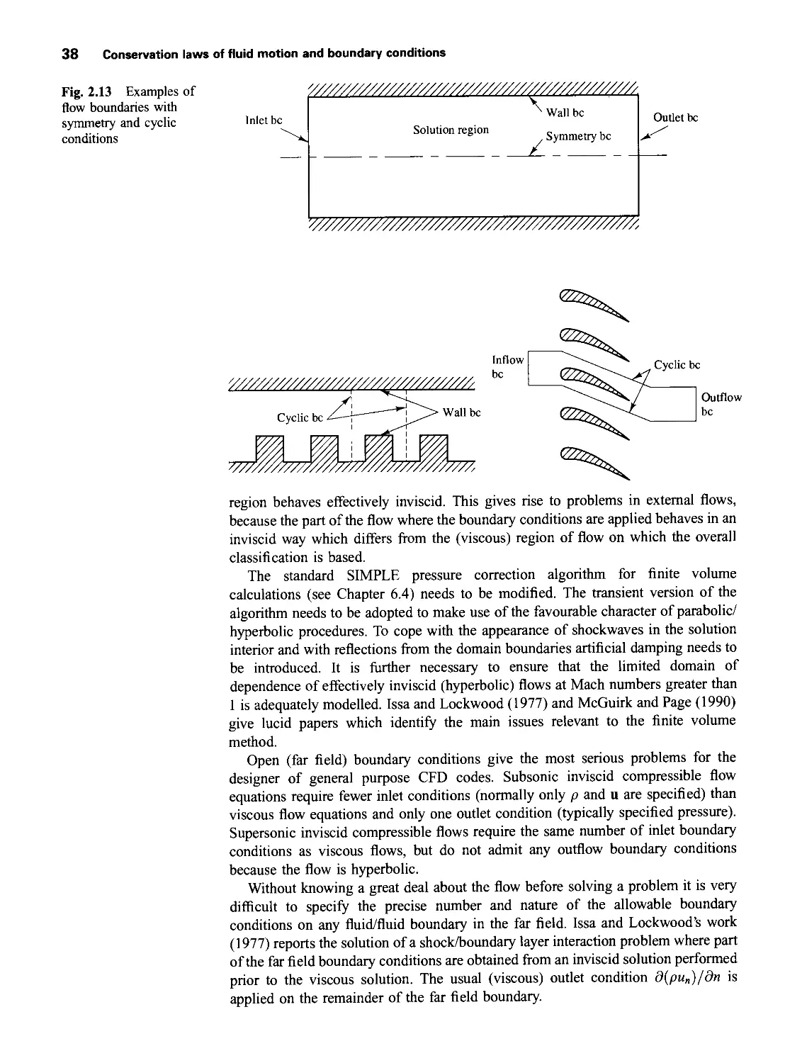
An introduction to
Computational
Fluid
An introduction to computational
fluid dynamics
The finite volume method
H. K. VERSTEEG and W. MALALASEKERA
Longman
Scientific &
Technical
Longman Scientific & Technical
Longman Group Limited
Longman House, Burnt Mill, Harlow
Essex CM20 2JE, England
and Associated Companies throughout the world
Copublished in the United States with
John Wiley & Sons Inc., 605 Third Avenue, New York
NY 10158
© Longman Group Ltd 1995
All right reserved; no part of this publication may be
reproduced, stored in any retrieval system, or transmitted in
any form or by any means, electronic, mechanical,
photocopying, recording or otherwise without either the prior
written permission of the Publishers or a licence permitting
restricted copying in the United Kingdom issued by the
Copyright Licensing Agency Ltd, 90 Tottenham Court Road,
London W1P 9HE.
First published 1995
British Library Cataloguing in Publication Data
A catalogue entry for this title is available from the British Library.
ISBN 0-582-21884-5
Library of Congress Cataloguing-in-Publication Data
A catalog entry for this title is available from the Library of Congress.
ISBN 0-470-23515-2 (USA only)
Typeset by 21 in 10/12 Times
Produced through Longman Malaysia, TCP
Contents
Preface	ix
Acknowledgements	xi
1	Introduction	1
1.1	What is CFD?	1
1.2	How does a CFD	code work?	2
1.3	Problem solving with	CFD	5
1.4	Scope of this book	8
2	Conservation Laws of Fluid	Motion and Boundary Conditions	10
2.1	Governing equations of fluid flow and heat transfer	10
2.1.1	Mass conservation in three dimensions	11
2.1.2 Rates of change following a fluid particle and for a fluid
element	13
2.1.3	Momentum equation in three dimensions	14
2.1.4	Energy equation in three dimensions	17
2.2	Equations of state	21
2.3	Navier-Stokes equations for a Newtonian fluid	21
2.4	Conservative form of the governing equations of fluid flow	24
2.5	Differential and integral forms of the general transport equations	25
2.6	Classification of physical behaviour	27
2.7	The role of characteristics in hyperbolic equations	30
2.8	Classification method for simple partial differential equations	32
2.9	Classification of fluid flow equations	34
2.10	Auxiliary conditions for viscous fluid flow equations	35
2.11	Problems in transonic and supersonic compressible flows	36
2.12	Summary	39
vi Contents
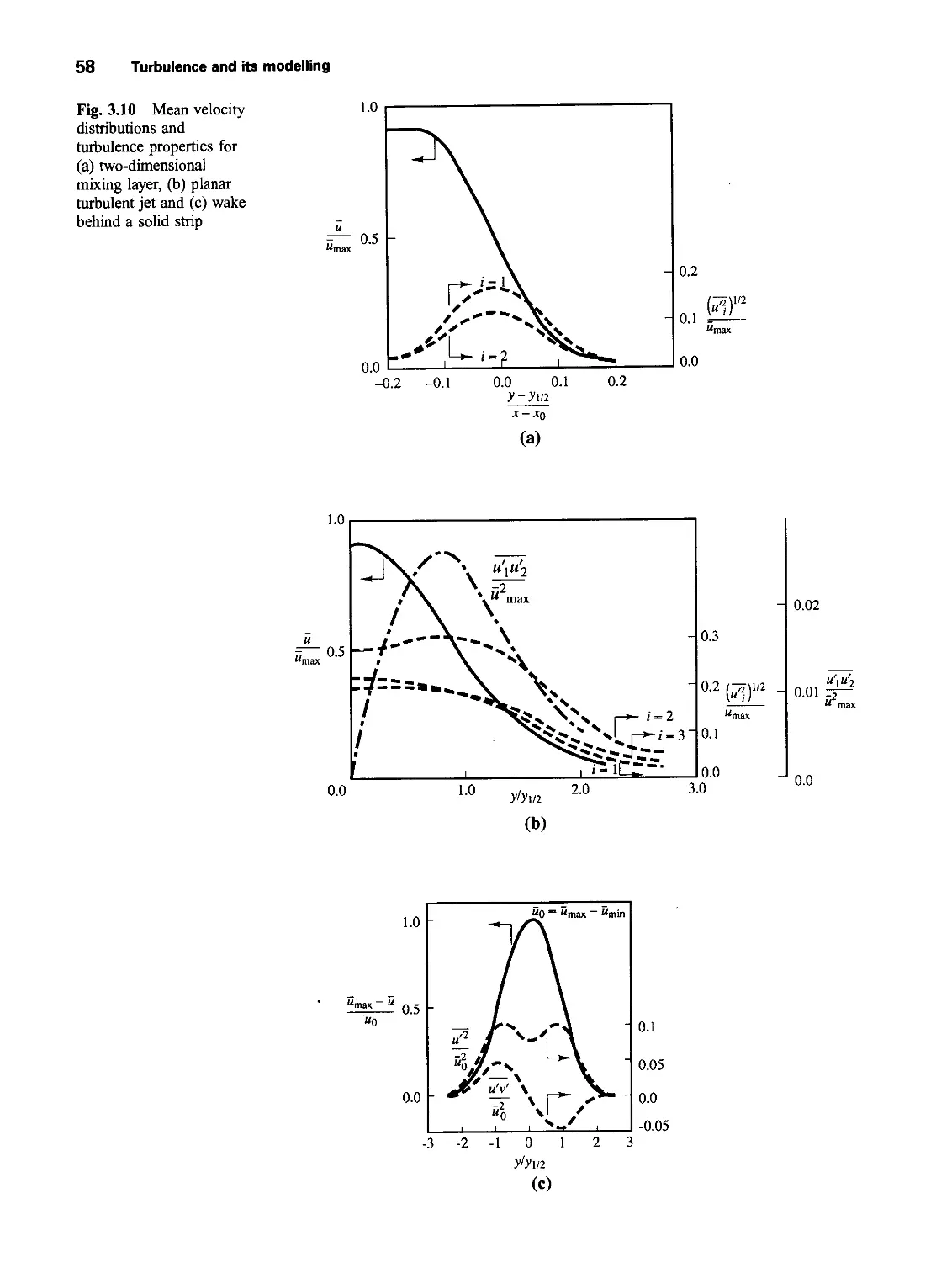
3	Turbulence and its Modelling	41
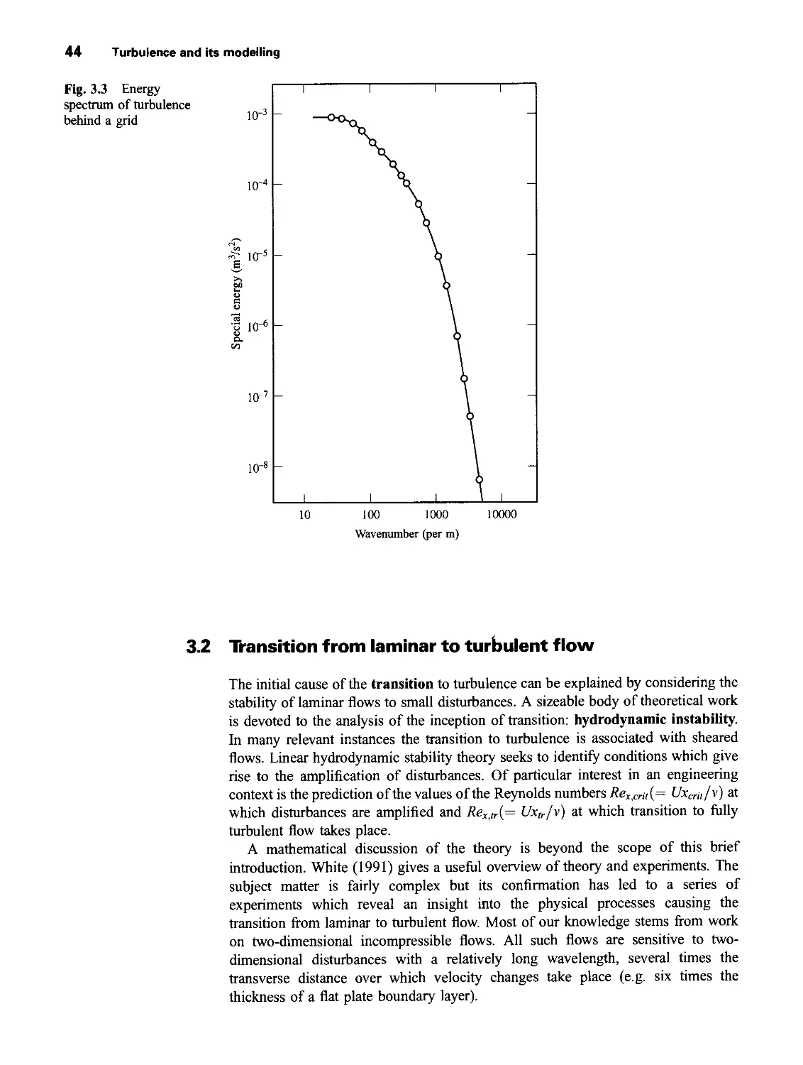
3.1	What is turbulence?	41
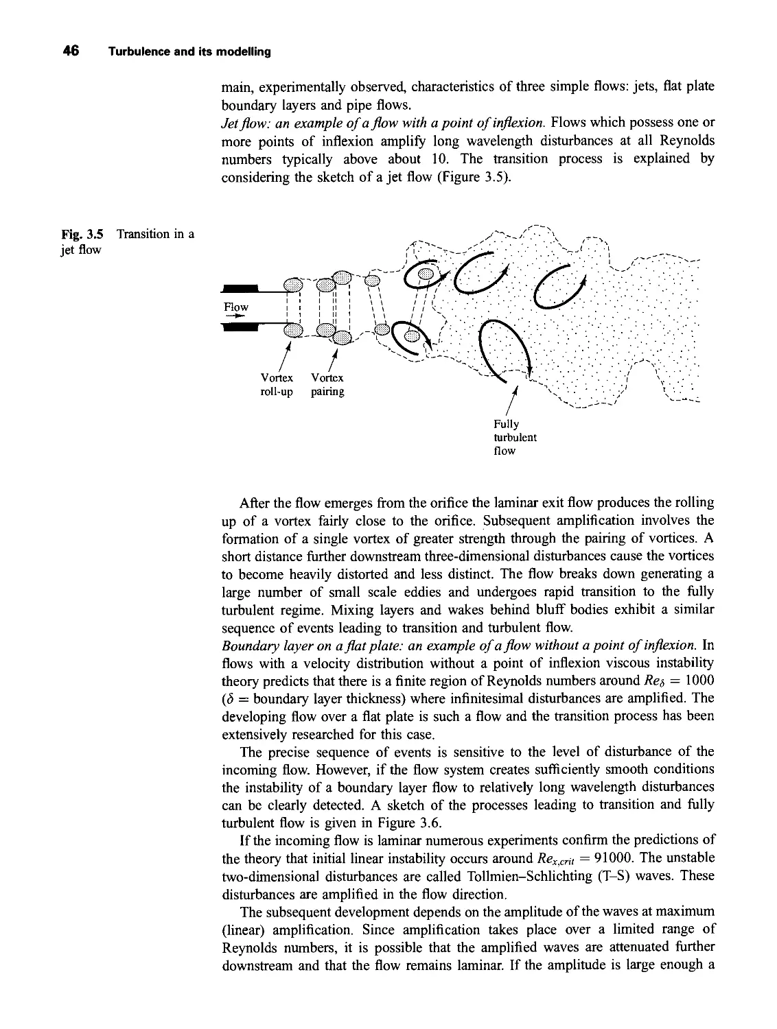
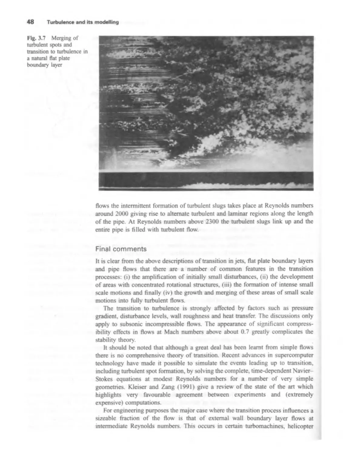
3.2	Transition from laminar to turbulent flow	44
3.3	Effect of turbulence on time-averaged Navier-Stokes equations 49
3.4	Characteristics of simple turbulent flows	54
3.4.1 Free turbulent flows	54
3.4.2 Flat plate boundary layer and pipe flow	57
3.4.3 Summary	62
3.5	Turbulence models	62
3.5.1	Mixing length model	64
3.5.2	The k-e model	67
3.5.3	Reynolds stress equation	models	75
3.5.4	Algebraic stress equation	models	79
3.5.5	Some recent advances	80
3.6	Final remarks	83
4	The Finite Volume Method	for	Diffusion	Problems	85
4.1	Introduction	85
4.2	Finite volume method for one-dimensional steady state diffusion	86
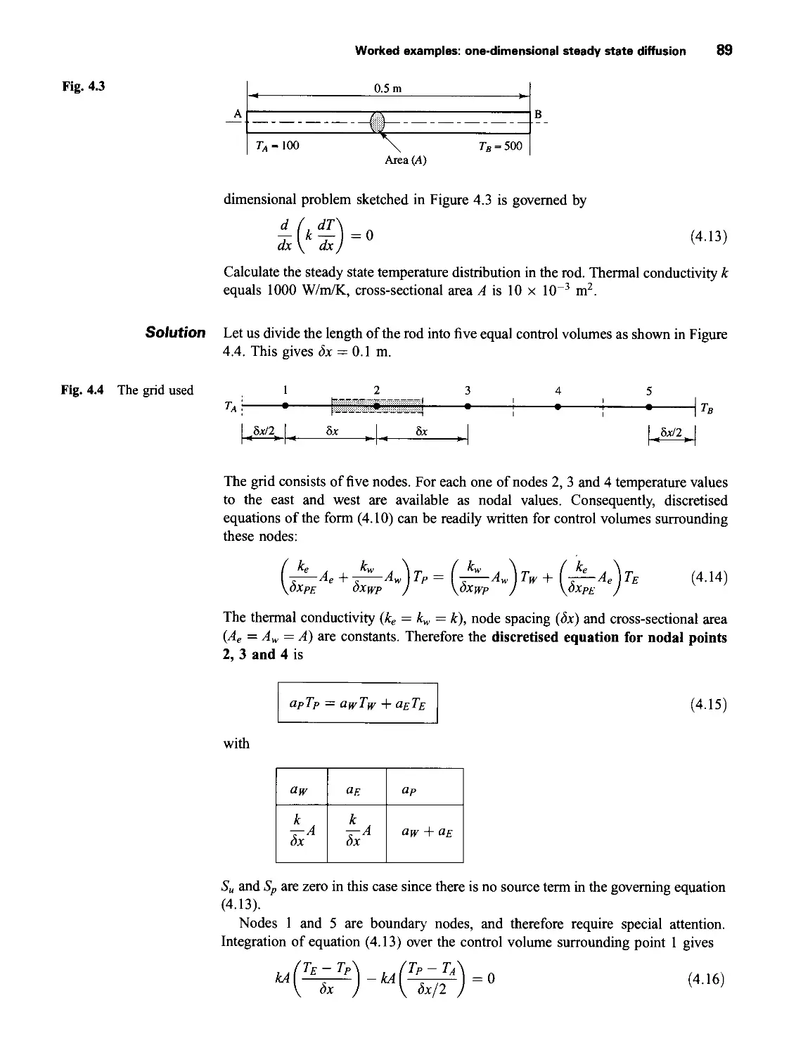
4.3	Worked examples: one-dimensional steady state diffusion	88
4.4	Finite volume method for two-dimensional diffusion problems	99
4.5	Finite volume method for three-dimensional diffusion problems	100
4.6	Summary of discretised equations for diffusion problems	102
5	The Finite Volume Method	for	Convection-Diffusion Problems	103
5.1	Introduction	103
5.2	Steady one-dimensional convection and diffusion	104
5.3	The central differencing scheme	105
5.4	Properties of discretisation schemes	110
5.4.1	Conservativeness	110
5.4.2	Boundedness	112
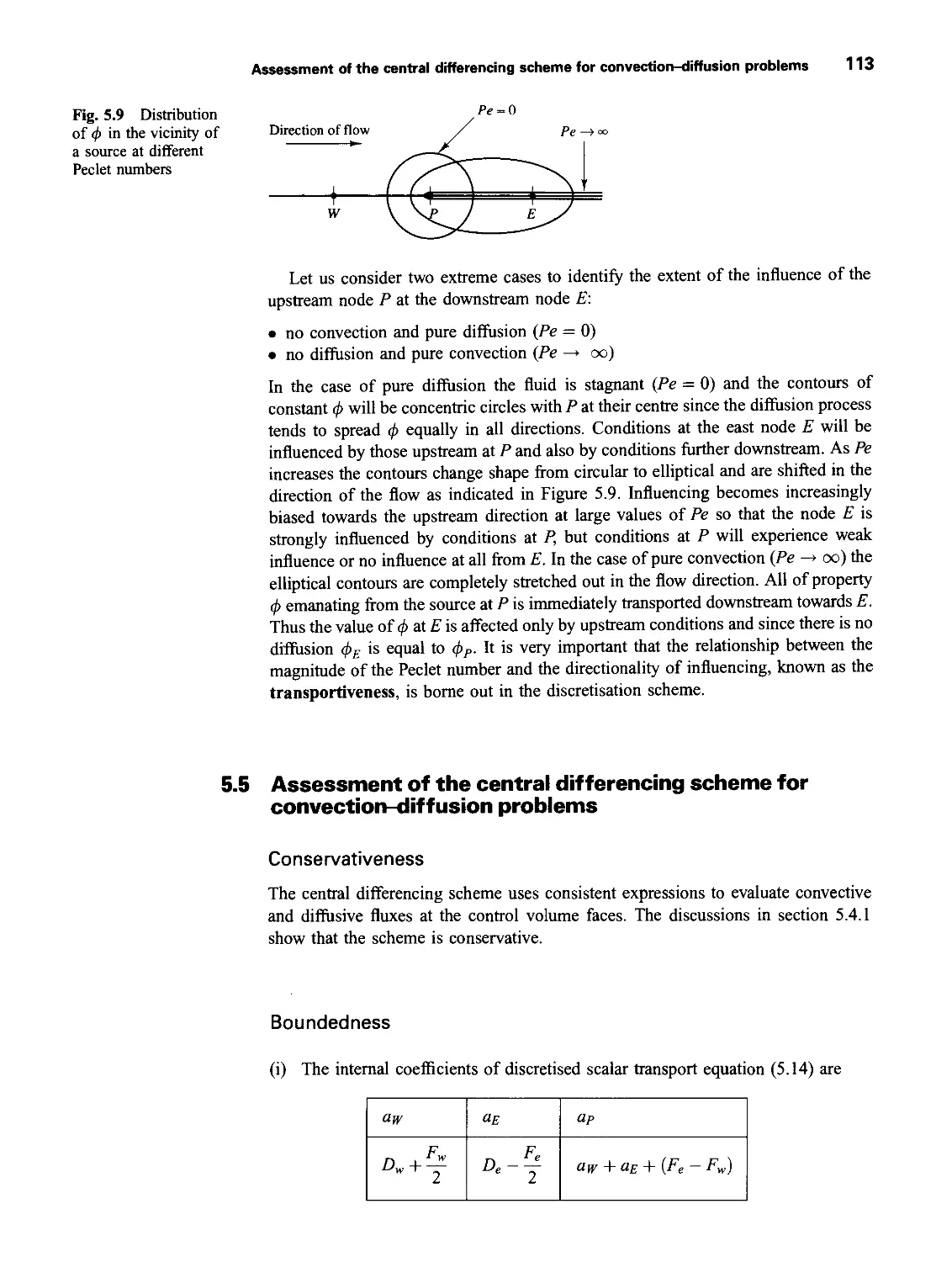
5.4.3	Transportiveness	112
5.5	Assessment of the central differencing scheme for
convection-diffusion problems	113
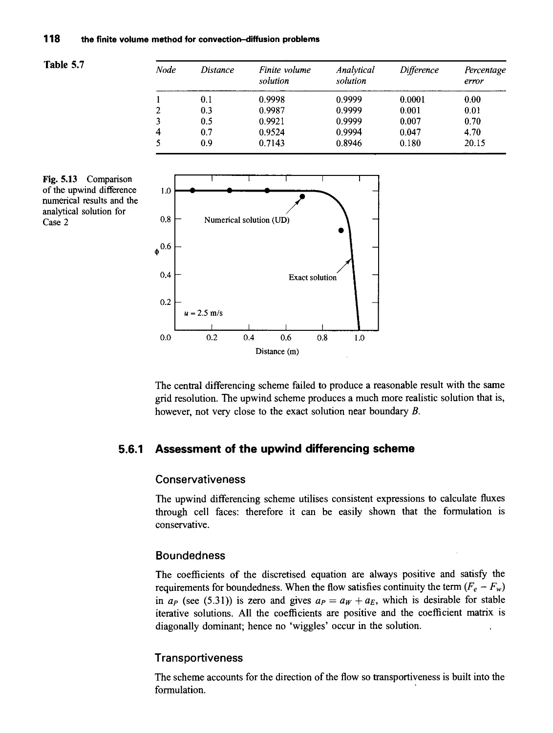
5.6	The upwind differencing scheme	114
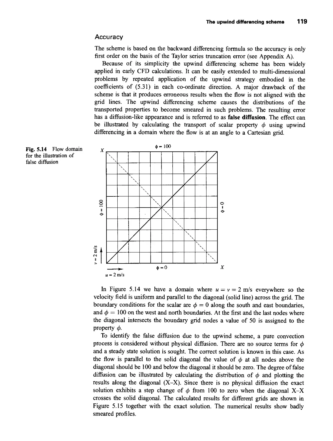
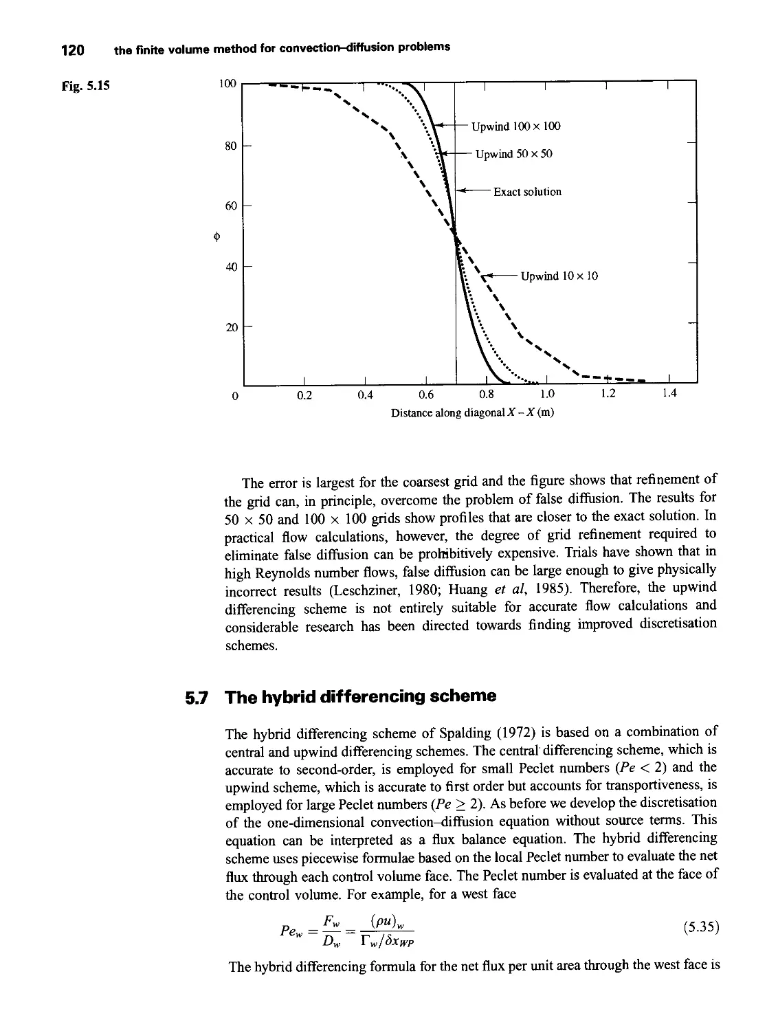
5.6.1 Assessment of the upwind differencing scheme	118
5.7	The hybrid differencing scheme	120
5.7.1 Assessment of the hybrid differencing scheme	123
5.7.2 Hybrid differencing scheme for multi-dimensional
convection-diffusion	12 3
5.8	The power-law scheme	124
5.9	Higher order differencing schemes for convection-diffusion
problems	125
5.9.1 Quadratic upwind differencing scheme: the QUICK scheme 125
5.9.2 Assessment of the QUICK scheme	130
5.9.3 Stability problems of the QUICK scheme and remedies	130
5.9.4 General comments on the QUICK differencing scheme	132
5.10	Other higher order schemes	133
5.11	Summary	133
Contents vii
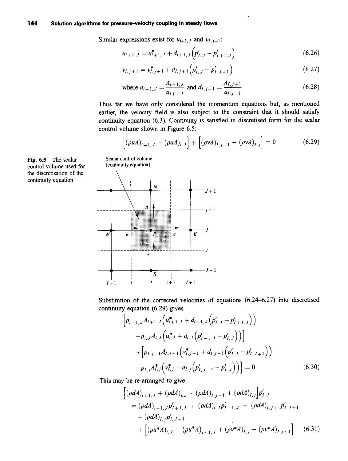
6	Solution Algorithms for Pressure-Velocity Coupling in Steady Flows 135
6.1	Introduction	135
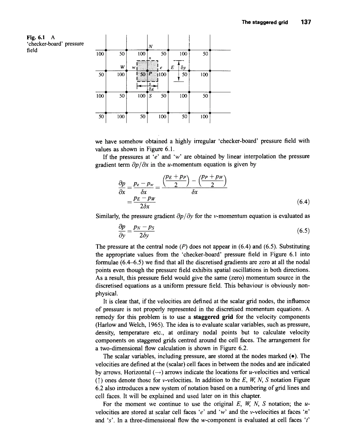
6.2	The staggered grid	136
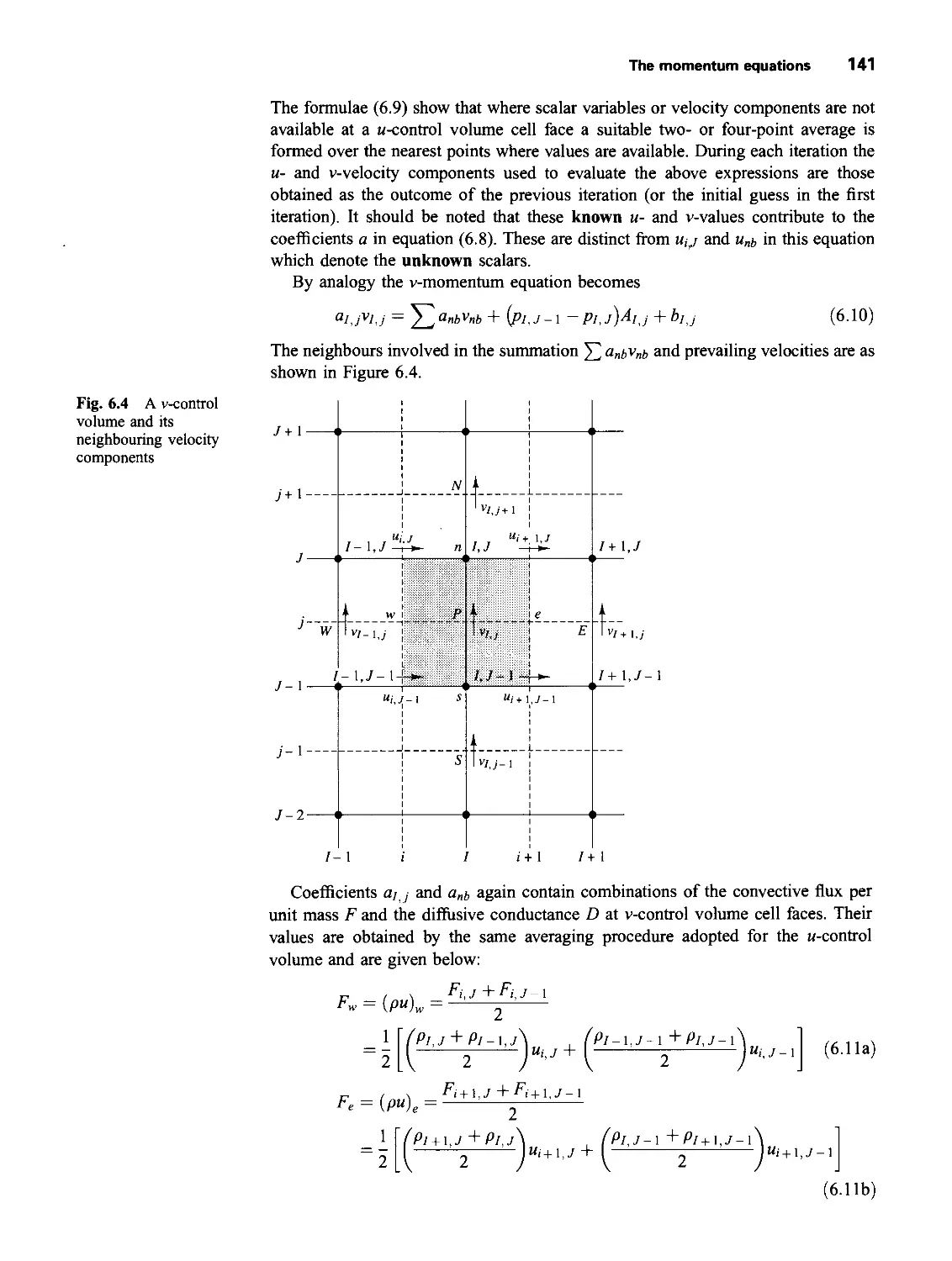
6.3	The momentum equations	139
6.4	The SIMPLE algorithm	142
6.5	Assembly of a complete method	146
6.6	The SIMPLER algorithm	146
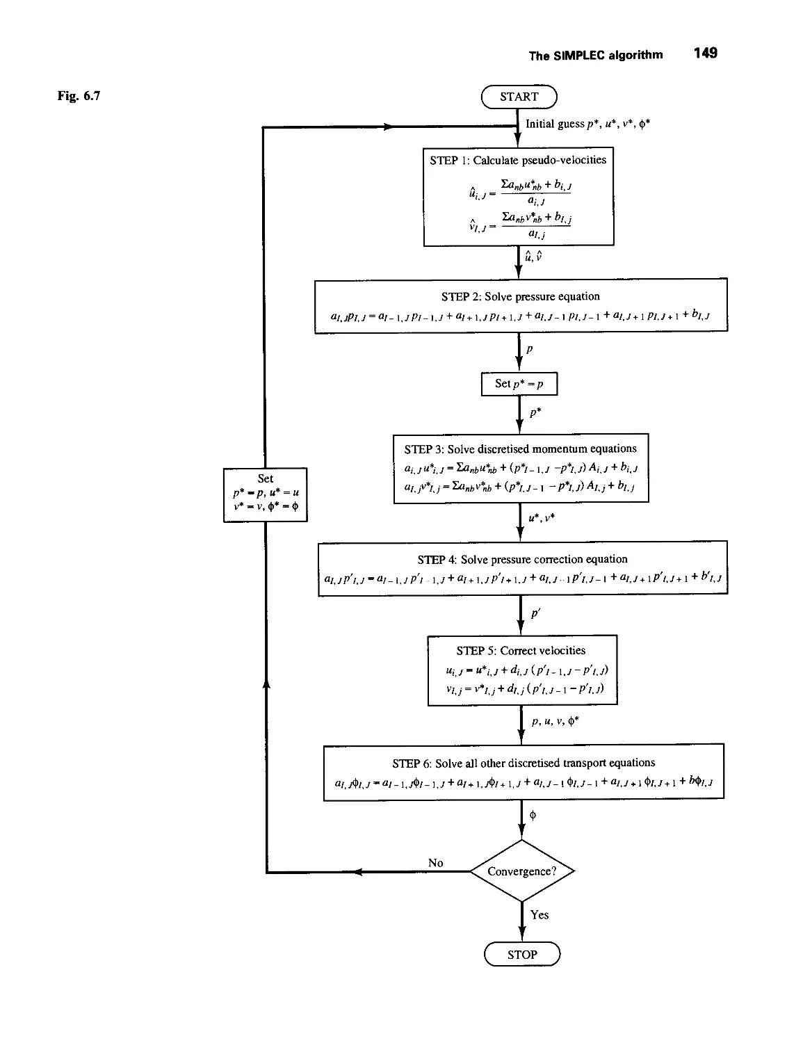
6.7	The SIMPLEC algorithm	148
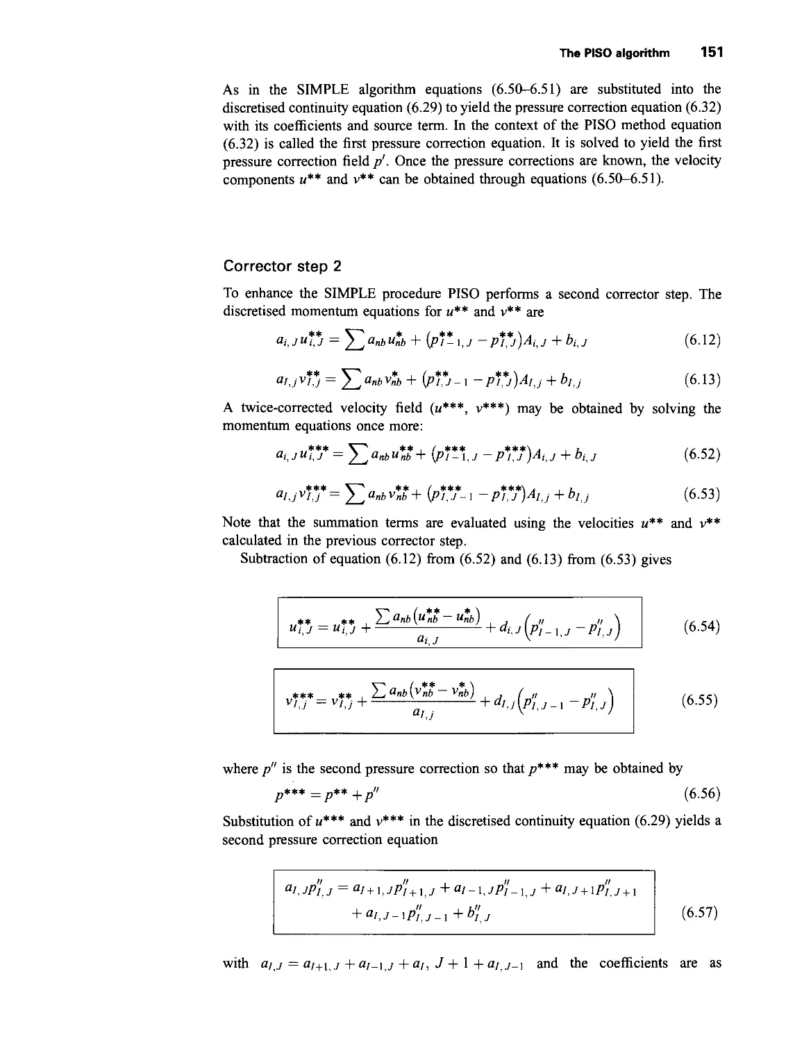
6.8	The PISO algorithm	150
6.9	General comments on SIMPLE, SIMPLER, SIMPLEC and PISO 152
6.10	Summary	154
7	Solution of Discretised Equations	156
7.1	Introduction	156
7.2	The tri-diagonal matrix algorithm	157
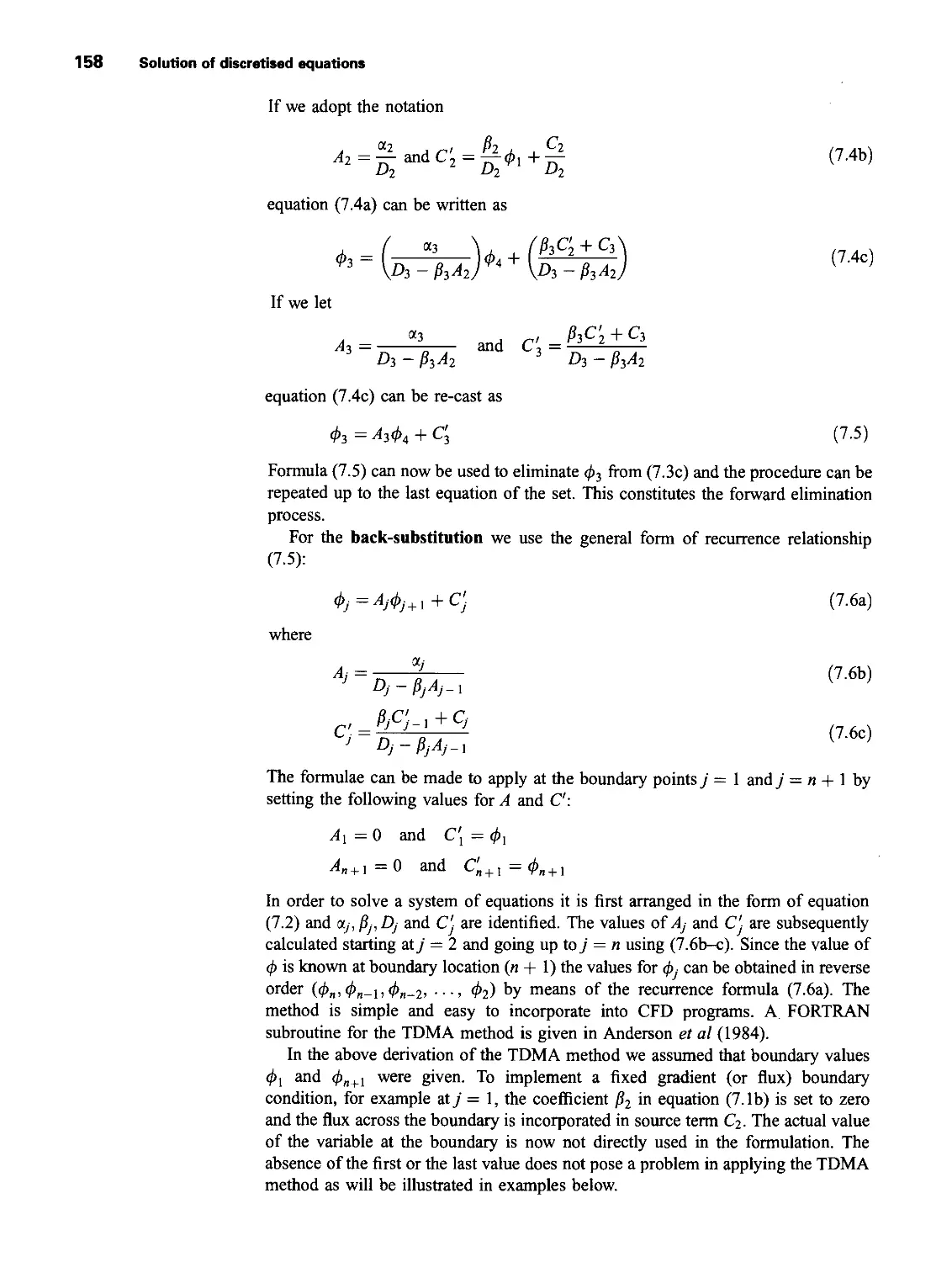
7.3	Application of TDMA to two-dimensional problems	159
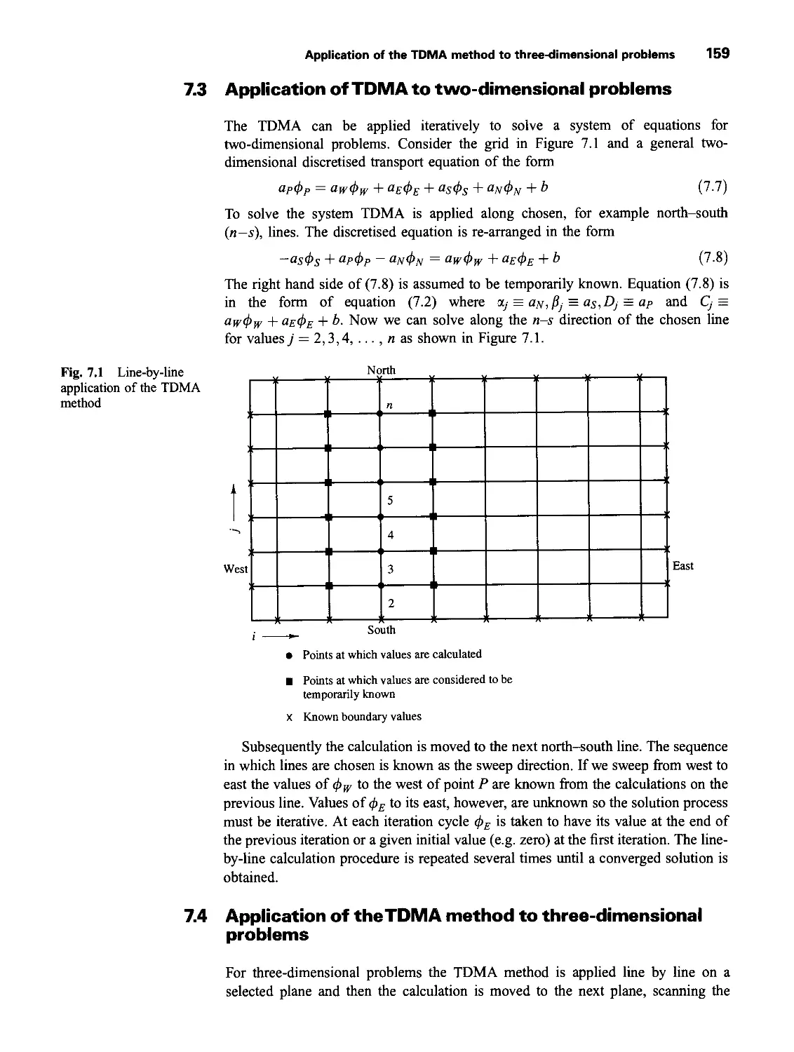
7.4	Application of the TDMA method	to three-dimensional problems 159
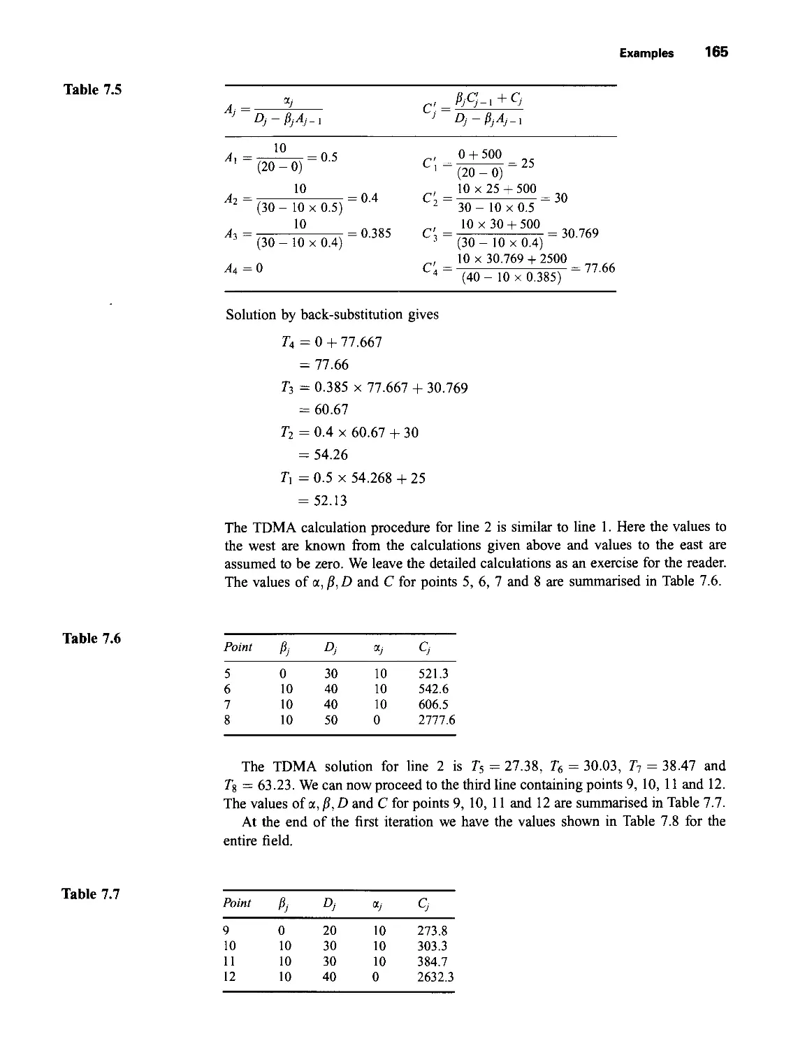
7.5	Examples	160
7.6	Other solution techniques used in CFD	166
7.7	Summary	167
8	The Finite Volume Method for Unsteady Flows	168
8.1	Introduction	168
8.2	One-dimensional unsteady heat conduction	169
8.2.1 Explicit scheme	171
8.2.2 Crank-Nicolson scheme	172
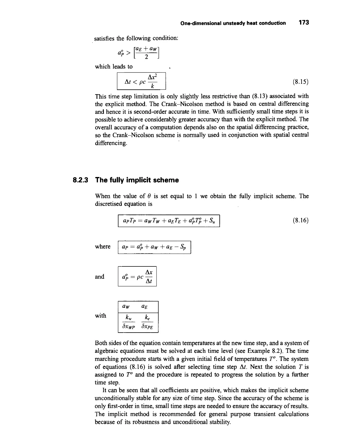
8.2.3 The fully implicit scheme	173
8.3	Illustrative examples	174
8.4	Implicit method for two-and three-dimensional problems	180
8.5	Discretisation of transient convection-diffusion equation	181
8.6	Worked example of transient convection-diffusion using QUICK
differencing	182
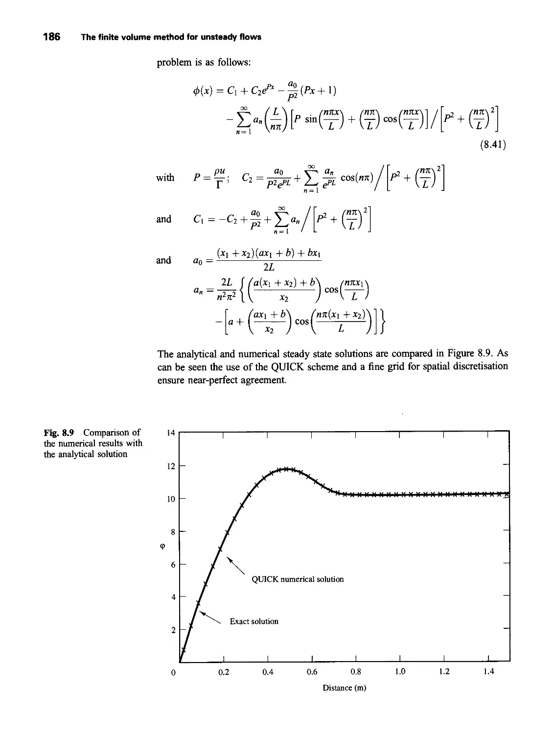
8.7	Solution procedures for unsteady flow calculations	186
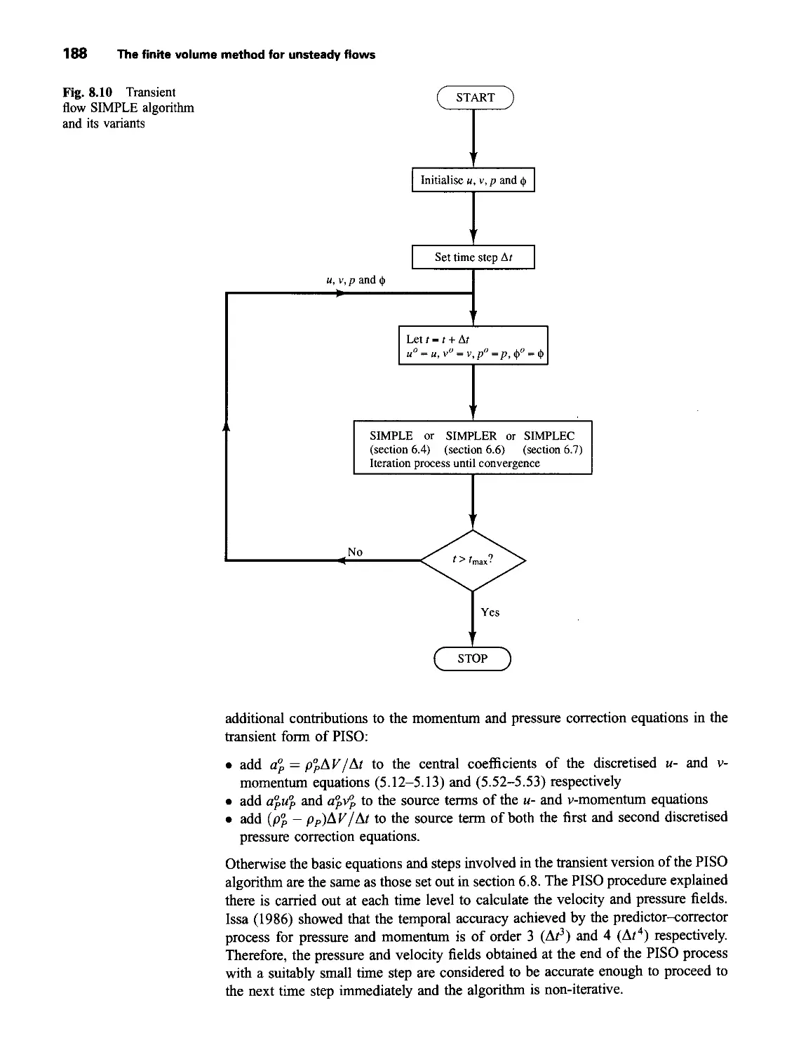
8.7.1 Transient SIMPLE	186
8.7.2 The transient PISO algorithm	187
8.8	Steady state calculations using the pseudo-transient approach	189
8.9	A brief work on other transient schemes	189
8.10	Summary	190
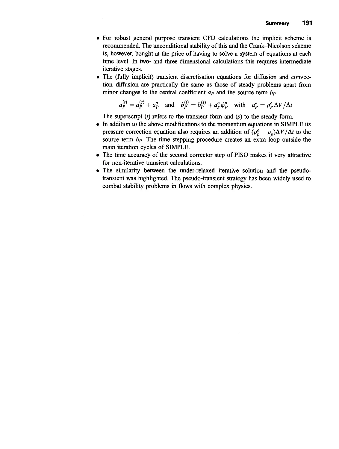
9	Implementation of Boundary Conditions	192
9.1	Introduction	192
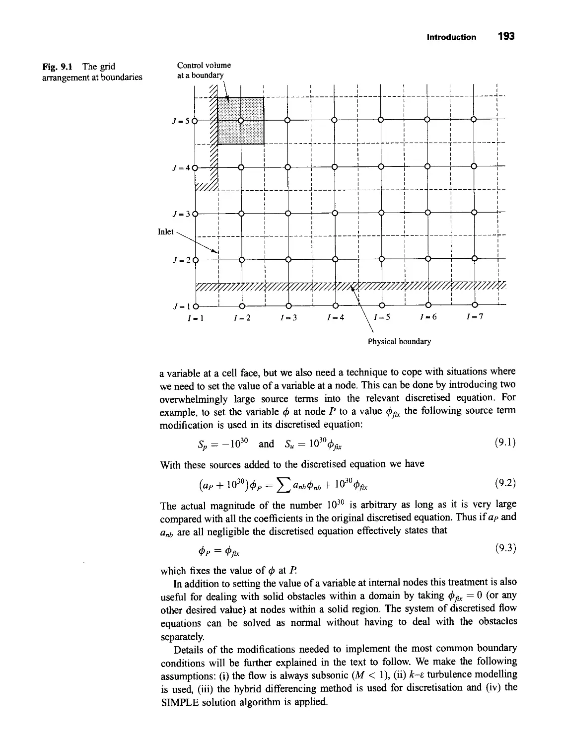
9.2	Inlet boundary conditions	194
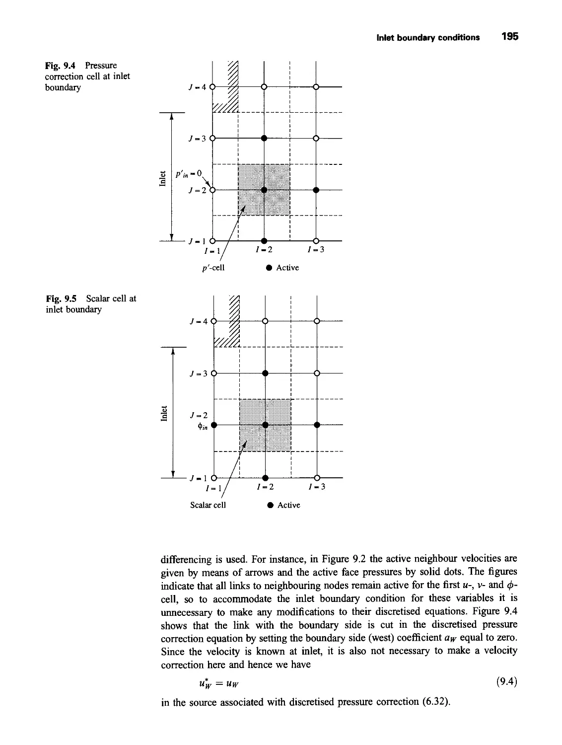
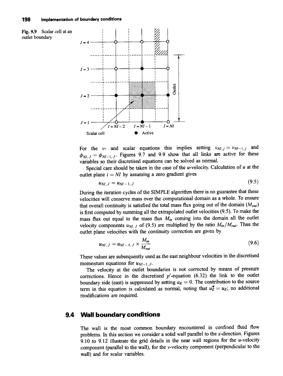
9.3	Outlet boundary conditions	196
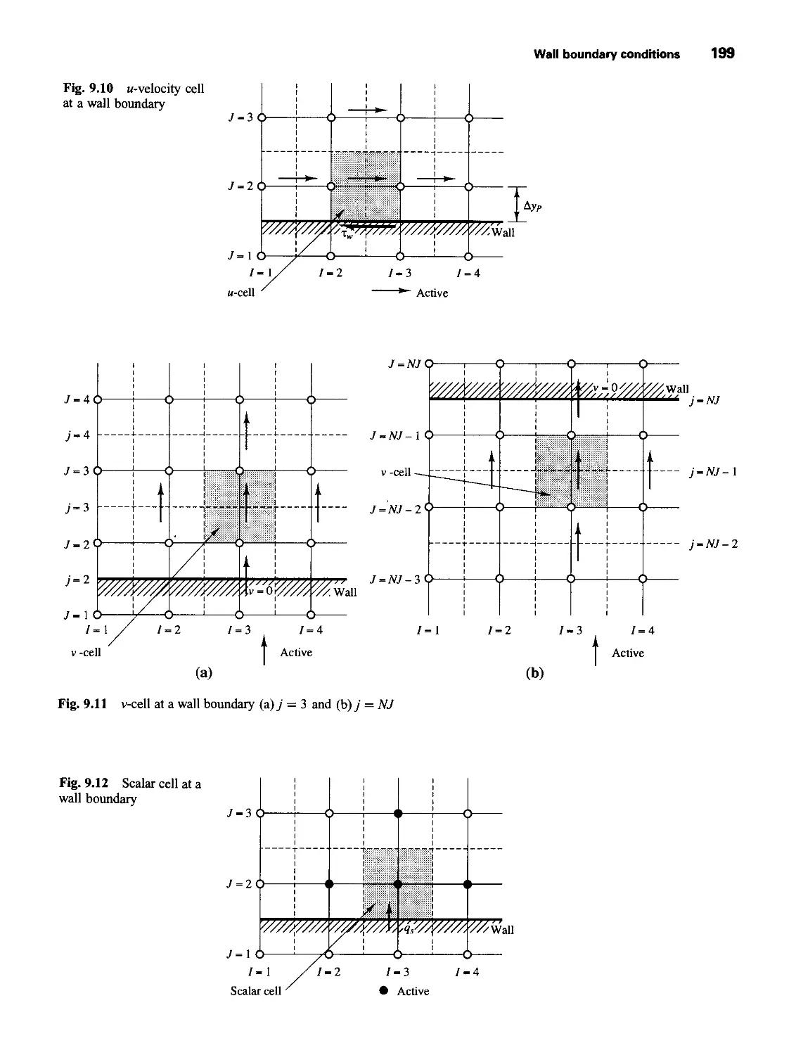
9.4	Wall boundary conditions	198
9.5	The constant pressure boundary condition	203
9.6	Symmetry boundary condition	205
9.7	Periodic or cyclic boundary condition	205
9.8	Potential pitfalls and final remarks	206
viii Contents
10	Advanced Topics and Applications	210
10.1	Introduction	210
10.2	Combustion modelling	210
10.2.1 The simple chemical	reacting system (SCRS)	212
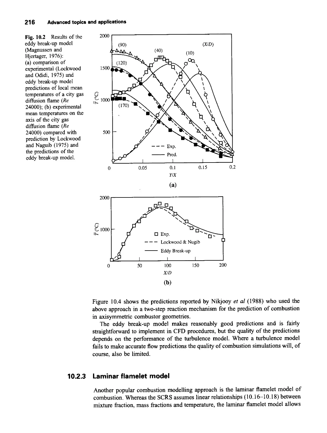
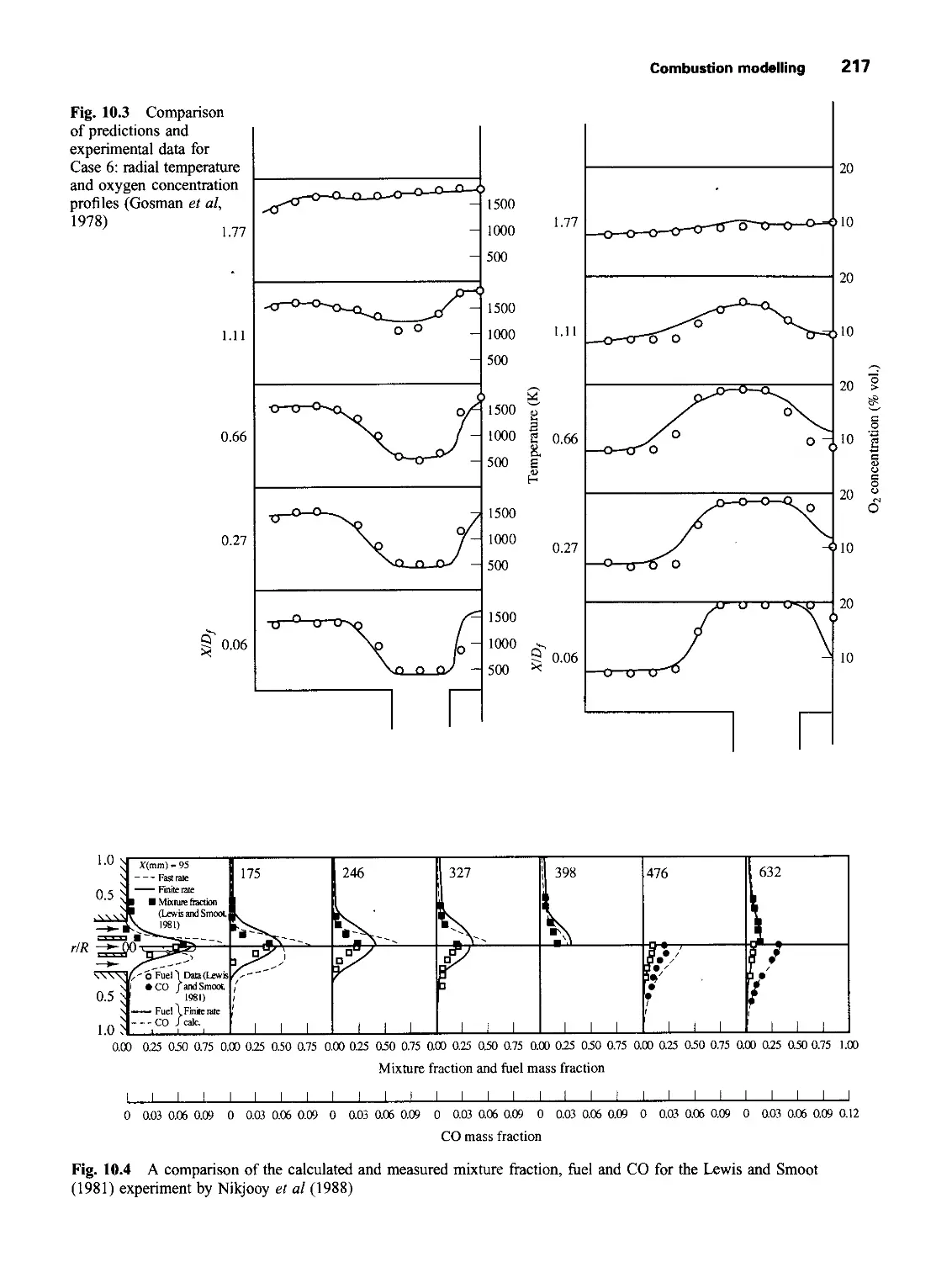
10.2.2 Eddy break-up of model of combustion	215
10.2.3 Laminar flamelet model	216
10.3	Calculation of buoyant flows and	flows	inside	buildings	218
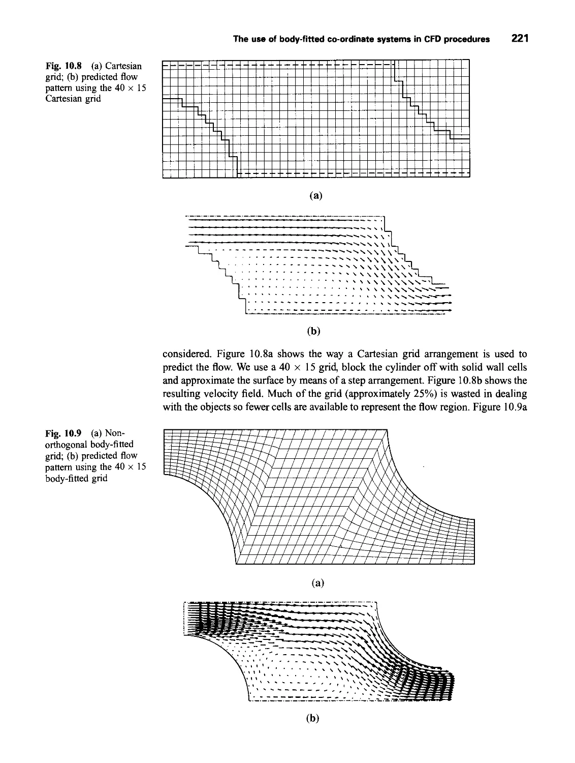
10.4	The use of body-fitted co-ordinate	systems	in	CFD	procedures	219
10.5	Advanced applications	222
10.5.1 Flow in a sudden pipe contraction	222
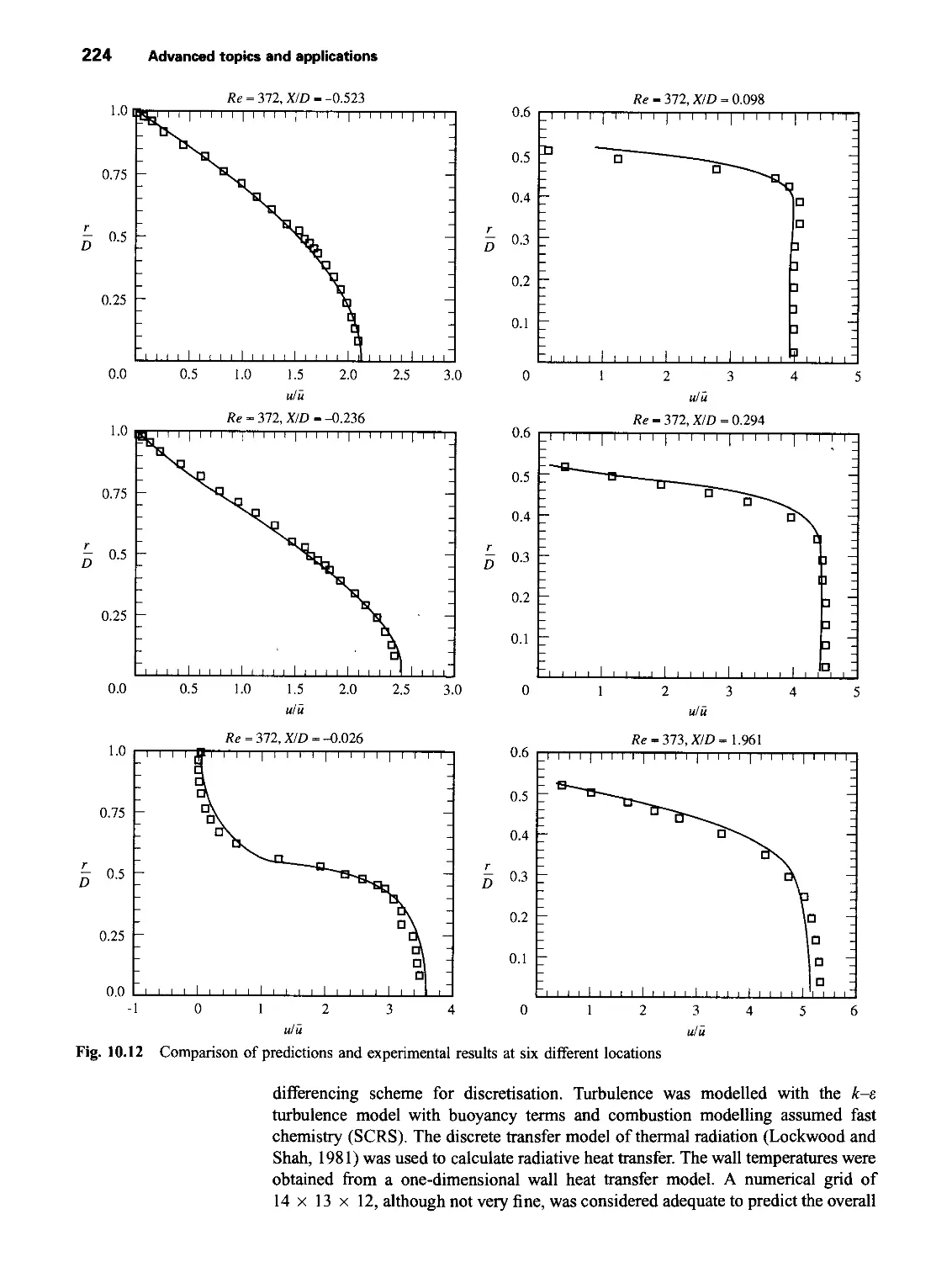
10.5.2 Modelling of a fire in a test room	223
10.5.3 Prediction of flow and heat transfer in a complex tube
matrix	227
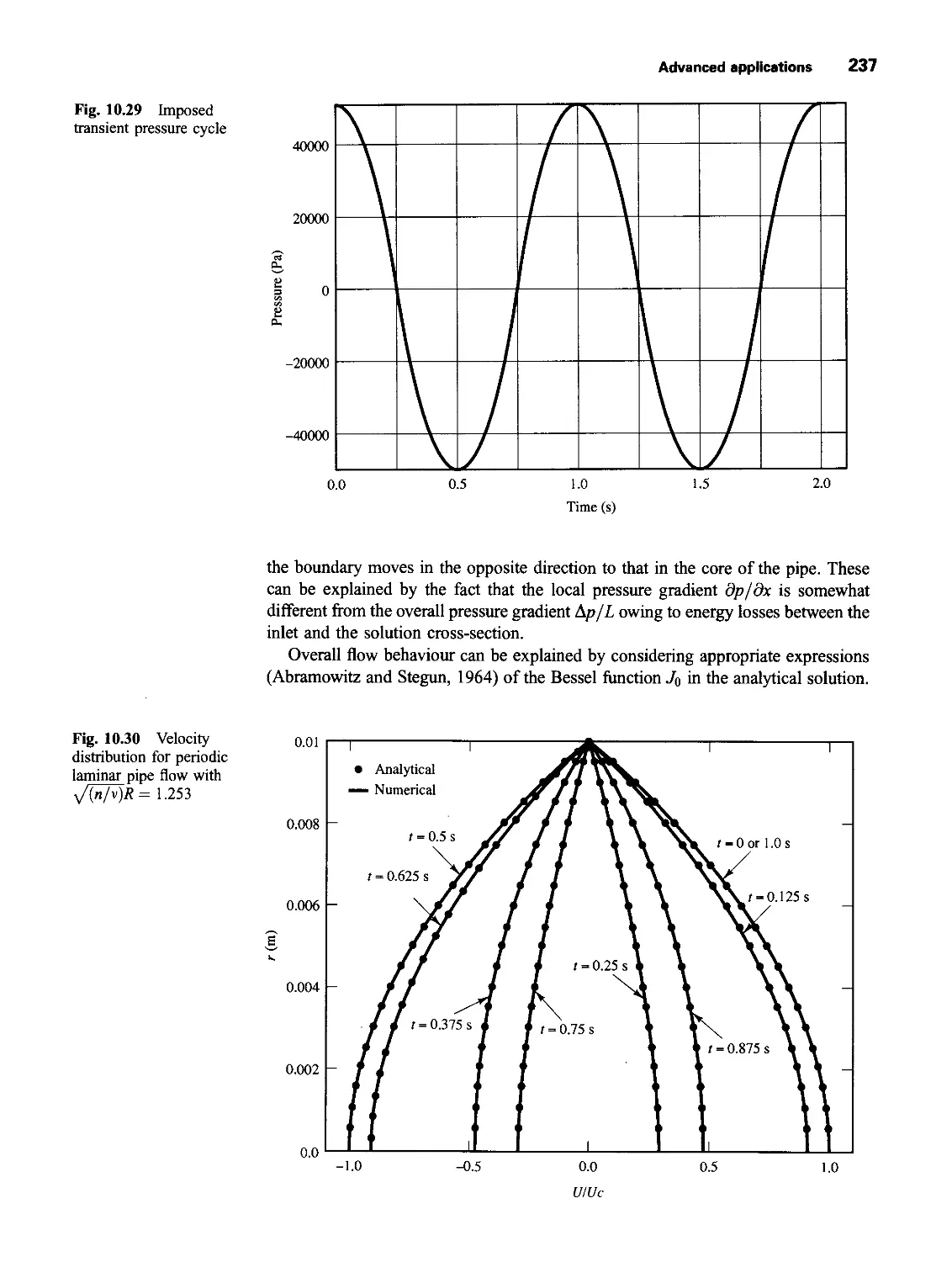
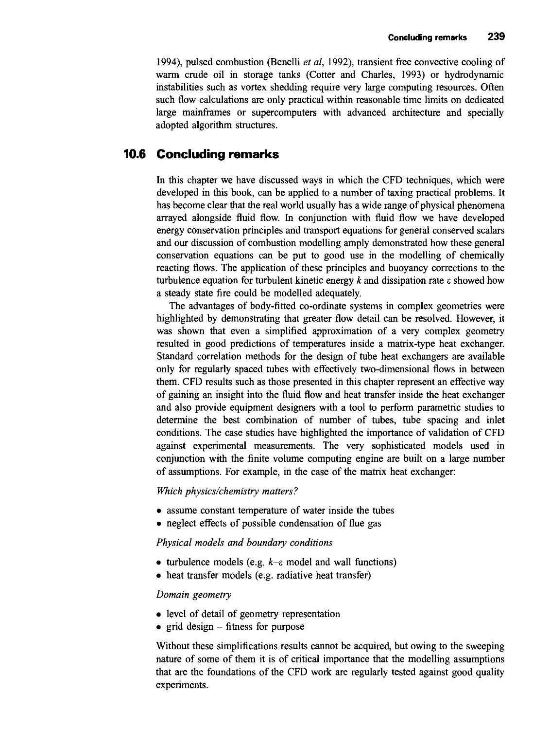
10.5.4 Laminar flow in a circular pipe driven by periodic
pressure variations	234
10.6	Concluding remarks	239
Appendix A	Accuracy of a Flow Simulation	240
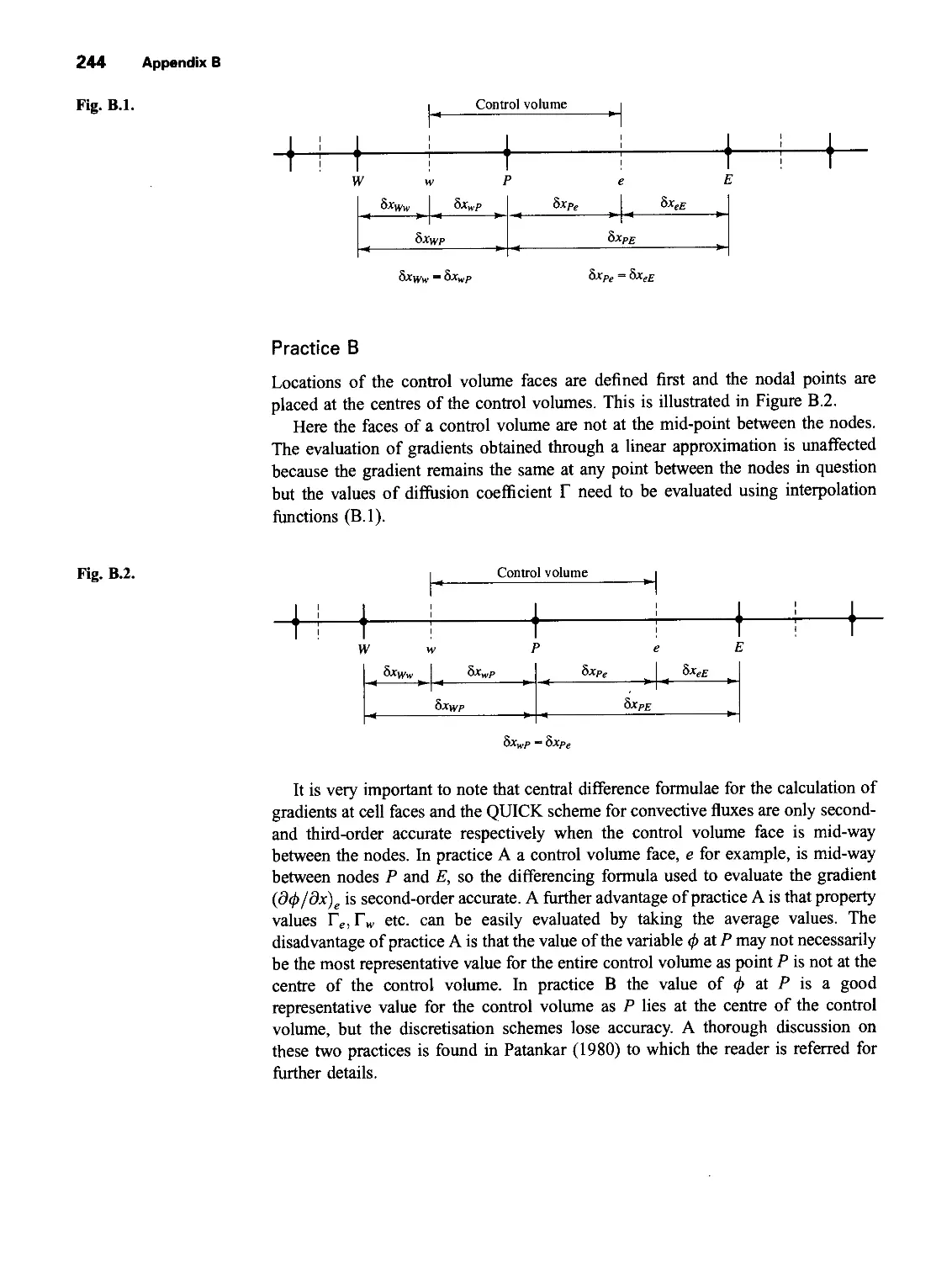
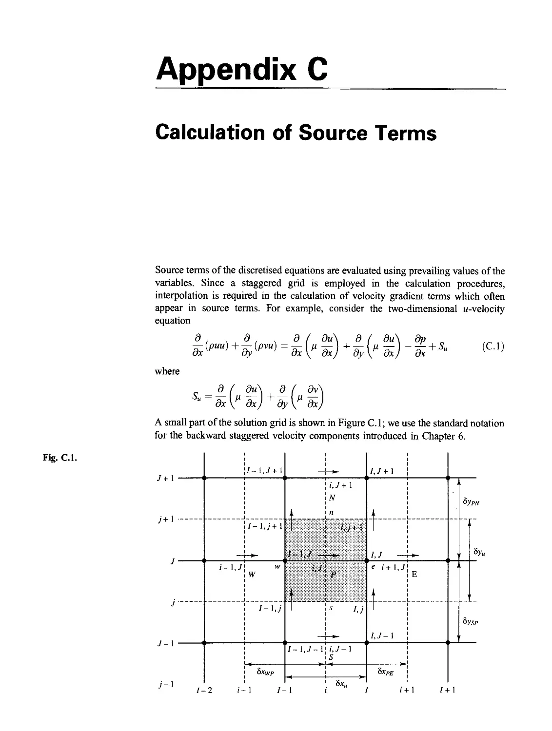
Appendix В	Non-uniform Grids	243
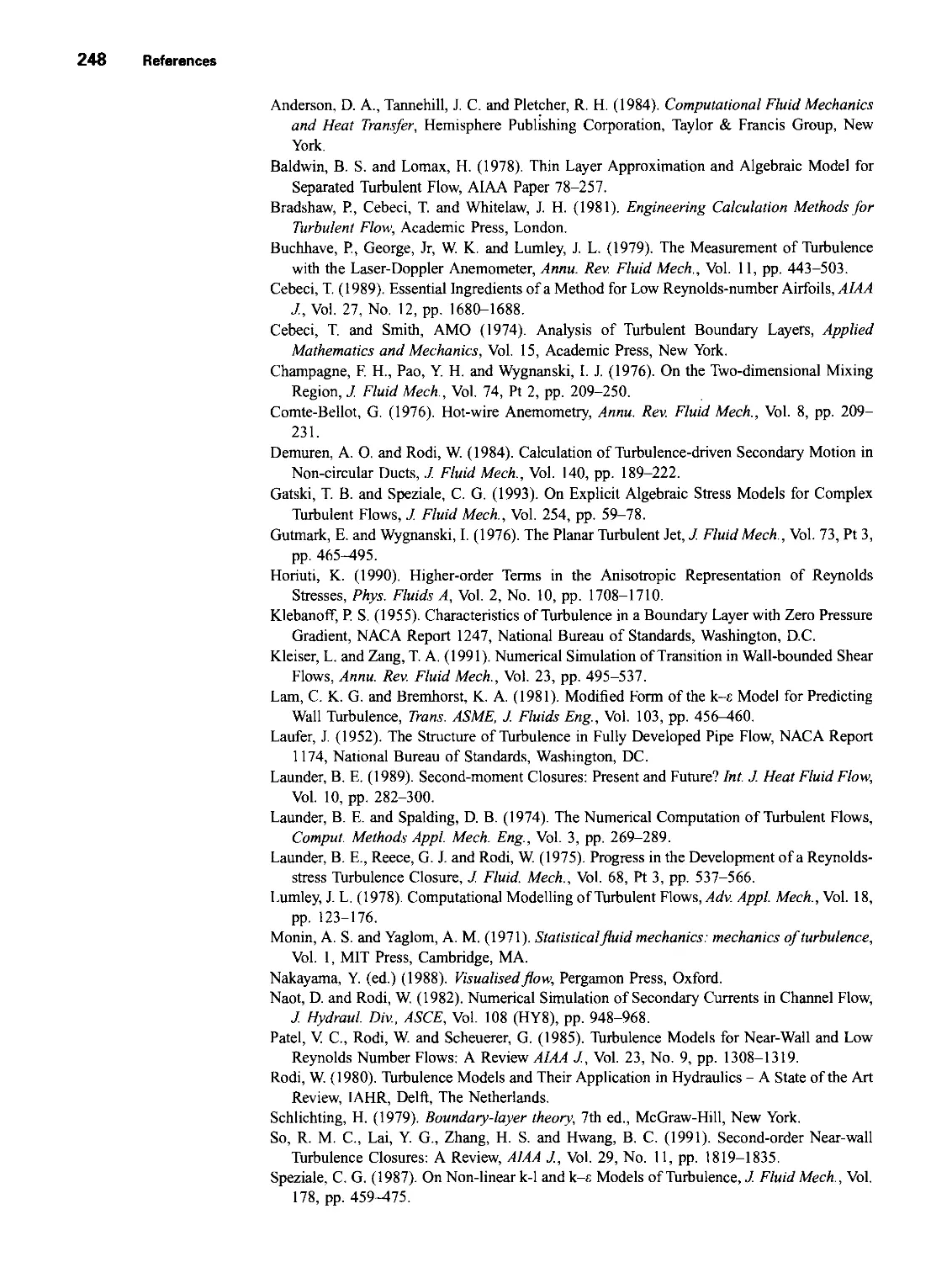
Appendix C	Calculation of Source Terms	245
References	247
Index
255
Preface
The use of computational fluid dynamics (CFD) to predict internal and external
flows has risen dramatically in the past decade. In the 1980s the solution of fluid flow
problems by means of CFD was the domain of the academic, postdoctoral or
postgraduate researcher or the similarity trained specialist with many years of
grounding in the area. The widespread availability of engineering workstations
together with efficient solution algorithms and sophisticated pre- and post-
processing facilities enable the use of commercial CFD codes by graduate
engineers for research, development and design tasks in industry. The codes that
are now on the market may be extremely powerful, but their operation still requires a
high level of skill and understanding from the operator to obtain meaningful results
in complex situations. The long learning curve, previously including apprenticeships
of up to four years - more widely known as MPhil and PhD studies - meant that the
users of the 1980s were, through their own experiences, very conscious of the
limitations of CFD. However, the pressure on engineers in industry to come up with
solutions to problems implies that there is not always the time available for the new
type of user of the 1990s to learn about the pitfalls of CFD by osmosis and frequent
failure.
It is the purpose of this book to fill a gap in the available literature for novice
CFD users who, whilst developing CFD skills by using commercially available
software, need a reader that provides the fundamentals of the fluid dynamics behind
complex engineering flows and of the numerical solution algorithms on which the
CFD codes are based. Although the material has been developed from first principles
wherever possible, the book will be of greatest benefit to those who are familiar with
the ideas of calculus, elementary vector and matrix algebra and basic numerical
methods. Furthermore, we assume a knowledge of the conservation laws for mass,
momentum and energy and an awareness of their application to fluid flow problems.
Although commercial CFD codes based on the finite element method have more
recently entered the fray, the market is currently dominated by four codes,
PHOENICS, FLUENT, FLOW3D and STAR-CD, that are all based on the finite
volume method. This book intends to provide the theoretical background required
X
Preface
for the effective use of this type of commercial code and covers the following subject
areas:
Fluid dynamics
•	Governing equations of viscous fluid flows
•	Boundary conditions
•	Introduction to the physics of turbulence
•	Turbulence modelling in CFD
The finite volume method and its implementation in CFD codes
•	Finite volume discretisation for the key transport phenomena in fluid flows:
diffusion, convection and sources
•	Discretisation procedures for unsteady phenomena
•	Iterative solution processes (SIMPLE and its derivatives) to ensure correct
coupling between all the flow variables
•	Solution algorithms for systems of discretised equations (TDMA)
•	Implementation of boundary conditions
The basic numerical techniques have been developed around a series of worked
examples, which can be easily programmed on a PC. However, it is impossible to get
to grips with the art of CFD without running a good quality code to explore the
issues raised in this book in greater detail. As an illustration of the power of CFD we
have presented a set of industrially relevant applications ranging from a benchmark
simulation to very complex fire modelling. Throughout, one of the key messages is
that CFD cannot be professed adequately without continued reference to
experimental validation. The early ideas of the computational laboratory to
supersede experimentation have fortunately gone out of fashion. Not all industrial
companies have the high cost experimental infrastructure in place to support CFD
activities, but the scientific literature contains a huge resource to the user of
commercial codes. Avast and ever-increasing number of journals cover all aspects of
CFD ranging from mathematically abstruse to applied work firmly rooted in
industry. In addition to the necessary theoretical grounding the book, therefore,
provides a set of connection points with up-to-date research literature giving the
reader access to source material for code validation and further study.
After starting to teach CFD at senior undergraduate level we became acutely
aware of the absence of a ‘suitable’ text pitched at ‘the right level’. Undeniably, this
book, which was developed from our course notes, was conceived with our own
students as a target audience so, first and foremost, we hope that the book will be
valuable as a learning and teaching resource to support CFD courses at
undergraduate and postgraduate level. Nevertheless, with its intent to bridge the
gap between introductory mathematics and fluid dynamics concepts, the academic
CFD literature and applied industrial practice, we believe that this book will also be
of use to professional engineers in industry, involved in R&D and design, who
require a thorough but user-friendly reference guide to all the background
knowledge needed to operate commercial CFD codes successfully.
We acknowledge Dr. S. Sivasegaram of Imperial College of Science Technology
and Medicine, and Mr. R. K. Turton of Loughborough University for helpful
comments on early drafts of this book. We are grateful to our wives, Helen and
Anoma, for all the support and encouragement given to us during the compilation of
this book.
March 1995
Loughborough
H. K. Versteeg
W. Malalasekera
Acknowledgements
The authors wish to acknowledge the following persons, organisations and
publishers for permission to reproduce from their publications in this book.
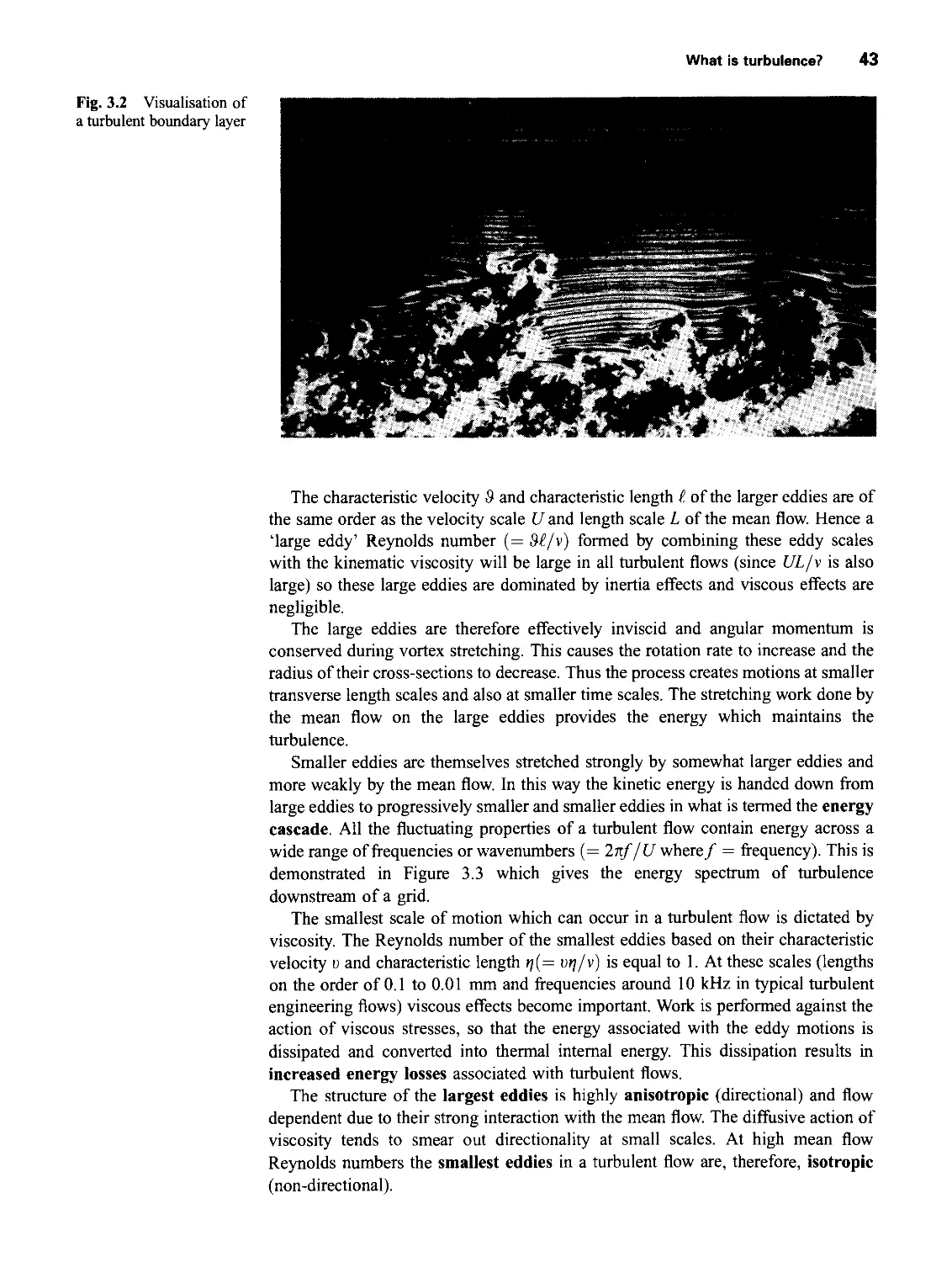
Professor H. Nagib for fig. 3.2; Professor S. Taneda and the Japan Society of
Mechanical Engineers for fig. 3.7; Professor W. Fiszdon and the Polish Academy of
Sciences for fig. 3.9; McGraw-Hill Inc. for fig. 3.13; The Combustion Institute for
figs. 10.2 and 10.3; and Gordon and Breach Science Publishers for fig. 10.4. While
every effort has been made to trace the owners of copyright, in some cases this has
proved impossible and we would like to apologise to anyone whose rights we may
have unwittingly infringed. All registered trade marks of CFD codes mentioned in
this text are also acknowledged.
1_________________________________
Introduction
1.1	What is CFD?
Computational Fluid Dynamics or CFD is the analysis of systems involving fluid
flow, heat transfer and associated phenomena such as chemical reactions by means of
computer-based simulation. The technique is very powerful and spans a wide range
of industrial and non-industrial application areas. Some examples are:
•	aerodynamics of aircraft and vehicles: lift and drag
•	hydrodynamics of ships
•	power plant: combustion in IC engines and gas turbines
•	turbomachinery: flows inside rotating passages, diffusers etc.
•	electrical and electronic engineering: cooling of equipment including micro-
circuits
•	chemical process engineering: mixing and separation, polymer moulding
•	external and internal environment of buildings: wind loading and heating/
ventilation
•	marine engineering: loads on off-shore structures
•	environmental engineering: distribution of pollutants and effluents
•	hydrology and oceanography: flows in rivers, estuaries, oceans
•	meteorology: weather prediction
•	biomedical engineering: blood flows through arteries and veins
From the 1960s onwards the aerospace industry has integrated CFD techniques into
the design, R&D and manufacture of aircraft and jet engines. More recently the
methods have been applied to the design of internal combustion engines,
combustion chambers of gas turbines and furnaces. Furthermore, motor vehicle
manufacturers now routinely predict drag forces, under-bonnet air flows and the in-
car environment with CFD. Increasingly CFD is becoming a vital component in the
design of industrial products and processes.
The ultimate aim of developments in the CFD field is to provide a capability
comparable to other CAE (Computer-Aided Engineering) tools such as stress
2
Introduction
analysis codes. The main reason why CFD has lagged behind is the tremendous
complexity of the underlying behaviour, which precludes a description of fluid flows
that is at the same time economical and sufficiently complete. The availability of
affordable high performance computing hardware and the introduction of user-
friendly interfaces have led to a recent upsurge of interest and CFD is poised to make
an entry into the wider industrial community in the 1990s.
We estimate the minimum cost of suitable hardware to be between £5000 and
£10000 (plus annual maintenance costs). The perpetual licence fee for commercial
software typically ranges from £10000 to £50000 depending on the number of
‘added extras’ required. CFD software houses can usually arrange annual licences as
an alternative. Clearly the investment costs of a CFD capability are not small, but the
total expense is not normally as great as that of a high quality experimental facility.
Moreover, there are several unique advantages of CFD over experiment-based
approaches to fluid systems design:
•	substantial reduction of lead times and costs of new designs
•	ability to study systems where controlled experiments are difficult or impossible
to perform (e.g. very large systems)
•	ability to study systems under hazardous conditions at and beyond their normal
performance limits (e.g. safety studies and accident scenarios)
•	practically unlimited level of detail of results
The variable cost of an experiment, in terms of facility hire and/or man-hour costs, is
proportional to the number of data points and the number of configurations tested. In
contrast CFD codes can produce extremely large volumes of results at virtually no
added expense and it is very cheap to perform parametric studies, for instance to
optimise equipment performance.
We also note that, in addition to a substantial investment outlay, an organisation
needs qualified people to run the codes and communicate their results and briefly
consider the modelling skills required by CFD users. We complete this otherwise
upbeat section by wondering whether the next constraint to the further spread of
CFD amongst the industrial community could be a scarcity of suitably trained
personnel instead of availability and/or cost of hardware and software.
1.2	How does a CFD code work?
CFD codes are structured around the numerical algorithms that can tackle fluid flow
problems. In order to provide easy access to their solving power all commercial CFD
packages include sophisticated user interfaces to input problem parameters and to
examine the results. Hence all codes contain three main elements: (i) a pre-processor,
(ii) a solver and (iii) a post-processor. We briefly examine the function of each of
these elements within the context of a CFD code.
Pre-processor
Pre-processing consists of the input of a flow problem to a CFD program by means
of an operator-friendly interface and the subsequent transformation of this input into
How does a CFD code work?
3
a form suitable for use by the solver. The user activities at the pre-processing stage
involve:
•	Definition of the geometry of the region of interest: the computational domain.
•	Grid generation-the sub-division of the domain into a number of smaller, non-
overlapping sub-domains: a grid (or mesh) of cells (or control volumes or
elements).
•	Selection of the physical and chemical phenomena that need to be modelled.
•	Definition of fluid properties.
•	Specification of appropriate boundary conditions at cells which coincide with or
touch the domain boundary.
The solution to a flow problem (velocity, pressure, temperature etc.) is defined at
nodes inside each cell. The accuracy of a CFD solution is governed by the number of
cells in the grid. In general, the larger the number of cells the better the solution
accuracy. Both the accuracy of a solution and its cost in terms of necessary computer
hardware and calculation time are dependent on the fineness of the grid. Optimal
meshes are often non-uniform: finer in areas where large variations occur from point
to point and coarser in regions with relatively little change. Efforts are under way to
develop CFD codes with a (self-)adaptive meshing capability. Ultimately such
programs will automatically refine the grid in areas of rapid variations. A substantial
amount of basic development work still needs to be done before these techniques are
robust enough to be incorporated into commercial CFD codes. At present it is still
up to the skills of the CFD user to design a grid that is a suitable compromise
between desired accuracy and solution cost.
Over 50% of the time spent in industry on a CFD project is devoted to the
definition of the domain geometry and grid generation. In order to maximise
productivity of CFD personnel all the major codes now include their own CAD-style
interface and/or facilities to import data from proprietary surface modellers and
mesh generators such as PATRAN and I-DEAS. Up-to-date pre-processors also give
the user access to libraries of material properties for common fluids and a facility to
invoke special physical and chemical process models (e.g. turbulence models,
radiative heat transfer, combustion models) alongside the main fluid flow equations.
Solver
There are three distinct streams of numerical solution techniques: finite difference,
finite element and spectral methods. In outline the numerical methods that form the
basis of the solver perform the following steps:
•	Approximation of the unknown flow variables by means of simple functions.
•	Discretisation by substitution of the approximations into the governing flow
equations and subsequent mathematical manipulations.
•	Solution of the algebraic equations.
The main differences between the three separate streams are associated with the way
in which the flow variables are approximated and with the discretisation processes.
Finite difference methods. Finite difference methods describe the unknowns ф of the
flow problem by means of point samples at the node points of a grid of co-ordinate
4
Introduction
lines. Truncated Taylor series expansions are often used to generate finite difference
approximations of derivatives of ф in terms of point samples of ф at each grid point
and its immediate neighbours. Those derivatives appearing in the governing
equations are replaced by finite differences yielding an algebraic equation for the
values of ф at each grid point. Smith (1985) gives a comprehensive account of all
aspects of the finite difference method.
Finite Element Method. Finite element methods use simple piecewise functions (e.g.
linear or quadratic) valid on elements to describe the local variations of unknown
flow variables ф. The governing equation is precisely satisfied by the exact solution
ф. If the piecewise approximating functions for ф are substituted into the equation it
will not hold exactly and a residual is defined to measure the errors. Next the
residuals (and hence the errors) are minimised in some sense by multiplying them by
a set of weighting functions and integrating. As a result we obtain a set of algebraic
equations for the unknown coefficients of the approximating functions. The theory
of finite elements has been developed initially for structural stress analysis. A
standard work for fluids applications is Zienkiewicz and Taylor (1991).
Spectral Methods. Spectral methods approximate the unknowns by means of
truncated Fourier series or series of Chebyshev polynomials. Unlike the finite
difference or finite element approach the approximations are not local but valid
throughout the entire computational domain. Again we replace the unknowns in the
governing equation by the truncated series. The constraint that leads to the algebraic
equations for the coefficients of the Fourier or Chebyshev series is provided by a
weighted residuals concept similar to the finite element method or by making the
approximate function coincide with the exact solution at a number of grid points.
Further information on this specialised method can be found in Gottlieb and Orszag
(1977).
The finite volume method. The finite volume method was originally developed as a
special finite difference formulation. This book shall be solely concerned with this
most well-established and thoroughly validated general purpose CFD technique. It is
central to four of the five main commercially available CFD codes: PHOENICS,
FLUENT, FL0W3D and STAR-CD. The numerical algorithm consists of the
following steps:
•	Formal integration of the governing equations of fluid flow over all the (finite)
control volumes of the solution domain.
•	Discretisation involves the substitution of a variety of finite-difference-type
approximations for the terms in the integrated equation representing flow
processes such as convection, diffusion and sources. This converts the integral
equations into a system of algebraic equations.
•	Solution of the algebraic equations by an iterative method.
The first step, the control volume integration, distinguishes the finite volume method
from all other CFD techniques. The resulting statements express the (exact)
conservation of relevant properties for each finite size cell. This clear relationship
between the numerical algorithm and the underlying physical conservation principle
forms one of the main attractions of the finite volume method and makes its concepts
much more simple to understand by engineers than finite element and spectral
methods. The conservation of a general flow variable ф, for example a velocity
component or enthalpy, within a finite control volume can be expressed as a balance
Problem solving with CFD 5
between the various processes tending to increase or decrease it. In words we
have:
Rate of change
of ф in the the control
volume with
respect to time
'Net flux of
ф due to
convection into
. the control volume.
'Net flux of
ф due to
diffusion into the
_ control volume
Net rate of creation
of ф inside the
control volume
CFD codes contain discretisation techniques suitable for the treatment of the key
transport phenomena, convection (transport due to fluid flow) and diffusion
(transport due to variations of ф from point to point) as well as for the source terms
(associated with the creation or destruction of ф) and the rate of change with respect
to time. The underlying physical phenomena are complex and non-linear so an
iterative solution approach is required. The most popular solution procedures are the
TDMA line-by-line solver of the algebraic equations and the SIMPLE algorithm to
ensure correct linkage between pressure and velocity. Commercial codes may also
give the user a selection of further, more recent, techniques such as Stone’s algorithm
and conjugate gradient methods.
Post-processor
As in pre-processing a huge amount of development work has recently taken place in
the post-processing field. Owing to the increased popularity of engineering
workstations, many of which have outstanding graphics capabilities, the leading
CFD packages are now equipped with versatile data visualisation tools. These
include:
•	Domain geometry and grid display
•	Vector plots
•	Line and shaded contour plots
•	2D and 3D surface plots
•	Particle tracking
•	View manipulation (translation, rotation, scaling etc.)
•	Colour postscript output
More recently these facilities may also include animation for dynamic result display
and in addition to graphics all codes produce trusty alphanumeric output and have
data export facilities for further manipulation external to the code. As in many other
branches of CAE the graphics output capabilities of CFD codes have revolutionised
the communication of ideas to the non-specialist.
1.3	Problem solving with CFD
In solving fluid flow problems we need to be aware that the underlying physics is
complex and the results generated by a CFD code are at best as good as the physics
6
Introduction
(and chemistry) embedded in it and at worst as good as its operator. Elaborating on
the latter issue first, the user of a code must have skills in a number of areas. Prior to
setting up and running a CFD simulation there is a stage of identification and
formulation of the flow problem in terms of the physical and chemical phenomena
that need to be considered. Typical decisions that might be needed are whether to
model a problem in two or three dimensions, to exclude the effects of ambient
temperature or pressure variations on the density of an air flow, to choose to solve
the turbulent flow equations or to neglect the effects of small air bubbles dissolved in
tap water. To make the right choices requires good modelling skills, because in all
but the simplest problems we need to make assumptions to reduce the complexity to
a manageable level whilst preserving the salient features of the problem in hand. It is
the appropriateness of the simplifications introduced at this stage that at least partly
governs the quality of the information generated by CFD, so the user must
continually stay aware of all the assumptions, clear-cut and tacit ones, that have been
made.
A good understanding of the numerical solution algorithm is also crucial. Three
mathematical concepts are useful in determining the success or otherwise of such
algorithms: convergence, consistency and stability. Convergence is the property of a
numerical method to produce a solution which approaches the exact solution as the
grid spacing, control volume size or element size is reduced to zero. Consistent
numerical schemes produce systems of algebraic equations which can be
demonstrated to be equivalent to the original governing equation as the grid
spacing tends to zero. Stability is associated with damping of errors as the numerical
method proceeds. If a technique is not stable even roundoff errors in the initial data
can cause wild oscillations or divergence.
Convergence is usually very difficult to establish theoretically and in practice we
use Lax’s equivalence theorem which states that for linear problems a necessary and
sufficient condition for convergence is that the method is both consistent and stable.
In CFD methods this theorem is of limited use since we shall see in Chapter 2 that
the governing equations are non-linear. In such problems consistency and stability
are necessary conditions for convergence, but not sufficient.
Our inability to prove conclusively that a numerical solution scheme is
convergent is perhaps somewhat unsatisfying from a theoretical standpoint, but
we need not be too concerned since the process of making the mesh spacing very
close to zero is not feasible on computing machines with a finite representation of
numbers (eight digits on Real*4). Roundoff errors would swamp the solution long
before a grid spacing of zero is actually reached. Engineers need CFD codes that
produce physically realistic results with good accuracy in simulations with finite
(sometimes quite coarse) grids. Patankar (1980) has formulated rules which yield
robust finite volume calculation schemes. These are discussed further in Chapter 5;
here we highlight three crucial properties of robust methods: conservativeness,
boundedness and transportiveness.
The finite volume approach guarantees local conservation of a fluid property ф
for each control volume. Numerical schemes which possess the conservativeness
property also ensure global conservation of the fluid property for the entire domain.
This is clearly important physically and is achieved by means of consistent
expressions for fluxes of ф through the cell faces of adjacent control volumes. The
boundedness property is akin to stability and requires that in a linear problem
without sources the solution is bounded by the maximum and minimum boundary
values of the flow variable. Boundedness can be achieved by placing restrictions on
Problem solving with CFD 7
the magnitude and signs of the coefficients of the algebraic equations. Although flow
problems are non-linear it is important to study the boundedness of a finite volume
scheme for closely related, but linear, problems.
Finally all flow processes contain effects due to convection and diffusion. In
diffusive phenomena, such as heat conduction, a change of temperature at one
location affects the temperature in more or less equal measure in all directions
around it. Convective phenomena involve influencing exclusively in the flow
direction so that a point only experiences effects due to changes at upstream
locations. Finite volume schemes with the transportiveness property must account
for the directionality of influencing in terms of the relative strength of diffusion to
convection.
Conservativeness, boundedness and transportiveness are designed into all finite
volume schemes and have been widely shown to lead to successful CFD simulations.
Therefore, they are now commonly accepted as alternatives for the more
mathematically rigorous concepts of convergence, consistency and stability. Good
CFD often involves a delicate balancing act between solution accuracy and stability.
The user needs a thorough appraisal of the extent to which conservativeness,
boundedness and transportiveness requirements are satisfied by a code.
Performing the actual CFD computation itself requires operator skills of a
different kind. Specification of the domain geometry and grid design are the main
tasks at the input stage and subsequently the user needs to obtain a successful
simulation result. The two aspects that characterise such a result are convergence of
the iterative process and grid independence. The solution algorithm is iterative in
nature and in a converged solution the so-called residuals - measures of the overall
conservation of the flow properties - are very small. Progress towards a converged
solution can be greatly assisted by careful selection of the settings of various
relaxation factors and acceleration devices. There are no straightforward guidelines
for making these choices since they are problem dependent. Optimisation of the
solution speed requires considerable experience with the code itself, which can only
be acquired by extensive use. There is no formal way of estimating the errors
introduced by inadequate grid design for a general flow. Good initial grid design
relies largely on an insight into the expected properties of the flow. A background in
the fluid dynamics of the particular problem certainly helps and experience with
gridding of similar problems is also invaluable. The only way to eliminate errors due
to the coarseness of a grid is to perform a grid dependence study, which is a
procedure of successive refinement of an initially coarse grid until certain key results
do not change. Then the simulation is grid independent. A systematic search for
grid-independent results forms an essential part of all high quality CFD studies.
Every numerical algorithm has its own characteristic error patterns. Well-known
CFD euphemisms for the word error are terms such as numerical diffusion, false
diffusion or even numerical flow. The likely error patterns can only be guessed on
the basis of a thorough knowledge of the algorithms. At the end of a simulation the
user must make a judgement whether the results are ‘good enough’. It is impossible
to assess the validity of the models of physics and chemistry embedded in a program
as complex as a CFD code or the accuracy of its final results by any means other
than comparison with experimental test work. Anyone wishing to use CFD in a
serious way must realise that it is no substitute for experimentation, but a very
powerful additional problem-solving tool. Validation of a CFD code requires highly
detailed information concerning the boundary conditions of a problem and generates
a large volume of results. To validate these in a meaningful way it is necessary to
8
Introduction
produce experimental data of similar scope. This may involve a programme of point
flow velocity measurements with hot-wire or laser Doppler anemometry. However, if
the environment is too hostile for such delicate laboratory equipment or if it is
simply not available, static pressure and temperature measurements complemented
by pitot-static tube traverses can also be useful to validate some aspects of a flow
field.
Sometimes the facilities to perform experimental work may not (yet) exist in
which case the CFD user must rely on (i) previous experience, (ii) comparisons with
analytical solutions of similar but simpler flows and (iii) comparisons with high
quality data from closely related problems reported in the literature. Excellent
sources of the last type of information can be found in Transactions of the ASME (in
particular the Journal of Fluids Engineering, Journal of Engineering for Gas
Turbines and Power and Journal of Heat Transfer), AIAA Journal, Journal of Fluid
Mechanics and Proceedings of the IMechE.
CFD computation involves the creation of a set of numbers that (hopefully)
constitutes a realistic approximation of a real-life system. One of the advantages of
CFD is that the user has an almost unlimited choice of the level of detail of the
results, but in the prescient words of C. Hastings (1955), written in pre-IT days: ‘The
purpose of computing is insight not numbers’. The underlying message is rightly
cautionary. We should make sure that the main outcome of any CFD exercise is
improved understanding of the behaviour of a system, but since there are no cast iron
guarantees with regard to the accuracy of a simulation we need to validate our results
frequently and stringently.
It is clear that there are guidelines for good operating practice which can assist the
user of a CFD code and repeated validation plays a key role as the final quality
control mechanism. However, the main ingredients for success in CFD are
experience and a thorough understanding of the physics of fluid flows and the
fundamentals of the numerical algorithms. Without these it is very unlikely that the
user gets the best out of a code. It is the intention of this book to provide all the
necessary background material for a good understanding of the internal workings of
a CFD code and its successfill operation.
1.4	Scope of this book
This book seeks to present all the fundamental material needed for a good simulation
of fluid flows by means of the finite volume method and is split into two parts. The
first part, consisting of Chapters 2 and 3, is concerned with the fundamentals of fluid
flows in three dimensions and turbulence. The treatment starts with the derivation of
the governing partial differential equations of fluid flows in Cartesian co-ordinates.
We stress the commonalties in the resulting conservation equations and arrive at the
so-called transport equation which is the basic form for the development of the
numerical algorithms that are to follow. Moreover, we look at the auxiliary
conditions required to specify a well-posed problem from a general perspective and
quote a set of recommended boundary conditions and a number of derived ones that
are useful in CFD practice. Chapter 3 represents the development of the concepts of
turbulence that are necessary for a full appreciation of the finer details of CFD in
many engineering applications. We look at the physics of turbulence and the
characteristics of some simple turbulent flows and at the consequences of the
appearance of the random fluctuations on the flow equations. The resulting equations
Scope of this book 9
are not a closed or solvable set unless we introduce a turbulence model. We discuss
the principal turbulence models that are used in industrial CFD, focusing our
attention on the k-e model which is very popular in general purpose flow
computations. Some of the more recent developments that are likely to have a major
impact on CFD in the near future are also reviewed.
Readers who are already familiar with the derivation of the three-dimensional
flow equations can move on to section 2.4. without loss of continuity. Apart from the
discussion of the k-e turbulence model, to which we return later, the material in
Chapters 2 and 3 is largely self-contained. This allows the use of this book by those
wishing to concentrate principally on the numerical algorithms, but requiring an
overview of the fluid dynamics and the mathematics behind it for occasional
reference in the same text.
The second part of the book is devoted to the numerical algorithms of the finite
volume method and covers the remaining Chapters 4 to 10. Discretisation schemes
and solution procedures for steady flows are discussed in Chapters 4 to 7. Chapter 4
describes the basic approach and derives the central difference scheme for diffusion
phenomena. In Chapter 5 we emphasise the key properties of discretisation schemes,
conservativeness, boundedness and transportiveness, which are used as a basis for
the further development of the upwind, hybrid and QUICK schemes for the
discretisation of convective terms. The non-linear nature of the underlying flow
phenomena and the linkage between pressure and velocity in variable density fluid
flows requires special treatment which is the subject of Chapter 6. We introduce the
SIMPLE algorithm and some of its more recent derivatives and also discuss the
PISO algorithm. In Chapter 7 we describe the TDMA algorithm for the solution of
the systems of algebraic equations that appear after the discretisation stage.
The theory behind all the numerical methods is developed around a set of worked
examples which can be easily programmed on a PC. This presentation gives the
opportunity for a detailed examination of all aspects of the discretisation schemes,
which form the basic building blocks of practical CFD codes, including the
characteristics of their solutions.
In Chapter 8 we assess the advantages and limitations of various schemes to deal
with unsteady flows and Chapter 9 completes the development of the numerical
algorithms by considering the practical implementation of the most common
boundary conditions in the finite volume method.
The book is primarily aimed at supporting those who have access to a CFD
package, so that the issues raised in the text can be explored in greater depth.
Readers without access to a commercial CFD package can acquire the renowned
TEAM CFD code free of charge from the public domain software bank HENSA.
The solution procedures in this book are nevertheless sufficiently well documented
for the interested reader to be able to start developing a CFD code from scratch.
In Chapter 10 we discuss ways in which advanced additional features such as
models of combustion and buoyancy effects can be incorporated into a CFD code
and evaluate the advantages of body-fitted co-ordinate systems. Finally we illustrate
the application of the techniques developed in the previous chapters by means of a
series of examples ranging from a benchmark test to the very complex subject of fire
modelling. These clearly demonstrate the power of the finite volume method when
used with appropriate backup of experimental validations.
2
Conservation Laws of Fluid Motion
and Boundary Conditions
In this chapter we develop the mathematical basis for a comprehensive general
purpose model of fluid flow and heat transfer from the basic principles of
conservation of mass, momentum and energy. This leads to the governing equations
of fluid flow and a discussion of the necessary auxiliary conditions - initial and
boundary conditions. The main issues covered in this context are:
•	Derivation of the system of partial differential equations (PDEs) that govern flows
in Cartesian (x, y, z) co-ordinates
•	Thermodynamic equations of state
•	Newtonian model of viscous stresses leading to the Navier-Stokes equations
•	Commonalities between the governing PDEs and the definition of the transport
equation
•	Integrated forms of the transport equation over a finite time interval and a finite
control volume
•	Classification of physical behaviours into three categories: elliptic, parabolic and
hyperbolic
•	Appropriate boundary conditions for each category
•	Classification of fluid flows
•	Auxiliary conditions for viscous fluid flows
•	Problems with boundary condition specification in high Reynolds number and
high Mach number flows
2.1 Governing equations of fluid flow and heat transfer
The governing equations of fluid flow represent mathematical statements of the
conservation laws of physics.
•	The mass of a fluid is conserved.
•	The rate of change of momentum equals the sum of the forces on a fluid particle
(Newton’s second law).
•	The rate of change of energy is equal to the sum of the rate of heat addition to and
the rate of work done on a fluid particle (first law of thermodynamics).
Governing equations of fluid flow and heat transfer
11
The fluid will be regarded as a continuum. For the analysis of fluid flows at
macroscopic length scales (say 1 pm and larger) the molecular structure of matter
and molecular motions may be ignored. We describe the behaviour of the fluid in
terms of macroscopic properties, such as velocity, pressure, density and temperature,
and their space and time derivatives. These may be thought of as averages over
suitably large numbers of molecules. A fluid particle or point in a fluid is then the
smallest possible element of fluid whose macroscopic properties are not influenced
by individual molecules.
We consider such a small element of fluid with sides dx, by and <5z (Figure 2.1).
Fig. 2.1 Fluid element
for conservation laws
The six faces are labelled N, S, E, W, T, В which stands for North, South, East,
West, Top and Bottom. The positive directions along the co-ordinate axes are also
given. The centre of the element is located at position (x,y,z). A systematic account
of changes in the mass, momentum and energy of the fluid element due to fluid flow
across its boundaries and, where appropriate, due to the action of sources inside the
element, leads to the fluid flow equations.
All fluid properties are functions of space and time so we would strictly need to
write p(x,y,z, t), p(x,y,z,f), T(x,y,z,t) and u(x,y,z, t) for the density, pressure,
temperature and the velocity vector respectively. To avoid unduly cumbersome
notation we will not explicitly state the dependence on space co-ordinates and time.
For instance, the density at the centre (x,y,z) of a fluid element at time t is denoted
by p and the x-derivative of, say, pressure p at (x,y,z) and time t by dp/dx. This
practice will also be followed for all other fluid properties.
The element under consideration is so small that fluid properties at the faces can
be expressed accurately enough by means of the first two terms of a Taylor series
expansion. So, for example, the pressure at the E and IV faces, which are both at a
distance of l/2dx from the element centre, can be expressed as
dp..	,	dp..
p - ~y~ 4dx and p + — fi)x
dx2	dx2
2.1.1 Mass conservation in three dimensions
The first step in the derivation of the mass conservation equation is to write down a
mass balance for the fluid element.
Rate of increase	Net rate of flow
of mass in = of mass into
fluid element	fluid element
12 Conservation laws of fluid motion and boundary conditions
The rate of increase of mass in the fluid element is
— (pbxbybz) — bxbybz
(2-1)
Next we need to account for the mass flow rate across a face of the element which is
given by the product of density, area and the velocity component normal to the face.
From Figure 2.2 it can be seen that the net rate of flow of mass into the element
across its boundaries is given by
9(pu) 1 t S (	, 9(pu) 1 X A X X
pu-------- A bx bybz - pu-\---— = bx bybz
dx 2 J \ ox L )
(	d(pv)	. \	/	d(pv) !	\
+ I pv------— I by I bxbz — pv H—-— 1 by bxbz
\ dy )	\ dy 2	/
/	d(pw)	. \	/	d(pw)	i \	, .
+ I pw------—Ibz jbxby — I pw-I----—jbzjbxby (2.2)
\ OZ )	\ oz J
Flows which are directed into the element produce an increase of mass in the
element and get a positive sign and those flows that are leaving the element are given
a negative sign.
Fig. 2.2 Mass flows in
and out of fluid element
The rate of increase of mass inside the element (2.1) is now equated to the net rate
of flow of mass into the element across its faces (2.2). All terms of the resulting mass
balance are arranged on the left hand side of the equals sign and the expression is
divided by the element volume bxbybz.
This yields
dp d{pu)	d(pv)	d(pw)
dt dx	dy dz
or in more compact vector notation
(2-3)
(2-4)
Equation (2.4) is the unsteady, three-dimensional mass conservation or
continuity equation at a point in a compressible fluid. The first term on the left
hand side is the rate of change in time of the density (mass per unit volume). The
Governing equations of fluid flow and heat transfer 13
second term describes the net flow of mass out of the element across its boundaries
and is called the convective term.
For an incompressible fluid (i.e. a liquid) the density p is constant and equation
(2.4) becomes
dz'vu = 0	(2.5)
or in longhand notation
du dv dw
"a—h дГ + "a- = 0
ox dy	dz
(2-6)
2.1.2 Rates of change following a fluid particle and for a fluid element
The momentum and energy conservation laws make statements regarding the
changes of properties of a fluid particle. Each property of such a particle is a function
of the position (x,y, z) of the particle and time t. Let the value of a property per unit
mass be denoted by ф. The total or substantive derivative of ф with respect to time
following a fluid particle, written as Оф/Dt, is
Оф дф дф dx дф dy дф dz
Dt dt dx dt^ dy dt dz dt
A fluid particle follows the flow, so dx/dt — u, dy/dt — v and dz/dt — w. Hence the
substantive derivative of ф is given by
Оф
~Dt
dф dф dф dф dф
= ~a7 + u^a~ + v~a~ + w~a~ = ^ + nZrad Ф
dt dx dy dz dt
(2-7)
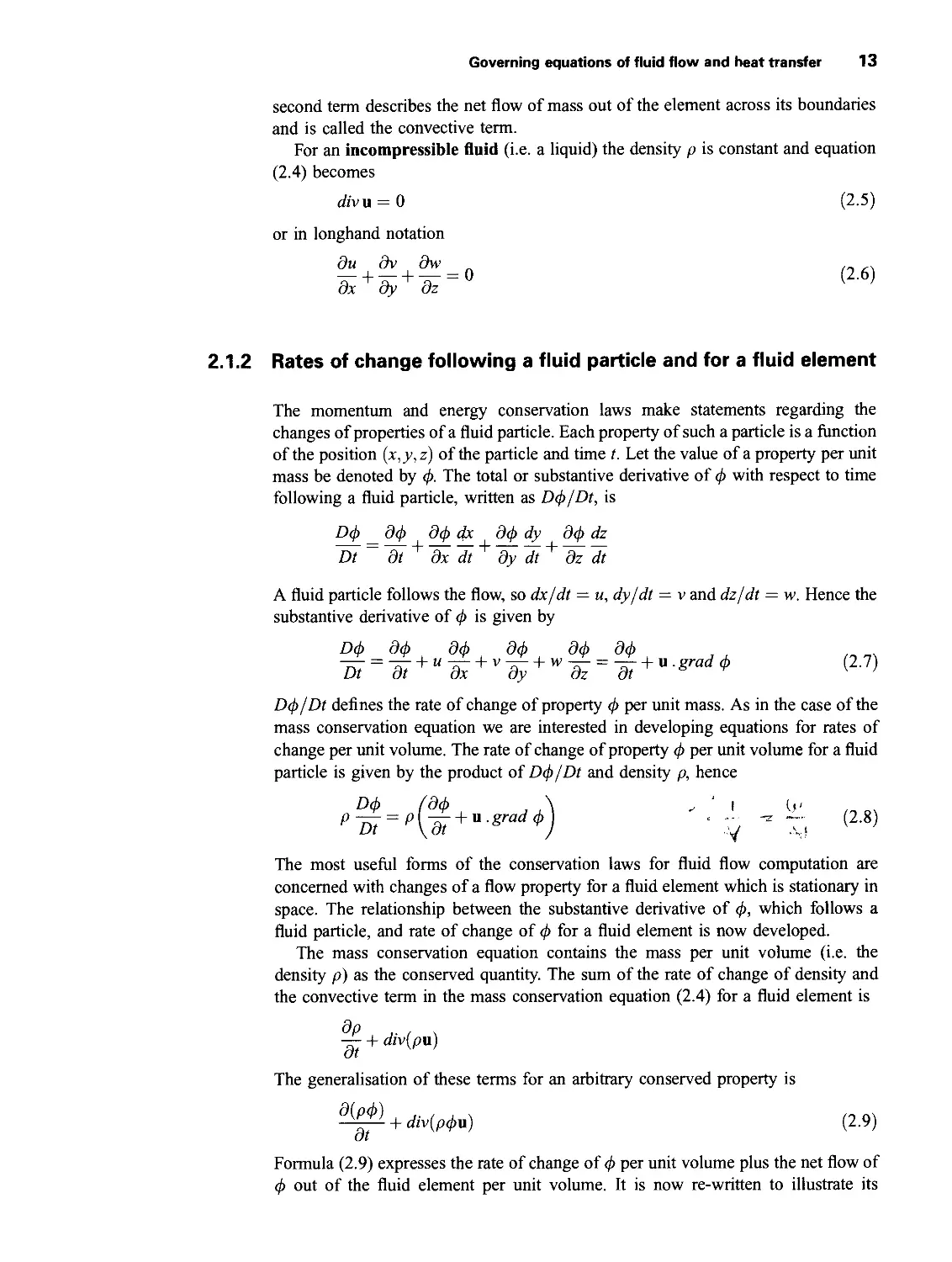
Оф/Dt defines the rate of change of property ф per unit mass. As in the case of the
mass conservation equation we are interested in developing equations for rates of
change per unit volume. The rate of change of property ф per unit volume for a fluid
particle is given by the product of Оф/Dt and density p, hence
Оф / dф
'’57 = '’U + “

I

(2-8)
The most useful forms of the conservation laws for fluid flow computation are
concerned with changes of a flow property for a fluid element which is stationary in
space. The relationship between the substantive derivative of ф, which follows a
fluid particle, and rate of change of ф for a fluid element is now developed.
The mass conservation equation contains the mass per unit volume (i.e. the
density p) as the conserved quantity. The sum of the rate of change of density and
the convective term in the mass conservation equation (2.4) for a fluid element is
Эр
a-+ *(/>")
The generalisation of these terms for an arbitrary conserved property is
“7^ + div(p^u)	(2.9)
dt
Formula (2.9) expresses the rate of change of ф per unit volume plus the net flow of
ф out of the fluid element per unit volume. It is now re-written to illustrate its
14	Conservation laws of fluid motion and boundary conditions
relationship with the substantive derivative of ф:
д(рф)
dt
+ Лг(рфи) = p ~ + ц • grad ф
Иф
Dt
+ ф +
(2.Ю)
The term ф[3р/3t + cfi'v(pu)] is equal to zero by virtue of mass conservation (2.4).
In words, relationship (2.10) states
Rate of increase	Net rate of flow	Rate of increase
of ф of	+ of ф out of	= of ф for a
fluid element	fluid element	fluid particle
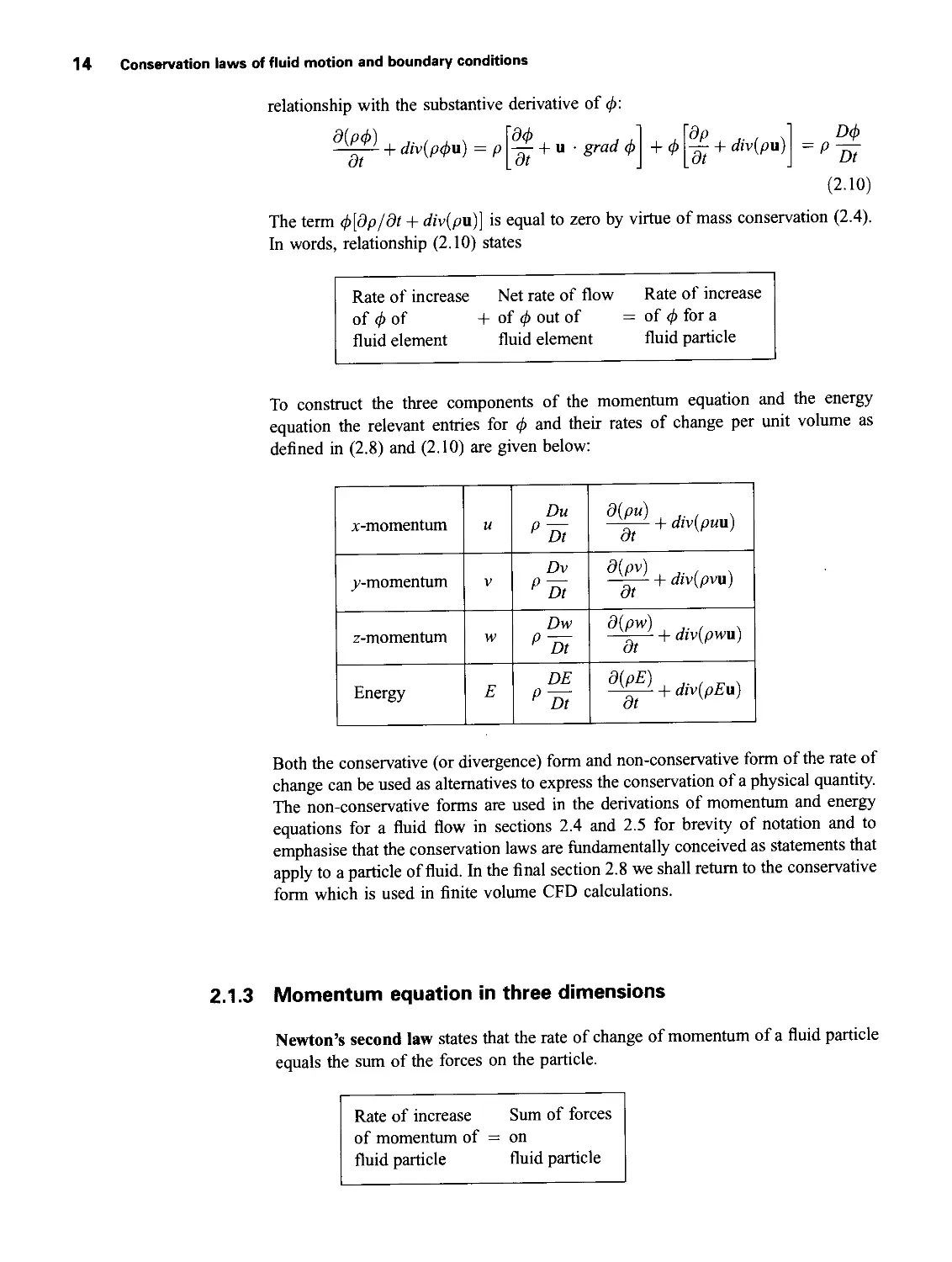
To construct the three components of the momentum equation and the energy
equation the relevant entries for ф and their rates of change per unit volume as
defined in (2.8) and (2.10) are given below:
x-momentum	u	Du p~5t	d(pu) -	+ divlpuu)
y-momentum	V	Dv PDi	d(pv) + div(pvu) dt
z-momentum	w	Dw P~Di	d(pw) - + div(pwu)
Energy	E	DE P ~Dt	X)+div^pEvp>
Both the conservative (or divergence) form and non-conservative form of the rate of
change can be used as alternatives to express the conservation of a physical quantity.
The non-conservative forms are used in the derivations of momentum and energy
equations for a fluid flow in sections 2.4 and 2.5 for brevity of notation and to
emphasise that the conservation laws are fundamentally conceived as statements that
apply to a particle of fluid. In the final section 2.8 we shall return to the conservative
form which is used in finite volume CFD calculations.
2.1.3 Momentum equation in three dimensions
Newton’s second law states that the rate of change of momentum of a fluid particle
equals the sum of the forces on the particle.
Rate of increase	Sum of forces
of momentum of = on
fluid particle	fluid particle
Governing equations of fluid flow and heat transfer 15
The rates of increase of x-, y- and z- momentum per unit volume of a fluid particle
are given by
Du	Dv	Dw
PDi PDt P ~Dt
(2.П)
We distinguish two types of forces on fluid particles:
• surface forces - pressure forces
- viscous forces
• body forces - gravity force
-	centrifugal force
-	Coriolis force
-	electromagnetic force
It is common practice to highlight the contributions due to the surface forces as
separate terms in the momentum equation and to include the effects of body forces
as source terms.
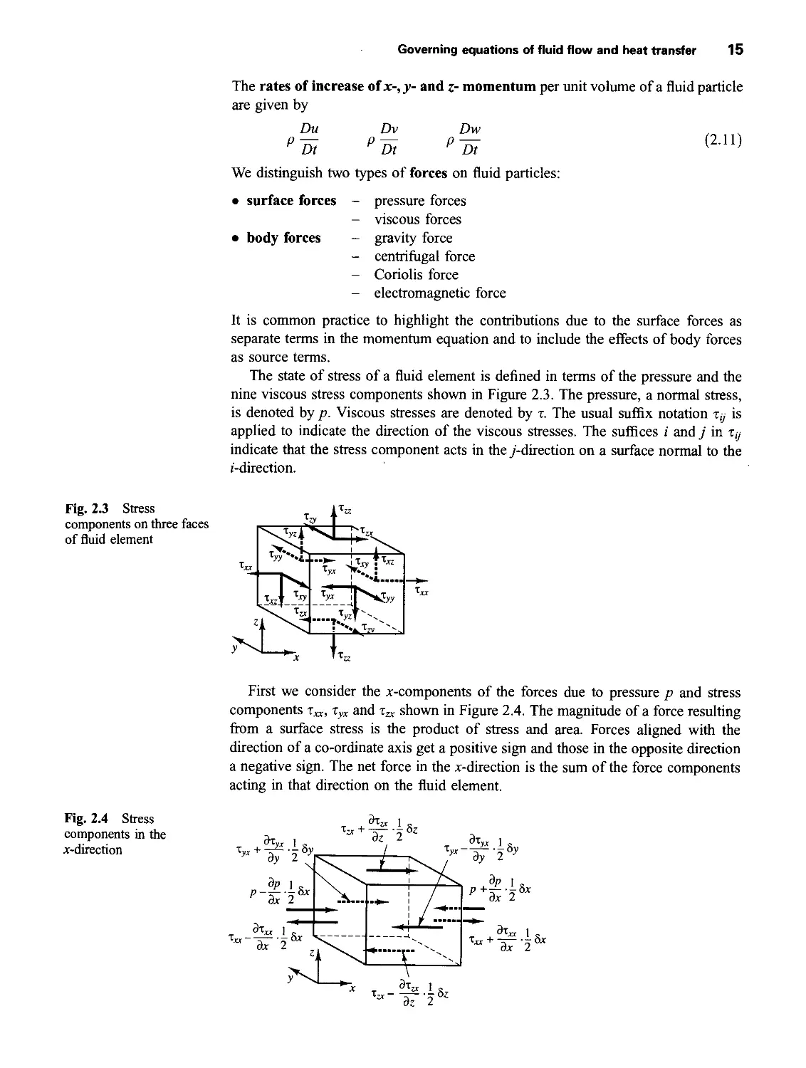
The state of stress of a fluid element is defined in terms of the pressure and the
nine viscous stress components shown in Figure 2.3. The pressure, a normal stress,
is denoted by p. Viscous stresses are denoted by r. The usual suffix notation is
applied to indicate the direction of the viscous stresses. The suffices z and j in т,у
indicate that the stress component acts in the j-direction on a surface normal to the
z-direction.
Fig. 2.3 Stress
components on three faces
of fluid element
First we consider the x-components of the forces due to pressure p and stress
components r„, xyx and rzx shown in Figure 2.4. The magnitude of a force resulting
from a surface stress is the product of stress and area. Forces aligned with the
direction of a co-ordinate axis get a positive sign and those in the opposite direction
a negative sign. The net force in the x-direction is the sum of the force components
acting in that direction on the fluid element.
Fig. 2.4 Stress
components in the
x-direction
16 Conservation laws of fluid motion and boundary conditions
P-
On the pair of faces (E, JV) we have
j \ f dzxx i „ \ „ -
— |dx - r„ - — jdx 8yoz
)X }	\ ox J
(	dp I ? )	(	dzxx	1 ? )	< c
+ -U’+n_Px + т«+-^-рл: ()ybz
\	dx1 J	\	ox )
( dp ,
-	dxdydz
\ dx ox J
The net force in the x-direction on the pair of faces (N, S) is
— f zyx —	dxdz + f Тух +	I dy^ dxdz =	dxdydz
\ z r+1) 2	/	\ z rhj 2	/	rn>
(2.12a)
(2.12b)
Finally the net force in the x-direction on faces T and В is given by
- ft» -	§x3y + (ta +	5<)z^ dxby = -^dxdydz
\ dz z /	\ dzL	oz
(2.12c)
The total force per unit volume on the fluid due to these surface stresses is equal to
the sum of (2.12a), (2.12b) and (2.12c) divided by the volume dxdydz:
d(~P + ?«) ' dzyx i dzzx
<~j	I О '	\		/
ox oy oz
Without considering the body forces in further detail their overall effect can be
included by defining a source Smx of x-momentum per unit volume per unit time.
The x-component of the momentum equation is found by setting the rate of
change of x-momentum of the fluid particle (2.11) equal to the total force in the
x-direction on the element due to surface stresses (2.13) plus the rate of increase of
x-momentum due to sources:
Du _ d(—p + Txr)	dzyx dzz,
? Dt dx	dy	dz
(2.14a)
It is not too difficult to verify that the у-component of the momentum equation is
given by
(2.14b)
and the z-component of the momentum equation by
Dw dzxz dzyz 3(-/2 + tzz)
= V + ~E~ 'I-----л------r
Dt dx dy	dz
(2.14c)
The sign associated with the pressure is opposite to that associated with the normal
viscous stress, because the usual sign convention takes a tensile stress to be the
positive normal stress so that the pressure, which is by definition a compressive
normal stress, has a minus sign.
Governing equations of fluid flow and heat transfer 17
The effects of surface stresses are accounted for explicitly; the source terms Syx,
SMy and SMz in (2.14a-c) include contributions due to body forces only. For example,
the body force due to gravity would be modelled by Smx = 0, SMy = 0 and
$Mz = ~Pg-
2.1.4 Energy equation in three dimensions
The energy equation is derived from the first law of thermodynamics which states
that the rate of change of energy of a fluid particle is equal to the rate of heat addition
to the fluid particle plus the rate of work done on the particle.
Rate of increase	Net rate of	Net rate of work
of energy of = heat added to + done on
fluid particle	fluid particle	fluid particle
As before we will be deriving an equation for the rate of increase of energy of a
fluid particle per unit volume which is given by
DE
P~Di
(2-15)
Work done by surface forces
The rate of work done on the fluid particle in the element by a surface force is
equal to the product of the force and velocity component in the direction of the force.
For example, the forces given by (2.12a-c) all act in the x-direction. The work done
by these forces is given by
PU H----- 2	"I--2 dx
dx 2 J \ dx £
frydz
d{Tzxu) 1 s \	, d^u) !	\
------z— 5 <5z + zzxu -I----------— ± dz oxoy
dz г )	\ dz J
The net rate of work done by these surface forces acting in the x-direction is given by
, 9(urzx)l
H----z--- dxdydz
dz
(2.16a)
Surface stress components in the y- and z-direction also do work on the fluid particle.
A repetition of the above process gives the additional rates of work done on the fluid
particle due to the work done by these surface forces:
and
dxdySz
(2.16b)
(2.16c)
d(wTxz) d(wTyz) d[w(—p + тд)]'
dx dy	dz
18 Conservation laws of fluid motion and boundary conditions
The total rate of work done per unit volume on the fluid particle by all the surface
forces is given by the sum of (2.16a-c) divided by the volume bxbybz. The terms
containing pressure can be collected together and written more compactly in vector
form:
d(up)	d(vp) d(wp)
dx dy dz
This yields the following total rate of work done on the fluid particle by surface
stresses:
(ПП\]4.	 ЭМ |	i	| д^У
I	-t- dx -t-	-t-	-t- Qx т
9(wrzz)
dz dx by dz
Energy flux due to heat conduction
The heat flux vector q has three components qx, qy and qz (Figure 2.5).
Fig. 2.5 Components of
the heat flux vector
j The net rate of heat transfer to the fluid particle due to heat flow in the x-
direction is given by the difference between the rate of heat input across face IV and
the rate of heat loss across face E:
dqx i x \	, dqx }
—-	- \qx + — kbx
dx 2 J \ dx
bybz =
— bxbybz
dx
(2.18a)
Similarly, the net rates of heat transfer to the fluid due to heat flows in the y- and z-
direction are
— bxbybz
’ dy
and
—— bxbybz
dz
(2.18b-c)
The total rate of heat added to the fluid particle per unit volume due to heat flow
across its boundaries is the sum of (2.18a-c) divided by the volume bxbybz
dqx
dx
dqy
dy
dqz
Fourier’s law of heat conduction relates the heat flux to the local temperature
(2-19)
Governing equations of fluid flow and heat transfer 19
gradient. So
, dT
Ях =
OX
ат	ат
q’ = -kdy ‘b = ~k&
This can be written in vector form as follows:
q= -k grad T	(2.20)
Combining (2.19) and (2.20) yields the final form of the rate of heat addition to the
fluid particle due to heat conduction across element boundaries:
—div q = div(k grad Г)	(2-21)
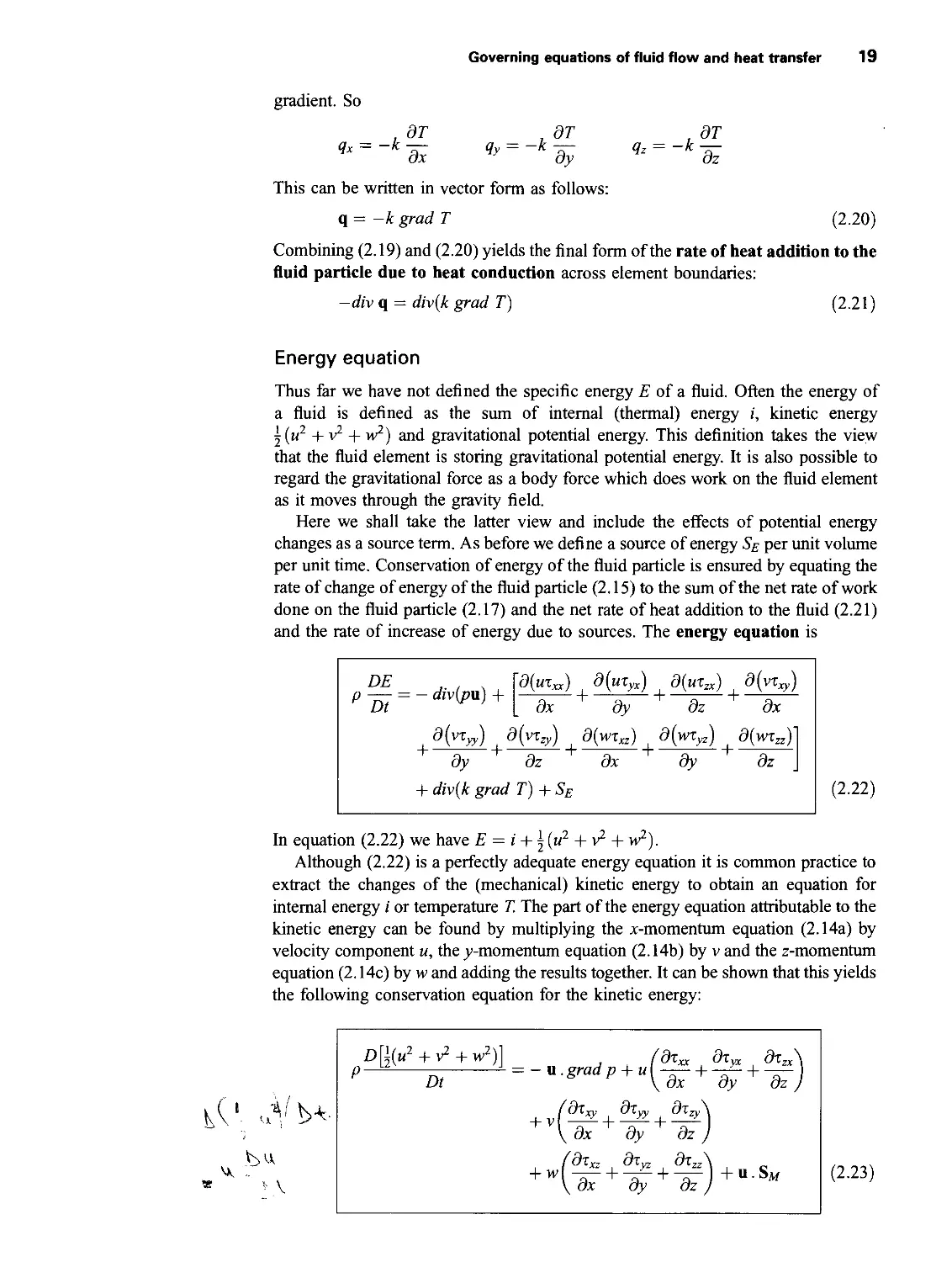
Energy equation
Thus far we have not defined the specific energy £ of a fluid. Often the energy of
a fluid is defined as the sum of internal (thermal) energy i, kinetic energy
| (u2 + v2 + w2) and gravitational potential energy. This definition takes the view
that the fluid element is storing gravitational potential energy. It is also possible to
regard the gravitational force as a body force which does work on the fluid element
as it moves through the gravity field.
Here we shall take the latter view and include the effects of potential energy
changes as a source term. As before we define a source of energy SE per unit volume
per unit time. Conservation of energy of the fluid particle is ensured by equating the
rate of change of energy of the fluid particle (2.15) to the sum of the net rate of work
done on the fluid particle (2.17) and the net rate of heat addition to the fluid (2.21)
and the rate of increase of energy due to sources. The energy equation is
DE	J' !	\ P = - div(pa) + dy + div(k grad	d{uTxx)	d(uTyX^	3(urzx)	3(vTxy) dx	dy	dz	dx *(VT^)	,	d(wTxz)	d(wtyz)	d(wrzz)~l dz	dx	dy	dz \ T)+SE	(2.22)
In equation (2.22) we have E = i + | (u2 + v2 + w2).
Although (2.22) is a perfectly adequate energy equation it is common practice to
extract the changes of the (mechanical) kinetic energy to obtain an equation for
internal energy i or temperature T. The part of the energy equation attributable to the
kinetic energy can be found by multiplying the x-momentum equation (2.14a) by
velocity component u, the у-momentum equation (2.14b) by v and the z-momentum
equation (2.14c) by w and adding the results together. It can be shown that this yields
the following conservation equation for the kinetic energy:
O[l(u2 + v2 + w2)]	P dixx	дтух	dtzx
P~------n,-----1 = - u SradP + “ V +	+
Dt	\ ox	oy	oz
(д^ху	дтуу дт2у\
\dx dy dz )
(d^xz	diyZ	dx2Z\
+ w (	—I- —H “x- I + u. Sjw
\ dx	dy	dz)
(2.23)
20 Conservation laws of fluid motion and boundary conditions
Subtracting (2.23) from (2.22) and defining a new source term as S’, = SE - u.SM
yields the internal energy equation
Di	du du
p- = -pdivu + div(k grad T) + r„ — + ty*
du	dv	dv	dv dw
dw	dw
+ r^z — + Tzz — + Sj
'dy	dz
(2-24)
In the special case of an incompressible fluid we have i = cT, where c is the specific
heat, and div u — 0. This allows us to recast equation (2.24) into a temperature
equation
DT	du	du	du
Pc~^ = div(k grad T) +	+ r^— + rzx —
Dt	dx	dy	dz
dv dv dv dw dw
dw
+ tzz H Si
dz
(2-25)
For compressible flows equation (2.22) is often re-arranged to give an equation for
the enthalpy. The specific enthalpy h and the specific total enthalpy ho of a fluid are
defined as
h = i+p/p and ho = h + |(u2 + v2 + w2)
Combining these two definitions with the one for specific energy E we get
ho = i+p/p + ^(u2 + v2 + w2) =E+p/p	(2-26)
Substituting of (2.26) into equation (2.22) and some re-arrangement yields the
(total) enthalpy equation
+ div(phou) = div(k grad T)
'djui^)	d(uzyx)	d(wrzx)
dx dy dz
dp
dt
d^xy)	djyTyy)	dlyr^
dx	dy	dz
d(wzxz)	d(wzy2}	d(wrzz)
dx	dy	dz
+ Sh
(2.27)
It should be stressed that equations (2.24), (2.25) and (2.27) are not new (extra)
conservation laws but merely alternative forms of the energy equation (2.22).
Navier-Stokes equations for a Newtonian fluid 21
2.2	Equations of state
The motion of a fluid in three dimensions is described by a system of five partial
differential equations: mass conservation (2.4), x-, y- and z-momentum equations
(2.14a-c) and energy equation (2.22). Among the unknowns are four thermo-
dynamic variables: p, p, i and T. In this brief discussion we point out the linkage
between these four variables. Relationships between the thermodynamic variables
can be obtained through the assumption of thermodynamic equilibrium. The fluid
velocities may be large, but they are usually small enough that, even though the
properties of a fluid particle change rapidly from place to place, the fluid can
thermodynamically adjust itself to new conditions so quickly that the changes are
effectively instantaneous. Thus the fluid always remains in thermodynamic
equilibrium. The only exceptions are certain flows with strong shockwaves, but
even some of those are often well enough approximated by equilibrium assumptions.
We can describe the state of a substance in thermodynamic equilibrium by means
of just two state variables. Equations of state relate the other variables to the two
state variables. If we use p and T as state variables we have state equations for
pressure p and specific internal energy i:
P = p(p, T) and i — i(p, T)	(2.28)
For a perfect gas the following, well-known, equations of state are useful:
p — pRT and i — CVT	(2.29)
The assumption of thermodynamic equilibrium eliminates all but the two
thermodynamic state variables. In the flow of compressible fluids the equations
of state provide the linkage between the energy equation on the one hand and mass
conservation and momentum equations on the other. This linkage arises through the
possibility of density variations as a result of pressure and temperature variations in
the flow field.
Liquids and gases flowing at low speeds behave as incompressible fluids.
Without density variations there is no linkage between the energy equation and the
mass conservation and momentum equations. The flow field can often be solved by
considering mass conservation and momentum equations only. The energy equation
only needs to be solved alongside the others if the problem involves heat transfer.
2.3	Navier-Stokes equations for a Newtonian fluid
The governing equations contain as further unknowns the viscous stress components
Ту. The most useful forms of the conservation equations for fluid flows are obtained
by introducing a suitable model for the viscous stresses Ту. In many fluid flows the
viscous stresses can be expressed as functions of the local deformation rate (or strain
rate). In three-dimensional flows the local rate of deformation is composed of the
linear deformation rate and the volumetric deformation rate.
All gases and many liquids are isotropic. Liquids which contain significant
quantities of polymer molecules may exhibit anisotropic or directional viscous stress
properties as a result of the alignment of the chain-like polymer molecules with the
flow. Such fluids are beyond the scope of this introductory course and we shall
continue the development by assuming that the fluids are isotropic.
22 Conservation laws of fluid motion and boundary conditions
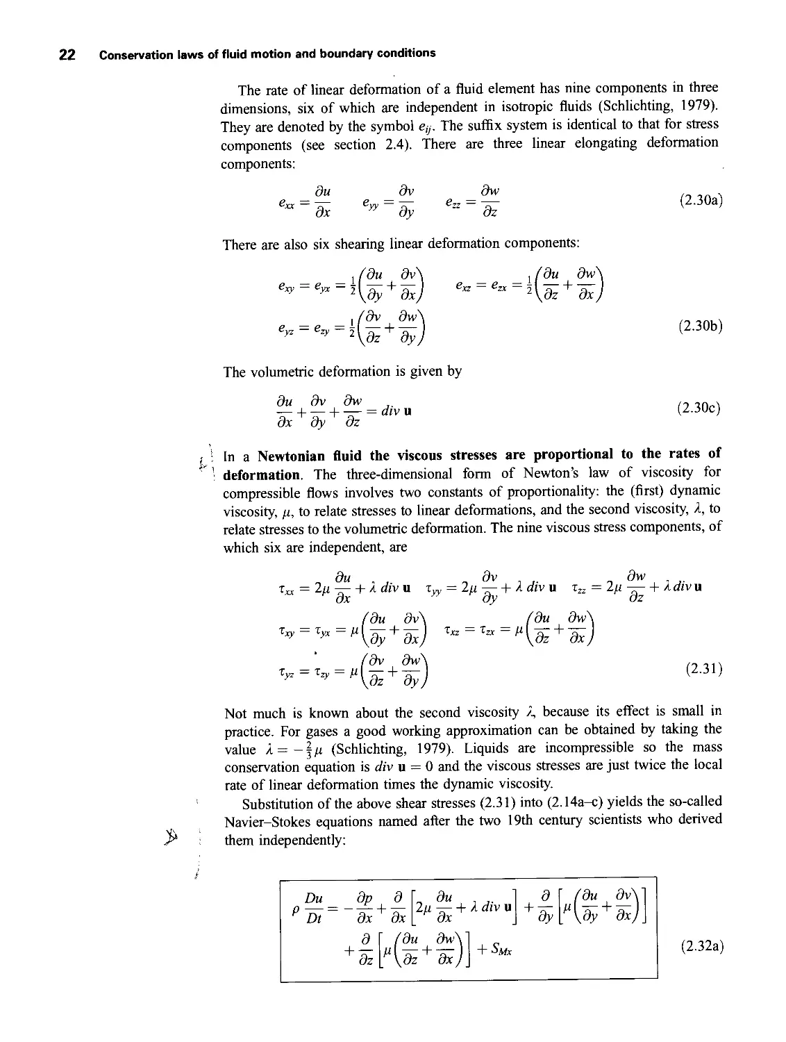
The rate of linear deformation of a fluid element has nine components in three
dimensions, six of which are independent in isotropic fluids (Schlichting, 1979).
They are denoted by the symbol ey. The suffix system is identical to that for stress
components (see section 2.4). There are three linear elongating deformation
components:
_ du	dv	dw
dx вуу dy 6zz dz
There are also six shearing linear deformation components:
, (du dv\	. (du dw
&xy еУх — 2 ( я h я~ I	=	= 21 "я
\dy dxj	z\dz	dx
. /dv	dw\
The volumetric deformation is given by
du dv	dw
---1-----1- —- = div u
dx dy	dz
(2.30a)
(2.30b)
(2.30c)
I • In a Newtonian fluid the viscous stresses are proportional to the rates of
* deformation. The three-dimensional form of Newton’s law of viscosity for
compressible flows involves two constants of proportionality: the (first) dynamic
viscosity, p., to relate stresses to linear deformations, and the second viscosity, Z, to
relate stresses to the volumetric deformation. The nine viscous stress components, of
which six are independent, are
du , ,	dv	~ dw .
txx = 2u — + z div u Tyy = 2u — + Z div u r2z = 2u — + Z div u
dx	dy	dz
(du dv\	/ du dw\
=	+ -j zxz = Tzx = p\^ + — J
(dv dw
^ = ^ = /z^- + —
(2.31)
Not much is known about the second viscosity z, because its effect is small in
practice. For gases a good working approximation can be obtained by taking the
value Z=—j/z (Schlichting, 1979). Liquids are incompressible so the mass
conservation equation is div u = 0 and the viscous stresses are just twice the local
rate of linear deformation times the dynamic viscosity.
Substitution of the above shear stresses (2.31) into (2.14a-c) yields the so-called
Navier-Stokes equations named after the two 19th century scientists who derived
P them independently:
dp
du
d Г (du dv
dy ^\dy ' dx
Du	dp	d _	~	i —
p	+ 7Г 2p—+2 div и + — Дк- + x-
Dt	dx dx (	л” ' я”
du
dz
dx
d_ ’
dz ‘
dx
dw
dx
+ $Мх
(2.32a)
Navier-Stokes equations for a Newtonian fluid 23
Dv	dp	d
P = ~P
Dt	dy dx
d Г
+ y 1
dz
dv
— + Z div u
dy
dv dw\
dz + dy)
+ Sm)
(2.32b)
d '
dx
+	2p^ + /.divu + SMz
dz dz
Dw	dp
Dt	dz +
d Г.
1 „
dz
du dw'
dz dx
d Pdv ЗиЛ
dy P \dz dy)
(2.32c)
Often it is useful to re-arrange the viscous stress terms as follows:
du dw\
dz dx )
d Г,
d Г	du	. ,	1	d Г	f du	dv\
y- 2/z — + Z dzv u +— p — + —	4
dx [	dx	J	dy [	\dy	dx)
\	9 (
+ 0- Д
/ dz\
dv\ d_
dx) + dz
du
dx
d Г i
dz p
du\
dz)
( dw
\Plh
dx
d / du\ d / du
^di V d^c) +dy V dyt
Г d ( du\ d f
ox \ ox J dy \
Q
+ — (2 div u) = div(p grad u) + s^x
The viscous stresses in the y- and z-component equations can be re-cast in a similar
manner. We clearly intend to simplify the momentum equations by ‘hiding’ the two
smaller contributions to the viscous stress terms in the momentum source. Defining
a new source by
Sm = Sm + $m	(2.33)
the Navier-Stokes equations can be written in the most useful form for the
development of the finite volume method:
Du	dp
P 75; = -	+ atv{p grad u) + SMx
L/l	куЛ'
(2.34a)
Dv dp
P~Dt = ~dy + 'P grad + SMy
(2.34b)
Dw	dp
P yr = - y- + div(p grad w) + SMz
L)t	OZ
(2.34c)
If we use the Newtonian model for viscous stresses in the internal energy equation
(2.24) we obtain after some re-arrangement
Di
P ~Dt= ~P div u + divik grad T) + Ф + 5,
(2-35)
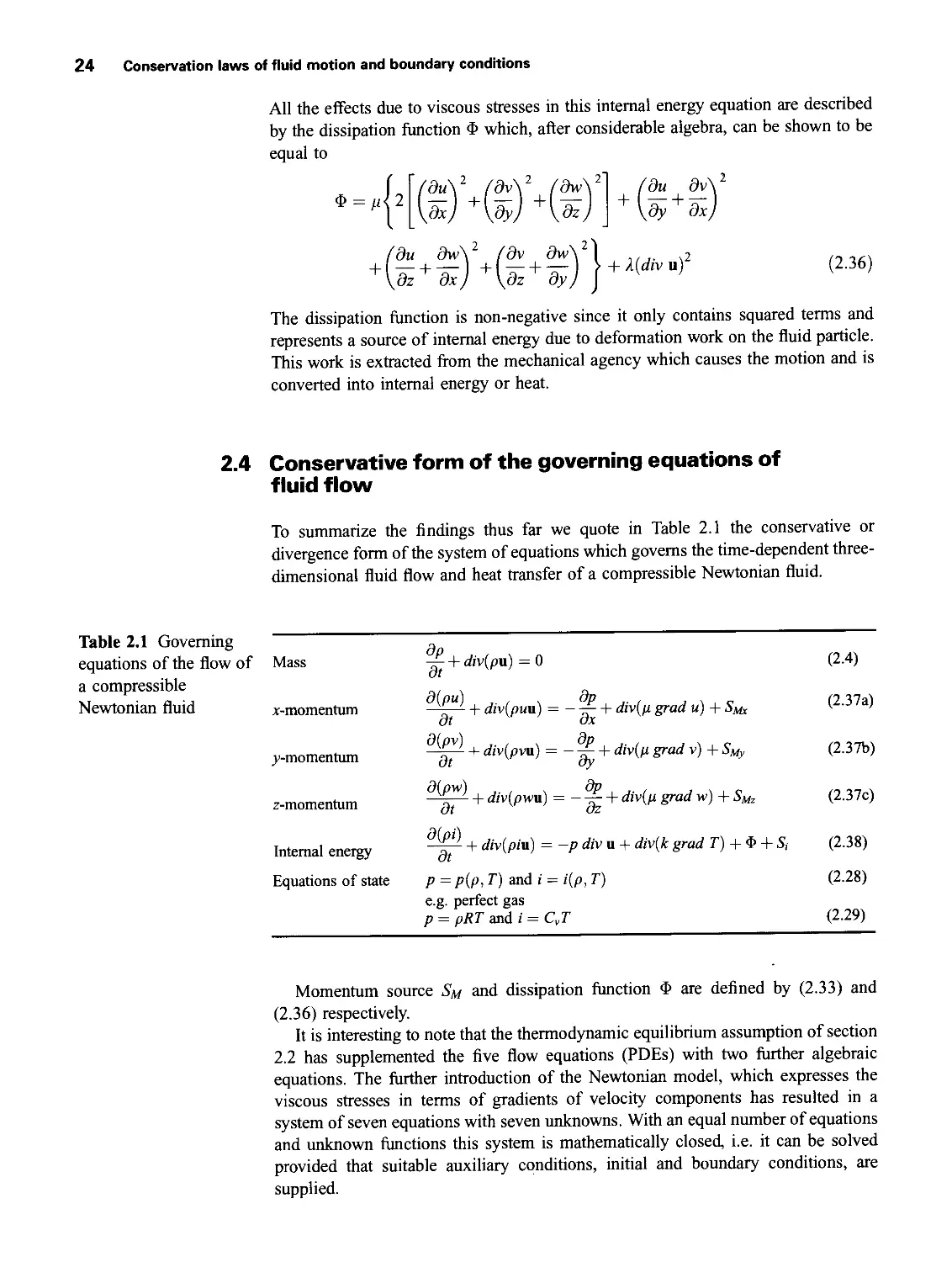
24 Conservation laws of fluid motion and boundary conditions
All the effects due to viscous stresses in this internal energy equation are described
by the dissipation function Ф which, after considerable algebra, can be shown to be
equal to
Ф = р<2
/ди dv\2
\fy + di)
du chv\2 /dv <ЭиЛ2
dz + dxJ + \dz dy)
+ 7/div u)2
(2.36)
The dissipation function is non-negative since it only contains squared terms and
represents a source of internal energy due to deformation work on the fluid particle.
This work is extracted from the mechanical agency which causes the motion and is
converted into internal energy or heat.
2.4	Conservative form of the governing equations of
fluid flow
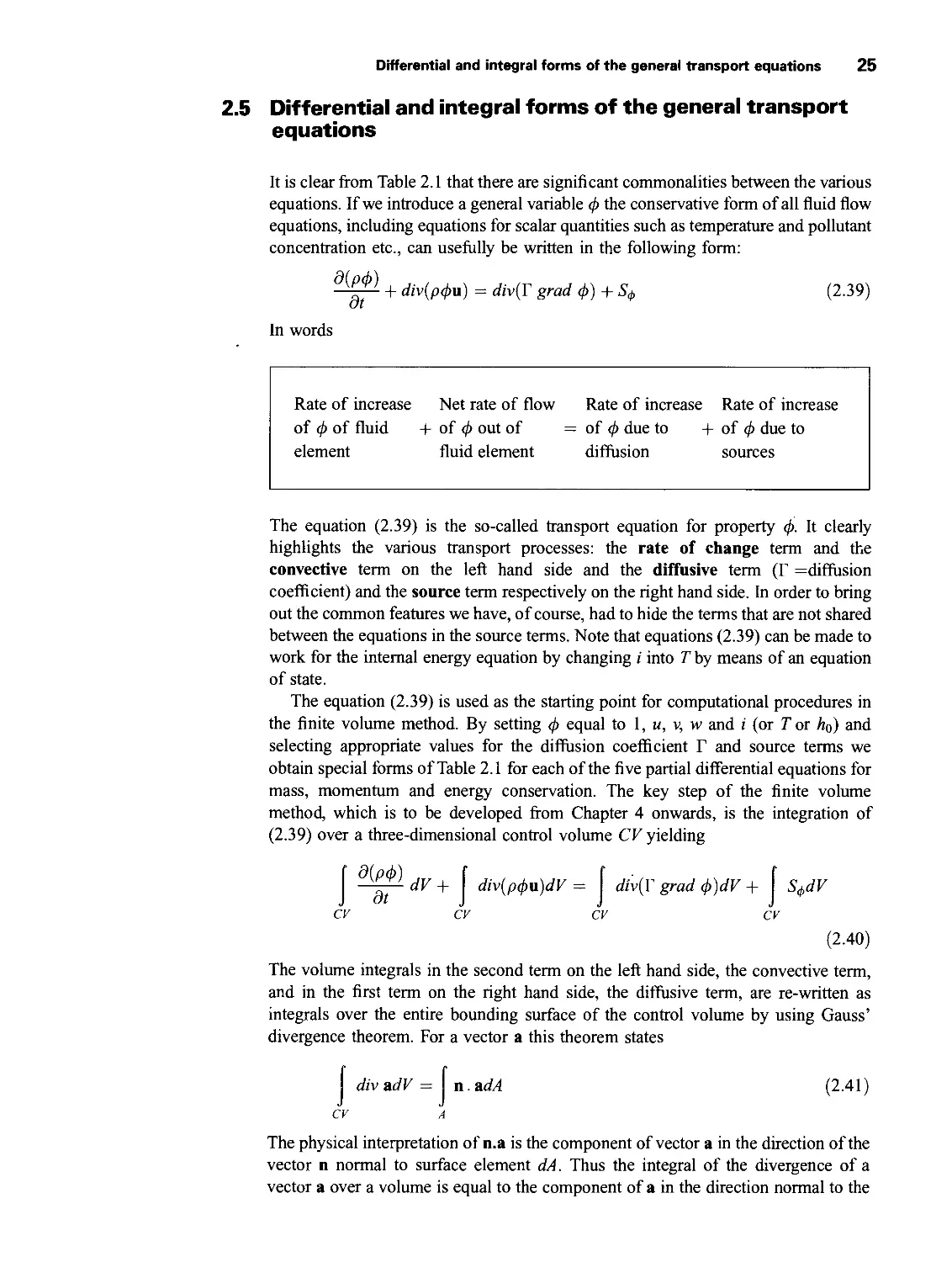
To summarize the findings thus far we quote in Table 2.1 the conservative or
divergence form of the system of equations which governs the time-dependent three-
dimensional fluid flow and heat transfer of a compressible Newtonian fluid.
Table 2.1 Governing
equations of the flow of
a compressible
Newtonian fluid
Mass	|^ + Av(pii) = 0	(2.4)
x-momentum	д( w)	d ; + div(pun) =	+ divfp grad u) + SMx	(2.37a)
y-momentum	+ div(pvu) = ~^ + div(p grad v) + SMy	(2.37b)
z-momentum	+ div(pwu) = -	+ div(p grad w) + SMz ot	oz	(2.37c)
Internal energy	+ div(piu) = -p div u + divik grad T) + Ф + S,	(2.38)
Equations of state	P=P^P,T) and i= i(p, T)	(2.28)
	e.g. perfect gas	
	p = pRT and i = CVT	(2.29)
Momentum source Sm and dissipation function Ф are defined by (2.33) and
(2.36) respectively.
It is interesting to note that the thermodynamic equilibrium assumption of section
2.2 has supplemented the five flow equations (PDEs) with two further algebraic
equations. The further introduction of the Newtonian model, which expresses the
viscous stresses in terms of gradients of velocity components has resulted in a
system of seven equations with seven unknowns. With an equal number of equations
and unknown functions this system is mathematically closed, i.e. it can be solved
provided that suitable auxiliary conditions, initial and boundary conditions, are
supplied.
Differential and integral forms of the general transport equations 25
2.5	Differential and integral forms of the general transport
equations
It is clear from Table 2.1 that there are significant commonalities between the various
equations. If we introduce a general variable ф the conservative form of all fluid flow
equations, including equations for scalar quantities such as temperature and pollutant
concentration etc., can usefully be written in the following form:
+ div(p<^u) = div(T grad ф) + S(l,
In words
(2.39)
Rate of increase	Net rate of flow	Rate of increase Rate of increase
of ф of fluid + of ф out of — of ф due to + of ф due to
element	fluid element	diffusion	sources
The equation (2.39) is the so-called transport equation for property ф. It clearly
highlights the various transport processes: the rate of change term and the
convective term on the left hand side and the diffusive term (Г =diffusion
coefficient) and the source term respectively on the right hand side. In order to bring
out the common features we have, of course, had to hide the terms that are not shared
between the equations in the source terms. Note that equations (2.39) can be made to
work for the internal energy equation by changing i into T by means of an equation
of state.
The equation (2.39) is used as the starting point for computational procedures in
the finite volume method. By setting ф equal to 1, u, v, w and i (or T or h0) and
selecting appropriate values for the diffusion coefficient Г and source terms we
obtain special forms of Table 2.1 for each of the five partial differential equations for
mass, momentum and energy conservation. The key step of the finite volume
method, which is to be developed from Chapter 4 onwards, is the integration of
(2.39) over a three-dimensional control volume CV yielding
dV + j div(jrfu)dV = j div(V grad ф^Р + j S(fldV
CV	CV	CV	CV
(2.40)
The volume integrals in the second term on the left hand side, the convective term,
and in the first term on the right hand side, the diffusive term, are re-written as
integrals over the entire bounding surface of the control volume by using Gauss’
divergence theorem. For a vector a this theorem states
div adV = n.ad/f	(2-41)
CV	A
The physical interpretation of n.a is the component of vector a in the direction of the
vector n normal to surface element dA. Thus the integral of the divergence of a
vector a over a volume is equal to the component of a in the direction normal to the
26 Conservation laws of fluid motion and boundary conditions
surface which bounds the volume summed (integrated) over the entire bounding
surface A. Applying Gauss’ divergence theorem, equation (2.40) can be written as
follows:
I рф/iV | + n. (рфъ)<1А = f n . (Г grad ф'^А + S(l)dV
\CK / A	A	CV
(2-42)
The order of integration and differentiation has been changed in the first term on the
left hand side of (2.42) to illustrate its physical meaning. This term signifies the rate
of change of the total amount of fluid property ф in the control volume. The
product n. (рфи) expresses the flux component of property ф due to fluid flow along
the outward normal vector n, so the second term on the left hand side of (2.42), the
convective term, is therefore the net rate of decrease of fluid property ф of the
fluid element due to convection.
A diffusive flux is positive in the direction of a negative gradient of the fluid
property ф, i.e. along direction -grad ф. For instance, heat is conducted in the
direction of negative temperature gradients. Thus, the product n. (-Г grad ф) is the
component of diffusion flux along the outward normal vector, and so out of the fluid
element. Similarly, the product n. (Г grad ф), which is also equal to Г(-п. (-grad
ф)), can be interpreted as a positive diffusion flux in the direction of the inward
normal vector -n, i.e. into the fluid element. The first term on the right hand side of
(2.42), the diffusive term, is thus associated with a flux into the element and
represents the net rate of increase of fluid property ф of the fluid element due to
diffusion. The final term on the right hand side of this equation gives the rate of
increase of property ф as a result of sources inside the fluid element.
In words, relationship (2.42) for the fluid in the control volume can be expressed
as follows:
	Net rate of	Rate of increase
Rate of	decrease of ф due to	of ф due to	Net rate of
increase of ф	+ . convection across	= + diffusion across creation of ф
	the boundaries	the boundaries
This discussion clarifies that integration of the partial differential equation generates
a statement of the conservation of a fluid property for a finite size (macroscopic)
control volume.
In steady state problems the rate of change term of (2.42) is equal to zero. This
leads to the integrated form of the steady transport equation
j n. (рфи^А = j n . (Г grad ф^А + | S<i>dV
A	A	CV
(2.43)
In time-dependent problems it is also necessary to integrate with respect to time t
over a small interval Д/ from, say, t until t + Д/. This yields the most general
Classification of physical behaviour 27
integrated form of the transport equation:
(2-44)
2.6	Classification of physical behaviour
Now that we have derived the conservation equations of fluid flows the time has
come to turn our attention to the issue of the initial and boundary conditions which
are needed in conjunction with the equations to construct a well-posed mathematical
model of a fluid flow. First we distinguish two principal categories of physical
behaviour:
•	Equilibrium problems
•	Marching problems
Equilibrium problems
The problems in the first category are steady state situations, e.g. the steady state
distribution of temperature in a rod of solid material, the equilibrium stress
distribution of a solid object under a given applied load as well as many steady fluid
flows. These and many other steady state problems are governed by elliptic
equations. The prototype elliptic equation is Laplace’s equation which describes the
irrotational flow of an incompressible fluid and steady state conductive heat transfer.
In two dimensions we have
Э2Ф
dx2 dy2
A very simple example of an equilibrium problem is the steady state heat conduction
(where ф = T in equation (2.45)) in an insulated rod of metal whose ends at x = 0
and x = L are kept at constant, but different, temperatures To and Ti (Figure 2.6).
This problem is one-dimensional and governed by the equation kd2 T/dx2 — 0.
Under the given boundary conditions the temperature distribution in the x-direction
Fig. 2.6 Steady state
temperature distribution
of an insulated rod
Problem specification
Heat flux q = 0
'///////////A/////////////.
T= To |	I T = TL
Solution
x-0
x = L
28 Conservation laws of fluid motion and boundary conditions
will, of course, be a straight line. A unique solution to this and all elliptic problems
can be obtained by specifying conditions on the dependent variable (here the
temperature or its normal derivative, the heat flux) on all the boundaries of the
solution domain. Problems requiring data over the entire boundary are called
boundary-value problems.
An important feature of elliptic problems is that a disturbance in the interior of the
solution, for example a change in temperature due to the sudden appearance of a
small local heat source, changes the solution everywhere else. Disturbance signals
travel in all directions through the interior solution. Consequently, the solutions to
physical problems described by elliptic equations are always smooth even if the
boundary conditions are discontinuous, which is a considerable advantage to the
designer of numerical methods. To ensure that information propagates in all
directions, the numerical techniques for elliptic problems must allow events at each
point to be influenced by all its neighbours.
Marching problems
Transient heat transfer, all unsteady flows and wave phenomena are examples of
problems in the second category, the marching or propagation problems. These
problems are governed by parabolic or hyperbolic equations. However, not all
marching problems are unsteady. We will see further on that certain steady flows are
described by parabolic or hyperbolic equations. In these cases the flow direction acts
as a time-like co-ordinate along which marching is possible.
Parabolic equations describe time-dependent problems which involve signifi-
cant amounts of dissipation. Examples are unsteady viscous flows and unsteady heat
conduction. The prototype parabolic equation is the diffusion equation
дф д2ф
~di = Old^
The transient distribution of temperature (again ф = T) in an insulated rod of metal
whose ends at x = 0 and x = L are kept at constant and equal temperature To is
governed by the diffusion equation. This problem arises when the rod cools down
after an initially uniform source is switched off at time t = 0. The temperature
distribution at the start is a parabola with a maximum at x = £/2 (Figure 2.7).
Fig. 2.7 Transient
distribution of
temperature in an
insulated rod
Problem specification
T(x, t = 0) -Д) and
heat flux q = 0
'(////////////^/////////////7.
T=T01.............................................................................................................................................1	T = T
Solution
The steady state consists of a uniform distribution of temperature T = TQ
throughout the rod. The solution of the diffusion equation (2.46) yields the
exponential decay of the initial quadratic temperature distribution. Initial conditions
Classification of physical behaviour 29
are needed in the entire rod and conditions on all its boundaries are required for all
times t > 0. This type of problem is termed an initial-boundary-value problem.
A disturbance at a point in the interior of the solution region (i.e. 0 < x < L and
time t\ > 0) can only influence events at later times t > ti (unless we allow time
travel!). The solutions move forward in time and diffuse in space. The occurrence of
dissipative effects ensures that the solutions are always smooth in the interior at
times t > 0 even if the initial conditions contain discontinuities. The steady state is
reached as time t —> oo and is elliptic. This change of character can be easily seen by
setting дф/dt = 0 in equation (2.46). The governing equation is now equal to the one
governing the steady temperature distribution in the rod.
Hyperbolic equations dominate the analysis of vibration problems. In general
they appear in time-dependent processes with negligible amounts of dissipation. The
prototype hyperbolic equation is the wave equation
Э2ф 2 д^Ф
W = c a?
(2-47)
The above form of the equation governs the transverse displacement (ф = у) of a
string under tension during small amplitude vibrations and also acoustic oscillations.
The constant c is the wave speed. It is relatively straightforward to compute the time
evolution of the fundamental mode of vibration of a string of length L using (2.47).
Fig. 2.8 Vibrations of a
string under tension
Problem specification	Solution
y(x, r = 0) = fix) and dy!dx(x, r-0)-0	for flrst cycle 0 < t < 2Llc
Solutions to the wave equation (2.47) and other hyperbolic equations can be
obtained by specifying two initial conditions on the displacement у of the string and
one condition on all boundaries for times t > 0. Thus hyperbolic problems are also
initial-boundary-value problems.
If the initial amplitude is given by a, the solution of this problem is
,	(HCt\ . HtX\
y(x, t) — a cos J sin
The solution shows that the vibration amplitude remains constant, which
demonstrates the lack of damping in the system. This absence of damping has a
further important consequence. Consider, for example, initial conditions correspond-
ing to a near-triangular initial shape whose apex is a section of a circle with very
small radius of curvature. This initial shape has a sharp discontinuity at the apex, but
it can be represented by means of a Fourier series as a combination of sine waves.
The governing equation is linear so each of the individual Fourier components (and
also their sum) would persist in time without change of amplitude. The final result is
30 Conservation laws of fluid motion and boundary conditions
that the discontinuity remains undiminished due to the absence of a dissipation
mechanism to remove the kink in the slope.
Compressible fluid flows at speeds close to and above the speed of sound exhibit
shockwaves and it turns out that the inviscid flow equations are hyperbolic at these
speeds. The shockwave discontinuities are manifestations of the hyperbolic nature of
such flows. Computational algorithms for hyperbolic problems are shaped by the
need to allow for the possible existence of discontinuities in the interior of the
solution.
It will be shown that disturbances at a point can only influence a limited region in
space. The speed of disturbance propagation through an hyperbolic problem is finite
and equal to the wave speed c. In contrast parabolic and elliptic models assume
infinite propagation speeds.
2.7	The role of characteristics in hyperbolic equations
Hyperbolic equations have a special behaviour which is associated with the finite
speed, namely the wave speed, at which information travels through the problem.
This distinguishes hyperbolic equations from the two other types. To develop the
ideas about the role of characteristic lines in hyperbolic problems we consider again
a simple hyperbolic problem described by the wave equation (2.47). It can be shown
(Open University, 1984) that a change of variables to £ = x — ct and t] = x + ct
transforms the wave equation into the following standard form:
*i=o
d^drj
The transformation requires repeated application of the chain rule for differentiation
to express the derivatives of equation (2.47) in terms of the derivatives of the
transform variables. The equation (2.48) can be solved very easily. The solution is,
of course, ф(£, tf) = Fi (£) + F2(//), where Fi and F2 can be any function.
A return to the original variables yields the general solution of equation (2.47):
ф(х, t) = Fi(x — ct) + F2(x + ct)	(2-49)
(2-48)
The first component of the solution, function F\, is constant if x — ct is constant, and
hence along lines of slope dt/dx = 1/c in the x-t plane. The second component F2
is constant if x + ct is constant, so along lines of slope dt/dx = — \/c. The lines
x - ct = const and x + ct = const are called the characteristics. Functions Fi and F2
represent the so-called simple wave solutions of the problem which are travelling
waves with velocities +c and — c without change of shape or amplitude.
The particular forms of functions F\ and F2 can be obtained from the initial and
boundary conditions of the problem. Let us consider a very long string
(—oo < x < oo) and let the following initial conditions hold:
ф(х, 0) = f(x) and дф/д1(х, 0) = g(x)	(2.50)
Combining (2.49) and (2.50) we obtain
Fi(x) + F2(x) =f(x) and - cF\(x) + cF'2{x) = g(x)	(2.51)
It can be shown (Bland, 1988) that the particular solution of wave equation (2.47)
The role of characteristics in hyperbolic equations 31
with initial conditions (2.50) is given by
x + ct
<KX, =^[f(x - Ct)+f(x +ct)]+-^_ [ g(s)ds	(2.52)
2	2c J
x-ct
Careful inspection of formula (2.52) shows that ф at point (x, t) in the solution
domain depends only on the initial conditions in the interval (x - ct,x + ct). It is
particularly important to note that this implies that the solution at (x,t) does not
depend on initial conditions outside this interval.
Figure 2.9 seeks to illustrate this point. The characteristics x — ct — constant and
x + ct = constant through the point (x',z') intersect the x-axis at the points
(x/ — ct1,0) and (x/ + ct', 0) respectively. The region in the x — t plane enclosed by
the x-axis and the two characteristics is termed the domain of dependence.
Fig. 2.9 Domain of
dependence and zone of
influence for an
hyperbolic problem
In accordance with formula (2.52) the solution at (x/,F) is influenced only by
events inside the domain of dependence and not those outside. Physically this is
caused by the limited propagation speed (equal to wave speed c) of mutual
influences through the solution domain. Changes at the point (x'. t') influence events
at later times within the zone of influence shown in Figure 2.9, which is again
bounded by the characteristics.
Figure 2.10a shows the situation for the vibrations of a string fixed at x = 0 and
x = L. For points very close to the x-axis the domain of dependence is enclosed by
two characteristics which originate at points on the x-axis. The characteristics
through points such as P intersect the problem boundaries. The domain of
Fig. 2.10 Domains of
dependence for
(a) hyperbolic,
(b) parabolic and
(c) elliptic problem
(a)
(b)
(c)
32 Conservation laws of fluid motion and boundary conditions
dependence of P is bounded by these two characteristics and the lines t = 0, x = 0
and x = L.
The shape of the domains of dependence (see Figure 2.10b and c) in parabolic
and elliptic problems is different because the speed of information travel is assumed
to be infinite. The bold lines which demarcate the boundaries of each domain of
dependence give the regions for which initial and/or boundary conditions are needed
in order to be able to generate a solution at the point P(x, t) in each case.
The way in which changes at one point affect events at other points depends on
whether a physical problem represents a steady state or a transient phenomenon and
whether the propagation speed of disturbances is finite or infinite. This has resulted
in a classification of physical behaviours, and hence attendant PDEs, into elliptic,
parabolic and hyperbolic problems. The distinguishing features of each of the
categories was illustrated by considering three simple prototype second-order
equations. In the following sections we shall discuss methods of classifying more
complex PDEs and briefly state the limitations of the computational methods that
will be developed later in this text in terms of the classification of the flow problems
to be solved. A summary of the main features which have been identified so far is
given in Table 2.2.
Table 2.2 Classification of physical behaviours
Problem type	Equation type	Prototype equation	Conditions	Solution domain	Solution smoothness
Equilibrium problems	Elliptic	div grad ф = 0	Boundary conditions	Closed domain	Always smooth
Marching problems with dissipation	Parabolic	= a div grad ф	Initial and boundary conditions	Open domain	Always smooth
Marching problems without dissipation	Hyperbolic	= c2 div grad ф	Initial and boundaty conditions	Open domain	May be discontinuous
2.8	Classification method for simple partial differential
equations
A practical method of classifying PDEs is developed for a general second-order PDE
in two co-ordinates x and y. Consider
д^ф	д2ф	д2ф	дф	дф
а	с	е И F/0+f>—0	(2.53)
дх1	дхду	ду2	дх	ду
At first we shall assume that the equation is linear and a, b, c, d, e, f and g are
constants.
The classification of a PDE is governed by the behaviour of its highest order
derivatives, so we need only consider the second-order derivatives. The class of a
second-order PDE can be identified by searching for possible simple wave solutions.
If they exist this indicates an hyperbolic equation. If not the equation is parabolic or
elliptic.
Simple wave solutions occur if the characteristic equation (2.54) below has two
Classification method for simple partial differential equations 33
Table 2.3
Classification of linear
second-order PDEs
b2 - 4ac	Equation type	Characteristics
> 0	Hyperbolic	Two real characteristics
= 0	Parabolic	One real characteristic
< 0	Elliptic	No characteristics
real roots:
+ c = 0
(2-54)
The existence or otherwise of roots of the characteristic equation depends on the
value of discriminant (b2 - 4ac). Table 2.3 outlines the three cases.
It is left as an exercise for the reader to verify the nature of the three prototype
PDEs in section 2.6 by evaluating the discriminant.
The classification method by searching for the roots of the characteristic equation
also applies if the coefficients a, b and c are functions of x and у or if the equation is
non-linear. In the latter case a, b and c may be functions of dependent variable ф or
its first derivatives. It is now possible that the equation type differs in various regions
of the solution domain. As an example we consider the following equation:
d^ =
y dx2 dy2
We look at the behaviour within the region -1 < у < 1. Hence
a = a(x,y) = y,b = 0 and c = 1. The value of discriminant (b2 — 4ac) is equal to
—4y. We need	to distinguish three cases:
•	If у	< 0	:	b2	— 4ac >	0	so the equation is	hyperbolic.
•	If у	= 0	:	b2	— 4ac =	0	so the equation is	parabolic.
•	If у	> 0	:	b2	— 4ac <	0	hence the equation is elliptic.
(2.55)
Equation (2.55) is of mixed type. The equation is locally hyperbolic, parabolic or
elliptic depending on the value of y. For the non-linear case similar remarks apply.
The classification of the PDE depends on the local values of a, b and c.
Second-order PDEs in N independent variables (xi,%2, ...,x/y) can be classified
by re-writing them first in the following form with Ajk = Akj :
" "	&ф
+ Я = 0	2.56
,6т 61	dxJdxk
Fletcher (1991) explains that the equation can be classified on the basis of the
eigenvalues of a matrix with entries A/k. Hence we need to find values for 2 for
which
det[4t -2Z] = 0	(2.57)
The classification rules are:
•	if any eigenvalue 2 = 0, the equation is parabolic
•	if all eigenvalues 2^0 and they are all of the same sign, the equation is elliptic
•	if all eigenvalues 2^0 and all but one are of the same sign, the equation is
hyperbolic
In the cases of the Laplace equation, the diffusion equation and the wave equation it
is simple to verify that this method yields the same results as the solution of
characteristic equation (2.54).
34 Conservation laws of fluid motion and boundary conditions
2.9	Classification of fluid flow equations
Systems of first-order PDEs with more than two independent variables are similarly
cast in matrix form. Their classification involves finding eigenvalues of the resulting
matrix. Systems of second-order PDEs or mixtures of first- and second-order PDEs
can also be classified with this method. The first stage of the method involves the
introduction of auxiliary variables which express each second-order equation in first-
order equations. Care must be taken to select the auxiliary variables in such a way
that the matrix which appears is non-singular.
The Navier-Stokes equation and its reduced forms can be classified using such a
matrix approach. The details are beyond the scope of this short introduction to the
subject. We quote the main results in Table 2.4 and refer the interested reader to
Fletcher (1991) for a full discussion.
Table 2.4
Classification of the
main categories of fluid
flow
	Steady flow	Unsteady flow
Viscous flow	Elliptic	Parabolic
Inviscid flow	M < 1 elliptic	Hyperbolic
	M > 1 hyperbolic	
Thin shear layers	Parabolic	Parabolic
The classifications in Table 2.4 are the ‘formal’ classifications of the flow
equations. In practice many fluid flows behave in a complex way. The steady Navier-
Stokes equations and the energy (or enthalpy) equations are formally elliptic and the
unsteady equations are parabolic.
The mathematical classification of inviscid flow equations is different from the
Navier-Stokes and energy equations due to the complete absence of the (viscous)
higher order terms. The classification of the resulting equation set depends on the
extent to which fluid compressibility plays a role and hence on the magnitude of the
Mach number M. The elliptic nature of inviscid flows at Mach numbers below 1
originates from the action of pressure. If M < 1 the pressure can propagate
disturbances at the speed of sound which is greater than the flow speed. But if
M > 1 the fluid velocity is greater than the propagation speed of disturbances and
the pressure is unable to influence events in the upstream direction. Limitations to
the zone of influence are a key feature of hyperbolic phenomena, so the supersonic
inviscid flow equations are hyperbolic. Below we shall see a simple example which
demonstrates this behaviour.
In thin shear layer flows all velocity derivatives in the flow (x- and z-)direction are
much smaller than those in the cross-stream (y-)direction. Boundary layers, jets,
mixing layers and wakes as well as fully developed duct flows fall within this
category. In these conditions the governing equations contain only one (second-
order) diffusion term and are therefore classified as parabolic.
As an illustration of the complexities which may arise in inviscid flows we
analyse the potential equation which governs steady, isentropic, inviscid,
compressible flow past a slender body (Shapiro, 1953) with a free stream Mach
number Mx:
+	= Q	(2.58)
'	' дхг dy1
Auxiliary conditions for viscous fluid flow equations 35
Taking %] = x and x^=y in equation (2.56) we have matrix elements
Ац = 1 —	^12 — ^21 = 0 and An — 1- To classify the equation we need to
solve
о 0
I) 1 — z
The two solutions are zi = 1 and Z2 = 1 — If the free stream Mach number is
smaller than 1 (subsonic flow) both eigenvalues are greater than zero and the flow is
elliptic. If the Mach number is greater than 1 (supersonic flow) the second
eigenvalue is negative and the flow is hyperbolic. The reader is left to demonstrate
that these results are identical to those obtained by considering the discriminant of
characteristic equation (2.54).
It is interesting to note that we have discovered an instance of hyperbolic
behaviour in a steady flow where both independent variables are space co-ordinates.
The flow direction behaves in a time-like manner in hyperbolic inviscid flows and
also in the parabolic thin shear layers. These problems are of the marching type and
flows can be computed by marching in the time-like direction of increasing x.
The above example shows the dependence of the classification of compressible
flows on the parameter Mx. The general equations of inviscid compressible flow
(the Euler equations) exhibit similar behaviour, but the classification parameter is
now the local Mach number M. This complicates matters greatly when flows around
and above M = 1 are to be computed. Such flows may contain shock discontinuities
and regions of subsonic (elliptic) flow and supersonic (hyperbolic) flow, whose exact
locations are not known a priori. Figure 2.11 gives a sketch of the flow around an
aerofoil at a Mach number somewhat greater than 1.
Fig. 2.11 Sketch of flow
around an aerofoil at
supersonic Mach free
stream speed
2.10 Auxiliary conditions for viscous fluid flow equations
The complicated mixture of elliptic, parabolic and hyperbolic behaviours has
implications for the way in which boundary conditions enter into a flow problem, in
particular at locations where flows are bounded by fluid boundaries. Unfortunately
few theoretical results regarding the range of permissible boundary conditions are
available for compressible flows. CFD practice is guided here by physical arguments
and the success of its simulations. The boundary conditions for a compressible
viscous flow are given in Table 2.5.
In the table suffices n and t indicate directions normal (outward) and tangential to
the boundary respectively and F is the given surface stress.
It is unnecessary to specify outlet or solid wall boundary conditions for the
density because of the special character of the continuity equation which describes
36 Conservation laws of fluid motion and boundary conditions
Table 2.5 Boundary conditions for compressible viscous flow	Initial conditions for unsteady flows: •	Everywhere in the solution region p, и and T must be given at time / — 0 Boundary conditions for unsteady and steady flows: •	On solid walls	и = uw (no-slip condition) T = Tw (fixed temperature) or кдТ/дп = —qw (fixed heat flux) •	On fluid boundaries inlet: p, и and T must be known as a function of position outlet: -p + pdufldn = Fn and pdut/dn = Ft (stress continuity)
the changes of density experienced by a fluid particle along its path for a known
velocity field. At the inlet the density needs to be known. Everywhere else the
density emerges as part of the solution and no boundary values need to be specified.
For an incompressible viscous flow there are no conditions on the density, but all
the other above conditions apply without modification.
Commonly outflow boundaries are positioned at locations where the flow is
approximately unidirectional and where surface stresses take known values. For high
Reynolds number flows far from solid objects in an external flow or in the fully
developed flow out of a duct there is no change in any of the velocity components in
the direction across the boundary and Fn — —p and Ft = 0. This gives the outflow
condition which is almost universally used in the finite volume method:
specified pressure, dun/dn = 0 and дТ/дп = 0
Gresho (1991) reviews the intricacies of open boundary conditions in incompress-
ible flow and states that there are some ‘theoretical concerns’ regarding open
boundary conditions which use dun/dn — 0; however, its success in CFD practice
leaves him to recommend it as the simplest and cheapest form when compared with
theoretically more satisfying selections.
Figure 2.12 illustrates the application of boundary conditions for a typical internal
and external viscous flow.
General purpose CFD codes also often include inlet and outlet pressure boundary
conditions. The pressures are set at fixed values and sources and sinks of mass
placed on the boundaries to carry the correct mass flow into and out of the solution
zone across the constant pressure boundaries. Furthermore, symmetric and cyclic
boundary conditions are supplied to take advantage of special geometrical features
of the solution region:
•	Symmetry boundary condition: дф/дп = 0
•	Cyclic boundary condition: = ф2
Figure 2.13 shows typical boundary geometries for which symmetry and cyclic
boundary conditions (be) may be useful.
2.11 Problems in transonic and supersonic compressible
flows
Difficulties arise when calculating flows at speeds near to and above the speed of
sound. At these speeds the Reynolds number is usually very high and the viscous
regions in the flow are usually very thin. The flow in a large part of the solution
Problems in transonic and supersonic compressible flows 37
(a)
Inflow	Open boundary	Outflow
boundary	boundary
Density, velocity and temperature given Fig. 2.12 (a) Boundary conditions for an internal flow problem; (b) boundary condition for external flow problem	Flow	Velocity = 0, temperature or 	►-	heat flux given Solid object Open boundary As inflow be where flow into	Or as outflow be where domain through open boundary	flow out of domain lb)
38 Conservation laws of fluid motion and boundary conditions
Fig. 2.13 Examples of
flow boundaries with
symmetry and cyclic
conditions
Inlet be

Solution region
Wall be
Outlet be
Symmetry be

region behaves effectively inviscid. This gives rise to problems in external flows,
because the part of the flow where the boundary conditions are applied behaves in an
inviscid way which differs from the (viscous) region of flow on which the overall
classification is based.
The standard SIMPLE pressure correction algorithm for finite volume
calculations (see Chapter 6.4) needs to be modified. The transient version of the
algorithm needs to be adopted to make use of the favourable character of parabolic/
hyperbolic procedures. To cope with the appearance of shockwaves in the solution
interior and with reflections from the domain boundaries artificial damping needs to
be introduced, ft is further necessary to ensure that the limited domain of
dependence of effectively inviscid (hyperbolic) flows at Mach numbers greater than
1 is adequately modelled. Issa and Lockwood (1977) and McGuirk and Page (1990)
give lucid papers which identify the main issues relevant to the finite volume
method.
Open (far field) boundary conditions give the most serious problems for the
designer of general purpose CFD codes. Subsonic inviscid compressible flow
equations require fewer inlet conditions (normally only p and u are specified) than
viscous flow equations and only one outlet condition (typically specified pressure).
Supersonic inviscid compressible flows require the same number of inlet boundary
conditions as viscous flows, but do not admit any outflow boundary conditions
because the flow is hyperbolic.
Without knowing a great deal about the flow before solving a problem it is very
difficult to specify the precise number and nature of the allowable boundary
conditions on any fluid/fluid boundary in the far field. Issa and Lockwood’s work
(1977) reports the solution of a shock/boundary layer interaction problem where part
of the far field boundary conditions are obtained from an inviscid solution performed
prior to the viscous solution. The usual (viscous) outlet condition d(pun)/dn is
applied on the remainder of the far field boundary.
Summary 39
Fletcher (1991) notes that under-specification of boundary conditions normally
leads to failure to obtain a unique solution. Over-specification, however, gives rise to
flow solutions with severe and unphysical ‘boundary layers’ close to the boundary
where the condition is applied.
If the location of the outlet or far field boundaries is chosen far enough away from
the region of interest within the solution domain it is possible to get physically
meaningful results. Most careful solutions test the sensitivity of the interior solution
to the positioning of outflow and far field boundaries. If results do not change in the
interior the boundary conditions are ‘transparent’ and the results are acceptable.
These complexities make it very difficult for general purpose finite volume CFD
codes to cope with general subsonic, transonic and/or supersonic viscous flows.
Although all commercially available codes claim to be able to make computations in
all flow regimes they perform most effectively at Mach numbers well below 1 as a
consequence of all the problems outlined above.
2.12 Summary
We have derived the complete set of governing equations of fluid flow from basic
conservation principles. The thermodynamic equilibrium assumption and the
Newtonian model of viscous stresses were enlisted to close the system
mathematically. Since no particular assumptions were made with regard to the
viscosity it is straightforward to accommodate a variable viscosity which is
dependent on local conditions. This facilitates the inclusion of fluids with
temperature-dependent viscosity and those with non-Newtonian characteristics
within the framework of equations.
We have identified a common differential form for all the flow equations, the so-
called transport equation and developed integrated forms which are central to the
finite volume CFD method: for steady state processes
J n. (рфи)с1А = J n. (Г grad ф^А + J .S^ dV
A	A	CV
(2-43)
and for time-dependent processes
(2-44)
The auxiliary conditions - initial and boundary conditions - needed to solve a fluid
flow problem were also discussed. It emerged that there are three types of distinct
physical behaviour, elliptic, parabolic and hyperbolic, and the governing fluid flow
equations were formally classified. Problems with this formal classification were
identified as resulting from: (i) boundary-layer-type behaviour in flows at high
40 Conservation laws of fluid motion and boundary conditions
Reynolds numbers and (ii) compressibility effects at Mach numbers around and
above 1. These lead to severe difficulties in the specification of boundary conditions
for completely general purpose CFD procedures working at any Reynolds number
and Mach number.
Experience with the finite volume method has yielded a set of auxiliary
conditions that give physically realistic flow solutions in many industrially relevant
problems. The most complete problem specification includes, in addition to the
initial values of all flow variables, the following boundary conditions:
•	complete specification of the distribution of all variables ф (except pressure) at all
inlets to the flow domain of interest
•	specification of pressure at one location inside the flow domain
•	set gradient of all variables ф to zero in the flow direction at suitably positioned
outlets
•	specification of all variables ф (except pressure and density) or their normal
gradients at solid walls
3
Turbulence and its Modelling
All flows encountered in engineering practice, both simple ones such as two-
dimensional jets, wakes, pipe flows and flat plate boundary layers and more
complicated three-dimensional ones, become unstable above a certain Reynolds
number (UL/v where U and L are characteristic velocity and length scales of the
mean flow and v is the kinematic viscosity). At low Reynolds numbers flows are
laminar. At higher Reynolds numbers flows are observed to become turbulent. A
chaotic and random state of motion develops in which the velocity and pressure
change continuously with time within substantial regions of flow.
Flows in the laminar regime are completely described by the equations developed
in Chapter 2. In simple cases the continuity and Navier-Stokes equations can be
solved analytically (Schlichting, 1979). More complex flows can be tackled
numerically with CFD techniques such as the finite volume method without
additional approximations.
Many, if not most, flows of engineering significance are turbulent so the turbulent
flow regime is not just of theoretical interest. Fluid engineers need access to viable
tools capable of representing the effects of turbulence. This chapter gives a brief
introduction to the physics of turbulence and to its modelling in CFD.
In sections 3.1 and 3.2, the nature of turbulent flows and the physics of the
transition from laminar flow to turbulence are examined. Next, in section 3.3,
the consequences of the appearance of the fluctuations associated with turbulence on
the time-averaged Navier-Stokes equations are analysed and in section 3.4 the
characteristics of some simple two-dimensional turbulent flows are described.
The velocity fluctuations give rise to additional stresses on the fluid, the so-called
Reynolds stresses. An engineering approach to the modelling of these extra stress
terms and its implementation will be discussed in section 3.5.
3.1	What is turbulence?
Here we take a brief look at the main characteristics of turbulent flows. The
Reynolds number of a flow gives a measure of the relative importance of inertia
42 Turbulence and its modelling
forces (associated with convective effects) and viscous forces. In experiments on
fluid systems it is observed that at values below the so-called critical Reynolds
number Recrit the flow is smooth and adjacent layers of fluid slide past each other in
an orderly fashion. If the applied boundary conditions do not change with time the
flow is steady. This regime is called laminar flow.
At values of the Reynolds number above Recrit a complicated series of events
takes place which eventually leads to a radical change of the flow character. In the
final state the flow behaviour is random and chaotic. The motion becomes
intrinsically unsteady even with constant imposed boundary conditions. The velocity
and all other flow properties vary in a random and chaotic way. This regime is called
turbulent flow. A typical point velocity measurement might exhibit the form shown
in Figure 3.1.
u
Fig. 3.1 Typical point
velocity measurement in
turbulent flow
u'(t)
t
The random nature of a turbulent flow precludes computations based on a
complete description of the motion of all the fluid particles. Instead the velocity in
Figure 3.1 can be decomposed into a steady mean value U with a fluctuating
component u'(t) superimposed on it: u(t) = U + In general, it is most
attractive to characterise a turbulent flow by the mean values of flow properties (C7, И
W, P etc.) and the statistical properties of their fluctuations (u'. v', w'.p' etc.).
Even in flows where the mean velocities and pressures vary in only one or two
space dimensions, turbulent fluctuations always have a three-dimensional spatial
character. Furthermore, visualisations of turbulent flows reveal rotational flow
structures, so-called turbulent eddies, with a wide range of length scales. Figure
3.2, which depicts a cross-sectional view of a turbulent boundary layer on a flat
plate, shows eddies whose length scale is comparable to that of the flow boundaries
as well as eddies of intermediate and small size.
Particles of fluid which are initially separated by a long distance can be brought
close together by the eddying motions in turbulent flows. As a consequence, heat,
mass and momentum are very effectively exchanged. For example, a streak of dye
which is introduced at a point in a turbulent flow will rapidly break up and be
dispersed right across the flow. Such effective mixing gives rise to high values of
diffusion coefficients for mass, momentum and heat.
The largest turbulent eddies interact with and extract energy from the mean flow
by a process called vortex stretching. The presence of mean velocity gradients in
sheared flows distorts the rotational turbulent eddies. Suitably aligned eddies are
stretched because one end is forced to move faster than the other.
What is turbulence? 43
Fig. 3.2 Visualisation of
a turbulent boundary layer
The characteristic velocity 9 and characteristic length I of the larger eddies are of
the same order as the velocity scale U and length scale L of the mean flow. Hence a
‘large eddy’ Reynolds number (= 3£/v) formed by combining these eddy scales
with the kinematic viscosity will be large in all turbulent flows (since UL/v is also
large) so these large eddies are dominated by inertia effects and viscous effects are
negligible.
The large eddies are therefore effectively inviscid and angular momentum is
conserved during vortex stretching. This causes the rotation rate to increase and the
radius of their cross-sections to decrease. Thus the process creates motions at smaller
transverse length scales and also at smaller time scales. The stretching work done by
the mean flow on the large eddies provides the energy which maintains the
turbulence.
Smaller eddies are themselves stretched strongly by somewhat larger eddies and
more weakly by the mean flow. In this way the kinetic energy is handed down from
large eddies to progressively smaller and smaller eddies in what is termed the energy
cascade. All the fluctuating properties of a turbulent flow contain energy across a
wide range of frequencies or wavenumbers (= Inf / U where f = frequency). This is
demonstrated in Figure 3.3 which gives the energy spectrum of turbulence
downstream of a grid.
The smallest scale of motion which can occur in a turbulent flow is dictated by
viscosity. The Reynolds number of the smallest eddies based on their characteristic
velocity v and characteristic length »/(= vrj/v) is equal to 1. At these scales (lengths
on the order of 0.1 to 0.01 mm and frequencies around 10 kHz in typical turbulent
engineering flows) viscous effects become important. Work is performed against the
action of viscous stresses, so that the energy associated with the eddy motions is
dissipated and converted into thermal internal energy. This dissipation results in
increased energy losses associated with turbulent flows.
The structure of the largest eddies is highly anisotropic (directional) and flow
dependent due to their strong interaction with the mean flow. The diffusive action of
viscosity tends to smear out directionality at small scales. At high mean flow
Reynolds numbers the smallest eddies in a turbulent flow are, therefore, isotropic
(non-directional).
44 Turbulence and its modelling
Fig. 3.3 Energy
spectrum of turbulence
behind a grid
3.2	Transition from laminar to turbulent flow
The initial cause of the transition to turbulence can be explained by considering the
stability of laminar flows to small disturbances. A sizeable body of theoretical work
is devoted to the analysis of the inception of transition: hydrodynamic instability.
In many relevant instances the transition to turbulence is associated with sheared
flows. Linear hydrodynamic stability theory seeks to identify conditions which give
rise to the amplification of disturbances. Of particular interest in an engineering
context is the prediction of the values of the Reynolds numbers Rex^rit{= Uxcrit/v) at
which disturbances are amplified and Rextr(= Uxlr/\') at which transition to fully
turbulent flow takes place.
A mathematical discussion of the theory is beyond the scope of this brief
introduction. White (1991) gives a useful overview of theory and experiments. The
subject matter is fairly complex but its confirmation has led to a series of
experiments which reveal an insight into the physical processes causing the
transition from laminar to turbulent flow. Most of our knowledge stems from work
on two-dimensional incompressible flows. All such flows are sensitive to two-
dimensional disturbances with a relatively long wavelength, several times the
transverse distance over which velocity changes take place (e.g. six times the
thickness of a flat plate boundary layer).
Transition from laminar to turbulent flow
45
Hydrodynamic stability of laminar flows
Two fundamentally different instability mechanisms operate, which are associated
with the shape of the two-dimensional laminar velocity profile of the base flow.
Flows with a velocity distribution which contains a point of inflexion as shown in
Figure 3.4a are always unstable with respect to infinitesimal disturbances if the
Reynolds number is large enough. This instability was first identified by making an
inviscid assumption in the equations describing the evolution of the disturbances.
Subsequent refinement of the theory by inclusion of the effect of viscosity changed
its results very little, so this type of instability is known as inviscid instability.
Velocity profiles of the type shown in Figure 3.4a are associated with jet flows,
mixing layers and wakes and also with boundary layers over flat plates under the
influence of an adverse pressure gradient (dp/dx > 0). The role of viscosity is to
dampen out fluctuations and stabilise the flow at low Reynolds numbers.
Fig. 3.4 Velocity
profiles susceptible to
(a) inviscid instability and
(b) viscous instability
Flows with laminar velocity distributions without a point of inflexion such as the
profile shown in Figure 3.4b are susceptible to viscous instability. The approximate
inviscid theory predicts unconditional stability for these velocity profiles, which are
invariably associated with flows near solid walls such as pipe, channel and boundary
layer flows without adverse pressure gradients (dp/dx < 0). Viscous effects play a
more complex role providing damping at low and high Reynolds numbers, but
contributing to the destabilisation of the flows at intermediate Reynolds numbers.
Transition to turbulence
The point where instability first occurs is always upstream of the point of transition
to fully turbulent flow. The distance between the point of instability where the
Reynolds number equals Rex„it and the point of transition Rex tr depends on the
degree of amplification of the unstable disturbances. The point of instability and
the onset of the transition process can be predicted with the linear theory of
hydrodynamic instability. There is, however, no comprehensive theory regarding the
path leading from initial instability to fully turbulent flows. Below we describe the
46 Turbulence and its modelling
main, experimentally observed, characteristics of three simple flows: jets, flat plate
boundary layers and pipe flows.
Jet flow: an example of a flow with a point of inflexion. Flows which possess one or
more points of inflexion amplify long wavelength disturbances at all Reynolds
numbers typically above about 10. The transition process is explained by
considering the sketch of a jet flow (Figure 3.5).
Fig- 3.5 Transition in a
jet flow
Fully
turbulent
flow
After the flow emerges from the orifice the laminar exit flow produces the rolling
up of a vortex fairly close to the orifice. Subsequent amplification involves the
formation of a single vortex of greater strength through the pairing of vortices. A
short distance further downstream three-dimensional disturbances cause the vortices
to become heavily distorted and less distinct. The flow breaks down generating a
large number of small scale eddies and undergoes rapid transition to the fully
turbulent regime. Mixing layers and wakes behind bluff bodies exhibit a similar
sequence of events leading to transition and turbulent flow.
Boundary layer on a flat plate: an example of a flow without a point of inflexion. In
flows with a velocity distribution without a point of inflexion viscous instability
theory predicts that there is a finite region of Reynolds numbers around Reh = 1000
(5 = boundary layer thickness) where infinitesimal disturbances are amplified. The
developing flow over a flat plate is such a flow and the transition process has been
extensively researched for this case.
The precise sequence of events is sensitive to the level of disturbance of the
incoming flow. However, if the flow system creates sufficiently smooth conditions
the instability of a boundary layer flow to relatively long wavelength disturbances
can be clearly detected. A sketch of the processes leading to transition and fully
turbulent flow is given in Figure 3.6.
If the incoming flow is laminar numerous experiments confirm the predictions of
the theory that initial linear instability occurs around Rex cnt = 91000. The unstable
two-dimensional disturbances are called Tollmien-Schlichting (T-S) waves. These
disturbances are amplified in the flow direction.
The subsequent development depends on the amplitude of the waves at maximum
(linear) amplification. Since amplification takes place over a limited range of
Reynolds numbers, it is possible that the amplified waves are attenuated further
downstream and that the flow remains laminar. If the amplitude is large enough a
Transition from laminar to turbulent flow
47
Fig- 3.6 Plan view
sketch of transition
processes in boundary
layer flow over a flat plate
T - S waves
secondary, non-linear, instability mechanism causes the Tollmien-Schlichting waves
to become three dimensional and finally evolve into hairpin Л-vortices. In the most
common mechanism of transition, the so-called К-type transition, the hairpin
vortices are aligned.
Above the hairpin vortices a high shear region is induced which subsequently
intensifies, elongates and rolls up. Further stages of the transition process involve a
cascading breakdown of the high shear layer into smaller units with the frequency
spectra of measurable flow parameters approaching randomness. Regions of intense
and highly localised changes occur at random times and locations near the solid
wall. Triangular turbulent spots burst from these locations. These turbulent spots are
carried along with the flow and grow by spreading sideways which causes increasing
amounts of laminar fluid to take part in the turbulent motion.
Transition of a natural flat plate boundary layer involves the formation of
turbulent spots at active sites and the subsequent merging of different turbulent spots
convected downstream by the flow. This takes place at Reynolds numbers
Rex tr к. 106. Figure 3.7 is a plan view snapshot of a flat plate boundary layer that
illustrates this process.
Pipe flow transition. The transition in a pipe flow represents an example of a special
category of flows without an inflexion point. The viscous theory of hydrodynamic
stability predicts that these flows are unconditionally stable to infinitesimal
disturbances at all Reynolds numbers. In practice, transition to turbulence takes
place between Re(= UD/v) 2000 and 105. Various details are still unclear, which
illustrates the limitations of current stability theories.
The cause of the apparent failure of the theory is almost certainly the role played
by distortions of the inlet velocity profile and the finite amplitude disturbances due
to entry effects. Experiments show that in pipe flows, as in flat plate boundary layers,
turbulent spots appear in the near wall region. These grow, merge and finally
subsequently fill the pipe cross-section to form turbulent slugs. In industrial pipe
48 Turbulence and its modelling
Fig. 3.7 Merging of
tutbulent spots and
transition to turbulence in
a natural flat plate
boundary layer
flows the intermittent formation of turbulent slugs takes place at Reynolds numbers
around 2000 giving rise to alternate turbulent and laminar regions along the length
of the pipe. At Reynolds numbers above 2300 the turbulent slugs link up and the
entire pipe is filled with turbulent flow.
Final comments
It is clear from the above descriptions of transition in jets, flat plate boundary layers
and pipe flows that there are a number of common features in the transition
processes: (i) the amplification of initially small disturbances, (ii) the development
of areas with concentrated rotational structures, (rii) the formation of intense small
scale motions and finally (iv> the growth and merging of these areas of small scale
motions into fully turbulent flows.
The transition to turbulence is strongly affected by factors such as pressure
gradient, disturbance levels, wall roughness and heat transfer. The discussions only
apply to subsonic incompressible flows. The appearance of significant compress-
ibility effects in flows at Mach numbers above about 0.7 greatly complicates the
stability theory;
It should be noted that although a great deal has been learnt from simple flows
there is no comprehensive theory of transition. Recent advances in supercomputer
technology have made it possible to simulate the events leading up to transition,
including turbulent spot formation, by solving the complete, time-dependent Navier-
Stokes equations at modest Reynolds numbers for a number of very simple
geometries. KJeiser and Zang (1991) give a review of the state of the art which
highlights very favourable agreement between experiments and (extremely
expensive) computations.
For engineering purposes the major case where the transition process influences a
sizeable fraction of the flow is that of external wall boundary layer flows at
intermediate Reynolds numbers. This occurs in certain turbomachines, helicopter
Effect of turbulence on time-averaged Navier-Stokes equations 49
rotors and some low speed aircraft wings. Cebeci (1989) presents an engineering
calculation method based on a combination of inviscid far field and boundary layer
computations in conjunction with a linear stability analysis to identify the critical
and transition Reynolds numbers. Transition is deemed to have occurred at the point
where an (arbitrary) amplification factor e9(~ 8000) of initial disturbances is found.
The procedure, which includes a mixing length model (see section 3.5.1) for the
fully turbulent part of the boundary layer, has proved very effective for aerofoil
calculations, but requires a substantial amount of empirical input and therefore lacks
generality.
Commercially available general purpose CFD procedures often ignore transition
entirely and classify flows as either laminar or fully turbulent. The transition region
often comprises only a very small fraction of the size of the flow domain and in those
cases it is assumed that the errors made by neglecting its detailed structure are only
small.
3.3	Effect of turbulence on time-averaged Navier-Stokes
equations
The crucial difference between visualisations of laminar and turbulent flows is the
appearance of eddying motions of a wide range of length scales in turbulent flows. A
typical flow domain of 0.1 by 0.1 m with a high Reynolds number turbulent flow
might contain eddies down to 10 to 100 /zm size. We would need computing meshes
of 109 up to 1012 points to be able to describe processes at all length scales. The
fastest events take place with a frequency on the order of 10 kHz so we would need
to discretise time into steps of about 100 /zs. Speziale (1991) states that the direct
simulation of a turbulent pipe flow at a Reynolds number of 500000 requires a
computer which is 10 million times faster than a current generation CRAY
supercomputer.
With present day computing power it has only recently started to become possible
to track the dynamics of eddies in very simple flows at transitional Reynolds number
(see section 3.2). The computing requirements for the direct solution of the time-
dependent Navier-Stokes equations of fully turbulent flows at high Reynolds
numbers are truly phenomenal and must await major developments in computer
hardware.
Meanwhile, engineers need computational procedures which can supply adequate
information about the turbulent processes, but which avoid the need to predict the
effects of each and every eddy in the flow. Fortunately this category of CFD users is
almost always satisfied with information about the time-averaged properties of the
flow (e.g. mean velocities, mean pressures and mean stresses etc.). In this section we
examine the effects of the appearance of turbulent fluctuations on the mean flow
properties.
Reynolds equations
First we define the mean Ф of a flow property <p as follows:
Д/
Ф = Л? J dt	(3
0
50 Turbulence and its modelling
In theory we should take the limit of time interval At approaching infinity, but At is
large enough if it exceeds the time scales of the slowest variations (due to the largest
eddies) of property <p. This definition of the mean of a flow property is adequate for
steady mean flows. In time-dependent flows the mean of a property at time t is taken
to be the average of the instantaneous values of the property over a large number of
repeated identical experiments: the so-called ‘ensemble average’.
The flow property <p is time dependent and can be thought of as the sum of a
steady mean component Ф and a time-varying fluctuating component <p' with zero
mean value; hence <p(t) = Ф + From now on we shall not write down the time
dependence of <p and <p' explicitly, so we write <p = Ф + tp1. The time average of the
fluctuations <p! is, by definition, zero:
A;
<P' = ^ | <p'(t)dt = O
о
(3-2)
Information regarding the fluctuating part of the flow can, for example, be obtained
from the root-mean-square (rms) of the fluctuations:
Al
1 ’
At.
о
(<P')2 dt
(3.3)
The rms values of the velocity components are of particular importance since they
can be easily measured with a velocity probe sensitive to the turbulent fluctuations
(e.g. a hot-wire anemometer) and simple electrical circuitry. The kinetic energy к
(per unit mass) associated with the turbulence is defined as
к = 1	(3.4)
The turbulence intensity T, is linked to the kinetic energy and a reference mean flow
velocity Uref as follows:
/2^1/2
Ti =
(3-5)
Before deriving the mean flow equations for a turbulent flow we summarise the
following rules which govern the time averages of fluctuating properties <p = Ф + <pr
and = *P + i/ and their combinations, derivatives and integrals:
<pds = <bds
<р' = ф=О; ф = ф; = —;
ds os
^+^ = Ф + Ч'; ^ = ФТ+^7; ^Р = ФТ; = 0	(3.6)
These relationships can be easily verified by application of (3.1) and (3.2) noting
that the time-averaging operation is itself an integration and that therefore the order
of time averaging and a further integration or differentiation can be swapped.
Since div and grad are both differentiations the above rules can be extended to a
fluctuating vector quantity a = A + a' and its combinations with a fluctuating scalar
g> = Ф + <p':
div a = div A; rizv(<pa) = div(tpa) = div(<I>A') + riiv(<p'a');
div grad <p = div grad Ф
(3-7)
Effect of turbulence on time-averaged Navier-Stokes equations 51
To illustrate the influence of turbulent fluctuations on the mean flow we consider the
instantaneous continuity and Navier-Stokes equations for an incompressible flow
with constant viscosity. This considerably simplifies the algebra involved without
detracting from the main messages. As usual we take Cartesian co-ordinates so that
the velocity vector u has x-component u, у-component v and z-component w:
(3-8)
div u = 0
ди	1 dp
— + divtuvi) =-------— + v div grad и
dt	p dx
(3.9a)
dv	1 dp
— + azv(vu) -------— + v div grad v
at	p ay
(3.9b)
dw	1 dp
— + dzv(wu) =-------— + v div grad w
at	p az
To investigate the effects of fluctuations we replace in equations (3.8) and (3.9a-c)
the flow variables u (hence also u, v and w) and p by the sum of a mean and
fluctuating component. Thus
u = U + u'; и = U + и'; v = И + v'; w = W + w'; p = P +p'
Then the time average is taken applying the rules stated in (3.7). Considering the
continuity equation (3.8) first we note that divu —div U. This yields the continuity
equation for the mean flow
div U = 0
(3.9c)
(3.10)
A similar process is now carried out on the x-momentum equation (3.9a). The time
averages of the individual terms in this equation can be written as follows:
du _ dU
dt dt ’
£ o»p_ 1 dP
p dx p dx’
Substitution of these results gives the time-average x-momentum equation
—- + 67iv([7U) + div(u'u’) —----^- + v div grad U
at	p dy
div(un) — div(U\P) +div(ulul)
v div grad и = v div grad U
(3.11a)
(I)	(П) (III) (IV) (V)
Repetition of this process on equations (3.9b) and (3.9c) yields the time-average y-
and z-momentum equations
ay		 — + div(KU) + t/zv(v/u')	£ dP P dy +	v div grad V
(I)	(И) (HI)	(IV)	(V)
aiy		 + div(W\J) + t/z'v(w'u'	. _ _£ dP_ p dz	+ v div grad W
(3.11b)
(3.11c)
(I)	(И) (HI)
(IV)
(V)
52 Turbulence and its modelling
It is important to note that the terms (I), (II), (IV) and (V) in (3.11 a-c) also appear in
the instantaneous equations (3.9a-c), but the process of time averaging has
introduced new terms (III) in the resulting time-average momentum equations. The
terms involve products of fluctuating velocities and constitute convective momentum
transfer due to the velocity fluctuations. It is customary to place these terms on the
right hand side of the equations (3.11 a-c) to reflect their role as additional turbulent
stresses on the mean velocity components U, V and W:
dU	,	,	1 dP + divlUVP) =	—- + v div grad U + dt	p dx	du'2 du'V	du'W dx	dy	dz	
(3.12a)
dV	,	,	1 dP —- + div{ KU) =	— + v div grad V + dt	p dy	_	_ dv’w’ dx dy dz	
(3.12b)
dW	1 dP div(WV) =	— + v div grad W + dt	p dz	du’w1	dv’w1 dw12 dx	dy	dz
(3.12c)
The extra stress terms have been written out in longhand to clarify their structure.
They result from six additional stresses, three normal stresses and three shear
stresses:
?xx = -pu'2 tyy = -pV2 rzz = -pw'2
Tjy = V =-p«v Txz = Tzx = -pu'w1 Tlz = Izy = -pv'w1 (3.13)
These extra turbulent stresses are termed the Reynolds stresses. In turbulent flows
the normal stresses -pi/2, —pV2 and -pwa are always non-zero because they
contain squared velocity fluctuations. The shear stresses —pu'V, —pu'w', and
-pv’w1 are associated with correlations between different velocity components. If,
for instance, u' and v* were statistically independent fluctuations the time average of
their product nV would be zero. However, the turbulent shear stresses are also non-
zero and usually very large compared to the viscous stresses in a turbulent flow. The
equation set (3.12a-c) is called the Reynolds equations.
Similar extra turbulent transport terms arise when we derive a transport equation
for an arbitrary scalar quantity. The time average transport equation for scalar <p
is
	
d<& — + Лу(Фи) =	grad Ф) +	du'cp'	dVcp' dxVq)' dx	dy	dz ] + Ф
(3-14)
Effect of turbulence on time-averaged Navier-Stokes equations 53
So far we have assumed that the fluid density is constant, but in practical flows the
mean density may vary and the instantaneous density always exhibits turbulent
fluctuations. Bradshaw et al (1981) state that small density fluctuations do not appear
to affect the flow significantly. If rms velocity fluctuations are on the order of 5% of
the mean speed they show that density fluctuations are unimportant up to Mach
numbers around 3 to 5. In free turbulent flows we shall see in section 3.4 that
velocity fluctuations can easily reach values around 20% of the mean velocity. In
such circumstances density fluctuations start to affect the turbulence around Mach
numbers of 1. To summarise the results of the current section we quote, without
proof, in Table 3.1 the density-weighted averaged (or Favre-averaged, see Anderson
et al, 1984) form of the mean flow equations for compressible turbulent flows where
the effects of density fluctuations are neglible but the mean density variations are
not. This form is widely used in commercial CFD packages. The symbol p stands for
the mean density.
Table 3.1 Turbulent flow equations for compressible flows
Continuity
4- dzv(pU) = 0
(3-15)
Reynolds equations
dP
-	4- div(p grad U) 4-
dx
dy
dz
(3.16a)
^p + div(PPV) =
dP
-~^~ + div(p grad V) 4-
div(pWV) = -	4- div(p grad W) 4-
ot	oz
d(pu'v')	d(pv^	d^Vw1)
dx dy dz
d^pu'w1^ d(pv'w')
dx
dy
dz
+ SUy
(3.16b)
(3.16c)
+ Smx
+ 5'w7
Scalar transport equation
——- + div(pOU) = <йу(Гф grad Ф) 4-
dt
d^pu'cp')	d^pv’tp’')	d(pw'<p1')
dx	dy	dz
(З.П)
Closure problem - the need for turbulence modelling
The instantaneous continuity and Navier-Stokes equations (3.8) and (3.9a-c) form a
closed set of four equations with four unknowns u, v, w and p. In the introduction to
this section it was demonstrated that these equations could not be solved directly in
the foreseeable future.
Engineers are content to focus their attention on certain mean quantities.
However, in performing the time-averaging operation on the momentum equations
we throw away all details concerning the state of the flow contained in the
instantaneous fluctuations. As a result we obtain six additional unknowns, the
Reynolds stresses, in the time averaged momentum equations. Similarly, time
average scalar transport equations show extra terms containing u'<p', Vcp' and w’cp'.
The complexity of turbulence usually precludes simple formulae for the extra
54 Turbulence and its modelling
stresses and turbulent scalar transport terms. It is the main task of turbulence
modelling to develop computational procedures of sufficient accuracy and generality
for engineers to predict the Reynolds stresses and the scalar transport terms.
3.4 Characteristics of simple turbulent flows
Most of the theory of turbulent flow and its modelling was initially developed by
careful examination of the turbulence structure of thin shear layers. In such flows
large velocity changes are concentrated in thin regions. Expressed more formally, the
rates of change of flow variables in the (x-)direction of the flow are negligible
compared to the rates of change in the cross-stream (y-)direction (д/дх d/dy).
Furthermore, the cross-stream width <5 of the region over which changes take place is
always small compared to any length scale L in the flow direction (fl/L <£ 1). In the
context of this brief introduction we review the overall characteristics of some
simple two-dimensional incompressible turbulent flows with constant imposed
pressure. The following flows will be considered here:
Free turbulent flows
•	mixing layer
•	jet
•	wake
Boundary layers near solid walls
•	flat plate boundary layer
•	pipe flow
Given an engineer’s recognised interest in mean quantities we review data for the
mean velocity distribution U = U(y) and the pertinent Reynolds stresses
—pu'2. — pV2, — pw'2 and —pu'v1. Local values of the above-mentioned quantities
can be measured very effectively by means of hot-wire anemometry (Comte-Bellot,
1976). More recently laser doppler anemometers have been widely used for mean
flow and turbulence measurements (Buchhave et al, 1979).
3.4.1 Free turbulent flows
Among the simplest flows of significant engineering importance are those in the
category of free turbulent flows: mixing layers, jets and wakes. A mixing layer forms
at the interface of two regions: one with fast and the other with slow moving fluid. In
a jet a region of high speed flow is completely surrounded by stationary fluid. A
wake is formed behind an object in a flow, so here a slow-moving region is
surrounded by fast-moving fluid. Figure 3.8 gives a sketch of the development of the
mean velocity distribution in the streamwise direction for these free turbulent flows.
It is clear that velocity changes across an initially thin layer are important in all
three flows: transition to turbulence occurs after a very short distance in the flow
direction from the point where the different streams initially meet, the turbulence
causes vigorous mixing of adjacent fluid layers and rapid widening of the region
across which the velocity changes take place.
Figure 3.9 shows a visualisation of a jet flow. It is immediately clear that the
turbulent part of the flow contains a wide range of length scales. Large eddies with a
Characteristics of simple turbulent flows 55
Jet	Mixing layer
Fig. 3.8 Free turbulent flows
size comparable to the width across the flow are occurring alongside eddies of very
small size.
The visualisation correctly suggests that the flow inside the jet region is fully
turbulent, but the flow in the outer region far away from the jet is smooth and largely
unaffected by the turbulence. The position of the edge of the turbulent zone is
determined by the (time-dependent) passage of individual large eddies. Close to the
edge these will occasionally penetrate into the surrounding region. During the
resulting bursts of turbulent activity in the outer region - called intermittency -
fluid from the surroundings is drawn into the turbulent zone. This process is termed
entrainment and is the main cause of the spreading of turbulent flows (including
wall boundary layers) in the flow direction.
Initially fast moving jet fluid will lose momentum to speed up the stationary
surrounding fluid. Owing to the entrainment of the surrounding fluid the velocity
gradients decrease in magnitude in the flow direction. This causes the decrease of the
mean speed of the jet at its centreline. Similarly the difference between the speed of
the wake fluid and its fast-moving surroundings will decrease in the flow direction.
In mixing layers the width of the layer containing the velocity change continues to
increase in the flow direction but the overall velocity difference between the two
outer regions is unaltered.
Experimental observations of many such turbulent flows show that after a certain
distance their structure becomes independent of the exact nature of the flow source.
Only the local environment appears to control the turbulence in the flow. The
appropriate length scale is the cross-stream layer width (or half width) b. We find
that if у is the distance in the cross-stream direction
Ц - t/min = ,m ^Лпах — t/min	и m C/max 8\b)
t/max ~ U = h
^Лпах t^min 'Ь/
for mixing layers	for jets	for wakes
In these formulae [7max and Umi„ represent the maximum and minimum mean
velocity at a distance x downstream of the source (see Figure 3.8). Hence, if these
local mean velocity scales are chosen and x is large enough, the functions f, g and h
are independent of distance x in the flow direction. Such flows are called self-
preserving.
56 Turbulence and it* modelling
Fig. 3.9 Visualisation of a jet flow
Characteristics of simple turbulent flows 57
The turbulence structure also reaches a self-preserving state albeit after a greater
distance from the flow source than the mean velocity. Then
The velocity scale Uref is, as above, (t/max - Lmin) for a mixing layer and wakes and
t7max for jets. The precise form of functions / g, h and/ varies from flow to flow.
Figure 3.10 gives mean velocity and turbulence data for a mixing layer (Champagne
et al, 1976), a jet (Gutmark and Wygnanski, 1976) and a wake flow (Wygnanski et
al, 1986).	______________________
The largest values of u'2, V2, w'2 and -uV are found in the region where the
mean velocity gradient dU/dy is largest highlighting the intimate connection
between turbulence production and sheared mean flows. In the flows shown above
the component u' gives the largest of the normal stresses; its rms value has a
maximum of 15-40% of the local maximum mean flow velocity. The fact that the
fluctuating velocities are not equal implies an anisotropic structure of the turbulence.
As \y/b\ increases above 1 the mean velocity gradients tend to zero and likewise
the values of the turbulence properties drop off to zero. The absence of shear means
that turbulence cannot be sustained in this region.
The mean velocity gradient is also zero at the centreline of jets and wakes and
hence no turbulence is produced here. Nevertheless, the values of u'2, C2 and w'2 do
not decrease very much because vigorous eddy mixing transports turbulent fluid
from nearby regions of high turbulence production towards and across the centreline.
By symmetry the value of —u'v1 has to become zero at the centreline of jet and wake
flows since the shear stress must change sign here.
3.4.2 Flat plate boundary layer and pipe flow
Next we will examine the characteristics of two turbulent flows near solid walls.
Owing to the presence of the solid boundary the flow behaviour and turbulence
structure are considerably different from free turbulent flows. Dimensional analysis
has greatly assisted in correlating the experimental data. In turbulent thin shear layer
flows a Reynolds number based on a length scale L in the flow direction (or pipe
radius), Rei, is always very large (e.g. U = 1 m/s, L — 0.1 m and v = 10 6m2/s
gives Rei — 105). This implies that the inertia forces are overwhelmingly larger than
the viscous forces at these scales.
If we form a Reynolds number based on a distance у away from the wall
(Rey = Uy/v) we see that if the value of у is on the order of L the above argument
holds. Inertia forces dominate in the flow far away from the wall. As у is decreased to
zero, however, a Reynolds number based on у will also decrease to zero. Just before
у reaches zero there will be a range of values of у for which Rey is on the order of 1.
At this distance from the wall and closer the viscous forces will be equal in order of
magnitude to the inertia forces or larger. To sum up, in flows along solid boundaries
there is usually a substantial region of inertia-dominated flow far away from the wall
and a thin layer within which viscous effects are important.
Close to the wall the flow is influenced by viscous effects and does not depend on
free stream parameters. The mean flow velocity only depends on the distance у from
58 Turbulence and its modelling
Fig. 3.10 Mean velocity
distributions and
turbulence properties for
(a) two-dimensional
mixing layer, (b) planar
turbulent jet and (c) wake
behind a solid strip
x-Xo
(a)
(b)
У/УИ2
(c)
Characteristics of simple turbulent flows 59
the wall, fluid density p and viscosity p and the wall shear stress rw. So
U =f(y, P, P, bv)
Dimensional analysis shows that

(3.18)
Formula (3.18) is called the law of the wall and contains the definitions of two
important dimensionless groups u+ andy+. Note that the appropriate velocity scale
is uT — (iw/p)*, the so-called friction velocity.
Far away from the wall we expect the velocity at a point to be influenced by the
retarding effect of the wall through the value of the wall shear stress, but not by the
viscosity itself. The length scale appropriate to this region is the boundary layer
thickness <5. In this region we have
U =g(y, <5, p, rw)
Dimensional analysis yields
The most useful form emerges if we view the wall shear stress as the cause of a
velocity deficit C7max — U which decreases the closer we get to the edge of the
boundary layer or the pipe centreline. Thus
(3-19)
This formula is called the velocity-defect law.
Linear sub-layer - the fluid layer in contact with a smooth wall
At the solid surface the fluid is stationary. Turbulent eddying motions must also stop
very close to the wall. In the absence of turbulent (Reynolds) shear stress effects the
fluid closest to the wall is dominated by viscous shear. This layer is in practice
extremely thin (y+ < 5) and we may assume that the shear stress is approximately
constant and equal to the wall shear stress ти, throughout the layer. Thus
, . dU
Ф) = P
dy
After integration with respect to у and application of boundary condition U = 0 if
у = 0 we obtain a linear relationship between the mean velocity and the distance
from the wall:
After some simple algebra and making use of the definitions of u+ and y+ this leads
to
4-
u =y
(3.20)
60 Turbulence and rts modelling
Because of the linear relationship between velocity and distance from the wall the
fluid layer adjacent to the wall is often known as the linear sub-layer.
Log-law layer - the turbulent region close to a smooth wall
Outside the viscous sublayer (30 < y' < 500) a region exists where viscous and
turbulent effects are both important. The shear stress т varies slowly with distance
from the wall and within this inner region it is assumed to be constant and equal to
the wall shear stress. One further assumption regarding the length scale of turbulence
(mixing length = ку, see section 3.5.1 and Schlichting, 1979) allows us to derive
a dimensionally correct form of the functional relationship between u+ and y'
u+ = — In y+ + В = -ln(Ey’)
к	к
(3-21)
Numerical values for the constants are found from measurements. We find к = 0.4
and В = 5.5 (or E — 9.8) for smooth walls; wall roughness causes a decrease in the
value of B. The values of к and В are universal constants valid for all turbulent flows
past smooth walls at high Reynolds number. Because of the logarithmic relationship
between u+ andy+ formula (3.21) is often called the log-law and the layer where y+
takes values between 30 and 500 the log-law layer.
Outer layer - the inertia-dominated region far from the wall
Experimental measurements show that the log-law is valid in the region
0.02 <y/<5 < 0.2. For larger values of у the velocity-defect law (3.19) provides
the correct form. In the overlap region the log-law and velocity-defect law have to
become equal. Tennekes and Lumley (1972) show that a matched overlap is obtained
by assuming the following logarithmic form:
(3.22)
where A is a constant. This velocity-defect law is often called the law of the wake.
Figure 3.11 from Schlichting (1979) shows the close agreement between
theoretical equations (3.20) and (3.21) in their respective areas of validity and
experimental data.
The turbulent boundary layer adjacent to a solid surface is composed of two
regions:
•	The inner region: 10 to 20% of the total thickness of the wall layer; the shear
stress is (almost) constant and equal to the wall shear stress tw. Within this region
there are three zones; in order of increasing distance from the wall we have:
- the linear sub-layer: viscous stresses dominate the flow adjacent to the surface
- the buffer layer: viscous and turbulent stresses are of similar magnitude
- the log-law layer: turbulent (Reynolds) stresses dominate.
•	The outer region or law-of-the-wake layer: inertia-dominated core flow far from
wall; free from direct viscous effects.
Characteristics of simple turbulent flows 61
Fig. 3.11 Velocity
distribution near a
solid wall
Figure 3.12 shows the mean velocity and turbulence property distribution data for a
flat plate boundary layer with a constant imposed pressure (Klebanoflf, 1955).
The mean velocity is at a maximum far away from the wall and sharply decreases
in the region y/д < 0.2 due to the no-slip condition. High values of и'2, V2, w12 and
-nV are found adjacent to the wall where the large mean velocity gradients ensure
that turbulence production is high. The eddying motions and associated velocity
fluctuations are, however, also subject to the no-slip condition at the wall. Therefore
all turbulent stresses decrease sharply to zero in this region. The turbulence is
anisotropic near the wall since the production process mainly creates component u'2.
This is borne out by the fact that this is the largest of the mean-squared fluctuations
in Figure 3.12.
Fig. 3.12 Mean velocity
distribution and
turbulence properties for a
flat plate boundary layer
at zero pressure gradient
y/8
In the case of the flat plate boundary layer the turbulence properties
asymptotically tend towards zero as y/д increases above a value of 0.8. The rms
values of all fluctuating velocities become almost equal here indicating that the
turbulence structure becomes more isotropic far away from the wall.
In pipe flows the eddying motions transport turbulence across the centreline from
areas of high production. Therefore, the rms fluctuations remain comparatively large
in the centre of a pipe. By symmetry the value of —u'v1 has to go to zero and change
sign at the centreline.
62 Turbulence and its modelling
The multi-layer structure is a universal feature of turbulent boundary layers near
solid surfaces. Monin and Yaglom (1971) plotted data from Klebanoff and Laufer in
the near wall region and found not only the universal mean velocity distribution but
also that data for the Reynolds stresses for flat plates and pipes collapse onto a single
curve if they are non-dimensionalised with the proper velocity scale иг.
Between these distinct layers there are intermediate zones which ensure that the
various velocity distribution laws merge smoothly. Interested readers may find
further details including formulae which cover the whole inner region and the log-
law/law-of-the-wake layer in Schlichting (1979) and White (1991).
3.4.3 Summary
In these sections we have reviewed the characteristics of a number of two-
dimensional turbulent flows. Although many common features were found it has
become clear that, even in these relatively simple thin shear layers, the details of the
turbulence structure are very much dependent on the flow itself. In particular the
geometry of the boundaries which create and maintain the turbulence is important.
Viscous shear stresses depend on the viscosity, a fluid property, but turbulent
Reynolds stresses are also affected by the flow itself. Computational procedures
must be able to cope with this complication.
3.5 Turbulence models
A turbulence model is a computational procedure to close the system of mean flow
equations (3.15), (3.16a-c) and (3.17) so that a more or less wide variety of flow
problems can be calculated. For most engineering purposes it is unnecessary to
resolve the details of the turbulent fluctuations. Only the effects of the turbulence on
the mean flow are usually sought. In particular, we always need expressions for the
Reynolds stresses in equations (3.16a-c) and the turbulent scalar transport terms in
equation (3.17). For a turbulence model to be useful in a general purpose CFD code
it must have wide applicability, be accurate, simple and economical to run. The most
common turbulence models are classified in Table 3.2.
Table 3.2 Turbulence	Classical models	Based on (time-averaged) Reynolds equations
models	Large eddy simulation	1.	zero equation model - mixing length model 2.	two-equation model - k-e model 3.	Reynolds stress equation model 4.	algebraic stress model Based on space-filtered equations
The classical models use the Reynolds equations developed in section 3.3 and
form the basis of turbulence calculations in currently available commercial CFD
codes. Large eddy simulations are turbulence models where the time-dependent
flow equations are solved for the mean flow and the largest eddies and where the
effects of the smaller eddies are modelled. It was argued earlier that the largest
eddies interact strongly with the mean flow and contain most of the energy so this
approach results in a good model of the main effects of turbulence. Large eddy
Turbulence models
63
simulations are at present at the research stage and the calculations are too costly to
merit consideration in general purpose computation at present. Although anticipated
improvements in computer hardware may change this perspective in the future we
will not discuss these models further; the interested reader may find a brief
introduction to these and other more advanced turbulence models in Abbott and
Basco (1989).
Of the classical models the mixing length and k-E models are presently by far the
most widely used and validated. They are based on the presumption that there exists
an analogy between the action of viscous stresses and Reynolds stresses on the mean
flow. Both stresses appear on the right hand side of the momentum equation and in
Newton’s law of viscosity the viscous stresses are taken to be proportional to the rate
of deformation of fluid elements. For an incompressible fluid this gives
/duj	ЗиЛ	.„ „,.
ty = peg = fi — + —	2.31)
\oxj ox J
In order to simplify the notation the so-called suffix notation has been used here. The
convention of this notation is that i or j = 1 corresponds to the x-direction, i or j = 2
the у-direction and i or j = 3 the z-direction. So for example
(дщ	du2\	(du	dv\
It is experimentally observed that turbulence decays unless there is shear in
isothermal incompressible flows. Furthermore, turbulent stresses are found to
increase as the mean rate of deformation increases. It was proposed by Boussinesq in
1877 that Reynolds stresses could be linked to mean rates of deformation. Using the
suffix notation we get
-г-. /ди, ЭЦ'
(3.23)
The right hand side is analogous to formula (2.31) above except for the appearance
of the turbulent or eddy viscosity /zr (dimensions Pa s). There is also a kinematic
turbulent or eddy viscosity denoted by vt = pj p, with dimensions m2/s.
Turbulent transport of heat, mass and other scalar properties is modelled similarly.
Formula (3.23) shows that turbulent momentum transport is assumed to be
proportional to mean gradients of velocity (i.e. gradients of momentum per unit
mass). By analogy turbulent transport of a scalar is taken to be proportional to the
gradient of the mean value of the transported quantity. In suffix notation we get
----- ЭФ
-pu'i(p' = Tr —	(3.24)
where Г( is the turbulent diffusivity.
Since turbulent transport of momentum and heat or mass is due to the same
mechanism - eddy mixing - we expect that the value of the turbulent diffusivity Гt is
close to that of the turbulent viscosity pt. We introduce a turbulent Prandtl/Schmidt
number defined as follows:
<7,=^	(3.25)
1 t
64 Turbulence and its modelling
Experiments in many flows have established that this ratio is often nearly constant.
Most CFD procedures assume this to be the case and use values of a, around 1.
It has become clear from our discussions of simple turbulent flows in section 3.4
that turbulence levels and turbulent stresses vary from point to point in a flow.
Mixing length models attempt to describe the stresses by means of simple algebraic
formulae for /z, as a function of position. The k-e model is a more sophisticated and
general, but also more costly, description of turbulence which allows for the effects
of transport of turbulence properties by the mean flow and diffusion and for the
production apd destruction of turbulence. Two transport equations (partial
differential equations or PDEs), one for the turbulent kinetic energy к and a
further one for the rate of dissipation of turbulent kinetic energy £, are solved.
The underlying assumption of both these models is that the turbulent viscosity /z(
is isotropic, in other words that the ratio between Reynolds stress and mean rate of
deformation is the same in all directions. This assumption fails in many categories of
flow where it leads to inaccurate flow predictions. Here it is necessary to derive and
solve transport equations for the Reynolds stresses themselves. It may at first seem
strange to think that a stress can be subject to transport. However, it is only necessary
to remember that the Reynolds stresses initially appeared on the left hand side of the
momentum equations and are physically due to convective momentum exchanges as
a consequence of turbulent velocity fluctuations. Fluid momentum - mean
momentum as well as fluctuating momentum - can be transported by fluid particles
and therefore the Reynolds stresses can also be transported.
The six transport equations, one for each Reynolds stress, contain diffusion,
pressure-strain and dissipation terms whose individual effects are unknown and
cannot be measured. In Reynolds stress equation models (also known in the
literature as second-order or second-moment closure models) assumptions are made
about these unknown terms and the resulting PDEs are solved in conjunction with
the transport equation for the rate of dissipation of turbulent kinetic energy e. The
design of Reynolds stress equation models is an area of vigorous research and the
models have not been validated as widely as the mixing length and k-e model.
Solving the seven extra PDEs gives rise to a substantial increase in the cost of CFD
simulations when compared to the k-e model, so the application of Reynolds stress
equation models outside the academic fraternity is relatively recent.
A much more far-reaching set of modelling assumptions reduces the PDEs
describing Reynolds stress transport to algebraic equations to be solved alongside
the к and £ equations of the k-e model. This approach leads to the algebraic stress
models that are the most economical form of Reynolds stress model able to
introduce anisotropic turbulence effects into CFD simulations.
In the following sections the mixing length and k-e models will be discussed in
detail and the main features of the Reynolds stress equation and algebraic stress
models will be outlined. Moreover, the results of some of the current research which
is likely to impact on industrial turbulence modelling in the immediate future are
briefly considered.
3.5.1 Mixing length model
On dimensional grounds we assume that the kinematic turbulent viscosity vh which
has dimensions m2 /s, can be expressed as a product of a turbulent velocity scale .9
(m/s) and a length scale I (m). If one velocity scale and one length scale suffice to
Turbulence models
65
describe the effects of turbulence dimensional analysis yields
vt = Ш	(3.26)
where C is a dimensionless constant of proportionality. Of course the dynamic
turbulent viscosity is given by
pt = Cp9£
Most of the kinetic energy of turbulence is contained in the largest eddies and the
turbulence length scale I is therefore characteristic of these eddies which interact
with the mean flow. If we accept that there is a strong connection between the mean
flow and the behaviour of the largest eddies we can attempt to link the characteristic
velocity scale of the eddies with the mean flow properties. This has been found to
work well in simple two-dimensional turbulent flows where the only significant
Reynolds stress is ~xy = ~„ = —pu'V and the only significant mean velocity
gradient is dU/dy. For such flows it is at least dimensionally correct to state that, if
the eddy length scale is £,
(3.27)
where c is a dimensionless constant. The absolute value is taken to ensure that the
velocity scale is always a positive quantity irrespective of the sign of the velocity
gradient.
Combining (3.26) and (3.27) and absorbing the two constants C and c which
appear in these formulae into a new length scale lm we obtain
«2 ™
v‘ -
(3.28)
This is Prandtl’s mixing length model. Using formula (3.23) and noting that
dU/dy is the only significant mean velocity gradient the turbulent Reynolds stress is
described by
*xy = Tyx = -pu'v1 = pfm
dU dU
(3.29)
Turbulence is a function of the flow and if the turbulence changes it is necessary to
account for this within the mixing length model by varying £m. For a substantial
category of simple turbulent flows which include the free turbulent flows and wall
boundary layers discussed in section 3.4 this can be achieved by means of simple
algebraic formulae. Some examples (source: Rodi, 1980) are given in Table 3.3.
The mixing length model can also be used to predict turbulent transport of scalar
quantities. The only turbulent transport term which matters in the two-dimensional
flows for which the mixing length is useful is modelled as follows:
— t r d*
-pv’cp1 = rr —
dy
(3.30)
where Г( = pt/at and vt is found from (3.28). Rodi (1980) recommends values for
<TZ of 0.9 in near wall flows, 0.5 for jets and mixing layers and 0.7 in axisymmetric
jets.
66 Turbulence and its modelling
Table 3.3 Mixing lengths for two-dimensional turbulent flows
Flow	Mixing length lm	L
Mixing layer	0.07L	Layer width
Jet	0.09L	Jet half width
Wake	0.16L	Wake half width
Axisymmetric jet Boundary layer (dp/dx = 0)	0.075L	Jet half width
viscous sub-layer and log-law layer (y/L < 0.22)	ку[1 - exp(-y+/26)]	Boundary layer thickness
outer layer (y/L > 0.22)	0.09L	
Pipes and channels	£[0.14-0.08(1 -y/£)2-0.06(l-y/L)4]	Pipe radius or
(fully developed flow)		channel half width
In the table у represents the distance from the wall and к = 0.41 is von Karman’s
constant. The expressions give very good agreement between computed results and
experiments for mean velocity distributions, wall friction coefficients and other flow
properties such as heat transfer coefficients etc. in simple two-dimensional flows.
The results for two flows from Schlichting (1979) are given in Figure 3.13a and b.
Fig. 3.13 Results of
calculations using mixing
length model for
(a) planar jet and
(b) wake behind a
long slender circular
cylinder
b
(a)
Turbulence models
67
The mixing length is clearly very useful in flows where the turbulence properties
develop in proportion to a mean flow length scale, so that can be described as a
function of position by means of a simple algebraic formula. This explains its
universal popularity in calculations of flows around wing sections. Sophisticated
modifications of the formulae for lm to describe the effects of pressure gradients,
small scale separation and boundary layer blowing or suction are available. Mixing
length models such as those developed by Baldwin and Lomax (1978) and Cebeci
and Smith (1974) are the most widely used turbulence models in external
aerodynamics calculations in the aerospace industry.
An overall assessment of the mixing length model is given in Table 3.4.
Table 3.4 Mixing
length model
assessment
Advantages
•	easy to implement and cheap in terms of computing resources
•	good predictions for thin shear layers: jets, mixing layers, wakes and boundary layers
•	well established
Disadvantages
•	completely incapable of describing flows with separation and recirculation
•	only calculates mean flow properties and turbulent shear stress
3.5.2 The k-e model
In two-dimensional thin shear layers the changes in the flow direction are always so
slow that the turbulence can adjust itself to local conditions. If the convection and
diffusion of turbulence properties can be neglected it is possible to express the
influence of turbulence on the mean flow in terms of the mixing length. If convection
and diffusion are not negligible - as is the case for example in recirculating flows - a
compact algebraic prescription for the mixing length is no longer feasible. The
mixing length model lacks this kind of generality. The way forward is to consider
statements regarding the dynamics of turbulence. The k-e model focuses on the
mechanisms that affect the turbulent kinetic energy.
Some preliminary definitions are required first. The instantaneous kinetic energy
k(t) of a turbulent flow is the sum of the mean kinetic energy
К — | (U2 + И2 + W2) and the turbulent kinetic energy к = | (и'2 + v72 + w'2):
k(t) — К + к
In the developments below we extensively need to use the rate of deformation and
the turbulent stresses. To facilitate the subsequent calculations it is common to write
the components of the rate of deformation e,y and the stresses ty in tensor (matrix)
form:
Decomposition of the rate of deformation of a fluid element in a turbulent flow into a
mean and a fluctuating component, ey(t) = Ey + e'i-, gives the following matrix
68 Turbulence and its modelling
elements:
6xx(f) = £« + 4		_dU_ du^ dx dx ’	eyy(t) ~ Eyy + eyy			dv “X—h dy		dV dy'
MO	— Ezz + e'zz	_ dW dw1 dz + dz						
	= Exy +	= eyx(t) = Eyx	+ 4 = 1	dU dV dy + dx	+	1 2	dy	dV] + dx
	— Exz + exz	— ezx(t) ~ ^zx	+ 4 = 5	dU dW dz + dx	+	1 2	dz	dw'' H— dx
	= Eyz + eyz	—	— &zy	+ 4 = 5	dV dW Jdz^ dy	+	1 2	'dv dz	dw'] H—r— dyj
The product of a vector a and a tensor by is a vector c whose components can be
calculated by application of the ordinary rules of matrix algebra:
(bn b\2 bn \
&21 b22 Ь2з
Ьз1 Ьз2 Ьзз /
(a\bn + Й2&21 + <23^31 \	/ Ci \
Й1&12 + «2^22 + «3^32	— C2 I = С, = С
a^bn + а2Ь2з + азЬзз / \сз/
The scalar product of two tensors ay and by is evaluated as follows
ay . by = a\ibn + <212^12 + «13^13 + «21^21 + «22^22 + «23^23
+ «31^31 + «32^32 + аззЬзз
We have used the convention of the suffix notation where the x-direction is denoted
by subscript 1, the у-direction by 2 and the z-direction by 3. It can be seen that
products are formed by taking the sum over all possible values of every repeated
suffix.
Governing equation for mean flow kinetic energy К
An equation for the mean kinetic energy К can be obtained by multiplying the x-
component Reynolds equation (3.12a) by U, the у-component equation (3.12b) by V
and the z-component equation (3.12c) by W. After adding the results together and a
fair amount of algebra it can be shown that the time-average equation governing the
mean kinetic energy of the flow is as follows (Tennekes and Lumley, 1972):
+ div(pKU) = div(-PV + 2pUEy - pVuty) - 2pEy . Ey + puty. Ey
(I)	(П)	(Ш) (IV) (V) (VI) (VII)
(3.31)
Turbulence models
69
Or in words, for the mean kinetic energy K, we have
Rate of Transport	Transport Transport
change + of К by = of К by + of К by
of К	convection pressure	viscous
stresses
Transport of
+ К by
Reynolds stress
Rate of
- dissipation +
of К
Turbulence
production
The transport terms (III), (IV) and (V) are all characterised by the appearance of the
div and it is common practice to place them together inside one pair of brackets. The
effects of the viscous stresses on К have been split into two parts: term (IV), the
transport of К due to viscous stresses, and term (VI), the viscous dissipation of mean
kinetic energy K. The two terms that contain the Reynolds stresses — pu'/Uj account
for the turbulence effects: term (V) is the turbulent transport of К by means of
Reynolds stresses and (VII) is the turbulence production term or the net decrease of
К due to deformation work by Reynolds stresses production. In high Reynolds
number flows the turbulent terms (V) and (VII) - are always much larger than their
viscous counterparts (IV) and (VI).
Governing equation for turbulent kinetic energy к
Multiplication of each of the instantaneous Navier-Stokes equations (3.9a-c) by the
appropriate fluctuating velocity components (i.e. x-component equation multiplied
by d etc.) and addition of all the results, followed by a repeat of this process on the
Reynolds equations (3.12a-c), subtraction of the two resulting equations and very
substantial re-arrangement yields the equation for turbulent kinetic energy к
(Tennekes and Lumley, 1972):
) + div(pk\f) = div^-p'u' + 2/ru'e^ -	. u'^	-2pe<.e(/-pu'u'.£’y
(I)	(II)	(III) (IV)	(V)	(VI)	(VII) (3.32)
In words, for the turbulent kinetic energy k, we have
Rate of change of к	Transport + of к by = convection	Transport of к by pressure	Transport	Transport + of к by + of к by viscous	Reynolds stress stresses
	—	Rate of dissipation of к	Turbulence production
70 Turbulence and its modelling
Equations (3.31) and (3.32) look very similar in many respects; however, the
appearance of primed quantities on the right hand side of the Л-equation shows that
changes to the turbulent kinetic energy are mainly governed by turbulent
interactions. Terms (VII) in both equations are equal in magnitude, but opposite
in sign. In two-dimensional thin shear layers we found (see section 3.4) that the only
significant Reynolds stress —pu'v1 was usually positive if the main term of Ey in
such a flow, the mean velocity gradient dU/dy, is positive. Hence term (VII) gives a
positive contribution in the Adequation and represents a production term. In the K-
equation, however, the term is negative, so there it destroys mean flow kinetic
energy. This expresses mathematically the conversion of mean kinetic energy into
turbulent kinetic energy.
The viscous dissipation term (V)
-2/^4 • 4 = -2iU (421 + «22 + 423 + 2e,|2 + 2e?l23 + 2ей)
gives a negative contribution to (3.32) due to the appearance of the sum of squared
fluctuating deformation rates e';. The dissipation of turbulent kinetic energy is
caused by work done by the smallest eddies against viscous stresses. The rate of
dissipation per unit mass, whose dimensions are m2/s\ is of vital importance in the
study of turbulence dynamics and is denoted by
e = 2ve;y . 4
(3.33)
It is always the main destruction term in the turbulent kinetic energy equation, of a
similar order of magnitude to the production term and never negligible. In contrast,
when the Reynolds number is high, the viscous transport term (IV) in (3.32) is
always very small compared to the turbulent transport term (VI).
The k-e model equations
It is possible to develop similar transport equations for all other turbulence quantities
including the rate of viscous dissipation e (see Bradshaw et al, 1981). The exact e-
equation, however, contains many unknown and unmeasurable terms. The standard
к-e model (Launder and Spalding, 1974) has two model equations, one for к and
one for в, based on our best understanding of the relevant processes causing changes
to these variables.
We use к and £ to define velocity scale 9 and length scale t representative of the
large scale turbulence as follows:
S = tw
£
One might question the validity of using the ‘small eddy’ variable e to define the
Targe eddy’ scale £. We are permitted to do this because at high Reynolds numbers
the rate at which large eddies extract energy from the mean flow is precisely matched
to the rate of transfer of energy across the energy spectrum to small, dissipating,
eddies. If this was not the case the energy at some scales of turbulence could grow or
diminish without limit. This does not occur in practice and justifies the use of e in
the definition of f.
Turbulence models
71
Applying the same approach as in the mixing length model we specify the eddy
viscosity as follows:
k2
= Cp9£ = рСц —
(3.34)
where is a dimensionless constant.
The standard model uses the following transport equations used for к and e:
- + div(pkU) = div —grad к
at	[at
(3.35)
+ dfr(pfiU) = div	—grad £	£	£2 к	к
In words the equations are
(3.36)
Rate of change Transport
of A: or e + of к or £ by
convection
Transport	Rate of
= of к or £ by + production of
diffusion	к or г
Rate of
— destruction
of A: or £
The equations contain five adjustable constants CZJ. C|,: and C2e. The standard
k—£ model employs values for the constants that are arrived at by comprehensive
data fitting for a wide range of turbulent flows:
Q = 0.09; <rk = 1.00; <rE = 1.30; CjE = 1.44; C2e = 1.92
(3-37)
The production term in the model А-equation is derived from the exact production
term in (3.32) by substitution of (3.23). A modelled form of the principal transport
processes in the k- and £-equation appears on the right hand side. The turbulent
transport terms are represented using the gradient diffusion idea introduced earlier in
the context of scalar transport (see equation 3.24). Prandtl numbers ak and <rs
connect the diffusivities of к and £ to the eddy viscosity pt. The pressure term (III) of
the exact А-equation cannot be measured directly. Its effect is accounted for in
equation (3.35) within the gradient diffusion term.
Production and destruction of turbulent kinetic energy are always closely linked.
The dissipation rate £ is large where production of к is large. The model equation
(3.36) for £ assumes that its production and destruction terms are proportional to the
production and destruction terms of the Adequation (3.35). Adoption of such forms
ensures that £ increases rapidly if к increases rapidly and that it decreases sufficiently
fast to avoid (non-physical) negative values of turbulent kinetic energy if к decreases.
72 Turbulence and its modelling
The factor &/k in the production and destruction terms makes these terms
dimensionally correct in the e-equation.
To compute the Reynolds stresses with the k-& model (3.34-3.36) an extended
Boussinesq relationship is used:
—i—	(dUi 9Uj\ 2	2
-pu'u; = fl, + -^pkdij = 2ptEy - -pkdy
(3.38)
Comparison with equation (3.23) shows that this form has an extra term on the right
hand side which involves dy, the Kronecker delta (dy — 1 if i = j and dy — 0 if
i j). The term serves to make the formula applicable to the normal Reynolds
stresses for which i = j, and hence for = —pu'2, tyy — —pv'2 and rzz = -pwl2.
We consider an incompressible flow and explore the behaviour of the first part of
(3.38) by itself. If we sum this over all the normal stresses (i.e. let i = 1,2 and 3
whilst keeping i = j) we find, using continuity, that it is zero, since
2р,Ец = 2p,
dU dV dW
dx + dy + dz
= 2p, div U = 0
Clearly in any flow the sum of the normal stresses — p(u'2 +v'2 + w'2) is equal to
minus twice the turbulence kinetic energy per unit volume (—2pk). An equal third is
allocated to each normal stress component to ensure that their sum always has its
physically correct value. It should be noted that this implies an isotropic assumption
for the normal Reynolds stresses which the data in section 3.4 have shown is
inaccurate even in simple two-dimensional flows.
Boundary conditions
The model equations for к and £ are elliptic by virtue of the gradient diffusion term.
Their behaviour is similar to the other elliptic flow equations, which gives rise to the
need for the following boundary conditions:
•	inlet:	distributions of к and £ must be given
•	outlet or symmetry axis: dk/dn = 0 and dt/dri — 0
•	free stream:	к = 0 and £ = 0
•	solid walls:	approach depends on Reynolds number (see below)
In exploratory design calculations the detailed boundary condition information
required to operate the model may not be available. Industrial CFD users rarely have
measurements of к and £ at their disposal. Progress can be made by entering values
of к and £ from the literature (e.g. publications referred to in section 3.4) and
subsequently exploring the sensitivity of the results to these inlet distributions. If no
information is available at all, crude approximations for the inlet distributions for к
and £ in internal flows can be obtained from the turbulence intensity Tt and a
characteristic length L of the equipment (equivalent pipe radius) by means of the
following simple assumed forms:
.	P/2
к = l(UrefT,)-, £ = C2/4 —; I = 0.07 L
The formulae are closely related to the mixing length formulae in section 3.5.1 and
the universal distributions near a solid wall given below.
Turbulence models
73
At high Reynolds number the standard k-s model (Launder and Spalding, 1974)
avoids the need to integrate the model equations right through to the wall by making
use of the universal behaviour of near wall flows discussed in section 3.4. If у is the
co-ordinate direction normal to a solid wall, the mean velocity at a point yp with
30 < y? < 500 satisfies the log-law (3.21) and measurements of turbulent kinetic
energy budgets indicate that the rate of turbulence production equals the rate of
dissipation. Using these assumptions and the eddy viscosity formula (3.34) it is
possible to develop the following wall functions:
rv
(3.39)
Von Karman’s constant к — 0.41 and the wall roughness parameter E = 9.8 for
smooth walls. Schlichting (1979) gives values of E that are valid for rough walls.
For heat transfer we use the universal near wall temperature distribution valid at
high Reynolds numbers (Launder and Spalding, 1974):
T+ = -('T Т^Сррщ = aTl\u+ +p(^LL\
iw	’ L \aT,tJ
(3.40)
with TP = temperature at near wall point yP aTyt = turbulent Prandtl number
Tw = wall temperature	<тг ; = рСр/Гт = Prandtl number
qw = wall heat flux	Гг = thermal conductivity
Cp — fluid specific heat at constant pressure
Finally P is the ‘рее-function’, a correction function dependent on the ratio of
laminar to turbulent Prandtl numbers (Launder and Spalding, 1974).
At low Reynolds numbers the log-law is not valid so the above-mentioned
boundary conditions cannot be used. Modifications to the k-e model to enable it to
cope with low Reynolds number flows are reviewed in Patel et al (1985). Wall
damping needs to be applied to ensure that viscous stresses take over from turbulent
Reynolds stresses at low Reynolds numbers and in the viscous sub-layer adjacent to
solid walls.
The equations of the low Reynolds number k-s model, which replace (3.34-
3.36), are given below:
k2
79 — pCpfp
£
(3-41)
d{pk)
dt
+ div(pkU) — div [ д + — )grad k + 1ptEy . Ey — pi'.
L\	J
(3-42)
d{.PE)
dt
+ div(peU) = div \ p + — \grad e
£	£^
+ Cie/1 —1y,tEy .Ey - Cufip ~r
К	к
(3.43)
74 Turbulence and its modelling
The most obvious modification, which is universally made, is to include a viscous
contribution in the diffusion terms in (3.42-3.43). The constants CA, Cf and Cie in
the standard k-£ model are multiplied by wall-damping functions, f. f and fi
respectively, that are themselves functions of the turbulence Reynolds number
(= 3f/v = k1 /(fiv)) and/or similar parameters. As an example we quote the Lam and
Bremhorst (1981) wall-damping functions which are particularly successful:
4= [1-ехр(-0.0165Яву)]2(\
/	OO5\3
/1 = ( 1 + ~y~) ; fi = 1 - ехр(-Яе3)
\ 7м /
(3-44)
In function /ц the parameter Rey is defined by kf^y/v. Lam and Bremhorst use
df/dy = 0 as a boundary condition.
Assessment of performance
The k-£ model is the most widely used and validated turbulence model. It has
achieved notable successes in calculating a wide variety of thin shear layer and
recirculating flows without the need for case-by case adjustment of the model
constants. The model performs particularly well in confined flows where the
Reynolds shear stresses are most important. This includes a wide range of flows with
industrial engineering applications, which explains its popularity. Examples of the
application of the k-£ model to a range of industrially relevant flows are given in
Chapter 10. Versions of the model are available which incorporate effects due to
buoyancy (Rodi, 1980). Such models are used to study environmental flows such as
pollutant dispersion in the atmosphere and in lakes and the modelling of fires.
In spite of the numerous successes the standard k-£ model shows only moderate
agreement in unconfined flows. The model is reported not to perform well in weak
shear layers (far wakes and mixing layers) and the spreading rate of axisymmetric
jets in stagnant surroundings is severely overpredicted. In large parts of these flows
the rate of production of turbulent kinetic energy is much less than the rate of
dissipation and the difficulties can only be overcome by making ad hoc adjustments
to model constants C.
Bradshaw et al (1981) state that the practice of incorporating the pressure
transport term of the exact ^-equation in the gradient diffusion expression of the
model equation is deemed to be acceptable on the grounds that the pressure term is
sometimes so small that measured turbulent kinetic energy budgets balance without
it. They note, however, that many of these measurements contain substantial errors
and it is certainly not generally true that pressure diffusion effects are negligible.
The model also has problems in swirling flows and flows with large, rapid, extra
strains (e.g. highly curved boundary layers and diverging passages) since it is does
not contain a description of the subtle effects of streamline curvature on turbulence.
Secondary flows in long non-circular ducts, which are driven by anisotropic normal
Reynolds stresses, can also not be predicted owing to the deficiencies of the
treatment of normal stresses within the к-г model. Finally, the model is oblivious to
body forces due to rotation of the frame of reference.
A summary of the performance assessment for the standard k-г model is given in
Table 3.5
Turbulence models
75
Table 3.5 k-s model
assessment
Advantages
•	simplest turbulence model for which only initial and/or boundary conditions need to be
supplied
•	excellent performance for many industrially relevant flows
•	well established; the most widely validated turbulence model
Disadvantages
•	more expensive to implement than mixing length model (two extra PDEs)
•	poor performance in a variety of important cases such as
(i)	some unconfined flows
(ii)	flows with large extra strains (e.g. curved boundary layers, swirling flows)
(iii)	rotating flows
(iv)	fully developed flows in non-circular ducts
3.5.3 Reynolds stress equation models
The most complex classical turbulence model is the Reynolds stress equation
model (RSM), also called the second-order or second-moment closure model.
Several major drawbacks of the к-e model emerge when it is attempted to predict
flows with complex strain fields or significant body forces. Under such conditions
the individual Reynolds stresses are poorly represented by formula (3.38) even if the
turbulent kinetic energy is computed to reasonable accuracy. The exact Reynolds
stress transport equation on the other hand can account for the directional effects of
the Reynolds stress field.
The modelling strategy originates from work reported in Launder et al (1975). We
follow established practice in the literature by calling Ry = —ty/p — и\и'у the
Reynolds stress, although the term kinematic Reynolds stress would be more
precise. The exact equation for the transport of Ry takes the following form:
DR
= Py + Dy - Ey + Пу + Qy
(3.45)
Rate of	Transport	Rate of	Transport	Rate of
change of + of Ry by Ry = u'jUj convection		= production + of Ry	of Ry by — diffusion	dissipation of Ry
		Transport of Ry due to turbulent + pressure- strain interactions	Transport of Ry due to rotation +	
Equation (3.45) describes six partial differential equations: one for the transport of
each of the six independent Reynolds stresses (u'2, u22, u3, u\u'2, u\u'3 and since
w2W| = u\u'2,u'3u.\ = u\u3 and u3u2 = u'2u3,). If it is compared with the exact
transport equation for the turbulent kinetic energy (3.32) two new physical processes
76 Turbulence and its modelling
appear in the Reynolds stress equations: the pressure-strain correlation term Пу,
whose effect on the kinetic energy can be shown to be zero, and the rotation term Qy.
CFD computations with the Reynolds stress transport equations retain the
production term in its exact form
(3-46)
To obtain a solvable form of (3.45) we need models for the diffusion, the dissipation
rate and the pressure-strain correlation terms on the right hand side. Launder et al
(1975) and Rodi (1980) give comprehensive details of the most general models. For
the sake of simplicity we quote those models derived from this approach that are
used in some commercial CFD codes. These models lack a little detail, but their
structure is most easy to understand and the main message is intact in all cases.
The diffusion term Dy can be modelled by the assumption that the rate of
transport of Reynolds stresses by diffusion is proportional to the gradients of
Reynolds stresses. This gradient diffusion idea recurs throughout turbulence
modelling. Commercial CFD codes often favour the simplest form
(3-47)
k2
with vt = Cu —; Cu = 0.09 and = 1.0
£
The dissipation rate Sy is modelled by assuming isotropy of the small dissipative
eddies. It is set so that it affects the normal Reynolds stresses (i = f) only and in
equal measure. This can be achieved by
£y — 2edy
(3-48)
where £ is the dissipation rate of turbulent kinetic energy defined by (3.33). The
Kronecker delta, dy is given by dy =1 if i = j and dy — 0 if i’ j.
The pressure-strain interactions constitute at the same time the most difficult term
in (3.45) and the most important one to model accurately. Their effect on the
Reynolds stresses is caused by two distinct physical processes: pressure fluctuations
due to two eddies interacting with each other and pressure fluctuations due to the
interaction of an eddy with a region of flow of different mean velocity. The overall
effect of the pressure-strain term is to re-distribute energy amongst the normal
Reynolds stresses O' = j) so as to make them more isotropic and to reduce the
Reynolds shear stresses (/' j).
Corrections are needed to account for the influence of wall proximity on the
pressure-strain terms. These corrections are different in nature from the wall-
damping functions encountered in the k-s model and need to be applied irrespective
of the value of the mean flow Reynolds number. Measurements indicate that the wall
effect increases the anisotropy of normal Reynolds stresses by damping out
fluctuations in the directions normal to the wall and decreases the magnitude of the
Turbulence models
77
Reynolds shear stresses. A comprehensive model that accounts for all these effects is
given in Launder et al (1975). They also give the following simpler form favoured by
some commercially available CFD codes:
Пу = -q - (Ry - jkdy) - C2(Py - jP3y)	(3.49)
with Ci = 1.8 and C2 — 0.6
The rotational term is given by
+ Rlm^jkm}
(3.50)
Here a>k is the rotation vector and e^ is the alternating symbol; eyk — +1 if i,j and к
are different and in cyclic order, eyk — — 1 if i,j and к are different and in anti-cyclic
order and eyk = 0 if any two indices are the same.
Turbulent kinetic energy к is needed in the above formulae and can be found by
adding the three normal stresses together:
к = j (Ли + R22 + 7?зз) = j (u't2 + 11'2 + u$).
The six equations for Reynolds stress transport are solved along with a model
equation for the scalar dissipation rate £. Again a more exact form is found in
Launder et al (1975), but the equation from the standard к-s model is used in
commercial CFD for the sake of simplicity.
f у?	\
— = div —grad £ + Ck - 2vtEy . Ey - C2e —
Dt \<rE J к	к
(3-51)
where Си = 1.44 and C2e — 1.92
Rate of change	Transport	Transport	Rate of	Rate of
of £	+ of £ by	= of £ by	+ production of	- destruction
	convection	diffusion	£	of £
The usual boundary conditions for elliptic flows are required for the solution of the
Reynolds stress transport equations:
•	inlet:	specified distributions of Ry and £
•	outlet and symmetry: dRy/dn = 0 and de/dn = 0
•	free stream:	Ry = 0 and £ = 0
•	solid wall:	wall functions
In the absence of any information approximate inlet distributions for Ry may be
calculated from the turbulence intensity 7) and a characteristic length L of the
equipment (e.g. equivalent pipe radius) by means of the following assumed
78 Turbulence and its modelling
relationships:
p/2	___
k = l(UrefTi)2- £ = C^4—-.	£ = 0.01L-,	u\2=k-
U22 = U'2 = U'iUj = 0(Z /•/)
Expressions such as these should not be used without a subsequent test of the
sensitivity of results to the assumed inlet boundary conditions.
For computations at high Reynolds numbers wall-function-type boundary
conditions can be used which are very similar to those of the k-E model. Near
wall Reynolds stress values are computed from formulae such as Ry = u-uj = cyk
where cy are obtained from measurements.
Low Reynolds number modifications to the models can be incorporated to add
the effects of molecular viscosity to the diffusion terms and to account for anisotropy
in the dissipation rate term in the 7?,y-equations. Wall-damping functions to adjust the
constants of the e-equation and a modified dissipation rate variable
£ (= £ — 2v(dkx!2/ду)2) give more realistic modelling near solid walls. So et al
(1991) give a recent review of the performance of near wall treatments where details
may be found.
Similar models, involving three further model partial differential equations - one
for every turbulent scalar flux of equation (3.17) - are available for scalar
transport. The interested reader is referred to Rodi (1980) for further material.
Commercial CFD codes use the simple expedient of adding a turbulent diffusion
coefficient Г, = ц,/оф to the laminar diffusion coefficient with the Prandtl/Schmidt
numbers вф for all scalars equal to 0.7. Very little is known about low Reynolds
number modifications to the scalar transport equations in near wall flows.
RSMs are clearly quite complex, but it is generally accepted that they are the
‘simplest’ type of model with the potential to describe all the mean flow properties
and Reynolds stresses without case-by-case adjustment (Table 3.6). The RSM is by
no means as well validated as the k-£ model and because of the high cost of the
computations it is currently not widely used in industrial flow calculations. The
extension and improvement of these models is an area of very active research. Once
a consensus about the precise form of the component models has been reached it is
likely that the availability of more powerful computing hardware will bring this form
of turbulence modelling within the reach of the industrial user in the not too distant
future.
Table 3.6 Reynolds
stress equation model
assessment
Advantages
•	potentially the most general of all classical turbulence models
•	only initial and/or boundary conditions need to be supplied
•	very accurate calculation of mean flow properties and all Reynolds stresses for many
simple and more complex flows including wall jets, asymmetric channel and non-
circular duct flows and curved flows
Disadvantages
•	very large computing costs (seven extra PDEs)
•	not as widely validated as the mixing length and k-e models
•	performs just as poorly as the k-e model in some flows owing to identical problems with
the ^-equation modelling (e.g. axisymmetric jets and unconfined recirculating flows)
Turbulence models
79
3.5.4 Algebraic stress equation models
The algebraic stress model (ASM) is an economical way of accounting for the
anisotropy of Reynolds stresses without going to the full length of solving the
Reynolds stress transport equations. The huge computational cost of solving the
RSM is caused by the fact that gradients of the Reynolds stresses Ry etc. appear in
the convective (D/Dt) and diffusive transport terms Dy of (3.47) and (3.49)
respectively. Rodi proposed the idea that if the convective and diffusive transport
terms are removed or modelled, the Reynolds stress equations reduce to a set of
algebraic equations.
The simplest method is to neglect the convection and diffusion terms altogether.
In some cases this appears to be sufficiently accurate (Naot and Rodi, 1982;
Demuren and Rodi, 1984). A more generally applicable method is to assume that the
sum of the convection and diffusion terms of the Reynolds stresses is proportional to
the sum of the convection and diffusion terms of turbulent kinetic energy. Hence
Du.'^	и'^, (Dk
DtJ — Dy «	. I — — [к-transport (i.e. div)terms\
u'iu'i ! ---- X
= —- . ( -u'jUj .Ey - e\	(3.52)
The terms in the brackets on the right hand side comprise the sum of the rate of
production and the rate of dissipation of turbulent kinetic energy from the exact k-
equation (3.32). The Reynolds stresses and the turbulent kinetic energy are both
turbulence properties and are closely related, so (3.52) is likely not to be too bad an
approximation provided that the ratio u'^/k does not vary too rapidly across the
flow. Further refinements may be obtained by relating the transport by convection
and diffusion independently to the transport of turbulent kinetic energy.
Introducing approximation (3.52) into the Reynolds stress transport equation
(3.45) with production term Py (3.46), modelled dissipation rate term (3.50) and
pressure-strain correlation term (3.49) on the right hand side yields after some
rearrangement the following algebraic stress model:
Rij = U'iU'j =	+

(3.53)
The Reynolds stresses appear on both sides of the equation - on the right hand side
they are contained within Py - so (3.53) is a set of six simultaneous algebraic
equations for the six unknown Reynolds stresses Ry that can be solved by matrix
inversion or iterative techniques if к and £ are known. Therefore, the formulae are
solved in conjunction with the standard к-s model equations (3.34-3.37).
The constant Сд is adjustable to make up for the physics ‘lost’ in the
approximation. One commercial CFD code recommends ASM for swirling flows
with the following constants:
Cd = 0.55 and C} = 2.2
(3-54)
Turbulent scalar transport can also be described by algebraic models derived from
their full transport equations that were alluded to in the previous section. Again Rodi
(1980) gives further information for the interested reader.
80 Turbulence and its modelling
	Demuren and Rodi (1984) report the computation of the secondary flow in non- circular ducts with a somewhat more sophisticated version of this model that includes wall corrections for the pressure-strain term and modified values of adjustable constants to get a good match with measured data in nearly homogeneous shear flows and channel flows. They achieved realistic predictions of the primary flow distortions and secondary flow in square and rectangular ducts. These effects are caused by anisotropy of the normal Reynolds stresses and can therefore not be represented in simulations of the same situation with the standard k-s model. The algebraic stress model is an economical method of incorporating the effects of anisotropy into the calculations of Reynolds stresses. The model is not as well validated as the k-£ model but can be used in flows where the latter is known to perform poorly and where the transport assumptions made do not compromise too severely the calculation accuracy (Table 3.7). Recent developments in the design of anisotropic eddy viscosity к-e models have caused a modest loss of popularity of the ASM.
Table 3.7 Algebraic stress model assessment	Advantages •	cheap method to account for Reynolds stress anisotropy •	potentially combines the generality of approach of the RSM (good modelling of buoyancy and rotation effects possible) with the economy of the к-f: model •	successfully applied to isothermal and buoyant thin shear layers •	if convection and diffusion terms are negligible the ASM performs as well as the RSM Disadvantages •	only slightly more expensive than the k-s model (two PDEs and a system of algebraic equations) •	not as widely validated as the mixing length and k-e models •	same disadvantages as RSM apply •	model is severely restricted in flows where the transport assumptions for convective and diffusive effects do not apply - validation is necessary to define the performance limits
3.5.5	Some recent advances The field of turbulence modelling provides an area of intense research activity for the CFD and fluid engineering community. The previous sections have outlined the modelling strategy of each of the main classical models which are applied in or are under development for commercially available general purpose codes. Now we report a necessarily small sample of recent developments. Behind much of the current advanced turbulence modelling research lies the belief that, irrespective of boundary conditions and geometry, there exists a (limited) number of universal features of turbulence which, when identified correctly, can form the basis of a complete description of flow variables of interest to an engineer. The emphasis must be on the word belief, because the very existence of a classical model - based on time-averaged equations - of this kind is contested by a number of renowned experts in the field. Encouraged by, for example, the success of the mixing length model in the external aerodynamics field, they favour the development of
Turbulence models
81
dedicated models for limited classes of flow. These two viewpoints naturally lead to
two distinct lines of research work:
1. The development and optimisation of turbulence models for limited categories of
flows.
2. The search for a comprehensive and completely general purpose turbulence
model.
Industry has many pressing flow problems to solve that will not wait for the
conception of a universal turbulence model. Fortunately many sectors of industry are
specifically interested in a limited class of flows only - e.g. pipe flows for the oil
transportation sector, turbines and combustors for power engineering. The large
majority of turbulence research consists of case-by-case examination and validation
of existing turbulence models for such specific problems.
The literature is far too extensive even to begin to review here. The main sources
of useful, applications-oriented information are: Transactions of the American
Society of Mechanical Engineers - in particular the Journal of Fluids Engineering,
Journal of Heat Transfer and Journal of Engineering for Gas Turbines and Power -
as well as the AIAA Journal, the International Journal of Heat and Mass Transfer
and the International Journal of Heat and Fluid Flow.
More fundamental turbulence modelling research has recently followed various
interesting new directions. Much of the work is published in the above-mentioned
journals, especially the AIAA Journal, but the Journal of Fluid Mechanics and
Physics of Fluids A provide further and often more in-depth coverage.
All turbulence models considered in this book have been initially conceived by
intuition combined with a semi-empirical approach. Launder, who played a key part
in the development of practically all the current general purpose models of
turbulence, gave a fairly recent review (Launder, 1989) of the position of the RSMs,
the most sophisticated models. Developments continue in this area, but Amano and
Goel (1987) confirm doubts that even the RSM, with its ‘crude’ modelling of the
right hand side terms, may not be a sufficiently general purpose tool for all
problems. They suggest that nothing short of a full third-moment closure model -
the solution of the transport equations for the quantities и'^и'к in the exact Reynolds
stress transport equations - will suffice for the accurate description of recirculating
flows such as that over a backward-facing step. Such a requirement is not without
consequence since third-moment closures increase the computing cost of solutions.
Moreover, it becomes progressively more difficult to make measurements to support
the development of models of diffusion, production and destruction terms in
transport equations of this kind.
It is therefore encouraging that a group of researchers at NASA Langley Research
Center led by Speziale have recently developed a framework for non-linear
extensions of the k-e model. In addition to this work they have derived a variant of
the ASM (Gatski and Speziale, 1993) that is claimed to be more computationally
stable. Here we briefly discuss the new k-e models. A major drawback of the
standard k-e model is the fact that the eddy viscosity is identical for all the Reynolds
stresses. Measurements indicate that this is not the case even in simple turbulent
flows. In two-dimensional thin shear layers the discrepancies often do not give cause
for concern because only one Reynolds shear stress is important.
The initial interest in the ASM arose from its ability to provide a cheap way of
accounting for anisotropy of the Reynolds stresses. The group of researchers
82 Turbulence and its modelling
NASA Langley Research Center led by Speziale have recently advanced non-linear
k-e models. The approach consists of deriving asymptotic expansions for the
Reynolds stresses which maintain terms that are quadratic in velocity gradients.
Invoking some powerful constraints on the mathematical shape of the resulting
models, most of which were first compiled and formulated by Lumley (1978), the
following non-linear expression emerges (Speziale, 1987, 1991):
(3.55)
ЭЕц	,/ x fdUi dUj
where E°j =-&- +и .grad(Ey) - (^— .Ekj+— .Eki
and Cd — 1.68
The value of adjustable constant Cd was found by calibration with experimental
data.
Equation (3.55) is the non-linear extension of the k-e model to flows with
moderate and large strains. Formula (3.38) is a special case of (3.55) at low rates of
deformation when terms that are quadratic in velocity gradients may be dropped.
Like the ASM this model can account for the secondary flow in fully developed non-
circular duct flows. Horiuti (1990) argues in favour of a variant of this approach
which retains terms up to third order in velocity gradients.
The statistical mechanics approach has led to new mathematical formalisms
which, in conjunction with a limited number of assumptions regarding the statistics
of small scale turbulence, provide a rigorous basis for the extension of eddy viscosity
models. The Renormalization Group (RNG) devised by Yakhot and Orszag of
Princeton University has to date attracted most interest.
These workers represent the effects of the small scale turbulence by means of a
random forcing function in the Navier-Stokes equation. The RNG procedure
systematically removes the small scales of motion from the governing equations by
expressing their effects in terms of larger scale motions and a modified viscosity.
The mathematics is highly abstruse; we only quote the RNG k-s model equations
which result from the work (Yakhot et al 1992):
О/ 1 \
+ div(pk\E) = div[akpeffgrad £] + 2р,Еу . Ey - pe
(3.56)
+ rfiv(p£U) = div^ptf grad e] + C*u^2ptEy . Ey - C^p^
(3-57)
k2
where	peff = p + p,; pt = pCy —
with = 0.0845;	= a£ = 1.39; Ci£ — 1.42; Сг£ — 1.68
(3.58)
Final remarks 83
and qe = C1£-^(1 У;	п=(2Еу.Е^/2-, Ло = 4.377;
1 1 pf]	о
Д = 0.012
Only the constant Д is adjustable; the above value is calculated from near wall
turbulence data. All other constants are explicitly computed as part of the RNG
process.
The e-equation has long been suspected as one of the main sources of accuracy
limitations for the standard version of the k-s model and the RSM in flows that
experience large rates of deformation. It is, therefore, interesting to note that the
model contains a strain-dependent correction term in the constant Cj£ of the RNG
model e-equation. The model can be applied with the isotropic Reynolds stress
formula (3.38) or with the non-linear form (3.57). Yakhot et al report very good
predictions of the flow over a backward-facing step, in particular when using the
non-linear Reynolds stress expression.
The model is essentially a variant of the k-s model and computations are only
slightly more expensive than those with the standard version. The performance
improvements for complex turbulent flows have aroused so much interest that a
number of commercial CFD codes now incorporate the RNG version of this model.
The user should, however, note that for all its promise the RNG model is only a
relative newcomer to turbulence and still needs to be widely validated.
3.6 Final remarks
This chapter provides a first glimpse of the role of turbulence in defining the broad
features of the flow and of the practice of turbulence modelling. Turbulence is a
phenomenon of great complexity and has puzzled theoreticians for over a hundred
years. Its appearance causes radical changes to the flow which can range from the
favourable (efficient mixing) to the detrimental (high energy losses) depending on
one’s point of view. The fluctuations associated with turbulence give rise to the extra
Reynolds stresses on the mean flow.
What makes turbulence so difficult to tackle mathematically is the wide range of
length and time scales of motion even in flows with very simple boundary
conditions. It should therefore be considered as truly remarkable that the two most
widely applied models, the mixing length and k-s models, succeed in expressing the
main features of many turbulent flows by means of one length scale and one time
scale defining variable. The standard k-s model still comes highly recommended for
general purpose CFD computations. Although many experts argue that the RSM is
the only viable way forward towards a truly general purpose classical turbulence
model, the recent advances in the area of non-linear к-s models are very likely to re-
invigorate research on two-equation models.
Large eddy simulation (LES) models require large computing resources and are
not (yet?) of use as general purpose tools. Nevertheless, in simple flows LES
computations can supply values of turbulence properties that cannot be measured in
the laboratory owing to the absence of suitable experimental techniques. Hence LES
models will increasingly be used to guide the development of classical models
through comparative studies.
Although the resulting mathematical expressions of turbulence models may be
quite complicated it should never be forgotten that they all contain adjustable
84 Turbulence and its modelling
constants that need to be determined as best-fit values from experimental data that
contain experimental uncertainties. Every engineer is aware of the dangers of
extrapolating an empirical model beyond its data range. The same risks occur when
abusing turbulence models in this fashion. CFD calculations of ‘new’ turbulent flows
should never be accepted without any validation against high quality experiments.
4
The Finite Volume Method for
Diffusion Problems
4.1 Introduction
The nature of the transport equations governing fluid flow and heat transfer and the
formal control volume integration were described in Chapter 2. Here we develop the
numerical method based on this integration, the finite volume (or control volume)
method, by considering the simplest transport process of all: pure diffusion in the
steady state. The governing equation of steady diffusion can easily be derived from
the general transport equation (2.39) for property ф by deleting the transient and
convective terms. This gives
div(T grad ф) +	= 0	(4.1)
The control volume integration, which forms the key step of the finite volume
method that distinguishes it from all other CFD techniques, yields the following
form:
j" div(T grad ф^У + j" S^dl7 = n . (Г grad ф'^А + j" S(f,dV = 0
CV	CV	A	CV
(4-2)
By working with the one-dimensional steady state diffusion equation the
approximation techniques that are needed to obtain the so-called discretised
equations are introduced. Later the method is extended to two- and three-
dimensional diffusion problems. Application of the method to simple one-
dimensional steady state heat transfer problems is illustrated through a series of
worked examples and the accuracy of the method is gauged by comparing numerical
results with analytical solutions.
86 The finite volume method for diffusion problems
4.2 Finite volume method for one-dimensional steady state
diffusion
Consider the steady state diffusion of a property ф in a one-dimensional domain
defined in Figure 4.1. The process is governed by
4(r#W = °	(4-3)
ax \ dx J
where Г is the diffusion coefficient and S is the source term. Boundary values of ф at
points A and В are prescribed. An example of this type of process, one-dimensional
heat conduction in a rod, is studied in detail in section 4.3.
Fig. 4.1
Fig. 4.2
Step 1: Grid generation
The first step in the finite volume method is to divide the domain into discrete
control volumes. Let us place a number of nodal points in the space between A and
B. The boundaries (or faces) of control volumes are positioned mid-way between
adjacent nodes. Thus each node is surrounded by a control volume or cell. It is
common practice to set up control volumes near the edge of the domain in such a
way that the physical boundaries coincide with the control volume boundaries.
At this point it is appropriate to establish a system of notation that can be used in
future developments. The usual convention of CFD methods is shown in Figure 4.2.
A general nodal point is identified by P and its neighbours in a one-dimensional
geometry, the nodes to the west and east, are identified by Wand E respectively. The
west side face of the control volume is referred to by ‘w’ and the east side control
volume face by ‘e’. The distances between the nodes IKand P, and between nodes P
and E, are identified by дхнр and dxpp respectively. Similarly the distances between
face w and point P and between P and face e are denoted by ЬхлР and bxpe
respectively. Figure 4.2 shows that the control volume width is Ax = bxwe.
_______&XWP________ __________§Xp£_______
[ t 8x№p f 8xPe f |
4-----------~	-----------4
W w	P	ie	E
Ax = 5xwg
Finite volume method for one-dimensional steady state diffusion 87
Step 2: discretisation
The key step of the finite volume method is the integration of the governing equation
(or equations) over a control volume to yield a discretised equation at its nodal point
P. For the control volume defined above this gives
dV + j SdV =
А И
+ 5AF = 0
(4-4)
Here A is the cross-sectional area of the control volume face, A К is the volume and S
is the average value of source S over the control volume. It is a very attractive feature
of the finite volume method that the discretised equation has a clear physical
interpretation. Equation (4.4) states that the diffusive flux of ф leaving the east face
minus the diffusive flux of ф entering the west face is equal to the generation of ф,
i.e. it constitutes a balance equation for ф over the control volume.
In order to derive useful forms of the discretised equations, the interface diffusion
coefficient Г and the gradient Аф/dx at east (‘e’) and west (‘w’) are required.
Following well-established practice, the values of the property ф and the diffusion
coefficient are defined and evaluated at nodal points. To calculate gradients (and
hence fluxes) at the control volume faces an approximate distribution of properties
between nodal points is used. Linear approximations seem to be the obvious and
simplest way of calculating interface values and the gradients. This practice is called
central differencing (see Appendix A). In a uniform grid linearly interpolated values
for Ге and Fw are given by
IV + Гр
----	(4.5a)
г Гр + Г£
Ге=-----------	(4.5b)
And the diffusive flux terms are evaluated as
= ГеЛе
Фе Фр
. &xpe ,
_ г л (Фр ~ Фм
— 1 W^W I с
\ 0XWP
(4-6)
(4-7)
w
In practical situations, as illustrated later, the source term 5 may be a function of the
dependent variable. In such cases the finite volume method approximates the source
term by means of a linear form:
SAV = SU+S^P	(4.8)
Substitution of equations (4.6), (4.7) and (4.8) into equation (4.4) gives
rJV5)-r',-(VE)+(s-+s*)=«	(«)
\ dXpE J	\ OXWP ) V
This can be re-arranged as
г rw	\	/ г	\	/ Г	\
1 Ae + т Aw ~ Sp ) фр = I t Aw I фу, + I - Ae I фЕ + Su
OXpE	OXfpp	J	\OXfyp	J	\OXpE	J
(4-10)
88 The finite volume method for diffusion problems
Identifying the coefficients of фцг and фЕ in equation (4.10) as aw and a£, and the
coefficient of фР as aP, the above equation can be written as
арфР — а^фи? + оеФе + Su
(4.П)
where
aw + Qe — Sp
The values of Su and Sp can be obtained from the source model (4.8):
5AK = Su + SpфР. Equations (4.11) and (4.8) represent the discretised form of
the equation (4.1). This type of discretised equation is central to all further
developments.
Step 3: Solution of equations
Discretised equations of the form (4.11) must be set up at each of the nodal points in
order to solve a problem. For control volumes that are adjacent to the domain
boundaries the general discretised equation (4.11) is modified to incorporate
boundary conditions. The resulting system of linear algebraic equations is then
solved to obtain the distribution of the property ф at nodal points. Any suitable
matrix solution technique may be enlisted for this task. In Chapter 7 we describe
matrix solution methods that are specially designed for CFD procedures. The
techniques of dealing with different types of boundary conditions will be examined
in detail in Chapter 9.
4.3 Worked examples: one-dimensional steady state
diffusion
The application of the finite volume method to the solution of simple diffusion
problems involving conductive heat transfer is presented in this section. The
equation governing one-dimensional steady state conductive heat transfer is
where thermal conductivity к takes the place of Г in equation (4.3) and the
dependent variable is temperature T. The source term can, for example, be heat
generation due to an electrical current passing through the rod. The incorporation of
boundary conditions as well as the treatment of source terms will be introduced by
means of three worked examples.
Example 4.1 Consider the problem of source-free heat conduction in an insulated rod whose ends
are maintained at constant temperatures of 100 °C and 500 °C respectively. The one-
Worked examples: one-dimensional steady state diffusion 89
Fig. 4.3
Area (A)
dimensional problem sketched in Figure 4.3 is governed by
d Л dT\ л
1 к — =0
dx \ dx J
(4-13)
Calculate the steady state temperature distribution in the rod. Thermal conductivity к
equals 1000 W/m/K, cross-sectional area A is 10 x 103 m2.
Solution Let us divide the length of the rod into five equal control volumes as shown in Figure
4.4. This gives dx = 0.1 m.
Fig. 4.4 The grid used
1	2	3	4	5
TA\-•--EZEZj-----•---1--•--:--•---17-s
| ,8л/2 I , 8x J , &x I	I 5л/2 I
The grid consists of five nodes. For each one of nodes 2, 3 and 4 temperature values
to the east and west are available as nodal values. Consequently, discretised
equations of the form (4.10) can be readily written for control volumes surrounding
these nodes:
+ s Tp — f W Tw + Ac^Te (4.14)
OXpE dXfyp ) \bX№p )	\OXpE /
The thermal conductivity (ke — kw = k), node spacing (<5x) and cross-sectional area
(Ae = Aw = A) are constants. Therefore the discretised equation for nodal points
2, 3 and 4 is
(4-15)
Su and Sp are zero in this case since there is no source term in the governing equation
(4.13).
Nodes 1 and 5 are boundary' nodes, and therefore require special attention.
Integration of equation (4.13) over the control volume surrounding point 1 gives
= 0
(4-16)
90 The finite volume method for diffusion problems
This expression shows that the flux through control volume boundary A has been
approximated by assuming a linear relationship between temperatures at boundary
point A and node P We can re-arrange (4.16) as follows:
f к 2k \ л fк Л /2А: \
(	/ Tp ~ ®	j Те + I j TA
\dx dx )	\dx j \dx )
(4.П)
Comparing equation (4.17) with equation (4.10) it can be easily identified that the
fixed temperature boundary condition enters the calculation as a source term
(Su + SpTp) with Su = (2kA/dx) T/t and Sp = ~2kA/dx and that the link to the (west)
boundary side has been suppressed by setting coefficient aw to zero.
Equation (4.17) may be cast in the same form as (4.11) to yield the discretised
equation for boundary node 1:
(4-18)
aPTp — awTw + oeTe + Su
(4-19)
= 0
As before we assume a linear temperature distribution between node P and boundary
point В to approximate the heat flux through the control volume boundary. Equation
(4.19)	can be re-arranged as
M л , 2k л\т (k Ат	, о	т 1	(2к л\т
-z-A + —А ]Тр — ( —Л Tw	+ 0	.	Те +	I ~е~А ITg
\dx dx j \dx )	\dx }
(4.20)
The discretised equation for boundary node 5 is
apTp = awTw + oeTe + Su
(4.21)
where
an-'	ЛЕ	ap	Sp	su
kA dx	0	aw + aE — Sp	2kA dx	2kA ^~TB dx
The discretisation process has yielded one equation for each of the nodal points 1 to
5. Substitution of numerical values gives кА/dx — 100 and the coefficients of each
discretised equation can easily be worked out. Their values are given in Table 4.1.
Worked examples: one-dimensional steady state diffusion 91
Table 4.1
Node	aw	as	Su	Sp	aP —	— Sp
1	0	100	200Ta	-200	300
2	100	100	0	0	200
3	100	100	0	0	200
4	100	100	0	0	200
5	100	0	2007b	-200	300
The resulting set of algebraic equations for this example is
ЗООТ] = 10072 + 2007л
20072 = 1007, + 10073
20073 = 10072 + 1007,	(4.22)
20074 = 10073 + 1007$
30075 = 1007, + 20075
This set of equations can be re-arranged as										
	300	-100	0	0	O'		'Ti'		200TA	
	-100	200	-100	0	0		T2		0	
	0	-100	200	-100	0		T3	—	0	(4-23)
	0	0	-100	200 -	-100		Ta		0	
	0	0	0	-100	300		t5		200TB	
The above set of equations yields the steady state temperature distribution of the
given situation. For simple problems involving a small number of nodes the resulting
matrix equation can easily be solved with a software package such as MATLAB
(The Student Edition of MATLAB, The Math Works Inc., Г992). For Ta = 100 and
Tb = 500 the solution of (4.23) can obtained by using, for example, Gaussian
elimination:
'Tf
T2
T3
Ta
Ts
140
220
300
380
460
(4-24)
The exact solution is a linear distribution between the specified boundary
temperatures: 7 = 800x 4-100. Figure 4.5 shows that the exact solution and the
numerical results coincide.
Fig. 4.5 Comparison of
the numerical result with
the analytical solution
92 The finite volume method for diffusion problems
Example 4.2 Now we discuss a problem that includes sources other than those arising from
boundary conditions.
Figure 4.6 shows a large plate of thickness L = 2 cm with constant thermal
conductivity к = 0.5 W/m/K. and uniform heat generation q = 1000 kW/m3. The
faces A and В are at temperatures of 100 °C and 200 °C respectively. Assuming that
the dimensions in the y- and z-directions are so large that temperature gradients are
significant in the x-direction only, calculate the steady state temperature distribution.
Compare the numerical result with the analytical solution. The governing equation is
d (kdT\
dx\ dx J
(4-25)
+ q = 0
Fig. 4.6
Solution As before the method of solution is demonstrated using a simple grid. The domain is
divided into five control volumes (see Figure 4.7) giving dx = 0.004 m; a unit area
is considered in the y-z plane.
Fig. 4.7
The grid used	I	I
1	Г"*	7	3	4	5
TA\-----•------(tEZaZEEi---------•------!-----•-----1-----•------\TB
W w	P	e	E
I 8л/2 I	' 5лг	I	8x	I	I 8л/2 I
Formal integration of the governing equation over a control volume gives
АГ
d
dx
dT\ ,
I к ]dV +
\ dx)
qdV = 0
(4-26)
We treat the first term of the above equation as in the previous example. The second
integral, the source term of the equation, is evaluated by calculating the average
generation (i.e. SAF = qAV) within each control volume. Equation (4.26) can be
written as
+ ?AK = 0
- kw A
(4-27)
ke A
TE - TP
dx
Tp — Tw
dx
4- qAdx = 0
(4-28)
Worked examples: one-dimensional steady state diffusion 93
The above equation can be re-arranged as
ke A kw	(ke	(kw A\	.
+ ]Tp= (-^-]Tw+{^-]TE+qAdx
dx ox j \ dx )	\ ox )
(4-29)
This equation is written in the general form of (4.11):
aPTP — awTw + QeTe + Su
(4.30)
Since ke = kw = к we have the following coefficients:
aw	aB	ap	sP	Su
kA dx	kA dx	aw + a£ — Sp	0	qAdx
Equation (4.30) is valid for control volumes at nodal points 2, 3 and 4.
To incorporate the boundary conditions at nodes 1 and 5 we apply the linear
approximation for temperatures between a boundary point and the adjacent nodal
point. At node 1 the temperature at the west boundary is known. Integration of
equation (4.25) at the control volume surrounding node 1 gives
V dT\ / dT
kA —— — [kA —
+ ?Дк = 0
(4.31)
Introduction of the linear approximation for temperatures between A and P yields
e[ dx ) A \ dx/2
+ qAdx = 0
(4-32)
The above equation can be re-arranged, using ke = kA = k, to yield the discretised
equation for boundary node 1:
where
aPTp — awTw + obTe + Su
(4-33)
aw	aE	aP	sP	Su
0	kA dx	aw + aE — Sp	2kA dx	. 2kA qAdx + —- Ta dx
At nodal point 5, the temperature on the east face of the control volume is known.
The node is treated in a similar way to boundary node 1. At boundary point 5 we
have
kB A
- kw A
+ 9ДИ = 0
TB - Tp\
dx/2 J
Tp ~ Tw
dx
4- qAdx — 0
(4-34)
(4.35)
The above equation can be re-arranged, noting that kB = kw = k, to give the
94 The finite volume method for diffusion problems
discretised equation for boundary node 5:
apTp — awTw + QeTe + Su
(4-36)
where
aw	aE	aP	sP	Su
kA dx	0	aw +ue — Sp	2kA dx	c 2kA qAdx + — TB dx
Substitution of numerical values for A = 1, к = 0.5 W/m/K, q = 1000 kW/m3 and
dx = 0.004 m everywhere gives the coefficients of the discretised equations
summarised in Table 4.2.
Table 4.2
Node	aw	ав	Su	Sp	ap — aw + ap — Sp
1	0	125	4000 + 250Тл	-250	375
2	125	125	4000	0	250
3	125	125	4000	0	250
4	125	125	4000	0	250
5	125	0	4000 + 250 Te	-250	375
Given directly in matrix form the equations are										
	375	-125	0	0	O'		T\		'29000'	
	-125	250	-125	0	0		Ti		4000	
	0	-125	250	-125	0		Тз	=	4000	(4-37)
	0	0	-125	250 -	-125		T.		4000	
	0	0	0	-125	375		Ъ		54000	
The solution to the above set of equations is
'Tx~
T2
T3
T.
T5
150
218
254
258
230
(4-38)
Comparison with the analytical solution
The analytical solution to this problem may be obtained by integrating equation
(4.25) twice with respect to x and by subsequent application of the boundary
conditions. This gives
T =
Тв - Тл q <T J
-------tT (^ ~	X+TA
L 2.K
(4-39)
The comparison between the finite volume solution and the exact solution is shown
in Table 4.3 and Figure 4.8 and it can be seen that, even with a coarse grid of five
nodes, the agreement is very good.
Worked examples: one-dimensional steady state diffusion 95
Table 4.3
Node number	1	2	3	4	5
x (m)	0.002	0.006	0.01	0.014	0.018
Finite volume solution	150	218	254	258	230
Exact solution	146	214	250	254	226
Percentage error	2.73	1.86	1.60	1.57	1.76
Fig. 4.8 Comparison of
the numerical results with
the analytical solution
Example 4.3
In the final worked example of this chapter we discuss the cooling of a circular fin by
means of convective heat transfer along its length. Convection gives rise to a
temperature-dependent heat loss or sink term in the governing equation.
Shown in Figure 4.9 is a cylindrical fin with uniform cross-sectional area A. The
base is at a temperature of 100 °C (7д) and the end is insulated. The fin is exposed to
an ambient temperature of 20 °C. One-dimensional heat transfer in this situation is
governed by
d / dT\ , ,	z
- Ш — - hP(T - 7^ = 0	(4.40)
dx\ dx)
where h is the convective heat transfer coefficient, P the perimeter, к the thermal
conductivity of the material and Тж the ambient temperature. Calculate the
temperature distribution along the fin and compare the results with the analytical
solution given by
Т-Тж = cosh[n(Z, — x)]
Tb ~ Too coshfnZ.)
where n2 = hP/(kA), L is the length of the fin and x the distance along the fin. Data:
L = 1 m, hP/(kA) = 25 m~2 (note kA is constant).
Fig. 4.9 The geometry
for Example 4.3
Insulated
(zero heat flux
across this boundary)
Tambient
96 The finite volume method for diffusion problems
Solution
Fig. 4.10 The grid used
in Example 4.3
The governing equation in the example contains a sink term, —hP(T — Тж), the
convective heat loss, which is a function of the local temperature T. As before the
first step in solving the problem by the finite volume method is to set up a grid. We
use a uniform grid and divide the length into five control volumes so that
dx — 0.2 m. The grid is shown in Figure 4.10.
TB = 100°C ।	2	3	4	5 Я “ 0
I------•-------------------------------•-------;-------•----------------------1
I 8x/2 I 8x I 8x I	I 8x/2 I
When kA = constant, the governing equation (4.40) can be written as
— f—- n2(T - Too) = 0 where n2 = hp/(kA)
dx \dxJ
(4-42)
Integration of the above equation over a control volume gives
n2(T-Tx)dV = 0
(4-43)
w
AV
The first integral of the above equation is treated as in Examples 4.1 and 4.2; the
second integral due to the source term in the equation is evaluated by assuming that
the integral is locally constant within each control volume.
- [n2(TP - TooM&c] - 0
First we develop a formula valid for nodal points 2, 3 and 4 by introducing the usual
linear approximations for the temperature gradient. Subsequent division by cross-
sectional area A gives
(TE-Tp\ (Tp-TtfYl г 2(T T \o ] n
---s-- ~ -----s---	~ L” \TP -	= 0
\ dx J \ OX J \	' J
(4.44)
This can be re-arranged as
1 _L
dx + dx
1 \	/1 \	, ,
-r- ) Tw + I — ) TE + ггёхТоо - n2dxTP
ox)	\ox)
(4-45)
For interior nodal points 2, 3 and 4 we write, using general form (4.11),
with
apTp = awTw + aETE + Su
(4.46)
	aE	ap	sp	Su
1 dx	1 dx	aw + aE — Sp	—n2dx	n2dxT^
Next we apply the boundary conditions at node points 1 and 5. At node 1 the west
control volume boundary is kept at a specified temperature. It is treated in the same
Worked examples: one-dimensional steady state diffusion 97
way as Example 4.1, i.e.
(TE - TA _ (Tp - TA
\ <5x /	\ dx/2 )
- [n2(Tp - Too)^] = 0
(4-47)
The coefficients of the discretised equation at boundary node 1 are
	aE	ap	sP	Su
0	1 dx	aw + aE — Sp	—n2dx — -p- dx	2 n^xT^ +-z-TB ox
At node 5 the flux across the east boundary is zero since the east side of the control
volume is an insulated boundary:
0-
TP — Tw
dx
- [n2(TP - ToJ&c] = 0
(4.48)
Hence the east coefficient is set to zero. There are no additional source terms
associated with the zero flux boundary condition. The coefficients at boundary
node 5 are given by
aw	aE	ap	sp	Su
1 dx	0	aw + aE — Sp	—n2dx	n2&xT,x
Substituting numerical values gives the coefficients in Table 4.4
Table 4.4
Node	aw	aE	Su	Sp	ap — aw + aE — Sp
1	0	5	100 + 10TB	-15	20
2	5	5	100	-5	15
3	5	5	100	-5	15
4	5	5	100	-5	15
5	5	0	100	-5	10
The matrix form of the equations set is
	’20 -5	0	0 O’		'T{'		’1100’	
	-5 15-5	0	0		T2		100	
	0 -5 15 -5	0		T3	—	100	(4.49)
	0	0 -5 15 -5		т<		100	
	0	0	0 -5 10		T5		100	
The solution to the above system is						
Ti’		’64.22’	
T2		36.91	
Тз	=	26.50	(4.50)
T4		22.60	
Ts		21.30	
98 The finite volume method for diffusion problems
Table 4.5
Table 4.6
Comparison with the analytical solution
Table 4.5 compares the finite volume solution with analytical expression (4.41). The
maximum percentage error ((analytical solution - finite volume solution)/analytical
solution) is around 6%. Given the coarseness of the grid used in the calculation the
numerical solution is reasonably close to the exact solution.
Node	Distance	Finite volume solution	Analytical solution	Difference	Percentage Error
1	0.1	64.22	68.52	4.30	6.27
2	0.3	36.91	37.86	0.95	2.51
3	0.5	26.50	26.61	0.11	0.41
4	0.7	22.60	22.53	-0.07	-0.31
5	0.9	21.30	21.21	-0.09	-0.42
The numerical solution can be improved by employing a finer grid. Let us
consider the same problem with the rod length subdivided into 10 control volumes.
The derivation of the discretised equations is the same as before, but the numerical
values of the coefficients and source terms are different owing to the smaller grid
spacing of dx = 0.1 m. The comparison of results of the second calculation with the
analytical solution is shown in Figure 4.11 and Table 4.6. The second numerical
results show better agreement with the analytical solution; now the maximum
deviation is only 2%.
Fig. 4.11 Comparison
of numerical and
analytical results
Node	Distance	Finite volume solution	Analytical solution	Difference	Percentage error
1	0.05	80.59	82.31	1.72	2.08
2	0.15	56.94	57.79	0.85	1.47
3	0.25	42.53	42.93	0.40	0.93
4	0.35	33.74	33.92	0.18	0.53
5	0.45	28.40	28.46	0.06	0.21
6	0.55	25.16	25.17	0.01	0.03
7	0.65	23.21	23.19	-0.02	-0.08
8	0.75	22.06	22.03	-0.03	-0.13
9	0.85	21.47	21.39	-0.08	-0.37
10	0.95	21.13	21.11	-0.02	-0.09
Finite volume method for two-dimensional diffusion problems 99
4.4 Finite volume method for two-dimensional diffusion
problems
The methodology used in deriving discretised equations in the one-dimensional case
can be easily extended to two-dimensional problems. To illustrate the technique let
us consider the two-dimensional steady state diffusion equation given by
A portion of the two-dimensional grid used for the discretisation is shown in Figure
4.12.
Fig. 4.12 A part of the
two-dimensional grid
In addition to the east (£) and west (W) neighbours a general grid node P now
also has north (A) and south (A) neighbours. The same notation as in the one-
dimensional analysis is used for faces and cell dimensions. When the above equation
is formally integrated over the control volume we obtain
(4-52)
So, noting that Ae = Aw = Ay and A„ = As = Ax, we obtain:
— G As
/ дф\
W/
+ AAF = 0
(4-53)
As before this equation represents the balance of the generation of ф in a control
volume and the fluxes through its cell faces. Using the approximations introduced in
the previous section we can write expressions for the flux through control volume
faces: Flux across the west face = Aw — dx	_ r . (Фр Фк) — 1 W -™w	c w	OXWP	(4.54a)
Flux across the east face = Ге Ae ~ dx e	_ r j (Фе ~ Фр) — 1 e	c OXpE	(4.54b)
О r Flux across the south face = Г. As dy	_ r J (Фр - Ф$) J	fysP	(4.54c)
0 2 Flux across the north face = Г„ An — dy	_ г л (Фм ~ Фр) „	fypN	(4.54d)
100 The finite volume method for diffusion problems
By substituting the above expressions into equation (4.53) we obtain
r . (Фе ~ Фр) r j (Фр ~ Фк) , г j (Фы ~ Фр)
1 e Sle c	1 w "w c	т 1 n sin c
ox PE	OXwp	OypN
-rsAs^p~^ + S\V = 0	(4.55)
fysp
When the source term is represented in linearised form SAV = Su + 5рфР, this
equation can be re-arranged as
frwAw	ГеАе	rsAs Г„А„	\
\ dxwp	dxpE	dysp fypN	p J P
(rw	fVeAe\	/Ts ЛД	/ГЛЛЛ\
~~	]9ir + [ -------I Фе +	I  I Фе + ( ч----1(4.56)
\ dXpE J	\ bySp J	\ dyPN /
Equation (4.56) is now cast in the general discretised equation form for interior
nodes:
аРфР — ан-фц, + чеФе + яеФе + а^ф^ + Su
(4-57)
where
aw	aE	as	aN	ap
Г A dxyyp	ГеАе dxpE	GA fysp	Гл A„ <tyPN	aw + ap + as + a^i — Sp
The face areas in a two-dimensional case are Aw = Ae = Ay;An = As = Ax.
We obtain the distribution of the property ф in a given two-dimensional situation
by writing discretised equations of the form (4.57) at each grid node of the
subdivided domain. At the boundaries where the temperatures or fluxes are known
the discretised equations are modified to incorporate boundary conditions in the
manner demonstrated in Examples 4.1 and 4.2. The boundary side coefficient is set
to zero (cutting the link with the boundary) and the flux crossing the boundary is
introduced as a source which is appended to any existing Su and Sp terms.
Subsequently, the resulting set of equations is solved to obtain the two-dimensional
distribution of the property ф. Example 7.2 in Chapter 7 shows how the method can
be applied to calculate conductive heat transfer in two-dimensional situations.
4.5 Finite volume method for three-dimensional diffusion
problems
Steady state diffusion in a three-dimensional situation is governed by
+5 = 0
dx \ dx J	dy\ dy J dz\ dz J
(4-58)
Now a three-dimensional grid is used to subdivide the domain. A typical control
volume is shown in Figure 4.13.
Finite volume method for three-dimensional diffusion problems 101
Fig. 4.13 A cell in three
dimensions and
neighbouring nodes
A cell containing node P now has six neighbouring nodes identified as west, east,
south, north, bottom and top nodes (W,E,S, N, В, T). As before, the notation, w, e, s,
n, b and t are used to refer to the west, east, south, north, bottom and top cell faces
respectively.
Integration of Equation (4.58) over the control volume shown gives
Following the procedure developed for one- and two-dimensional cases the
discretised form of the equation (4.59) is obtained:
(Фе ~ Фр)Ае _ p (фр — фцг)А№
Ьхре	дхцгр
P (0v ~ Фр)Ап _ p (фР - 05)A
. " fypN S fysP
г,^:ФМ- гЛА-Н + (s,+s,^)=о
OZpT	&ZBP J
(4.60)
As before this can be re-arranged as to give the discretised equation for interior
nodes:
арфр — а^Фн' + аЕфЕ + аЕфЕ + а^ф^ + авФв + атФт + А (4-61)
where
a»'	Ле	as	aN	ав	Gp	ap
	ГеЛ	Гл As	VnA„	ГьАь	г'A'	aw + aE + a$ + a^
dxwp	дхРЕ	<tySP	fyPN	д?ВР	SzpT	-Уав + ap — Sp
Boundary conditions can be introduced by cutting links with the appropriate face(s)
and modifying the source term as described in section 4.3.
102 The finite volume method for diffusion problems
4.6 Summary of discretised equations for diffusion problems
•	The discretised equations for one-, two- and three-dimensional diffusion problems
have been found to take the following general form:
арфр — апьф„ь + Su	(4-62)
where E indicates summation over all neighbouring nodes (nb), and а„ь are
the neighbouring coefficients, aw,aE in ID, aw,aE,as-,an in 2D and
aw,aE,as,aN,ae,aT in 3D; фпЬ are the values of the property ф at the
neighbouring nodes and (Su + $рфр) is the linearised source term.
•	In all cases the coefficients around point P satisfy the following relation:
Qnb Sp
(4-63)
•	A summary of the neighbour coefficients for one-, two- and three-dimensional
diffusion problems is given in Table 4.7.
Table 4.7
		aE	as	ац	aB	Ат
ID	rw4w	ГеЛ				
	6Xfyp					
2D	Г w^w	Г 4 i esie	PSAS	Г„Л		
	&XWP	8xpE	fysp	fypN		
3D	Г	Г A 1 еле		Г A 1 плп	РьАь	Г/At
	SXfyp	dxpE	fysp	fypN	&УВР	dzpf
•	Source terms can be included by identifying their linearised form SW =
Su + 5рфР and specifying values for Su and Sp.
•	Boundary conditions are incorporated by cutting the link to the boundary side and
introducing the boundary side flux - exact or linearly approximated-through
additional source terms Su and Sp. For a one-dimensional control volume of width
Af with a boundary B:
link cutting : set coefficient aB = 0
source contributions :
c ,	, A . c _
fixed value фр . Sy —

AC Фв'
2kBAB
"дГ
fixed flux qB  Su + 8рфР = qB
(4.64)
(4.65)
(4.66)
5
The Finite Volume Method for
Convection-Diffusion Problems
5.1	Introduction
In problems where fluid flow plays a significant role we must account for the effects
of convection. Diffusion always occurs alongside convection in nature so here we
examine methods to predict combined convection and diffusion. The steady
convection-diffusion equation can be derived from the transport equation (2.39) for
a general property ф by deleting the transient term
с1ы(риф) = div(T grad ф) +5^	(5.1)
Formal integration over a control volume gives
n. (рфи)(1А = j n. (Г grad ф'^А 4- j S^dV	(5.2)
A	A	CV
This equation represents the flux balance in a control volume. The left hand side
gives the net convective flux and the right hand side contains the net diffusive flux
and the generation or destruction of the property ф within the control volume.
The principal problem in the discretisation of the convective terms is the
calculation of the value of transported property ф at control volume faces and its
convective flux across these boundaries. In Chapter 4 we introduced the central
differencing method of obtaining discretised equations for the diffusion and source
terms on the right hand side of equation (5.2). It would seem obvious to try out this
practice, which worked so well for diffusion problems, on the convective terms.
However, the diffusion process affects the distribution of a transported quantity
along its gradients in all directions, whereas convection spreads influence only in the
flow direction. This crucial difference manifests itself in a stringent upper limit to the
grid size, that is dependent on the relative strength of convection and diffusion, for
stable convection-diffusion calculations with central differencing.
Naturally, we also present the case for a number of alternative discretisation
practices for the convective effects which enable stable computations under less
104 the finite volume method for convection-diffusion problems
restrictive conditions. In the current analysis no reference will be made to the
evaluation of face velocities. It is assumed that they are ‘somehow’ known. The
method of computing velocities will be discussed in Chapter 6.
5.2	Steady one-dimensional convection and diffusion
In the absence of sources, the steady convection and diffusion of a property ф in a
given one-dimensional flow field и is governed by
^-(риф) =^~	(5.3)
ax	ax \ dx J
The flow must also satisfy continuity so
= о	(5.4)
ax
We consider the one-dimensional control volume shown in Figure 5.1 and use the
notation introduced in Chapter 4. Our attention is focused on a general node P;
the neighbouring nodes are identified by W and E and the control volume faces by
w and e.

volume around node P
Fig. 5.1 A control
5xPe
Integration of transport equation (5.3) over the control volume of Figure 5.1 gives
иАФ)е - (Р“АФ')К =	“ (ГЛ
And integration of continuity equation (5.4) yields
(риЛ)е - (puA)w = 0	(5.6)
To obtain discretised equations for the convection-diffusion problem we must
approximate the terms in equation (5.5). It is convenient to define two variables F
and D to represent the convective mass flux per unit area and diffusion conductance
at cell faces:
Г
F = pu and D = —	(5.7)
ox
The cell face values of the variables F and D can be written as
Fw = (pu)w,	Fe = (pu)e	(5.8a)
Dw = ^,	De = ^-	(5.8b)
OXwP	OX PE
We develop our techniques assuming that Aw = Ae — A and employ the central
differencing approach to represent the contribution of the diffusion terms on the right
The central differencing scheme 105
hand side. The integrated convection-diffusion equation (5.5) can now be written as
Fe(j>e - Рмф.л = Ое(фЕ - фр) - Ок(фр - фп)	(5.9)
and the integrated continuity equation (5.6) as
Fe-Fw = 0	(5.10)
We also assume that the velocity field is ‘somehow known’, which takes care of the
values of Fe and Fw. In order to solve equation (5.9) we need to calculate the
transported property ф at the e and w faces. Schemes for this purpose are assessed in
the following sections.
5.3	The central differencing scheme
The central differencing approximation has been used to represent the diffusion
terms which appear on the right hand side of equation (5.9) and it seems logical to
try linear interpolation to compute the cell face values for the convective terms on
the left hand side of this equation. For a uniform grid we can write the cell face
values of property ф as
фе = (фР + фЕ)/2	(5.11a)
Фк -	+ Фр)/2	(5.11b)
Substitution of the above expressions into the convection terms of (5.9) yields
— (фР + фЕ) - (Фиг + Фр) = Ве(фЕ — фр) — Ок(фр — ф^,)	(5.12)
This can be re-arranged to give
Ок + ^\ф№+(ое-^\фЕ (5.13)
Identifying the coefficients of ф№- and фЕ as aw and aE the central differencing
expressions for the discretised convection-diffusion equation are
врфр — ац/фцг -f- с>еФе
where
a	dE	aP
F D 4- — w+ 2	Fe D	- e 2	“w + dE + (Fe — Fw)
(5-14)
106 the finite volume method for convection-diffusion problems
Fig. 5.2
Example 5.1
Solution
Fig. 5.3 The grid used
for discretisation
It can be easily recognised that equation (5.14) for steady convection-diffusion
problems takes the same general form as equation (4.11) for pure diffusion
problems. The difference is that the coefficients of the former contain additional
terms to account for convection. To solve a one-dimensional convection-diffusion
problem we write discretised equations of the form (5.14) for all grid nodes. This
yields a set of algebraic equations that is solved to obtain the distribution of the
transported property ф. The process is now illustrated by means of a worked
example.
A property ф is transported by means of convection and diffusion through the one-
dimensional domain sketched in Figure 5.2. The governing equation is (5.3);
boundary conditions are ф0 = 1 at x = 0 and фЕ — 0 at x = L. Using five equally
spaced cells and the central differencing scheme for convection and diffusion
calculate the distribution of ф as a function of x for (i) Case 1: и = 0.1 m/s, (ii) Case
2: и = 2.5 m/s, and compare the results with the analytical solution
ф-фр = ехр(рих/Г) - 1
Ф/. - Фо ехр(риС/Г) - 1
(iii) Case 3: recalculate the solution for и = 2.5 m/s with 20 grid nodes and compare
the results with the analytical solution. The following data apply: length L = 1.0 m,
p = 1.0 kg/m3, Г = 0.1 kg/m/s.
и
—| Ф-о
x = L
The method of solution is demonstrated using the simple grid shown in Figure 5.3.
The domain has been divided into five control volumes giving dx = 0.2 m. Note that
F — pu, D — Г/<5х, Fe — Fw = F and De — Dw = D everywhere. The boundaries
are denoted by A and B.
&x
A
Ф=1Н
x = Q
I	2	3 U 4
'	W w P	e E
j ( 8x t j 8x > |
В
H Ф-0
x = L
The discretisation equation (5.14) and its coefficients apply at internal nodal points
2, 3 and 4, but control volumes 1 and 5 need special treatment since they are
adjacent to the domain boundaries. We integrate governing equation (5.3) and use
central differencing both for the diffusion terms and the convective flux through the
east face of cell 1. The value of ф is given at the west face of this cell (ф.л = фА = 1)
so we do not need to make any approximations in the convective flux term at this
boundary. This yields the following equation for node 1:
^фр + фЕ) - РаФа = Р>е(ФЕ - фр) - Р>а(Фр ~ Фа)	(5-16)
The central differencing scheme 107
For control volume 5, the ф-value at the east face is known (фе = фв = 0). We
obtain
РвФв —(Фр + Фи^ ~ °в(Фв ~ Фр} ~ В*(.Фр ~ 0ir) (5-17)
Re-arrangement of equations (5.16) and (5.17), noting that DA=DB =
2Г/&С = 2D and FA = FB = F, gives discretised equations at boundary nodes of
the following form:
арфр — ацгфц, -f- ЯеФд 4- Su	(5.18)
with central coefficient
ap = ajy + ap + (Fe — Fw) — Sp
and
Node	aw	йЕ	sP	Su
1	0	D-F/2	-(2D + F)	^d + f^a
2, 3, 4	D + Ffl	D-F/2	0	0
5	D + F/2	0	—(2D — F)	(2D — Р)фв
To introduce the boundary conditions we have suppressed the link to the boundary
side and entered the boundary flux through the source terms.
(i)	Case 1
и = 0.1 m/s: F — pu = 0.1, D = V/дх = 0.1/0.2 = 0.5 gives the coefficients as
summarised in Table 5.1.
Table 5.1
Node	aw	as	Su	Sp	apP = aw+aE- Sp
1	0	0.45	1ЛФА	-1.1	1.55
2	0.55	0.45	0	0	1.0
3	0.55	0.45	0	0	1.0
4	0.55	0.45	0	0	1.0
5	0.55	0	0.9фв	-0.9	1.45
The matrix form of the equation set, using фА = 1 and фв = 0 is
	1.55 -0.45	0	0	0‘		’01		'1.Г	
	-0.55	1.0 -0.45	0	0		02		0	
	0 -0.55	1.0 -0.45	0		03	=	0	(5-19)
	0	0 -0.55	1.0 -0.45		04		0	
	0	0	0 -0.55	1.45		.05.		0	
The solution to the above system is						
’01’ 02 03			'0.942 Г 0.8006 0.6276	(5.20)
04		0.4163	
.05.		0.1579	
108 the finite volume method for convection-diffusion problems
Comparison with the analytical solution. Substitution of the data into equation
(5.15) gives the exact solution of the problem:
2.7183 - exp(x)
<p(x) —------------------
’	1.7183
The numerical and analytical solutions are compared in Table 5.2 and in Figure 5.4.
Table 5.2
Node	Distance	Finite volume solution	Analytical solution	Difference	Percentage error
1	0.1	0.9421	0.9387	-0.003	-0.36
2	0.3	0.8006	0.7963	-0.004	-0.53
3	0.5	0.6276	0.6224	-0.005	-0.83
4	0.7	0.4163	0.4100	-0.006	-1.53
5	0.9	0.1579	0.1505	-0.007	-4.91
Fig. 5.4 Comparison of
numerical and analytical
solutions for Case 1
Given the coarseness of the grid the central differencing scheme gives reasonable
agreement with the analytical solution.
(ii)	Case 2
и = 2.5 m/s: F = pu = 2.5, D = Г/5х = 0.1/0.2 = 0.5 gives the coefficients as
summarised in Table 5.3.
Comparison of numerical and analytical solutions The matrix equations are formed
from the coefficients in Table 5.3 by the same method used in Case 1 and
subsequently solved. The analytical solution for the data that apply here is
, . .	,	1 - exp(25x)
° 1 + 7.20 x 10'»
Table 5.3
Node	aw	ОЕ	Su	Sp	aP — aw +	— Sp
1	0	-0.75	3.5фА	-3.5	2.75
2	1.75	-0.75	0	0	1.0
3	1.75	-0.75	0	0	1.0
4	1.75	-0.75	0	0	1.0
5	1.75	0	— 1.5<^fi	1.5	0.25
The central differencing scheme 109
Table 5.4
Fig. 5.5 Comparison of
numerical and analytical
solutions for Case 2
Node	Distance	Finite volume solution	Analytical solution	Difference	Percentage error
1	0.1	1.0356	1.0000	-0.035	-3.56
2	0.3	0.8694	0.9999	0.131	13.05
3	0.5	1.2573	0.9999	-0.257	-25.74
4	0.7	0.3521	0.9994	0.647	64.70
5	0.9	2.4644	0.9179	-1.546	-168.48
The numerical and analytical solutions are compared in Table 5.4 and shown in
Figure 5.5. The central differencing scheme produces a solution that appears to
oscillate about the exact solution. These oscillations are often called ‘wiggles’ in the
literature; the agreement with the analytical solution is clearly not very good.
(iii)	Case 3
и — 2.5 m/s: a grid of 20 nodes gives dx = 0.05, F = pu = 2.5,
D = Г/dx = 0.1/0.05 = 2.0. The coefficients are summarised in Table 5.5 and
the resulting solution is compared with the analytical solution in Figure 5.6.
Table 5.5
Node	aw	aE	Su	Sp	ap — aw + ap — Sp
1	0	0.75	6-5фл	-6.5	7.25
2-19	3.25	0.75	0 	0	4.00
20	3.25	0	5</>B	-1.5	4.75
The agreement between the numerical results and the analytical solution is now
good. Comparison of the data for this case with the one computed on the five-point
grid of Case 2 shows that grid refinement has reduced the F/D ratio from 5 to 1.25.
The central differencing scheme seems to yield accurate results when the F/D ratio is
low. The influence of the F/D ratio and the reasons for the appearance of ‘wiggles’ in
central difference solutions when this ratio is high will be discussed below.
110 the finite volume method for convection-diffusion problems
Fig. 5.6 Comparison of
numerical and analytical
solutions for Case 3
5.4 Properties of discretisation schemes
The failure of central differencing in certain cases involving combined convection
and diffusion forces us to take a more in-depth look at the properties of discretisation
schemes. In theory numerical results may be obtained that are indistinguishable from
the ‘exact’ solution of the transport equation when the number of computational cells
is infinitely large irrespective of the differencing method used. However, in practical
calculations we can only use a finite - sometimes quite small - number of cells and
our numerical results will only be physically realistic when the discretisation scheme
has certain fundamental properties. The most important ones are:
•	Conservativeness
•	Boundedness
•	Transportiveness
5.4.1 Conservativeness
Integration of the convection-diffusion equation over a finite number of control
volumes yields a set of discretised conservation equations involving fluxes of the
transported property ф through control volume faces. To ensure conservation of ф
for the whole solution domain the flux of ф leaving a control volume across a certain
face must be equal to the flux of ф entering the adjacent control volume through the
same face. To achieve this the flux through a common face must be represented in a
consistent manner - by one and the same expression - in adjacent control volumes.
For example, consider the one-dimensional steady state diffusion problem
without source terms shown in Figure 5.7.
The fluxes across the domain boundaries are denoted by qa and qB- Let us
consider four control volumes and apply central differencing to calculate the
diffusive flux across the cell faces. The expression for the flux leaving the element
around node 2 across its west face is FW2(02 — ф})/dx and the flux entering across
its east face is Ге2(ф3 — ф2'}/&х. An overall flux balance may be obtained by
summing the net flux through each control volume taking into account the boundary
Properties of discretisation schemes 111
Fig. 5.7 Example of
consistent specification
of diffusive fluxes
Gradient = (d>2 - <|>i )/5x
4a
4b

fluxes for the control volumes around nodes 1 and 4.
. (Фа ~ Фз) г (Фз Ф2)
е' дх W3 дх
г- (Фа Фз)] _ „
Яв 1 щ	— QB Яа
(5-21)
Since Гв1 = Гн,2, Ге2 = Гн,3 and Ге, = Гн,4 the fluxes across control volume faces
are expressed in a consistent manner and cancel out in pairs when summed over the
entire domain. Only the two boundary fluxes qA and qe remain in the overall balance
so equation (5.21) expresses overall conservation of property ф. Flux consistency
ensures conservation of ф over the entire domain for the central difference
formulation of the diffusion flux.
Inconsistent flux interpolation formulae give rise to unsuitable schemes that do
not satisfy overall conservation. For example, let us consider the situation where a
quadratic interpolation formula, based on values at 1,2 and 3, is used for the control
volume 2, and a quadratic profile, based on values at points 2, 3 and 4, is used for
control volume 3.
As shown in Figure 5.8 the resulting quadratic profiles can be quite different.
Consequently, the flux values calculated at the east face of control volume 2 and the
west face of control volume 3 may be unequal if the gradients of the two curves are
different at the cell face. If this is the case the two fluxes do not cancel out when
summed and overall conservation is not satisfied. The example should not suggest to
the reader that quadratic interpolation is entirely bad. Further on we shall meet a
popular quadratic discretisation practice - the so-called QUICK scheme - that is
consistent.
Fig. 5.8 Example of
inconsistent specification
of diffusive fluxes
112 the finite volume method for convection-diffusion problems
5.4.2 Boundedness
The discretised equations at each nodal point represent a set of algebraic equations
that needs to be solved. Normally iterative numerical techniques are used to solve
large equation sets. These methods start the solution process from a guessed
distribution of the variable ф and perform successive updates until a converged
solution is obtained. Scarborough (1958) has shown that a sufficient condition for a
convergent iterative method can be expressed in terms of the values of the
coefficients of the discretised equations:
12 la«bl Г < 1 at all nodes
|a^|	( < 1 at one node at least
(5-22)
Here a'p is the net coefficient of the central node P (i.e. ap — Sp) and the summation
in the numerator is taken over all the neighbouring nodes (nb). If the differencing
scheme produces coefficients that satisfy the above criterion the resulting matrix of
coefficients is diagonally dominant. To achieve diagonal dominance we need large
values of net coefficient (ap — Sp) so the linearisation practice of source terms
should ensure that Sp is always negative. If this is the case —Sp is always positive
and adds to aP.
Diagonal dominance is a desirable feature for satisfying the ‘boundedness’
criterion. This states that in the absence of sources the internal nodal values of the
property ф should be bounded by its boundary values. Hence in a steady state
conduction problem without sources and with boundary temperatures of 500 °C and
200 °C all interior values of T should be less than 500 °C and greater than 200 °C.
Another essential requirement for boundedness is that all coefficients of the
discretised equations should have the same sign (usually all positive). Physically
this implies that an increase in the variable ф at one node should result in an increase
in ф at neighbouring nodes. If the discretisation scheme does not satisfy the
boundedness requirements it is possible that the solution does not converge at all or,
if it does, that it contains ‘wiggles’. This is powerfully illustrated by the results of
Case 2 of Example 5.1. In all other worked examples we have developed discretised
equations with positive coefficients ap and апь, but in Case 2 most of the east
coefficients were negative (see Table 5.3) and the solution contained large under-
and overshoots!
5.4.3 Transportiveness
The transportiveness property of a fluid flow (Roache, 1976) can be illustrated by
considering a constant source of ф at a point P as shown in Figure 5.9. We define the
non-dimensional cell Peclet number as a measure of the relative strengths of
convection and diffusion:
F pu
D ~ Г/Зх
(5-23)
where 3x = characteristic length (cell width). The lines in Figure 5.9 indicate the
general shape of contours of a constant ф (say ф = 1) for different values of Pe.
Assessment of the central differencing scheme for convection-diffusion problems 113
Fig. 5.9 Distribution
of ф in the vicinity of
a source at different
Peclet numbers
Let us consider two extreme cases to identify the extent of the influence of the
upstream node P at the downstream node E:
•	no convection and pure diffusion (Pe = 0)
•	no diffusion and pure convection (Pe —» oo)
In the case of pure diffusion the fluid is stagnant (Pe = 0) and the contours of
constant ф will be concentric circles with P at their centre since the diffusion process
tends to spread ф equally in all directions. Conditions at the east node E will be
influenced by those upstream at P and also by conditions further downstream. As Pe
increases the contours change shape from circular to elliptical and are shifted in the
direction of the flow as indicated in Figure 5.9. Influencing becomes increasingly
biased towards the upstream direction at large values of Pe so that the node E is
strongly influenced by conditions at P, but conditions at P will experience weak
influence or no influence at all from E. In the case of pure convection (Pe -> oo) the
elliptical contours are completely stretched out in the flow direction. All of property
ф emanating from the source at P is immediately transported downstream towards E.
Thus the value of ф at E is affected only by upstream conditions and since there is no
diffusion фЕ is equal to фР. It is very important that the relationship between the
magnitude of the Peclet number and the directionality of influencing, known as the
transportiveness, is borne out in the discretisation scheme.
5.5	Assessment of the central differencing scheme for
convection-diffusion problems
Conservativeness
The central differencing scheme uses consistent expressions to evaluate convective
and diffusive fluxes at the control volume faces. The discussions in section 5.4.1
show that the scheme is conservative.
Boundedness
(i)	The internal coefficients of discretised scalar transport equation (5.14) are
a ip	dE	aP
p D + — 2	De- — 2	aw + aE + (Fe - Fw)
114 the finite volume method for convection-diffusion problems
A steady one-dimensional flow field is also governed by the discretised
continuity equation (5.10). This equation states that (Fe — Fw) is zero when the
flow field satisfies continuity. Thus the expression for aP in (5.14) becomes
equal to aP = aw + aE. The coefficients of the central differencing scheme
satisfy the Scarborough criterion (5.22).
(ii)	With aE = De — Fe/2 the convective contribution to the east coefficient is
negative; if the convection dominates it is possible for aE to be negative. Given
that Fw > 0 and Fe > 0 (i.e. the flow is unidirectional), for aE to be positive De
and Fe must satisfy the following condition:
Fe/De = Pee<2	(5.24)
If Pee is greater than 2 the east coefficient will be negative. This violates one of
the requirements for boundedness and may lead to physically impossible
solutions.
In the example of section 5.3 we took Pe = 5 in Case 2 so condition (5.24) is
violated. The consequences were evident in the results which showed large
‘undershoots’ and ‘overshoots’. Taking Pe less than 2 in Cases 1 and 3 gave bounded
answers close to the analytical solution.
Transportiveness
The central differencing scheme introduces influencing at node P from the directions
of all its neighbours to calculate the convective and diffusive flux. Thus the scheme
does not recognise the direction of the flow or the strength of convection relative to
diffusion. It does not possess the transportiveness property at high Pe.
Accuracy
The Taylor series truncation error of the central differencing scheme is second order
(see Appendix A for further details). The requirement for positive coefficients in the
central differencing scheme as given by formula (5.24) implies that the scheme will
be stable and accurate only if Pe = F/D < 2. It is important to note that the cell
Peclet number, as defined by (5.23), is a combination of fluid properties (p and Г), a
flow property (u) and a property of the computational grid (<5x). So for given values
of p and Г it is only possible to satisfy condition (5.24) if the velocity is small, hence
in diffusion-dominated low Reynolds number flows, or if the grid spacing is small.
Owing to this .limitation central differencing is not a suitable discretisation practice
for general purpose flow calculations. This creates the need for discretisation
schemes which possess more favourable properties. Below we discuss the upwind,
hybrid, power-law and QUICK schemes.
5.6	The upwind differencing scheme
One of the major inadequacies of the central differencing scheme is its inability to
identify flow direction. The value of property ф at a west cell face is always
influenced by both фР and ф№ in central differencing. In a strongly convective flow
from west to east, the above treatment is unsuitable because the west cell face should
The upwind differencing scheme 115
receive much stronger influencing from node W than from node P The upwind
differencing or ‘donor cell’ differencing scheme takes into account the flow direction
when determining the value at a cell face: the convected value of ф at a cell face is
taken to be equal to the value at the upstream node. In Figure 5.10 we show the nodal
values used to calculate cell face values when the flow is in the positive direction
(west to east) and in Figure 5.11 those for the negative direction.
Fig. 5.10
Fig. 5.11
When the flow is in the positive direction, uw >0, ue > 0(Fw > 0,Fe > 0),
the upwind scheme sets
</>w = фк and фе = фР	(5.25)
and the discretised equation (5.9) becomes
Рефр — Ркфцг = Ое(фЕ — фр) — Ок(фр — фцг)	(5.26)
which can be re-arranged as
-|- De + Ре)фр = (Dw + Рк)фц, + ОефЕ
to give
[(•Dw + Fw) + De + (Fe — Р„)]фр = (Dw +	+ ОефЕ (5-27)
When the flow is in the negative direction, uw <0, ue < 0(Fw < 0,Fe < 0), the
scheme takes
</>w = фР and фе = фЕ	(5.28)
Now the discretised equation is
T7ефЕ — Р„фр = Ое1фЕ — фр) — Ож(фр — ф^г)	(5.29)
ог
[7)w + (De — Fe) + (Fe — Р№)]фр — Ркфцг + (De — Ре)фЕ
(5.30)
116 the finite volume method for convection-diffusion problems
Identifying the coefficients of and фЕ as and aE the equations (5.27) and
(5.30) can be written in the usual general form
арфр — а^фцг + яеФе
(5-31)
with central coefficient
ap — aw + ав + (Fe — Fw)
and neighbour coefficients
	aw	ap
Fw > 0, Fe > 0	Dw + Fw	De
Fw < 0, Fe < 0	Dw	De-Fe
A form of notation for the neighbour coefficients of the upwind differencing
method that covers both flow directions is given below:
aw	oe
Dw + max(FH., 0)	De + max(0, -Fe)
Example 5.2 Solve the problem considered in Example 5.1 using the upwind differencing scheme
for (i) и = 0.1 m/s, (ii) и — 2.5 m/s with the coarse five-point grid.
Solution The grid shown in Figure 5.3 is again used here for the discretisation. The
discretisation equation at internal nodes 2, 3 and 4 and the relevant neighbour
coefficients are given by (5.31) and its accompanying tables. Note that in this
example F = Fe = Fw = pu and D = De = Dw = Г/dx everywhere.
At the boundary node 1, the use of upwind differencing for the convective terms
gives
Рефр — РАфА = Ое1фЕ — фр) — ОА(фР — фА)	(5-32)
And at node 5
ГвФр — Р^Фн' = Вв(Фв — фр) — В„(фР — фк)	(5.33)
At the boundary nodes we have DA= DB = 2Г/dx = 2D and FA = FB = F and as
usual the boundary conditions enter the discretised equations as source
contributions:
(5.34)
арфр — а^-фц, + аЕфЕ + Su
with
ap — aw + aE + (Fe — Fw) — Sp
The upwind differencing scheme 117
and
Node	aw	ClE	Sp	su
1	0	D	— (2D + F)	(2О + Р)фА
2, 3, 4	D + F	D	0	0
5	D + F	0	-2D	2D<j)B
The reader will by now be familiar with the process of calculating coefficients and
constructing and solving the matrix equation. For the sake of brevity we leave this as
an exercise and concentrate on the evaluation of the results. The analytical solution is
again given by equation (5.15) and is compared with the numerical, upwind
differencing, solution.
Case 1
и = 0.1 m/s: F = pu = QA,D = Г/<5х = 0.1/0.2 = 0.5 so Pe = F/D = 0.2. The
results are summarised in Table 5.6 and Figure 5.12 shows that the upwind
differencing scheme produces good results at this cell Peclet number.
Table 5.6 
Node	Distance	Finite volume solution	Analytical solution	Difference	Percentage error
1	0.1	0.9337	0.9387	0.005	0.53
2	0.3	0.7879	0.7963	0.008	1.05
3	0.5	0.6130	0.6224	0.009	1.51
4	0.7	0.4031	0.4100	0.007	1.68
5	0.9	0.1512	0.1505	-0.001	-0.02
Fig. 5.12 Comparison
of the upwind difference
numerical results and the
analytical solution for
Case 1
Case 2
и = 2.5 m/s: F = pu = 2.5,D = V/дх 0.1/0.2 = 0.5 now Pe = 5. The numer-
ical results are compared with the analytical solution in Table 5.7 and Figure 5.13.
118 the finite volume method for convection-diffusion problems
Table 5.7
Node	Distance	Finite volume solution	Analytical solution	Difference	Percentage error
1	0.1	0.9998	0.9999	0.0001	0.00
2	0.3	0.9987	0.9999	0.001	0.01
3	0.5	0.9921	0.9999	0.007	0.70
4	0.7	0.9524	0.9994	0.047	4.70
5	0.9	0.7143	0.8946	0.180	20.15
Fig. 5.13 Comparison
of the upwind difference
numerical results and the
analytical solution for
Case 2
The central differencing scheme failed to produce a reasonable result with the same
grid resolution. The upwind scheme produces a much more realistic solution that is,
however, not very close to the exact solution near boundary B.
5.6.1 Assessment of the upwind differencing scheme
Conservativeness
The upwind differencing scheme utilises consistent expressions to calculate fluxes
through cell faces: therefore it can be easily shown that the formulation is
conservative.
Boundedness
The coefficients of the discretised equation are always positive and satisfy the
requirements for boundedness. When the flow satisfies continuity the term (Fe — Fw)
in ap (see (5.31)) is zero and gives ap — aw + ap, which is desirable for stable
iterative solutions. All the coefficients are positive and the coefficient matrix is
diagonally dominant; hence no ‘wiggles’ occur in the solution.
Transportiveness
The scheme accounts for the direction of the flow so transportiveness is built into the
formulation.
The upwind differencing scheme 119
Accuracy
The scheme is based on the backward differencing formula so the accuracy is only
first order on the basis of the Taylor series truncation error (see Appendix A).
Because of its simplicity the upwind differencing scheme has been widely
applied in early CFD calculations. It can be easily extended to multi-dimensional
problems by repeated application of the upwind strategy embodied in the
coefficients of (5.31) in each co-ordinate direction. A major drawback of the
scheme is that it produces erroneous results when the flow is not aligned with the
grid lines. The upwind differencing scheme causes the distributions of the
transported properties to become smeared in such problems. The resulting error
has a diffusion-like appearance and is referred to as false diffusion. The effect can
be illustrated by calculating the transport of scalar property ф using upwind
differencing in a domain where the flow is at an angle to a Cartesian grid.
Fig. 5.14 Flow domain
for the illustration of
false diffusion
и - 2 m/s
In Figure 5.14 we have a domain where и — v = 2 m/s everywhere so the
velocity field is uniform and parallel to the diagonal (solid line) across the grid. The
boundary conditions for the scalar are ф = 0 along the south and east boundaries,
and ф = 100 on the west and north boundaries. At the first and the last nodes where
the diagonal intersects the boundary grid nodes a value of 50 is assigned to the
property ф.
To identify the false diffusion due to the upwind scheme, a pure convection
process is considered without physical diffusion. There are no source terms for ф
and a steady state solution is sought. The correct solution is known in this case. As
the flow is parallel to the solid diagonal the value of ф at all nodes above the
diagonal should be 100 and below the diagonal it should be zero. The degree of false
diffusion can be illustrated by calculating the distribution of ф and plotting the
results along the diagonal (X-X). Since there is no physical diffusion the exact
solution exhibits a step change of ф from 100 to zero when the diagonal X-X
crosses the solid diagonal. The calculated results for different grids are shown in
Figure 5.15 together with the exact solution. The numerical results show badly
smeared profiles.
120 the finite volume method for convection-diffusion problems
Fig. 5.15
The error is largest for the coarsest grid and the figure shows that refinement of
the grid can, in principle, overcome the problem of false diffusion. The results for
50 x 50 and 100 x 100 grids show profiles that are closer to the exact solution. In
practical flow calculations, however, the degree of grid refinement required to
eliminate false diffusion can be prohibitively expensive. Trials have shown that in
high Reynolds number flows, false diffusion can be large enough to give physically
incorrect results (Leschziner, 1980; Huang et al, 1985). Therefore, the upwind
differencing scheme is not entirely suitable for accurate flow calculations and
considerable research has been directed towards finding improved discretisation
schemes.
5.7	The hybrid differencing scheme
The hybrid differencing scheme of Spalding (1972) is based on a combination of
central and upwind differencing schemes. The central differencing scheme, which is
accurate to second-order, is employed for small Peclet numbers (Pe < 2) and the
upwind scheme, which is accurate to first order but accounts for transportiveness, is
employed for large Peclet numbers (Pe > 2). As before we develop the discretisation
of the one-dimensional convection-diffusion equation without source terms. This
equation can be interpreted as a flux balance equation. The hybrid differencing
scheme uses piecewise formulae based on the local Peclet number to evaluate the net
flux through each control volume face. The Peclet number is evaluated at the face of
the control volume. For example, for a west face
Ре” = ^ = т^Г~	(5'35)
Uw * w / OX WP
The hybrid differencing formula for the net flux per unit area through the west face is
The hybrid differencing scheme 121
as follows:
<7» — FwAw(/)w
Qw — FwA-^фр
for — 2 < Pew < 2
for Pew > 2
for Pew < -2
(5.36)
It can be easily seen that for low Peclet numbers this is equivalent to using central
differencing for the convection and diffusion terms, but when | Pe | > 2 it is
equivalent to upwinding for convection and setting the diffusion to zero. The general
form of the discretised equation is
арфр — aw<l>w + aE<l>E
(5-37)
The central coefficient is given by
ap = aw + «£ + {Fe ~ Fw)
After some re-arrangement it is easy to establish that the neighbour coefficients for
the hybrid differencing scheme for steady one-dimensional convection-diffusion
can be written as follows:
aw
max Fw,
max
Example 5.3 Solve the problem considered in Case 2 of Example 5.1 using the hybrid scheme for
и — 2.5 m/s. Compare a five-node solution with a 25 node solution.
Solution If we use the five node grid and the data of Case 2 of Example 5.1 and и = 2.5 m/s
we have: F = Fe = Fw = pu = 2.5 and D = De = Dw = Г/<5х = 0.5 and hence a
Peclet number Pew — Pee = ридх/V — 5. Since the cell Peclet number Pe is greater
than 2 the hybrid scheme uses the upwind expression for the convective terms and
sets the diffusion to zero.
The discretisation equation at internal nodes 2, 3 and 4 is defined by (5.37) and its
coefficients. We also need to introduce boundary conditions at nodes 1 and 5 which
need special treatment. At the boundary node 1 we write
РефР-РАфА =0-ОА{фр- фА)	(5.38)
and at node 5
Fвфp ~ F-^ф^ = Ов{фв — фр) — 0	(5.39)
It can be seen that the diffusive flux at the boundary is entered on the right hand side
and the convective fluxes are given by means of the upwind method. We note that
122 the finite volume method for convection-diffusion problems
Fa = FB = F and DB = 2Г/<5х = 2D so the discretised equation can be written as
арфр — а^фц, + аЕфЕ + Su
(5.40)
with
ap = aw + aE + (Fe — Fw) — Sp
and
Node	aw	aE		Su
1	0	0	-(2D + F)	{2О + Р)фА
2, 3, 4	F	0	0	0
5	F	0	-2D	2/)^
Substitution of numerical values gives the coefficients summarised in Table 5.8.
Table 5.8
Node	aw	ap	Su	Sp	ap — aw + aE — Sp
1	0	0	У5Фа	-3.5	3.5
2	2.5	0	0	0	2.5
3	2.5	0	0	0	2.5
4	2.5	0	0	0	2.5
5	2.5	0	1.0фа	-1.0	3.5
T
The matrix form of the equation set is
3.5	0	0	0	O’		'Ф\'		’3.5’
-2.5	2.5	0	0	0		ф2		0
0	-2.5	2.5	0	0		Фз	—	0
0	0	-2.5	2.5	0		Фа		0
0	0	0	-2.5	3.5		_Ф$.		0
(5.41)
The solution to the above system is
>1’		1.0’
Ф1		1.0
Фз	—	1.0
Фа		1.0
.Ф$.		0.7143
(5-42)
Comparison with the analytical solution
The numerical results are compared with the analytical solution in Table 5.9 and,
since the cell Peclet number is high, they are the same as those for pure upwind
differencing. When the grid is refined to an extent that the cell Pe < 2 the scheme
reverts to central differencing and produces an accurate solution. This is illustrated
The hybrid differencing scheme 123
Table 5.9
Node	Distance	Finite volume solution	Analytical solution	Difference	Percentage error
1	0.1	1.0	0.9999	-0.0001	-0.01
2	0.3	1.0	0.9999	-0.0001	-0.01
3	0.3	1.0	0.9999	-0.0001	-0.01
4	0.7	1.0	0.9994	-0.0006	-0.06
5	0.9	0.7143	0.8946	0.1843	20.15
by using a 25 node grid with dx = 0.04 m so F = D = 2.5. Both the results
computed on the coarse and the fine grids are shown in Figure 5.16 together with the
analytical solution. Now Pe = 1, the hybrid scheme reverts to central differencing
and it can be seen that the solution obtained with the fine grid is remarkably good.
Fig. 5.16
5.7.1 Assessment of the hybrid differencing scheme
The hybrid difference scheme exploits the favourable properties of the upwind and
central differencing schemes. It switches to the upwind differencing when the central
differencing produces inaccurate results at high Pe numbers. The scheme is fully
conservative and since the coefficients are always positive it is unconditionally
bounded. It satisfies the transportiveness requirement by using an upwind
formulation for large values of Peclet number. The scheme produces physically
realistic solutions and is highly stable when compared with the higher order schemes
to be discussed later in the chapter. Hybrid differencing has been widely used in
various computational fluid dynamics (CFD) procedures and has proved to be very
useful for predicting practical flows. The disadvantage is that the accuracy in terms
of Taylor series truncation error is only first-order.
5.7.2 Hybrid differencing scheme for multi-dimensional
convection-diffusion
The hybrid differencing scheme can easily be extended to two- and three-
dimensional problems by repeated application of the derivation in each new
124 the finite volume method for convection-diffusion problems
coordinate direction. The discretised equation that covers all cases is given by
арфр — aw(j>w + яеФе + а$ф$ + акФк + авФв 4" атФт
(5-43)
with central coefficient
aP = aw + o.e + as + aN + ав + aT + ^F
and the coefficients of this equation for the hybrid differencing scheme are as
follows:
	One-dimensional flow			Two-dimensional flow			Three-dimensional flow		
aw	max	Fw, (ow + ^, 0		max	Fw, (Av+y), 0		max	fw,(dw + ^, 0	
aE	max	-Fe, (De - y), 0		max	-Fe, (^-y), 0		max	-Fe, (^-y)> 0	
as	-			max	Fs, (д+у), 0		max	fs,(ds + ^, 0	
aN	-			max	-f„,(d„-^, 0		max	—Fn,	(	
ав	-			-			max	/ Fh\ Fb, (A+y 0	
Up	-			-			max	О ьЕк*' i i	
&F	Fe-Fw			Fe - Fw + Fn - Fs			Fe - Fw + Fn - Fs + Ft - Fb		
In the above expressions the values of F and D are calculated with the following
formulae:
Face	w	e	s	n	b	t
F	(pu)wAK	(P“)eAe	(Pv)sAs	(pv)„An	{Pw)bAb	(pw)tA,
D	Гц| j о	71W oxWp	OXpE	fysp s	_Lfa e Лп oyPN	x	Ah OZpN	uZpT
Modifications to these coefficients to cater for boundary conditions in two and three
dimensions are available in the form of expressions such as (5.40).
5.8	The power-law scheme
The power-law differencing scheme of Patankar (1980) is a more accurate
approximation to the one-dimensional exact solution and produces better results
Higher order differencing schemes for convection-diffusion problems 125
than the hybrid scheme. In this scheme diffusion is set to zero when cell Pe exceeds
10. If 0 < Pe < 10 the flux is evaluated by using a polynomial expression; for
example, the net flux per unit area at the west control volume face is evaluated using
qw = Fw\j>w -	- ф^] for 0 < Pe < 10
where /?w = (1 - 0.1Pew)5/Pew
and
qw = Ржф^ for Pe > 10
(5.44a)
(5.44b)
The coefficients of the one-dimensional discretised equation utilising the power-law
scheme for steady one-dimensional convection-diffusion are given by
central coefficient: aP — aw + aE + (Fe - Fw)
and
а и7	aE
Dw max|o, (1 - 0.1|Pew )5] + max[Fw, 0]	De maxjo, (1 — 0.1|Pee|)5] +max[—Fe, 0]
Properties of the power-law differencing scheme are similar to those of the hybrid
scheme. The power-law differencing scheme is more accurate for one-dimensional
problems since it attempts to represent the exact solution more closely. The scheme
has proved to be useful in practical flow calculations and can be used as an
alternative to the hybrid scheme. Some commercial computer codes, for example
FLUENT version 4.22, use this scheme as the default scheme for flow calculations
(FLUENT Users’ Manual, 1992).
5.9	Higher order differencing schemes for convection -
diffusion problems
The accuracy of hybrid and upwind schemes is only first-order in terms of Taylor
series truncation error (TSTE). The use of upwind quantities ensures that the
schemes are very stable and obey the transportiveness requirement but the first-order
accuracy makes them prone to numerical diffusion errors. Such errors can be
minimised by employing higher order discretisation. Higher order schemes involve
more neighbour points and reduce the discretisation errors by bringing in a wider
influence. The central differencing scheme which has second-order accuracy proved
to be unstable and does not possess the transportiveness property. Formulations that
do not take into account the flow direction are unstable and, therefore, more accurate
higher order schemes, which preserve upwinding for stability and sensitivity to the
flow direction, are needed. Some of the widely used approaches are discussed below.
5.9.1 Quadratic upwind differencing scheme: the QUICK scheme
The quadratic upstream interpolation for convective kinetics (QUICK) scheme of
Leonard (1979) uses a three-point upstream-weighted quadratic interpolation for cell
face values. The face value of ф is obtained from a quadratic function passing
126 the finite volume method for convection-diffusion problems
Fig. 5.17 Quadratic
profiles used in the
QUICK scheme
through two bracketing nodes (on each side of the face) and a node on the upstream
side (Figure 5.17).
For example, when uw > 0 and ue > 0 a quadratic fit through WW, W and P is
used to evaluate ф№, and a further quadratic fit through W, P and E to calculate фе.
For uw < 0 and ue < 0 values of ф at W, P and E are used for фж, and values at P, E
and EE for фе. It can be shown that for a uniform grid the value of ф at the cell face
between two bracketing nodes i and i — 1, and upstream node i — 2 is given by the
following formula:
6	3	1
Ф/асе	= Ji-l+o	Ф>	~	о Ф,-2	(5.45)
о	о	О
When uw > 0,	the bracketing	nodes for the west face ‘w’ are W and P, the upstream
node is WW (Figure 5.17), and
6	3	1
‘/’w —	+	_	(5.46)
When ue > 0, the bracketing nodes for the east face ‘e’ are P and E, the upstream
node is W, so
6	3	1
Фе = яФ/’ + ъФе ~ ^Фк	(5-47)
The diffusion terms may be evaluated using the gradient of the appropriate parabola.
It is interesting to note that on a uniform grid this practice gives the same
expressions as central differencing for diffusion. If Fw > 0 and Fe > 0 and if we use
equations (5.46-5.47) for the convective terms and central differencing for the
diffusion terms, the discretised form of the one-dimensional convection-diffusion
transport equation (5.9) may be written as
’ (6	3 ,	1	\	/6 ,	3	1
Ре\^Фр +	8^J ~ Fw\R<t>ir +	—
= Ое(фЕ — фр) — Вж(фр — фф)
which can be re-arranged to give
3	6
— -Fw + De + -
О	О
6	1
+ - Fw + -
О	о
Г 3 1
+ -De — -Fe фЕ — -Рпффф
w
1
8
This is now written in the standard form for discretised equations
арфр — ац'фц, + аЕфЕ -|-
(5-48)
(5-49)
Higher order differencing schemes for convection-diffusion problems 127
where
aw	aE	aww	ap
Г) 6 /7	1/7 i g1 w i g 2 e	D --F g1 e	g^w	aw + aE + aww + (Fe ~ Fw)
For Fw < 0 and Fe < 0 the flux across the west and east boundaries is given by the
expressions
2	6 ±	3 ±	1
— g 0P + g “ g
6 ±	3 ±	1
Фе — g Фе + g Фр - g Фее
(5.50)
Substitution of these two formulae for the convective terms in the discretised
convection-diffusion equation (5.9) together with central differencing for the
diffusion terms leads, after re-arrangement as above, to the following coefficients:
aw		aEE	ap
+ OO | w	D-6-F-l-F e 8 е 8 w		aw + aE + aEE + (Fe — Fw)
General expressions, valid for positive and negative flow directions, can be obtained
by combining the two sets of coefficients above.
The QUICK scheme for one-dimensional convection-diffusion problems can
be summarised as follows:
арфр — awфw + аЕфЕ + аи'Н'Фи'к + @ееФЕе
(5.51)
with central coefficient
ap — aw + aE + aww + aEE + (Fe — F„)
and neighbour coefficients
aw	aww	aE	aEE
Dw + — y.wFи. -|- — <xeFe о	о 3 + -(1 - clw)Fw о	-\f g	w	De g	e g (1 Q 0 ^-w)FW о	n (1 — V-ejFe О
where
aw = 1 for Fw > 0 and ae = 1 for Fe > 0
aw = 0 for Fw < 0 and ae = 0 for Fe < 0
Example 5.4 Using the QUICK scheme solve the problem considered in Example 5.1 for
и - 0.2 m/s on a five-point grid. Compare the QUICK solution with the exact and
the central differencing solution.
128 the finite volume method for convection-diffusion problems
Solution
As before the five-node grid introduced in Example 5.1 is used for the discretisation.
With the data of this example and и = 0.2 m/s we have F = Fe = Fw = 0.2 and
D — De — Dw — 0.5 everywhere so that the cell Peclet number becomes
Pew = Pee = ридх/V = 0.4. The discretisation equation with the QUICK scheme
at internal nodes 3 and 4 is given by (5.51) together with its coefficients.
In the QUICK scheme the ф-value at cell boundaries is calculated with formulae
(5.46-5.47) that use three nodal values. Nodes 1, 2 and 5 are all affected by the
proximity of domain boundaries and need to be treated separately. At the boundary
node 1 ф is given at the west (w) face (фж = фА), but there is no west (И) node to
evaluate фе at the east face by (5.47). To overcome this problem Leonard (1979)
suggests a linear extrapolation to create a ‘mirror’ node at a distance <5x/2 to the west
of the physical boundary. This is illustrated in Figure 5.18.
Fig. 5.18 Mirror node
treatment at the boundary
Mirror node	Domain	Node 1
boundary
It can be easily shown that the linearly extrapolated value at the mirror node is
given by
Фо = ^Фа ~ Фр	(5.52)
The extrapolation to the ‘mirror’ node has given us the required W node for the
formula (5.47) that calculates фе at the east face of control volume 1:
Фе — g Фр + g Фе ~ g (2</>л - ФР)
7	3	2
= 1Фр + 1Фе~1Фа
At the boundary nodes the gradients must be evaluated using an expression
consistent with formula (5.53). It can be shown that the diffusive flux through the
west boundary is given by
dx
(5-53)
= (9Фр ~ Ча ~ Фе)
A
The discretised equation at node 1 is
Г7 3	2
Fe ^Фр F ~фЕ — ~фА
(5.54)
- РлфА = Ое(фЕ -фР)-у (9фР - 8фА - фЕ)
(5.55)
At control volume 5, the ф-value at the east face is known (фе = фв) and the
diffusive flux of ф through the east boundary is given by
dx
= V Ш>в - 9Фр +
в
(5.56)
Higher order differencing schemes for convection-diffusion problems 129
(5.57)
At node 5 the discretised equation becomes
г ,	[6 ,	3	1
ГвФв ~ Fw ~^w F - фр — -фи^
= ^Фв ~ 9фР + фw) — Ок(фР — фц,)
Since a special expression is used to evaluate ф at the east face of the control volume
1 we must use the same expression for ф to calculate the convective flux through the
west face of control volume 2 to ensure flux consistency. So at node 2 we have
Г7 3	2'
~FW j^w + %Фр ~ %Фа
Г6 ±	3 ±	1	'
Fe $Фр+$Фе ~f^W
= Ое(фЕ — фр) — Ол(фр — фцг)	(5.58)
The discretised equations for nodes 1,2 and 5 are now written to fit into the standard
form to give:
арфр —	+ ацгфц, + аЕфЕ + St
(5.59)
with
ap = aww + aw + aE + (Fe — Fw) — Sp
and
Node	aww	a ip	dE	Sp	su
1	0	0	1	3 De + ~^Dji — —Fe 3	0	/8	2	\ — ( т Da + -Fe + Fa j уз	о	J	\\DA + -Fe + FA j фА \3	0	у
2	0	7	1 Dw + -Fw + -Fe 0	0	fa? СП 1 00	1	— ~^кфА
5		Dw + -F>b + -Fw 3	0	0	- DB - Fb^	(% n	p, \	, ( ^Db - FB \ фв
Table 5.10
Substitution of numerical values gives the coefficients summarised in Table 5.10.
Node	aw	as	aww	Su	Sp	ap
1	0	0.592	0	1.583фл	-1.583	2.175
2	0.7	0.425	0	-0.05фл	0.05	1.075
3	0.675	0.425	-0.025	0	0	1.075
4	0.675	0.425	-0.025	0	0	1.075
5	0.817	0	-0.025	1.1330s	-1.133	1.925
The matrix form of the equation set is
’2.175	-0.592	0	0	O’		Ф\		’ 1.583’
-0.7	1.075	-0.425	0	0		Ф1		-0.05
0.025	-0.675	1.075	-0.425	0		Фз		0
0	0.025	-0.675	1.075	-0.425		Ф4		0
0	0	0.025	-0.817	1.925		.Фз.		0
(5.60)
130 the finite volume method for convection-diffusion problems
The solution to the above system is
Ф}
Ф2
Фз
Ф1
Фз
0.9648
0.8707
0.7309
0.5226
0.2123
(5.61)
Fig. 5.19 Comparison
of QUICK solution with
the analytical solution
Comparison with the analytical solution
Figure 5.19 shows that the QUICK solution is almost indistinguishable from the
exact solution. Table 5.11 confirms that the errors are very small even with this
coarse mesh. Following the steps outlined in Example 5.1 the central differencing
solution is computed with the data given above. The sum of absolute errors in Table
5.11 indicates that the QUICK scheme gives a more accurate solution than the
central differencing scheme.
Table 5.11
Node	Distance	Analytical solution	QUICK solution	Difference	CD solution	Difference
1	0.1	0.9653	0.9648	0.0005	0.9696	0.0043
2	0.3	0.8713	0.8707	0.0006	0.8786	0.0073
3	0.5	0.7310	0.7309	0.0001	0.7421	0.0111
4	0.7	0.5218	0.5226	-0.0008	0.5374	0.0156
5	0.9	0.2096	0.2123	-0.0027	0.2303	0.0207
52 Absolute error				0.0047		0.059
5.9.2 Assessment of the QUICK scheme
The scheme uses consistent quadratic profiles - the cell face values of fluxes are
always calculated by quadratic interpolation between two bracketing nodes and an
upstream node - and is therefore conservative. Since the scheme is based on a
Higher order differencing schemes for convection-diffusion problems 131
quadratic function its accuracy in terms of the Taylor series truncation error is third
order on a uniform mesh. The transportiveness property is built into the scheme as
the quadratic function is based on two upstream and one downstream nodal values. If
the flow field satisfies continuity the coefficient ap equals the sum of all neighbour
coefficients which is desirable for boundedness.
On the downside, the main coefficients (E and W) are not guaranteed to be
positive and the coefficients and a ее are negative. For example, if uw > 0 and
ue > 0 the east coefficient becomes negative at relatively modest cell Peclet numbers
(Pee — Fe/De > 8/3). This gives rise to stability problems and unbounded solutions
under certain flow conditions. Similarly the west coefficient can become negative
when the flow is in the negative direction. The QUICK scheme is therefore
conditionally stable.
Another notable feature is the fact that the discretised equations involve not only
immediate-neighbour nodes but also nodes further away. Tri-diagonal matrix
solution methods (see Chapter 7) are not directly applicable.
5.9.3 Stability problems of the QUICK scheme and remedies
Since the QUICK scheme in the form presented above can be unstable due to the
appearance of negative main coefficients it has been re-formulated in different ways
that alleviate stability problems. These formulations all involve placing troublesome
negative coefficients in the source term so as to retain positive main coefficients. The
contributing part is appropriately weighted to give better stability and positive
coefficients as far as possible. Some of the better known practical approaches are
described in Han et al (1981), Pollard and Siu (1982) and Hayase et al (1992). The
last authors generalised the approach for re-arranging QUICK schemes and derived
a stable and fast converging variant.
The Hayase et al (1990) QUICK scheme can be summarised as follows:
Фк = </’»' + g [Зфр ~ 2фм ~ Фяту]
Фе — Фр + g [^Фе ~ 2фр ~ Фк]
Фк = Фр + 8 ^Ф<у ~ ^Фр ~ Фе\
Фе ~ Фе + q \3фр ~ 2фЕ ~ Фее]
for Fw > 0
for Fe > 0
for Fw < 0
for Fe < 0
(5.62)
The discretisation equation takes the form
арфр = а^ф^ + оеФе + S
(5.63)
The central coefficient is
ap — aw + ap + (Fe — Fw)
132 the finite volume method for convection-diffusion problems
and
aw		S
Dw “b w	De — (1 — a.e)Fe	- (ЗфР — 2</>ir — <l>ww)oiwFw + - (фц, + 2фР — ЗфЕ)а^е о	б + 1(Зфк~2Фр ~Фе)( 1 ~	+ 1(.2Фе + Фее ~ Зфр)() ~ ^e)Fe О	о
where
= 1 for Fw > 0 and a.e = 1 for Fe > 0
a.w — 0 for Fw < 0 and a.e = 0 for Fe < 0
The advantage of this approach is that the coefficients are always positive and now
satisfy the requirements for conservativeness, boundedness and transportiveness. It
should be noted that all variations of QUICK, including the one developed by
Hayase et al., give the same solution upon convergence.
5.9.4 General comments on the QUICK differencing scheme
The QUICK differencing scheme has greater formal accuracy than the central
differencing or hybrid schemes and it retains the upwind weighted characteristics.
The resultant false diffusion is small and solutions achieved with coarse grids are
often considerably more accurate than those of the upwind or hybrid schemes.
Figure 5.20 shows a comparison between upwind and QUICK for the two-
dimensional test case considered in section 5.6.1. It can be seen that the QUICK
scheme matches the exact solution much more accurately than the upwind scheme
on a 50 x 50 grid.
Fig. 5.20 Comparison
of QUICK and upwind
solutions for the 2D test
case considered in section
5.6.1
Distance along diagonal X-X
The QUICK scheme can, however, give (minor) undershoots and overshoots as is
evident in Figure 5.20. In complex flow calculations, the use of QUICK can lead to
subtle problems caused by such unbounded results: for example, they could give rise
to negative turbulence kinetic energy (k) in k-s model (see Chapter 3) computations.
The possibility of undershoots and overshoots needs to be considered when
interpreting solutions.
Summary 133
5.10	Other higher order schemes
Schemes of order 3 and above have been developed for the discretisation of
convective terms with varying degrees of success. Implementation of boundary
conditions can be problematic with such higher order schemes. Computational cost
is another factor which needs to be considered in using higher order schemes. The
fact that the QUICK scheme can give ‘undershoots’ and ‘overshoots’ has led to the
development of second-order schemes that avoid these problems. The class of TVD
(Total Variation Diminishing) schemes are specially formulated to achieve
oscillation-free solutions and have proved to be useful in CFD calculations. A
discussion of such schemes is beyond the scope of this book and the reader is
referred to Hirsch (1990), Van Leer (1973, 1974, 1979), Boris and Book (1973,
1976), Osher (1984), Osher and Chakravarthy (1984), Zhu (1991) and Alvarez et al
(1993) for further details.
5.11	Summary
The problems of discretising the convection-diffusion equation, under the
assumption that the flow field is known, have been discussed. The crucial issue is
the formulation of suitable expressions for the values of the transported property ф at
cell faces when accounting for the convective contribution in the equation.
•	All the finite volume schemes presented in this chapter describe the effects of
simultaneous convection and diffusion by means of discretised equations whose
coefficients are weighted combinations of the convective mass flux per unit area F
and the diffusion conductance D.
•	The discretised equations for a general internal node for the central, upwind and
hybrid differencing and the power-law schemes of a one-dimensional convection-
diffusion problem take the following form:
(5.64)
арфр = амфк + яеФе
with
ap — aw + aE + (Fe — Fw)
• The neighbour coefficients for these schemes are
Scheme	aw	
Central differencing	Dw + Fw/2	De - Fe/2
Upwind differencing	Dw +max(Fw, 0)	De + max(0, -Fe}
Hybrid differencing	max[Fw. (Dw + Fw/2), 0]	max[—Fe, (De - Fe/2), 0]
Power law	Dw max[o. (I -0.1|Реи|)5] + max(Fl,, 0)	De max|o, (1 — O.l PeJ)5] + max(-Fe, 0)
134 the finite volume method for convection-diffusion problems
•	The boundary conditions enter the discretised equations via source terms. Their
treatment is specific to each discretisation scheme.
•	Discretisation schemes that possess conservativeness, boundedness and trans-
portiveness give physically realistic results and stable iterative solutions:
-	The central differencing method is not suitable for general purpose convection-
diffusion problems because it lacks transportiveness and gives unrealistic
solutions at large values of the cell Peclet number.
-	Upwind, hybrid and power-law differencing all possess conservativeness,
boundedness and transportiveness and are highly stable, but suffer from false
diffusion in multi-dimensional flows if the velocity vector is not parallel to one
of the co-ordinate directions.
•	The discretised equations of the standard QUICK method of Leonard (1979) have
the following form for a general internal node point:
арфр — awфw + аЕфЕ + awwФww + яееФее
(5.65)
where
ap — aw + oe + aww + «ее + (Fe — Fw)
The neighbour coefficients of the standard QUICK scheme are
	Standard QUICK
aw	Dw “b q *WFW “b q e “b q (1 ООО
aww	--a F 8	w
aE	De -a.eFe “(1	-(1 a.w)Fw о	о	о
oee	|(1 - a.e)Fe
with — 1 for Fw > 0 and ae = 1 for Fe > 0
a.w = 0 for Fw < 0 and a.e = 0 for Fe < 0
- Higher order schemes, such as QUICK, can minimise false diffusion errors but
are less computationally stable. This manifests itself as small over- and
undershoots in the solution of some problems including those with large
gradients of ф leading to non-physical behaviour, e.g. negative turbulence
properties к and £, in extreme cases. Nevertheless, if used with care and
judgement the QUICK scheme can give very accurate solutions of convection-
diffusion problems.
6
Solution Algorithms for
Pressure-Velocity Coupling in
Steady Flows
6.1 Introduction
The convection of a scalar variable ф depends on the magnitude and direction of the
local velocity field. To develop our methods in the previous chapter we assumed that
the velocity field was somehow known. In general the velocity field is, however, not
known and emerges as part of the overall solution process along with all other flow
variables. In this chapter we look at the most popular strategies for computing the
entire flow field.
Transport equations for each velocity component - momentum equations - can
be derived from the general transport equation (2.39) by replacing the variable ф by
u, v and w respectively. The velocity field must, of course, also satisfy the continuity
equation. Let us consider the equations governing a two-dimensional laminar steady
flow:
x-momentum equation
d	d	d / du\ d / du\ dp	..
— (puu)+ — (pvu) =5" +д ~^~ + Su (6.1)
dx	dy	dx\	dx)	dy\ dy)	dx
у-momentum equation
d	d	d (	dv\	d ( dv\	dp
Д- pwv)+— pw )= — д— +— p — --£ + Sv	(6.2)
dx dy dx \ dx) dy \ dy) dy
continuity equation
-f-(H +-Д (И = °	(6.3)
dx dy
The pressure gradient term, which forms the main momentum source term in most
flows of engineering importance, has been written separately to facilitate the
discussion that follows.
136 Solution algorithms for pressure-velocity coupling in steady flows
The solution of equation set (6.1-6.3) presents us with two new problems:
•	The convective terms of the momentum equation contain non-linear quantities, for
example the first term of equation (6.1) is the x-derivative of pu2.
•	All three equations are intricately coupled because every velocity component
appears in each momentum equation and the continuity equation. The most
complex issue to resolve is the role played by the pressure. It appears in both
momentum equations, but there is evidently no (transport or other) equation for
pressure.
If the pressure gradient is known, the process of obtaining discretised equations for
velocities from the momentum equations is similar to that for any other scalar, and
schemes based on those explained in Chapter 5 are applicable. In general purpose
flow computations we also wish to calculate the pressure field as part of the solution
so its gradient is not normally known beforehand. If the flow is compressible the
continuity equation may be used as a transport equation for density and, in addition
to (6.1-6.3), the energy equation is a transport equation for temperature. The
pressure may then be obtained from the density and temperature by using the
equation of state p = p(p, T). However, if the flow is incompressible the density is
constant and hence by definition not linked to the pressure. In this case coupling
between pressure and velocity introduces a constraint on the solution of the flow
field: if the correct pressure field is applied in the momentum equations the resulting
velocity field should satisfy continuity.
Both the problems associated with the non-linearities in the equation set and the
pressure-velocity linkage can be resolved by adopting an iterative solution strategy
such as the SIMPLE algorithm of Patankar and Spalding (1972). In this algorithm
the convective fluxes per unit mass F through cell faces are evaluated from so-called
guessed velocity components. Furthermore, a guessed pressure field is used to solve
the momentum equations and a pressure correction equation, deduced from the
continuity equation, is solved to obtain a pressure correction field which is in turn
used to update the velocity and pressure fields. To start the iteration process we use
initial guesses for the velocity and pressure fields. As the algorithm proceeds our aim
must be progressively to improve these guessed fields. The process is iterated until
convergence of the velocity and pressure fields. The main features of the SIMPLE
algorithm and its more recent enhancements will be discussed in this chapter.
6.2	The staggered grid
The solution procedure for the transport of a general property ф developed in
Chapter 5 will, of course, be enlisted to solve the momentum equations. Matters are,
however, not completely straightforward since there are problems associated with the
pressure source terms of the momentum equations that need special treatment.
The finite volume method starts, as always, with the discretisation of the flow
domain and of the relevant transport equations (6.1-6.3). First we need to decide
where to store the velocities. It seems logical to define these at the same locations as
the scalar variables such as pressure, temperature etc. However, if the velocities and
pressures are both defined at the nodes of an ordinary control volume a highly non-
uniform pressure field can act like a uniform field in the discretised momentum
equations. This can be demonstrated with the simple two-dimensional situation
shown in Figure 6.1, where a uniform grid is used for simplicity. Let us assume that
The staggered grid 137
Fig. 6.1 A
‘checker-board’ pressure
field
we have somehow obtained a highly irregular ‘checker-board’ pressure field with
values as shown in Figure 6.1.
If the pressures at ‘e’ and ‘w’ are obtained by linear interpolation the pressure
gradient term dp/dx in the u-momentum equation is given by
/Ре +Pp\ _ /Pp + pw\
dp=pe-pw=\ 2	7	\	2	7
dx dx	dx
_Pe ~Pw
2dx
(6-4)
Similarly, the pressure gradient dp/ду for the v-momentum equation is evaluated as
dp Pn ~Ps
dy 2dy
(6-5)
The pressure at the central node (P) does not appear in (6.4) and (6.5). Substituting
the appropriate values from the ‘checker-board’ pressure field in Figure 6.1 into
formulae (6.4-6.5) we find that all the discretised gradients are zero at all the nodal
points even though the pressure field exhibits spatial oscillations in both directions.
As a result, this pressure field would give the same (zero) momentum source in the
discretised equations as a uniform pressure field. This behaviour is obviously non-
physical.
It is clear that, if the velocities are defined at the scalar grid nodes, the influence
of pressure is not properly represented in the discretised momentum equations. A
remedy for this problem is to use a staggered grid for the velocity components
(Harlow and Welch, 1965). The idea is to evaluate scalar variables, such as pressure,
density, temperature etc., at ordinary nodal points but to calculate velocity
components on staggered grids centred around the cell faces. The arrangement for
a two-dimensional flow calculation is shown in Figure 6.2.
The scalar variables, including pressure, are stored at the nodes marked (•). The
velocities are defined at the (scalar) cell faces in between the nodes and are indicated
by arrows. Horizontal (—>) arrows indicate the locations for u-velocities and vertical
()) ones denote those for v-velocities. In addition to the E, W, N, S notation Figure
6.2 also introduces a new system of notation based on a numbering of grid lines and
cell faces. It will be explained and used later on in this chapter.
For the moment we continue to use the original E, W, N, S notation; the u-
velocities are stored at scalar cell faces ‘e’ and ‘w’ and the v-velocities at faces ‘n’
and ls\ In a three-dimensional flow the w-component is evaluated at cell faces 7’
138	Solution algorithms for pressure-velocity coupling in steady flows
Fig. 6.2
and ‘ft’. We observe that the control volumes for и and v are different from the scalar
control volumes and different from each other. The scalar control volumes are
sometimes referred to as the pressure control volumes because, as we shall see later,
the discretised continuity equation is turned into a pressure correction equation,
which is evaluated on scalar control volumes.
In the staggered grid arrangement, the pressure nodes coincide with the cell faces
of the u-control volume. The pressure gradient term dp/dx is given by
dp _Pp ~Pw
dx dxu
(6-6)
where dxu is the width of the u-control volume. Similarly dp/dy for the v-control
volume shown is given by
dp =Pp ~ps
dy dyv
(6-7)
where dyv is width of the v-control volume.
If we consider the ‘checker-board’ pressure field again, substitution of the
appropriate nodal pressure values into equations (6.6) and (6.7) now yields very
significant non-zero pressure gradient terms. The staggering of the velocity avoids
the unrealistic behaviour of the discretised momentum equation for spatially
The momentum equations 139
oscillating pressures like the ‘checker-board’ field. A further advantage of the
staggered grid arrangement is that it generates velocities at exactly the locations
where they are required for the scalar transport - convection-diffusion -
computations. Hence, no interpolation is needed to calculate velocities at the
scalar cell faces.
6.3	The momentum equations
As mentioned earlier, if the pressure field is known, the discretisation of velocity
equations and the subsequent solution procedure is similar to that of a scalar
equation. Since the velocity grid is staggered the new notation based on grid line and
cell face numbering will be used. In Figure 6.2 the unbroken grid lines are numbered
by means of capital letters. In the x-direction the numbering is ...' I — 1,7,/ + 1,
... etc. and in the y-direction ..., J - 1, J, J + 1, ... etc. The dashed lines that
construct the scalar cell faces are denoted by lower case letters ..., i — 1, i, i + 1, ...
and .. ,,j — 1 ,J,J + 1, ... in the x- and у-direction respectively.
A subscript system based on this numbering allows us to define the locations of
grid nodes and cell faces with precision. Scalar nodes, located at the intersection of
two grid lines, are identified by two capital letters: e.g. point P in Figure 6.2 is
denoted by (I, J). The u-velocities are stored at the e- and w-cell faces of a scalar
control volume. These are located at the intersection of a line defining a cell
boundary and a grid line and are, therefore, defined by a combination of a lower case
letter and a capital: e.g. the w-face of the cell around point P is identified by
For the same reasons the storage locations for the v-velocities are combinations of a
capital and a lower case letter: e.g. the .s-face is given by
We may use forward or backward staggered velocity grids. The uniform grids in
Figure 6.2 are backward staggered since the /-location for the u-velocity u,y is at a
distance of — l/2<5xu from the scalar node (I, J). Likewise, the у-location for the v-
velocity vjj is — 1 /2<5yv from node (I, J). Expressed in the new co-ordinate system
the discretised u-momentum equation for the velocity at location (/, J) is given by
= \\anbUnb ~P,’J	+ S AK„
bxu
or
= 5? anbunb + {pi-\,j	(6.8)
where AKU is the volume of the u-cell, = 5AKU is the momentum source term,
Airj is the (east or west) cell face area of the u-control volume. The pressure gradient
source term in (6.8) has been discretised by means of a linear interpolation between
the pressure nodes located at the u-control volume boundaries.
In the new numbering system the E, W, N and S neighbours involved in the
summation ^апьипъ are (/-1,J), (i + 1, J), (i,J + 1) and (i.J - 1). Their
locations and the prevailing velocities are shown in more detail in Figure 6.3. The
values of coefficients atj and апь may be calculated with any of the differencing
methods (upwind, hybrid, QUICK) suitable for convection-diffusion problems. The
coefficients contain combinations of the convective flux per unit mass F and the
diffusive conductance D at u-control volume cell faces. Applying the new notation
140	Solution algorithms for pressure-velocity coupling in steady flows
Fig. 6.3 A u-control
volume and its
neighbouring velocity
components
system we give the values of F and D for each of the faces e, w, n and v of the u-
control volume:
„	, x Ft j +Fi_] j
Fw = (pu)w =-------------
1 \(Pl,J + Pl-\,j\	. (Pl-\,J + Pl-2,j\
= I —-------2---- ) Ui'J + I------2-------J Ui~1 ’7
(6.9a)
(6.9b)
(6.9c)
(6.9d)
Г/1, у + Гл у + Г/-1, y-i + Г/,j
4(yj -yj-i)
Г/-i,/+i + Г/, y+i + Г/ i, j + Гд у
4(yj+i ~yj)
(6.9e)
(6.9f)
(6-9g)
(6.9h)
The momentum equations	141
The formulae (6.9) show that where scalar variables or velocity components are not
available at a u-control volume cell face a suitable two- or four-point average is
formed over the nearest points where values are available. During each iteration the
u- and v-velocity components used to evaluate the above expressions are those
obtained as the outcome of the previous iteration (or the initial guess in the first
iteration). It should be noted that these known u- and v-values contribute to the
coefficients a in equation (6.8). These are distinct from u,j and и„ь in this equation
which denote the unknown scalars.
By analogy the v-momentum equation becomes
aIJVIJ = ^2anbVnb + ~Pl,j)AI,j + bI,j	(6.10)
The neighbours involved in the summation anbVnb and prevailing velocities are as
shown in Figure 6.4.
Fig. 6.4 A v-control
volume and its
neighbouring velocity
components
Coefficients a/ 7 and а„ь again contain combinations of the convective flux per
unit mass F and the diffusive conductance D at v-control volume cell faces. Their
values are obtained by the same averaging procedure adopted for the u-control
volume and are given below:
„	/ x Fi,J + Fi, J -1
Fw = (pu)w =---------------
1 \(Pi,j + Pi-i,, (Pi-1,J-1 + Pi,j-A
= 2 I-------2------/ J + I-----------2--------) J ~1
(6.11a)
(6.11b)
142
Solution algorithms for pressure-velocity coupling in steady flows
P I x Fl j_]+ F{ j
Fs = (pv)s = —L—^----------~
1
2
Pi, j- i + Pi, j-i\
------5-----ГЛУ-1 +
Pi, j + Pi, j - A
--------s--------PV
p / \ Fij + FIJ+\
Fn = (pv)„ =	----У—
_ 1
~ 2
2
Pi, j + Pi,j-i
Pi,j + \ + Pi, j
Dw —
D.
4(x/+1 -x/)
n =_______lii__
yj+i -yj
(6.11c)
(6. lid)
(6.11e)
(6.1 If)
(6.Hg)
(6.11h)
A = —
2
2
4(x/ -X/-1)
Again at each iteration level the values of Fare computed using the u- and v-velocity
components resulting from the previous iteration.
Given a pressure field p, discretised momentum equations of the form (6.8) and
(6.10) can be written for each u- and v-control volume and then solved to obtain the
velocity fields. If the pressure field is correct the resulting velocity field will satisfy
continuity. As the pressure field is unknown, we need a method for calculating
pressure.
6.4	The SIMPLE algorithm
The acronym SIMPLE stands for Semi-Implicit Method for Pressure-Linked
Equations. The algorithm was originally put forward by Patankar and Spalding
(1972) and is essentially a guess-and-correct procedure for the calculation of
pressure on the staggered grid arrangement introduced above. The method is
illustrated by considering the two-dimensional laminar steady flow equations in
Cartesian co-ordinates.
To initiate the SIMPLE calculation process a pressure field p* is guessed.
Discretised momentum equations (6.8) and (6.10) are solved using the guessed
pressure field to yield velocity components u* and v* as follows:
at,ju*j —	апьи*ь + (p*-i, j - p* j)Ai j + ft,- j	(6-12)
aiJv*j = ^anbv*b + (p*J-i ~Pi,j)Aij + b,j	(6-13)
Now we define the correction p' as the difference between the correct pressure field
The SIMPLE algorithm 143
p and the guessed pressure field p*, so that
P=P*+p'
(6-14)
Similarly we define velocity corrections u' and v' to relate the correct velocities и
and v to the guessed velocities u* and v*
(6.15)
и — и* + и'
(6.16)
Substitution of the correct pressure field p into the momentum equations yields the
correct velocity field (u,v). Discretised equations (6.8) and (6.10) link the correct
velocity fields with the correct pressure field.
Subtraction of equations (6.12) and (6.13) from (6.8) and (6.10), respectively,
gives
Ui,j) ' anb (Pnb Unb)
+ [(?/-!, J ~P*-l,j) ~ (pi,j ~Pi	(6-17)
~ v*j) - ^anb(vnb - v*b)
+ [(?/,/-1 -p*j-i) - (pi,J -p*,j)]A!j	(6.18)
Using correction formulae (6.14-6.16) the equations (6.17-6.18) may be rewritten
as follows:
ai,JU'i,J =	+ (P'l-Kj ~P'l,j)AbJ	(6‘19)
aiAV'lJ = 52 a^'nb + -p'l,j)AI,j	(6.20)
At this point an approximation is introduced: anbu'nb and anb^nb are dropped to
simplify equations (6.19) and (6.20) for the velocity corrections. Omission of these
terms is the main approximation of the SIMPLE algorithm. We obtain
= dij(p'i-\,j-p'i,j)	(6-21)
v'ij = dij (p'j j _ ] - p)	(6.22)
where d, j — and di j =	(6.23)
ai,J ’ aI,j
Equations (6.21) and (6.22) describe the corrections to be applied to velocities
through formulae (6.15) and (6.16), which gives
Ui,j = Ulj+di,j(p'I-\,j-Pi,j)	(6-24)
vi,j — v*j + dij (p) j _ j pi j
(6.25)
144 Solution algorithms for pressure-velocity coupling in steady flows
Similar expressions exist for и,+ц and v/,y+i:
Wi+I,j = W,*+1,J	+	(6-26)
vi,j+1 = vij +1 + dij+\ {pi j ~Pi j+ i)	(6-27)
where <4 +1 j = l + 1’~/ and <Z/,7 + i = 7,7 + 1	(6.28)
ai+l,J	’	a/.J + l
Thus far we have only considered the momentum equations but, as mentioned
earlier, the velocity field is also subject to the constraint that it should satisfy
continuity equation (6.3). Continuity is satisfied in discretised form for the scalar
control volume shown in Figure 6.5:
[(риЛ),.+1 7 - (puA)i + [(ри4)/ у+1 - (руЛ)/ у.] = 0	(6.29)
Scalar control volume
Fig. 6.5 The scalar
control volume used for
the discretisation of the
continuity equation
Substitution of the corrected velocities of equations (6.24—6.27) into discretised
continuity equation (6.29) gives
[Pi+l,	+ J + di+\, j(p'l, J ~ +
~Pi, JAt, J («* J + di, J (p'i -1, j - P'i,j} ) ]
+ \pi,j+\Ai,j+1 (v*/+i + djj+\(p'i,j ~Pi,j + i))
=0	(6.30)
This may be re-arranged to give
[(P^)/+1,7 + {pdA\j + (pdA)I j + i + (pdA),^ j
= {pdA)i+\jPi + i,j + (pdA)it jp'j-1, j + {pdA)ij+\Pij+\
+
+ [(Pu*A)i,j - (Pu*A)i+i,j + (Pv*a)i,j - (Pv*Aj+i] (6-31)
The SIMPLE algorithm 145
Identifying the coefficients of p' this may be written as
ai,JP'i,j - ai+i,JP'i + \,j +ai~\,JP'i-\,j +aij+\P'ij + \
+ ai,J -iPi,j -i +^/,j
(6-32)
where a/j = a/+i,j + aj^i,j + ai,j+i + and the coefficients are given below:
aI + \,J		ai,J+\	ai, J - 1	b'l,J
		(P^ij+i	(Л/,;	
Equation (6.32) represents the discretised continuity equation as an equation for
pressure correction p'. The source term b' in the equation is the continuity
imbalance arising from the incorrect velocity field u*, v*. By solving equation
(6.32), the pressure correction field p' can be obtained at all points. Once the
pressure correction field is known, the correct pressure field may be obtained using
formula (6.14) and velocity components through correction formulae (6.24-6.27).
The omission of terms such as )T) anbu'nb in the derivation does not affect the final
solution because the pressure correction and velocity corrections will all be zero in a
converged solution giving p*— p,u*= и and v*= v.
The pressure correction equation is susceptible to divergence unless some under-
relaxation is used during the iterative process and new, improved, pressures pnew are
obtained with
pnew = p* + XpP'	(6.33)
where ap is the pressure under-relaxation factor. If we select ap equal to 1 the
guessed pressure fieldp* is corrected by p'. However, the corrections p', in particular
when the guessed field p* is far away from the final solution, is often too large for
stable computations. A value of ap equal to zero would apply no correction at all,
which is also undesirable. Taking <xp between 0 and 1 allows us to add to guessed
field p* a fraction of the correction field p' that is large enough to move the iterative
improvement process forward, but small enough to ensure stable computation.
The velocities are also under-relaxed. The iteratively improved velocity
components unew and v"w are obtained from
«"^ = ^«+(1-a„)«(',~1’	(6.34)
^w = avv + (l-ajvf”-1)	(6.35)
where a„ and av are the u- and v-velocity under-relaxation factors with values
between 0 and 1, и and v are the corrected velocity components without relaxation
and u(n-1) and represent their values obtained in the previous iteration. After
some algebra it can be shown that with under-relaxation the discretised u-momentum
equation takes the form
j = 'S^anbunb + (pi- \ j - pi j) A,j + bt j +
a„ ’
a.
и
(»-
i)
(6.36)
146 Solution algorithms for pressure-velocity coupling in steady flows
and the discretised v-momentum equation
= ^2anbVnb +
-Pi,j)Aij + bij + (l-av)— v^j
OCy
(6.37)
The pressure correction equation is also affected by velocity under-relaxation and it
can be shown that (/-terms of the pressure correction equation become
Aijccu	Ai+	Ajjccv
d,,j —------, di+\j —-------------, dij —---------
ai,J	ai+\,J	ai,j
and
Note that in these formulae aij,ai+itj,aij and a/,7+i are the central coefficients of
discretised velocity equations at positions (z, J), (z + 1, J), (I,j) and (I,j + 1) of a
scalar cell centred around P.
A correct choice of under-relaxation factors a is essential for cost-effective
simulations. Too large a value of a may lead to oscillatory or even divergent iterative
solutions and a value which is too small will cause extremely slow convergence.
Unfortunately, the optimum values of under-relaxation factors are flow dependent
and must be sought on a case-by-case basis. The use of under-relaxation will be
discussed further in Chapter 8.
6.5	Assembly of a complete method
The SIMPLE algorithm gives a method of calculating pressure and velocities. The
method is iterative and when other scalars are coupled to the momentum equations,
the calculation needs to be done sequentially. The sequence of operations in a CFD
procedure which employs the SIMPLE algorithm is given in Figure 6.6.
6.6	The SIMPLER algorithm
The SIMPLER (SIMPLE Revised) algorithm of Patankar (1980) is an improved
version of SIMPLE. In this algorithm the discretised continuity equation (6.29) is
used to derive a discretised equation for pressure, instead of a pressure correction
equation as in SIMPLE. Thus the intermediate pressure field is obtained directly
without the use of a correction. Velocities are, however, still obtained through the
velocity corrections (6.24-6.27) of SIMPLE.
The discretised momentum equations (6.12-6.13) are re-arranged as
^2/a”b4nb "F b, j Ai j /	\	/г эо\
Ui j =----------------1-----{Pi -1, j — Pi, j )	(6.38)
a., J a,, J
Vl = EW + 6/J +	)	(6.39)
'J	a,j	a/j w
The SIMPLER algorithm 147
Fig. 6.6 The SIMPLE
algorithm
In the SIMPLER algorithm pseudo-velocities u and v are now defined as follows:
У? Unb Unb “b J
(6.40)
У) Unb^nb “b
(6-41)
148 Solution algorithms for pressure-velocity coupling in steady flows
Equations (6.38) and (6.39) can now be written as
j = Uitj +	~Pi,j)	(6-42)
vij = vij + dij{pi,j-\	(6-43)
The definition for d, introduced in the developments of section 6.4, is applied in
(6.42-6.43). Substituting for j and vij from these equations into the discretised
continuity equation (6.29), using similar forms for mi+i j and v/j+i, results in
|Pi+1,JA' +1,+ +di+\yj(piij -pl+i,j))
+di,j(pi-\,J -P/,/))]
+ [p/,;+i^/,j + i (y/j+i +diJ+i(pItJ -p/,j + i))
-Pi,jAi,j(vij + dIJ(p1,j_\ -P/,/))] =0	(6.44)
Equation (6.44) may be re-arranged to give a discretised pressure equation
ai,jPi,j — «/ + \,jPi + i,j + ai -\,jPi ~\,j + ajj+\pij+\
+ ai,j -\Pi,j -i +b/,j
(6.45)
where a/,j = a/+i,j + a/-i,j + адj+i + адj-i and the coefficients are given
below:
Hl + \,J	hi-\,j	ai,J+1	Я/, J - 1	bl, J
(pdA\+\,J	(PdA\,j	(P^)/,/+i		(p^j ~ (p^A)i+i,j + (pvA)fJ - (pvA)IJ+i
Note that the coefficients of equation (6.45) are the same as those in the discretised
pressure correction equation (6.32), with the difference that the source term b is
evaluated using the pseudo-velocities. Subsequently, the discretised momentum
equations (6.12-6.13) are solved using the pressure field obtained above. This yields
the velocity components u* and v*. The velocity correction equations (6.24—6.27)
are used in the SIMPLER algorithm to obtain corrected velocities. Therefore, the
//-equation (6.32) must also be solved to obtain the pressure corrections needed for
the velocity corrections. The full sequence of operations is described in Figure 6.7.
6.7	The SIMPLEC algorithm
The SIMPLEC (SIMPLE-Consistent) algorithm of Van Doormal and Raithby (1984)
follows the same steps as the SIMPLE algorithm, with the difference that the
momentum equations are manipulated so that the SIMPLEC velocity correction
equations omit terms that are less significant than those omitted in SIMPLE.
The w-velocity correction equation of SIMPLEC is given by
where
(6.46)
(6-47)
AU
Hi, J У) Яп/,
The SIMPLEC algorithm 149
Fig. 6.7
150 Solution algorithms for pressure-velocity coupling in steady flows
Similarly the modified v-velocity correction equation is
= dij (p'i, j -1 _ p'i, j)	(6.48)
where di j =--------——	(6.49)
aIJ ~ > anb
The discretised pressure correction equation is the same as in SIMPLE, except that
the (7-terms are calculated from equations (6.47) and (6.49). The sequence of
operations of the SIMPLEC algorithm is identical to that of SIMPLE (see section
6.5).
6.8	The PISO algorithm
The PISO algorithm, which stands for Pressure Implicit with Splitting of Operators,
of Issa (1986) is a pressure-velocity calculation procedure developed originally for
the non-iterative computation of unsteady compressible flows. It has been adapted
successfully for the iterative solution of steady state problems. PISO involves one
predictor step and two corrector steps and may be seen as an extension of SIMPLE,
with a further corrector step to enhance it.
Predictor step
Discretised momentum equations (6.12-6.13) are solved with a guessed or
intermediate pressure field p* to give velocity components u* and v* using the
same method as the SIMPLE algorithm.
Corrector step 1
The fields u* and v* will not satisfy continuity unless the pressure fieldp* is correct.
The first corrector step of SIMPLE is introduced to give a velocity field (u**, v**)
which satisfies the discretised continuity equation. The resulting equations are the
same as the velocity correction equations (6.21-6.22) of SIMPLE but, since there is
a further correction step in the PISO algorithm, we use a slightly different notation:
p** = p* -|-p'
u** _ u* M'
y** _ y* _|_ y'
These formulae are used to define corrected velocities u** and v**:
♦♦	*	> J f /	/1
Ui,j = Ui, j +	Pi, j )
(6.50)
♦♦	♦	J (	/	/	\
vi,j= vi,j+.dij\Pi j_x -PlJ)
(6-51)
The PISO algorithm
151
As in the SIMPLE algorithm equations (6.50-6.51) are substituted into the
discretised continuity equation (6.29) to yield the pressure correction equation (6.32)
with its coefficients and source term. In the context of the PISO method equation
(6.32) is called the first pressure correction equation. It is solved to yield the first
pressure correction field p'. Once the pressure corrections are known, the velocity
components u** and v** can be obtained through equations (6.50-6.51).
Corrector step 2
To enhance the SIMPLE procedure PISO performs a second corrector step. The
discretised momentum equations for u** and v** are
aI ju** — ^2anbU*b + (p*-1, j — p*i*j)Ai j + bij	(6.12)
ai,jv** = ^2anbv*b + (p**j_j -p**j)AItj + bhj	(6.13)
A twice-corrected velocity field (u***, v***) may be obtained by solving the
momentum equations once more:
(P***-' -pTjKj + bu	(6.52)
ai,jv/** = 52a»bv*b+ (р**Л1 -р***И; + bjj	(6.53)
Note that the summation terms are evaluated using the velocities u** and v**
calculated in the previous corrector step.
Subtraction of equation (6.12) from (6.52) and (6.13) from (6.53) gives
(6.54)
12 a»b (vnb Vnb) / „	„ \
----------------+ dij\Pi, J -1 - Pi, j )
an--------------\ ’	’ /
(6-55)
where p" is the second pressure correction so that p*** may be obtained by
p*** = p** _|_p"	(6.56)
Substitution of u*** and v*** in the discretised continuity equation (6.29) yields a
second pressure correction equation
ai,JPi,j ~ ai + \,JP"i + \,j + ai-\.,JP'i~\,j + ai,J + \P'i,J + \
+ ai,j-\p"i,j -i +b" j
(6.57)
with a/y = U/+1, j + a/_] j + a/, J + 1 + «/, j-i and the coefficients are as
152
Solution algorithms for pressure-velocity coupling in steady flows
follows:
«/ + 1, J		aI,J + l		bl,J	
(p<M+l,J	(pdA\,J	(pdA)IJ+\	{pdA)Ij		\ a ' 1 + 1, J + f— \ a / i,_j -f— \аЛ,7+1
In the derivation of (6.57) the source term
[(рЛи**),.
is zero since the velocity components u** and v** satisfy continuity.
Equation (6.57) is solved to obtain the second pressure correction field p" and a
twice-corrected pressure field is obtained from
p*** = p** -|-p" = p* + p> + p"
(6.58)
Finally the twice-corrected velocity field is obtained from equations (6.54-6.55).
In the non-iterative calculation of unsteady flows the pressure field p*** and the
velocity fields u*** and v*** are considered to be the correct u, v and p. The
sequence of operations for an iterative steady state PISO calculation is given in
Figure 6.8.
The PISO algorithm solves the pressure correction equation twice so the method
requires additional storage for calculating the source term of the second pressure
correction equation. As before under-relaxation is required with the above procedure
to stabilise the calculation process. Although this method implies a considerable
increase in computational effort it has been found to be efficient and fast. For
example, for a benchmark, laminar, backward-facing step problem Issa et al (1986)
report a reduction of CPU time by a factor of 2 compared to standard SIMPLE.
The PISO algorithm presented above is the adapted, steady state version of an
algorithm that was originally developed for non-iterative time-dependent calcula-
tions. The transient algorithm can also be applied to steady state calculations by
starting with guessed initial conditions and solving as a transient problem for a long
period of time until the steady state is achieved. This will be discussed in Chapter 8.
6.9	General comments on SIMPLE, SIMPLER, SIMPLEC
and PISO
The SIMPLE algorithm is relatively straightforward and has been successfully
implemented in numerous CFD procedures. The other variations of SIMPLE can
General comments on SIMPLE, SIMPLER, SIMPLEXIC and PISO 153
Fig. 6.8 The PISO
algorithm
produce savings in computational effort due to improved convergence. In SIMPLE,
the pressure correction p' is satisfactory for correcting velocities but not so good for
correcting pressure. Hence the improved procedure SIMPLER uses the pressure
corrections to obtain velocity corrections only. A separate, more effective, pressure
equation is solved to yield the correct pressure field. Since no terms are omitted to
derive the discretised pressure equation in SIMPLER the resulting pressure field
corresponds to the velocity field. Therefore, in SIMPLER the application of the
154 Solution algorithms for pressure-velocity coupling in steady flows
correct velocity field results in the correct pressure field, whereas it does not in the
SIMPLE algorithm. Consequently, the method is highly effective in calculating
the pressure field correctly. This has significant advantages when solving the
momentum equations. Although the number of calculations involved in the
SIMPLER algorithm is about 30% larger than that for SIMPLE, the fast
convergence rate reportedly reduces the computer time by 30-50% (Anderson et
al, 1984). The SIMPLER algorithm is therefore often used as the default procedure
in commercial CFD codes. Further details of SIMPLE and its variants may be found
in Patankar (1980).
SIMPLEC and PISO have proved to be as efficient as SIMPLER in certain types
of flows but it is not clear whether it can be categorically stated that they are better
than SIMPLER. Comparisons have shown that the performance of each algorithm
depends on the flow conditions, the degree of coupling between the momentum
equation and scalar equations - in combusting flows, for example, due to the
dependence of the local density on concentration and temperature - and on the
amount of under-relaxation used, and sometimes even on the details of the numerical
technique used for solving the algebraic equations. A comprehensive comparison of
PISO, SIMPLER and SIMPLEC methods for a variety of steady flow problems by
Jang et al (1986) showed that, for problems in which momentum equations are not
coupled to a scalar variable, the PISO algorithm showed robust convergence
behaviour and required less computational effort than SIMPLER and SIMPLEC. It
was also observed that when the scalar variables were closely linked to velocities,
PISO had no significant advantage over the other methods. Iterative methods using
SIMPLER and SIMPLEC have robust convergence characteristics in strongly
coupled problems, but it could not be ascertained which of SIMPLER or SIMPLEC
was superior.
6.10	Summary
The most popular solution algorithms for pressure and velocity calculations with the
finite volume method have been discussed. They all possess the following common
characteristics:
•	The problems associated with the non-linearity of the momentum equations and
the coupling between transport equations are tackled by adopting an iterative
solution strategy.
•	Velocity components are defined on staggered grids to avoid problems associated
with pressure field oscillations of high spatial frequency.
•	In the staggered grid arrangement velocities are stored at the cell faces of scalar
control volumes. The discretised momentum equations are solved on staggered
control volumes whose cell faces contain the pressure nodes.
•	The SIMPLE algorithm is an iterative procedure for the calculation of pressure
and velocity fields. Starting from an initial pressure fieldp* its principal steps are:
- solve the discretised momentum equation to yield the intermediate velocity
field (w*, v*).
-	solve the continuity equation in the form of an equation for pressure correction
P'-
Summary 155
-	correct pressure and velocity by means of
Pi,J =P*,J +p'i,j
ui,J = u*j +	-p'i j)
vi,j = v*j + di,Ap'i,j-i ~P'i,j)
-	solve all other discretised transport equations for scalars ф.
-	repeat until the fields p, u, v and ф have all converged.
Refinements to SIMPLE have produced more economical and stable iteration
methods.
The steady state PISO algorithm adds an extra correction step to SIMPLE to
enhance its performance per iteration.
The SIMPLER method is currently used as the default algorithm in many
commercial CFD codes. It is still unclear which of the SIMPLE variants is the best
for general purpose computation.
Under-relaxation is required in all methods to ensure stability of the iteration
process.
7
Solution of Discretised Equations
7.1 Introduction
In the previous chapters we have discussed methods of discretising the governing
equations of fluid flow and heat transfer. This process results in a system of linear
algebraic equations which needs to be solved. The complexity and size of the set of
equations depends on the dimensionality of the problem, the number of grid nodes
and the discretisation practice. Although any valid procedure can be used to solve
the algebraic equations, the available computer resources set a powerful constraint.
There are two families of solution techniques for linear algebraic equations: direct
methods and indirect or iterative methods. Simple examples of direct methods are
Cramer’s rule matrix inversion and Gaussian elimination. The number of operations
to the solution of a system of N equations with N unknowns by means of a direct
method can be determined beforehand and is on the order of TV3. The simultaneous
storage of all TV2 coefficients of the set of equations in core memory is required.
Iterative methods are based on the repeated application of a relatively simple
algorithm leading to eventual convergence after a - sometimes large - number of
repetitions. Well-known examples are the Jacobi and Gauss-Seidel point-by-point
iteration methods. The total number of operations, typically on the order of N per
iteration cycle, cannot be predicted in advance. Stronger still, it is not possible to
guarantee convergence unless the system of equations satisfies fairly exacting
criteria. The main advantage of iterative solution methods is that only non-zero
coefficients of the equations need to be stored in core memory.
The one-dimensional conduction example in Chapter 4, section 4.3.1, led to a tri-
diagonal system - a system with only three non-zero coefficients per equation. When
QUICK differencing is applied to a convection-diffusion problem this gives rise to a
penta-diagonal system that has five non-zero coefficients, which is somewhat more
complex to deal with. Nevertheless, the finite volume method usually yields systems
of equations each of which has a vast majority of zero entries. Since the systems are
often very large - up to 100000 or 1 million equations - we find that iterative
methods are generally much more economical than direct methods.
The tri-diagonal matrix algorithm 157
Jacobi and Gauss-Seidel iterative methods are easy to implement in simple
computer programs, but they can be slow to converge when the system of equations
is large. Hence they are not considered suitable for general CFD procedures. Thomas
(1949) developed a technique for rapidly solving tri-diagonal systems that is now
called the Thomas algorithm or the tri-diagonal matrix algorithm (TDMA). The
TDMA is actually a direct method for one-dimensional situations, but it can be
applied iteratively, in a line-by-line fashion, to solve multi-dimensional problems and
is widely used in CFD programs. It is computationally inexpensive and has the
advantage that it requires a minimum amount of storage. In this chapter the TDMA
method is explained in detail together with alternative methods which will be
discussed briefly.
7.2 The tri-diagonal matrix algorithm
Consider a system of equations that has a tri-diagonal form
</>,	=	Ci	(7.1a)
~РгФ\	+ Р2ф2- <Хгф3	=	C2	(7. lb)
-Р3Ф2	+ Язф3 ~	У-зФд	=	C3	(7.1с)
—РдФз + Вдфд —	<Х3фд	—	Сд
-РпФп-t +О„фп- а„фп + 1	=	С„	(7. In)
Фп + 1	~	Сл + 1
(7.1м + 1)
In the above set of equations ф} and </>„+1 are known boundary values. The general
form of any single equation is
“My-i + %-a^+, = Cj	(7.2)
Equations (7.1b-n) of the above set can be rewritten as
<t>2	(7-3a)
/>2	z>2	£>2
, a? ,	. C3
(”b>
04 =	+ (у’Фз +	(7-3c)
U4	U4	‘ U4
Ф	+^ф	+£l
Vn D„n + X D„ 1 Dn
These equations can be solved by forward elimination and back-substitution. The
forward elimination process starts by removing ф2 from equation (7.3b) by
substitution from equation (7.3a) to give
Фз —
(r К
Pw'+pj+c3
°з-Рз%-
(7.4а)
158 Solution of discretised equations
If we adopt the notation
.	«2	, Pl , . C2
Л2=-тАС2=-^ф,+-^
equation (7.4a) can be written as
(7.4b)
If we let
Л —	“3 and C' —PiC'l+C3
Аъ —------z-- and Ci —-------------
£>3 - ^3Л2	D3 - P3A2
(7.4c)
equation (7.4c) can be re-cast as
Фз — Азф4 + C3
(7-5)
Formula (7.5) can now be used to eliminate ф3 from (7.3c) and the procedure can be
repeated up to the last equation of the set. This constitutes the forward elimination
process.
For the back-substitution we use the general form of recurrence relationship
(7.5):
ф) — Aj(j)j+ ] + Cj
(7.6a)
where
=	2
1 Dj-PjAj.,
„ PjCj-^+Cj
J Dj-PjAj-t
(7.6b)
(7.6c)
The formulae can be made to apply at the boundary points j = 1 and j = n + 1 by
setting the following values for A and C:
A] = 0 and C'j = ф1
+1 = 0 and Cn +1 — ф„ + j
In order to solve a system of equations it is first arranged in the form of equation
(7.2) and a7, Pj,Dj and CJ are identified. The values of Aj and CJ are subsequently
calculated starting at j = 2 and going up to j = n using (7.6b-c). Since the value of
ф is known at boundary location (n + 1) the values for фJ can be obtained in reverse
order (</>„,</>„_],</>„-2, •• •, Ф2) by means of the recurrence formula (7.6a). The
method is simple and easy to incorporate into CFD programs. A FORTRAN
subroutine for the TDM A method is given in Anderson et al (1984).
In the above derivation of the TDMA method we assumed that boundary values
Ф1 and </>„+1 were given. To implement a fixed gradient (or flux) boundary
condition, for example at j = 1, the coefficient *n equation (7.1b) is set to zero
and the flux across the boundary is incorporated in source term C2. The actual value
of the variable at the boundary is now not directly used in the formulation. The
absence of the first or the last value does not pose a problem in applying the TDMA
method as will be illustrated in examples below.
Application of the TDMA method to three-dimensional problems 159
7.3 Application of TDMA to two-dimensional problems
The TDMA can be applied iteratively to solve a system of equations for
two-dimensional problems. Consider the grid in Figure 7.1 and a general two-
dimensional discretised transport equation of the form
арфр = а^фц, + аЕфЕ + а$фЕ + a^N + b	(7.7)
To solve the system TDMA is applied along chosen, for example north-south
(n—s), lines. The discretised equation is re-arranged in the form
~а$ФЕ + арфр ~ а\!Ф\’ =	+ аЕфЕ +	(7-8)
The right hand side of (7.8) is assumed to be temporarily known. Equation (7.8) is
in the form of equation (7.2) where aj = on, = a$,Dj = ap and C} =
а^ф^ + аЕфЕ + b. Now we can solve along the n-s direction of the chosen line
for values j = 2,3,4, ... , n as shown in Figure 7.1.
Fig. 7.1 Line-by-line					North							
application of the TDMA method						n						
												
												
						5						
						4						
	West					3						East
						2						
					A		 		 South							
				• Points at which values are calculated								
 Points at which values are considered to be
temporarily known
X Known boundary values
Subsequently the calculation is moved to the next north-south line. The sequence
in which lines are chosen is known as the sweep direction. If we sweep from west to
east the values of to the west of point P are known from the calculations on the
previous line. Values of фЕ to its east, however, are unknown so the solution process
must be iterative. At each iteration cycle фЕ is taken to have its value at the end of
the previous iteration or a given initial value (e.g. zero) at the first iteration. The line-
by-line calculation procedure is repeated several times until a converged solution is
obtained.
7.4 Application of theTDMA method to three-dimensional
problems
For three-dimensional problems the TDMA method is applied line by line on a
selected plane and then the calculation is moved to the next plane, scanning the
160 Solution of discretised equations
Fig. 7.2 Application of
the TDMA method in a
3D geometry
domain plane by plane. For example, to solve along an n-s line in the x-y plane of
Figure 7.2, a discretised transport equation is written as
—а$ф$ + арфр - ахфх = а^ф^ + аЕфЕ + авфв + атфг + b (7.9)
The values at Wand E as well as those at В and T on the right hand side of equation
(7.9) are considered to be temporarily known. Using the TDMA procedure values of
ф along a selected north-south line are computed. The calculation is moved to the
next line and subsequently swept through the whole plane until all unknown values
on each line have been calculated. After completion of one plane the process is
moved on to the next plane.
In two- and three-dimensional computations the convergence can often be
accelerated by alternating the sweep direction so that all boundary information is
fed into the calculation more effectively. To solve along an east-west line in the
present three-dimensional case the discretised equation is re-arranged as follows:
—а^ф^ + арфр — аЕфЕ — авфв + а^ф^, + авфв + аЕфт + b (7.10)
7.5 Examples
Example 7.1
An illustration of TDMA in one dimension. We consider the one-dimensional steady
state conductive/convective heat transfer from a bar of material first discussed in
Example 4.3 of section 4.3.3. The geometry is shown in Figure 7.3. The temperature
on the left hand boundary is taken to be 100 °C and the right hand boundary is
insulated so the heat flux across it is zero. Heat is lost to the surroundings by
convective heat transfer. Solve the matrix equation (3.52) for this problem using
TDMA.
Fig. 7.3 The grid for
Example 7.1
TB - 100°C ,	2
I-------•---------
I 8x/2 I 8л I 8x
| )8x/2> |
Examples 161
Solution The matrix equation found in section 4.3.3 was
’ 20	-5	0	0	O'		'Ф1'		'1100'	
-5	15	-5	0	0		Ф1		100	
0	-5	15	-5	0		Фз	=	100	(4.49)
0	0	-5	15	-5		Фа		100	
0	0	0	-5	10		Фь.		100	
	The general form of the equation used in the TDMA method is -М -1 + Drfj -<*1Ф] + \ = ci	C7-2) Nodes 1 and 5 are boundary nodes so we set /?j = 0 and as = 0. The ф at the boundaries is not used; the boundary conditions enter into the calculation through the source terms C,. To show the results most clearly the values of a, /?, D and C are tabulated for each point in Table 7.1 and Aj and dj, calculated using the recurrence formulae (7.6b) and (7.6c), are given in Table 7.2.
Table 7.1	Point Pj	Dj	a.j	Cj	Aj	Cj 1	0	20	5	1100	0.25	55 2	5	15	5	100	0.3636	27.2737 3	5	15	5	100	0.3793	17.9311 4	5	15	5	100	0.3816	14.4736 5	5	10	0	100	0.00	22.1852
Table 7.2 Specimen calculation	X —	Ql _	+ d 1 Dj-PjA^	i Dj-PjAj^ + 1 =	м	=	0 25	C	- °+ 1100 - SS (20	-	0)	Cl	(20 _ 0) 55 +2 = -			г = 0.3636	C'2	= 5 x 55 + 100 = 27.2727 (15	-	5	x	0.25)	2	(15 - 5 x 0.25) , n	5 x 14.4735+ 100 As = 0	C( = -	= 21.30 5	(10-5x0.3816) Solution with the back-substitution formula (7.6a), фJ = Ауф^\ + dj, gives </>5 =0 + 21.30 = 21.30 ф4 = 0.3816 x 21.30+ 14.4735 = 22.60 ф3 = 0.3793 x 22.60+ 17.9308 = 26.50 ф2 = 0.3636 x 26.50 + 27.2727 = 36.91 ф} =0.25 х 36.91+55 = 64.22
162 Solution of discretised equations
Example 7.2
A two-dimensional line-by-line application of TDMA. In Figure 7.4 a two-
dimensional plate of thickness 1 cm is shown. The thermal conductivity of the
plate material is k — 1000 W/m/K. The west boundary receives a steady heat flux of
500 kW/m2 and the south and east boundaries are insulated. If the north boundary is
maintained at a temperature of 100 °C, use a uniform grid with Ax — tsy — 0.1 m to
calculate the steady state temperature distribution at nodes 1, 2, 3, 4, ... etc.
Fig. 7.4 Boundary
conditions for the 2D heat
transfer problem
described in Example 7.2
Solution The two-dimensional steady state heat transfer in the plate is governed by
This can be written in discretised form as
apTp = awTw + apTp + a$Ts + aNTx
where
k	k	k	k
Cw = "7	= ~7 &S = "7 a^ — — An
Ax	Ax	Ay	Ay
ap = aw + ap + as + ay
In this case, the values of all neighbour coefficients are equal:
1000 ,	4 .
aw — ap = aN = as = x (0.1 x 0.01) = 10
At interior points 6 and 7
ap — aw + ap + as + a^ — 40
(7.П)
(7.12a)
(7.12b)
(7.12c)
So the discretised equation at node 6 is
40T6 = 10T2 + lOTio + ЮТ5 + 10r7
All nodes except 6 and 7 are adjacent to boundaries.
Examples 163
At a boundary node the discretised equation takes the form
apTp = awTw + apTp + a$Ts + aNTx + Su
ap — aw + ap + as + ax — Sp
The boundary conditions are incorporated into the discretised equations by setting
the relevant coefficient to zero and by the inclusion of source terms through Su and
Sp. Otherwise, the procedure is the same as in the one-dimensional example 7.1. We
demonstrate the approach by forming the discretised equations for boundary nodes
1 and 4.
At node 1
West is a constant flux boundary; let bw be the contribution to the source term from
the west:
= 0
bw = qw-Aw = 500 x 103 x (0.1 x 0.01) = 500
South is an insulated boundary; no flux enters the control volume through the south
boundary:
as -0
bs — 0
Total source
Su = bw + bs = 500
Sp = 0
The discretised equation at node 1 is
20Ti = 107г + 10T5 + 500
At node 4
West is a constant flux boundary
aw = 0
bw = 500 x 103 x (0.1 x 0.01) = 500
North is a constant temperature boundary
aN — 0
2k
bN = — A„ x 100 = 2000
Ay
SpN = — ~r~ An = —20
Ay
Total source
Su — bw + bN = 500 + 2000
Sp = -20
164 Solution of discretised equations
Now we have
cip = a$ + aE — Sp = 10 + 10 + 20 = 40
Su = 2500
The discretised equation at node 4 is
4074 = 107з + 107g + 2500
The coefficients and the source term of the discretisation equation for all points are
summarised in Table 7.3.
Table 7.3
Point	aN	as	a и-	aE	ap	Su
1	10	0	0	10	20	500
2	10	10	0	10	30	500
3	10	10	0	10	30	500
4	0	10	0	10	40	2500
5	10	0	10	10	30	0
6	10	10	10	10	40	0
7	10	10	10	10	40	0
8	0	10	10	10	50	2000
9	10	0	10	0	20	0
10	10	10	10	0	30	0
11	10	10	10	0	30	0
12	0	10	10	0	40	2000
Let us apply TDMA along north-south lines, sweeping from west to east. The
discretisation equation is given by
—asTs + apTp — aNTx — а^Тк + aETE + b
(7-13)
For convenience the line in Figure 7.4 containing points 1 to 4 is referred to as line 1,
the one containing points 5 to 8 as line 2, and the one with points 9 to 12 as line 3.
Table 7.4
Point (ij		Dj	aj	Cj	Л	Ct
1	0	20	10	500	0.5	25
2	10	30	10	500	0.4	30
3	10	30	10	500	0.385	30.769
4	10	40	0	2500	0	77.667
All west coefficients are zero at points 1, 2, 3 and 4, and hence the values to the west
of line 1 do not enter into the calculation. East values (points 5, 6, 7 and 8) are
required for the evaluation of C. They are unknown at this stage and are assumed to
be zero as an initial guess. The values of a, fi,D and C can be calculated using the
equations (7.2) and (7.13). Now we have a.j =-aN, =-as,Dj = aP and
Cj = awTw + aETE + Su. The values of a, fi,D and C and Aj and C< for line 1
are summarised in Table 7.4 and the calculations for Aj and CJ in Table 7.5.
Examples 165
Table 7.5
	4	C’	-PjV-i + q
	Dj-HjAj-i	J	Dj-PjAj-i
Ai		C’l	_ 0 + 500 (20 - 0)
	10		10 x 25 + 500 ,
	0 4	c'	in
			
	(30 - 10 x 0.5)		30 - 10 x 0.5
	10		10 x 30 + 500
A3	= 77	г = 0.385	С'з	= 77	1	г = 30.769
	(30 - 10 x 0.4)		(30 - 10 x 0.4)
			10 x 30.769 + 2500
	= 0	C'.	= -			r- = 77.66
			40 - 10 x 0.385)
Solution by back-substitution gives
T4 = 0 + 77.667
= 77.66
T3 = 0.385 x 77.667 + 30.769
= 60.67
T2 = 0.4 x 60.67 + 30
= 54.26
7)	= 0.5 x 54.268 + 25
= 52.13
The TDMA calculation procedure for line 2 is similar to line 1. Here the values to
the west are known from the calculations given above and values to the east are
assumed to be zero. We leave the detailed calculations as an exercise for the reader.
The values of a, fl.D and C for points 5, 6, 7 and 8 are summarised in Table 7.6.
Table 7.6
Point (Jj			+	q
5	0	30	10	521.3
6	10	40	10	542.6
7	10	40	10	606.5
8	10	50	0	2777.6
The TDMA solution for line 2 is 7\. — 27.38,	= 30.03, T2 = '$$4'1 and
7g = 63.23. We can now proceed to the third line containing points 9, 10, 11 and 12.
The values of a, /?, D and C for points 9, 10, 11 and 12 are summarised in Table 7.7.
At the end of the first iteration we have the values shown in Table 7.8 for the
entire field.
Table 7.7
Point	4	Dj	+	q
9	0	20	10	273.8
10	10	30	10	303.3
11	10	30	10	384.7
12	10	40	0	2632.3
166 Solution of discretised equations
Table 7.8 Values at the end of the first iteration
Point	1	2	3	4	5	6	7	8	9	10	11	12
T	52.13	54.26	60.65	77.66	27.38	30.03	38.47	63.23	32.79	38.21	51.82	78.76
Table 7.9 The converged solution after 37 iterations
Point	1	2	3	4	5	6	7	8	9	10	11	12
T	260.0	242.2	205.6	146.3	222.7	211.1	178.1	129.7	212.1	196.5	166.2	124.0
The entire procedure is now repeated until a converged solution is obtained. In
this case after 37 iterations we obtain the converged solution (total error less than
1.0) shown in Table 7.9.
7.6	Other solution techniques used in CFD
For two- and three-dimensional problems, the TDMA method can be applied only in
a line-by-line fashion and therefore the spread of boundary information into the
calculation domain is slow. In CFD calculations the convergence rate depends on the
direction of flow, with sweeping from upstream to downstream producing much
faster convergence than sweeping against the flow or parallel to the flow direction.
Although convergence problems can be alleviated by alternating the sweep
directions, in three-dimensional recirculating flows, where the dominant flow
direction is unknown in advance, convergence can be slow. When overall stability
considerations require coupling between the values over the whole calculation
domain the TDMA can be unsatisfactory for the solution of discretised equations.
Higher order schemes for the discretisation process will link each discretisation
equation to nodes other than the immediate neighbours. Here, the TDMA method
can only be applied by incorporating a large number of neighbouring contributions
in the source term. This may be undesirable in terms of stability, can impair the
effectiveness of the higher order scheme and may hinder, if applicable, the implicit
nature of the scheme.
When the system of equations to be solved has the form of a penta-diagonal
matrix, as may be the case in QUICK and other higher order discretisation schemes,
a generalised version of TDMA, known as the penta-diagonal matrix algorithm, is
available. Basically a sequence of operations is carried out on the original matrix to
reduce it to upper-triangular form and back-substitution is performed to obtain the
solution. Details of the method can be found in Fletcher (1991). The method is, of
course, not nearly as economical as the TDMA.
In advanced CFD procedures that use body-fitted co-ordinate systems, the
discretised equations normally contain a large number of contributions from
surrounding nodes and therefore the TDMA method may prove awkward to
incorporate. The strongly implicit procedure (SIP) due to Stone (1968), in particular
with the improvements suggested by Schneider and Zedan (1981), is more suitable
in this case. Details are not presented here in the interest of brevity and the interested
Summary 167
reader is referred to Anderson et al (1984). Another solution procedure which is
being used in CFD calculations is the conjugate gradient method (CGM) of Hestenes
and Stiefel (1952). This method is based on matrix factorisation techniques.
Improvements by Reid (1971), Concus et al (1976) and Kershaw (1978) ensure
accelerated convergence in the CFD calculations. The CGM, nevertheless, requires
greater storage than the other iterative methods described earlier. Further details of
the method can also be found in Press et al (1992).
7.7	Summary
We have discussed the solution of systems of equations with the TDMA method.
This algorithm is highly economical for tri-diagonal systems. It consists of a forward
elimination and a back-substitution stage:
• Forward elimination
-	arrange system of equations in the form of (7.2): — [ффр\+О]ф}- —	— Cj
-	calculate coefficients ay, fy- Dj and Cj
-	starting atj = 2 calculate Aj and Cj using (7.6b-c): Aj = UjlDj - [ijAj-i')-' and
C^^C^+Cj^Dj-PjAj^-1
-	repeat for j = 3 to j = n
• Back-substitution
-	starting at j = n obtain фп by evaluating (7.6a): фj = AjфJ+i + Cj
-	repeat for j — n — 1 to j = 2 giving фп_{ to ф2 in reverse order
The TDMA can be applied, in an iterative fashion, to two- and three-dimensional
computations and is the standard algorithm for the solution of the flow equations in
Cartesian co-ordinates. Problems arise if discretisation schemes are used that
incorporate influences from locations other than the immediate neighbours, or if
body-fitted co-ordinate systems are chosen. In these cases it may be necessary to
resort to alternative techniques such as the penta-diagonal matrix algorithm or
Stone’s strongly implicit procedure and the conjugate gradient method.
8
The Finite Volume Method for
Unsteady Flows
8.1
Introduction
Having finished the task of developing the finite volume method for steady flows we
are now in a position to consider the more complex category of time-dependent
problems. The conservation law for the transport of a scalar in an unsteady flow has
the general form
(рф) + Jiv(pu</>) = div(T grad ф) + 8ф	(8.1)
The first term of the equation represents the rate of change term and is zero for
steady flows. To predict transient problems we must retain this term in the
discretisation process. The finite volume integration of equation (8.1) over a control
volume (CT) must be augmented with a further integration over a finite time step At.
By replacing the volume integrals of the convective and diffusive terms with surface
integrals as before (see section 2.5) and changing the order of integration in the rate
of change term we obtain
cv
t + &t	\	t+&t /
• rj	\	/	•
— (p</>)A I dV + I
. t	/	t M
n . (риф^А I dt
)t + &t
dt +
t
,8ф dV dt
cv
(8-2)
So far we have made no approximations but to make progress we need techniques
for evaluating the integrals. The control volume integration is essentially the same as
in steady flows and the measures explained in Chapters 4 and 5 are again adopted to
ensure successful treatment of convection, diffusion and source terms. Here we focus
our attention on methods necessary for the time integration. The process is
illustrated below using the one-dimensional unsteady diffusion (heat transfer)
equation and is later extended to multi-dimensional unsteady diffusion and
convection-diffusion problems.
One-dimensional unsteady heat conduction 169
8.2 One-dimensional unsteady heat conduction
Unsteady one-dimensional heat conduction is governed by the equation
_ - A (k
dt dx \ dx) +
(8-3)
In addition to the usual variables we have c, the specific heat of the material (J/kg/K).
Fig. 8.1
Consider the one-dimensional control volume in Figure 8.1. Integration of
equation (8.3) over the control volume and over a time interval from z to Z + Az gives
dT
pc — dV dt =
dt
(8.4)
This may be written as
/ +Д/
dV =
t
dT ,
/ +Д/
kA — | dt + Ш' dt
. dx)w\
(8-5)
In equation (8.5), A is the face area of the control volume, A К is its volume, which is
equal to Atxx where Ax is the width of the control volume, and A is the average
source strength. If the temperature at a node is assumed to prevail over the whole
control volume, the left hand side can be written as
dT
dV = pc(TP - T°p)\V
(8-6)
In equation (8.6) superscript ‘o’ refers to temperatures at time Z; temperatures at time
level t + Az are not superscripted. The same result as (8.6) would be obtained by
substituting (Tp — T°)l\t for dT/dt so this term has been discretised using a first-
order (backward) differencing scheme. Higher order schemes, which may be used to
discretise this term, will be discussed briefly later in this chapter. If we apply central
differencing to the diffusion terms on the right hand side equation (8.5) may be
written as
t + \t
pc(TP - T°P)\V = J (keA
t
Те - ГА
ЬХРЕ /
kKA
Tp - Tw
dxjfp
dt
t + &t
SAK dt
(8.7)
170 The finite volume method for unsteady flows
To evaluate the right hand side of this equation we need to make an assumption
about the variation of TP, Те and Ту with time. We could use temperatures at time t
or at time t + At to calculate the time integral or, alternatively, a combination of
temperatures at time t and t + At. We may generalise the approach by means of a
weighting parameter 0 between 0 and 1 and write the integral It of temperature TP
with respect to time as
z + A(
iT = rPdt= [otp + (i - eyr°]&t	(8.8)
Hence
0	0	1/2	1
It	T°P At	1(7> + 7?)At	7>At
We have highlighted the following values of integral It- if 6 = 0 the temperature at
(old) time level t is used; if 0 = 1 the temperature at new time level t + At is used;
and finally if 9 — 1 /2, the temperatures at t and t + At are equally weighted.
Using formula (8.8) for Ту and TE in equation (8.7), and dividing by A At
throughout, we have
/ T	TO\
pel P . p)Ax = 0
\ At /
ке(ТЕ - TP) _ £w(7> - Ту)
dxPE	дХуР
+ (I - 0)-------------------------------
bxPE
+ 5Ax

(8-9)
Гр
which may be re-arranged to give
Ax	( ke kw \
pc — + 0  ---н   
Ш	\OXPE OXwp J
= [0TE + (1 - 0)T°\ + [0Tw + (1 - 0)7^,]
OX PE	OXWP
+ L^-(1-0)-^-(1-0)A-]t? + 5Ax
At v ' bxPE	<5*жр]
(8.10)
Now we identify the coefficients of Ту and TE as ay and aE and write equation
(8.10) in the familiar standard form:
aPTP — ay \9Ty + (1 — 0)7’^] + aE [0TE + (1 — 0)7))]
+ [aP — (1 — 9)ay — (1 — 0)«e] TP + b
(8.H)
where aP — 0(ay + aE) + a°p
and
о
aP = pcTt
One-dimensional unsteady heat conduction 171
with
aw	Че	b
dxwp	ке Ьхре	SAx
The exact form of the final discretised equation depends on the value of 0. When 0 is
zero, we only use temperatures Tp, and Tj at the old time level t on the right
hand side of equation (8.11) to evaluate TP at the new time; the resulting scheme is
called explicit. When 0 < 9 < 1 temperatures at the new time level are used on both
sides of the equation; the resulting schemes are called implicit. The extreme case of
0 = 1 is termed fully implicit and the case corresponding to в = 1/2 is called the
Crank-Nicolson scheme (Crank and Nicolson, 1947).
8.2.1
Explicit scheme
In the explicit scheme the source term is linearised as b — Su + SPT°. Now the
substitution of 0 = 0 into (8.11) gives the explicit discretisation of the unsteady
conductive heat transfer equation:
The right hand side of equation (8.12) only contains values at the old time step so the
left hand side can be calculated by forward marching in time. The scheme is based
on backward differencing and its Taylor series truncation error accuracy is first-order
with respect to time. As explained in Chapter 5 all coefficients need to be positive in
the discretised equation. The coefficient of Tp may be viewed as the neighbour
coefficient connecting the values at the old time level to those at the new time level.
For this coefficient to be positive we must have a°p - aw - aE > 0. For constant к
and uniform grid spacing, dxPP = dxWP — Ax, this condition may be written as
Ax 2k
рстгАх
(8.13a)
172 The finite volume method for unsteady flows
or
At < pc
(M2
2k
(8.13b)
This inequality sets a stringent maximum limit to the time step size and represents a
serious limitation for the explicit scheme. It becomes very expensive to improve
spatial accuracy because the maximum possible time step needs to be reduced as the
square of Ax. Consequently, this method is not recommended for general transient
problems. Explicit schemes with greater formal accuracy than the above one have
been designed. Examples are the Richardson and the DuFort-Frankel method which
use temperatures at more than two time levels. These methods also have fewer
stability restrictions than the ordinary explicit method. Details of such schemes can
be found in Abbot and Basco (1990), Anderson et al (1984) and Fletcher (1991).
Nevertheless, provided that the time step size is chosen with care, the explicit
scheme described above is efficient for simple conduction calculations. This will be
illustrated through a further example in section 8.3.
8.2.2
Crank-Nicolson scheme
The Crank-Nicolson method results from setting в — 1/2 in equation (8.11). Now
the discretised unsteady heat conduction equation is
apTp — ap
'Те + T°E
+ aw
'Tw + T°w
' о aE «и') To , ,
a'-y-l\T'+b
2
2
(8.14)
where
aP — 2 (aw + aE) + a°p ~ 2$p
and
a^ = pcXt
aw	aE	b
kw $Xwp	ke dxPE	SU + \SPT°P
Since more than one unknown value of T at the new time level is present in equation
(8.14) the method is implicit and simultaneous equations for all node points need to
be solved at each time step. Although schemes with 1/2 < в < 1, including the
Crank-Nicolson scheme, are unconditionally stable for all values of the time step
(Fletcher, 1991) it is more important to ensure that all coefficients are positive for
physically realistic and bounded results. This is the case if the coefficient of T°
One-dimensional unsteady heat conduction 173
satisfies the following condition:
4 >
which leads to
Ax2
AZ < pc ——
к
(8.15)
This time step limitation is only slightly less restrictive than (8.13) associated with
the explicit method. The Crank-Nicolson method is based on central differencing
and hence it is second-order accurate in time. With sufficiently small time steps it is
possible to achieve considerably greater accuracy than with the explicit method. The
overall accuracy of a computation depends also on the spatial differencing practice,
so the Crank-Nicolson scheme is normally used in conjunction with spatial central
differencing.
8.2.3 The fully implicit scheme
When the value of в is set equal to 1 we obtain the fully implicit scheme. The
discretised equation is
and
where
with
(8.16)
Both sides of the equation contain temperatures at the new time step, and a system of
algebraic equations must be solved at each time level (see Example 8.2). The time
marching procedure starts with a given initial field of temperatures T°. The system
of equations (8.16) is solved after selecting time step Az. Next the solution T is
assigned to T° and the procedure is repeated to progress the solution by a further
time step.
It can be seen that all coefficients are positive, which makes the implicit scheme
unconditionally stable for any size of time step. Since the accuracy of the scheme is
only first-order in time, small time steps are needed to ensure the accuracy of results.
The implicit method is recommended for general purpose transient calculations
because of its robustness and unconditional stability.
174 The finite volume method for unsteady flows
8.3 Illustrative examples
We now demonstrate the properties of the explicit and implicit discretisation
schemes by means of a comparison of numerical results for a one-dimensional
unsteady conduction example with analytical solutions to assess the accuracy of the
methods.
Example 8.1 A thin plate is initially at a uniform temperature of 200 °C. At a certain time t — 0
the temperature of the east side of the plate is suddenly reduced to 0 °C. The other
surface is insulated. Use the explicit finite volume method in conjunction with a
suitable time step size to calculate the transient temperature distribution of the
slab and compare it with the analytical solution at time (i) t — 40 s, (ii) t — 80 s and
(iii) t = 120 s. Recalculate the numerical solution using a time step size equal
to the limit given by (8.13) for t — 40 s and compare the results with the
analytical solution. The data are: plate thickness L = 2 cm, thermal conductivity
k = 10 W/m/K and pc = 10 x 106 J/m3/K.
Solution The one-dimensional transient heat conduction equation is
дТ	d / dT\
Pc	\k -5-
Ot	oxy OX J
and the initial conditions are
T = 200 at t = 0
(8-17)
and the boundary conditions are
dT л	л
— = 0 at x = 0, t > 0
Ox
T = 0 at x — L, t > 0
The analytical solution is given in Ozisik (1985) as
T(x t) 4 y—' ( —1)" + * 7 12 \ /1 \	/0 10\
4ooT = n	2n — 1 exP(~aM COS(M	<8Л8)
n= 1
,	,	(2n — 1)tc .	, .
where Zn =----—-----ana a = к/ pc
The numerical solution with the explicit method is generated by dividing the domain
width L into five equal control volumes with Ax = 0.004 m. The resulting one-
dimensional grid is shown in Figure 8.2.
Fig. 8.2 Geometry for
Example 8.1
Illustrative examples 175
The discretised form of governing equation (8.17) for an internal control volume
using the explicit method is given by (8.12). Control volumes 1 and 5 adjoin
boundaries, so the links are cut in the direction of the boundary and the boundary
fluxes are included in the source terms. At the control volume 1, the west boundary
is insulated; hence the flux across that boundary is zero. We modify the equation
(8.9) where the physics can be most easily discerned. The discretised equation at
node 1 becomes
pc
(TP - 7?)
At
(8-19)
For time t > 0, the temperature of the east boundary of control volume 5 is constant
(say TB). The discretised equation at node 5 becomes
(Tp ~Tp) Л [ pc -— 	-Nx = '	At	[ All discretised equations can и aPTp =	+ aBT „	A* where aP = ap — pc —			]r iow be written in standard form: г + [aP — (aw + a^)] 7? + Su		
	Node	“w	aE	Su	
	1	0	k/\x	0	
	2, 3, 4	k/Nx	k/\x	0	
	5	k/\x	0	?	- T°p) Ax	
(8.20)
(8-21)
The time step for the explicit method is subject to the condition that
Af pc(Ax)2
2k
10 x 106(0.004)2
? <	2 x 10
At < 8 s
Let us select At = 2 s. Substituting numerical values we have
Ax	, 0.004
pc — = 10 x 106 x------= 20000
At	2
After substitution of numerical values and some simplification the discretisation
equations for the various nodes are:
Node 1 :	2007> = 257? + 1757?
Nodes 2-4: 2007> = 25T°W + 257? + 1507?
Node 5 :	200TP = 25 T°w + 125 7?
(8.22)
176 The finite volume method for unsteady flows
Starting with the initial condition where all the nodes are at a temperature of 200 °C,
the solution at each time step is obtained using equations (8.22). Although the
calculations are not complicated, their number is large and they are most effectively
carried out by a computer program. Table 8.1 gives a sample of the calculations for
the first two time steps.
Table 8.2 shows the results for 10 consecutive time steps and Table 8.3 shows the
numerical and analytical results at times 40, 80 and 120 s. As can be seen from the
Table 8.1 Specimen calculations for the explicit method
Time	Node 1	Node 2	Node 3	Node 4	Node 5
t = 0s	7? = 200	T% = 200	T? = 200	T% = 200	7? = 200
1	200Т/ = 25 x 200 +175 x 200	2OOT2 = 25 x 200 +25 x 200	200 f,1 = 25 x 200 +25 x 200	2007^ = 25 x 200 +25 x 200	2OOT5 = 25 x 200 + 125 x 200
t = 2s	+150 x 200 T,1 = 200	+150 x 200 T2 = 200	+150 x 200 T‘ = 200	T} = 200	Tl = 150
2 t = 4s	200T2 = 25 x 200 +175 x 200 T2 = 200	200 T2 = 25 x 200 +25 x 200 + 150 x 200 T2 = 200	200f2 = 25 x 200 +25 x 200 +150 x 200 T} = 200	2OOT4 = 25 x 200 +25 x 150 +150 x 200 T2 = 193.75	200f2 = 25 x 200 +125 x 150 Tj = 118.75
Note: 1	Subscripts denote the node number, superscripts denote the time step				
Table 8.2 Results for Example 8.1 (explicit method)
Time step	Time (s)	Node number						
		1		2	3	4	5	
		x = 0.0	x = 0.002	x = 0.006	x = 0.01	x = 0.014	x = 0.016	x — 0.018
0	0	200	200	200	200	200	200	200
1	2	200	200	200	200	200	150	0
2	4	200	200	200	200	193.75	118.75	0
3	6	200	200	200	199.21	185.16	98.43	0
4	8	200	200	199.9	197.55	176.07	84.66	0
5	10	199.98	199.98	' 199.62	195.16	167.33	74.92	0
6	12	199.94	199.94	199.11	192.24	159.26	67.74	0
7	14	199.83	199.83	198.35	188.98	151.94	62.24	0
8	16	199.65	199.65	197.36	185.52	145.36	57.89	0
9	18	199.37	199.37	196.17	181.98	139.45	54.35	0
10	20	198.97	198.97	194.79	178.44	134.12	51.40	0
Table 8.3								
Point	Time = 40 5		Time = 80 s			Time = 120 s'			
	Numerical	Analytical	% error	Numerical	Analytical	% error	Numerical	Analytical	% error
1	188.64	188.39	-0.13	153.33	152.65	-0.43	120.53	119.87	-0.55
2	176.41	175.76	-0.36	139.05	138.36	-0.50	108.82	108.21	-0.56
3	148.29	147.13	-0.79	111.29	110.63	-0.59	86.47	85.96	-0.58
4	100.76	99.50	-1.26	72.06	71.56	-0.69	55.58	55.25	-0.60
5	35.94	35.38	-1.57	24.96	24.77	-0.75	19.16	19.05	-0.59
Illustrative examples 177
Fig. 8.3 Comparison of
numerical and analytical
solutions at different times
Fig. 8.4 Comparison of
results obtained using
different time step values
error analysis the results are in good agreement with the analytical solution. Figure
8.3 shows the comparison in a graphical form.
Figure 8.4 shows the solution for time t = 40 s with a time step of 8 s. The previous
result with a step size of 2 s and the exact solution are also shown for comparison.
We conclude that a time step equal to the limiting value of 8 s gives a very
inaccurate and unrealistic numerical solution that oscillates about the exact solution.
178 The finite volume method for unsteady flows
Example 8.2
Solve the problem of Example 8.1 again using the fully implicit method and
compare the explicit and implicit method solutions for a time step of 8 s.
Solution
Let us use the same grid arrangement as in Figure 8.2. The fully implicit method
describes events at internal control volumes 2, 3 and 4 by means of discretised
equation (8.16). Boundary control volumes 1 and 5 again need special treatment.
Upon incorporating the boundary conditions into equation (8.9) we get for node 1:

and for node 5 :
„	- T°p) Av P IT T J [ k (T T t
pC .........[д^72(Гд-Р “ [^Tp~Tw\
The discretised equations are written in standard form:
apTp — ацгТцг + aETE + apTp + Su
where aP = aw + aE + a°p — Sp
Ax
and a°P = pc
r r At
and
(8.23)
(8-24)
(8.25)
Node		aE		Su
1	0	к/Ax	0	0
2, 3, 4	A:/Ax	к/ Ax	0	0
5	fc/Ax	0	_2fc Ax	2£ Ax
Although the implicit method permits large values for the time step At, we will use
reasonably small time steps of 2 s to ensure good accuracy. The grid spacing and
other data are as before so again we have
S = O®4 = 250°
pc = 10 X 106 x = 20000
After substitution of numerical values and the necessary simplification the
discretised equations for the various nodes are:
Node 1 :	2257> = 25TE + 2007;
Nodes 2-4: 2507> = 25TW + 25TE + 2007;
Node 5 :	275TP = 25TW + 200+ 507s
Illustrative examples 179
Noting that TB = 0, the set of equations to be solved at each time step is
’ 225	-25	0	0	01		t,’	Г20077’		
-25	250	-25	0	0		Ti		2007^	
0	-25	250	-25	0		T3	=	200Tj	(8.26)
0	0	-25	250	-25		T4		20077	
0	0	0	-25	275		t5		2OOT5	
The matrix form emphasises that the equations for each point contain unknown
neighbouring temperatures. The explicit scheme involves a straightforward
evaluation of a single algebraic equation to find each new nodal temperature, but
the fully implicit method requires the (more expensive) solution of a system (8.26) at
each time level. The values of temperature at the previous time level are used to
calculate the right hand side. Table 8.4 and Figure 8.5 show that the numerical
results again compare favourably with the analytical solution.
In Figure 8.6 we give the solution at t = 40 s obtained using the implicit and
explicit methods with a time step of 8 s along with the analytical solution. Whereas
the explicit method gives unrealistic oscillations at this step size, the implicit method
Table 8.4
Point	Time = 40 s	Time = 80 s					Time = 120 s		
	Numerical	Analytical	% error	Numerical	Analytical	% error	Numerical	Analytical	% error
1	187.38	188.38	0.51	153.72	152.65	-0.70	121.52	119.87	-1.42
2	176.28	175.76	-0.29	139.79	138.36	-1.03	109.78	108.21	-1.24
3	150.04	147.13	-1.97	112.38	110.63	-1.57	87.33	85.96	-1.59
4	103.69	99.50	-4.20	73.09	71.56	-2.13	56.20	55.25	-1.71
5	37.51	35.38	-6.02	25.38	24.77	-2.46	19.39	19.05	-1.78
Fig. 8.5 Comparison of
numerical results with the
analytical solution
(implicit method)
180	The finite volume method for unsteady flows
Fig. 8.6 Comparison of
implicit and explicit
solutions for Az = 8s
gives results that are in reasonable agreement with the exact solution. This clearly
illustrates a key advantage of the implicit method, which tolerates much larger time
steps. However, we stress that good solution accuracy can, of course, only be
achieved with small time steps.
8.4	Implicit method for two- and three-dimensional problems
The fully implicit method is recommended for general purpose CFD computations
on the grounds of its superior stability. We now quote its extension to calculations in
two and three space dimensions. Transient diffusion in three dimensions is governed
by
дф
PC^ =
dx \ dx) dy \ dy)	dz\ dz)
(8.27)
A three-dimensional control volume is considered for the discretisation. The
resulting equation is
арфр — а^-ф^ + аЕфЕ + а$ф$ + а\'ф,\ + авфв + атфр
+ арфр + Su
(8.28)
where
аР — а^г + аЕ + ав + а^/ + ав + ар + йр — Sp
а°Р = рс ——
А/
Discretisation of transient convection-diffusion equation 181
The neighbouring coefficients аге a^.aE in one-dimensional problems, and
aw,aE,as,aN in two and ак,аЕ,аЕ,ах,ав,ат in three dimensions;
b = (Su+ 8рфр) is the linearised source. A summary of the relevant neighbour
coefficients is given below:
	a ft		as	aN	aB	Qj'
ID	^>XWP	ГеЛе bxPE	—	—	—	—
2D	Г A dxWP	Terie bxPE	fysP	г„л„ fypN	—	—
3D	Г A bx^p	ГеАе bxPE	rsAs bysp	ГпАп fypN	ГьАь bzBp	dzpT
The following values for the volume and cell face areas apply in the three cases:
	ID	2D	3D
AV	Ax	AxAy	Ax Ay Az
Aw — Ae	1	Ay	AyAz
An =AS	—	Ax	AxAz
Ab =At	—	—	AxAy
8.5	Discretisation of transient convection-diffusion equation
In the fully implicit discretisation approach outlined above for multi-dimensional
diffusion problems, the term arising from temporal discretisation appears as (i) the
contribution of a° to the central coefficient aP and (ii) the contribution of а°ф° as an
additional source term on the right hand side. The other coefficients are unaltered
and are the same as in the discretised equations for steady state problems. Using this
as a basis the discretised equations for transient convection-diffusion equations are
also simple to obtain. The unsteady transport of a property ф is given by
(рф) + (Иу(риф) = div(T grad ф) + Зф	(8.29)
The hybrid differencing scheme was recommended in Chapter 5 on the grounds of
its stability as the preferred method for the treatment of convection terms, so here we
quote the implicit/hybrid difference form of the transient convection-diffusion
equations.
Transient three-dimensional convection-diffusion of a general property ф in a
velocity field u is governed by
д(рф) д(риф) д(руф') д(р-мф)
dt dx
dz
d (' dф\ d ( dф\	d	(	dф\
( Г ~Б~ I + тг- ( Г I	+ б-	( Г	— j	+ S
dx\ dx J dy\ dy J	dz	\	dz J
(8.30)
182 The finite volume method for unsteady flows
The fully implicit discretisation equation is
арфр — ацгфцг + яеФе + авФв + ДмФм + авФв + атФт
+ а°рфр + Su
where
(8-31)
ар —	+ ар + as + аы + ав + ар 4- а°р + AF — Sp
with
ао P°^V
F kt
and
SkV — Su + 8рфр
The neighbour coefficients of this equation for the hybrid differencing scheme are as
follows:
	One-dimensional flow			Two-dimensional flow			Three-dimensional flow		
a ft	max	Fw, (D-+y), 0		max	Fw, (Av + у)’ 0		max	Fw,(dw+^, 0	
oe	max	~Fe, ^A + y), 0		max	-Fe,	0		max	Г / Fe\ -Fe, (A-y), °	
as	—			max	о +		max	Fs, ^A+y), о	
aN	—			max	-F„,(d„-^, 0		max	-Fn, (A-y), (	
ав	—			—			max	/ Fh\ Fb,\Db + ^\, 0	
Q.T				—			max	Г /	F,\ -Ft, (A-у L о	
kF	F — F 1 e 1 w			Fe -Fw +Fn — Fs			Fe — Fw + Fn — Fs + Ft — Fb		
In the above expressions the values of F and D are calculated with the following
formulae:
Face	w	e	S	n	b	t
F	(pu)wAw	(Pu)e^e	(pv)sAs	(pv)„A„	(pw)bAb	{pw),At
D	J Av Aw ОХцгр	ОХРЕ	^-A 5 -Fi-S aysp	-^A e	-^П WEN	А л s	Ab OZbp	-^A Ьгрт ‘
The volumes and cell face areas given in section 8.4 apply here as well.
Worked example of transient convection-diffusion using QUICK differencing 183
Other schemes such as linear upwind or QUICK may be incorporated into these
equations by substituting the appropriate expressions for the coefficients as will be
demonstrated in the following example.
8.6	Worked example of transient convection-diffusion using
QUICK differencing
Example 8.3 Consider convection and diffusion in the one-dimensional domain sketched in
Figure 8.7. Calculate the transient temperature field if the initial temperature is zero
everywhere and the boundary conditions are ф = 0 at x — 0 and дф/дх = 0 at
x = L. The data are L = 1.5 m, и = 2 m/s, p = 1.0 kg/m3 and Г =0.03 kg/m/s. The
Fig. 8.7
и - 2.0 m/s
x = 0
ф = 0
x = L
d<t>/dx = 0
source distribution defined by Figure 8.8 applies at times t > 0 with
a = -200, b — 100, X] = 0.6 m, xi = 0.2 m. Write a computer program to
calculate the transient temperature distribution until it reaches a steady state using
the implicit method for time integration and the Hayase et al variant of the QUICK
scheme for the convective and diffusive terms and compare this result with the
analytical steady state solution.
Fig. 8.8 Geometry and
the source distribution for
Example 8.3
ax + b
x = L
x = 0
Solution	Transient convection-diffusion of a property ф subjected to a distributed source term
is governed by
д(рф) д(риф') = д_ / дф\
dt дх дх\ дх)
(8.32)
We use а 45 point grid to subdivide the domain and perform all calculations with a
computer program. It is convenient to use the Hayase et al formulation of QUICK
(see Section 5.9.3) since it gives a tri-diagonal system of equations which can be
solved iteratively with the TDMA (see section 7.2).
The velocity is и = 2.0 m/s and the cell width is Ax = 0.0333 so F — pu = 2.0
and D = Г/Зх = 0.9 everywhere. The Hayase et al formulation gives ф at cell faces
184 The finite volume method for unsteady flows
by means of the following formulae:
Фе — Фр + ~2фр Фм)
(8.33)
Ф№ — Фтг+ о@Фр ~2Фг ~ Фиф)	(8-34)
о
The implicit discretisation equation at a general node with Hayase’s et al QUICK
scheme is given by
р(фр - ф°р)Лх
Аг
+ Fe Фр + q(4e — ^Фр Фу)
О
— Fw Ф»г + - (3</>р — 2ф,г — Фмк)
О
— Ве(ФЕ ~ Фр) ~ Dw4p — Ф»г)
(8.35)
The first and last nodes need to be treated separately. At control volume 1 the mirror
node approach, introduced in section 5.9.1, can be used to create a west (W) node
beyond the boundary at x = 0. Since фА — 0 at this boundary (A) the linearly
extrapolated value at the mirror node is given by
Фо = -Фр	(8.36)
and the diffusive flux at the boundary by
r^=y(9^-8^-0£)
The discretisation equation at node 1 may be written as
(8-37)
р(фр — ф°р)&х Г 1	, 1
T" ь Fe Фр + % №Фе ~ Фр) ~ РаФа
IXl	о
= De№E -Фр)--,- (9фр - Ча - Фе)
(8.38)
At the last control volume, the zero gradient boundary condition applies so the
diffusive flux through the boundary В equals zero and the value ф at the boundary is
equal to the upstream nodal value, i.e. фв = фР. The discretisation equation for
control volume 45 becomes

’/’ft + g (30P ~ 4w Фтг)
= 0 — О№(фр — фуг)
These discretisation equations (8.35), (8.37) and (8.40) are now cast in standard
form:
арфР — ацгфц, + аЕфЕ + ЯрФр + $и	(8.40)
with аР = aw + аЕ + а°Р + (Fe - Fw) - Sp
pAx
Ar
Worked example of transient convection-diffusion using QUICK differencing 185
and
Node	aw	Oe		Su
1	0	Da De + -y	~(^Da T Fa^	(jDa + Fa jФа + о^е(Фр — ЗФе) \J	у	о
2	Dw + Fw	De	0	-^(Зфр — ф^) + -Ре(фф + 2фР — ЗфЕ) О	о
3-44	Dw + Fw	De	0	$Р„(ЗфР — 2ф,г — ф1Ги') + о fe^w + ^Фр - ?>Фе) О
45	Dw + Fw	0	0	-РДЗфр — 2ф№ — фн^,-) О
The discretisation equation for control volume 2 has been adjusted to take into
account the special expression that was used to evaluate the convective flux through
the cell face it has in common with control volume 1.
A time step At = 0.01 s is selected, which is well within the stability limit for
explicit schemes so we can look forward to reasonably accurate and stable results
with the implicit method. At any given time level substitution of numerical values
gives the coefficients summarised in Table 8.5.
Table 8.5
Node	aw	ле	Яр	Total source	sp	ар
1	0	1.2	3.33	4Афл + 0.25(фр - ЗфЕ) + 3.33ф“	-4.4	8.93
2	2.9	0.9	3.33	0.025(5фР - Зф£) + 3.33ф°	0	7.13
3^44	2.9	0.9	3.33	0.25(5фР фцр Фщу ^Фе) “Ь З.ЗЗфр	0	7.13
45	2.9	0	3.33	0.25(ЗфР Зф^ — Ф^ту) З.ЗЗфр	0	6.23
Starting with an initial field of ф°Р = 0 at all nodes, the set of equations defined
by the coefficients and source contributions in Table 8.5 is solved iteratively until a
converged solution фР is obtained. Subsequently, the фр-values at the current time
level are assigned to ф°Р and the solution proceeds to the next time level. To monitor
whether the steady state has been reached we track the difference between old and
new фр-values. When this attains a magnitude less than a prescribed small tolerance
(say 10-9) the solution is regarded as having reached the steady state.
The Analytical Solution
To find the exact steady state solution of (8.32) its time derivative is set to zero and
the resulting ordinary differential equation is integrated twice with respect to x. The
even periodic extension of the source distribution on an interval (-L.L) is
represented by means of a Fourier cosine series, which gives the forcing function in
the differential equation. Under the given boundary conditions the solution to the
186	The finite volume method for unsteady flows
problem is as follows:
</>(x) = Ci+C2/x-^(Px+l)
(8-41)
with
pu
a° , V a"
2 -	+ ePL
n = 1
and
Ci --C2+^+j\„ / P1 + (у)
n = 1 ' L
and
(*! +x2)(ax! + b) + bx\
an
2L f /a(xi + x2) + (nnx\\
2 2 I I	) COS I 7 I
n2Tt2 [ \ x2 J \ L )
(ax\ + b\	f n7t(x] + x2)
-------- cos ----------------
x2 J \ L
The analytical and numerical steady state solutions are compared in Figure 8.9. As
can be seen the use of the QUICK scheme and a fine grid for spatial discretisation
ensure near-perfect agreement.
Fig. 8.9 Comparison of
the numerical results with
the analytical solution
Solution procedures for unsteady flow calculations 187
8.7 Solution procedures for unsteady flow calculations
8.7.1 Transient SIMPLE
Algorithms such as SIMPLE, described in Chapter 6 for the calculation of steady
flows, may be extended to transient calculations. The discretised momentum
equations will now include transient terms formulated with the procedure described
in section 8.5. An additional term is also required in the pressure correction
equation. The continuity equation in a transient two-dimensional flow is given by
| + ^ + ^ = 0	(8.42)
dt dx dy
The integrated form of this equation over a two-dimensional scalar control volume
becomes
^a/^AK +	+ [(P*4)„~(puJ)s] = 0	(8.43)
The pressure correction equation is derived from the continuity equation and should
therefore contain terms representing its transient behaviour. For example, the
equivalent of pressure correction equation (6.32) for a two-dimensional transient
flow will take the form
+ ai,J-iP'i,j-i + b'[j	(8.44)
where a/, j = a/ + i, j + a/-i, j + az,J+i +
and b1, j = (pu*A\ j - (pu*A)i+liJ + (pv*A){J - (pv*A)I j+i
, (p°P-pP)\V
+ At
with neighbour coefficients
	ai+i,J		ai,J+\
(pdA)iJ	(PdA\+i,j	(pdA^j	(pd^ij+i
The extension to three-dimensional flows includes the same extra term in the source.
In transient flow calculations with the implicit formulation, the iterative
procedures described for steady state calculations employing SIMPLE, SIMPLER
or SIMPLEC are applied at each time level until conveigence is achieved. Figure
8.10 shows the algorithm structure.
8.7.2 The transient PISO algorithm
The PISO algorithm is a non-iterative transient calculation procedure. It relies on the
temporal accuracy gained by the discretisation practice, in particular the operator
splitting technique (Issa, 1986). In the transient algorithm all time-dependent terms
are retained in the momentum and continuity equations. This gives the following
188 The finite volume method for unsteady flows
Fig. 8.10 Transient
flow SIMPLE algorithm
and its variants
additional contributions to the momentum and pressure correction equations in the
transient form of PISO:
•	add a°p — p°AV / At to the central coefficients of the discretised u- and v-
momentum equations (5.12-5.13) and (5.52-5.53) respectively
•	add a°pU°p and a°pV°p to the source terms of the u- and v-momentum equations
•	add (pp - Pp)AV/At to the source term of both the first and second discretised
pressure correction equations.
Otherwise the basic equations and steps involved in the transient version of the PISO
algorithm are the same as those set out in section 6.8. The PISO procedure explained
there is carried out at each time level to calculate the velocity and pressure fields.
Issa (1986) showed that the temporal accuracy achieved by the predictor-corrector
process for pressure and momentum is of order 3 (At3) and 4 (At4) respectively.
Therefore, the pressure and velocity fields obtained at the end of the PISO process
with a suitably small time step are considered to be accurate enough to proceed to
the next time step immediately and the algorithm is non-iterative.
Steady state calculation using the pseudo-transient approach 189
Since the algorithm relies on the higher order temporal accuracy gained by the
splitting technique, small time steps are recommended to ensure accurate results. If
necessary a higher order temporal differencing scheme may be incorporated in the
algorithm for improved performance, such as a second-order implicit scheme that
uses three time levels n + 1, n, n — 1 at intervals of At. We may use the gradient at
time level n of the quadratic profile passing through 7’n+1!<7’n and T"”1 to evaluate
dT/dt. The resulting time discretisation with second-order accuracy is
ВТ 1
-^- = ^r-CiTn + 1 -4Tn + Tn-[)	(8.45)
dt 2Atv	7
Incorporation of the scheme to formulate discretised equations is relatively
straightforward. The values at time level n and n — 1 known from previous time
steps are treated as source terms and are placed on the right hand side of the
equation.
The PISO method has yielded accurate results with sufficiently small time steps
(see, for example, Issa et al, 1986; Kim and Benson, 1992). Since the PISO method
does not require iterations within a time level it is less expensive than the implicit
SIMPLE algorithm. CFD simulation of flow and heat transfer in internal combustion
engines requires transient calculations that are inevitably time consuming and
expensive especially with three-dimensional geometries. Ahmadi-Befrui et al (1990)
have presented a version of PISO known as EPISO suitable for predicting engine
flows.
8.8	Steady state calculations using the pseudo-transient
approach
It was mentioned in Chapter 6 that under-relaxation is necessary to stabilise the
iterative process of obtaining steady state solutions. The under-relaxed form of the
two-dimensional u-momentum equation, for example, takes the form
62/, J	.
~ ui, j ~	. anb unb + \pi - 1, J — Pl.JjAi J + bi j-^r (1
(8.46)
Compare this with the transient (implicit) u-momentum equation
At
—H---U
At
(8.47)
In equation (8.46) the superscript n — 1 indicates the previous iteration and in
equation (8.47) superscript о represents the previous time level. We immediately
note a clear analogy between transient calculations and under-relaxation in steady
state calculations. It can be easily deduced that
\ai,J P‘,
This formula shows that it is possible to achieve the effects of under-relaxed iterative
steady state calculations from a given initial field by means of a pseudo-transient
computation starting from the same initial field by taking a step size that satisfies
ДК
At
(8.48)
190 The finite volume method for unsteady flows
(8.48).	Alternatively steady state calculations may be interpreted as pseudo-transient
solutions with spatially varying time steps. The pseudo-transient approach is useful
for situations in which governing equations gives rise to stability problems, e.g.
buoyant flows, highly swirling flows and compressible flows with shocks.
8.9	A brief note on other transient schemes
Other transient flow calculation procedures such as MAC (Harlow and Welch, 1965),
SMAC (Amsden and Harlow, 1970), ICE (Harlow and Amsden, 1971) and ICED-
ALE (Hirt et al, 1974) are available to the user. The calculation methodology of this
class of schemes includes the direct solution of a Poisson equation for the pressure as
a central feature of the algorithm. The overall calculation process is, therefore,
substantially different from the techniques explained here and the interested reader is
referred to the cited references for more details. In the well-known engine prediction
code KIVA-II the ICED-ALE method is used as the core solution procedure. The
method has been shown to be reliable for predicting practical internal combustion
engine flows and is widely used for internal combustion engine research (see
Amsden et al, 1985, 1989; Zellat et al, 1990; Blunsdon et al, 1992, 1993). Kim and
Benson (1992) compared the PISO method with SMAC algorithms for the
prediction of unsteady flows and reported that SMAC was more efficient, faster and
more accurate than PISO. The MAC/ICE class of methods are, however,
mathematically complex and not widely used in general purpose CFD procedures.
8.10	Summary
Techniques for the solution of transient flow problems were developed by
considering the unsteady diffusion and convection-diffusion equations. We
distinguish between the following time-stepping algorithms for the computation of
a variable ф at a new time level:
•	explicit - uses only ф from the previous time level
•	Crank-Nicolson - uses a mixture of ф from the previous time level and ф at a new
time level
•	implicit - uses mainly surrounding ф-values at the new time level
The stability and accuracy properties of each of the schemes are given in Table 8.6
and described further below.
Table 8.6
Scheme	Stability	Accuracy	Positive coefficient criterion
Explicit	Conditionally stable	First order	At < р(&)2/2Г At < р(Ах)7Г
Crank-Nicolson	Unconditionally stable	Second order	
Implicit	Unconditionally stable	First order	Always positive
Summary 191
For robust general purpose transient CFD calculations the implicit scheme is
recommended. The unconditional stability of this and the Crank-Nicolson scheme
is, however, bought at the price of having to solve a system of equations at each
time level. In two- and three-dimensional calculations this requires intermediate
iterative stages.
The (fully implicit) transient discretisation equations for diffusion and convec-
tion-diffusion are practically the same as those of steady problems apart from
minor changes to the central coefficient a? and the source term bp:
a'p — a'p + a'p and tiP — tip' + аорфр with a°p=p°pW/\t
The superscript (t) refers to the transient form and (5) to the steady form.
In addition to the above modifications to the momentum equations in SIMPLE its
pressure correction equation also requires an addition of (p“ - рр)ДК/ At to the
source term bP. The time stepping procedure creates an extra loop outside the
main iteration cycles of SIMPLE.
The time accuracy of the second corrector step of PISO makes it very attractive
for non-iterative transient calculations.
The similarity between the under-relaxed iterative solution and the pseudo-
transient was highlighted. The pseudo-transient strategy has been widely used to
combat stability problems in flows with complex physics.
9
Implementation of Boundary
Conditions
9.1	Introduction
All CFD problems are defined in terms of initial and boundary conditions. It is
important that the user specifies these correctly and understands their role in the
numerical algorithm. In transient problems the initial values of all the flow variables
need to be specified at all solution points in the flow domain. Since this involves no
special measures other than initialising the appropriate data arrays in the CFD code
we do not need to discuss this topic further. The present chapter describes the
implementation of the following most common boundary conditions in the
discretised equations of the finite volume method:
•	inlet
•	outlet
•	wall
•	prescribed pressure
•	symmetry
•	periodicity (or cyclic boundary condition)
In constructing a staggered grid arrangement we set up additional nodes
surrounding the physical boundary, as illustrated in Figure 9.1. The calculations are
performed at internal nodes only (1 = 2 and J = 2 onwards). Two notable features
of the arrangement are (i) the physical boundaries coincide with the scalar control
volume boundaries and (ii) the nodes just outside the inlet of the domain (along
I = 1 in Figure 9.1) are available to store the inlet conditions. This enables the
introduction of boundary conditions to be achieved with small modifications to the
discretised equations for near-boundary internal nodes.
In Chapters 4 and 5 we have seen that boundary conditions enter the discretised
equations by suppression of the link to the boundary side and modification of the
source terms. The appropriate coefficient of the discretised equation is set to zero
and the boundary side flux - exact or linearly approximated - is introduced through
source terms Su and Sp. We shall frequently make use of this device to fix the flux of
Introduction
193
Fig. 9.1 The grid
arrangement at boundaries
Control volume
a variable at a cell face, but we also need a technique to cope with situations where
we need to set the value of a variable at a node. This can be done by introducing two
overwhelmingly large source terms into the relevant discretised equation. For
example, to set the variable ф at node P to a value ф^ the following source term
modification is used in its discretised equation:
S/; = -IO30 and Su=\0v^fix	(9.1)
With these sources added to the discretised equation we have
(^ + io3O)</>/J = £wnfe + io%tt	(9.2)
The actual magnitude of the number IO30 is arbitrary as long as it is very large
compared with all the coefficients in the original discretised equation. Thus if ap and
anb are all negligible the discretised equation effectively states that
Фр = Фрх	(9-3)
which fixes the value of ф at P.
In addition to setting the value of a variable at internal nodes this treatment is also
useful for dealing with solid obstacles within a domain by taking ф^1Х = 0 (or any
other desired value) at nodes within a solid region. The system of discretised flow
equations can be solved as normal without having to deal with the obstacles
separately.
Details of the modifications needed to implement the most common boundary
conditions will be further explained in the text to follow. We make the following
assumptions: (i) the flow is always subsonic (M < 1), (ii) k-e turbulence modelling
is used, (iii) the hybrid differencing method is used for discretisation and (iv) the
SIMPLE solution algorithm is applied.
194 Implementation of boundary conditions
9.2	Inlet boundary conditions
The distribution of all flow variables needs to be specified at inlet boundaries. Here
we discuss the case of an inlet perpendicular to the x-direction. Figures 9.2 to 9.5
show the grid arrangement in the immediate vicinity of an inlet for u- and v-
momentum, scalar and pressure correction equation cells. The flow direction is
assumed to be broadly from the left to the right in the diagrams. As mentioned, the
grid extends outside the physical boundary and the nodes along the line I — 1 (or
i = 2 for u-velocity) are used to store the inlet values of flow variables (indicated by
uin, vin and pjn). Just downstream of this extra node we start to solve the discretised
equation for the first internal cell, which is shaded.
The diagrams also show the ‘active’ neighbours and cell faces which are
represented in the discretised equation for the shaded cell assuming that hybrid
Fig. 9.2 u-velocity cell
at the inlet boundary
Fig. 9.3 v-velocity cell
at the inlet boundary
Inlet boundary conditions 195
Fig. 9.4 Pressure
correction cell at inlet
boundary
Fig. 9.5 Scalar cell at
inlet boundary
differencing is used. For instance, in Figure 9.2 the active neighbour velocities are
given by means of arrows and the active face pressures by solid dots. The figures
indicate that all links to neighbouring nodes remain active for the first u-, v- and ф-
cell, so to accommodate the inlet boundary condition for these variables it is
unnecessary to make any modifications to their discretised equations. Figure 9.4
shows that the link with the boundary side is cut in the discretised pressure
correction equation by setting the boundary side (west) coefficient aw equal to zero.
Since the velocity is known at inlet, it is also not necessary to make a velocity
correction here and hence we have
u*w = uw	(9.4)
in the source associated with discretised pressure correction (6.32).
196 Implementation of boundary conditions
Reference pressure
The pressure field obtained by solving the pressure correction equation does not give
absolute pressures (Patankar, 1980). It is common practice to fix the absolute
pressure at one inlet node and set the pressure correction to zero at that node. Having
specified a reference value the absolute pressure field inside the domain can now be
obtained.
Estimation of к and e at inlet boundaries
The most accurate simulations can only be achieved by supplying measured values
of turbulent kinetic energy к and dissipation rate £. However, if we perform outline
design calculation such data are often not available. In this case commercial CFD
codes often estimate к and £ with the approximate formulae described in section
3.5.2, based on a turbulence intensity - typically between 1 and 6% - and a length
scale.
Inlet boundaries perpendicular to the y-direction
The above procedure is, of course, not restricted to an inlet boundary perpendicular
to the x-direction. When we have an inlet perpendicular to the у-direction the
velocity component v, for which inlet value vin is available at j = 2, takes the place of
velocity component и and the calculations start at j = 3. The inlet values of the
remaining variables are stored at J = 1 and solution starts at J = 2. They are
otherwise treated as above.
9.3 Outlet boundary conditions
Outlet boundary conditions may be used in conjunction with the inlet boundary
conditions of section 9.2. If the location of the outlet is selected far away from
Fig. 9.6 «-control
volume at an outlet
boundary
Outlet boundary conditions 197
geometrical disturbances the flow often reaches a fully developed state where no
change occurs in the flow direction. In such a region we can place an outlet surface
and state that the gradients of all variables (except pressure) are zero in the flow
direction. It is normally possible to make a reasonably accurate prediction of the flow
direction far away from obstacles. This gives us the opportunity to locate the outlet
surface perpendicular to the flow direction and take gradients in the direction normal
to the outlet surface equal to zero.
Figures 9.6 to 9.9 show the grid arrangements near such an outlet boundary. We
have shaded the last cells upstream of the outlet, for which a discretised equation is
solved, and, as before, highlighted the active neighbours and faces.
If NI is the total number of nodes in the x-direction, the equations are solved for
cells up to I (or z) = NI — 1. Before the relevant equations are solved the values of
flow variables at the next node (NI), just outside the domain, are determined by
extrapolation from the interior on the assumption of zero gradient at the outlet plane.
Fig. 9.7 v-control
volume at an outlet
boundary
Fig. 9.8 Pressure
correction cell at an
outlet boundary
198 Implementation of boundary conditions
Fig. 9.9 Scalar cell at an
outlet boundary
For the v- and scalar equations this implies setting vy/j — vyr-ij and
фм j = ^>M_] j. Figures 9.7 and 9.9 show that all links are active for these
variables so their discretised equations can be solved as normal.
Special care should be taken in the case of the u-velocity. Calculation of и at the
outlet plane i = NI by assuming a zero gradient gives
uni,j = uni-\,j	(9-5)
During the iteration cycles of the SIMPLE algorithm there is no guarantee that these
velocities will conserve mass over the computational domain as a whole. To ensure
that overall continuity is satisfied the total mass flux going out of the domain (Mout)
is first computed by summing all the extrapolated outlet velocities (9.5). To make the
mass flux out equal to the mass flux Min coming into the domain all the outlet
velocity components 7 of (9.5) are multiplied by the ratio Min/Mout. Thus the
outlet plane velocities with the continuity correction are given by
la
uni,j = um-\ j x ——	(9.6)
Mout
These values are subsequently used as the east neighbour velocities in the discretised
momentum equations for uni-\,j.
The velocity at the outlet boundaries is not corrected by means of pressure
corrections. Hence in the discretised //-equation (6.32) the link to the outlet
boundary side (east) is suppressed by setting aE = 0. The contribution to the source
term in this equation is calculated as normal, noting that uE = uE; no additional
modifications are required.
9.4 Wall boundary conditions
The wall is the most common boundary encountered in confined fluid flow
problems. In this section we consider a solid wall parallel to the x-direction. Figures
9.10 to 9.12 illustrate the grid details in the near wall regions for the w-velocity
component (parallel to the wall), for the v-velocity component (perpendicular to the
wall) and for scalar variables.
Wall boundary conditions 199
Fig. 9.10 «-velocity cell
at a wall boundary
(a)
(b)
Fig. 9.11 v-cell at a wall boundary (a) j = 3 and (b) j = NJ
-NJ
-NJ- 1
-NJ-2
wall boundary
Fig. 9.12 Scalar cell at a
200 Implementation of boundary conditions
The no-slip condition (u = v — 0) is the appropriate condition for the velocity
components at solid walls. The normal component of the velocity can simply be set
to zero at the boundary (j = 2) and the discretised momentum equation at the next
v-cell in the flow (j — 3) can be evaluated without modification. Since the wall
velocity is known it is also unnecessary to perform a pressure correction here. In the
discretised p'-equation (6.32) for the cell nearest to the wall the wall link (south) is,
therefore, cut by setting as = 0 and we take vj = vs in its source term.
For all other variables special sources are constructed, the precise form of which
depends on whether the flow is laminar or turbulent. In Chapter 3 we studied the
multi-layered structure of the near wall turbulent boundary layer. Immediately
adjacent to the wall we have an extremely thin viscous sub-layer followed by the
buffer layer and the turbulent core. The number of mesh points required to resolve
all the details in a turbulent boundary layer would be prohibitively large and
normally we employ the ‘wall functions’ introduced in Chapter 3 to represent the
effect of the wall boundaries.
The implementation of wall boundary conditions in turbulent flows starts with the
evaluation of
(9-7)
v \ p
where AyP is the distance of the near wall node P to the solid surface (see Figure
9.10). A near-wall flow is taken to be laminar ify+ < 11.63. The wall shear stress is
assumed to be entirely viscous in origin. If y+ > 11.63 the flow is turbulent and the
wall function approach is used. The criterion places the changeover from laminar to
turbulent near wall flow in the buffer layer between the linear and log-law regions of
a turbulent wall layer. The exact value ofy+ = 11.63 is the intersection of the linear
profile and the log-law so it is obtained from the solution of
У+ = - ln(£y+)
In this formula к is von Karman’s constant (0.4187) and E is an integration constant
that depends on the roughness of the wall (see section 3.4.2). For smooth walls with
constant shear stress E has a value of 9.793.
(9.8)
Laminar Flow/Linear Sub-layer
The wall conditions described under this heading apply in two cases: for solutions of
(i) laminar flow equations and (ii) turbulent flow equations when y+ < 11.63. In
both cases the near wall flow is taken to be laminar. The wall force is entered into the
discretised u-momentum equation as a source. The wall shear stress value is obtained
from
Up
riv = M T---
AyP
(9-9)
where up is the velocity at the grid node. Figure 9.13 illustrates that this formula is
based on the assumption that the velocity varies linearly with distance from the wall
in a laminar flow.
The shear force Fs is now given by
Es — ^w-^Cell
Up л
= -Ц \—АСец
\yP
(9.Ю)
Wall boundary conditions 201
Fig. 9.13 Velocity
distribution at a wall
(9-И)
(9-12)
where ACeii is the wall area of the control volume. The appropriate source term in the
u-equation is defined by
Sp ~ ^yPAce“
Heat transfer from a wall at fixed temperature Tw into the near wall cell in laminar
flow is calculated from
/z Cp(TP - Tw)
qs =----------\------Acell
a Ixyp
where CP is the specific heat of the fluid, TP is the temperature at the node P and a is
the laminar Prandtl number. It is easy to see that the corresponding source terms for
the temperature equation are given by
c Cp л _______________j о CPTW
Sp — — -г—Aceii and Su — —-—АСец
a ixyp	a Ixyp
A fixed heat flux enters the source terms directly by means of the normal source term
linearisation:
<}s = Su + SpTp
For an adiabatic wall we have, of course, Su — Sp — 0.
(9-13)
(9-14)
Turbulent Flow
If the value of y+ is greater than 11.63 node P is considered to be in the log-law
region of a turbulent boundary layer. In this region wall function formulae (3.40) and
(3.41) associated with the log-law are used to calculate shear stress, heat flux and
other variables. The formulae have been applied in many different ways but Table
9.1 gives the optimum near wall relationships from extensive computing trials.
Table 9.1 Near wall	• Momentum equation tangential to wall	
relationships for the	wall shear stress rw = pC^kpUp/u+	(9.15)
standard k-e model	wall force Fs = -TwACeii = -(рС^к^2иР/и+)АСец •	Momentum equation normal to wall normal velocity = 0 •	Turbulent kinetic energy equation	(9.16)
	net ^-source per unit volume = (twuP - pC^4kp2u+)AV/&yP • Dissipation rate equation	(9.17)
	set nodal value e.P = C3^k2p2 /(к&уР) • Temperature (or energy) equation	(9.18)
	wall heat flux = -pCPC]/*k}l2(TP - Tw)/T+	(9-19)
202 Implementation of boundary conditions
These relationships should be used in conjunction with the universal velocity and
temperature distributions for near wall turbulent flows in (3.40-3.41):
u+ — - ln(£y+)
and
T+ = aT '(u+ + P — )
\ J/
(3.40)
(3-41)
In these equations the values of к and E are as given in (9.8), ay / is the laminar (or
molecular) Prandtl number and is the turbulent Prandtl number («0.9) and
function P{aT,ilaT,t) is called the ‘рее-function’ that can be evaluated using the
following expression derived by Jayatilleke (1969).
= 924
\GT,tJ
x < 1 + 0.28 exp
/ &T I \
-0.007 —
\GT.t).
(9.20)
In order of their appearance in Table 9.1 variables are treated as follows in their
discretised equations.
и-velocity component parallel to jhe wall. The link with the wall (south) is
suppressed by setting as — 0 and the wall force Fs from (9.16) is introduced into the
discretised u-equation as a source term, so
pC'IW2
Sp =----------Acell
U+
(9.21)
k-equation. The link at the boundary is suppressed; we set as — 0. In the volume
source (9.17) the second term contains k3?2. This is linearised as k*P^2 .kp, where k*
is the Л-value at the end of the previous iteration, which yields the following source
terms Sp and Su in the discretised Л-equation:
Sp —
\yp
j c twUp
and Su =——ДК
(9.22)
E-equation. In the discretised £-equation the near wall node is fixed to the value given
by (9.18) by means of setting the source terms Sp and Su as follows:
z-3/41?/2
S = -1030 and Su = \ P x 1030	(9.23)
p	к\уР
Temperature equation. The link with the wall is suppressed in the ^equation by
setting the boundary side coefficient as to zero. The wall heat flux is calculated using
equation (9.19) and introduced by means of the following source terms:
Sp —
рС^к'Р/2Ср	pC^klp/2CPTwall
-----JTjZ---A Cell and Su =-----------—--------A Cell
(9-24)
A fixed heat flux enters the source terms directly by means of the normal source term
The constant pressure boundary conditions 203
linearisation:
qs=Su+SpTP	(9.25)
For an adiabatic wall we have Su = Sp = 0, as before.
Rough walls
In the wall function approach described above, the changeover from laminar to
turbulent flow as the distance from the wall increases was assumed to occur at
y+ — 11.63 which is the solution of equation (9.8) with E = 9.8. This criterion
applies to smooth walls; if the walls are not smooth E should be adjusted accordingly
and a new limiting value of y+ would result. E may be estimated on the basis of
measured absolute roughness values. Schlichting (1979), among others, gives further
details.
Moving walls.
Note that it has been tacitly assumed that the wall is stationary. Wall movement in the
x-direction is felt by the fluid by a change in the wall shear stress. Its value is
adjusted by replacing velocity up by the relative velocity Up — ижац. This modifies
the laminar wall force formula (9.10) as follows:
(up — uwaii)	,	,
Fs = -ц-------------ACeii	(9-26)
Ду?
and the turbulent wall force formula (9.16) as
- uwati)
Fs =------------—----------ACeU	(9.27)
The relevant source terms (9.11) and (9.21) are similarly adjusted.
Wall motion also alters the volume source term of the Л-equations which becomes
[zw(up - uwall) - Pc^k3p/2u+] AV/AyP	(9.28)
It should be noted that the wall functions described above have been derived on the
basis of the following assumptions:
•	the velocity is parallel to the wall and varies only in the direction normal to the
wall
•	no pressure gradients in the flow direction
•	no chemical reactions at the wall
•	high Reynolds number
If any one of these assumptions does not hold the accuracy of the predictions using
this wall function approach may be reduced or even seriously compromised.
9.5 The constant pressure boundary condition
The constant pressure condition is used in situations where exact details of the flow
distribution are unknown but the boundary values of pressure are known. Typical
problems where this boundary condition is appropriate include external flows around
objects, free surface flows, buoyancy-driven flows such as natural ventilation and
fires, and also internal flows with multiple outlets.
204 Implementation of boundary conditions
In applying the fixed pressure boundary the pressure correction is set to zero at
the nodes. The grid arrangement of the p'-cells near a flow inlet and outlet is shown
in Figures 9.14 and 9.15.
A convenient way of dealing with a constant pressure boundary condition is to fix
pressure at the nodes just inside the physical boundary as indicated in the diagrams
by solid squares. The pressure corrections are set to zero by taking Su — 0.0 and
Sp = - IO30 and the nodal pressure is set to the required boundary pressure Pflx. The
u-momentum equation is solved from i = 3 and the v-momentum and other
equations from 1 = 2 onwards. The main outstanding problem is the unknown flow
direction which is governed by the conditions inside the calculation domain. The u-
velocity component across the domain boundary is generated as part of the solution
process by ensuring that continuity is satisfied at every cell. For example, in Figure
Fig. 9.14 p'-cell at an
inlet boundary
Fig. 9.15 //-cell at an
outlet boundary
 Fixed p' = 0
Periodic or cyclic boundary condition 205
9.14 the values of ue and of v5 and v„ emerge from solving the discretised u- and v-
momentum equations inside the domain. Given these values we can compute uw by
insisting that mass is conserved for the //-cell. This yields
+	(9.29)
This implementation of the boundary condition causes the //-cell nearest to the
boundaries to act as a source or sink of mass. The process is repeated for each
pressure boundary cell. Other variables such as v, T, к and £ must be assigned inflow
values where the flow direction is into the domain. Where the flow is outwards their
values just outside the domain may be obtained by means of extrapolation (see
section 9.3).
There are several variations that can be useful in practical circumstances. Some
codes apply (i) a condition at inlet that fixes the stagnation pressure of the inlet
flow just outside the domain (at i — 2) instead of the static pressure just inside the
domain (at i = 3) and/or (ii) the extrapolation procedure at outlets for all variables
including u.
9.6 Symmetry boundary condition
The conditions at a symmetry boundary are: (i) no flow across the boundary and
(ii) no scalar flux across the boundary. In the implementation, normal velocities are
set to zero at a symmetry boundary and the values of all other properties just outside
the solution domain (say I or i = 1) are equated to their values at the nearest node
just inside the domain (I or i = 2):
Фх, j = Фи	(9-30)
In the discretised //-equations the link with the symmetry boundary side is cut by
setting the appropriate coefficient to zero; no further modifications are required.
9.7 Periodic or cyclic boundary condition
Periodic or cyclic boundary conditions arise from a different type of symmetry in a
problem. Consider for example swirling flow in a cylindrical furnace shown in
Figure 9.16. In the burner arrangement gaseous fuel is introduced through six
Fig. 9.16 An example of
a cyclic boundary
condition
Fuel
L^e
k-JVx\ I 7*-l
Burner details
(enlarged)
206 Implementation of boundary conditions
symmetrically placed holes and swirl air enters through the outer annulus of the
burner.
This problem can be solved in cylindrical polar co-ordinates (z, r, 0) by
considering a 60 ° angular sector as shown in the diagram where к refers to r-z
planes in the ^-direction. The flow rotates in this direction, and under the given
conditions the flow entering the first Л-plane of the sector should be exactly the same
as that leaving the last Л-plane. This is an example of cyclic symmetry. The pair of
boundaries Л = 1 and Л = NK are called periodic or cyclic boundaries.
To apply cyclic boundary conditions we need to set the flux of all flow variables
leaving the outlet cyclic boundary equal to the flux entering the inlet cyclic
boundary. This is achieved by equating the values of each variable at the nodes just
upstream and downstream of the inlet plane to the nodal values just upstream and
downstream of the outlet plane. For all variables except the velocity component
across the inlet and outlet planes (say w) we have
Ф\, j — Фь’к-1, j and Ф\'к.^ = Ф1^	(9-31)
For the velocity component across the boundary we have
— wnk-i,j and Wx+i.j = w3. j	(9.32)
9.8 Potential pitfalls and final remarks
Flows inside a CFD solution domain are driven by the boundary conditions. In a
sense the process of solving a field problem (e.g. a fluid flow) is nothing more than
the extrapolation of a set of data defined on a boundary contour or surface into the
domain interior. It is, therefore, of paramount importance that we supply physically
realistic, well-posed boundary conditions, otherwise severe difficulties are encoun-
tered in obtaining solutions. The single most common cause of rapid divergence of
CFD simulations is the inappropriate selection of boundary conditions.
In Chapter 2 we summarised a set of ‘best’ boundary conditions for viscous fluid
flows which included the inlet, outlet and wall condition. Their finite volume method
implementation was discussed in sections 9.2 to 9.4 and in sections 9.5 to 9.7 we
developed three further conditions, constant pressure, symmetry and periodicity,
Fig. 9.17
Configurations for a
simple duct flow
Inlet
Inlet
Constant
pressure
Potential pitfalls and final remarks 207
which are physically realistic and very useful in practical calculations. These are by
no means the only boundary conditions. Commercial CFD packages may include the
time-dependent movement of boundaries, facilities to include rotating and
accelerating boundaries and special conditions for transonic and supersonic flows.
It would be beyond the scope of this introductory book to discuss the ways of
implementing all of them.
A simple illustration of the poor selection of boundary conditions might be an
attempt to generate a steady state solution in a domain with wall boundaries and a
flow inlet but without an outlet boundary. It is obvious that mass cannot be
conserved in the steady state and CFD calculations will ‘blow up’ swiftly. This
almost trivial example also suggests that certain types of boundary conditions must
be accompanied by particular other ones. We now briefly state some permissible
combinations in subsonic flows:
•	walls only
•	walls and inlet and at least one outlet
•	walls and inlet and at least one constant pressure boundary
•	walls and constant pressure boundaries
Figure 9.17 illustrates these configurations for a simple duct flow.
Particular care must be taken in applying the outlet boundary condition. It can
only be used if all flows entering the calculation domain are given by means of inlet
boundary conditions (i.e. velocity and scalars fixed at inlet) and is only
recommended for flow domains with a single exit. Physically the exit pressures
govern the flow split between multiple outlets so it is better to specify this quantity at
exits than (zero gradient) outlet conditions. It is not permitted to combine an outlet
condition with one or more constant pressure boundaries, because the zero gradient
outlet condition specifies neither the flow rate nor the pressure at the exit, thus
leaving the problem under-specified.
We have glossed over a number of very complex problems by only considering
subsonic flows. We merely warn the CFD user to tread very carefully when
attempting to tackle flows that may have regions of transonic and supersonic flows.
Accuracy limitations of the individual boundary conditions have already been
pointed out. Here we note a small selection of the more subtle pitfalls of practical
CFD that need to be avoided to ensure that simulation accuracy is optimal.
Positioning of outlet boundaries
If outlet boundaries are placed too close to solid obstacles it is possible that the flow
will not have reached a fully developed state (zero gradients in the flow direction)
which may lead to sizeable errors. Figure 9.18 gives typical velocity profiles
downstream of an obstacle, which illustrate the potential hazards.
If the outlet is placed close to an obstacle it may range across a wake region with
recirculation. Not only does the assumed gradient condition not hold, but there is an
area of reverse flow where the fluid enters the domain whilst we had assumed an
outward flow. Of course, we cannot trust the solution if this condition arises.
Somewhat further downstream there may not be reverse flow, but the zero gradient
condition does not hold since the velocity profile still changes in the flow direction.
It is imperative that the outlet boundary is placed much further downstream than 10
heights downstream of the last obstacle to give accurate results. For high accuracy it
is necessary to demonstrate that the interior solution is unaffected by the choice of
208 Implementation of boundary conditions
Fig. 9.18 Velocity
profiles at different
locations downstream of
an obstacle
Good
Poor
Totally unrealistic
location of the outlet by means of a sensitivity study for the effect of different
downstream distances.
Near wall grid
The most accurate way of solving turbulent flows in a general purpose CFD code is
to make use of the good empirical fits provided by the wall function approach. To
obtain the same accuracy by means of a simulation which includes points inside the
(laminar) linear sub-layer the grid spacing must be so fine as to be uneconomical.
The criterion thaty+ must be greater than 11.63 sets a lower limit to the distance
from the wall Дур of the nearest grid point. The main mechanism for improving
accuracy available to us is grid refinement, but in a turbulent flow simulation we
must ensure that, whilst refining the grid, the value ofy+ stays greater than 11.63 and
is preferably between 30 and 500.
It is very often impossible to ensure that this is the case everywhere in a general
flow; one pertinent example is a flow with recirculation. Near the re-attachment point
the velocity component parallel to the wall is zero, so by virtue of the criterion that
y+ must be greater than 11.63 the simulation reverts to the laminar case. There are
additional problems associated with the k-e model in these regions that give rise to
further, even more important, inaccuracies. Nevertheless, the point that it is difficult
to keep y+ above its lower limit is well illustrated.
Misapplication of the symmetry condition
It is important to realise that geometric symmetry of the flow domain does not
always imply that the flow possesses the same symmetry. An example shown in
Figure 9.19 is the flow through a circular pipe with a side jet.
Fig. 9.19 A
non-symmetric flow
situation in a cylindrical
geometry
Flow
in
Potential pitfalls and final remarks 209
In spite of the fact that the domain has axisymmetry the occurrence of the cross-
flow jet makes the flow non-axisymmetric. Although it is tempting to solve the
problem in cylindrical polar co-ordinates the flow solution will be inaccurate
because flow may not cross the centreline.
We have discussed the implementation of the most important boundary
conditions. Moreover, we have outlined suitable combinations of boundary
conditions and highlighted particular problem areas. It is of crucial importance
that the CFD user has a good understanding of all the relevant issues as a first step
towards accurate flow simulations with the finite volume method.
10
Advanced Topics and Applications
10.1 Introduction
Engineering applications of CFD involve not only fluid flow and heat transfer but
also combustion, phase change, multi-phase flow and chemical reactions. Examples
of such complex flow systems are furnaces, internal combustion engines, pipelines
for the transport of solid-liquid mixtures, heat exchangers with evaporation and/or
condensation, and mixers of polymers in moulding processes. Adequate physical
models that are appropriate to the problem under consideration must be incorporated
in a CFD code to predict the wide variety of processes involved in practical
engineering situations. It is impossible to discuss the additional physics and
chemistry needed to solve all engineering problems, but we shall demonstrate the
method of incorporating extra models into the finite volume framework by looking
at some simple combustion modelling concepts. This is particularly appropriate
since CFD has been very successful in the prediction of combusting flows. The
application of CFD to the modelling of flows in buildings, which has become
popular in recent years, is also discussed in this chapter. Attention is paid to the
special turbulence modelling required for these buoyancy-driven flows.
The geometrical configurations of many flow problems are complicated.
Cartesian/cylindrical grid systems are compared with advanced CFD techniques
of modelling irregular geometries by means of body-fitted co-ordinate systems.
Finally, we give examples of the use of CFD for the prediction of industrial flows.
10.2 Combustion modelling
During combustion a fuel (e.g. a mixture of hydrocarbons) reacts with an oxidant
stream (e.g. air) to form products of combustion. The products are not usually
formed in a single chemical reaction; the fuel components and the oxidant undergo a
series of reactions. For example, over 40 elementary reactions are involved in the
Combustion modelling	211
combustion of methane (CH4), the simplest hydrocarbon fuel. In addition to all the
flow equations, the transport equations for the mass fraction of each species j
must be solved. The species equations can be written down by using the general
transport equation (2.39):
d(pm,\ ,	.	,	,
—+ div^pmju) = div(Tj grad mj) + Sj	(10.1)
The volumetric rate of generation (or destruction) of a species due to chemical
reactions appears as the source (or sink) term Sj in each of their transport equations.
The total of the mass fractions of fuel, oxidant and inert species is equal to 1, so
E mj = 1	(10.2)
all species J
Chemical energy is released as heat during combustion and the resulting enthalpy is
obtained by solving its transport equation:
+ div(phv) = div(Th grad h) + Sh	(10.3)
The source term of the transport equation for enthalpy includes the radiation loss or
gain, pressure work as well as the chemical energy. Viscous energy dissipation is
normally assumed to be negligible in low Mach combusting number flows. The
temperature can be calculated from the enthalpy by means of
(10.4)
Cp
where is the calorific value of fuel,
T
Cp = -7--------7 |* Cp dT
{T-Tref)\
I ref
and Ср = mjCj
all species J
and Cj is the specific heat of species j.
The local density of the mixture is dependent on the reactant and product
concentrations and on the mixture temperature. Its value can be calculated from
where Mj is the molecular weight of species j.
The flow field is in turn affected by changes in temperature and density, so in
addition to the species and enthalpy equations we must solve all the flow equations.
The resultant set of PDEs can be very large. Models that consider many intermediate
reactions require a vast amount of computing resource, so simple models that
incorporate only a few reactions are often preferred in numerical combustion
procedures used in CFD. The simplest known procedure is the simple chemical
reacting system (SCRS) of Pun and Spalding (1967) described below in some detail.
Other approaches of modelling turbulent combustion, such as the eddy break-up
model and the laminar flamelet model, are briefly discussed later.
212 Advanced topics and applications
10.2.1 The simple chemical reacting system (SCRS)
(10.6)
If we are concerned with the global nature of the combustion process and with final
species concentrations only detailed kinetics are unimportant and a global one-step,
infinitely fast, chemical reaction can be assumed where the oxidant combines with
the fuel in stoichiometric proportions to form products:
1 kg of fuel + s kg of oxidant —> (1 + s) kg of products
For methane combustion the equation becomes
CH4 +	2O2	CO2 + 2H2O
1 mol of CH4	2 mols of O2	1 mol of CO2	2 mols of H2O
i.e.
1 kg of CH4 + f| kg of O2 —> (1 + f|) kg of products
The stoichiometric oxygen/fuel ratio by mass is 4 for the above reaction.
In SCRS infinitely fast chemical reactions are assumed and the intermediate
reactions are ignored. The transport equations for the fuel and oxygen mass fraction
may be written as
д(ртл) /	\ i	\
——-------1- div[pmfilu) = div(Tfu grad mju) + Sfu
(10.7)
(10.8)
+ div(pmoxn) = div(Tox grad mox) + Sox
Let us consider a variable defined by
ф = srrtfi, - mox
(10-9)
(10.11)
(10.12)
(10.13)
(10.10)
We also assume that all mass exchange coefficients (Гу) which appear in the
transport equations of species are equal and constant; hence Гуи = Гох = Гу,.
Equations (10.8) and (10.9) can now be re-written as a transport equation for </>:
+ div(p<j>u) = div(r,i, grad </>) + (s.Sfi, - 5OX)
From the one-step reaction assumption (10.6) we conclude that (s.Sfi, — Sox) — 0,
and equation (10.11) reduces to
+ divfjrfu) = бйу(Гу, grad ф)
Here ф is a passive scalar: it obeys the scalar transport equation with no source
terms. A non-dimensional variable f called the mixture fraction may be defined in
terms of ф as
Ф~ Фо
Ф1 ~ Фо
where the suffix 0 denotes the oxidant stream and 1 denote the fuel stream. The local
value of f equals 0 if the mixture at a point contains only oxidant and equals 1 if it
contains only fuel.
Equation (10.13) may be written in expanded form as
_ [smfi, - mox] - [^ - mox]0
[smfi, - mox]; - [smfi, - mox] 0
(10.14)
Combustion modelling 213
If the fuel stream has fuel only we have
[mfu], = 1, lmox]i = 0
and if the oxidant stream contains no fuel we have
No= i
In such conditions equation (10.14) may be simplified as
J. _ [smfit -	- [-wox]0 _ smfu - mox + mox 0	(10 15)
у [ Wox]^	SWlfu, 1 “H WoX, 0
In a stoichiometric mixture neither fuel nor oxygen is present in the products and the
stoichiometric mixture fraction fst may be defined as
ft =---------------- (10.16)
smfuj + mOXt0
Fast chemistry implies that if there is an excess of oxidant at a certain point there will
be no fuel present in the products; hence m/u = 0 if mox > 0 and
+ Wox,0	(1017)
J “I- Wox, Q
Conversely, if there is a local excess of fuel in the mixture there will be no oxidant in
the products, so mox = 0 if > 0 and
if/>/s„	/ =	+	(10.18)
smfUt j + mox о
The above formulae show that the mass fractions of the fuel mfU and oxygen mox are
linearly related to the mixture fraction f.
By equation (10.13) the mixture fraction f is linearly related to ф so it is also a
passive scalar and obeys the transport equation
+ div(pfu) = div(Tf gradf)	(10.19)
Equation (10.19) can be solved, subject to suitable boundary conditions - the
mixture fractions of fuel and oxidant streams are known and zero normal flux of f
across solid walls - to obtain the distribution of f. Given the resulting mixture
fraction we can employ equations (10.17-10.18) to give values for the oxygen and
fuel mass fractions after combustion:
fst <f < 1 rnox = 0; mfu =? mfUi,	(10.20)
1 ~fst
Q<f<ft mfu = Q; mox =^y-^m°x’0	(10-21)
Jst
The reactants may be accompanied by inert species, such as Уг, that do not take part
in the reaction. The mass of inert species in the mixtures can be obtained by the
linear relationship for inert mixing illustrated in Figure 10.1. Simple geometry gives
the total mass fraction of the inert species min after combustion at any value of f as
Win = m,„i0(l-/)+ m,•„././	(10.22)
The mass fraction of the products of combustion may be obtained from
mpr = 1 - (mfu + mox + min)	(10.23)
214 Advanced topics and applications
Fig. 10.1 Mixing and
fast reaction between fuel
and oxidant streams
The above equations represent the SCRS and are shown graphically in Figure 10.1.
When the reaction product contains two or more species, the ratio of the mass
fraction of each component to the total product mass fraction is known from the
equation for the chemical reaction and can be used to deduce the mass fraction
of different product components. For example, consider the burning of methane
with Ch:
СЩ +	2O2	-» CO2 + 2H2O
ImolofCFU	2molsofC>2	lmolofCC>2	ZmolsofFhO
16kg	64kg	44kg	36kg	(10.24)
Ratio of CO2 in products by mass (rco2) = 44/80
Ratio of H2O in products by mass <лн2о) = 36/80
If the product mass fraction from equation (10.23) is mpr then the CO2 mass
fraction in the products is mpr.rco2 and the H2O mass fraction is трг.ги2о-
The SCRS model has made the following simplifications: (i) single step reaction
between fuel and oxidant and (ii) one reactant which is locally in excess causes all
the other reactants to be consumed stiochiometrically to form reaction products.
These assumptions fix algebraic relationships between the mixture fraction/and all
the mass fractions	and mpr. As a consequence it is only necessary to
solve one extra PDE (for /) to calculate combusting flows rather than individual
PDEs for each mass fraction. An example which uses this approach for combustion
calculations will be presented later in this chapter.
As density varies in combusting flows, the transport equations solved in turbulent
combusting flows are those obtained by Favre averaging (Favre, 1969; Jones and
Whitelaw, 1982). In the SCRS approach, fluctuations of temperature are often taken
into account by incorporating a probability density function (pdf) to calculate mean
properties. In the pdf method (which originates from turbulence modelling) the
average value of a scalar variable (т^,т^ etc.) is obtained by weighting the
instantaneous value with a probability density function for mixture fraction / The
mean value <p of a property <p is given by
1
Ф = J <?(/>(/)#
0
Combustion modelling 215
where q> is any variable which is a function off alone, and p( f ) is the probability
density function. Various different probability distribution functions have been used,
but the clipped Gaussian and beta functions give the best results. The interested
reader is referred to Bilger and Kent (1974), Lockwood and Naguib (1975),
Tamanini (1975), Bilger (1976), Pope (1976), Jones (1979), Lockwood and Monib
(1980) and Pope (1985), among others, for further details.
10.2.2 Eddy break-up model of combustion
In the eddy break-up model, due to Spalding (1971), the rate of consumption of fuel
is specified as a function of local flow properties. The mixing-controlled rate of
reaction is expressed in terms of the turbulence time scale k/e, where к is the
turbulent kinetic energy and e is the rate of dissipation of к. The model considers the
dissipation rates of fuel, oxygen and products, and takes the slowest rate as the
reaction rate of fuel. The turbulent dissipation rate of fuel, oxygen and products may
be expressed as
Rfii — CRpfflfu
D	mox e
Rox — —CrP----- -
s к
Rpr~ C rP (1 + к
(10.25a)
(10.25b)
(10.25c)
A transport equation for the mass fraction of fuel is solved, where the reaction rate of
fuel is taken as the smallest of the turbulent dissipation rates of fuel, oxygen and
products:
mpr
S' Л 1 + ;
Sfa = -p min CRmfu,	c'r
(10.26)
Cr and C'R are model constants. In addition to the equation for mfu a transport
equation for mixture fraction f is also solved to deduce the product and oxygen mass
fractions using relationships (10.16-10.18). Figures 10.2a and b show the results of
Magnussen and Hjertager (1976) who obtained good predictions of the temperature
field in furnace configurations with the eddy break-up model. Figure 10.3 shows a
further application of the eddy break-up approach combined with the pdf method to
account for scalar fluctuations by Gosman et al (1978) and again the prediction
compares very well with the experimental data.
The eddy break-up model can also accommodate kinetically controlled reaction
terms. When the combustion processes are kinetically controlled, the fuel dissipation
rate may be expressed by the Arrhenius kinetic rate expression
Rfu,kinetic = -А\Р~ать^тсох exp(-E/RT)	(10.27)
where Aj is the pre-exponential constant for the Arrhenius reaction rate, a, b and c
are model constants, T the temperature in К, E the activation energy and R the gas
constant. Now the reaction rate of fuel is given by
t mRr
k^...JU,	s ,,k^Rl+s, ^kinetic
Sfu = - min p-CRmfi,, p—Cr —, Ptcr
(10.28)
216 Advanced topics and applications
Fig. 10.2 Results of the
eddy break-up model
(Magnussen and
Hjertager, 1976):
(a) comparison of
experimental (Lockwood
and Odidi, 1975) and
eddy break-up model
predictions of local mean
temperatures of a city gas
diffusion flame (Re
24000); (b) experimental
mean temperatures on the
axis of the city gas
diffusion flame (Re
24000) compared with
prediction by Lockwood
and Naguib (1975) and
the predictions of the
eddy break-up model.
YIX
(a)
(b)
Figure 10.4 shows the predictions reported by Nikjooy et al (1988) who used the
above approach in a two-step reaction mechanism for the prediction of combustion
in axisymmetric combustor geometries.
The eddy break-up model makes reasonably good predictions and is fairly
straightforward to implement in CFD procedures, but the quality of the predictions
depends on the performance of the turbulence model. Where a turbulence model
fails to make accurate flow predictions the quality of combustion simulations will, of
course, also be limited.
10.2.3
Laminar flamelet model
Another popular combustion modelling approach is the laminar flamelet model of
combustion. Whereas the SCRS assumes linear relationships (10.16-10.18) between
mixture fraction, mass fractions and temperature, the laminar flamelet model allows
Combustion modelling 217
Fig. 10.3 Comparison
O2 concentration (% vol.)
0.00 0.25 050 0.75 0.00 0.25 0.50 0.75 0.00 0.25 050 0.75 0.00 0.25 0.50 0.75 0.00 025 050 0.75 0.00 0.25 050 0.75 0.00 0.25 050 0.75 1.00
Mixture fraction and fuel mass fraction
I______I_____I______I______I_____I I I I____________________I_____I______I_____I______I_____I______I______I_____I______I_____I______I______I_____I______I_____I______I_____I______I______I
0 0.03 0.06 0.09 0 0.03 0.06 0.09 0 0.03 0.06 0.09 0 0.03 0.06 0.09 0 0.03 0.06 0.09 0 0.03 0.06 0.09 0 0.03 0.06 0.09 0.12
CO mass fraction
Fig. 10.4 A comparison of the calculated and measured mixture fraction, fuel and CO for the Lewis and Smoot
(1981) experiment by Nikjooy et al (1988)
218 Advanced topics and applications
the inclusion of experimental information to describe more sophisticated relation-
ships between these variables. As implied by the name of the model the necessary
additional data are acquired from measurements in laminar diffusion flames. A
transport equation for the mixture fraction is solved and the species mass fractions
are deduced from laminar flamelet relationships. Interested readers are referred to
Liew et al (1984), Bray et al (1985), Askari-Sardhai et al (1985) and Peters (1986).
10.3 Calculation of buoyant flows and flows inside buildings
The modelling of buoyant flows also requires additional modelling effort. Flows
inside buildings fall within the buoyant flow category because they are frequently
driven by natural ventilation resulting from temperature differences inside the
building. When modelling buoyant flows, the momentum equation in the direction of
gravity should include the body force resulting from buoyancy. For example, in two-
dimensional flows with buoyancy in the у-direction, the v-momentum equation is
given by
d . . d .	.	d , .	d Г dvl	d	Г	dv
~ (pv) + — (puv)	+ — (pw	= — p —	+ —	p	—
dt dx	dy	dx [ ox]	dy	[	dy
-g(p-p0)-^ + 5v	(10.29)
Here —g(p — p0) is the buoyancy term, where p0 is a reference density. The
buoyancy term in the discretised form of the above equation can give rise to serious
instabilities in the solution processes. Severe under-relaxation is often required in
buoyancy-related problems and sometimes a transient approach is recommended for
obtaining steady state solutions.
Standard turbulence models need additional modifications when applied to
buoyant flows. For example, an additional generation term, recommended by Rodi
(1978), in the ^-equation of the k-s turbulence model is used in modelling turbulent
buoyant flows. The ^-equation takes the form
-|- div(pkv) = div(r* grad k) + G + В — pe	(10.30)
dt
where G is the usual production or generation term (see section 3.5.2) and В is the
generation term relating to buoyancy. The latter is given by
В =	(Ю.31)
ay dx,
where T is the temperature, and g( is the gravitational acceleration in the x,-direction.
The volumetric expansion coefficient is defined by
P=--^	(Ю-32)
p dT
The modelled transport equation for the dissipation of turbulence kinetic energy (e)
is given by
~ + div(peu) = div(Te grad e) + С1Л (G + B) (1 + C3R/) - С2ер —
ut	к	к
(10.33)
The use of body-fitted co-ordinate systems in CFD procedures 219
where Rf is the flux Richardson number and C3 is an additional model constant
(Rodi, 1978). Hossain and Rodi (1976) defined Rf by the relation Rf — -B/G. A
single value of C3 cannot be used in the definition of Rf because C3 is close to unity
in vertical buoyant shear layers and close to zero in horizontal shear layers. Rodi
(1978) proposed an alternative definition of the flux Richardson number which
allows the use of a single value of C3 « 0.8 both for horizontal and vertical layers:
= <10-34>
were Gi is the buoyancy production in the lateral energy component. In a horizontal
shear layer where the lateral velocity component is in the direction of gravity, the
entire buoyancy production is in the direction of gravity so that
Gi = 2B	(10.35)
In vertical shear layers, the lateral component is normal to the direction of gravity
and has no buoyancy contribution so that Gi = 0. Accordingly, the flux Richardson
number is
Rf = ~BTG
Rf — 0
for horizontal layers
for vertical layers
If the flow in the problem considered is dominated by vertical shear layers, then Rf
may be set to zero and C3 taken as 0.8. The importance of C3 to CFD prediction of
fire problems in buildings was closely studied by Markatos et al (1982) to which the
reader is referred for more details.
10.4 The use of body-fitted co-ordinate systems in
CFD procedures
Computational fluid dynamics methods based on Cartesian or cylindrical co-ordinate
systems have certain limitations in irregular geometries. Practical boundary
geometries can be complex and often irregular and they can only be approximated
in Cartesian and cylindrical co-ordinate systems by treating surfaces in a stepwise
manner as illustrated in Figure 10.5. To calculate the flow past the half cylinder of
Figure 10.5 using a Cartesian coordinate system, the cylindrical surface may be
represented by a step approximation and cells inside the solid part of the cylinder are
blocked in the calculation. This has considerable disadvantages since the
Fig. 10.5 Cartesian grid
arrangement for the
prediction of flow over a
cylinder
220 Advanced topics and applications
approximate boundary description is tedious to set up and introduces errors,
especially if the wall shear stresses need to be calculated to good accuracy. Further
disadvantages of the Cartesian/cylindrical co-ordinate system include a wastage of
computer storage and resources due to (i) blocking of the cells in solid regions and
(ii) the introduction of a fine Cartesian mesh in one region of particular interest
could imply unnecessary refinement in another region of minimal interest.
Methods based on body-fitted grid or non-orthogonal grid systems have been
developed to overcome the limitations referred to above (Rhie and Chow, 1983;
Peric, 1985; Demirdzic et al, 1987; Shyy et al, 1988; Karki and Patankar, 1988) and
are used increasingly in present-day CFD procedures. Figure 10.6 shows a body-
fitted grid for the cylinder problem. The geometrical flexibility offered by body-
fitted grid techniques is useful in the modelling of practical problems involving
irregular geometries because (i) all geometrical details can be accurately
incorporated and (ii) the grid properties can be controlled to capture useful features
in regions of interest. The governing equations with body-fitted grids are, however,
much more complex than their Cartesian equivalents. Detailed discussions of the
available methods of formulating the governing equations can be found in Demirdzic
(1982) and Shyy and Vu (1991). The main difference between the formulations lies
in the grid arrangement and in the choice of dependent variables in the momentum
equations. In CFD procedures based on body-fitted co-ordinates the use of non-
staggered or collocated grid systems for velocities is increasingly preferred to
staggered grids which require additional storage allocations. However, non-
staggered grids require special procedures to ensure proper velocity and pressure
coupling and to avoid the unrealistic pressure fields discussed in section 6.2. Details
of some of these special procedures can be found in Hirt et al (1974), Rhie and
Chow (1983), Peric (1985), Reggio and Camarero (1986) and Rodi et al (1986),
among others.
Figure 10.7 shows a part of a tube bank where CFD can be used to predict the
flow field. Considering symmetry only the shaded part of the geometry needs to be
Fig. 10.6 Body-fitted
grid arrangement for the
prediction of flow over a
cylinder
Fig. 10.7 Flow in a tube
bank (only a part shown)
Tubes
The use of body-fitted co-ordinate systems in CFD procedures 221
Fig. 10.8 (a) Cartesian
grid; (b) predicted flow
pattern using the 40 x 15
Cartesian grid
(b)
considered. Figure 10.8a shows the way a Cartesian grid arrangement is used to
predict the flow. We use a 40 x 15 grid, block the cylinder off with solid wall cells
and approximate the surface by means of a step arrangement. Figure 10.8b shows the
resulting velocity field. Much of the grid (approximately 25%) is wasted in dealing
with the objects so fewer cells are available to represent the flow region. Figure 10.9a
Fig. 10.9 (a) Non-
orthogonal body-fitted
grid; (b) predicted flow
pattern using the 40 x 15
body-fitted grid
(b)
222 Advanced topics and applications
shows a non-orthogonal body-fitted grid arrangement with the same number of cells
(i.e. 40 x 15) for the same problem. Now the whole grid occupies the computational
domain, and the cylinder surfaces can be accurately represented. The resulting
velocity prediction is given in Figure 10.9b and shows a considerably greater level of
detail near the inlet and outlet regions. This example clearly demonstrates the
advantage of the body-fitted grid: computational resources are well utilised, so grid-
independent results can be obtained with coarser grids compared to Cartesian-based
methods (see Peric, 1985; Rodi et al, 1989).
10.5 Advanced applications
In this section we give examples of industrially relevant CFD applications. The
boundary conditions and problem specification are briefly described and specimen
results are presented to illustrate how CFD and the modelling of combustion and
other phenomena can be applied to practical situations. The examples are presented
without the finer details of the calculations which can be found in the cited
references.
10.5.1 Flow in a sudden pipe contraction
The problem considered
This problem was selected to illustrate the application of CFD to a benchmark
problem with a set of well-documented data for the comparison of predictions with
experiments. The problem considered here is laminar pipe flow in a sudden
contraction shown in Figure 10.10. Durst and Loy (1985) have provided the
experimental data for a range of Reynolds numbers. The flow with a Reynolds
number (Re = pUDj p) of 372 was considered for CFD modelling, where U is the
average velocity in the pipe with diameter D.
Fig. 10.10 Experimental
configuration of Durst
and Loy (1985)
0.3 m
0.3 m
D = 0.0191 m
d~ 0.0102 m
CFD simulation
The geometry was modelled with a two-dimensional axisymmetric grid of 100 x 60.
The velocity profile for fully developed laminar flow was imposed at the inlet and
the no-slip condition was applied at wall boundaries. At the exit plane, all derivatives
in the axial direction were set to zero. The CFD calculation was carried out using the
SIMPLER algorithm and the hybrid differencing scheme.
Advanced applications 223
Specimen results
Since the flow is laminar, the governing equations are exact (i.e. no turbulence
modelling involved here). The predicted streamlines of the flow are shown in Figure
10.11. The velocity profiles are shown in Figure 10.12 for six different cross-
sections of the domain, three before, and three after, the contraction. The
experimental data of Durst and Loy (1985) are also included for comparison. It
can be seen that the predictions agree well with the experimental measurements.
Further grid refinement did not cause significant changes in the predictions and
therefore these results can be considered to be grid independent. It should be noted
that comparisons for locations other than those shown in the figure and for other
Reynolds numbers also agree well with the experimental data. This simple example
shows the capability of CFD to predict practical flow situations, with a good degree
of accuracy.
Fig. 10.11 Predicted
streamline pattern
10.5.2 Modelling of a fire in a test room
The problem considered
In contrast to the previous benchmark problem we now study a case at the other end
of the spectrum of complexity. We compare CFD calculations with experimental fire
tests carried out by the Lawrence Livermore National Laboratory (LLNL) in the test
room shown in Figure 10.13. The details of the experiments have been reported in
Alvarez et al (1984). The fire was at the centre of the floor and clean air was
introduced along the floor of the test cell, which is approximated in the model by a
0.12 m high and 2 m long slot for air entry, located 0.1 m above the floor. The fire
sources in the experiments were a burner, a spray and a pool of fuel in a tray. The
products of combustion were extracted near the top of the cell using an axial flow fan
through a rectangular 0.65 m square duct placed 3.6 m above the floor as shown in
Figure 10.13. A total of 27 tests were reported by Alvarez et al (1984), and the one
designated MOD08 has been selected for CFD modelling here. In this test, a spray of
isopropyl alcohol from an opposed-jet nozzle located at the centre of the pan was
used, and the fuel evaporated quickly to bum in a way similar to a natural pool fire.
The fuel injection rate was 13.1 g/s with a total heat release rate of 400 kW. These
data were used to specify burner conditions at the fire source. The measured
extraction rate, 400 1/s in the steady state, was used to specify the outflow. The mass
flow rate of air into the domain and the inlet and outlet velocities are calculated as
part of the solution. The walls, the floor and the ceiling of the compartment were
of 0.1 m thick refractory. The estimated thermal conductivity, density and specific
heat were, respectively, 0.39 W/m/K, 1400 kg/m3 and 1 kJ/kg/K for the walls and
0.63 W/m/K, 1920 kg/m3 and 1 kJ/kg/K for the ceiling and the floor. The walls
were assumed to be perfectly black for radiation calculations.
CFD simulation
The simulation of the aerodynamics and combustion was carried out using a three-
dimensional CFD procedure based on the SIMPLE algorithm and the hybrid
224 Advanced topics and applications
и/и	и/и
Fig. 10.12 Comparison of predictions and experimental results at six different locations
differencing scheme for discretisation. Turbulence was modelled with the k-e
turbulence model with buoyancy terms and combustion modelling assumed fast
chemistry (SCRS). The discrete transfer model of thermal radiation (Lockwood and
Shah, 1981) was used to calculate radiative heat transfer. The wall temperatures were
obtained from a one-dimensional wall heat transfer model. A numerical grid of
14 x 13 x 12, although not very fine, was considered adequate to predict the overall
Advanced applications 225
Fig. 10.13 Schematic
diagram of the Lawrence
Livermore National
Laboratory (LLNL) fire
test cell
properties of the fire. Further details of the model can be found in Malalasekera
(1988) and Lockwood and Malalasekera (1988). Some specimen results are
presented below.
Fig. 10.14 Predicted
flow inside the
compartment: velocity
vector plots in the Z-Y
plane at X = 5.25 m
Specimen results
Figure 10.14 shows the predicted steady state flow pattern in the Y — Z plane at
X = 3.25 m. The buoyancy-generated flow is clearly reproduced by the simulation
226 Advanced topics and applications
which also shows the entrainment induced by the strong buoyancy effects. The
predicted temperature distribution in the F-Z plane at X = 3.00 m (Figure 10.15)
shows the hot gases around the central flame and the formation of a hot layer at
ceiling level. The flame structure and tilt due to induced air flow are also clearly
visible. Figure 10.16 compares the room temperature predictions with the
experimental data of Alvarez et al (1984). The experimental temperatures were
recorded using two thermocouple rakes (TRI-east rake - and TR2-west rake) with
15 thermocouples each placed 1.5 m on either side of the fire and located in the
central plane as shown in Figure 10.13. The predictions and experiments show good
agreement which illustrates the capability of CFD in predicting complex flows. The
predictions reproduce the main features of the experiments and, despite the coarse
grid, the predictions agree well with the experimental data.
Fig. 10.15 Predicted
temperature (K) field in
the Y-Z plane at
X = 3.00 m
Advanced applications 227
Height (m)
Fig. 10.16 Comparison of predicted and measured temperature distributions for LLNL test MOD08
10.5.3 Prediction of flow and heat transfer in a complex tube matrix
Problem considered
The application of CFD to the prediction of flow and heat transfer in the secondary
heat exchanger of a condensing boiler is considered. Figure 10.17 shows a schematic
diagram of a part of the heat exchanger which consists of six layers of tubes arranged
in a cross-matrix manner. The ends of the tubes are welded to an outer jacket and
water enters the jacket at 40 °C before circulating through the tubes. Each layer
comprises 32 tubes, each 200 mm in length and with a constant diameter of 4.8 mm.
The transverse pitch is 5.8 mm while the longitudinal pitch is 13 mm. The overall
dimensions of the tube matrix are 200 mm x 200 mm x 60 mm as shown in Figure
10.18 which also gives the co-ordinate system used in the modelling. In operation,
the flue gas initially enters the heat exchanger through the first X-Y plane, flows in
the positive direction of the Z-axis and leaves at the last X-Y plane. During flow, the
flue gas passes through the six layers of tubes (Figure 10.18) to exchange heat with
the tubes carrying water so that its temperature is reduced on exit from the heat
exchanger.
228 Advanced topics and applications
Fig. 10.18 Schematic
diagram of the full
geometry and the
co-ordinate system
Fig. 10.17 Schematic
diagram of a part of the
heat exchanger
75 mm
Advanced applications 229
CFD simulation
The geometry shown in Figure 10.18 has four-fold symmetry and only a quarter of
the full geometry is required to be considered for modelling. Symmetry boundary
conditions are employed on the O-X and O-Y boundaries. Ideally, a CFD code
written in a body-fitted co-ordinate system is necessary to represent the tube surfaces
accurately. Here the tube arrangement is very complex and generating a grid for this
geometry is a difficult task in Cartesian or body-fitted co-ordinates. It was decided to
carry out the simulation in a three-dimensional Cartesian framework. The tube
surfaces are approximated by stepwise surfaces. A fine grid of 85 x 85 x 33 cells
was used to accommodate all the necessary geometrical details; the grid arrangement
adopted is shown in Figures 10.19 and 10.20 which show the calculation grid in the
X-Y plane and in the X-Z plane respectively. Figure 10.20 also compares the
approximated tube cross-sections used in the calculations with the actual cross-
sections. As can be seen, there is very little difference between them and therefore
the approximation of the surfaces does not undermine the accuracy of the simulation.
The simulation of the flow was carried out using the SIMPLE algorithm. Heat
transfer from the hot flue gases to the water circulating in the tubes was evaluated by
solving the transport equation for enthalpy defined in this case as h — CpNT with
Cp assigned a value of 1092.0 J/kg/°C. This is compatible with the typical
composition of flue gas at a temperature of 170 °C at the inlet to the heat exchanger.
Fig. 10.19 Compu-
tational grid in the X-Y
plane
X
230 Advanced topics and applications
Fig. 10.20 Compu-
tational grid in the X-Z
plane (at J = 16 location)
The variation of Cp with temperature was neglected in the simulation. At the inlet to
the heat exchanger, the velocity (derived from the specified mass flow rate) and the
enthalpy (corresponding to the inlet gas temperature) were specified. The outer walls
of the heat exchanger were assumed to be adiabatic. The tube surface temperature
was specified as 40 °C. The results shown below correspond to a mass flow rate of
gas equal to 8.24 x 10-3 kg/s. The other inlet conditions of the gas were:
temperature 170 °C, density 0.797 kg/m3, turbulent kinetic energy к,„ = 0.03W2,
where win is the inlet velocity, and turbulence energy dissipation e,„ = Л3/2/Л, where
A was taken as 0.001£>, where D is the external tube diameter.
Specimen results
Typical predicted flow patterns at two sections in the X-Z planes, identified as
J = 36 and J = 38 in Figure 10.19, are shown in Figures 10.21 and 10.22. The
plane J = 36 contains all six rows of tubing and the flow is severely obstructed by
the presence of tubes. Figure 10.22 gives the flow between the planes J = 38 and 39
and shows the flow pattern in the gaps between the planes. Here, the flow pattern is
much stronger in the Z direction. Since the distance between the layers of tubes is
small, the flow passing one layer of tubes immediately changes direction to pass
through the next set of gaps perpendicular to those of the preceding layer. Therefore,
the overall flow pattern is strongly three dimensional, and the heat transfer
characteristics depend strongly on the flow structure in the tube matrix as will be
described below.
Figures 10.23 and 10.24 show specimen predictions of the temperature field in
the X-Z plane inside the matrix at locations J = 36 and 38. Most of the heat transfer
takes place in the first two rows and the temperature field appears to follow the flow
features seen in the velocity plots. The gas temperature undergoes a large decrease
when it passes the first row of tubes. Near to the walls, the temperature remains
Advanced applications 231
Fig. 10.21 Velocity
vector field in the X-Z
plane at J = 36
(y = 0.0460 tn)
т—>—r	л*>, J v—v —v- . ' V-.иfT.T	f.. vv.. vv.. o
i I //zz>/z>j//x j//. 17 ..	<() <t< .,i	.,v	.,\I..'V
0<
higher than at other locations. This is largely due to mixing at these points with the
hot gases which escape from the larger gaps available at the wall ends.
Typical heat flux distributions are given for the upstream side of two layers of
tubes (in the X-Y plane) in Figures 10.25 and 10.26 by plotting the predicted
convective heat fluxes (W/m2). The heat flux is given on the basis of the projected
area of the flow section ignoring the gaps between tubes. Figure 10.25 shows a large
convective flux at the first layer. Although the tubes in the second layer are at right
232 Advanced topics and applications
Fig. 10.23 Temperature
distribution in the X-Z
plane at J = 36
(y = 0.0460 m)
Above 160
Q 140-160
Г~1 120-140
F~1	100-120
EM '80-100
Bill 70 - 80
|	| Below 70
Fig. 10.24 Temperature
distribution in the X-Z
plane at J = 38
(y = 0.0484 m)
m| Above 160
□	140-160
[Щ 120-140
—	100-120
MM 80-100
Bin 70 - 80
Г I Below 70
Advanced applications 233
МЯ Above 3300
FH 3150-3300
ИМ 3000-3150
ИМ 2850-3000
ГИ 2700-2850
[	| Below 2700
Fig. 10.25 Convective heat flux (W/m2) at the upstream side of the first tube layer (K = 2, z = 0.0070)
angles to those of the first, the heat transfer pattern resembles that for the first layer.
This is because the flow emerging from the first layer dominates the heat transfer on
the upstream side of the second layer. This clearly shows that the flow features have a
direct bearing on the resultant heat transfer. It is desirable to maximise the heat
transfer rates to achieve a larger temperature difference across the heat exchanger,
but this could result in condensation on the tube surfaces at some locations. From the
point of view of heat transfer, this may not be desirable since the condensate could
act as an impediment to the heat transfer process. The mean Nusselt numbers,
calculated on the basis of total convective heat transfer in each tube layer, are given
on the right hand side of Figures 10.25 and 10.26. From an engineering point of
view these can be used to compare the performance of different heat transfer
arrangements. It should be noted that the calculated Nusselt numbers are small
because of low flow velocities and the Nusselt number is defined on the basis of the
overall difference in temperature (Tin - Ttuhe).
Figure 10.27 shows the predicted temperature contours at the exit plane of the
heat exchanger (K = 31, Y-У plane). The high temperature regions can be clearly
seen in the comer where the hot gases entering the heat exchanger escape through
the larger gaps. There is a marked decrease in temperature as the centre of the heat
exchanger is approached. The points marked А, В, C and D are the locations where
experimental temperature measurements were made and the bracketed values are the
234 Advanced topics and applications
ПИ Above 3200
H 2900 - 3200
ШИ 2500 - 2900
2200 - 2500
Bil 1800 - 2200
ИИ 1500- 1800
Г~~I Below 1500
Fig. 10.26 Convective heat flux (W/m2) at the upstream side of the second tube layer (K = 7, z = 0.0200)
experimentally measured temperatures. The measured temperatures are in reason-
ably good agreement with the predicted values. For further details of this simulation
see Malalasekera et al (1993).
10.5.4 Laminar flow in a circular pipe driven by periodic pressure
variations
The problem considered
Many engineering problems involve unsteady behaviour. In some cases, for instance
paint mixing, the flow may be steady but the distribution of a transported scalar
variable changes with time. In the present example we consider one of the simplest
cases of the class of problems with genuinely unsteady flow fields: the periodic
oscillations of an incompressible laminar flow in a circular pipe driven by harmonic
pressure variations between inlet and outlet. Blood flows in veins and arteries,
pressure waves in oil pipelines and air flows in intake manifolds of internal
combustion engines can be modelled as periodic duct flows.
The applied pressure difference between the pipe ends is varied according to
ДР = К cos nt	(10.36)
Advanced applications 235
Fig. 10.27 Temperature
A (82.0 °C) В (83.0 °C)
C (92.9 °C)
distribution at the exit
plane (X-Y plane, at
£ = 31)
D(91.2 °C)
90- 105
75-90
ow 75
The amplitude К is taken to be 50000 (Pa) and the circular frequency n is equal to 2л
Hz giving an oscillation period of 1 s. Schlichting (1979) gives the analytical
solution for the axial velocity component u(r, t) as a function of radius r and time t
for periodic laminar flow in a very long pipe as the real part of the following
expression:
ulr, t) = -i(—}eml
\npLJ
(10.37)
In this formula p, v and L are the fluid density, kinematic viscosity and the length of
the pipe respectively, Jo denotes the Bessel function of the first kind of order 0 and i
is v^T. The general features of the velocity distributions are dependent on the value
of the non-dimensional parameter (n/v)R. The solution behaviour for small and
large values of this parameter will be discussed below. Here we calculate the flow for
two intermediate values of n by taking the pipe radius R equal to 0.01 m and
frequency n as 2 л Hz in conjunction with a constant fluid density of 1000 kg/m3 and
dynamic viscosity of 0.4 and 0.1 kg/m/s. This yields values of у/(n/v)R of 1.253
and 2.507 respectively.
236 Advanced topics and applications
CFD simulation
In order to set up a valid comparison between the analytical and finite volume
solution of this problem we need to consider a pipe of sufficient length. The
boundary layer flow near the inlet of a pipe changes in the downstream direction and
in a steady flow the velocity distribution becomes fully developed after a distance Ie
given by (Schlichting, 1979)
к = 0.25 —	(10.38)
R v
An estimate of the maximum possible mean velocities u (approximately 4 m/s here)
can be obtained from the Hagen-Poiseuille formula (Schlichting, 1979). This leads
to a maximum Reynolds number of 800 and hence a value of Ie of 1 m. Since the
flow switches direction in the course of a cycle it is necessary to employ a
computational domain of length greater than two times Ie to ensure that there is
always a section of fully developed flow halfway along the duct. In this simulation
we use a domain with a length L equal to 2.5 m and consider the solution in a cross-
sectional plane at a distance of 1.25 m from its ends.
The flow is axisymmetric and we use a grid of 250 axial and 20 radial nodes
distributed uniformly in the z and r directions. Figure 10.28 shows a sketch of the
solution domain and part of the mesh used. At r = 0 a symmetry boundary condition
ensures that there is no flow across the axis and that the gradients of all variables in
the radial direction are locally zero. At r — R = 0.01 m the usual wall boundary
condition is maintained. The cosinusoidal driving pressure difference given by
Figure 10.29 and equation 10.36 is applied by means of prescribed pressure
boundary conditions at z = 0 and z = L = 2.5 m. The solution procedure is
SIMPLER with fully implicit time marching; the time step is 1 ms. The parabolic
velocity profile of a steady laminar pipe flow is used as the initial velocity field.
Fig. 10.28 Solution
domain and a part of the
mesh for simulation of
periodic laminar pipe flow
Fully developed flow
2.5 m
Specimen results
Figures 10.30 and 10.31 compare the numerical and analytical solutions halfway
along the pipe at time intervals of 0.125 s. The finite volume solution is studied after
three pressure cycles, allowing time for the initial transients to die out. It is clear
from the solution that the agreement between numerical and analytical solutions is
generally excellent. There are minor discrepancies in the simulation with
y/(n/v)R — 2.507 during those parts of the solution cycle where the flow near
Advanced applications 237
Fig. 10.29 Imposed
transient pressure cycle
the boundary moves in the opposite direction to that in the core of the pipe. These
can be explained by the fact that the local pressure gradient dp/dx is somewhat
different from the overall pressure gradient &p/L owing to energy losses between the
inlet and the solution cross-section.
Overall flow behaviour can be explained by considering appropriate expressions
(Abramowitz and Stegun, 1964) of the Bessel function Jo in the analytical solution.
Fig. 10.30 Velocity
distribution for periodic
laminar pipe flow with
y/(n/v)R = 1.253
238 Advanced topics and applications
Fig. 10.31 Velocity
distribution for periodic
laminar pipe flow with
^/(n/v) R = 2.507
For very slow oscillations (n/v)R —> 0 we obtain
К
u(r, t) = — (Я2 — r2) cos nt
(10.39)
This exhibits the parabolic velocity distribution of a steady, fully developed, laminar
pipe flow with a periodic time variation. The amplitude depends on the fluid
viscosity and the oscillations are in phase with the driving pressure difference. For
fast oscillations >/(n/v)A —> oo we have
К
V
sin nt —
(10.40)
Expression (10.40) contains two sinusoidal terms, the first of which is independent
of viscosity. It describes the flow in the central core of the pipe which has a uniform
velocity distribution with an amplitude inversely proportional to the oscillation
frequency and a phase lag of л/2 radians behind the excitation force. The amplitude
and the phase of the second term are viscosity dependent. The term decays quickly
with distance (Я — r) from the pipe wall owing to the exponential factor. It can be
shown that this boundary layer flow lags behind the driving pressure difference by
л/4 radians. The phase difference between the core and the boundary layer gives rise
to an annular flow pattern during fast oscillations. It is clear that the results of
Figures 10.30 and 10.31 exhibit the main characteristics of the slow and fast solution
respectively.
The above flow can be comfortably calculated on a workstation or small
mainframe computer, but this success should not mislead the prospective user of
commercial CFD codes. Other types of unsteady flow problems with complex
geometries and/or fluid physics such as turbulent intake manifold flows (Chen,
Concluding remarks 239
1994), pulsed combustion (Benelli et al, 1992), transient free convective cooling of
warm crude oil in storage tanks (Cotter and Charles, 1993) or hydrodynamic
instabilities such as vortex shedding require very large computing resources. Often
such flow calculations are only practical within reasonable time limits on dedicated
large mainframes or supercomputers with advanced architecture and specially
adopted algorithm structures.
10.6 Concluding remarks
In this chapter we have discussed ways in which the CFD techniques, which were
developed in this book, can be applied to a number of taxing practical problems. It
has become clear that the real world usually has a wide range of physical phenomena
arrayed alongside fluid flow. In conjunction with fluid flow we have developed
energy conservation principles and transport equations for general conserved scalars
and our discussion of combustion modelling amply demonstrated how these general
conservation equations can be put to good use in the modelling of chemically
reacting flows. The application of these principles and buoyancy corrections to the
turbulence equation for turbulent kinetic energy к and dissipation rate e showed how
a steady state fire could be modelled adequately.
The advantages of body-fitted co-ordinate systems in complex geometries were
highlighted by demonstrating that greater flow detail can be resolved. However, it
was shown that even a simplified approximation of a very complex geometry
resulted in good predictions of temperatures inside a matrix-type heat exchanger.
Standard correlation methods for the design of tube heat exchangers are available
only for regularly spaced tubes with effectively two-dimensional flows in between
them. CFD results such as those presented in this chapter represent an effective way
of gaining an insight into the fluid flow and heat transfer inside the heat exchanger
and also provide equipment designers with a tool to perform parametric studies to
determine the best combination of number of tubes, tube spacing and inlet
conditions. The case studies have highlighted the importance of validation of CFD
against experimental measurements. The very sophisticated models used in
conjunction with the finite volume computing engine are built on a large number
of assumptions. For example, in the case of the matrix heat exchanger:
Which physics/chemistry matters?
•	assume constant temperature of water inside the tubes
•	neglect effects of possible condensation of flue gas
Physical models and boundary conditions
•	turbulence models (e.g. к-s model and wall functions)
•	heat transfer models (e.g. radiative heat transfer)
Domain geometry
•	level of detail of geometry representation
•	grid design - fitness for purpose
Without these simplifications results cannot be acquired, but owing to the sweeping
nature of some of them it is of critical importance that the modelling assumptions
that are the foundations of the CFD work are regularly tested against good quality
experiments.
Appendix A
Accuracy of a Flow Simulation
In the derivations of Chapter 4 a linear profile assumption was used to calculate the
gradients (дф/дх), (дф/ду) etc. at the faces of the control volume. For simple
diffusion problems the practice was shown to give reasonably accurate results even
for coarse grids. In Example 4.3 we also observed that by refining the grid the
accuracy of the solution can be improved. Grid refinement is the main tool at the
disposal of the CFD user for the improvement of the accuracy of a simulation. The
user would typically perform a simulation on a coarse mesh first to get an impression
of the overall features of the solution. Subsequently the grid is refined in stages until
no (significant) differences of results occur between successive grid refinement
stages. Results are then called ‘grid independent’. Here we briefly demonstrate the
theoretical basis of this method of accuracy improvement and compare the order of
discretisation schemes as a measure of their efficacy.
Consider the equally spaced one-dimensional grid (spacing Дх) shown in Figure
A.l.
Fig. А.1.
Accuracy of a flow simulation 241
For a function ф(х) the Taylor series development of ф(х + Ax) around the point i
at x is
</>(х + Дх) =ф(х)+ Ax+	+ • •	(A.l)
In our notation we use discrete values фР and фЕ for ф(х) and ф(х + Ar)
respectively so that equation (A.l) can be written as
, fдф\	/(^Ф\ Ax2	. .
Фе = Фр+\^)рЛх+\^)р~Т +	(A'2)
This may be re-arranged to give
[дф\ 4	,	^(^Ф\ Ax2
Ш ^ = Фе-Фр-[gj -2--------------
Jp	У Jp	(A.3)
/дф\	фЕ — фР /д2ф\ Ах
\<3х/р Ах \дх2)Р 2
So
(дф\ фр фр
-т— = -—- + truncated terms	(А.4)
ах/р	Ах
By neglecting the truncated terms which involve the multiplying factor Ax we may
write
дф\
dx) p
Фе ~ Фр
Ax
(A.5)
The error involved in the approximation (A.5) is due to neglecting the truncated
terms. Formula (A.3) suggests that the truncation error can be reduced by decreasing
Ar. In general the truncated terms of a finite difference scheme contain factors Ax".
The power n of Ax governs the rate at which the error tends to zero as the grid is
refined and is called the order of the difference approximation. Therefore equation
(A.5) is said to be first order in Ax and we write
(A.6)
Since it uses values at point E and P (where xE > xP) to evaluate the gradient
(дф/дх) at P, formula (A.6) is called a forward difference formula with respect to
point P.
Similarly we may derive a backward difference formula for (дф/дх) at P from
ф(х - Ax) = 0(x) - Ax 4- fCy) ^-+ ••	(A.7)
\ zx	' '-AA' / x “
After some algebra we find the backward difference formula for (дф/дх) at P:
= ^^ + O(Ax)
ox Jp	Ax
(A.8)
Equations (A.7) and (A.8) are both first-order accurate. The backward and forward
difference formulae described here involve values of ф at two points only.
242 Appendix A
By subtracting Equation (A.7) from (A.8) we get
ф(х + Ах)-ф(х-Ах) = 2^>) Ax+f^jj ^-+ ...
\oxJp \oxJ)p 3!
(A.9)
A third formula for (дф/дх)Р can be obtained by re-arranging the equation (A.9) as
(_ Фе ~ Ф]у ,
\dx/p	2Ax
(A.10)
Equation (A. 10) uses values at E and W to evaluate the gradient at the mid-point P,
and is called a central difference formula. The central differencing formula is
second-order accurate. The quadratic dependence of the error on grid spacing means
that after grid refinement the error reduces more quickly in a second-order accurate
differencing scheme than in a first-order accurate scheme.
In the finite volume discretisation procedure developed in section 4.2 the gradient
at a cell face, for example, at ‘e’ , was evaluated using
(~ ^p — ^E — Фр	CA 111
\dxj~ &x ~2(Ax/2)	1	'
By comparing formulae (A. 10) and (A.l 1) it can be easily recognised that equation
(A. 11) evaluates the gradient at the mid-point between P and E through a central
difference formula at point ‘e’; therefore its accuracy is second order for uniform
grids.
It is relatively straightforward to demonstrate the third-order accuracy of the
QUICK differencing scheme for the convective flux at a mid-point cell face in a
uniform grid of spacing Ax. The QUICK scheme calculates the value фе at the east
cell face of a general node as
Фе = | Фе + 1 Фр~ | Фк	(A-12)
Taylor series expansion about the east face gives
</>£ = </>е + 1Дх^) +|(1Дх)2^) +O(Ax3)	(A.13)
фР = фе-±Лх(^ +|(-5Лх)2(^) +O(Ax3)	(A.14)
</>и, = </>е-|Ах^) +^(4Ax)2^^ +O(Ax3)	(A.15)
If we add together 3/8 x (A.13) + 6/8 x (A.14) - 1/8 x (A.15) we obtain:
1фЕ + 1фр-1фк = Фе + О(ЛхЗ)	(A.16)
ООО
The terms involving orders Ax and Ax2 cancel out in this uniform grid and the
QUICK scheme is a third-order accurate approximation.
If necessary formulae involving more points (in backward or forward directions)
can be derived which have higher order accuracy; see texts such as Abbott and Basco
(1989) or Fletcher (1991) for further details.
AppendixB
Non-uniform Grids
For the sake of simplicity the worked examples have focused on uniform grids of
nodal points. However, the derivation of discretised equations in Chapters 4 and 5
used general geometrical dimensions such as dxpp. dxwp etc. and is also valid for
non-uniform grids. In a non-uniform grid the faces e and w of a general node may
not be at the mid-points between nodes E and P, and nodes W and P, respectively. In
this case the interface values of diffusion coefficients Г are calculated as follows:
— (1 ~fw)r w +fwEp
where the interpolation factor fw is given by
j. _ &xWw
dXww + &xwP
and
Ге = (1 — fp)Ep +fpPE
where
fp - 5xpe
3xPe + dxeE
(B.la)
(B.lb)
(B.lc)
(B.ld)
For a uniform grid these expressions simplify to equations (4.5a-b): since
fw = 0.5, fp = 0.5, we have Ги, = (Г> + ГР)/2 and Ге = (Гр + Г£)/2.
Basically there are two practices used to locate control volume faces in non-
uniform grids (Patankar, 1980).
Practice A
Nodal points are defined first and the control volume faces located mid-way between
the grid points. This is illustrated in Figure B.l
244 Appendix В
Fig. B.l.
“ &XwP
&Xpe =
Practice В
Locations of the control volume faces are defined first and the nodal points are
placed at the centres of the control volumes. This is illustrated in Figure B.2.
Here the faces of a control volume are not at the mid-point between the nodes.
The evaluation of gradients obtained through a linear approximation is unaffected
because the gradient remains the same at any point between the nodes in question
but the values of diffusion coefficient Г need to be evaluated using interpolation
functions (B.l).
Fig. B.2.
Control volume
—* 0xPe
It is very important to note that central difference formulae for the calculation of
gradients at cell faces and the QUICK scheme for convective fluxes are only second-
and third-order accurate respectively when the control volume face is mid-way
between the nodes. In practice A a control volume face, e for example, is mid-way
between nodes P and E, so the differencing formula used to evaluate the gradient
(дф/дх)е is second-order accurate. A further advantage of practice A is that property
values Ге)Ги, etc. can be easily evaluated by taking the average values. The
disadvantage of practice A is that the value of the variable ф at P may not necessarily
be the most representative value for the entire control volume as point P is not at the
centre of the control volume. In practice В the value of ф at P is a good
representative value for the control volume as P lies at the centre of the control
volume, but the discretisation schemes lose accuracy. A thorough discussion on
these two practices is found in Patankar (1980) to which the reader is referred for
further details.
Appendix С
Calculation of Source Terms
Source terms of the discretised equations are evaluated using prevailing values of the
variables. Since a staggered grid is employed in the calculation procedures,
interpolation is required in the calculation of velocity gradient terms which often
appear in source terms. For example, consider the two-dimensional u-velocity
equation
д	д	д /	ди\	d f	du\	ofp	,.
— (puu) + — (pvu) =	+	СЛ)
дх	ду	дх \	дх)	ду\	дхJ	дх
where
д / ди\ д /
“ дх \ дх) + ду \ дх)
A small part of the solution grid is shown in Figure C. 1; we use the standard notation
for the backward staggered velocity components introduced in Chapter 6.
Fig. С.1.
		I-l,J + 1			7,2 + 1				
		1- l,j + 1	f	 l-UJ —	i,J+1 N n l,j+i	f-- 7,2 —			8j	PN by
	2-1,2	w W /- 1,2	+--Г--77		e i + 1,2 7,2- 1	E		8)	SP
/-	-2	i-		7- 1,2-1 1,2- 1 5			1	/4	1		
		8xWp 1	I-	1		<4				
			,	'. 8*„ 1	I						
246 Appendix С
The discretised form of equation (C. 1) for the u-control volume centred at (z, J) is
a,, j ut, j
VI, j	4IZ 7, * tz
Unb^nb	z	"b SulSVu
OXU
(C.2)
where <5x„ is the width of the u-control volume and AK„ is the volume of the
u-control volume.
The source term for the u-velocity equation at the cell shown is evaluated as
5„AK =
dii\	(	du\ /	chA	/	dv\
лТ /	~ V fir)	v йх) ~~ V dx/
ч ил/ east face	\	ил / west face	( \	с^л/ north face	\	south face
dxu
. Л7
8yu
(C.3)
The source terms of other equations are also calculated in a similar manner.
References
Chapter 1
Gottlieb, D. and Orszag, S. A. (1977). Numerical Analysis of Spectral Methods: Theory and
Applications, SIAM, Philadelphia.
Hastings, C. (1985). Approximations for Digital Computers. Princeton University Press,
Princeton, NJ.
Patankar, S. V (1980). Numerical Heat Transfer and Fluid Flow, Hemisphere Publishing
Corporation, Taylor & Francis Group, New York.
Smith, G. D. (1985). Numerical Solution of Partial Differential Equations: Finite Difference
Methods, 3rd edn, Clarendon Press, Oxford
Zienkiewicz, О. C. and Taylor, R. L. (1991). The Finite Element Method - Vol. 2: Solid and
Fluid Mechanics, McGraw-Hill, New York.
Chapter 2
Bland, D. R. (1988). Wave theory and applications, Clarendon Press, Oxford.
Fletcher, C. A. J. (1991). Computational Techniques for Fluid Dynamics, Volumes I and II,
Springer-Verlag, Berlin.
Gresho, P. M. (1991). Incompressible Fluid Dynamics: Some Fundamental Formulation
Issues, Annu. Rev. Fluid Meeh., Vol. 23, pp. 413 -453.
Issa, R. I. and Lockwood, F. C. (1977). On the Prediction of Two-dimensional Supersonic
Viscous Interactions near Walls, AIAA J., Vol. 15, No. 2, pp. 182-188.
McGuirk, J. J. and Page, G. J. (1990). Shock Capturing Using a Pressure-Correction Method,
AIAA J., Vol. 28, No. 10, pp. 1751-1757.
Schlichting, H. (1979). Boundary-layer theory, 7th ed, McGraw-Hill, New York.
Shapiro, A. H. (1953). Compressible fluid flow, Vol. 1, John Wiley & Sons, New York.
The Open University, (1984). Mathematical methods and fluid mechanics, Course MST322,
The Open University Press, Milton Keynes, England.
Chapter 3
Abbott, M. B. and Basco, D. R. (1989). Computational Fluid Dynamics-An Introduction for
Engineers, Longman Scientific & Technical, Harlow, England.
Amano, R. S. and Goel, P. (1987). Investigation of Third-order Closure Model of Turbulence
for the Computation of Incompressible Flows in a Channel with a Backward-facing Step,
Trans. ASME, J. Fluids Eng., Vol. 109, pp. 424-428.
248
References
Anderson, D. A., Tannehill, J. C. and Pletcher, R. H. (1984). Computational Fluid Mechanics
and Heat Transfer, Hemisphere Publishing Corporation, Taylor & Francis Group, New
York.
Baldwin, B. S. and Lomax, H. (1978). Thin Layer Approximation and Algebraic Model for
Separated Turbulent Flow, AIAA Paper 78-257.
Bradshaw, P., Cebeci, T. and Whitelaw, J. H. (1981). Engineering Calculation Methods for
Turbulent Flow, Academic Press, London.
Buchhave, P, George, Jr, W. K. and Lumley, J. L. (1979). The Measurement of Turbulence
with the Laser-Doppler Anemometer, Annu. Rev. Fluid Meeh., Vol. 11, pp. 443-503.
Cebeci, T. (1989). Essential Ingredients of a Method for Low Reynolds-number Airfoils, AIAA
J., Vol. 27, No. 12, pp. 1680-1688.
Cebeci, T. and Smith, AMO (1974). Analysis of Turbulent Boundary Layers, Applied
Mathematics and Mechanics, Vol. 15, Academic Press, New York.
Champagne, F. H., Pao, Y. H. and Wygnanski, I. J. (1976). On the Two-dimensional Mixing
Region, J. Fluid Meeh., Vol. 74, Pt 2, pp. 209-250.
Comte-Bellot, G. (1976). Hot-wire Anemometry, Annu. Rev. Fluid Meeh., Vol. 8, pp. 209-
231.
Demuren, A. O. and Rodi, W. (1984). Calculation of Turbulence-driven Secondary Motion in
Non-circular Ducts, J. Fluid Meeh., Vol. 140, pp. 189-222.
Gatski, T. B. and Speziale, C. G. (1993). On Explicit Algebraic Stress Models for Complex
Turbulent Flows, J. Fluid Meeh., Vol. 254, pp. 59-78.
Gutmark, E. and Wygnanski, I. (1976). The Planar Turbulent Jet, J. Fluid Meeh., Vol. 73, Pt 3,
pp. 465-495.
Horiuti, K. (1990). Higher-order Terms in the Anisotropic Representation of Reynolds
Stresses, Phys. Fluids A, Vol. 2, No. 10, pp. 1708-1710.
Klebanoff, P. S. (1955). Characteristics of Turbulence in a Boundary Layer with Zero Pressure
Gradient, NACA Report 1247, National Bureau of Standards, Washington, D.C.
Kleiser, L. and Zang, T. A. (1991). Numerical Simulation of Transition in Wall-bounded Shear
Flows, Annu. Rev. Fluid Meeh., Vol. 23, pp. 495-537.
Lam, С. K. G. and Bremhorst, K. A. (1981). Modified Form of the k-e Model for Predicting
Wall Turbulence, Trans. ASME, J. Fluids Eng., Vol. 103, pp. 456—460.
Laufer, J. (1952). The Structure of Turbulence in Fully Developed Pipe Flow, NACA Report
1174, National Bureau of Standards, Washington, DC.
Launder, В. E. (1989). Second-moment Closures: Present and Future? Int. J. Heat Fluid Flow,
Vol. 10, pp. 282-300.
Launder, В. E. and Spalding, D. B. (1974). The Numerical Computation of Turbulent Flows,
Comput. Methods Appl. Meeh. Eng., Vol. 3, pp. 269-289.
Launder, В. E., Reece, G. J. and Rodi, W. (1975). Progress in the Development of a Reynolds-
stress Turbulence Closure, J. Fluid. Meeh., Vol. 68, Pt 3, pp. 537-566.
Lumley, J. L. (1978). Computational Modelling ofTurbulent Flows, Adv. Appl. Meeh., Vol. 18,
pp. 123-176.
Monin, A. S. and Yaglom, A. M. (1971). Statistical fluid mechanics: mechanics of turbulence,
Vol. 1, MIT Press, Cambridge, MA.
Nakayama, Y. (ed.) (1988). Visualised flow, Pergamon Press, Oxford.
Naot, D. and Rodi, W. (1982). Numerical Simulation of Secondary Currents in Channel Flow,
J. Hydraul. Div, ASCE, Vol. 108 (HY8), pp. 948-968.
Patel, V C., Rodi, W. and Scheuerer, G. (1985). Turbulence Models for Near-Wall and Low
Reynolds Number Flows: A Review AIAA J., Vol. 23, No. 9, pp. 1308-1319.
Rodi, W. (1980). Turbulence Models and Their Application in Hydraulics - A State of the Art
Review, IAHR, Delft, The Netherlands.
Schlichting, H. (1979). Boundary-layer theory, 7th ed., McGraw-Hill, New York.
So, R. M. C., Lai, Y. G., Zhang, H. S. and Hwang, В. C. (1991). Second-order Near-wall
Turbulence Closures: A Review, AIAA J., Vol. 29, No. 11, pp. 1819-1835.
Speziale, C. G. (1987). On Non-linear k-1 and k-e Models of Turbulence, J. Fluid Meeh., Vol.
178, pp. 459-475.
References
249
Speziale, C. G. (1991). Analytical Methods for the Development of Reynolds-stress Closures
in Turbulence, Annu. Rev. Fluid Meeh., Vol. 23, pp. 107-157.
Tennekes, H. and Lumley, J. L. (1972). A first course in turbulence, MIT Press, Cambridge,
MA.
Tritton, D. J. (1977). Physical fluid dynamics, Van Nostrand Reinhold, Wokingham, England.
Van Dyke, M. (1982). An Album of Fluid Motion, Parabolic Press, Stanford, CA, USA.
White, E M. (1991). Viscous Fluid Flow, 2nd edn, McGraw-Hill, New York.
Wygnanski, I., Champagne, E and Marasli, B. (1986). On the Large-scale Structures in Two-
dimensional, Small-Deficit, Turbulent Wakes, J. Fluid Meeh., Vol. 168, pp. 31-71.
Yakhot, V, Orszag, S. A., Thangam, S., Gatski, T. B. and Speziale, C. G. (1992). Development
of Turbulence Models for Shear Flows by a Double Expansion Technique, Phys. Fluids A,
Vol. 4, No. 7, pp. 1510-1520.
Chapter 4
MATLAB, (1992). The Student Edition of MATLAB, The Math Works Inc., Prentice Hall,
Englewood Cliffs, NJ.
Chapter 5
Alvarez, J., Jones, W. P. and Seoud, R. (1993). Prediction of Momentum and Scalar Fields in a
Jet Cross-Flow using First and Second Order Turbulence Closures, AGARD Symposium on
Computational and Experimental Assessment of Jets in Cross Flow, Winchester, England,
April 1993.
Borris, J. P. and Brook, D. L. (1973). Flux Corrected Transport I: SHASTA, A Fluid Transport
Algorithm that Works, J. Comput. Phys., Vol. 11, pp. 38-69.
Borris, J. P. and Brook, D. L. (1976). Solution of the Continuity Equation by the Method of
Flux Corrected Transport, J. Comput. Phys., Vol. 16, pp. 85-129.
FLUENT Users’ Manual Version 4.22 (1992), Fluent Europe Ltd, Sheffield, UK.
Han, T., Humphrey, J. A. C. and Launder, В. E. (1981). A Comparison of Hybrid and
Quadratic-Upstream Differencing in High Reynolds Number Elliptic Flows, Comput.
Methods Appl. Meeh. Eng., Vol. 29, pp. 81-95.
Huang, P. G., Launder, В. E. and Leschziner, M. A. (1985). Discretization of Non-linear
Convection Processes: A Broad-range Comparison of Four Schemes, Comput. Methods
Appl. Meeh. Eng., Vol. 48, pp. 1-24.
Hayase, T, Humphrey, J. A. C. and Greif, R. (1992) A Consistently Formulated QUICK
Scheme for Fast and Stable Convergence Using Finite-volume Iterative Calculation
Procedures, J. Comput. Phys., Vol. 98, pp. 108-118.
Hirsch, C. (1990). Numerical Computation of Internal and External Flows, Vol. 2, p. 493.
John Wiley & Sons, Chichester, England.
Leonard, В. P. (1979). A Stable and Accurate Convective Modelling Procedure Based
on Quadratic Upstream Interpolation, Comput. Methods Appl. Meeh. Eng., Vol. 19,
pp. 59-98.
Leschziner, M. A. (1980). Practical Evaluation of Three Finite Difference Schemes for the
Computation of Steady-State Recirculating Flows, Comput. Methods Appl. Meeh. Eng.,
Vol. 23, pp. 293-312.
Osher, S. (1984). Riemann Solvers, the Entropy Condition and Difference Approximations,
SIAM J. Numer. Anais., Vol. 21, pp. 217-235.
Osher, S. and Chakravarthy, S. (1984). High Resolution Schemes and the Entropy Condition,
SIAM J. Numer. Anal., Vol. 21. pp. 955-984.
Patankar, S. V (1980). Numerical Heat Transfer and Fluid Flow, Hemisphere Publishing
Corporation, Taylor & Francis Group, New York.
250
References
Pollard, A. and Siu, A. L. W. (1982). The Calculation of Some Laminar Flows Using Various
Discretization Schemes, Comput. Methods Appl. Meeh. Eng., Vol. 35, pp. 293-313.
Roache, P J. (1976). Computational Fluid Dynamics, Hermosa, Albuquerque, NM.
Scarborough, J. B. (1958). Numerical Mathematical Analysis, 4th edn, Johns Hopkins
University Press, Baltimore, MD.
Spalding, D. B. (1972). A Novel Finite-difference Formulation for Differential Expressions
Involving Both First and Second Derivatives, Int. J. Numer. Methods Eng., Vol. 4, p. 551.
Van Leer, B. (1973). Towards the Ultimate Conservative Difference Scheme I. The Quest of
Monotonicity, Lecture Notes in Physics, Vol. 18, pp. 163-168. Springer-Verlag, Berlin.
Van Leer, B. (1974). Towards the Ultimate Conservative Difference Scheme II. Monotonicity
and Conservation Combined in a Second-order Scheme, J. Comput. Phys., Vol. 14, pp.
361-370.
Van Leer, B. (1979). Towards the Ultimate Conservative Difference Scheme V A Second
Order Sequel to Gadunov’s Method, J. Comput. Phys., Vol. 32, pp. 101-136.
Zhu, J. (1991). A Low-diffusive and Oscillation-free Convective Scheme, Commun. Appl.
Numer. Methods, Vol. 7, p. 225.
Chapter 6
Anderson, D. A., Tannehill, J. C. and Pletcher, R. H. (1984). Computational Fluid Mechanics
and Heat Transfer, Hemisphere Publishing Corporation, Taylor & Francis Group,
New York.
Harlow, F. H. and Welch, J. E. (1965). Numerical Calculation of Time-dependent Viscous
Incompressible Flow of Fluid with Free Surface, Phys. Fluids, Vol. 8, pp. 2182-2189.
Issa, R. I. (1986). Solution of the Implicitly Discretised Fluid Flow Equations by Operator-
Splitting, J. Comput. Phys., Vol. 62, pp. 40-65.
Issa, R. L, Gosman, A. D. and Watkins, A. P. (1986). The Computation of Compressible and
Incompressible Recirculating Flows, J. Comput. Phys., Vol. 62, pp. 66-82.
Jang, D. S., Jetli, R. and Acharya, S. (1986). Comparison of the PISO, SIMPLER, and
SIMPLEC Algorithms for the Treatment of the Pressure-Velocity Coupling in Steady Flow
Problems, Numer. Heat Transfer, Vol. 19, pp. 209-228.
Patankar, S. V (1980). Numerical Heat Transfer and Fluid Flow, Hemisphere Publising
Corporation, Taylor & Francis Group, New York.
Patankar, S. V and Spalding, D. B. (1972). A Calculation Procedure for Heat, Mass and
Momentum Transfer in Three-dimensional Parabolic Flows, Int. J. Heat Mass Transfer,
Vol. 15, p. 1787.
Van Doormal, J. P. and Raithby, G. D. (1984). Enhancements of the SIMPLE Method for
Predicting Incompressible Fluid Flows, Numer. Heat Transfer, Vol. 7, pp. 147-163.
Chapter 7
Anderson, D. A., Tannehill, J. C. and Pletcher, R. H. (1984). Computational Fluid Mechanics
and Heat Transfer, Hemisphere Publishing Corporation, Taylor & Francis Group, New
York.
Concus, P., Golub, G. H. and O’Leary, D. P. (1976), A Generalised Conjugate Gradient
Method for the Numerical Solution of Elliptic Partial Equations, in J. R. Bunch and D. J.
Rose (eds) Sparse Matrix Computations, Academic Press, New York.
Fletcher, C. A. J. (1991). Computational Techniques for Fluid Dynamics, Volumes I and II,
Springer-Verlag, Berlin.
Hestenes, M. R. and Stiefel, E. L. (1952). NBS J. Res., Vol. 49, pp. 409-436.
Kershaw, D. S. (1978). The Incomplete Cholesky Conjugate Gradient Method for the Iterative
Solution of Linear Equations, J. Comput. Phys., Vol. 26, pp. 43-65.
Press, W H., Flannery, B. P., Teukolsky, S. A. and Velterling, W T. (1992). Numerical Recipes
References
251
- The Art of Scientific Computing (FORTRAN Version), Cambridge University Press,
Cambridge.
Reid, J. K. (1971). On the Method of Conjugate Gradients for the Solution of Large Sparse
Systems of Linear Equations, in J. K. Reid (ed.) Large Sparse Sets of Linear Equations,
Academic Press, New York.
Schneider, G. E. and Zedan, M. (1981). A Modified Strongly Implicit Procedure for the
Numerical Solution of Field Problems, Numer. Heat Transfer, Vol. 4, pp. 1-9.
Stone, H. L. (1968), Iterative Solution of Implicit Approximations of Multidimensional Partial
Differential Equations, SIAM, J. Numer. Anal., Vol. 5, No. 3, pp. 530-558.
Thomas, L. H. (1949). Elliptic Problems in Linear Difference Equations over a Network,
Watson Sci. Comput. Lab. Report, Columbia University, New York.
Chapter 8
Abbott, M. B. and Basco, B. R. (1989). Computational Fluid Dynamics - An Introduction for
Engineers, Longman Scientific & Technical, Harlow, UK.
Ahmadi-Befrui, Gosman A. D., Issa, R. I. and Watkins, A. P. (1990). EPISO - An Implicit
Non-iterative Solution Procedure for the Calculation of Flows in Reciprocating Engine
Chambers, Comput. Methods Appl. Meeh. Eng., Vol. 79, pp. 249-279.
Amsden, A. A. and Harlow, F. H. (1970). The SMAC Method: A Numerical Technique for
Calculating Incompressible Fluid Flows, Las Alamos Scientific Laboratory Report LA-
4370, Los Alamos, New Mexico.
Amsden, A. A., Butler, T. D., O’Rourke, P. J. and Ramshaw, J. D. (1985). KIVA - A
Comprehensive Model of 2D and 3D Engine Simulations, SAE Paper No. 850554.
Amsden, A. A., O’Rourke, P. J. and Butler, T. D. (1989). KIVA-II - A Computer Program
for Chemically Reactive Flows with Sprays, Los Alamos National Laboratory Report
LA-11560-MS.
Anderson, D. A., Tannehill, J. C. and Pletcher, R. H. (1984). Computational Fluid Mechanics
and Heat Transfer, Hemisphere Publishing Corporation, Taylor & Francis Group,
New York.
Blunsdon, C. A., Malalasekera, W. M. G. and Dent, J. C. (1992). Application of the Discrete
Transfer Model of Thermal Radiation in CFD Simulation of Diesel Engine Combustion
and Heat Transfer, SAE Paper No. 922305.
Blunsdon, C. A., Malalasekera, W. M. G. and Dent, J. C. (1993). Modelling Infrared Radiation
from the Combustion Products in a SI Engine, SAE Paper No. 932699.
Crank, J. and Nicolson, P. (1947). A Practical Method for Numerical Evaluation of Solutions
of Partial Differential Equations of the Heat-conduction Type, Proc. Cambridge Phil. Soc.,
Vol. 43, pp. 50-67.
Fletcher, C. A. J. (1991). Computational Techniques for Fluid Dynamics, Volumes I and II,
Springer-Verlag, Berlin.
Harlow, F. H. and Amsden, A. A. (1971). A Numerical Fluid Dynamics Calculation Method
for All Flow Speeds, J. Comput. Phys., Vol. 8, pp. 197-213.
Harlow, F. H. and Welch, J. E. (1965). Numerical Calculation of Time-dependent Viscous
Incompressible Flow of Fluid with Free Surface, Phys. Fluids, Vol. 8, pp. 2182-2189.
Hirt, C. W, Amsden, A. A. and Cook, J. L. (1974). An Arbitrary Lagrangian-Eulerian
Computing Method for All Flow Speeds, J. Comput. Phys., Vol. 14, pp. 227-253.
Issa, R. I. (1986). Solution of Implicitly Discretised Fluid Flow Equations by Operator-
Splitting, J. Comput. Phys., Vol. 62, pp. 40-65.
Issa, R. I., Gosman, A. D. and Watkins, A. P. (1986). The Computation of Compressible and
Incompressible Recirculating Flows, J. Comput. Phys., Vol. 62, pp. 66-82.
Kim, S. W. and Benson, T. J. (1992). Comparison of the SMAC, PISO and Iterative Time-
advancing Schemes for Unsteady Flows, Comput. Fluids, Vol. 21, No. 3, pp. 435-454.
Ozisik, M. N. (1985). Heat Transfer - A Basic Approach, McGraw-Hill, New York.
252 References
Zellat, M., Rolland, Th. and Poplow, F. (1990). Three Dimensional Modelling of Combustion
and Soot Formation in an Indirect Injection Diesel Engine, SAE Paper No. 900254.
Chapter 9
Jayatilleke, C. L. V (1969). The Influence of Prandtl Number and Surface Roughness on the
Resistance of the Laminar Sublayer to Momentum and Heat Transfer, Prog. Heat Mass
Transfer, Vol. 1, p. 193.
Patankar, S. V (1980) Numerical Heat Transfer and Fluid Flow, Hemisphere Publishing
Corporation, Taylor & Francis Group, New York.
Schlichting, H. (1979). Boundary-layer theory, 7th edn, McGraw-Hill, New York.
Chapter 10
Abramowitz, M. and Stegun, A. (eds) (1964). Handbook of Mathematical Functions, Dover
Publications, New York.
Alvarez, N. J., Foote, K. L. and Pagni, P. J. (1984). Forced Ventilated Enclosure Fires,
Combust. Sci. Technol., Vol. 39, p. 55.
Askari-Sardhai, A. Liew, S. K. and Moss, J. B. (1985). Flamelet Modelling of Propane Air
Chemistry in Turbulent Non-premixed Combustion, Combust. Sci. Technol., Vol. 44,
pp. 89-95.
Benelli, G., Michele, G. D. E., Cossalter, V, Lio, M. D. A. and Rossi, G. (1992). Simulation of
Large Non-linear Thermo-acoustic Vibrations in a Pulsating Combustor, Twenty-Fourth
Symposium (International) on Combustion, The Combustion Institute, pp. 1307-1313.
Bilger, R. W. (1976). Turbulent Jet Diffusion Flames, Prog. Energ. Combust. Sci., Vol. 1,
pp. 87-109.
Bilger, R. W. and Kent, J. H. (1974). Concentration Fluctuations in Turbulent Jet Diffusion
Flames, Combust. Sci. Technol., Vol. 9, p. 25.
Bray, K. N. C., Libby, P. A. and Moss, J. B. (1985). Unified Modelling Approach for Pre-
mixed Turbulent Combustion - Part I: General Formulation, Combust. Flame, Vol. 61,
pp. 87-102.
Chen, A. (1994). Application of Computational Fluid Dynamics to the Analysis of Inlet Port
Design in Internal Combustion Engines, PhD. Thesis, Loughborough University.
Cotter, M. A. and Charles, M. E. (1993). Transient Cooling of Petroleum by Natural
Convection in Cylindrical Storage Tanks - I. Development and Testing of a Numerical
Simulator, Int. J. Heat Mass Transfer, Vol. 36, No. 8, pp. 2165-2174.
Demirdzic, I. (1982). A Finite Volume Method for Computation of Fluid Flow in Complex
Geometries, Ph.D. Thesis, Imperial College, London.
Demirdzic, I., Gosman, A. D., Issa, R. I. and Peric, M. (1987). A Calculation Procedure for
Turbulent Flow in Complex Geometries, Comput. Fluids, Vol. 15, No. 3, pp. 251-273.
Durst, F. and Loy, T. (1985). Investigations of Laminar Flow in a Pipe with Sudden
Contraction of Cross Sectional Area, Comput. Fluids, Vol. 13, No. 1, pp. 15-36.
Favre, A. (1969). Statistical Equations of Turbulent Gases, in Problems of Hydrodynamics and
Continuum Mechanics, p. 231. SIAM, Philadelphia.
Gosman, A. D, Lockwood, F. C. and Salooja, A. P. (1978). The Prediction of Cylindrical
Furnaces Gaseous Fuelled with Premixed and Diffusion Burners, Seventeenth Symposium
(International) on Combustion, The Combustion Institute, pp. 747-760.
Harlow, F. H. and Welch, J. E. (1965). Numerical Calculation of Time-dependent Viscous
Incompressible Flow of Fluid with Free Surface, Phys. Fluids, Vol. 8, pp. 2182-2189.
Hirt, C. W, Amsden, A. A. and Cook, J. L. (1974). An Arbitrary Lagrangian-Eulerian
Computing Method for All Flow Speeds, J. Comput. Phys., Vol. 14, pp. 227-253.
References
253
Jones, W. P. (1979). Models for Turbulent Flows with Variable Density, in W. Kollmann (ed.)
Prediction Methods for Turbulent Flows, VKI Lecture Series, pp. 378-421. Hemisphere
Publishing Corporation, New York.
Jones, W. P. and Whitelaw, J. H. (1982). Calculation Methods for Reacting Turbulent Flows:
A Review, Combust, Flame, Vol. 48, No. 1, pp. 1-26.
Karki, К. C. and Patankar, S. V (1988). Calculation Procedure for Viscous Incompressible
Flows in Complex Geometries, Numer, Heat Transfer, Vol. 14, pp. 295-307.
Lewis, M. H. and Smoot, L. D. (1981) Turbulent Gaseous Combustion. Part I: Local Species
Concentration Measurements, Comb. Flame, Vol. 42, p. 183.
Liew, S. K., Bray, K. N. C. and Moss, J. B. (1984). A Stretched Laminar Flamelet Model of
Turbulent Nonpremixed Combustion, Combust. Flame, Vol. 56, pp. 199-213.
Lockwood, F. C. and Malalasekera, W. M. G. (1988). Fire Computation: The Flashover
Phenomenon, Twenty-second Symposium (International) on Combustion, The Combustion
Institute, pp. 1319-1328.
Lockwood, F. C. and Monib, H. A. (1980). Fluctuating Temperature Measurements in a
Heated Round Free Jet, Combust. Sei. Technol., Vol. 22, p. 63.
Lockwood, F. C. and Naguib, A. S. (1975). The Prediction of the Fluctuations in the Properties
of Free, Round Jet Turbulent Diffusion Flames, Combust. Flame, Vol. 24, pp. 109-124.
Lockwood, F. C. and Odidi, A. O. (1975). Measurement of Mean and Fluctuating Temperature
and Ion Concentration in Round Jet Turbulent Diffusion and Premixed Flames, Fifteenth
Symposium (International) on Combustion, The Combustion Institute, p. 561.
Lockwood, F. C. and Shah, N. G. (1981). ANew Radiation Solution Method for Incorporation
in General Combustion Prediction Procedures, Eighteenth Symposium (International) on
Combustion, The Combustion Institute, pp. 1405-1414.
Magnussen, B. F. and Hjertager, В. H. (1976). On Mathematical Modelling of Turbulent
Combustion with Special Emphasis on Soot Formation and Combustion, Sixteenth
Symposium (International) on Combustion, The Combustion Institute, pp. 719-729.
Malalasekera, W. M. G. (1988). Mathematical Modelling of Fires and Related Processes,
Ph.D. Thesis, Imperial College, London
Malalasekera, W. M. G., James, E. H., Tayali, N. E. and Lee, N. E. K. (1993). Flow and Heat
Transfer in a Secondary Heat Exchanger of a Condensing Boiler, 29th US National Heat
Transfer Conference, Atlanta, GA, HTD Vol. 237, pp. 83-92.
Markatos, N. C., Malin, M. R. and Cox, G. (1982). Mathematical Modelling of Buoyancy
Induced Smoke Flow in Enclosures, Int. J. Heat Mass Transfer, Vol. 25, No. 1, pp. 63-75.
Nikjooy, M., So, R. M. C. and Peck, R. E. (1988). Modelling of Jet-Swirl-Stabilised Reacting
Flows in Axisymmetric Combustors, Combust. Sci. Technol., Vol. 58, pp. 135-153.
Peric, M. (1985). Finite Volume Method for the Prediction of Three-Dimensional Fluid Flow
in Complex Ducts, Ph.D. Thesis, Imperial College, London.
Peters, N. (1986). Laminar Flamelet Concepts in Turbulent Combustion, Twenty-first
Symposium (International) on Combustion, The Combustion Institute, pp. 1321-1250.
Pope, S. B. (1976). The Probability Approach to the Modelling of Turbulent Reacting Flows,
Combust. Flame, Vol. 27, p. 299.
Pope, S. B. (1985). PDF Methods for Turbulent Reacting Flows, Prog. Energ. Combust. Sci.,
Vol. 11, pp. 119-192.
Pun, W. M. and Spalding, D. B. (1967). A Procedure for Predicting the Velocity and
Temperature Distributions in Confined, Steady, Turbulent, Gaseous Diffusion Flames,
Proc. Int. Astronautical Federation Meeting, Belgrade.
Reggio, M. and Camarero, R. (1986). Numerical Solution Procedure for Viscous
Incompressible Flows, Numer. Heat Transfer, Vol. 10, pp. 131-146.
Rhie, С. M. and Chow, W. L. (1983). Numerical Study of the Turbulent Flow Past an Aerofoil
with Trailing Edge Separation, AIAA J., Vol. 21, No. 11, pp. 1525-1532.
Rodi, W. (1978). Turbulence Models and Their Applications in Hydraulics - A State of the Art
Review, University of Karlsruhe SFB 80/T/127.
Rodi, W. and Hossain, M. S. (1976). Influence of Buoyancy on the Turbulent Intensities in
Horizontal and Vertical Jets, in Heat Transfer and Turbulent Buoyant Convection Studies,
D. B. Spalding and Afgan N. (eds.), Hemisphere Publishing Corporation, Washington, D.C.
254
References
Rodi, W., Majumdar, S. and Schonung, B. (1989). Finite Volume Methods for Two-
dimensional Incompressible Flows with Complex Boundaries, Comput. Methods Appl.
Meeh. Eng., Vol. 75, pp. 369-392.
Schlichting, H. (1979). Boundary-layer theory, 7th edn, McGraw-Hill, New York.
Shyy, W. and Vu, T. G. (1991). On the Adaptation of Velocity Variable and Grid Systems for
Fluid Flow in Curvilinear Co-ordinates, J. Comput. Phys., Vol. 92, pp. 82-105.
Shyy, W., Correa, S. M. and Braaten, M. E. (1988). Computation of Flow in a Gas Turbine
Combustor, Combust. Sei. Technol., Vol. 58, No. 1-3, pp. 97-117.
Spalding, D. B. (1971). Mixing and Chemical Reaction in Steady Confined Turbulent Flames,
Thirteenth Symposium (International) on Combustion, The Combustion Institute,
pp. 649-657.
Tamanini, F. (1975). Numerical Model for the Prediction of Buoyancy Controlled Turbulent
Diffusion Flames, Factory Mutual Research, Norwood, MA, Report No. FMRC 22360-1.
Appendix A
Abbott, M. B. and Basco, D. R., (1989). Computational Fluid Dynamics - An Introduction for
Engineers’, Longman Scientific & Technical, Harlow, England.
Fletcher, C. A. J. (1991). Computational Techniques for Fluid Dynamics, Volumes I and II,
Springer-Verlag, Berlin.
Appendix В
Patankar, S. V (1980). Numerical Heat Transfer and Fluid Flow, Hemisphere Publishing
Corporation, Taylor & Francis Group, New York.
Index
Accuracy, 3, 114, 119, 171, 187-8, 241
Algebraic equations, 3, 91, 106, 131, 173
Algebraic stress model (ASM), 64,
79-80
assessment of, 80
constants for, 79
Analytical solution, 92, 94-5, 98, 106,
108-9, 122, 130, 174, 177, 179, 185,
235-7
Application areas of CFD, 1, 222-239
Arrhenius kinetic rate, 215
Auxiliary conditions (see boundary condi-
tions)
Back-substitution, 158
Backward difference formulae, 242
Backward differencing, 119, 169, 171
Backward staggered, 139
Body-fitted coordinate system, 167, 219—
22, 239
Body force, 15
Boundary conditions, 35-6, 88, 93-4, 94,
96-7, 102, 107, 121, 124, 134, 192,
197-209, 213
constant pressure 36, 204
cyclic, 36, 192, 205
for k-E model, 73, 201-2
for Reynolds stress equation model, 77
inlet, 36, 192, 194
outlet, 36, 192, 196
periodic, 192, 205
symmetry, 192, 205
wall, 192, 198
Boundary value problem, 28
Boundedness, 6, 110, 112-13, 118, 134
Buffer layer, 200
Buoyancy term, 248
Buoyant flows, 218
Calculation of source terms, 246
Cells, 3
Central coefficient, 131
Central difference formulae, 243
Central differencing, 87, 103-6, 109-10,
114, 118, 120, 123, 125-6, 134, 169
assessment of, 113
Characteristics, 30-3
Checker-board pressure field, 137, 138
Chemical reaction, 210-11
Classical turbulence models, 62
Classification, 27-30, 32-3, 34-5
of flow equations, 34-5
methods, 32-3
Closure problem, 53
Coefficients, 88, 93, 105, 116, 122, 129,
133, 139, 141, 145, 195
Combustion modelling, 210
Conductive heat transfer, 88
boundaries, 11
Conjugate gradient method (CGM), 167
Conservation laws, 10
Conservation principle, 4
Conservative form of flow equations, 14,
24
Conservativeness, 6, 110, 118, 134
Consistency, 6
Constant pressure boundary condition,
203, 206
Continuity equation, 11-12, 104, 135-6,
138, 144, 146, 151
Control volume, 3, 11
Control volume method, 85
integration, 4, 85, 92, 103-4, 168
nodes, 11
faces, 11
Convection, 26, 103, 113, 135
Convection-diffusion 103-4, 139, 156,
168
Convection-diffusion equation, 104-5,
133
one-dimensional, 104
three-dimensional, 123
transient, 181-3
two-dimensional, 123
Convective flux, 103, 106, 129, 185
Convective heat transfer, 95
Convective mass flux, 104, 139-40
Convective terms, 103, 105
Convergence, 6, 167
Correction formulae, 143
Corrector step, 150-1
Crank-Nicolson scheme, 171, 172-3
Cyclic boundary condition, 36, 205
Deformation rate, 22, 67
Diffusion, 26, 28, 85, 103, 113
false, 7, 119-20, 132
numerical, 7, 125
Diffusion coefficient, 86
interface, 87
Diffusion term, 105-6
Diffusive conductance, 104
Diffusive flux, 87, 103, 121, 128, 184
Direct methods, 156
Discrete control volumes, 86
Discretisation, 3, 4, 87, 103, 139, 180-1
Discretisation schemes
properties of, 110
higher order, 125, 133
Discretised
continuity equation, 151
momentum equations, 142, 146, 151
pressure correction equation, 150-1
u-momentum equation, 145
v-momentum equation, 146
Discretised equations, 85-90, 94, 97-8,
101-2, 104, 106, 115-16, 121-2, 129,
131, 133, 136, 145-6, 171, 175, 178,
181, 184-5, 188, 192 4
Dissipation
k-e model, 67-75
rate in turbulent flow, 70
Reynolds stress equation model, 76
viscous, 24
Domain, 3
of dependence, 31
Donor cell differencing, 115
Eddy, 42-3
viscosity, 63, 71
Eddy-break-up model, 211, 215-16
Elliptic problem, 27
flow, 34
Energy equation 17-20
internal, 20
kinetic, 19
specific, 19
Enthalpy, 20, 211
total, 20
Entrainment, 55
EPISO, 189
Equation of state, 21, 136
Equilibrium problems, 27
Errors, 7
Exchange coefficient, 212
Explicit scheme, 171, 172-6, 179
False diffusion, 119-20, 132
Favre averaged equations, 53
Favre averaging, 214
Finite difference method, 3
Finite element method, 4
Finite volume method, 4, 85, 103
Fire modelling, 223
First-order, 125, 169, 242
FLOW3D, 4
FLUENT, 4, 125
Flux consistency, 111
Forward difference formulae, 242
Forward elimination, 156
Forward marching, 171
Fully implicit, 171, 173
Gauss’ theorem, 25
Gauss-Seidel iteration method, 156
General transport equation, 25, 85, 103,
135, 211
Generation term, 87, 103
Governing equations, 10-20, 92, 88, 95
energy conservation, 19
kinetic energy of mean flow, 19, 68
mass conservation, 12-13
momentum conservation, 16
turbulent kinetic energy, 69
Grid, 3
Grid generation, 86
Grid refinement, 3
256
Index
Guessed pressure field, 142
Heat conduction, 18
HENSA, 9
Higher order differencing schemes, 125,
133^4
How does CFD work?, 2
Hybrid differencing scheme, 114, 120-1,
123^4, 133^4
Hyperbolic problems, 28-9
equations, 30
flow, 34
simple wave solutions, 30
Indirect methods, 156
Initial-boundary value problems, 29
Inlet boundary condition, 36, 72, 192, 194
Instability, hydrodynamic, 44-5
Integration,control volume, 4, 92, 103-4,
168
Integration constant (wall functions), 60,
200
Interface diffusion coefficient, 87
Intermittency, 55
Implicit scheme, 171, 173-4, 178-9, 181,
188
Iterative methods, 156
Jacobi iteration method, 156
k-s turbulence model, 64, 67-75, 81-3,
218, 224
approximate boundary conditions, 73
assessment of, 74-5
boundary conditions, 73-5
constants, 71
RNG, 82-3
standard, 70-2
Kinetic energy
equation for, 19, 68
mean, 68
Laplace’s equation, 27
Laminar flamelet model, 211, 216
Laminar flow, 42, 200
Laminar steady flow, 135, 142
Law of the wake, 60
Law of the wall, 59
Linear approximation, 87, 96
Linear extrapolation, 128
Linear interpolation, 105
Linear sub-layer, 59, 200, 208
Line-by-line method (TDMA), 159
Link suppression, 102
Log-law, 60, 66, 200, 208
Mach number, 10, 34-5, 38-40
Marching problems, 28
Mass conservation, 10, 11-13
compressible flow, 12
incompressible flow, 13
MATLAB, 91
Matrix equation, 91, 117
Matrix form, 94, 97, 107, 122, 129, 179
Mesh, 3
Mixing length, 65, 66
Mixing length model, 62, 64-67
assessment of, 67
Baldwin and Lomax, 67
Cebeci and Smith, 67
Mixture fraction, 212-15, 218
Modelling skills, 7
Momentum equation, 14-17, 135-6, 139
Moving walls, 203
Navier-Stokes equations, 21-4
Neighbour coefficients 102, 116, 133-4,
171, 180
Neighbouring nodes, 101, 102, 104
Neighbours, 86, 99, 139
Newton’s law of viscosity, 22
Newton’s second law, 10, 14
Nodal point, 86-7, 89-90, 93, 96, 106
Nodes, 3, 89, 101-2, 107, 111-12, 121,
129
Non-linear k-s model, 82
Non-orthogonal grid system, 220
Non-uniform grids, 244
No-slip condition, 200
Notation, 86, 137, 139
Numerical diffusion, 125
Obstacles, 193, 207
One-dimensional
convection-diffusion, 104, 106, 120-1,
125, 127
heat conduction, 88
steady state diffusion, 86, 88, 102
unsteady heat conduction, 169
One-step reaction, 212
Operator, skills, 7
Outlet, boundary condition, 36, 192, 196
‘P’ function, 73, 202
Parabolic
equations, 28
flows, 34
problems, 28
Peclet number, 112, 114, 120-2
Periodicity boundary condition, 36, 192,
205
PHOENICS, 4
PISO algorithm, 150-3, 187, 189
transient, 187
Post-processor, 2, 5
Power law, 114, 124, 133-4
Prandtl number, 71, 201-2
Predictor step, 150, 187
Pre-processor, 2
Pressure boundary condition, 36
Pressure control volume, 138
Pressure correction, 38, 145-7
Pressure correction equation, 136, 146,
151, 187, 194, 196
Pressure gradient source term, 139
Pressure-velocity coupling, 135
Problem solving, 5
Propagation of information, 28-30
Pseudo-velocities, 147
Quadratic interpolation, 111, 125, 130
Quadratic upwind differencing scheme, 125
QUICK scheme, 111, 125, 127-8, 131—4,
156, 166, 182-3, 243
assessment of, 130
Rate of change, 25
following fluid element, 14
following fluid particle, 13
Reference pressure, 196
Refinement (see grid refinement), 3
Renormalisation Group (RNG) k-s model,
82-3
Residuals, 7
Reynolds equations, 52
Reynolds number, 10, 36, 40-9, 57, 60,
69-70, 73-8, 114, 120, 203, 222,
224
critical, 42
large eddy, 43
Reynolds stress, 52, 54, 63
flat plate boundary layer, 61
in jets, 57-8
mixing layer, 58
wake, 58
Reynolds stress equation model, 64, 75-8
approximate boundary conditions, 78
assessment of, 78
boundary conditions for, 77
Richardson number, 219
Roughness, 200
Rough walls, 203
Scalar control volume, 138, 144
Second-order, 125, 173, 188
Self preservation, 55, 56
Shear force, 200
SIMPLE algorithm, 38, 136, 142-3, 146,
148, 150-3, 187-9, 198, 223
transient, 186
Simple Chemical reacting system, 211,
212
SIMPLEC algorithm, 148, 154, 187
SIMPLER algorithm, 146-8, 152-5,
187-8, 222, 236
Solution of algebraic equations, 2-4
Sources, 26
Source terms, 86-7, 92, 102-3, 168,
192-3, 202-3
calculation of, 246
linearisation, 87, 112, 201
momentum, 139
pressure gradient, 139
Spectral method, 4
Stability, 6
Staggered grid, 137-8, 142, 192
STAR-CD, 4
Steady state diffusion, 85, 99
Strain rate (see deformation rate)
Stress, 15, 67
Reynolds, 63
tensor, 67
viscous, 63
Stoichiometric, 212-13
Strongly implicit procedure (SIP), 167
Subsonic flow, 35
Supersonic flow, 35, 36-9
Sweep direction, 159
Index
257
Symmetry boundary condition, 36, 192,
205
Г, 202
Taylor Series Truncation Error (TSTE),
114, 125, 131, 171
TDMA method, 157 65, 183
three-dimensional, 159
two-dimensional, 159
TEAM, 9
Temperature equation, 20, 201-2
Tensor algebra, 68
Thermal conductivity, 88
Thermodynamics, first law of, 10
Thin shear layers, 34, 54-62
Three-dimensional
convection-diffusion, 123
diffusion, 100, 102
flow, 124, 182
implicit method, 180
Time averaged transport equations, 52
kinetic energy, 68
Reynolds equations, 52
turbulence kinetic energy, 69
Time averaging, 49-51
Time dependent, 168
Time-step, 168, 172, 176-8, 187
Transient convection-diffusion, 181
Transient PfSO algorithm, 187
Transition, 44-9
flat plate, 46
jets, 46
pipe flow, 47
Transitional flow
Cebeci’s method, 48
computation of, 48
Transonic flow, 36-9
Transportiveness, 7, 110, 112-14, 118,
123
Transport equation, 25, 85, 103, 104, 135,
211
Tri-diagonal matrix algorithm (TDMA),
157
Tri-diagonal matrix solution, 131
Tri diagonal system, 156
Turbulence
fluctuations, 42
intensity, 50, 194
modelling, 53
nature of, 42
what is ... ?, 41
Turbulence models, 62-84
classical, 62
k-e, 64, 67-75, 81-3
large eddy simulations, 62
Reynolds stress equations, 64, 75-8
Turbulence production, 69-70
Turbulence time scale, 215
Turbulent core, 200
Turbulent flow, 200, 201
Turbulent kinetic energy, 67, 132, 196, 201
transport equation for, 69
Turbulent length scale, 64-5
velocity scale, 64—5
Turbulent Prandtl number, 202
Turbulent scalar transport
mixing length model, 65
TVD schemes, 133
Two-dimensional
convection-diffusion, 123
diffusion, 99, 102
flow, 124, 182
implicit method, 180
laminar steady flow, 135, 142
u+, 202
u-control volume, 140
«-momentum equation, 139, 194, 204
Underrelaxation, 145, 189
Underrelaxation factor, 145
Uniform grid, 105
Unsteady flow, 168
Unsteady heat conduction, 169
Upwind, 114, 125
Upwind differencing scheme, 114,
116-20, 132 4, 139
assessment of, 118
v-control volume, 141
v-momentum equation, 141, 194, 204
Validation, 8
reference material for, 8, 81
Velocity defect law, 59
Velocity corrections, 143
Velocity distribution
flat plate boundary layer, 61
jets, 55, 58
mixing layer, 58
near solid walls, 61
wake, 58
Viscous dissipation, 69-70
Viscous stresses, 43, 52, 60, 63, 69, 73
Viscous sub-layer, 66, 200
Von Karman’s constant, 73, 200
Wall boundary condition, 72, 192, 196
Wall bounded flows, 57-62
multi-layer structure in, 58
Wall damping functions, 74
Wall force, 201-3
Wall functions, 73, 200
Wall heat flux, 73, 201-3
Wall shear stress, 200-3
Wave equation, 29
What is turbulence?, 41-3
Wiggles, 109, 112, 118
y+, 200-2, 208
Zero gradient (boundary conditions), 197,
207
Zone of influence, 31